call_3220
DESCRIPTION
communicatin exammmmTRANSCRIPT
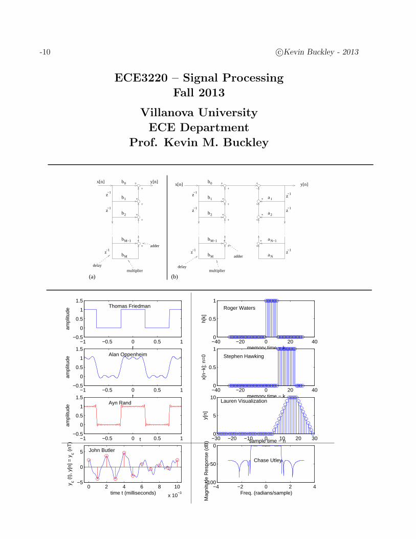
-10 c©Kevin Buckley - 2013
ECE3220 – Signal Processing
Fall 2013
Villanova University
ECE Department
Prof. Kevin M. Buckley
delay
adder
multiplier
adder
delaymultiplier
(b)(a)
−1z
−1z
−1z
+
+
+
+
+
+
+
+ y[n]x[n] 0
1
2
M−1
M
b
b
b
b
b
−1z
−1z
−1z
−1z
−1z
−1z
y[n]x[n]
+
+
+
+
+
+
+
−
0
1
2
M−1
M
+
+
+
+
+
+
+
+
1
2
N−1
N
b
b
b
b
b
a
a
a
a
−1 −0.5 0 0.5 1−0.5
0
0.5
1
1.5
t
ampl
itude
Thomas Friedman
−1 −0.5 0 0.5 1−0.5
0
0.5
1
1.5
t
ampl
itude
Alan Oppenheim
−1 −0.5 0 0.5 1−0.5
0
0.5
1
1.5
t
ampl
itude
Ayn Rand
0 2 4 6 8 10
x 10−3
−5
0
5
time t (milliseconds)
y c (t)
, y[n
] = y
c (nT
)
John Butler
−40 −20 0 20 400
0.5
1
memory time − k
h[k]
Roger Waters
−40 −20 0 20 400
0.5
1
memory time − k
x[n−
k]; n
=0 Stephen Hawking
−30 −20 −10 0 10 20 300
5
10
sample time − n
y[n]
Lauren Visualization
−4 −2 0 2 4−100
−50
0
Freq. (radians/sample)
Mag
nitu
de R
espo
nse
(dB
)
Chase Utley

c©Kevin Buckley - 2013 -9
.
-8 c©Kevin Buckley - 2013
Contents
1 Introduction 11.1 Motivation & Background . . . . . . . . . . . . . . . . . . . . . . . . . . . . 31.2 Signal Processing Examples . . . . . . . . . . . . . . . . . . . . . . . . . . . 5
1.2.1 Discussion on Sampling & Reconstruction . . . . . . . . . . . . . . . 51.2.2 An RC Circuit . . . . . . . . . . . . . . . . . . . . . . . . . . . . . . 61.2.3 Channel Equalization . . . . . . . . . . . . . . . . . . . . . . . . . . . 71.2.4 An FIR Filter Example . . . . . . . . . . . . . . . . . . . . . . . . . . 81.2.5 A Simple Discrete-Time (DT) System . . . . . . . . . . . . . . . . . . 9
1.3 Course Objective, Linear Combinations & Two Basic Concepts . . . . . . . . 111.4 Discrete & Continuous Time Signals & Operators . . . . . . . . . . . . . . . 15
1.4.1 Basic Discrete-Time Signals & Operators . . . . . . . . . . . . . . . . 151.4.2 Basic Continuous-Time Signals & Operators . . . . . . . . . . . . . . 221.4.3 Signal Classes . . . . . . . . . . . . . . . . . . . . . . . . . . . . . . . 251.4.4 Periodic Signals and Sinusoids . . . . . . . . . . . . . . . . . . . . . . 281.4.5 Basic Signal Sets and Transforms . . . . . . . . . . . . . . . . . . . . 32
1.5 Linear Time-Invariant (LTI) Systems . . . . . . . . . . . . . . . . . . . . . . 341.5.1 System Examples . . . . . . . . . . . . . . . . . . . . . . . . . . . . . 341.5.2 System Properties . . . . . . . . . . . . . . . . . . . . . . . . . . . . . 411.5.3 Linear Time-Invariant (LTI) Systems . . . . . . . . . . . . . . . . . . 481.5.4 Linear Constant Coefficient System I/O Equations . . . . . . . . . . 51
1.6 Practicum 1 . . . . . . . . . . . . . . . . . . . . . . . . . . . . . . . . . . . . 531.7 Appendix 1A: Complex Numbers and Signals . . . . . . . . . . . . . . . . . 59
1.7.1 Complex Numbers . . . . . . . . . . . . . . . . . . . . . . . . . . . . 591.7.2 Algebra with Complex Numbers . . . . . . . . . . . . . . . . . . . . . 601.7.3 Complex-Valued Signals . . . . . . . . . . . . . . . . . . . . . . . . . 621.7.4 Why Consider Complex-Valued Signals? . . . . . . . . . . . . . . . . 65
1.8 Problems . . . . . . . . . . . . . . . . . . . . . . . . . . . . . . . . . . . . . . 67
2 Time Domain Analysis of LTI Systems 792.1 DT Signal Impulse Expansion . . . . . . . . . . . . . . . . . . . . . . . . . . 802.2 DT LTI System I/O Calculation: The Convolution Sum . . . . . . . . . . . 81
2.2.1 The Impulse Response of a DT LTI System & Convolution Sum . . . 812.2.2 Approaches for the Calculation of the Convolution Sum . . . . . . . . 942.2.3 Convolution Sum Properties . . . . . . . . . . . . . . . . . . . . . . . 95
2.3 DT LTI System Issues . . . . . . . . . . . . . . . . . . . . . . . . . . . . . . 1002.3.1 System Properties . . . . . . . . . . . . . . . . . . . . . . . . . . . . . 1002.3.2 DT LTI Subsystem Interconnections . . . . . . . . . . . . . . . . . . 1022.3.3 DT LTI System Response to Sinusoidal Inputs . . . . . . . . . . . . . 105
2.4 CT Signal Impulse Expansion . . . . . . . . . . . . . . . . . . . . . . . . . . 1082.5 CT LTI System I/O Calculation: Convolution Integral . . . . . . . . . . . . 109
2.5.1 The Impulse Response of a CT LTI System . . . . . . . . . . . . . . 1092.5.2 Convolution Integral . . . . . . . . . . . . . . . . . . . . . . . . . . . 1092.5.3 Convolution Integral Properties and Examples . . . . . . . . . . . . . 110
c©Kevin Buckley - 2013 -7
2.6 CT LTI System Issues . . . . . . . . . . . . . . . . . . . . . . . . . . . . . . 1172.7 Generalizing the Utility of Convolution . . . . . . . . . . . . . . . . . . . . . 1202.8 Practicum 2 . . . . . . . . . . . . . . . . . . . . . . . . . . . . . . . . . . . . 1212.9 Problems . . . . . . . . . . . . . . . . . . . . . . . . . . . . . . . . . . . . . . 127
3 Continuous Time Transforms 1453.1 Some Motivation for the Study of Transforms . . . . . . . . . . . . . . . . . 146
3.1.1 Preliminary View of Spectral Representation . . . . . . . . . . . . . . 1463.1.2 System Response to Complex Exponential Signals . . . . . . . . . . . 152
3.2 CT Fourier Series (CTFS) Representation of Periodic Signals . . . . . . . . . 1553.2.1 A Few CTFS Properties . . . . . . . . . . . . . . . . . . . . . . . . . 163
3.3 The Continuous Time Fourier Transform (CTFT) . . . . . . . . . . . . . . . 1663.3.1 The Generalized CTFT . . . . . . . . . . . . . . . . . . . . . . . . . . 171
3.4 The Laplace Transform (LT) . . . . . . . . . . . . . . . . . . . . . . . . . . . 1733.4.1 The Bilateral Laplace Transform (BLT) . . . . . . . . . . . . . . . . . 1733.4.2 Relationship Between the BLT and the CTFT . . . . . . . . . . . . . 1773.4.3 The Inverse Bilateral Laplace Transform . . . . . . . . . . . . . . . . 1783.4.4 The Unilateral Laplace Transform (ULT) . . . . . . . . . . . . . . . . 1803.4.5 Some Useful Rules-of-Thumb on When to Use Different Transforms . 180
3.5 Continuous Time Transform Properties . . . . . . . . . . . . . . . . . . . . . 1813.6 Practicum 3 . . . . . . . . . . . . . . . . . . . . . . . . . . . . . . . . . . . . 2063.7 Problems . . . . . . . . . . . . . . . . . . . . . . . . . . . . . . . . . . . . . . 215
4 Applications of CT Transforms 2274.1 Continuous Time LTI Systems . . . . . . . . . . . . . . . . . . . . . . . . . . 227
4.1.1 CT LTI System I/O Descriptions . . . . . . . . . . . . . . . . . . . . 2294.1.2 Partial Fraction Expansion (PFE) . . . . . . . . . . . . . . . . . . . . 2324.1.3 Stability, Causality, the jω Axis and ROC . . . . . . . . . . . . . . . 2374.1.4 Frequency Response and Pole/Zero Locations . . . . . . . . . . . . . 2404.1.5 The Unilateral Laplace Transform and System Initial Conditions . . . 2414.1.6 CT LTI System Block Diagrams . . . . . . . . . . . . . . . . . . . . . 243
4.2 Signal Processing Functions . . . . . . . . . . . . . . . . . . . . . . . . . . . 2454.2.1 Filtering . . . . . . . . . . . . . . . . . . . . . . . . . . . . . . . . . . 2464.2.2 Sampling . . . . . . . . . . . . . . . . . . . . . . . . . . . . . . . . . 2534.2.3 Modulation . . . . . . . . . . . . . . . . . . . . . . . . . . . . . . . . 2624.2.4 RLC Circuits . . . . . . . . . . . . . . . . . . . . . . . . . . . . . . . 2694.2.5 Spectrum Estimation . . . . . . . . . . . . . . . . . . . . . . . . . . . 271
4.3 Practicum 4a . . . . . . . . . . . . . . . . . . . . . . . . . . . . . . . . . . . 2724.4 Practicum 4b . . . . . . . . . . . . . . . . . . . . . . . . . . . . . . . . . . . 2774.5 Problems . . . . . . . . . . . . . . . . . . . . . . . . . . . . . . . . . . . . . . 283
5 Discrete Time Transforms 2995.1 The Frequency Response & Transfer Function of a DT LTI System . . . . . 3015.2 The DTFS Representation of DT Periodic Signals . . . . . . . . . . . . . . . 3065.3 The DTFT Representation of DT Energy Signals . . . . . . . . . . . . . . . 310

-6 c©Kevin Buckley - 2013
5.4 The DTFT Representation of Periodic Signals . . . . . . . . . . . . . . . . . 3155.5 Properties of the DTFT . . . . . . . . . . . . . . . . . . . . . . . . . . . . . 318
5.5.1 Periodicity of X(ejω) . . . . . . . . . . . . . . . . . . . . . . . . . . . 3185.5.2 Symmetry of X(ejω) . . . . . . . . . . . . . . . . . . . . . . . . . . . 3205.5.3 Time Delay . . . . . . . . . . . . . . . . . . . . . . . . . . . . . . . . 3225.5.4 Linearity . . . . . . . . . . . . . . . . . . . . . . . . . . . . . . . . . . 3235.5.5 Convolution . . . . . . . . . . . . . . . . . . . . . . . . . . . . . . . . 3245.5.6 Parseval’s Theorem . . . . . . . . . . . . . . . . . . . . . . . . . . . . 3275.5.7 Multiplication . . . . . . . . . . . . . . . . . . . . . . . . . . . . . . . 3285.5.8 Modulation . . . . . . . . . . . . . . . . . . . . . . . . . . . . . . . . 331
5.6 The z-Transform . . . . . . . . . . . . . . . . . . . . . . . . . . . . . . . . . 3345.6.1 The Bilateral z-Transform and its Region of Convergence . . . . . . . 3345.6.2 Selected Properties of the z-Transform . . . . . . . . . . . . . . . . . 339
5.7 Problems . . . . . . . . . . . . . . . . . . . . . . . . . . . . . . . . . . . . . . 342
6 Applications of DT Transforms 3496.1 The DTFT and DT LTI Systems . . . . . . . . . . . . . . . . . . . . . . . . 350
6.1.1 The Frequency Response . . . . . . . . . . . . . . . . . . . . . . . . . 3506.1.2 Bringing in the I/O Difference Equation . . . . . . . . . . . . . . . . 351
6.2 The z-Transform and the LTI System Transfer Function . . . . . . . . . . . . 3546.2.1 Frequency Response . . . . . . . . . . . . . . . . . . . . . . . . . . . 3576.2.2 Partial Fraction Expansion (PFE) of Rational H(z) . . . . . . . . . . 3626.2.3 Stability, Causality, the Unit Circle and ROC . . . . . . . . . . . . . 3696.2.4 DT LTI System Block Diagrams . . . . . . . . . . . . . . . . . . . . . 372
6.3 Signal Processing Functions & Implementation . . . . . . . . . . . . . . . . . 3756.3.1 Channel Equalization . . . . . . . . . . . . . . . . . . . . . . . . . . . 3756.3.2 Sampling: A DT Perspective . . . . . . . . . . . . . . . . . . . . . . . 3796.3.3 Filter Banks . . . . . . . . . . . . . . . . . . . . . . . . . . . . . . . . 3796.3.4 Spectrum Estimation . . . . . . . . . . . . . . . . . . . . . . . . . . . 3796.3.5 Real-Time DT Systems . . . . . . . . . . . . . . . . . . . . . . . . . . 379
6.4 Practicum 4c . . . . . . . . . . . . . . . . . . . . . . . . . . . . . . . . . . . 3806.5 Practicum 5a . . . . . . . . . . . . . . . . . . . . . . . . . . . . . . . . . . . 3856.6 Practicum 5b . . . . . . . . . . . . . . . . . . . . . . . . . . . . . . . . . . . 3916.7 Problems . . . . . . . . . . . . . . . . . . . . . . . . . . . . . . . . . . . . . . 401
7 Introduction to Random Processes 4197.1 Review of Random Variables . . . . . . . . . . . . . . . . . . . . . . . . . . . 4207.2 DT Random Processes . . . . . . . . . . . . . . . . . . . . . . . . . . . . . . 4267.3 Power Spectral Density . . . . . . . . . . . . . . . . . . . . . . . . . . . . . . 4317.4 DT Random Processes & DT LTI Systems . . . . . . . . . . . . . . . . . . . 4347.5 Problems . . . . . . . . . . . . . . . . . . . . . . . . . . . . . . . . . . . . . . 437
c©Kevin Buckley - 2013 -5
List of Figures
1 An illustration of sampling. . . . . . . . . . . . . . . . . . . . . . . . . . . . 52 Ideal sampling and reconstruction block diagrams. . . . . . . . . . . . . . . . 63 A simple parallel RC circuit. . . . . . . . . . . . . . . . . . . . . . . . . . . . 64 A multipath communication channel. . . . . . . . . . . . . . . . . . . . . . . 75 The FIR filter structure (the “D” block represents a delay; combined, the set
of delays form a “delay line”, a.k.a. a “shift register”). . . . . . . . . . . . . 96 A simple DT system. . . . . . . . . . . . . . . . . . . . . . . . . . . . . . . . 97 Representation of a CT square wave as a linear combination of sinusoids. The
idea of “harmonics” will be established in Chapter 3 of this Course. . . . . . 148 A delayed (a.k.a. shifted) step. . . . . . . . . . . . . . . . . . . . . . . . . . 169 A folded and shifted step. . . . . . . . . . . . . . . . . . . . . . . . . . . . . 1810 A right-sided decaying exponential. . . . . . . . . . . . . . . . . . . . . . . . 1811 A pulse formed from two steps. . . . . . . . . . . . . . . . . . . . . . . . . . 1912 An exponential pulse. . . . . . . . . . . . . . . . . . . . . . . . . . . . . . . . 1913 y[n] = x[n] h[4− n]. . . . . . . . . . . . . . . . . . . . . . . . . . . . . . . . 1914 Block diagram of an accumulator. . . . . . . . . . . . . . . . . . . . . . . . . 2015 Basic CT signals: (a) step; (b) ramp; (c) pulse; (d) impulse. . . . . . . . . . 2216 Differentiation and integration involving impulses. . . . . . . . . . . . . . . . 2317 Compression (scaling with a > 1). . . . . . . . . . . . . . . . . . . . . . . . . 2418 Expansion (scaling with 0 < a < 1). . . . . . . . . . . . . . . . . . . . . . . . 2419 A periodic pulse train. . . . . . . . . . . . . . . . . . . . . . . . . . . . . . . 2720 A delayed (therefore phase shifted) cosine signal. . . . . . . . . . . . . . . . . 2821 Two periodic signals (to be summed). . . . . . . . . . . . . . . . . . . . . . . 3122 A simple DT system. . . . . . . . . . . . . . . . . . . . . . . . . . . . . . . . 3523 The FIR filter structure. . . . . . . . . . . . . . . . . . . . . . . . . . . . . . 3624 A parallel interconnection of subsystems. . . . . . . . . . . . . . . . . . . . . 3925 A cascade interconnection of subsystems. . . . . . . . . . . . . . . . . . . . . 4026 A feedback interconnection of subsystems. . . . . . . . . . . . . . . . . . . . 4027 Inverting the effect of a degrading physical system. . . . . . . . . . . . . . . 4128 Assuming linearity, given outputs for x1(t) and x2(t), what are the outputs
for x3(t) and x4(t)? . . . . . . . . . . . . . . . . . . . . . . . . . . . . . . . . 4429 Illustration of the test for time-invariance. . . . . . . . . . . . . . . . . . . . 4530 Assuming time-invariance, given the output for x1(t), what are the outputs
for x2(t) and x3(t)? . . . . . . . . . . . . . . . . . . . . . . . . . . . . . . . . 4631 An LTI system and the impulse I/O pair. . . . . . . . . . . . . . . . . . . . . 4632 An LTI system and the impulse I/O pair. . . . . . . . . . . . . . . . . . . . . 4733 A Discrete-Time Linear Time-Invariant (DT LTI) system. . . . . . . . . . . 4834 Assuming linearity and time-invariance, given the output for x1(t), what are
the outputs for x2(t) and x3(t)? . . . . . . . . . . . . . . . . . . . . . . . . . 4935 DT LTI system structures: a) FIR filter; and b) general IIR filter. . . . . . . 5236 A complex number x in the complex plane. . . . . . . . . . . . . . . . . . . . 5937 An in-phase/quadrature (I/Q) receiver. . . . . . . . . . . . . . . . . . . . . . 6638 Representation of a DT signal as linear combination of delayed impulses. . . 80

-4 c©Kevin Buckley - 2013
39 A DT LTI system and the convolution sum. . . . . . . . . . . . . . . . . . . 8140 Example 2.1 convolution sum illustration. . . . . . . . . . . . . . . . . . . . 8241 Example 2.3 convolution sum illustration. . . . . . . . . . . . . . . . . . . . 8342 Example 2.4 convolution sum illustration. . . . . . . . . . . . . . . . . . . . 8443 Plots generated by the Convolution Sum Demo. . . . . . . . . . . . . . . . . 8844 The FIR filter structure (implementing a convolution sum directly). . . . . . 8945 Given convolution result for Example 2.15. . . . . . . . . . . . . . . . . . . . 9746 Illustration of the overlap-and-add convolution sum calculation. . . . . . . . 9947 Parallel interconnection of DT LTI subsystems. . . . . . . . . . . . . . . . . 10248 Cascade interconnection of DTLTI subsystems. . . . . . . . . . . . . . . . . 10349 Example 2.23 interconnection of DTLTI subsystems. . . . . . . . . . . . . . 10450 Representation of a CT LTI system using its impulse response h(t). . . . . . 10951 A CT LTI system and the convolution integral. . . . . . . . . . . . . . . . . 10952 Example 2.31 CT convolution integral illustration. . . . . . . . . . . . . . . . 11253 Convolution integral result for Example 2.38. . . . . . . . . . . . . . . . . . . 11554 CTLTI subsystem interconnection for Example 2.41. . . . . . . . . . . . . . . 11855 Serial RLC circuit for Example 2.43. . . . . . . . . . . . . . . . . . . . . . . 11956 Serial RC circuit for Example 2.44. . . . . . . . . . . . . . . . . . . . . . . . 11957 An example of the spectrum of a sum of sinusoids. . . . . . . . . . . . . . . . 14858 The plot of an AM signal and its spectrum. . . . . . . . . . . . . . . . . . . 14959 Frequency spectra: (a) as a representation of frequency content for all time;
(b) the time-frequency spectrum of a real-valued sinusoid; (c) the time-frequencyspectrum of a musical scale; and (d) an estimate of the time-frequency spectrum.150
60 The CT LTI system response for an exponential input. . . . . . . . . . . . . 15361 CTFS approximations of a square wave using different numbers of harmonics. 15962 A sawtooth waveform and its DC, 1-st harmonic approximation. . . . . . . . 16063 A fullwave rectified sinusoid. . . . . . . . . . . . . . . . . . . . . . . . . . . . 16264 Example 3.11 signals. . . . . . . . . . . . . . . . . . . . . . . . . . . . . . . . 16465 CTFT of a periodic signal. . . . . . . . . . . . . . . . . . . . . . . . . . . . . 17066 CTFT of a impulse train. . . . . . . . . . . . . . . . . . . . . . . . . . . . . 17167 CTFT of an AM signal. . . . . . . . . . . . . . . . . . . . . . . . . . . . . . 17268 ROC illustrations for different types of signals. . . . . . . . . . . . . . . . . . 17569 CTFT of an AM modulated sinc2 signal. . . . . . . . . . . . . . . . . . . . . 19070 Illustration of the multiplication property of the CTFT. . . . . . . . . . . . . 19371 Transform based I/O representations of a CT LTI system. . . . . . . . . . . 22872 Converting between different CT LTI system I/O descriptions. . . . . . . . . 23073 Illustration of the relationship between pole positions, ROC and causality of
impulse response components. . . . . . . . . . . . . . . . . . . . . . . . . . . 23774 s-plane illustration for Example 4.9. . . . . . . . . . . . . . . . . . . . . . . . 23975 (a) Pole/zero locations; and (b) frequency response for a CT notch filter. . . 24076 Block diagram for Example 4.11. . . . . . . . . . . . . . . . . . . . . . . . . 24377 Block diagram for Example 4.12. . . . . . . . . . . . . . . . . . . . . . . . . 24478 Typical CT lowpass filter design specifications. . . . . . . . . . . . . . . . . . 25079 Pole plot (there are no zeros) for a Butterworth CT lowpass filter. . . . . . . 252
c©Kevin Buckley - 2013 -3
80 Frequency response (magnitude-squared in db) and phase response for a But-terworth CT lowpass filter. . . . . . . . . . . . . . . . . . . . . . . . . . . . . 252
81 An idealistic C-to-D converter. . . . . . . . . . . . . . . . . . . . . . . . . . . 25382 An idealistic D-to-C converter. . . . . . . . . . . . . . . . . . . . . . . . . . . 25583 An antialiasing filter as a preprocessor before a C-to-D converter. . . . . . . 25584 A spectral illustration of aliasing. . . . . . . . . . . . . . . . . . . . . . . . . 25685 A visualization of sampling, as modeled using an impulse train multiplication
and studied using the CTFT. . . . . . . . . . . . . . . . . . . . . . . . . . . 25886 Reconstruction of x(t) from xT (t) (i.e. from its “samples”) . . . . . . . . . . 25987 AM modulation. . . . . . . . . . . . . . . . . . . . . . . . . . . . . . . . . . 26388 A practical asynchronous AM transmitter and receiver. . . . . . . . . . . . . 26489 System for Example 4.22. . . . . . . . . . . . . . . . . . . . . . . . . . . . . 26590 System for Example 4.23. . . . . . . . . . . . . . . . . . . . . . . . . . . . . 26691 System for Example 4.24. . . . . . . . . . . . . . . . . . . . . . . . . . . . . 26792 System for Example 4.25. . . . . . . . . . . . . . . . . . . . . . . . . . . . . 26893 Laplace transform representation of: (a) a resistor; (b) an inductor; (c) a
capacitor. . . . . . . . . . . . . . . . . . . . . . . . . . . . . . . . . . . . . . 26994 Serial RLC circuit for Example 4.26. . . . . . . . . . . . . . . . . . . . . . . 27095 RLC circuit for Example 4.27. . . . . . . . . . . . . . . . . . . . . . . . . . . 27096 A DT LTI system and the convolution sum. . . . . . . . . . . . . . . . . . . 30197 Frequency response for Example 5.1. . . . . . . . . . . . . . . . . . . . . . . 30398 Frequency response for Example 5.3. . . . . . . . . . . . . . . . . . . . . . . 30499 Transform based I/O representations of a DT LTI system. . . . . . . . . . . 305100 Illustration of the ambiguity of DTFS frequencies. . . . . . . . . . . . . . . . 306101 DTFS coefficients for Example 5.4. . . . . . . . . . . . . . . . . . . . . . . . 307102 DTFS coefficients for Example 5.5. . . . . . . . . . . . . . . . . . . . . . . . 308103 DTFS coefficients for Example 5.6. . . . . . . . . . . . . . . . . . . . . . . . 308104 DTFT for Example 5.7. . . . . . . . . . . . . . . . . . . . . . . . . . . . . . 311105 DTFT for Example 5.10. . . . . . . . . . . . . . . . . . . . . . . . . . . . . . 312106 DTFT for Example 5.14. . . . . . . . . . . . . . . . . . . . . . . . . . . . . . 315107 DTFT for Example 5.15. . . . . . . . . . . . . . . . . . . . . . . . . . . . . . 316108 DTFT for Example 5.16. . . . . . . . . . . . . . . . . . . . . . . . . . . . . . 316109 DTFT for Example 5.17. . . . . . . . . . . . . . . . . . . . . . . . . . . . . . 317110 DTFT for Example 5.18. . . . . . . . . . . . . . . . . . . . . . . . . . . . . . 317111 Frequency response for Example 5.19. . . . . . . . . . . . . . . . . . . . . . . 319112 Phase response for Example 5.20. . . . . . . . . . . . . . . . . . . . . . . . . 321113 DTFT for Example 5.21. . . . . . . . . . . . . . . . . . . . . . . . . . . . . . 323114 Frequency domain circular convolution for Example 5.29. . . . . . . . . . . . 329115 Frequency domain circular convolution for Example 5.30. . . . . . . . . . . . 330116 Frequency domain circular convolution for Example 5.34. . . . . . . . . . . . 332117 The DTFT convolution property and DT LTI systems. . . . . . . . . . . . . 350118 A DT LTI system and its transfer function. . . . . . . . . . . . . . . . . . . 354119 The effect of poles and zeros on the transfer function H(z). . . . . . . . . . . 356120 (a) evaluation of the z-plane on the unit circle (illustrating the DTFT/z-
transform relationship); (b) relationships between DT LTI system descriptions.357
-2 c©Kevin Buckley - 2013
121 Pole/zero plot, and corresponding magnitude response, for Example 6.7. . . 360122 Pole/zero locations and frequency responses for two DT lowpass filters. . . . 361123 Pole/zero plot, and corresponding magnitude response, for Example 6.9. . . 361124 Illustration of the relationship between pole positions, ROC and causality of
impulse response components. . . . . . . . . . . . . . . . . . . . . . . . . . . 369125 Pole/zero plot, and possible ROC’s, for Example 6.16. . . . . . . . . . . . . . 371126 DT LTI model of the digital communication channel equalization problem. . 375127 The uniform pdf. . . . . . . . . . . . . . . . . . . . . . . . . . . . . . . . . . 421128 The Gaussian pdf. . . . . . . . . . . . . . . . . . . . . . . . . . . . . . . . . . 421129 A 2 dimensional pdf. . . . . . . . . . . . . . . . . . . . . . . . . . . . . . . . 422130 Illustration of a realization of DT white noise. . . . . . . . . . . . . . . . . . 426
c©Kevin Buckley - 2013 -1
List of Tables
1 A Summation Table. . . . . . . . . . . . . . . . . . . . . . . . . . . . . . . . 212 Basic Signal Sets and corresponding transforms. . . . . . . . . . . . . . . . . 323 Convolution Sum Results. . . . . . . . . . . . . . . . . . . . . . . . . . . . . 944 Convolution Integral Results. . . . . . . . . . . . . . . . . . . . . . . . . . . 1115 Transforms. . . . . . . . . . . . . . . . . . . . . . . . . . . . . . . . . . . . . 1516 Continuous Time Fourier Series (CTFS) Pairs. . . . . . . . . . . . . . . . . . 1617 Continuous Time Fourier Transform (CTFT) Pairs. . . . . . . . . . . . . . . 1688 Bilateral Laplace Transform (BLT) Pairs. . . . . . . . . . . . . . . . . . . . . 1769 Continuous Time Transform Properties. . . . . . . . . . . . . . . . . . . . . 18210 Continuous Time Fourier Transform (CTFT) Properties. . . . . . . . . . . . 20411 Bilateral Laplace Transform (BLT) Properties. . . . . . . . . . . . . . . . . . 20512 Discrete Time Fourier Series (DTFS) Pairs. . . . . . . . . . . . . . . . . . . 30913 Discrete Time Fourier Transform (DTFT) Pairs. . . . . . . . . . . . . . . . . 31414 DTFT Properties. . . . . . . . . . . . . . . . . . . . . . . . . . . . . . . . . . 33315 z-Transform Pairs. . . . . . . . . . . . . . . . . . . . . . . . . . . . . . . . . 33816 z-Transform Properties. . . . . . . . . . . . . . . . . . . . . . . . . . . . . . . 339

0 c©Kevin Buckley - 2013
c©Kevin Buckley - 2013 1
1 Introduction
This Course is an introduction to the theory and methods of:
1. signal analysis and synthesis; and
2. system analysis, design and implementation.
We consider both continuous-time (CT) and discrete-time (DT) signals and systems. Forelectrical engineering students our emphasis is slightly more on CT than DT. For computerengineers our focus will be on DT, though it will be necessary to consider CT signals as theyrelate to the DT signals derived from them via sampling. As we will see, the methods forDT are very similar to those for CT, so both the EE student and CPE student approachesprovide useful experience for both CT and DT signals and systems.
There are two basic topics that encompass the methods developed throughout this Course.These are:
1. convolution; and
2. transforms.
These basic topics are relevant to both CT and DT systems. The objective of this Course isto become familiar with these two basic topics, and to learn how they are applied to signalsand systems.
This Chapter of the Course consists of introductory material. Its overall objective isthreefold:
1. to motivate the topics of this Course;
2. to establish required background; and
3. to introduce, informally, several basic concepts which are central to this Course.
After completing this Chapter, you should be prepared to begin learning the theory andmethods covered in this Course. Refer to the Chapter 1 Objective Checklist on the nextpage for a list of specific Chapter 1 objectives.
A word of caution – although no principal Course topics are covered in this Chapter, wedo establish required prerequisites, important notation and basic concepts. Over the firsttwo weeks, as we progress through this introduction, make sure you are comfortable withthe material we cover (e.g. complex sinusoids, signal classes, the basic concept of linearcombinations as it relates to transforms, basic system properties). Students who strugglewith this Course are usually students who do not apply themselves during this introduction.

2 c©Kevin Buckley - 2013
Chapter 1 Objective Checklist
• Be comfortable with complex numbers, including simple algebraic operations (e.g. ad-dition, multiplication, powers) and the use of Euler’s Identities.
• Be familiar with basic DT and CT signals (e.g. impulses, steps, ramps, exponentials)and basic operations on them (e.g. fold, shift, fold and shift).
• Be comfortable with real and complex-valued DT and CT sinusoids.
• Be comfortable with the application of integration as a tool for the solution of basicsignal processing problems.
• Be comfortable with the application of summation, including the use of Table 1, as atool for the solution of basic signal processing problems.
• Be able to compute the energy and power of DT and CT signals.
• Be comfortable with periodic signals.
• Understand the idea of a set of basic signals.
• Understand the basic concept of linear combinations of basic signals.
• Understand the the first basic concept of this Course – to represent and analyze signalsas linear combinations of basic signals.
• Be familiar with some simple DT systems. (You are already familiar with some CTsystems from your circuits course.)
• Be able to compute the output of some simple DT systems due to simple inputs. Thisincludes the ability to identify the impulse response of a simple DT system.
• Be able to compute the output of some simple CT & DT systems due to complexsinusoidal inputs.
• Be familiar with basis (CT and DT) system properties (i.e. linearity, time-invariance,causality and stability).
• Understand the the second basic concept of this Course – to describe and analyzesystems in terms of their response to basic signals.

c©Kevin Buckley - 2013 3
1.1 Motivation & Background
As with many engineering areas, signals and systems is about the effective use of mathe-matical and/or scientific methods to application problems. For this area, the methods areprimarily mathematical, and the applications are very diverse. In this Subsection we sug-gest motivation for studying signals and systems, discuss some applications, and provide anoverview and some background for the topics we will consider.
Motivation
Professionally, engineers are valued in part because they can solve complex technical designand analysis problems. The topics covered in this Course (i.e. signals and systems topics)provide the most important basic tools for a systematic approach to solving complex technicalproblems. That is, they are the tools for converting challenging problems into easy ones.
Engineering is interesting because of the challenge of solving complex technical problems,and because the problems engineers work on are practical and “real-world” in nature. Al-though the topics covered in this Course are mathematical, they are all about applications.Signal processing engineers work on some very interesting and important applications. Herewe list just a few of these. In the first class we will briefly discuss a few of these, andthroughout the semester (for example, in the Practicums) we will consider examples of howsignals and systems topics relate to applications.
Applications
Here is a list of just few of the many applications of signals and systems.
• Multimedia signal processing: audio & video processing, data compression, A/D andD/A converters, HDTV, audio special effects.
• Communications: cell phones, satellite communications, deep space communication.
• Physical sciences: geophysical exploration, astrophysical exploration.
• Biomedical engineering: biomedical imaging, cardiac pacemakers and defibrillators,health monitoring, cognitive studies, hearing aids, Brain/Computer Interface (BCI).Biomedical Signal Processing (BSP) is the topic of ece5251.
• Traditional electronic systems: SONAR, RADAR.
• Control systems: manufacturing process control, trajectory control.
• Machine diagnostics: engine monitoring and control, fault detection.
• Circuit and electronic modeling.
• Forecasting: weather, economic trends.
From this list, it is clear that signal processing occurs all around us and we use signalprocessing systems on a regular basis.
In the first lecture we will discuss signal processing applications. Prepare for this bythinking a little about: 1) how and why you use signal processing in your daily life; 2) what

4 c©Kevin Buckley - 2013
problems you are aware of that signal processing might solve; and 3) what signal processingproblems you may be interested in professionally.
Implementation
Engineers implement useful things. Signal processing is implemented in various ways thatelectrical and computer engineers have expertise in. This is one reason signals and systemsis an important core course in any ECE curriculum. Implementation platforms include thefollowing:
• Continuous-time hardware: circuits, electronics.
• Digital hardware: microprocessors, ASIC’s, FPGA’s.
• Digital software implemented on general purpose digital systems: C++, Java, Matlab.
• Digital software implemented on microprocessors (e.g. on Digital Signal Processing(DSP) chips): assembly language, cross-compiled C programs.
In this Course we will implement signal processing, digitally, using Matlab. This is what thePracticums are about. In ece5790 we cover more advanced implementation issues. To learnhow to implement signal processing in software on DSP chips, consider ece7710. To learnhow to implement signal processing in hardware on FPGA’s, consider ece7711.
Prerequisites
The formal prerequisites for this Course are listed on the Course Information page. Thetopics you need to be familiar coming into this Course are:
• Calculus (i.e. integration, differentiation): assumes background algebra and trigonom-etry.
• Differential equations: in particular, linear, constant coefficient (LCC) differentialequations.
• Complex numbers and basic complex variables (see Appendix 1A, Section 1.7 of theseNotes, for a review).
• Basic circuits - linear circuits (e.g. RLC circuits, natural response, step response,frequency response) and superposition.
• Matlab.
If you are concerned about your background in any of these prerequisite topic, please feelfree to discuss your concerns with me.
My experience with this Course is that, with these prerequisites, you should be fine aslong as you keep working. This is not a guarantee, but this Course is set up so that if youkeep trying there’s a very high probability that you will be OK. That said, remember thatit is very important to take this first Chapter seriously. It may not look like much is goingon, but familiarity with the basic concepts and the notation developed over this Chapter, aswell as the math reviewed, is critical as we move on.
c©Kevin Buckley - 2013 5
1.2 Signal Processing Examples
1.2.1 Discussion on Sampling & Reconstruction
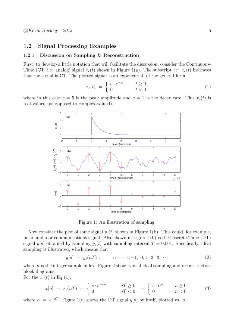
First, to develop a little notation that will facilitate the discussion, consider the Continuous-Time (CT, i.e. analog) signal xc(t) shown in Figure 1(a). The subscript “c” xc(t) indicatesthat the signal is CT. The plotted signal is an exponential, of the general form
xc(t) =
c · e−at t ≥ 00 t < 0
(1)
where in this case c = 5 is the peak amplitude and a = 2 is the decay rate. This xc(t) isreal-valued (as opposed to complex-valued).
−2 −1 0 1 2 3 4 5 6
0
2
4
6
time t (seconds)
x c (t)
(a)
0 1 2 3 4 5 6 7 8 9 10
x 10−3
−5
0
5
time t (milliseconds)
y c (t)
, y[n
] = y
c (nT
)
(b)
0 1 2 3 4 5 6 7 8 9 10−5
0
5
time n (samples)
y[n]
(c)
Figure 1: An illustration of sampling.
Now consider the plot of some signal yc(t) shown in Figure 1(b). This could, for example,be an audio or communications signal. Also shown in Figure 1(b) is the Discrete-Time (DT)signal y[n] obtained by sampling yc(t) with sampling interval T = 0.001. Specifically, idealsampling is illustrated, which means that
y[n] = yc(nT ) ; n = · · · ,−1, 0, 1, 2, 3, · · · (2)
where n is the integer sample index. Figure 2 show typical ideal sampling and reconstructionblock diagrams.For the xc(t) in Eq (1),
x[n] = xc(nT ) =
c · e−anT nT ≥ 00 nT < 0
=
c · αn n ≥ 00 n < 0
(3)
where α = e−aT . Figure 1(c) shows the DT signal y[n] by itself, plotted vs. n.
6 c©Kevin Buckley - 2013
cy (t)
cy (t)
cy[n] = y (nT)
Ideal Sampler
(T)
Ideal
(T)
Reconstruction
Figure 2: Ideal sampling and reconstruction block diagrams.
Since signals of interest are usually CT, and they are often processed with DT processors,sampling is an important signal processing function. Two fundamental questions of interestwhen sampling and reconstructing a signal are:
• Can yc(t) be exactly reconstructed from its samples in y[n]? Generally the answer isno, as you may intuitively expect since when sampling yc(t) we seemingly loose anyindication of its value between the samples in y[n]. However, as shown in this Course,it is possible to exactly reconstruct yc(t) from y[n] if the frequency content of yc(t) isproperly limited (i.e. if yc(t) is not changing too quickly) and if T is small enough.This is a surprising and extremely important result.
• How can sampling and reconstruction be implemented? In this Course we describe sam-pling and reconstruction mathematically. However, these descriptions directly suggesta variety of part digital, part analog implementation approaches.
1.2.2 An RC Circuit
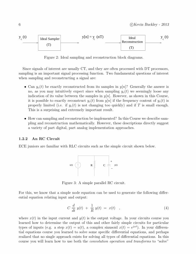
ECE juniors are familiar with RLC circuits such as the simple circuit shown below.
CR+
−x(t) y(t)
Figure 3: A simple parallel RC circuit.
For this, we know that a simple node equation can be used to generate the following differ-ential equation relating input and output:
Cd
dty(t) +
1
Ry(t) = x(t) , (4)
where x(t) in the input current and y(t) is the output voltage. In your circuits course youlearned how to determine the output of this and other fairly simple circuits for particulartypes of inputs (e.g. a step x(t) = u(t), a complex sinusoid x(t) = ejωt). In your differen-tial equations course you learned to solve some specific differential equations, and perhapsrealized that no single approach exists for solving all types of differential equations. In thiscourse you will learn how to use both the convolution operation and transforms to “solve”
c©Kevin Buckley - 2013 7
(i.e. compute outputs for given inputs) this and much more complex circuits for any given in-put. For example, the following integral equation, which is a convolution, solves this systemfor any input x(t) (assuming initial condition y(0−) = 0):
y(t) =∫ t
0
1
Ce−(t−τ)/RC x(τ) dτ t ≥ 0 . (5)
So, regardless of what the input x(t) is, you plug it into Eq (5) and solve for output y(t).
1.2.3 Channel Equalization
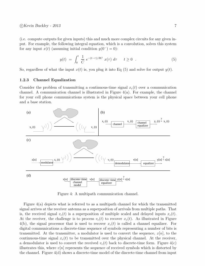
Consider the problem of transmitting a continuous-time signal xc(t) over a communicationchannel. A communication channel is illustrated in Figure 4(a). For example, the channelfor your cell phone communications system is the physical space between your cell phoneand a base station.
x (t)c v (t)c
channelequalizerchannel
x (t)c v (t)c cy (t) = ?
x (t)c
modulatorx (t)c v (t)cx[n] v[n]
?y[n] = x[n]
equalizerdemodulator
discrete−timechannelmodel
discrete−timeequalizer
y[n] = x[n]?
x[n] v[n]
(a) (b)
(c)
(d)
Figure 4: A multipath communication channel.
Figure 4(a) depicts what is referred to as a multipath channel for which the transmittedsignal arrives at the receiver antenna as a superposition of arrivals from multiple paths. Thatis, the received signal vc(t) is a superposition of multiple scaled and delayed inputs xc(t).At the receiver, the challenge is to process vc(t) to recover xc(t). As illustrated in Figure4(b), the signal processor that is used to recover xc(t) is called a channel equalizer. Fordigital communications a discrete-time sequence of symbols representing a number of bits istransmitted. At the transmitter, a modulator is used to convert the sequence, x[n], to thecontinuous-time signal xc(t) to be transmitted over the physical channel. At the receiver,a demodulator is used to convert the received vc(t) back to discrete-time form. Figure 4(c)illustrates this, where v[n] represents the sequence of received symbols which is distorted bythe channel. Figure 4(d) shows a discrete-time model of the discrete-time channel from input
8 c©Kevin Buckley - 2013
sequence x[n] to output v[n]. It also shows a discrete-time equalizer used to invert the effectof the channel. This discrete-time channel model, which is commonly used for digital com-munication system design, encompasses the physical channel, the modulator/demodulatorand the transmitter/receiver antennae and front end electronics.
The objective at the receiver is to acquire the transmitted signal xc(t) from the receiversignal vc(t), or in the digital communications system to recover x[n] from v[n]. The discrete-time equalizer operates to invert the effect of the channel, ideally providing the outputy[n] = x[n]. In Practicum 1 we will explore the digital communication channel equalizationproblem. We will consider a relatively simple discrete-time channel model of the form
v[n] = x[n] + a x[n− 1] . (6)
At symbol time n, the channel output is the desired symbol x[n] superimposed with thescaled/delayed previous symbol (e.g. via the reflection off a building). We will observe theeffectiveness of two proposed equalizers.
Eq (6) represents a very simple channel. The two equalizers considered in Practicum 1were designed specifically for this simple channel. In a realistic cell phone application, thechannel can be much more complex, it is not known (depending of the cell phone locationrelative to the base station), and it varies over time (as the cell phone moves). As we developdesign and analysis tools in this Course, we will see how the two Practicum 1 equalizers weredesigned, and we will begin to be able to handle more realistic channel equalization problems.
1.2.4 An FIR Filter Example
A filter is a system that separates things. It takes a mixture of several things as an input,and works to provide an output which contains only some of these things. In DT systems,a filter processes a DT input signal, say
x[n] = s[n] + n[n] (7)
where s[n] is a desired signal and n[n] is additive interfering noise, creating an output, sayy[n], which is an approximate of s[n]. The most common type of discrete-time filter in termedan FIR filter1. An FIR filter forms the output y[n] at time n by processing the present andprevious N − 1 input values, i.e. x[n], x[n− 1], · · · , x[n− (N − 1)], as follows
y[n] = b0 x[n] + b1 x[n− 1] + · · ·+ bN−1 x[n−N + 1] =N−1∑
k=0
bk x[n− k] (8)
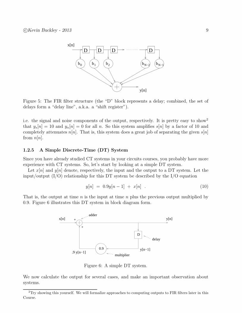
where the bk are the multipliers applied to the input values, i.e. x[n] is multiplied by b0 andthen summed with all the other multiplier outputs. Figure 5 is a block diagram illustrationof this type of system.
Suppose, for example that N = 10, bk = 1; k = 0, 1, · · · , 9, s[n] = 1 for all time n, andn[n] = (−1)n for all n. Let the output y[n] be expressed as
y[n] = ys[n] + yn[n] , (9)
1We will explain this terminology later.
c©Kevin Buckley - 2013 9
D D D D
b0 b1 b2
x[n]
y[n]
b bN−1N−2
Figure 5: The FIR filter structure (the “D” block represents a delay; combined, the set ofdelays form a “delay line”, a.k.a. a “shift register”).
i.e. the signal and noise components of the output, respectively. It is pretty easy to show2
that ys[n] = 10 and yn[n] = 0 for all n. So this system amplifies s[n] by a factor of 10 andcompletely attenuates n[n]. That is, this system does a great job of separating the given s[n]from n[n].
1.2.5 A Simple Discrete-Time (DT) System
Since you have already studied CT systems in your circuits courses, you probably have moreexperience with CT systems. So, let’s start by looking at a simple DT system.
Let x[n] and y[n] denote, respectively, the input and the output to a DT system. Let theinput/output (I/O) relationship for this DT system be described by the I/O equation
y[n] = 0.9y[n− 1] + x[n] . (10)
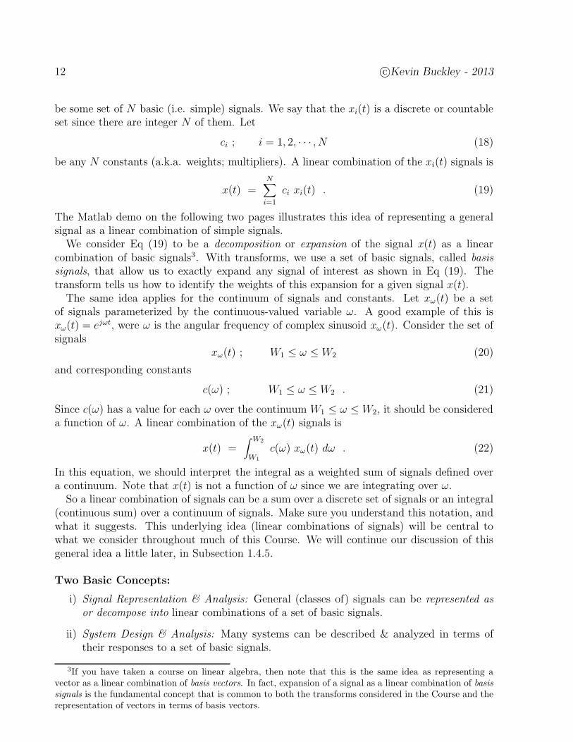
That is, the output at time n is the input at time n plus the previous output multiplied by0.9. Figure 6 illustrates this DT system in block diagram form.
delay
x[n] +
+
.9 y[n−1]
y[n]
D
0.9
adder
y[n−1]
multiplier
Figure 6: A simple DT system.
We now calculate the output for several cases, and make an important observation aboutsystems.
2Try showing this yourself. We will formalize approaches to computing outputs to FIR filters later in thisCourse.

10 c©Kevin Buckley - 2013
a) Find the impulse response, which is denoted below as ya[n]. That is, find the outputto the impulse input
xa[n] =
1 n = 00 n 6= 0
(11)
when the initial condition is ya[−1] = 0.
Solution: use either Eq (10) or Figure (6).
b) Find the step response, which is denoted below as yb[n]. That is, find the response tothe step
xb[n] =
1 n ≥ 00 n < 0
(12)
when the initial condition is yb[−1] = 0.
Solution: This isn’t too bad. We’ll learn formal approaches for doing this later in theCourse. For now, here’s the answer. Verify and sketch it yourself.
yb[n] =
∑nk=0 0.9
k = 1−0.9n+1
1−0.9n ≥ 0
0 n < 0(13)
Sketch:

c©Kevin Buckley - 2013 11
c) Find the response yc[n] to initial condition yc[−1] = 1 when there is no input.
Solution: Try this one yourself. It’s pretty straightforward. The answer is
yc[n] =
0.9n+1 n ≥ −10 n < −1 . (14)
Note that this is just ya[n] shifted to the right (i.e. advanced in time) by one sample.
Sketch:
d) Find the response yd[n] to input
xd[n] = 3xa[n] − 4xb[n] (15)
when the initial condition is yd[−1] = 5.
Solution: Even though the system is very simple, and the input is not too complex, thisis already starting to get challenging. Fortunately, for reasons identified later in thecourse, this system has a very useful property called linearity (a.k.a. superposition).Thus,
yd[n] = 3ya[n] − 4yb[n] + 5yc[n] . (16)
An observation: Linearity is a useful property! Are there other useful system properties?
1.3 Course Objective, Linear Combinations & Two Basic Con-
cepts
Course Objective: to introduce the theory, methods and applications of signal processingand system analysis. This theory and these methods effectively decompose complex problemsinto simpler ones. Case d) of the Subsection 1.2.5 example illustrates this. The principalapproach is to decompose signals into simpler ones using transforms.
Linear Combinations (a.k.a weighted sums) and signal expansions: as an example,we will describe this with CT signals. It’s the same idea for DT signals. Let
xi(t) ; i = 1, 2, · · · , N (17)
12 c©Kevin Buckley - 2013
be some set of N basic (i.e. simple) signals. We say that the xi(t) is a discrete or countableset since there are integer N of them. Let
ci ; i = 1, 2, · · · , N (18)
be any N constants (a.k.a. weights; multipliers). A linear combination of the xi(t) signals is
x(t) =N∑
i=1
ci xi(t) . (19)
The Matlab demo on the following two pages illustrates this idea of representing a generalsignal as a linear combination of simple signals.
We consider Eq (19) to be a decomposition or expansion of the signal x(t) as a linearcombination of basic signals3. With transforms, we use a set of basic signals, called basissignals, that allow us to exactly expand any signal of interest as shown in Eq (19). Thetransform tells us how to identify the weights of this expansion for a given signal x(t).
The same idea applies for the continuum of signals and constants. Let xω(t) be a setof signals parameterized by the continuous-valued variable ω. A good example of this isxω(t) = ejωt, were ω is the angular frequency of complex sinusoid xω(t). Consider the set ofsignals
xω(t) ; W1 ≤ ω ≤W2 (20)
and corresponding constants
c(ω) ; W1 ≤ ω ≤W2 . (21)
Since c(ω) has a value for each ω over the continuum W1 ≤ ω ≤W2, it should be considereda function of ω. A linear combination of the xω(t) signals is
x(t) =∫ W2
W1
c(ω) xω(t) dω . (22)
In this equation, we should interpret the integral as a weighted sum of signals defined overa continuum. Note that x(t) is not a function of ω since we are integrating over ω.
So a linear combination of signals can be a sum over a discrete set of signals or an integral(continuous sum) over a continuum of signals. Make sure you understand this notation, andwhat it suggests. This underlying idea (linear combinations of signals) will be central towhat we consider throughout much of this Course. We will continue our discussion of thisgeneral idea a little later, in Subsection 1.4.5.
Two Basic Concepts:
i) Signal Representation & Analysis: General (classes of) signals can be represented asor decompose into linear combinations of a set of basic signals.
ii) System Design & Analysis: Many systems can be described & analyzed in terms oftheir responses to a set of basic signals.
3If you have taken a course on linear algebra, then note that this is the same idea as representing avector as a linear combination of basis vectors. In fact, expansion of a signal as a linear combination of basissignals is the fundamental concept that is common to both the transforms considered in the Course and therepresentation of vectors in terms of basis vectors.
c©Kevin Buckley - 2013 13
echo on
%
% Matlab Demo
% Representing a CT Square Wave as a Linear Combination of Sinusoids
%
% x(t) == unit magnitude square wave of period 1, w_0 = 2 \pi
%
% x(t) =? 0.5 + 1/pi cos(2*pi*t) - 1/(3pi) cos(6*pi*t) +
% 1/(5pi) cos(10*pi*t) - 1/(7pi) cos(14*pi*t) + ...
%
% Enter N (odd) == highest harmonic before running
%
pause
% Construct and plot samples of x(t) for -1 <= t <= 1.
%
t = -1:.005:1;
x=ones(1,401);
x(51:151) = zeros(1,101), x(251:351) = zeros(1,101);
pause
subplot(221)
plot(t,x),xlabel(’t’),ylabel(’amplitude’),title(’square wave’)
text(0.5,1.5,’Thomas Friedman’),axis([-1 1 -0.5 1.5])
pause
% Generate array of required CTFS coefficients
%
Ak = zeros(1,N+1);
Ak(1) = 0.5; % DC
kk = 1:N;
Ak(2:N+1) = sin(kk*pi/2)./(kk*pi);
%
% Approximate x(t) with harmonics 1,3
%
omega0 = 2*pi;
x1 = Ak(1)*ones(1,length(t));
for k=1:3
x1 = x1 + 2*abs(Ak(k+1)*cos(k*omega0*t+angle(Ak(k+1)));
end
pause
subplot(222)
plot(t,x1,’b’),xlabel(’t’),ylabel(’amplitude’),title(’1,3 harmonics’)
text(0.5,1.5,’Alan Oppenheim’),axis([-1 1 -0.5 1.5])
pause
% Approximate x(t) with harmonics 0,1,3,5,7,9,11
%
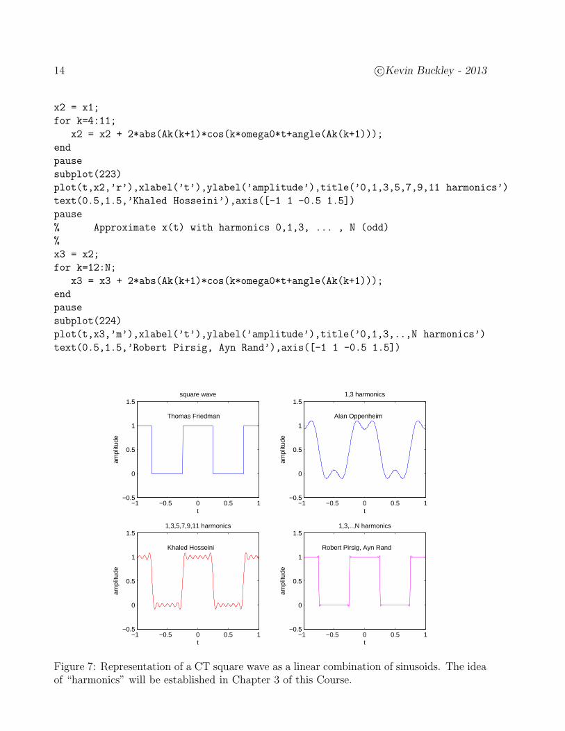
14 c©Kevin Buckley - 2013
x2 = x1;
for k=4:11;
x2 = x2 + 2*abs(Ak(k+1)*cos(k*omega0*t+angle(Ak(k+1)));
end
pause
subplot(223)
plot(t,x2,’r’),xlabel(’t’),ylabel(’amplitude’),title(’0,1,3,5,7,9,11 harmonics’)
text(0.5,1.5,’Khaled Hosseini’),axis([-1 1 -0.5 1.5])
pause
% Approximate x(t) with harmonics 0,1,3, ... , N (odd)
%
x3 = x2;
for k=12:N;
x3 = x3 + 2*abs(Ak(k+1)*cos(k*omega0*t+angle(Ak(k+1)));
end
pause
subplot(224)
plot(t,x3,’m’),xlabel(’t’),ylabel(’amplitude’),title(’0,1,3,..,N harmonics’)
text(0.5,1.5,’Robert Pirsig, Ayn Rand’),axis([-1 1 -0.5 1.5])
−1 −0.5 0 0.5 1−0.5
0
0.5
1
1.5
t
ampl
itude
square wave
Thomas Friedman
−1 −0.5 0 0.5 1−0.5
0
0.5
1
1.5
t
ampl
itude
1,3 harmonics
Alan Oppenheim
−1 −0.5 0 0.5 1−0.5
0
0.5
1
1.5
t
ampl
itude
1,3,5,7,9,11 harmonics
Khaled Hosseini
−1 −0.5 0 0.5 1−0.5
0
0.5
1
1.5
t
ampl
itude
1,3,..,N harmonics
Robert Pirsig, Ayn Rand
Figure 7: Representation of a CT square wave as a linear combination of sinusoids. The ideaof “harmonics” will be established in Chapter 3 of this Course.
c©Kevin Buckley - 2013 15
1.4 Discrete & Continuous Time Signals & Operators
The purpose of this Section is to establish some basic notation and concepts that we willrely heavily on throughout the Course.
1.4.1 Basic Discrete-Time Signals & Operators
Examples of Signals:
• Impulse (or unit impulse)
δ[n] =
1 n = 00 n 6= 0
(23)
• Step
u[n] =
1 n ≥ 00 n < 0
(24)
• Ramp
r[n] =
n n ≥ 00 n < 0
(25)
• Pulse (of length N)
pN [n] =
1 n = 0, 1, · · · , N − 10 otherwise
(26)
Plot: impulse step ramp pulse
• Exponential: For complex constants c and α, consider
x[n] = c αn . (27)
Let c = A ejφ and α = r ejωo. Then
x[n] = A ejφ(
r ejωo
)n= A ejφ rn ejωon = A rn ej(ωon+φ)
= A rn cos(ωon+ φ) + jA rn sin(ωon+ φ) .
Note that r and ω determines the decay and oscillation rates, respectively. One formof Euler’s identity is used in going from the first to second line of the equation above.We will see much more on complex exponentials and Euler’s identities later, so reviewexponential algebra and Euler’s identities now as needed.
16 c©Kevin Buckley - 2013
Euler’s Identities: relating real-valued and complex-valued sinusoids
ejx = cos x + j sin x (28)
cos x =1
2ejx +
1
2e−jx (29)
sin x =1
2jejx − 1
2je−jx . (30)
• Real & complex valued DT sinusoids: much more on these later.
Basic Operators: The following operations on signals could be considered as very simplesystems, but they are so elementary we introduce them here, before any formal discussionof systems.
• Shift (i.e. delay): A delay shifts a signal in time. Mathematically, we replace thediscrete-time variable n with n−m, where m is the (constant) amount of shift.
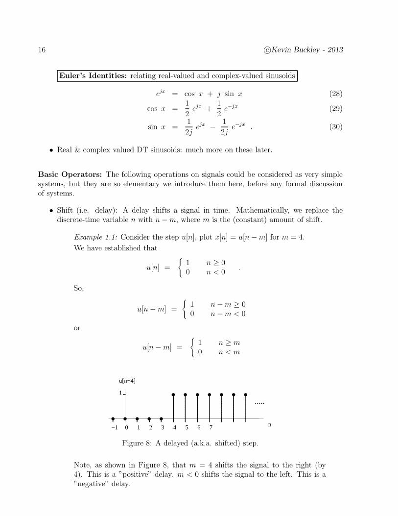
Example 1.1: Consider the step u[n], plot x[n] = u[n−m] for m = 4.
We have established that
u[n] =
1 n ≥ 00 n < 0
.
So,
u[n−m] =
1 n−m ≥ 00 n−m < 0
or
u[n−m] =
1 n ≥ m0 n < m
.....1
1 6 n
u[n−4]
2 3 4 5 70−1
Figure 8: A delayed (a.k.a. shifted) step.
Note, as shown in Figure 8, that m = 4 shifts the signal to the right (by4). This is a ”positive” delay. m < 0 shifts the signal to the left. This is a”negative” delay.

c©Kevin Buckley - 2013 17
• Fold: A fold is a reflection of a signal about n = 0. Mathematically, we replace thediscrete-time variable n with −n.
Example 1.2: Plot x[n] = u[−n].
Solution:
Example 1.3: Plot y[n] = x[−n], where
x[n] =
0.5n n ≥ 00 n < 0
.
Solution:
y[n] =
0.5−n −n ≥ 00 −n < 0
=
2n n ≤ 00 n > 0
.
Plot:
This x[n] is called a ”right-sided” signal since it is zero as n→ −∞ and notzero as n→∞. y[n] is a ”left-sided” signal.
18 c©Kevin Buckley - 2013
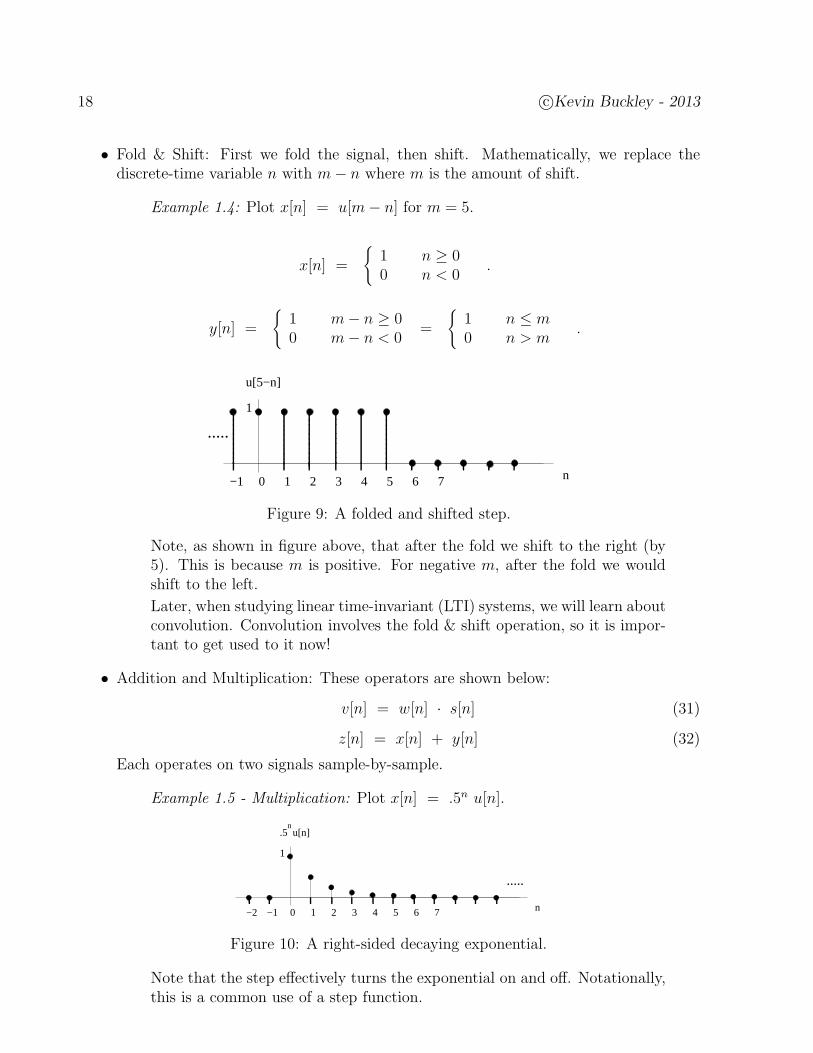
• Fold & Shift: First we fold the signal, then shift. Mathematically, we replace thediscrete-time variable n with m− n where m is the amount of shift.
Example 1.4: Plot x[n] = u[m− n] for m = 5.
x[n] =
1 n ≥ 00 n < 0
.
y[n] =
1 m− n ≥ 00 m− n < 0
=
1 n ≤ m0 n > m
.
1
1 6 n2 3 4 5 70−1
.....
u[5−n]
Figure 9: A folded and shifted step.
Note, as shown in figure above, that after the fold we shift to the right (by5). This is because m is positive. For negative m, after the fold we wouldshift to the left.
Later, when studying linear time-invariant (LTI) systems, we will learn aboutconvolution. Convolution involves the fold & shift operation, so it is impor-tant to get used to it now!
• Addition and Multiplication: These operators are shown below:
v[n] = w[n] · s[n] (31)
z[n] = x[n] + y[n] (32)
Each operates on two signals sample-by-sample.
Example 1.5 - Multiplication: Plot x[n] = .5n u[n].
1
1 6 n2 3 4 5 70−1−2
.5 u[n]n
.....
Figure 10: A right-sided decaying exponential.
Note that the step effectively turns the exponential on and off. Notationally,this is a common use of a step function.
c©Kevin Buckley - 2013 19
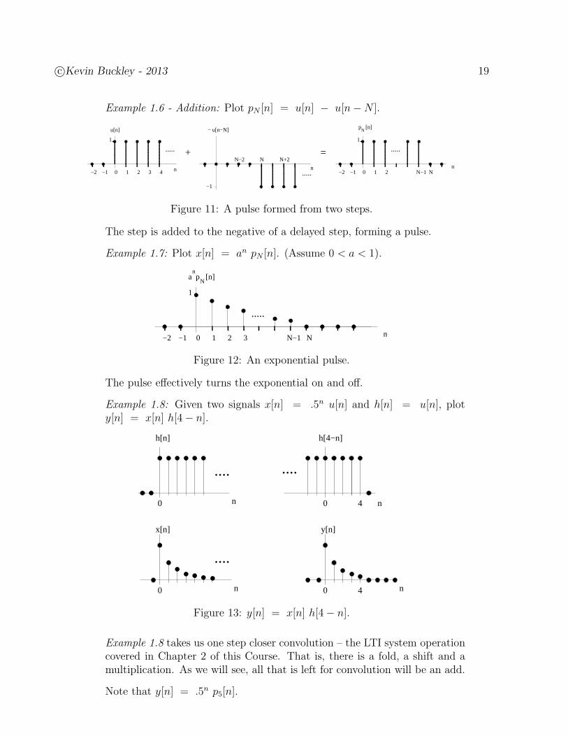
Example 1.6 - Addition: Plot pN [n] = u[n] − u[n−N ].
u[n]
1
1 2 3 40−1−2
.....
n
N N+2N−2
.....n
−1
− u[n−N]
1
1 20−1−2
.....
nNN−1
Np [n]
+ =
Figure 11: A pulse formed from two steps.
The step is added to the negative of a delayed step, forming a pulse.
Example 1.7: Plot x[n] = an pN [n]. (Assume 0 < a < 1).
1
1 n2 30−1−2
n
NN−1
.....
a p [n]N
Figure 12: An exponential pulse.
The pulse effectively turns the exponential on and off.
Example 1.8: Given two signals x[n] = .5n u[n] and h[n] = u[n], ploty[n] = x[n] h[4− n].
h[4−n]
........
h[n]
400 n n
0 n
y[n]
4
....
x[n]
0 n
Figure 13: y[n] = x[n] h[4− n].
Example 1.8 takes us one step closer convolution – the LTI system operationcovered in Chapter 2 of this Course. That is, there is a fold, a shift and amultiplication. As we will see, all that is left for convolution will be an add.
Note that y[n] = .5n p5[n].
20 c©Kevin Buckley - 2013
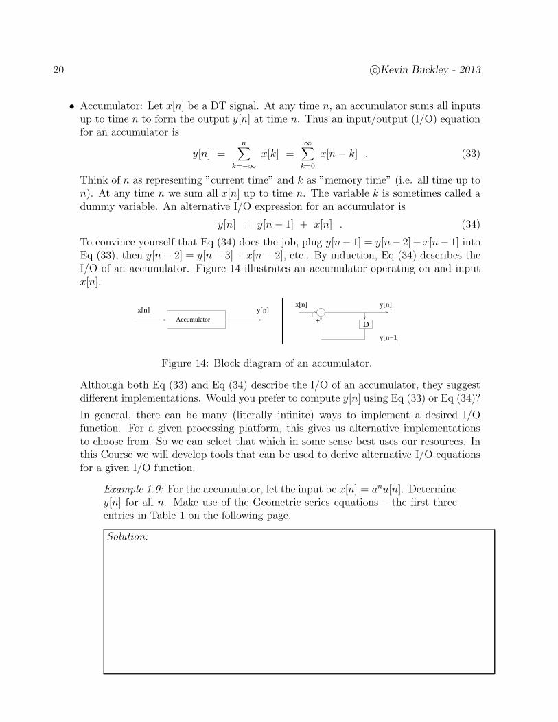
• Accumulator: Let x[n] be a DT signal. At any time n, an accumulator sums all inputsup to time n to form the output y[n] at time n. Thus an input/output (I/O) equationfor an accumulator is
y[n] =n∑
k=−∞x[k] =
∞∑
k=0
x[n− k] . (33)
Think of n as representing ”current time” and k as ”memory time” (i.e. all time up ton). At any time n we sum all x[n] up to time n. The variable k is sometimes called adummy variable. An alternative I/O expression for an accumulator is
y[n] = y[n− 1] + x[n] . (34)
To convince yourself that Eq (34) does the job, plug y[n− 1] = y[n− 2]+ x[n− 1] intoEq (33), then y[n− 2] = y[n− 3] + x[n− 2], etc.. By induction, Eq (34) describes theI/O of an accumulator. Figure 14 illustrates an accumulator operating on and inputx[n].
y[n]Accumulator
x[n]x[n] y[n]
D
y[n−1]
++
Figure 14: Block diagram of an accumulator.
Although both Eq (33) and Eq (34) describe the I/O of an accumulator, they suggestdifferent implementations. Would you prefer to compute y[n] using Eq (33) or Eq (34)?
In general, there can be many (literally infinite) ways to implement a desired I/Ofunction. For a given processing platform, this gives us alternative implementationsto choose from. So we can select that which in some sense best uses our resources. Inthis Course we will develop tools that can be used to derive alternative I/O equationsfor a given I/O function.
Example 1.9: For the accumulator, let the input be x[n] = anu[n]. Determiney[n] for all n. Make use of the Geometric series equations – the first threeentries in Table 1 on the following page.
Solution:
c©Kevin Buckley - 2013 21
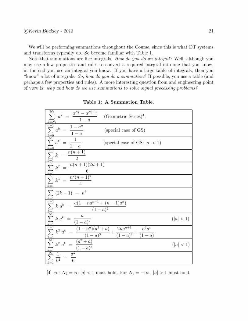
We will be performing summations throughout the Course, since this is what DT systemsand transforms typically do. So become familiar with Table 1.
Note that summations are like integrals. How do you do an integral? Well, although youmay use a few properties and rules to convert a required integral into one that you know,in the end you use an integral you know. If you have a large table of integrals, then you“know” a lot of integrals. So, how do you do a summation? If possible, you use a table (andperhaps a few properties and rules). A more interesting question from and engineering pointof view is: why and how do we use summations to solve signal processing problems?
Table 1: A Summation Table.
N2∑
k=N1
ak =aN1 − aN2+1
1− a(Geometric Series)4;
n−1∑
k=0
ak =1− an
1− a(special case of GS)
∞∑
k=0
ak =1
1− a(special case of GS; |a| < 1)
n∑
k=1
k =n(n+ 1)
2n∑
k=1
k2 =n(n + 1)(2n+ 1)
6n∑
k=1
k3 =n2(n+ 1)2
4n∑
k=1
(2k − 1) = n2
n−1∑
k=1
k ak =a(1 − nan−1 + (n− 1)an)
(1− a)2∞∑
k=1
k ak =a
(1− a)2(|a| < 1)
n−1∑
k=1
k2 ak =(1− an)(a2 + a)
(1− a)3+
2nan+1
(1− a)2+
n2an
(1− a)∞∑
k=1
k2 ak =(a2 + a)
(1− a)3(|a| < 1)
∞∑
k=1
1
k2=
π2
6
[4] For N2 =∞ |a| < 1 must hold. For N1 = −∞, |a| > 1 must hold.
22 c©Kevin Buckley - 2013
1.4.2 Basic Continuous-Time Signals & Operators
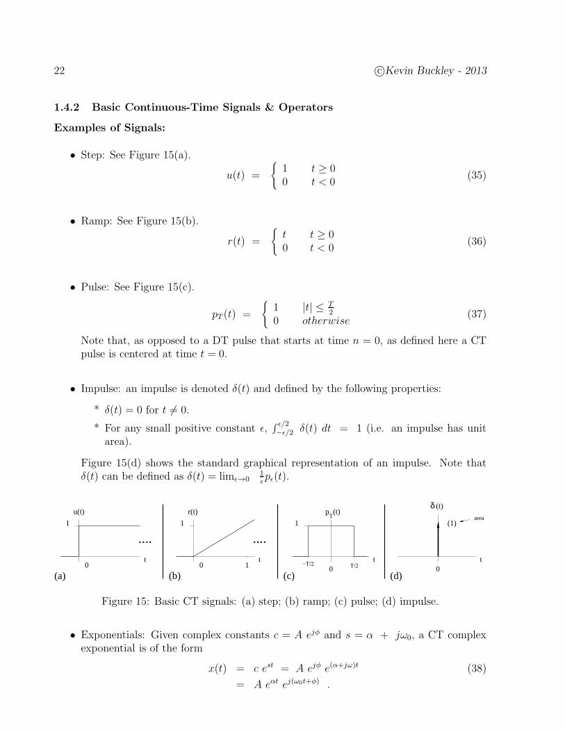
Examples of Signals:
• Step: See Figure 15(a).
u(t) =
1 t ≥ 00 t < 0
(35)
• Ramp: See Figure 15(b).
r(t) =
t t ≥ 00 t < 0
(36)
• Pulse: See Figure 15(c).
pT (t) =
1 |t| ≤ T2
0 otherwise(37)
Note that, as opposed to a DT pulse that starts at time n = 0, as defined here a CTpulse is centered at time t = 0.
• Impulse: an impulse is denoted δ(t) and defined by the following properties:
* δ(t) = 0 for t 6= 0.
* For any small positive constant ǫ,∫ ǫ/2−ǫ/2 δ(t) dt = 1 (i.e. an impulse has unit
area).
Figure 15(d) shows the standard graphical representation of an impulse. Note thatδ(t) can be defined as δ(t) = limǫ→0
1ǫpǫ(t).
t
u(t)
0
1
....
(a)
t0
1
(b)
r(t)
1
p (t)T
t
1
(c)0 T/2−T/2
(t)δ
....
t0
(d)
(1)area
Figure 15: Basic CT signals: (a) step; (b) ramp; (c) pulse; (d) impulse.
• Exponentials: Given complex constants c = A ejφ and s = α + jω0, a CT complexexponential is of the form
x(t) = c est = A ejφ e(α+jω)t (38)
= A eαt ej(ω0t+φ) .

c©Kevin Buckley - 2013 23
Basic Operators:
• Shift (delay): x(t) → x(t− τ)
• Fold: x(t) → x(−t)
• Fold and Shift: x(t) → x(τ − t)
• Multiplication & Addition: (point by point in time)
Example 1.10: Let x(t) = e−.5tu(t). Plot y(t) = x(4 − t).
Solution:
• Differentiation and Integration: Differentiation (i.e. slope calculation) is as defined inyour calculus course. Integration, defined as
y(t) =∫ t
−∞x(τ) dτ =
∫ ∞
0x(t− τ) dτ , (39)
is analogous to the accumulator for DT signals – for any time t you accumulate theinput up to that time.
Example 1.11: Differentiate the scaled step. Integrate the scaled impulse.
Solution:
d
dtc u(t) = c δ(t)
The slope is zero everywhere. The derivative at the discontinuity results inan impulse (infinite slope) with area equal to the height of the discontinuity.
∫ t
−∞c δ(τ) dτ = c u(t)
For t < 0 we are not integrating across the impulse. For t > 0 we areintegrating across the scaled impulse, which has area c.
t
cddt
t
(c)
t
(c) −8
( ) dt
τ
t
c
Figure 16: Differentiation and integration involving impulses.
24 c©Kevin Buckley - 2013
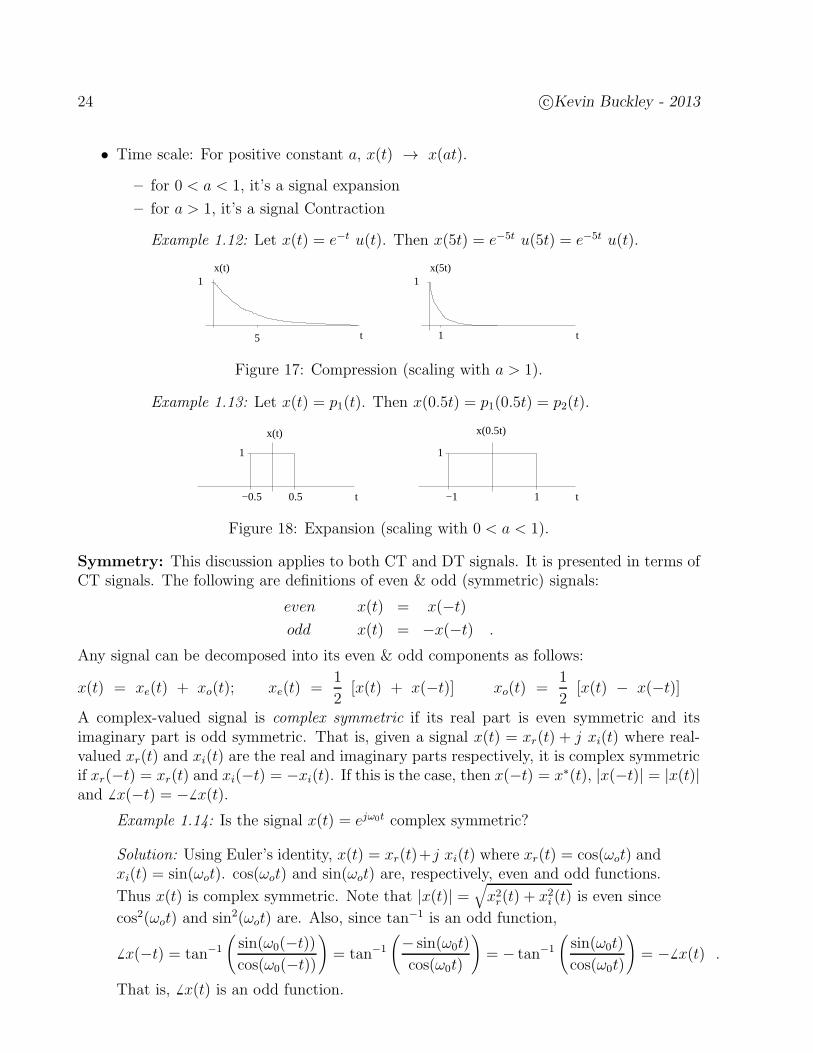
• Time scale: For positive constant a, x(t) → x(at).
– for 0 < a < 1, it’s a signal expansion
– for a > 1, it’s a signal Contraction
Example 1.12: Let x(t) = e−t u(t). Then x(5t) = e−5t u(5t) = e−5t u(t).
t
x(t)1
t
x(5t)1
5 1
Figure 17: Compression (scaling with a > 1).
Example 1.13: Let x(t) = p1(t). Then x(0.5t) = p1(0.5t) = p2(t).
tt
x(t) x(0.5t)
1
−1−0.5 0.5 1
1
Figure 18: Expansion (scaling with 0 < a < 1).
Symmetry: This discussion applies to both CT and DT signals. It is presented in terms ofCT signals. The following are definitions of even & odd (symmetric) signals:
even x(t) = x(−t)odd x(t) = −x(−t) .
Any signal can be decomposed into its even & odd components as follows:
x(t) = xe(t) + xo(t); xe(t) =1
2[x(t) + x(−t)] xo(t) =
1
2[x(t) − x(−t)]
A complex-valued signal is complex symmetric if its real part is even symmetric and itsimaginary part is odd symmetric. That is, given a signal x(t) = xr(t) + j xi(t) where real-valued xr(t) and xi(t) are the real and imaginary parts respectively, it is complex symmetricif xr(−t) = xr(t) and xi(−t) = −xi(t). If this is the case, then x(−t) = x∗(t), |x(−t)| = |x(t)|and 6 x(−t) = −6 x(t).
Example 1.14: Is the signal x(t) = ejω0t complex symmetric?
Solution: Using Euler’s identity, x(t) = xr(t)+j xi(t) where xr(t) = cos(ωot) andxi(t) = sin(ωot). cos(ωot) and sin(ωot) are, respectively, even and odd functions.
Thus x(t) is complex symmetric. Note that |x(t)| =√
x2r(t) + x2
i (t) is even since
cos2(ωot) and sin2(ωot) are. Also, since tan−1 is an odd function,
6 x(−t) = tan−1
(
sin(ω0(−t))cos(ω0(−t))
)
= tan−1
(
− sin(ω0t)
cos(ω0t)
)
= − tan−1
(
sin(ω0t)
cos(ω0t)
)
= −6 x(t) .
That is, 6 x(t) is an odd function.
c©Kevin Buckley - 2013 25
1.4.3 Signal Classes
A signal class is a set of signals sharing a common characteristic of interest. As a topic,signal classes is important because it differentiates the different transforms we will learn inthis course. That is, all transforms do basically the same thing – break complex signals intosimpler ones. We use different transforms on different classes of signals. Below we define thefollowing signal classes: DT, CT, energy, power and periodic.
• DT vs. CT Signals: As already established, DT signals are a function of a discrete-valued (i.e. integer-valued) parameter, say n. The set of all possible DT signals formsthe class of DT signals. It should be noted that although in this Course we refer tothese signals at discrete time, the important characteristic is that the independentparameter is discrete-valued. So, for example, in Practicums 1 & 2 we process rowsof an image the same way we process a DT signal, because the positions in a row areindexed as a discrete-valued variable.
Similarly, we refer to signals that are a function of a continuous-valued variable, say t,as CT signals. The set of all possible CT signals forms the class of CT signals.
• Energy Signals: For DT and CT signals, respectively, energy is defined as
E =∞∑
n=−∞|x[n]|2 (40)
E =∫ ∞
−∞|x(t)|2 dt (41)
An energy signal is a signal which has finite energy, i.e. E < ∞. The class of DTenergy signals, for example, is the set of all possible DT signals with E <∞.
Example 1.15: Is x[n] = .5n u[n + 3] an energy signal? Using the geometricseries,
E =∞∑
n=−3
(0.5n)2 =∞∑
n=−3
0.52n =∞∑
n=−3
(0.52)n =∞∑
n=−3
0.25n
=0.25−3 − 0
1− 0.25=
43
0.75= 85
1
3.
Note that x[n] has infinite duration, yet it has finite energy. So some infiniteduration signals have finite energy, but of course some don’t.
Question: Again, how in general does someone do a summation like the onerequired in Example 1.15? How do you do integrals?

26 c©Kevin Buckley - 2013
Example 1.16: Is x(t) = cos(10πt) an energy signals? What is its energy inone period?
Since x2(t) has infinite area, i.e. since clearly
E =∫ ∞
−∞cos2(10πt) dt = ∞ ,
x(t) is not an energy signal. Note that its energy over one period is
E1 period =∫ 1/5
0cos2(10πt) dt =
∫ 1/5
0
[
1
2+
1
2cos(20πt)
]
dt
=∫ 1/5
0
1
2dt +
∫ 1/5
0
1
2cos(20πt) dt =
1
10.
• Power Signals: For DT and CT signals, respectively, power is defined as
P = limN→∞
1
2N + 1
N∑
n=−N
|x[n]|2 (42)
P = limT→∞
1
2T
∫ T
−T|x(t)|2 dt (43)
That is, the power is the average energy over all time. A power signal is a signal whichhas nonzero but finite power, i.e. 0 < P < ∞. The class of CT power signals, forexample, is the set of all possible CT signals with 0 < P <∞.
The limits in Eqs (42,43) can be difficult to compute. Note, however, that in thisCourse we will be interested in only a subclass of power signals – periodic signals.We will talk more about periodic signals a little later. For now note that for periodicsignals with period N (for DT) or T (for CT), power can be computed, respectively,as follows:
P =1
N
N−1∑
n=0
|x[n]|2 (44)
P =1
T
∫ T
0|x(t)|2 dt . (45)
That is, the power is the average energy over a period. Note that average energy canbe computed over any period.
Example 1.17: Is x(t) = e−t u(t) a power signal?
Solution:
An energy signal has zero power, and a power signal has infinite energy.

c©Kevin Buckley - 2013 27
Example 1.18: Is x(t) =∑∞
k=−∞ p2(t− 4k) a power signal?
Solution:
x(t)
t3−1
....
4 51
....
−4
Figure 19: A periodic pulse train.
P =1
4
∫ 2
−2x2(t) dt =
1
4
∫ 1
−1dt =
1
2.
This signal has finite power (and thus infinite energy). It is a power signal.
Example 1.19: What is the power of the signal x[n] = 5?
Solution:
P = 52 = 25 .
The average energy of a constant signal is just the square of its amplitude.
Example 1.20: Determine the power of the signal x[n] =∑∞
k=−∞ x1[n−10k]where x1[n] = (−0.9)n p10[n].
Solution:
28 c©Kevin Buckley - 2013
1.4.4 Periodic Signals and Sinusoids
• General Definitions: First consider CT signals. Let T be a positive, real number.The CT signal x(t) is periodic if for all t and some T
x(t+ T ) = x(t) . (46)
The fundamental period T0 is the smallest T such that this equation holds. The fun-damental frequency, in radians/second, is ω0 =
2πT0.
For DT signals, Let N be a positive integer. The DT signal x[n] is periodic if for all nand some N
x[n +N ] = x[n] . (47)
The fundamental period N0 is the smallest N such that this equation holds. Thefundamental frequency, in radians/sample, is ω0 =
2πN0
.
• CT Sinusoids: A real-valued CT sinusoid has the form:
x(t) = A cos(ω0t + φ) (48)
where A is the amplitude, ω0 is the frequency (in radians/sec.), and φ is the phase (inradians). It is easy to show (using trigonometric identities or by plotting) that thissignal is periodic with fundamental period T0 =
2πω0. So the fundamental frequency, in
Hz, is f0 =ω0
2π= 1
T0.
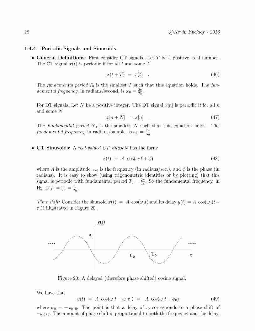
Time shift: Consider the sinusoid x(t) = A cos(ω0t) and its delay y(t) = A cos(ω0(t−τ0)) illustrated in Figure 20.
T0τ 0
.... ....
t
y(t)
A
Figure 20: A delayed (therefore phase shifted) cosine signal.
We have thaty(t) = A cos(ω0t− ω0τ0) = A cos(ω0t+ φ0) (49)
where φ0 = −ω0τ0. The point is that a delay of τ0 corresponds to a phase shift of−ω0τ0. The amount of phase shift is proportional to both the frequency and the delay.

c©Kevin Buckley - 2013 29
A complex-valued sinusoid is a special case of the CT exponential signal x(t) = c eαt ej(ω0t+φ)
introduced is Subsection 1.4.2 of these Notes. For the general CT exponential of Sub-section 1.4.2, let c = A and α = 0. We then have
x(t) = A ej(ω0t+φ) . (50)
As in Subsection 1.4.2, A is the amplitude, ω0 the frequency (in radians/second), andφ is the phase (in radians).
Is this signal periodic? Sure, let T = 2πω0. Then
x(t+T ) = A ej(ω0(t+T )+φ) = A ej(ω0t+φ+2π) = A ej(ω0t+φ) ej2π = A ej(ω0t+φ) . (51)
This proves it is periodic (i.e. that x(t+ T ) = x(t) for all t). The fundamental periodis T0 =
2πω0.
• DT Sinusoids: Real-valued DT sinusoids are of the form
x[n] = A cos(ω0n + φ) . (52)
Complex-valued DT sinusoids are of the form
x[n] = A ej(ω0n+φ) . (53)
A is the amplitude, ω0 the frequency (now in radians/sample), and φ is the phase (inradians).
Example 1.21: Let x[n] = ej0.5πn. Find the fundamental period N0.
Solution:
x[n +N0] = ej0.5π(n+N0) = ej0.5πn ej0.5πN0 .
For N0 = 4, ej0.5πN0 = ej2π = 1. Thus, for N0 = 4,
x[n +N0] = ej0.5πn = x[n] ∀n .
N0 = 4 is the smallest positive integer such that this is true. So, x[n] isperiodic (of course?) with fundamental period N0 = 4.
30 c©Kevin Buckley - 2013
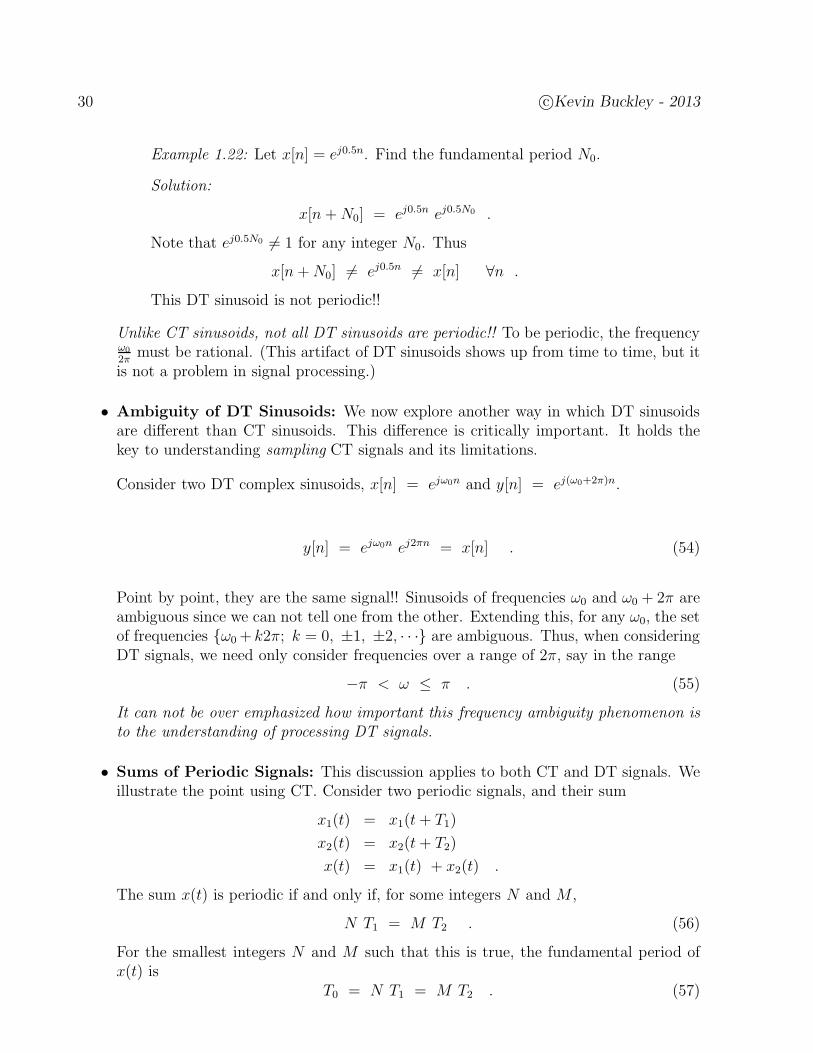
Example 1.22: Let x[n] = ej0.5n. Find the fundamental period N0.
Solution:
x[n +N0] = ej0.5n ej0.5N0 .
Note that ej0.5N0 6= 1 for any integer N0. Thus
x[n +N0] 6= ej0.5n 6= x[n] ∀n .
This DT sinusoid is not periodic!!
Unlike CT sinusoids, not all DT sinusoids are periodic!! To be periodic, the frequencyω0
2πmust be rational. (This artifact of DT sinusoids shows up from time to time, but it
is not a problem in signal processing.)
• Ambiguity of DT Sinusoids: We now explore another way in which DT sinusoidsare different than CT sinusoids. This difference is critically important. It holds thekey to understanding sampling CT signals and its limitations.
Consider two DT complex sinusoids, x[n] = ejω0n and y[n] = ej(ω0+2π)n.
y[n] = ejω0n ej2πn = x[n] . (54)
Point by point, they are the same signal!! Sinusoids of frequencies ω0 and ω0 + 2π areambiguous since we can not tell one from the other. Extending this, for any ω0, the setof frequencies ω0+ k2π; k = 0, ±1, ±2, · · · are ambiguous. Thus, when consideringDT signals, we need only consider frequencies over a range of 2π, say in the range
−π < ω ≤ π . (55)
It can not be over emphasized how important this frequency ambiguity phenomenon isto the understanding of processing DT signals.
• Sums of Periodic Signals: This discussion applies to both CT and DT signals. Weillustrate the point using CT. Consider two periodic signals, and their sum
x1(t) = x1(t+ T1)
x2(t) = x2(t+ T2)
x(t) = x1(t) + x2(t) .
The sum x(t) is periodic if and only if, for some integers N and M ,
N T1 = M T2 . (56)
For the smallest integers N and M such that this is true, the fundamental period ofx(t) is
T0 = N T1 = M T2 . (57)
c©Kevin Buckley - 2013 31
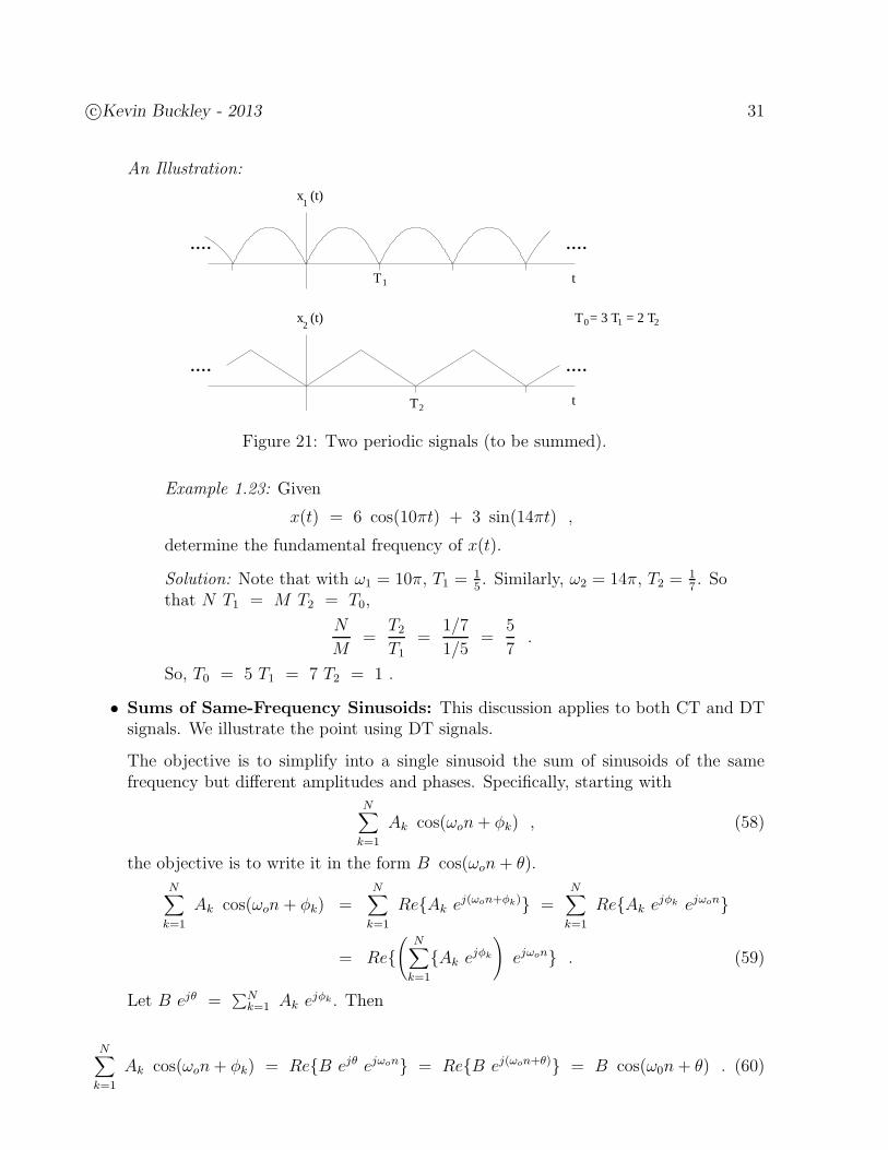
An Illustration:
T2
20T = 3 T = 2 T1
.... ....
t
x (t)2
.... ....
t
x (t)
T1
1
Figure 21: Two periodic signals (to be summed).
Example 1.23: Given
x(t) = 6 cos(10πt) + 3 sin(14πt) ,
determine the fundamental frequency of x(t).
Solution: Note that with ω1 = 10π, T1 =15. Similarly, ω2 = 14π, T2 =
17. So
that N T1 = M T2 = T0,
N
M=
T2
T1=
1/7
1/5=
5
7.
So, T0 = 5 T1 = 7 T2 = 1 .
• Sums of Same-Frequency Sinusoids: This discussion applies to both CT and DTsignals. We illustrate the point using DT signals.
The objective is to simplify into a single sinusoid the sum of sinusoids of the samefrequency but different amplitudes and phases. Specifically, starting with
N∑
k=1
Ak cos(ωon+ φk) , (58)
the objective is to write it in the form B cos(ωon+ θ).
N∑
k=1
Ak cos(ωon + φk) =N∑
k=1
ReAk ej(ωon+φk) =N∑
k=1
ReAk ejφk ejωon
= Re(
N∑
k=1
Ak ejφk
)
ejωon . (59)
Let B ejθ =∑N
k=1 Ak ejφk . Then
N∑
k=1
Ak cos(ωon+ φk) = ReB ejθ ejωon = ReB ej(ωon+θ) = B cos(ω0n+ θ) . (60)

32 c©Kevin Buckley - 2013
1.4.5 Basic Signal Sets and Transforms
In Section 1.3 we introduced the general concept of representing a signal as a linear com-bination of basic signals. Now that we have introduced a number of basic signals, we candescribe the main topics of this Course in terms of this general concept.
The main topics of this Course are the entries of the third column of Table 2. The purposeof this table is to show that each of these topics can be interpreted in terms of a process ofrepresenting a general class of signals (listed in the second column) as a linear combination(i.e. a weighted sum) of a set of basic signals (listed in the first column). The first four rowsrepresent CT signals and systems topics. The last four rows represent DT topics. For boththe CT and the DT entries, the first row leads to a very useful time domain approach tosystems analysis called convolution. This is the topic of Chapter 2 of this Course. The lastthree rows of both the CT and the DT entries of Table 2 represent transforms. Note that themajority of these transforms concern the representation of signals as linear combinations ofcomplex-valued sinusoids. These transforms, which facilitate transform domain approachesto signal & system design & analysis, will be covered in Chapters 3 & 5 of this Course.
Table 2: Basic signal sets and corresponding transforms.
Signal Set Class Represents Transform
δ(t− τ) ; −∞ ≤ τ ≤ ∞ all CT signals none, but leads to convolution
ejkω0t ; k = 0,±1,±2, · · · all periodic CT signals CT Fourier Series (CTFS)ω0 =
2πT
with period T
ejωt ; −∞ ≤ ω ≤ ∞ all CT energy signals CT Fourier Transform (CTFT)
est ; all complex s all CT signals Laplace Transform (LT)
δ[n− k] ; k = 0,±1,±2, · · · all DT signals none, but leads to convolution
ejkω0n ; k = 0, 1, · · · , N − 1 all periodic DT signals DT Fourier Series (DTFS)ω0 =
2πN
with period N
ejωn ; −π ≤ ω ≤ π all DT energy signals DT Fourier Transform (DTFT)
zn ; all complex z all DT signals z-Transform (ZT)
c©Kevin Buckley - 2013 33
Consider, for example, entry #3 of Table 2 – the Continuous Time Fourier Transform(CTFT). This entry suggests that the CTFT can be employed to represent any CT energysignal as a linear combination of the CT complex-valued sinusoids ejωt were we use allfrequency over the continuum of range −∞ ≤ ω ≤ ∞. When we study the CTFT wewill see specifically how to do this. Generally, we need to identify the weighting on eachCT complex-valued sinusoid that is required to represent a CT energy signal x(t) underconsideration. For this x(t), denote this weighting function as X(ω). X(ω) is a functionof frequency ω since we need to weight each sinusoid differently in order to represent thegiven x(t). To represent an x(t), Entry #3 of Table 2 indicates that in general we will needto identify X(ω) over the entire range −∞ ≤ ω ≤ ∞. Then, following the idea of linearcombinations proposed in Subsection 1.3, Entry #3 of Table 2 suggests that we can constructthis x(t) from CT complex-valued sinusoids as follows:
x(t) =∫ ∞
−∞X(ω) ejωt dω . (61)
In this equation, the ejωt are the basic signals being used to represent or construct the generalsignal x(t). X(ω) is the function that describes the weighting applied to each basic signal.The integral does the combining (summing) of the weighted basic signals, and implies thatwe need basic signals defined over a continuum (of frequency in this case). The integralbounds indicate that the continuum goes from −∞ to ∞ (in this case, in frequency).
In this Course we will establish how to determine the weighting functions for these trans-forms. This is relatively easy once you are comfortable with this general idea of a transform.We will also consider how this basic idea, and these specific transforms, are employed for awide range of signal and system design and analysis problems. At this point consider, as anexample, that for those transforms that use complex-valued sinusoids as the basic signals,the weighting function tells us the frequency content of the signal. That is, computing theweighting function is equivalent to performing spectrum estimation (i.e. frequency analysis).
Example 1.24: You are interested in the amount of base and treble in a score ofmusic you have recorded on an analog tape. Specifically, of the transforms listedin Table 2, which would you use to determine the frequency content of a onesecond segment of your music signal.
Solution: On the one hand, your music is stored as a CT signal, and one secondof music will be an energy signal. This suggests that the CTFT (Entry #3 ofTable 2) could be used.
On the other hand, if you have an A/D converter that you can apply to yourstored music (e.g. a sound card on your laptop), and you wish to process yoursignal digitally (e.g. with Matlab), then you will be working with a DT energysignal. So perhaps it is the DTFT (Entry # 7 of Table 2) that you are interestedin.
34 c©Kevin Buckley - 2013
1.5 Linear Time-Invariant (LTI) Systems
The term system can mean a lot of different things. As considered in this Course, a systemoperates on an input signal to generate an output signal. The system input/output (I/O)characterization is a description of how the system maps inputs to outputs. Although ingeneral there are other important system considerations – for example how they are imple-mented/applied and what happens internal to a system – in this Course we will focus on I/Ocharacterizations. However, we will be implementing a number of DT systems in Matlaband discuss applications from time to time in class.
We begin this Subsection by briefly considering a number of common DT and CT systems.We then identify several important system characteristics. Linearity, which we have alreadyconsidered informally, is one of these. Time-invariance is another. We will conclude byintroducing one very common type of system - the linear, time-invariant (LTI) system.
1.5.1 System Examples
Since I/O characterization of systems is a central theme of this Course, with each systemexample below some aspect of I/O is discussed.
An RC Circuit: Consider the RC circuit discussed in Subsection 1.2.2 above. An I/Oequation for it, which is equivalent to Eq (5), is y(t) =
∫ t−∞
1Ce−(t−τ)/RC x(τ) dτ .
Example 1.25: For this RC circuit, determine an expression for its output forcomplex sinusoidal input x(t) = ejω0t.
Solution:

c©Kevin Buckley - 2013 35
Simple DT Feedback System
In Subsection 1.1.2 and in Practicum 1 we considered a DT system which fed back thepresent output through a multiplier to compute the next output. In Figure 22 we generalizethis system by using a arbitrary multiplier with value a. In equation form, the I/O is
y[n] = a y[n− 1] + x[n] . (62)
delay
x[n] +
+
y[n]
D
adder
y[n−1]
multiplier
a y[n−1]a
Figure 22: A simple DT system.
One thing we did in Subsection 1.1.2 was to compute the impulse response. (i.e. theresponse due to x[n] = δ[n]). We will see that the impulse response of a system is a veryuseful characterization of the system – so much so that we give it its own notation. In thisCourse we will follow convention by denoting the impulse response of a DT system h[n] (weuse h(t) for a CT system). The impulse response of the system in Figure 22 is
h[n] = an u[n] . (63)
We will learn to do a lot with the impulse response, both to compute system outputs togeneral inputs, and to study system properties. For now note that if |a| > 1, the impulseresponse magnitude gets bigger as n increases – i.e. it “blows up”. A system whose outputblows up for any expected or reasonable input should be avoided.
N Point Averagers and Finite Impulse Response (FIR) Filters
An N point averager is a DT system that averages the N most recent inputs to producethe current output. That is,
y[n] =N−1∑
k−0
1
Nx[n− k] =
1
N
N−1∑
k−0
x[n− k] . (64)
Averagers are used quite a bit in signal processing, for example to smooth signals. Oneattractive computational aspect of this system is that it requires only one multiply peroutput. Although we apply the 1
Nmultiplier once per output to the sum of the N most
recent inputs, effectively we are applying the multiplier to each input used to compute theoutput (i.e. to the current and past N − 1 inputs). Also note that, in Eq (64), both n andk represent time – n output time, and k memory time.
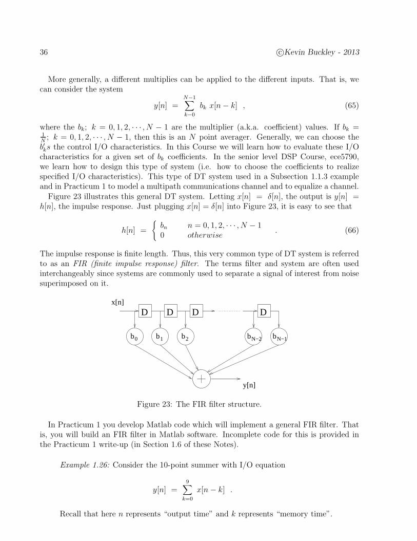
36 c©Kevin Buckley - 2013
More generally, a different multiplies can be applied to the different inputs. That is, wecan consider the system
y[n] =N−1∑
k−0
bk x[n− k] , (65)
where the bk; k = 0, 1, 2, · · · , N − 1 are the multiplier (a.k.a. coefficient) values. If bk =1N; k = 0, 1, 2, · · · , N − 1, then this is an N point averager. Generally, we can choose the
b′ks the control I/O characteristics. In this Course we will learn how to evaluate these I/Ocharacteristics for a given set of bk coefficients. In the senior level DSP Course, ece5790,we learn how to design this type of system (i.e. how to choose the coefficients to realizespecified I/O characteristics). This type of DT system used in a Subsection 1.1.3 exampleand in Practicum 1 to model a multipath communications channel and to equalize a channel.
Figure 23 illustrates this general DT system. Letting x[n] = δ[n], the output is y[n] =h[n], the impulse response. Just plugging x[n] = δ[n] into Figure 23, it is easy to see that
h[n] =
bn n = 0, 1, 2, · · · , N − 10 otherwise
. (66)
The impulse response is finite length. Thus, this very common type of DT system is referredto as an FIR (finite impulse response) filter. The terms filter and system are often usedinterchangeably since systems are commonly used to separate a signal of interest from noisesuperimposed on it.
D D D D
b0 b1 b2
x[n]
y[n]
b bN−1N−2
Figure 23: The FIR filter structure.
In Practicum 1 you develop Matlab code which will implement a general FIR filter. Thatis, you will build an FIR filter in Matlab software. Incomplete code for this is provided inthe Practicum 1 write-up (in Section 1.6 of these Notes).
Example 1.26: Consider the 10-point summer with I/O equation
y[n] =9∑
k=0
x[n− k] .
Recall that here n represents “output time” and k represents “memory time”.

c©Kevin Buckley - 2013 37
a) What is the impulse response, h[n], for this system? Rewrite the I/O equa-tion given above using the general h[n] notation.
b) Sketch this FIR filter twice, once using the general h[n] notation and oncefor the specific h[n]. For general time n, label each delay line node with thecorrect delayed x[n].
c) Visualize the input shifted through this system. To do this plot the impulseresponse as a function of k (i.e. plot h[k]). Now, sketch some input x[n].For this input, directly below your h[k] plot, sketch x[n − k] as a functionof k for n = 0. Now visualize how x[n− k] shifts by h[k] as n varies.
d) Using your part c) visualization, write down the expression for y[n] as a sumof the products, over k, of the samples in your h[k] and x[n− k] plots.
e) Use the visualization you developed in part c) to determine the output ofthis 10-point summer for input x[n] = p20[n].
Solution:
38 c©Kevin Buckley - 2013
Concerning part b), note that h[n] depicts the memory structure of this system(i.e. it shows how the system operates on each input in the system memory toform the output).
Concerning part c), the data in your x[n − k]; n = 0 plot over the range k =0, 1, · · · , 9 is the data in the FIR filter delay line at time n = 0. This data linesup with the FIR filter multipliers plotted in h[k]. In terms of the basic signaloperators discussed in Subsection 1.4.1, as a function of memory time k, x[n−k]is folded and shifted by h[k]. That is, the input is folded and then shifted throughthe memory structure of the system.
Concerning part d), the result is just your FIR filter I/O equation from part a).
What this example develops is a general process for determining the output to anFIR filter. It involves: 0) plotting h[k], the impulse response as a function of k;1) plotting x[n− k]; n = 0 as a function of k (i.e. folding the input); 2) shiftingthe input by the impulse response (i.e. shifting the input); 3) multiplying h[k]and x[n − k] for each output time n of interest; and 4) adding this multiplierresults to form the output.
You are already familiar with the steps of this process (they are basic operatorsintroduced and exemplified in Subsection 1.4.1). This process, which we willformalize and generalize in Chapter 2, is called convolution. Convolution is theprinciple topic of Chapter 2. So if you take the time to understand this examplenow, you will be well on your way to mastering Chapter 2 of this Course.
Example 1.27: Consider the N point averager described in Subsection 1.5.1 asan example of a system. This is an FIR filter. Determine an expression for itsoutput for complex sinusoidal input x[n] = ejω0n.
Solution:
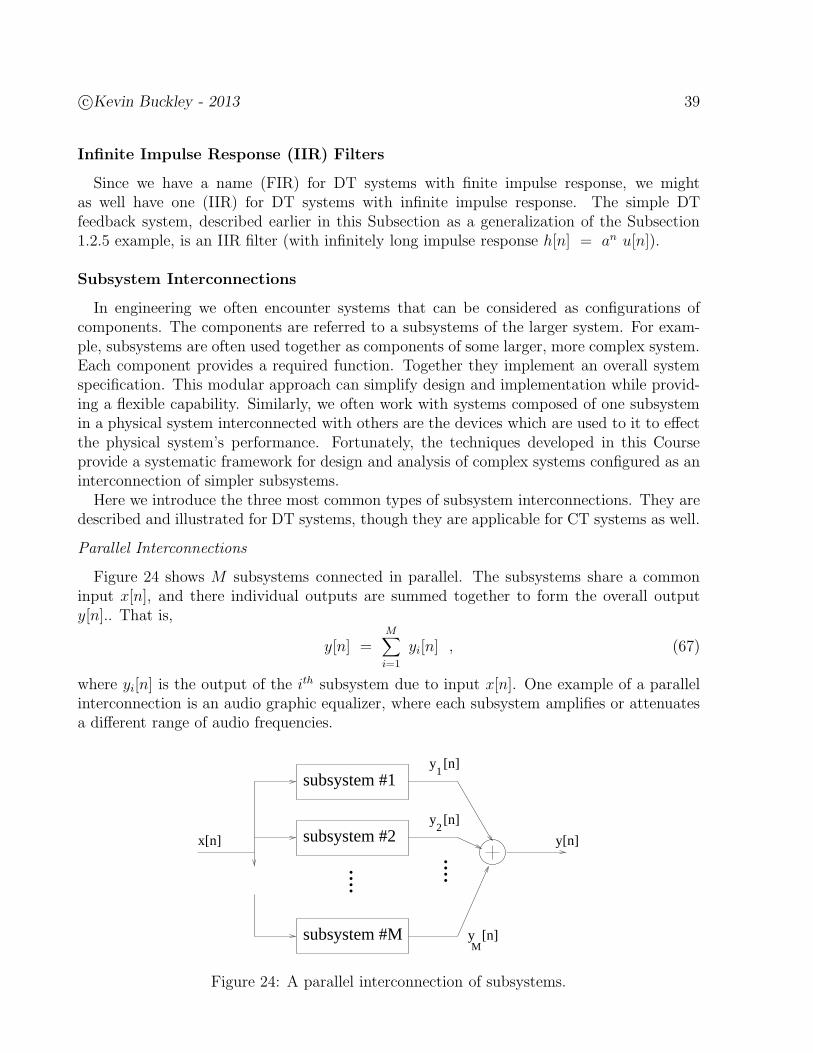
c©Kevin Buckley - 2013 39
Infinite Impulse Response (IIR) Filters
Since we have a name (FIR) for DT systems with finite impulse response, we mightas well have one (IIR) for DT systems with infinite impulse response. The simple DTfeedback system, described earlier in this Subsection as a generalization of the Subsection1.2.5 example, is an IIR filter (with infinitely long impulse response h[n] = an u[n]).
Subsystem Interconnections
In engineering we often encounter systems that can be considered as configurations ofcomponents. The components are referred to a subsystems of the larger system. For exam-ple, subsystems are often used together as components of some larger, more complex system.Each component provides a required function. Together they implement an overall systemspecification. This modular approach can simplify design and implementation while provid-ing a flexible capability. Similarly, we often work with systems composed of one subsystemin a physical system interconnected with others are the devices which are used to it to effectthe physical system’s performance. Fortunately, the techniques developed in this Courseprovide a systematic framework for design and analysis of complex systems configured as aninterconnection of simpler subsystems.
Here we introduce the three most common types of subsystem interconnections. They aredescribed and illustrated for DT systems, though they are applicable for CT systems as well.
Parallel Interconnections
Figure 24 shows M subsystems connected in parallel. The subsystems share a commoninput x[n], and there individual outputs are summed together to form the overall outputy[n].. That is,
y[n] =M∑
i=1
yi[n] , (67)
where yi[n] is the output of the ith subsystem due to input x[n]. One example of a parallelinterconnection is an audio graphic equalizer, where each subsystem amplifies or attenuatesa different range of audio frequencies.
y [n]1
x[n] y[n]
subsystem #1
subsystem #2
subsystem #M
y [n]2
y [n]M
....
....
Figure 24: A parallel interconnection of subsystems.
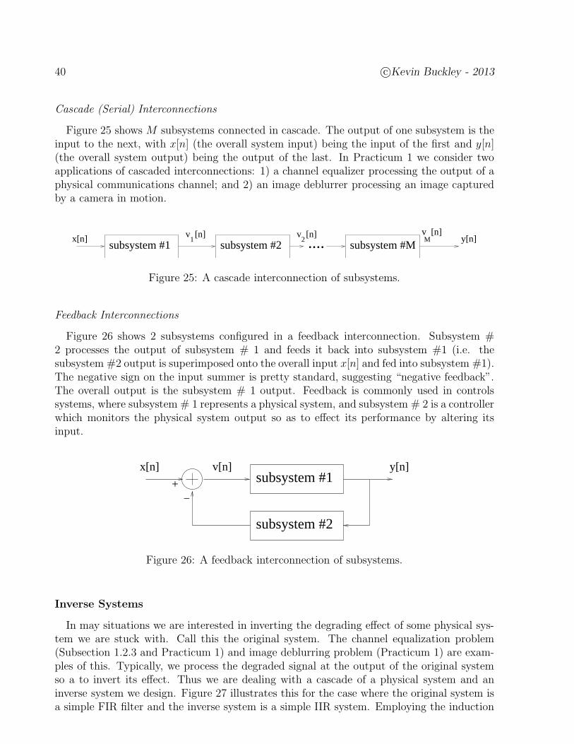
40 c©Kevin Buckley - 2013
Cascade (Serial) Interconnections
Figure 25 shows M subsystems connected in cascade. The output of one subsystem is theinput to the next, with x[n] (the overall system input) being the input of the first and y[n](the overall system output) being the output of the last. In Practicum 1 we consider twoapplications of cascaded interconnections: 1) a channel equalizer processing the output of aphysical communications channel; and 2) an image deblurrer processing an image capturedby a camera in motion.
subsystem #11
v [n]2
v [n]Mv [n]
subsystem #2 subsystem #My[n]....x[n]
Figure 25: A cascade interconnection of subsystems.
Feedback Interconnections
Figure 26 shows 2 subsystems configured in a feedback interconnection. Subsystem #2 processes the output of subsystem # 1 and feeds it back into subsystem #1 (i.e. thesubsystem #2 output is superimposed onto the overall input x[n] and fed into subsystem #1).The negative sign on the input summer is pretty standard, suggesting “negative feedback”.The overall output is the subsystem # 1 output. Feedback is commonly used in controlssystems, where subsystem # 1 represents a physical system, and subsystem # 2 is a controllerwhich monitors the physical system output so as to effect its performance by altering itsinput.
subsystem #1
subsystem #2
v[n]x[n] y[n]
−+
Figure 26: A feedback interconnection of subsystems.
Inverse Systems
In may situations we are interested in inverting the degrading effect of some physical sys-tem we are stuck with. Call this the original system. The channel equalization problem(Subsection 1.2.3 and Practicum 1) and image deblurring problem (Practicum 1) are exam-ples of this. Typically, we process the degraded signal at the output of the original systemso a to invert its effect. Thus we are dealing with a cascade of a physical system and aninverse system we design. Figure 27 illustrates this for the case where the original system isa simple FIR filter and the inverse system is a simple IIR system. Employing the induction
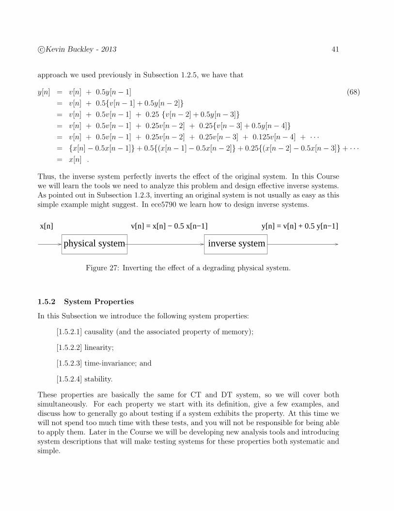
c©Kevin Buckley - 2013 41
approach we used previously in Subsection 1.2.5, we have that
y[n] = v[n] + 0.5y[n− 1] (68)
= v[n] + 0.5v[n− 1] + 0.5y[n− 2]= v[n] + 0.5v[n− 1] + 0.25 v[n− 2] + 0.5y[n− 3]= v[n] + 0.5v[n− 1] + 0.25v[n− 2] + 0.25v[n− 3] + 0.5y[n− 4]= v[n] + 0.5v[n− 1] + 0.25v[n− 2] + 0.25v[n− 3] + 0.125v[n− 4] + · · ·= x[n]− 0.5x[n− 1]+ 0.5(x[n− 1]− 0.5x[n− 2]+ 0.25(x[n− 2]− 0.5x[n− 3]+ · · ·= x[n] .
Thus, the inverse system perfectly inverts the effect of the original system. In this Coursewe will learn the tools we need to analyze this problem and design effective inverse systems.As pointed out in Subsection 1.2.3, inverting an original system is not usually as easy as thissimple example might suggest. In ece5790 we learn how to design inverse systems.
physical system inverse system
v[n] = x[n] − 0.5 x[n−1] x[n] y[n] = v[n] + 0.5 y[n−1]
Figure 27: Inverting the effect of a degrading physical system.
1.5.2 System Properties
In this Subsection we introduce the following system properties:
[1.5.2.1] causality (and the associated property of memory);
[1.5.2.2] linearity;
[1.5.2.3] time-invariance; and
[1.5.2.4] stability.
These properties are basically the same for CT and DT system, so we will cover bothsimultaneously. For each property we start with its definition, give a few examples, anddiscuss how to generally go about testing if a system exhibits the property. At this time wewill not spend too much time with these tests, and you will not be responsible for being ableto apply them. Later in the Course we will be developing new analysis tools and introducingsystem descriptions that will make testing systems for these properties both systematic andsimple.
42 c©Kevin Buckley - 2013
1.5.2.1 Causality (and the associated property of memory)
Causality: A system is causal it, for any time t1 (or n1), the output y(t1) (or y[n1]) innot a function of inputs x(t) for times t > t1 (or x[n] for times n > n1). That is: thepresent output is not a function of future inputs.
Test: Basically by inspection. (The right system I/O description makes it easy.) A“real-time system”, that operates on inputs as they occur to generate outputs, mustbe causal. However it is possible and not uncommon to implement concausal systemswhich process input data that is stored, say on a CD.
Example 1.28: The following is an I/O expression for a parallel RC circuit(see Subsection 1.5.1 above). Is this circuit casual?
y(t) =∫ t
0
1
Ce−
1RC
(t−τ) x(τ) dτ t > 0
Solution: Yes. From the I/O equation, note that for time t > 0 only thepresent and past input is used to compute the present output, i.e. for y(t),only x(τ); 0 ≤ τ ≤ t is used.
Example 1.29: Is each of the following accumulators causal?
a) y1[n] =∑∞
k=0 x1[n − k]. Solution: Yes, only x1[k]; −∞ ≤ k ≤ n isused to compute y1[n].
b) y2[n] =∑n+1
k=−∞ x2[k]. Solution: No, x2[n+1] is used to compute y2[n].
Memory (stated for CT, but applicable for DT too): A system is memoryless if theoutput y(t) at any time t1 is a function of the input x(t) for only that time t1. Asystem has memory if: any present output is a function of either past or future inputs.
Example 1.30: Do the following systems have memory?
a) y(t) = cos(x(t)). Solution: No, the output at time t is a function ofthe input for only time t.
b) y[n] = x[n+1]. Solution: Yes, this system “remembers” 1 sample intothe future. It has negative memory, so it is noncausal.
c) y(t) = ddt
x(t). Solution: Yes, from circuits we know that ddt
meansinput energy storage. The slope of a CT signal at a given time dependson values of that signal incrementally close to that time.
For some system I/O descriptions, i.e. for the RC circuit in Example 1.28 and theaccumulators in Example 1.29, the memory structure is obvious. For example, withthe accumulator I/O expressions, you can see by inspection of the range of memorytime k what inputs effect the output at output (or current) time n. Similarly, for theRC circuit, τ represents memory time and t output (or current) time. With other I/Odescriptions, the memory structure might be less obvious.
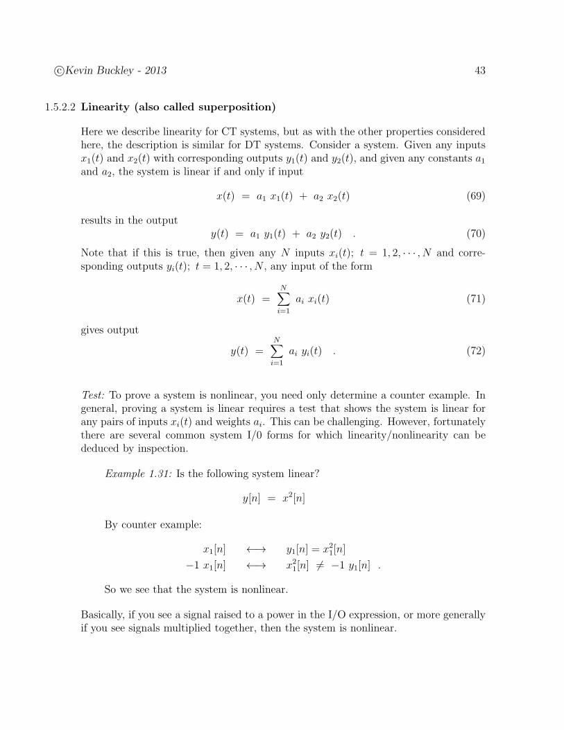
c©Kevin Buckley - 2013 43
1.5.2.2 Linearity (also called superposition)
Here we describe linearity for CT systems, but as with the other properties consideredhere, the description is similar for DT systems. Consider a system. Given any inputsx1(t) and x2(t) with corresponding outputs y1(t) and y2(t), and given any constants a1and a2, the system is linear if and only if input
x(t) = a1 x1(t) + a2 x2(t) (69)
results in the outputy(t) = a1 y1(t) + a2 y2(t) . (70)
Note that if this is true, then given any N inputs xi(t); t = 1, 2, · · · , N and corre-sponding outputs yi(t); t = 1, 2, · · · , N , any input of the form
x(t) =N∑
i=1
ai xi(t) (71)
gives output
y(t) =N∑
i=1
ai yi(t) . (72)
Test: To prove a system is nonlinear, you need only determine a counter example. Ingeneral, proving a system is linear requires a test that shows the system is linear forany pairs of inputs xi(t) and weights ai. This can be challenging. However, fortunatelythere are several common system I/0 forms for which linearity/nonlinearity can bededuced by inspection.
Example 1.31: Is the following system linear?
y[n] = x2[n]
By counter example:
x1[n] ←→ y1[n] = x21[n]
−1 x1[n] ←→ x21[n] 6= −1 y1[n] .
So we see that the system is nonlinear.
Basically, if you see a signal raised to a power in the I/O expression, or more generallyif you see signals multiplied together, then the system is nonlinear.
44 c©Kevin Buckley - 2013
Example 1.32: Given that a CT system is linear, and given the following twoI/O pairs, if possible determine the output due to the each of the two inputsshown.
x (t)1
t
1y (t)
y (t)2
t
t
t
x (t)
t
−1 1 3
1
1/2
2
1−1
1
x (t)2
3
x (t)4
1
−1 2
1
t1 3 1 2 3 4
1
−1/2
Solution:
Figure 28: Assuming linearity, given outputs for x1(t) and x2(t), what are the outputs forx3(t) and x4(t)?
Example 1.32 illustrates the power of linearity. Given the response of a linear systemto two inputs, we know its response to any linear combination of those two inputs.This is useful and important enough that, if possible, we would like to work with (i.e.develop or interact with) linear systems. This example also shows that linearity, byitself, has its limitations.
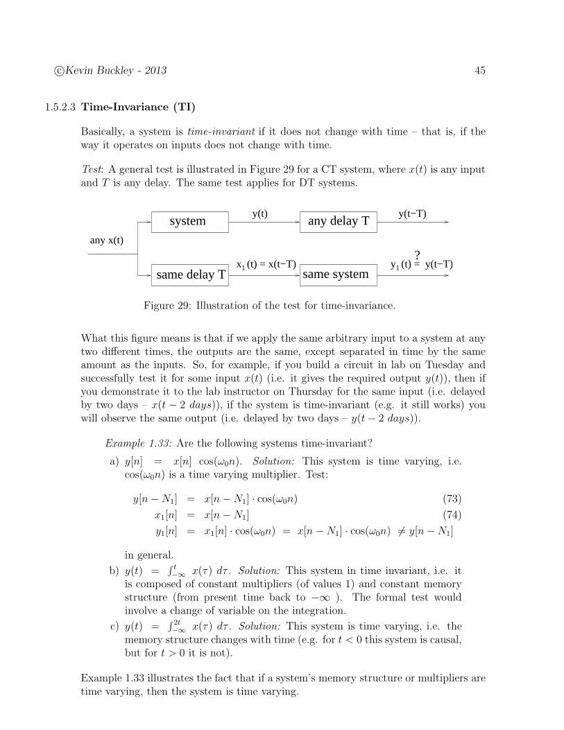
c©Kevin Buckley - 2013 45
1.5.2.3 Time-Invariance (TI)
Basically, a system is time-invariant if it does not change with time – that is, if theway it operates on inputs does not change with time.
Test: A general test is illustrated in Figure 29 for a CT system, where x(t) is any inputand T is any delay. The same test applies for DT systems.
system
same delay T same system
any delay Ty(t) y(t−T)
any x(t)
11x (t) = x(t−T) y (t) = y(t−T)?
Figure 29: Illustration of the test for time-invariance.
What this figure means is that if we apply the same arbitrary input to a system at anytwo different times, the outputs are the same, except separated in time by the sameamount as the inputs. So, for example, if you build a circuit in lab on Tuesday andsuccessfully test it for some input x(t) (i.e. it gives the required output y(t)), then ifyou demonstrate it to the lab instructor on Thursday for the same input (i.e. delayedby two days – x(t − 2 days)), if the system is time-invariant (e.g. it still works) youwill observe the same output (i.e. delayed by two days – y(t− 2 days)).
Example 1.33: Are the following systems time-invariant?
a) y[n] = x[n] cos(ω0n). Solution: This system is time varying, i.e.cos(ω0n) is a time varying multiplier. Test:
y[n−N1] = x[n−N1] · cos(ω0n) (73)
x1[n] = x[n−N1] (74)
y1[n] = x1[n] · cos(ω0n) = x[n−N1] · cos(ω0n) 6= y[n−N1]
in general.
b) y(t) =∫ t−∞ x(τ) dτ . Solution: This system in time invariant, i.e. it
is composed of constant multipliers (of values 1) and constant memorystructure (from present time back to −∞ ). The formal test wouldinvolve a change of variable on the integration.
c) y(t) =∫ 2t−∞ x(τ) dτ . Solution: This system is time varying, i.e. the
memory structure changes with time (e.g. for t < 0 this system is causal,but for t > 0 it is not).
Example 1.33 illustrates the fact that if a system’s memory structure or multipliers aretime varying, then the system is time varying.

46 c©Kevin Buckley - 2013
Example 1.34: Given a CT TI system, and given the following I/O pair, ifpossible determine the output due to the each of the two inputs shown.
1y (t)x (t)1
t
t
t
x (t)
−1
1
1/2
1−1
1
x (t)2
3
−1 2
1
1 3
t
31
−1.2
Solution:
Figure 30: Assuming time-invariance, given the output for x1(t), what are the outputs forx2(t) and x3(t)?
Example 1.35 shows the power of time-invariance. Given the response of a TI systemto any input, we know its response to any delayed version of that input. This is usefuland important enough that, if possible, we would prefer to work with TI systems. Thisexample also shows that time-invariance, by itself, has its limitations.
Example 1.35: Given a CT LTI system, and given the impulse response h(t)shown below, if possible determine the output due to the inputs shown.
τ0
τ0
h(t)
t
1
x(t)
−T 2T t
1
T 2T−T
.... .... .... ....
y(t)
t T
Solution:
( )δ t
t
(1)
(1)
Figure 31: An LTI system and the impulse I/O pair.Examples 1.32 & 1.34 illustrate that linearity and time-invariance are usefuland desirable system properties, though separately they are limited. Ex-ample 1.35 shows that together they can be quite powerful – if you knowthe response to one input, you know the response to any linear combinationof all the delays of that one input. Example 1.36 (below) also shows this.As a result, in engineering, Linear Time-Invariance (LTI) systems are verycommon. In Subsection 1.5.3 we will expand on this idea of a LTI system.

c©Kevin Buckley - 2013 47
Example 1.36: Given an DT LTI system, and given that input p2[n] producesoutput p4[n], if possible determine the output due to the given x[n].
2p [n]
p [n−1]2
n1 2
n0 1 0 1 2 3 n
10=
n2
x[n]
+
0 1 2 3 n4
+
=
y[n]
0 1 2 3 n4
Solution:
Figure 32: An LTI system and the impulse I/O pair.
1.5.2.4 Stability
Bounded-Input Bounded-Output (BIBO) Stability is the only definition of stability ofconcern in this course. A system is BIBO stable if and only if for any bounded input,i.e. for any x[n] such that
|x[n]| < B1 , ∀n (75)
where B1 is finite, the output is bounded, i.e.
|y[n]| < B2 , ∀n (76)
where B2 is finite. (Note that the notation ∀n reads “for all n”.) This definition appliesto CT systems too.
Test: For now, we can prove a system is not BIBO stable via counter example (i.e.find one bounded input that results in an unbounded output). We can show that asystem is BIBO stable by showing it is BIBO stable for the worst possible input case.Later, when we have easy I/O descriptions to work with, the test (for some types ofsystems) will be much easier.
Example 1.37: Is the following system stable?
y(t) =∫ t
−∞x(τ) dτ
Solution: No. Proof is by counter example. Let x(t) = u(t), which isbounded.
y(t) =
0 t < 0∫ t0 dr = t t ≥ 0
.
So, limt→∞ y(t) =∞, which is unbounded.
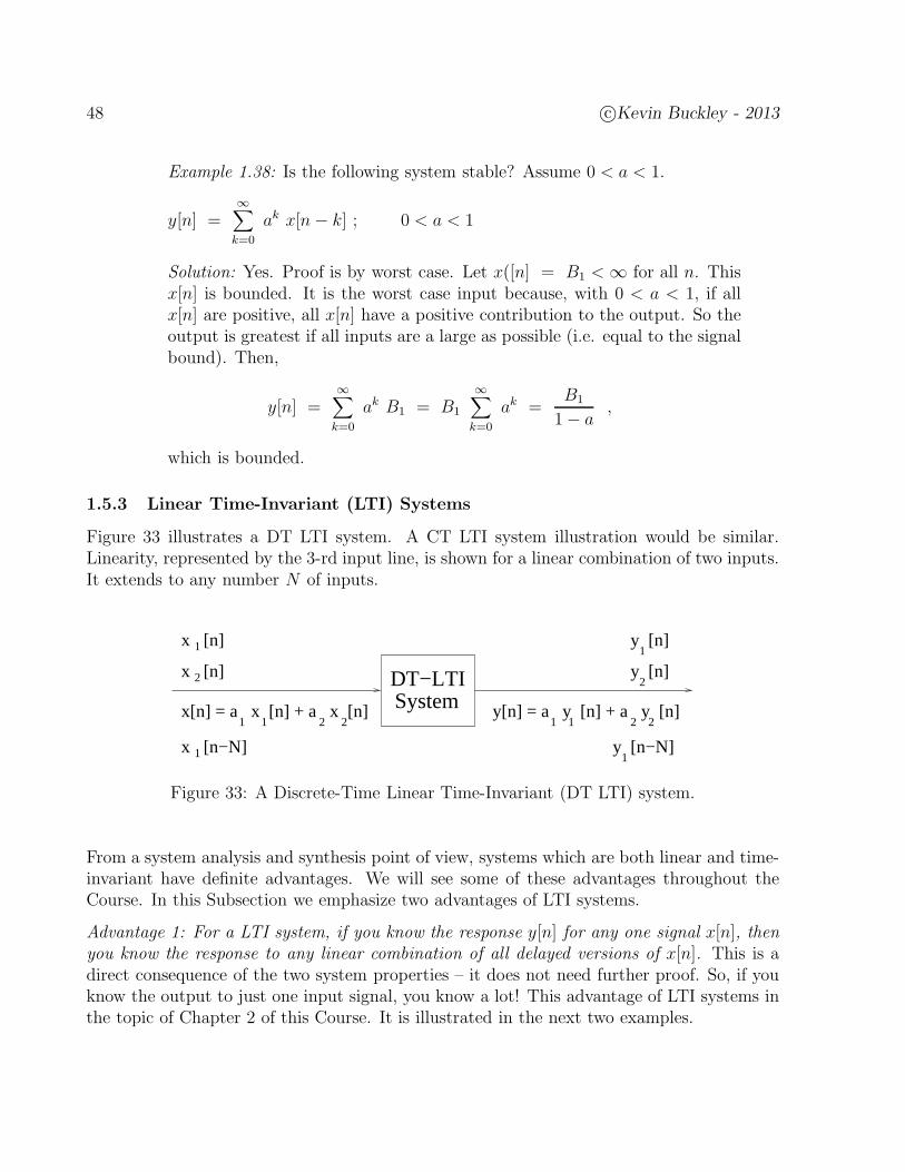
48 c©Kevin Buckley - 2013
Example 1.38: Is the following system stable? Assume 0 < a < 1.
y[n] =∞∑
k=0
ak x[n− k] ; 0 < a < 1
Solution: Yes. Proof is by worst case. Let x([n] = B1 <∞ for all n. Thisx[n] is bounded. It is the worst case input because, with 0 < a < 1, if allx[n] are positive, all x[n] have a positive contribution to the output. So theoutput is greatest if all inputs are a large as possible (i.e. equal to the signalbound). Then,
y[n] =∞∑
k=0
ak B1 = B1
∞∑
k=0
ak =B1
1− a,
which is bounded.
1.5.3 Linear Time-Invariant (LTI) Systems
Figure 33 illustrates a DT LTI system. A CT LTI system illustration would be similar.Linearity, represented by the 3-rd input line, is shown for a linear combination of two inputs.It extends to any number N of inputs.
1y [n]
y [n]2
y [n−N]1
1x [n]
x [n]2
1x [n−N]
SystemDT−LTI
x[n] = a x [n] + a x [n]1 1
y[n] = a y [n] + a y [n]1 1 2 2 2 2
Figure 33: A Discrete-Time Linear Time-Invariant (DT LTI) system.
From a system analysis and synthesis point of view, systems which are both linear and time-invariant have definite advantages. We will see some of these advantages throughout theCourse. In this Subsection we emphasize two advantages of LTI systems.
Advantage 1: For a LTI system, if you know the response y[n] for any one signal x[n], thenyou know the response to any linear combination of all delayed versions of x[n]. This is adirect consequence of the two system properties – it does not need further proof. So, if youknow the output to just one input signal, you know a lot! This advantage of LTI systems inthe topic of Chapter 2 of this Course. It is illustrated in the next two examples.
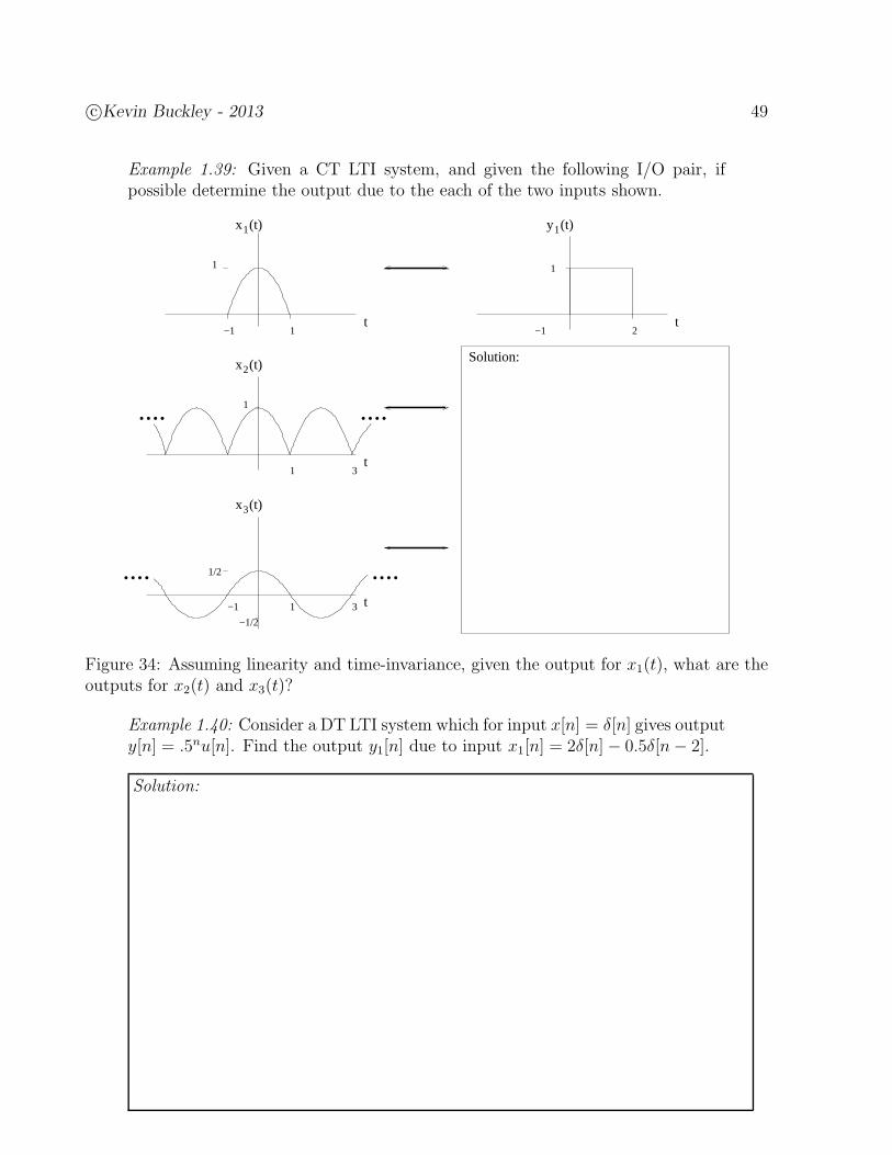
c©Kevin Buckley - 2013 49
Example 1.39: Given a CT LTI system, and given the following I/O pair, ifpossible determine the output due to the each of the two inputs shown.
1y (t)x (t)1
t
t
t
x (t)
−1
1
1/2
1−1
x (t)2
3
−1 2
1
1 3
t
31
1
........
.... ....
−1/2
Solution:
Figure 34: Assuming linearity and time-invariance, given the output for x1(t), what are theoutputs for x2(t) and x3(t)?
Example 1.40: Consider a DT LTI system which for input x[n] = δ[n] gives outputy[n] = .5nu[n]. Find the output y1[n] due to input x1[n] = 2δ[n]− 0.5δ[n− 2].
Solution:
50 c©Kevin Buckley - 2013
Advantage 2: For a LTI system, the output due to a complex sinusoid input will be a complexsinusoid of the same frequency – the effect of the system is simply to scale this input. Wehave not proved this property of LTI systems. We will do so in Chapter 2. However, thisproperty of LTI systems has already been illustrated in Examples 1.25 & 1.27 (i.e. the RCcircuit and the FIR filter considered in these examples are LTI systems).
Example 41: Consider the simple IIR filter introduced in Subsection 1.2.5. Itcan be shown that this is a LTI system. Generally, this system has I/O equationy[n] = a y[n − 1] + x[n]. In Subsection 1.2.5 we used a = 0.9. For theaccumulator considered in Subsection 1.4.1, a = 1. It is straightforward to showthat the I/O of this simple IIR filter can be written as
y[n] =∞∑
k=0
ak x[n− k] .
Determine the output for complex sinusoidal input x[n] = A ejω0n+φ.
Solution:
Example 42: Consider FIR filter with I/O equation y[n] =∑5
k=0 (−1)k x[n−k].Determine the output for input x[n] = ejω0n.
Solution:

c©Kevin Buckley - 2013 51
1.5.4 Linear Constant Coefficient System I/O Equations
The I/O response of a system is often represented as an I/O differential (CT) or difference(DT) equation. For example, performing loop and/or node analysis of an RLC circuit yieldsan I/O differential equation which is linear (as long as the circuit components are linear) withconstant coefficient (as long as the circuit components are time invariant). Furthermore,the simple IIR and FIR DT systems we have dealt with thus far, as Examples and inPracticum 1, have I/O equations that are difference equations which are linear with constantcoefficients. On the other hand, we have just established that LTI systems have very desirablecharacteristics. Below we establish a very important relationship between LTI systems anddifferential/difference equation I/O representation.
LCC Differential Equation Representation of CT LTI Systems:
A CT system is LTI if and only if it can be represented as follows:
N∑
l=0
al y(l)(t) =
M∑
k=0
bk x(k)(t) (77)
where x(i)(t) = di
dtix(t). This is the form of a LCC differential equation.
Comments:
• The a′ls and b′ks are time-invariant constants (so the system is TI).
• y(t) and x(t), and their derivatives, appear as linear combinations only (i.e. no productsof signals, powers of signals, etc.) (so the system is L).
• If a system’s I/O can be represented as a LCC differential equation, the system is LTI.
• The solution, y(t); t ≥ 0 depends on the input and the initial conditionsy(i)(0−); l = 0, 1, · · · , N − 1 and x(k)(0−); k = 0, 1, · · · ,M − 1.
• Given an input and initial conditions, such a system can be solved (i.e. the I/O LCCdifferential equations can be solved) in a systematic way using Laplace transforms orContinuous-Time Fourier Transforms (CTFT’s). We will learn how to do this later.
So any CT LTI system’s I/O can be expressed in the Eq (77) form. Also, any CT systemwhat has an I/O relationship in the form of Eq (77) is a CT LTI system. Reflecting back toyour circuits courses, recall that any RLC circuit (with input and output which are voltagesand/or currents) has an I/O expression in the form of Eq (77). In this Course we will learnhow to handle I/O issues for CT LTI systems in systematic ways, regardless on how largeM on N is (i.e. regardless of how complicated the system is), and for any type of input.
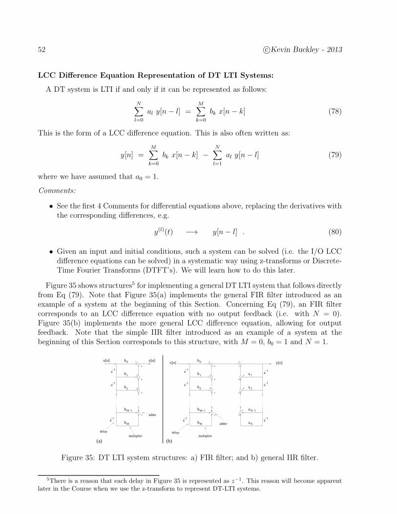
52 c©Kevin Buckley - 2013
LCC Difference Equation Representation of DT LTI Systems:
A DT system is LTI if and only if it can be represented as follows:
N∑
l=0
al y[n− l] =M∑
k=0
bk x[n− k] (78)
This is the form of a LCC difference equation. This is also often written as:
y[n] =M∑
k=0
bk x[n− k] −N∑
l=1
al y[n− l] (79)
where we have assumed that a0 = 1.
Comments:
• See the first 4 Comments for differential equations above, replacing the derivatives withthe corresponding differences, e.g.
y(l)(t) −→ y[n− l] . (80)
• Given an input and initial conditions, such a system can be solved (i.e. the I/O LCCdifference equations can be solved) in a systematic way using z-transforms or Discrete-Time Fourier Transforms (DTFT’s). We will learn how to do this later.
Figure 35 shows structures5 for implementing a general DT LTI system that follows directlyfrom Eq (79). Note that Figure 35(a) implements the general FIR filter introduced as anexample of a system at the beginning of this Section. Concerning Eq (79), an FIR filtercorresponds to an LCC difference equation with no output feedback (i.e. with N = 0).Figure 35(b) implements the more general LCC difference equation, allowing for outputfeedback. Note that the simple IIR filter introduced as an example of a system at thebeginning of this Section corresponds to this structure, with M = 0, b0 = 1 and N = 1.
delay
adder
multiplier
adder
delaymultiplier
(b)(a)
−1z
−1z
−1z
+
+
+
+
+
+
+
+ y[n]x[n] 0
1
2
M−1
M
b
b
b
b
b
−1z
−1z
−1z
−1z
−1z
−1z
y[n]x[n]
+
+
+
+
+
+
+
−
0
1
2
M−1
M
+
+
+
+
+
+
+
+
1
2
N−1
N
b
b
b
b
b
a
a
a
a
Figure 35: DT LTI system structures: a) FIR filter; and b) general IIR filter.
5There is a reason that each delay in Figure 35 is represented as z−1. This reason will become apparentlater in the Course when we use the z-transform to represent DT-LTI systems.
c©Kevin Buckley - 2013 53
1.6 Practicum 1
Introduction to Discrete Time Signals & Systems
Reporting Requirements: At the beginning of the semester it will be announced whetherthe practicum reporting requirement will be: 1) a full practicum report; or 2) submission ofa practicum Sign Off Sheet & Report Form only. Either way, the Sign Off Sheet & ReportForm, which appears at the back of the Practicum Section, should be submitted.
The full report, if required, should be headed with your name, the course name, and thepracticum number and title. The first section should be titled Objectives and Conclu-sions and should describe your understanding of objectives and conclusions. Nominally,this section should contain two or three paragraphs. The second section should be titledResults and Comments and should be organized in the same way that the procedures inthe practicum are organized. Provide all derivations, comments, answers, plots and compar-isons requested. (The Matlab Diary command might be used to generate the body of thissection.) Each plot should have a title, x,y coordinate labels, and your name printed on theplot using Matlab (e.g. using the “text” command). Include printouts of all Matlab .m filesused (i.e. to compute values and generate plots). As a heading for each program printout,include a comment line with your name on it. The Sign Off Sheet & Report Form should beattached as the last page of the full report.
Background: Read Subsection 1.2.3 of these Course Notes.
Procedures: Procedures 1(a), 2(a) and 3(a) should be completed before the first lab session.
1. Finite Impulse Response (FIR) Filter: Consider the following DT system:
y[n] =M−1∑
k=0
bk x[n− k] . (1)
(a) On paper, for input x[n] = δ[n], determine the output y[n] = h[n], i.e. findthe impulse response. (h[n] is standard notation for the impulse response of asystem.) Note that we can also express the FIR filter I/O equation in terms ofthe impulse response as
y[n] =M−1∑
k=0
h[k] x[n− k] . (2)
Why is this general type of system called an FIR filter?
(b) In file FIR mine.m, write a Matlab function that implements a general FIR filterwhich is called by the command
y = FIR_mine (h,x) ,
where
• x is the input array containing the N input values x[n]; n = 0, 1, · · · , N − 1,
• h is the M element array of impulse response valuesh[k] = bk; k = 0, 1, · · · ,M − 1, and
• y is the output array containing y[n]; n = 0, 1, · · · , N − 1.
Your code should look something like the following (completed):
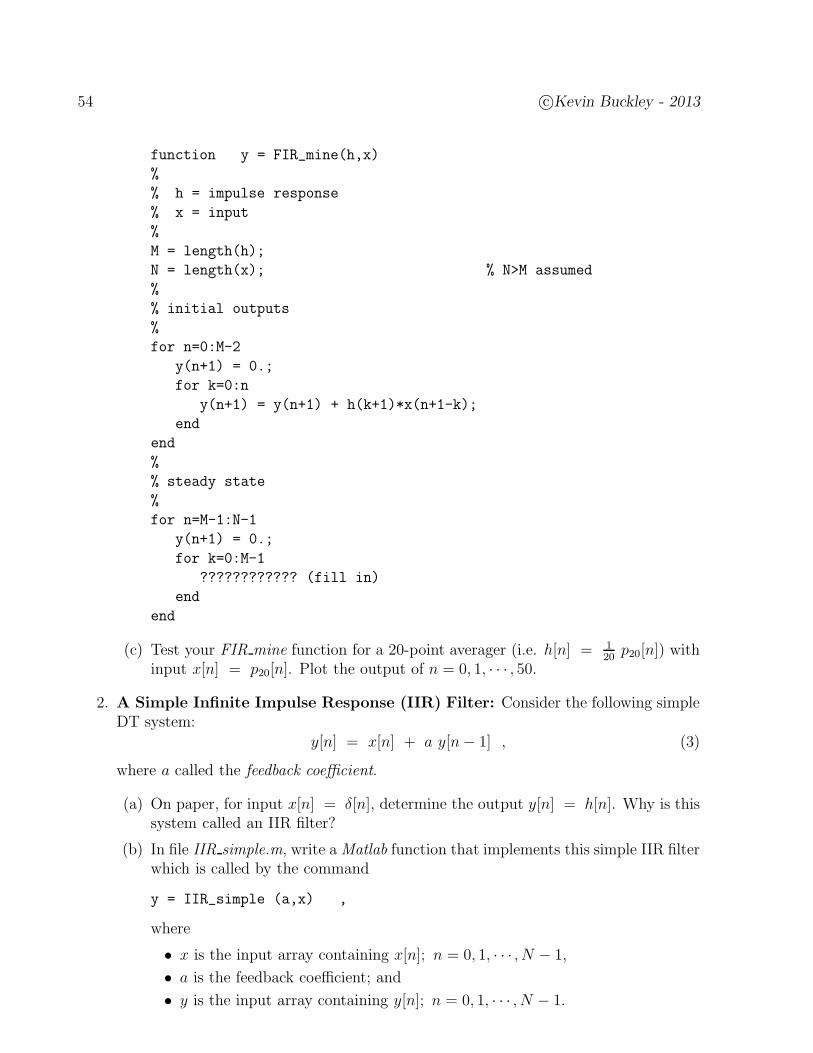
54 c©Kevin Buckley - 2013
function y = FIR_mine(h,x)
%
% h = impulse response
% x = input
%
M = length(h);
N = length(x); % N>M assumed
%
% initial outputs
%
for n=0:M-2
y(n+1) = 0.;
for k=0:n
y(n+1) = y(n+1) + h(k+1)*x(n+1-k);
end
end
%
% steady state
%
for n=M-1:N-1
y(n+1) = 0.;
for k=0:M-1
???????????? (fill in)
end
end
(c) Test your FIR mine function for a 20-point averager (i.e. h[n] = 120
p20[n]) withinput x[n] = p20[n]. Plot the output of n = 0, 1, · · · , 50.
2. A Simple Infinite Impulse Response (IIR) Filter: Consider the following simpleDT system:
y[n] = x[n] + a y[n− 1] , (3)
where a called the feedback coefficient.
(a) On paper, for input x[n] = δ[n], determine the output y[n] = h[n]. Why is thissystem called an IIR filter?
(b) In file IIR simple.m, write aMatlab function that implements this simple IIR filterwhich is called by the command
y = IIR_simple (a,x) ,
where
• x is the input array containing x[n]; n = 0, 1, · · · , N − 1,
• a is the feedback coefficient; and
• y is the input array containing y[n]; n = 0, 1, · · · , N − 1.
c©Kevin Buckley - 2013 55
Your code should look something like the following (completed):
function y = IIR_simple(a,x)
%
% a = feedback coefficient
% x = input
%
N = length(x);
%
% initial output
y(1) = x(1);
%
% steady state
for n=2:N
???????????? (fill in)
end
(c) Test your IIR simple function for an accumulator (i.e. a = 1) with inputx[n] = p20[n]. Plot the output of n = 0, 1, · · · , 50.
3. Discrete Time Channel Equalization: Consider the following two DT systems.The first has input x[n] and output v[n]. The second has input v[n] and output y[n].
v[n] = x[n] − .9 x[n− 1] (4)
y[n] = v[n] + .9 v[n− 1] + .81 v[n− 2] + .729 v[n− 3] + .6561 v[n− 4] . (5)
For example, the first system might be a discrete model of a multipath communicationchannel, and the 2-nd system might be designed as part of a receiver to compensatefor (or ”equalize” or invert the effect of) the channel.
(a) On paper, determine and plot the impulse responses of the channel and the equal-izer. Do the same for the overall impulse response of the cascade of the two systems(i.e. the response from the input to the first system to the output of the second,if the output of the 1-st system is the input to the second).
(b) Use FIR mine to compute the response of the first system to input x[n] = p2[n].Plot this for n = 0, 1, · · · , 10. Do the same for the output of the cascade of thetwo systems. Comment on the effectiveness of the second system at equalizingthe first. Reflecting on characteristics of y[n], suggest how the equalizer could beimproved, describing this in terms of the impulse response of the equalizer.
(c) Instead of using the second system to equalize the first, consider the third system:
y[n] = v[n] + .9y[n− 1] . (6)
Repeat Part (a).
(d) For the cascade of the first and third systems, use your FIR mine and IIR simplefunctions to compute the impulse response and the response to x[n] = p2[n]. Plotthe equalizer output for n = 0, 1, · · · , 10.

56 c©Kevin Buckley - 2013
(e) In terms of the impulse responses of the two equalizers, explain why the 2-nd oneworks better than the 1-st.
4. Image Deblurring: For this procedure you will process a black and white image.There are three files you will need, lighthouse.mat, lighthouse1.mat and show img.m,which can be found in directory
v:/Electrical Computer/ece3240
(a) Copy the three files into your working directory or otherwise assure that you haveaccess to them within Matlab.
(b) Load lighthouse.mat into Matlab. In Matlab, what is the image name? Whatsize is it? Display the image using the command show img(xx). Comment on thequality of the image. Do the same for lighthouse1.mat.
(c) The image yy[i, n] has been processed to simulate the effects of horizontal cameramotion. That is, the original image xx[i, n] has been blurred along the horizontalto generate yy. The blurring was simulated using the following equation for eachhorizontal image line (i.e. each row)
yy[i, n] =10∑
j=0
0.8j xx[i, n− j] ; i = 1, 2, · · · , 326 ; n = 1, 2, · · · , 426 . (7)
To deblur the given image yy, use your FIR mine function to process each row asfollows to generate the deblurred image zz.
zz[i, n] = yy[i, n] − 0.8 yy[i, n−1] ; i = 1, 2, · · · , 326 ; n = 1, 2, · · · , 426 . (8)
Use yy[i, 0] = 0.0, i = 1, 2, · · · , 326.(d) Display the deblurred image zz. Compare its quality to that of the yy image, and
the original image xx stored in file lighthouse.mat.
(e) How do the systems and results of this (the Image Deblurring) Section relate tothose of the previous (Channel Equalization) Section?

c©Kevin Buckley - 2013 57
Practicum 1: Instructor/TA Sign Off Sheet, & Report Form
Student’s Name:
1. Procedures 1(c): 20-pt. averager output
2. Procedure 2(c): accumulator output
3. Procedure 3(a): below, sketch the three impulse responses.
4. Procedure 3(b): output plot of 1-st equalizerRecord requested comments.
5. Procedure 3(c): sketch the impulse response from the channel input to the 2-nd equal-izer output.
6. Procedure 3(d,e): output plot of 2-nd equalizerRecord requested comments.
7. Procedure 4: displays of original, blurred and deblurred imagesRecord requested comments.

58 c©Kevin Buckley - 2013
.

c©Kevin Buckley - 2013 59
1.7 Appendix 1A: Complex Numbers and Signals
In this Appendix we review complex numbers and signals, and common operations appliedto them. We assume that students in this course are familiar with these topics, but thatsome will benefit from a review which is focused on the specifics required for this Course.The objective of this Appendix is to provide students on this Course a convenient referenceon complex-valued signals that we can build on in support of the topics of this Course.
1.7.1 Complex Numbers
Let j =√−1. Consider a complex-valued number x such that
x = xr + j xi = |x| ej 6 x , (1)
where xr = Rex and xi = Imx are, respectively, the real and imaginary parts of x,and where |x| and 6 x are, respectively, the magnitude and phase of x. Figure 36 illustratesa complex number x visualized in the complex plane. Note that xr, xi, |x| and 6 x are allreal-valued. Although 6 x can be any real number, since it represents an angle relative tothe positive real axis, ej
6 x = ej(6 x +2π) for any 6 x (i.e. ej
6 x = ej[(6 x)modulo 2π]). Thus, in
any discussion, we typically limit this angle as either 0 ≤ 6 x < 2π or −π < 6 x ≤ π.
x i
x r
x
.
complex planeImx
Rex
|x|
Figure 36: A complex number x in the complex plane.
We sometimes consider the xr, xi representation of x to be the rectangular coordinaterepresentation of x, and |x|, 6 x to be the polar coordinate representation. The conversionsbetween these two representations are
xr = |x| cos( 6 x) ; xi = |x| sin( 6 x) (2)
|x| =√
x2r + x2
i ; 6 x =
tan−1(
xi
xr
)
xr ≥ 0
π + tan−1(
xi
xr
)
xr < 0 and xi > 0
−π + tan−1(
xi
xr
)
xr < 0 and xi < 0
. (3)
There are various equivalent ways to express the conversion from rectangular coordinates to6 x. Above, the conversion is given which results in the range −π < 6 x ≤ π. Also note thattan−1 (inverse tangent) and arctan (arc tangent) mean the same thing.
The conjugate of a complex number, denoted x∗ for complex-valued x, is defined as
x∗ = xr − j xi = |x| e−j 6 x . (4)
So, Rex = Rex∗, Imx = −Imx∗, |x| = |x∗|) and 6 x = −6 x∗.

60 c©Kevin Buckley - 2013
Example a1: Given w = 1+ j, x = −1 + j2, y = 2 ejπ/2 and z = 3 e−jπ/5,determine: a) w in polar representation; b) x in polar coordinates;c) y in rectangular representation; and d) z in rectangular coordinates.
Solution: Sketch each of these numbers in the complex plane so as to verify theplausibility of the results given below.
a) w = |w| ej 6 w =√12 + 12 ej tan
−1(1/1) =√2 ejπ/4.
b) x = |x| ej 6 x =√
(−1)2 + (2)2 ej(π+tan−1(2/(−1)) =√5 ej(2.0344).
c) y = yr + j yi = 2 cos(π/2) + j 2 sin(π/2) = j 2.
d) z = zr + j zi = 3 cos(−π/5) + j 3 sin(−π/5) = 2.4271 − j 1.7634 .
Before proceeding, you should make sure you are comfortable with the fact that to followingresults can be obtained by inspection: −j = e−jπ/2; ejπ = e−jπ = −1; ej6π = ej2π = 1;and ej7π/2 = ej3π/2 = e−j π/2 = −j.
1.7.2 Algebra with Complex Numbers
Consider two complex-valued numbers x and y. Then
x + y = (xr + yr) + j (xi + yi) (5)
x − y = (xr + yr) + j (xi − yi) (6)
x · y = |x| · |y| ej(6 x+ 6 y) (7)
x
y=|x||y| e
j(6 x−6 y) . (8)
Note that when adding or subtracting complex numbers, it is advantageous to representthem in terms of rectangular coordinates. When multiplying or dividing them, it is betterto represent them in polar coordinates. So be willing to convert between rectangular andpolar coordinates as needed.
c©Kevin Buckley - 2013 61
Example a2: Given x =√2 ej3π/4 and y = −1 −j 2, determine: a) za = x + y;
b) zb = 2 x + 3 y; c) zc = x · y; d) zd = 2 · x · y; and e) ze = 2xy.
Solution:
a) za = (−1+j)+(−1+j(−2)) = (−1−1)+j(1−2) = −2−j = 2.2361 e−j(2.6779).
b) zb = 2(−1 + j) + 3(−1 + j(−2)) = (−2 − 3) + j(2 − 6) = −5 − j4 =6.4031 e−j(2.4669).
c) zc =√2 ej3π/4 ·
√5 e−j(2.0344) =
√10 ej(2.3562−2.0344) = 3.1623 ej(0.3218).
d) zd = 2 · zc = 6.3246 ej(0.3218).
e) ze = 2√2 ej3π/4√
5 e−j(2.0344) = 2√
25ej(2.3562+2.0344) = 1.2649 ej(4.3906) = 1.2649 e−j(1.8926).
Note that, for consistency, when presented in terms of polar coordinates, anglesof results have all been represented in the range −π, π.
As an extension of the rule for multiplication of complex numbers, let n be a positiveinteger and x a complex number. We have that
xn = (|x| ej n 6 x)n = |x|n (ej6 x)n = |x|n ej n 6 x . (9)
As an extension of the multiplication and division rules, let xi; i = 1, 2, · · · ,M andyj; j = 1, 2, · · · , N be sets of complex numbers. Then
∏Mi=1 xi
∏Ni=j yj
=
∏Mi=1 |xi|
∏Ni=j |yj|
ej
(
∑M
i=16 xi −
∑N
j=16 yj
)
. (10)
Example a3: Consider the complex numbers x = 3 + j 4 and y = ejπ/12.Determine: a) va = x3; b) vb = x100, c) vc = y12 and vd = y24.
Solution:
a) va = (3 + j4)3 = (5 ej(0.2953)π)3 = 53 (ej(0.2953)π)3 = 125 ej3(0.2953)π =125 ej(0.8855)π .
b) vb = 5100 ej100(0.2953)π = 7.886× 1069 ej(29.53)π = 7.886× 1069 ej(1.53)π.
c) vc = (ejπ/12)12 = ej12π/12 = ejπ = −1.d) vd = ej24π/12 = ej2π = 1.
62 c©Kevin Buckley - 2013
1.7.3 Complex-Valued Signals
A complex-valued DT signal is just a sequence of complex-valued numbers. So, for a complex-valued signal x[n], we have that, for each sample time n,
x[n] = xr[n] + j xi[n] = |x[n]| ej 6 x[n] . (11)
Conversion between real/imaginary parts (i.e. rectangular coordinates) and magnitude/phase(i.e. polar coordinates) is as described above for each complex number (i.e. for each sam-ple time). When adding, subtracting, multiplying and dividing signals, the arithmetic rulesfor complex numbers described above apply for each sample time. For complex-valued CTsignals, it’s the same story. That is, at each time t, a complex-valued CT signal is complexnumber.
Example a4: Consider the DT complex sinusoid x[n] = ej(π/4)n. Consider an Npoint averager, i.e.
y[n] =1
N
N−1∑
k=0
x[n− k] .
a) Determine a general expression for y[n]. b) Determine y[n] for N = 16.c) Determine y[n] for N = 12.
Solution:
a) For general N ,
y[n] =1
N
N−1∑
k=0
ej(π/4)(n−k) =1
Nej(π/4)n
N−1∑
k=0
e−j(π/4)k
= ej(π/4)n1
N
1− e−j(π/4)N
1− e−j(π/4).
The last equation was derived using the Geometric series summation.
b) For N = 16,
y[n] = ej(π/4)n1
16
1− e−j(4π)
1− e−j(π/4)= ej(π/4)n
1
16
1− 1
1− e−j(π/4)= 0 .
A 16-point averager completely attenuates a complex sinusoid of frequencyω = π
4.
c) For N = 12,
y[n] = ej(π/4)n1
12
1− e−j(3π)
1− e−j(π/4)= ej(π/4)n
1
12
1− (−1))1− e−j(π/4)
= ej(π/4)n2
12
1
1− e−j(π/4)= ej(π/4)n
1
61.3066 e−j(1.1781) = 0.2178 ej((π/4)n−1.1781) .
The output of a 12-point averager to a complex sinusoid input of frequencyω = π
4is a complex sinusoid of the same frequency. It is attenuated by a
factor of 0.2178 and phase shifted by −1.1871 radians/sample.
c©Kevin Buckley - 2013 63
Example a5: Consider the DT complex sinusoid x[n] = ej(ω0n). Consider a10-point averager, i.e.
y[n] =1
10
9∑
k=0
x[n− k] .
a) Determine a general expression for y[n]. b) Determine y[n] for ω0 = 0.c) Determine y[n] for ω0 = π.
Solution:
a) In general we have
y[n] =1
10
9∑
k=0
ejω0(n−k) = ejω0n1
10
9∑
k=0
e−jω0k
= ejω0n1
10
1− e−jω010
1− e−jω0.
b) For ω0 = π we have
y[n] = ejπn1
10
1− e−jπ10
1− e−jπ= ejπn
1
10
1− 1
1− (−1) = 0 .
Note that the input is completely attenuated.
c) For ω0 = 0 the input is just x[n] = 1, and the output is
y[n] =1
10
9∑
k=0
x[n− k] =1
10
9∑
k=0
1 = 1 .
Note that we did not use the general output expression derived in a) tosolve this part of the Example. Let’s resolve this problem using this generalexpression.
y[n] = ej0n1
10
1− e−j0·10
1− e−j0=
1
10
1− 1
1− 1.
This 00is a problem which you know how to deal with using tools from your
calculus courses. Try using L’Hospital’s rule on your own. Here we will usea Taylor series expansion approach. Starting with
y[n] = ejω0n1
10
1− e−jω010
1− e−jω0,
and using the Taylor series expansion ex = 1 + x+ x2 + x3 + · · ·, we havethat
y[n] = ejω0n1
10
1− (1 + ω010 + (ω010)2 + · · ·)
1− (1 + ω0 + ω20 + · · ·)
= ejω0n1
10
−(ω010 + (ω010)2 + · · ·)
−(ω0 + ω20 + · · ·)
.
64 c©Kevin Buckley - 2013
For ω0 = 0, we consider the limit
limω0−→0
−(ω010 + (ω010)2 + · · ·)
−(ω0 + ω20 + · · ·)
=−ω010
−ω0= 10 ,
(i.e. we keep only the lowest order term of each expansion), so
y[n] = ej(0)n1
1010 = 1 .
Either way, we see that the output is passed through the system withoutchange. We call a system that attenuated some inputs while passing otherswithout change a filter.
Example a6: Consider the DT signal x[n] = ej(ω0n) Consider the simple DTsystem
y[n] = 0.9 y[n− 1] + x[n]
which can be shown to have output
y[n] =∞∑
k=0
0.9k x[n− k] .
a) Determine a general expression for y[n]. b) Determine y[n] for ω0 = 0.c) Determine y[n] for ω0 = π.
Solution:
a) In general we have
y[n] =∞∑
k=0
0.9k ejω0(n−k) = ejω0n∞∑
k=0
(0.9 e−jω0)k
= ejω0n1
1− 0.9 e−jω0.
b) For ω0 = 0, that is for x[n] = 1, we have
y[n] = ej(0)n1
1− 0.9(1)= 10 .
The input is amplified by a factor of 10.
c) For ω0 = π, that is for x[n] = (−1)n, we have
y[n] = ejπn1
1− 0.9(−1) = 0.5263 ejπn .
The input is slightly attenuated (by a factor of 0.5263).
c©Kevin Buckley - 2013 65
Example a7: Consider the CT complex sinusoid x[n] = ejω0t and the system
y(t) = x(t) ej100πt .
So this system simply multiplies the input x(t) by a complex sinusoid of frequency100π radians/second. Determine a general expression for y(t).
Solution:
y(t) = ejω0t · ej100πt = ej(ω0+100π)t .
So the output is also a complex sinusoid, with frequency ω0 + 100π. That is,the frequency of the input has been shifted by an amount equal to the frequencyof the sinusoid the system multiplies it by. We call this process of shifting thefrequency of an input modulation. We will consider modulation later in thisCourse.
1.7.4 Why Consider Complex-Valued Signals?
At this point you may be wondering why we consider complex-valued numbers and signals.The math and algebra seems to be harder (if you are not used to it), and complex numbersdon’t appear to exist in the real engineering world. So why?
There are several ways to answer this question. One has to do with working with sinusoids.First you have to acknowledge that we are centrally interested sinusoidal signals. That is,we are interested in them almost all of the time. At the end of this Course you shouldunderstand this. At this point you should at least understand the we naturally think ofsignals in terms of their sinusoidal content (e.g. the base and treble of an audio signal, orthe transmission frequency band of a cell phone or a radio station, or the color of light).So then the question is – why consider complex-valued sinusoids as opposed to real-valuedsinusoids?
One answer to this is that the algebra of complex-valued sinusoids is easier. Easier algebracan be advantageous in the analysis and the design of signals and systems. Consider, forexample, the simple task of multiplying two CT sinusoids and expressing the result as aweighted-sum of sinusoids. First consider the product cos(ω1t) · cos(ω2t). You probablyrecall that there is a trigonometric identity for this, but let’s say you don’t remember it.You could look it up, or to save time you could use Euler’s identities, i.e.
cos(ω1t) · cos(ω2t) =1
2
(
ejω1t + e−jω1t) 1
2
(
ejω2t + e−jω2t)
(12)
=1
4
(
ej(ω1+ω2)t + e−j(ω1+ω2)t + ej(ω1−ω2)t + e−j(ω1−ω2)t)
(13)
=1
2cos((ω1 + ω2)t) +
1
2cos((ω1 − ω2)t) . (14)
So complex sinusoids can be used to derive trigonometric identities. To a mathematicianthis might be happy hour conversation, but an engineer this is not a big deal. The point isthat, in contrast, the multiplication of two complex-valued sinusoids is simply
ejω1t · ejω2t = ej(ω1+ω2)t . (15)

66 c©Kevin Buckley - 2013
This illustrates that when you are analyzing a signal or designing a system, and you encounteroperations involving sinusoids, if you couch the derivations in terms of complex-valued sinu-soids, the math will generally be easier. Would you rather spend your time looking throughtrig identity tables, or proceeding with little resistance to a solution. What would youremployer rather pay you $400.00 a day to do?
Another argument for the use of complex-valued sinusoids involves what are called in-phase/quadrature (I/Q) receivers. These are commonly found in systems such as mobilephones, radio, RADAR and SONAR where modulation is required. An I/Q receiver is shownin Figure 37. The input x(t) is the signal from the receiver antenna, after some precondi-tioning (e.g. amplification and filtering). The two real-valued outputs shown, termed thein-phase output xi(t) and the quadrature output xq(t), are treated in subsequent processingas a single complex-valued output
xiq(t) = xi(t) + j xq(t) = x(t) ejω0t . (16)
ωocos ( t)
ωosin ( t)
x (t)i
qx (t)
x(t)
Figure 37: An in-phase/quadrature (I/Q) receiver.
Since this is a very common receiver structure, that generates “complex-valued” signalsthat must be processed, this is a strong motivation for getting comfortable with complexnumbers and signals. But why are I/Q receivers so common in the first place? Basically,because subsequent processing is simplified in the same way that algebra with complex-valued sinusoids is simplified. Processors which are analogous to I/Q receivers are foundcommonly in Digital Signal Processing (DSP) systems for many applications.
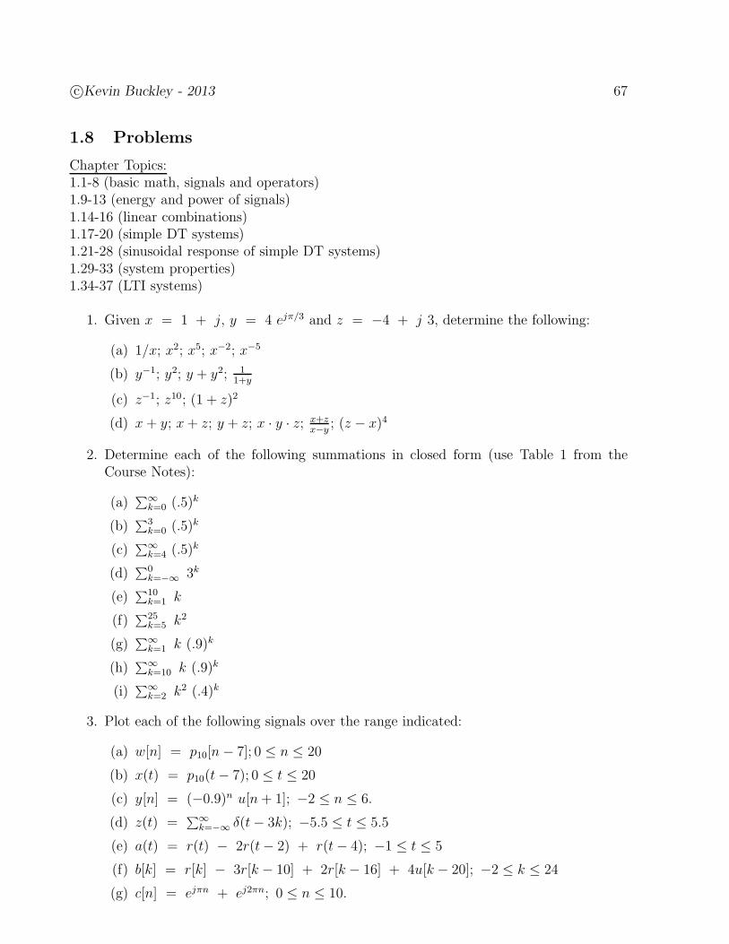
c©Kevin Buckley - 2013 67
1.8 Problems
Chapter Topics:1.1-8 (basic math, signals and operators)1.9-13 (energy and power of signals)1.14-16 (linear combinations)1.17-20 (simple DT systems)1.21-28 (sinusoidal response of simple DT systems)1.29-33 (system properties)1.34-37 (LTI systems)
1. Given x = 1 + j, y = 4 ejπ/3 and z = −4 + j 3, determine the following:
(a) 1/x; x2; x5; x−2; x−5
(b) y−1; y2; y + y2; 11+y
(c) z−1; z10; (1 + z)2
(d) x+ y; x+ z; y + z; x · y · z; x+zx−y
; (z − x)4
2. Determine each of the following summations in closed form (use Table 1 from theCourse Notes):
(a)∑∞
k=0 (.5)k
(b)∑3
k=0 (.5)k
(c)∑∞
k=4 (.5)k
(d)∑0
k=−∞ 3k
(e)∑10
k=1 k
(f)∑25
k=5 k2
(g)∑∞
k=1 k (.9)k
(h)∑∞
k=10 k (.9)k
(i)∑∞
k=2 k2 (.4)k
3. Plot each of the following signals over the range indicated:
(a) w[n] = p10[n− 7]; 0 ≤ n ≤ 20
(b) x(t) = p10(t− 7); 0 ≤ t ≤ 20
(c) y[n] = (−0.9)n u[n+ 1]; −2 ≤ n ≤ 6.
(d) z(t) =∑∞
k=−∞ δ(t− 3k); −5.5 ≤ t ≤ 5.5
(e) a(t) = r(t) − 2r(t− 2) + r(t− 4); −1 ≤ t ≤ 5
(f) b[k] = r[k] − 3r[k − 10] + 2r[k − 16] + 4u[k − 20]; −2 ≤ k ≤ 24
(g) c[n] = ejπn + ej2πn; 0 ≤ n ≤ 10.
68 c©Kevin Buckley - 2013
4. Using the geometric series equation, evaluate the sum∑7
n=0 ejπn/4. The answer is aspecific real-valued number. As a means of verifying your answer, in the complex plane,plot the 8 values that are summed, and comment on why their positions lead to youranswer.
5. Plot the following two signals over the range n = 0, 1, 2, · · · , 9. (Use Matlab if youwish.)
(a) v1[n] = 2 cos(2π10n)
(b) v2[n] = 2 cos(22π10
n)
Compare the plots, commenting on and explaining similarities and differences.
6. Basic signal operators:
(a) Plot the discrete-time signal x[n] = u[n − 2] − u[n − 6]. Express x[n] as ashifted pulse (i.e. determine N and m for x[n] = pN [n−m]) & as a sum of shiftedimpulses.
(b) Given that z1[n] = (0.5)n p4[n], plot z2[n] = z1[−4− n].
(c) Consider the CT signal
x(t) = − r(−(t + 1)) · p1(t+3
2) + p1(t +
1
2) + 2 p1(t−
1
2) − r(−(t− 2)) · p1(t−
3
2) .
i. Sketch x(t).
ii. Sketch x(2− t).
iii. Sketch x(t) · [δ(t+ 32)− δ(t− 3
2)].
(d) Consider the DT signal
x[n] = − δ[n+ 4] − 1
2δ[n+ 3] +
1
2δ[n+ 2] + p4[n + 1] +
1
2δ[n− 3] .
i. Sketch x[n].
ii. Sketch x[n] · u[3− n].
(e) Consider the signal x(t) = 3u(t + 2) − 5u(t − 1) + 3u(t − 4). Sketch it.Determine and sketch y(t) = d
dtx(t).
7. For each of the following DT signals, determine if it is periodic. If periodic, determineits period.
(a) sin(n8− π)
(b) cos(6π7n + 1)
(c) 2 cos(π4n) + sin(π
8n)− 2 cos(π
2n + π
4)
(d) 3 cos(π3n) − sin(34π
18n)

c©Kevin Buckley - 2013 69
8. Periodic signals:
(a) First plot the signal
x1[n] = δ[n] − δ[n− 1] + δ[n− 2]
over the range −4 ≤ n ≤ 6. Now consider the signal
x[n] =∞∑
k=−∞x1[n− 6k] .
Plot this signal over the range 0 ≤ n ≤ 15.
(b) Consider the periodic continuous-time signal
x(t) =∞∑
k=−∞x1(t− 2k) ; x1(t) = e|t| p2(t) .
Sketch both x1(t) and x(t).
(c) Sketch
x(t) =∞∑
k=−∞x1(t− 2k)
where
x1(t) = 3 cos(πt) p2(t− 1) .
9. Determine the energy and power for the following DT signals:
(a) x[n] = 1nu[n− 3].
(b) x[n] = ejπ2n. x1[n] = 3 ejπ/2 ej(3π/7)n. x2[n] = x1[n] p20[n].
(c) y[n] = n .5n u[n].
(d) x1[n] = 3 (0.2)n−4 u[n− 4]. x3[n] = 0.91/2 0.5n u[n]. x4[n] = 1.2n u[n− 20].x5[n] = 4 (0.01)n u[n+ 3].
(e) x2[n] = 3 cos(πn) − 2.
(f) x3[n] =∑∞
i=−∞ δ[n− 2i].
(g) x[n] = .9|n|. (Hints: Draw x[n] to see what it looks like, take advantage ofsymmetry, and use the geometric series formula.)
(h) y[n] = 2 (−.8)|n|.(i) x[n] = r[n] p20[n].
10. Determine the energy and power for the following CT signals:
(a) w(t) = 2 p8(t− 100.2).
70 c©Kevin Buckley - 2013
(b) x(t) = 5 e−t u(t− 1).
(c) y(t) =∑9
k=0 r(t− k) · p1(t− 12− k).
(d) z(t) =∑∞
k=−∞ z1(t− 10k); z1(t) = t2 p10(t− 5).
(e) x2(t) = ej100t.
11. Determine the energy and power for the following DT signals:
(a) v[n] = 5 ej((2π/18)n+(π/4)).
(b) x[n] =∑∞
k=−∞ x1[n− 20k] where x1[n] = (−.5)n p10[n]
(c) x[n] =∑∞
k=−∞ x1[n− 8k] where x1[n] = 5 p3[n].
(d) x[n] =∑∞
k=−∞ x1[n− 8k] where x1[n] = δ[n] − 3δ[n− 2] + 4δ[n− 5]
(e) x[n] =∑∞
k=−∞ x1[n− 20k] where x1[n] = r[n] p10[n]
(f) x[n] =∑∞
k=−∞ x1[n− 12k] where x1[n] =√n p10[n− 1].
(g) x6[n] =∑3
l=1 lδ[n− l].
12. Determine the energy and power for the following CT signals:
(a) y(t) =∑∞
n=−∞ 3 p2(t− 4n)
(b) x(t) =∑∞
k=−∞ x1(t− 2k) where x1(t) = e|t| p2(t)
(c) y(t) =∑∞
k=−∞(t− k) p1(t− k)
(d) z(t) =∑∞
k=−∞ δ(t− k) (Hint: consider the definition of a CT impulse –δ(t) = limǫ→0
1ǫpǫ(t)).
13. Let N be some positive integer. Consider the DT energy signal
x1[n] = r[n] pN [n]
and DT periodic power signal
x[n] =∞∑
k=−∞x1[n− kN ] .
(a) For N = 6, plot x1[n]; −2 ≤ n ≤ 8.
(b) For general N , determine the energy in x1[n]. Use Table 1, p. 14 to determinethis expression in closed form.
(c) For general N , what is the power of x[n].
(d) For N = 22, what is the energy in x1[n].
14. Write x(t) = cos2(2t+ π2) as a linear combination of complex sinusoids.
15. Represent the signal as a linear combination of basic signals from the set:
c©Kevin Buckley - 2013 71
(a) signal -
x3(t) =
1 −1 ≤ t < 02 0 ≤ t < 11 1 ≤ t < 20 otherwise
;
set - all delayed steps
(b) signal -
y1(t) =
2t 0 ≤ t < 14− 2t 1 ≤ t < 20 otherwise
;
set - all delayed ramps
1y (t)
t
2
0 1 2
3x (t)
t−1 0 1 2
2
1
(c) signal - x1(t) = | 2 cos(0.5t) |;set of all delayed x(t) where x(t) = cos(.5t)[u(t+ π)− u(t− π)].
16. Use Matlab to plot the following linear combinations:
(a) Let xk(t) = cos(2πkt) for integer k be some basic signals. Consider
x(t) =10∑
k=1
1
kπxk(t) .
Plot x(t); 0 ≤ t ≤ 4, using the Matlab “plot” function and a dense sampling oft. What type of signal does x(t) look like? What do you think would happen ifwe increased the upper summation bound?
(b) Let s(t) be a symbol shape used in an Amplitude Modulated (AM) digital com-munications scheme. Specifically, let s(t) = cos(ω0t) · pT (t) where T is thesymbol duration and ω0 is called the carrier frequency. For a particular digitalAM scheme, let T = 1, ω0 = 10π and let ak ∈ −3,−1, 1, 3 be the possible trans-mission amplitudes (with four amplitudes, we can represent 2 bits per transmittedsymbol). The transmitted signal would be of the form
x(t) =∞∑
k=−∞ak s(t− kT ) ,
i.e. a linear combination of delayed symbol shapes. So the symbol rate is 1T
and the bit rate is 2T. Let a0, a1, a2, a3 = −1,−3, 1, 3. Use Matlab to plot
x(t); 0 ≤ t ≤ 4 using the Matlab “plat” function and a dense sampling of t.
72 c©Kevin Buckley - 2013
17. Finding the impulse response of simple DT IIR systems:
(a) Consider the discrete-time signal x[n] = δ[n], and the simple feedback system
y[n] = x[n]− .9 y[n− 1] ,
where x[n] is the input, y[n] is the output, and y[−1] = 0. Determine an expressionfor y[n];n = 0, 1, 2, 3 · · · .
(b) Consider the discrete-time signal x[n] = δ[n], and the simple feedback system
y[n] = y[n− 1] + 0.5x[n] ,
where x[n] is the input, y[n] is the output, and y[−1] = 0. Determine an expressionfor y[n];n = 0, 1, 2, ....
(c) Find the impulse response (i.e. the output when the input is an impulse and theinitial conditions are zero) of the following system:
y[n] − y[n− 1] = x[n] − x[n− 1] .
(d) Consider the DT system
y[n] = 0.8 y[n− 2] + x[n]
with input x[n] = δ[n] and initial conditions y[−1] = y[−2] = 0. Determine anexpression for y[n] for all time 0 ≤ n ≤ ∞, and plot y[n] for 0 ≤ n ≤ 10.
18. Finding the output of simple DT IIR systems:
(a) Consider the DT system
y[n] = 0.8 y[n− 1] + x[n]
with input x[n] = δ[n] − 0.8 δ[n − 1] and y[−1] = 0. Plot the output y[n] forall time 0 ≤ n ≤ 10.
(b) Consider the discrete-time signal x[n] = p2[n] as the input to a simple feedbacksystem
y[n] = x[n]− .5 y[n− 2] ,
where y[n] is the output. Assume initial conditions y[−1] = y[−2] = 0. Determineand plot y[n] for 0 ≤ n ≤ 7 .
(c) Consider the DT system
y[n] = 0.5 y[n− 1] + x[n− 1].
For input x[n] = δ[n] + 0.5 δ[n− 1] and y[−1] = 0, determine the output y[n]for all time n ≥ 0.
(d) Consider the DT system
y[n] = 0.5 y[n− 1] + x[n− 1].
For input x[n] = δ[n] − 0.5 δ[n− 1] and y[−1] = 0, determine the output y[n]for all time n ≥ 0.
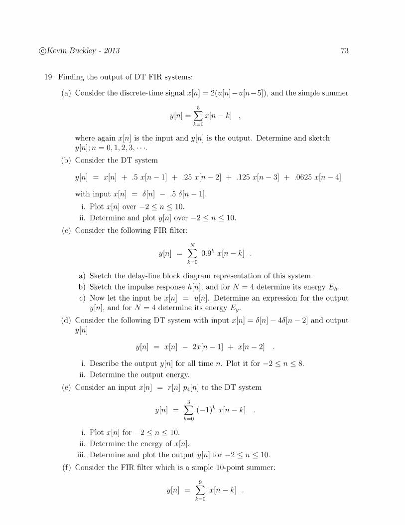
c©Kevin Buckley - 2013 73
19. Finding the output of DT FIR systems:
(a) Consider the discrete-time signal x[n] = 2(u[n]−u[n−5]), and the simple summer
y[n] =5∑
k=0
x[n− k] ,
where again x[n] is the input and y[n] is the output. Determine and sketchy[n];n = 0, 1, 2, 3, · · ·.
(b) Consider the DT system
y[n] = x[n] + .5 x[n− 1] + .25 x[n− 2] + .125 x[n− 3] + .0625 x[n− 4]
with input x[n] = δ[n] − .5 δ[n− 1].
i. Plot x[n] over −2 ≤ n ≤ 10.
ii. Determine and plot y[n] over −2 ≤ n ≤ 10.
(c) Consider the following FIR filter:
y[n] =N∑
k=0
0.9k x[n− k] .
a) Sketch the delay-line block diagram representation of this system.
b) Sketch the impulse response h[n], and for N = 4 determine its energy Eh.
c) Now let the input be x[n] = u[n]. Determine an expression for the outputy[n], and for N = 4 determine its energy Ey.
(d) Consider the following DT system with input x[n] = δ[n]− 4δ[n− 2] and outputy[n]
y[n] = x[n] − 2x[n− 1] + x[n− 2] .
i. Describe the output y[n] for all time n. Plot it for −2 ≤ n ≤ 8.
ii. Determine the output energy.
(e) Consider an input x[n] = r[n] p4[n] to the DT system
y[n] =3∑
k=0
(−1)k x[n− k] .
i. Plot x[n] for −2 ≤ n ≤ 10.
ii. Determine the energy of x[n].
iii. Determine and plot the output y[n] for −2 ≤ n ≤ 10.
(f) Consider the FIR filter which is a simple 10-point summer:
y[n] =9∑
k=0
x[n− k] .

74 c©Kevin Buckley - 2013
i. Determine the output when the input is the impulse δ[n] (i.e. find the impulseresponse). What is the energy and power of this output?
ii. Determine the output when the input is the step u[n] (i.e. find the stepresponse). What is the energy of this output?
(g) Consider the FIR filter which is a simple 10-point summer:
y[n] =4∑
k=0
(−2)k x[n− k] .
i. Sketch the delay-line block diagram (i.e. with the input delay line).
ii. Determine the output for input δ[n] (i.e. find the impulse response).
iii. Determine the output for input x[n] = δ[n] + 2δ[n − 1]. What is the energyof this output?
20. Finding the output of simple DT FIR systems: Consider the DT FIR system
y[n] =5∑
k=0
x[n− k] .
The impulse response for this system is h[n] = p6[n].
a) Describe for all time n the output y1[n] due to input x1[n] = δ[n].What is the Energy E1 of y1[n]?
b) Describe for all time n the output y2[n] due to input x2[n] = u[n].What is the Energy E2 of y2[n]?
c) Describe for all time n the output y3[n] due to input x3[n] = (−1)n u[n].What is the Energy E3 of y3[n]?
21. Consider the following simple summer
y[n] =5∑
k=0
x[n− k] .
Determine the output for the following inputs:
(a) x1[n] = 1 for all n.
(b) x1a[n] = 5 for all n.
(c) x2[n] = ej(π/3)n for all n.
(d) x3[n] = ej(π/2)n.
22. Consider the simple system (a summer)
y[n] =4∑
k=0
x[n− k] ,
where x[n] is the input and y[n] is the output.
c©Kevin Buckley - 2013 75
(a) For input x[n] = r[n] p5[n], determine and sketch y[n]. Determine Ey, the energyof the output y[n].
(b) Consider input
x[n] = 5 ej2πn/5 .
Determine the output y[n] for all time n. As a means of verifying your answer fortime n = 0, in the complex plane, plot the 5 values (phasors) that are summed,and comment on why their positions lead to your answer. Determine Py, thepower of the output y[n].
23. Consider the following DT system:
y[n] =9∑
k=0
.5k x[n− k] .
(a) First let the input be x1[n] = 1 for all time n. The output will be a constant, i.e.y1[n] = c1. Determine c1. (To obtain a simplified approximate answer, assumethat .510 ≈ 0.) Is this input amplified or attenuated?
(b) Now let the input be x2[n] = ejπn for all time n. The output will in the formy2[n] = c2 ejπn. Determine c2. (Again, to obtain a simplified approximateanswer, assume that .510 ≈ 0.) Is this input amplified or attenuated?
24. Consider a DT system with output y[n] = x[n + 2] + x[n− 2] and input x[n] = ejω0n.
(a) The output is of the form y[n] = K ejω0n where K is a constant depending on ω0.Determine K explicitly as a real-valued constant.
(b) For ω0 = 0, determine y[n].
(c) For ω0 = π, determine y[n].
25. Consider the FIR filter:
y[n] =10∑
k=0
(−1)k x[n− k] .
a) For input x[n] = ejω0n, determine an expression for the output which is in “closedform” (i.e. do the geometric series).
b) Using results from a), determine the simplest expression you can for y[n] whenω0 = 0.
c) Using results from a), determine the simplest expression you can for y[n] whenω0 =
π11.
d) Determine the simplest expression you can for y[n] when ω0 = π. (Hint: eitherbe very careful using part a) results; or go back and use Eq (1) directly, notingthat x[n] = (−1)n.)
76 c©Kevin Buckley - 2013
26. Consider the following DT system:
y[n] =21∑
k=0
(−0.9)k x[n− k] .
Let x[n] = ejω0n for all time n.
(a) Determine a closed form expression for y[n] (closed form means do the summation;assume that .922 ≈ 0.1.)
(b) Determine y[n] specifically for ω0 = 0 (i.e. for x[n] = 1).
(c) Determine y[n] specifically for ω0 = π.
(d) For which frequency, ω0 = 0 or ω0 = π, does the system amplify the input?Attenuate?
(e) Determine y[n] specifically for ω0 = π/2.
27. Consider the following DT system:
y[n] =∞∑
k=0
.8k x[n− k] .
Let x[n] = ejω0n for all time n.
(a) Determine a closed form expression for y[n] (Closed form means do the summa-tion.)
(b) Determine y[n] specifically for ω0 = 0 (i.e. for x[n] = 1).
(c) Determine y[n] specifically for ω0 = π.
28. Consider the following DT system:
y[n] =∞∑
k=0
(−0.9)k x[n− k] .
Let x[n] = ejω0n for all time n.
(a) Determine a closed form expression for y[n] (closed form means do the summa-tion.)
(b) Determine y[n] specifically for ω0 = 0 (i.e. for x[n] = 1).
(c) Determine y[n] specifically for ω0 = π.
(d) For which frequency, ω0 = 0 or ω0 = π, does the system amplify the input?Attenuate?
(e) Determine y[n] specifically for ω0 = π/2.
29. For each system below, determine which of the following properties hold: (1) memo-ryless, (2) time invariance, (3) linear, (4) casual, (5) stable.
c©Kevin Buckley - 2013 77
(a) y(t) = x(t− 2) + x(2 − t).
(b) y(t) = cos(3t) x(t).
(c) y(t) =∫ 2t−∞ x(τ) dτ .
30. For each of the following systems, with input x and output y, determine whether thecorresponding system is: linear; time-invariant; and causal.
(a) y[n] = n2x[n + 1]
(b) y[n] = |x[n]|(c) y(t) =
∫ t0 x(t− τ) dτ
(d) x[n] =∑n+1
k=−∞ x[n− k]
31. We know the following I/O pairs for a CT linear system:
x(t) = ej2t −→ y(t) = ej3t
x(t) = e−j2t −→ y(t) = e−j3t
(a) Let x1(t) = cos(2t). Determine the corresponding output y1(t).
(b) Let x2(t) = cos(2(t− 12)). Determine the corresponding output y2(t).
32. Determine whether or not the following systems are stable:
(a) y[n] =∑∞
k=−∞ .5|n|x[n− k]
(b) y[n] =∑10
k=0 2k x[n− k]
(c) y[n] =∑∞
k=0 2k x[n− k]
33. Consider a linear system. Say that, for any integer k, we know that inputxk(t) = cos(π(t− k)) p1(t− k) results in output yk(t) = 2 p1(t− k).
(a) Sketch x0(t) and y0(t), and x1(t) and y1(t).
(b) Let x(t) = 3 | cos(πt)|. Determine the resulting output y(t). Sketch both x(t)and y(t) for −2 ≤ t ≤ 2.
34. The impulse response of a DT LTI system is h[n] = u[n]. Determine and plot theoutput y[n] due to input x[n] = δ[n + 3]− 2δ[n− 1] + 2δ[n− 4].
35. Consider a DT LTI system which for input x[n] = u[n] results in output y[n] = δ[n].Determine the output y1[n] do to the input x1[n] =
∑3k=0 p4[n− 6k]. Sketch y1[n]; 0 ≤
n ≤ 20.
36. Consider the following DT LTI system y[n] = x[n] + .5x[n− 1].
(a) First determine the response to input p2[n]. Call this y2[n].
78 c©Kevin Buckley - 2013
(b) Now, in terms of y2[n], determine an expression for the output y[n] due to input
x[n] =∞∑
k=0
(−1)k p2[n− 2k] .
Plot this y[n] for n = 0, 1, 2, 3, 4.
37. Consider the CT LTI system that has response y1(t) = p1(t− 12)− p1(t− 3
2) to input
x1(t) = p1(t− 12). Determine the response y(t) to input
x(t) = p1(t−1
2) + p1(t−
3
2) + p1(t−
5
2) .
Sketch y(t); 0 ≤ t ≤ 5.
38. Consider the following DT LTI system and input:
y[n] =4∑
k=0
0.5k x[n− k] ,
n1 3
2
−0.5
0.5
1
x[n]
a) Express the input x[n] as a weighted-sum of delayed impulses.
b) Let h[n] denote the system impulse response. For the given x[n], express theoutput y[n] as a weighted-sum of delayed h[n].
c) Sketch the impulse response h[n] of the given DT LTI system.
d) Combining your results from b) & c), determine and plot the output y[n].
39. Match exactly one impulse response with each of the DT LTI system descriptions.
Impulse response h[n] DT LTI system description
a ha[n] = 0.5n ej(π/2)n u[n] a delay
b hb[n] = u[n] causal, stable IIR
c hc[n] = ej(π/2)n an averager
d hd[n] = 0.5n ej(π/2)n u[n+ 3] non causal, stable IIR
e he[n] = 10 δ[n] non causal, non stable IIR
f hf [n] = p7[n] a summer
g hg[n] =15p5[n] IIR accumulator
h hh[n] = δ[n− 3] an amplifier

c©Kevin Buckley - 2013 79
2 Time Domain Analysis of LTI Systems
In this Chapter we establish that for an LTI system the impulse response is an importantI/O description, and we show how it can be employed to compute output of a LTI systemgiven any input. We start with DT LTI systems, and then consider CT. For each, we firstshow how to represent any signal as a linear combination of delayed impulses. Recall thatin Section 1.3 we emphasized that expressing general signals as linear combinations of basicsignals was an important concept. Also recall that the first two rows of Table 2 in Subsection1.4.5 suggest that using a set of delayed impulses as basic functions would be useful. Thisrepresentation of a signal as a linear combination of delayed impulses is easier to visualizefor DT signals, which is why we cover DT first.
We know from Chapter 1 that, for a LTI system, once we have the response to an impulse,we can compute the response to any linear combination of delayed impulses. That is, for aLTI system, the output due to a given linear combination of delayed impulses is computed asthe same linear combination of delayed impulse responses. This computation is a convolution.So convolution is the primary topic of this Chapter. We will first study the convolution sumfor DT LTI systems, and then the convolution integral for CT.
In Chapter 1 we considered numerous examples of computing the output of a LTI systemgiven its impulse response and input. In these examples we were effectively computingconvolutions. In this Chapter we formalize this procedure (convolution), focus on techniquesand properties that assist in its computation, and generalize its applicability. We also analyzethe impulse response as a useful characterization of a LTI system.
Convolution has important applications beyond LTI system I/O calculation. We willsee some of these applications later in the Course. The objectives in this Chapter are: tobecome proficient at performing convolution; and to understand how it is used to computeLTI system outputs.
Chapter 2 Objective Checklist
• Be comfortable with the idea of expanding any DT signal as a linear combination ofdelayed impulses.
• Understand how the expansion of a DT signal as a linear combination of delayedimpulses leads to the convolution sum as a DT LTI system I/O computation.
• Understand that the impulse response is an I/O characterization of a DT LTI system,and realize how it is used to compute I/O (as a convolution of the impulse responseand the input).
• Be proficient with the graphical approach to the convolution sum.
• Be proficient with the analytical approach to the convolution sum.
• Be able to use convolution sum and DT LTI system properties to assist in performinga convolution sum.
• Have a mature ability to perform convolution sums, such that you can pick the bestapproach or combination of approaches for a given problem.
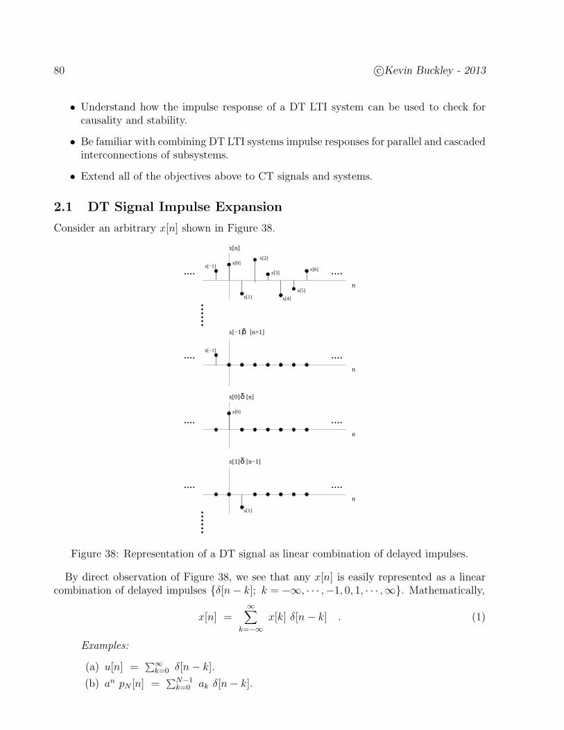
80 c©Kevin Buckley - 2013
• Understand how the impulse response of a DT LTI system can be used to check forcausality and stability.
• Be familiar with combining DT LTI systems impulse responses for parallel and cascadedinterconnections of subsystems.
• Extend all of the objectives above to CT signals and systems.
2.1 DT Signal Impulse Expansion
Consider an arbitrary x[n] shown in Figure 38.
n
x[n]
x[3]x[−1]
.... ....x[2]
x[0]
x[1] x[4]
x[5]
x[6]
n
.... ....x[0]
x[0] [n]δ
n
x[−1].... ....
x[−1] [n+1]δ
n
.... ....
x[1]
x[1] [n−1]δ
............
Figure 38: Representation of a DT signal as linear combination of delayed impulses.
By direct observation of Figure 38, we see that any x[n] is easily represented as a linearcombination of delayed impulses δ[n− k]; k = −∞, · · · ,−1, 0, 1, · · · ,∞. Mathematically,
x[n] =∞∑
k=−∞x[k] δ[n− k] . (1)
Examples:
(a) u[n] =∑∞
k=0 δ[n− k].
(b) an pN [n] =∑N−1
k=0 ak δ[n− k].

c©Kevin Buckley - 2013 81
2.2 DT LTI System I/O Calculation: The Convolution Sum
With Chapter 1 of this Course behind us, we are familiar with the impulse response h[n] ofDT LTI systems. We were able to identify h[n] for some relatively simple systems. Laterin the Course we well see how to systematically determine h[n] for any DT LTI system,regardless of how complex it is. For now, assume that for any DT LTI system we areinterested in, we have h[n].
2.2.1 The Impulse Response of a DT LTI System & Convolution Sum
Figure 99 develops the convolution sum of the input and the impulse response as the time-domain I/O calculation of a DT LTI system.
[n]δ
[n−k]δ
x[k] [n−k]δ
k
δx[k] [n−k]
(by the TI property)
(by the LTI properties)
(by the LTI properties)
impulse resp. h[n]
h[n]DT LTI system
Figure 39: A DT LTI system and the convolution sum.
So, from the box in Figure 99, the I/O calculation for any DT LTI system is
y[n] =∞∑
k=−∞x[k] h[n− k] . (2)
This is the convolution sum of input x[n] with impulse response h[n]. Since h[n] is all weneed to know about the DT LTI system to compute the output, the impulse response h[n] isa very useful I/O characterization. From Chapter 1, we already have some experience withfinding the impulse response of simple LTI systems. Later in the Course we will establish ageneral approach for identifying the impulse response which can be systematically appliedto any LTI system, no matter how complicated it is. In this Chapter we will assume thatwe know the impulse response.
Considering Eq (2), with the change of variables k → n− k, we equivalently have
y[n] =∞∑
k=−∞h[k] x[n− k] . (3)
Since the convolution of two signals, in this case an input x[n] and an impulse response h[n],is such an important operation, it has its own notation. We represent Eqs (2,3) as
y[n] = h[n] ∗ x[n] = x[n] ∗ h[n] . (4)
Note that in Eqs (2,3) the index k can be thought of as memory time. That is, the outputat time n is in general effected by the input for all memory time k.
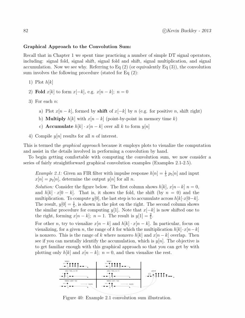
82 c©Kevin Buckley - 2013
Graphical Approach to the Convolution Sum:
Recall that in Chapter 1 we spent time practicing a number of simple DT signal operators,including: signal fold, signal shift, signal fold and shift, signal multiplication, and signalaccumulation. Now we see why. Referring to Eq (2) (or equivalently Eq (3)), the convolutionsum involves the following procedure (stated for Eq (2):
1) Plot h[k]
2) Fold x[k] to form x[−k], e.g. x[n− k]; n = 0
3) For each n:
a) Plot x[n− k], formed by shift of x[−k] by n (e.g. for positive n, shift right)
b) Multiply h[k] with x[n− k] (point-by-point in memory time k)
c) Accumulate h[k] · x[n− k] over all k to form y[n]
4) Compile y[n] results for all n of interest.
This is termed the graphical approach because it employs plots to visualize the computationand assist in the details involved in performing a convolution by hand.
To begin getting comfortable with computing the convolution sum, we now consider aseries of fairly straightforward graphical convolution examples (Examples 2.1-2.5).
Example 2.1: Given an FIR filter with impulse response h[n] = 15p5[n] and input
x[n] = p2[n], determine the output y[n] for all n.
Solution: Consider the figure below. The first column shows h[k], x[n−k] n = 0,and h[k] · x[0 − k]. That is, it shows the fold, the shift (by n = 0) and themultiplication. To compute y[0], the last step is to accumulate across h[k]·x[0−k].The result, y[0] = 1
5, is shown in the plot on the right. The second column shows
the similar procedure for computing y[1]. Note that x[−k] is now shifted one tothe right, forming x[n− k]; n = 1. The result is y[1] = 2
5.
For other n, try to visualize x[n − k] and h[k] · x[n − k]. In particular, focus onvisualizing, for a given n, the range of k for which the multiplication h[k] ·x[n−k]is nonzero. This is the range of k where nonzero h[k] and x[n− k] overlap. Thensee if you can mentally identify the accumulation, which is y[n]. The objective isto get familiar enough with this graphical approach so that you can get by withplotting only h[k] and x[n− k]; n = 0, and then visualize the rest.
h[k] x[0−k]
k0
1/5
n
1/52/5
y[n]
k0
1/5
h[k] x[1−k]
1
k0
x[n−k]; n=1
1
sumsum
x[n−k]; n=0
k0−1
h[k]
4 k0
h[k]
4 k0
1
1/5
1
1/5
Figure 40: Example 2.1 convolution sum illustration.
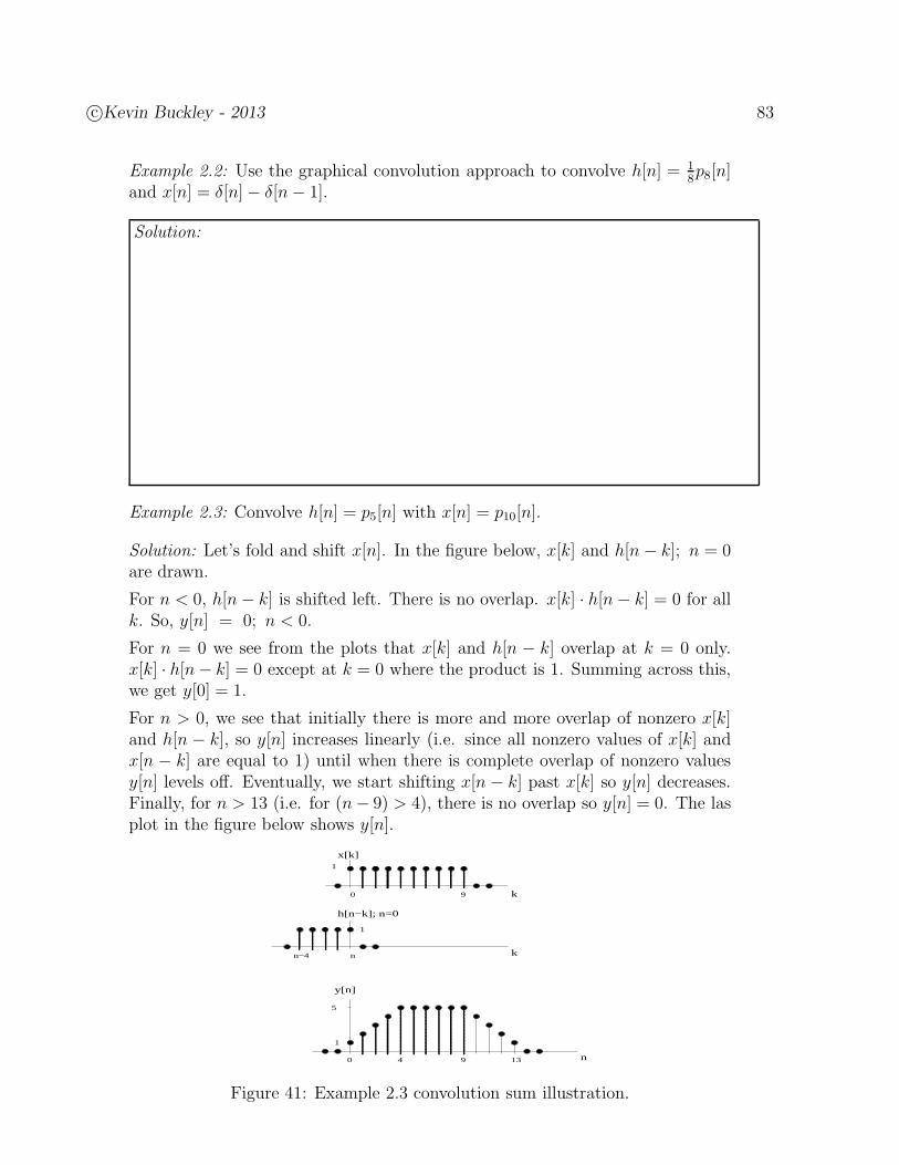
c©Kevin Buckley - 2013 83
Example 2.2: Use the graphical convolution approach to convolve h[n] = 18p8[n]
and x[n] = δ[n]− δ[n− 1].
Solution:
Example 2.3: Convolve h[n] = p5[n] with x[n] = p10[n].
Solution: Let’s fold and shift x[n]. In the figure below, x[k] and h[n− k]; n = 0are drawn.
For n < 0, h[n− k] is shifted left. There is no overlap. x[k] · h[n− k] = 0 for allk. So, y[n] = 0; n < 0.
For n = 0 we see from the plots that x[k] and h[n − k] overlap at k = 0 only.x[k] · h[n− k] = 0 except at k = 0 where the product is 1. Summing across this,we get y[0] = 1.
For n > 0, we see that initially there is more and more overlap of nonzero x[k]and h[n − k], so y[n] increases linearly (i.e. since all nonzero values of x[k] andx[n − k] are equal to 1) until when there is complete overlap of nonzero valuesy[n] levels off. Eventually, we start shifting x[n − k] past x[k] so y[n] decreases.Finally, for n > 13 (i.e. for (n− 9) > 4), there is no overlap so y[n] = 0. The lasplot in the figure below shows y[n].
1
0
x[k]
k9
h[n−k]; n=0
k
1
nn−4
y[n]
n
5
1
0 4 9 13
Figure 41: Example 2.3 convolution sum illustration.

84 c©Kevin Buckley - 2013
Example 2.4: Using the graphical approach, find h[n] = h1[n] ∗ h2[n] whereh1[n] = 2n p10[n] and h2[n] = 2n p10[n]. Specifically,
1. Sketch h1[k] and h2[2− k].
2. Sketch h1[k] · h2[2− k].
3. Determine h[2].
4. Determine, for all n, h[n].
Solution: h1[k], h2[2 − k] and h1[k] · h2[2 − k] are shown in part a) of the figurebelow. h1[k] · h2[2− k] is shown in part b). As indicated in part c) of the figure,h[2] is computed as accumulation of h1[k] · h2[2− k]. The result is h[2] = 12.
1h [k] 2h [2−k]
k
h[2] = = 4 + 4 + 4 = 12
1h [k]
k1 2 9
....21
4
512
2h [2−k]
1h [k] 2h [2−k]
1h [k]
2n
512
k
4
21
....
1−7 2 k
....
2h [n−k]; n=0
n − 9= −9
−1
n=0
12
4
512
1k1 2
21
4
21h [k]h [n−k]; 0 < n < 9
....21
4
512
k1 2 9
kn
....
a)
b)
c)
d)
2
2k
n−k
Figure 42: Example 2.4 convolution sum illustration.
Part d) of this figure shows the plots that, hopefully with practice, will be suffi-cient to determine h[n] for all n. Note the this first plot in part d) is just h1[k](the signal not to be folded) plotted as a function of k. Note that the nonzerovalues of h1[k] are labeled with their values. Then h2[n− k] (the signal is whichfolded and shifted) is plotted as a function of k for n = 0. Again note thatits nonzero values are labeled with their values. Also note that the leading anlagging edges of the signal are labeled (as a function of n). All these labels assistin determining the solution.
Now visualize shifting the signal in this plot left (for n < 0) and right (for n > 0),and for different shifts identify the range of k where h1[k] and h2[n− k] overlap.For each n, this will be the range of k that must be accumulated. For example:
• For n < 0 there will be no overlap, so h1[k] · h2[n− k] will be zero for all k,so its accumulation (i.e. h[n]) will be zero.

c©Kevin Buckley - 2013 85
• or 0 ≤ n ≤ 9, the last plot shows h1[k] ·h2[n−k]. We see that, for this rangeof n, h1[k] and h2[n− k] will overlap from k = 0 ((when h1[k] turns on) tok = n (after which h2[n− k] turns off). We see this by observing where thesignal edges are, as a function of k, which are identified in the plots. Notingwhat the h1[k] and h2[n−k] values are for this range of k (i.e. from the plotlabels h1[k] = 2k and h2[n− k] = 2n−k), we have that h1[k] · h2[n− k] = 2n
over its nonzero range. Accumulating across these nonzero values, we havethat h[n] = (n+ 1) · 2n.• For 10 ≤ n ≤ 18, the overlap of nonzero h1[k] and h2[n−k] is from k = n−9(when h2[n − k] turns on) till k = 9 (after which h1[k] turns off). Againh1[k] · h2[n− k] = 2n over its nonzero range. Thus, h[n] = (9 − (n− 9) +1) · 2n = (19− n) · 2n over this range.
• Finally, for n > 18 h[n] = 0 since there is no overlap of nonzero h1[k] andh2[n−k]. This is because the lagging edge of h2[n−k] (which is at k = n−9)we greater that the leading edge of h1[k] (which is at k = 9).
In summary, we have that
h[n] =
0 n < 0(n+ 1) · 2n 0 ≤ n ≤ 9(19− n) · 2n 10 ≤ n ≤ 180 n > 18
(5)
Note that in Example 2.4 we are dealing with signals h1[n] and h2[n], the implication beingthat these are not necessarily the input and impulse response of a DT LTI system. Thischoice of signal notation drives home the point that the convolution sum is a general operationapplied to two signal that has utility that goes beyond an I/O calculation for DT LTI systems.
If you can follow Example 2.4, you should be able to handle any graphical convolution,regardless of its complexity. Again, note the utility of labeling the nonzero values of theplotted signals (e.g. h1[k] and h2[n−k] in Example 2.4) and labeling the leading and laggingedges of these signals. Also note that the advantage of this graphical approach to convolutionstems from the fact that it assists in determining: 1) the different regions of n where thereare different types of overlap (over k); and 2) what range of overlap in k there is for eachregion of n.
Example 2.5: Convolve h[n] = p10[n] with x[n] = p15[n−5], first graphically thenusing Matlab.
Solution: This Example is a lot like Example 2.3. The pulses are of differentwidth, and one is delayed, but you can still expect the result to look like atriangle with its top chopped off (as in Example 2.3). The graphical approachcan be used to identify the details of the result (i.e. when the triangle turns onan off, and where the top is chopped off). Try this yourself, and compare yourresult to the Matlab generated plots below.
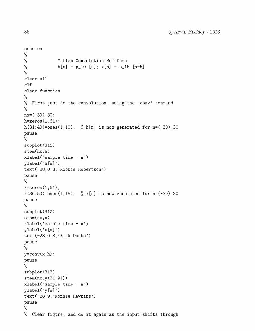
86 c©Kevin Buckley - 2013
echo on
%
% Matlab Convolution Sum Demo
% h[n] = p_10 [n]; x[n] = p_15 [n-5]
%
clear all
clf
clear function
%
% First just do the convolution, using the "conv" command
%
nx=(-30):30;
h=zeros(1,61);
h(31:40)=ones(1,10); % h[n] is now generated for n=(-30):30
pause
%
subplot(311)
stem(nx,h)
xlabel(’sample time - n’)
ylabel(’h[n]’)
text(-28,0.8,’Robbie Robertson’)
pause
%
x=zeros(1,61);
x(36:50)=ones(1,15); % x[n] is now generated for n=(-30):30
pause
%
subplot(312)
stem(nx,x)
xlabel(’sample time - n’)
ylabel(’x[n]’)
text(-28,0.8,’Rick Danko’)
pause
%
y=conv(x,h);
pause
%
subplot(313)
stem(nx,y(31:91))
xlabel(’sample time - n’)
ylabel(’y[n]’)
text(-28,9,’Ronnie Hawkins’)
pause
%
% Clear figure, and do it again as the input shifts through
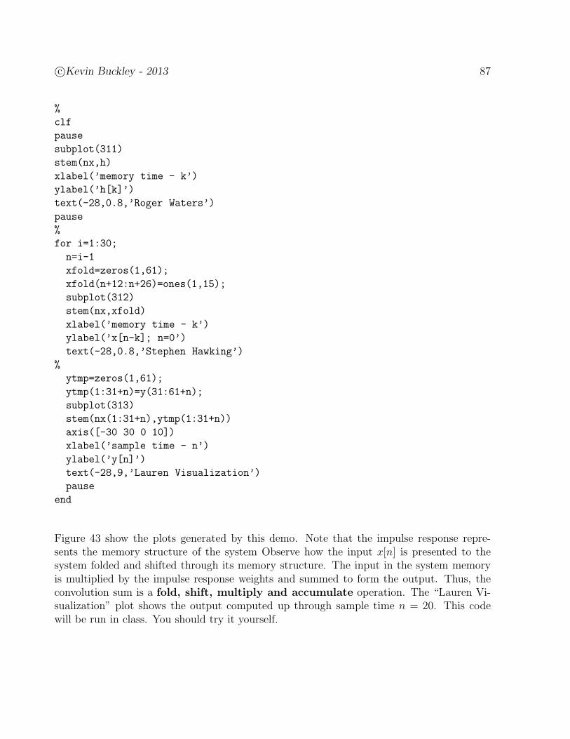
c©Kevin Buckley - 2013 87
%
clf
pause
subplot(311)
stem(nx,h)
xlabel(’memory time - k’)
ylabel(’h[k]’)
text(-28,0.8,’Roger Waters’)
pause
%
for i=1:30;
n=i-1
xfold=zeros(1,61);
xfold(n+12:n+26)=ones(1,15);
subplot(312)
stem(nx,xfold)
xlabel(’memory time - k’)
ylabel(’x[n-k]; n=0’)
text(-28,0.8,’Stephen Hawking’)
%
ytmp=zeros(1,61);
ytmp(1:31+n)=y(31:61+n);
subplot(313)
stem(nx(1:31+n),ytmp(1:31+n))
axis([-30 30 0 10])
xlabel(’sample time - n’)
ylabel(’y[n]’)
text(-28,9,’Lauren Visualization’)
pause
end
Figure 43 show the plots generated by this demo. Note that the impulse response repre-sents the memory structure of the system Observe how the input x[n] is presented to thesystem folded and shifted through its memory structure. The input in the system memoryis multiplied by the impulse response weights and summed to form the output. Thus, theconvolution sum is a fold, shift, multiply and accumulate operation. The “Lauren Vi-sualization” plot shows the output computed up through sample time n = 20. This codewill be run in class. You should try it yourself.

88 c©Kevin Buckley - 2013
−30 −20 −10 0 10 20 300
0.5
1
sample time − n
h[n]
Robbie Robertson
−30 −20 −10 0 10 20 300
0.5
1
sample time − n
x[n]
Rick Danko
−30 −20 −10 0 10 20 300
5
10
sample time − n
y[n]
Ronnie Hawkins
−30 −20 −10 0 10 20 300
0.5
1
memory time − k
h[k]
Roger Waters
−30 −20 −10 0 10 20 300
0.5
1
memory time − k
x[n−k
]; n=0
Stephen Hawking
−30 −20 −10 0 10 20 300
5
10
sample time − n
y[n]
Lauren Visualization
Figure 43: Plots generated by the Convolution Sum Demo.
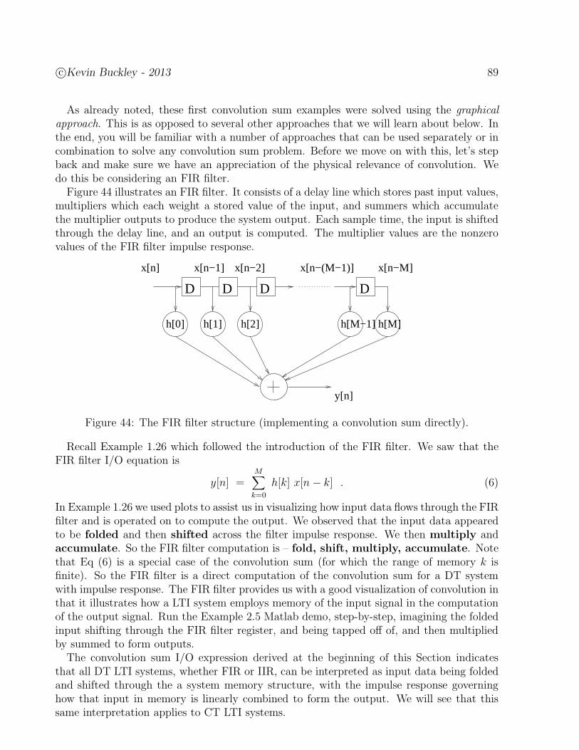
c©Kevin Buckley - 2013 89
As already noted, these first convolution sum examples were solved using the graphicalapproach. This is as opposed to several other approaches that we will learn about below. Inthe end, you will be familiar with a number of approaches that can be used separately or incombination to solve any convolution sum problem. Before we move on with this, let’s stepback and make sure we have an appreciation of the physical relevance of convolution. Wedo this be considering an FIR filter.
Figure 44 illustrates an FIR filter. It consists of a delay line which stores past input values,multipliers which each weight a stored value of the input, and summers which accumulatethe multiplier outputs to produce the system output. Each sample time, the input is shiftedthrough the delay line, and an output is computed. The multiplier values are the nonzerovalues of the FIR filter impulse response.
D D D D
y[n]
h[0] h[1] h[2]
x[n] x[n−1] x[n−2] x[n−(M−1)] x[n−M]
h[M]h[M−1]
Figure 44: The FIR filter structure (implementing a convolution sum directly).
Recall Example 1.26 which followed the introduction of the FIR filter. We saw that theFIR filter I/O equation is
y[n] =M∑
k=0
h[k] x[n− k] . (6)
In Example 1.26 we used plots to assist us in visualizing how input data flows through the FIRfilter and is operated on to compute the output. We observed that the input data appearedto be folded and then shifted across the filter impulse response. We then multiply andaccumulate. So the FIR filter computation is – fold, shift, multiply, accumulate. Notethat Eq (6) is a special case of the convolution sum (for which the range of memory k isfinite). So the FIR filter is a direct computation of the convolution sum for a DT systemwith impulse response. The FIR filter provides us with a good visualization of convolution inthat it illustrates how a LTI system employs memory of the input signal in the computationof the output signal. Run the Example 2.5 Matlab demo, step-by-step, imagining the foldedinput shifting through the FIR filter register, and being tapped off of, and then multipliedby summed to form outputs.
The convolution sum I/O expression derived at the beginning of this Section indicatesthat all DT LTI systems, whether FIR or IIR, can be interpreted as input data being foldedand shifted through the a system memory structure, with the impulse response governinghow that input in memory is linearly combined to form the output. We will see that thissame interpretation applies to CT LTI systems.
90 c©Kevin Buckley - 2013
The convolution sum examples considered to this point have involved two finite durationsignals. The next two examples consider some infinitely long signals. If anything, infinitelylong signals can be easier to graphically convolve because they result in fewer regions of nfor which different ranges of summation over k must identified and solved.
Example 2.6: For a DT LTI system with impulse response h[n] = an u[n], witha = 0.9, determine the output due to input x[n] = δ[n]− .9δ[n− 1].
Solution: For the graphical approach, we choose to fold and shift x[n]. The figurebelow shows h[k] and x[n− k]; n = 0 as functions of k.
k0.9
k0
.....
h[k]
1
0
1
y[n]
n
.....
k
x[n−k]; n=01
n−1n
−0.9
Visualizing the shift of x[n− k], we get
y[n] =
0 n < 01 n = 00.9 − 0.9 = 0 n = 10.9n − 0.9n = 0 n ≥ 1
= δ[n] .
How does this Example relate to the result using the second equalizer consideredin Practicum 1?
Example 2.7: Convolve h[n] = an u[n] with x[n] = bn u[n]. Assume that a 6= b,and for plotting purposes that 0 < a, b < 1.
Solution:
c©Kevin Buckley - 2013 91
Example 2.8: Convolve h[n] = an u[n] with x[n] = p10[n + 2].
Solution:
For the next four examples, it is easier to use the convolution sum expression directly. Thisis called the analytical approach.
Example 2.9: Convolve h[n] = an u[n] with x[n] = ejω0n. Assume |a| < 1 (so thethe infinitely long geometric series summation involved in the solutions can besolved). Note that for this example you will probably find it easier to fold andshift x[n]. However, you might try it both ways.
Solution:
Example 2.10: Convolve h[n] = p10[n] with x[n] = ejω0n. First determine theanswer for general ω0, and then specifically for ω0 =
2π10.
Solution:
y[n] =∞∑
k=−∞h[k] x[n− k] =
9∑
k=0
ejω0(n−k) = ejω0n9∑
k=0
e−jω0k
= ejω0n1 − e−jω010
1 − e−jω0.
From this general solution, for ω0 =2π10
we have that
y[n] = ej(2π/10)n1 − e−j(2π/10)10
1 − e−j(2π/10)= ej(2π/10)n
1 − 1
1 − e−j(2π/10)= 0.
Note that this 10-point summer completely attenuates a complex-valued sinusoidof frequency ω0 =
2π10. What other frequencies are completely attenuated?
92 c©Kevin Buckley - 2013
Example 2.11: Let’s go back an solve Example 2.7, this time using the analyticalapproach. Convolve h[n] = an u[n] with x[n] = bn u[n]. Assume that a 6= b.
Solution:
Consider the convolution of a DT LTI system impulse response h[n] = δ[n−2] with a generalinput x[n]. The output is
y[n] = δ[n− 2] ∗ x[n] =∞∑
k=−∞x[k] δ[n− k − 2] .
For each n, δ[n− k − 2] is zero for all k except for k = n− 2. Thus, for each n, the infinitesum has only one nonzero entry, the k = n− 2 term, which is x[n− 2]. Thus,
y[n] = x[n− 2] .
Note that we have identified the impulse response of a new type of simple DT LTI system.The impulse response of an m sample delay is simply h[n] = δ[n−m].
c©Kevin Buckley - 2013 93
In the next example, we take advantage of a previous result (specifically from Example 2.7).
Example 2.12: Find the step response of the simple IIR filter impulse responseh[n] = an u[n].
Solution:
In the next two examples we take advantage of both previous results and properties of theLTI system that the convolution calculation represents.
Example 2.13: Determine the y[n] of the LTI system with h[n] = an u[n] due toinput x[n] = bn−5 u[n− 5]. Use the Example 2.7 result and exploit system timeinvariance.
Solution: This example is like Example 2.7, except the input is delayed gotm = 5. Since the system is time invariant, the output is just the output fromExample 2.7 delayed by m = 5.
y[n] =bn−4 − an−4
b − au[n− 5] .
Example 2.14: Determine the output y[n] of the LTI system with h[n] = an u[n]due to input x[n] = bn p20[n]. Use the Examples 2.7,2.13 results and exploitsystem linearity.
Solution: First note that
x[n] = bn u[n] − bn u[n− 20] = bn u[n] − b20 bn−20 u[n− 20] .
Then, exploiting the linearity and time invariance properties of the system,
y[n] =bn+1 − an+1
b − au[n] − b20
bn−19 − an−19
b − au[n− 20] .
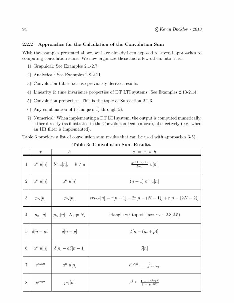
94 c©Kevin Buckley - 2013
2.2.2 Approaches for the Calculation of the Convolution Sum
With the examples presented above, we have already been exposed to several approaches tocomputing convolution sums. We now organizes these and a few others into a list.
1) Graphical: See Examples 2.1-2.7
2) Analytical: See Examples 2.8-2.11.
3) Convolution table: i.e. use previously derived results.
4) Linearity & time invariance properties of DT LTI systems: See Examples 2.13-2.14.
5) Convolution properties: This is the topic of Subsection 2.2.3.
6) Any combination of techniques 1) through 5).
7) Numerical: When implementing a DT LTI system, the output is computed numerically,either directly (as illustrated in the Convolution Demo above), of effectively (e.g. whenan IIR filter is implemented).
Table 3 provides a list of convolution sum results that can be used with approaches 3-5).
Table 3: Convolution Sum Results.
x h y = x ∗ h
1 an u[n] bn u[n]; b 6= a bn+1−an+1
b−au[n]
2 an u[n] an u[n] (n + 1) an u[n]
3 pN [n] pN [n] tri2N [n] = r[n+ 1]− 2r[n− (N − 1)] + r[n− (2N − 2)]
4 pN1 [n] pN2 [n]; N1 6= N2 triangle w/ top off (see Exs. 2.3,2.5)
5 δ[n−m] δ[n− p] δ[n− (m+ p)]
6 an u[n] δ[n]− aδ[n− 1] δ[n]
7 ejω0n an u[n] ejω0n 11 − a e−jω0
8 ejω0n pN [n] ejω0n 1 − e−jω0N
1 − e−jω0
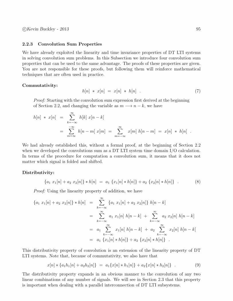
c©Kevin Buckley - 2013 95
2.2.3 Convolution Sum Properties
We have already exploited the linearity and time invariance properties of DT LTI systemsin solving convolution sum problems. In this Subsection we introduce four convolution sumproperties that can be used to the same advantage. The proofs of these properties are given.You are not responsible for these proofs, but following them will reinforce mathematicaltechniques that are often used in practice.
Commutativity:h[n] ∗ x[n] = x[n] ∗ h[n] . (7)
Proof: Starting with the convolution sum expression first derived at the beginningof Section 2.2, and changing the variable as m −→ n− k, we have
h[n] ∗ x[n] =∞∑
k=−∞h[k] x[n− k]
=−∞∑
m=∞h[n−m] x[m] =
∞∑
m=−∞x[m] h[n−m] = x[n] ∗ h[n] .
We had already established this, without a formal proof, at the beginning of Section 2.2when we developed the convolutions sum as a DT LTI system time domain I/O calculation.In terms of the procedure for computation a convolution sum, it means that it does notmatter which signal is folded and shifted.
Distributivity:
a1 x1[n] + a2 x2[n] ∗ h[n] = a1 x1[n] ∗ h[n] + a2 x2[n] ∗ h[n] . (8)
Proof: Using the linearity property of addition, we have
a1 x1[n] + a2 x2[n] ∗ h[n] =∞∑
k=−∞a1 x1[n] + a2 x2[n] h[n− k]
=∞∑
k=−∞a1 x1[n] h[n− k] +
∞∑
k=−∞a2 x2[n] h[n− k]
= a1∞∑
k=−∞x1[n] h[n− k] + a2
∞∑
k=−∞x2[n] h[n− k]
= a1 x1[n] ∗ h[n]+ a2 x2[n] ∗ h[n] .
This distributivity property of convolution is an extension of the linearity property of DTLTI systems. Note that, because of commutativity, we also have that
x[n] ∗ a1h1[n] + a2h2[n] = a1x[n] ∗ h1[n] + a2x[n] ∗ h2[n] . (9)
The distributivity property expands in an obvious manner to the convolution of any twolinear combinations of any number of signals. We will see in Section 2.3 that this propertyis important when dealing with a parallel interconnection of DT LTI subsystems.
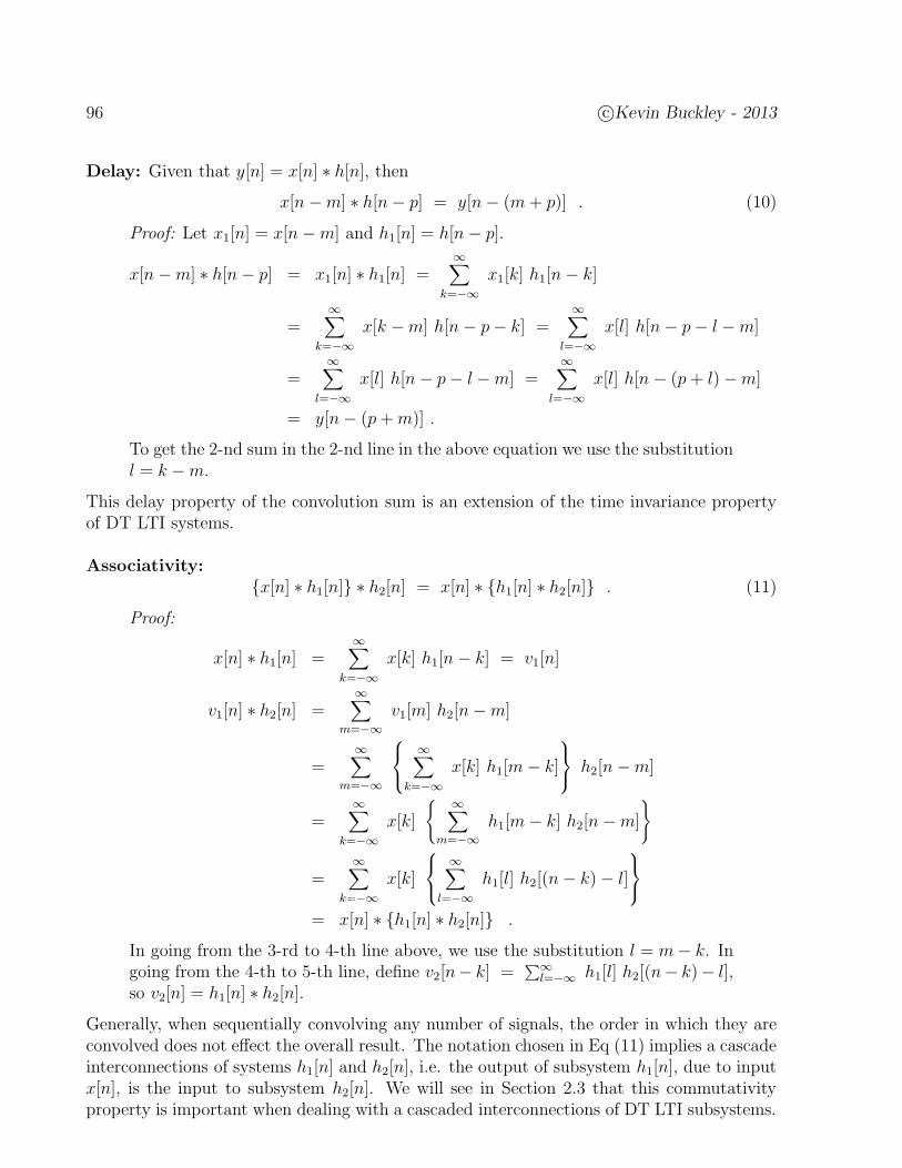
96 c©Kevin Buckley - 2013
Delay: Given that y[n] = x[n] ∗ h[n], thenx[n−m] ∗ h[n− p] = y[n− (m+ p)] . (10)
Proof: Let x1[n] = x[n−m] and h1[n] = h[n− p].
x[n−m] ∗ h[n− p] = x1[n] ∗ h1[n] =∞∑
k=−∞x1[k] h1[n− k]
=∞∑
k=−∞x[k −m] h[n− p− k] =
∞∑
l=−∞x[l] h[n− p− l −m]
=∞∑
l=−∞x[l] h[n− p− l −m] =
∞∑
l=−∞x[l] h[n− (p+ l)−m]
= y[n− (p+m)] .
To get the 2-nd sum in the 2-nd line in the above equation we use the substitutionl = k −m.
This delay property of the convolution sum is an extension of the time invariance propertyof DT LTI systems.
Associativity:x[n] ∗ h1[n] ∗ h2[n] = x[n] ∗ h1[n] ∗ h2[n] . (11)
Proof:
x[n] ∗ h1[n] =∞∑
k=−∞x[k] h1[n− k] = v1[n]
v1[n] ∗ h2[n] =∞∑
m=−∞v1[m] h2[n−m]
=∞∑
m=−∞
∞∑
k=−∞x[k] h1[m− k]
h2[n−m]
=∞∑
k=−∞x[k]
∞∑
m=−∞h1[m− k] h2[n−m]
=∞∑
k=−∞x[k]
∞∑
l=−∞h1[l] h2[(n− k)− l]
= x[n] ∗ h1[n] ∗ h2[n] .
In going from the 3-rd to 4-th line above, we use the substitution l = m− k. Ingoing from the 4-th to 5-th line, define v2[n− k] =
∑∞l=−∞ h1[l] h2[(n− k)− l],
so v2[n] = h1[n] ∗ h2[n].
Generally, when sequentially convolving any number of signals, the order in which they areconvolved does not effect the overall result. The notation chosen in Eq (11) implies a cascadeinterconnections of systems h1[n] and h2[n], i.e. the output of subsystem h1[n], due to inputx[n], is the input to subsystem h2[n]. We will see in Section 2.3 that this commutativityproperty is important when dealing with a cascaded interconnections of DT LTI subsystems.
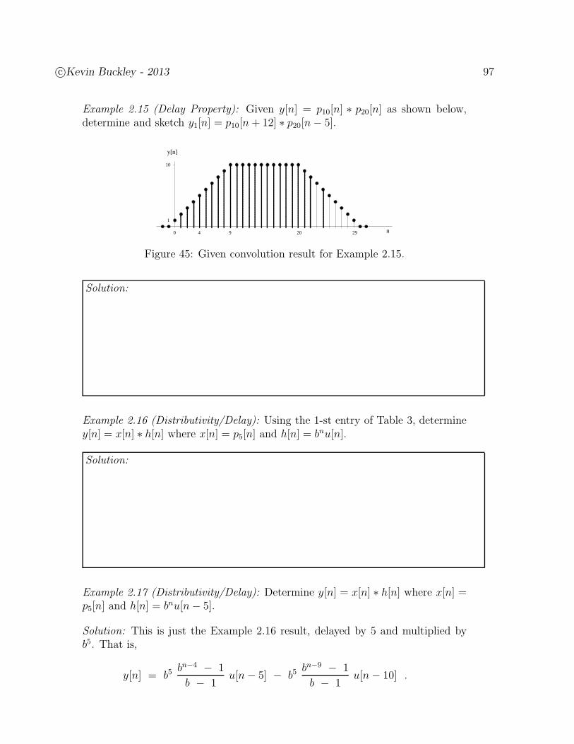
c©Kevin Buckley - 2013 97
Example 2.15 (Delay Property): Given y[n] = p10[n] ∗ p20[n] as shown below,determine and sketch y1[n] = p10[n+ 12] ∗ p20[n− 5].
1
0 4 9
y[n]
n
10
20 29
Figure 45: Given convolution result for Example 2.15.
Solution:
Example 2.16 (Distributivity/Delay): Using the 1-st entry of Table 3, determiney[n] = x[n] ∗ h[n] where x[n] = p5[n] and h[n] = bnu[n].
Solution:
Example 2.17 (Distributivity/Delay): Determine y[n] = x[n] ∗ h[n] where x[n] =p5[n] and h[n] = bnu[n− 5].
Solution: This is just the Example 2.16 result, delayed by 5 and multiplied byb5. That is,
y[n] = b5bn−4 − 1
b − 1u[n− 5] − b5
bn−9 − 1
b − 1u[n− 10] .
98 c©Kevin Buckley - 2013
Example 2.18 (Distributivity): Determine the output of an N -point averagergiven input x[n] = cos(ω0n).
Solution: The impulse response of an N -point averager is h[n] = 1N
pN [n]. Byand Euler’s identity, x[n] = 1
2ejω0n + 1
2e−jω0n. Using Table 3 Entry # 8, and
distributivity, we have,
y[n] =1
2
ejω0n1
N
1 − e−jω0N
1 − e−jω0+ e−jω0n
1
N
1 − ejω0N
1 − ejω0
.
Note that the two additive terms in the solution form a complex conjugate pair.Thus the form of this solution can be simplified into a real-valued expression,which should be expected since both the input and impulse response are real-valued. Instead of pursuing this simplified form here, we will postpone this issueuntil Subsection 2.3.3 below, where we specifically study the sinusoidal responseof DT LTI systems. Specifically, we will revisit this problem in Example 2.27.
Example 2.19: Consider using the Matlab conv function to convolve an FIR filterimpulse response h[n] which is nonzero only over the range 0 ≤ n ≤ N − 1 withan indefinitely duration signal x[n] that turns on at time n = 0.
Solution: This can be be accomplished by breaking x[n] into contiguous blocksof length P as follows:
x[n] = x1[n] + x2[n− P ] + x3[n− 2P ] + · · ·
xi[n] =
x[n− (i− 1)P ] n = 0, 1, · · · , P − 10 otherwise
i = 1, 2, · · · .
We can now use conv to convolve each xi[n] with h[n] to form
yi[n] = xi[n] ∗ h[n] i = 0, 1, 2, · · · .
By the linearity and delay properties, the overall FIR filter output is then
y[n] = y1[n] + y2[n− P ] + y3[n− 2P ] + · · · .
This approach is called the overlap-and-add method of FIR filter implementation,so called because the outputs of the different input blocks, which are overlappedin time, are added together. Figure 46 illustrates this for N = 8 and P = 17.
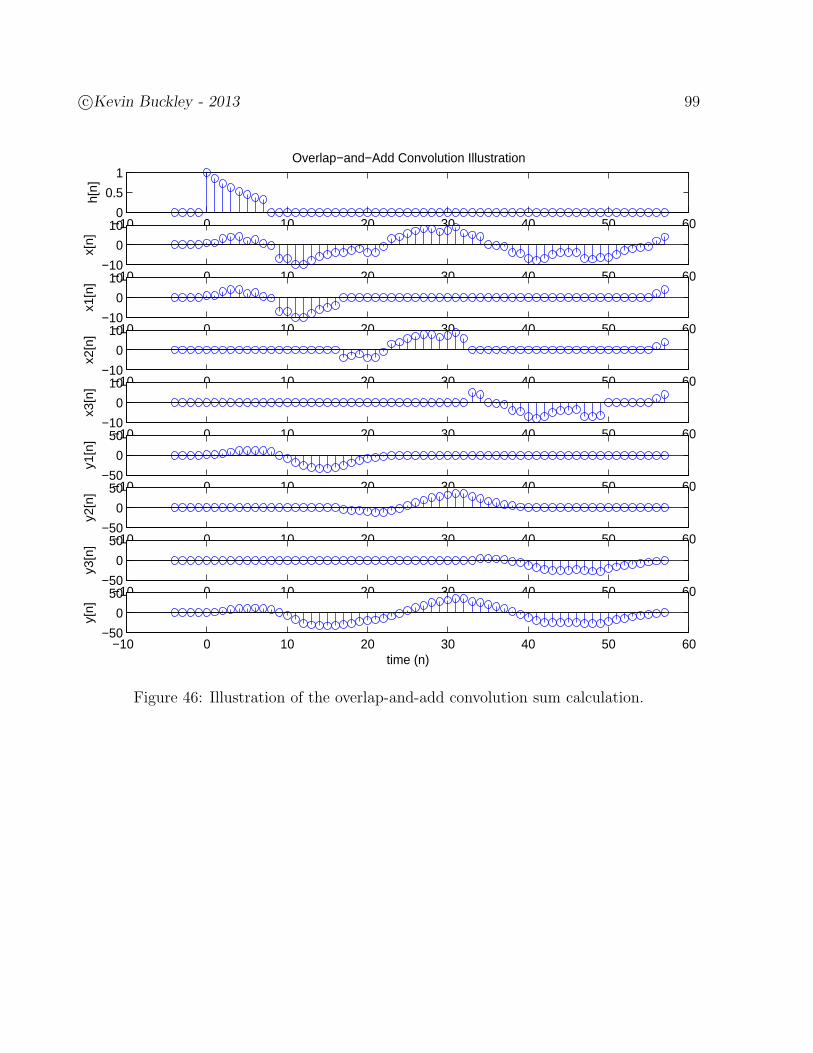
c©Kevin Buckley - 2013 99
−10 0 10 20 30 40 50 600
0.5
1
h[n]
Overlap−and−Add Convolution Illustration
−10 0 10 20 30 40 50 60−10
0
10
x[n]
−10 0 10 20 30 40 50 60−10
0
10
x1[n
]
−10 0 10 20 30 40 50 60−10
0
10
x2[n
]
−10 0 10 20 30 40 50 60−10
0
10
x3[n
]
−10 0 10 20 30 40 50 60−50
0
50
y1[n
]
−10 0 10 20 30 40 50 60−50
0
50
y2[n
]
−10 0 10 20 30 40 50 60−50
0
50
y3[n
]
−10 0 10 20 30 40 50 60−50
0
50
y[n]
time (n)
Figure 46: Illustration of the overlap-and-add convolution sum calculation.
100 c©Kevin Buckley - 2013
2.3 DT LTI System Issues
In Section 1.5 of this Course we considered four system properties: linearity, time-invariance,causality and stability. In this Section we first relate these properties to the impulse responseh[n] of a DT LTI system. Concerning the system interconnections described earlier in Sub-section 1.5.1, we then consider relationships between the overall impulse response of a DTLTI system and those of the constituent DT LTI subsystems.
2.3.1 System Properties
By assumption, a DT LTI system is linear and time-invariant. Recall that one thing thismeans is that if we are given a DT LTI system description in the form of a LCC differenceequation, we know that the system is liner and we know it is time-invariant. So we needonly consider causality and stability.
Causality: Generally, a DT LTI system,
y[n] =∞∑
k=−∞h[k] x[n− k] (12)
uses past, present and future inputs to compute an output. This is clear from this generalconvolution I/O expression. However, for
h[n] = 0 n < 0 (13)
we have that
y[n] =∞∑
k=0
h[k] x[n− k] , (14)
which uses only past and present inputs to compute the output. Thus a DT LTI system iscausal if and only if
h[n] = 0 n < 0 . (15)
Is an FIR filter Causal? The answer is yes, usually. That is, usually an FIR filter ischaracterized as a DT LTI system that has an impulse response with h[n] 6= 0 only forn = 0, 1, 2, · · · , N−1, even though, generally speaking, a finite impulse response filter impulseresponse my range over any finite interval of n. Under the usual characterization of an FIRfilter,
y[n] =N−1∑
k=0
h[k] x[n− k] , (16)
and the system is causal. Thus the answer is a qualified yes.
c©Kevin Buckley - 2013 101
Stability: Recall that for BIBO stability, for any bounded x[n], i.e.
|x[n]| ≤ B1 < ∞ all n (17)
the output y[n] is bounded, i.e.
|y[n]| ≤ B2 < ∞ all n . (18)
Consider any DT LTI system. We have that
|y[n]| =
∣
∣
∣
∣
∣
∣
∞∑
k=−∞h[k] x[n− k]
∣
∣
∣
∣
∣
∣
(19)
≤∞∑
k=−∞| h[k] x[n− k] | (20)
≤∞∑
k=−∞| h[k]| |x[n− k] | . (21)
For worst the case bounded input, i.e. for |x[n]| = B1, we then have that
|y[n]| ≤∞∑
k=−∞| h[k]| B1 (22)
= B1
∞∑
k=−∞| h[k]| . (23)
From this we conclude that |y[n]| is bounded if and only if
∞∑
k=−∞| h[k]| < ∞ . (24)
This is a very useful result, in that for DT LTI systems it provides an simple test for stability.Later in the Course we will see that it also contributes to the importance of another LTIdescription – in terms of poles and zeros.
Example 2.20: Is the DT LTI system with h[n] = .5|n| causal? Stable?
Solution:
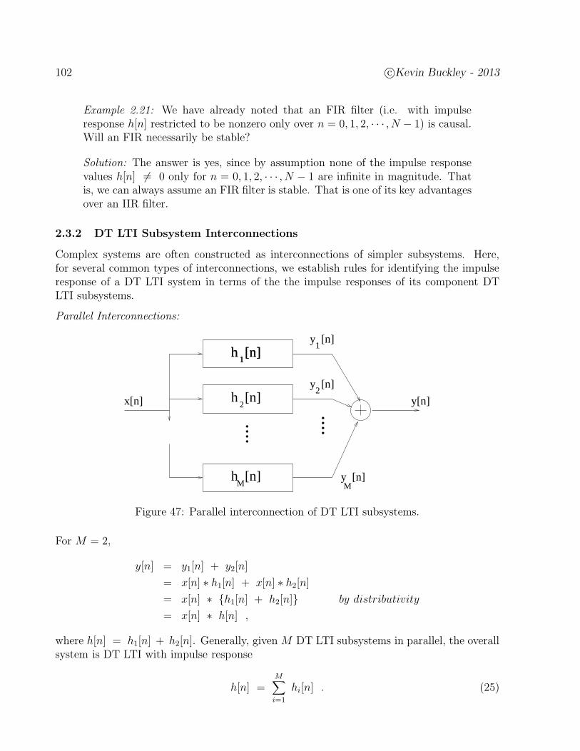
102 c©Kevin Buckley - 2013
Example 2.21: We have already noted that an FIR filter (i.e. with impulseresponse h[n] restricted to be nonzero only over n = 0, 1, 2, · · · , N − 1) is causal.Will an FIR necessarily be stable?
Solution: The answer is yes, since by assumption none of the impulse responsevalues h[n] 6= 0 only for n = 0, 1, 2, · · · , N − 1 are infinite in magnitude. Thatis, we can always assume an FIR filter is stable. That is one of its key advantagesover an IIR filter.
2.3.2 DT LTI Subsystem Interconnections
Complex systems are often constructed as interconnections of simpler subsystems. Here,for several common types of interconnections, we establish rules for identifying the impulseresponse of a DT LTI system in terms of the the impulse responses of its component DTLTI subsystems.
Parallel Interconnections:
y [n]1
h [n]1
h [n]1
h [n]2
h [n]M
x[n] y[n]
y [n]2
y [n]M
....
....
Figure 47: Parallel interconnection of DT LTI subsystems.
For M = 2,
y[n] = y1[n] + y2[n]
= x[n] ∗ h1[n] + x[n] ∗ h2[n]
= x[n] ∗ h1[n] + h2[n] by distributivity
= x[n] ∗ h[n] ,
where h[n] = h1[n] + h2[n]. Generally, given M DT LTI subsystems in parallel, the overallsystem is DT LTI with impulse response
h[n] =M∑
i=1
hi[n] . (25)

c©Kevin Buckley - 2013 103
Cascade (Series) Interconnections:
1v [n]
2v [n]
Mv [n]
h [n]1
h [n]2
h [n]M
y[n]....x[n]
Figure 48: Cascade interconnection of DTLTI subsystems.
For M = 2,
y[n] = v[n] ∗ h2[n]
= x[n] ∗ h1[n] ∗ h2[n]
= x[n] ∗ h1[n] ∗ h2[n] by associativity
= x[n] ∗ h[n] ,
where h[n] = h1[n] ∗ h2[n]. Generally, given M DT LTI subsystems in cascade, the overallsystem is DT LTI with impulse response
h[n] = h1[n] ∗ h2[n] ∗ · · · ∗ hM [n] . (26)
Feedback Interconnections: This representation of DT LTI systems, in terms of impulseresponses, does not easily lead to an overall system I/O expression in terms of the individualsubsystems.
Example 2.22: Determine the impulse responses of the combined channel/equalizerfor the channel and each of the equalizers considered in Practicum 1.
Solution:
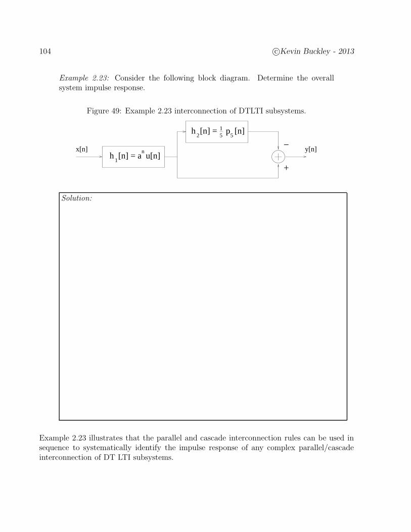
104 c©Kevin Buckley - 2013
Example 2.23: Consider the following block diagram. Determine the overallsystem impulse response.
Figure 49: Example 2.23 interconnection of DTLTI subsystems.
1h [n] = a u[n]
nx[n]
51
2h [n] = p [n]
5
y[n]−
+
Solution:
Example 2.23 illustrates that the parallel and cascade interconnection rules can be used insequence to systematically identify the impulse response of any complex parallel/cascadeinterconnection of DT LTI subsystems.
c©Kevin Buckley - 2013 105
2.3.3 DT LTI System Response to Sinusoidal Inputs
In Examples 2.8, 2.9 & 2.18, as illustrations of the analytical approach and convolutionproperties approaches to performing a convolution sum, we considered applying sinusoidalinputs to a DT LTI system. Here, through a sequence of examples, we more systematicallyfocus on how DT LTI systems process sinusoidal inputs.
Example 2.24: Consider an FIR filter with impulse response h[n] = 116
p16[n] (i.e.a 16-point averager). Determine its response to complex-valued sinusoidal inputx[n] = 1 + ej(2π5/16)n.
Solution: This problem is similar to Example 2.18 in that we have the superpo-sition of two complex-valued sinusoids (in this case one is DC – i.e. ω0 = 0) intoa DT LTI system (in both cases a 16-point averager). Paralleling the Example2.18 solution,
y[n] =∞∑
k=−∞h[k] x[n− k] =
15∑
k=0
1
16x[n− k] = =
1
16
15∑
k=0
x[n− k]
=1
16
15∑
k=0
(
1 + ej2π(5/16)(n−k))
=1
16
15∑
k=0
1 +1
16
15∑
k=0
ej2π(5/16)(n−k)
= 1 +1
16ej2π(5/16)n
15∑
k=0
e−j2π(5/16)k = 1 + ej2π(5/16)n1
16
1 − e−j2π(5/16)16
1 − e−j2π(5/16)
= 1 +1
N
1 − 1
1 − e−j2π(5/16)= 1 .
Note that the sinusoidal component of the input, with frequency ω0 = 2π(5/16),is completely filtered out (i.e. ∞ attenuation). The DC component of the inputis not ”filtered out”. In fact it appears at the output without distortion. Filteringis one of the main things we do with LTI systems.
The filter analysis problem is to determine the filtering characteristics of a given LTIsystem. We focus on this later in this Course.
The filter design problem is to select (in the FIR case) N and h[n]; n = 0, 1, · · · , N − 1so as to realize some given filtering specification. Filter design is a topic of a senior levelDigital Signal Processing (DSP) course.
106 c©Kevin Buckley - 2013
Example 2.25: Again consider the 16-point averager.
a) Determine the response for a general complex-valued sinusoid x[n] = A ej(ω0n+φ),where A and φ are constants and ω0 is some value of frequency.
b) For what frequencies ω0 over the range −π < ωo ≤ π is the output y[n] = 0for all n?
c) You will see from the 1-st part of this problem that for this system anda complex-valued sinusoidal input, the output will be a scaled version ofthe input. Note that in general this scaling is complex-valued, thus boththe magnitude and phase of the input signal are altered. As a functionof the input frequency ω0, determine this complex-valued scaling function.Roughly sketch its magnitude for −π < ω0 ≤ π.
Solution:
a) This follows the Example 2.24 solution.
y[n] =∞∑
k=−∞h[k] x[n− k] =
15∑
k=0
1
16x[n− k] = =
1
16
15∑
k=0
x[n− k]
=1
16
15∑
k=0
A ej(2ω0(n−k)+φ) = A ej(ω0n+φ) 1
16
15∑
k=0
e−jω0k
= A ej(ω0n+φ) 1
16
1 − e−jω0·16
1 − e−jω0.
b) y[n] = 0 for ω0 such that (1 − e−jω0·16) = 0 as long as (1 − e−jω0) 6= 0.For −π < ω0 ≤ π, this occurs for ω0 =
2π16k; k = −7,−6,−5, · · · , 8, except
for k = 0. For k = 0, i.e. for ω0 = 0, the denominator (1 − e−jω0) = 0. Forthis case, to determine y[n] you can note from Example 2.24 that a DC isunchanged by the system.
c) We can express the output as y[n] = A ej(ω0n+φ) H(ω0), where
H(ω) =1
16
1 − e−jω·16
1 − e−jω=
e−jω·16/2
e−jω/2
1
N
ejω·16/2 − e−jω·16/2
ejω/2 − e−jω/2= e−jω·15/2
1
16
sin(ω16/2)
sin(ω/2)
,
i.e. the output is the input times H(ω0), where H(ω0) = H(ω)|ω=ω0. For a
given ω0, H(ω0) is a (frequency dependent) complex-valued constant. Let
H(ω0) = |H(ω0)| ej 6 H(ω0). Then
y[n] = A |H(ω0)| ej(ω0n+φ+ 6 H(ω0)) .
Frequency response magnitude plot:
c©Kevin Buckley - 2013 107
In Example 2.25, |H(ω)| indicates the sinusoidal amplitude gain as a function of frequency.6 H(ω) is the sinusoidal phase shift as a function of frequency. |H(ω)| is termed the frequencyresponse of the system.
Example 2.26: Again consider the 16-point averager. Determine the response fora general real-valued sinusoid x[n] = A cos(ω0n + φ). Express the result as areal-valued sinusoid.
Solution: This is basically Example 2.18, except we set N = 16 and we generalizethe input by including an arbitrary input magnitude A and phase φ. This time,we will express the answer in terms of the frequency response H(ω) identifieddirectly above in Example 2.25. Generalizing the result from Example 2.18 wehave that that
y[n] =1
2
A ej(ω0n+φ) 1
16
1 − e−jω016
1 − e−jω0+ A e−j(ω0n+φ) 1
16
1 − ejω016
1 − ejω0
.
Following Example 2.25 above, let H(ω) = 116
1 − e−jω16
1 − e−jω .
Note that H(−ω) = 116
1 − ejω16
1 − ejω= 1
16
(
1 − e−jω16
1 − e−jω
)∗, i.e. H(−ω) = H∗(ω). Thus,
y[n] =1
2
A ej(ω0n +φ) |H(ω0)| ej 6 H(ω0) + A e−j(ω0n+φ) |H(ω0)| e−j 6 H(ω0)
= A |H(ω0)| cos(ω0n + φ + 6 H(ω0)) .
Example 2.27: Consider the DT LTI system y[n]− .8y[n− 1] = x[n]. determineits response to input x[n] = A ej(ω0n+φ).
Solution:
Examples 2.8, 2.9, 2.18 & 2.24-27 all illustrate an extremely important characteristic ofany LTI system – that its output to a sinusoidal input is a sinusoid of the same frequency.The system simply alters the magnitude and phase of the input sinusoid. This, combinedwith the assumption that the system is linear, suggests that the output of a LTI system willcontain only sinusoidal components that are present in the input. That is, LTI systems donot generate new frequency components. This basic characteristic of LTI systems will beformally established later in the Course using transforms.
108 c©Kevin Buckley - 2013
2.4 CT Signal Impulse Expansion
In Sections 2.1 through 2.3 we developed the convolution sum representation of the I/Ocalculation of a DT LTI system. To do this, in Section 2.1 we first established how torepresent an arbitrary DT signal as a linear combination of delayed impulses. This lead,in Section 2.2, to the derivation of the convolution sum as an I/O calculation of a DT LTIsystem, and the identification of the impulse response as a useful DT LTI system description.In this Section we also established a number of approaches to performing convolution sums.In Section 2.3 we considered a number of DT LTI system issues related to the convolutionsum, including: system properties, system response to input sinusoids (i.e. the frequencyresponse), and subsystem interconnections.
We now proceed, In Section 2.4 through 2.6, with a parallel discussion for CT signalsand LTI systems. This discussion follows the convolution sum discussion very closely, sincethe two topics are very similar. This CT discussion takes advantage of and reinforces theprevious DT discussion. Because of this, the following CT discussion is rather brief, thoughit is as important as the DT discussion. The DT discussion was presented first only becausethe CT signal impulse expansion is a little less obvious, and there is no simple CT LTIsystem example that visualizes convolution as clearly as the DT FIR filter.
We first develop the representation of any CT signal x(t) as a linear combination of shiftedimpulses. The result is similar to the impulse representation of a DT signal. However thedevelopment is a little less obvious, since we are less familiar with the CT impulse δ(t).Consider the following equation that we first saw when we defined the impulse and thenlooked at the differentiation and integration operators:
u(t) =∫ ∞
0δ(t− τ) dτ . (27)
In this equation the step u(t) is represented as a linear combination of delayed impulses.Delayed impulses δ(t − τ) over the delay range 0 ≤ τ ≤ ∞ are used, corresponding to therange 0 ≤ t ≤ ∞ where u(t) is nonzero. The weightings on these delayed impulses areall one, corresponding to the values of u(t) over 0 ≤ t ≤ ∞. How do you think this willgeneralize to any CT signal x(t)?
Let
x(t) =∞∑
k=−∞x(k∆) δ∆(t−∆k) ∆ (28)
where
δ∆(t) =1
∆p∆(t−
∆
2) . (29)
In the limit as ∆ −→ 0, we have that x(t) −→ x(t), δ∆(t) −→ δ(t), the summation becomesan integral, k∆ −→ τ , and ∆ −→ dτ (an incremental delay). So,
lim∆−→0
x(t) = x(t) =∫ ∞
−∞x(τ) δ(t− τ) dτ . (30)
This is the desired result. Any signal x(t) can be represented as a linear combination ofdelayed impulses, where the weighting function is just the function of signal values (i.e .thesignal itself).
c©Kevin Buckley - 2013 109
2.5 CT LTI System I/O Calculation: Convolution Integral
Below, we will see that the topics of this Section closely parallel those in Section 2.2.
2.5.1 The Impulse Response of a CT LTI System
Figure 50 illustrates a CT LTI system. By convention, the impulse response of a CT LTI isdenoted h(t). This figure suggests that h(t) will be a system characterization.
CT LTI system
h(t)
x(t)
(t) h(t)
y(t)
δ
Figure 50: Representation of a CT LTI system using its impulse response h(t).
Paralleling our DT LTI systems discussion, this is the CT LTI system representation weconsider in this Chapter. For now, assume that we know h(t). In Section 2.6. we willconsider several simple circuits examples for which we will be able to identify h(t). Later inthe Course we will see how this representation can be systematically identified for any CTLTI system.
2.5.2 Convolution Integral
Figure 51 develops the convolution integral of the input and the impulse response as thetime-domain I/O calculation of a CT LTI system.
(by the TI property)
(by the LTI properties)
(by the LTI properties)
δ
δ
δ
δ
(t) h(t)
(t− )τimpulse resp. h(t)CT LTI system
x( ) (t− ) dτ
τ
ττ
x( ) (t − )τ
Figure 51: A CT LTI system and the convolution integral.
So, the I/O calculation for any CT LTI system is
y(t) =∫ ∞
−∞x(τ) h(t− τ) dτ = x(t) ∗ h(t) (31)
=∫ ∞
−∞h(τ) x(t− τ) dτ = h(t) ∗ x(t) . (32)
The second expression can be derived from the first by a simple change of variables. Note thesimilarities/differences between the convolution sum and integral. The impulse response h(t)is an I/O representation of a CT LTI system. The convolution integral is an I/O calculation.
110 c©Kevin Buckley - 2013
2.5.3 Convolution Integral Properties and Examples
The properties of the convolution integral, and their utility, are the same as those we estab-lished earlier for the convolutions sum.
Commutativity: x(t) ∗ h(t) = h(t) ∗ x(t).
Distributivity: a1x1(t) + a2x2(t) ∗ h(t) = a1x1(t) ∗ h(t)+ a2x2(t) ∗ h(t)
Associativity: h1(t) ∗ h2(t) ∗ h3(t) = h1(t) ∗ h2(t) ∗ h3(t).
Delay: Given that y(t) = x(t) ∗ h(t), then x(t− τ1) ∗ h(t− τ2) = y(t− (τ1 + τ2)).
Example 2.28: Graphically convolve x(t) = p1(t) with h(t) = p3(t).
Solution:
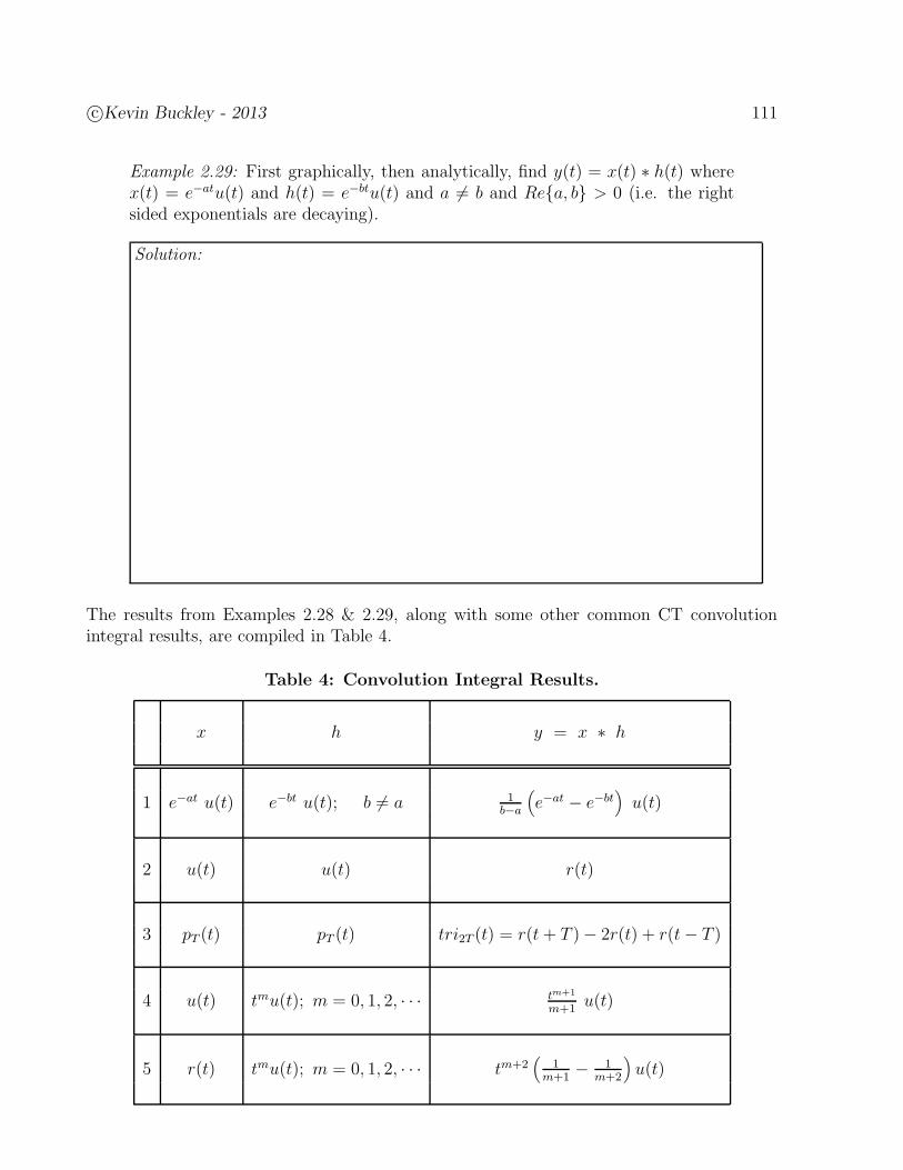
c©Kevin Buckley - 2013 111
Example 2.29: First graphically, then analytically, find y(t) = x(t) ∗ h(t) wherex(t) = e−atu(t) and h(t) = e−btu(t) and a 6= b and Rea, b > 0 (i.e. the rightsided exponentials are decaying).
Solution:
The results from Examples 2.28 & 2.29, along with some other common CT convolutionintegral results, are compiled in Table 4.
Table 4: Convolution Integral Results.
x h y = x ∗ h
1 e−at u(t) e−bt u(t); b 6= a 1b−a
(
e−at − e−bt)
u(t)
2 u(t) u(t) r(t)
3 pT (t) pT (t) tri2T (t) = r(t+ T )− 2r(t) + r(t− T )
4 u(t) tmu(t); m = 0, 1, 2, · · · tm+1
m+1u(t)
5 r(t) tmu(t); m = 0, 1, 2, · · · tm+2(
1m+1− 1
m+2
)
u(t)
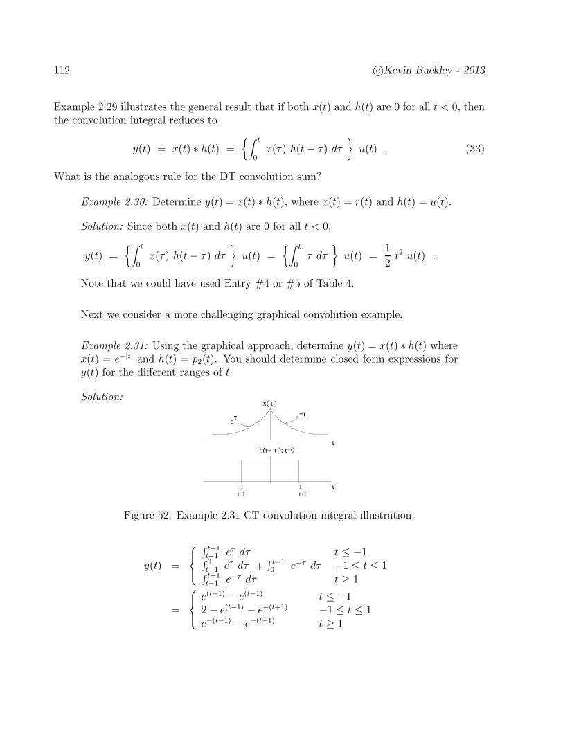
112 c©Kevin Buckley - 2013
Example 2.29 illustrates the general result that if both x(t) and h(t) are 0 for all t < 0, thenthe convolution integral reduces to
y(t) = x(t) ∗ h(t) =∫ t
0x(τ) h(t− τ) dτ
u(t) . (33)
What is the analogous rule for the DT convolution sum?
Example 2.30: Determine y(t) = x(t) ∗ h(t), where x(t) = r(t) and h(t) = u(t).
Solution: Since both x(t) and h(t) are 0 for all t < 0,
y(t) =∫ t
0x(τ) h(t− τ) dτ
u(t) =∫ t
0τ dτ
u(t) =1
2t2 u(t) .
Note that we could have used Entry #4 or #5 of Table 4.
Next we consider a more challenging graphical convolution example.
Example 2.31: Using the graphical approach, determine y(t) = x(t) ∗ h(t) wherex(t) = e−|t| and h(t) = p2(t). You should determine closed form expressions fory(t) for the different ranges of t.
Solution:
τe−τe
τh(t− ); t=0
τ
τ
−1t−1
1t+1
τx( )
Figure 52: Example 2.31 CT convolution integral illustration.
y(t) =
∫ t+1t−1 eτ dτ t ≤ −1∫ 0t−1 eτ dτ +
∫ t+10 e−τ dτ −1 ≤ t ≤ 1
∫ t+1t−1 e−τ dτ t ≥ 1
=
e(t+1) − e(t−1) t ≤ −12− e(t−1) − e−(t+1) −1 ≤ t ≤ 1e−(t−1) − e−(t+1) t ≥ 1

c©Kevin Buckley - 2013 113
The next seven examples illustrate the application of convolution integral properties.
Example 2.32: Consider the convolution y(t) = x(t) ∗ h(t), where h(t) = p2(t)and x(t) is the triangle x(t) = r(t)− 2r(t− 2) + r(t− 4). First, use Table 4 (orExample 2.31 results) and properties to solve this for all time t. Then use thegraphical approach, and specifically:
1. Plot x(τ) and h(1− τ) as functions of τ.
2. Plot x(τ)h(1 − τ) as a function of τ.
3. Determine y(1). The answer is a number.
4. For what value of t does y(t) peak? Explain your answer
5. For what values of t is y(t) = 0? Explain your answer.
Solution:
114 c©Kevin Buckley - 2013
Example 2.33: Convolve x(t) = e−atu(t) and h(t) = u(t).
Solution: Using Entry # 1 of Table 4 directly, with b = 0, we have
y(t) = x(t) ∗ h(t) =1
a
(
1 − e−at)
u(t) .
Example 2.34: Convolve x(t) = Ae−a(t−T )u(t− T ) and h(t) = u(t).
Solution: Using Entry # 1 of Table 4, along with the convolution integral delayproperty and linearity, we have
y(t) = x(t) ∗ h(t) =A
a
(
1 − e−a(t−T ))
u(t− T ) .
Example 2.35: Convolve x(t) = A1e−a1tu(t) + A2e
−a2tu(t) and h(t) = e−btu(t).
Solution: Again using Entry # 1 of Table 4, along with the convolution integraldistributivity property, we have
y(t) = x(t) ∗ h(t) =A1
b− a1
(
e−a1t − e−bt)
u(t) +A2
b− a2
(
e−a2t − e−bt)
u(t) .
Example 2.36: Convolve x(t) = e−bt u(t− 5) with h(t) = e−at p10(t− 5).
Solution: Again using Entry # 1 of Table 4, along with the convolution integraldistributivity and delay properties, we have
y(t) = x(t) ∗ h(t) = e−b·5 e−b(t−5) u(t− 5) ∗(
e−at u(t) − e−a·10 e−a(t−10) u(t− 10))
=e−b·5
b− a
(
e−a(t−5) − e−b(t−5))
u(t− 5) − e−b·5e−a·10
b− a
(
e−a(t−15) − e−b(t−15))
u(t− 15) .
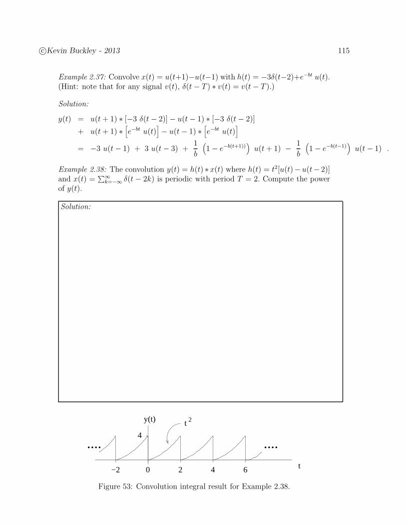
c©Kevin Buckley - 2013 115
Example 2.37: Convolve x(t) = u(t+1)−u(t−1) with h(t) = −3δ(t−2)+e−bt u(t).(Hint: note that for any signal v(t), δ(t− T ) ∗ v(t) = v(t− T ).)
Solution:
y(t) = u(t+ 1) ∗ [−3 δ(t− 2)]− u(t− 1) ∗ [−3 δ(t− 2)]
+ u(t+ 1) ∗[
e−bt u(t)]
− u(t− 1) ∗[
e−bt u(t)]
= −3 u(t− 1) + 3 u(t− 3) +1
b
(
1− e−b(t+1)))
u(t+ 1) − 1
b
(
1− e−b(t−1))
u(t− 1) .
Example 2.38: The convolution y(t) = h(t) ∗ x(t) where h(t) = t2[u(t)−u(t− 2)]and x(t) =
∑∞k=−∞ δ(t− 2k) is periodic with period T = 2. Compute the power
of y(t).
Solution:
t 2y(t)
0 4 62−2 t
4........
Figure 53: Convolution integral result for Example 2.38.
116 c©Kevin Buckley - 2013
This next example illustrates the use of the analytical approach to convolution to determinethe response of a CT LTI system to a complex sinusoidal input.
Example 2.39: For a CT LTI system with impulse response h(t) = C e−at u(t),determine to response y(t) to input x(t) = A ej(ωt+φ). Assume Rea > 0.
Solution:
In Example 2.39, note that the output is a sinusoid of the same frequency as the input. Thesystem alters the magnitude and phase of the input as dictated by the function
H(ω) =∫ ∞
−∞h(t) e−jωt dt . (34)
This is a function of frequency, indicating that the effect of the system on the input sinusoiddepends on the frequency of that sinusoid. Also note that this effect can be derived fromthe LTI system impulse response.
We have seen this kind of result before – that for a sinusoidal input, the output of a LTIsystem is consists solely of a sinusoid of the same frequency. For DT LTI systems, this wasthe point of Subsection 2.3.3. We also saw this in Chapter 1 with Examples 1.39 & 1.40.

c©Kevin Buckley - 2013 117
2.6 CT LTI System Issues
Since the tools for working with CT and DT LTI systems are so similar, for the mostpart this Subsection looks like an abbreviated version of Subsection 2.2.4 (DT LTI systemissues). Paralleling Subsection 2.2.4, we briefly cover system properties and interconnections.However, in two respects the discussions diverge. First, for CT LTI systems, there are nocommon finite impulse response systems, so we don’t emphasize this. Second, with severalexamples we do emphasize CT LTI circuits.
System Properties:
Since we are considering CT LTI systems, linearity and time-invariance are covered. ACT LTI system is causal if and only if
h(t) = 0 ; t < 0 . (35)
A CT LTI system is stable, if and only if
∫ ∞
−∞|h(t)| dt < ∞ . (36)
System Interconnections:
If M CT LTI systems, with impulse responses hi(t); i = 1, 2, · · · ,M are connected inparallel, than the overall system impulse response is
h(t) =M∑
i=1
hi(t) . (37)
IfM CT LTI systems, with impulse responses hi(t); i = 1, 2, · · · ,M are connected in cascade,than the overall system impulse response is
h(t) = hi(t) ∗ h2(t) ∗ · · · ∗ hM (t) . (38)
For feedback systems, there is no direct expression for the overall impulse response in termsof the impulse responses of the subsystems.
Example 2.40: A CT LTI system has impulse response h(t) = (t+1) e−100t u(t+5).Is this system: Linear? Time-invariant? Causal? Stable?
Solution:

118 c©Kevin Buckley - 2013
Example 2.41: Determine h(t), the overall system impulse response, for the sys-tem shown below.
h (t) = (t − T )1 1δ1Delay T :
Multiply a:h (t) = a (t)δ3
Integrator:h (t) = u(t)4
+
y(t)+h (t) = (t)2 δx(t)
δh (t) = (t − T )5 2
Delay T :2
Figure 54: CTLTI subsystem interconnection for Example 2.41.
Solution:
Example 2.42: Determine the impulse response h(t) from the step response.
Solution:
The DT analogy is h[n] = s[n]− s[n− 1] (i.e. δ[n] = u[n]− u[n− 1]).
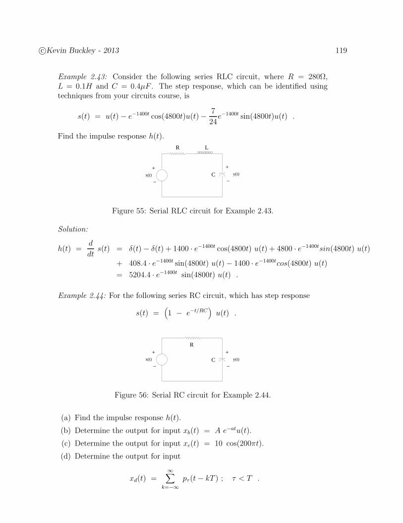
c©Kevin Buckley - 2013 119
Example 2.43: Consider the following series RLC circuit, where R = 280Ω,L = 0.1H and C = 0.4µF . The step response, which can be identified usingtechniques from your circuits course, is
s(t) = u(t)− e−1400t cos(4800t)u(t)− 7
24e−1400t sin(4800t)u(t) .
Find the impulse response h(t).
+
−y(t)x(t)
+
−
R L
C
Figure 55: Serial RLC circuit for Example 2.43.
Solution:
h(t) =d
dts(t) = δ(t)− δ(t) + 1400 · e−1400t cos(4800t) u(t) + 4800 · e−1400tsin(4800t) u(t)
+ 408.4 · e−1400t sin(4800t) u(t)− 1400 · e−1400tcos(4800t) u(t)
= 5204.4 · e−1400t sin(4800t) u(t) .
Example 2.44: For the following series RC circuit, which has step response
s(t) =(
1 − e−t/RC)
u(t) .
C+
−x(t) y(t)
+
−
R
Figure 56: Serial RC circuit for Example 2.44.
(a) Find the impulse response h(t).
(b) Determine the output for input xb(t) = A e−atu(t).
(c) Determine the output for input xc(t) = 10 cos(200πt).
(d) Determine the output for input
xd(t) =∞∑
k=−∞pτ (t− kT ) ; τ < T .

120 c©Kevin Buckley - 2013
Solution:
2.7 Generalizing the Utility of Convolution
In this Chapter of the Course we introduced convolution as the I/O calculation for a LTIsystem. Note that this is not the only application of convolution we have considered – recallthat the impulse response of two LTI systems in cascade is the convolution of the subsystemimpulses responses. In engineering, the convolution operation crops up in a wide variety ofcircumstances. To a large extent this is due to the nature of linear interactions between onedimensional or multidimension signals and systems.
Here, within the context of examples of the convolution operator, we suggest several newapplications of convolution.
Example 2.45 - Correlation:
See Problem 2.101 in the back of this Chapter.
Example 2.46 - Spectral Smearing:
See Problem 2.102 in the back of this Chapter.
Example 2.47 - Image Smearing:
See Parcticums 1 & 2.
c©Kevin Buckley - 2013 121
2.8 Practicum 2
Convolution
Reporting Requirements: See the “Reporting Requirements” at the beginning of Practicum1.
ProceduresBefore the lab session, Procedure 1(a) should be completed and the example in Appendix 1should be studied. Also, identify the impulse response for Procedure 2(d).
1. Convolutions sum for finite duration DT signals:
(a) By hand, compute and plot the convolution of the signals x1[n] = p20[n] andh1[n] = p10[n].
(b) Now use Matlab to compute and plot the convolution of these two signals. Specif-ically, do this twice, using the two methods illustrated in the attached Appendix1: 1) by using the Matlab conv command; and 2) by programming the convolutionoperation yourself. For both methods, plot the result for n = 0, 1, 2, · · · , 27, 28.
(c) Repeat (b) using your FIR mine function. You can just directly input your arraysfrom the 2-nd part of (b) (i.e. from your convolution program).
(d) Let q be the number of contiguous nonzero elements of h[n] (i.e. the length ofh[n]). Let p be the length of x[n]. Generalizing the results observed above, whatis the length of y[n] = x[n] ∗ h[n]?
2. Differential Code Decoding:
As for Practicum 1, for this part of the practicum you will process a black andwhite image. There are three files you will need, lighthouse.mat, lighthouse2.mat andshow img.m, which can be found in directory
v:/Electrical Computer/ece3240
(a) Copy the three files into your working directory or otherwise assure that you haveaccess to them within Matlab.
(b) Load lighthouse2.mat into Matlab. In Matlab, what is the image name? Whatsize is it? Display the image using the command show img( . ). Do the same forlighthouse.mat.
(c) To reduce the numerical range of the image amplitudes prior to image compres-sion, the image xx[i, n] has been differentially encoded along the horizontal tocreate zz[i, n] using the following equation for each row
zz[i, n] = xx[i, n] − 0.9 xx[i, n−1] ; i = 1, 2, · · · , 326 ; n = 1, 2, · · · , 426 , (1)
with xx[i, 0] = 0.0, i = 1, 2, · · · , 326. Note that each row is processed with asystem the looks like the channel for Procedure 2 of Practicum 1. How did youinvert the effect of that channel?
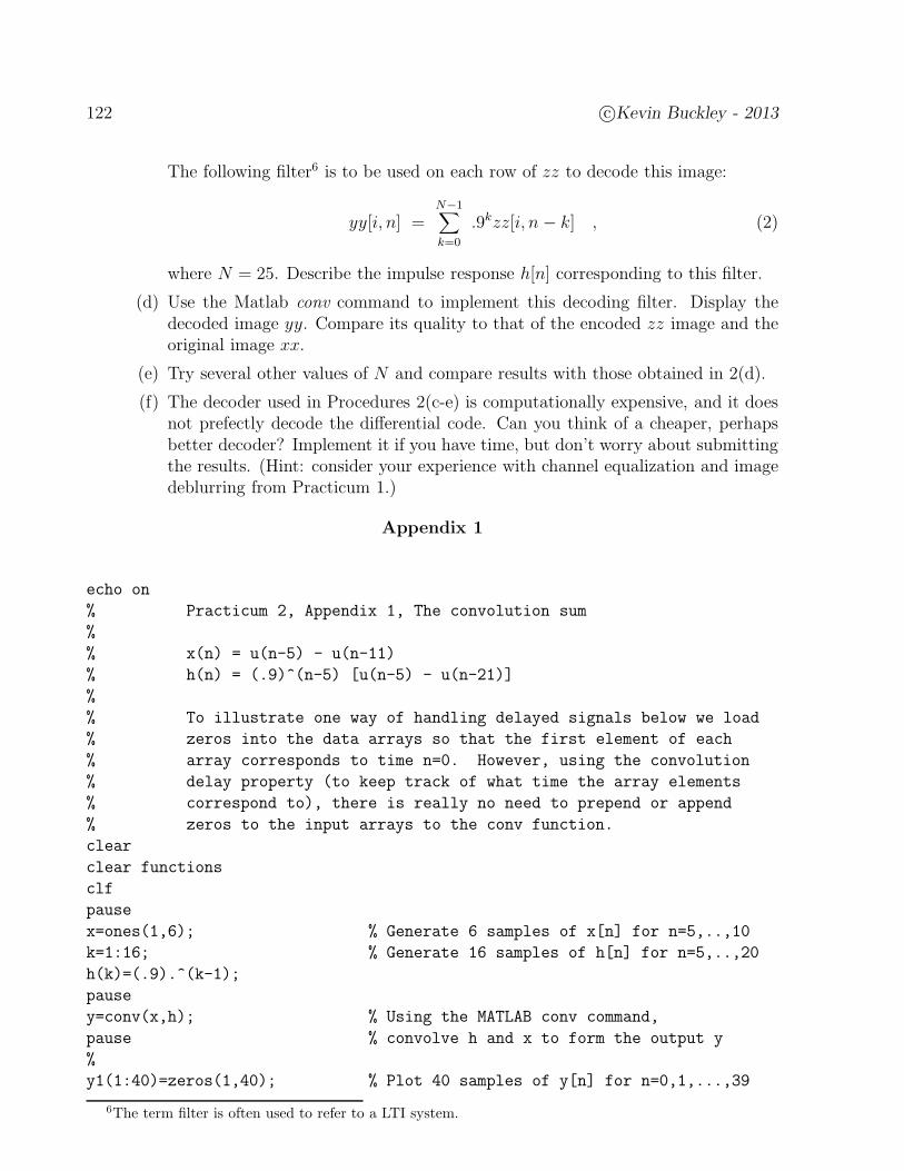
122 c©Kevin Buckley - 2013
The following filter6 is to be used on each row of zz to decode this image:
yy[i, n] =N−1∑
k=0
.9kzz[i, n − k] , (2)
where N = 25. Describe the impulse response h[n] corresponding to this filter.
(d) Use the Matlab conv command to implement this decoding filter. Display thedecoded image yy. Compare its quality to that of the encoded zz image and theoriginal image xx.
(e) Try several other values of N and compare results with those obtained in 2(d).
(f) The decoder used in Procedures 2(c-e) is computationally expensive, and it doesnot prefectly decode the differential code. Can you think of a cheaper, perhapsbetter decoder? Implement it if you have time, but don’t worry about submittingthe results. (Hint: consider your experience with channel equalization and imagedeblurring from Practicum 1.)
Appendix 1
echo on
% Practicum 2, Appendix 1, The convolution sum
%
% x(n) = u(n-5) - u(n-11)
% h(n) = (.9)^(n-5) [u(n-5) - u(n-21)]
%
% To illustrate one way of handling delayed signals below we load
% zeros into the data arrays so that the first element of each
% array corresponds to time n=0. However, using the convolution
% delay property (to keep track of what time the array elements
% correspond to), there is really no need to prepend or append
% zeros to the input arrays to the conv function.
clear
clear functions
clf
pause
x=ones(1,6); % Generate 6 samples of x[n] for n=5,..,10
k=1:16; % Generate 16 samples of h[n] for n=5,..,20
h(k)=(.9).^(k-1);
pause
y=conv(x,h); % Using the MATLAB conv command,
pause % convolve h and x to form the output y
%
y1(1:40)=zeros(1,40); % Plot 40 samples of y[n] for n=0,1,...,39
6The term filter is often used to refer to a LTI system.
c©Kevin Buckley - 2013 123
y1(11:31)=y;
n=0:1:39;
subplot(211)
plot(n,y1,’*’),xlabel(’n’),ylabel(’y(n)’),
title(’1-st Convolution Result’),text(25,4,’John Butler’)
pause
% Now let’s do it again without using the MATLAB conv command.
% We’ll do it ourselves.
clear
x=zeros(1,11); % Generate 11 samples of x[n] for n=0,..,10
x(6:11)=ones(1,6); %
h=zeros(1,21); % Generate 21 samples of h[n] for n=0,..,20
k=0:1:15; %
h(6:21)=(.9).^k; %
pause
%
x(12:40)=zeros(1,29); % Directly convolve h and x --> output y
h(22:40)=zeros(1,19);
for n=1:40;
y(n)=0.;
for k=1:n;
y(n)=y(n)+x(k)*h(n+1-k);
end
end
pause
%
clear n
n=0:1:39;
subplot(212)
plot(n,y,’*’),xlabel(’n’),ylabel(’y(n)’)
title(’2-nd Convolution Result’),text(25,4,’Garret Dutton’)

124 c©Kevin Buckley - 2013
.

c©Kevin Buckley - 2013 125
Practicum 2Instructor/TA Sign Off Sheet, & Report Form
Student’s Name:
1. Pract. 2, Procedure 1(b,c): output plots
2. Pract. 2, answer for Procedure 1(d): (a function of p and q)
3. Pract. 2, Procedure 2(d,e): displays of original, coded and decoded images
4. Pract. 2, for Procedure 2(c), discuss the similarities and differences in characteristicsand performance between: 1) the coder and decoder for this Procedure; and 2) thechannel and 1-st equalizer used in Practicum 1.
5. Pract. 2, for Procedure 2(f), describe the decoder which is analogous to the 2-ndequalizer in Practicum 1.

126 c©Kevin Buckley - 2013
.

c©Kevin Buckley - 2013 127
2.9 Problems
Chapter Topics:2.1-10 (graphical DT convolution sum with basic finite duration signals)2.11-24 (graphical DT convolution sum with basic infinite duration signals)2.25-43 (graphical DT convolution sum with more challenging signals)2.44-50 (analytical DT convolution sum, with sinusoids)2.51-58 (DT convolution sum properties)2.59-74 (DT convolution sum and DT LTI system issues)2.75-87 (graphical CT convolution integral)2.88-92 (CT convolution integral properties)2.93-100 (CT convolution integral and CT LTI system issues)2.101-102 (other convolution applications)
1. Using the graphical approach, find y[n] = x[n] ∗ y[n] where h[n] = p4[n] and x[n] =(−1)n u[n].
a) Sketch x[n] and h[n].
b) Sketch x[k] and h[n− k]; n = 3.
c) Working off of part b) results, sketch x[k] · h[3− k].
d) Working off of part c) results, determine y[3].
e) Plot y[n] for −2 ≤ n ≤ 10.
2. Consider a DT LTI system with impulse response
h[n] = δ[n] + a2δ[n− 2] + a4δ[n− 4] + a6δ[n− 6] .
Determine the output y[n] for input x[n] = δ[n] − a2δ[n − 2]. First, use the linearityand time-invariance properties of the system directly. Then convolve h[n] with x[n].
3. Consider a DT LTI system with inpulse response h[n] = δ[n] − δ[n − 1] + δ[n −2] − δ[n − 3] and input x[n] = r[n] p6[n]. Using the graphical approach, findy[n] = x[n] ∗ h[n]. Specifically
(a) sketch x[k] and h[n− k]; n = 4;
(b) sketch x[k] · h[4− k];
(c) determine y[4]; and
(d) plot y[n] for −2 ≤ n ≤ 10.
4. Consider two sequences h1[n] = δ[n]− 0.9 δ[n− 1] and h2[n] = 0.9n p5[n].
(a) Plot these and use the graphical approach to determine the convolutionh[n] = h1[n] ∗ h2[n].
(b) With the h[n] you derived in (a), and x[n] = p2[n], use the graphical approach todetermine y[n] = x[n] ∗ h[n].
128 c©Kevin Buckley - 2013
5. Using the graphical approach, find y[n] = x[n] ∗ h[n] where h[n] = .5n p4[n] andx[n] = δ[n] + .5 δ[n− 1] − .5 δ[n− 2]. Specifically,
(a) Sketch h[k] and x[n− k]; n = 1.
(b) Sketch h[k] · x[1 − k].
(c) Determine y[1].
(d) Plot y[n] for −2 ≤ n ≤ 6.
6. A signal x[n] = δ[n]+ 0.2 δ[n−1]−0.8 δ[n−2] is the input to a DT LTI system withimpulse response h[n] = 0.8n p25[n]. Determine y[n] = x[n] ∗ h[n]. Specifically:
(a) Sketch h[k] and x[0− k] as functions of k.
(b) Sketch h[k] x[0− k] as a function of k.
(c) Determine y[0]. The answer is a number.
(d) Sketch y[n] over the range of n that it is nonzero.
(e) List the times n and corresponding values y[n] of the nonzero outputs.
7. Using the graphical approach, find y[n] = x[n] ∗ h[n] where h[n] = 2n−5 p5[n] andx[n] = − δ[n] + 2 δ[n− 1]. Specifically,
a) Sketch h[k].
b) Sketch x[n− k] for n = 0.
c) Sketch h[k] x[n− k] for n = 1.
d) Determine and plot y[n] for −2 ≤ n ≤ 8. What is y[n] outside this range of n?
8. Convolving pulses:
(a) Convolve x[n] = p3[n− 1] with h[n] = p5[n+ 3]. Plot y[n].
(b) Convolve x[n] = p5[n] with h[n] = p10[n− 3]. Plot y[n].
9. Two DT LTI systems are connected in cascade. The 1-st has impulse responseh1[n] = 2np5[n] and the 2-nd h2[n] = δ[n] + 2δ[n − 1] + δ[n − 2]. Assume theresulting system has impulse response h[n] = h1[n] ∗ h2[n]. Using the graphicalconvolution approach, determine h[n].
Specifically:
(a) Sketch h1[k] and h2[2− k] as functions of k.
(b) Sketch h1[k] h2[2− k] as a function of k.
(c) Determine h[2]. The answer is a number.
(d) Sketch h[n] over the range of n that it is nonzero. Label time and h[n] values.
10. Using the graphical approach, find the output y[n] = x[n] ∗ h[n] of a DT LTI systemwith impulse response h[n] = p10[n] and x[n] = n p5[n]. Minimally, you should:
c©Kevin Buckley - 2013 129
(a) Sketch x[k] and h[n− k]; n = 0 as a function of k.
(b) Sketch y[n] over its entire non-zero range, making sure to show details.
11. Using the graphical approach, find y[n] = x[n] ∗ h[n] where h[n] = 2 u[n] andx[n] = (n− 1
2) u[n− 1]. Specifically:
a) Sketch x[n] and h[n].
b) Sketch x[k] and h[n− k]; n = 0.
c) Working off of part b) results, list each region of n that has a different y[n]expression.
d) For each region of n from part c), determine an expression for y[n].
e) Describe y[n] as a single closed-form expression.
12. Consider y[n] = x[n] ∗ h[n], where h[n] = 0.5n p5[n] and x[n] = u[n]. Using thegraphical convolution approach, determine y[n] (i.e. the step response). Specifically:
(a) Plot h[k] and x[4− k] as functions of k.
(b) Plot h[k]x[4 − k] as a function of k.
(c) Determine y[4]. The answer is a number.
(d) Determine y[2010].
(e) Determine expressions for y[n] for all ranges of n.
13. Using the graphical approach, find y[n] = x[n] ∗ h[n] where h[n] = 0.5n u[n] andx[n] = 0.5n p20[n+ 10]. Specifically,
(a) Sketch x[k] and h[n− k]; n = 0.
(b) Determine the different ranges of n that have different expressions for y[n].
(c) For each of your ranges of n determine a closed-form expression for y[n].
14. Consider a simple IIR DT-LTI system with impulse response h[n] = 0.5n u[n] andinput x[n] = p3[n].
(a) Plot, as a function of memory index k, h[k] and x[n− k]; n = 0.
(b) Plot, as a function of k, h[k] x[n− k]; n = 2.
(c) Using your result from (b), determine y[2].
(d) Determine y[0] and y[1]. Draw additional graphs only if you need to.
(e) For n ≥ 2, the output has the form: y[n] = K 0.5n. Determine the constant K.Show all work.
15. Determine y2[n] = x2[n] ∗ h2[n] where x2[n] = (−1)nu[n] and h2[n] = p4[n].
16. Consider y[n] = x[n] ∗ h[n], where h[n] = 0.5nu[n] and x[n] = p3[n]. Using thegraphical convolution approach, determine y[n]. Specifically:
130 c©Kevin Buckley - 2013
(a) Plot h[k] and x[4− k] as functions of k.
(b) Plot h[k]x[4 − k] as a function of k.
(c) Determine y[4]. The answer is a number.
(d) Determine an expression for y[n] for all n.
17. Consider y[n] = x[n] ∗ h[n], where h[n] = 0.99nu[n] and x[n] = u[n− 5]. Specifically:
(a) Plot h[k] and x[n− k], as functions of k, for n = 0.
(b) Plot h[k]x[n − k], as a function of k, for n = 0.
(c) Determine an expression for y[n] for all n.
(d) Determine y[100] and y[∞]. The answers are numbers.
18. Using what ever approach you wish, convolve x[n] = .5n u[n] with h[n] = .5n u[n].Describe the result for all n. Show all work.
19. Consider a DT LTI system with impulse response h[n] = n (.5)n u[n] and inputx[n] = u[n− 10]. The output is y[n] = h[n] ∗ x[n]. Using the graphical approachto convolution, determine:
(a) y[0].
(b) y[10].
(c) y[12].
(d) A closed-form (i.e. do summation) expression for y[n] that is good for all n.
(e) y[∞].
20. Graphically solve y[n] = h[n] ∗ x[n] for x[n] = 6n p20[n] and h[n] = 0.5 (0.8)n u[n].Specifically,
a) Plot x[k] (vs. k), labeling the axes and important values of k and x[k].
b) Plot h[n− k] (vs. k), labeling the axes and important values of k and h[n− k].
c) Identify the different regions of n that result in different convolution sum expres-sions.
d) For each region identified in c), determine the summation expression for y[n].(You must clearly show the ranges of k summed over and the expressions insidethe summations. Leave the answers in summation form.)
e) For the highest positive region of n identified in procedure c), the output is of theform y[n] = K (0.8)n. Determine K.
21. Graphically solve y[n] = h[n] ∗ x[n] for x[n] = 10n u[−n] and h[n] = 0.4n u[n]. Specifi-cally,
a) Plot h[k] (vs. k), labeling the axes and important values of k and h[k].
b) Plot x[n− k] (vs. k), labeling the axes and important values of k and x[n− k].

c©Kevin Buckley - 2013 131
c) Identify the different regions of n that result in different convolution sum expres-sions.
d) For each region identified in c), determine the summation expression for y[n].(You must clearly show the ranges of k summed over and the expressions insidethe summations. Leave the answers in summation form.)
22. Consider the impulse response h[n] = u[n] of a DT LTI system with inputx[n] = p3[n] − p3[n− 3]. Graphically compute y[n] = h[n] ∗ x[n]. Specifically,
a) Plot x[k] and a function of k.
b) Plot h[n− k]; n = 0 as a function of k.
c) Using a) and b), determine and plot y[n] for −4 ≤ n ≤ 10.
d) Now let x1[n] =∑∞
m=0 x[n − 6m]. Graphically determine and plot y1[n] =h[n] ∗ x1[n] for −4 ≤ n ≤ 14.
23. Using the graphical approach, determine y[n] = h[n] ∗ x[n], for all n, where h[n] =0.9n u[n− 6] and x[n] = u[n] + 2 u[n− 10]. Specifically,
a) Sketch h[k] and h[n− k]; n = 0 as a function of k.
b) Using your sketches, determine all regions of n that have different expressions fory[n].
c) For each of your regions of n, determine the expression for y[n]. Leave expressionsin summation form. That is, don’t solve the summations. However, make surethe sum limits and expressions in the summation are correct.
d) Determine y[40].
24. Graphically convolve h1[n] = n (.8)n u[n] with h2[n] = (.8)n p20[n− 3] to form h[n].Specifically,
(a) Plot h1[k] vs. k and h2[n− k]; n = 0 vs. k.
(b) Identify the different regions of n that have different expressions for h[n].
(c) For each region of n determine the expression for h[n] (i.e. in summation form).
(d) For the region including n = 15, determine the closed form expression for h[n](i.e. do the summation). Use this to determine h[15].
25. Determine y5[n] = tri10[n] ∗ u[n].
26. Plot x[n] = p5[n + 2] and h[n] = r[n] p5[n]. Determine the convolutiony[n] = x[n] ∗ h[n] and plot the resulting y[n] over the range of n where y[n] 6= 0.
27. Graphically solve y[n] = h[n] ∗ x[n] for x[n] = n2p10[n] and h[n] = p20[n]. Specifically,
(a) Plot x[k] (vs. k), labeling the axes and important values of k and h[k].
(b) Plot x[n− k] (vs. k), labeling the axes and important values of k and x[n− k].
132 c©Kevin Buckley - 2013
(c) Identify the different regions of n that result in different convolution sum expres-sions.
(d) For each region identified in c), determine the summation expression for y[n].(You must clearly show the ranges of k summed over and the expression insidethe summation. Leave the answers in summation form.)
(e) What are y[7] and y[35]?
28. Your are given input x[n] = n p21[n] to a DT LTI system with impulse responseh[n] = p10[n− 3]. Derive a closed form expression for the output y[n] = x[n] ∗ h[n] foreach range n. Using your expressions, specifically determine y[6] and y[20].
29. Consider a DT-LTI system with impulse response h[n] = u[n− 5] and inputx[n] = 3 (.5)n u[n] + 2 u[n− 4] − 7 r[n− 10]. Determine output y[n] as follow.
(a) Determine ya[n] = u[n] ∗ (.5)n u[n].
(b) Determine yb[n] = u[n] ∗ u[n].
(c) Determine yc[n] = u[n] ∗ r[n].
(d) Use your results from parts (a-c) to determine an expression for y[n].
(e) Use your result from part (d) to determine y[6].
30. Combined graphical/property convolution problem:
(a) First determine h3[n] = h1[n] ∗ h2[n] where h1[n] = u[n] and h2[n] = r[n].
(b) Using convolution properties and your result from part (a) above, determine anexpression for h[n] = h1[n] ∗ h3[n], where
h3[n] = tri10[n] = r[n+ 1] − 2r[n− 4] + r[n− 8] . (3)
(c) Using your expression from (b), determine h3[5].
31. Let x[n] = (√0.5)n u[n]. Determine the energy of w[n] = x[n] ∗ x[n]. Feel free to
use the summation and convolution tables provided in the Course Notes.
32. Consider y1[n] = x1[n] ∗ h1[n], where h1[n] = 0.5nu[n− 3] and x1[n] = .5n p20[n].Specifically:
(a) Plot x1[k] and h1[3− k] as functions of k.
(b) Plot h1[k] x1[3− k] as a function of k.
(c) Determine y1[3]. The answer is a number.
(d) Determine an expression for y1[n] for all n.
33. Convolve x3[n] = n · u[n] with h3[n] = n2 · u[n]. Use either the graphical or analyticalapproach. Determine a closed form expression for the resulting y3[n] for all n.
34. Using the graphical approach, convolve x[n] = 2n u[n] with h[n] = .9n u[n]. Describethe result for all n. Specifically, what is y[5]?
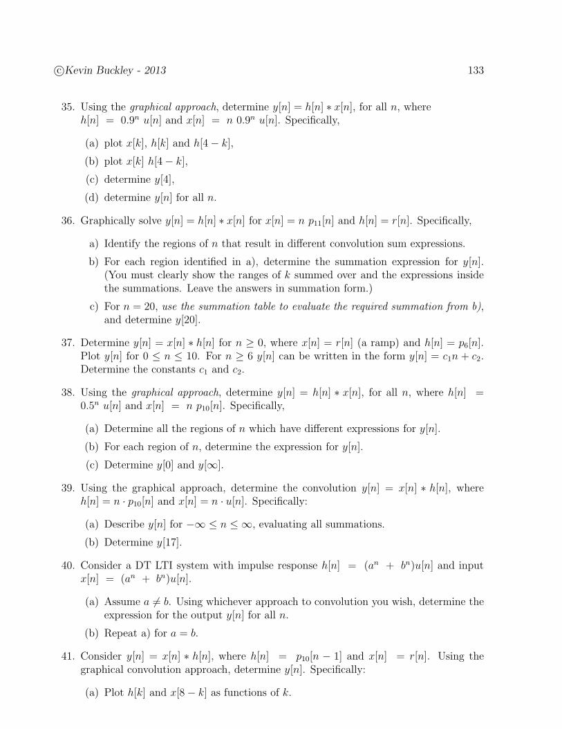
c©Kevin Buckley - 2013 133
35. Using the graphical approach, determine y[n] = h[n] ∗ x[n], for all n, whereh[n] = 0.9n u[n] and x[n] = n 0.9n u[n]. Specifically,
(a) plot x[k], h[k] and h[4− k],
(b) plot x[k] h[4− k],
(c) determine y[4],
(d) determine y[n] for all n.
36. Graphically solve y[n] = h[n] ∗ x[n] for x[n] = n p11[n] and h[n] = r[n]. Specifically,
a) Identify the regions of n that result in different convolution sum expressions.
b) For each region identified in a), determine the summation expression for y[n].(You must clearly show the ranges of k summed over and the expressions insidethe summations. Leave the answers in summation form.)
c) For n = 20, use the summation table to evaluate the required summation from b),and determine y[20].
37. Determine y[n] = x[n] ∗ h[n] for n ≥ 0, where x[n] = r[n] (a ramp) and h[n] = p6[n].Plot y[n] for 0 ≤ n ≤ 10. For n ≥ 6 y[n] can be written in the form y[n] = c1n + c2.Determine the constants c1 and c2.
38. Using the graphical approach, determine y[n] = h[n] ∗ x[n], for all n, where h[n] =0.5n u[n] and x[n] = n p10[n]. Specifically,
(a) Determine all the regions of n which have different expressions for y[n].
(b) For each region of n, determine the expression for y[n].
(c) Determine y[0] and y[∞].
39. Using the graphical approach, determine the convolution y[n] = x[n] ∗ h[n], whereh[n] = n · p10[n] and x[n] = n · u[n]. Specifically:
(a) Describe y[n] for −∞ ≤ n ≤ ∞, evaluating all summations.
(b) Determine y[17].
40. Consider a DT LTI system with impulse response h[n] = (an + bn)u[n] and inputx[n] = (an + bn)u[n].
(a) Assume a 6= b. Using whichever approach to convolution you wish, determine theexpression for the output y[n] for all n.
(b) Repeat a) for a = b.
41. Consider y[n] = x[n] ∗ h[n], where h[n] = p10[n − 1] and x[n] = r[n]. Using thegraphical convolution approach, determine y[n]. Specifically:
(a) Plot h[k] and x[8− k] as functions of k.

134 c©Kevin Buckley - 2013
(b) Plot h[k]x[8 − k] as a function of k.
(c) Determine y[8]. The answer is a number.
42. Using the graphical approach, determine y[n] = x[n] ∗ h[n] where
x[n] = 0.1|n|
and
h[n] = 0.4n u[n] .
43. Given that x[n] = h[n] =√0.9
nu[n], determine :
(a) y[n] = x[n] ∗ h[n],
(b) the energy of y[n].
44. Consider input x12[n] = A ej(ω0n+φ) u[n] to a DT LTI system with impulse responseh12[n] = p6[n]. Determine closed form expressions for the output y12[n] for all timesn. (Note that x12[n] turns on at n = 0.)
45. Consider a general N point averager, i.e. with impulse response h[n] = 1N
pN [n].
(a) Determine its output y[n] due to complex sinusoidal input x[n] = ejωon. Specifi-cally, what is the output when ωo = 0? ωo = π, assuming N is even?
(b) Let N = 16 and
x[n] = 5 + 3 ej(π/4)n .
Determine the output y[n].
46. Using the analytical approach to convolution, determine y[n] = h[n]∗x[n] where h[n] =bn u[n] and x[n] = (a ejω)n. Perform any summations. Evaluate y[n] specifically fora = 1, b = .5 and ω = π.
47. Consider a DT LTI system with impulse response h[n] = (−0.8)n u[n].
(a) Determine its output y[n] due to complex sinusoidal input x[n] = ejωon. Specifi-cally, what is the output when ωo = 0? ωo = π?
(b) Determine its output y[n] due to input x[n] = ejωon u[n]. Specifically, what is theoutput when ωo = 0? ωo = π?
48. Let x11[n] = ejω0n be the input to a DT LTI system with impulse response h11[n] =δ[n] − δ[n − 2]. Determine an expression for the output y11[n]. Over the range−π ≤ ω0 ≤ π, for what values of ω0 is y11[n] = 0?
49. Given a DT LTI system with impulse response h[n] = n (.9)n u[n] and inputx[n] = ejω0n,
c©Kevin Buckley - 2013 135
(a) Analytically determine y[n] = h[n] ∗ x[n].
(b) For ω0 = 0, determine y[n]. Is this input amplified or attenuated?
(c) For ω0 = π, determine y[n]. Is this input amplified or attenuated? What is thephase shift from input to output?
50. Given h[n] = (−1)n p12[n] and x[n] = A ej(ωn+φ),
(a) Analytically, determine y[n] = h[n] ∗ x[n]. Since x[n] is a complex sinusoid, y[n]is of the form y[n] = x[n] H(ω). What is H(ω)?
(b) For ω = 0, determine y[n].
(c) For ω = π, determine y[n]. You should be a little more careful with this one.
51. Using the convolution table in the Course Notes, determine x[n] ∗ h[n] for:
(a) h[n] = p10[n] and x[n] =∑∞
k=−∞ p10[n− 20k].
(b) h[n] = p20[n] and x[n] = r[n− 3].
(c) h[n] = r[n] p10[n] and x[n] = r[n].
(d) h[n] = .9nu[n] and x[n] = .9np10[n− 10].
52. Determine x[n] = δ[n− 2] ∗ δ[n+ 3] ∗ u[n+ 1] ∗ u[n− 4].
53. Consider the input x[n] = 3n u[−n− 1] +(
13
)nu[n] a DT LTI system with impulse
response h[n] =(
14
)nu[n+ 3].
(a) Determine y[n] = x[n] ∗ h[n] without using the distributivity property of convo-lution.
(b) Determine y[n] = x[n] ∗ h[n] using the distributivity property of convolution.
54. Perform the convolution y[n] = x[n] ∗ h[n], where
x[n] = p10[n] ; h[n] = δ[n− 3] + u[n] − .5nu[n] .
Specifically,
a) State the approaches you will use (e.g. graphical, analytical, tables, properties).
b) Derive an expression for y[n]. Do all convolutions, but don’t worry too muchabout making the answer compact.
c) Evaluate your expression to obtain y[3].
55. In this problem you are to perform the convolution y[n] = x[n] ∗ h[n], wherex[n] = p10[n] and h[n] is plotted below. You are to use convolution properties asdetailed below.
Note that h[n] = r[n] − r[n− 10] − r[n− 15] + r[n− 25].
a) First, determine the convolution y1[n] = r[n] ∗ u[n].
136 c©Kevin Buckley - 2013
..... ......
...5
10
0
h[n]
n24
...
... .........
. ..
10 15
b) Now, using the delay and distributivity properties, determine an expression fory[n] in terms of y1[n]. Using this expression, determine y[15].
56. In this problem you are to perform the convolution y[n] = x[n] ∗ h[n], where x[n] =r[n − 3] and h[n] is plotted below. You are to use convolution properties as detailedbelow.
..... ......
................10 19
n
5
10
0
h[n]
Note that h[n] = r[n] − 2 r[n− 10] + r[n− 20].
a) First, graphically perform the convolution y1[n] = r[n] ∗ r[n]. Provide a closedform expression good for all n. Using this expression, determine y1[10].
b) Now, using the delay and distributivity properties, determine an expression fory[n] in terms of y1[n]. Using this expression, determine y[13].
57. Consider the convolution y[n] = x[n] ∗ h[n], where h[n] = 0.9nu[n] andx[n] =
∑∞i=0 δ[n− 3i]. Specifically:
(a) Plot x[k] and h[6− k] as functions of k.
(b) Plot x[k]h[6 − k] as a function of k.
(c) Determine y[6]. The answer is a number.
(d) For what values of n is y[n] = 0? Explain your answer.
58. You are given a DT LTI system with impulse response h[n] =∑10
k=1 k p4[n− 8k].
(a) First determine s1[n] = u[n] ∗ p4[n] any way you wish.
(b) Now use convolution properties to determine the step response s[n] of this DTLTI system in terms of s1[n].
59. For each of the following LTI systems, find the impulse response. Is the system casual?Stable? Explain your answers in terms of your impulse response characteristics.
c©Kevin Buckley - 2013 137
(a) LTI system (a).
y[n] =∞∑
k=0
ej(π/3)k x[n− k] .
(b) LTI system (b).
y[n] = x[n + 5] + 2 y[n− 1] .
60. Consider a DT LTI system with impulse response h[n] = 0.7np30[n]. Use systemlinearity to determine the output for input x[n] = δ[n − 1] + u[n − 7] + 0.7nu[n].Determine the general expression, and y[5].
61. Consider a LTI DT system with impulse response h1[n] = 5 p11[n].
(a) Is this system linear? Why?
(b) Is this system time invariant? Why?
(c) Is this system causal? Why?
(d) Is this system stable? Why?
(e) Determine the output y1[n] due to input x1[n] = 1.
(f) Determine the output y2[n] due to input x2[n] = ejπn.
(g) Now find the output y3[n] due to input x2[n] and the LTI DT system with impulseresponse h2[n] = 5 δ[n]− h1[n].
62. Consider a DT LTI system with impulse response h[n] = 116
ejω0n p16[n] and input.x[n] = 3 ejω1n. The output is a constant times the input. What is the expression forthis constant?
63. Consider two parallel DT LTI subsystems, one with impulse response h1[n] = 0.7nu[n]and the other with h2[n] = −0.49 δ[n − 2] ∗ 0.7nu[n]. Determine the overall systemimpulse response h[n].
64. Consider a DT LTI system that consists of two subsystems in cascade, h1[n] and h2[n],which together are in parallel with subsystem h3[n]. The hi[n]; i = 1, 2, 3 are subsystemimpulse responses. Given that
h1[n] = δ[n] − .9δ[n− 1]
h2[n] = δ[n] + .9δ[n− 1] + .81δ[n− 2] + .729δ[n− 3]
h3[n] = .6561δ[n− 4],
determine the overall system impulse response h[n].
65. The DT LTI system consists of two subsystems connected in parallel. One has impulseresponse h1[n] = (−.5)nu[n] and the other h2[n] = .5nu[n].
(a) Determine h[n], the overall impulse response of the system.
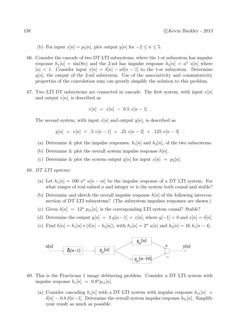
138 c©Kevin Buckley - 2013
(b) For input x[n] = p2[n], plot output y[n] for −2 ≤ n ≤ 5.
66. Consider the cascade of two DT LTI subsystems, where the 1-st subsystem has impulseresponse h1[n] = sin(8n) and the 2-nd has impulse response h2[n] = an u[n] where|a| < 1. Consider input x[n] = δ[n] − aδ[n − 1] to the 1-st subsystem. Determiney[n], the output of the 2-nd subsystem. Use of the associativity and commutativityproperties of the convolution sum can greatly simplify the solution to this problem.
67. Two LTI DT subsystems are connected in cascade. The first system, with input x[n]and output v[n], is described as
v[n] = x[n] − 0.5 x[n− 1] .
The second system, with input v[n] and output y[n], is described as
y[n] = v[n] + .5 v[n− 1] + .25 v[n− 2] + .125 v[n− 3] .
(a) Determine & plot the impulse responses, h1[n] and h2[n], of the two subsystems.
(b) Determine & plot the overall system impulse response h[n].
(c) Determine & plot the system output y[n] for input x[n] = p3[n].
68. DT LTI systems:
(a) Let h1[n] = 100 an u[n − m] be the impulse response of a DT LTI system. Forwhat ranges of real-valued a and integer m is the system both causal and stable?
(b) Determine and sketch the overall impulse response h[n] of the following intercon-nection of DT LTI subsystems? (The subsystem impulses responses are shown.)
(c) Given h[n] = 12n p15[n], is the corresponding LTI system causal? Stable?
(d) Determine the output y[n] = 3 y[n−1] + x[n], where y[−1] = 0 and x[n] = δ[n].
(e) Find h[n] = h1[n] ∗ (δ[n]− h2[n]), with h1[n] = 2n u[n] and h2[n] = 16 h1[n− 4].
10p [n−10]
30p [n]
[n−1]δ p [n]10
x[n] y[n]
−
+
69. This is the Practicum 1 image deblurring problem. Consider a DT LTI system withimpulse response hc[n] = 0.8np11[n].
(a) Consider cascading hc[n] with a DT LTI system with impulse response he1[n] =δ[n] − 0.8 δ[n−1]. Determine the overall system impulse response ht1[n]. Simplifyyour result as much as possible.
c©Kevin Buckley - 2013 139
(b) Alternatively, consider cascading hc[n] with a DT LTI system with impulse re-sponsehe2[n] = he1[n] + 0.811 he1[n − 11]. Determine the overall system impulseresponse ht2[n]. Simplify your result as much as possible.
(c) Given your answers from part (a) and (b), deduce what the impulse response isfor the he[n] which perfectly inverts hc[n].
70. Consider the following DT LTI system. System 1 is a 10 pt. averager. For input x1[n]and output y1[n], System 2 is described by I/O difference equation
y1[n] = x1[n− 5] − 0.9 y1[n− 1] .
Determine the overall system impulse response. Is the overall system causal? Explainwhy.
System #1 System #2
System #1System #2
x[n] y[n]+
+
71. Two DT LTI subsystems are connected in cascade. The first system, with input x[n]and output v[n], is described as
v[n] = x[n] − 0.5 x[n− 1] .
The second system, with input v[n] and output y[n], is described as
y[n] = v[n] + .5 v[n− 1] + .25 v[n− 2] + .125 v[n− 3] .
(a) Determine & plot the impulse responses, h1[n] and h2[n], of the two subsystems.
(b) Determine & plot the overall system impulse response h[n].
(c) Determine & plot the system output y[n] for input x[n] = p3[n].
(d) Is the overall system stable? Why?
(e) Is the overall causal stable? Why?
72. You are given a DT LTI channel with impulse response hc[n] = 0.9δ[n] + δ[n − 1]and a DT LTI equalizer with impulse response
he[n] = (0.9)4 δ[n] − (0.9)3 δ[n− 1] + (0.9)2 δ[n− 2] − (0.9) δ[n− 3] + δ[n− 4] .
(a) Determine the impulse response h[n] from channel input to equalizer output.
(b) For your h[n] from (a), what is the corresponding I/O difference equation? (Letx[n] and y[n] denote, respectively, the channel input and the equalizer output).

140 c©Kevin Buckley - 2013
(c) Say you do not mind a delay between the channel input and equalizer output.Considering your experience with equalizers from Practicum 1 and your subse-quent experience with designing similar systems in Practicum 2, describe a moreeffective equalizer and give the resulting channel-input to equalizer-output I/Odifference equation.
73. Consider two DT LTI systems connected in cascade. These have impulses responsesh1[n] = δ[n] − 2δ[n− 1] and h2[n] = 2n u[n].
(a) Is the h1[n] system causal? Stable? Why?
(b) Is the h2[n] system causal? Stable? Why?
(c) Is the overall system, with impulse response h[n], causal? Stable? Why?
(d) Is the DT LTI system with impulse response h3[n] = ejω0n u[n] causal? Stable?Why?
74. Any convolution required in this problem should be done graphically. Consider two DTLTI systems connected in cascade. The first has impulse response h1[n] = n (.8)n u[n].The second has impulse response h2[n] = (.8)n u[n].
(a) Determine the overall system impulse response h[n].
(b) Specifically, using your expression from (a), determine h[5].
(c) Is the overall system causal? Why?
(d) Is the overall system causal? Prove your answer?
75. Consider the convolution y(t) = x(t) ∗ h(t), where h(t) = p2(t) and x(t) is the trianglex(t) = r(t)− 2r(t− 2) + r(t− 4). Specifically:
(a) Plot x(λ) and h(2− λ) as functions of λ.
(b) Plot x(λ)h(2− λ) as a function of λ.
(c) Determine y(2). The answer is a number.
(d) For what value of t does y(t) peak? Explain your answer.
(e) For what values of t is y(t) = 0? Explain your answer.
76. Using the graphical approach, determine y(t) = x(t) ∗ h(t) for 0 ≤ t ≤ 4, wherex(t) = e−(t−1)u(t− 1)− 3e−(t−3)u(t− 3) and h(t) = u(t− 1)− u(t− 5). Specifically,
i) plot x(τ) and h(t− τ) as a function of τ for t = 0
ii) plot x(τ)h(3 − τ) as a function of τ
iii) determine y(3)
iv) determine and plot y(t) for 0 ≤ t ≤ 4.
77. Graphically convolve x(t) = p4(t) with h(t) = e−t p2(t− 1). Specifically:
(a) Identify each region of t that has a different output expression.

c©Kevin Buckley - 2013 141
(b) For each region, completely and exactly identify the integral equation that de-scribes the output, but don’t bother doing all the integrals.
(c) Determine y(1) (the answer is a number).
78. Convolve x(t) = e−bt u(t− 5) with h(t) = e−at p10(t− 5).
79. Given h(t) = e−2t u(t) and x(t) = e−2t p4(t − 2), using the graphical convolutionapproach, determine y(t) = h(t) ∗ x(t) for all t. What is y(4)?
80. Using the graphical approach, determine y(t) = h(t) ∗ x(t), for all t, whereh(t) = p2(t− 1) and x(t) = p4(t+ 3). Specifically,
(a) Determine all the regions of t which have different expressions for y(t).
(b) For each region of t, determine the integral expression for y(t).
(c) Plot y(t) for −10 ≤ t ≤ 10.
81. Graphically convolve x(t) = e−2t p3(t− 1.5) and h(t) = e−2tu(t− 1).
82. Using the graphical approach, determine y(t) = x(t) ∗ h(t) for 0 ≤ t ≤ 3, wherex(t) = e−tu(t)− 3e−(t−2)u(t− 2) and h(t) = u(t− 1)− u(t− 5). Specifically,
(a) sketch x(τ) and h(t− τ) as a function of τ for t = 0
(b) sketch x(τ) h(2− τ) as a function of τ
(c) determine y(2)
(d) determine and sketch y(t) for 0 ≤ t ≤ 3.
83. Consider the periodic signal
x(t) =∞∑
k=−∞x1(t−
k
60) ; x1(t) = 4 sin(2π60t) p(1/120)(t−
1
240) .
Also consider a CT LTI system with impulse response h(t) = p(1/120)(t− 1240
).
(a) Sketch x1(t), x(t) and h(t).
(b) Using the graphical convolution approach, perform the convolutiony1(t) = x1(t) ∗ h(t). Specifically, for each region of t, provide the integral thatwhen solved gives y1(t) over that region. Don’t bother solving the integrals.
(c) In terms of y1(t), describe y(t) = x(t) ∗ h(t).
84. Consider the CT LTI system with impulse response h(t) = u(t).
a) First consider input x1(t) = t2 p1(t− 12). Use the graphical approach to determine
the output y1(t). Clearly identify the output for each range of time t. Sketch thisoutput for −2 ≤ t ≤ 10.
142 c©Kevin Buckley - 2013
b) Now consider the input x(t) = t2 p1(t− 12) − t2 p1(t− 3
2). Use your result from
part a), plus convolution integral properties, to determine an expression for theoutput y(t). Explain how you used properties to determine this expression.
c) Extra credit (2 pts.): Continuing part b), determine y(12) and y(100).
85. Determine z(t) = u(t) ∗ u(t) ∗ u(t).
86. Given input x(t) = e5tu(−t) to a LTI system with impulse response h(t) = e−5tu(t−1),use the graphical approach to convolution to determine the output y(t) = x(t) ∗ h(t).
87. Using the graphical approach, determine y(t) = h(t) ∗ x(t), for all t, whereh(t) = e−at u(t− T ) and x(t) = r(t) = t u(t). Specifically,
(a) Determine all the regions of t which have different expressions for y(t).
(b) For each region of t, determine the expression for y(t). Leave expressions inintegral form. That is, don’t solve the integrals. However, make sure the integrallimits and integrands are correct.
88. Using convolution properties, convolve h(t) = p2(t) with
x(t) =∞∑
k=−∞δ(t− k) .
Sketch the result for −2 ≤ t ≤ 2.
89. Given the following results on convolution
tmu(t) ∗ u(t) =tm+1
m+ 1u(t) ; m = 0, 1, 2, · · ·
tmu(t) ∗ r(t) = tm+2(
1
m+ 1− 1
m+ 2
)
u(t) ; m = 0, 1, 2, · · ·
use convolution properties to determine y(t) = h(t) ∗ x(t) where:
(a) x(t) = 3 t p2(t− 1) and h(t) = 4 u(t− 3). Determine y(6).
(b) h(t) = r(t− 2) and x(t) = (t2 − 1) u(t− 1). What is y(6)? (Hint: t2 = (t− 1)2 +2(t− 1) + 1.)
90. Use the convolution table & properties to determine an expression for y(t) = h(t)∗x(t)for h(t) = r(t+ 1) and x(t) = u(t) + u(t− 1)− 2u(t− 2). Determine y(3).
91. Using entries in the provided convolution table, and convolution properties, determine
h(t) = h1(t) ∗ [h2(t)− h3(t) ∗ h4(t)] ,
where h1(t) = p10(t − 3), h2(t) = p20(t − 3), h3(t) = δ(t − 10) and h4(t) = p20(t − 3).Sketch h(t) over the range that it is non-zero.
c©Kevin Buckley - 2013 143
92. Use convolution properties and the table provided to determine y(t) = x(t) ∗ h(t)where x(t) = δ(t− 4) + r(t− 3) and h(t) = δ(t− 3)+u(t) ∗u(t− 3). What is y(5)?
93. Given the input x(t) = 5 ej2t to a CT LTI system with impulse responseh(t) = e−2t u(t), use the analytical convolution approach to determine the outputy(t). The result is a complex sinusoid. What is its frequency, amplitude and phase?
94. Let h1(t) = e−atu(t), h2(t) = e−a(t−1)u(t− 1), h3(t) = e−a(t−3)u(t− 3) andh4(t) = e−a(t−4)u(t− 4). Using convolution and LTI system interconnection properties,determine the overall impulse response h(t), where h1(t) in parallel with h2(t) is cas-caded to h3(t) in parallel with h4(t). Use the fact that e−atu(t) ∗ e−atu(t) = te−atu(t).Simplify your answer as much as possible.
95. Consider two LTI subsystems with impulse responses h1(t) = e−tu(t) and h2(t) = p2(t).
(a) Determine the impulse response, h(t), of the cascade of these subsystems.
(b) What is the output y(t) of this cascaded system for input x(t) = δ(t− 3).
96. Consider the following CT LTI system (all components are CT LTI).
(a) For just the part of the system between points a, b, find the impulse responsehab(t).
(b) Is hab(t) a stable system?
(c) What is the impulse response h(t) of the overall system?
(d) Is h(t) a causal system?
2δh (t) = (t−1) h (t) = e u(t)t
3 4h (t) = e (t)δ
h (t) = e u(t)t1 5
h (t) = e u(t)−ty(t)x(t) (b)(a)
−
+
97. For each LTI system, determine if it is stable and/or causal. For each, show why.
(a) h(t) = e−(3+j10π)t u(t+ 2).
98. For the following CT LTI system, find the overall impulse response. Is the systemcasual? Stable? Explain your answers in terms of your impulse response characteristics.Which subsystems are causal? Stable?
99. Consider an RC circuit with impulse response h(t) = 1RC
e−t/RC u(t). Assume RC = 2.Consider input x(t) = ejω0t u(t).
(a) Use analytical convolution to determine the output y(t) for all time t.
144 c©Kevin Buckley - 2013
10.5th (t) = e u(t)
3−1.5h (t) = e (t)δ
−
+x(t)
2δh (t) = (t−3)
y(t)
4h (t) = u(t)
(b) The steady state response for this problem is the output expression for largeenough values of time t so that the effect of turning the input on at t = 0 is neg-ligible). Determine the steady state response for ω0 =
12. What is the frequency,
amplitude and phase of this steady state response?
100. Channel equalization (i.e. the cascade of two DT LTI systems): Consider a DT LTIchannel with impulse response hc[n] = δ[n] + 2δ[n− 1]. The ideal equalizer wouldhave impulse response he[n] such that hc[n] ∗ he[n] = δ[n].
(a) Consider the equalizer he1[n] = δ[n] − 2δ[n − 1] + 4δ[n − 2] − 8δ[n − 3].Determine the channel/equalizer impulse response h1[n] = hc[n] ∗ he1[n]. Whatis the problem with this equalizer?
(b) Consider the equalizer y[n] = x[n] − 2y[n−1], where x[n] is the input and y[n] isthe output. What is its impulse response he2[n]. Determine the channel/equalizerimpulse response h2[n] = hc[n] ∗ he2[n]. What is the problem with this equalizer?
(c) Consider the equalizer he3[n] = − 116δ[n+4] + 1
8δ[n+3] − 1
4δ[n+2] + 1
2δ[n+1].
Determine the channel/equalizer impulse response h3[n] = hc[n] ∗ he3[n]. Whatis the problem with this equalizer?
(d) Given your experience with (a-c), suggest an effective, causal, stable equalizer forthis channel? A delay from the channel input to equalizer output is OK.
101. Correlation: For many signal processing applications it is necessary to compare twosignals. Often, the most effective operator for comparing signals x[n] and v[n] is thecorrelation
c[n] = x[n] ∗ v[−n] .
When this operator is used to compare a signal to itself, it is called the autocorrelation.Determine, for all n, the autocorrelation of x[n] = 0.9nu[n].
102. Consider two functions X(ω) and W (ω) of the independent variable ω which is definedfor continuous values over −∞ ≤ ω ≤ ∞. Using the graphical approach to convolution,determine V (ω) = X(ω) ∗W (ω), for all ω, where X(ω) = p2(ω − 1) andW (ω) = p4(ω + 3). Specifically,
(a) Determine all the regions of ω which have different expressions for V (ω).
(b) For each region of ω, determine the integral expression for V (ω).
(c) Plot V (ω) for −10 ≤ ω ≤ 10.
c©Kevin Buckley - 2013 145
3 Continuous Time Transforms
In Subsection 1.4.5 of the Course Notes we introduced the general concept of representingclasses of signals as linear combinations of signals from basic signal sets. Table 2 (in thatSubsection) lists the topics of this Course in terms of this concept. In Chapter 2 we employedthis concept when we used signal representations in terms of delayed impulses to establishthe convolution operation as the “time domain” calculation of the output of a LTI systemgiven the input and impulse response. This corresponds to rows #1 and #5 of Table 2. Inthis and the next Chapter we introduce transform based analysis of signals and systems.Transforms are mathematical procedures for representing signals from a general class as alinear combinations of basic signals. The transforms we consider are representations in termsof complex-valued sinusoids and exponentials. In this Chapter we consider the following CTtransforms: the CT Fourier Series (CTFS), the CT Fourier Transform (CTFT), and theLaplace Transform (LT). These correspond, respectively, to rows #2, #3 and #4 of Table2. In Chapter 5 we cover analogous DT transforms. Chapter 3 is organized as follows:
1. In Section 3.1 we begin with two motivating discussions: one on the spectrum of asignal, which displays the signal’s frequency content; and the other on considerationof how CT LTI systems respond to exponential inputs, which both illustrates an im-portant characteristic of CT LTI system, and provides a motivation for consideringdecompositions of signals in terms of sinusoids and exponentials.
2. In Section 3.2 we then introduce the CTFS as a transform for representing CT periodicsignals in terms of harmonically related sinusoids. This yields the frequency contentof periodic signals.
3. In Section 3.3 we next show how the CTFT is used to represent CT energy signals aslinear combinations of complex sinusoids of all frequencies. We generalize the CTFTto include periodic signals (incorporating the CTFS into the CTFT).
4. In Section 3.4 we next develop the LT representation of any CT signal in terms of com-plex exponentials. Since complex sinusoids are complex exponentials, we can considerthe LT as a generalization of the CTFT, though the CTFT, with its frequency contentconnotation, is worth separate treatment.
5. In Section 3.5 we look at transform properties. Since all transforms are based on thecommon theme of representing signals in terms of basic signal sets, these differenttransforms have properties which are similar. Thus we will focus primarily on onetransform, the CTFT, and bring in other transforms when there are specific resultsworth emphasizing. A transform property usually relates directly to one or moreimportant engineering problems.
146 c©Kevin Buckley - 2013
Chapter 3 Objective Checklist
• Understand, on a basic level, what a transform is.
• Understand specifically what class of signals are represented by and what basic signalsare employed for the CTFS, the CTFT and the Laplace transform.
• Be able to use the CTFS, CTFT and Laplace transform synthesis/analysis equationsand understand what information these equations derive.
• Be familiar with the transform properties covered in this Chapter, understanding whichare more important in this Course and why.
• Be able to identify transforms and inverse transforms of signals, using analysis/synthesisequations and tables/properties.
3.1 Some Motivation for the Study of Transforms
We begin with two preliminary discussions that suggest advantages of transforms: 1) on thespectrum of a signal, which displays the signal’s frequency content; and 2) on considerationof how CT LTI systems respond to exponential inputs.
3.1.1 Preliminary View of Spectral Representation
In this Subsection of the Course we begin our study of frequency spectrum representationand analysis of signals. This topic is universally referred to as Fourier analysis, honoringthe fundamental contributions of Jean Baptiste Fourier starting in the later 1700’s. We firstconsider CT signals which are sums of real-valued sinusoids, since these signals are easiestto visualize in terms of frequency content. The resulting spectrum is a representation of asignal’s frequency content over all time. It is this type of spectrum that we will focus onin this Course. However, in some cases we are interested in characterizing the frequencycontent of a signal whose frequency characteristics are different at different times. That is,we are interested in a time-frequency spectrum. For example, the music signals you generatedfor Practicum 3 have time-varying frequency content, and the spectrogram Matlab functionwas used to analyze this. To close this Subsection, we briefly discuss this issue.
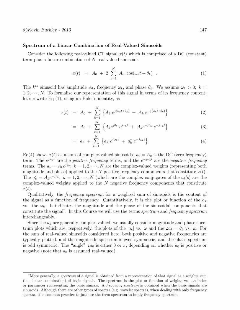
c©Kevin Buckley - 2013 147
Spectrum of a Linear Combination of Real-Valued Sinusoids
Consider the following real-valued CT signal x(t) which is comprised of a DC (constant)term plus a linear combination of N real-valued sinusoids:
x(t) = A0 + 2N∑
k=1
Ak cos(ωkt+ θk) . (1)
The kth sinusoid has amplitude Ak, frequency ωk, and phase θk. We assume ωk > 0; k =1, 2, · · · , N . To formalize our representation of this signal in terms of its frequency content,let’s rewrite Eq (1), using an Euler’s identity, as
x(t) = A0 +N∑
k=1
Ak ej(ωkt+θk) + Ak e−j(ωkt+θk)
(2)
= A0 +N∑
k=1
Akejθk ejωkt + Ake
−jθk e−jωkt
(3)
= a0 +N∑
k=1
ak ejωkt + a∗k e−jωkt
(4)
Eq(4) shows x(t) as a sum of complex-valued sinusoids. a0 = A0 is the DC (zero frequency)term. The ejωkt are the positive frequency terms, and the e−jωkt are the negative frequencyterms. The ak = Ake
jθk ; k = 1, 2, · · · , N are the complex-valued weights (representing bothmagnitude and phase) applied to the N positive frequency components that constitute x(t).The a∗k = Ake
−jθk ; k = 1, 2, · · · , N (which are the complex conjugates of the ak’s) are thecomplex-valued weights applied to the N negative frequency components that constitutex(t).
Qualitatively, the frequency spectrum for a weighted sum of sinusoids is the content ofthe signal as a function of frequency. Quantitatively, it is the plot or function of the akvs. the ωk. It indicates the magnitude and the phase of the sinusoidal components thatconstitute the signal7. In this Course we will use the terms spectrum and frequency spectruminterchangeably.
Since the ak are generally complex-valued, we usually consider magnitude and phase spec-trum plots which are, respectively, the plots of the |ak| vs. ω and the 6 ak = θk vs. ω. Forthe sum of real-valued sinusoids considered here, both positive and negative frequencies aretypically plotted, and the magnitude spectrum is even symmetric, and the phase spectrumis odd symmetric. The “angle” 6 a0 is either 0 or π, depending on whether a0 is positive ornegative (note that a0 is assumed real-valued).
7More generally, a spectrum of a signal is obtained from a representation of that signal as a weights sum(i.e. linear combination) of basic signals. The spectrum is the plot or function of weights vs. an indexor parameter representing the basic signals. A frequency spectrum is obtained when the basic signals aresinusoids. Although there are other types of spectra (e.g. wavelet spectra), when dealing with only frequencyspectra, it is common practice to just use the term spectrum to imply frequency spectrum.
148 c©Kevin Buckley - 2013
Example 3.1: Plot the spectra for
x(t) = −5 + 3 cos(2πt+π
2) − 4 cos(9t− π
2) .
Solution: Using an Euler’s identity, we can rewrite x(t) as
x(t) = −5 +3
2ej(2πt+(π/2)) +
3
2e−j(2πt+(π/2)) − 2 ej(9t−(π/2)) − 2 e−j(9t−(π/2))
= −5 +3
2ejπ/2 ej2πt +
3
2e−jπ/2 e−j2πt − 2e−jπ/2 ej9t − 2ejπ/2 e−j9t .
The following figures are, respectively, the spectrum, the magnitude spectrumand the phase spectrum for this signal.
ak
ω0 2π 9
−π
π/2π/2−9 −2π
−π/2 −π/2
phasespectrum(to scale)
magnitudespectrum(to scale)
spectrum(not to scale,just a visualization)
ak
23
23
ω0 92π−2π−9
5
22
ak
23 j2
3 j
ω0 92π−2π−9
−5−2j 2j−
Figure 57: An example of the spectrum of a sum of sinusoids.
Example 3.2: Consider the ”carrier sinusoid” x(t) = cos(ωct) and an ”informationsignal” v(t) (usually all positive-valued). The signal
x(t) = v(t) cos(ωct)
is called an amplitude modulated (AM) signal. Given v(t) = 5+ 2 cos(40πt) andωc = 400π, sketch x(t) and plot the spectrum of x(t).
Solution: The first plot shown below illustrates v(t) and x(t). To derive thespectrum, rewrite x(t) as:
x(t) = (5 + 2 cos(40πt)) cos(400πt)
=(
5 + ej40πt + e−j40πt)
(
1
2ej400πt +
1
2e−j400πt
)
=5
2ej400πt +
5
2e−j400πt +
1
2ej360πt +
1
2e−j360πt +
1
2ej440πt +
1
2e−j440πt .
(5)
The 2-nd and 3-rd plots show the spectra of v(t) and x(t) respectively.

c©Kevin Buckley - 2013 149
akv
40π ω0−40π
5
1
akx
5/2
1/2
5/2
1/2
0 ω440π360π
−400π 400π−360π−440π
t
x(t)
v(t)
Figure 58: The plot of an AM signal and its spectrum.
So the idea of a frequency spectrum is to identify or describe the frequency components ofa signal – i.e. the sinusoidal components that constitute it. In this Chapter we introduce twotransforms which are used to determine a signal’s frequency content. One, the Continuous-Time Fourier Series (CTFS), is applicable to continuous-time periodic signals. The other,the Continuous-Time Fourier Transform (CTFT), is appropriate for continuous-time energysignals.
Time-Frequency Spectrum
In this Course we simply introduce the idea of a time-frequency spectrum. You will notbe responsible for this on homeworks, quizzes or tests. In Practicum 3 you computed time-frequency spectrum estimates using the Matlab spectrogram function.
Consider the sinusoid x(t) = A cos(ω0t + φ). Its spectrum is illustrated in Figure 59(a).This spectrum is applicable for all time. More generally, the CTFS describes the frequencycontent of a periodic signal for all time. An alternative spectral representation is shown inFigure 59(b). This spectrum describes the frequency content of the signal as a function oftime. (As is common with this type of plot, only the positive frequency content is shown,and frequency in Hertz is used.) For the x(t) we are considering here, the frequency contentis constant for all time.

150 c©Kevin Buckley - 2013
0f
t (time)
f (frequency)
Each note has a0.2 sec. duration.They are concatenated.
A2
e −j φ A2
e j φ
π 0−2 f π2 f0 ω
k
k 0 1 2 3 4 5 6 7
middlenote C D E F G A B C
523
494
440
392
349
294
262
330
t (time)
f (frequency)
0.2 .4 .6 .8 1.0 1.2 1.4
f 262 294 330 349 392 440 494 523
(b)
(c)
(d)
(a)
Figure 59: Frequency spectra: (a) as a representation of frequency content for all time; (b)the time-frequency spectrum of a real-valued sinusoid; (c) the time-frequency spectrum of amusical scale; and (d) an estimate of the time-frequency spectrum.
Some signals have frequency content that changes over time. If we are interested in howit changes, then we want a frequency characterization of the signal that changes with time.That is, we want a time-frequency spectrum which is often referred to as a spectrogram. As anexample, consider the stepped frequency signal described as a sequence of musical notes inPracticum 3, as illustrated in Figure 59(c). Figure 59(d) shows the time-frequency spectrumestimate you will generate in Practicum 3.
c©Kevin Buckley - 2013 151
Generalizing the Idea of Spectral Representation
If you understand the above discussion on frequency spectrum, and if you buy into thenotion that knowing the frequency content of a signal may be useful, then the logical ex-tension is to pursue a more general approach to determining the spectrum of any signal. InTable 5 we present six transforms which are used to identify the frequency content of variousclasses of signals. Note that, as presented in Table 5, these transforms are applicable todifferent classes of signals, e.g. the column #2 transforms are for CT signals, and the row#2 transforms are for energy signals. We will cover these six transforms in this Course.
Table 5: Transforms
Discrete Time Continuous TimeP Discrete Time Fourier Series Continuous Time Fourier Seriese (DTFS): Period N (CTFS): Period T0; ω0 =
2πT0
rio x[n] =
∑
k=<N> X [k] ej(2π/N)kn x(t) =∑∞
k=−∞ ak ejkω0t
di X [k] = 1
N
∑
n=<N> x[n] e−j(2π/N)nk ak =1T0
∫
<T0>x(t) e−jkωot dt
c
E Discrete Time Fourier Transform Continuous Time Fourier Transformn (DTFT) (CTFT)erg x[n] = 1
2π
∫ π−π X(ejω) ejωn dω x(t) = 1
2π
∫∞−∞X(jω) ejωt dω
yX(ejω) =
∑∞n=−∞ x[n] e−jωn X(jω) =
∫∞−∞ x(t) e−jωt dt
G z-Transform Laplace Transformen
e x[n] = 12πj
∫
C X(z) zn−1 dz x(t) = 12πj
∫ c+j∞c−j∞ X(s) est ds
ra X(z) =
∑∞n=−∞ x[n] z−n X(s) =
∫∞−∞ x(t) e−st dt
l
As an example of how these transforms address the concept of a frequency spectrum,consider the Continuous Time Fourier Series (CTFS) in row #1, column #2 of Table 5.Note from its position in the table that the CTFS is for CT periodic (power) signals. Aswith the other transforms, two equations are given. The first equation is called the synthesisequation because it indicates how we can construct a given signal as a linear combinationof basic signals. In the CTFS case, we see from the synthesis equation that the basicsignals are the set of all complex-valued sinusoids that have frequencies that are integer
152 c©Kevin Buckley - 2013
multiples of ω0 = 2πT, where T is the period of the signal. These frequencies are called
the harmonics of ω0. This set of basic signals has an infinite number of members, but themembership is countable. This synthesis equation suggests that in general a CT periodicsignal is composed of an infinite number of harmonic frequency components. The spectrumis the plot or function of the ak vs. the ωk = kω0. The second equation is called the analysisequation because to indicates how to analyze the signal x(t) to determine the ak. That is, itcomputes the spectrum.
In the context of spectral representation, the CTFS is the easiest of the six transformsin Table 5 to understand. So we will cover the CTFS first, in Section 3.2. Then, in theremainder of this Chapter, we will introduce and consider the application of the other CTtransform in Table 5 (i.e. column #2). In Chapter 5 we introduce the DT transforms inTable 5.
We will see that there are many similarities between these transforms. There should be,since they basically do the same thing – they represent, via a synthesis and an analysisequation, general signals as linear combinations of basic signals. As the old saying goes,
“if you’ve seen one transform, you’ve seen them all”.
That is, if you understand one transform, then you understand the basic idea behind alltransforms. The key, then, to making a lot of money and to earning the clear adoration ofyour peers and loved ones, is to know how to use transforms.
3.1.2 System Response to Complex Exponential Signals
Consider a CT LTI system with impulse response h(t). Let the input be x(t) = est, wheres = σ + jω is a complex valued constant of arbitrary value8. Then the output is
y(t) = h(t) ∗ x(t) =∫ ∞
−∞h(τ) x(t− τ) dτ (6)
=∫ ∞
−∞h(τ) es(t−τ) dτ (7)
= est∫ ∞
−∞h(τ) e−sτ dτ . (8)
Note that on the right side of this equation,
∫ ∞
−∞h(τ) e−sτ dτ (9)
is not a function of t. However, it is a function of s. In general it is complex-valued.
8x(t) = eσt ejωt is a complex exponential. Its oscillation rate is dictated by ω. Its decays as dictated byσ. If σ < 0, it decays as t −→ ∞. If decay rate σ > 0, it decays as t −→ −∞. For σ = 0, it does not decay(i.e. it’s a complex sinusoid).
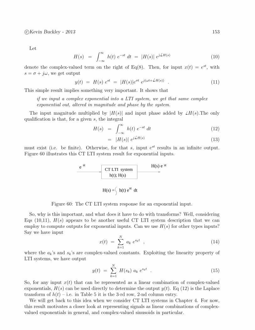
c©Kevin Buckley - 2013 153
Let
H(s) =∫ ∞
−∞h(t) e−st dt = |H(s)| ej 6 H(s) (10)
denote the complex-valued term on the right of Eq(8). Then, for input x(t) = est, withs = σ + jω, we get output
y(t) = H(s) est = |H(s)|eσt ej(ωt+ 6 H(s)) . (11)
This simple result implies something very important. It shows that
if we input a complex exponential into a LTI system, we get that same complexexponential out, altered in magnitude and phase by the system.
The input magnitude multiplied by |H(s)| and input phase added by 6 H(s).The onlyqualification is that, for a given s, the integral
H(s) =∫ ∞
−∞h(t) e−st dt (12)
= |H(s)| ej 6 H(s) (13)
must exist (i.e. be finite). Otherwise, for that s, input est results in an infinite output.Figure 60 illustrates this CT LTI system result for exponential inputs.
e H(s) eCT LTI system
h(t); H(s)
st st
H(s) = h(t) e dtst
Figure 60: The CT LTI system response for an exponential input.
So, why is this important, and what does it have to do with transforms? Well, consideringEqs (10,11), H(s) appears to be another useful CT LTI system description that we canemploy to compute outputs for exponential inputs. Can we use H(s) for other types inputs?Say we have input
x(t) =N∑
k=1
ak eskt , (14)
where the ak’s and sk’s are complex-valued constants. Exploiting the linearity property ofLTI systems, we have output
y(t) =N∑
k=1
H(sk) ak eskt . (15)
So, for any input x(t) that can be represented as a linear combination of complex-valuedexponentials, H(s) can be used directly to determine the output y(t). Eq (12) is the Laplacetransform of h(t) – i.e. in Table 5 it is the 3-rd row, 2-nd column entry.
We will get back to this idea when we consider CT LTI systems in Chapter 4. For now,this result motivates a closer look at representing signals as linear combinations of complex-valued exponentials in general, and complex-valued sinusoids in particular.
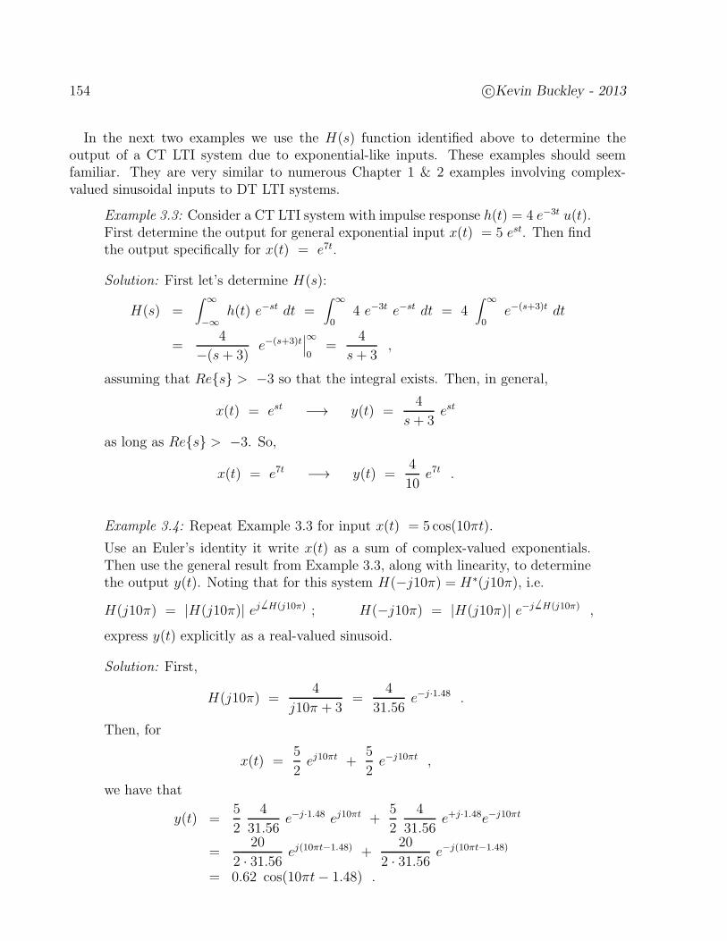
154 c©Kevin Buckley - 2013
In the next two examples we use the H(s) function identified above to determine theoutput of a CT LTI system due to exponential-like inputs. These examples should seemfamiliar. They are very similar to numerous Chapter 1 & 2 examples involving complex-valued sinusoidal inputs to DT LTI systems.
Example 3.3: Consider a CT LTI system with impulse response h(t) = 4 e−3t u(t).First determine the output for general exponential input x(t) = 5 est. Then findthe output specifically for x(t) = e7t.
Solution: First let’s determine H(s):
H(s) =∫ ∞
−∞h(t) e−st dt =
∫ ∞
04 e−3t e−st dt = 4
∫ ∞
0e−(s+3)t dt
=4
−(s+ 3)e−(s+3)t
∣
∣
∣
∞
0=
4
s+ 3,
assuming that Res > −3 so that the integral exists. Then, in general,
x(t) = est −→ y(t) =4
s+ 3est
as long as Res > −3. So,
x(t) = e7t −→ y(t) =4
10e7t .
Example 3.4: Repeat Example 3.3 for input x(t) = 5 cos(10πt).
Use an Euler’s identity it write x(t) as a sum of complex-valued exponentials.Then use the general result from Example 3.3, along with linearity, to determinethe output y(t). Noting that for this system H(−j10π) = H∗(j10π), i.e.
H(j10π) = |H(j10π)| ej 6 H(j10π) ; H(−j10π) = |H(j10π)| e−j 6 H(j10π) ,
express y(t) explicitly as a real-valued sinusoid.
Solution: First,
H(j10π) =4
j10π + 3=
4
31.56e−j·1.48 .
Then, for
x(t) =5
2ej10πt +
5
2e−j10πt ,
we have that
y(t) =5
2
4
31.56e−j·1.48 ej10πt +
5
2
4
31.56e+j·1.48e−j10πt
=20
2 · 31.56 ej(10πt−1.48) +20
2 · 31.56 e−j(10πt−1.48)
= 0.62 cos(10πt− 1.48) .

c©Kevin Buckley - 2013 155
3.2 CT Fourier Series (CTFS) Representation of Periodic Signals
In this Section we consider how to express any CT periodic signal as a linear combinationof complex sinusoids. In pursuit of this, first consider the complex sinusoid ejω0t which hasfundamental frequency ω0 and therefore fundamental period T where
ω0 =2π
T(radians/sec.) . (16)
For integers k = ±1, ±2, ±3, · · ·, the frequencies kω0 are called the harmonics of ωo, andthe set of signals
φk(t) = ejkω0t = ejk2πTt ; k = 0, ±1, ±2, ±3, · · · (17)
are the set harmonically related complex sinusoids (including DC, the k = 0 term).Every signal φk(t) has a period of T (not necessarily its fundamental period). Thus, any
signal of the form
x(t) =∞∑
k=−∞ak φk(t)
=∞∑
k=−∞ak ejkωot (18)
is periodic with period T . For all possible weights ak, Eq (18) forms the class of all signalsthat are linear combinations of signals from the basic set ejkωot; k = 0,±1,±2, · · ·. Allsignals from this class are periodic with period T .
Combined, the k = ±N components of the x(t) in Eq (18) are called the N th harmonic.As mentioned earlier, the k = 0 component is the DC (a.k.a. constant, zero-th harmonic)term. We can write x(t) from Eq (18) in the form
x(t) = a0 +∞∑
k=1
ak ejkωot +−1∑
k=−∞ak ejkωot (19)
= a0 +∞∑
k=1
ak ejkωot + a−k e−jkωot
(20)
which shows the DC component a0 and the sum for all the other harmonics.Let ak = Ake
jθk , where the Ak and θk, i.e. the magnitudes and phases respectively, arereal-valued. Then for the x(t) considered in Eq (20) we have
x(t) = a0 +∞∑
k=1
Ak ej(kωot+θk) + A−k e−j(kωot−θ−k)
. (21)
If a−k = a∗k (i.e. if the ak coefficients are complex symmetric in k), then a−k = Ake−jθk , so
that
x(t) = a0 +∞∑
k=1
Ak ej(kωot+θk) + Ak e−j(kωot+θk)
(22)
= a0 + 2∞∑
k=1
Ak cos(kωot + θk) . (23)
In this case, if we assume a0 is real-valued, x(t) is real-valued.
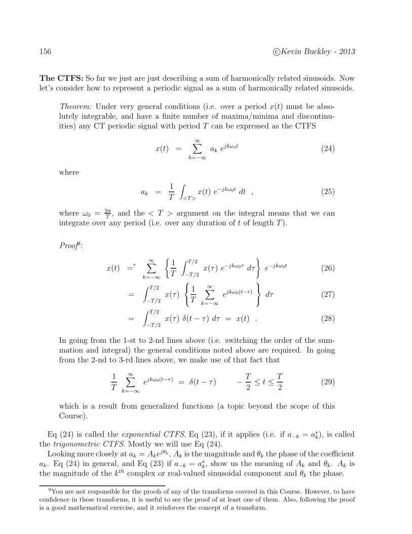
156 c©Kevin Buckley - 2013
The CTFS: So far we just are just describing a sum of harmonically related sinusoids. Nowlet’s consider how to represent a periodic signal as a sum of harmonically related sinusoids.
Theorem: Under very general conditions (i.e. over a period x(t) must be abso-lutely integrable, and have a finite number of maxima/minima and discontinu-ities) any CT periodic signal with period T can be expressed as the CTFS
x(t) =∞∑
k=−∞ak ejkωot (24)
where
ak =1
T
∫
<T>x(t) e−jkω0t dt , (25)
where ω0 = 2πT, and the < T > argument on the integral means that we can
integrate over any period (i.e. over any duration of t of length T ).
Proof9:
x(t) =?∞∑
k=−∞
1
T
∫ T/2
−T/2x(τ) e−jkω0τ dτ
e−jkω0t (26)
=∫ T/2
−T/2x(τ)
1
T
∞∑
k=−∞ejkω0(t−τ)
dτ (27)
=∫ T/2
−T/2x(τ) δ(t− τ) dτ = x(t) . (28)
In going from the 1-st to 2-nd lines above (i.e. switching the order of the sum-mation and integral) the general conditions noted above are required. In goingfrom the 2-nd to 3-rd lines above, we make use of that fact that
1
T
∞∑
k=−∞ejkω0(t−τ) = δ(t− τ) − T
2≤ t ≤ T
2(29)
which is a result from generalized functions (a topic beyond the scope of thisCourse).
Eq (24) is called the exponential CTFS. Eq (23), if it applies (i.e. if a−k = a∗k), is calledthe trigonometric CTFS. Mostly we will use Eq (24).
Looking more closely at ak = Akejθk , Ak is the magnitude and θk the phase of the coefficient
ak. Eq (24) in general, and Eq (23) if a−k = a∗k, show us the meaning of Ak and θk. Ak isthe magnitude of the kth complex or real-valued sinusoidal component and θk the phase.
9You are not responsible for the proofs of any of the transforms covered in this Course. However, to haveconfidence in these transforms, it is useful to see the proof of at least one of them. Also, following the proofis a good mathematical exercise, and it reinforces the concept of a transform.
c©Kevin Buckley - 2013 157
Example 3.5: Let x(t) =∑∞
l=−∞ p2T1(t − lT ) where T > 2T1. Determine theCTFS coefficients.
Solution:
Example 3.6: Continuing Example 3.5, let T1 =T4. Determine the CTFS coeffi-
cients.
Solution:
The following Matlab Demo provides a visualization of the CTFS. The periodic signalfrom Example 3.6 is considered. For several values of N , the periodic signal is approximatedby summing all harmonic components up to N . Figure 61 shows the result, for maximumN = 151. As N increases, the quality of the approximation improves. Run this programyourself, and on the 4-th plot zoom in on a transition region of the square wave.
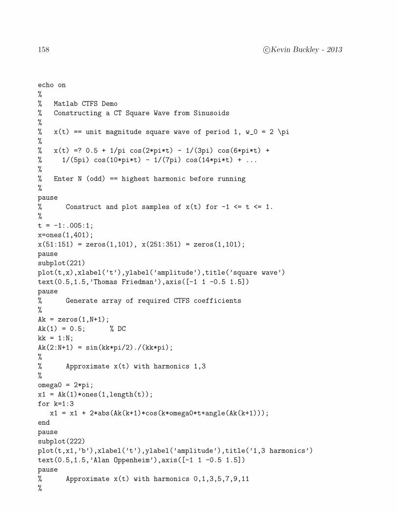
158 c©Kevin Buckley - 2013
echo on
%
% Matlab CTFS Demo
% Constructing a CT Square Wave from Sinusoids
%
% x(t) == unit magnitude square wave of period 1, w_0 = 2 \pi
%
% x(t) =? 0.5 + 1/pi cos(2*pi*t) - 1/(3pi) cos(6*pi*t) +
% 1/(5pi) cos(10*pi*t) - 1/(7pi) cos(14*pi*t) + ...
%
% Enter N (odd) == highest harmonic before running
%
pause
% Construct and plot samples of x(t) for -1 <= t <= 1.
%
t = -1:.005:1;
x=ones(1,401);
x(51:151) = zeros(1,101), x(251:351) = zeros(1,101);
pause
subplot(221)
plot(t,x),xlabel(’t’),ylabel(’amplitude’),title(’square wave’)
text(0.5,1.5,’Thomas Friedman’),axis([-1 1 -0.5 1.5])
pause
% Generate array of required CTFS coefficients
%
Ak = zeros(1,N+1);
Ak(1) = 0.5; % DC
kk = 1:N;
Ak(2:N+1) = sin(kk*pi/2)./(kk*pi);
%
% Approximate x(t) with harmonics 1,3
%
omega0 = 2*pi;
x1 = Ak(1)*ones(1,length(t));
for k=1:3
x1 = x1 + 2*abs(Ak(k+1)*cos(k*omega0*t+angle(Ak(k+1)));
end
pause
subplot(222)
plot(t,x1,’b’),xlabel(’t’),ylabel(’amplitude’),title(’1,3 harmonics’)
text(0.5,1.5,’Alan Oppenheim’),axis([-1 1 -0.5 1.5])
pause
% Approximate x(t) with harmonics 0,1,3,5,7,9,11
%
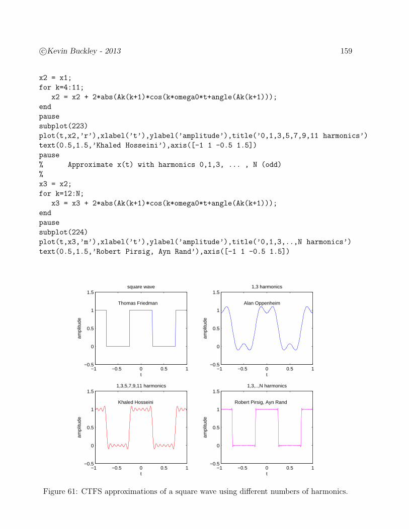
c©Kevin Buckley - 2013 159
x2 = x1;
for k=4:11;
x2 = x2 + 2*abs(Ak(k+1)*cos(k*omega0*t+angle(Ak(k+1)));
end
pause
subplot(223)
plot(t,x2,’r’),xlabel(’t’),ylabel(’amplitude’),title(’0,1,3,5,7,9,11 harmonics’)
text(0.5,1.5,’Khaled Hosseini’),axis([-1 1 -0.5 1.5])
pause
% Approximate x(t) with harmonics 0,1,3, ... , N (odd)
%
x3 = x2;
for k=12:N;
x3 = x3 + 2*abs(Ak(k+1)*cos(k*omega0*t+angle(Ak(k+1)));
end
pause
subplot(224)
plot(t,x3,’m’),xlabel(’t’),ylabel(’amplitude’),title(’0,1,3,..,N harmonics’)
text(0.5,1.5,’Robert Pirsig, Ayn Rand’),axis([-1 1 -0.5 1.5])
−1 −0.5 0 0.5 1−0.5
0
0.5
1
1.5
t
ampl
itude
square wave
Thomas Friedman
−1 −0.5 0 0.5 1−0.5
0
0.5
1
1.5
t
ampl
itude
1,3 harmonics
Alan Oppenheim
−1 −0.5 0 0.5 1−0.5
0
0.5
1
1.5
t
ampl
itude
1,3,5,7,9,11 harmonics
Khaled Hosseini
−1 −0.5 0 0.5 1−0.5
0
0.5
1
1.5
t
ampl
itude
1,3,..,N harmonics
Robert Pirsig, Ayn Rand
Figure 61: CTFS approximations of a square wave using different numbers of harmonics.
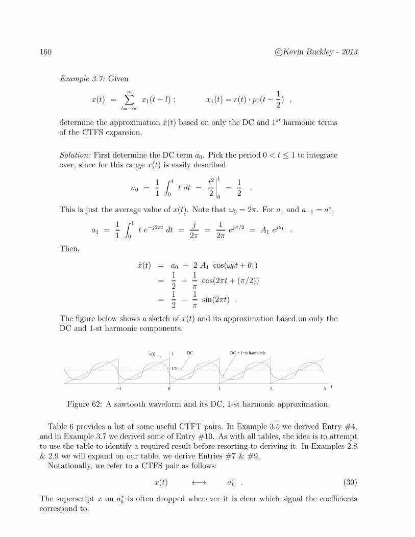
160 c©Kevin Buckley - 2013
Example 3.7: Given
x(t) =∞∑
l=−∞x1(t− l) ; x1(t) = r(t) · p1(t−
1
2) ,
determine the approximation x(t) based on only the DC and 1st harmonic termsof the CTFS expansion.
Solution: First determine the DC term a0. Pick the period 0 < t ≤ 1 to integrateover, since for this range x(t) is easily described.
a0 =1
1
∫ 1
0t dt =
t2
2
∣
∣
∣
∣
∣
1
0
=1
2.
This is just the average value of x(t). Note that ω0 = 2π. For a1 and a−1 = a∗1,
a1 =1
1
∫ 1
0t e−j2πt dt =
j
2π=
1
2πejπ/2 = A1 ejθ1 .
Then,
x(t) = a0 + 2 A1 cos(ω0t+ θ1)
=1
2+
1
πcos(2πt+ (π/2))
=1
2− 1
πsin(2πt) .
The figure below shows a sketch of x(t) and its approximation based on only theDC and 1-st harmonic components.
DC + 1−st harmomicDC1
1/2
x(t)
0−1 1 2 3 t
Figure 62: A sawtooth waveform and its DC, 1-st harmonic approximation.
Table 6 provides a list of some useful CTFT pairs. In Example 3.5 we derived Entry #4,and in Example 3.7 we derived some of Entry #10. As with all tables, the idea is to attemptto use the table to identify a required result before resorting to deriving it. In Examples 2.8& 2.9 we will expand on our table, we derive Entries #7 & #9.
Notationally, we refer to a CTFS pair as follows:
x(t) ←→ axk . (30)
The superscript x on axk is often dropped whenever it is clear which signal the coefficientscorrespond to.
c©Kevin Buckley - 2013 161
Table 6: Continuous Time Fourier Series (CTFS) Pairs.
signal Periodic Signal ω0 CTFStype (x(t) = x(t + T0), all t) (ak; k = 0,±1,±2, · · · ,±∞)
1 DC x(t) = A (i.e. a DC signal) a0 = Aak = 0, otherwise
2 cosine x(t) = A cos(2πf0t+ φ) 2πf0 a1 =A2ejφ; a−1 =
A2e−jφ
ak = 0, otherwise
3 sine x(t) = A sin(2πf0t + φ) 2πf0 a1 =A2ej(φ−π/2); a−1 =
A2e−j(φ−π/2)
ak = 0, otherwise
4 pulse x(t) =∞∑
n=−∞x1(t− nT ); 2π
Tak =
Akπ
sin(kπτ/T ), all k
train x1(t) = A pτ (t); τ < T
5 square x(t) =∞∑
n=−∞x1(t− nT ); 2π
Ta0 = a±2 = a±4 = · · · = 0
wave x1(t) = 2A pT/2(t− T4) − A ak =
2Akπ
e−jπk/2, otherwise
6 impulse x(t) =∞∑
n=−∞A δ(t− nT ) 2π
Tak =
AT; all k
train
7 halfwave x(t) =∞∑
n=−∞x1(t− nT ); 2π
Ta0 =
Aπ; a1 = a−1 =
A4
rectified x1(t) = A cos(
2πTt)
· pT/2(t) ak =Aπ
(−1)(k+2)/2
(k2−1), k = ±2,±4 · · ·
cosine ak = 0, otherwise
8 fullwave x(t) =∣
∣
∣A cos(
2πTt)∣
∣
∣
4πT
a0 =2Aπ
rectified
cosine ak =2Aπ
(−1)k
(1−4k2), k = ±1,±2 · · ·
9 every x(t) =∞∑
n=−∞x1(t− nT ); 2π
Ta2 =
A4j, a−2 =
−A4j
other
sine x1(t) =
A sin((4π/T )t) 0 ≤ t ≤ T/20 T/2 < t ≤ T
ak = e−j(k−1)π/2 2A sin(kπ/2)π(4−k2)
otherwise
10 saw x(t) =∞∑
n=−∞x1(t− nT ); 2π
Ta0 =
AT2
tooth x1(t) = A t pT (t− T2) ak = j AT
2kπ, otherwise
11 exp. ak’s1−c2
1+c2 − 2c cos(ωot)ω0 ak = c|k| (−1 < c < 1)
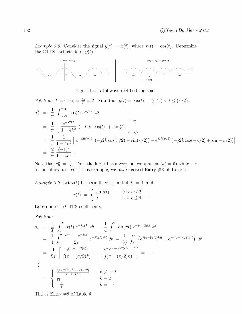
162 c©Kevin Buckley - 2013
Example 3.8: Consider the signal y(t) = |x(t)| where x(t) = cos(t). Determinethe CTFS coefficients of y(t).
t
........ 1
y(t) = | x(t) | = | cos(t) |
−π 0 π 2π
Τ = π
t
........ 1
−π π 2π
x(t) = cos(t)
0
Figure 63: A fullwave rectified sinusoid.
Solution: T = π, ω0 =2πT
= 2. Note that y(t) = cos(t); −(π/2) < t ≤ (π/2).
ayk =1
π
∫ π/2
−π/2cos(t) e−j2kt dt
=1
π
[
e−j2kt
1− 4k2(−j2k cos(t) + sin(t))
]π/2
−π/2
=1
π
1
1− 4k2
[
e−j2k(π/2) (−j2k cos(π/2) + sin(π/2))− ej2k(π/2) (−j2k cos(−π/2) + sin(−π/2))]
=2
π
(−1)k1− 4k2
.
Note that ay0 = 2π. Thus the input has a zero DC component (axo = 0) while the
output does not. With this example, we have derived Entry #8 of Table 6.
Example 3.9: Let x(t) be periodic with period T0 = 4, and
x(t) =
sin(πt) 0 ≤ t ≤ 20 2 < t ≤ 4
.
Determine the CTFS coefficients.
Solution:
ak =1
T
∫ T
0x(t) e−jω0kt dt =
1
4
∫ 2
0sin(πt) e−j(π/2)kt dt
=1
4
∫ 2
0
ejπt − e−jπt
2je−j(π/2)kt dt =
1
8j
∫ 2
0
(
ej(π−(π/2)k)t − e−j(π+(π/2)k)t)
dt
=1
8j
[
ej(π−(π/2)k)t
j(π − (π/2)k)− e−j(π+(π/2)k)t
−j(π + (π/2)k)
]2
0
= · · ·
...
=
2j e−jkπ/2 sin(kπ/2)π (4−k2)
k 6= ±214j
k = 2
− 14j
k = −2.
This is Entry #9 of Table 6.

c©Kevin Buckley - 2013 163
3.2.1 A Few CTFS Properties
Properties are important features of transform. They make the transform easier to workwith, and thus extend the transform’s utility. Furthermore, as we will see later in thisCourse, a transform property is often directly related to one or more important engineeringproblems. Since transform all do the same thing (i.e. decompose a general signal into alinear combination of basic signals), properties for different transforms are often similar.So learning a set of properties for one transform directly contributes to understanding andemploying other transforms.
In this Subsection we introduce just a few of the many properties of the CTFS. Later inthis Section, in a more general context of CT transforms, we will more systematically andextensively cover transform properties. Becoming familiar with the properties presented herewill reduce the stress of learning properties later.
Linearity: Consider two signals, x1(t) and x2(t), each periodic with period T , with CTFScoefficients ax1
k and ax2k respectively. Given any two constants c1 and c2, the CTFS pair is
c1 x1(t) + c2x2(t) ←→ c1 ax1k + c2 ax2
k . (31)
Time Shift (i.e. Delay): Given a signal x(t), periodic with period T , with CTFS coeffi-cients ak, then for any delay τ , x(t− τ) is also periodic with period T with CTFS pair
x(t− τ) ←→ e−jkω0τ ak = e−jkω0τ Akejθk = Ake
j(θk−kω0τ) . (32)
This property makes sense. If you delay a periodic signal x(t), then you delay each of itssinusoidal components. This does not alter the sinusoidal components magnitudes. It onlychanges their phases. The more delay, the more phase shift. The higher the frequency, thegreater the phase shift.
Symmetry: For real-valued periodic x(t), with CTFS coefficients ak, we have that
a−k = a∗k . (33)
That is, the CTFS coefficients are complex symmetric.
These three properties, and Parseval’s Theorem which we present after a few examples,are enough to serve our objectives for the time being. We will develop more properties later,after we introduce the CTFT (and the generalization of it that includes the CTFS) and theLaplace transform. Below we use the properties just introduced, along with known CTFSpairs from Table 6, to solve some new CTFS problems.
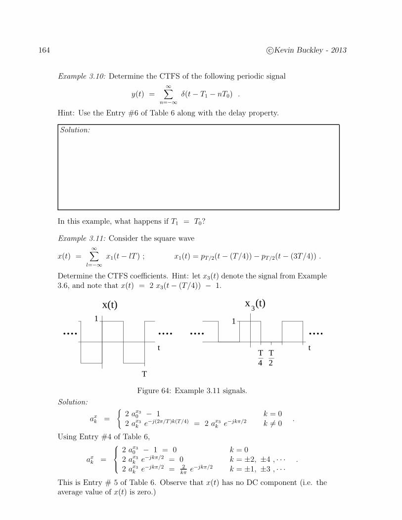
164 c©Kevin Buckley - 2013
Example 3.10: Determine the CTFS of the following periodic signal
y(t) =∞∑
n=−∞δ(t− T1 − nT0) .
Hint: Use the Entry #6 of Table 6 along with the delay property.
Solution:
In this example, what happens if T1 = T0?
Example 3.11: Consider the square wave
x(t) =∞∑
l=−∞x1(t− lT ) ; x1(t) = pT/2(t− (T/4))− pT/2(t− (3T/4)) .
Determine the CTFS coefficients. Hint: let x3(t) denote the signal from Example3.6, and note that x(t) = 2 x3(t− (T/4)) − 1.
3x (t)
T4
T2
x(t)
t
1
T
........t
.... ....1
Figure 64: Example 3.11 signals.
Solution:
axk =
2 ax30 − 1 k = 0
2 ax3k e−j(2π/T )k(T/4) = 2 ax3
k e−jkπ/2 k 6= 0.
Using Entry #4 of Table 6,
axk =
2 ax30 − 1 = 0 k = 0
2 ax3k e−jkπ/2 = 0 k = ±2, ±4 , · · ·
2 ax3k e−jkπ/2 = 2
kπe−jkπ/2 k = ±1, ±3 , · · ·
.
This is Entry # 5 of Table 6. Observe that x(t) has no DC component (i.e. theaverage value of x(t) is zero.)

c©Kevin Buckley - 2013 165
Example 3.12: Determine the CTFS of the following periodic signal
z(t) =∞∑
n=−∞z1(t− 4n) ; z1(t) = (4− t) p4(t− 2) .
Solution: Let z3(t) denote the sawtooth wave in Entry #10 of Table 6, withA = 1 and T = 4. Then
z(t) = 4 − z3(t)
so
azk =
4 − az3k = 2 k = 0−az3k = −j 2
kπk 6= 0
.
This is the signal you will analyze in Practicum 4a.
Parseval’s Theorem: The power of a CT periodic signal with period T can be computedin either the time domain or frequency domain as follows
P =1
T
∫
<T>|x(t)|2 dt =
∞∑
k=−∞|ak|2 . (34)
By the symmetry property, if x(t) is real-valued,
P = |a0|2 + 2∞∑
k=1
|ak|2 . (35)
Example 3.13: For the signal in Example 3.7, determine the percentage of totalpower that is in DC and the 1-st harmonic combined.
Solution:

166 c©Kevin Buckley - 2013
3.3 The Continuous Time Fourier Transform (CTFT)
In this Section we introduce the CTFT. This transform provides the decomposition of CTenergy signals, so it is the column #2, row #2 entry in our transform table – Table 5. Thedecomposition is in terms of complex-valued sinusoids, so it generates a frequency spectrum ofan CT energy signal. We begin by introducing the transform equations, and then consider anumber of examples that generate entries in a CTFT table. We then develop a generalizationof the CTFT so as to include periodic signals, thus enabling us to represent both periodicpower and energy signals using a single frequency transform. After introducing the LaplaceTransform (LT) in Section 3.4, we will return the our study of the CTFT in Section 3.5where we cover both CTFT and LT properties.
Let x(t) be an energy signal. The CTFT indicates that x(t) can be represented as
x(t) =1
2π
∫ ∞
−∞X(jω) ejωt dω . (36)
That is, x(t) can be represented as or decomposed into a linear combination of all the CTcomplex-valued sinusoids ejωt over the frequency range −∞ ≤ ω ≤ ∞. Eq (36), called theInverse CTFT (ICTFT), is the synthesis equation since it generates x(t) from basic signals.The CTFT is
X(jω) =∫ ∞
−∞x(t) e−jωt dt . (37)
It is the analysis equation because it derives the weighting function X(jω) for the synthesisequation10. The reason for the j in the argument of X(jω) has to do with the relationshipbetween the CTFT and the LT (we will explain this later). For now remember that X(jω)is simply a function of ω.
10Proof of the CTFT involves plugging Eq (37) into Eq (36) and simplifying to show that the right sideof Eq (36) does reduce to x(t). This derivation, specifically a change of the order of two nested integrals,requires certain assumptions. These assumptions are that x(t): be absolutely integrable, and have a finitenumber of minima/maxima and discontinuities. The absolutely integrable requirement essentially (but notexactly) means that x(t) be an energy signal.
c©Kevin Buckley - 2013 167
Example 3.14: Determine the CTFT of the signal x(t) = p2T1(t). Based on theresult, comment on the frequency content of the signal.
Solution:
Note that X(jω) has infinite extent, indicating that it contains infinitely highfrequency components. This should not be surprising since x(t) has discontinu-ities, which require infinitely high frequency components to synthesize. Also notethe X(jω) is largest for lower frequencies, indicating that in some sense x(t) inmostly a low frequency signal.
This Example derives Entry #8 of the CTFT table, Table 7, on the next page.
Example 3.15: Determine the ICTFT of X(jω) = p2W (ω). Compare character-istics of x(t) and X(jω).
Solution:
Note that with the X(jω) given in this example, x(t) is a purely low frequencysignal. The manifestation of this in the time domain is that x(t) is smooth (e.g.there are no discontinuities).
This Example derives Entry #9 of Table 7.

168 c©Kevin Buckley - 2013
Table 7: Continuous Time Fourier Transform (CTFT) Pairs.
# Signal CTFT(∀ t) (∀ ω)
1 δ(t) 1
2 δ(t− τ) e−jωτ
3 u(t) 1jω
+ πδ(ω)
4 e−atu(t); Rea > 0 1a+jω
5 te−atu(t); Rea > 0 1(a+jω)2
6 tn−1
(n−1)!e−atu(t); Rea > 0 1
(a+jω)n
7 e−a|t|; Rea > 0 2aa2+ω2
8 e−at cos(ω0t) u(t); Rea > 0 jω+a(jω+a)2+ω2
9 e−at sin(ω0t) u(t); Rea > 0 ω0
(jω+a)2+ω2
10 pT (t) = u(t+ T2)− u(t− T
2) 2
ωsin
(
ωT2
)
11 1πtsin(Wt) p2W (ω)
12 sin2(Wt)(πt)2
12π
p2W (ω) ∗ p2W (ω)
13 cc2+t2
π e−c|ω|
14 ejω0t 2πδ(ω − ω0)
15 cos(ω0t) πδ(ω − ω0) + πδ(ω + ω0)
16 sin(ω0t)πjδ(ω − ω0)− π
jδ(ω + ω0)
17 ak ejkω0t 2πak δ(ω − kω0)
18∞∑
k=−∞ak ejkω0t
∞∑
k=−∞2πak δ(ω − kω0)
19∞∑
n=−∞δ(t− nT ) 2π
T
∞∑
k=−∞δ(
ω − 2π
Tk)
c©Kevin Buckley - 2013 169
Example 3.16: Determine the CTFT of the signal x(t) = δ(t). Based on theresult, comment on the frequency content of the signal.
Solution:
Note the consistence between the time and frequency domain representationsof this signal. x(t) changes infinitely over zero time, which implies very highfrequency components. In fact, X(jω) indicates that the impulse consists ofequal content over all frequency. It’s the most wideband signal.
This Example derives Entries #1 & #2 of Table 7.
Example 3.17: Determine the CTFT of x(t) = e−atu(t) where Rea > 0.
Solution:
This Example derives Entry #4 of Table 7.
Example 3.18: Determine the CTFT of x(t) = e−a|t| where Rea > 0. Compar-ing the solution derivation and result to those of Example 3.17, can you anticipateone or more properties of the CTFT?
Solution:
x(t) = e−at u(t) + eat u(−t)
X(jω) =∫ ∞
0e−at e−jωt dt +
∫ 0
−∞eat e−jωt dt =
1
jω + a+∫ 0
−∞e(jω−a)t dt
=1
jω + a+
1
−jω + a=
2a
a2 + ω2
How about linearity? Perhaps there’s some kind of symmetry property.
This Example derives Entry #7 of Table 7.
170 c©Kevin Buckley - 2013
Example 3.19: Determine the ICTFT of X(jω) = 2πδ(ω − ω0). Note the x(t) isa periodic (power) signal. Try deriving this X(jω) from your x(t).
Solution:
This is not an energy signal! What’s up? See Subsection 3.3.1 below.
This Example derives Entry #13 of Table 7.
Example 3.20: Starting with the result of Example 3.19 (i.e. starting with theCTFT pair established in Example 3.19), determine the CTFT ofx(t) = ak ejkω0t, where ak is an arbitrary complex constant and kω0 is thefrequency of sinusoidal x(t). Does this result suggest a useful CTFT property?
Solution: By the linearity property of the integral (in the CTFT equation),
ak ejkω0t ←→ ak 2π δ(ω − kω0)
This Example derives Entry #15 of Table 7.
Example 3.21: Extending Example 3.20, determine the CTFT of
x(t) =∞∑
k=−∞ak ejkω0t .
Solution: To extend the Example 3.20 result, we anticipate the linearity propertyof the CTFT (recall this property for the CTFS).
x(t) =∞∑
k=−∞ak ejkω0t ←→ X(jω) =
∞∑
k=−∞ak 2π δ(ω − kω0)
X(j )ω
−ω0 2ω0ω0
π(a 2 )0
π(a 2 )2−1 π(a 2 ) π(a 2 )1
CTFTSpectrum
ω
.... ....
Figure 65: CTFT of a periodic signal.
This Example derives Entry #18 of Table 7, and leads the main point on thenext Subsection.

c©Kevin Buckley - 2013 171
3.3.1 The Generalized CTFT
For CT energy signals, the generalized CTFT is just the CTFT described above. ConcerningCT periodic signals, first recall form our CTFS discussion that for any periodic power signalx(t) with fundamental frequency ω0 has CTFS representation
x(t) =∞∑
k=−∞ak ejkω0t . (38)
From Example 3.21, we then have that, in terms of the CTFS coefficients, the generalizedCTFT of a periodic signal is
X(jω) =∞∑
k=−∞2π ak δ(ω − kω0) . (39)
That’s it. We now have a single CT transform, the generalize CTFT (or, for now on, theCTFT for short) that can be used to represent and analyze the frequency content of bothenergy and periodic CT signals. Note, however, that we can’t just ignore the CTFS. For theCTFT representation of periodic signals, we still need to know the CTFS coefficients.
Example 3.22: Determine the CTFT of the impulse train
x(t) =∞∑
n=−∞δ(t− nT ) .
Solution: Using Entry # 6 of the CTFS table (Table 6),
X(jω) =2π
T
∞∑
k=−∞δ(ω − kω0)
.... ....
(1)
T t−2T −T 0 2T 3T
x(t) X(j )ωπ(2 /T)
ω0 2ω0−ω0ω
.... ....03ω−2ω0 0
= 2 /Tπω0
CTFT
Figure 66: CTFT of a impulse train.
This is Entry #19 of Table 7. In Chapter 4 we will see that this CTFT pair, whilenot representing a realizable signal, is key to understanding why sampling works(i.e. why and when we can exactly reconstruct a CT signal from its samples).
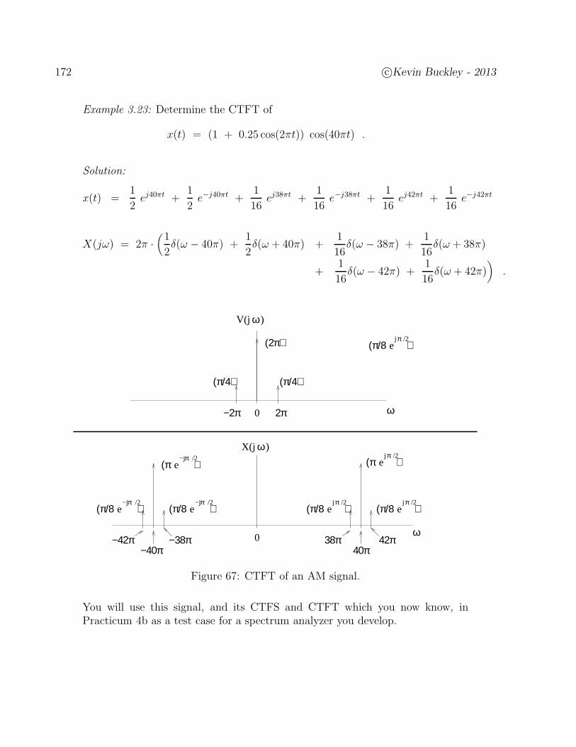
172 c©Kevin Buckley - 2013
Example 3.23: Determine the CTFT of
x(t) = (1 + 0.25 cos(2πt)) cos(40πt) .
Solution:
x(t) =1
2ej40πt +
1
2e−j40πt +
1
16ej38πt +
1
16e−j38πt +
1
16ej42πt +
1
16e−j42πt
X(jω) = 2π ·(
1
2δ(ω − 40π) +
1
2δ(ω + 40π) +
1
16δ(ω − 38π) +
1
16δ(ω + 38π)
+1
16δ(ω − 42π) +
1
16δ(ω + 42π)
)
.
ωV(j )
j /2πe(π/8 )
ω0−2π 2π
(2π)
(π/4) (π/4)
−j /2e(π )
π
j /2πe(π/8 )
j /2πe(π/8 )
j /2πe(π )
e−j /2
(π/8 )π
e−j /2
(π/8 )π
0 ω
ωX(j )
40π−40π42π38π−38π−42π
Figure 67: CTFT of an AM signal.
You will use this signal, and its CTFS and CTFT which you now know, inPracticum 4b as a test case for a spectrum analyzer you develop.
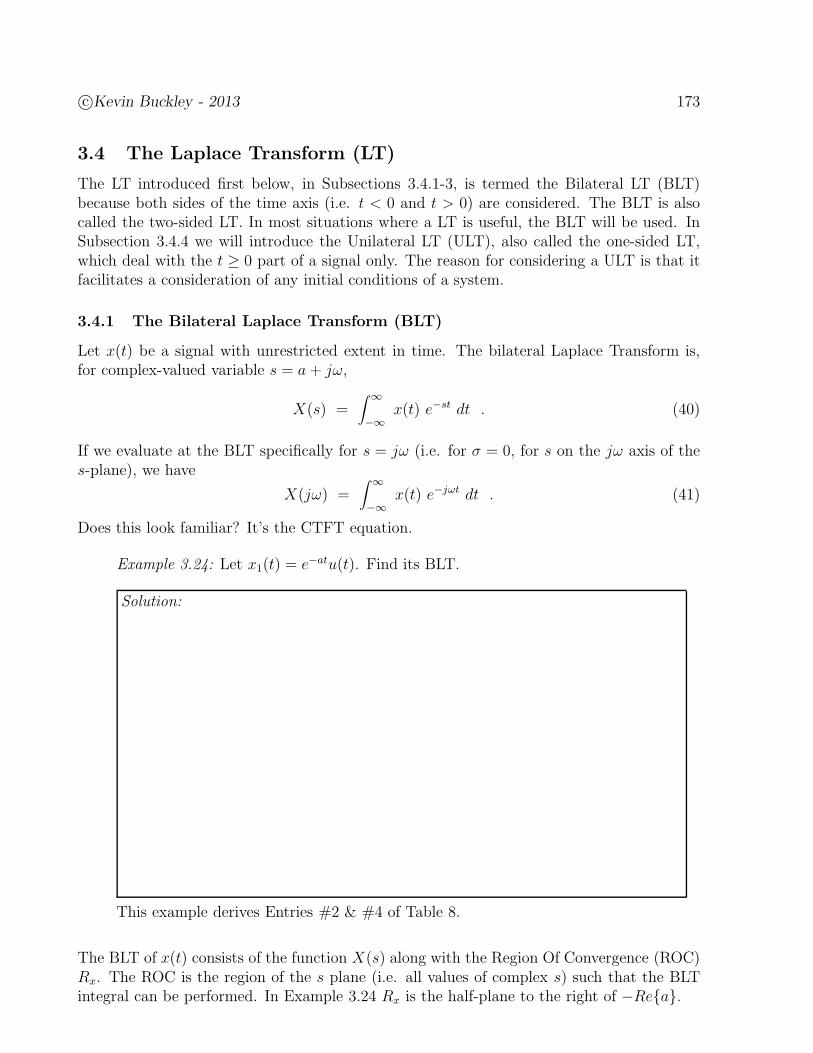
c©Kevin Buckley - 2013 173
3.4 The Laplace Transform (LT)
The LT introduced first below, in Subsections 3.4.1-3, is termed the Bilateral LT (BLT)because both sides of the time axis (i.e. t < 0 and t > 0) are considered. The BLT is alsocalled the two-sided LT. In most situations where a LT is useful, the BLT will be used. InSubsection 3.4.4 we will introduce the Unilateral LT (ULT), also called the one-sided LT,which deal with the t ≥ 0 part of a signal only. The reason for considering a ULT is that itfacilitates a consideration of any initial conditions of a system.
3.4.1 The Bilateral Laplace Transform (BLT)
Let x(t) be a signal with unrestricted extent in time. The bilateral Laplace Transform is,for complex-valued variable s = a + jω,
X(s) =∫ ∞
−∞x(t) e−st dt . (40)
If we evaluate at the BLT specifically for s = jω (i.e. for σ = 0, for s on the jω axis of thes-plane), we have
X(jω) =∫ ∞
−∞x(t) e−jωt dt . (41)
Does this look familiar? It’s the CTFT equation.
Example 3.24: Let x1(t) = e−atu(t). Find its BLT.
Solution:
This example derives Entries #2 & #4 of Table 8.
The BLT of x(t) consists of the function X(s) along with the Region Of Convergence (ROC)Rx. The ROC is the region of the s plane (i.e. all values of complex s) such that the BLTintegral can be performed. In Example 3.24 Rx is the half-plane to the right of −Rea.

174 c©Kevin Buckley - 2013
Example 3.25: Let x2(t) = −e−atu(−t). Find the BLT X(s).
Solution:
This example derives Entries #3 & #5 of Table 8.
The BLT functions X1(s) and X2(s) from Examples 3.24 & 3.25 are equivalent. The ROCsare different. To uniquely identify a signal, both the BLT function and ROC must bespecified.
Example 3.26: Find the inverse BLT x(t) of X(s) = 1s−5
with Rx = Res < 5.
Solution: (Hint - use Table 8 entry #4 or #5)
Example 3.26 illustrates the most common way in which inverse LTs are found – by finding asimilar LT pair in a table, and manipulating it to get the desired result. The formal approachto ”manipulating” the table entry is the use of LT properties. We will discuss inverse LTsin more depth a little later. After we establish a relationship between the BLT and CTFT,in Subsection 3.4.2, we will cover BLT and CTFT properties together in Section 3.5.
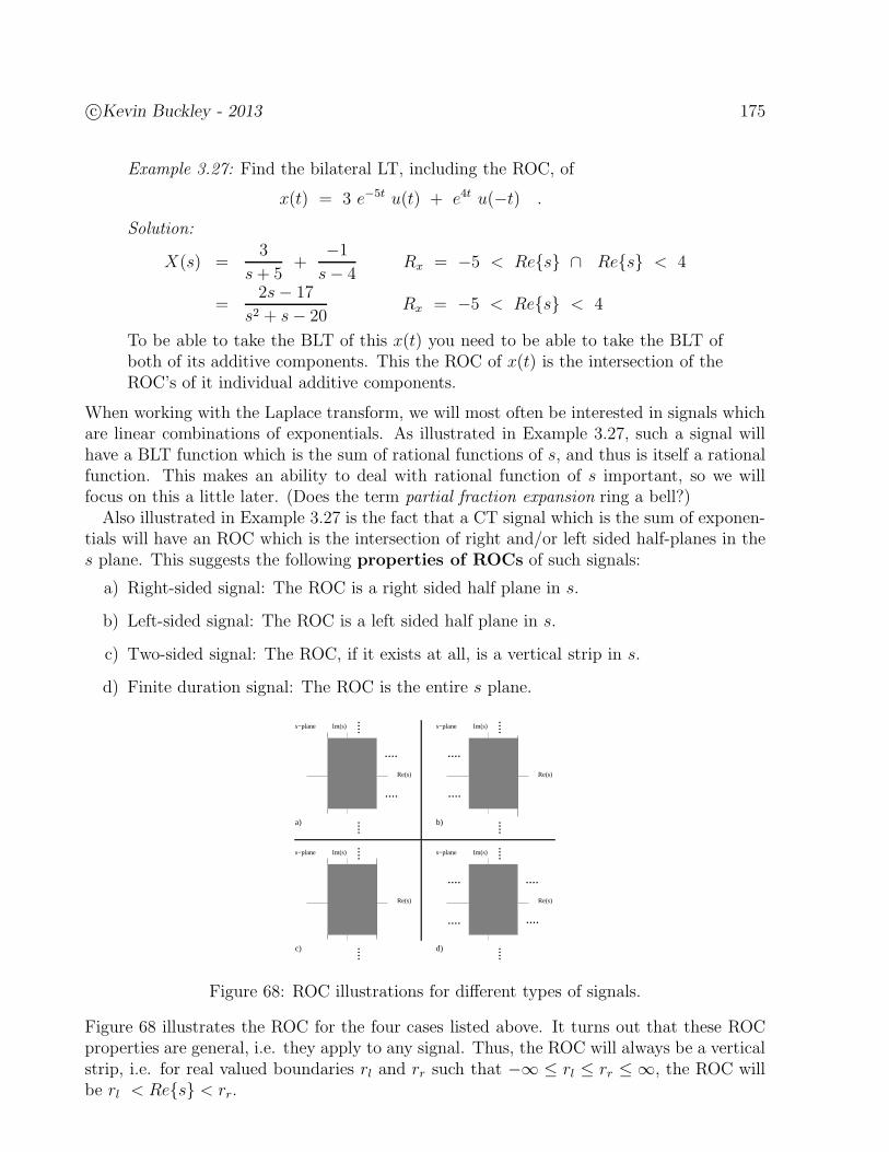
c©Kevin Buckley - 2013 175
Example 3.27: Find the bilateral LT, including the ROC, of
x(t) = 3 e−5t u(t) + e4t u(−t) .
Solution:
X(s) =3
s+ 5+−1s− 4
Rx = −5 < Res ∩ Res < 4
=2s− 17
s2 + s− 20Rx = −5 < Res < 4
To be able to take the BLT of this x(t) you need to be able to take the BLT ofboth of its additive components. This the ROC of x(t) is the intersection of theROC’s of it individual additive components.
When working with the Laplace transform, we will most often be interested in signals whichare linear combinations of exponentials. As illustrated in Example 3.27, such a signal willhave a BLT function which is the sum of rational functions of s, and thus is itself a rationalfunction. This makes an ability to deal with rational function of s important, so we willfocus on this a little later. (Does the term partial fraction expansion ring a bell?)
Also illustrated in Example 3.27 is the fact that a CT signal which is the sum of exponen-tials will have an ROC which is the intersection of right and/or left sided half-planes in thes plane. This suggests the following properties of ROCs of such signals:
a) Right-sided signal: The ROC is a right sided half plane in s.
b) Left-sided signal: The ROC is a left sided half plane in s.
c) Two-sided signal: The ROC, if it exists at all, is a vertical strip in s.
d) Finite duration signal: The ROC is the entire s plane.
Re(s)
....
....
........Im(s)s−plane
....
....
....
....
....
....
Re(s)
........Im(s)s−plane
Re(s)
........Im(s)s−plane
Re(s)
........Im(s)s−plane
b)a)
c) d)
Figure 68: ROC illustrations for different types of signals.
Figure 68 illustrates the ROC for the four cases listed above. It turns out that these ROCproperties are general, i.e. they apply to any signal. Thus, the ROC will always be a verticalstrip, i.e. for real valued boundaries rl and rr such that −∞ ≤ rl ≤ rr ≤ ∞, the ROC willbe rl < Res < rr.
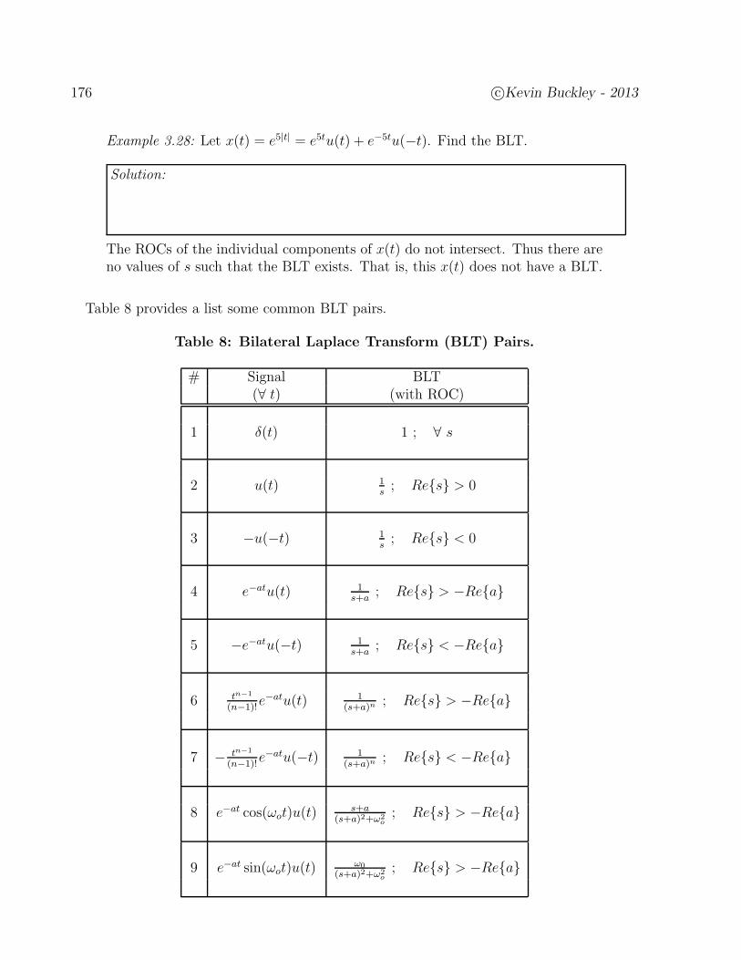
176 c©Kevin Buckley - 2013
Example 3.28: Let x(t) = e5|t| = e5tu(t) + e−5tu(−t). Find the BLT.
Solution:
The ROCs of the individual components of x(t) do not intersect. Thus there areno values of s such that the BLT exists. That is, this x(t) does not have a BLT.
Table 8 provides a list some common BLT pairs.
Table 8: Bilateral Laplace Transform (BLT) Pairs.
# Signal BLT(∀ t) (with ROC)
1 δ(t) 1 ; ∀ s
2 u(t) 1s; Res > 0
3 −u(−t) 1s; Res < 0
4 e−atu(t) 1s+a
; Res > −Rea
5 −e−atu(−t) 1s+a
; Res < −Rea
6 tn−1
(n−1)!e−atu(t) 1
(s+a)n; Res > −Rea
7 − tn−1
(n−1)!e−atu(−t) 1
(s+a)n; Res < −Rea
8 e−at cos(ωot)u(t)s+a
(s+a)2+ω2o; Res > −Rea
9 e−at sin(ωot)u(t)ω0
(s+a)2+ω2o; Res > −Rea
c©Kevin Buckley - 2013 177
3.4.2 Relationship Between the BLT and the CTFT
Consider the CTFT and BLT equations for a signal x(t):
X(jω) =∫ ∞
−∞x(t) e−jωt dt (42)
X(s) =∫ ∞
−∞x(t) e−st dt . (43)
Comparing these, we see that
X(jω) = X(s)|s=jω . (44)
This necessitates that the ROC of x(t) includes the jω axis, and states that the CTFT is(essentially) the BLT evaluated on the jω axis. It should now be clear why we use thejω argument for the CTFT (i.e. why we use the X(jω) notation). It is because of thisCTFT/BLT relationship.
Example 3.29: Given the following BLT pair (i.e. Entry # 9 in Table 8),
e−αt sin(ω0t) u(t) ←→ ω0
(s+ α)2 + ω20
; Res > −α
determine the CTFT of x(t) = e−2t sin(10t) u(t) (which is not in Table 7).
Solution:

178 c©Kevin Buckley - 2013
3.4.3 The Inverse Bilateral Laplace Transform
Let real-valued σ be in the ROC for a signal x(t), and let X(s) be the BLT function. Thenthe inverse BLT is the line integral
x(t) =1
2πj
∫ σ+j∞
σ−j∞X(s) est ds . (45)
This equation shows x(t) expressed as a linear combination of the basic signals est fors = σ + jω for ω over the continuous range −∞ ≤ ω ≤ ∞. The weighting function, appliedto these basic signals, is X(s)
2π. So, the BLT computes the coefficients of this expansion of
x(t). Note that different choices of σ, within the ROC, result in different expansions. Thusthe BLT provides a class of expansions of x(t) (one of which is the CTFT expansion if theROC includes the jω axis). That is, if for a given x(t) the ROC includes σ = 0, and in theinverse BLT equation we let s = jω (i.e. σ = 0), we have
x(t) =1
2πj
∫ 0+j∞
0−j∞X(s) est ds s = jω (46)
=1
2πj
∫ ∞
−∞X(jω) ejωt j dω (47)
=1
2π
∫ ∞
−∞X(jω) ejωt dω . (48)
So again we see that the CTFT can be viewed as the BLT evaluated on the jω axis.An important issue is this: given X(s) and the ROC, how can we derive x(t)? There
are several approaches. The direct one is to evaluate the inverse BLT line integral directly.We show a general example of this directly above, for which we chose σ = 0, assuming theROC includes the jω axis. You will note be responsible for this approach. A more commonapproach, which you are responsible for, is to use BLT tables and properties. Example 3.26above provides an illustration of the use of tables to determine inverse BLTs.
We will cover BLT properties, along with those of the CTFS and CTFT, in Section 3.5 ofthe Course. We will also make extensive use of BLT properties in Chapter 4 of this Coursewhen discussing CT LTI system analysis. In the example directly below we make use of thefollowing BLT linearity property:
Given two signals x1(t) & x2(t) and corresponding BLTs X1(s) & X2(s) andROCs Rx1 & Rx2 , and given constants a1 and a2,
x(t) = a1 x1(t) + a2 x2(t) ←→ X(s) = a1 X1(s) + a2 X2(s) Rx = Rx1∩Rx2 .(49)
c©Kevin Buckley - 2013 179
Example 3.30: Given the following BLT,
H(s) =8s2 + 17s + 37
s3 + 4s2 + 9s + 10Rh = Res > −1
determine the inverse BLT h(t).
Solution: First note that since the ROC is a right half plane in the s-plane, h(t)will be a right-sided signal.
Next note that H(s) is not in Table 8 of these Notes. Thus, we can not use anentry in that table directly to determine the inverse BLT. However, it can beshown that
H(s) =7
s+ 2+
s+ 1
(s+ 1)2 + 4.
The method for breaking this H(s) into a sum of lower order terms, called PartialFraction Expansion (PFE), will be covered later in the Course (in Chapter 4).For now, note that the two terms in the above equation are entries #4 & #8 inTable 8. Thus, using the linearity property,
h(t) = 7 e−2t u(t) + e−t cos(2t) u(t) .
Note that the ROC of H(s) is consistent with the table entries and with thelinearity property. That is, Rh is the intersection of Res > −2 andRes > −1.Also, you can prove the decomposition of H(s) shown above is correct by recom-bining it (i.e. by finding the common denominator, a procedure you need to befamiliar with).
180 c©Kevin Buckley - 2013
3.4.4 The Unilateral Laplace Transform (ULT)
The Laplace transform is a powerful tool for the design and analysis of CT LTI systems.Although the BLT provides much of what is needed, it does not provide for the ability toaccount for system initial conditions. The ULT does. Here we introduce the ULT, and inChapter 4 of the Course Notes we will show how it can be used to represent initial conditions.
Given a signal x(t), the ULT is defined as
X (s) =∫ ∞
0−x(t) e−st dt . (50)
The lower bound on the integral, t = 0−, means that the we integrate across t = 0, so thatif there is an impulse at t = 0, it will be included in the integral.
Example 3.31: The signals x(t) = e−t u(t) and y(t) = e−|t| have that same ULTsince x(t) = y(t); t ≥ 0−. That is,
X (s) = Y(s) = X(s) =1
s+ 1ROC = Res > −1 ,
where X(s) is the BLT of x(t) (from Table 8). Note that, with the ULT, theROC is not needed in uniquely determining the inverse LT. Basically, with theULT, left sided signals are not considered.
Example 3.32: Determine the ULT of x(t) = e−2t sin(10t) u(t)
Solution: Note that right-sided signal entries in a BLT tables can be used todetermine ULTs and inverse ULTs.
X (s) =10
(s+ 2)2 + 100.
3.4.5 Some Useful Rules-of-Thumb on When to Use Different Transforms
1. Use the generalized CTFT instead of the CTFS when representing both energy andperiodic signals. Note, however, that for periodic signals the CTFS must still be usedto determine the weights of the impulses at the harmonic frequencies in the CTFTrepresentation.
2. Use the CTFT when analyzing signals and when interested in frequency response ofCT LTI systems.
3. Use the Laplace transform when dealing general system analysis issues.
4. Use the ULT when specifically dealing with initial conditions. Otherwise use the BLT.
c©Kevin Buckley - 2013 181
3.5 Continuous Time Transform Properties
We have already studied the linearity, delay, symmetry and Parseval’s Theorem propertiesof the CTFS. We saw that the linearity and delay properties provided, in conjunctions withTable 6 of CTFS pairs, an ability to identify CFTS coefficients, without directly computingthe coefficients, for any linear combination of delayed signals represented in Table 6. Simi-larly, these properties and Table 6 provide a means for identifying signals given their CTFScoefficients. While introducing the CTFT and Laplace transform, we mentioned that similarproperties exist (e.g. linearity) and can be useful.
The utility of transform properties goes well beyond that of helping us derive transformsand inverse transforms. The CTFS properties we’ve studied so far (e.g. delay, Parseval’stheorem) have provided us with insight into the CTFS and the signals they represent. Otherproperties will provide us with additional insight. Transform properties are also useful insolving engineering problems. In fact we will see that many of the transform properties weconsider represent important engineering applications. With this in mind, in the followinglectures we will investigate continuous time transform properties.
For several reasons we will cover the properties of the CTFS, CTFT and Laplace transformtogether. First and foremost, the approach we take emphasizes the similarity between thetransforms. (Remember that the Laplace transform can be viewed as a generalization ofthe CTFT, and the generalized CTFT encompasses the CTFS.) Additionally, there is anefficiency in covering properties for all three transforms together. Instead of covering sixteentransform properties three different times, we will cover them all at once. So we will be ableto focus on each property a little longer, hopefully making sure we understand it.
Since the transforms are different (e.g. they represent different signal classes), any givenproperty may look slightly different for each transform. Additionally, a property that isimportant within the context of one transform, may be irrelevant or unenlightening foranother. Thus for a given property we may choose to focus more on one transform thananother.
Table 9 is a list of CTFS, CTFT and Laplace transform properties. Those which are dis-cussed in these Course Notes are indicated with an “EC” (Explicitly Covered). Subsequentlyin these Notes, we will sometimes refer to these properties using the number designated inTable 9. For example, Property #11 is the convolution property. Of the properties listedin Table 9, Properties #1 to #7 are relevant on a basic level, though they may additionallysuggest applications. For example, Properties #6 & #7 (time and frequency domain scal-ing) are important for a basic understanding of audio pitch shifting. Properties #8 through#11 are fundamental to basic signal processing functions which we will overview later: mul-tiplication for spectrum estimation, radio and sampling; modulation for radio; Parseval’stheorem for spectrum estimation; and convolution for CT LTI system analysis (of course).The last five properties are important, but for topics that we will not focus on in this Course(e.g. Property #16 is important for controls), so we will only mention these properties inthe Notes.
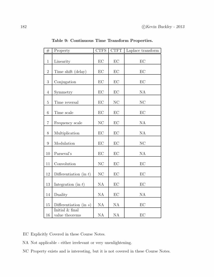
182 c©Kevin Buckley - 2013
Table 9: Continuous Time Transform Properties.
# Property CTFS CTFT Laplace transform
1 Linearity EC EC EC
2 Time shift (delay) EC EC EC
3 Conjugation EC EC EC
4 Symmetry EC EC NA
5 Time reversal EC NC NC
6 Time scale EC EC EC
7 Frequency scale NC EC NA
8 Multiplication EC EC NA
9 Modulation EC EC NC
10 Parseval’s EC EC NA
11 Convolution NC EC EC
12 Differentiation (in t) NC EC EC
13 Integration (in t) NA EC EC
14 Duality NA EC NA
15 Differentiation (in s) NA NA ECInitial & final
16 value theorems NA NA EC
EC Explicitly Covered in these Course Notes.
NA Not applicable - either irrelevant or very unenlightening.
NC Property exists and is interesting, but it is not covered in these Course Notes.
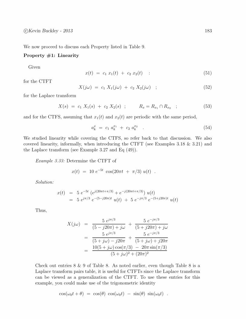
c©Kevin Buckley - 2013 183
We now proceed to discuss each Property listed in Table 9.
Property #1: Linearity
Givenx(t) = c1 x1(t) + c2 x2(t) : (51)
for the CTFTX(jω) = c1 X1(jω) + c2 X2(jω) ; (52)
for the Laplace transform
X(s) = c1 X1(s) + c2 X2(s) ; Rx = Rx1 ∩Rx2 ; (53)
and for the CTFS, assuming that x1(t) and x2(t) are periodic with the same period,
axk = c1 ax1k + c2 ax2
k . (54)
We studied linearity while covering the CTFS, so refer back to that discussion. We alsocovered linearity, informally, when introducing the CTFT (see Examples 3.18 & 3.21) andthe Laplace transform (see Example 3.27 and Eq (49)).
Example 3.33: Determine the CTFT of
x(t) = 10 e−5t cos(20πt + π/3) u(t) .
Solution:
x(t) = 5 e−5t (ej(20πt+π/3) + e−j(20πt+π/3)) u(t)
= 5 ejπ/3 e−(5−j20π)t u(t) + 5 e−jπ/3 e−(5+j20π)t u(t)
Thus,
X(jω) =5 ejπ/3
(5− j20π) + jω+
5 e−jπ/3
(5 + j20π) + jω
=5 ejπ/3
(5 + jω)− j20π+
5 e−jπ/3
(5 + jω) + j20π
=10(5 + jω) cos(π/3) − 20π sin(π/3)
(5 + jω)2 + (20π)2
Check out entries 8 & 9 of Table 8. As noted earlier, even though Table 8 is aLaplace transform pairs table, it is useful for CTFTs since the Laplace transformcan be viewed as a generalization of the CTFT. To use these entries for thisexample, you could make use of the trigonometric identity
cos(ω0t + θ) = cos(θ) cos(ω0t) − sin(θ) sin(ω0t) .
184 c©Kevin Buckley - 2013
Example 3.34: Determine the CTFT of
x(t) = 5 e−3t u(t) − 4 t e−2t u(t) .
Solution:
X(jω) =5
3 + jω− 4
(2 + jω)2=
5
3 + jω− 4
4 + 4(jω) + (jω)2
=5(jω)2 + 16(jω) + 8
(jω)3 + 7(jω)2 + 16(jω) + 12.
Note that X(jω) is a rational function of jω. As noted earlier, similar rationalfunctions occur frequently when dealing with transforms, so we need to learn howto deal with (i.e. identify inverse transforms for) them.
Example 3.35: Determine the inverse Laplace transform of
H(s) =s2 + 11
s3 − 4s2 + s+ 6Rh = Res > 3 .
Solution: This H(s) does not appear in Table 8 on Laplace transform pairs.However, note that
H(s) =1
s+ 1− 5
s− 2+
5
s− 3.
You can prove this by recombining the 1-st order terms to form the original H(s).Now, using linearity, we have
h(t) = e−t u(t) − 5 e2t u(t) + 5 e3t u(t) .
The technique for breaking the rational function H(s) into a sum of lower orderrational terms is called partial fraction expansion. We will focus on this techniquelater, in Chapter 4 of these Notes when considering CT LTI systems.
c©Kevin Buckley - 2013 185
Property #2: Time shift (delay)
Giveny(t) = x(t− τ) : (55)
for the CTFTY (jω) = X(jω) e−jωτ ; (56)
for the Laplace transform
Y (s) = X(s) e−sτ ; Ry = Rx ; (57)
and for the CTFSayk = axk e−jkω0τ . (58)
We studied this property for the CTFS, so refer back to that discussion. Note that forboth the CTFS and the CTFT, the effect on the frequency domain representation (i.e. theeffect on the weight applied to each complex sinusoid that constitutes the signal x(t)) is aphase shift which is proportional to both the frequency and delay. Make sure that this makessense to you!
Example 3.36: Let x(t) be periodic with period T = 4, and let y(t) = x(t + 8).Determine the CTFS coefficients of y(t) in terms of those of x(t).
Solution:
ayk = axk e−jk(2π/4)8 = axk e−jk(4π)
= axk ∀k
Since the CTFS coefficients for y(t) are equal to those of x(t), we have thaty(t) = x(t). This is because y(t) is x(t) delayed by exactly two periods.
Example 3.37: Consider x(t) = e−3t u(t− 3): a) Determine the CTFT of x(t).b) Let y(t) = 6 x(t − 5). Determine the phase shift between the ω0 = π
3
components of x(t) and y(t).
Solution: a)
x(t) = e−9 e−3(t−3) u(t− 3)
X(jω) = e−9 e−j3ω
jω + 3=
e−(9+j3ω)
jω + 3.
b) The gain of 6 between x(t) and y(t) does not effect relative phases betweenthese two signals. The delay of 5 does. Since by the delay property Y (jω) =X(jω) e−jωτ , in general the phase shift for frequency ω and delay τ is −ωτ . Forω0 =
π3and τ = 5 we have phase shift −5π
3.
186 c©Kevin Buckley - 2013
Property #10: Parseval’s theorem (energy and power)
For energy signals:
E =∫ ∞
−∞|x(t)|2 dt =
1
2π
∫ ∞
−∞|X(jω)|2 dω . (59)
For periodic power signals:
P =1
T
∫
<T>|x(t)|2 dt =
∞∑
k=−∞|ak|2 =
∞∑
k=−∞A2
k , (60)
where ak = Akejθk .
Recall that we covered Parseval’s theorem for the CTFS, so refer back to that discussion.Parseval’s theorem quantifies the idea of content as a function for frequency. Note thatpower and energy are not effected by the phase of the frequency description, but only themagnitude. Thus, for example, delaying a signal does not effect its energy or power.
For the CTFT, Parseval’s theorem establishes that for a signal x(t) with total energy E,
the function |X(jω)|22π
plotted vs. ω gives the distribution of total energy over frequency. Thuswe call this plot the energy spectrum. Similarly, for periodic power signals, |ak|2 vs. k (orω) is called the power spectrum.
Example 3.38: Let x(t) = 2πt
sin(100πt). Determine the % of energy over thefrequency band −50π ≤ ω ≤ 50π.
Solution:
c©Kevin Buckley - 2013 187
Example 3.39: Let x(t) = 11−.8ej120πt . Determine the % power in the DC term.
Solution: First note that x(t) is periodic, so it is a power signal. Its fundamentalperiod is T = 1
60, so ω0 = 120π. Its CTFS coefficients are
axk =
0.8k k ≥ 00 k < 0
(For practice, derive this expression directly, or write x(t) as a geometric se-ries and observe the CTFS coefficients by inspection.) Let PT and P0 denote,respectively, the total and DC powers.
PT =∞∑
k=−∞|axk|2 =
∞∑
k=0
(0.64)k = 2.777... P0 = |ax0 |2 = 1 .
Thus P0
PT× 100% = 36%.
Parseval’s theorem does not say that the energy (or power) of a sum of signals is equal tothe sum of the energies (or powers) of the individual signals being summed. In general, thisis not true. It is only true if the signals do not overlap either in time or in frequency. Why?
Example 3.40: Let x1(t) = cos(10πt) and x2(t) = cos(10πt + π). Determine thepower of x(t) = x1(t) + x2(t).
Solution: P x1 = P x2 = 12since
axik =
12
k = ±10 otherwise
Note that P x 6= P x1 + P x2 = 1 since these two signals overlap in frequency. Infact, P x = 0 since x(t) = 0.
Example 3.41: Find the energy of x(t) = 14+t2
.
Solution: Consider Table 7, entry # 7. Although not directly applicable, the2a
a2+ω2 term in that entry is similar to x(t) (for a = 2). The main differenceis that t and ω domains are switched. However, considering the CTFT andICTFT equations, they are similar, except that the domains are switched. So itis reasonable to postulate that
1
4 + t2←→ K e−2|ω| (61)
for some constant K. If true, then using the ICTFT, we will have
x(t) =K
2π
∫ ∞
−∞e−2|ω| ejωt dω
=K
2π
∫ 0
−∞e2ω ejωt dω +
∫ ∞
0e−2ω ejωt dω
These are easy enough integrals to solve. So try it, and show thatK = π providesthe required x(t). Eq (61), with K = π is entry #13 of Table 7 for c = 2. Wehave effectively derived that entry. Later we will consider the duality property,Property # 14, which formalizes this idea of switching domains for entries inTable 7 in order to derive new CTFT pairs.

188 c©Kevin Buckley - 2013
Magnitude and phase Spectra: We have already defined, for periodic power and forenergy signals, respectively, the power spectrum |ak|2 vs. k (or ω) and energy spectrum|X(jω)|2
2πvs. ω. Also of interest are the:
1. Magnitude spectrum – Ak vs. k (or ω) for periodic power signals and|X(jω)| vs. ω for energy signals; and
2. Phase spectrum – θk vs. k (or ω) for periodic power signals and6 X(jω) vs. ω for energy signals.
Example 3.42: Plot the magnitude and phase spectra of x(t) = δ(t− 5).
Solution:
Example 3.43: Given the following magnitude and phase plots, determine x(t).
Solution:
c©Kevin Buckley - 2013 189
Property #4: Symmetry
Symmetry is exhibited in CTFS and CTFT in several ways. Of these, the most usefulsymmetry characteristics are captured by the following statement: real-valued in one domainresults in complex symmetry in the other. This statement means that, for real-values x(t),for the CTFT
X(−jω) = X∗(jω) , (62)
and for the CTFS,a−k = a∗k . (63)
We have already considered this property for the CTFS. This statement also means that, iffor the CTFT X(jω) is real-valued or if for the CTFS the ak are real-valued, then
x(−t) = x∗(t) . (64)
As examples, check out some of the previous examples and some of the entries in Tables 6& 7.
Example 3.44: Given a signal x(t) with CTFT X(jω) = 44+ω2 , is x(t) real valued?
Solution:
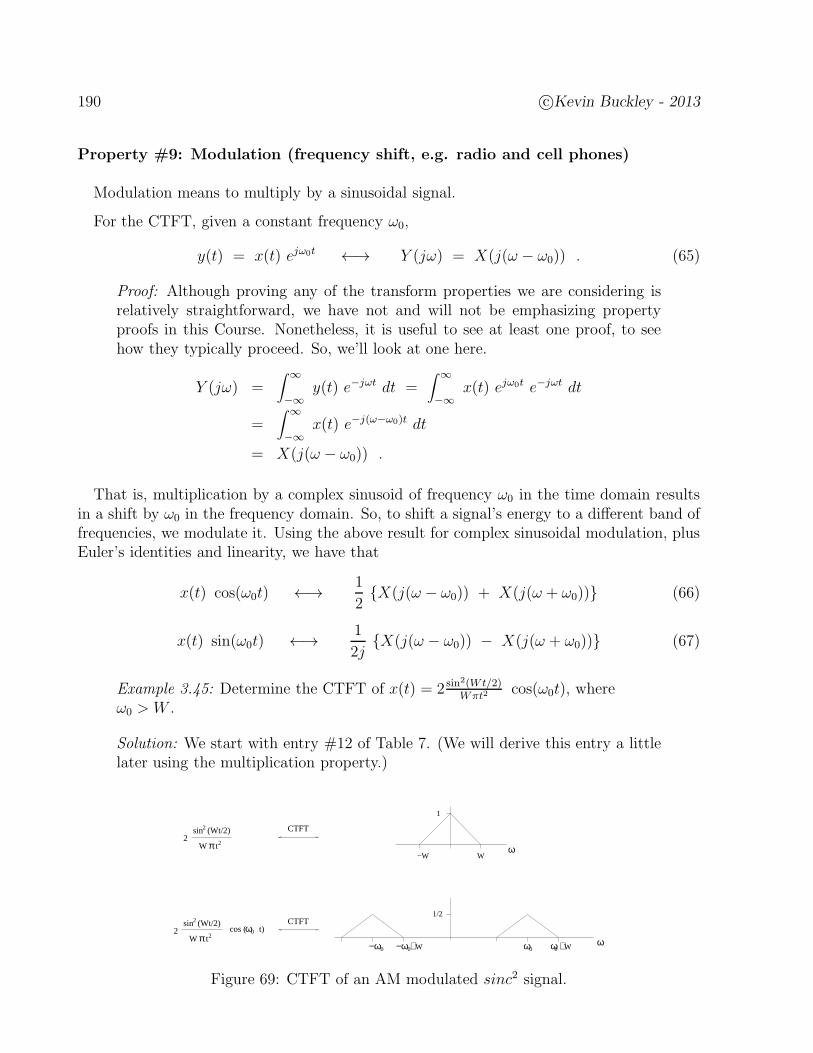
190 c©Kevin Buckley - 2013
Property #9: Modulation (frequency shift, e.g. radio and cell phones)
Modulation means to multiply by a sinusoidal signal.
For the CTFT, given a constant frequency ω0,
y(t) = x(t) ejω0t ←→ Y (jω) = X(j(ω − ω0)) . (65)
Proof: Although proving any of the transform properties we are considering isrelatively straightforward, we have not and will not be emphasizing propertyproofs in this Course. Nonetheless, it is useful to see at least one proof, to seehow they typically proceed. So, we’ll look at one here.
Y (jω) =∫ ∞
−∞y(t) e−jωt dt =
∫ ∞
−∞x(t) ejω0t e−jωt dt
=∫ ∞
−∞x(t) e−j(ω−ω0)t dt
= X(j(ω − ω0)) .
That is, multiplication by a complex sinusoid of frequency ω0 in the time domain resultsin a shift by ω0 in the frequency domain. So, to shift a signal’s energy to a different band offrequencies, we modulate it. Using the above result for complex sinusoidal modulation, plusEuler’s identities and linearity, we have that
x(t) cos(ω0t) ←→ 1
2X(j(ω − ω0)) + X(j(ω + ω0)) (66)
x(t) sin(ω0t) ←→ 1
2jX(j(ω − ω0)) − X(j(ω + ω0)) (67)
Example 3.45: Determine the CTFT of x(t) = 2 sin2(Wt/2)Wπt2
cos(ω0t), whereω0 > W .
Solution: We start with entry #12 of Table 7. (We will derive this entry a littlelater using the multiplication property.)
−ω −ω +W0
−W Wω
1
sin (Wt/2)2
22πW t
ω0cos ( t)
sin (Wt/2)2
πW t22
CTFT
CTFT
1/2
ω0 ω ω +0 0 W
Figure 69: CTFT of an AM modulated sinc2 signal.
c©Kevin Buckley - 2013 191
For the CTFS version of the modulation property, assume a periodic signal x(t) withfundamental frequency ω0, and let m be an integer. Then
x(t) ejmω0t ←→ axk−m . (68)
Example 3.46: Derive the CTFS modulation properties for x(t) cos(mω0t) andx(t) sin(mω0t). (Assume x(t) is periodic with fundamental period T = 2π
ω0.)
Solution:
Example 3.47: Determine the CTFS coefficients of
x(t) =0.36
1.64 − 1.6 cos(ω0t)cos(5ω0t)
Solution: Let v(t) = 0.361.64 − 1.6 cos(ω0t)
, which is periodic with fundamental fre-
quency ω0 since cos(ω0t) (the only part of it that is a function of t) is. Notethat
v(t) =1
1− 0.8ejω0t+
0.8e−jω0t
1− 0.8e−jω0t
=∞∑
k=0
0.8k ejω0tk +∞∑
k=1
0.8k e−jω0tk
=∞∑
k=−∞0.8|k| ejkω0t
Don’t worry about how the steps above were arrived at. The point is that v(t)is now expressed as a CTFS expansion, where the coefficients are avk = 0.8|k|.Now, using the modulation property of the CTFS,
axk =1
2avk−5 +
1
2avk+5 =
1
20.8|k−5| +
1
20.8|k+5|
192 c©Kevin Buckley - 2013
Property #8: Multiplication (e.g. windowing, modulation, sampling)
For the CTFT,
x(t) · y(t) ←→ 1
2πX(jω) ∗ Y (jω) =
1
2π
∫ ∞
−∞X(jλ) Y (j(ω − λ)) dλ (69)
Example 3.48: Modulation again -
Solution:
Example 3.49: Determine the CTFT of
x(t) =sin2(Wt)
(πt)2
Solution:
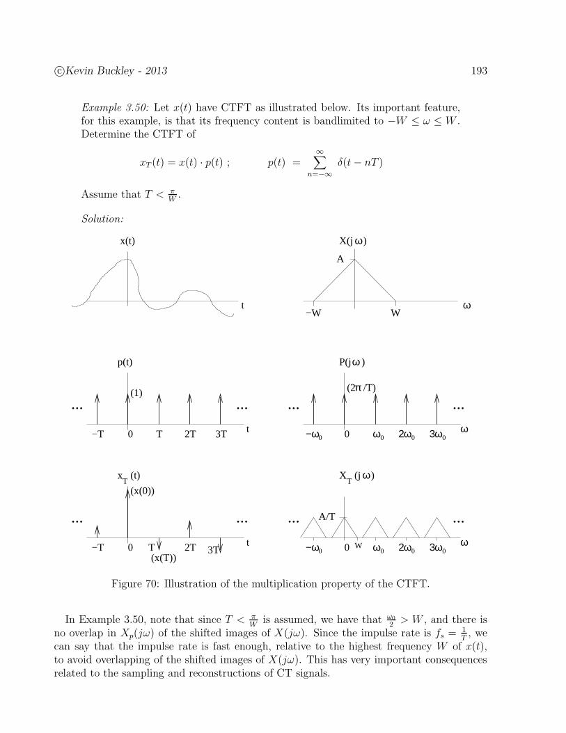
c©Kevin Buckley - 2013 193
Example 3.50: Let x(t) have CTFT as illustrated below. Its important feature,for this example, is that its frequency content is bandlimited to −W ≤ ω ≤ W .Determine the CTFT of
xT (t) = x(t) · p(t) ; p(t) =∞∑
n=−∞δ(t− nT )
Assume that T < πW.
Solution:
π(2 /T)
P(j )ω
0
......
−ω ω 3ω2ω ω0 0 0 0
p(t)
t0 T 2T 3T−T
(1)......
ω
X(j )ω
t
x(t)
0
......
−ω ω 3ω2ω ω0 0 0 0
A
T
A/T
t0 2T−T
......
x (t)T
3T
(x(0))
T(x(T))
X (j )ω
W−W
W
Figure 70: Illustration of the multiplication property of the CTFT.
In Example 3.50, note that since T < πW
is assumed, we have that ω0
2> W , and there is
no overlap in Xp(jω) of the shifted images of X(jω). Since the impulse rate is fs =1T, we
can say that the impulse rate is fast enough, relative to the highest frequency W of x(t),to avoid overlapping of the shifted images of X(jω). This has very important consequencesrelated to the sampling and reconstructions of CT signals.

194 c©Kevin Buckley - 2013
Property #6, #7: Time & frequency scale
Beyond their general utility in signal analysis, these two transform properties, especiallyas they apply to the CTFT and the CTFS, build and reinforce an intuitive understanding.They state that, concerning the time and frequency domain representations of signals, if youspread a signal out in one domain you contract it in the other. This should make sense toyou. For example, if you spread a signal out in time, it changes at a slower rate, whichmeans it has become more lowpass.
The time & frequency scale property is, for real-valued α > 0,
x(αt) ←→ 1
αX(
jω
α
)
. (70)
If α > 1, x(αt) is a contraction of x(t) (since the argument αt changes more quickly than t)and thus an expansion of X(jω). Conversely, if 0 < α < 1, x(αt) is an expansion of x(t) andthus a contraction of X(jω).
Example 3.51: Starting with the CTFT pair
x(t) =1
πtsin(10πt) ←→ p20π(ω)
the CTFT pair of x(10t) is
x(10t) =1
π10tsin(100πt) ←→ 1
10p40π
(
ω
10
)
=1
10p200π(ω) .
The new signal oscillates at a 10 times faster rate, and its bandwidth has ex-panded by a factor of 10.
You may have noticed that these properties are not that useful for expanding the set ofsignals that you can take CTFTs and inverse CTFTs. However the intuition, that expansionin one domain means contraction in the other, is very important.
For the CTFS, the combined time & frequency scale property is simply
y(t) = x(αt) =∞∑
k=−∞axk ejk(αω0)t . (71)
That isayk = axk . (72)
The only change is in the fundamental frequency.
c©Kevin Buckley - 2013 195
Property #5: Time reversal (i.e. fold)
Givenx(t) ←→ X(jω) (73)
orx(t) ←→ axk , (74)
Let y(t) = x(−t). Then,Y (jω) = X(−jω) (75)
orayk = ax−k . (76)
Combining the time & frequency scale and the time reversal properties, we have that, forany nonzero real number α,
x(αt) ←→ 1
|α| X(
jω
α
)
(77)
and, for the CTFSx(αt) ←→ axsign(α)·k , (78)
where the original fundamental frequency ω0 is changed to |α|ω0.
Example 3.52: Determine the CTFT of x(t) = e−α|t|, with Reα > 0.
Solution: Note that x(t) = e−αt u(t) + eαt u(−t). From Table 7 and from thetime reversal property we have, respectively,
e−αt u(t) ←→ 1
α + jω
eαt u(−t) ←→ 1
α − jω
So,
X(jω) =1
α − jω+
1
α + jω=
2α
α2 + ω2.
This derives Entry #7 of Table 7.

196 c©Kevin Buckley - 2013
Property #3: Conjugation
For the CTFT,x∗(t) ←→ X∗(−jω) . (79)
For the CTFS,x∗(t) ←→ a∗−k . (80)
Example 3.53: Let x(t) be a real-valued energy signal. By the conjugation prop-erty
x∗(t) ←→ X∗(−jω) .
However, by the symmetry property of real-valued signals,
X(−jω) = X∗(jω)
so
X∗(−jω) = X(jω)
meaning that
x∗(t) ←→ X(jω) ,
which is of course true since x(t) is assumed real-valued in this Example.
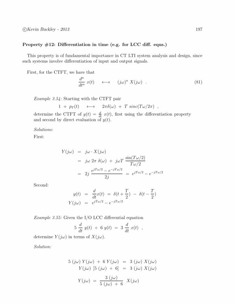
c©Kevin Buckley - 2013 197
Property #12: Differentiation in time (e.g. for LCC diff. equs.)
This property is of fundamental importance in CT LTI system analysis and design, sincesuch systems involve differentiation of input and output signals.
First, for the CTFT, we have that
dn
dtnx(t) ←→ (jω)n X(jω) . (81)
Example 3.54: Starting with the CTFT pair
1 + pT (t) ←→ 2πδ(ω) + T sinc(Tω/2π) ,
determine the CTFT of y(t) = ddt
x(t), first using the differentiation propertyand second by direct evaluation of y(t).
Solutions:
First:
Y (jω) = jω ·X(jω)
= jω 2π δ(ω) + jωTsin(Tω/2)
Tω/2
= 2jejTω/2 − e−jTω/2
2j= ejTω/2 − e−jTω/2
Second:
y(t) =d
dtx(t) = δ(t +
T
2) − δ(t− T
2)
Y (jω) = ejTω/2 − e−jTω/2
Example 3.55: Given the I/O LCC differential equation
5d
dty(t) + 6 y(t) = 3
d
dtx(t) ,
determine Y (jω) in terms of X(jω).
Solution:
5 (jω) Y (jω) + 6 Y (jω) = 3 (jω) X(jω)
Y (jω) [5 (jω) + 6] = 3 (jω) X(jω)
Y (jω) =3 (jω)
5 (jω) + 6X(jω)
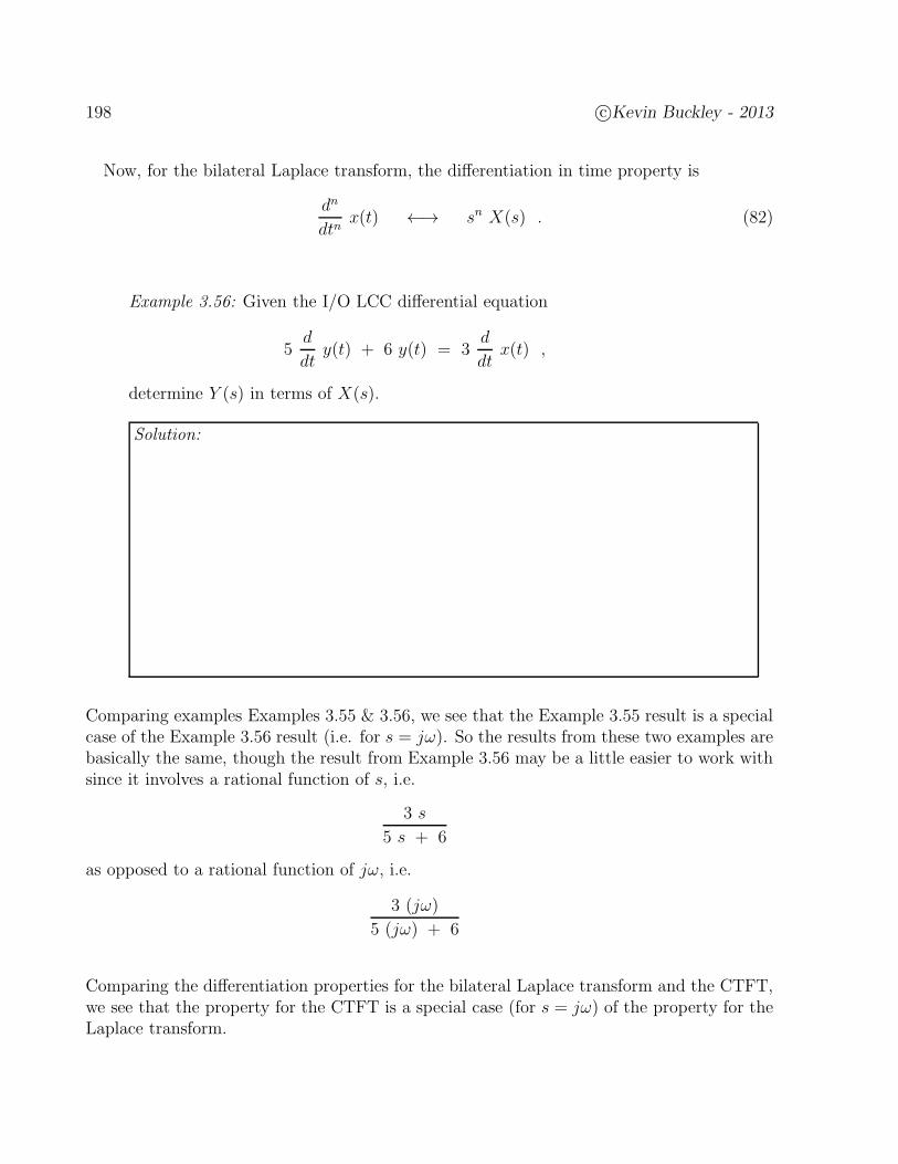
198 c©Kevin Buckley - 2013
Now, for the bilateral Laplace transform, the differentiation in time property is
dn
dtnx(t) ←→ sn X(s) . (82)
Example 3.56: Given the I/O LCC differential equation
5d
dty(t) + 6 y(t) = 3
d
dtx(t) ,
determine Y (s) in terms of X(s).
Solution:
Comparing examples Examples 3.55 & 3.56, we see that the Example 3.55 result is a specialcase of the Example 3.56 result (i.e. for s = jω). So the results from these two examples arebasically the same, though the result from Example 3.56 may be a little easier to work withsince it involves a rational function of s, i.e.
3 s
5 s + 6
as opposed to a rational function of jω, i.e.
3 (jω)
5 (jω) + 6
Comparing the differentiation properties for the bilateral Laplace transform and the CTFT,we see that the property for the CTFT is a special case (for s = jω) of the property for theLaplace transform.

c©Kevin Buckley - 2013 199
For the unilateral Laplace transform, the differentiation property is a little more involvedWe have that
x(1)(t) =d
dtx(t) ←→ s X (s) − x(0−) (83)
x(2)(t) ←→ s2 X (s) − s x(0−) − x(1)(0−) (84)
x(3)(t) ←→ s3 X (s) − s2 x(0−) − s x(1)(0−) − x(2)(0−) (85)
x(n)(t) ←→ sn X (s) − sn−1 x(0−) − sn−2 x(1)(0−) − · · · − x(n−1)(0−) (86)
where x(k)(0−) is the kth derivative of x(t) evaluated at incrementally less than t = 0.
The differentiation property of the Laplace transform, in this unilateral form, allows us todeal with initial conditions of CT LTI systems.
Example 3.57: Given the I/O LCC differential equation
5 y(1)(t) + 6 y(t) = 3 x(1)(t) ,
determine Y(s) in terms of X (s).
Solution:
5 (s Y(s) − y(0−)) + 6 Y(s) = 3 (s X (s) − x(0−))
Y(s) [5 s + 6] − 5 y(0−) = 3 s X (s) − 3 x(0−))
Y(s) =3 s
5 s + 6X (jω) +
−3 x(0−) + 5 y(0−)
5 s + 6
Note that in Example 3.57 the output is composed of an input term and an initial conditionterm. In general, for CT LTI systems, these two terms will result from the unilateral Laplacetransform of the LCC differential equation.
Property #11: Integration
For the CTFT,∫ t
−∞x(τ) dτ ←→ 1
jωX(jω) + π X(0) δ(ω) (87)
Example 3.58: Determine the CTFT of the step function u(t). That is, deriveentry # 3 of Table 7.
Solution: Starting with the CTFT pair δ(t) ←→ 1, we have that
u(t) =∫ t
−∞δ(τ) dτ =
1
jω(1) + π (1) δ(ω)
=1
jω+ π δ(ω) .

200 c©Kevin Buckley - 2013
Property #13: Convolution (CT LTI systems!)
Let x(t) and h(t) be two signals (i.e. an input to and the impulse response of a DT LTIsystem). Then, for the CTFT
y(t) = x(t) ∗ h(t) ←→ Y (jω) = X(jω) ·H(jω) . (88)
A convolution in the time domain is a product in the frequency domain. Do you not likeconvolution but love Fourier transforms? If so, then this property provides an alternativeto the time domain convolution calculation – an alternative to the folding and shifting andproducting and integrating.
Proof of the Convolution Property of the CTFT: As mentioned earlier, you arenot responsible for proofs of properties, but it is good to see a few.
Y (jω) =∫ ∞
−∞
( ∫ ∞
−∞x(τ) h(t− τ) dτ
)
e−jωt dt
=∫ ∞
−∞x(τ) e−jωτ
( ∫ ∞
−∞h(t− τ) e−jω(t−τ) dt
)
dτ
Noting that
∫ ∞
−∞h(t− τ) e−jω(t−τ) dt = H(jω) (89)
since with the integral over −∞ ≤ t ≤ ∞ it is independent of τ , we have
Y (jω) = H(jω) ·∫ ∞
−∞x(τ) e−jωτ dτ
= H(jω) ·X(jω)
Since convolution is central to CT LTI systems, this property is central to CT LTI systemanalysis and design. We will stress this in Chapter 4. Specifically, Within the context of CTLTI systems, H(jω) is the CTFT of the impulse response h(t) – we will see that H(jω) isan important characterization of a CT LTI system.
Considering the relationship between the Laplace transform and the CTFT, it should beno surprised that for the bilateral Laplace transform,
y(t) = x(t) ∗ h(t) ←→ Y (s) = X(s) ·H(s) . (90)
The ROC for y(t) will be at least the intersection11 of the ROCs of x(t) and h(t). For theCTFS,
y(t) = x(t) ∗ h(t) ←→ ayk = axk H(jkω0) . (91)
11It could be larger if there is pole/zero cancellation – a topic of Chapter 4.

c©Kevin Buckley - 2013 201
Example 3.59: Let x(t) = 1πtsin(2Wt) and h(t) = 1
πtsin(Wt). Determine the
CTFT of y(t) = x(t) ∗ h(t).
Solution:
Example 3.60: Given the H(jω) plotted below and the signal x(t) = A cos(ω0t),determine y(t) = x(t) ∗ h(t).
Solution:
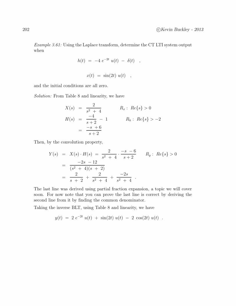
202 c©Kevin Buckley - 2013
Example 3.61: Using the Laplace transform, determine the CT LTI system outputwhen
h(t) = −4 e−2t u(t) − δ(t) ,
x(t) = sin(2t) u(t) ,
and the initial conditions are all zero.
Solution: From Table 8 and linearity, we have
X(s) =2
s2 + 4Rx : Res > 0
H(s) =−4s+ 2
− 1 Rh : Res > −2
=−s + 6
s+ 2
Then, by the convolution property,
Y (s) = X(s) ·H(s) =2
s2 + 4· −s − 6
s+ 2Ry : Res > 0
=−2s − 12
(s2 + 4)(s + 2)
=2
s + 2+
2
s2 + 4+
−2ss2 + 4
.
The last line was derived using partial fraction expansion, a topic we will coversoon. For now note that you can prove the last line is correct by deriving thesecond line from it by finding the common denominator.
Taking the inverse BLT, using Table 8 and linearity, we have
y(t) = 2 e−2t u(t) + sin(2t) u(t) − 2 cos(2t) u(t) .
c©Kevin Buckley - 2013 203
Property #14: Duality
If you compare the CTFT and inverse CTFT equations,
X(jω) =∫ ∞
−∞x(t) e−jωt dt (92)
x(t) =1
2π
∫ ∞
−∞X(jω) ejωt dω (93)
you notice that they are very similar, but not identical. Also, referring to Table 7, if youcompare entries #8 & #9, or entries #2 & #12, or entries #7 & #11 with itself, you willnotice a duality between domains. If you have a transform pair
x(t) ←→ X(jω) , (94)
then the CTFT of X(t) will look like x(jω) and the inverse CTFT of x(jω) will look likeX(t).
The duality property states that, given a CTFT pair
x1(t) ←→ X1(jω) , (95)
then we also have the pair
x2(t) =1
2πX1(t) ←→ X2(jω) = x1(ω) . (96)
Note also that there is a duality of CTFT properties.
We’ve seen just the right number of CT transform properties for this Course, so as thesaying goes, we’ll quite while we’re ahead. Two other properties which are note covered here,and you will not be responsible for learning in this Course:
Property #15: Differentiation in s
Property #16: Initial and final value theorems
On the following pages we provide Tables of the CTFT properties (Table 10) and the Laplacetransform properties (Table 11) covered in this Section of the Course.

204 c©Kevin Buckley - 2013
Table 10: Continuous Time Fourier Transform (CTFT) Properties.
Property Time Domain Frequency Domain
Symmetry real-valued x(t) X(−jω) = X∗(jω)
Delay x(t− τ) X(jω) e−jωτ = |X(jω)| ej[ 6 X(jω)−ωτ ]
Time Scale/Fold x(at) 1|a|X
(
j ωa
)
Linearity a1x1(t) + a2x2(t) a1X1(jω) + a2X2(jω)
Convolution x(t) ∗ h(t) X(jω) H(jω)
Differentiation ddtx(t) jωX(jω)
Integration∫ t
−∞x(λ) dλ 1
jωX(jω) + πX(0)δ(ω)
Parseval’s Theorem E =∫ ∞
−∞|x(t)|2 dt E = 1
2π
∫ ∞
−∞|X(jω)|2 dω
Parseval’s Theorem P = 1T
∫ T
0|x(t)|2 dt P =
∞∑
k=−∞|ak|2
Multiplication x(t) w(t) 12π
∫ ∞
−∞X(jλ)W (j(ω − λ))dλ
Modulation x(t) ejω0t X(j(ω − ω0))
Modulation x(t) cos(ω0t)12[X(j(ω − ω0)) +X(j(ω + ω0))]
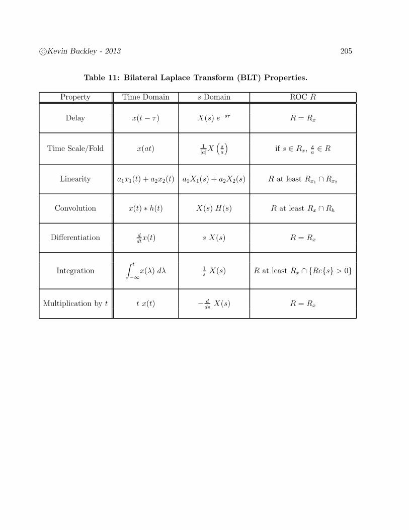
c©Kevin Buckley - 2013 205
Table 11: Bilateral Laplace Transform (BLT) Properties.
Property Time Domain s Domain ROC R
Delay x(t− τ) X(s) e−sτ R = Rx
Time Scale/Fold x(at) 1|a|X
(
sa
)
if s ∈ Rx,sa∈ R
Linearity a1x1(t) + a2x2(t) a1X1(s) + a2X2(s) R at least Rx1 ∩Rx2
Convolution x(t) ∗ h(t) X(s) H(s) R at least Rx ∩ Rh
Differentiation ddtx(t) s X(s) R = Rx
Integration∫ t
−∞x(λ) dλ 1
sX(s) R at least Rx ∩ Res > 0
Multiplication by t t x(t) − dds
X(s) R = Rx
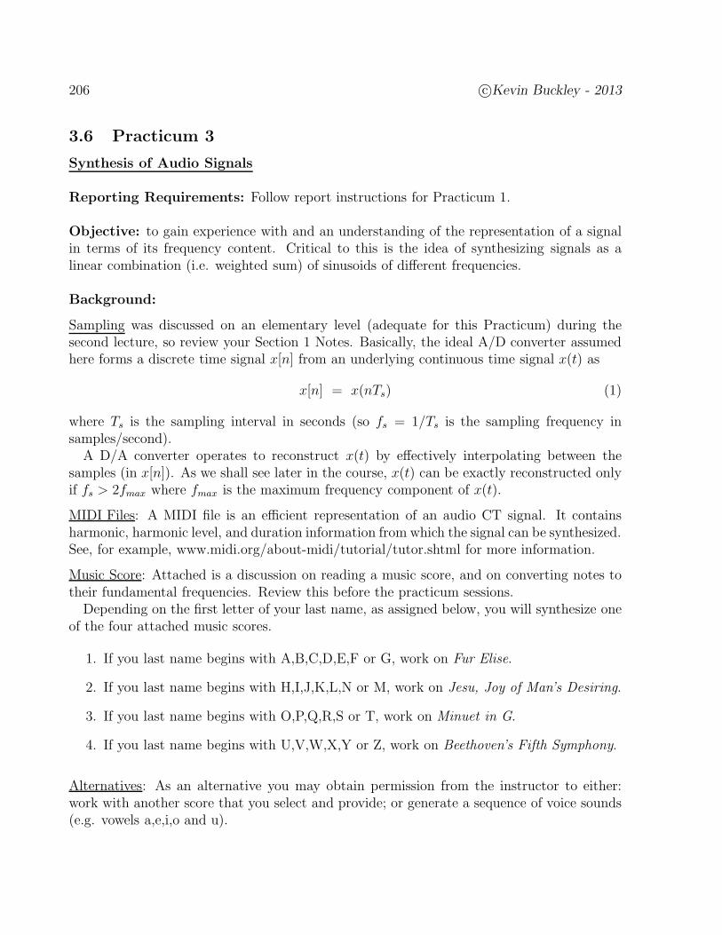
206 c©Kevin Buckley - 2013
3.6 Practicum 3
Synthesis of Audio Signals
Reporting Requirements: Follow report instructions for Practicum 1.
Objective: to gain experience with and an understanding of the representation of a signalin terms of its frequency content. Critical to this is the idea of synthesizing signals as alinear combination (i.e. weighted sum) of sinusoids of different frequencies.
Background:
Sampling was discussed on an elementary level (adequate for this Practicum) during thesecond lecture, so review your Section 1 Notes. Basically, the ideal A/D converter assumedhere forms a discrete time signal x[n] from an underlying continuous time signal x(t) as
x[n] = x(nTs) (1)
where Ts is the sampling interval in seconds (so fs = 1/Ts is the sampling frequency insamples/second).
A D/A converter operates to reconstruct x(t) by effectively interpolating between thesamples (in x[n]). As we shall see later in the course, x(t) can be exactly reconstructed onlyif fs > 2fmax where fmax is the maximum frequency component of x(t).
MIDI Files: A MIDI file is an efficient representation of an audio CT signal. It containsharmonic, harmonic level, and duration information from which the signal can be synthesized.See, for example, www.midi.org/about-midi/tutorial/tutor.shtml for more information.
Music Score: Attached is a discussion on reading a music score, and on converting notes totheir fundamental frequencies. Review this before the practicum sessions.
Depending on the first letter of your last name, as assigned below, you will synthesize oneof the four attached music scores.
1. If you last name begins with A,B,C,D,E,F or G, work on Fur Elise.
2. If you last name begins with H,I,J,K,L,N or M, work on Jesu, Joy of Man’s Desiring.
3. If you last name begins with O,P,Q,R,S or T, work on Minuet in G.
4. If you last name begins with U,V,W,X,Y or Z, work on Beethoven’s Fifth Symphony.
Alternatives: As an alternative you may obtain permission from the instructor to either:work with another score that you select and provide; or generate a sequence of voice sounds(e.g. vowels a,e,i,o and u).
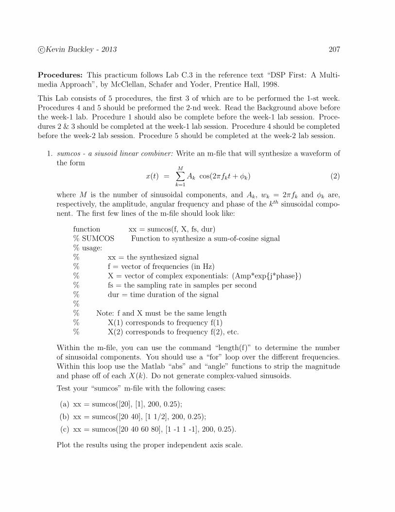
c©Kevin Buckley - 2013 207
Procedures: This practicum follows Lab C.3 in the reference text “DSP First: A Multi-media Approach”, by McClellan, Schafer and Yoder, Prentice Hall, 1998.
This Lab consists of 5 procedures, the first 3 of which are to be performed the 1-st week.Procedures 4 and 5 should be preformed the 2-nd week. Read the Background above beforethe week-1 lab. Procedure 1 should also be complete before the week-1 lab session. Proce-dures 2 & 3 should be completed at the week-1 lab session. Procedure 4 should be completedbefore the week-2 lab session. Procedure 5 should be completed at the week-2 lab session.
1. sumcos - a siusoid linear combiner: Write an m-file that will synthesize a waveform ofthe form
x(t) =M∑
k=1
Ak cos(2πfkt + φk) (2)
where M is the number of sinusoidal components, and Ak, wk = 2πfk and φk are,respectively, the amplitude, angular frequency and phase of the kth sinusoidal compo-nent. The first few lines of the m-file should look like:
function xx = sumcos(f, X, fs, dur)% SUMCOS Function to synthesize a sum-of-cosine signal% usage:% xx = the synthesized signal% f = vector of frequencies (in Hz)% X = vector of complex exponentials: (Amp*expj*phase)% fs = the sampling rate in samples per second% dur = time duration of the signal%% Note: f and X must be the same length% X(1) corresponds to frequency f(1)% X(2) corresponds to frequency f(2), etc.
Within the m-file, you can use the command “length(f)” to determine the numberof sinusoidal components. You should use a “for” loop over the different frequencies.Within this loop use the Matlab “abs” and “angle” functions to strip the magnitudeand phase off of each X(k). Do not generate complex-valued sinusoids.
Test your “sumcos” m-file with the following cases:
(a) xx = sumcos([20], [1], 200, 0.25);
(b) xx = sumcos([20 40], [1 1/2], 200, 0.25);
(c) xx = sumcos([20 40 60 80], [1 -1 1 -1], 200, 0.25).
Plot the results using the proper independent axis scale.
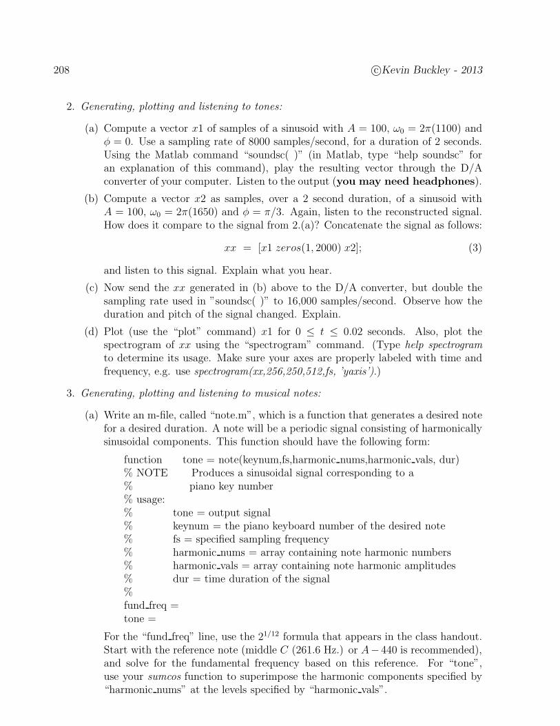
208 c©Kevin Buckley - 2013
2. Generating, plotting and listening to tones:
(a) Compute a vector x1 of samples of a sinusoid with A = 100, ω0 = 2π(1100) andφ = 0. Use a sampling rate of 8000 samples/second, for a duration of 2 seconds.Using the Matlab command “soundsc( )” (in Matlab, type “help soundsc” foran explanation of this command), play the resulting vector through the D/Aconverter of your computer. Listen to the output (you may need headphones).
(b) Compute a vector x2 as samples, over a 2 second duration, of a sinusoid withA = 100, ω0 = 2π(1650) and φ = π/3. Again, listen to the reconstructed signal.How does it compare to the signal from 2.(a)? Concatenate the signal as follows:
xx = [x1 zeros(1, 2000) x2]; (3)
and listen to this signal. Explain what you hear.
(c) Now send the xx generated in (b) above to the D/A converter, but double thesampling rate used in ”soundsc( )” to 16,000 samples/second. Observe how theduration and pitch of the signal changed. Explain.
(d) Plot (use the “plot” command) x1 for 0 ≤ t ≤ 0.02 seconds. Also, plot thespectrogram of xx using the “spectrogram” command. (Type help spectrogramto determine its usage. Make sure your axes are properly labeled with time andfrequency, e.g. use spectrogram(xx,256,250,512,fs, ’yaxis’).)
3. Generating, plotting and listening to musical notes:
(a) Write an m-file, called “note.m”, which is a function that generates a desired notefor a desired duration. A note will be a periodic signal consisting of harmonicallysinusoidal components. This function should have the following form:
function tone = note(keynum,fs,harmonic nums,harmonic vals, dur)% NOTE Produces a sinusoidal signal corresponding to a% piano key number% usage:% tone = output signal% keynum = the piano keyboard number of the desired note% fs = specified sampling frequency% harmonic nums = array containing note harmonic numbers% harmonic vals = array containing note harmonic amplitudes% dur = time duration of the signal%fund freq =tone =
For the “fund freq” line, use the 21/12 formula that appears in the class handout.Start with the reference note (middle C (261.6 Hz.) or A− 440 is recommended),and solve for the fundamental frequency based on this reference. For “tone”,use your sumcos function to superimpose the harmonic components specified by“harmonic nums” at the levels specified by “harmonic vals”.
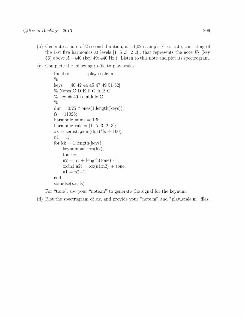
c©Kevin Buckley - 2013 209
(b) Generate a note of 2 second duration, at 11,025 samples/sec. rate, consisting ofthe 1-st five harmonics at levels [1 .5 .3 .2 .3], that represents the note E5 (key56) above A−440 (key 49; 440 Hz.). Listen to this note and plot its spectrogram.
(c) Complete the following m-file to play scales:
function play scale.m%keys = [40 42 44 45 47 49 51 52]% Notes C D E F G A B C% key # 40 is middle C%dur = 0.25 * ones(1,length(keys));fs = 11025;harmonic nums = 1:5;harmonic vals = [1 .5 .3 .2 .3];xx = zeros(1,sum(dur)*fs + 100);n1 = 1;for kk = 1:length(keys);
keynum = keys(kk);tone =n2 = n1 + length(tone) - 1;xx(n1:n2) = xx(n1:n2) + tone;n1 = n2+1;
endsoundsc(xx, fs)
For “tone”, use your “note.m” to generate the signal for the keynum.
(d) Plot the spectrogram of xx, and provide your ”note.m” and ”play scale.m” files.
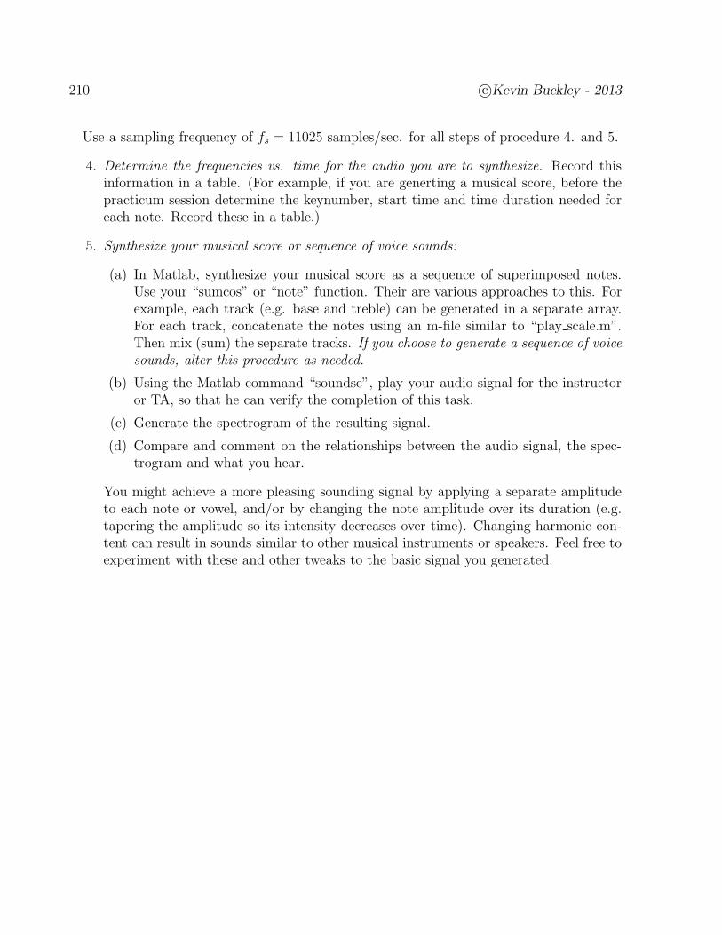
210 c©Kevin Buckley - 2013
Use a sampling frequency of fs = 11025 samples/sec. for all steps of procedure 4. and 5.
4. Determine the frequencies vs. time for the audio you are to synthesize. Record thisinformation in a table. (For example, if you are generting a musical score, before thepracticum session determine the keynumber, start time and time duration needed foreach note. Record these in a table.)
5. Synthesize your musical score or sequence of voice sounds:
(a) In Matlab, synthesize your musical score as a sequence of superimposed notes.Use your “sumcos” or “note” function. Their are various approaches to this. Forexample, each track (e.g. base and treble) can be generated in a separate array.For each track, concatenate the notes using an m-file similar to “play scale.m”.Then mix (sum) the separate tracks. If you choose to generate a sequence of voicesounds, alter this procedure as needed.
(b) Using the Matlab command “soundsc”, play your audio signal for the instructoror TA, so that he can verify the completion of this task.
(c) Generate the spectrogram of the resulting signal.
(d) Compare and comment on the relationships between the audio signal, the spec-trogram and what you hear.
You might achieve a more pleasing sounding signal by applying a separate amplitudeto each note or vowel, and/or by changing the note amplitude over its duration (e.g.tapering the amplitude so its intensity decreases over time). Changing harmonic con-tent can result in sounds similar to other musical instruments or speakers. Feel free toexperiment with these and other tweaks to the basic signal you generated.

c©Kevin Buckley - 2013 211
Practicum 3Instructor/TA Sign Off Sheet
Student’s Name:
1. Pract. 3, Procedure 1: plots for (a,b,c)
2. Pract. 3, Procedure 2(d): spectrogram plot
3. Pract. 3, Procedure 3(d): spectrogram plot
4. Pract. 3, Procedure 5(b,c): audio and spectrogram

212 c©Kevin Buckley - 2013
.

c©Kevin Buckley - 2013 213
Reading music and frequency mapping:

214 c©Kevin Buckley - 2013
Musical scores:

c©Kevin Buckley - 2013 215
3.7 Problems
Chapter Topics:3.1-25 (introductory CTFS and CTFS properties);3.26-34 (introductory CTFT and the generalized CTFT);3.35-38 (introductory Laplace transforms and ROC);3.39-60 (CT transform properties);
1. Consider two sinusoids x1(t) = 8 cos(4πt− 0.3π) and x2(t) = cos(7πt). Determinethe fundamental frequency and the period of the signal x(t) = x1(t) + x2(t).
2. For each of the following the signals, determine the fundamental frequency, and sketchits power spectrum, labeling the frequencies (in radians/second) and the complex “co-efficient” of each frequency component.
(a) x(t) =∑2
k=0 0.5k cos((2π10k)t + (π/2)).
(b) x(t) = cos(2π60t) + 4 cos(2π70t) − 2 cos(2π90t).
3. Consider the signal x(t) = cos(2πt). Since x(t) is periodic with period 1, it is also peri-odic with period N where N is any positive integer. Determine the CTFS coefficientsof x(t) under the assumption that the fundamental period is N = 3. Generalizing this,what is a basic characteristic of the CTFS coefficients computed assuming that thefundamental period is positive integer N times what it actually is?
4. Consider a signal x(t) that consists of an infinite number of impulses, one at each timet = 0.01 n for all integer n.
a) What is the fundamental period T and fundamental frequency ω0 of x(t)?
b) Plot the magnitude spectrum of x(t) over −1100π ≤ ω ≤ 1100π.
c) Plot the phase spectrum of x(t) over −1100π ≤ ω ≤ 1100π.
d) Describe the 2-nd harmonic component of x(t). The answer to this is a sinusoid.
5. Given that a signal x(t) is periodic with period T = 3, and that its exponential CTFScoefficients are
ak =
.9k k ≥ 00 k < 0
Determine x(t).
6. Using the CTFS analysis equation, derive the expression for the CTFS coefficients forof the sawtooth wave given in the CTFS Pair Table of the Course Notes.
7. Consider the CT periodic signal
x(t) =∞∑
n=−∞x1(t− 2n) ; x1(t) = e−|t| p2(t) .
216 c©Kevin Buckley - 2013
(a) Plot x1(t) and x(t).
(b) For x(t), find the DC CTFS coefficient ax0 .
8. Consider the CT periodic signal
x(t) =∞∑
n=−∞x1(t− 0.1n) ; x1(t) = p.02(t) .
(a) Plot x1(t) and x(t).
(b) Using the CTFS analysis equation, determine the CTFS coefficient ax0 as well asthe rest of the axk.
(c) Determine the total power in x(t).
(d) Determine the power in the DC component (this is |ax0 |2). What is the percentageof the total power in the DC component?
(e) Plot the magnitude spectrum of x(t) over the range of frequency −80π ≤ ω ≤ 80π.
9. Use the CTFS table and the linearity & delay properties to determine the CTFScoefficients ayk for
y(t) =∞∑
n=−∞y1(t− n) ; y1(t) = δ(t− 1
4) + δ(t+
1
4) .
10. Consider the periodic continuous-time signal
y(t) =∞∑
n=−∞y1(t− 4n) ; y1(t) = e−2t p4(t) .
(a) Sketch y1(t) and y(t).
(b) Using the analysis equations, determine the CTFS coefficient ay0, and the ayk.
(c) Determine the total power, and the power in DC (zeroth harmonic).
(d) What percentage of the total power is in the DC component?
(e) Plot the Spectrum of y(t) over the range of frequency −4π ≤ ω ≤ 4π.
11. Consider the following periodic signal with fundamental frequency ω0 = 2π:
x(t) =sin
(
(N + 12)ω0t
)
sin(
12ω0t
) ←→ axk =
1 |k| ≤ N0 otherwise
Let N = 20. Determine the percentage of total power in the frequency band−11π ≤ ω ≤ 11π.
12. Consider the signal x(t) =∑∞
n=−∞ 10 δ(t− 0.5n).
(a) Determine its fundamental period T and fundamental frequency ω0.
c©Kevin Buckley - 2013 217
(b) Determine its CTFS coefficients, the axk.
(c) Sketch its power spectrum (i.e. |axx|2 vs. ω) for −10π ≤ ω ≤ 10π.
(d) Determine the power in the frequency range −200π ≤ ω ≤ 200π.
(e) What is the % of total power in the frequency range −200π ≤ ω ≤ 200π?
13. Consider the following CT periodic signal:
x(t) =0.75
1.25 − cos(θ0t).
(a) For θ0 = 120π, what is the fundamental frequency ω0 and the period T ?
(b) What are the CTFS coefficients?
(c) What is the power of the DC (i.e. 0-th harmonic) component of this signal?
(d) What fraction of the total power of the signal is in its DC component?
(e) Now let θ0 = 200π. Let x1(t) be the part of x(t) which is in the frequencyrange −500π ≤ ω ≤ 500π. What is the fundamental period T and fundamentalfrequency ω0 of x(t)? Sketch the magnitude spectrum of x1(t). Determine thepercentage of the total power in x(t) that is in x1(t).
14. Consider a periodic signal x(t) with period T = 0.01 and CTFS coefficients
ak =
(.5)|k| k = 0, ±1, ±2,±3,±40 otherwise
(a) Determine the total power PT .
(b) If x(t) is processed with a filter that passes without any change all input sinusoidalcomponents in the frequency range |f | ≤ 150 while completely attenuating sinu-soidal components outside this range, determine the % of the total input powerthat passes through the filter.
15. Consider the periodic CT signal x(t), with period T = 0.01, that has CTFS coefficients
ak =
|k|1/2 k = 0,±1,±2, · · · ,±200 otherwise
.
a) Determine the total power PT of x(t).
b) Determine the percentage of PT in the frequency band −1100π ≤ ω ≤ 1100π.
16. Consider the periodic continuous-time signal
x(t) =∞∑
n=−∞x1(t− 4n) ; x1(t) = t p4(t− 2) .
(a) Sketch x1(t) and x(t) for −4 ≤ t ≤ 8.
(b) Sketch the magnitude spectrum for −2π ≤ ω ≤ 2π (i.e. for −1 ≤ f ≤ 1).
218 c©Kevin Buckley - 2013
(c) What is the power of x(t)?
(d) What percentage of the power of x(t) is NOT in the DC plus 1-st harmonic terms?
17. Consider a fullwave rectified cosine wave x(t) = |4 cos(120πt)|.
(a) What is its fundamental period and frequency?
(b) Carefully plot x(t) and x(t) over two of their periods, where x(t) is the sum ofthe DC and first harmonic components of x(t).
(c) What is the total power PT of x(t).
(d) Plot the magnitude spectrum of x(t) over the frequency range −360π ≤ ω ≤ 360π.
(e) What is the percentage of x(t) power in its DC plus first harmonic?
18. A DC source can be generated from an AC source x(t) (e.g. a 120 Volt AC wall signal)by first full wave rectifying the AC signal to form y(t) = |x(t)|, and then removing (viaa filter) all but the DC component. Let x(t) = 170 cos(120πt).
(a) Sketch both x(t) and y(t).
(b) What are the fundamental periods of x(t) and y(t)?
(c) What are the powers of x(t) and y(t)? Are they the same?
(d) What percentage of the power of x(t) is in the DC component of y(t)? This isthe percentage of power of the original source x(t) preserved in the DC source (ie.the DC component of y(t))?
19. A DC source can be generated from an AC source x(t) (e.g. a 120 Volt AC wall signal)by first half wave rectifying the AC signal to form
y(t) =
x(t) x(t) ≥ 00 x(t) < 0
and then removing (via a filter) all but the DC component. Let x(t) = 170 cos(120πt).
(a) Sketch both x(t) and y(t).
(b) What are the powers of x(t) and y(t)? (Px is easy. Py is simply related to Px.)
(c) Describe the power of y(t) as a function of frequency ω.
(d) What percentage of the power of x(t) is in the DC component of y(t)?
20. Consider the periodic continuous-time signal
z(t) =∞∑
n=−∞z1(t− 4n) ; z1(t) = (2t− 4) p4(t− 2) .
(a) Sketch z1(t) and z(t).
(b) Using Table 6 of the Course Notes and linearity, for z(t) determine the CTFScoefficient a0, and the ak.
c©Kevin Buckley - 2013 219
(c) Determine the total power, and the power in DC (zeroth harmonic).
(d) Plot the Spectrum of z(t) over the range of frequency −2 ≤ f ≤ 2.
21. Consider the signal
x(t) =∞∑
n=−∞x1(t+ 4n) ; x1(t) = (4 + 2t) p4(t) .
(a) Sketch x(t).
(b) Determine its power Px.
(c) Using Table 6 and CTFS properties, determine its CTFS coefficients, the axk.
(d) Determine the percentage of power of x(t) not in its DC component.
(e) Determine the power of the signal z(t) with CTFS coefficients azk = axk e−j π2(k/6)2 .
22. Consider the half-wave rectified cosine with CTFS coefficients given in the CTFS PairTable of the Course Notes. For A = 1 and T0 = 1, denote the signal x(t).
(a) What are the CTFS coefficients ax0 , ax1 , a
x−1, a
x2 and ax−2?
(b) Consider the signal y(t) = − x(t − 12). What are the CTFS coefficients ay0, a
y1,
ay−1, ay2 and ay−2?
(c) Consider z(t) = x(t) + y(t). What are the CTFS coefficients az0, az1, a
z−1, a
z2 and
az−2?
(d) Plot z(t); 0 ≤ t ≤ 2.
23. Consider the following CT periodic signal x(t)
t
2
x(t)
0 0.1 0.2 0.3 0.4−0.1
a) What is its fundamental period T and frequency ω0?
b) To find the CTFS coefficients (i.e. the axk ’s) using Table 6 of the Course Notesand properties,what properties do you need? What Table 6 entries (i.e. whatsignal types) do you need?
c) Determine axo , ax1 and ax2 .
d) Determine the power in the DC component of x(t).
24. Consider the signal x(t) = 3 + | cos(200πt) |.
a) Sketch x(t) over two periods. What is the fundamental frequency ω0 and thefundamental period T ?
b) Using the CTFS Pairs table and the linearity property, determine expressions forthe CTFS coefficients, the axk ’s. Plot axk vs. ω for −1000π ≤ ω ≤ 1000π.
220 c©Kevin Buckley - 2013
c) Determine the combined power in the DC and 1-st harmonic components of x(t).
d) Given y(t) = x(t − 1), determine expressions for the CTFS coefficients, the ayk’s.
25. Consider the periodic signal
x(t) =∞∑
n=−∞x1(t− n6) ; x1(t) =
23t −3 < t ≤ 30 otherwise
(a) Plot x1(t) and x(t), each over the range −3 < t ≤ 9.
(b) What it the fundamental frequency ω0 of x(t)?
(c) What is the total power of x(t)?
(d) Using Table 6 of the Course Notes, and CTFS properties, determine the CTFScoefficients of x(t) for all harmonics k.
(e) Determine the percentage of total power in the DC component.
(f) Determine the percentage of total power in the first harmonic (positive & negativefrequency).
26. Using the CTFT analysis equation, determine the CTFT of x(t) = δ(t+3) − δ(t−3).
27. Consider the energy signal x(t) = e−5t u(t− 3). Sketch x(t). By direct evaluation ofthe CTFT integral, determine X(jω).
28. Given any constant c and any CTFT pair
x(t) ←→ X(jω) ,
it is true thatc x(t) ←→ c X(jω)
is a CTFT pair. Determine the CTFT of y(t) = sin(t)t
and sketch it for −2π ≤ ω ≤ 2π.
29. a) By evaluating the inverse CTFT integral for t = 0, determine x(0) given thatX(jω) = 5e−|ω−2|.b) Using the CTFT synthesis equation, determine the ICTFT of P (jω) = e−|ω−10|.
30. Using the CTFT analysis equation, determine the CTFT of the signal
x(t) =19∑
k=0
0.9k δ(t− k5) .
31. Using the CTFT analysis equation, determine the CTFT of
x(t) =∞∑
k=0
ck δ(t− kT ) .
Assume |c| < 1.
c©Kevin Buckley - 2013 221
32. Consider a signal x(t) which is periodic with fundamental period T = 8. Over therange −4 ≤ t ≤ 4 it is
x(t) = δ(t+ 1) + δ(t− 1) − 4 ≤ t ≤ 4 .
Determine and plot its generalized CTFT.
33. Determine the generalized CTFT of the signal
z(t) = 6 cos(2t) +1
2cos(3t + π/3) .
34. Transform Pair Problems:
(a) Find the CTFT of x1(t) = δ(t+ 1)− δ(t− 1).
(b) Find the CTFT of x2(t) = e−2t u(t+ 1).
(c) Find the BLT of x3(t) = cos(3t) δ(t).
(d) Find the ULT of x4(t) = e−t u(t+ 1).
(e) Find the inverse CTFT of X5(jω) = ej5ω.
(f) Find the causal inverse BLT of X6(s) = js+j3
− js−j3
explicitly as a real-valuedsignal.
(g) Determine the CTFT X(jω) for x(t) = (1 + cos(10πt)) cos(100πt). What is thefundamental frequency of this periodic signal?
(h) Determine the CTFT Y (jω) of y(t) = t e−tu(t) ∗ e−tu(t).
(i) Find the energy Ez of z(t) = 7 sin(10π(t−4))(t−4)
ej100t.
(j) Determine the BLT W (s), with ROC Rw, for w(t) = cos(2, 009πt) u(t).
35. Determine the bilateral Laplace transform and the associated ROC for the signals.Express your X(s) as a single rational function of s.
(a) x(t) = e−2tu(t) + e3tu(−t).(b) x(t) = 4 e−2t u(t) − 6 e−3t u(t).
36. Determine the Bilateral Laplace Transform (BLT), including the Region of Convergence(ROC), of the signal
x(t) = 6 e−5|t| + 4 cos(1, 000, 000, 000πt) u(t) .
37. Consider the following CT signal:
x(t) = 3 e−2t u(t) + 7 e5t u(t) .
a) Determine its BLT X(s), including the ROC Rx.
222 c©Kevin Buckley - 2013
b) Your X(s) should be a rational function of s (i.e. a numerator polynomial ins over a denominator polynomial in s). Express your X(s) in rational functionform.
38. Find the inverse BLT of the following:
(a) Y4(s) = s+3(s+2)2
. Assume y4(t) is causal.
(b) Determine the inverse Bilateral Laplace Transform for
H(s) =2
s+ (1 + j)+
2
s+ (1− j)+
5
s− 7,
where the ROC includes Res = 0. Express your h(t) explicitly as a real-valuedsignal.
(c) Determine the BLT X(s) and ROC of the signal
x(t) = 4 e3tu(−t) − t e−5tu(t) .
Express X(s) as a rational function of s (i.e. find the common denominator).
39. Determine the CTFT of x(t) = u(t)− u(t− 3).
40. Basic CTFS and CTFT problems:
(a) Consider a periodic signal x(t) with period T0 = 0.001 and CTFS coefficientsak = (−0.9)k u[k].
i. Is x(t) real-valued? Why?
ii. Determine the total power of x(t).
iii. Determine the percentage of x(t) power in the frequency band−10, 000π ≤ ω ≤ 10, 000π.
41. For the following four CT convolution problems, solve one using graphical convolution,one using the convolution table and properties, one using Laplace transforms and oneusing which ever method you wish. For each, show all work.
(a) x1(t) = e−4t u(t) and h1(t) = e−4t cos(8πt) u(t) .
(b) x2(t) = δ(t− 10) + u(t) + ej100t and h2(t) = e−5t u(t) .
(c) x3(t) = p5(t) and h3(t) = p2(t− 1) .
(d) x4(t) = ej30t and h4(t) = e−10|t| .
42. Determine the generalized CTFT the signal
x(t) =∞∑
n=−∞x1(t− 3n) , x1(t) = p3(t− 1.5) + p1(t− 1.5) .
c©Kevin Buckley - 2013 223
43. Your are given two periodic signals, each with period T0 = 0.01 seconds. Specifically,one is the sinusoid x1(t) = cos(400πt), and the other is the square wave
x2(t) =∞∑
n=−∞x3[t− n(.01)] ; x3(t) = p.005(t) .
For the signal x(t) = 2x1(t) + 5x2(t), determine the CTFS coefficients. Determine thepower of x(t) in the frequency range −250π ≤ ω ≤ 250π.
44. Basic CT transforms & properties:
(a) Using the BLT integral equation, derive the BLT (including the ROC) ofx1(t) = p3(t− 4).
(b) Using tables and properties, determine the CTFT of the following x2(t)).
x (t)2
t
4
−10 −5 5 10
2
(c) You are given that x3(t) is a CT periodic signal with fundamental frequencyω0 = 100π and CTFS coefficients ak = .9k u[k]. Plot the a′ks as a function of ω.Using the geometric series equation, determine x3(t).
(d) Consider the saw tooth signal x4(t) from the CFTS table in the Course Notes,with A = 1 and To = 1. Using the delay property, determine the CTFS coefficientsof x5(t) = x4(t− 10).
45. Consider the following signal
x(t) =
(
1 + 0.25sin2(2πt)
(πt)2
)
cos(40πt) .
a) Determine and sketch the CTFT X(jω).
b) Identify on your plot the power and the energy portions of X(jω).
c) Concerning the energy portion only, what % of the energy is in the frequencyband 0 ≤ ω ≤ 40π.
46. Consider the CT signal x(t) = sin(20πt)πt
.
a) Determine its CTFT X(jω). Plot its CTFT magnitude |X(jω)|. Determine itsenergy Ex.
b) Let y(t) = x(t− 2). Plot |Y (jω)|. Determine its energy Ey.
c) Let z(t) = x(t) · ej30πt. Plot |Z(jω)|. Determine its energy Ez.

224 c©Kevin Buckley - 2013
d) Let v(t) = z(t− 2). Plot |V (jω)|. Determine its energy Ev.
Label and show axis details on each plot.
47. The CTFT:
(a) Let
x(t) =∞∑
n=−∞δ(t− n) y(t) = x(t) · ej2πt .
Determine the power of y(t) in the frequency band −6π ≤ ω ≤ 6π.
(b) Determine y(t) and Y (jω) given
y(t) =sin(20π(t− 1))
π(t− 1)∗ sin2(10πt)
(πt)2
48. Parseval’s theorem problems:
(a) Given an input x(t) = e−|t| to a CT LTI system with ideal lowpass filter frequencyresponse H(jω) = p2(ω), determine the percentage of input energy that makes itto the output. You may have use for the indefinite integral
∫ 1
(1 + ω2)2dω =
ω
2(1 + ω2)+
1
2tan−1(ω)
and the facts that tan−1(1) = π4and tan−1(0) = 0.
(b) Consider the signal v(t) = x(t) · ej10πt, where x(t) = e−3t cos(2πt)u(t). Whatpercentage of x(t) energy is in v(t)?
(c) Given that −1 < c < 1, a periodic signal x(t) has CTFS coefficients axk = c|k|.This signal is the input to a CT LTI system with impulse response h(t) = δ(t−5).Determine the percentage of the input power that makes it to the output.
49. Consider a signal x(t) with exponential CTFS expansion is
x(t) =∞∑
n=−∞axne
j(nπ/2)t
where
axn =
12
n = 02
π2n2 n = ±1,±3,±5, ...0 otherwise
Find the exponential CTFS coefficients for:
(a) v(t) = x(t− 2)
(b) w(t) = x(t− 4)
c©Kevin Buckley - 2013 225
(c) y(t) = x(t)ej(π/2)t
Simplify the coefficient expressions as much as possible.
50. CT Transforms and Properties: The following problems are independent of one an-other.
(a) Consider the signal xa(t) =∑∞
n=−∞ δ(t−4). Determine its total power, and thepower in the frequency band −6π ≤ ω ≤ 6π.
(b) Consider the signal xb(t) = 2πt
sin(20πt) − 1πt
sin(10πt). Determine the per-centage of its energy in the frequency band −10π ≤ ω ≤ 10π.
(c) Let ya(t) = 11+t2
. Determine the energy of:
i. ya(t).
ii. yb(t) = ya(t− 5).
iii. yc(t) = ya(t) ej4πt.
iv. yd(t) = 6 ya(t− 5) ej4πt.
51. Determine the ICTFT for
X(jω) = |X(jω)| ej 6 X(jω) |X(jω)| = |ω| p2(ω) 6 X(jω) = −3ω .
52. Determine the energy of the signal x(t) which has CTFT
X(jω) =2
jω + 1+ sinc(ω) ej4πω .
Note that this will be much more easily done in one domain rather than the other.
53. Consider the signal x(t) with CTFT X(jω) = X1(ω − 1) +X1(ω + 1) whereX1(ω) = e−|ω| p2(ω).
a) Sketch X(jω).
b) Determine the percentage of the total energy that’s in the band −1 ≤ ω ≤ 1.
54. Let v(t) = x(t) y(t) where x(t) = 1 + cos(3t) and Y (jω) =∑∞
n=−∞ .4|n|δ(ω − n),determine the CTFS coefficients cv0 and cv5.
55. Consider two signals, y(t) = 34+t2
and z(t) = ej10t y(t).
a) Determine Y (jω) and Ey (the energy of y(t)).
b) Determine Z(jω) and Ez.
c) What percentage of Ez is in the frequency band ω > 10?
d) What percentage of Ey is in the frequency band |ω| > 0.25?
226 c©Kevin Buckley - 2013
56. Consider the spectrum analysis problem of computing the CTFT of a signal x(t) givenonly a window of it, x(t); −T ≤ t ≤ T . A standard practice is to just compute theCTFT of
xw(t) = x(t) · w(t)
where w(t) = p2T (t) is called the window. (That is, we compute the CTFT of thepart of the signal which is available.) Let x(t) = ej8πt and T = 1. Determine andsketch Xw(jω) and compare this approximate spectrum to the true spectrum X(jω).
57. Consider the CT signals x(t) = sin(100πt)πt
, z1(t) = ej200πt and z2(t) = cos(200πt).
(a) Plot the CTFT of x(t) and determine the percentage of x(t) energy in the fre-quency band 0 ≤ ω ≤ ∞.
(b) Plot the CTFT of v1(t) = x(t) · z1(t) and determine the percentage of v1(t)energy in the frequency band −200π ≤ ω ≤ 200π.
(c) Plot the CTFT of v2(t) = x(t) · z2(t) and determine the percentage of v2(t)energy in the frequency band −200π ≤ ω ≤ 200π.
58. Transform property problems:
(a) Find the CTFT of y1(t) = sinc(5t) ∗ sinc(10t).
(b) Find y2(t) = cos(4t) ∗ h(t), where H(jω) = e−|ω|.
(c) Find the input x3(t) = h(t) ∗ y3(t) where h(t) = δ(t − 1) and output CTFTY3(jω) =
3jω+2
.
59. The deterministic autocorrelation function cx(t) of a CT signal x(t) is defined as
cx(t) = x(t) ∗ x(−t) .
That is, it is the convolution of signal x(t) with the folded signal x(−t). Use CTFTsand properties to determine cx(t) for x(t) = e−t p1(t). Verify your result usinggraphical convolution.
60. Consider the signal
v(t) =2
πtsin(10πt) +
1
(πt)2sin2(5πt) .
(a) Determine and sketch its CTFT.
(b) Determine and sketch the CTFT of x(t) = 2 v(t) cos(100πt).
(c) Determine the percent energy of x(t) in the frequency band |ω| < 50π.
(d) Determine the percent energy of x(t) in the frequency band |ω| < 100π.

c©Kevin Buckley - 2013 227
4 Applications of CT Transforms
1. In Section 4.1 we then explore how CT transforms can be used to characterize, analyze,implement and design CT LTI systems.
2. In Section 4.2 we use CT transforms to facilitate descriptions of several higher levelsignal processing function.
Chapter 4 Objective Checklist
• Be familiar with the various CT LTI system descriptions discussed in this Chapter,including: the impulse response, the frequency response, the transfer function andsystem poles/zeros. Understand the relationships between these system descriptions.
• Know how to solve CT LTI system I/O problems using different system descriptions.Understand the relationship between different CT LTI system descriptions and stabil-ity/causality. At least understand how the Laplace transform can be used to deal withCT LTI system initial conditions.
• Be comfortable with how the CT transforms covered in this Chapter are applied to theadvanced topics discussed in Section 3.7.
4.1 Continuous Time LTI Systems
Recall the discussion in Section 3.1 on the response of a CT LTI system to an exponentialinput. We showed that for an exponential input, of the form x(t) = est, where s = σ+ jω isa complex valued constant of arbitrary value, the output is
y(t) = H(s) est = |H(s)|eσt ej(ωt+ 6 H(s)) (1)
whereH(s) =
∫ ∞
−∞h(t) e−st dt (2)
and h(t) is the system impulse response. Note that the output is an exponential with thesame argument s. The system alters only the magnitude and phase of the exponential, asgoverned by H(s). We now recognize H(s) as the bilateral Laplace transform of the impulseresponse h(t). So, what if any is the role of the ROC of h(t)? Is the Bilateral Laplacerepresentation of the system H(s), termed the transfer function, a useful representation ofthe system? These are questions we explore in this Section.
Additionally, note that since the system is linear and we can use the Laplace transformto write and input x(t) as a linear combination of exponentials, i.e.
x(t) =1
2πj
∫ σ+j∞
σ−j∞X(s) est ds σ ∈ Rx , (3)
we have a way to use the Laplace transform to compute the output y(t) due to any inputx(t). Is this a useful approach to computing system outputs?
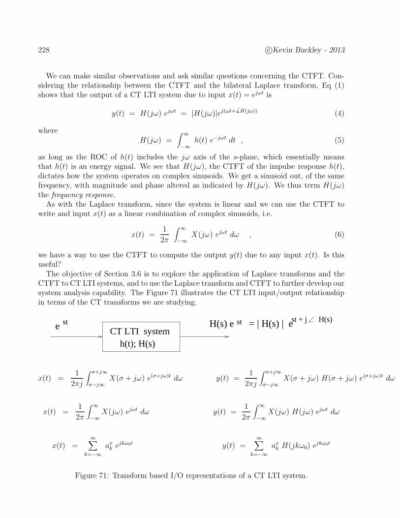
228 c©Kevin Buckley - 2013
We can make similar observations and ask similar questions concerning the CTFT. Con-sidering the relationship between the CTFT and the bilateral Laplace transform, Eq (1)shows that the output of a CT LTI system due to input x(t) = ejωt is
y(t) = H(jω) ejωt = |H(jω)|ej(ωt+ 6 H(jω)) (4)
whereH(jω) =
∫ ∞
−∞h(t) e−jωt dt , (5)
as long as the ROC of h(t) includes the jω axis of the s-plane, which essentially meansthat h(t) is an energy signal. We see that H(jω), the CTFT of the impulse response h(t),dictates how the system operates on complex sinusoids. We get a sinusoid out, of the samefrequency, with magnitude and phase altered as indicated by H(jω). We thus term H(jω)the frequency response.
As with the Laplace transform, since the system is linear and we can use the CTFT towrite and input x(t) as a linear combination of complex sinusoids, i.e.
x(t) =1
2π
∫ ∞
−∞X(jω) ejωt dω , (6)
we have a way to use the CTFT to compute the output y(t) due to any input x(t). Is thisuseful?
The objective of Section 3.6 is to explore the application of Laplace transforms and theCTFT to CT LTI systems, and to use the Laplace transform and CTFT to further develop oursystem analysis capability. The Figure 71 illustrates the CT LTI input/output relationshipin terms of the CT transforms we are studying.
e CT LTI systemh(t); H(s)
st stH(s) e = | H(s) | est + j H(s)
x(t) =1
2πj
∫ σ+j∞
σ−j∞X(σ + jω) e(σ+jω)t dω y(t) =
1
2πj
∫ σ+j∞
σ−j∞X(σ + jω) H(σ + jω) e(σ+jω)t dω
x(t) =1
2π
∫ ∞
−∞X(jω) ejωt dω y(t) =
1
2π
∫ ∞
−∞X(jω) H(jω) ejωt dω
x(t) =∞∑
k=−∞axk ejkω0t y(t) =
∞∑
k=−∞axk H(jkω0) e
jkω0t
Figure 71: Transform based I/O representations of a CT LTI system.
c©Kevin Buckley - 2013 229
Recalling that, for a CT LTI system with impulse response h(t), the output y(t) due toinput x(t) is the convolution y(t) = x(t) ∗ h(t). Recalling the convolution properties for theCTFT and bilateral Laplace transform, we have the following transform pairs:With the bilinear Laplace transform
y(t) = x(t) ∗ h(t) ←→BLT Y (s) = X(s) H(s) (7)
where H(s) = BLTh(t), the BLT of h(t), is the system transfer function.With the CTFT
y(t) = x(t) ∗ h(t) ←→CTFT Y (jω) = X(jω) H(jω) (8)
where H(jω) = CTFSh(t), the CTFT of h(t), is the system frequency response.With the CTFS
y(t) = x(t) ∗ h(t) ←→CTFS ayk = axk H(jkω0) ; k = 0,±1,±2, · · · (9)
where H(jkω0) is the CTFT of h(t), is the system frequency response, evaluated at ω = kω0.
4.1.1 CT LTI System I/O Descriptions
• Frequency response: H(jω)
• Transfer function: H(s)
• Impulse response: h(t)
• LCC differential equation:
N∑
k=0
ak y(k)(t) =M∑
k=0
bk x(k)(t) (10)
If we take the bilateral Laplace transform of the LCC differential equation, using thedifferentiation and linearity properties, we get
N∑
k=0
ak sk Y (s) =M∑
k=0
bk sk X(s) (11)
Y (s)N∑
k=0
ak sk = X(s)M∑
k=0
bk sk (12)
Y (s)
X(s)=
∑Mk=0 bk sk
∑Nk=0 ak sk
. (13)
From the convolution property of the BLT, then, we have
H(s) =Y (s)
X(s)=
∑Mk=0 bk sk
∑Nk=0 ak sk
. (14)
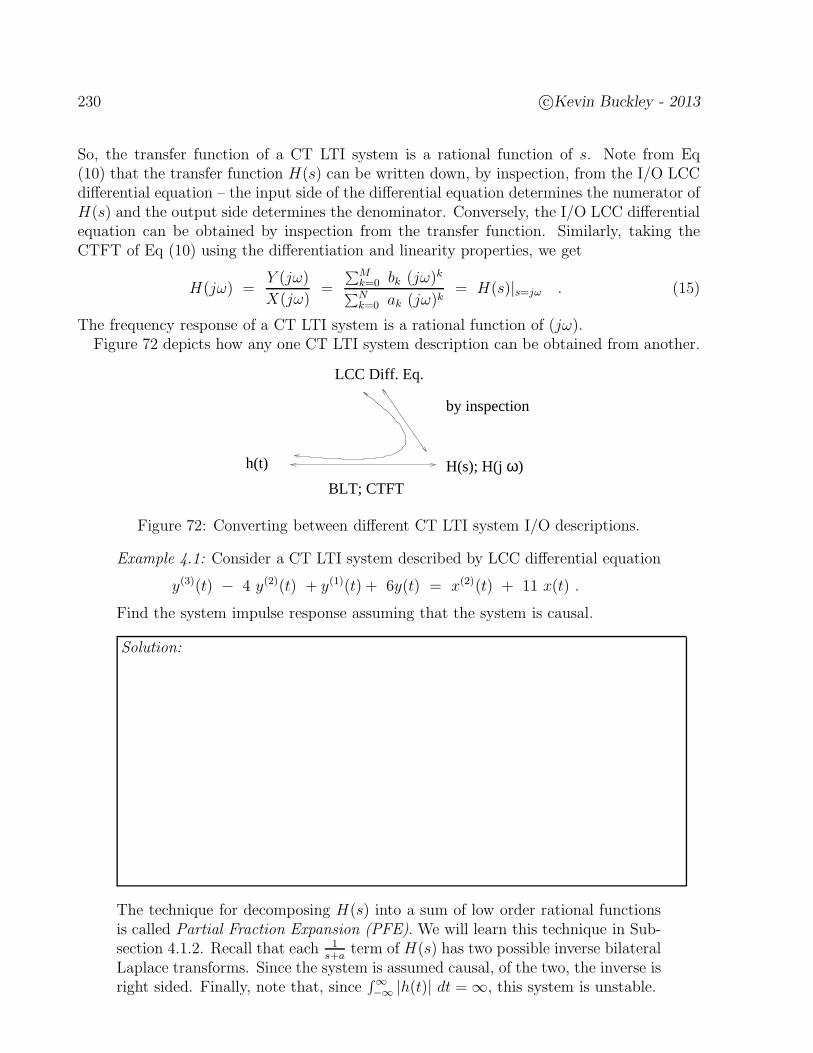
230 c©Kevin Buckley - 2013
So, the transfer function of a CT LTI system is a rational function of s. Note from Eq(10) that the transfer function H(s) can be written down, by inspection, from the I/O LCCdifferential equation – the input side of the differential equation determines the numerator ofH(s) and the output side determines the denominator. Conversely, the I/O LCC differentialequation can be obtained by inspection from the transfer function. Similarly, taking theCTFT of Eq (10) using the differentiation and linearity properties, we get
H(jω) =Y (jω)
X(jω)=
∑Mk=0 bk (jω)k
∑Nk=0 ak (jω)k
= H(s)|s=jω . (15)
The frequency response of a CT LTI system is a rational function of (jω).Figure 72 depicts how any one CT LTI system description can be obtained from another.
H(s); H(j )ωh(t)
LCC Diff. Eq.
by inspection
BLT; CTFT
Figure 72: Converting between different CT LTI system I/O descriptions.
Example 4.1: Consider a CT LTI system described by LCC differential equation
y(3)(t) − 4 y(2)(t) + y(1)(t) + 6y(t) = x(2)(t) + 11 x(t) .
Find the system impulse response assuming that the system is causal.
Solution:
The technique for decomposing H(s) into a sum of low order rational functionsis called Partial Fraction Expansion (PFE). We will learn this technique in Sub-section 4.1.2. Recall that each 1
s+aterm of H(s) has two possible inverse bilateral
Laplace transforms. Since the system is assumed causal, of the two, the inverse isright sided. Finally, note that, since
∫∞−∞ |h(t)| dt =∞, this system is unstable.
c©Kevin Buckley - 2013 231
Poles and Zeros:
Consider the representation shown below of the transfer function H(s), obtained by factor-ing the numerator and denominator polynomials, N(s) and D(s) respectively, into productsof 1-st order sections (one for each polynomial root):
H(s) =N(s)
D(s)= G
∏Mi=1 (s − zi)
∏Ni=1 (s − pi)
(16)
where G = bMaN
is a gain term. The numerator polynomial roots, the zi; i = 1, 2, · · ·M , arecalled the zeros of the system. The denominator polynomial roots, the pi; i = 1, 2, · · · , N ,are called the poles of the system.
Example 4.2: Determine the zeros and poles of the system in Example 4.1.
Solution:
poles: p1 = −1, p2 = 2, p3 = 3
zeros: z1 = j√11, z2 = −j
√11, (i.e. s2 + 11 = (s+ j
√11)(s− j
√11))
Example 4.3: Consider the CT LTI system with impulse response
h(t) = e−t cos(2t− π/4) u(t) − t u(t) .
Find the transfer function, the I/O LCC differential equation, and the poles/zeros.
Solution: We could break h(t) up using Euler’s identity, but instead we’ll use atrig identity here.
h(t) =1√2e−t cos(2t) u(t) +
1√2e−t sin(2t) u(t) − t u(t)
Using the BLT table in the Course Notes, and linearity, we have
H(s) =1√2
[
s+ 1
(s+ 2)2 + 4+
2
(s+ 2)2 + 4
]
− 1
s2
=
1√2s3 + 1.12s2 − 2s− 5
s4 + 2s3 + 5s2.
By inspection,
y(4)(t) + 2 y(3)(t) + 5 y(2)(t) =1√2x(3)(t) + 1.12 x(2)(t) − 2 x(1)(t) − 5 x(t) .
poles (roots of (s4 + 2s3 + 5s2)): p1 = p2 = 0, p3,4 = −1± j2
zeros (roots of ( 1√2s3+1.12s2−2s−5)): z1 = 1.89, z2,3 = −1.7372±j0.8498
Considering h(t), note that, due to the t u(t) term, this system is nonstable. This termcorresponds to the 2 poles at s = 0. This suggests that the poles may somehow be relatedto stability. We will explore this relationship in Subsection 4.1.3.
232 c©Kevin Buckley - 2013
4.1.2 Partial Fraction Expansion (PFE)
Here we study the PFE of a transfer function of the form
H(s) =bMsM + bM−1s
M−1 + · · · + b1s + b0aNsN + aN−1sM−1 + · · · + a1s + a0
(17)
Our objective is to decompose H(s) into a sum of lower order rational functions so that,using linearity and Laplace transform tables, we can identify the inverse Laplace transformh(t) = L−1H(s).
Note that if we wish to take the inverse CTFT of a frequency response
H(jω) =bM (jω)M + bM−1(jω)
M−1 + · · · + b1(jω) + b0aN (jω)N + aN−1(jω)M−1 + · · · + a1(jω) + a0
(18)
we can just replace the jω’s with s’s and use the techniques described below. Severaltechniques are required, depending on whether H(s) is strictly proper (i.e. M < N) or not,and on whether or not there are repeated poles.
1. Strictly proper transfer function (M < N), with distinct poles: Let pi; i = 1, 2, · · · , Nbe the system poles, which are assumed distinct. Then H(s) can be expressed as aweighted sum of first order rational terms as follows,
H(s) =N∑
i=1
ris− pi
(19)
where the ri, termed the residues, are computed as
ri = (s− pi) H(s)|s=pi(20)
Then, for example assuming a causal h(t),
h(t) =N∑
i=1
ri epit u(t) . (21)
Regardless on whether or not H(s) is strictly proper or not, and on whether there arerepeated roots or not, we will be able to expand H(s) as a linear combination of low orderrational functions. The coefficients of the expansion, which we denote as the r′is, are calledresidues.
Each pi, ri pair corresponds to an exponential component of the inverse transform. Itmay be causal or not, depending on the ROC. Note that there is no requirement that thepoles or residues be real-valued. If the ai and bi coefficients of H(s) are real-valued, thenthe poles and corresponding residues will either be real-valued or exist in complex conjugatepairs. Any complex-valued poles corresponds to a complex exponential component (i.e. anoscillating and perhaps decaying/expanding component) of the impulse response. We willexplore this in detail in an example below.
Partial fraction expansion (PFE) is not restricted to transfer functions. Any rationalfunction can be expressed this way. So PFE is a generally useful procedure in determiningthe inverse transform (e.g. of input and output signals).
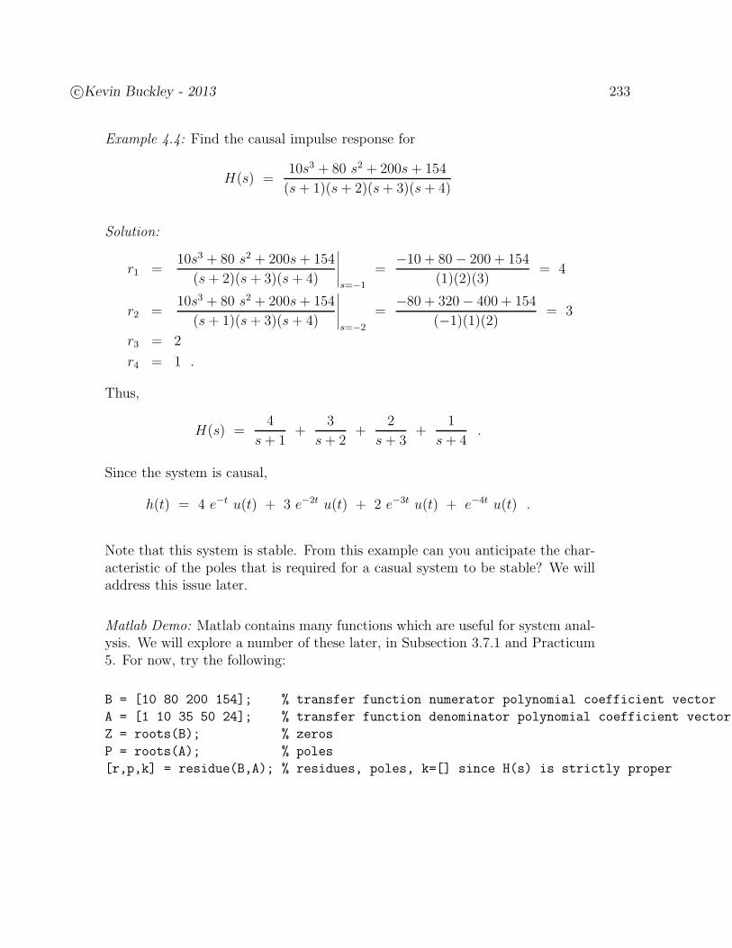
c©Kevin Buckley - 2013 233
Example 4.4: Find the causal impulse response for
H(s) =10s3 + 80 s2 + 200s+ 154
(s+ 1)(s+ 2)(s+ 3)(s+ 4)
Solution:
r1 =10s3 + 80 s2 + 200s+ 154
(s+ 2)(s+ 3)(s+ 4)
∣
∣
∣
∣
∣
s=−1
=−10 + 80− 200 + 154
(1)(2)(3)= 4
r2 =10s3 + 80 s2 + 200s+ 154
(s+ 1)(s+ 3)(s+ 4)
∣
∣
∣
∣
∣
s=−2
=−80 + 320− 400 + 154
(−1)(1)(2) = 3
r3 = 2
r4 = 1 .
Thus,
H(s) =4
s+ 1+
3
s+ 2+
2
s+ 3+
1
s+ 4.
Since the system is causal,
h(t) = 4 e−t u(t) + 3 e−2t u(t) + 2 e−3t u(t) + e−4t u(t) .
Note that this system is stable. From this example can you anticipate the char-acteristic of the poles that is required for a casual system to be stable? We willaddress this issue later.
Matlab Demo: Matlab contains many functions which are useful for system anal-ysis. We will explore a number of these later, in Subsection 3.7.1 and Practicum5. For now, try the following:
B = [10 80 200 154]; % transfer function numerator polynomial coefficient vector
A = [1 10 35 50 24]; % transfer function denominator polynomial coefficient vector
Z = roots(B); % zeros
P = roots(A); % poles
[r,p,k] = residue(B,A); % residues, poles, k=[] since H(s) is strictly proper
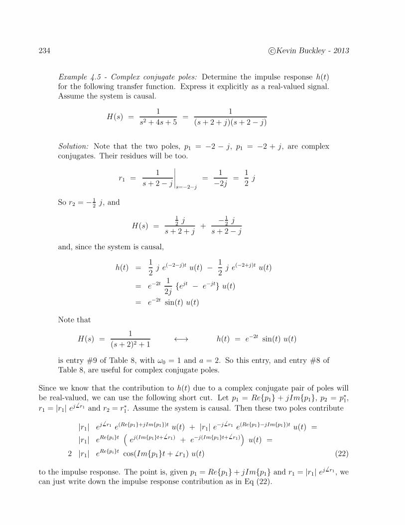
234 c©Kevin Buckley - 2013
Example 4.5 - Complex conjugate poles: Determine the impulse response h(t)for the following transfer function. Express it explicitly as a real-valued signal.Assume the system is causal.
H(s) =1
s2 + 4s+ 5=
1
(s+ 2 + j)(s+ 2− j)
Solution: Note that the two poles, p1 = −2 − j, p1 = −2 + j, are complexconjugates. Their residues will be too.
r1 =1
s+ 2− j
∣
∣
∣
∣
∣
s=−2−j
=1
−2j =1
2j
So r2 = −12j, and
H(s) =12j
s+ 2 + j+
−12j
s+ 2− j
and, since the system is causal,
h(t) =1
2j e(−2−j)t u(t) − 1
2j e(−2+j)t u(t)
= e−2t 1
2jejt − e−jt u(t)
= e−2t sin(t) u(t)
Note that
H(s) =1
(s+ 2)2 + 1←→ h(t) = e−2t sin(t) u(t)
is entry #9 of Table 8, with ω0 = 1 and a = 2. So this entry, and entry #8 ofTable 8, are useful for complex conjugate poles.
Since we know that the contribution to h(t) due to a complex conjugate pair of poles willbe real-valued, we can use the following short cut. Let p1 = Rep1 + jImp1, p2 = p∗1,
r1 = |r1| ej 6 r1 and r2 = r∗1. Assume the system is causal. Then these two poles contribute
|r1| ej6 r1 e(Rep1+jImp1)t u(t) + |r1| e−j 6 r1 e(Rep1−jImp1)t u(t) =
|r1| eRepit(
ej(Imp1t+ 6 r1) + e−j(Imp1t+ 6 r1))
u(t) =
2 |r1| eRepit cos(Imp1t + 6 r1) u(t) (22)
to the impulse response. The point is, given p1 = Rep1+ jImp1 and r1 = |r1| ej 6 r1 , wecan just write down the impulse response contribution as in Eq (22).
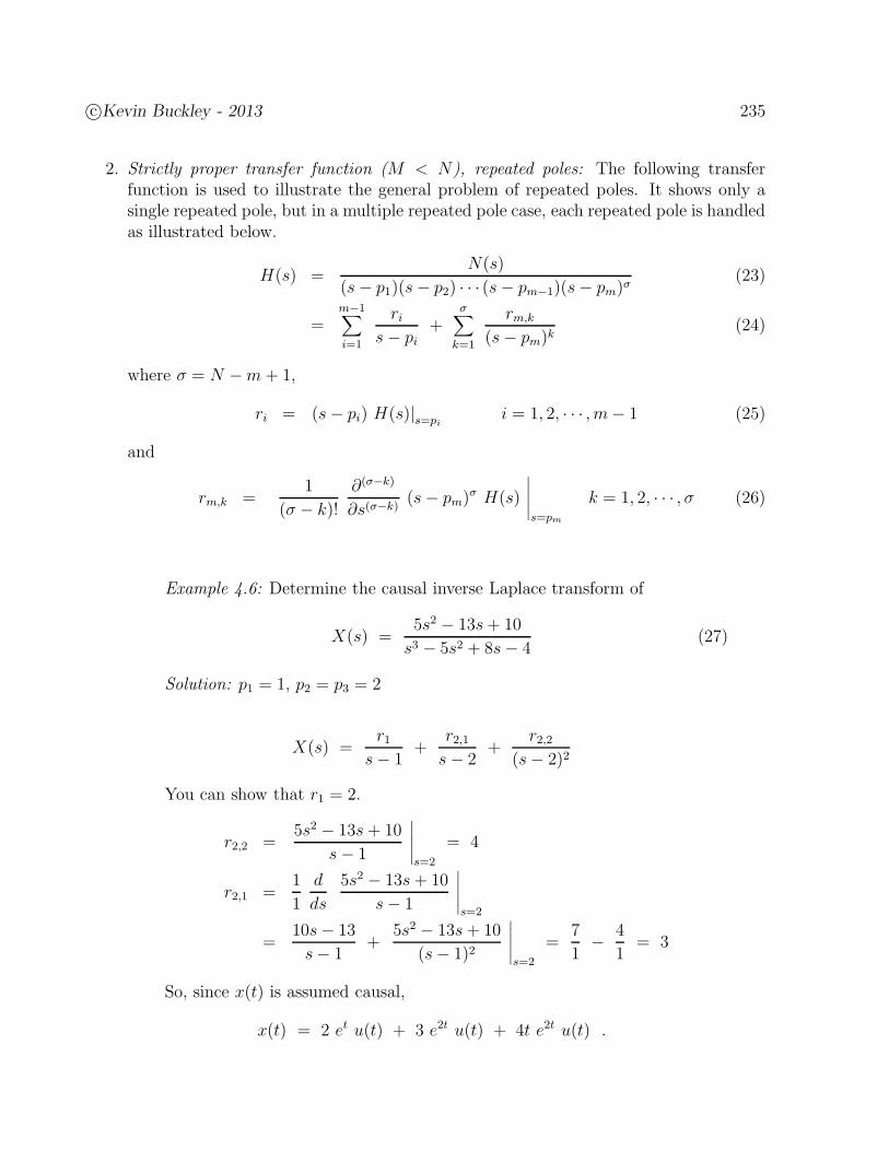
c©Kevin Buckley - 2013 235
2. Strictly proper transfer function (M < N), repeated poles: The following transferfunction is used to illustrate the general problem of repeated poles. It shows only asingle repeated pole, but in a multiple repeated pole case, each repeated pole is handledas illustrated below.
H(s) =N(s)
(s− p1)(s− p2) · · · (s− pm−1)(s− pm)σ(23)
=m−1∑
i=1
ris− pi
+σ∑
k=1
rm,k
(s− pm)k(24)
where σ = N −m+ 1,
ri = (s− pi) H(s)|s=pii = 1, 2, · · · , m− 1 (25)
and
rm,k =1
(σ − k)!
∂(σ−k)
∂s(σ−k)(s− pm)
σ H(s)
∣
∣
∣
∣
∣
s=pm
k = 1, 2, · · · , σ (26)
Example 4.6: Determine the causal inverse Laplace transform of
X(s) =5s2 − 13s+ 10
s3 − 5s2 + 8s− 4(27)
Solution: p1 = 1, p2 = p3 = 2
X(s) =r1
s− 1+
r2,1s− 2
+r2,2
(s− 2)2
You can show that r1 = 2.
r2,2 =5s2 − 13s+ 10
s− 1
∣
∣
∣
∣
∣
s=2
= 4
r2,1 =1
1
d
ds
5s2 − 13s+ 10
s− 1
∣
∣
∣
∣
∣
s=2
=10s− 13
s− 1+
5s2 − 13s+ 10
(s− 1)2
∣
∣
∣
∣
∣
s=2
=7
1− 4
1= 3
So, since x(t) is assumed causal,
x(t) = 2 et u(t) + 3 e2t u(t) + 4t e2t u(t) .

236 c©Kevin Buckley - 2013
3. Non strictly proper transfer function (M ≥ N): Use long division as follows
H(s) =N(s)
D(s)=
R(s)
D(s)+ P (s) (28)
where
P (s) (29)
D(s)√
N(s)
...
R(s) ←− order less than N
Example 4.7: Determine the causal inverse Laplace transform of
X(s) =s3 + 2s− 4
s2 + 4s− 2
Solution: Since M > N we must first perform long division until R(s) hasorder less than D(s)
s− 4
s2 + 4s+ 2√s3 + 2s− 4
s3 + 4s2 − 2s
−4s2 + 4s− 4
−4s2 − 16s+ 8
20s − 12
Thus,
X(s) =20s − 12
s2 + 4s− 2+ s − 4 .
The causal inverse BLT of this is
x(t) = L−1
20s − 12
s2 + 4s− 2
+d
dtδ(t) − 4 δ(t) .
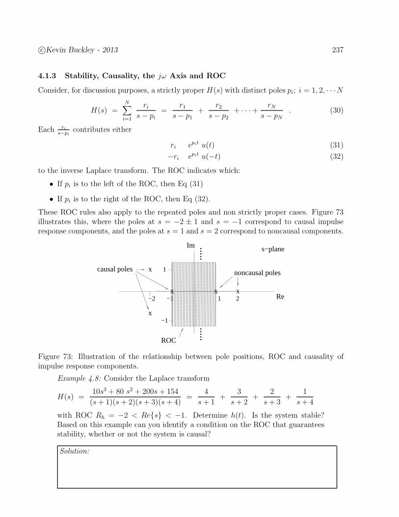
c©Kevin Buckley - 2013 237
4.1.3 Stability, Causality, the jω Axis and ROC
Consider, for discussion purposes, a strictly proper H(s) with distinct poles pi; i = 1, 2, · · ·N
H(s) =N∑
i=1
ris− pi
=r1
s− p1+
r2s− p2
+ · · ·+ rNs− pN
. (30)
Each ris−pi
contributes either
ri epit u(t) (31)
−ri epit u(−t) (32)
to the inverse Laplace transform. The ROC indicates which:
• If pi is to the left of the ROC, then Eq (31)
• If pi is to the right of the ROC, then Eq (32).
These ROC rules also apply to the repeated poles and non strictly proper cases. Figure 73illustrates this, where the poles at s = −2 ± 1 and s = −1 correspond to causal impulseresponse components, and the poles at s = 1 and s = 2 correspond to noncausal components.
x
x
x x
x
Re
.....
.....Im s−plane
−1
ROC
causal poles noncausal poles
−1−2 1 2
1
Figure 73: Illustration of the relationship between pole positions, ROC and causality ofimpulse response components.
Example 4.8: Consider the Laplace transform
H(s) =10s3 + 80 s2 + 200s+ 154
(s+ 1)(s+ 2)(s+ 3)(s+ 4)=
4
s+ 1+
3
s+ 2+
2
s+ 3+
1
s+ 4
with ROC Rh = −2 < Res < −1. Determine h(t). Is the system stable?Based on this example can you identify a condition on the ROC that guaranteesstability, whether or not the system is causal?
Solution:
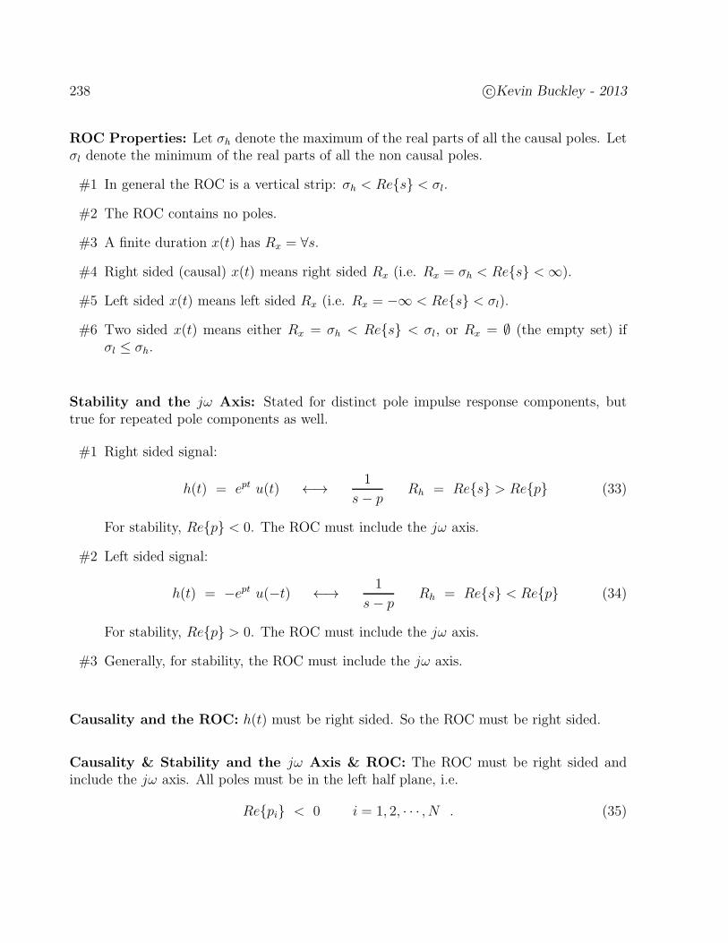
238 c©Kevin Buckley - 2013
ROC Properties: Let σh denote the maximum of the real parts of all the causal poles. Letσl denote the minimum of the real parts of all the non causal poles.
#1 In general the ROC is a vertical strip: σh < Res < σl.
#2 The ROC contains no poles.
#3 A finite duration x(t) has Rx = ∀s.
#4 Right sided (causal) x(t) means right sided Rx (i.e. Rx = σh < Res <∞).
#5 Left sided x(t) means left sided Rx (i.e. Rx = −∞ < Res < σl).
#6 Two sided x(t) means either Rx = σh < Res < σl, or Rx = ∅ (the empty set) ifσl ≤ σh.
Stability and the jω Axis: Stated for distinct pole impulse response components, buttrue for repeated pole components as well.
#1 Right sided signal:
h(t) = ept u(t) ←→ 1
s− pRh = Res > Rep (33)
For stability, Rep < 0. The ROC must include the jω axis.
#2 Left sided signal:
h(t) = −ept u(−t) ←→ 1
s− pRh = Res < Rep (34)
For stability, Rep > 0. The ROC must include the jω axis.
#3 Generally, for stability, the ROC must include the jω axis.
Causality and the ROC: h(t) must be right sided. So the ROC must be right sided.
Causality & Stability and the jω Axis & ROC: The ROC must be right sided andinclude the jω axis. All poles must be in the left half plane, i.e.
Repi < 0 i = 1, 2, · · · , N . (35)
c©Kevin Buckley - 2013 239
Example 4.9: Consider the transfer function
H(s) =2s+ 1
(s− 2)(s+ 3)=
1
s− 2+
1
s+ 3
Determine all possible impulse responses, and for each comment on stability andcausality.
Solution: The figure below shows the different regions of the s-plane that couldbe the ROC, depending on the causality/stability of the system.
x x
Ims
Res
s−plane
−3 2
Figure 74: s-plane illustration for Example 4.9.
Case 1: both poles are causal – the ROC is Res > 2
h(t) = e2t u(t) + e−3t u(t) .
The 1-st impulse response component is non stable.
Case 2: both poles are noncausal – the ROC is Res < −3
h(t) = −e2t u(−t) − e−3t u(−t) .
The 2-nd impulse response component is non stable.
Case 3: the s = −3 pole is causal, the s = 2 pole is noncausal – the ROC is−3 < Res < 2
h(t) = −e2t u(−t) − e−3t u(−t) .
Both impulse response components are stable.
Case 4: the s = −3 pole is noncausal, the s = 2 pole is causal – the ROC doesnot exist
h(t) = e2t u(t) − e−3t u(−t) .
Both impulse response component are non stable.

240 c©Kevin Buckley - 2013
4.1.4 Frequency Response and Pole/Zero Locations
In Subsection 4.1.1 we established that the frequency response H(jω) of a CT LTI systemis the transfer function H(s) evaluated “on the jω axis” – i.e. H(jω) = H(s)|s=jω. Thus,for any CT LTI system, the frequency response can be expressed in terms of its poles andzeros as
H(jω) =Y (jω)
X(jω)=
∑Mk=0 bk (jω)k
∑Nk=0 ak (jω)k
=N(jω)
D(jω)= G
∏Mi=1 (jω − zi)
∏Ni=1 (jω − pi)
. (36)
By properties of magnitudes and phases of sums and products of complex numbers, we havethat the magnitude response of a CT LTI system can be written as
|H(jω)| = |G|∏M
i=1 |jω − zi|∏N
i=1 |jω − pi|(37)
and the phase response as
6 H(jω) =M∑
k=1
6 (jω − zi) −N∑
k=1
6 (jω − pi) . (38)
These two equations show how pole and zero locations effect the magnitude and phaseresponse of an CT LTI. We will focus on the magnitude response below.
The magnitude response is obtained be evaluating the magnitude of the transfer function|H(s)| on the s = jω axis for −∞ ≤ ω ≤ ∞. Consider a zero zi which is close to the jω axisfor some ω0. For ω close to ω0, the numerator term |jω − zi| will be small, so |H(jω)| willbe close to zero. That’s why the zi are called zeros. On the other hand, consider a pole piwhich is close to the jω axis for some ω0. For ω close to ω0, the denominator term |jω − pi|will be small, so |H(jω)| will be large. That’s why the Pi are called poles – because the plotof |H(jω)| looks like a high pole close to ω0.
In Subsection 4.2.1 and Practicum 5a we will explore this relationship between CT LTIfrequency response and pole/zero locations using Matlab CT filter design capabilities. Belowwe consider using pole/zero placement to realize a notch filter.
Example 2.30: Figure 75 illustrates this magnitude response, pole/zero locationrelationship for a notch filter with transfer function
H(s) =(s− jω0)(s+ jω0)
(s− (−0.1− jω0))(s− (−0.1 + jω0)).
j
− 0.1
ω0−ω0−ω0
(a)
ω
H ( )ω
(b)
Re
Im
o
ox
x
ω0
Figure 75: (a) Pole/zero locations; and (b) frequency response for a CT notch filter.
c©Kevin Buckley - 2013 241
4.1.5 The Unilateral Laplace Transform and System Initial Conditions
Consider the differentiation property of the unilateral Laplace transform
dn
dtnx(t) = sn X (s) − sn−1x(0−) + sn−2x(1)(0−) + · · ·+ sx(n−2)(0−)+ x(n−1)(0−) . (39)
Using this and taking the unilateral Laplace transform of the CT LTI I/O LCC differentialequation of a causal system, for the 1-st order case,
y(1)(t) + a0y(t) = b0x(t) , (40)
we gets Y(s)− y(0−) + a0Y(s) = b0X (s) (41)
or, after moving things around (using algebra rules),
Y(s) =N(s)
D(s)X (s) +
C(s)
D(s). (42)
The first term on the right is due to the input and looks just like the bilateral Laplacetransform output expression (i.e. H(s) = N(s)
D(s)= b0
s+a0). The second term on the right is due
to initial conditions. D(s) = s + a0 is the transfer function denominator polynomial, andC(s) = y(0−).
For the 2-nd order case, assume x(0−) = 0., as in the Course test. We have
y(2)(t) + a1y(1)(t) + a0y(t) = b1x
(1)(t) + b0x(t) . (43)
Taking the unilateral Laplace transform, we get
s2Y(s)− sy(0−) + y(1)(0−)+ a1s Y(s)− a1y(0−) + a0Y(s) = b1sX (s) + b0X (s) (44)
or, after moving things around (using algebra rules)
Y(s) =N(s)
D(s)X (s) +
C(s)
D(s). (45)
Again, the first term on the right is due to the input and looks just like the bilateral Laplacetransform output expression (i.e. H(s) = N(s)
D(s)= b1s+b0
s2+a1s+a0). The second term on the right
is due to initial conditions. D(s) = s2 + sa1s + a0 is the transfer function denominatorpolynomial, and C(s) = y(0−)(s+ a1) + y(1)(0−).
The extension to an N -th order transfer function is straightforward.

242 c©Kevin Buckley - 2013
Example 4.10: Find the output of the causal CT LTI system
y(2)(t) + 3y(1)(t) + 2y(t) = x(t)
given input x(t) = 2u(t), y(0−) = 3 and y(1)(0−) = −5.
Solution:
Y(s) =1
s2 + 3s+ 2X (s) +
3(s+ 3) + (−5)s2 + 3s+ 2
.
The 1-st term on the right is due to the input. The 2-nd term is due to initialconditions. X (s) = 2
s. Performing PFE on each term,
Y(s) =(
1
s+
1
s+ 2− 2
s+ 1
)
+(
2
s + 2+
1
s + 1
)
.
Since the system is causal,
y(t) =(
u(t) + e−2t u(t) − 2e−t u(t))
+(
2e−2t u(t) + e−t u(t))
,
where again, the 1-st term is due to the input and the 2-nd term is due to initialconditions. Combining these, we have
y(t) = u(t) + 3e−2t u(t) − e−t u(t) .
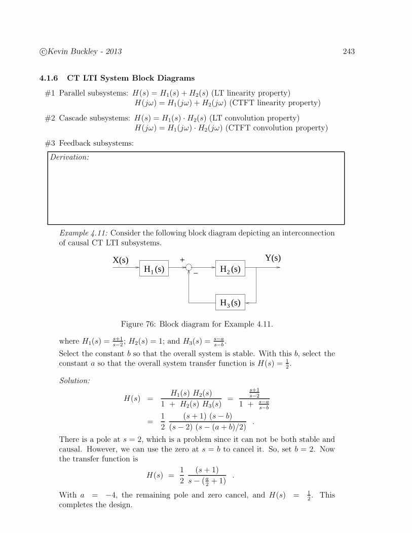
c©Kevin Buckley - 2013 243
4.1.6 CT LTI System Block Diagrams
#1 Parallel subsystems: H(s) = H1(s) +H2(s) (LT linearity property)H(jω) = H1(jω) +H2(jω) (CTFT linearity property)
#2 Cascade subsystems: H(s) = H1(s) ·H2(s) (LT convolution property)H(jω) = H1(jω) ·H2(jω) (CTFT convolution property)
#3 Feedback subsystems:
Derivation:
Example 4.11: Consider the following block diagram depicting an interconnectionof causal CT LTI subsystems.
1H (s) H (s)2
H (s)3
X(s) +
−
Y(s)
Figure 76: Block diagram for Example 4.11.
where H1(s) =s+1s−2
; H2(s) = 1; and H3(s) =s−as−b
.
Select the constant b so that the overall system is stable. With this b, select theconstant a so that the overall system transfer function is H(s) = 1
2.
Solution:
H(s) =H1(s) H2(s)
1 + H2(s) H3(s)=
s+1s−2
1 + s−as−b
=1
2
(s+ 1) (s− b)
(s− 2) (s− (a+ b)/2).
There is a pole at s = 2, which is a problem since it can not be both stable andcausal. However, we can use the zero at s = b to cancel it. So, set b = 2. Nowthe transfer function is
H(s) =1
2
(s+ 1)
s− (a2+ 1)
.
With a = −4, the remaining pole and zero cancel, and H(s) = 12. This
completes the design.

244 c©Kevin Buckley - 2013
Example 4.12: Consider a causal CT LTI system with transfer function
H(s) =2s2 + 5s+ 2
s3 + 2s2 + s.
For the following parallel three subsystem configuration, determine r1, r2, r3 , p1 , p2and p3.
r 1
s − p1
r 2
(s − p )2
2
s − p
r 3
3
x(t) y(t)+
+
+
Figure 77: Block diagram for Example 4.12.
Solution: This structure looks like it could be a direct parallel implementation ofthe PFE of H(s), where the pi are the poles and the ri the corresponding residuesof the system. Rooting the denominator polynomial, we have that p1 = p2 = −1and p3 = 0. With the repeated root, we have that
H(s) =r1
s− p1+
r2(s− p1)2
+r3
s− p3.
So the structure does implement the system. Performing the PFE, we get thatr1 = 0, r2 = 1 and r3 = 2. Thus the top path of this parallel structure is notrequired.
Note that, in general, the PFE of a transfer function H(s) describes a parallel implementa-tion of the system. On the other hand, by factoring H(s) into a product of lower order terms,using the pole/zero product factorizations of the numerator/denominator polynomials, wecan generate cascaded realizations of the system.

c©Kevin Buckley - 2013 245
4.2 Signal Processing Functions
This Course primarily concerns basic signal & systems tools, specifically transforms and con-volution. In the study of signal processing, what else is there? With a general understandingof convolution and several CT transforms we now have, it’s a good time to step back, lookat the bigger picture, address this question, and consider a few more-advanced topics.
There are various ways to categorize signals and systems issues. A useful one follows:
• Basic tools: Within the context of signals and systems, convolution and the transformscovered in this and the next Chapter are the basic tools. Of course, there are morebasic mathematical tools we commonly use such as: algebra, linear algebra, calculusand differential equations. Beyond this, we get into advanced tools and functions.
• More advanced tools: there are plenty of these, including: more advanced transforms(e.g. wavelets, time-frequency); stochastic modeling (dealing with randomness, whichwe overview in Chapter 7); and optimization (used, for example, in signal and systemdesign).
• Signal processing functions: these are the more advanced thing we do, across variousapplications, including: modulation, filtering, detection and classification, parameterestimation, spectral estimation, control, and sampling/reconstruction. These functionsall apply to one dimensional signals (e.g. a single sensor output), multidimensionalsignals (e.g. the output of multiple sensors), images and video.
• System design: this concerns the use of basic and more advanced tools to create systemsthat effectively perform the desired signal processing function.
• System implementation: we mentioned this category of signals and systems topics inthe introduction (see Section 1.1). Implementation topics include: circuits, electronics,digital hardware and software. Concerning all of these, we are interested in accuracy,reliability, flexibility, sustainability and cost.
• Applications: we also mentioned this category of signals and systems topics in the in-troduction. Spend a few minutes reminding yourself about some of these. As engineers,applications are the reason we are interested in signals and systems.
You can learn more about these topics in senior and graduate level courses either: here orat another educational institution; or less formally but perhaps more directedly in industry.Below we overview a few topics that cut across these categories.
246 c©Kevin Buckley - 2013
4.2.1 Filtering
In a broad context, filtering implies the separation of something into components, keepingsome and discarding others. Filters are prevalent both in nature and in the systems humanscreate. In the context of signal processing a filter is a system which separates a desired signalcomponent from a superimposed undesired component. For example, the signal might be theoutput of a sensor or sensor preamp, consisting of a desired signal superimposed with noiseand interfering signals. The filter operates on an input signal to pass the desired componentof the input with amplification or unit gain while attenuating undesired components. Tofilter the desired signal from the noise and interference, we must exploit differences betweenthem. Although, depending on the application, there are different signal characteristicsthat may be exploited to differentiate desired signal from noise and interference, a verycommon characteristic used is frequency content. If this is the case, then a LTI systemcan be effectively employed since, as we know from previous discussions, a LTI system hasfrequency selectivity – as determined by its frequency response.
We have already considered many examples of DT and CT LTI system frequency response.This Subsection provides a brief introduction to the practical implementation and design ofCT frequency selective filters. We will consider DT frequency selective filters in Chapter 4 ofthis Course. Frequency selective filter design and implementation is a principle topic severalsenior and graduates level courses (e.g. on microwave systems, digital signal processing,optimum and adaptive filtering).
From discussions earlier in this Chapter, we know that a CT LTI system effects anyfrequency component of an input signal x(t) as indicated by the system’s frequency response,denoted H(jω). That is, for any input signal
x(t) =1
2π
∫ ∞
−∞X(jω) ejωt dt , (46)
the CT LTI system output is
y(t) =1
2π
∫ ∞
−∞Y (jω) ejωt dt , (47)
where Y (jω) = X(jω) · H(jω). An important consequence of this is that we can considerhow a LTI system operates on each frequency component separately. Additionally, a LTIsystem does not output any frequency component that is not already in the input.
Considering the magnitudes and phases of the different signal components, we have thatthe output frequency components are weighted by the output CTFT
Y (jω) = |Y (jω)| ej 6 Y (jω) = |X(jω)| · |H(jω)| ej(6 X(jω)+ 6 H(jω)) . (48)
This shows how the magnitude and phase of the input are effected by the CT LTI system,and suggests that concerning frequency selective filtering we are in general interested in:
• the magnitude response - |H(jω)| vs. ω, or equivalently
• the magnitude-squared response, in dB - 10 log10|H(jω)|2 vs. ω; and
• the phase response - 6 H(jω) vs. ω, or equivalently
c©Kevin Buckley - 2013 247
• the group delay - τ(ω) = − ddω
6 H(jω).
Although in many applications the system’s phase response 6 H(jω) and group delay τ(ω)are important (e.g. in high fidelity audio phase distortion is undesirable), in this introductorydiscussion we will focus on magnitude |H(jω)| and magnitude-squared |H(jω)|2 responsessince these functions indicate frequency selectivity (i.e. they tell us which frequencies areamplified and which are attenuated). The magnitude-squared response is often plotted in dB,i.e. 10 log10|H(jω)|2, because it displays details of the response over a wide dynamic range.We begin with a sequence of examples which consider filters which have ideal frequencycharacteristics. This will motivate a subsequent discussion on filer specifications and design.
Example 4.13: Consider an ideal lowpass filter with frequency response
Hlp(jω) =
1 |ω| ≤ W0 |ω| > W
,
where W is called the cutoff frequency. Determine the impulse response hlp(t),the magnitude response |Hlp(jω)|, the phase response 6 Hlp(ω) and the groupdelay τlp(ω). Given these results, comment on the practicality of this filter.
Solution: From the CTFT table developed in Section 3.3, we have
hlp(t) = ICTFTHlp(jω) =sin(Wt)
πt.
By inspection, |Hlp(jω)| = Hlp(jω), 6 Hlp(jω) = 0, and τlp(ω) = 0.
This system has ideal frequency response characteristics since it passes low fre-quencies without magnitude or phase distortion while perfectly attenuating highfrequencies. However the system is not realizable because it is noncausal, withan impulse response that suggests that the current output is a function of theinput infinitely far into the future. Furthermore, although it may not be obviousgiven the foundation we have established in this Course, this system does notcorrespond to a LCC differential equation of finite order (since the frequencyresponse is not a rational function of (jω)). Thus, even if causal, it would notbe implementable as, for example, an RLC circuit with a finite number of com-ponents.

248 c©Kevin Buckley - 2013
Example 4.14: Consider the following filter with delay added in an attempt todeal with the causality problem uncovered in Example 4.13:
h(t) = hlp(t− τ1) .
Determine its magnitude and phase responses and its group delay. Comment onits realizability.
Solution: using the delay property of the CTFT, we have
H(jω) = Hlp(jω) e−jωτ1 . (49)
The delay introduces a phase term only, so does not effect the magnitude re-sponse. Thus,
|H(jω)| = Hlp(jω); 6 H(jω) = 6 Hlp(jω) − ωτ1 = − ωτ1 ,
and
τ(ω) = − d
dω6 H(jω) = − d
dω(−ωτ1) = τ1 .
Note that this system is still noncausal. So it is not realizable, although for largepositive τ1 most of the energy of the impulse response is in the causal range,which is perhaps an improvement. 6 H(jω) = τ1, which again implies no phasedistortion. (Constant group delay implies pure delay, which for example doesnot effect our perception of an acoustic signal.) This example provides someexperience with the consideration of group delay τ(ω).
Example 4.15: Consider an ideal highpass filter Hhp(jω) with zero phase responseand cutoff frequency W . Sketch this frequency response. Sketch the block di-agram of an implementation for this filter as a parallel of a ideal lowpass filterand a short circuit. Considering this implementation, and linearity, determinethe impulse response hhp(t). Comment on its realizability.
Solution:

c©Kevin Buckley - 2013 249
Example 4.16: Consider an ideal bandpass filterHbp(jω) with zero phase responseand passband W1 ≤ |ω| ≤W2. Sketch this frequency response. Sketch the blockdiagram of an implementation for this filter as a parallel of two ideal lowpassfilters. Considering this implementation, and linearity, determine the impulseresponse hbp(t). Comment on its realizability.
Solution:
Example 4.17: Consider an ideal bandstop filterHbs(jω) with zero phase responseand stopband W1 ≤ |ω| ≤W2. Sketch this frequency response. Sketch the blockdiagram of an implementation for this filter as a parallel of two ideal lowpassfilters and a short circuit. Considering this implementation, and linearity, deter-mine the impulse response hbs(t). Comment on its realizability.
Solution:

250 c©Kevin Buckley - 2013
Example 4.13-17 demonstrate that ideal frequency selective filters are not realizable. Thisfact has motivated the development of a considerable volume of results on frequency selectiveCT filter design. Basically, the frequency selective design procedure begins with a frequencyresponse specification and results with a filter transfer function and then a realization de-scription. We now illustrate a frequency response specification and provide a Matlab transferfunction design example. The topics of filter design and implementation are covered in seniorand graduate level courses.
Since ideal frequency selective filters are not realizable, we can realize only an approxima-tion of a desired ideal response. In CT filter design, we start with a set of specifications thatreflect the degree of accuracy which we require of this approximation. Figure 78 illustratesCT lowpass filter design specifications. Only positive frequencies are shown since we are tar-geting a real-valued coefficient transfer function, so that the frequency response is complexsymmetric. ωp and ωs are, respectively, the passband and stopband cutoff frequencies. δp andδs are, respectively, the passband and stopband tolerances. The frequency band ωp ≤ ω ≤ ωs
is called the transition band. Since no desired phase response characteristics are provided,the implication is that in this example we are not concerned with phase distortion.
Highpass, bandpass and bandstop filters frequency response specifications are similarlydescribed.
1 +
1 −
transition band
stopbandpassband
......δs
δp
δp
ωp ωs ω
| H( ) |ωj
Figure 78: Typical CT lowpass filter design specifications.
Matlab Demo: Matlab provides a wide variety of filter design functions, including a numberfor frequency selective filters. In this demo, a CT lowpass Butterworth is designed andevaluated. This filter will have a lowpass 3 dB cut-off frequency of ω = 1 rad/sec.. TheMatlab function freqs computes frequency response and can automatically plot its magnitudeand phase. In Matlab, type help freqs for more details and options for its use.
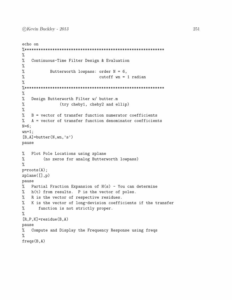
c©Kevin Buckley - 2013 251
echo on
%************************************************************
%
% Continuous-Time Filter Design & Evaluation
%
% Butterworth lowpass: order N = 6,
% cutoff wn = 1 radian
%
%************************************************************
%
% Design Butterworth Filter w/ butter.m
% (try cheby1, cheby2 and ellip)
%
% B = vector of transfer function numerator coefficients
% A = vector of transfer function denominator coefficients
N=6;
wn=1;
[B,A]=butter(N,wn,’s’)
pause
% Plot Pole Locations using zplane
% (no zeros for analog Butterworth lowpass)
%
p=roots(A);
zplane([],p)
pause
% Partial Fraction Expansion of H(s) - You can determine
% h(t) from results. P is the vector of poles.
% R is the vector of respective residues.
% K is the vector of long-devision coefficients if the transfer
% function is not strictly proper.
%
[R,P,K]=residue(B,A)
pause
% Compute and Display the Frequency Response using freqs
%
freqs(B,A)
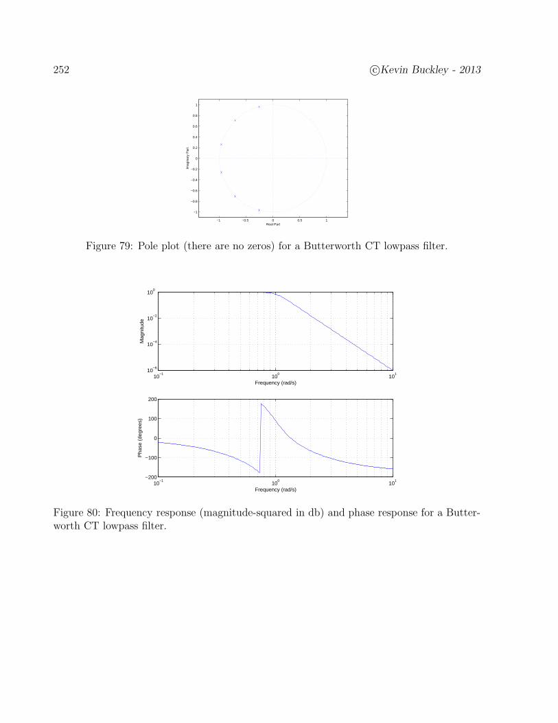
252 c©Kevin Buckley - 2013
−1 −0.5 0 0.5 1
−1
−0.8
−0.6
−0.4
−0.2
0
0.2
0.4
0.6
0.8
1
Real Part
Imag
inar
y P
art
Figure 79: Pole plot (there are no zeros) for a Butterworth CT lowpass filter.
10−1
100
101
−200
−100
0
100
200
Frequency (rad/s)
Pha
se (
degr
ees)
10−1
100
101
10−6
10−4
10−2
100
Frequency (rad/s)
Mag
nitu
de
Figure 80: Frequency response (magnitude-squared in db) and phase response for a Butter-worth CT lowpass filter.
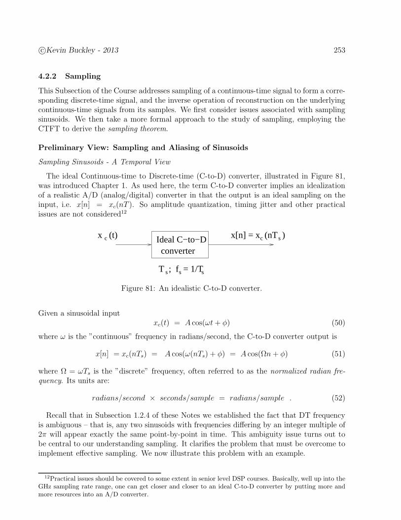
c©Kevin Buckley - 2013 253
4.2.2 Sampling
This Subsection of the Course addresses sampling of a continuous-time signal to form a corre-sponding discrete-time signal, and the inverse operation of reconstruction on the underlyingcontinuous-time signals from its samples. We first consider issues associated with samplingsinusoids. We then take a more formal approach to the study of sampling, employing theCTFT to derive the sampling theorem.
Preliminary View: Sampling and Aliasing of Sinusoids
Sampling Sinusoids - A Temporal View
The ideal Continuous-time to Discrete-time (C-to-D) converter, illustrated in Figure 81,was introduced Chapter 1. As used here, the term C-to-D converter implies an idealizationof a realistic A/D (analog/digital) converter in that the output is an ideal sampling on theinput, i.e. x[n] = xc(nT ). So amplitude quantization, timing jitter and other practicalissues are not considered12
converterIdeal C−to−Dx (t)c x[n] = x (nT )c
T ; f = 1/Ts s s
s
Figure 81: An idealistic C-to-D converter.
Given a sinusoidal inputxc(t) = A cos(ωt+ φ) (50)
where ω is the ”continuous” frequency in radians/second, the C-to-D converter output is
x[n] = xc(nTs) = A cos(ω(nTs) + φ) = A cos(Ωn+ φ) (51)
where Ω = ωTs is the ”discrete” frequency, often referred to as the normalized radian fre-quency. Its units are:
radians/second × seconds/sample = radians/sample . (52)
Recall that in Subsection 1.2.4 of these Notes we established the fact that DT frequencyis ambiguous – that is, any two sinusoids with frequencies differing by an integer multiple of2π will appear exactly the same point-by-point in time. This ambiguity issue turns out tobe central to our understanding sampling. It clarifies the problem that must be overcome toimplement effective sampling. We now illustrate this problem with an example.
12Practical issues should be covered to some extent in senior level DSP courses. Basically, well up into theGHz sampling rate range, one can get closer and closer to an ideal C-to-D converter by putting more andmore resources into an A/D converter.
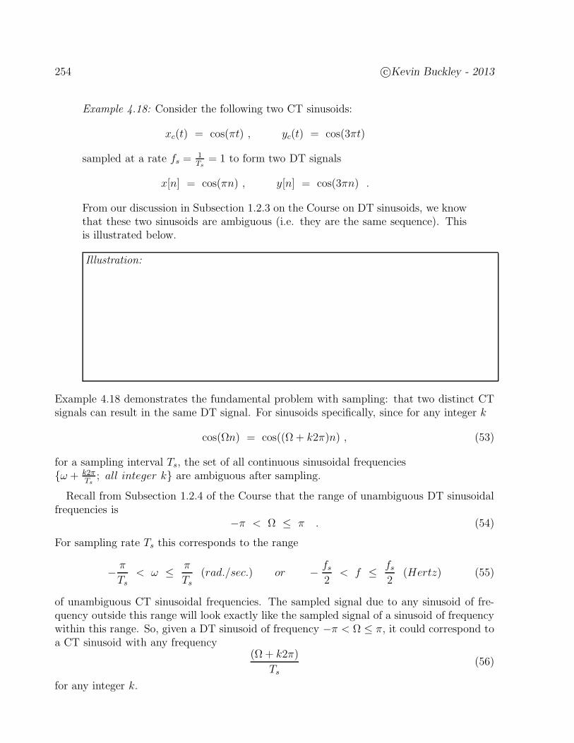
254 c©Kevin Buckley - 2013
Example 4.18: Consider the following two CT sinusoids:
xc(t) = cos(πt) , yc(t) = cos(3πt)
sampled at a rate fs =1Ts
= 1 to form two DT signals
x[n] = cos(πn) , y[n] = cos(3πn) .
From our discussion in Subsection 1.2.3 on the Course on DT sinusoids, we knowthat these two sinusoids are ambiguous (i.e. they are the same sequence). Thisis illustrated below.
Illustration:
Example 4.18 demonstrates the fundamental problem with sampling: that two distinct CTsignals can result in the same DT signal. For sinusoids specifically, since for any integer k
cos(Ωn) = cos((Ω + k2π)n) , (53)
for a sampling interval Ts, the set of all continuous sinusoidal frequenciesω + k2π
Ts; all integer k are ambiguous after sampling.
Recall from Subsection 1.2.4 of the Course that the range of unambiguous DT sinusoidalfrequencies is
−π < Ω ≤ π . (54)
For sampling rate Ts this corresponds to the range
− π
Ts< ω ≤ π
Ts(rad./sec.) or − fs
2< f ≤ fs
2(Hertz) (55)
of unambiguous CT sinusoidal frequencies. The sampled signal due to any sinusoid of fre-quency outside this range will look exactly like the sampled signal of a sinusoid of frequencywithin this range. So, given a DT sinusoid of frequency −π < Ω ≤ π, it could correspond toa CT sinusoid with any frequency
(Ω + k2π)
Ts
(56)
for any integer k.
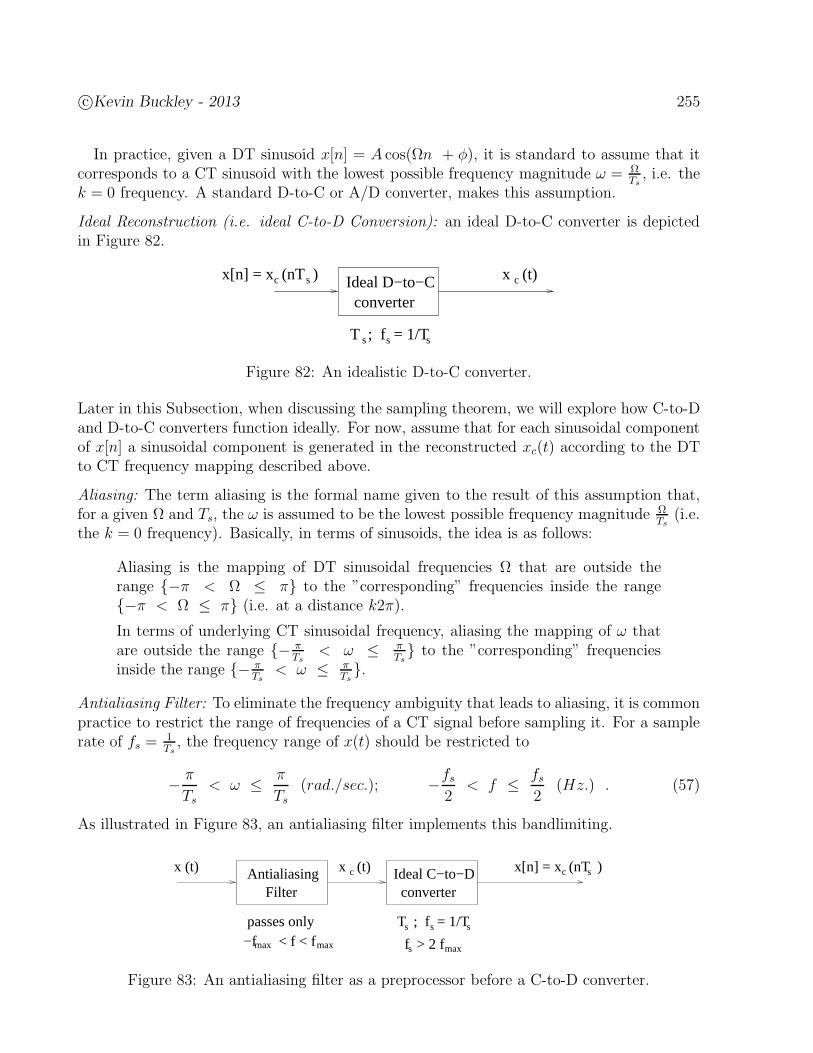
c©Kevin Buckley - 2013 255
In practice, given a DT sinusoid x[n] = A cos(Ωn + φ), it is standard to assume that itcorresponds to a CT sinusoid with the lowest possible frequency magnitude ω = Ω
Ts, i.e. the
k = 0 frequency. A standard D-to-C or A/D converter, makes this assumption.
Ideal Reconstruction (i.e. ideal C-to-D Conversion): an ideal D-to-C converter is depictedin Figure 82.
converterIdeal D−to−C cx[n] = x (nT )c
s sT ; f = 1/Ts
x (t)s
Figure 82: An idealistic D-to-C converter.
Later in this Subsection, when discussing the sampling theorem, we will explore how C-to-Dand D-to-C converters function ideally. For now, assume that for each sinusoidal componentof x[n] a sinusoidal component is generated in the reconstructed xc(t) according to the DTto CT frequency mapping described above.
Aliasing: The term aliasing is the formal name given to the result of this assumption that,for a given Ω and Ts, the ω is assumed to be the lowest possible frequency magnitude Ω
Ts(i.e.
the k = 0 frequency). Basically, in terms of sinusoids, the idea is as follows:
Aliasing is the mapping of DT sinusoidal frequencies Ω that are outside therange −π < Ω ≤ π to the ”corresponding” frequencies inside the range−π < Ω ≤ π (i.e. at a distance k2π).
In terms of underlying CT sinusoidal frequency, aliasing the mapping of ω thatare outside the range − π
Ts< ω ≤ π
Ts to the ”corresponding” frequencies
inside the range − πTs
< ω ≤ πTs.
Antialiasing Filter: To eliminate the frequency ambiguity that leads to aliasing, it is commonpractice to restrict the range of frequencies of a CT signal before sampling it. For a samplerate of fs =
1Ts, the frequency range of x(t) should be restricted to
− π
Ts
< ω ≤ π
Ts
(rad./sec.); −fs2
< f ≤ fs2
(Hz.) . (57)
As illustrated in Figure 83, an antialiasing filter implements this bandlimiting.
AntialiasingFilter
sx[n] = x (nT )cIdeal C−to−Dconverter
cx (t)
passes only T ; f = 1/Ts
x (t)
−f < f < fmax sf > 2 fss
max max
Figure 83: An antialiasing filter as a preprocessor before a C-to-D converter.
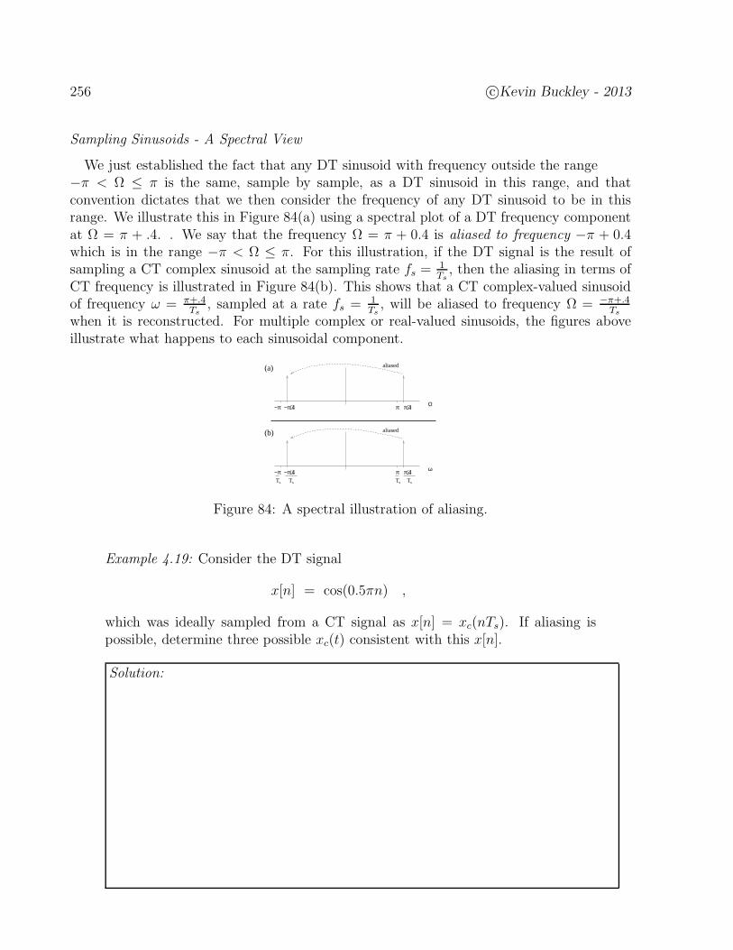
256 c©Kevin Buckley - 2013
Sampling Sinusoids - A Spectral View
We just established the fact that any DT sinusoid with frequency outside the range−π < Ω ≤ π is the same, sample by sample, as a DT sinusoid in this range, and thatconvention dictates that we then consider the frequency of any DT sinusoid to be in thisrange. We illustrate this in Figure 84(a) using a spectral plot of a DT frequency componentat Ω = π + .4. . We say that the frequency Ω = π + 0.4 is aliased to frequency −π + 0.4which is in the range −π < Ω ≤ π. For this illustration, if the DT signal is the result ofsampling a CT complex sinusoid at the sampling rate fs =
1Ts, then the aliasing in terms of
CT frequency is illustrated in Figure 84(b). This shows that a CT complex-valued sinusoidof frequency ω = π+.4
Ts, sampled at a rate fs = 1
Ts, will be aliased to frequency Ω = −π+.4
Ts
when it is reconstructed. For multiple complex or real-valued sinusoids, the figures aboveillustrate what happens to each sinusoidal component.
aliased
Ω−π −π+.4 π π+.4
Ts TsTs Ts
aliased
−π −π+.4 π π+.4 ω
(a)
(b)
Figure 84: A spectral illustration of aliasing.
Example 4.19: Consider the DT signal
x[n] = cos(0.5πn) ,
which was ideally sampled from a CT signal as x[n] = xc(nTs). If aliasing ispossible, determine three possible xc(t) consistent with this x[n].
Solution:
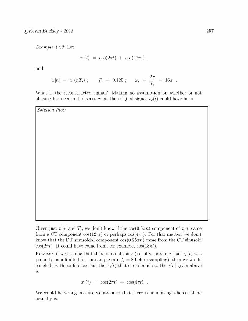
c©Kevin Buckley - 2013 257
Example 4.20: Let
xc(t) = cos(2πt) + cos(12πt) ,
and
x[n] = xc(nTs) ; Ts = 0.125 ; ωs =2π
Ts
= 16π .
What is the reconstructed signal? Making no assumption on whether or notaliasing has occurred, discuss what the original signal xc(t) could have been.
Solution Plot:
Given just x[n] and Ts, we don’t know if the cos(0.5πn) component of x[n] camefrom a CT component cos(12πt) or perhaps cos(4πt). For that matter, we don’tknow that the DT sinusoidal component cos(0.25πn) came from the CT sinusoidcos(2πt). It could have come from, for example, cos(18πt).
However, if we assume that there is no aliasing (i.e. if we assume that xc(t) wasproperly bandlimited for the sample rate fs = 8 before sampling), then we wouldconclude with confidence that the xc(t) that corresponds to the x[n] given aboveis
xc(t) = cos(2πt) + cos(4πt) .
We would be wrong because we assumed that there is no aliasing whereas thereactually is.
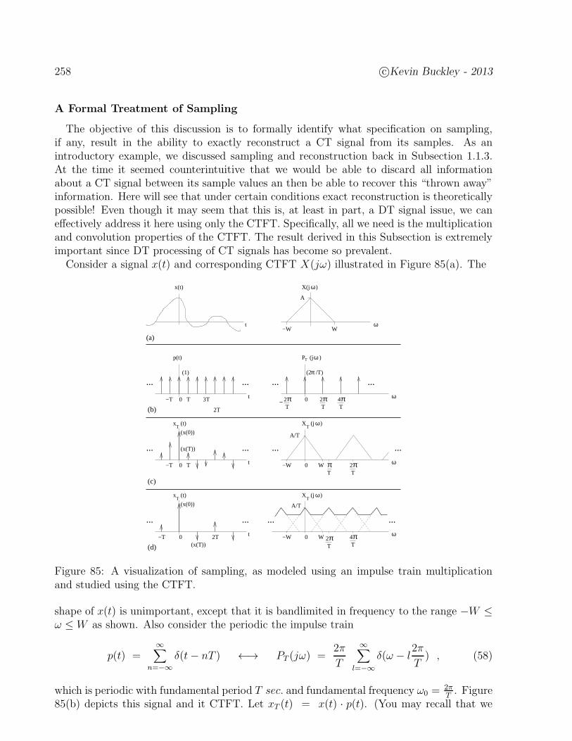
258 c©Kevin Buckley - 2013
A Formal Treatment of Sampling
The objective of this discussion is to formally identify what specification on sampling,if any, result in the ability to exactly reconstruct a CT signal from its samples. As anintroductory example, we discussed sampling and reconstruction back in Subsection 1.1.3.At the time it seemed counterintuitive that we would be able to discard all informationabout a CT signal between its sample values an then be able to recover this “thrown away”information. Here will see that under certain conditions exact reconstruction is theoreticallypossible! Even though it may seem that this is, at least in part, a DT signal issue, we caneffectively address it here using only the CTFT. Specifically, all we need is the multiplicationand convolution properties of the CTFT. The result derived in this Subsection is extremelyimportant since DT processing of CT signals has become so prevalent.
Consider a signal x(t) and corresponding CTFT X(jω) illustrated in Figure 85(a). The
π(2 /T)
2Tπ2
Tπ−
Tπ4
t0
......
x (t)T
(x(0))
T
(x(T))
−T
2Tπ
Tπ4
Tπ 2
Tπ0
...
TX (j )ω
A/T
−W W ω
...
ω
X(j )ω
t
x(t)
A
W−W
(a)
(b)
(c)
0
......
ω
p(t)
0
......(1)
T−T
2T
3T
(d)
t0
......
x (t)T
(x(0))
0
TX (j )ω
−W W ω−T(x(T))
2T
...
A/T
...
P (j )ω
t
T
Figure 85: A visualization of sampling, as modeled using an impulse train multiplicationand studied using the CTFT.
shape of x(t) is unimportant, except that it is bandlimited in frequency to the range −W ≤ω ≤W as shown. Also consider the periodic the impulse train
p(t) =∞∑
n=−∞δ(t− nT ) ←→ PT (jω) =
2π
T
∞∑
l=−∞δ(ω − l
2π
T) , (58)
which is periodic with fundamental period T sec. and fundamental frequency ω0 =2πT. Figure
85(b) depicts this signal and it CTFT. Let xT (t) = x(t) · p(t). (You may recall that we
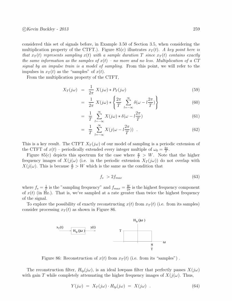
c©Kevin Buckley - 2013 259
considered this set of signals before, in Example 3.50 of Section 3.5, when considering themultiplication property of the CTFT.). Figure 85(c) illustrates xT (t). A key point here isthat xT (t) represents sampling x(t) with a sample duration T since xT (t) contains exactlythe same information as the samples of x(t) – no more and no less. Multiplication of a CTsignal by an impulse train is a model of sampling. From this point, we will refer to theimpulses in xT (t) as the “samples” of x(t).
From the multiplication property of the CTFT,
XT (jω) =1
2πX(jω) ∗ PT (jω) (59)
=1
2πX(jω) ∗
2π
T
∞∑
l=−∞δ(ω − l
2π
T)
(60)
=1
T
∞∑
l=−∞X(jω) ∗ δ(ω − l
2π
T) (61)
=1
T
∞∑
l=−∞X(j(ω − l
2π
T)) . (62)
This is a key result. The CTFT XT (jω) of our model of sampling is a periodic extension ofthe CTFT of x(t) – periodically extended every integer multiple of ω0 =
2πT.
Figure 85(c) depicts this spectrum for the case where πT
> W . Note that the higherfrequency images of X(j(ω) (i.e. in the periodic extension XT (jω)) do not overlap withX(j(ω). This is because π
T> W which is the same as the condition that
fs > 2fmax (63)
where fs =1Tis the ”sampling frequency” and fmax = W
2πis the highest frequency component
of x(t) (in Hz.). That is, we’ve sampled at a rate greater than twice the highest frequencyof the signal.
To explore the possibility of exactly reconstructing x(t) from xT (t) (i.e. from its samples)consider processing xT (t) as shown in Figure 86.
H (j )lp ωx (t)T y(t)
T
H (j )lp ω
ω
Tπ
Figure 86: Reconstruction of x(t) from xT (t) (i.e. from its “samples”) .
The reconstruction filter, Hlp(jω), is an ideal lowpass filter that perfectly passes X(jω)with gain T while completely attenuating the higher frequency images of X(j(ω). Thus,
Y (jω) = XT (jω) ·Hlp(jω) = X(jω) . (64)
260 c©Kevin Buckley - 2013
That is, y(t) = x(t). We have perfectly reconstructed x(t) from its “samples”. The require-ments are fs > 2fmax (which implies that x(t) is bandlimited), and the use of an ideallowpass reconstruction filter.
Figure 85(d) illustrates what happens when fmax > fs2. The higher frequency images of
X(jω) in the periodic extension XT (jω) overlap with X(jω). So X(jω) can not be separatedfrom these other images, and thus x(t) can not be reconstructed from its “samples”. If thisis the case, and we attempt to reconstruct x(t) as illustrated in Figure 86, we will notproduce the original x(t). The frequency content we will get is as illustrated by XT (jω) inFigure 85(d). After lowpass filtering, we will have the part of XT (jω) over − π
T≤ ω ≤ π
T.
We observe that in this range that some of the higher frequencies in X(jω) are mapped tolower frequencies. For example, if x(t) and y(t) are audio signals, some of the higher pitchcomponents in x(t) will sound like lower pitch components in y(t). As with the sampling ofsinusoids, we call this effect aliasing. Aliasing is bad. Very, very bad!
The Sampling Theorem: So, to reconstruct a signal from its “samples”, one mustsample the signal at a sample rate fs which is at least twice the highest frequency fmax ofthe signal. fs = 2 · fmax is termed the Nyquist rate. If a signal is sampled at at least itsNyquist rate, we have shown that it can be reconstructed by ideal lowpass filtering. In otherwords,
x(t) = xT (t) ∗ hlp(t) (65)
where
hlp(t) = Tsin( π
Tt)
πt(66)
is the ICTFT of Hlp(jω). So,
x(t) = xT (t) ∗ hlp(t) =
∞∑
n=−∞x(nT ) δ(t− nT )
∗ Tsin( π
Tt)
πt(67)
=∞∑
n=−∞x(nT )
δ(t− nT ) ∗ Tsin( π
Tt)
πt
(68)
=∞∑
n=−∞x(nT )
sin( πT(t− nT ))
πT(t− nT )
. (69)
Eq (69) shows that x(t) can be reconstructed from its samples x(nT ); n = 0, ±1, ±2, · · ·as an interpolation between the samples using the interpolation function hlp(t). This is calledthe sampling theorem.

c©Kevin Buckley - 2013 261
Example 4.21: Let xc(t) = Aπ50
sin2(50πt)(πt)2
. Determine the CTFT of the re-
constructed signal for sampling rates of fs = 100 samples/second and fs =75 samples/second.
Solution:
262 c©Kevin Buckley - 2013
4.2.3 Modulation
We begin this Subsection with a discussion on Amplitude Modulation (AM), which exploreson a basic level how AM radio is implemented. This discussion motivates a set of basic signalprocessing tasks which are commonly found in many applications. These tasks (movingsignals around in frequency, selecting certain frequency components, and quantifying theselected signal) correspond to the modulation, filtering and Parseval’s theorem propertiesof the CTFT. We close this Subsection with several examples which employ these threeproperties.
Amplitude Modulation
The modulation property of the CTFT tells us that if multiply a signal by a sinusoid offrequency ω0, then we shift its frequency content by ω0. Mathematically, we have alreadyestablished that
y(t) = x(t) ejω0t ←→ Y (jω) = X(j(ω − ω0)) , (70)
x(t) cos(ω0t) ←→ 1
2X(j(ω − ω0)) + X(j(ω + ω0)) , (71)
and
x(t) sin(ω0t) ←→ 1
2jX(j(ω − ω0)) − X(j(ω + ω0)) . (72)
In applications such as broadcast radio (e.g. AM and FM), cell phones, RADAR, SONAR,astrophysical exploration and ultrasound imaging, to name just a few, we wish to move thefrequency content of a signals of interest to different frequencies. So some form of modulationis a central function in many applications. Beyond this, modulation is very commonly usedin signal processing systems as part of a strategy to reduce implementational complexity,thereby reducing cost and/or improving performance.If you look into the detailed descriptionof a spectrum analyzer, speech processor or audio system, for example, you may very wellobserve that one or more modulators are employed. So if you enroll in an advanced signalprocessing or signal processing application course, you will likely see a lot of modulation. Inthis Subsection we briefly overview one important application, Amplitude Modulation (AM)radio.
Synchronous AM Communications
Consider the simple modulation scheme shown in Figure 87(a). In the context of com-munications (e.g. radio), x(t) is called the information signal which is bandlimited to−ωm ≤ ω ≤ ωm (e.g. for speech, ωm = 2π4000 is assumed). cos(ωct) is termed the carrierwhere ωc is the carrier frequency. The resulting signal y(t), the modulated or transmissionsignal, would be amplified and transmitted over a communication channel. We call thisamplitude modulation because the information signal is transmitted as the amplitude of thetransmitted sinusoidal carrier.
Figure 87(b) illustrates the information and modulated signal frequency content. Since thecarrier is a real-valued sinusoid, the information signal frequency content is translated bothup and down in frequency by ωc. (Note that, as illustrated, X(jω) is complex symmetricsince we will assume x(t) is real-valued. Then y(t) is also real-valued, and Y (jω) is complex

c©Kevin Buckley - 2013 263
ωcy(t) = x(t) cos( t)
ωccos( t)
x(t)
mωm−ω
H (j )lp ω
ω
2
H (j )lp ω1x (t)
ωc φccos( t + )
y(t) w(t)
ωm−ωm
ωX(j )
ωcωc−ωm
ωY(j )
2ωc−2ωc
A2
cφcos( )
ωm
(a) (c)
(b)
ω
A
A/2
ω−ωc
ωW(j )
ω
(d)
Figure 87: AM modulation.
symmetric.) The motivation of this modulation scheme is that it is necessary (either byallocation and/or performance considerations) for the information signal to be transmittedover the frequency range ωc − ωm ≤ |ω| ≤ ωc + ωm.
Now consider the demodulation scheme shown in Figure 87(b). It consists of anothermodulator (to translate the information signal in frequency back to its original location) anda lowpass filter whose purpose is identified below. The received signal is assumed to be y(t).Thus we are ignoring possible channel distortion and noise. (Although in practice channeldistortion and noise may require a more sophisticated receiver, the demodulation principledepicted in this scheme still represents the primary receiver function.) The output of thereceiver modulator is
w(t) = x(t) cos(ωct) cos(ωct + φc) (73)
= x(t)(
1
2cos(φc)
)
+ x(t)(
1
2cos(2ωc + φc)
)
. (74)
The phase φc represents the fact that the receiver local oscillator in general may not bephase synchronous with the received carrier. Again as dictated by the modulation propertyof the CTFT, the frequency content of w(t) will be as illustrated in Fig 87(d). It consists ofthe information signal’s original spectrum, scaled by 1
scos(φc), plus a term modulated up to

264 c©Kevin Buckley - 2013
frequency 2ωc. After lowpass filtering to remove the 2ωc component of w(t), we have
x1(t) = x(t) cos(φc) . (75)
For φc = 0, i.e. for the receiver oscillator synchronized with the transmitter oscillator,x1(t) = x(t). Regardless of synchronization, the output is a scaled version of the input, sothat in the absence of channel distortion and noise, we get exactly what we want.
Asynchronous AM Communications
The problem with the AM receiver depicted in Figure 87(b) is that if φc 6= 0, x1(t)might be a significant attenuation of x(t). In fact, for φc =
π2, for example, the information
signal is completely absent in w(t) and x1(t). In the presence of channel noise, cos(φc) ≈ 0would render the received signal useless. There are receiver circuits, such as phased-lockedloops, that can be used to assure that φc ≈ 0. However for commercial AM radio thesecircuits are considered to be too expensive to implement in a radio receiver. Thus, inpractice, an alternative approach to AM radio reception is employed. Below, very brieflydescribe the idea behind the practical receiver commonly used for AM broadcast reception.Although there is not much to this receiver in terms of demonstration of transform theory,the value of a transform domain analysis of AM modulation/demodulation has nonethelessbeen established.
As an alternative to the synchronous AM scheme discussed earlier, consider the transmittershown below in Figure 88(a). The multiplier value A is selected such that A > |x(t)| forall t for any expected x(t). The transmitted signal y(t) is the carrier with an amplitude(termed the envelope) which has the shape of the information signal. An example y(t) isshown in Figure 88(b). Its spectrum is illustrated in Figure 88(c). Figure 88(d) shows aninexpensive circuit that is commonly used to demodulate the received signal, extracting theenvelope from the carrier, and the resulting signal x1(t) is illustrated in Figure 88(b). Besidesa DC component that can be subsequently removed, and some undesirable fast changes(high frequency components) that can be smoothed out (lowpass filtered), this output is anacceptable received signal for (low fidelity) AM radio.

c©Kevin Buckley - 2013 265
ωcωc−ωm
ωY(j )
A/2
ω−ωcωm−ωm
ωX(j )
ω
A
ωccos( t)
ωcy(t) = (A+x(t)) cos( t)
y(t) x (t)1
(b)
(a)
(c)
x(t)
A
+
t
(d)
y(t)
x (t)1
A+x(t)
Figure 88: A practical asynchronous AM transmitter and receiver.
Modulation, Filtering and Parseval’s Theorem Examples
Example 4.22: Consider the system below.
a) Sketch the CTFT’s of x(t), v(t) and y(t), showing peak magnitudes andcut-off frequencies.
b) How can m(t) be recovered from y(t)?
This is just another look a synchronous AM radio.
cos(50 t)π cos(50 t)π
ω
ω
10 π−10 π
M (j )
1
ω
ω
1
H (j )
30 π−30 π
m(t) 1 + m(t)H (j )ω
y(t)v(t)x(t)
1
Figure 89: System for Example 4.22.

266 c©Kevin Buckley - 2013
Solution:

c©Kevin Buckley - 2013 267
Example 4.23: Consider the following system with input x(t).
a) Sketch, showing frequency cutoffs and peak values, Y (jω), Z(jω) and V (jω).
b) Determine the energy of v(t).
ωX(j )
ω
10
10−10
ω
ω
1
5−5
H (j )1 ω
ω
H (j )2
10
1
ej 10 t
x(t)ωH (j )1
y(t)ωH (j )2
z(t) v (t)
Figure 90: System for Example 4.23.
Solution:
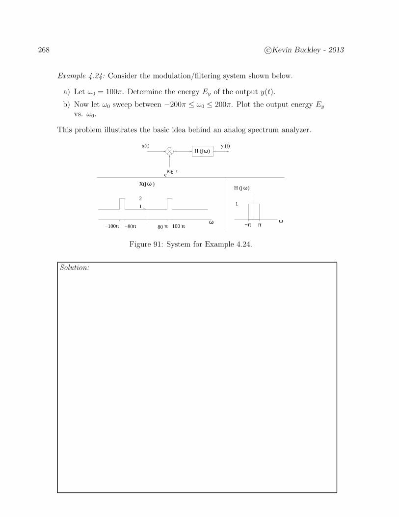
268 c©Kevin Buckley - 2013
Example 4.24: Consider the modulation/filtering system shown below.
a) Let ω0 = 100π. Determine the energy Ey of the output y(t).
b) Now let ω0 sweep between −200π ≤ ω0 ≤ 200π. Plot the output energy Ey
vs. ω0.
This problem illustrates the basic idea behind an analog spectrum analyzer.
ωX(j )
−100π −80π 100π80π
ωοej t
x(t)H (j )ω
y (t)
ω
2
1
ω
1
H (j )ω
π−π
Figure 91: System for Example 4.24.
Solution:

c©Kevin Buckley - 2013 269
Example 4.25: Consider the system below.
a) Sketch the CTFT of v(t), showing center & cutoff frequencies, and ampli-tudes.
b) Specify ω0 and the filter frequency response H(jω) so y(t) = x1(t) (i.e. sothat x1(t) is received). For this ω0, sketch the CTFT of r(t) and y(t).
c) Instead of b), let ω0 = 12, 500π (i.e. the receiver is mis-tuned), and assumethat the filter H(jω) is ideal lowpass with a gain of one over the bandbetween ±2500π. Sketch the CTFT of r(t) and y(t).
This example illustrates the basic idea behind multiuser broadcast radio.
πcos(10,000 t)
1x (t)
ω0cos( t )
ω
X (j )ω1
−2,500 π 2,500 π
1
x (t)
π
2
cos(15,000 t)
H (j )ωr(t) y(t)v(t) = v (t) + v (t)
1v (t)
2
1 2
v (t)
ω
ω
−2,500 π 2,500 π
1
X (j )2
Figure 92: System for Example 4.25.
Solution:

270 c©Kevin Buckley - 2013
4.2.4 RLC Circuits
In your basic circuits course, you learned the following voltage/current relationships for thethree basic circuits elements:
v(t) = R i(t) (resistor) (76)
v(t) = Ld
dti(t) (inductor) (77)
v(t) =1
C
∫ t
−∞i(τ) dτ (capacitor) . (78)
Taking the bilateral Laplace transform of these equations, we have:
V (s) = R I(s) (resistor) (79)
V (s) = Ls I(s) (inductor) (80)
V (s) =1
CsI(s) (capacitor) . (81)
This leads to the Laplace domain circuit diagram representations shown in Figure 93.
+
−R
+
−L s s C
1+
−
(b)(a) (c)
Figure 93: Laplace transform representation of: (a) a resistor; (b) an inductor; (c) a capac-itor.
The next two Examples illustrate the usefulness of these representations in directly an-alyzing the circuit transfer function. In following these Examples keep in mind how theextension of the analysis procedure to higher order (more energy storage element) circuitswound be systematic. It essentially reduces to analysis to that of a pure resistor circuit, soloop and node differential/integral equations are replaced with algebraic equations.
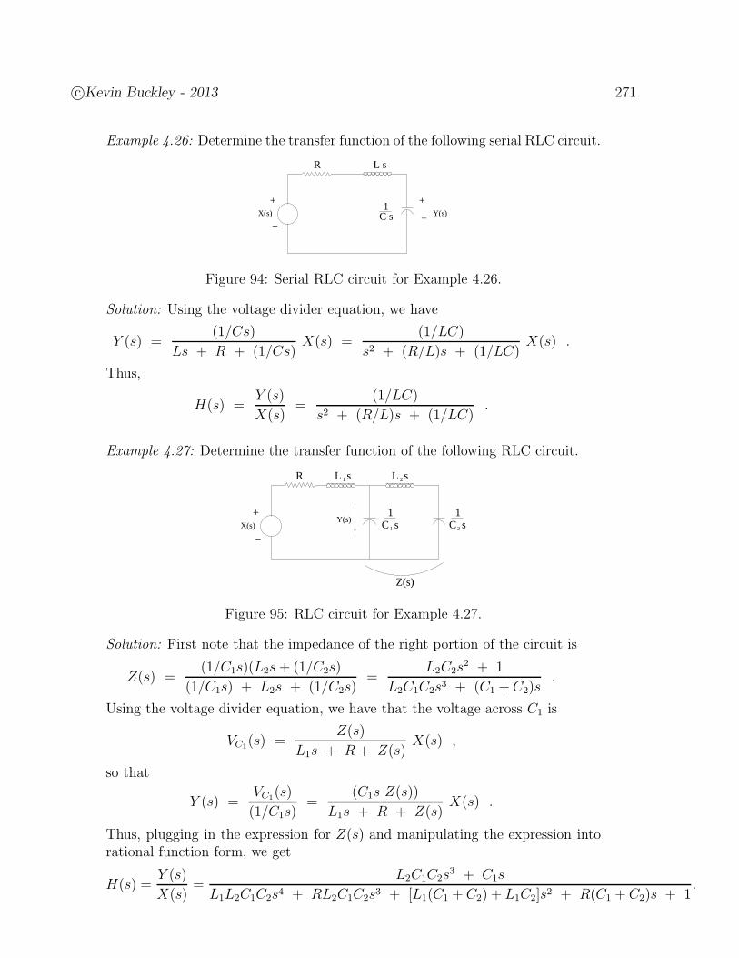
c©Kevin Buckley - 2013 271
Example 4.26: Determine the transfer function of the following serial RLC circuit.
C s1
+
−
+
−
R
X(s) Y(s)
L s
Figure 94: Serial RLC circuit for Example 4.26.
Solution: Using the voltage divider equation, we have
Y (s) =(1/Cs)
Ls + R + (1/Cs)X(s) =
(1/LC)
s2 + (R/L)s + (1/LC)X(s) .
Thus,
H(s) =Y (s)
X(s)=
(1/LC)
s2 + (R/L)s + (1/LC).
Example 4.27: Determine the transfer function of the following RLC circuit.
1L s
C s1
12C s1+
−
R
X(s)
L s2
Y(s)
Z(s)
Figure 95: RLC circuit for Example 4.27.
Solution: First note that the impedance of the right portion of the circuit is
Z(s) =(1/C1s)(L2s+ (1/C2s)
(1/C1s) + L2s + (1/C2s)=
L2C2s2 + 1
L2C1C2s3 + (C1 + C2)s.
Using the voltage divider equation, we have that the voltage across C1 is
VC1(s) =Z(s)
L1s + R + Z(s)X(s) ,
so that
Y (s) =VC1(s)
(1/C1s)=
(C1s Z(s))
L1s + R + Z(s)X(s) .
Thus, plugging in the expression for Z(s) and manipulating the expression intorational function form, we get
H(s) =Y (s)
X(s)=
L2C1C2s3 + C1s
L1L2C1C2s4 + RL2C1C2s3 + [L1(C1 + C2) + L1C2]s2 + R(C1 + C2)s + 1.
272 c©Kevin Buckley - 2013
4.2.5 Spectrum Estimation
See Practicums 4(a) & 4(b) for an introductory experience on this topic. If you take theBiomedical Signal Processing Course, you will learn much more about this topic.

c©Kevin Buckley - 2013 273
4.3 Practicum 4a
Continuous Time Fourier Series (CTFS) & an Initial Consideration of Spectrum Analysis
Reporting Requirements: Follow report instructions for Practicum 1.
IntroductionIn this practicum you will study the representation of CT periodic signals using the CTFS.
Specifically, you will see, via Matlab, how periodic signals can be built as weighted sums ofsinusoids. You will examine the effect of representing a periodic signal using only some ofthe terms of its CTFS expansion. Finally, you will study the effect that modification of theCTFS coefficients has on a periodic signal.
To simplify coding and interpretation, in this practicum we will consider a real-valuedsignal and its CTFS in cosine (i.e. trigonometric) form. For a real-valued periodic signalwith period T and fundamental frequency ω0 = 2π/T, the CTFS can be written as
x(t) = a0 + 2∞∑
k=1
|ak| cos(kω0t+ 6 ak) (1)
where the ak as the exponential CTFS coefficients
ak =1
T
∫ T
0x(t)e−jkω0tdt . (2)
Specifically, we will consider a periodic signal x(t) with period T = 4 which is defined overone period as
x(t) = (4 − t) 0 ≤ t ≤ 4 (3)
Its CTFS coefficients are
ak =
2 k = 0−j2kπ
= 2kπ
e−jπ/2 otherwise(4)
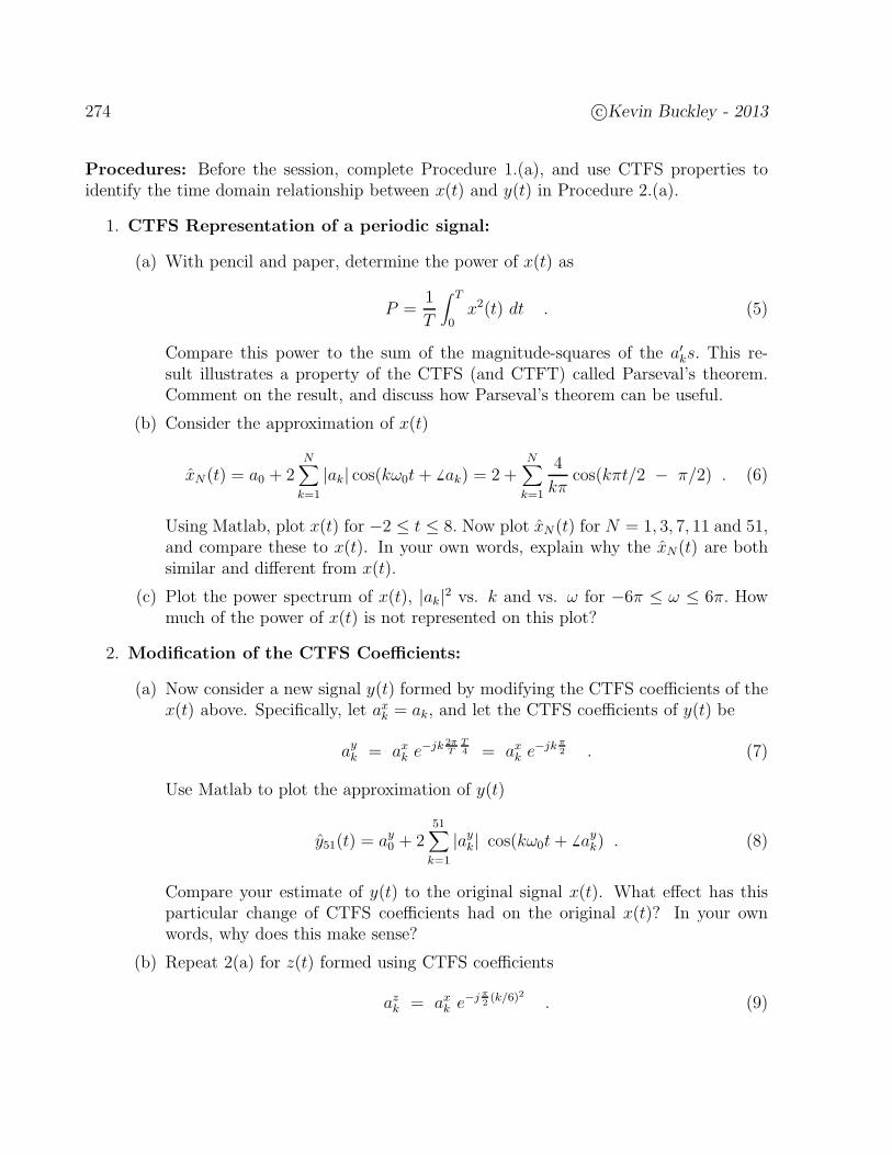
274 c©Kevin Buckley - 2013
Procedures: Before the session, complete Procedure 1.(a), and use CTFS properties toidentify the time domain relationship between x(t) and y(t) in Procedure 2.(a).
1. CTFS Representation of a periodic signal:
(a) With pencil and paper, determine the power of x(t) as
P =1
T
∫ T
0x2(t) dt . (5)
Compare this power to the sum of the magnitude-squares of the a′ks. This re-sult illustrates a property of the CTFS (and CTFT) called Parseval’s theorem.Comment on the result, and discuss how Parseval’s theorem can be useful.
(b) Consider the approximation of x(t)
xN (t) = a0 + 2N∑
k=1
|ak| cos(kω0t+ 6 ak) = 2 +N∑
k=1
4
kπcos(kπt/2 − π/2) . (6)
Using Matlab, plot x(t) for −2 ≤ t ≤ 8. Now plot xN (t) for N = 1, 3, 7, 11 and 51,and compare these to x(t). In your own words, explain why the xN(t) are bothsimilar and different from x(t).
(c) Plot the power spectrum of x(t), |ak|2 vs. k and vs. ω for −6π ≤ ω ≤ 6π. Howmuch of the power of x(t) is not represented on this plot?
2. Modification of the CTFS Coefficients:
(a) Now consider a new signal y(t) formed by modifying the CTFS coefficients of thex(t) above. Specifically, let axk = ak, and let the CTFS coefficients of y(t) be
ayk = axk e−jk 2πT
T4 = axk e−jk π
2 . (7)
Use Matlab to plot the approximation of y(t)
y51(t) = ay0 + 251∑
k=1
|ayk| cos(kω0t+ 6 ayk) . (8)
Compare your estimate of y(t) to the original signal x(t). What effect has thisparticular change of CTFS coefficients had on the original x(t)? In your ownwords, why does this make sense?
(b) Repeat 2(a) for z(t) formed using CTFS coefficients
azk = axk e−j π2(k/6)2 . (9)
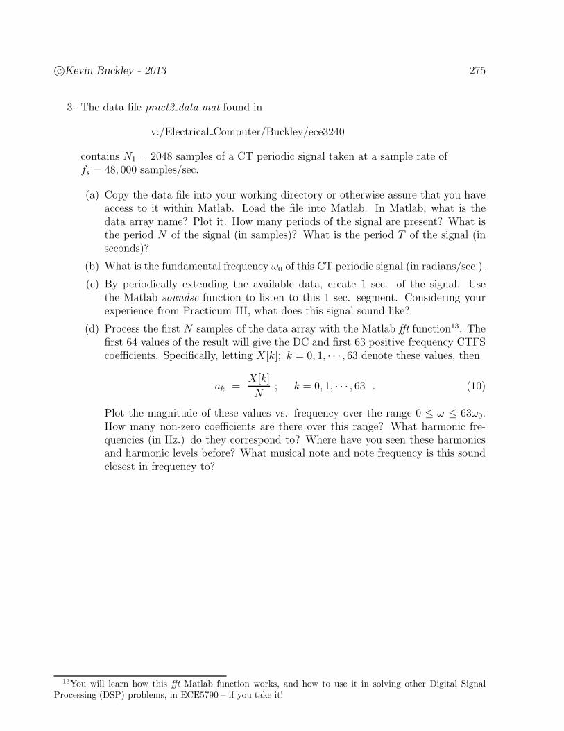
c©Kevin Buckley - 2013 275
3. The data file pract2 data.mat found in
v:/Electrical Computer/Buckley/ece3240
contains N1 = 2048 samples of a CT periodic signal taken at a sample rate offs = 48, 000 samples/sec.
(a) Copy the data file into your working directory or otherwise assure that you haveaccess to it within Matlab. Load the file into Matlab. In Matlab, what is thedata array name? Plot it. How many periods of the signal are present? What isthe period N of the signal (in samples)? What is the period T of the signal (inseconds)?
(b) What is the fundamental frequency ω0 of this CT periodic signal (in radians/sec.).
(c) By periodically extending the available data, create 1 sec. of the signal. Usethe Matlab soundsc function to listen to this 1 sec. segment. Considering yourexperience from Practicum III, what does this signal sound like?
(d) Process the first N samples of the data array with the Matlab fft function13. Thefirst 64 values of the result will give the DC and first 63 positive frequency CTFScoefficients. Specifically, letting X [k]; k = 0, 1, · · · , 63 denote these values, then
ak =X [k]
N; k = 0, 1, · · · , 63 . (10)
Plot the magnitude of these values vs. frequency over the range 0 ≤ ω ≤ 63ω0.How many non-zero coefficients are there over this range? What harmonic fre-quencies (in Hz.) do they correspond to? Where have you seen these harmonicsand harmonic levels before? What musical note and note frequency is this soundclosest in frequency to?
13You will learn how this fft Matlab function works, and how to use it in solving other Digital SignalProcessing (DSP) problems, in ECE5790 – if you take it!

276 c©Kevin Buckley - 2013
Practicum 4aInstructor/TA Sign Off Sheet, & Report Form
Student’s Name:
1. Procedure 1(a): derive the power of x(t)
2. Procedure 1(b): plots of xN (t); N = 1, 3, 7, 11, 51
3. Procedure 1(c): plots of |axk|2 vs. k and |axk|2 vs. ω
4. Procedure 2(a): write down the equation relating y(t) and x(t)
5. Procedures 2(a,b): plots of y51(t) and z51(t)

c©Kevin Buckley - 2013 277
.
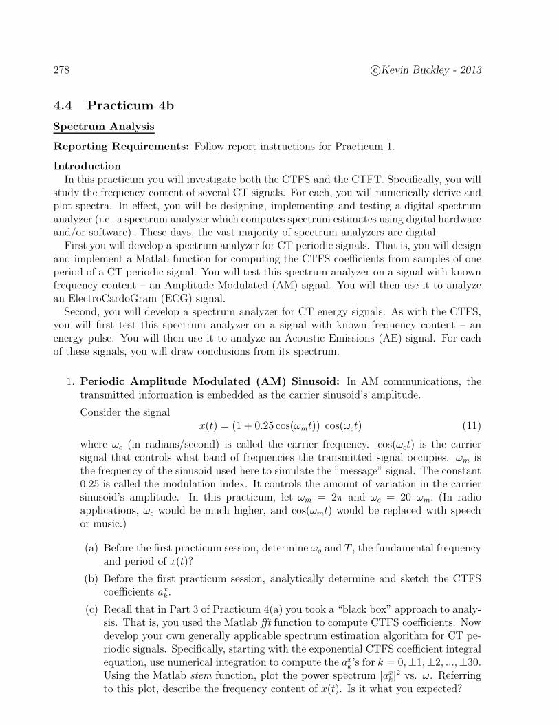
278 c©Kevin Buckley - 2013
4.4 Practicum 4b
Spectrum Analysis
Reporting Requirements: Follow report instructions for Practicum 1.
IntroductionIn this practicum you will investigate both the CTFS and the CTFT. Specifically, you will
study the frequency content of several CT signals. For each, you will numerically derive andplot spectra. In effect, you will be designing, implementing and testing a digital spectrumanalyzer (i.e. a spectrum analyzer which computes spectrum estimates using digital hardwareand/or software). These days, the vast majority of spectrum analyzers are digital.
First you will develop a spectrum analyzer for CT periodic signals. That is, you will designand implement a Matlab function for computing the CTFS coefficients from samples of oneperiod of a CT periodic signal. You will test this spectrum analyzer on a signal with knownfrequency content – an Amplitude Modulated (AM) signal. You will then use it to analyzean ElectroCardoGram (ECG) signal.
Second, you will develop a spectrum analyzer for CT energy signals. As with the CTFS,you will first test this spectrum analyzer on a signal with known frequency content – anenergy pulse. You will then use it to analyze an Acoustic Emissions (AE) signal. For eachof these signals, you will draw conclusions from its spectrum.
1. Periodic Amplitude Modulated (AM) Sinusoid: In AM communications, thetransmitted information is embedded as the carrier sinusoid’s amplitude.
Consider the signalx(t) = (1 + 0.25 cos(ωmt)) cos(ωct) (11)
where ωc (in radians/second) is called the carrier frequency. cos(ωct) is the carriersignal that controls what band of frequencies the transmitted signal occupies. ωm isthe frequency of the sinusoid used here to simulate the ”message” signal. The constant0.25 is called the modulation index. It controls the amount of variation in the carriersinusoid’s amplitude. In this practicum, let ωm = 2π and ωc = 20 ωm. (In radioapplications, ωc would be much higher, and cos(ωmt) would be replaced with speechor music.)
(a) Before the first practicum session, determine ωo and T , the fundamental frequencyand period of x(t)?
(b) Before the first practicum session, analytically determine and sketch the CTFScoefficients axk.
(c) Recall that in Part 3 of Practicum 4(a) you took a “black box” approach to analy-sis. That is, you used the Matlab fft function to compute CTFS coefficients. Nowdevelop your own generally applicable spectrum estimation algorithm for CT pe-riodic signals. Specifically, starting with the exponential CTFS coefficient integralequation, use numerical integration to compute the axk’s for k = 0,±1,±2, ...,±30.Using the Matlab stem function, plot the power spectrum |axk|2 vs. ω. Referringto this plot, describe the frequency content of x(t). Is it what you expected?
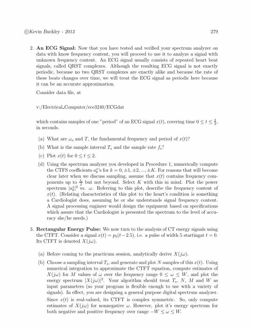
c©Kevin Buckley - 2013 279
2. An ECG Signal: Now that you have tested and verified your spectrum analyzer ondata with know frequency content, you will proceed to use it to analyze a signal withunknown frequency content. An ECG signal usually consists of repeated heart beatsignals, called QRST complexes. Although the resulting ECG signal is not exactlyperiodic, because no two QRST complexes are exactly alike and because the rate ofthese beats changes over time, we will treat the ECG signal as periodic here becauseit can be an accurate approximation.
Consider data file, at
v:/Electrical Computer/ece3240/ECGdat
which contains samples of one ”period” of an ECG signal x(t), covering time 0 ≤ t ≤ 23,
in seconds.
(a) What are ωo and T , the fundamental frequency and period of x(t)?
(b) What is the sample interval Ts and the sample rate fs?
(c) Plot x(t) for 0 ≤ t ≤ 2.
(d) Using the spectrum analyzer you developed in Procedure 1, numerically computethe CTFS coefficients axk’s for k = 0,±1,±2, ...,±K. For reasons that will becomeclear later when we discuss sampling, assume that x(t) contains frequency com-ponents up to fs
2but not beyond. Select K with this in mind. Plot the power
spectrum |axk|2 vs. ω. Referring to this plot, describe the frequency content ofx(t). (Relating characteristics of this plot to the heart’s condition is somethinga Cardiologist does, assuming he or she understands signal frequency content.A signal processing engineer would design the equipment based on specificationswhich assure that the Cardiologist is presented the spectrum to the level of accu-racy she/he needs.)
3. Rectangular Energy Pulse: We now turn to the analysis of CT energy signals usingthe CTFT. Consider a signal x(t) = p5(t−2.5), i.e. a pulse of width 5 startingat t = 0.Its CTFT is denoted X(jω).
(a) Before coming to the practicum session, analytically derive X(jω).
(b) Choose a sampling interval Ts, and generate and plotN samples of this x(t). Usingnumerical integration to approximate the CTFT equation, compute estimates ofX(jω) for M values of ω over the frequency range 0 ≤ ω ≤ W , and plot theenergy spectrum |X(jω)|2. Your algorithm should treat Ts, N , M and W asinput parameters (so your program is flexible enough to use with a variety ofsignals). In effect, you are designing a general purpose digital spectrum analyzer.
Since x(t) is real-valued, its CTFT is complex symmetric. So, only computeestimates of X(jω) for nonnegative ω. However, plot it’s energy spectrum forboth negative and positive frequency over range −W ≤ ω ≤W.
280 c©Kevin Buckley - 2013
The idea is to compute an accurate estimate of X(jω) without resorting to ex-cessive computation. Select Ts, N , M and W (the analysis bandwidth) so as toobtain an accurate estimate of X(jω). Justify your choices of the design param-eters, and compare your plot to the known |X(jω)|2.In effect, you have employed your general purpose digital spectrum analyzer toperform analysis on a specific signal of interest.
(c) In retrospect, can the general purpose spectrum analyzer you developed in thisprocedure for CT energy signals be used to analyze CT periodic signals?
4. AE Signal: The data file
v:/Electrical Computer/ece3240/AEdat
contains a dense sampling of an AE signal y(t) over its duration 0 ≤ t ≤ .8 msec..This signal was measured using a small acoustic sensor attached to a piece of metal asit was bent so as to cause cracking.
(a) What is the spacing Ts between samples.
(b) Plot y(t) vs. time. Select values of Ts, N, M and W .
(c) Using the analyzer and analysis procedure you developed in Procedure 3., nu-merically compute samples of its CTFT Y (jω), and plot the energy spectrum|Y (jω)|2. As in Procedure 3., the plot should be over both positive and negativefrequency. Justify your choice of analysis parameters. From the plot, describethe frequency content of the signal. Compare characteristics of the spectrum (e.g.frequency positions of spectral peaks) to characteristics of the AE signal (e.g. thefrequency of oscillation).

c©Kevin Buckley - 2013 281
.

282 c©Kevin Buckley - 2013
Practicum 4b: Spectrum AnalysisInstructor/TA Sign Off Sheet, & Report Form
Student’s Name:
For this Practicum, attach all plots requiring sign off below.
1. Procedure 1(a,b): write down T and ω0. “Analytically” derive the axk’s (e.g. using theCTFS equation or Table 6 of the Course Notes), and sketch them vs. ω.
2. Procedure 1(c): numerically computed |axk|2 vs. ω plot
3. Procedure 1(c): Are you convinced that your spectrum analyzer is functioning cor-rectly?
4. Procedure 2(a): Record ω0 and T for this signal . Also, record thesampling interval Ts and rate fs for this data .
5. Procedure 2(a): For reasons that will become clear to you later in the Course whenwe study sampling, assume that x(t) contains frequency components up to fs
2but no
higher. With this in mind, determine the highest harmonic, K, that you will computea CTFS coefficient for .
6. Procedure 2(b,c): x(t), and numerically computed |axk|2 vs. ω plots
7. Procedure 2(c): Comment on the frequency content of the ECG signal.

c©Kevin Buckley - 2013 283
8. Procedure 3(a): “Analytically” derive (e.g. using the CTFT equation or Table 7 ofthe Coruse Notes), and sketch X(jω).
9. Procedure 3 (a,b): write down your selected values for T, N, M and W .Explain your choices.
10. Procedures 3(b): plot of numerically computed |X(jω)|2
11. Procedures 3(b): Are you convinced that your spectrum analyzer is functioning cor-rectly? . Are you comfortable with your selected values of T, N, M and W ,and your rationale for them?
12. Procedures 4(b): Write down and explain your choice for values of T, N, M and W .
13. Procedures 4(c): plots of y(t) and numerically computed |Y (jω)|2Discuss your time-domain vs. frequency-domain comparison (i.e. how are characteris-tics in one domain manifested in the other).
284 c©Kevin Buckley - 2013
4.5 Problems
Chapter Topics:4.1-21 (CT transforms and LTI systems);4.22-26 (ideal filters);4.27-41 (sampling sinusoids & the sampling theorem);4.42-51 (modulation, filtering and Parseval’s theorem);4.52-59 (circuits)
1. Consider a CT LTI system with impulse response
h(t) =sin(10πt)
πt
and input x(t) =∑∞
n=−∞ p1/6(t− 13n). Determine the percentage of input power that
makes it to the output.
2. Consider a CT LTI system with zero initial conditions and impulse response
h(t) =sin(10πt)
πtcos(20πt)
and input x(t) =∑∞
n=−∞ δ(t− 0.25n). Determine the output power Py.
3. Consider the CT LTI system
y(2)(t) + 9 y(t) = x(1)(t) + 2 x(t)
(assume h(t) is right sided), and input
x(t) = 4 e−2t u(t) .
(a) Determine the system transfer function H(s).
(b) Determine the impulse response h(t).
(c) Determine the output y(t) (assuming zero initial conditions).
4. Consider the causal DT LTI system with I/O LCC differential equation
y(2)(t) + 3 y(1)(t) + 2 y(t) = x(2)(t) + 4 x(1)(t) + 3 x(t) .
This system has zeros z1 = −1 and z2 = −3 and poles p1 = −1 and p2 = −2.
a) Determine the transfer function H(s). Simplify it as much as possible.
b) From H(s), determine the impulse response h(t). (Hint: Consider the BLT linear-ity and differentiation properties. It is important to complete a) properly first.)
5. Consider a CT LTI system with transfer function
H(s) =1
(s+ 2)(s+ 4)(s− 1− j5)(s− 1 + j5).
c©Kevin Buckley - 2013 285
(a) If the system is causal, what is the ROC? Is the system stable? Explain youranswers.
(b) If the system is stable, what is the ROC? Is the system causal? Explain youranswers.
(c) Given that s = −3 is in the ROC, is the system causal? Is the system stable?Explain your answers.
6. A LTI system has impulse response h(t) = u(t) + e−2t cos(3t)u(t). Determine thedifferential equation that relates input x(t) and output y(t).
7. The following problems are independent of each other.
(a) Determine the CTFTs of x1(t) = 2 p10(t− 10) and x2(t) = 2 sin(5t)πt
. Which hasmore energy? Why?
(b) Determine the inverse BLT of
X(s) =2s
s2 + 5s+ 6=
6
s+ 3− 4
s+ 2Rx = Res > −2 . (12)
(c) Determine the BLT, Y (s) and ROC Ry, of y(t) = 6 e−3tu(t) + 4 e−2tu(−t).Write Y (s) as a single rational function.
8. Consider a causal CT LTI system for which input x(t) = δ(t) + 2 e−4tu(t) resultsin output y(t) = e−4tu(t) − e−6tu(t). Determine the system transfer function H(s)and the impulse response h(t).
9. Basic CT LTI Systems and Transforms:
(a) Consider the CT LTI system described by the following LCC differential equation
2y(3)(t) − 5y(1)(t) + y(t) = x(3)(t) + x(2)(t) + x(1)(t) .
Determine H(jω).
(b) Consider a CT LTI system with transfer function
H(s) =1
(s+ 2)(s− 4).
i. If the system is causal, what is the ROC? Is the system stable? Explain youranswers.
ii. If the system is stable, what is the ROC? Is the system causal? Explain youranswers.
iii. Given that s = −3 is in the ROC, is the system causal? Is the system stable?Explain your answers.
10. Consider a CT LTI system with transfer function
H(s) =s+ 10
(s+ 2)(s+ 4)Rh = Res > −2 .
286 c©Kevin Buckley - 2013
(a) What is the system frequency response?
(b) What is the system I/O differential equation?
(c) What are the system poles and zeros?
(d) Derive the partial fraction expansion of H(s). Show all steps and intermediateresults, or get no credit.
(e) What is the system impulse response?
(f) Is the system stable? Why? Causal? Why?
11. Consider the following causal CT LTI system
y(2)(t) + 6 y(1)(t) + 9 y(t) = 8 x(t) .
Given zero initial conditions, its output is y(t) = 4024
t4 e−3t u(t). Determine its inputx(t). (Note that s2 + 6s+ 9 = (s+ 3)2.)
12. Consider a CT LTI system with the following I/O differential equation:
y(3)(t) − y(1)(t) = 2 x(2)(t) − 8 x(t) . (13)
This system is causal with poles p1 = 0, p2 = 1 and p3 = −1.
(a) Is this system stable? Why?
(b) Determine the transfer function H(s), along with its ROC.
(c) Determine the impulse response h(t). Show all work in forming the PFE.
13. Consider a causal CT LTI system with I/O differential equation
y(2)(t) + y(1)(t) − 20 y(t) = x(1)(t) − 58 x(t) . (14)
This system has poles at s = 4 and s = −5.
(a) Determine its transfer function H(s).
(b) Determine its impulse response h(t). Show all work for the required PFE.
(c) Is this system stable? Explain your answer in terms of the impulse response. Ifunstable, which pole causes the instability? What is the characteristic of this polethat results in the instability?
14. A CT LTI system has transfer function H(s) = 20100−s2
.
(a) What is its frequency response H(jω)?
(b) Given input x1(t) = 4 cos(10t), determine the output y1(t).
(c) Given output y2(t) = 4 cos(10t), determine the input x2(t).
c©Kevin Buckley - 2013 287
15. Consider a CT LTI system with input
x(t) = −3 e−3t u(t) + 4 e−4t u(t)
and resulting output
y(t) = − e−t u(t) + 2 e−2t u(t) .
Determine the system transfer function, input/output differential equation and impulseresponse.
16. Consider a CT LTI system. You know that an input x(t) with Bilateral LaplaceTransform (BLT)
X(s) =4s + 10
(s+ 2)(s+ 1); ROC = Res > −1
results in output y(t) = e−2tu(t).
(a) Derive the partial fraction expansion of X(s). Show all steps and intermediateresults, or get no credit.
(b) Determine the input x(t).
(c) Determine the BLT of y(t).
(d) Determine the system’s transfer function H(s) and ROC.
(e) Determine the system’s I/O differential equation.
(f) Is the system stable? Why?
(g) (3-pts. extra credit) Determine the impulse response h(t).
17. Consider a causal CT LTI system with I/O differential equation
y(1)(t) + 2 y(t) = x(1)(t) + 4 x(t) .
Given zero initial conditions, the output is observed to be
y(t) = δ(t) − 2 e−3tu(t) .
What is the input x(t)?
18. Consider a causal LTI CT system with I/O differential equation
d
dty(t) + 4y(t) =
d
dtx(t) + 3x(t)
with input x(t) = 3e−3tu(t) − 2e−2tu(t) and initial conditions x(0−) = 0 andy(0−) = −2. Determine the output for t ≥ 0.
19. Consider a CT LTI multipath communications channel
y(t) = x(t− 0.5) + x(t− 2.5) .
288 c©Kevin Buckley - 2013
(a) What is the impulse response h(t) of this channel (i.e. y(t) = h(t) for x(t) = δ(t))?
(b) What is the frequency response H(jω) of the channel? (Hint: to assist with part(c), think of using the delay property and an Euler identity.)
(c) Plot the magnitude and phase of the frequency response over −2π ≤ ω ≤ 2π.
(d) If x(t) = cos(π2t) is transmitted through the channel, what is the output y(t)?
What do your answers to part (b) and (c) suggest about the problem with com-munications through multipath channels?
(e) If the output is y(t) = 5 cos(2πt), what is the input x(t)?
20. Consider the following CT LTI system composed of CT LTI subsystems with transferfunctions
H1(s) =1
s+ 3; H2(s) =
1
s+ 5; H3(s) =
1
s+ (1 + j); H4(s) =
1
s+ (1− j).
(a)H (s)1
(b) (c)+
+
H (s)3
H (s)4
H (s)2
x(t) y(t)
(a) Determine the transfer function from node (b) to node (c).
(b) Assuming that there is no pole/zero cancellation when combining these subsys-tems into the overall system (from node (a) to node (c)), what are the poles ofthe overall system?
(c) If the overall system is causal, is it stable? Why?
21. For each system description on the left, determine the one system description on theright which is equivalent to it.
c©Kevin Buckley - 2013 289
h(t) = ej10πt u(t) a H(jω) = 2π δ(ω − 10π)
H(jω) = 20ω2+100
b y(2)(t)− 100 y(t) = −20 x(t)
h(t) = u(t) c h(t) = cos(10πt)
H(jω) = 10π100π2−ω2 d y(1)(t) = x(t)
h(t) = ej10πt e y(1)(t)− j10π y(t) = x(t)
y(2)(t) + 10 y(t) = x(t) f h(t) = sin(10πt) u(t)
H(jω) = πδ(ω + 10π) + πδ(ω − 10π) g H(s) = 1s2+10
; Rh = Res > 0
h H(s) = 1s−10π
; Rh = Res < 0
i poles : p1,2 = ±10π; Rh = Ims > 5
22. Given an input x(t) = e−|t| to a CT LTI system with ideal lowpass filter frequencyresponse H(jω) = p2(ω), determine the percentage of input energy that makes it tothe output. You may have use for the indefinite integral
∫
1
(1 + ω2)2dω =
ω
2(1 + ω2)+
1
2tan−1(ω)
and the facts that tan−1(1) = π4and tan−1(0) = 0.
23. Given a LTI system with frequency response H(jω) = p12(ω), determine the outputy(t), and its energy & power, for the following inputs:
(a) x(t) = cos(12t).
(b) x(t) = cos(12t) u(t).
(c) x(t) = cos(12t) · sinc(6t/π).
24. Use the CTFT synthesis equation to derive the impulse response of each of the followingideal frequency selective filters, and compare the result to that given in the example:
(a) the highpass filter of Example 4.15;
(b) the bandpass filter of Example 4.16;
(c) the bandstop filter of Example 4.17.
25. Starting with the ideal lowpass filter impulse response derived in Example 4.13, use themodulation property of the CTFT to derive the impulse response of an ideal bandpassfilter. Compare your result to that of Example 4.16.
290 c©Kevin Buckley - 2013
26. Consider the following CT lowpass filter I/O differential equation:
y(2)(t) +√2 y(1)(t) + y(t) = x(t) .
(a) Determine the frequency response. Use Matlab to plot the magnitude and phaseresponses.
(b) Determine if this filter meets the following lowpass filtering specification:|H(j3)| < .1.
(c) Determine if this filter meets the following lowpass filtering specification:|H(j 0.5)|db > −3dB.
27. Consider an ideal C-to-D converter, operating at sample rate fs = 300, that samples asignal
x(t) = 5 cos(100πt) + 2 cos(400πt)
to generate x[n] = x(nTs) where Ts =1fs. The signal x[n] is then processed by an ideal
D-to-C converter, also operating at fs = 300, to derive output y(t).
(a) Determine and plot the spectrum for x(t), x[n] and y(t).
(b) Determine y(t).
28. Sampling Sinusoids: Consider an ideal C-to-D converter, operating at sample ratefs = 300, that samples the complex-valued signal
x(t) = 5 e j100πt + 5 e j500πt
to generate x[n] = x(nTs) where Ts =1fs. The signal x[n] is then processed by an ideal
D-to-C converter, also operating at fs = 300, to derive complex-valued output y(t).(a) Determine and plot the spectrum for x(t), x[n] and y(t). (b) Determine y(t).
29. An ideal C-to-D converter, operating at sampling rate fs = 8, 000 samples/sec., hasinput x(t) and output x[n]. Say that x[n] = cos(π
4n), and you know that the input is
of the form x(t) = cos(2πf0t), but you don’t know f0. Given that you know only thatf0 ≤ 10, 000, give three possible values of f0. Justify your answers.
30. Sampling Sinusoids:
(a) A CT signal xc(t) = 6 + 3 cos(12, 000πt) + 4 cos(20, 000πt) is sampled at ratefs = 10, 000 samples/sec. with an ideal C-to-D converter to form x[n]. Anideal D-to-C converter operating at rate fs is then used to form yc(t) from x[n].Accurately sketch the frequency spectra of xc(t) and yc(t). Determine yc(t).
(b) A CT audio signal x(t) = 10 cos(12, 000πt) was ideally sampled at a rate of 8000samples/second to form samples x[n]; n = 0, 1, · · · , 999 which were loaded intothe Matlab array xx. By mistake, Shane plays this audio signal using the Matlabcommand soundsc(xx,6000) (i.e. he plays it back assuming a sample rate of 6000samples/second). Let y(t) denote this CT signal. Sketch the spectra of x(t), x[n]and y(t).

c©Kevin Buckley - 2013 291
31. Consider an ideal C-to-D converter, operating at a typical speech sampling rate offs = 10, 000 samples/sec.. It samples the audio signal
x(t) = 2 cos(1, 600πt) + 2 cos(12, 000πt)
to generate x[n] = x(nTs) where Ts =1fs. The signal x[n] is then processed by an ideal
audio D-to-C converter, also operating at fs = 10, 000 samples/sec., to generate audiooutput y(t).
(a) Determine and plot the spectra for x(t), x[n] and y(t).
(b) Determine y(t).
(c) If you listen the the input x(t), what frequencies (in Hertz) will you hear?
(d) If you listen the the output y(t), what frequencies (in Hertz) will you hear?
32. Consider an ideal C-to-D converter, operating at the high fidelity audio sampling ratefs = 44, 100 samples/sec., that samples the audio signal
x(t) = 5 cos(30, 000πt) + 2 cos(50, 000πt)
to generate x[n] = x(nTs) where Ts =1fs. The signal x[n] is then processed by an ideal
audio D-to-C converter, also operating at fs = 44, 100 samples/sec., to generate audiooutput y(t).
(a) Determine and plot the spectra for x(t), x[n] and y(t).
(b) Determine y(t).
33. Consider a real-valued signal xc(t) which is a musical note, middle C – with fundamentalfrequency f0 = 260 Hz, that is composed of the first five harmonics with CTFScoefficients axk; k = 1, 2, 3, 4, 5 = 1, .5, .3, .2, .1
(a) Write the equation for xc(t) and carefully sketch the power spectrum |ak|2 vs. ω(in radians/second) showing all values.
xc(t) is sampled with an ideal C-to-D converter with sample rate fs =1Ts
= 1, 600 samples/sec.to form x[n] = xc(nTs). yc(t) is then “reconstructed” from x[n] via an ideal D-to-Cconverter operating at the same sample rate fs.
(b) Which harmonics of xc(t) are aliased when yc(t) is formed. Why? Demonstratethis aliasing using a spectrum plot.
(c) Write the equation for yc(t).
34. A real-valued CT signal x(t) consisting of two sinusoidal components is sampled as atrate of fs = 8, 000 samples/second and later ideally reconstructed assuming the samesample rate. The reconstructed signal is y(t). The sinusoidal components of x(t) are3k Hz and its 5-th harmonic.
(a) What are the two frequencies in x(t)?
292 c©Kevin Buckley - 2013
(b) Of these, which are the same in both x(t) and y(t)? Why?
(c) Which frequencies in x(t) are not the same in y(t)? What are they in y(t)? Why?
35. Consider a real-valued xc(t) which is the musical note, middle C (with fundamen-tal frequency f0 = 260 Hz). It is composed of four harmonics – those with CTFScoefficients axk; k = 1, 3, 5, 10 = 2, 2, 1, .5.
(a) Write the equation for xc(t) and carefully sketch the power spectrum |ak|2 vs. ω(in radians/second) showing all values.
xc(t) is sampled with an ideal C-to-D converter with sample rate fs =1Ts
= 2, 000 samples/sec.to form x[n] = xc(nTs). yc(t) is then “reconstructed” from x[n] via an ideal D-to-Cconverter operating at the same sample rate fs.
(b) Which harmonics of xc(t) are aliased when yc(t) is formed. Why? Demonstratethis aliasing by drawing the power spectrum plot of yc(t), labeling all frequencies.
(c) Write the equation for yc(t).
36. Consider the periodic signal
x(t) =0.75
1.25 − cos(100πt).
(a) You wish to sample this signal at the minimum sample rate fs required such that90% of the signal power is unaliased. Determine this rate.
(b) For the sample rate fs you determined in part (a), say you process x(t) with theproper antialiasing filter to eliminate all components which would otherwise bealiased. You then ideally sample this filtered signal at rate fs and “reconstruct”it using an ideal D-to-C converter operating at rate fs. Call this reconstructedsignal ya(t). Determine an expression for ya(t).
37. The musical note A above middle C has fundamental frequency ω0 = 880π. An organgenerates this note with the first few odd harmonics as follows
x(t) = cos(ω0t) + 0.3 cos(3ω0t) + 0.3 cos(5ω0t) .
Say x(t) is ideally sampled at rate fs = 3000 samples/second and then ideally recon-structed to form y(t). Find y(t).
38. Consider the CT signal xp(t) = x(t) · p(t), where
x(t) =1
πtsin(10, 000πt) ; p(t) =
∞∑
n=−∞δ(t − n
1
8, 000)
(i.e. x(t) is effectively sampled at a rate fs = 1T
= 8, 000 samples/second). x(t) islater “reconstructed” as y(t) = xp(t) ∗ h(t), where
H(jω) =
T |ω| < 8, 000π0 otherwise
.

c©Kevin Buckley - 2013 293
a) Sketch the CTFT’s of xp(t) and y(t), over −16, 000π ≤ ω ≤ 16, 000π, showingimportant frequencies and levels. Is there aliasing? Why?
b) What is the energy of x(t) and of y(t)?
39. Consider the CT signal xp(t) = x(t) · p(t), where
x(t) = p1(t) ; p(t) =∞∑
n=−∞δ(t − n)
(i.e. x(t) is effectively sampled at a rate fs = 1T
= 1 sample/second). x(t) is later“reconstructed” as y(t) = xp(t) ∗ h(t), where
H(jω) =
1 |ω| ≤ π0 otherwise
.
(a) Sketch x(t), xp(t) and y(t).
(b) Sketch the CTFT’s of x(t), xp(t) and y(t), over −2π ≤ ω ≤ 2π, showing importantfrequencies and levels. Is there aliasing? Why?
40. Consider the following system, with x(t) = 1πtsin(100πt), pT (t) =
∑∞n=−∞ δ(t− nT ),
H(jω) =
1 400π ≤ |ω| ≤ 600π0 otherwise
.
Let T = 1100
. Determine/sketch XT (jω). Determine xT (t) and y(t).
ωH(j )x(t)
p (t)T
y(t)
41. In this problem we consider ideal sampling (i.e. C-to-D conversion), ideal reconstruc-tion (i.e. D-to-C conversion) and aliasing. Assume a sampling rate of fs = 10, 000samples/sec. and corresponding sampling interval Ts =
1fs.
(a) Consider the signal
x2(t) = 2 cos(1, 000πt) − 2 cos(19, 000πt) .
The C-to-D forms x2[n] = x2(n/fs) and the D-to-C “reconstructs” y2(t) fromx2[n] as discussed in class. Plot X2(jω) and Y2(jω).
(b) Let x3(t) be a signal with CTFT as shown below. Let xTs(t) = x3(t) · p(t)mathematically represent the ideal sampling of x3(t), where p(t) =
∑∞n=−∞ δ(t−
nTs). We then lowpass filter xTs(t) as shown to exactly reconstruct x3(t) if thereis no aliasing.
Accurately plot P (jω), XTs(jω) and Y3(jω). Why is y3(t) not equal to x3(t) ?
294 c©Kevin Buckley - 2013
20,000 π−20,000π
3
−1
X (j )ω
1
ω ωH(j )
Ts
ωπ π−10,000 10,000
x (t)3
y (t) 3
ωH(j )
42. Let X(jω) = cos(
140
ω)
· p40π(ω).Let v(t) = x(t) · cos(100πt). Let w(t) = v(t) · cos(80πt). Let Y (jω) = W (jω) · p40π(ω).
(a) Carefully sketch X(jω), V (jω), W (jω), and Y (jω).
(b) What percentage of energy of w(t) is in y(t)? (Hint: can you determine this byinspection of the sketches?)
43. Consider the system shown below which consists of a modulator and a frequency se-lective filter. The input is x(t) = sin(10πt)
πt.
ωH(j )
πj 30 t
ωH(j )
1
π40π20ω
x(t) v(t) CT LTI y(t)
e
a) Sketch V (jω) showing pertinent axis values.
b) Sketch Y (jω) showing pertinent axis values.
c) Determine y(t) and its energy.
44. Consider the CT system shown below. Let x(t) = 1πt
sin(10πt), ω0 = 10π, ω1 = 50πand hhp(t) = δ(t) − 1
πtsin(50πt).
ω0
cos ( t)
x(t)
adder multiplier
cos ( t)ω1
v(t) CT LTI y(t)
h (t)hp
r(t)
(a) Carfully sketch the CTFT’s of r(t), v(t) and y(t). Show frequency and CTFTvalues.
(b) What is the energy of y(t)? Is y(t) an energy signal?
45. Consider a CT system in which input x(t) is first multiplied by a complex sinusoidej10t and then lowpass filtered by H(jω) = p2(ω). For input with CTFTX(jω) = 1 + p20(ω), determine the energy Ey of the output signal y(t).
c©Kevin Buckley - 2013 295
46. The CT system illustrated below in part shows the ideal C/D and D/C convertermodel (i.e. the sinusoid sampling and aliasing results established in this course apply).Let xc(t) = cos(45πt), and assume p0.1(t) is an impulse train with impulse spacingT = 0.1 seconds (i.e the C/D converter operates at a fs = 10 sample/second rate).The ideal lowpass reconstruction filter has cutoff frequency W = 10π.
p (t)0.1
x (t)0.1
cos ( t)ω1
CT LTI
h (t)hp
x (t)cx (t)c
ideal lowpassreconstructionfilter
h (t)lp
r(t)y(t)
Ideal D−to−C and C−to−D converter model
DT LTI
modulator section
ideal highpassfilter
(a) Sketch the CTFT of y(t) over the range |ω| ≤ 50π.
(b) The purpose of the modulator section of the figure above is to recover xc(t) fromy(t). What values of modulator frequency ω1 and highpass filter cutoff frequencyW1 will accomplish this? Justify your choices with a brief discussion and/orsketches.
(c) Sketch the CTFT of x0.1(t) over the range |ω| ≤ 50π.
47. Consider the following system. The input has CTFT X(jω) = 1 + A p2(ω − ω0).Denote the energy of the output as Ey(ω1). Note that it depends (i.e. is a function of)the modulation frequency ω1.
ωH(j )
ω−1 1
1ωH(j )
x(t) v(t) CT LTI y(t)
e−j tω 1
(a) For what range of ω1 will Ey(ω1) NOT be effected by the pulse in X(jω)? Whatis Ey(ω1) for this case? Denote this value E0.
(b) As we sweep through values of ω1, we want to monitor Ey(ω1) to detect thepresence of a pulse in X(jω). We do this by comparing Ey(ω1) to a thresholdlevel T . If Ey(ω1) > T we “detect” the pulse. Set T = 2E0 (so we don’t get afalse detection if something minor goes wrong with our circuit). Determine theminimum value of A required to detect the pulse (when ω1 = ω0).
(c) Plot Ey(ω1) vs. ω1 for ω0 = 10.
48. Consider the common model, shown in Figure (a) below, for ideal sampling a CT signalxa(t), where pT (t) =
∑∞n=−∞ δ(t− nT ) and T = 1
125is the sampling interval.
Let xa(t) = cos(100πt) + cos(200πt) + cos(300πt). Determine y(t).
296 c©Kevin Buckley - 2013
Tp (t)
Tx (t)
ωH(j )
CT LTI
ωH(j )
/Τ−π π/Τ
ωH(j )
Tp (t)
Tx (t) y(t)
Τ
ω
CT LTI
H (j )ωa
(a) (b)
CT LTI y(t)x (t) x (t)
a a
Now consider Figure (b) above which is the same as Figure (a) except it includes alowpass filter Ha(jω) = p2W (jω). This filter is called an anti-aliasing filter since itscutoff frequency W is selected to eliminate all frequency components of xa(t) thatwould be aliased, but no other frequency components. Determine W in terms of thesampling interval T .
49. Consider the following CT system. The input x(t) has CTFT as shown, and it energy
is Ex = 14. The CT LTI system has impulse response h(t) = sin(30πt)
πt.
X(j )ω
ωπ/2−π/2 πj 30 te
πj 30 tv(t) = x(t) e
h(t)
CT LTIx(t) y(t) = v(t) * h(t)1
a) Sketch V (jω), and determine its energy Ev.
b) Sketch H(jω).
c) Sketch Y (jω), and determine its energy Ey.
Label and show axis details on each plot.
50. Consider the following system, where x1(t) = cos(5πt) and x2(t) =1πtsin(5πt).
1x (t)
ω0cos( t )x (t)2
H (j )ωr(t) y(t)v(t) = v (t) + v (t)
1v (t)
2
1 2
v (t)
cos(100 t)
cos(122 t)
π
π
a) Sketch the CTFT of v(t).
b) Determine the energy of v(t) over the frequency band 10π ≤ ω ≤ 30π.
c) Select ω0 and the filter frequency response H(jω) so y(t) = x1(t).
c©Kevin Buckley - 2013 297
d) For your part c) selections, sketch the CTFT of r(t) and y(t).
51. Consider the modulation/filtering system illustrated below. The input x(t) has CTFTX(jω) = |X(jω)| e−jω3, where |X(jω)|2 is shown.
ωX(j )2
ω4−4
8
ej tω 0
ωH(j )
x(t) v(t) CT LTI y(t)
ωH(j )
ω2−2
1
(a) Is x(t) real-valued? Why?
(b) What is Ex, the energy of x(t)?
(c) Determine the value of the modulation frequency ω0 that maximizes the energyEy in the output y(t).
(d) For your ω0, what is the energy in y(t)?
52. Consider the following capacitor circuit.
(a) Determine the transfer function H(s), frequency response H(jω) and impulseresponse h(t).
(b) Is the system stable? Give two reasons why.
(c) Determine the step response s(t).
(d) Determine the output y(t) due to input x(t) = cos(0.1πt) u(t).
C+
−y(t)x(t)
53. Consider the following circuit. Let R = 1 MΩ and C = 1 µF . Determine thetransfer function H(s) = Y (s)
X(s).
x(t)
+
−
R
C+
−y(t)C
R
298 c©Kevin Buckley - 2013
54. Consider the following current divider.
(a) Determine the transfer function H(s), I/O differential equation, and poles/zeros.
(b) For L1 = L2 = 1 H , R1 = 1Ω and R2 = 7Ω, find the impulse response h(t).
(c) For the inductor/resistors in (b), find the frequency response and sketch |H(jω)|2.(d) Determine ω3dB such that |H(jω3dB)|2
|H(jω)|2max= 0.5.
R1
L 1
R2
L 2
x(t)
y(t)
55. For the following RL circuit, let R = 1 kΩ and L = 10 mH .
(a) Determine the frequency response H(jω).
(b) Determine y(t) for x(t) = 1 volt.
(c) Determine y(t) for x(t) = cos(109 t) volts.
(d) Based parts (b,c) results, what type of filter would you say this is? Why?
x(t)
+
−
+
−y(t)R
L
56. Consider the following circuit.
x(t)
+
−
R
C L R
y(t)
(a) Determine the transfer function H(s).
c©Kevin Buckley - 2013 299
(b) Let R = 1 Ω, L = 2.5 H , and C = 0.4 F . Find the step response y(t) = s(t).
(c) For L = R2C, determine the response to x(t) = sin2(10πt) u(t).
57. For the following circuit, let R = 1, C1 = 2 and C2 = 6.
C1 C2x(t)
+
−
R
R+
−
y(t)
(a) Determine the transfer function H(s) and the impulse response h(t).
(b) Let x1(t) = 2 e−t/2. Find the output y1(t).
(c) Let x(t) = 2 e−t/2. Find the output yzs(t); t ≥ 0.
(d) Let x(t) = 0, y(0−) = 1 and y(1)(0−) = 0. Determine the output yzi(t); t ≥ 0.
(e) Sketch |H(jω)|2 and determine 6 H(jω).
58. Consider a parallel RL circuit, shown below, with input current source x(t). Let theoutput y(t) be the voltage across the components.
(a) Determine H(s), H(jω), h(t), the I/O differential equation, and the poles/zeros.
(b) For stability, what are the restrictions on R and L?
(c) For R = 100 and L = 0.1, determine the output for input x(t) = cos(1, 000t).
x(t)
+
−y(t)L R
59. Consider the following circuit, for which C = 1 and R = 2.
C2x(t)
+
−
R
+
−y(t)
(a) Determine the circuit impulse response h(t).
(b) Given that the output voltage is y(t) = δ(t) − 32e−2tu(t) so that Y (s) =
s+ 12
s+2,
determine the input voltage x(t).

300 c©Kevin Buckley - 2013

c©Kevin Buckley - 2013 301
5 Discrete Time Transforms
In the introduction to Chapter 3, we considered the table of the transforms that are coveredin this Course. This Table, Table 5, is reproduced below. In Chapter 3 we covered thetransforms in column 2 of this table. That is, we covered CT transform. In this Chapterwe consider the DT transforms which are most commonly used for DT signal and systemanalysis. We cover the three transforms in column 1 of Table 5: the Discrete-Time FourierSeries (DTFS); the Discrete-Time Fourier Transform (DTFT); and the z-transform.
Table 5: Transforms
Discrete Time Continuous TimeP Discrete Time Fourier Series Continuous Time Fourier Seriese (DTFS): Period N (CTFS): Period T0; ω0 =
2πT0
rio x[n] =
∑
k=<N> X [k] ej(2π/N)kn x(t) =∑∞
k=−∞ ak ejkω0t
di X [k] = 1
N
∑
n=<N> x[n] e−j(2π/N)nk ak =1T0
∫
<T0>x(t) e−jkωot dt
c
E Discrete Time Fourier Transform Continuous Time Fourier Transformn (DTFT) (CTFT)er x[n] = 1
2π
∫ π−π X(ejω) ejωn dω x(t) = 1
2π
∫∞−∞X(jω) ejωt dω
gy X(ejω) =
∑∞n=−∞ x[n] e−jωn X(jω) =
∫∞−∞ x(t) e−jωt dt
G z-Transform Laplace Transformen
e x[n] = 12πj
∫
C X(z) zn−1 dz x(t) = 12πj
∫ c+j∞c−j∞ X(s) est ds
ra X(z) =
∑∞n=−∞ x[n] z−n X(s) =
∫∞−∞ x(t) e−st dt
l
Recall that for each transform in Table 5 a synthesis and an analysis equation is presented.The synthesis equation, listed first, shows a signal represented (or synthesized) as a linearcombination of the basic signals used for that transform. This synthesis equation is also calledthe inverse transform. The second equation is called the analysis or transform equation. Itanalyzes the signal to generate the weightings for the linear combination representation. Forexample, as we will formalize later, note that with the DTFT (Table 5, 1-st column, secondrow), DT energy signals are synthesized as linear combination of complex-valued sinusoidover the continuous range of frequency −π < ω ≤ π.
Because of the close DT/CT analogy between these two sets of three transforms in Table5, the material in this Chapter and Chapter 6 is very similar to that of Chapters 3 & 4. This
302 c©Kevin Buckley - 2013
should be expected since the transforms considered in this Chapter are the DT analogies ofthose introduced in Chapter 3 (i.e. they use the same basic signals to represent the sameclasses of signals, except that in this Chapter they are DT). Plus, after all, a transformis a transform. Therefore, we will see that many of the properties and the applicationsof these DT transforms will parallel those of CT transforms. This Chapter can be coveredindependent of Chapters 3 & 4, although it is recommended that at least the introduction andCTFS Sections of Chapter 3 be discussed first, since developing a qualitative understandingof the frequency content of a signal is probably most easily accomplished with the CTFS(i.e. for CT periodic signals). Whichever set of Chapters is covered first, 3 & 4 or 5 & 6,take the second set of Chapters covered as an opportunity to reinforce and validate whatyou’ve already learned in the first, and to extend the basic idea of transforms to new classesof signals.
The organization of this Chapter closely parallels that of Chapter 3. In Section 5.1 of thisChapter we provide an introduction which formalizes the fact that any exponential inputto a DT LTI system results in a exponential output with the same exponent. (Recall thatwe have already established this in Chapter 2 through multiple examples.) In Sections 5.2and 5.3 we introduce, respectively, the DTFS and the DTFT. In Section 5.4 we generalizethe DTFT to include the DTFS. In Section 5.5 we consider some of the most importantproperties of the DTFT. In Section 5.6 we focus on those aspects of the z-transform whichare most relevant to DT LTI system representation and analysis.
Chapter 5 Objective Checklist
• Understand, on a basic level, what a transform is.
• Understand specifically what class of signals are represented by and what basic signalsare employed for the DTFS, the DTFT and the z-transform.
• Be able to use the DTFS, DTFT and z-transform synthesis/analysis equations andtransform tables.
• Be familiar with the transform properties covered in this Chapter, understanding whichare more important in this Course and why.

c©Kevin Buckley - 2013 303
5.1 The Frequency Response & Transfer Function of a DT LTISystem
This Section parallels the CT discussion in Section 3.1 on CT LTI system response to complexexponential inputs. Let x[n] be a DT signal – for example an impulse δ[n], a step u[n], anexponential anu[n], a complex sinusoid ejω0n; −π < ω0 < π (in radians/sample), or a real-valued sinusoid A cos(ω0n + θ). Recall that for DT sinusoidal signals we restrict frequencyto the range −π < ω ≤ π, or sometimes 0 ≤ ω < 2π, because outside a range of width 2πsinusoidal frequencies are ambiguous. As depicted in Figure 96, if x[n] is the input to a DTLTI system with impulse response h[n], then the output is
y[n] = x[n] ∗ h[n] =∞∑
k−∞x[k] h[n− k] , (1)
i.e. as established in Chapter 2, the output is the convolution of the input and the impulseresponse.
[n]δ
k
δx[k] [n−k]
k
impulse resp. h[n]
h[n]
x[n] = y[n] = x[k] h[n−k]
DT LTI system
Figure 96: A DT LTI system and the convolution sum.
Let the input to a DT LTI system be an exponential zn (where z = rejω is any complexnumber with magnitude r and phase ω). Then the output is
y[n] =∞∑
k=−∞h[k] x[n− k] (2)
=∞∑
k=−∞h[k] z(n−k) (3)
= zn
∞∑
k=−∞h[k] z−k
. (4)

304 c©Kevin Buckley - 2013
So, for an exponential input x[n] = zn to a DT LTI system, the output is an exponentialwith the same z. We’ve seen this behavior before for CT LTI systems. So, for this specific(exponential) type of signal,
y[n] = H(z) zn (5)
where
H(z) =∞∑
n=−∞h[n] z−n (6)
is called the transfer function. If we specifically look at values of z on the unit circle, i.e.z = ejω, we have that for complex sinusoidal inputs, of the form x[n] = ejω0n, the output is
y[n] = H(ejωo) ejω0n (7)
where H(ejω0) is
H(ejω) =∞∑
n=−∞h[n] e−jωn
∣
∣
∣
∣
∣
ω=ω0
, (8)
which is called the frequency response function, evaluated at ω = ω0.In general, H(ejω) is a complex-valued function. If we write it in terms of its magnitude
and phase, i.e.
H(ejω) = |H(ejω)| ej 6 H(ejω) , (9)
then for input x[n] = A ej(ω0n+θ), the output is
y[n] = A |H(ejω)| ej(ω0n+θ+ 6 H(ejω)) . (10)
This shows that for a LTI system, for a sinusoidal input, the output is sinusoid with thesame frequency, with magnitude and phase altered by the system as dictated by the frequencyresponse H(ejω). Using the linearity property of the DT LTI system and Euler’s identity,we have that the output for a real-valued sinusoidal input A cos(ω0n+ θ) is
y[n] = A |H(ejω0)| cos(ω0n + θ + 6 H(ejω0)) . (11)
This last result requires that H(e−jω0) = H∗(ejω0), a symmetry property which we will coverlater that holds only for real-valued h[n]. (See, for example, Example 2.26 in Chapter 2.)

c©Kevin Buckley - 2013 305
Example 5.1: Consider the impulse response h[n] = δ[n] + δ[n− 1] for a DT LTIsystem. Determine the frequency response and plot its magnitude and phase.
Solution:
H(ejω) =∞∑
n=−∞h[n] e−jωn
= 1 + e−jω = e−jω/2 (ejω/2 + e−jω/2)
= e−jω/2 2 cos(ω
2)
|H(ejω)| = 2 cos(ω
2) |ω| ≤ π
6 H(ejω) = − ω
2
jω jω
ω
2
.... .... ω−π
π−π
π/2
−π/2
−1/2 π
| H(e ) | H(e )
Figure 97: Frequency response for Example 5.1.
Example 5.2: Let the impulse response for a DT LTI system be h[n] = 110
p10[n],i.e. a 10-point averager. Determine the frequency response and identify itsmagnitude and phase.
Solution:

306 c©Kevin Buckley - 2013
Example 5.3: The impulse response for a DT LTI system is h[n] = δ[n]−δ[n−1].Determine the frequency response and plot its magnitude and phase. Determinethe output when the input is x[n] = x1[n] + x2[n] = 1 + ejπn.
Solution:
H(ejω) =∞∑
n=−∞h[n] e−jωn
= 1 − e−jω = e−jω/2 (ejω/2 − e−jω/2)
= je−jω/2 2 sin(ω
2)
|H(ejω)| =
2 sin(ω2) 0 < ω ≤ π
−2 sin(ω2) −π ≤ ω < 0
6 H(ejω) =
π2− ω
20 < ω ≤ π
−π2− ω
2−π ≤ ω < 0
jωjω
ω
2
.... ω−π
π−π
π/2
−π/2
π....
H(e )| H(e ) |
Figure 98: Frequency response for Example 5.3.
From this we see that H(ej0) = 0 and H(ejπ) = 2. So y[n] = 2 ejπn.

c©Kevin Buckley - 2013 307
Exploiting the linearity property of the DT LTI system, results we just established forexponential and sinusoidal inputs extends to basically any input as shown below.
jω
jω
H(z) znz n
DT LTI system
h[n]; H(e )
e 0 e 0ωj n ω 0H(e ) j n
x[n] =N−1∑
k=0
axk ejkω0n; ω0 =2π
Ny[n] =
N−1∑
k=0
axk H(ejkω0) ejkω0n
x[n] =1
2π
∫ π
−πX(ejω) ejωn dω y[n] =
1
2π
∫ π
−πX(ejω) H(ejω) ejωn dω
x[n] =1
2πj
∫
CX(z) zn−1 dz y[n] =
1
2πj
∫
CX(z) H(z) zn−1 dz
Figure 99: Transform based I/O representations of a DT LTI system.
This in part motivates the following transforms:
1. The DTFS: this is the representation of a DT periodic signal as a linear combina-tion of harmonically related complex sinusoids. Unlike the CTFS, in general only Nfrequencies are required, essentially because of the ambiguity of DT frequency.
2. The DTFT: This is the representation of a DT energy signal as a linear combinationof complex sinusoids over a continuum of frequencies. Unlike the CTFT, only a finiterange of frequencies are required (i.e. −π < ω ≤ π). This is because of the ambiguityof DT frequency.
3. The z-transform: This is a representation of a almost any DT signal as a linear com-bination of zn signals over certain continuous sets of z.
Of course, as pointed out earlier on several occasions, since transforms provide a decomposi-tion of a signal as a linear combination of simple signals (e.g. complex sinusoids), the studyof transforms needs no further motivation.
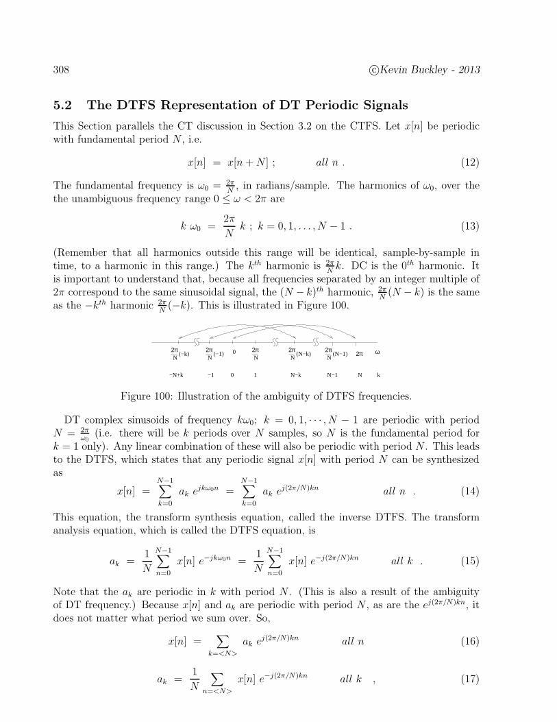
308 c©Kevin Buckley - 2013
5.2 The DTFS Representation of DT Periodic Signals
This Section parallels the CT discussion in Section 3.2 on the CTFS. Let x[n] be periodicwith fundamental period N , i.e.
x[n] = x[n +N ] ; all n . (12)
The fundamental frequency is ω0 = 2πN, in radians/sample. The harmonics of ω0, over the
the unambiguous frequency range 0 ≤ ω < 2π are
k ω0 =2π
Nk ; k = 0, 1, . . . , N − 1 . (13)
(Remember that all harmonics outside this range will be identical, sample-by-sample intime, to a harmonic in this range.) The kth harmonic is 2π
Nk. DC is the 0th harmonic. It
is important to understand that, because all frequencies separated by an integer multiple of2π correspond to the same sinusoidal signal, the (N − k)th harmonic, 2π
N(N − k) is the same
as the −kth harmonic 2πN(−k). This is illustrated in Figure 100.
2πN
2πN
(−1)2πN
(−k)2πN
(N−k)2πN
(N−1)0 ω
k
2π
0 NN−1N−k−N+k 1−1
Figure 100: Illustration of the ambiguity of DTFS frequencies.
DT complex sinusoids of frequency kω0; k = 0, 1, · · · , N − 1 are periodic with periodN = 2π
ω0(i.e. there will be k periods over N samples, so N is the fundamental period for
k = 1 only). Any linear combination of these will also be periodic with period N . This leadsto the DTFS, which states that any periodic signal x[n] with period N can be synthesizedas
x[n] =N−1∑
k=0
ak ejkω0n =N−1∑
k=0
ak ej(2π/N)kn all n . (14)
This equation, the transform synthesis equation, called the inverse DTFS. The transformanalysis equation, which is called the DTFS equation, is
ak =1
N
N−1∑
n=0
x[n] e−jkω0n =1
N
N−1∑
n=0
x[n] e−j(2π/N)kn all k . (15)
Note that the ak are periodic in k with period N . (This is also a result of the ambiguityof DT frequency.) Because x[n] and ak are periodic with period N , as are the ej(2π/N)kn, itdoes not matter what period we sum over. So,
x[n] =∑
k=<N>
ak ej(2π/N)kn all n (16)
ak =1
N
∑
n=<N>
x[n] e−j(2π/N)kn all k , (17)
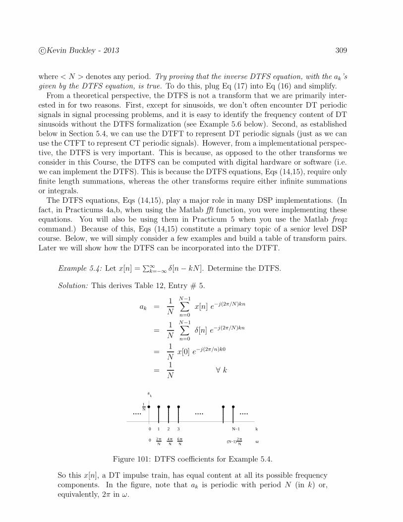
c©Kevin Buckley - 2013 309
where < N > denotes any period. Try proving that the inverse DTFS equation, with the ak’sgiven by the DTFS equation, is true. To do this, plug Eq (17) into Eq (16) and simplify.
From a theoretical perspective, the DTFS is not a transform that we are primarily inter-ested in for two reasons. First, except for sinusoids, we don’t often encounter DT periodicsignals in signal processing problems, and it is easy to identify the frequency content of DTsinusoids without the DTFS formalization (see Example 5.6 below). Second, as establishedbelow in Section 5.4, we can use the DTFT to represent DT periodic signals (just as we canuse the CTFT to represent CT periodic signals). However, from a implementational perspec-tive, the DTFS is very important. This is because, as opposed to the other transforms weconsider in this Course, the DTFS can be computed with digital hardware or software (i.e.we can implement the DTFS). This is because the DTFS equations, Eqs (14,15), require onlyfinite length summations, whereas the other transforms require either infinite summationsor integrals.
The DTFS equations, Eqs (14,15), play a major role in many DSP implementations. (Infact, in Practicums 4a,b, when using the Matlab fft function, you were implementing theseequations. You will also be using them in Practicum 5 when you use the Matlab freqzcommand.) Because of this, Eqs (14,15) constitute a primary topic of a senior level DSPcourse. Below, we will simply consider a few examples and build a table of transform pairs.Later we will show how the DTFS can be incorporated into the DTFT.
Example 5.4: Let x[n] =∑∞
k=−∞ δ[n− kN ]. Determine the DTFS.
Solution: This derives Table 12, Entry # 5.
ak =1
N
N−1∑
n=0
x[n] e−j(2π/N)kn
=1
N
N−1∑
n=0
δ[n] e−j(2π/N)kn
=1
Nx[0] e−j(2π/n)k0
=1
N∀ k
2Nπ
Nπ4
Nπ6 2
Nπ
(N−1)
1N
k
0
0
a
1 2 3 N−1 k
ω
........ ....
Figure 101: DTFS coefficients for Example 5.4.
So this x[n], a DT impulse train, has equal content at all its possible frequencycomponents. In the figure, note that ak is periodic with period N (in k) or,equivalently, 2π in ω.

310 c©Kevin Buckley - 2013
Example 5.5: Let x[n] =∑∞
k=−∞ x1[n−k16] where x1[n] = 2δ[n+1] + 2δ[n−1].Determine the DTFS.
Solution:
ak =1
16
8∑
n=−7
x[n] e−j(2π/16)kn
=1
8
(
ej(π/8)k + e−j(π/8)k)
=1
4cos
(
π
8k)
∀ k
0 1 2 3
x[n]
1
.... .... ....
N n
ak
....8−7
k
....DTFS; N=16
Figure 102: DTFS coefficients for Example 5.5.
Example 5.6: Let x[n] = A cos(32π10n); N = 10. Determine the ak’s.
Solution: This derives Table 12, Entry # 3.
x[n] =A
2ej(2π/10)3n +
A
2e−j(2π/10)3n
Since this is already expressed in the DTFS expansion form, we can pick out theDTFS coefficients by inspection. With N + 10 we see that x[n] consists of k = 3and k = −3 harmonics. So,
ak =A
2(δ(k + 3) + δ(k − 3)) k = −4, −3, · · · , 4, 5
=A
2(δ(k − 3) + δ(k − 7)) k = 0, 1, · · · , 8, 9
2A
k
0
a
1 2 3
....
k4 5−1−2−3−4
....
2A
k
0
a
1 2 3 4 5 k
........
6 7 8 9
or
Figure 103: DTFS coefficients for Example 5.6.
Note that in this example we describe ak over the two ranges commonly used,i.e. 0 ≤ k ≤ N − 1 and, assuming N is even, −(N/2) + 1 ≤ k ≤ N/2.
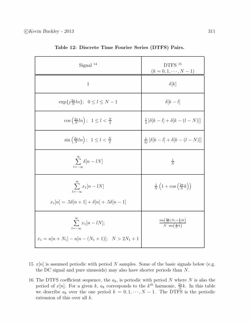
c©Kevin Buckley - 2013 311
Table 12: Discrete Time Fourier Series (DTFS) Pairs.
Signal 14 DTFS 15
(k = 0, 1, · · · , N − 1)
1 δ[k]
expj 2πNln; 0 ≤ l ≤ N − 1 δ[k − l]
cos(
2πNln)
; 1 ≤ l < N2
12[δ[k − l] + δ[k − (l −N)]]
sin(
2πNln)
; 1 ≤ l < N2
12j[δ[k − l] + δ[k − (l −N)]]
∞∑
l=−∞δ[n− lN ] 1
N
∞∑
l=−∞x1[n− lN ] 1
N
(
1 + cos(
2πNk))
x1[n] = .5δ[n+ 1] + δ[n] + .5δ[n− 1]
∞∑
l=−∞x1[n− lN ];
sin( 2πN
(N1+12)k)
N sin( πNk)
x1 = u[n+N1]− u[n− (N1 + 1)]; N > 2N1 + 1
15 x[n] is assumed periodic with period N samples. Some of the basic signals below (e.g.the DC signal and pure sinusoids) may also have shorter periods than N .
16 The DTFS coefficient sequence, the ak, is periodic with period N where N is also theperiod of x[n]. For a given k, ak corresponds to the kth harmonic, 2π
Nk. In this table
we describe ak over the one period k = 0, 1, · · · , N − 1. The DTFS is the periodicextension of this over all k.
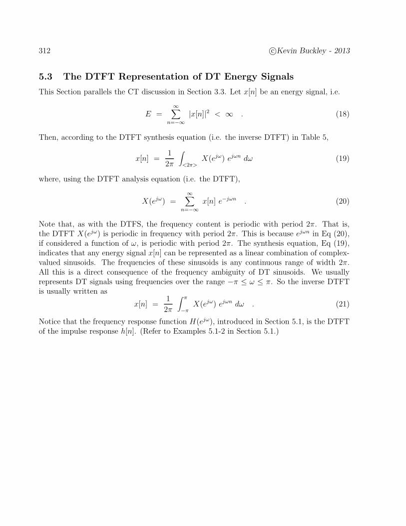
312 c©Kevin Buckley - 2013
5.3 The DTFT Representation of DT Energy Signals
This Section parallels the CT discussion in Section 3.3. Let x[n] be an energy signal, i.e.
E =∞∑
n=−∞|x[n]|2 < ∞ . (18)
Then, according to the DTFT synthesis equation (i.e. the inverse DTFT) in Table 5,
x[n] =1
2π
∫
<2π>X(ejω) ejωn dω (19)
where, using the DTFT analysis equation (i.e. the DTFT),
X(ejω) =∞∑
n=−∞x[n] e−jωn . (20)
Note that, as with the DTFS, the frequency content is periodic with period 2π. That is,the DTFT X(ejω) is periodic in frequency with period 2π. This is because ejωn in Eq (20),if considered a function of ω, is periodic with period 2π. The synthesis equation, Eq (19),indicates that any energy signal x[n] can be represented as a linear combination of complex-valued sinusoids. The frequencies of these sinusoids is any continuous range of width 2π.All this is a direct consequence of the frequency ambiguity of DT sinusoids. We usuallyrepresents DT signals using frequencies over the range −π ≤ ω ≤ π. So the inverse DTFTis usually written as
x[n] =1
2π
∫ π
−πX(ejω) ejωn dω . (21)
Notice that the frequency response function H(ejω), introduced in Section 5.1, is the DTFTof the impulse response h[n]. (Refer to Examples 5.1-2 in Section 5.1.)
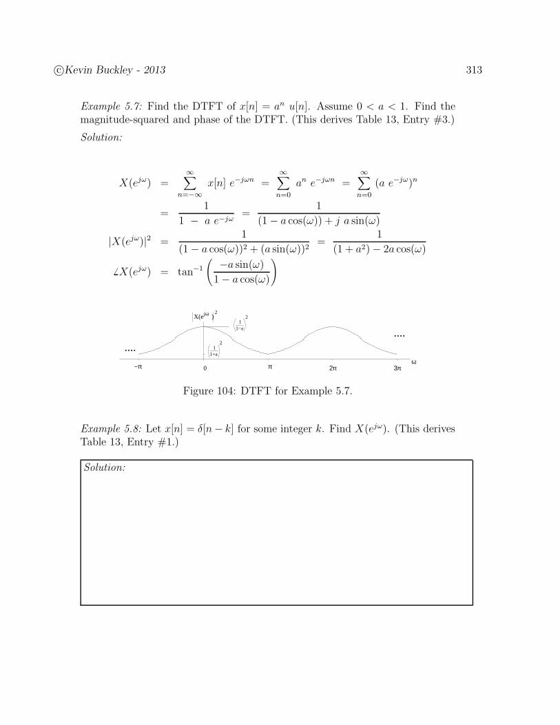
c©Kevin Buckley - 2013 313
Example 5.7: Find the DTFT of x[n] = an u[n]. Assume 0 < a < 1. Find themagnitude-squared and phase of the DTFT. (This derives Table 13, Entry #3.)
Solution:
X(ejω) =∞∑
n=−∞x[n] e−jωn =
∞∑
n=0
an e−jωn =∞∑
n=0
(a e−jω)n
=1
1 − a e−jω=
1
(1− a cos(ω)) + j a sin(ω)
|X(ejω)|2 =1
(1− a cos(ω))2 + (a sin(ω))2=
1
(1 + a2)− 2a cos(ω)
6 X(ejω) = tan−1
(
−a sin(ω)1− a cos(ω)
)
X(e )jω 2
12
1+a
12
1−a
....
−π π0ω
3π2π
....
Figure 104: DTFT for Example 5.7.
Example 5.8: Let x[n] = δ[n− k] for some integer k. Find X(ejω). (This derivesTable 13, Entry #1.)
Solution:
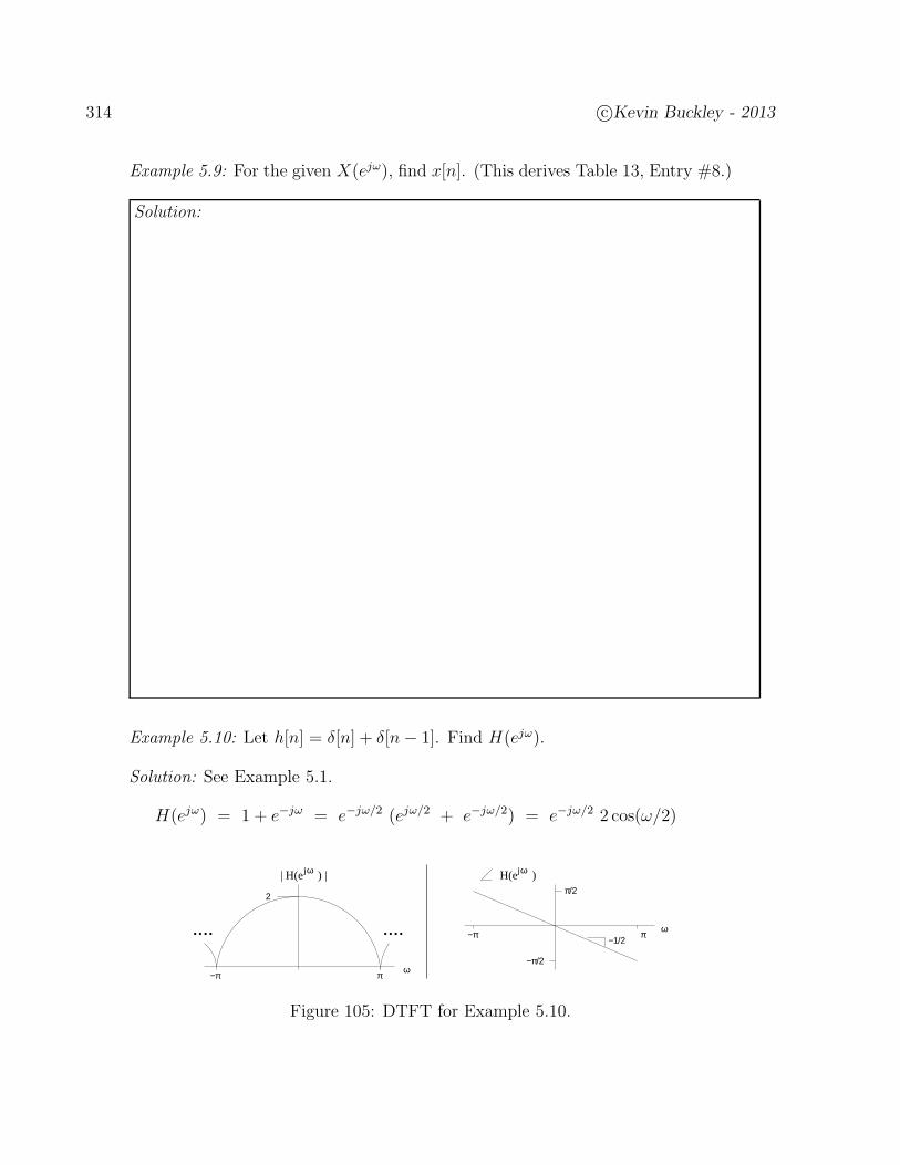
314 c©Kevin Buckley - 2013
Example 5.9: For the given X(ejω), find x[n]. (This derives Table 13, Entry #8.)
Solution:
Example 5.10: Let h[n] = δ[n] + δ[n− 1]. Find H(ejω).
Solution: See Example 5.1.
H(ejω) = 1 + e−jω = e−jω/2 (ejω/2 + e−jω/2) = e−jω/2 2 cos(ω/2)
jω jω
ω
2
.... .... ω−π
π−π
π/2
−π/2
−1/2 π
| H(e ) | H(e )
Figure 105: DTFT for Example 5.10.
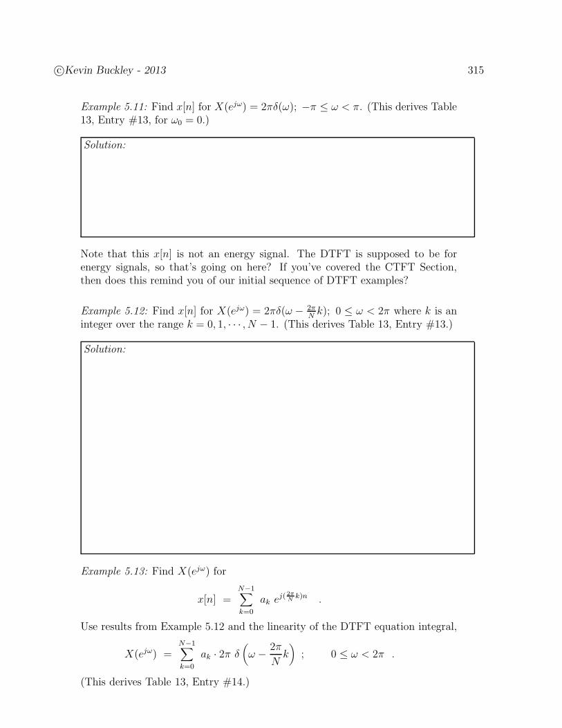
c©Kevin Buckley - 2013 315
Example 5.11: Find x[n] for X(ejω) = 2πδ(ω); −π ≤ ω < π. (This derives Table13, Entry #13, for ω0 = 0.)
Solution:
Note that this x[n] is not an energy signal. The DTFT is supposed to be forenergy signals, so that’s going on here? If you’ve covered the CTFT Section,then does this remind you of our initial sequence of DTFT examples?
Example 5.12: Find x[n] for X(ejω) = 2πδ(ω − 2πNk); 0 ≤ ω < 2π where k is an
integer over the range k = 0, 1, · · · , N − 1. (This derives Table 13, Entry #13.)
Solution:
Example 5.13: Find X(ejω) for
x[n] =N−1∑
k=0
ak ej(2πN
k)n .
Use results from Example 5.12 and the linearity of the DTFT equation integral,
X(ejω) =N−1∑
k=0
ak · 2π δ(
ω − 2π
Nk)
; 0 ≤ ω < 2π .
(This derives Table 13, Entry #14.)
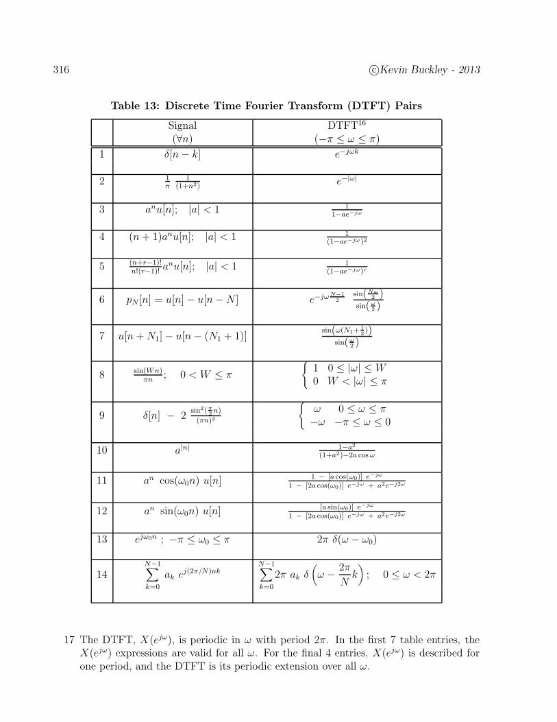
316 c©Kevin Buckley - 2013
Table 13: Discrete Time Fourier Transform (DTFT) Pairs
Signal DTFT16
(∀n) (−π ≤ ω ≤ π)
1 δ[n− k] e−jωk
2 1π
1(1+n2)
e−|ω|
3 anu[n]; |a| < 1 11−ae−jω
4 (n+ 1)anu[n]; |a| < 1 1(1−ae−jω)2
5 (n+r−1)!n!(r−1)!
anu[n]; |a| < 1 1(1−ae−jω)r
6 pN [n] = u[n]− u[n−N ] e−jωN−12
sin(Nω2 )
sin(ω2 )
7 u[n+N1]− u[n− (N1 + 1)]sin(ω(N1+
12))
sin(ω2 )
8 sin(Wn)πn
; 0 < W ≤ π
1 0 ≤ |ω| ≤W0 W < |ω| ≤ π
9 δ[n] − 2sin2(π
2n)
(πn)2
ω 0 ≤ ω ≤ π−ω −π ≤ ω ≤ 0
10 a|n| 1−a2
(1+a2)−2a cosω
11 an cos(ω0n) u[n]1 − [a cos(ω0)] e−jω
1 − [2a cos(ω0)] e−jω + a2e−j2ω
12 an sin(ω0n) u[n][a sin(ω0)] e−jω
1 − [2a cos(ω0)] e−jω + a2e−j2ω
13 ejω0n ; −π ≤ ω0 ≤ π 2π δ(ω − ω0)
14N−1∑
k=0
ak ej(2π/N)nkN−1∑
k=0
2π ak δ(
ω − 2π
Nk)
; 0 ≤ ω < 2π
17 The DTFT, X(ejω), is periodic in ω with period 2π. In the first 7 table entries, theX(ejω) expressions are valid for all ω. For the final 4 entries, X(ejω) is described forone period, and the DTFT is its periodic extension over all ω.
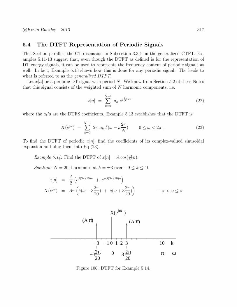
c©Kevin Buckley - 2013 317
5.4 The DTFT Representation of Periodic Signals
This Section parallels the CT discussion in Subsection 3.3.1 on the generalized CTFT. Ex-amples 5.11-13 suggest that, even though the DTFT as defined is for the representation ofDT energy signals, it can be used to represents the frequency content of periodic signals aswell. In fact, Example 5.13 shows how this is done for any periodic signal. The leads towhat is referred to as the generalized DTFT.
Let x[n] be a periodic DT signal with period N . We know from Section 5.2 of these Notesthat this signal consists of the weighted sum of N harmonic components, i.e.
x[n] =N−1∑
k=0
ak ej2πN
kn (22)
where the ak’s are the DTFS coefficients. Example 5.13 establishes that the DTFT is
X(ejω) =N−1∑
k=0
2π ak δ(ω − k2π
N) 0 ≤ ω < 2π . (23)
To find the DTFT of periodic x[n], find the coefficients of its complex-valued sinusoidalexpansion and plug them into Eq (23).
Example 5.14: Find the DTFT of x[n] = A cos(3π10n).
Solution: N = 20; harmonics at k = ±3 over −9 ≤ k ≤ 10
x[n] =A
2
(
ej(3π/10)n + e−j(3π/10)n)
X(ejω) = Aπ(
δ(ω − 32π
20) + δ(ω + 3
2π
20))
− π < ω ≤ π
ωj
π(A ) π(A )
π−3220 20
π23
k
X(e )
0 ωπ
−1 210 10−3 3
Figure 106: DTFT for Example 5.14.
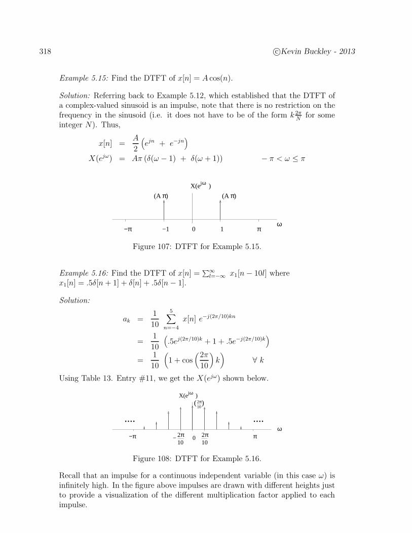
318 c©Kevin Buckley - 2013
Example 5.15: Find the DTFT of x[n] = A cos(n).
Solution: Referring back to Example 5.12, which established that the DTFT ofa complex-valued sinusoid is an impulse, note that there is no restriction on thefrequency in the sinusoid (i.e. it does not have to be of the form k 2π
Nfor some
integer N). Thus,
x[n] =A
2
(
ejn + e−jn)
X(ejω) = Aπ (δ(ω − 1) + δ(ω + 1)) − π < ω ≤ π
ωj
π(A ) π(A )
X(e )
0 πω
−1 1−π
Figure 107: DTFT for Example 5.15.
Example 5.16: Find the DTFT of x[n] =∑∞
l=−∞ x1[n− 10l] wherex1[n] = .5δ[n + 1] + δ[n] + .5δ[n− 1].
Solution:
ak =1
10
5∑
n=−4
x[n] e−j(2π/10)kn
=1
10
(
.5ej(2π/10)k + 1 + .5e−j(2π/10)k)
=1
10
(
1 + cos(
2π
10
)
k)
∀ k
Using Table 13. Entry #11, we get the X(ejω) shown below.
π210
ωjX(e )π2
10( )
........ω
0 π−π π210
−
Figure 108: DTFT for Example 5.16.
Recall that an impulse for a continuous independent variable (in this case ω) isinfinitely high. In the figure above impulses are drawn with different heights justto provide a visualization of the different multiplication factor applied to eachimpulse.
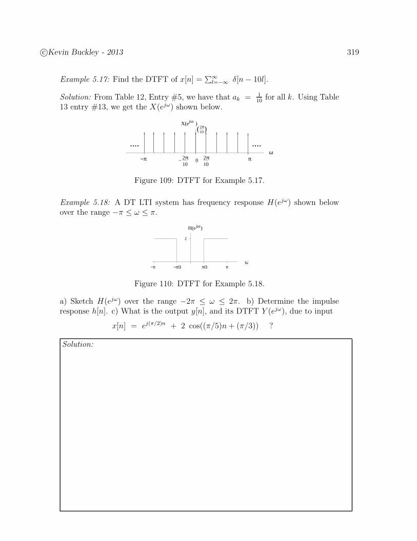
c©Kevin Buckley - 2013 319
Example 5.17: Find the DTFT of x[n] =∑∞
l=−∞ δ[n− 10l].
Solution: From Table 12, Entry #5, we have that ak = 110
for all k. Using Table13 entry #13, we get the X(ejω) shown below.
π210
ωjX(e )π2
10( )
ω0 π−π
.... ....
π210
−
Figure 109: DTFT for Example 5.17.
Example 5.18: A DT LTI system has frequency response H(ejω) shown belowover the range −π ≤ ω ≤ π.
ωjH(e )
2
ωπ/3−π/3−π π
Figure 110: DTFT for Example 5.18.
a) Sketch H(ejω) over the range −2π ≤ ω ≤ 2π. b) Determine the impulseresponse h[n]. c) What is the output y[n], and its DTFT Y (ejω), due to input
x[n] = ej(π/2)n + 2 cos((π/5)n+ (π/3)) ?
Solution:

320 c©Kevin Buckley - 2013
5.5 Properties of the DTFT
If you have already covered Chapter 3 of these Notes, on CT transforms, then you are alreadyfamiliar with transform property concepts, and this Section will serve to reinforce theseconcepts and to fine tune them for DT applications. If you have not yet covered transformproperties in Chapter 3, then even though this Section may be your first formal treatmentof transform properties, you should find the topic somewhat familiar. Upon reflection, youwill see that several properties are exhibited in the Examples we have already consideredin this Chapter. As we proceed through this Section we will reflect back on some of theseprevious examples.
There are several reasons that we consider transform properties. One is that these prop-erties enable us to use transform tables to an extended realm of synthesis and analysisproblems. So, for example, we will be able to use DTFT properties along with the DTFTpairs in Table 13 to identify DTFTs and IDTFTs for a broad range of signals. However,the utility of transform properties goes well beyond this. Properties will provide us withinsight into the transforms themselves and into the signals and systems they represent. Thedelay property and Parseval’s theorem for both the DFTS and DTFT are examples of this.Transform properties are also useful in solving engineering problems. Finally, and mostimportantly, we will see that many of the transform properties we consider represent im-portant engineering applications. So with this in mind, in the following Subsections we willinvestigate transform properties.
Our coverage of DT transform properties in this Chapter will proceed as follows. First,in this Section, we consider some of the more useful and important properties of the DTFT.Since the DTFT encompasses DT periodic signals, through the generalized DTFT, theseproperties are also DTFS properties. Then, in Section 5.7, after we introduce the z-transform,we will consider only those z-transform properties which are particularly useful for DT LTIsystem analysis. The intent here is not to exhaustively list, prove, exemplify and motivateevery possible transform property. That would be exhausting. Rather it is to focus on afew of the most basic and important properties, and to nourish a sense of the relevance ofthis topic. You should keep in mind that there are other transform properties that down theroad you may find useful. After completing this Chapter, you might skim through Section3.5, on CT transform properties, to expand and reinforce what you learn here.
5.5.1 Periodicity of X(ejω)
The DTFT X(ejω) of a signal x[n] is periodic with period 2π. That is,
X(ejω) = X(ej(ω+2π)) ∀ ω . (24)
This is a consequence of the fact that DT sinusoids are unique only over a 2π range offrequency. This property is also explained by looking at the DTFT equation
X(ejω) =∞∑
n=−∞x[n] e−jωn . (25)
Each e−jωn term in the summation is periodic over ω with period 2π. So the weighted sumis periodic too.
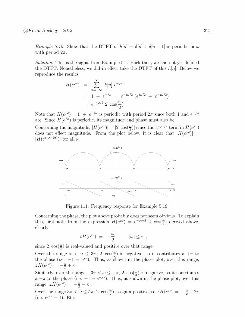
c©Kevin Buckley - 2013 321
Example 5.19: Show that the DTFT of h[n] = δ[n] + δ[n − 1] is periodic in ωwith period 2π.
Solution: This is the signal from Example 5.1. Back then, we had not yet definedthe DTFT. Nonetheless, we did in effect take the DTFT of this h[n]. Below wereproduce the results.
H(ejω) =∞∑
n=−∞h[n] e−jωn
= 1 + e−jω = e−jω/2 (ejω/2 + e−jω/2)
= e−jω/2 2 cos(ω
2)
Note that H(ejω) = 1 + e−jω is periodic with period 2π since both 1 and e−jω
are. Since H(ejω) is periodic, its magnitude and phase must also be.
Concerning the magnitude, |H(ejω)| = |2 cos(ω2)| since the e−jω/2 term in H(ejω)
does not effect magnitude. From the plot below, it is clear that |H(ejω)| =|H(ej(ω+2π))| for all ω.
jω
jω H(e )
2
π−π
| H(e ) |
ω
....
−3π 3π
....
π/2
−π/2
−1/2 π ω
....
3π−3π −π
....
Figure 111: Frequency response for Example 5.19.
Concerning the phase, the plot above probably does not seem obvious. To explainthis, first note from the expression H(ejω) = e−jω/2 2 cos(ω
2) derived above,
clearly
6 H(ejω) = − ω
2|ω| ≤ π ,
since 2 cos(ω2) is real-valued and positive over that range.
Over the range π < ω ≤ 3π, 2 cos(ω2) is negative, so it contributes a +π to
the phase (i.e. −1 = ejπ). Thus, as shown in the phase plot, over this range,6 H(ejω) = −ω
2+ π.
Similarly, over the range −3π < ω ≤ −π, 2 cos(ω2) is negative, so it contributes
a −π to the phase (i.e. −1 = e−jπ). Thus, as shown in the phase plot, over thisrange, 6 H(ejω) = −ω
2− π.
Over the range 3π < ω ≤ 5π, 2 cos(ω2) is again positive, so 6 H(ejω) = −ω
2+ 2π
(i.e. ej2π = 1). Etc.
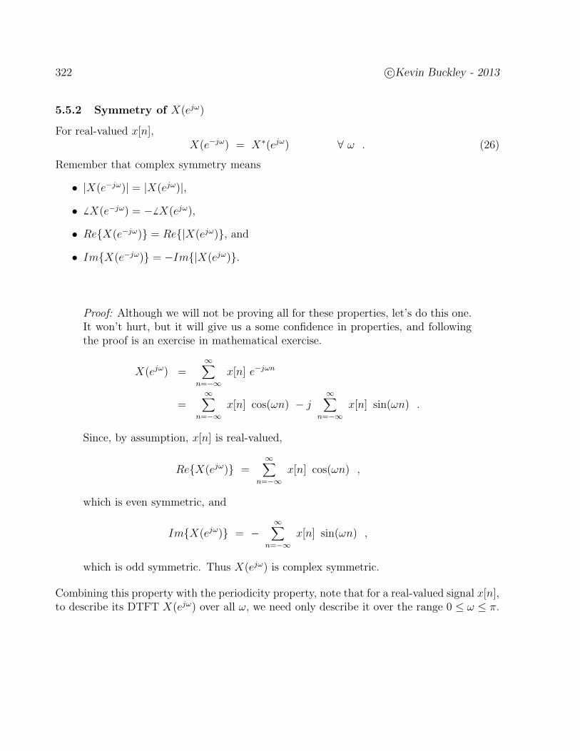
322 c©Kevin Buckley - 2013
5.5.2 Symmetry of X(ejω)
For real-valued x[n],X(e−jω) = X∗(ejω) ∀ ω . (26)
Remember that complex symmetry means
• |X(e−jω)| = |X(ejω)|,
• 6 X(e−jω) = −6 X(ejω),
• ReX(e−jω) = Re|X(ejω), and
• ImX(e−jω) = −Im|X(ejω).
Proof: Although we will not be proving all for these properties, let’s do this one.It won’t hurt, but it will give us a some confidence in properties, and followingthe proof is an exercise in mathematical exercise.
X(ejω) =∞∑
n=−∞x[n] e−jωn
=∞∑
n=−∞x[n] cos(ωn) − j
∞∑
n=−∞x[n] sin(ωn) .
Since, by assumption, x[n] is real-valued,
ReX(ejω) =∞∑
n=−∞x[n] cos(ωn) ,
which is even symmetric, and
ImX(ejω) = −∞∑
n=−∞x[n] sin(ωn) ,
which is odd symmetric. Thus X(ejω) is complex symmetric.
Combining this property with the periodicity property, note that for a real-valued signal x[n],to describe its DTFT X(ejω) over all ω, we need only describe it over the range 0 ≤ ω ≤ π.
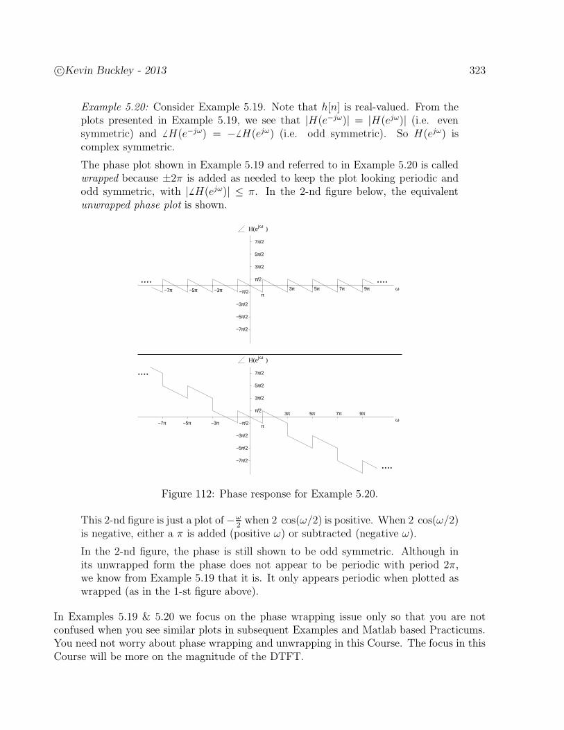
c©Kevin Buckley - 2013 323
Example 5.20: Consider Example 5.19. Note that h[n] is real-valued. From theplots presented in Example 5.19, we see that |H(e−jω)| = |H(ejω)| (i.e. evensymmetric) and 6 H(e−jω) = −6 H(ejω) (i.e. odd symmetric). So H(ejω) iscomplex symmetric.
The phase plot shown in Example 5.19 and referred to in Example 5.20 is calledwrapped because ±2π is added as needed to keep the plot looking periodic andodd symmetric, with | 6 H(ejω)| ≤ π. In the 2-nd figure below, the equivalentunwrapped phase plot is shown.
jω H(e )
π
3π 5π
−π/2
−3π/2
−5π/2
ω
π/2
3π/2
9π
....
7π
−7π/2
....5π/2
7π/2
−3π−7π −5π
jω H(e )
π−π/2
−3π/2
−5π/2
ω
π/2
3π/2
−7π/2
5π/2
7π/2
3π 5π 7π 9π−3π−5π−7π
.... ....
Figure 112: Phase response for Example 5.20.
This 2-nd figure is just a plot of−ω2when 2 cos(ω/2) is positive. When 2 cos(ω/2)
is negative, either a π is added (positive ω) or subtracted (negative ω).
In the 2-nd figure, the phase is still shown to be odd symmetric. Although inits unwrapped form the phase does not appear to be periodic with period 2π,we know from Example 5.19 that it is. It only appears periodic when plotted aswrapped (as in the 1-st figure above).
In Examples 5.19 & 5.20 we focus on the phase wrapping issue only so that you are notconfused when you see similar plots in subsequent Examples and Matlab based Practicums.You need not worry about phase wrapping and unwrapping in this Course. The focus in thisCourse will be more on the magnitude of the DTFT.
324 c©Kevin Buckley - 2013
5.5.3 Time Delay
Given a DTFT pairx[n] ←→ X(ejω) (27)
the delay property says that, for any integer k,
x[n− k] ←→ X(ejω) e−jωk = |X(ejω)| ej(6 X(ejω) − ωk) . (28)
It is important to the general understanding on what a transform is to step back and makesure you understand what this property suggests. Recall that for a given x[n] and corre-sponding X(ejω), the complex-sinusoidal component of x[n] at frequency ω is
X(ejω) ejωn . (29)
If we delay the signal by k samples, then we delay each of its sinusoidal components by ksamples. Then you delay a sinusoid, you don’t effect its magnitude, only its phase. You shiftits phase by −ωk, which is proportional to the frequency and to the amount of delay. Thus,after the delay, the component of x[n− k] at frequency ω is
X(ejω) e−jωk ejωn = |X(ejω)| ej(ωn + 6 X(ejω) − ωk) . (30)
The idea is that a delay in the time domain is a phase shift in the frequency domain. Thisphase shift is proportional to both the frequency of the sinusoidal component and the lengthof the delay.
Example 5.21: Determine the DTFT of: (a) p11[n− 5]; and (b) p11[n+ 5].
Solutions: From Table 13, entry #6,
p11[n] ←→ e−j5ωsin
(
11ω2
)
sin(
ω2
)
(a) Then, for delay k = 5, we have that
p11[n− 5] ←→ e−j10ωsin
(
11ω2
)
sin(
ω2
) .
(b) For delay k = −5 we have that
p11[n + 5] ←→sin
(
11ω2
)
sin(
ω2
) .
We see that the application of the delay property is pretty straightforward.
In Example 5.21, note that p11[n + 5] is symmetric around n = 0 and that its DTFT isreal-valued. This looks like the symmetry property introduced in Subsection 5.5.2, exceptthat the domains are switched.
More Symmetry Properties: If X(ejω) is real-valued, then x[n] is complex symmetric.If x[n] is real-valued and symmetric, then so is X(ejω).Just remember, concerning Fourier transforms, real-valued in one domain, means complexsymmetric in the other.
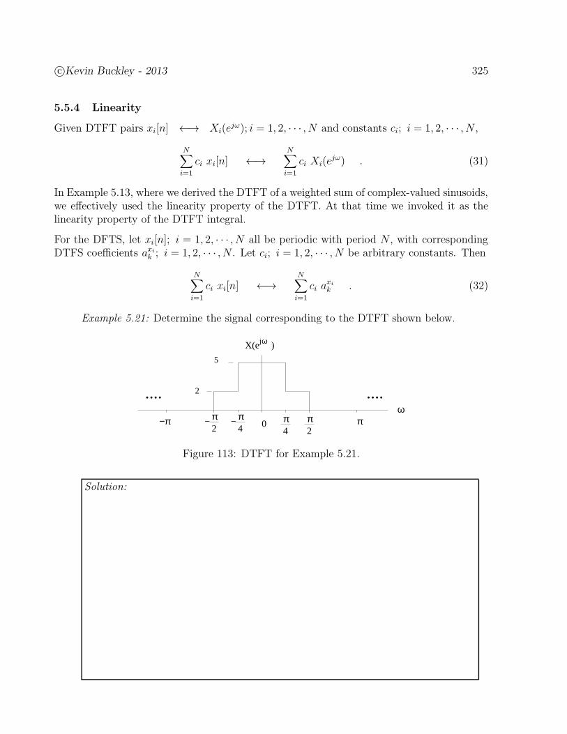
c©Kevin Buckley - 2013 325
5.5.4 Linearity
Given DTFT pairs xi[n] ←→ Xi(ejω); i = 1, 2, · · · , N and constants ci; i = 1, 2, · · · , N ,
N∑
i=1
ci xi[n] ←→N∑
i=1
ci Xi(ejω) . (31)
In Example 5.13, where we derived the DTFT of a weighted sum of complex-valued sinusoids,we effectively used the linearity property of the DTFT. At that time we invoked it as thelinearity property of the DTFT integral.
For the DFTS, let xi[n]; i = 1, 2, · · · , N all be periodic with period N , with correspondingDTFS coefficients axi
k ; i = 1, 2, · · · , N . Let ci; i = 1, 2, · · · , N be arbitrary constants. Then
N∑
i=1
ci xi[n] ←→N∑
i=1
ci axik . (32)
Example 5.21: Determine the signal corresponding to the DTFT shown below.
ωjX(e )
π4
π4
ω.... ....
−π π
5
2
0−− π π2 2
Figure 113: DTFT for Example 5.21.
Solution:
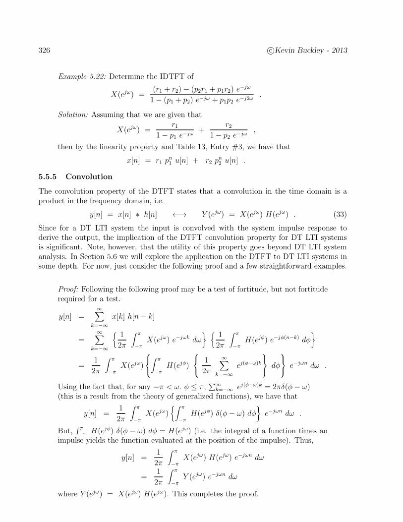
326 c©Kevin Buckley - 2013
Example 5.22: Determine the IDTFT of
X(ejω) =(r1 + r2)− (p2r1 + p1r2) e
−jω
1− (p1 + p2) e−jω + p1p2 e−j2ω.
Solution: Assuming that we are given that
X(ejω) =r1
1− p1 e−jω+
r21− p2 e−jω
,
then by the linearity property and Table 13, Entry #3, we have that
x[n] = r1 pn1 u[n] + r2 pn2 u[n] .
5.5.5 Convolution
The convolution property of the DTFT states that a convolution in the time domain is aproduct in the frequency domain, i.e.
y[n] = x[n] ∗ h[n] ←→ Y (ejω) = X(ejω) H(ejω) . (33)
Since for a DT LTI system the input is convolved with the system impulse response toderive the output, the implication of the DTFT convolution property for DT LTI systemsis significant. Note, however, that the utility of this property goes beyond DT LTI systemanalysis. In Section 5.6 we will explore the application on the DTFT to DT LTI systems insome depth. For now, just consider the following proof and a few straightforward examples.
Proof: Following the following proof may be a test of fortitude, but not fortituderequired for a test.
y[n] =∞∑
k=−∞x[k] h[n− k]
=∞∑
k=−∞
1
2π
∫ π
−πX(ejω) e−jωk dω
1
2π
∫ π
−πH(ejφ) e−jφ(n−k) dφ
=1
2π
∫ π
−πX(ejω)
∫ π
−πH(ejφ)
1
2π
∞∑
k=−∞ej(φ−ω)k
dφ
e−jωn dω .
Using the fact that, for any −π < ω. φ ≤ π,∑∞
k=−∞ ej(φ−ω)k = 2πδ(φ− ω)(this is a result from the theory of generalized functions), we have that
y[n] =1
2π
∫ π
−πX(ejω)
∫ π
−πH(ejφ) δ(φ− ω) dφ
e−jωn dω .
But,∫ π−π H(ejφ) δ(φ − ω) dφ = H(ejω) (i.e. the integral of a function times an
impulse yields the function evaluated at the position of the impulse). Thus,
y[n] =1
2π
∫ π
−πX(ejω) H(ejω) e−jωn dω
=1
2π
∫ π
−πY (ejω) e−jωn dω
where Y (ejω) = X(ejω) H(ejω). This completes the proof.
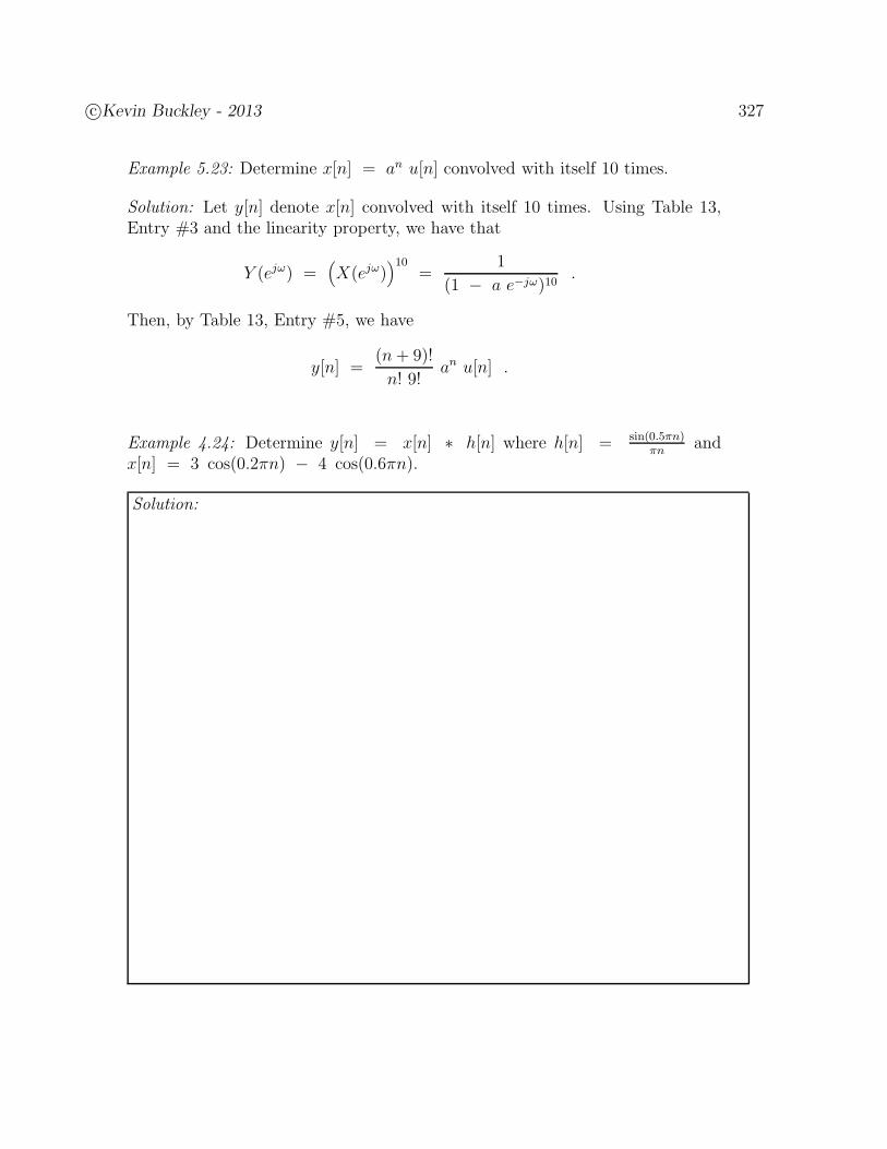
c©Kevin Buckley - 2013 327
Example 5.23: Determine x[n] = an u[n] convolved with itself 10 times.
Solution: Let y[n] denote x[n] convolved with itself 10 times. Using Table 13,Entry #3 and the linearity property, we have that
Y (ejω) =(
X(ejω))10
=1
(1 − a e−jω)10.
Then, by Table 13, Entry #5, we have
y[n] =(n+ 9)!
n! 9!an u[n] .
Example 4.24: Determine y[n] = x[n] ∗ h[n] where h[n] = sin(0.5πn)πn
andx[n] = 3 cos(0.2πn) − 4 cos(0.6πn).
Solution:
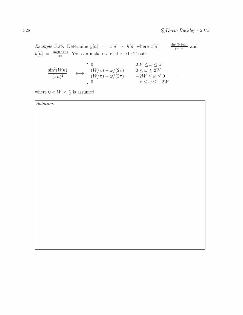
328 c©Kevin Buckley - 2013
Example 5.25: Determine y[n] = x[n] ∗ h[n] where x[n] = sin2(0.4πn)(πn)2
and
h[n] = sin(0.5πn)πn
. You can make use of the DTFT pair
sin2(Wn)
(πn)2←→
0 2W ≤ ω ≤ π(W/π)− ω/(2π) 0 ≤ ω ≤ 2W(W/π) + ω/(2π) −2W ≤ ω ≤ 00 −π ≤ ω ≤ −2W
,
where 0 < W < π2is assumed.
Solution:
c©Kevin Buckley - 2013 329
5.5.6 Parseval’s Theorem
For DT energy signals
E =∞∑
n=−∞|x[n]|2 =
1
2π
∫
<2π>|X(ejω)|2 dω . (34)
For DT periodic power signals
P =1
N
∑
n=<N>
|x[n]|2 =∑
k=<N>
|ak|2 . (35)
If you have already covered Parseval’s theorem for the CTFS and/or CTFT, refer back tothat discussion. Either way, Parseval’s theorem quantifies the idea of content as a functionfor frequency. Note that power and energy are not effected by the phase of the frequencydescription, but only the magnitude. Thus, for example, delaying a signal does not effect itsenergy or power.
For the DTFT, Parseval’s theorem establishes that for a signal x[n] with total energy E,
the function |X(ejω)|22π
plotted vs. ω gives the distribution of total energy over frequency. Thuswe call this plot the energy spectrum. Similarly, for periodic power signals, |ak|2 vs. k (orω) is called the power spectrum.
Spectra:
• Energy spectrum: |X(ejω)|2 vs. ω
• Magnitude spectrum: |X(ejω)| vs. ω• Magnitude spectrum in dB: 20 log10|X(ejω)| = 10 log10|X(ejω)|2 vs. ω• Phase spectrum: 6 X(ejω) vs. ω
• Power spectrum: |ak|2 vs. ω or k
Example 5.26: Determine the percentage of energy of the signal x[n] = 5sin(π
2n)
πn
over the frequency band −π3≤ ω ≤ π
3.
Solution:
330 c©Kevin Buckley - 2013
Example 5.27: Consider the signal x[n] =∑∞
k=−∞ δ[n− 5k] which is the input
to a DT LTI system with impulse response h[n] = sin(0.5πn)πn
. What percentageof the input power is present in the output?
Solution:
5.5.7 Multiplication
In Subsection 5.5.5 we saw that, for the DTFT, convolution in the time domain correspondsto multiplication in the frequency domain. It turns out to be more general than this. Foreither the CTFT or the DTFT, a convolution in one domain corresponds to a multiplicationin the other domain. Any specific example of this could be proved by paralleling the proofin Subsection 5.5.5.
The multiplication property for the DTFT is
y[n] = x1[n] · x2[n] ←→ Y (ejω) =1
2π
∫
<2π>X1(e
jθ) X2(ej(ω−θ)) dθ . (36)
This is a convolution, of X1(ejω) and X2(e
jω), in the frequency domain. For each ω, asa function of “dummy” variable θ one is folded and shifted by ω, then producted with theother, and the result integrated. There is a new twist here (compared to the convolution sumand integral covered in Chapter 2). When folding and shifting the one signal (in frequency),you must remember that in frequency it is of infinite duration and periodic with period2π. Also note that the integral is over one period only. This type of convolution, which isapplicable to periodic functions, is called periodic or circular convolution.
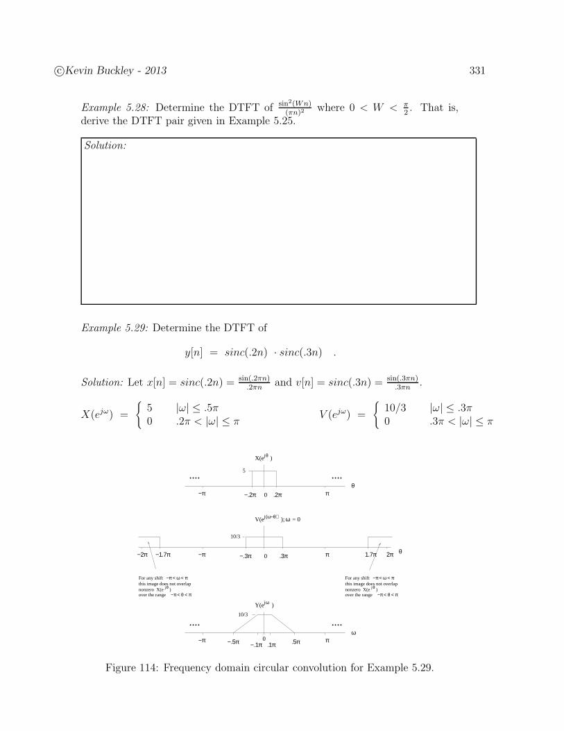
c©Kevin Buckley - 2013 331
Example 5.28: Determine the DTFT of sin2(Wn)(πn)2
where 0 < W < π2. That is,
derive the DTFT pair given in Example 5.25.
Solution:
Example 5.29: Determine the DTFT of
y[n] = sinc(.2n) · sinc(.3n) .
Solution: Let x[n] = sinc(.2n) = sin(.2πn).2πn
and v[n] = sinc(.3n) = sin(.3πn).3πn
.
X(ejω) =
5 |ω| ≤ .5π0 .2π < |ω| ≤ π
V (ejω) =
10/3 |ω| ≤ .3π0 .3π < |ω| ≤ π
θjnonzero X(e )
For any shift
over the range
this image does not overlap−π < ω < π
−π < θ < πθjnonzero X(e )
−π π0
j(ω−θ)
.3π−.3πθ2π−2π −1.7π 1.7π
For any shift
over the range
this image does not overlap−π < ω < π
−π < θ < π
.... ....
−π π
j
ω
ωY(e )
.5π−.5π 0−.1π .1π
10/3
.... ....
−π π0−.2π .2π
5
j
θ
θX(e )
V(e ); = 0ω
10/3
Figure 114: Frequency domain circular convolution for Example 5.29.
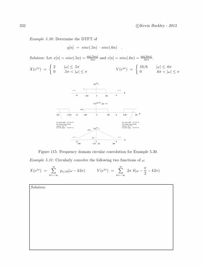
332 c©Kevin Buckley - 2013
Example 5.30: Determine the DTFT of
y[n] = sinc(.5n) · sinc(.6n) .
Solution: Let x[n] = sinc(.5n) = sin(.5πn).5πn
and v[n] = sinc(.6n) = sin(.6πn).6πn
.
X(ejω) =
2 |ω| ≤ .5π0 .5π < |ω| ≤ π
V (ejω) =
10/6 |ω| ≤ .6π0 .6π < |ω| ≤ π
θjnonzero X(e ) θjnonzero X(e )jωY(e )
−π π
j(ω−θ)
θ2π−2π
over the range −π < θ < π
.... ....ω
0−.1π .1π
−1.4π 1.4π−.6π .6π0
For some shifts −π < ω < πthis image does overlap
over the range −π < θ < π
−π < ω < πthis image does overlap
10/6
−π π.9π−.9π
For some shifts
2/6
.... ....
−π π0
j
θ
θ
2
−.5π .5π
X(e )
10/6
V(e ); = 0ω
Figure 115: Frequency domain circular convolution for Example 5.30.
Example 5.31: Circularly convolve the following two functions of ω.
X(ejω) =∞∑
k=−∞pπ/10(ω − k2π) V (ejω) =
∞∑
k=−∞2π δ(ω − π
2− k2π)
Solution:
c©Kevin Buckley - 2013 333
5.5.8 Modulation
Modulation is a special case of multiplication where one of the signals is a real-valued orcomplex-valued sinusoid. For example, let x[n] be a signal with with DTFT X(ejω).
x[n] ·ejωon ←→ 1
2π
∫
<2π>X(ejθ) 2π δ(ω−θ−ωo)) dθ = X(ej(ω−ω0)) |ω| ≤ π . (37)
Similarly,
x[n] · cos(ωon) ←→ 1
2
(
X(ej(ω−ω0) + X(ej(ω+ω0)))
|ω| ≤ π , (38)
and
x[n] · cos(ωon) ←→ 1
2j
(
X(ej(ω−ω0) − X(ej(ω+ω0)))
|ω| ≤ π . (39)
Example 5.33: Determine the frequency response of a FIR with impulse responseh[n] = 1
Nejω0n pN [n].
Solution:
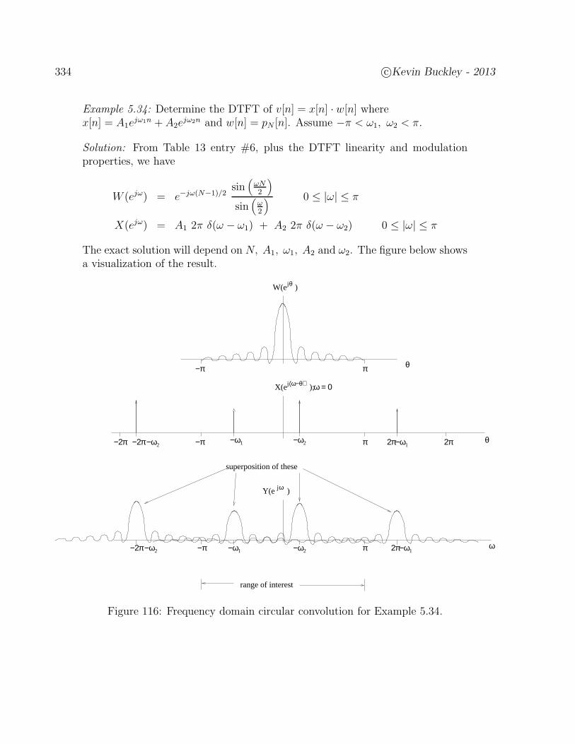
334 c©Kevin Buckley - 2013
Example 5.34: Determine the DTFT of v[n] = x[n] · w[n] wherex[n] = A1e
jω1n + A2ejω2n and w[n] = pN [n]. Assume −π < ω1, ω2 < π.
Solution: From Table 13 entry #6, plus the DTFT linearity and modulationproperties, we have
W (ejω) = e−jω(N−1)/2sin
(
ωN2
)
sin(
ω2
) 0 ≤ |ω| ≤ π
X(ejω) = A1 2π δ(ω − ω1) + A2 2π δ(ω − ω2) 0 ≤ |ω| ≤ π
The exact solution will depend on N, A1, ω1, A2 and ω2. The figure below showsa visualization of the result.
W(e )jθ
−ω1 −ω2 −ω12π−ω2−2π
−ω2−ω1−ω2−2π −ω12π
jωY(e )
X(e );ω = 0
θπ−π
θπ−π 2π−2π
j(ω−θ)
−π π
superposition of these
range of interest
ω
Figure 116: Frequency domain circular convolution for Example 5.34.
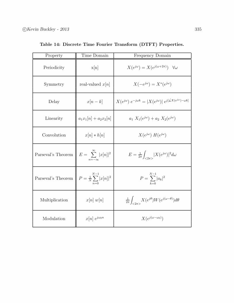
c©Kevin Buckley - 2013 335
Table 14: Discrete Time Fourier Transform (DTFT) Properties.
Property Time Domain Frequency Domain
Periodicity x[n] X(ejω) = X(ej(ω+2π)) ∀ω
Symmetry real-valued x[n] X(−ejω) = X∗(ejω)
Delay x[n− k] X(ejω) e−jωk = |X(ejω)| ej[ 6 X(ejω)−ωk]
Linearity a1x1[n] + a2x2[n] a1 X1(ejω) + a2 X2(e
jω)
Convolution x[n] ∗ h[n] X(ejω) H(ejω)
Parseval’s Theorem E =∞∑
n=−∞|x[n]|2 E = 1
2π
∫
<2π>|X(ejω)|2dω
Parseval’s Theorem P = 1N
N−1∑
n=0
|x[n]|2 P =N−1∑
k=0
|ak|2
Multiplication x[n] w[n] 12π
∫
<2π>X(ejθ)W (ej(ω−θ))dθ
Modulation x[n] ejω0n X(ej(ω−ω0))
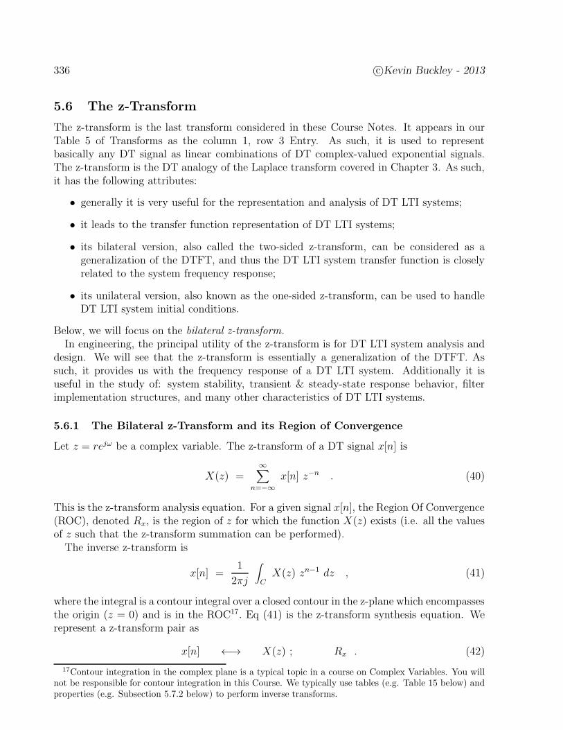
336 c©Kevin Buckley - 2013
5.6 The z-Transform
The z-transform is the last transform considered in these Course Notes. It appears in ourTable 5 of Transforms as the column 1, row 3 Entry. As such, it is used to representbasically any DT signal as linear combinations of DT complex-valued exponential signals.The z-transform is the DT analogy of the Laplace transform covered in Chapter 3. As such,it has the following attributes:
• generally it is very useful for the representation and analysis of DT LTI systems;
• it leads to the transfer function representation of DT LTI systems;
• its bilateral version, also called the two-sided z-transform, can be considered as ageneralization of the DTFT, and thus the DT LTI system transfer function is closelyrelated to the system frequency response;
• its unilateral version, also known as the one-sided z-transform, can be used to handleDT LTI system initial conditions.
Below, we will focus on the bilateral z-transform.In engineering, the principal utility of the z-transform is for DT LTI system analysis and
design. We will see that the z-transform is essentially a generalization of the DTFT. Assuch, it provides us with the frequency response of a DT LTI system. Additionally it isuseful in the study of: system stability, transient & steady-state response behavior, filterimplementation structures, and many other characteristics of DT LTI systems.
5.6.1 The Bilateral z-Transform and its Region of Convergence
Let z = rejω be a complex variable. The z-transform of a DT signal x[n] is
X(z) =∞∑
n=−∞x[n] z−n . (40)
This is the z-transform analysis equation. For a given signal x[n], the Region Of Convergence(ROC), denoted Rx, is the region of z for which the function X(z) exists (i.e. all the valuesof z such that the z-transform summation can be performed).
The inverse z-transform is
x[n] =1
2πj
∫
CX(z) zn−1 dz , (41)
where the integral is a contour integral over a closed contour in the z-plane which encompassesthe origin (z = 0) and is in the ROC17. Eq (41) is the z-transform synthesis equation. Werepresent a z-transform pair as
x[n] ←→ X(z) ; Rx . (42)
17Contour integration in the complex plane is a typical topic in a course on Complex Variables. You willnot be responsible for contour integration in this Course. We typically use tables (e.g. Table 15 below) andproperties (e.g. Subsection 5.7.2 below) to perform inverse transforms.
c©Kevin Buckley - 2013 337
It is important to remember what inverse transform equations suggest. The inverse z-transform indicates that a signal x[n] can be represented as a linear combination the basicsignals zn−1 for z along a closed contour C. The weighting function for the linear combi-nation is the z-transform function X(z). Since C can be any closed contour in the regionof convergence which surrounds to origin, the synthesis equation suggests that there arean infinite number of ways to represent x[n] as a linear combination of DT complex-valuedexponential functions.
Example 5.35: Find the z-transform, including the ROC, for x[n] = δ[n − n0]where n0 is an integer delay. This Example derives Entries #1,2 of Table 15.
Solution:
Example 5.36: Determine the inverse z-transform of the function
X(z) = 1 + 2z−1 + 3z−2 + z−3 .
Solution: Comparing this X(z) to the z-transform expression
X(z) =∞∑
n=−∞x[n] z−n = · · ·+ x[−2]z2 + x[−1]z1 + x[0]z0 + x[1]z−1 + · · ·
we can pick out the nonzero values of x[n] as the coefficients of the polynomial(in z−1) given in this problem. We see that there are nonzero values of x[n] onlyfor n = 0, 1, 2, 3. We get,
x[n] = δ[n] + 2δ[n− 1] + 3δ[n− 2] + δ[n− 3] .
The ROC for this signal will be Rx = ∀z.
Example 5.37: Determine the z-transform, including the ROC, of x[n] = u[n−n0]where n0 is an integer delay.
Solution:
338 c©Kevin Buckley - 2013
Example 5.38: Determine the z-transform, including the ROC, of x[n] = an u[n].This Example derives Entry #3 of Table 15.
Solution:
Example 5.39: Determine the z-transform, including the ROC, ofx[n] = −an u[−n− 1]. This Example derives Entry #4 of Table 15.
Solution:
Note that the signals in Examples 5.38,5.39 have the same z-transform function. Whatdifferentiates them is their ROC’s. This is reminiscent of the bilateral Laplace transform.In these z-transform examples the ROC’s are, respectively, the exterior and the interior of acircle in the z-plane.
c©Kevin Buckley - 2013 339
Example 5.40: For the z-transform, determine h[n].
H(z) =2
1− 34z−1 + 1
8z−2
; Rh = |z| > 1
2.
Solution: Although there are some rational functions of z−1 in Table 15, nonematch this H(z). Using PFE on H(z), for which we will describe a detailedprocedure a little later, we have
H(z) =4
1− 12z−1
+−2
1− 14z−1
.
(Check this by combining the two terms using the common denominator). An-ticipating the linearity property of the z-transform, and recognizing that sincethe ROC is the exterior of a circle the inverse will be right-sided, we have
h[n] = 4(
1
2
)n
u[n] − 2(
1
4
)n
u[n]
If h[n] is the impulse response of a DT LTI system, the system would be bothcausal (h[n] = 0 for n < 0) and stable (h[n] decays as n→∞ so since it is a sumof exponentials it is absolutely summable).
Example 5.41: Same as Example 5.40, but with Rh = |z| < 14.
Solution: As opposed to the Example 5.40 solution, we now have that h[n] willbe left-sided since the ROC is the interior of a circle. Thus,
h[n] = −4(
1
2
)n
u[−n− 1] + 2(
1
4
)n
u[−n− 1]
This h[n] is neither causal nor stable.
Example 5.42: Same as Example 5.40, but with Rh = 14< |z| < 1
2.
Solution: As opposed to the Example 5.40 solution, we now have that the 1-stterm of H(z), with the denominator root z = 1
2, will be contribute a left-sided
term to h[n]. The 2-nd term, with the denominator root z = 14, will be contribute
a right-sided term to h[n]. So
h[n] = −4(
1
2
)n
u[−n− 1] − 2(
1
4
)n
u[n]
This h[n] is neither causal nor stable.
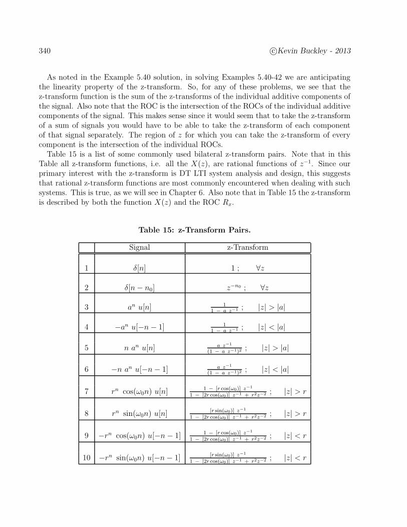
340 c©Kevin Buckley - 2013
As noted in the Example 5.40 solution, in solving Examples 5.40-42 we are anticipatingthe linearity property of the z-transform. So, for any of these problems, we see that thez-transform function is the sum of the z-transforms of the individual additive components ofthe signal. Also note that the ROC is the intersection of the ROCs of the individual additivecomponents of the signal. This makes sense since it would seem that to take the z-transformof a sum of signals you would have to be able to take the z-transform of each componentof that signal separately. The region of z for which you can take the z-transform of everycomponent is the intersection of the individual ROCs.
Table 15 is a list of some commonly used bilateral z-transform pairs. Note that in thisTable all z-transform functions, i.e. all the X(z), are rational functions of z−1. Since ourprimary interest with the z-transform is DT LTI system analysis and design, this suggeststhat rational z-transform functions are most commonly encountered when dealing with suchsystems. This is true, as we will see in Chapter 6. Also note that in Table 15 the z-transformis described by both the function X(z) and the ROC Rx.
Table 15: z-Transform Pairs.
Signal z-Transform
1 δ[n] 1 ; ∀z
2 δ[n− n0] z−n0 ; ∀z
3 an u[n] 11 − a z−1 ; |z| > |a|
4 −an u[−n− 1] 11 − a z−1 ; |z| < |a|
5 n an u[n] a z−1
(1 − a z−1)2; |z| > |a|
6 −n an u[−n− 1] a z−1
(1 − a z−1)2; |z| < |a|
7 rn cos(ω0n) u[n]1 − [r cos(ω0)] z−1
1 − [2r cos(ω0)] z−1 + r2z−2 ; |z| > r
8 rn sin(ω0n) u[n][r sin(ω0)] z−1
1 − [2r cos(ω0)] z−1 + r2z−2 ; |z| > r
9 −rn cos(ω0n) u[−n− 1] 1 − [r cos(ω0)] z−1
1 − [2r cos(ω0)] z−1 + r2z−2 ; |z| < r
10 −rn sin(ω0n) u[−n− 1] [r sin(ω0)] z−1
1 − [2r cos(ω0)] z−1 + r2z−2 ; |z| < r
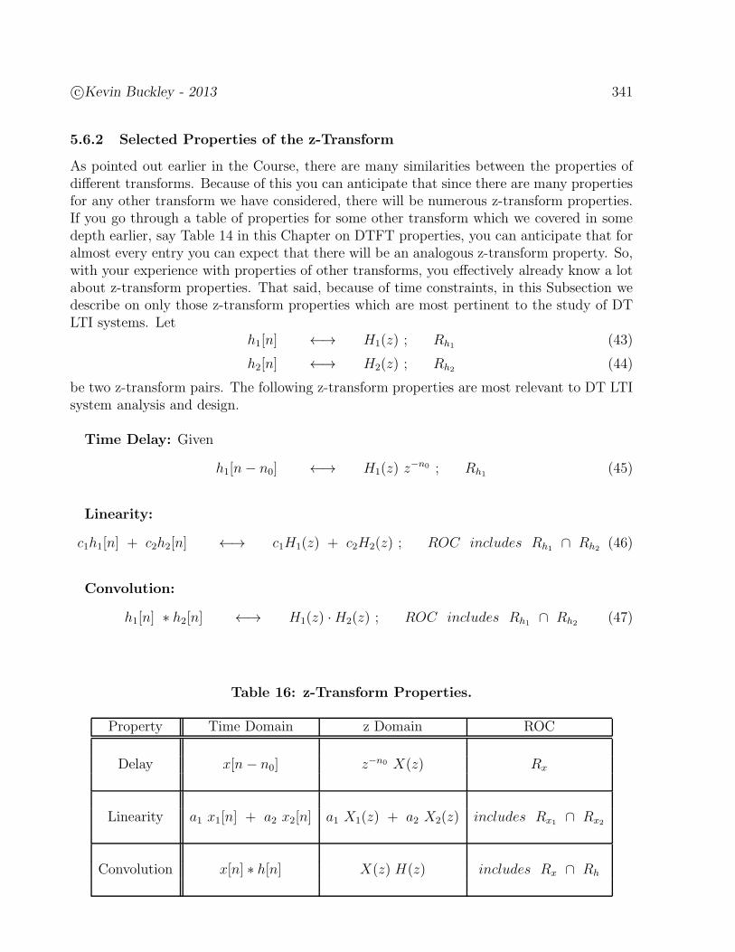
c©Kevin Buckley - 2013 341
5.6.2 Selected Properties of the z-Transform
As pointed out earlier in the Course, there are many similarities between the properties ofdifferent transforms. Because of this you can anticipate that since there are many propertiesfor any other transform we have considered, there will be numerous z-transform properties.If you go through a table of properties for some other transform which we covered in somedepth earlier, say Table 14 in this Chapter on DTFT properties, you can anticipate that foralmost every entry you can expect that there will be an analogous z-transform property. So,with your experience with properties of other transforms, you effectively already know a lotabout z-transform properties. That said, because of time constraints, in this Subsection wedescribe on only those z-transform properties which are most pertinent to the study of DTLTI systems. Let
h1[n] ←→ H1(z) ; Rh1 (43)
h2[n] ←→ H2(z) ; Rh2 (44)
be two z-transform pairs. The following z-transform properties are most relevant to DT LTIsystem analysis and design.
Time Delay: Given
h1[n− n0] ←→ H1(z) z−n0 ; Rh1 (45)
Linearity:
c1h1[n] + c2h2[n] ←→ c1H1(z) + c2H2(z) ; ROC includes Rh1 ∩ Rh2 (46)
Convolution:
h1[n] ∗ h2[n] ←→ H1(z) ·H2(z) ; ROC includes Rh1 ∩ Rh2 (47)
Table 16: z-Transform Properties.
Property Time Domain z Domain ROC
Delay x[n− n0] z−n0 X(z) Rx
Linearity a1 x1[n] + a2 x2[n] a1 X1(z) + a2 X2(z) includes Rx1 ∩ Rx2
Convolution x[n] ∗ h[n] X(z) H(z) includes Rx ∩ Rh
342 c©Kevin Buckley - 2013
Consider Examples 5.40-42 as illustrations of the linearity property.
Example 5.43: Determine the causal inverse z-transform of
X(z) =b + c z−1
1 + d z−1.
Solution:
X(z) =b
1 + d z−1+
c z−1
1 + d z−1.
In the 2-nd term, the z−1 in the numerator represents a delay of one sample.Using the linearity property and Entry #3 of Table 15 (since we are looking fora causal solution), we have that
x[n] = b (−d)n u[n] + c (−d)n−1 u[n− 1] .
Example 5.44: Given the input
x[n] = 6(
1
2
)n−1
u[n]
and output
y[n] = 4(
1
2
)n
u[n] − 2(
1
4
)n
u[n]
to a causal DT LTI system, determine the system impulse response.
Solution:
This is an example of an important signal processing function, systems identifi-cation.
A note on ROC: The ROC will always be an annular ring in the z-plane. Let the innerand outer radii of this ring be denoted as rin and rout, respectively. A right-sided signalwill have rout = ∞. A left-sided signal will have rin = 0. A finite duration signal will haverin = 0 and rout =∞.

c©Kevin Buckley - 2013 343
Example 5.45: Determine the causal inverse z-transform of
H(z) =−2z−1 + 5z−2 − z−3
1 − 34z−1 + 1
8z−2
=4z−2
1 − 12z−1
− 2z−1
1 − 14z−1
.
Solution:
344 c©Kevin Buckley - 2013
5.7 Problems
Chapter Topics:5.1-16 (frequency response of simple DT LTI systems);5.17-24 (DTFS and DTFT);5.25-37 (DTFT properties);5.38-41 (basic z-transform and properties)
1. Consider the pure delay system
y[n] = x[n− n0] .
(a) Determine its frequency, magnitude and phase responses.
(b) For n0 = 10, determine the response to x[n] = 4 ej(4π/10n).
2. Consider the simple first-difference system y[n] = x[n] − x[n−1], which has impulseresponse h[n] = δ[n] − δ[n− 1].
(a) Determine the frequency response H(ejω) and sketch its magnitude over the range−π ≤ ω ≤ π.
(b) Determine the response y[n] to input x[n] = −3 + 5 cos(πn).
3. Consider a DT LTI system with input/output equation
y[n] = x[n + 1] − x[n− 1] .
Determine the frequency responseH(ejω) and plot its magnitude (or magnitude squared)for −π ≤ ω ≤ π. Determine the output for input
x[n] = 5 + 2 sin(πn) .
4. Consider the DT LTI system with difference equation y[n] = 4 x[n+1] − 4 x[n− 1],which has impulse response h[n] = 4 δ[n + 1] − 4 δ[n− 1].
(a) Determine the frequency response H(ejω) and sketch its magnitude over the range−π ≤ ω ≤ π.
(b) Determine the response y[n] to input x[n] = −3 + 6 cos(π2n) + 5 cos(πn).
5. Consider the DT LTI system
y[n] = x[n] − x[n− 2] .
Determine its frequency response H(ejω). Determine the output for input
x[n] = 1 + 2 ejπ2n + 3 ejπn .
Determine and plot |H(ejω)|2 .
c©Kevin Buckley - 2013 345
6. For the DT LTI system with impulse response h[n] = δ[n] + δ[n− 2], determine thefrequency response H(ejω) and sketch its magnitude over the range −π ≤ ω ≤ π.
7. Consider a DT LTI system with input/output equation
y[n] = 4 x[n+ 1] + 4 x[n− 1] .
Determine the frequency responseH(ejω) and plot its magnitude (or magnitude squared)for −π ≤ ω ≤ π. Determine the output for input
x[n] = 3 + 5 cos(πn) .
8. Consider the DT LTI system
y[n] = 2x[n + 1] + 3x[n] + 2x[n− 1] .
(a) Determine its frequency response H(ejω).
(b) Plot |H(ejω)| for −π ≤ ω ≤ π.
(c) Determine the response y[n] for input x[n] = −2 + 12cos(π
2n) + 4 cos(πn).
9. Consider the simple system
y[n] = x[n] − 0.5 x[n− 1] .
(a) Determine its frequency response, and plots its magnitude and phase.
(b) Determine the response to input
x[n] = 4 + cos(πn) .
10. Frequency response of a DT LTI system:
(a) For a DT LTI system, given input x[n] = cos(π2n) and output y[n] = 2 cos(π
2n+ π
3),
determine H(ejπ/2), the frequency response evaluated at ω = π2.
(b) You know that a DT LTI system has a real-valued impulse response, and for inputx[n] = ejπn/2 the output is y[n] = 3 ej(πn/2 − π/3). Determine the output dueto input x1[n] = 5 cos(πn/2).
11. Consider a 10-point averager. Determine its frequency response, its magnitude re-sponse, its phase response, and its response to input
x[n] = 4 + cos(
2π
10n+
π
2
)
+ cos(
π
10n+ π
)
.
12. Consider an 8 point averager which is a LTI system with impulse responseh[n] = 1
8p8[n]. Remember that the output of a LTI system, when the input is a
sinusoid, is a sinusoid of the same frequency. Determine the output sinusoid magnitudeand phase, and write down the equation for the output, for the following inputs:
346 c©Kevin Buckley - 2013
(a) x1[n] = 5
(b) x2[n] = ej3πn/8
(c) x3[n] = 4 cos(πn/4) .
13. For a DT LTI system, the frequency response is
H(ejω) =
π − ω 0 ≤ ω ≤ ππ + ω −π ≤ ω ≤ 0
.
Sketch H(ejω). Determine the response y[n] to input x[n] = −3 + 5 cos(π2n).
14. Determine the frequency response for the causal DT LTI system
y[n] = x[n] + 0.5 y[n− 1] .
Determine its magnitude and plot its magnitude-squared responses.
15. Sinusoidal inputs to DT LTI systems:
(a) Consider the DT LTI system with impulse response h[n] = .5n u[n]. The inputis x[n] = 2 ejπn. The output is of the form y[n] = A ej(ω0n+θ). Determine A, ω0
and θ. Justify your answer.
(b) Consider the DT LTI system and input
y[n] = x[n + 2] + x[n− 2] , x[n] = 3 cos(π
4n +
π
6) = 5 cos(
π
2n+
π
7) .
Plot the magnitude & phase of the frequency response. Determine output y[n].
16. Consider a noncausal DT LTI system with impulse response h[n] = .5|n|.
(a) Determine the frequency response H(ejω). Sketch its magnitude and its phaseover −π ≤ ω ≤ π.
(b) Determine the output y1[n] for input x1[n] = ejω0n with ω0 = 0.
(c) Determine the output y2[n] for input x2[n] = 3 cos(πn).
17. Determine the DTFS coefficients of x[n] = sin(
2π3n)
· cos(
π2n)
.
18. Consider a DT signal x[n] which is periodic with period N = 10 and has discrete-timeFourier series coefficients X [k] = .9k; k = 0, 1, · · · , 9.
(a) Describe the DTFT of x[n] over the range −π ≤ ω ≤ π.
(b) Determine the power of x[n].
(c) If x[n] is the input to a DT LTI ideal lowpass filter with frequency responseH(ejω) = pπ(ω); −π ≤ ω ≤ π, what is the power of the filter output y[n]?
19. Given the DTFS coefficients shown below, determine the signal x[n].
c©Kevin Buckley - 2013 347
ak
x
0 1 2 k3−1−2−3
........
4
2
1
.5
.25
20. Determine the DTFT or inverse DTFT for each of the following.
a) w[n] = p64[n]. Also determine W (ej0).
b) X(ejω) = pπ(ω) + δ(ω − π/2); |ω| ≤ π.
c) y[n] = (0.5)n cos((π/2)n) u[n].
d) z[n] = n (0.2)n u[n] (hint: use linearity and two table entries).
21. Determine the IDTFT of the following functions:
(a) X1(ejω) =
1 π4≤ |ω| ≤ 3π
4
0 3π4≤ |ω| ≤ π , 0 ≤ |ω| ≤ π
4
.
(b) X2(ejω) = 1 + 3e−jω + 2e−j2ω − 4e−j3ω + e−j10ω.
(c) X3(ejω) = e−jω/2 for −π ≤ ω ≤ π.
22. Consider a DT signal x[n] with DTFT X(ejω) = 3pπ(ω) + 2p2π(ω); −π ≤ ω ≤ π.Sketch X(ejω) for −3π ≤ ω ≤ 3π and determine x[n].
23. Given the DTFT
Z(ejω) =0.5
1 − 0.9 ejπ/3 e−jω+
0.5
1 − 0.9 e−jπ/3 e−jω, (48)
determine z[n] expicitely as a real-valued signal. What entry in Table 13 does thiscorrespond to?
24. DTFT/IDTFT Problems:
(a) Given the DTFT
X(ejω) =2 + e−jω + e−j2ω − 0.5e−j3ω
1− 0.25e−j2ω=
2
1 − 0.5 e−jω+
e−j2ω
1 + 0.5 e−jω,
(49)determine x[n].
(b) Given
y[n] = 2 (0.9)n u[n] − (−0.8)n−1 u[n− 1] , (50)
determine its DTFT Y (ejω) and express it as a rational function of e−jω.
348 c©Kevin Buckley - 2013
25. Determine the DTFT V (ejω) of the signal v[n] = x[n] w[n] where x[n] = 1nsin
(
n3
)
and
w[n] = 1nsin
(
3n5
)
.
26. Sketch the DTFT of x4[n] = ej(2π/10)n − 2 sin(πn)πn
.
27. Solve the following using the DTFT pair table and DTFT properties:
(a) Determine the DTFT Y (ejω) of the signal y[n] = an u[n− 3].
(b) Determine the DTFT Z(ejω) of the signal z[n] = .5|n−2|.
28. Determine the energy of x3[n] for
X3(ejω) =
1 + e−jω
1− 0.3e−jω.
29. DTFT
(a) Using the DTFT pairs Table, determine the convolution y[n] = x[n] ∗ h[n] whereh[n] = .9n u[n] and x[n] = (n+ 1) (.9)n u[n].
(b) Determine the energy of the signal s[n] =sin(π
2n)
πn− sin(π
3n)
πn.
30. Consider the DT signal x[n] with DTFT
X(ejω) =
ω 0 ≤ ω ≤ π−ω −π ≤ ω ≤ 0
(a) Plot X(ejω) over the range −π ≤ ω ≤ π.
(b) Determine x[n].
(c) Determine the percentage of x[n] energy in the frequency band −π2≤ ω ≤ π
2.
31. Given a DT signal x[n] with DTFT
X(ejω) = 1 + pπ/2(ω) − π ≤ ω ≤ π ,
determine the percentage of the total energy in the frequency band −3π4≤ ω ≤ 3π
4.
32. Determine the DTFT V (ejω) of the signal v[n] = x[n] w[n] where x[n] = cos(
π4n)
and
w[n] = 1nsin
(
n4
)
.
33. Consider a signal x[n]. Say you know it is real-valued, and that its DTFT is 1 over therange 0 ≤ ω ≤ π
2and 0 over the range π
2< ω ≤ π.
(a) Accurately sketch X(ejω) over the range −2π ≤ ω ≤ 2π.
(b) Determine x[n].
(c) Determine and sketch Y (ejω); −π ≤ ω ≤ π for y[n] = x[n] ej(π/4)n.
c©Kevin Buckley - 2013 349
(d) For the y[n] in part (c), determine the percentage of energy in the frequency band−π
4≤ ω ≤ π
4.
34. For each signal described below, state whether it is a power or energy signal. Determineits power or energy.
(a) X1(ejω) = 6 cos(ω)
(b) x2[n] = 3sin(π
4n)
πn
(c) x3[n] = 3 cos(πn) − 2
(d) X4(ejω) = 1
1 − .5 e−jω − .5 e−jω
1 − .5 e−jω
35. DTFT pairs and properties:
(a) Given
X(ejω) =1 + 3 e−j2ω
1 + .5 e−jω,
determine x[n].
(b) Given
z[n] =1
π
1
(1 + n2),
determine the fraction of its energy in the band −π2≤ ω ≤ π
2.
(c) Sketch the DTFT of the signal x[n] = 4 sin(2πn/3)πn
−√24 sin2(πn/6)
(πn)2. Determine
the percentage of its total energy in the band π3≤ ω ≤ 2π
3.
(d) Given a signal x[n] with DTFT
X(ejω) =
1 0 ≤ ω ≤ π2
0 otherwise over − π ≤ ω ≤ π
use an entry in the DTFT table and the DTFT modulation property to determinex[n]. What percentage of the total energy of x[n] is in the frequency band0 ≤ ω ≤ π
10.
36. Determine the DTFT and energy of the following signals:
(a) a[n] = sin((π/8)n)πn
;
(b) b[n] = a[n] · cos((π/2)n);(c) c[n] = b[n] ∗ δ(n− 5);
(d) d[n] = c[n] ∗ sin2((π/8)n)(πn)2
.
37. Determine the DTFT (or IDTFT) and energy of the following signals:
350 c©Kevin Buckley - 2013
a) A(ejω) = 11 − 0.9 e−jω ;
b) B(ejω) = A(ejω) 2 ej4ω;
c) c[n] = b[n] ej(π/2)n;
d) D(ejω) = A(ejω)1 − 0.9 e−jω ;
e) E(ejω) = A(ejω) (1 − 0.9 e−jω).
38. Determine the z-transform pair for:
(a) X(z) = 3 − 2 z−2 + 4 z−5.
(b) Y (z) = 31 + 0.25 z−1 . Assume y[n] is causal.
(c) V (z) = 6 zz − .6
. Assume v[n] is causal.
(d) x2[n] = −4 cos(πn) u[n− 1] (Hint: use Euler’s identities and linearity).
(e) Use the delay property to determine the right-sided inverse z-transform ofH(z) = 1
z−4 − 0.25 z−5 .
(f) A causal y[n] has z-transform Y (z) = 1(1−0.8z−1)3
. Determine y[n] and its DTFT
(not necessarily in that order).
39. Find the z-transform, including the ROC, for x[n] = 0.4n u[n] + 1.25n u[−n].
40. Using and Euler’s identity, linearity and Entry #4 of Table 15 of the Course Notes,determine the z-transform, including the ROC, of x[n] = 4n cos(2π
6n + π
2) u[−n− 1].
41. Consider a DT signal x[n] with z-transform
X(z) =4− 7z−1 + 3.68z−2 − 0.128z−3
1− 1.6z−1 + 0.8z−2 − 0.128z−3= 1 +
3
1 − 0.8z−1− 3 z−1
(1 − 0.4z−1)2.
Given that the ROC is Rx = .4 < |z| < .8, determine x[n].
42. Consider two signals x1[n] = δ[n]+δ[n−1]+δ[n−2] and x2[n] = δ[n]−δ[n−1]+δ[n−2],along with x[n] = x1[n] ∗ x2[n].
(a) Determine the z-transforms X1[z] and X2[z].
(b) From X1[z] and X2[z], determine the z-transform, X(z), of x[n].
(c) From X [z], determine x[n].
43. Determine the inverse z-transform (or z-transform) and energy for the following:
a) A(z) = 11 − 0.9 z−1 ; Ra = |z| > 0.9;
b) B(z) = 2 A(z) z−5 ; Rb = Ra;
c) C(z) = A(z) ; Rc = |z| < 0.9;
d) D(z) = A(z) (1 − 0.9 z−1)(1 + 0.9 z−1).
c©Kevin Buckley - 2013 351
6 Applications of DT Transforms
1. In Sections 6.1 & 6.2 we then explore how DT transforms can be used to characterize,analyze, implement and design DT LTI systems.
2. In Section 6.3 we use DT transforms to facilitate descriptions of several higher levelsignal processing function.
Chapter 6 Objective Checklist
• Be familiar with the various DT LTI system descriptions discussed in this Chapter,including: the impulse response, the frequency response, the transfer function andsystem poles/zeros. Understand the relationships between these system descriptions.
• Know how to solve DT LTI system I/O problems using different system descriptions.Understand the relationship between different DT LTI system descriptions and stabil-ity/causality.
• Be comfortable with how the DT transforms covered in this Chapter are applied tothe advanced topics discussed in Section 5.9.
352 c©Kevin Buckley - 2013
6.1 The DTFT and DT LTI Systems
In this Section we employ a few DTFT properties to expand on our ability to work with DTLTI systems. The fact that this Section is brief should not lead you to conclude that theDTFT does not provide much benefit in dealing with DT LTI systems. The facts are that:
1. At the beginning of Chapter 5 we spent a significant amount of effort using the functionH(ejω), the DTFT of the impulse response, to identify DT LTI system outputs forsinusoidal inputs. We just didn’t call H(ejω) a DTFT back then.
2. In Section 6.2 we will consider, in depth, the application of both the DTFT and z-transform to the analysis of DT LTI systems.
Here we simply formalize and exemplify two concepts.
6.1.1 The Frequency Response
Figure 117 illustrates the DTFT convolution property as applied to DT LTI systems.
jω
jωX(e ) jωX(e ) jωH(e )jωY(e ) =
x[n] y[n] = x[n] * h[n]DT LTI system
h[n]; H(e )
Figure 117: The DTFT convolution property and DT LTI systems.
As in Section 5.1, H(ejω) is called the frequency response. We now recognize it as being theDTFT of h[n]. So, the output DTFT is the product of the input DTFT and the frequencyresponse. The most important consequence of the fact that Y (ejω) = X(ejω) H(ejω) is thatit indicates that the frequency response characterizes the frequency selectivity of a DT LTIsystem. To see this, consider some frequency ω0. X(ejω0) is the weight on the ω0 frequencycomponent of the input. Y (ejω0) = X(ejω0) H(ejω0) is then weight on the ω0 frequencycomponent of the output. If |H(ejω0)| << 1, then that frequency component of the inputis attenuated by the system. If |H(ejω0)| > 1, then that component is amplified. Similarly,6 H(ejω) dictates input phase shift as a function of frequency.
Another use of the DTFT for system analysis is derived by simply rearranging the DTFTI/O relationship as follows:
H(ejω) =Y (ejω)
X(ejω)(1)
X(ejω) =Y (ejω)
H(ejω). (2)
Back in Chapter 2 we developed a method, called convolution, for computing the output ofa DT LTI system given the input x[n] and the impulse response h[n]. However, determiningx[n] given y[n] and h[n], or h[n] given y[n] and x[n] was not addressed. In other words, wecould not do deconvolution. Well, now we can.
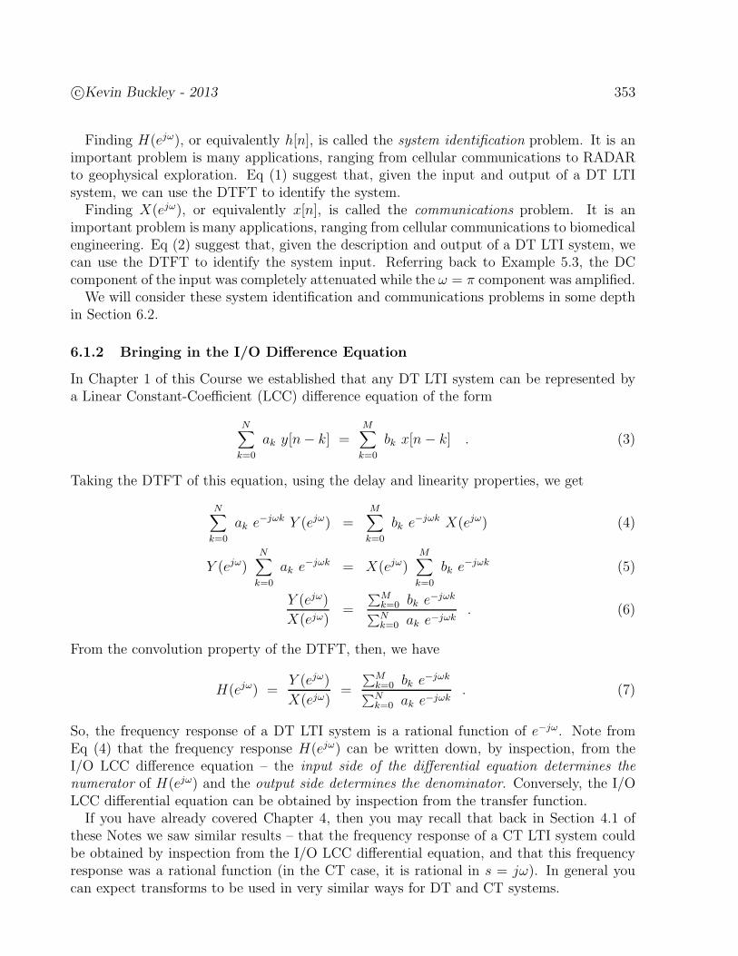
c©Kevin Buckley - 2013 353
Finding H(ejω), or equivalently h[n], is called the system identification problem. It is animportant problem is many applications, ranging from cellular communications to RADARto geophysical exploration. Eq (1) suggest that, given the input and output of a DT LTIsystem, we can use the DTFT to identify the system.
Finding X(ejω), or equivalently x[n], is called the communications problem. It is animportant problem is many applications, ranging from cellular communications to biomedicalengineering. Eq (2) suggest that, given the description and output of a DT LTI system, wecan use the DTFT to identify the system input. Referring back to Example 5.3, the DCcomponent of the input was completely attenuated while the ω = π component was amplified.
We will consider these system identification and communications problems in some depthin Section 6.2.
6.1.2 Bringing in the I/O Difference Equation
In Chapter 1 of this Course we established that any DT LTI system can be represented bya Linear Constant-Coefficient (LCC) difference equation of the form
N∑
k=0
ak y[n− k] =M∑
k=0
bk x[n− k] . (3)
Taking the DTFT of this equation, using the delay and linearity properties, we get
N∑
k=0
ak e−jωk Y (ejω) =M∑
k=0
bk e−jωk X(ejω) (4)
Y (ejω)N∑
k=0
ak e−jωk = X(ejω)M∑
k=0
bk e−jωk (5)
Y (ejω)
X(ejω)=
∑Mk=0 bk e−jωk
∑Nk=0 ak e−jωk
. (6)
From the convolution property of the DTFT, then, we have
H(ejω) =Y (ejω)
X(ejω)=
∑Mk=0 bk e−jωk
∑Nk=0 ak e−jωk
. (7)
So, the frequency response of a DT LTI system is a rational function of e−jω. Note fromEq (4) that the frequency response H(ejω) can be written down, by inspection, from theI/O LCC difference equation – the input side of the differential equation determines thenumerator of H(ejω) and the output side determines the denominator. Conversely, the I/OLCC differential equation can be obtained by inspection from the transfer function.
If you have already covered Chapter 4, then you may recall that back in Section 4.1 ofthese Notes we saw similar results – that the frequency response of a CT LTI system couldbe obtained by inspection from the I/O LCC differential equation, and that this frequencyresponse was a rational function (in the CT case, it is rational in s = jω). In general youcan expect transforms to be used in very similar ways for DT and CT systems.

354 c©Kevin Buckley - 2013
Example 6.1: Consider the DT LTI system described by the following LCC dif-ference equation.
y[n] − 0.25y[n− 1] + y[n− 2] = x[n] + x[n− 2] .
Determine the frequency response H(ejω) and the output due to inputx[n] = A cos((π/2)n).
Solution:
c©Kevin Buckley - 2013 355
Example 6.2: Given the following DT LTI system frequency response, find theimpulse response and the LCC difference equation.
H(ejω) =2− 0.5e−jω
1− 0.9e−jω.
Solution:
Example 6.3: Determine the impulse response for the system described by theLCC difference equation
y[n] − 3
4y[n− 1] +
1
8y[n− 2] = x[n] .
Solution:
From Example 6.3 it should be clear that it is important to be able to break any orderrational function of e−jω into a sum of lower order rational functions. As is also the casefor CT LTI systems, we can use partial fraction expansion to do this. We defer to later inSection 6.2 of these Notes for coverage of the details for doing this.
356 c©Kevin Buckley - 2013
6.2 The z-Transform and the LTI System Transfer Function
Consider the DT LTI system block diagram shown below.
DT LTI systemz H(z) zn n
h[n]; H(z )
X(z) Y(z) = X(z) H(z)
H(z) =∞∑
n=−∞h[n] z−n . (8)
Figure 118: A DT LTI system and its transfer function.
By the convolution property of the z-transform, we have that Y (z) = X(z) H(z). Thez-transform of the system impulse response, H(z), impulse response, is called the transferfunction. It is also referred to as the system function.
Example 6.4: Determine the transfer function for the following FIR filter
y[n] = x[n] + 2 x[n− 1] + x[n− 2].
Solution:
Example 6.5: For a general FIR filter, with impulse response
h[n] =M∑
k=0
h[k] δ[n− k] =M∑
k=0
bk δ[n− k] ,
determine the I/O difference equation and the transfer function.
Solution:
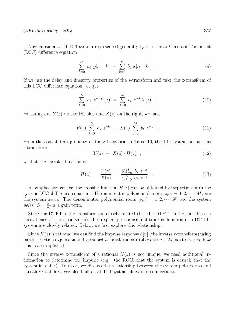
c©Kevin Buckley - 2013 357
Now consider a DT LTI system represented generally by the Linear Constant-Coefficient(LCC) difference equation
N∑
k=0
ak y[n− k] =M∑
k=0
bk x[n− k] . (9)
If we use the delay and linearity properties of the z-transform and take the z-transform ofthis LCC difference equation, we get
N∑
k=0
ak z−kY (z) =M∑
k=0
bk z−kX(z) . (10)
Factoring out Y (z) on the left side and X(z) on the right, we have
Y (z)N∑
k=0
ak z−k = X(z)M∑
k=0
bk z−k . (11)
From the convolution property of the z-transform in Table 16, the LTI system output hasz-transform
Y (z) = X(z) ·H(z) , (12)
so that the transfer function is
H(z) =Y (z)
X(z)=
∑Mk=0 bk z−k
∑Nk=0 ak z−k
. (13)
As emphasized earlier, the transfer function H(z) can be obtained by inspection form thesystem LCC difference equation. The numerator polynomial roots, zi; i = 1, 2, · · · ,M , arethe system zeros. The denominator polynomial roots, pi; i = 1, 2, · · · , N , are the systempoles. G = b0
a0is a gain term.
Since the DTFT and z-transform are closely related (i.e. the DTFT can be considered aspecial case of the z-transform), the frequency response and transfer function of a DT LTIsystem are closely related. Below, we first explore this relationship.
SinceH(z) is rational, we can find the impulse response h[n] (the inverse z-transform) usingpartial fraction expansion and standard z-transform pair table entries. We next describe howthis is accomplished.
Since the inverse z-transform of a rational H(z) is not unique, we need additional in-formation to determine the impulse (e.g. the ROC; that the system is causal; that thesystem is stable). To close, we discuss the relationship between the system poles/zeros andcausality/stability. We also look a DT LTI system block interconnections.
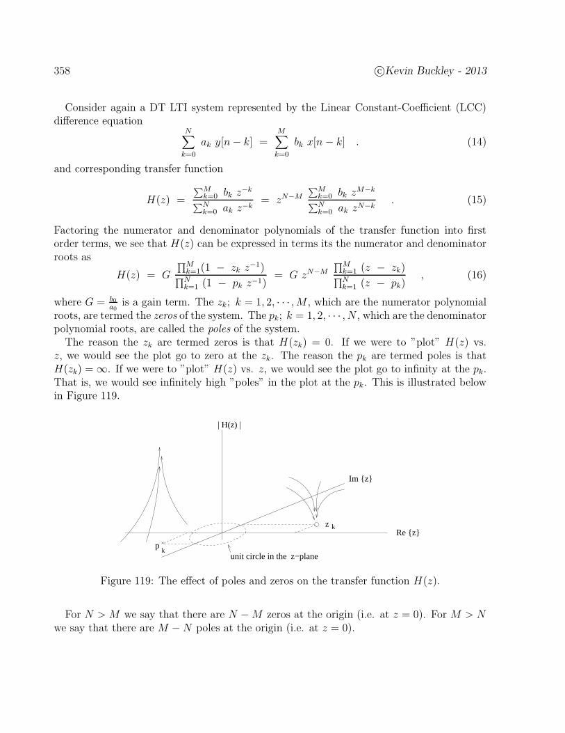
358 c©Kevin Buckley - 2013
Consider again a DT LTI system represented by the Linear Constant-Coefficient (LCC)difference equation
N∑
k=0
ak y[n− k] =M∑
k=0
bk x[n− k] . (14)
and corresponding transfer function
H(z) =
∑Mk=0 bk z−k
∑Nk=0 ak z−k
= zN−M
∑Mk=0 bk zM−k
∑Nk=0 ak zN−k
. (15)
Factoring the numerator and denominator polynomials of the transfer function into firstorder terms, we see that H(z) can be expressed in terms its the numerator and denominatorroots as
H(z) = G
∏Mk=1(1 − zk z−1)
∏Nk=1 (1 − pk z−1)
= G zN−M
∏Mk=1 (z − zk)
∏Nk=1 (z − pk)
, (16)
where G = b0a0
is a gain term. The zk; k = 1, 2, · · · ,M , which are the numerator polynomialroots, are termed the zeros of the system. The pk; k = 1, 2, · · · , N , which are the denominatorpolynomial roots, are called the poles of the system.
The reason the zk are termed zeros is that H(zk) = 0. If we were to ”plot” H(z) vs.z, we would see the plot go to zero at the zk. The reason the pk are termed poles is thatH(zk) =∞. If we were to ”plot” H(z) vs. z, we would see the plot go to infinity at the pk.That is, we would see infinitely high ”poles” in the plot at the pk. This is illustrated belowin Figure 119.
Re z
Im z
unit circle in the z−planep
z k
k
| H(z) |
Figure 119: The effect of poles and zeros on the transfer function H(z).
For N > M we say that there are N −M zeros at the origin (i.e. at z = 0). For M > Nwe say that there are M −N poles at the origin (i.e. at z = 0).
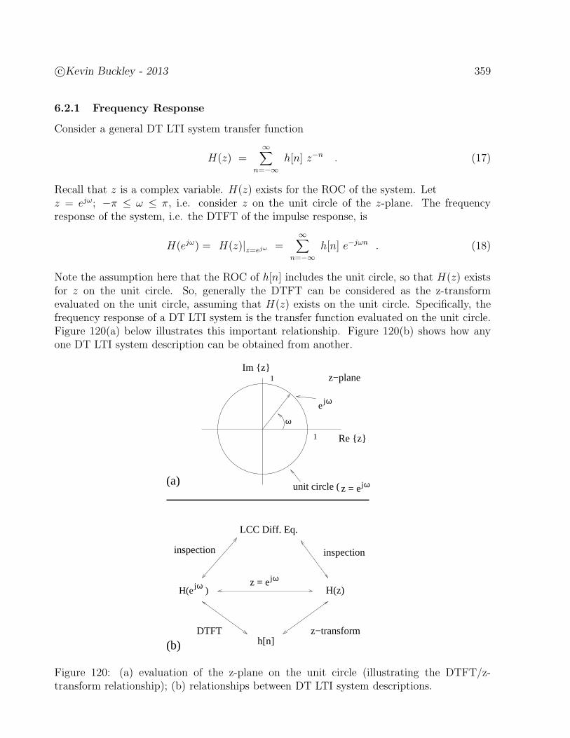
c©Kevin Buckley - 2013 359
6.2.1 Frequency Response
Consider a general DT LTI system transfer function
H(z) =∞∑
n=−∞h[n] z−n . (17)
Recall that z is a complex variable. H(z) exists for the ROC of the system. Letz = ejω; −π ≤ ω ≤ π, i.e. consider z on the unit circle of the z-plane. The frequencyresponse of the system, i.e. the DTFT of the impulse response, is
H(ejω) = H(z)|z=ejω =∞∑
n=−∞h[n] e−jωn . (18)
Note the assumption here that the ROC of h[n] includes the unit circle, so that H(z) existsfor z on the unit circle. So, generally the DTFT can be considered as the z-transformevaluated on the unit circle, assuming that H(z) exists on the unit circle. Specifically, thefrequency response of a DT LTI system is the transfer function evaluated on the unit circle.Figure 120(a) below illustrates this important relationship. Figure 120(b) shows how anyone DT LTI system description can be obtained from another.
jωH(e )jωz = e
jωz = e unit circle ( )
ejω
z−planeIm z
Re z
h[n]
LCC Diff. Eq.
H(z)
DTFT
inspectioninspection
z−transform
1
1
ω
(b)
(a)
Figure 120: (a) evaluation of the z-plane on the unit circle (illustrating the DTFT/z-transform relationship); (b) relationships between DT LTI system descriptions.
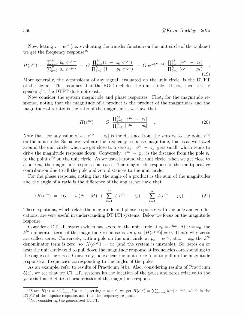
360 c©Kevin Buckley - 2013
Now, letting z = ejω (i.e. evaluating the transfer function on the unit circle of the z-plane)we get the frequency response18
H(ejω) =
∑Mk=0 bk e−jωk
∑Nk=0 ak e−jωk
= G
∏Mk=1(1 − zk e−jω)
∏Nk=1 (1 − pk e−jω)
= G ejω(N−M)
∏Mk=1 (ejω − zk)
∏Nk=1 (ejω − pk)
.
(19)More generally, the z-transform of any signal, evaluated on the unit circle, is the DTFTof the signal. This assumes that the ROC includes the unit circle. If not, then strictlyspeaking19, the DTFT does not exist.
Now consider the system magnitude and phase responses. First, for the magnitude re-sponse, noting that the magnitude of a product is the product of the magnitudes and themagnitude of a ratio is the ratio of the magnitudes, we have that
|H(ejω)| = |G|∏M
k=1 |ejω − zk|∏N
k=1 |ejω − pk|. (20)
Note that, for any value of ω, |ejω − zk| is the distance from the zero zk to the point ejω
on the unit circle. So, as we evaluate the frequency response magnitude, that is as we travelaround the unit circle, when we get close to a zero zk, |ejω − zk| gets small, which tends todrive the magnitude response down. Conversely, |ejω − pk| is the distance from the pole pkto the point ejω on the unit circle. As we travel around the unit circle, when we get close toa pole pk, the magnitude response increases. The magnitude response is the multiplicativecontribution due to all the pole and zero distances to the unit circle.
For the phase response, noting that the angle of a product is the sum of the magnitudesand the angle of a ratio is the difference of the angles, we have that
6 H(ejω) = 6 G + ω(N −M) +M∑
k=1
6 (ejω − zk) −N∑
k=1
6 (ejω − pk) . (21)
These equations, which relate the magnitude and phase responses with the pole and zero lo-cations, are very useful in understanding DT LTI systems. Below we focus on the magnituderesponse.
Consider a DT LTI system which has a zero on the unit circle at zk = ejω0. At ω = ω0, thekth numerator term of the magnitude response is zero, so |H(ejω0)| = 0. That’s why zerosare called zeros. Conversely, with a pole on the unit circle at pk = ejω0 , at ω = ω0, the kth
denominator term is zero, so |H(ejω0)| = ∞ (and the system is unstable). So, zeros on ornear the unit circle tend to pull down the magnitude response at frequencies corresponding tothe angles of the zeros. Conversely, poles near the unit circle tend to pull up the magnituderesponse at frequencies corresponding to the angles of the poles.
As an example, refer to results of Practicum 5(b). Also, considering results of Practicum5(a), we see that for CT LTI systems its the location of the poles and zeros relative to thejω axis that dictates characteristics of the magnitude response.
18Since H(z) =∑
∞
n=−∞h[n] z−n, setting z = ejω , we get H(ejω) =
∑
∞
n=−∞h[n] e−jωn, which is the
DTFT of the impulse response, and thus the frequency response.19Not considering the generalized DTFT.

c©Kevin Buckley - 2013 361
Example 6.6: Given the LCC I/O difference equation of a DT LTI system
y[n] + 0.81 y[n− 2] = 5 x[n] − 5 x[n− 2] ,
determine H(z), the poles and zeros, and sketch |H(ejω)|.
Solution:
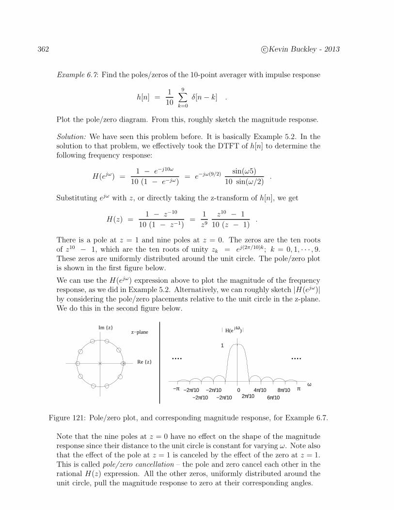
362 c©Kevin Buckley - 2013
Example 6.7: Find the poles/zeros of the 10-point averager with impulse response
h[n] =1
10
9∑
k=0
δ[n− k] .
Plot the pole/zero diagram. From this, roughly sketch the magnitude response.
Solution: We have seen this problem before. It is basically Example 5.2. In thesolution to that problem, we effectively took the DTFT of h[n] to determine thefollowing frequency response:
H(ejω) =1 − e−j10ω
10 (1 − e−jω)= e−jω(9/2) sin(ω5)
10 sin(ω/2).
Substituting ejω with z, or directly taking the z-transform of h[n], we get
H(z) =1 − z−10
10 (1 − z−1)=
1
z9z10 − 1
10 (z − 1).
There is a pole at z = 1 and nine poles at z = 0. The zeros are the ten rootsof z10 − 1, which are the ten roots of unity zk = ej(2π/10)k; k = 0, 1, · · · , 9.These zeros are uniformly distributed around the unit circle. The pole/zero plotis shown in the first figure below.
We can use the H(ejω) expression above to plot the magnitude of the frequencyresponse, as we did in Example 5.2. Alternatively, we can roughly sketch |H(ejω)|by considering the pole/zero placements relative to the unit circle in the z-plane.We do this in the second figure below.
Re z
Im zz−plane H(e )
02π/10
4π/10 8π/10 π−2π/10−2π/10−2π/10 −2π/10
−π
........
6π/10
ω
jω
1
Figure 121: Pole/zero plot, and corresponding magnitude response, for Example 6.7.
Note that the nine poles at z = 0 have no effect on the shape of the magnituderesponse since their distance to the unit circle is constant for varying ω. Note alsothat the effect of the pole at z = 1 is canceled by the effect of the zero at z = 1.This is called pole/zero cancellation – the pole and zero cancel each other in therational H(z) expression. All the other zeros, uniformly distributed around theunit circle, pull the magnitude response to zero at their corresponding angles.
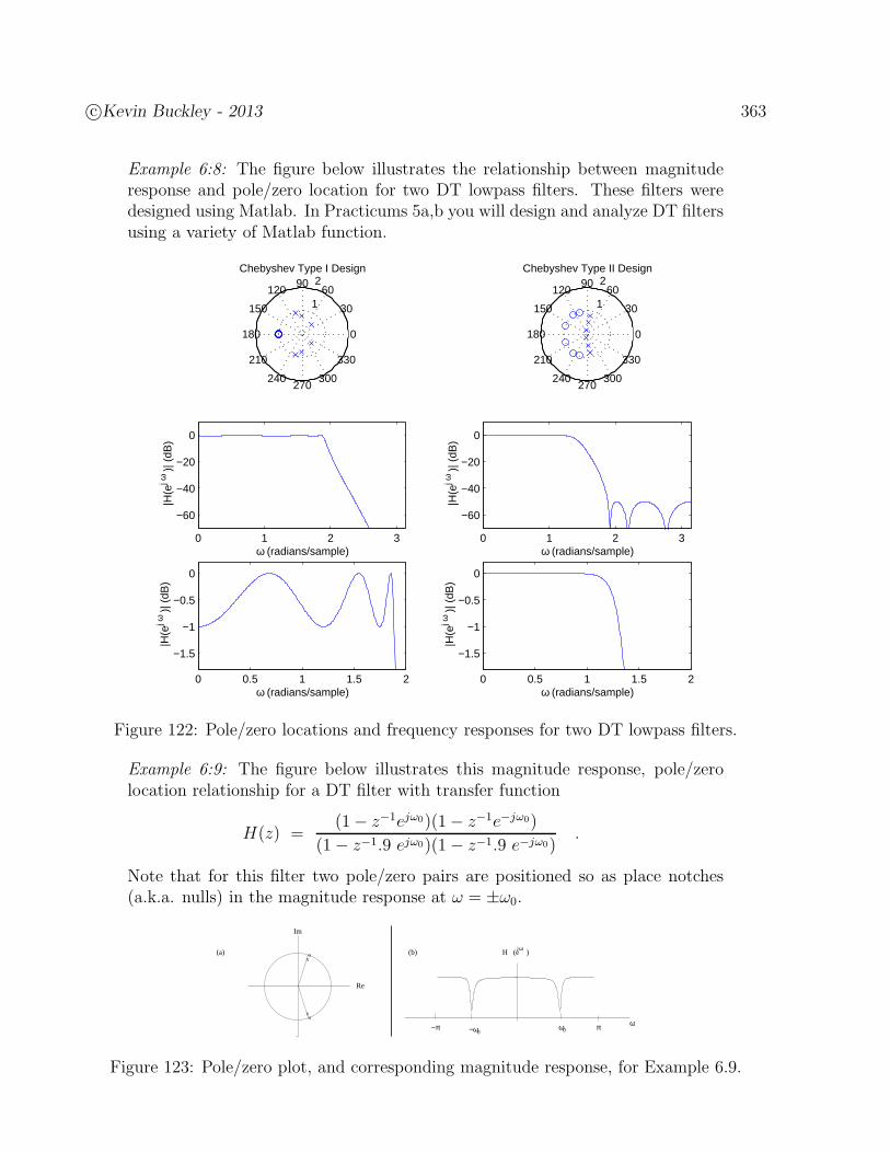
c©Kevin Buckley - 2013 363
Example 6:8: The figure below illustrates the relationship between magnituderesponse and pole/zero location for two DT lowpass filters. These filters weredesigned using Matlab. In Practicums 5a,b you will design and analyze DT filtersusing a variety of Matlab function.
1
2
30
210
60
240
90
270
120
300
150
330
180 0
Chebyshev Type I Design
0 1 2 3
−60
−40
−20
0
ω (radians/sample)
|H(e
j ω )
| (dB
)
0 0.5 1 1.5 2
−1.5
−1
−0.5
0
ω (radians/sample)
|H(e
j ω )
| (dB
)
1
2
30
210
60
240
90
270
120
300
150
330
180 0
Chebyshev Type II Design
0 1 2 3
−60
−40
−20
0
ω (radians/sample)
|H(e
j ω )
| (dB
)
0 0.5 1 1.5 2
−1.5
−1
−0.5
0
ω (radians/sample)
|H(e
j ω )
| (dB
)
Figure 122: Pole/zero locations and frequency responses for two DT lowpass filters.
Example 6:9: The figure below illustrates this magnitude response, pole/zerolocation relationship for a DT filter with transfer function
H(z) =(1− z−1ejω0)(1− z−1e−jω0)
(1− z−1.9 ejω0)(1− z−1.9 e−jω0).
Note that for this filter two pole/zero pairs are positioned so as place notches(a.k.a. nulls) in the magnitude response at ω = ±ω0.
j ωH (e )
ωω π−π −ω 00
(b)
Re
Im
ox
xo
(a)
Figure 123: Pole/zero plot, and corresponding magnitude response, for Example 6.9.
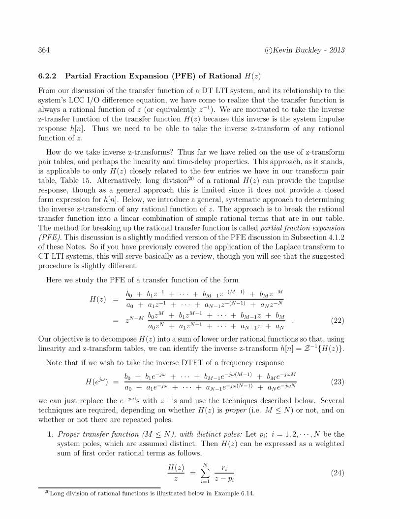
364 c©Kevin Buckley - 2013
6.2.2 Partial Fraction Expansion (PFE) of Rational H(z)
From our discussion of the transfer function of a DT LTI system, and its relationship to thesystem’s LCC I/O difference equation, we have come to realize that the transfer function isalways a rational function of z (or equivalently z−1). We are motivated to take the inversez-transfer function of the transfer function H(z) because this inverse is the system impulseresponse h[n]. Thus we need to be able to take the inverse z-transform of any rationalfunction of z.
How do we take inverse z-transforms? Thus far we have relied on the use of z-transformpair tables, and perhaps the linearity and time-delay properties. This approach, as it stands,is applicable to only H(z) closely related to the few entries we have in our transform pairtable, Table 15. Alternatively, long division20 of a rational H(z) can provide the impulseresponse, though as a general approach this is limited since it does not provide a closedform expression for h[n]. Below, we introduce a general, systematic approach to determiningthe inverse z-transform of any rational function of z. The approach is to break the rationaltransfer function into a linear combination of simple rational terms that are in our table.The method for breaking up the rational transfer function is called partial fraction expansion(PFE). This discussion is a slightly modified version of the PFE discussion in Subsection 4.1.2of these Notes. So if you have previously covered the application of the Laplace transform toCT LTI systems, this will serve basically as a review, though you will see that the suggestedprocedure is slightly different.
Here we study the PFE of a transfer function of the form
H(z) =b0 + b1z
−1 + · · · + bM−1z−(M−1) + bMz−M
a0 + a1z−1 + · · · + aN−1z−(N−1) + aNz−N
= zN−M b0zM + b1z
M−1 + · · · + bM−1z + bMa0zN + a1zN−1 + · · · + aN−1z + aN
. (22)
Our objective is to decompose H(z) into a sum of lower order rational functions so that, usinglinearity and z-transform tables, we can identify the inverse z-transform h[n] = Z−1H(z).
Note that if we wish to take the inverse DTFT of a frequency response
H(ejω) =b0 + b1e
−jω + · · · + bM−1e−jω(M−1) + bMe−jωM
a0 + a1e−jω + · · · + aN−1e−jω(N−1) + aNe−jωN(23)
we can just replace the e−jω’s with z−1’s and use the techniques described below. Severaltechniques are required, depending on whether H(z) is proper (i.e. M ≤ N) or not, and onwhether or not there are repeated poles.
1. Proper transfer function (M ≤ N), with distinct poles: Let pi; i = 1, 2, · · · , N be thesystem poles, which are assumed distinct. Then H(z) can be expressed as a weightedsum of first order rational terms as follows,
H(z)
z=
N∑
i=1
riz − pi
(24)
20Long division of rational functions is illustrated below in Example 6.14.
c©Kevin Buckley - 2013 365
where the ri, termed the residues, are computed as
ri = (z − pi)H(z)
z
∣
∣
∣
∣
∣
z=pi
. (25)
The reason we are expanding H(z)z
instead of H(z) is that the 1-st order terms of theexpansion, the ri
z−piare not in our z-transform table. However, multiplying Eq (24) by
z, we have
H(z) =N∑
i=1
zriz − pi
=N∑
i=1
ri1− piz−1
. (26)
The ri1−piz−1 terms are in the Table 15.
Then, assuming for example a causal21 h[n], taking the inverse z-transform, we have
h[n] =N∑
i=1
ri pni u[n] . (27)
Regardless on whether or not H(z) is proper or not, and on whether there are repeatedroots or not, we will be able to expand H(z) as a linear combination of low order rationalfunctions. The coefficients of the expansion, which we denote as the r′is, are called residues.
Each pi, ri pair corresponds to an exponential component of the inverse transform. Itmay be causal or not, depending on the ROC. Note that there is no requirement that thepoles or residues be real-valued. If the ai and bi coefficients of H(z) are real-valued, thenthe poles and corresponding residues will either be real-valued or exist in complex conjugatepairs. Any complex-valued poles corresponds to a complex exponential component (i.e. anoscillating and perhaps decaying/expanding component) of the impulse response. We willexplore this in detail in an example below.
Partial fraction expansion (PFE) is not restricted to transfer functions. Any rationalfunction can be expressed this way. So PFE is a generally useful procedure in determiningthe inverse transform (e.g. of input and output signals).
21Recall that 1
1−az−1 has two inverse z-transforms, an u[n] and −an u[−n − 1], depending of the ROC.Here, we will assume an u[n]. That is, we will assume the casual inverse transform.

366 c©Kevin Buckley - 2013
Example 6.10: Determine the impulse response of the causal DT LTI systemwith LCC difference equation
y[n] − 7
12y[n− 1] +
1
12y[n− 2] = 3x[n] − 5
6x[n− 1] .
Solution:
H(z) =3 − 5
6z−1
1 − 712z−1 + 1
12z−2
=3 − 5
6z−1
(1 − 13z−1)(1 − 1
4z−1)
=z(3z − 5
6)
(z − 13)(z − 1
4)
.
H(z)
z=
3z − 56
(z − 13)(z − 1
4)
=r1
z − 13
+r2
z − 14
.
r1 =3z − 5
6
z − 14
∣
∣
∣
∣
∣
z=(1/3)
= 2 , r2 =3z − 5
6
z − 13
∣
∣
∣
∣
∣
z=(1/4)
= 1 .
H(z)
z=
2
z − 13
+1
z − 14
.
H(z) =2z
z − 13
+z
z − 14
=2
a − 13z−1
+1
1 − 14z−1
.
h[n] = 2(
1
3
)n
u[n] +(
1
4
)n
u[n] .
Note that this system is stable, i.e. h[n] is absolutely summable because eachexponential component is decaying. From this example, can you anticipate thecharacteristic of the poles that is required for a casual system to be stable? Wewill address this issue later.

c©Kevin Buckley - 2013 367
Example 6.11: Determine the impulse response of the causal DT LTI system withLCC I/O difference equation
y[n] − 0.3 y[n− 1] − 0.4 y[n− 2] = x[n] − 2.1 x[n− 1] .
Solution:
Matlab Demo - Matlab contains many functions which are useful for systemanalysis. We will explore a number of these later, in Practicums 5a,b. For now,try the following:
B = [1 -2.1]; % transfer function numerator polynomial coefficient vector
A = [1 -0.3 -0.4]; % transfer function denominator polynomial coefficient vector
Z = zeros(B); % zeros
P = zeros(A); % poles
[r,p,k] = residue(B,A); % residues, poles, k=[] since H(z)/z is strictly proper
This provides the PFE of the H(z)/z for this example.
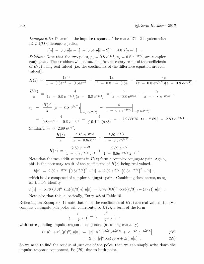
368 c©Kevin Buckley - 2013
Example 6.12: Determine the impulse response of the causal DT LTI system withLCC I/O difference equation
y[n] − 0.8 y[n− 1] + 0.64 y[n− 2] = 4.0 x[n− 1] .
Solution: Note that the two poles, p1 = 0.8 ejπ/3, p2 = 0.8 e−jπ/3, are complexconjugates. Their residues will be too. This is a necessary result of the coefficientsof H(z) being real-valued (i.e. the coefficients of the difference equation are real-valued).
H(z) =4z−1
1 − 0.8z−1 + 0.64z−2=
4z
z2 − 0.8z + 0.64=
4z
(z − 0.8 e−jπ/3)(z − 0.8 ejπ/3).
H(z)
z=
4
(z − 0.8 e−jπ/3)(z − 0.8 ejπ/3)=
r1z − 0.8 ejπ/3
+r2
z − 0.8 e−jπ/3.
r1 =H(z)
z(z − 0.8 ejπ/3)
∣
∣
∣
∣
∣
z=(0.8ejπ/3)
=4
z − 0.8 e−jπ/3
∣
∣
∣
∣
z=(0.8ejπ/3)
=4
0.8ejπ/3 − 0.8 e−jπ/3=
4
j 0.4 sin(π/3)= −j 2.88675 ≈ −2.89j = 2.89 e−jπ/2 .
Similarly, r2 ≈ 2.89 ejπ/2.
H(z)
z=
2.89 e−jπ/2
z − 0.8ejπ/3+
2.89 ejπ/2
z − 0.8e−jπ/3.
H(z) =2.89 e−jπ/2
1 − 0.8ejπ/3 z−1+
2.89 ejπ/2
1 − 0.8e−jπ/3 z−1.
Note that the two additive terms in H(z) form a complex conjugate pair. Again,this is the necessary result of the coefficients of H(z) being real-valued.
h[n] = 2.89 e−jπ/2(
0.8ejπ/3)n
u[n] + 2.89 ejπ/2(
0.8e−jπ/3)n
u[n] ,
which is also composed of complex conjugate pairs. Combining these terms, usingan Euler’s identity,
h[n] = 5.78 (0.8)n sin((π/3)n) u[n] = 5.78 (0.8)n cos((π/3)n− (π/2)) u[n] .
Note also that this is, basically, Entry #8 of Table 15.
Reflecting on Example 6.12 note that since the coefficients of H(z) are real-valued, the twocomplex conjugate pair poles will contribute, to H(z), a term of the form
r
1 − p z−1=
r∗
1 − p∗ z−1,
with corresponding impulse response component (assuming causality)
(r pn + r∗ (p∗)n) u[n] = |r| |p|n[
ej6 r ej
6 p n + e−j 6 r e−j 6 p n]
(28)
= 2 |r| |p|n cos( 6 p n+ 6 r) u[n] . (29)
So we need to find the residue of just one of the poles, then we can simply write down theimpulse response component, Eq (29), due to both poles.

c©Kevin Buckley - 2013 369
2. Proper transfer function (M < N), repeated poles: The following transfer function isused to illustrate the general problem of repeated poles. It shows only a single repeatedpole, but in a multiple repeated pole case, each repeated pole is handled as illustratedbelow.
H(z)
z=
N(z)
(z − p1)(z − p2) · · · (z − pm−1)(z − pm)σ(30)
=m−1∑
i=1
riz − pi
+σ∑
k=1
rm,k
(z − pm)k(31)
where σ = N −m+ 1,
ri = (z − pi)H(z)
z
∣
∣
∣
∣
∣
z=pi
i = 1, 2, · · · , m− 1 (32)
and
rm,k =1
(σ − k)!
∂(σ−k)
∂z(σ−k)(z − pm)
σ H(z)
z
∣
∣
∣
∣
∣
z=pm
k = 1, 2, · · · , σ (33)
Example 6.13: Determine the partial fraction expansion of
X(z) =5z3 − 13z2 + 10z
z3 − 5z2 + 8z − 4.
Solution: Note that p1 = 1, p2 = p3 = 2.
X(z)
z=
5z2 − 13z + 10
z3 − 5z2 + 8z − 4=
r1z − 1
+r2,1z − 2
+r2,2
(z − 2)2
Which is strictly proper, so we can do a PFE. You can show that r1 = 2.
r2,2 =5z2 − 13z + 10
z − 1
∣
∣
∣
∣
∣
z=2
= 4
r2,1 =1
1
d
dz
5z2 − 13z + 10
z − 1
∣
∣
∣
∣
∣
z=2
=10z − 13
z − 1+
5z2 − 13z + 10
(z − 1)2
∣
∣
∣
∣
∣
z=2
=7
1− 4
1= 3 .
So,
X(z) =2
1− z−1+
3
1− 2z−1+
4 z−1
(1− 2z−1)2
In taking the inverse transform of this, for the last term we can use eitherEntry #5 or #6 of Table 15, depending on whether or not the inverse iscausal.
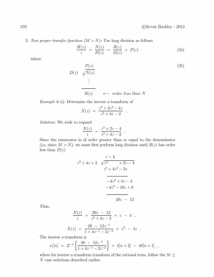
370 c©Kevin Buckley - 2013
3. Non proper transfer function (M > N): Use long division as follows
H(z)
z=
N(z)
D(z)=
R(z)
D(z)+ P (z) (34)
where
P (z) (35)
D(z)√
N(z)
...
R(z) ←− order less than N
Example 6.14: Determine the inverse z-transform of
X(z) =z4 + 2z2 − 4z
z2 + 4z − 2.
Solution: We wish to expand
X(z)
z=
z3 + 2z − 4
z2 + 4z − 2.
Since the numerator is of order greater than or equal to the denominator(i,e, since M > N), we must first perform long division until R(z) has orderless than D(z)
z − 4
z2 + 4z + 2√z3 + 2z − 4
z3 + 4z2 − 2z
−4z2 + 4z − 4
−4z2 − 16z + 8
20z − 12
Thus,
X(z)
z=
20z − 12
z2 + 4z − 2+ z − 4 ,
X(z) =20 − 12z−1
1 + 4z−1 − 2z−2+ z2 − 4z .
The inverse z-transform is
x([n] = Z−1
20 − 12z−1
1 + 4z−1 − 2z−2
+ δ[n+ 2] − 4δ[n+ 1] ,
where for inverse z-transform transform of the rational term, follow the M ≤N case solutions described earlier.
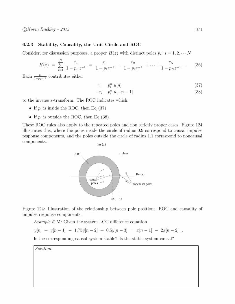
c©Kevin Buckley - 2013 371
6.2.3 Stability, Causality, the Unit Circle and ROC
Consider, for discussion purposes, a proper H(z) with distinct poles pi; i = 1, 2, · · ·N
H(z) =N∑
i=1
ri1− pi z−1
=r1
1− p1z−1+
r21− p2z−1
+ · · ·+ rN1− pNz−1
. (36)
Each ri1−piz−1 contributes either
ri pni u[n] (37)
−ri pni u[−n− 1] (38)
to the inverse z-transform. The ROC indicates which:
• If pi is inside the ROC, then Eq (37)
• If pi is outside the ROC, then Eq (38).
These ROC rules also apply to the repeated poles and non strictly proper cases. Figure 124illustrates this, where the poles inside the circle of radius 0.9 correspond to causal impulseresponse components, and the poles outside the circle of radius 1.1 correspond to noncausalcomponents.
xx
x
x
x
x
x
z−plane
Im z
polescausal
ROC
Re z
noncausal poles
0.9 1.1
Figure 124: Illustration of the relationship between pole positions, ROC and causality ofimpulse response components.
Example 6.15: Given the system LCC difference equation
y[n] + y[n− 1] − 1.75y[n− 2] + 0.5y[n− 3] = x[n− 1] − 2x[n− 2] ,
Is the corresponding causal system stable? Is the stable system causal?
Solution:
372 c©Kevin Buckley - 2013
ROC Properties: Let rh denote the maximum of the magnitudes of all the causal poles.Let rl denote the minimum of the magnitudes of all the noncausal poles.
#1 In general the ROC is an annular ring: rh < |z| < rl.
#2 The ROC contains no poles.
#3 A finite duration x[n] has Rx = ∀z.
#4 Right sided (causal) x[n] means Rx is the exterior of a circle (i.e. Rx = rh < |z| <∞).
#5 Left sided x[n] means Rx is the interior of a circle (i.e. Rx = 0 ≤ |z| < rl).
#6 Two sided x[n] means either Rx = rh < |z| < rl, or Rx = ∅ (the empty set) if rl ≤ rh.
Stability and the Unit Circle: Stated for distinct pole impulse response components,but true for repeated pole components as well.
#1 Right sided signal:
h[n] = pn u[n] ←→ 1
1 − p z−1Rh = |z| > |p| (39)
For stability, |p| < 1. The ROC must include the unit circle.
#2 Left sided signal:
h[n] = −pn u[−n− 1] ←→ 1
1 − p z−1Rh = |z| < |p| (40)
For stability, |p| > 1. The ROC must include the unit circle.
#3 Generally, for stability, the ROC must include the unit circle.
Causality and the ROC: h[n] must be right sided. So the ROC must be the exterior of acircle.
Causality & Stability and the Unit Circle & ROC: The ROC must be the exterior ofa circle and include the unit circle. All poles must be inside the unit circle, i.e.
|pi| < 1 i = 1, 2, · · · , N . (41)
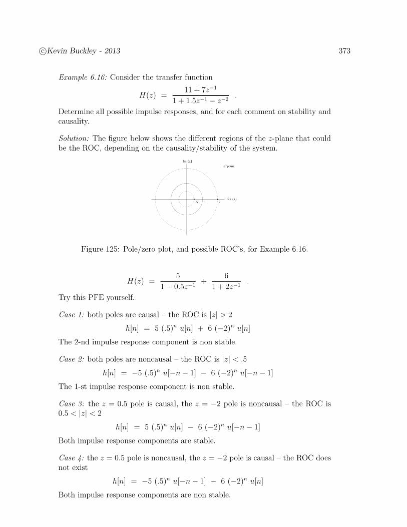
c©Kevin Buckley - 2013 373
Example 6.16: Consider the transfer function
H(z) =11 + 7z−1
1 + 1.5z−1 − z−2.
Determine all possible impulse responses, and for each comment on stability andcausality.
Solution: The figure below shows the different regions of the z-plane that couldbe the ROC, depending on the causality/stability of the system.
Im z
x x2.5 1
Re z
z−plane
Figure 125: Pole/zero plot, and possible ROC’s, for Example 6.16.
H(z) =5
1− 0.5z−1+
6
1 + 2z−1.
Try this PFE yourself.
Case 1: both poles are causal – the ROC is |z| > 2
h[n] = 5 (.5)n u[n] + 6 (−2)n u[n]
The 2-nd impulse response component is non stable.
Case 2: both poles are noncausal – the ROC is |z| < .5
h[n] = −5 (.5)n u[−n− 1] − 6 (−2)n u[−n− 1]
The 1-st impulse response component is non stable.
Case 3: the z = 0.5 pole is causal, the z = −2 pole is noncausal – the ROC is0.5 < |z| < 2
h[n] = 5 (.5)n u[n] − 6 (−2)n u[−n− 1]
Both impulse response components are stable.
Case 4: the z = 0.5 pole is noncausal, the z = −2 pole is causal – the ROC doesnot exist
h[n] = −5 (.5)n u[−n− 1] − 6 (−2)n u[n]
Both impulse response components are non stable.
374 c©Kevin Buckley - 2013
6.2.4 DT LTI System Block Diagrams
#1 Parallel subsystems: H(z) = H1(z) +H2(z) (z-transform linearity property)H(ejω) = H1(e
jω) +H2(ejω) (DTFT linearity property)
#2 Cascade subsystems: H(z) = H1(z) ·H2(z) (z-transform convolution property)H(ejω) = H1(e
jω) ·H2(ejω) (DTFT convolution property)
#3 Feedback subsystems:
Derivation:
Note that, in general, the PFE of a transfer functionH(z) describes a parallel implementationof the system. On the other hand, by factoring H(z) into a product of lower order terms,using the pole/zero product factorizations of the numerator/denominator polynomials, wecan generate cascaded realizations of the system.
Example 6.17: Consider the causal DT LTI feedback system, where for the causalfeed forward subsystem
y[n]− 2y[n− 1] = v[n] ,
and for the feedback subsystem
H2[z] = 1.5z−1 .
a) Is the feed forward subsystem H1(z) stable? Why?
b) What is the overall system transfer function H(z)?
c) Is the overall system stable? Why?
Solution:
a) The feed forward subsystem has transfer function H1(x) = 11 − 2 z−1 . It has
one pole, at p1 = 2. With this pole, since the system is causal, it is unstable.
b) H(z) =H1(z)
1 + H1(z) H2(z)=
11 − 2 z−1
1 + 1.5 z−1
1 − 2 z−1
=1
1 − 2 z−1 + 1.5 z−1=
1
1 − 0.5 z−1.
c) The overall system has one pole, at p1 = 0.5. With this pole, since the systemis causal, it is stable.
c©Kevin Buckley - 2013 375
Example 6.18: Consider two causal LTI subsystems connected in parallel. Lettheir transfer functions be
H1(z) =1 + z−1
1− 14z−2
, H2(z) =3
1 + 12z−1
.
Determine the overall system transfer function. Determine the impulse responseof the overall system, both directly from the overall system transfer function andby combining the individual impulse response results. Compare the two results.
Solution:
376 c©Kevin Buckley - 2013
Example 6.19: Consider the cascade of two DT LTI systems. The first hastransfer function H1(z) = 1− (0.9)10 z−10. This subsystem has zeros atzk = 0.9 ej2πk/10; k = 0, 1, · · · , 9. The second has transfer function H2(z) =
11+0.9z−1 .
1. Determine the impulse response of each subsystem.
2. Draw the pole/zero diagram for each subsystem, and for the cascade of thetwo subsystems.
3. Determine the transfer function of the cascade of the two subsystems.
4. Roughly sketch the frequency response of the cascade of the two subsystems.
Solution:
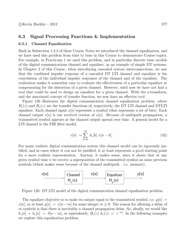
c©Kevin Buckley - 2013 377
6.3 Signal Processing Functions & Implementation
6.3.1 Channel Equalization
Back in Subsection 1.2.3 of these Course Notes we introduced the channel equalization, andwe have used this problem from time to time in this Course to demonstrate Course topics.For example, in Practicum 1 we used this problem, and in particular discrete time modelsof the digital communications channel and equalizer, as an example of simple DT systems.In Chapter 2 of this Course, when introducing cascaded system interconnections, we sawthat the combined impulse response of a cascaded DT LTI channel and equalizer is theconvolution of the individual impulse responses of the channel and of the equalizer. Therealization makes it somewhat easy to evaluate the effectiveness of a particular equalizer atcompensating for the distortion of a given channel. However, until now we have not had atool that could be used to design an equalizer for a given channel. With the z-transform,and the associated concept of transfer function, we now have an effective tool.
Figure 126 illustrates the digital communication channel equalization problem, whereHc(z) and He(z) are the transfer functions of, respectively, the DT LTI channel and DTLTIequalizer. Each channel input x[n] represents a symbol (that represents a set of bits). Eachchannel output v[n] is our received version of x[n]. Because of multipath propagation, atransmitted symbol appears at the channel output spread over time. A general model for aLTI channel is the FIR filter model,
v[n] =M∑
k=0
hc[k] x[n− k] . (42)
For many realistic digital communication system this channel model can be rigorously jus-tified, and in cases where it con not be justified, it at least represents a good starting pointfor a more realistic representation. Anyway, it makes sense, since it shows that at anygiven symbol time n we receive a superposition of the transmitted symbol an some previoussymbols (which makes sense because of the channel multipath – i.e. memory).
H (z)c
ChannelH (z)
e
Equalizerx[n] v[n] y[n]
Figure 126: DT LTI model of the digital communication channel equalization problem.
The equalizer objective to to make its output equal to the transmitted symbol, i.e. y[n] =x[n], or at least y[n] = x[n−m] for some integer m ≥ 0. The reason for allowing a delay ofm symbols is that there is inevitably a channel propagation delay. So, ideally, we would likehc[n] ∗ he[n] = δ[n−m], or equivalently, Hc(z) he(z) = z−m. In the following exampleswe explore this equalization problem.
378 c©Kevin Buckley - 2013
Example 6.19: Consider the equalizer problem first considered in Practicum 1.Let the channel transfer function be H(z) = 1 − 2z−1
1 − .5z−1 . Denote as G(z) theequalizer transfer function.
a) Consider G(z) = H−1(z). Show that this exactly equalizes the channel.What is the problem with this solution?
b) Consider G(z) = 1 − .5z−1
−2 + z−1 . Identify a positive and a negative aspect of thissolution.
Solution:
Example 6.20: Two LTI subsystems, a channel and an equalizer, have impulseresponses hc[n] = δ[n] + 0.9δ[n− 1] and he[n] = (−.9)nu[n].1. Identify, on a z-plane diagram, the locations of the poles/zeros of these two
individual subsystems.
2. Consider the cascade of these two subsystems. Identify the locations of theresulting system’s poles/zeros, and use these to roughly sketch the magni-tude response |H(ejω)|.
Solution:
c©Kevin Buckley - 2013 379
Example 6.21: Consider two cascaded causal DT LTI subsystems, a channel andan equalizer. The channel has difference equation
v[n] = x[n− 4]− 0.25x[n− 6]
where x[n] is the input and v[n] is the output. The equalizer has transfer function
He(z) =z
(z − 0.5)(z + 0.5).
1. Determine the impulse responses hc[n] and he[n] of the two subsystems.
2. Determine the impulse response of the cascade of these two subsystems.
Solution:
Example 6.22: Consider a DT LTI channel with transfer function Hc(z) =1 − 0.81 z−2. Consider the cascade of Hc(z) and a DT LTI equalizer He(z)which exactly inverts the effect of the channel.
1. Design the equalizer. That is, determine its transfer function He(z).
2. Can this equalizer be realized as a causal/stable system? Why?
3. Starting with the PFE of He(z), determine the causal impulse responsehe[n].
Solution:
380 c©Kevin Buckley - 2013
Example 6.23: Consider a DT LTI communications channel with impulse re-sponse hc[n] = δ[n] + 2δ[n− 1]. At the receiver, we use a DT LTI equalizer (asin Practicum 1) to counteract the effect of the channel. Determine the transferfunction, He(z), of the ideal equalizer (i.e. which will have an output equal tothe channel input for any channel input). Assuming that this equalizer is causal,what is its impulse response? Explain the problem with implementing this equal-izer, and identify the characteristic of the channel poles/zeros that causes thisproblem.
Solution:
Examples 6.20-6.23 are relatively simple channel equalization problems. Example 6.21illustrates the typical need to design for delay. What do you think would happen if youattempted to design the equalizer without allowing for a delay in the overall channel/equalizerresponse? Try designing and evaluating without the delay. Example 6.23 suggests a veryimportant realistic consideration – equalizer stability. In part because of stability concerns,in practice channel equalizers are almost always FIR filters. Even for the simple channelsconsidered in the examples above, do you think an FIR equalizer can be effective?
Equalizer design starts with the understanding developed in the examples above. A seniorlevel DSP course would typically develop some more advanced design tools to apply to theproblem of designing an equalizer for a DT LTI channel. In a graduate digital communi-cations course you would learn how to tackle this problem for situations when the channelis unknown and time varying. Think about a cellular mobile phone application. Can youexpect the channel transfer function from the cell phone to a base station to be known? No.Can you expect that channel transfer function to remain constant over time? No. Even so,the solution to this more realistic channel equalization problem starts with the understandingdeveloped in this Subsection.
c©Kevin Buckley - 2013 381
6.3.2 Sampling: A DT Perspective
6.3.3 Filter Banks
6.3.4 Spectrum Estimation
6.3.5 Real-Time DT Systems
Presentations by:
• Brian McCarthy: chairman and founder, Adaptive Digital Technologies Inc., PlymouthMeeting, PA; BSEE Villanova Un. 1978; VU ECE Dept. Adjunct Professor. Brian isthe instructor for ece7710, Real-Time Digital Signal Processing.
• Sean Gallagher: Senior DSP Specialist, Xilinx; MSEE Villanova Un. 1992; VU ECEDept. Adjunct Professor. Sean is the instructor for ece7711, Hardware Digital SignalProcessing.
382 c©Kevin Buckley - 2013
6.4 Practicum 4c
Spectrum Analysis of DT Energy Signals
Introduction
In this practicum you will investigate the DTFT. Specifically, you will study the frequencycontent of several DT signals. For each, you will numerically derive and plot spectra. Ineffect, you will be designing, implementing and testing a digital spectrum analyzer (i.e.a spectrum analyzer which computes spectrum estimates using digital hardware and/orsoftware). These days, the vast majority of spectrum analyzers are digital.
You will develop a spectrum analyzer for DT energy signals. You will first test thisspectrum analyzer on a signal with known frequency content. You will then use it to analyzean Acoustic Emissions (AE) signal. For each of these signals, you will draw conclusions fromits spectrum.
Background
The DTFT analysis equation, shown below, calculates the frequency content of an DTenergy signal:
X(ejω) =∞∑
n=−∞x[n] e−jωn ; −π < ω ≤ π . (1)
We know that the range of ω is usually restricted to −π < ω ≤ π because of theambiguity of discrete-time frequency. We also know that if x[n] is derived as samples of anunderlying CT signal xc(t), i.e. if x[n] = xc(nTs) where fs = 1
Tsis the sample rate, then
discrete-time frequency ω (in radians/sample) corresponds to continuous-time frequency Ω(in radians/second) as ω = ΩTs. Thus, if xc(t) is sampled without aliasing, then xc(t) isbandlimited to the frequency range − π
Ts< Ω ≤ π
Ts. In Subsection 4.2.2 of the Course
Notes it is shown that, with no aliasing, the DTFT of x[n] is related to the Continuous-TimeFourier Transform (CTFT) of xc(t) as
Xc(jΩ) =1
Ts
X(ejΩTs) ; − π
Ts
< Ω ≤ π
Ts
, (2)
where Xc(jΩ), the CTFT of xc(t), is the content of xc(t) (i.e. similar to what X(ejω) isfor x[n]). By Parseval’s theorem for the DTFT, |X(ejω)|2 vs. ω is the energy spectrum ofX(ejω). Similarly,
|Xc(jΩ)|2 =1
T 2s
|X(ejΩTs)|2 ; − π
Ts
< Ω ≤ π
Ts
(3)
is the energy spectrum of xc(t) (again assuming no aliasing).In application, there are two practical problems associated with computing the DTFT.
First, in general a signal x[n] has infinite duration, so that the DTFT (Eq (1)) can notbe computed. In practice, only a finite duration of x[n] is processed, say the N samplesx[n]; n = N1, N1 + 1, N1 + 2, · · · , N2 where N = N2 −N1 + 1. Then
X(ejω) =N2∑
n=N1
x[n] e−jωn ; −π < ω ≤ π (4)

c©Kevin Buckley - 2013 383
is computed, which will in general be an approximation. The second practical problem isthat X(ejω) is a function of continuous ω. With a computer, we can compute this for onlya finite number of ω′s, say for the M samples
ωk =2W
Mk; k = −M
2+ 1, · · · , −1, 0, 1, 2, · · · , M
2(5)
(in Eq (5) it is assumed that M is an even integer), where 0 < W ≤ π defines the lowpassrange of ω you wish to observe. So, we compute only samples of X(ejω), which in turn arein general approximate samples of the true X(ejω).
In designing a spectrum analyzer for DT energy signals, or for an underlying CT sig-nal from which the DT signal was derived, you must choose N1, N2, W and M . Yourimplementation should have these as selectable analyzer parameters.
Procedures
1. Code up you spectrum analyzer keeping N1, N2, W and M as selectable parameters.
2. Select a signal x1[n] with known DTFT X1(ejω) (e.g. from a table of DTFT pairs),
keeping in mind that this is to be a test signal for your spectrum analyzer. SelectN1, N2, W and M . In Matlab, use the “plot” function to view |X1(e
jω)|2 vs. ω for−W < ω ≤ W . Make sure you plot a dense enough sampling of |X1(e
jω)|2 to getan accurate representation of it.
Generate x1[n]; n = N1, N1 + 1, N1 + 2, · · · , N2 and use the “stem” function to plotit. Using your spectrum analyzer, compute the M samples of X1(e
jω). Use the Matlab“plot” function to view |X1(e
jω)|2. Compare your |X1(ejω)|2 and |X1(e
jω)|2 plots.
You have now tested you spectrum analyzer.
3. The data file
v:/Electrical Computer/ece3240/AEdat
contains y[n] = yc(nTs), a dense sampling of an AE signal yc(t) over its duration0 ≤ t ≤ .8 msec.. This signal was measured using a small acoustic sensor attached toa piece of metal as it was bent so as to cause cracking.
(a) What is the spacing Ts between samples. Plot yc(t) vs. time (in seconds).
(b) Use the spectrum analyzer you developed and tested in Procedure 2. to processy[n]. What values of N1 and N2 should you use? Select and justify values ofW and M . (You may have to try several joint values.) Plot your estimate of|Y (ejω)|2 vs. ω and the corresponding estimate of |Yc(jΩ)|2 vs. Ω. Consideringyour |Yc(jΩ)|2 estimate plot, describe the frequency content of the signal yc(t).Compare characteristics of this spectrum (e.g. frequency positions of spectralpeaks) to characteristics of the AE signal (e.g. the frequency of oscillation).

384 c©Kevin Buckley - 2013
.

c©Kevin Buckley - 2013 385
Practicum 4cInstructor/TA Sign Off Sheet
Student’s Name:
1. Procedure 2: Write down the equations for x1[n] and corresponding X1(ejω) you se-
lected to test your analyzer. Explain why you choose this pair.
2. Procedure 2: List the values of N1, N2, W and M you selected for analyzing x1[n].Briefly explain why you choose these values.
3. Procedure 2: Plot of |X1(ejω)|2.
4. Procedure 2: Plots of x1[n] and |X1(ejω)|2.
5. Procedure 2: Comment on your comparison between your |X1(ejω)|2 and |X1(e
jω)|2plots, explaining any noticeable differences. Explain why you are convinced that yourspectrum analyzer is working properly.

386 c©Kevin Buckley - 2013
6. Procedure 3(a): What is Ts? Plot of yc(t).
Procedure 3(b): What are your selected values of N1, N2, W and M? Explain howyou arrived at your value of M .
7. Procedure 3(b): Plots of your estimates of |Y (ejω)|2 and |Yc(jΩ)|2.
8. Procedure 3(b): Compare characteristics of this spectrum to characteristics of the AEsignal.
c©Kevin Buckley - 2013 387
6.5 Practicum 5a
CT & DT Filter Design & Analysis
IntroductionIn this practicum you will investigate CT & DT filter design and evaluation. Filter design
and analysis is easily accomplished with Matlab, which provides numerous CT and DT filterdesign and analysis functions. In Matlab, type ”help signal” to view a list that includesavailable filter design options.
Procedures: Procedure 1 should be completed before the 1-st practicum session. Proce-dures 2-4, on CT filter design and evaluation, should be completed the 1-st practicum session.Procedures 5-7, on DT filter design and evaluation, should be completed at the 2-nd session.
1. Before the practicum session, study the accompanying Matlab program. This programdesigns and analyzes a 6-th order CT lowpass Butterworth filter with a lowpass cutofffrequency of 1 rad./sec.. It generates a pole/zero plot, as well as plots of magnitudeand phase responses. Note the use of the butter, roots, zplane, residue and freqs Matlabfunctions. Using the Matlab help resource, become familiar with these. Implement thisprogram and consider the resulting plots.
2. Following the Butterworth filter example discussed above, design and analyze in a sim-ilar manner a Chebyshev Type II low pass filter of order 6, with stop band attenuationof 40 dB and with cut off frequency ωo = 120π. First design a ”low pass prototype” thathas a cut off of 1 rad./sec. and the correct stop band attenuation using the command[B,A]=cheby2(6,40,1,’s’). Write down the transfer function.
3. Now convert the prototype from Procedure 2. to have a cutoff of ωo = 120π usingthe lp2lp function (type “help lp2lp” for information on how to use this function). Forthis 2-nd filter, provide a pole/zero plot, and frequency response magnitude and phaseplots. Write down the impulse response h(t) explicitly as a real-valued function.
4. Comment on the relationship between the filter’s pole and zero locations in the s-planeand characteristics of its frequency response.
5. Using the Matlab ellip command, design a 6-th order (i.e. N = 6) discrete timelowpass filter with a cutoff frequency ω0 =
π3, passband peak-to-peak ripple of 0.5dB,
and stopband attenuation of 40dB. Write down its input/output difference equation,the transfer function, and the ROC (assuming the filter is causal).
6. Plot the poles and zeros using zplane, and use the Matlab freqz command to computeand plot, over the range −π ≤ ω ≤ π, the phase response and the magnitude responsein dB. (The magnitude response, in dB, is 20 log10|H(ejω)| = 10 log10|H(ejω)|2.)

388 c©Kevin Buckley - 2013
7. Generate 300 samples, for n = 0, 1, 2, · · · , 299, of two seperate real-valued sinusoidalsignals, one with frequency in the passband and one in the stopband. What frequenciesdid you choose? By analyzing the frequency response plots you generated in Procedure6, record the magnitude and phase responses for the two frequencies you selected. Usethe Matlab filter function to process both of your sinusoidal signals with the filteranalyzed in Procedure 6. For each signal use Matlab to plot the input and output onthe same figure, and in steady state carefully compare the input and output sinusoidamplitudes and phases to observe that system’s effect on the input sinusoid. Do theseobserved results match the frequency responses you recorded from the Procedure 6plots? Why?

c©Kevin Buckley - 2013 389
echo on
%************************************************************
%
% Continuous-Time Filter Design & Evaluation
%
% Butterworth lowpass: order N = 6,
% cutoff wn = 1 radian
%
%************************************************************
%
% Design Butterworth Filter w/ butter.m
% (try cheby1, cheby2 and ellip)
%
% B = vector of transfer function numerator coefficients
% A = vector of transfer function denominator coefficients
N=6;
wn=1;
[B,A]=butter(N,wn,’s’)
pause
% Plot Pole Locations using zplane
% (no zeros for analog Butterworth lowpass)
%
p=roots(A);
zplane([],p)
pause
% Partial Fraction Expansion of H(s) - You can determine
% h(t) from results. P is the vector of poles.
% R is the vector of respective residues.
% K is the vector of long-division coefficients if the transfer
% function is not strictly proper.
%
[R,P,K]=residue(B,A)
pause
% Compute and Display the Frequency Response using freqs
%
freqs(B,A)

390 c©Kevin Buckley - 2013
.

c©Kevin Buckley - 2013 391
Practicum 5aInstructor/TA Sign-Off and Comment Sheet
Student’s Name:
1. Procedure 2: write down the prototype Chebychev filter transfer function
2. Procedure 3: pole/zero, Mag. and phase response plots
3. Procedure 3: write down the impulse response h(t) as a real-valued function
4. Procedure 4: relate the pole/zero locations to the frequency response plots
5. Procedure 5: write down the Elliptic filter difference equation, transfer function andROC.
6. Procedure 6: pole/zero and mag./phase plots
7. Procedure 7: compare theoretical and observed magnitude/phase responses

392 c©Kevin Buckley - 2013
.
c©Kevin Buckley - 2013 393
6.6 Practicum 5b
DT Filters
IntroductionIn Week 1 of this Practicum you will observe the frequency response of an FIR filter, by
analyzing the impulse and frequency responses and by observing their responses to sinusoidalinputs and speech. You will learn how to evaluate the frequency response, first directly bycomputing the DTFT of the impulse response and then using the Matlab function freqz. Youwill also learn to filter an input signal (specifically a sinusoid and speech) with an FIR filter.In previous Practicums you had done some filtering directly. Here you will learn to use theMatlab function firfilt for some simple FIR filters. (Note: the firfilt.m file can be found in theCourse Folder .../electrical computer/ece3240.) You will then use a few specialized plottingfunctions in the Course Folder to analyze and implement some more interesting FIR filtersoperating on a speech signal
In Week 2 you will investigate discrete time filter design and evaluation. Filter design iseasily accomplished with Matlab, which provides numerous CT and DT filter design func-tions. In Matlab, type ”help signal” to view a list that includes available filter design options.Also browse help specifically for several of the filter design functions.
Procedures:
Week 1: Do Procedure 1(a) before the Week 1 lab session.
1. A 3-pt. averager:
y[n] =1
3
2∑
k=0
x[n− k] . (1)
(a) On paper, show that the frequency response of the 3-pt. averager is
H(ejω) =2 cos(ω) + 1
3e−jω . (2)
Sketch the magnitude of the frequency response. Determine the magnitude andphase of the frequency response at ω = 0.25π. Determine the filter transferfunction H[z], and the system poles & zeros.
394 c©Kevin Buckley - 2013
(b) Use the Matlab function freqz to compute the frequency response. Specifically,implement the following Matlab code:
>> bb = (1/3)*ones(1,3);>> ww = -pi:(pi/200):pi;>> H = freqz(bb,1,ww);>> subplot(211)>> plot(ww,abs(H))>> xlabel(’normalized frequency (rad/sample)’)>> ylabel(’abs(H)’)>> subplot(212)>> plot(ww,angle(H))>> xlabel(’normalized frequency (rad/sample)’)>> ylabel(’angle(H)’)
Type help freqz to see how, in general, to use this function. (Note that magnitudeand phase are plotted. Plots of the real and imaginary parts of the frequencyresponse are not very interesting.)
(c) Compare the frequency response results derived in (a,b) above, both over −π ≤ω ≤ π and specifically at ω = 0.25π.
(d) Generate 50 samples of the DT cosine signal x[n] = 7 cos(0.25πn+ (π/3)); n =0, 1, · · ·49 and store them in the vector xx.
(e) Using the provided function firfilt, generate the corresponding output yy. (Notethat xx and yy are not the same length.)
(f) Using subplot, plot the first 50 values of xx and yy on the same figure. Use thestem function and label the time axis 0 ≤ n ≤ 49. From the xx plot, measure(and record) the input magnitude, frequency and phase. How were these valuesidentified from the plot?
(g) Except for the first few values, yy appears to be a sinusoid. As in (f) above,measure (and record) its magnitude, frequency and phase.
(h) Characterize the filter’s performance, for this input, by computing the magnitudegain and phase shift using your input/output measurements from (f) & (g) above.Compare these results to the frequency response of this filter derived in (a-b)directly above, evaluated at ω = 0.25π.
2. Filtering Speech Samples:
(a) Make sure you have access to files lab6dat.mat, inout.m and striplot.m which canbe found in the Course Folder. To understand the Matlab functions you will use,type help filename for the filenames inout and striplot.
(b) Load the data file lab6dat.mat. Get familiar with the data that this loads (e.g.type who, look at the filter coefficient vectors h1, h2, and listen to the speechsignal x2).
c©Kevin Buckley - 2013 395
(c) Filter the speech signal with the filter h1 and observe results using the commands
>> y1 = firfilt(h1,x2);>> inout(x2,y1,3000,1000,3);
Compare and comment on the input and output signals. For example, is theoutput ”rougher” or ”smoother” than the input?
(d) Use freqz to plot the frequency response of filter h1 as a function of frequencyover −π ≤ ω ≤ π. Why is h1 called a lowpass filter? Use the stem plot toplot h1. What value of n are these filter impulse response coefficients symmetricabout?
(e) Repeat (c) and (d) using the highpass filter h2. Denote the filter output y2.
(f) Make an ”A-B-C” listening comparison using the command
>> soundsc([x2;y1;y2],8000);
Comment on your perception of the filtered outputs vs. the original signal.
(g) Make an ”A-D” listening comparison using the command
>> soundsc([x2;(y1+y2)],8000);
Comment on your perception of the composite signal vs. the original. Did youexpect this result? Why?
Week 2: Do Procedure 2(a) and review the attached filter design & analysis example beforethe Week 2 practicum session.
1. DT Filter Analysis:
(a) Consider the LTI discrete time filter with input/output difference equation
y[n] − 1.556 y[n− 1] + 1.272 y[n− 2] − 0.398 y[n− 3]
= 0.0798 (x[n] + x[n− 1] + x[n− 2] + x[n− 3]) .
(b) Use the Matlab freqz command to compute the frequency response of this fil-ter over the range −π ≤ ω ≤ π. Plot the phase response, the magnitude re-sponse, and the magnitude response in dB. (The magnitude response, in dB, is20 log10|H(ejω)|.)
(c) What type of filter is this? What is the cutoff frequency?
(d) Using this Butterworth filter, and the Matlab filter function, filter the x2 signalin the lab6dat.mat file used in Practicum V. Use the inout function to plot theinput and output. Comment on the effect of the filter on the input. Using thesoundsc function, listen to the input and output, and again comment on the effectof the filter.

396 c©Kevin Buckley - 2013
2. Filter Design:Using Matlab, design a discrete time lowpass filter. This filter should be the minimumorder filter that meets the specification given below.
Specifications:
i. Type: if your last name begins with a letter A through G - Chebychev Type I (usethe Matlab command cheby1); if your last name begins with a letter H through M- Chebychev Type II (use the Matlab command cheby2); if your last name beginswith a letter N through Z - Elliptical (use the Matlab command ellip).
ii. Passband ripple: 2dB.
iii. Stopband attenuation: 50dB.
iv. Passband cutoff ωp =π3· your grade on Test 2
80.
v. Stopband cutoff: ωs = 1.5 ωp.
Procedures:
(a) On a piece of paper, note your filter type. Write down and sketch your designspecifications. Bring this to the Practicum session.
(b) Determine the minimum filter order which meets these specification. Discuss howyou selected this order.
(c) Determine the transfer function, and the input/output difference equation.
(d) Determine the filter impulse response (explicitly as a real-valued function). De-scribe this derivation starting with the partial fraction expansion, generated usingthe Matlab residue command, of the transfer function.
(e) Using your filter analysis experience gained by conducting the CT filtering Practicum(Practicum 5a) and by reviewing the DT filter design & analysis Matlab examplereferred to above, conduct your own procedures to analyze your DT filter. UseMatlab to verify that your filter meets specifications, and that its characteristicsare consistent with your understanding of the relationships between these filtercharacteristics and the frequency response specifications. Gather plots and otherresults to be attached to your sign off sheet.
(f) By direct implementation of the I/O difference equation, implement your filterin Matlab. (Consider extending your simple IIR filter code from Practicum 1.)Using a technique explored in Practicum 5a, verify that your filter is functioningproperly by analyzing outputs for one or more inputs.
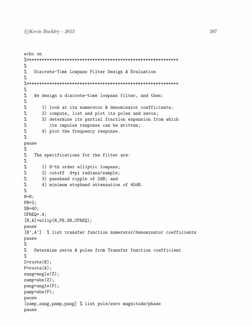
c©Kevin Buckley - 2013 397
echo on
%************************************************************
%
% Discrete-Time Lowpass Filter Design & Evaluation
%
%************************************************************
%
% We design a discrete-time lowpass filter, and then:
%
% 1) look at its numerator & denominator coefficients;
% 2) compute, list and plot its poles and zeros;
% 3) determine its partial fraction expansion from which
% its impulse response can be written;
% 4) plot the frequency response.
%
pause
%
% The specifications for the filter are:
%
% 1) 8-th order elliptic lowpass;
% 2) cutoff .4*pi radians/sample;
% 3) passband ripple of 2dB; and
% 4) minimum stopband attenuation of 40dB.
%
N=8;
PB=2;
SB=40;
CFREQ=.4;
[B,A]=ellip(N,PB,SB,CFREQ);
pause
[B’,A’] % list transfer function numerator/denominator coefficients
pause
%
% Determine zeros & poles from Transfer function coefficient
%
Z=roots(B);
P=roots(A);
zang=angle(Z);
zamp=abs(Z);
pang=angle(P);
pamp=abs(P);
pause
[zamp,zang,pamp,pang] % list pole/zero magnitude/phase
pause
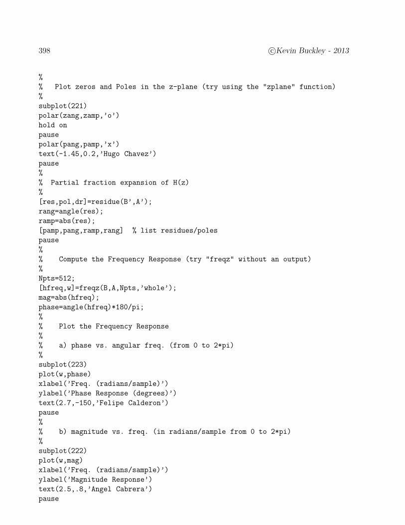
398 c©Kevin Buckley - 2013
%
% Plot zeros and Poles in the z-plane (try using the "zplane" function)
%
subplot(221)
polar(zang,zamp,’o’)
hold on
pause
polar(pang,pamp,’x’)
text(-1.45,0.2,’Hugo Chavez’)
pause
%
% Partial fraction expansion of H(z)
%
[res,pol,dr]=residue(B’,A’);
rang=angle(res);
ramp=abs(res);
[pamp,pang,ramp,rang] % list residues/poles
pause
%
% Compute the Frequency Response (try "freqz" without an output)
%
Npts=512;
[hfreq,w]=freqz(B,A,Npts,’whole’);
mag=abs(hfreq);
phase=angle(hfreq)*180/pi;
%
% Plot the Frequency Response
%
% a) phase vs. angular freq. (from 0 to 2*pi)
%
subplot(223)
plot(w,phase)
xlabel(’Freq. (radians/sample)’)
ylabel(’Phase Response (degrees)’)
text(2.7,-150,’Felipe Calderon’)
pause
%
% b) magnitude vs. freq. (in radians/sample from 0 to 2*pi)
%
subplot(222)
plot(w,mag)
xlabel(’Freq. (radians/sample)’)
ylabel(’Magnitude Response’)
text(2.5,.8,’Angel Cabrera’)
pause

c©Kevin Buckley - 2013 399
%
% c) magnitude (dB) vs. freq. (in radians/sample from -pi to pi)
% (try using "fftshift" to convert w ang mag to -pi to pi range)
%
w1(1:Npts/2)=w(1+Npts/2:Npts)-(2*pi);
w1(1+Npts/2:Npts)=w(1:Npts/2);
mag1(1:Npts/2)=mag(1+Npts/2:Npts);
mag1(1+Npts/2:Npts)=mag(1:Npts/2);
subplot(224)
plot(w1,20*log10(mag1))
xlabel(’Freq. (radians/sample)’)
ylabel(’Magnitude Response (dB)’)
text(-1,-40,’Lula da Salva’)

400 c©Kevin Buckley - 2013
.

c©Kevin Buckley - 2013 401
Practicum 5bInstructor/TA Sign Off Sheet, & Report Form
Student’s Name:
1. Week 1, Procedure 1(a,b): Mag. & phase response plots
2. Week 1, Procedure 1(h): Computed Mag. & phase response, comparison
3. Week 1, Procedure 2(f,g): soundsc results
4. Week 2, Procedure 1(b): three frequency response plots
5. Week 2, Procedure 1(d): input/output plots
6. Week 2, Procedure 2(a): with a paper clip, attach the page with your filter frequencyresponse specifications drawing and other required information
7. Week 2, Procedure 2(b): below, record your filter order and state how you arrived atthis value
8. Week 2, Procedure 2(c): record your I/O difference equation (which will be used forProcedure 2(f)).

402 c©Kevin Buckley - 2013
9. Week 2, Procedure 2(d): record your poles/residues, and write down your impulseresponse explicitly as a real-valued function.
10. Week 2, Procedure 2(e): with a paper clip, attach the plots and other informationresulting from your filter analysis. State the goals of your analysis. Using yourplots/results as a reference, discuss your observations that verify that your filter char-acteristics are consistent with your specifications.
11. Week 2, Procedure 2(f): with a paper clip, attach your Matlab IIR filter implemen-tation code, along with any plots/results used to verify the your filter is properlyfunctioning. Provide your argument that these plots/results verify proper functional-ity.
c©Kevin Buckley - 2013 403
6.7 Problems
Chapter Topics:6.1-30 (DTFT and DT LTI systems);6.31-51 (z-transform and DT LTI systems);6.52-63 (stability, causality and ROC);6.64-70 (DT LTI system interconnections)6.71-75 (applications)
1. Consider a DT LTI system with input x[n] = p5[n] and impulse response
h[n] = sin(0.25πn)πn
. Determine Y (ejω), the frequency content of the output y[n]. Plot|Y (ejω)| over −π ≤ ω ≤ π.
2. Consider a DT LTI system with input x[n], impulse response h[n] and output y[n] =x[n] ∗ h[n].
(a) Let h[n] = sin(.5πn)πn
− sin(.25πn)πn
and x[n] = 5δ[n−1]. Determine and plot H(ejω).Determine Y (ejω). Using Y (ejω) determine the output energy Ey.
(b) Let x[n] = δ[n]−1.8δ[n−1]+ .81δ[n−2] and h[n] = (n+1) .9n u[n]. DetermineH(ejω) and X(ejω). From these, determine Y (ejω) (simplify the expression asmuch as possible). From this determine y[n].
(c) Consider a DT LTI system with frequency response
H(ejω) = [2 + 2 cos(2ω)] e−j2ω; |ω| ≤ π . (3)
Consider input x[n] = 1 + 2 cos((π/8)n) + 3 cos((π/4)n) + 4 cos((π/2)n).Determine the output y[n].
(d) Consider a DT LTI system with impulse response h[n] = n an u[n]. Using entries#3 and #4 of the DTFT table, and linearity, determine the frequency responseH(ejω) and the I/O difference equation.
3. Consider a DT LTI system with |H(ejω)| = 2 and 6 H(ejω) = sin(ω). Its input isx[n] = .5nu[n]. What is the energy of the output y[n]?
4. Consider a DT LTI system with impulse response
h[n] =1
10(.9)nu[n]
and input
x[n] =∞∑
k=−∞δ[n− 5k] ,
Determine Y (ejω), the DTFT of the output. Determine the input power Px and theoutput power Py.

404 c©Kevin Buckley - 2013
5. The DTFT of a|n| is
1− a2
(1 + a2)− 2a cosω.
Consider a DT LTI system with impulse response h[n] = 0.5|n|. Determine the fre-quency response H(ejω), and sketch it for −π ≤ ω ≤ π. Determine the output forinput
x[n] = 4 + 5 cos(πn/2) − 3 cos(πn) .
6. Consider a DT LTI system with impulse response
h[n] =sin(.25πn)
πn.
Determine the system’s frequency response H(ejω). Plot H(ejω) for −2π ≤ ω ≤ 2π.Determine its output for input
x[n] = −3 + 2 cos(.1πn+ π) + 5 cos(πn) .
7. Given the DT LTI filter frequency response
H(ejω) =
1 π3≤ |ω| ≤ 2π
3
0 otherwise over − π ≤ ω ≤ π
Determine the impulse response h[n]. (The answer should be written explicitly as areal-valued signal.)
8. Consider a DT LTI system with frequency response
H(ejω) =sin(2.5 ω)
sin(0.5 ω).
Determine and plot the impulse response h[n]. What frequencies over the range−π ≤ ω ≤ π are completely attenuated by this system.
Now consider a DT LTI system with frequency response
H(ejω) = e−j10ω sin(2.5 ω)
sin(0.5 ω).
Determine and plot the impulse response h[n]. What is the output y[n] for inputx[n] = 5 + cos(2π
5n)?
9. Consider a DT LTI system with input x[n], impulse response h[n] and output y[n].
(a) Let h[n] =sin(π
2n)
πn. Determine & sketch the frequency response H(ejω) for
−π ≤ ω ≤ π.
c©Kevin Buckley - 2013 405
(b) Let x[n] = δ[n + 2] + 2δ[n] + δ[n− 2]. Determine its DTFT X(ejω).
(c) Using an Euler’s identity, your X(ejω) from (b) can be expressed in the formX(ejω) = c1 + c2 cos(2ω), where c1 and c2 are constants. Determine theseconstants and then sketch X(ejω); −π ≤ ω ≤ π.
(d) Determine and sketch the DTFT of y[n]. From your sketches, determine thepercentage of the energy of x[n] in y[n].
10. A DT LTI system has impulse response h[n] = δ[n] + 3δ[n − 1] + n(.5)nu[n − 1].Determine a I/O difference equation for this system.
11. Consider a DT LTI system with input x[n] = δ[n + 2] + δ[n] + δ[n − 2] and impulse
response h[n] =sin(π
2n)
πn.
a) Determine X(ejω), and plot it over |ω| < π (Hints: X(ejω) is real-valued. ThinkEuler’s identities.)
b) Determine H(ejω) and Y (ejω), and plot them over |ω| < π.
c) What percentage of input energy Ex makes it to the filter output?
12. DT LTI Systems:
(a) Given a DT LTI system with impulse response h[n] = n 0.9n u[n], determinethe system input/output difference equation.
(b) Consider a DT LTI system with input/output difference equation
y[n] − 0.9 y[n− 2] = x[n] + 0.9 x[n− 2] .
The input is x[n] = s[n] + n[n], where s[n] = ejπn is a signal of interest, andn[n] = 4 ej(π/2)n is noise. SNR is defined as signal power divided by noise power.What is the input SNR, SNRin? What is the output SNR, SNRout? Determinethe gain G = SNRout
SNRin.
13. Consider a DT LTI lowpass filter with frequency response H(ejω) = pπ(ω); |ω| < π.Consider input x[n] = s[n] + n[n], where s[n] = δ[n] is a desired signal andn[n] = 1
2δ[n + 2] + δ[n] + 1
2δ[n− 2] is noise. Signal-to-Noise Ratio (SNR) is defined as
signal energy over noise energy.
(a) Determine the filter input SNR, SNRin.
(b) Determine the filter output SNR, SNRout.
(c) The filter gain is defined as G = SNRout
SNRin. Describe a filter that has greater gain
than H(ejω) = pπ(ω); |ω| < π. Justify your answer.
14. Consider the third-difference DT LTI system
y[n] = x[n]− x[n− 3] .
(a) Determine the impulse response h[n] and the frequency response H(ejω).

406 c©Kevin Buckley - 2013
(b) Plot the magnitude and phase of the frequency response.
(c) Determine the output for input x[n] = 8− 3 cos(πn+ (π/10)).
(d) Determine the output for input x[n] = 2 cos((π/2)n).
15. Consider the LTI filter with impulse response
h[n] = −2δ[n + 1] + δ[n]− 2δ[n− 1] .
(a) Determine H(ejω).
(b) Plot |H(ejω)| for −π ≤ ω ≤ π.
(c) Determine output y[n] for input x[n] = 3 cos(πn).
16. Consider a DT LTI system with I/O difference equation
y[n] − 0.5 y[n− 1] = x[n− 2] + x[n− 3] .
a) Determine the frequency response H(ejω).
b) Determine the output for input x1[n] = δ[n− 3].
c) Determine the output for input x2[n] = 3 cos(πn+ π3).
d) [Extra credit] Determine the output for input x3[n] = cos(π2n). (1 + 0.5j =
1.118 ej(.1476)π)
17. Consider a ideal DT lowpass filter with frequency response H(ejω) = 2 pπ(ω) over thefrequency range −π ≤ ω ≤ π.
(a) Given an input signal with DTFT X1(ejω) = e−|ω|; −π ≤ ω < π, determine the
percentage of input energy that makes it to the output.
(b) Given input signal x2[n] =∑∞
l=−∞ δ[n − l5], determine the percentage of inputpower that makes it to the output.
18. Consider a DT LTI system with input x[n], impulse response h[n] and output y[n].
a) h[n] = 12δ[n+ 2] + δ[n] + δ[n− 2]. Determine the frequency response. Use an
Euler’s identity to express it as a real-valued function. Sketch it over −π ≤ ω ≤ π.
b) x[n] =sin(π
2n)
πn. Determine and sketch its DTFT, and the DTFT of y[n]. Determine
Ex, the energy of x[n].
c) Without integrating over |Y (ejω)|2, determine the output energy Ey.
19. Consider a DT LTI system with impulse response
h[n] = 2 n 0.5n u[n] .
a) Use linearity and the DTFT pairs table to determine the system frequency re-sponse.
b) What is the DC gain (i.e. |H(ej0)|) ?
c©Kevin Buckley - 2013 407
c) What is the gain for ω = π (i.e. |H(ejπ)|) ?
20. Consider a DT LTI system with frequency response
H(ejω) =(1− .9 e−jω)
(1− .5 e−jω)(1 + .5 e−jω)
a) What is the system difference equation?
b) Noting that Y (ejω) = X(ejω) H(ejω) (by the convolution property of the DTFT),determine Y (ejω) then y[n] due to input with DTFT
X(ejω) =(1 + .5 e−jω)
(1− .9 e−jω)
c) Now find the output y[n] due to input x[n] = δ[n] + .5 δ[n− 1] .
21. Given the impulse response
h[n] = .5n u[n] − n .9nu[n]
determine the system input/output difference equation.
22. Consider a DT LTI system with impulse response
h[n] = 5 (.8)n u[n] + 2 (−.5)n u[n] .
Determine the system frequency response and LCC difference equation.
23. Given a DT LTI system with input/output difference equation
2 y[n− 1] − y[n− 2] = x[n] − .5 x[n− 1] .
where x[n] is the input and y[n] is the output, determine the system impulse responseh[n].
24. Given a system with input/output difference equation
y[n] − .2y[n− 1] + .2y[n− 3] = x[n− 1] + x[n− 2] ,
determine the output y[n] for input x[n] = 5.
25. Consider the DT LTI system which, for input x[n] = .5n u[n], has output y[n] withDTFT
Y (ejω) =2
(1 + .9 e−jω)(1 − .5 e−jω).
a) Determine the system frequency response H(ejω).
b) Determine the impulse response h[n].
408 c©Kevin Buckley - 2013
c) Now that you have identified the system, find the output y1[n] due to inputx1[n] = 3 + ejπn.
d) Based on your results in c), would you say that this system is a highpass orlowpass filter?
26. Consider a DT LTI system with frequency response
H(ejω) =(1− .9 e−jω)
(1− .5 e−jω)(1 + .5 e−jω).
(a) What is the system difference equation?
(b) Given output y[n] = 3 (.5)n−1 u[n− 1], determine the input x[n].
27. Consider a DT LTI system with input/output equation
y[n] − .9y[n− 1] = x[n] − .7x[n− 1] .
We know that the output is y[n] = .9n u[n]. Find the frequency response of thesystem, and the DTFT of the output. Use these to determine the input x[n] thatresulted in this output y[n].
28. Given input
x[n] = δ[n] +5
2(.5)n−1u[n− 1]
and output
y[n] = (.5)nu[n]
to a DT LTI system, determine the system impulse response h[n]. Is the system stable?Why?
29. We have a DT LTI system with unknown impulse response h[n]. For this system, wehave the following two input/output (I/O) pairs:
x1[n] = (−1)n u[n] ; y1[n] = .7n u[n]
x2[n] = cos(πn) ; y1[n] = 0.
Determine the impulse response h[n]. Do you need both I/O pairs to solve this prob-lem? Why? Can you solve this problem with either I/O pair? Why?
30. System Identification:
(a) Determine what you can about the DT LTI system frequency response giveninput/output pair
x1[n] = cos(n(π/2)) ; y1[n] = 2 cos(n(π/2) + (π/3)) .

c©Kevin Buckley - 2013 409
(b) Determine what you can about the DT LTI system frequency response giveninput/output pair
x2[n] = δ[n] − 0.5 δ[n− 1] ; y2[n] = δ[n] − δ[n− 1] .
31. Consider a DT LTI system with impulse responseh[n] = 2 (0.5)nu[n] − 0.5 (0.25)n−1u[n− 1].
(a) Determine the system transfer function H(z).
(b) Determine the system input/output difference equation.
(c) Determine the system poles and zeros.
(d) Determine the system frequency response H(ejω).
32. DT Transform Pairs and DT LTI System Descriptions:
(a) Consider a causal DT LTI system with transfer function
Ha(z) =z + 4
z + 0.5. (4)
Determine its impulse response ha[n].
(b) Consider a DT LTI system with impulse response
hb[n] = δ[n] + 10 (0.5)n u[n− 1] . (5)
Determine its difference equation and the ROC of its transfer function.
(c) Consider a DT LTI system with frequency response
Hc(ejω) = sin(2ω) . (6)
Determine its impulse response hc[n].
(d) Consider a DT LTI system with impulse response
hd[n] = 2n cos(0.5πn) u[−n− 1] . (7)
Determine its frequency response Hd(ejω).
(e) Consider a DT LTI system with frequency response
He(ejω) = ej0.5ω . (8)
Determine its impulse response he[n].
33. Given a causal DT LTI system with transfer function
H1(z) =2(1 + j) z
z − .4 ejπ/4+
2(1− j) z
z − .4 e−jπ/4,
determine its impulse response h1[n]. Write it explicitly as a real-valued signal.
410 c©Kevin Buckley - 2013
34. Transfer functions of DT LTI systems:
(a) Given transfer function H1(z) =1
1−0.25z−1 − 1 with ROC |z| > 14, find h1[n].
(b) Given impulse response h2[n] = cos(0.5πn) u[n], determine H2(z) and the ROC.Find the poles/zeros.
(c) Given impulse response h3[n] = 0.5n u[n] + n (2)n u[−n − 1], determine thesystem difference equation.
(d) Consider a DT LTI system with impulse response
h[n] = 4 (1/2)n−2 u[n− 2] − 2 (1/4)n−1 u[n− 1] .
Determine the z-transform function H(z), expressed as a rational function (i.e.with a common denominator). Sketch the region-of-convergence Rh.
35. Consider a causal DT LTI system with I/O difference equation
ya[n] − 0.5 ya[n− 1] = xa[n] + 6 xa[n− 1]
and input xa[n] =(
−18
)nu[n]. Determine ya[n]. (You need to do a PFE. You must
show all steps of this to receive significant credit.)
36. Consider a DT LTI system with impulse response hc[n] = an u[n] and measuredoutput yc[n] = 2 (a)|n|. Determine the corresponding input xc[n].
37. Consider a DT LTI system with transfer function
H2(z) =(z − ejπ/2)(z − ej3π/2)
(z − 0.95)(z + 0.95).
Sketch the pole/zero diagram. Considering only the pole/zero diagram, roughly sketchthe magnitude of the frequency response. What is H(ejπ) ?
38. Consider input x[n] = 2n .5nu[n] + .3n cos(π2n) u[n] to a DT LTI system with impulse
response h[n] = δ[n] − δ[n − 1] + .25δ[n− 2], determine the output z-transform Y (z).Simplify your expression for Y (z) and then determine y[n].
39. Given a DT LTI system with impulse response
h[n] = 2 · 2n u[−n− 1] − 4 · .5n cos(π
2n) u[n] ,
determine the transfer function H(z), the ROC Rh, the frequency response H(ejω),the I/O difference equation, and the poles. How would you find the zeros?
40. Consider a causal DT LTI system with I/O difference equation
y[n] = x[n] − .25 x[n− 2] .
This system has zeros at z1 = 0.5 and z2 = −0.5. Determine the input x[n] thatproduces output y[n] = p2[n]. (x[n] will be causal.) To do this use z-transforms.There’s a PFE required. For this, show all calculations required to derive the residues.
c©Kevin Buckley - 2013 411
41. Consider a DT LTI system with transfer function of the form
H(z) =(z − z1)(z − z2)
(z − p1)(z − p2).
Consider the following different sets of system parameters:
i) z1 = 0, z2 = 0, p1 = 0.9j, p2 = −0.9jii) z1 = 0.9, z2 = 0.9, p1 = −0.9, p2 = −0.9iii) z1 = 0.9, z2 = −0.9, p1 = 0.9, p2 = −0.9iv) z1 = −0.9, z2 = −0.9, p1 = 0.9, p2 = 0.9
v) z1 = −1, z2 = 1, p1 = 0, p2 = 0
Answer the following:
(a) Which set of parameters corresponds to a lowpass filter? Why?
(b) Which set of parameters corresponds to a highpass filter? Why?
(c) Which set of parameters corresponds to a filter which has a zero response at somefrequencies? Why?
(d) Which set of parameters corresponds to a filter which has a maximum frequencyresponse at frequencies ω = ±π
2? Why?
(e) Which set of parameters corresponds to a filter which has constant gain at allfrequencies? Why?
Roughly sketch the magnitude of the frequency response for one of these set of param-eters. Clearly indicate which set you are considering.
42. Consider a DT LTI system with transfer function of the form
H(z) =(z − z1)(z − z2)
(z − p1)(z − p2).
Consider the following different sets of system parameters:
i) z1 = 0, z2 = 0, p1 = 0.9j, p2 = −0.9jii) z1 = 0.9, z2 = 0.9, p1 = −0.9, p2 = −0.9iii) z1 = 0.9, z2 = −0.9, p1 = 1.1, p2 = −1.1iv) z1 = −0.9, z2 = −0.9, p1 = 0.9, p2 = 0.9
v) z1 = −j, z2 = j, p1 = −.9j, p2 = .9j
Answer the following:
(a) Which set of parameters corresponds to a lowpass filter? Why?
(b) Which set of parameters corresponds to a highpass filter? Why?
412 c©Kevin Buckley - 2013
(c) Which set of parameters corresponds to a filter which has a zero response at somefrequencies? Why?
(d) Which set of parameters corresponds to a filter which has a maximum frequencyresponse at frequencies ω = ±π
2? Why?
(e) Which set of parameters corresponds to a filter which has constant gain at allfrequencies? Why?
Roughly sketch the magnitude of the frequency response for one of these set of param-eters. Clearly indicate which set you are considering.
43. Consider a DT LTI system with impulse response
h[n] = 2 (0.5)n u[n] + 1.96 (0.7)n−1 cos(π
2n) u[n] .
Determine the transfer function H(z). Sketch the pole/zero diagram. What is the sys-tem ROC? Determine the system difference equation. Based on the pole/zero locations,roughly sketch the overall system frequency response magnitude.
44. A DT LTI system is described by the LCC difference equation
y[n] + 0.3y[n− 1] − 0.4y[n− 2] = x[n] + 6x[n− 1] .
The poles of this system are p1 = −0.8 and p2 = 0.5. Determine the system impulseresponse. Explicitly write it as a real-valued signal.
45. Given a causal system with transfer function,
H(z) =7
1 + 0.1 z−1 − 0.12 z−2=
7
(1 − 0.3 z−1) (1 + 0.4 z−1)
find the partial fraction expansion of H(z) and the corresponding impulse responseh[n].
46. Consider the following causal DT LTI system with difference equation
y[n] − 1.5y[n− 1] − y[n− 2] = x[n] + 8x[n− 1] .
(a) Find the impulse response. (The poles of the system are p1 = 2 and p2 = −0.5.)(b) Find the response to x[n] = δ[n] + 0.5δ[n− 1].
47. A causal DT LTI system is described by the LCC difference equation
y[n] − .9y[n− 1] + .81y[n− 2] − .729y[n− 3] = 4x[n] − 1.8x[n− 1] + 1.62x[n− 2] .
The poles of this system are p1 = .9, p2 = .9j and p3 = −.9j. Determine the systemimpulse response. Write it explicitly as a real-valued signal.
c©Kevin Buckley - 2013 413
48. Consider a causal DT LTI system with transfer function
H(z) =1 − 0.9 z−1
(1 − 0.5 z−1)(1 + 0.5 z−1).
Given output y[n] = 3 (.5)n−1 u[n− 1], determine the input x[n].
49. Consider a DT LTI system which, for input x[n] = (−0.2)n u[n], produces outputy[n] = (−0.4)n cos(π
2n) u[n]. Determine the real-valued systems impulse response. A
partial fraction expansion is required. Show all steps in its derivation.
50. Consider a causal DT LTI system with output z-transform
Y (z) =3 z−1
1 − 0.5 z−1; Ry = |z| > 0.5
and input
x[n] = 3 (0.9)n−1u[n− 1] + 1.5 (0.9)n−2u[n− 2] .
(a) Determine X(z) in rational function form.
(b) Determine the system transfer function H(z), simplified as much as possible.
(c) Sketch the system pole/zero diagram.
(d) Determine the system I/O difference equation.
(e) Determine the impulse response h[n].
51. Consider a DT LTI system with impulse response h[n] = δ[n] − 3 n (0.5)n u[n] andinputx[n] = δ[n] − δ[n− 1] + 0.25 δ[n− 2].
a) Determine the system transfer function H(z) and write it in rational functionform.
b) What is the system I/O difference equation?
c) What is the system frequency response H(ejω)?
d) Determine the z-transform X(z) of the input.
e) Determine the output z-transform Y (z) and from that the output y[n].
52. Consider a DT LTI system with I/O difference equation
y[n] =9∑
k=0
2k x[n− k] .
(a) Determine the transfer function. Use the geometric series to express it as a rationalfunction of z.
(b) Determine its poles and zeros. (Note that the roots of zN − aN area ej(2π/N)k; k = 0, 1, · · · , N − 1. Plot these on the z-plane.

414 c©Kevin Buckley - 2013
(c) Is this system stable? Why?
53. Consider a DT LTI system with impulse response
h2[n] =(
−13
)n
u[n] −(
1
2
)n
u[n] .
(a) Find its transfer function H2(z) and ROC.
(b) Determine its I/O difference equation.
(c) What are its poles and zeros?
(d) Is the system stable? Explain why in terms of the ROC. Explain why in terms ofthe pole/zero locations.
54. Consider a stable DT LTI system with transfer function
H(z) =1 + 4.8 z−1
1 + 1.2 z−1 − 1.6 z−2
which has poles p1 = 0.8 and p2 = −2.
(a) Is the system causal? Why?
(b) Determine the PFE ofH(z). To receive any credit, you must show all calculations.
(c) Determine the impulse response h[n].
55. Consider a DT LTI system with transfer function
H(z) =9 z2
(z + 0.5)(z − 0.25)ROC = 0.25 < |z| < 0.5 .
(a) What is the system frequency response?
(b) What is the system I/O differential equation?
(c) What are the system poles and zeros?
(d) Derive the partial fraction expansion of H(z). Show all steps and intermediateresults, or get no credit.
(e) What is the system impulse response?
(f) Is the system stable? Why? Causal? Why?
56. Consider a causal DT LTI system with transfer function
H(z) =1 − 1.05 z−1
1 − 2.1 z−1 + 0.2 z−2=
1 − 1.05 z−1
(1 − 2 z−1) (1 − 0.1 z−1).
a) Find the partial fraction expansion of H(z) & the corresponding impulse responseh[n].
b) What is the system difference equation?

c©Kevin Buckley - 2013 415
c) What is the system frequency response?
d) What are the system poles and zeros?
e) What is the ROC, Rh, of h[n]?
f) Is the system stable? In terms of h[n],why? In terms of Rh,why?
57. Consider the following causal DT LTI system with difference equation
y[n− 1] − .5 y[n− 2] − .5 y[n− 3] = −x[n− 1] + 4 x[n− 2] .
The poles of the system are p1 = 1 and p2 = −0.5. Determine the transfer functionH(z) and the impulse response h[n] of this system. Is the system stable?
58. The z-transform and DT LTI systems:
(a) Given a DT LTI system with impulse response h[n] = (−.8)nu[n] with outputz-transform Y (z) = 1−.7z−1
1+.8z−1 , determine the input x[n].
(b) A stable DT LTI system is described by the LCC difference equation
y[n] − 1.5y[n− 1] − y[n− 2] = −5 x[n− 1] .
The poles of the system are p1 = −.5 and p2 = 2. Determine the system impulseresponse h[n].
59. Consider a DT LTI system with impulse response h[n] which has z-transform
H(z) =1 + 12z−1
1 + 1.5z−1 − z−2=
5
1 − 0.5z−1− 4
1 + 2z−1.
(a) If the ROC is Rh = 0.5 < |z| < 2, what is h[n]?(b) If h[n] is stable (i.e. decays as n→∞ and n→ −∞), what is it?
(c) Determine the h[n] which would be consistent with this H(z) except that it hasno ROC (i.e. it has no z-transform).
60. Consider the DT LTI system
y[n] − 1.4 y[n− 1] + 0.4 y[n− 2] = 2 x[n] + 0.6 x[n− 1] .
(a) Provide a pole/zero diagram for this system.
(b) Can this system be stable? To get credit you must explain your answer.
(c) If the system is causal, what is its impulse response h[n]? A partial fraction ex-pansion (PFE) is required. To get full credit you must show all work in performingthis PFE.
416 c©Kevin Buckley - 2013
61. Consider a DT LTI system with input
x[n] = δ[n] − 4(−.8)nu[n− 1] ←→ X(z) =1 + 4z−1
1 + .8z−1
and corresponding output
y[n] = 5(.5)nu[n] − 4(−.8)nu[n] ←→ Y (z) =1 + 2z−1
(1 + .8z−1)(1 − .5z−1).
(a) Determine the system transfer function H(z), the poles, and the difference equa-tion.
(b) Assume that the systems is stable. Determine the system region of convergenceand impulse response.
62. The following three parts are independent of one another.
(a) Consider the following two transfer functions:
Ha(z) =1
1 − 0.9z−1; Hb(z) =
1
1 − 1.1z−1.
i. Which one, if any, can be stable/causal. If any, give the corresponding ROC.
ii. Which one, if any, can be stable/non-causal. If any, give the correspondingROC.
iii. Which one, if any, can be non-stable/causal. If any, give the correspondingROC.
iv. Which one, if any, can be non-stable/non-causal. If any, give the correspond-ing ROC.
(b) Given the following DT LTI system transfer function, sketch the pole/zero dia-gram. Sketch the magnitude of the frequency response in enough detail to illus-trate the effect of each pole and zero.
H(z) =(z − 1)(z + 1)(z − 0.9j)(z + 0.9j)
(z − 0.95j)(z + 0.95j).
(c) Given a causal DT LTI system with transfer function
H1(z) =2j z
z − .9 ej3π/4+
−2j z
z − .9 e−j3π/4,
determine its impulse response h1[n]. Write it explicitly as a real-valued signal.
63. Consider the following Matlab code:
[B,A] = butter(2,[0.25 0.75],’stop’)
Z = roots(B)
[R,P,K] = residue(B,A)
c©Kevin Buckley - 2013 417
Note that “B” is the array of transfer function numerator polynomial coefficients. Saythis code generates the following results:
i. Z1 = Z2 = ej2, Z3 = Z4 = e−j2.
ii. P1 = 0.8 ej2.3, P2 = 0.8 e−j2.3, P3 = 0.7 ej1.6, P4 = 0.7 e−j1.6.
iii. R1 = 0.2 ej1.1, R2 = 0.2 e−j1.1, R3 = 0.24 ej1.4, R4 = 0.24 e−j1.4.
iv. K = 0.6.
Consider the following questions/tasks.
(a) Is the designed system stable? Explain your answer.
(b) Sketch the pole/zero diagram.
(c) Roughly sketch the magnitude of the system frequency response. What kind offilter is this (e.g. lowpass, highpass, bandpass, bandstop)?
64. DTFT and DT LTI systems:
(a) Recall that the impulse response of the cascade of two systems is the convolutionof the individual impulse responses. Consider the cascade of a first DT LTI systemwith LCC difference equation
v[n] = −0.7 v[n− 1] + x[n]
(where x[n] is the input and v[n] is the output) with a second DT LTI systemwith impulse response
h2[n] = δ[n− 1] + 0.7δ[n− 2] .
Determine the frequency responses of the first, second and combined systems.What is the impulse response of the combined system?
(b) Given a DT LTI system with impulse response
h[n] = (n+ 1) 0.2n u[n] ,
determine the frequency response and LCC difference equation.
65. Consider two DT LTI systems connected in parallel. One has impulse responseh1[n] = n (0.7)n−1 u[n−1], and the other h2[n] = δ[n]. Determine the input/outputLCC difference equation of the overall system.
66. Consider two LTI subsystems connected in parallel. Let their system functions be
H1(z) =1− 1
2z−1
1− 18z−1
, H2(z) =3
1 + 18z−1
.
Determine the causal impulse response of the overall system.
418 c©Kevin Buckley - 2013
67. Two LTI subsystems have impulse responses h1[n] = δ[n]− 0.5δ[n− 1] andh2[n] = 0.5nu[n].
(a) Identify, on a z-plane diagram, the locations of the poles/zeros of these two indi-vidual subsystems.
(b) Consider the cascade of these two subsystems. Identify the locations of the result-ing system’s poles/zeros, and use these to roughly sketch the magnitude response|H(eω)|.
68. Consider two causal DT LTI subsystems connected in cascade. The first subsystemhas I/O difference equation
y[n] + 0.9 y[n− 1] = x[n] − 0.5 x[n− 1] .
The second subsystem has impulse response
h2[n] = (0.5)nu[n] .
(a) First determine the transfer function H(z) of the overall system.
(b) From your H(z) above, determine the overall impulse response h[n].
69. Consider two causal DT LTI subsystems in cascade. The first has I/O differenceequation
yb[n] − 0.7 yb[n− 1] = 2 xb[n] + 1.2 xb[n− 1] .
Determine the I/O difference equation of the second subsystem such that its output isequal to the input of the first subsystem.
70. Consider the following feedback interconnection of DT LTI systems.
+
− H (z)Y(z)
H (z)
1
2
X(z)
This system has overall transfer function H(z) = H1(z)1 + H1(z) H2(z)
. Let H1[z] = 1z+2
and H2(z) = g where g is a constant gain term. Assume that H1(z) is causal.
(a) Determine the range of gain g for which the the overall system is stable.
(b) For values of g within the range identified in part (a), which value maximizes theDC gain?
71. Consider the following channel/equalizer block diagram. Assume both subsystems areDT LTI.

c©Kevin Buckley - 2013 419
H (z)c
ChannelH (z)
e
Equalizerx[n] v[n] y[n]
(a) First let Hc(z) = 1 + 0.9 z−1 and He(z) = 1 − 0.9 z−1 + 0.81 z−2 − 0.729 z−3.Determine the overall impulse response from x[n] to y[n]. For random processinput x[n], with correlation function Rx[m] = 2 δ[n], determine the outputcorrelation function Ry[m].
(b) Again let Hc(z) = 1 + 0.9 z−1. Using DT transforms, design a better equalizerthan that used in (a). For your equalizer, determine the overall transfer functionand impulse from x[n] to y[n]. Is your equalizer causal and stable? Why?
(c) Now let Hc(z) = 1 + 2 z−1. Using your previous experience with equalizers,design an equalizer. Analyze it (i.e. look at causality, stability, effectiveness).
72. The following system is called a linear predictor structure when the FIR (finite impulseresponse) DT LTI filter is designed to minimize the power of the signal e[n]. Then theFIR filter output x[n] is a prediction of input x[n] based on past values of this input.
−Dz
h [n]firx[n]^
−
+
FIR filter
x[n−D]
D sample delay
e[n](b)x[n] (a)
Assume that the FIR filter has impulse response hfir[n] =110
p10[n].
(a) What is Hfir(ejω), the frequency response of the FIR filter? What is its response
to a DC input (e.g. to x[n−D] = 1)?
(b) What is the impulse response of the entire structure (i.e. from (a) to (b))? Whatis its response to a DC input (e.g. to x[n] = 1)?
73. Consider a digital communications channel modeled as a DT LTI system with transferfunction
Hc(z) =(z − 0.9)(z + 0.1)
z3 + 0.5 z2
which you wish to equalize.
(a) Denote the channel input and output as, respectively, x[n] and v[n]. Determinethe channel I/O difference equation. Without solving for the channel impulseresponse, determine if the channel can be both causal and stable. Identify thecharacteristics of Hc(z) and the difference equation which justify your answer.
(b) Determine the transfer function He(z) of the equalizer which exactly equalizesthis channel.
420 c©Kevin Buckley - 2013
(c) For your He(z), using PFE, determine the right-sided impulse response he[n]. Toget any credit for this part you must show all steps of the PFE.
(d) Is your he[n] causal? Stable? (Note that it should not be both.) Suggest how youcan modify your he[n] so that you have an effective causal and stable equalizer.
74. Consider a DT LTI channel that given input x[n] = δ[n] + δ[n− 1] has outputv[n] = δ[n] + 3δ[n− 1] + 2δ[n− 2].
(a) Determine the channel transfer function Hc(z) and corresponding impulse re-sponse hc[n].
(b) Determine the impulse response, denoted he1[n], of the causal equalizer whichexactly inverts this channel. Is there a problem with this equalizer? Why?
(c) Consider as an alternative an equalizer with impulse response
he2[n] = −0.0625δ[n] + 0.125δ[n− 1]− 0.25δ[n− 2] + 0.5δ[n− 3] .
Determine the overall channel/equalizer impulse response ht2[n]. Is this equalizereffective? How could it be improved?
75. Consider the channel/equalizer problem. For each of the following channels determinethe exact equalizer transfer function and impulse response, and using system charac-teristics discuss each equalizer’s practicality (i.e. its stability and causality).
(a) hc1[n] = (0.5)n u[n].
(b) hc2[n] = δ[n] − δ[n− 1].
(c) hc3[n] = δ[n− 3].
For the following channel just identify the ideal equalizer transfer function in rationalfunction form.
(d) hc4[n] =∑10
k=0 0.8k δ[n − k]. (Hint: use the geometric series equation on the
transfer function.)
c©Kevin Buckley - 2013 421
7 Introduction to Random Processes
The signals we have considered to this point in this Course have been both known anddeterministic. That is, we assume they are determined (or described) by equations and weknow what the equations are. We have seen that very effective tools and practices existfor analyzing and processing signals under these assumptions. However, most signals weobserve in nature have some random characteristics, meaning that there is some uncertaintyabout them. Either we have no equation to describe them (they are not deterministic), orwe have an equation to describe them but there is something unknown about this equationin which case they are deterministic but unknown. An example of an unknown deterministicsignal is a sinusoid with unknown frequency, magnitude and/or phase. Signals with randomcharacteristics are called random processes (a.k.a. random signals, stochastic processes).In this Chapter of the Course we briefly describe and mathematically characterize randomprocesses.
It would certainly be advantageous if the tools and practices we have learned in this Coursecould be effectively applied to random processes. It turns out that they can. Our objectivehere is to show at the most basic level how the theory considered up to this point in the Course(i.e. concerning transforms and LTI systems) applies to random processes. Specifically, wewill learn how Fourier transforms can be used to characterize the frequency content of arandom signal, and how LTI systems effect random signals. Since we have only two lecturesto introduce this topic, we will focus on DT random processes. The representation andprocessing of CT random processes closely parallels our discussion below.
Some of this material is a review of probability, which is included here to refresh theunderstanding you acquired, in your engineering probability course, of the representationand analysis you random phenomena. This constitutes Section 7.1, which is a review ofrandom variables. The probabilistic representation of random processes is a direct extensionof that of a random variable and of multiple random variables. We develop this representationin Sections 7.2, and use it in Section 7.3 in conjunction with Fourier transforms to develop arepresentation of the frequency content of a random process. In Section 6.4 we will see howLTI systems effect random signals.
You will see this topic again in future communications courses. It may also covered asa brief overview in a senior level DSP course. It may also be studied in some depth andemployed extensively in some other senior level course (e.g. Biomedical DSP elective, sincebiomedical signals are almost always random). If you are really interested in a more in-depth understanding of this topic, find a way to take a level graduate course on StochasticProcesses.
For testing purposes, you will only be responsible for a few basic topics that closely relateto material already covered in this Course. These topics are the contents of Sections 7.2,3,4.
Chapter 7 Objective Checklist
• Learn what a random process is, and basically how to characterize it.
• Learn what a DT wide-sense stationary random process is, and how to characterize it.
• Learn how a DT LTI system effects a DT wide-sense stationary random process.
422 c©Kevin Buckley - 2013
7.1 Review of Random Variables
Recall that, strictly speaking, a random variable is a mapping from the outcomes of a randomexperiment to the set of numbers. In signal processing problems, the outcomes of a randomexperiment are often already numbers (e.g. the voltage at the output of a sensor), so we tendto think of random variables as the data itself, and forget about any mapping. Rememberthat a random variable is characterized by the numerical values it can take on, and by theprobabilities of these values.
A Single Random Variable
Let X denote a real-valued random variable which generally takes on values x over therange −∞ ≤ x ≤ ∞. Its probability distribution function (PDF) is defined as
FX(x) = P (X ≤ x) . (1)
That is, for a given value x, the PDF FX(x) of the random variable X is the probability thatthe random variable X will be less than or equal to the value x. The PDF is a function ofvalues x. The PDF has the following properties:
1. FX(−∞) = 0.
2. FX(∞) = 1.
3. FX(x) is a nondecreasing function of x.
4. P (a < X ≤ b) = FX(b) − FX(a).
The probability density function (pdf) of a random variable X is defined as
fX(x) =d
dxFX(x) . (2)
The pdf has the following properties:
1. fX(−∞) = fX(∞) = 0.
2. fX(x) ≥ 0 ; ∀ x.
3.∫∞−∞ fX(x) dx = 1.
4. P (a < X ≤ b) =∫ ba fX(x) dx.
This last property is the reason that fX(x) is referred to as a probability density function -probabilities are computed by integrating over it (the area under the curve is the probability).Note, from calculus or by property 4., that
FX(x) =∫ x
−∞fX(ξ) dξ . (3)

c©Kevin Buckley - 2013 423
Example 7.1: A uniform random variable - consider the following pdf
fX(x) =
1b−a
a < x ≤ b
0 otherwise
f (x)X
x 1 x 2
b − a1
a b x (the values of X)
Figure 127: The uniform pdf.
Assume a < x1 < x2 < b. Determine the expression for P (x1 ≤ X ≤ x2).
Solution:
P (x1 ≤ X ≤ x2) =x2 − x1
b − a
Example 7.2: A Gaussian (normal) random variable - consider the following pdf
fX(x) =1√2πσ2
e−(x−µ)2/2σ2
σ2 > 0
f (x)X
x (the values of X)µ
Figure 128: The Gaussian pdf.
Assume x1 < x2. Determine the expression for P (x1 ≤ X ≤ x2).
Solution:
P (x1 ≤ X ≤ x2) =∫ x2
x1
1√2πσ2
e−(x−µ)2/2σ2
dx = Q(
x1 − µ
σ
)
− Q(
x2 − µ
σ
)
The Q-function is defined numerically as
Q(x) =∫ ∞
x
1√2π
e−x2/2 dx .
Although it is necessary to find probabilities of Gaussian and other random variables inmany applications, you will not be required to do this in this course.
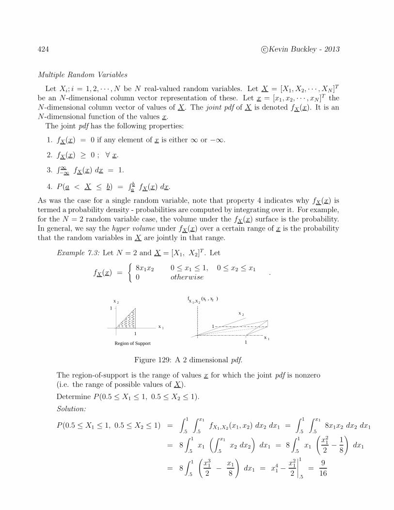
424 c©Kevin Buckley - 2013
Multiple Random Variables
Let Xi; i = 1, 2, · · · , N be N real-valued random variables. Let X = [X1, X2, · · · , XN ]T
be an N -dimensional column vector representation of these. Let x = [x1, x2, · · · , xN ]T the
N -dimensional column vector of values of X. The joint pdf of X is denoted fX(x). It is anN -dimensional function of the values x.
The joint pdf has the following properties:
1. fX(x) = 0 if any element of x is either ∞ or −∞.
2. fX(x) ≥ 0 ; ∀ x.
3.∫∞−∞ fX(x) dx = 1.
4. P (a < X ≤ b) =∫ ba fX(x) dx.
As was the case for a single random variable, note that property 4 indicates why fX(x) istermed a probability density - probabilities are computed by integrating over it. For example,for the N = 2 random variable case, the volume under the fX(x) surface is the probability.In general, we say the hyper volume under fX(x) over a certain range of x is the probabilitythat the random variables in X are jointly in that range.
Example 7.3: Let N = 2 and X = [X1, X2]T . Let
fX(x) =
8x1x2 0 ≤ x1 ≤ 1, 0 ≤ x2 ≤ x1
0 otherwise.
x 2
x 1
x 1
x 2
Region of Support
1
1
X ,X 21f (x , x )
1
1
1 2
Figure 129: A 2 dimensional pdf.
The region-of-support is the range of values x for which the joint pdf is nonzero(i.e. the range of possible values of X).
Determine P (0.5 ≤ X1 ≤ 1, 0.5 ≤ X2 ≤ 1).
Solution:
P (0.5 ≤ X1 ≤ 1, 0.5 ≤ X2 ≤ 1) =∫ 1
.5
∫ x1
.5fX1,X2(x1, x2) dx2 dx1 =
∫ 1
.5
∫ x1
.58x1x2 dx2 dx1
= 8∫ 1
.5x1
(∫ x1
.5x2 dx2
)
dx1 = 8∫ 1
.5x1
(
x21
2− 1
8
)
dx1
= 8∫ 1
.5
(
x31
2− x1
8
)
dx1 = x41 −
x21
2
∣
∣
∣
∣
∣
1
.5
=9
16
c©Kevin Buckley - 2013 425
Marginalization:
Let X = [X1, X2, · · · , XN ]T be a set of random variables, and consider some partitioning
of these, for example X1 = [X1, X2, · · · , XP ]T and X2 = [XP+1, X2, · · · , XN ]
T . To obtain thejoint pdf fX1
(x1) we marginalize over X2 as follows:
fX1(x1) =
∫ ∞
−∞fX(x) dx2 . (4)
That is, you integrate over x2 to eliminate it.
Statistical Independence:
Consider X = [X1, X2, · · · , XN ]T partitioned, for example, as X1 = [X1, X2, · · · , XP ]
T andX2 = [XP+1, X2, · · · , XN ]
T . Then, by definition, the random variable sets X1 and X2 arestatistically independent of each other if and only if
fX(x) = fX1(x1) · fX2
(x2) . (5)
Example 7.4: For X = [X1, X2]T , let
fX(x) = e−(x1+x2) u(x1) u(x2) .
Are X1 and X2 statistically independent?
Solution:
fX(x) = e−x1 u(x1) e−x2 u(x2) = fX1(x1) · fX2(x2)
(i.e. the joint pdf factors into the product of the two single-dimensional pdf’s).Try marginalizing over X1 to get fX2(x2), and over X2 to get fX1(x1), So X1 andX2 are statistically independent.
Expectation
Let X be a single real-valued random variable with pdf fX(x). The expected value of Xis defined as
EX =∫ ∞
−∞x fX(x) dx . (6)
E· =∫∞−∞ · fX(x) dx is the expectation operator. (In this case we are simply considering
the expected value of X .) Evaluating this equation, observe that EX is a weightedaverage of the values x, where the weighting function is the pdf. This probabilistic weightingemphasized values x which are more probable. That makes sense.
It is useful to remember that the expectation operator is linear. Thus, for constants a andb, and random variable X ,
EaX + b = a EX + b . (7)
426 c©Kevin Buckley - 2013
Moments
Consider, for positive integer ν, the class of functions g(X) = Xν . The moments aboutthe origin are defined as:
ξν = EXν =∫ ∞
−∞xν fX(x) dx . (8)
For example, the 1-st moment about the origin of X , ξ1 = EX, is termed the mean of X .The mean of X is denoted µx, i.e. ξ1 = µx. It is useful to think of the 2-nd moment aboutthe origin, ξ2 = EX2, as the energy (or power) of the random variable.
Again for positive integer ν, consider the class of functions g(X) = (X−µ)ν . The centralmoments are defined as:
mν = E(X − µx)ν =
∫ ∞
−∞(x− µ)ν fX(x) dx . (9)
The most commonly considered central moment is the 2-nd order central moment
m2 = E(X − µx)2 =
∫ ∞
−∞(x− µx)
2 fX(x) dx . (10)
We term this moment the variance. The variance of X is denote σ2x, i.e. m2 = σ2
x. Itis useful to think of the variance as the energy (or power) of the variation of the randomvariable from its mean. Note that
σ2x = ξ2 − µ2
x . (11)
You can use the linearity of the expectation operator to prove this.
Example 7.5: Determine the mean and variance of the uniform random variableX considered in Example 7.1.
Solution: For the mean,
µx =∫ b
a
1
b− ax dx =
1
b− a
x2
2
∣
∣
∣
∣
∣
b
a
=1
b− a
a2 − b2
2=
a+ b
2
For the variance, let q = b− a be the width of the density function. Then
σ2x =
1
q
∫ b
a
(
x− a + b
2
)2
dx =1
q
∫ q/2
−q/2x2 dx =
1
q
x3
3
∣
∣
∣
∣
∣
q/2
−q/2
=1
q
(
q3
24+
q3
24
)
=q2
12
The variance of a uniform random variable is σ2 = q2
12, i.e. the width squared
over twelve.
The mean of a random variable with symmetric fX(x) is always the point of symmetry.
c©Kevin Buckley - 2013 427
Joint Moments of Two Random Variables
Consider two random variables X and Y , and let Z = g(X, Y ) be some function of them.The expectation of Z is
EZ = Eg(X, Y ) =∫ ∞
−∞
∫ ∞
−∞g(x, y) fX,Y (x, y) dx dy . (12)
This generalizes to g(Xi; i = 1, 2, · · · , N) is an obvious manner.Given two random variables X and Y , the ijth moment about the origin is
ξij = EX iY j =∫ ∞
−∞
∫ ∞
−∞xiyj fX,Y (x, y) dx dy . (13)
For example, the mean of X , is
µx = ξ10 = EX1Y 0 = EX =∫ ∞
−∞
∫ ∞
−∞x fX,Y (x, y) dx dy
=∫ ∞
−∞x∫ ∞
−∞fX,Y (x, y) dy dx
=∫ ∞
−∞x fX(x) dx .
Correlation, an important joint moment about the origin, is defined for random variablesX and Y as
CorrX, Y = rxy = ξ11 = EXY . (14)
We say that X and Y are uncorrelated if rxy = µx µy. We say that X and Y are orthogonalif rxy = 0. Note the mixed terminology.
Given two random variables X and Y , the ijth joint central moment is
mij = E(X − µx)i(Y − µy)
j =∫ ∞
−∞
∫ ∞
−∞(x− µx)
i(y − µy)j fX,Y (x, y) dx dy . (15)
For both joint central moments ξij and joint moments about the origin mij , the order of themoment is i+ j.
The covariance between X and Y , the 2-nd order central moment, is
CovX, Y = cxy = m11 = E(X − µx)(Y − µy) . (16)
Note that if both X and Y are zero mean, then cxy = rxy, the correlation is equal to thevariance.
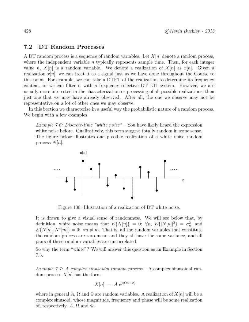
428 c©Kevin Buckley - 2013
7.2 DT Random Processes
A DT random process is a sequence of random variables. Let X [n] denote a random process,where the independent variable n typically represents sample time. Then, for each integervalue n, X [n] is a random variable. We denote a realization of X [n] as x[n]. Given arealization x[n], we can treat it as a signal just as we have done throughout the Course tothis point. For example, we can take a DTFT of the realization to determine its frequencycontent, or we can filter it with a frequency selective DT LTI system. However, we areusually more interested in the characterization or processing of all possible realizations, thenjust one that we may have already observed. After all, the one we observe may not berepresentative on a lot of other ones we may observe.
In this Section we characterize in a useful way the probabilistic nature of a random process.We begin with a few examples
Example 7.6: Discrete-time ”white noise” – You have likely heard the expressionwhite noise before. Qualitatively, this term suggest totally random in some sense.The figure below illustrates one possible realization of a white noise randomprocess N [n].
n
.... ....
n[n]
Figure 130: Illustration of a realization of DT white noise.
It is drawn to give a visual sense of randomness. We will see below that, bydefinition, white noise means that EN [n] = 0; ∀n, E|N [n]|2 = σ2
n, andEN [n] ·N∗[m] = 0; ∀n 6= m. That is, all the random variables that constitutethe random process are zero-mean and they all have the same variance, and allpairs of these random variables are uncorrelated.
So why the term “white”? We will answer this question as an Example in Section7.3.
Example 7.7: A complex sinusoidal random process – A complex sinusoidal ran-dom process X [n] has the form
X [n] = A ej(Ωn+Φ)
where in general A, Ω and Φ are random variables. A realization of X [n] will be acomplex sinusoid, whose magnitude, frequency and phase will be some realizationof, respectively, A, Ω and Φ.
c©Kevin Buckley - 2013 429
Consider, for example, the case where A and Ω are constant (i.e. known, non-random), and Φ is uniformly distributed with pdf
fΦ(φ) =
12π
0 ≤ φ < 2π0 otherwise
The mean of each random variable that constitutes this random process is
µx[n] = EX [n] = EA ej(Ωn+Φ) = AejΩn EejΦ
= AejΩn 1
2π
∫ 2π
0ejφ dφ = 0 .
In general, the mean of the random variables is different at different times. Thisone has constant (zero) mean for all time, i.e. µx[n] = µx = 0.
The correlation between any two random variables, say at times n and m, is
EX [m] X∗[n] = EAej(Ωm+Φ) Ae−j(ωn+Φ) = A2ejΩ(m−n) EejΦe−jΦ= A2ejΩ(m−n) E1 = A2 ejΩ(m−n)
We see from this expression that form = n, i.e. when we are correlating a randomsample with itself, we just get the variance of that random variable, σ2
x[n] = A2.
Note that this is not a function of n, i.e. σ2x[n] = σ2
x = A2. Also note thatthe correlation between two random variables, at times n and m, is a function ofonly the distance in time m− n between them. It is not a function of where thesamples are in time.
Partial Characterizations of DT Random Processes: The Mean & Correlation Functions
A complete probabilistic description of a DT random process consists of the set of alljoint pdf’s of all combinations of the random variables that constitutes the random process.In many situations all of this information is not available, and in most situations it is notnecessary for the effective processing of the random process. An effective, common andsomewhat general representation of random processes is in terms of moments. Althoughhigher order moments are sometimes, in the vast majority of applications the 1-st and 2-ndorder moments of a random process can be effectively employed. Here we describe the 1-stand 2-nd order moment descriptions of DT random processes.
• The Mean Function: The mean function of a DT random process X [n] is defined as
µx[n] = EX [n] =∫ ∞
−∞x[n] fX[n](x[n]) dx[n] ; ∀ n . (17)
It is the function of means of all the random variables that constitute the randomprocess. In general, as the notation µx[n] implies, the mean is time varying.

430 c©Kevin Buckley - 2013
• The Correlation Function: The correlation function of a DT random process X [n] isdefined as
Rxx[m,n] = EX [m]X∗[n] =∫ ∞
−∞
∫ ∞
−∞x[m] x∗[n] fX[m],X[n](x[m], x[n]) dx[m] dx[n] ; ∀m,n.
(18)It is the function of all correlations between the random variables that constitute therandom process. It is a two dimensional function of the times m and n of the twosamples which are being correlated.
• The Covariance Function: The covariance function of a DT random process X [n] isdefined as
Cxx[m,n] = E(X [m]− µx[m]) (X [n]− µx[n])∗ (19)
= Rxx[m,n] − µx[m] · µ∗x[n] . (20)
Eq (20) can be derived from Eq (19) using the linearity property of the expectation.Note that if the random process is zero-mean for all time, then Cxx[m,n] = Rxx[m,n].
One way that random processes are characterized is in terms of properties of their mean andcorrelation functions. We now identify the most common category of DT random processes.
Wide-Sense Stationary DT ProcessesQualitatively, stationarity of a random process means that its probabilistic characteristics
do not change with time. There are different types of stationarity corresponding to differentcharacteristics. Stationarity in the mean means
µx[n] = EX [n] = µx . (21)
That is, the mean is not a function of time n. Wide-sense stationarity means stationarity inthe mean plus
Rxx[n + l, n] = EX [n+ l] X∗[n] = Rxx[l] . (22)
That is, in addition to the mean is not being function of time n, the autocorrelation functionis not a function of time n, but only a function of the difference in time l between samplesbeing correlated. This distance, l, is termed the lag.
Example 7.8: Discrete-Time White Noise – In Example 7.6 DT white noisewas described as a DT random process, say N [n], with EN [n] = 0; ∀n,E|N [n]|2 = σ2
n, and EN [n] · N∗[m] = 0; ∀n 6= m. We now recognize thatwith these properties, white noise is zero mean, i.e.
µn[n] = µn = 0 ,
with correlation function
Rnn[n + l, n] = Rnn[l] = σ2n δ[l] .
So, white noise is wide-sense stationary.
c©Kevin Buckley - 2013 431
Example 7.9: A complex sinusoidal random process – In Example 7.7 we consid-ered the DT random process
X [n] = A ej(Ωn+Φ)
where A and Ω are constant, and Φ is uniformly distributed over values 0 ≤ φ <2π.
We observed that µx[n] = 0, i.e. we now say that the random process has zeromean. We also concluded that EX [m] X∗[n] = A2 ejΩ(m−n). That is, thecorrelation function is Rxx[n + l, n] = Rxx[l] = A2 ejΩl. So the correlationfunction is a function of only the lag (the distance in time between the randomvariables).
As in Example 7.8, this random process is wide-sense stationary.
Example 7.10: Another complex sinusoidal random process – As in Example 7.9,consider
X [n] = A ej(Ωn+Φ)
where Ω is still constant and Φ is uniformly distributed over values 0 ≤ φ < 2π,but now let A be a Gaussian random variable with zero mean and variance σ2
a.Assume that A and φ are statistically independent. Determine the mean andcorrelation functions. Is this random process wide-sense stationary?
Solution: Note that fA,Φ(a, φ) = fA(a) · fΦ(φ), since A and Φ are statisticallyindependent. The mean function is
µx[n] =∫ ∞
−∞
∫ ∞
−∞x[n] fA,Φ(a, φ) da dφ = ejΩn
∫ ∞
−∞ejφfΦ(φ) dφ ·
∫ ∞
−∞a fA(a) da
= ejΩn 1
2π
∫ 2π
0dφ ·
∫ ∞
−∞a
1√
2πσ2a
e−a2/2σ2a = 0.
That is, both integrals in the last line are zero. This random process is zero-mean.
The correlation function can be shown to be
Rxx[n + l, n] = Rxx[l] = σ2a ejΩl .
So this DT sinusoidal random process is also wide-sense stationary.
432 c©Kevin Buckley - 2013
Example 7.11: A real-valued sinusoidal random process – Consider the randomprocess
X [n] = A cos(Ωn+ Φ)
where A and Ω are constants and Φ is uniformly distributed over values0 ≤ φ < 2π. It can be shown that
µx[n] = µx = 0 ,
and
Rxx[n + l, n] = Rxx[l] = A2 cos(Ωl) .
So, yet again, the sinusoidal random process is wide-sense stationary.
Not all sinusoidal random processes are wide-sense stationary. The above examples wereselected because we are only interested in wide-sense stationary processes in this overview.
Example 7.12: Additive White Gaussian Noise (AWGN) – A very common typeof random process, often observed at the sampled output of a sensor (or thesampled output of a preamplifier connected directly to a sensor) when there isno signal received by the sensor, is AWGN.
White means that all the sample are zero-mean, uncorrelated with one another,and all have the same variance (i.e. see Example 7.8).
Gaussian means that each sample is Gaussian distributed. Let N [n] denote theAWGN process. Then,
fN [n](n[n]) =1
√
2πσ2n
e−n2[n]/2σ2n (23)
and since uncorrelated Gaussian random variables are statistically independent22,the joint pdf of any set of samples is the product of their individual pdf’s, each ofthe Eq (23) form. So for this random process we know the complete statisticaldescription.
Additive implies that, in the presence of a signal, the noise is added to it. It alsotypically implies that the signal, if also a random process, is uncorrelated withthe noise. Let X [n] = S[n] +N [n] be the sampled sensor output, where S[n] is asignal and N [n] is AWGN. Then it is easy to show that, since S[n] and N [n] areuncorrelated,
Rxx[l] = Rss[l] + Rnn[l] ∀ l ,
where we already know that Rnn[l] = σ2n δ[l].
22Hopefully you recall this from your Probability course. If not, trust me on this one.
c©Kevin Buckley - 2013 433
Signal-to-Noise Ratio (SNR): For wide-sense stationary random processes, as with otherpower signals, SNR is defined as the ration of the signal power to the noise power. For arandom process X [n] = S[n]+N [n], consisting of wide-sense stationary signal S[n] and noiseN [n], the SNR is
SNR =Rss[0]
Rnn[0]; SNRdb = 10 log10(SNR) . (24)
Example 7.13: Let X [n] = S[n] + N [n], where the signal S[n] is a complexsinusoidal process as described in Example 7.10, andN [n] is AWGN with varianceσ2n. Let σ
2a = 20 and σ2
n = 10. The SNR is
SNR =Rss[0]
Rnn[0]=
σ2a
σ2n
=20
10= 2; SNRdb ≈ 3 dB .
7.3 Power Spectral Density
Let X [n] be a wide-sense stationary random process. Let x[n] be a realization. Denote theDTFT of a 2N + 1 sample window of the random process as
XN(ejω) = XN(ω) =
N∑
n=−N
x[n] e−jnω . (25)
The power spectral density is defined as
Sxx(ejω) = lim
N−→∞
1
2N + 1E|XN(e
jω)|2 . (26)
The power spectral density is the expected value of the magnitude-squared of the DTFT ofa window of the random process, as the window width approaches infinity. This definitioncaptures what we want as a measure of the frequency content of a DT random process.
Let’s take an alternative view of Sxx(ejω). First consider the term on the right of the Eq
(26), without the limit and expectation:
1
2N + 1|XN(e
jω)|2 =1
2N + 1
N∑
n=−N
x[n] e−jnωN∑
l=−N
x∗[l] ejlω
=1
2N + 1
N∑
n=−N
N∑
l=−N
x[n] x∗[l] e−j(n−l)ω
=1
2N + 1
N∑
n=−N
n+N∑
m=n−N
x[n] x∗[n−m] e−jmω .
Taking the expected value, we have
1
2N + 1E|XN(e
jω)|2 =1
2N + 1
N∑
n=−N
n+N∑
m=n−N
Rxx[m] e−jmω . (27)
434 c©Kevin Buckley - 2013
Now, taking the limit as N −→∞, we have
Sxx(ejω) = lim
N−→∞
1
2N + 1E|XN(e
jω)|2
= limN−→∞
1
2N + 1
N∑
n=−N
∞∑
m=−∞Rxx[m] e−jmω
=∞∑
m=−∞Rxx[m] e−jmω lim
N−→∞
1
2N + 1
N∑
n=−N
1
=∞∑
m=−∞Rxx[m] e−jmω .
Thus, the power spectral density and the autocorrelation function of a wide-sense stationaryrandom process form the DTFT pair
Sxx(ejω) =
∞∑
l=−∞Rxx[l] e
−jlω (28)
Rxx[l] =1
2π
∫ π
−πSxx(e
jω) ejlω dω . (29)
Example 7.14 - Given the correlation function Rxx[l] = σ2x 0.5|l|, determine and
sketch the power spectral density Sxx(ejω).
Solution:

c©Kevin Buckley - 2013 435
Example 7.15 - Consider the complex sinusoidal random signal described in Ex-ample 7.10 embedded in AWGN. Determine the mean function, the correlationfunction and the power spectral density.
Solution:
436 c©Kevin Buckley - 2013
7.4 DT Random Processes & DT LTI Systems
Consider a wide-sense stationary random process X [n] with mean µx and autocorrelationfunction Rx[l], and a DT LTI system with impulse response h[n]. For x[n], a realization ofX [n], the input/output relationship is the convolution sum
y[n] =∞∑
k=−∞h[k] x[n− k] (30)
1. The output mean function is:
Ey[n] =∞∑
k=−∞h[k] Ex[n− k]
µy = µx
∞∑
k=−∞h[k] (31)
2. The output correlation function is:
Ryy[l] = EY [n + l] Y ∗[n]
=∞∑
m=−∞
∞∑
k=−∞h[k] h∗[m] Ex[n + l − k] x∗[n−m]
=∞∑
m=−∞h∗[m]
∞∑
k=−∞h[k] Rxx[(l +m)− k]
=∞∑
m=−∞h∗[m] (h[l] ∗ Rxx[l +m])
= h[l] ∗( ∞∑
m=−∞h∗[m] Rxx[l +m]
)
= h[l] ∗
∞∑
i=−∞h∗[i− l] Rxx[i]
= h[l] ∗ h∗[−l] ∗ Rxx[l] (32)
3. The output power spectral density: From the above result on DT LTI system in-put/output autocorrelation functions, and DTFT properties, it can be shown that
Syy(ejω) = Sxx(e
jω) |H(ejω)|2 . (33)

c©Kevin Buckley - 2013 437
Example 7.16: Consider a zero-mean AWGN input X [n], with variance σ2n, and
a DT LTI system with impulse response h[n] = δ[n] + δ[n − 1]. Determine thecorrelation function and power spectral density of the output Y [n].
Solution:
438 c©Kevin Buckley - 2013
Example 7.17: Let input X [n] be as in Example 7.15, and let the DT LTI systemimpulse response be h[n] = an u[n], where |a| < 1. Determine the correlationfunction and power spectral density of the output Y [n].
Solution:
Example 7.18: Let h[n] = 1N(u[n] − u[n − N ]), and let X [n] be a wide-sense
stationary complex sinusoidal process with correlation function Rxx[l] = σ2x ejω0l
where |ω0| ≤ π. Determine the correlation function and power spectral densityof the output Y [n].
Solution:
c©Kevin Buckley - 2013 439
7.5 Problems
1. Correlation function, power spectral density problems (feel free to use Fourier Trans-form tables):
(a) Given Rxx[l] = −δ[l + 1] + 2δ[l]− δ[l − 1], determine Sxx(ejω).
(b) Given Rxx[l] = A2 cos(ω0l), describe Sxx(ejω); −π < ω ≤ π. Assume −π < ω0 ≤
π.
(c) Given the following power spectral density, determine to autocorrelation functionRxx[l]:
Sxx(ejω) =
1 |ω| ≤ π2
0 π2< |ω| ≤ π
(d) Given the following power spectral density, determine to autocorrelation functionRxx[l]:
Sxx(ejω) =
0 |ω| ≤ π2
1 π2< |ω| ≤ π
(e) Given power spectral density Syy(ejω) = 2 + 2 cos(2ω), determine correlation
function Ryy[m].
2. Assume random processes are DT and wide-sense stationary:
(a) Given X [n] with correlation function Rxx[l] = 3δ[l]−(δ[l+1]+δ[l−1]), determineand plot the power spectral density Sxx(e
jω). What percentage of X [n] power isin the frequency band 0 ≤ ω ≤ π?
(b) Given Y [n] with power spectral density
Syy(ejω) =
1 + 2ω 0 ≤ ω ≤ π1− 2ω −π ≤ ω ≤ 0
,
determine the correlation function Ryy[l]. What is the power of Y [n]? (Hint: usethe DTFT pair table and linearity.)
3. Assume random processes are DT and wide-sense stationary, and systems are DT LTI:
(a) By performing the required convolutions, determine and plot the correlation func-tion of the output Y [n] of a system with impulse response h[n] = p3[n] and inputX [n] with correlation function Rxx[l] = 2δ[l] + δ[l + 1] + δ[l − 1].
(b) Consider the following system:
y[n] − .5 y[n− 2] = x[n] + .5 x[n− 2] .
i. For input correlation function Rxx[l] = 4 δ[l], determine the expression forthe output power spectral density.
440 c©Kevin Buckley - 2013
ii. For input correlation function Rxx[l] = 3 ej(π/2)l, determine the outputcorrelation function.
4. Given the 3-point averager considered in the first week of Practicum 5, i.e. with I/Odifference equation
y[n] =1
3(x[n] + x[n− 1] + x[n− 2]) ,
with a wide-sense stationary random process input. For each of the following inputs,determine the output correlation function and power spectral density.
(a) X1[n] with correlation function Rx1,x1[l] = δ[l] + 0.5 δ[l − 1] + 0.5 δ[l + 1].(You must first compute Ry1,y1[l] directly using graphical convolution to receivecredit for this problem.)
(b) X2[n] with correlation function Rx2,x2[l] = ej(π/4)l. (You must first computeSy2,y2(ω) using the frequency response H(ejω) to receive credit for this problem.)
(c) X3[n] with correlation function Rx3,x3[l] = cos(23πl). (You can do this whichever
way you wish.)
5. A DT LTI system has impulse response h[n] = p4[n]. The input is zero-mean whitenoise with variance σ2
x.
(a) What is the output mean function µy[n]?
(b) What is the correlation function of the output?
6. Correlation functions and LTI systems:
(a) Consider a wide-sense stationary random process X [n], with correlation functionRxx[l] = −0.5 δ[l+1] + 1.25 δ[l]−0.5 δ[l−1]. It is the input to a LTI system withimpulse response h[n] = 0.5n u[n]. Determine the output signal’s correlationfunction and power spectral density.
(b) Consider a wide-sense stationary input X [n] to a LTI system with frequencyresponse H(ejω) = e−jωπ/2. Let the autocorrelation function of the input beRxx[l] = 5δ[l] + a−|l|. Determine the autocorrelation function Ryy[l] of the outputY [n].
7. Consider a WSS autoregressive signal X [n] which is the output of the all-pole filter
X [n] = .5X [n− 1] + W [n]
with zero-mean, unit-variance, uncorrelated input W [n]. This signal X [n] is the inputto a DT linear time invariant system described by the following difference equation
Y [n] + .9Y [n− 1] = X [n] − .25X [n− 2] .
Determine the power spectral density of the output Y [n].
c©Kevin Buckley - 2013 441
8. A zero-mean random process X [n] with autocorrelation function Rxx[l] = 0.5|l| is ap-plied to a DT LTI system with impulse response h[n] = δ[n] + δ[n− 1].
(a) What is the power spectral density of the input?
(b) What is the correlation function of the output?
(c) What is the power spectral density of the output?
9. Consider a DT LTI system with impulse response h[n] = .5n u[n] and let wide-sensestationary random process X [n], with autocorrelation function Rxx[m] = 3 δ[m], bethe input. Determine the output autocorrelation function Ryy[m].
10. The power of any wide-sense stationary random process X [n] is
Px = Rxx[0] =1
2π
∫ π
−πSxx(e
jω) dω .
Let such an X [n], with autocorrelation function Rxx[m] = 12δ[m+2]+δ[m]+ 1
2δ[m−2],
be the input to an ideal lowpass filter with frequency response
H(ejω) =
1 |ω| ≤ π2
0 π2< |ω| ≤ π
.
Determine the power of the output wide-sense stationary random process Y [n].
11. Determine the mean and the autocorrelation function for the random process
X [n] = V [n] + 3V [n− 1]
where V [n] is a sequence of independent random variables with mean µv and varianceσ2v . Is X [n] wide-sense stationary?
12. Consider a zero-mean AWGN input X [n], with variance σ2n = 1, and a DT LTI system
with impulse response h[n] = −1n p4[n]. Determine the correlation function and powerspectral density of the output Y [n].
13. Consider a wide-sense stationary input with correlation function Rxx[l] = ρ|l| with|ρ| < 1, and a DT LTI system with impulse response h[n] = δ[n] − δ[n−1]. Determinethe correlation function and power spectral density of the output Y [n]. Also find theoutput mean function.
14. In all parts below, the input is wide-sense stationary random process & the system issome LTI system.
a) Given zero-mean input X1[n], with correlation function Rx1x1 [l] = 5 (0.9)|l|, canthe output correlation function be
(a) Ry1y1[l] = Rx1x1 [l], or
(b) Ry1y1[l] = Rx1x1 [l − 5]?
Why?
442 c©Kevin Buckley - 2013
b) Given zero-mean input X2[n], with correlation function Rx2x2 [l] = 4 ej(π/2)l, toa system with impulse response h2[n] = (0.8)nu[n], is the output power densityspectrum
(a) Sy2y2(ejω) = 0; −π ≤ ω ≤ π, or
(b) Sy2y2(ejω) = 8π
1.64δ(ω − π
2); −π ≤ ω ≤ π?
Why?
c) Given input X3[n], with mean µx3 = 5 and correlation function Rx3x3[l] = 25 +(0.9)|l|, to a system with impulse response h3[n] = δ[n] − δ[n − 1], determineRy3y3 [0], the zero lag of the output correlation function. (Hint: Find h[n] ∗ h[−l].Then convolve it, as much as needed, with Rx3x3 [l].)
15. Consider a DT LTI system with impulse response h[n] = δ[n] − δ[n−1], with randomprocess input X(t) resulting in random process output Y [n].
(a) Determine and plot h[n] ∗ h[−n] and |H(ejω)|2.(b) Given that Rxx[l] = 4 δ[l], determine Ryy[l] and Syy(e
jω).
(c) Given that
Sxx(ejω) =
4 δ(ω) + 5 δ(ω − π2) −π < ω ≤ π
0 otherwise over − π < ω ≤ π,
determine Ryy[l] and Syy(ejω).
(d) Given that Rxx[l] = 6sin(π
2l)
πl, determine Syy(e
jω).
16. Consider a DT LTI system frequency response
H(ejω) =
1 |ω| ≤ π2
0 π2< |ω| ≤ π
.
(a) Given that the input is the wide-sense stationary process X [n] from Example6.6,8 in the Course Notes, determine the autocorrelation function and the powerspectral density of the output Y [n].
(b) Given that the input is the wide-sense stationary process X [n] from Examples6.7,9 the Course Notes, with frequency ω0 = π
3, determine the autocorrelation
function and the power spectral density of the output Y [n].
(c) Given that the input is the wide-sense stationary process X [n] from Example 6.11the Course Notes, with frequency ω0 =
2π3, determine the autocorrelation function
and the power spectral density of the output Y [n].
17. Consider a DT LTI system with impulse response h[n] = δ[n] + δ[n− 1].
(a) Given that the input is the wide-sense stationary process X [n] from Example6.6,8 in the Course Notes, determine the autocorrelation function and the powerspectral density of the output Y [n].
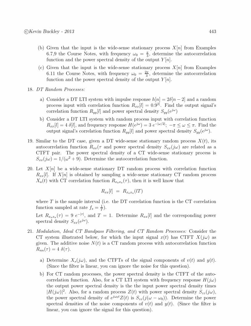
c©Kevin Buckley - 2013 443
(b) Given that the input is the wide-sense stationary process X [n] from Examples6.7,9 the Course Notes, with frequency ω0 = π
3, determine the autocorrelation
function and the power spectral density of the output Y [n].
(c) Given that the input is the wide-sense stationary process X [n] from Examples6.11 the Course Notes, with frequency ω0 = 2π
3, determine the autocorrelation
function and the power spectral density of the output Y [n].
18. DT Random Processes:
a) Consider a DT LTI system with impulse response h[n] = 2δ[n− 2] and a randomprocess input with correlation function Rxx[l] = 0.9|l|. Find the output signal’scorrelation function Ryy[l] and power spectral density Syy(e
jω)
b) Consider a DT LTI system with random process input with correlation functionRxx[l] = 4 δ[l], and frequency response H(ejω) = 3 e−|ω/2|; −π ≤ ω ≤ π. Find theoutput signal’s correlation function Ryy[l] and power spectral density Syy(e
jω).
19. Similar to the DT case, given a DT wide-sense stationary random process X(t), itsautocorrelation function Rxx(τ and power spectral density Sxx(jω) are related as aCTFT pair. The power spectral density of a CT wide-sense stationary process isSxx(jω) = 1/(ω2 + 9). Determine the autocorrelation function.
20. Let X [n] be a wide-sense stationary DT random process with correlation functionRxx[l]. If X [n] is obtained by sampling a wide-sense stationary CT random processXa(t) with CT correlation function Rxaxa(τ), then it is well know that
Rxx[l] = Rxaxa(lT )
where T is the sample interval (i.e. the DT correlation function is the CT correlationfunction sampled at rate fs =
1T).
Let Rxaxa(τ) = 9 e−|τ |, and T = 1. Determine Rxx[l] and the corresponding powerspectral density Sxx(e
jω).
21. Modulation, Ideal CT Bandpass Filtering, and CT Random Processes: Consider theCT system illustrated below, for which the input signal x(t) has CTFT X(jω) asgiven. The additive noise N(t) is a CT random process with autocorrelation functionRnn(τ) = 4 δ(τ).
a) Determine Xs(jω), and the CTFTs of the signal components of v(t) and y(t).(Since the filter is linear, you can ignore the noise for this question).
b) For CT random processes, the power spectral density is the CTFT of the auto-correlation function. Also, for a CT LTI system with frequency response H(jω)the output power spectral density is the the input power spectral density times|H(jω)|2. Also, for a random process Z(t) with power spectral density Szz(jω),the power spectral density of ejω0tZ(t) is Szz(j(ω − ω0)). Determine the powerspectral densities of the noise components of v(t) and y(t). (Since the filter islinear, you can ignore the signal for this question).
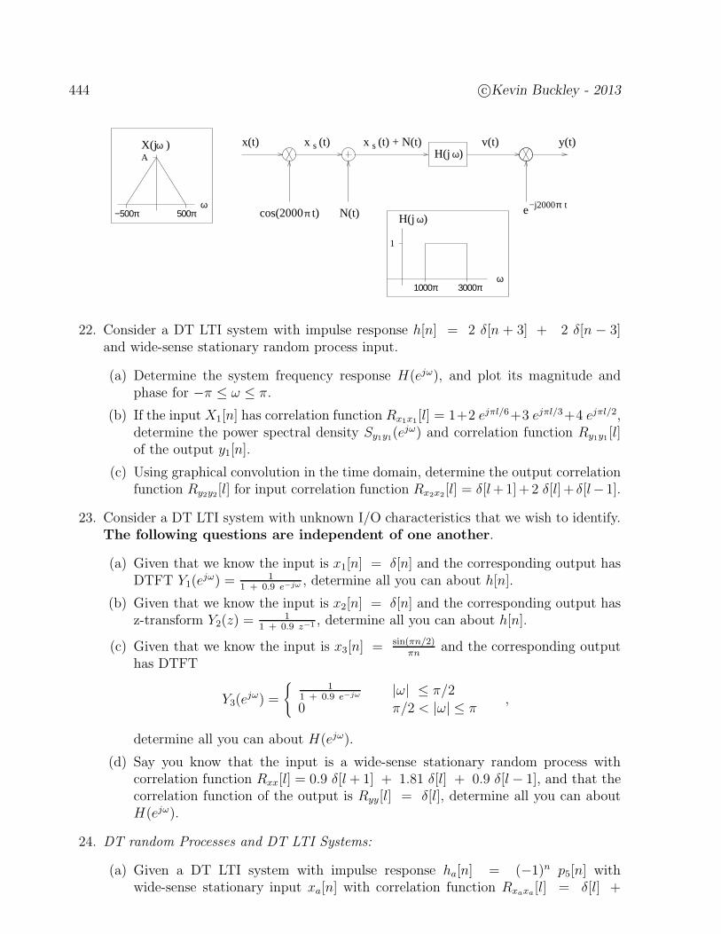
444 c©Kevin Buckley - 2013
H(j )ω
−j2000 tπecos(2000 t)π
x (t)s sx (t) + N(t)x(t) v(t)
N(t)
y(t)
H(j )ω
ω1000π
1
3000π
AωX(j )
500π−500πω
22. Consider a DT LTI system with impulse response h[n] = 2 δ[n + 3] + 2 δ[n − 3]and wide-sense stationary random process input.
(a) Determine the system frequency response H(ejω), and plot its magnitude andphase for −π ≤ ω ≤ π.
(b) If the input X1[n] has correlation function Rx1x1[l] = 1+2 ejπl/6+3 ejπl/3+4 ejπl/2,determine the power spectral density Sy1y1(e
jω) and correlation function Ry1y1 [l]of the output y1[n].
(c) Using graphical convolution in the time domain, determine the output correlationfunction Ry2y2[l] for input correlation function Rx2x2[l] = δ[l+1]+2 δ[l]+ δ[l−1].
23. Consider a DT LTI system with unknown I/O characteristics that we wish to identify.The following questions are independent of one another.
(a) Given that we know the input is x1[n] = δ[n] and the corresponding output hasDTFT Y1(e
jω) = 11 + 0.9 e−jω , determine all you can about h[n].
(b) Given that we know the input is x2[n] = δ[n] and the corresponding output hasz-transform Y2(z) =
11 + 0.9 z−1 , determine all you can about h[n].
(c) Given that we know the input is x3[n] = sin(πn/2)πn
and the corresponding outputhas DTFT
Y3(ejω) =
11 + 0.9 e−jω |ω| ≤ π/2
0 π/2 < |ω| ≤ π,
determine all you can about H(ejω).
(d) Say you know that the input is a wide-sense stationary random process withcorrelation function Rxx[l] = 0.9 δ[l + 1] + 1.81 δ[l] + 0.9 δ[l− 1], and that thecorrelation function of the output is Ryy[l] = δ[l], determine all you can aboutH(ejω).
24. DT random Processes and DT LTI Systems:
(a) Given a DT LTI system with impulse response ha[n] = (−1)n p5[n] withwide-sense stationary input xa[n] with correlation function Rxaxa[l] = δ[l] +
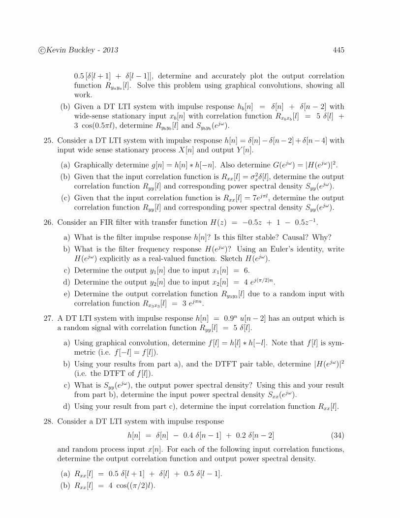
c©Kevin Buckley - 2013 445
0.5 [δ[l + 1] + δ[l − 1]], determine and accurately plot the output correlationfunction Ryaya[l]. Solve this problem using graphical convolutions, showing allwork.
(b) Given a DT LTI system with impulse response hb[n] = δ[n] + δ[n − 2] withwide-sense stationary input xb[n] with correlation function Rxbxb
[l] = 5 δ[l] +3 cos(0.5πl), determine Rybyb [l] and Sybyb(e
jω).
25. Consider a DT LTI system with impulse response h[n] = δ[n]− δ[n− 2]+ δ[n− 4] withinput wide sense stationary process X [n] and output Y [n].
(a) Graphically determine g[n] = h[n] ∗ h[−n]. Also determine G(ejω) = |H(ejω)|2.(b) Given that the input correlation function is Rxx[l] = σ2
xδ[l], determine the outputcorrelation function Ryy[l] and corresponding power spectral density Syy(e
jω).
(c) Given that the input correlation function is Rxx[l] = 7ejπl, determine the outputcorrelation function Ryy[l] and corresponding power spectral density Syy(e
jω).
26. Consider an FIR filter with transfer function H(z) = −0.5z + 1 − 0.5z−1.
a) What is the filter impulse response h[n]? Is this filter stable? Causal? Why?
b) What is the filter frequency response H(ejω)? Using an Euler’s identity, writeH(ejω) explicitly as a real-valued function. Sketch H(ejω).
c) Determine the output y1[n] due to input x1[n] = 6.
d) Determine the output y2[n] due to input x2[n] = 4 ej(π/2)n.
e) Determine the output correlation function Ry3y3 [l] due to a random input withcorrelation function Rx3x3[l] = 3 ejπn.
27. A DT LTI system with impulse response h[n] = 0.9n u[n− 2] has an output which isa random signal with correlation function Ryy[l] = 5 δ[l].
a) Using graphical convolution, determine f [l] = h[l] ∗ h[−l]. Note that f [l] is sym-metric (i.e. f [−l] = f [l]).
b) Using your results from part a), and the DTFT pair table, determine |H(ejω)|2(i.e. the DTFT of f [l]).
c) What is Syy(ejω), the output power spectral density? Using this and your result
from part b), determine the input power spectral density Sxx(ejω).
d) Using your result from part c), determine the input correlation function Rxx[l].
28. Consider a DT LTI system with impulse response
h[n] = δ[n] − 0.4 δ[n− 1] + 0.2 δ[n− 2] (34)
and random process input x[n]. For each of the following input correlation functions,determine the output correlation function and output power spectral density.
(a) Rxx[l] = 0.5 δ[l + 1] + δ[l] + 0.5 δ[l − 1].
(b) Rxx[l] = 4 cos((π/2)l).