calibration of afm cantilevers of arbitrary...
TRANSCRIPT

Applied Physics
Calibration of AFM Cantilevers of Arbitrary
Shape.
Per-Anders Thorén [email protected]
SK200X Master of Science ThesisDepartment of Applied Physics, Nanostructured Physics
Royal Institute of Technology (KTH)
Examinator: David B. HavilandSupervisors: Daniel Forchheimer, Daniel Platz
TRITA-FYS 2013:36 ISSN 0280-316X ISRN KTH/FYS/--13:36SE
June 13, 2013


Abstract
Recent studies in the eld of atomic force microscopy have pro-
posed new non-invasive methods for determining the spring constant
of cantilever beams of arbitrary shape. These new calibration meth-
ods are derived and evaluated with real experiemnts which measures
the thermal excitation of the cantilever from the surrounding air. By
studying the power spectral density of cantilevers response due to this
excitation we calibrate the linear response function of the cantilever
to an external force.
i

ii
Sammanfattning
Nya forskningsresultat inom atomkraftmikroskopi (AFM) föreslår
en ny metod för att kalibrera fjäderkonstanten hos AFM-cantilevrar av
olika former utan att förstöra spetsen. I denna rapport härleds dessa
kalibreringsmetoder och de är sedan utvärderade med hjälp av exper-
iment i vilka det termiska bruset från den omgivande luften exciterar
cantilevern. Genom att studera cantileverns spektraltäthet från det
termiska bruset kalibreras den cantileverns linjära överföringsfunktion.
iii

iv
Contents
1 Introduction 1
2 The Atomic Force Microscope 3
2.1 History . . . . . . . . . . . . . . . . . . . . . . . . . . . . . . . 32.2 Typical Design of a SPM . . . . . . . . . . . . . . . . . . . . . 42.3 Atomic Force Microscope . . . . . . . . . . . . . . . . . . . . . 5
2.3.1 Measurement Modes . . . . . . . . . . . . . . . . . . . 52.3.2 Intermodulation AFM . . . . . . . . . . . . . . . . . . 7
3 Theoretical Background 9
3.1 Beam Theory . . . . . . . . . . . . . . . . . . . . . . . . . . . 93.2 The Real Cantilever . . . . . . . . . . . . . . . . . . . . . . . 123.3 Harmonic Oscillator . . . . . . . . . . . . . . . . . . . . . . . . 143.4 Detecting the Deection . . . . . . . . . . . . . . . . . . . . . 163.5 Hydrodynamic Formulation of the Viscous Damping . . . . . . 18
3.5.1 Derivation . . . . . . . . . . . . . . . . . . . . . . . . . 183.5.2 Reference Measurement Formulation . . . . . . . . . . 20
3.6 Calibrating the Linear Response Function . . . . . . . . . . . 20
4 Results from the new Calibration Algorithm 25
4.1 Measurement . . . . . . . . . . . . . . . . . . . . . . . . . . . 254.2 Experimental Procedure . . . . . . . . . . . . . . . . . . . . . 264.3 Calibration Data - All Plots . . . . . . . . . . . . . . . . . . . 274.4 Analysis and Discussion . . . . . . . . . . . . . . . . . . . . . 34
5 Analysis of Calibration Error for ImAFM 39
5.1 The Tip-Surface Force . . . . . . . . . . . . . . . . . . . . . . 395.1.1 Reconstruct the Force in the Quasi-Static Case . . . . 405.1.2 van der Waals - Derjaguin-Muller-Toporov Model . . . 41
5.2 Reconstructing the Force for Dynamic AFM . . . . . . . . . . 425.3 Theoretical Expectations of the Calibration . . . . . . . . . . 43
v

6 Changes in the Software Suite 47
7 Conclusions 51
8 Outlook 53
9 Summary 55
10 Appendix 61
10.1 Derivations and/or Extra Algebra . . . . . . . . . . . . . . . . 6110.1.1 Derivation: Sader Reference Method . . . . . . . . . . 6110.1.2 Integrating PSD . . . . . . . . . . . . . . . . . . . . . . 6210.1.3 Deriving Eq. (3.39) . . . . . . . . . . . . . . . . . . . . 64
10.2 Fit Algorithm Code . . . . . . . . . . . . . . . . . . . . . . . . 65
vi
Chapter 1
Introduction
In all branches of experimental science a high degree of accuracy is neededto make quantitative statements about nature. Therefore new and morepowerful measurement methods are always desirable and they may be usedto conrm or reject our current view of the world and develop tomorrow'stheories. One such measurement method is the so called Atomic Force Micro-scope, which has a resolution much higher than the best resolution obtainablewith optical microscopes. The Atomic Force Microscope can for example beused to determine the topography of a surface with a resolution down tosingle atoms.
The aim with this thesis is to implement a recent result derived by John E.Sader [1], according to which it should be possible to perform the cantilevercalibration without ever touching the surface. The objective is to makethis calibration method accessible to AFM users in the Center for DynamicNanotechnology. Cantilever calibration is crucial for atomic force microscopy.Beginning from a basic assumption where the exing of the cantilever ismodelled with classical beam theory we introduce the harmonic oscillatorapproximation. The harmonic oscillation requires the spring constant alongwith the resonance frequency and the quality factor to uniquely characterizethe cantilever. We examine this method for calibration, its measurementshave been made to test this new calibration for usage within the softwaresuite.
1

2
Chapter 2
The Atomic Force Microscope
The Atomic Force Microscope (AFM) is a scanning probe microscope (SPM)with one of the highest resolutions known today, down to a few nano meter.There are several dierent types of SPMs, but they all rely on the same basicmeasurement method - namely scanning a sample with a probe and analysingthe interaction between the sample surface and the scanning probe. In thischapter I will give a quick review of SPMs in general and AFM in particular,their elds of application and advantageous/disadvantageous of the dierentmethods.
2.1 History
The rst Scanning Probe Microscope was the Scanning Tunnelling Micro-scope (STM) invented in 1981 by Gerd Binning and Heinrich Rohrer at IBM.This invention gave both of them the Nobel Prize in Physics 1986 [2].
The idea behind STM is to use the quantum phenomenon called tunneling.Tunnelling occurs when a particle passes through a potential barrier, whichshould be forbidden from a classical point of view but in the world of quantumphysics this transition is allowed, with a certain probability. In our every-dayworld this does not happen at all, since the probability of this event to takeplace is so close to zero that it in all practical scenarios is zero. If a footballis kicked towards a wall, it will always hit the wall and bounce back in theopposite direction, no-one would ever expect the ball to go through the walland end up on the other side unless the wall is too weak and gets destroyed.This however, is not the case in the quantum world; the probability thatthings will tunnel is larger than zero.
If the sample is a metal or something with good conductivity and thetip is a good conductor, it is possible to get tunnelling of electrons between
3
the tip and the sample. This will give rise to a measurable current owingthrough the probe. From the current signal it is possible to deduce theproperties of the surface. For example the response if the tip is on top of anatom is dierent from the response when it is in the space between atoms.When sweeping the probe head over some area (usually done line-by-line)it's possible to produce a map over the scanned area with a resolution downto a fraction of one nano meter.
Since the STM utilizes the tunnelling eect, which only occurs if thesample and the tip are both conductors, it puts a constraint on the use ofthe STM. If non-conducting surfaces are to be mapped other methods mustbe developed. Several new probing methods have been developed over theyears since the invention of the SPM, but the two most used and versatileSPM methods are the STM and the Atomic Force Microscope.
2.2 Typical Design of a SPM
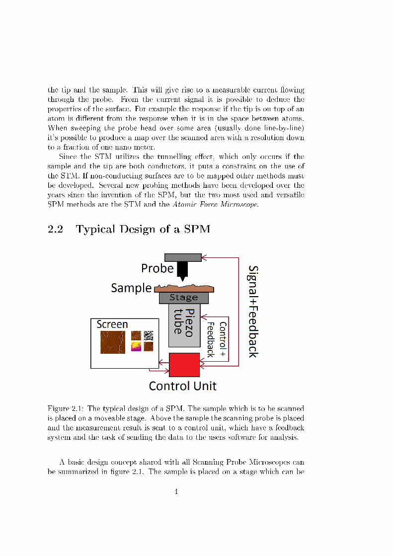
Figure 2.1: The typical design of a SPM. The sample which is to be scannedis placed on a moveable stage. Above the sample the scanning probe is placedand the measurement result is sent to a control unit, which have a feedbacksystem and the task of sending the data to the users software for analysis.
A basic design concept shared with all Scanning Probe Microscopes canbe summarized in gure 2.1. The sample is placed on a stage which can be
4

moved with piezoelectric actuators in the x-y plane. Some SPM systems havethe stage movable in the z-direction such that when engaging the sample itis the stage that is moved up and down. On top of the sample the scanningprobe is placed. In the STM the probe is a metallic tip and in the AFM itis a cantilever. The control unit runs feedback on the signal from the probesuch that some specic condition is fullled. In the case of the STM or AFMthe feedback is usually used to keep the probe at a xed height above thesurface, so the feedback signal will give the topography of the surface. Themovement of the tip and sample are controlled by piezoelectrics.
2.3 Atomic Force Microscope
The Atomic Force Microscope is also a member of the SPM family. Themeasurement procedure of AFM is to feel or touch the sample's surface witha very sharp tip located at the end of a small beam, known as a cantilever.When the cantilever is brought closer to the surface it will experience thesurface forces and bend towards or away from the surface. This bendingof the cantilever is measured and analysed and the information that can beobtained with an AFM is not only the topography of the sample, but alsothe surface mechanical properties, or any physical property which gives riseto a force on the cantilever. Also electric and magnetic properties can bemeasured if the material of the cantilever is chosen correctly. One of thebiggest advantages with the AFM is the resolution in the images - typicallya resolution 25 times better than the optical diraction limit when scanningin the x-y plane. The height resolution is even better; it can be as high as1000 times better than optical microscopes.
2.3.1 Measurement Modes
Static AFM
The two most prominent measurement methods (or modes) are the so calledstatic and dynamic AFM. In static AFM (or contact AFM), the cantilever ismoved towards the surface till the cantilever touches it. Then the cantileveris swept over the surface while constantly in contact with the sample. Afeedback loop is being run on the deection trying to keep it constant, so thatthe force between the surface and tip is kept constant. The sharp cantilevertip or the surface will in most cases become damaged during a static AFMscanning process, so the sensitivity is reduced. One big advantage with thestatic mode is that it's possible to measure not only the z-deection of thecantilever but also twisting forces and friction forces. On the other hand,
5
measuring more components of the tip-surface force require more parametersto be calibrated1 before it's possible make qualitative measurements. Oneadditional disadvantage is that soft cantilevers can snap to the surface, whichinhibits the measurement of strong attractive surface forces.
Dynamic AFM
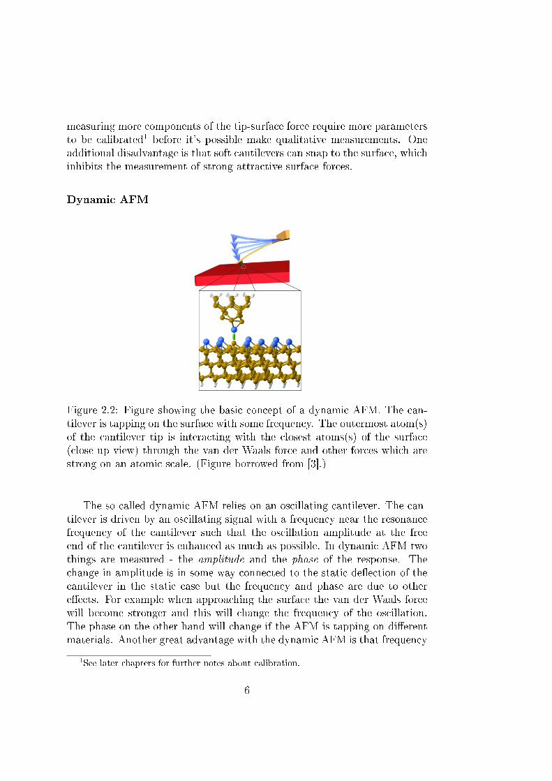
Figure 2.2: Figure showing the basic concept of a dynamic AFM. The can-tilever is tapping on the surface with some frequency. The outermost atom(s)of the cantilever tip is interacting with the closest atoms(s) of the surface(close up view) through the van der Waals force and other forces which arestrong on an atomic scale. (Figure borrowed from [3].)
The so called dynamic AFM relies on an oscillating cantilever. The can-tilever is driven by an oscillating signal with a frequency near the resonancefrequency of the cantilever such that the oscillation amplitude at the freeend of the cantilever is enhanced as much as possible. In dynamic AFM twothings are measured - the amplitude and the phase of the response. Thechange in amplitude is in some way connected to the static deection of thecantilever in the static case but the frequency and phase are due to othereects. For example when approaching the surface the van der Waals forcewill become stronger and this will change the frequency of the oscillation.The phase on the other hand will change if the AFM is tapping on dierentmaterials. Another great advantage with the dynamic AFM is that frequency
1See later chapters for further notes about calibration.
6

is one quantity in physics which can be measured to very high precision withtoday's measurement tools.
The feedback in dynamic AFM is run on either the frequency or the am-plitude. When the cantilever is engaging the surface the resonance frequencyof the cantilever will change. Due to this change the oscillation amplitude ofthe cantilever will change also, but feedback is used to keep the drive phaseshifted 90 degrees to the response phase. This feedback mode is called FM-AFM (frequency modulated AFM). It is also possible to keep the oscillatingamplitude constant by changing the drive amplitude from the piezo, whichthen is called AM-AFM (amplitude modulated AFM).
2.3.2 Intermodulation AFM
At KTH, a group at the department of applied physics (Nanostructure physics)have invented a new type of dynamic AFM. This new mode is called Inter-modulation Atomic Force Microscopy (ImAFM) [4]. Instead of driving thecantilever with one single frequency near its resonance, the cantilever is drivenwith two frequencies centred around the resonance peak. These two drivefrequencies and the nonlinear tip-surface force will give rise to so called in-termodulation, or frequency mixing. If the oscillating cantilever is non-linear,there will be a strong response at many dierent frequencies, not only atmultiples of the two drive tones, but also at integer linear combinations ofthe two drive tones.
In signal processing there is a common way of picking out signals atspecic frequencies is called lockin. Doing lockin measurement on all inter-modulation products of interest allows the response signal to be measuredwith a very high signal-to-noise ratio. This lockin procedure is built-in intothe ImAFM mode giving very pure signals at frequencies of interest.
Another advantage with Intermodulation AFM is that using this methodmakes it possible to reconstruct the force curve in every pixel scanned atthe same time as scanning the topography [5]. In other AFM modes thescanning of the topography and creating a force curve must be done withtwo dierent methods, and creating a force curve in every pixel is extremelytime consuming2.
2The standard way of creating force curves is to do a slow approach (ramping) at somepixel. Each approach takes approximately 0.1-10 s and a standard AFM-image is typically256× 256 pixels giving almost one week for each full force curve image.
7
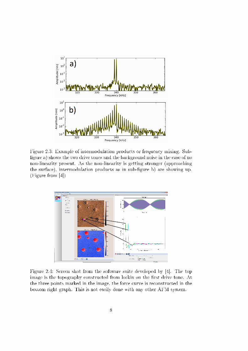
Figure 2.3: Example of intermodulation products or frequency mixing. Sub-gure a) shows the two drive tones and the background noise in the case of nonon-linearity present. As the non-linearity is getting stronger (approachingthe surface), intermodulation products as in sub-gure b) are showing up.(Figure from [4])
Figure 2.4: Screen shot from the software suite developed by [4]. The topimage is the topography constructed from lockin on the rst drive tone. Atthe three points marked in the image, the force curve is reconstructed in thebottom right graph. This is not easily done with any other AFM system.
8
Chapter 3
Theoretical Background
When working with the AFM we detect a voltage on a split-quadrant photodetector which will change depending on the motion of the cantilever. Beforewe can analyse this uctuating voltage signal we must develop tools andtheory to help us understand what is happening. This includes beam theoryfor describing the cantilever, hydrodynamics for the damping in a viscoussurrounding uid of the cantilever, optics used in the detection of the laserbeam and signal processing in the electronics, to mention a few.
3.1 Beam Theory
Consider the cantilever to be approximated by a homogeneous beam of lengthL, xed at one end (the base) and free at the other end where a sharp tip islocated. It is of interest to know the deection of the cantilever as it is possibleto relate this deection into force on the tip. If the behaviour of the force isunderstood, material properties can be deduced. The dynamic deection ofthe cantilever, w(x, t), is described by the Euler-Bernoulli equation, which isa forth order partial dierential equation in time and space and is in generalrather hard to solve analytically.
The Euler-Bernoulli equation reads
EI∂4w(x, t)
∂x4+ µ
∂2w(x, t)
∂t2= F (x, t), (3.1)
where E is the Youngs elastic modulus and I is the moment of inertia. Theproduct EI can be interpreted as the beams resistance to deformation. µ isthe mass per unit length of the beam and the right hand side, F (x, t), areall combined forces acting on the beam.
To get a rst feeling for the Euler-Bernoulli equation, the deection for asimple case is derived analytically. Consider a beam of length L xed at one
9

end, free at the other end, and without any external forces. In this case the
Figure 3.1: Cantilever modelled as a clamped beam. The deection at x = Lis marked as X(L) in the gure (rst mode shown).
force term is F (x, t) = 0 and the boundary conditions for X(x) are
X(x)|x=0 =∂X(x)
∂x
∣∣∣∣x=0
=∂2X(x)
∂x2
∣∣∣∣x=L
=∂3X(x))
∂x3
∣∣∣∣x=L
= 0. (3.2)
The solution can be found by separation of variables such that w(x, t) =X(x)T (t).This gives two dierential equations which both are equal to aconstant, ω2
n
EI
µ
1
X(x)
∂4X(x)
∂x4= − 1
T (t)
∂2T (t)
∂t2= ω2
n. (3.3)
The solution to the time equation is
Tn(t) = An cosωnt+Bn sinωnt (3.4)
but the space solution is a bit more complicated
Xn(x) = c1ea1x + c2e
a2x + c3ea3x + c4e
a4x, (3.5)
where
a1,2,3,4 = ±
√±√
ω2nµ
EI= ±
√±√α4n (3.6)
are the roots to the characteristic polynomial EIµX(IV ) = ω2
nX. Rewritingthis using Euler formula for exponents to convert to trigonometric functions
Xn(x) = d1 (cosαnx+ coshαnx) + (3.7)
d2 (cosαnx− coshαnx) +
d3 (sinαnx+ sinhαnx) +
d4 (sinαnx− sinhαnx) .
10

First boundary condition gives d1 = 0 and the second condition gives d3 = 0.What is left are
d2X
dx2
∣∣∣∣x=L
= d2α2n (− cosαnL− coshαnL) + (3.8)
d4α2n (− sinαnL− sinhαnL) = 0,
d3X
dx3
∣∣∣∣x=L
= d2α3n (sinαnL− sinhαnL) + (3.9)
d4α3n (− cosαnL− coshαnL) = 0.
Solving for d2 in (3.9) and replacing it in (3.8)
Eq. (3.9) ⇒ d2 = d4cosαnL+ coshαnL
sinαnL− sinhαnL. (3.10)
−d4cosαnL+ coshαnL
sinαnL− sinhαnL(cosαnL+ coshαnL) = d4(sinαnL+ sinhαnL)
⇔ coshαnL cosαnL = −1. (3.11)
The last equation (3.11) is very interesting since it will only have a solutionfor certain values of the product αnL ≡ λn. Solving coshλn cosλn = −1numerically gives the roots
λn ∈ (±1.8751,±4.6940,±7.8547,±10.9955, ...) , (3.12)
but since λn = αnL = L(
ω2nµEI
)1/4
is real, the negative roots must be rejected.
For the natural frequencies
ωn =1
L2
(EI
µ
)1/2
(3.5160, 22.0336, 61.6963, 120.9010, ...) (3.13)
which further implies that resonance frequencies are connected to the fun-damental resonance frequency ω0 as ω1 = 6.27ω0, ω2 = 17.55ω0 and ω3 =34.39ω0. The positive roots on the other hand are connected to the so callednatural frequencies and the eigenmodes of the beam, more about that later.
Now the deection function of the beam is known and it is
w(x, t) =∑n
Tn(t)Xn(x) =∑n
(An cosωnt+Bn sinωnt) · (3.14)((cosαnx− coshαnx)−
cosαnL+ coshαnL
sinαnL+ sinhαnL(sinαnx− sinhαnx)
),
11

with α4n ≡ ω2
nµEI
. If only consider the spatial part of the deection (the staticdeection) the bending of the beam takes the following shapes for the dier-ent values of λn found earlier and the rst four eigenmodes of the cantileverbeam without any external load. For most AFM systems typically the rstmode of the cantilever is used, but new techniques for higher exural modesare being developed [68].
Figure 3.2: Solutions to the Euler-Bernoulli equation for the four rst modes.The most important mode for AFM-cantilevers is the mode with n = 1.
3.2 The Real Cantilever
The beam theory approach given in section 3.1 is only an exact model if thecantilever is approximated by a "beam" extending in one direction only andwithout any external forces. This is of course not the case for a real cantilever,but the result obtained is a good approximation for the z-deection of mostcommercial cantilever if excited near its resonance. For a real beam, therealso exist other degrees of freedom, not only the z-deection. Since a realcantilever is a three dimensional object there are actually three deectiondegrees of freedom (contraction/extension along the length axis, deectionin the width direction and the z-deection). Adding these three degrees offreedom is not enough either, since there might be twisting of the cantileveras well (one extra degree) and one degree caused by adding a momentumat the free end giving an angular deection (not the same as a deection).Some AFM systems have tools to measure the torsional twisting, but thelongitudinal bending moment is often ignored in commercial AFM systemssince it cant be separated from the z-deection).
12
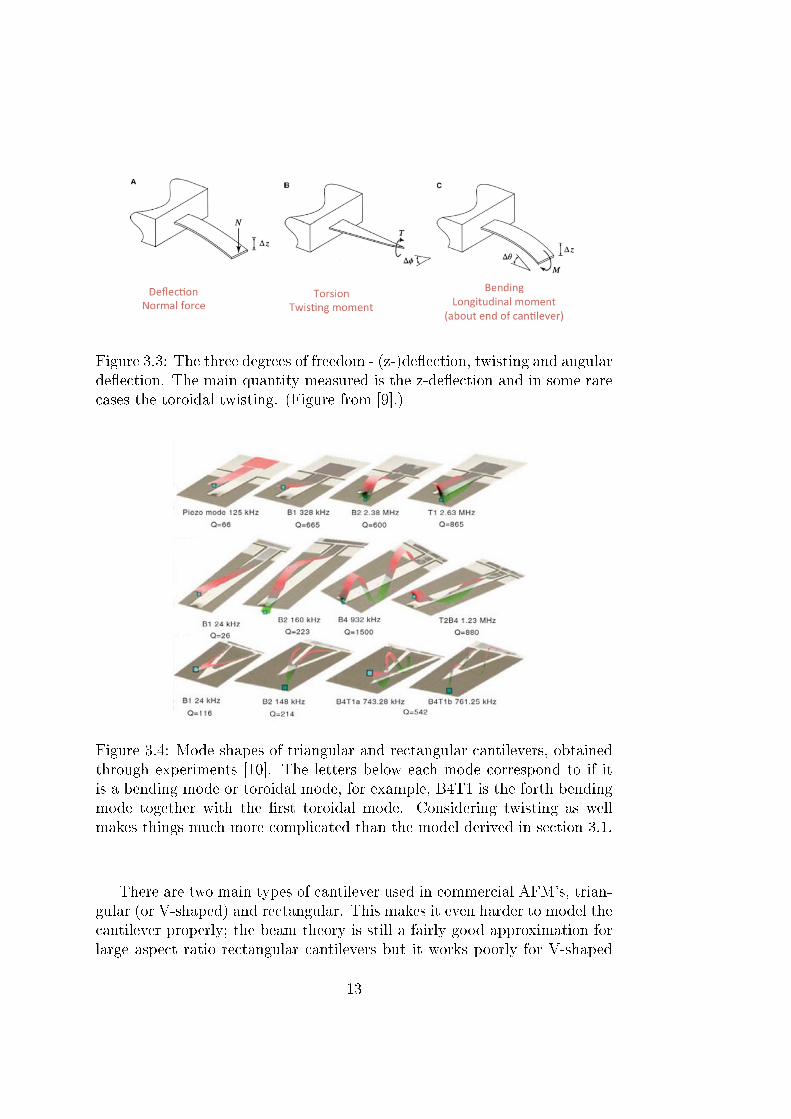
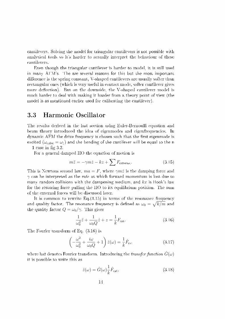
Figure 3.3: The three degrees of freedom - (z-)deection, twisting and angulardeection. The main quantity measured is the z-deection and in some rarecases the toroidal twisting. (Figure from [9].)
Figure 3.4: Mode shapes of triangular and rectangular cantilevers, obtainedthrough experiments [10]. The letters below each mode correspond to if itis a bending mode or toroidal mode, for example, B4T1 is the forth bendingmode together with the rst toroidal mode. Considering twisting as wellmakes things much more complicated than the model derived in section 3.1.
There are two main types of cantilever used in commercial AFM's, trian-gular (or V-shaped) and rectangular. This makes it even harder to model thecantilever properly; the beam theory is still a fairly good approximation forlarge aspect ratio rectangular cantilevers but it works poorly for V-shaped
13
cantilevers. Solving the model for triangular cantilevers is not possible withanalytical tools so it's harder to actually interpret the behaviour of thesecantilevers.
Even though the triangular cantilever is harder to model, it is still usedin many AFM's. The are several reasons for this but the most importantdierence is the spring constant, V-shaped cantilevers are usually softer thanrectangular ones (which is very useful in contact mode, softer cantilever givesmore deection). But on the downside, the V-shaped cantilever model ismuch harder to deal with making it harder from a theory point-of-view (themodel is as mentioned earlier used for calibrating the cantilever).
3.3 Harmonic Oscillator
The results derived in the last section using Euler-Bernoulli equation andbeam theory introduced the idea of eigenmodes and eigenfrequencies. Indynamic AFM the drive frequency is chosen such that the rst eigenmode isexcited (ωdrive = ω1) and the bending of the cantilever will be equal to the n= 1 case in g 3.2.
For a general damped HO the equation of motion is
mz = −γmz − kz +∑
Fexternal. (3.15)
This is Newtons second law, ma = F , where γmz is the damping force andγ can be interpreted as the rate at which forward momentum is lost due tomany random collisions with the dampening medium, and kx is Hook's lawfor the restoring force pulling the HO to its equilibrium position. The sumof the external forces will be discussed later.
It is common to rewrite Eq.(3.15) in terms of the resonance frequencyand quality factor. The resonance frequency is dened as ω0 =
√k/m and
the quality factor Q = ω0/γ. This gives
1
ω20
z +1
ω0Qz + z =
1
kFext. (3.16)
The Fourier transform of Eq. (3.16) is(−ω2
ω20
+iω
ω0Q+ 1
)z(ω) =
1
kFext (3.17)
where hat denotes Fourier transform. Introducing the transfer function G(ω)it is possible to write this as
z(ω) = G(ω)1
kFext, (3.18)
14

where
G(ω) =
(−ω2
ω20
+iω
ω0Q+ 1
)−1
. (3.19)
This equation relates the response of the system to an external force. Res-onance eects for example can be explained by studying the transfer functionof a system. In standard linear response theory k and G are put together
such that χ(ω) ≡ G(ω)k
, which is then referred to as the linear response func-
tion. One advantage with G is that it's dimensionless and the amplitude ofG is called transfer gain.
0.0 0.5 1.0 1.5 2.0 2.5Frequency ω/ω0
10-1
100
101
102
Tra
nsf
er
Funct
ion |G
(ω)| Q = 0.5
Q = 1.0
Q = 5.0
Q = 100.0
(a) Transfer Function
0.0 0.5 1.0 1.5 2.0 2.5Frequency ω/ω0
3.0
2.5
2.0
1.5
1.0
0.5
0.0Phase
G(ω
)
Q = 0.5
Q = 1.0
Q = 5.0
Q = 100.0
(b) Phase
Figure 3.5: The transfer function and phase plot for a damped harmonicoscillator.
It is worth spending some time on the transfer function in gure 3.5, sinceit has some useful properties worth mentioning. From the appearance of thedierent curves, it is evident that the system responds very dierently to thesame force applied at dierent frequencies. The blue curve for example hasits maximum at low frequencies, which means that force with low frequenciesis enhanced compared to higher frequencies which will be suppressed and canbe neglected compared to the amplied low frequencies. When increasing thequality factor of the system the system is turning into a so called band-passlter, only responding at frequencies within a narrow band near the resonanceof the system.
An other interesting property of the transfer function can be seen bystudying the eect of the quality factor. If the peak is very sharp (highquality factor) the system is much more sensitive than if the quality factoris lower. When driving a high-Q system near resonance a slight shift in thedrive frequency will give rise to a large amplitude increase/decrease due tothe very sharp peak compared to a low-Q resonator (which is not as sensitive
15

to shifts of the drive frequency, but in turn give lower amplication of everyfrequency). This is also true for the phase as seen in 3.5 (b). If the resonatorhas a high quality factor the phase will jump very quickly when close toresonance while if the quality factor is low the phase will change slowly.The sensitivity of high-Q resonators can therefore be used to detect verysmall changes in the resonance frequency for example. Cantilevers with highquality factors are therefore advantageous to use in dynamic AFM.
3.4 Detecting the Deection
When performing an AFM scan, the quantity being measured is a voltagedierence induced by the motion of the reected laser spot on a photo detec-tor as shown in gure 3.4. The photo detector is divided into four quadrantsand when a fraction of the laser spot hit one of the quadratures a voltage canbe measured on that photo detector. For simplicity, assume that two photo
Detector
MirrorLaser source
Piezo-shaker
CantileverSample
d
V
Figure 3.6: The laser reected on the back of the cantilever and guided intothe photo detector. As the cantilever moves (d in gure) the laser spot willmove a distance on the photo detector giving rise to a measurable voltage V.
detectors, one on the bottom and one on top of the other. Now assumethat the laser beam reects such that the total area of illumination is spreadevenly over the two detectors. This gives an equal voltage from each of thephoto detectors. If the cantilever is moved a little, the area of illuminationon each photo detector is changed, and this will give rise to a dierence in thetwo measured voltages. The voltage dierence is still in volts, but the actualdeection of the cantilever is in units of meters. Therefore a relation convert-ing volt to meter is needed. Assuming it is a linear relation between these
16
two quantities1 such that V = αd, where the constant of proportionality isall that's needed. The constant relating voltage from the photo detectors tothe actual deection of the cantilever is often called the inverse optical leversensitivity (or invOLS) [m/V ] and optical lever responsivity, since the laterconstant describes the response of the voltage to a change in deection.
Calibrating α is an important part of quantitative AFM. One calibrationmethod is derived by Higgins et al [12] and it uses the Equipartition Theorem(ET), a well known theorem from statistical mechanics. The main idea isthat in equilibrium each degree of freedom of the system gives an averageenergy contribution to the total energy of 1
2kBT . For example, a particle free
to move in three directions x, y and z have three degrees of freedom and thusthe average energy of 3
2kBT . It has been proven that this is true for each
gas molecule in noble gases for example. When limiting the motion of thecantilever to the single eigenmode model, discussed in previous section 3.3,there will only be one degree of freedom and the motion of the cantileveris well described. Applying the equipartition theorem we nd that thatthis energy must be equal to the energy stored in the cantilever (from thedeection from its equilibrium position).
Eequipartition = Espring (3.20)
1
2kBT = 1
2k⟨z⟩2
Next, the Power Spectral Density (PSD) (which is the DFT of the measureddata) for a harmonic oscillator is equal to
SVV(f) = Pwhite +PDCf
4R
(f 2 − f 2R)
2 +f2f2
R
Q2
, (3.21)
where Pwhite is the white noise background from the detector and the secondterm is the cantilever noise, with fR the resonance frequency and Q thequality factor. Neglecting the white noise term and integrating the PSD ofthe cantilever noise over all frequencies gives2
⟨V ⟩2 = π
2fRPDCQ. (3.22)
Using the relation between volt and meter gives
⟨z⟩2 = π
2
1
α2fRPDCQ. (3.23)
1This relation is only an approximation, but it works very well for relatively smalldeections (which is the case in most AFM applications). But if the deection get too large(very soft cantilevers and surfaces with high adhesion or very high driving amplitudes),this relation is not linear. See e.g. [11] for discussion about this non-linearity eect.
2The derivation of this is presented in the (see Appendix 10.1.2).
17

Plugging this back into equation (3.20) gives an expression for α
α =
√πkfRPDCQ
2kBT. (3.24)
This is the result we were looking for.
3.5 Hydrodynamic Formulation of the Viscous
Damping
3.5.1 Derivation
This section is a summary of the derivation done by J. E. Sader [1]. A exingbeam will reach its maximum deection amplitude, A, if the drive force isthe resonance frequency of the beam. The energy stored in the rst bendingmode of the beam is then
Estored =1
2kdA
2, (3.25)
with kd the mode stiness3. The quality factor of an oscillating system canbe dened as
Q = 2π
(Estored
Edissipated
)ω=ω0
, (3.26)
where Ediss is the dissipated energy for each oscillation cycle. Furthermore,the spring constant of a cantilever at any point is dened as
k(x) ≡ Q
2π
∂2Ediss
∂A(x)2. (3.27)
Using equations (3.25) - (3.27) it is possible to get an expression for thespring constant at the free end
k(L) =
(Q
2π
∂2Ediss
∂A(L)2
)ω=ω0
(3.28)
3The dierence between the dynamic spring constant (kd) and the static spring constant(ks) is that ks is related to the static bending of the cantilever if it is pressed on a surface(harder than the cantilever). In the static case a force and deection is related as F = ksdwhile in the dynamic case the relation is F = kdG
−1(ω)d for each eigenmode. The staticspring constant can then be calculated as kd =
∑knG
−1n (ω = 0). The contribution from
higher modes will be very weak, but they will still contribute slightly, such that ks . kd.Since everything is regarding dynamic AFM in this thesis, I will skip the index d suchthat kd → k.
18
where L is the length of the cantilever (assuming the free end is the onlyinteresting part of the cantilever, thus dropping the L for simplicity).
In this equation, Q is supposed to be known, but the second derivative∂2Ediss/∂A is not. Sader solved this with dimension analysis (the so calledBuckingham Π-rule), see [13] for derivation. The result is
1
2π
∂2Ediss
∂A2= ρL3
0ω20Ω(β), (3.29)
with
β ≡ ρL20ωR
µ. (3.30)
The Ω(β)-function is a dimensionless function depending on the dimension-less parameter β. Here ρ is the density of the surrounding uid, µ is theviscosity and L0 is a characteristic length scale of the ow around the beam.
In hydrodynamics, it is common to use the so called Reynolds number todescribe the eect of motion in uids due to their viscosity and density. TheReynold number is dened as
Re ≡ ρb2ωR
4µ, (3.31)
where b is the width of the cantilever. Rewriting equation (3.29) and (3.30)with the Reynold number
β = Re
(2L0
b
)2
, Λ(Re) ≡ L30
b2LΩ(β) (3.32)
and using this to re-express (3.29) and plugging it back into (3.27)
k = ρb2LΛ(Re)ω2RQ. (3.33)
The equation (3.33) is the nal expression and it relates the shape ofthe cantilever, its quality factor and its resonance frequency to the springconstant. Everything in this equation is known, except the hydrodynamicfunction Λ(Re) and nding this analytically is hard, if even possible forarbitrary shaped cantilevers. What Sader did to solve this problem wasto measure the spring constant by some accurate external method, in hiscase a thermal noise as measured by a laser vibrometer, see Appendix of[1]. Then he varied the Reynolds number by tuning the density of thesurrounding gas. Since he knows the Reynold number, he can determineΛ(Re) = kd/(ρb
2Lω2RQ). Sader found that the functional form of Λ is well
approximated by Λ(Re) = a0Rea1+a2 log10 Re, where the constants ai must be
19
found by some curve t algorithm. When the three constants (which areunique for each cantilever shape) are known, it is possible to use equation(3.33), with the tted form of Λ(Re), to calibrate the spring constant.
The non-invasive calibration algorithm derived in this section is powerfulin that it works for arbitrary shaped probes once you know the Λ(Re) forthat probe shape. This is great since more and more cantilever designs arebeing developed all the time, and this algorithm is supposed to work for allof these (more about how to actually implement this algorithm is presentedlater in this chapter).
3.5.2 Reference Measurement Formulation
The hydrodynamic function can be approximated with
Λ(Re) ≈ aRe−0.7 (3.34)
since according to table III in [1] a1 ≈ −0.7 in all measurements and a2 logReis negligible compared to 0.7, leaving only one unknown constant. Using thisobservation it is enough with one reference measurement of Q, k and ω0 tocalculate k as (Appendix 10.1.1 for derivation)
k ≈ k∗ Q
Q∗
(ω0
ω∗0
)2−a1
, a1 ≈ 0.7 [1], (3.35)
where (*) denotes measurement on reference cantilever. Noting that thereference values can be expressed as one constant A ≡ k∗/(Q∗(ω∗
0)1.3) giving
the slightly simpler formk ≈ AQω1.3
0 . (3.36)
The A-constant is possible to nd from the quality factor, resonance fre-quency and spring constant of one reference cantilever, where the spring con-stant must be determined by some external method. Therefore, if the userwants to use a cantilever for which a0, a1 and a2 have not been determined,this approximation should be good enough if one reference measurement hasbeen done.
3.6 Calibrating the Linear Response Function
In the AFM-community most people tend to talk about calibrating the springconstant of the cantilever when talking about calibration. This is a residuefrom the quasi-static AFM calibrations where the static spring constant isall that is required to convert from deection to force. The aim of nearly all
20
AFM measurements at some point is to reconstruct the tip-surface force asa function of separation between the tip and the surface.
In this thesis, the goal is to calibrate the entire response function (de-termining k, m and γ). What needs to be done is to calibrate the linearresponse to some applied force, according to linear response theory (givenin Eq. (3.18)), where the deection of the cantilever can be calculated byknowing the transfer function χ(ω), which means that the parameters inχ(ω) = 1
kG(ω, ω0, Q) have to be found.
When doing a measurement in the lab, the best way of representing thedata is in the frequency space, accessed through a discrete Fourier transformof the time data. This allows the user to get the power spectral density of theuctuation of the detector voltage SV V (ω). Assuming the harmonic oscillatormodel once again, the spectral density should be equal to Eq. (3.21), whichcan be rewritten in terms of the transfer function of the cantilever as
SVV(ω, (ω0, Q, k))︸ ︷︷ ︸measured (voltage) signal
= Scantilever, vv(ω, (ω0, Q, k))︸ ︷︷ ︸cantilever response in [V]
+ Soor, vv︸ ︷︷ ︸noise oor in [V]
, (3.37)
where SVV, Scantilever, vv and Soor, vv are in units of [V2/Hz]. Of course it'smore convenient to have the cantilever power spectrum in [m], since it isa deection, but keeping Soor, vv in volts because the noise oor is due tolimitations in the electronics. The responsivity α dened in a previous sectionconverts Scantilever,vv[V ] =
1α2Scantilever,zz[m]
SVV(ω;ω0, Q, k)︸ ︷︷ ︸measured signal [V]
=1
α2Scantilever, zz(ω;ω0, Q, k)︸ ︷︷ ︸
cantilever response in [m]
+ Soor, vv︸ ︷︷ ︸noise oor in [V]
. (3.38)
The cantilever's power spectrum can be written as (derivation in Appendix10.1.2)
Szz(ω;ω0, Q, k) =2kBT
πω0QkGG∗, (3.39)
with G = G(ω, ω0, Q) as in equation (3.19) and star is complex conjugate.Equation (3.38) is therefore equal to
SVV =1
α2
2kBT
πω0QkGG∗ + Soor, vv = PGG∗ + Soor, vv, (3.40)
with P = 2kBTα2πkω0Q
, where kB and T are known and the entire constant P can
be viewed as an amplitude (or strength) of the thermal noise. The aim nowis to nd the unknown parameters k, ω0, Q and α, but all of them cannotbe determined from one t since the y-axis is scaled in the wrong units. The
21
resonance frequency and quality factor though are independent of the y-axisscale so they can be found with numerical tting to the measured data andusing the hydrodynamic result derived in section 3.5, the spring constant canbe calculated. If k, Q and ω0 are known it is possible to solve for α in theexpression for P4.
α =
√πPkω0Q
2kBT. (3.41)
If the steps above are done properly, everything is known about the can-tilever and the detectors optical path. Linear response theory now gives theopportunity to to describe the response of the cantilever due to any appliedforce
z =1
kGF z = χF , (3.42)
or if the deection is known (which it is since it is being measured with thedetector) it should be possible to calculate the applied force. This is exactlywhat the goal is with nearly all AFM measurements, since the force is ofsuch importance because it tells so much about what is going on between thesurface and the tip.
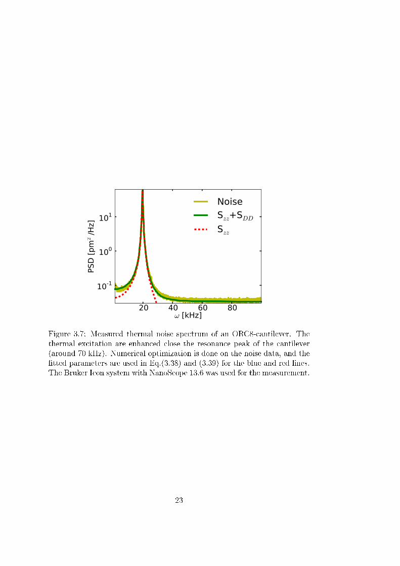
In gure 3.7 the power spectrum for a cantilever is shown. From thet, it is evident that the model presented in Eq. (3.38) is a very accurateapproximation for a thermally driven cantilever5.
4This is very similar to the result derived Higgins in 3.4, which is not surprising sinceit relies on the same physical arguments.
5If the peak is too weak (signal-to-noise ration too small), it is hard to t since thecantilever resonance peak is in the same order of magnitude as the noise. The peak shouldpreferably be more than one order of magnitude larger than the background noise oor.
22
20 40 60 80ω [kHz]
10-1
100
101
PSD
[pm
2/H
z]
Noise
Szz+SDDSzz
Figure 3.7: Measured thermal noise spectrum of an ORC8-cantilever. Thethermal excitation are enhanced close the resonance peak of the cantilever(around 70 kHz). Numerical optimization is done on the noise data, and thetted parameters are used in Eq.(3.38) and (3.39) for the blue and red lines.The Bruker Icon system with NanoScope 13.6 was used for the measurement.
23

24
Chapter 4
Results from the new Calibration
Algorithm
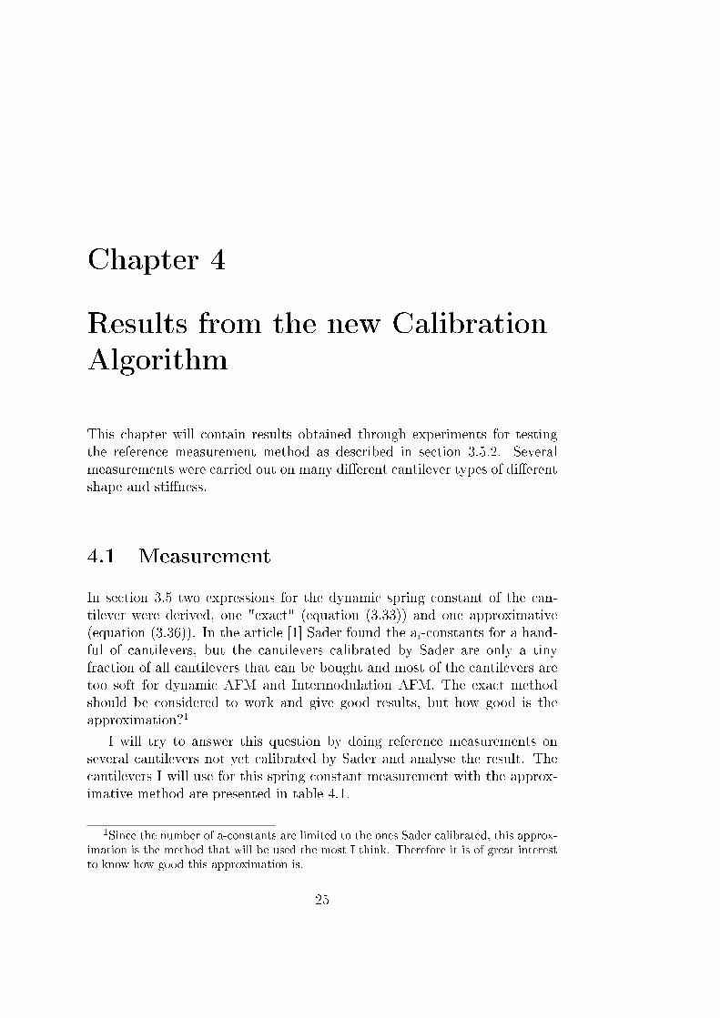
This chapter will contain results obtained through experiments for testingthe reference measurement method as described in section 3.5.2. Severalmeasurements were carried out on many dierent cantilever types of dierentshape and stiness.
4.1 Measurement
In section 3.5 two expressions for the dynamic spring constant of the can-tilever were derived, one "exact" (equation (3.33)) and one approximative(equation (3.36)). In the article [1] Sader found the ai-constants for a hand-ful of cantilevers, but the cantilevers calibrated by Sader are only a tinyfraction of all cantilevers that can be bought and most of the cantilevers aretoo soft for dynamic AFM and Intermodulation AFM. The exact methodshould be considered to work and give good results, but how good is theapproximation?1
I will try to answer this question by doing reference measurements onseveral cantilevers not yet calibrated by Sader and analyse the result. Thecantilevers I will use for this spring constant measurement with the approx-imative method are presented in table 4.1.
1Since the number of a-constants are limited to the ones Sader calibrated, this approx-imation is the method that will be used the most I think. Therefore it is of great interestto know how good this approximation is.
25

Cant. Manuf. ks [N/m] f0 [kHz] L [µm] b [µm]AC160TS Olympus 42 (12-103) 300 (200-400) 160 (150-170) 50 (48-52)DNPB Bruker 0.12 (0.06-0.24) 65 (16-28) 205 (200-210) 40 (35-45)ORC8C Bruker 0.38 (0.19-0.74) 68 (47-89) 100 (90-110) 20 (19-21)ORC8D Bruker 0.05 (0.02-0.1) 18 (12-24) 200 (180-220) 20 (19-21)SNLD Bruker 0.06 (0.03-0.12) 18 (12-24) 205 (200-210) 25 (20-30)TAP300 Bruker 40 (20-60) 300 (200-400) 125 (115-135) 35 (30-40)TAP525 Bruker 200 (100-400) 525 (375-675) 125 (115-135) 40 (35-45)
Table 4.1: The cantilevers used in this thesis. Nominal values for the springconstant, resonance frequency, length and width are taken from the Bruk-er/Olympus homepages. The values are written on the following format:Nominal (Min - Max).
4.2 Experimental Procedure
The reference calibration method proposed in section 3.5.2 relies on one refer-ence measurement by some external method of the spring constant, resonancefrequency and quality factor. As this other method I used the thermal tunebuilt into the NanoScope version 13.4, to extract calibrated noise data, andthen use numerics to obtain the values of k, ω0 and Q. The optical lever iscalibrated by doing a ramp on a hard sample. The sample I used in my exper-iments for the ramp was a at oxide sample (SiO2) surface. It is importantthat the sample is harder than the cantilever such that only the cantilever isbeing deformed in the ramp. All experiments were carried out in the Nano-Fabrication Lab located at Alba Nova, KTH (Stockholm). Each experimentwas done with an ambient temperature of 23-25C and with normal roompressure and humidity. The AFM system used for all experiments was theDimension Icon system from Bruker.
The procedure for measuring the reference values is presented below
1. Mount cantilever into the AFM and align laser and photo detector
2. Engage surface (SiO2) and start continuous ramping with a ramp size,trigger threshold and ramp speed (≈ 0.1 Hz was used in ramp speed)such that good ramps are obtained. Update optical lever responsivity
3. Disengage from surface and do thermal tune with updated responsivity
4. Export x-y data of the noise spectrum for t later
5. Change cantilever and start over again (four cantilevers for each can-tilever type was used).
26

The cantilevers ORC, SNL and DNP have four cantilevers mounted onthe same chip, so some care have to be taken when xing the laser on thecantilever such that the right cantilever is focused. I experienced problemswith aligning the laser on the DNP-cantilevers, not sure why. Therefore, thiscantilever will not be used since no good data was obtained for it. For eachcantilever the calibrated thermal noise power spectrum from the NanoScopesoftware was stored.
Using a Python script (presented in the Appendix) the parameters of thelinear response function (k, ω0 and Q) were found by optimizing the functionin (3.40) to the measured thermal noise power spectrum2. The parametersobtained through the t procedure is then used as reference values for thereference method as in section 3.5.2 to give a gure for the A-constant, where
A =k∗
Q∗(ω∗0)
1.3(4.1)
as before.The key point here is that if this approximation is valid, the A-constant
should be the same for each cantilever of the same type, and similar fordierent types of cantilevers if they share the same planar view. To checkthis, four cantilevers for each cantilever type was chosen.
4.3 Calibration Data - All Plots
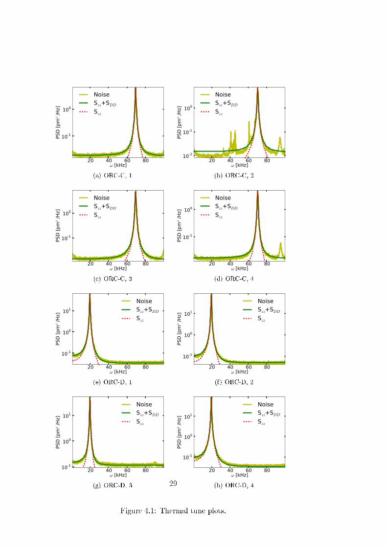
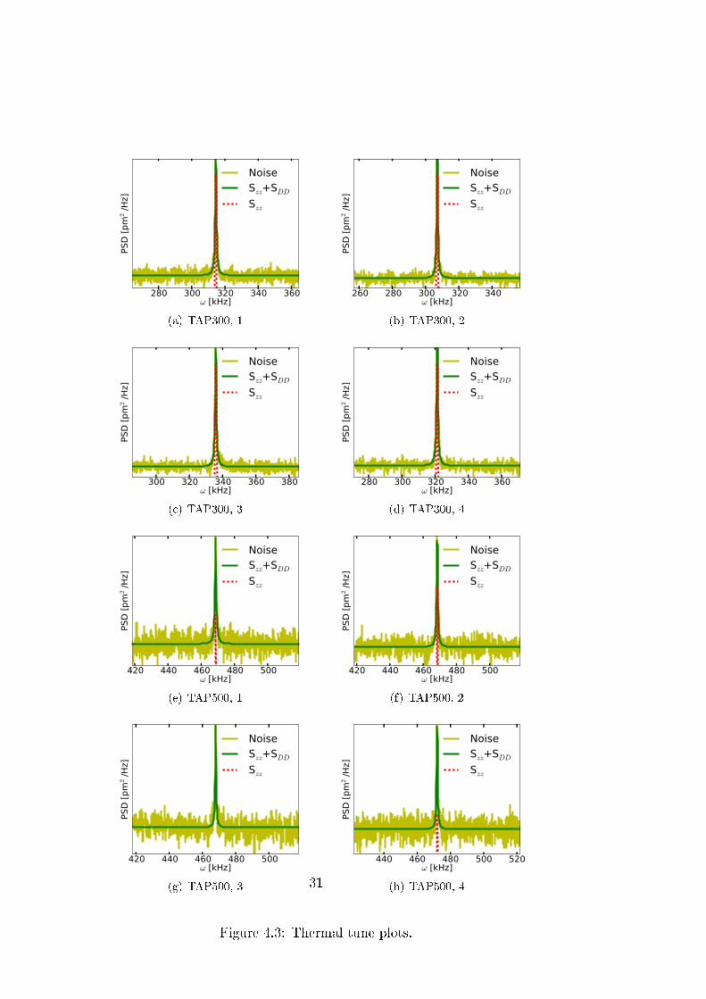
The following plots are the data obtained by the thermal tune-mode inBruker's Nanoscope software suite v 13.6. The optical lever responsivity,α was calibrated on a hard surface (SiO2). The yellow line is the measurednoisy data, the green line is the tted curve from equation (3.40) (detectornoise + cantilever) and the red dotted line is the cantilever power spectrumreconstructed (equation (3.39)) with the tted values.
The t is working very well for the soft cantilevers (Orc8-C, Orc8-D andSNL-D), but not so good for the stier cantilevers (AC160TS, TAP 300 andTAP 500). The second resonance peak for SNL-D, cantilever 2 (Fig. 4.2(d)) was excluded when doing the t the t. Fitted values for all graphs arepresented in table 4.2.
The real value for the dierent parameters measured and presented intable 4.2 or gure 4.4 are not known so it is not possible to compare this to
2Please note that it is possible to t all of ω0, Q, k and Sdd since the optical leverresponsivity is known (from the ramping)! This is not the case in a "real" measurement,but now when doing these reference measurements, α is actually known allowing the tdirectly.
27
the proper value of each parameter. Therefore the deviance presented in thetable and graph is calculated as
deviance =|max(mean− data)|
mean, (4.2)
which gives an estimate of spread in the data points. As discussed in previoussection, this deviance is allowed to be large for the measured values of k, Qand ω0 but it should still result in the same A-constant (small deviance inA).
According to the experimental procedure presented in Appendix 4.2, theNanoScope v13.6 was used to export thermal noise data for each cantilever.Using the script from Appendix 10.2, the data in table 4.2 was obtained.The values given in Tab. 4.2 are the ones used as "reference values" forthe reference calibration method described in section 3.5.2. The calculatedA-values are plotted in Fig. 4.4 and the maximum
28
20 40 60 80ω [kHz]
10-1
100
PSD
[pm
2/H
z]
Noise
Szz+SDDSzz
(a) ORC-C, 1
20 40 60 80ω [kHz]
10-2
10-1
100
PSD
[pm
2/H
z]
Noise
Szz+SDDSzz
(b) ORC-C, 2
20 40 60 80ω [kHz]
10-1
100
PSD
[pm
2/H
z]
Noise
Szz+SDDSzz
(c) ORC-C, 3
20 40 60 80ω [kHz]
10-1
100
PSD
[pm
2/H
z]
Noise
Szz+SDDSzz
(d) ORC-C, 4
20 40 60 80ω [kHz]
10-1
100
101
PSD
[pm
2/H
z]
Noise
Szz+SDDSzz
(e) ORC-D, 1
20 40 60 80ω [kHz]
10-1
100
101
PSD
[pm
2/H
z]
Noise
Szz+SDDSzz
(f) ORC-D, 2
20 40 60 80ω [kHz]
10-1
100
101
PSD
[pm
2/H
z]
Noise
Szz+SDDSzz
(g) ORC-D, 3
20 40 60 80ω [kHz]
10-1
100
101
PSD
[pm
2/H
z]
Noise
Szz+SDDSzz
(h) ORC-D, 4
Figure 4.1: Thermal tune plots.
29

20 40 60 80ω [kHz]
10-1
100
101
PSD
[pm
2/H
z]
Noise
Szz+SDDSzz
(a) SNL-D, 1
20 40 60 80ω [kHz]
10-1
100
101
102
PSD
[pm
2/H
z]
Noise
Szz+SDDSzz
(b) SNL-D, 2
20 40 60 80ω [kHz]
10-1
100
101
PSD
[pm
2/H
z]
Noise
Szz+SDDSzz
(c) SNL-D, 3
20 40 60 80ω [kHz]
10-1
100
101
PSD
[pm
2/H
z]
Noise
Szz+SDDSzz
(d) SNL-D, 4
200 220 240 260 280ω [kHz]
105
PSD
[pm
2/H
z]
Noise
Szz+SDDSzz
(e) AC160TS, 1
280 300 320 340 360ω [kHz]
PSD
[pm
2/H
z]
Noise
Szz+SDDSzz
(f) AC160TS, 2
200 220 240 260 280ω [kHz]
105
PSD
[pm
2/H
z]
Noise
Szz+SDDSzz
(g) AC160TS, 3
240 260 280 300 320ω [kHz]
105
PSD
[pm
2/H
z]
Noise
Szz+SDDSzz
(h) AC160TS, 4
Figure 4.2: Thermal tune plots. Note that second peak is not included inthe t for SNL-D,2 in subgure (b).
30
280 300 320 340 360ω [kHz]
PSD
[pm
2/H
z]
Noise
Szz+SDDSzz
(a) TAP300, 1
260 280 300 320 340ω [kHz]
PSD
[pm
2/H
z]
Noise
Szz+SDDSzz
(b) TAP300, 2
300 320 340 360 380ω [kHz]
PSD
[pm
2/H
z]
Noise
Szz+SDDSzz
(c) TAP300, 3
280 300 320 340 360ω [kHz]
PSD
[pm
2/H
z]
Noise
Szz+SDDSzz
(d) TAP300, 4
420 440 460 480 500ω [kHz]
PSD
[pm
2/H
z]
Noise
Szz+SDDSzz
(e) TAP500, 1
420 440 460 480 500ω [kHz]
PSD
[pm
2/H
z]
Noise
Szz+SDDSzz
(f) TAP500, 2
420 440 460 480 500ω [kHz]
PSD
[pm
2/H
z]
Noise
Szz+SDDSzz
(g) TAP500, 3
440 460 480 500 520ω [kHz]
PSD
[pm
2/H
z]
Noise
Szz+SDDSzz
(h) TAP500, 4
Figure 4.3: Thermal tune plots.
31

Cantilever kt [ N/m ] ω0−t [ Hz ] Qt [ - ] A [N/(m·Hz1.3)]AC160TS 1 19.9 2.36e5 3.21e2 6.42e-9AC160TS 2 73.4 3.21e5 3.81e2 1.34e-8AC160TS 3 32.8 2.49e5 3.82e2 8.28e-9AC160TS 4 45.6 2.80e5 3.94e2 9.57e-9
Mean 42.9 2.72e5 3.70e2 9.41e-9Dev. % 71.1 18.2 13.0 42.1
ORC-C 1 0.507 6.93e4 83.3 3.09e-9ORC-C 2 0.453 7.00e4 83.3 2.73e-9ORC-C 3 0.406 6.94e4 82.3 2.51e-9ORC-C 4 0.644 7.00e4 82.7 3.91e-9Mean 0.502 6.97e4 82.9 3.06e-9Dev. % 28.1 0.533 0.700 27.7
ORC-D 1 8.33e-2 1.96e4 36.3 6.04e-9ORC-D 2 6.53e-2 1.97e4 36.6 4.67e-9ORC-D 3 0.102 1.97e4 36.3 7.32e-9ORC-D 4 5.75e-2 1.97e4 36.4 4.13e-9Mean 7.69e-2 1.97e4 36.4 5.54e-9Dev. % 32.2 0.213 0.549 32.1
SNL-D 1 8.91e-2 1.89e4 30.3 8.13e-9SNL-D 2 3.59e-2 1.12e4 19.1 1.03e-8SNL-D 3 7.89e-2 1.78e4 29.0 8.13e-9SNL-D 4 8.39e-2 1.79e4 30.1 8.27e-9Mean 7.20e-2 1.64e4 27.1 8.71e-9Dev. % 50.1 32.0 29.7 18.3
TAP300 1 61.5 3.15e5 5.19e2 8.44e-9TAP300 2 58.6 3.07e5 5.25e2 8.22e-9TAP300 3 73.8 3.36e5 5.49e2 8.80e-9TAP300 4 68.4 3.34e5 5.51e2 8.19e-9Mean 65.6 3.23e5 5.36e2 8.41e-9Dev.% 12.6 4.97 3.12 4.55
TAP500 1 1.54e2 4.69e5 5.91e2 1.10e-8TAP500 2 1.64e2 4.69e5 6.92e2 1.00e-8TAP500 3 1.83e2 4.68e5 7.33e2 1.06e-8TAP500 4 1.94e2 4.72e5 7.68e2 1.06e-8Mean 1.74e2 4.69e5 6.96e2 1.06e-08Dev. % 11.9 62.1 15.1 5.18
Table 4.2: Fitted values for dierent cantilevers. Could not get a good signalfor the DNP-cantilever, so it is not tted. For each cantilever the A-constant(as in Eq. (3.36)) is calculated. The deviation is the maximum deviationfrom the mean. 32

ORC-D SNL-D ORC-CAC160TS TAP300 TAP500
0.2
0.4
0.6
0.8
1.0
1.2
1.4
A-v
alu
es
1e 8
32%
18%
28%42%
5%5%
Data
Mean
Figure 4.4: Measured A-values for each cantilever. The per cent number foreach cantilever is the maximum deviation from the mean value.
ORC-D SNL-D ORC-CAC160TS TAP300 TAP500
0
5
10
15
20
25
30
35
40
45
%
32.1
18.3
27.7
42.1
4.6 5.2
Figure 4.5: Deviance from mean for each cantilever.
33

4.4 Analysis and Discussion
Table 4.2 shows the calculated A-constant of dierent cantilevers of the sametype and for dierent types. If the simplication made in section 3.5.2 is avalid simplication, the A-constant should be the same for any cantilever ofa specic type (it should not matter what cantilever from the box we use asthe reference cantilever). But why does the calculated A-constant vary muchfor the soft cantilevers, but not for the stier? The approximations donewhen getting from the full Sader-model as in section 3.5 to the referencemethod in section 3.5.2 is a simplication based on the values presented inTab. III [1], where the log-term in the exponent is supposed to vanish andthe a1 constant can be approximated to -0.7. But if we check Tab. III thea1 actually varies between -0.67 to -0.76. If the a1-constant is way o -0.7the approximation made in the simplication is of course awed, but thisis hard to check for an arbitrary cantilever, unless all three a-constants areknown (but why would we then use the reference method for that cantilever?).So the biggest source of the error for the result is probably due to an over-simplication; the approximations made in the reference method are not validfor every cantilever type. How to actually check if the reference method isvalid for a specic cantilever is probably very hard unless we know the fullΛ-expression.
According to the previous section where the reference method is derivedand motivated the calibrated spring constant is directly proportional to theA-constant, and assuming high enough accuracy in the measurement of ω0
and Q on the cantilever that needs to be calibrated (not the reference valuesused to calculate A) the only uncertainty is in the calculated A. Apparentlyfrom the table, this deviation is very large (around 30 %) for the soft can-tilevers and the AC160TS while it is smaller (around 5%) for the TAP300 andTAP525. This would result in the same error in the calibrated spring con-stant, which of course, is bad. On the other hand, the cantilevers that are ofgreatest interest for the Intermodulation AFM are the sti cantilevers (withk & 40 N/m), especially the TAP300-cantilever and for these cantilevers themethod seems to works well.
The tted curves in section 4.3, the tting algorithm is working very wellfor all measurements (note that the PSD for ORC-C, 2 is very noisy, but thet still gives a good t but slightly overestimates the detector noise). Thisimplies that the model used for the noise power spectrum is a good model.The tted k, Q and ω0 for the soft cantilevers tend to deviate much morebetween each other than the hard cantilevers do. My guess to this is thatwhen making the cantilever, the length and width can be controlled to fairlyhigh precision (or at least the uncertainty is way less than the length scales
34
involved, typical value 120 µm±5µm) while the thickness of the cantileveris only a few microns (down to a fraction of microns) with an uncertaintyin the same order. The thickness of the cantilever aect several things,such as the stiness, quality factor and resonance frequency. This will aectthe softest cantilevers the most, since the softest cantilevers tend to be thethinnest. Also, even if the hard cantilevers dier, the characteristic constantsof interest are much higher and the a slight change in the spring constant forexample will not aect the result as much. Please note that if the referencemethod is working as it should, the deviation in the three tted parametersk, ω0 and Q should not aect the A-constant. For example, assume that thecantilever is slightly more stier on one of the reference cantilevers used, thenthis should be compensated by a slightly higher quality factor for examplewhich in the ideal case should give the same A-constant.
Then doing the calibration of the optical lever α, there is a risk of in-troducing errors in the spring constant (of the reference cantilever). Whencalibrating α it is important that the tail of the approach curve from whichit is calculated is good enough. With good I mean that it is as linear aspossible and is covering enough data points to give an accurate answer. Theshape of the approach curve is sensitive to the stiness of the cantilever - astier cantilever will require a larger force pushing on the surface to get anice approach curve, while the soft cantilevers does not require as large force.This increase in force also requires that the surface is sti enough such that itis not deformed when pressing on the surface with the cantilever. Even toughthe surface can be considered sti, there will probably be artefacts from thiscalibration between soft and sti cantilevers since the stiest cantilever usedin my experiments was 2000 times as sti as the softest.
Other sources of errors are numerical uncertainty from the tting algo-rithm. If the data is smooth and the peak is several orders of magnitudelarger than the background noise as in the Fig. 3.7 the tted values shouldbe very accurate, and vice versa. Therefore, it is preferred to get a spectraas clean as possible for the t, but noise can enter from so many dierentplaces. Since the noise spectra is obtained from the thermal excitation only,very weak perturbations might give rise to spurious spikes if they are closeto the cantilever resonance frequency, such as electronic leakage, backgroundacoustic noise or vibrations from other equipments present in the room suchat the ventilation. Even though all of these sources was tried to be minimizedas much as possible, there is always limits for how much noise that actuallycan be ltered out.
The piezo shaker and cantilever holder also adds an error source. As alloscillating components, there is a risk of self oscillations and eigen frequencieswithin the material itself. This also apply to the piezo crystal. In most cases
35

such perturbations are ltered out by the large quality factor of the cantileveritself, but if the piezo resonance frequency happen to be close to the resonancefrequency of the cantilever it will be enhanced, ruining that measurement.When mounting the cantilever into the cantilever holder there is always therisk of snapping pieces of silicon o the chip with the tweezers. Such piecesmight end up between the cantilever chip and the holder, distorting theshaking giving false spikes or they might get stuck at the cantilever itself.If they are stuck on the cantilever the eective mass of the cantilever willchange which changes the resonance frequency for example since ω2
0 = k/m. Ifeared that this might be the case with the large uncertainty in the AC160TScantilever. The sticky surface in the box to which the cantilevers are glued towas very sticky in this box compared to the other boxes. This extra stickinessrequired larger force when pulling it out of the box, hence making the brittlesilicon crack more than for the other cantilevers and therefore enlarging therisk of silicon pieces getting stuck on the cantilever.
A quick summary:
• If the reference calibration is a valid simplication the measurement ofthe A-constants for one cantilever type should be the same, since theA-constant essentially takes the planar geometry into account (and itdoes not vary between cantilevers from the same box of course)
• Measurements showed that the reference calibration worked well forthe TAP300 and TAP525 cantilevers
• Main error source for why it does not worked for the other cantilevers:probably oversimplied model
Edit:After the presentation we3 had a discussion about the large deviation
found for the AC160TS cantilever. According to Prof. Sader the referencemethod should work very well so we started some detective work to try to ndthe error source. We concluded that the most probable source of error wasthe large deviance in the spring constant and we also noted that the qualityfactor was surprisingly small (compared to what it should be, around 500).So we started to investigate the data in more detail around the peak and wesaw that the data points are grouped in a strange way, see gure 4.6. If amoving average is applied to the data, such behaviour is what you would ex-pect so we fear that the Bruker system have this feature which modies theraw data. Doing such averaging will smooth the data, making sharp peaks
3Per-Anders Thorén, Prof. David Haviland (KTH), Prof. John Sader (University ofMelbourne), Ph.D Daniel Forchheimer, Ph. D Daniel Platz.
36
less sharp. But these sharp peaks are exactly what we are interested in! Ifthe (very sharp) resonance peak for the sti cantilevers are smoothed, thequality factor will drop rapidly and also the calculated value for k will be wayo the proper value.
Also, in the Bruker system you could only choose between two frequencylimits when doing the thermal noise data acquisition, either 1 Hz-100 kHzor 1 Hz-2 MHz. I do not know if the number of data points used for the 2MHz data acquisition is increased compared to the 100 kHz range, but myguess is that the frequency resolution is decreased for the larger range. Weare essentially interested in a similarly large zone around the peak in bothcases (say ±50 kHz around the peak value), so if the frequency resolution isway less in the 2 MHz case, there will be less number of points to use inthe t. Together with the smearing of the data, we deduced that the two mostprobable error sources, at least for the sti cantilevers are this smearing eectand the reduced number of data points.
37

322 323 324 325 326ω [kHz]
PSD
[pm
2/H
z]
Noise
Szz+SDDSzz
(a) AC160TS 2
321.0 321.5 322.0ω [kHz]
105
PSD
[pm
2/H
z]
Noise
Szz+SDDSzz
(b) AC160TS 2
318 320 322 324 326ω [kHz]
PSD
[pm
2/H
z]
Noise
Szz+SDDSzz
(c) AC160TS 2
232 234 236 238 240ω [kHz]
105
PSD
[pm
2/H
z]
Noise
Szz+SDDSzz
(d) AC160TS 1
Figure 4.6: Zoomed features of the AC160TS cantilever. Measured datapoints are grouped. Normal white noise is not supposed to be like that.Note also the periodic behaviour found in Fig. 4.6(a).
38

Chapter 5
Analysis of Calibration Error for
ImAFM
In the previous section I calculated the A-constant of the reference methodproposed in section (3.5.2). The reference method relies on that the planarview of each cantilever type can be described by one single constant (the A-constant), and this implies that each cantilever type should have the same A-constant. It turned out that the A-constant actually varied between dierentmeasurements. Therefore, this section will contain an error analysis regardingerror propagation in one of the most common force models used in the AFMcommunity - the vdW-DMT model (presented in section 5.1.2). The erroranalysis will be based on simulated data and using an Intermodulation AFMreconstruction algorithm [14].
5.1 The Tip-Surface Force
The interactions with the surface can be probed by several methods, one ofthese is to study the force in the interaction between the probe tip and thesurface of your sample. The standard way of investigating the force is a slowquasi-static1 approach towards the surface while measuring the deection ofthe cantilever. Such a measurement gives the so called approach curve whichcan be transformed to get the force in the interaction by using Hook's lawfor an extended spring. If we want to interpret the result and extract surfaceproperties, the data needs to be tted to some model which relates the forceto the parameters of interest. One very common model is the so called vander Waals-DMT model presented below.
1Slow enough such that any oscillations on the cantilever dies out within each newmovement.
39

5.1.1 Reconstruct the Force in the Quasi-Static Case
Figure 5.1: A so called approach curve (or sometimes called force curve) fora quasi-static approach towards a surface. Hysteresis can be seen betweenthe approach path and retract path.
When doing an slow (quasi-static) approach and measure both the baseposition and the deection of the cantilever we can plot a graph like Fig. 5.1.There is a dierence between the approach curve of the cantilever and theretract curve. The reason for this is that when approaching, the cantileverwill at some point snap to the surface due to the attractive van der Waalsforces. When pulling the cantilever away from the surface, the cantilever isin contact with the surface much longer. This might be due to other forces,including the van der Waals force again, but also adhesive forces from thesurface. Depending on the stiness of the cantilever the distance at whichthe cantilever snaps to the surface and the force required to pull it o thesurface is changed.
It is more interesting to investigate the force as a function of tip distanceto the surface. Doing an axis transformation and use Hook's law for a spring2
it is possible to plot the force as a function of deection. The force versusdeection curve for Fig. 5.1 is shown in gure 5.2. If material propertiesare of interest one can t some model to this data set. Since in the quasi-static case, the cantilever and surface is supposed to be in equilibrium at alltimes, there must be a force balance between all forces acting in this frame ofreference. This makes it possible to propose FHook = Fmodel, and dependingon the model dierent parameters might be found.
2Such that F (d) = ksd, where ks is the static spring constant of the cantilever andz = h − d if h is the cantilever base height above the surface and z is the cantilever tipheight over the surface.
40

Figure 5.2: Transforming gure 5.1 into a force versus deection plot willgive this plot. Note that the jump in Fig. 5.1 give rise to undetermined areain this plot.
5.1.2 van der Waals - Derjaguin-Muller-Toporov Model
Consider the cantilever tip engaging the surface and maybe indenting it. If weassume that the indentation is slow, such that each step closer to the surfacetaken by the cantilever is followed by enough time for the cantilever and thesurface to reach equilibrium, we must have a balance between the force fromthe cantilever pressing on the surface and the force from the surface tryingto push the cantilever away, such that FHook = Fsurface. We will use ContactMechanics for describing the surface interaction.
Contact mechanics describes the eect of something indenting somethingelse. There are several elementary cases in contact mechanics, for examplean hard sphere indenting an elastic surface, two spheres indenting each otheror a rigid cone indenting a surface. In the case of the cantilever it's commonto describe the tip of the cantilever tip as a sphere with a certain radius ofperhaps a few nano meters indenting the surface of interest. Depending onhow hard the cantilever tip is compared to the surface we expect the defor-mation of the tip to be dierent from one set of parameters compared to another. For the typical cantilever the so called van der Waals - Derjaguin-Muller-Toporov (VdW-DMT) model is a good approximation since the DMTmodel describes both the actual deformation of the cantilever tip and pos-sible adhesion between the surface and the tip while the VdW part modelsthe electrical attractive/repulsive force between the outermost atom of thecantilever and the atoms close to the indention spot of the sample.
The VdW-DMT model can be divided into two regimes with slightlydierent appearance of the force, one when we are away from the surface and
41
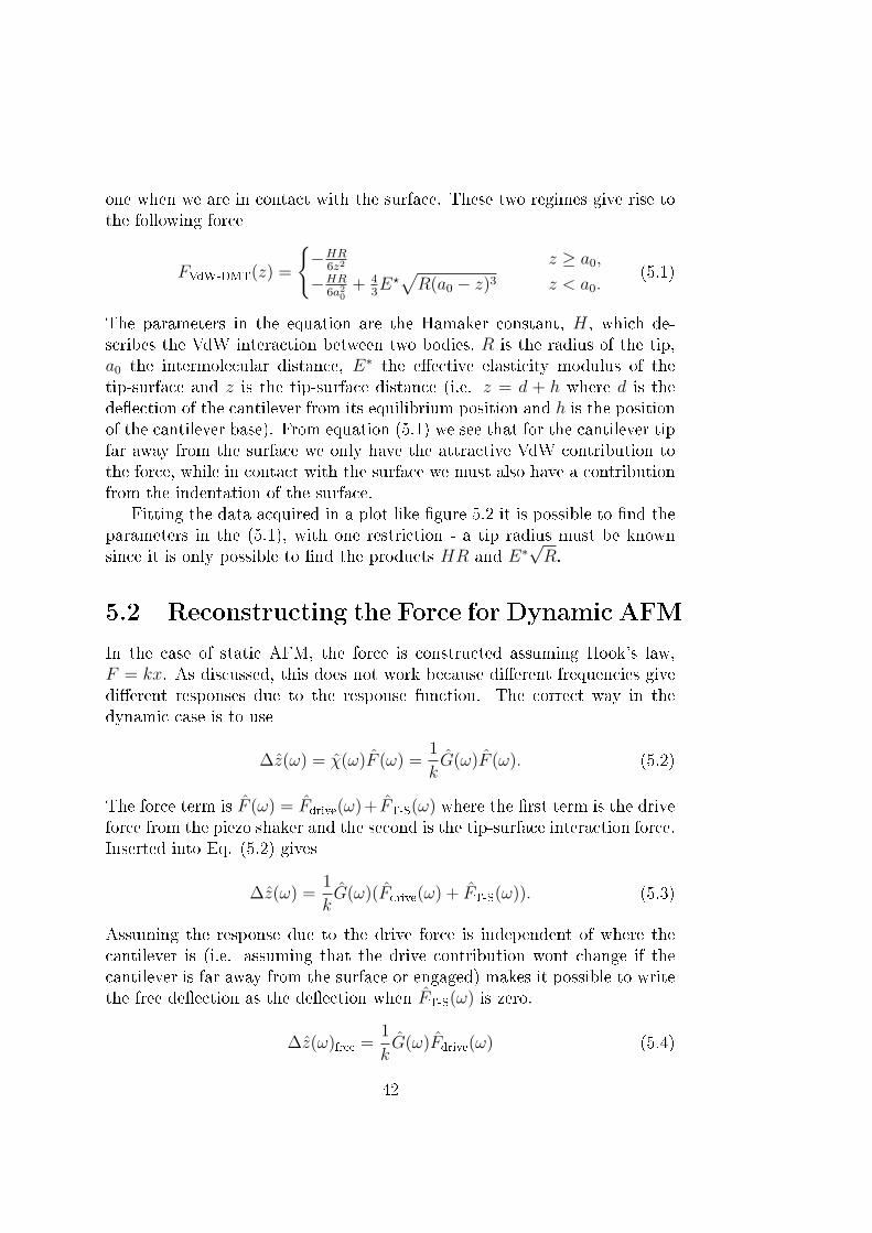
one when we are in contact with the surface. These two regimes give rise tothe following force
FVdW-DMT(z) =
−HR
6z2z ≥ a0,
−HR6a20
+ 43E⋆
√R(a0 − z)3 z < a0.
(5.1)
The parameters in the equation are the Hamaker constant, H, which de-scribes the VdW interaction between two bodies, R is the radius of the tip,a0 the intermolecular distance, E∗ the eective elasticity modulus of thetip-surface and z is the tip-surface distance (i.e. z = d + h where d is thedeection of the cantilever from its equilibrium position and h is the positionof the cantilever base). From equation (5.1) we see that for the cantilever tipfar away from the surface we only have the attractive VdW contribution tothe force, while in contact with the surface we must also have a contributionfrom the indentation of the surface.
Fitting the data acquired in a plot like gure 5.2 it is possible to nd theparameters in the (5.1), with one restriction - a tip radius must be knownsince it is only possible to nd the products HR and E∗
√R.
5.2 Reconstructing the Force for Dynamic AFM
In the case of static AFM, the force is constructed assuming Hook's law,F = kx. As discussed, this does not work because dierent frequencies givedierent responses due to the response function. The correct way in thedynamic case is to use
∆z(ω) = χ(ω)F (ω) =1
kG(ω)F (ω). (5.2)
The force term is F (ω) = Fdrive(ω)+ FT-S(ω) where the rst term is the driveforce from the piezo shaker and the second is the tip-surface interaction force.Inserted into Eq. (5.2) gives
∆z(ω) =1
kG(ω)(Fdrive(ω) + FT-S(ω)). (5.3)
Assuming the response due to the drive force is independent of where thecantilever is (i.e. assuming that the drive contribution wont change if thecantilever is far away from the surface or engaged) makes it possible to writethe free deection as the deection when FT-S(ω) is zero.
∆z(ω)free =1
kG(ω)Fdrive(ω) (5.4)
42
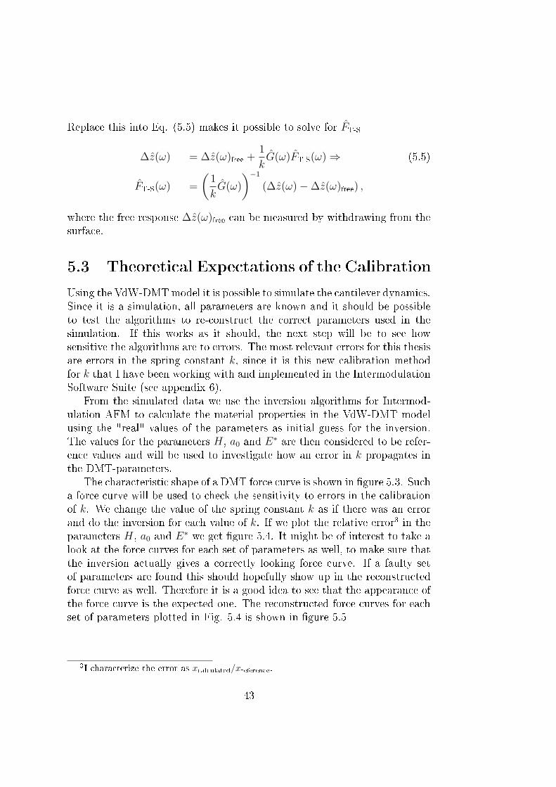
Replace this into Eq. (5.5) makes it possible to solve for FT-S
∆z(ω) = ∆z(ω)free +1
kG(ω)FT-S(ω) ⇒ (5.5)
FT-S(ω) =
(1
kG(ω)
)−1
(∆z(ω)−∆z(ω)free) ,
where the free response ∆z(ω)free can be measured by withdrawing from thesurface.
5.3 Theoretical Expectations of the Calibration
Using the VdW-DMTmodel it is possible to simulate the cantilever dynamics.Since it is a simulation, all parameters are known and it should be possibleto test the algorithms to re-construct the correct parameters used in thesimulation. If this works as it should, the next step will be to see howsensitive the algorithms are to errors. The most relevant errors for this thesisare errors in the spring constant k, since it is this new calibration methodfor k that I have been working with and implemented in the IntermodulationSoftware Suite (see appendix 6).
From the simulated data we use the inversion algorithms for Intermod-ulation AFM to calculate the material properties in the VdW-DMT modelusing the "real" values of the parameters as initial guess for the inversion.The values for the parameters H, a0 and E∗ are then considered to be refer-ence values and will be used to investigate how an error in k propagates inthe DMT-parameters.
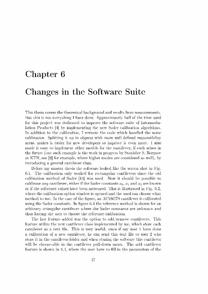
The characteristic shape of a DMT force curve is shown in gure 5.3. Sucha force curve will be used to check the sensitivity to errors in the calibrationof k. We change the value of the spring constant k as if there was an errorand do the inversion for each value of k. If we plot the relative error3 in theparameters H, a0 and E∗ we get gure 5.4. It might be of interest to take alook at the force curves for each set of parameters as well, to make sure thatthe inversion actually gives a correctly looking force curve. If a faulty setof parameters are found this should hopefully show up in the reconstructedforce curve as well. Therefore it is a good idea to see that the appearance ofthe force curve is the expected one. The reconstructed force curves for eachset of parameters plotted in Fig. 5.4 is shown in gure 5.5
3I characterize the error as xcalculated/xreference.
43
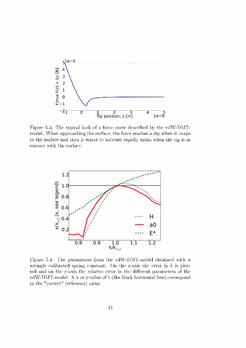
Figure 5.3: The typical look of a force curve described by the vdW-DMT-model. When approaching the surface, the force reaches a dip when it snapsto the surface and then it starts to increase rapidly again when the tip is incontact with the surface.
0.8 0.9 1.0 1.1 1.2k/kref
0.2
0.4
0.6
0.8
1.0
1.2
x/xref
(x, se
e legend)
H
a0
E*
Figure 5.4: The parameters from the vdW-DMT-model obtained with awrongly calibrated spring constant. On the x-axis the error in k is plot-ted and on the y-axis the relative error in the dierent parameters of thevdW-DMT-model. A x or y-value of 1 (the black horizontal line) correspondto the "correct" (reference) value.
44

Figure 5.5: The reconstructed force curves for each triplet of dots in gure5.4. The red curve is the reconstructed reference. It is evident from the gurethat the reconstruction did something wrong with the ve curves from theleft, since these ve curves does not follow the same decrease in the depth forexample as the curves to the right. This can also be seen in Fig. 5.4; the vedot triplet from the left does not follow the same trend as their neighboursto the right.
45

From the two gures 5.4 and 5.5 it is clear that the calibration of k isvery important. One additional eect of an error in k that is not shown inthe gures is that if we pick a wrong k, this will result in an error in α aswell since if we use the non-invasive method described by equation (3.24) weknow that this gives an error α = invOLS−1 ∝
√k and this error will rescale
all deection measurements in the wrong way when going from the measuredvoltage to the desired meters. But lets leave it for the moment and considerthe two gures only, it is clear that if we use the VdW-DMT model we haveto be careful with the calibration of k. The elasticity modulus E∗ is more orless linearly dependent on the error, while the other two parameters a0 andH are more sensitive - an error in the spring constant of 5% gives an errorin H of about 15%. This is a large error and such a big error need to beavoided if possible if the material parameters are needed to be known withhigh precision.
One note about the ve reconstructions to the far left, corresponding to anunderestimate in k of about 25%: When using the reconstruction algorithmthat was used in this simulation the initial guess is always the same (the truevalues), and when we get far away from the true values we feed the wronginitial guess into the reconstruction t algorithm. Since the system is verycomplex the initial guess is important and if we use the wrong guess there isalways a risk that the reconstruction nds the wrong solution. If assumingthat the ve values of H, a0 and E∗ to the far left should follow the sametrends as their neighbours it is clear that the error is very large from the truevalue (that we use as initial guess). This might be the reason to why the tis so bad for these ve simulations giving the strange appearance of the forcecurves in gure 5.5 and the jump in the a0 and E∗ in gure 5.4.
46
Chapter 6
Changes in the Software Suite
This thesis covers the theoretical background and results from measurements.But this is not everything I have done. Approximately half of the time usedfor this project was dedicated to improve the software suite of Intermodu-lation Products [4] by implementing the new Sader calibration algorithms.In addition to the calibration, I rewrote the code which handled the noisecalibration. Splitting it up in objects with more well-dened responsibilityareas, makes it easier for new developers to improve it even more. I alsomade it easy to implement other models for the cantilever, if such arises inthe future (one such example is the work in progress by Stanislav S. Borysovat KTH, see [8] for example, where higher modes are considered as well), byintroducing a general cantilever class.
Before my master thesis the software looked like the screen shot in Fig.6.1. The calibration only worked for rectangular cantilevers since the oldcalibration method of Sader [13] was used. Now it should be possible tocalibrate any cantilever, either if the Sader constants a0, a1 and a2 are knownor if the reference values have been measured. This is illustrated in Fig. 6.2,where the calibration option window is opened and the used can choose whatmethod to use. In the case of the gure, an AC160TS cantilever is calibratedusing the Sader constants. In gure 6.3 the reference method is shown for anarbitrary triangular cantilever where the Sader constants are unknown andthus forcing the user to choose the reference calibration.
The last feature added was the option to add/remove cantilevers. Thisfeature utilize the new cantilever class implemented by me, which store eachcantilever as a text le. This is very useful, since if say user 1 have donea calibration of a new cantilever, he can send this text le to user 2 whostore it in the cantilever-folder and when staring the software this cantileverwill be choose-able in the cantilever pull-down menu. The add cantileverfeature is shown in 6.4, where the user have to ll in the parameters of the
47

cantilever, and have the option to ll in known Sader constants or measuredreference values. The remove cantilever allow the user to remove user-createdcantilevers (there are several built-in cantilevers that cannot be removed withthis feature).
Figure 6.1: The Intermodulation Products software suite as it looked beforemy master of science thesis project.
48

Figure 6.2: The Intermodulation Products software suite as it is now.
Figure 6.3: Calibration option for reference cantilever.
49

Figure 6.4: Create new cantilever dialogue.
50
Chapter 7
Conclusions
According to the theoretical simulations using the DMT-vdW-model but witha wrongly calibrated spring constant caused large errors in the calculated ma-terial properties. This implies that it is of great importance to calibrate thespring constant very accurately. The calibration method derived by Sader,summarized in section 3.5 proposes an exact characterization of the dampingforce due to the surrounding air derived from hydrodynamics. Using this the-ory for the spring constant calibration is exact if three constants are known.These three constants are only measured for certain cantilever types; thus itis not possible to use it for any cantilever.
To address this issue the approximative formulation of the hydrodynamictheory presented in section 3.5.2 was used to be able to calibrate any can-tilever. By doing reference measurements on several cantilevers of sevendierent shapes this method turned out to be a very powerful approximationfor sti cantilevers, with a spring constant of ≥ 40 N/m. For softer can-tilevers I found that the uncertainty in the "reference parameter" was toolarge. Therefore my conclusion with this algorithm is that it can, withoutadding too much errors, be used when calibrating dynamic AFM cantilevers,which tends to be stier than contact cantilevers. The fact that this does notwork to well for soft cantilevers does not cause that big of a problem, sincethe soft cantilevers are normally used for quasi-static AFM. For quasi-staticmeasurements the tip is blunted fast during measurements anyway, so doingthe classic ramp calibration will not completely destroy such measurements.
My guess is that the AFM community will move towards dynamic AFMwith stier and stier cantilevers since a stier cantilever is more sensitive(due to higher Q-factors). Therefore, when performing high-resolution imag-ing stier cantilevers are needed. The limitations today for sti cantilevers isthat stier cantilevers also have higher resonance frequency. This is demand-ing more from the detector since it has to be able to detect faster oscillations.
51

Therefore I think that the limitation to sti cantilevers is no real limitation,rather a hint of how the AFM world is being evolved.
52

Chapter 8
Outlook
Since this master thesis project is limited in time to 20 weeks, not all aspectsof this problem was investigated. This thesis aimed on giving a motivationto why calibration of the spring constant is important, which was showedby simulations and measurements. The measurements was limited to noisemeasurements in air only and with seven dierent cantilever types and atmost four cantilevers of the same type.
If more time would have been available it would be interesting to see if itis possible to improve the accuracy in the calculated A-constants connectingthe resonance frequency, quality factor and spring constant of the referencecantilever. This can be done in several ways, for example by measuring onmore cantilevers of the same type, giving more data to work with. Anotherpossible approach is to use other ambient substances, such as dierent gasesor uids, and from this calculate the A-constant.
The spring constant is later used at several dierent places when analysingthe raw data from the AFM. For example when doing the inversion algo-rithms to extract the tip-surface force the spring constant is needed, and awrongly calibrated spring constant will cause errors in the force as well. Howsuch errors aect the DMT-vdW-model have been investigated in this thesisthrough simulations. But it would be interesting to investigate how this errorpropagate for other force models as well, and if there are any dierences fromexperiments.
There are several more possible topics that can be investigated from theresults obtained in this thesis as well, for example if the imaging qualitychanges, how dierent ambient substances is being aected or if there areany dierences when using other AFM modes.
53

54

Chapter 9
Summary
The aim with this master of science thesis project was to implement recentresult regarding cantilever spring constant calibrations into the software suitefrom Intermodulation Products. In doing so, the theoretical background ofcalibrating the spring constant is needed, together with knowledge of thecantilever dynamics when moving in an viscous uid. The theory is derivedin this thesis.
Moreover, theoretical expectations of the spring constant calibration ob-tained by both numerical simulations and experiments using the atomic forcemicroscopes at KTH (Stockholm) are presented and used as motivation towhy it is important to do the calibration. The conclusion is that the springconstant of the cantilever have to be calibrated to within at most 10% of theactual value (preferably ≤ 5%).
An approximation to the full method derived by Sader [1] was used forthe experiments and from the measured data it was possible to concludethat this "reference method" was accurate enough for sti cantilevers suchas the TAP300 from Bruker, while it did not work out that well for softercantilevers. This does however not cause big problems if applied to dynamicAFM, since when working with this mode the stier cantilevers are usuallywanted.
55

56
Acknowledgements
I would like to thank my two supervisors Daniel Forchheimer and DanielPlatz for their valuable help, suggestions and improvements for this Masterof Science thesis project. Their patient guidance have been very useful forme when working with this project.
I would also like to express my gratitude to my Professor David B. Hav-iland for his constructive critique and advices during the project.
Also addressing a thanks to Docent Anders Liljeborg for his technicalassistance with both the questions regarding the Nano-Lab and computerissues.
My fellow students who shared the same oce as me have also given somevery useful comments regarding certain aspects of this thesis must also becredited.
Thanks to you all!
57

58
List of References
[1] J. E. Sader, J. A. Sanelli, B. D. Adamson, J. P. Monty, X. Wei, S. A.Crawford, J. R. Friend, I. Marusic, P. Mulvaney, and E. J. Bieske,Spring constant calibration of atomic force microscope cantilevers ofarbitrary shape, Review of Scientic Instruments, vol. 83, no. 10,p. 103705, 2012.
[2] "The Nobel Prize in Physics 1986". Nobelprize.org. 25 May 2013http://www.nobelprize.org/nobel_prizes/physics/laureates/1986/.
[3] Y. Sugimoto, P. Pou, M. Abe, P. Jelinek, R. Perez, S. Morita, andO. Custance, Chemical identication of individual surface atoms byatomic force microscopy, Nature Letters, vol. 446, pp. 6467, March2007.
[4] Patent owned by Intermodulation Products AB, Sweden. Seehttp://www.intermodulation-products.com/ for more info.
[5] D. Platz, D. Forchheimer, E. A. Tholen, and D. B. Haviland, Therole of nonlinear dynamics in quantitative atomic force microscopy,Nanotechnology, vol. 23, no. 26, p. 265705, 2012.
[6] R. Proksch, Multifrequency, repulsive-mode amplitude-modulatedatomic force microscopy, Applied Physics Letters, vol. 89, no. 11,p. 113121, 2006.
[7] T. R. Rodríguez and R. García, Compositional mapping of surfaces inatomic force microscopy by excitation of the second normal mode of themicrocantilever, Applied Physics Letters, vol. 84, no. 3, pp. 449451,2004.
[8] S. S. B. et. al, Reconstruction of tip-surface interactions with multi-modal intermodulation atomic force microscopy, arXiv.org, 2013.
[9] Lecture notes by David Haviland, KTH.
59

[10] A. Raman, J. Melcher, and R. Tung, Cantilever dynamics in atomicforce microscopy, Nano Today, vol. 3, no. 1-2, pp. 20 27, 2008.
[11] E. Thormann, T. Pettersson, and P. M. Claesson, How to measure forceswith atomic force microscopy without signicant inuence from nonlin-ear optical lever sensitivity, Review of Scientic Instruments, vol. 80,no. 9, p. 093701, 2009.
[12] M. J. Higgins, R. Proksch, J. E. Sader, M. Polcik, S. M. Endoo, J. P.Cleveland, and S. P. Jarvis, Noninvasive determination of optical leversensitivity in atomic force microscopy, Review of Scientic Instruments,vol. 77, no. 1, p. 013701, 2006.
[13] J. E. Sader, Frequency response of cantilever beams immersed in vis-cous uids with applications to the atomic force microscope, Journalof Applied Physics, vol. 84, no. 1, pp. 6476, 1998.
[14] D. Forchheimer, D. Platz, E. A. Tholén, and D. B. Haviland, Model-based extraction of material properties in multifrequency atomic forcemicroscopy, Phys. Rev. B, vol. 85, p. 195449, May 2012.
[15] Unpublished work by Daniel Platz.
60
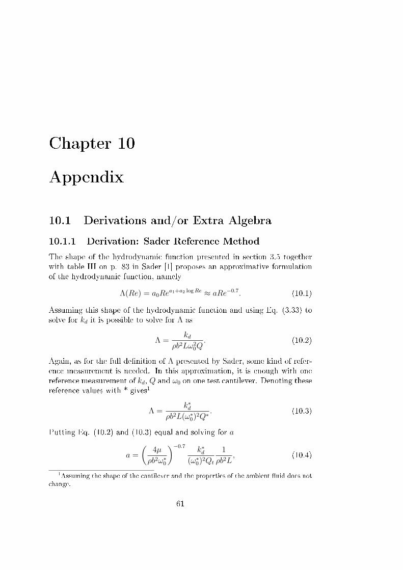
Chapter 10
Appendix
10.1 Derivations and/or Extra Algebra
10.1.1 Derivation: Sader Reference Method
The shape of the hydrodynamic function presented in section 3.5 togetherwith table III on p. 83 in Sader [1] proposes an approximative formulationof the hydrodynamic function, namely
Λ(Re) = a0Rea1+a2 logRe ≈ aRe−0.7. (10.1)
Assuming this shape of the hydrodynamic function and using Eq. (3.33) tosolve for kd it is possible to solve for Λ as
Λ =kd
ρb2Lω20Q
. (10.2)
Again, as for the full denition of Λ presented by Sader, some kind of refer-ence measurement is needed. In this approximation, it is enough with onereference measurement of kd, Q and ω0 on one test cantilever. Denoting thesereference values with * gives1
Λ =k∗d
ρb2L(ω∗0)
2Q∗ . (10.3)
Putting Eq. (10.2) and (10.3) equal and solving for a
a =
(4µ
ρb2ω∗0
)−0.7k∗d
(ω∗0)
2Qt
1
ρb2L, (10.4)
1Assuming the shape of the cantilever and the properties of the ambient uid does notchange.
61

and it is possible to write Λ(Re)
Λ(Re) =
(4µ
ρb2ω∗0
)−0.7k∗d
(ω∗0)
2Q∗1
ρb2L︸ ︷︷ ︸a
ρb2ω0
4µ
−0.7
︸ ︷︷ ︸Re−0.7
=k∗d
(ω∗0)
2Q∗1
ρb2L
(ω0
ω∗0
)−0.7
,
(10.5)which gives the nal expression for kd according to
kd = k∗d
Q
Q∗
(ω20
(ω∗0)
2
). (10.6)
10.1.2 Integrating PSD
The integral ∫ ∞
0
G(ω)G∗(ω)dω =
∫ ∞
0
Q2ω40
Q2(ω2 − ω20)
2 + ω2ω20
dω (10.7)
appears when integrating the power spectral density of the harmonic oscil-lator for example. This integral cannot be evaluated by normal means, butif assuming ω ∈ C it is possible to use the residue theorem from complexanalysis [15]. The residue theorem gives∫ ∞
−∞f(z)dz = 2πi
∑Res(f, ak) (10.8)
where f(z) is the function that needs to be integrated and Res(f, ak) isthe residue for the pole ak, located in the upper half complex plane (polesare where the function blows up, for example f(x) = x−1 have one pole atx = 0). In the case of rational functions f = g/h, as in Eq. (10.7) the residueis dened as
Res(f, ak) =g(ak)
D[h(ak)](10.9)
where D is derivative with respect to the variable of interest (ω in the caseof Eq. (10.7)).
In equation (10.7) g(ω) = Q2ω40 and h(ω) = Q2(ω2
0 − ω2)2 + ω2ω20, which
gives the poles as the roots to h(ω). Rewriting the equation to a simplerform gives∫ ∞
0
Q2ω40
Q2(ω2 − ω20)
2 + ω2ω20
dω = ω0
∫ ∞
0
dω(ω2
ω20− ω2
0
)2
+ ω2
Q2ω20
=(10.10)
[x =
ω
ω0
, dω = dxω0
]= ω0
∫ ∞
0
dx
(1− x2)2 + x2
Q2
.
62

The limits of Eq. (10.11) are between 0 and ∞, but in the residue theorem(10.8) the limits are between −∞ to ∞. Due to symmetry of Eq. (10.11),when applying the theorem to the integral it gives
ω0
∫ ∞
−∞
dx
(1− x2)2 + x2
Q2
=ω0
2
∫ ∞
0
dx
(1− x2)2 + x2
Q2
= 2πi∑
Res(f, ak).
(10.11)The poles to h(ω) can be calculated as
h(ω) = Q2(ω20 − ω2)2 + ω2ω2
0 = 0 ⇒ (10.12)
h(x) = (1− x2)2 +x2
Q2=
x4 −(2− 1
Q2
)x2 + 1 = 0 ⇒
[z = x2
]⇒ z2 −
(2− 1
Q2
)︸ ︷︷ ︸
≡κ
z + 1 = 0 ⇒
z± =κ
2± i
√1− κ2
4⇒
x1,2,3,4 = ±√z±.
The poles can be written as xi = αi + iβ but the only interesting poles arethe ones located in the upper half plane, such that αi ≥ 0. Due to the rootit is not clear which of the xi's that are located where, but an arbitrarycomplex number can be written as Z = reiϕ = r(cosϕ + i sinϕ) where r isthe amplitude and ϕ is the phase of Z. Noting that the squared poles z± canbe written as z± = eiϕ± = cosϕ± sinϕ since r = |z±| = 1, makes it possibleto write
xi =√z± =
(eiϕi
)1/2= cos
ϕi
2± i sin
ϕi
2. (10.13)
Now using the trigonometric relation for half angles, such that
sinϕ
2=
√1 + cosϕ
2, cos
ϕ
2=
√1− cosϕ
2, (10.14)
xi =
√1 + cosϕ
2± i
√1− cosϕ
2.
Identifying cosϕ from Eq. (9.12) and using symmetry between the poles2
2The poles are related as x1 =√z+, x2 = −√
z+, x3 =√z− =
√z∗+ and x4 = −√
z− =
−√z∗+ where ∗ is complex conjugate. Thus it is possible to write xi using z+ only.
63

gives
x1 =1
2
(√2− κ+ i
√2− κ
)=
√z+, (10.15)
x2 = −x1 = −√z+, (10.16)
x3 =1
2
(√2− κ− i
√2− κ
)=
√z∗+
x4 = −x3 = −√
z∗+
This gives that the only poles that are in the upper half plane are x1 and x3.Putting this into the residue theorem let us evaluate the integral
ω0
2
∫ ∞
−∞
dx
(1− x2)2 + x2
Q2
= ω0πi(Res(f, x1) + Res(f, x3)) =πω0Q
2. (10.17)
10.1.3 Deriving Eq. (3.39)
Consider the cantilever being excited by thermal noise and thermal noiseonly. The thermal noise is due to collisions with molecules from the ambientuid, and they are completely uncorrelated over long time scales since onecollision at t = t1 and one collision at t = t2 = t1 are not aecting eachother at all. If measuring the force at exactly the same time, of course givesthe same force. This is in statistics commonly described with the so calledautocorrelation function, ⟨FN(t)FN(t− t′)⟩ = cδ(t′) where FN(t) is the forceimpulse at time t and δ is Dirac delta function. This means that correlationbetween forces at two dierent time instances are only correlated i t = t′.
Using ergodicity together with the convolution theorem for Fourier trans-form and dening the power spectrum of some quantity as Sxx = ⟨XX∗⟩gives the power spectrum of the cantilever position
Szz(ω) = ⟨zN z∗N⟩ =∫ ∞
−∞dτe−iωτ ⟨zN(t)zN(t− τ)⟩. (10.18)
Since there is no such thing as negative frequencies, the lower limit is from 0,not from −∞. Making use of linear response theory as Eq. (3.18) connectsthe response of the system due to an applied force. This makes it possible toexpress z as a force instead transforming Eq. (10.18)
Szz(ω) =
∫ ∞
0
dτe−iωτ ⟨1kGFN(t)
1
kG∗FN(t− τ)⟩ = (10.19)
=
∫ ∞
0
dτe−iωτ GG∗
k2⟨FN(t)FN(t− τ)⟩︸ ︷︷ ︸
cδ(τ)
=cGG∗
k2.
64
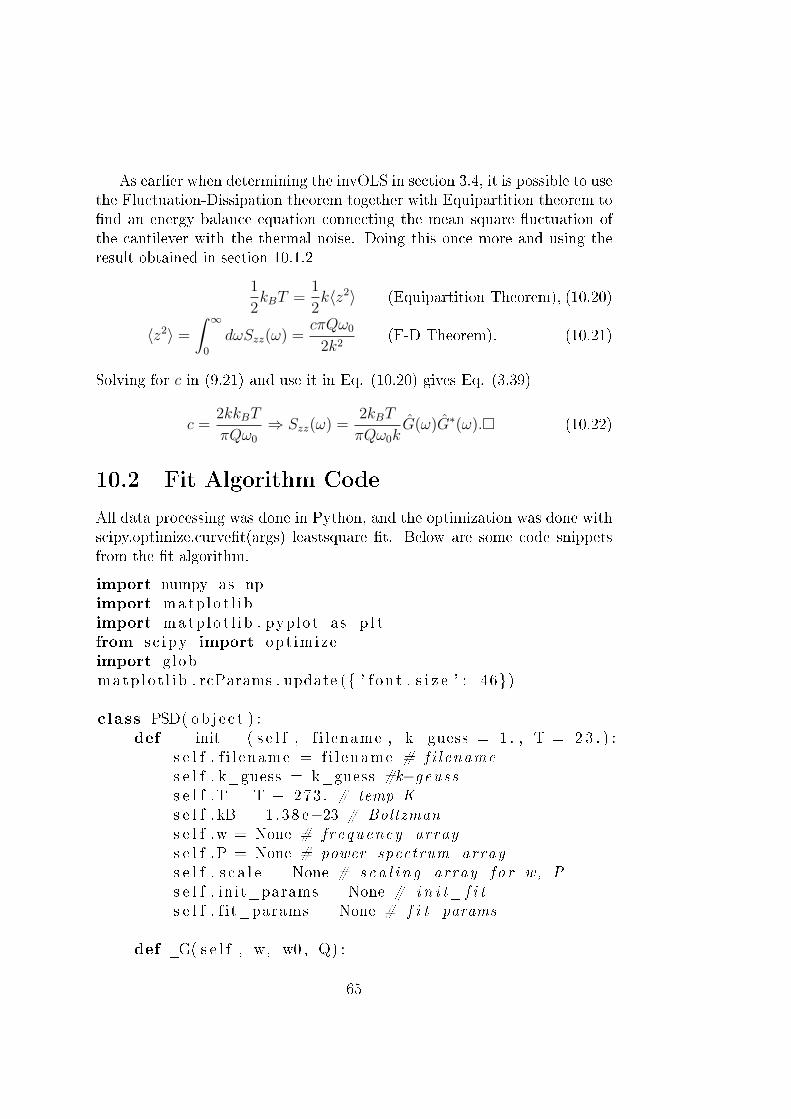
As earlier when determining the invOLS in section 3.4, it is possible to usethe Fluctuation-Dissipation theorem together with Equipartition theorem tond an energy balance equation connecting the mean square uctuation ofthe cantilever with the thermal noise. Doing this once more and using theresult obtained in section 10.1.2
1
2kBT =
1
2k⟨z2⟩ (Equipartition Theorem), (10.20)
⟨z2⟩ =∫ ∞
0
dωSzz(ω) =cπQω0
2k2(F-D Theorem). (10.21)
Solving for c in (9.21) and use it in Eq. (10.20) gives Eq. (3.39)
c =2kkBT
πQω0
⇒ Szz(ω) =2kBT
πQω0kG(ω)G∗(ω). (10.22)
10.2 Fit Algorithm Code
All data processing was done in Python, and the optimization was done withscipy.optimize.curvet(args) leastsquare t. Below are some code snippetsfrom the t algorithm.
import numpy as npimport matp lo t l i bimport matp lo t l i b . pyplot as p l tfrom s c ipy import opt imizeimport globmatp lo t l i b . rcParams . update ( ' f ont . s i z e ' : 46)
class PSD( ob j e c t ) :def __init__( s e l f , f i l ename , k_guess = 1 . , T = 2 3 . ) :
s e l f . f i l ename = f i l ename # fi l enames e l f . k_guess = k_guess #k−geusss e l f .T = T + 273 . # temp Ks e l f . kB = 1.38 e−23 # Boltzmans e l f .w = None # frequency arrays e l f .P = None # power spectrum arrays e l f . s c a l e = None # sca l i n g array f o r w, Ps e l f . init_params = None # i n i t _ f i ts e l f . f it_params = None # f i t params
def _G( s e l f , w, w0 , Q) :
65
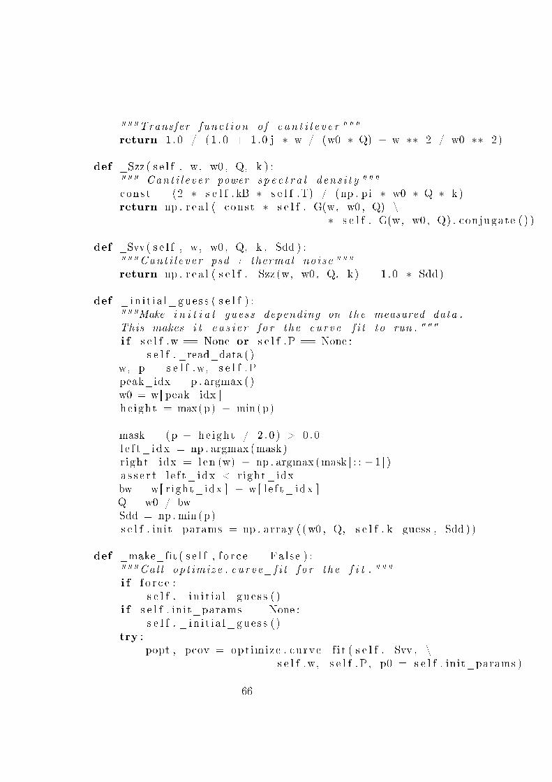
"""Transfer f unc t i on o f c a n t i l e v e r """return 1 .0 / ( 1 . 0 + 1 .0 j ∗ w / (w0 ∗ Q) − w ∗∗ 2 / w0 ∗∗ 2)
def _Szz ( s e l f , w, w0 , Q, k ) :""" Can t i l e v e r power s p e c t r a l d en s i t y """const = (2 ∗ s e l f . kB ∗ s e l f .T) / (np . p i ∗ w0 ∗ Q ∗ k )return np . r e a l ( const ∗ s e l f ._G(w, w0 , Q) \
∗ s e l f ._G(w, w0 , Q) . conjugate ( ) )
def _Svv( s e l f , w, w0 , Q, k , Sdd ) :""" Can t i l e v e r psd + thermal no i se """return np . r e a l ( s e l f . _Szz (w, w0 , Q, k ) + 1 .0 ∗ Sdd)
def _in i t i a l_gue s s ( s e l f ) :"""Make i n i t i a l guess depending on the measured data .This makes i t e a s i e r f o r the curve_f i t to run . """i f s e l f .w == None or s e l f .P == None :
s e l f . _read_data ( )w, p = s e l f .w, s e l f .Ppeak_idx = p . argmax ( )w0 = w[ peak_idx ]he ight = max(p) − min(p)
mask = (p − he ight / 2 . 0 ) > 0 .0l e f t_ idx = np . argmax (mask )r ight_idx = len (w) − np . argmax (mask [ : : − 1 ] )a s s e r t l e f t_ idx < right_idxbw = w[ r ight_idx ] − w[ l e f t_ idx ]Q = w0 / bwSdd = np . min (p)s e l f . init_params = np . array ( (w0 , Q, s e l f . k_guess , Sdd ) )
def _make_fit ( s e l f , f o r c e = False ) :""" Ca l l op t imize . cu rve_f i t f o r the f i t . """i f f o r c e :
s e l f . _ in i t i a l_gue s s ( )i f s e l f . init_params == None :
s e l f . _ in i t i a l_gue s s ( )try :
popt , pcov = opt imize . curve_f i t ( s e l f . _Svv , \s e l f .w, s e l f .P, p0 = s e l f . init_params )
66

except :print ' F i t f a i l e d f o r ' . format ( s e l f . f i l ename )s e l f . f it_params = s e l f . init_paramsreturn
s e l f . f it_params = popt
def plot_psd ( s e l f ) :""" Plo t rou t ine f o r f o r s t a r t i n g the p l o t . """
. . .
psd = PSD( p s d f i l e . txt )psd . plot_psd ( )p l t . show ( )
67