Discussion

Paper

|D

iscussionP

aper|

Discussion

Paper

|D

iscussionP

aper|

Atmos. Meas. Tech. Discuss., 5, 8271–8311, 2012www.atmos-meas-tech-discuss.net/5/8271/2012/doi:10.5194/amtd-5-8271-2012© Author(s) 2012. CC Attribution 3.0 License.

AtmosphericMeasurement

TechniquesDiscussions

This discussion paper is/has been under review for the journal Atmospheric MeasurementTechniques (AMT). Please refer to the corresponding final paper in AMT if available.

Calibration and validation of the advancedE-Region Wind Interferometer

S. K. Kristoffersen1, W. E. Ward1, S. Brown2, and J. R. Drummond3

1Department of Physics, University of New Brunswick, Fredericton, NB, E3B 5A3, Canada2CSIL, York University, 4700 Keele St. Toronto, ON, M3J 1P3, Canada3Department of Physics and Atmospheric Science, Dalhousie University, Halifax, NS,B3H 4R2, Canada

Received: 31 October 2012 – Accepted: 2 November 2012 – Published: 14 November 2012

Correspondence to: W. E. Ward (wward@unb.ca)

Published by Copernicus Publications on behalf of the European Geosciences Union.

8271

Discussion

Paper

|D

iscussionP

aper|

Discussion

Paper

|D

iscussionP

aper|

Abstract

The advanced E-Region Wind Interferometer (ERWIN II) combines the imaging capa-bilities of a CCD detector with the wide field associated with field widened Michelsoninterferometry. This instrument is capable of simultaneous multi-directional wind ob-servations for three different airglow emissions (oxygen green line (O(1S)), the PQ(7)5

and PP(7) emission lines in the O2(0–1) atmospheric band and P1(3) emission line inthe (6,2) hydroxyl Meinel band) on a three minute cadence. In each direction, for 45 smeasurements for typical airglow brightness the instrument is capable of line-of-sightwind precisions of ∼ 1 ms−1 for hydroxyl and O(1S) and ∼ 4 ms−1 for O2. This precisionis achieved using a new data analysis algorithm which takes advantage of the imaging10

capabilities of the CCD detector along with knowledge of the instrument phase variationas a function of pixel location across the detector. This instrument is currently locatedin Eureka, Nunavut as part of the Polar Environment Atmospheric Research Labora-tory (PEARL). The details of the physical configuration, the data analysis algorithm,the measurement calibration and validation of the observations are described. Field15

measurements which demonstrate the capabilities of this instrument are presented. Toour knowledge, the wind determinations with this instrument are the most accurate andhave the highest observational cadence for airglow wind observations of this region ofthe atmosphere and match the capabilities of other wind measuring techniques.

1 Introduction20

Interferometric methods have been the primary means for the past thirty years to pas-sively observe mesospheric and thermospheric winds using Doppler shifts in airglowemissions. Progress in detector technologies have led to advances in the observa-tion capabilities of these instruments by allowing the interference fringes and/or thescene of interest to be imaged. Apart from the Wind Imaging Interferometer (WINDII)25

on the Upper Atmosphere Research Satellite (Shepherd et al., 1993), publications on

8272

Discussion

Paper

|D

iscussionP

aper|

Discussion

Paper

|D

iscussionP

aper|

working instruments have generally been associated with the Fabry-Perot (Aruhliahet al., 2010; Anderson et al., 2012; Shiokawa, et al., 2012) and Spatial HeterodyneSpectroscopy (SHS) techniques (the Doppler Asymmetric Spatial Heterodyne (DASH)of Englert et al., 2012). The success of these instruments demonstrates how incorpo-rating imaging capabilities improves the accuracy and temporal resolution over earlier5

configurations.In this paper, a configuration which implements these imaging capabilities in combi-

nation with a field widened Michelson interferometer is described. The approach buildson the foundation developed during work on the WINDII instrument. The imaging ca-pability permits simultaneous viewing in multiple directions (as opposed to sequential10

viewing in each direction) and allows the fringe profile to be imaged and analysed ona bin-by-bin basis using new data analysis algorithms. The resulting instrument, termedthe advanced E-Region Wind Interferometer (ERWIN II), generates simultaneous windobservations in 5 directions (the four cardinal directions and zenith) at three differentheights using three different emissions (the oxygen green line (O(1S)) at 557.7 nm, the15

PP(7) and PQ(7) lines in the O2 (0–1) atmospheric band at 859.9 and 860.0 nm and theP1(3) emission line in the OH(6,2) Meinel band at 843.5 nm) every three minutes. Thewind accuracy is ∼ 1 ms−1 for all the emissions and the precision is ∼ 1 ms−1 for thegreen line and hydroxyl observations and ∼ 4 ms−1 for the O2 observations for standardoperating conditions.20

ERWIN II is based on the E-region wind interferometer (Gault et al., 1996) whichwas built in the mid-1990’s using a photo-multiplier tube as a detector. Winds wereobtained by sequentially viewing different directions. This instrument was stationed atResolute Bay for close to a decade and several papers on the associated observa-tions published (Fisher et al., 2000, 2002; Bhattacharya and Gerrard, 2010). In 2005,25

funding through a Canadian Foundation of Innovation grant became available and wasused to design and build an improved version of the instrument. The interferometer andfilters from the old version of the instrument were retained but the optical configurationand imaging detectors were new. The imaging capability allowed a new data analysis

8273

Discussion

Paper

|D

iscussionP

aper|

Discussion

Paper

|D

iscussionP

aper|

algorithm to be developed which improved the accuracy and precision of the instru-ment. Once completed, ERWIN II was moved to the Polar Environment AtmosphericResearch Laboratory (PEARL) in Eureka, Nunavut (80 N, 86 W) in February 2008. Itoperated satisfactorily for three winters till spring 2011 when some minor issues withits operation occurred. These have been fixed and normal operations will resume in5

the winter of 2012/2013.This paper is organized as follows. The next two sections deal with concepts and

details necessary for understanding the instrument namely the measurement and in-strument concept, and a description of the new instrument and its operation. In thesubsequent section, the data analysis algorithms are described. A section on the pre-10

cision and accuracy of these measurements and their validation follows this. Some ini-tial results along with a comparison with other wind measuring instruments and a briefsummary of the planned scientific studies with this instrument are then presented. Thepaper finishes with some concluding remarks.

2 Measurement and instrument concept15

Doppler shifts in isolated quasi-monochromatic emissions when viewed through anideal Michelson interferometer are seen as changes in the modulation of the interfer-ence fringes as a function of path difference. The measured irradiance I(∆,λ,x) for anisolated monochromatic emission line has the following form:

I(∆,λ,x) = I0

(1+UV cos(

2πλ∆+x)

)+ IB (1)20

Here I0 is the irradiance of the emission, ∆ is the path difference of the interferometer,λ is the wavelength of the emission, x represents small variations in path (typically lessthan λ) that the experimenter can introduce into the interferometer to sample a fringe,U is the relative reduction in fringe amplitude due to instrument effects, V is the relativereduction in fringe amplitude due to the finite width of the emission line and the path25

8274

Discussion

Paper

|D

iscussionP

aper|

Discussion

Paper

|D

iscussionP

aper|

difference and IB is the sum of the background irradiance of the scene being viewedand the dark count.

The phase, θ, of the fringe is defined as 2πλ ∆. A small change in wavelength due

to a Doppler shift, λ+δλ, results in a change in phase of δθ = −(2πλ2 )∆δλ plus a small

correction associated with the dispersion of the glass. For small line of sight velocities,5

vlos, the Doppler shift is δλ = −λ(vlos/c

)with positive line of sight velocities corre-

sponding to a velocity towards the observer. Hence the phase change associated withthis Doppler shift is:

δθ =2π∆vlos

cλ(2)

Observation of the phase shift relative to the zero wind phase allows the line-of-sight10

velocity to be derived.As described in detail elsewhere (Shepherd, 2002), Doppler Michelson interferome-

try determines winds by determining phase shifts in the interference by measuring theirradiance passing through the interferometer at specific path differences and determin-ing the fringe parameters from these measurements. Typically the interferometer path15

is varied in phase steps of π/2. The standard 4-point algorithm (for ideal conditions:no background or dark count) uses irradiance measurements at four such sequentialsteps to derive the fringe parameters, (irradiance, visibility and phase) as follows:

I0 =I1 + I2 + I3 + I4

4

UV =

[(I1 − I3)2 + (I4 − I2)2

]1/2

2I0(3)20

θ = tan−1(I4 − I2I1 − I3

)In passive remote sensing of winds using airglow emissions, the fundamental parame-ter controlling the measurement quality is the instrument throughput, AΩ defined as the

8275

Discussion

Paper

|D

iscussionP

aper|

Discussion

Paper

|D

iscussionP

aper|

product of the area, A, over which the signal is detected multiplied by the solid angle atthe detector, Ω, that the scene of interest subtends. A field-widened Michelson interfer-ometer is a configuration of this interferometer which minimizes the path variation asa function of angle through the interferometer (Shepherd, 2002; details and referencespertinent to the following summary can be found in this monograph). Generally the field5

is collimated through the interferometer so the phase variation as a function of anglethrough the interferometer is projected onto the observed scene. The field widening isachieved by optimally inserting excess glass in one of the arms of the interferometerand positioning the mirror in the other arm at the apparent position of the mirror of thearm with the excess glass in it so that the conditions when the arms are the exactly the10

same are approximately achieved. This configuration eliminates the second order de-pendence of path as a function of angle and can eliminate the fourth order dependencefor specific mirror positions (Zwick and Shepherd, 1971).

The precision of a wind measurement is basically related to how well the sinusoidalvariation associated with a variation in path can be discerned relative to the inherent15

noise associated with that measurement. For a shot noise limited observation underthe ideal conditions described above, a reasonable estimate of accuracy of the phasedetermination is the standard deviation in θ, σθ which is given by Ward (1988)

σθ =1

aUV√I0

(4)

where a is a constant which depends on the number of steps used to determine the20

fringe phase. For the four point measurement described above a = 2. For the 8 stepscans used for ERWIN II, a = 2

√2.

The two fringe-related parameters in this equation are the net visibility, UV , and√I0 which is the signal to noise ratio. In practice, the measurement precision can be

reduced by increasing the signal (longer integration times and enhanced instrument25

responsivity) or the visibility. The visibility is determined by the emission line-width,background emissions, the instrument imperfections and the phase variation over the

8276

Discussion

Paper

|D

iscussionP

aper|

Discussion

Paper

|D

iscussionP

aper|

region used to detect the light (essentially the aperture effect discussed by Hilliard andShepherd, 1966).

Contributions of background or dark signal to the observed irradiance also affect themeasurement precision. In terms of the above formulation for ideal conditions this canbe accommodated by determining effective irradiances and effective visibilities where5

the effective irradiance is Ie0 = I0 + IB and the effective visibility is UV e = UV (I0/(I0 +IB)). In the rest of this paper, for simplicity, expressions will be provided for the idealconditions (i.e. no dark and no background) with the understanding that for non-idealconditions, the effective irradiance and visibility can be used without any change totheir form.10

The wind accuracy is a function of both the measurement precision and knowledge ofthe phase for a stationary source, termed here the zero-wind phase. Generally, prac-tical sources for the airglow emissions are not available so the zero-wind phase isdetermined by using lamps with emission lines at wavelengths close to the airglowemissions and using nightly averages of the wind in the vertical direction under the15

assumption that vertical motions average to zero.

3 Instrument description and operation

ERWIN II differs from the original instrument in that the photomultiplier tube was re-placed by an imaging detector, the optics were modified so that light from the fourcardinal directions and the vertical could be viewed simultaneously, and the interfer-20

ometer was placed in an air-tight housing to prevent pressure changes associated withweather fronts from affecting the phase. The interferometer, airglow emissions, calibra-tion lines and the filters used are the same as ERWIN and are described in detail inGault et al. (1996).

In summary, the interferometer is a three glass design with the mirror position con-25

trolled using piezoelectric cylinders and a capacitive feedback system. The front faceis square with sides of 7.62 cm. It was designed to accept a beam with a 2.5 degree

8277

Discussion

Paper

|D

iscussionP

aper|

Discussion

Paper

|D

iscussionP

aper|

half angle. The interferometer is set to a path difference slightly larger than 11 cm andthe glass lengths were chosen so that the interferometer is field widened at all wave-lengths and thermally compensated. The specific path difference was selected to su-press possible fringes from thermospheric oxygen green line emissions, and to ensurethe fringes of the pair of O2 lines and the Λ doubled hydroxyl lines were each in phase.5

The calibration lines used are the 557.0 nm Krypton line, the 840.8 nm Argon line andthe 866.7 nm Argon line.

Figure 1 is a schematic view of the mechanical layout of ERWIN II. It shows a cutthrough the centre of the instrument such that two of the cardinal viewing directionsand the vertical can be seen (the other viewing directions project out of the plane of10

the figure). The centers of each cardinal viewing direction are at an elevation angle of38.7 degrees relative to the horizontal. Light from the sky from all the viewing directionsis collected and focused on what is termed the quad mirror where they are combinedinto a single beam and then passed through the interferometer. The interferometeris tilted 1.77 degrees horizontally and 1.77 degrees vertically relative to the optical15

axis of the system to ensure that no light was reflected off optical components andrecycled back through the system. The optical components which collect the light andcollimate it through the interferometer form what is termed the front telescope. Afterthe interferometer, a second optical system, termed the back telescope directs the lightto the filters where the light is again collimated. Both telescopes are 1 : 1. The camera20

system then focuses the beam onto the detector.The quad mirror consists of four trapezoidal mirrors canted appropriately with

a square hole in the middle. This serves to redirect light from each direction so that theycombine with the zenith light into a single beam through the rest of the optical system.Each of the cardinal directions views an irregularly shaped piece of the sky approxi-25

mately 0.0013 steradians at an elevation angle of 38.7 degrees. Zenith is viewed witha solid angle of 0.0007 steradians. Light from each of the cardinal directions is focusedonto one of the trapezoidal facets of the quad mirror using spherical mirrors and zenithis focused onto the plane of this mirror. The quad mirror is located at the field stop of

8278

Discussion

Paper

|D

iscussionP

aper|

Discussion

Paper

|D

iscussionP

aper|

the front telescope. The light from these various viewing directions is passed as colli-mated light through the interferometer and then focused using a second telescope andcamera onto the detector. The sky from each direction is thus focused onto different re-gions of the detector so that each of these five directions is simultaneously measured.The effective field of view of the instrument is the same as that allowed through the5

interferometer, a beam of 2.5 degrees half angle.The camera was built in house at York University and uses a 512 by 512 pixel,

back-thinned, low-noise, frame-transfer CCD (E2V Technologies CCD57-10) with anactive area of 6.656 by 6.656 mm. The CCD camera is used with 16 by 16 binning,resulting in a final image size of 35 by 32 bins. It has a quantum efficiency of 0.85 for10

the O(1S) emission and 0.45 and 0.4 for the O2 and OH emissions. This is a significantimprovement over the photomultiplier tube for which the quantum efficiency was ∼ 0.14,0.08 and 0.06 for the same emissions. An additional advantage arises because, asnoted above because of the imaging capability, measurements could be made withenhanced visibility over the original instrument. The increased sensitivity allows for15

a decrease in the exposure times, while still maintaining comparable signal to noise.Figure 2 illustrates the manner in which the field is imaged onto the CCD detector.

The dark bins indicate where the edges of the areas illuminated by the various regionsof the sky. The light from each viewing direction is imaged such that the top is east, thebottom-west, the right-north, the left-south, and centre-zenith. The background colors20

indicate the how the interferometer phase in radians varies across the field and indicatehow much variation there is across each region. Variations in phase away from thisbackground along with consideration of the zero wind provide a measure of the Dopplershift in each viewing direction.

The observation procedure of ERWIN has been updated relative to that described in25

Gault et al. (1996). Since all viewing directions are now viewed simultaneously there isno need to cycle through the viewing directions. The basic procedure is to cycle throughthe three emission measurements in sequence and then after a user specified numberof cycles to perform a set of calibrations. A measurement consists of 8 exposures of

8279

Discussion

Paper

|D

iscussionP

aper|

Discussion

Paper

|D

iscussionP

aper|

the detector each at a different value of the Michelson path. The steps (relative to thereference phase which coincides with the initial mirror position) are set to 0, π/2, π,3π/2, 3π/2, π, π/2, and 0 radians. These steps are different for each emission with2π radians corresponding to a physical change in path of λ, the wavelength of theemission being viewed. A calibration consists of measurements (again one for each5

emission) using the calibration lamps and a dark measurement. Initially a calibrationwas undertaken after every eight emission scans but later this was changed to everyset of emission scans to provide better precision for determining the interferometerdrift. Overall, this results in a set of observations (wind determinations for 5 directionsand all three emissions) approximately every 3 min.10

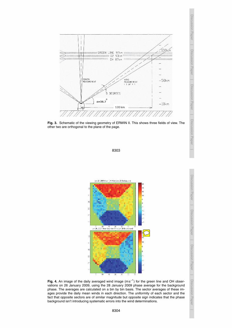
The observing geometry is illustrated in Fig. 3. All three emission layer are shownschematically and occur roughly at nominal heights of 97, 93 and 87 km for the O(1S),O2 and OH emissions respectively. Thus by cycling through the different emissionsinformation on various heights in the mesopause region is acquired. The azimuthalviewing directions are at an elevation angle of α = 38.7 degrees from the horizontal.15

Since winds are determined by observing Doppler shifts in the emission frequencies,the observed, line-of-sight winds are combinations of the horizontal and vertical winds(save for the zenith line-of-sight winds, which observes the vertical winds).

The meridional wind, v , is determined using the difference of the line-of-sight northand south winds20

v =(V LOS

S − V LOSN )

2cosα(5)

where

V LOSN = −v cosα+w sinα (6)

V LOSS

= v cosα+w sinα (7)25

Here w is the vertical component of the wind and α is the viewing angle of the azimuthallook directions relative to the horizontal.

8280

Discussion

Paper

|D

iscussionP

aper|

Discussion

Paper

|D

iscussionP

aper|

Similarly, the zonal wind, u, can be determined using the east and west line-of-sightwinds,

u =(V LOS

W − V LOSE )

2cosα(8)

The vertical winds can also be obtained using several different approaches. The first isto simply use the zenith line-of-sight winds5

w = V LOSZ (9)

Less directly, the vertical winds can be determined using the cardinal direction line-of-sight winds,

w =V LOS

N + V LOSS

2sinα=

V LOSE + V LOS

W

2sinα(10)

In theory, this provides the means to check the internal consistency of the wind de-10

terminations. In practice, however, the effects of gravity waves of scales of the sameorder as the distance between the viewing points in the airglow layer mean that thesecomparisons can only be undertaken in some sort of average sense.

4 Data analysis procedure

The essential issue for wind measurements is distinguishing the phase increments,15

δθ, associated with Doppler shifts in the emission of interest from the phase associ-ated with other factors. In general, the observed phase is a combination of the phaseassociated with the instrument configuration as manifested for the emission of interest(motionless) plus a shift associated with atmospheric motion of the source region beingviewed. In practice, for imaging applications, the phase associated with the instrument20

configuration can be separated into three terms:8281

Discussion

Paper

|D

iscussionP

aper|

Discussion

Paper

|D

iscussionP

aper|

– θB(i , j ): a term associated with the phase variation across the field as a functionof angle through the interferometer (or pixel location (i , j ) on the detector) rela-tive to the phase associated with rays passing at normal incidence through theinterferometer (background phase). This variation is illustrated in Fig. 2.

– θT(t): a term giving the thermal drift phase relative to the phase at a particular5

time (thermal drift term).

– θ0 : a term identifying the phase that a motionless source would have (zero windphase).

Hence the measured phase, θa, can be expressed as a function of time, t, and locationon the field as10

θa(i , j ,t) = θB(i , j )+θ0 +θT(t)+δθ(t) (11)

This formulation of the phase assumes that the background phase stays constant (gen-erally satisfied for carefully maintained interferometers) and temporal variations can betracked with a single phase parameter, the thermal drift which is only a function of time.

In theory, the zero wind phase should be easy to determine since it only requires15

a stationary source for the emission of interest. In practice however, this is difficult toachieve since portable sources for the airglow emissions are unavailable and the at-mosphere is generally in motion. As with other ground based wind instruments, a dailyaverage of the observed vertical wind is used to determine this parameter. In the caseof ERWIN II this average is measured using the quadrant looking vertical. For mea-20

surements at Eureka, where close to 24 h each day is observed, this determination isexpected to be a good measure of the actual zero wind; all periods of tidal motionsare covered during this time period, variations associated with gravity waves are ex-pected to average to zero, vertical winds associated with planetary waves are of theorder of cms−1 and mean vertical winds are small (an ascent or descent of 10 kmday−1

25

corresponds to a vertical velocity of 0.11 ms−1).

8282

Discussion

Paper

|D

iscussionP

aper|

Discussion

Paper

|D

iscussionP

aper|

For ERWIN II, the background phase determination was more difficult than expected.Initially, it was thought the phase variation associated with the reference emissionswould be suitable to use since they were within a few Angstroms of the emission ofinterest. However, it was found that use of such a background resulted in phase varia-tions of ∼ 10 ms−1 across several of the quadrants when daily averages of the winds5

were calculated. Instead, the background phase which was used was determined usingwind observations from a period when it was known to be cloudy (this phase variation isillustrated in Fig. 2 for the green line). Light from the sky was suitably scattered so thatall directions gave the same Doppler shift. Daily averages of this wind for the oxygengreen line and hydroxyl observations using this background are presented in Fig. 4.10

The resulting wind variations are minimal in each quadrant and the mean wind in eachquadrant provides a measure of the mean wind for the day. Details of the analysiswhich lead to this choice of background wind are contained in Kristoffersen (2011).

Although the analysis approach described in Gault et al. (1996), could be imple-mented for ERWIN II by integrating the signal in each quadrant and treating each15

quadrant as a single detector, a new bin-by-bin least mean squares approach simi-lar to that implemented in Ward (1988) was preferred. The latter approach was moreprecise since it avoids any visibility reduction that occurs as a result of the integrationover the phase in each quadrant and it allows bins contaminated by stars or cosmicray hits to be eliminated. In addition, a rigorous determination of the wind error can be20

undertaken.For this approach, a non-linear least mean squares analysis using the Levenberg

Marquardt method (as described in Press et al., 2007) is implemented. The irradiancevariation during the kth 8-point scan is modeled according to the following equation:

I(i , j ,tk ,s) = I0(tk)(1+UV (tk)cos(δθ(tk)+θI (i , j ,tk ,s))) (12)25

where the parameters being solved for are I0(tk), the irradiance, UV (tk),the net visibility,and δθ(tk), the phase variation associated with the wind. Here tk is the time of the kthscan. To ensure that the variation in phase angles being determined is small, all the

8283

Discussion

Paper

|D

iscussionP

aper|

Discussion

Paper

|D

iscussionP

aper|

known phases associated with a particular bin are added together so that θI (i , j ,tk ,s) =θB(i , j )+θ0+θT(tk)+(∆θs) where (∆θs) is the step size increment associated with mirrorstep of index s (expressed as a phase angle).

The merit function is

χ2 =N∑s=1

(Is(i , j ,tk ,s)− y(I(i , j ,tk ,s);al )

)σ2

s (i , j ,tk ,s)(13)5

where

y(I(i , j ,tk ,s);al ) = al (1) (1+al (2)cos(al (3)+θI (i , j ,tk ,s)))

al = (I0l(tk),UV l (tk),δθl (tk))

Is(i , j ,tk ,s) is the irradiance measured for step s, bin (i , j ) and scan k, and σ2s (i , j ,tk ,s)10

is the variance (estimated as shot noise) of this irradiance. l is the iteration index soy(I(i , j ,tk ,s);al ) is the irradiance determined using the constants determined on thel th iteration. θI (i , j ,tk ,s) with ∆θs = 0 is used to seed the first iteration of this method.Typically only a few iterations are needed for convergence to a solution.

In practice, there are two approaches used to determine the zero wind and thermal15

drift phase, one using the calibration lamp phase determinations (the standard proce-dure) and the other when the calibration lamp phase is not available (as occurred forthe O2 and OH emissions when the lamps malfunctioned). For the standard procedure,the calibration phase was determined on a regular basis throughout the night by cal-culating the average Michelson phase over the full field of the calibration lamp using20

the same 8-point scan as for the airglow observations. The resulting time-series of cal-ibration phase is interpolated using cubic splines to the airglow observation times toprovide the variation in thermal drift phase. The relative airglow phase throughout theobservation period is then calculated using the non-linear approach with the zero windphase set to zero. The actual zero wind phase then provides an offset to this relative25

8284

Discussion

Paper

|D

iscussionP

aper|

Discussion

Paper

|D

iscussionP

aper|

phase and is determined using the mean of the zenith over the entire day. The windsare determined by shifting the relative airglow phase by the zero wind phase and usingEq. (2) to convert the phase to velocity.

If the calibration lamps are not available, then the zenith measurements can be usedto estimate the phase associated with the thermal drift and zero wind. In this case, the5

analysis approach as described above is undertaken but with the thermal drift and zerowind terms set to zero. For each image, the phase for the vertical view is then taken asan estimate of the sum of these two terms and subtracted off the four other quadrants.The disadvantage of this approach is that the vertical wind cannot be determined andphase variations associated with vertical winds are mixed into the phase determina-10

tions for each of the cardinal directions. This reduces the precision and accuracy of theradial wind determination. Nevertheless, the meridional and zonal wind determinationsare unaffected by the lack of an independent zero wind determination since they aredetermined through a difference in radial wind determinations in opposite directionsand hence the zero wind contribution to the two directions is eliminated (see Eqs. 515

and 8).There are several advantages associated with the standard approach described

above. This algorithm can be run for fewer than the 8 steps comprising a typical scan.Because the steps are in phase multiples of π/2 and all phases steps are repeatedtwice, anomalous irradiances are identified by comparing steps of the same phase20

and examining the sums of steps which are π radians apart. If one or two anomaloussteps are identified in a scan they are eliminated from the phase determination therebyreducing the likelihood of outliers. In addition, there are ∼ 150 bins used for wind deter-minations in each of the cardinal directions and ∼ 80 bins for the vertical. As a result,any additional outliers beyond three standard deviations of the mean wind phase in25

each of the quadrants can be identified and are eliminated and the standard error as-sociated with the wind determination for each quadrant calculated. Implementation ofthese checks results in a robust statistical framework for the wind determinations withthis instrument.

8285

Discussion

Paper

|D

iscussionP

aper|

Discussion

Paper

|D

iscussionP

aper|

5 Measurement validation

In this section, results which verify the precision and accuracy of the ERWIN II instru-ment are presented. Crucial is an accurate determination of the background phasevariation across the field, the thermal drift and the zero wind. Each of these aspects ofthe wind determination contributes to the measurement precision and accuracy. Eval-5

uation of the measurement quality in terms of these aspects is possible because ofredundancies in the approach and tests which were undertaken to investigate specificaspects of the measurement approach.

As noted above, the background phase was determined using observations takenon 28 January 2009 during a period when it was cloudy so that the directional asym-10

metry in the Doppler shifts was negligible as a result of scattering in the clouds. Duringthe eight hours of observations used to determine this phase variation, ∼ 160 mea-surements were taken. The background phase was determined by taking the averageof these measurements. For the fringe parameters associated with these measure-ments, the standard deviation of the wind determination for each bin on each scan15

was ∼ 15 ms−1 so that the standard error for the background phase determination was∼ 1.1 ms−1 for each bin. Since winds are determined by averaging the phases deter-mined on a bin-by-bin basis in each sector, this error makes a negligible contribution tothe measurement precision.

Equally important is determining whether there are any systematic errors in the back-20

ground determination. This is important since the winds in opposite directions are de-termined relative to the background phase so errors in the background phase wouldresult in systematic errors in these winds. Figure 4 shows the daily average wind imagemeasured on 26 January 2009 for the oxygen green line and hydroxyl observations.Shown for each emission is the daily average of each bin in the image. The average25

of each sector gives the mean radial wind in each direction for this day. Two things ofparticular note are the uniformity of the winds in each quadrant and that opposite quad-rants are close to the same magnitude but oppositely signed. The uniformity indicates

8286

Discussion

Paper

|D

iscussionP

aper|

Discussion

Paper

|D

iscussionP

aper|

that the background phase has been effectively removed from the wind determinations,since the gradient associated with the angular dependence of the background phaseis not observed. The fact that the winds in opposing directions are consistent withwhat would be expected geometrically indicates that errors in the background phasedetermination are minimal and do not result in systematic errors in the radial wind de-5

terminations. The wind is defined as positive towards the instrument so the observationof a positive (negative) wind in one sector would correspond to a wind of the oppositesign in the opposite quadrant.

This self-consistency of ERWIN is further demonstrated by considering the aver-ages of these sectors for several days, shown in Table 1. Since the winds in opposing10

directions should have the same magnitude but opposite sign, the sum of these valuesshould be zero. The table provides the values of the average daily phase for each ofthe four sectors corresponding to the cardinal directions for three days in January 2009for the hydroxyl and green line observations. The means for each sector over the threedays is calculated (4th column) and then the sum of the phases of opposite sectors15

determined. Since the winds in opposing directions should have the same magnitude,but opposite sign, the sum of these values should be close to zero, as observed. Onaverage, the difference is of the order of a meter per second. This further validatesthat the background is suitable for the wind determinations and at most a systematicerror of 1 ms−1 is introduced into the radial wind observations. The use of this phase20

background has been checked for the subsequent years and it is a stable feature of theinterferometer.

These results also demonstrate that on average the thermal drift is being calculatedproperly. Since the thermal drift would be a constant value added to the phase for everybin, at a given time, this value would have the same sign for each section. This would25

result in an addition of the thermal drift terms, rather than the cancellation of the winds,as is observed.

Depending on the thermal stability of the instrument short term measurement errorscan also be introduced if the thermal drift is not followed with sufficient precision. As

8287

Discussion

Paper

|D

iscussionP

aper|

Discussion

Paper

|D

iscussionP

aper|

described earlier, initially calibration phase measurements were taken on a slower ca-dence than the measurements. For the first two years of observations, one scan of thecalibration lamps was taken for every eight scans of the atmospheric emissions. Forthe third year (March 2010 to March 2011) this was increased to a calibration everymeasurement scan of the atmospheric emissions.5

Figure 6 gives an indication of the precision of the thermal drift determination. Panela (upper panel) shows a time series of the green line zenith phase (blue points) alongwith the phase determined with the calibration lamp (red dots – corrected with the zerowind offset so that both time series have the same daily average). On this figure theuncertainties in the phase determinations is smaller than the diameter of the dots in10

the plots. The two phase determinations follow each other closely.Panel b (lower panel) is a time series of the difference between the observed zenith

phase and the calibration phase interpolated using cubic splines to the times of theatmospheric observations. In this figure the measurement precision is close to thesize of the dots. The standard deviation of the difference is 1.02 degrees or 4.5 ms−1.15

This number includes geophysical variability (vertical winds, irradiance variations) andSchott noise and hence is not a clean measure of the uncertainty introduced throughthe thermal drift calibrations.

To explore this aspect of the measurement in more detail, an experiment which in-cluded frequent calibration measurements was performed (a calibration measurement20

was taken after every atmospheric measurement). The resulting calibration phase timeseries was compared to one constructed by sampling this time series at a the samerate as other typical days and then interpolating (using cubic splines) these measure-ments to the times of the original time series. This process duplicated the thermalphase determinations associated with the atmospheric measurements.25

Figure 6 shows the result of this experiment. The phase error in the cubic splineis never more than a degree, and the standard deviation of the phase error over theduration of this experiment is 0.389 degrees (1.69 ms−1). This is significantly smallerthan the standard deviation of the difference of the calibration phase and the zenith

8288

Discussion

Paper

|D

iscussionP

aper|

Discussion

Paper

|D

iscussionP

aper|

emission phase, which was 1.02 degrees (4.5 ms−1). This demonstrates that the errorsassociated with the cubic spline are acceptably small compared to the other errors andgeophysical noise. This uncertainty is reduced for observations with the more frequentcalibration cadence.

Using the value of “a” appropriate for the 8 step scan, and Eqs. (2) and (4), the5

precision of a wind measurement is estimated by the standard deviation

σw =cλ

4√

2π∆effUV√I. (14)

Here σw is the error in ms−1, ∆eff is the effective path difference, UV is the visibility,I is the observed irradiance, c is the speed of light, and λ is the wavelength of theemission. The wind standard deviation is inversely proportional to the visibility, the path10

difference and the square root of the irradiance. Comparison of the estimated varianceusing this formula to the observed variance provides an indication of how closely theobservations conditions during individual scans match the assumptions associated withthe derivation of this formula (namely that the irradiance and visibility remain constantduring a scan).15

This is illustrated in Fig. 7 which provides time series of the actual standard errorand the standard error estimated using Eq. (14) (calculated as a variance for each binin the sector using Eq. (14) and then averaged in the same way as the actual standarderror is calculated) for the north sector on 22 December 2008. The variability in bothdata sets is due to variations in the irradiance and visibility during that day. It is striking20

that the two measures follow each other so closely since this indicates that intensityand visibility variations during scans is generally insignificant. If it was a factor then thestandard error would be significantly larger than the estimated precision.

Figure 8 shows time series of the standard error for all four cardinal direction sec-tors for 26 January 2009. For this date, some twilight was present in the afternoon25

centered at ∼ 17:00 LT. The increase in the standard error in the vicinity of this time isthe expected result of increases in the background relative to the emission irradiance

8289

Discussion

Paper

|D

iscussionP

aper|

Discussion

Paper

|D

iscussionP

aper|

(see discussion at the end of Sect. 2). The time series of all four sectors follow eachother well. The daily average of the green line standard error for the zenith section is1.91 ms−1, and that for all of the cardinal directions is 1.22 ms−1. The daily average ofthe precision based on the visibility and intensity of the green line emission for zenithis 1.88 ms−1, and that for the cardinal directions is 1.24 ms−1. The values for zenith5

are greater than for the cardinal directions because of geometrical considerations. Theeffective layer thickness (and hence irradiance) is greater by 1/cos(α) where α is theinclination angle relative to zenith (here α = 51.3 degrees). The irradiance during thisday was lower on average so these values are slightly higher than the typical precisionof these measurements.10

Plots of the winds provide a final, and satisfactory, check that the results are accu-rate. Meridional winds from 23 January 2009 for green line and hydroxyl calculated inseveral different ways are shown in Fig. 9. The meridional, north direction and southdirection winds are calculated using Eqs. (5), (6) and (7), respectively. The time seriesdesignated “without subtracting zenith”, is a time series of the wind determined from the15

northern sector without zenith subtracted. The meridional winds are reasonable, andindicate that there was a significant semi-diurnal tidal variation present. The manner inwhich this wind is determined renders it independent of vertical wind and thermal drift.Although perturbations due to gravity waves will result in small deviations from the truelarge scale meridional wind above the station, to good approximation this time series20

can be considered a good measure of the true meridional wind. Issues with thermaldrift, zero wind or background phase will result in the meridional winds determinedsolely from the north or south directions deviating significantly from this time series.

All the green line winds agree well with each other. The north and south winds,which are the winds determined from the respective sectors with the zenith phase sub-25

tracted off to remove any thermal drift, follow the meridional wind very closely. Thisdemonstrates that the winds viewed from the different directions are self-consistent.The fourth wind plotted on this figure is the north wind without the zenith phase sub-tracted. Since this also fits the meridional wind very closely, it demonstrates that the

8290

Discussion

Paper

|D

iscussionP

aper|

Discussion

Paper

|D

iscussionP

aper|

thermal drift has been effectively removed from the wind phase for observations withthis emission.

The OH observations are taken during the time when the associated calibration lampwas not working. As with the green line observations the north and south winds followthe meridional wind closely. In contrast the north wind without zenith subtracted de-5

viates significantly from the other winds. As expected since there are no calibrationmeasurements to provide thermal drift information, omission of the zenith phase re-sults in winds which exhibit significant systematic errors.

Since the contribution of the thermal drift variance to the wind observations is∼ 2.85 m2 s−2 for the time when the longer cadence calibration period was imple-10

mented, it is possible to use the zenith phase to examine the vertical wind (for theshorter cadence calibration period this will be even more feasible). While the explo-ration of this possibility will require careful analysis, an indication that this is plausiblecomes from a comparison (see Fig. 10) between the vertical wind determined using thezenith phase (blue dots), and the vertical wind determined using Eq. (10) (black dots).15

Both of these methods provide similar results on the larger temporal scales. Over theday, the vertical wind is modulated sinusoidally by a few ms−1. This could be due toa diurnal tide although since this day was during the 2009 major stratospheric warm-ing other dynamical effects could be present. The variance in the directly measuredvertical wind is 30.9 m2 s−2, which is significantly greater than the contribution asso-20

ciated with the thermal drift determination. The variance in the indirect determinationof the vertical wind is 89.4 m2 s−2. This calculation however also includes contributionsfrom horizontal motions. Further analysis of the vertical winds will be undertaken in thefuture to determine whether definitive geophysical results are possible.

In this section, the various factors affecting the precision and accuracy of the ERWIN25

II wind results have been discussed and results demonstrating the internal consis-tency of the winds presented. The main factors affecting the measurement precisionare the uncertainties associated with the Schott noise and the thermal drift determi-nation. For the observations with the low cadence calibration measurements the net

8291

Discussion

Paper

|D

iscussionP

aper|

Discussion

Paper

|D

iscussionP

aper|

variance is ∼ 4 m2 s−2 (i.e. (1.22)2 + (1.69)2) for the green line and OH observationsand ∼ 19 m2 s−2 (i.e. (4.0)2+ (1.69)2) for the O2 observations. These values depend onthe manner in which the thermal drift varies and for the observations taken with thehigh cadence calibrations will be close to the Schott noise values alone. The O2 valuesare significantly greater than the other two emissions because its irradiance is signifi-5

cantly smaller. For all the emissions, the precision is dependent on the irradiance andvisibility and there are occasions when the irradiance is close to a factor of four greaterthan that for the days used in this paper to validate the instrument and on these daysthe variance will be less than 1 m2 s−2 for high calibration cadence observations.

The measurement accuracy for radial winds is determined by the uncertainty in the10

background phase determination (< 1 ms−1) and uncertainties in the zero wind deter-mination. Based on the arguments presented in Sect. 4, this is expected to be less that1 ms−1 also. Hence, for the best observation procedure (high cadence calibrations),the precision and accuracy are both ∼ 1 ms−1.

6 Discussion15

Comparisons between the capabilities of ERWIN II and other optical wind measuringinstruments are not straightforward. Few papers have discussed the precision and ac-curacy of a technique in as much detail and as clearly as has been undertaken in thispaper. In part this is because a standard for comparison has not been developed, inpart because the precision is dependent on the integration time (i.e. amount of light col-20

lected), instrument aperture and field of view, and thermal stability, and in part becauseclear identification of the zero wind is difficult in practice. Instead, estimates of the mea-surement precision tend to be embedded in measurement papers using the particulartechnique in question. Since most techniques use some sort of average of the verticalwind over a night to estimate the true zero, unless there are other systematic errors,25

one can assume that the measurement accuracies are similar. As a result the mea-surement precision (taken as the standard deviation of the velocity determination) and

8292

Discussion

Paper

|D

iscussionP

aper|

Discussion

Paper

|D

iscussionP

aper|

the integration time needed for the measurement as quoted in the literature are theonly pragmatic means to use in comparing different instruments.

For ERWIN II, five velocity measurements at a precision of 1 ms−1 in 45 s are ob-served for an airglow brightness slightly below average. In a recent paper on multipleorder Fabry-Perot wind observations (Shiokawa et al., 2012) (similar to the observa-5

tion technique used by Makela et al., 2011; Meriwether et al., 2011) random errorsranging from 2 to 13 ms−1 are quoted for a single wind observation with an exposuretime of 60 s. Assuming that observing conditions in the middle of this range correspondto those for ERWIN II, it would take this instrument ∼ 5 min to observe the same fivevelocities with a precision of ∼ 7 ms−1.10

The Scanning Doppler Interferometer (SCANDI) described by Arulia et al. (2010) isused for all-sky auroral imaging by using multiple fringes. They note that it takes ∼ 7–8 min to obtain a 25 sector wind measurement for these emissions which are aboutan order of magnitude greater in brightness than they are at mid-latitudes (i.e. airglowas with ERWIN II). For measurements on 8 March 2007 an uncertainty of 15 ms−1 is15

quoted. Assuming that the measurement uncertainty scales roughly as the reciprocalof the square root of the brightness, the uncertainty in these measurements would be∼ 45 ms−1 (i.e. 15ms−1 ·

√10) for a brightness an order of magnitude less than that

observed. If this was reduced to a 5 sector measurement by combining the observedirradiances then the precision would be ∼ 20 ms−1 (i.e. 45/

√5) for a ∼ 7 min measure-20

ment.The DASH instrument (Englert et al., 2007) was recently used in field measurements

at a mid-latitude site to compare results to a Fabry-Perot interferometer (Englert et al.,2012). For this comparison, 5 min integrations were taken and the oxygen red line wasobserved. Uncertainties at the one sigma level ranged from ∼ 5 to 15 ms−1 based on25

the plots in this paper. It would take > 25 min to achieve the five measurement cycle ofERWIN II at a precision ≥ 5 ms−1 .

This comparison indicates that ERWIN II is a significantly superior wind measur-ing instrument than any other ground based airglow wind instrument. Of these, the

8293

Discussion

Paper

|D

iscussionP

aper|

Discussion

Paper

|D

iscussionP

aper|

multiple order Fabry-Perot of Shiokawa et al. (2012) comes closest to the ERWIN IIperformance. Even with this instrument (again assuming the uncertainty scales with ir-radiance as described above) it would require an integration time of 225 min (5min ·72)to achieve the 1 ms−1 precision that ERWIN II achieves. These comparisons are notdefinitive since the instruments described in these papers do not necessarily represent5

their optimal configuration. However, the advantage shown by ERWIN II is unlikely tobe matched by minor changes in the configurations of these instruments. At this time itprovides the most precise and rapid airglow wind measurements in the world.

Lidar and radar are two other techniques used to measure winds in the mesopauseregion. She et al. (2003) state that their sodium lidar has a vertical resolution of 2 km10

and measures winds between 81 and 107 km. The wind precision is ∼ 1.5 ms−1 atthe peak of the layer (∼ 91 km) and ∼ 15 ms−1 at the upper and lower bounds of theirmeasurements for a one hour integration during night. In a comparison between radar(Middle and Upper atmosphere (MU) radar (meteor mode)) and Fabry-Perot windsobserved over Shigaraki, Japan, Fujii et al. (2004) quote uncertainties of 2–5 ms−1

15

for 1 km resolution and 30 min integrations at ∼ 93 km which is close the height ofmaximum meteor trail detection. Radial wind uncertainties associated with a meteorradar in a paper by Frank et al. (2004) which compares lidar winds to meteor radarwinds are quoted as being a few ms−1 for (time/height) bins of (60min/4km). For thelidar used in this study, vector winds were obtained with ∼ 1 ms−1 precision between20

85 and 100 km with a 12 min cycle and vertical resolution of ∼ 1 km (Liu and Gardener,2005).

As discussed by Frank et al. (2004) and Fujii et al. (2004) the geometries of theobserving conditions associated with the various wind measuring instruments are dif-ferent. They are sensitive to different temporal and spatial scales, so the measurement25

variances are affected differently by geophysical variability. ERWIN II views a bright-ness weighted wind so it can be considered to provide winds for a volume of atmo-sphere of ∼ 5 km in the vertical and 5 km by 6 km in the horizontal. (It will not be sen-sitive to vertical scales less than approximately half the thickness of the airglow layer

8294

Discussion

Paper

|D

iscussionP

aper|

Discussion

Paper

|D

iscussionP

aper|

(∼ 5 km)). The horizontal dimension is determined from the beam width at 90 km (∼ 5degree lateral cross section) and elevation angle of 38.7. In contrast, the lidar collectsinformation from volumes with heights of 1 km and a diameter of ∼ 50 m and the me-teor radar collects information per velocity measurement from a volume 4 km thick and200 km diameter (Franke et al., 2005). The sampling area of the MU radar per veloc-5

ity measurement is from a volume 1 km thick and 200 km in diameter. Based on theheight range and vertical resolution of the best of these various instruments, the lidarachieves 15 velocity measurements at a 1 ms−1 precision in 12 min, and the MU radarachieves 40 velocity measurements at a 3–5 ms−1 precision (recent upgrades to theMU radar may have enhanced its capabilities). At a vector wind measurement every10

45 s at a precision of ∼ 1ms−1 ERWIN II has similar capabilities to these instruments.Figure 11 shows time series of the meridional and zonal winds observed by ERWIN

II on 22 December 2012 for all three emissions. As expected for larger scale upwardpropagating waves, the phase progression is downward with the green line winds lead-ing, followed by O2 and then OH. Standard errors for each wind measurement are15

smaller than the dots in the figure for green line and OH and about the size of the dotfor O2. The smaller scale variations are real and provide the opportunity to investigatethe wind fields at these heights on smaller temporal scales than previously possible.Given that ERWIN II simultaneously provides observations of the relative brightness ofthe airglow emissions that it observes, the relationship between the winds and airglow20

can be explored in detail. Of particular interest, is the investigation of gravity waves andthe associated vertical velocities and airglow variations.

The PEARL facility where ERWIN II is currently located, houses three other instru-ments which take measurements in the upper mesosphere and lower thermosphere.These include an All Sky Imager (ASI) (observes OH, Na, O(1S), O(1D) and N+

2 ),25

a Spectral Airglow Temperature Imager (SATI: O2, OH; Sargoytchev et al., 2004; Shep-herd et al., 2010), and a meteor radar (Manson et al., 2009). The measurement ca-dence of the ASI and SATI are of the order of minutes and the meteor radar providesan hourly vertical profile of horizontal wind in the mesopause region. Intercomparisons

8295

Discussion

Paper

|D

iscussionP

aper|

Discussion

Paper

|D

iscussionP

aper|

between simultaneous observations taken with these instruments open up many pos-sibilities for new scientific studies. The dynamical signatures of specific events (such asstratospheric warmings), wave signatures and the relationships between temperature,wind and emission rate over a broad range of scales are topics which this researchstation is uniquely capable of investigating.5

7 Conclusions

The construction of ERWIN II and the completion of new data analysis algorithms haveresulted in a powerful new capability for investigating the dynamics of the mesopauseregion. The most important physical changes to the instrument include the additionof a quad mirror to the ERWIN optical train so that multiple viewing directions can be10

simultaneously observed and the inclusion of a CCD camera so that each of thesedirections can be simultaneously imaged. The new data analysis algorithm takes ad-vantage of the imaging capabilities of the new instrument to provide a more preciseand better monitored wind and irradiance observations.

In this paper, the capabilities of this instrument have been thoroughly discussed. For15

the standard observation sequence, wind measurements have a precision and accu-racy of ∼ 1 ms−1 and a three minute observation cadence which incorporates obser-vations in five viewing directions for each of three different emissions. This accuracy,precision and observing cadence was shown to the best to date for optical instrumentswhich use airglow to measure winds. Comparisons with superior radar and lidar sys-20

tems indicate that ERWIN II wind observations are among the best in the world.New science is anticipated with this instrument. On its own, vertical winds and re-

lationships between the wind components and airglow irradiance can be investigatedat temporal scales previously unachievable. Of particular interest in this respect is theinvestigation of the relationships between these variables in gravity waves and tides,25

and the investigation of the velocity spectra at these heights.

8296

Discussion

Paper

|D

iscussionP

aper|

Discussion

Paper

|D

iscussionP

aper|

The installation of ERWIN II at PEARL along with several other instruments whichobserve temperature, airglow and wind in the mesopause region establishes a uniqueand potent capability both amongst Arctic observatories and worldwide. These instru-ments include a SATI, an All Sky Imager and a meteor radar. Together they supportthe investigation of the spatial and temporal variability of the temperature, wind and5

airglow on temporal scales of minutes to months and spatial scales from kilometers tohundreds of kilometers.

Acknowledgements. The Canadian Network for the Detection of Atmospheric Change (CAN-DAC)/PEARL funding partners are: the Arctic Research Infrastructure Fund, Atlantic Innova-tion Fund/Nova Scotia Research Innovation Trust, Canadian Foundation for Climate and Atmo-10

spheric Science, Canadian Foundation for Innovation, Canadian Space Agency, EnvironmentCanada, Government of Canada International Polar Year, Natural Sciences and EngineeringResearch Council, Ontario Innovation Trust, Ontario Research Fund, Indian and Northern Af-fairs Canada, and the Polar Continental Shelf Program. Funds from the Canadian Foundationof Innovation were essential for the construction of the ERWIN II instrument. Research support15

through grants from the Natural Sciences and Engineering Council (NSERC), research fund-ing from the Canadian Foundation for Climate and Atmospheric Science (CFCAS), and supportfrom the CREATE program of NSERC as well as the University of New Brunswick and York Uni-versity are acknowledged. Financial support for Stephen Brown was provided through CSISLat York University. Brian Solheim and Gordon Shepherd are also thanked for their support of20

the design and construction of ERWIN II.

References

Anderson, C., Conde, M., and McHarg, M. G.: Neutral thermospheric dynamics observed withtwo scanning Doppler imagers: 1. monostatic and bistatic winds, J. Geophys. Res., 117,A03304, doi:10.1029/2011JA017041, 2012.25

Aruliah, A. L., Griffin, E. M., Yiu, H.-C. I., McWhirter, I., and Charalambous, A.: SCANDI – anall-sky Doppler imager for studies of thermospheric spatial structure, Ann. Geophys., 28,549–567, doi:10.5194/angeo-28-549-2010, 2010.

Bhattacharya, Y. and Gerrard, A. J.: Wintertime mesopause region vertical winds from ResoluteBay, J. Geophys. Res., 115, D00N07, doi:10.1029/2010JD014113, 2010.30

8297

Discussion

Paper

|D

iscussionP

aper|

Discussion

Paper

|D

iscussionP

aper|

Englert, C. R., Babcock, D. D., and Harlander, J. M.: Doppler Asymmetric Spatial HeterodyneSpectroscopy (DASH): concept and experimental demonstration, Appl. Optics, 46, 7297–7307, 2007.

Englert, C. R., Harlander, J. M., Brown, C. M., Meriwether, J. W., Makela, J. J., Castelaz, M.,Emmert, J. T., Drob, D. P., and Marr, K. D.: Coincident thermospheric wind measurements5

using ground-based Doppler Asymmetric Spatial Heterodyne (DASH) and Fabry-Perot Inter-ferometer (FPI) instruments, J. Atmos. Sol.-Terr. Phy., 86, 92–98, 2012.

Fisher, G. M., Killeen, T. L., Wu, Q., Reeves, J. M., Hays, P. B., Gault, W. A., Brown, S., andShepherd, G. G.: Polar cap mesosphere wind observations: comparisons of simultaneousmeasurements with a Fabry-Perot interferometer and a field-widened Michelson interferom-10

eter, Appl. Optics, 39, 4284–4291, 2000.Fisher, G. M., Niciejewski, R. J., Killeen, T. L., Gault, W. A., Shepherd, G. G., Brown, S., and Wu,

Q.: Twelve-hour tides in the winter northern polar mesosphere and lower thermosphere, J.Geophys. Res., 107, 1211, doi:10.1029/2001JA000294, 2002.

Franke, S. J., Chu, X., Liu, A. Z., and Hocking, W. K.: Comparison of meteor radar and Na15

Doppler lidar measurements of winds in the mesopause region above Maui, Hawaii, J. Geo-phys. Res., 110, D09S02, doi:10.1029/2003JD004486, 2005.

Fujii, J., Nakamura, T., Tsudaa, T., and Shiokawa, K.: Comparison of winds measured by MUradar and Fabry-Perot interferometer and effect of OI5577 airglow height variations, J. Atmos.Sol.-Terr. Phy., 66, 573–583, 2004.20

Gault, W. A., Brown, S., Moise, A., Liang, D., Sellar, G., Shepherd, G. G., and Wimperis, J.:ERWIN: an E region wind interferometer, Appl. Optics, 35, 2913–2922, 1996.

Hilliard, R. L. and Shepherd, G. G.: Wide-angle Michelson interferometer for measuring Dopplerline widths, J. Opt. Soc. Am., 56, 362–369, 1966.

Kristoffersen, S. K.: The E-Region Wind Interferometer (ERWIN): Description of the Least Mean25

Squares Data Analysis Routine, Wind Results and Comparisons with the Meteor Radar,University of New Brunswick, Fredericton, NB, Canada, 2012.

Liu, A. Z. and Gardner, C. S.: Vertical heat and constituent transport in the mesopause region bydissipating gravity waves at Maui, Hawaii (20.7 N), and Starfire Optical Range, New Mexico(35 N), J. Geophys. Res., 110, D09S13, doi:10.1029/2004JD004965, 2005.30

Manson, A. H., Meek, C. E., Chshyolkova, T., Xu, X., Aso, T., Drummond, J. R., Hall, C. M.,Hocking, W. K., Jacobi, Ch., Tsutsumi, M., and Ward, W. E.: Arctic tidal characteristics at Eu-reka (80 N, 86 W) and Svalbard (78 N, 16 E) for 2006/07: seasonal and longitudinal varia-

8298

Discussion

Paper

|D

iscussionP

aper|

Discussion

Paper

|D

iscussionP

aper|

tions, migrating and non-migrating tides, Ann. Geophys., 27, 1153–1173, doi:10.5194/angeo-27-1153-2009, 2009.

Meriwether, J. W., Makela, J. J., Huang, Y., Fisher, D. J., Buriti, R. A., Medeiros, A. F.,and Takahashi, H.: Climatology of the nighttime equatorial thermospheric winds andtemperatures over Brazil near solar minimum, J. Geophys. Res., 116, A04322,5

doi:10.1029/2011JA016477, 2011.Makela, J. J., Meriwether, J. W., Huang, Y., and Sherwood, P. J.: Simulation and analysis of

a multi-order imaging Fabry-Perot interferometer for the study of thermospheric winds andtemperatures, Appl. Optics, 50, 4403–4416, 2011.

Sargoytchev, S. I., Brown, S., Solheim, B. H., Cho, Y.-M., Shepherd, G. G., and Lopez-10

Gonzalez, M. J.: Spectral airglow temperature imager SATI: a ground-based instrument forthe monitoring of mesosphere temperature, Appl. Optics, 43, 5712–5721, 2004.

She, C. Y., Sherman, J., Yuan, T., Williams, B. P., Arnold, K., Kawahara, T. D., Li, T., Xu, L. F.,Vance, J. D., Acott, P., and Krueger, D. A.: The first 80-hour continuous lidar campaign forsimultaneous observation of mesopause region temperature and wind, Geophys. Res. Lett.,15

30, 1319, doi:10.1029/2002GL016412, 2003.Shepherd, G. G., Thuillier, G., Gault, W. A., Solheim, B. H., Hersom, C., Alunni, J. M., Brun, J.-

F., Charlot, P., Cogger, L. L., Desaulniers, D.-L., Evans, W. F. J., Gattingert, R. L., Girod, F.,Harvie, D., Hum, R. H., Kendall, D. J. W., Llewellyn, E. J., Lowe, R. P., Ohrt, J., Pasternak, F.,Peillet, O., Powell, I., Rochon, Y., Ward, W. E., Weins, R. H., and Wimperis, J.: WINDII, the20

wind imaging interferometer on the upper atmosphere research satellite, J. Geophys. Res.,98, 10725–10750, 1993.

Shepherd, M. G., Cho, Y.-M., Shepherd, G. G., Ward, W. E., and Drummond, J. R.: Meso-spheric temperature and atomic oxygen response during the January 2009 major strato-spheric warming, J. Geophys. Res., 115, A07318, doi:10.1029/2009JA015172, 2010.25

Shiokawa, K., Otsuka, Y., Oyama, S., Nozawa, S., Satoh, M., Katoh, Y., Hamaguchi, Y., andYamamoto, Y.: Development of low-cost sky-scanning Fabry-Perot interferometers for airglowand auroral studies, Earth Planets Space, in press, doi:10.5047/eps.2012.05.004, 2012.

Ward, W. E.: Design and Implementation of a wide angle Michelson interferometer to ObserveThermospheric Winds, Ph.D. Thesis, York University, Toronto, ON, Canada, 1988.30

Zwick, H. H. and Shepherd, G. G.: Defocusing a Wind-Angle Michelson Interferometer, Appl.Optics, 10, 2569–2571, 1971.

8299

Discussion

Paper

|D

iscussionP

aper|

Discussion

Paper

|D

iscussionP

aper|

Table 1. Comparisons of the mean differences of the daily averages of the opposite sight direc-tions for the green line and OH emissions using the 28 January 2009 background phase.

Green line – 28 Jan Background

Mean Phase (rad)Difference (ms−1)

23 Jan 25 Jan 26 Jan Mean Difference

Bottom-West −0.0396 −0.0913 −0.0754 −0.0688 −0.0057 −1.4216Top-East 0.0381 0.0977 0.0534 0.0631Left-South −0.0412 −0.0074 0.0223 −0.0088 −0.0002 −0.0416Right-North 0.0612 −0.0030 −0.0324 0.0086

OH – 28 Jan Background

Mean Phase (rad)Difference (ms−1)

23 Jan 25 Jan 26 Jan Mean Difference

Bottom-West −0.0329 −0.0463 −0.0510 −0.0434 0.0034 0.8563Top-East 0.0338 0.0598 0.0469 0.0468Left-South −0.0439 −0.0484 −0.0156 −0.0360 0.0038 0.9477Right-North 0.0602 0.0407 0.0184 0.0398

8300

Discussion

Paper

|D

iscussionP

aper|

Discussion

Paper

|D

iscussionP

aper|

Fig. 1. Diagram of ERWIN mechanical layout.

8301

Discussion

Paper

|D

iscussionP

aper|

Discussion

Paper

|D

iscussionP

aper|

Fig. 2. Green line background phase (in radians) from 26 January 2009. The blackened binsrepresent the borders between the sections of the quad mirror. The top section measures east,the bottom, west, the left, south, the right, north, and the centre zenith.

8302

Discussion

Paper

|D

iscussionP

aper|

Discussion

Paper

|D

iscussionP

aper|

Fig. 3. Schematic of the viewing geometry of ERWIN II. This shows three fields of view. Theother two are orthogonal to the plane of the page.

8303

Discussion

Paper

|D

iscussionP

aper|

Discussion

Paper

|D

iscussionP

aper|

Fig. 4. An image of the daily averaged wind image (ms−1) for the green line and OH obser-vations on 26 January 2009, using the 28 January 2009 phase average for the backgroundphase. The averages are calculated on a bin by bin basis. The sector averages of these im-ages provide the daily mean winds in each direction. The uniformity of each sector and thefact that opposite sectors are of similar magnitude but opposite sign indicates that the phasebackground isn’t introducing systematic errors into the wind determinations.

8304

Discussion

Paper

|D

iscussionP

aper|

Discussion

Paper

|D

iscussionP

aper|

Fig. 5. (a) Plot of Green line emission zenith phase (blue dots) and the calibration phase (reddots) on 26 January 2009. The measurement uncertainty of the phase measurements is smallerthan the size of the dots in this plot. (b) Plot of the difference between the zenith phase and thecalibration phase interpolated using cubic splines to the times of the atmospheric observations.The zenith observations include geophysical variability.

8305

Discussion

Paper

|D

iscussionP

aper|

Discussion

Paper

|D

iscussionP

aper|

Fig. 6. Plot of the error in the cubic spline interpolation for the green line calibration lampsampled every ∼ 30 min relative to the original time series and interpolated to the times of theoriginal time series. Every 8th point of the original time series is used for the interpolation (theerror for these points is identically zero). The data was recorded on 20 March 2010.

8306

Discussion

Paper

|D

iscussionP

aper|

Discussion

Paper

|D

iscussionP

aper|

Fig. 7. Comparison of the standard error (blue points) for northern sector compared to theexpected standard deviation (red points).

8307

Discussion

Paper

|D

iscussionP

aper|

Discussion

Paper

|D

iscussionP

aper|

Fig. 8. Standard errors for each of the cardinal direction sectors of the CCD on from 26 Jan-uary 2009.

8308

Discussion

Paper

|D

iscussionP

aper|

Discussion

Paper

|D

iscussionP

aper|

Fig. 9. Time series of meridional winds (ms−1) from 23 January 2009 for the green line (a)and hydroxyl emission (b) observations showing the consistency of the observations in thenorth and south directions when thermal drift and zero wind are appropriately accounted forand the problems (green points in panel b) when they are not. The standard errors of theseobservations are approximately the size of the points in the figure. Detailed discussion is in thetext.

8309

Discussion

Paper

|D

iscussionP

aper|

Discussion

Paper

|D

iscussionP

aper|

Fig. 10. Green line vertical wind (ms−1) 25 January 2009 as directly observed (blue dots) andas calculated using the north and south winds (black dots) according to Eq. (10).

8310

Discussion

Paper

|D

iscussionP

aper|

Discussion

Paper

|D

iscussionP

aper|

Fig. 11. Time series of the zonal and meridional winds for all three emissions on 22 December2008. It is interesting to note that larger scale variations first show up in the green line winds,followed by O2 and then OH. This is expected for upward propagating tides for which the phasefront propagates downward. Standard errors for each wind measurement are smaller than thedots in the figure for green line and OH and about the size of the dot for O2.

8311