Calibration and Uncertainty Analysis for

Computer Simulations with Multivariate

Output

John McFarland∗ and Sankaran Mahadevan†

Vanderbilt University, Nashville, TN 37235

Vicente Romero‡ and Laura Swiler§

Sandia National Laboratories¶, Albuquerque, NM 87185

Model calibration entails the inference about unobservable modeling pa-

rameters based on experimental observations of system response. When the

model being calibrated is an expensive computer simulation, special tech-

niques such as surrogate modeling and Bayesian inference are often fruit-

ful. In this work we show how the flexibility of the Bayesian calibration

approach can be exploited in order to account for a wide variety of un-

certainty sources in the calibration process. We propose a straightforward

approach for simultaneously handling Gaussian and non-Gaussian errors,

as well as a framework for studying the effects of prescribed uncertainty

distributions for model inputs that are not treated as calibration parame-

ters. Further, we discuss how Gaussian process surrogate models can be

used effectively when simulator response may be a function of time and/or

space (multivariate output). All of the proposed methods are illustrated

through the calibration of a simulation of thermally decomposing foam.

∗Doctoral Candidate, Department of Mechanical Engineering, Student Member AIAA†Professor, Department of Civil and Environmental Engineering and Mechanical Engineering, Member

AIAA‡Senior Member of Technical Staff, Model Validation and Uncertainty Quantification Department, Senior

Member AIAA§Principal Member of Technical Staff, Optimization and Uncertainty Estimation Department, Member

AIAA¶Sandia is a multiprogram laboratory operated by Sandia Corporation, a Lockheed Martin Company,

for the United States Department of Energy’s National Nuclear Security Administration under ContractDE-AC04-94AL8500.

1 of 33

Nomenclature

Gaussian process modeling

m Number of training points

p Dimensionality of input

x Input variables

Y Response value

β Process mean

λ Process variance

φ Parameters of the correlation function

Bayesian calibration

d Experimentally observed values of the response

G(·) Simulation model operator

n Number of experimental observations of the response

s Scenario-descriptor inputs to the simulator

u Characterized observation or modeling uncertainty

ε Random variable describing difference between predictions and observations

θ Calibration inputs to the simulator

σ2 Variance of ε

ξ Simulation inputs with prescribed uncertainty

I. Introduction

The importance of uncertainty in the modeling and simulation process is often overlooked.

No model is a perfect representation of reality, so it is important to ask how imperfect a model

is before it is applied for prediction. The scientific community relies heavily on modeling and

simulation tools for forecasting, parameter studies, design, and decision making. However,

these are all activities which can strongly benefit from meaningful representations of modeling

uncertainty. For example, forecasts can contain error bars, designs can be made more robust,

and decision makers can be better-informed when modeling uncertainty is quantified to

support these activities.

The set of activities which involve the quantification of uncertainty in the modeling and

simulation process includes verification, validation, calibration, and uncertainty propagation.

Verification involves the comparison of a computational implementation with a conceptual

model, in order to “verify” the implementation and assess the amount of error introduced via

numerical processes. Validation, on the other hand, is a process for comparing the computa-

2 of 33

tional implementation of a model against experimentally observed outcomes: this is another

opportunity to quantify errors and uncertainties. Similarly, calibration involves comparing

the implementation of a model with observations, but the objective is to use this comparison

to make inferences about unknown parameters which govern the computational implemen-

tation. Uncertainty propagation is simply the process of determining the uncertainty on the

model output that is implied by uncertainty on the model inputs.

Calibration is a far-reaching term and can mean quite different things to different people.

This work deals only with a specific form of model calibration which is actually a special

case of inverse problem analysis, in that the objective is to use observations of the simulator

output to make inference about simulator inputs. This type of calibration analysis poses

several problems in practice:

1. The simulation is often expensive, rendering an exhaustive exploration of the parameter

space infeasible.

2. Various ranges and/or combinations of input parameters may yield comparable fits to

the observed data.

3. The observed data contain some degree of error or uncertainty.

4. When the response quantity of interest is multivariate, the most appropriate measure

of agreement between the simulator output and observed data is not obvious.

Previous work adressing the challenges listed above is limited. Ref. 1 gives an overview

of various statistical methods which have been proposed for the calibration of computer

simulations. One of the most straightforward approaches is to pose the calibration problem

in terms of nonlinear regression analysis. The problem is then attacked using standard

optimization techniques to minimize, for example, the sum of the squared errors between

the predictions and observations. Ref. 2 illustrates the use of such a method to obtain point

estimates and various types of confidence intervals for a groundwater flow model.

Other methods which have been proposed include the Generalized Likelihood Uncertainty

Estimation (GLUE) procedure,3 which is somewhat Bayesian in that it attempts to char-

acterize a predictive response distribution by weighting random parameter samples by their

likelihoods. However, the GLUE method does not assume a particular distributional form

for the errors, which prevents the application of rigorous probabilistic approaches, including

maximum likelihood estimation. Methods having their foundation in system identification

and being related to the Kalman filter have also been proposed for model calibration, and

are particularly suited for situations in which new data become available over time.4,5

One of the milestone papers for model calibration is the work of Kennedy and O’Hagan.6

Not only does their formulation treat the computational simulation as a black-box, replacing

3 of 33

it by a Gaussian process surrogate, but it also purports to account for all of the uncertainties

and variabilities which may be present. Towards this end, they formulate the calibration

problem using a Bayesian framework, and both multiplicative and additive “discrepancy”

terms are included to account for any deviations of the predictions from the experimental

data which are not taken up in the simulation input parameters. Further, the additive

discrepancy term is formulated as a Gaussian process indexed by the scenario variables

(boundary conditions, initial conditions, etc.) which describe the system being modeled. In

this regard, their formulation is particularly powerful for cases in which experimental data

are available at a relatively large number of different scenarios, and predictions of interest are

characterized by extrapolations (or interpolations) in this scenario space. Implementation

of their complete framework is quite demanding and requires extensive use of numerical

integration techniques such as quadrature or Markov Chain Monte Carlo integration.

There have been few attempts in the literature to illustrate how calibration methodologies

providing uncertainty representations should be applied to “large-scale” problems, in which

simulation time is long, the number of parameters to be estimated may be high, the amount of

experimental data is small, and the response quantity is multivariate. The example reported

in Ref. 6 deals with a relatively large amount of experimental data, a small parameter space,

and a scalar response quantity.

Furthermore, part of the power of the Bayesian approach is its flexibility, but there

has been little previous work which shows how the Bayesian model calibration approach

can be extended to account for additional forms of uncertainty which are common to real-

world modeling and simulation applications. Such extensions include the ability to handle

measurement uncertainty characterized with bounds (as opposed to a Gaussian distribution)

and model input parameters with prescribed uncertainty distributions.

The purpose of this paper is to illustrate the state of the art in Bayesian model cal-

ibration, including the development and illustration of the extensions mentioned above.

Section II describes the use of Gaussian process interpolation as a surrogate modeling tech-

nique, and Section II.B introduces our proposed approach for capturing simulator response

which is highly multivariate, particularly response which is a function of temporal and/or

spatial coordinates. Section III discusses the theory underlying the Bayesian calibration ap-

proach, including two extensions for uncertainty quantification described in Sections III.A.1

and III.A.2. Finally, Section IV presents a case study based on the thermal simulation of

decomposing foam to illustrate the entire Bayesian calibration methodology.

4 of 33

II. Gaussian Process Models

Gaussian process (GP) modeling (which is in most cases equivalent to the family of

methods which go by the name of “kriging” predictors) is a powerful technique based on

spatial statistics for interpolating data. Not only can Gaussian process models be used to

fit a wide variety of functional forms, they also provide a direct estimate of the uncertainty

associated with all predictions. Gaussian process models are increasingly being used as sur-

rogates to expensive computer simulations for the purposes of optimization and uncertainty

propagation.

The basic idea of the GP model is that the response values, Y , are modeled as a group

of multivariate normal random variables.7,8 A parametric covariance function is then con-

structed as a function of the inputs, x. The covariance function is based on the idea that

when the inputs are close together, the correlation between the outputs will be high. As a

result, the uncertainty associated with the model’s predictions is small for input values which

are close to the training points, and large for input values which are not close to the training

points. In addition, the mean function of the GP may capture large-scale variations, such

as a linear or quadratic regression of the inputs (generally referred to as a trend function in

the kriging literature9). The effect of the mean function on predictions which interpolate the

training data is generally small, but when the model is used for extrapolation, the predictions

will follow the mean function very closely. Since the models used here are intended for data

interpolation only, and also for simplicity, we consider only Gaussian process models with a

constant mean function.

Thus, we denote by Y a Gaussian process with mean and covariance given by

E[Y (x)] = β (1)

and

Cov[Y (x), Y (x∗)] = λc(x, x∗ | φ), (2)

where c(x, x∗ | φ) is the correlation between x and x∗, φ is the vector of parameters

governing the correlation function, and λ is the process variance.

Consider that we have observed the process at m locations (the training or design points)

x1, . . . , xm of a p-dimensional input variable, so that we have the resulting observed random

vector Y = (Y (x1), . . . , Y (xm))T . By definition, the joint distribution of Y satisfies

Y ∼ Nm (β1, λR) , (3)

where R is the m×m matrix of correlations among the training points. Under the assumption

that the parameters governing both the trend function and the covariance function are

5 of 33

known, the expected value and variance (uncertainty) at any (possibly untested) location x

are calculated as

E[Y (x)] = β + rT (x)R−1(Y − β1) (4)

and

Var [Y (x)] = λ(

1 − rT R−1r)

, (5)

where r is the vector of correlations between x and each of the training points. Further, the

full covariance matrix associated with a vector of predictions can be constructed using the

following equation for the pairwise covariance elements:

Cov [Y (x), Y (x∗)] = λ[

c(x, x∗) − rT R−1r∗

]

, (6)

where r is as above, and r∗ is the vector of correlations between x∗ and each of the training

points.

There are a variety of possible parametrizations of the correlation function.8,9 Statisti-

cians have traditionally recommended the Matern family,9,10 while engineers often use the

squared-exponential formulation11,12 for its ease of interpretation and because it results in

a smooth, infinitely differentiable function.8 This work uses the squared-exponential form,

which is given by

c(x, x∗) = exp

[

−p

∑

i=1

φi(xi − x∗i )

2

]

, (7)

where p is the dimension of x, and the p parameters φi must be non-negative.

II.A. Parameter Estimation

Before applying the Gaussian process model for prediction, values of the parameters φ and

β must be chosen. Further, the value for λ also must be selected if Eq. (5) is to be used for

uncertainty estimation. The most commonly used method for parameter estimation with

Gaussian process models is the method of maximum likelihood estimation (MLE).7,11

Maximum likelihood estimation involves finding those parameters which maximize the

likelihood function; the likelihood function describes the probability of observing the training

data for a particular parameter set, and is in this case based on the multivariate normal dis-

tribution. For computational reasons, the problem is typically formulated as a minimization

of the negative log of the likelihood function:

− log l(φ, β, λ) = m log λ + log |R| + λ−1(Y − β1)T R−1(Y − β1). (8)

The numerical minimization of Eq. (8) can be an expensive task, since the m×m matrix

6 of 33

R must be inverted for each evaluation. Fortunately, the gradients are available in analytic

form.7,11 Further, the optimal values of the process mean and variance, conditional on the

correlation parameters φ can be computed exactly. The optimal value of β is equivalent to

the generalized least squares estimator:

β =(

1T R−11)−1

1T R−1Y . (9)

However, Eq. (9) is highly susceptible to round-off error, particularly when R is ill-conditioned.

We have obtained better results by using the ordinary least squares estimator, which in this

case is simply the mean of Y . The conditional optimum for the process variance is given by

λ =1

m(Y − β1)T

R−1 (Y − β1) . (10)

II.B. Multivariate output: time and space

In many cases, the computer simulation may output the response quantity of interest (e.g.

temperature) at a large number of time instances and/or spatial locations. Such cases are

sometimes termed multivariate output, because the response at each time or space instance

can be thought of as a separate output variable.

Unfortunately, though, this introduces a considerable amount of additional complexity

when we want to use a Gaussian process to model the code output. The simplest solution

is probably to use a small number of features to represent the entire output. However, in

many cases we would like to take account of the entire output spectrum, in order to ensure

agreement to the experimental data at all output locations.

If the dimensionality of the output spectrum is small (say, four or five outputs), we

might consider building a separate, independent Gaussian process model for each output

quantity. However, this approach becomes far too cumbersome when there are many time

and/or space instances to consider. When we want to consider a large output spectrum, one

possible approach is to treat those variables which index the output spectrum (e.g. time,

location) as additional inputs to the surrogate. In this way, we deal with only one surrogate,

and the output can be treated as a scalar quantity.

This approach, however, introduces its own difficulties. Consider a design of computer

experiments based on 50 LHS samples for a computer simulation that outputs the response

quantity at 1,000 time instances. When time is parametrized as an input, this gives a total

of 50,000 training points for the Gaussian process model. This will make the MLE process

virtually impossible, since it will require the repeated inversion of a 50, 000×50, 000 correla-

tion matrix. Further, if there is a significant degree of autocorrelation with time (which will

almost certainly be the case, particularly if the code output uses small time intervals), this

7 of 33

correlation matrix will be highly ill-conditioned, and likely singular to numerical precision.

There are several possible methods for dealing with these issues. One approach that has

been used in the past is a decomposition of the correlation matrix that is applicable when the

training data form a grid design13,14 (i.e., the output from each code run gives the response

at the same time instances). The inverse of the correlation matrix is then computed based

on a Kronecker product, so instead of inverting a 50, 000× 50, 000 matrix, two matrices are

inverted, one of size 50 × 50 and one of size 1, 000 × 1, 000. However, this method is fairly

complicated to implement, and it does not avoid the problem with ill-conditioned correlation

matrices.

Most other solutions are based on the omission of a subset of the available points. Since

the response is most likely strongly autocorrelated in time, many of the points are redundant

anyway. The difficulty, though, is how do we decide which points to throw away? Considering

again the above example, even if the number of time instances is reduced from 1,000 to 20,

there are still 1,000 training points (20 time instances × 50 LHS samples) for the Gaussian

process, which is likely too many.

To circumvent this problem, we propose an algorithm, based on the “greedy algorithm”

concept, for selecting among a set of candidate training points. The underlying concept of

a greedy algorithm is to follow a problem solving procedure such that the locally optimal

choice is made at each step.15 We apply this concept to the problem of choosing among

available surrogate model training points by iteratively adding points one at a time, where

the point added at each step is that point corresponding to the largest prediction error. This

approach has several advantages:

1. The point selection technique is easier to implement than the Kronecker product fac-

torization of the correlation matrix.

2. It is not restricted to maintaining the grid design. That is, we may choose a subset

of points such that code run 1 may be represented at time instance 1, but code run 2

may not get represented at time instance 1. Further, a non-uniform time spacing may

be selected: perhaps there is more “activity” in the early time portion, so more points

are chosen in that region.

3. The amount of subjectivity associated with choosing which points to retain is strongly

reduced. Instead of deciding on a new grid spacing, we can instead choose a desired

total sample size or maximum error.

4. The one-at-a-time process of adding points to the model makes it easy to pinpoint

exactly when numerical matrix singularity issues begin to come into play (if at all).

This is particularly useful for very large data sets containing redundant information.

8 of 33

The greedy point selection approach is outlined below. Let us denote the total number

of available points by mt, the set containing the selected points by Θ, the set containing the

points not yet selected by Ω, and the size of Θ by m. Also, denote the maximum allowed

number of points as m∗, the desired cross-validation prediction error by δ∗, and the current

vector of cross-validation prediction errors by δ.

1. Generate a very small (∼ 5) initial subset Θ. Ideally, this is chosen randomly, since

the original set of points is most likely structured.

2. Use MLE to compute the Gaussian process model parameters associated with the

points in Θ.

3. Repeat until m ≥ m∗ or max(δ) ≤ δ∗:

(a) Use the Gaussian process model built with the points in Θ to predict the mt −m

points in the set Ω. Store the absolute values of these prediction errors in the

vector δ.

(b) Transfer the point with the maximum prediction error from Ω to Θ.

(c) For the current subset Θ, estimate the Gaussian process model parameters using

MLE.

As an example, we build a Gaussian process model for the two dimensional Rosenbrock

function,

f(x1, x2) = (1 − x1)2 + 100

(

x2 − x21

)2,

on the usual bounds −2 ≤ x1 ≤ 2, −2 ≤ x2 ≤ 2. We randomly generate a set of 10,000 points

within these bounds, and use the “greedy” point selection algorithm to choose a subset of

m = 35. The resulting maximum prediction error is 1.58 × 10−2, with a median prediction

error of 2.87 × 10−3. The 5 random initial points, along with the remaining selected points

are plotted in Figure 1. The convergence of the maximum prediction error is plotted with a

semi-log scale in Figure 2.

This example clearly shows the power of Gaussian process modeling for data interpola-

tion. From Figure 1, it is obvious that the point selection algorithm tends to pick points on

the boundary of the original set. This is expected, and is because the Gaussian process model

needs these points in order to maintain accuracy over the entire region. Only a relatively

small number of points are needed at the interior because of the interpolative accuracy of

the model.

It is also interesting to note that the decrease in maximum prediction error is not strictly

monotonic. Adding some points may actually worsen the predictive capability of the Gaus-

sian process model in other regions of the parameter space. Nevertheless, we still expect

9 of 33

-2

-1.5

-1

-0.5

0

0.5

1

1.5

2

-2 -1.5 -1 -0.5 0 0.5 1 1.5 2

x2

x1

InitialSelected

Figure 1. Initial and selected points chosen by the “greedy” algorithm with Rosenbrock’s function.

0.01

0.1

1

10

100

1000

10000

5 10 15 20 25 30 35

Ma

x (

de

lta

)

Number of training points

Figure 2. Semi-log plot of maximum prediction error versus m for Rosenbrock’s function.

10 of 33

the overall trend to show a decrease in maximum prediction error, at least until matrix

ill-conditioning issues start coming into play.

III. Bayesian model calibration

Model calibration is a particular type of inverse problem in which one is interested in

finding values for a set of computer model inputs which result in outputs that agree well

with observed data. There are several ways to approach the model calibration problem, and

one of the most straightforward is to formulate it as a non-linear least squares optimization

problem, in which one wants to minimize the sum of the squares of the residuals between

the model predictions and the observed data.16 This approach can be attractive because of

its simplicity, but it also has several drawbacks:

1. Finding the set of model inputs which minimizes the sum of squares may require a large

number of evaluations of the model (depending on the type of optimization algorithm

being employed). When the model is very expensive to run, this approach may not

even be feasible.

2. There may be a wide range of model inputs which provide comparable fits to the

observed data (this is sometimes termed the problem of uniqueness).17

3. Small changes in some of the model inputs may cause drastic variations of the model

output, resulting in an ill-posed optimization problem.17

Further, approaching the calibration problem as a least-squares optimization problem will

yield only one solution, and it can be difficult to construct meaningful information about the

uncertainty associated with this solution (although some approaches have been attempted,

for example, that of Ref. 2). Thus, there would be a large amount of utility in any method

which overcomes the difficulties associated with the non-linear least squares approach, and

provides a more comprehensive treatment of the uncertainties present. Fortunately, the field

of Bayesian analysis provides such a method.

The fundamental concept of Bayesian analysis is that unknown variables are treated as

random variables. The power of this approach is that the established mathematical methods

of probability theory can then be applied. Uncertain variables are given “prior” probability

distribution functions, and these distribution functions are refined based on the available

data, so that the resulting “posterior” distributions represent the new state of knowledge, in

light of the observed data. While the Bayesian approach can be computationally intensive

in many situations, it is attractive because it provides a very comprehensive treatment of

uncertainty.

11 of 33

Bayesian analysis is founded on the equation known as Bayes’ theorem, which is a fun-

damental relationship among conditional probabilities. For continuous variables, Bayes’

theorem is expressed as

f(θ | d) =π(θ)f(d | θ)

∫

π(θ)f(d | θ) dθ, (11)

where θ is the vector of unknowns, d contains the observations, π(θ) is the prior, f(d | θ) is

the likelihood, and f(θ | d) is the posterior. Note that the likelihood is commonly written

L(θ) because the data in d hold a fixed value once observed.

The primary computational difficulty in applying Bayesian analysis is the evaluation of

the integral in the denominator of Eq. (11), particularly when dealing with multidimensional

unknowns. When closed form solutions are not available, computational sampling techniques

such as Markov Chain Monte Carlo (MCMC) sampling are often used. In particular, this

work employs the component-wise scheme18 of the Metropolis algorithm.19,20

III.A. Bayesian analysis for model calibration

Consider that we are interested in making inference about a set of computer model inputs

θ. Now let the simulation be represented by the forward model operator G(θ, s), where the

vector of inputs s represents a set of “scenario-descriptor” inputs, which may typically rep-

resent boundary conditions, initial conditions, geometry, etc. Kennedy and O’Hagan6 term

these inputs “variable inputs”, because they take on different values for different realizations

of the system. Thus, y = G(θ, s) is the response quantity of interest associated with the

simulation. Also, we assume that the value of the calibration inputs θ should not depend

on s, the particular realization of the system being modeled.6

Now consider a set of n experimental measurements

d = d1, . . . , dn,

which are to be used to calibrate the simulation. Note that each experimental measurement

corresponds to a particular value of the scenario-descriptor inputs, s, and we assume that

these values are known for each experiment. Thus, we are interested in finding those values

of θ for which the simulation outputs (G(θ, s1), . . . , G(θ, sn)) agree well with the observed

data in d. But as mentioned above, we are interested in more than simply a point estimate

for θ: we would like a comprehensive assessment of the uncertainty associated with this

estimate.

First, we define a probabilistic relationship between the model output, G(θ, s), and the

observed data, d:

di = G(θ, si) + εi, (12)

12 of 33

where εi is a random variable that can encompass both measurement errors on di and mod-

eling errors associated with the simulation G(θ, s). The most frequently used assumption

for the εi is that they are i.i.d N(0, σ2), which means that the εi are independent, zero-

mean Gaussian random variables, with variance σ2. Of course, more complex models may

be applied, for instance enforcing a parametric dependence structure among the errors.

The probabilistic model defined by Eq. (12) results in a likelihood function for θ which

is the product of n normal probability density functions:

L(θ) = f(d | θ) =

n∏

i=1

1

σ√

2πexp

[

−(di − G(θ, si))2

2σ2

]

. (13)

We can now apply Bayes’ theorem (Eq. (11)) using the likelihood function of Eq. (13) along

with a prior distribution for θ, π(θ), to compute the posterior distribution, f(θ | d), which

represents our belief about θ in light of the data d:

f(θ | d) ∝ π(θ)L(θ). (14)

The posterior distribution for θ represents the complete state of knowledge, and may

even include effects such as multiple modes, which would represent multiple competing hy-

potheses about the true (best-fitting) value of θ. Summary information can be extracted

from the posterior, including the mean (which is typically taken to be the the “best guess”

point estimate) and standard deviation (a representation of the amount of residual uncer-

tainty). We can also extract one or two-dimensional marginal distributions, which simplify

visualization of the features of the posterior.

However, as mentioned above, the posterior distribution can not usually be constructed

analytically, and this will almost certainly not be possible when a complex simulation model

appears inside the likelihood function. Markov Chain Monte Carlo (MCMC) sampling is

considered here, but this requires hundreds of thousands of evaluations of the likelihood

function, which in the case of model calibration equates to hundreds of thousands of evalu-

ations of the computer model G(·, ·). For most realistic models, this number of evaluations

will not be feasible. In such situations, the analyst must usually resort to the use of a more

inexpensive surrogate (a.k.a response surface approximation) model. Such a surrogate might

involve reduced order modeling (e.g., a coarser mesh) or data-fit techniques such as Gaussian

process (a.k.a kriging) modeling.

This work adopts the approach of using a Gaussian process surrogate to the true sim-

ulation. We find such an approach to be an attractive choice for use within the Bayesian

calibration framework for several reasons:

1. The Gaussian process model is very flexible, and can be used to fit data associated

13 of 33

with a wide variety of functional forms.

2. The Gaussian process model is stochastic, thus providing both an estimated response

value and an uncertainty associated with that estimate. Conveniently, the Bayesian

framework allows us to take account of this uncertainty.

3. With regards to fit accuracy, the Gaussian process model has been shown to be com-

petitive with most other modern data fit methods, including Bayesian neural networks

and Multiple Adaptive Regression Splines.7,21

For model calibration with an expensive simulation, the uncertainty associated with the

use of a Gaussian process surrogate can be accounted for through the likelihood function.

There are a couple of possible approaches for doing so:

1. Treat the parameters governing the Gaussian process surrogate as objects of Bayesian

inference along with the calibration inputs. Thus, they are given a prior distribution

and allowed to develop a posterior based on both the observed simulator outputs and

the experimental data.

2. Estimate the parameters of the Gaussian process surrogate a priori using the observed

code runs. These parameters are then treated as constant, known values for the remain-

der of the analysis. The direct variance estimates provided by the Gaussian process

model can still be incorporated into the calibration analysis.

The first, more complete, approach is outlined in detail by Kennedy and O’Hagan.6 By

treating the Gaussian process parameters as unknowns, the uncertainty that arises because

these parameters must be estimated from the data is taken account of. However, this ap-

proach is computationally demanding, and it is often difficult to specify appropriate prior

distributions for these parameters. For these reasons, Kennedy and O’Hagan6 suggest that

the second, simpler approach should be used, and that doing so does not have a significant

effect on the resulting uncertainty analysis. For our work, we adopt the second approach, and

the parameters are estimated a priori using the method of maximum likelihood, as discussed

in Section II.A.

Through the assumptions used for Gaussian process modeling, the surrogate response

conditional on a set of observed “training points” follows a multivariate normal distribution.

For a discrete set of new inputs, this response is characterized by a mean vector and a covari-

ance matrix (see Eqs. (4) through (6)). Let us denote the mean vector and covariance matrix

corresponding to the inputs (θ, s1), . . . , (θ, sn) as µGP and ΣGP , respectively. It is easy to

show that the likelihood function for θ is then given by a multivariate normal probability

14 of 33

density function (note that the likelihood function of Eq. (13) can also be expressed as a

multivariate normal probability density, with Σ diagonal):

L(θ) = (2π)−n/2 |Σ|−1/2 exp

[

−1

2(d − µGP )TΣ−1(d − µGP )

]

, (15)

where Σ = σ2I + ΣGP , so that both µGP and Σ depend on θ.

Simply put, since the uncertainty associated with the surrogate model is independent of

the modeling and observation uncertainty captured by the εi, the covariance of the Gaussian

process predictions (ΣGP ) simply adds to the covariance of the error terms (σ2I). As men-

tioned before, if a more complicated error model is desired (i.e. one that does not assume

the errors to be independent of each other), we can replace σ2I by a full covariance matrix.

Also, in some cases where there is a large amount of experimental data available, we may

even want to model different “segments” of the output (e.g., different spatial locations or

different time intervals) using separate, independent Gaussian process surrogates. In such

a case, the likelihood function is a product of multivariate normal densities, where each

density contains a particular partition of d and the corresponding surrogate predictions µGP

and ΣGP . Such a formulation may improve the accuracy of and decrease the uncertainty in

the surrogates because they are more localized, but the implementation is somewhat more

cumbersome.

III.A.1. Prescribed input uncertainties

In some cases it may be of interest to study how the results of a calibration analysis are

affected when additional simulator inputs are subject to uncertainty. In most cases we

would do so in the Bayesian setting by augmenting the set of calibration parameters θ

with the additional uncertain model inputs. If the data d do not provide any information

about these additional uncertain inputs, then they will essentially be sampled over their

prior distribution, potentially resulting in an increase in the uncertainty in the original

calibration parameters. On the other hand, if the data d do provide information about the

additional inputs, then their posterior distribution will reflect less uncertainty than their

prior. However, if we are strictly interested in the effect of additional prescribed input

uncertainties, such inputs can not be treated as calibration inputs, because their posterior

may not match the prescribed distribution of interest. Thus, this section presents a method

which allows the Bayesian calibration analysis to take account of prescribed uncertainties

for additional model inputs.

Let us denote those inputs to the simulation G(·) having prescribed probability distri-

butions by ξ. Thus, our simulation model is now a function of the calibration inputs, the

scenario-descriptor inputs, and the inputs with prescribed distributions: y = G(θ, s, ξ). De-

15 of 33

note the probability density function associated with ξ by f(ξ). In order to develop the

posterior distribution for (θ, ξ) in which the distribution of ξ is not refined by d, we must

assume artificially that the data d are statistically independent of ξ. Whether or not this is

true in reality can be checked by treating ξ as a calibration parameter in θ, but by artificially

enforcing the assumption, the parameters ξ are held to the prescribed distribution f(ξ).

By assuming that ξ is independent of d, we have:

f(θ, ξ | d) ∝ π(θ)L(θ)f(ξ).

Since the simulation output is a function of ξ, L(θ) is as well, so for clarity we write L(θ; ξ)a,

which yields:

f(θ, ξ | d) ∝ π(θ)L(θ; ξ)f(ξ). (16)

Ultimately, though, we are interested in the posterior of θ after marginalizing over the

“nuisance” variable ξ, so we want

f(θ | d) ∝∫

π(θ)L(θ; ξ)f(ξ) dξ. (17)

This marginalization is trivial if f(θ, ξ | d) is constructed using Markov Chain Monte

Carlo sampling. One possibility for constructing f(θ, ξ | d) is to use a component-wise

scheme to sequentially sample each component of (θ, ξ) from its respective full conditional

distribution. Each component of θ can be sampled using the Metropolis algorithm, by

sampling the ith component from its full conditional:

f(θi | θ−i, ξ, d) ∝ π(θ)L(θ; ξ), (18)

where θ−i contains all components of θ except for θi. Notice that f(ξ) does not appear in

Eq. (18) because it does not depend on θ.

Further, if the joint distribution of ξ is sampleable (in particular, if the components of ξ

are independent, with sampleable marginals), the vector ξ can be directly sampled at each

iteration. This is because the full conditional of ξ is equal to f(ξ), so at each iteration we

draw a sample of ξ from f(ξ), which is its full conditional.

In short, the process of accounting for prescribed input uncertainties within the Bayesian

calibration analysis is very simple, given that Markov Chain Monte Carlo is used to construct

the posterior for θ. To account for the additional total uncertainty introduced by the inputs,

ξ, having prescribed uncertainties, we simply sample a random realization of ξ at each

aAlthough it is tempting to write L(θ, ξ), we avoid doing so because this is really f(d | θ, ξ); since ξ is(assumed to be) statistically independent of d, this would reduce to f(d | θ) = L(θ). Thus, we write L(θ; ξ)to emphasize that it is a function of ξ, but there is no statistical relationship between ξ and d.

16 of 33

iteration of the MCMC sampler.

III.A.2. Characterized observation and modeling uncertainty

In the probabilistic error model of Eq. (12), ε is a random variable that encompasses both

observation uncertainty in the data d and modeling error: together, these effects result in a

difference between the observations and the predictions. In most cases, the overall magnitude

of this net effect (represented by the variance of ε, σ2) is not known, and σ2 is treated as an

object of Bayesian inference along with the calibration inputs, θ. However, in some cases,

the experimental instrumentation may be understood well enough that the error associated

with the observed data d can be characterized using a parametric probability distribution.

For example, the experimenter might claim that the errors in the measurements d follow a

Gaussian distribution with zero mean and standard deviation equal to 10% of the measured

value.

Similarly, the error associated with the analysis code G(·) might also be characterized

as a random quantity in some cases. For example, based on a mesh convergence study, an

analyst may be able to quantitatively characterize the magnitude of the error associated with

the output of G(·), which might, for example, be used to derive a probabilistic representation

for that error.

When the error/uncertainty associated with the observations and/or analysis code can

be characterized, we would like to include it in our probabilistic model. In most cases, we

would still want to retain a separate ε term, which would represent all other sources of error

that lead to a difference between the predictions and observations. Thus, we might formulate

a new probabilistic model as:

di = G(θ, si) + εi + ui, (19)

where the random variable ui represents the characterized uncertainty associated with ei-

ther the observation di or the analysis code output G(θ, si). Note that the additive error

model of Eq. (19) is used here as an example, although this formulation is not necessarily a

requirement.

For simple cases in which both ε and u are Gaussian random variables, we can replace

the two of them with one random variable which is their sum, and it will be Gaussian as well.

However, while ε is most often taken to be Gaussian, other distributions might be chosen for

u. For example, the experimentalist might characterize the measurement uncertainty with

bounds, in which case it would be most appropriate to use a uniform probability distribution

for u. In such cases, it is difficult to analytically express the probability distribution of the

sum ε + u, and alternative methods may be more prudent.

One possibility is to use the same approach that was taken in Section III.A.1 and sample

17 of 33

u along with θ. First, let us denote the joint probability density function for u = (u1, . . . , un)

by f(u). Then, analogously to Eq. (16), we have

f(θ, u | d) ∝ π(θ)L(θ; u)f(u). (20)

If we consider the case in which u represents characterized observation uncertainty, we see

that the likelihood function for θ depends on u in the sense that after subtracting the effect

of ui, the observation is actually given by di−ui. That is, the likelihood function of Eq. (13)

would become

L(θ; u) =

n∏

i=1

1

σ√

2πexp

[

−(di − ui − G(θ, si))2

2σ2

]

. (21)

Thus, as outlined in Section III.A.1, the approach is to sample a random realization of u from

f(u) at each iteration of the MCMC sampler. Then, before computing L(θ), we artificially

perturb the observed data as d − u.

III.B. Summary of ideas

In summary, a variety of new ideas have been proposed to enhance the Bayesian framework

for model calibration under uncertainty. First, we have presented a simple point selection

algorithm applicable to Gaussian process surrogate modeling which is particularly useful

for modeling code output that is a function of time or space. We have also outlined two

methods for expanding on the uncertainty estimation capabilities of the Bayesian calibration

framework. The first method, discussed in Section III.A.1 illustrates the procedure through

which one can study the effects on the calibration parameters of prescribed uncertainties

on additional model inputs. Finally, Section III.A.2 illustrates a procedure for account-

ing for characterized observation or modeling uncertainty. This characterized uncertainty

may be accounted for in addition to uncharacterized effects producing a difference between

predictions and observations, even when different distributional forms are desired for the

characterized and uncharacterized effects.

In what follows, Section IV presents a case study which illustrates all of the proposed

ideas. The case study involves the Bayesian calibration of a computer simulation which

models the thermal response of a decomposing foam.

IV. Case study: thermal simulation of decomposing foam

A series of experiments have been conducted at Sandia National Laboratories in an effort

to support the physical characterization and modeling of thermally decomposing foam.22

An associated thermal model is described in Ref. 23. The system considered here, often

18 of 33

referred to as the “foam in a can” system, consists of a canister containing a mock weapons

component encapsulated by a foam insulation. Several illustrations of this setup are shown

in Figures 3 and 4.

Figure 3. Schematic of the “foam in a can” system

Figure 4. Experimental setup

The simulation model is a finite element model developed for simulating heat transfer

through decomposing foam. The model contains roughly 81,000 hexahedral elements, and

has been verified to give spatially and temporally converged temperature predictions. The

heat transfer model is implemented using the massively parallel code CALORE,24 which has

been developed at Sandia National Laboratories under the ASC (Advanced Simulation and

Computing) program of the NNSA (National Nuclear Security Administration).

The simulator has been configured to model the “foam in a can” experiment, but several

of the input parameters are still unknowns (not measured or measurable). In particular, we

consider five calibration parameters: q2, q3, q4, q5, and FPD. The parameters q2 through

q5 describe the applied heat flux boundary condition, which is not well-characterized in the

experiments. The last calibration parameter, FPD, represents the foam final pore diameter,

and is the parameter of most interest, because it will play a role in the ultimate modeling and

prediction process. We want to consider the calibration of the simulator for the temperature

response up to 2200 seconds at nine different locations on the structure (six external and

19 of 33

three internal).

IV.A. Preliminary analysis

The first step is to collect a database of simulator runs for different values of the calibration

parameters, from which the surrogate model will be constructed. Ideally, we would like our

design of computer experiments to provide good coverage for the posterior distribution of

the calibration inputs. However, since we don’t know the form of the posterior beforehand,

we have to begin with an initial guess for the appropriate bounds. Fortunately the Bayesian

method provides feedback, so if our original bounds are not adequate, they can be revised

appropriately. This type of sequential approach has previously been used for Bayesian model

calibration and other studies.6,25–27

We make use of the DAKOTA28 software package for our design and collection of com-

puter experiments. DAKOTA is an object-oriented framework for design optimization, pa-

rameter estimation, uncertainty quantification, and sensitivity analysis that can be config-

ured to interface with the thermal simulator via external file input/output and a driver

script. For our initial design, we use the DAKOTA software package to generate an LHS

sample of size 50 using the variable bounds listed in Table 1.

Table 1. Original design of computer experiments

Variable Lower bound Upper bound

FPD 2.0 × 10−3 15.0 × 10−3

q2 25,000 150,000

q3 100,000 220,000

q4 150,000 300,000

q5 50,000 220,000

The Bayesian calibration using these bounds illustrates that some adjustment to the

bounds would be useful, because the resulting posterior distribution directly indicates which

regions of the parameter space are feasible, including whether or not the parameter space

should be expanded in the subsequent design. Thus, we construct a new LHS sample of size

50 using the revised design described in Table 2. The revised bounds are chosen so that they

will cover the entire range of the posterior distribution for the calibration inputs.

Using the results from the simulation runs, we can compare the ensemble of predicted

time histories against the experimental time histories to see if the experimental data are

“enveloped” by the simulation data. Figures 5 and 6 compare the envelope of simulator

outputs against the experimental data for locations 1 and 9, respectively. In general, the

experimental observations are enveloped by the simulator outputs, although at locations 5

and 6, the experimental response exceeds the maximum of the simulator outputs for t < 800

20 of 33

Table 2. Revised design of computer experiments

Variable Lower bound Upper bound

FPD 4.0 × 10−3 6.0 × 10−3

q2 25,000 150,000

q3 0 200,000

q4 100,000 400,000

q5 120,000 160,000

seconds, as seen in Figure 7.

200

400

600

800

1000

1200

1400

0 500 1000 1500 2000

Te

mp

era

ture

(K

)

Time (seconds)

Simulator outputExperimental data

Figure 5. Temperature response comparison for envelope of 50 simulator outputs with observed data forlocation 1 (average lid temperature)

IV.B. Bayesian calibration analysis: nominal case

Here we consider the “nominal” Bayesian calibration of the CALORE simulator using data

from all nine “locations” of interest. Some of these “locations” (for example, location 1)

are averages of multiple thermocouple readings, while others represent single thermocouple

readings. The application of the Bayesian calibration extensions discussed in Sections III.A.1

and III.A.2 will be presented in Sections IV.C and IV.D.

The variance of ε in Eq. (12), σ2, is not considered as a function of time or location.

It would be straightforward to incorporate a parametric dependence for the variance on

temporal or spatial coordinates if such a formulation were desired. We do, however, treat σ2

as an object of Bayesian inference, making use of the standard reference prior:29

π(σ2) ∝ 1

σ2. (22)

For the prior distributions of the calibration parameters, we choose independent uniform

distributions based on the bounds given in Table 1 for the initial analysis, and after revising

the design of computer experiments the prior bounds are adjusted to reflect those listed in

21 of 33

250

300

350

400

450

500

550

600

650

0 500 1000 1500 2000

Te

mp

era

ture

(K

)

Time (seconds)

Simulator outputExperimental data

Figure 6. Temperature response comparison for envelope of 50 simulator outputs with observed data forlocation 9 (internal thermocouple)

250

300

350

400

450

500

550

0 500 1000 1500 2000

Te

mp

era

ture

(K

)

Time (seconds)

Simulator outputExperimental data

Figure 7. Temperature response comparison for envelope of 50 simulator outputs with observed data forlocation 6 (average of thermocouples 13 through 16)

22 of 33

Table 2.

Each of the nine “locations” are modeled separately with two independent surrogates

representing the response before and after 500 seconds, which results in a total of 18 surrogate

models for the simulator output. We employ the use of multiple Gaussian process surrogate

models because a single stationary Gaussian process representation of the response at all

locations and time instances does not seem to be appropriate. Our choice of dividing the

surrogates at 500 seconds is admittedly subjective (and a more comprehensive approach

might choose different time divisions for different locations), but on average for the different

locations, there is a significant change in the response behavior around 500 seconds (for

example, the process variance increases; see Figures 5, 6 and 7).

For each surrogate, we employ the point selection algorithm discussed in Section II.B to

select an optimal subset of points with which to build the surrogate. At each location, the

first surrogate is based on 75 points chosen optimally from the 1,950 available points (39

time instances × 50 LHS samples), while the second is based on 100 points chosen optimally

from 8,550 points. We emphasize that the process for constructing these surrogate models is

not trivial: for each of 18 separate surrogate models, we employ the iterative MLE process

described in Section II.B. This results in approximately 3,000 numerical MLE optimization

problems in six dimensions, which is why an efficient MLE scheme is critical, and the use of

gradient information, as discussed in Section II.A, can be very important.

For the experimental data, we use 21 points evenly spaced at time intervals of 100 seconds

for each of the 9 locations. The MCMC simulation is adjusted appropriately and run for

100,000 iterations. The resulting marginal posterior distributions for the two parameters of

most interest, FPD and q5, are shown in Figures 8 and 9, where the plotting ranges are

representative of the bounds of the prior distribution (see Table 2).

0.004 0.0045 0.005 0.0055 0.006

Pro

ba

bili

ty D

en

sity

FPD

Figure 8. Posterior distribution of FPD (x-range represents prior bounds)

The statistics of the marginal posteriors are given in Table 3, and the pairwise correlation

23 of 33

1.2e+05 1.3e+05 1.4e+05 1.5e+05 1.6e+05P

rob

ab

ility

De

nsity

q5

Figure 9. Posterior distribution of q5 (x-range represents prior bounds)

coefficients are given in Table 4. The correlation coefficients indicate a strong negative

relationship between q2 and q3, as well as moderate negative relationships between FPD

and q5, and q3 and q4. For a more visual interpretation of these relationships, we can use

kernel density estimation30 to visualize the two-dimensional density functions. For example,

Figure 10 plots the 95% plausibility region for FPD and q5 based on a kernel density estimate

to the two-dimensional posterior of these two variables.

Table 3. Posterior statistics based on the nominal calibration analysis

Variable Mean Std. Dev.

FPD 5.22 × 10−3 1.17 × 10−4

q2 88,546 16,977

q3 113,100 11,307

q4 246,270 11,652

q5 138,390 1,565

Table 4. Pairwise correlation coefficients within the posterior distribution for nominal analysis

FPD q2 q3 q4 q5

FPD 1.00 0.02 0.02 -0.25 -0.67

q2 0.02 1.00 -0.80 0.18 -0.02

q3 0.02 -0.80 1.00 -0.58 -0.01

q4 -0.25 0.18 -0.58 1.00 0.00

q5 -0.67 -0.02 -0.01 0.00 1.00

It is also possible to define a simple error measure that allows for the quantification of

the agreement of the simulator output to the experimental data. An intuitive error measure

is the sum of the squared errors (SSE), or equivalently the square root of the mean of the

squared errors (RMS; the RMS measure is used here because it has the same units as the

24 of 33

0.0040 0.0045 0.0050 0.0055 0.0060

120000

130000

140000

150000

160000

q5

FPD

Figure 10. 95% plausibility region for FPD and q5. Plotting bounds represent prior bounds.

response quantity). The root-mean-squared (RMS) error between the experiments and the

predictions is defined as:

RMS =

√

√

√

√

1

n

n∑

i=1

(di − G(θ, si).)2 (23)

In order to consider the accuracy of the Bayesian estimate when only a small number

of simulator runs are available, we consider the posterior mean based on the analysis with

the original bounds on the calibration parameters (Table 1), which analysis corresponded to

only 50 runs of the simulator. The RMS agreement to the experimental data for this case is

19.4 Kelvin.

We now derive an alternative estimate to the calibration parameters, which we use as a

baseline for comparison with the Bayesian mean estimate. For the baseline estimate we adopt

an admittedly ad-hoc non-linear least squares approach. We simply construct a deterministic

optimization problem in which the design variables are the calibration inputs, θ, and the

objective function is the RMS error measure, as defined in Eq. (23). We apply the global

optimization algorithm DIRECT,31 using convergence criteria which limit the number of

objective function evaluations (equivalently, runs of the CALORE simulation) to a number

comparable to that used in the Bayesian calibration analysis (50). In order to keep the

comparison fair, we provide the DIRECT algorithm with the same variable bounds that

were available to the Bayesian analysis (the prior bounds, listed in Table 1).

After 65 function evaluations, the DIRECT algorithm reduces the RMS error to 32.3

Kelvin. What we notice is that the while the Bayesian approach provides a comprehensive

framework for representing uncertainty in the parameter estimates, this framework is still

capable of providing an efficient (in terms of number of simulator runs) means for obtain-

ing accurate point estimates to the calibration parameters, as compared to the alternative

25 of 33

non-linear least squares optimization approach. We acknowledge that a surrogate-based op-

timization approach might be preferred to interfacing directly with the expensive simulator,

but we do not make such a comparison because we feel it would be too similar (in turns of the

resulting point estimates) to the Bayesian approach itself, which has made use of Gaussian

process surrogates.

Finally, as a check on the surrogate models, we compute the total RMS difference (over

all nine locations, with five second time increments) between the surrogate output and the

true simulator output for the posterior mean of the calibration inputs. This RMS difference

is found to be only 2.4 K, which suggests that the surrogate has accurately captured the

relationship between the simulator inputs and outputs. Figure 11 illustrates how the sur-

rogate compares to the actual simulator output at location 9. The discrepancy is almost

indistinguishable. The experimental observations have been plotted as well, for illustration.

250

300

350

400

450

500

550

600

0 500 1000 1500 2000 2500

Te

mp

era

ture

(K

)

Time (seconds)

CALORE simulationSurrogate

Experiments

Figure 11. Comparison of surrogate model output to actual CALORE output for location 9, based on theposterior mean of the calibration inputs.

IV.C. Accounting for characterized measurement uncertainty

In this section we adopt the approach described in Section III.A.2 to account for character-

ized measurement uncertainty associated with the thermocouple readings. We expect this

addition to be reflected by a broadening of the posterior distribution of the calibration in-

puts. In addition, since some of the thermocouples are biased, we also expect to see a shift

in the posterior, which accounts for this bias.

The thermocouple reading uncertainty is characterized by bounds, so we use uniform

random variables to represent this uncertainty (not to be confused with a prior distribution,

since the thermocouple error is not an object of Bayesian inference). For the thermocou-

ples on the sides and bottom of the structure (corresponding to “locations” two through

six), the uncertainty is characterized with bounds ui ∼ Uniform(−0.02 × di, 0), which is a

time-dependent percentage of the measured temperature, di. As is apparent from Eq. (19),

26 of 33

negative values of u correspond to measurements that underestimate the actual value.

For the remaining thermocouples (corresponding to “locations” 1, 7, 8, and 9), the FEM

simulation itself is used to estimate the measurement uncertainty. This is possible because

these thermocouples are explicitly modeled in the FEM simulation, along with an associ-

ated contact parameter, which represents the amount of contact between the thermocouple

and the structure. By varying the contact parameter, we are able to use the simulator

to estimate the magnitude of the effect that imperfect contact might have on the thermo-

couple reading. As a result, the uncertainty for these thermocouples is characterized as

ui ∼ Uniform(−δi, δi), where δi is the difference between the simulator output for mini-

mum and maximum contact. Note that δi varies over the time instances and thermocouple

locations.

Also, we note that several of the “locations” are averages of multiple thermocouple read-

ings. For example, location one is the average of four thermocouples mounted on the lid.

In these cases the thermocouple measurement errors average as well, and the generation of

random realizations from such averages is handled using simulation.

The resulting statistics of the posterior distribution for this case (based on 100,000 MCMC

samples) are reported in Table 5, where we notice small shifts in the means and small

increases in the variance. This is illustrated graphically for FPD and q5 in Figure 12, which

compares a contour of the posterior density with and without the effect of characterized

measurement uncertainty.

Table 5. Posterior statistics based on the calibration analysis with characterized measurement uncertainty

Variable Mean Std. Dev.

FPD 5.27 × 10−3 1.24 × 10−4

q2 87,477 16,723

q3 116,900 12,223

q4 242,680 12,864

q5 140,290 1,647

The shift in the means for both q5 and FPD is explainable in terms of the thermocouple

uncertainty. Since q5 represents applied heat flux, it is positively related to temperature

response. Similarly, the negative correlation between q5 and FPD suggests that the foam

final pore diameter is also positively related to temperature response. Since the external

thermocouples are known to provide readings that underestimate the actual temperature

response, we expect that accounting for this bias will result in an increase in the estimates

for q5 and FPD, and this is in fact what we see.

27 of 33

0.0040 0.0045 0.0050 0.0055 0.0060

120000

130000

140000

150000

160000

q5

FPD

Nominal

Thermocouple uncertainty

Figure 12. Comparisons of joint posterior distribution for FPD and q5 with and without characterized ther-mocouple uncertainty (95% plausibility regions)

IV.D. Adding prescribed input uncertainties

In this section we extend the nominal analysis to include additional modeling uncertainties,

as discussed in Section III.A.1. While we have so far considered the calibration of five model

inputs, there are actually many additional inputs to the simulator which are subject to

uncertainty or lack of knowledge. Here we study the effect on the calibration results when

we treat thirteen additional model inputs as having prescribed uncertainties (in this case

simply feasible bounds, represented by uniform probability density functions).

While it is also possible to treat these additional model inputs as calibration parameters,

along with the original five, the primary reason for holding their uncertainties fixed is simply

because there is an interest in knowing what effect this will have on the results. On the

other hand, if they are treated as additional calibration parameters, their prior uncertainties

may be reduced in light of the data d, which would not give a picture of the effect of the

prescribed uncertainties. Nevertheless, we conduct each of these analyses, as well as one

“control” analysis, for comparison:

1. To make a fair comparison, we first conduct the analysis while holding the additional

uncertain inputs fixed at their mean values. Although conceptually the same as the

analysis discussed in Section IV.C, it is based on a different set of training data, and

the surrogates must now model the relationship between the additional thirteen inputs

and the response, which we expect to result in additional overall uncertainty.

2. Using the method outlined in Section III.A.1, we perform the analysis while allowing

the additional inputs to vary according to their prescribed uncertainty distributions.

3. For comparison, we also perform the analysis in which the additional thirteen inputs

are treated as calibration parameters, along with the original five.

28 of 33

The first step is to collect a new set of simulator data, which is necessary because the

Gaussian process surrogates must now model the relationship between the temperature re-

sponse and the thirteen new inputs, in addition to the five original calibration inputs. This

results in a design of computer experiments over eighteen variables, and surrogates that are

based on nineteen inputs (since time is an input to the surrogates). We use a random LHS

sample of size 50, with the bounds for the original parameters shown in Table 6 (for brevity,

the information on the thirteen additional parameters is not shown). Generous bounds are

used for the calibration parameters, since it is not known how much extra uncertainty will

be introduced by the additional uncertain inputs.

Table 6. Design of computer experiments for study with additional prescribed input uncertainties (specifica-tions for additional thirteen inputs not listed)

Variable Lower bound Upper bound

FPD 2.0 × 10−3 10.0 × 10−3

q2 0 200,000

q3 0 200,000

q4 100,000 400,000

q5 50,000 200,000

With the new code runs, we use the same structure for our surrogates as before: two

surrogates (for response before and after 500 seconds) are used at each of nine locations on

the structure, for a total of eighteen surrogate models. We emphasize that the surrogates

capture the temperature response as a function of time, the five original calibration inputs,

and the thirteen additional uncertain inputs. We again employ the point selection process

discussed in Section II.B, and this time between 40 and 128 points are used for each surrogate,

depending on the complexity of the response.

Each of the three analyses described above are then conducted. For each case, we use

50,000 MCMC samples to construct the posterior. We note that these analyses are consid-

erably more expensive than those described in Sections IV.B and IV.C. Of the three, the

most expensive is the third case, in which the new inputs are treated as calibration inputs:

the computational cost here is high because the MCMC sampler must evaluate the likeli-

hood ratio (see Eq. (15)) once per iteration for each calibration input. Running on a Linux

machine with a 64-bit, 2.4GHz processor, the third analysis took approximately 30 hours,

while the first two took on the order of 10 hours each.

Since the calibration parameter FPD is of most interest for the thermal simulation,

we illustrate its marginal posterior distribution in Figure 13, comparing each of the three

analyses listed above. As expected, the posterior distribution for analysis 1 (holding the

additional uncertain parameters fixed to their nominal, mean, values) is basically the same

posterior that was obtained in the nominal analysis described in Section IV.B. We also

29 of 33

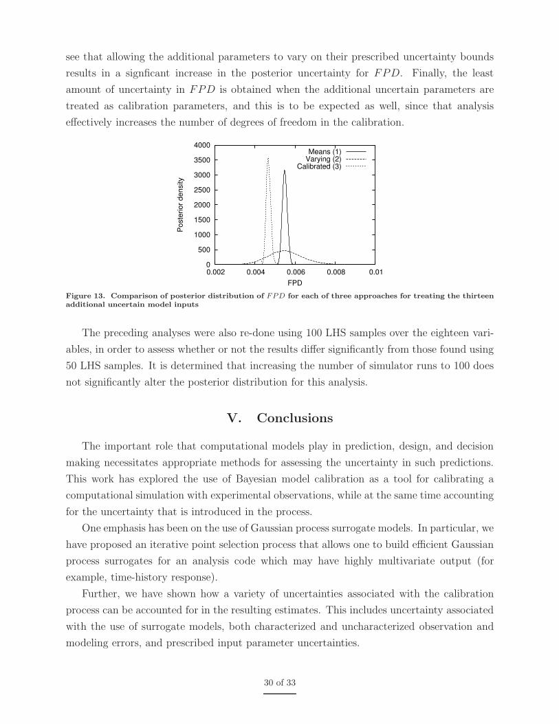
see that allowing the additional parameters to vary on their prescribed uncertainty bounds

results in a signficant increase in the posterior uncertainty for FPD. Finally, the least

amount of uncertainty in FPD is obtained when the additional uncertain parameters are

treated as calibration parameters, and this is to be expected as well, since that analysis

effectively increases the number of degrees of freedom in the calibration.

0

500

1000

1500

2000

2500

3000

3500

4000

0.002 0.004 0.006 0.008 0.01

Po

ste

rio

r d

en

sity

FPD

Means (1)Varying (2)

Calibrated (3)

Figure 13. Comparison of posterior distribution of FPD for each of three approaches for treating the thirteenadditional uncertain model inputs

The preceding analyses were also re-done using 100 LHS samples over the eighteen vari-

ables, in order to assess whether or not the results differ significantly from those found using

50 LHS samples. It is determined that increasing the number of simulator runs to 100 does

not significantly alter the posterior distribution for this analysis.

V. Conclusions

The important role that computational models play in prediction, design, and decision

making necessitates appropriate methods for assessing the uncertainty in such predictions.

This work has explored the use of Bayesian model calibration as a tool for calibrating a

computational simulation with experimental observations, while at the same time accounting

for the uncertainty that is introduced in the process.

One emphasis has been on the use of Gaussian process surrogate models. In particular, we

have proposed an iterative point selection process that allows one to build efficient Gaussian

process surrogates for an analysis code which may have highly multivariate output (for

example, time-history response).

Further, we have shown how a variety of uncertainties associated with the calibration

process can be accounted for in the resulting estimates. This includes uncertainty associated

with the use of surrogate models, both characterized and uncharacterized observation and

modeling errors, and prescribed input parameter uncertainties.

30 of 33

We have applied this methodology to an expensive thermal simulation of a “foam in

a can” system with a database of time-dependent experimental observations. The results

illustrate the ability of the Bayesian method to provide a comprehensive representation of

the uncertainty present in the resulting parameter estimates, but we have also shown that

the point estimates obtained from our analysis are not only very efficient (in terms of number

of runs of the FEM simulation), but also very accurate, and competitive with other methods

not providing an uncertainty representation.

Acknowledgments

This study was partly supported by funds from the National Science Foundation, through

the IGERT multidisciplinary doctoral program in Risk and Reliability Engineering at Van-

derbilt University, and partly by funds from Sandia National Laboratories, Albuquerque,

NM through summer internship for the first author. The first author would also like to

acknowledge helpful discussions with Youssef Marzouk regarding the theory of Bayesian in-

ference for inverse problems, and valuable assistance from Tarn Duong for contour plotting

of bivariate density estimates.

References

1Campbell, K., “A brief survey of statistical model calibration ideas,” International Conference on

Sensitivity Analysis of Model Output , 2004.

2Vecchia, A. and Cooley, R., “Simultaneous confidence and prediction intervals for nonlinear regression

models, with application to a groundwater flow model,” Water Resources Research, Vol. 23, No. 7, 1987,

pp. 1237–1250.

3Beven, K. and Binley, A., “The future of distributed models: model calibration and uncertainty

prediction,” Hydrological Processes , Vol. 6, 1992, pp. 279–298.

4Stigter, J. and Beck, M., “A new approach to the identification of model structure,” Environmetrics ,

Vol. 5, 1994, pp. 315–333.

5Banks, H., “Remarks on uncertainty assessment and management in modeling and computation,”

Mathematical and Computer Modeling, Vol. 33, 2001, pp. 33–47.

6Kennedy, M. C. and O’Hagan, A., “Bayesian calibration of computer models,” Journal of the Royal

Statistical Society B , Vol. 63, No. 3, 2001.

7Rasmussen, C., Evaluation of Gaussian processes and other methods for non-linear regression, Ph.D.

thesis, University of Toronto, 1996.

8Santner, T., Williams, B., and Noltz, W., The Design and Analysis of Computer Experiments,

Springer-Verlag, New York, 2003.

9Ripley, B., Spatial Statistics , John Wiley, New York, 1981.

10Stein, M., Interpolation of Spatial Data: Some Theory for Kriging, Springer Series in Statistics,

Springer-Verlag, New York, 1999.

31 of 33

11Martin, J. and Simpson, T., “Use of kriging models to approximate deterministic computer models,”

AIAA Journal , Vol. 43, No. 4, 2005, pp. 853–863.

12Simpson, T., Peplinski, J., Koch, P., and Allen, J., “Metamodels in computer-based engineering deisgn:

survey and recommendations,” Engineering with Computers , Vol. 17, No. 2, 2001, pp. 129–150.

13Bayarri, M. J., Berger, J. O., Higdon, D., Kennedy, M. C., kottas, A., Paulo, R., Sacks, J., Cafeo,

J. A., Cavendish, J., Lin, C. H., and Tu, J., “A framework for validation of computer models,” Tech. Rep.

128, National Institute of Statistical Sciences, 2002.

14Kennedy, M. C. and O’Hagan, A., “Supplementary details on Bayesian calibration of computer codes,”

University of Sheffield, Sheffield, 2000, Available from http://www.shef.ac.uk/∼st1ao/ps/calsup.ps.

15Cormen, T., Leiserson, C., Rivest, R., and Stein, C., Introduction to Algorithms , MIT Press, 2001.

16Trucano, T., Swiler, L., Igusa, T., Oberkampf, W., and Pilch, M., “Calibration, validation, and

sensitivity analysis: what’s what,” Reliability Engineering and System Safety, Vol. 91, 2006.

17Marzouk, Y., Najm, H., and Rahn, L., “Stochastic spectral methods for efficient Bayesian solution of

inverse problems,” Journal of Computational Physics, Vol. 224, No. 2, June 2007, pp. 560–568.

18Hastings, W. K., “Monte Carlo sampling methods using Markov chains and their applications,”

Biometrika, Vol. 57, 1970, pp. 97–109.

19Metropolis, N., Rosenbluth, A., Rosenbluth, M., Teller, A., and Teller, E., “Equations of state calcu-

lations by fast computing machines,” Journal of Chemical Physics, Vol. 21, 1953, pp. 1087–1092.

20Chib, S. and Greenberg, E., “Understanding the Metropolis-Hastings algorithm,” American Statisti-

cian, Vol. 49, 1995, pp. 327–335.

21Giunta, A. A., McFarland, J. M., Swiler, L. P., and Eldred, M. S., “The promise and peril of uncertainty

quantification using response surface approximations,” Structure and Infrastructure Engineering, Vol. 2, No.

3–4, 2006, pp. 175–189.

22Erickson, K., Trujillo, S., Oelfke, J., Thompson, K., Hanks, C., Belone, B., and Ramirez, D.,

“Component-scale Removable Epoxy Foam (REF) thermal decomposition experiments (”MFER” series)

Part 1: Temperature data,” Sandia National Laboratories report in revision.

23Romero, V., Shelton, J., and Sherman, M., “Modeling boundary conditions and thermocouple re-

sponse in a thermal experiment,” Proceedings of the 2006 International Mechanical Engineering Congress

and Exposition, No. IMECE2006-15046, ASME, Chicago, IL, November 2006.

24Sandia National Laboratories, Albuquerque, NM, Calore: a computational heat transfer program. Vol.

2 user reference manual for Version 4.1 , 2005, Available from http://www.scico.sandia.gov/calore.

25Bernardo, M. C., Buck, R. J., Liu, L., Nazaret, W. A., Sacks, J., and Welch, W. J., “Integrated

circuit design optimization using a sequential strategy,” IEEE Transactions on Computer Aided Design of

Integrated Circuits and Systems, Vol. 11, 1992, pp. 361–372.

26Craig, P. S., Goldstein, M., Seheult, A. H., and Smith, J. A., “Bayes linear strategies for matching

hydrocarbon reservoir history,” Bayesian Statistics 5 , edited by J. M. Bernardo, J. O. Berger, A. P. Dawid,

and A. F. M. Smith, Oxford University Press, Oxford, 1996, pp. 69–95.

27Aslett, R., Buck, R. J., Duvall, S. G., Sacks, J., and Welch, W. J., “Circuit optimization via sequential

computer experiments: design of an output buffer,” Applied Statistics , Vol. 47, 1998, pp. 31–48.

28Eldred, M., Brown, S., Adams, B., Dunlavy, D., Gay, D., Swiler, L., Giunta, A., Hart, W., Watson,

J., Eddy, J., Griffin, J., Hough, P., Kolda, T., Martinez-Canales, M., and Williams, P., “DAKOTA, a

multilevel parallel object-oriented framework for design optimization, parameter estimation, uncertainty

32 of 33

quantification, and sensitivity analysis: Version 4.0 reference manual,” Tech. Rep. SAND2006-4055, Sandia

National Laboratories, October 2006.

29Lee, P., Bayesian Statistics, an Introduction, Oxford University Press, Inc., New York, 2004.

30Silverman, B., Density Estimation for Statistics and Data Analysis , Chapman & Hall/CRC, New York,

1986.

31Jones, D., Perttunen, C., and Stuckman, B., “Lipschitzian optimization without the Lipschitz con-

stant,” Journal of Optimization Theory and Application, Vol. 79, 1993, pp. 157–181.

33 of 33