calibration and extension of a discrete event operations

Air Force Institute of TechnologyAFIT Scholar

Theses and Dissertations Student Graduate Works

3-21-2013

Calibration and Extension of a Discrete EventOperations Simulation Modeling Multiple Un-Manned Aerial Vehicles Controlled by a SingleOperatorJonathan W. Welborn

Follow this and additional works at: https://scholar.afit.edu/etd

Part of the Systems Engineering Commons

This Thesis is brought to you for free and open access by the Student Graduate Works at AFIT Scholar. It has been accepted for inclusion in Theses andDissertations by an authorized administrator of AFIT Scholar. For more information, please contact [email protected].

Recommended CitationWelborn, Jonathan W., "Calibration and Extension of a Discrete Event Operations Simulation Modeling Multiple Un-Manned AerialVehicles Controlled by a Single Operator" (2013). Theses and Dissertations. 1019.https://scholar.afit.edu/etd/1019

https://scholar.afit.edu?utm_source=scholar.afit.edu%2Fetd%2F1019&utm_medium=PDF&utm_campaign=PDFCoverPages

https://scholar.afit.edu/etd?utm_source=scholar.afit.edu%2Fetd%2F1019&utm_medium=PDF&utm_campaign=PDFCoverPages

https://scholar.afit.edu/graduate_works?utm_source=scholar.afit.edu%2Fetd%2F1019&utm_medium=PDF&utm_campaign=PDFCoverPages

https://scholar.afit.edu/etd?utm_source=scholar.afit.edu%2Fetd%2F1019&utm_medium=PDF&utm_campaign=PDFCoverPages

http://network.bepress.com/hgg/discipline/309?utm_source=scholar.afit.edu%2Fetd%2F1019&utm_medium=PDF&utm_campaign=PDFCoverPages

https://scholar.afit.edu/etd/1019?utm_source=scholar.afit.edu%2Fetd%2F1019&utm_medium=PDF&utm_campaign=PDFCoverPages

mailto:[email protected]

CALIBRATION AND EXTENSION OF A DISCRETE EVENT OPERATIONS SIMULATION MODELING MULTIPLE UN-MANNED AERIAL VEHICLES

CONTROLLED BY A SINGLE OPERATOR

THESIS

Jonathan W. Welborn, BS

Major, USA

AFIT-ENV-13-M-34

DEPARTMENT OF THE AIR FORCE

AIR UNIVERSITY

AIR FORCE INSTITUTE OF TECHNOLOGY

Wright-Patterson Air Force Base, Ohio

DISTRIBUTION STATEMENT A

APPROVED FOR PUBLIC RELEASE; DISTRIBUTION IS UNLIMITED

The views expressed in this thesis are those of the author and do not reflect the official policy or position of the United States Air Force, Department of Defense, or the United States Government. This material is declared a work of the U.S. Government and is not subject to copyright protection in the United States.

AFIT-ENV-13-M-34



THESIS

Presented to the Faculty

Department of Systems Engineering

Graduate School of Engineering and Management

Air Force Institute of Technology

Air University

Air Education and Training Command

In Partial Fulfillment of the Requirements for the

Degree of Master of Science in Systems Engineering

Jonathan W. Welborn, BS

Major, USA

March 2013

DISTRIBUTION STATEMENT A

APPROVED FOR PUBLIC RELEASE; DISTRIBUTION IS UNLIMITED

AFIT-ENV-13-M-34



Jonathan W. Welborn, BS Major, USA

Approved:

___________________________________ __________ John M. Colombi, PhD (Chairman) Date ___________________________________ __________ David R. Jacques, PhD (Member) Date ___________________________________ __________ John J. Elshaw, Lt Col, USAF (Member) Date

AFIT-ENV-13-M-34

iv

Abstract

As Unmanned Aerial Vehicles continue to take a greater role in modern military

affairs, the Department of Defense is seeking ways to increase autonomy and to improve

interoperability – both within systems of UAVs and between UAVs and the operators

that use them. The next step for small UAVs in this direction is for one operator to be

able to control multiple UAVs. New tools and capabilities require new tactics,

techniques, and procedures to obtain optimal results. There is also a need for a more

realistic and versatile simulation that can be used for mission planning to represent the

expected results of UAV operations under a wide variety of conditions.

This research improved a simulation that models a single operator responsible for

multiple UAV rovers. The improvement calibrated the model by increasing the realism

of its expected time that the target will be within the field of view of a UAV’s camera and

how much of that will be observed by an operator that has multiple tasks to perform

throughout the mission.

The calibration was derived from multiple flight tests, by using a Field of View

Algorithm in MATLAB and by visually recording times for loiter loops by hand. It was

determined that the target will be within the field of view of a UAV loitering in a circular

pattern between 62% and 66% of the overall loiter time. For an 8 hour beyond line of

sight mission, the model’s optimal results were 145 min of Value Added Time in low

wind conditions and 137 min in high wind. For an 8 hour within line of sight mission,

the optimal mean was 287 min in low wind conditions and 268 min in high wind.

AFIT-ENV-13-M-34

v

Keep Studying!

(to Mike and Kamilla)

vi

Acknowledgments

This thesis integrated multiple varied tools and fields. It took a great effort on the

part of a great many people in order to bring this research and analysis to fruition. First, I

would like to thank Dr. John Colombi for his help in identifying potential research ideas

and for providing course corrections along the way. Dr. Colombi also spent a

considerable amount of time and effort on the manipulation and modification of the

MATLAB Field of View Algorithm. I could not have asked for a better thesis advisor.

Dr. Jacques set the AFIT UAV Team up for success by ensuring it received the

funding and resources it needed. He also supported the AFIT UAV Team’s testing

efforts, both in the planning and execution stages.

The flight tests would never have taken place without the tremendous assistance

of Don Smith and Rick Patton from Cooperative Engineering Solutions, Inc. Their

assistance in modifying, maintaining, and repairing the Un-manned Aerial Vehicles was

invaluable. Their experience and expertise were also critical in the execution of flight

tests.

Camp Atterbury should be recognized for allowing the AFIT UAV Team to use

its runway and airspace for the purpose of flight testing. First Lieutenant Charlie Neal

provided critical assistance in transforming telemetry logs into data that could be used in

the MATLAB Field of View Algorithm.

It takes a good team to accomplish an epic work like a thesis, but it takes a great

team to make it fun!

Jonathan W. Welborn

vii

Table of Contents

Page

Abstract .............................................................................................................................. iv

Acknowledgments.............................................................................................................. vi

List of Figures .................................................................................................................... ix

List of Tables ..................................................................................................................... xi

I. Introduction .....................................................................................................................1

1.1 General Issue ............................................................................................................1 1.2 Unmanned Aerial Systems .......................................................................................1 1.3 Simulations ...............................................................................................................2 1.4 Research Objectives .................................................................................................3 1.5 Overview ..................................................................................................................5

II. Literature Review ...........................................................................................................6

2.1 Needs of the DOD ....................................................................................................6 2.2 Discrete Event Simulation .......................................................................................7

2.2.1 System Configuration.......................................................................................72.2.2 The OWL Operation Simulation ....................................................................10 2.2.3 Initial Validation ............................................................................................12

2.3 Verification and Validation of Discrete Event Simulations ...................................13 2.4 Current Status .........................................................................................................16 2.5 Conclusion .............................................................................................................17

III. Methodology ...............................................................................................................18

3.1 Conceptual Model Validation ................................................................................18 3.2 Experimental Approach .........................................................................................20

3.2.1 Testing Environment ......................................................................................20

3.2.2 Test Setup .......................................................................................................21 3.2.3 Experimental Design ......................................................................................22

3.3 Summary ................................................................................................................24

IV. Results and Analysis ...................................................................................................25

4.1 Operational Test Flight Results ..............................................................................25 4.2 Field of View Algorithms ......................................................................................28 4.3 Operations Discrete Event Simulation Results ......................................................35

4.3.1 Development of the Time Observing Target Correction Factor ....................36

viii

Page

4.3.2 Integration of the TOT Correction Factor into the Simulation ......................38 4.3.3 Modification to Value Added Sub-Model......................................................42 4.3.4 Analysis of Simulation Results ......................................................................46

V. Conclusions and Recommendations ............................................................................77

5.1 Conclusions.....................................................................................................77 5.2 Recommendations for Future Work ...............................................................80

Bibliography ......................................................................................................................83

Appendix A: ARENA Model Images ................................................................................85

Appendix B: UAV Team Flight Test Procedures ..............................................................93

Appendix C: Field of View Algorithm – Loiter Pattern .................................................104

Appendix D: Field of View Algorithm – Sensor Aimpoint ............................................111

Appendix E: Field of View Algorithm – Footprint ........................................................113

ix

List of Figures Page Figure 1: Operational View of OWL system [5] ............................................................... 9 Figure 2: Simple depiction of the modeling process (Sargent, 2009) .............................. 17 Figure 3: Flight pattern of an OWL in a circular loiter.................................................... 26 Figure 4: Flight pattern of an OWL in a racetrack loiter ................................................. 27 Figure 5: Flight pattern of an OWL in a circular loiter pattern with aimpoints included ............................................................................................................................. 30

Figure 6: Flight pattern of an OWL in a circular loiter pattern with aimpoints and footprints for one lap ......................................................................................................... 31 Figure 7: Flight pattern of an OWL in a circular loiter pattern with aimpoints for a lap and footprints for a small period of flight ................................................................... 32 Figure 8: Flight pattern of an OWL in a racetrack loiter pattern with aimpoint densities............................................................................................................................. 33 Figure 9: Flight pattern of an OWL in a racetrack loiter pattern with a few aimpoints and footprints ................................................................................................... 34 Figure 10: OWL Rover percent of Time Over Target that the UAV Observes the Target Histogram, Fit with Probability Distribution......................................................... 37 Figure 11: Implementation of theTime Observing Target Correction Factor and the Welborn Correction Factor in the Arena simulation ................................................... 40 Figure 12: Modified Value Added Sub-Model ................................................................ 43 Figure 13: Original Value Added Create Single Operator Entity Module, Operator Busy Hold Module with Time Measuring and Time Summing Modules ......... 43

Figure 14: Modified Value Added Sub-Model ................................................................ 45 Figure 15: Modified Value Added Sub-Model ................................................................ 46 Figure 16: Full Arena Model with Accompanying Sub-models ...................................... 85 Figure 17: Rover Entity Creation and Rover Pairing Logic ............................................. 86

x

Page Figure 18: Launch Process for Rover with No Relays ..................................................... 87 Figure 19: Assignment of Wind Speed Variable, Wind Speed Correction Factor, and Battery Endurance ...................................................................................................... 88 Figure 20: Rover travel to target processes....................................................................... 89 Figure 21: Time Over Target Correction Factor and Rover Travel Time to Rally ........... 90 Figure 22: Repair and Maintenance .................................................................................. 90 Figure 23: Time Over Target Sub-Model ......................................................................... 91 Figure 24: Value Added Time Sub-Model ....................................................................... 92

xi

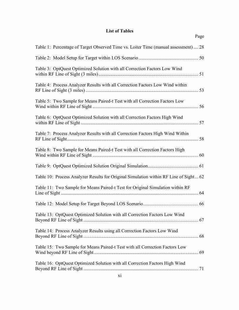
List of Tables Page Table 1: Percentage of Target Observed Time vs. Loiter Time (manual assessment) .... 28 Table 2: Model Setup for Target within LOS Scenario ................................................... 50 Table 3: OptQuest Optimized Solution with all Correction Factors Low Wind within RF Line of Sight (3 miles) ..................................................................................... 51 Table 4: Process Analyzer Results with all Correction Factors Low Wind within RF Line of Sight (3 miles) ................................................................................................ 53 Table 5: Two Sample for Means Paired-t Test with all Correction Factors Low Wind within RF Line of Sight .......................................................................................... 56 Table 6: OptQuest Optimized Solution with all Correction Factors High Wind within RF Line of Sight .................................................................................................... 57 Table 7: Process Analyzer Results with all Correction Factors High Wind Within RF Line of Sight................................................................................................................ 58 Table 8: Two Sample for Means Paired-t Test with all Correction Factors High Wind within RF Line of Sight .......................................................................................... 60 Table 9: OptQuest Optimized Solution Original Simulation ........................................... 61

Table 10: Process Analyzer Results for Original Simulation within RF Line of Sight ... 62 Table 11: Two Sample for Means Paired-t Test for Original Simulation within RF Line of Sight ..................................................................................................................... 64 Table 12: Model Setup for Target Beyond LOS Scenario ............................................... 66

Table 13: OptQuest Optimized Solution with all Correction Factors Low Wind Beyond RF Line of Sight .................................................................................................. 67

Table 14: Process Analyzer Results using all Correction Factors Low Wind Beyond RF Line of Sight .................................................................................................. 68 Table 15: Two Sample for Means Paired-t Test with all Correction Factors Low Wind beyond RF Line of Sight ......................................................................................... 69 Table 16: OptQuest Optimized Solution with all Correction Factors High Wind Beyond RF Line of Sight .................................................................................................. 71

xii

Page

Table 17: Process Analyzer Results using all Correction Factors High Wind Beyond RF Line of Sight .................................................................................................. 72 Table 18: Two Sample for Means Paired-t Test with all Correction Factors High Wind beyond RF Line of Sight ......................................................................................... 73 Table 19: OptQuest Optimized Solution Original Simulation Beyond RF Line of Sight 74 Table 20: Process Analyzer Results using Original Simulation Beyond RF Line of Sight .............................................................................................................................. 75

Table 21: Two Sample for Means Paired-t Test for Original Simulation beyond RF Line of Sight................................................................................................................ 76 Table 22: Summary Results (8 Hour Mission) ................................................................ 79

1



I. Introduction

1.1 General Issue

This thesis will seek to optimize tactics, techniques, and procedures (TTPs) for small

unmanned aerial vehicles (SUAVs), currently used by the US Army and other agencies.

The research will test the validity of a discrete event simulation to determine the optimal

TTPs for operating multiple SUAVs cooperatively in order to extend reconnaissance

range. One concept to extend range uses one SUAS as a communication “relay” vehicle

with another as the ISR “rover”. The scenarios tested in simulation will use one operator

to control one to four UAVs. These can be in the form of one to two rover/relay pairs or

one to four rovers . Two use case scenarios were selected to mirror potential scenarios

for future operators in the field.

1.2 Unmanned Aerial Systems

Unmanned aerial systems have seen extensive operations in counter-insurgency

operations in Iraq and Afghanistan over the past decade. The Army, Navy, and Air Force

each possess an arsenal of UAVs. The Navy chose to further develop the RQ-4 into the

MQ-4C BAMS UAS known as the Triton which the Navy still uses[1]. All three services

use the MQ-9 Reaper[2]. The Reaper is an upgraded version of the MQ-1 Predator[2].

The Predator is a mid-range UAV built to conduct reconnaissance at the operational

2

level[3]. The Reaper added the capability to carry a significant payload[2]. It also

extended the range and altitude of the Predator and possesses a faster top speed[2].

The focus of this thesis will be small UAVs that are used at the tactical level. The

primary SUAV to be considered is a modified version of the widely used, hand portable

tactical reconnaissance SUAV known as the RQ-11 Raven. The US Army awarded the

SUAV contract to AeroVironment in 2005 to build the Raven and it went into Full-Rate

Production in 2006[4]. As of early 2012, AeroVironment distributed over 19,000

airframes to various militaries around the world[4].

The Raven can be flown by remote control or on auto-pilot using GPS

waypoints[4]. The Raven can carry one sensor per sortie, either a color video camera or

infrared night vision camera[4]. The Raven can stay in the air for 60-90 minutes and has

an effective operational radius of approximately 10 km (6.2 miles)[4]. It weighs 4.2 lbs

and costs $35,000 for a single Raven or $250,000 for a total system including a ground

control station with applicable software and four Ravens[4].

The experimental variant to the Raven that will be used for testing is the AFIT

Overhead Watch and Loiter (OWL). The OWL shares the same airframe and propulsion

system as the Raven, but the OWL’s controls and communications hardware and

software are modified.

1.3 Simulations

The simulations used for this thesis are all discrete event simulations using

software called Arena which is licensed under Rockwell. The original simulation was

created by Capt Wellbaum in his 2010 thesis[5]. This simulation used a series of use

3

case scenarios to show the effects of the number of paired rover/relay teams (between one

and four teams) and the time between launching the paired teams on the desired outcome,

the time that a rover surveills a target (i.e. loiters over a target) and the time that a user

observes the video feedback (i.e. the operator is not performing another task requiring

his/her attention)[5]. Capt Wellbaum conducted initial simulation validation by

comparing the results of his simulation with the empirical results of test flights run at

Camp Atterbury using a single OWL[5]. Due to technical issues with the hardware, no

actual rover/relay paired flights were conducted[5].

The second iteration validation was conducted by 1Lt Cottle in his 2011 thesis

entitled “Initial Operational Validation of an Unmanned Aerial Vehicle Mission

Simulation Model”[6]. Cottle found that the endurance of the UAV in the original

simulation overestimates the endurance of the battery by 22% on average and

underestimates the occurrence of non-routine maintenance by 14% and the duration of

routine maintenance was underestimated by 15%[6]. Cottle applied correction factors to

the simulation to more closely resemble the experimental results [6]. The simulation did

not cover rover/relay pairs nor three or four simultaneous rover use cases[6].

1.4 Research Objectives

Research objectives were determined by considering the validity of assumptions

used by Wellbaum and Cottle in their thesis work for AFIT. It was determined that a

fallacy was being introduced into the simulation by a faulty assumption. The entire loiter

time over target is being used as the time observing the target, but it is common

4

knowledge among UAV operators that only a percentage of this time is actually captured

in observation or recordings. This will be the focus for this thesis.

The research questions will include:

1) What is a more realistic simulation for multiple SUAV operations?

2) How should multiple SUAVs be employed based on an improved simulation?

In order to answer these two questions, the following tasks must be performed:

1) Calibrate and extend the discrete event computer simulation that models

operations of one operator controlling multiple UAVs by developing a correction

factor to account for the intermittent loss of the target from the field of view of the

OWL’s camera.

2) Determine optimal Tactics, Techniques, and Procedures for single operators using

multiple OWLs to maximize the amount of time that an OWL is observing the

target and the operator is watching or is able to watch the video feedback (this

will be referred to from now on as Value Added Time).

The completion of these objectives will allow the military to extend the range of

its small UAVs beyond line-of-sight and to conduct operations in an optimal manner with

confidence using the new TTPs.

5

1.5 Overview

This thesis follows the standard thesis format. Chapter 1 introduces the research

topic, gives background information and definitions, and outlines the rest of the thesis.

Chapter 2 discusses relevant literature that contributed to the development of validation

techniques pertaining to discrete event simulations. Chapter 3 proposes a methodology

for validating the rover/relay discrete event operations simulation. Chapter 4 uses

empirical data to draw conclusions based on statistical comparisons to the results of the

simulation. Chapter 5 discusses the ramifications of this research and recommendations

for future work.

6

II. Literature Review

2.1 Needs of the DOD

In order to properly engineer a system, the requirements of the primary

stakeholders should be considered. This will guide and constrain how to proceed while

ensuring research is geared towards the goals of the users. At the highest level,

unmanned vehicles and systems are of vital importance because of their persistence,

versatility, and reduced risk to human life.

The Office of the Secretary of Defense created a roadmap for integrating unmanned

systems for the Department of Defense [7]. The key challenges facing the US military

with regard to unmanned systems integration are:

1) Interoperability

2) Autonomy

3) Airspace Integration

4) Communications

5) Training

6) Propulsion and Power

7) Manned-Unmanned Teaming

The first two of these challenges will coincide with the purposes of our simulation

and its subsequent calibrations. The Department of Defense goes on to state its vision for

unmanned systems which follows:

“…the seamless integration of diverse unmanned capabilities that provide flexible

options for the joint warfighter while exploiting the inherent advantages of unmanned

7

technologies, including persistence, size, speed, maneuverability, and reduced risk to

human life. DOD envisions unmanned systems seamlessly operating with manned

systems while gradually reducing the degree of human control and decision making

required for the unmanned portion of the force structure [7].”

The simulation used in this thesis provides a forward look at a type of surveillance

that utilizes an increased ratio of unmanned to manned forces and greater autonomy and

interoperability in order to achieve greater results envisioned by the Department of

Defense.

The purposes of this thesis will especially center on the battlespace awareness.

The simulation is seeking out ways to enhance surveillance through cooperative UAV

paired teams. Greater confidence in the optimal way to operate these teams will ensure

that they are used to their greatest effect.

2.2 Discrete Event Simulation

2.2.1 System Configuration

The system prototype developed by Wellbaum [5] was given the designation of

OWL (Overhead Watch and Loiter). This thesis, however, will use the term OWLs to

represent the small un-manned aerial vehicles that either conduct aerial reconnaissance

(the rover) or act as an airborne communications hub which relays communications from

the rover to the ground station (the relay). The operational concept (OV-1 diagram) on

the following page is a visual overview of how the system’s sub-components work

together to complete the reconnaissance mission. In the scenario depicted, a single

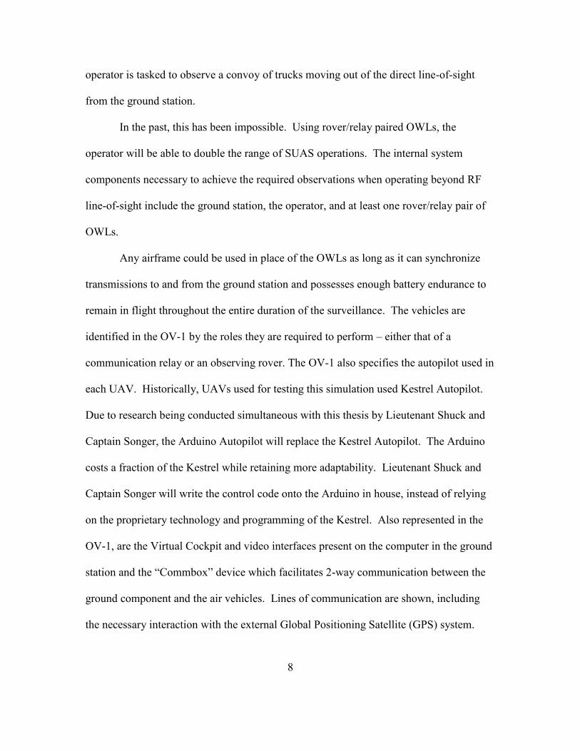
8

operator is tasked to observe a convoy of trucks moving out of the direct line-of-sight

from the ground station.

In the past, this has been impossible. Using rover/relay paired OWLs, the

operator will be able to double the range of SUAS operations. The internal system

components necessary to achieve the required observations when operating beyond RF

line-of-sight include the ground station, the operator, and at least one rover/relay pair of

OWLs.

Any airframe could be used in place of the OWLs as long as it can synchronize

transmissions to and from the ground station and possesses enough battery endurance to

remain in flight throughout the entire duration of the surveillance. The vehicles are

identified in the OV-1 by the roles they are required to perform – either that of a

communication relay or an observing rover. The OV-1 also specifies the autopilot used in

each UAV. Historically, UAVs used for testing this simulation used Kestrel Autopilot.

Due to research being conducted simultaneous with this thesis by Lieutenant Shuck and

Captain Songer, the Arduino Autopilot will replace the Kestrel Autopilot. The Arduino

costs a fraction of the Kestrel while retaining more adaptability. Lieutenant Shuck and

Captain Songer will write the control code onto the Arduino in house, instead of relying

on the proprietary technology and programming of the Kestrel. Also represented in the

OV-1, are the Virtual Cockpit and video interfaces present on the computer in the ground

station and the “Commbox” device which facilitates 2-way communication between the

ground component and the air vehicles. Lines of communication are shown, including

the necessary interaction with the external Global Positioning Satellite (GPS) system.

9

The Operational View for the entire small un-manned aerial system is in Figure 1 on the

following page:

The airframe that will be utilized for this thesis, the OWL, is based on the U.S.

Army’s RQ-11A Raven UAV. The original aircraft was acquired and modified to fit

AFIT’s research purposes with a new power plant and new autopilot and communications

system. More details of the modifications and other detailed descriptions of the vehicle

can be found in Section 3.2.2 of Seibert, Stryker, Ward, & Wellbaum [5].

Figure 1: Operational View of OWL system [5]

10

2.2.2 The OWL Operation Simulation

The original simulation, created by Capt. Chris Wellbaum in 2010 [5], utilized

four use case scenarios:

1) Stationary target within line of sight (LOS) [requiring only a rover]

2) Stationary target beyond line of sight [requiring a rover/relay pair]

3) Obscured stationary target beyond RF range [requiring a rover/relay pair]

4) Moving target missions within and beyond LOS

All UAVs in the operation will be controlled by one operator in the simulation.

The purpose of the operations simulation was to determine the optimal tactics, techniques,

and procedures to be used in such use cases where a rover will need to have its range

extended by pairing it with a relay UAV.

The two measures of performance developed for the purpose of the simulation and

consequent validation were Time Over Target (TOT) and Total Value Added Time

(TVAT). These were both used as dependent variables in the experiments. Time Over

Target describes the amount of time that a UAV was observing a given target. Total

Value Added Time consists of the time that a UAV is observing a target, i.e. the time that

the UAV is loitering over the target in a surveillance pattern, simultaneously with the

operator observing the video feedback, i.e. not being busy maintaining, repairing,

launching or retrieving another UAV.

The original simulation used two independent variables per use case scenario.

These independent variables that would be input into the simulation to determine effects

on the desired outcome are the total number of rover/relay paired UAVs and the Time

Between Initial Paired Launch (TBIPL). It was assumed that both rover and relay would

11

be launched together because one relay could communicate with only one rover. This

also has a simplifying effect on the simulation because the endurance times for both

batteries can be assumed to be the same. The number of rover/relay pairs were varied

from one to four by increments of one. The Time Between Initial Paired Launch varied

from launching one immediately after the other (0 minutes TBIPL) to waiting 40 minutes

between each paired launch with increments of ten minutes. The distance to target in

each scenario is varied to understand the effects of distance on the dependent input

variables discussed above.

The simulation starts by launching one or more rover/relay teams [or rovers when

the target is within line of sight]. The UAVs fly to the target and loiter there until the

battery only has enough power left to return to the operator. At this time, the UAV

returns to the operator and “Lands”. The operator performs necessary preparatory

maintenance, called “Turning” in the simulation, represented by a probability distribution.

The operator will then determine if there is time to fly another sortie before the end of

mission time. If the operator determines that enough time exists, the operator will

“Retrieve the UAV” and re-launch the aircraft. Otherwise, the operator will cease

operations. All times associated with these actions are based off of probability

distributions using means and variances arrived at by numerous tests.

The only time that was not based on a distribution is the time to “Fix an OWL”.

Due to lack of empirical data on the time it takes to fix an OWL, the simulation designer

asked the experts. The experts stated that five minutes was the average time to fix an

OWL with a minimum of 3 minutes and a max of 10 minutes. However, these numbers

were based off of expert opinion and not empirical data. A triangular distribution was

12

given to this event. Therefore, any time an OWL develops a problem, the simulation will

assign a number between 3 and 10 minutes according to a triangular distribution with a

mean of five.

This assumption is not an accurate reflection of the variance involved in repair

times or in the distribution of repair times. This would be a primary cause of friction

between the simulation results and actual results as will be discussed in the next section.

The original simulation accounts for repair time for broken OWLs by assigning

each sortie a 1% chance of breaking. This also turned out to be an issue that will be

discussed in the next section. Each time an OWL needed repair, it was assigned a hold

module which kept the OWL from flying until it was fixed according to the triangular

probability distribution listed above.

2.2.3 Initial Validation

Initial Validation was conducted by First Lieutenant Cottle in his 2011 thesis. He

conducted flight tests to determine the validity of the 2010 operational model. The

empirical evidence suggests that the endurance of the aircraft were over-estimated by

22% in two cases and 100% on the third, that the occurrence of non-routine maintenance

was under-estimated by about 14%, and that the duration of routine maintenance was

over-estimated by 15% [6].

Cottle hypothesized that the over-estimation of battery endurance was caused by

the fact that Wellbaum’s simulation allowed the aircraft to fly until the batteries were

completely exhausted. When conducting operations, however, the operator never allows

the aircraft to fly until the battery is completely exhausted because the measurement of

13

the voltage is not precise. This would pose a considerable risk of losing the aircraft or

damaging the batteries. Therefore, operators adopt a cushion when flying the OWLs to

ensure that the battery voltage does not go below a reasonable level before returning the

OWL to the operator. Also, strong wind gusts have negative effects on the battery

endurance. This was not accounted for in the original simulation.

Cottle also states that the non-routine maintenance actions recorded did not fit

neatly into the triangular distribution for the Repair process. This casts doubt on the

validity of this probability distribution.

After determining gaps between the simulation results and experimental results,

Cottle created correction factors and applied them to the simulation’s probability

distributions to achieve more accurate simulation results.

2.3 Verification and Validation of Discrete Event Simulations

Verification is defined by Banks, Carson II, Nelson, & Nicol [8] as “…assur[ing]

that the conceptual model is reflected accurately in the operational model.” The purpose

of model verification, in other words, is to ensure that the model is functioning properly

according to its design.

Validation is “…the overall process of comparing the model and its behavior to

the real system and its behavior” [8] . So, validation seeks to ensure that the model inputs

the relevant parameters and result in the same output that you would expect from the

actual system. A hard look must be taken at the assumptions necessary for the simulation

and their effects on the outcome of the simulation. Validation often uses statistical

analysis to determine how accurately the behavior of the model should reflect that of the

14

system.

When it comes to validation, there are four areas that must be checked. A proper

validation must check the validity of the input data, the transformative model, the output

data, and the assumptions. It is helpful to identify the required amount of accuracy for

each validation [9].

Before starting validation, a framework should be established. Naylor and Finger

[10] put forth a three step process for validating models that will serve as a foundation for

this calibration:

“Step 1. Build a model that has high face validity.

Step 2. Validate the assumptions.

Step 3. Compare the model input-output transformations to corresponding input-

output transformations for the real system.”

This thesis is a prime example of a calibration. The term “calibration” refers to

the iterative process of validation. Each time a modeler compares the simulation to the

real system, adjustments are made. Each time adjustments are made, the modeler must

compare the revised simulation to the system being modeled[8]. This validation will be

the third iteration in the calibration sequence.

Validation of assumptions should actually be conducted as soon as the face

validity is confirmed. The assumptions must match the system operation to a high degree

of fidelity. Variables can be assumed out of the simulation only if they do not affect the

outcome of the system [8]. Assumptions can be useful tools to simplify simulations, but

if a different outcome is possible from an assumption proving false, the decision maker

should receive this information before making the decision.

15

For this specific calibration of the simulation model, data collection will be of

vital importance. Before the simulation can be validated, the data should be validated

[11]. Data validation is often not conducted because it is “difficult, time consuming, and

costly to obtain sufficient, accurate, and appropriate data” [12]. Two issues in data

validation that should be considered are [11]:

1) How should the trial be designed?

2) What data should be collected?

Often during data collection, it is impossible to obtain a large enough sampling to

provide statistical validity [11]. This can be problematic and could potentially pose a

problem for the OWL operation simulation as there is limited time to conduct flights.

Cowdale recommends Design of Experiments methodology to plan data collection

techniques [11].

When it comes to data collection, Cowdale makes 6 recommendations to be

successful [11]:

1) “Think very hard about what you want.

2) If in doubt collect it.

3) Make sure you are collecting what you think you are collecting.

4) Ensure you document what you collected and what you didn’t

5) If possible confirm via two sources.

6) Remain Flexible.”

These tips will be useful when designing and executing future experiments.

Checking the face validity is the first step in validating the transformative model.

Face validity is the reasonableness of the simulation when compared to the system by

16

experts. Sensitivity analyses are often used to check the model’s face validity [13].

The final validation is output analysis. Balci recommends using design of

experiments and statistical inference for output analysis [13]. Techniques of output

analysis follow [8], [14]:

1. Response-surface methodologies can be used to find the optimal combination of

parameter values which maximize or minimize the value of a response variable.

2. Factorial designs can be employed to determine the effect of various input

variables on an output variable.

3. Variance reduction techniques can be employed to determine the effect of various

input variables on an output variable.

4. Ranking and selection techniques can be implemented to obtain greater

statistical accuracy for the same amount of simulation.

5. Method of replication, method of batch means, regenerative method, and others

can be used for statistical analysis of simulation output data.

2.4 Current Status

Cottle [6] referred to a diagram from Sargent’s work [15] describing the process

of model construction. For continuity and to show further progress in the iterative

calibration cycle, this illustration is shown in Figure 2 below.

17

Figure 2: Simple depiction of the modeling process (Sargent, 2009)

Wellbaum [5] established the system, created the conceptual model, and used

Arena discrete event simulation software to write the computerized model. Wellbaum

went on to conduct verification of his simulation. Cottle [6] conducted test flights to

validate the model. He then incorporated his findings back into the conceptual model and

computerized model using correction factors. Thus, the modeling process has come full

circle and is ready for the next iteration of validation.

2.5 Conclusion

The literary review covered the current body of knowledge on validation of

discrete event simulations, the past iterations of simulation validation, and introduced the

current status. Also, the original simulation was explained for background purposes. The

next chapter will explain the design of the experiments used to further calibrate the

original simulation.

18

III. Methodology

3.1 Conceptual Model Validation

The conceptual model must be considered in an attempt to validate the simulation.

First, the validation must ensure that the intent of the simulation correlates with DoD

goals. Then, the operational concept of the simulation must be compared to the actual

operation of the Raven to ensure that flaws are not being introduced into the simulation

from faulty operational assumptions. After confirming the above correlations and

assumptions, the model will possess a basic degree of fidelity in the big picture.

The first step in this validation is to ensure there is value in our use case scenarios

and our ability to simulate them. Our use case scenarios involve one to four rovers or

rover/relay pairs conducting surveillance on various targets and being operated by a

single operator. This experiment will focus on two use cases. The first use case will be a

single stationary target within line of sight. The second use case will be surveillance of a

road, where the road will be simulated by a runway.

The Chairman of the Joint Chiefs of Staff listed in its Universal Joint Task List as

a critical task for each service the surveillance of targets and environments [16].

Surveillance serves as a foundation for this simulation. Using paired rover / relay teams,

the UAVs cooperate to increase their effectiveness. This correlates well with the

guidance from the Secretary of Defense to increase interoperability. Meanwhile, the

enhanced surveillance capabilities fulfill the critical task of surveilling targets and

environments listed by the Joint Chiefs of Staff.

The Joint Capability Areas (JCAs) were created by the Department of Defense to

provide a framework for comparing capabilities and capability gaps across services. The

19

Joint Capability Areas for unmanned systems are battlespace awareness, force

application, protection, and logistics [7].

It appears that the goals of the thesis are closely aligned with those of the

Department of Defense and the Joint Chiefs of Staff. Therefore, to complete conceptual

validation, all that remains is to see if the simulation actually models what the operators

will experience.

It is not impractical to believe that operators would use OWLs in a manner similar

to current use of Ravens. Currently, operators fly one Raven as a rover at a time to

observe a given target. Users are not currently flying multiple rovers simultaneously or

using paired rover/relay teams. If, however, this thesis validates the results of prior OWL

operation simulations and funding is available, the military could adopt these Tactics,

Techniques, and Procedures.

Some assumptions must be made to conduct experiments for the OWL operations

simulation that might differ from actual operations. The test environment is an extremely

controlled environment that will be discussed below. In operations, there are many more

variables that will surely develop that are not considered in flight tests. Most of these

pertain to the difficulties of operating in a hostile environment.

The flight tests are conducted without interference. For example, in an

operational environment the repair rate used in the simulation would be much higher and

the times longer because of hostile fire. Also, the time to recover a downed or broken

UAV could be much longer. The UAV may not be recoverable at all. These are serious

differences that the simulation does not address. Obstacles and/or enemy fire can wreak

havoc on distributions established for simulation times.

20

Another assumption that is questionable is that the camera is focused on the target

100% of the time that the UAV is loitering. The camera on the OWL, as well as the

Raven, is fixed and can temporarily lose sight of the target while turning, flying in windy

conditions or from flight patterns not matching ideal patterns. Thus, further testing and

analysis is needed to find the true percentage of time that the target is in the field of view

of the camera while loitering.

This Time Loitering over Target to Time Observing Target ratio can be used to

create a correction factor and apply it to the original simulation. This correction factor

along with the factors created by Cottle should make the simulation more accurate to the

real world and more valid for any potential users.

Other assumptions hold true. The effects of strong wind gusts and user judgment

are accounted for using Cottle’s correction factors that were applied to the UAV

simulation. Since the combat effects cannot be simulated easily in a testing environment,

they must be assumed to be negligible for purposes of the simulation and testing.

3.2 Experimental Approach

3.2.1 Testing Environment

Testing will be conducted in the form of flight tests at a designated runway at

Camp Atterbury that has been of historical use to prior AFIT UAV teams. The range is

run by military personnel stationed at Camp Atterbury. Flight planning and operation is

assisted by Cooperative Engineering Solutions, Inc. (CESI). CESI consists of a small

group of contractors stationed at AFIT’s Advanced Navigation Technology (ANT)

Center. Experiments are designed and conducted by AFIT UAV team members.

21

One constraint when using the runway consists of having to share it with

helicopters on the adjacent helipad or other low flying aircraft. Clearance must always be

obtained from the tower before flying any aircraft, including the AFIT UAV Team’s

unmanned aerial vehicles.

Another environmental concern is that of weather. Strong winds, rain or lightning

can cause the flight tests to shut down. Even mild winds of 15 knots or less have been

shown to reduce battery life, thus throwing off the test results. To combat against

potential weather hazards, the AFIT UAV Team generally requests one more day than is

needed for experimentation in order to shut down operations on a day of bad weather and

still be able to gather all necessary test data by using the backup day to fly.

The AFIT OWLs are maintained and modified by the AFIT UAV Team with

Cooperative Egineering Solutions, Inc. (CESI) providing consulting, equipment support,

and flight support. During operation of the OWL at Camp Atterbury, there must always

be a certified pilot to fly the OWL manually in case of communication failure between

the OWL and the comm box. It also protects the team from losing an OWL due to GPS

failure or a failed autopilot. Finally, funding constrains the experiments that can be

conducted and the amount of data that can be collected, and tech support provided.

3.2.2 Test Setup

To record data, the OWL will send telemetry to the ground control station at a rate

of 10 times each second. This will be recorded for future analysis. Also, a video

transmitter operating on a wavelength of 5.8 MHz will be integrated into the OWL to

send video feedback to the ground station. The video will be observed on the screen as

well as recorded to DVDs for future reference.

22

3.2.3 Experimental Design

The Measure of Effectiveness used by both Wellbaum’s simulation and Cottle’s

initial validation was the Time that the OWL Observes the Target. However, the Time

Observing Target event in the simulation is assumed to be the entire time that the OWL

maintains a loiter pattern over an assigned target. The assumption is that 100% of the

time that the OWL is loitering over the target, the target is in the field of view of the

camera. This assumption is suspect and further verification is needed.

Also, the AFIT UAV Team has altered many hardware components to improve

performance and flexibility while reducing cost. The team replaced the Kestrel Autopilot

with the Arduino Autopilot which costs less and allows the UAV Team to add its own

code. This brings into question the input data distributions developed by Wellbaum and

the correction factors used by Cottle.

For these purposes, the AFIT Team will execute a series of test flights to train and

familiarize the team members, evaluate the equipment, and to gather information for

simulation validation purposes.

First, the AFIT UAV Team will fly a series of familiarization flights over the

course of two days. The goal for these flights is to certify team members on UAV

operations conducted at Camp Atterbury. The team will familiarize itself with range

safety, UAV operations, flight software, and UAV maintenance. The OWL will be the

primary vehicle for these flights. The UAV Team will fly two OWLs on autopilot

simultaneously to ensure equipment and user operations are functional.

23

The second flight test series will take place at Camp Atterbury over two days.

The flight test will verify the new autopilot and the inter-communications between

OWLs. There will be no operational data gathered at this flight test.

The third flight test series will take place at Camp Atterbury over the course of

three days. There are multiple test objectives for this flight test. Six test objectives will

be to further verify the functionality of the hardware. These are necessary, but not

necessarily relevant to the efforts of this thesis. The seventh test objective will further the

purposes of this thesis.

The seventh test objective is to determine the ratio of time that an OWL keeps a

target in its field of view to the amount of time that the OWL loiters around the target.

This will potentially give a correction factor to apply to Wellbaum’s operation

simulation.

For the purpose of accomplishing this test objective, the UAV Team will fly the

OWL in an operational manner for no less than 30 minutes using two use cases. The first

use case will have a single OWL monitoring a stationary target within communications

line of sight. The OWL will fly directly to the target and will then loiter over the target.

The second use case will use the OWL to conduct surveillance on a roadway (simulated

in our experiment by a runway on the flying range plus adjacent roads). For this use

case, the OWL will fly an elongated racetrack pattern over the zone of observation.

While the OWL is flying its route and surveilling the target, it will also send video

feedback to the ground control station. There the feedback will be monitored on a screen

and recorded using a Digital Video Recorder (DVR). The data will be written onto a

DVD-R. This will allow analysis to determine the ratio in question.

24

Independent variables that will be noted for this test are wind speed, camera type,

speed of the OWL, and operating height. The camera type is side facing infrared. The

wind speed will depend on conditions. The OWL will fly at a speed of 30 mph and an

elevation of 300 feet. Further variation can be used with speed and elevation, if time and

weather permit, for a more in-depth analysis upon completion of the tests.

While one team member runs the ground control station and records telemetry

data, a second team member will observe and record data video feedback from the

operation.

3.3 Summary

The data gathered from the above experiments will be applied to the original

simulation and Cottle’s additional correction factors to enable the simulation to be

applied to the new software and hardware configuration with confidence. It will also be

used to create a new correction factor that will be applied to the primary measure of

effectiveness for the operational simulation – the Time the Target is Observed and the

Total Value Added.

25

IV. Results and Analysis

4.1 Operational Test Flight Results

The flight testing took place over a three day period from 5-7 November 2012.

Multiple sorties were flown. Winds throughout the test period were low, between 0-5

mph with gusts up to 10 mph. The temperature ranged from 25 – 50 degrees Fahrenheit.

A hardware problem burned out the cameras in the nose cones of the OWLs by

the end of the first day. However, telemetry was recorded from three operational test

flights and video was recorded from a fourth. These data points will serve as input data

that will be analyzed and transformed into a distribution that can be used in the

simulation.

The flight tests were designed to resemble tactical surveillance missions. The two

scenarios used were the overhead circular loiter and the overhead racetrack pattern. The

circular overhead loiter pattern was re-created, using actual telemetry from a test flight,

via a MATLAB algorithm to estimate camera aimpoint and zero elevation footprint. This

will be discussed in greater detail in Section 4.2. Figures 3-9 were all created using the

aforementioned MATLAB algorithm. Figure 3, on the following page, used the

MATLAB algorithm to plot the flight path of an OWL in a circular loiter pattern:

26

Figure 3: Flight pattern of an OWL in a circular loiter

The same program was used to re-create the flight of a racetrack pattern loiter that

was used to monitor a runway (used to represent monitoring a road). It can be seen in the

pattern the effects that even a light wind can have on the loiter pattern. The racetrack

loiter pattern can be seen in Figure 4:

27

Figure 4: Flight pattern of an OWL in a racetrack loiter

The curve in the middle of the pattern was part of its launch and approach to the

pattern. These data points were not considered when determining the percentage of the

time that the OWL was observing the target.

The circular loiter pattern represent the surveillance of a stationary target. The

racetrack pattern represents the surveillance of a road. Video feedback was only gathered

on the racetrack pattern loiter. This data was recorded and measured to provide the

following results where each observation represents one complete lap and the percentage

of time that the runway could be seen:

28

Table 1: Percentage of Target Observed Time vs. Loiter Time (manual assessment)

Racetrack Pattern Lap 1 65% Racetrack Pattern Lap 2 60% Racetrack Pattern Lap 3 57% Racetrack Pattern Lap 4 68% Racetrack Pattern Lap 5 66% Racetrack Pattern Lap 6 60%

The amount of time the camera is focused on the target should closely resemble

that of the tactical scenarios. One constraint that might alter the results is that, during the

test for the roadway surveillance scenario, the target was limited to the length of the

runway. With a longer target, such as a roadway, the turn time would be less. This

would cause tactical missions to have a higher ratio of time that the target is observed

compared to total loiter time. Also, the calm winds will result in a higher ratio of the

same statistic for tests as opposed to expected results for flights on windy days.

On the third day of flight testing, another surveillance mission was flown utilizing

both scenarios but without any video feedback. This was to increase the sample size

from which telemetry data for the tactical mission set will be drawn.

4.2 Field of View Algorithms

In order to determine a more precise method of measuring target observed time

versus loiter time (and to be able to use telemetry data from flight tests), an algorithm

written in MATLAB was used. This algorithm originally came from Lozano’s thesis

work in 2011[17]. It was slightly modified to better comply with our sorties (both

clockwise and counterclockwise loiters).

29

The Sensor Aimpoint function takes location, attitude and camera selection.

Location of the UAV is expressed in meters (latitude, longitude and elevation) in relation

to the start point or base, in a North (positive x axis), West (positive y axis) frame.

Attitude reflects the yaw, pitch, and roll in an aircraft reference frame. Positive yaw is

counter-clockwise, positive pitch is nose up and positive roll is counterclockwise (right

wing up). The camera assumes a RAVEN RQ-11 body which has a nose with two

cameras out the front and left side (90 degree yaw from nose). The left camera is

depressed toward the ground 39 degrees. The front sensor is depressed toward the

ground by 49 degrees. While the RAVEN RQ-11 body does not have a right side

camera, we assume one could be present with the same 49 degree downward look angle

as the left.

The Sensor Footprint function also written in MATLAB takes location, attitude

and camera selection. However, this MATLAB function also makes use of the camera

field of view (FOV) to project a footprint (trapezoid) on the 0 elevation plane. From

earlier work by Lozano, this function assumes an approximate FOV of 48 degrees

horizontal and 40 degrees vertical, or ± 24 degrees and ± 20 degrees respectively.

Data is saved and processed every tenth of a second from the raw telemetry. For

stationary loiter points, one can check if a hypothesized target (located at the loiter point)

is contained within the sensor footprint. Then a percentage of data points that contain the

target with respect to all data point can be calculated. Two flight test scenarios, which

contain dozens of rotations around a loiter point, contained 7000 and 14,000 samples. It

should be noted changes in elevation have a distinct impact on all other aspects of the

30

simulation. The circular loiter pattern with aim points, derived using the above functions

and plotted on a two-dimensional graph, looks as follows:

Figure 5: Flight pattern of an OWL in a circular loiter pattern with aimpoints included

The above simulation included every aimpoint. This is useful for seeing the

densities of the locations of the aimpoints. The densest section forms a circle directly

around the target. A smaller radius loiter would have tightened the aimpoint density into

a solid point in the middle of the loiter rather than the empty space as seen above.

31

Next, the footprints will be added. If every footprint were included, it would be

difficult to see patterns. Therefore, one lap is observed with footprints. This can be seen

in Figure 6:

Figure 6: Flight pattern of an OWL in a circular loiter pattern with aimpoints and footprints for one lap

The effects of the wind can be seen in the erratic behavior of the green aimpoint

trace. This is a constant effect that causes the UAV to roll back and forth at a rate and

range that depend on the wind speed and rate of change. These flight tests were

conducted in low winds. However, the effects of these winds are still noticeable.

32

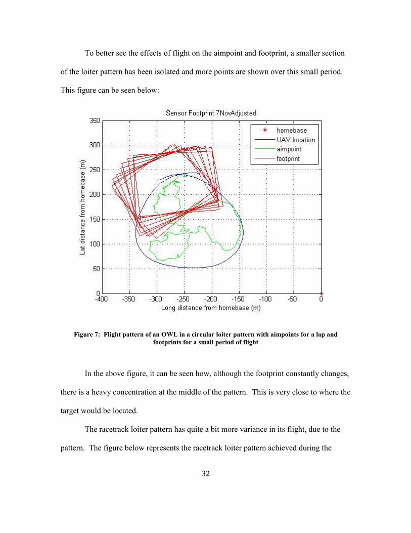
To better see the effects of flight on the aimpoint and footprint, a smaller section

of the loiter pattern has been isolated and more points are shown over this small period.

This figure can be seen below:

Figure 7: Flight pattern of an OWL in a circular loiter pattern with aimpoints for a lap and footprints for a small period of flight

In the above figure, it can be seen how, although the footprint constantly changes,

there is a heavy concentration at the middle of the pattern. This is very close to where the

target would be located.

The racetrack loiter pattern has quite a bit more variance in its flight, due to the

pattern. The figure below represents the racetrack loiter pattern achieved during the

33

flight tests conducted earlier with the location of the aimpoints on the same two-

dimensional map as was shown for the circular loiter pattern. All aimpoints for the entire

mission were included again to better see the densities. Racetrack loiter pattern with

aimpoint densities is shown below:

Figure 8: Flight pattern of an OWL in a racetrack loiter pattern with aimpoint densities

The above figure shows the effects of slight winds via the wavy motion of the

aimpoints inside the loiter pattern. The effects of sudden wind gusts can be seen during

the times where the aimpoint has left the loiter pattern entirely (evidently due to high

roll). The highest densities of aimpoints follow very closely to the linear target, i.e. the

runway representing a road.

34

When a few footprints are included in the simulation outputs you get the

following:

Figure 9: Flight pattern of an OWL in a racetrack loiter pattern with a few aimpoints and footprints

The variance in the placement and size of the footprints is easy to see. The

smaller the footprint the more the UAV was aimed straight down. The larger footprints

were caused by strong gusts of wind that caused the UAV to roll substantially. With the

exception of a few outliers, the vast majority of footprints fell around the linear target.

The above figures help understand the capabilities of the UAV and its limitations.

The flight patterns and aiming of the camera are fairly reliable but are definitely not

35

perfect. This is why there needs to be a correction factor for the amount of time that the

UAV is loitering over the target compared to the amount of time the UAV is actually

observing the target.

The modified Field of View Algorithm also gathered the percentage of time that

the target location fell inside the footprint for the circular loiter pattern. Telemetry data

for two circular loiter pattern sorties were run through the simulation. The first had

14,000 data points and resulted in a target observed time percentage of 62%. The second

simulation used 7,000 data points and resulted in a target observed time percentage of

66%.

These readings correlate very closely with the experimental flight video recording

measurements discussed earlier in this chapter that resulted in a mean target observed

time percentage of 63% and the distribution derived from input analyzer of .55 + .15 *

BETA (1.06, 1.02) that was used in the simulation to represent the target observed time

percentage (the derivation of this distribution is discussed in greater detail in Section

4.3.1 and can be seen in Figure 10). The results of the Field of View Algorithm further

strengthen the validity of the data and assumptions used for our correction factors.

4.3 Operations Discrete Event Simulation Results

The percentage of time that the OWL rover is observing the target in comparison

to the time that the OWL rover is loitering over the target (determined in sections 4.1 and

4.2) can be input into the previous two simulations as a correction factor and the results

can be compared.

36

For each simulation, a method called Common Random Numbers will be used to

obtain results that have less variance induced by the simulation. Random numbers used

in the computer simulation are not truly random. Computer programs are incapable of

creating a truly random number.

The simulation can, however, create a series of numbers that closely resemble

random numbers. By repeating the same streams of random numbers created by the

simulation, the simulation inputs the same random numbers into each varying run. This

allows the user to better focus on the variance of the operational data without introducing

variance into the system created by the random number generator.

4.3.1 Development of the Time Observing Target Correction Factor

The experimental data obtained from the flight tests must be transformed into a

correction factor that can be applied to the simulation in order to change its behavior to

more accurately reflect that of reality without changing the behavior of the other

processes already modeled.

First, the input data must be analyzed. To do this, a tool within the Rockwell

Arena software can be utilized called Input Analyzer. This tool aids in ascertaining the

best fit probability distribution to match the experimental data. The results from this

analysis are shown in Figure 10 on the following page:

37

Percentage of Target Observed Time vs. Loiter Time

Figure 10: OWL Rover percent of Time Over Target that the UAV Observes the Target Histogram, Fit with Probability Distribution

The Best Fit was applied by the Input Analyzer tool in the Arena simulation

software. The Best Fit command compares the p-values and square errors from each

distribution fit to the input data to determine the distribution that most closely resembles

the data. The results of this data input analysis showed that the Beta distribution most

closely resembles the input data. More data points from test flights would have

strengthened the conclusion that the Beta distribution is the best fit for future simulations.

Using the distribution arrived at from the Input Data Analysis Best Fit command,

the expression that best represents the experimental data, the Time Over Target

Correction Factor is derived. It will be applied when a single UAV is loitering over the

Distribution: Beta Number of Data Points 6

Expression: 0.55 + 0.15 * BETA(1.06, 1.02) Min Data Value 0.57

Square Error: 0.077647 Max Data Value 0.68

Sample Mean 0.627

Sample Std Dev 0.0427

Test Statistic 0.152

Corresponding p-value > 0.15

Histogram Range = 0.55 to 0.7

Number of Intervals 5

Distribution Summary Data Summary

Histogram Summary

Kolmogorov-Smirnov Test

Number of

Occurrences

.055 .058 .061 .064 .067 .07

0

2

1

38

target. The Time Over Target Correction Factor that will be integrated into the modified

discrete event operations simulation is shown below:

corrected_time_over_target =

(0.55 + 0.15 * BETA(1.06, 1.02)) * time_over_target

Note: where BETA represents the Beta distribution

4.3.2 Integration of the TOT Correction Factor into the Simulation

The simplest solution would be to simply multiply the un-modified Time over

Target by the average ratio received from experimentation. However, this will not be an

accurate reflection in the simulation. It does not account for the possible variation in the

ratio of time that the target is observed to time that the UAV loiters over the target.

Another way to model this would simply be to create a distribution based off of

experimental results and apply it to reduce the Time Over Target module. This would

properly reduce the amount of time that the UAV is observing the target and would

introduce the correct amount of variance by using the distribution. However, it still does

not accurately represent the effects of the broken continuum of the OWL observing the

target.

When the OWL loiters over the target, the loiter time will be represented by, for

the purposes of the simulation, the same distribution of time. If the above method were

used, the time observing the target would be diminished but without breaks. What the

simulation needs is a way to represent one to four OWLs loitering over the target and the

39

field of view of the OWLs being intermittently broken at random times that are

independent of one another.

In a one rover simulation, the above method will continue to offer the correct

solution. However, once multiple rovers have over lapping loiters over a single target, a

more sophisticated means of recording Value Added Time and Target Observed Time is

needed.

In order to assign probabilities of total failure to each set of UAVs loitering over

the target, the time that there are 1, 2, 3, or 4 UAVs loitering over the target needs to be

recorded separately.

Before the times can be recorded separately, the time of each individual UAVs

loiter time must be recorded. A module was added called “Assign Individual Flight

Times”. This module records the current simulation time (after the individual UAV has

finished observing the target and before it begins the flight back to the rally point) and

subtracts the simulation time when the UAV began its loiter over the target. This

provides the simulation with an individual loiter time for each UAV.

The simulation already has a counter to keep track of how many UAVs are

loitering over the target that gets updated whenever the number changes. This data is

time stamped in the simulation.

With the individual loiter times and the number of UAVs over the target, the

simulation can now separate the times into categories of how many UAVs were loitering

over the target simultaneously and for how long. To do this, the simulation needs a

decision module to separate the time being recorded into 1, 2, 3, or 4 UAVs. This can be

seen in Figure 11 on the following page:

40

Figure 11: Implementation of theTime Observing Target Correction Factor and the Welborn Correction Factor in the Arena simulation

After being separated into separate flows within the simulation, an assignment

module will use the Time Observing Target Correction Factor and the Welborn

Correction Factor to create the updated time that the UAV observed the target. The

assign module will then create a new variable that will represent this corrected time of

observation. The Welborn Correction Factor is a formula that is applied in the Arena

simulation to correct the time the target is observed when multiple rovers are observing

the target. The Welborn Correction Factor in Arena can be seen below:


(1-((1-(.55+.15*BETA(1.06,1.02))) (#_UAVs_over_target))) * individual_time_over_target

Note: BETA represents the Beta distribution

TargetUAVs over

Sum Time of 4

TargetUAVs over

Sum Time of 3

TargetUAVs over

Sum Time of 2

Separate into # of UAVs

#_Ov er_Targe t_Coun te r == 4

#_Ov er_Targe t_Coun te r==3

#_Ov er_Targe t_Coun te r==2Els e

1Target CorrectedAssign Time over

Corrected 4Over TargetAssign Time



UAV over TargetSum Time of 1

Flight TimesAssign Individual

CategoriesSum Times for

41

The breakdown of probabilities of observing the target during loiter by number of

UAVs loitering over the target, assuming independence, is listed below:

1 Aircraft: P (1) = .55 + 0.15 * Beta (1.06, 1.02) means approximately 62.5% of

total loiter time will be collected as coverage time

2 Aircraft: P (2) = (1-((1-(.55+.15*Beta (1.06,1.02)))2)) means approximately

85.9% of total loiter time will be collected as coverage time





The entity in the simulation then travels into another assign module that adds the

corrected time observing the target to a variable that represents the total time of its

respective number of UAVs spent observing the target.

Finally, the separate flows converge into a module, “Sum Times for Categories”,

which sums the total corrected observation times for all the categories previously

mentioned and assigns the total corrected observed time to a new variable called

“coverage_time”.

42

4.3.3 Modification to Value Added Sub-Model

The current value added sub-model acts as a switch that records time while there

is one or more UAVs over the target and the operator is available to observe the video

feedback. There is another part of the sub-model that includes logic that adds the last

loiter time into the value added or non-value added categories using the same criteria.

This must be altered by applying the correction factors developed earlier that

account for the time that the UAVs did not observe the target while loitering. Since the

formula is altered depending on how many UAVs are loitering over the target, the

simulation needs a means of separating the value added times every time the number of

UAVs loitering over the target changes.

In order to do this, a decision module was added to the value added model as can

be seen below. This module separates the value added entity into five different streams

depending on a variable that keeps track of how many UAVs are over the target at any

time. The first four flows all add value to the total of value added. The fifth flow screens

out time periods during which there is no value being added due to there being no UAV

over the target, shown below:

43

Figure 12: Modified Value Added Sub-Model

It executes the screen by looping the entity back to the original model’s “Operator

Busy” stream which records the time that there is no value being added by holding the

entity until two conditions are met: 1) the number of UAVs loitering over the target is

greater than zero and 2) the operator (represented in the simulation as a resource) is not

otherwise utilized (i.e. fixing a UAV, launching a UAV, etc…). This section of the value

added sub- model can be seen below:

Figure 13: Value Added Create Single Operator Entity Module, Operator Busy Hold Module with Time Measuring and Time Summing Modules

The modules on either side of the “Operator Busy” Hold Module measure the

amount of time that the operator spends not adding value by observing video feedback

Screen No UAVs

Separate into # of UAVs and

# _ Ov e r_ T a rg e t _ C o u n t e r= = 4



# _ Ov e r_ T a rg e t _ C o u n t e r= = 1E l s e

Variable 3Assign to a

Added Time andOperator Value

Sum Total



Sum Total



Sum Total

Screen Operator BusyT ru e

F a l s e

Added Time 3

Operator Value

TNOW 3Time Attribute to

Value AddedAssign Operator

Time Attribute 3Value Added

Assign Operator

Added Time 2

Operator Value




Assign Operator

Added Time 1

Operator Value




Assign Operator

Added Time 4

Operator Value




Assign Operator



Sum Total

0

0

OperatorCreate Single

Operator BusyTNOW

Busy Attribute toAssign Operator

AttributeBusy Time

Assign Operator

to a VariableBusy and AssignSum Total Time

0

44

from the UAV. The last module adds each recorded time to a running total of Total Busy

Time.

The evolution of the simulation shown below uses a nested loop. The criteria for

exiting the inner loop, once the value starts being added, is that either the operator

becomes busy or there are no more UAVs over the target. When the exit criteria are met,

the entity returns to the original time assignment and hold modules listed above.

The inner loop was created to keep the model adding value but to assign different

times to the value added based off of how many UAVs are over the target. More UAVs

over the target at once will reduce the intermittent loss of coverage by providing less

chance of failure to observe.

The inner loop has four possible streams. This represents there being up to four

UAVs over the target at any time. Each of the streams has a time initiator module, a hold

module, a module to assign the time of observation (after applying the correction factor)

to a variable, and a total value added variable that adds the individual value added times

together to get the total value added time for each iteration.

Each “Operator Value Added Time” hold module will hold the entity and scan for

the condition that either the operator is busy or the number of UAVs over the target has

changed. When this happens, the entity has its time that it added value recorded and

added into the sum. It then loops back to the beginning of the inner loop where it will be

screened against busy operators.

If the operator is busy, the entity is looped out of the inner loop. If the operator is

free, the entity proceeds to the separation decision module. If the change in UAVs over

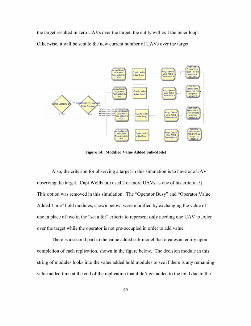
45

the target resulted in zero UAVs over the target, the entity will exit the inner loop.

Otherwise, it will be sent to the new current number of UAVs over the target.

Figure 14: Modified Value Added Sub-Model

Also, the criterion for observing a target in this simulation is to have one UAV

observing the target. Capt Wellbaum used 2 or more UAVs as one of his criteria[5].

This option was removed in this simulation. The “Operator Busy” and “Operator Value

Added Time” hold modules, shown below, were modified by exchanging the value of

one in place of two in the “scan for” criteria to represent only needing one UAV to loiter

over the target while the operator is not pre-occupied in order to add value.

There is a second part to the value added sub-model that creates an entity upon

completion of each replication, shown in the figure below. The decision module in this

string of modules looks into the value added hold modules to see if there is any remaining

value added time at the end of the replication that didn’t get added to the total due to the

Screen No UAVs

Separate into # of UAVs and




# _ Ov e r_ T a rg e t _ C o u n t e r= = 1E l s e



Sum Total



Sum Total



Sum Total

Screen Operator BusyT ru e

F a l s e

Added Time 3

Operator Value




Assign Operator

Added Time 2

Operator Value




Assign Operator

Added Time 1

Operator Value




Assign Operator

Added Time 4

Operator Value




Assign Operator



Sum Total

0

0

46

operation coming to an end. If there is an entity any of the value added hold modules, the

time is added to the total value added time.

The final value added sub-model measures the simulation time that the entity was

in the hold module. It does not give it a chance to apply the correction factor. Therefore,

this was added into the original sub-model.

Figure 15: Modified Value Added Sub-Model End of Replication

4.3.4 Analysis of Simulation Results

To better understand the effects of the correction factors, the results of the

Wellbaum simulation without correction factors will be compared to the results of the

simulation with correction factors from Cottle’s 2011 thesis and the correction factors

arrived at in this research[6]. For the sake of isolating just the changes due to the

correction factors, common random numbers will again be used for each simulation run

and the same input variables will be used.

Added TimeCollect Final Value

Final_Value EntityDispose of

NQ(Op e ra to r Va lu e Ad d e d T im e 4 .Qu e u e ) = = 1



NQ(Op e ra to r Va lu e Ad d e d T im e 1 .Qu e u e ) = = 1El s e

Operator In?

Which Queue is Single

Variable 1Value Added TimeAdd Final Time to

VariableTotal Time BusyAdd Final Time to




Added

Write Total Value

0

0

47

The tools used to analyze the output data are part of the Rockwell Arena

Simulation software suite. The tools are the OptQuest optimization tool and the Process

Analyzer tool.

OptQuest determines the optimal choice of control variables to minimize or

maximize a response variable that is named as the objective variable. The user may input

constraints for the optimization and set parameters for the control variables. The

OptQuest tool uses three replications for each scenario. It runs a different simulation for

each possible combination of control variables within the parameters set by the user.

OptQuest keeps a record of the simulation resulting in the most desirable response

variable.

All of the simulations run for this research use the Total Value Added Time as the

objective response variable. This is the total amount of time that an OWL is loitering

over the target, the target is in the field of view of an OWL, and the operator is observing

the video and not otherwise utilized. The goal for the optimization program is to

maximize the Total Value Added Time.

Process Analyzer was designed for quickly running and comparing multiple

scenarios using multiple controls. The user specifies which simulation to run and which

variables are the control and response variables. The user can then set up each desired

instantiation to observe. The Process Analyzer will continuously run through all stated

scenarios with the various values for the controls given by the user.

Process Analyzer runs as many replications as the user sets in the Arena

simulation “Run Control”. For the purposes of this work, each simulation for each

scenario is run for 100 replications. Process Analyzer then lists the mean for the 100

48

replications. This makes Process Analyzer a more accurate reflection of the most likely

results. The results from Process Analyzer can be compared with the OptQuest results,

which represent the best case scenario, to get an idea of the range of possible solutions.

The simulations that are considered modified have received not only the

correction factors from this body of work but also Cottle’s correction factors. Cottle

reduced the total battery endurance by eight minutes for a safety factor. He added a

variable for wind speed that in high wind conditions (speeds > 15 mph) further reduced

the battery endurance by an additional five minutes. He increased the chance of non-

routine maintenance from one percent to five percent and increased the repair time

distribution from TRIA(3, 5, 10) to TRIA(4, 7, 11). Finally, the time to conduct routine

maintenance was increased by 60 seconds. Each of these correction factors adds more

realism to the original scenario but diminishes the amount of time over the target from

the original.

It is also expected that the Time Over Target Correction Factor and Welborn

Correction Factors will also reduce the amount of time that the operator is able to observe

the target. Thus, the Total Value Added Time is expected to be reduced further from the

original simulation’s results.

There are three effects that are critical to the outcomes of the simulation runs.

First, the total time that there is at least one UAV over the target. An OWL will observe

the target roughly 63% of the time that it loiters overhead. Big gaps with no UAV

overhead result in a loss of the 63% observation rate.

Second, for every additional OWL that is over the target at the same time, the

percentage of time that gets recorded increases due to overlapping observation patterns

49

greatly reducing the amount of intermittently lost target observation. With four OWLs

loitering overhead the efficiency of observing the target increases to 99% of the loiter

time, assuming the causes of the intermittent losses in target observation are independent

and not caused by a single factor that has the same effect on all OWLs at one time.

The third critical factor to affect the outcome of the simulation is the amount of

time that the operator is busy and cannot observe the video feedback. The more UAVs

being used, the more tasks the operator has to perform that pull him or her from

observing video. The operator must Launch, Retrieve and Maintain each OWL. The

operator also has a 5% chance to have to have to repair an OWL for every UAV

launched. This reduces the value added time by a mean of seven minutes and can take as

much as 11 minutes.

These factors are all competing against each other to determine the optimal

solution. Also affecting the simulation is wind speed, but separate simulations will be

run for low and high wind speeds in order to further isolate this factor. High wind speeds

result in a reduction of battery endurance by five minutes. This reduction in battery

endurance, in turn, is expected to cause the UAV over target time to decrease and the

value added time to decrease.

After analyzing the results of the long distance and short distance simulations,

using independent scenarios for low and high wind, the results of the simulations will be

compared to the results of the original simulation before any of the correction factors

were included.

50

4.3.4.1 Corrected Simulation Results for Short Range, Low Wind Scenario

The first scenario for comparison will be the results of the target within radio

frequency line-of-sight (LOS) range. There will be one modified model run with low

wind conditions and another run with high wind conditions. This is not necessary with

the original model because it has no changes for either. Variables for this scenario are

defined in Table 2 below:

Table 2: Model Setup for Target within LOS Scenario

Model Setup for Target Within LOS Scenario

Constant Variables Value Independent Variables

Value

Range

#_OWL_Relays 0 #_of_OWL_Rovers 1 – 4

Mission_Length_Hours 8

Time_Between_Initial_Launch

(Minutes) 1 – 40

Rover_Max_Range_Miles 3

Distance_to_Target_Miles 3 Dependent_Variables

Speed_to_Target_MPH 30 Total_Value_Added_Time

Wind_Speed_MPH

10 (Low)

20 (High) Total_UAV_Over_Target Time

51

The optimization using Rockwell Arena’s OptQuest tool can be seen in Table 3:

The first OptQuest Optimization shows that during operations within radio

frequency line of sight and in low wind conditions (less than or equal to 15 mph), the best

outcome possible for Total Value Added Time is approximately 296 minutes. To achieve

this time, OptQuest used the combination of 4 rovers with a time between initial

launching of 32 minutes each.

Table 3: OptQuest Optimized Solution with all Correction Factors Low Wind within RF Line of Sight (3 miles)

52

The highest value added results alternate between using three and four OWLs

with neither one providing the dominant solution. This means that optimal results can be

obtained with either three or four OWLs. The difference between the top simulation and

the 25th simulation was a difference of 15 minutes Value Added Time.

The results of the Process Analyzer runs can be seen in Table 4 on the following

page:

53

Table 4: Process Analyzer Results with all Correction Factors Low Wind within RF Line of Sight (3 miles)

The Process Analyzer results above represent 100 replications for each control

set. These results give the mean of those hundred replications. This will be most useful

for predicting the most likely outcomes of varying combinations of rovers and time

54

between initial launch. All of the input variables are the same as those listed in the model

setup table previously shown.

Mean times will let us know the value that is being added to our objective

variable by increasing the number of OWLs. The mean times for value added results

follow:

1) 4 OWLs – 277 minutes (4 hours and 37 minutes)



4) 1OWL – 174 minutes (2 hours and 54 minutes)

The average time to be gained from increasing the number of OWLs goes up 26

and 24 minutes respectively for 2 and 3 OWLs versus using a single OWL. There is

added value of 103 minutes for using 4 OWLs compared to 1 OWL. This is not taking

proper Tactics, Techniques, and Procedures for times between initial launches. If proper

Time Between Initial Launch TTPs are adhered to, the results will be as follows:

1) 4 OWLs with TBIL 35 minutes – 287 minutes (4 hours and 47 minutes)



4) 1 OWL – 174 minutes (2 hours and 54 minutes)

55

This means that when the OWLs are properly utilized, there is a difference of 82,

107, and 113 minutes for 2, 3, and 4 OWLs respectively when compared to using 1

OWL.

Based on these results we see continued improvement in Value Added Time for

each OWL added into the scenario. The returns for each OWL, assuming the optimal

TBILs are always adhered to, diminish quickly so that the difference between 3 and 4

OWLs is only 6 minutes compared to a difference of 82 minutes for the first additional

OWL (for a total of 2 OWLs).

Statistical analysis was used to determine whether the differing value added times

resulting from using the TTPs recommended or not using the TTPs is statistically

significant.

The statistical method to compare the two samples was the paired-t test. The

formula used in the paired-t test can be seen in Equation 1 below:

1 2 2, 1 Dv

st R

R (Eq. 1)

Where is the mean of the MOP, SD is the standard deviation, and R is the

number of replications. The means of the total value-added time when using four OWLs

with no TTPs (i.e. the OWLs were thrown at random times between 1 and 40) was

compared to the mean of the total value-added time when four OWLs were flown using a

TBIL of 35 minutes. Nine hundred replications were run for each sample.

The results of this paired-t test can be seen in Table 5:

56

Table 5: Two Sample for Means Paired-t Test with all Correction Factors Low

Wind within RF Line of Sight

Variable 1 Variable 2

Mean 277.331888 285.7239203

Variance 2764.711865 2230.175806

Observations 900 900

Pearson Correlation 0.00243895 Hypothesized Mean Difference 0 df 899

t Stat -

3.566586349 P(T<=t) one-tail 0.000190375 t Critical one-tail 1.646550346 P(T<=t) two-tail 0.000380751 t Critical two-tail 1.962606226

Since the P(T<=t) is less than .05, we can reject the H0 and conclude that, on

average, using the recommended TBIL TTPs creates more value added than launching

the UAVs at random.

If a unit had 4 OWLs and needed to monitor a target less than three miles away

with wind speeds equal to or less than 15 mph, the optimal solution would be to use 4

OWLs and to launch them 35 minutes apart. The resulting Value Added Time for an 8

hour mission will be, on average, 4 hours and 47 minutes.

4.3.4.2 Corrected Simulation Results for Short Range, High Wind

Scenario

The next scenario mirrors the last scenario in every way except that low wind

speeds (10 mph) are used instead of high wind speeds (20 mph). This should result in a

reduced battery endurance and, therefore, less value added time. It is necessary,

however, to understand how this will affect the overall simulation.

57

The OptQuest results for the modified simulation using a high wind variable can

be seen in Table 6 below:

Table 6: OptQuest Optimized Solution with all Correction Factors High Wind within RF

Line of Sight

The top 25 results, according to OptQuest, (see above) range from 262 minutes to

272 minutes. The top results alternate between using three or four OWLs with the

number one result coming from using 4 OWLs with a TBIL of 36 minutes.

58

The results of the Process Analyzer tool using the same scenario can be seen in

Table 7 on the following page:

Table 7: Process Analyzer Results with all Correction Factors High Wind Within RF Line of Sight

The mean times for the value added times broken down by the number of OWLs

used are as follows:




4) 1 OWL – 159 minutes ( 2 hours and 39 minutes)

59

This means that an operator working in high wind conditions and launching at

random can achieve equivalent benefits from either three or four OWLs and would be

expected to achieve 257 minutes (4 hours and 17 minutes) of value added time over an

eight hour mission.

Applying proper TBIL TTPs will result in more value added time. The number of

OWLs and their respective optimal TBILs are listed below:


2) 3 OWLS with TBIL 20 minutes – 264 minutes (4 hours and 24 minutes)


4) 1 OWL – 159 minutes (2 hours and 39 minutes)

The best time expected for the value added time is 19 minutes less in high wind

than in low wind. By using Common Random Numbers and changing only the one

variable, it can be determined that the 19 minute loss of value added time can be directly

attributed to the effects of the high wind speed.

Again, we see a diminishing increase in value added time to a max with four

OWLs. In order to achieve the best results in a short distance (3 miles away) stationary

target in high wind conditions, the operator will launch all four OWLs with 30 minutes in

between each launch and will achieve 268 minutes of value added time out of a 480

minute mission.

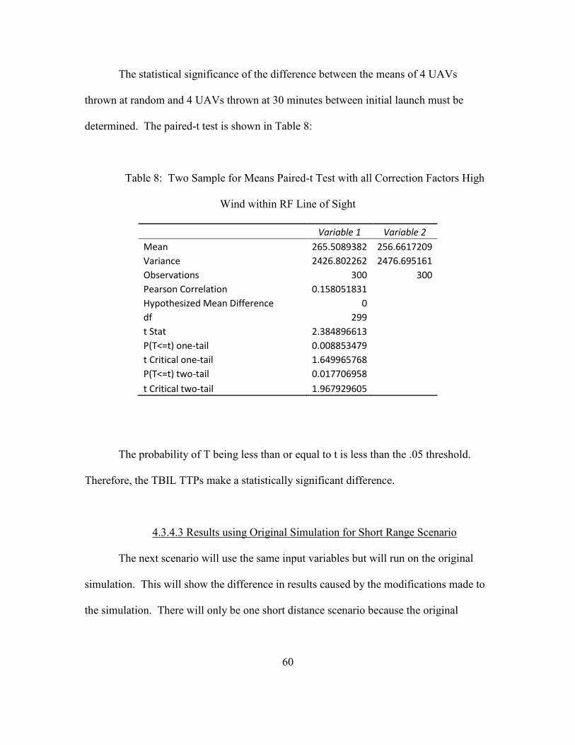
60

The statistical significance of the difference between the means of 4 UAVs

thrown at random and 4 UAVs thrown at 30 minutes between initial launch must be

determined. The paired-t test is shown in Table 8:

Table 8: Two Sample for Means Paired-t Test with all Correction Factors High

Wind within RF Line of Sight


Mean 265.5089382 256.6617209

Variance 2426.802262 2476.695161


Pearson Correlation 0.158051831 Hypothesized Mean Difference 0 df 299 t Stat 2.384896613 P(T<=t) one-tail 0.008853479 t Critical one-tail 1.649965768 P(T<=t) two-tail 0.017706958 t Critical two-tail 1.967929605

The probability of T being less than or equal to t is less than the .05 threshold.

Therefore, the TBIL TTPs make a statistically significant difference.

4.3.4.3 Results using Original Simulation for Short Range Scenario

The next scenario will use the same input variables but will run on the original

simulation. This will show the difference in results caused by the modifications made to

the simulation. There will only be one short distance scenario because the original

61

simulation did not take into effect the wind speeds. The OptQuest results for the original

simulation can be seen in Table 9 below:

Table 9: OptQuest Optimized Solution Original Simulation within RF Line of Sight

As can be seen in the OptQuest results above, the top ten solutions range from

405 minutes (6 hours and 44 minutes) to 406 minutes (6 hours and 45 minutes). All of

the top ten optimized alternatives involve using 2 OWLs. The Process Analyzer results

can be seen in Table 10 on the following page:

62

Table 10: Process Analyzer Results for Original Simulation within RF Line of Sight

The mean times for the value added times broken down by the number of OWLs used

are as follows:




4) 1 OWL – 360 minutes (6 hours)

63

If the operator launched the OWLs at random, the original model with no

correction factors gives the greatest value added when using two OWLs. The value

added time increases by 42 minutes when flying two OWLs as opposed to one OWL.

Every OWL added after that results in a decreased total value added time.

Using proper TBIL TTPs should again lead to improved value added times. The

number of OWLs and their respective optimal TBILs are listed below:




4) 1 OWL – 360 minutes (6 hours)

Thus, using proper TBIL TTPs, the operator would use 2 OWLs with 35 minutes

TBIL to achieve 406 minutes of total value added time out of a 480 minute mission time.

The modified model resulted in a total value added time that is 138 minutes less in high

wind and 119 minutes less in low wind than the original model. That is a 34% and 29%

reduction respectively.

A paired-t test was conducted to determine statistical significance. The

probability of T being less than or equal to t is lower than .05. Therefore, the means of

the launches using TBIL TTPs is statistically different from the mean when the UAVs are

launched at random. The results of the paired-t test are shown in Table 11:

64

Table 11: Two Sample for Means Paired-t Test for Original Simulation within

RF Line of Sight


Mean 407.1757675 400.9539896

Variance 121.8961845 192.3027886

Observations 99 99

Pearson Correlation -

0.078413304 Hypothesized Mean Difference 0 df 98 t Stat 3.366192821 P(T<=t) one-tail 0.000544852 t Critical one-tail 1.660551218 P(T<=t) two-tail 0.001089705 t Critical two-tail 1.984467404

This is to be expected with every correction factor diminishing the returns of the

total value added time with no correction factors to the contrary. What was more difficult

to predict was the affect on the number of OWLs in the optimal solution. Why did the

original simulation determine that 2 OWLs would be better than the 4 OWLs that each of

the modified models concluded?

The most likely answer is that the original simulation had such large advantages

from extended battery endurance and the capture rate of 100% for the loiter time as time

that the target was observed. The original simulation could observe 85% of the time with

just 2 OWLs. This left little room for improvement. Since there is no advantage in the

original simulation for having more than one OWLs flying over the target, the extra

OWLs resulted in a waste of time for the operator that yielded relatively little advantage

in the total added value time.

65

4.3.4.4 Corrected Simulation Results Long Range, Low Wind Scenario

The next set of scenarios will all be long distance. Long distance in this

simulation will be 5 miles. This will require the OWLs to be split up into rover/relay

pairs because the target is beyond radio frequency line of sight. These scenarios are

expected to yield a much lower total value added time because the flight times to and

from the target are longer, the max number of rovers to loiter over the target is two, and

the operator must expend the amount of time necessary to take care of four OWLs while

only getting the added observation time from the one or two rovers loitering over the

target.

Each of the following scenarios will define its parameters using Table 12 on the

next page:

66

Table 12: Model Setup for Target Beyond LOS Scenario

Model Setup for Target Beyond LOS Scenario

Constant Variables Value Independent Variables

Value

Range

Mission_Length_Hours 8 #_of_OWL_Rovers 1 - 2

Rover_Max_Range_Miles(RF) 3 #_of_OWL_Relays 1 - 2

Speed_to_Target_MPH 30

Time_Between_Initial_Launch

(Minutes) 1 - 40

Wind_Speed_MPH

10 (Low)

20 (High)

Distance_to_Target_Miles 5

Dependent_Variables

Total_Value_Added_Time

Total_UAV_Over_Target Time

In Table 13 on the following page, we see the results from the OptQuest running

the above variables using low wind speed:

67

Table 13: OptQuest Optimized Solution with all Correction Factors Low Wind Beyond RF Line of Sight

The results of the OptQuest show that the highest value added is 154 minutes.

This is achieved by using 2 rovers and 2 relays and launching with a TBIL of 32 minutes.

The Process Analyzer results for this scenario are shown in Table 14:

68

Table 14: Process Analyzer Results using all Correction Factors Low Wind Beyond RF Line of Sight

The mean of the Process Analyzer results above broken down by number of

OWLs are as follows:

1) 2 Rover/Relay Pairs – 145 minutes (2 hours and 25 minutes)

2) 1 Rover/Relay Pair – 88 minutes (1 hour and 28 minutes)

If the operator were to launch each rover/relay pair randomly with no attention

being paid to TBIL, the operator would achieve on average 145 minutes of value added

time by using 2 rover/relay pairs. If the operator used the TBIL TTPs, the value added

times will increase as seen below:

1) 2 Rover/Relay Pairs with TBIPL 30 minutes – 149 minutes (2 hours and 29 minutes)


69

Before looking further into this data, it needs to be determined whether there is a

significant difference between the means of using no particular TBIL or using the

recommended TBIL TTP. Using a paired-t test again results in Table 15:

Table 15: Two Sample for Means Paired-t Test with all Correction Factors Low

Wind beyond RF Line of Sight


Mean 148.8432401 148.7126833

Variance 3208.55359 3234.79012



The probability of T being less than or equal to t is high in this comparison. This

means that the comparison fails to reject the H0 hypothesis and there is no statistical

difference, on average, between the two means.

This makes it clear that it is preferable to use 2 rover/relay pairs in long distance,

low wind scenarios. It adds over one additional hour to the total value added time when

compared to the single rover/relay pair. When compared to our short distance, low wind

scenario we achieve 2 hours and 18 minutes less total value added time. This is a 48%

70

reduction. This shows how much more effective the OWLs are at short distance than

long distance.

Therefore, the operator in this scenario should use 2 rover/relay pairs, but it is not

important how long to wait between launching each pair because the difference between

the optimal TBIL and the mean of all TBILs is not statistically significant.

4.3.4.5 Corrected Simulation Results for Long Range, High Wind

Scenario

The same simulation will now be run with high winds speeds (>15 mph) to

determine the effects of wind speed on long distance flights. The results of this OptQuest

optimization can be seen in Table 16:

71

Table 16: OptQuest Optimized Solution with all Correction Factors High Wind Beyond RF Line of Sight

The same scenario was put into OptQuest with a wind speed of 20 mph instead of

10 mph to analyze the results of high winds on long distance rover/relay pairs. The range

in the top ten results range from 136 minutes to 147 minutes. The optimal results all use

2 rover/relay pairs. The optimal TBIPL for two rover/relay pairs is 12 minutes. This is

feasible for a OWL operator. The Process Analyzer results for the same scenario can be

seen in Table 17 below:

72

Table 17: Process Analyzer Results using all Correction Factors High Wind Beyond RF Line of Sight

The means from the Process Analyzer results for the modified simulation at a

distance of 5 miles to target under high wind conditions are broken down below:



If thrown at random, the results above suggest that the operator should use 2

rover/relay pairs and will achieve 137 minutes of value added time. If the operator

utilizes the suggested TBIPL TTPs, the operator can achieve the following results:



The difference between these scenarios is a reduction of 4 minutes total value

added time when using optimal TTPs in high wind versus low wind. There are only eight

73

minutes to be gained by using the TBIPL TTPs versus launching them randomly as long

as 2 rover/relays are used.

To determine if this small difference is statistically significant, the data analysis

tool in excel was used. The results can be seen in Table 18:

Table 18: Two Sample for Means Paired-t Test with all Correction Factors High

Wind beyond RF Line of Sight


Mean 137.349154 135.867227

Variance 3207.023097 3382.07193



The probability that T is less than or equal to t for two-tails is greater than the .05

threshold. Therefore, the effects of the TBIL TTPs at long range during high winds are

not statistically different from the mean of launching the rover / relay pairs at random.

4.3.4.6 Results using Original Simulation for Long Range Scenario

The last scenario to simulate will be the original simulation modeling a long range

scenario. The results of the optimization can be seen in Table 19:

74

Table 19: OptQuest Optimized Solution Original Simulation Beyond RF Line of Sight

The OptQuest results show that 2 rover/relay pairs dominate 1 rover/relay pair for

every TBIPL. The top ten results range from 310 to 313 minutes. The optimal TBIPL,

according to the OptQuest is 36 minutes. This will result in a value added time of 313

minutes.

The Process Analyzer results for this scenario are shown in Table 20 on the

following page:

75

Table 20: Process Analyzer Results using Original Simulation Beyond RF Line of Sight

The respective means for the value added times are:


2) 1 Rover/Relay Pair – 239 minutes (3 hours and 59 minutes)

If the OWLs were launched at random, the original simulation predicts 297

minutes of value added time using 2 rover/relay pairs. If the TBIPL TTPs are used the

results will be altered to the following:


2) 1 Rover/Relay Pair – 239 minutes (3 hours and 59 minutes)

The statistical significance has been checked using the paired-t test. The results

of this test are shown in Table 21:

76

Table 21: Two Sample for Means Paired-t Test for Original Simulation beyond

RF Line of Sight


Mean 312.2099161 297.5424219

Variance 893.6530613 1650.861617


Pearson Correlation -

0.013839816 Hypothesized Mean Difference 0 df 99 t Stat 2.888704446 P(T<=t) one-tail 0.002376058 t Critical one-tail 1.660391157 P(T<=t) two-tail 0.004752117 t Critical two-tail 1.9842169

The data above shows that the difference in means for the original simulation

between the mean of value added when launched at random and the value added when

launched according to the recommended TBIL TTPs is statistically significant.

Using the TBIPL TTPs, the operator manages to gain an additional 11 months.

The modified simulation resulted in a reduction of 163 minutes for high winds and 159

minutes for low winds in comparison to the original simulation. This is a 53% and 52%

reduction, respectively.

77

V. Conclusions and Recommendations

5.1 Conclusions

This thesis integrated multiple simulation and analysis tools in order to better

predict the outcome of a single operator using multiple UAVs with varying Tactics,

Techniques, and Procedures applied to the Time Between Initial Launches (or Paired

Launches).

The results have multiple useful applications. Optimal TTPs will be

recommended to use in military operations using small Ravens with multiple UAVs used

by one operator.

Also, the simulation more effectively estimates the amount of time that an

operator will be able to observe data from OWLs conducting reconnaissance. This will

help with mission planning and future cost analyses to determine the proper number of

UAVs to be purchased and issued to units.

There were two goals in this research. The first was to develop a correction factor

that will make the predictions of Value Added Time more realistic due to loss of the

target within the camera’s field of view during loiter.

This was done by creating two correction factors. The first is the Time Observing

Target Correction Factor. The Time Over Target Correction Factor is aspplied when a

single UAV is loitering over the target. This arena code can be seen below:


(0.55 + 0.15 * BETA(1.06, 1.02)) * time_over_target

Note: where BETA represents the Beta distribution

78

The second correction factor is the Welborn Correction Factor. This is the factor

used when multiple UAVs are loitering simultaneously around the target. The Welborn

Correction Factor can be seen below:


(1-((1-(.55+.15*BETA(1.06,1.02))) (#_UAVs_over_target))) * individual_time_over_target

Note: BETA represents the Beta distribution

These two correction factors were integrated into the simulation to improve the

accuracy and realism of the simulation when predicting the outcomes of various TTPs

applied to various scenarios.

The second goal of this thesis was to develop TTPs for the military to use to

optimize the benefits received from the use of multiple rovers with one operator. The

recommended TTPs are summarized in Table 22 on the next page:

79

Table 22: Summary Results (8 Hour Mission)

Scenario

Recommended # of

UAVs (Rovers/Relays)

Recommended

TBIL / TBIPL

Expected Value Added

Time with TTPs

Expected Value

Added Time

without TTPs

Max Value Added

Time (TBIL or

TBIPL)

3 Miles, Winds <= 15 mph 4 / 0 35 min 287 min 277 min 296 min (32 min)

3 Miles, Winds > 15mph 4 / 0 30 min 257 min 268 min 272 min (36 min)

5 Miles, Winds <= 15 mph 2 / 2 n/a n/a 145 min 154 min (32 min)

5 Miles, Winds > 15 mph 2 / 2 n/a n/a 137 min 147 min (12 min)

Original Simulation

within LOS 2 / 0 35 min 406 min 402 min 406 min (34 min)

Original Simulation

beyond LOS 2 / 2 40 min 308 min 297 min 313 min (2 min)

80

Using TBIL TTPs for is useful for short range scenarios. The TTPs above should

be used in such cases. However, the TBIL TTPs lose their statistical significance when

operating at longer range. In such cases, the deciding factor should be based solely on

operational preferences. Longer TBILs might be easier for the operator, whereas shorter

TBILs will initially result in optimal surveillance until completion of the first sortie.

The launch times recommended in Table 17 above are feasible for an operator.

For routine surveillance, the above numbers of UAVs and Time Between Initial

Launches should be used. For other contingencies, knowledge of the effects of the

simulation will be useful for TTPs in such cases.

For example, the TTPs recommended above are optimized for routine continued

surveillance over eight hours. What if a firefight arises and it is more important to

maximize the percentage of time that the target is observed as soon as possible? What if

the mission will not last eight hours? What if the first hour is critically important and the

last seven hours are much less important? In these cases, the TTP could be to launch

every UAV with as small a TBIL as possible because it is more important to get 99% of

the time observing target for the first half hour than to have the optimal time observing

target over an eight hour period.

5.2 Recommendations for Future Work

There are areas of improvement in other fields that could play an important part in

the validity of the simulation. One of these areas is human factors. The current

simulation assumes that a human can observe the video transmission 100% of the time.

This is clearly not the case. There are many issues that would affect the operator’s ability

81

to effectively monitor the various simultaneous transmissions under various conditions.

This is an extremely rich area for further calibration of the simulation.

While this study sought to find the best TTPs for operating multiple UAVs with a

single operator in varying operational scenarios and conditions, another interesting

question that came up was whether it would be worth the money. A cost analysis should

be done to determine if the value added by additional UAVs supports the monetary cost

of each additional UAV. Often, there are gains had by employing a fourth OWL over the

first three OWLs, but the diminished return is not substantial enough to be worth the

additional $35,000 that each UAV costs.

In addition to potential areas of improvement that would require experience in

another specialization, there are a few simulation aspects that could be improved by the

next round of simulation calibrations. These are an improved wind speed correction

factor, a correction factor for the effects of elevation, and a correction factor for the

effects of varying speeds or distances.

The wind correction factor currently used is very simplistic. It relies on a single

switch between high winds and low winds. A scale should be developed that accounts

for the effects on battery life and the effects on the percent of time that the UAV loiters

over the target that the target will be observed.

Elevation plays a huge effect on the size of the footprint from the camera. Further

work can be done to determine the effects of elevation in the simulation and its effects on

the percent of time that the UAV loiters over the target that the target will be observed.

82

The loiter radius, roll of the UAV, and speed of the aircraft should also receive

further calibration in order to further the realism and accuracy of the simulation in

mission planning.

In the simulation looked at in this research, the speed of flight for the UAV was

fixed at 30 mph. The effects of changing speeds should be looked at in future simulation

calibrations. Also, the distance to target was fixed for each scenario. Three miles to

target was used to achieve an all rover scenario and five miles to target was used to

require a rover/relay scenario. In future calibrations, this could be optimized according to

a sliding scale for speed and distance.

83

Bibliography

[1] "Wikipedia," 25 November 2012. [Online]. Available: http://en.wikipedia.org/wiki/Northrop_Grumman_MQ-4C_Triton. [Accessed 20 January 2013].

[2] "Wikipedia," 20 January 2013. [Online]. Available: http://en.wikipedia.org/wiki/MQ-9_Reaper. [Accessed 20 January 2013].

[3] "Wikipedia," 14 January 2013. [Online]. Available: http://en.wikipedia.org/wiki/Predator_drone. [Accessed 20 January 2013].

[4] "Wikipedia," 24 June 2012. [Online]. Available: http://en.wikipedia.org/w/index.php?title=AeroVironment_RQ-11_Raven&printable=yes. [Accessed 5 July 2012].

[5] M. J. Seibert, A. J. Stryker, J. R. Ward and C. T. Wellbaum, "System Analysis and Prototyping for Single Operator Management of Multiple Unmanned Aerial Vehicles Operating Beyond Line of Sight," Air Force Institute of Technology, Wright-Patterson Air Force Base, 2010.

[6] A. E. Cottle, "Initial Validation of an Unmanned Aerial Vehicle Mission Simulation Model," Air Force Institute of Technology, Wright-Patterson Air Force Base, 2011.

[7] Office of the Secretary of Defense, "Unmanned Systems Integrated Roadmap FY 2011 - 2036," Joint Staff, Washington DC, 2011.

[8] J. Banks, J. S. Carson II, B. L. Nelson and D. M. Nicol, Discrete Event System Simulation (5ed.), Upper Saddle River: Prentice Hall, 2010.

[9] R. G. Sargent, "Verification and Validation of Simulation Models," in Winter

Simulation Conference, Piscataway, NJ, 2010.

[10] T. H. Naylor and Finger, "Verification of Computer Simulation Models," Management Science, pp. Vol. 2, B92 - B101, 1967.

84

[11] A. Cowdale, "Real World data Collection for Model Validation," in Winter




[13] O. Balci, "Verification, Validation, and Certification of Modeling and Simulation Applications," in Winter Simulation Conference, Piscataway, NJ, 2003.

[14] A. M. Law and M. D. Kelton, Simulation Modeling and Analysis, third edition, New York: McGraw-Hill, 2000.



[16] Joint Staff, "Universal Task List," Joint Chiefs of Staff, Washington, D.C., 2006.

[17] B. D. Lozano, "Improving Unmanned Aircraft Persistence by Enhancing Endurance and Effective Surveillance Using Design of Experiments and Regression Analysis," Air Force Institute of Technology, Wright-Patterson Air Force Base, 20111.

[18] Report to Congressional Committees, "Defense Acquisitions: Assessments of Selected Weapon Programs," Government Accountability Office, Washington, DC, March 2012.

[19] O. Balci, "Verification, Validation, and Accreditation," in Winter Simulation

Conference, Piscataway, NJ, 1998.

[20] J. S. Carson II, "Model Verification and Validation," in Winter Simulation

Conference, Piscataway, NJ, 2002.

[21] R. A. Pomranky, "Human Robotics Interaction Army Technology Objective Raven Small Unmanned Aerial Vehicle Task Analysis and Modeling," Army Research Labs, January 2006.

85

Appendix A: ARENA Model Images

Figure 16: Full Arena Model with Accompanying Sub-models

The Moving Target sub-model has been removed from the original because it was not utilized in this study.

86

Figure 17: Rover Entity Creation and Rover Pairing Logic

87

Figure 18: Launch Process for Rover with No Relays

88

Figure 19: Assignment of Wind Speed Variable, Wind Speed Correction Factor, and Battery Endurance

89

Figure 20: Rover travel to target processes

90

Figure 21: Time Over Target Correction Factor and Rover Travel Time to Rally

Figure 22: Repair and Maintenance

91

Figure 23: Time Over Target Sub-Model

92

Figure 24: Value Added Time Sub-Model

93

Appendix B: UAV Team Flight Test Procedures

(Operational Tests are tests 9 and 10 – highlighted)

Flight Test #1 (24-25 September 2012)

1. Preflight testing (completed at AFIT and in field) a. Communication check (initial) b. Control Surface check c. Trim Radio and save settings d. Communication check (distance)

2. In Flight Testing With Mission Planner a. OWL_A1 & OWL_A2

i. Zero Sensors ii. Set Fail Safe Parameters

iii. Trim Radio iv. Load Waypoints v. Launch OWL_A*

vi. RC Pilot Flight 1. Adjust Trim

vii. Engage Autopilot 1. Adjust Gains (as necessary)

viii. RC Pilot Landing ix. Group Discussion Observations

b. Sig Rascal_P1 (Petrol) & Sig Rascal_E1 (Electric) i. Zero Sensors

ii. Set Fail Safe Parameters iii. Trim Radio iv. Load Waypoints v. Launch Rascal_*

vi. RC Pilot Flight 1. Adjust Trim

vii. Engage Autopilot 1. Adjust Gains (as necessary)

viii. RC Pilot Landing ix. Group Discussion Observations

3. In Flight Testing With QGroundControl a. Communication check (initial) b. Control Surface check c. OWL_A1 Flight

i. Zero Sensors ii. Set Fail Safe Parameters

iii. Trim Radio

94

iv. Load Waypoints v. Launch OWL_A1

vi. RC Pilot Flight To Elevation vii. Engage Autopilot (observe QGroundControl)

1. Try update of race track in flight 2. Observe data logging capabilities

viii. Land OWL_A1 ix. Group Discussion Observations

d. OWL_A2 Flight i. Zero Sensors

ii. Set Fail Safe Parameters iii. Trim Radio iv. Load Waypoints v. Launch OWL_A2

vi. RC Pilot Flight To Elevation vii. Engage Autopilot

viii. Land OWL_A2 4. Multi-Aircraft Simultaneous Flight 1 With QGroundControl

a. Replace batteries in OWL_A1 & OWL_A2 b. Zero Sensors in OWL_A1 & OWL_A2 c. Set Fail Safe Parameters in OWL_A1 & OWL_A2 d. Load Waypoints for OWL_A1(elevation 350ft) & OWL_A2 (elevation

200ft) e. Launch OWL_A1 f. RC Pilot Flight To Elevation g. Engage Autopilot Observe Lap h. Launch OWL_A2 i. RC Pilot Flight To Elevation j. Engage Autopilot Observe Lap k. Update Waypoints OWL_A1 l. Update Waypoints OWL_A2 m. Land OWL_A1 n. Land OWL_A2 o. Group Discussion Observations

5. Multi-Aircraft Simultaneous Flight 1 With QGroundControl a. Replace batteries in OWL_A1 & Refill Petrol in Sig Rascal_P1 b. Zero Sensors in OWL_A1 & Sig Rascal_P1 c. Set Fail Safe Parameters in OWL_A1 & Sig Rascal_P1 d. Load Waypoints for OWL_A1(elevation 250ft) & Sig Rascal_P1

(elevation 400ft) e. Launch Sig Rascal_P1 f. RC Pilot Flight To Elevation g. Engage Autopilot Observe Lap h. Launch OWL_A1 i. RC Pilot Flight To Elevation

95

j. Engage Autopilot Observe Lap k. Update Waypoints Sig Rascal_P1 l. Update Waypoints OWL_A1 m. Land OWL_A1 n. Land Sig Rascal_P1 o. Group Discussion Observations

Flight Test #2 (5-7 November 2012)

1. Initial communications check out a. Video feed check (5.4 GHz)

i. Initial Operation 1. Is Video feed working?

b. RC Safety Pilot check (2.4 GHz) i. Initial Operation

1. Is RC Communications working? ii. Distance check

1. On the ground place the FrSky transmitter in range check mode and walk the MAV down the flight line until communications are lost. Do conversion for approximated RC range. Record here _________________

c. Auto Pilot check (914 MHz) i. Initial Operation

1. Is RC Communications working? ii. Distance check

1. Walk the MAV down the flight line until communications are lost. Record distance here _________________

d. Record and Measure time spent fixing, recovering, launching, turning, flight time, wind speed, battery endurance

2. Verify MAVs are flying properly (In Flight Testing With Mission Planner) a. Power on RC controllers for OWL_A1 and OWL_A2 b. For Each OWL_A1, OWL_A2 and Sig_AP

i. Open Mission Planner ii. Connect to MAV at baud rate of 57600

iii. On the Flight Data tab select the Actions tab and click Set Home Alt

iv. Verify that the altitude read out on the right of the flight data screen reads 0

v. Repeat iii-iv as necessary until successful vi. Trim Radio

96

vii. Load Waypoints viii. Launch MAV

ix. RC Pilot Flight 1. Adjust Trim

x. Engage Autopilot 1. Adjust Gains (as necessary) SEE APPENDIX

xi. RC Pilot Landing c. Group Discussion Observations d. Record and Measure time spent fixing, recovering, launching, turning,

flight time, wind speed, battery endurance 3. Single MAV flight using QGroundControl (First test OWL_A2 , repeat procedure

for Sig_AP ) a. Power on RC controllers OWL_A2 and Sig_AP b. Zero Sensors

i. Open Mission Planner ii. Connect to MAV at baud rate of 57600



v. Repeat as necessary until successful vi. Close Mission Planner but do NOT power off MAV

c. Trim Radio d. Open UNMODIFIED qgroundcontrol e. Connect to MAV at baud rate of 57600 f. Wait for GPS to find location g. Load Waypoints using waypoint widget h. Verify Waypoints by going to the onboard tab of the waypoint widget

and clicking refresh i. Launch j. RC Pilot Flight To Elevation k. Engage Autopilot

i. Try update of race track in flight ii. Observe data logging capabilities

l. Land m. Group Discussion Observations n. Record and Measure time spent fixing, recovering, launching, turning,

flight time, wind speed, battery endurance 4. Single MAV Distance Flight to Loss of Communications

a. Power on RC controllers for OWL_A2 b. Zero Sensors

i. Open Mission Planner ii. Connect to OWL_A2 at baud rate of 57600

97



v. Repeat as necessary until successful c. Trim Radio d. Wait for GPS to find location e. Load Waypoints using waypoint widget f. Verify Waypoints by going to the onboard tab of the waypoint widget

and clicking refresh g. Send Safety pilot and Observers to remote location (Must have range

radio) i. Observer will have map of flight pattern

h. Verify both teams are ready and we are clear for launch i. Launch j. RC Pilot Flight To Elevation k. RC Pilot flies OWL_A2 toward primary ground station l. Ground control operator is continually attempting to connect m. Monitor telemetry to observe when 914 MHz communications are

established n. Ground control operator notes distance on map where communications

were established o. Observe if after 30 seconds of flight OWL_A2 beings to navigate toward

RTL p. Operator then notifies RC pilot to land OWL_A2 q. Record and Measure time spent fixing, recovering, launching, turning,

flight time, wind speed, battery endurance 5. Multi-MAV Multi-Ground Station Familiarity Test (Direct LOS) Non-

autonomous Relay Navigation a. Power on RC controllers for OWL_A1 and OWL_A2 b. On two separate Laptops connect two Digi modems (one to each laptop) c. Open X-CTU and verify that each computer is talking to the attached

modem successfully i. Select the test/query button. The computer is successfully

connected if the type and model information is not garbled text d. On laptop one (L1) open Mission Planner

i. Power on OWL_A1 while holding the MAV level and steady ii. Connect to OWL_A1 at baud rate of 57600



v. Repeat iii-iv as necessary until successful

98

vi. Trim Radio vii. Load Waypoints

e. On laptop two (L2) open Mission Planner i. Zero Sensors

1. Open Mission Planner 2. Connect to OWL_A2 at baud rate of 57600 3. On the Flight Data tab select the Actions tab and click Set

Home Alt 4. Verify that the altitude read out on the right of the flight

data screen reads 0 5. Repeat as necessary until successful 6. Close Mission Planner but do NOT power off MAV

ii. Trim Radio iii. Open UNMODIFIED qgroundcontrol iv. Connect to MAV at baud rate of 57600 v. Wait for GPS to find location

vi. Load Waypoints using waypoint widget vii. Verify Waypoints by going to the onboard tab of the waypoint

widget and clicking refresh f. Launch OWL_A1

i. RC Pilot Flight To Elevation ii. Engage Autopilot

iii. Verify Operation Status (if oddities are observed, land and trouble shoot) else

g. Launch OWL_A2 i. RC Pilot Flight To Elevation

ii. Engage Autopilot iii. Verify Operation Status (if oddities are observed, land and trouble

shoot) else h. Maximize flight time of OWL_A1 to 15 minutes of flight without

exceeding time limit i. Record and Measure time spent fixing, recovering, launching, turning,

flight time, wind speed, battery endurance 6. Multi-MAV Multi-Ground Station Familiarity Test (Direct LOS) Autonomous

Relay Navigation a. Power on RC controllers for OWL_A1 and OWL_A2 b. On two separate Laptops connect two Digi modems (one to each laptop) c. Open X-CTU and verify that the computer is talking to the modem

successfully i. Select the test/query button. The computer is successfully

connected if the type and model information is not garbled text d. On laptop one (L1) open Mission Planner

99

i. Power on OWL_A1 while holding the MAV level and steady ii. Connect to OWL_A1 at baud rate of 57600




vii. Load Waypoints at altitude of 550 ft e. On laptop two (L2) open Mission Planner

i. Zero Sensors 1. Open Mission Planner 2. Connect to OWL_A2 at baud rate of 57600 3. On the Flight Data tab select the Actions tab and click Set


data screen reads 0 5. Repeat as necessary until successful 6. Close Mission Planner but do NOT power off OWL_A2

ii. Trim Radio iii. Open MODIFIED qgroundcontrol iv. Connect to both MAVs at baud rate of 57600 (do not enable

multiplexing) v. Wait for GPS to find location

vi. Click on map as close as possible to the location of the ground station as possible

f. Launch OWL_A1 i. RC Pilot Flight To Elevation


shoot) else g. Launch OWL_A2


iii. Every 5 seconds click anywhere on the map iv. Verify Operation Status (if oddities are observed, land and trouble

shoot) else h. Maximize flight time of first MAV to 15 minutes of flight without

exceeding time limit i. Take manual control of MAV OWL_A2 and land it

ii. Take manual control of MAV OWL_A1 and land it

i. Record and Measure time spent fixing, recovering, launching, turning, flight time, wind speed, battery endurance

100

7. Multi-MAV Multi-Ground Station Familiarity Test (Direct LOS) Autonomous Relay Navigation with SIG_AP in place of OWL_A2

a. Power on RC controllers for OWL_A1 and OWL_A2 b. Switch Sig_AP Aircraft ON (leave Autopilot switch OFF) c. Power on OWL_A1 while holding the MAV level and steady d. On laptop one (L1) open Mission Planner

i. Plug in Ch1-Relay modem to laptop L1 ii. Connect to OWL_A1 at baud rate of 57600




vii. Load Waypoints e. Switch Sig_AP Autopilot ON f. On laptop two (L2) open Mission Planner

i. Plug in Ch1-Sig modem to laptop L2 ii. Zero Sensors

1. Open Mission Planner 2. Connect to Sig_AP at baud rate of 57600 3. On the Flight Data tab select the Actions tab and click Set


data screen reads 0 5. Repeat as necessary until successful 6. Hold Sig_AP level 7. Under the configuration tab click on the calibrate level 8. Verify on the flight data tab that the hud is showing level

flight 9. Close Mission Planner but do NOT power off MAV

iii. Trim Radio iv. Open MODIFIED qgroundcontrol v. Connect to Sig_AP at baud rate of 57600

vi. Wait for GPS to find location vii. Select MAV001 (Sig) for control

viii. Load Waypoints using waypoint widget ix. Verify Waypoints by going to the onboard tab of the waypoint

widget and clicking refresh g. Launch OWL_A1


101


h. Launch Sig_AP i. RC Pilot Flight To Elevation


shoot) else i. Maximize flight time of OWL_A1 to 15 minutes of flight without

exceeding time limit i. Take manual control of MAV Sig_AP and land it

ii. Take manual control of MAV OWL_A1 and land it j. Record and Measure time spent fixing, recovering, launching, turning,

flight time, wind speed, battery endurance 8. Beyond Communications Line Of Sight (BCLOS) Flight Test

a. Power on RC controllers for OWL_A1 and OWL_A2 b. Switch Sig_AP Aircraft ON (leave Autopilot switch OFF) c. Power on OWL_A1 while holding the MAV level and steady d. On laptop one (L1) open Mission Planner

i. Plug in Ch1-Relay modem to laptop L1 ii. Connect to OWL_A1 at baud rate of 57600




vii. Load Waypoints e. Switch Sig_AP Autopilot ON f. On laptop two (L2) open Mission Planner

i. Plug in Ch1-Sig modem to laptop L2 ii. Zero Sensors

1. Open Mission Planner 2. Connect to Sig_AP at baud rate of 57600 3. On the Flight Data tab select the Actions tab and click Set


data screen reads 0 5. Repeat as necessary until successful 6. Hold Sig_AP level 7. Under the configuration tab click on the calibrate level 8. Verify on the flight data tab that the hud is showing level

flight

102

9. Close Mission Planner but do NOT power off MAV i. Trim Radio

ii. Open MODIFIED qgroundcontrol iii. Connect to Sig_AP at baud rate of 57600 iv. Wait for GPS to find location v. Select MAV001 (Sig) for control

vi. Load Waypoints using waypoint widget vii. Verify Waypoints by going to the onboard tab of the waypoint

widget and clicking refresh b. Send out RC pilot and distant area observer with map of flight path, cell

phone and range radio c. Launch SIG_AP

i. RC Pilot Flight To Elevation and approximate relay position d. Launch OWL_A1



e. Ground Control Operator verifies that relay of communications is operational

i. Is telemetry data displaying in the ground control software? ii. Can information be written to the rover MAV?

iii. If yes proceed. If no fly OWL_A1 closer to Sig_AP. f. On Sig_AP

i. Engage Autopilot ii. Every 5 seconds click anywhere on the map

iii. Verify Operation Status (if oddities are observed, land and trouble shoot)

g. Maximize flight time of OWL_A1 to 15 minutes of flight without exceeding time limit

h. On ground control operator’s que both RC pilots take control of their respective MAVs and land the MAVs

i. Record and Measure time spent fixing, recovering, launching, turning, flight time, wind speed, battery endurance

10. Stationary Target Flight Test a. Emplace stationary target b. Set waypoint pattern to loiter over target c. Launch OWL and monitor to ensure proper flight path d. Record and Measure loiter time and target observed time

11. Road Surveillance Flight Test a. Designate linear zone of observation

103

b. Set waypoint pattern to observe linear zone of observation c. Launch OWL and monitor to ensure proper flight path d. Record and Measure loiter time and target observed time

104

Appendix C: Field of View Algorithm – Loiter Pattern

% % Plots for J. Welborn thesis, March 2013 %

% data set for Loiter, counterclockwise adjdata=xlsread('Welborn Telemetry Log_7Nov12.xlsx','Adjusted Data');

% time/date not used timedata=adjdata(:,1:3);

%extract 6 columns: yaw, pitch, roll, long lat, elev data=adjdata(:,[6 4 2 12 16 18]); clear adjdata;

%change North (0 yaw) to positive x axis data2 = [ data(:,1)-90 data(:,2:6)]; clear data

figure plot(0,0,'r*');hold on; plot(data2(1:5:14000,4),data2(1:5:14000,5)) xlabel('Long distance from homebase (m)') ylabel('Lat distance from homebase (m)') legend('homebase', 'UAV location') title('Aircraft Location - Full 7NovAdjusted data') axis([-400 0 0 300]) grid

figure plot(0,0,'r*');hold on; plot(data2(1:5:600,4),data2(1:5:600,5)) s=[]; for i = 1:5: 600 t=sensoraimpoint2(data2(i,4:6),[-data2(i,1) data2(i,2) -

data2(i,3)],'l'); s=[s; t]; end plot(s(:,1), s(:,2),'g') legend('homebase', 'UAV location', 'aimpoint') xlabel('Long distance from homebase (m)') ylabel('Lat distance from homebase (m)') title('Sensor aimpoint - 7NovAdjusted data') axis([-400 0 0 300]) grid

figure startt=1; stept=50;

105

endt=600; s=[]; for i = 1:600 t=sensoraimpoint2([data2(i,4:5) 100],[-data2(i,1) data2(i,2) -

data2(i,3)],'l'); s=[s; t]; end plot(0,0,'r*'); hold on; plot(data2(startt:stept:endt,4),data2(startt:stept:endt,5)) plot(s(startt:stept:endt,1), s(startt:stept:endt,2),'g') for i=startt:stept:endt f=footprint3([data2(i,4:5) 100],[-data2(i,1) data2(i,2) -

data2(i,3)],'l'); plot(f(:,1), f(:,2),'r') end legend('homebase', 'UAV location', 'aimpoint','footprint') xlabel('Long distance from homebase (m)') ylabel('Lat distance from homebase (m)') title('Sensor Footprint 7NovAdjusted data') axis([-400 0 0 300]) grid

%calculate %view of target %assume target is located at -240, 140 is loiter point cnt=0; endt=14000; for i = 1:endt f=footprint3([data2(i,4:6)],[-data2(i,1) data2(i,2) -

data2(i,3)],'l'); cnt=cnt+inpolygon(-240, 140,f(:,1),f(:,2)); end fprintf('The %2.2f percent of telemetry points have a sensor footprint

that covers the loiter point (-240, 140)\n', 100*cnt/endt);

% % clear all % % % data set for Loiter, clockwise adjdata=xlsread('Welborn Telemetry Log_7Nov12 #2.xlsx','Adjusted Data

Loiter'); data=adjdata(:,[6 4 2 12 16 18]); clear adjdata;

data2= [ data(:,1)-90, data(:,2:6)]; clear data

figure plot(0,0,'r*');hold on; plot(data2(1:5:7000,4),data2(1:5:7000,5)) xlabel('Long distance from homebase (m)') ylabel('Lat distance from homebase (m)')

106

legend('homebase', 'UAV location') title('Aircraft Location - Full Log_7Nov12 #2 Adjusted data') axis([-250 50 -100 200]) grid

figure plot(0,0,'r*');hold on; plot(data2(1:5:800,4),data2(1:5:800,5)) xlabel('Long distance from homebase (m)') ylabel('Lat distance from homebase (m)') legend('homebase', 'UAV location') title('Aircraft Location - First rotation Log_7Nov12 #2 Adjusted data') axis([-250 50 -100 200]) grid


data2(i,3)],'r'); s=[s; t]; end plot(s(:,1), s(:,2),'g') legend('homebase', 'UAV location', 'aimpoint') xlabel('Long distance from homebase (m)') ylabel('Lat distance from homebase (m)') title('Sensor aimpoint - Full Log_7Nov12 #2 Adjusted data') grid axis([-250 50 -100 200])


data2(i,3)],'r'); s=[s; t]; end plot(s(:,1), s(:,2),'g') legend('homebase', 'UAV location', 'Sensor aimpoint') xlabel('Long distance from homebase (m)') ylabel('Lat distance from homebase (m)') title('Sensor aimpoint Resonance - Full Log_7Nov12 #2 Adjusted data') grid axis([-250 50 -100 200])

% this block focuses on a natural resonance in the aimpoint (wind?) figure plot(0,0,'r*');hold on; plot(data2(1:1:800,4),data2(1:1:800,5))

107

s=[]; for i = 400:1: 600 t=sensoraimpoint2(data2(i,4:6),[-data2(i,1) data2(i,2) -

data2(i,3)],'r'); s=[s; t]; end plot(s(:,1), s(:,2),'g') legend('homebase', 'UAV location', 'Sensor aimpoint') xlabel('Long distance from homebase (m)') ylabel('Lat distance from homebase (m)') title('Sensor aimpoint Resonance - Full 7Nov12 #2 Adjusted data') grid plot(data2(400:1:600,4),data2(400:1:600,5),'k*') axis([-250 50 -100 200])

%actual altitude figure startt=1; stept=50; endt=800; s=[]; for i = 1:800 t=sensoraimpoint2([data2(i,4:6)],[-data2(i,1) data2(i,2) -

data2(i,3)],'r'); s=[s; t]; end plot(0,0,'r*'); hold on; plot(data2(startt:5:endt,4),data2(startt:5:endt,5)) plot(s(startt:5:endt,1), s(startt:5:endt,2),'g') for i=startt:stept:endt f=footprint3([data2(i,4:6)],[-data2(i,1) data2(i,2) -

data2(i,3)],'r'); plot(f(:,1), f(:,2),'r') end legend('homebase', 'UAV location', 'aimpoint','footprint') xlabel('Long distance from homebase (m)') ylabel('Lat distance from homebase (m)') title('Sensor Footprint 7NovAdjusted #2 data') axis([-250 50 -100 200]) grid

%what if altitude was only 100m figure startt=1; stept=50; endt=800; s=[]; for i = 1:800 t=sensoraimpoint2([data2(i,4:5) 100],[-data2(i,1) data2(i,2) -

data2(i,3)],'r'); s=[s; t]; end plot(0,0,'r*');

108

hold on; plot(data2(startt:5:endt,4),data2(startt:5:endt,5)) plot(s(startt:5:endt,1), s(startt:5:endt,2),'g') for i=startt:stept:endt f=footprint3([data2(i,4:5) 100],[-data2(i,1) data2(i,2) -

data2(i,3)],'r'); plot(f(:,1), f(:,2),'r') end legend('homebase', 'UAV location', 'aimpoint','footprint') xlabel('Long distance from homebase (m)') ylabel('Lat distance from homebase (m)') title('Sensor Footprint 7NovAdjusted #2 data (100m altitude)') axis([-250 50 -100 200]) grid

%calculate %view of target using actual altitude %assume target is located at -100 50 is loiter point cnt=0; endt=7000; for i = 1:7000 f=footprint3([data2(i,4:6)],[-data2(i,1) data2(i,2) -

data2(i,3)],'r'); cnt=cnt+inpolygon(-100, 50,f(:,1),f(:,2)); end

fprintf('The %2.2f percent of telemetry points have a sensor footprint

that covers the loiter point (-100 50)at actual altitude\n',

100*cnt/7000); %calculate %view of target at 100m altitude %assume target is located at -100 50 is loiter point cnt=0; endt=7000; for i = 1:7000 f=footprint3([data2(i,4:5) 100],[-data2(i,1) data2(i,2) -

data2(i,3)],'r'); cnt=cnt+inpolygon(-100, 50,f(:,1),f(:,2)); end

fprintf('The %2.2f percent of telemetry points have a sensor footprint

that covers the loiter point (-100 50) at 100m altitude\n',

100*cnt/7000);

% % clear all % % % data set for Hex Pattern (road runway surveillance), clockwise adjdata=xlsread('Welborn Telemetry Log_7Nov12 #2.xlsx','Adjusted Data

Hex'); data=adjdata(:,[6 4 2 12 16 18]); clear adjdata; data2= [ data(:,1)-90, data(:,2:6)]; clear data

109

figure plot(0,0,'r*');hold on; plot(data2(1:5:13000,4),data2(1:5:13000,5)) xlabel('Long distance from homebase (m)') ylabel('Lat distance from homebase (m)') legend('homebase', 'UAV location') title('Aircraft Location - Full 7NovAdjusted Hex data') axis([-200 100 -300 300]) grid

figure plot(0,0,'r*');hold on; plot(data2(1000:5:13000,4),data2(1000:5:13000,5)) s=[]; for i = 1000:5: 13000 t=sensoraimpoint2( [data2(i,4:5) 100],[-data2(i,1) data2(i,2) -

data2(i,3)],'r'); s=[s; t]; end plot(s(:,1), s(:,2),'g') legend('homebase', 'UAV location', 'aimpoint') xlabel('Long distance from homebase (m)') ylabel('Lat distance from homebase (m)') title('Sensor aimpoint - 7NovAdjusted Hex data') grid axis([-200 100 -300 300])

%what if altitude was 100m figure startt=2500; stept=25; endt=2800; s=[]; for i = 1:3000 t=sensoraimpoint2([data2(i,4:5) 100],[-data2(i,1) data2(i,2) -

data2(i,3)],'r'); s=[s; t]; end figure plot(0,0,'r*'); hold on; grid on; plot(data2(1000:5:3000,4),data2(1000:5:3000,5)) plot(s(startt:5:endt,1), s(startt:5:endt,2),'g') for i=startt:stept:endt f=footprint3([data2(i,4:5) 100],[-data2(i,1) data2(i,2) -

data2(i,3)],'r'); plot(f(:,1), f(:,2),'r') end road=[-90 185; -30 -175]; plot(road(:,1),road(:,2),'k') plot(data2(startt:stept:endt,4),data2(startt:stept:endt,5),'k*')

110

legend('homebase', 'UAV location', 'aimpoint','footprint') xlabel('Long distance from homebase (m)') ylabel('Lat distance from homebase (m)') title('Sensor Footprint 7NovAdjusted Hex data (100m altitude)') axis([-200 100 -300 300])

%actual altitude figure startt=2500; stept=25; endt=2800; s=[]; for i = 1:3000 t=sensoraimpoint2([data2(i,4:6)],[-data2(i,1) data2(i,2) -

data2(i,3)],'r'); s=[s; t]; end figure plot(0,0,'r*'); hold on; grid on; plot(data2(1000:5:3000,4),data2(1000:5:3000,5)) plot(s(startt:5:endt,1), s(startt:5:endt,2),'g') for i=startt:stept:endt f=footprint3([data2(i,4:6)],[-data2(i,1) data2(i,2) -

data2(i,3)],'r'); plot(f(:,1), f(:,2),'r') end road=[-90 185; -30 -175]; plot(road(:,1),road(:,2),'k') plot(data2(startt:stept:endt,4),data2(startt:stept:endt,5),'k*') legend('homebase', 'UAV location', 'aimpoint','footprint') xlabel('Long distance from homebase (m)') ylabel('Lat distance from homebase (m)') title('Sensor Footprint 7NovAdjusted Hex data (actual altitude)') axis([-200 100 -300 300])

111

Appendix D: Field of View Algorithm – Sensor Aimpoint

function sensor_aimpoint = sensoraimpoint2(acft_pos,acft_att,camera) % sensor_aimpoint = sensoraimpoint(acft_pos,acft_att,sens_att) % Determines the position on the ground where the sensor is currently % aimed, based on aircraft position, aircraft attitude, and sensor % attitude. Assumes a North-East-Down system. % % INPUTS: % acft_pos : a 1x3 vector of the aircraft's current postion in m % (x, y, z). Assumes z is same as AGL altitude. % acft_att : a 1x3 vector of the aircraft attitude angles in degrees % (yaw, pitch, roll) % camera : 'c', 'l','r' center left or right camera on RAVEN RQ-11B % % OUTPUTS: % sensor_aimpoint : a 1x3 vector of the sensor aimpoint, assuming z =

0 % if the aircraft (x,y) position is given as (0,0), the sensor % aimpoint is relative to the aircraft position, not to the

earth % % NOTES: % x-axis - positive out the nose % y-axis - positive out the RIGHT wing % z-axis - positive TOWARDS the GROUND % Yaw - positive as nose goes to the right from pilot's

perspective % 0 out the nose; +90deg out right wing; -90deg out left

wing % Pitch - positive nose up % Roll - positive as left wing rises % % Sensor Roll should always be 0. It just changes with Azmith (Yaw)

and % Elevation (Pitch).

if nargin==0 % Edit these to change the default test case acft_pos = [00,00,100]; acft_att = [deg2rad(0) deg2rad(0) deg2rad(0)]; %sens_att = [deg2rad(00) deg2rad(-49) deg2rad(00)]; % Front Sensor sens_att = [deg2rad(-90) deg2rad(-39) deg2rad(00)]; % Side Left

Sensor % sens_att = [deg2rad(90) deg2rad(-39) deg2rad(00)]; % Side

"right" Sensor end if nargin == 2 acft_att= deg2rad(acft_att); sens_att = [deg2rad(-90) deg2rad(-39) deg2rad(00)]; % Side left

Sensor assumed end if nargin == 3 acft_att= deg2rad(acft_att);

112

if camera == 'c' sens_att = [deg2rad(00) deg2rad(-49) deg2rad(00)]; % Front

Sensor elseif camera == 'l' sens_att = [deg2rad(-90) deg2rad(-39) deg2rad(00)]; % Side

Left Sensor else %'r' sens_att = [deg2rad(90) deg2rad(-39) deg2rad(00)]; % Side

"right" Sensor end end

% Create a sensor unit vector that points out the nose of the aircraft. % This can then be rotated to find the unit vector where the sensor is % aimed. sens_vec = [1 0 0]';

% angle2dcm is a MATLAB command that does the direction cosine matrix

from % rotation angles. It finds reference to body direction cosine

matrix. % C = data( yaw, pitch, roll ) where C is direction cosine matrix. % angle2dcm' finds body to reference frames

% This produces a unit vector that points at the target from the sensor

and % is in NED coordinate system. aim_vector =

angle2dcm(acft_att(1),acft_att(2),acft_att(3))'*angle2dcm(sens_att(1),s

ens_att(2),sens_att(3))'*sens_vec;

% Get the angle in the vertical realm from target to sensor unit

vector. tan_theta = aim_vector(3)/sqrt(aim_vector(1)^2+aim_vector(2)^2);

% Get the horizontal distance across an assumed 2-D flat-plane earth horizontal_distance = acft_pos(3)/tan_theta;

% Get the angle in the horizontal plane from target to sensor unit

vector. psi = atan2(aim_vector(2),aim_vector(1));

% Get the (x,y) of the target if aim_vector(3)>0 % if z is pointed towards the ground x = acft_pos(1)+horizontal_distance*cos(psi); y = acft_pos(2)+horizontal_distance*sin(psi); z = 0; sensor_aimpoint = [x,y,z]; else % if z does not aim towards the ground sensor_aimpoint = [NaN,NaN,NaN]; end

113

Appendix E: Field of View Algorithm – Footprint

function footprint = footprint3(acft_pos,acft_att,camera) %footprint = footprint(acft_pos,acft_att,sens_att,fov) % Generates a sensor footprint for a RAVEN aircraft from

location/attitude % % INPUTS: % acft_pos : a 1x3 vector of the aircraft's current postion in

m % (x,y,z). Assumes z is same as AGL altitude. % acft_att : a 1x3 vector of the aircraft attitude angles in

degrees % (yaw, pitch, roll) % camera : 'c', 'l','r' center left or right camera on RAVEN

RQ-11B

% OUTPUTS: % footprint : a 5x3 vector of the sensor footprint % row 1 = bottom right corner % row 2 = bottom left corner % row 3 = top left corner % row 4 = top right corner % row 5 = bottom right corner

if nargin==0 acft_pos = [-173,00,100]; %test case acft_att = [deg2rad(00) deg2rad(00) deg2rad(00)]; sens_att = [deg2rad(-90) deg2rad(-39) deg2rad(00)]; % Side left

Sensor fov = [deg2rad(48),deg2rad(40)]; % h_fov and v_fov end if nargin==2 sens_att = [deg2rad(-90) deg2rad(-39) deg2rad(00)]; % Side left

Sensor acft_att = [deg2rad(acft_att)]; fov = [deg2rad(48),deg2rad(40)]; % h_fov and v_fov end if nargin==3 fov = [deg2rad(48),deg2rad(40)]; % h_fov and v_fov acft_att = deg2rad(acft_att); if camera == 'c' sens_att = [deg2rad(00) deg2rad(-49) deg2rad(00)]; % Front

Sensor elseif camera == 'l' sens_att = [deg2rad(-90) deg2rad(-39) deg2rad(00)]; % Side

Left Sensor else %'r' sens_att = [deg2rad(90) deg2rad(-39) deg2rad(00)]; % Side

"right" Sensor end end

114

% Set up the maximum distance allowed for the footprint to reach before % cutting it off max_dist = inf; % meters

% Set up the field of view h_fov = fov(1);v_fov = fov(2);

% Create the sensor footprint for a sensor out the front footprint = [ 1 +tan(h_fov/2) +tan(-v_fov/2); % bottom right

corner 1 -tan(h_fov/2) +tan(-v_fov/2); % bottom left

corner 1 -tan(h_fov/2) +tan(+v_fov/2); % top left corner 1 +tan(h_fov/2) +tan(+v_fov/2); % top right corner 1 +tan(h_fov/2) +tan(-v_fov/2)];% bottom right

corner

% Rotate the sensor footprint for jj=1:5 a= angle2dcm(acft_att(1),acft_att(2),acft_att(3))'; b=angle2dcm(sens_att(1),sens_att(2),sens_att(3))'; c=footprint(jj,:)'; footprint(jj,:) = a*b*c;

% Parametericize the footprint t = acft_pos(3)/footprint(jj,3); t = acft_pos(3)/abs(footprint(jj,3)); z = 0; y = acft_pos(2)+t*footprint(jj,2); x = acft_pos(1)+t*footprint(jj,1); if norm([x y z])>max_dist theta = atan2(y,x); x = max_dist*cos(theta); y = max_dist*sin(theta); end footprint(jj,:)=[x y z]; end

115

REPORT DOCUMENTATION PAGE Form Approved OMB No. 074-0188

The public reporting burden for this collection of information is estimated to average 1 hour per response, including the time for reviewing instructions, searching existing data sources, gathering and maintaining the data needed, and completing and reviewing the collection of information. Send comments regarding this burden estimate or any other aspect of the collection of information, including suggestions for reducing this burden to Department of Defense, Washington Headquarters Services, Directorate for Information Operations and Reports (0704-0188), 1215 Jefferson Davis Highway, Suite 1204, Arlington, VA 22202-4302. Respondents should be aware that notwithstanding any other provision of law, no person shall be subject to any penalty for failing to comply with a collection of information if it does not display a currently valid OMB control number.

PLEASE DO NOT RETURN YOUR FORM TO THE ABOVE ADDRESS.

1. REPORT DATE (DD-MM-YYYY)

21-03-2013 2. REPORT TYPE

Master’s Thesis 3. DATES COVERED (From – To)

Aug 2011 - Mar 2013 4. TITLE AND SUBTITLE

Calibration and Extension of a Discrete Event Operations Simulation Modeling Multiple Un-Manned Aerial Vehicles Controlled by a Single Operator

5a. CONTRACT NUMBER

5b. GRANT NUMBER

5c. PROGRAM ELEMENT NUMBER

6. AUTHOR(S)

Welborn, Jonathan, Major, USA

5d. PROJECT NUMBER

5e. TASK NUMBER

5f. WORK UNIT NUMBER

7. PERFORMING ORGANIZATION NAMES(S) AND ADDRESS(S)

Air Force Institute of Technology Graduate School of Engineering and Management (AFIT/EN) 2950 Hobson Way, Building 640 WPAFB OH 45433

8. PERFORMING ORGANIZATION REPORT NUMBER

AFIT-ENV-13-M-34

9. SPONSORING/MONITORING AGENCY NAME(S) AND ADDRESS(ES)

Mr Derek Kingston AFRL/RQQA 2210 8TH ST Wright-Patterson AFB, OH (937)255-6301

10. SPONSOR/MONITOR’S ACRONYM(S)

AFRL/RQQA 11. SPONSOR/MONITOR’S REPORT NUMBER(S)

12. DISTRIBUTION/AVAILABILITY STATEMENT

DISTRIBUTION STATEMENT A. APPROVED FOR PUBLIC RELEASE; DISTRIBUTION IS UNLIMITED. 13. SUPPLEMENTARY NOTES

This material is declared a work of the U.S. Government and is not subject to copyright protection in the United States

14. ABSTRACT This research improved a simulation that models a single operator responsible for multiple UAV rovers. The improvement calibrated the model by increasing the realism of its expected time that the target will be within the field of view of a UAV’s camera and how much of that will be observed by an operator that has multiple tasks to perform throughout the mission.The calibration was derived from multiple flight tests, by using a Field of View Algorithm in MATLAB and by visually recording times for loiter loops by hand. It was determined that the target will be within the field of view of a UAV loitering in a circular pattern between 62% and 66% of the overall loiter time. For an 8 hour beyond line of sight mission, the model’s optimal results were 145 min of Value Added Time in low wind conditions and 137 min in high wind. For an 8 hour within line of sight mission, the optimal result was 287 min in low wind conditions and 268 min in high wind. 15. SUBJECT TERMS

Multiple Un-manned Aerial Vehicles with Single Operator Discrete Event Simulation

16. SECURITY CLASSIFICATION OF: 17. LIMITATION OF ABSTRACT

UU

18. NUMBER OF PAGES

128

19a. NAME OF RESPONSIBLE PERSON

Dr. John Colombi (AFIT/ENV) a. REPORT

U b. ABSTRACT

U c. THIS PAGE

U 19b. TELEPHONE NUMBER (Include area code)

(937) 255-3355, x 3347 ( [email protected])

Standard Form 298 (Rev. 8-98) Prescribed by ANSI Std. Z39-18

calibration and extension of a discrete event operations

Documents