calculus of variations
DESCRIPTION
This book is about variational calculationsTRANSCRIPT


CAMBRIDGE STUDIES IN ADVANCED MATHEMATICS 64
EDITORIAL BOARD D.J.H. GARLING, W. FULTON, K. RIBET, T. TOM DIECK, P. WALTERS
CALCULUS OF VARIATIONS

Already published 1 W.M.L. Holcombe Algebraic automata theory 2 K. Petersen Ergodic theory 3 P.T. Johnstone Stone spaces 4 W,H. Schikhof Ultrametric calculus 5 J.-P. Kahane Some random series of functions, 2nd edition 6 H. Cohn Introduction to the construction of class fields 7 J . Lambek & P.J. Scott Introduction to higher-order categorical logic 8 H. Matsumura Commutative ring theory 9 C.B. Thomas Characteristic classes and the cohomology of finite groups 10 M. Aschbaeher Finite group theory 11 J . L . Alperin Local representation theory 12 P. Koosis The logarithmic integral I 13 A. Pietsch Eigenvalues and S-numbers 14 S.J. Patterson An introduction to the theory of the Riemann
zeta-function 15 H.J. Baues Algebraic homotopy 16 V.S. Varadarajan Introduction to harmonic analysis on semisimple
Lie groups 17 W. Dicks & M. Dunwoody Groups acting on graphs 18 L . J . Corwin & F.P. Greenleaf Representations of nilpotent Lie groups
and their applications 19 R. Pritsch & R. Piccinini Cellular structures in topology 20 H Klingen Introductory lectures on Siegel modular forms 21 P. Koosis The logarithmic integral II 22 M.J. Collins Representations and characters of finite groups 24 H. Kunita Stochastic flows and stochastic differential equations 25 P. Wojtaszczyk Banach spaces for analysts 26 J . E . Gilbert & M.A.M. Murray Clifford algebras and Dirac operators
in harmonic analysis 27 A. Prohlich & M.J. Taylor Algebraic number theory 28 K. Goebel & W.A. Kirk Topics in metric fixed point theory 29 J . F . Humphreys Reflection groups and Coxeter groups 30 D.J. Benson Representations and cohomology I 31 D.J . Benson Representations and cohomology II 32 C. Allday & V. Puppe Cohomological methods in transformation groups 33 C. Soule et al Lectures on Arakelov geometry 34 A. Ambrosetti & G. Prodi A primer of nonlinear analysis 35 J . Palis & F . Takens Hyperbolicity and sensitive chaotic dynamics at
homoclinic bifurcations 36 M. Auslander, I. Reiten & S. Smalo Representation theory of Artin algebras 37 Y . Meyer Wavelets and operators 38 C . Weibel An introduction to homological algebra 39 W. Bruns & J . Herzog Cohen-Macaulay rings 40 V. Snaith Explicit Brauer induction 41 G. Laumon Cohomology of Drinfeld modular varieties I 42 E . B . Davies Spectral theory and differential operators 43 J . Diestel, H. Jarchow & A. Tonge Absolutely summing operators 44 P. Mattila Geometry of sets and measures in Euclidean spaces 45 R. Pinsky Positive harmonic functions and diffusion 46 G. Tenenbaum Introduction to analytic and probabilistic number theory 47 C. Peskine An algebraic introduction to complex projective geometry I 48 Y . Meyer & R. Coifman Wavelets and operators II 49 R. Stanley Enumerative combinatories 50 I. Porteous Clifford algebras and the classical groups 51 M. Audin Spinning tops 52 V. Jurdjevic Geometric control theory 53 H. Voelklein Groups as Galois groups 54 J . Le Potier Lectures on vector bundles 55 D. Bump Automorphic forms 56 G. Laumon Cohomology of Drinfeld modular varieties II 59 P. Taylor Practical foundations of mathematics 60 M. Brodmann & R. Sharp Local cohomology 64 J . Jost & X. Li-Jost Calculus of variations

Calculus of Variations
Jiirgen Jost and Xianqing Li-Jost Max-Planck-Institute for Mathematics in the Sciences,
Leipzig
C A M B R I D G E UNIVERSITY PRESS

P U B L I S H E D B Y T H E P R E S S S Y N D I C A T E O F T H E U N I V E R S I T Y O F C A M B R I D G E The Pitt Building, Trumpington Street, Cambridge C B 2 1RP, United Kingdom
C A M B R I D G E U N I V E R S I T Y P R E S S The Edinburgh Building, Cambridge C B 2 2RU, U K http://www.cup.ac.uk 40 West 20th Street, New York, N Y 10011-4211, U S A http://www.cup.org
10 Stamford Road, Oakleigh, Melbourne 3166, Australia
© Cambridge University Press 1998
This book is in copyright. Subject to statutory exception and to the provisions of relevant collective licensing agreements,
no reproduction of any part may take place without the written permission of Cambridge University Press.
First published 1998
Typeset in Computer Modern by the authors using IAl^X 2e
A catalogue record of this book is available from the British Library
Library of Congress Cataloguing in Publication data
Jost, Jurgen, 1956-Calculus of variations / Jurgen Jost and Xianqing Li-Jost.
p. cm. Includes index.
I S B N 0 521 64203 5 (he.) 1. Calculus of variations. I . Li-Jost, Xianqing, 1956-
I I . Title. QA315.J67 1999
515'.64-dc21 98-38618 C I P
I S B N 0 521 64203 5 hardback
Transferred to digital printing 2003
Dedicated to Stefan Hildebrandt

Contents
Preface and summary page x Remarks on notation xv
Part one: One-dimensional variational problems 1
1 T h e classical theory 3 1.1 The Euler-Lagrange equations. Examples 3 1.2 The idea of the direct methods and some regularity
results 10 1.3 The second variation. Jacobi fields 18 1.4 Free boundary conditions 24 1.5 Symmetries and the theorem of E. Noether 26
2 A geometric example: geodesic curves 32 2.1 The length and energy of curves 32 2.2 Fields of geodesic curves 43 2.3 The existence of geodesies 51
3 Saddle point constructions 62 3.1 A finite dimensional example 62 3.2 The construction of Lyusternik-Schnirelman 67
4 T h e theory of Hamilton and Jacobi 79 4.1 The canonical equations 79 4.2 The Hamilton-Jacobi equation 81 4.3 Geodesies 87 4.4 Fields of extremals 89 4.5 Hilbert's invariant integral and Jacobi's theorem 92 4.6 Canonical transformations 95
vi i
vi i i Contents
5 Dynamic optimization 104 5.1 Discrete control problems 104 5.2 Continuous control problems 106 5.3 The Pontryagin maximum principle 109
Part two: Multiple integrals in the calculus of variations 115
1 Lebesgue measure and integration theory 117 1.1 The Lebesgue measure and the Lebesgue integral 117 1.2 Convergence theorems 122
2 Banach spaces 125 2.1 Definition and basic properties of Banach and Hilbert
spaces 125 2.2 Dual spaces and weak convergence 132 2.3 Linear operators between Banach spaces 144 2.4 Calculus in Banach spaces 150
3 L p and Sobolev spaces 159 3.1 L p spaces 159 3.2 Approximation of LP functions by smooth functions
(mollification) 166 3.3 Sobolev spaces 171 3.4 Rellich's theorem and the Poincare and Sobolev
inequalities 175
4 T h e direct methods in the calculus of variations 183 4.1 Description of the problem and its solution 183 4.2 Lower semicontinuity 184 4.3 The existence of minimizers for convex variational
problems 187 4.4 Convex functional on Hilbert spaces and Moreau-
Yosida approximation 190 4.5 The Euler-Lagrange equations and regularity questions 195
5 Nonconvex functionals. Relaxation 205 5.1 Nonlower semicontinuous functionals and relaxation 205 5.2 Representation of relaxed functionals via convex
envelopes 213
6 T-convergence 225 6.1 The definition of T-convergence 225
Contents ix
6.2 Homogenization 231 6.3 Thin insulating layers 235
7 BV-functionals and T-convergence: the example of Modica and Mortola 241
7.1 The space BV{Q) 241 7.2 The example of Modica-Mortola 248
Appendix A The coarea formula 257 Appendix B The distance function from smooth hypersurfaces 262
8 Bifurcation theory 266 8.1 Bifurcation problems in the calculus of variations 266 8.2 The functional analytic approach to bifurcation theory 270 8.3 The existence of catenoids as an example of a bifurca
tion process 282
9 T h e Palais—Smale condition and unstable critical points of variational problems 291
9.1 The Palais-Smale condition 291 9.2 The mountain pass theorem 301 9.3 Topological indices and critical points 306
Index 319
Preface and summary
The calculus of variations is concerned with the construction of optimal shapes, states, or processes where the optimality criterion is given in the form of an integral involving an unknown function. The task of the calculus of variations then is to demonstrate the existence and to deduce the properties of some function that realizes the optimal value for this integral. Such variational problems occur in many-fold applications, in particular in physics, engineering, and economics, and the variational integral may represent some action, energy, or cost functional. The calculus of variations also has deep and important connections with other fields of mathematics. For instance, in geometrically defined classes of objects, a variational principle often permits the selection of a unique optimal representative, and the properties of this representative can frequently be used to much advantage to deduce additional information about its class. For these reasons, the calculus of variations is a rich and ample mathematical subject, and a good impression of this diversity can be obtained by reading the beautiful book by S. Hildebrandt and A. Tromba, The Parsimonious Universe, Springer, 1996.
In this textbook, we have attempted to present some of the many faces of the calculus of variations, and a brief summary may be useful before putting the contents into a broader perspective. At the same time, we shall also describe the logical connections between the various chapters, in order to facilitate reading for readers with a specific aim. The book is divided into two parts. The first part treats variational problems for functions of one independent variable; the second, problems for functions of several variables. The distinction between these two parts, however, is also that the first treats the more elementary and more classical aspects of the subject, while the second is concerned wi th some more difficult topics and uses somewhat more abstract reasoning. In this second part,
x

Preface and summary xi
also some examples are presented in detail that occurred in recent applications of the calculus of variations. This second part leads the reader to some topics and questions of current research in the calculus of variations.
The first chapter of Part I is of a somewhat introductory nature and attempts to develop some intuition for the properties of solutions of variational problems. In the basic Section 1.1, we derive the Euler-Lagrange equations that any smooth solution of a variational problem has to satisfy. The topics of the other sections of that chapter contain some regularity questions and an outline of the so-called direct methods of the calculus of variations (a subject that wi l l be taken up in much more detail in Chapter 4 of Part I I ) , Jacobi's theory of the second variation and stability of solutions, and Noether's theorem that deduces conservation laws from invariance properties of variational integrals. A l l those results wil l not be directly applied in subsequent chapters, but should rather serve as a motivation. In any case, basically all the chapters of Part I can be read independently, after the reader has gone through Section 1.1.
In Chapter 2, we treat one of the most important variational problems, namely that of geodesies, i.e. of finding (locally) shortest curves under smooth geometric constraints. Geodesies are of fundamental importance in Riemannian geometry and several physical applications. We shall make use of the geometric nature of this problem and develop some elementary geometric constructions, to deduce the existence not only of length-minimizing curves, but also of curves that furnish unstable crit ical points of the length functional. In Chapter 3, we present some more abstract aspects of such so-called saddle point constructions. At this point, however, we can only treat problems that allow the reduction to a finite dimensional situation. A deeper treatment needs additional tools and therefore has to wait until Chapter 9 of Part I I . Geodesies wil l only occur once more in the remainder, namely as an example in Section 4.3.
Chapter 4 is concerned with one of the classical highlights of the calculus of variations, the theory of Hamilton and Jacobi. This theory is of particular importance in mechanics. Presently, its global aspects are resurging in connection wi th symplectic geometry, one of the most active fields of present mathematical research.
Chapter 5 is a brief introduction to dynamic optimization and control theory The canonical equations of Hamilton and Jacobi of Section 4.1 briefly reoccur as an example of the Pontryagin maximum principle at the end of Section 5.3.
As mentioned, Part I I is of a less elementary nature. We therefore need

xi i Preface and summary
to develop some general theory first. In Chapter 1 of that part, Lebesgue integration theory is summarized (without proofs) for the convenience of the reader. While in Part I , the Riemann integral entirely suffices (with the exception of some places in Section 1.2), the function spaces that are basic for Part I I , namely the LP and Sobolev spaces, are essentially based on Lebesgue's notion of the integral. In Chapter 2, we develop some results from functional analysis about Banach and Hilbert spaces that wil l be applied in Chapter 3 for deriving the fundamental properties of the L p and Sobolev spaces. (In fact, as the tools from functional analysis needed in subsequent chapters are of a quite varied nature, Chapter 2 can also serve as a brief introduction into the field of functional analysis itself.) These chapters serve the purpose of making the book self-contained, and for most readers the best strategy might be to start with Chapter 4, or at most with Chapter 3, and look up the results of the previous chapters only when they are applied. Chapter 4 is fundamental. I t is concerned with the existence of minimizers of variational integrals under appropriate convexity and lower semicontinuity assumptions. We treat both the standard method based on weak compactness and a more abstract method for minimizing convex functionals that does not need the concept of weak convergence. Chapters 5-7 essentially discuss situations where those assumptions are no longer satisfied. Chapter 5 deals with the method of relaxation, while Chapters 6 and 7 present the important concept of T-convergence for minimizing functionals that can be represented only in an indirect manner as limits of other functionals. Such problems occur in many applications, including homogenization and phase transitions, and several such examples are treated in detail. Chapter 8 discusses bifurcation theory. We first discuss the variational aspects (Jacobi fields), taking up the constructions of Sections 1.1 and 1.3 of Part I , then develop a general functional analytic framework for analyzing bifurcation phenomena and then treat the example of minimal surfaces of revolution (catenoids) in the light of that framework. Chapter 8 is independent of Chapters 4-7, and of a more elementary nature than those. The key tool is the implicit function theorem in Banach spaces, proved in Section 2.4. The last Chapter 9 returns to the topic of the existence of non-miminizing, unstable critical points of variational integrals. While such solutions usually cannot be observed in physical applications because of their unstable nature, they are of considerable mathematical interest, for example in the context of Riemannian geometry. Chapter 9 is independent of Chapters 4-8.

Preface and summary xi i i
The present book is self-contained, wi th very few exceptions. Prerequisites are only the calculus of one and several variables.
Although, as indicated, there are important connections between the calculus of variations and geometry, the present book is of an analytic nature and does not explore those connections. One such connection concerns the global aspects of the space of solutions of one-dimensional variational problems and their trajectories that started wi th the qualitative investigations of Poincare and is for example represented in V . I . Arnold, Mathematical Methods of Classical Mechanics, G T M 60, Springer, New York, 2nd edition, 1987. Here, geometric methods are used to study variational problems. In the opposite direction, variational methods can often be used to solve geometric problems. This is the topic of geometric analysis; we refer the interested reader to J. Jost, Riemannian Geometry and Geometric Analysis, Springer, Berlin, 2nd edition, 1998, and the references contained therein.
There is one important omission in this textbook. Namely, the regularity theory for solutions of variational problems is not treated, wi th the exception of the one-dimensional case in Section 1.2 of Part I , and the simplest example of the multi-dimensional theory, namely harmonic functions (plus an easy generalization) in Section 4.5 of Part I I . Therefore, the solutions of the variational problems that are discussed usually only are obtained in some Sobolev space. We think that a detailed treatment of regularity theory more properly belongs to the realm of partial differential equations, and therefore we have to refer the reader to textbooks and monographs on partial differential equations, for example D. Gilbarg and N . Trudinger, Elliptic Partial Differential Equations of Second Order, Springer, Berlin, 2nd edition, 1983, or J. Jost, Partielle Differentialgleichungen, Springer, Berlin, 1998.
In any case, the present textbook cannot cover all the many diverse aspects of the calculus of variations. For readers who are interested in a more extensive treatment, we strongly recommend M . Giaquinta and St. Hildebrandt, Calculus of Variations, several volumes, Springer, Berlin, 1996 ff., as well as E. Zeidler, Nonlinear Functional Analysis and its Applications, Vols. I l l and IV , Springer, New York, 1984 ff. (a second edition of Vol. I V appeared in 1995). Additional references are given in the course of the text. Since the present book, however, is neither a research monograph nor an account of the historical development of the calculus of variations, references to individual contributions are usually not given. We just list our sources, and refer the interested readers as well as the contributing mathematicans to those for references to the original contributions.
xiv Preface and summary
The authors thank Felicia Bernatzki, Ralf Muno, Xiao-Wei Peng, Mar-ianna Rolf, and Wilderich Tuschmann for their help in proofreading and checking the contents and various corrections, and Michael Knebel and Micaela Krieger for their competent typing.
The present authors owe much of their education in the calculus of variations to their teacher, Stefan Hildebrandt. In particular, the presentation of the material of Chapters 1 and 4 in Part I is influenced by his lectures that the authors attended as students. For example, the regularity arguments in Section 1.2 are taken directly from his lectures. For these reasons, and for his generous support of the authors over many years, and for his profound contributions to the subject, in particular to geometric variational problems, the authors dedicate this book to him.

Remarks on notation
A dot always denotes the Euclidean scalar product in R d , i.e. if
x = (x\...,xd) ,y = (y\...,yd)eRd,
then
d
x - y — x%y% — x%y% (Einstein summation convention) , 2=1
and
| x | 2 = X • X.
For a function u(t), we write
In Part I , the independent variable is usually called t, because in many physical applications, i t is interpreted as the time parameter. Here, the dependent variables are mostly called u(t) or x(t). In Part I I , the independent variables are denoted by x = ( x 1 , . . . , x d ) , conforming to established conventions. We use the standard notation
ck(n)
for the space of A;-times continuously differentiable functions on some open set Q C M d , for k = 0 (continuous functions), 1,2,. . . , oo (infinitely often differentiable functions). For vector valued functions, wi th values in M d , we write
Ck(fl,Rd)
xv

xvi Remarks on notation
for the corresponding spaces.
Co°°(ft)
denotes the space of functions of class C°° on ft that vanish identically outside some compact subset K C ft (where K may depend on the function, of course). Occasionally, we also use the notation
<?0
fc(fi)
for Ck functions on ft that again vanish outside some compact subset K Cft.
Finally, we use the notation
to indicate that the expression on the left of this symbol is defined by the expression on the right of i t .
P a r t o n e
One-dimensional variational problems

1
The classical theory
1.1 T h e Euler-Lagrange equations. Examples
The classical calculus of variations consists in minimizing expressions of the form
where F : [a, 6] x Rd x Rd —> E is given. One seeks a function u : [a, 6] —• Rd minimizing J. More generally, one is also interested in other critical points of J. Usually, u has to satisfy some constraints, the most common one being a Dirichlet boundary condition
Also, one needs to specify a class of admissible functions among which one seeks a minimizing u. For example, one might want to take the class of continuously differentiable or piecewise continuously differen-tiable functions. Let us consider some examples of such variational problems:
(1) We want to minimize the arc-length of the graph of a function u : [a, 6] —• K, i.e. the length of the curve (t,u(t)) C K 2 among all graphs with prescribed boundary values u(a),u(b). This leads to the variational problem
Of course, one knows and easily proves that the solution is the straight line between u(a) and u(b), i.e. satisfies u(t) = 0.
u(a) = u\
u(b) = 1*2-
m m .
3
4 The classical theory
(2) Historically, the calculus of variations started with the so-called brachystochrone problem that was posed by Johann Bernoulli. Here, one wants to connect two points (to,yo) and (t\,y\) in R 2
by such a curve that a particle obeying Newton's law of gravitation and moving without friction travels the distance between those points in the fastest possible way. After falling the height y, the particle has speed {2gy)^ where g is the gravitational acceleration. The time the particle needs to traverse the path y = u(t) then is
I [ u ) = L i - ^ w d t
(3) A generalization of (1) and (2) is
fb Jl 4- u(t)2 , I(u) = / ~rdt,
V ; Ja 7 ( t , « ( t ) )
where 7 : [a, 6] x R —• R is a given positive function. This variational problem also arises from Fermat's principle..That principle says that a light ray chooses the path that needs the shortest time to be traversed among all possible paths. I f the speed of light in a given medium is y(t,u(t)), we obtain the preceding variational problem.
I f one seeks a minimum of a smooth function
/ : fi —• R ( f i open in R d ) ,
one knows that at a minimizing point Zo € fi, one necessarily has
Df(z0) - 0,
where Df is the derivative of / . The first variation of / actually has to vanish at any stationary point, not only at minimizers. In order to distinguish a minimizer from other critical points, one has the additional necessary condition that the Hessian D2f(z0) is positive semidefinite and (at least for a local minimizer) the sufficient condition that i t is positive definite.
In the present case, however, we do not have a function / of finitely many independent real variables, but a functional Z o n a class of functions. Nevertheless, we expect that a first derivative of J — something still to be defined — needs to vanish at a minimizer, and moreover that a suitably defined second derivative is positive (semi)definite.
1.1 The Euler-Lagrange equations. Examples 5
In order to investigate this more closely, we assume that F is of class C 1 and that we have a minimizer or, more generally, a critical point of / that also is C1. We also assume prescribed Dirichlet boundary conditions u(a) = u i , u(b) = U2. In other words, we assume that u minimizes / in the class of all functions of class C 1 satisfying the prescribed boundary condition. We then have for any 77 G CQ ([a, 6], M d ) f and any s G R
I(u + sri) > I(u).
Now
I(u + sri)= I F(t,u(t) + sri(t),u(t) + sf}(t))dt. J a
Since F , u, and 77 are assumed to be of class C 1 , we may differentiate the preceding expression w.r.t. s and obtain at s = 0
±I(u + sr,)Uo (1.1.1)
= J {Fu(t,u{t),u{t))-r)(t) + Fp(t,u{t),u{t))-T](t)}dt, J a
where Fu is the vector of partial derivatives of F w.r.t . the components of u, and Fp the one w.r.t . the components of u(t).
We now keep 77 fixed and let s vary. We are thus just in the situation of a real valued f(s), s G R, (f(s) = I(u + srj)), and the condition / ' ( 0 ) = 0 translates into
0 = / (1.1.2) «/ a
and this actually then has to hold for all rj £ CQ. We now assume that F and u are even of class C 2 . Equation (1.1.2) may then be integrated by parts. Noting that we do not get a boundary term since 77(a) = 0 = 77(6), we thus obtain
0 = ^ b | ( F „ ( t , u ( t ) , u ( < ) ) - | ( F p ( i ) U ( < ) ) ^ ) ) ) ) •!,(«) J d« (1.1.3)
for all 7] € Co ([a, 6 ] ,R d ) . In order to proceed, we need the so-called fundamental lemma of the calculus of variations:
f This means that r) is continuously differentiable as a function on [a, b) with values in Rd and that there exist a < a\ < b\ < b with rj(x) = 0 if x is not contained in [aiM]-
6 The classical theory
L e m m a 1.1.1. If h e C° ( (a ,6) ,R d ) satisfies
b
h(t)(p(t)dt = 0 for all <p G CQ° ((a, 6), R D ) ,
then h = 0 on (a, 6). Proo/. Otherwise, there exists some t0 G (a, 6) wi th
M*o) ^ 0.
Thus, hl°(to) i=- 0 for some index io € { 1 , . . . , d}. Since / i is continuous, there exists some <5 > 0 wi th
a<t0-6<t0 + 6<b
and
\hio(t)\ > ^ | / i i o ( t 0 ) | whenever | t 0 - t\ < 6.
We then choose <p G C§° ((a, 6), R d ) with
<p(t) = 0 i f \t0-t\>6
<pio(t)>0 i f | t 0 - t | < ( 5
< ^ ° ( t ) = 0 f o r t ^ t o , t € { l , . . . , d } .
For this choice of </?, however
/ h(t)(p(t)dt= / h(t)(p(t)dt ^ 0, . /a J to —6
contradicting our assumption. Thus, necessarily /i(£o) = 0 f ° r all € (a, 6).
g.e.d.
Lemma 1.1.1 and (1.1.3) imply that a minimizer of I of class C2 has to satisfy the so-called Euler-Lagrange equations, namely:
Theorem 1.1.1. Let F G C 2 ([a , 6 ] x R d x R d , R ) , and letu G C 2 ( [a , 6 ] , R D ) be a minimizer of
I(u) = J F(t,u{t),u(t))dt J a
among all functions with prescribed boundary values u(a) andu(b). Then u is a solution of the following system of second order ordinary differential equations, the Euler-Lagrange equations
± (Fp(t,u(t),u(t))) - Fu(t,u(t),u(t)) = 0. (1.1.4)
L

1.1 The Euler-Lagrange equations. Examples 7
Written out, the Euler-Lagrange equations are
Fpp(t, u(t),u(t))u(t) + Fpu(t, u(t), u(t))u(t)
+ Fpt(t,u(t),u(t)) - Fu(t,u(t),u(t)) = 0, (1.1.5)
i. e. a system of d ordinary differential equations of second order that are linear in the second derivatives of the unknown function u.
Let us compute the Euler-Lagrange equations for our preceding three examples:
(1) Here Fu = 0, Fp = / t ^ a > and we get i / i + u ( t )
d u( 0 =
d u(t) u(t) u(t)2il(t)
3 '
i.e.
u(t) = 0
meaning that u has to be a straight line, a fact that we know of course.
(3) For the general example (3), we obtain as Euler-Lagrange equations
o = | + 2 ^ + ^ d*7(t ,«(*))>/l + «(*) 2 T 8
u{t) ii{t)2u(t) 7 t
hence
0 = u(t) - ^ u ( t ) (1 + 7i(t) 2) + ^ (1 + < i ( t ) 2 ) . (1.1.6)
(2) We just need to insert 7 = yj2gu(t) into (1.1.6) to obtain
0 = fi(t) + ( l + « ( * ) » )

The classical theory
Actually, (2) is an example of an integrand F(t,u,ii) that does not depend explicitly on t, i.e. Ft = 0. In this case
jt(F - uFp) = u(Fu - jFp) = 0 by (1.1.4),
and hence every solution of the Euler-Lagrange equation (1.1.4) satisfies
F(t,u{t),u{t)) -u(t)Fp(t,u(t),u(t)) = constant. (1.1.7)
Conversely, every solution of (1.1.7), wi th the exception of ii = 0, i.e. u = constant, also satisfies (1.1.4).
In the case of example (2), we have F = and (1.1.7) becomes
= ^(1 + u2), i f we denote the constant in (1.1.7) by A.
In all examples ( l ) - (3 ) , we actually had d = 1. I f one modifies e.g. (1) and seeks a curve g(t) = ( # i ( £ ) , . . . , 9d(t)) C Rd connecting two given points g(a) and ^(6), our variational problem becomes
The Euler-Lagrange equations in this case are
d d
, . 9i J2(9j)2-9i E 9j9j Q = d ^ ) _ _ ^ = _ J = i i - i
d t ( d \ * ( d \ §
f j g f t W 3 ) L s { ^ ' ) 2 )
for i = 1 , . . . , d. We now recall that any smooth curve g(t) C Rd may be parameterized
by arc-length, i.e.
= 1. (1.1.9)
We also know that a reparameterization of a curve g(t) does not change its arc-length 1(g). Consequently, we may assume (1.1.9) in (1.1.8). The latter then becomes
0 for i = l d
so that we see again that a length minimizing curve in E d is a straight line.

1.1 The Euler-Lagrange equations. Examples
Often, one also meets the task of minimizing
I(u) = / F(t,u{t),u(t))dt J a
subject to some constraint, for example
S(u)= G(t,u(t),u(t))dt = c0 (a given constant). (1.1.10) J a
As in the case of finite dimensional minimization problems, one then finds a Lagrange multiplier A with
0 = A (I(u + srj) + \S{u + sr])) | 5 = o (1.1.11) as
for all rj G Cg([a,6] ,E d ) . This leads to the Euler-Lagrange equations
j t (Fp(t,u(t),ii(t)) + \Gp(t,u(t),ii(t)))
- (Fu(t,u(t),u(t)) + \Gu(t,u(t),u(t))) = 0. (1.1.12)
Example. We wish to miminize
J(M) = / <i(*)2d* . /a
under the constraint
5 ( t i ) = / u(t)2dt=l, (1.1.13)
with u(a) = 0 = u(b). (1.1.12) becomes
u(t)-Xu{t) = 0. (1.1.14)
Thus, A is an eigenvalue for the differential operator d2/dt2 under the Dirichlet boundary conditions u(a) = 0 = u(b). Of course, this example can easily be generalized.
Summary. We seek solutions of the variational problem
I(u) —> min,
with
I(u) = J F(t,u(t),ii(t))dt J a
10 The classical theory
for given F and unknown u : [a, 6] —• R d . I f F and u are differentiate, one may consider some kind of partial derivative, namely
If F and u are of class C 2 , this leads to the Euler-Lagrange equations
consists in solving the Euler-Lagrange equations and then investigating whether a solution of the equations is a minimum of / or not.
1.2 T h e idea of the direct methods and some regularity results
So far, our formulation of the variational problem
has been rather vague, because we did not specify in which class of functions u we are trying to minimize / . The only things we did prescribe were boundary conditions of Dirichlet type, i.e. we prescribed the values u(a) and u(b) for our functions u : [a, 6] —* R d .
Because of our derivation of the Euler-Lagrange equations in the preceding section, i t would be desirable to have a solution u of class C2. So one might want to specify in advance that one minimizes / only among functions of class C2. This, however, directly leads to the question whether / achieves its infimum among functions of class C2 (with prescribed Dirichlet boundary conditions, as always) or not, and if i t does, whether the infimum of / in some larger class of functions, say C 1 , could be strictly smaller than the one in C2. In the light of this question, i t might be preferable to minimize / in the class of all functions u for which
61{u,rj) := —I{u + srj)y
for rj E Co([a,6],R d ) . For a minimizer u then
61 (u, rj) = 0 for all such rj.
-Fp(t,u(t),ii(t)) - F*(t,u(t),u(t)) = 0.
The classical strategy for solving the problem
I(u) —> min
I(u) —> min

1.2 Direct methods, regularity results 11
is meaningful. Here, we assume that F(t,u,p) is continuous in u and p and measurable in t. For this purpose, one needs the class of functions for which the derivative u(t) exists almost everywhere and is finite. This is the class
AC([a,b})
of absolutely continuous functions. A function u G AC([a,b]) satisfies for ti,t2e [a,6]
u{t2)-u(h) = / ii(t)dt. Jti
Note that F(t, u(t),u(t)) is a measurable function of t for u € AC by our assumptions on F and the fact that the composition of a measurable and a continuous function is measurablef. The idea of the direct methods in the calculus of variations, as opposed to the classical methods described in the preceding section then consists in minimizing / in a class of functions like AC([a,b]) and then trying to show that a solution u because of its minimizing character actually enjoys better regularity properties, for example to be of class C 2 , provided F satisfies suitable assumptions.
This minimizing procedure wil l be treated later J, since we want to return to the classical theory for a while. Nevertheless, even for the classical theory, one occasionally needs certain regularity results, and therefore we now briefly address the regularity theory. To simplify our notation, we put / := [a, 6]§. A class of functions intermediate between C 1 and AC is
D 1 ( / , E d ) := {u : / —• M d , u continuous and piecewise continuously differentiable, i.e. there exist a = to < t\ < ... < tm = b wi th u G C H M j + i ] , M d ) for j = 0 , . . . , m - l } .
u G D 1 then has left and right derivatives u~(tj) and u+(tj) even at the points where the derivative is discontinuous, and
f Lebesgue integration theory is summarized in Chapter 1 of Part I I . The required composition property is stated there as Theorem 1.1.2. Here, this point will not be pursued or used any further.
t See Chapter 4 of Part I I . § We shall use the same letter J to denote the functional to be minimized and the
domain of definition of the functions, inserted into this functional. This conforms to standard notations. The reader should be aware of this and not be confused.

12 The classical theory
Examples
Example 1.2.1. [a, 6] = [ -1 ,1] , d = 1
I(u) = ( l - ( f k ( t ) ) 2 ) 2 d i ,
t i ( - l ) = 1 = u ( l ) .
A minimizer is
t i (0 = | t | € D 1 ( / , R )
which is not of class C 1 . The minimizer of / is not unique (exercise: determine all minimizers), but none of them is of class C 1 .
Example 1.2.2. [a,6] = [ -1 ,1 ] ,d = 1
I(u) = J (l-u(t))2u(t)2dt
u ( - l ) = 0 , t i ( l ) = l .
Here, the unique minimizer is
, x . f 0 for - 1 < t < 0 u { t ) = \ t f o r O < * < !
which again is of class D 1 , but not C 1 .
Example 1.2.3. [a, 6] = [ -1 ,1] , d = 1
J(u) = ^ (2t~u(t))2u(t)2dt,
u ( - l ) = 0 , t i ( l ) = l .
The unique minimizer is
, ± . f 0 for - 1 < t < 0 = f o r O < * < !
which is of class C 1 , but not of class C2.
T h e o r e m 1.2.1. Let F(t,u,p) be of class C1 w.r.t. u and p and continuous w.r.t t ( F : J x Rd x Rd -+ R), and let u G AC(I,Rd) be a solution of
6I(u,rj) = J {Fu(t,u,u)-rj + Fp(t,u,u)-f)}dt = 0 (1.2.1) J a
1.2 Direct methods, regularity results 13
for all rj G AC0(I,Rd) (i.e. rj G AC(I,Rd)) and we require that if I = [a, 6], there exist a < a\ <b\ < b with rj(x) — 0 if x is not contained in [a i ,&i] , as in the definition of C$([a, 6], Rd)). Then for almost all points in I
jtFp(t, u(t), u(t)) = Fu(t, u(t), u(t)) (1.2.2)
(note, however, that the derivative on the left hand side cannot be computed by the chain rule). If u G Cl(I,Rd), (1.2.2) holds for all t G J, and if u G JD 1 ( / ,E d ) , at those points tj where u(tj) is discontinuous
~ (Fp(tj,u(tj),u„(tj))_ = Fuitjiuit&ii-itj)),
and analogously for the right derivative.
Remark. I t actually suffices to assume (1.2.1) for all rj G Co°(I,Rd), because functions in ACQ may be approximated by CQ° functions. I f u G C 1 or D 1 , the proof anyway only requires (1.2.1) for 77 G CQ or Dp, respectively (where Dg is defined analogously to C Q ) .
Proof. We have, omitting the obvious arguments of F,FU, etc.,
jf Furjdt = j[ ^ (j[ F^dy) T]dt = ~ Ja ( /
Fudy) Vdt
(1.2.1) then implies
0 = J ( F p - J Fudy^f]dt.
We now make use of:
L e m m a 1.2.1. Let h G LX(I,R) satisfy
b h(t)ip(t)dt = 0 for all <p G AC0(I, E) . (1.2.3)
Then there exists a constant c G E
/i(£) = c / o r almost all t G / .
Remark. I t actually suffices to assume (1.2.3) for all <p G C Q ° ( / , R ) . I f h G C 1 , one directly sees from the proof that cp £ C$ suffices.
Proof. We put
1 c : = / h(t)dt
b ~ a J a
14 The classical theory
and
<p(t):= J (h(y)~c)dy. J a
Then
<p(a) = 0, and (p(b) = f (p(t)dt = 0. (1.2.4) J a
Equation (1.2.3) implies
0 = f \h{y)-c)h{y)dy = f \h(y) - cf dy J a J a
because of (1.2.4). This implies the claim. q.e.d.
We now may complete the proof of Theorem 1.2.1: By Lemma 1.2.1 there exists c G Rd wi th
Fp{t,u(t),u(t)) = f Fu{y,u{y),u(y))dy + c (1.2.5) J a
for almost all t e l . Therefore, Fp is of class AC, and differentiating (1.2.5) gives (1.2.3). The claims for u e C1 or D1 are obvious from the proof.
q.e.d.
Theorem 1.2.2. Let F : I x Rd x Rd be of class C1, and let Fp be also of class Cl, and let det (Fpipj (t, u ( t ) , ^ ® for all t E I and a solution u G Cl(I,Rd) of
6I(u,T])=0 for allr)eCl(I,Rd).
Then u is of class C2.
Proof. We define
<f>: R x Rd x Rd x Rd R
via
<t)(t,u,p,q) := Fp(t,u,p) - q.
Our assumption d e t F p p ^ 0 makes i t possible to apply the implicit function theorem to conclude that
<t>(t,u,p,q) = 0
may be uniquely solved w.r.t. p near UQ — u(t0), po = u(t0), q0 =
1.2 Direct methods, regularity results 15
F(to,u0,po) for any to G I . Thus, there exists a neighbourhood U of (to,uo,qo) such that for each (t,u,q) G £/, <t> — 0 has a unique solution p = <p(t, u, q) and that (p : U —• E d is of class C 1 . Since we already know a solution of <fi = 0, namely (£, u(t), u(t), Fp(t, u(t),u(t))), the uniqueness of the solution cp implies
u(t) = </?(£, ii(£),F p(£,i£(£),u(£))) for t near £0-
Since <p is of class C 1 , so then is ii(t), hence t i G C 2 . Since to e I was
arbitrary, i i G C 2 ( J , E d ) .
Theorem 1.2.3. Let F satisfy the assumptions of Theorem. 1.2.2, and
in addition assume that Fpp is (positive or negative) definite on ft x Rd
where ft C E d + 1 contains {(t,u(t)) : t G / } . Let u G AC(I,Rd) satisfy
61{u, rj) = 0 for all rj G AC0(I, Rd)
(assume that Fu(t,u(t),u(t)) and Fp(t,u(t),u(t)) are integrable). Then ueC2{I,Rd).
Proof. Since the uniqueness result of the implicit function theorem is only local, i t cannot be applied anymore because u(t) might be discontinuous. We thus need a global argument. Thus, assume that for given (t,u,q) G ft x Rd, there are two solutions pi,p2 G Rd of (f)(t,u,p,q) = 0, i.e.
q = Fp(t,u,pi) and q = Fp(t,u,p2).
Thus
/ Fpp(t,u,Pl + s(p2~Pl))ds ( p 2 - p i ) = 0 . (1.2.6) Jo
By our assumption on Fpp, (1.2.6) is invertible, hence p2 = Pi , hence uniqueness.
Using this global uniqueness together wi th the existence result of the implicit function theorem, we now see that for any (t,u,q) in a sufficiently small neighbourhood of (£0,^(b<Zo) ( o € I , Ho = u(to), qo = Fp(t0,^(bPo), Po = ^o(^o)), there is a unique solution (p(t,u,q) of
Fp(t,u,p) -q = 0
and <p is of class C 1 . Thus, as in the proof of Theorem 1.2.2,
u(t) = <p(t,u(t),Fp(t,u(t),u(t)))
16 The classical theory
for almost all f i n a neighbourhood of to. Since u(t) and Fp(t,u(t),u(t)) are absolutely continuous w.r.t. t (the latter by Theorem 1.2.1), u(t) coincides for almost all t near to wi th an absolutely continuous function v(t). We put
w then is of class C 1 . Since u is absolutely continuous, by a theorem of Lebesgue
Since v = u almost everywhere, we conclude u = w, hence u G C1 near to, which was arbitrary in / . Theorem 1.2.2 then gives u G C2.
Corollary 1.2.1. Under the assumptions of Theorem 1.2.3, any AC-solution of 6I(u,rj) = 0 for all rj G ACo(I,Rd) is a solution of the Euler-Lagrange equations
or equivalently of
Fpp(t, u(t),u(t))ii(t) + Fpu(t, u(t), u(t))u(t)
+Fpt(t,u(t),ii(t)) - Fu(t,u(t),u(t)) = 0. (1.2.8)
The same holds under the assumptions of Theorem 1.2.2 for a Cl- solution of6I(u,rj) = 0 for all rj G C<J(J,Rd).
q.e.d.
Theorem 1.2.4. Let F : I x Rd x Rd -+ R be of class Ck, and let Fp
also be of class Ck, k G { 2 , 3 , . . . , o o } . Suppose u is of class C1 and a solution of 6I(u,rj) = 0 for all rj G C o ( / , R d ) , and suppose
det (Fpipj (*, u{t), ii(t))ij=li...id) ^ 0 for all t G / . (1.2.9)
Then u G Ck+l(I,Rd). (The same result holds if we assume that u G C 1
is a solution of the Euler-Lagrange equations (1.2.8).)
Proof. By Theorem 1.2.2, u is of class C 2 , and by Corollary 1.2.1, i t
to
q.e.d.
TFp(t,u(t),ii(t)) - Fu(t,u(t),u(t)) = 0 (1.2.7)

1.2 Direct methods, regularity results 17
solves (1.2.8). Because of (1.2.9), Fpp(t, u(t),u(t)) is an invertible matrix, hence
il(t) = Fpp
1(t,u(t),u(t))
{-Fpu(t,u(t),u(t)) - Fpt(t,u(t),u(t)) + Fu(t,u(t),ii(t))} •
(1.2.10)
Let now j < k, and suppose inductively u E C3. The right hand side of (1.2.10) then is of class C3~x. Therefore, u is of class C- 7 " 1 , hence u is of class Cj+1.
q.e.d.
The preceding proof most clearly shows the importance of the assumption det(Fpt pj(t, u(t),ii(t))) ^ 0 that already occurred in the proof of Theorem 1.2.2. Namely, i t implies that the Euler-Lagrange equations (1.2.8) can be solved for u in terms of u and u.
Corollary 1.2.2. If under the assumption of Theorem 1.2.3, F and Fp
are of class Ck, then a solution u of 6I(u,rj) = 0 for all rj £ ACo is of class C k + 1 .
q.e.d.
Summary. I f one wants to solve
I(u) —> min
by a direct minimization procedure, i t is preferable to admit a class of comparison functions u that is as large as possible. AC (I, E d ) seems to be a good choice, because this is the largest class for which
7(u)= J F(t,u(t),u(t))
is well defined, assuming F(t,u,p) to be continuous in u and p and measurable in t. However, if one then finds a minimizer u, i t might not be a solution of the Euler-Lagrange equations, because it is not regular enough. I f the invertibility condition d e t F p p ^ 0 is satisfied, however, one may show that a minimizer u is as regular as F allows. Namely, if F and Fp are of class C f c , k G { 1 , 2 , . . . , oo}, then u is of class C k + 1 . Examples show that without such an invertibility condition, regularity need not hold. This invertibility condition det Fpp ^ 0 implies that the Euler-Lagrange equations allow the expression of u(t) in terms of u(t) and u(t).
18 The classical theory
1.3 T h e second variation. Jacobi fields
We assume that u G D 1 ( / , E d ) is a critical point of
I(u) = / F(t,u(t),u(t))dt, J a
i.e.
6I(u,T]) = 0 for all 77 G £>o(/ ,M d ) . (1.3.1)
We recall that
:= ^ / ( u + s 7 7 ) u = 0 ,
and 8I(u,rj) = 0 is equivalent to s = 0 being a critical point of the function
f(s)=I(u + sri).
I f we want to decide if a given solution u minimizes J instead of just being a critical point, we immediately see that a necessary condition would be
/ " (0 ) > 0 (1.3.2)
for the above function / and all 77 G Do(J ,R d ) . Namely, by Taylor's theorem, since / ' (0 ) = 0
m-f(0) = \s2f"(0)+o(s2) f o r s ^ O .
More precisely, (1.3.2) is needed for u to minimize / when compared wi th u 4- srj for sufficiently small s. In other words, we want u to minimize i" in a D 1-neighbourhood of itself, i.e. among functions
with
u(a) = v(a), u(b) = v(b) and (1.3.3)
sup (\u(t) - v(t)\ + \ii-(t) - v-(t)\ 4- \ii+(t) - < e (1.3.4)
for some e > 0. (Note: I t is not clear that e may be chosen independently of v.) We define the second variation of / at u in the direction rj e DQ as
d2
62I(u,rj) : = _ / ( w - f s 7 ? ) u = 0 .
1.3 The second variation. Jacobi fields 19
In order that this variation exists, we require for the rest of the section that F is of class C 2 . We then compute
62I(u, 77) = ^ J" F(t, u(t) + sr](t), ii(t) + «7(<))d*|.»„
rb
I J a + 2FpiUJ(t,u(t),u(t))r)i{t)r)j{t)
+ F^j^ui^^uit^rji^rjjit)} dt. (1.3.5)
Here, and in the sequel, we employ the standard summation conventions, e.g.
d
Fpipjrjirjj = ] T Fpipjfiifjj.
We abbreviate (1.3.5) as
fb 62I{u,r])= {Fppr)r) + 2Fpur)rj + Fuurjrj} dt. (1.3.6)
J a
Our preceding considerations imply:
Theorem 1.3.1. SupposeF e < 7 2 ( J x R d x R d x R ) andletu G Dl(I,Rd) satisfy I(u) < I(v) for all v with {1.3.3), (1.3.4). Then
62I(u,rj)>0 forallrjeDl(I,Rd). (1.3.7)
We now put, for given u,
<p(t, 77, TT) : = Fpipj (t, u(t), u(t))'Ki'Kj + 2FpiUJ (t, u(t), u^))-*^
( £ , u ( £ ) , ^ ) ) ^ % ,
and we define the accessory variational problem for J(M) —• min as
Q(rj) := / cf)(t,r)(t),r)(t))dt -> min among all 77 G Z ^ ( J , R d ) .
(1.3.8) If u satisfies the assumptions of Theorem 1.3.1, then
Q(rj) > 0 for all 77 G £>J, (1.3.9)
and hence 77 = 0 is a trivial solution of (1.3.8). We are interested in the question whether there are others. The Euler-Lagrange equations for (1.3.8) are
= ^ ( * , r ? W , i ) W ) , (1.3.10)
20 The classical theory
i.e.
~ (Fpp(t, u(t), u(t))f)(t) + Fpu{t, u(t), u(t))ri(t))
= Fpu(t, u(t), u(t))fj(t) + Fuu(t, u(t), u(t))rj(t). (1.3.11)
Since u is considered as given, our first observation is that (1.3.11) is a linear homogeneous system of second order equations for the unknown 77. These equations are called Jacobi equations.
Definition 1.3.1. A solution 77 G C2(I,Rd) of the Jacobi equations (1.3.11) is called a Jacobi field along u(t).
L e m m a 1.3.1. Let F G C3(I x Rd x R d , R ) , det Fpp{t, u{t), u{t)) ^ 0 for all t e I , u e C 2 ( J , R d ) . Then any solution of rj e AC0{I,Rd), 6Q(rj,(p) = 0 for all <p € ACo(I, Rd) is of class C2 and hence a Jacobi field.
Proof. We apply Theorem 1.2.3. For that purpose, we note that
0wir(*, *K*)> V(t)) = Fpp(t, u{t), u(t)) for all t and 77
and so the assumption det Fpp(t, u(t), u(t)) ^ 0, that is seemingly weaker than the one of Theorem 1.2.3, indeed suffices to apply that Theorem.
q.e.d.
We now derive the so-called necessary Legendre condition:
Theorem 1.3.2. Under the assumption of Theorem 1.3.1, i.e. u G D 1 ( / , R d ) minimizes I in the sense described there, we have that
Fpp(t,u(t),u(t)) is positive semidefinite for all t G / ,
i.e.
Fpipj (t, u(t), u{t))?? > 0 for all £ = (£\ ..., £d) e Rd.
(At points where ii(t) is discontinuous, this holds for the left and right derivatives.)
Proof. We may assume that t0 e I and ii is continuous at t0. The result at the points where u jumps then follows by taking appropriate limits, and likewise at to — a, 6. We then consider 0 < e < min(to — a, b — to) and define 77 G Z ^ ( J , R d ) by
{ 0 for a < t < 10 — e and to 4- e < t < b
e£ for t - to linear for to — e < t < 10 and for to < t < to + e
1.3 The second variation. Jacobi fields 21
for given £ £ Rd. Then
{ 0 for a < t < t0 or t0 + e < t < 6 £ for t 0 - e < t < t0
- £ for t 0 < t < t 0 + c.
We apply Theorem 1.3.1 to obtain
0 < 62I(u, rj) = r ° + C F p V (t, ix(t), u(t))CZJdt + 0 (e 2 ) for c 0, Jto-e
since all other terms contain a factor e, and we integrate over an interval of length 2e. Hence
FpipJ(t0,u{t0),u(to))Cl;j - l im - / Fpipj{t,u{t),u(t))C^jdt > 0. €—0 Jt0-e
q.e.d.
The Jacobi equations and the notion of Jacobi fields are meaningful for arbitrary solutions of the Euler-Lagrange equations, not only for minimizing ones. In fact, Jacobi fields are solutions of the linearized Euler-Lagrange equations. Namely:
Theorem 1.3.3. Let F e C3{I x Rd x R d , R ) , and let us(t) be a family of C2-solutions of the Euler-Lagrange equations
jtFp(t,us(t),iis(t)) - Fu(t,us(t),us(t)) = 0, (1.3.12)
with us depending differentiably on a parameter s 6 (—e,e). Then
ds rj(t) := - ^ s ( % = 0
is a Jacobi field along u = uo.
Proof. We differentiate (1.3.12) w.r.t. s at s = 0 to obtain
~ (Fpp(t, u(t), u(t))r)(t) + Fpu(t, u(t), u(t))ri(t))
-Fpu(t,u(t),u(t))r)(t) - Fuu{t,u(t),u(t))r](t) = 0.
i.e. the Jacobi equation (1.3.11). q.e.d.
L e m m a 1.3.2. Let a < a\ < a2 <b, and let F and Fp be of class C2
in [ a i , a 2 ] , and suppose r\ G Cl([a\,a2],Rd) is a Jacobi field on [ a i , a 2 ] with r](ai) = 0 = r)(a2). Then
<p(t,r)(t),r)(t))dt = 0. (1.3.13) /

2 2 The classical theory
Proof. Since <f> is homogeneous of second order in (77,7r), we have
2<f>(t, 77, 7T) = (f)v(t, 77, 7r)77 -h (f>n(t, 77, 7T)7T.
Therefore
2 / <f>(t,r),r,)dt = / {^,(«,»?, 1 7 ) + • ) ) • ' ) } * • (1-3-14) «/ai «/ai
Comparing (1.3.10) and (1.3.11), we see that (f>n is of class C 1 as a function of t. We may hence integrate the last term in (1.3.14) by parts. Since 77(01) = 0 = 77(02), we obtain
2 j <t>(t,T7,r))dt = j (j>ri{tiT7,rj) - jf<t>A^V,• ^ = 0 ,
since 77 is a Jacobi field. q.e.d.
As before, let F be of class C 3 , and let u(t) be a solution of class C2
on [a, 6] of the Euler-Lagrange equations
jtFp{t, u(t), ii(t)) - Fu(t, u(t), ii(t)) = 0.
Definition 1.3.2. Let a < a\ < a2 < b. We call the parameter value a2 conjugate to a\ and the point (a2,u(a2)) conjugate to (a\,u(a\)) if there exists a not identically vanishing Jacobi field 77 on [a\,a2] with 77(01) = 0 = 77(02).
We may derive the important result of Jacobi:
Theorem 1.3.4. LetF e < 7 3 ( J x R d x R d , R) and suppose u e C2(I,Rd). Suppose that Fpp(t,u(t),u(t)) is positive definite on I. If there exists a* with a < a* < b that is conjugate to a, then u cannot be a local minimum of I. More precisely, for any e > 0, there exists v € Dl(I, Rd) with v(a) = u(a), v(b) = u(b),
sup (\u{t) - v(t)\ 4 \u{t) - v±(t)\) < e t€l
and
I(v) < I(u).
Proof. Let rj(t) be a nontrivial Jacobi field on [a, a*]. We put
rj(t) for a <t < a* 7 7 w ' 1 " for a* < t < b.
1.3 The second variation. Jacobi fields 23
Then 77* G £ ^ ( J , ] R d ) , and by Lemma 1.3.2
Q(V*)= f* <P(t,v*,v*)dt = o. Ja
I f u were a local minimum, then by Theorem 1.3.1
0 < S2I(u,fj) = Q(fj) for all 77 G Z ^ ( J , M d ) .
Hence 77* would be a minimizer of Q, hence by Lemma 1.3.1 77* G C2(I,Rd). Since ?)*(a*) = 0, then
7)*(a*)=0.
Since also 77*(a*) = 0, and since 77* solves the Jacobi equation, a (linear) second order ordinary differential equation, the uniqueness theorem for solutions of such equations implies
a contradiction, because by assumption 77 does not vanish identically. Hence u cannot be a local minimizer.
In words, Theorem 1.3.4 says that a solution of the Euler-Lagrange equations cannot be minimizing beyond the first conjugate point. Turned the other way round, Theorem 1.3.4 says that i f u is a local minimizer, then there cannot be any parameter value a* wi th a < a* < b that is conjugate to a. I t may happen, however, that 6 is conjugate to a. An example wil l be given in the next chapter.
Summary. In order to obtain necessary conditions for a solution of the Euler-Lagrange equations
q.e.d.
Fp(t,u(t),ii(t)) = Fu(t,u(t),ii(t))
to minimize
one needs to study the second variation
Qfa) := 62I(U,T]) = - ^ I ( U + ST1)1 for r? € Do-

24 The classical theory
If, for fixed u, we consider the variational problem Q(rj) —* 0, we are led to the Jacobi equations
~ (Fpp(t, u(t), u(t))rj(t) + Fpu(t, u(t),u(t))rj(t))
= Fup(t, u(t),u(t))r)(t) + Fuu(t, u(t),u(t))ri(t)
for 77. Solutions rj wi th 77(a) = 77(6) = 0 are called Jacobi fields, a* G (a, 6) for
which there exists a nontrivial Jacobi field on [a, a*] is called conjugate to a, and if there exists such a*, u cannot be locally minimizing on [a, 6]. In other words, a solution of the Euler-Lagrange equations cannot be minimizing beyond the first conjugate point.
1.4 Free boundary conditions
We recall the definition of an n-dimensional embedded differentiable sub-manifold M of R d : For every p G M , there have to exist a neighbourhood V = V(p) C M d , an open set U cRn and an injective differentiable map / : U —* V of everywhere maximal rank n (i.e. for every z £ U, the derivative Df(z), a linear map from E n to E d , has rank n) wi th
M nv = f(U).
An example is the sphere Sn described in detail in Section 2.1 (Example 2.1.1). The tangent space TPM of M at p then is the vector space D / ( z ) ( E n ) . I t can be considered as a subspace of the vector space T p E d , the tangent space of E d at p.
As in 1.1, we now consider the variational problem
I(u)= / F(t,u(t),u(t))dt —> min Ja
with F of class C2. This time, however, we do not impose the Dirichlet boundary condition that the values of u(a) and u(b) were prescribed, but the more general condition that for given submanifolds M i , M2
(differentiable, embedded) of E d , we require that
u(a) G M i , i i ( 6 ) G M 2 .
(Dirichlet boundary conditions constitute the special case where M\ and M2 are points.)
In this section, we do not consider regularity questions. As an exercise,
1.4 Free boundary conditions 25
the reader should supply the necessary regularity assumptions on F , w, etc. at each step.
Let u be a solution. Then, as before, u has to satisfy the Euler-Lagrange equations, because if u(a) G M i , 77(a) = 0, then also u(a) + 577(a) G M i for any s, and likewise at 6, and so we may again consider variations of the form 72 + 577, 77 G DQ. This time, however, also more general variations are admissible. Namely, let us(t) be a family of maps from / into M.d depending differentiably on s G (—e, c), wi th u(t) = Uo(t) and
us(a) G M i , us(b) G M 2 for all s.
Let
Then again
0 = ^ / K ) | . _ 0 = ± £F(t,u(t),u(t))dt^0
= f {Fp{t,u(t),u(t))-f,{t) + Fu{t,u(t),u{t))-T}(t)}dt J a
= fa \ - j F P + ^ « } - v + F P ( * . « ( * ) , « ( * ) ) • m l z i
= Fp(t,u(t)M*))-V(t)\iZa>
since u solves the Euler-Lagrange equations. We now observe that 77(a) G T u ( a ) M i (and likewise at 6), since we may
find a 'local chart' / as above wi th MiDV(u(a)) = f(U) for a neighbourhood V of u(a) and some open set U C M n i (n i = dim M i ) . By choosing e smaller i f necessary, we may assume us(a) G M i f l V = f(U) for 5 G (~€, e). Since / is injective, there then has to exist a curve 7(5) C U wi th us(a) = fo>y(s) for all s. Hence 77(a) = £us(a)u=0 = D / ( / - 1 7 i ( a ) ) 7
, ( 0 ) is indeed tangent to M i at u(a). Moreover, any tangent vector to M i at u(a) can be realized in this manner. Therefore, since we may choose the values of 77 at a and 6 independently of each other, we conclude
Fp(a,u(a),u(a)) • V = 0 for all V G Tu{a)Mu
and likewise
F p (6, u(6), u(b)) -W = 0 for all W G r u ( 6 ) M 2 .

26 The classical theory
We have thus shown:
Theorem 1.4.1. Let u be a critical point of I among curves withu(a) G Mi, u(b) G M2 {Mi, M2 given differentiable embedded submanifolds of Rd), i.e. ^ ^ ( ^ s ) | s = 0 = 0 for all variations us(t) differentiable in s with us(a) G M b us(b) G M2 for all s G ( -e , e ) (e > 0) . Then u is a solution of the Euler-Lagrange equations for I , and in addition, Fp(a,u(a),u(a)) and Fp(b,u(b),u(b)) are orthogonal to Tu^Mi and T U ( 5 ) M 2 , respectively. In particular, if for example Mi = Rd, then Fp(a,u(a),u(a)) = 0.
Summary. I f instead of a Dirichlet boundary condition, we more generally impose a free boundary condition that u(a) and u(b) are only required to be contained in given differentiable submanifolds Mi and M 2 , respectively, of E d , then Fp(a,u(a),u(a)) and Fp(b,u(b),u(b)) are orthogonal to these submanifolds for a critical point of / under those boundary conditions.
1.5 Symmetries and the theorem of E . Noether
In the variational problems of classical mechanics, one often encounters conserved quantities, like energy, momentum, or angular momentum. I t was realized by E. Noether that all those conservation laws result from a general theorem stating that invariance properties of the variational integral / lead to corresponding conserved quantities. We first treat a special case.
Theorem 1.5.1. We consider the variational integral
I(u) = / F(t,u(t),u(t))dt, J a
with F G C 2([a,6] x l d x E d , E ) . We suppose that there exists a smooth one-parameter family of differentiable maps
hs : Rd -> Rd
(the precise smoothness requirement is that
h(s,z) := hs(z)
is of class C 2 ( ( - e 0 , e 0 ) x E d , E ) for some e0 > 0), with
h0(z) = z for all zeRd

1.5 Symmetries and the theorem of E. Noether 27
and satisfying
j\(t,hs(u(t)), fths(u(t)^J dt = j\(t,u(t), jtu(t^J dt (1.5.1)
for all s G (~e,e) and all u G C 2 ([a , 6], Rd).
Then, for any solution u(t) of the Euler-Lagrange equations (1.1.4) fori,
Fp (t, u(t),ii(t)) ~hs(u(t))\s=0 (1.5.2)
is constant in t G [a, 6].
Definition 1.5.1. A quantity C(t,u(t),u(t)) that is constant in t for each solution of the Euler-Lagrange equations of a variational integral I(u) is called a (first) integral of motion.
Proof of Theorem 1.5.1: Equation (1.5.1) yields for any t0 G [a, 6], using h0(z) = z,
° = ^ s J a ° F { t ' h s ^ ^ J t k s { u { t ) ) ) d t ^ s = 0
= jT° {Fu (t,u(t),ii(t)) ^hs(u(t)) (1.5.3)
+FP (t, u(t),u(t)) Jtfs
hsW))}dt\s=o-
We recall the Euler-Lagrange equations (1.1.4) for u:
0 = jtFp (t, u(t), ii(t)) - Fu (t, u(t),u(t)). (1.5.4)
Using (1.5.4) in (1.5.3) to replace Fu, we obtain
0 = f ° [jFp{t,u(t),u(t)) fha{u{t))
+FP (t,u{t),u(t)) Jt-ffs
hs(u(t))}dt\s=o (1-5.5)
= f ° j t (Fp(t,u(t),u(t))^-sh3(u(t))\s=0) dt.
Therefore
Fp(t0,u(to),u(t0))~hs(u(t0))\s=0 = Fp(a,u(a),u(a))~hs(u(a))\s=0
(1.5.6) for any to G [a, 6]. This means that (1.5.2) is constant on [a, 6].
q.e.d.

28 The classical theory
Examples
Example 1.5.1. We consider for u : E —> E 3 n , u = (ui,...,un) wi th
F(t,u(t),u(t)) = pmj-^f-- ^ I I ^ H 2 = E ^ i j ,
i.e. a mechanical system in E 3 wi th point masses m*, and a potential V(u) that is independent of the third coordinates of the Ui. Then
ha(z) = z + se 3 ,
where e 3 is the third unit vector in M 3 , leaves F invariant in the sense of Theorem 1.5.1. Since
d ^-hs\s=o = e 3 ,
we conclude that
1=1
i.e. the third component of the momentum vector of the system is conserved.
Example 1.5.2. Similarly, i f a system as in Example 1.5.1 is invariant under rotations about the e3-axis, and if h8 now denotes such rotations, then (up to a constant factor)
d L , — ns\s=oUi = es A Ui. as
Hence, the conserved quantity is the angular momentum w.r.t. the e3-axis,
n ^ Fvez A Ui = ] P (miui) ' ( e 3 A Ui) = ] P (ui A ra^) • e 3 . i=l i i
We now come to the general form of E. Noether's theorem
Theorem 1.5.2 (Theorem of E . Noether). We consider the variational integral
rb I(u) = I F(t,u(t),u(t))dt
J a

1.5 Symmetries and the theorem of E. Noether 29
with F € C 2 ([a,6] x Rd x E d , E ) . We suppose that there exists a smooth one-parameter family of differentiate maps
hs = (h°s,hs) : [a,b] x E d —> E x E d
(s G ( -eo , e 0 ) as before) with
h0(t, z) = (t, z) for all (t, z) G [a, b] x E d
and satisfying
rh°3(b) ( d \ rb
/ F(ts,hs(u(ts)),—hs(u(ts)))dts= / F(t,u(t),u(t))dt
(1.5.7) forts = h°s(t), all s G ( - e 0 , e 0 ) and a// i t G C 2 ( [ a , 6 ] , E d ) . Then, for any solution u(t) of the Euler-Lagrange equations (1.1.4) for I ,
'ds' Fp{t,u(t),u(t)) — hs{u{t))\s=0
+ (F( t , t i ( t ) , t i ( t ) ) - F p(*,ti(*),A(*))wW) ^ f c 2 W I - = o (1-5.8)
is constant in t G [a, 6].
Proof. We reduce the statement to the one of Theorem 1.5.1 by artificially considering t as a dependent variable on the same footing with u. Thus, we consider the integrand
F(t(T),u(t(T)),^,^u(t(r))
\ dr dr :=F t M t ) , * ^ ) Z (1.5-9)
Then
I(t,u) := j H F ( i ( r ) ,u ( i ( r ) ) , | : « ( * ( r ) ) ) dr
= J F(t,u(t),u{t))dt, i f i ( r 0 ) = a, f ( n ) = 6 (1.5.10)
= / ( « ) •
By our assumption, F remains invariant under replacing (t,u) by hs(t,u). Consequently, Theorem 1.5.1 applied to I yields that
Fp{t,u(t)Mt))~hs(u(t))\s=Q^
30 The classical theory
with p° standing for the place of the argument ^ of F (while p stands as before for the arguments ii), is invariant. Since, by (1.5.9),
F — F p — pi Fpo = F - Fpu
at s = 0 (note ^ = 1 for s = 0 since h^t) = t), this implies the invariance of (1.5.8).
q.e.d.
Example 1.5.3. Suppose F = F(u,u), i.e. F does not depend explicitly on t. Then
hs(t,z) = (t + s,z)
leaves / invariant as required in Theorem 1.5.2. Therefore, the 'energy'
F(t, u(t),u{t)) - Fp(t, u(t), u(t))u{t)
is conserved. We shall see another proof of this fact in Section 4.1.
Summary. The theorem of E. Noether identifies a quantity that is preserved along any solution u(t) of the Euler-Lagrange equations of a variational integral, a so-called first integral of motion, wi th any differentiable symmetry of the integrand. For example, in classical mechanics, conservation of momentum and angular momentum correspond to translational and rotational invariance of the integral, respectively, while time invariance leads to the conservation of energy.
Exercises
1.1 For mappings u : [a, 6] —> E d , consider
E(u) : = i f\u{t)\2dt
(| • | is the Euclidean norm of E d , i.e. for z — (zl,..., zd), | z | 2 _ J2i=i(z1)2). Compute the Euler-Lagrange equations and the second variation. Also, let
L(u) := I \ii{t)\dt. J a
Show that
L(u) < yj2(b-a)E(u),
Exercises 31
1.2
1.3
1.4
wi th equality if \u(t)\ = constant almost everywhere. (What is an appropriate regularity class for the mappings u that are considered here?) Determine all minimizers of the variational integral
wi th u(~l) = 0 = u{l). Develop a theory of Jacobi fields for variational problems with free boundary conditions. In particular, you should obtain an analogue of Jacobi's theorem. For mappings u : [a, 6] —• E d , consider
Compute the first and second variation of / and the Jacobi equation. Can you find Jacobi fields?

2 A geometric example: geodesic curves
2.1 T h e length and energy of curves
We let M be an n-dirnensional embedded submanifold of R d . In this section, we assume that / is of class C 3 , i.e. that all local charts are thrice differentiable. We let c G AC([0,T],M) be a curve on M . This means that c is an absolutely continuous map from the interval [0, T] into Rd with the property that c(t) G M for every t G [0,T]. The derivative of c w.r.t. t wi l l be denoted by a dot ' ,
c(t) := Jt{t).
The length of c is given by
L(c):=£\c(t)\dt = £ ^ ( n a y j dt, (2.1.1)
where ( c 1 , . . . , cd) are the coordinates of c = c(t). We also define the energy of c as
E(c) := ^ £ \c(t)\2 d t = \ £ Y . (<H 2 (2.1-2)
We let now
f:U-~>V , f(U) = Mf)V
be a local chart for M as defined in Section 1.4. We assume for a moment that c([0, T]) is contained in /(J7). Since / maps U bijectively onto f(U), there exists a curve
7 ( t ) C C/
32
2.1 The length and energy of curves 33
wi th
c(t) = f(1(t)). (2.1.3)
Since the derivative Df(z) has maximal rank everywhere (by definition of a chart, cf. 1.4), 7 is absolutely continuous, since c is, and we have the chain rule
c(t) = (Df) ( 7 ( « ) ) o 7 ( t ) ,
or
where the index i is summed from 1 to n. Thus
L(c) = £ (^(7W)7 < (« )^(7(*) )7 , ' (* ) ) 2 dt
and
1 fT dfa dfa
In these formulae, and in sequel, the index is summed from 1 to d. For
zeU, we put
9 f a dfa
W i t h this notation, the preceding formulae become
L{c)= I * (9iMt))fmj(t))hdt (2.1.5) Jo
and E{c) = ±J 9iMmW(t)dt (2.1.6)
Definition 2.1.1. QfOt QfOt
is co//ed! £/ie metric tensor of M w.r.t the chart f U —>V.
We note that (gij(z))i J = 1 n is symmetric, i.e.
9ij(*) =9ji(z) f o r a 1 1 hi
and positive definite, i.e.
9ij{z)rfrf > 0 whenever 77 = ( 7 7 1 , . . . , rf) ^ 0 G E n .

34 Geodesic curves
Remark 2.1.1. The use of local charts for M seerns to have the obvious disadvantage that the expressions for length and energy of curves become more complicated. The advantage of this approach, namely not to consider curves on M as curves in Rd satisfying a constraint, is that this constraint now is automatically fulfilled. A l l curves represented in local charts lie on M . This more than compensates for the complication in the formulae for L and E.
Our aim wil l be to find curves of shortest length or of smallest energy on M , i.e. to minimize the functionals L and E among curves on M . For this purpose i t wil l be useful to observe certain invariance properties of L and E. First of all, whenever i : H&d —> H&d is a Euclidean isometry, i.e. i(y) = Ay + b wi th A G 0(d) , the orthogonal group, and b G E d , then
L(i(c)) = L(c) (2.1.7)
E(i(c)) = E(c) (2.1.8)
for any curve c : [0, T] -> Rd. Secondly, L is parameterization invariant in the sense that whenever
T : [0 ,S ] -> [0 , r ]
is a diffeornorphisrn (i.e. r is bijective, and both r and its inverse r~l
are everywhere differentiable), then
L(c) = L(co r ) ,
Namely
L(cor)

2.1 The length and energy of curves 35
E, however, is not parameterization invariant. By the Schwarz inequality, we have instead
L(c) = J l<\c(t)\dt<U dt\ [J \c(t)\2dt) =VWy/E(cj,
(2.1.10)
wi th equality iff
\c(t)\ = constant for almost all t. (2.1.11)
We have shown:
L e m m a 2.1.1. For every c e A C ( [ 0 , T ] , E d )
L(c) < V^>/E(cj,
with strict inequality, unless
\c(t)\ = constant almost everywhere.
I f
\c(t)\ = constant almost everywhere ,
we say that the curve c is parameterized proportionally to arc-length, and if
\c(t)\ = 1,
we say that i t is parameterized by arc-length. We recall that a Jordan curve, i.e. an injective curve c : [0, T] —• Rd, is rectifiable if i t is absolutely continuous (which we always assume), and this implies that i t may be parameterized by arc-length, i.e. there exists a diffeornorphisrn
r : [ 0 , L ( c ) ] ^ [ 0 , T ]
with
^ • (co r)(s) = 1 for almost all s,
i.e. the reparameterized curve
C — CO T
is parameterized by arc-length. From Lemma 2.1.1, we obtain:
Corollary 2.1.1. Let c : [0, L(c)] —• Rd be a curve parameterized on [0,L(c)]. Among all reparameterizations
T:[0,L(C)}^[0,L(C)}
36 Geodesic curves
(i.e. we keep the interval of definition fixed, namely [0, L(c)]), the parameterization by arc-length leads to the smallest energy. Namely, if c : [0, L(c)] —• E d is parameterized by arc-length
L(c) = 2JE7(c), (2.1.12)
whereas for any other parameterization of c on the same interval,
L(c) < 2E(c). (2.1.13)
We now return to those curves c that are confined to lie on M , in order to discover a third invariance. Namely,we compare the two expressions (2.1.1) and (2.1.5) for the length of c, and similarly (2.1.2) and (2.1.6) for its energy. (2.1.1) is obviously independent of the chart / : U —• V and its metric tensor, and therefore (2.1.5) has to be independent of them, too. In order to study this more closely, let
f:U-+V
be another chart wi th
C ( [ 0 , T ] ) c / ( £ / ) .
Then there exists a curve 7 in U wi th c(t) = /(7(£)) for all t. Putting
QfOt QfOt
we then also have
L{c) = £ (s«(7(*))7*7 (*)) * dt. (2.1.14)
In order to study this invariance property more closely, we define
f == r 1 of-.r1 (/([/) n / (#)) ^ r 1 (/([/) n /"(#))
(see Figure 2.1). (p is called a coordinate transformation, (p is a diffeomorphism, i.e. a
bijective map between open subsets of E n whose derivative Dp(z) has maximal rank ( = n) at every z. Then from
/ o 7 ( t ) = c(t) = / o 7 ( t ) ,
7(0 = ^(7(0), hence ?(t) = ^ ( 7 ( t ) ) V ( t ) (2.1.15)
and from
fob)) = f(z)

2.1 The length and energy of curves 37
Figure 2.1.
we get
9ij(z) = ~9ki(<p(z))^(z)^j(z). (2.1.16)
From (2.1.15) and(2.1.16), we see
9iJ (7(0) ¥(t)ij(t) = hi m)) t W (*), (2-1.17)
and this shows again the equivalence of (2.1.5) and (2.1.1), and likewise for the corresponding expressions of the energy. The important transformation formula (2.1.16) shows how the metric tensor transforms under coordinate transformations. This invariance property of L and E makes it possible to express the length and energy of an arbitrary curve c on M that is not necessarily contained in the image of a single chart as follows: One finds a subdivision
t0 = 0 < U < ... < t m „ i <tm=T
of [0, T] wi th the property that
c ( [ ^ _ i , ^ ] )
is contained in the image of a single chart
U : Uv - Vv
for each v = 1 , . . . , m. Let (9ij(z)). j . = = 1 n be the metric tensor of M

38 Geodesic curves
w.r.t. the chart / „ . Then
m
m lf x
= E / ( ^ ( 7 , W ) 7 i W 7 i W ) ' * t i y — 1
where c(t) = fvO~fu(t) for t G By the preceding considerations, this does not depend on the choice of charts / „ . For this reason, one usually just says that for a curve c on M
L(c) = fT (9ij^(t))f(t)jHt))h dt, (2.1.18) Jo
where 7 is the representation for c w.r.t. a local chart, and (9ij)ij=i,...,n
is the metric tensor of M w.r.t. this chart. Similarly
E(c) = \ j T ^ ( 7 ( * ) ) f ( * ) y (*)*• (2-1.19)
We now assume that the charts for M are twice differentiable and return to the question of finding shortest curves on M , for example between two given points. By Corollary. 2.1.1, i t is preferable to minimize E instead of L , because a minimizer for E contains more information than one for L; namely, minimizers for E are precisely those minimizers for L that are parameterized proportionally to arc-length. Thus, minimizing E not only selects shortest curves but also convenient parameterizations of such curves.
We now compute the Euler-Lagrange equations for E as given by (2.1.19):
d 0 = — E^i for i = 1 , . . . , m
^ 0 = j t (29ij(7(WJ(t)) - ( ^ ) (7(*))7*(t)7>(*)
(the factor 2 in the first term results from the symmetry = gji)
& 0 = 29irf + 2 ^ y 7 f c 7 > - ^ i f l y y V - (2.1.20)
We now introduce some further notation:
(gij) • , W / t,j = l,. . . ,n

2.1 The length and energy of curves 39
is the matrix inverse to (gij)ij i.e.
9*9jk = 6k := 1 for i = k 0 for i ^ k
for all i,
and finally the Christoffel symbols
Equation (2.1.20) then becomes
0 = f 4- \gil (2gij,kih¥ - 9kjtrikV)
= f + ^ +Abu - ffiM) 7 * y
by using symmetries. Thus:
L e m m a 2.1.2. The Euler-Lagrange equations for the energy E for curves on M are
0 = f(t) + ri
jk(1(t)W(t)jk(t) fori = l,...,n. (2.1.21)
The theorem of Picard-Lindelof about solutions of ordinary differential equations implies:
Lemma 2.1.3. For any z E U, v e K n , the system (2.1.21) has a unique solution y(t) with
7(0) = z , 7(0) = v for t E [—e, e] and some e > 0.
Moreover, 7(2) depends differentiably on the initial values z, v.
Definition 2.1.2. The solutions of (2.1.21) are called geodesies on M.
is a differentiable manifold of dimension n. In order to construct local charts, we put
Examples
Example 2.1.1. The sphere
in+l
:= Sn \ { ( 0 , 0 , . . . , 0 , l ) } , f i 2 :=Sn\ { ( 0 , 0 , . . . , 0 , - 1 ) }
and
40 Geodesic curves
and define
gi : fix - E n , g2 : fi2 - E n
as
*"+,> - ( I ^ j t nSsr) (#1 and g2 are the stereographic projections from the south and north pole, respectively). We then obtain charts
/ 1 = j r 1 : r - ^ \ { ( o 0,1)}
/ 2 = 9 2 - 1 : R " - » 5 n \ { ( 0 , . . . , 0 , - l ) } .
More explicitly, / i can be computed as follows: W i t h
/ 1 n , _ f X1 Xn \
1 = X<*X<* = z*zi(l - x " + ! ) 2 4- x
n + 1 X n + 1 ,
hence
and then
4 - 1
2 z J / • 1 ^ 0 = l , . . . ,n ) .
Thus
1 4- ^
i / 2zl 2zn zlz{ - 1 , . . . , 2
For the metric tensor, we compute
dfj_ 26jk 4 * V
dzk ~ (1 + z V ) 2 '
2.1 The length and energy of curves 41
Hence
9ij(z) = = ^-6ij. (2.1.22)
Actually, the metric tensor w.r.t. the chart f2 is given by the same formula. In order to compute the expression for geodesies, we also need to compute the Christoffel symbols. I t turns out that adding a little generality wi l l actually facilitate the computations. We consider a metric of the form
9ij = (2.1-23)
where (\>: Rn —• E + is positive and differentiable. Then
gij =<l>28ij. (2.1.24)
We also put
Then
<p := log</>.
_ % i _ _ , _2__^0 _ _ r 2 dip
Next
It,- = \gkl (9iu + 9ji,i ~ 9ij,i) (2.1.25)
= (9ikj + £?M - 9ij,k)
dip dip dip = - 6 i k d z l ~ 6 j k ^ + 6 i j d z ^ '
Thus, • vanishes if all three indices i, j , k are distinct, and for all i , j
T)i = Ttj = - ^ j , a n d l ^ g fari^j. (2.1.26)
In the present case,
<p = log(l 4- |z | 2 ) - log 2
hence
dip _ 2zJ'
dz~j " 1 + N 2 "

42 Geodesic curves
Therefore, the equations for geodesies become n n
o = f + 2 £ r * , . ( 7 ) 7 V ' - r j i ( 7 ) 7 i 7 i + £ W W
(using the symmetry F\j = T^)
= V - 2 £ r r r V y V + S TTTP W - ( 2 - L 2 7 )
1 + |7l j^x 1 + 171 We now claim that the geodesic 7 ( t ) through the origin, i.e. 7 ( 0 ) = 0, wi th 7(0) = a € R n is given by
7(«) = aa(t), (2.1.28)
where a : E —• E then satisfies a(0) = 0, d(0) = 1. Making the ansatz (2.1.28) in (2.1.27) leads to
i 2a3 a . . o 2a* a „• . 2
fr[l + a2\a\2 fril + a*\a\2
if.. 2\a\2a . 2 \ . 1
= a1 a L - L « — c r i = 1 , . . . , n.
V l + \a\2a* y Since we may assume a ^ 0 (otherwise the solution with 7 ( 0 ) = a is a point curve, hence uninteresting), this equation holds, if a(t) satisfies the ordinary differential equation (ODE)
0 = a ! - 4 — a . (2.1.29) 1 4- |a| a 2
The theorem of Picard-Lindelof implies that (2.1.29) has a unique solution in a neighbourhood of t = 0. We then have found a solution j(t) of (2.1.27) of the desired form (2.1.28). The image of 7(f ) is a straight line through 0. By Lemma 2.1.3, we have thus found all solutions through 0. The images of the straight lines under the chart / 1 are the great circles on Sn through the south pole. We can now use a symmetry argument to conclude that all the geodesic lines on Sn are given by the great circles on Sn. Namely, the south pole does not play any distinguished role, and we could have constructed a local chart by stereographic projection from any other point on Sn as well, and the metric tensor would have assumed the same form (2.1.22). More generally, one may also argue as follows: We want to find the geodesic arc j(t) on Sn wi th 7 ( 0 ) = po, 7 ( 0 ) = V0 for some p0 e Sn,V0 e TPoSn. Let c0(t) be the great circle on

2.2 Fields of geodesic curves 43
Sn parameterized such that Co(0) = po> co(0) = V0. Co is contained in a unique two-dimensional plane through the origin in E n + 1 . Let i denote the reflection across this plane. This is an isometry of R n + 1 mapping Sn
onto itself. I t therefore maps geodesies on Sn onto geodesies, because we have observed that the length and energy functionals are invariant under isornetries, and so isometries have to map critical points to critical points. Now i maps po and Vo to themselves. I f 7 were not invariant under i , i o 7 would be another geodesic wi th initial values po, Vo, contradicting the uniqueness result of Lemma 2.1.3. Therefore, 2 0 7 = 7 , and therefore 7 = c 0.
We draw some conclusions: The geodesic arc through two given points need not be unique. Namely,
let p, q be antipodal points on 5 n , e.g. north and south pole. Then there exist infinitely many great circles that pass through both p and q.
We shall later on see that the first conjugate point of a point p £ Sn
along a great circle is the antipodal point q of p. One also sees by explicit comparison that a geodesic arc on Sn ceases to be minimizing beyond the first conjugate point, in accordance with Theorem 1.3.4.
2.2 Fields of geodesic curves
Let M be an embedded, differentiate submanifold of E d , or, more generally, a Riemannian manifold of dimension nf, again of class C 3 . Let M q be a submanifold of M ; this means that Mo itself is a differentiable submanifold of E d , respectively a Riemannian manifold, and that the inclusion i : M 0 ^ M is a differentiable embedding. We assume that M q has dimension n — 1, and that i t is also of class C 3 .
Theorem 2.2.1. For any x 0 M 0 , there exist a neighbourhood V of x0 in M, and a chart f : U —* V with the following properties:
(i) U contains the origin o / E n , / (0 ) = #o-(ii) M0nV = f{UD{xn = 0})
(Hi) The curves xl = C\, C \ — constant, i = l , . . . , n — 1, are geodesies parameterized by arc-length. The arcs £ 1 < xn < £2 on any such
f We do not introduce the concept of an abstract Riemannian manifold here, but some readers may know that concept already, and in fact it provides the natural setting for the theory of geodesies. On the other hand, the embedding theorem of J.Nash says that any Riemannian manifold can be isometrically embedded into some Euclidean space E d , hence considered as a submanifold of Md. Therefore, from that point of view, no generality is gained by considering Riemannian manifolds instead of submanifolds of Rd.

44 Geodesic curves
curve between the hypersurfaces xn = £ 1 and xn = £2 are M of the same length £ 1 — £2 •
(iv) The metric tensor on U satisfies
9nn = 1, gin = 0 for all i = 1 , . . . , n - 1 (2.2.1)
(T/ie second relation means that the curves xl = C\, i = 1 , . . . , n — 1, intersect the hypersurfaces xn = constant orthogonally.)
Proof. Since Mo is a hypersurface, for every p G Mo, there exist two unit normal vectors n±(p) to Mo at p, i.e.
n±(p)eTpM,
| | n±(p) | | = l
(n±(p) , v) = 0 for all v G r p M 0 C T P M .
In a sufficiently small neighbourhood V of #o, we may assume that such a normal vector n(p) may be chosen so that it depends smoothly on p G Mo f l V =: Vo. We assume that there is a local chart (p0 : Uo —* VQ for M q (Uo C M 7 1 "" 1 ), possibly choosing V smaller, i f necessary. For every p G Mo f l V, we then consider the geodesic arc 7 P ( £ ) wi th
7P(0) = P,
7P(0) = n ( p ) . (2.2.2)
This geodesic exists for |f| < e = e(p) by Lemma 2.1.3. By choosing V smaller i f necessary, we may assume that e > 0 is independent of p. Instead of 7 P (£), we write ~/(p,t). Since the solution of (2.2.2) depends differentiably on its initial values (see Lemma 2.1.3), hence on p, the map
/ : 0 b * ( - e , € ) - M
(x, t) - > 7((^(x),f)
is likewise differentiable, where (p : C/o —• Vo is a local chart for Mo- We may assume
x0 = y?(0),
by composing </? with a diffeomorphism if necessary. At (0,0) G Uo x (—c, c), the Jacobian of / is spanned by the linearly independent vectors a i ^ T ' n M z ) ) ( n o t e that 7(y>(a?),0) = y>(a?) and n(y?(x))
2.2 Fields of geodesic curves 45
are orthogonal to all the vectors J- r € X ^ ^ M o , j = 1 , . . . , n — 1). Therefore, by the inverse function theorem, / yields a chart in some neighbourhood U of (0,0) e Uo x (—€,€). / obviously satisfies (i) , (ii) (after redefining V ) . (iii) also holds by construction (putting x n = t). Next, gnn = 1, since the curves x% = c , namely / ( c i , . . . , c n _ i , £), t 6 (—e, e), are geodesies parameterized by arc-length, hence gnn = = 1. Finally, the system of equations for these curves to be geodesic is
- — + r * ^ S : (* n = *) * * * = ! , . . . , n . (dxn)2 t3dxndxn
Hence in particular
r*n = 0 for fc = l , . . . , n .
1 Now
1 r n n = ^9M(l9nl,n ~ 9nn,l) = ^ ' f f n l . n ,
since # n n = 1. Therefore
gnkjn = 0 for all k = 1,... , n .
Since furthermore ^ ( x 1 , . . . , x n _ 1 , 0 ) = 0, because the geodesic arc xn ~ t, xl — Ci ~ constant, is orthogonal to the surface ^ ( x 1 , . . . , x n _ _ 1 ) = / ( x 1 , . . . , x n ~ 1 , 0 ) , we obtain
9nk = 0.
DejRnition 2.2.1. T/ie coordinates whose existence is affirmed by Theorem 2.2.1 are called geodesic parallel coordinates based on the hyper-surface M0.
Theorem 2.2.2. Let f : U —• V be a chart with the properties described in Theorem 2.2.1. In particular, the curves x% = Ci, Ci — constant,, for i = l , . . . , n — 1 are geodesic arcs. Then any such curve is the shortest connection of its endpoints when compared with all curves contained entirely in U and having the same endpoints.
Proof We consider the geodesic
7(t) = {x* = ^ , x n = t, -e < t < c},
where U = / 7 0 x (-e, e). Let 7 ( f ) , t\ < t < t2 be another curve in U with 7 (^1) = 7 ( - e ) , 7 ( t 2 ) = 7(e). We have to prove
Hi) > i ( 7 ) , (2-2.3)

46 Geodesic curves
with strict inequality, unless 7 is a reparameterization of 7 . Now
£(7) - ( £ 9ij (7 (0 )7 W ^ W + ( T ^ ) ) j (2.2.4)
• / T L V , J = I /
since # n n = 1, gin = 0 for i = 1,..., n - 1 by Theorem 2.2.1(iv),
r i 7 n ( o > = 1 ( 7 ) .
* > 7 n ( < 2 ) - 7 n ( < i ) = 7 n ( e ) - 7 n ( - e )
The first inequality is strict, unless 7* is constant for i = 1,... , n — 1, and the second one is strict, unless 7 n ( £ ) is monotonic.
q.e.d.
Following Weierstrafi, we say that the geodesies
7(£) = {x* = C i , x n = t,-e<t<e}
constitute a field of geodesies. Theorem 2.2.2 essentially says that any geodesic arc in this field is shorter than any other curve with the same endpoints in the region covered by the field. Both properties are essential. Namely geodesic arcs on Sn that are longer than a great semicircle show that geodesies not embedded in a field need not minimize the length between their endpoints. And geodesic arcs on a cylinder, contained in meridians, but longer than a semicircle show that there may be shorter curves not contained in the field.
We observe that i f 7( f ) solves (2.1.21), so does y(\t) for A = constant. We fix Zo G U and denote the geodesic arc 7 of Lemma 2.1.2 with
7(0) = s 0 ,7(0) = t;
by 7 „ . Then by the above observation
7 * W = 7 A V Q ) for A ^ O . (2.2.5)
Thus 7 A v is defined on j], if 7 is defined on [—c, e]. Since *yv depends differentiably on v, and since v G E n , \v\ = 1, is compact, there exists €0 > 0 with the property that for all v wi th \v\ = 1, 7 V is defined on [—eo,eo]. From (2.2.5), we then conclude that for any w £ Rn with M < eo, 7tu is defined on [—1,1]. For later purposes, we also note that by Lemma 2.1.3, CQ may be chosen to depend continuously on ZQ.
2.2 Fields of geodesic curves 47
We now define a map
e = eZ0 : {w G E n : \w\ < e0} -+ U
w H-» 7tu(l).
Then e(0) = z 0 . We compute the derivative of e at 0 as
De(0)(v) = | 7 t » ( l ) | „ „
= ^ 7 « ( % . o by (2.2.5)
= 7«(0)
Hence, the derivative of e at 0 G E n is the identity, and the inverse mapping theorem implies:
Theorem 2.2.3. e maps a neighbourhood of 0 G E n diffeomorphically (i.e. e is bijective, and both e and e~l are differentiable) onto a neighbourhood of ZQ G U. q.e.d.
We want to normalize our chart / : £ / — • V for M. First of all, we may assume
z0 = 0 (2.2.6)
for the point zo G U under consideration. Secondly, the transformation formula (2.1.16) implies that we may perform a linear change of coordinates (i.e. replace / by / o A, where A G GL(n ,R) ) in order to achieve
ffy(0) = fy. (2.2.7)
We assume that / : U —• V satisfies these normalizations. We then replace / by / o e defined on {w G E n : \w\ < e 0 } .
Theorem 2.2.4. In this new chart, the metric tensor satisfies
fti(0) = «<i (2.2.8)
rj f c(0) - 0 - ftj,fc(0) for all i, j , fc. (2.2.9)
Proof. By (2.1.16), <ftj = 6ij holds, since the metric tensor w.r.t . the chart / satisfies this property and De(0) is the identity by the proof of Theorem 2.2.3. In order to verify (2.2.9), we observe that in our new chart, the straight lines tv (v G E n , t \v\ < e) are geodesies. Namely, tv is mapped to 7 ^ ( 1 ) = yv(t) (see (2.2.5)), where *yv(t) is the geodesic with
48 Geodesic curves
initial direction v. We thus insert 7(f) = tv into the geodesic equation (2.1.21). Then 7 = 0, hence
Ti
jk(tv)vjvk = 0 for i = l , . . . , n .
In particular, inserting t = 0, we get
T j f c ( 0 y = 0 for all v e E n , i = 1 , . . . , n.
We use t; = e*, where {ei)l=1 n is an orthonormal basis of E n . Then
17,(0) = 0 for a l i i and/.
We next insert v = \(ei 4- e m ) , / ^ m. The symmetry TJ.fc = Tl
h - (which directly follows from the definition of Tl-k and the symmetry = gkj) then yields
rjm(0) = 0 for a l i i , / , m.
The vanishing of gij^ for all i , j , then is an easy exercise in linear algebra. q.e.d.
D e f i n i t i o n 2.2.2. The local coordinates xl,...,xn constructed before Theorem 2.2.4 a r e called Riemannian normal coordinates.
We let x 1 , . . . , x n be Riemannian normal coordinates. We transform them into polar coordinates r, y? 1 , . . . , (pn~l in the standard manner (e.g. i f n = 2, x1 = r c o s ^ 1 , x 2 = rsiny? 1). This coordinate transformation is of course singular at 0. We now express the metric tensor w.r.t. these polar coordinates. We write grr instead of gn, and we write gr(p instead of gu, I = 2, . . . , n , and g w instead of (9ki)k,i=2,...,d' * n Particular, by Theorem 2.2.4 and the transformation rule (2.1.16)
ffrr(0) = l , f f r V ( 0 ) = 0 . (2.2.10)
The lines through the origin are geodesies by the construction of Riemannian normal coordinates, and in polar coordinates, they now become the curves (p — (y? 1 , . . . , <pn~l) = constant; thus they can be written as
7(t) = (£, (po) wi th fixed (p0.
Therefore, the geodesic equation (2.1.21) gives
r*r = 0 for all i
(where of course Tl
rr stands for T ^ ) , i.e.
7}9il (29rt,r ~ grr,i) = 0 for a l i i ,

2.2 Fields of geodesic curves 49
hence
2#w,r ~ 9rr,i = 0 for a l l / . (2.2.11)
Putting r — I gives
grr = 0,
and with (2.2.10) then
Using this in (2.2.11) gives
hence with (2.2.10) again
We have thus shown:
grr = 1. (2.2.12)
grip = 0. (2.2.13)
Theorem 2.2.5. In the preceding coordinates, so called Riemannian polar coordinates, that are obtained by transforming Riemannian normal coordinates into polar coordinates, the metric tensor has the form
(I 0 . . . o x
0
Vo /
where # w stands for the (n — 1) x (n — 1)-matrix of the components of the metric tensor w.r.t. the angular variables y? 1 , . . . , y?71""1.
Note that this generalizes the situation for Euclidean polar coordinates. The Euclidean metric on M 2 , written in polar coordinates, e.g. takes the form
Note that Theorem 2.2.5, in contrast to Theorem 2.2.4, is valid on the whole chart, not only at the origin.
Co ro l l a ry 2.2.1. Riemannian polar coordinates are geodesic parallel coordinates based on the hypersurfaces r = constant (r ^ 0, since r = 0 corresponds to a single point, and not a hypersurface).
Proof. By Theorem 2.2.5, all properties stated in Theorem 2.2.1 hold. q.e.d.
50 Geodesic curves
By Corollary 2.2.1 and Theorem 2.2.1, the curves p = constant, n < T < T2, are shortest connections between their end points among all curves lying in the chart. We are now going to observe that this holds even globally, i.e. also in comparison with curves that may leave the chart:
T h e o r e m 2.2.6. For each p € M, there exists Co > 0 with the property that Riemannian polar coordinates centered at p may be introduced with domain
€Q may be chosen to depend continuously on p. We denote the subset of M corresponding to this coordinate domain by B(p,€o). For any e with 0 < e < €o and any q G dB(p,e), there exists precisely one geodesic of shortest length e) from p to q. Namely, if q has coordinates (e,(po), this geodesic arc is given by y(t) = (t, po), 0 < t < e.
Proof. The first claim follows from Theorem 2.2.3, since Riemannian polar coordinates are based on the diffeomorphism e (see the constructions before Theorems 2.2.4 and 2.2.5). As already noted before Theorem 2.2.3, Lemma 2.1.3 implies that .we may choose e0 as a continuous function of p. In order to verify the second claim, let c(t) be a curve from p to g, wi th c(0) = p. Let
Since w.l.o.g. e > 0 and c is continuous, to is positive. We are going to show that
Since the curve (£,y>o)> 0 < f < e, has length e as easily follows from Theorem 2.2.5, this wi l l imply the claim. In order to verify (2.2.14), we proceed as follows:
{ ( r , ^ ) : 0 < r < e 0 } ,
t0 := sup{£ > 0 : c(r) G B(p, e) for 0 < r < t}.
(2.2.14)
(identifying cj [ 0 j wi th its coordinate representation)

2.3 The existence of geodesies 51
by Theorem 2.2.5 and since g w is positive definite (writing c(t) =
(r(t)Mt)))
— \ \r\dt, again by Theorem 2.2.5 Jo
> / rdt = r{t0) = e. Jo
Here, equality only holds i f gwifiip = 0, i.e. (p(t) = constant, r > 0, i.e. i f C| [ 0 j is a straight line through the origin. The second claim now easily follows. q.e.d.
Corollary 2.2.2. If M is compact, there exists e0 > 0 with the property that for every p G M, there exist Riemannian polar coordinates with domain
{ ( r , ^ ) : 0 < r < e 0 } .
Proof. This follows from Theorem 2.2.6, since the constructions employed for polar coordinates depend continuously on p (see essentially the construction of the diffeomorphism e). q.e.d.
2.3 T h e existence of geodesies
Definition 2.3.1. Let M be a connected differentiable submanifold of Euclidean space Md, or, more generally^, a connected Riemannian manifold. The distance between p,q G M is
d(p,q) := in f{L(c ) | c : [a, 6] —• M
rectifiable curve with c(a) = p, c(6) = q}.
Theorem 2.3.1. Let M (as in Definition 2.3.1) be compact. There exists eo > 0 with the property that any two points p, q G M with
d(p, q) < to
can be connected by a unique shortest geodesic arc (i.e. of length d(p,q)). This geodesic arc depends continuously on p and q.
Proof. We take eo as described in Corollary 2.2.2. This gives a unique shortest geodesic arc from p to q which furthermore depends continuously on q. Exchanging the roles of p and q then yields continuous dependence on p, too. q.e.d.
f See footnote on p. 43.

52 Geodesic curves
We now proceed to establish a global result:
Theorem 2.3.2. Let M be a compact connected differentiable subman-ifold ofW*, or, more generally, a compact connected Riemannian manifold. Then any two points p, q G M can be connected by a shortest geodesic arc (i.e. of length d(p,q)).
Proof. Let ( c n ) n € N be a minimizing sequence. We may assume w.l.o.g. that all cn are parameterized on the interval [0,1] and proportionally to arc-length. Thus
Cn(0) = p, c n ( l ) = q,
L(cn) —> d(p, q) for n oo.
For each n, we may find
^0,n = 0 < £ i ? n < . . . < £ m , n = 1
with
wi th e0 given by Theorem 2.3.1. By Theorem 2.3.1, there exists a unique shortest geodesic arc between cn (tj-i,n) =: P j - i , n and cn (tjjTl) = : P j , n . We replace cn\[t ^ t j by this shortest geodesic arc and obtain a new minimizing sequence, again denoted by c n , that now is piecewise geodesic. Since the length of the cn are bounded because of the minimizing property, we may actually assume that m is independent of n. Since M is compact, after selecting a subsequence of c n , the points pjyTl
converge to limit points p^, ( j = 0 , . . . , m) as n —• oo. c n j [ t i t ^ the unique shortest geodesic arc between P j _ i , n and P j , n , then converges to the unique shortest geodesic arc between Pj-\ and pj (for this point, one verifies that limits of geodesic arcs are again geodesic arcs, that limits of shortest arcs are again shortest arcs, that d(pj-\,pj) < €Q, and one uses Theorem 2.3.1). We thus obtain a piecewise geodesic l imit curve c, wi th c(0) = p, c( l ) = g, and
L(c) = l im L ( c n ) , n—•oo
since we have for the geodesic pieces
L ( c i i « i - . . « , . ) =
B ^ L ( c » i « ^ - » . - ^ - i )
for all j (tj = l im ^ , n ) . Since the cn constitute a minimizing sequence, n—•oo '
L(c) = d(p,g),
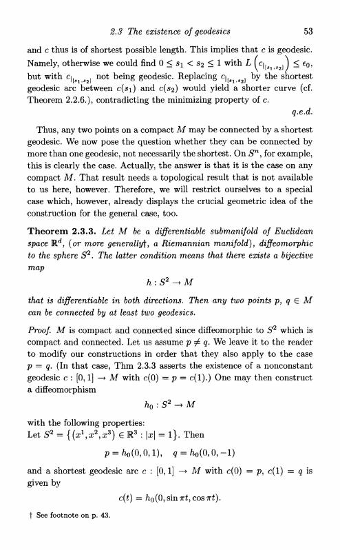
2.3 The existence of geodesies 53
and c thus is of shortest possible length. This implies that c is geodesic. Namely, otherwise we could find 0 < s\ < s2 < 1 wi th L ( c | [ s i ) S 2 ] ) < e0, but wi th C | ( S I not being geodesic. Replacing c j { a i 8 2 ) by the shortest geodesic arc between c(s\) and c(s 2) would yield a shorter curve (cf. Theorem 2.2.6.), contradicting the minimizing property of c.
q.e.d.
Thus, any two points on a compact M may be connected by a shortest geodesic. We now pose the question whether they can be connected by more than one geodesic, not necessarily the shortest. On 5 n , for example, this is clearly the case. Actually, the answer is that i t is the case on any compact M. That result needs a topological result that is not available to us here, however. Therefore, we wil l restrict ourselves to a special case which, however, already displays the crucial geometric idea of the construction for the general case, too.
Theorem 2.3.3. Let M be a differentiable submanifold of Euclidean space W*, (or more generally^, a Riemannian manifold), diffeomorphic to the sphere S2. The latter condition means that there exists a bijective map
h:S2 ~*M
that is differentiable in both directions. Then any two points p, q G M can be connected by at least two geodesies.
Proof. M is compact and connected since diffeomorphic to S2 which is compact and connected. Let us assume p ^ q. We leave it to the reader to modify our constructions in order that they also apply to the case p = q. (In that case, Thm 2.3.3 asserts the existence of a nonconstant geodesic c : [0,1] —> M wi th c(0) = p = c(l).) One may then construct a diffeomorphism
ho : S2 - M
with the following properties: Let S2 = { ( £ \ £ 2 , £ 3 ) G M 3 : |x| = l } . Then
p = M0,0,l), g = MO, 0,-1) and a shortest geodesic arc c : [0,1] —• M wi th c(0) = p, c ( l ) = q is given by
c(t) = M 0 , s i n 7 r £ , c o s 7 r £ ) .
f See footnote on p. 43.

54 Geodesic curves
Let us point out that these normalizations are not at all essential, but only convenient for our constructions. We look at the family of curves
7(£,s) = /io(sin27rssin7r£, cos27rssin7r£,cos7r£), 0 < s,t < 1. (2.3.1)
Then
7 (* ,0 ) = 7 ( M ) = c(t) for all t
and
7(0, s) = c(0), 7(1, s) = c ( l ) for all s.
We find some number K wi th
L{n(-,8))<K for all s. (2.3.2)
Redefining the parameter t, we may also assume that all curves 7(-,s) are parameterized proportionally to arc-length. By Theorem 2.3.1, there exists €o > 0 such that the shortest geodesic between any p, q G M, wi th d(p, q) < €o is unique. Let
0 = t0 < * i < . . . < tm = 1
be a partition of [0,1] wi th
h ~ tj-i < § for j = 1 , . . . , m. (2.3.3)
Let another partition ( T I , . . . , r m ) satisfy
To = t0 < r l < h < T2 < • • • < T M < tm = T m + i
and
T j ~ T j ~ 1 < : ? forj = l , . . . , m + l . (2.3.4)
I f 7 : [0,1] —• M is any curve parameterized proportionally to arc-length wi th
L(l) < K,
we then have for j = 1 , . . . , m
d (7 (^ -1 ) ,7(*j)) < I ( T | [ t j _ l ! ( j ) ) < * f =
Therefore, by Theorem 2.3.1, the shortest geodesic from y(tj-i) to y(tj) is unique. We then define 7*1(7) to be that piecewise geodesic curve for which r i ( 7 ) j [ t i t ] coincides wi th the shortest geodesic from 7(£j_i) to 7(^j), j = 1 , . . . , m. Likewise, we let ^ ( 7 ) by that piecewise geodesic curve for which r2 (7) | [r. r j coincides wi th the — again unique — shortest geodesic from 7 ( T J _ I ) to 7 ( T J ) , j = 1 , . . . , m + 1. We now observe:

2.3 The existence of geodesies 55
L e m m a 2 .3 .1 . Suppose d(7(fy)»7(fy-i)) < e0 and d(y(Tj),7(r7_i)) < €Q /or a// j .
r (7) : = r 2 o r i ( 7 )
sa£is/ies
L ( r ( 7 ) ) < L ( 7 ) (2.3.5)
equality iffy is geodesic.
Proof. By uniqueness of the shortest geodesic between y(tj-\) and 7(£j), we have
i ( r i ( 7 ) ) < i ( 7 )
wi th equality only in case
7*1(7) = 7-
Likewise, for every curve 7', L (7,' ] < €Q for all j ,
L ( r 2 ( 7 ' ) ) < L ( V )
wi th equality only in case
r 2 ( 7 ; ) = 7 ; -
Therefore
L ( r ( 7 ) ) < L ( 7 )
wi th equality only i f
r(7) = 7.
I f r (7) = 7, however, 7| [ t and 7 | [ t I T J are geodesic for every j , and hence 7 is geodesic itself. (If 7*1(7) = 7, then 7 i s piecewise geodesic wi th corners at most at the £j, and if r 2 ( r i (7)) = r\ (7), then r i ( 7 ) is geodesic wi th corners at most at the Tj. Thus, i f r(y) = 7, 7 cannot have any corners at all.)
q.e.d.
L e m m a 2.3.2. Let 7 : [0,1] —+ M be a curve parameterized proportionally to arc-length and with L("y) < K. Then a subsequence of>n(7) ( = ro. . .or(7)) converges uniformly to a geodesic with the same endpoints as 7.

56 Geodesic curves
Proof. Each curve r N ( 7 ) , n € N, is a piecewise geodesic with corners r n 7 ( n ) , . . . , r N 7 ( r m ) and endpoints r N 7 ( r 0 ) = 7 ( 0 ) , r N 7 ( r m + i ) = 7(1) . The individual segments are the unique shortest connections between these points. Therefore, each such curve is uniquely determined by the m-tupel
A n : = = ( r n 7 ( T l ) > _ ? r n
7 ( r m ) ) G M x . . . x M .
m times
Since M is compact, a subsequence of A n converges to some limit
(p i , . . . ,Pm) 6 M x ... x M .
r N ( 7 ) then converges uniformly towards the piecewise geodesic 70 with endpoints 70(0) = 7(0)>7o(l) = 7(1) and nodes 70(r<) = Pi (i = 1,... ,m) wi th segments 7 0 | { T i t } being the shortest geodesic arcs between their endpoints. This follows from the continuous dependence of the occurring geodesic arcs on their endpoints (Theorem 2.3.1). We denote the convergent subsequence of ( r N ( 7 ) ) N € N by ( 7 J , ) „ g N . For all v € N then
7 l / + 1 = r n M 7 „ with n[y) 6 N.
By the minimizing property of the subsegments of the 7 „ ,
L O H T , - ! , ^ ) = d ( l v ( r i ~ i ) »7i/ fo)) >
hence ra+1
L ( 7 ^ ) = £ <*(7«/ , 7 „ ( r j ) ) .
Since ^ ( T J ) converges to pj = 70 (T7), L(7 i , ) converges to ra+1
L (7o) = £ d (7o ( T J - I ) , 7 0 fa-))
for v —• oo. Then also
L ( 7 o ) = l im L ( 7 l / + 1 ) = l im L(r n <"> 7 „) i/—•oo 1/—•oo
< l im L(7i/) by Lemma 2.3.1 v—>oo
= i (7o ) ,
and equality has to hold throughout. Moreover, r ( 7 „ ) converges to r ( 7 0 ) ,
2.3 The existence of geodesies 57
and
L ( r ( 7 o ) ) = Urn L ( r ( 7 „ ) ) V—•oo
> l im L f r N ^ 7 ^ ) by Lemma 2.3.1 again
= £(7o) . Lemma 2.3.1 then implies that 70 is geodesic.
q.e.d.
We now return to the proof of Theorem 2.3.3: We apply the preceding curve shortening process to all curves 7 ( - , $ ) ,
s£ [0,1], simultaneously. For each 5, a subsequence of r N 7 ( - , s ) then converges to a geodesic from p to q. We want to exclude the situation that all those l imit geodesies coincide with c. Let
K0 := L(c) ,
and
K\ := sup l im L ( r N 7 ( - , s ) ) .
Since 7 ( - , 0) = c(-) is geodesic, r N 7 ( - , 0) = 7 ( - , 0) for all n, hence K\ > K 0 . We distinguish two cases:
(1) K\ > K0
Since 7 ( - , s) is continuous in s, so is r N 7 ( - , s) for every n G N . We now claim: Whenever
supL( r N 7( - , s ) ) < KI + e (2.3.6)
there exists s n € [0,1] with
L ( r n
7 ( - , *»)) - i ( r n + 1 7 ( - , »„)) < 2c (2.3.7)
and
L ( r n
7 ( - , « „ ) ) > « ! - € . (2.3.8)
Indeed, otherwise
s u p L ( r n + 1
7 ( - , « ) ) < « i - c ,
contradicting the definition of K\ (note that sup 5 L ( r N + 1 7 ( - , $ ) )
58 Geodesic curves
is monotonically decreasing in n by Lemma 2.3.1). By definition of K i , there exists a subsequence ( e n ) n € N -* 0 with
s u p L ( r n 7 ( - , 5 ) ) < fti + e n . 3
A subsequence of ( r n 7 ( - , s n))neN has to converge to some limit curve c as above, and because of (2.3.7) with e = e n, we conclude as in the proof of Lemma 2.3.2 that
L(r(c)) = L(c),
and c is hence geodesic by Lemma 2.3.1. Because of (2.3.8) and continuity of L in the limit as in the proof of Lemma 2.3.2, we get
L(c) — K\.
Since c and c are both defined on [ 0 , 1 ] and have different lengths, they have to be different curves. Thus, c is the desired second geodesic.
(2) K\ = K0
We are going to show that in this case, there even exist infinitely many geodesies from p to q. For that purpose, we consider the curve
This is a closed curve with 7 ( 0 ) = 7 ( 1 ) = c(\) (see Figure 2.2).
Since ho is a diffeomorphism and r n 7 ( t , s) is obtained through a process that can easily be made continuous from
7(^,5) = /io(sin27T5sin7rt,cos27T5sin7rt,cos7rt),
r n 7 ( £ , s ) has to map [ 0 , 1 ] x [ 0 , 1 ] surjectively onto M . Therefore, for every n € N and every 5 G [ 0 , 1 ] , there exists cr n(s) wi th
7(5) G r n
7 ( . , a n ( 5 ) ) = : 7 n , s ( 0
(in other words, r n 7 ( - , o - n ( s ) ) is a curve passing through 7 (5)) . 7 n,s(*) then is a curve with
7n,a(0) = C ( 0 ) = p , 7 n , « ( l ) = c( l ) = q,
and because of K \ = KQ, we obtain
lim L ( 7 n , s ( . ) ) < sup l im L ( r n
7 ( . , 5 ) ) = ^ 0 . (2.3.9) " 0<s<l n ->°°

2.3 The existence of geodesies 59
P
q
Figure 2.2.
After selection of a subsequence, (7n , s (*))n€N again converges to some limit curve cs(-) wi th
c s(0) = p , c a ( l ) = q
and
By (2.3.5),
and since K,Q is the infimum of the energies of all curves from p to q («o = L(c), and c is minimizing), cs(-) is a minimizing curve itself, hence geodesic.
Therefore, we have shown that for every 5, there exists a geodesic from p to q that passes through 7 (5) . Hence there exist infinitely many geodesies from p to g, as claimed.
q.e.d. Remarks:
(1) Lemmas 2.3.1 and 2.3.2 do not need that M is diffeomorphic to S2. Compactness suffices.

60 Geodesic curves
(2) We may construct the curves 7n,s(*) at the end of the proof also in case K\ > K 0 . In that case, however, limits of such curves need not be geodesic anymore.
(3) See Section 3.1 for an abstract version of the argument at the end of the preceding proof.
Exercises
2.1 For curves j(t) = (j\j2) : R -+ {(x\x2) e E 2 | x 2 > 0} , consider
Compute the Euler-Lagrange equations and determine all solutions.
2.2 For curves d
7 ( t ) = ( 7 1 , • • •, 7 d ) : R - {{x\ . ..,xd)€ Rd\ 5 > ' ) 2 < 1}, 1 = 1
consider
Compute the Euler-Lagrange equations and determine all solutions.
2.3 Determine all geodesies between two given points on a cylinder
{ ( x , y , z ) e K 3 : x 2 + y 2 = = l } .
2.4 Let E be a surface of revolution in E 3 , i.e.
Z = {(x,y,z)em3:x2+y2=f(z)}
for a smooth, positive / : E —• E. What can you say about geodesies on E? For example, are the curves (x, y) = constant geodesies? When are the curves z = constant geodesies?
2.5 Determine Riemannian polar coordinates on the sphere Sn wi th a domain of definition that is as large as possible.
2.6 Let p be the center of Riemannian polar coordinates on M , wi th domain of definition {v G E d : | |v| | < g}. Let c : [0, e] —• M be a geodesic with c(0) = p that is parameterized by arc-length, 0 < e < Q. Show that c([0,c]) does not contain a point that is conjugate to p.
Exercises
2.7 Let M be a differentiable submanifold of Rd that is diffeomor-phic to S2. Show that for any p G M , there exists a nonconstant geodesic c : [0,1] —• M wi th c(0) = c( l ) = p.
2.8 Try to find other topological classes of manifolds wi th the property that there always exists more than one geodesic connection between any two points.

3 Saddle point constructions
3.1 A f in i te d imensional example
Let F : E d —• E be a function of class C1 which is bounded from below and which is 'proper' in the following sense:
F{x) -+ oo for |x| -» oo. (3.1.1)
Since F is bounded from below, (3.1.1) is equivalent to: For every s G E,
{x G E d : F(x) < $} is compact. (3.1.2)
Therefore, F assumes its infimum. Namely, we take any
s0 > inf F(x). x£Rd
Then
{x G E d : F(x) < so}
is compact and nonempty, and since F is continuous, it has to assume its infimum on that set. We now assume that F even has two relative minima, x i , #2 in E d , and that they are strict in the following sense: For x = # i , #2 , we have
3<50Vt/ with 0 < \y-x\ < 60 : F(y) > F(x). (3.1.3)
T h e o r e m 3.1.1. Under the above assumptions, F has a third critical point £3 (i.e. VF(xs) = 0) with
F(x3) > m a x ( F ( x i ) , F ( x 2 ) ) = : «o
Proof. We consider curves 7 : [0,1] —• Rd with
7(0) = x i ,7(1 )=*2. (3.1.4)
62

3.1 A finite dimensional example 63
We first observe that there exists a > 0 with the property that for any such curve, there exists t0 € (0,1) with
F^(t0))>K0 + a. (3.1.5)
In order to verify this, we may assume w.l.o.g.
F(xx) < F ( x 2 ) .
We then choose <5 wi th
0 < 6 < min((50, ^ | x i - x 2 | ) . (3.1.6)
For every y wi th |y - x 2 | = <5 then by (3.1.3)
F(y) > F(x2),
and since {\y — x2\ = 6} is compact, F assumes its minimum on this set, hence for some a > 0
min F(y)> F(x2)+a = K0 + a. (3.1.7) \y-x2\=S
Since for every curve 7 wi th (3.1.4) we have
| 7 ( 1 ) - x2\ = 0, | 7 ( 0 ) - x2\ = \xi - x2\,
there has to exist some t0 € [0,1] with
\7(t0) - x2\ = 6 (recall (3.1.6)) .
By (3.1.7) then
F( 7 (^o)) > «o 4- a,
and (3.1.5) follows indeed. We now define
K\ := inf sup F(i(t)), 7 *€[0,1]
where 7 again is a curve in Rd wi th 7(0) = x i , 7(1) = x2. By (3.1.5)
«i > K 0 . (3.1.8)
Our intention now is to find a critical point X3 of F wi th
F ( x 3 ) = « i .
Since
F ( x i ) , F ( x 2 ) < « 0 ,
64 Saddle point constructions
#3 wi l l then be necessarily be different from X\ and #2- As a step towards the existence of such a point £3 , we claim
Ve > 0 3<5 > 0 V curves 7 with 7(0) = #1,7(1) = x2
with
sup F(7(0) <n\+6 (3.1.9)
t€[0,l]
3 1 0 € [0,1] with:
F(-y(t0)) > «i - 6 (3.1.10)
| ( V F ) ( 7 ( * o ) ) | < c . (3.1.11)
Suppose this is not the case. Then
3to > 0 V n € N 3 curve 7 „ between Xi and x2 wi th
supF (7„( t ) ) < « i + - (3 .1 .12) t n
V< 0 wi th F ( 7 „ ( t 0 ) ) > K I - € 0 (3 .1 .13)
| ( V F ) ( 7 „ ( « o ) ) | > € 0 . (3 .1 .14)
For s > 0, we define a new curve 7 „ i S by
7 » , . ( < ) : = 7 n ( « ) - « ( V F ) ( 7 „ ( * ) ) -
Since x\ and #2 are minima, VF{x\) — 0 = VF(#2)> and so
7n,*(0) = x i ,7 n , 5 ( l ) = x 2 ,
so that the curves 7 n > s are valid comparison curves. By our properness assumption (3.1.2) and (3.1.12), 7 n (£) stays in a bounded subset of E d , and VF wi l l then be bounded on that bounded set, and hence for any So > 0 and all 0 < 5 < so, the curves 7n,s(0 stay in some bounded set, too. This set is independent of n (as long as 0 < 5 < 5 0 , for fixed SQ > 0). By Taylor's formula
F ( 7 n , , ( 0 ) = F(ln(t)) - sVF(ln(t)) • V F ( 7 „ ( « ) ) + o(s).
Since F is continuously differentiable and 7 n , s ( £ ) is contained in a bounded set, 0(5) can be estimated independently of n and t (as long as 0 < s < s 0 ) . * n Particular, after possibly choosing s0 > 0 smaller,
F ( 7 n , . W ) < ^ ( 7 » ( * ) ) - I | V F ( 7 n ( < ) ) | 2 (3 .1 .15)

3.1 A finite dimensional example 65
for all n, s wi th 0 < s < s 0, and t wi th
| V F ( 7 n ( * ) ) | > c 0. (3.1.16)
Thus, in particular,
F(ln,s0(t)) < F(ln(t)) - ^ 4 (3.1.17)
for all such t and all n. We now simply choose n so large that
i < f 4 (3.1.18)
Then by our assumption, all t0 wi th F ( 7 n ( £ 0 ) ) > «i - e 0 satisfy (3.1.14), and hence for all such to
F(ln,s0(to)) < F ( 7 „(*o) ) - | e 2
< « i + - - ? € o by (3.1.12) (3.1.19)
< «i by (3.1.18).
Having proved (3.1.19), there are now various ways to construct a path 7 from X\ to X2 wi th
F(7(*)) < «i for all * € [0,1]. (3.1.20)
One way is to refine the above construction by letting s depend on t as follows: we choose a smooth function
v(t):[0, l ] - [ 0 , * 0 ]
with
a(t) = 0 whenever F(yn(t)) < K\ — e0
and
a(t) = s0 whenever F(yn(t)) > K \ - ~ .
We then look at the path 7 ( f ) = 7n,<7(t)(0- Then for t wi th F ( 7 n ( £ ) ) <
F(7(0 ) = i ? ( 7 n ( 0 ) < « i - e 0 ,
for £ with K \ - e0 < F ( 7 n ( £ ) ) < «i - ~
F(7(*)) < F ( 7 n ( t ) ) - < K l - ? - ^
66 Saddle point constructions
(cf. (3.1.15), (3.1.16), (3.1.14)), and finally for all t wi th F(yn(t)) >
K l ~ 2
F ( 7 ( t ) ) = F ( 7 n , . 0 ( * ) ) < « ! (cf- (3.1.19)).
Thus, (3.1.20) holds indeed. This, however, contradicts the definition of « i . Therefore, the assumption that our claim was not correct led to a contradiction, and the claim holds. I t is now simple to prove the theorem. Namely, we let e n —> 0 for n —• oo, and for e = e n, we find <5 = 6n as in the claim. We than choose a curve 7 n from x\ to x% wi th
sup F ( 7 „ ( * ) ) < «i + min(e n,<5 n). (3.1.21) t€[0,lj
According to the claim, there exists tn e [0,1] with
F(~fn(tn))>Ki-en (3.1.22)
| ( V F ) ( 7 n ( * n ) ) | < e n . (3.1.23)
After selection of a subsequence, (/yn(tn))neN then converges to some point x 3 , because of (3.1.2) and (3.1.21). x$ then satisfies by continuity of F and V F
F ( x 3 ) = «i (3.1.24)
V F ( x 3 ) = 0. (3.1.25)
Thus, £3 is the desired critical point. q.e.d.
Theorem 3.1.1 may be refined as follows:
Theorem 3.1.2. Let F as above again have two relative minima, not necessarily strict anymore. Then either F has a critical point x$ with
F(x3) > m a x ( F ( x i ) , F ( x 2 ) ) = « 0 ,
or it has infinitely many critical points.
Proof. For the argument of the proof of Theorem 3.1.1, we only need
inf sup F ( 7 ( * ) ) > « 0 , (3.1.26) 7 t€[0,l]
where the infimum again is taken over curves 7 : [0,1] —• E d wi th 7(0) = # i , 7(1) = #2. So, suppose that (3.1.26) does not hold. We then want to
3.2 The construction of Lyusternik-Schnirelman 67
show the existence of infinitely many critical points. As in the proof of Theorem 3.1.1, we may assume
F(xx) < F(x2).
The argument at the beginning of the proof of Theorem 3.1.1 then shows that (3.1.26) holds if x2 is a strict relative minimum. I f x2 is a relative minimum, which is not strict, for all sufficiently small 6 > 0, say <5 < <5Q, we have
F(x2) < F(x) for all x wi th \x - x2\ < <50 (3.1.27)
and there always exists some x$ wi th 0 < \xs — x2\ < 6 and
F(x6) = F{x2). (3.1.28)
We then put 8\ = <50/2. Then xsx is a relative minimum of F by (3.1.27), (3.1.28), hence a critical point. Having found a critical point xsn wi th 0 < \x6n - x2\ < \x6n_1 - x 2 | , we put
<Wl = \ \x6n - X2\
and find a critical point xsn+1 wi th
0 < \xgn+1 - x2\ < <5 n + i .
Thus, xsn+1 is a critical point of F different from all preceding ones. q.e.d.
Remark. I t is not very hard to sharpen the statement of Theorem 3.1.2 from 'infinitely many' to 'uncountably many'.
3.2 T h e construction of Lyusternik-Schnire lman
In this section, we want to prove the following theorem, in order to exhibit some important global construction in the calculus of variations, introduced by Lyusternik-Schnirelman. The result presented is much more elementary than the theorem of Lyusternik-Schnirelman, which says that on any surface wi th a Riemannian metric, e.g. a surface embedded in some Euclidean space, diffeomorphic to the two-dimensional sphere, there exist at least three closed geodesies without self-intersections. The more elementary character of our setting allows us to bypass essential geometric difficulties encountered in a detailed proof of the Lyusternik-Schnirelman Theorem.

68 Saddle point constructions
Figure 3.1.
T h e o r e m 3.2.1. Let 7 be a closed convex Jordan curved of class C1 in the plane E 2 . (7 then divides the plane into a bounded region A, and an unbounded one, by the Jordan curve Theorem. That 7 is convex means that the straight line between any two points of 7 is contained in the closure A of A.) Then there exist at least two such straight lines between points on 7 meeting 7 orthogonally at both end points (see Figure 3.1).
Proof. We start by finding one such line. Let C be the set of all straight lines / in A wi th dl C 7. We say that a sequence (ln)neN C £ converges to / E £ , i f the end points of the ln converge to those of /. In order to have a closed space, we allow lines to be trivial i.e. to consist of a single point on 7 only. We denote the space of these point curves on 7 by £ 0 -We let / := [0,1] be the unit interval. We consider continuous maps
v:I-*C
with the following two properties:
(i) v(0) = v(l). (ii) To any such family, we may assign two subregions A\(t) and A2(t)
of A in a certain manner. Namely, we let A\(t) and A2(t) be the two regions into which v(t) divides A. Having chosen A\(0) and A2(0), A\(t) and A2(t) then are determined by the continuity
t A closed Jordan curve is a curve 7 : [0, T] —• Rd with 7 (0 ) = 7(T") that is injective on [0, T ) . Cf. the definition of a Jordan curve on p. 35.

3.2 The construction of Lyusternik-Schnirelman 69
Figure 3.2.
requirement. We then require
A1(1) = A2(0).
We let Vi be the class of all such families v.
The construction is visualized in Figure 3.2. (0 corresponds to 0 £ J, /to\J/ to I / / / to | , 1 to 1)
Actually, in order to simplify the visualization, if v(0) is a point curve (on 7), i) may be relaxed to just requiring that v(l) also is a point curve (on 7), not necessarily coinciding with v(0) (see Figure 3.3). Namely, any point curves can be connected through point curves, i.e. wi th vanishing length.
We denote by L(l) the length oil € C and define
K\ := inf supL(v(t)). v^yi tei
1
Figure 3.3.

70 Saddle point constructions
We want to show that
«i > 0.
For this purpose, let p > 0 be the inner radius of 7, i.e. the largest p for which there exists a disc
B(x0lp) C A
for some XQ G A (B(xo,p) := {x G E 2 : \x - x 0 | < p})- Then
«i > «i := inf sup L(v(t) P\ B(XQ, p)).
We let Aft) := ^ ( t ) n B(xo,p), i = 1,2. Because of (ii) and the continuous dependence of J4*(£) and hence also of Af
{(t) on t, there exists some to £ I wi th
Area ( t 0 ) ) = Area (A'2(t0)).
Thus v(to) divides B(xo,p) into two subregions of equal area. v(to) then has to be a diameter of B(xo,p), i.e.
L(v(to)nB(x0,p))=2p.
Therefore
«i > «i = 2p > 0
and Ki is positive indeed. We are now going to show by a line of reasoning already familiar from Sections 2.3 and 3.1 that K\ is realized by a critical point / of L among all lines with end points in 7, i.e. by / meeting 7 orthogonally (see Theorem 1.4.1). For that purpose we shall assume for the moment that 7 is of class C 3 . Later on, we shall reduce the case where 7 is only C 1 to the present one by an approximation argument. We now claim
V e > 0 3(5 > 0 : Vv € Vi wi th
supL (v(t)) < Ki+6 tei
3 to G I wi th L (v(to)) > «i - c
and |cos(ai (v (t0)))\ , |cos ( a 2 {v (t0)))\ < c,
where a\(l) and a2(l) are the angles of / at its endpoints wi th 7.

3.2 The construction of Lyusternik-Schnirelman 71
Otherwise
3e 0 > 0 : V n G N 3vn G V\ wi th
s u p L ( v n ( t ) ) < «i 4- £ t
V t 0 wi th L (v n(*o)) > K I _ €o
|cosai (v n(*o))| > eo
or |cosa2 (vn(*o))| > €o-
The idea to reach a contradiction from that assumption is simple, once the following Lemma is proved:
L e m m a 3.2.1 . For every planar closed Jordan curve 7 of class C3, there exists (3 > 0 with the following property: Whenever x G E 2 satisfies
dist(x,7) := inf \x — y\ < (3 ye-y
there exists a unique y G 7 with dist(#,7) = \x — y\.
Proof. We consider 7 as an embedded submanifold of the Euclidean plane E 2 . 7 is then covered by the images of charts / : U —• V of the type constructed in Theorem 2.2.1. Here, U and V are open in E 2 , and
7 n v = f (u n {x2 = 0 } ) .
Furthermore, the curves x1 = constant in U correspond to geodesies, i.e. straight lines in V perpendicular to 7, and they form shortest connections to 7 f l V. By shrinking U, i f necessary, we may assume that i t is of the form ( - £ , £) x (-77, rj), wi th £ > 0, rj > 0. Since 7 is compact, i t can be covered by finitely many such charts
fi : ( - 6 , 6 ) x (-WiVi) ~*yi , i = l , . . . , m .
I f we then restrict fi to ( - 6 , 6 ) x ( " f 1 ' ^ J , lines x1 = constant, ~ k < x2 < ^ , then correspond to shortest geodesies to 7, since the part of 7 not contained in V{ is not contained in the image of fi, and hence has distance at least ^ from the image of the smaller set ( — & ) x , ) . This is indicated in Figure 3.4 where the broken lines correspond to x2 = ^ and this is depicted for two different indices i.
Therefore, (3 := min ( ^ ) satisfies the claim. i=l,...,n
q.e.d.

Saddle point constructions
Figure 3.5.
We now return to the proof of Theorem 3.2.1:
Without loss of generality eo < 0 < Assume e.g.
cosai (vn (to)) > e0.
The following construction is depicted in Figure 3.5. Choose si(to) €

3.2 The construction of Lyusternik-Schnirelman 73
vn(to) wi th
|ai(*o)-Pi(to)|=0, where p\(to) is the endpoint of vn(to) where i t forms the angle a\(to) with 7. We replace the subarc v^(to) of vn(to) between p i ( t 0 ) and si(£o) by the shortest line segment vf
n(to) from s\(to) to 7. By the theorem of Pythagoras and the convexity of 7
L (v'n (t0)) < L (yl
n (t0)) s ina i (vn (t0))
<L(vi(t0))yfl^.
We then let
Vn(to)
be the straight line from the second endpoint p2(to) of vn(to) to the point where vf
n(to) meets 7. Then, letting v„(to) denote the segment of vn(to) between s\(to) and p2(to), by the triangle inequality
L(v*n(t0))<L(v'n(t0)) + L{v2
n(t0))
<L{vl{t*))J^l + L{vl(tQ))
= f 3 ^ 4 + L(v2
n(t0)).
Since L (y\ (to)) = /?, we have
L(v2
n(t0)) < K I - / ? +
We then choose n so large that
Py/l ~4 + Ki-0+^<Ki-ri
for some rj > 0. Hence
M < (*(>)) <*!-*/. We now continuously select points si(£), 52(t) on v n ( t ) for every t e I with
\Pi(t) - Si(t)\ = 0, whenever L (vn (t)) > Ki - 0
and
Pi(t) = Si(t), whenever L (vn (t)) < K\ — 20 i = 1,2
and
\Pi(t) - Si(t)\ < 0 f o r a l U .

74 Saddle point constructions
We then choose again the shortest lines from Si (t) to 7 and replace vn (t) by the straight line vn(t) between those points, where these two shortest lines meet 7. By our geometric argument above
L (vs
n (t)) < K\ — rj for some rj > 0,
whenever
L(vn (t)) > KI - e0.
Since also always
L K (t)) < L (vn (t)),
we may then construct a family i £ € V\ wi th
sup L « (t)) <KX- min(77, (3) tei
contradicting the definition of K \ . Consequently, our claim is correct. We then find a sequence (tn)neN C / and (vn)neN C V\ wi th
supL(vn (t)) < K \ + -tei n
L(vn (tn)) > K\ - -n
|cos ( a i (vn (tn)))\, |cos ( a 2 (vn (tn)))\ < n
A subsequence of (vn (tn))ne^ then converges to a straight line l\ in A of length K\ meeting 7 orthogonally at its endpoints.
In order to construct a second line l2 meeting 7 orthogonally at its endpoints, we proceed as follows:
We denote by V2 the class of all continuous maps
v : J x J -+ C
with
v({0} x / ) and v({l} x I) C C0 (3.2.1)
and with the following property: For all continuous maps
T(8) = (h(8)MB))
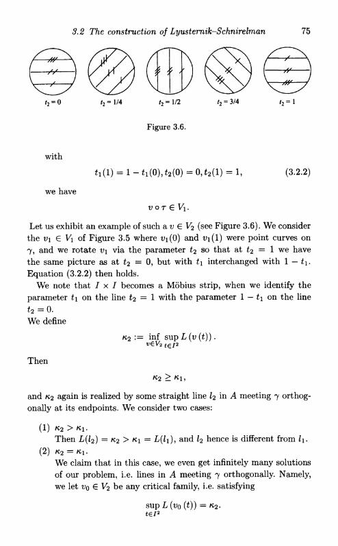
3.2 The construction of Lyusternik-Schnirelman 75
f 2 - o t2 = 1/4 t2 = 1/2 f2 = 3/4 r 2 - l
Figure 3.6.
wi th
t i ( l ) = 1 - t i ( 0 ) , t 2 ( 0 ) = 0 , t 2 ( l ) = 1, (3.2.2)
we have
Let us exhibit an example of such a v 6 V2 (see Figure 3.6). We consider the v\ G V\ of Figure 3.5 where i>i(0) and V\(\) were point curves on 7, and we rotate v\ via the parameter t2 so that at £2 = 1 we have the same picture as at t2 = 0, but wi th t\ interchanged wi th 1 — t i . Equation (3.2.2) then holds.
We note that I x I becomes a Mobius strip, when we identify the parameter t\ on the line t2 = 1 wi th the parameter 1 — t\ on the line t2 = 0 . We define
and K 2 again is realized by some straight line l2 in A meeting 7 orthogonally at its endpoints. We consider two cases:
(1) K2 > K\. Then L(l2) = K 2 > K \ = L ( i i ) , and l2 hence is different from l\.
(2) K2 = tti. We claim that in this case, we even get infinitely many solutions of our problem, i.e. lines in A meeting 7 orthogonally. Namely, we let VQ G V2 be any critical family, i.e. satisfying
K2 := inf sup L (v (t)). v€V2te[2
Then
K2 > Ki
supL(i>o (t)) = ^ 2 -ten

76 Saddle point constructions
(It is not hard to see that in the present case such a VQ G V2
indeed exists.)
We then have for any r : J -+ I 2 wi th (3.2.2)
sup L (v0 (T (s))) < K 2 . (3.2.3) sei
On the other hand, since VQOT eVi,
KX < sup L ( v o ( r (*))) , (3.2.4) sei
and since K \ = K 2 , we have equality in (3.2.3) and (3.2.4). This means that VOOT is a critical family for « i , and i t then has to contain a solution lr of our problem.
Let S C {(s,t) e I x 11 L(i;o(s,£)) = K 2 ) } denote the set in J x J corresponding to all solutions induced by vo. After carrying out the identification prescribed by (3.2.2), which makes I x I into a Mobius strip, we see that the complement of S in this Mobius strip is not path connected. Namely, otherwise we could find r satisfying (3.2.2) for which T ( J ) avoids 5, and for such a r , vo o r would then not contain a solution, as S is the set of all solutions in the family VQ. This, however, contradicts what has just been said (see Figure 3.7). In fact, S has to carry a one dimensional cyclef on the Mobius strip. Otherwise, S would be contractible (in the Mobius strip) and one could reparameterize VQ on I 2 so that the set of solutions corresponds to a finite number of points. But this is incompatible wi th K 2 = K \ as we have just seen. Since for each path r as in (3.2.2) wi th r ( J ) C S, vo o r G V\ is nonconstant by (3.2.1) and (3.2.2), we obtain an uncountable number of solutions.
We thus have shown our result if 7 is of class C 3 . I f 7 is only of class C 1 , we choose a sequence of curves yn of class C 3 approximating 7 . This means that there are parameterizations 7 U ( T ) , 7 ( T ) by arc-length wi th
l im s u p ( | 7 n ( r ) - 7 ( r ) | + n—•oo r \
= 0.
We then let li,n and Z2,n be the corresponding solutions for j n . After selection of subsequences, l\in and l2yU then converge to solutions Zi, l2 for 7 , and those l\ and l2 realize the critical values K \ and K 2 , respectively. Since the argument to produce infinitely many solutions in case K \ — K 2
f We have to employ here some constructions from algebraic topology. A reference is any good book on that subject, e.g. M.Greenberg, Lectures on Algebraic Topology, Benjamin, Reading, Mass., 1967, pp. 33-45, 186. While this is somewhat technical we strongly urge the reader to try to understand the essential geometric idea of the preceding construction.
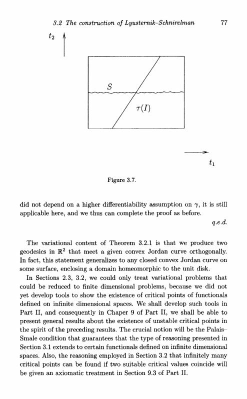
3.2 The construction of Lyusternik-Schnirelman 77
^
ti
Figure 3.7.
did not depend on a higher differentiability assumption on 7, i t is stil l applicable here, and we thus can complete the proof as before.
q.e.d.
The variational content of Theorem 3.2.1 is that we produce two geodesies in E 2 that meet a given convex Jordan curve orthogonally In fact, this statement generalizes to any closed convex Jordan curve on some surface, enclosing a domain homeomorphic to the unit disk.
In Sections 2.3, 3.2, we could only treat variational problems that could be reduced to finite dimensional problems, because we did not yet develop tools to show the existence of critical points of functionals defined on infinite dimensional spaces. We shall develop such tools in Part I I , and consequently in Chaper 9 of Part I I , we shall be able to present general results about the existence of unstable critical points in the spirit of the preceding results. The crucial notion wil l be the Palais-Smale condition that guarantees that the type of reasoning presented in Section 3.1 extends to certain functionals defined on infinite dimensional spaces. Also, the reasoning employed in Section 3.2 that infinitely many critical points can be found if two suitable critical values coincide wi l l be given an axiomatic treatment in Section 9.3 of Part I I .
78 Saddle point constructions
Exercises
3.1 Let F € C ^ M j R ) ( M an embedded, connected, differentiable submanifold of Rd) be bounded from below and proper (i.e. for all 5 € R, {x € M : F(x) < s} is compact), and suppose F has two relative minima X i , x 2 . Let
KO : = max(F(#i ) , Ffa))-
Show that F either possesses a critical point £3 wi th F(x^) > ^o, or that i t has uncountably many critical points.
3.2 Let F € C x ( R d , R ) be bounded from below and proper, and suppose i t has three strict relative minima £ i , # 2 , £ 3 . Try to identify conditions under which F then has to possess more than two additional critical points, e.g. three or four.
3.3 Let A be a compact convex subset of the unit sphere S2 C R 3 , and suppose OA is a smooth curve 7; the convexity condition here means that for any two points in A, one can find precisely one geodesic arc inside A that connects them. Show the existence of at least two geodesic arcs in A that meet 7 orthogonally at both endpoints.

4
The theory of Hamilton and Jacobi
4.1 T h e canonical equations
We let t be a real parameter varying between t\ and t2. We consider the variational integral
I = f 2 L fax1^),... ,xn(t),xl(t),... ,xn(t)) dt (4.1.1) Jti
for the unknown functions x(t) = (x1^),..., xn(t)) wi th fixed endpoints x(t\) and x(t2). Here,
.i _ <W_ X :~ dt'
We assume that L is of class C 2 . The Euler-Lagrange equations for / are
^-L±i-Lxi=0 ( i = l , . . . , n ) . (4.1.2)
We assume the invertibility condition
detL±i±j ^ 0 . (4.1.3)
As shown in 1.2, this implies that solutions of (4.1.2) are of class C 2 . (4.1.3) also implies that we may perform a Legendre transformation. Namely, by the implicit function theorem, we may then locally solve
Pi = L ± i (4.1.4)
w.r.t. x l , i.e.
xi = x * ( t , x , p ) ( p = ( p i , . . . , P n ) ) . (4.1.5)
79

80 The theory of Hamilton and Jacobi
The expressions pi are called momenta. The Hamiltonian H is defined as
H(t,x,p) := x%pi - L(£ ,x ,x) . (4.1.6)
We obtain
H x i - p j M ~ L i J d x ^ ~ L x i >
and with (4.1.4) then
Hx% = ~Lxi.
and with (4.1.2) and (4.1.4) then
Hxi = - p . . (4.1.7)
Also
nPi — Pj r X — L/Xj ——, dpi dpi
and thus again with (4.1.4)
HPi=x\ (4.1.8)
(4.1.7) and (4.1.8) constitute a so-called canonical system. We are going to see that (4.1.7) and (4.1.8) also arise as Euler-Lagrange equations of the variational problem obtained by expressing L in (4.1.1) through H via (4.1.6). Namely,
I = j 2 [xj
Pj -H(t,x,p)) dt, (4.1.9) Jti
where the unknown functions are x(t) and p(t), has Euler-Lagrange equations (4.1.7) and (4.1.8), and so does
J = - [ 2 (xjpj+H(t,x,p))dt. (4.1.10)
Before proceeding, we observe that i f H does not depend explicitely on t, i.e. H = H(x,p), then i f is a constant of motion, i.e. constant along any solution x(t) of the equations, Namely,
~H (x(t),p(t)) = Hxixl + HPipi = 0 (4.1.11)
by (4.1.7) and (4.1.8).
4-2 The Hamilton-Jacobi equation 81
Example. For L = | |x| — V(x), we have
H=1-\p\2 + V(x),
and the canonical equations become
x = p
P=-Vx.
This example, which describes the Newtonian motion of a particle of unit mass subject to a potential F , is helpful for remembering the signs in the canonical equations.
4.2 T h e Hamilton-Jacobi equation
Assumption. There is given a set fi C M n + 1 = { ( ^ x 1 , . . . , £ n ) } wi th the property that for any points A, B € fi, A = (a, ft1, . . . , ft71), B = (s, q1,..., qn), there is a unique solution x(t) = ..., xn(t)) of (4.1.2) contained in fi wi th (a, x(o~)) = A, (s,x(s)) = B.
Thus, fi is covered by solutions of (4.1.2), and those can be considered as functions of their endpoints. Thus
= (t;s,q\...,qn;a^\...^n) (4.2.1)
and also
Pi = gi(t;s,q\...,qn;o-,K,l,...,K,n) = L±i. (4.2.2)
In particular,
= (a; s , ? 1 , . . . , ^ ; a, ft1,..., ft71) (4.2.3)
Q* = fi(s\s,q1,...,qn;a,K,1,...,K,n).
We also define
ipi := gi(a; 5 , ql,..., qn; a, ft1,..., ftn) = Lki (a, ft, ft) (4.2.4)
Vi := gi(s; s,qx,... ,qn;a, ft1,..., ftn) = L^(s,q,q).
In the sequel, /* etc. wi l l mean a derivative w.r.t. the first independent variable, fl etc. a derivative w.r.t. the second one. Inserting (4.2.1), (4.2.2) into i " , we obtain
J = I(s,q,a,K) (4.2.5)

82 The theory of Hamilton and Jacobi
and call this expression the geodesic distance betweeen A and B. In this connection, I is called eiconal. Recalling (4.1.9), we may write
I = j (p<£< -H(t,x,p))dt. (4.2.6)
We want to compute the derivatives of I(s, q, a, K).
I s = Viq{ - H(s, q, v) + j f {g'J + 9if' - HXif' - HPigty dt
Equations (4.1.7) and (4.1.8) yield Hxi = —fa, HPi = /*, and thus
Is = - H{s, q,v) + J (oif) •
= ^<f - H(s,tf, v) + gif1
\t = (T Equation (4.2.3) yields
p + f = 0 for t = s
f = 0 for t = a,
dt
• l I t—s
and thus altogether
h = Vi<jl - H(s,q,v) - Vitf
= -H{s,q, v)
= L(s,q,q)-qiL^. (4.2.7)
Next
q3~l [Wf + *W~ *W]
t=s
Thus
9 i ^ \ again by (4.1.7), (4.1.8)
^•(s; 5, g 1 , . . . , qn; G , K 1 , . . . , KN) by (4.2.3)
and ——: = 0, ~P~~~t = 6{j. dqi dq3 13
I q j =Vj =L#(s,q,q). (4.2.8)
4-2 The Hamilton-Jacobi equation
Analogously,
Ia = H(a, ft, ip) = —L(o, ft, ft) 4- klLkx. (4.2.9)
4* = -¥>j = -LkJ(o-,K,,k). (4.2.10)
Inserting (4.2.8) into(4.2.7), we obtain
h + H( (4.2.11)
Thus, the geodesic distance as function of the endpoint satisfies (4.2.11), a Hamilton-Jacobi equation. In the present context that equation then is also called eiconal equation. We observed at the end of Section 4.1 that H is constant along solutions i f i t does not depend on t explicitly. In that case, (4.2.11) implies that / then depends linearly on 5. I t may be useful for understanding the preceding formulae if we derive them without the use of the Legendre transformation. Thus
1= f L(t,x(t),x(t))dt= f L(t,fJ)dt J a J o
and
The Euler-Lagrange equations give
and so
= L(s,q,q)+ L±if
As before, we obtain from (4.2.3)
p =-f fort = 5
/*' = 0 for t = a,
hence
I s = L(s,q,q) - L#q\
84 The theory of Hamilton and Jacobi
i.e. (4.2.7). Likewise,
dp
dq3 x dq3
I t = s r§T"
L + i •
i.e. (4.2.8). Thus, the Hamilton-Jacobi equation (4.2.11) is
Is-L(s,q,q) + Iqiqi =0. (4.2.12)
We have seen in the preceding how solutions of the canonical equations yield solutions of the Hamilton-Jacobi equations. We now want to establish a converse result.
Let (p(t, x 1 , . . . , xn) be a solution of the Hamilton-Jacobi equation which we now write as
po + H(t, x\ . . . , x n , P l , . . . , p n ) = 0 (4.2.13)
with
Po = ¥>t
Pi = <Px*-
D e f i n i t i o n 4 .2 .1 . If
<p = G(t, x 1 , . . . , x n , A i , . . . , A n ) with G e C2 (4.2.14)
and
d e t ( G x % ) . . = 1 n ^ 0 (4.2.15)
is a family of solutions of (4-2.13) depending on n parameters A i , . . . , Xn, we call
<p = G(t, x\ . . . , x n , A i , . . . , A n ) + A (4.2.16)
(where A is a free real parameter) a complete integral of (4-2.13).
We have the following theorem of Jacobi:
T h e o r e m 4 .2 .1 . Let <p = G(t, x 1 , . . . , x n , A i , . . . , A n ) - f A be a complete integral of (4.2.13). Then one may obtain a family of solutions of the

4-2 The Hamilton-Jacobi equation 85
canonical equations
HPi=x{ (4.2.17)
Hx. = -Pi (4.2.18)
depending on 2n parameters A i , . . . , A n , / i 1 , . . . , / i n by solving
GXi = V? (4.2.19)
Gxi = P i . (4.2.20)
Proof. Because of (4.2.15), (4.2.19) may be solved w.r.t. x*,
xl = £*(£, A i , . . . , A n , / / 1 , . . . , / / 7 1 ) .
Inserting this into (4.2.20) then yields
Pi =Pi(t, A i j - . - j A n , / / 1 , . . . , / / " ) .
We have to show that x% and Pi satisfy the canonical equations. For this purpose, we differentiate (4.2.13) w.r.t. xl and obtain:
Gtxi + HPkGxkxi + Hxi = 0. (4.2.21)
Differentiating (4.2.13) w.r.t. A , we obtain
GtXi+HPkGxkXi=0, (4.2.22)
since the terms containing ^ cancel by (4.2.21). Differentiating (4.2.19) w.r.t. t, we obtain
dxk
GXit + GXixk—=0. (4.2.23)
Comparing (4.2.22) and (4.2.23) and recalling (4.2.15) yields (4.2.17). Differentiating (4.2.20) w.r.t. t, we obtain
^ = GxH + G x i x ^ . (4.2.24)
Comparing (4.2.24) and (4.2.21) and using the relation (4.2.17) just derived, we then obtain (4.2.18).
q.e.d.
The canonical equations are a system of ODE whereas the Hamilton-Jacobi equation is a 1 s t order partial differential equation (PDE). The preceding considerations show the equivalence of these equations. While in general, one may consider a PDE as being more difficult than a system of ODE, in applications, one may often find a solution of the canonical

86 The theory of Hamilton and Jacobi
equations by solving the Hamilton-Jacobi equation. Here, i t is typically of great help that the Hamilton-Jacobi equation does not depend on the unknown function itself, but only on its derivatives.
Let us consider the following example of geometric optics:
/ = / </?(£, x) y/l + x2dt (</?(£, x) > 0 ) , Jti
already explained in Example (3) of Section 1.1 in a slightly different notation. The physical meaning is that x(t) is considered as the graph of a light ray travelling in a medium with light velocity ^ ^ y , where c is the velocity of light in vacuum. In this example, putting
L( t , x, x) = <p(t, x) \ / l + x 2 , (4.2.25)
we have
p = L x = ipx VTTx2
H = px-L = - v V - P 2 - (4.2.26)
7(s, g, cr, K) here is the time that a light ray needs to travel from A = (a, K) to B = (5, q). The Hamilton-Jacobi equation I s + H (5, g, Iq) = 0 becomes the eiconal equation
I2
s+I2
q=<p2. (4.2.27)
The surfaces 7(5, q) = constant are called wave fronts. Another simple example comes from a quadratic
L( t , x, x) = i ( x 2 + a x 2 ) (a = constant). (4.2.28)
Then
p = L x = x,H = p x - L = \(p2 - a x 2 ) , (4.2.29)
and the Hamilton-Jacobi equation becomes
/ ( + i ( / x
2 - a x 2 ) = 0. (4.2.30)
I f we substitute I = p(t)x2, we are led to the Riccati equation
p + 2p2-^=0. (4.2.31)

4.3 Geodesies 87
I f we substitute I = — Xt + ip(x) wi th a parameter A, we obtain from (4.2.30)
1 (nlJ<„\2 2\ - A + ^ ' ( x ) 2 - a x 2 ) = 0 ,
i.e.
and a solution
The equation
means
i/>'(x) = \ A * x 2 + 2A
fx
I = -\t+ v / a £ 2 + 2Ad£. (4.2.32) Jo
I\(t, x, A) = \i
7o x / a f 1 V < 2 + 2A
This can be solved for x; let us assume for example a < 0; then the solution is
x = y sin (v'—a (£ 4- / ^ ) ) .
x of course solves the Euler-Lagrange equation for (4.2.28)
x = ax.
A physical realization is the harmonic oscillator, where x(t) is the displacement of an oscillating spring, wi th a — —~ (rn — mass, k = spring constant). Since
p = I x , I t + H(x,Ix) = 0,
we obtain from (4.2.32)
A = H(x,p),
i.e. A is the energy of the spring.
4.3 Geodesies
We consider the case where L is homogeneous of degree 1, i.e.
L = L&x\ (4.3.1)
Then
det Lxixj = 0 , (4.3.2)

88 The theory of Hamilton and Jacobi
and we cannot perform a Legendre transformation as in Section 4.1. We have
H = ~ L + x % i = 0 , (4.3.3)
and the computations of Section 4.2 yield (writing Lxi instead of pi etc.)
I, = L(8,q,q)-qiL4i=0 (4.3.4)
An example are the geodesic lines considered in Chapter 2. Here,
L = s/Q
with
Q = gij(x\...,xn)xixj. (4.3.5)
The Euler-Lagrange equations are
s ( ^ j Q " ) - 7 5 Q " = 0 ( 4 - 3 ' 6 )
Since t does not occur explicitely in (4.3.5) and since I is invariant under transformations of t, we may choose t such that
Q = 1, (4.3.7)
i.e. that solutions are parameterized by arc-length. Equation (4.3.6) then becomes
jtQi* ~ = 0. (4.3.8)
Conversely, along a solution of (4.3.8), we have Q = constant, justifying our choice of t. Namely, Q is homogeneous of degree 2 w.r.t. the variables x 1 , hence
QxiXl = 2Q. (4.3.9)
Differentiating (4.3.9) w.r.t. t along a solution,
{ l t Q ± i ) ^ + Q ± i ± i = 2 J t Q = 2 Q x i ± i + 2 Q x i ± ^
and (4.3.8) indeed yields
~ Q = 0 along a solution. dt
4-4 Fields of extremals 89
As already demonstrated in 2.1, (4.3.8) are the Euler-Lagrange equations for
E = \ja Q(x(t)^(t))dt=^^ gijixityxWxi^dt. (4.3.10)
We recall (Lemma 2.1.1) that the Schwarz inequality implies
j y/Qdt <(s-a) (^j Qdt^j
with equality precisely i f Q = constant, and the extremals of E are precisely those extremals of I parameterized proportionally to arc-length. In contrast to J, E is no longer invariant under transformations of t. Therefore, for solutions of the Euler-Lagrange equations corresponding to E, the parameterization is determined up to a constant factor. The Hamiltonian for E is
H = Qxix{ -Q = Q because of (4.3.9) . (4.3.11)
Moreover,
Pi = Qxi=2gijxj. (4.3.12)
Thus
H = \gijPiPj (with g** = (gij)-1). (4.3.13)
The Hamilton-Jacobi equation becomes
Et + \gijEx<EXJ = 0 cf. (4.3.13), (4.2.11), (4.3.10) (4.3.14)
and the canonical equations are
x* = ^gijPj cf. (4.1.8), (4.3.13) (4.3.15)
1 daki
pi = - j - ^ rP feP i c f-1 4- 1- 7) ' ( 4- 3-N)> ( 4- 3- 5)-As observed at the end of Section 4.2, E depends linearly on t.
4.4 Fields of extremals
Let Q C M n + 1 satisfy the assumptions of 4.2, T € C ^ f y R ) . The equation
T(a,K,\...,K,N) = 0 (4.4.1)
90 The theory of Hamilton and Jacobi
then defines a possibly degenerate hypersurface E (assume E ^ 0). Given B = (s, g 1 , . . . , qn) G fi, we seek A = (a, K 1 , . . . , K N ) G E that minimizes
I(s,q\...,qn,a, K \ . . . , K U )
as a function of (a, K 1 , . . . , ttn) satisfying (4.4.1). At such a minimizing A, we have with some Lagrange multiplier A
I a + \Ta = 0 (4.4.2)
4 ; + A T ^ = 0 ( j = l , . . . , n ) .
Unless the situation is degenerate (A = 0 or Ta = TKt = 0 for all i), this means that the vector (Ia, IKi,..., IKn) is proportional to the gradient of T, hence orthogonal to E. From (4.2.9), (4.2.10), we then obtain
-H(cr, K, <p) = L(a, K, k) - kiLk. = XTa (4.4.3)
These are equations for the tangent vector ( K 1 , . . . , kn) of the solution from A to B. A solution satisfying (4.4.3) is called orthogonal to E. We want to use the following:
A s s u m p t i o n . Through each point of fi, there is precisely one solution orthogonal to E.
For each B — (s, g 1 , . . . , qn), we thus find a unique A = (a (5, q), K (5, q)) G E minimizing 7(s, g, a, K). We call
J ( 5 , g) := 7 (5, g, a (5, g) , K ( S , g))
the geodesic distance from the hypersurface E.
T h e o r e m 4 .4 .1 . Given such a field of solutions orthogonal to E, the geodesic distance satisfies
J9 = -H(s,q,L4) (4.4.4)
and
JQJ =Ly, (4.4.5)
hence also the eiconal equation
Js+H(s,q,Jq)=0. (4.4.6)
44 Fields of extremals 91
Proof.
Js=Is + I<rO-s + IKiKs (4.4.7)
7 - T T T D ^
T(a(s, q), ft(s, q)) = 0 implies
asTa + fc*T^ = 0
and likewise
I f we then use (4.4.2), we obtain in (4.4.7)
Js — Is
Jqi = Iqi »
and the result follows from (4.2.7), (4.2.8), (4.2.11). q.e.d.
Conversely
T h e o r e m 4.4.2. If J(s,q) is a solution of (4-4-6) of class C2, there exists a field of solutions orthogonal to the hypersurfaces J(s, q) = constant, and J is the geodesic distance from the hypersurface J = 0.
Proof. Let J satisfy (4.4.6). We put
Vi'.= JAs,q). (4.4.8)
The following system of ODE
ql = HPi(s,qi,JqJ) (4.4.9)
then defines an n-parameter family of curves. By (4.4.8), we have along any such curve
Pi = JqiS + JqiqJQ3,
and (4.4.6) gives
JSq{ + Hqi + HpjJq3q% = ®-
Recalling (4.4.9), we obtain
P i = ~Hqi. (4.4.10)
92 The theory of Hamilton and Jacobi
Equations (4.4.9) and (4.4.10) state that the curves q(s) constitute a field of solutions. (4.4.6) and (4.4.8) yield
-H = JS
Pj = Jqi •
This means that (4.4.3) is satisfied for T = J wi th A = 1, and the solutions are orthogonal to the hypersurfaces J = constant.
q.e.d.
Theorem 4.4.1 gives solutions of the Hamilton-Jacobi equation (4.4.6) depending on an arbitrarily given function T G C 1 ( M n + 1 ) (namely, we obtain those solutions that start on T = 0), whereas Theorem 4.4.2 implies that all solutions are obtained in that way. The surfaces J = constant are called parallel surfaces of the field. In the special case where the hypersurface T — 0 degenerates into a point, we recover the considerations of Section 4.2.
4.5 Hilbert ' s invariant integral and Jacobi 's theorem
For a solution J(t, x 1 , . . . , x n ) of the Hamilton-Jacobi equation, we put again
Pi : = Jx^ti x1, • • • > xn).
I f A = (a, K 1 , . . . , Kn) and B = (s, q1,..., qn) are connected by an arbitrary differentiable path x*(r) , the integral
J(B)-J(A) = J°jtJ(T,x(T))dT
-h r dx* r \ j
Jxi — + JT J dr does not depend on this particular path, but only on the end points A and B. We rewrite this integral as
' dxi \ Pi-^-H(r,x(T),p(T)))dT (4.5.1)
and call i t Hilbert's invariant integral. Conversely now let functions Pi(r, x 1 , . . . , x n ) be given in a region ft C E n + 1 for which the integral (4.5.1) does not depend on the path x ( r ) connecting A = (a, x (a)) and
4-5 Hilbert's invariant integral and Jacobi's theorem 93
B = (s,x (s)). Thus, we may define J : fi —> R by
J(B) - J{A) = £ ( p I ^ - - H (T, x ( r ) ,p ( T ) ) ) dr. (4.5.2)
Since this integral does not depend on the path connecting A and B, we must have
J x i = P i (4.5.3)
Jt = -H(t,x,p).
J then solves the Hamilton-Jacobi equation. By Theorem 4.4.2, any solution of the Hamilton-Jacobi equation is the geodesic distance function for a field of solutions of the canonical equations. Thus, any invariant integral of the form (4.5.1) yields a field of solutions.
Let us now reconsider Jacobi's Theorem 4.2.1. Let
v? = G ( t , x 1 , . . . , x n , A 1 , . . . , A n ) + A (4.5.4)
be a complete integral of
p + H(t, x \ ..., x n , P l , . . . , p n ) = 0 (4.5.5)
(with p = (pt, Pi — (pxi); in particular
d e t ( G x < A , ) ^ 0 . (4.5.6)
Jacobi's theorem says that we obtain a 2n-parameter family of solutions of the canonical equations by solving
Gxi = P i ,
where the parameters are A i , . . . , A n , fi\ . . . , /Lin. For fixed values of A i , . . . , A n , A, G determines a field of solutions of the canonical equations, and by the preceding consideration, i t is given by the corresponding invariant integral
G(B) - G(A) = £ (Gx. ^-H^Jdr (4.5.7)
= £ | l (r , ^ ( r ) , ±*(r)) + - £ « ( r ) ) L» J dr,
where xl(r) now denotes the derivative in the direction of the solution and not in the direction of the arbitrary curve xl(r) connecting A and B.
We now vary A i , . . . , A n , but keep the curve x*(r) fixed. Then the field

94 The theory of Hamilton and Jacobi
of solutions varies, and so then does X1(T). We also determine A so that G(A) = 0. Differentiating (4.5.7) then yields
a * < 4 - 5 - 8 )
In the same way as G(B), this expression only depends on B (A is kept fixed for the moment) but not on the particular x3(r). For each J3, we find Bo on the surface
G ( t , x 1 , . . . , x n , A 1 , . . . , A n ) = 0
that can be connected with B by a solution of the canonical equations. Along such a solution, we have
dx3 ,
and the integrand in (4.5.8) thus vanishes along this curve. Instead of integrating from A to B, i t therefore suffices to integrate from A to JBo, and we obtain
GXi = ii\ (4.5.9)
wi th \i% being the value of the integral from A to Bo- Thus, \i% can be considered as a constant for the solution passing through BQ.
If, conversely, (4.5.9) defined a family of curves xl(t, \j,fjtJ) (the family is locally unique because of (4.5.6)), then, since G\3 is constant, the integrand in (4.5.8) has to vanish along any curve of the family Thus
/dx3 \
l — -x>)Lx,Xi=0 (t = l , . . . , n ) . (4.5.10)
In our field we have (cf. (4.2.8))
hence by assumption (4.5.6)
detLXJX. = detGXJXl + 0.
Equation (4.5.10) then implies
dx3 .,
this means that the curves defined by (4.5.9) are solutions of the canonical equations contained in the field defined by G(t, x 1 , . . . , x n , A i , . . . , A n ) . We also observe that the parameter A is only used for specifying the surface G = 0 and has no geometric meaning beside that.

4-6 Canonical transformations 95
4.6 Canonical transformations
We want to find transformations, i.e. diffeomorphismsf
ip : R 2 n -> R 2 n
H-> (£,7r),
that preserve the canonical equations
x = Hp
(4.6.1)
This means that £ = £(x ,p) , TT = 7r(x,p) satisfy
(4.6.2)
with #* ( f^ (x ,p ) , 7r (x ,p ) ) = H(t,x,p). Equation (4.6.1) constitutes a system of ODE and if the assump
tions of the Picard-Lindelof theorem are satisfied, a solution exists for given initial values x(to) = XQ, p(to) = po on some interval [ to , t i ] . For any i E [^o^i ] 5
w e then obtain such a transformation by letting £(x,p) = x(f) , 7r(x,p) = p(i) where (x(t),p(t)) is the solution of (4.6.1) with x(t0) = x,p(to) = p. Thus, the evolution of (4.6.1) in time t, the so-called Hamiltonian flow, yields 'canonical t r ansfor mat ions'. However, the concept of canonical transformations is more general as we now shall see.
f A diffeomorphism is a bijective map that together with its inverse is everywhere differentiable.
Since
b y ( 4 - 6 - 1 }
96 The theory of Hamilton and Jacobi
and
Hr
dxi
d7T4 + H Pi
dpi On,
dxi dpi
we obtain the conditions
dpi dp dnj ~
dxi dp drci dpi dpi dwj dp dx* dxi diTj dp dpi'
or in matrix notation
07T dp («r -(«)
l -(ff) T
(4.6.3)
(4.6.4)
where AT denotes the transpose of a matrix A. Obviously, this is a condition that does not depend anymore on the particular Hamiltonian H.
Definition 4.6.1. A diffeomorphism ip : R 2 n —• R 2 n , (x,p) H-> (£,7r), satisfying (4-6.3) (orfequivalently (4*6.4)) is called canonical transformation.
Canonical transformations can often be used to simplify the canonical equations. Before we return to that topic, however, we interrupt the discussion of the Hamilton-Jacobi theory in order to describe some basic points of symplectic geometry (for more information on that subject, we refer to D.Mc Duff, D.Salamon, Introduction to Symplectic Topology, Oxford University Press, Oxford, 1995). We denote the (n x n) unit matrix by I n and put
Then obviously
J2 = ~hn. (4.6.5)

4-6 Canonical transformations 97
Equation (4.6.4) may then be written as
(DI/J)~1 = -J(Dil>)TJ, (4.6.6)
or equivalently
(Di))TJD<4> = J. (4.6.7)
In this connection, a satisfying (4.6.7), i.e. a canonical transformation, is also called symplectomorphism. Prom these relations, one also easily sees that ^ is a canonical transformation iff is.
In terms of J , the canonical equations (4.6.1) can also be written as
z = -JV°H(t,z) (4.6.8)
where z = (x,p) , V°H(t,z) = (HX,HP). For a reader who knows the calculus of exterior differential forms, the
following explanation should be useful. We consider the two-form
u = dx1 A dpi on E 2 n
(here, as always, we use a summation convention: dx1 A dpi means Y17-1 dxlAdpi). According to the transformation rules for exterior differential forms (i.e. d^3 = J^dx1 etc.), we have, for £ = £(# ,p) , n = 7r(x,p),
d£J A dnj = y ^ i g ^ ~ ~g~[ j d>x A dpk-
Thus, UJ remains invariant under the transformation ip, i.e.
dtf A diTj = dx* A dpi (4.6.9)
precisely i f ^ is a canonical transformation. In fact, this is often used as the definition of a canonical transformation. I f UJ is left invariant under
so is
ujn := ( J A - A ( J = n\(—l)n^z^'dxlA' • -Adx n AdpiA- • -Adp n . (4.6.10) n times
Since
d£ x A• • • A d £ n AdTTi A• • • Ad7Tn = (det Dip)dxl A• • • Adxn Adpx A • • • A d p n ,
we conclude Liouville's:
98 The theory of Hamilton and Jacobi
T h e o r e m 4 .6 .1 . Every canonical transformation ip : R 2 n —> R 2 n satisfies
det Dip-zl. (4.6.11) q.e.d.
One also expresses this result by saying that a canonical transformation is volume preserving in phase space as dxl A • • • A dxn A dpi A • • • A dpn
can be interpreted as the volume form of R2n. By what was observed in the beginning of this section, this applies in particular to the Hamilto-nian flow which constitutes Liouville's original statement.
After this excursion and interruption, we return to our canonical equations (4.6.1) and try to simplify them by suitable canonical transformations. Canonical transformations may be easily obtained from the variational integral
I — I L(t,x,x)dt
with
L(t, x, x) — x • p - H(t, x,p) (p = Lx).
I f W is any differentiable function, then
dW\ * = J* (^L(t)x,x) + ~)dt dt J
has the same critical points as / , because
I*=I + W(t2)-W(ti), so that /* and / differ only by a constant independent of the particular path x(t). Thus, we may for example take any function W(£,x ,£) and require that for all choices of x, £, x, £
dW
x-p- H(t,x,p) = £ • 7T - H £ , T T ) + — . (4.6.12)
Then, with
differs from 7 only by a constant. Thus, i f x(t) is a critical path for 7,
4-6 Canonical transformations 99
£ (x(t),p(t)) then becomes a critical path for I * . Since
dW — = W t + Wx.x + WrZ,
(4.6.12) becomes
x-(p-Wx)-£-(n + Wz)-H + H*-Wt=0 (4.6.13)
Since (4.6.13) is required to hold for all choices of x, £, x, £, we obtain:
T h e o r e m 4.6.2. Given an arbitrary (differentiable) function W(t, x, £), a canonical transformation (transforming (4-6.1) into (4-6.2)) is obtained through the equations
P^WX
7T = -\\\ (4.6.14)
H* — H , i.e. Wt=0.
Wt = 0 of course means that W = W(x , £).
In the same manner, we may also take a function W(t,p, £), W(t, x, 7r) or W( t ,p , 7r). In the first case, we obtain for example the equations
x = Wp
H* — H , i.e. Wt = 0.
Here and above, of course H* = H*(t,£,ir). We may now easily explain Jacobi's method for solving the canonical
equations. We t ry to find W(x,£) satisfying
H(t,x,Wx(x,Q) = H*(Q, (4.6.15)
i.e. reduce the Hamiltonian to a function of the variable £ alone. We have to require that
detWxtv 7^0. (4.6.16)
This ensures that the equation 7r = —W^ determines x, and p then is determined from p = Wx. I f (4.6.15) holds, (4.6.2) becomes
i = o 7r = - i f | . (4.6.17)
This implies that are constants of motion (i.e. independent of t), or so-called integrals of the Hamiltonian flow. A system for which

100 The theory of Hamilton and Jacobi
n independent integrals can be found is called completely integrable. Thus, if we can find a so-called generating function W(x, £) of the above type reducing the Hamiltonian to a function of £ alone, the canonical system is completely integrable. Clearly, since in this case £ x , . . . , £ n are constant in t, the relation 7r = —if|(£) can then be used to determine 7 T i , . . . , 7rn. In other words, a completely integrable canonical system may be solved explicitly through quadratures. Actually, one may show in this case that the sets Tc = {£ x = c 1 , . . . , £ n = cn} for a constant vector c = ( c 1 , . . . , c n ) are n-dimensional tori , if compact and connected. Thus, the so-called phase space { (x ,p ) G R2n} is foliated by tori that are invariant under the motion, and on each such torus, the motion is given by straight lines.
I t should be pointed out, however, that completely integrable dynamical systems are quite rare, in the sense that the complete integrabil-i ty usually depends on particular symmetries, and their dynamical behaviour is quite exceptional in the class of all Hamiltonian systems. The invariant tori may disappear under arbitrarily small perturbations. By way of contrast, the Kolmogorov-Arnold-Moser theory asserts that these invariant tori persist under sufficiently small and smooth perturbations if the coordinates of H£ are rationally independent and satisfy certain Diophantine inequalities, and if the matrix H^ of second derivatives is invertible.
In the older literature, the notion of 'canonical transformation' is usually applied to any transformation ip : R2n —> R2n that preserves the form of the canonical equations, i.e. (4.6.1) is transformed into (4.6.2), but without requiring that
An example of a canonical transformation in this wider sense is
I f we now take a generating function W(t, x, £) as above, the Hamiltonian is transformed into
H*(t,£,ir)=H(t,x,p).
£ = 2x , TV = p
with H * = IE.
H* = H + Wt (4.6.18)
while the first two relations of (4.6.14), i.e.
p — Wx , 7T = —W$ (4.6.19)

4-6 Canonical transformations 101
still hold. This may be used to explain Jacobi's theorem once more, as we now shall see.
Let I(t,x1,..., x n , A i , . . . , A n ) be a solution of the Hamilton-Jacobi equation
J t + # ( * , x , J x ) = 0 , (4.6.20)
depending on parameters A i , . . . , A n and satisfying as usually
d e t / x i A j ^ 0 . (4.6.21)
We now choose
W{t,x\...,xn,t1,...,Sn) = I(t,x1,...,xn,tu...,Zn).
The corresponding transformation then is
P = h
7T = -It: (4.6.22)
H*(t,t,n) = H(t,x,p) + It.
Because of (4.6.20),
H* = 0 .
Thus, the new canonical equations are just
i = o
7T = 0.
Solutions are of course
£ = A = constant
7r = —I\ = —fi = constant.
We have thus obtained the statement of Jacobi's Theorem 4.2.1, namely that from a solution of (4.6.20) wi th (4.6.21), we may obtain solutions of the canonical equations by solving
h =
Ix = P
wi th parameters A = ( A i , . . . , A n ) , fi = ( / i 1 , . . . , /L*n).

102 The theory of Hamilton and Jacobi
Classical references for this chapter include:
C.G.J. Jacobi, Vorlesungen iiber Analytische Mechanik (ed. H. Pulte), Vieweg, Braunschweig, Wiesbaden 1996,
C. Caratheodory, Variationsrechnung und partielle Differentialgleich-ungen erster Ordnung, Teubner, Leipzig 1935,
R. Courant, D. Hilbert, Methoden der Mathematischen Physik II, Springer, Berlin, 2nd edition, 1968.
The global aspects are developed in
V . I . Arnold, Mathematical Methods of Classical Mechanics, GTM60, Springer, New York, 1978.
A recent advanced monograph is
H. Hofer, E. Zehnder, Symplectic Invariants and Hamiltonian Dynamics, Birkhauser, Basel, 1994.
That text wil l give readers a good perspective on the present research directions in the field.
Exercises
4.1 Discuss the relation between the canonical equations for the energy functional E and the equations for geodesies derived in Chapter 2.
4.2 (Kepler problem) Consider the Lagrangian
L(x,x) = \ \x\2 + r i r for x G E 3 . 2 |x|
Compute the corresponding Hamiltonian and write down the canonical equations. Show that the three components of the angular momentum x A x are integrals of the Hamiltonian flow.
4.3 For smooth functions F,G : E 2 n —• E, define their Poisson bracket as
X ' ] ' dxidpj dpjdxi'
where z = (x,p) = ( x 1 , . . . , x n , p \ , . . . ,pn) are Euclidean coordinates of E 2 n . Let z(t) = (x(t),p(t)) be a solution of a canonical system
x = Hp
P = ~HX

Exercises 103
for some Hamiltonian H(x,p) that is independent of t. Show that for any (smooth) F : E 2 n —• R
jtF{z{t)) = {F,H}.
Show that the Poisson bracket is antisymmetric, i.e.
{F,G} = -{G,F}
and satisfies the Jacobi identity
{{F, G},L} + {{G, L},F} + {{L, F}, G} = 0
for all smooth F, G, L . Show that a diffeomorphism ip : R 2 n ~> R 2 n is a canonical transformation if
{ F , G } o ^ = { F o ^ , G o ^ }
for all smooth F, G.
5 Dynamic optimization
Optimal control theory is concerned with time dependent processes that can be influenced or controlled via the tuning of certain parameters. The aim is to choose these parameters in such a manner that a desired result is achieved and the cost resulting from the intermediate states of the process and from the application or change of the parameters is minimized. In some problems, the control parameter can be applied only at discrete time steps, while other problems can be continuously controlled. As we shall see, however, the discrete and the continuous case can be treated by the same principles. Since the end result may be prescribed, and the value of a parameter at some given time influences the state of the system at subsequent times and therefore typically wi l l also contribute through this influence to the cost of the process at those later times, the determination of the optimal control parameters is best performed in a backward manner. This means in the discrete case that one first selects the best value of the control parameter at the last stage, whatever state the system is in at that time, then the value at the second-to-last stage, so that at this step the contribution of the value of the control parameter at the last stage to the total cost function is already determined and one only needs to optimize the cost function w.r.t. the second-to-last parameter value, and so on.
5.1 Discrete control problems
We consider a process with n states x i , . . . , xn £ M d . At each state # i , we may choose a control parameter
K e Ai, (5.1.1)
104

5.1 Discrete control problems 105
where A* is a given control restriction (A* C M c ) to determine
Xi+i = (pi(xi,\i) (5.1.2)
wi th cost
ki(Xii A$).
The total cost of the process starting at the initial state xv is
n
Ku(xu,\u,... ,\n) := ^ f c t ( x j , A i ) , wi th xi+\ = (fi(xi, A<). (5.1.3)
We wish to minimize the total cost of the process and define the Bellman function
Iu(xu):= inf # „ ( £ „ , A „ , . . . , A „ ) ( i / = 1 , . . . , n). (5.1.4)
T h e o r e m 5.1.1. The Bellman function satisfies the Bellman equation
Iv(xv) = inf (kv (xv, A„) + Iv+i ((ft, (x„, A„))) forv=l,...,n A„€A„
(5.1.5) (here, we put In+i = 0). Furthermore, ( A „ , . . . , A n ) G A^ x • • • x A n , ( x „ , . . . ,xn) with (5.1.2) are solutions of (5.1.4) iff
Ij(xj) = ^(XJ^XJ) + Ij+1(xj+i) for j = i / , . . . , n . (5.1.6)
Proof. Since
K.v(xv\ \ v , . . . , A n ) = kv(xv, \ v ) -h i ^ - i - i ((pv(xv, \v)\ A | / 4 - i , . . . , A n ) ) ,
we get
J,/(x„) = inf jFf„(x„ ;A„, . . . ,A n ) i = t / , . . . , n
= inf 1 inf Kv(xv\A„,..., A n ) I
= inf \kv(xv,\v)+ inf Kv+1 ( < / v ( ^ A„); A „ + i , . . . , A n ) ] A„€A„ \ A i e A i /
= inf (kv(xVi\u) + Iv+i(<pv{xVi\v))) i A„€A„
which is (5.1.5). For ( A „ , . . . , A„) G A„ x • • • x A n , Xj+i = <PJ(XJ,\J) for
106 Dynamic optimization
j = i / , . . . , n ,
< kvixv, Xv) -f- • • • -f- kn(xn, A n ) = ¥iv(xv, A n , . . . , A n ) .
I f the infimum w.r.t. Xj G Aj (j = v,..., n) is realized, we must have equality, and (5.1.6) follows.
q.e.d.
Corollary 5.1.1. ( A i , . . . , A„) € A i x • • • x A n , ( x i , . . . , x n ) with (5.1.2) is a solution of (5.1.4), iff for all v — 1 , . . . , n, ( A „ , . . . , A n ) G A„ x • • • x A n ? ( x j , , . . . , x n ) with (5.1.2) is a solution of (5.1.4)-
Corollary 5.1.2. (Bellman's method) An optimal solution of the process can be calculated as follows:
For any value of xn, compute A n ( x n ) minimizing (5.1.5) for v = n. Having computed XJ(XJ) for j = v + l , . . . , n , compute A„(x„) for any value of xu as to minimize (5.1.5) and put xv+\ = Kpv (xv, Xv(xv)). For an arbitrary initial value x\, an optimal process thus is given by:
Ai := A i ( x i ) , x2 := ^ i ( x i , A i ) , A 2 = A 2 ( x 2 ) , . . . .
5.2 Continuous control problems
We want to minimize
K(h,x(ti)) for a path x : [ t 0 , * i ] Rd
under the following conditions: We have the initial condition
x(t0) = x 0
and the final condition
x(h) G Bt
with a given set B\ G Rd- We have the control equation
x(t) = f(t, x(t), X(t)) for almost all t G (*0, h)
for a piecewise continuous control function X(t) satisfying
X(t) G A
5.2 Continuous control problems 107
for some given A C Rc. Pairs (\(t),x(t)) satisfying all these restrictions are called admissible, and the set of admissible pairs is called P(to,xo). We put
I{t0,x0):= inf K(ti,x(ti)) (A(t),x(t))€P(to,*o)
(Bellman function).
L e m m a 5.2.1.
(i) I(t\, x\) = K(ti, xi) for all xi G Bi (ii) For any path (\(t),x(t)) G P(t0,xo), I(t,x(t)) is a monotonically
increasing function oft£ [to, t i ] .
Proof, (i) is obvious. For ( i i ) , if t0 < T\ < r 2 < t\, the set of all admissible paths from ( T 2 , X ( T 2 ) ) to (ti,Bi) can be considered as a subset of those ones from ( T I , X ( T I ) ) to (ti,x(ti)). Namely, if we have any path from ( T 2 , X ( T 2 ) ) to (ti,xi) for some xi G S i , we may compose i t wi th x(t)\[ri r a ] to obtain a path from ( T I , X ( T I ) ) to (ti,xi). Thus, every end-point in Bi that can be reached from ( T 2 , X ( T 2 ) ) by an admissible path can also be reached from ( T I , X ( T I ) ) by an admissible path. This implies monotonicity.
q.e.d.
Theorem 5.2.1. (\(t),x(t)) is a solution of the problem, if I(t,x(t)) is constant in t. Moreover, if there exist a function J(t,x) that satisfies J(ti,xi) = K(ti,xi) for all xi G Bi and is monotonically increasing along any admissible path, and an admissible path (\(t),x(t)), along which J is constant, then that path is a solution of the problem.
Proof. For a solution,
I(t0,x0) = K(tux(ti)) = I(tux{ti) (x0 = x ( t 0 ) ) , (5.2.1)
I(t,x(t)) then is constant by Lemma 5.2.1 (i i) . I f I(t,x(t)) is constant, then (5.2.1) holds, and by Lemma 5.2.1, we have a solution. Given J as described, by the monotonicity of J , for any admissible path J(to,xo) < K(ti,x(ti)) and for the path (\(t),x(t)),
J{t0,x0) = J(h,x{ti)) = K(ti,x(ti)),
and optimality follows. q.e.d.
108 Dynamic optimization
Lemma 5.2.1 implies that for those t for which I(t,x(t)) is differentiable ((\(t),x(t)) e P(t0,x0))
It(t, x(t)) + Ix(t, x(t))f(t, x(t), A(0) > 0.
For an optimal (A(£), #(£)), we have by Theorem 5.2.1 then
It{t, x(t)) + Ix(t, x(t))f(t, x(t), \(t)) = 0.
Coro l l a ry 5.2.1. (Bellman equation) Let t € [£o>*iL £ £ Assume that for every A € A, there exists an admissible pair (\(t),x(t)) with \(r) = A, x(r) = £. Then
inf: ( / t ( r , O + / « ( r , O / ( r , f , A ) ) = 0 .
Proof. This follows from the proof of Lemma 5.2.1. Namely, the assumption implies that we may select A such that the path is optimal at the point (r, £) under consideration.
q.e.d.
Example. We want to minimize the integral
[ t l (u2(t) + \2(t))dt Jt0
with the initial condition
u(t0) = 1i 0
and the control equation
u(t) = au(t) + p\(t) with given a, (3 e E. (5.2.2)
In order to express this problem as a control problem, we introduce a new dependent variable v(t) as solution of the equation
v(t) = u
2(t) + X2(t) , v(t0) = 0. (5.2.3)
We then want to minimize
v(h). Given p : [to,t\] —• E with
p{h) = 0
and satisfying the Riccati equation
p(t) = -2ap(t)+0ip2(t)-l, (5.2.4)

5.3 The Pontryagin maximum principle 109
we put
J(t,u,v) = p(t)u2(t) +v(t).
Then
J(h,u{t1),v(t1))=v(t1)
and from (5.2.2), (5.2.3), (5.2.4)
^-J(t,u(t),v(t)) = (32p2u2 + 2p(5u\ + A 2 = (/Jpu + A ) 2 > 0,
By Theorem 5.2.1, x(t) = (u(t),v(t)) and X(t) = ~(3p(t)u(t) yield an optimal solution.
I f we substitute X(t) through the control equation (5.2.2) in the variational integral, we obtain the integral
which is essentially the same as the one considered at the end of 4.2 with integrand given by (4.2.28). We recall that the latter one had also been reduced to a Riccati equation.
Equation (5.2.5) expresses the control parameter as a function of the state of the system. We just have a feedback control: knowing the state at a given time determines the control needed to reach an optimal state at the next time.
and this expression vanishes precisely i f
X(t) = -f3p(t)u(t). (5 .2 .5)
5.3 T h e Pontryagin maximum principle
We consider the control problem
(x
(5.3.1)
with the control conditions
x(t0) (5 .3 .2)
x(t)=f(t,x(t),X(t))

110 Dynamic optimization
with controls
X(t) € A C RC
and the end condition
g(t1,x(t1))=0. (5.3.3)
Here, X(t) is required to be piecewise continuous, and x(t) to be continuous. (Equation (5.3.2) then has to be interpreted as an integral equation x(t) = x0 + f*Q / ( r , X ( T ) , A(r))dr . ) F , / , and g are required to be of class C 1 . Also, to is fixed, whereas t\ > to is variable subject to the restriction (5.3.3). We define the Pontryagin function
H(x, A ,p , t , / / 0 ) :=p- f(t,x,\) - ii0F(t,x,\).
We now state the Pontryagin maximum principle
T h e o r e m 5.3.1. If (x(t),\(t)) is a solution of the control problem, there exist fi0 > 0, a = ( O J I , . . . , ay) € M.D (a ^ 0 i f HQ — 0) and a continuous p = ( p i , . . . ,p^) on [fo, f i ] swcft f/iof of a// points where X(t) is continuous, we have
H(x(t), A(f),p(f), *,W>) = max W(x(0 , A,p(t), W>) (5.3.4)
ond
p = -Hx , x = Hp (5.3.5)
and of f/ie end poinf f i , we /love the trans vers ality condition
daj
P(h) = --£:(tux(t1))-aj. (5.3.6)
There also exists a continuous function rj : [ fo^ i ] —* R swc/i f/iof of o// points where X(t) is continuous
ri(t)=H(x{t),\(t),p{t),t,iM>) (5.3.7)
and
r)(t) = Ht (5.3.8)
V(h) = ^ ( t u x ^ a j . (5.3.9)
i4/so, one mo?/ always achieve HQ = 0 or 1.
5.3 The Pontryagin maximum principle 111
Remarks:
(1) The equation x = Hp is just the control equation
x = f(t,x(t),\(t)).
(2) I f A = M c , then (5.3.4) becomes
Hx(x(t),\(t),p(t),t,tM))=0-
(3) I f we want to guarantee a fixed end time ?i, we simply introduce an additional variable
xd+1 = t
with control conditions
xd+1 = 1
xd+l(t0)=t0
and end condition
xd+\h) = h.
We now want to exhibit the Hamilton-Jacobi theory as a special case of optimal control theory. Concretely, we want to derive the Euler-Lagrange equations which are equivalent to the canonical equations of Chapter 4 from the Pontryagin maximum principle. We thus consider the variational problem
L(t, x(t), x(t))dt —• min
with x(to) = #o, #(^i) = x i , x : [to, t i ] —• Rd and where x(t) is required to have piecewise continuous first derivatives. We introduce the control variable through the control equation
X(t) = x(t)
with A = M d , i.e. no constraint imposed. We have g(ti,x(ti)) = x\ — x(t\). The Pontryagin function of this problem is
H(x, A,p, t, no) = p • A - n0L(t, x, A).
By Theorem 5.3.1 there exists fi0 = 0 or 1, a G Rd (a ^ 0 for fi0 = 0)

112 Dynamic optimization
a n d p e C 0 ( [ t 0 , t i ] , R d ) wi th
P = - n x
p(ti) = a
H(t,x(t),\(t),p(t),ii0) = max«( t , x ( t ) ,A ,PW,W>)
and 77 € C ° ( [ t 0 , t i ] , R ) wi th
r ? ( t )=W(t , r c ( t ) ,A( t ) ,p ( t ) , W ) )
q ( t i ) = 0 .
We now want to exclude that /L^O = 0. In that case, we would have
rj = Ht=0 , hence 77 = 0 since rj(t\) = 0
and
p = —Hx=0 , hence p = a since p(t\) = a.
Thus
W = a • A,
and since Ht = 0, « ( x ( t ) , A(t) ,p(t) , t, 0) = 0, and thus
a = 0,
contradicting the statement of the theorem that a ^ 0 in case ^ 0 = 0. We may thus assume == 1-
The Pontryagin maximum principle then gives the Weierstrafi condition
L ( t , x ( t ) , A) - L(t,x(t),x(t)) > p . (A - ±(t)) for all A e Rd (5.3.10)
and
W A ( t , x ( t ) , A ( t ) , p ( t ) , l ) = 0 (5.3.11)
and the Legendre condition
Lxx(t,x(t),x(t)) is positive semidefinite. (5.3.12)
Equation (5.3.11) implies
P = L x ,
and together with
5.3 The Pontryagin maximum principle 113
we obtain the Euler-Lagrange equations
~M = L x . (5.3.13) at
A basic reference for the variational aspects of optimization and control theory where also a detailed proof of the Pontryagin maximum principle together with many applications is given is
E. Zeidler, Nonlinear Functional Analysis and its Applications, I I I , Springer, New York, 1984, pp. 93-6, 422-40.


Part two Multiple integrals in the calculus of
variations

1 Lebesgue measure and integration theory
1.1 T h e Lebesgue measure and the Lebesgue integral
In this section, we recall the basic notions and results about the Lebesgue measure and the Lebesgue integral that wi l l be used in the sequel. Most proofs are omitted as they can be readily found in standard textbooks, e.g. J. Jost, Postmodern Analysis, Springer, Berlin, 1998, pp. 151-97 and 209-15.
Definition 1.1.1. A collection E of subsets ofRd is called a a-algebra (on Rd) if
(i) Rd G E (ii) / / A G E, then also Rd \ A G E
(iii) / / An G E, n = 1,2,3... , then also JJ^Li An e E.
The Borel a-algebra is the smallest a-algebra containing all open subsets of Rd. The elements of the Borel a-algebra are called Borel sets.
Easy consequences of (i)—(iii) are
(iv) 0 G E
(v) I f An G E, n = 1,2,3 . . . , then also (XLi 6 E.
(vi) ISA, Be E, then also A - B := A \ (A f l B) G E.
Definition 1.1.2. Let E be a a-algebra. A measure [i on E is a count-ably additive function
fi: E R+ Pi {oo}.
117

118 Lebesgue measure and integration theory
'Countably additive1 here means that
( oo \ oo U A n ) = E n = l / TO=1
/or on?/ collection of mutually disjoint (AmCiAn = 0 form ^ n) elements of 12. A measure defined on the Borel a-algebra is called a Borel measure. A Borel measure \i is called a Radon measure if n(K) < oo for every compact K cM.d and fi(B) — sup{fi(K) \ K C B, K compact} for every Borel set B.
A measure / i o n E enjoys the following properties:
(vii) jx(0) = 0 (viii) I f A, B G E, A c B , then fi(A) < fi(B)
(ix) I f An G E, n = 1,2,3,... and An C A n + 1 for all n, then
00 \ 1 J A n = l im fi(An).
/ n—>oo n=l /
T h e o r e m 1.1.1. There exist a (unique) a-algebra E on Rd and a (unique) measure [i in E satisfying
(x) i4nt/ open subset ofRd is contained in E (i.e. E contains the Borel a-algebra)
(xi) For
Q := [x = (x\ . ..,xd)eRd\ aj < xj < bj , j = 1 , . . . , d] ,
/or numbers a\,..., a^, 6 i , . . . , bd, we have d
v(Q) = Yl(bJ~aA i = i
(xii) (translation invariance) For x G E d , A G E we /love
x + A := {# + i/1 i / G A} G E and + A) = n(A)
(xiii) / / A C B, B G E, / / (JB) = 0, f/ien A G E (and, consequently,
This ji is called Lebesgue measure, and the elements of E are called (Lebesgue) measurable. In later chapters, we shall however write meas in place of fi for Lebesgue measure.
1.1 The Lebesgue measure and the Lebesgue integral 119
One should note that the a-algebra of (Lebesgue) measurable sets is larger than the Borel a-algebra.
We say that a property holds almost everywhere in A C E d i f i t holds on A \ B for some B C A wi th n(B) = 0. We say that two functions f,g : A —• E U { ± 0 0 } are equivalent if f(x) = g(x) for almost all x £ A. A set contained in a set of measure 0 is called a null set.
We usually write meas A instead of n(A) for a measurable set A.
D e f i n i t i o n 1.1.3. Let A C Rd be measurable. A function
f : A —• E U {±oc}
is called measurable if
{xeA\ f(x)<\}
is measurable for every A G E.
I f / n , n G N , are measurable, c G E, then / i + / 2 , c / i , / i / 2 , m a x ( / i , / 2 ) , m i n ( / i , / 2 ) , l i m s u p n _ o c / n , liminf n_>oo fn are likewise measurable. Any continuous function / is measurable, because in that case { / (# ) < A} is open in its domain of definition. We have the following important composition property:
T h e o r e m 1.1.2. Let g : A —• E c be measurable (i.e. g = (#\..., #c), and each component g3 is measurable), y : E c —• E continuous. Then y o g is measurable.
The characteristic function \A of A C E d is defined as
1 if x £ A otherwise.
Thus, A is measurable if and only if its characteristic function \A is measurable.
More generally, s : A —• E is called a simple function or a step function if i t assumes only finitely many values, say s(A) — { A i , . . . , A^} , and if all the sets {s(x) = Xi} are measurable. Thus
k
T h e o r e m 1.1.3. / : A —• E is measurable if and only if it is the point-wise limit of a sequence of simple functions. If f : A —* E is measurable and bounded, then it is the uniform limit of a sequence of simple functions.
120 Lebesgue measure and integration theory
D e f i n i t i o n 1.1.4.
(1) Let AcRd be measurable with fi(A) < oo,
k
a simple function on A. The Lebesgue integral of s is
k
s(x)dx := ] T \in({s(x) = Xi}). i=l
(2) Let A be as in (1), f : A —» E measurable and bounded. Let sn : A —• E 6e o sequence of simple functions converging uniformly to f according to Theorem 1.1.3. The Lebesgue integral of f then is
I f(x)dx := l im / sn(x)dx JA N-*°° JA
(this integral is independent of the choice of the sequence (sn)n€^). (3) A as in (1), / : i - ^ E U { ± 0 0 } measurable. Put
{ m if f(x) < m n iff(x)>n f(x) ifm<f(x)<n.
We say that f is integrable if
l im / fmAx)d:i
exists. That limit then is called the Lebesgue integral fA f(x)dx off.
(4) A c l d measurable, / : i - > R U { ± 0 0 } measurable, f is called integrable if for any increasing sequence A\ C A2 C • • • C A of measurable subsets of A with fi(An) < 00 for all n, fXAn is integrable on An and
l im / f(x)xAn(x)dx
exists. That limit then is independent of the choice of (An) and called the Lebesgue integral JAf(x)dx of f.
T h e o r e m 1.1.4. The Lebesgue integral is a linear nonnegative functional on CX(A), the vector space of Lebesgue integrable functions on a measurable set A, and it satisfies:

1.1 The Lebesgue measure and the Lebesgue integral 121
(1) If f e £X(A), and if f — g almost everywhere on A, i.e.
»{xeA\ f(x)^g(x)}=0,
then g e CX(A), and
I f(x)dx = I g(x)dx. JA JA
In particular,
f f(x)dx = Oiffi(A) = 0. JA
(2) Iffe Cl(A), then \f\ e Cl(A), and
\[ f{x)dx\< [ \f(x)\dx. \JA I JA
(3) If f € C1^), h: A-> R U { ± 0 0 } measurable with \h\ < / , then h € Cl{A) and
I h(x)dx < I f(x)dx. JA JA
(4) If 11(A) < 00, / : A —• R measurable with m < f < M, then feC1 (A), and
mfi(A) < [ f(x)dx < Mfi(A). JA
(5) / / (-An)n€N is a sequence of mutually disjoint (Am n An = 0 for m^n) measurable sets, A := U^Li An, f £ ^(An) for every n, and if
00 .
/ \f(x)\dx<oo, n = l j A n
then f e Cl(A), and
[ f(x)dX = f ; / f(x)dx. J A n=ijAn
Conversely, if f e CX(A), then this equation holds for any such sequence (An)ne^.
122 Lebesgue measure and integration theory
(6) Iff G £l(A), then for every e > 0, there exists
<p G C$(Rd) := {g :Rd -+R continuous] {x \ g(x) ^ 0} bounded}
with r
\f{x) - (p{x)\dx < e.
Theorem 1.1.5 (Fubini) . Let A C R c , B C Rd be measurable, and write x = (£,77) G A x B. If f : A x B —• R U { ± o c } is integrable, then
j f(x)dx= j ( [ f(a,r))dri)dt JAxB JA \JB /
ffor,)di) dn. IB [JA
(Here, for example j B /(£, n)dn exists for almost all A )
For / € Cl(A), we put
We then have Jensen's inequality:
Theorem 1.1.6. Let A C Rd be bounded and measurable, f a convex function. Then for all ip G Cl(A)
1.2 Convergence theorems
In this section, again no proofs are given, and the reader is referred to J. Jost, loc. cit., pp. 199-208.
Theorem 1.2.1 ( B . Lev i ) . Let A C Rd be measurable, and let fn : A — » R U { ± 0 0 } be a monotonically increasing sequence (i.e. fn(x) < / n + i ( x ) for all x G A, n € N) of integrable functions. If
l im / fn(x)dx < 00, n-^ooJA
then f := l i m n _ > 0 0 fn (pointwise limit) is integrable, and
/ f(x)dx = l im / fn(x)dx. JA n - ° ° JA
1.2 Convergence theorems 123
Coro l l a ry 1.2.1. Let A C R d be measurable, fn : A R+ U { ± 0 0 } (nonnegative and) integrable. If
00 ~
Y] / fn(x)dx < O C ,
then YlnLi fn i>s integrable, and
J A ^ ^ J A
T h e o r e m 1.2.2 (Fa tou) . Let A C R d be measurable, fn : A R U {ztoo} integrable for n G N . Assume that there exists some integrable F : A R U { ± 0 0 } with
L fn>F for all n G N,
fn(x)dx < K < 00 for some K independent of n. 1A
Then l im infn^oo fn is integrable, and
/ l iminf fn(x)dx < l iminf / fn(x)dx. JA N ^ ° ° n ^ ° ° JA
T h e o r e m 1.2.3 (Lebesgue). Let A C R d fee measurable, fn : A —* RU{±oo} o sequence of integrable functions converging pointwise almost everywhere on A to some function f : A —» R U { ± 0 0 } . Suppose there exists some integrable F : A —• R U { ± 0 0 } with
\fn\<F for all n.
Then f is integrable, and
/ f(x)dx = l im / fn(x)dx. JA N ^ ° ° JA
Thoerem 1.2.3 is called the theorem on dominated convergence. Let us consider an example that shows the necessity of the hypotheses
in the previous results: fn : [0,1] —• R is defined as
t ( \ f n for 1/n < x < 2/n , ^ ^ U(x) :=< 1 - - 1 ( n > 2 ) 10 otherwise.

124 Lebesgue measure and integration theory
Then
lim fn = 0,
and
n l im / fn(x)dx = 1 ^ 0 = / f(x)dx.
Jo Jo The fn do not form a monotonically increasing sequence so that B.Levi's theorem does not apply, and they are not bounded by some integrable function that is independent of n so that Lebesgue's theorem does not apply either. Considering — fn instead of / n , we finally obtain a sequence for which Fatou's theorem does not hold.
As a corollary of Theorem 1.2.3 one has (approximate the derivative by difference quotients):
Corollary 1.2.2 (Differentiation under the integral). Let I C R be an open interval, A C R d measurable, and suppose f : A x I —* R U { ± 0 0 } satisfies (i) for any t £ I , / ( • , t) is integrable on A (ii) for almost all x £ A, / ( # , •) is differentiable on I (Hi) there exists an integrable (j>: A —• R U { ± 0 0 } with the property that for all t £ I and almost all x £ A
57/OM) <<Kx).
Then
is a differentiable function oft £ I , with
q.e.d.

2 Banach spaces
In this chapter, we present some results from functional analysis that wi l l be needed in the sequel, in particular in the next chapter. A l l proofs are supplied. As a reference, one may use any good book on functional analysis, e.g. K. Yosida, Functional Analysis, Springer, Berlin, 5th edition, 1978, pp. 52-5, 81-3, 90-92, 102-28, 139-45 or F. Hirzebruch, W. Schar-lau, Einfuhrung in die Funktionalanalysis, Bibliograph. Inst., Mannheim, 1971, pp. 60-88, 107-12. (These were also our main sources when compiling this chapter.)
2.1 Definition and basic properties of Banach and Hilbert spaces
Definition 2.1.1. A vector space V overR is called a normed space if there exists a map
||-|| : V —• R, called norm,
satisfying
(i) | M | >0 for alive V, v^O (ii) | |Av|| = |A|\\v\\ for all A G R, v e V
(iii) \\v + w\\ < \\v\ \ + | |w|| for all v,w G V (triangle inequality)
A sequence ( f n ) n £ N C V is said to converge to v € V if
l im \\vn — v\\ = 0. n—•oo
(In order to distinguish the notion of convergence just defined from the notion of weak convergence to be defined in the next section, we sometimes call it norm convergence or strong convergence.)
125

126 Banach spaces
A sequence (vn)neN C V is called a Cauchy sequence if for every e > 0 we may find N G N such that for all n,m > N
\\vn-Vm\\ < €.
A normed space (V, | |- | |) is called a Banach space if it is complete w.r.t the notion of convergence just defined, i.e. if every Cauchy sequence converges to some v G V.
Examples
(1) Every finite dimensional normed vector space is a Banach space, for example Rd wi th its Euclidean norm |-|.
(2) Let K C Rd be compact. C°(K) := {/ : K R continuous}, ll/lloo : = S U P Z G A : l / ( x ) l f ° r f € C°(K)> defines a Banach space. I f we equip Cm(K) := {/ : K —• R m-times continuously differentiable}, m G N, wi th the norm I H I ^ , i t is not a Banach space, because it is not complete. Namely the convergence w.r.t. IN loo * s u n i f ° r m convergence, and while the uniform limit of continuous functions is continuous, in general the uniform limit of differentiable functions is not necessarily differentiable.
(3) Let (V, 11-||) be a Banach space, W cV & linear subspace that is closed w.r.t. ||-|| i.e. if (u> n)n€N C W converges to v G V^limn-^oo\\w n - v\\ = 0), then v G W. Then (W, | |- | |) is a Banach space itself.
Definition 2.1.2. A Hilbert space is a vector space H overR equipped with a scalar product, i.e. a map (-,-): H x H -*R satisfying
(i) (v, w) = (w, v) for all v,w G H (ii) ( A i ^ i + \2v2,w) = Ai(i>i,w) + A 2(t>2,w) for all A i , A 2 G R,
vi,v2,w G H (iii) (v, v) > 0 for alive H\ { 0 } .
In addition, we require
(iv) H is complete w.r.t. the norm \ \v\\ : = (v, i.e. a Banach space.
In order to justify the preceding definition, we need to verify that II?;11 = (v, v ) i defines indeed a norm in the sense of Definition 2.1.1. Since the properties (i), (ii) of Definition 2.1.1 are clearly satisfied, we only need to check the triangle inequality:

2.1 Basic properties of Banach and Hilbert spaces 127
L e m m a 2.1.1. Let (-,-): H x H -> R satisfy (i)-(iii) of Definition 2.1.2. Then we have the Schwarz inequality: \(v,w)\ < \\v\ \ • | |w| | for all v,w G H, with equality if and only if v and w are linearly dependent.
Proof. We have for v, w G H, A G R
(v + \w, v + Xw) > 0 by (iii) .
Inserting A = — and expanding with the help of (i) , (ii) yields the Schwarz inequality Since + w | | 2 = (v + w, v + w) = \\v\\2 + | |w | | 2 +2 (v , i u ) , the Schwarz inequality in turn implies the triangle inequality.
q.e.d.
Definition 2.1.3. Let V be a vector space (overR, as always). M CV is called convex if whenever x,y G M, then also
tx + (1 - t)y G M for allO <t< 1.
Example 2.1.1. Let (V, | |- | |) be a normed space. Then for every \i < 0, := {# G V | | |x | | < fi} is convex. Namely if x,y G i.e. |x| <
< A*, then for 0 < t < 1
|to + (1 - t)y| <t\x\ + (l-t)\y\ <n,
hence -h (1 — t)y G
The following definition contains a sharpening of the convexity of the balls B^ I t wi l l be formulated only for fi = 1, but by homogeneity ((ii) of Definition 2.1.1), i t implies an analogous condition for any fi > 0.
Definition 2.1.4. A normed space (V, | | - | | ) is called uniformly convex if for all e > 0 there exists 6 > 0 with the property that for all x,y eV with \\x\\ = \\y\\ = 1, we have
> 1 \x - y\\ < e. (2.1.1)
Remark 2.1.1. An equivalent form of the implication (2.1.1) is
(again for | |x|
x-y\\ > 1 =>
= 1).
<l-6 (2.1.2)

128 Banach spaces
Example 2.1.2. In a Hilbert space (H, (•, •)), we have the parallelogram identity
(2.1.3) 2 ^ + 2/)
which follows by expanding the norms in terms of the scalar product. Therefore, any Hilbert space is uniformly convex.
L e m m a 2.1.2. In Definition 2.1.3, the condition \\x\\ = \\y\\ — 1 may be replaced by
N l < i , l l v l l < i .
Proof. In the situation of Definition 2.1.3, for eo > 0, we may find So > 0 such that for all z,w wi th \\z\\ = \\w\\ = 1, we have
> l-S0=> \\z-w\\ <e0. (2.1.4)
Let now c > 0, | |x | | < 1, \\y\\ < 1. I f for 6 < \
1 - 6 <
then
II H > 1 - 26 , | | y | | > l - 2 £ .
In particular, x, y ^ 0, and by the triangle inequality,
2 ( l W I + IMl) 2 ^ + ^) >
> 1 - 3<5.
x R llyll
We apply (2.1.4) wi th z = w €Q = §. I f 36 < <5Q, we then get
x R
Now
1 — < x Ml +
y llyll
y
e < 2 -
IMI + x
by the triangle inequality
< 4 * + f .

2.1 Basic properties of Banach and Hilbert spaces 129
Choosing 8 = min(3<5o, e/8), we have shown the implication
>l-6=>\\x-y\\<e
for | |*| | < 1, | |y| | < 1. q.e.d.
L e m m a 2.1.3. Let (V, | |- | |) be a uniformly convex Banach space. Let (^n)n€N C V be a sequence with
l im sup | | x n | | < 1 for all n G
and
l im n,m—•oo
2 (xn H" %m) l .
(2.1.5)
(2.1.6)
Then (xn) converges to some x G V with \\x\\ = 1.
Proof. Let e > 0. (2.1.5) and (2.1.6) imply l i m | | x n | | = 1. Therefore, by replacing xn by jjf^jp we may assume w.l.o.g | | x n | | = 1. Because of (2.1.5), we may apply Lemma 2.1.2. By (2.1.6), we may find N G N such that for n, m > N
1 2 (xn H" #m) > 1 " « ,
wi th (5 determined by Lemma 2.1.2. We obtain
|\%n %m j j ^ »
i.e. ( # n ) n e N is a Cauchy sequence. Since (V, | | - | | has a l imit x, and
\\x\\ = l im | | x n | | = 1.
is a Banach space, i t
q.e.d.
In order to formulate the Hahn-Banach theorem, a fundamental extension result for linear functionals from a linear space to the whole space, we need:
D e f i n i t i o n 2.1.5. Let V be a (real) vector space.
p : V -+ R+ ( R + := {t G R | t > 0})
130 Banach spaces
is called convex if
(i) p(x + y) < p(x) + p(y) for all x,y eV (ii) p(Xx) = \p(x) for all x eV, A > 0
Example 2.1.3. The norm on a normed vector space.
Let VQ be a linear subspace of the vector space V, /o : Vb —• R linear. A linear / : V —» R is called an extension of fo if
f\v0 = /o-
Theorem 2.1.1 ( H a h n - B a n a c h ) . Le£ Vo be a linear subspace of the vector space V, p : V —• R + convex. Suppose that /o : Vo —» R *5 linear and satisfies
fo(x)<p(x) forallxeVo. (2.1.7)
T/ien there exists an extension f : V —• R o/ /o m^/i
/ ( x ) < p(x) for all xeV. (2.1.8)
Remark 2.1.2. We shall need the Hahn-Banach theorem only in the case where V possesses a countable basis, i.e. is separable (see p. 130).
Proof. We may assume VQ ^ V. Let v G V r\Vb, V\ be the linear subspace of V spanned by Vo and v, i.e.
Vi := {x + tv \ x G Vb, , t G l } .
We shall now investigate how /o can be extended to f\ : V\ —• R with
h(x)<p(x) f o r a l l x G ^ i . (2.1.9)
We put fi(v) =: a. Then as an extension of /o, f\ satisfies
fi(x + tv) = fQ(x) +ta.
Equation (2.1.9) requires
f0(x) + ta< p(x 4- tv). (2.1.10)
For t > 0, this is equivalent to
o < p ( f + « ) - / 0 ( f ) , (2.1.11)
and for t < 0 to
^ - p H H - M f ) - ( 2-L12)
2.1 Basic properties of Banach and Hilbert spaces 131
For # i , # 2 £ V, w e have
h(x2) ~ fo{xi) < p{x2 - xi)
= p((x2 + v) - ( x i +v))
< p(x2 + v) + p(~xi - v),
hence
~fo(x2) +p(x2 + v) > -fo(xi) - p ( - x i - v) . (2.1.13)
Thus
a2 := inf ( - f0{x2) + p (x 2 - f £f))
> ai : = s u p ( - /o (x i ) - p{-xi -v)).
Therefore, any a wi th
ot\ < cx < a2
satisfies (2.1.11) and (2.1.12), hence (2.1.10). Thus, the desired extension / i exists. I f V possesses a countable basis, we may use the preceding construction to extend /o inductively to all of V.
I f V does not possess a countable basis, we need to use Zorn's lemma to complete the proof. For that purpose, let
<!>:={</?: W —• E extension of /o to some linear subspace W, Vo C W C V , satisfying </?(#) < p(x) for all x G W}
On <£, we have an obvious ordering relation (namely, for <£>i : Wi —> E, i = 1,2, we have (pi < (p2 if V^i C W2 and = <£i), and every totally ordered subset 3>o of $ possesses a maximal element, namely <Po defined on the union of the domains of all (p € <fio and coinciding with each such (p on its domain of definition. By Zorn's lemma, $ then contains a maximal element / . Let W be the domain of definition of / . / then extends fo to W. I f W were not the whole space V, we could use the preceding construction to extend / to a larger subspace of V, contradicting the maximality of / . Therefore, / furnishes the desired extension of /o.
q.e.d.
Coro l l a ry 2 .1 .1 . Let Vo be a linear subspace of the normed vector space (V, | | . | | ) , A > 0, f0 : V0 -> E linear with
\fo(x)\ < X\\x\\ for allxe V0.
132 Banach spaces
Then there exists an extension f : V —» R of /o with
\f(x)\ < X\\x\\ forallxeV.
Theorem 2.1.2 (Helly) . Let (V, | |- | |) be a Banach space, / i , . . . , / n
linear functionals V —» R t/iot ore continuous w.r.t. the norm convergence, / i , c * i , . . . , a n G R. Suppose that for any X\,..., A n G R
(2 .1 .14)
Then for each e > 0, there exists xe G V with
fi(xi)=ai for t = 1 , 2 , . . . , n (2 .1 .15)
and
| |X € | | < / * + €.
Proof. Let m < n be the maximal number of linearly independent fi, i = l , . . . , n . I t suffices to consider m linearly independent fi, w.l.o.g. /i» • • •»/m» since the remaining ones are easily seen to be taken care of by (2.1.14) . F(x) := ( / i ( x ) , . . . , fm(x)) may then be considered as a linear map onto R m . We equip R m wi th its Euclidean structure. Let
Bp+e:={xeV\ \\x\\ <» + €}.
Then F(B^e) is a convex set containing 0 as an interior point. Also, F(B^+e) is balanced in the sense that wi th p G R m i t also contains —p.
We now assume that a i , . . . , a m is not contained in F(JE?M+C). Because of the properties of F(Bfl+e) just noted, we may then find A = ( A i , . . . , A m ) wi th
^2 ^iOLi — S U P 2=1
0* + €)
$ > / < ( * ) = 1 TO
5 > / <
contradicting (2 .1.14) . Thus ( a i , . . . , a m ) G F ( J B M + C ) , implying the
claim. q.e.d.
2.2 Dual spaces and weak convergence
Let V be a vector space. The linear functionals
f:V-+R

2.2 Dual spaces and weak convergence 133
then also form a vector space. I f (V, | |- | |) is a normed vector space, we define the norm of a linear functional / : V —» E as
+ : = s u p I M G | + u W (2.2.1) x*o I F I I
L e m m a 2.2.1. A linear functional f :V —• E is continuous if and only
W I I . < ° o .
The easy proof is left to the reader. (See also Lemma 2.3.1 below.) q.e.d.
D e f i n i t i o n 2.2.1. V* := {/ : V E linear with \\f\\^ < oo} equipped with the norm (2.2.1) is called the dual space of (V, | | - | | ) . (It is easy to verify that (2.2.1) defines a norm on V* in the sense of Definition 2.1.1.)
L e m m a 2.2.2. (V*, | | - | | # ) is a Banach space.
Proof. Let (fn)neN C V* be a Cauchy sequence. For every e > 0 we may then find N G N such that for n, ra G N
\\fn-fm\l <€.
By (2.2.1), this implies that for every x G V
\fn(x) ~ fm(x)\ < C.
Therefore, since E is complete, (fn{x))neN converges for every x G X. We denote the l imit by f(x). f : V —• E then is a linear functional. I t is an easy consequence of the triangle inequality that \\f\\* < oc and that l im n _oo | | / n - / I I * = °- T n i s implies that (fn)nen converges to / G V*, and (V*, I H U therefore is complete, hence a Banach space.
q.e.d.
Remark 2.2.1. We did not assume that V itself is a Banach space.
We now consider
(V*)* = : V**,
the dual space of V*, wi th norm denoted by | | - | | + + . Any x G V defines a linear functional
i(x) :V* -+R
i(x)(f) := (/,*) :=/(*).
134 Banach spaces
L e m m a 2.2.3. = Thus, the linear functional i(x) : V* —> E is contained in V**, i.e. we have a linear isometric map i : V —» V**.
Proof. We have
l ( / , * ) l < l l / I U M I ,
and therefore
I N I > sup \ f ^ = \\i(x)\\„. (2.2.2) fev*
Conversely, let x G V. Let
f0(tx) := t\\x\\ for t G E.
By the Hahn-Banach theorem (Corollary 2.1.1), we may extend / 0 from { £ x | £ G E } t o V a s a linear functional / wi th
= 1
and
l ( / , * ) l = N I -
Therefore
l l ^ ) I L = sup i ^ > | | x | | . (2.2.3)
Equations (2.2.2) and (2.2.3) imply the result. q.e.d.
D e f i n i t i o n 2.2.2. A normed linear space (V, | |- | |) is called reflexive if
i :V -> V**
is a bijective isometry (i.e. \\x\\ = \\i(x)\\^^ for all x G V).
Remark 2.2.2.
(1) Since (V**, | | - | | # # ) is a Banach space by Lemma 2.2.2, any reflexive space is complete, i.e. a Banach space.
(2) By the remark before Definition 2.2.2, the crucial condition in that definition is the surjectivity of i.

2.2 Dual spaces and weak convergence
D e f i n i t i o n 2.2.3.
135
(i) Let (V, 1 b e a normed linear space. (x n)nGN C V is said to be weakly convergent to x G V if f(xn) converges to f(x) for all f G V*, in symbols:
XJI v x.
(ii) Let (V*, be the dual of a normed linear space. (fn)nen C V* is said to be weak* convergent to f G V* if fn(x) converges to f(x) for all x G V.
T h e o r e m 2 .2 .1 . Let V be a separable] normed linear space. Let (/n)nGN C V* be bounded, i.e. | | / n | | * ^ constant (independent of n). Then (fn) contains a weak* convergent subsequence.
Proof. Let (y^^^n by a dense subset of V. Since (fn(yi))neN is bounded, a subsequence (fn(yi)) of (fn(yi)) converges. Having iteratively found a subsequence (f™) of ( / n ) for which ( / ^ ( ^ ) ) n € N converges for 1 < v < m, we may find a subsequence ( / ^ + 1 ) of (f™) for which also ( / r + 1 (2 /m+i) )n€N converges. The diagonal sequence (/£)n€N then converges at every yv, v G N, and since (yv)v^ is dense in V , (fn{x))nen has to converge for every x G V. Thus, we have found a weak* convergent subsequence of ( / n ) n e N .
q.e.d.
Remark 2.2.3.
(1) The argument employed in the preceding proof is called Cantor diagonalization.
(2) Theorem 2.2.1 remains true without the assumption that V is separable, and so does the following:
Coro l l a ry 2 .2 .1 . Let (V, ||-||)6e a separable reflexive Banach space. Then every bounded sequence (#n)nGN contains a weakly convergent subsequence.
Proof. By (2.2.2) or reflexivity, (i(xn))nen is a bounded sequence in V** and therefore contains a weak* convergent subsequence. Since V is
f Separable means that V contains a countable subset {yu)veN that is dense w.r.t. 1 i . e . for every y 6 V , e > 0 there exists yu with \\y — yu\\ < e.

136 Banach spaces
reflexive, the limit is of the form i(x) for some x G V. Thus
f(xn) = (/, xn) -> ( / , ar) = f(x) for every / G F *
so that ( x n ) n G N converges weakly to x. q.e.d.
Theorem 2.2.2. Am/ weakly convergent sequence (# n)n€N o, Banach space is bounded.
Proof. We shall show that i(xn) is uniformly bounded on {feV*\ H/IL < 1 } . Then also
I M = I I ^ » ) I I „ = sup (2.2.4) fev* 11/11*
is bounded (see Lemma 2.2.3 for the first equality). Since i(xn) is linear, it suffices to show uniform boundedness on some ball in V*. Otherwise, we find a sequence Bj of closed balls,
Bj = { / G V* | ||/ - fj\\ < Qi} for some ft e V* , Qj > 0
with
Bj+x C JBJ and l im Qj = 0 j—*oo
and a subsequence (x'n) of (xn) wi th
| ( / , x ; ) | > i for all fsBj. (2.2.5)
By construction, (fj)jeN forms a Cauchy sequence and therefore converges to some /o G V*, with
oo
/o e n -Si-
Because of (2.2.5), we have
| ( / o , O l > J f o r a l l j G N .
This is impossible since (fo,xf
n) converges because (#{JnGN converges weakly. q.e.d.
Example 2.2.1.
(1) In a finite dimensional normed vector space (which automatically is complete, i.e. a Banach space), weak convergence is just componentwise convergence and therefore equivalent to the usual convergence w.r.t. the norm.
2.2 Dual spaces and weak convergence 137
(2) In an infinite dimensional reflexive Banach space (V, | | - | | ) , this is no longer so, because one may always find a sequence ( e n ) n G N C V with ||e$|| < 1 for all i and ||e* — ej\\ > 1 for i ^ j . Such a sequence cannot converge w.r.t. ||-||, because i t is not a Cauchy sequence, but i t always contains a weakly convergent subsequence according to Corollary 2.2.1 (we have shown Corollary 2.2.1 only under the assumption of separability, but i t holds true in general).
L e m m a 2.2.4. Let (V, ||-||)6e a separable normed space. Then V* satisfies the first axiom of countability w.r.t. the weak* topology, i.e. for each f G V*, there exists a sequence (U^^jq of subsets of V* that are open in the weak* topology such that every U that is open in this topology and contains x is contained in some Un. Consequently, if (V, ||*||)is also reflexive, then V* satisfies the first axiom of countability w.r.t. the weak topology.
Proof. Let f eV*. Every neighbourhood of / w.r.t . the weak* topology contains a neighbourhood of the form
Ut,vl,...,Vk(f)-={geV*\ \g(vi) - f(vt)\ < € f o r i = l , . . . , f c } .
Since V is separable, there exists a sequence (wn)nen C V that is dense w.r.t the 1 t o p o l o g y . We claim that the neighbourhoods of the form
u±tWilt...tWik(f)
form a basis of the neighbourhood system of / of the required type, i.e. every Ue;Vu,,,yVk(/) contains some such U±.w }...iWik ( / ) • For that purpose, we choose n wi th ^ < e and , . . . , Wik wi th \VJ — Wij | < ^ for j = 1 , . . . , k. For g G U±.Wii ^ . . ^ ( / ) , we then have
\9(VJ) - f(vj)\ < | $ K ) - / K ) | + \(g - f)(vj - wij)\ < i + ~ < 6,
i.e. g G v€.Vlim.,iVk(f) as required. Finally, i f V is reflexive, then the weak* and the weak topology of V*
coincide. q.e.d.
We now present some further applications of the Hahn-Banach theorem that wi l l be used in Chapter 3.
L e m m a 2.2.5. Let (V, | |- | |) be a normed space, Vo a closed linear subspace. Then VQ is also closed w.r.t. weak convergence.
138 Banach spaces
Proof. By the Hahn-Banach theorem (Corollary 2.1.1), for every XQ G V \ Vb, we may find a continuous linear functional fo : V —• R wi th
/ o (x 0 ) = 1
/ o k = 0 .
Thus, xo cannot be a weak limit of a sequence in Vb-q.e.d.
L e m m a 2.2.6. Let (V, ||-||)6e a reflexive Banach space, VQ a closed linear subspace. Then Vb is reflexive.
Proof We may identify VQ** wi th a subspace of V * * , by putting v(f) = v(f\Vo) for f eV*, v e Vb**. Let v G Vb**. Since V is reflexive, there exists x G V with
!>(/) = / ( * ) for all / G T .
We claim x G Vb- Otherwise, by the Hahn-Banach theorem (Corollary 2.1.1), there exists f eV* with
/ ( * ) ± o
/ k = o .
Since / ( x ) = v(f\y0) by the above, this is impossible. Since every fo G VQ can be extended to / G V*, again by Hahn-Banach, we conclude
v(fo) = fo(x) f o r a l l / G V o * .
Thus, v = i(x). This implies VQ* = i(Vb), i.e. reflexivity of Vb. g.e.d.
Corollary 2.2.2. yl Banach space (V, ||-||)is reflexive if and only if its dual (V*, \ is reflexive.
Proof. I f V = F**, then also F* = V***. Thus, i f V is reflexive, so is V*. Consequently, i f conversely V* is reflexive, so then is V**. Since V can be identified with a closed subspace of V** by Lemma 2.2.2, Lemma 2.2.6 then yields reflexivity of V.
q.e.d.
L e m m a 2.2.7. Let (V, ||-||)6e a normed space, and suppose that ( x n ) n G N C V converges weakly to x G V . Then
\\x\\ < l iminf | | x n | | .
2.2 Dual spaces and weak convergence 139
Proof. After selection of a subsequence, we may assume that | | x n | | converges (see Theorem 2.2.2). Assume
| |x | | > l im | | x n | | . n—>oo
As in the proof of Lemma 2.2.3, we may find f eV* wi th
11/11. = i l / ( x ) | = I N I -
But then
| / ( x ) | > l im | | x n | | > l i m s u p | / ( x n ) | , n—*oo n—>oo
while the weak convergence of ( # n ) n eN to x implies
f(x) = l im f(xn). n—+oo
This contradiction establishes the claim. q.e.d.
Theorem 2.2.3 (Milman) . Any uniformly convex Banach space is reflexive.
Proof (Kakutani). Let (V, ||-||)be a uniformly convex Banach space, and let XQ* G V**. We need to show that there exists some x 0 € V wi th
t ( x 0 ) = x*,* (2.2.6)
(see Remark 2 after Definition 2.2.2). We may assume w.l.o.g. that
11*5*11 = 1- (2-2.7)
For every n € N , we may then find / „ € V* wi th | | / n | | = 1 and
1 - - < x*0*(fn) < 1. n
(2.2.8)
We now claim that for every n G N , we may find xn G V wi th
fi(xn)=x*0*(fi) fo r t = l , . . . , n (2.2.9)
and
M < | | x S * | | + n
For any A i , . . . , A n G R, we have
4* U > / i
1 + - .
< i ixoir
(2.2.10)
|i=l
140 Banach spaces
and so the claim follows from Helly's Theorem 2.1.2. Since in addition to (2.2.10) also
I K H = | | / n | | I k n l l > fn(Xn) = %0*(fn) > 1 ~ K
we must have
lim | | x n | | = 1. n—*oo
For ra > n, we have
2 2 2 - - < fn(Xn) + fn(Xm) < | |x„ + Xm\\ < \\xm\\ + | | x m | | < 2 + - .
n n By Lemma 2.1.3, ( # n ) n € N is a Cauchy sequence and converges to some xo eV, satisfying
I |xo|| = 1 (2-2.11)
and
/<(*o)=x5*(/<) f o r i = 1,2,3,... (2.2.12) The solution XQ of (2.2.11), (2.2.12) is unique. Namely, if there were another solution xf
0, on one hand, we would have I N + Xoll < 2 (2.2.13)
by uniform convexity. On the other hand
fi(x0 + x'0) = 2x1*(fi) f o r a 1 1 h
hence
2 - T < 2xl*(fi) = fi(x0 + x'0) < \\x0 + 4 | | ,
hence
I N + 4 1 1 > 2 -
This contradicts (2.2.13), and so x0 is unique. We now claim that
fo(x0) = *5*(/ 0 ) for any / 0 G V\ (2.2.14)
so that XQ* = i(xo), proving the theorem. Let this /o G be given. In the above reasoning, we replace the sequence / i , / 2 , / 3 , . . . by /o, fi, /2 , /3 , • • We then obtain a?Q G V wi th
and
/ < K ) = * S * ( / * ) for i = 0 , l , 2 , 3 , . . . (2.2.15)
2.2 Dual spaces and weak convergence 141
Since the solution x 0 of (2.2.11), (2.2.12) was shown to be unique, however, we must have xf
0 = x$. Equation (2.2.15) for i = 0 then is (2.2.14). q.e.d.
Corollary 2.2.3 (Riesz) . Any Hilbert space (H, (•, •)) can be identified with its dual H*.
Proof. Since a Hilbert space is uniformly convex, Therem 2.2.3 implies H = H**. On the other hand, any x G H induces an fx G H* by
fx{y) '= {x,y) for y G H.
We have
\\fx\\ = sup (x,y) < \\x\\ llvll=i
and fx(x) — (x,x) = \\x\\2, hence
l l / x l l = I N | .
Thus, H is isometrically embedded into H*. For the same reason, H* is isometrically embedded into H**, and since H = i f * * , one readily verifies that these embeddings must be surjective, hence H = H* = H** .
q.e.d.
Let M be a linear subspace of a Hilbert space H. The orthogonal complement ML of M is defined as
ML := {x e H : (x, y) = 0 for all y e M} .
I t is clear that ML is a closed linear subspace of H. M need not be closed here, but the orthogonal complement of M is the same as the one of its closure M in H.
Corollary 2.2.4. Let M be a closed linear subspace of the Hilbert space H. Then every x G H can be uniquely decomposed as
x = xi + x2 with xi G M , x2 G M1-.
Proof. By the proof of Corollary 2.2.3, x G H corresponds to fx G H* with
fx(y) = (x,y) for all y G H.
We let f^f be the restriction of fx to M. M , since closed, is a Hilbert
142 Banach spaces
space itself, and f*f is an element of the dual M*. By Corollary 2.2.3, i t corresponds to some X\ € M , i.e.
/ f ( y ) = ( * i , y ) for all y G M .
We put #2 • = x — x\. Then for all t/ € M ,
(a? - = fx(y) - f**(y) = 0 since = / f on M.
Therefore, #2 £ M x . Thus, we have constructed the required decomposition. Concerning uniqueness, i f
x — X\ + #2 = # i 4- #2 w ^ n # i £ Af, #2, #2 ^ Af" 1 ,
then for all y € M
Or, j / ) = =
and by Corollary 2.2.3 applied to M , # i = x' j , and therefore also x2 •= x'2. q.e.d.
Of course, the reader knows the preceding result in the case where H is finite dimensional, i.e. a Euclidean space. x\ is interpreted as the orthogonal projection of x onto the subspace M , and therefore Corollary 2.2.4 is called the projection theorem.
The next result wil l be needed for Sections 4.2 and 4.3 when we establish the existence of minimizers for lower semicontinuous, convex functionals.
Theorem 2.2.4 (Mazur) . Suppose (xn)nm converges weakly to x in some Banach space V. For every e > 0, we may then find a convex combination
N N
]P A n Xn (A n > 0, ]T A n = 1) 71=1 71=1
with N
< e. (2.2.16)
Proof. We consider the set Co of all convex combinations of the x n , i.e.
( N N \
Co := I X n X n w i t h > 0, ^ A n = 1 > . <n=l n=l
2.2 Dual spaces and weak convergence 143
Replacing all xn by xn — x\ and x by x - # i , we may assume 0 € Co. I f (2.2.16) is not true, then there exists e > 0 wi th
\\x-y\\>e for all y G C0. (2.2.17)
Ci := {z G V : ||z - y\\ < | for some y G C0}
is convex and contains the ball wi th radius | and center 0. We consider the Minkowski functional p of C\ defined by
p(z) : = i n f { A > 0 ; A - ^ G C i } .
p is convex in the sense of Definition 2.1.5 since C\ is convex, and continuous since C\ contains the ball of radius | > 0 about 0. Since, because of (2.2.17),
| |x — z\\ > ^ for every z G C i ,
we have
p(x) > 1.
More precisely, there exists yo wi th
x = A _ 1 i / o , 0 < A < 1
p(yo) = 1.
We consider the linear subspace
V0 = {Mo,ti€R}C V
and the linear functional
/ o ( » ) = fionV0.
Then
fo <p on Vb,
and by the Hahn-Banach Theorem 2.1.1, there exists an extension / of fo to all V wi th
Since p is continuous, / is also continuous (see Lemma 2.2.1). We have
sup f(y) < sup f(y) < sup p(y) = 1 yeC0 y € C i y € C i
< A " 1 = fiX-'yo) = /(*).

144 Banach spaces
This, however, contradicts the fact that ( x n ) n € j v C Co converges weakly to x. Thus, (2.2.17) cannot hold, and (2.2.16) is established.
q.e.d.
2.3 Linear operators between Banach spaces
The results of this section wil l be used in Chapter 8. In Section 2.2, we considered linear functionals
in the beginning, V was a normed linear space, wi th norm denoted by 1 a n d later, we also assumed that V was complete, i.e. a Banach space. In the present section, we replace the target E by a general Banach space W, with norm also denoted by ||*||. We thus consider linear operators
T:V ->W,
and we put
\\Tx\ | r | | : = s u p i L - i
IF!I L e m m a 2.3 .1 . The linear operator T : V only if\\T\\ < oo.
Proof. I f | |T | | < oo, then the inequality
I W < | | r | | | N |
€ E + U { o o } . (2.3.1)
W is continuous if and
(2.3.2)
implies that T is continuous. (Of course, this uses the linearity of T.) Conversely, if T is continuous, we recall the usual e — 6 criterion for continuity, and so for e = 1, we find some 6 > 0 with the property that
\\Ty\\ < 1 if Ili/H < 6.
For x G V \ { 0 } , we then have with y = SjAr (\\y\\ < 6)
\\Tx\ [Ty
PIT
Thus
l | T | | < £ < o o .
q.e.d.
2.3 Linear operators between Banach spaces 145
The space of continuous linear operators T : V —• W between the normed spaces (V, | |- | |) and (W, | |- | |) is denoted by L(V, W). I t becomes a normed space wi th norm | |T | | .
L e m m a 2.3.2. If(W, ||-||) is a Banach space, then so is (L(V, W ) , | | - | | ) .
The proof is the same as the one of Lemma 2.2.2, simply replacing (R, | • |)
b y W I N D .
Remark 2.3.1. Again, (V, | |- | |) need not be a Banach space here.
L e m m a 2.3.3. Let T G L(V, W). Then
k e r T : = {x G V : Tx = 0}
is a closed linear subspace of V.
Proof, ker T = T - 1 (0) is the pre-image of a closed set under a continuous map, hence closed.
q.e.d.
In the sequel, we shall encounter bijective continuous linear operators
T :V ->W
between Banach spaces. I t is a general theorem in functional analysis, the inverse operator theorem, that the inverse of T, denoted by T - 1 , is then continuous as well. Here, however, we do not want to prove that result, and we shall therefore frequently assume that T"1 is continuous although that assumption is automatically fulfilled in the light of that theorem.
L e m m a 2.3.4. Let
T:V ->W
be a bijective continuous linear map between Banach spaces, with a continuous inverse T - 1 . If S G L(V,W) satisfies
I I T - S I K p i j j p (2.3.3)
then S is bijective, and S~l is continuous, too.
Proof. We have
S = T(Id-T~1(T-S)).

146 Banach spaces
As with the geometric series, the inverse of S then is given by
^( r~ 1 ( r - s )H T~\ (2.3.4) ^ = 0
provided that series converges. However,
Y^{T-l{T-s)y <J2\\(T-l(T-s)y\\ v—m
< ^(WT-'WWT-SWY,
and since |J^ 11J \\T - S\\ < 1 by assumption, the series satisfies the Cauchy property and hence converges to a linear operator wi th finite norm.
q.e.d.
I f V is a vector space, we say that V is the direct sum of the subspaces
v = Vi e v2
if for every x G V, we can find unique elements X \ G V i , x2 G V2, wi th
x = X\ + x2.
We then also call V\ and V2 complementary subspaces of V . Easy linear algebra also shows that if V\ possesses a complementary subspace of finite dimension, then the dimension of that space is uniquely determined, i.e. i f Vi 0 V2 = Vi 0 V 2', then dim V2 = dim V2.
We now consider a normed vector space (V, | | - | | ) . Then every finite dimensional subspace Vo is complete, hence closed. We also have:
L e m m a 2.3.5. Let Vo C V be a finite dimensional subspace of the normed vector space (V, | | - | | ) . Then Vo possesses a closed complementary subspace V\, i.e. V = Vo 0 V\.
Proof. Let e i , e n be a basis of V 0 , /Q : Vo —* R be the linear functionals wi th
fo(ei) = sij (hj = l , . - , n ) .
By Corollary 2.1.1, we may find extensions p : V —• R wi th f3^ = f^.
2.3 Linear operators between Banach spaces 147
We define 7 r : V —> V as n
7T is continuous, wi th ir(V) = Vb.
Vi := ker 7r
then is closed as the kernel of a continuous linear operator (Lemma 2.3.3), and every x € V admits the unique decomposition
x = n(x) + (x — n(x))
with ir(x) € Vb, x — ir(x) € V i , because 7r O TT = 7r.
D e f i n i t i o n 2 .3 .1 . Lef T : V -+ W be a continuous linear operator between Banach spaces (V, | |- | |) ond! (W, | | - | | ) . T is co//ed! o Fredholm operator if the following conditions hold:
(i) Vb = kerT is finite dimensional. Consequently, according to Lemma 2.3.5, there exists a closed subspace V\ ofV with
V = V b S V i . (2.3.5)
(ii) There exists a finite dimensional subspace WQ of W, called the cokernel ofT (cokerT) giving rise to a decomposition ofW into closed subspaces
W = W0® W\ (2.3.6)
with
Wi = T(V) =: R(T) {range ofT).
Thus, T yields bijective continuous linear operator T\ : V\ —> W\. We finally require
(iii) T~l : W\ —> V\ is continuous.
For a Fredholm operator T, we call
ind T := dim V0 - dim W0 ( = dim ker T - dim coker T)
the index ofT. The set of all Fredholm operators T : V —> W is denoted by F(V,W).
Remark 2.3.2. Question to the reader: Why is F(V,W) not a vector space?
148 Banach spaces
Remark 2.3.3. As mentioned, condition (iii) is automatically satisfied as a consequence of the inverse operator theorem.
Remark 2.3.4- I * 1 o u r conventions, the cokernel of T is only determined up to isomorphism, i.e. any Wo satisfying (2.3.6) wi th W\ = T(V) is a cokernel. Usually, one defines the cokernel as the quotient space WjW\, but here we do not want to introduce quotient spaces of Banach spaces.
Theorem 2.3.1. Let V,W be Banach spaces. F(V,W) is open in L(V,W), and
ind : F(V, W) -> Z
is continuous, hence constant on each connected component of F(V, W).
Proof. Let T : V —> W be a Fredholm operator. We use the decompositions
V - Vo 0 Vi wi th Vo = kerT
W = Wo 0 Wi wi th W0 = coker T
of Definition 2.3.1. For S G L(V, W ) , we define a continuous linear operator
S' :VxxWo^W
(x, z) v-* Sx - f 2,
and we obtain a continuous linear operator
L(V, W ) —> L(Vi x i y 0 , W )
Since T\ : V\ —> VFi is bijective wi th a continuous inverse, T ; is also bijective wi th a continuous inverse, and by Lemma 2.3.4 this then also holds for all S in some neighbourhood of T. For such 5, S'(Vi) is closed as Vi is closed and S' is continuous, and we have the decomposition
w = s'(v1)esf{w0), and since 5 ; ( V i ) = 5(Vi) also
W = 5(V"i)0 5 / ( i y o ) , (2.3.7)
and since Wo is finite dimensional, so is S'(Wo). Then S(V) D S(V\) is also closed since S(V\) is closed and possesses a complementary subspace of finite dimension.
Finally, the dimension of the kernel of S is upper semicontinuous.
2.3 Linear operators between Banach spaces 149
Namely, i f S is in our above neighbourhood of T, then since S is bijective, S is injective on V i , and hence the kernel of S is contained in some complementary subspace of V i , and as observed above, the dimension of such a subspace equals the one of Vo- Thus
dim ker S < dim ker T (2.3.8)
if S is in a suitable neighbourhood of T in L(V, W). Altogether, we have verified that S is a Predholm operator i f i t is
sufficiently close to T. Prom the preceding, we see that there exist finite dimensional sub-
spaces VQ = ker S and V 0" of V with
v = v 0 ' e v 0 " e V i ,
and thus
dim V0' + dim V 0" = dim V 0 (V 0 = ker T ) . (2.3.9)
S thus is injective on V 0" © V i , and since S coincides wi th S' on V i , we get a decomposition
w = s(v1)®s(v£)®w^ with WQ = cokerS and from (2.3.7)
dim S(V 0") + dim W£ = dim S'(W0) = dim W0 (2.3.10)
since Sf is bijective.
Consequently
ind S = dim ker S — dim coker S
= dimV 0
/ - d i m V ^
= (dim V 0 - dim V 0
/ ; ) - (dim JV0 - dimS(V 0 ")) by (2.3.9), (2.3.10)
= dim Vo - dim W0 since S is injective on V 0
/ ;
= indT.
for S in some neigborhood of T. q.e.d.
The following result motivates the definition of a Predholm operator:
T h e o r e m 2.3.2 (F redho lm a l t e rna t ive ) . Let V be a Banach space, T : V —• V a Fredholm operator of index 0. We consider the equation
Tx = y. (2.3.11)

150 Banach spaces
Either
(i) Either Tx = y is solvable for all y, and thus T is surjective, hence also injective as i n d T = 0, and so the solution x is uniquely determined by y,
or
(ii) Tx = y is only solvable if y is contained in some proper subspace ofV (with a finite dimensional complementary subspace), and for each such y, the solutions x constitute a finite dimensional affine subspace.
Proof. A direct consequence of the definition. q.e.d.
2.4 Calculus in Banach spaces
In this section, we collect some material that wi l l only be used in Chapters 8 and 9.
Definition 2.4.1. Let (V, \\-\\v), (W, | |- | |w) be Banach spaces, F :V -> W a map. F is called differentiable (in the sense of Frechet) at u € V if there exists a bounded linear map
DF(u) : V - + W
with l im \\nu + v)-F(u)-DF{um\\w =
<:;o0> I H I v
/ is called differentiable in U CV if it is differentiable at every u EU. f is said to be of class C1 if DF(u) depends continuously on u. f is said to be of class C2 if DF(u) is differentiable in u and the derivative D2F(u) := D(DF)(u) depends continuously on u.
I t is easy to show that a differentiable map is continuous. We now wish to derive the implicit and inverse function theorems in
Banach spaces that wi l l be used in Chapter 8. We shall need a technical tool, the Banach fixed point theorem:
L e m m a 2.4.1. Let A be a closed subset of some Banach space (V, | | - | | ) . Let 0 < q < 1, and suppose G : A —• A satisfies
\\Gyi - Gy2\\ < q\\yi - y2\\ for all yuy2 e A. (2.4.2)
2.4 Calculus in Banach spaces 151
Then there exists a unique y G A with
Gy = y. (2.4.3)
If we have a continuous family G(x) where all the G(x) satisfy (2.4-2) (with q not depending on x), then the solution y = y(x) of (2.4-3) depends continuously on X.
Proof. We choose yo G A and put iteratively
Vn := Gyn-\.
We have n n
Vn = (W - W - 0 +2/0 = 2 ( G ' _ 1 y i - Gi~lVo) + Vo- (2-4.4) i=l i=l
We obtain from (2.4.2)
E l l G ' - V - G ^ j / o l l < X y - 1 | | y i - ftll < j 1 - Wvi ~ Vo\\• t = l i=l 9
Consequently, the series yn in (2.4.4) converges absolutely and uniformly to some y G A, noting that A is assumed to be closed and the l imit function y = y(x) is continuous. We have
V = l im Gyn = G ( l i m yn) = Gy, n—•oo \n—•oo /
hence (2.4.3). The uniqueness of a solution of (2.4.3) follows from (2.4.2), since q < 1.
q.e.d.
T h e o r e m 2.4.1 ( I m p l i c i t F u n c t i o n T h e o r e m ) . Let Vi,V2,W be Banach spaces with all norms denoted by \\-\\, U C V\ x V2 open, (xo>S/o) G U, F £ C1(J7, W ) , i.e. F is continuously differentiable. For purposes of normalization solely, we assume
F(x0,y0)=0. (2.4.5)
We also suppose that
D2F(x0,y0):V2^W,
the derivative of F(XQ, •) '- V2 ^ W at y = yo, is invertible. By our differentiability assumption, D2F(xo1yo) is continuous, and we assume that
152 Banach spaces
its inverse is likewise continuous. Then there exist open neighbourhoods U\ of XQ, U2 of yo with U\ x U2 € U, and a differentiable map
(p:U1^U2
with
F(x,(p(x))=0 (2.4.6)
and
D<p(x) = - ( D 2 F ( x , ifix)))-1 o D1F(x1 tp(x)) for all xeUx
(2.4.7)
(DxF(-,y) : Vi -+ W is the derivative of F(-,y) : Vi -+ I V ) . I n /ac*, /or et;er?/ x € C/i, <p(x) is the only solution of (2.4-6) in U2.
The content of the implicit function theorem is that the equation
F(x,y)=0
can be solved locally uniquely for y as a function of x, i f the derivative of F w.r.t. y is continuously invertible.
Proof. The idea is to transform the problem into a fixed point problem for which the Banach fixed point theorem is applicable. We put
l:=D2F(X(hyo)-
W i t h this notation, our fixed point equation is
$(x,y):=y-r1F(x1y)=y (2.4.8)
which clearly is equivalent to our orginal equation F(x, y) = 0. For every x, we thus want to find a fixed point of
&(x,y).
Using l~l o / == id (note that / is invertible by assumption), we get
*(ar, yi) - y2) = l~x(D2 F(x0j y0)(yi - y2) - (F(x, yi) - F(x, y2)).
In Lemma 2.4.1, we take q = ^, and by the differentiability of F at (xOiyo) and the continuity of Z""1, we may find 6* > 0,£ > 0 with the property that for
\\x — xo\\ < 6f
and
112/1 ~ 2/o 11 < II2/2 - 2/011 < £ ( hence also - y2\\ < 2e ) ,
2.4 Calculus in Banach spaces 153
we have
| | * ( r r , y i ) - *(a?,ifc)|| < ~ | | y i - y2\\.
Furthermore, we may find <5" > 0 wi th the property that for
I I * - s o i l
we have
||*(ar,2/o) - * ( » o , 2 / o ) | | < | -
Since $(sco, t/o) = 2/o by assumption, we then have for ||y — j/o|| < £
- voll < - * ( z , y 0 ) l l + l l*(»,yo) - * (ao ,»>) | |
< ^ l l y - y o l l + l < e
whenever — x 0 | | < <5 := min(<5',6"). This means that i f \\x — #o|| < <5, $(x , y) maps the closed ball
A : = {y € Vi : | | y - l / o | | <
onto itself. By Lemma 2 .4 .1, for every x with \\x — x0\\ < <5, there exists a unique y =: tp(x) wi th ||y — y 0 | | < £ a n d 2/ = $(#, t/), i.e. F(x,y) = 0. Moreover, t/ depends continuously on x. We consider the open balls
Ux : = { x : H* - soil < «}, ^2 := { 2 / : ||y - l/o|| < e}.
(<&(sc, •) also maps the open ball t/2 onto itself.) By choosing <$,£ > 0 smaller, i f necessary, we may assume
U1XU2C U.
I t remains to show that <p(x) is differentiable and that its derivative is given by (2.3.7). We consider
(xu<p(xi)) eUxX U2y
and abbreviate y\ := <p(x\). We put
h := DiF(xi,yi),l2 := D2F(xuyi).
Since F is differentiable, we may write
F(x,y)=h(x-xi)+ l2(x - x2) + r(ar,y)
where the remainder term satisfies
l im Tl
r4Ml M = 0 - ( 2 - 4 - 9 )
V-+V1

154 Banach spaces
Since F(x , <£>(#)) = 0 for x £ U\ by construction of we obtain
ip(x) = -l2Xh(x - x i ) + y i - Z^VC^, <p(x)). (2.4.10)
By (2.4.9), we may find rj,p> 0 such that for
I k - x i H < rj, | | 2 / -2 / i | | < p
Mx>v)\\ < 2 | | r i | | ( l k - * i | | + \\y-yill)-
Thus
I K * , <p(x))\\ < (\\x - Xl\\ + \\<p(x) - V ( x i ) | | ) . (2.4.11)
By (2.4.10), (2.4.11),
| | ^ (x ) - < ^ i ) l l < WtfhW\\x - x i | | + \ \\x - x i 11 + ~\\<p{x) - V ( x i ) | | ,
hence
||(/?(x) — ^ ( x i ) | | < c\\x — x\\\ for a constant c.
We abbreviate r0(x) := - Z ^ r ^ , </?(#)) and rewrite (2.4.10) as
ip(x) - ip(xi) = -l^hix - xi) + r 0 ( x ) , (2.4.12)
with
lim , , r ° ^ „ = 0 from (2.4.9). (2.4.13) x-+xi \\x — Xi\\
(2.4.12) and (2.4.13) yields the differentiability of (p and (2.4.7). q.e.d.
Coro l l a ry 2.4.1 (Inverse Func t ion T h e o r e m ) . LetV,W be Banach spaces, U C V open, yo G U. Let f : U —• W be continuously differentiable, and assume that the derivative Df(yo) is invertible with a continuous inverse. Then there exist open neighbourhoods U2 C U of yo, U\ of f(yo) = : XQ SO that f maps U2 bijective onto U\, and the inverse <p := f~l : U\ —> U2 is differentiable with
ZtyOro) = (Dfiyo))'1. (2.4.14)
Proof. We shall apply Theorem 2.4.1 to F(x}y) := f(y) — x, and find an open neighbourhood U\ of XQ and a differentiable function
if : Ui -+ V

2.4 Calculus in Banach spaces 155
with (f(U\) C U2 for a neighbourhood U2 of yo, wi th (^(xo) = yo and
F(x,(p(x)) = 0, i.e. f(<p(x)) = x for x e U\.
As y>(£/i) = f~1(U\) is open, we may redefine t/2 as </?(C/i), and y> then yields a bijection between U\ and U2. As f(<p(x)) = the chain rule implies
Df(<p(x0)) • Zty(a?0)) = L e " ( 2 - 4 - 1 4 ) -
q.e.d.
The next topic concerns ordinary differential equations in Banach spaces. In Chapter 9, we shall use the Picard-Lindelof theorem in a Banach space that we shall now derive.
We need the integral of a continuous function
x . I ^ V
from some interval / = [a, 6] C R into some Banach space V ,
/ x(t)dt. Ja
This can be defined as a Riemann integral as in the case of real-valued functions through approximation by step functions.
Given a continouous
$ : R x V -+ V,
we say that x(t) solves the ODE (ordinary differential equation) on / ,
4-x(t) = x(t) = x(t)) wi th x(a) = x0 (2.4.15) dt
i f for silt e I
x(t)=x0+ [ $(T,x(T))dT. (2.4.16)
Theorem 2.4.2 (Picard-Lindelof ) . Suppose that $ is uniformly Lip-schitz continuous, i.e. suppose there exists some L < 00 with
| | * ( t i , x i ) - * ( t 2 , x 2 ) | | < L - t2\ 4- | | x i - x2\\)
for allt G I,xi,x2 G V. (2.4.17)
Then for any XQ G V, there exists a unique solution of (2.4-15).

156 Banach spaces
Proof. We shall solve (2.4.16) wi th the help of Lemma 2.4.1. For a continuous y : I —• V , we define Gy G C° ( J , V ) ,
(Gy)(t) : = x 0 + / * ( r , » ( r ) )dT . /a
We note that C°(7 , V ) , the space of continuous functions from / wi th values in V, is a Banach space w.r.t. the norm
\\y\\c0:= sup | |y( t ) | | .
(To verify this, one just needs to observe that any sequence (yn)neN C C°(I,V) with
l im \\yn - ym\\Co ( = l im sup \yn(t) - ym(t)\) = 0 n,m—»oo \ n,m—*oo f^j J
converges uniformly to some continuous function y : I —• V.) We have
- Gy2\\co = supl f ( * ( T , y ! ( T ) ) - * ( T , H , ( T ) ) ) d r
<\t-a\ L\\yi - y2\\Co because of (2.4.17).
We choose e > 0 so small that
u<_\.
Lemma 2.4.1 with V replaced by C°([a, a + e], V) and with q = \ then implies that there exists a unique y G C°([a, a + c], V) wi th
Gt/(£) = #o 4- / $ ( T , y(r))dT for a < t < a + e.
Repeating the construction with a - f e in place of a and y(t + e) in place of #o yields the solution on [a, a + 2c], and so on.
q.e.d.
Remark 2.^.1. I f / is an infinite or semi-infinite interval, e.g. / = [a, oo), and if (2.4.17) holds on J, we obtain a solution of (2.4.15) on / , since Theorem 2.4.2 yields a solution on every interval [a, 6] wi th 6 < oo.
Coro l l a ry 2.4.2. Let the assumptions of Theorem 2.4-2 be satisfied on the interval I = [0, oo), and suppose that $ does not depend explicitly ont, i.e. $ : V —• V, $ = $(#). For x0 G V we thus consider the ODE
x(t) = * ( x ( t ) ) , x(0) = x0. (2.4.18)

Exercises 157
(x(0), the value at 'time' 0, is called initial value). We denote the solution by X(XQ, t). Then for s, t > 0,
x(x$, t + s) = x(x(t), s) (semigroup property).
Thus, the solution with initial value XQ at 'time11 + s is the same as the solution with initial value x(t) computed at 'time's.
Proof. This follows from the uniqueness statement in Theorem 2.4.2, as both sides of (2.4.18) are solutions.
q.e.d.
Exercises
2.1 Let (V,\\ ' \\y) (W, \ \ - \ \ w ) be normed linear spaces. For a linear functional
put
/ : V - . W,
xev\{o} \\x\\v
Show that / is continuous iff | | / | | < oo. Let L(V,W) := {/ : V -+ W linear with | | / | | < oo}. Show that i f ( W ^ I H I ^ ) is a Banach space then so is (L(V, W), ||-||).
2.2 Show that a normed space (V, | |- | |) is uniformly convex if the following condition holds: Whenever ( x n ) n € N , (y n)n€N C V satisfy
limsup| |ar n | | < 1 , limsup | | y n | | < 1
and
then
l im ||arn + yn\ n—•co
l im (xn - yn) = 0. 71—•OO
2.3 A normed space (V, | |- | | ) is called strictly normed i f the following condition holds: Whenever x , t / G ^ , x , | / / 0 satisfy
l k + y| | = I W I + l l » l l »
then there exists a > 0 with
x = ay.
Banach spaces
Show that any uniformly convex normed space is strictly normed. Does the Banach fixed point theorem (Lemma 2.4.1) continue to hold if we replace (2.4.2) by the condition
\\Gyi - Gy2\\ < \\yi - y2\\ for all yx,y2 e AI

3 U and Sobolev spaces
3.1 L p spaces
In the sequel, instead of functions / : A —• R U { ± 0 0 } (A measurable), we shall consider equivalence classes of functions, where / and g are equivalent if f(x) = g(x) for almost all x G A. We shall be lax wi th the notation, however, not distinguishing between a function and its equivalence class. The equivalence class of the zero function is called the null class, and a function in that class is called a null function.
D e f i n i t i o n 3 .1 .1 . Let A C Rd be measurable, p G R \ { 0 } .
LP(A) = {(equivalence classes of) measurable functions f : A —• R U {=boc} with \f(x)f € Cl(A)}.
For f e Lp(A), we put
I I / I I P ^ I I / I I L P ( A ) : = ( / J / W I P ^ ) P - (3-1.1)
The notation suggests that ||-|| is a norm, and we now proceed to verify this for p > 1. First of all,
| | / | | p = 0 & f is a null function. (3.1.2)
Thus, ||-|| is positive definite (on the set of equivalence classes). Next, for c G R,
l | c / | | p = | c | | | / | | p . (3.1.3)
I t remains to verify the triangle inequality. This is obvious for p = 1:
| | / i + h\\Li{A) < WIIWLHA) + l l / a l l t ^ ) • ( 3 - L 4 )
159
160 L p and Sobolev spaces
For p > 1, we need
L e m m a 3.1.1 (Holder's inequality). Letp,q > 1 satisfy 1 + ^ = 1, fi € L*(J4) , / 2 € L«(A). Then fuf2 £ Ll(A), and
| | / i / 2 l l i < | | / i | | p l l / 2 l l f l . (3.1.5)
Proof. By homogeneity, we may assume w.l.o.g.
H/iHP = l . I l / 2 | | , = 1. (3-1.6)
Recalling Young's inequality, namely
ap bq 1 1 ab < — + — for a,6 > 0 , p,g > 1 , - + - = 1, (3.1.7)
p q p q
we have for x £ A
/1W/2W ^ — z — + — ~ — » p g
hence by our normalization (3.1.6)
/ \fl(x)f2{x)\dx<± + l = l = \\h\\ JA P q
q.e.d.
p \\J*\\q
We now obtain the triangle inequality:
L e m m a 3.1.2 (Minkowski's inequality). Let / i , / 2 € U>(A), p > 1. Then
| | / i + / 2 l | p < | | / i | | p + l l / a | | p . (3.1.8)
Proof. The case p = 1 is given by (3.1.4). We now consider p > 1 and - ^ T (so that \ + I p-1 v q p
put q ~ j£. (so that 1 + 1 = 1). For ${x) ~ \h{x) + / 2 (a ; ) | p \ we have
^ = l / i + / 2 | P ,
i.e. V € Li (A). Since
\h(x) + f2(x)\p < \Mx)1>(x)\ + \f2(x)1>(x)\,
we get
| | / 1 + / 2 | | P < | | / l V ' l l 1 + l l /2V' l l 1
< l l / i l l p l M I , + l l / 2 | | p I I V ' l l ,
by Holder's inequality
= (i i / i i i P +ii/ 2 | i P )n/i+/ 2 | | )

3.1 L p spaces 161
Since p - | = 1, (3.1.8) follows. q.e.d.
We have thus verified that ||-|| pis a norm on LP(A). In fact, we have:
T h e o r e m 3.1.1 (Riesz-Fischer) . Let A be measurable, p > 1. Then LP(A) is a Banach space.
Proof. Let ( / n ) n e N C LP(A) be a Cauchy sequence. For every v G N, we may then find nv G N wi th
l l / n - / n j | p < ^7 for all n > n„ .
This implies that the series CO
H/mllp + E l l ^ - ^ l l p ( 3 " L 9 )
converges. We claim that the series CO
then converges in LP(A). Since all elements of the series are nonnega-tive, ( # m ) m £ N converges to some g : A —• R + U {oo} pointwise in A, and Corollary 1.2.1 implies that (gm) also converges to g in L P ( A ) . In particular, g(x) < oo for almost all x G A. Thus, our original sequence (3.1.10) is absolutely convergent for almost all x £ A, towards some / wi th \f\<g+ | /m|; in particular / G L p ( 0 ) . We interrupt the proof to record:
L e m m a 3.1.3. Let (fn)neN converge to f in LP(A). Then some subsequence converges pointwise almost everywhere to f.
In order to complete the proofs of Lemma 3.1.3 and Theorem 3.1.1, i t remains to show that the series (3.1.10) converges to / in LP(A). (Then a subsequence of ( / n ) converges to / in LP(A). Since ( / n ) was assumed to be a Cauchy sequence in LP(A), the whole sequence has to converge in LP(A). I t is in general not true, however, that the whole sequence also converges pointwise almost everywhere to / . ) This is easy:
CO
/ n > ( * ) + E ( / » . + » ( * ) " " / ( * )
162 L p and Sobolev spaces
converges to 0 almost everywhere in A, and since
conclude that we get convergence also w.r.t. ||-||
/ m ( s ) + E O W * ) ~ / « . » ) - / ( * ) ^ 2 + 2 \fm(x)\, i/=i
we may apply Lebesgue's Theorem 1.2.3 on dominated convergence to
q.e.d.
Coro l l a ry 3.1.1. L2(A) is a Hilbert space with scalar product
( / i , / 2 ) : = / fi(x)f2(x)dx. JA
Proof. I t follows from Holder's inequality (Lemma 3.1.1) that
| ( / l , / 2 ) | < | l / l | l 2 l l / 2 l l 2 -
Thus (•, •) is finite on L2(A) x L2(A). A l l the other properties are obvious or follow from Theorem 3.1.1.
q.e.d.
D e f i n i t i o n 3.1.2. Let A C Rd be measurable, f : A -> R U { ± 0 0 } measurable.
ess sup / (x) := inf {A G R | f(x) < X for almost all x £ A} x€A
(essential supremum), and
L°°(A) := {(equivalence classes of) measurable functions f : A —• R U { ± 0 0 } with
l l / l l o o : = == esssup | / ( x ) | < 00} xeA
T h e o r e m 3.1.2. L°°(A) is a Banach space.
Proof. I f is straightforward to verify that I H I ^ is a norm. I t remains to show completeness. Thus, let (fn)neN be a Cauchy sequence in L°°. For v G N, we find n„ G N such that for ra, n > n„
Thus
| | / n /m|loo < *
| x € . 4 | | / „ ( x ) - / m ( x ) | > i j

3.1 L p spaces 163
is a null set for ra, n > n„ , and so then is
N:= |J | x € A | | / „ ( x ) - / m ( x ) | > i ; }
m , n > n
as the countable union of null sets. Since
\fn(x) - fm(x)\ < ~
for ra, n > n„ and x £ A\N, fn converges uniformly on A \ N towards some / . We simply put f(x) = 0 for x G N. Then
ess sup | / n ( x ) - / ( x ) | = ess sup | / „ (x ) - / ( x ) | , xeA xeA\N
since the essential supremum is not affected by null sets, J_
and fn converges to / in L°°(A). q.e.d.
We also note that Holder's inequality admits the following extension to the case p = 1, q = oo:
L e m m a 3.1.4. Let fx G Ll(A), f2 G L°°(A). Then fxf2 G Ll(A), and
< l l / i l lx l l /a l loo- (3.1-11)
Proof.
\ \fi{x)f2(x))\dx < esssup|/ 2 (x) | / | / i ( x ) | d x JA xeA JA
H l / a l U I / i l l ! -
q.e.d.
T h e o r e m 3.1.3. Let A C Rd be measurable. Let 1 < p < oo, q = i.e. ~ + ^ = 1. T/ien L 9 ( A ) is t/ie dual space of LP(A). In particular, LP(A) is reflexive.
Remark 3.1.1. The dual space of Ll(A) is given by L°°(A) while the dual space of L°°(A) is larger than Ll(A). Therefore, neither Ll(A) nor L°°(A) is reflexive.
In order to prepare the proof of Theorem 3.1.3, we first derive:

164 LP and Sobolev spaces
Theorem 3.1.4 (Cla rkson) . Let A CRd be measurable, 2 < q < oo. Then Lq(A) is uniformly convex.
Remark 3.1.2. Clarkson's theorem holds more generally for 1 < q < oo. The proof for 1 < q < 2 is a litt le more complicated than the one for 2 < q < oo.
The proof of Theorem 3.1.4 is based on:
L e m m a 3.1.5. Let 2 < q < oo, f,g <E Lq{A). Then
11/ + g\\q
q +11/ - 9\\q
q < 2*- 1 (H/H; + y i ; ) . (3.1.12)
Proof. For x, 1/ > 0, we have
{xq + yq)« < ( x 2 + t / 2 ) * <2a*r(xq + yq)i. (3.1.13)
(In order to verify the left inequality in (3.1.13), we may assume w.l.o.g. x2 + y2 = 1. Then xq < x 2 , yq < y2 since g < 2, and the desired inequality easily follows. The right inequality follows for example from Holder's inequality (Lemma 3.1.1) applied to the following functions
/ i , / 2 : ( - U ) - R fx = 1, , . / a2 for - 1 < t < 0
h ( t } ~ \ 6 2 for 0 < t < 1. )
The left hand side of (3.1.13) implies
(|a + b\q + \a- 6 | 9 ) ' < (|a + 6| 2 + |a - 6 | 2 ) *
< v ^ ( a 2 + 6 2 ) 5 (3.1.14)
for a, 6 € R, and by the right-hand-side of (3.1.13), we have
V2(a2 + b2)i < 2 ^ (\a\q + | 6 | 9 ) ' . (3.1.15)
Equations (3.1.14) and (3.1.15) imply
| / ( : r) + gix)]* + \f(x) - 5 ( r r ) | 9 < 2"~l {\f{x)\" + | f f ( x ) | 9 ) , (3.1.16)
and (3.1.12) follows by integrating (3.1.16). q.e.d.
Proof {Theorem 3.14). Let f,g e L"{A) wi th
= N I 0 = i.
3.1 L " spaces 165
By (3.1.12),
\\f+9\\q
q + \\f-9\\q
q<y-
Therefore, for e > 0, we may find 6 > 0 such that
\\f-9\\g<e
whenever | | | ( / + g)\\q > 1 — 6. This shows uniform convexity. q.e.d.
Proof (Theorem 3.1.3). We consider the map
i: Lp(A) -> Lq(A)
with
i(f)(9) := J f(x)g(x)dx.
By Holder's inequality (Lemma 3.1.1)
| | i ( / ) | | = sup | i ( / ) ( « ? ) | < | | / | | p . (3.1.17) Il9llq<l
Thus i(f) is indeed an element of Lq(A)*. We claim that we have equality in (3.1.17). This means that there exists some g G L q wi th
/ f(x)g(x)dx JA
l l / I L I M L . (3.1.18)
We put g(x) := s ign / (x) \f(x)\p'K Then \g\q = hence g G Lq(A), and
(x)\ dx
ipdx
/ f(x)g(x)dx\ = / | / (x)^(a
= / j / ( * ) i ?
= (yjA\f{x)\pdXy (jA\f(x)\pdXy
= H/llplMI,-This verifies (3.1.18), hence equality in (3.1.17). Equality in (3.1.17) implies that i is an isometry, in particular injective. In order to complete the proof we need to show that i is surjective. Suppose on the contrary that
L"(A)* \ i{W{A)) / 0.

166 L p and Sobolev spaces
Since LP(A) is complete and i is continuous, i(Lp(A)) is complete, hence closed. By the Hahn-Banach theorem (Corollary 2.1.1), there then exists veL<*(A)**,v^0, wi th
v\i(LP(A)) = 0.
We now suppose for a moment that 1 < p < 2. Then 2 < q < oo, and Lq(A) is reflexive by Theorems 3.1.4 and 2.2.3. We may therefore find a g in Lq{A) wi th
F(g) = v(F) for all F G Lq(A)*.
We then have for any <p G L P ( A )
0 = v(i(<p)) = i(<p){g) = ^ <p(x)g(x)dx,
hence # = 0 (by a reasoning as in the derivation of (3.1.18)), hence also v = 0, a contradiction. We have shown that i furnishes an isomorphism between LP(A) and Lq(A)*. Since Lq(A) is reflexive, so is Lq(A)* by Corollary 2.2.2, hence LP(A). In conclusion, LP(A) has to be reflexive for any 1 < p < oo, and its dual space is given by Lq(A).
q.e.d.
3.2 Approximation of L p functions by smooth functions (mollification)
In this section, we shall smooth out L p functions by integrating them against smooth kernels. As these kernels approach the Dirac distribution, these regularizations wi l l tend towards the original function. For that purpose, we need some g G Co°(R d ) f with
g(x) > 0 for all x G Rd (3.2.1)
Q{X) = 0 for |x| > 1 (3.2.2)
/ g(x)dx[= I g(x)dx)=l. (3.2.3) JRd \ JB{0,1) j
Such a g is called a Friedrichs mollifier. In this §, ft wi l l always denote an open subset of Rd. Let / G L^ft). We extend / to all of Rd by putting
t For Q C Rd open, Cg°(Q) is the space of all C ° ° functions <p on O for which the closure of {x E Q \ ip(x) ^ 0} , the support of ip (supp<p), is a compact subset of O. Elements of C^°(Q) are often called test functions.
3.2 Approximation of LP functions by smooth functions 167
f{x) = 0 for x £ Rd \ fi. Let h > 0.
fh is called the mollification of / wi th parameter h. In order to appreciate this definition, we first observe
supp Q C B(y, h) := {z £ Rd \ \z-y\< h}> (3.2.5)
where Q (^7^) is considered as a function of x, and
For these reasons, one expects that fh tends towards / as h tends to 0. I t remains to clarify the type of convergence, however. The advantage of approximating / by fh comes from:
L e m m a 3.2 .1 . Let Qf C C fif> h < d is t ( fy ,df i ) . Then
fh £ C°°(f i ' ) .
Proof By Corollary 1.2.2, we may differentiate w.r.t. x under the integral sign in (3.2.4), and since Q £ C°° so then is fh.
q.e.d.
We now start investigating the convergence of fh towards / .
L e m m a 3.2.2. If f £ C°(f i ) , then for each ft' C C ft, fh converges uniformly to f onW as h —• 0. In symbols: fh^f on Q' as h —• 0.
Proof. We have
f{x) = f g(w)f(x)dw by (3.2.3) (3.2.7) J\w\<l
and
fh(x) = j Q{w)f(x - hw)dw (3.2.8) J\w\<l
by using the substitution w = in (3.2.4). For fi' C C ft and h <
f 'ft' CC H' means that the closure of Qf is compact and contained in fi. We say that Q' is relatively compact in Q.
168 LP and Sobolev spaces
\ d is t ( f i ' ,df i ) , we then have
sup - h(x)\ < sup / g(w)\f(x) - f(x - hw)\dw x€Q' xefl' J\w\<l t\w\<
< sup - f{x - hw)\ M<i using (3.2.3) once more.
Since ft' is bounded, {x G fi | dist(x, fi') < h} is compact (recall the choice of h). Therefore, / is uniformly continuous on that set, and we conclude that
sup - fh(x)\ -> 0 as h -+ 0, x£Q'
i.e. uniform convergence. q.e.d.
T h e o r e m 3.2 .1 . Let f G LP(Q), 1 < p < oo. Then fh converges to f in Lp(Q) as h -+ 0.
Proof. We have for g G LP(Q)
/ \gh(x)\pdx
= I I g(w)g(x — hw)dwdx JQ J\W\<1
< / I / g(w)dw J I / g(w) \g(x - hw)\p dw J . JQ \J\W\<1 J \J\U)\<1 J
by Holder's inequality
= / Q(W) / \g(x - hw)\pdxdw, J\w\<i Jn
using (3.2.3) and Fubini's theorem,
= / Q(w) / \g{y)\pdydw J\w\<l JRd
= [ \g(y)\pdy, J n using (3.2.3) again.
H ^ l l L p ( n ) < I M l L p ( n ) - ( 3 - 2 - 9 )
Thus

3.2 Approximation of LP functions by smooth functions 169
Let e > 0. By Theorem 1.1.4, (6), we may find <p G C$(RD) wi th
I I / - V H L P ( R - ) < | - ( 3 - 2 - 1 0 )
Since <p has compact support, we may apply Lemma 3.2.2 to conclude that for sufficiently small h > 0,
I k - W I I I L P ( R * ) ^ | - (3.2.11)
Applying (3.2.9) to / - </?, we obtain
l l / n - </?n||Lp(Rd) < 1 1 / - ^ I I L P ( M ^ ) ' (3.2.12)
(3.2.10)-(3.2.12) yield
1 1 / ~ M I L P ( Q ) < H / - /nllLP(R-) < E ' ( 3 ' 2 ' 1 3 )
g.e.d.
Corollary 3.2.1. For 1 < p < oo, Cg°(f2) is dense in L p ( f2) .
Proo/. Let / G L p ( 0 ) , e > 0. We may then find Q' C C 0 wi th
H / l lLp(n \n ' ) < 2*
We put / ' : = / X L P ( O ' ) - T h e n
H / - / / l l L p ( n ) < 5 - ( 3 - 2 - 1 4 )
By Theorem 3.2.1, for sufficiently small h,
\\ff-ffh\\LP(n)<~- (3.2.15)
By (3.2.13), (3.2.14)
1 1 / ~ " / ^ I I L P ( Q ) < 2*
Since G C^(Q) for /i < dist(fi ' ,dfi), the claim follows. q.e.d.
Corollary 3.2.2. Lp(fl) is separable for 1 < p < oo. Every f G L P ( Q ) con be approximated by piecewise constant functions.
Proof. By Corollary 3.2.1, i t suffices to find a countable subset BQ of LP(Q) with the property that for every <p G CQ°(Q) and every e > 0, there exists some a G BQ wi th
l l v - a l l i - ( n ) < € ( 3 - 2 - 1 6 )

170 LP and Sobolev spaces
Let B the set of all functions a on Rd of the following form: There exist some fc, N G N and rational numbers c * i , . . . , a* and cubes Qi,..., Qk G Md wi th corners having all their coordinates in -^Z and of edge length •fa such that
for x £ Qi otherwise.
Clearly, B is countable. Since a continuous function (p wi th compact support is uniformly continuous, we may easily find some a G B wi th
I l a ~ ^ I I L P ( Q ) ^ H A - <P\\LP(**) < E - (3 .2 .17)
We put BQ := {axn | a G B } . B Q is likewise countable, and from (3.2.15) , (3 .2 .16) , we conclude that BQ is dense in LP(Q).
q.e.d.
Remark 3.2.1. The separability of Lp(ft) can also be seen by using Corollary 3.2.1 and the Weierstrass approximation theorem that allows the approximation of continuous function with compact support by polynomials with rational coefficients.
The preceding results do not hold for L°°(fi). Namely, i f a sequence of continuous functions converges w.r.t. I H I X ^ Q ) , then it converges uniformly, and therefore, the l imit is again continuous. Therefore, noncon-tinuous elements of Loc(ft) cannot be approximated by continuous functions in the L°°-norm. Also, L°°(fi) is not separable. To see this, let (a n)n€N be any subsequence of { 0 , 1 } , i.e. an G { 0 , 1 } for all n . To ( a n ) , we associate the function / ( t t n ) on ( 0 , 1 ) defined by
for < x < 2F=r if ak = 1 0 for < x < 2FTT if ak = 0
for k G N. / ( a n ) { 0
Then for any two different sequences (a n ) , (6 n ) ,
| | / ( a w ) - / ( M | | L ~ ( ( 0 , 1 ) ) = L
Since the set of subsequences of { 0 , 1 } is uncountable, this implies that L ° ° ( ( 0 , 1 ) ) is not separable. Of course, a similar construction is possible for f2 any open subset of Rd.
We finally note:
L e m m a 3.2.3. Let f G L2(Q), and suppose that for all ip G C™(Q)
j f(x)(p(x)dx = 0.
Then f = 0.

3.3 Sobolev spaces 1 1 1
Proof. Since Co°(fi) is dense in L 2 ( f i ) , and since
9*-> I f(x)g(x)dx JQ
is a continuous linear functional on L 2 ( f i ) , we obtain that
f(x)g(x)dx = 0 for all g G L 2 ( Q ) . / JQ IQ
Putting g = / yields the result. q.e.d.
3.3 Sobolev spaces
In this section, we wish to introduce certain extensions of the L p spaces, the so-called Sobolev spaces. They wil l play a fundamental role in subsequent chapters because they constitute function spaces that are complete w.r.t. norms naturally occurring in variational problems. In this section, Q wi l l always denote an open subset of Rd. We shall use the following notation: For a d-tuple a := ( a i , . . . ,a^) of nonnegative integers,
|«| : = | > ,A»:=(^r) • • • ( ^ ) •
Definition 3.3.1. Let u,v G L1(Q). Then v is said to be the oc-th weak derivative ofu, v := Dau, if
j (pvdx = (-l)W j uDaipdx (3.3.1)
for every <p G CQ*'. We can now define, for k G N and 1 < p < oo, the Sobolev space
Wk*(Q) := {u G LP(Q) | Dau exists and lies in Lp(Q) for all\a\ < k } ,
\\<*\<kjQ
Finally, let Hk*(n) andHk*(Q) be the closures of C°°(fi) f l Wk,p(£l) and C$° n Wk*(Q), respectively in Wk*(Q).
172 L p and Sobolev spaces
We shall use the following abbreviations for u G 1 < i < d. D{U is the weak derivative for the multiindex ( 0 , . . . , 0 ,1 ,0 , . . . , 0), 1 at the 2 t h position, and Du is the vector ( D i u , . . . , D^u) of all first weak derivatives.
The following result is obvious.
L e m m a 3.3.1 . Let u G Ck(Q), and suppose all derivatives ofu of order < k are in L p ( f i ) . Then u G Wk,p(Q), and the weak derivatives are given by the ordinary derivatives.
Thus, the Wk>p spaces constitute a generalization of the spaces of k times differentiable functions. The Wk,p norm is considerably weaker than the C f c-norm, and so the WkyP spaces are larger than the Ck spaces.
Before investigating the properties of these spaces, it should be useful to consider an example: Let fi = ( -1 ,1) C E, u(x) := We claim that u G Wl'p(Q) for 1 < p < oo. In order to see this it suffices that the first weak derivative of u is given by
We claim, however, that u is not contained in W2,p(ft). Namely i f w(x) were the second weak derivative of u, i t would have to be the first weak derivative of and consequently, we would have w(x) = 0 for x ^ 0. The rule for integration by parts (3.3.1) would then require that for all
q.e.d.
for 0 < x < 1 for - 1 < x < 0.
Indeed, we have for (p G CQ(( i . i ) )
V > € C 3 ( ( - 1 , 1 ) )
0 =
= 2^(0)
which is not the case. Thus, v does not have a first weak derivative.
3.3 Sobolev spaces 173
Remark 3.3.1. Some readers may have encountered the notion of a distributional derivative. I t is important to distinguish between weak and distributional derivatives. Any L 1 ( f i ) function possesses distributional derivatives of any order, but as the preceding example shows, not necessarily weak derivatives. In the example, of course, the second distributional derivative of u is 2<5o, where <5o is the Dirac delta distribution at 0. u does not possess a second weak derivative because the delta distribution cannot be represented by an L 1 function.
Theorem 3.3.1. The Sobolev spaces WkyP(ft) are separable Banach
spaces w.r.t. ||-|liyfc,P(n)-
Proof. That |Hlw*.p(n) 18 a norm follows from the fact that I H I X ^ Q ) is a norm (see section 3.1). Similarly, we shall now derive completeness of Wk*(ft) from the completeness of the Lp(ft) spaces (Theorem 3.1.1). Thus, let ( v n ) n € N C Wk,p(ft) be a Cauchy sequence w.r.t . ||-||w*.p(n)-This implies that (Daun)ne^ is a Cauchy sequence w.r.t. I H I ^ Q ) for all |Q| < k. By Theorem 3.1.1, (Daun) therefore converges in Lp(ft) towards some va. For <peCla](n)
Therefore, va is the a- th weak derivative of t>o, the L p - l i m i t of ( u n ) n € N , and consequently vo G Wk,p(ft). The separability again follows from the corresponding property for Lp(ft) (Corollary 3.2.2).
Theorem 3.3.2. Wk*(fl) = Hk*(ft).
This result says that elements of WkyP(ft) can be approximated by C°°(Q) functions w.r.t. IHIivfc.p(Q)' I n general, however, for k > 1 one has #o ' p (Q) ^ Wk'p(ft) so that Wk*(ft) functions cannot be approximated by Cg° ( f i ) functions, in contrast to Lp(ft) functions where this is possible (Corollary 3.2.1). This is seen from the following simple example:
ft = (—1,1) C K, u(x) = 1. I f (<pn)neN C C^3 (ft) converges to u in L 1 ( f i ) , then after selection of a subsequence, i t converges pointwise almost everywhere (Lemma 3.1.3), and therefore, for sufficiently large n, there exists xn G ( -1 ,1 ) wi th ipn(xn) > \. Since <pn(—l) = 0 = y>n(l)> this implies that
(3.3.2)
q.e.d.
174 LP and Sobolev spaces
Therefore, <pf
n cannot converge to v! = 0 in L p ( ( - 1 , 1 ) ) , and therefore (pn cannot converge to u in W 1 , p ( (—1,1) ) .
Proof (Theorem 3.3.2). We have to show that any u E Wk<p(fl) can be approximated by C°°(fi) functions. As in §3.2, we extend u to be 0 outside f i and consider the mollifications UH € C°°(fi) . We compute
Da(uh(x)) = DaiXQ (^J^j ' u(y)dV ( u s i n g Corollary 1.2.2)
where DA,X is the derivative w.r.t. x ,
by definition of Dau
= (Dau)h(x). (3.3.3)
Thus, the derivative of the mollification is the mollification of the derivative. Since Dau E Lp(ft)1 by Theorem 3.2.1, (Dau)h converges to Dau in LP(Q) for h —• 0. By (3.3.4), we conclude that Da(uh) converges to Dau in LP(Q)> for all |a | < fc, and this means that Uh converges to u in wk*(n).
q.e.d.
Theorem 3.3.3. Wk*p(Q) is reflexive for k e N , 1 < p < oo.
Proof. I t follows from Theorem 3.1.3 that the dual space of WkyP(ft) is given by Wk,q(fl), wi th ~ + ~ = 1. This implies reflexivity.
g.e.d.
Theorem 3.3.4. HQ,p(Q) is closed under weak convergence in WK,P(Q).
Proof. This follows from Lemma 2.2.5, since HQ,p(Q) by its definition is a closed subspace (w.r.t. strong convergence) of Wk,p(fl).
q.e.d.
Theorem 3.3.5. For 1 < p < oo, k € N , any sequence in Wk,p(Q) that is bounded w.r.t. IHIjy*.p(n) contains a weakly convergent subsequence.

3.4 Rellich's theorem, Poincare and Sobolev inequalities 175
Proof. By Theorems 3.3.1 and 3.3.3, Wk'p(ft) is separable and reflexive. Therefore, the result follows from Corollary 2.2.1.
q.e.d.
3.4 Rellich's theorem and the Poincare and Sobolev inequalities
The compactness theorem of Rellich is:
Theorem 3 .4 .1 . Let ft C R d be open and bounded. Let (w n)n€N C HQ'p(Q) be bounded, i.e. \\un\\Wi,P^ < c (independent of n). Then a subsequence of (u n)neN converges in Lp(ft).
Remark 3.4-1- Rellich originally proved the theorem for p = 2. Kon-drachev proved the stronger result that some subsequence converges in L«(fi) for 1 < q < ^ if p < d and for 1 < q < oo if p > d. Of course, these exponents come from the Sobolev Embedding Theorem (see (3.4.12)). See Corollary 3.4.1 below.
Proof. Since un G HQ'p(Q), for every n G N and e > 0, there exists some vn G CQ (ft) wi th
r n ~ t ; n| |v^i .p(n) < o •
Therefore
bn||wn,p(n) < c ' (— c +
(3.4.1)
(3.4.2)
We consider the mollification
vn,h(x) = Jfi J^Q (~/~) vn(y)dy
of vn and estimate
\vn(x) - Vnyh(x)\
L \w\<\ g(w)(vn(x) — vn(x — hw))dw by (3.2.7), (3.2.8)
< r rh\w\
/ Q{w) / J\w\<l JO \dr
vn(x - n?) drdw wi th w M
. (3.4.3)

176
This implies
LP and Sobolev spaces
drdw dx
/ \vn(x) - vn,h(x)\pdx JQ
f ( f f h M \ d Y < / I / g(w) / — vn(x-rd) drdw] dx
JQ \J\W\<I JO \ur J
f ( f f i \ i f^\w\ I Q
= Jn\J\ |< i V ^ ^ 1 " " / 6^w^ J \drVn^X
< ( j g{w)dw] ( [ g{w)hp\w\p f \Dvn(x)\pdxdw] , V M < i / v M < i J j
using Holder's inequality, Fubini's theorem and the notation
Dvn dxiVn"-"dx<*VnJ'
Since J ^ < 1 l g{w)dw = 1 (by (3.2.3)), we obtain
I K - vnM\LP(Q) ^ H 11 D v n 11 LP (Q)
< he' by (3.4.2)
Next,
< - if h is sufficiently small. (3.4.4)
KMX)\ ^ ^ c o l K I I L i ( n )
with CQ := sup^ g(z) by definition of vn,h
- ^co(measn) p | K H L p ( n )
by Holder's inequality,
(3.4.5)
and similarly
dx' Vn,h(X) ^ J ^ i c i ( m e a s n y lp\K\\LP{Q) (3.4.6)
with Ci := sup 2 From (3.4.2), (3.4.5), (3.4.6), we see that for fixed h > 0,
K , h | | C i ( Q ) < constant (3.4.7)
(where the constant depends on h). Therefore, (vn^)neN contains a uniformly convergent subsequence by the Arzela-Ascoli theorem. Since uni-
3.4 Rdlich's theorem, Poincare and Sobolev inequalities 111
form convergence implies Lp-convergence (e.g. by Theorem 1.2.3), the closure of vUyh is compact in L p ( f i ) . Since a compact subset of a metric space (e.g. a Banach space) is totally bounded, there exist finitely many wi,... ,U)N € L p ( f i ) such that for every n € N there exists 1 < j < N with
\\vn,h - W j | | L P ( n ) < I' (3-4-8)
By (3.4.1), (3.4.4), (3.4.8), for every n € N we find 1 < j < N wi th
\\un — ^jH^p(Q) < c.
Thus, (w n )n€N is totally bounded in L p ( f i ) . Therefore, the closure of (un)n€w in L p ( f i ) is compact (again, a general result for metric spaces), and i t thus contains a convergent subsequence in L p ( f i ) .
q.e.d.
We now come to the Poincare inequality:
Theorem 3.4.2. Let fi C Rd be open and bounded. For any u e H^p(ft) i
I H I z , P ( n ) < ( E ^ ) d | l ^ l l L p ( n ) (3-4-9)
where u?d is the Lebesgue measure of the unit ball in Rd.
Proof. Since CQ(Q) is dense in iJQ' p (fi) , we may assume u e C(j(fi). We put u(x) = 0 for all x e E d \ S l . For $ e Rd wi th = 1, we have
f°° d ulx) = — —u(x 4- rd)dr.
Jo dr
Integration w.r.t. d yields
1 f°° t d —•— / / —u(x + rfodddr
dujd Jo J w = 1 dr
I f 1 , .
178 L p and Sobolev spaces
Therefore
(J\u{x)\>dxY
£ k ( i (L J T ^ F I D u i v ) r d y ) [L ^ d y ) p-1
dx
by Holder's inequality i /
1 du,d \ J — 1 W N \x - V " 1
| D u ( y ) | p d » ) ( / - ~—dx\ (3.4.10)
using Fubini's theorem to exchange the order of integration in the first factor.
In order to control
L \ x - y \ d - l d X ' y\°
we choose R wi th
meas ft = meas B(y, R) = UdRd
(B(y,R):={zeRd\ \z\ < R}). Since
J ^ ^ - J F * **\*-v\>R
^ T ^ - ^ ior\x-y\<R,
we have
j d-i^x - / d~i^x
JQ \x - y\ JB(yyR) \x - y\ y\ JB(y,R) \x - y\
= dwdR (3.4.11)
= dwd
1 (meas ft)1.
Equations (3.4.10) and (3.4.11) yield (3.4.9). q.e.d.

3.4 Rellich's theorem, Poincare and Sobolev inequalities 179
We now come to somewhat stronger results that wi l l however only be needed in Chapter 9. Namely, we have the Sobolev inequalities.
T h e o r e m 3.4.3. Let u G H^P(Q).
(i) If p < d, then u G Ld~^p(Q), and
\\u\\^<c\\Du\\p. (3.4.12)
(ii) Ifp>d, then u G C°(f i ) , and
sup|u| < c(measfi)^~p \\Du\\ (3.4.13)
with constants c depending only on p and d. (Actually, by a Theorem of Morrey, forp > d, u G HQ,P(Q) is even Holder continuous with exponent 1 — . )
We only prove (i) as (ii) wi l l not be used in the present book:
Proof. We first assume u G CQ(Q). Since u has compact support, we have
/
oo f o r t = l , 2 , . . . , d .
-OO
Multiplying these inequalities for i; = 1 , . . . , d yields
a ( d f°°
H y ) \ ^ < Ml / IAti(»W Using Holder's inequalityf, we compute
/
o o d
\u(x)\*=* dx1
- o o
< ( r \DMV)\dy1)7=1 r ( n r d y i ) d x i
\J — oo / J— oo \ J — oo J
1 d1
< (y°° iDMy^dy1^ (jlf°° | A « ( » ) | d y ' d x ^ .
f More precisely, one uses Exercise (2) below with pi = • • = Pd-i = d — 1.
180 L p and Sobolev spaces
Iteratively also integrating w.r.t d x 2 , . . . , dxd finally yields i d
H i L A ( f i ) ^ ( n / n i ^ ) i ^
1 j l P « I L i ( n ) - (3-4-14)
This is (3.4.12) for p = 1. The case of general p may now be obtained by applying (3.4.14) to for suitable fi > 1 and using Holder's inequality. Namely, from (3.4.14) for in place of u
H M I I l A <gjf Nx)rMiM*)i<fc
< ^ | | H -by Holder's inequality.
For p < d, we may take = ^7}^p and obtain
which yields (3.4.12), since = q.e.d.
As a consequence, we obtain the theorem of Kondrachev:
Coro l l a ry 3.4.1. Let ft G Rd be open and bounded. Let (un)nen C HQP(ft) be bounded for some 1 < p < d. 77ien a subsequence converges in Lq(ft) for anyl<q<-^.
Proof. From Theorem 3.4.1 we know already that a subsequence converges in Lp(ft). We may assume q > p as otherwise the result is an easy consequence of Holder's inequality since ft is bounded. We denote this converging subsequence again by (un). From Holder's inequality, we obtain
\\un ~ wm||£,a(Q\ ^ \\un ~ ^rnW^itQ) \\un ~ um\\ dp
i f fi satisfies - = - f (1 — /z) ( - — q \p d
< c\\un - t z m | | £ i ( n ) \ \D(un - Wm)|lip(
Mn) (3.4.15)
by Theorem 3.4.3 (i) .

Exercises 181
Since Dun is bounded in LP(Q) by assumption, and (un) is a Cauchy sequence in L p ( f i ) , hence also in (3.4.15) then implies the Cauchy property in Lq(ft).
q.e.d.
Exercises
3.1
3.2
Let
Ai :== {x G Rd | > 1} , A2 := {x E < i } .
and consider
f{x) = \\x\\x for A E R .
For which values of d,p, A is / G L P ( A X ) , or / G £ P ( A 2 ) ?
Let A C R d be measurable. Let pi,... ,p/t > 1, ]Ci=i jr = 1> /< G LP* (A) for * = 1 , . . . , k. Show / i •... • fk G L X ( A ) , wi th
^nii/'iu-i <=i
3.3 Let A C R d be measurable, meas A < oo, 1 < p < g < oc. Then Lq(A) C L P ( A ) , and for / G L«(i4)
3.4
< " 7 7 T II . / I I L P ( A ) - , - v i II-/ I I L « ( A ) ' (meas A) p (meas A)«
(Hint: Apply Holder's inequality with / x = 1, / 2 = / )
Let A C Rd be measurable, 1 < p < ? < r, 5 = § + i i 7 £ i , / G L p ( A ) f l L r ( A ) . Then / G L«(A), and
L « ( A ) ^ LP (A) l - Q L " ( A ) '
3.5 Let A C R d be measurable, meas A < oo, / : A - » R U { ± 0 0 } measurable. Then
l im T I I / I I LP (A)
p->oo ( m e a s ^4) p
(where we allow these quantities to be infinite).
Loo (A)
182 L P and Sobolev spaces
3.6 Let A C R d be measurable, ( / „ ) „ € N C L P ( A ) wi th
ll/nllp < constant.
Suppose fn converges pointwise almost everywhere on A to some / . Is / G LP(A), and do we necessarily get
| | / „ - / | | p ^ 0 a s n ^ o o ?
3.7 Let A\,A2lf be as in exercise 1). For which d,fc,p, A is / in Wk*(Ai) or in Wk*(A2)l
3.8 Consider the sequence (s in (nx) ) n e N in L 2 ( (0 ,1 ) ) . Does i t converge in the L 2-norm? Does i t converge weakly? I f so, what is the limit?

4 The direct methods in the calculus of
variations
4.1 Description of the problem and its solution
The typical problem of the calculus of variations is to minimize an integral of the form
where fi is some open subset of R d (in most cases, fi is bounded), among functions
belonging to some suitable class of functions and satisfying a boundary condition, for example a Dirichlet boundary condition
u(y) = g(y) for ye on
for some given g : d f i —• R. Thus, the problem is
F(u) —• min for u G C ,
where C is some space of functions. The strategy of the direct method is very simple: Take a minimizing sequence (un)nen C C, i.e.
and show that some subsequence of (un) converges to a minimizer u G C. To make this strategy be successful, several conditions should be met:
(1) Some compactness condition has to hold so that a minimizing sequence contains a convergent subsequence. This requires the careful selection of a suitable topology on C.
u : fi -+ R
n—*oo u€C l im F(un) = inf F(u)
183
184 Direct methods
(2) The limit u of such a subsequence should be contained in C. This is a closedness condition on C. In particular, for (1) and (2) to hold, C should not be too restrictive. In other words, one should not specify too many properties for a solution u in advance.
(3) Some lower semicontinuity condition of the form
F(u) < l iminf F(un) i f un converges to u n—+oo
has to hold, in order to ensure that the l imit of a minimizing sequence is indeed a minimizer for F.
The lower semicontinuity condition becomes easier if the topology of C is more restrictive, because the stronger the convergence of un to u is, the easier that condition is satisfied. That is at variance, however, with the requirement of (1) since for too strong a topology, sequences do not always contain convergent subsequences. Therefore, we expect that the topology for C has to be carefully chosen so as to balance these various requirements. In order to gain some insights into this aspect, i t is useful to approach the problem from an abstract point of view. Thus, we shall return to the concrete integral variational problem raised in the beginning only later.
4.2 Lower semicont inu i ty
We say that a topological space X satisfies the first axiom of countability, if the neighbourhood system of each point x £ X has a countable base, i.e. there exists a sequence (t / I / ) 1 / eN °f open subsets of X wi th x G Uv
with the property that for every open set U C X with x G U there exists n G N wi th
VncV.
X satisfies the second axiom of countability if its topology has a countable base, i.e. there exists a family {Uu)y^n of open subsets of X wi th the property that for every open subset V of X , there exists n G N with
UnCV.
We note that separable metric spaces X satisfy the second axiom of countability. In fact, let be a dense subset of X, and let ( r ^ ) ^ ^ be dense in 1R+. Then
{ 7 ( x „ , r M ) := {x G X : d{x,xv) < r^}
4-2 Lower semicontinuity 185
•) the distance function of X) forms a countable base for the topology.
I f the first countability axiom is satisfied, topological notions usually admit sequential characterizations. For example, i f ( # n ) n € N C X is a sequence in a topological space X satisfying the first axiom of countability, then any accumulation point of (xn) (i.e. any x £ X wi th the property that for every neighbourhood U of x and any m G N , there exists n > m with xn G U) can be obtained as the limit of some subsequence of (xn). Although we shall often employ weak topologies which typically do not satisfy the first axiom of countability, for our purposes i t wi l l usually be sufficient to use sequential versions of topological properties. For that reason, we shall define our topological notions in sequential terms, without adding the word 'sequentially'.
Definition 4.2.1. Let X be a topological space. A function F : X —> R := R U { ± 0 0 } is called lower semicontinuous (Isc) at x if
F(x) < l iminf F(xn) n—•00
for any sequence ( x n ) n € N C X converging to x. F is called lower semi-continuous if it is Isc at every x G X.
The following properties are immediate:
L e m m a 4.2.1.
(i) If F :X -^Ris Isc, X > 0, then XF is Isc. (ii) / / F, G : X —> R are Isc, and if their sum F - f G is well defined
(i.e. there is no x G X for which one of the values F(x),G(x) is -hoo and the other one is —00), then F + G is also Isc.
(iii) For F, G : X -+ R Isc, inf (F, G) is also Isc. (iv) / / (Fi)i£i is a family of Isc functions, then s u p i € / Fi is also Isc.
Examples.
(1) Any continuous function is lower semicontinuous. (2) I f X satisfies the first axiom of countability, then A C X is open
if and only if its characteristic function \ A is Isc.
Definition 4.2.2.
(i) Let X be a normed space, with norm ||-||. F : X —• R is weakly proper, if for every sequence ( x n ) n € N C X with \\xn\\ —• 00 we have F(xn) —• oo for n —• oo.

186 Direct methods
(ii) Let X be a topological space. F : X —• R is coercive if every sequence (xn) C X with F(xn) < constant (independent of n) has an accumulation point.
We now formulate the following general existence theorem for minimizers:
Theo rem 4 .2 .1 . Let X be a separable reflexive Banach space, F : X —» R weakly proper and lower semicontinuous w.r.t. weak convergence. Then there exists a minimizer Xo for F, i.e.
F(x0) = inf F(x) (> -oo) .
Proof. Let ( x n ) n £ N be a minimizing sequence for F , i.e.
l im F(xn) = inf F(x). n—•oo x€X
Since F is weakly proper, | | x n | | is bounded. Since X is reflexive, after selection of a subsequence, xn converges weakly to some x0 G X by Corollary 2.2.1. By lower semicontinuity of F ,
F ( x 0 ) < l im F ( x n ) = inf F ( x ) , n—•oo x£X
and since xo G X , we must have in fact equality. Also, since F assumes only finite values by assumption, this implies that
inf F(x) > -oo . xex v y
q.e.d.
Remark 4-2.1. The argument of the preceding proof also shows that in a separable reflexive Banach space, a weakly proper functional is coercive w.r.t. the weak topology.
Lower semicontinuity w.r.t. weak convergence is a rather strong property, in fact much stronger than lower semicontinuity w.r.t. to the Banach space topology of X. Fortunately, there exists a general class of functionals, namely the convex ones for which the latter property implies the former.
D e f i n i t i o n 4.2.3. Let V be a convex subset of a vector space; F : V —> R is called convex if for any x, y EV, 0 < £ < 1 ,
F{tx + (1 - t)y) < tF{x) + (1 - t)F(y)
(convexity of V means that tx + (1 - t)y G V whenever x,y G V, 0 < t < 1).
4-3 Existence ofminimizers 187
Lemma 4.2.2. Let V be a convex subset of a separable reflexive Banach space, F : V —» R convex and lower semicontinuous. Then F is also lower semicontinuous w.r.t. weak convergence.
Proof. Let ( x n ) n £ N C V converge weakly to x G V. We may assume that F(xn) converges to some K G R. By Theorem 2.2.4, for every m G N and every e > 0, we may find a convex combination
N N
Vm '•= ^ ^ Xnxn (Xn > 0, ^ ^ A n = 1) n—m n=m
with
\\Vm ~ X\\ < £•
Since F is convex,
N
F(ym) < XnF(*n)- (4.2.1) n=m
Given e > 0, we choose m = m(e) G N so large that for all n > m,
F(xn) < K + e.
Letting e tend to 0, we get from (4.2.1)
l imsupF(?/ m ) < K. ra—•oo
Since F is lower semicontinuous
F(x) < l imin f F(ym) < l i m s u p F ( i / m ) < K = l i m F ( x n ) . m — o o m - ^ o o
This shows weak lower semicontinuity of F . q.e.d.
4.3 T h e existence of minimizers for convex variational problems
We return to the concrete variational problem discussed in Section 4.1 and begin with:
L e m m a 4.3.1. Let Q C Rd be open, f : fl x R d —• R, with f(-,v) measurable for all v G M.d, /(#, •) continuous for all x eft, and
f(x,v) > -a(x) + b\v\p

188 Direct methods
for almost all x G ft, and all v G Rd, with a G L1(ft), b G R, p > 1.
25 o /ower semicontinuous functional on Lp(ft), $ : L p ( f i ) —> R U {oo} .
Proof. Since / is continuous in v, f(x,v(x)) is a measurable function, and so $ is well-defined on L p ( f i ) , by Theorem 1.1.2. Suppose (vn)n£N converges to v in Lp(ft). Then a subsequence converges pointwise almost everywhere to v by Lemma 3.1.3. We shall denote this subsequence again by ( t ; n ) , noting that the subsequent arguments may also be applied to any remaining subsequence. Since / is continuous in v (actually, i t would suffice to have / lower semicontinuous in v), we have
with a G Lx(ft), we may apply the Theorem 1.2.2 of Fatou to conclude
$(v) := / f(x,v(x))dx JQ
f(x,v(x)) - b\v(x)\p < l iminf ( / ( x , v n ( x ) ) -b\vn(x)\p). n—•oo
Because of the lower bound
f(x,vn(x)) -b\vn(x)\p > -a(x)
(f(x,v(x)) — b\v(x)\p)dx < l imin f / {f(x,vn(x)) - b\vn(x)\p)dx. Q
Since vn converges to v in L p ( f i ) ,
JQ JQ f b\v(x)\pdx — l im / b\vn(x)\pdx,
and we conclude lower semicontinuity, namely
f(x,v(x))dx < l iminf / f(x,vn(x))dx.
q.e.d.
L e m m a 4.3.2. Under the assumptions of Lemma 4-3.1, assume that /(#,-) is a convex function on Rd for every x G ft. Then $(v) := J Q / (# , v(x))dx defines a convex functional on Lp(ft).

4-3 Existence of minimizers 189
Proof Let v,w G LP (ft), 0 < t < 1. Then
*(*v + ( l = / / ( x , * v ( x ) + ( l - * ) ^ ( x ) ) d x
< / {*/(x , t ; (x)) + ( l - t ) / ( ^ ^ ) ) } d x
by the convexity of /
= **(v) + ( l - * ) * ( w ) .
g.e.d.
We may now obtain a general existence result for the minimizer of a convex variational problem.
T h e o r e m 4 .3 .1 . Let fl C Rd be open, and suppose f : fl x Rd —• E
(i) / ( • , v) fcs measurable for all v G E d . (ii) / ( # , •) 25 convex for all x Efl.
(iii) f(x,v) > —a(x) 4- 6|t;| p /or almost all x € fl, all v £ Rd, with a£Lx(fl), 6 > 0 , p > 1.
Le* # G i f 1 > p(f2), and /e* A := ^ + #o' P(fi)-
F(u) := / f(x,Du(x))dx Jn
assumes its infimum on A, i.e. there exists uo G A with
F(u0) = inf F(u).
Proof. By Lemma 4.3.1, F is lower semicontinuous w.r.t. HliP(fl) con-vergencef, and by Lemma 4.2.2, F then is also lower semicontinuous w.r.t. weak H1,p(fl) convergence, since H 1,p(fl) is separable and reflexive for p > 1 (see Theorems 3.3.1 and 3.3.3). Let ( u n ) n e N be a minimizing sequence in A, i.e.
l im F(un) = inf F(u). n—•oo u€A
Since
/ \Dun\p < \F(un)+ \ [ a(x)dx, Jn o b JQ
(Dun)nen is bounded in L p ( f i ) , hence (w n )n€N C g+H^p(fl) is bounded in H1*^) by the Poincare inequality (see Theorem 3.4.2). Since H^p(fl)
f Note that convex functions on Rd are continuous.

190 Direct methods
is a separable reflexive Banach space, by Theorem 3.3.5, after selection of a subsequence, (w n )n€N converges weakly to some UQ £ A (A is closed under weak convergence, Theorem 3.3.4). Since F is convex by Lemma 4.3.2 and lower semicontinuous by Lemma 4.3.1, i t is also lower semicontinuous w.r.t. weak HliP(Q) convergence by Lemma 4.4.2. Therefore
F(u0) < l im F(un) = inf F(u) , n—•oo u£A
and since UQ £ A, we must have equality.
q.e.d.
Remark 4.3.1. The condition u £ g^H^p(ft), i.e. u-g£ HQ,p(Q), is a (generalized) Dirichlet boundary condition. I t means that u = g on dQ in the sense of Sobolev spaces.
4.4 Convex functionals on Hilbert spaces and Moreau-Yosida approximation
In this section, we develop a more abstract method for showing the existence of minimizers of variational problems. I t has the advantages that i t does not need the concept of weak convergence and that it provides a constructive approach for finding the minimizer. In order to concentrate on the essential aspects, we shall only treat a special situation.
Definition 4.4.1. Let X be a metric space with metric d(-,-)> and let F : X —> R U {oo} be a functional. For X > 0, we define the Moreau-Yosida approximation Fx of F as
Fx(x) := mi(\F(y) + d2(x, y)) (4.4.1) yex
for x £ X.
Remark 4-4-1- This is different from the definition in Section 5.1 where we shall take d(x,y) instead of d2(x,y). Here, one might take da(x,y) for any exponent a > 1. For our present purposes, it is most convenient to work with a = 2.
We now let i f be a Hilbert space with scalar product (•, •) and norm ||-|| and induced metric d(x,y) = | | : r - 2 / | | . Let D(F) C i f , and let F : D(F) - > l b e a functional. We say that F is densely defined i f D(F)
4-4 Convex functionals 191
is dense in i f . For x £ D ( F ) , we put F(x) = oo. We say that F is convex if whenever 7 : [0,1] —> i f is a straight line segment, then for 0 < t < 1
F ( 7 ( * ) ) < tF( 7 (0)) + (1 - i ) F ( 7 ( l ) ) . (4.4.2)
In particular, i f 7(0) , 7(1) G D ( F ) , then also 7(f) G D ( F ) for 0 < t < 1.
L e m m a 4 .4 .1 . Le£ F : i f —• R U { 0 0 } 6e convex, bounded from below, and lower semicontinuous. Then for every x G i f and X > 0, there exists a unique
yx =: J\x)
with
Fx(x) = \F(yx) + d2(x,yx) (4.4.3)
Proof. We have to show that the infimum in (4.4.1) is realized by a unique yx. Uniqueness: Let yx,y2 be solutions of (4.4.3), and let
Vo = \(Vi +02)
be their mean value. By convexity of F
F(yZ)<\(F(yx)+F(yx)), (4.4.4)
and by Euclidean geometry, i f yx ^ y2, we have
lk-J/o A H 2 <^( |k-^ir + | | x - ^ | | 2 ) , (4.4.5)
hence
XF(yx) + | |x - j /o A | | 2 < mvi) + Ik - 2/2 If
= AF(j / 2
A) + | | z - 2 / 2
A | | 2 ,
contradicting the minimizing property of yx and 1/2 • Thus, we must have 2/i = 2/2 > proving uniqueness. Existence: (4.4.5) may be refined as follows: For 1/1,1/2 £ i f and
2/o := ^(2 /1+1/2)
we have for any x G i f
l b ~ 2/o||2 = 5 ( | | * ~ yi\\2 + \\x - 1/2II2) - \ l i f t - 2/2II 2 • (4.4.6)
192 Direct methods
We now let (yn)neN be a minimizing sequence, i.e.
XF(yn) + \\x - yn\\2 - inf (xF(y) + | |x - y | | 2 ) = : « A . (4.4.7) y€H \ /
We claim that (yn) is a Cauchy sequence. For /, k G N, we put
Vi,k '•= +
Using the convexity of F as in (4.4.4) and (4.4.6), we obtain
><F(yk,i) + \\x-yk,i\\2
yi\\2> < \ (\F(yk) + \\x - yk\\2) + \ (\F(yt) + \\x - yi\\2) - \\\yk
(4.4.8) By definition of K\ (see (4.4.7)), the left hand side of (4.4.8) cannot be smaller than K\, and so we conclude that
l l i f c - w l l 2 - o
as fc, I —> oo, establishing the Cauchy property. Since the norm is continuous and F is assumed to be lower semicontinuous, the l imit yx of (Vn)neN then solves (4.4.3). q.e.d.
L e m m a 4.4.2. Let F and yx = Jx(x) be as in Lemma 4-4-1- Let x be in the closure of D(F). Then
x = l im Jx(x). (4.4.9) A—+0
Proof. Since x is in the closure of D(F), for every 6 > 0, we may find
x6€B(x,6) := {yeH :\\x~y\\<6}
with
Then
F(xs) < oo.
l im (\F(x6) + \\x - £ , 5 1 1 2 ) < 6 2
and therefore
l im sup K\ < 0 (4.4.10) A-+0
(see (4.4.7) for the definition of K,\).
Let us now assume that there exists a sequence A n —• 0 for n —• oo with
\\x-yXn\\2 >a>0 for all n. (4.4.11)
4-4 Convex Junctionals 193
Then from (4.4.10)
]im8up(\nF(yx») + \\x-yXn\\2) < 0, (4.4.12)
hence
F (yXn) -> -oo a s n ^ o o . (4.4.13)
(4.4.12) and (4.4.13) imply
Fiy1) + | | x - yx\\2 < F(yXn) + \\x - yXn\f -+ -oo as n ^ oo
which is impossible. Thus, (4.4.11) cannot hold, and (4.4.9) follows. q.e.d.
T h e o r e m 4 .4 .1 . Let F : H —• E U { o o } be convex, bounded from below, and lower semicontinuous, and F ^ oo. For x € M, we let yx = Jx(x) as in Lemma 4-4*1- If (yXn)neN is bounded for some sequence Xn —• oo, then (yx)\>o converges to a minimizer of F as X —• oo.
Proof. Since (yXn)neN is bounded and since yXn minimizes
F(j/) + i - | | a ; - j , | | 2 ,
we obtain
F(yx«)^ inf F(y) yen
so that (yXn)nen is a minimizing sequence for F. We now claim that
n * - » A i r
is monotonically increasing in A. Indeed, let 0 < fi\ < fa- Then by definition of y^1
W 2 ) + — \\x - y^\\2 > W l ) + — | | x - y^\\2, Mi Mi
hence
W 2 ) + - | | x - y^\\2 > F(y^) + — \\x - y» ||2
M2 M2
+ ( r - r ) ( l ^ - ^ l l l 2 - l l x - ^ 2 i i 2 ) .
\ M i M2/ V /
This is compatible with the minimizing property of y^2 only i f | | * - J H I 2 > I I * - 2 / ' 2 I I 2

194 Direct methods
and monotonicity follows. This monotonicity then implies that
\\*-ir\\a
is bounded independently of A since it is assumed to be bounded for the sequence A n —> oo. We next claim that
F(yx)
monotonically decreases towards
inf F(y). y€H
Indeed, from the definition of t / A ,
F(yx) = inf F(t/), {y.\\x-y\\<\\x-y>\\}
and therefore yx has to decrease since | \x — yx 11 increases. The l imit has to be i n f y € # F(y) since this is so for the subsequence {yXn)neN- We now claim that (?/a)A>O satisfies the Cauchy property, i.e. for every e > 0, there exists Ao > 0 such that for all A,// > A 0
\\yx-y»\\2<e.
For that purpose, we choose AQ SO large that for A, \i > AQ
< \ (4-4.14)
which is possible by the preceding monotonicity and boundedness results. We may also assume
i V ) > F(yn- (4-4.15)
We let
Then from the convexity of F , (4.4.15), and (4.4.6),
F(y^) + {\\x-y^\f
< * V ) + \ { \ \ \ x - y x \ \ 2 + \ I I * - w " l l a - \ \ \ y x - y"\\2)
>M .. 1 (ll~ . . A M 2 , 6 1 | L , A <F(y*) + ^ \ \ x - y * \ \ + - 4 - - 4 \ \ y * - y » \
by (4.4.14).

4-5 Euler-Lagrange equations 195
This, however, is compatible with the minimizing property of y only i f
Thus (yx)\>o satisfies the Cauchy property for A —• oo, and i t therefore converges to some y £ H. y then minimizes F , because F(yx) decreases towards i n f y € / f F(y) for A — oo, and F is lower semicontinuous.
The preceding reasoning is adapted from J. Jost, Convex functionals and generalized harmonic maps between metric spaces. Comment. Math. Helv. 70 (1995), 659-673.
For a more general construction, see J. Jost, Nonpositive Curvature: Geometric and Analytic Aspects, Birkhauser, Basel, 1997, pp. 61-4. In particular, the method also works in uniformly convex Banach spaces.
General references for Moreau-Yosida approximation are the books of Attouch and dal Maso quoted in Chapter 6.
Theorem 4.4.1 yields an alternative proof of Theorem 4.3.1 in case p = 2. Namely, Lemma 4.3.1 implies the lower semicontinuity, Lemma 4.3.2 the convexity of the functional, and the Poincare inequality the boundedness of any minimizing sequence, as described in the proof of Theorem 4.3.1. The present proof, however, does not need the concept of weak convergence. As mentioned, the method extends to uniformly convex Banach spaces, and thus can handle also arbitrary values of p > 1 (see Remark 3.1.2).
4.5 T h e Euler-Lagrange equations and regularity questions
In this section, we return to the variational problems considered in Sections 4.1 and 4.3; we consider variational integrals of the form
on a bounded, open subset fl of R d , and we make the following assumptions o n / : f i x E x E ( i ^ E = E U {±oo}:
(i) / ( • , u, v) is measurable for all u £ E, v £ R d . (ii) f(x, •, •) is differentiable for almost all x £ ft.
(iii) \f(x,u,v)\ < c 0 - f ci \u\p - f c 2 \v\p, c 0 , c i , c 2 constants, for almost all x £ fl, and all u £ E, v £ Rd.
Condition (iii) implies that #(u) is finite for u £ H1,p(fl), since fl is bounded. (If fl is unbounded, this still holds provided c 0 = 0.) In the
yx-y'
q.e.d.
196 Direct methods
preceding section, we have obtained some results on the existence of a minimizer for # in the class g + i ?o , p ( f i ) , for given g G Hl'p(fl). In the present section, we wish to characterize such minimizers by necessary conditions. These conditions wi l l assume the form of differential equations. In fact, these differential equations wil l hold for arbitrary critical points of # (as specified in the assumptions of our subsequent results), and not only for minimizers.
Theorem 4.5 .1 . Let f satisfy (in addition to (i)-(iii))
(iv)
du (x, u, v)
2 = 1
df
dv r(x,W, v) < c 3 + c 4 \u\p + c 5 \v\p ,
C3, C4, C5 constants, for almost all x G fl, and all u G R , V G M.d.
Let u be a minimizer for # m £he c/ass g + HQ*p(£l) (g G i f ^ f i ) given). We then have for all <p G C^°(ft)
f f d f d d f d *\
= 0. (4.5.1)
Proof. Since u is a minimizer for $ in # - f i fQ ' p (0 ) ,
< *(w 4- tip) for t G E, <p G <7g°( n)- (4.5.2)
We have
* ( u + ty>)= / f(x,u(x) + tip(x),Du(x) + tDip(x))dx. Jn
By (ii) , ( i i i) , (iv), we may apply Corollary 1.2.2 to conclude that $(u+t(p) is differentiable w.r.t. </?, and
$ (u 4- tip)
= J | ^ ( x , u ( x ) +t<p(x),Du(x) +tDip(x))ip(x)
+J2^~i(x^u^+^fr)+^(x)) ^ ? } d x - (4-5-3) d</?(x)'
t=l

4-5 Euler-Lagrange equations 197
Furthermore, (4.5.2) implies
jt$(u + t<p)\t=0 = 0. (4.5.4)
Equations (4.5.3) and (4.5.4) imply (4.5.1). q.e.d.
Remark 4-5.1. From the preceding proof, i t is clear that we do not need to assume that u is a minimizer for I f suffices that u is a critical point for # in the sense that
~ $ ( u + tip)\t=0 for all if G C 0°°(ft). (4.5.5) at
Corollary 4.5.1. Suppose that f satisfies (i)-(iv), and in addition, f G C 2 . If u G C 2 ( Q ) minimizes $ in the class g + HQ}P(Q) (or, more generally, satisfies (4-5.5)), then
ij=l i=l
d
du
+ E ^ ( a : ' w ( x ) ' I ) u ( a : ) ) - ^(x,u(x),Du(x))=0.
(4.5.6)
Definition 4.5.1. Equation (4-5.6) is called the Euler-Lagrange equation for
Proof (Corollary 4-5.1). By the differentiability assumptions made, we may integrate (4.5.1) by parts to obtain
—u{x,u{X),Du{X))-^-{X) 1=1
- Y . S L { x ' u { x ) ' D u { x ) ) ] i p { x ) d x - ( 4 5 - 7 )
1=1 From Lemma 3.2.3 (applied to supp</? C C fi so that the term in {• • •} is in L 2 ) , we then obtain (4.5.6).
q.e.d.
198 Direct methods
Equations (4.5.6) constitutes a quasilinear partial differential equation of second order for u. Many such partial differential equations arise as Euler-Lagrange equations of variational problems. Therefore, i f one wants to solve such an equation, one might t ry to find a minimizer of the associated variational problem. However, the existence theory for minimizers as described in Section 4.3 naturally yields an element u of the Sobolev space H^p(fl), whereas in Corollary 4.5.1 it is required that u be of class C2(ft). Thus, there exists a gap, since in general elements of Hl'p(ft) are not of class C2. I t is the task of regularity theory to bridge this gap, i.e. to show that under suitable assumptions on / , any minimizer of # is smooth, and specifically here of class C2. The theory of partial differential equations indicates that such a result does not hold without additional assumptions on / , like an ellipticity assumption, meaning that the matrix (a t J ' (x))tj=i,. . . ,d wi th coefficients a^(x) = dyiQvj (x, u(x), Du(x)) is positive definite. Indeed, examples show that without such an assumption, in general one does not get smoothness of minimizers. On the positive side, however, we do have de Giorgi's and Nash's:
Theorem 4.5.2. Let ft be open and bounded inRd, f : ft x R d —* E be of class C°°, with
(i)
A M 2 < / ( x , t ; ) < A ( l + | t ; | 2 )
and
for all x G fi, u E E , G E d , with constants X > 0, A < oo,
(")
^-(x v) < M(l + \v\) for a constant M < oo.
Let u G g + HQ2(Q) be a bounded minimizer of F(u) :=
/f(x,Du(x))dx (g G H1,p(ft) given). Then u is smooth in ft (u G
n C°°(ft)).
The proof of the theorem of de Giorgi and Nash is too long to be presented here. We refer to M . Giaquinta, Introduction to Regularity Theory for Nonlinear Elliptic Systems, Birkhauser, Basel, 1993, pp. 76-99 and
4-5 Euler-Lagrange equations 199
J. Jost, Partielle Differentialgleichungen, Springer, Berlin, 1998 where a detailed proof is given. Of course, there also exist extensions of this result to more general integrands of the form / ( x , u, v). We refer the interested reader to O. Ladyzhenskaya, N . Ural'tseva, Linear and Quasilinear Elliptic Equations, Academic Press, New York, 1968 (translated from the Russian), Chapters I V - V I .
One remark is in order here: Since Sobolev functions are only equivalence classes of functions (in the sense specified at the beginning of Section 3.1), a more precise version of Theorem 4.5.2 is: Under the stated assumptions, the equivalence class of u contains a function of class C°°. This point, however, usually is assumed to be implicitly understood in statements of regularity theorems.
In order to display at least one regularity result, however, we consider a particular example:
For a bounded, open ft C E d , g G J c f 1 ' 2 (n) , we wish to minimize Dirichlet's integral
D(u) := I \Du(x)\2dx (4.5.8) JQ
in the class g + HQyP(ft). By Theorem 4.3.1, a minimizer u exists, and by Theorem 4.5.1, i t satisfies
/ Du(x) • Dip(x)dx = 0 for all </? G C£°(n) (4.5.9) JQ
(here Du(x) • D<p(x) := Yli=i Diu(x)Di<p(x)). I f u can be shown to be of class C2, i t would satisfy
(A is called Laplace operator.) by Corollary 4.5.1, i.e. i t is harmonic. This is the famous D i r i c h l e t p r inc ip le : obtain a harmonic function u in ft wi th boundary values g by minimizing the Dirichlet integral among all functions with those boundary values.
In order to justify Dirichlet's principle i t thus remains to show that any solution of (4.5.9) is of class C2. Actually, one can show more, namely, u G C°° (in fact, u is even real analytic in ft but this wi l l not be demonstrated here), and at the same time weaken the assumption. Namely, we have:
200 Direct methods
Theorem 4.5.3 (Weyl 's lemma). Let u £ L 1 ( f i ) satisfy
[ u(x)Aip(x) = 0 for allv GC 0°°(O). (4.5.10) JQ
Thenu£C°°(Q).
Remark 4-5.2.
(1) Clearly, (4.5.9) implies (4.5.10) by definition of Du. (2) The remark made after Theorem 4.5.2 again applies.
Proof (Theorem 4-5.3). We consider the mollifications with a rotation-ally symmetric p (and we express this by writing p as a function of \x\)
Uh{x) = hjjici^)u{y)dy
as in Section 3.2. Given (p £ Co°(Q), we restrict h to be smaller than dist(supp</?, dft). We obtain
u(y)dyA(p(x)dx
= / u(x)A<ph{x)dx, (4.5.11) JQ
using Fubini's theorem. q.e.d.
Remark 4-5.3. We have also used the fact that A commutes wi th mollification, i.e.
(A<p)h = A(<ph). (4.5.12)
For this, one needs that g is a function of |x| only, i.e. rotationally symmetric. Also, this point needs the rotational invariance of the Laplace operator A . Therefore, the present proof does not generalize to other variational problems.
After this interruption, we return to (4.5.11) and conclude that
/ uh(x)Aip(x)dx = 0 (4.5.13) JQ
by applying (4.5.10) to tph £ CQ°(Q) (by our choice of h). Since UH is smooth, we obtain e.g. from Corollary 4.5.1
Auh = 0
4-5 Euler-Lagrange equations 201
in Slh '•— {x € Q | d i s t ( i ,9Q) > h}. Also
\dy
\dx (4.5.14)
/ K ( y ) l <
< / M * ) l < Jn
by Fubini's theorem, using ~ J ^ X
fe ^ dy = 1 by (3.2.3)
< oo since u £ L 1 ( f i ) .
Therefore, the functions Uh are uniformly bounded in L 1 . We now need
L e m m a 4 .5 .1 . Let f £ C2(Q) be harmonic, i.e.
Af(x) = 0 into.
Then f satisfies the mean value property, i.e. for every ball B(xo,r) C 0,,
f(xo) = " ^ 3 / /(*)<** = ^ - ^ r r / f(x)da(x) (4.5.15) yB(a:o,r) JdB(x0,r)
where uJd is the volume of the unit ball in Rd.
Proof. For 0 < g < r
0 = / Af(x)dx JB{X0,Q)
I JdB(x0,Q)
j£(x)da(x),
where v denotes the exterior normal of S(xo, g)
(y + gu)gd~lduj JdB(0X i) dg
in polar coordinates UJ Q
°Q JdB(0,\)
dg Q1-* f f(x)da(x))
( d W d ^ " 1 JDL
202 Direct methods
Thus,
is constant in g, and since its l imit for g —• 0 is / (so) as / is continuous, it has to coincide with f(xo) for all 0 < g < r. Since
- i - y / f(x)dx = 4 M T - V T / f(x)da(x)) gd~ldQ)
the first inequality in (4.5.15) also follows. q.e.d.
We return to the proof of Theorem 4.5.3: Since UH is harmonic, i t satisfies the mean value properties of Lemma 4.5.1. Since the family Uh is bounded in L 1 ,
Uh(x0) = —~ j uh(x)dx
is bounded for fixed r wi th B(xo,r) C fi^. Therefore, the Uh are uniformly bounded in flh0 for 0 < / i < ^ . Furthermore, from (4.5.15)
\uh(xi) - uh(x2)\ < ~ (-) [ \uh{x)\dx dWd XT 1 / B ( x 1 , r ) \ B ( 8 2 ) r )
X / U B ( i 2 l r ) \ B ( * i , r )
< c(r)\xi -x2\ (4.5.16)
for some constant depending on r , i f B(x\, r ) , B(x2,r) C . Therefore, the gradient of Uh is also uniformly bounded on fi^0. Likewise, derivatives of Uh of all orders can be uniformly bounded on £lh0 (0 < h < ^ ) , either by repeating the same procedure, or by observing that together with Uh, also all derivatives of UH are harmonic so that (4.5.16) can be iteratively applied to all derivatives in order to convert a bound on some derivative into a bound for a higher one. Therefore, a subsequence of un converges towards some smooth function v, together with all its derivatives, as h —• 0. Since all the Uh satisfy Auh = 0 so then does v:
Av = 0 in Q.
Since on the other hand Uh converges to u in L x ( 0 ) by Theorem 3.2.1, the two limits have to coincide (e.g. by Lemma 3.1.3). Therefore u = v, and consequently u is smooth and harmonic.
q.e.d. As an application, we consider the following

Exercises 203
Example 4-5.1. Let a : R —• R be Lipschitz continuous wi th
0 < A < a(y) < A < oo for all y G R.
Let fi C R d be open. We want to minimize
r d
F(u):= / V]a(u(x))AM(a:)Aw(a:)da; (4.5.17)
in the class A := # + # d ' p ( f i ) , wi th given # G i f 1» p(f2). By the Picard-Lindelof theorem, the ordinary differential equation
P = (4-5.18)
admits a solution u(v) of class C 1 ' 1 . We then have
. . du du ,, „ „„. « ( . ) - - = !. (4.5.19)
Since ^ > A~* > 0, the inverse function v(u) exists and is of class C ' as well, and we have by (4.5.19) and a chain rule for Sobolev functions that easily follows from the chain rule for differentiable functions by an approximation argument that
d d
a(u)DiuDiU — 2 F>ivDiV. i=l i=l
Therefore, (4.5.17) is transformed into Dirichlet's integral
F(u) = D(v).
Since the latter admits a smooth minimizer, the original problem (4.5.17) then admits a minimizer that is of class C 1 ' 1 in fi.
Exercises
4.1 Weaken the growth assumption required for | £ in (iv) of Theorem 4.5.1. Hint: Use the Sobolev Embedding Theorem.
4.2 Compute the Euler-Lagrange equations for the variational integral
A(u) := / y/l + \Du{x)2\dx. Jn
(A(u) represents the volume of the graph of u over fi. Critical points are minimal hypersurfaces that can be represented as graphs over fl.)
204 Direct methods
4.3 Compute the Euler-Lagrange equations for
E(u) := / glj(x)Diu(x)Dju(x) (detgij(x))^ dx, Jn
where (<7u(£))i,j=i,.,,,d is the inverse matrix of {gij{x))ij=i,...,d. Assume that (0ij(x))i,j:=i,...,d is positive definite for all x G ft. Show that for given g G Hx'2 (ft), there exists a unique minimizer of J? among all u G i ? 1 , 2 ( f i ) wi th u — g G i f 1 , 2 ( f i ) . (Minimizers for J? are harmonic functions w.r.t. the metric gij(x).)
5 Nonconvex functionals. Relaxation
5.1 Nonlower semicontinuous functionals and relaxation
From Section 4.3, we recall the following
Theorem 5.1.1. Let ft C Rd be open, l < p < o o , / : f 2 x E d - > E measurable and suppose:
(i) For almost all x eft, / ( # , •) is convex on Rd
(ii) There exist a G L1(ft), b G E with
is Isc and convex on H1,p(ft) equipped with its weak topology and assumes its infimum in the class of all f G HlyP(ft) with f — g G H0
yP(ft) for some given g G HlyP(ft).
Here, (ii) is just a coercivity condition ensuring that a minimizing sequence stays bounded w.r.t. the HlyP -norm (w.l.o.g. F ^ oo) (i) implies that F is lsc, w.r.t . the norm topology of Hx'p, and the convexity then implies that F is also lsc w.r.t. the weak Hl,p topology. Since bounded sequences in H1,p have weakly convergent subsequences, any minimizing sequence has a convergent subsequence, and a l imit of such a subsequence then minimizes F by lower semicontinuity.
Not all functionals that one wishes to consider in the calculus of variations are convex, however. As a motivation for what follows, we consider
f{x,v) > -a(x) + b\v\p
for almost all x G ft and all v G E d .
Then
205
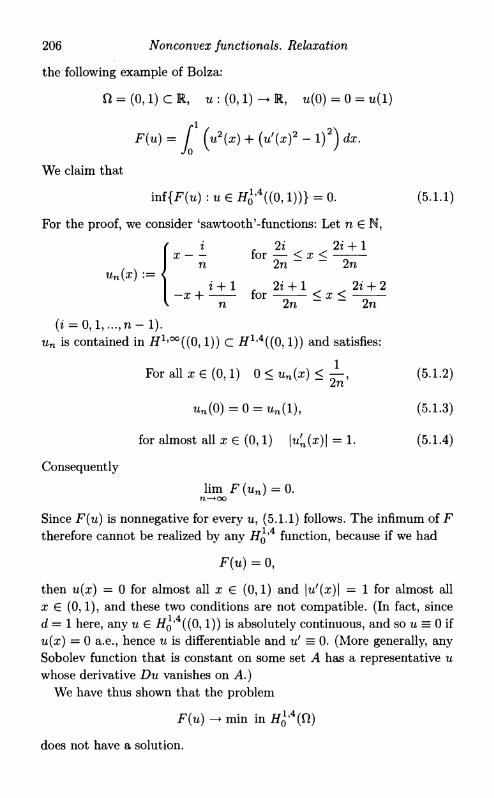
206 Nonconvex functionals. Relaxation
the following example of Bolza:
fi = ( 0 , l ) c R , u : ( 0 , l ) - > R , u(0) = 0 = u{l)
F(u) = (u2(x) + (u'(x)2 - l ) 2 ) dx.
We claim that
i n f{F (u ) : u G H ^ 4 ( ( 0 , 1 ) ) } = 0. (5.1.1)
For the proof, we consider 'sawtooth'-functions: Let n G N ,
un(x) := {
i r 2i 2i + 1 x for — < x <
n 2n 2n
, i + 1 f 2i: + 1 ^ ^ 2i + 2 —x H for — — < x < — —
n 2n 2n (2 = 0 , l , . . . , n - l ) .
un is contained in ^ ^ ^ ( ( 0 , 1 ) ) C # M ( ( 0 , 1 ) ) and satisfies:
For all x G (0,1) 0 < u n ( x ) < (5.1.2) 2n
M n(0)=o = ti n(l), (5.1.3)
for almost all x G (0,1) K ( x ) | = 1. (5.1.4)
Consequently
l im F(un) = 0.
Since F(u) is nonnegative for every u, (5.1.1) follows. The infimum of F therefore cannot be realized by any H Q ' 4 function, because if we had
F(u) = 0,
then u(x) = 0 for almost all x G (0,1) and | w ; ( x ) | = 1 for almost all x G (0,1), and these two conditions are not compatible. (In fact, since d = 1 here, any u G # Q ' 4 ( ( 0 , 1)) is absolutely continuous, and so u = 0 i f u(x) = 0 a.e., hence u is differentiable and u' = 0. (More generally, any Sobolev function that is constant on some set A has a representative u whose derivative Du vanishes on A.)
We have thus shown that the problem
F(u) -+ min in # 0
M ( f i )
does not have a solution.

5.1 Nonlower semicontinuous functionals and relaxation 207
We observe that our minimizing sequence (un) converges to zero weakly in # d ' 4 , by (5.1.2) and
/ u'n{x)<p(x)dx = - f un(x)<p'(x)dx 0 for all (p G C^°((0,1)) . Jo Jo
However,
F(0) = 1 > 0 = l im F{un). n—»oo
Therefore, F is not lsc w.r.t . weak H1 ^-convergence although the integrand is continuous in u'. As we shall see this results from the lack of convexity of the integrand. We also observe that any sequence of sawtooth functions u n , i.e. satisfying
\u'n\ = 1 a.e.
that converges to 0 in L 2 is a minimizing sequence for F .
Remark 5.1.1. Functionals of the type of our example often arise in optimal control theory as described in Section 5.2 of Part I . For example, one considers problems of the following type
[ f(t, u(t),a(t))dt -+ min (5.1.5) Jo
under the side conditions
u(0) = u 0 , u{T) = uT (5.1.6)
u'(t)=g(t,u(t),a(t)) (5.1.7)
wi th given functions / and g. u is called a state variable, a a control variable. This means that one assumes that u describes the state of some system evolving in time t whose derivative or rate of change can be controlled through a parameter a. The aim then is to choose a in such a manner that the functional, often considered as 'cost function', is minimized.
Thus, one needs to find some equation
a(t)=<p(t,u(t))
for an optimal control a at time t assuming a given state u(t) of the system. I f one knows the optimal control, one can reconstruct the evolution u(t) of the state of the system from (5.1.6) and (5.1.7) under appropriate assumptions. The simplest control equation (5.1.7) is
u'(t)=a(t),

208 Nonconvex functionals. Relaxation
and this leads to minimizing functionals of the type
/ f(t,u(t),u'(t))dt. Jo
Expressions of the type (uf(t)2 — l ) 2 can occur in many technical examples, like boats sailing against the wind.
Faced wi th a problem that one cannot solve, one may contemplate several options:
One could try to modify the problem, or one might generalize the concept of a solution, or both.
We shall discuss several such strategies. We first modify the problem via relaxation. This is an important method in the calculus of variations, and we therefore discuss i t in some generality.
D e f i n i t i o n 5.1.1. Let X be a topological space, F : X —• E. We define the lower semicontinuous envelope or relaxed function sc~F of F as follows:
(sc~F)(x) := sup { $ ( # ) : $ : X —• E is lower semicontinuous with < F(y) for ally e X}
L e m m a 5.1.1. sc~F is the largest Isc function on X that is < F everywhere.
In particular, F is lower semicontinuous if and only if F = sc~F.
Proof. sc~F is Isc as a supremum of Isc functions, see Lemma 4.2.1 (iv). Obviously, sc~F < F , and for all Isc $ wi th # < F , we have
$ < sc~F
by definition of sc~F. q.e.d.
T h e o r e m 5.1.2. Let X be a topological space, F : X —• E a function. Then every accumulation point of a minimizing sequence for F is a minimum point for sc~F. Consequently, if F is coercive, then sc~F assumes its minimum, and
min sc~ F = inf F. x x
5.1 Nonlower semicontinuous functionals and relaxation 209
Proof Let (# n )neN C X be a minimizing sequence for F wi th accumulation point #0- Then
(sc~F)(x0) < l im in f ( s c~F) (x n ) by lower semicon-n—•oo , . _ .
tinuity of sc F (see Lemma 5.1.1)
< l im inf F(xn) since sc~ F < F n—>oo
= inf F(y) since (xn) is a min- (5.1.8) lmizing sequence tor b .
On the other hand, the constant function
* ( * ) = inf y€X
is Isc and < F , hence by Lemma 5.1.1 for every x G X
inf F(t/) < {sc~F)(x). (5.1.9)
From (5.1.8) and (5.1.9) we conclude
{sc~F)(x0) = inf F(y) = min(5c"F)(x) . (5.1.10) y£X x£X
This implies the first claim. I f F is coercive, then every minimizing sequence has an accumulation point, and the second claim also follows.
q.e.d.
What does Theorem 5.1.2 tell us for our example? I t simply says that i f we cannot minimize our original functional F due to its lack of lower semicontinuity, we then minimize another functional instead, one that is lower semicontinuous and as close as possible to F . Theorem 5.1.2 then says that limits (or more generally, accumulation points) of minimizing sequences for F do not minimize F , but the relaxed functional sc~F. Since sc~~F is the largest Isc functional < F by Lemma 5.1.1 that is the best one can hope for.
I t then remains the task to determine the relaxed functional of some given F . Before proceeding to do so for our example, let us relax ourselves a litt le and derive some easy consequences of the definition of the relaxed functional and consider some easier examples first.
L e m m a 5.1.2. Let X satisfy the first axiom of countability. Then sc~F is the relaxed function for F : X —• R iff the following two conditions are satisfied:

210 Nonconvex functionals. Relaxation
(i) whenever xn —• x
(sc~F)(x) < l imin f F ( x n ) n—•oo
(ii) for every x G X, there exists a sequence xn —• x with
(sc~F)(x) > lirn F ( x n ) n — • c o
Proof. We claim that, since X satisfies the first axiom of countability,
(sc~F)(x) = inf { l im inf F(xn) : xn x in X}. (5.1.11)
We denote the right hand side of (5.1.11) by F~(x). Then F ~ is lsc. In order to verify this, we have to check
l iminf (inf { l i m i n f F (y^.n) : Vv.n —• Vv\) > inf { l i m inf F (x n j • Xn • X j
v—>oo
(5.1.12) whenever yv —•> x. Indeed, otherwise, for some 5 > 0, we would find some diagonal sequence yu,nu —• ^ as v —• oo wi th
^ ( 2 / ^ , nJ < inf { l im inf F ( x n ) : x n x } - 6
which is impossible. Thus, F~ is sequentially lsc, hence lsc, because X is assumed to satisfy the first axiom of countability. Also, F~ < F, and for every lsc $ < F , we have for x n —• x
$(x) < l imin f $ ( x n ) < l i m i n f F ( x n ) , n — • o o n — + c o
and hence
< F " ( x ) .
Thus, F"* is the largest lsc functional < F , and (5.1.11) follows from Lemma 5.1.1. I t is then easy to see (and left as an exercise) that F ~ ( x ) satisfies and is characterized by the properties (i) and (i i) .
q.e.d.
Example 5.1.1. Let X be a topological space, A C X a subset. The indicator function %A is defined by
t A ( x ) . = l ° i i x * A
{oo if X iA.
We then have
SC~%A — i A,
where A is the closure of A in X.
5.1 Nonlower semicontinuous functionals and relaxation 211
The characteristic function \ A is defined by
XA{X)1={1 tf* G A iA.
Then
sc \A = XA
where A is the complement of X \ A.
Example 5.1.2. Let fl C Rd be open, 1 < p < oo,
/ : Lp(fl) -> R
defined by
/(U) := I L \Du\" d x + fa M " d x i f « € C 1 ^ ) i oo otherwise.
(Note that 7(u) may also be infinite for some u G C 1(f2).) We claim
( * r / ) ( « ) = ( / n l ^ u l " d x + / n M " d * i f u € # 1 , P ( n ) 1 oo otherwise.
In order to show this, we shall verify the conditions of Lemma 5.1.2:
(i) (sc~I) is lower semicontinuous on L p which yields condition (i) . The lower semicontinuity is seen as follows: Suppose un —• u in Lp(fl). For the purpose of lower semicontinuity, we may select a subsequence (w„)„eN C (w n)n€N wi th
l im (sc~I)(wl/) = l iminf(sc~J) (u n ) , v—>oo n—•oo
and we may also assume that this l imit is finite. ( W „ ) „ € N then is bounded in J cf 1 ' p(f2). A subsequence of (wv) then converges weakly in H^p(fl) (Theorem 3.3.5), and by the Rellich-Kondra-chev compactness Theorem 3.4.1, i t also converges strongly in Lp(fl). The limit has to be u, because the original sequence (un) was assumed to converge to this l imit . Since the HliP-norm is Isc w.r.t. weak Hl,p convergence (Lemma 2.2.7), we have
(sc~I)(u) < l im (sc~J)(uv) V—KX)
= l i m i n f ( s c ~ / ) ( u n ) .

212 Nonconvex functionals. Relaxation
(ii) Let u E H^(n). Since C 1(f2) f l HllP(Q) is dense in / f ^ f i ) , we may find a sequence ( w n ) n € N C C ^ f i ) f l ff 1 , p ( f i ) wi th
l im f/ | £>u n | p + / K | p ) = / | D u | p + H P , N ^ ° ° \JQ JQ ) JQ
i.e.
l im I(un) — (sc~I)(u).
HugH1*^), then
7(u) = (sc~/)(ti) = oo.
This verifies condition (i i) .
Example 5.1.3. Similarly, for
o K ' ' \oo if w € L P ( n ) \ c 0
1 ( n ) ,
the relaxed functional is
(sc-l0)(u) = U \ D < i f t c e ^ n ) I oo otherwise.
Remark 5.1.2. We may also define the above functionals 7, J 0 on L f o c ( f i ) instead of L p ( f i ) . The relaxed functionals wil l be given by the same formulae.
Remark 5.1.3. For p = 1, the relaxations of I and I 0 are not given anymore by the J cf1'1-norm, but by the BV-norm which is defined in Chapter 7.
In metric spaces, there is an alternative useful characterization of the relaxation of a given functional which we now want to describe.
D e f i n i t i o n 5.1.2. Let X be a metric space with distance function d(-, F : X RU {oo} be bounded from below, F ^ oo. For X > 0, we define the Moreau- Yosida transform of F as
Fx(x) := inf (F(y) + \d(x,y)). (5.1.13)
T h e o r e m 5.1.3. The functionals F\ satisfy
\Fx(Xl) - Fx(x2)\ < A d ( x i , x 2 ) (5.1.14)
for every X > 0, # i , x2 € X. In particular, they are Lipschitz continuous. For any x G X
(sc~F)(x) = l im Fx(x). (5.1.15)

5.2 Representation of relaxed functionals via convex envelopes 213
Proof. For # i , x 2 , t / G X , A > 0, we obtain from the triangle inequality
F(y) + Xd{xuy) < F(y) + \d(x2,y) + Xd(xux2).
The definition of Fx (#2) implies then
inf (F(y) + Xd(xuy)) < Fx(x2) + Xd(xux2), yex
hence
Fx{xi) < F A ( x 2 ) + A d ( x 1 , x 2 ) .
Interchanging the roles of # i and x 2 , we conclude
\Fx(xi)-Fx(x2)\<\d(xux2).
Since we have now shown that F\ is Lipschitz continuous, and since F\ < F , we obtain
F A < 5C"F,
hence for all x G X
supF A (x) < (sc'F)(x). (5.1.16) A>0
For any A > 0, we find x\ € X wi th
F ( x A ) + Ad(x ,x A ) <Fx(x) + j .
Therefore
l im x A = x A—+00
and
(sc~F)(x) < l imin f F ( x A ) < l imin f F A ( x ) . (5.1.17) A—+00 A—+00
Equations (5.1.16) and (5.1.17) imply (5.1.15). q.e.d.
5.2 Representation of relaxed functionals via convex envelopes
Theorem 5.2.1. Let Q C Rd be open, 1 <p < 00, f :Rd -+R continuous with
Co \v\p < f(v) < C\ | v | p + c2 for some constants CQ, C I , c2.

214 Nonconvex functionals. Relaxation
Let F :{u£ Hhp{Q) : u - u0 e # 0
1 , p ( f t ) } -+ R 6e given by
F(u) := / f(Du(x))dx , (u0 G Hhp(Q) given). JQ
Then the relaxed function of F w.r.t. the weak HlyP topology is given by
(sc~F)(u)= / (cvx~ f) (Du(x)) dx JQ
where
(cvx~f)(v) := sup{g(v) : g < f,g convex}
is the largest convex function < f.
For the proof, we shall need the following:
L e m m a 5.2.1. Let W = UUi^M c R d b e
an open rectangle, 1 < p < oo. We let f G LP(W) and extend f periodically to R d , i.e.
f (x1 + m i (0i - ai),... , x d + md (0d - ad)) = / ( x 1 , . . . , x d )
for m i , . . . , md E Z, x = ( x 1 , . . . , x d ) G W, and put
fn(x) : = f{nx) for n G N.
ITien we £/ie lyeo/c convergence
fn-f = l-TTr I f(x)dx i n L P ( W ) f°r n-^oo. (5.2.1) meas W Jw
Proof. First
/ \fn(x)\pdx = I \f(nx)\pdx = ^ f \f(y)\pdy= f \f(x)\pdx JW JW n JnW JW
by the periodicity of / . Thus
\\fn\\LP{w) = l l /H L P { W ) - (5-2-2)
In the same manner,
/ fn{x)dx= [ f(x)dx= [ fdx. (5.2.3) Jw Jw Jw
Let now WQ be a subrectangle of W, written in the form
d
WQ = J J (ai + 6;0!i, a* + 6;$) , 2 = 1
or more compactly
W0 = a + bW (a = ( a x , . . . , a d ) , 6 = (&i, ...,&<*)) •
5.2 Representation of relaxed functionals via convex envelopes 215
Then
/ (/«(*) ~f)dx= f (f(nx) - f) dx JWo Ja+bW
= - d l (f(y)~f)dy n Jna+nbW
= A / ( / (» ) - f) dV 7 1 Jna+[nb]W
+ - d I (/(») - f) dy n Jna+(nb-\nb\)W
+ A / {f(y)~f)dy n Jna+(nb-[nb})W i+(nb-[nb})W
by periodicity of / .
The first term in the right-hand side vanishes by (5.2.3), and thus, again using the periodicity of / ,
1/ {fn{x)-f)dx\<-d [ \f(y)~f\dy. \JWo I 7 1 JW
Letting n oo, we obtain for every subrectangle WQ of W
l im / (fn(x)-f)dx = 0.
Let now g £ Lq(W), wi th ± + ± = 1. We have to show
lim / fn(x)g(x)dx = / fg(x)dx. n-*°°Jw Jw
Given e > 0, we then find subrectangles W\,..., Wk {k \ { e R (i = l , . . . , f c ) wi th
< e
(5.2.4)
(5.2.5)
k(e)) and
(5.2.6) L*(W)
(The possibility of approximating Lq(fl) functions g (Q open in Rd) in such a manner by step functions can easily be seen as follows: Since Cg°(ft) is dense in L 9 ( f i ) , there exist y>€ £ C£°(fi) wi th 110 "~ c l l / ^ n ) < §• I t is then easy to construct a step function A^x^t (Xi £ R, Wi disjoint rectangles contained in supp</?€) wi th
e sup
supp <p€
2 meas supp (p€

216
Then indeed
Then
Nonconvex functionals. Relaxation
9 ~ YlXi*w* LP(Q)
+
k
/ (fn(x) ~ f) 9(x)dx \Jw
I {fn(x) ~ f)Y^XiXWi(x) Jw {
{fn(x) - f) ^g(x) - ] T \ X w A x )
< I > l | / {fn(x)-f)dx + e | | / n - / | |
by (5.2.6) and Holder's inequality (Lemma 3.1.1).
The first term tends to zero as n oo by (5.2.4), whereas the second one is bounded by 2e | | / | | £ , P ( W ) by (5.2.2) and can hence be made arbitrarily small. Therefore, (5.2.5) holds.
q.e.d.
The proof of Theorem 5.2.1 wil l be broken up into several steps:
(1) We put
(q-f)(v):=ud{^Juf(v + DV(x))dx: <p G H**(U),
U bounded domain in R d | ,
(5.2.7)
and we claim:
L e m m a 5.2.2. (sc-F)(u) < [ (q~f)(Du(x))dx.
JQ
Proof. Replacing F(u) by G(v) := F(v + UQ) forv = u — UQ, we may assume u0 = 0, i.e. u G HQ'P(Q). Since the piecewise affine functions, i.e. those u for which Du is constant on disjoint rectangles W{ C fi, wi th \ (J W\ arbitrarily small, are dense in HLYP (for the same reason that the functions that are piecewise constant on disjoint rectangles W{ are dense in L p ) , and since F
5.2 Representation of relaxed functionals via convex envelopes 217
is continuous under strong H^-convergence, it suffices to treat the case where
Du = VQ = constant
on some rectangle W. We next observe that for a given constant vector v, (q~ f)(v) is independent of the choice of U in (5.2.7). First, the value of the inf on the right hand side of (5.2.7) does not change under translations or homotheties of U. The general case of U\ and XJi then is handled by approximating U\ by disjoint homothetical translations of U2 and vice versa. We may therefore take U = W in (5.2.7). We now choose a sequence (y>n)n€N C H*'P(W) wi th
(q~f)(vo) + - > ^ 7 / f(v0 + D<pn(x))dx > (q-f)(v0). n meas W Jw
(5.2.8)
We extend (pn periodically from W to E d and put
u(x) := vox (then Du = v0)
and un(x) := u(x) + -( /? n (nx).
n
By Lemma 5.2.1, u n converges to u weakly in HlyP. Then un = u on dW by periodicity of (pn and ^ n ( a v v = 0. We have
/ f(Dun(x))dx = j f(v0 + -D(pn(nx))dx Jw Jw n
= I f(vo + D(Pn(y))dy n d JnW
f(v0 + D<pn(y))dy (5.2.9) / W
since (pn is periodic.
Equations (5.2.8) and (5.2.9) imply
l im F(un) = l im / f(Dun(x))dx n-KX) Jw
= f (q-f)(v0) = (q-f)(v0)measW. Jw
The claim then follows from the characterization of (sc~F), see e.g. Lemma 5.1.2(i).
q.e.d.
218 Nonconvex functionals. Relaxation
(2) We observe
(q~f)(v)<f(v) (put p = 0 in (5.2.7)). (5.2.10)
W i t h
(q~F)(u) := / (q-f)(Du(x))dx, Jn
we obtain from Lemma 5.2.2 and (5.2.10)
s c - F = 5C - (g~F) , (5.2.11)
and upon iteration
sc-F = sc-((q~)nF), (5.2.12)
where (q~~)n means performing the construction q~ iteratively n times. From the growth conditions on / assumed in Theorem 5.2.1, we conclude that
(Q-nf)(v)
is monotonically decreasing and bounded from below in n, hence converges to some limit
(Qf)(v).
From B. Levi's Theorem 1.2.1, we conclude
l im (q~nF)(u) = l im f (q~nf)(Du(x))dx n—•oo n—>oo J
= f (Qf)(Du(x))dx =: (QF)(u). (5.2.13)
Since by (5.2.12)
(sc~F)(u) < (q~nF)(u) for all n,
we conclude from (5.2.13)
(sc-F)(u) < (QF)(u).
From the definition of Q / , we also conclude
Q/(t;) = i n f { — 1 — / (Qf)(v + D<p(x))dx, meas U Jv
<p e H^P(U), UcRd open, bounded}. (5.2.14)
As before, this expression is independent of the choice of U.

5.2 Representation of relaxed functionals via convex envelopes 219
Definition 5.2.1. g : Rd —> R is called quasiconvex if for all v G Rd, <p C H^P(U), U C Rd bounded and open
g{v) < — l — r T I g{v + D<p{x))dx. (5.2.15) meas U J v
Equation (5.2.14) then implies that Qf is quasiconvex.
(3) L e m m a 5.2.3. / : Rd —• E is convex if and only if it is quasi-convex.
Proof. '=>': Jensen's inequality says that i f / is convex, for every ip G L1{Rd,Rd)
f (J^dx^ <jf(i>(x))dx (5.2.16)
(see Theorem 1.1.6). Since, as observed above, in Definition 5.2.1 it suffices to consider one fixed domain U, we may assume
meas U = 1
and put
ip(x) = v 4- D<p(x).
Since <p G H^p, f ip(x) = v meas U = v, and (5.2.16) therefore implies that / is quasiconvex.
We assume that / is quasiconvex, i.e.
f{Vo) = ^bjlf{vo)dx
for all ip e HQ'P{U).
We have to show that for all v i , v2 € Rd, 0 < t < 1
f(tVl + (1 - t)v2) < tf(Vl) + (1 - t)f(v2). (5.2.18)
Equation (5.2.17) implies
f(tvi + (1 - t)v2) < —!— f f(tVl + (1 - t)v2 + D<p{y)) dy meas U Ju
(5.2.19)
for all U and all (p € HQP(U). After a rotation, we may assume

220 Nonconvex functionals. Relaxation
that v\ — V2 is a positive multiple of the first basis vector of our standard basis of R d , i.e. V\ — v2 points in the ^-direct ion. We shall take a cube W := (a, b)d C Rd as our set U and construct a family of functions
(v>„)„ 6 N C H^{W)
on a set W™ C W wi th meas W? = t(b-a)(b-a-±)d-1
on a set Wg C W with meas
WT = ( i - * ) ( f c - o ) ( f c - o - s ) d _ 1
HV^nl l^oo^) < Co for some fixed constant Co that does not
depend on n.
Using these (pn in (5.2.19) yields
f(tvx + (1 - t)v2) < tf(V!) + (1 - t ) / ( v 2 ) 4- Pn
with pn —• 0 as n —• oo, hence (5.2.18). I t remains to construct (pn. We divide the interval (a, 6) into 2 n + 1
subintervals as follows:
h = (a,a+^(b-a))
l2 = (a+^(b-a),a+^(b-a))
h = (a+~(b~a),a+~(b-a) + ^(b-a))
with
V(pn(x) = {l-t)(Vl-V2)
-t(vx - v2)
and
i.e. the intervals hv-i have length ~(b — a), and they alternate with the intervals I2v of length ^ ^ ( 6 - a). We then put
Wr'=((jl2,-i)x(a+-)b--)d-1
X n n i/=i
W 2
n : = ( M / 2 , , ) x ( a + - , & - - ) d ~ 1 -- n. n.

5.2 Representation of relaxed functionals via convex envelopes 221
We then put <pn(a,x2, ...,xd) = 0,
d<pn( . f (1 - *)|«i - v2\ for x e W? 8xl[X> \ -t\vi-V2\ forxeW?,
*$>=0«*i = 2,...,d.
(Remember that we assume that V\ — v2 points in the positive x1 -direction.)
We then have <pn(b, x2, ...yxd) = 0. We also put
(pn = 0 on dW,
and on W \ (W™ U W2) we choose an interpolation that is affine linear in x 2 , Since
, / ., t(l — t),, ., , Ci sup \ipn(x)\ < n w (6 - a) |vi - v 2 | — 2 \ - r * n
we get
xdipn(x)\ Ci
sup • < n — .
Thus, for large enough n,
sup |Vy>„(x)| = sup 1 " 1 < |v i - v2\ = : c0. x€W xEWfUW? ux
This completes the construction of (pn and the proof of Lemma 5.2.3.
q.e.d.
(4) We may now complete the proof of Theorem 5.2.1 From (2), we know
(sc'F)(u) < QF(u) = jQf{Du(x))dx.
By Lemma 5.2.3, Qf is convex. By Lemma 4.3.1, Qf{u) therefore is lsc w.r.t. weak H1,p convergence. Since QF < F (see (5.2.10) and the definition of QF) , we must also have from the definition of sc~F that
QF(u) < (sc~F){u).
Hence equality. Thus
(sc-F)(u) = J (Qf)(Du(x))dz

222 Nonconvex functionals. Relaxation
Moreover, for every convex function g < /,
G(u) := j g(Du(x))dx
is a weakly HltP Isc functional < F . Therefore, from the definition of sc~F, the convex function Qf must in fact be the largest convex function < / . This completes the proof.
q.e.d.
Corollary 5.2.1. F as in Theorem 5.2.1 is weakly lower semicontinuous in H1,p if and only if f is convex.
Proof. Lemma 4.3.1 says that convex functionals are weakly lower semi-continuous. I f / is not convex, then by Theorem 5.2.1 sc~~F F , hence F is not weakly Isc by Lemma 5.1.1.
q.e.d.
Remark 5.2.1. One may also consider variational problems for vector valued functions u : fl C R d -+ E n ,
F(u) := [ f(Du(x))dx. Jn
Again, / is called quasiconvex i f for all open and bounded U cRd and sl\ ip e H^p(U;Rn), v eRnd
/ ( ^ n ^ / / ( ^ ^
In this case, however, while convex functions are still quasiconvex, the converse is no longer true. Theorem 5.2.1 continues to hold but wi th convexity replaced by quasiconvexity. Also, one may consider more general problems of the form
F(u) = J f(x,u(x),Du(x))dx
with similar results and conceptually similar, but technically more involved proofs.
Remark 5.2.2. The notation of quasiconvexity and many of the basic corresponding lower semicontinuity results are due to C. Morrey. In fact, the quasiconvex functionals are precisely the weakly lower semicon-
5.2 Representation of relaxed functionals via convex envelopes 223
tinuous ones. For detailed references to the work of Morrey and other researchers, see the book of Dacorogna quoted at the end of this chapter.
Remark 5.2.3. Theorem 5.2.1 can be considered as a representation theorem for relaxed functionals. In particular, i t says that a functional on
obtained by integrating an integrand f(Du(x)) (with certain technical assumptions on / ) has a relaxed functional of the same type, i.e. again representable by integration w.r.t. to some integrand g(Du(x)) of the same type. Furthermore, g may be computed explicitly from / .
We now return to our initial example
F(u) = j f * | u 2 ( x ) + (u'(x)2 - l ) 2 } dx
for u € # o
M ( ( 0 , l ) ) . F(u) is the sum of a functional which is continuous w.r.t. strong L2-convergence, hence also w.r.t. weak H1*4 convergence, and another one to which Theorem 5.2.1 applies. We conclude that
(sc~F)(u)= f1 {u2(x) + Q(u'(x))}dx, Jo
with
Q(v) = l ( v 2 - 1 ) 2 i f H ^
\ 0 otherwise,
the largest convex function < (v2 — l ) 2 .
References For the definition of relaxation and its general properties: G. dal Maso, An Introduction to F-Convergence, Birkhauser, Boston 1993,
pp. 28-37. G. Buttazzo, Semicontinuity, Relaxation and Integral Representation in the
Calculus of Variations, Pitman Research Notes in Math. 207, Longman Scientific, Harlow, Essex, 1989, pp. 7-28.
For Theorem 5.2.1 and generalizations thereof: B. Dacorogna, Direct Methods in the Calculus of Variations, Springer,
Berlin, 1989, pp. 197-249.

Nonconvex functionals. Relaxation
Exercises
Determine sc~F and discuss the relaxation for
F(u) = J (l-u'(x))2u(x)2dx f o r u G t f 1 ' 4
with = 0 ,u ( l ) = 1,
F(u) = J {2x-u,{x))2u(x)2dx for ueH1A
with = 0 ,u ( l ) = 1, and
F(u) = J1 ((u(x)2 - a) + ( u ; ( x ) 2 - 1)) dx for u G / J 1 ' 4
with a G i
Determine sc"I for / : L p ( f i ) —• R (f i G Rd open and bounded),
J(ii) := { / n W <** + Jn cfa i f ti € C 1 ^ ) I oo otherwise.
Why does the proof of Lemma 5.3.3 not work for vector-valued mappings Rd -+ M n with n > 1, i.e. # : M d n -+ R, v G R d n , y> G # o ' p ( R , R n ) as in Remark 5.2.1?

6 r~convergence
6.1 T h e definition of T-convergence
In this chapter, we treat the important concept of T-convergence, introduced and developed by de Giorgi and his school.
Definition 6.1.1. Let X be a topological space satisfying the first axiom of countability, Fn : X —> R functions (n G N). We say that Fn
T-converges to F,
and
(ii) for every x £ X, there exists a sequence xn converging to x with
F(x) = l im Fn(xn).
F = T- l im Fr n
if
(i) for every sequence (xn)n^ converging to some x G l ,
F(x) < l imin f Fn(xn)
Example 6.1.1. Fn : R -+ R
1 for x > — n
Fn(x) nx for — — < x < — n n
-1 for x < . n
Then for x > 0 for x < 0
225

226 r'-convergence
while the pointwise l imit is 0 for x = 0, 1(—1) for x > 0(< 0).
Example 6.1.2. F n : R —• R
nx for o < x <
Fn{x) := n
1 2 2 — nx for — < x < —
n n 0 otherwise.
Then
(r-UmF n )(x) = 0
which is the same as the pointwise l imit .
Example 6.1.3. F n : R —• R
Fn(x) := I
—nx for 0 < x < — n
1 2 nx — 2 for — < x < —
n n 0 otherwise.
Then
( r - l imF n ) (x ) = { - 1 for x = 0 0 otherwise.
whereas the pointwise l imit is again identically 0. Note that the F n of 6.1.3 is the negative of the F n of 6.1.2. Thus, in general
Example 6.1.4- Fn :
Fn(x) := {
( r - l i m F n ) ^ r - l i m ( - F n ) .
—nx for 0 < x < — n
nx — 2 for — < x < — for odd n n n
0 otherwise for even n. 0
F n then converges pointwise to 0, but does not T-converge at x = 0.
Example 6.1.5. F n : R —• R
F n ( x ) = sinnx.
Then
( r - l imF n ) (x ) = - l ,
whereas F n does not converge pointwise.
6.1 The definition ofT-convergence 227
From Examples 6.1.4 and 6.1.5, we see that among the two notions of pointwise convergence and T-convergence, neither one implies the other.
Example 6.1.6. Fn : X —• E converges continuously to F : X —• E if for every x G X and every neighbourhood V of F(x) in E (i.e. V = {y G E : |F(x) - i / | < e} for some e > 0 in case F(x) G E, V = {y G E : y > i f } U { o o } for some K G E in case F(x) = oo, and analogously for F(x) = —oo), there exist no G N and a neighbourhood U of x wi th
F n ( i / ) G V
for all n > no, y £ U. Fn converges continuously if and only if both Fn and — Fn converge to F and —F, respectively. Continuous convergence implies pointwise convergence, and we conclude from Examples 6.1.2 and 6.1.3 that T-convergence is weaker than continuous convergence.
Example 6.1.7. Let X satisfy the first axiom of countability,
F n EE F : X -> E
a constant sequence. Then
r - l i m F n = (sc~F)
is the relaxed function of F . Thus, we have the remarkable phenomenon that a constant sequence may converge to a l imit different from the constant sequence element.
Remark 6.1.1. Without changing the content of the definition of T-convergence, condition (ii) may be replaced by the following condition which is weaker and therefore easier to verify:
(ii ') for every x G X , there exists a sequence xn converging to x wi th
l i m s u p F n ( x n ) < F(x). n—•oo
The following result is useful in approximation arguments:
L e m m a 6.1.1. Let X satisfy the first axiom of countability. Suppose (xm)meN converges to x in X, and
l i m s u p F ( x m ) < F{x). m—•oo
Suppose that (ii') is satisfied for every xm (i.e. for every m, there exists a sequence {xm,n)neN converging to xm with
l im sup F n ( x m , n ) < F(xm)). n—•oo

228 T-convergence
Then (ii') also holds for x.
Proof. Since X satisfies the first axiom of countability, we may take a neighbourhood system (Uu)u^ of x and renumber i t and take intersections so that
xm G Um for all m G N,
and that every sequence (y^^n with yv G U^u) for all v and some sequence ^(y) —• oo as v —• oo converges to x. For n G N , we let
ran := max jra G N : x m , n G Um , F n ( x m ) n ) < — - f F ( x m ) j .
Then
l im mn = oo. n—+oo
Namely, otherwise, we would find fco G N with
Fnu O & f c . u J > ~ +F(xk)
or
%k,nu £ Uk for all k > ko and some sequence n „ —• oo for z/ —> oo.
To see that this is impossible we simply observe that since xko G Uk0
and since Xk0>n converges to Xk0 as n —• oo we have
^fc0,n £ £ 4 0 f ° r a ^ sufficiently large n,
and likewise since we assume
l i m s u p F n ( x f c o > n ) < F ( x f c o ) , 71—• OO
we have
Fn{%k0 n) < F(xk0) + 7 - for all sufficiently large n .
We then have %mn ,n G f / m n
1 F n ( x m n , n ) < ^ O m J +
Therefore yn := x m n y n converges to x as n —• oo, and
l imsupF n ( t / n ) < l im sup ( F(xmn) + — J < F(x) n—+oo n—+oo \ rnn J

6.1 The definition ofT-convergence 229
by assumption and since mn —• oo as n —> oo. Thus, (i/n)neN is the desired sequence.
q.e.d.
Let F : X -> R U {00} satisfy
inf F(t/) > - 0 0 .
Given e > 0, we say that x G X is an e-minimizer of X i f
F ( x ) < inf +
Note that x is a minimizer of F i f i t is an e-minimizer for every e > 0. In contrast to minimizers, e-minimizers always exist for any e > 0.
The following result is a tr ivial consequence of the definition of T-convergence, but quite important.
T h e o r e m 6.1 .1 . (Let X satisfy the first axiom of countability). Let the sequence of functions Fn : X —> R F-converge to F : X —> R. Let i n f y € x Fn(y) > —00 for every n G N . Let xn be an en-minimizer for Fn. Assume en —> 0 and xn —> x for some x G X. Then x is a minimizer for Fj and
F(x) = l im Fn(xn). (6.1.1) n-+oo
Proof. I f x were not a minimizer for F , there would exist x' G X wi th
F{x') < F(x). (6.1.2)
Since F n T-converges to F , there exists a sequence (x'n) C X with
l im x'n = x'
\imFn(x,
n)=F(x').
We put 6 := \(F(x) - F(x')). We may choose n so large that
en<6 (6.1.3)
Fn(x'n)<F(x') + 6 (6.1.4)
^n(^n) > F(x) - 6 (by property (i) of Definition 6.1.1). (6.1.5)

230 T-convergence
Since xn is an e n-minimizer of F n ,
F n « ) > Fn(xn) - en (6.1.6)
>Fn(xn)-S by (6.1.3)
> F ( x ) - 2 « by (6.1.5).
From (6.1.4) and (6.1.6), we get
F(x) < F(x') + 36
contradicting (6.1.2) by definition of 8. Thus, x is a minimizer for F . I f (6.1.1) did not hold, then after selection of a subsequence,
F(x) < l i m F n ( x n )
whereas by property (ii) of Definition 6.1.1, there would exist a sequence (x'n) converging to x with
F (x ) = l i m F n ( x ' n ) ,
and we would again contradict the e n-minimizing property of xn. q.e.d.
Corollary 6.1.1. (Let X satisfy the first axiom of countability.) Let Fn : X —• R r-converge to F : X —• R. Let xn be a minimizer for Fn. If xn —• x, then x minimizes F, and
F(x) = l im inf Fn(xn).
The following result is similarly both trivial and important.
Theorem 6.1.2. (Let X satisfy the first axiom of countability.) Let Fn
Y-converge to F. Then F is lower semicontinuous.
Proof. Otherwise, there exist some x G l and some sequence ( x m ) m ^ N with
l im Xm = x m—*oo
l im F{xm) < F{x). (6.1.7) m—•oo
By T-convergence, for every m, there exists a sequence ( x m , n ) n G N C X with
l im xm n — xm n—>oo
l im F „ ( x m > n ) = F(xm). (6.1.8)

6.2 Homogenization 231
We assume —oo < l i m F ( x m ) , F(x) < oo simply to avoid case distinctions. We let
6 := ] (F(x) - l im F(xmj) > 0 by (6.1.7). 4 \ ra—+00 /
For every ra G N, we may find n m G N with
Fnm(xmtnm)-F(xm)<6 (6.1.9)
l im x m , n m = x , l im n m = oo. 771—• oo ra—•oo
Then by T-convergence
F(x)< l im i n f F n m ( x m , n m ) . (6.1.10) ra—>oo
We may then choose ra so large that
F(xm) <F(x)-36 (6.1.11)
and Fnm(xm,nJ > F(x) - 6. (6.1.12)
Equations (6.1.9), (6.1.11) and (6.1.12) are not compatible, and the resulting contradiction proves the lower semicontinuity.
q.e.d.
Remark. As a consequence of Corollary 3.2.2 and Theorems 3.1.3, 3.3.1, and 3.3.3, in combination wi th Lemma 2.2.4, the weak topology of Lp(ft) and WkyP(Q) for 1 < p < oo satisfies the first axiom of countability so that the preceding notions are applicable.
The reference for this section is G. dal Maso, An Introduction to V-Convergence, Birkhauser, Boston, 1993
6.2 Homogenization
In this section and the next one, we describe two important examples of T-convergence. They are taken from H. Attouch, Variational Convergence for Functions and Operators, Pitman, Boston, 1984.
In the discussion of these two examples, we shall be more sketchy about some technical details than in the rest of the book, because the main point of these examples is to show how the concept of T-convergence can be usefully applied to concrete problems that arise in various applications of the calculus of variations.

232 T-convergence
Let M be a smooth subset of the open unit cube (0, l)d of Rd. M is considered as a hole. Let
M c : = ( J e (M + ra) mGZd
(e(M + 777.) := { x = y + em with ^ G M}) be a periodic lattice of 'holes' of scale €.
Let ft C R d , fic := ft \ ( M c f l ft), i.e. a domain with many small holes. Such domains occur in many physical problems like crushed ice, porous media etc. Often, the physical value of e is so small that it is useful to perform the mathematical analysis for e —• 0. This is called homogenization. Let
, x / x f 0 f o r x G M d \ M i ^ oo for x G M i
be the indicator function of Rd \ M\. a (~) then is the indicator function of Rd\Me. We consider the functional
Fe(u):=\e2 [ | D u ( x ) | 2 d x + / a (-) u2(x)dx (6.2.1) 2 Jn Jn V e '
for u G # o ' 2 ( n ) . A minimizer of the functional
Fe(u) — / f(x)u(x)dx Jn
(for given / G £ 2 ( f i ) ) satisfies
A u = - ~ in fic and u = 0 on dfte. (6.2.2)
Here d f i c = d f i U (dMef)ft). The boundary condition on dft comes from the requirement that u G jfiFo'2(fi), while the boundary condition on dMe
is forced by the functional.
Theorem 6.2.1. With respect to weak L2(ft) convergence
r - l i m F c = F, (6.2.3)
with
where
fi(M):= j \Drj{x)\2dx= [ r/(x)dx, J(o,i)d\M J(o,i)d
6.2 Homogenization 233
and 77 is the solution of
AT? = - 1 m ( 0 , l ) d \ M
77 = 0 inM (6.2.4)
77 25 Zd~periodic (i.e. rj(x + ra) = 77(0;) /or x G (0, l ) d , ra G Z d ) .
Proof. We put 77e(x) := 77(f). By Lemma 5.2.1, 77e converges weakly in L 2 ( f i ) to fJ>(M) as e —» 0. Let now u G L2(ft). By approximation, we may assume that u is smooth, e.g. contained in W / 1 ' 2 ( f i ) f l C°(Q) . We put
Then u c converges weakly in L2(Q) to u, and
ue — 0 on M c .
Moreover
^ e K ) = ~ / l ^ c l 2 (6.2.5) 2 ^2
• l^ j f (u2\Drif + 2ur]eDu-Drie + r1
2\Du\2) 2 /x (M) 2
I f C/ C fl is open, because of the periodicity, J V |-DT7 c| 2 asymptotically behaves like
meas U f . ^ ,2 meas U
J(0,e)d\Me
€ J(0,l)d\M
This means that
l im e2 / \Drje\2 = messU [ \Dn\2 = measU • fi(M) (6.2.6) c~>0 JU J(0,l)d\M
hence, approximating u by step functions, we also get
l i m e 2 / u2 \Drje\2 = fi(M) [ u2 (6.2.7)
(note that we assume u to be continuous). Moreover, since % is bounded independently of e,
l i m e 2 / 772|£>u|2 = 0, (6.2.8)
and from (6.2.6), (6.2.7) and the Schwarz inequality, also
l im e2 / uneDu • £>77c = 0. (6.2.9) C-+° JQ€

234 r-convergence
Equations (6.2.5)-(6.2.9) imply
lim Fe(ue) = F(u). (6.2.10)
In order to complete the proof of T-convergence, we need to verify that whenever functions v€ that vanish on M e converge weakly in L2(Q) to tx, then
l iminf Fe(ve) > F(u). (6.2.11)
By an approximation argument, we may assume u G Co°(fi). We put
as before. We have
Fe(ve) + Fe(u€) >e2 [ Dve • Due
e2 f (m V(M) ! w*Dve'Du + uDv€-Dri€). (6.2.12)
Using (6.2.10), we obtain from (6.2.12) in the limit e -+ 0
UminfF e ( t ; e ) + — I r j r f u2 > l im inf - 1 — / uDveDr]e (6.2.13)
since the other term on the right hand side of (6.2.12) goes to 0 by a similar reasoning as above. Equation (6.2.4) implies
e2Ar)e = - 1 in fic. (6.2.14)
Moreover
6 2 £ DuveDVt < e2 (^j \Du\2v2)j ' (^J \DVe\2^ ' - 0, (6.2.15)
since ve as a weakly converging sequence is bounded in L 2 , \Du\ is bounded by our approximation assumption that u is smooth enough, and since we may use (6.2.6). Integrating the right-hand side of (6.2.13) by parts, and using (6.2.14) and (6.2.15), we obtain
= M M ) i u 2 '

6.3 Thin insulating layers 235
since ve converges weakly in L 2 to u. This implies (6.2.11) and concludes the proof.
q.e.d.
6.3 T h i n insulating layers
We consider an insulating layer of width 2e and conductivity A, and we want to analyse the limit where e and A tend to 0.
Let fi C R 3 be bounded and open, S a smooth complete surface in R 3 , e.g. a plane, S := fl f l 5,
S e := {x € R 3 : dist(rr, 5) < e}
S c := fl f l Se
flc : = f l \ S c .
Conductivity coefficient
_ f 1 on flc
a c ' A : ~ \ A o n E c ( A > 0 ) .
Variational problem:
J C ' A : # 0
1 , 2 ( f l ) -> R
r*(u):=\f \Du\2dx+~f \Du\2dx (6.3.1) 2 JQ€
2 «/£c
J c ' A (u) - / fu -> min ( / € L 2 ( f l ) given).
The Euler-Lagrange equations are
AueA + / = 0 on flc (6.3.2)
A A u C ) A + / = 0 on S c (6.3.3)
W C , A | Q C = W C , A | E c on d f l c f l d £ c (6.3.4)
A dux*
on d f l c f l d £ c (6.3.5)
(where nu denotes the exterior normal of a set U)
u€iX = 0 on d f l . (6.3.6)

236 r -convergence
T h e o r e m 6.3.1. We let e -> 0, \ -+ 0. If j -> a with 0 < a < oo, then Ue,x —* u weakly in L 2 ( f i ) uet\ =t u uniformly on every fl0 C C fi \ E, w/iere w solves
Aw + / = 0 on fl \ E
w|an = 0
•^p = ^ = « H E a n d a n | 2
w/iere is the jump ofu across E, and and ore the exterior normal derivatives for the two components of ft \ E. (In case a = oo, u is continuous across E, and! A u = / in fi.) Furthermore
\ f l^e,A|2 + / |^e,A|2
/ | D u | 2 + ^ / [u] |dE.
J e , A r-converges w.r.t. the weak L2-topology to I(u):
0 < a < oo : I(u) = ( J / n \ £ l ^ f + f # « e " o ' 2 ( " \ E) I oo otherwise
a = oo:I(u)=iUn\Du\2 ifuZH^{Sl) I oo otherwise
(in this case, the result holds
a = Q : 1 { u ) = / \ J n V E \Du\2 if u e H^2(Q \ E) for the strong l o o otherwise L -topology
in place of the weak one)
Thus, in case a = 0, we obtain a perfect insulation in the limit, whereas for a = oo, the limiting layer does not insulate at all.
We assume for simplicity S = {x3 = 0}.
L e m m a 6.3 .1 . There exists a constant c\ (depending on / , fl, 5, but not on €, A) such that for all sufficiently small e, A
6.3 Thin insulating layers 237
Proof.
[ \Due,\\2 + \ f \Bue,x\2
Jne JdQ€ °nn€ Jz€
+ A / W C , A ^ ~ -
= / / * W C ) A because of the Euler-Lagrange equations
^ l / L 2 ( Q ) ' l M € . A l x , 2 ( N ) •
By the Poincare inequality (Theorem 3.4.2),
/ < A <C2 [ \Due,x\2
[ < A <C3 / | ^ C , A | 2 .
By a change of scale
y3 = ex3 (y1 = x\y2 = x2),
( < A <c3e [ \Du€yX\2
(we only get e instead of e2, because the area of the portion of #E C on which U C ) A vanishes, namely Oil f l 5 C , is proportional to e). Altogether
£ < A < C 4 ( l + ^ ) (jf \Due,X\2 + \J^ | £ > W e , A | 2 )
and the estimates follow. q.e.d.
Proof (Theorem 6.3.1). We only consider the case 0 < a < oo (the other cases follow from a limiting argument). We first observe
T- l im J c ' A (u) = oo i f u e L 2 ( f i ) \ H^2(Q \ E).
We assume for simplicity
A = A(£) = €a , J c : = J c ' A ( c ) .
Let u e H1,2 ( f i \ E). We first check property (ii) of T-convergence:

238 T-convergence
We need to find ue —x u weakly in L 2 ( f i ) wi th l i m / c ( u c ) = I(u). We define
[ ^ ( a : 1 , ^ 2 , ^ 3 ) i f | z 3 | > e
u € ( a r , a r , a r ) := < i { u ( x 1 , x 2 , e ) - f w ( a : 1 , a : 2 , - e ) }
x 3
+—{u(x1,x2,e)-u(x1,x2,-e)}
i f rc3 < € .
Then ue € # o ' 2 ( f i \ E) , w€ — w weakly in L 2 ( f i ) for c -> 0,
J«(ti e)
= 5 / \Du\2 + ^ [ \\D(u(z\x2,e)+u(x\x2,-e)) * JQ€
2 J\x*\<e \* / 3 \ ^
+ D ( y€ (u(x\x2,e) - u(x\x2,-e))J
- I I \Du\2 + ?L [ \D(x*(u(x\x2,e)-u(x\x2,-e)))\2
~\l \ D u \ 2 + rf Hx\x2,e)-u(z\x2,-e)\2
- f terms that contain xz and go to zero as e —> 0 ( |# 3 | < e). I f u is smooth (which we may assume by an approximation argument), therefore for e —> 0
i / | D « | 2 + f / [ « ] 2 J Q \ E 4 « / E
We now check property (i) of T-convergence: Let ve —* u weakly in L 2 ( f i ) . We need to show
l i m i n f / c ( t ; c ) > / ( u ) . e—>0
For ue as above,
~ f \Dve\2 + ^ [ \Due\2>aef Due • Dv(
v E e •'Eg </ E e
> f / e ( ! > { u ( . , 6 ) + u ( . , - 6 ) }
+ — £ ) { « ( - , e) - « ( - , - e ) }
+ ^ ( u ( . , e ) - u ( . , - e ) )
where £3 of course is the unit vector in the x 3 direction.
6.3 Thin insulating layers 239
We may assume u smooth (otherwise, we use an approximation argument). Then as above
> l im inf £ / ( D e) - - c ) ) ) • D f e z 3
+ l im inf ^ / e 3 • D?J c e) - - c ) ) . c-^° 2 J E E
Without loss of generality l iminf e _^ 0 Jc(^e) < oo. Then
supe / \Dve\2 < oo. (6.3.7)
Consequently,
l imae J Ql)w(-,c) + ^£>w(- , -€)^ • £>v€ < c a e (^J \Dv*
cae
-+ 0 for e -+ 0.
Similarly,
l im sup a / (D (w(-, e) - it(-, -e ) ) ) • Dt; c x3 -* 0
since | # 3 | < e. Thus
> l im inf - / e 3 • £>v€ c) - - c ) ) .
Since u( - , c) and u(- , —e) do not depend on x 3 , we obtain by integration
^ / e 3 - / ? v € ( w ( - , c ) - w ( - , - c ) )
= 77 / ve €) - W(., - € ) ) - ^ / V C (u ( . , C) - - c ) ) ,
where here of course dUf = 0 0 {x3 = ±e}. Since we may assume l i m i n f c _ o ^ c(^c) < oo, ve is bounded in Hly2(Qe). Therefore, we may
240 r-convergence
assume that the traces of ve on d £ c converge*)-. Since u is assumed smooth and ve converges to u weakly in L 2 , we may assume
^ , ( 0 E e ) ± - w( ' ,0 ± ) weakly in L 2 ( d £ € ) .
We then get
e
h ^ 2 / ^•Dv{(u(-,e)-u(-,-e)) = - / [«]§.. J Eg J E
Altogether
, i m < i „ f f / E _ | D v , | ' + ^ / c M | > 2 / M | .
Therefore
l i m i n f r K ) > i / \Du\2 + ^ f [u)l.
q.e.d.
Exercises
6.1 Determine the T-limits of the following sequences of functions
Fn(x) := n(smnx + 1)
F n (£) : - | Q ^ f^ I ^ ^ ^ 2
for a: = 0 n 2 z for 0 < x < -
— — n 2n - n2x for £ < x < ~
n — — n Fn(x) := sinnrr + cosnrr.
6.2 Show the following result: Let X be a topological space satisfying the first axiom of countability, F n , Gn : X —• R. Suppose that F n T-converges to F , G n T-converges to G, F n - f G n T-converges to H (assume that the sums F n + G n , F + G are always well defined; for example, there must not exist x £ X with F(x) = oo, G(x) = -oo or vice versa). Then
F + G < H.
Does one get equality instead of ' < ' here? (Hint: Consider Fn(x) — sinnrr, Gn(x) = - s innr r . )
f For this technical point, see e.g. W . Ziemer, Weakly Differentiable Functions, Springer, G T M 120, New York, 1989, pp. 189ff.

7 BV-functionals and T-convergence:
the example of Modica and Mortola
7.1 T h e space BV(Q)
Let Co(M d ) be the space of continuous functions on Rd wi th compact support. For each Radon measure fi and each //-measurable function v : Rd —• R wi th = 1 //-almost everywhere, we can form a linear functional
L : C$(Rd) -* R
L(f) = f fudpi. JRd
Conversely, we have the Riesz representation theorem, given here without proof (see e.g. N . Dunford, J. Schwartz, Linear Operators, Vol. I , Interscience, New York, 1958, p. 265).
Theorem 7.1.1. Let L : Co(M d) —» R be a linear functional with
\\L\\K := sup{L( / ) : / € C 0 ° (E d ) , | / | < l , s u p p / C K] < oo (7.1.1)
for each compact K C Rd. Then there exist a Radon measure ii on Rd and a ji-measurable function v : Rd —» R with \u\ = 1 ji-almost everywhere with
L(f)= f fisdfi forallf£C°(Rd). (7.1.2)
If L is nonnegative, i.e. L(f) > 0 whenever f > 0 everywhere, then v = 1, i.e.
L(f) = / / r f / i . (7.1.3)
241
242 Modica-Mortola example
Thus, the Radon measures on Rd are precisely the nonnegative linear functionals on Co(R d ) . (Note that (7.1.1) automatically holds i f L is nonnegative; namely
\\L\\K = L(XK)
in that case where XK is the characteristic function of K.) The same result more generally holds for C o ( R d , # ) where H is a
finite dimensional Hilbert space with scalar product ( • , ) . Then linear functionals L : C g ( M d , # ) —• R satisfying (7.1.1) are represented as
L(f)= I (f,")dn, (7.1.4) JRd
where // again is a Radon measure and v : Rd —» H is //-measurable with |z/| = 1 //-almost everywhere. Also, in the situation of Theorem 7.1.1, one has
/x(n) = sup{L( / ) : / G C 0°(fi), | / | < 1}
for any open ft C E d . The expression z/d// in (7.1.4) = 1 //-almost everywhere) is called
a vector-valued signed measure. (// is supposed to be a Radon measure and v a //-measurable function with values in H.)
D e f i n i t i o n 7.1.1. Let ft € Rd be open. The space BV(ft) consists of all functions u £ L1(ft) for which there exists a vector-valued signed measure z/// with / / ( f i ) < oo and
udivg = — j gvdfi (7.1.5)
for all g £ Co° ( f i ,R d ) . In this case, we write Du = z///, DiU = z/ // (y = ( z / l 5 . . . , i / r f ) , i = 1 , . . . ,d) . For u £ BV(ft), we put
\\Du\\(n) :=// = sup { / n udivgdx :g = (g\...,gd)£C%G ( f i , Rd), \g(x)\ < 1
for all x £ fi} < oo
and
L
Wu\\Bv(n) :=IHlLt(n) + IP«ll(n)-
7.1 The space BV{SI) 243
For u € B V ( f i ) , \\Du\\ is a Radon measure on f l :
| |Du | | (fio) = sup I j f udivgdx : g G C 0°°(fto,M d), M < 1 J
for fto open in fi. We write
| | Z > « | | ( n o ) = : / l l ^ l l , Jftn /Oo
and also
| | D u | | ( / ) = : / / | | D u | | for a nonnegative Borel n measurable function /
on ft.
We have for / € Cg(fi), / > 0:
\\Du\\(f)
= suPy^udiyg:g£C0
x(n,Rd),\g(x)\<f(x) V x £ fij . (7.1.6)
L e m m a 7.1.1. If u £ W^ift), then u £ BV(fl), and
dfi = dx where Du is the weak derivative ofu anddx is d-dimensional Lebesgue measure,
and D U { X ) ifDu(x)^0
u(x) = { \Du(x)
0 otherwise. The proof is obvious. q.e.d.
On a compact hypersurface S CRd oi class C°° , we have an induced metric and in particular a volume form dS. The (d — l)-dimensional volume of 5 then is
| S l d - i = / dS. Js
L e m m a 7.1.2. Let E be a bounded open set in Rd with a boundary dE of class C°°. Then
1 ^ 1 ^ = 1 1 ^ 1 1 ^ ) , (7.1.7)
where \ E is the characteristic function of E.
244 Modica-Mortola example
Proof. We have to show
\dE\d_x = sup | ^ d i v 5 : 5 € C 0 ° ° ( R d , R d ) , \g\ < 1 J .
By the Gauss theorem
[ dlvg= [ g(x)n(x)d(dE) JE JdE
where n(x) is the exterior normal. Therefore
\dE\d_t >saPy divg:geCZ>(Rd,Rd),\g\ < l j .
For the converse inequality, we use a partition of unity to extend n to a C°°-vector field V on R d wi th | V ( x ) | < 1 for all x € R d . For <p € Cg° with \ip\ < 1, we put g = <pV and get
/ divg = f ipd(dE). JE JdE IdE
Consequently
sup j ^ d i v 5 : c ? eC 0
o o ( lR d
) lR d ) , | 5 | < l j
> s u p | y ipd(dE) : y > € C S ° ( R d ) . M < l j
This completes the proof. q.e.d.
The same conclusion holds if J? C C for some bounded open set; namely
IdEl^i = \\DXE\\(0) = sup [Je^9 • 9 € C 0 ° ° ( n , R d ) , |<?| < 1 J
in that case.
D e f i n i t i o n 7.1.2. A Borel set £ c R d has finite perimeter in an open set fi if X E \ N £ BV(Q). The perimeter of E in fi m that case is
P(E,Q) := \\DxE\m
( = s u p | ^ d i v f f : 5 € C 0 ° ° ( n , R d ) , | 5 | < l | ) . (7.1.8)
E is a set of finite perimeter if XE € S V ( R d ) .
7.1 The space BV(Q) 245
The following lower semicontinuity result is easy to prove and very useful.
Theorem 7.1.2. Let ft C Rd be open, (u n ) n eN C BV(ft), and suppose
un —• u in Ll(ft).
Then for every open U C ft
\\Du\\(U) < l im inf \\Dun\\(U). (7.1.9) n—•oo
// in addition
sup {\\Dun\\(fi) : n £ N} < oo, (7.1.10)
then
u £ BV(Q).
Proof. Let g £ C$°{U,Rd) wi th \g\ < 1. Then
/ udivg = l im / undiv g < l iminf | | D u n | | (U). JU n-^oc JJJ n-^oo
Taking the supremum over all such g, we obtain (7.1.9). I f (f £ Co°(Q), then for i = 1 , . . . d
l im / (fDiUn = - l im / unDi(p = - uDup n ~ + °° i n n -*°° i n i n
and hence
i n uDiip < sup\<p\ l iminf | | D w n | | (ft) < oo
/ n
in case (7.1.10) holds. Since C%°{ft) is dense in C£(f2), for i = 1 , . . . , d
Diu((p) : = - / uDup, i n
then is a bounded linear functional on CQ(Q), and thus u £ BV(ft). q.e.d.
We next discuss the approximation of BV-functionals by smooth ones through mollification. As usually, we let p £ Co° (R d ) by a mollifier wi th p > 0, suppp C S(0,1), fRd p(x)dx = 1, and we also impose the symmetry condition
p{x) = p{-x). (7.1.11)

246 Modica-Mortola example
We then put as in Section 3.2
ph{x) := h-dp{j^
and for u £ Ll(fl), we extend u to Ll(Rd) by defining u(x) = 0 for x € R d \ fl and put
uh(x) := p^ * u(x) := / p^(x - y)u(y)dy £ C°°(Q).
T h e o r e m 7.1.3. If u £ BV(ft), then uh ~+u in L ^ f i ) and \\Duh\\ -> \\Du\\ in the sense of Radon measures as h —* 0, i.e. for every f £ C® (ft)
l im / f\\Duh\\^ f f\\Du\\. (7.1.12)
In particular,
Um \\Duh\\ (SI) = \\Du\\ (SI). (7.1.13) h—•()
Proof. Uh —• u in Ll(ft) by Theorem 3.2.1. I t suffices to consider the case / > 0. Prom (7.1.3) i t follows as in the proof of Theorem (7.1.2) that for every / £ C§ (fi) with / > 0
/ / | | D u | | < l iminf / f\\Duh\\. (7.1.14) JQ H~*° JQ
I t thus remains to prove that for such /
limsup / f\\Duh\\< f f\\Du\\. (7.1.15) h~+o JQ JQ
For that purpose, we first obtain from (7.1.6)
/ f\\Duh\\ = Ja
s u p j y g(x)Duh(x)dx : g £ Cf(Sl,R),\g(x)\ < f(x) V x £ fij .
(7.1.16)
Here, Dun = ( g f r w ^ , . . . , ^ J U A ) is the gradient of u/,, since UH is smooth.
7.1 The space BV(ft) 247
For any such g as in (7.1.16)
/ g(x)Duh(x)dx = — / Uh(x) divg(x)dx Jn J
= - J J ph(x - y)u(y)dy divg(x)dx
= -j J ph(y - x) div g(x)dx u(y)dy by (7.1.11)
= - j u(y)div(gh)(y)dy. (7.1.17)
Since we assume \g\ < / , we have
\9h\ < \g\h < A ,
and since / is continuous, fh =3 / uniformly as h 0 (see Lemma 3.2.2), i.e. \fh(x) - f(x)\ < r)h for all x € fi, wi th \\mh^r]h = 0. By definition of the right hand side of (7.1.17) therefore is bounded
b y / n ( / + »fr)l |0«ll-Thus, for every such g
l im / g(x)Duh{x)dx < / / | | D u | | , h—°Jn Jn h
and (7.1.15) follows (cf. (7.1.16)). q.e.d.
Corollary 7.1.1. Let ft be a bounded, open subset of Rd. Then any sequence (un)ne^ C BV(ft) with
\\UTI\\BV - K for s o m e K
contains a subsequence that converges in L1(ft) to some u £ BV(ft) with
\ H B V < K -
Proof. By Theorem 7.1.3, there exist functions vn £ C°°(fi) wi th
\\Un ~ ^ n | | L i ( n ) < n
\\Dvn\\(Q)<K + l.
Therefore ( f n ) n € N is bounded in Wlyl(ft). By the Rellich-Kondrachev compactness theorem 3.4.1, after selection of a subsequence, ( f n ) n G N converges in L1(ft) to some u £ L1(ft). (un) has to converge to u as well (in L x ( f i ) ) . By Theorem 7.1.1, u £ BV{Q), and
\H\BV<K.
q.e.d.

248 Modica-Mortola example
A reference for the BV theory is W. Ziemer, Weakly Differentiable Functions, Springer, G T M 120, New York, 1989, Chapter 5.
7.2 T h e example o f M o d i c a - M o r t o l a
We now come to the theorem of Modica-Mortola:
T h e o r e m 7.2.1. Let
v oo otherwise,
F{u) := { t L ] D U l = * l | Z ? U | 1 U € B V ( R d )
\ oo otherwise.
Then w.r.t. to L1(Md) convergence
F = T- l im Fn. (7.2.1)
Proof.
(i) We first want to show
F(u) < l im inf Fn(un) (7.2.2) n—*oo
whenever
un~+u \nLl(Rd).
For that purpose, we put
1 fnt
h n ( t ) : = - / |sin(7rr)| dr. n Jo
We note that
\hn(s) - hn{t)\ <\s-t\ for all n G N, 5, t G » .
Therefore
H n °Un~- hno u\\L1 < \\un - u\\L1 —• 0 as n —• oo. (7.2.3)
Also
lim hn(t) = (7.2.4)
7.2 The example of Modica-Mortola 249
We now obtain
, 2 nn o un u
7T
< | | / i n o u n - / i n o u | | L 1 -f L 1
, 2 hnou u
7T L 1
0 as n oo (7.2.5)
by (7.2.3), (7.2.4), and Lebesgue's Theorem 1.2.3 on dominated convergence. We may assume
un G Hh2{Rd) for every n G N , (7.2.6)
because otherwise Fn(un) = oo, and (7.2.2) is tr ivial . Then
l imin f Fn(un) > 2 l im inf / \Dun\ |sin(7rnw n)| n—+oo n—>oo J^d
= 21iminf / \D(hnoun)\ n—oo J
> - f \Du\ by (7.2.5) and Theorem 7.1.2
= F(u).
This shows (7.2.2). (ii) We want to show that for every u G L x ( E d ) , there exists a se
quence (tXn)nGN C L 1 (Rd) converging to u in L x ( R d ) wi th
l i m s u p F n K ) < F(u) , (7.2.7) n—•oo
thereby completing the proof of T-convergence. This inequality wil l be much harder to show than (7.2.2), however. We shall proceed in several steps:
(1) We may assume u G C o ° ( E d ) . By a slight extension of the reasoning of Theorem 7.1.3, we may find Uh G C™(Rd) (take a smooth (fh wi th (fh = 1 on B(0, ^ ) , ip(h) = 0 on Rd \ JB(0, £ + 1), \D(fh\ < 2 and multiply the mollification of u with parameter h by tp^) with
l im / \uh(x) - u(x)\ dx = 0
l im F(uh) = F(u). h—•O
Applying Lemma 6.1.1, we may indeed assume u G Co°(Rd). (2) We now want to show that i t suffices to verify the claim
for certain step functions.

Modica-Mortola example
By (1), we assume u e <7£°(R d). By Sard's theorem, for almost all t G l ,
u~l(t) = {x : u(x) = t}
is a hypersurface of class C°°. For every v G Z, n G N , we may then choose tv,n wi th this property, wi th
v v+l n n
and satisfying
The coarea formula (Theorem A . l ) then implies
/ \Du(x)\dx^ I [u^^l^dt Jud Ju
oo r»±l
* E / " l ^ w L v l / = - 0 0 J n
OO j * E ^ l u _ 1 ( ^ » ) L - i
v— — oo oo 1
= 2 ^ l l D X { t i > t , , n } | | by Lemma 7.1.2. t>= — oo
We choose iV(n) G N with iV(n) > (nmax \u\ + 1) and put
N(n) 1 ^ t/=-AT(n)
The preceding inequality implies
l i m s u p F ( u n ) < F(u) . n—>oo
I f tv,n < u(x) < £ i / , n + i , then u n ( x ) = — . Therefore n
suppu n C suppu,
and for all x 2
\u(x) - un(x)\ < —. n

7.2 The example of Modica-Mortola 251
Since u is assumed to have compact support, therefore
l im / \un(x) — u(x)\dx = 0.
Lemma 6.1.1 then implies that i t suffices to prove the claim for the functions un.
(3) In (2), we have reduced the claim to step functions
N
2=1
where the fti are disjoint bounded open sets with boundary dfti of class C°°. Since the general case is completely analogous, for simplicity, we only consider the case N = 1, i.e.
u = aXn (7.2.8)
with ft bounded and dft of class C°°. Thus
F(u) = | a n | d - 1 (cf. Lemma 7.1.1). (7.2.9)
We let 0 < p < €o, where eo is given in Lemma B . l . Thus, the signed distance function d(x) as defined in Appendix B is smooth on {x G Rd : dist(x, dft) < p). We need the following auxiliary result:
L e m m a 7.2.1. Let n G N , let an G R, with limn_>oo an = Q G R , nan G Z ,
4>n{x) := fjy ^ + nsin 2(7mx(«))} *
6e £/ie one-dimensional analogue of Fn. Then there exist Lipschitz functions \n • R —• R
XnW = 0 / o r K O
XnW = « n for t> -~=
\/n 0<Xn(t)<an / o r O < K - f ,
and 4
l i m s u p 0 n ( x n ) < -ex. (7.2.10) n—+oo fl"
Modica-Mortola example
We postpone the proof of Lemma 7.2.1 and proceed with the proof of the theorem. We choose a sequence
with
l im a n = a, n—»oo
and nan € Z as in Lemma 7.2.1. We put
fin := j x e f i : d ( x ) < - - ^ = J
and
wn(a:) := Xn(d(x)) wi th %n as in Lemma 7.2.1. (7.2.11)
Then
un(x) = 0 for x e R d \ f i
« n ( x ) = a n for X G fi \ fin
0 < un(x) < an for x e fin-
We also note
l im I f i J . = 0. (7.2.12)
Thus (cf. (7.2.8))
lim / |u(x) - u n ( x ) | dx = 0, (7.2.13)
and un converges to u in L 1 . We also let (as in Appendix
B)
E t := {x € R d : d(x) = t}.
We note
Dun(x) = 0 , sin(n7n/ n(z)) = 0 for x e R d \ fin, (7.2.14)
and
|Dd(x) | = 1 for x € fin by Lemma B . l . (7.2.15)

7.2 The example of Modica-Mortola 253
Then
l im sup F n ( u n )
= limsup / ( l D U n { x ) l + nsm2(n7run(x)) \ \Dd{x)\dx
l i m s u p ^ ^ X n ( * ) l 2
+ n s i n 2 ( n 7 r X w ( t ) ) > j rft
by Corollary B I (coarea formula)
< limsup sup 0 n ( X n ) * | E t | d _ i J n->oo y )<t<^= y
4 < - a by Lemma 7.2.1 and Lemma B . l
= F(u) (cf. (7.2.9)).
This is (7.2.7). (4) I t only remains to prove Lemma 7.2.1:
The idea is of course to minimize 4>n{x) under the given side conditions on x- The Euler-Lagrange equations for <fin
are
•^x" = 7rnsin(7rnx) cos(7rnx),
and these are implied by
^ X ' 2 = s i n 2 ( 7 m x ) + c i . (7.2.16)
We now construct a solution of (7.2.16) with the desired properties: w.l.o.g. a > 0 (the case a < 0 is analogous). We choose ci = £ in (7.2.16). We put
i 2
*n(0 := / ~ I 1 ^ r I ds 7o n ^ +sm2(n7T5) y
Then
We let
Vn := </>n(c*n).
0 < rjn < A=an.
Xn : [0, Vn] -+ [0, a„ ]

254 Modica-Mortola example
be the inverse of i/jn. Then x-n is of class C 1 and
-Xn (0 = ^ - + sin>7rX n(*))J . (7.2.17)
We extend Xn to R as a Lipschitz function by putting
Xn(t) = 0 for t < 0
Xn(0 = «n for t > rjn.
Then
<MXn)
+ n s i n ^ ( 7 r n x n ( 0 ) I ^
^ v ' (f>2 / 1 X b 1 ' - + n ( - + s in 2 (7 rn X nW)
n \ n
= 2 / f — h sin2(7rns) 1 ds io V™ /
i
n + s i n 2 ( 7 r n X n ( 0 ) ) ' X n b y (7.2.17)
and Lemma 7.2.1 follows. q.e.d.
References L. Modica and St. Mortola, Un esempio di r~-convergenza, Boll. U.M.I. (5),
14-B (1977), 285-99. L. Modica, The gradient theory of phase transitions and the minimal
interface criterion, Arch. Rat. Mech. Anal. 98 (1987), 123-42
Let us also quote without proof the following result of L . Modica, loc. cit., which plays an important role in the theory of phase transitions:
Let fl C Rd be open and bounded with Lipschitz boundary, W : R —• R+
be continuous with precisely two zeroes a,/3 (which then are absolute minima, because W is nonnegative)
Fn{u) := { In (£ IP«(*)Ha + nW(u(x))) dx for u e H™{Q) v oo otherwise
and
Fo(u) = { 2 c ° h H^ u l l for u e BV(Q) and for almost all x G E I oo otherwise
7.2 The example of Modica-Mortola 255
with
co= W2(s)ds. Ja
Then F0 is the T-limit of Fn w.r.t L 1 -convergence. The proof is similar to the one of Theorem 7.2.1, except that we cannot
apply Sard's lemma anymore, because even for a smooth function u, a and (3 need not be regular values. Thus, one has to consider nonsmooth level sets as well and appeal to some general results about BV-functions and sets of finite perimeter.
The interpretation of Modica's theorem is the following: Consider first the problem
W(u(x)) dx —• min
under the constraint
— 1 _ / u(x) = 7, meas S 2
with a < 7 < (3 (w.l.o.g. assume a < (3). A minimizer then is of the form
f a for A\ C ft / p ? n l o , = for^Cfi ( ? - 2 - l 8 )
such that Ai U A<i = ft,
a meas A\ + /3 meas A2 = 7 meas ft. (7.2.19)
uy thus jumps from the value a to the value (3 along dAiilft = dA2C\fl =: T. However, apart from the preceding relations (7.2.19), A\ and A2 and hence also T are completely arbitrary. In particular, Y may be very irregular. In order to gain some control over the transition hypersurface T, one adds the the regularizing term fQ \ \Du(x)\\2 to the functional, albeit with an arbitrarily small weight, and in fact one passes to the l imit where this weight vanishes so that one preserves (7.2.18), (7.2.19). A l though this regularizing term disappears in the limit i t still has the effect of regularizing the hypersurface T along which the transition from a to (3 occurs. Namely, the hypersurface of discontinuity of the minimizer u now is constrained by the requirement that the BV norm of u, Jn \ \Du\\, be minimized. This means that T is a so-called minimal hypersurface. The existence and regularity theory for such minimal hypersurfaces may be found for example in E. Giusti, Minimal Surfaces and Functions of Bounded Variation, Birkhauser, Boston 1984, pp. 3-134.
L
256 Modica-Mortola example
Exercises
7.1 Try to construct bounded sets in R d that do not have a finite perimeter.
7.2 Prove the preceding theorem of L. Modica for d = 1.
Appendix A The coarea formula
Theorem A . l (coarea formula for smooth functions). Let u G C#(R d ) . Then by Sard's theorem,
Cu := {t G R : 3x G R d : Du(x) = 0, u(x) = t}
has one-dimensional Lebesgue measure zero, and thus, for almost all t G R, w~"1(0 is a smooth hypersurface by the implicit function theorem. We then have for every open ft C R d
/ \Du{x)\dx= f 1 ^ ( 0 r i f l e d * . (A.l) Jn J-oo
Proof.
(1) We first show the result for a linear map
/ : R d —> R
(w.l.o.g. / ^ 0). Let 7r : R d —• R be the projection onto the first coordinate. We may find A G G/(1,R), R G 0 ( d , R ) f wi th
I = A O 7T o R.
For every measurable subset E of R d , we have by Fubini's theorem
\E\d = ^ {Enir-Wl^dt, J — OO
where
\E\d = [ XE
t Gl(d,R) := {d x d-matrices A with real entries and det A / 0} , 0(d,R) := {A € Gl(d,R) | A1 = A~1} (orthogonal group).
257
258 Appendix A
is the Lebesgue measure of E. Since R is orthogonal, we likewise have
/oo
l E n i T W ^ I ^ e f t . -oo
We then change variables via s = At and obtain
/
oo lEnR-'on-'oA'^s^ds
-oo
{Enr'is^ds. (A.2)
Since \A\ = |dZ|, and / is linear, this is the coarea formula for linear maps.
(2) Let
Su = {x G Rd : Du(x) = 0}
We put
Then
Ut := {x G Rd : u(x) > t} for t G R.
f Xt/ t at > 0 U t " 1 -Xn*\c/ t i f * < 0.
u(x) = / ut(x)dt. JR
Let G Q ° ( R d \ Su), \(p\ < 1. Then
/ tt(x) div (/?(#) dx = / / ut(x) div (p(x)dtdx JRD JR<* JR
ut(x) div ip(x)dxdt - I S
JR JR R JRd
by Fubini's theorem. (A.3)
By definition of Su and the implicit function theorem, 0 Rd \ Su is a hypersurface of class Cd. Since we assume supp<£ C Rd \ Su, we may apply the divergence theorem to obtain
/ div(p(x)dx= / (f(x)n(x)d(dUt)(x) Jut J(dUt)nRd\su
and
- / div(p(x)dx= / (p(x)n(x)d(dUt)(x), jR*\Ut J (dUt)r\R<*\Su

The coarea formula 259
where n(x) is the exterior normal of Ut. We use this in (3) (recall the definition of Ut) to obtain
— / Du(x)ip(x)dx JRd
= / u{x) div (p(x)dx JRd
= [ [ <p(x)n(x)d(dUt)(x)dt Jm Jdutnmd\su
< / \u-1(t)nRd\Su\d_1dt since we assume \(p < 1| JR
JR
Taking the supremum over all such (p, we obtain
/ \Du{x)\dx= [ \Du{x)\dx< [ I ^ W L i ^ . (A.4) JRd JRd\Su JR
(3) We now prove the reverse inequality. We let ln : R d —> E be piecewise linear maps wi th
l im / \ln - u\ = 0 (A.5) n-^°° jRd
l im / \Dln\= [ \Du\. (A.6) n-*°° jRd JRd
Let
U? := {x e Rd : ln{x) > t}.
By (A.5), there exists a countable set T\ C R with the property that for all t T i
l im / |Xt - X?l = 0, (A.7) n ~ > 0 ° JRd
where \t is the characteristic function of {u(x) > t}, and Xt the one of {ln(x) > t}. As noted above, by Sard's theorem and the implicit function theorem, there exists a null set T2 C R such that for all t £ T 2 , u - 1 ( £ ) is a smooth hypersurface of class Cd. We put
T := T i U T 2 .
Appendix A
Let t e R \ T , e > 0. By Lemma 7.1.2, there exists g £ CQ* with \g\ < 1 and
div g(x)dx + - . (A.8)
We let M := JRd \div g(x)\dx. We choose no so large that for n > n 0
e / \Xt-Xt\ (A.9)
Then for n > UQ
(A.10)
div g{x)dx + -(*)>*} 2
< / div g(x)dx + e
/ div g(x)dx — j div g(x)da J{u(x)>t} J{ln(x)>t}
<M [ | X t - x ? | d s < 5 .
(A.8) and (A. 10) imply
/ J{1
= j g{x)n(x)d{d{ln{x) > t}) + e, ./0{M*)>t} n(x) denoting the exterior normal of {ln(x) > t}
<K1(t)\d_1 + ^
Thus, for t <£ T,
From Fatou's lemma (Theorem 1.2.2), (A.2) and (A.6), we obtain
/ R d I t i - V * ) ! ^ ! * < l imtaf jf I ^ W I ^ dt
< l im inf / \Dln(x)\dx n->oo JRd
= / |Du(x) |dx . ( A . l l )
(A.4) and ( A . l l ) easily imply the claim. q.e.d.

The coarea formula 261
Coro l l a ry A . l . Let u e C$(Rd), # : R -» R integrable, Q C Rd open. Then
[ g(u(x))\Du{x)\dx= f g(t)\u~\t) DQl^dt. (A.12) i n J-oo
Proof. (A.12) follows from Theorem A . l i f g is the characteristic function of an open set and similarly i f g is the characteristic function of a measurable set. By considering
g+(t) :=max(0, (?(*))
g~(t) :=max(0, -g(t))
separately, i t suffices to consider the case where g > 0, since always g(t) = g+(t) — g~(t). We thus assume g > 0. Let now (p n)neN C R +
with
l im pn = 0
n—*oo
oo X) Pn = OO, n = l
and put inductively
A n := I x € R : g(x) > pn + ] T ^ x ^ (x)
Then for all x € Rd
oo 0(x) = ] T p n X A n ( z ) . (A.13)
n = l
Since we observed that (A.12) holds for \ A n in place of g, the representation in (A.13) in conjunction wi th Beppo Levi's Theorem 1.2.1 on monotone convergence then implies (A.12) for g.
q.e.d.
Remark A.l. The coarea formula is due to Federer. I t holds more generally for Lipschitz functions u : Rd —> R. See H. Federer, Geometric Measure Theory, Springer, New York, 1969, pp. 241-760, 268-71.
Appendix B The distance function from smooth
hypersurfaces
We also need some elementary results about the (signed) distance function from a smooth hypersurface. Let ft C E d be open with nonempty boundary dft. We put
M \ _ / dist(x,dft) if x G ft dW:~ \ _ d i s t ( x , 0 f t ) i f x G E d \ a
d is Lipschitz continuous with Lipschitz constant 1. Namely, for x,y G R d , we find 7ry G dft wi th d(t/) = | j / — 7r y|, hence
< \x - 7ry| < |x - y\ 4- |y - ?ry| = |x - y| 4- % ) ,
and interchanging the roles of x and t/ yields
\d(x)-d(y)\ <\x-y\.
We now assume that dft is of class C2. Let #o € dft. Let n ( x 0 ) be the outer normal vector of ft at #o, and let be the tangent plane of dft at xo. We rotate the coordinates of W* so that the xd coordinate axis is pointing in the direction of -n(#o) . I * 1 some neighbourhood U(xo) of #o, # 0 can then be represented as
(B . l )
wi th x1 = ( x 1 , . . . , x d - 1 ) , where / G C 2 ( T i 0 D C/(x 0)), Df(x'Q) = 0. The Hessian D2f(xo) is symmetric, and therefore, after a further rotation of coordinates, i t becomes diagonalized,
D2f(x0) = ( Kl 0 \
(B.2)
262
The distance function from smooth hypersurfaces 263
K I , . . . , K d - i are the eigenvalues of D2f(xo), and they do not depend on the special position of our coordinates. They are invariants of df i , and are called the principal curvatures of dQ at x$. The mean curvature of dft at #o is
1 d _ 1 1 H ( x o ) = E ^ = rfnA/(^o). (B .3)
2 = 1
The outer normal vector n(x) at x G dfl f l ^ ( X Q ) has components
T Z ( X ' ) n ' (x) = ^ ' ^ ' , , i = l , . . . , d - l (B.4)
nd(a;) = — (B.5) ( l + |Z? / (x ' ) | ) '
(#' = ( x 1 , . • • > x d _ 1 ) ) . In particular
— n ' ( x 0 ) = for t , j = 1 , . . . , d - 1. (B.6)
L e m m a B . l . Suppose is open in R d and that dfl is bounded and of class Ck with k > 2. For rj e R, pu£
:= {x € R d : d(x) = r /} .
TTiere exists eo > 0 (depending on dQ) with the property that for
M < c 0 ,
is a hypersurface of class Ck. vMso,
l im 12,1 = ^ 1 ^ . (B.7)
Proof Since d f i is compact and of class C 2 , there exists e > 0 with the following property: Whenever \rj\ < e for each x$ £ d f i , there exist two unique open balls Bu B2 wi th Bx C fi, JB 2 C R d \ f i ,
Bi n a n = x0 = B2 n a n
of radius |r/|. The eigenvalues of the Hessian D2f(xo) of a normalized representation / of d Q at #o as above then have to lie between — - and i , i . e .
\i*\<\ (B .8)
for the principal curvatures K i , . . . , Kd_i . I f a; is a centre of such a ball,
264 Appendix B
then #o — K X . Also, by uniqueness, these balls depend continuously on #o € dft. Thus, i f \rj\ < e, each x € is the centre of such a ball, and
nx = x 4- n(x)d(x) wi th n(x) : = n(nx) (B.9)
is the unique point in dfl wi th |x — 7rx| = We once again employ the coordinates used for the definition of / and rewrite (B.9) as
x = F(x', d) = {x\ f(x')) - n(x', f{x'))d. (B.10)
Then F G C f c _ 1 ( ( (T X o n C/(x 0)) x R) , R d ) and at the point (x'0,d(x))
( 1 - Kid(x) 0 \
DF
V 0
By (B.8) and since \q\ < e,
Kd-\d(x)
det D F ^ 0.
by (6) . ( B . l l )
1/
By the inverse function theorem, x' and d therefore locally are Ck x-functions of x (cf. (B.9)). Since
d(x) = d(x0 ~ rjn(xo)) = 77,
we have
Dd(x) - U(XQ) = — 1.
Since d is Lipschitz wi th Lipschitz constant 1, we conclude
\Dd(x)\ = 1
and
Dd(x) =-n(x0) € C*-1.
Thus d e Ck locally, and the level hypersurfaces Y>v are of class Ck. For (B.7), we may w.l.o.g. take n > 0 as the case n < 0 succumbs to the same reasoning. We consider the vector field
V(x) = Dd(x).
The Gauss theorem yields
/ d i v V ( x ) = / K ( x ) n ( x ) d { E 0 } ( x ) + / K(a?)n t |(x)d{E t |}(ar) >
J{0<d(x)<rj} JHo
The distance function from smooth hypersurfaces 265
where is the normal vector of pointing in the direction opposite to n. Since the measure of { 0 < d(x) < 77} goes to zero wi th 77 and
V{x) = -n(x) for x G E 0 = dQ
V(x) = n^x) for x G £ 7 ? ,
(B.7) easily follows. q.e.d.
References D. Giibarg, N. Trudinger, Elliptic Partial Differential Equations, Springer,
Berlin, 2nd edition, 1983, pp. 354-6.
8 Bifurcation theory
8.1 Bifurcation problems in the calculus of variations
We wish to consider a variational problem depending on a parameter A, and to investigate how the space of solutions depends on this parameter. We thus consider
A is supposed to vary in some open set A C E 1 . Often, one has / = 1. We assume that
is sufficiently often differentiable so that all derivatives taken in the sequel exist. For that purpose, one may simply assume that F is of class C°° in all its arguments although that is a li t t le stronger than needed in the sequel.
Remark 8.1.1. One may also impose boundary conditions depending on A, i.e.
u(a) = ui(X)
u(b) = u2(\),
and finally, one may vary the boundary points themselves,
This latter variation, however, can formally be incorporated in the variation of F , by transforming the integral.
F : [a, 6] x R d x R d x A —• R
a = a(A)
6 = 6(A).
266

8.1 Bifurcation problems in the calculus of variations 267
Let
T(-,A):[a(Ao),&(Ao)]-»[a(A),6(A)]
be a bijective linear map, for some fixed Ao- Then
,6(A) / F(T,tl(T),u(T))dT
Ja(X)
dr(t, A) dt
rb(X0)
yields a parameter-dependent variational integral for v wi th fixed boundary points a(Ao),6(Ao).
As established in Theorem 1.1.1 of Part I , a critical point u of / ( • , A) of class C2 satisfies the Euler-Lagrange equations
Fpp(t, u(t), u(t), X)u(t) + Fpu(t, u(t), ii(t), X)u(t) (8.1.1)
+ F p t ( * , u(t), ii(t), A) - Fu(t, u(t), ii(t), A) = 0.
We abbreviate (8.1.1) as
In the light of Theorems 1.2.2 and 1.2.4 and Lemma 1.3.1 of Part I , we shall assume
for all functions u occurring in the sequel. Equation (8.1.3) implies that (8.1.1) can be solved for u in terms of u and i.e.
ii = -Fpp(t, t i ( t ) , ii(t), A ) " 1 {Fpu(t, u(t), u(t), X)u(t)
+Fpt(t, u(t), u(t), A) - Fu(t, u{t), u(t), A)} (8.1.4)
L\u = 0. (8.1.2)
det Fpp(t,u(t),u(t),X) ^ 0 (8.1.3)
=:f(t,u(t),u(t),X),

268 Bifurcation theory
see (1.2.10) of Part I . (8.1.2) thus is equivalent to
u(t) ~ / ( t , u { t ) , A) = 0. (8.1.5)
The topic of bifurcation theory then is to study the space of solutions of (8.1.5) in its dependence on the parameter A. Before approaching this problem from a general point of view in the next section, we should briefly comment on the relations with the Jacobi theory introduced in Section 1.3 of Part I . For a critical point u of / ( • , A) and rj G Dl(I,Rd), we had established the expansion
I(u 4 sr), A) = J(u, A) 4 ~s262I(u, ly, A) + o(s) for s -» 0, (8.1.6)
wi th
d2 fb
62I(u, r/, A) = Qx(n) := ^ J F(t, u(t) 4 sn(t), u{t) + A)cft, a = = 0
= / {Fpipj{t,u,u,X)rji7jj + 2FptUJ(t,u,u,\)rjirjj (8.1.7)
4- Fuiuj(t,u,u,\)r)ir)j}dt,
abbreviated as b
{F A , p p r ) r ) 4 2FXypU'nV + FXyUuVV} dt. f Critical points of Q satisfy the Jacobi equations
Jx(u)n:= ^(Fpp(t,u,u,\)r) + Fpu(t,u,u, \)rj) (8.1.8)
-Fpu(t, u, ii, A)r) - Fuu(t, u, u, X)rj = 0.
J\(u) is called the Jacobi operator associated wi th the critical point u of / ( • , A). We also observe that
d_ ds'
J\(u)n = —„Lx(u 4 srj)ls=0. (8.1.9)
Of course, this is not surprising since L \ represents the first variation of / ( • , A) and J\ the second one. From the expansion (8.1.6) we see that
I(u 4 si/, A) < A) if 62I{uy ny A) < 0. (8.1.10)
No such conclusions can be achieved, however, if
6 2 / ( u , 7 7 , A ) = 0 . (8.1.11)
8.1 Bifurcation problems in the calculus of variations 269
Now by Lemma 1.3.2 of Part I , for a Jacobi field 77 that vanishes at the boundary points a and 6, (8.1.11) holds. This indicates that Jacobi fields play a decisive role for deciding about the minimizing property of a critical point u of / ( • , A). Jacobi fields satisfy
Jx(u)rj = 0, (8.1.12)
i.e. are solutions of the linearization of the equation L\u = 0 satisfied by u. This also indicates that Jacobi fields wil l play a decisive role in analysing the bifurcation behaviour of L\u = 0 as A varies. Namely, in finite dimensional problems, the presence of a nontrivial solution of the linearization of a parameter-dependent equation L\u = 0 at some parameter value Ao either results from a nontrivial family u(r) of solutions of L\0U(T) = 0 by differentiating the equation w.r.t the parameter r , or i t indicates a nontrivial bifurcation as A varies in the vicinity of Ao- In the next section, we shall see that under appropriate assumptions, the same also holds in the present infinite dimensional context. In fact, the bifurcation problem wil l be reduced to a finite dimensional one via Lyapunov-Schmid reduction. The reason why this is possible in our variational context is that under our assumption (8.1.3), the space of Jacobi fields is always finite dimensional. Namely, analogously to (8.1.4), (8.1.5), the assumption (8.1.3) implies that (8.1.8) can be solved w.r.t 77, i.e
77 — <£>(£, u, u, 77,77, A) = 0. (8.1.13)
(Although this is not indicated by the notation, (8.1.13) is a linear equation for 77, and so the space of solutions is a linear space.)
Now suppose that we have a sequence (rjn)ne^ of solutions of (8.1.13) (for fixed A) that are bounded in some appropriate function space like C2(I) or W2,2(I). For concreteness, let us consider C 2 (7) , i.e. for example
H^Hc2(7) — 1-
By the Arzela-Ascoli theorem, after selection of a subsequence, (f]n)neN then converges in Cl(I) to some limit denoted by 770. (8.1.13) then implies that (77 ) n £N converges in C°(I) (as it follows from our assumptions on the differentiability of F that ip is smooth, in particular continuous). Thus (since the uniform limit of derivatives is the derivative of the l imi t ) , ( 7 7 n ) n e N converges in C2(I) to 770, and consequently 770 also solves (8.1.13). From this compactness result, one easily deduces that the space of solutions of (8.1.13) has finite dimension.

270 Bifurcation theory
8.2 T h e functional analytic approach to bifurcation theory
We consider the following general situation. We have Banach spaces V, W, and a parameter space A . We assume that A is an open subset of some Banach space. We consider a parameter dependent family of equations
Lxu = 0, (8.2.1)
with
V x A - > W
(u, A) H-+ L\u.
We assume that L\U is sufficiently often differentiable w.r.t. to u and A so that all subsequent expansions are valid. The aim of bifurcation theory is to study the set of solutions u of (8.2.1) as A varies, to identify the bifurcation values of A, i.e. those values of A where the structure of the solution set changes, and to investigate that structure at such bifurcation points. In order to arrive at concrete results, we need an additional assumption. We consider the derivative of L\u w.r.t. u,
Jx{u)v : = (DuLx{u))v : = ^ L A ( u + tv)^0 (8 .2 .2)
for v € V. We assume that J\ is a Predholm operator of index 0, i.e. that ker JA and coker J\ are of finite and equal dimension, and furthermore that there exists a canonical isomorphism
ker J A ^ coker J A . (8 .2 .3)
We first consider the case where
LXou0 = 0 (8.2.4)
ker JAO(^O) = { 0 } tor some Ao G A , uo G V. (8 .2 .5)
We shall see that in this case, no bifurcation can occur at Ao- Namely, we have:
Theorem 8.2.1. Let L\0uo — 0 for some Ao € A , UQ € V, ker J A 0 ( ^ O ) = { 0 } . Then there exist neighbourhoods U(\Q) of Ao in A and V(UQ) of UQ in V such that for all A G U(\Q), there exists a unique u € V(UQ) with
Lxu = 0.
8.2 The functional analytic approach to bifurcation theory 271
Proof. Since J\0 is assumed to be a Fredholm operator of index 0, (8.2.5) implies that
J A 0 : V - W
is an isomorphism. Thus the derivative w.r.t. the variable u of the map
VxA->W
(u, A) i—• L\u
is an isomorphism at (tto,Ao), and the implicit function Theorem 2.4.1 implies that the equation
L\u = 0
can be locally resolved w.r.t. u, i.e. there exist neighbourhoods J7(Ao), V(uo) and a map
U(X0) - V(u0)
A i-+ u(X)
such that
Lxu = 0
precisely i f
u = u(X).
q.e.d.
We next consider the case where
LXou0 = 0 (8.2.6)
K := ker J \ 0 ( U Q ) is one-dimensional. (8.2.7)
The assumption that this kernel is one-dimensional may look restrictive, but i t is typically satisfied in variational problems, and in this situation, we can already see the typical phenomena of bifurcation while avoiding additional technical complications that arise for higher dimensional kernels. In the sequel, we shall assume for simplicity
uQ = 0
272 Bifurcation theory
(which can always be achieved by changing the dependent variables in our equation by a translation). In the sequel, we shall also usually write J\0 in place of J\0(uo) = J\o(0). We may write
V = K®VU (8.2.8)
and in view of (8.2.3), we may also write
W = K®WU (8.2.9)
with
We denote by
Wx = Jx0(V) = J A W ) . (8.2.10)
:V-+K
the projection onto K according to (8.2.8), and we consider n(V) as a subspace of W, according to (8.2.9). Thus, i f
wi th £ € K, w € V i , then
I n particular,
We consider the map
u = £ - f w
n{u) = £.
TT(0) = 0.
AXo :V^W
u L A 0 W + n(u).
L e m m a 8.2.1. A\0 is a local diffeomorphism, i.e. the derivative DA\0 = DA\0 (0) : V —• W is an isomorphism.
Proof. The derivative is computed as
DAXov = J A o f + 7r(v) for v G V. (8.2.11)
The Fredholm operator J A o yields a bijective continuous linear map between V\ and W\ because of the decompositions (8.2.8), (8.2.9), (8.2.10), and its inverse is likewise continuous (by Definition 2.3.1). From the definition of K and TT and (8.2.3) we then conclude that DA\0 is an isomorphism.
q.e.d.

8.2 The functional analytic approach to bifurcation theory 273
We now consider the map
A: V x A - > W
(tx, A) >-+ A\(u) := L\{u) + 7r(tx).
By Lemma 2.3.4, there exists a neighbourhood V(Ao) of Ao in A such that for all A € V ( A 0 ) , A\(0) is a local diffeomorphism. We may therefore apply the implicit function Theorem 2.4.1. Consequently, as
i4(0,A 0 ) = 0, (8.2.12)
there exist neighbourhoods U(0) of u0 = 0 in V, Ui(0) of 0 in W such that for all A € V ( A 0 ) and £ G t / i (0) , there exists a unique u e U(0) with
A(u,\) = £, (8.2.13)
i.e.
L A n + T T ( U ) = £. (8.2.14)
We write
tx = tx(f,A)
for the solution tx of (8.2.13). We have in particular
u(0 ,A 0 ) = 0, (8.2.15)
since L\o0 = 0, 7r(0) = 0 (remember txo = 0). In this notation, (8.2.13) is
A{u{t,\)A)) = Z-
The aim now is to find £ with
T ( « t f , A ) ) = £ , (8.2.16)
because (8.2.14) wi l l then give
LAtx(£,A) = 0, (8.2.17)
which is the equation that we wish to solve. Since the image of IT is assumed to be one-dimensional (and in any case finite dimensional as J A
is supposed to be a Predholm operator), we have reduced our bifurcation problem to a finite dimensional problem. In the sequel, we shall thus let £ vary only in K, the image of TX. Thus, we may consider £ as a scalar quantity, £ = a£o, with a G l , where £o is a generator of K. We denote
274 Bifurcation theory
the derivative of u(a:£o> A) w.r.t. a and A, respectively, at a — 0, A — Ao by
dau and d\u, respectively.
(Note that A in general is not a scalar quantity, as we do not assume that A is one-dimensional.) Differentiating (8.2.14) w.r.t. a yields
JXodau + 7T(dau) = ^ (8.2.18)
Since £ 0 G K, also
</A0£o + 7r(£o) = £o. (8.2.19)
Lemma 8.2.1 then implies
dau = £ 0 . (8.2.20)
We are now ready for the essential point, namely the asymptotic expansion of the equation (8.2.16), i.e.
7r(u(£,A)) = £ (8.2.21)
near £ — 0, A = Ao-We let d2u, d\u be the second derivatives of u(a£o> A) w.r.t. a and A,
respectively, at a = 0, A = Ao, and likewise d\ xu be the mixed second derivative w.r.t. a and A. Higher derivatives wi l l be denoted similarly by corresponding symbols. The Taylor expansion of (8.2.16) then is
£ = 7r(u(£, A)) = 7r(0) 4- 7r(dau)a 4- n(d\u)/i 1 1
-f terms of higher order in a and / i . (8.2.22)
Since 7r(0) — 0 and since, by (8.2.20), dau = £0> hence n(dau)a — a£o = £, we may write (8.2.22) as
0 = ir{d\u)fji - f ^n(d2u)a2 4- higher order terms in a only (8.2.23)
-f 7r(<9 xu)a/i - f higher order terms that also involve / i .
Remark 8.2.1. In order to interprete the terms in this expansion, we differentiate (8.2.14), i.e
Lxu(t A) 4- 7r(n(£, A))£ = a £ 0 (8.2.24)
twice w.r.t. a. One differentiation yields
Jx(u)dau + 7T(dau) = Zo, (8.2.25)

8.2 The functional analytic approach to bifurcation theory 275
and differentiating once more gives
DJx{dauf + Jxd2
au + 7T{d2
au) = 0. (8.2.26)
We put A — Ao and project onto K in the decomposition (8.2.9). We may also denote that projection by 7r, and we then have TT O J \ 0 — 0. Also, from (8.2.20), dau = £o, and so we get
n(DJxe0) = -*{d2
au). (8.2.27)
Thus, the first term in the expansion of Q in (8.2.24) can be expressed via DJ\. In a variational context, J\ represents the second variation, and so DJ\ represents the third variation of the variational integral. Likewise, if d2u vanishes, i.e. if the third variation vanishes on the Jacobi field £o> then 7r(d^u) can be expressed by the fourth variation, and so on.
We now discuss the simplest case of a bifurcation, namely where
7T{d2
aii) ^ 0. (8.2.28)
We put a := tr, ji = : £ 2/i, ao := 7v(d\u)p, a\ := ~7r(d2
yu), and (8.2.23) becomes
0 = a0t2 + ait2r2 + t 2 E ( t , r , p) (8.2.29)
with
£(£, r , ft) = 0(t) for fixed r, ft for t 0. (8.2.30)
For £ 0, (8.2.29) is equivalent to
0 = a 0 + a i r 2 + £(*, r, /2). (8.2.31)
We shall now see by a simple application of the implicit function theorem that the bifurcation behaviour of equation (8.2.31) is equivalent to the one of
0 = a 0 - f a i r 2 . (8.2.32)
We assume ao 0; as will be discussed below (see Lemma 8.2.2), this can be derived from a suitable assumption about the variation of L \ as a function of A. (8.2.28) of course means that a\ ^ 0. I f ^ > 0, then there is no solution r of (8.2.32), whereas for ^ < 0, we have two solutions T i , T 2 . We keep / i fixed for the moment and write (8.2.31) as
0 = a 0 + a i r 2 - f £(£, r , p) = : #(£, r ) . (8.2.33)

276 Bifurcation theory
We consider the case ^ < 0 with the solutions T I , T 2 of (8.2.32). As E(0,£,/2) = 0, we have
#(0 ,Ti) = 0 f o r i = 1,2, (8.2.34)
whereas
_ $ ( 0 , T J ) ^ 0, because of a 0 , a i ^ 0 and (8.2.30). (8.2.35)
The implicit function theorem then implies the existence of (locally unique) functions
n{t) : - > R
for i = 1,2, 0 < |t | < £, for some £ > 0 that satisfy
$(t , r<(t)) = 0. (8.2.36)
We have thus found two solutions T I ( £ ) , T 2 ( £ ) of (8.2.33), hence (8.2.22), hence (8.2.16), hence (8.2.17), i.e. (8.2.1) for t ^ 0, for the parameters
A t = A 0 + t2Jl. (8.2.37)
In the other case, ^ > 0, (8.2.30) implies that for sufficiently small \t\ ^ 0, there is no solution of (8.2.33), i.e. of (8.2.1). Thus, as promised, the bifurcation behaviour in case 7r(9^n) ^ 0 ( (8.2.28)) is completely described by the simple quadratic equation (8.2.32). Of course, replacing ft by —ft changes the sign of ao and thus interchanges the cases ^ > 0 and < 0.
ai We summarize our result in:
Theorem 8.2.2. We consider a parameter dependent family of equations
Lxu = 0 (8.2.38)
as above,
V x A->W
(u, A) i • Lxu,
where V, W are Banach spaces and A is an open subset of some Banach space, and L\u is smooth in u and A. We suppose that
LXo0 = 0,
and we wish to find the solutions of L\u = 0 in the vicinity of 0 as A

8.2 The functional analytic approach to bifurcation theory 277
varies in the vicinity of Ao. With
L dt
we assume that there is a canonical isomorphism
J\{u)v := (DuL\(u))v = -j;Lx{u + * v ) | t = 0 ,
ker J A = coker Jx (see (8.2.3)), (8.2.39)
and we let
ir:V^kevJXo (JXo = JXo(0))
be a projection as defined above (see (8.2.8)-(8.2.10)). We assume furthermore that
dim ker J A o = 1 (see (8.2.7)). (8.2.40)
We assume that there exists some ft with
a 0 := 7T(dxu)ft (= jtv(u(Q, Ao + t/2))| t=o) ^ 0 (8-2.41)
(see Lemma 8.2.2 below), and also
2 a i :=7T(dlu)^0 (8.2.42)
(nonvanishing of the third variation, see Remark 8.2.1). Then there exist e > 0 and a variation Xt = Ao - f t2ft of Ao with the property that for 0 < t < e, there exists a neighbourhood Ut of 0 in V such that the number of solutions u € Ut of
LXtu = 0 (8.2.43)
equals the number of solutions of the quadratic equation
a0 + aXT2 = 0. (8.2.44) q.e.d.
Remark 8.2.2. Since kerJA 0, the image of 7r, is assumed to be one-dimensional, we have simply considered ir(dxu), 7r(d2u) as scalar quantities.
We now consider the case where
ir(d2
au) = 0, (8.2.45)
but
n(dlu) ^ 0. (8.2.46)

278 Bifurcation theory
(8.2.23) then becomes
0 = ir(d\u)ii 4- ^7r(dlu)a3 + 7 r ( ^ a , A w ) a / i + higher order terms. (8.2.47)
For a complete description of the bifurcation behaviour, this time we need to consider a two parameter variation. We assume that there exist / i i , / i 2 with
7r(9Aw)/ii + 0 (see Lemma 8.2.2 below) (8.2.48)
and
K(dl)Xu)ti2 + 0, but ir(dxu)ii2 = 0- (8.2.49)
We put a := t r , /x = £ 3 6i / i i -f £ 2 6 2 / i 2 , with parameters b\, 6 2, and rewrite (8.2.47) as
0 = t 3 (7r(a A w)/i i6i + TT(dl)Xu)fi2b2T (8.2.50)
+ h{dlu)T3 + Z{t,T^Ufl2))
= : c 0 t 3 ( a 0 - f a i r - f r 3 - f E(£, r, / i i , / i 2 ) ) ,
wi th c 0 = ^ T T ( ^ 3 ^ ) 0 (see (8.2.46)). For t 7 0, this is equivalent to
0 = a 0 + a i r + r 3 + E(£, r, / i i , / i 2 ) . (8.2.51)
Again
E ( t , r , / i i , / i 2 ) = O(t) as £ -> 0, for fixed r, / i i , / i 2 . (8.2.52)
As before, we may thus invoke the implicit function theorem to conclude that the qualitative description of the bifurcation behaviour is furnished by the solution structure of the cubic equation
0 = a 0 - f a i r 4 - r 3 . (8.2.53)
In particular, locally there exist at most three solutions. We summarize our result in:
T h e o r e m 8.2.3. As in Theorem 8.2.2, assume the general conditions (8.2.38)-{8.2.40). Furthermore, we assume that there exist parameter variations / i i , / i 2 with
7 T ( 9 A U ) / X I + 0, (8.2.54)
*{tiLt\v)ii2 + 0, but 7r(<9Au)/i2 = 0 {see {8.2.48), {8.2.49)). (8.2.55)

8.2 The functional analytic approach to bifurcation theory 279
Then there exist e > 0 and a two-parameter variation of Ao,
Xt = A 0 + t%fn + t 2 b 2 ^ (8.2.56)
suc/i that for 0 < £ < e, there exists a neighbourhood Ut of 0 in V for which the number of solutions u G Ut of
LXtu = 0 (8.2.57)
equals the number of solutions of the cubic equation
a0 + a i T + r 3 = 0. (8.2.58)
(ao = ^TT(d\u)bi^i/u(dltu),ai = 6Tx(d2
xu)b2fi2/n(daU), noting Remark 8.2.2 again.) q.e.d.
What we are seeing in Theorem 8.2.3 is the so-called cusp catastrophe (in the language of R. Thorn's theory of catastrophes), the bifurcation of the zero set of a cubic polynomial depending on the parameters ao, a\. In the same manner, one may also identify conditions where the bifurcation behaviour is described by other so-called elementary catastrophes, as classified by R. Thorn (see e.g. Th. Brocker, Differentiable Germs and Catastrophes, LMS Lect. Notes 17, Cambridge Univ. Press, Cambridge, 1975). The higher the order of the polynomial involved, however, the more independent parameters one needs. The general idea is that the singular behaviour at a bifurcation point, in particular the nonsmooth structure of the solution set at such a point, is simply the result of the projection of a smooth hypersurface in the product of the solution space and the parameter space onto the solution space. The singularity arises because that hypersurface happens to have a vertical tangent plane over the solution space at the bifurcation point.
In order to discuss the assumption (8.2.41), (8.2.54), we provide
L e m m a 8.2.2. Assume that for every there exists some \i with
(3 = TX(DXLXQU(0, A O ) fa) (:= 7 r ( i L A o + t M u ( 0 , A 0 ) ) | T = 0 ) . (8-2.59)
(Again, we write (3 in place of /3£o and consider it as a scalar quantity, as the image of TX is assumed to be one-dimensional.) Then for every J S G R , there exists some /i with
Tx((dxu)v) - /?. (8.2.60)
Proof. We abbreviate
At = AQ - f t/j( as A is open, AQ - f tfi € A for sufficiently small \t\).
280 Bifurcation theory
By (8.2.14)
L A . « ( € , A T ) + A T ) ) = £ .
Taking the derivative w.r.t. t at t = 0 and £ = 0 gives
n((dxu)fi) = - ^ ( L A t w ( 0 , A t ) ) | t = 0
= ~ ~ ( ; ^ L * t M 0 ' Ao)|t=o
- ( D u L A o ) ^ u ( 0 , A t ) | t = 0 .
Since DUL\0 = J A o , and 7r o J A o = 0 by definition of 7r, applying 7r to both sides of the preceding equation gives
ir((d\u)ti) = -n{DxLxo)u(0, A 0 ) ,
and by assumption (8.2.59), we may find fi for which the right-hand side becomes /3£o- (We take -/? in place of (3 in (8.2.59).)
a.e.d.
The approach to bifurcation theory presented here originated with L. Lichtenstein, Untersuchung (iber zweidimensionale regulare Vari-ationsprobleme, Monatsh. Math. Phys. 28 (1917), and was developed in X. Li-Jost, Eindeutigkeit und Verzweigung von Minimalflachen, Thesis, Bonn, 1991, see also X. Li-Jost, Bifurcation near solutions of variational problems wi th degenerate second variation, Manuscr. Math. 86 (1995), 1-14, J. Jost, X. Li-Jost, X. W. Peng, Bifurcation of minimal surfaces in Riemannian manifolds, Trans. AMS 347 (1995), 51-62, Correction ibid. 349 (1997), 4689-90.
The reduction of a bifurcation problem in an infinite dimensional setting to a finite dimensional one is an example of the Lyapunov-Schmid reduction which we now wish to discuss.
As before, we consider a parameter dependent family of equations
L\u = 0 (8.2.61)
with
V xA-*W
(u, A) i-» L\u.
(V, W Banach spaces, A an open subset of some Banach space) near (u 0 , A 0 ) wi th
LXouo = 0. (8.2.62)
8.2 The functional analytic approach to bifurcation theory 281
Again, we assume that J\(u) = DUL\(u) is a Fredholm operator. Thus
V0 := ker J\0{u0)
is finite dimensional, and we have decompositions
V = V0 0 Vi (8.2.63)
W = W0 © Wi, with W i = R{J\0{u0)), W0 finite dimensional.
(8.2.64)
(R denotes the range of an operator as in Definition 2.3.1.) We let
TV : W -+ Wo
be the projection defined by the decompostion (8.2.64). Then our equation L\u = 0 is equivalent to
TXLXU = 0 and {Id - TT)LXU = 0. (8.2.65)
We first consider
{Id-n) : Vi x V 0 x A W i ,
and with X := VQ X A, we write
L\(v" + t / ) = 0(1/" , A) with v ; € V 0 , € V i , A e A.
Then, at v" + v' = uo,
Dv»g(v", v', A 0 ) = Dv»LXo{v" 4-1/) : V x W i
is an isomorphism by definition of V i , W\\ namely it is simply J\0(uo), considered as a map from Vi to W\. Therefore, by the implicit function Theorem 2.4.1, near ( n 0 , A 0 ) , we may find a unique
v" = <p(v',\)
with
{Id - TT)LX{V' 4- <p{v', A)) - 0. (8.2.66)
Thus u = v' 4- <p(v', A) solves L\u = 0 if and only if
irL\{v' + <p{v\\)) - 0 . (8.2.67)
Equation (8.2.67) is a finite dimensional system of equations, because the image of TT, Wo, is finite dimensional. This is a Lyapunov-Schmid reduction, and we have seen an instance of this in detail in the preceding for the case where Vo and Wo are one-dimensional. A general reference for this and other topics and methods in bifurcation theory is S. N . Chow, J. Hale, Methods of Bifurcation Theory, Springer, New York, 1982.
282 Bifurcation theory
8.3 T h e existence o f catenoids as an example o f a b i fu rca t ion process
We consider the variational problem
I(u)= j F(t,u(t),u(t))dt (8.3.1) J a
with
F(£, u, u) = u \ A + u2. (8.3.2)
This variational problem is of the type considered in Section 1.1 of Part I . I(u) with F given by (8.3.2) is the area of the surface of revolution obtained by rotating the curve u(t), a < t < 6, about the t-axis. Critical points are so-called minimal surfaces of revolution. According to Theorem 1.1.1 of Part I , the corresponding Euler-Lagrange equation is computed as
jtFp(t,u{t),u{t)) -Fu(t,u{t),u{t))
= Fpp (t, u{t), i ( t ) ) i i ( t ) + Fpu ( t , u( i ) , u(t))tz(t)
+ Fpt ( t , u(£), u(£)) - Fu ( t , u{t),
= 0
which in the present case becomes
dt V v / l T ^ 2 y/l - f 6 2
2
+ - 7 ^ = ^ " \ A + u 2 - 0, (8.3.3) ( v / T T ^ 2 ) 3 v / I T ^ 2
or equivalently
nix - i i 2 - 1 = 0. (8.3.4)
By (1.1.7) of Part I , we have F - iiFp = constant, since Ft = 0, hence in our case F = u\/l - f u 2 ,
= constant = : A.
Therefore, for A 7 0, the general solution of (8.3.4) is
u{t) = A cosh A
8.3 Example: bifurcation of catenoids 283
with parameters A, t 0 . Here A ^ 0, and we may assume A > 0 as the ease A < 0 is symmetric to the case A > 0. Also, since to just represents a translation of the independent variables, we may assume to = 0, i.e.
u(t) = A c o s h ^ . (8.3.5)
The curve u(t) is called a catenary, and the minimal surface of revolution obtained by revolving u(t) about the t-axis is called a catenoid. For the sake of normalization, we consider the interval I = [—1,1]. In order to use the general theory of Section 8.2, we need to choose appropriate Banach spaces V, W and A = E and consider the operator
L x : VxA-^W (8.3.6)
( n , A ) f _ > (it (vTT6*) " ^ 1 + i 2 ^ ~ Aeoshl ,?x(-f )
— A cosh j
On the right hand side, we have a differential operator of second order and a Dirichlet boundary condition. The boundary values are real numbers, and so W should contain R 2 as a factor as we have two boundary points. Otherwise, V and W shouM differ by two orders of differentiability. Thus, possible choices are Sobolev spaces
V = Wk+2'P(I), W = Wk>p(I) x E 2 for some k,p
or spaces of differentiable functions
V = C * + 2 ( I ) , W = Ck(I) x E 2 .
Here, we shall take
V = W 2 ' 2 ( / ) , W = L2(I) x M 2 , (8.3.7)
but the reader should also convince herself or himself that the other choices work as well, although the space L 2 wi l l always play some auxiliary role.
In the sequel, we shall denote the scalar product in L2(I) by (•, - ) L 2 , i.e.
(WI,W2)L* = J wi(t)w2(t) dt
284 Bifurcation theory
for w i , w 2 G L2(I). The scalar product on W = L2(I) x E 2 for wx =
w2 = (w2,s2) (wi,w2 G L2(I),sx,s2 € K 2 ) ,
(wi,W2)W = (WI,W2)L* + S I - 8 2
is obtained from the scalar products on L2(I) and on E 2 . The Jacobi operator is given by
J\(u)v = DuL\(u)v
- ( M r * ) ( 8 ' 3 - 8 )
by (8.3.5). In order to determine the kernel of J\(u), we need to solve the equation
Jx(u)v = 0. (8.3.9)
This is equivalent to
v(t) - f tanh {v(t) + ^v(t) = 0 (8.3.10)
v ( - l ) = v ( l ) = 0. (8.3.11)
The space of solutions of (8.3.10) is generated by
Vi(t) = — sinh j
v2(t) = cosh j - j sinh j .
(These solutions are simply obtained by differentiating the general solution A cosh (^x* 1) °f (8.3.4) w.r.t. the parameters A and t0 (at to = 0), cf. Theorem 1.3.3 of Part I.) The boundary condition (8.3.11) cannot be satisfied by V\, and so we have to find out for which values of A
v(t) := v2(t) = cosh { - { sinh { (8.3.12)
satisfies v(l) = v(—l) = 0. This is the case precisely i f
A = tanh A. (8.3.13)
We agreed above to consider only positive values of A, and this equation has precisely one positive solution which we denoted by Ao, and likewise, we put
uo(t) = A 0cosh (J^j '
cf. (8.3.5).

8.3 Example: bifurcation of catenoids 285
The only solutions of (8.3.10), (8.3.11) are av(t) with a G R and v(t) given in (8.3.12), and so we have
dimker J A o ( u 0 ) = 1. (8.3.14)
We call v a weak solution of the Jacobi equation i f
for all rje Cg°(J) .
In the sequel, we shall need a li t t le regularity result, namely that any solution v of (8.3.15) of class L2(I) is automatically smooth, in fact of class C°°(I). As we are dealing with a one-dimensional problem here, this result is not too hard to demonstrate, but since that would lead us too far astray, we omit the proof. I t can be found in most good books on differential equations or functional analysis, e.g. K. Yosida, Functional Analysis, Springer-Verlag, Berlin, 5th edition, 1978, pp. 177-82.
Of course, i f v is of class C 2 , (8.3.15) is equivalent to
for all 17 G C n i ) ,
and by Lemma 1.1.1 of Part I , this is equivalent to v being a solution of the Jacobi equation.
We shall now identify ker J A o (uo) and coker JA o(t*o) as required in (8.2.3). We shall simply write J A o in place of J\0(uo). According to our choice (8.3.7), we consider J A o as an operator
J X O : W22(I) - L2(I) x R 2 .
I f w G Ro(J\0) ; = R(J\0\H2>2(I))I L-E- there exists v G H2'2(I) with J\0v = w, then for all cp G ker J A o
(w,ip)w = (J\0v,(p)L2 = (v,JXocp)L2
= 0
(in the same manner as the equivalence of (8.3.15) and (8.3.16) and noting that cp is smooth and v and <p both vanish on dl.) Thus i f w G Ro(J\0), then also w G (ker J ^ ) - 1 , where - 1 denotes the orthogonal complement in the Hilbert space L2(I), as in Corollary 2.2.4. Consequently, if we denote the closure of a linear subspace M of L2(I) x R 2

286 Bifurcation theory
by M , then also
Ro(Jxo) C (ker J A J - 1 .
Conversely, if w G Ro(J\0)±(= ( ^ o ^ A o ) ) " 1 ) , then
(w, ^A 0^)vy = 0 for all v e H2'2(I).
By the regularity result mentioned above, this implies that w is smooth, and so we may integrate by parts to get
(w, J\0v)w = (JXow, v)w for all v G H$2(I)
and hence w G k e r J A o . Altogether, we have shown that
ker J A o = RoiJxo)-1.
Since, according to Corollary 2.2.4, we have the decomposition
L2(I) = Ro(JxQ)L2 (BRoiJxo)-1,
we may also consider Ro(J\0)~L as coker J A o , and so we get the required identification
ker J A o 2* coker J A o . (8.3.17)
We note that this depends on the fact that J A o is formally self-adjoint in the sense that
(v,JXow) = (JXov,w) (8.3.18)
if e.g. v,weH2'2(I).
Remark 8.3.1. The situation here is slightly different from the one in Section 8.2 inasmuch as we identify coker J A ( ) here with Ro(J\0)'L and not with R^JXQ)^. Therefore, in the present situation, if IT denotes the orthogonal projection onto ker J A o = coker J A o , we have
^(^Ao^) = 0
only for v G H2'2(I), but not for all v G H2'2(I). This is for example relevant for the argument of the proof of Lemma 8.2.2.
Regularity theory also implies that R(JXo) is closed. Namely, i f for (Vn JnGN C (ker J A J 1 C W2'2(I), we have
J\o^n — fni
and fn converges to fo in L2{I) x E 2 , then | |f n | |vi/ 2< 2(/) is bounded.

8.3 Example: bifurcation of catenoids 287
By Rellich's Theorem 3.4.1, after selection of a subsequence, vn then converges in Wl'2(I). Prom the equation, i.e.
1 .. d ( 1 \ . 1 1 Vn + "J! , 2 t Vn + To 7TTVn = fn, c o s h 2 ^ n ' dt ^ c o s h 2 i ^ n 1 A 2 c o s h 2 ^
we then see that vn also converges in L2(I). Thus, vn converges in W2'2(I), and the limit VQ then satisfies
J\ovo = /o-
Thus, the image of J\0 is closed. Thus, J A o is a Fredholm operator of index 0.
Our aim is now to check that the assumptions of Theorem 8.2.2 hold. In order to verify (8.2.42), i.e. ir(d2u) ^ 0, according to Remark 8.2.1, we need to compute o\7Ao, i.e. the second derivative of L \ Q . Starting from (8.3.3) and inserting (8 .3.6), i.e. no = Aocosht/Ao, we obtain
J T / w x d ( 2 • 3 A t a n h ^ . 2 \ 1 . 2
By (8.2.27), we have to project this onto the kernel of J\0(uo) and check that the result is nonzero, for our Jacobi field v given in (8.3.12), i.e. v = cosh tjA — t /As inht /A. Since here the projection TT is given by the orthogonal projection in the Hilbert space L2(I) x E 2 onto ker J A o (uo), which is generated by the Jacobi field v, we simply have to verify that the L 2 - product of dJ\0(uo)(v, v) wi th v is nonzero. Thus, we compute
1
cosh A
3 A t a n h | , 3 0 I
/ | cosh3 ^ cosh' j
by an integration by parts
3v(t)2
« , (Atanh { ?)(£) - v(t)) dt. cosh -A
Now with v = cosh j — j sinh ^ , we have
A tanh j v(t) - v(t) = - cosh ^ ,

288 Bifurcation theory
and so
(dJXo(u0)(v,v),v)L2 = < 0.
Thus, indeed
ir(d3
au) > 0. (8.3.19)
We finally consider (8.2.41). Thus, we have to verify that
it{d\u) ^ 0, wi th d\u = ^t)\t=o f ° r a suitable family
A t of parameters. (8.3.20)
We start with (8.2.14), i.e. in the notations of Section 8.2
L A t n(£ ,A t ) + 7r(n(£,At)) = £. (8.3.21) In the present case L \ is given by (8.3.6), and IT is the orthogonal projection in L2(I) onto ker J A o , the one-dimensional space generated by v(t) = cosht/Ao — t/Ao sinht/Ao (see (8.3.12)), where Ao is so chosen that v(l) = v(-l) = 0. Thus, this v can be taken as the £ 0 of Section 8.2. However, since
^ ( A c o s h i ) | A = A o = 0
by choice of A 0 (see (8.3.13)), we shall need to employ a variation of the parameter somewhat different from the family At = A - f tfi employed in Section 8.2. Here, we put
i / 0 := A 0 cosh-^
and choose the family Xt such that
At cosh ^ = vo + tfi. (8.3.22)
We then differentiate (8.3.21) w.r.t. t at t = 0, £ = 0 to obtain
JXo(u0)dxu - f T J - ^ (d\u,v)L2v = 0 (8.3.23) \ \ v \ \ L 2 ( / )
d\u(l) = d\u(-l) = fi.
Then
(J\0(u0)dxu,v)L2 = j ^ c Q s ^ 2 _L (dxUW^J
+ ^0^^dxU{t)Ht)dt
Exercises 289
12-rdxu(t)v{t)\l_v
cosh A q
integrating by parts and using J\0(uo)v = 0 v(l) 0 = v(-l).
_ 2 A 0 cosh ~ ^
< 0 for fi < 0.
Equation (8.3.23) then implies
= T T ^ T Q V)V ^ 0,
l l v l l L 2 ( / )
i.e. (8.3.20). We thus have verified all the assumptions of Theorem 8.2.2 (for the
family Xt defined by (8.3.22) in place of the family At = Ao + tfi). Theorem 8.2.2 thus describes the bifurcation behaviour of the solutions of (8.3.3) or (8.3.4), i.e. the critical points of (8.3.1), (8.3.2) near Uo(t) = Aocosh^ : For boundary values u(l) = u(—1) < Aocosh^ , there is no solution (at least in the vicinity of no), whereas for u ( l ) = u(—1) > Aocosh^ , we may find two solutions. Of course, this may also be verified directly without going through all the abstract machinery of Section 8.2, but hopefully this example can serve to illustrate the general scheme. The catenoids are frequently discussed in books on the calculus of variations, e.g. O. Bolza, Vorlesungen uber Variation-srechnung, Teubner, Leipzig, Berlin, 1909, or M . Giaquinta, St. Hilde-brandt, Calculus of Variations, Springer, Berlin, 1996, I , p. 366 and I I , pp. 263-70. A discussion in terms of bifurcation theory also in the case of not necessarily symmetric boundary conditions (i.e. not requiring u(l) = u(—1)) is given by H. Wenk, Extremverhalten der Stabilitat von Catenoiden als Rotationsminimalflache, Diplom thesis, Bochum, 1994.
Exercises
8.1 How many parameters are needed for a complete description of the bifurcation behaviour of the roots of a fourth-order polynomial?

290 Bifurcation theory
8.2 Consider the problem of finding critical points
I(u) = J u(t)^/l + u(t)2dt
U(K) = U(—K) = 1
for a parameter n > 0. Determine the value no for which a bifurcation occurs. (Hint: This problem can be reduced to the one considered in Section 8.3.)
8.3 Consider geodesies on S2 as in Chapter 2 of Part I . More precisely, we take two points p,q G S2 wi th distance d(p, q) = A, and consider geodesic arcs between p and q of length A, i.e. length minimizing arcs. What happens at A = 7r? Does this fit into the framework described in Section 8.2?
9
The Palais-Smale condition and unstable critical points of variational problems
9.1 T h e Palais-Smale condition
In this chapter, we take up a direction that has already been presented in Chapter 3 of Part I , namely the search for nonminimizing critical points of variational problems. This chapter wi l l consequently be independent of Chapters 4-8 of the present Part I I . In Section 3.1 of Part I , we presented existence results for unstable critical points of functionals F of class C1 on some finite dimensional Euclidean space Rd. We only needed a coercivity condition on the functional guaranteeing that a critical sequence ( x n ) n € N (i.e. satisfying DF(xn) —• 0, | F ( x n ) | bounded) stayed in a bounded set. The local compactness of Rd then allowed the extraction of a convergent subsequence whose l imit XQ satisfied DF(xo) = 0, because of the continuity of DF. In Sections 2.3 and 3.2 of Part I , we also presented examples where variational problems could be reduced to such finite dimensional problems. The domain was a little more complicated than E d , but being finite dimensional, i t was still locally compact so that we had no difficulties finding limits of subsequences for critical sequences. In the remainder of this book, however, we have had ample opportunity to realize that variational problems are typically and naturally posed on some infinite-dimensional Hilbert or Banach space. Such a space is not locally compact anymore w.r.t. its Hilbert or Banach space topology, so that the previous strategy encounters a serious problem. Also weak topologies do not help much as the functionals under consideration typically are not continuous w.r.t. the weak topology. I f one searches for minimizers, this problem can be overcome by introducing convexity assumptions as we have seen in Chapters 4 and 8, but any convexity assumption excludes the existence of critical points other than minima.
291

292 The Palais-Smale condition
Nevertheless, the lack of compactness of the underlying space must be compensated by an assumption on the functional that guarantees the appropriate compactness of critical sequences. In other words we do not require the compactness of arbitrary bounded sequences on our space — which is impossible as argued — but only of critical sequences. This is the idea of the Palais-Smale condition which we now formulate:
Definition 9.1.1. Let (V, | |- | |) be a Banach space, F : V —> E a functional of class C1. We say that F satisfies the Palais-Smale condition, abbreviated as (PS) , if any sequence ( x n ) n € N C V satisfying
(i) | F ( x n ) | < c for some constant c
(ii) \\DF(xn)\\->0 / o r r w o o
contains a convergent subsequence.
Note that a l imit XQ of such a subsequence satisfies DF(xo) = 0 (i.e. is a critical point of F) because DF is continuous.
A direct consequence of the definition is:
L e m m a 9.1.1. Suppose F : V —• E satisfies (PS). Then for any a e E
Ka := {x e V : F(x) = a, DF(x) = 0}
(the set of critical points of F with value a) is compact.
q.e.d.
We also have:
L e m m a 9.1.2. Suppose F : V —> E satisfies (PS). For a G E, we put Ua,P:= | J {zeV\ | | x - * | | < p } ( p > 0 ) ,
xeKa
Na,6 := {y e V | \F(y) - a | < 6 , \\DF(y)\\ < 6} (6 > 0).
Then the families (UayP)p>o and (Na^)s>o are fundamental systems of neighbourhoods of Ka (i.e. each neighbourhood of Ka contains some Ua,p
and some Naj).
Proof. I f is clear that Ua,P and Naj are neighbourhoods of Ka for p > 0 respectively <5 > 0. I t follows from the compactness of Ka that each neighbourhood of Ka contains some Ua,P- Concerning the same property of the i V a < 5 , let us assume on the contrary that there exist a neighbourhood U of Ka and a sequence (yn)ne?$ wi th yn e iV a ± \ (UDNa L )
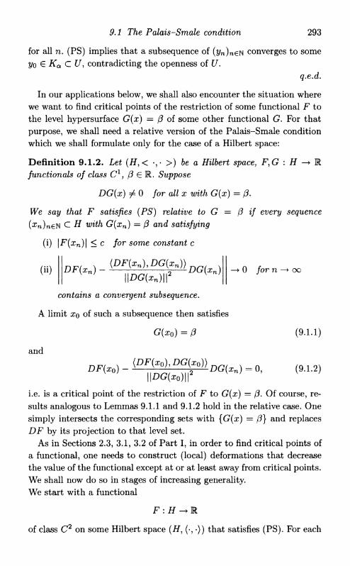
9.1 The Palais-Smale condition 293
for all n. (PS) implies that a subsequence of (yn)nen converges to some yo e Ka C U, contradicting the openness of U.
q.e.d.
In our applications below, we shall also encounter the situation where we want to find critical points of the restriction of some functional F to the level hypersurface G(x) = (3 of some other functional G. For that purpose, we shall need a relative version of the Palais-Smale condition which we shall formulate only for the case of a Hilbert space:
D e f i n i t i o n 9.1.2. Let (H,< •,• >) be a Hilbert space, F,G : H -* R functionals of class C1, (3 G E . Suppose
DG{x) ^ 0 for all x with G(x) = (3.
We say that F satisfies (PS) relative to G = (3 if every sequence ( x n ) n € N C H with G(xn) = (3 and satisfying
(i) | F ( x n ) | < c for some constant c
\\DG(xn)\\2 ( 0 for n —+ oo
contains a convergent subsequence.
A limit xo of such a subsequence then satisfies
G(xQ) = f3 (9.1.1)
and
\\DG(x0)\\2
i.e. is a critical point of the restriction of F to G(x) = (3. Of course, results analogous to Lemmas 9.1.1 and 9.1.2 hold in the relative case. One simply intersects the corresponding sets wi th {G(x) = (3} and replaces DF by its projection to that level set.
As in Sections 2.3, 3.1, 3.2 of Part I , in order to find critical points of a functional, one needs to construct (local) deformations that decrease the value of the functional except at or at least away from critical points. We shall now do so in stages of increasing generality. We start wi th a functional
F : H —• R
of class C2 on some Hilbert space (H, (•, •)) that satisfies (PS). For each

294 The Palais-Smale condition
u E H, DF(u) is a linear functional on H, and by Corollary 2.2.3, i t can therefore be identified with an element VF(w) of H , called the gradient of F at u. Thus, VF(u) satisfies
DF(u)(VF(u)) = | |£>F(u) | | 2 (9.1.3)
\\VF(u)\\ = \\DF(u)\\. (9.1.4)
Since F is assumed to be of class C 2 , DF and hence V F are of class C 1
in their dependence on u. In particular, V F is locally Lipschitz. We now consider the (negative) gradient flow induced by F :
—i/>(u, t) = -VF(V>(u, 0 ) for t > 0 (9.1.5) ot
V>(u,0) = u. (9.1.6)
Because of the Lipschitz property, by Theorem 2.4.2 and Corollary 2.4.2, for small t > 0, there exists a unique solution tp(u, t) satisfying the semigroup property
V>(M + s) = ^ ( M ) , * ) (9.1.7)
for sufficiently small 5, £ > 0. Moreover,
ip(u,t) = u for all u wi th V F ( u ) = 0, i.e. for all critical points of F . (9.1.8)
Finally
F ( ^ ( u , i ) ) = F(u) + J* ~F{^{u, r))dr
= F(u) + jT DF(i/>(u,t))-^il>(u,T)dT
= F(u)- f \\DF(ip(u,T))\\2 dr by (9.1.5), (9.1.3) Jo
< F(u) for t > 0, i f £>F(u) = D F ( ^ ( u , 0 ) ) ^ 0, (9.1.9)
i.e. i f u is not a critical point of F .
Thus, we have found the prototype of a deformation that decreases the value of F except at its critical points. For technical reasons, however, the above flow wi l l need some modifications and generalizations.
First of all, a solution of (9.1.5) need not exist for a l H > 0 because i t

9.1 The Palais-Smale condition 295
may become unbounded in finite ' t ime ' t . This can be easily remedied by using the Lipschitz function
77 : M + -> M +
1 for 0 < s < 1 T](S) = { 1
for 5 > 1 s
and putting
V F ( u ) :=n(\\VF(u)\\)VF{u)
(i.e. VF(w) = V F ( u ) for | |VF(u) | | < 1 and | | V F ( u ) | | < 1 for all u) and
replacing (9.1.5) by
J ^ ( M ) = - V F ( i K « , t ) ) . (9.1.10)
Of course, we still use (9.1.6).
Since V F ( u ) < 1 for all u, the solution of (9.1.10), (9.1.6) now exists for all t > 0, and satisfies (9.1.7) for all s,t > 0. Equation (9.1.8) also still holds, and as in the derivation of (9.1.9), we get
F ( i K u , t ) ) = F(u) - T r / ( | | V F ( ^ ( u , r ) ) | | ) | |DF(^(u , r ) ) | | 2 d r Jo
< F(u) for t > 0,
if tx is not a critical point of F . More generally, we have
F(-0(u, t)) < F(V>(u, 5)) whenever 0 < 5 < t, for all u. Next, we wish to localize the construction near a level a. Thus, for given eo > 0 and a neighbourhood U of Ka we want to have a flow ip(u, t) with (9.1.7), (9.1.8) and also
i)(u,t) = u i f | F ( u ) - a | > c 0, (9.1.11)
and the following more explicit local decrease of the value of F : For a E R, we put
F a : = {veH I F(v) <a}.
We want to find 0 < e < e0 wi th
^ ( F a + e \ U, 1) C F Q _ C (9.1.12)
^ ( f / , l ) c F a _ e U [ / , (9.1.13)
296 The Palais-Smale condition
and of course also
< F(i>(u,s)) i f 0 < s < t for all u. (9.1.14)
We let (p : E —• E be Lipschitz continuous wi th
(p(s) = 0 for |a - s\ > e0
<p(s) = 1 for |a — s\ < ^~
0 < <p(s) < 1 for all 5
and replace (9.1.10) by
~*P(u, t) = -y>(F(V>(u, t)))VF(1>(u, t)). (9.1.15)
Again, a solution ip(u,t) exists for all £ > 0 and satisfies (9.1.7) for all 5 , t > 0, as well as (9.1.8) and (9.1.14) (for the latter i t was necessary to require (p > 0). (9.1.11) also is clear from the choice of (p. We now verify (9.1.12), (9.1.13). I f 0 < c < f and u G F a + C and i f F{i>(u, 1)) > a - e, from (9.1.14)
|F(V>(tx, t)) ~a\<e for all 0 < t < 1,
and therefore
<p(F(i/>(u,t))) = 1 for all 0 < t < 1. (9.1.16)
As before, we may now compute
F(i>(u,l))
f1 d = F(u)+ / — F ( V ( w , r ) ) d r
Jo d T
= F(u)- f v » ( i ; , W « , T ) ) i 7 ( | | V F ( V ' ( u , T ) ) | | ) | | Z ? i ! ' W « , r ) ) | | 2 d T JO
<a + e- [ m i n ( l , | | D F ( ^ ( u , r ) | | 2 ) ( i r (9.1.17) Jo
since we assume u G F a + C , using (9.1.16) and the properties of 77.
By Lemma 9.1.2, we may find 6, p > 0 wi th tfa,« C UatP C t / a , 2 p C U (9.1.18)
(here, we are using (PS)!). From the definition of NQj, thus \\DF(ip(u}T)\\2 > 62 whenever ip(u,r) ^ Naf Without loss of generality 6 < 1. (9.1.17) then yields
F(i){u, 1)) < a + c - (meas {0 < r < 11 i/>(u, r ) i V M } ) 6 2 . (9.1.19)
9.1 The Palais-Smale condition 297
From (9.1.18), we have for v G H \ U
dist(v,Nas) I := inf —w|| ) > p. ' 1 w€Nai6
Since 8 d t ^ M < 1, (9.1.20)
therefore, i f u fi £/, then also t/>(u, r ) ^ 7Va<5 for 0 < r < p, and similarly, if ^ ( u , 1) fi t / , then also ip(u,r) fi Naj for 1 - p < r < 1. Therefore, if either tx fi U or -0(tt, 1) ^ (7, then
meas {0 < r < 1 1 ip(u, r) fi Naj} > p.
Thus, from (9.1.19), i f u fi U or i f ^ ( u , 1) fi U,
F(^(u, 1)) < a + e - p<52
< a ~ e i f we choose e < ^p<52. (9.1.21)
Thus, for 0 < e < min(±€§, | p 6 2 ) , we get (9.1.12), (9.1.13). In conclusion, we have shown the following deformation result:
Theorem 9.1.1. Let F : H —> R be a C2 functional on a Hilbert space H, satisfying (PS). Let a G R, and put
FA := {v G H : F(v) < a } ,
Ka := {v e H : = a, DF(v) = 0} .
Let eo > 0 and a neighbourhood U of Ka be given. Then there exist 0 < e < to and a continuous family
rj): H x [0, oo) -+ H
with the semigroup property ip(ijj(u, s),t) = ip(u,s + t) for all s,t > 0, u £ H and with
(i) -0(w, 0) = it /or all u E H (ii) F(tp(u,t)) is nonincreasing in t for all u G H
(iii) tp(u,t) = u /or a// t whenever DF(u) = 0, in particular for u G
(iv) 4>(u,t) = u whenever \F(u) — a\ > e0, for all t (v) </>(FQ + c \ U, 1) C F a _ € , </>(F a + c , 1) C F Q _ C U [/
(vi) IfF(u) is even (i.e. F(u) = F(—u) for all u), then also F(IJJ(U, t)) is even in u for all t (i.e. F(ip(u,t)) = F(ip(—u,t))).

298 The Palais-Smale condition
(Property (vi) follows from the construction: A l l the auxiliary functions are invariant under replacing u by — u i f F is even, and V F ( - w ) = —VF(u) in the even case.) q.e.d.
C o r o l l a r y 9 .1 .1 . If under the preceding assumptions, F has no critical point with value a, i.e. Ka = 0, then there exist a deformation I/J with the preceding properties and
V> ( F a + C , 1) C Fa-€ for some e > 0. (9.1.22)
Proof. I f Ka = 0, we may choose U = 0 in Theorem 9.1.1. q.e.d.
We shall now extend Theorem 9.1.1 in two directions. First, we consider the relative case, where in addition to F , we have another C2
functional F : H —• R wi th
DF(x) ^ 0 for all x wi th G(x) = 0,
for some given value (3 G R. We wish to find critical points of the restriction of F to G = /3. We assume that F satisfies the relative (PS) condition of Definition 9.1.2 on G = f3. We then perform the preceding construction wi th
VGF(u) := VF(u) - ( V i ^ V G ( K ) ) (9.1.23) K ' K J l |VG(«) | | 2 K J K '
in place of V F ( u ) . We then have
| G W M ) ) = -<p(F(i,(u, t)))r,(\\VGF(u)\\) (VGFW(u, t)), VG(i>(u, t)))
from the chain rule and the analogue of (9.1.15)
= 0,
since (VGF(v),VG(v)) = 0 for all v G H. Therefore, the flow tp(u,t) now leaves G = /3 invariant. We obtain:
T h e o r e m 9.1.2. Let F,G : H —• R beC2 functionals on a Hilbert space ( i f , (•, •)) with F satisfying (PS) relative to G = (3. Let a G R,
:= {veH\F(v)<a,G(v) = (3},
K°>P := {v G H | F(v) = a, G(v) = (3, VGF(v) = 0} .

9.1 The Palais-Smale condition 299
Let e0 > 0, and let U be a neighbourhood of K®^ in {G(v) = /3}. Then there exist e > 0 and a continuous semigroup family
4,:{G(v) = p}x[0,oo)^{G(v) = l3}
satisfying
(i) ip(u, 0) = u for all u G {G(v) = (3} (ii) F(ip(u,t)) is nonincreasing in t
(iii) ip(u, t) = u for all u G (iv) ip(u,t) = u for all t if \F(u) — a\ > eo (v) \U,1)C F™, i>{F°ft, 1) C F^t U U
(vi) If F and G are even, so is F(i/>(-,£)) for all t.
Secondly, we wish to extend the preceding construction to functionals on Banach spaces. For a functional on a Banach space, in general one does not have a good notion of a gradient. We therefore need to introduce Palais' concept of a pseudo-gradient:
D e f i n i t i o n 9.1.3. Let (V, | |- | |) be a Banach space, U C V, F : U -+ R afunctional of class C1. A pseudo-gradient vector field for F is a locally Lipschitz continuous vector field v : U —• V satisfying
(i) H U ) | | < m i n ( l , | | D F ( u ) | | ) (ii) DF(u)(v) > I m i n ( | | J D F ( M ) | | , | | £ » F ( M ) | | 2 )
for all u G U.
L e m m a 9.1.3. Let F : V —• R be a functional of class C1 on the Banach space V. Then F admits a pseudo-gradient vector field on
V':={ueV \ DF(u)^0}.
Proof. For each u G V, we can find w = w(u) wi th
|HI <min(l,| |DF(u)||) (9.1.24)
DF(u)(w) > \ m i n ( | | D F ( u ) | | , \ \ D F ( u ) \ \ 2 ) . (9.1.25)
Since DF is continuous (as we assume F G C 1 ) , w satisfies (9.1.24), (9.1.25) also for all v in some neighbourhood Nu of u. Since {Nu : u G V'} is an open covering of V, i t possesses a locally finite refinement { M a } a G / f . Let
pa(v) : = d i s t ( t ; , V " \ M a ) .
f This holds for any open covering of a paracompact set, see e.g. J . Dieudonne, Grundziige der Modemen Analysis, 2, Vieweg, Braunschweig, second edition, 1987, pp. 26-9; V is paracompact for example because it is metrizable.

300 The Palais-Smale condition
pa is Lipschitz continuous, and pa(v) = 0 for v £ Ma. We put
/ x Pa(v)
Since each v is only contained in finitely many M ^ , because of the local finiteness of the covering, the denominator of (pa is a finite sum. ((fa)aei is a partition of unity subordinate to { M a } , i.e. 0 < ipa < 1, (pa = 0 outside M a , Ylaei = Also, the (pa are Lipschitz continuous. Then
V(U) '' = Yla€lV<*(U)W(U<*) S O m e U« e M<*
is a convex combination of vectors satisfying (9.1.24), (9.1.25) and hence satisfies these relations, too. v(u) thus is a pseudo-gradient vector field for F.
q.e.d.
Note that we only need to require F G C 1 , and not F G C 2 , in order to construct a locally Lipschitz pseudo-gradient field. We then have the following deformation for C1-functionals on Banach spaces.
T h e o r e m 9.1.3. Let F : V —> E be a C1-functional on a Banach space V satisfying (PS). Let a G E, eo > 0, U a neighbourhood of Ka as in Theorem 9.1.1. Then there exist 0 < e < 1 and a continuous family I/J : V x [0, oo) —• V satisfying the semigroup property w.r.t. t > 0, and
(i) ip(u, 0) = u for allu eV (ii) F(ip(u, s)) < F ( ^ ( u , t)) whenever 0 < t < s, u G H
(iii) ip(u, t) = u for all t whenever DF(u) — 0 (iv) ip(u,t) = u whenever \F(u) - a\ > e0, for all t (v) ^(Fa+e \ U, 1) C F a _ c , 1>(U, 1) C F a _ c U U
(vi) If F(-) is even, so is F(ip(-,t)) for all t.
Proof. The proof is the same as the one of Theorem 9.1.1, replacing VF(u) by a pseudo-gradient vector field v(u) — except for the following technical point: Lemma 9.1.3 asserts the existence of a pseudo-gradient field only on {x G V \ DF(x) ^ 0}. We therefore have to choose another Lipschitz continuous cut-off function 7 : V —• E wi th 0 < 7 < 1, 7(1*) = 0 if u G J V a j j , 7(14) = 1 for u G V \ Na^. We may then consider
= -7(^,<))v(F(V'Kt)))ry( | | t ; (V(«, t)) | | ) U (V(«,<)) (9-1.26)
with </?, 77 as before. This has the additional effect that
dj>(u,t) _ dt

9.2 The mountain pass theorem 301
whenever tp(u,t) G JV Q («, which is a neighbourhood of Ka, while the evolution is the same as before (with v(u) in place of VF(w)) outside Naj- This cut-off near Ka does not affect the rest of the construction. I f F is even, we may also choose 7 even.
However, there might still exist critical points of F in F a + C \ Nays- In order to take account of those, we strengthen the requirements on the above cut-off function (p to
p(s) = 0 for |a - s\ > min(e 0 , - )
(p(s) = 1 for |a - s\ < m i n ( y , - ) .
W i t h such a </?, the right-hand side of (9.1.26) vanishes near any critical point of F , and i t is therefore defined on all of V. I f we then also impose the additional restriction
« 4 everything works out as before.
q.e.d.
I t is possible, and not overly difficult, to extend Theorem 9.1.3 to the relative case and to obtain a result analogous to Theorem 9.1.2. Here, however, we refrain from doing so.
9.2 T h e m o u n t a i n pass t heo rem
W i t h the help of the deformation theorems of the previous section, one may easily derive existence results for critical points of a functional satisfying (PS). To illustrate this point, we start wi th the tr ivial
L e m m a 9.2 .1 . Let F : V —• R be a C1 functional on a Banach space satisfying (PS). If
a := inf F(u) > - 0 0 ,
then F possesses a critical point UQ with value a (i.e. F(uo) = a, DF(u0)=0).
Proof. Suppose that KQ = 0. Then U = 0 is a neighbourhood of Ka. Let e0 > 0 be arbitrary. Choose e as in Theorem 9.1.3. From the definition of a,
F a + C ^ 0 , F a _ c = 0.
302 The Palais-Smale condition
Therefore, i t is impossible that as Theorem 9.1.3 (v) asserts, the deformation tp(-, 1) maps F a + C into F a _ c . This contradiction implies Ka ^ 0 , which means the existence of the desired critical point.
q.e.d.
Of course, the methods presented in Chapter 4 yield more general existence results for minimizers of variational problems. The strength of the Palais-Smale approach rather lies in its capability of producing nonminimizing critical points. To demonstrate this, we now present the mountain pass theorem of Ambrosetti-Rabinowitz.
Theorem 9.2.1. Let F :V —• M be a C1 functional on a Banach space (V, ll-ll) satisfying (PS). Suppose F(0) = 0 and
(i) 3p > 0,/3 > 0: F(u) > (3 for all u with \\u\\ = p
(ii) 3t*i with \\u\\\ > p and F(u) < (3. We let
r := { 7 € C°([0,1], V) | 7(0) = 0,7(1) = U i } . Then
a := inf sup F(I(T)) (> 0) 7 € r r € [ 0 ) 1 ]
is a critical value ofF (i.e. there exists UQ with F(u0) = a, DF(UQ) = 0).
Proof. Suppose again that Ka = 0 , and take the neighbourhood U = 0 of Ka. We let e0 = min(/?, f3 - E(u\)). Choose e as in Theorem 9.1.3. Prom the definition of a, there exists 70 G T wi th
sup F(7O(T ) ) < a + e, T€[0,1]
while no such 7 can satisfy
sup F(y(t)) < a - e, «€[0,11
i.e. satisfy 7Q0,1]) C F a _ c . However, i f we apply the deformation ?/>(•, 1) of Theorem 9.1.3, we obtain a path
7 ( r ) :=V>(7o(r),l)CFa_c
with 7(0) = 7o(0) = 0 and 7(1) = 7o(l) = u\ by choice of e0. This contradiction implies KQ ^ 0 , i.e. the existence of the desired critical point.
q.e.d.
9.2 The mountain pass theorem 303
Let us summarize the essential features of the preceding reasoning:
(1) One chooses a family of sets, here T, that exploits some properties of F and is invariant under the deformation ?/>(•, 1).
(2) This family yields a minimax value a. (3) a can be estimated from above wi th the help of any member of
our family r (a < s u p r € [ 0 x j F(7( t ) ) ) for any 7 G T), and from below through the constraints that the members of T have to satisfy (in Theorem 9.2.1, every 7 G T intersects dB(0, p), and therefore a > f3 > 0, and therefore in particular, the critical point produced is different from 0).
(4) A reasoning by contradiction, based on the deformation theorem, shows that a is a critical value.
As an application of the mountain pass theorem, we consider the following example:
Theorem 9.2.2. Let Q C R d be a bounded domain, 2 < p < ^ (respectively < 00 for d = 1,2). Then the Dirichlet problem
Au+ \u\p~2u = 0 in Q (9.2.1)
u = 0 on dn (9.2.2)
admits at least two nontrivial (weak) solutions ('nontrivial' means not identically 0).
Proof. I f u is a solution, so is — u. Therefore, i t suffices to verify the existence of one nontrivial solution. (9.2.1), (9.2.2) are the Euler-Lagrange equations in HQy2(ft) for the functional
F(u) = \ f \Du\2-- f \uf. (9.2.3) ^ JQ P JQ
This functional is a continuous functional on HQ'2(Q), because J Q \Du\2
clearly is continuous there, and J \u\p too, because of the Sobolev Embedding Theorem 3.4.3 as we assume p < -j^. F is also differentiable, wi th
DF(u)(<p)= j Du • Dip - j \u\p'2u(p. (9.2.4) JQ JQ
Again
(p 1—• / Du • Dip JQ
304 The Palais-Smale condition
clearly is continuous on HQ,2(Q), whereas
Jn
is continuous, because we have by Holder's inequality
p - i i
I\ur2u<p <([\u\A p (f M P ) P
<co\\u\\p
Hi\{Q)\\<p\\Hi,2{Q)
(9.2.5)
(9.2.6)
by the Sobolev Embedding Theorem 3.4.3
for some constant c 0. Thus F : H^2(Vt) —• R is of class C 1 . We shall verify the Palais-Smale condition for F: Suppose ( u n ) n € N C
H Q ' 2 ( 0 ) satisfies
| F ( u n ) | < Ci for some constant c\ (9.2.7)
DF(un) ^ 0 for u ^ oo. (9.2.8)
Thus
and
sup / DunDip 1,2<1 •'O
< ci (9.2.9)
u ny>| —• 0 for n —• oo.
(9.2.10)
In (9.2.10), we use (p = n^)"^ 2
a n d obtain
- J \Dun\2 + j \un\p < c2\\un\\H1,2. (9.2.11)
Since p > 2, (9.2.9) and (9.2.11) imply
J \Dun\2 < c 3 | |w„ | |„ i ,2 + cA. (9.2.12)
Since by the Poincare inequality (Theorem 3.4.2)
= / + j \Dun\2 < c 5 J \Dun\2 , (9.2.13)
we conclude from (9.2.12)
H«nllHi.»(fl) ^ C 6- (9-2-14)
Thus, any 'critical sequence' ( u n ) n £ N is bounded. We now claim that
9.2 The mountain pass theorem 305
such a sequence ( u n ) n € N contains a convergent subsequence, thereby completing the verification of (PS). We need to show that, after selection of a subsequence,
j \Dun — Dum\2 —• 0 for n, ra —• oo (9.2.15)
(using again the Poincare inequality as in (9.2.13)). Now
J DunD(un - Um) - j | u n | p ~ 2 un(un - um) —• 0 for 71, ra —> oo
(9.2.16) by (9.2.10), (9.2.14). By the Rellich-Kondrachev theorem (Corollary 3.4.1), we may also assume (by selecting a subsequence) that (un)ne^ is a Cauchy sequence in 1^(0,). Then, using Holder's inequality as in (9.2.5),
p-i i
Jy \un\P~2 Un(un - Um) < (^J \un\P^j (^J | t Z n - U m | P ^ ^ 0 f o r n , r a - > o o . (9.2.17)
Equation (9.2.16) then implies
J Dun - D(un — um) —• 0 for ra, n —> oo,
which implies (9.2.15). We have thus verified (PS) for F. We shall now check the remaining assumptions of Theorem 9.2.1. First of all,
F(0) = 0.
Recalling that by the Sobolev Embedding Theorem 3.4.3 (and the Poincare inequality, see (9.2.13))
i
( / n M f £ C ' ( / n
| D " | ! ) " ' we have
F(u) > ( i - C8 ||«||££(n)) I M I i » . . ( n > > 0 > o i f IM|#i .2(Q) = p is sufBciently small.
Finally, take any u2 G HQi2(Q) wi th / n \u2\p ^ 0. Then for sufficiently large A > 0, u\ — Xu2 satisfies
^(«l) = T / \ D U 2 \ 2 ~ - f \U2\P<0. 2 J P Jn
306 The Palais-Smale condition
We have now verified all the assumptions of the mountain pass Theorem 9.2.1, and we consequently get a critical point u of F wi th
F(u) > (3 > 0.
This is the desired nontrivial solution. (In fact, regularity theory implies that any weak solution of (9.2.1) is smooth in fi, see e.g. Gilbarg-Trudinger, loc. cit.)
q.e.d.
Remark 9.2.1. By the same method, we can also treat the equation
Au - Xu + \u\p'2 u = 0 for any A > 0. (9.2.18)
9.3 Topological indices and critical points
In Section 3.2 of Part I , we have seen an example where a topological construction permitted to deduce the existence of more than one (unstable) critical point of a functional. In the present section, we first give an axiomatic approach to such constructions and then apply this in conjunction wi th the Palais-Smale condition to a concrete variational problem to show the existence of infinitely many solutions.
Such global topological constructions originated wi th the work of Lyusternik. Contributors also include Schnirelman, and, more recently, Rabinowitz, and many others. The reader wi l l find detailed references in the monographs quoted at the end of this chapter.
Definition 9.3.1. Let X be a topological space, F : X —> R continuous, x € X is called a special point for F, with value a,
x G spec a F (a then is called a special value)
if x is contained in all A C X with the following property: For each open U D A there exist e = e(U) > 0 and a continuous
t/> : X x [0,1] ^ X
satisfying
(i) \j)(y,0)=y foryeX (ii) F(^(y, t)) < F(^(y, s)) for all y G X, 0 < s < t < 1
9.3 Topological indices and critical points 307
(iii) For every y G X \ U with
F(y) < a + e,
we have
F ( ^ ( » , l ) ) < a - c .
Of course, the ip of the preceding definition is an abstract version of the deformations constructed in Section 9.1, and the notion of special point is a topological version of the notion of critical point.
Remark 9.3.1. Since the composition of any two deformations ipi,ip2
satisfying the properties of Definition 9.3.1 continues to satisfy these properties, the intersection of any two sets A\, A2 still satisfies the property expressed in Definition 9.3.1 i f Ai,A2 do. Therefore, i f speca F — 0, we may take U = A = 0 in Definition 9.3.1 and find a deformation ip that satisfies ( i ) - ( i i i ) for all y G X.
In order to illustrate the notion of special point as well as the topological constructions to follow, we now present the simple:
L e m m a 9.3 .1 . Let F : X —• E be a continuous function on the topological space X. Let M be a (nonempty) class of nonempty subsets of X. If speca F = 0, we require that M is invariant under the deformations considered in Definition 9.3.1:
IfAeM, then also ip(A, 1) G A i . (9.3.1)
Suppose
-oo < a = inf sup F(y) < oo. (9.3.2) AeMyeA
Then a is a special value for F, i.e. there exists
xo G spec aF.
Proof. Suppose spec a F = 0. According to the preceding remark, we may then take U = 0 and find ^ : l x [ 0 , a n d e > 0 wi th
F(ip(y, 1)) < a - e whenever F(y) < a + e. (9.3.3)
We may find AQ G M wi th
sup F(y) < a + e, y£A0
(9.3.4)
308 The Palais-Smale condition
but no A G M can satisfy
supF(y) < a-e. (9.3.5) y€A
However, i f we take A\ := ip(Ao, 1) then A\ G M. by assumption, and by (9.3.3)
sup F(y) < a - e, y€Ax
contradicting (9.3.5). Thus, speca F ^ 0. q.e.d.
In order to obtain the existence of further special points, we now shall introduce the notion of a (topological) index. Such an index is based on symmetry or invariance properties of the functional under consideration. Here, we only consider the case of the simplest nontrivial symmetry group, namely Z 2 , although the subsequent constructions easily generalize to any compact group G. We thus make the following symmetry assumptions:
• X is a topological space with a nontrivial involution, i.e. there exists a continuous map j : X —> X , j ^ id, wi th
j 2 = i d .
• F : X —• E is continuous and even, i.e.
F(j(x)) = F(x) for all x G X.
• M := {A C X I j(A) = A and for all x G A,j(x) ^ x (i.e. A contains no fixed points of j ) } .
We now also require ip(j(x),t) — j(ip(x, t)) for all the deformations of Definition 9.3.1.
D e f i n i t i o n 9.3.2. An index for (X , F) is a map
i : M -+ { 0 , 1 , 2 , . . . , 0 0 }
satisfying for all A, A\,A2 G M:
(i) i(A) = 0 ^ A = 0 (ii) A finite (A ^ 0) i (A) = 1
(iii) 2(^1 U A 2 ) < i(Ai) + i(A2) (iv) Ai C A 2 =» < i(A2) (v) t(i4) < i(j(A))

9.3 Topological indices and critical points 309
(vi) A compact =£• 3 neighbourhood U of A in X with U G M,
i(A) = i(U) < oo.
For n € { 0 , 1 , 2 , . . . , oo}, we put
Mn:= {AeM\ i(A) >n}.
Remark 9.3.2. More precisely, one should call an i as in Definition 9.3.2 an index for (X, F, Z 2 ) , in order to specify the symmetry group involved.
For n E { 0 , 1 , 2 , . . . , 00}, we define
an := inf sup F(y). A£Mn yeA
Theorem 9.3.1. Suppose the above symmetry assumptions hold, an index i for (X, F) exists, and
—00 < an < oof
(i) Then
s p e c Q n F ^ 0 (9.3.6)
(ii) If furthermore for some k > 1, an = c* n+i = . . . = an_|_fc, ^ e n specQ n F 25 infinite.
Proof We note that property (v) of Definition 9.3.2 implies that Mn
is invariant under (symmetric) deformations ip. Therefore, Lemma 9.3.1 implies specQ n F ^ 0 . For the second statement, we claim that for Ao = specQ n F ,
i(Ao) >k+l. (9.3.7)
I f k > 1, property (ii) of Definition 9.3.2 then implies the existence of infinitely many special points wi th value an. Suppose on the contrary that
i(A0) < k. (9.3.8)
By Definition 9.3.2 (vi), we may find a neighbourhood U of Ao wi th U e M and
t(i4o) = i(U). (9.3.9)
Since A0 consists of special points, we may find a (symmetric) deformation ip wi th
F(ip(y, 1)) < an - e for all y e X \ U wi th F(y)<an + e
f Since the infimum over an empty set is 00, this contains the assumption Mn / 0-
310 The Palais-Smale condition
for some e > 0. Since an — a n + k , we may find A e Mn+k wi th
sup F(y) < an + e, y£A
hence
sup F(z)<an-e. (9.3.10) zeif(A\u,i)
We have
i(A\U)>i(A)-i(U) by (iii)
> n + k - k, using (9.3.8), (9.3.9), A e Mn+k
= n.
Thus
A\UeMn,
hence A \ ( 7 ^ 0 by (i) . Since, as noted in the beginning, Mn is invariant under we get
i>(A\U,l) G Mn,
hence
sup F(y) > a n , y€V(^\t/,l)
contradicting (9.3.10). q.e.d.
In order to apply the preceding considerations, we need to construct an index wi th the properties listed in Definition 9.3.2. We shall present here Coffman's version of the genus of Krasnoselskij.
D e f i n i t i o n 9.3.3. Suppose the symmetry assumptions stated before Definition 9.3.2 hold. The genus of A ^ 0, A e M is defined as follows:
gen(A) := inf { n G { 1 , 2 , 3 , . . . ,00} | 3 continuous f : A -> R n \ {0}
with f(j(x)) = —f(x) for all xeA}
while gen(0) := 0.
As an example, we state:
L e m m a 9.3.2. The genus of the unit sphere S'n""1 = { | |x | | = 1} in R n
(with involution j(x) = —x) is equal to n.

9.3 Topological indices and critical points 311
Proof. The inclusion map S'n""1 R n satisfies the properties of Definition 9.3.3, and so g e n ( 5 n _ 1 ) < n. I f n > 2, 5 n _ 1 is connected, and therefore, by the mean value theorem, there is no continuous map / : S^- 1 -+ R ^ j o } with f(-x) = -f(x) for all x. Hence g e n ^ " 1 ) > 2. In fact, by the Borsuk-Ulam theoremf, there is no such continuous map to R m \ {0} wi th m < n. Therefore, gen(5 n ~ 1 ) > n.
q.e.d.
Coro l l a ry 9 .3 .1 . The genus of the unit sphere S := {x € V : \\x\\ = 1}
in an infinite dimensional Banach space (V, | |- | |) is oo.
Proof. For any n-dimensional subspace Vn of V,
gen(S) > gen(S f l Vn) > n by Lemma 9.3.2 .
q.e.d.
T h e o r e m 9.3.2. The genus as defined in Definition 9.3.3 is an index in the sense of Definition 9.3.2.
Proof. We need to check the properties ( i ) - (vi ) of Definition 9.3.2.
(i) is obvious. (ii) I f A € A I is finite, then A is of the form {x1/,j(x1/) \ v — 1 , . . . , k}
for some k. We define / : A -+ R 1 \ {0} by f(x„) = 1, f{j{xu)) = - 1 for all v (of course, we may assume xp ^ j(xu) for all fi, v).
(hi) Let gen(A„) = n„ < oo, v = 1,2, and let the continuous fv : Av -> R n " \ {0} satisfy U(j(x)) = ~U(x) for all x. By the Tietze extension theorem^, fv can be continuously extended to
fv : X - + R n " .
By considering \(fv(x) ~ fv(j{x))) in place of fv, we may assume that the extension still satisfies
/ „ ( j (x ) ) = -fv{x) for all x.
The map ( / i , / 2 ) : Ax U A2 R n i + n 2 \ {0} then shows that
gen(Ai U A2) < n i + n 2 = gen(Ai) 4- gen(A 2 ).
(iv) is obvious. (v) follows, since / o j shares the necessary properties with / .
f See e.g. E . Zeidler, Nonlinear Functional Analysis and its Applications, I , Springer, New York, 1984, p. 708, for a proof.
$ See E . Zeidler, loc. cit., p. 49.
312 The Palais-Smale condition
(vi) Let A € M be compact. Since j(x) ^ x for all x € A (by the properties of A i ) , for each x € A, we may find a neighbourhood £/(#) wi th U(x) n j(U(x)) = 0. Since A is compact, i t can be covered by finitely many such neighbourhoods Uv, v = 1 , . . . , n. For each we choose a continuous function <pv : X —• R with </?j,(x) > 0 for x € £/|,, <pu(x) = 0 for sc E X \ t/„. We then define h = (h\...,hn): A ^ R n \ { 0 } b y
^ ( x ) . = J f o r x € t / ^ \ —<Pv{x) for x € A \ Uy, in particular for x € j{Uu).
(Since every x € A is contained in some we have h(x) ^ 0 for all x € A.) Thus gen(A) < n < 00. I f A € M is compact with gen(A) = n, and
/ : A -> R n \ {0} is continuous with f(j(x)) = - / ( x ) ,
we may extend / as before to / : X —• R n (with the same symmetry property). Since A is compact, so is / ( A ) , and therefore, we may find an open neighbourhood V of f(A) wi th V C R n \ { 0 } . Then U := f l(A) satisfies
n = gen(A)
< gen(U) by (iv)
< n since J(U) is contained in V C R n \ { 0 } .
Thus gen(U) = gen(A) as required. q.e.d.
We may now obtain a general existence theorem for critical points of functionals satisfying (PS):
T h e o r e m 9.3.3. Let F, G : H —• R be C2 functionals on a Hilbert space (H, (•, •)) that are even, i.e. F(x) = F(—x), G(x) = G(—x) for all x € H. Suppose F satisfies (PS) relative to G = (3, and is bounded from below. Let
M:={Ac{G(x) = (3}\0<£A and (xeA^-xeA)}.
Let 70 := sup{gen(if) | K € M compact} (< 0 0 ) . Then F possesses at least 70 critical points relative to G = (3.
Proof. Since (PS) holds, by Theorem 9.1.2, all special points (in the
9.3 Topological indices and critical points 313
sense of Definition 9.3.1) for the restriction of F to X := {x € H | G(x) = 0) are critical points for F relative to G = (3. Hence, i t suffices to produce 70 special points of F on 1 . Let
an := inf sup F(x). A£M,gen(A)>n X£A
Since F is bounded below, and since in the definition of 70, we only consider compact sets, we have
—00 < an < 00 whenever n < 70 .
By Theorem 9.3.2, we may apply Theorem 9.3.1 to the genus as an index. We have in fact
—00 < ot\ < cx<i < • • • < an < - - - < 00 whenever n < 70.
I f we always have strict equality, then the
xn € spec Q n F
produced by Theorem 9.3.2 (i) are all different, because their values F(xn) are all different. I f however any two such numbers a n _ i and an
are equal, then by Theorem 9.3.2 (ii) we even obtain infinitely many special points. Thus, in any case, we have at least 70 special, hence critical points.
q.e.d.
As an application of Theorem 9.3.3, we consider the example of the previous section:
C o r o l l a r y 9.3.2. Let ft C Rd be a bounded domain, 2 < p < j ~ (respectively < 00 for d = 1,2). Then for any A > 0, the Dirichlet problem
Au - Xu + \u\p~2 u = 0 infl (9.3.11)
u = 0 on dft (9.3.12)
admits infinitely many (weak) solutions.
Proof. We consider the even functionals
F{u) = \j^(\Du\2 + \u2)
G(u) = lf \u\p. P Jn
We claim that F satisfies (PS) relative to G = 1. The proof is similar

314 The Palais-Smale condition
to the argument employed for the demonstration of Theorem 9.2.2: let (w n )n€N be a critical sequence, i.e.
F(un) < ci (9.3.13)
(DGMDFM)
\\DG(un)\f 0 f o r n - > o o (9.3.14)
where all norms and scalar products are from H Q ' 2 ( Q ) . From (9 .3.13) (and the Poincare inequality in case A = 0), we obtain
(9 .3 .15)
We obtain as in the proof of Theorem 9.2.2 (cf. (9.2.5)), by using Holder's inequality, that
\DG(un)(un - um)\ = j \un\p 2un(un-Um)
2^1
" ( / | U n | P ) P ( / l ^ - U - | P ) P ' ( 9 - 3 - 1 6 )
Since p < from (9.3.15) and Sobolev's Embedding Theorem 3.4.3, we conclude that / | u n | p is bounded, whereas (9.3.15) and the Rellich-Kondrachev theorem (Corollary 3.4.1) imply that (un)ne^ is a Cauchy sequence in L p ( f i ) . Thus, from (9.3.16)
Also
DG(un)(un — Um) —> 0 for n, m —• oo.
\DG(un)(w)\
(9.3.17)
\\DG(un) sup
> \DG(un)(un)\
| | U „ | | „ 1 , 2
! K \ P
| |«n| | f l-«.a
> 0 from (9.3.15) and
- / \un\p = G(un) = 1. P J
(9.3.18)
(9.3.19)

9.3 Topological indices and critical points 315
Prom (9.3.17), (9.3.18) we conclude that there exist h n m e H^2(ft) wi th
DG(un)(un - Um + hnm) = 0 for all n , m (9.3.20)
l l ^ n m ! ! / ^ - 2 —• 0 for n, ra —• oo. (9.3.21)
Therefore, from (9.3.14)
DF(un)(un - um 4 hnm) -+ 0,
i.e.
j {Dun (D(un - um) 4 Dhnm) 4 Xun{un - u m + hnrn)) 0
for n, ra — oo
and because of (9.3.21) then also
J (Dun(D(un - um)) 4 Xun(un - Um)) 0.
This implies
J (\{D(un - um)\2 4 A | ( u n - um)\2^ -+ 0 f o r n , r a - > o o ,
and consequently, ( u n ) n e N is a Cauchy sequence in Ho , 2 (n ) . This verifies (PS) relative to G = 1.
In order to apply Theorem 9.3.2, we thus only need to check that in the present case, 70 = 00. However,
is the intersection of a sphere centered at the origin in Lp(ft) wi th the subspace HQ,2(Q). Therefore, the argument of Lemma 9.3.2 easily implies 70 = 00. Theorem 9.3.2 thus produces infinitely many solutions
n ! \\DG(un)\\2 y n >
i.e. wi th
= (DG(un),DF(un))
^ ' ||r>G(«„)||a ' weak solutions of
Aun - Xun 4 fin \un\P~2 un=0 in ft
un = 0 on dft.

316 The Palais-Smale condition
I f we choose vn wi th z / P ~ 2 / i n = 1, then vn := vnun solves (9.3.11), (9.3.12) weakly. Again, we remark that elliptic regularity theory implies that all un and vn are smooth in fi, so that in fact we obtain classical solutions of (9.3.11), (9.3.12).
q.e.d.
In Theorem 9.2.2 and in Corollary 9.3.1, we had imposed the restriction
2d p < — - ( i n case d > 3) ,
d — 2 and the reader may wonder whether this is necessary. To pursue this question, we shall now discuss the theorem of Pohozaev:
T h e o r e m 9.3.4. Let fi C R d be a smooth domain which is strictly star shaped w.r.t. 0 £ R d (this means that the outer normal v of Vt satisfies (x, v(x)) > 0 for all x £ dft). Then for X > 0, any solution of
Au - Xu - f M ^ u = 0 in fi (9.3.22)
u = 0 on dft (9.3.23)
vanishes identically.
We shall present a complete proof only for A > 0 and for smooth solutions u (elliptic regularity implies that any weak solution of (9.3.21), (9.3.22) is automatically smoothf on fi, but the present book does not treat this topic): We multiply (9.3.22) by YlLi a n d o b t a i n
0 = (Au - Xu + \u\&* uj E ^ ' J ^ (9.3.24)
= div ( W g ~^f~r M 2 + ±w* + ^ | D u | 2
+ ^ H 2 - - ^ H ^ . (9.3.25)
By (9.3.23), we have w = 0 o n Ofi, hence also X > * | * T = E ^ V § ^ (y = ( z / 1 , . . . , vd) is the exterior normal of fi). Integrating (9.3.25) therefore yields
d-2 f _ l 2 Ad f , l 2 d - 2 f , l A W 9 u ' 2
/an ^ 2 > V = o.
(9.3.26)
f See for example Appendix B in M. Struwe, Variational Methods, Springer, Berlin, 2nd edition, 1996.

9.3 Topological indices and critical points 317
On the other hand, multiplying (9.3.22) by u leads to
Jn Jn Jn
Equations (9.3.26) and (9.3.27) imply
(9.3.27)
Jn Jan du (9.3.28)
I f A > 0, this implies u = 0, hence the result. (If A = 0, one still concludes that | ^ = 0 on dft. Since also u = 0 on dft by (9.3.23) one may invoke a unique continuation theorem for solutions of elliptic equations to obtain u = 0 in ft. We omit the details.)
Theorem 9.3.4 implies that for p — j ~ in Theorem 9.2.2 and Corollary 9.3.2, the Palais-Smale condition no longer holds. Namely, i f i t did, the proofs of those results would yield the existence of nontrivial solutions. I t also shows that i f the Palais-Smale condition fails the whole scheme developed in the present chapter for producing critical points breaks down.
Since for p < (PS) does hold, the case p — can be considered as as l imit case for (PS). In fact, such limit cases of the Palais-Smale condition occur in many variational problems that are of importance in Riemannian geometry, e.g. the Yang-Mills functional on a four-dimensional Riemannian manifold, two-dimensional harmonic maps, surfaces of constant mean curvature, the Yamabe functional etc. The interested reader is for example referred to
K. C. Chang, Infinite Dimensional Morse Theory and Multiple Solution Problems, Birkhauser, Boston, 1993,
J. Jost, Riemannian Geometry and Geometric Analysis, Springer, Berlin, 2nd edition, 1998,
M. Struwe, Variational Methods, Springer, Berlin, 2nd edition, 1996,
and the references contained therein. The basic references that have been used in writing the present chapter
are the monograph of M.Struwe just quoted, as well as
P. Rabinowitz, Minimax Methods in Critical Point Theory with Applications to Differential Equations, CBMS Reg. Conf. Ser. 65, AMS, Providence,
q.e.d.
1986
and
318 The Palais-Smale condition
E. Zeidler, Nonlinear Functional Analysis and its Applications, I I I , Springer, Berlin, 1984.
These three monographs contain not only detailed bibliographical references — which the reader is urged to consult in order to find the original sources of the results of the present chapter — but also many further results and examples concerning the Palais-Smale condition and index theories.
Exercises
9.1 Why is Theorem 9.2.1 called 'mountain pass theorem'? Hint: Try to find an analogy between the statement of that result and the geometry of mountain passes.
9.2 Try to find conditions for a function
/ : ft x R - > R
so that the reasoning of Theorem 9.2.2 can be extended to the Dirichlet problem
Au(x) = f(x,u(x)) for x G ft
u(x) = 0 for x € dft
in a smooth bounded domain ft. (An answer can be found in Theorem 6.2 of the quoted monograph of M.Struwe.)
9.3 Develop an index theory for a general compact group G in place of Z 2 .
9.4 Extend Theorem 9.1.3 to the relative case as indicated at the end of Section 9.1.
Index
x • y = J2i=i = x v
|cc|2 = X • X, X V
u(t) = £ u ( t ) , X V Ck(Q), xv C f c ( n , R d ) , xvi c°°(n), xvi c0°°(n), xvi qjf(n), xvi / ( u ) = / 0
b F ( t , u ( t ) , u ( t ) ) i f t , 3 D / , 4 r 7 € C i ( [ a , 6 ] , I R d ) , 5 F u , 5 i^P, 5 6 J ( U , I J ) := £ / ( u 4 - s r / ) , _ a = 0 1 0 AC{[a,b\), 11 D 1 ( / , R < * ) , 11
13
6 2 / ( U , T J ) := ^ / ( u + « t y ) , ^ = 0 1 9
Fpipj'Hi'nj = 12^=1 FpipiViVj, 19 c(t) : = g ( t ) , 32 ^ ( c ) : = / 0
T | c ( t ) | d t =
/ o T (E i» i (0 2 )** , 32 E(c) :=yT\c(t)\2dt =
fl'y.fc:= ~$t9v> 3 9
r J f c : = ^(gjitk+gku-gjid), 39
5 n :=
39
d(p,q) := in f {L(c ) | c : [a,6] —• M rectifiable curve with c(a) = p,c(b) = q}, 51
meas, 118 fA f(x)dx of / , 120 Cl{A), 120 <p € Cg(R d ) , 122 INI. 125 ( v ) , 126 R + := {t e R | t > 0} , 130 H / I L : = s u p ^ 0 i ^ | l , 1 3 3 V * := { / : V — R linear with
| | / I U < o o } , 133 (V*)* = : V * * , 133 3Jn —* X , 135 M x :=
{a: € # : (x, y) = 0 for all y € A / } , 141
| | T | | := s u p x ^ 0 l | ^ f l e R + U {oo}, 144
L ( V , W), 145 k e r T := {a; 6 V : To; = 0} , 145 V = Vi e V 2 , 146 coker, 147 H ( T ) , 147 i n d T , 147 F ( V , W ) , 147 DF(u), 150 C 1 , 150 C 2 , 150 £ > 2 F ( u ) , 150 ODE, 155 I M | c o : = s u p t € / | | y ( t ) | | , 156 H/llp : = H / H L P M ) : = UA\f(x)\pdx)p,
159 e s s s u p x € j 4 f(x) := inf {A G R | f(x) <
X for almost all xeA}, 162
C0°°(n), 166 supp^J, 166
319

320 Index
ft' cc ft, 167 fh =3 / , 167
a := ( a x , . . . , a d ) , 171
l « l 171 t; := D a w , 171 Wfc>*>(ft), 171
Nl lV* .p (n ) — (E|a|<fc Jn \Dau\p) P , 171
Hk>P(Q), 171
H 0
f e ' p ( n ) , 171 Diu, 172 Dw, 172 Isc, 185 F A ( x ) := i n f y € X ( A F ( y ) + d 2 (* , t / ) ) , 190 Jx(x), 191
( A : = E t i ( a f V ) , 1 9 9 s c ~ F , 208 i A , 210 9 " / , 216 r - l i m n - o o Fn, 225 £V(ft), 242 \\Du\\, 242 N I B V ( Q ) '= \M\mn) + H D w l l (n)> 2 4 2
l ^ l d - i , 2 4 3
P(E,Q) :=\\DXE\\(n), 244 * u(x), 246
G / ( d , R ) , 257 0 ( d , R ) , 257 J\{u)v, 270 ( • , ) L 2 , 2 8 3 ( P S ) , 292 Ka, 292 V F ( w ) , 294 spec a , 306 gen(A), 310 accessory variational problem, 19 accumulation point, 185, 208 Ambrosetti, 302 angular momentum, 26, 28, 30 arc-length, 3 Arzela-Ascoli theorem, 176
Banach fixed point theorem, 150, 152 Banach space, 126, 129, 132-134, 138,
145, 161, 162, 270, 291, 292, 299-301
Banach spaces, 150 Bellman equation, 105, 108 Bellman function, 105, 107 Bellman's method, 106 bifurcation theory, 268, 270 Borel measure, 118 Borel set, 117
Borel cr-algebra, 117 brachystochrone, 4
canonical equation, 85, 89, 95, 97, 99-101, 111
canonical equations, 80, 93 canonical system, 80 canonical transformation, 95-100, 103 Cantor diagonalization, 135 catenary, 283 catenoid, 283 Cauchy sequence, 126 characteristic function, 119, 211, 243 Christoffel symbols, 39 classical calculus of variations, 3 closed geodesic, 67 coarea formula, 250, 257 coercive, 186 coercivity condition, 291 Coffman, 310 cokernel, 147 compactness condition, 183 compactness of critical sequences, 292 complementary subspace, 146 complete, 126, 134 complete integral, 84, 93 completely integrable, 100 conjugate, 22, 24 conjugate point, 43 conservation law, 26 conserved quantities, 26 constant of motion, 80, 99 continuous linear functional, 133 continuous linear operator, 144 control condition, 109 control equation, 106, 108, 109, 111, 207 control parameter, 104 control problem, 109 control restriction, 105 control variable, 111, 207 converge, 125 convex, 68, 127, 130, 143, 186, 191, 193,
214, 219, 222 convex combination, 142 convex curve, 68 convex function, 122 convex functional, 188 convexity, 291 coordinate transformation, 36 cost, 105 cost function, 207 countable base, 184 countably additive, 118 critical family, 75 critical point, 5, 62, 66, 293, 294, 298,
301, 303, 306, 307, 312, 317 critical sequence, 291, 292, 304, 314

Index 321
critical value, 302, 303 cusp catastrophe, 279
de Giorgi, 225 deformation, 293, 294, 297, 298, 302,
307-309 dense, 169 diffeomorphism, 34, 95 differentiable, 150 differentiable map, 150 differentiation under the integral, 124 Dirac delta distribution, 173 Dirac distribution, 166 direct method, 183 Dirichlet boundary condition, 3, 26,
183, 190 Dirichlet principle, 199 Dirichlet's integral, 199, 203 distance, 51 distance function from a smooth
hypersurface, 262 distributional derivative, 173 dual space, 133, 163
eiconal, 82 eiconal equation, 83, 86, 90 elementary catastrophes, 279 ellipticity assumption, 198 energy, 26, 30, 32, 34 e-minimizer, 229 equivalence classes of functions, 159 essential supremum, 162 Euler-Lagrange equation, 6, 8-10, 16,
17, 19, 21-23, 29, 38, 60, 79, 80, 83, 88, 89, 111, 197, 267, 282, 303
example of Bolza, 206 extension, 130
Federer, 261 feedback control, 109 Fermat's principle, 4 field of geodesies, 46 field of solutions, 90, 93 finite perimeter, 244 first axiom of countability, 137, 184,
185, 209, 225, 227, 228 first conjugate point, 23 first integral of motion, 30 flow, 298 foliated by tori, 100 Frechet differentiable, 150 Fredholm alternative, 149 Fredholm operator, 147-149, 270, 281,
287 free boundary condition, 26 Friedrichs mollifier, 166
fundamental lemma of the calculus of variations, 5
T-convergence, 225, 227, 229, 231 generating function, 100 genus, 310, 311, 313 genus of Krasnoselskij, 310 geodesic, 39, 43, 45, 50, 51, 55, 57, 58,
60, 88, 102 geodesic distance, 82, 90, 93 geodesic parallel coordinates, 45, 49 geometric optics, 86 gradient, 294, 299 gradient flow, 294 great circle, 42
Holder continuous, 179 Holder's inequality, 160, 163 Hahn-Banach theorem, 129, 134, 137,
143, 166 Hamilton-Jacobi equation, 83-86, 89,
92, 93, 101 Hamilton-Jacobi theory, 111 Hamiltonian, 80, 89 Hamiltonian flow, 95, 98 harmonic, 199, 201 harmonic oscillator, 87 Hessian, 4 Hilbert space, 126, 128, 141, 162, 293,
297 Hilbert's invariant integral, 92 homogenization, 232
implicit function theorem, 151, 152 index, 147, 308, 311, 313, 318 indicator function, 210 inner radius, 70 insulating layer, 235 integrable, 120 integral, 155 integral of motion, 27 integral of the Hamiltonian flow, 99 invariant integral, 93 inverse function theorem, 154 inverse operator theorem, 145 involution, 308 isometry, 34
Jacobi, 22 Jacobi equation, 20, 24, 268 Jacobi field, 20-22, 24, 269 Jacobi identity, 103 Jacobi operator, 268, 284 Jacobi's method, 99 Jensen's inequality, 122 Jordan curve, 35 Jordan curve Theorem, 68
322 Index
Kakutani, 139 Kepler problem, 102 Kolmogorov-Arnold-Moser theory, 100 Kondrachev, 175
Lagrange multiplier, 9 Laplace operator, 199, 200 Lebesgue integral, 117, 120 Lebesgue measure, 117, 118 Legendre condition, 20, 112 Legendre transformation, 79, 88 length, 32, 34 length minimizing curve, 8 light ray, 4 limit cases of the Palais-Smale
condition, 317 linear functional, 132, 133, 241 linear functionals, 129 linear operator, 144 Lipschitz continuous, 155, 203 local chart, 25, 32 local minimum, 22 lower semicontinuity, 184 lower semicontinuous, 185, 186, 188,
193, 208, 230 lower semicontinuous w.r.t. weak
convergence, 187 lower semicontinuous envelope, 208 Lyapunov-Schmid, 280 Lyapunov-Schmid reduction, 269 Lyusternik, 306 Lyusternik-Schnirelman, 67
mean curvature, 263 mean value property, 201 measurable, 118-120 measure, 117 metric tensor, 33, 47 minimal hypersurface, 255 minimal hypersurfaces, 203 minimal surface of revolution, 282 minimax value, 303 minimizer, 4-6, 12, 183, 186, 229, 291,
302 minimizer of a convex variational
problem, 189 minimizing, 3 minimizing sequence, 183 Minkowski functional, 143 Minkowski's inequality, 160 Modica, 254 Mobius strip, 75, 76 mollification, 167, 174, 175, 200, 245 momenta, 80 momentum, 26, 28, 30 monotonically increasing sequence, 122 Moreau-Yosida approximation, 190
Moreau-Yosida transform, 212 Morrey, 222 mountain pass theorem, 302, 303, 306,
318
neighbourhood system, 184 Newtonian motion, 81 Noether, 26 nonminimizing critical point, 291, 302 norm, 125 norm convergence, 125, 132 norm of a linear functional, 133 normed space, 125 null class, 159 null function, 159
optimal control theory, 111, 207 ordinary differential equation, 155 ordinary differential equations in
Banach spaces, 155 orthogonal, 90 orthogonal complement, 141
Palais, 299 Palais-Smale condition, 77, 292, 293,
304, 306, 312, 317 parallel surfaces, 92 parallelogram identity, 128 parameterization invariant, 34 parameterized by arc-length, 8, 35, 36,
43, 88 parameterized proportionally to
arc-length, 35, 38, 55, 89 perimeter, 244 phase space, 98, 100 phase transition, 254 Picard-Lindelof theorem, 155 Poincare* inequality, 177, 304 Poisson bracket, 102 polar coordinate, 49 polar coordinates, 48 Pontryagin function, 110, 111 Pontryagin maximum principle, 110-112 principal curvature, 263 projection theorem, 142 proper, 62 pseudo-gradient, 299, 300
quasiconvex, 219, 222 quasilinear partial differential equation,
198
Rabinowitz, 302, 306 Radon measure, 118, 241 range, 147 rectifiable, 35
Index 323
reflexive, 134, 135, 137-139, 163, 174, 186
regularity, 11 regularity theory, 198, 286, 306, 316 regularizing term, 255 relative minimum, 62, 66 relatively compact, 167 relaxation, 208 relaxed function, 208, 214 relaxed functional, 209 Rellich, 175 Rellich-Kondrachev theorem, 305 reparameterization, 8 Riccati equation, 86, 108 Riemannian manifold, 43, 52, 53 Riemannian normal coordinates, 48 Riemannian polar coordinate, 49, 51, 60 Riesz representation theorem, 241 rotational invariance, 200
Sard's theorem, 250, 257 scalar product, 126 Schnirelman, 306 Schwarz inequality, 35, 127 second axiom of countability, 184 second variation, 18, 23 semigroup family, 299 semigroup property, 157, 294, 297, 300 separable, 135, 169, 173, 184, 186 shortest geodesic, 52, 53, 55 shortest length, 50 cr-algebra, 117 signed measure, 242 simple function, 119 smoothing kernel, 166 Sobolev Embedding Theorem, 175, 179,
303, 305 Sobolev inequalities, 179 Sobolev space, 171, 173 special point, 306-309, 312 special value, 306, 307 sphere, 39 star shaped, 316 state variable, 207 step function, 119 strictly normed, 157 strong convergence, 125, 174 submanifold, 24, 32, 43, 52, 53 summation convention, xv, 19 support, 166 surface of revolution, 60, 282 symmetry assumption, 308-310 symplectic geometry, 96 symplectomorphism, 97
Taylor expansion, 274 test functions, 166 theorem of B . Levi, 122
theorem of Clarkson, 164 theorem of de Giorgi and Nash, 198 theorem of E . Noether, 28 theorem of Fatou, 123 theorem of Fubini, 122 theorem of Helly, 132 theorem of Jacobi, 84, 93, 101 theorem of Kondrachev, 180 theorem of Lebesgue, 123 theorem of Liouville, 98 theorem of Lyusternik-Schnirelman, 67 theorem of Mazur, 142 theorem of Milman, 139 theorem of Modica-Mortola, 248 theorem of Morrey, 179 theorem of Picard-Lindelof, 39, 155 theorem of Pohozaev, 316 theorem of Rellich, 175 theorem of Riesz, 141 theorem of Riesz-Fischer, 161 theorem of Sobolev, 179 theorem on dominated convergence, 123 theory of catastrophes, 279 Thorn, 279 topological space, 185 translation invariance, 118 transversality condition, 110 triangle inequality, 125, 126, 159
uniform convergence, 126, 168 uniformly continuous, 168 uniformly convex, 127, 129, 139, 157,
164 unstable critical point, 291
variational problem, 9 volume preserving, 98
weak convergence, 135-137, 142, 174, 186, 214
weak* convergence, 135 weak* convergent, 135 weak derivative, 171, 172 weak limit, 138 weak solution, 306, 315 weak solution of the Jacobi equation,
285 weak topology, 291 weak* topology, 137 weakly convergent, 135, 136 weakly lower semicontinuous, 222 weakly proper, 185 Weierstrafi, 46 Weierstrass approximation theorem, 170 Weierstrafi condition, 112 Weyl's lemma, 199
Young's inequality, 160
Zorn's lemma, 131