calculus, applications and theory - unamvalle.fciencias.unam.mx/librosautor/calcbooka.pdf ·...
TRANSCRIPT

Calculus, Applications and Theory
Kenneth Kuttler
April 29, 2004

2

Contents
1 Introduction 11
I Preliminaries 13
2 The Real Numbers 152.1 The Number Line And Algebra Of The Real Numbers . . . . . . . . . . . . . 152.2 Exercises . . . . . . . . . . . . . . . . . . . . . . . . . . . . . . . . . . . . . . 192.3 Order . . . . . . . . . . . . . . . . . . . . . . . . . . . . . . . . . . . . . . . . 20
2.3.1 Set Notation . . . . . . . . . . . . . . . . . . . . . . . . . . . . . . . . 212.4 Exercises With Answers . . . . . . . . . . . . . . . . . . . . . . . . . . . . . . 222.5 Exercises . . . . . . . . . . . . . . . . . . . . . . . . . . . . . . . . . . . . . . 232.6 The Absolute Value . . . . . . . . . . . . . . . . . . . . . . . . . . . . . . . . 232.7 Exercises . . . . . . . . . . . . . . . . . . . . . . . . . . . . . . . . . . . . . . 262.8 Well Ordering Principle And Archimedian Property . . . . . . . . . . . . . . 272.9 Exercises . . . . . . . . . . . . . . . . . . . . . . . . . . . . . . . . . . . . . . 302.10 Divisibility And The Fundamental Theorem Of Arithmetic . . . . . . . . . . 332.11 Exercises . . . . . . . . . . . . . . . . . . . . . . . . . . . . . . . . . . . . . . 352.12 Systems Of Equations . . . . . . . . . . . . . . . . . . . . . . . . . . . . . . . 362.13 Exercises . . . . . . . . . . . . . . . . . . . . . . . . . . . . . . . . . . . . . . 402.14 Completeness of R . . . . . . . . . . . . . . . . . . . . . . . . . . . . . . . . . 422.15 Review Exercises . . . . . . . . . . . . . . . . . . . . . . . . . . . . . . . . . . 43
3 Basic Geometry And Trigonometry 473.1 Similar Triangles And Pythagorean Theorem . . . . . . . . . . . . . . . . . . 473.2 Cartesian Coordinates And Straight Lines . . . . . . . . . . . . . . . . . . . . 493.3 Exercises . . . . . . . . . . . . . . . . . . . . . . . . . . . . . . . . . . . . . . 523.4 Distance Formula And Trigonometric Functions . . . . . . . . . . . . . . . . . 523.5 The Circular Arc Subtended By An Angle . . . . . . . . . . . . . . . . . . . . 553.6 The Trigonometric Functions . . . . . . . . . . . . . . . . . . . . . . . . . . . 603.7 Exercises . . . . . . . . . . . . . . . . . . . . . . . . . . . . . . . . . . . . . . 633.8 Some Basic Area Formulas . . . . . . . . . . . . . . . . . . . . . . . . . . . . . 65
3.8.1 Areas Of Triangles And Parallelograms . . . . . . . . . . . . . . . . . 653.8.2 The Area Of A Circular Sector . . . . . . . . . . . . . . . . . . . . . . 66
3.9 Exercises . . . . . . . . . . . . . . . . . . . . . . . . . . . . . . . . . . . . . . 673.10 Parabolas, Ellipses, and Hyperbolas . . . . . . . . . . . . . . . . . . . . . . . 69
3.10.1 The Parabola . . . . . . . . . . . . . . . . . . . . . . . . . . . . . . . . 693.10.2 The Ellipse . . . . . . . . . . . . . . . . . . . . . . . . . . . . . . . . . 703.10.3 The Hyperbola . . . . . . . . . . . . . . . . . . . . . . . . . . . . . . . 71
3

4 CONTENTS
3.11 Exercises . . . . . . . . . . . . . . . . . . . . . . . . . . . . . . . . . . . . . . 72
4 The Complex Numbers 734.1 Exercises . . . . . . . . . . . . . . . . . . . . . . . . . . . . . . . . . . . . . . 76
II Functions Of One Variable 79
5 Functions 815.1 General Considerations . . . . . . . . . . . . . . . . . . . . . . . . . . . . . . . 815.2 Exercises . . . . . . . . . . . . . . . . . . . . . . . . . . . . . . . . . . . . . . 855.3 Continuous Functions . . . . . . . . . . . . . . . . . . . . . . . . . . . . . . . 875.4 Sufficient Conditions For Continuity . . . . . . . . . . . . . . . . . . . . . . . 915.5 Continuity Of Circular Functions . . . . . . . . . . . . . . . . . . . . . . . . . 925.6 Exercises . . . . . . . . . . . . . . . . . . . . . . . . . . . . . . . . . . . . . . 935.7 Properties Of Continuous Functions . . . . . . . . . . . . . . . . . . . . . . . 935.8 Exercises . . . . . . . . . . . . . . . . . . . . . . . . . . . . . . . . . . . . . . 975.9 Limits Of A Function . . . . . . . . . . . . . . . . . . . . . . . . . . . . . . . 975.10 Exercises . . . . . . . . . . . . . . . . . . . . . . . . . . . . . . . . . . . . . . 1025.11 The Limit Of A Sequence . . . . . . . . . . . . . . . . . . . . . . . . . . . . . 103
5.11.1 Sequences And Completeness . . . . . . . . . . . . . . . . . . . . . . . 1065.11.2 Decimals . . . . . . . . . . . . . . . . . . . . . . . . . . . . . . . . . . 1095.11.3 Continuity And The Limit Of A Sequence . . . . . . . . . . . . . . . . 110
5.12 Exercises . . . . . . . . . . . . . . . . . . . . . . . . . . . . . . . . . . . . . . 1105.13 Uniform Continuity . . . . . . . . . . . . . . . . . . . . . . . . . . . . . . . . . 1135.14 Exercises . . . . . . . . . . . . . . . . . . . . . . . . . . . . . . . . . . . . . . 1145.15 Theorems About Continuous Functions . . . . . . . . . . . . . . . . . . . . . 114
6 Derivatives 1196.1 Velocity . . . . . . . . . . . . . . . . . . . . . . . . . . . . . . . . . . . . . . . 1196.2 The Derivative . . . . . . . . . . . . . . . . . . . . . . . . . . . . . . . . . . . 1206.3 Exercises With Answers . . . . . . . . . . . . . . . . . . . . . . . . . . . . . . 1256.4 Exercises . . . . . . . . . . . . . . . . . . . . . . . . . . . . . . . . . . . . . . 1266.5 Local Extrema . . . . . . . . . . . . . . . . . . . . . . . . . . . . . . . . . . . 1266.6 Exercises With Answers . . . . . . . . . . . . . . . . . . . . . . . . . . . . . . 1286.7 Exercises . . . . . . . . . . . . . . . . . . . . . . . . . . . . . . . . . . . . . . 1306.8 Mean Value Theorem . . . . . . . . . . . . . . . . . . . . . . . . . . . . . . . . 1326.9 Exercises . . . . . . . . . . . . . . . . . . . . . . . . . . . . . . . . . . . . . . 1346.10 Curve Sketching . . . . . . . . . . . . . . . . . . . . . . . . . . . . . . . . . . 1356.11 Exercises . . . . . . . . . . . . . . . . . . . . . . . . . . . . . . . . . . . . . . 136
7 Some Important Special Functions 1397.1 The Circular Functions . . . . . . . . . . . . . . . . . . . . . . . . . . . . . . . 1397.2 Exercises . . . . . . . . . . . . . . . . . . . . . . . . . . . . . . . . . . . . . . 1417.3 The Exponential And Log Functions . . . . . . . . . . . . . . . . . . . . . . . 142
7.3.1 The Rules Of Exponents . . . . . . . . . . . . . . . . . . . . . . . . . . 1427.3.2 The Exponential Functions, A Wild Assumption . . . . . . . . . . . . 1437.3.3 The Special Number, e . . . . . . . . . . . . . . . . . . . . . . . . . . . 1457.3.4 The Function ln |x| . . . . . . . . . . . . . . . . . . . . . . . . . . . . . 1467.3.5 Logarithm Functions . . . . . . . . . . . . . . . . . . . . . . . . . . . . 146
7.4 Exercises . . . . . . . . . . . . . . . . . . . . . . . . . . . . . . . . . . . . . . 147

CONTENTS 5
8 Properties And Applications Of Derivatives 1498.1 The Chain Rule And Derivatives Of Inverse Functions . . . . . . . . . . . . . 149
8.1.1 The Chain Rule . . . . . . . . . . . . . . . . . . . . . . . . . . . . . . 1498.1.2 Implicit Differentiation And Derivatives Of Inverse Functions . . . . . 150
8.2 Exercises . . . . . . . . . . . . . . . . . . . . . . . . . . . . . . . . . . . . . . 1528.3 The Function xr For r A Real Number . . . . . . . . . . . . . . . . . . . . . . 153
8.3.1 Logarithmic Differentiation . . . . . . . . . . . . . . . . . . . . . . . . 1548.4 Exercises . . . . . . . . . . . . . . . . . . . . . . . . . . . . . . . . . . . . . . 1558.5 The Inverse Trigonometric Functions . . . . . . . . . . . . . . . . . . . . . . . 1568.6 The Hyperbolic And Inverse Hyperbolic Functions . . . . . . . . . . . . . . . 1598.7 Exercises . . . . . . . . . . . . . . . . . . . . . . . . . . . . . . . . . . . . . . 1608.8 L’Hopital’s Rule . . . . . . . . . . . . . . . . . . . . . . . . . . . . . . . . . . 161
8.8.1 Interest Compounded Continuously . . . . . . . . . . . . . . . . . . . 1658.9 Exercises . . . . . . . . . . . . . . . . . . . . . . . . . . . . . . . . . . . . . . 1668.10 Related Rates . . . . . . . . . . . . . . . . . . . . . . . . . . . . . . . . . . . . 1678.11 Exercises . . . . . . . . . . . . . . . . . . . . . . . . . . . . . . . . . . . . . . 1688.12 The Derivative And Optimization . . . . . . . . . . . . . . . . . . . . . . . . . 1708.13 Exercises . . . . . . . . . . . . . . . . . . . . . . . . . . . . . . . . . . . . . . 1738.14 The Newton Raphson Method . . . . . . . . . . . . . . . . . . . . . . . . . . . 1758.15 Exercises . . . . . . . . . . . . . . . . . . . . . . . . . . . . . . . . . . . . . . 177
9 Antiderivatives And Differential Equations 1799.1 Initial Value Problems . . . . . . . . . . . . . . . . . . . . . . . . . . . . . . . 1799.2 Areas . . . . . . . . . . . . . . . . . . . . . . . . . . . . . . . . . . . . . . . . 1819.3 Area Between Graphs . . . . . . . . . . . . . . . . . . . . . . . . . . . . . . . 1829.4 Exercises . . . . . . . . . . . . . . . . . . . . . . . . . . . . . . . . . . . . . . 1849.5 The Method Of Substitution . . . . . . . . . . . . . . . . . . . . . . . . . . . 1869.6 Exercises . . . . . . . . . . . . . . . . . . . . . . . . . . . . . . . . . . . . . . 1889.7 Integration By Parts . . . . . . . . . . . . . . . . . . . . . . . . . . . . . . . . 1909.8 Exercises . . . . . . . . . . . . . . . . . . . . . . . . . . . . . . . . . . . . . . 1919.9 Trig. Substitutions . . . . . . . . . . . . . . . . . . . . . . . . . . . . . . . . . 1929.10 Exercises . . . . . . . . . . . . . . . . . . . . . . . . . . . . . . . . . . . . . . 1969.11 Partial Fractions . . . . . . . . . . . . . . . . . . . . . . . . . . . . . . . . . . 1979.12 Rational Functions Of Trig. Functions . . . . . . . . . . . . . . . . . . . . . . 2029.13 Exercises . . . . . . . . . . . . . . . . . . . . . . . . . . . . . . . . . . . . . . 2029.14 Practice Problems For Antiderivatives . . . . . . . . . . . . . . . . . . . . . . 2039.15 Volumes . . . . . . . . . . . . . . . . . . . . . . . . . . . . . . . . . . . . . . . 2109.16 Exercises . . . . . . . . . . . . . . . . . . . . . . . . . . . . . . . . . . . . . . 2139.17 Lengths And Areas Of Surfaces Of Revolution . . . . . . . . . . . . . . . . . . 2149.18 Exercises . . . . . . . . . . . . . . . . . . . . . . . . . . . . . . . . . . . . . . 2199.19 The Equation y′ + ay = 0 . . . . . . . . . . . . . . . . . . . . . . . . . . . . . 2209.20 Exercises . . . . . . . . . . . . . . . . . . . . . . . . . . . . . . . . . . . . . . 2219.21 Force On A Dam And Work Of A Pump . . . . . . . . . . . . . . . . . . . . . 2229.22 Exercises . . . . . . . . . . . . . . . . . . . . . . . . . . . . . . . . . . . . . . 224
10 The Integral 22710.1 Upper And Lower Sums . . . . . . . . . . . . . . . . . . . . . . . . . . . . . . 22710.2 Exercises . . . . . . . . . . . . . . . . . . . . . . . . . . . . . . . . . . . . . . 23010.3 Functions Of Riemann Integrable Functions . . . . . . . . . . . . . . . . . . . 23110.4 Properties Of The Integral . . . . . . . . . . . . . . . . . . . . . . . . . . . . . 23310.5 Fundamental Theorem Of Calculus . . . . . . . . . . . . . . . . . . . . . . . . 237

6 CONTENTS
10.6 Exercises . . . . . . . . . . . . . . . . . . . . . . . . . . . . . . . . . . . . . . 24010.7 Return Of The Wild Assumption . . . . . . . . . . . . . . . . . . . . . . . . . 24110.8 Exercises . . . . . . . . . . . . . . . . . . . . . . . . . . . . . . . . . . . . . . 24510.9 Techniques Of Integration . . . . . . . . . . . . . . . . . . . . . . . . . . . . . 247
10.9.1 The Method Of Substitution . . . . . . . . . . . . . . . . . . . . . . . 24710.9.2 Integration By Parts . . . . . . . . . . . . . . . . . . . . . . . . . . . . 248
10.10 Exercises . . . . . . . . . . . . . . . . . . . . . . . . . . . . . . . . . . . . . . 24910.11 Improper Integrals . . . . . . . . . . . . . . . . . . . . . . . . . . . . . . . . . 25210.12 Exercises . . . . . . . . . . . . . . . . . . . . . . . . . . . . . . . . . . . . . . 255
11 Infinite Series 25711.1 Approximation By Taylor Polynomials . . . . . . . . . . . . . . . . . . . . . 25711.2 Exercises . . . . . . . . . . . . . . . . . . . . . . . . . . . . . . . . . . . . . . 25911.3 Infinite Series Of Numbers . . . . . . . . . . . . . . . . . . . . . . . . . . . . . 261
11.3.1 Basic Considerations . . . . . . . . . . . . . . . . . . . . . . . . . . . . 26111.3.2 More Tests For Convergence . . . . . . . . . . . . . . . . . . . . . . . 26611.3.3 Double Series . . . . . . . . . . . . . . . . . . . . . . . . . . . . . . . . 269
11.4 Exercises . . . . . . . . . . . . . . . . . . . . . . . . . . . . . . . . . . . . . . 27411.5 Taylor Series . . . . . . . . . . . . . . . . . . . . . . . . . . . . . . . . . . . . 275
11.5.1 Operations On Power Series . . . . . . . . . . . . . . . . . . . . . . . . 27711.6 Exercises . . . . . . . . . . . . . . . . . . . . . . . . . . . . . . . . . . . . . . 28411.7 Some Other Theorems . . . . . . . . . . . . . . . . . . . . . . . . . . . . . . . 286
III Vector Valued Functions 291
12 Rn 29312.1 Algebra in Rn . . . . . . . . . . . . . . . . . . . . . . . . . . . . . . . . . . . . 29412.2 Exercises . . . . . . . . . . . . . . . . . . . . . . . . . . . . . . . . . . . . . . 29512.3 Distance in Rn . . . . . . . . . . . . . . . . . . . . . . . . . . . . . . . . . . . 29612.4 Exercises . . . . . . . . . . . . . . . . . . . . . . . . . . . . . . . . . . . . . . 29912.5 Lines in Rn . . . . . . . . . . . . . . . . . . . . . . . . . . . . . . . . . . . . . 30012.6 Exercises . . . . . . . . . . . . . . . . . . . . . . . . . . . . . . . . . . . . . . 30212.7 Open And Closed Sets . . . . . . . . . . . . . . . . . . . . . . . . . . . . . . . 30212.8 Exercises . . . . . . . . . . . . . . . . . . . . . . . . . . . . . . . . . . . . . . 30512.9 Vectors . . . . . . . . . . . . . . . . . . . . . . . . . . . . . . . . . . . . . . . 30512.10 Exercises . . . . . . . . . . . . . . . . . . . . . . . . . . . . . . . . . . . . . . 309
13 Vector Products 31113.1 The Dot Product . . . . . . . . . . . . . . . . . . . . . . . . . . . . . . . . . 31113.2 The Geometric Significance Of The Dot Product . . . . . . . . . . . . . . . . 313
13.2.1 The Angle Between Two Vectors . . . . . . . . . . . . . . . . . . . . . 31313.2.2 Work And Projections . . . . . . . . . . . . . . . . . . . . . . . . . . . 31513.2.3 The Parabolic Mirror . . . . . . . . . . . . . . . . . . . . . . . . . . . 31713.2.4 The Equation Of A Plane . . . . . . . . . . . . . . . . . . . . . . . . . 319
13.3 Exercises . . . . . . . . . . . . . . . . . . . . . . . . . . . . . . . . . . . . . . 32013.4 The Cross Product . . . . . . . . . . . . . . . . . . . . . . . . . . . . . . . . 321
13.4.1 The Distributive Law For The Cross Product . . . . . . . . . . . . . 32413.4.2 Torque . . . . . . . . . . . . . . . . . . . . . . . . . . . . . . . . . . . 32613.4.3 The Box Product . . . . . . . . . . . . . . . . . . . . . . . . . . . . . 328
13.5 Exercises . . . . . . . . . . . . . . . . . . . . . . . . . . . . . . . . . . . . . . 329

CONTENTS 7
13.6 Vector Identities And Notation . . . . . . . . . . . . . . . . . . . . . . . . . . 33013.7 Exercises . . . . . . . . . . . . . . . . . . . . . . . . . . . . . . . . . . . . . . 332
14 Functions 33314.1 Exercises . . . . . . . . . . . . . . . . . . . . . . . . . . . . . . . . . . . . . . 33414.2 Continuous Functions . . . . . . . . . . . . . . . . . . . . . . . . . . . . . . . 334
14.2.1 Sufficient Conditions For Continuity . . . . . . . . . . . . . . . . . . . 33514.3 Exercises . . . . . . . . . . . . . . . . . . . . . . . . . . . . . . . . . . . . . . 33514.4 Limits Of A Function . . . . . . . . . . . . . . . . . . . . . . . . . . . . . . . 33614.5 Exercises . . . . . . . . . . . . . . . . . . . . . . . . . . . . . . . . . . . . . . 33914.6 The Limit Of A Sequence . . . . . . . . . . . . . . . . . . . . . . . . . . . . . 339
14.6.1 Sequences And Completeness . . . . . . . . . . . . . . . . . . . . . . . 34114.6.2 Continuity And The Limit Of A Sequence . . . . . . . . . . . . . . . . 342
14.7 Properties Of Continuous Functions . . . . . . . . . . . . . . . . . . . . . . . 34314.8 Exercises . . . . . . . . . . . . . . . . . . . . . . . . . . . . . . . . . . . . . . 34314.9 Some Advanced Calculus . . . . . . . . . . . . . . . . . . . . . . . . . . . . . 344
15 Limits And Derivatives 35115.1 Limits Of A Vector Valued Function . . . . . . . . . . . . . . . . . . . . . . . 35115.2 The Derivative And Integral . . . . . . . . . . . . . . . . . . . . . . . . . . . . 352
15.2.1 Geometric And Physical Significance Of The Derivative . . . . . . . . 35415.2.2 Differentiation Rules . . . . . . . . . . . . . . . . . . . . . . . . . . . . 355
15.3 Leibniz’s Notation . . . . . . . . . . . . . . . . . . . . . . . . . . . . . . . . . 35715.4 Exercises . . . . . . . . . . . . . . . . . . . . . . . . . . . . . . . . . . . . . . 35815.5 Newton’s Laws Of Motion . . . . . . . . . . . . . . . . . . . . . . . . . . . . 359
15.5.1 Kinetic Energy . . . . . . . . . . . . . . . . . . . . . . . . . . . . . . . 36315.5.2 Impulse And Momentum . . . . . . . . . . . . . . . . . . . . . . . . . 364
15.6 Exercises . . . . . . . . . . . . . . . . . . . . . . . . . . . . . . . . . . . . . . 36515.7 Systems Of Ordinary Differential Equations . . . . . . . . . . . . . . . . . . . 366
15.7.1 Picard Iteration . . . . . . . . . . . . . . . . . . . . . . . . . . . . . . 36715.7.2 Numerical Methods For Differential Equations . . . . . . . . . . . . . 371
15.8 Exercises . . . . . . . . . . . . . . . . . . . . . . . . . . . . . . . . . . . . . . 373
16 Line Integrals 37516.1 Arc Length And Orientations . . . . . . . . . . . . . . . . . . . . . . . . . . . 37516.2 Line Integrals And Work . . . . . . . . . . . . . . . . . . . . . . . . . . . . . . 37816.3 Exercises . . . . . . . . . . . . . . . . . . . . . . . . . . . . . . . . . . . . . . 38016.4 Motion On A Space Curve . . . . . . . . . . . . . . . . . . . . . . . . . . . . . 38116.5 Exercises . . . . . . . . . . . . . . . . . . . . . . . . . . . . . . . . . . . . . . 38416.6 Independence Of Parameterization . . . . . . . . . . . . . . . . . . . . . . . . 385
17 The Circular Functions Again 38717.1 The Equations Of Undamped And Damped Oscillation . . . . . . . . . . . . . 39217.2 Exercises . . . . . . . . . . . . . . . . . . . . . . . . . . . . . . . . . . . . . . 395
18 Curvilinear Coordinate Systems 39718.1 Polar Cylindrical And Spherical Coordinates . . . . . . . . . . . . . . . . . . 39718.2 The Acceleration In Polar Coordinates . . . . . . . . . . . . . . . . . . . . . . 39918.3 Planetary Motion . . . . . . . . . . . . . . . . . . . . . . . . . . . . . . . . . . 40118.4 Exercises . . . . . . . . . . . . . . . . . . . . . . . . . . . . . . . . . . . . . . 406

8 CONTENTS
IV Functions Of More Than One Variable 409
19 Linear Algebra 41119.1 Matrices . . . . . . . . . . . . . . . . . . . . . . . . . . . . . . . . . . . . . . . 411
19.1.1 Finding The Inverse Of A Matrix . . . . . . . . . . . . . . . . . . . . . 41719.2 Exercises . . . . . . . . . . . . . . . . . . . . . . . . . . . . . . . . . . . . . . 41919.3 Linear Transformations . . . . . . . . . . . . . . . . . . . . . . . . . . . . . . 421
19.3.1 Least Squares Problems . . . . . . . . . . . . . . . . . . . . . . . . . . 42319.3.2 The Least Squares Regression Line . . . . . . . . . . . . . . . . . . . . 42519.3.3 The Fredholm Alternative . . . . . . . . . . . . . . . . . . . . . . . . . 426
19.4 Exercises . . . . . . . . . . . . . . . . . . . . . . . . . . . . . . . . . . . . . . 42719.5 Moving Coordinate Systems . . . . . . . . . . . . . . . . . . . . . . . . . . . 428
19.5.1 The Coriolis Acceleration . . . . . . . . . . . . . . . . . . . . . . . . . 42819.5.2 The Coriolis Acceleration On The Rotating Earth . . . . . . . . . . . 432
19.6 Exercises . . . . . . . . . . . . . . . . . . . . . . . . . . . . . . . . . . . . . . 43719.7 Determinants . . . . . . . . . . . . . . . . . . . . . . . . . . . . . . . . . . . . 43819.8 Exercises . . . . . . . . . . . . . . . . . . . . . . . . . . . . . . . . . . . . . . 44519.9 The Mathematical Theory Of Determinants . . . . . . . . . . . . . . . . . . . 44719.10 Exercises . . . . . . . . . . . . . . . . . . . . . . . . . . . . . . . . . . . . . . 45819.11 The Determinant And Volume . . . . . . . . . . . . . . . . . . . . . . . . . . 45819.12 Exercises . . . . . . . . . . . . . . . . . . . . . . . . . . . . . . . . . . . . . . 46219.13 Linear Systems Of Ordinary Differential Equations . . . . . . . . . . . . . . 46219.14 Exercises . . . . . . . . . . . . . . . . . . . . . . . . . . . . . . . . . . . . . . 466
20 Functions Of Many Variables 46920.1 The Graph Of A Function Of Two Variables . . . . . . . . . . . . . . . . . . . 46920.2 The Directional Derivative . . . . . . . . . . . . . . . . . . . . . . . . . . . . . 47020.3 Exercises . . . . . . . . . . . . . . . . . . . . . . . . . . . . . . . . . . . . . . 47320.4 Mixed Partial Derivatives . . . . . . . . . . . . . . . . . . . . . . . . . . . . . 47420.5 The Limit Of A Function Of Many Variables . . . . . . . . . . . . . . . . . . 47520.6 Exercises . . . . . . . . . . . . . . . . . . . . . . . . . . . . . . . . . . . . . . 47820.7 Approximation With A Tangent Plane . . . . . . . . . . . . . . . . . . . . . . 47820.8 Exercises . . . . . . . . . . . . . . . . . . . . . . . . . . . . . . . . . . . . . . 48420.9 Differentiation And The Chain Rule . . . . . . . . . . . . . . . . . . . . . . . 484
20.9.1 The Chain Rule . . . . . . . . . . . . . . . . . . . . . . . . . . . . . . 48420.9.2 Differentiation And The Derivative . . . . . . . . . . . . . . . . . . . . 489
20.10 Exercises . . . . . . . . . . . . . . . . . . . . . . . . . . . . . . . . . . . . . . 49220.11 The Gradient . . . . . . . . . . . . . . . . . . . . . . . . . . . . . . . . . . . . 49320.12 Exercises . . . . . . . . . . . . . . . . . . . . . . . . . . . . . . . . . . . . . . 49520.13 Nonlinear Ordinary Differential Equations Local Existence . . . . . . . . . . 49620.14 Lagrange Multipliers . . . . . . . . . . . . . . . . . . . . . . . . . . . . . . . 49920.15 Exercises . . . . . . . . . . . . . . . . . . . . . . . . . . . . . . . . . . . . . . 50420.16 Taylor’s Formula For Functions Of Many Variables . . . . . . . . . . . . . . 506
20.16.1 Some Linear Algebra . . . . . . . . . . . . . . . . . . . . . . . . . . . 50820.16.2 The Second Derivative Test . . . . . . . . . . . . . . . . . . . . . . . . 509
20.17 Exercises . . . . . . . . . . . . . . . . . . . . . . . . . . . . . . . . . . . . . . 513

CONTENTS 9
21 The Riemann Integral On Rn 51921.1 Methods For Double Integrals . . . . . . . . . . . . . . . . . . . . . . . . . . . 51921.2 Exercises . . . . . . . . . . . . . . . . . . . . . . . . . . . . . . . . . . . . . . 52721.3 Methods For Triple Integrals . . . . . . . . . . . . . . . . . . . . . . . . . . . 52821.4 Exercises With Answers . . . . . . . . . . . . . . . . . . . . . . . . . . . . . . 53321.5 Exercises . . . . . . . . . . . . . . . . . . . . . . . . . . . . . . . . . . . . . . 53721.6 Different Coordinates . . . . . . . . . . . . . . . . . . . . . . . . . . . . . . . . 53821.7 Exercises With Answers . . . . . . . . . . . . . . . . . . . . . . . . . . . . . . 54321.8 Exercises . . . . . . . . . . . . . . . . . . . . . . . . . . . . . . . . . . . . . . 54921.9 The Moment Of Inertia . . . . . . . . . . . . . . . . . . . . . . . . . . . . . . 551
21.9.1 The Spinning Top . . . . . . . . . . . . . . . . . . . . . . . . . . . . . 55121.9.2 Kinetic Energy . . . . . . . . . . . . . . . . . . . . . . . . . . . . . . . 55421.9.3 Finding The Moment Of Inertia And Center Of Mass . . . . . . . . . 556
21.10 Exercises . . . . . . . . . . . . . . . . . . . . . . . . . . . . . . . . . . . . . . 55721.11 Theory Of The Riemann Integral . . . . . . . . . . . . . . . . . . . . . . . . 558
21.11.1 Basic Properties . . . . . . . . . . . . . . . . . . . . . . . . . . . . . . 56021.11.2 Iterated Integrals . . . . . . . . . . . . . . . . . . . . . . . . . . . . . 57321.11.3 Some Observations . . . . . . . . . . . . . . . . . . . . . . . . . . . . 577
22 The Integral On Other Sets 57922.1 Exercises With Answers . . . . . . . . . . . . . . . . . . . . . . . . . . . . . . 58722.2 Exercises . . . . . . . . . . . . . . . . . . . . . . . . . . . . . . . . . . . . . . 591
23 Vector Calculus 59323.1 Divergence And Curl Of A Vector Field . . . . . . . . . . . . . . . . . . . . . 59323.2 Exercises . . . . . . . . . . . . . . . . . . . . . . . . . . . . . . . . . . . . . . 59723.3 The Divergence Theorem . . . . . . . . . . . . . . . . . . . . . . . . . . . . . 59823.4 Exercises . . . . . . . . . . . . . . . . . . . . . . . . . . . . . . . . . . . . . . 60223.5 Some Applications Of The Divergence Theorem . . . . . . . . . . . . . . . . . 603
23.5.1 Hydrostatic Pressure . . . . . . . . . . . . . . . . . . . . . . . . . . . . 60323.5.2 Archimedes Law Of Buoyancy . . . . . . . . . . . . . . . . . . . . . . 60323.5.3 Equations Of Heat And Diffusion . . . . . . . . . . . . . . . . . . . . . 60423.5.4 Balance Of Mass . . . . . . . . . . . . . . . . . . . . . . . . . . . . . . 60523.5.5 Balance Of Momentum . . . . . . . . . . . . . . . . . . . . . . . . . . 60623.5.6 The Wave Equation . . . . . . . . . . . . . . . . . . . . . . . . . . . . 61023.5.7 A Negative Observation . . . . . . . . . . . . . . . . . . . . . . . . . . 611
23.6 Exercises . . . . . . . . . . . . . . . . . . . . . . . . . . . . . . . . . . . . . . 61123.7 Stokes Theorem . . . . . . . . . . . . . . . . . . . . . . . . . . . . . . . . . . . 612
23.7.1 Green’s Theorem . . . . . . . . . . . . . . . . . . . . . . . . . . . . . . 61623.8 Green’s Theorem Again . . . . . . . . . . . . . . . . . . . . . . . . . . . . . . 61723.9 Stoke’s Theorem From Green’s Theorem . . . . . . . . . . . . . . . . . . . . . 619
23.9.1 Conservative Vector Fields . . . . . . . . . . . . . . . . . . . . . . . . 62223.9.2 Maxwell’s Equations And The Wave Equation . . . . . . . . . . . . . 625
23.10Exercises . . . . . . . . . . . . . . . . . . . . . . . . . . . . . . . . . . . . . . 626
A The Fundamental Theorem Of Algebra 629

10 CONTENTS

Introduction
Calculus consists of the study of limits of various sorts and the systematic exploitationof the completeness axiom. It was developed by physicists and engineers over a periodof several hundred years in order to solve problems from the physical sciences. It is thelanguage by which precision and quantitative predictions for many complicated problemsare obtained. It is used to find lengths of curves, areas and volumes of regions which are notbounded by straight lines. It is used to predict and account for the motion of satellites. Itis essential in order to solve many maximization problems and it is prerequisite material inorder to understand models based on differential equations. These and other applicationsare discussed to some extent in this book.
It is assumed the reader has a good understanding of algebra on the level of collegealgebra or what used to be called algebra II along with some exposure to geometry andtrigonometry although the book does contain an extensive review of these things. I havetried to keep the book a manageable length in order to focus more on the important ideas.I have also tried to give complete proofs of all theorems in one variable calculus and toat least give plausibility arguments for those in multiple dimensions. Physical models arederived in the usual way through the use of differentials leading to differential equationswhich are introduced early and used throughout the book as the basis for physical models.
I expect the reader to be able to use a calculator whenever it would be helpful to do so.Many of the exercises will be very troublesome without one. Having said this, calculus is notabout using calculators or any other form of technology. I believe that when the syntax andarcane notation associated with technology are presented, these things become the topic ofstudy rather than the concepts of calculus. This is a book on calculus and should not beconsidered an instruction manual for the use of technology.
Pictures are often helpful in seeing what is going on and there are many pictures in thisbook for this reason. However, calculus is not about drawing pictures and ultimately restson logic and definitions. Algebra plays a central role in gaining the sort of understandingwhich generalizes to higher dimensions where pictures are not available. Therefore, I haveemphasized the algebraic aspects of this subject far more than is usual, especially linearalgebra which is absolutely essential to understand in order to do multivariable calculus.I have also featured the repeated index summation convention and the usual reductionidentities which allow one to discover vector identities.
11

12 INTRODUCTION

Part I
Preliminaries
13


The Real Numbers
An understanding of the properties of the real numbers is essential in order to understandcalculus. This section contains a review of the algebraic properties of real numbers.
2.1 The Number Line And Algebra Of The Real Num-bers
To begin with, consider the real numbers, denoted by R, as a line extending infinitely far inboth directions. In this book, the notation, ≡ indicates something is being defined. Thusthe integers are defined as
Z ≡· · · − 1, 0, 1, · · · ,
the natural numbers,N ≡ 1, 2, · · ·
and the rational numbers, defined as the numbers which are the quotient of two integers.
Q ≡m
nsuch that m,n ∈ Z, n 6= 0
are each subsets of R as indicated in the following picture.
0
1/2
1 2 3 4−1−2−3−4-¾
As shown in the picture, 12 is half way between the number 0 and the number, 1. By
analogy, you can see where to place all the other rational numbers. It is assumed that R hasthe following algebra properties, listed here as a collection of assertions called axioms. Theseproperties will not be proved which is why they are called axioms rather than theorems. Ingeneral, axioms are statements which are regarded as true. Often these are things whichare “self evident” either from experience or from some sort of intuition but this does nothave to be the case.
Axiom 2.1.1 x + y = y + x, (commutative law for addition)
Axiom 2.1.2 x + 0 = x, (additive identity).
Axiom 2.1.3 For each x ∈ R, there exists −x ∈ R such that x + (−x) = 0, (existence ofadditive inverse).
15

16 THE REAL NUMBERS
Axiom 2.1.4 (x + y) + z = x + (y + z) , (associative law for addition).
Axiom 2.1.5 xy = yx, (commutative law for multiplication).
Axiom 2.1.6 (xy) z = x (yz) , (associative law for multiplication).
Axiom 2.1.7 1x = x, (multiplicative identity).
Axiom 2.1.8 For each x 6= 0, there exists x−1 such that xx−1 = 1.(existence of multiplica-tive inverse).
Axiom 2.1.9 x (y + z) = xy + xz.(distributive law).
These axioms are known as the field axioms and any set (there are many others besidesR) which has two such operations satisfying the above axioms is called a field. Division andsubtraction are defined in the usual way by x−y ≡ x+(−y) and x/y ≡ x
(y−1
). It is assumed
that the reader is completely familiar with these axioms in the sense that he or she can dothe usual algebraic manipulations taught in high school and junior high algebra courses. Theaxioms listed above are just a careful statement of exactly what is necessary to make theusual algebraic manipulations valid. A word of advice regarding division and subtractionis in order here. Whenever you feel a little confused about an algebraic expression whichinvolves division or subtraction, think of division as multiplication by the multiplicativeinverse as just indicated and think of subtraction as addition of the additive inverse. Thus,when you see x/y, think x
(y−1
)and when you see x−y, think x+(−y) . In many cases the
source of confusion will disappear almost magically. The reason for this is that subtractionand division do not satisfy the associative law. This means there is a natural ambiguity inan expression like 6− 3− 4. Do you mean (6− 3)− 4 = −1 or 6− (3− 4) = 6− (−1) = 7?It makes a difference doesn’t it? However, the so called binary operations of addition andmultiplication are associative and so no such confusion will occur. It is conventional tosimply do the operations in order of appearance reading from left to right. Thus, if you see6− 3− 4, you would normally interpret it as the first of the above alternatives.
In doing algebra, the following theorem is important and follows from the above axioms.The reasoning which demonstrates this assertion is called a proof. Proofs and definitionsare very important in mathematics because they are the means by which “truth” is deter-mined. In mathematics, something is “true” if it follows from axioms using a correct logicalargument. Truth is not determined on the basis of experiment or opinions and it is thiswhich makes mathematics useful as a language for describing certain kinds of reality in aprecise manner.1 It is also the definitions and proofs which make the subject of mathemat-ics intellectually worth while. Take these away and it becomes a gray wasteland filled withendless tedium and meaningless manipulations.
In the first part of the following theorem, the claim is made that the additive inverseand the multiplicative inverse are unique. This means that for a given number, only onenumber has the property that it is an additive inverse and that, given a nonzero number,only one number has the property that it is a multiplicative inverse. The significance of thisis that if you are wondering if a given number is the additive inverse of a given number, allyou have to do is to check and see if it acts like one.
Theorem 2.1.10 The above axioms imply the following.
1. The multiplicative inverse and additive inverses are unique.
1There are certainly real and important things which should not be described using mathematics becauseit has nothing to do with these things. For example, feelings and emotions have nothing to do with math.

2.1. THE NUMBER LINE AND ALGEBRA OF THE REAL NUMBERS 17
2. 0x = 0, − (−x) = x,
3. (−1) (−1) = 1, (−1)x = −x
4. If xy = 0 then either x = 0 or y = 0.
Proof: Suppose then that x is a real number and that x+ y = 0 = x+ z. It is necessaryto verify y = z. From the above axioms, there exists an additive inverse, −x for x. Therefore,
−x + 0 = (−x) + (x + y) = (−x) + (x + z)
and so by the associative law for addition,
((−x) + x) + y = ((−x) + x) + z
which implies0 + y = 0 + z.
Now by the definition of the additive identity, this implies y = z. You should prove themultiplicative inverse is unique.
Consider 2. It is desired to verify 0x = 0. From the definition of the additive identityand the distributive law it follows that
0x = (0 + 0)x = 0x + 0x.
From the existence of the additive inverse and the associative law it follows
0 = (−0x) + 0x = (−0x) + (0x + 0x)= ((−0x) + 0x) + 0x = 0 + 0x = 0x
To verify the second claim in 2., it suffices to show x acts like the additive inverse of −xin order to conclude that − (−x) = x. This is because it has just been shown that additiveinverses are unique. By the definition of additive inverse,
x + (−x) = 0
and so x = − (−x) as claimed.To demonstrate 3.,
(−1) (1 + (−1)) = (−1) 0 = 0
and so using the definition of the multiplicative identity, and the distributive law,
(−1) + (−1) (−1) = 0.
It follows from 1. and 2. that 1 = − (−1) = (−1) (−1) . To verify (−1) x = −x, use 2. andthe distributive law to write
x + (−1) x = x (1 + (−1)) = x0 = 0.
Therefore, by the uniqueness of the additive inverse proved in 1., it follows (−1)x = −x asclaimed.
To verify 4., suppose x 6= 0. Then x−1 exists by the axiom about the existence ofmultiplicative inverses. Therefore, by 2. and the associative law for multiplication,
y =(x−1x
)y = x−1 (xy) = x−10 = 0.

18 THE REAL NUMBERS
This proves 4. and completes the proof of this theorem.Recall the notion of something raised to an integer power. Thus y2 = y×y and b−3 = 1
b3
etc.Also, there are a few conventions related to the order in which operations are performed.
Exponents are always done before multiplication. Thus xy2 = x(y2
)and is not equal
to (xy)2 . Division or multiplication is always done before addition or subtraction. Thusx − y (z + w) = x − [y (z + w)] and is not equal to (x− y) (z + w) . Parentheses are donebefore anything else. Be very careful of such things since they are a source of mistakes.When you have doubts, insert parentheses to resolve the ambiguities.
Also recall summation notation. If you have not seen this, the following is a short reviewof this topic.
Definition 2.1.11 Let x1, x2, · · ·, xm be numbers. Then
m∑
j=1
xj ≡ x1 + x2 + · · ·+ xm.
Thus this symbol,∑m
j=1 xj means to take all the numbers, x1, x2, · · ·, xm and add them allup. Note the use of the j as a generic variable which takes values from 1 up to m. Thisnotation will be used whenever there are things which can be added, not just numbers.
As an example of the use of this notation, you should verify the following.
Example 2.1.12∑6
k=1 (2k + 1) = 48.
Be sure you understand why
m+1∑
k=1
xk =m∑
k=1
xk + xm+1.
As a slight generalization of this notation,
m∑
j=k
xj ≡ xk + · · ·+ xm.
It is also possible to change the variable of summation.
m∑
j=1
xj = x1 + x2 + · · ·+ xm
while if r is an integer, the notation requires
m+r∑
j=1+r
xj−r = x1 + x2 + · · ·+ xm
and so∑m
j=1 xj =∑m+r
j=1+r xj−r.Summation notation will be used throughout the book whenever it is convenient to do
so.Another thing to keep in mind is that you often use letters to represent numbers. Since
they represent numbers, you manipulate expressions involving letters in the same manneras you would if they were specific numbers.

2.2. EXERCISES 19
Example 2.1.13 Add the fractions, xx2+y + y
x−1 .
You add these just like they were numbers. Write the first expression as x(x−1)(x2+y)(x−1) and
the second asy(x2+y)
(x−1)(x2+y) . Then since these have the same common denominator, you addthem as follows.
x
x2 + y+
y
x− 1=
x (x− 1)(x2 + y) (x− 1)
+y
(x2 + y
)
(x− 1) (x2 + y)
=x2 − x + yx2 + y2
(x2 + y) (x− 1).
2.2 Exercises
1. Consider the expression x + y (x + y)− x (y − x) ≡ f (x, y) . Find f (−1, 2) .
2. Show − (ab) = (−a) b.
3. Show on the number line the effect of adding two positive numbers, x and y.
4. Show on the number line the effect of subtracting a positive number from anotherpositive number.
5. Show on the number line the effect of multiplying a number by −1.
6. Add the fractions xx2−1 + x−1
x+1 .
7. Find a formula for (x + y)2 , (x + y)3 , and (x + y)4 . Based on what you observe forthese, give a formula for (x + y)8 .
8. When is it true that (x + y)n = xn + yn?
9. Find the error in the following argument. Let x = y = 1. Then xy = y2 and soxy − x2 = y2 − x2. Therefore, x (y − x) = (y − x) (y + x) . Dividing both sides by(y − x) yields x = x+y. Now substituting in what these variables equal yields 1 = 1+1.
10. Find the error in the following argument.√
x2 + 1 = x + 1 and so letting x = 2,√5 = 3. Therefore, 5 = 9.
11. Find the error in the following. Let x = 1 and y = 2. Then 13 = 1
x+y = 1x + 1
y =1 + 1
2 = 32 . Then cross multiplying, yields 2 = 9.
12. Simplify x2y4z−6
x−2y−1z .
13. Simplify the following expressions using correct algebra. In these expressions thevariables represent real numbers.
(a) x2y+xy2+xx
(b) x2y+xy2+xxy
(c) x3+2x2−x−2x+1
14. Find the error in the following argument. Let x = 3 and y = 1. Then 1 = 3 − 2 =3− (3− 1) = x− y (x− y) = (x− y) (x− y) = 22 = 4.

20 THE REAL NUMBERS
15. Verify the following formulas.
(a) (x− y) (x + y) = x2 − y2
(b) (x− y)(x2 + xy + y2
)= x3 − y3
(c) (x + y)(x2 − xy + y2
)= x3 + y3
16. Find the error in the following.
xy + y
x= y + y = 2y.
Now let x = 2 and y = 2 to obtain3 = 4
17. Show the rational numbers satisfy the field axioms. You may assume the associative,commutative, and distributive laws hold for the integers.
2.3 Order
The real numbers also have an order defined on them. This order can be defined veryprecisely in terms of a short list of axioms but this will not be done here. Instead, propertieswhich should be familiar are listed here as axioms.
Definition 2.3.1 The expression, x < y, in words, (x is less than y) means y lies to theright of x on the number line. The expression x > y, in words (x is greater than y) meansx is to the right of y on the number line. x ≤ y if either x = y or x < y. x ≥ y if eitherx > y or x = y. A number, x, is positive if x > 0.
If you examine the number line, the following should be fairly reasonable and are listedas axioms, things assumed to be true. I suggest you plug in some numbers to reassureyourself about these axioms.
Axiom 2.3.2 The sum of two positive real numbers is positive.
Axiom 2.3.3 The product of two positive real numbers is positive.
Axiom 2.3.4 For a given real number x, one and only one of the following alternativesholds. Either x is positive, x = 0, or −x is positive.
Axiom 2.3.5 If x < y and y < z then x < z (Transitive law).
Axiom 2.3.6 If x < y then x + z < y + z (addition to an inequality).
Axiom 2.3.7 If x ≤ 0 and y ≤ 0, then xy ≥ 0.
Axiom 2.3.8 If x > 0 then x−1 > 0.
Axiom 2.3.9 If x < 0 then x−1 < 0.
Axiom 2.3.10 If x < y then xz < yz if z > 0, (multiplication of an inequality by a positivenumber).
Axiom 2.3.11 If x < y and z < 0, then xz > zy (multiplication of an inequality by anegative number).

2.3. ORDER 21
Axiom 2.3.12 Each of the above holds with > and < replaced by ≥ and ≤ respectivelyexcept for 2.3.8 and 2.3.9 in which it is also necessary to stipulate that x 6= 0.
Axiom 2.3.13 For any x and y, exactly one of the following must hold. Either x = y,x < y, or x > y (trichotomy).
Note that trichotomy could be stated by saying x ≤ y or y ≤ x.
Example 2.3.14 Solve the inequality 2x + 4 ≤ x− 8
Subtract 2x from both sides to yield 4 ≤ −x−8. Next add 8 to both sides to get 12 ≤ −x.Then multiply both sides by (−1) to obtain x ≤ −12. Alternatively, subtract x from bothsides to get x + 4 ≤ −8. Then subtract 4 from both sides to obtain x ≤ −12.
Example 2.3.15 Solve the inequality (x + 1) (2x− 3) ≥ 0.
If this is to hold, either both of the factors, x + 1 and 2x − 3 are nonnegative or theyare both nonpositive. The first case yields x + 1 ≥ 0 and 2x− 3 ≥ 0 so x ≥ −1 and x ≥ 3
2yielding x ≥ 3
2 . The second case yields x + 1 ≤ 0 and 2x− 3 ≤ 0 which implies x ≤ −1 andx ≤ 3
2 . Therefore, the solution to this inequality is x ≤ −1 or x ≥ 32 .
Example 2.3.16 Solve the inequality (x) (x + 2) ≥ −4
Here the problem is to find x such that x2 + 2x + 4 ≥ 0. However, x2 + 2x + 4 =(x + 1)2 + 3 ≥ 0 for all x. Therefore, the solution to this problem is all x ∈ R.
To simplify the way such things are written, involves set notation. This is describednext.
2.3.1 Set Notation
A set is just a collection of things called elements. For example 1, 2, 3, 8 would be a setconsisting of the elements 1,2,3, and 8. To indicate that 3 is an element of 1, 2, 3, 8 , it iscustomary to write 3 ∈ 1, 2, 3, 8 . 9 /∈ 1, 2, 3, 8 means 9 is not an element of 1, 2, 3, 8 .Sometimes a rule specifies a set. For example you could specify a set as all integers largerthan 2. This would be written as S = x ∈ Z : x > 2 . This notation says: the set of allintegers, x, such that x > 2.
If A and B are sets with the property that every element of A is an element of B,then A is a subset of B. For example, 1, 2, 3, 8 is a subset of 1, 2, 3, 4, 5, 8 , in symbols,1, 2, 3, 8 ⊆ 1, 2, 3, 4, 5, 8 . The same statement about the two sets may also be writtenas 1, 2, 3, 4, 5, 8 ⊇ 1, 2, 3, 8.
The union of two sets is the set consisting of everything which is contained in at leastone of the sets, A or B. As an example of the union of two sets, 1, 2, 3, 8 ∪ 3, 4, 7, 8 =1, 2, 3, 4, 7, 8 because these numbers are those which are in at least one of the two sets. Ingeneral
A ∪B ≡ x : x ∈ A or x ∈ B .
Be sure you understand that something which is in both A and B is in the union. It is notan exclusive or.
The intersection of two sets, A and B consists of everything which is in both of the sets.Thus 1, 2, 3, 8 ∩ 3, 4, 7, 8 = 3, 8 because 3 and 8 are those elements the two sets havein common. In general,
A ∩B ≡ x : x ∈ A and x ∈ B .
22 THE REAL NUMBERS
When with real numbers, [a, b] denotes the set of real numbers, x, such that a ≤ x ≤ band [a, b) denotes the set of real numbers such that a ≤ x < b. (a, b) consists of the set ofreal numbers, x such that a < x < b and (a, b] indicates the set of numbers, x such thata < x ≤ b. [a,∞) means the set of all numbers, x such that x ≥ a and (−∞, a] means theset of all real numbers which are less than or equal to a. These sorts of sets of real numbersare called intervals. The two points, a and b are called endpoints of the interval. Otherintervals such as (−∞, b) are defined by analogy to what was just explained. In general, thecurved parenthesis indicates the end point it sits next to is not included while the squareparenthesis indicates this end point is included. The reason that there will always be acurved parenthesis next to ∞ or −∞ is that these are not real numbers. Therefore, theycannot be included in any set of real numbers.
A special set which needs to be given a name is the empty set also called the null set,denoted by ∅. Thus ∅ is defined as the set which has no elements in it. Mathematicians liketo say the empty set is a subset of every set. The reason they say this is that if it were notso, there would have to exist a set, A, such that ∅ has something in it which is not in A.However, ∅ has nothing in it and so the least intellectual discomfort is achieved by saying∅ ⊆ A.
If A and B are two sets, A \ B denotes the set of things which are in A but not in B.Thus
A \B ≡ x ∈ A : x /∈ B .
Set notation is used whenever convenient.To illustrate the use of this notation consider the same three examples of inequalities.
Example 2.3.17 Solve the inequality 2x + 4 ≤ x− 8
This was worked earlier and x ≤ −12 was the answer. This is written as (−∞,−12].
Example 2.3.18 Solve the inequality (x + 1) (2x− 3) ≥ 0.
This was worked earlier and x ≤ −1 or x ≥ 32 was the answer. In terms of set notation
this is denoted by (−∞,−1] ∪ [ 32 ,∞).
Example 2.3.19 Solve the inequality (x) (x + 2) ≥ −4
Recall this inequality was true for any value of x. It is written as R or (−∞,∞) .
2.4 Exercises With Answers
1. Solve (3x + 1) (x− 2) ≤ 0.
This happens when the two factors have different signs. Thus either 3x + 1 ≤ 0 andx − 2 ≥ 0 in which case x ≤ −1
3 and x ≥ 2, a situation which never occurs, or else3x + 1 ≥ 0 and x− 2 ≤ 0 so x ≥ −1
3 and x ≤ 2. Written as[−1
3 , 2].
2. Solve (3x + 1) (x− 2) > 0.
This is just everything not included in the above problem. Thus the answer would be(−∞, −13
) ∪ (2,∞) .
3. Solve x+12x−2 < 0.
Note that x+12x−2 is positive if x > 1, negative if x ∈ (−1, 1) , and nonnegative if
x ≤ −1. Therefore, the answer is (−1, 1) . To identify the interesting intervals, all thatwas necessary to do was to look at the two factors, (x + 1) and (2x− 2) and determinewhere these equal zero.

2.5. EXERCISES 23
4. Solve 3x+7x2+2x+1 ≥ 1.
On something like this, subtract 1 from both sides to get
6 + x− x2
x2 + 2x + 1=
(3− x) (2 + x)(x + 1)2
.
When x = 3 or x = −2, this equals zero. For x ∈ (−2, 3) the expression is positiveand it is negative if x > 3 or if x < −2. Therefore, the answer is [−2, 3].
2.5 Exercises
1. Solve (3x + 2) (x− 3) ≤ 0.
2. Solve (3x + 2) (x− 3) > 0.
3. Solve x+23x−2 < 0.
4. Solvex+1x+3 < 1.
5. Solve (x− 1) (2x + 1) ≤ 2.
6. Solve (x− 1) (2x + 1) > 2.
7. Solve x2 − 2x ≤ 0.
8. Solve (x + 2) (x− 2)2 ≤ 0.
9. Solve 3x−4x2+2x+2 ≥ 0.
10. Solve 3x+9x2+2x+1 ≥ 1.
11. Solve x2+2x+13x+7 < 1.
2.6 The Absolute Value
A fundamental idea is the absolute value of a number. This is important because theabsolute value defines distance on R. How far away from 0 is the number 3? How about thenumber −3? Look at the number line and observe they are both 3 units away from 0. Todescribe this algebraically,
Definition 2.6.1 |x| ≡
x if x ≥ 0,−x if x < 0.
Thus |x| can be thought of as the distance between x and 0. It may be useful to thinkof this function in terms of its graph if you recall the notion of the graph of a function.
¡¡
¡¡
¡
@@
@@
@
x
y
The following is a fundamental theorem about the absolute value.
Theorem 2.6.2 |xy| = |x| |y| .

24 THE REAL NUMBERS
Proof: If both x, y ≤ 0, then |xy| = xy because in this case xy ≥ 0 while
|x| |y| = (−x) (−y) = (−1)x (−1) y = (−1) (−1)xy = xy.
Therefore, in this case the result of the theorem is verified. You should verify the othercases, both x, y ≥ 0 and x ≤ 0 while y ≥ 0.
This theorem is the basis for the following fundamental result which is of major impor-tance in calculus.
Theorem 2.6.3 The following inequalities hold.
|x + y| ≤ |x|+ |y| , ||x| − |y|| ≤ |x− y| .
Either of these inequalities may be called the triangle inequality.
Proof: By Theorem 2.6.2,
|x + y|2 =∣∣∣(x + y)2
∣∣∣ = (x + y)2
= x2 + y2 + 2xy ≤ x2 + y2 + 2 |x| |y|= |x|2 + |y|2 + 2 |x| |y| = (|x|+ |y|)2 .
Now note that if 0 ≤ a ≤ b then 0 ≤ a2 ≤ ab ≤ b2 and that if a, b ≥ 0 then if a2 ≤ b2 itfollows that b2 ≥ ba ≥ a2 and so b ≥ a (see the above axioms. Multiply by a−1 if a 6= 0.)Applying this observation to the above inequality,
|x + y| ≤ |x|+ |y| .
This verifies the first of these inequalities. To obtain the second one, note
|x| = |x− y + y|≤ |x− y|+ |y|
and so|x| − |y| ≤ |x− y| (2.1)
Now switch the letters to obtain
|y| − |x| ≤ |y − x| = |x− y| . (2.2)
Therefore,||x| − |y|| ≤ |x− y|
because if |x| − |y| ≥ 0, then the conclusion follows from (2.1) while if |x| − |y| ≤ 0, theconclusion follows from (2.2). This proves the theorem.
Note there is an inequality involved. Consider the following.
|3 + (−2)| = |1| = 1
while|3|+ |(−2)| = 3 + 2 = 5.
You observe that 5 > 1 and so it is important to remember that the triangle inequality isan inequality.
Example 2.6.4 Solve the equation |x− 1| = 2

2.6. THE ABSOLUTE VALUE 25
This will be true when x− 1 = 2 or when x− 1 = −2. Therefore, there are two solutionsto this problem, x = 3 or x = −1.
Example 2.6.5 Solve the inequality |2x− 1| < 2
From the number line, it is necessary to have 2x − 1 between −2 and 2 because theinequality says that the distance from 2x− 1 to 0 is less than 2. Therefore, −2 < 2x− 1 < 2and so −1/2 < x < 3/2. In other words, −1/2 < x and x < 3/2.
Example 2.6.6 Solve the inequality |2x− 1| > 2.
This happens if 2x − 1 > 2 or if 2x − 1 < −2. Thus the solution is x > 3/2 or x <−1/2,
(32 ,∞) ∪ (−∞,− 1
2
).
Example 2.6.7 Solve |x + 1| = |2x− 2|There are two ways this can happen. It could be the case that x + 1 = 2x− 2 in which
case x = 3 or alternatively, x + 1 = 2− 2x in which case x = 1/3.
Example 2.6.8 Solve |x + 1| ≤ |2x− 2|In order to keep track of what is happening, it is a very good idea to graph the two
relations, y = |x + 1| and y = |2x− 2| on the same set of coordinate axes. This is not ahard job. |x + 1| = x + 1 when x > −1 and |x + 1| = −1− x when x ≤ −1. Therefore, it isnot hard to draw its graph. Similar considerations apply to the other relation. The result is
0
2
4
6
8
10
-4 -2 2 4
Equality holds exactly when x = 3 or x = 13 as in the preceding example. Consider x
between 13 and 3. You can see these values of x do not solve the inequality. For example
x = 1 does not work. Therefore,(
13 , 3
)must be excluded. The values of x larger than 3 do
not produce equality so either |x + 1| < |2x− 2| for these points or |2x− 2| < |x + 1| forthese points. Checking examples, you see the first of the two cases is the one which holds.Therefore, [3,∞) is included. Similar reasoning obtains (−∞, 1
3 ]. It follows the solution setto this inequality is (−∞, 1
3 ] ∪ [3,∞).
Example 2.6.9 Obtain a number, δ, such that if |x− 2| < δ, then∣∣x2 − 4
∣∣ < 1/10.
If |x− 2| < 1, then ||x| − |2|| < 1 and so |x| < 3. Therefore, if |x− 2| < 1,∣∣x2 − 4
∣∣ = |x + 2| |x− 2|≤ (|x|+ 2) |x− 2|≤ 5 |x− 2| .
Therefore, if |x− 2| < 150 , the desired inequality will hold. Note that some of this is arbitrary.
For example, if |x− 2| < 3, then ||x| − 2| < 3 and so |x| < 5. Therefore, for such x,∣∣x2 − 4
∣∣ = |x + 2| |x− 2|≤ (|x|+ 2) |x− 2|≤ 7 |x− 2|

26 THE REAL NUMBERS
and so it would also suffice to take |x− 2| < 170 . The example is about the existence of a
number which has a certain property, not the question of finding a particular such number.There are infinitely many which will work because if you have found one, then any which issmaller will also work.
Example 2.6.10 Suppose ε > 0 is a given positive number. Obtain a number, δ > 0, suchthat if |x− 1| < δ, then
∣∣x2 − 1∣∣ < ε.
First of all, note∣∣x2 − 1
∣∣ = |x− 1| |x + 1| ≤ (|x|+ 1) |x− 1| . Now if |x− 1| < 1, itfollows |x| < 2 and so for |x− 1| < 1,
∣∣x2 − 1∣∣ < 3 |x− 1| .
Now let δ = min(1, ε
3
). This notation means to take the minimum of the two numbers, 1
and ε3 . Then if |x− 1| < δ,
∣∣x2 − 1∣∣ < 3 |x− 1| < 3
ε
3= ε.
2.7 Exercises
1. Solve |x + 1| = |2x− 3| .2. Solve |3x + 1| < 8. Give your answer in terms of intervals on the real line.
3. Solve |x + 2| < |3x− 3| .4. Tell when equality holds in the triangle inequality.
5. Solve |x + 2| ≤ 8 + |2x− 4| .6. Verify the axioms for order listed above are reasonable by consideration of the number
line. In particular, show that if x ≤ z and y < 0 then xy ≥ yz.
7. Solve (x + 1) (2x− 2)x ≥ 0.
8. Solve x+32x+1 > 1.
9. Solve x+23x+1 > 2.
10. Describe the set of numbers, a such that there is no solution to |x + 1| = 4− |x + a| .11. Suppose 0 < a < b. Show a−1 > b−1.
12. Show that if |x− 6| < 1, then |x| < 7.
13. Suppose |x− 8| < 2. How large can |x− 5| be?
14. Obtain a number, δ > 0, such that if |x− 1| < δ, then∣∣x2 − 1
∣∣ < 1/10.
15. Obtain a number, δ > 0, such that if |x− 4| < δ, then |√x− 2| < 1/10.
16. Suppose ε > 0 is a given positive number. Obtain a number, δ > 0, such that if|x− 1| < δ, then |√x− 1| < ε. Hint: This δ will depend in some way on ε. You needto tell how.

2.8. WELL ORDERING PRINCIPLE AND ARCHIMEDIAN PROPERTY 27
2.8 Well Ordering Principle And Archimedian Prop-erty
Definition 2.8.1 A set is well ordered if every nonempty subset S, contains a smallestelement z having the property that z ≤ x for all x ∈ S.
Axiom 2.8.2 Any set of integers larger than a given number is well ordered.
In particular, the natural numbers defined as
N ≡1, 2, · · ·is well ordered.
The above axiom implies the principle of mathematical induction.
Theorem 2.8.3 (Mathematical induction) A set S ⊆ Z, having the property that a ∈ Sand n + 1 ∈ S whenever n ∈ S contains all integers x ∈ Z such that x ≥ a.
Proof: Let T ≡ ([a,∞) ∩ Z) \ S. Thus T consists of all integers larger than or equalto a which are not in S. The theorem will be proved if T = ∅. If T 6= ∅ then by thewell ordering principle, there would have to exist a smallest element of T, denoted as b. Itmust be the case that b > a since by definition, a /∈ T. Then the integer, b − 1 ≥ a andb− 1 /∈ S because if b ∈ S, then b− 1 + 1 = b ∈ S by the assumed property of S. Therefore,b− 1 ∈ ([a,∞) ∩ Z) \ S = T which contradicts the choice of b as the smallest element of T.(b− 1 is smaller.) Since a contradiction is obtained by assuming T 6= ∅, it must be the casethat T = ∅ and this says that everything in [a,∞) ∩ Z is also in S.
Mathematical induction is a very useful devise for proving theorems about the integers.
Example 2.8.4 Prove by induction that∑n
k=1 k2 = n(n+1)(2n+1)6 .
By inspection, if n = 1 then the formula is true. The sum yields 1 and so does theformula on the right. Suppose this formula is valid for some n ≥ 1 where n is an integer.Then
n+1∑
k=1
k2 =n∑
k=1
k2 + (n + 1)2
=n (n + 1) (2n + 1)
6+ (n + 1)2 .
The step going from the first to the second line is based on the assumption that the formulais true for n. This is called the induction hypothesis. Now simplify the expression in thesecond line,
n (n + 1) (2n + 1)6
+ (n + 1)2 .
This equals
(n + 1)(
n (2n + 1)6
+ (n + 1))
and
n (2n + 1)6
+ (n + 1) =6 (n + 1) + 2n2 + n
6
=(n + 2) (2n + 3)
6

28 THE REAL NUMBERS
Therefore,
n+1∑
k=1
k2 =(n + 1) (n + 2) (2n + 3)
6
=(n + 1) ((n + 1) + 1) (2 (n + 1) + 1)
6,
showing the formula holds for n + 1 whenever it holds for n. This proves the formula bymathematical induction.
Example 2.8.5 Show that for all n ∈ N, 12 · 3
4 · · · 2n−12n < 1√
2n+1.
If n = 1 this reduces to the statement that 12 < 1√
3which is obviously true. Suppose
then that the inequality holds for n. Then
12· 34· · · 2n− 1
2n· 2n + 12n + 2
<1√
2n + 12n + 12n + 2
=√
2n + 12n + 2
.
The theorem will be proved if this last expression is less than 1√2n+3
. This happens if andonly if (
1√2n + 3
)2
=1
2n + 3>
2n + 1(2n + 2)2
which occurs if and only if (2n + 2)2 > (2n + 3) (2n + 1) and this is clearly true which maybe seen from expanding both sides. This proves the inequality.
Lets review the process just used. If S is the set of integers at least as large as 1 for whichthe formula holds, the first step was to show 1 ∈ S and then that whenever n ∈ S, it followsn + 1 ∈ S. Therefore, by the principle of mathematical induction, S contains [1,∞) ∩ Z,all positive integers. In doing an inductive proof of this sort, the set, S is normally notmentioned. One just verifies the steps above. First show the thing is true for some a ∈ Zand then verify that whenever it is true for m it follows it is also true for m + 1. When thishas been done, the theorem has been proved for all m ≥ a.
Definition 2.8.6 The Archimedian property states that whenever x ∈ R, and a > 0, thereexists n ∈ N such that na > x.
Axiom 2.8.7 R has the Archimedian property.
This is not hard to believe. Just look at the number line. This Archimedian propertyis quite important because it shows every real number is smaller than some integer. It alsocan be used to verify a very important property of the rational numbers.
Theorem 2.8.8 Suppose x < y and y − x > 1. Then there exists an integer, l ∈ Z, suchthat x < l < y. If x is an integer, there is no integer y satisfying x < y < x + 1.
Proof: Let x be the smallest positive integer. Not surprisingly, x = 1 but this can beproved. If x < 1 then x2 < x contradicting the assertion that x is the smallest naturalnumber. Therefore, 1 is the smallest natural number. This shows there is no integer, y,satisfying x < y < x + 1 since otherwise, you could subtract x and conclude 0 < y − x < 1for some integer y − x.

2.8. WELL ORDERING PRINCIPLE AND ARCHIMEDIAN PROPERTY 29
Now suppose y − x > 1 and let
S ≡ w ∈ N : w ≥ y .
The set S is nonempty by the Archimedian property. Let k be the smallest element of S.Therefore, k − 1 < y. Either k − 1 ≤ x or k − 1 > x. If k − 1 ≤ x, then
y − x ≤ y − (k − 1) =
≤0︷ ︸︸ ︷y − k + 1 ≤ 1
contrary to the assumption that y − x > 1. Therefore, x < k − 1 < y and this proves thetheorem with l = k − 1.
It is the next theorem which gives the density of the rational numbers. This means thatfor any real number, there exists a rational number arbitrarily close to it.
Theorem 2.8.9 If x < y then there exists a rational number r such that x < r < y.
Proof: Let n ∈ N be large enough that
n (y − x) > 1.
Thus (y − x) added to itself n times is larger than 1. Thus,
n (y − x) = ny + n (−x) = ny − nx > 1.
It follows from Theorem 2.8.8 there exists m ∈ Z such that
nx < m < ny
and so take r = m/n.
Definition 2.8.10 A set, S ⊆ R is dense in R if whenever a < b, S ∩ (a, b) 6= ∅.
Thus the above theorem says Q is “dense” in R.You probably saw the process of division in elementary school. Even though you saw it
at a young age it is very profound and quite difficult to understand. Suppose you want todo the following problem 79
22 . What did you do? You likely did a process of long divisionwhich gave the following result.
7922
= 3 with remainder 13.
This meant79 = 3 (22) + 13.
You were given two numbers, 79 and 22 and you wrote the first as some multiple of thesecond added to a third number which was smaller than the second number. Can this alwaysbe done? The answer is in the next theorem and depends here on the Archimedian propertyof the real numbers.
Theorem 2.8.11 Suppose 0 < a and let b ≥ 0. Then there exists a unique integer p andreal number r such that 0 ≤ r < a and b = pa + r.

30 THE REAL NUMBERS
Proof: Let S ≡ n ∈ N : an > b . By the Archimedian property this set is nonempty.Let p + 1 be the smallest element of S. Then pa ≤ b because p + 1 is the smallest in S.Therefore,
r ≡ b− pa ≥ 0.
If r ≥ a then b − pa ≥ a and so b ≥ (p + 1) a contradicting p + 1 ∈ S. Therefore, r < a asdesired.
To verify uniqueness of p and r, suppose pi and ri, i = 1, 2, both work and r2 > r1. Thena little algebra shows
p1 − p2 =r2 − r1
a∈ (0, 1) .
Thus p1 − p2 is an integer between 0 and 1, contradicting Theorem 2.8.8. The case thatr1 > r2 cannot occur either by similar reasoning. Thus r1 = r2 and it follows that p1 = p2.
This theorem is called the Euclidean algorithm when a and b are integers.
2.9 Exercises
1. The Archimedian property implies the rational numbers are dense in R. Now considerthe numbers which are of the form k
2m where k ∈ Z and m ∈ N. Using the numberline, demonstrate that the numbers of this form are also dense in R.
2. Show there is no smallest number in (0, 1) . Recall (0, 1) means the real numbers whichare strictly larger than 0 and smaller than 1.
3. Show there is no smallest number in Q ∩ (0, 1) .
4. Show that if S ⊆ R and S is well ordered with respect to the usual order on R then Scannot be dense in R.
5. Prove by induction that∑n
k=1 k3 = 14n4 + 1
2n3 + 14n2.
6. It is a fine thing to be able to prove a theorem by induction but it is even better tobe able to come up with a theorem to prove in the first place. Derive a formula for∑n
k=1 k4 in the following way. Look for a formula in the form An5 + Bn4 + Cn3 +Dn2 + En + F. Then try to find the constants A,B, C, D, E, and F such that thingswork out right. In doing this, show
(n + 1)4 =(A (n + 1)5 + B (n + 1)4 + C (n + 1)3 + D (n + 1)2 + E (n + 1) + F
)
−An5 + Bn4 + Cn3 + Dn2 + En + F
and so some progress can be made by matching the coefficients. When you get youranswer, prove it is valid by induction.
7. Prove by induction that whenever n ≥ 2,∑n
k=11√k
>√
n.
8. If r 6= 0, show by induction that∑n
k=1 ark = a rn+1
r−1 − a rr−1 .
9. Prove by induction that∑n
k=1 k = n(n+1)2 .
10. Let a and d be real numbers. Find a formula for∑n
k=1 (a + kd) and then prove yourresult by induction.

2.9. EXERCISES 31
11. Consider the geometric series,∑n
k=1 ark−1. Prove by induction that if r 6= 1, then
n∑
k=1
ark−1 =a− arn
1− r.
12. This problem is a continuation of Problem 11. You put money in the bank andit accrues interest at the rate of r per payment period. These terms need a littleexplanation. If the payment period is one month, and you started with $100 thenthe amount at the end of one month would equal 100 (1 + r) = 100 + 100r. In thisthe second term is the interest and the first is called the principal. Now you have100 (1 + r) in the bank. How much will you have at the end of the second month? Byanalogy to what was just done it would equal
100 (1 + r) + 100 (1 + r) r = 100 (1 + r)2 .
In general, the amount you would have at the end of n months would be 100 (1 + r)n.
(When a bank says they offer 6% compounded monthly, this means r, the rate perpayment period equals .06/12.) In general, suppose you start with P and it sits inthe bank for n payment periods. Then at the end of the nth payment period, youwould have P (1 + r)n in the bank. In an ordinary annuity, you make payments, Pat the end of each payment period, the first payment at the end of the first paymentperiod. Thus there are n payments in all. Each accrue interest at the rate of r perpayment period. Using Problem 11, find a formula for the amount you will have in thebank at the end of n payment periods? This is called the future value of an ordinaryannuity. Hint: The first payment sits in the bank for n − 1 payment periods and sothis payment becomes P (1 + r)n−1
. The second sits in the bank for n − 2 paymentperiods so it grows to P (1 + r)n−2
, etc.
13. Now suppose you want to buy a house by making n equal monthly payments. Typi-cally, n is pretty large, 360 for a thirty year loan. Clearly a payment made 10 yearsfrom now can’t be considered as valuable to the bank as one made today. This is be-cause the one made today could be invested by the bank and having accrued interestfor 10 years would be far larger. So what is a payment made at the end of k paymentperiods worth today assuming money is worth r per payment period? Shouldn’t it bethe amount, Q which when invested at a rate of r per payment period would yieldP at the end of k payment periods? Thus from Problem 12 Q (1 + r)k = P and soQ = P (1 + r)−k
. Thus this payment of P at the end of n payment periods, is worthP (1 + r)−k to the bank right now. It follows the amount of the loan should equal thesum of these “discounted payments”. That is, letting A be the amount of the loan,
A =n∑
k=1
P (1 + r)−k.
Using Problem 11, find a formula for the right side of the above formula. This is calledthe present value of an ordinary annuity.
14. Suppose the available interest rate is 7% per year and you want to take a loan for$100,000 with the first monthly payment at the end of the first month. If you want topay off the loan in 20 years, what should the monthly payments be? Hint: The rateper payment period is .07/12. See the formula you got in Problem 13 and solve for P.

32 THE REAL NUMBERS
15. Consider the first five rows of Pascal’s2 triangle
11 1
1 2 11 3 3 1
1 4 6 4 1
What would the sixth row be? Now consider that (x + y)1 = 1x + 1y , (x + y)2 =x2 + 2xy + y2, and (x + y)3 = x3 + 3x2y + 3xy2 + y3. Give a conjecture about that(x + y)5 would be.
16. Based on Problem 15 conjecture a formula for (x + y)n and prove your conjecture byinduction. Hint: Letting the numbers of the nth row of Pascal’s triangle be denoted by(n0
),(n1
), · · ·, (n
n
)in reading from left to right, there is a relation between the numbers
on the (n + 1)st row and those on the nth row, the relation being(n+1
k
)=
(nk
)+
(n
k−1
).
This is used in the inductive step.
17. Let(nk
) ≡ n!(n−k)!k! where 0! ≡ 1 and (n + 1)! ≡ (n + 1) n! for all n ≥ 0. Prove that
whenever k ≥ 1 and k ≤ n, then(n+1
k
)=
(nk
)+
(n
k−1
). Are these numbers,
(nk
)the
same as those obtained in Pascal’s triangle? Prove your assertion.
18. The binomial theorem states (a + b)n =∑n
k=0
(nk
)an−kbk. Prove the binomial theorem
by induction. Hint: You might try using the preceding problem.
19. Show that for p ∈ (0, 1) ,∑n
k=0
(nk
)kpk (1− p)n−k = np.
20. Using the binomial theorem prove that for all n ∈ N,(1 + 1
n
)n ≤(1 + 1
n+1
)n+1
.
Hint: Show first that(nk
)= n·(n−1)···(n−k+1)
k! . By the binomial theorem,
(1 +
1n
)n
=n∑
k=0
(n
k
)(1n
)k
=n∑
k=0
k factors︷ ︸︸ ︷n · (n− 1) · · · (n− k + 1)
k!nk.
Now consider the term n·(n−1)···(n−k+1)k!nk and note that a similar term occurs in the
binomial expansion for(1 + 1
n+1
)n+1
except that n is replaced with n + 1 whereeverthis occurs. Argue the term got bigger and then note that in the binomial expansion
for(1 + 1
n+1
)n+1
, there are more terms.
21. Prove by induction that for all k ≥ 4, 2k ≤ k!
22. Use the Problems 21 and 20 to verify for all n ∈ N,(1 + 1
n
)n ≤ 3.
23. Prove by induction that 1 +∑n
i=1 i (i!) = (n + 1)!.
24. I can jump off the top of the empire state building without suffering any ill effects.Here is the proof by induction. If I jump from a height of one inch, I am unharmed.Furthermore, if I am unharmed from jumping from a height of n inches, then jumpingfrom a height of n + 1 inches will also not harm me. This is self evident and providesthe induction step. Therefore, I can jump from a height of n inches for any n. Whatis the matter with this reasoning?
2Blaise Pascal lived in the 1600’s and is responsible for the beginnings of the study of probability.

2.10. DIVISIBILITY AND THE FUNDAMENTAL THEOREM OF ARITHMETIC 33
25. All horses are the same color. Here is the proof by induction. A single horse is thesame color as himself. Now suppose the theorem that all horses are the same color istrue for n horses and consider n + 1 horses. Remove one of the horses and use theinduction hypothesis to conclude the remaining n horses are all the same color. Putthe horse which was removed back in and take out another horse. The remaining nhorses are the same color by the induction hypothesis. Therefore, all n + 1 horses arethe same color as the n− 1 horses which didn’t get moved. This proves the theorem.Is there something wrong with this argument?
2.10 Divisibility And The Fundamental Theorem Of Arith-metic
It is not necessary to read this section in order to do calculus. However, it is good generalknowledge and so is included. The following definition describes what is meant by a primenumber and also what is meant by the word “divides”.
Definition 2.10.1 The number, a divides the number, b if in Theorem 2.8.11, r = 0. Thatis there is zero remainder. The notation for this is a|b, read a divides b and a is called afactor of b. A prime number is one which has the property that the only numbers whichdivide it are itself and 1. The greatest common divisor of two positive integers, m,n is thatnumber, p which has the property that p divides both m and n and also if q divides both mand n, then q divides p. Two integers are relatively prime if their greatest common divisoris one.
Theorem 2.10.2 Let m,n be two positive integers and define
S ≡ xm + yn ∈ N : x, y ∈ Z .
Then the smallest number in S is the greatest common divisor, denoted by (m, n) .
Proof: First note that both m and n are in S so it is a nonempty set of positive integers.By well ordering, there is a smallest element of S, called p = x0m + y0n. Either p divides mor it does not. If p does not divide m, then by Theorem 2.8.11,
m = pq + r
where 0 < r < p. Thus m = (x0m + y0n) q + r and so, solving for r,
r = m (1− x0) + (−y0q)n ∈ S.
However, this is a contradiction because p was the smallest element of S. Thus p|m. Similarlyp|n.
Now suppose q divides both m and n. Then m = qx and n = qy for integers, x and y.Therefore,
p = mx0 + ny0 = x0qx + y0qy = q (x0x + y0y)
showing q|p. Therefore, p = (m,n) .
Theorem 2.10.3 If p is a prime and p|ab then either p|a or p|b.Proof: Suppose p does not divide a. Then since the only factors of p are 1 and p it
follows(p, a) = 1 and therefore, there exists integers, x and y such that
1 = ax + yp.

34 THE REAL NUMBERS
Multiplying this equation by b yields
b = abx + ybp.
Since p|ab, ab = pz for some integer z. Therefore,
b = abx + ybp = pzx + ybp = p (xz + yb)
and this shows p divides b.
Theorem 2.10.4 (Fundamental theorem of arithmetic) Let a ∈ N\ 1. Then a =∏n
i=1 pi
where pi are all prime numbers. Furthermore, this prime factorization is unique except forthe order of the factors.
Proof: If a equals a prime number, the prime factorization clearly exists. In particularthe prime factorization exists for the prime number 2. Assume this theorem is true for alla ≤ n− 1. If n is a prime, then it has a prime factorization. On the other hand, if n is nota prime, then there exist two integers k and m such that n = km where each of k and mare less than n. Therefore, each of these is no larger than n− 1 and consequently, each hasa prime factorization. Thus so does n. It remains to argue the prime factorization is uniqueexcept for order of the factors.
Supposen∏
i=1
pi =m∏
j=1
qj
where the pi and qj are all prime, there is no way to reorder the qk such that m = n andpi = qi for all i, and n + m is the smallest positive integer such that this happens. Thenby Theorem 2.10.3, p1|qj for some j. Since these are prime numbers this requires p1 = q1.Reordering if necessary it can be assumed that qj = q1. Then dividing both sides by p1 = q1,
n−1∏
i=1
pi+1 =m−1∏
j=1
qj+1.
Since n + m was as small as possible for the theorem to fail, it follows that n− 1 = m− 1and the prime numbers, q2, · · ·, qm can be reordered in such a way that pk = qk for allk = 2, · · ·, n. Hence pi = qi for all i because it was already argued that p1 = q1, and thisresults in a contradiction, proving the theorem.
The next theorem is a very nice high school theorem which characterizes all possiblerational roots for polynomials having integer coefficients.
Theorem 2.10.5 (rational root theorem) Let
anxn + · · ·+ a1x + a0 = 0
where each ai is an integer and an 6= 0. Then if the equation has any rational solutions,these are of the form
± factor of a0
factor of an.
Proof: Let pq be a rational solution. Dividing p and q by (p, q) if necessary, the fraction
may be reduced to lowest terms such that (p, q) = 1. Substituting into the equation,
anpn + an−1pn−1q + · · ·+ a1pqn−1 + a0q
n = 0.

2.11. EXERCISES 35
Henceanpn = − (
an−1pn−1q + · · ·+ a0q
n)
and q divides the right side of the equation and therefore, q must divide the left side also.However, (q, pn) = 1 and so by Theorem 2.10.3 q|an because it does not divide pn due tothe fact that pn and q have no prime factors in common.
Similarly,a0q
n = − (anpn + · · ·+ a1pqn−1
)
and so p|a0qn but (p, qn) = 1. By Theorem 2.10.3 again, p|a0 and this proves the theorem.
Example 2.10.6 An irrational number is one which is not rational. Show√
2 is irrationalif it exists.
√2 is the solution of the equation x2 − 2 = 0. However, from Theorem 2.10.5, the only
possible rational roots to this equation are ±2 and ±1 and none of these work. Therefore,√2 must be irrational.
2.11 Exercises
1. Using Theorem 2.10.5, show 7√
6, 3√
7, 5√
5 are all irrational numbers. This means theyare not rational.
2. Using the fact that√
2 is irrational, (not rational) show that numbers of the form r√
2where r ∈ Q are dense in R. Then verify these numbers are irrational.
3. Euclid3 showed there were infinitely many prime numbers using a very simple argu-ment. He assumed there were only finitely many, p1, · · ·, pn and then consideredthe number p1 · · · pn + 1 consisting of the product of all the primes plus 1. Thenthis number can’t be prime because it is larger than every prime number. Therefore,some prime number, pk from the above list must divide it. Now obtain a terriblecontradiction.
4. If a, b are integers, [a, b] will denote their least common multiple. This is the smallestnumber which has both a and b as factors. Show [a, b] = ab/ (a, b) . Hint: Show[a, b] must divide ab. Here is how you might proceed. If not, ab = [a, b] q + r where0 < r < [a, b] . Then verify r is a common multiple of a and b contradicting that [a, b]is the least common multiple. Hence r = 0. Therefore, [a, b] = ab/q for some q aninteger. Since [a, b] is a common multiple of a and b, argue that q must divide both aand b. Now what is the largest such q? This would yield the smallest ab/q. You fill inthe details.
5. Show that if a, b, c are three positive integers, they have a greatest common divisorwhich may be written as ax + by + cz for some integers x, y, z.
6. Let an = 22n
+ 1 for n = 1, 2, · · ·. Show that if n 6= m, then an and am are relativelyprime. Either an is prime or it is not. If it is not, then all the numbers dividing itother than 1 fail to divide am for all m < n. Explain why this shows there must beinfinitely many primes. This argument about infinitely many primes is due to Polya.It gives more information than the argument of Euclid. The numbers, 2(2n) + 1 are
3He lived about 300 B.C.
36 THE REAL NUMBERS
prime numbers for several values of n but Euler4 showed that when n = 5, the numberis not prime5. When numbers of this form are prime, they are called Fermat6 primes.At this time it is unknown whether there are infinitely many Fermat primes. Formore information on these matters, you should see the book by Chahal, [4]. Hint:To verify an and am are relatively prime for m > n,suppose they are not and that forsome number, p 6= 1, an = pk1 while am = pk2. Then letting m = n + r,explain why
pk2 = am =(22n
)2r
+ 1 = (pk1 − 1)2r
+ 1
= p (integer) + 2.
Consequently, p (integer) = 2. What does this say about p? How does pk1 = 22n
+ 1yield a contradiction?
2.12 Systems Of Equations
Sometimes it is necessary to solve systems of equations. For example the problem could beto find x and y such that
x + y = 7 and 2x− y = 8. (2.3)
The set of ordered pairs, (x, y) which solve both equations is called the solution set. Forexample, you can see that (5, 2) = (x, y) is a solution to the above system. To solve this,note that the solution set does not change if any equation is replaced by a non zero multipleof itself. It also does not change if one equation is replaced by itself added to a multipleof the other equation. For example, x and y solve the above system if and only if x and ysolve the system
x + y = 7,
−3y=−6︷ ︸︸ ︷2x− y + (−2) (x + y) = 8 + (−2) (7). (2.4)
The second equation was replaced by −2 times the first equation added to the second. Thusthe solution is y = 2, from −3y = −6 and now, knowing y = 2, it follows from the otherequation that x + 2 = 7 and so x = 5.
Why exactly does the replacement of one equation with a multiple of another added toit not change the solution set? The two equations of (2.3) are of the form
E1 = f1, E2 = f2 (2.5)
where E1 and E2 are expressions involving the variables. The claim is that if a is a number,then (2.5) has the same solution set as
E1 = f1, E2 + aE1 = f2 + af1. (2.6)
Why is this?If (x, y) solves (2.5) then it solves the first equation in (2.6). Also, it satisfies aE1 = af1
and so, since it also solves E2 = f2 it must solve the second equation in (2.6). If (x, y)4Leonhard Euler, born in Switzerland, lived from 1707 to 1783. He was the most prolific mathematician
ever to live. He made major contributions to number theory, analysis, algebra, mechanics, and differentialequations. He and Lagrange invented the branch of mathematics known as calculus of variations. Hiscollected papers take up more shelf space than a typical encyclopedia. His memory was prodigious and hecould do unbelievable feats of computation in his head. He had 13 children.
5The number in this case is 4, 294 , 967 , 297.6Fermat lived from 1601 to 1665. He is generally regarded as the founder of number theory. His most
famous conjecture was that there is no solution to the equation xn + yn = zn if n ≥ 3. That is there isno analog to pythagorean triples with higher exponents than 2. This was finally proved in the 1990’s byAndrew Wiles.

2.12. SYSTEMS OF EQUATIONS 37
solves (2.6) then it solves the first equation of (2.5). Also aE1 = af1 and it is given thatthe second equation of (2.6) is verified. Therefore, E2 = f2 and it follows (x, y) is a solutionof the second equation in (2.5). This shows the solutions to (2.5) and (2.6) are exactly thesame which means they have the same solution set. Of course the same reasoning applieswith no change if there are many more variables than two and many more equations thantwo. It is still the case that when one equation is replaced with a multiple of another oneadded to itself, the solution set of the whole system does not change.
The other thing which does not change the solution set of a system of equations consistsof listing the equations in a different order. Here is another example.
Example 2.12.1 Find the solutions to the system,
x + 3y + 6z = 252x + 7y + 14z = 58
2y + 5z = 19(2.7)
To solve this system replace the second equation by (−2) times the first equation addedto the second. This yields. the system
x + 3y + 6z = 25y + 2z = 8
2y + 5z = 19(2.8)
Now take (−2) times the second and add to the third. More precisely, replace the thirdequation with (−2) times the second added to the third. This yields the system
x + 3y + 6z = 25y + 2z = 8
z = 3(2.9)
At this point, you can tell what the solution is. This system has the same solution as theoriginal system and in the above, z = 3. Then using this in the second equation, it followsy + 6 = 8 and so y = 2. Now using this in the top equation yields x + 6 + 18 = 25 and sox = 1.
This process is not really much different from what you have always done in solving asingle equation. For example, suppose you wanted to solve 2x + 5 = 3x − 6. You did thesame thing to both sides of the equation thus preserving the solution set until you obtainedan equation which was simple enough to give the answer. In this case, you would add −2xto both sides and then add 6 to both sides. This yields x = 11.
In (2.9) you could have continued as follows. Add (−2) times the bottom equation tothe middle and then add (−6) times the bottom to the top. This yields
x + 3y = 19y = 6z = 3
Now add (−3) times the second to the top. This yields
x = 1y = 6z = 3
,
a system which has the same solution set as the original system.

38 THE REAL NUMBERS
It is foolish to write the variables every time you do these operations. It is easier towrite the system (2.7) as the following “augmented matrix”
1 3 6 252 7 14 580 2 5 19
.
It has exactly the same information as the original system but here it is understood there is
an x column,
120
, a y column,
372
and a z column,
6145
. The rows correspond
to the equations in the system. Thus the top row in the augmented matrix corresponds tothe equation,
x + 3y + 6z = 25.
Now when you replace an equation with a multiple of another equation added to itself, youare just taking a row of this augmented matrix and replacing it with a multiple of anotherrow added to it. Thus the first step in solving (2.7) would be to take (−2) times the firstrow of the augmented matrix above and add it to the second row,
1 3 6 250 1 2 80 2 5 19
.
Note how this corresponds to (2.8). Next take (−2) times the second row and add to thethird,
1 3 6 250 1 2 80 0 1 3
which is the same as (2.9). You get the idea I hope. Write the system as an augmentedmatrix and follow the procedure of either switching rows, multiplying a row by a non zeronumber, or replacing a row by a multiple of another row added to it. Each of these operationsleaves the solution set unchanged. These operations are called row operations.
Example 2.12.2 Give the complete solution to the system of equations, 5x+10y−7z = −2,2x + 4y − 3z = −1, and 3x + 6y + 5z = 9.
The augmented matrix for this system is
2 4 −3 −15 10 −7 −23 6 5 9
Multiply the second row by 2, the first row by 5, and then take (−1) times the first row andadd to the second. Then multiply the first row by 1/5. This yields
2 4 −3 −10 0 1 13 6 5 9
Now, combining some row operations, take (−3) times the first row and add this to 2 timesthe last row and replace the last row with this. This yields.
2 4 −3 −10 0 1 10 0 1 21
.

2.12. SYSTEMS OF EQUATIONS 39
Putting in the variables, the last two rows say z = 1 and z = 21. This is impossible sothe last system of equations determined by the above augmented matrix has no solution.However, it has the same solution set as the first system of equations. This shows there is nosolution to the three given equations. When this happens, the system is called inconsistent.
This should not be surprising that something like this can take place. It can even happenfor one equation in one variable. Consider for example, x = x+1. There is clearly no solutionto this.
Example 2.12.3 Give the complete solution to the system of equations, 3x − y − 5z = 9,y − 10z = 0, and −2x + y = −6.
The augmented matrix of this system is
3 −1 −5 90 1 −10 0−2 1 0 −6
Replace the last row with 2 times the top row added to 3 times the bottom row. This gives
3 −1 −5 90 1 −10 00 1 −10 0
Next take −1 times the middle row and add to the bottom.
3 −1 −5 90 1 −10 00 0 0 0
Take the middle row and add to the top and then divide the top row which results by 3.
1 0 −5 30 1 −10 00 0 0 0
.
This says y = 10z and x = 3 + 5z. Apparently z can equal any number. Therefore, thesolution set of this system is x = 3 + 5t, y = 10t, and z = t where t is completely arbitrary.The system has an infinite set of solutions and this is a good description of the solutions.This is what it is all about, finding the solutions to the system.
The phenomenon of an infinite solution set occurs in equations having only one variablealso. For example, consider the equation x = x. It doesn’t matter what x equals.
Definition 2.12.4 A system of linear equations is a list of equations,n∑
j=1
aijxj = fj , i = 1, 2, 3, · · ·,m
where aij are numbers, fj is a number, and it is desired to find (x1, · · ·, xn) solving each ofthe equations listed.
As illustrated above, such a system of linear equations may have a unique solution, nosolution, or infinitely many solutions. It turns out these are the only three cases which canoccur for linear systems. Furthermore, you do exactly the same things to solve any linearsystem. You write the augmented matrix and do row operations until you get a simplersystem in which it is possible to see the solution. All is based on the observation that therow operations do not change the solution set. You can have more equations than variables,fewer equations than variables, etc. It doesn’t matter. You always set up the augmentedmatrix and go to work on it. These things are all the same.

40 THE REAL NUMBERS
Example 2.12.5 Give the complete solution to the system of equations, −41x+15y = 168,109x− 40y = −447, −3x + y = 12, and 2x + z = −1.
The augmented matrix is
−41 15 0 168109 −40 0 −447−3 1 0 122 0 1 −1
.
To solve this multiply the top row by 109, the second row by 41, add the top row to thesecond row, and multiply the top row by 1/109. This yields
−41 15 0 1680 −5 0 −15−3 1 0 122 0 1 −1
.
Now take 2 times the third row and replace the fourth row by this added to 3 times thefourth row.
−41 15 0 1680 −5 0 −15−3 1 0 120 2 3 21
.
Take (−41) times the third row and replace the first row by this added to 3 times the firstrow. Then switch the third and the first rows.
123 −41 0 −4920 −5 0 −150 4 0 120 2 3 21
.
Take −1/2 times the third row and add to the bottom row. Then take 5 times the thirdrow and add to four times the second. Finally take 41 times the third row and add to 4times the top row. This yields
492 0 0 −14760 0 0 00 4 0 120 0 3 15
It follows x = −1476492 = −3, y = 3 and z = 5.
You should practice solving systems of equations. Here are some exercises.
2.13 Exercises
1. Give the complete solution to the system of equations, 3x − y + 4z = 6, y + 8z = 0,and −2x + y = −4.
2. Give the complete solution to the system of equations, 2x+ z = 511, x+6z = 27, andy = 1.

2.13. EXERCISES 41
3. Consider the system −5x + 2y − z = 0 and −5x − 2y − z = 0. Both equations equalzero and so −5x + 2y − z = −5x − 2y − z which is equivalent to y = 0. Thus x andz can equal anything. But when x = 1, z = −4, and y = 0 are plugged in to theequations, it doesn’t work. Why?
4. Give the complete solution to the system of equations, 7x+14y +15z = 22, 2x+4y +3z = 5, and 3x + 6y + 10z = 13.
5. Give the complete solution to the system of equations, −5x−10y+5z = 0, 2x+4y−4z =−2, and −4x− 8y + 13z = 8.
6. Give the complete solution to the system of equations, 9x−2y +4z = −17, 13x−3y +6z = −25, and −2x− z = 3.
7. Give the complete solution to the system of equations, 9x− 18y + 4z = −83, −32x +63y − 14z = 292, and −18x + 40y − 9z = 179.
8. Give the complete solution to the system of equations, 65x + 84y + 16z = 546, 81x +105y + 20z = 682, and 84x + 110y + 21z = 713.
9. Give the complete solution to the system of equations, 3x− y + 4z = −9, y + 8z = 0,and −2x + y = 6.
10. Give the complete solution to the system of equations, 8x+2y+3z = −3, 8x+3y+3z =−1, and 4x + y + 3z = −9.
11. Give the complete solution to the system of equations, −7x − 14y − 10z = −17,2x + 4y + 2z = 4, and 2x + 4y − 7z = −6.
12. Give the complete solution to the system of equations, −8x + 2y + 5z = 18,−8x +3y + 5z = 13, and −4x + y + 5z = 19.
13. Give the complete solution to the system of equations, 2x+2y−5z = 27, 2x+3y−5z =31, and x + y − 5z = 21.
14. Give the complete solution to the system of equations, 3x − y − 2z = 3, y − 4z = 0,and −2x + y = −2.
15. Give the complete solution to the system of equations, 3x − y − 2z = 6, y − 4z = 0,and −2x + y = −4.
16. Four times the weight of Gaston is 150 pounds more than the weight of Ichabod.Four times the weight of Ichabod is 660 pounds less than seventeen times the weightof Gaston. Four times the weight of Gaston plus the weight of Siegfried equals 290pounds. Brunhilde would balance all three of the others. Find the weights of the fourgirls.
17. Give the complete solution to the system of equations, −19x+8y = −108,−71x+30y =−404, −2x + y = −12, 4x + z = 14.
18. Give the complete solution to the system of equations, −9x+15y = 66,−11x+18y = 79,−x + y = 4, and z = 3.

42 THE REAL NUMBERS
2.14 Completeness of RBy Theorem 2.8.9, between any two real numbers, points on the number line, there exists arational number. This suggests there are a lot of rational numbers, but it is not clear fromthis Theorem whether the entire real line consists of only rational numbers. Some peoplemight wish this were the case because then each real number could be described, not just asa point on a line but also algebraically, as the quotient of integers. Before 500 B.C., a groupof mathematicians, led by Pythagoras believed in this, but they discovered their beliefs werefalse. It happened roughly like this. They knew they could construct the square root of twoas the diagonal of a right triangle in which the two sides have unit length; thus they couldregard
√2 as a number. Unfortunately, they were also able to show
√2 could not be written
as the quotient of two integers. This discovery that the rational numbers could not evenaccount for the results of geometric constructions was very upsetting to the Pythagoreans,especially when it became clear there were an endless supply of such “irrational” numbers.
This shows that if it is desired to consider all points on the number line, it is necessaryto abandon the attempt to describe arbitrary real numbers in a purely algebraic mannerusing only the integers. Some might desire to throw out all the irrational numbers, andconsidering only the rational numbers, confine their attention to algebra, but this is not theapproach to be followed here because it will effectively eliminate every major theorem ofcalculus. In this book real numbers will continue to be the points on the number line, aline which has no holes. This lack of holes is more precisely described in the following way.
Definition 2.14.1 A non empty set, S ⊆ R is bounded above (below) if there exists x ∈ Rsuch that x ≥ (≤) s for all s ∈ S. If S is a nonempty set in R which is bounded above,then a number, l which has the property that l is an upper bound and that every other upperbound is no smaller than l is called a least upper bound, l.u.b. (S) or often sup (S) . If S is anonempty set bounded below, define the greatest lower bound, g.l.b. (S) or inf (S) similarly.Thus g is the g.l.b. (S) means g is a lower bound for S and it is the largest of all lowerbounds. If S is a nonempty subset of R which is not bounded above, this information isexpressed by saying sup (S) = +∞ and if S is not bounded below, inf (S) = −∞.
Every existence theorem in calculus depends on some form of the completeness axiom.
Axiom 2.14.2 (completeness) Every nonempty set of real numbers which is bounded abovehas a least upper bound and every nonempty set of real numbers which is bounded below hasa greatest lower bound.
It is this axiom which distinguishes Calculus from Algebra. A fundamental result aboutsup and inf is the following.
Proposition 2.14.3 Let S be a nonempty set and suppose sup (S) exists. Then for everyδ > 0,
S ∩ (sup (S)− δ, sup (S)] 6= ∅.If inf (S) exists, then for every δ > 0,
S ∩ [inf (S) , inf (S) + δ) 6= ∅.
Proof: Consider the first claim. If the indicated set equals ∅, then sup (S) − δ is anupper bound for S which is smaller than sup (S) , contrary to the definition of sup (S) asthe least upper bound. In the second claim, if the indicated set equals ∅, then inf (S) + δwould be a lower bound which is larger than inf (S) contrary to the definition of inf (S) .

2.15. REVIEW EXERCISES 43
2.15 Review Exercises
1. Let S = [2, 5] . Find sup S. Now let S = [2, 5). Find sup S. Is sup S always a numberin S? Give conditions under which supS ∈ S and then give conditions under whichinf S ∈ S.
2. Show that if S 6= ∅ and is bounded above (below) then sup S (inf S) is unique. Thatis, there is only one least upper bound and only one greatest lower bound. If S = ∅can you conclude that 7 is an upper bound? Can you conclude 7 is a lower bound?What about 13.5? What about any other number?
3. Let S be a set which is bounded above and let −S denote the set −x : x ∈ S . Howare inf (−S) and sup (S) related? Hint: Draw some pictures on a number line. Whatabout sup (−S) and inf S where S is a set which is bounded below?
4. Solve the following equations which involve absolute values.
(a) |x + 1| = |2x + 3|(b) |x + 1| − |x + 4| = 6
5. Solve the following inequalities which involve absolute values.
(a) |2x− 6| < 4
(b) |x− 2| < |2x + 2|
6. Which of the field axioms is being abused in the following argument that 0 = 2? Letx = y = 1. Then
0 = x2 − y2 = (x− y) (x + y)
and so0 = (x− y) (x + y) .
Now divide both sides by x− y to obtain
0 = x + y = 1 + 1 = 2.
7. Give conditions under which equality holds in the triangle inequality.
8. Let k ≤ n where k and n are natural numbers. P (n, k) , permutations of n thingstaken k at a time, is defined to be the number of different ways to form an orderedlist of k of the numbers, 1, 2, · · ·, n . Show
P (n, k) = n · (n− 1) · · · (n− k + 1) =n!
(n− k)!.
9. Using the preceding problem, show the number of ways of selecting a set of k thingsfrom a set of n things is
(nk
).
10. Prove the binomial theorem from Problem 9. Hint: When you take (x + y)n, note
that the result will be a sum of terms of the form, akxn−kyk and you need to determinewhat ak should be. Imagine writing (x + y)n = (x + y) (x + y) · · · (x + y) where thereare n factors in the product. Now consider what happens when you multiply. Eachfactor contributes either an x or a y to a typical term.
11. Prove by induction that n < 2n for all natural numbers, n ≥ 1.

44 THE REAL NUMBERS
12. Prove by the binomial theorem and Problem 9 that the number of subsets of a givenfinite set containing n elements is 2n.
13. Let n be a natural number and let k1 + k2 + · · ·kr = n where ki is a non negativeinteger. The symbol (
n
k1k2 · · · kr
)
denotes the number of ways of selecting r subsets of 1, · · ·, n which contain k1, k2 ···kr
elements in them. Find a formula for this number.
14. Is it ever the case that (a + b)n = an + bn for a and b positive real numbers?
15. Is it ever the case that√
a2 + b2 = a + b for a and b positive real numbers?
16. Is it ever the case that 1x+y = 1
x + 1y for x and y positive real numbers?
17. Derive a formula for the multinomial expansion, (∑p
k=1 ak)n which is analogous to thebinomial expansion. Hint: See Problem 10.
18. Suppose a > 0 and that x is a real number which satisfies the quadratic equation,
ax2 + bx + c = 0.
Find a formula for x in terms of a and b and square roots of expressions involvingthese numbers. Hint: First divide by a to get
x2 +b
ax +
c
a= 0.
Then add and subtract the quantity b2/4a2. Verify that
x2 +b
ax +
b2
4a2=
(x +
b
2a
)2
.
Now solve the result for x. The process by which this was accomplished in addingin the term b2/4a2 is referred to as completing the square. You should obtain thequadratic formula7,
x =−b±√b2 − 4ac
2a.
The expression b2 − 4ac is called the discriminant. When it is positive there are twodifferent real roots. When it is zero, there is exactly one real root and when it equalsa negative number there are no real roots.
19. Suppose f (x) = 3x2 + 7x − 17. Find the value of x at which f (x) is smallest bycompleting the square. Also determine f (R) and sketch the graph of f. Hint:
f (x) = 3(
x2 +73x− 17
3
)= 3
(x2 +
73x +
4936− 49
36− 17
3
)
= 3
((x +
76
)2
− 4936− 17
3
).
7The ancient Babylonians knew how to solve these quadratic equations sometime before 1700 B.C. Itseems they used pretty much the same process outlined in this exercise.

2.15. REVIEW EXERCISES 45
20. Suppose f (x) = −5x2 + 8x − 7. Find f (R) . In particular, find the largest value off (x) and the value of x at which it occurs. Can you conjecture and prove a resultabout y = ax2 + bx + c in terms of the sign of a based on these last two problems?
21. Show that if it is assumed R is complete, then the Archimedian property can be proved.Hint: Suppose completeness and let a > 0. If there exists x ∈ R such that na ≤ xfor all n ∈ N, then x/a is an upper bound for N. Let l be the least upper bound andargue there exists n ∈ N ∩ [l − 1/4, l] . Now what about n + 1?

46 THE REAL NUMBERS

Basic Geometry AndTrigonometry
This section is a review some basic geometry which is especially useful in the study ofcalculus. The purpose here is not to give a complete treatment of plane geometry, just asuitable introduction. To do this right, you should consult the books of Euclid written about300 B.C. [6]
3.1 Similar Triangles And Pythagorean Theorem
Definition 3.1.1 Two triangles are similar if they have the same angles. For example, inthe following picture, the two triangles are similar because the angles are the same.
´´
´´
´´
A
B
C
a
b
c
´´
´´
´´
´´
´´
´´
A
B
C
a∗
b∗
c∗
The fundamental axiom for similar triangles is the following.
Axiom 3.1.2 If two triangles are similar then the ratios of corresponding parts are thesame.
For example in the above picture, this says that
a
b=
a∗
b∗
Definition 3.1.3 Two lines in the plane are said to be parallel if no matter how far theyare extended, they never intersect.
Definition 3.1.4 If two lines l1 and l2 are parallel and if they are intersected by a line, l3,the alternate interior angles are shown in the following picture labeled as α.
47
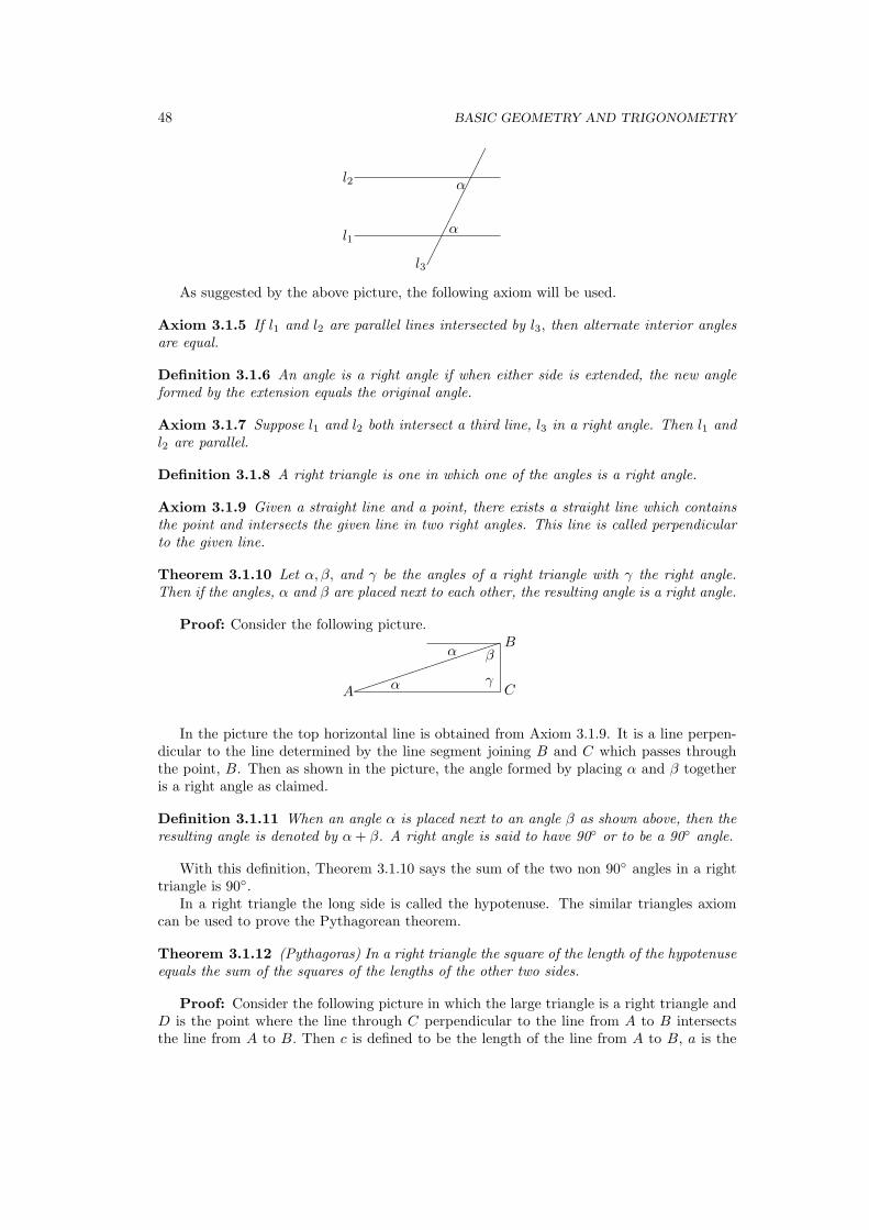
48 BASIC GEOMETRY AND TRIGONOMETRY
¢¢¢¢¢¢¢¢
α
αl2
l1
l3
As suggested by the above picture, the following axiom will be used.
Axiom 3.1.5 If l1 and l2 are parallel lines intersected by l3, then alternate interior anglesare equal.
Definition 3.1.6 An angle is a right angle if when either side is extended, the new angleformed by the extension equals the original angle.
Axiom 3.1.7 Suppose l1 and l2 both intersect a third line, l3 in a right angle. Then l1 andl2 are parallel.
Definition 3.1.8 A right triangle is one in which one of the angles is a right angle.
Axiom 3.1.9 Given a straight line and a point, there exists a straight line which containsthe point and intersects the given line in two right angles. This line is called perpendicularto the given line.
Theorem 3.1.10 Let α, β, and γ be the angles of a right triangle with γ the right angle.Then if the angles, α and β are placed next to each other, the resulting angle is a right angle.
Proof: Consider the following picture.
³³³³³³³³³³
C
B
A α
α β
γ
In the picture the top horizontal line is obtained from Axiom 3.1.9. It is a line perpen-dicular to the line determined by the line segment joining B and C which passes throughthe point, B. Then as shown in the picture, the angle formed by placing α and β togetheris a right angle as claimed.
Definition 3.1.11 When an angle α is placed next to an angle β as shown above, then theresulting angle is denoted by α + β. A right angle is said to have 90 or to be a 90 angle.
With this definition, Theorem 3.1.10 says the sum of the two non 90 angles in a righttriangle is 90.
In a right triangle the long side is called the hypotenuse. The similar triangles axiomcan be used to prove the Pythagorean theorem.
Theorem 3.1.12 (Pythagoras) In a right triangle the square of the length of the hypotenuseequals the sum of the squares of the lengths of the other two sides.
Proof: Consider the following picture in which the large triangle is a right triangle andD is the point where the line through C perpendicular to the line from A to B intersectsthe line from A to B. Then c is defined to be the length of the line from A to B, a is the

3.2. CARTESIAN COORDINATES AND STRAIGHT LINES 49
length of the line from B to C, and b is the length of the line from A to C. Denote by DBthe length of the line from D to B.
Aα
β
γ
δC
B
c a
b
D
Then from Theorem 3.1.10, δ + γ = 90 and β + γ = 90. Therefore, δ = β. Also fromthis same theorem, α + δ = 90 and so α = γ. Therefore, the three triangles shown in thepicture are all similar. By Axiom 3.1.2,
c
a=
a
DB, and
c
b=
b
c−DB.
Therefore, cDB = a2 and
c(c−DB
)= b2
so
c2 = cDB + b2
= a2 + b2.
This proves the Pythagorean theorem. 1
This theorem implies there should exist some such number which deserves to be called√a2 + b2 as mentioned earlier in the discussion on completeness of R.
3.2 Cartesian Coordinates And Straight Lines
Recall the notion of the Cartesian coordinate system. It involved an x axis, a y axis, twolines which intersect each other at right angles and one identifies a point by specifying a pairof numbers. For example, the number (2, 3) involves going 2 units to the right on the x axisand then 3 units directly up on a line perpendicular to the x axis. For example, considerthe following picture.
1This theorem is due to Pythagoras who lived about 572-497 B.C. This was during the Babyloniancaptivity of the Jews. Thus Pythagoras was probably a contemporary of the prophet Daniel, sometimebefore Ezra and Nehemiah. Alexander the great would not come along for more than 100 years. There was,however, an even earlier Greek mathematician named Thales, 624-547 B.C. who also did fundamental workin geometry. Greek geometry was organized and published by Euclid about 300 B.C.

50 BASIC GEOMETRY AND TRIGONOMETRY
y
x
• (2, 3)
Because of the simple correspondence between points in the plane and the coordinatesof a point in the plane, it is often the case that people are a little sloppy in referring to thesethings. Thus, it is common to see (x, y) referred to as a point in the plane. I will oftenindulge in this sloppiness.
The reader has likely encountered the notion of graphing relations of the form y = 2x+3or y = x2 + 5. Recall that you first found lots of ordered pairs which satisfied the relation.For example (0, 3),(1, 5), and (−1, 1) all satisfy the first relation which describes a straightline. Here are some simple examples which you should see that you understand. First hereis the graph of y = x2 + 1.
–1
0
1
2
3
4
5
–2 –1 1 2
Now here is the graph of the relation y = 2x + 1 which is a straight line.

3.2. CARTESIAN COORDINATES AND STRAIGHT LINES 51
–1
0
1
2
3
4
5
–2 –1 1 2
Sometimes a relation is defined using different formulas depending on the location of oneof the variables. For example, consider
y =
6 + x if x ≤ −2x2 if −2 < x < 3
1− x if x ≥ 3
Then the graph of this relation is sketched below.
–4
–2
0
2
4
6
8
–4 –2 2 4
A very important type of relation is one of the form y − y0 = m (x− x0) , where m,x0,and y0 are numbers. The reason this is important is that if there are two points, (x1, y1) ,and (x2, y2) which satisfy this relation, then
y1 − y2
x1 − x2=
(y1 − y0)− (y2 − y0)x1 − x2
=m (x1 − x0)−m (x2 − x0)
x1 − x2
=m (x1 − x2)
x1 − x2= m.
Remember the slope of the line segment through two points is always the difference in they values divided by the difference in the x values, taken in the same order. Sometimes this

52 BASIC GEOMETRY AND TRIGONOMETRY
is referred to as the rise divided by the run. This shows that there is a constant slope, m,the slope of the line, between any pair of points satisfying this relation. Such a relation iscalled a straight line. Also, the point (x0, y0) satisfies the relation. This is more often calledthe equation of the straight line.
Example 3.2.1 Find the relation for a straight line which contains the point (1, 2) and hasconstant slope equal to 3.
From the above discussion, (y − 2) = 3 (x− 1) .
3.3 Exercises
1. Sketch the graph of y = x3 + 1.
2. Sketch the graph of y = x2 − 2x + 1.
3. Sketch the graph of y = xx2+1 .
4. Sketch the graph of 11+x2 .
5. Sketch the graph of the straight line which goes through the points (1, 0) and (2, 3)and find the relation which describes this line.
6. Suppose a, b 6= 0. Find the equation of the line which goes through the points (0, a) ,and (b, 0) .
7. Two lines are parallel if they have the same slope. Find the equation of the linethrough the point (2, 3) which is parallel to the line whose equation is 2x + 3y = 8.
8. Sketch the graph of the relation defined as
y =
1 if x ≤ −21− x if −2 < x < 31 + x if x ≥ 3
3.4 Distance Formula And Trigonometric Functions
As just explained,points in the plane may be identified by giving a pair of numbers. Supposethere are two points in the plane and it is desired to find the distance between them. Thereare actually many ways used to measure this distance but the best way, and the only wayused in this book is determined by the Pythagorean theorem. Consider the following picture.

3.4. DISTANCE FORMULA AND TRIGONOMETRIC FUNCTIONS 53
y
x
•
•
(x1, y1)
(x0, y0) (x1, y0)•
In this picture, the distance between the points denoted by (x0, y0) and (x1, y1) shouldbe the square root of the sum of the squares of the lengths of the two sides. The lengthof the side on the bottom is |x0 − x1| while the length of the side on the right is |y0 − y1| .Therefore, by the Pythagorean theorem the distance between the two indicated points is√
(x0 − x1)2 + (y0 − y1)
2. Note you could write
√(x1 − x0)
2 + (y1 − y0)2
or even
√(x0 − x1)
2 + (y1 − y0)2
and it would make no difference in the resulting number. The distance between the twopoints is written as |(x0, y0)− (x1, y1)| or sometimes when P0 is the point determined by(x0, y0) and P1 is the point determined by (x1, y1) , as d (P0, P1) or |P0P | .
The trigonometric functions cos and sin are defined next. Consider the following picturein which the small circle has radius 1, the large circle has radius R, and the right side ofeach of the two triangles is perpendicular to the bottom side which lies on the x axis.
¾ (cos(θ), sin(θ))
θ¢¢¢¢¢¢
¾ (Rcos(θ), Rsin(θ))
By Theorem 3.1.10 on Page 48 the two triangles have the same angles and so they aresimilar. Now define by (cos θ, sin θ) the coordinates of the top vertex of the smaller triangle.Therefore, it follows the coordinates of the top vertex of the larger triangle are as shown.This shows the following definition is well defined.

54 BASIC GEOMETRY AND TRIGONOMETRY
Definition 3.4.1 For θ an angle, define cos θ and sin θ as follows. Place the vertex of theangle (The vertex is the point.) at the point whose coordinates are (0, 0) in such a way thatone side of the angle lies on the positive x axis and the other side extends upward. Extendthis other side until it intersects a circle of radius R. Then the point of intersection, is givenas (R cos θ,R sin θ) . In particular, this specifies cos θ and sin θ by simply letting R = 1.
Proposition 3.4.2 For any angle, θ, cos2 θ + sin2 θ = 1.
Proof: This follows immediately from the above definition and the distance formula.Since (cos θ, sin θ) is a point on the circle which has radius 1, the distance of this point to(0, 0) equals 1. Thus the above identity holds.
The other trigonometric functions are defined as follows.
tan θ ≡ sin θ
cos θ, cot θ ≡ cos θ
sin θ, sec θ ≡ 1
cos θ, csc θ ≡ 1
sin θ. (3.1)
It is also important to understand these functions in terms of a right triangle. Consider thefollowing picture of a right triangle.
A C
B
c a
b
You should verify sin A ≡ a/c, cos A ≡ b/c, tan A ≡ a/b, sec A ≡ c/b, and csc A ≡ c/a.Having defined the cos and sin there is a very important generalization of the Pythagorean
theorem known as the law of cosines. Consider the following picture of a triangle in whicha, b and c are the lengths of the sides and A,B, and C denote the angles indicated.
A
B
C
a
b
c
The law of cosines is the following.
Theorem 3.4.3 Let ABC be a triangle as shown above. Then
c2 = a2 + b2 − 2ab cos C
Proof: Situate the triangle so the vertex of the angle, C, is on the point whose coor-dinates are (0, 0) and so the side opposite the vertex, B is on the positive x axis as shownin the above picture. Then from the definition of the cosC, the coordinates of the vertex,

3.5. THE CIRCULAR ARC SUBTENDED BY AN ANGLE 55
B are (a cosC, a sin C) while it is clear the coordinates of A are (b, 0) . Therefore, from thedistance formula, and Proposition 3.4.2,
c2 = (a cos C − b)2 + a2 sin2 C
= a2 cos2 C − 2ab cosC + b2 + a2 sin2 C
= a2 + b2 − 2ab cosC
as claimed.
Corollary 3.4.4 Let ABC be any triangle as shown above. Then the length of any side isno longer than the sum of the lengths of the other two sides.
Proof: This follows immediately from the law of cosines. From Proposition 3.4.2,|cos θ| ≤ 1 and so c2 = a2 + b2 − 2ab cosC ≤ a2 + b2 + 2ab = (a + b)2 . This provesthe corollary.
Corollary 3.4.5 Suppose T and T ′ are two triangles such that one angle is the same inthe two triangles and in each triangle, the sides forming that angle are equal. Then thecorresponding sides are proportional.
Proof: Let T = ABC with the two equal sides being AC and AB. Let T ′ be labeled inthe same way but with primes on the letters. Thus the angle at A is equal to the angle atA′. The following picture is descriptive of the situation.
©©©©©©©©©©©
A B
C
ab
c©©©©©©©©
A′ B′
C ′
a′b′
c′
Denote by a, a′, b, b′, c and c′ the sides indicated in the picture. Then by the law ofcosines,
a2 = b2 + c2 − 2bc cos A
= 2b2 − 2b2 cos A
and so a/b =√
2 (1− cos A). Similar reasoning shows a′/b′ =√
2 (1− cosA) and so
a/b = a′/b′.
Similarly, a/c = a′/c′. By assumption c/b = 1 = c′/b′.Such triangles in which two sides are equal are called isoceles.
3.5 The Circular Arc Subtended By An Angle
How can angles be measured? This will be done by considering arcs on a circle. To see howthis will be done, let θ denote an angle and place the vertex of this angle at the center of

56 BASIC GEOMETRY AND TRIGONOMETRY
the circle. Next, extend its two sides till they intersect the circle. Note the angle could beopening in any of infinitely many different directions. Thus this procedure could yield anyof infinitely many different circular arcs. Each of these arcs is said to subtend the angle. Infact each of these arcs has the same length. When this has been shown, it will be easy tomeasure angles. Angles will be measured in terms of lengths of arcs subtended by the angle.Of course it is also necessary to define what is meant by the length of a circular arc in orderto do any of this. First I will describe an intuitive way of thinking about this and then givea rigorous definition and proof. If the intuitive way of thinking about this satisfies you, noharm will be done by skipping the more technical discussion which follows.
Take an angle and place its vertex (the point) at the center of a circle of radius r. Then,extending the sides of the angle if necessary till they intersect the circle, this determines anarc on the circle. If r were changed to R, this really amounts to a change of units of length.Think, for example, of keeping the numbers the same but changing centimeters to metersin order to produce an enlarged version of the same picture. Thus the picture looks exactlythe same, only larger. It is reasonable to suppose, based on this reasoning that the way tomeasure the angle is to take the length of the arc subtended in whatever units being usedand divide this length by the radius measured in the same units, thus obtaining a numberwhich is independent of the units of length used just as the angle itself is independent ofunits of length. After all, it is the same angle regardless of how far its sides are extended.This is in fact how to define the radian measure of an angle and the definition is well defined.Thus, in particular, the ratio between the circumference (length) of a circle and its radiusis a constant which is independent of the radius of the circle2. Since the time of Euler inthe 1700’s, this constant has been denoted by 2π. In summary, if θ is the radian measureof an angle, the length of the arc subtended by the angle on a circle of radius r is rθ.
This is a little sloppy right now because no precise definition of the length of an arcof a circle has been given. For now, imagine taking a string, placing one end of it on oneend of the circular arc and then wrapping the string till you reach the other end of the arc.Stretching this string out and measuring it would then give you the length of the arc. Suchintuitive discussions involving string may or may not be enough to convey understanding.If you need to see more discussion, read on. Otherwise, skip to the next section.
To give a precise description of what is meant by the length of an arc, consider thefollowing picture.
A1
θ
A2
In this picture, there are two circles, a big one having radius, R and a little one havingradius r. The angle, θ is situated in two different ways subtending the arcs A1 and A2 asshown.
Letting A be an arc of a circle, like those shown in the above picture, A subset of
2In 2 Chronicles 4:2 the “molten sea” used for “washing” by the priests and found in Solomon’s templeis described. It sat on 12 oxen, was round, 5 cubits high, 10 across and 30 around. Thus the Bible, takenliterally, gives the value of π as 3. This is not too far off. Later, methods will be given which allow one tocalculate π more precisely. A better value is 3.1415926535 and presently this number is known to thousandsof decimal places. It was proved by Lindeman in the 1880’s that π is transcendental which is the worst sortof irrational number.

3.5. THE CIRCULAR ARC SUBTENDED BY AN ANGLE 57
A, p0, · · ·, pn is a partition of A if p0 is one endpoint, pn is the other end point, and thepoints are encountered in the indicated order as one moves in the counter clockwise directionalong the arc. To illustrate, see the following picture.
p1
p0
p2
p3
Also, denote by P (A) the set of all such partitions. For P = p0, · · ·, pn , denoteby |pi − pi−1| the distance between pi and pi−1. Then for P ∈ P (A) , define |P | ≡∑n
i=1 |pi − pi−1| . Thus |P | consists of the sum of the lengths of the little lines joiningsuccessive points of P and appears to be an approximation to the length of the circulararc, A. By Corollary 3.4.4 the length of any of the straight line segments joining successivepoints in a partition is smaller than the sum of the two sides of a right triangle having thegiven straight line segment as its hypotenuse. For example, see the following picture.
A
B
C
D
The sum of the lengths of the straight line segments in the part of the picture found inthe right rectangle above is less than A + B and the sum of the lengths of the straight linesegments in the part of the picture found in the left rectangle above is less than C + D andthis would be so for any partition. Therefore, for any P ∈ P (A) , |P | ≤ M where M is theperimeter of a rectangle containing the arc, A. To be a little sloppy, simply pick M to be theperimeter of a rectangle containing the whole circle of which A is a part. The only purposefor doing this is to obtain the existence of an upper bound. Therefore, |P | : P ∈ P (A) isa set of numbers which is bounded above by M and by completeness of R it is possible todefine the length of A, l (A) , by l (A) ≡ sup |P | : P ∈ P (A).
A fundamental observation following from Corollary 3.4.4 is that if P,Q ∈ P (A) andP ⊆ Q, then |P | ≤ |Q| . To see this, add in one point at a time to P . This effect of addingin one point is illustrated in the following picture.

58 BASIC GEOMETRY AND TRIGONOMETRY
Also, letting p0, · · ·, pn be a partition of A, specify angles, θi as follows. The angle θi
is formed by the two lines, one from the center of the circle to pi and the other line from thecenter of the circle to pi−1. Furthermore, a specification of these angles yields the partitionof A in the following way. Place the vertex of θ1 on the center of the circle, letting one sidelie on the line from the center of the circle to p0 and the other side extended resulting in apoint further along the arc in the counter clockwise direction. When the angles, θ1, · · ·, θi−1
have produced points, p0, · · ·, pi−1 on the arc, place the vertex of θi on the center of thecircle and let one side of θi coincide with the side of the angle θi−1 which is most counterclockwise, the other side of θi when extended, resulting in a point further along the arc, Ain the counterclockwise direction as shown below.
ÃÃÃÃá
¡¡
¡¡
¥¥¥¥¥¥¥¥
θi−1
θi
Now let ε > 0 be given and pick P1 ∈ P (A1) such that |P1|+ε > l (A1) . Then determin-ing the angles as just described, use these angles to produce a corresponding partition of A2,P2. If |P2| + ε > l (A2) , then stop. Otherwise, pick Q ∈ P (A2) such that |Q| + ε > l (A2)and let P ′2 = P2 ∪ Q. Then use the angles determined by P ′2 to obtain P ′1 ∈ P (A1) . Then|P ′1| + ε > l (A1) , |P ′2| + ε > l (A2) , and both P ′1 and P ′2 determine the same sequence ofangles. Using Corollary 3.4.5
|P ′1||P ′2|
=R
r
and sol (A2) < |P ′2|+ ε =
r
R|P ′1|+ ε ≤ r
Rl (A1) + ε.
Since ε is arbitrary, this shows Rl (A2) ≤ rl (A1) . But now reverse the argument and write
l (A1) < |P ′1|+ ε =R
r|P ′2|+ ε ≤ R
rl (A2) + ε
which implies, since ε is arbitrary that Rl (A2) ≥ rl (A1) and this has proved the followingtheorem.
Theorem 3.5.1 Let θ be an angle which subtends two arcs, AR on a circle of radius R andAr on a circle of radius r. Then denoting by l (A) the length of a circular arc as describedabove, Rl (Ar) = rl (AR) .

3.5. THE CIRCULAR ARC SUBTENDED BY AN ANGLE 59
Before proceeding further, note the proof of the above theorem involved showing l (A1) <Rr l (A2) + ε where ε > 0 was arbitrary and from this, the conclusion that l (A1) ≤ R
r l (A2).This is a very typical way of showing one number is no larger than another. To show a ≤ bfirst show that for every ε > 0 it follows that a < b+ε. This implies a−b < ε for all positiveε and so it must be the case that a − b ≤ 0 since otherwise, you could take ε = a−b
2 andconclude 0 < a− b < a−b
2 , a contradiction.With this preparation, here is the definition of the measure of an angle.
Definition 3.5.2 Let θ be an angle. The measure of θ is defined to be the length of thecircular arc subtended by θ on a circle of radius r divided by r. This is also called the radianmeasure of the angle.
You should note the measure of θ is independent of dimension. This is because the unitsof length cancel when the division takes place.
Proposition 3.5.3 The above definition is well defined and also, if A is an arc subtendedby the angle θ on a circle of radius r then the length of A, denoted by l (A) is given byl (A) = rθ.
Proof: That the definition is well defined follows from Theorem 3.5.1. The formula alsofollows from Theorem 3.5.1 and letting R = 1.
Now is a good time to present a useful inequality which may or may not be self evident.Here is a picture which illustrates the conclusion of this corollary.
θ¡¡
¡¡¡
(cos(θ), sin(θ))
©©©©¼
(1− cos(θ))
The following corollary states that the length of the subtended arc shown in the pictureis longer than the vertical side of the triangle and smaller than the sum of the vertical sidewith the segment having length 1− cos θ. To me, this seems abundantly clear but in case itis hard to believe, the following corollary gives a proof.
Corollary 3.5.4 Let 0 < radian measure of θ < π/4. Then letting A be the arc on the unitcircle resulting from situating the angle with one side on the positive x axis and the otherside pointing up from the positive x axis,
(1− cos θ) + sin θ ≥ l (A) ≥ sin θ (3.2)
Proof: Situate the angle, θ such that one side is on the positive x axis and extendthe other side till it intersects the unit circle at the point, (cos θ, sin θ) . Then denoting theresulting arc on the circle by A, it follows that for all P ∈ P (A) the inequality (1− cos θ)+sin θ ≥ |P | ≥ sin θ. It follows that (1− cos θ) + sin θ is an upper bound for all the |P | whereP ∈ P (A) and so (1− cos θ)+sin θ is at least as large as the sup or least upper bound of the

60 BASIC GEOMETRY AND TRIGONOMETRY
|P | . This proves the top half of the inequality. The bottom half follows because l (A) ≥ Lwhere L is the length of the line segment joining (cos θ, sin θ) and (1, 0) due to the definitionof l (A) . However, L ≥ sin θ because L is the length of the hypotenuse of a right trianglehaving sin θ as one of the sides.
3.6 The Trigonometric Functions
Now the Trigonometric functions will be defined as functions of an arbitrary real variable.Up till now these have been defined as functions of pointy things called angles. The followingtheorem will make possible the definition.
Theorem 3.6.1 Let b ∈ R. Then there exists a unique integer p and real number r suchthat 0 ≤ r < 2π and b = p2π + r.
Proof: First suppose b ≥ 0. Then from Theorem 2.8.11 on Page 29 there exists a uniqueinteger, p such that b = 2πp + r where 0 ≤ r < 2π. Now suppose b < 0. Then there exists aunique integer, p such that −b = 2πp + r1 where r1 ∈ [0, 2π). If r1 = 0, then b = (−p) 2π.
Otherwise, b = (−p) 2π + (−r1) = (−p− 1) 2π +
≡r︷ ︸︸ ︷2π − r1
and r ≡ 2π − r1 ∈ (0, 2π) .
The following definition is for sin b and cos b for b ∈ R.
Definition 3.6.2 Let b ∈ R. Then sin b ≡ sin r and cos b ≡ cos r where b = 2πp + r for pan integer, and r ∈ [0, 2π).
Several observations are now obvious from this.
Observation 3.6.3 Let k ∈ Z, then the following formulas hold.
sin b = − sin (−b) , cos b = cos (−b) , (3.3)sin (b + 2kπ) = sin b, cos (b + 2kπ) = cos b (3.4)
cos2 b + sin2 b = 1 (3.5)
The other trigonometric functions are defined in the usual way as in (3.1) provided theymake sense.
From the observation that the x and y axes intersect at right angles the four arcs onthe unit circle subtended by these axes are all of equal length. Therefore, the measure of aright angle must be 2π/4 = π/2. The measure of the angle which is determined by the arcfrom (1, 0) to (−1, 0) is seen to equal π by the same reasoning. From the definition of thetrig functions, cos (π/2) = 0 and sin (π/2) = 1. You can easily find other values for cos andsin at all the other multiples of π/2.
The next topic is the important formulas for the trig. functions of sums and differences ofnumbers. For b ∈ R, denote by rb the element of [0, 2π) having the property that b = 2πp+rb
for p an integer.
Lemma 3.6.4 Let x, y ∈ R. Then rx+y = rx + ry + 2kπ for some k ∈ Z.
Proof: By definition,
x + y = 2πp + rx+y, x = 2πp1 + rx, y = 2πp2 + ry.

3.6. THE TRIGONOMETRIC FUNCTIONS 61
From this the result follows because
0 = ((x + y)− x)− y = 2π
≡−k︷ ︸︸ ︷((p− p1)− p2) + rx+y − (rx + ry) .
Let z ∈ R and let p (z) denote the point on the unit circle determined by the length rz
whose coordinates are cos z and sin z. Thus, starting at (1, 0) and moving counter clockwisea distance of rz on the unit circle yields p (z) . Note also that p (z) = p (rz) .
Lemma 3.6.5 Let x, y ∈ R . Then the length of the arc between p (x + y) and p (x) is equalto the length of the arc between p (y) and (1, 0) .
Proof: The length of the arc between p (x + y) and p (x) is |rx+y − rx| . There are twocases to consider here.
First assume rx+y ≥ rx. Then |rx+y − rx| = rx+y − rx = ry + 2kπ. Since both rx+y andrx are in [0, 2π), their difference is also in [0, 2π) and so k = 0. Therefore, the arc joiningp (x) and p (x + y) is of the same length as the arc joining p (y) and (1, 0) . In the other case,rx+y < rx and in this case |rx+y − rx| = rx− rx+y = −ry−2kπ. Since rx and rx+y are bothin [0, 2π) their difference is also in [0, 2π) and so in this case k = −1. Therefore, in this case,|rx+y − rx| = 2π− ry. Now since the circumference of the unit circle is 2π, the length of thearc joining p (2π − ry) to (1, 0) is the same as the length of the arc joining p (ry) = p (y) to(1, 0) . This proves the lemma.
The following theorem is the fundamental identity from which all the major trig. iden-tities involving sums and differences of angles are derived.
Theorem 3.6.6 Let x, y ∈ R. Then
cos (x + y) cos y + sin (x + y) sin y = cos x. (3.6)
Proof: Recall that for a real number, z, there is a unique point, p (z) on the unit circleand the coordinates of this point are cos z and sin z. Now from the above lemma, the lengthof the arc between p (x + y) and p (x) has the same length as the arc between p (y) andp (0) . As an illustration see the following picture.
p(y)
p(x + y)
p(x)
(1, 0)
It follows from the definition of the radian measure of an angle that the two anglesdetermined by these arcs are equal and so, by Corollary 3.4.5 the distance between thepoints p (x + y) and p (x) must be the same as the distance from p (y) to p (0) . Writing thisin terms of the definition of the trig functions and the distance formula,
(cos (x + y)− cos x)2 + (sin (x + y)− sin x)2 = (cos y − 1)2 + sin2 x.

62 BASIC GEOMETRY AND TRIGONOMETRY
cos2 (x + y) + cos2 x− 2 cos (x + y) cos x + sin2 (x + y) + sin2 x− 2 sin (x + y) sin x
= cos2 y − 2 cos y + 1 + sin2 y
From Observation 3.6.3 this implies (3.6). This proves the theorem.Letting y = π/2, this shows that
sin (x + π/2) = cos x. (3.7)
Now let u = x + y and v = y. Then (3.6) implies
cosu cos v + sin u sin v = cos (u− v) (3.8)
Also, from this and (3.3),
cos (u + v) = cos (u− (−v))= cos u cos (−v) + sin u sin (−v)= cos u cos v − sinu sin v (3.9)
Thus, letting v = π/2,
cos(u +
π
2
)= − sinu. (3.10)
It follows
sin (x + y) = − cos(x +
π
2+ y
)
= −[cos
(x +
π
2
)cos y − sin
(x +
π
2
)sin y
]
= sin x cos y + sin y cosx (3.11)
Then using Observation 3.6.3 again, this implies
sin (x− y) = sin x cos y − cosx sin y. (3.12)
In addition to this, Observation 3.6.3 implies
cos 2x = cos2 x− sin2 x (3.13)
= 2 cos2 x− 1 (3.14)
= 1− 2 sin2 x (3.15)
Therefore, making use of the above identities, and Observation 3.6.3,
cos (3x) = cos 2x cos x− sin 2x sin x
=(2 cos2 x− 1
)cos x− 2 cos x sin2 x
= 4 cos3 x− 3 cos x (3.16)
With these fundamental identities, it is easy to obtain the cosine and sine of many specialangles, called reference angles. First, cos
(π4
).
0 = cos(π
2
)= cos
(π
4+
π
4
)= 2 cos2
(π
4
)− 1
and so cos(
π4
)=√
2/2. (Why do isn’t it equal to −√2/2? Hint: Draw a picture.) Thussin
(π4
)=√
2/2 also. (Why?) Here is another one. From (3.16),
0 = cos(π
2
)= cos 3
(π
6
)
= 4 cos3(π
6
)− 3 cos
(π
6
).

3.7. EXERCISES 63
Therefore, cos(
π6
)=
√3
2 and consequently, sin(
π6
)= 1
2 . Here is a short table includingthese and a few others. You should make sure you can obtain all these entries. In the table,θ refers to the radian measure of the angle. From now on, angles are considered as realnumbers, not as pointy things.
θ 0 π6
π4
π3
π2
cos θ 1√
32
√2
212 0
sin θ 0 12
√2
2
√3
2 1
3.7 Exercises
1. Find cos θ and sin θ for θ ∈ 2π3 , 3π
4 , 5π6 , π, 7π
6 , 5π4 , 4π
3 , 3π2 , 5π
3 , 7π4 , 11π
6 , 2π
.
2. Prove cos2 θ = 1+cos 2θ2 and sin2 θ = 1−cos 2θ
2 .
3. π/12 = π/3−π/4. Therefore, from Problem 2, cos (π/12) =√
1+(√
3/2)2 . On the other
hand,cos (π/12) = cos (π/3− π/4) = cos π/3 cos π/4 + sin π/3 sin π/4
and so cos (π/12) =√
2/4 +√
6/4. Is there a problem here? Please explain.
4. Prove 1 + tan2 θ = sec2 θ and 1 + cot2 θ = csc2 θ.
5. Prove that sin x cos y = 12 (sin (x + y) + sin (x− y)) .
6. Prove that sin x sin y = 12 (cos (x− y)− cos (x + y)) .
7. Prove that cosx cos y = 12 (cos (x + y) + cos (x− y)) .
8. Using Problem 5, find an identity for sinx− sin y.
9. Suppose sinx = a where 0 < a < 1. Find all possible values for
(a) tan x
(b) cot x
(c) sec x
(d) csc x
(e) cos x
10. Solve the equations and give all solutions.
(a) sin (3x) = 12
(b) cos (5x) =√
32
(c) tan (x) =√
3
(d) sec (x) = 2
(e) sin (x + 7) =√
22
(f) cos2 (x) = 12
(g) sin4 (x) = 4
11. Find a formula for tan (x + y) in terms of trig. functions of x and y.

64 BASIC GEOMETRY AND TRIGONOMETRY
12. Find a formula for tan (2x) in terms of trig. functions of x.
13. Find a formula for tan(
x2
)in terms of trig. functions of x.
14. Sketch a graph of y = sin x.
15. Sketch a graph of y = cos x.
16. Sketch a graph of y = sin 2x.
17. Sketch a graph of y = tanx.
18. Using Problem 2 graph y = cos2 x.
19. If f (x) = A cosαx + B sin αx, show there exists φ such that
f (x) =√
A2 + B2 sin (αx + φ) .
Show there also exists ψ such that f (x) =√
A2 + b2 cos (αx + ψ) . This is a veryimportant result, enough that some of these quantities are given names.
√A2 + B2 is
called the amplitude and φ or ψ are called phase shifts.
20. Using Problem 19 graph y = sin x +√
3 cos x.
21. Give all solutions to sin x +√
3 cos x =√
3. Hint: Use Problem 20.
22. If ABC is a triangle where the capitol letters denote vertices of the triangle and theangle at the vertex. Let a be the length of the side opposite A and b is the lengthof the side opposite B and c is the length of the side opposite the vertex, C. Thelaw of sines says sin (A) /a = sin (B) /b = sin (C) /c. Prove the law of sines from thedefinition of the trigonometric functions.
23. In the picture, a = 5, b = 3, and θ = 23π. Find c.
@@
@@@
θ
c
a
b
24. In the picture, θ = 14π, α = 2
3π and c = 3. Find a.
@@
@@@
θ
α
β
c
a
b

3.8. SOME BASIC AREA FORMULAS 65
3.8 Some Basic Area Formulas
3.8.1 Areas Of Triangles And Parallelograms
This section is a review of how to find areas of some simple figures. The discussion will besomewhat informal since it is assumed the reader has seen this sort of thing already. Firstof all, consider a right triangle as indicated in the following picture.
c a
b
The area of this triangle shown above must equal ab/2 because it is half of a rectanglehaving sides a and b. Now consider a general triangle in which a line perpendicular to theline from A to C has been drawn through B.
D
c
a
b
C
A
B
The area of this triangle would be the sum of the two right triangles formed. Thus thisarea would be 1
2
(BD
) (AD + CD
)= 1
2
(BD
)b. In words, the area of the triangle equals
one half the base times the height. This also holds if the height and base are chosen withrespect to any other side of the triangle.
A parallelogram is a four sided figure which is formed when two identical triangles arejoined along a corresponding side with the corresponding angles not adjacent. For example,see the picture in which the two triangles are ABC and CDA.
D
C
A
B
Note the height of triangle ABC taken with respect to side AB is the same as the height ofthe parallelogram taken with respect to this same side. Therefore, the area of this parallelo-gram equals twice the area of one of these triangles which equals 2AB (height of parallelogram) 1
2 =AB (height of parallelogram) . Similarly the area equals height times base where the baseis any side of the parallelogram and the height is taken with respect to that side, as justdescribed in the case where AB is the side.

66 BASIC GEOMETRY AND TRIGONOMETRY
3.8.2 The Area Of A Circular Sector
Consider an arc, A, of a circle of radius r which subtends an angle, θ. The circular sectordetermined by A is obtained by joining the ends of the arc, A, to the center of the circle.The sector, S (θ) denotes the points which lie between the arc, A and the two lines justmentioned. The angle between the two lines is called the central angle of the sector. Theproblem is to define the area of this shape. First a fundamental inequality must be obtained.
Lemma 3.8.1 Let 1 > ε > 0 be given. Then whenever the positive number, α, is smallenough,
1 ≤ α
sin α≤ 1 + ε (3.17)
and1 + ε ≥ α
tanα≥ 1− ε (3.18)
Proof: This follows from Corollary 3.5.4 on Page 59. In this corollary, l (A) = α and so
1− cosα + sin α ≥ α ≥ sin α.
Therefore, dividing by sin α,
1− cosα
sin α+ 1 ≥ α
sin α≥ 1. (3.19)
Now using the properties of the trig functions,
1− cosα
sinα=
1− cos2 α
sin α (1 + cos α)
=sin2 α
sin α (1 + cos α)=
sin α
1 + cos α.
From the definition of the sin and cos, whenever α is small enough,
sin α
1 + cos α< ε
and so (3.19) implies that for such α, (3.17) holds. To obtain (3.18), let α be small enoughthat (3.17) holds and multiply by cos α. Then for such α,
cosα ≤ α
tanα≤ (1 + ε) cos α
Taking α smaller if necessary and noting that for all α small enough, cos α is very close to1, yields (3.18). This proves the lemma.
This lemma is very important in another context.
Theorem 3.8.2 Let S (θ) denote the sector of a circle of radius r having central angle, θ.
Then the area of S (θ) equals r2
2 θ.
Proof: Let the angle which A subtends be denoted by θ and divide this sector into nequal sectors each of which has a central angle equal to θ/n. The following is a picture ofone of these.

3.9. EXERCISES 67
©©©©©©©©©©©©©©©©©©©
r
S(θ/n)
In the picture, there is a circular sector, S (θ/n) and inside this circular sector is atriangle while outside the circular sector is another triangle. Thus any reasonable definitionof area would require
r2
2sin (θ/n) ≤ area of S (θ/n) ≤ r2
2tan (θ/n) .
It follows the area of the whole sector having central angle θ must satisfy the followinginequality.
nr2
2sin (θ/n) ≤ area of S (θ) ≤ nr2
2tan (θ/n) .
Therefore, for all n, the area of S (θ) is trapped between the two numbers,
r2
2θsin (θ/n)
(θ/n),
r2
2θtan (θ/n)
(θ/n).
Now let ε > 0 be given, a small positive number less than 1, and let n be large enough that
1 ≥ sin (θ/n)(θ/n)
≥ 11 + ε
and1
1 + ε≤ tan (θ/n)
(θ/n)≤ 1
1− ε.
Therefore,r2
2θ
(1
1 + ε
)≤ Area of S (θ) ≤
(1
1− ε
)r2
2θ.
Since ε is an arbitrary small positive number, it follows the area of the sector equals r2
2 θ asclaimed. (Why?)
3.9 Exercises
1. Give another argument which verifies the Pythagorean theorem by supplying the de-tails for the following argument3. Take the given right triangle and situate copies ofit as shown below. The big four sided figure which results is a rectangle because allthe angles are equal. Now from the picture, the area of the big square equals c2, thearea of each triangle equals ab/2, since it is half of a rectangle of area ab, and the area
3This argument is old and was known to the Indian mathematician Bhaskar who lived 1114-1185 A.D.
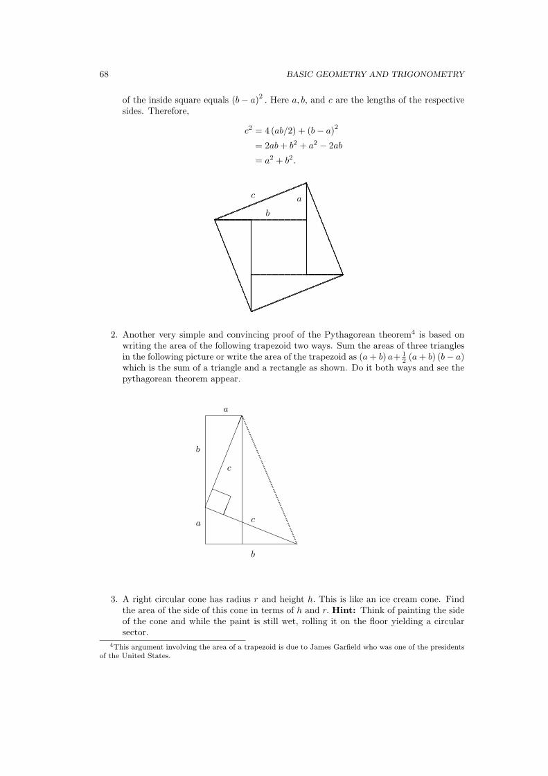
68 BASIC GEOMETRY AND TRIGONOMETRY
of the inside square equals (b− a)2 . Here a, b, and c are the lengths of the respectivesides. Therefore,
c2 = 4 (ab/2) + (b− a)2
= 2ab + b2 + a2 − 2ab
= a2 + b2.
c a
b
2. Another very simple and convincing proof of the Pythagorean theorem4 is based onwriting the area of the following trapezoid two ways. Sum the areas of three trianglesin the following picture or write the area of the trapezoid as (a + b) a+ 1
2 (a + b) (b− a)which is the sum of a triangle and a rectangle as shown. Do it both ways and see thepythagorean theorem appear.
¯¯¯¯¯¯¯¯¯¯
aaaaaaaaaa
aa¯
¯c
c
a
b
a
b
3. A right circular cone has radius r and height h. This is like an ice cream cone. Findthe area of the side of this cone in terms of h and r. Hint: Think of painting the sideof the cone and while the paint is still wet, rolling it on the floor yielding a circularsector.
4This argument involving the area of a trapezoid is due to James Garfield who was one of the presidentsof the United States.

3.10. PARABOLAS, ELLIPSES, AND HYPERBOLAS 69
4. An equilateral triangle is one in which all sides are of equal length. Find the area ofan equilateral triangle whose sides have length l.
5. Draw two parallel lines one having length a and the other having length b suppose alsothese lines are at a distance of h from each other. Now join the ends of these lines toobtain a four sided figure. What is the area of this four sided figure?
3.10 Parabolas, Ellipses, and Hyperbolas
3.10.1 The Parabola
A parabola is a collection of points, P in the plane such that the distance from P to a fixedline is the same as the distance from P to a given point, P0. From this definition, one canobtain an equation which will describe a parabola. Suppose then that the line is y = c andthe point is (a, b) where b 6= c as shown in the picture.
·P0 = (a, b)
y = c
The distance from the point, P = (x, y) to the line is |c− y| . Therefore, the descriptionof the parabola requires that
√(x− a)2 + (y − b)2 = |c− y| .
Squaring both sides,
x2 − 2xa + a2 + y2 − 2yb + b2 = c2 − 2cy + y2
and so(x− a)2 + b2 − c2 = (2b− 2c) y. (3.20)
The simplest case is when a = 0 and b = −c. Then in this case, it reduces to
x2 = 4cy.
Now consider an arbitrary equation of the form, y = dx2 + ex + f where d 6= 0. By this ismeant the set of points (x, y) such that the equation holds. Such a set of points always is aparabola. To see this, complete the square on the right as follows:
y = dx2 + ex + f
= d
(x2 +
e
dx +
f
d
)
= d
(x2 +
e
dx +
e2
4d2
)− e2d
4d2
= d
(x−
(−e
2d
))2
− e2d
4d2.
Therefore, letting a = −e2d ,
1dy = (x− a)2 − e2
4d2

70 BASIC GEOMETRY AND TRIGONOMETRY
Now you can show that there exists numbers, b and c such that
− e2
4d2= b2 − c2,
1d
= 2b− 2c. (3.21)
Then the above equation reduces to (3.20).The line, y = c is called the directrix and the point, P0 in the above is called the focus.
Exactly similar results occur if the directrix is of the form x = c and by similar argumentsto those above, the set of points in the plane satisfying ay2 + by + c = x is also a parabola.
3.10.2 The Ellipse
With an ellipse, there are two points, P1 and P2 which are fixed and the ellipse consists ofthe set of points, P such that d (P, P1) + d (P, P2) = c, where c is a fixed positive number.These two points are called the foci of the ellipse. Each is called a focus point by itself.Now one can obtain an equation which will describe an ellipse much as was done with theparabola. Let the two given points be (a, b) and (a, b + h) . Let a generic point on the ellipsebe (x, y) . Then according to the description of an ellipse and the distance formula,
√(x− a)2 + (y − b)2 +
√(x− a)2 + (y − b− h)2 = c. (3.22)
Subtracting√
(x− a)2 + (y − b)2 from both sides,√
(x− a)2 + (y − b− h)2 = c−√
(x− a)2 + (y − b)2 ≥ 0.
Now squaring both sides yields
(x− a)2 + (y − b− h)2 = c2 − 2√
(x− a)2 + (y − b)2c
+(x− a)2 + (y − b)2 .
Therefore,
(y − b)2 − 2h (y − b) + h2 = c2 − 2√
(x− a)2 + (y − b)2c
+(y − b)2
and so−2h (y − b) + h2 = c2 − 2
√(x− a)2 + (y − b)2c
Therefore,
−2h (y − b) + h2 − c2 = −2√
(x− a)2 + (y − b)2c
Now square both sides again to obtain(h2 − c2
)2 − 4h (y − b)(h2 − c2
)+ 4h2 (y − b)2 = 4c2
((x− a)2 + (y − b)2
).
Simplifying this yields
(c2 − h2
)(y − b)2 + h (y − b)
(h2 − c2
)+ c2 (x− a)2 =
14
(c2 − h2
)2
which simplifies further to
(y − b)2 − h (y − b) +h2
4+
(c2
c2 − h2
)(x− a)2 =
1 + h2
4

3.10. PARABOLAS, ELLIPSES, AND HYPERBOLAS 71
which is equivalent to (y − b− h
2
)2
(1+h2
4
) +(x− a)2(
1+h2
4 / c2
c2−h2
) = 1.
Thus, redefining the constants, an ellipse has the form
(y − β)2
b2+
(x− α)2
a2= 1. (3.23)
Note that if a = b = r, this reduces to the equation for a circle of radius r centered at thepoint (α, β) . This last expression is the generic equation for an ellipse. Here is the graph ofa typical ellipse.
x
yβ + bXXXz
»»»:β − b
¡¡ªα + aα− a
@@R(α, β)
¡¡ª
In this ellipse, b < a. If b > a, the ellipse would be long in the y direction ratherthan the x direction. (Why?) Suppose (x1, y1) and (x2, y2) are two points on the aboveellipse in which b > a, then |x1 − x2| ≤ 2a because from the above equation, it follows that|xi − α| ≤ a for i = 1, 2 implying that
|x1 − x2| ≤ |x1 − α|+ |α− x2| ≤ a + a = 2a
and similarly, |y1 − y2| ≤ 2b. Therefore,
|(x1, y1)− (x2, y2)| ≤√
4a2 + 4b2 ≤ 2√
a2 + b2 ≤ 2b
Thus the greatest distance between two points on the ellipse equals 2b and occurs when thetwo points are (α, b + β) and (α, β − b) . This greatest distance between any two points iscalled the diameter and this shows the diameter of an ellipse is twice the larger of the twonumbers appearing in the denominators on the left in (3.23).
3.10.3 The Hyperbola
With a hyperbola, there are two points, P1 and P2 which are fixed and the hyperbola consistsof the set of points, P such that d (P, P1)−d (P, P2) = c, where c is a fixed positive number.These two points are called the foci of the hyperbola. Each is called a focus point by itself.Now one can obtain an equation which will describe a hyperbola. Let the two given pointsbe (a, b) and (a, b + h) . Let a generic point on the hyperbola be (x, y) . Then according tothe description of a hyperbola and the distance formula,
√(x− a)2 + (y − b)2 −
√(x− a)2 + (y − b− h)2 = c.
You can now show that the equation of a hyperbola is of the form
(x− α)2
a2− (y − β)2
b2= 1 (3.24)

72 BASIC GEOMETRY AND TRIGONOMETRY
or(y − β)2
b2− (x− α)2
a2= 1. (3.25)
If you like, you can simply take these last two equations as the definition of a hyperbola.
3.11 Exercises
1. Consider y = 2x2 + 3x + 7. Find the focus and the directrix of this parabola.
2. Find the numbers, b, c which make (3.21) hold.
3. Derive a similar formula to (3.20) in the case that the directrix is of the form x = c.
4. Sketch a graph of the ellipse whose equation is (x−1)2
4 + (y−2)2
9 = 1.
5. Sketch a graph of the ellipse whose equation is (x−1)2
9 + (y−2)2
4 = 1.
6. Sketch a graph of the hyperbola, x2
4 − y2
9 = 1.
7. Sketch a graph of the hyperbola, y2
4 − x2
9 = 1.
8. What is the diameter of the ellipse, (x−1)2
9 + (y−2)2
4 = 1.
9. Verify that either (3.24) or (3.25) holds for a hyperbola.
10. Show that the set of points which satisfies either (3.24) or (3.25) is unbounded. (Ifn is any positive number there exist points (x, y) satisfying the equations given suchthat |(x, y)| > n.)

The Complex Numbers
This chapter gives a brief treatment of the complex numbers. This will not be needed inCalculus but you will need it when you take differential equations and various other subjectsso it is a good idea to consider the subject. These things used to be taught in precalculusclasses and people were expected to know them before taking calculus. However, if you arein a hurry to get to calculus, you can skip this short chapter.
Just as a real number should be considered as a point on the line, a complex number isconsidered a point in the plane which can be identified in the usual way using the Cartesiancoordinates of the point. Thus (a, b) identifies a point whose x coordinate is a and whosey coordinate is b. In dealing with complex numbers, such a point is written as a + ib. Forexample, in the following picture, I have graphed the point 3 + 2i. You see it correspondsto the point in the plane whose coordinates are (3, 2) .
q 3 + 2i
Multiplication and addition are defined in the most obvious way subject to the conventionthat i2 = −1. Thus,
(a + ib) + (c + id) = (a + c) + i (b + d)
and
(a + ib) (c + id) = ac + iad + ibc + i2bd
= (ac− bd) + i (bc + ad) .
Every non zero complex number, a+ib, with a2+b2 6= 0, has a unique multiplicative inverse.
1a + ib
=a− ib
a2 + b2=
a
a2 + b2− i
b
a2 + b2.
You should prove the following theorem.
Theorem 4.0.1 The complex numbers with multiplication and addition defined as aboveform a field satisfying all the field axioms listed on Page 15.
The field of complex numbers is denoted as C. An important construction regardingcomplex numbers is the complex conjugate denoted by a horizontal line above the number.
73

74 THE COMPLEX NUMBERS
It is defined as follows.a + ib ≡ a− ib.
What it does is reflect a given complex number across the x axis. Algebraically, the followingformula is easy to obtain. (
a + ib)(a + ib) = a2 + b2.
Definition 4.0.2 Define the absolute value of a complex number as follows.
|a + ib| ≡√
a2 + b2.
Thus, denoting by z the complex number, z = a + ib,
|z| = (zz)1/2.
With this definition, it is important to note the following. Be sure to verify this. It isnot too hard but you need to do it.
Remark 4.0.3 : Let z = a+ ib and w = c+ id. Then |z − w| =√
(a− c)2 + (b− d)2. Thusthe distance between the point in the plane determined by the ordered pair, (a, b) and theordered pair (c, d) equals |z − w| where z and w are as just described.
For example, consider the distance between (2, 5) and (1, 8) . From the distance formula
this distance equals√
(2− 1)2 + (5− 8)2 =√
10. On the other hand, letting z = 2 + i5 andw = 1+ i8, z−w = 1− i3 and so (z − w) (z − w) = (1− i3) (1 + i3) = 10 so |z − w| = √
10,the same thing obtained with the distance formula.
Complex numbers, are often written in the so called polar form which is described next.Suppose x + iy is a complex number. Then
x + iy =√
x2 + y2
(x√
x2 + y2+ i
y√x2 + y2
).
Now note that (x√
x2 + y2
)2
+
(y√
x2 + y2
)2
= 1
and so (x√
x2 + y2,
y√x2 + y2
)
is a point on the unit circle. Therefore, there exists a unique angle, θ ∈ [0, 2π) such that
cos θ =x√
x2 + y2, sin θ =
y√x2 + y2
.
The polar form of the complex number is then
r (cos θ + i sin θ)
where θ is this angle just described and r =√
x2 + y2.A fundamental identity is the formula of De Moivre which follows.
Theorem 4.0.4 Let r > 0 be given. Then if n is a positive integer,
[r (cos t + i sin t)]n = rn (cos nt + i sin nt) .

75
Proof: It is clear the formula holds if n = 1. Suppose it is true for n.
[r (cos t + i sin t)]n+1 = [r (cos t + i sin t)]n [r (cos t + i sin t)]
which by induction equals
= rn+1 (cos nt + i sin nt) (cos t + i sin t)
= rn+1 ((cos nt cos t− sinnt sin t) + i (sinnt cos t + cos nt sin t))
= rn+1 (cos (n + 1) t + i sin (n + 1) t)
by the formulas for the cosine and sine of the sum of two angles.
Corollary 4.0.5 Let z be a non zero complex number. Then there are always exactly k kth
roots of z in C.
Proof: Let z = x + iy and let z = |z| (cos t + i sin t) be the polar form of the complexnumber. By De Moivre’s theorem, a complex number,
r (cos α + i sin α) ,
is a kth root of z if and only if
rk (cos kα + i sin kα) = |z| (cos t + i sin t) .
This requires rk = |z| and so r = |z|1/k and also both cos (kα) = cos t and sin (kα) = sin t.This can only happen if
kα = t + 2lπ
for l an integer. Thus
α =t + 2lπ
k, l ∈ Z
and so the kth roots of z are of the form
|z|1/k
(cos
(t + 2lπ
k
)+ i sin
(t + 2lπ
k
)), l ∈ Z.
Since the cosine and sine are periodic of period 2π, there are exactly k distinct numberswhich result from this formula.
Example 4.0.6 Find the three cube roots of i.
First note that i = 1(cos
(π2
)+ i sin
(π2
)). Using the formula in the proof of the above
corollary, the cube roots of i are
1(
cos(
(π/2) + 2lπ
3
)+ i sin
((π/2) + 2lπ
3
))
where l = 0, 1, 2. Therefore, the roots are
cos(π
6
)+ i sin
(π
6
), cos
(56π
)+ i sin
(56π
),
and
cos(
32π
)+ i sin
(32π
).
Thus the cube roots of i are√
32 + i
(12
), −
√3
2 + i(
12
), and −i.
The ability to find kth roots can also be used to factor some polynomials.

76 THE COMPLEX NUMBERS
Example 4.0.7 Factor the polynomial x3 − 27.
First find the cube roots of 27. By the above procedure using De Moivre’s theorem,these cube roots are 3, 3
(−12 + i
√3
2
), and 3
(−12 − i
√3
2
). Therefore, x3 + 27 =
(x− 3)
(x− 3
(−12
+ i
√3
2
))(x− 3
(−12− i
√3
2
)).
Note also(x− 3
(−12 + i
√3
2
))(x− 3
(−12 − i
√3
2
))= x2 + 3x + 9 and so
x3 − 27 = (x− 3)(x2 + 3x + 9
)
where the quadratic polynomial, x2 + 3x + 9 cannot be factored without using complexnumbers.
4.1 Exercises
1. Let z = 5 + i9. Find z−1.
2. Let z = 2 + i7 and let w = 3− i8. Find zw, z + w, z2, and w/z.
3. Give the complete solution to x4 + 16 = 0.
4. Graph the complex cube roots of 8 in the complex plane. Do the same for the fourfourth roots of 16.
5. If z is a complex number, show there exists ω a complex number with |ω| = 1 andωz = |z| .
6. De Moivre’s theorem says [r (cos t + i sin t)]n = rn (cos nt + i sin nt) for n a positiveinteger. Does this formula continue to hold for all integers, n, even negative integers?Explain.
7. You already know formulas for cos (x + y) and sin (x + y) and these were used to proveDe Moivre’s theorem. Now using De Moivre’s theorem, derive a formula for sin (5x)and one for cos (5x). Hint: Use Problem 18 on Page 32 and if you like, you might usePascal’s triangle to construct the binomial coefficients.
8. If z and w are two complex numbers and the polar form of z involves the angle θ whilethe polar form of w involves the angle φ, show that in the polar form for zw the angleinvolved is θ + φ. Also, show that in the polar form of a complex number, z, r = |z| .
9. Factor x3 + 8 as a product of linear factors.
10. Write x3 + 27 in the form (x + 3)(x2 + ax + b
)where x2 + ax + b cannot be factored
any more using only real numbers.
11. Completely factor x4 + 16 as a product of linear factors.
12. Factor x4 + 16 as the product of two quadratic polynomials each of which cannot befactored further without using complex numbers.

4.1. EXERCISES 77
13. If z, w are complex numbers prove zw = zw and then show by induction that z1 · · · zm =z1 · · · zm. Also verify that
∑mk=1 zk =
∑mk=1 zk. In words this says the conjugate of a
product equals the product of the conjugates and the conjugate of a sum equals thesum of the conjugates.
14. Suppose p (x) = anxn + an−1xn−1 + · · ·+ a1x + a0 where all the ak are real numbers.
Suppose also that p (z) = 0 for some z ∈ C. Show it follows that p (z) = 0 also.
15. I claim that 1 = −1. Here is why.
−1 = i2 =√−1
√−1 =√
(−1)2 =√
1 = 1.
This is clearly a remarkable result but is there something wrong with it? If so, whatis wrong?
16. De Moivre’s theorem is really a grand thing. I plan to use it now for rational exponents,not just integers.
1 = 1(1/4) = (cos 2π + i sin 2π)1/4 = cos (π/2) + i sin (π/2) = i.
Therefore, squaring both sides it follows 1 = −1 as in the previous problem. Whatdoes this tell you about De Moivre’s theorem? Is there a profound difference betweenraising numbers to integer powers and raising numbers to non integer powers?

78 THE COMPLEX NUMBERS

Part II
Functions Of One Variable
79


Functions
5.1 General Considerations
The concept of a function is that of something which gives a unique output for a given input.
Definition 5.1.1 Consider two sets, D and R along with a rule which assigns a uniqueelement of R to every element of D. This rule is called a function and it is denoted by aletter such as f. The symbol, D (f) = D is called the domain of f. The set R, also writtenR (f) , is called the range of f. The set of all elements of R which are of the form f (x) forsome x ∈ D is often denoted by f (D) . When R = f (D), the function, f , is said to be onto.It is common notation to write f : D (f) → R to denote the situation just described in thisdefinition where f is a function defined on D having values in R.
Example 5.1.2 Consider the list of numbers, 1, 2, 3, 4, 5, 6, 7 ≡ D. Define a functionwhich assigns an element of D to R ≡ 2, 3, 4, 5, 6, 7, 8 by f (x) ≡ x + 1 for each x ∈ D.
In this example there was a clearly defined procedure which determined the function.However, sometimes there is no discernible procedure which yields a particular function.
Example 5.1.3 Consider the ordered pairs, (1, 2) , (2,−2) , (8, 3) , (7, 6) and let
D ≡ 1, 2, 8, 7 ,
the set of first entries in the given set of ordered pairs, R ≡ 2,−2, 3, 6 , the set of secondentries, and let f (1) = 2, f (2) = −2, f (8) = 3, and f (7) = 6.
Sometimes functions are not given in terms of a formula. For example, consider thefollowing function defined on the positive real numbers having the following definition.
Example 5.1.4 For x ∈ R define
f (x) =
1n if x = m
n in lowest terms for m, n ∈ Z0 if x is not rational (5.1)
This is a very interesting function called the Dirichlet function. Note that it is notdefined in a simple way from a formula.
Example 5.1.5 Let D consist of the set of people who have lived on the earth except forAdam and for d ∈ D, let f (d) ≡ the biological father of d. Then f is a function.
81

82 FUNCTIONS
Example 5.1.6 Consider a weight which is suspended at one end of a spring which isattached at the other end to the ceiling. Suppose the weight has extended the spring so thatthe force exerted by the spring exactly balances the force resulting from the weight on thespring. Measure the displacement of the mass, x, from this point with the positive directionbeing up, and define a function as follows: x (t) will equal the displacement of the spring attime t given knowledge of the velocity of the weight and the displacement of the weight atsome particular time.
Example 5.1.7 Certain chemicals decay with time. Suppose A0 is the amount of chemicalat some given time. Then you could let A (t) denote the amount of the chemical at time t.
These last two examples show how physical problems can result in functions. Examples5.1.6 and 5.1.7 are considered later in the book and techniques for finding x (t) and A (t)from the given conditions are presented.
In this chapter the functions are defined on some subset of R having values in R. Laterthis will be generalized. When D (f) is not specified, it is understood to consist of everynumber for which f makes sense. The following definition gives several ways to make newfunctions from old ones.
Definition 5.1.8 Let f, g be functions with values in R. Let a, b be elements of R. Thenaf + bg is the name of a function whose domain is D (f) ∩D (g) which is defined as
(af + bg) (x) = af (x) + bg (x) .
The function, fg is the name of a function which is defined on D (f) ∩D (g) given by
(fg) (x) = f (x) g (x) .
Similarly for k an integer, fk is the name of a function defined as
fk (x) = (f (x))k
The function, f/g is the name of a function whose domain is
D (f) ∩ x ∈ D (g) : g (x) 6= 0
defined as(f/g) (x) = f (x) /g (x) .
If f : D (f) → X and g : D (g) → Y, then g f is the name of a function whose domain is
x ∈ D (f) : f (x) ∈ D (g)
which is defined asg f (x) ≡ g (f (x)) .
This is called the composition of the two functions.
You should note that f (x) is not a function. It is the value of the function at thepoint, x. The name of the function is f. Nevertheless, people often write f (x) to denote afunction and it doesn’t cause too many problems in beginning courses. When this is done,the variable, x should be considered as a generic variable free to be anything in D (f) . Iwill use this slightly sloppy abuse of notation whenever convenient. Thus, x2 +4 may meanthe function, f, given by f (x) = x2 + 4.

5.1. GENERAL CONSIDERATIONS 83
Example 5.1.9 Let f (t) = t and g (t) = 1 + t. Then fg : R→ R is given by
fg (t) = t (1 + t) = t + t2.
Example 5.1.10 Let f (t) = 2t + 1 and g (t) =√
1 + t. Then
g f (t) =√
1 + (2t + 1) =√
2t + 2
for t ≥ −1. If t < −1 the inside of the square root sign is negative so makes no sense.Therefore, g f : t ∈ R : t ≥ −1 → R.
Note that in this last example, it was necessary to fuss about the domain of gf becauseg is only defined for certain values of t.
The concept of a one to one function is very important. This is discussed in the followingdefinition.
Definition 5.1.11 For any function, f : D (f) ⊆ X → Y, define the following set knownas the inverse image of y.
f−1 (y) ≡ x ∈ D (f) : f (x) = y .
There may be many elements in this set, but when there is always only one element in thisset for all y ∈ f (D (f)) , the function f is one to one sometimes written, 1 − 1. Thus fis one to one, 1 − 1, if whenever f (x) = f (x1) , then x = x1. If f is one to one, theinverse function, f−1 is defined on f (D (f)) and f−1 (y) = x where f (x) = y. Thus fromthe definition, f−1 (f (x)) = x for all x ∈ D (f) and f
(f−1 (y)
)= y for all y ∈ f (D (f)) .
Defining id by id (z) ≡ z this says f f−1 = id and f−1 f = id .
Polynomials and rational functions are particularly easy functions to understand.
Definition 5.1.12 A function f is a polynomial if
f (x) = anxn + an−1xn−1 + · · ·+ a1x + a0
where the ai are real numbers and n is a nonnegative integer. In this case the degree of thepolynomial, f (x) is n. Thus the degree of a polynomial is the largest exponent appearing onthe variable.
f is a rational function if
f (x) =h (x)g (x)
where h and g are polynomials.
For example, f (x) = 3x5 + 9x2 + 7x + 5 is a polynomial of degree 5 and
3x5 + 9x2 + 7x + 5x4 + 3x + x + 1
is a rational function.Note that in the case of a rational function, the domain of the function might not be all
of R. For example, if
f (x) =x2 + 8x + 1
,
the domain of f would be all real numbers not equal to −1.Closely related to the definition of a function is the concept of the graph of a function.

84 FUNCTIONS
Definition 5.1.13 Given two sets, X and Y, the Cartesian product of the two sets, writtenas X × Y, is assumed to be a set described as follows.
X × Y = (x, y) : x ∈ X and y ∈ Y .
R2 denotes the Cartesian product of R with R.
The notion of Cartesian product is just an abstraction of the concept of identifying apoint in the plane with an ordered pair of numbers.
Definition 5.1.14 Let f : D (f) → R (f) be a function. The graph of f consists of the set,
(x, y) : y = f (x) for x ∈ D (f) .
Note that knowledge of the graph of a function is equivalent to knowledge of the function.To find f (x) , simply observe the ordered pair which has x as its first element and the valueof y equals f (x) . The graph of f can be represented by drawing a picture as mentionedearlier in the section on Cartesian coordinates beginning on Page 49. For example, considerthe picture of a part of the graph of the function f (x) = 2x− 1.
¢¢¢¢¢¢¢¢¢¢
1 2−2 −1
1
2
−2
x
y
Here is the graph of the function, f (x) = x2 − 2
x
y
1 2−2 −1
1
2
Definition 5.1.15 A function whose domain is defined as a set of the form k, k + 1, k + 2, · · ·for k an integer is known as a sequence. Thus you can consider f (k) , f (k + 1) , f (k + 2) ,etc. Usually the domain of the sequence is either N, the natural numbers consisting of1, 2, 3, · · · or the nonnegative integers, 0, 1, 2, 3, · · · . Also, it is traditional to write f1, f2,etc. instead of f (1) , f (2) , f (3) etc. when referring to sequences. In the above context, fk iscalled the first term, fk+1 the second and so forth. It is also common to write the sequence,not as f but as fi∞i=k or just fi for short.
Example 5.1.16 Let ak∞k=1 be defined by ak ≡ k2 + 1.

5.2. EXERCISES 85
This gives a sequence. In fact, a7 = a (7) = 72 + 1 = 50 just from using the formula forthe kth term of the sequence.
It is nice when sequences come to us in this way from a formula for the kth term.However, this is often not the case. Sometimes sequences are defined recursively. Thishappens, when the first several terms of the sequence are given and then a rule is specifiedwhich determines an+1 from knowledge of a1, · · ·, an. This rule which specifies an+1 fromknowledge of ak for k ≤ n is known as a recurrence relation.
Example 5.1.17 Let a1 = 1 and a2 = 1. Assuming a1, · · ·, an+1 are known, an+2 ≡an + an+1.
Thus the first several terms of this sequence, listed in order, are 1, 1, 2, 3, 5, 8,· · ·.This particular sequence is called the Fibonacci sequence and is important in the study ofreproducing rabbits.
Definition 5.1.18 Let an be a sequence and let n1 < n2 < n3, ··· be any strictly increasinglist of integers such that n1 is at least as large as the first index used to define the sequencean . Then if bk ≡ ank
, bk is called a subsequence of an .
For example, suppose an =(n2 + 1
). Thus a1 = 2, a3 = 10, etc. If
n1 = 1, n2 = 3, n3 = 5, · · ·, nk = 2k − 1,
then letting bk = ank, it follows
bk =((2k − 1)2 + 1
)= 4k2 − 4k + 2.
5.2 Exercises
1. Let g (t) ≡ √2− t and let f (t) = 1
t . Find g f. Include the domain of g f.
2. Give the domains of the following functions.
(a) f (x) = x+33x−2
(b) f (x) =√
x2 − 4
(c) f (x) =√
4− x2
(d) f (x) =√
x 43x+5
(e) f (x) =√
x2−4x+1
3. Let f : R→ R be defined by f (t) ≡ t3 + 1. Is f one to one? Can you find a formulafor f−1?
4. Suppose a1 = 1, a2 = 3, and a3 = −1. Suppose also that for n ≥ 4 it is known thatan = an−1 +2an−2 +3an−3. Find a7. Are you able to guess a formula for the kth termof this sequence?
5. Let f : t ∈ R : t 6= −1→ R be defined by f (t) ≡ tt+1 . Find f−1 if possible.
6. A function, f : R→ R is a strictly increasing function if whenever x < y, it follows thatf (x) < f (y) . If f is a strictly increasing function, does f−1 always exist? Explainyour answer.

86 FUNCTIONS
7. Let f (t) be defined by
f (t) =
2t + 1 if t ≤ 1t if t > 1 .
Find f−1 if possible.
8. Suppose f : D (f) → R (f) is one to one, R (f) ⊆ D (g) , and g : D (g) → R (g) is oneto one. Does it follow that g f is one to one?
9. If f : R→ R and g : R→ R are two one to one functions, which of the following arenecessarily one to one on their domains? Explain why or why not by giving a proofor an example.
(a) f + g
(b) fg
(c) f3
(d) f/g
10. Draw the graph of the function f (x) = x3 + 1.
11. Draw the graph of the function f (x) = x2 + 2x + 2.
12. Draw the graph of the function f (x) = x1+x .
13. Suppose an = 1n and let nk = 2k. Find bk where bk = ank
.
14. If Xi are sets and for some j, Xj = ∅, the empty set. Verify carefully that∏n
i=1 Xi = ∅.
15. Suppose f (x) + f(
1x
)= 7x and f is a function defined on R\ 0 , the nonzero real
numbers. Find all values of x where f (x) = 1 if there are any. Does there exist anysuch function?
16. Does there exist a function f , satisfying f (x) − f(
1x
)= 3x which has both x and 1
xin the domain of f?
17. In the situation of the Fibonacci sequence show that the formula for the nth term canbe found and is given by
an =√
55
(1 +
√5
2
)n
−√
55
(1−√5
2
)n
.
Hint: You might be able to do this by induction but a better way would be to lookfor a solution to the recurrence relation, an+2 ≡ an + an+1 of the form rn. You willbe able to show that there are two values of r which work, one of which is r = 1+
√5
2 .Next you can observe that if rn
1 and rn2 both satisfy the recurrence relation then so
does crn1 + drn
2 for any choice of constants c, d. Then you try to pick c and d such thatthe conditions, a1 = 1 and a2 = 1 both hold.

5.3. CONTINUOUS FUNCTIONS 87
5.3 Continuous Functions
The concept of function is far too general to be useful by itself. There are various waysto restrict the concept in order to study something interesting and the types of restrictionsconsidered depend very much on what you find interesting. In Calculus, the most funda-mental restriction made is to assume the functions are continuous. Continuous functionsare those in which a sufficiently small change in x results in a small change in f (x) . Theyrule out things which could never happen physically. For example, it is not possible for acar to jump from one point to another instantly. Making this restriction precise turns outto be surprisingly difficult although many of the most important theorems about continuousfunctions seem intuitively clear.
Before giving the careful mathematical definitions, here are examples of graphs of func-tions which are not continuous at the point x0.
x
y •c
x0 1 2−2 −1
1
2
You see, there is a hole in the picture of the graph of this function and instead offilling in the hole with the appropriate value, f (x0) is too large. This is called a removablediscontinuity because the problem can be fixed by redefining the function at the point x0.Here is another example.
x
y rb
x0 1 2−2 −1
1
2
You see from this picture that there is no way to get rid of the jump in the graph ofthis function by simply redefining the value of the function at x0. That is why it is calleda nonremovable discontinuity or jump discontinuity. Now that pictures have been given ofwhat it is desired to eliminate, it is time to give the precise definition.

88 FUNCTIONS
The definition which follows, due to Cauchy1 and Weierstrass2 is the precise way toexclude the sort of behavior described above and all statements about continuous functionsmust ultimately rest on this definition from now on.
Definition 5.3.1 A function f : D (f) ⊆ R → R is continuous at x ∈ D (f) if for eachε > 0 there exists δ > 0 such that whenever y ∈ D (f) and
|y − x| < δ
it follows that
|f (x)− f (y)| < ε.
A function, f is continuous if it is continuous at every point of D (f) .
In sloppy English this definition says roughly the following: A function, f is continuousat x when it is possible to make f (y) as close as desired to f (x) provided y is taken closeenough to x. In fact this statement in words is pretty much the way Cauchy described it.The completely rigorous definition above is due to Weierstrass. This definition does indeedrule out the sorts of graphs drawn above. Consider the second nonremovable discontinuity.
1Augustin Louis Cauchy 1789-1857 was the son of a lawyer who was married to an aristocrat. He was bornin France just after the fall of the Bastille and his family fled the reign of terror and hid in the countrysidetill it was over. Cauchy was educated at first by his father who taught him Greek and Latin. EventuallyCauchy learned many languages. He was also a good Catholic.
After the reign of terror, the family returned to Paris and Cauchy studied at the university to be an engi-neer but became a mathematician although he made fundamental contributions to physics and engineering.Cauchy was one of the most prolific mathematicians who ever lived. He wrote several hundred papers whichfill 24 volumes. He also did research on many topics in mechanics and physics including elasticity, opticsand astronomy. More than anyone else, Cauchy invented the subject of complex analysis. He is also creditedwith giving the first rigorous definition of continuity.
He married in 1818 and lived for 12 years with his wife and two daughters in Paris till the revolution of1830. Cauchy refused to take the oath of allegience to the new ruler and ended up leaving his family andgoing into exile for 8 years.
Notwithstanding his great achievments he was not known as a popular teacher.2Wilhelm Theodor Weierstrass 1815-1897 brought calculus to essentially the state it is in now. When
he was a secondary school teacher, he wrote a paper which was so profound that he was granted a doctor’sdegree. He made fundamental contributions to partial differential equations, complex analysis, calculusof variations, and many other topics. He also discovered some pathological examples such as space fillingcurves. Cauchy gave the definition in words and Weierstrass, somewhat later produced the totally rigorousε δ definition presented here. The need for rigor in the subject of calculus was only realized over a longperiod of time.

5.3. CONTINUOUS FUNCTIONS 89
The removable discontinuity case is similar.
2 + ε
2− ε
•
c
x0
x0 + δ
x0 − δ
1 2−2 −1
1
2
f(x)
x
@@
@@
@@
¡¡
¡¡
¡¡
For the ε shown you can see from the picture that no matter how small you take δ,there will be points, x, between x0 − δ and x0 where f (x) < 2 + ε. In particular, for thesevalues of x, |f (x)− f (x0)| > ε. Therefore, the definition of continuity given above excludesthe situation in which there is a jump in the function. Similar reasoning shows it excludesthe removable discontinuity case as well. There are many ways a function can fail to becontinuous and it is impossible to list them all by drawing pictures. This is why it is soimportant to use the definition. The other thing to notice is that the concept of continuityas described in the definition is a point property. That is to say it is a property which afunction may or may not have at a single point. Here is an example.
Example 5.3.2 Let
f (x) =
x if x is rational0 if x is irrational .
This function is continuous at x = 0 and nowhere else.
To verify the assertion about the above function, first show it is not continuous at x ifx 6= 0. Take such an x and let ε = |x| /2. Now let δ > 0 be completely arbitrary. In theinterval, (x− δ, x + δ) there are rational numbers, y1 such that |y1| > |x| and irrationalnumbers, y2. Thus |f (y1)− f (y2)| = |y1| > |x| . If f were continuous at x, there would existδ > 0 such that for every point, y ∈ (x− δ, x + δ), |f (y)− f (x)| < ε. But then, letting y1

90 FUNCTIONS
and y2 be as just described,
|x| < |y1| = |f (y1)− f (y2)|≤ |f (y1)− f (x)|+ |f (x)− f (y2)| < 2ε = |x| ,
which is a contradiction. Since a contradiction is obtained by assuming that f is continuousat x, it must be concluded that f is not continuous there. To see f is continuous at 0, letε > 0 be given and let δ = ε. Then if |y − 0| < δ = ε, Then
|f (y)− f (0)| = 0 if y is irrational|f (y)− f (0)| = |y| < ε if y is rational.
either way, whenever |y − 0| < δ, it follows |f (y)− f (0)| < ε and so f is continuous atx = 0. How did I know to let δ = ε? That is a very good question. The choice of δ for aparticular ε is usually arrived at by using intuition, the actual ε δ argument reduces to averification that the intuition was correct. Here is another example.
Example 5.3.3 Show the function, f (x) = −5x + 10 is continuous at x = −3.
To do this, note first that f (−3) = 25 and it is desired to verify the conditions forcontinuity. Consider the following.
|−5x + 10− (25)| = 5 |x− (−3)| .This allows one to find a suitable δ. If ε > 0 is given, let 0 < δ ≤ 1
5ε. Then if 0 < |x− (−3)| <δ, it follows from this inequality that
|−5x + 10− (25)| = 5 |x− (−3)| < 515ε = ε.
Sometimes the determination of δ in the verification of continuity can be a little moreinvolved. Here is another example.
Example 5.3.4 Show the function, f (x) =√
2x + 12 is continuous at x = 5.
First note f (5) =√
22. Now consider:
∣∣∣√
2x + 12−√
22∣∣∣ =
∣∣∣∣2x + 12− 22√2x + 12 +
√22
∣∣∣∣
=2√
2x + 12 +√
22|x− 5| ≤ 1
11
√22 |x− 5|
whenever |x− 5| < 1 because for such x,√
2x + 12 > 0. Now let ε > 0 be given. Choose δ
such that 0 < δ ≤ min(1, ε
√22
2
). Then if |x− 5| < δ, all the inequalities above hold and
∣∣∣√
2x + 12−√
22∣∣∣ ≤ 2√
22|x− 5| < 2√
22ε√
222
= ε.
Exercise 5.3.5 Show f (x) = −3x2 + 7 is continuous at x = 7.

5.4. SUFFICIENT CONDITIONS FOR CONTINUITY 91
First observe f (7) = −140. Now
∣∣−3x2 + 7− (−140)∣∣ = 3 |x + 7| |x− 7| ≤ 3 (|x|+ 7) |x− 7| .
If |x− 7| < 1, it follows from the version of the triangle inequality which states ||s| − |t|| ≤|s− t| that |x| < 1 + 7. Therefore, if |x− 7| < 1, it follows that
∣∣−3x2 + 7− (−140)∣∣ ≤ 3 ((1 + 7) + 7) |x− 7|
= 3 (1 + 27) |x− 7| = 84 |x− 7| .Now let ε > 0 be given. Choose δ such that 0 < δ ≤ min
(1, ε
84
). Then for |x− 7| < δ, it
follows
∣∣−3x2 + 7− (−140)∣∣ ≤ 84 |x− 7| < 84
( ε
84
)= ε.
These ε δ proofs will not be emphasized any more than necessary. However, you shouldtry a few of them because until you master this concept, you will not really understandcalculus as it has been understood for approximately 150 years. The best you can dowithout this definition is to gain an understanding of the subject as it was understood bypeople in the 1700’s, before the need for rigor was realized. Don’t be discouraged by thesehistorical observations. If you are able to master calculus as understood by Lagrange orLaplace3, you will have learned some very profound ideas even if they did originate in theeighteenth century.
5.4 Sufficient Conditions For Continuity
The next theorem is a fundamental result which will allow us to worry less about the ε δdefinition of continuity.
Theorem 5.4.1 The following assertions are valid for f, g functions and a, b numbers.
1. The function, af +bg is continuous at x when f , g are continuous at x ∈ D (f)∩D (g)and a, b ∈ R.
2. If f and g are each real valued functions continuous at x, then fg is continuous at x.If, in addition to this, g (x) 6= 0, then f/g is continuous at x.
3. If f is continuous at x, f (x) ∈ D (g) ⊆ R, and g is continuous at f (x) ,then g f iscontinuous at x.
4. The function f : R→ R, given by f (x) = |x| is continuous.
The proof of this theorem is in the last section of this chapter but its conclusions are notsurprising. For example the first claim says that (af + bg) (y) is close to (af + bg) (x) wheny is close to x provided the same can be said about f and g. For the third claim, continuityof f indicates that if y is close enough to x then f (x) is close to f (y) and so by continuityof g at f (x) , g (f (y)) is close to g (f (x)) . The fourth claim is verified as follows.
|x| = |x− y + y| ≤ |x− y|+ |y|and so
|x| − |y| ≤ |x− y| .3Lagrange and Laplace were two great physicists of the 1700’s. They made fundamental contributions
to the calculus of variations and to mechanics and astronomy.

92 FUNCTIONS
Similarly,|y| − |x| ≤ |x− y| .
Therefore,||x| − |y|| ≤ |x− y| .
It follows that if ε > 0 is given, one can take δ = ε and obtain that for |x− y| < δ = ε,
||x| − |y|| ≤ |x− y| < δ = ε
which shows continuity of the function, f (x) = |x| .
5.5 Continuity Of Circular Functions
The functions sin x and cos x are often called the circular functions. This is because for eachx ∈ R, (cos x, sin x) is a point on the unit circle.
Theorem 5.5.1 The functions, cos and sin are continuous.
Proof: First it will be shown that cos and sin are continuous at 0. By Corollary 3.5.4on Page 59 the following inequality is valid for small positive values of θ.
1− cos θ + sin θ ≥ θ ≥ sin θ.
It follows that for θ small and positive, |θ| ≥ |sin θ| = sin θ. If θ < 0, then −θ = |θ| > 0 and−θ ≥ sin (−θ) . But then this means |sin θ| = − sin θ = sin (−θ) ≤ −θ = |θ| in this case also.Therefore, whenever |θ| is small enough,
|θ| ≥ |sin θ| .Now let ε > 0 be given and take δ = ε. Then if |θ| < δ, it follows
|sin θ − 0| = |sin θ − sin 0| = |sin θ| ≤ |θ| < δ = ε,
showing sin is continuous at 0.Next, note that for |θ| < π/2, cos θ ≥ 0 and so for such θ,
sin2 θ ≥ sin2 θ
1 + cos θ=
1− cos2 θ
1 + cos θ= 1− cos θ ≥ 0. (5.2)
From the first part of this argument for sin, given ε > 0 there exists δ > 0 such that if|θ| < δ, then |sin θ| < √
ε. It follows from (5.2) that if |θ| < δ, then ε > 1− cos θ ≥ 0. Thisproves these functions are continuous at 0. Now y = (y − x) + x and so
cos y = cos (y − x) cos x− sin (x− y) sin x.
Therefore,cos y − cos x = cos (y − x) cos x− sin (x− y) sin x− cos x
and so, since |cos x| , |sin x| ≤ 1,
|cos y − cosx| ≤ |cosx (cos (y − x)− 1)|+ |sinx| |sin (y − x)|≤ |cos (y − x)− 1|+ |sin (y − x)| .
From the first part of this theorem, if |y − x| is sufficiently small, both of these last two termsare less than ε/2 and this proves cos is continuous at x. The proof that sin is continuous isleft for you to verify.

5.6. EXERCISES 93
5.6 Exercises
1. Let f (x) = 2x + 7. Show f is continuous at every point x. Hint: You need to letε > 0 be given. In this case, you should try δ ≤ ε/2. Note that if one δ works in thedefinition, then so does any smaller δ.
2. Let f (x) = x2 + 1. Show f is continuous at x = 3. Hint:
|f (x)− f (3)| = ∣∣x2 + 1− (9 + 1)∣∣
= |x + 3| |x− 3| .
Thus if |x− 3| < 1, it follows from the triangle inequality, |x| < 1 + 3 = 4 and so
|f (x)− f (3)| < 4 |x− 3| .
Now try to complete the argument by letting δ ≤ min (1, ε/4) . The symbol, min meansto take the minimum of the two numbers in the parenthesis.
3. Let f (x) = x2 + 1. Show f is continuous at x = 4.
4. Let f (x) = 2x2 + 1. Show f is continuous at x = 1.
5. Let f (x) = x2 + 2x. Show f is continuous at x = 2. Then show it is continuous atevery point.
6. Let f (x) = |2x + 3|. Show f is continuous at every point. Hint: Review the twoversions of the triangle inequality for absolute values.
7. Let f (x) = 1x2+1 . Show f is continuous at every value of x.
8. Show sin is continuous.
9. Let f (x) =√
x show f is continuous at every value of x in its domain. Hint: Youmight want to make use of the identity,
√x−√y =
x− y√x +
√y
at some point in your argument.
10. Using Theorem 5.4.1, show all polynomials are continuous and that a rational functionis continuous at every point of its domain. Hint: First show the function given asf (x) = x is continuous and then use the theorem.
11. Let f (x) =
1 if x ∈ Q0 if x /∈ Q and consider g (x) = f (x) sin x. Determine where g is
continuous and explain your answer.
5.7 Properties Of Continuous Functions
Continuous functions have many important properties which are consequences of the com-pleteness axiom. Proofs of these theorems are in the last section at the end of this chapter.

94 FUNCTIONS
The next theorem is called the intermediate value theorem and the following picture illus-trates its conclusion. It gives the existence of a certain point.
x
y
c
a b
You see in the picture there is a horizontal line, y = c and a continuous function whichstarts off less than c at the point a and ends up greater than c at point b. The intermediatevalue theorem says there is some point between a and b such that the value of the functionat this point equals c. You see this taking place in the above picture where the line andthe graph of the function cross. The x value at this point is the one whose existence isguaranteed by the theorem. It may seem this is obvious but without completeness theconclusion of the theorem cannot be drawn. Nevertheless, the above picture makes thistheorem very easy to believe.
Theorem 5.7.1 Suppose f : [a, b] → R is continuous and suppose f (a) < c < f (b) . Thenthere exists x ∈ (a, b) such that f (x) = c.
Example 5.7.2 Does there exist a solution to the equation√
x4 + 7− x3 sin x = 0?
By Theorem 5.4.1 and Problem 9 on Page 93 it follows easily that the function, f, givenby f (x) =
√x4 + 7− x3 sin x is continuous. Also, f (0) =
√7 > 0 while
f
(5π
2
)=
√(5π
2
)4
+ 7−(
5π
2
)3
sin(
5π
2
)
which is approximately equal to −422. 731 331 831 631 6 < 0. Therefore, by the intermediatevalue theorem there must exist x ∈ (
0, 5π2
)such that f (x) = 0.
This example illustrates the use of this major theorem very well. It says something existsbut it does not tell how to find it.
Definition 5.7.3 A function, f, defined on some interval is strictly increasing if wheneverx < y, it follows f (x) < f (y) . The function is strictly decreasing if whenever x < y, itfollows f (x) > f (y) .
You should draw a picture of the graph of a strictly increasing or decreasing functionfrom the definition.
Lemma 5.7.4 Let φ : [a, b] → R be a one to one continuous function. Then φ is eitherstrictly increasing or strictly decreasing.
This lemma is not real easy to prove but it is one of those things which seems obvious.To say a function is one to one is to say that every horizontal line intersects the graph of thefunction in no more than one point. (This is called the horizontal line test.) Now if yourfunction is continuous (having no jumps) and is one to one, try to imagine how this couldhappen without it being either strictly increasing or decreasing and you will soon see thisis highly believable and in fact, for it to fail would be incredible. The proof of this lemmais in the last section of this chapter in case you are interested.

5.7. PROPERTIES OF CONTINUOUS FUNCTIONS 95
Corollary 5.7.5 Let φ : (a, b) → R be a one to one continuous function. Then φ is eitherstrictly increasing or strictly decreasing.
The proof of this corollary is the same as the proof of the lemma. The next corollaryfollows from the above.
Corollary 5.7.6 Let f : (a, b) → R be one to one and continuous. Then f (a, b) is anopen interval, (c, d) and f−1 : (c, d) → (a, b) is continuous. Also, if f : [a, b] → R is oneto one and continuous, then f ([a, b]) is a closed interval, [c, d] and f−1 : [c, d] → [a, b] iscontinuous.
This corollary is not too surprising either. To view the graph of the inverse function,simply turn things on the side and switch x and y. If the original graph has no jumps init, neither will the new graph. Of course, the concept of continuity is tied to a rigorousdefinition, not to the drawing of pictures. This is why there is a proof in the last section ofthis chapter.
In Russia there is a kind of doll called a matrushka doll. You pick it up and notice itcomes apart in the center. Separating the two halves you find an identical doll inside. Thenyou notice this inside doll also comes apart in the center. Separating the two halves, youfind yet another identical doll inside. This goes on quite a while until the final doll is in onepiece. The nested interval lemma is like a matrushka doll except the process never stops. Itinvolves a sequence of intervals, the first containing the second, the second containing thethird, the third containing the fourth and so on. The fundamental question is whether thereexists a point in all the intervals.
Lemma 5.7.7 Let Ik =[ak, bk
]and suppose that for all k = 1, 2, · · ·,
Ik ⊇ Ik+1.
Then there exists a point, c ∈ R which is an element of every Ik.
Proof: Since Ik ⊇ Ik+1, this implies
ak ≤ ak+1, bk ≥ bk+1. (5.3)
Consequently, if k ≤ l,al ≤ al ≤ bl ≤ bk. (5.4)
Now definec ≡ sup
al : l = 1, 2, · · ·
By the first inequality in (5.3), and (5.4)
ak ≤ c = supal : l = k, k + 1, · · · ≤ bk (5.5)
for each k = 1, 2 · · · . Thus c ∈ Ik for every k and this proves the lemma. If this went toofast, the reason for the last inequality in (5.5) is that from (5.4), bk is an upper bound toal : l = k, k + 1, · · · . Therefore, it is at least as large as the least upper bound.
This is really quite a remarkable result and may not seem so obvious. Consider theintervals Ik ≡ (0, 1/k) . Then there is no point which lies in all these intervals because nonegative number can be in all the intervals and 1/k is smaller than a given positive numberwhenever k is large enough. Thus the only candidate for being in all the intervals is 0 and0 has been left out of them all. The problem here is that the endpoints of the intervalswere not included contrary to the hypotheses of the above lemma in which all the intervalsincluded the endpoints.
With the nested interval lemma, it becomes possible to prove the following lemma whichshows a function continuous on a closed interval in R is bounded.

96 FUNCTIONS
Lemma 5.7.8 Let I = [a, b] and let f : I → R be continuous. Then f is bounded. That isthere exist numbers, m and M such that for all x ∈ [a, b] ,
m ≤ f (x) ≤ M.
Proof: Let I ≡ I0 and suppose f is not bounded on I0. Consider the two sets,[a, a+b
2
]
and[
a+b2 , b
]. Since f is not bounded on I0, it follows that f must fail to be bounded on at
least one of these sets. Let I1 be one of these on which f is not bounded. Now do to I1
what was done to I0 to obtain I2 ⊆ I1 and for any two points, x, y ∈ I2
|x− y| ≤ 2−1 b− a
2≤ 2−2 (b− a) .
Continue in this way obtaining sets, Ik such that Ik ⊇ Ik+1 and for any two points inIk, x, y, |x− y| ≤ 2−k (b− a). By the nested interval lemma,there exists a point, c which iscontained in each Ik. Also, by continuity, there exists a δ > 0 such that if |c− y| < δ, then
|f (c)− f (y)| < 1. (5.6)
Let k be so large that 2−k (b− a) < δ. Then for every y ∈ Ik, |c− y| < δ and so (5.6) holdsfor all such y. But this implies that for all y ∈ Ik,
|f (y)| ≤ |f (c)|+ 1
which shows that f is bounded on Ik contrary to the way Ik was chosen. This contradictionproves the lemma.
Example 5.7.9 Let f (x) = 1/x for x ∈ (0, 1) .
Clearly, f is not bounded. Does this violate the conclusion of the nested interval lemma?It does not because the end points of the interval involved are not in the interval. Thesame function defined on [.000001, 1) would have been bounded although in this case theboundedness of the function would not follow from the above lemma because it fails toinclude the right endpoint.
The next theorem is known as the max min theorem or extreme value theorem.
Theorem 5.7.10 Let I = [a, b] and let f : I → R be continuous. Then f achieves itsmaximum and its minimum on I. This means there exist, x1, x2 ∈ I such that for all x ∈ I,
f (x1) ≤ f (x) ≤ f (x2) .
Proof: By completeness of R and Lemma 5.7.8 f (I) has a least upper bound, M. If forall x ∈ I, f (x) 6= M, then by Theorem 5.4.1, the function, g (x) ≡ (M − f (x))−1 = 1
M−f(x)
is continuous on I. Since M is the least upper bound of f (I) there exist points, x ∈ I suchthat (M − f (x)) is as small as desired. Consequently, g is not bounded above, contrary toLemma 5.7.8. Therefore, there must exist some x ∈ I such that f (x) = M. This provesf achieves its maximum. The argument for the minimum is similar. Alternatively, youcould consider the function h (x) = M − f (x) . Then use what was just proved to concludeh achieves its maximum at some point, x1. Thus h (x1) ≥ h (x) for all x ∈ I and soM − f (x1) ≥ M − f (x) for all x ∈ I which implies f (x1) ≤ f (x) for all x ∈ I. This provesthe theorem.

5.8. EXERCISES 97
5.8 Exercises
1. Give an example of a continuous function defined on (0, 1) which does not achieve itsmaximum on (0, 1) .
2. Give an example of a continuous function defined on (0, 1) which is bounded but whichdoes not achieve either its maximum or its minimum.
3. Give an example of a discontinuous function defined on [0, 1] which is bounded butdoes not achieve either its maximum or its minimum.
4. Give an example of a continuous function defined on [0, 1)∪ (1, 2] which is positive at2, negative at 0 but is not equal to zero for any value of x.
5. Give an example of a function which is one to one but neither strictly increasing norstrictly decreasing. Hint: Look for discontinuous functions satisfying the horizontalline test.
6. Do you believe in 7√
8? That is, does there exist a number which multiplied by itselfseven times yields 8? Before you jump to any conclusions, the number you get on yourcalculator is wrong. In fact, your calculator does not even know about 7
√8. All it can
do is try to approximate it and what it gives you is this approximation. Why does itexist? Hint: Use the intermediate value theorem on the function, f (x) = x7 − 8.
7. Let f (x) = x−√2 for x ∈ Q, the rational numbers. Show that even though f (0) < 0and f (2) > 0, there is no point in Q where f (x) = 0. Does this contradict theintermediate value theorem? Explain.
8. It has been known since the time of Pythagoras that√
2 is irrational. If you throw outall the irrational numbers, show that the conclusion of the intermediate value theoremcould no longer be obtained. That is, show there exists a function which starts off lessthan zero and ends up larger than zero and yet there is no number where the functionequals zero. Hint: Try f (x) = x2 − 2. You supply the details.
5.9 Limits Of A Function
A concept closely related to continuity is that of the limit of a function.
Definition 5.9.1 Let f : D (f) ⊆ R→ R be a function where D (f) ⊇ (x− r, x)∪(x, x + r)for some r > 0. Note that f is not necessarily defined at x. Then
limy→x
f (y) = L
if and only if the following condition holds. For all ε > 0 there exists δ > 0 such that if
0 < |y − x| < δ,
then,|L− f (y)| < ε.
If everything is the same as the above, except y is required to be larger than x and f isonly required to be defined on (x, x + r) , then the notation is
limy→x+
f (y) = L.

98 FUNCTIONS
If f is only required to be defined on (x− r, x) and y is required to be less than x,with thesame conditions above, we write
limy→x−
f (y) = L.
Limits are also taken as a variable “approaches” infinity. Of course nothing is “close” toinfinity and so this requires a slightly different definition.
limx→∞
f (x) = L
if for every ε > 0 there exists l such that whenever x > l,
|f (x)− L| < ε (5.7)
andlim
x→−∞f (x) = L
if for every ε > 0 there exists l such that whenever x < l, (5.7) holds.
The following pictures illustrate some of these definitions.
c
c
x
a
b
sc
c
x
b
sc
In the left picture is shown the graph of a function. Note the value of the functionat x equals c while limy→x+ f (y) = b and limy→x− f (y) = a. In the second picture,limy→x f (y) = b. Note that the value of the function at the point x has nothing to do withthe limit of the function in any of these cases. The value of a function at x is irrelevantto the value of the limit at x! This must always be kept in mind. You do not evaluateinteresting limits by computing f (x)! In the above picture, f (x) is always wrong! It maybe the case that f (x) is right but this is merely a happy coincidence when it occurs and asexplained below in Theorem 5.9.6, this is equivalent to f being continuous at x.
Theorem 5.9.2 If limy→x f (y) = L and limy→x f (y) = L1, then L = L1.
Proof: Let ε > 0 be given. There exists δ > 0 such that if 0 < |y − x| < δ, then
|f (y)− L| < ε, |f (y)− L1| < ε.
Therefore, for such y,
|L− L1| ≤ |L− f (y)|+ |f (y)− L1| < ε + ε = 2ε.
Since ε > 0 was arbitrary, this shows L = L1.The above theorem holds for any of the kinds of limits presented in the above definition.Another concept is that of a function having either ∞ or −∞ as a limit. In this case,
the values of the function do not ever get close to their target because nothing can be closeto ±∞. Roughly speaking, the limit of the function equals ∞ if the values of the functionare ultimately larger than any given number. More precisely:

5.9. LIMITS OF A FUNCTION 99
Definition 5.9.3 If f (x) ∈ R, then limy→x f (x) = ∞ if for every number l, there existsδ > 0 such that whenever |y − x| < δ, then f (x) > l. limx→∞ f (x) = ∞ if for all k, thereexists l such that f (x) > k whenever x > l. One sided limits and limits as the variableapproaches −∞, are defined similarly.
It may seem there is a lot to memorize here. In fact, this is not so because all thedefinitions are intuitive when you understand them.
Theorem 5.9.4 In this theorem, the symbol, limy→x denotes any of the limits describedabove. Suppose limy→x f (y) = L and limy→x g (y) = K where K and L are real numbers inR. Then if a, b ∈ R,
limy→x
(af (y) + bg (y)) = aL + bK, (5.8)
limy→x
fg (y) = LK (5.9)
and if K 6= 0,
limy→x
f (y)g (y)
=L
K. (5.10)
Also, if h is a continuous function defined near L, then
limy→x
h f (y) = h (L) . (5.11)
Suppose limy→x f (y) = L. If f (y) ≤ a all y of interest, then L ≤ a and if f (y) ≥ a thenL ≥ a.
Proof: The proof of (5.8) is left for you. It is like a corresponding theorem for continuousfunctions. Next consider (5.9). Let ε > 0 be given. Then by the triangle inequality,
|fg (y)− LK| ≤ |fg (y)− f (y)K|+ |f (y)K − LK|≤ |f (y)| |g (y)−K|+ |K| |f (y)− L| . (5.12)
There exists δ1 such that if 0 < |y − x| < δ1, then
|f (y)− L| < 1,
and so for such y, and the triangle inequality, |f (y)| < 1 + |L| . Therefore, for 0 < |y − x| <δ1,
|fg (y)− LK| ≤ (1 + |K|+ |L|) [|g (y)−K|+ |f (y)− L|] . (5.13)
Now let 0 < δ2 be such that for 0 < |x− y| < δ2,
|f (y)− L| < ε
2 (1 + |K|+ |L|) , |g (y)−K| < ε
2 (1 + |K|+ |L|) .
Then letting 0 < δ ≤ min (δ1, δ2), it follows from (5.13) that
|fg (y)− LK| < ε
and this proves (5.9). Limits as x → ±∞ and one sided limits are handled similarly.The proof of (5.10) is left to you. It is just like the theorem about the quotient of
continuous functions being continuous provided the function in the denominator is non zeroat the point of interest.

100 FUNCTIONS
Consider (5.11). Since h is continuous near L, it follows that for ε > 0 given, there existsη > 0 such that if |y−L| < η, then
|h (y)− h (L)| < ε
Now since limy→x f (y) = L, there exists δ > 0 such that if 0 < |y−x| < δ, then
|f (y)− L| < η.
Therefore, if 0 < |y−x| < δ,|h (f (y))− h (L)| < ε.
The same theorem holds for one sided limits and limits as the variable moves toward±∞. The proofs are left to you. They are minor modifications of the above.
It only remains to verify the last assertion. Assume f (y) ≤ a. It is required to show thatL ≤ a. If this is not true, then L > a. Letting ε be small enough that a < L− ε, it followsthat ultimately, for y close enough to x, f (y) ∈ (L− ε, L + ε) which requires f (y) > acontrary to assumption.
A very useful theorem for finding limits is called the squeezing theorem.
Theorem 5.9.5 Suppose limx→a f (x) = L = limx→a g (x) and for all x near a,
f (x) ≤ h (x) ≤ g (x) .
Thenlimx→a
h (x) = L.
Proof: If L ≥ h (x) , then
|h (x)− L| ≤ |f (x)− L| .If L < h (x) , then
|h (x)− L| ≤ |g (x)− L| .Therefore,
|h (x)− L| ≤ |f (x)− L|+ |g (x)− L| .Now let ε > 0 be given. There exists δ1 such that if 0 < |x− a| < δ1,
|f (x)− L| < ε/2
and there exists δ2 such that if 0 < |x− a| < δ2, then
|g (x)− L| < ε/2.
Letting 0 < δ ≤ min (δ1, δ2), if 0 < |x− a| < δ, then
|h (x)− L| ≤ |f (x)− L|+ |g (x)− L|< ε/2 + ε/2 = ε.
This proves the theorem.
Theorem 5.9.6 For f : I → R, and I is an interval of the form (a, b) , [a, b), (a, b], or[a, b] , then f is continuous at x ∈ I if and only if limy→x f (y) = f (x) .
Proof: You fill in the details. Compare the definition of continuous and the definitionof the limit just given.

5.9. LIMITS OF A FUNCTION 101
Example 5.9.7 Find limx→3x2−9x−3 .
Note that x2−9x−3 = x + 3 whenever x 6= 3. Therefore, if 0 < |x− 3| < ε,
∣∣∣∣x2 − 9x− 3
− 6∣∣∣∣ = |x + 3− 6| = |x− 3| < ε.
It follows from the definition that this limit equals 6.You should be careful to note that in the definition of limit, the variable never equals
the thing it is getting close to. In this example, x is never equal to 3. This is verysignificant because, in interesting limits, the function whose limit is being taken will usuallynot be defined at the point of interest.
Example 5.9.8 Let
f (x) =x2 − 9x− 3
if x 6= 3.
How should f be defined at x = 3 so that the resulting function will be continuous there?
In the previous example, the limit of this function equals 6. Therefore, by Theorem 5.9.6it is necessary to define f (3) ≡ 6.
Example 5.9.9 Find limx→∞ x1+x .
Write x1+x = 1
1+(1/x) . Now it seems clear that limx→∞ 1 + (1/x) = 1 6= 0. Therefore,Theorem 5.9.4 implies
limx→∞
x
1 + x= lim
x→∞1
1 + (1/x)=
11
= 1.
Example 5.9.10 Show limx→a√
x =√
a whenever a ≥ 0. In the case that a = 0, take thelimit from the right.
There are two cases. First consider the case when a > 0. Let ε > 0 be given. Multiplyand divide by
√x +
√a. This yields
∣∣√x−√a∣∣ =
∣∣∣∣x− a√x +
√a
∣∣∣∣ .
Now let 0 < δ1 < a/2. Then if |x− a| < δ1, x > a/2 and so
∣∣√x−√a∣∣ =
∣∣∣∣x− a√x +
√a
∣∣∣∣ ≤|x− a|(√
a/√
2)
+√
a
≤ 2√
2√a|x− a| .
Now let 0 < δ ≤ min(δ1,
ε√
a
2√
2
). Then for 0 < |x− a| < δ,
∣∣√x−√a∣∣ ≤ 2
√2√a|x− a| < 2
√2√a
ε√
a
2√
2= ε.
Next consider the case where a = 0. In this case, let ε > 0 and let δ = ε2. Then if0 < x− 0 < δ = ε2, it follows that 0 ≤ √
x <(ε2
)1/2 = ε.

102 FUNCTIONS
5.10 Exercises
1. Find the following limits if possible
(a) limx→0+|x|x
(b) limx→0+x|x|
(c) limx→0−|x|x
(d) limx→4x2−16x+4
(e) limx→3x2−9x+3
(f) limx→−2x2−4x−2
(g) limx→∞ x1+x2
(h) limx→∞−2 x1+x2
2. Find limh→0
1(x+h)3
− 1x3
h .
3. Find limx→44√x−√2√
x−2.
4. Find limx→∞5√3x+ 4√x+7
√x√
3x+1.
5. Find limx→∞(x−3)20(2x+1)30
(2x2+7)25.
6. Find limx→2x2−4
x3+3x2−9x−2 .
7. Find limx→∞(√
1− 7x + x2 −√1 + 7x + x2).
8. Prove Theorem 5.9.2 for right, left and limits as y →∞.
9. Prove from the definition that limx→a3√
x = 3√
a for all a ∈ R. Hint: You might wantto use the formula for the difference of two cubes,
a3 − b3 = (a− b)(a2 + ab + b2
).
10. Find limh→0(x+h)2−x2
h .
11. Prove Theorem 5.9.6 from the definitions of limit and continuity.
12. Find limh→0(x+h)3−x3
h
13. Find limh→0
1x+h− 1
x
h
14. Find limx→−3x3+27x+3
15. Find limh→0
√(3+h)2−3
h if it exists.
16. Find the values of x for which limh→0
√(x+h)2−x
h exists and find the limit.
17. Find limh→0
3√
(x+h)− 3√x
h if it exists. Here x 6= 0.

5.11. THE LIMIT OF A SEQUENCE 103
18. Suppose limy→x+ f (y) = L1 6= L2 = limy→x− f (y) . Show limy→x f (x) does notexist. Hint: Roughly, the argument goes as follows: For |y1 − x| small and y1 > x,|f (y1)− L1| is small. Also, for |y2 − x| small and y2 < x, |f (y2)− L2| is small.However, if a limit existed, then f (y2) and f (y1) would both need to be close to somenumber and so both L1 and L2 would need to be close to some number. However, thisis impossible because they are different.
19. Show limx→0sin x
x = 1. Hint: You might consider Theorem 5.5.1 on Page 92 to writethe inequality |sin x|+1−cosx ≥ |x| ≥ |sin x| whenever |x| is small. Then divide bothsides by |sinx| and use some trig. identities to write sin2 x
|sin x|(1+cos x) + 1 ≥ |x||sin x| ≥ 1
and then use squeezing theorem.
5.11 The Limit Of A Sequence
A closely related concept is the limit of a sequence. This was defined precisely a little beforethe definition of the limit by Bolzano4. The following is the precise definition of what ismeant by the limit of a sequence.
Definition 5.11.1 A sequence an∞n=1 converges to a,
limn→∞
an = a or an → a
if and only if for every ε > 0 there exists nε such that whenever n ≥ nε ,
|an − a| < ε.
In words the definition says that given any measure of closeness, ε, the terms of thesequence are eventually all this close to a. Note the similarity with the concept of limit.Here, the word “eventually” refers to n being sufficiently large. Earlier, it referred to ybeing sufficiently close to x on one side or another or else x being sufficiently large in eitherthe positive or negative directions.
Theorem 5.11.2 If limn→∞ an = a and limn→∞ an = a1 then a1 = a.
Proof: Suppose a1 6= a. Then let 0 < ε < |a1 − a| /2 in the definition of the limit. Itfollows there exists nε such that if n ≥ nε, then |an − a| < ε and |an − a1| < ε. Therefore,for such n,
|a1 − a| ≤ |a1 − an|+ |an − a|< ε + ε < |a1 − a| /2 + |a1 − a| /2 = |a1 − a| ,
a contradiction.
Example 5.11.3 Let an = 1n2+1 .
Then it seems clear thatlim
n→∞1
n2 + 1= 0.
4Bernhard Bolzano lived from 1781 to 1848. He was a Catholic priest and held a position in philosophyat the University of Prague. He had strong views about the absurdity of war, educational reform, and theneed for individual concience. His convictions got him in trouble with Emporer Franz I of Austria andwhen he refused to recant, was forced out of the university. He understood the need for absolute rigor inmathematics. He also did work on physics.

104 FUNCTIONS
In fact, this is true from the definition. Let ε > 0 be given. Let nε ≥√
ε−1. Then if
n > nε ≥√
ε−1,
it follows that n2 + 1 > ε−1 and so
0 <1
n2 + 1= an < ε..
Thus |an − 0| < ε whenever n is this large.Note the definition was of no use in finding a candidate for the limit. This had to be
produced based on other considerations. The definition is for verifying beyond any doubtthat something is the limit. It is also what must be referred to in establishing theoremswhich are good for finding limits.
Example 5.11.4 Let an = n2
Then in this case limn→∞ an does not exist. Sometimes this situation is also referred toby saying limn→∞ an = ∞.
Example 5.11.5 Let an = (−1)n.
In this case, limn→∞ (−1)n does not exist. This follows from the definition. Let ε = 1/2.If there exists a limit, l, then eventually, for all n large enough, |an − l| < 1/2. However,|an − an+1| = 2 and so,
2 = |an − an+1| ≤ |an − l|+ |l − an+1| < 1/2 + 1/2 = 1
which cannot hold. Therefore, there can be no limit for this sequence.
Theorem 5.11.6 Suppose an and bn are sequences and that
limn→∞
an = a and limn→∞
bn = b.
Also suppose x and y are real numbers. Then
limn→∞
xan + ybn = xa + yb (5.14)
limn→∞
anbn = ab (5.15)
If b 6= 0,
limn→∞
an
bn=
a
b. (5.16)
Proof: The first of these claims is left for you to do. To do the second, let ε > 0 begiven and choose n1 such that if n ≥ n1 then
|an − a| < 1.
Then for such n, the triangle inequality implies
|anbn − ab| ≤ |anbn − anb|+ |anb− ab|≤ |an| |bn − b|+ |b| |an − a|≤ (|a|+ 1) |bn − b|+ |b| |an − a| .

5.11. THE LIMIT OF A SEQUENCE 105
Now let n2 be large enough that for n ≥ n2,
|bn − b| < ε
2 (|a|+ 1), and |an − a| < ε
2 (|b|+ 1).
Such a number exists because of the definition of limit. Therefore, let
nε > max (n1, n2) .
For n ≥ nε,
|anbn − ab| ≤ (|a|+ 1) |bn − b|+ |b| |an − a|< (|a|+ 1)
ε
2 (|a|+ 1)+ |b| ε
2 (|b|+ 1)≤ ε.
This proves (5.15). Next consider (5.16).Let ε > 0 be given and let n1 be so large that whenever n ≥ n1,
|bn − b| < |b|2
.
Thus for such n,
∣∣∣∣an
bn− a
b
∣∣∣∣ =∣∣∣∣anb− abn
bbn
∣∣∣∣ ≤2|b|2 [|anb− ab|+ |ab− abn|]
≤ 2|b| |an − a|+ 2 |a|
|b|2 |bn − b| .
Now choose n2 so large that if n ≥ n2, then
|an − a| < ε |b|4
, and |bn − b| < ε |b|24 (|a|+ 1)
.
Letting nε > max (n1, n2) , it follows that for n ≥ nε,
∣∣∣∣an
bn− a
b
∣∣∣∣ ≤ 2|b| |an − a|+ 2 |a|
|b|2 |bn − b|
<2|b|
ε |b|4
+2 |a||b|2
ε |b|24 (|a|+ 1)
< ε.
Another very useful theorem for finding limits is the squeezing theorem.
Theorem 5.11.7 Suppose limn→∞ an = a = limn→∞ bn and an ≤ cn ≤ bn for all n largeenough. Then limn→∞ cn = a.
Proof: Let ε > 0 be given and let n1 be large enough that if n ≥ n1,
|an − a| < ε/2 and |bn − b| < ε/2.
Then for such n,|cn − a| ≤ |an − a|+ |bn − a| < ε.
This proves the theorem.As an example, consider the following.

106 FUNCTIONS
Example 5.11.8 Let
cn ≡ (−1)n 1n
and let bn = 1n , and an = − 1
n . Then you may easily show that
limn→∞
an = limn→∞
bn = 0.
Since an ≤ cn ≤ bn, it follows limn→∞ cn = 0 also.
Theorem 5.11.9 limn→∞ rn = 0. Whenever |r| < 1.
Proof:If 0 < r < 1 if follows r−1 > 1. Why? Letting α = 1r − 1, it follows
r =1
1 + α.
Therefore, by the binomial theorem,
0 < rn =1
(1 + α)n ≤ 11 + αn
.
Therefore, limn→∞ rn = 0 if 0 < r < 1. Now in general, if |r| < 1, |rn| = |r|n → 0 by thefirst part. This proves the theorem.
An important theorem is the one which states that if a sequence converges, so does everysubsequence. You should review Definition 5.1.18 on Page 85 at this point.
Theorem 5.11.10 Let xn be a sequence with limn→∞ xn = x and let xnk be a subse-
quence. Then limk→∞ xnk= x.
Proof: Let ε > 0 be given. Then there exists nε such that if n > nε, then |xn − x| < ε.Suppose k > nε. Then nk ≥ k > nε and so
|xnk− x| < ε
showing limk→∞ xnk= x as claimed.
5.11.1 Sequences And Completeness
You recall the definition of completeness which stated that every nonempty set of realnumbers which is bounded above has a least upper bound and that every nonempty set ofreal numbers which is bounded below has a greatest lower bound and this is a property ofthe real line known as the completeness axiom. Geometrically, this involved filling in theholes. There is another way of describing completeness in terms of sequences which I believeis more useful than the least upper bound and greatest lower bound property.
Definition 5.11.11 an is a Cauchy sequence if for all ε > 0, there exists nε such thatwhenever n,m ≥ nε,
|an − am| < ε.
A sequence is Cauchy means the terms are “bunching up to each other” as m,n getlarge.
Theorem 5.11.12 The set of terms in a Cauchy sequence in R is bounded above and below.

5.11. THE LIMIT OF A SEQUENCE 107
Proof: Let ε = 1 in the definition of a Cauchy sequence and let n > n1. Then from thedefinition,
|an − an1 | < 1.
It follows that for all n > n1,|an| < 1 + |an1 | .
Therefore, for all n,
|an| ≤ 1 + |an1 |+n1∑
k=1
|ak| .
This proves the theorem.
Theorem 5.11.13 If a sequence an in R converges, then the sequence is a Cauchy se-quence.
Proof: Let ε > 0 be given and suppose an → a. Then from the definition of convergence,there exists nε such that if n > nε, it follows that
|an − a| < ε
2
Therefore, if m,n ≥ nε + 1, it follows that
|an − am| ≤ |an − a|+ |a− am| < ε
2+
ε
2= ε
showing that, since ε > 0 is arbitrary, an is a Cauchy sequence.
Definition 5.11.14 The sequence, an , is monotone increasing if for all n, an ≤ an+1.The sequence is monotone decreasing if for all n, an ≥ an+1.
If someone says a sequence is monotone, it usually means monotone increasing. Thereexists different descriptions of the completeness axiom. If you like you can simply add thethree new criteria in the following theorem to the list of things which you mean when yousay R is complete and skip the proof. All versions of completeness involve the notion offilling in holes and they are really just different ways of expressing this idea.
In practice, it is often more convenient to use the first of the three equivalent versions ofcompleteness in the following theorem which states that every Cauchy sequence converges.In fact, this version of completeness, although it is equivalent to the completeness axiom forthe real line, also makes sense in many situations where Definition 2.14.1 on Page 42 doesnot make sense. For example, the concept of completeness is often needed in settings wherethere is no order. This happens as soon as one does multivariable calculus. From now oncompleteness will mean any of the three conditions in the following theorem.
It is the concept of completeness and the notion of limits which sets analysis apart fromalgebra. You will find that every existence theorem, a theorem which asserts the existenceof something, in analysis depends on the assumption that some space is complete.
Theorem 5.11.15 The following conditions are equivalent to completeness.
1. Every Cauchy sequence converges
2. Every monotone increasing sequence which is bounded above converges.
3. Every monotone decreasing sequence which is bounded below converges.

108 FUNCTIONS
Proof: Suppose every Cauchy sequence converges and let S be a non empty set whichis bounded above. In what follows, sn ∈ S and bn will be an upper bound of S. If, in theprocess about to be described, sn = bn, this will have shown the existence of a least upperbound to S. Therefore, assume sn < bn for all n. Let b1 be an upper bound of S and let s1
be an element of S. Suppose s1, · · ·, sn and b1, · · ·, bn have been chosen such that sk ≤ sk+1
and bk ≥ bk+1. Consider sn+bn
2 , the point on R which is mid way between sn and bn. If thispoint is an upper bound, let
bn+1 ≡ sn + bn
2and sn+1 = sn. If the point is not an upper bound, let
sn+1 ∈(
sn + bn
2, bn
)
and let bn+1 = bn. It follows this specifies an increasing sequence sn and a decreasingsequence bn such that
0 ≤ bn − sn ≤ 2−n (b1 − s1) .
Now if n > m,0 ≤ bm − bn = |bm − bn|
=n−1∑
k=m
bk − bk+1 ≤n−1∑
k=m
bk − sk ≤n−1∑
k=m
2−k (b1 − s1)
=2−m − 2−n
2−1(b1 − s1) ≤ 2−m+1 (b1 − s1)
and limm→∞ 2−m = 0 by Theorem 5.11.9. Therefore, bn is a Cauchy sequence. Similarly,sn is a Cauchy sequence. Let l ≡ limn→∞ sn and let l1 ≡ limn→∞ bn. If n is large enough,
|l − sn| < ε/3, |l1 − bn| < ε/3, and |bn − sn| < ε/3.
Then
|l − l1| ≤ |l − sn|+ |sn − bn|+ |bn − l1|< ε/3 + ε/3 + ε/3 = ε.
Since ε > 0 is arbitrary, l = l1. Why? Then l must be the least upper bound of S. It is anupper bound because if there were s > l where s ∈ S, then by the definition of limit, bn < sfor some n, violating the assumption that each bn is an upper bound for S. On the otherhand, if l0 < l , then for all n large enough, sn > l0, which implies l0 is not an upper bound.This shows 1 implies completeness.
First note that 2 and 3 are equivalent. Why? Suppose 2 and consequently 3. Thenthe same construction yields the two monotone sequences, one increasing and the otherdecreasing. The sequence bn is bounded below by sm for all m and the sequence sn isbounded above by bm for all m. Why? Therefore, the two sequences converge. The rest ofthe argument is the same as the above. Thus 2 and 3 imply completeness.
Now suppose completeness and let an be an increasing sequence which is boundedabove. Let a be the least upper bound of the set of points in the sequence. If ε > 0 is given,there exists nε such that a − ε < anε . Since an is a monotone sequence, it follows thatwhenever n > nε, a−ε < an ≤ a. This proves limn→∞ an = a and proves convergence. Since3 is equivalent to 2, this is also established. If follows 3 and 2 are equivalent to completeness.It remains to show that completeness implies every Cauchy sequence converges.

5.11. THE LIMIT OF A SEQUENCE 109
Suppose completeness and let an be a Cauchy sequence. Let
inf ak : k ≥ n ≡ An, sup ak : k ≥ n ≡ Bn
Then An is an increasing sequence while Bn is a decreasing sequence and Bn ≥ An. Fur-thermore,
limn→∞
Bn −An = 0.
The details of these assertions are easy and are left to the reader. Also, An is boundedbelow by any lower bound for the original Cauchy sequence while Bn is bounded aboveby any upper bound for the original Cauchy sequence. By the equivalence of completenesswith 3 and 2, it follows there exists a such that a = limn→∞An = limn→∞Bn. Since Bn ≥an ≥ An, the squeezing theorem implies limn→∞ an = a and this proves the equivalence ofthese characterizations of completeness.
Theorem 5.11.16 Let an be a monotone increasing sequence which is bounded above.Then limn→∞ an = sup an : n ≥ 1
Proof: Let a = sup an : n ≥ 1 and let ε > 0 be given. Then from Proposition 2.14.3on Page 42 there exists m such that a − ε < am ≤ a. Since the sequence is increasing, itfollows that for all n ≥ m, a− ε < an ≤ a. Thus a = limn→∞ an.
5.11.2 Decimals
You are all familiar with decimals. In the United States these are written in the form.a1a2a3 ··· where the ai are integers between 0 and 9.5 Thus .23417432 is a number written asa decimal. You also recall the meaning of such notation in the case of a terminating decimal.For example, .234 is defined as 2
10 + 3102 + 4
103 . Now what is meant by a nonterminatingdecimal?
Definition 5.11.17 Let .a1a2 · ·· be a decimal. Define
.a1a2 · ·· ≡ limn→∞
n∑
k=1
ak
10k.
Proposition 5.11.18 The above definition makes sense.
Proof: Note the sequence∑n
k=1ak
10k
∞n=1
is an increasing sequence. Therefore, if thereexists an upper bound, it follows from Theorem 5.11.16 that this sequence converges and sothe definition is well defined.
n∑
k=1
ak
10k≤
n∑
k=1
910k
= 9n∑
k=1
110k
.
Now
910
(n∑
k=1
110k
)=
n∑
k=1
110k
− 110
n∑
k=1
110k
=n∑
k=1
110k
−n+1∑
k=2
110k
=110− 1
10n+1
5In France and Russia they use a comma instead of a period. This looks very strange but that is justthe way they do it.

110 FUNCTIONS
and son∑
k=1
110k
≤ 109
(110− 1
10n+1
)≤ 10
9
(110
)=
19.
Therefore, since this holds for all n, it follows the above sequence is bounded above. Itfollows the limit exists.
5.11.3 Continuity And The Limit Of A Sequence
There is a very useful way of thinking of continuity in terms of limits of sequences foundin the following theorem. In words, it says a function is continuous if it takes convergentsequences to convergent sequences whenever possible.
Theorem 5.11.19 A function f : D (f)→ R is continuous at x ∈ D (f) if and only if,whenever xn → x with xn ∈ D (f) , it follows f (xn) → f (x) .
Proof: Suppose first that f is continuous at x and let xn → x. Let ε > 0 be given. Bycontinuity, there exists δ > 0 such that if |y − x| < δ, then |f (x)− f (y)| < ε. However,there exists nδ such that if n ≥ nδ, then |xn − x| < δ and so for all n this large,
|f (x)− f (xn)| < ε
which shows f (xn) → f (x) .Now suppose the condition about taking convergent sequences to convergent sequences
holds at x. Suppose f fails to be continuous at x. Then there exists ε > 0 and xn ∈ D (f)such that |x− xn| < 1
n , yet|f (x)− f (xn)| ≥ ε.
But this is clearly a contradiction because, although xn → x, f (xn) fails to converge tof (x) . It follows f must be continuous after all. This proves the theorem.
5.12 Exercises
1. Find limn→∞ n3n+4 .
2. Find limn→∞ 3n4+7n+1000n4+1 .
3. Find limn→∞2n+7(5n)4n+2(5n) .
4. Find limn→∞ n tan 1n . Hint: See Problem 19 on Page 103.
5. Find limn→∞ n sin 2n . Hint: See Problem 19 on Page 103.
6. Find limn→∞√(
n sin 9n
). Hint: See Problem 19 on Page 103.
7. Find limn→∞√
(n2 + 6n)− n. Hint: Multiply and divide by√
(n2 + 6n) + n.
8. Find limn→∞∑n
k=11
10k .
9. For |r| < 1, find limn→∞∑n
k=0 rk. Hint: First show∑n
k=0 rk = rn+1
r−1 − 1r−1 . Then
recall Theorem 5.11.9.
5.12. EXERCISES 111
10. Suppose x = .3434343434 where the bar over the last 34 signifies that this repeatsforever. In elementary school you were probably given the following procedure forfinding the number x as a quotient of integers. First multiply by 100 to get 100x =34.34343434 and then subtract to get 99x = 34. From this you conclude that x =34/99. Fully justify this procedure. Hint: .34343434 = limn→∞ 34
∑nk=1
(1
100
)k nowuse Problem 9.
11. Suppose D (f) = [0, 1]∪9 and f (x) = x on [0, 1] while f (9) = 5. Is f continuous atthe point, 9? Use whichever definition of continuity you like.
12. Suppose xn → x and xn ≤ c. Show that x ≤ c. Also show that if xn → x and xn ≥ c,then x ≥ c. Hint: If this is not true, argue that for all n large enough xn > c.
13. Let a ∈ [0, 1]. Show a = .a1a2a3 · ·· for a unique choice of integers, a1, a2, · · · if it ispossible to do this. Otherwise, give an example.
14. Show every rational number between 0 and 1 has a decimal expansion which eitherrepeats or terminates.
15. Consider the number whose decimal expansion is .010010001000010000010000001· · ·.Show this is an irrational number. Now using this, show that between any two integersthere exists an irrational number. Next show that between any two numbers thereexists an irrational number.
16. Using the binomial theorem prove that for all n ∈ N,(1 + 1
n
)n ≤(1 + 1
n+1
)n+1
.
Hint: Show first that(nk
)= n·(n−1)···(n−k+1)
k! . By the binomial theorem,
(1 +
1n
)n
=n∑
k=0
(n
k
)(1n
)k
=n∑
k=0
k factors︷ ︸︸ ︷n · (n− 1) · · · (n− k + 1)
k!nk.
Now consider the term n·(n−1)···(n−k+1)k!nk and note that a similar term occurs in the
binomial expansion for(1 + 1
n+1
)n+1
except you replace n with n + 1 whereever thisoccurs. Argue the term got bigger and then note that in the binomial expansion for(1 + 1
n+1
)n+1
, there are more terms.
17. Prove by induction that for all k ≥ 4, 2k ≤ k!
18. Use the Problems 21 and 16 to verify for all n ∈ N,(1 + 1
n
)n ≤ 3.
19. Prove limn→∞(1 + 1
n
)n exists and equals a number less than 3.
20. Using Problem 18, prove nn+1 ≥ (n + 1)n for all integers, n ≥ 3.
21. Find limn→∞ n sin n if it exists. If it does not exist, explain why it does not.
22. Recall the axiom of completeness states that a set which is bounded above has a leastupper bound and a set which is bounded below has a greatest lower bound. Show thata monotone decreasing sequence which is bounded below converges to its greatestlower bound. Hint: Let a denote the greatest lower bound and recall that because ofthis, it follows that for all ε > 0 there exist points of an in [a, a + ε] .

112 FUNCTIONS
23. Let An =∑n
k=21
k(k−1) for n ≥ 2. Show limn→∞An exists. Hint: Show there existsan upper bound to the An as follows.
n∑
k=2
1k (k − 1)
=n∑
k=2
(1
k − 1− 1
k
)
=12− 1
n− 1≤ 1
2.
24. Let Hn =∑n
k=11k2 for n ≥ 2. Show limn→∞Hn exists. Hint: Use the above problem
to obtain the existence of an upper bound.
25. Let a be a positive number and let x1 = b > 0 where b2 > a. Explain why there existssuch a number, b. Now having defined xn, define xn+1 ≡ 1
2
(xn + a
xn
). Verify that
xn is a decreasing sequence and that it satisfies x2n ≥ a for all n and is therefore,
bounded below. Explain why limn→∞ xn exists. If x is this limit, show that x2 = a.Explain how this shows that every positive real number has a square root. This is anexample of a recursively defined sequence. Note this does not give a formula for xn,just a rule which tells us how to define xn+1 if xn is known.
26. Let a1 = 0 and suppose that an+1 = 99−an
. Write a2, a3, a4. Now prove that for alln, it follows that an ≤ 9
2 + 32
√5 (By Problem 6 on Page 97 there is no problem with
the existence of various roots of positive numbers.) and so the sequence is boundedabove. Next show that the sequence is increasing and so it converges. Find the limitof the sequence. Hint: You should prove these things by induction. Finally, to findthe limit, let n →∞ in both sides and argue that the limit, a, must satisfy a = 9
9−a .
27. If x ∈ R, show there exists a sequence of rational numbers, xn such that xn → x anda sequence of irrational numbers, x′n such that x′n → x. Now consider the followingfunction.
f (x) =
1 if x is rational0 if x is irrational .
Show using the sequential version of continuity in Theorem 5.11.19 that f is discon-tinuous at every point.
28. If x ∈ R, show there exists a sequence of rational numbers, xn such that xn → x anda sequence of irrational numbers, x′n such that x′n → x. Now consider the followingfunction.
f (x) =
x if x is rational0 if x is irrational .
Show using the sequential version of continuity in Theorem 5.11.19 that f is continuousat 0 and nowhere else.
29. The nested interval lemma and Theorem 5.11.19 can be used to give an easy proof ofthe intermediate value theorem. Suppose f (a) > 0 and f (b) < 0 for f a continuousfunction defined on [a, b] . The intermediate value theorem states that under theseconditions, there exists x ∈ (a, b) such that f (x) = 0. Prove this theorem as follows:Let c = a+b
2 and consider the intervals [a, c] and [c, b] . Show that on one of theseintervals, f is nonnegative at one end and nonpositive at the other. Now consider thatinterval, divide it in half as was done for the original interval and argue that on one ofthese smaller intervals, the function has different signs at the two endpoints. Continuein this way. Next apply the nested interval lemma to get x in all these intervals and
5.13. UNIFORM CONTINUITY 113
argue there exist sequences, xn → x and yn → x such that f (xn) < 0 and f (yn) > 0.By continuity, you can assume f (xn) → f (x) and f (yn) → f (x). Show this requiresthat f (x) = 0.
30. If limn→∞ an = a, does it follow that limn→∞ |an| = |a|? Prove or else give a counterexample.
31. Show the following converge to 0.
(a) n5
1.01n
(b) 10n
n!
32. Prove limn→∞ n√
n = 1. Hint: Let en ≡ n√
n − 1 so that (1 + en)n = n. Now observethat en > 0 and use the binomial theorem to conclude 1 + nen + n(n−1)
2 e2n ≤ n. This
nice approach to establishing this limit using only elementary algebra is in Rudin [14].
5.13 Uniform Continuity
There is a theorem about the integral of a continuous function which requires the notion ofuniform continuity. This is discussed in this section. Consider the function f (x) = 1
x forx ∈ (0, 1) . This is a continuous function because, by Theorem 5.4.1, it is continuous at everypoint of (0, 1) . However, for a given ε > 0, the δ needed in the ε, δ definition of continuitybecomes very small as x gets close to 0. The notion of uniform continuity involves beingable to choose a single δ which works on the whole domain of f. Here is the definition.
Definition 5.13.1 Let f : D ⊆ R → R be a function. Then f is uniformly continuousif for every ε > 0, there exists a δ depending only on ε such that if |x− y| < δ then|f (x)− f (y)| < ε.
It is an amazing fact that under certain conditions continuity implies uniform continuity.
Definition 5.13.2 A set, K ⊆ R is sequentially compact if whenever an ⊆ K is a se-quence, there exists a subsequence, ank
such that this subsequence converges to a point ofK.
The following theorem is part of the Heine Borel theorem.
Theorem 5.13.3 Every closed interval, [a, b] is sequentially compact.
Proof: Let xn ⊆ [a, b] ≡ I0. Consider the two intervals[a, a+b
2
]and
[a+b2 , b
]each of
which has length (b− a) /2. At least one of these intervals contains xn for infinitely manyvalues of n. Call this interval I1. Now do for I1 what was done for I0. Split it in half andlet I2 be the interval which contains xn for infinitely many values of n. Continue this wayobtaining a sequence of nested intervals I0 ⊇ I1 ⊇ I2 ⊇ I3 · ·· where the length of In is(b− a) /2n. Now pick n1 such that xn1 ∈ I1, n2 such that n2 > n1 and xn2 ∈ I2, n3 suchthat n3 > n2 and xn3 ∈ I3, etc. (This can be done because in each case the intervalscontained xn for infinitely many values of n.) By the nested interval lemma there exists apoint, c contained in all these intervals. Furthermore,
|xnk− c| < (b− a) 2−k
and so limk→∞ xnk= c ∈ [a, b] . This proves the theorem.

114 FUNCTIONS
Theorem 5.13.4 Let f : K → R be continuous where K is a sequentially compact set inR. Then f is uniformly continuous on K.
Proof: If this is not true, there exists ε > 0 such that for every δ > 0 there exists apair of points, xδ and yδ such that even though |xδ − yδ| < δ, |f (xδ)− f (yδ)| ≥ ε. Taking asuccession of values for δ equal to 1, 1/2, 1/3, · · ·, and letting the exceptional pair of pointsfor δ = 1/n be denoted by xn and yn,
|xn − yn| < 1n
, |f (xn)− f (yn)| ≥ ε.
Now since K is sequentially compact, there exists a subsequence, xnk such that xnk
→z ∈ K. Now nk ≥ k and so
|xnk− ynk
| < 1k
.
Consequently, ynk→ z also. ( xnk
is like a person walking toward a certain point andynk
is like a dog on a leash which is constantly getting shorter. Obviously ynkmust also
move toward the point also. You should give a precise proof of what is needed here.) Bycontinuity of f and Problem 12 on Page 111,
0 = |f (z)− f (z)| = limk→∞
|f (xnk)− f (ynk
)| ≥ ε,
an obvious contradiction. Therefore, the theorem must be true.The following corollary follows from this theorem and Theorem 5.13.3.
Corollary 5.13.5 Suppose I is a closed interval, I = [a, b] and f : I → R is continuous.Then f is uniformly continuous.
5.14 Exercises
1. A function, f : D ⊆ R→ R is Lipschitz continuous or just Lipschitz for short if thereexists a constant, K such that
|f (x)− f (y)| ≤ K |x− y|
for all x, y ∈ D. Show every Lipschitz function is uniformly continuous.
2. If |xn − yn| → 0 and xn → z, show that yn → z also.
3. Consider f : (1,∞) → R given by f (x) = 1x . Show f is uniformly continuous even
though the set on which f is defined is not sequentially compact.
4. If f is uniformly continuous, does it follow that |f | is also uniformly continuous? If|f | is uniformly continuous does it follow that f is uniformly continuous? Answerthe same questions with “uniformly continuous” replaced with “continuous”. Explainwhy.
5.15 Theorems About Continuous Functions
In this section, proofs of some theorems which have not been proved yet are given.
Theorem 5.15.1 The following assertions are valid

5.15. THEOREMS ABOUT CONTINUOUS FUNCTIONS 115
1. The function, af +bg is continuous at x when f , g are continuous at x ∈ D (f)∩D (g)and a, b ∈ R.
2. If and f and g are each real valued functions continuous at x, then fg is continuousat x. If, in addition to this, g (x) 6= 0, then f/g is continuous at x.
3. If f is continuous at x, f (x) ∈ D (g) ⊆ R, and g is continuous at f (x) ,then g f iscontinuous at x.
4. The function f : R→ R, given by f (x) = |x| is continuous.
Proof: First consider 1.) Let ε > 0 be given. By assumption, there exist δ1 > 0such that whenever |x− y| < δ1, it follows |f (x)− f (y)| < ε
2(|a|+|b|+1) and there existsδ2 > 0 such that whenever |x− y| < δ2, it follows that |g (x)− g (y)| < ε
2(|a|+|b|+1) . Thenlet 0 < δ ≤ min (δ1, δ2) . If |x− y| < δ, then everything happens at once. Therefore, usingthe triangle inequality
|af (x) + bf (x)− (ag (y) + bg (y))|
≤ |a| |f (x)− f (y)|+ |b| |g (x)− g (y)|
< |a|(
ε
2 (|a|+ |b|+ 1)
)+ |b|
(ε
2 (|a|+ |b|+ 1)
)< ε.
Now consider 2.) There exists δ1 > 0 such that if |y − x| < δ1, then |f (x)− f (y)| < 1.Therefore, for such y,
|f (y)| < 1 + |f (x)| .It follows that for such y,
|fg (x)− fg (y)| ≤ |f (x) g (x)− g (x) f (y)|+ |g (x) f (y)− f (y) g (y)|
≤ |g (x)| |f (x)− f (y)|+ |f (y)| |g (x)− g (y)|≤ (1 + |g (x)|+ |f (y)|) [|g (x)− g (y)|+ |f (x)− f (y)|] .
Now let ε > 0 be given. There exists δ2 such that if |x− y| < δ2, then
|g (x)− g (y)| < ε
2 (1 + |g (x)|+ |f (y)|) ,
and there exists δ3 such that if |x−y| < δ3, then
|f (x)− f (y)| < ε
2 (1 + |g (x)|+ |f (y)|)Now let 0 < δ ≤ min (δ1, δ2, δ3) . Then if |x−y| < δ, all the above hold at once and so
|fg (x)− fg (y)| ≤
(1 + |g (x)|+ |f (y)|) [|g (x)− g (y)|+ |f (x)− f (y)|]
< (1 + |g (x)|+ |f (y)|)(
ε
2 (1 + |g (x)|+ |f (y)|) +ε
2 (1 + |g (x)|+ |f (y)|))
= ε.
This proves the first part of 2.) To obtain the second part, let δ1 be as described above andlet δ0 > 0 be such that for |x−y| < δ0,
|g (x)− g (y)| < |g (x)| /2
116 FUNCTIONS
and so by the triangle inequality,
− |g (x)| /2 ≤ |g (y)| − |g (x)| ≤ |g (x)| /2
which implies |g (y)| ≥ |g (x)| /2, and |g (y)| < 3 |g (x)| /2.Then if |x−y| < min (δ0, δ1) ,
∣∣∣∣f (x)g (x)
− f (y)g (y)
∣∣∣∣ =∣∣∣∣f (x) g (y)− f (y) g (x)
g (x) g (y)
∣∣∣∣
≤ |f (x) g (y)− f (y) g (x)|(|g(x)|2
2
)
=2 |f (x) g (y)− f (y) g (x)|
|g (x)|2
≤ 2|g (x)|2 [|f (x) g (y)− f (y) g (y) + f (y) g (y)− f (y) g (x)|]
≤ 2|g (x)|2 [|g (y)| |f (x)− f (y)|+ |f (y)| |g (y)− g (x)|]
≤ 2|g (x)|2
[32|g (x)| |f (x)− f (y)|+ (1 + |f (x)|) |g (y)− g (x)|
]
≤ 2|g (x)|2 (1 + 2 |f (x)|+ 2 |g (x)|) [|f (x)− f (y)|+ |g (y)− g (x)|]
≡ M [|f (x)− f (y)|+ |g (y)− g (x)|]
where M is defined by
M ≡ 2|g (x)|2 (1 + 2 |f (x)|+ 2 |g (x)|)
Now let δ2 be such that if |x−y| < δ2, then
|f (x)− f (y)| < ε
2M−1
and let δ3 be such that if |x−y| < δ3, then
|g (y)− g (x)| < ε
2M−1.
Then if 0 < δ ≤ min (δ0, δ1, δ2, δ3) , and |x−y| < δ, everything holds and∣∣∣∣f (x)g (x)
− f (y)g (y)
∣∣∣∣ ≤ M [|f (x)− f (y)|+ |g (y)− g (x)|]
< M[ε
2M−1 +
ε
2M−1
]= ε.
This completes the proof of the second part of 2.)Note that in these proofs no effort is made to find some sort of “best” δ. The problem
is one which has a yes or a no answer. Either is it or it is not continuous.Now consider 3.). If f is continuous at x, f (x) ∈ D (g) ⊆ Rp, and g is continuous at
f (x) ,then g f is continuous at x. Let ε > 0 be given. Then there exists η > 0 such that if

5.15. THEOREMS ABOUT CONTINUOUS FUNCTIONS 117
|y−f (x)| < η and y ∈ D (g) , it follows that |g (y)− g (f (x))| < ε. From continuity of f atx, there exists δ > 0 such that if |x−z| < δ and z ∈ D (f) , then |f (z)− f (x)| < η. Then if|x−z| < δ and z ∈ D (g f) ⊆ D (f) , all the above hold and so
|g (f (z))− g (f (x))| < ε.
This proves part 3.)To verify part 4.), let ε > 0 be given and let δ = ε. Then if |x−y| < δ, the triangle
inequality implies
|f (x)− f (y)| = ||x| − |y||≤ |x−y| < δ = ε.
This proves part 4.) and completes the proof of the theorem.Next here is a proof of the intermediate value theorem.
Theorem 5.15.2 Suppose f : [a, b] → R is continuous and suppose f (a) < c < f (b) . Thenthere exists x ∈ (a, b) such that f (x) = c.
Proof: Let d = a+b2 and consider the intervals [a, d] and [d, b] . If f (d) ≥ c, then on [a, d] ,
the function is ≤ c at one end point and ≥ c at the other. On the other hand, if f (d) ≤ c,then on [d, b] f ≥ 0 at one end point and ≤ 0 at the other. Pick the interval on which fhas values which are at least as large as c and values no larger than c. Now consider thatinterval, divide it in half as was done for the original interval and argue that on one of thesesmaller intervals, the function has values at least as large as c and values no larger than c.Continue in this way. Next apply the nested interval lemma to get x in all these intervals. Inthe nth interval, let xn, yn be elements of this interval such that f (xn) ≤ c, f (yn) ≥ c. Now|xn − x| ≤ (b− a) 2−n and |yn − x| ≤ (b− a) 2−n and so xn → x and yn → x. Therefore,
f (x)− c = limn→∞
(f (xn)− c) ≤ 0
whilef (x)− c = lim
n→∞(f (yn)− c) ≥ 0.
Consequently f (x) = c and this proves the theorem. (For the last step, see Problem 12 onPage 111).
Lemma 5.15.3 Let φ : [a, b] → R be a continuous function and suppose φ is 1−1 on (a, b).Then φ is either strictly increasing or strictly decreasing on [a, b] .
Proof: First it is shown that φ is either strictly increasing or strictly decreasing on(a, b) .
If φ is not strictly decreasing on (a, b), then there exists x1 < y1, x1, y1 ∈ (a, b) such that
(φ (y1)− φ (x1)) (y1 − x1) > 0.
If for some other pair of points, x2 < y2 with x2, y2 ∈ (a, b) , the above inequality does nothold, then since φ is 1− 1,
(φ (y2)− φ (x2)) (y2 − x2) < 0.
Let xt ≡ tx1 + (1− t)x2 and yt ≡ ty1 + (1− t) y2. Then xt < yt for all t ∈ [0, 1] because
tx1 ≤ ty1 and (1− t)x2 ≤ (1− t) y2

118 FUNCTIONS
with strict inequality holding for at least one of these inequalities since not both t and (1− t)can equal zero. Now define
h (t) ≡ (φ (yt)− φ (xt)) (yt − xt) .
Since h is continuous and h (0) < 0, while h (1) > 0, there exists t ∈ (0, 1) such thath (t) = 0. Therefore, both xt and yt are points of (a, b) and φ (yt)−φ (xt) = 0 contradictingthe assumption that φ is one to one. It follows φ is either strictly increasing or strictlydecreasing on (a, b) .
This property of being either strictly increasing or strictly decreasing on (a, b) carriesover to [a, b] by the continuity of φ. Suppose φ is strictly increasing on (a, b) , a similarargument holding for φ strictly decreasing on (a, b) . If x > a, then pick y ∈ (a, x) and fromthe above, φ (y) < φ (x) . Now by continuity of φ at a,
φ (a) = limx→a+
φ (z) ≤ φ (y) < φ (x) .
Therefore, φ (a) < φ (x) whenever x ∈ (a, b) . Similarly φ (b) > φ (x) for all x ∈ (a, b). Thisproves the lemma.
Corollary 5.15.4 Let f : (a, b) → R be one to one and continuous. Then f (a, b) is anopen interval, (c, d) and f−1 : (c, d) → (a, b) is continuous.
Proof: Since f is either strictly increasing or strictly decreasing, it follows that f (a, b) isan open interval, (c, d) . Assume f is decreasing. Now let x ∈ (a, b). Why is f−1 is continuousat f (x)? Since f is decreasing, if f (x) < f (y) , then y ≡ f−1 (f (y)) < x ≡ f−1 (f (x)) andso f−1 is also decreasing. Let ε > 0 be given. Let ε > η > 0 and (x− η, x + η) ⊆ (a, b) .Then f (x) ∈ (f (x + η) , f (x− η)) . Let δ = min (f (x)− f (x + η) , f (x− η)− f (x)) . Thenif
|f (z)− f (x)| < δ,
it followsz ≡ f−1 (f (z)) ∈ (x− η, x + η) ⊆ (x− ε, x + ε)
so ∣∣f−1 (f (z))− x∣∣ =
∣∣f−1 (f (z))− f−1 (f (x))∣∣ < ε.
This proves the theorem in the case where f is strictly decreasing. The case where f isincreasing is similar.

Derivatives
6.1 Velocity
Imagine an object which is moving along the real line in the positive direction and that attime t > 0, the position of the object is r (t) = −10+30t+ t2 where distance is measured inkilometers and t in hours. Thus at t = 0, the object is at the point −10 kilometers and whent = 1, the object is at 21 kilometers. The average velocity during this time is the distancetraveled divided by the elapsed time. Thus the average velocity would be 21−(−10)
1 = 31kilometers per hour. It came out positive because the object moved in the positive directionalong the real line, from −10 to 21. Suppose it was desired to find something which deservesto be referred to as the instantaneous velocity when t = 1/2? If the object were a car, itis reasonable to suppose that the magnitude of the average velocity of the object over avery small interval of time would be very close to the number that would appear on thespeedometer. For example, if considering the average velocity of the object on the interval[.5, .5 + .0001] , this average velocity would be pretty close to the thing which deserves to becalled the instantaneous velocity at t = .5 hours. Thus the velocity at t = .5 would be closeto
(r (.5 + .0001)− r (.5)) /.0001
=(30 (.5 + .01) + (.5 + .0001)2 − 30 (.5)− (.5)2
)/.0001 = 31. 000 1
Of course, you would expect to be even closer using a time interval of length .000001 insteadof just .0001. In general, consider a time interval of length h and then define the instan-taneous velocity to be the number which all these average velocities get close to as h getssmaller and smaller. Thus in this case form the average velocity on the interval, [.5, .5 + h]to get
(30 (.5 + h) + (.5 + h)2 −
(30 (.5) + (.5)2
))/h = 30 + 2 (.5) + h.
What number does this average get close to as h gets smaller and smaller? Clearly itgets close to 31 and for this reason, the velocity at time .5 is defined as 31. It is positivebecause the object is moving in the positive direction. If the object were moving in thenegative direction, the number would be negative. The notion just described of finding aninstantaneous velocity has a geometrical application to finding the slope of a line tangent
119

120 DERIVATIVES
to a curve.
@@
@@
@@
@@t0 + h1
¢¢¢¢¢¢¢¢¢¢¢¢
¡¡¡
(t0 + h1, r(t0 + h1))
t0¡
¡¡
¡¡
¡¡¡
t0 + h
t
r(t)
¡¡
¡¡
(t0 + h, r(t0))
(t0 + h, r(t0 + h))
In the above picture, you see the slope of the line joining the two points (t0, r (t0)) and(t0 + h, r (t0 + h)) is given by
r (t0 + h)− r (t0)h
which equals the average velocity on the time interval, [t0, t0 + h] . You can also see theeffect of making h closer and closer to zero as illustrated by changing h to the smaller h1 inthe picture. The slope of the resulting line segment appears to get closer and closer to whatought to be considered the slope of the line tangent to the curve at the point (t0, r (t0)) .
It is time to make this heuristic material much more precise.
6.2 The Derivative
The derivative of a function of one variable is a function given by the following definition.
Definition 6.2.1 The derivative of a function, f ′ (x) , is defined as the following limit when-ever the limit exists. If the limit does not exist, then neither does f ′ (x) .
limh→0
f (x + h)− f (x)h
≡ f ′ (x) (6.1)
The function of h on the left is called the difference quotient.
Note that the difference quotient on the left of the equation is a function of h which isnot defined at h = 0. This is why, in the definition of limit, |h| > 0. It is not necessaryto have the function defined at the point in order to consider its limit. Thedistinction between the limit of a function and its value is very important and must be keptin mind. Also it is clear from setting y = x + h that
f ′ (x) = limy→x
f (y)− f (x)y − x
. (6.2)

6.2. THE DERIVATIVE 121
Theorem 6.2.2 If f ′ (x) exists, then f is continuous at x.
Proof: Suppose ε > 0 is given and choose δ1 > 0 such that if |h| < δ1,
∣∣∣∣f (x + h)− f (x)
h− f ′ (x)
∣∣∣∣ < 1.
then for such h, the triangle inequality implies
|f (x + h)− f (x)| < |h|+ |f ′ (x)| |h| .
Now letting δ < min(δ1,
ε1+|f ′(x)|
)it follows if |h| < δ, then
|f (x + h)− f (x)| < ε.
Letting y = h + x, this shows that if |y − x| < δ,
|f (y)− f (x)| < ε
which proves f is continuous at x.It is very important to remember that just because f is continuous, does not mean f
has a derivative. The following picture describes the situation.
f ′(x)exists
f is continuous at x
f(x) = |x|
As indicated in the above picture the function f (x) = |x| does not have a derivative atx = 0. To see this,
limh→0+
f (h)− f (0)h
= limh→0+
h
h= 1
while
limh→0−
f (h)− f (0)h
= limh→0−
−h
h= −1.
Thus the two limits, one from the right and one from the left do not agree as they would haveto do if the function had a derivative at x = 0. See Problem 18 on Page 103. Geometrically,this lack of differentiability is manifested by there being a pointy place in the graph ofy = |x| at x = 0. In short, the pointy places don’t have derivatives.
Example 6.2.3 Let f (x) = c where c is a constant. Find f ′ (x) .
Set up the difference quotient,
f (x + h)− f (x)h
=c− c
h= 0
Therefore,
limh→0
f (x + h)− f (x)h
= limh→0
0 = 0
Example 6.2.4 Let f (x) = cx where c is a constant. Find f ′ (x) .

122 DERIVATIVES
Set up the difference quotient,
f (x + h)− f (x)h
=c (x + h)− cx
h=
ch
h= c.
Therefore,
limh→0
f (x + h)− f (x)h
= limh→0
c = c.
Example 6.2.5 Let f (x) =√
x for x > 0. Find f ′ (x) .
Set up the difference quotient,
f (x + h)− f (x)h
=√
x + h−√x
h=
x + h− x
h(√
x + h +√
x)
=1√
x + h +√
x
and so
limh→0
f (x + h)− f (x)h
= limh→0
1√x + h +
√x
=1
2√
x.
There are rules of derivatives which make finding the derivative very easy.
Theorem 6.2.6 Let a, b ∈ R and suppose f ′ (t) and g′ (t) exist. Then the following formulasare obtained.
(af + bg)′ (t) = af ′ (t) + bg′ (t) . (6.3)
(fg)′ (t) = f ′ (t) g (t) + f (t) g′ (t) . (6.4)
The formula, (6.4) is referred to as the product rule.If g (t) 6= 0, (
f
g
)′(t) =
f ′ (t) g (t)− g′ (t) f (t)g2 (t)
. (6.5)
Formula (6.5) is referred to as the quotient rule.If f is differentiable at ct where c 6= 0, Then letting g (t) ≡ f (ct) ,
g′ (t) = cf ′ (ct) . (6.6)
Written with a slight abuse of notation,
(f (ct))′ = cf ′ (ct) . (6.7)
If f is differentiable on (a, b) and if g (t) ≡ f (t + c) , then g is differentiable on (a− c, b− c)and
g′ (t) = f ′ (t + c) . (6.8)
Written with a slight abuse of notation,
(f (t + c))′ = f ′ (t + c) (6.9)
For p an integer and f ′ (t) exists, let gp (t) ≡ f (t)p. Then
(gp)′ (t) = pf (t)p−1
f ′ (t) . (6.10)
(In the case where p < 0, assume f (t) 6= 0.)Written with a slight abuse of notation, an easy to remember version of (6.10) says
(f (t)p)′ = pf (t)p−1f ′ (t) .

6.2. THE DERIVATIVE 123
Proof: The first formula is left for you to prove. Consider the second, (6.4).
fg (t + h)− fg (t)h
=f (t + h) g (t + h)− f (t + h) g (t)
h+
f (t + h) g (t)− f (t) g (t)h
= f (t + h)(g (t + h)− g (t))
h+
(f (t + h)− f (t))h
g (t)
Taking the limit as h → 0 and using Theorem 6.2.2 to conclude limh→0 f (t + h) = f (t) , itfollows from Theorem 5.9.4 that (6.4) follows. Next consider the quotient rule.
h−1
(f
g(t + h)− f
g(t)
)=
f (t + h) g (t)− g (t + h) f (t)hg (t) g (t + h)
=f (t + h) (g (t)− g (t + h)) + g (t + h) (f (t + h)− f (t))
hg (t) g (t + h)
=−f (t + h)
g (t) g (t + h)(g (t + h)− g (t))
h+
g (t + h)g (t) g (t + h)
(f (t + h)− f (t))h
and from Theorem 5.9.4 on Page 99,(
f
g
)′(t) =
g (t) f ′ (t)− g′ (t) f (t)g2 (t)
.
Now consider Formula (6.6).
(g (t + h)− g (t)) h−1 = h−1 (f (ct + ch)− f (ct))
= cf (ct + ch)− f (ct)
ch
= cf (ct + h1)− f (ct)
h1
where h1 = ch. Then h1 → 0 if and only if h → 0 and so taking the limit as h → 0 yields
g′ (t) = cf ′ (ct)
as claimed. Formulas (6.7) and (6.8) are left as an exercise.First consider (6.10) in the case where p equals a nonnegative integer. If p = 0, (6.10)
holds because g0 (t) = 1 and so by Example 6.2.3,
g′0 (t) = 0 = 0 (f (t))−1f ′ (t) .
Next suppose (6.10) holds for p an integer. Then
(gp+1 (t)) = f (t) gp (t)
and so by the product rule,
g′p+1 (t) = f ′ (t) gp (t) + f (t) g′p (t)
= f ′ (t) (f (t))p + f (t)(pf (t)p−1
f ′ (t))
= (p + 1) f (t)pf ′ (t) .
If the formula holds for some integer, p then it holds for −p. Here is why.
g−p (t) = gp (t)−1

124 DERIVATIVES
and sog−p (t + h)− g−p (t)
h=
(gp (t)− gp (t + h)
h
)(1
gp (t) gp (t + h)
).
Taking the limit as h → 0 and using the formula for p,
g′−p (t) = −pf (t)p−1f ′ (t) (f (t))−2p
= −p (f (t))−p−1f ′ (t) .
This proves the theorem.
Example 6.2.7 Let p (x) = 3 + 5x + 6x2 − 7x3. Find p′ (x) .
From the above theorem, and abusing the notation,
p′ (x) =(3 + 5x + 6x2 − 7x3
)′
= 3′ + (5x)′ +(6x2
)′+
(−7x3)′
= 0 + 5 + (6) (2) (x) (x)′ + (−7) (3)(x2
)(x)′
= 5 + 12x− 21x2.
Note the process is to take the exponent and multiply by the coefficient and then make thenew exponent one less in each term of the polynomial in order to arrive at the answer. Thisis the general procedure for differentiating a polynomial as shown in the next example.
Example 6.2.8 Let ak be a number for k = 0, 1, · · ·, n and let p (x) =∑n
k=0 akxk. Findp′ (x) .
Use Theorem 6.2.6
p′ (x) =
(n∑
k=0
akxk
)′
=n∑
k=0
ak
(xk
)′
=n∑
k=0
akkxk−1 (x)′ =n∑
k=0
akkxk−1
Example 6.2.9 Find the derivative of the function f (x) = x2+1x3 .
Use the quotient rule
f ′ (x) =2x
(x3
)− 3x2(x2 + 1
)
x6= − 1
x4
(x2 + 3
)
Example 6.2.10 Let f (x) =(x2 + 1
)4 (x3
). Find f ′ (x) .
Use the product rule and (6.10). Abusing the notation for the sake of convenience,((
x2 + 1)4 (
x3))′
=((
x2 + 1)4
)′ (x3
)+
(x3
)′ ((x2 + 1
)4)
= 4(x2 + 1
)3(2x)
(x3
)+ 3x2
(x2 + 1
)4
= 4x4(x2 + 1
)3+ 3x2
(x2 + 1
)4
Example 6.2.11 Let f (x) = x3/(x2 + 1
)2. Find f ′ (x) .

6.3. EXERCISES WITH ANSWERS 125
Use the quotient rule to obtain
f ′ (x) =3x2
(x2 + 1
)2 − 2(x2 + 1
)(2x)x3
(x2 + 1)4=
3x2(x2 + 1
)2 − 4x4(x2 + 1
)
(x2 + 1)4
Obviously, one could consider taking the derivative of the derivative and then the deriva-tive of that and so forth. The main thing to consider about this is the notation. The secondderivative is denoted with two primes.
Example 6.2.12 Let f (x) = x3 + 2x2 + 1. Find f ′′ (x) and f ′′′ (x) .
To find f ′′ (x) take the derivative of the derivative. Thus f ′ (x) = 3x2 + 4x and sof ′′ (x) = 6x + 4. Then f ′′′ (x) = 6.
When high derivatives are taken, say the 5th derivative, it is customary to write f (5) (t)putting the number of derivatives in parentheses.
6.3 Exercises With Answers
1. For f (x) = x3+6x+2x2+2 , find f ′ (x) .
Answer:
−−x4−12+4x(x2+2)2
2. For f (x) =(3x3 + 6x + 3
) (3x2 + 3x + 9
), find f ′ (x) .
Answer:(9x2 + 6
) (3x2 + 3x + 9
)+
(3x3 + 6x + 3
)(6x + 3)
3. For f (x) =√
5x2 + 1, find f ′ (x) from the definition of the derivative.
Answer:5x√
(5x2+1)
4. For f (x) = 3√
6x2 + 1, find f ′ (x) from the definition of the derivative.
Answer:4x(
3√
(6x2+1))2
5. For f (x) = (−5x + 2)9 , find f ′ (x) from the definition of the derivative. Hint: Youmight use the formula
bn − an = (b− a)(bn−1 + bn−2a + · · ·+ an−2b + bn−1
)
Answer:
−45 (−5x + 2)8
6. Let f (x) = (x + 5)2 sin (1/ (x + 5))+6 (x− 2) (x + 5) for x 6= −5 and define f (−5) ≡0. Find f ′ (−5) from the definition of the derivative if this is possible. Hint: Notethat |sin (z)| ≤ 1 for any real value of z.
Answer:
−42

126 DERIVATIVES
6.4 Exercises
1. For f (x) = −3x7 + 4x5 + 2x3 + x2 − 5x, find f (3) (x) .
2. For f (x) = −x7 + x5 + x3 − 2x, find f (3) (x) .
3. For f (x) = − 3x3−x−13x2+1 , find f ′ (x) .
4. For f (x) =(−2x3 + x + 3
) (−2x2 + 3x− 1), find f ′ (x) .
5. For f (x) =√
4x2 + 1, find f ′ (x) from the definition of the derivative.
6. For f (x) = 3√
3x2 + 1, find f ′ (x) from the definition of the derivative. Hint: Youmight use
b3 − a3 =(b2 + ab + a2
)(b− a) for b = 3
√3 (x + h)2 + 1 and a = 3
√3x2 + 1.
7. For f (x) = (−3x + 5)5 , find f ′ (x) from the definition of the derivative. Hint: Youmight use the formulabn − an = (b− a)
(bn−1 + bn−2a + · · ·+ an−2b + bn−1
)
8. Let f (x) = (x + 2)2 sin (1/ (x + 2))+6 (x− 5) (x + 2) for x 6= −2 and define f (−2) ≡0. Find f ′ (−2) from the definition of the derivative if this is possible. Hint: Notethat |sin (z)| ≤ 1 for any real value of z.
9. Let f (x) = (x + 5) sin (1/ (x + 5)) for x 6= −5 and define f (−5) ≡ 0. Show f ′ (−5)does not exist. Hint: Verify that limh→0 sin (1/h) does not exist and then explainwhy this shows f ′ (−5) does not exist.
6.5 Local Extrema
When you are on top of a hill, you are at a local maximum although there may be otherhills higher than the one on which you are standing. Similarly, when you are at the bottomof a valley, you are at a local minimum even though there may be other valleys deeper thanthe one you are in. The word, “local” is applied to the situation because if you confineyour attention only to points close to your location, you are indeed at either the top or thebottom.
Definition 6.5.1 Let f : D (f) → R where here D (f) is only assumed to be some subset ofR. Then x ∈ D (f) is a local minimum (maximum) if there exists δ > 0 such that whenevery ∈ (x− δ, x + δ) ∩D (f), it follows f (y) ≥ (≤) f (x) .
Derivatives can be used to locate local maximums and local minimums.
Theorem 6.5.2 Suppose f : (a, b) → R and suppose x ∈ (a, b) is a local maximum orminimum. Then f ′ (x) = 0.
Proof: Suppose x is a local maximum. If h > 0 and is sufficiently small, then f (x + h) ≤f (x) and so from Theorem 5.9.4 on Page 99,
f ′ (x) = limh→0+
f (x + h)− f (x)h
≤ 0.
Similarly,
f ′ (x) = limh→0−
f (x + h)− f (x)h
≥ 0.
The case when x is local minimum is similar. This proves the theorem.
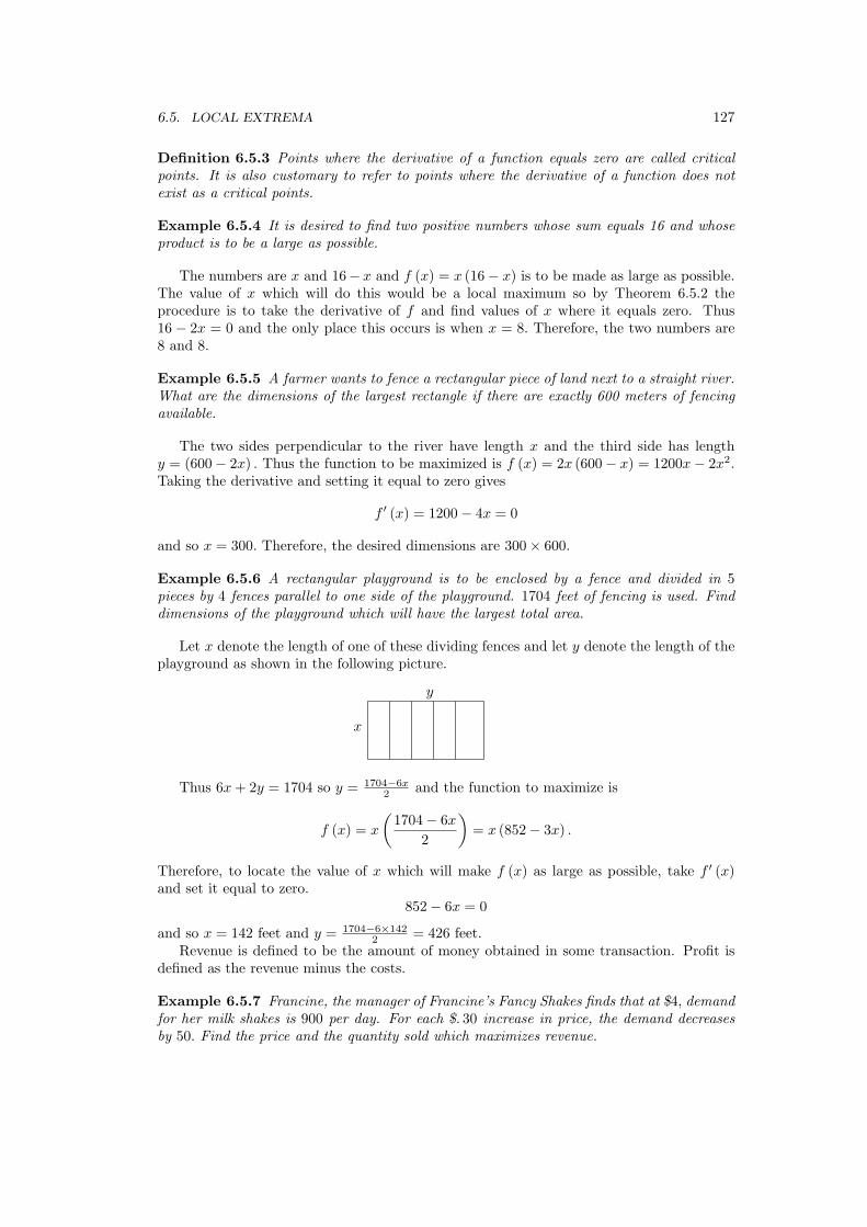
6.5. LOCAL EXTREMA 127
Definition 6.5.3 Points where the derivative of a function equals zero are called criticalpoints. It is also customary to refer to points where the derivative of a function does notexist as a critical points.
Example 6.5.4 It is desired to find two positive numbers whose sum equals 16 and whoseproduct is to be a large as possible.
The numbers are x and 16− x and f (x) = x (16− x) is to be made as large as possible.The value of x which will do this would be a local maximum so by Theorem 6.5.2 theprocedure is to take the derivative of f and find values of x where it equals zero. Thus16 − 2x = 0 and the only place this occurs is when x = 8. Therefore, the two numbers are8 and 8.
Example 6.5.5 A farmer wants to fence a rectangular piece of land next to a straight river.What are the dimensions of the largest rectangle if there are exactly 600 meters of fencingavailable.
The two sides perpendicular to the river have length x and the third side has lengthy = (600− 2x) . Thus the function to be maximized is f (x) = 2x (600− x) = 1200x− 2x2.Taking the derivative and setting it equal to zero gives
f ′ (x) = 1200− 4x = 0
and so x = 300. Therefore, the desired dimensions are 300× 600.
Example 6.5.6 A rectangular playground is to be enclosed by a fence and divided in 5pieces by 4 fences parallel to one side of the playground. 1704 feet of fencing is used. Finddimensions of the playground which will have the largest total area.
Let x denote the length of one of these dividing fences and let y denote the length of theplayground as shown in the following picture.
x
y
Thus 6x + 2y = 1704 so y = 1704−6x2 and the function to maximize is
f (x) = x
(1704− 6x
2
)= x (852− 3x) .
Therefore, to locate the value of x which will make f (x) as large as possible, take f ′ (x)and set it equal to zero.
852− 6x = 0
and so x = 142 feet and y = 1704−6×1422 = 426 feet.
Revenue is defined to be the amount of money obtained in some transaction. Profit isdefined as the revenue minus the costs.
Example 6.5.7 Francine, the manager of Francine’s Fancy Shakes finds that at $4, demandfor her milk shakes is 900 per day. For each $. 30 increase in price, the demand decreasesby 50. Find the price and the quantity sold which maximizes revenue.

128 DERIVATIVES
Let x be the number of $. 30 increases. Then the total number sold is (900− 50x) . Therevenue is
R (x) = (900− 50x) (4 + . 3x) .
Then to maximize it, R′ (x) = 70− 30x = 0. The solution is x = 2. 33 and so the optimumprice is at $4. 70 and the number sold will be 783.
Example 6.5.8 Sam, the owner of Spider Sam’s Tarantulas and Creepy Critters finds hecan sell 6 tarantulas every day at the regular price of $30 each. At his last spider celebrationsale he reduced the price to $24 and was able to sell 12 tarantulas every day. He has to pay$.0 5 per day to exhibit a tarantula and his fixed costs are $30 per day, mainly to maintainthe thousands of tarantulas he keeps on his tarantula breeding farm. What price should hecharge to maximize his profit.
He assumes the demand for tarantulas is a linear function of price. Thus if y is thenumber of tarantulas demanded at price x, it follows y = 36− x. Therefore, the revenue forprice x equals R (x) = (36− x)x. Now you have to subtract off the costs to get the profit.Thus
P (x) = (36− x)x− (36− x) (.05)− 30.
It follows the profit is maximized when P ′ (x) = 0 so −2.0x + 36. 05 = 0 which occurs whenx =$18. 025. Thus Sam should charge about $18 per tarantula.
Exercise 6.5.9 Lisa, the owner of Lisa’s gags and gadgets sells 500 whoopee cushions peryear. It costs $. 25 per year to store a whoopee cushion. To order whoopee cushions it costs$8 plus $. 90 per cushion. How many times a year and in what lot size should whoopeecushions be ordered to minimize inventory costs?
Let x be the times per year an order is sent for a lot size of 500x . If the demand is
constant, it is reasonable to suppose there are about 5002x whoopee cushions which have to
be stored. Thus the cost to store whoopee cushions is 125.02x = .25
(5002x
). Each time an order
is made for a lot size of 500x it costs 8 + 450.0
x = 8 + .9(
500x
)and this is done x times a
year. Therefore, the total inventory cost is x(8 + 450.0
x
)+ 125.0
2x = C (x) . The problem is tominimize C (x) = x
(8 + 450.0
x
)+ 125.0
2x . Taking the derivative yields
C ′ (x) =16x2 − 125
2x2
and so the value of x which will minimize C (x) is 54
√5 = 2. 79 · ·· and the lot size is 500
54
√5
=178. .88. Of course you would round these numbers off. Order 179 whoopee cushions 3 timesa year.
6.6 Exercises With Answers
1. Find the x values of the critical points of the function f (x) = x2 − x3.
Answer:23 , 0
2. Find the x values of the critical points of the function f (x) =√
3x2 − 6x + 6.
Answer:
1

6.6. EXERCISES WITH ANSWERS 129
3. Find the extreme points of the function, f (x) = 2x2 − 20x + 55 and tell whether theextreme point is a maximum or a minimum.
Answer:
The extremum is at x = 5. It is a maximum.
4. Find the extreme points of the function, f (x) = x + 9x and tell whether the extreme
point is a local maximum or a local minimum or neither.
Answer:
The extrema are at x = ±3. The one at 3 is a local minimum and the one at −3 is alocal maximum.
5. A rectangular pasture is to be fenced off beside a river with no need of fencing alongthe river. If there is900 yards of fencing material, what are the dimensions of thelargest possible pasture that can be enclosed?
Answer:
225× 45
6. A piece of property is to be fenced on the front and two sides. Fencing for the sidescosts $3. 50 per foot and fencing for the front costs $5. 60 per foot. What are thedimensions of the largest such rectangular lot if the available money is $840.0?
Answer:
60× 75.
7. In a particular apartment complex of 120 units, it is found that all units remain oc-cupied when the rent is $300 per month. For each $30 increase in the rent, one unitbecomes vacant, on the average. Occupied units require $60 per month for mainte-nance, while vacant units require none. Fixed costs for the buildings are $30 000 permonth. What rent should be charged for maximum profit and what is the maximumprofit?
Answer:
Need to maximize f (x) = (300 + 30x) (120− x)− 37 200 + 60x for x ∈ [0, 120] wherex is the number of $30 increases in rent.
$92 880 when the rent is $1980.
8. A picture is 5 feet high and the eye level of an observer is 2 feet below the bottomedge of the picture. How far from the picture should the observer stand if he wantsto maximize the angle subtended by the picture?
Answer:
Let the angle subtended by the picture be θ and let α denote the angle between ahorizontal line from the observer’s eye to the wall and the line between the observer’seye and the base of the picture. Then letting x denote the distance between the wall
and the observer’s eye, 7 = x tan (θ + α) = x(
tan θ+tan α1−tan θ tan α
)= x
(tan θ+ 2
x
1−tan θ( 2x )
). The
problem is equivalent to maximizing tan θ so denote this by z and solve for it. Thus
x
(z+ 2
x
1−z( 2x )
)= 7 and so z = 5 x
14+x2 . It follows dzdx = 5 14−x2
(14+x2)2and setting this equal
to zero, x =√
14.

130 DERIVATIVES
9. Find the point on the curve, y =√
81− 6x which is closest to (0, 0) .
Answer:(3,√
63)
10. A street is 200 feet long and there are two lights located at the ends of the street.One of the lights is 27
8 times as bright as the other. Assuming the brightness of lightfrom one of these street lights is proportional to the brightness of the light and thereciprocal of the square of the distance from the light, locate the darkest point on thestreet.
Answer:
80 feet from one light and 120 feet from the other.
11. Two cities are located on the same side of a straight river. One city is at a distanceof 3 miles from the river and the other city is at a distance of 8 miles from the river.The distance between the two points on the river which are closest to the respectivecities is 40 miles. Find the location of a pumping station which is to pump water tothe two cities which will minimize the length of pipe used.
Answer:12011 miles from the point on the river closest to the city which is at a distance of 3miles from the river.
6.7 Exercises
1. If f ′ (x) = 0, is it necessary that x is either a local minimum or local maximum? Hint:Consider f (x) = x3.
2. Two positive numbers add to 32. Find the numbers if their product is to be as largeas possible.
3. The product of two positive numbers equals 16. Find the numbers if their sum is tobe as small as possible.
4. The product of two positive numbers equals 16. Find the numbers if twice the firstplus three times the second is to be as small as possible.
5. Theodore, the owner of Theodore’s tarantulas finds he can sell 6 tarantulas at theregular price of $20 each. At his last spider celebration day sale he reduced the priceto $14 and was able to sell 14 tarantulas. He has to pay $.0 5 per day to maintain atarantula and his fixed costs are $30 per day. What price should he charge to maximizehis profit.
6. Lisa, the owner of Lisa’s gags and gadgets sells 500 whoopee cushions per year. Itcosts $. 25 per year to store a whoopee cushion. To order whoopee cushions it costs $2plus $. 25 per cushion. How many times a year and in what lot size should whoopeecushions be ordered to minimize inventory costs?
7. A continuous function, f defined on [a, b] is to be maximized. It was shown abovein Theorem 6.5.2 that if the maximum value of f occurs at x ∈ (a, b) , and if f isdifferentiable there, then f ′ (x) = 0. However, this theorem does not say anythingabout the case where the maximum of f occurs at either a or b. Describe how to findthe point of [a, b] where f achieves its maximum. Does f have a maximum? Explain.
6.7. EXERCISES 131
8. Find the maximum and minimum values and the values of x where these are achievedfor the function, f (x) = x +
√25− x2.
9. A piece of wire of length L is to be cut in two pieces. One piece is bent into the shapeof an equilateral triangle and the other piece is bent to form a square. How shouldthe wire be cut to maximize the sum of the areas of the two shapes? How should thewire be bent to minimize the sum of the areas of the two shapes? Hint: Be sure toconsider the case where all the wire is devoted to one of the shapes separately. Thisis a possible solution even though the derivative is not zero there.
10. A cylindrical can is to be constructed of material which costs 3 cents per square inchfor the top and bottom and only 2 cents per square inch for the sides. The can needsto hold 90π cubic inches. Find the dimensions of the cheapest can. Hint: The volumeof a cylinder is πr2h where r is the radius of the base and h is the height. The areaof the cylinder is 2πr2 + 2πrh.
11. A rectangular sheet of tin has dimensions 10 cm. by 20 cm. It is desired to make atopless box by cutting out squares from each corner of the rectangular sheet and thenfolding the rectangular tabs which remain. Find the volume of the largest box whichcan be made in this way.
12. Let f (x) = 13x3−x2− 8x on the interval [−1, 10] . Find the point of [−1, 10] at which
f achieves its minimum.
13. A rectangular garden 200 square feet in area is to be fenced off against rabbits. Findthe least possible length of fencing if one side of the garden is already protected by abarn.
14. A feed lot is to be enclosed by a fence and divided in 5 pieces by 4 fences parallel toone side. 1272 feet of fencing is used. Find dimensions of the feed lot which will havethe largest total area.
15. Find the dimensions of the largest rectangle that can be inscribed in a semicircle ofradius r where r = 8.
16. A smuggler wants to fit a small cylindrical vial inside a hollow rubber ball with a eightinch diameter. Find the volume of the largest vial that can fit inside the ball. Thevolume of a cylinder equals πr2h where h is the height and r is the radius.
17. A function, f, is said to be odd if f (−x) = f (x) and a function is said to be even iff (−x) = f (x) . Show that if f ′ is even, then f is odd and if f ′ is odd, then f is even.Sketch the graph of a typical odd function and a typical even function.
18. Recall sin is an odd function and cos is an even function. Determine whether each ofthe trig functions is odd, even or neither.
19. Find the x values of the critical points of the function f (x) = 3x2 − 5x3.
20. Find the x values of the critical points of the function f (x) =√
3x2 − 6x + 8.
21. Find the extreme points of the function, f (x) = x + 25x and tell whether the extreme
point is a local maximum or a local minimum or neither.
22. A piece of property is to be fenced on the front and two sides. Fencing for the sidescosts $3. 50 per foot and fencing for the front costs $5. 60 per foot. What are thedimensions of the largest such rectangular lot if the available money is $1400?

132 DERIVATIVES
23. In a particular apartment complex of 200 units, it is found that all units remain oc-cupied when the rent is $400 per month. For each $40 increase in the rent, one unitbecomes vacant, on the average. Occupied units require $80 per month for mainte-nance, while vacant units require none. Fixed costs for the buildings are $20 000 permonth. What rent should be charged for maximum profit and what is the maximumprofit?
24. A picture is 9 feet high and the eye level of an observer is 2 feet below the bottomedge of the picture. How far from the picture should the observer stand if he wantsto maximize the angle subtended by the picture?
25. Find the point on the curve, y =√
25− 2x which is closest to (0, 0) .
26. A street is 200 feet long and there are two lights located at the ends of the street.One of the lights is 1
8 times as bright as the other. Assuming the brightness of lightfrom one of these street lights is proportional to the brightness of the light and thereciprocal of the square of the distance from the light, locate the darkest point on thestreet.
27. Two cities are located on the same side of a straight river. One city is at a distanceof 3 miles from the river and the other city is at a distance of 8 miles from the river.The distance between the two points on the river which are closest to the respectivecities is 40 miles. Find the location of a pumping station which is to pump water tothe two cities which will minimize the length of pipe used.
6.8 Mean Value Theorem
The mean value theorem is one of the most important theorems about the derivative. Thebest versions of many other theorems depend on this fundamental result. The mean valuetheorem says that under suitable conditions, there exists a point in (a, b), x, such that f ′ (x)equals the slope of the secant line,
f (b)− f (a)b− a
.
The following picture is descriptive of this situation.
©©©©©©©©©
©©©©©©©©
a b
This theorem is an existence theorem and like the other existence theorems in analysis,it depends on the completeness axiom. The following is known as Rolle’s1 theorem.
Theorem 6.8.1 Suppose f : [a, b] → R is continuous,
f (a) = f (b) ,
1Rolle is remembered for Rolle’s theorem and not for anything else he did. Ironically, he did not likecalculus.

6.8. MEAN VALUE THEOREM 133
andf : (a, b) → R
has a derivative at every point of (a, b) . Then there exists x ∈ (a, b) such that f ′ (x) = 0.
Proof: Suppose first that f (x) = f (a) for all x ∈ [a, b] . Then any x ∈ (a, b) is a pointsuch that f ′ (x) = 0. If f is not constant, either there exists y ∈ (a, b) such that f (y) > f (a)or there exists y ∈ (a, b) such that f (y) < f (b) . In the first case, the maximum of f isachieved at some x ∈ (a, b) and in the second case, the minimum of f is achieved at somex ∈ (a, b). Either way, Theorem 6.5.2 on Page 126 implies f ′ (x) = 0. This proves Rolle’stheorem.
The next theorem is known as the Cauchy mean value theorem.
Theorem 6.8.2 Suppose f, g are continuous on [a, b] and differentiable on (a, b) . Thenthere exists x ∈ (a, b) such that
f ′ (x) (g (b)− g (a)) = g′ (x) (f (b)− f (a)) .
Proof: Leth (x) ≡ f (x) (g (b)− g (a))− g (x) (f (b)− f (a)) .
Then letting x = a and then letting x = b, a short computation shows h (a) = h (b) . Also,h is continuous on [a, b] and differentiable on (a, b) . Therefore Rolle’s theorem applies andthere exists x ∈ (a, b) such that
h′ (x) = f ′ (x) (g (b)− g (a))− g′ (x) (f (b)− f (a)) = 0.
This proves the theorem.The usual mean value theorem, sometimes called the Lagrange mean value theorem,
illustrated by the above picture is obtained by letting g (x) = x.
Corollary 6.8.3 Let f be continuous on [a, b] and differentiable on (a, b) . Then there existsx ∈ (a, b) such that f (b)− f (a) = f ′ (x) (b− a) .
Corollary 6.8.4 Suppose f ′ (x) = 0 for all x ∈ (a, b) where a ≥ −∞ and b ≤ ∞. Thenf (x) = f (y) for all x, y ∈ (a, b) . Thus f is a constant.
Proof: If this is not true, there exists x1 and x2 such that f (x1) 6= f (x2) . Then by themean value theorem,
0 6= f (x1)− f (x2)x1 − x2
= f ′ (z)
for some z between x1 and x2. This contradicts the hypothesis that f ′ (x) = 0 for all x. Thisproves the theorem.
Corollary 6.8.5 Suppose f ′ (x) > 0 for all x ∈ (a, b) where a ≥ −∞ and b ≤ ∞. Then fis strictly increasing on (a, b) . That is, if x < y, then f (x) < f (y) . If f ′ (x) ≥ 0, then f isincreasing in the sense that whenever x < y it follows that f (x) ≤ f (y) .
Proof: Let x < y. Then by the mean value theorem, there exists z ∈ (x, y) such that
0 < f ′ (z) =f (y)− f (x)
y − x.
Since y > x, it follows f (y) > f (x) as claimed. Replacing < by ≤ in the above equationand repeating the argument gives the second claim.
134 DERIVATIVES
Corollary 6.8.6 Suppose f ′ (x) < 0 for all x ∈ (a, b) where a ≥ −∞ and b ≤ ∞. Then fis strictly decreasing on (a, b) . That is, if x < y, then f (x) > f (y) . If f ′ (x) ≤ 0, then f isdecreasing in the sense that for x < y, it follows that f (x) ≥ f (y)
Proof: Let x < y. Then by the mean value theorem, there exists z ∈ (x, y) such that
0 > f ′ (z) =f (y)− f (x)
y − x.
Since y > x, it follows f (y) < f (x) as claimed. The second claim is similar except insteadof a strict inequality in the above formula, you put ≥ .
6.9 Exercises
1. Sally drives her Saturn over the 110 mile toll road in exactly 1.3 hours. The speedlimit on this toll road is 70 miles per hour and the fine for speeding is 10 dollars permile per hour over the speed limit. How much should Sally pay?
2. Two cars are careening down a freeway weaving in and out of traffic. Car A passes carB and then car B passes car A as the driver makes obscene gestures. This infuriatesthe driver of car A who passes car B while firing his handgun at the driver of car B.Show there are at least two times when both cars have the same speed. Then showthere exists at least one time when they have the same acceleration. The accelerationis the derivative of the velocity.
3. Show the cubic function, f (x) = 5x3 + 7x− 18 has only one real zero.
4. Suppose f (x) = x7 + |x| + x − 12. How many solutions are there to the equation,f (x) = 0?
5. Let f (x) = |x− 7|+ (x− 7)2 − 2 on the interval [6, 8] . Then f (6) = 0 = f (8) . Doesit follow from Rolle’s theorem that there exists c ∈ (6, 8) such that f ′ (c) = 0? Explainyour answer.
6. Suppose f and g are differentiable functions defined on R. Suppose also that it isknown that |f ′ (x)| > |g′ (x)| for all x and that |f ′ (t)| > 0 for all t. Show thatwhenever x 6= y, it follows |f (x)− f (y)| > |g (x)− g (y)| . Hint: Use the Cauchymean value theorem, Theorem 6.8.2.
7. Show that, like continuous functions, functions which are derivatives have the interme-diate value property. This means that if f ′ (a) < 0 < f ′ (b) then there exists x ∈ (a, b)such that f ′ (x) = 0. Hint: Argue the minimum value of f occurs at an interior pointof [a, b] .
8. Consider the function
f (x) ≡
1 if x ≥ 0−1 if x < 0 .
Is it possible that this function could be the derivative of some function? Why?

6.10. CURVE SKETCHING 135
6.10 Curve Sketching
The theorems and corollaries given above can be used to aid in sketching the graphs offunctions. The second derivative will also help in determining the shape of the function.
Definition 6.10.1 A differentiable function, f , defined on an interval, (a, b) , is concaveup if f ′ is an increasing function. A differentiable function defined on an interval, (a, b) , isconcave down if f ′ is a decreasing function.
From the geometric description of the derivative as the slope of a tangent line to thegraph of the function, to say derivative is an increasing function means that as you movefrom left to right, the slopes of the lines tangent to the graph of f become larger. Thusthe graph of the function is bent up in the shape of a smile. It may also help to think ofit as a cave when you view it from above, hence the term concave up. If the derivativeis decreasing, it follows that as you move from left to right the slopes of the lines tangentto the graph of f become smaller. Thus the graph of the function is bent down in theform of a frown. It is concave down because it is like a cave when viewed from beneath.The following theorem will give a convenient criterion in terms of the second derivative forfinding whether a function is concave up or concave down. The term, concavity, is usedto refer to this property. Thus you determine the concavity of a function when you findwhether it is concave up or concave down.
Theorem 6.10.2 Suppose f ′′ (x) > 0 for x ∈ (a, b) . Then f is concave up on (a, b) . Sup-pose f ′′ (x) < 0 on (a, b) . Then f is concave down.
Proof: This follows immediately from Corollaries 6.8.6 and 6.8.5 applied to the firstderivative. The following picture may help in remembering this.
In this picture, the plus signs and the smile on the left correspond to the second derivativebeing positive. The smile gives the way in which the graph of the function is bent. In thesecond face, the minus signs correspond to the second derivative being negative. The frowngives the way in which the graph of the function is bent.
Example 6.10.3 Sketch the graph of the function, f (x) =(x2 − 1
)2 = x4 − 2x2 + 1
Take the derivative of this function, f ′ (x) = 4x3 − 4x = 4x (x− 1) (x + 1) which equalszero at −1, 0, and 1. It is positive on (−1, 0) , and (1,∞) and negative on (0, 1) and(−∞,−1) . Therefore, x = 0 corresponds to a local maximum and x = −1 and x = 1correspond to local minimums. The second derivative is f ′′ (x) = 12x2 − 4 and this equalszero only at the points −1/
√3 and 1/
√3. The second derivative is positive on the intervals(
1/√
3,∞)and
(−∞,−1/√
3)
so the function, f is smiling on these intervals. The secondderivative is negative on the interval
(−1/√
3, 1/√
3)
and so the original function is frowningon this interval. This describes in words the qualitative shape of the function. It only re-mains to draw a picture which incorporates this description. The following is such a sketch.It is not intended to be an accurate drawing made to scale, only to be a qualitative pictureof what was just determined.

136 DERIVATIVES
−1√3
1√3
−1 1
A better graph of this function is the following, done by a computer algebra system.However the computer worked a lot harder.
0
1
-1 1x
4
In general, if you are interested in getting a nice graph of a function, you should usea computer algebra system. An effective way to accomplish your graphing is to go to thehelp menu and copy and paste an example from this menu changing it as needed. Bothmathematica and Maple have good help menus. Keep in mind there are certain conventionswhich must be followed. For example to write x raised to the second power you enter x ˆ2.In Maple, you also need to place an asterisk between quantities which are multiplied sinceotherwise it will not know you are multiplying and won’t work. There are also easy to useversions of Maple available which involve essentially pointing and clicking. You won’t learnany calculus from playing with a computer algebra system but you might have a lot of fun.
6.11 Exercises
1. Sketch the graph of the function, f (x) = x3−3x+1 showing the intervals on which thefunction is concave up and down and identifying the intervals on which the functionis increasing.
2. Find intervals on which the function, f (x) =√
1− x2 is increasing and intervals onwhich it is concave up and concave down. Sketch a graph of the function.
3. Sketch the graphs of y = x4, y = x3, and y = −x4. What do these graphs tell youabout the case when the second derivative equals zero?
4. Sketch the graph of f (x) = 1/(1 + x2
)showing the intervals on which the function
is increasing or decreasing and the intervals on which the graph is concave up and

6.11. EXERCISES 137
concave down.
5. Sketch the graph of f (x) = x/(1 + x2
)showing the intervals on which the function
is increasing or decreasing and the intervals on which the graph is concave up andconcave down.
6. Inflection points are points where the graph of a function changes from being concaveup to concave down or from being concave down to being concave up. Show that in-flection points can be identified by looking at those points where the second derivativeequals zero but that not every point where the second derivative equals zero is aninflection point. Hint: For the last part consider y = x3 and y = x4.
7. Find all inflection points for the function, f (x) = x2/(1 + x2
).

138 DERIVATIVES

Some Important SpecialFunctions
7.1 The Circular Functions
The Trigonometric functions are also called the circular functions. Thus this section will beon the functions, cos, sin, tan, sec, csc, and cot. The first thing to do is to give an importantlemma. There are several approaches to this lemma. To see it done in terms of areas ofa circular sector, see Apostol, [2], or almost any other calculus book. However, the bookby Apostol has no loose ends in the presentation unlike most other books which use thisapproach. The proof given here is a modification of that found in Tierney, [17] and Rose,[13] and is based on arc length.
Lemma 7.1.1 The following limits hold.
limx→0
sin x
x= 1 (7.1)
limx→0
1− cos x
x= 0 (7.2)
Proof: First consider (7.1). In the following picture, it follows from Corollary 3.5.4 onPage 59 that for small positive x,
sin x + (1− cosx) ≥ x ≥ sin x. (7.3)
x
¡¡
¡¡¡
(cos(x), sin(x))
©©©©¼
(1− cos(x))
Now divide by sin x to get
1 +1− cos x
|sin x| = 1 +1− cosx
sin x≥ x
sinx≥ 1.
139

140 SOME IMPORTANT SPECIAL FUNCTIONS
For small negative values of x, it is also true that
1 +1− cosx
|sin x| ≥ x
sin x≥ 1.
(Why?) From the trig. identities, it follows that for all small values of x,
1 +sin2 x
|sin x| (1 + cos x)= 1 +
|sin x|(1 + cos x)
≥ x
sin x≥ 1
and so from the squeezing theorem, Theorem 5.9.5 on Page 100,
limx→0
x
sin x= 1
and consequently, from the limit theorems,
limx→0
sin x
x= lim
x→0
1(x
sin x
) = 1.
Finally,1− cosx
x=
1− cos2 x
x (1 + cos x)= sin x
sinx
x
11 + cos x
.
Therefore, from Theorem 5.5.1 on Page 92 which says limx→0 sin (x) = 0, and the limittheorems,
limx→0
1− cosx
x= 0.
This proves the Lemma.With this, it is easy to find the derivative of sin. Using Lemma 7.1.1,
limh→0
sin (x + h)− sin x
h= lim
h→0
sin (x) cos (h) + cos (x) sin (h)− sin x
h
= limh→0
(sinx) (cos (h)− 1)h
+ cos xsin (h)
h= cos x.
The derivative of cos can be found the same way. Alternatively,
cos (x) = sin (x + π/2)
and so
cos′ (x) = sin′ (x + π/2)= cos (x + π/2)= cos x cos (π/2)− sinx sin (π/2)= − sinx.
The following theorem is now obvious and the proofs of the remaining parts are left for you.
Theorem 7.1.2 The derivatives of the trig. functions are as follows.
sin′ (x) = cos x
cos′ (x) = − sin x
tan′ (x) = sec2 (x)cot′ (x) = − csc2 (x)sec′ (x) = sec x tanx
csc′ (x) = − csc x cot x

7.2. EXERCISES 141
Here are some examples of extremum problems which involve the use of the trig. func-tions.
Example 7.1.3 Two hallways intersect at a right angle. One is 5 feet wide and the otheris 2 feet wide. What is the length of the longest thin rod which can be carried horizontallyfrom one hallway to the other?
You must minimize the length of the rod which touches the inside corner of the two hallsand extends to the outside walls. Letting θ be the angle between this rod and the outsidewall for the hall having width 2, minimize
f (θ) =
length of rod︷ ︸︸ ︷2 csc θ + 5 sec θ.
Therefore, using the rules of differentiation,
f ′ (θ) =2 cos3 θ − 5 sin θ + 5 sin θ cos2 θ
(cos2 θ) (−1 + cos2 θ)= 0
should be solved to get the angle where this length is as small as possible. Thus
2 cos3 θ − 5 sin θ + 5 sin θ cos2 θ = 0.
and 2 cos3 θ − 5 sin3 θ = 0 and so tan θ = 15
3√
2(
3√
5)2
. Drawing a triangle, you see that
at this value of θ, you have sec θ =
√( 3√5)2
+( 3√2)2
3√5and csc θ =
√( 3√5)2
+( 3√2)2
3√2. Therefore,
the minimum is obtained by substituting these values in to the equation for f (θ) yielding(√((3√
5)2
+(
3√
2)2
))3
.
Example 7.1.4 A fence 9 feet high is 2 feet from a building. What is the length of theshortest ladder which will lean against the top of the fence and touch the building?
Let θ be the angle of the ladder with the ground. Then the length of this ladder makingthis angle with the ground and leaning on the top of the fence while touching the buildingis
f (θ) =9
sin θ+
2cos θ
.
Then the final answer is(√(
3 3√
3 +(
3√
2)2
))3
. The details are similar to the problem of
the two hallways.
7.2 Exercises
1. Prove all parts of Theorem 7.1.2.
2. Prove tan′ (x) = 1 + tan2 (x) .
3. Find and prove a formula for the derivative of sinm (x) for m an integer.
4. Find the derivative of the function, sin6 (5x) .
5. Find the derivative of the function, tan7 (4x) .

142 SOME IMPORTANT SPECIAL FUNCTIONS
6. Find the derivative of the function, sec3(2x)tan3(3x) .
7. Find all intervals where sin (2x) is concave down.
8. Find the intervals where cos (3x) is increasing.
9. Two hallways intersect at a right angle. One is 3 feet wide and the other is 4 feet wide.What is the length of the longest thin rod which can be carried horizontally from onehallway to the other?
10. A fence 5 feet high is 2 feet from a building. What is the length of the shortest ladderwhich will lean against the top of the fence and touch the building?
11. Suppose f (x) = A cos ωx + B sin ωx. Show there exists an angle, φ such that f (x) =√A2 + B2 sin (ωx + φ) . The number,
√A2 + B2 gives the “amplitude” and φ is called
the “phase shift” while ω is called the “frequency”. This is very important becauseit allows us to understand what is going on. The amplitude gives the height of theperiodic function, f. Hint: Remember a point on the unit circle determines an angle.Write f (x) in the form
√A2 + B2
(A√
A2 + B2cos ωx +
B√A2 + B2
sinωx
)
and note that(
B√A2+B2 , A√
A2+B2
)is a point on the unit circle.
12. Repeat Problem 11 but this time show f (x) =√
A2 + B2 cos (ωx + φ) . How couldyou find φ?
7.3 The Exponential And Log Functions
7.3.1 The Rules Of Exponents
As mentioned earlier, bm means to multiply b by itself m times assuming m is a positiveinteger. b0 ≡ 1 provided b 6= 0. In the case where b = 0 the symbol is undefined. If m < 0,bm is defined as 1
b−m . Then the following algebraic properties are obtained. Be sure youunderstand these properties for x and y integers.
bx+y = bxby, (ab)x = axbx (7.4)
bxy = (bx)y, b−1 =
1b
(7.5)
These properties are called the rules of exponents.When x and y are not integers, the meaning of bx is no longer clear. For example,
suppose b = −1 and x = 1/2. What exactly is meant by (−1)1/2? Even in the case whereb > 0 there are difficulties. If x is a rational number, m/n and b > 0 the symbol bm/n
means n√
bm. That is its definition and it is a useful exercise for you to verify (7.4) and (7.5)hold with this definition. There are no mathematical questions about the existence of thisnumber. To see this, consider Problem 6 on Page 97. The problem is not one of theory butof practicality. Could you use this definition to find 2
12345678123451234567812344 ? Consider what you would
do. First find the number 21234567812345 and then · · ·? Can you find this number? It is justtoo big. However, a calculator can find 2
12345678123451234567812344 . It yields 2
12345678123451234567812344 = 2. 000 000 000
001 123 as an approximate answer. Clearly something else must be going on. To makematters even worse, what would you do with 2
√2? As mentioned earlier,
√2 is irrational
and so cannot be written as the quotient of two integers. These are serious difficulties andmust be dealt with.

7.3. THE EXPONENTIAL AND LOG FUNCTIONS 143
7.3.2 The Exponential Functions, A Wild Assumption
Using your calculator or a computer you can obtain graphs of the functions, y = bx forvarious choices of b. The following picture gives a few of these graphs.
3x
2x(1/2)x
0
2
4
6
8
–2 –1 1 2x
These graphs suggest that if b < 1 the function, y = bx is decreasing while if b > 1,the function is increasing but just how was the calculator or computer able to draw thosegraphs? Also, do the laws of exponents continue to hold for all real values of x? The shortanswer is that they do and this is shown later but for now here is a wild assumption whichglosses over these issues.
Wild Assumption 7.3.1 For every b > 0 there exists a unique differentiable functionexpb (x) ≡ bx valid for all real values of x such that (7.4) and (7.5) both hold for all x, y ∈ R,expb (m/n) = n
√bm whenever m,n are integers, and bx > 0 for all x ∈ R. Furthermore, if
b 6= 1 and h 6= 0, then expb (h) = bh 6= 1.
Instead of writing expb (x) I will often write bx and I will also be somewhat sloppy andregard bx as the name of a function and not just as expb (x), a given function defined at x.This is done to conform with usual usage. Also, the last claim in Wild Assumption 7.3.1follows from the first part of this assumption. See Problem 1. I want it to be completelyclear that the Wild Assumption is just that. No reason for believing in such an assumptionhas been given notwithstanding the pretty pictures drawn by the calculator. Later in thebook, the wild assumption will be completely justified. Based on Wild Assumption 7.3.1one can easily find out all about bx.
Theorem 7.3.2 Let expb be defined in Wild Assumption 7.3.1 for b > 0. Then there existsa unique number, denoted by ln b for b > 0 satisfying
exp′b (x) = ln b expb (x) . (7.6)
Furthermore,ln (ab) = ln (a) + ln (b) , ln 1 = 0, (7.7)
and for all y ∈ R,ln (by) = y ln b. (7.8)

144 SOME IMPORTANT SPECIAL FUNCTIONS
ln(a
b
)= ln (a)− ln (b) (7.9)
The function, x → ln x is differentiable and defined for all x > 0 and
ln′ (x) =1x
. (7.10)
The function, x → ln x is one to one on (0,∞) . Also, ln maps (0,∞) onto (−∞,∞) .
Proof: First consider (7.6).
limh→0
expb (x + h)− expb (x)h
= limh→0
bx+h − bx
h
= limh→0
(bh − 1
h
)bx.
The expression, limh→0
(bh−1
h
)is assumed to exist thanks to Wild Assumption 7.3.1 and
this is denoted by ln b. This proves (7.6).To verify (7.7), if b = 1 then bx = 1x for all x ∈ R. Now by (7.4) and (7.5),
1x1x = 1x+x =(12
)x= 1x
and so, dividing both sides by 1x, an operation justified by Wild Assumption 7.3.1, 1x = 1for all x ∈ R. Therefore, exp1 (x) = 1 for all x and so exp′1 (x) = ln 1 exp1 (x) = 0. Thusln 1 = 0 as claimed. Next, by the product rule and Wild Assumption 7.3.1,
ln (ab) (ab)x = ((ab)x)′
= (axbx)′ = (ax)′ bx + ax (bx)′
= (ln a) axbx + (ln b) bxax
= [ln a + ln b] (ab)x.
Therefore, ln (ab) = ln a + ln b as claimed.Next consider (7.8). Keeping y fixed, consider the function x → bxy = (by)x
. Then,
ln (by) (by)x = ((by)x)′ = g′ (x)
where g (x) ≡ bxy. Therefore, using (6.7) on Page 122,
g′ (x) = y exp′b (xy)
and soln (by) (by)x = y exp′b (xy) = y (ln b) (bxy) = y (ln b) (by)x
.
Now dividing both sides by (by)x verifies (7.8).To obtain (7.9) from this, note
ln(a
b
)= ln
(ab−1
)= ln (a) + ln
(b−1
)= ln (a)− ln (b) .
It remains to verify (7.10). From (6.2) and the continuity of 2x,
ln′ (1) = limh→0
ln(2h
)− ln 12h − 1
= limh→0
h ln 22h − 1
=ln 2ln 2
= 1.

7.3. THE EXPONENTIAL AND LOG FUNCTIONS 145
ln 2 6= 0 because if it were, then (2x)′ = (ln 2) 2x = 0 and by Corollary 6.8.4, this wouldimply 2x is a constant function which it is not. Now the first part of this lemma implies
ln′ (x) = limy→x
ln y − ln x
y − x= lim
y→x
1x
ln(
yx
)− ln 1(yx
)− 1
=1x
ln′ (1) =1x
.
It remains to verify ln is one to one. Suppose ln x = ln y. Then by the mean value theorem,there exists t between x and y such that (1/t) (x− y) = ln x − ln y = 0. Therefore, x = yand this shows ln is one to one as claimed.
It only remains to verify that ln maps (0,∞) onto (−∞,∞) . By Wild Assumption 7.3.1and the mean value theorem, Corollary 6.8.3, there exists y ∈ (0, 1) such that
0 <21 − 1
1= ln (2) 2y
Since 2y > 0 it follows ln (2) > 0 and so x → 2x is strictly increasing. Therefore, byCorollary 6.8.3
21 − 11
= ln (2) 2y ≤ ln (2) 21
and it follows that12≤ ln 2. (7.11)
Also, from (7.7)
0 = ln (2) + ln(
12
)≥ 1
2+ ln
(12
)
which shows that
ln(
12
)≤ −1
2. (7.12)
It follows from (7.11) and (7.12) that ln achieves values which are arbitrarily large andarbitrarily large in the negative direction. Therefore, by the intermediate value theorem, lnachieves all values.
More precisely, let y ∈ R. Then choose n large enough that n2 > y and −n
2 < y. Thenfrom (7.11) and (7.12)
ln((
12
)n)≤ −n
2< y <
n
2< ln (2n) .
By the intermediate value theorem, there exists x ∈ ((12
)n, 2n
)such that ln x = y. This
proves the theorem.
7.3.3 The Special Number, e
Since ln is one to one onto R, it follows there exists a unique number, e such that ln (e) = 1.Therefore,
exp′e (x) ≡ (ex)′ = ln (e) ex ≡ ln (e) expe (x) = expe (x)
showing that expe has the remarkable property that it equals its own derivative. Thiswonderful number is called Euler’s number and it can be shown to equal approximately 2.718 3.

146 SOME IMPORTANT SPECIAL FUNCTIONS
7.3.4 The Function ln |x|The function, ln is only defined on positive numbers. However, it is possible to write ln |x|whenever x 6= 0. What is the derivative of this function?
Corollary 7.3.3 Let f (x) = ln |x| for x 6= 0. Then
f ′ (x) =1x
.
Proof: If x > 0 the formula is just (7.10). Suppose then that x < 0. Then ln |x| = ln (−x)so by (6.7) on Page 122,
(ln |x|)′ = (ln (−x))′ = (ln ((−1) x))′
=1−x
(−1) =1x
.
This proves the corollary.
7.3.5 Logarithm Functions
Next a new function called logb will be defined.
Definition 7.3.4 For all b > 0 and b 6= 1
logb (x) ≡ ln x
ln b. (7.13)
Notice this definition implies (7.7) - (7.9) all hold with ln replaced with logb.The fundamental relationship between the exponential function, bx and logb x is in the
following proposition. This proposition shows this new function is logb you may have studiedin high school.
Proposition 7.3.5 Let b > 0 and b 6= 1. Then for all x > 0,
blogb x = x, (7.14)
and for all y ∈ R,logb by = y, (7.15)
Also,
log′b (x) =1
ln b
1x
. (7.16)
Proof: Formula (7.14) follows from (7.8).
ln(blogb x
)= logb x ln b = ln x
and so, since ln is one to one, it follows (7.14) holds.
logb by ≡ ln (by)ln b
=y ln b
ln b= y
and this verifies (7.15). Formula (7.16) is obvious from (7.13).The functions, logb are only defined on positive numbers. However, it is possible to write
logb |x| whenever x 6= 0. What is the derivative of these functions?

7.4. EXERCISES 147
Corollary 7.3.6 Let f (x) = logb |x| for x 6= 0. Then
f ′ (x) =1
(ln b) x.
Proof: If x > 0 the formula is just (7.16). Suppose then that x < 0. Then logb |x| =logb (−x) so by (6.7) on Page 122,
(logb |x|)′ = (logb (−x))′ = (logb ((−1) x))′
=1
−x ln b(−1) =
1x ln b
.
This proves the corollary.
Example 7.3.7 Using properties of logarithms, simplify the expression, log3
(19x
).
From (7.7) - (7.9),
log3
(19x
)= log3
(19
)+ log3 (x)
= log3
(3−2
)+ log3 (x) = −2 + log3 (x) .
Example 7.3.8 Using properties of logarithms, solve 5x−1 = 32x+2.
Take ln of both sides. Thus (x− 1) ln 5 = (2x + 2) ln 3. Then solving this for x yieldsx = ln 5+2 ln 3
ln 5−2 ln 3 .
Example 7.3.9 Solve log3 (x) + 2 = log9 (x + 3) .
From the given equation,
3log3(x)+2 = 3log9(x+3) = 912 (log9(x+3)) = 9log9
√(x+3)
and so 9x =√
x + 3. Therefore, x = 1+√
1+12×812(81) = 1
162 + 1162
√973. In the use of the
quadratic formula, only one solution was possible. (Why?)
Example 7.3.10 Compare ln (x) and loge (x)
Recall thatloge (x) ≡ ln x
ln e.
Since ln e = 1 from the definition of e, it follows loge (x) = ln x. These logarithms are callednatural logarithms.
7.4 Exercises
1. Prove the last part of the Wild Assumption follows from the first part of this assump-tion. That is, show that if b 6= 1, then expb (h) 6= 1 if h 6= 0 follows from the first part.Hint: If bh = 1 for h 6= 0, show bx = 1 for all x ∈ R.
2. Simplify
(a) log4 (16x) .
(b) log3
(27x3
)

148 SOME IMPORTANT SPECIAL FUNCTIONS
(c) (logb a) (loga b) for a, b positive real numbers not equal to 1.
3. Explain why the function 6x (1− x ln 6) is never larger than 1. Hint: Consider f (x) =6x (1− x ln 6) and find its maximum value.
4. Solve log2 (x) + 3 = log2 (3x + 8) .
5. Solve log4 (x) + 3 = log2 (x + 8) .
6. Solve the equation 52x+9 = 7x in terms of logarithms.
7. Using properties of logarithms, simplify the expression, log4
(164x
).
8. Using properties of logarithms, solve 4x−1 = 32x+2.
9. The Wild Assumption gave the existence of a function, bx satisfying certain properties.Show there can be no more than one such function. Hint: Recall the rational numberswere dense in R and so one can obtain a rational number arbitrarily close to a givenreal number. Exploit this and the assumed continuity of expb to obtain uniqueness.
10. Prove the function, bx is concave up and logb (x) is concave down.
11. Prove that logb : (0,∞) → R is onto. Hint: You know it is differentiable so it iscontinuous (Why?). Now show from (7.8) that it assumes values which are large andnegative and values which are large and positive. Then use the intermediate valuetheorem to fill in the gaps.
12. Using properties of logarithms and exponentials, solve 3 + ln (−3x) = 4 + ln 3x2.
13. Let f be a differentiable function and suppose f (a) ≥ 0 and that f ′ (x) ≥ 0 for x ≥ a.Show that f (x) ≥ f (a) for all x ≥ a. Hint: Use the mean value theorem.
14. Let e be defined in Problem ?? and suppose e < x < y. Find a relationship between xy
and yx. Hint: Use Problem 13 and at some point consider the function h (x) = ln xx .
15. Suppose f is any function defined on the positive real numbers and f ′ (x) = g (x)where g is an odd function. (g (−x) = −g (x) .) Show (f (|x|))′ = g (x) .

Properties And Applications OfDerivatives
8.1 The Chain Rule And Derivatives Of Inverse Func-tions
8.1.1 The Chain Rule
The chain rule is one of the most important of differentiation rules. Special cases of it arein Theorem 6.2.6. Now it is time to consider the theorem in full generality.
Theorem 8.1.1 Suppose f : (a, b) → (c, d) and g : (c, d) → R. Also suppose that f ′ (x)exists and that g′ (f (x)) exists. Then (g f)′ (x) exists and
(g f)′ (x) = g′ (f (x)) f ′ (x) .
Proof: Define
H (h) ≡
g(f(x+h))−g(f(x))f(x+h)−f(x) if f (x + h)− f (x) 6= 0
g′ (f (x)) if f (x + h)− f (x) = 0.
Then for h 6= 0,
g (f (x + h))− g (f (x))h
= H (h)f (x + h)− f (x)
h.
Note that limh→0 H (h) = g′ (f (x)) due to Theorems 5.9.6 on Page 100 and 6.2.2 on Page121. Therefore, taking the limit and using Theorem 5.9.4,
limh→0
g (f (x + h))− g (f (x))h
= g′ (f (x)) f ′ (x) .
This proves the chain rule.
Example 8.1.2 Let f (x) = ln∣∣ln (
x4 + 1)∣∣ . Find f ′ (x) .
From the chain rule,
f ′ (x) = ln′(ln
(x4 + 1
)) (ln
(x4 + 1
))′
=1
ln (x4 + 1)1
x4 + 1(x4
)′
=(
1ln (x4 + 1)
)(1
x4 + 1
) (4x3
).
149

150 PROPERTIES AND APPLICATIONS OF DERIVATIVES
Example 8.1.3 Let f (x) = (2 + ln |x|)3 . Find f ′ (x) .
Use the chain rule again. Thus
f ′ (x) = 3 (2 + ln |x|)2 (2 + ln |x|)′
=3x
(2 + ln |x|)2 .
8.1.2 Implicit Differentiation And Derivatives Of Inverse Functions
Sometimes a function is not given explicitly in terms of a formula. For example, you mighthave x2 + y2 = 4. This relation defines y as a function of x near a given point such as (0, 1) .Near this point, y =
√4− x2. Near the point, (0,−1) , you have y = −√4− x2. Near the
point, (1, 0) , you can’t solve for y in terms of x but you can solve for x in terms of y. Thusnear (1, 0) , x =
√4− y2. This was a simple example but in general, you can’t use algebra to
solve for one of the variables in terms of the others even if the relation defines that variableas a function of the others. Here is an example in which, even though it is impossible tofind y (x) you can still find the derivative of y. The procedure by which this is accomplishedis nothing more than the chain rule and other rules of differentiation.
Example 8.1.4 Suppose y is a differentiable function of x and y3 + 2yx = x3 + 7 + ln |y| .Find y′ (x) .
This illustrates the technique of implicit differentiation. If you believe y is some differ-entiable function of x, then you can differentiate both sides with respect to x and write,using the chain rule and product rule.
3y2y′ + 2xy′ + 2y = 3x2 +y′
y.
Now you can solve for y′ and obtain y′ = − 2y−3x2
3y3+2xy−1y.Of course there are significant mathematical considerations which are being ignored
when it is assumed y is a differentiable function of x. It turns out that for problems likethis, the equation relating x and y actually does define y as a differentiable function of xnear points where it makes sense to formally solve for y′ as just done. The theorems whichgive this justification are called the implicit and inverse function theorems. They are someof the most profound theorems in mathematics and are topics for advanced calculus. Theinterested reader should consult the book by Rudin, [14] for this and generalizations of allthe hard theorems given in this book. One case is of special interest in which y = f (x) andit is desired to find dx
dy or in other words, the derivative of the inverse function.It happens that if f is a differentiable one to one function defined on an interval, [a, b] ,
and f ′ (x) exists and is non zero then the inverse function, f−1 has a derivative at the pointf (x) . Recall that f−1 is defined according to the formula
f−1 (f (x)) = x.
Definition 8.1.5 Let f : [a, b] → R be a continuous function. Define
f ′ (a) ≡ limx→a+
f (x)− f (a)x− a
, f ′ (b) ≡ limx→b−
f (x)− f (b)x− b
.

8.1. THE CHAIN RULE AND DERIVATIVES OF INVERSE FUNCTIONS 151
Recall the notation x → a+ means that only x > a are considered in the definition oflimit. The notation x → b− is defined similarly. Thus, this definition includes the derivativeof f at the endpoints of the interval and to save notation,
f ′ (x1) ≡ limx→x1
f (x)− f (x1)x− x1
where it is understood that x is always in [a, b] .
Theorem 8.1.6 Let f : [a, b] → R be continuous and one to one. Suppose f ′ (x1) exists forsome x1 ∈ [a, b] and f ′ (x1) 6= 0. Then
(f−1
)′ (f (x1)) exists and is given by the formula,(f−1
)′ (f (x1)) = 1f ′(x1)
.
Proof: By Lemma 5.7.4, and Corollary 5.7.6 on Page 95 f is either strictly increasingor strictly decreasing and f−1 is continuous. Therefore there exists η > 0 such that if0 < |f (x1)− f (x)| < η, then
0 < |x1 − x| = ∣∣f−1 (f (x1))− f−1 (f (x))∣∣ < δ
where δ is small enough that for 0 < |x1 − x| < δ,∣∣∣∣
x− x1
f (x)− f (x1)− 1
f ′ (x1)
∣∣∣∣ < ε.
It follows that if 0 < |f (x1)− f (x)| < η,∣∣∣∣f−1 (f (x))− f−1 (f (x1))
f (x)− f (x1)− 1
f ′ (x1)
∣∣∣∣ =∣∣∣∣
x− x1
f (x)− f (x1)− 1
f ′ (x1)
∣∣∣∣ < ε
Therefore, since ε > 0 is arbitrary,
limy→f(x1)
f−1 (y)− f−1 (f (x1))y − f (x1)
=1
f ′ (x1)
and this proves the theorem.The following obvious corollary comes from the above by not bothering with end points.
Corollary 8.1.7 Let f : (a, b) → R be continuous and one to one. Suppose f ′ (x1) existsfor some x1 ∈ (a, b) and f ′ (x1) 6= 0. Then
(f−1
)′ (f (x1)) exists and is given by the formula,(f−1
)′ (f (x1)) = 1f ′(x1)
.
This is one of those theorems which is very easy to remember if you neglect the difficultquestions and simply focus on formal manipulations. Consider the following.
f−1 (f (x)) = x.
Now use the chain rule on both sides to write(f−1
)′(f (x)) f ′ (x) = 1,
and then divide both sides by f ′ (x) to obtain
(f−1
)′(f (x)) =
1f ′ (x)
.
Of course this gives the conclusion of the above theorem rather effortlessly and it is formalmanipulations like this which aid many of us in remembering formulas such as the one givenin the theorem.

152 PROPERTIES AND APPLICATIONS OF DERIVATIVES
Example 8.1.8 Let f (x) = ln(1 + x2
)+ x3 + 7. Show that f has an inverse and find(
f−1)′ (7) .
I am not able to find a formula for the inverse function. This is typical in useful ap-plications so you need to get used to this idea. The methods of algebra are insufficient tosolve hard problems in analysis. You need something more. The question is to determinewhether f has an inverse. To do this,
f ′ (x) =2x
1 + x2+ 3x2 + 7
> −1 + 3x2 + 7> 6 > 0.
By Corollary 6.8.5 on Page 133, this function is strictly increasing on R and so it has aninverse function although I have no idea how to find an explicit formula for this inversefunction. However, I can see that f (0) = 7 and so by the formula for the derivative of aninverse function,
(f−1
)′(7) =
(f−1
)′(f (0)) =
1f ′ (0)
=17.
Example 8.1.9 Suppose f (a) = 0 and f ′ (x) =√
1 + x4 + ln (1 + x2). Find(f−1
)′ (0) .
The function, f is one to one because it is strictly increasing due to the fact that itsderivative is positive for all x. As in the last example, I have no idea how to find a formulafor f−1 but I do see that f (a) = 0 and so
(f−1
)′(0) =
(f−1
)′(f (a)) =
1f ′ (a)
=1√
1 + a4 + ln (1 + a2).
The chain rule has a particularly attractive form in Leibniz’s notation. Suppose y = g (u)and u = f (x) . Thus y = g f (x) . Then from the above theorem
(g f)′ (x) = g′ (f (x)) f ′ (x)= g′ (u) f ′ (x)
or in other words,dy
dx=
dy
du
du
dx.
Notice how the du′s cancel. This particular form is a very useful crutch and is used exten-sively in applications.
8.2 Exercises
1. In each of the following, find dydx .
(a) y = esin x
(b) y = ln(sin
(x2 + 7
))
(c) y = tan(cos
(x2
))

8.3. THE FUNCTION XR FOR R A REAL NUMBER 153
(d) y = log2 (sin (x) + 6)
(e) y = sin(log3
(x2 + 1
))
(f) y =√
x3+7√sin(x)+4
(g) y = 3tan(sin(x))
(h) y =(
x2+2xtan(x2+1)
)6
2. In each of the following, assume the relation defines y as a function of x for values ofx and y of interest and use the process of implicit differentiation to find y′ (x) .
(a) xy2 + sin (y) = x3 + 1
(b) y3 + x cos(y2
)= x4
(c) y cos (x) = tan (y) cos(x2
)+ 2
(d)(x2 + y2
)6 = x3y + 3
(e) xy2+yy5+x + cos (y) = 7
(f)√
x2 + y4 sin (y) = 3x
(g) y3 sin (x) + y2x2 = 2x2y + ln |y|
(h) y2 sin (y) x + log3 (xy) = y2 + 11
(i) sin(x2 + y2
)+ sec (xy) = ex+y + y2y + 2
(j) sin(tan
(xy2
))+ y3 = 16
(k) cos (sec (tan (y))) + ln (5 + sin (xy)) = x2y + 3
3. Show that if D (g) ⊆ U ⊆ D (f) , and if f and g are both one to one, then f g is alsoone to one.
4. Using Problem 3 show that the following functions are one to one and find the deriva-tive of the inverse function at the indicated point.
(a) y = ex3+1, e2
(b) y =(x3 + 7x + 1
)3, 0
(c) y = tan(x3 + π
4
), 1
(d) y = tan(−x5 + π
4
), 1
(e) y = 25x+sin(x), 5(
π2
)+ 1
8.3 The Function xr For r A Real Number
Theorem 7.3.2 on Page 143 says that for x > 0, and for r a real number,
ln (xr) = r ln (x) (8.1)
By this theorem, it also follows that ln−1 : R→ (0,∞) exists. Then by Corollary 8.1.7 ln−1
is differentiable. This function is so important it is given a special symbol, exp . Thus
exp (ln x) = x, ln (exp (y)) = y.

154 PROPERTIES AND APPLICATIONS OF DERIVATIVES
Proposition 8.3.1 There exists a unique number e such that ln e = 1. Then exp (x) = ex.Furthermore, exp′ (x) = exp (x) .
Proof: From Theorem 7.3.2 on Page 143 there exists a unique number, e such thatln e = 1. Now by this theorem again, ln (ex) = x ln e = x. Also, from the above, ln (exp x) = xand so since ln is one to one, it follows ex = exp x as claimed.
To establish the last claim, note ln (exp x) = x and so using the chain rule and Corollary8.1.7, it follows
exp′ (x)exp (x)
= 1
which gives the desired result.Note that
x = ln(exp (x)), x = x ln (e) = ln (ex) = ln (expe (x))
and so, since ln is one to one, it follows exp (x) = expe (x) = ex.With this understanding, it becomes possible to find derivatives of functions raised to
arbitrary real powers. First, note that (8.1) can be written as
xr = exp (r ln x) (8.2)
Theorem 8.3.2 For x > 0, (xr)′ = rxr−1.
Proof: Differentiate both sides of (8.2) using the chain rule. From the Wild Assumptionon Page 143, in particular, the part about the validity of the laws of exponents,
(xr)′ = exp′ (r ln x)r
x= exp (r ln x)
r
x=
r
xxr = rxr−1. (8.3)
and this shows from (8.3) that (xr)′ = rxr−1 as claimed.
Example 8.3.3 Suppose f (x) is a non zero differentiable function. Find the derivative of|f (x)|r .
From (8.2),|f (x)|r = exp (r ln |f (x)|) .
Therefore,
(|f (x)|r)′ = exp (r ln |f (x)|) (r ln |f (x)|)′
= |f (x)|r rf ′ (x)f (x)
= r |f (x)|r−2f (x) f ′ (x) .
8.3.1 Logarithmic Differentiation
Example 8.3.4 Let f (x) =(1 + x2
)x. Find f ′ (x) .
One way to do this is to take ln of both sides and use the chain rule to differentiate bothsides with respect to x. Thus
ln (f (x)) = x ln(1 + x2
)
and so, taking the derivative of both sides, using the chain and product rules,
f ′ (x)f (x)
=2x2
1 + x2+ ln
(1 + x2
).

8.4. EXERCISES 155
Then solve for f ′ (x) to obtain
f ′ (x) =(1 + x2
)x(
2x2
1 + x2+ ln
(1 + x2
)).
This process is called logarithmic differentiation.
Example 8.3.5 Let f (x) =3√
x3+sin(x)6√x4+2x
. Find f ′ (x) .
You could use the quotient and chain rules but it is easier to use logarithmic differenti-ation.
ln (f (x)) =13
ln(x3 + sin (x)
)− 16
ln(x4 + 2x
).
Differentiating both sides,
f ′ (x)f (x)
=13
(3x2 + cos x
x3 + sin x
)− 1
64x3 + 2x4 + 2x
.
Therefore, the answer is
f ′ (x) =3√
x3 + sin (x)6√
x4 + 2x
(13
(3x2 + cosx
x3 + sin x
)− 1
64x3 + 2x4 + 2x
).
I think you can see the advantage of doing it this way over using the quotient rule.
8.4 Exercises
1. Let f (x) ≡ x3 + 1. Find f−1 (y) . Now find(f−1
)′ (1) .
2. Let f (x) ≡ x3 + 7x + 3. Explain why f has an inverse. Find(f−1
)′ (3) .
3. Derive the quotient rule from the product rule and the chain rule. This shows youdon’t need to remember the wretched quotient rule if you don’t want to. It followsfrom two rules which you cannot survive without.
4. What is wrong with the following “proof” of the chain rule? Here g′ (f (x)) exists andf ′ (x) exists.
limh→0
g (f (x + h))− g (f (x))h
= limh→0
g (f (x + h))− g (f (x))f (x + h)− f (x)
f (x + h)− f (x)h
= g′ (f (x)) f ′ (x) .
5. Is the derivative of a function always continuous? Hint: Consider a differentiablefunction which is periodic of period 1 and non constant, f. Periodic of period 1 meansf (x + 1) = f (x) for all x ∈ R. Now consider
h (x) =
x2f(
1x
)if x 6= 0
0 if x = 0 .
Show h′ (0) = 0. What is h′ (x) for x 6= 0? Is h′ also periodic of period 1?

156 PROPERTIES AND APPLICATIONS OF DERIVATIVES
6. Let f (x) = x3 +1. Find an explicit formula for f−1 and use it to compute(f−1
)′ (9) .Then use the formula given in the theorem of this section to see you get the sameanswer.
7. Find the derivatives of the following functions.
(a) sin(x2
)ln
(x2 + 1
)
(b) ln(1 + x2
)
(c)(x3 + 1
)6 sin(x2 + 7
)
(d) ln((
x3 + 1)6 sin
(x2 + 7
))
(e) tan(sec
(sin
(x2 + 1
)))
(f)(sin2
(x2 + 5
))√7
8. Use (8.2) or logarithmic differentiation to differentiate the following functions.
(a)(2 + sin
(x2 + 6
))tan x
(b) xx
(c) (xx)x
(d)(tan2
(x4 + 4
)+ 1
)cos x
(e)(sin2 (x)
)tan x
8.5 The Inverse Trigonometric Functions
It is desired to consider the inverse trigonometric functions. Graphing the function y = sin x,is clear sin is not one to one on R and so it is not possible to define an inverse function.
-1
-0.5
0
0.5
1
-4 -2 2 4
However, a little thing like this will not prevent the definition of useful inverse trig.functions. Observe the function, sin, is one to one on the interval
[−π2 , π
2
]shown in the
above picture as the interval containing zero on which the function climbs from −1 to 1.Also note that for y on this interval, cos (y) ≥ 0. Now the arcsin function is defined as theinverse of the sin when its domain is restricted to
[−π2 , π
2
]. In words, arcsin (x) is defined
to be the angle whose sine is x which lies in[−π
2 , π2
]. From Theorem 8.1.6 on Page 151
about the derivative of the inverse function, the derivative of x → arcsin (x) exists for allx ∈ [−1, 1] . The formula in this theorem could be used to find the derivative of arcsin butit is more useful to simply use that theorem to resolve the existence question and apply

8.5. THE INVERSE TRIGONOMETRIC FUNCTIONS 157
the chain rule to find the formula. It is a mistake to memorize too many formulas. Lety = arcsin (x) so sin (y) = x. Now taking the derivative of both sides,
cos (y) y′ = 1
and soy′ =
1cos y
=1√
1− sin2 (y)=
1√1− x2
.
The positive value of the square root is used because for y ∈ [−π2 , π
2
], cos (y) ≥ 0. Thus
1√1− x2
= arcsin′ (x) . (8.4)
Next consider the inverse tangent function. You are aware that tan is periodic of periodπ because
tan (x + π) =sin (x + π)cos (x + π)
=sin (x) cos (π) + cos (x) sin (π)cos (x) cos (π)− sin (x) sin (π)
=− sin (x)− cos (x)
= tan (x) .
Therefore, it is impossible to take the inverse of tan. However, tan is one to one on(−π
2 , π2
)and
limx→π
2−tan (x) = +∞, lim
x→−π2 +
tan (x) = −∞
as shown in the following graph of y = tan (x) in which the vertical lines represent verticalasymptotes.
π2−π
2
Therefore, arctan (x) for x ∈ (−∞,∞) is defined according to the rule: arctan (x) is theangle whose tangent is x which is in
(−π2 , π
2
). By Theorem 8.1.6 arctan has a derivative.
Therefore, letting y = arctan (x) , tan (y) = x and by the chain rule,
sec2 (y) y′ = 1.
Therefore,
y′ =1
sec2 (y)=
11 + tan2 (y)
=1
1 + x2.
and so1
1 + x2= arctan′ (x) . (8.5)
The inverse secant function can be defined similarly. There is no agreement on the bestway to restrict the domain of sec. I will follow the way of doing it which is used in the book
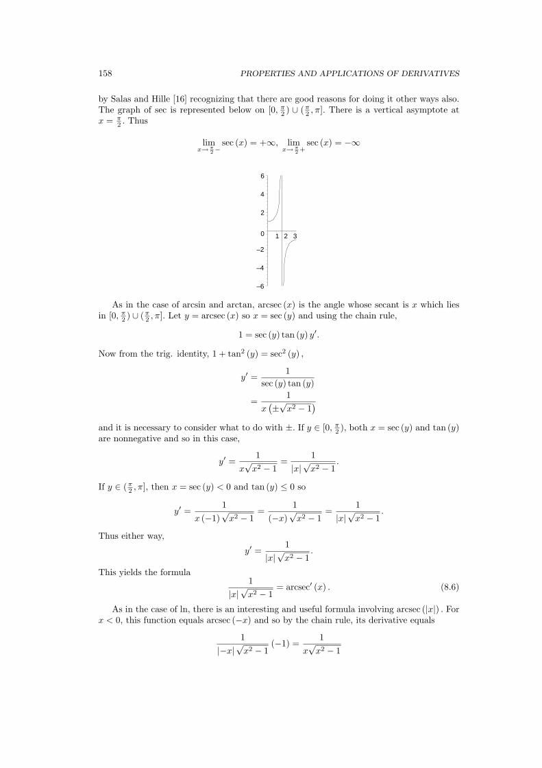
158 PROPERTIES AND APPLICATIONS OF DERIVATIVES
by Salas and Hille [16] recognizing that there are good reasons for doing it other ways also.The graph of sec is represented below on [0, π
2 ) ∪ (π2 , π]. There is a vertical asymptote at
x = π2 . Thus
limx→π
2−sec (x) = +∞, lim
x→π2 +
sec (x) = −∞
–6
–4
–2
0
2
4
6
1 2 3
As in the case of arcsin and arctan, arcsec (x) is the angle whose secant is x which liesin [0, π
2 ) ∪ (π2 , π]. Let y = arcsec (x) so x = sec (y) and using the chain rule,
1 = sec (y) tan (y) y′.
Now from the trig. identity, 1 + tan2 (y) = sec2 (y) ,
y′ =1
sec (y) tan (y)
=1
x(±√x2 − 1
)
and it is necessary to consider what to do with ±. If y ∈ [0, π2 ), both x = sec (y) and tan (y)
are nonnegative and so in this case,
y′ =1
x√
x2 − 1=
1|x|√x2 − 1
.
If y ∈ (π2 , π], then x = sec (y) < 0 and tan (y) ≤ 0 so
y′ =1
x (−1)√
x2 − 1=
1(−x)
√x2 − 1
=1
|x|√x2 − 1.
Thus either way,
y′ =1
|x| √x2 − 1.
This yields the formula1
|x| √x2 − 1= arcsec′ (x) . (8.6)
As in the case of ln, there is an interesting and useful formula involving arcsec (|x|) . Forx < 0, this function equals arcsec (−x) and so by the chain rule, its derivative equals
1|−x| √x2 − 1
(−1) =1
x√
x2 − 1

8.6. THE HYPERBOLIC AND INVERSE HYPERBOLIC FUNCTIONS 159
If x > 0, this function equals arcsec (x) and its derivative equals
1|x|√x2 − 1
=1
x√
x2 − 1
and so either way,
(arcsec (|x|))′ =1
x√
x2 − 1. (8.7)
8.6 The Hyperbolic And Inverse Hyperbolic Functions
The hyperbolic functions are given by
sinh (x) ≡ ex − e−x
2, cosh (x) ≡ ex + e−x
2,
and
tanh (x) ≡ sinh (x)cosh (x)
.
The first of these is called the hyperbolic sine and the second the hyperbolic cosine. Iimagine you can guess what the third is called. If you guessed “hyperbolic tangent” you gotit right. The other hyperbolic functions are defined by analogy to the circular functions.
The reason these are called hyperbolic functions is that
cosh2 t− sinh2 t = 1 (8.8)
and so the point, (cosh t, sinh t) is a point on the hyperbola whose equation is x2 − y2 = 1.This is not important but is the source for the term hyperbolic. Using the chain rule,
cosh′ (x) = sinh (x) , sinh′ (x) = cosh x.
Also, you see that sinh (0) = 0, cosh (0) = 1 and that sinh (x) < 0 if x < 0 while sinh (x) > 0for x > 0, but cosh (x) > 0 for all x. Therefore, sinh is an increasing function, concave downfor x < 0 and concave up for x > 0 because sinh′′ (x) = sinh (x) while cosh is decreasing forx < 0 and increasing for x > 0. Since cosh′′ (x) = cosh (x) , it is concave up for all x. Thusthe graphs of these functions are as follows.
–4
–2
0
2
4
–2 –1 1 2
0
1
2
3
4
–2 –1 1 2
y = sinh(x) y = cosh(x)
Also, you can use the graph of the function x → exp (x) = ex to verify that the graphof tanh (x) is as given below

160 PROPERTIES AND APPLICATIONS OF DERIVATIVES
–1
0
1
–3 –2 –1 1 2 3
Since x → sinh (x) is strictly increasing, it has an inverse function, sinh−1 (x) . If y =sinh−1 (x) , then sinh (y) = x and so using the chain rule and the theorem about the existenceof the derivative of the inverse function, y′ cosh (y) = 1. From the identity (8.8) cosh (y) =√
1 + sinh2 (y) =√
1 + x2. Therefore,
y′ =1√
1 + x2
which gives the formula1√
1 + x2=
(sinh−1
)′(x) . (8.9)
The derivative of the hyperbolic tangent is also easy to find. This yields after a shortcomputation
(tanhx)′ = 1− tanh2 x. (8.10)
Another notation for the inverse hyperbolic functions which is sometimes used is arcsinhor arccosh or arctanh.
8.7 Exercises
1. Verify (8.10).
2. Find derivatives of the following functions.
(a) sinh−1(x2 + 7
)
(b) tanh−1 (x)(c) sin
(sinh−1
(x2 + 2
))
(d) sin (tanh (x))(e) x2 sinh (sin (cos (x)))
(f)(cosh
(x3
))√6
(g)(1 + x4
)sin x
3. Simplify arcsinx + arccos x.
4. A wonderful identity which was used to compute π for over 200 years1 is the following.
π
4= 4 arctan
(15
)− arctan
(1
239
).
1John Machin computed π to 100 decimal places in 1706 through the use of this identity. Later in 1873William Shanks did it to over 700 places using this identity. The next advance was in 1948, 808 decimalplaces. After this, computers began to be used and currently π is “known” to millions of decimal places.Many other schemes have been used besides this identity for computing π.

8.8. L’HOPITAL’S RULE 161
Establish this identity by taking the tangent of both sides and using an appropriateformula for the tangent of the difference of two angles. Use De Moivre’s theorem toget some help in finding a formula for tan (4θ) .
5. Find a formula for tanh−1 in terms of ln.
6. Find a formula for sinh−1 in terms of ln .
7. Prove 1− tanh2 x = sech2 x.
8. Prove coth2x− 1 = csch2 x.
9. What about cosh−1? Define it by restricting the domain of cosh to be nonnegativenumbers? What is cosh−1 in terms of ln?
10. Show arcsinx = arctan(
x√1−x2
). It is possible to start with the arctan function and
obtain all the other trig functions in terms of this one. If you knew the function,arctan explain how to define sin and cos. This is interesting because there is a simpleway to define arctan directly as a function of a real variable[9]. Approaches like theseavoid all reference to plane geometry.
8.8 L’Hopital’s Rule
There is an interesting rule which is often useful for evaluating difficult limits called L’Hopital’s2
rule. The best versions of this rule are based on the Cauchy Mean value theorem, Theorem6.8.2 on Page 133.
Theorem 8.8.1 Let [a, b] ⊆ [−∞,∞] and suppose f, g are functions which satisfy,
limx→b−
f (x) = limx→b−
g (x) = 0, (8.11)
and f ′ and g′ exist on (a, b) with g′ (x) 6= 0 on (a, b). Suppose also that
limx→b−
f ′ (x)g′ (x)
= L. (8.12)
Then
limx→b−
f (x)g (x)
= L. (8.13)
Proof: By the definition of limit and (8.12) there exists c < b such that if t > c, then∣∣∣∣f ′ (t)g′ (t)
− L
∣∣∣∣ <ε
2.
Now pick x, y such that c < x < y < b. By the Cauchy mean value theorem, there existst ∈ (x, y) such that
g′ (t) (f (x)− f (y)) = f ′ (t) (g (x)− g (y)) .
2L’Hopital published the first calculus book in 1696. This rule, named after him, appeared in this book.The rule was actually due to Bernoulli who had been L’Hopital’s teacher. L’Hopital did not claim the ruleas his own but Bernoulli accused him of plagarism. Nevertheless, this rule has become known as L’Hopital’srule ever since. The version of the rule presented here is superior to what was discovered by Bernoulli anddepends on the Cauchy mean value theorem which was found over 100 years after the time of L’Hopital.

162 PROPERTIES AND APPLICATIONS OF DERIVATIVES
Since g′ (s) 6= 0 for all s ∈ (a, b) it follows g (x)− g (y) 6= 0. Therefore,
f ′ (t)g′ (t)
=f (x)− f (y)g (x)− g (y)
and so, since t > c, ∣∣∣∣f (x)− f (y)g (x)− g (y)
− L
∣∣∣∣ <ε
2.
Now letting y → b−, ∣∣∣∣f (x)g (x)
− L
∣∣∣∣ ≤ε
2< ε.
Since ε > 0 is arbitrary, this shows (8.13).The following corollary is proved in the same way.
Corollary 8.8.2 Let [a, b] ⊆ [−∞,∞] and suppose f, g are functions which satisfy,
limx→a+
f (x) = limx→a+
g (x) = 0, (8.14)
and f ′ and g′ exist on (a, b) with g′ (x) 6= 0 on (a, b). Suppose also that
limx→a+
f ′ (x)g′ (x)
= L. (8.15)
Then
limx→a+
f (x)g (x)
= L. (8.16)
Here is a simple example which illustrates the use of this rule.
Example 8.8.3 Find limx→05x+sin 3x
tan 7x .
The conditions of L’Hopital’s rule are satisfied because the numerator and denomina-tor both converge to 0 and the derivative of the denominator is nonzero for x close to 0.Therefore, if the limit of the quotient of the derivatives exists, it will equal the limit of theoriginal function. Thus,
limx→0
5x + sin 3x
tan 7x= lim
x→0
5 + 3 cos 3x
7 sec2 (7x)=
87.
Sometimes you have to use L’Hopital’s rule more than once.
Example 8.8.4 Find limx→0sin x−x
x3 .
Note that limx→0 (sinx− x) = 0 and limx→0 x3 = 0. Also, the derivative of the de-nominator is nonzero for x close to 0. Therefore, if limx→0
cos x−13x2 exists and equals L,
it will follow from L’Hopital’s rule that the original limit exists and equals L. However,limx→0 (cos x− 1) = 0 and limx→0 3x2 = 0 so L’Hopital’s rule can be applied again to con-sider limx→0
− sin x6x . From L’Hopital’s rule, if this limit exists and equals L, it will follow
that limx→0cos x−1
3x2 = L and consequently limx→0sin x−x
x3 = L. But from Lemma 7.1.1 onPage 139, limx→0
− sin x6x = −1
6 . Therefore, by L’Hopital’s rule, limx→0sin x−x
x3 = −16 .
Warning 8.8.5 Be sure to check the assumptions of L’Hopital’s rule before usingit.

8.8. L’HOPITAL’S RULE 163
Example 8.8.6 Find limx→0+cos 2x
x .
The numerator becomes close to 1 and the denominator gets close to 0. Therefore, theassumptions of L’Hopital’s rule do not hold and so it does not apply. In fact there is no limitunless you define the limit to equal +∞. Now lets try to use the conclusion of L’Hopital’srule even though the conditions for using this rule are not verified. Take the derivativeof the numerator and the denominator which yields −2 sin 2x
1 , an expression whose limit asx → 0+ equals 0. This is a good illustration of the above warning.
Some people get the unfortunate idea that one can find limits by doing experiments witha calculator. If the limit is taken as x gets close to 0, these people think one can find thelimit by evaluating the function at values of x which are closer and closer to 0. Theoretically,this should work although you have no way of knowing how small you need to take x to geta good estimate of the limit. In practice, the procedure may fail miserably.
Example 8.8.7 Find limx→0ln|1+x10|
x10 .
This limit equals limy→0ln|1+y|
y = limy→0( 1
1+y )1 = 1 where L’Hopital’s rule has been
used. This is an amusing example. You should plug .001 in to the function,ln|1+x10|
x10 andsee what your calculator or computer gives you. If it is like mine, it will give the answer, 0and will keep on returning the answer of 0 for smaller numbers than .001. This illustratesthe folly of trying to compute limits through calculator or computer experiments.
There is another form of L’Hopital’s rule in which limx→b− f (x) = ±∞ and limx→b− g (x) =±∞.
Theorem 8.8.8 Let [a, b] ⊆ [−∞,∞] and suppose f, g are functions which satisfy,
limx→b−
f (x) = ±∞ and limx→b−
g (x) = ±∞, (8.17)
and f ′ and g′ exist on (a, b) with g′ (x) 6= 0 on (a, b). Suppose also
limx→b−
f ′ (x)g′ (x)
= L. (8.18)
Then
limx→b−
f (x)g (x)
= L. (8.19)
Proof: By the definition of limit and (8.18) there exists c < b such that if t > c, then∣∣∣∣f ′ (t)g′ (t)
− L
∣∣∣∣ <ε
2.
Now pick x, y such that c < x < y < b. By the Cauchy mean value theorem, there existst ∈ (x, y) such that
g′ (t) (f (x)− f (y)) = f ′ (t) (g (x)− g (y)) .
Since g′ (s) 6= 0 on (a, b) , it follows g (x)− g (y) 6= 0. Therefore,
f ′ (t)g′ (t)
=f (x)− f (y)g (x)− g (y)
and so, since t > c, ∣∣∣∣f (x)− f (y)g (x)− g (y)
− L
∣∣∣∣ <ε
2.

164 PROPERTIES AND APPLICATIONS OF DERIVATIVES
Now this implies ∣∣∣∣∣∣f (y)g (y)
(f(x)f(y) − 1
)(
g(x)g(y) − 1
) − L
∣∣∣∣∣∣<
ε
2
where for all y large enough, both f(x)f(y) − 1 and g(x)
g(y) − 1 are not equal to zero. Continuingto rewrite the above inequality yields
∣∣∣∣∣∣f (y)g (y)
− L
(g(x)g(y) − 1
)(
f(x)f(y) − 1
)∣∣∣∣∣∣<
ε
2
∣∣∣∣∣∣
(g(x)g(y) − 1
)(
f(x)f(y) − 1
)∣∣∣∣∣∣.
Therefore, for y large enough,
∣∣∣∣f (y)g (y)
− L
∣∣∣∣ ≤∣∣∣∣∣∣L− L
(g(x)g(y) − 1
)(
f(x)f(y) − 1
)∣∣∣∣∣∣+
ε
2
∣∣∣∣∣∣
(g(x)g(y) − 1
)(
f(x)f(y) − 1
)∣∣∣∣∣∣< ε
due to the assumption (8.17) which implies
limy→b−
(g(x)g(y) − 1
)(
f(x)f(y) − 1
) = 1.
Therefore, whenever y is large enough,∣∣∣∣f (y)g (y)
− L
∣∣∣∣ < ε
and this is what is meant by (8.19). This proves the theorem.As before, there is no essential difference between the proof in the case where x → b−
and the proof when x → a+. This observation is stated as the next corollary.
Corollary 8.8.9 Let [a, b] ⊆ [−∞,∞] and suppose f, g are functions which satisfy,
limx→a+
f (x) = ±∞ and limx→a+
g (x) = ±∞, (8.20)
and f ′ and g′ exist on (a, b) with g′ (x) 6= 0 on (a, b). Suppose also that
limx→a+
f ′ (x)g′ (x)
= L. (8.21)
Then
limx→a+
f (x)g (x)
= L. (8.22)
Theorems 8.8.1 8.8.8 and Corollaries 8.8.2 and 8.8.9 will be referred to as L’Hopital’srule from now on. Theorem 8.8.1 and Corollary 8.8.2 involve the notion of indeterminateforms of the form 0
0 . Please do not think any meaning is being assigned to the nonsenseexpression 0
0 . It is just a symbol to help remember the sort of thing described by Theorem8.8.1 and Corollary 8.8.2. Theorem 8.8.8 and Corollary 8.8.9 deal with indeterminate formswhich are of the form ±∞
∞ . Again, this is just a symbol which is helpful in remembering thesort of thing being considered. There are other indeterminate forms which can be reducedto these forms just discussed. Don’t ever try to assign meaning to such symbols.

8.8. L’HOPITAL’S RULE 165
Example 8.8.10 Find limy→∞(1 + x
y
)y
.
It is good to first see why this is called an indeterminate form. One might think that asy →∞, it follows x/y → 0 and so 1+ x
y → 1. Now 1 raised to anything is 1 and so it wouldseem this limit should equal 1. On the other hand, if x > 0, 1 + x
y > 1 and a number raisedto higher and higher powers should approach ∞. It really isn’t clear what this limit shouldbe. It is an indeterminate form which can be described as 1∞. By definition,
(1 +
x
y
)y
= exp(
y ln(
1 +x
y
)).
Now using L’Hopital’s rule,
limy→∞
y ln(
1 +x
y
)= lim
y→∞
ln(1 + x
y
)
1/y
= limy→∞
11+(x/y)
(−x/y2)
(−1/y2)
= limy→∞
x
1 + (x/y)= x
Therefore,
limy→∞
y ln(
1 +x
y
)= x
Since exp is continuous, it follows
limy→∞
(1 +
x
y
)y
= limy→∞
exp(
y ln(
1 +x
y
))= ex.
8.8.1 Interest Compounded Continuously
Suppose you put money in the bank and it accrues interest at the rate of r per paymentperiod. These terms need a little explanation. If the payment period is one month, andyou started with $100 then the amount at the end of one month would equal 100 (1 + r) =100 + 100r. In this the second term is the interest and the first is called the principal. Nowyou have 100 (1 + r) in the bank. This becomes the new principal. How much will you haveat the end of the second month? By analogy to what was just done it would equal
100 (1 + r) + 100 (1 + r) r = 100 (1 + r)2 .
In general, the amount you would have at the end of n months is 100 (1 + r)n.
When a bank says they offer 6% compounded monthly, this means r, the rate per paymentperiod equals .06/12. Consider the problem of a rate of r per year and compounding theinterest n times a year and letting n increase without bound. This is what is meant bycompounding continuously. The interest rate per payment period is then r/n and thenumber of payment periods after time t years is approximately tn. From the above theamount in the account after t years is
P(1 +
r
n
)nt
(8.23)
Recall from Example 8.8.10 that limy→∞(1 + x
y
)y
= ex. The expression in (8.23) can bewritten as
P[(
1 +r
n
)n]t

166 PROPERTIES AND APPLICATIONS OF DERIVATIVES
and so, taking the limit as n →∞, you get
Pert = A.
This shows how to compound interest continuously.
Example 8.8.11 Suppose you have $100 and you put it in a savings account which pays6% compounded continuously. How much will you have at the end of 4 years?
From the above discussion, this would be 100e(.06)4 = 127. 12. Thus, in 4 years, youwould gain interest of about $27.
8.9 Exercises
1. Find the limits.
(a) limx→03x−4 sin 3x
tan 3x
(b) limx→π2− (tan x)x−(π/2)
(c) limx→1arctan(4x−4)arcsin(4x−4)
(d) limx→0arctan 3x−3x
x3
(e) limx→0+9sec x−1−13sec x−1−1
(f) limx→03x+sin 4x
tan 2x
(g) limx→π/2ln(sin x)x−(π/2)
(h) limx→0cosh 2x−1
x2
(i) limx→0− arctan x+x
x3
(j) limx→0x8 sin 1
x
sin 3x
(k) limx→∞ (1 + 5x)2x
(l) limx→0−2x+3 sin x
x
(m) limx→1ln(cos(x−1))
(x−1)2
(n) limx→0+ sin1x x
(o) limx→0 (csc 5x− cot 5x)
(p) limx→0+3sin x−12sin x−1
(q) limx→0+ (4x)x2
(r) limx→∞ x10
(1.01)x
(s) limx→0 (cos 4x)(1/x2)
2. Find the following limits.
(a) limx→0+1−√cos 2x
sin4(4√x) .
(b) limx→02x2−25x
sin(
x25
)−sin(3x)
.

8.10. RELATED RATES 167
(c) limn→∞ n(
n√
7− 1).
(d) limx→∞(
3x+25x−9
)x2
.
(e) limx→∞(
3x+25x−9
)1/x
.
(f) limn→∞(cos 2x√
n
)n
.
(g) limn→∞(cos 2x√
5n
)n
.
(h) limx→3xx−27x−3 .
(i) limn→∞ cos(π√
4n2+13nn
).
(j) limx→∞(
3√
x3 + 7x2 −√x2 − 11x).
(k) limx→∞(
5√
x5 + 7x4 − 3√
x3 − 11x2).
(l) limx→∞(
5x2+72x2−11
) x1−x
.
(m) limx→∞(
5x2+72x2−11
) x ln x1−x
.
(n) limx→0+
ln(
e2x2+7√
x)
sinh(√x) .
(o) limx→0+7√x− 5√x9√x− 11√x
.
3. Find the following limits.
(a) limx→0+ (1 + 3x)cot 2x
(b) limx→0tan(sin x)−sin(tan x)
x7
(c) limx→0sin(x2)−sin2(x)
x4
(d) limx→0e−(1/x2)
x
(e) limx→0
(1x − cot (x)
)
(f) limx→0cos(sin x)−1
x2
(g) limx→∞(x2
(4x4 + 7
)1/2 − 2x4)
(h) limx→0cos(x)−cos(4x)
tan(x2)
(i) limx→0arctan(3x)
x
(j) limx→∞[(
x9 + 5x6)1/3 − x3
]
8.10 Related Rates
Sometimes some variables are related by a formula and it is known how fast all are changingbut one. The related rates problem asks for how fast the remaining variable is changing.
Example 8.10.1 A cube of ice is melting such that dVdt = −4cm3/ sec where V is the
volume. How fast are the sides changing when they are equal to 5 centimeters in length?

168 PROPERTIES AND APPLICATIONS OF DERIVATIVES
The volume is V = x3 where x is the length of a side of the cube. Therefore, the chainrule implies
−4 =dV
dt= 3x2 dx
dt
and the problem is to find dxdt when x = 5. Therefore,
dx
dt=
−43 (25)
=−475
cm/second
at this time.Note there is no way of knowing the volume or the sides as a functions of t.
Example 8.10.2 One car travels north at 70 miles per hour and the other travels east at60 miles per hour toward an intersection. How fast is the distance between the two carschanging when this distance equals five miles and the car heading north is at a distance ofthree miles from the intersection?
Let l denote the distance between the cars. Thus if x is the distance from the intersectionof the car traveling east and y is the distance from the intersection of the car traveling north,l2 = x2 + y2. When y = 3, it follows that x = 4. Therefore, at the instant described
2ll′ = 2xx′ + 2yy′
10l′ = 8 (−60) + 6 (−70)
and so l′ = −90 miles per hour at this instant.
8.11 Exercises
1. One car travels north at 70 miles per hour toward an intersection and the other travelseast at 60 miles per hour away from the intersection. How fast is the distance betweenthe two cars changing when this distance equals five miles and the car heading northis at a distance of three miles from the intersection?
2. A trash compactor compacts some trash which is in the shape of a box having a squarebase and a height equal to twice the length of a side of the base. Suppose each sideof the base is changing at the rate of −3 inches per second. How fast is the volumechanging when the side of the base equals 10 inches?
3. An isosceles triangle has two sides of equal length. Imagine such a triangle in whichthe two legs have length 8 inches and denote the included angle by θ and the area byA. Suppose dA
dt =√
3 square inches per minute. How fast is θ changing when θ = π/6radians?
4. A point having coordinates (x, y) moves over the ellipse, x2
4 + y2
9 = 1. If dydt = 2, find
dxdt at the point (2, 3).
5. A spectator at a tennis tournament sits 10 feet from the end of the net and on the linedetermined by the net. He watches the ball go back and forth, and will have a verysore neck when he wakes up the next morning. How fast is the angle between his lineof sight and the line determined by the net changing when the ball crosses over thenet at a point 12 feet from the end assuming the ball travels at a speed of 60 milesper hour?

8.11. EXERCISES 169
6. The surface area of a sphere of radius r equals 4πr2 and the volume of the ball ofradius r equals (4/3)πr3. A balloon in the shape of a ball is being inflated at the rateof 6 cubic inches per minute. How fast is the surface area changing when the volumeof the ball equals 20π cubic inches?
7. A mother cheetah attempts to fix dinner, a Thompson gazelle, for her hungry children.She moves at 100 feet per second while dinner travels at 80 feet per second. How fast isthe distance between her and dinner decreasing when she is located at the point (0, 40)feet and dinner is moving in the direction of the positive x axis at the point (30, 0)feet? Is your answer a little surprising? Hint: Let (x, y) denote the coordinates of thecheetah and let (z, 0) denote the coordinates of the gazelle. Then if l is the desireddistance, l2 = (x− z)2 + y2. At the instant described, assuming the cheetah moves
toward the gazelle at all times, y′/x′ = −4/3 (why?) and also√
(x′)2 + (y′)2 = 100.
8. A six foot high man walks at a speed of 5 feet per second away from a light post whichis 12 feet high that has the light right on the top. How fast is the end of his shadowmoving when he is at a distance of 10 feet from the base of the light pole. How fast isthe end of the shadow moving when he is 5 feet from the pole? (Assume he does notwalk normally but instead oozes along like a giant amoeba so that his head is alwaysexactly 6 feet above the ground.)
9. The volume of a right circular cone is 13πr2h. Grain comes off a conveyor belt and
falls to the ground making a right circular cone. It is observed that r′ (t) = .5 feet perminute and h′ (t) = .3 feet per minute. It is also known that the rate at which thegrain falls off the conveyor belt is 100π cubic feet per minute. When the radius of thecone is 10 feet what is the height of the cone?
10. A hemispherical dish of radius 5 inches is sitting on a table. Soup is being poured inat the constant rate of 4 cubic inches per second. How fast is the level of soup risingwhen the radius of the top surface of the soup equals 3 inches? The volume of soupat depth y will be shown later to equal V (y) = π
(5y2 − y3
3
).
11. A vase of water is sitting on a table.
It will be shown later that if V (y) is the total volume of the vase up to height y,then dV
dy = A (y) where A (y) is the surface area of the top surface of the water at thisheight. (To see this is very reasonable, note that a little chunk of volume of the vasebetween heights y and y + dy would be dV = A (y) dy, area times height.) Also, therate at which the water evaporates is proportional to the surface area of the exposedwater. Thus dV
dt = −kA (y). Show dydt is a constant even though the surface area of
the exposed water is constantly changing in a typical vase.
12. A revolving search light at a prison makes one revolution per minute. How fast is thelight travelling along the nearest point on a wall 1/4 mile away? Give your answer inmiles per hour.

170 PROPERTIES AND APPLICATIONS OF DERIVATIVES
13. A painter is on top of a 13 foot ladder which leans against a house. The base of theladder is moving away from the house at the rate of 2 feet per second causing the topof the ladder to move down the house. How fast is the painter descending when thebase of the ladder is at a distance of 5 feet from the house?
14. A rope fastened to the bow of a row boat has the other end wound around a windlasswhich is 4 feet above the level of the bow of the boat. The current pulls the boat awayat the rate of 2 feet per second. How fast is the rope unwinding when the distancebetween the bow of the boat and the windlass is 10 feet?
15. A kite 100 feet above the ground is being blown away from the person holding itsstring in a direction parallel to the ground at the rate of 10 feet per second. At whatrate must the string be let out when the length of string already let out is 200 feet?
16. A certain volume of an ideal gas satisfies PV = kT where T is the absolute temper-ature, P is the pressure, V is the volume and k is a constant which depends on theamount of the gas and the sort of gas in the sample. Find a formula for dV
dt in termsof k, P, V and their derivatives.
17. A disposable cup is made in the shape of a right circular cone with height 5 inches andradius 2 inches. Water flows in to this conical cup at the rate of 4 cubic inches perminute. How fast is the water level rising when the water in the cone is three inchesdeep? The volume of a cone is 1
3πr2h.
18. The two equal sides of an isosceles triangle have length x inches and the third leg haslength y inches. Suppose dx
dt = 2 inches per minute and that the length of the otherside changes in such a way that the area of the triangle is always 10 square inches.For θ the angle between the two equal sides, find dθ
dt when x = 5 inches.
8.12 The Derivative And Optimization
There are existence theorems such as Theorem 5.7.10 on Page 96 which ensure a maximumor minimum of a function exists but in this section the goal is to give ways to find themaximum or minimum values of a function.
Suppose f is continuous on [a, b]. The minimum or maximum could occur at either endpoint or it could occur at a point in the open interval, (a, b). If it occurs at a point of theopen interval, (a, b) , say at x0, and if f ′ (x0) exists, then from Theorem 6.5.2 on Page 126f ′ (x0) = 0. Therefore, the following simple procedure can be used to locate the maximumor minimum of a function, f . Find all points, x, in (a, b) where f ′ (x) = 0 and all points, x,in (a, b) where f ′ (x) does not exist. Then consider these points along with the end pointsof the interval. Evaluate f at the end points and at these points where the derivative is zeroor does not exist. The largest must be the maximum value of f on the interval, [a, b] , andthe smallest must be the minimum value of f on the interval, [a, b]. Typically, this involveschecking only finitely many points.
Sometimes there are no end points. In this case, you do not necessarily know a maximumvalue or a minimum value of a continuous function even exists. However, if the function isdifferentiable and if a maximum or minimum exists, it can still be found by looking at thepoints where the derivative equals zero.
Example 8.12.1 Find the maximum and minimum values of the function, f (x) = x3 −3x + 1 on the interval [−2, 2].

8.12. THE DERIVATIVE AND OPTIMIZATION 171
The points where f ′ (x) = 3x2 − 3 = 0 are x = 1 or −1. There are no points wherethe derivative does not exist. Therefore, evaluate the function at −1,−2, 2, and 1. Thusf (−1) = 3, f (1) = −1, f (−2) = −1, and f (2) = 3. Therefore, the maximum value of thefunction occurs at the point −1 and 2 and has the value of 3 while the minimum value ofthe function occurs at −1 and −2 and equals −1. The following is a graph of this function.
-4
-2
0
2
4
6
-2 -1 1 2
4
Example 8.12.2 Find the maximum and minimum values of the function f (x) =∣∣x2 − 1
∣∣on the interval [−.5, 2].
You should verify that this function fails to have a derivative at the point x = 1. Forx ∈ (−.5, 1) the function equals 1 − x2 and so its derivative equals zero at x = 0. Forx > 1, the function equals x2− 1 and so there is no point larger than 1 where the derivativeequals zero. Therefore, the points to look at are the end points, −.5, 2, the points wherethe derivative fails to exist, 1 and the point where the derivative equals zero, x = 0. Nowf (−.5) = . 75, f (0) = 1, f (1) = 0, and f (2) = 3. It follows the function achieves itsmaximum at the end point, x = 2 and its minimum at the point, x = 1 where the derivativefails to exist. The following is a graph of this function.
-0.5 0.5 1 1.5 2
4
Example 8.12.3 Find the minimum value of the function f (x) = x + 1x for x ∈ (0,∞).
The graph of this function is given below.

172 PROPERTIES AND APPLICATIONS OF DERIVATIVES
0
1
2
3
4
5
1 2 3 4 5
From the graph, it seems there should exist a minimum value at the bottom of the graph.To find it, take the derivative of f and set it equal to zero and then solve for the value of x.Thus
1− 1x2
= 0
and so x = 1. The solution to the equation, x = −1 is of no interest because it is notgreater than zero. Therefore, the minimum value of the function on the interval, (0,∞)equals f (1) = 2 as suggested by the graph.
Example 8.12.4 An eight foot high wall stands one foot from a warehouse. What is thelength of the shortest ladder which extends from the ground to the warehouse.
A diagram of this situation is the following picture.
¡¡
wall
@@
@@warehouse
JJ
JJ
JJ
JJx
y
In this picture, the slanted line represents the ladder and x and y are as shown. Bysimilar triangles, y/1 = 8/x. Therefore, xy = 8. From the Pythagorean theorem the lengthof the ladder equals
√1 + y2 +
√x2 + 64. Now using the relation between x and y, the
function of a single variable, x, to minimize is
f (x) =
√1 +
64x2
+√
x2 + 64,
Clearly x > 0 so there are no endpoints to worry about. (Why?) Also the function isdifferentiable and so it suffices to consider only points where the derivative equals zero.This is a little messy but finally
f ′ (x) =1√
(x2 + 64)−64 + x3
x2
and the value where this equals zero is x = 4. It follows the shortest ladder is of length√1 + 64
42 +√
42 + 64 = 5√
5 feet.

8.13. EXERCISES 173
Example 8.12.5 Fermat’s principle says that light travels on a path which will minimizethe total time. Consider the following picture of light passing from (x1, y1) to (x2, y2) asshown. The angle θ1 is called the angle of incidence while the angle, θ2 is called the angleof refraction. The picture indicates a situation in which c1 > c2.
PPPPPPPPP@
@@
@@
@
θ1
θ2
•
•
(x1, y1)
(x2, y2)
Speed equals c1
Speed equals c2(xp, 0)¡¡
Then define by x the quantity xp − x1. What is the relation between θ1 and θ2?
The time it takes for the light to go from (x1, y1) to the point (xp, 0) equals√
x2 + y21/c1
and the time it takes to go from (xp, 0) to (x2, y2) is√
(x2 − x1 − x)2 + y22/c2. Therefore,
the total time is
T =
√x2 + y2
1
c1+
√(x2 − x1 − x)2 + y2
2
c2
Thus T is minimized if
dT
dx=
d
dx
√x2 + y2
1
c1+
√(x2 − x1 − x)2 + y2
2
c2
=x
c1
√x2 + y2
1
− (x2 − x1 − x)
c2
√(x2 − x1 − x)2 + y2
2
=sin (θ1)
c1− sin (θ2)
c2= 0
at this point. Therefore, this yields the desired relation between θ1 and θ2. This is calledSnell’s law.
8.13 Exercises
1. A cylindrical can is to be constructed to hold 30 cubic inches. The top and bottom ofthe can are constructed of a material costing one cent per square inch and the sidesare constructed of a material costing 2 cents per square inch. Find the minimum costfor such a can.
2. Two positive numbers sum to 8. Find the numbers if their product is to be as largeas possible.
3. The ordered pair, (x, y) is on the ellipse, x2 + 4y2 = 4. Form the rectangle which has(x, y) as one end of a diagonal and (0, 0) at the other end. Find the rectangle of thissort which has the largest possible area.
4. A rectangle is inscribed in a circle of radius r. Find the formula for the rectangle ofthis sort which has the largest possible area.

174 PROPERTIES AND APPLICATIONS OF DERIVATIVES
5. A point is picked on the ellipse, x2 + 4y2 = 4 which is in the first quadrant. Then aline tangent to this point is drawn which intersects the x axis at a point, x1 and they axis at the point y1. The area of the triangle formed by the y axis, the x axis, andthe line just drawn is thus x1y1
2 . Out of all possible triangles formed in this way, findthe one with smallest area.
6. Find maximum and minimum values if they exist for the function, f (x) = ln xx for
x > 0.
7. Describe how you would find the maximum value of the function, f (x) = ln x2+sin x for
x ∈ (0, 6) if it exists. Hint: You might want to use a calculator to graph this and getan idea what is going on.
8. A rectangular beam of height h and width w is to be sawed from a circular log ofradius 1 foot. Find the dimensions of the strongest such beam assuming the strengthis of the form kh2w. Here k is some constant which depends on the type of wood used.
9. A farmer has 600 feet of fence with which to enclose a rectangular piece of land thatborders a river. If he can use the river as one side, what is the largest area that hecan enclose.
10. An open box is to be made by cutting out little squares at the corners of a rectangularpiece of cardboard which is 20 inches wide and 40 inches long. and then folding upthe rectangular tabs which result. What is the largest possible volume which can beobtained?
11. A feeding trough is to be made from a rectangular piece of metal which is 3 feet wideand 12 feet long by folding up two rectangular pieces of dimension one foot by 12 feet.What is the best angle for this fold?
12. Find the dimensions of the right circular cone which has the smallest area given thevolume is 30π cubic inches. The volume of the right circular cone is (1/3) πr2h andthe area of the cone is πr
√h2 + r2.
13. A wire of length 10 inches is cut into two pieces, one of length x and the other oflength 10−x. One piece is bent into the shape of a square and the other piece is bentinto the shape of a circle. Find the two lengths such that the sum of the areas of thecircle and the square is as large as possible. What are the lengths if the sum of thetwo areas is to be as small as possible.
14. A hiker begins to walk to a cabin in a dense forest. He is walking on a road whichruns from East to West and the cabin is located exactly one mile north of a point twomiles down the road. He walks 5 miles per hour on the road but only 3 miles per hourin the woods. Find the path which will minimize the time it takes for him to get tothe cabin.
15. A refinery is on a straight shore line. Oil needs to flow from a mooring place for oiltankers to this refinery. Suppose the mooring place is two miles off shore from a pointon the shore 8 miles away from the refinery and that it costs five times as much to laypipe under water than above the ground. Describe the most economical route for apipeline from the mooring place to the refinery.
16. Two hallways, one 5 feet wide and the other 6 feet wide meet. It is desired to carrya ladder horizontally around the corner. What is the longest ladder which can becarried in this way? Hint: Consider a line through the inside corner which extends

8.14. THE NEWTON RAPHSON METHOD 175
to the opposite walls. The shortest such line will be the length of the longest ladder.You might also consider Example 7.1.3 on Page 141.
17. A triangle is inscribed in a circle in such a way that one side of the triangle is alwaysthe same length, s. Show that out of all such triangles the maximum area is obtainedwhen the triangle is an isosceles triangle. Hint: From theorems in plane geometry, theangle opposite the side having fixed length is a constant, no matter how you draw thetriangle. Use the law of sines and this fact. In the following picture, α is a constant.
α
s
18. A window is to be constructed for the wall of a church which is to consist of a rectangleof height b surmounted by a half circle of radius a. Suppose the total perimeter ofthe window is to be no more than 4π + 8 feet. Find the shape and dimensions of thewindow which will admit the most light.
19. You know limx→∞ ln x = ∞. Show that if α > 0, then limx→∞ ln xxα = 0.
20. Suppose p and q are two positive numbers larger than 1 which satisfy 1p + 1
q = 1. Nowlet a and b be two positive numbers and consider f (t) = 1
p (at)p + 1q
(bt
)qfor t > 0.
Show the minimum value of f is ab. Prove the important inequality, ab ≤ ap
p + bq
q .
21. Using Problem 20 establish the following magnificent inequality which is a case ofHolder’s inequality. For 1
p + 1q = 1, and ai, bi positive numbers,
n∑
i=1
aibi ≤(
n∑
i=1
api
)1/p (n∑
i=1
bqi
)1/q
.
8.14 The Newton Raphson Method
The Newton Raphson method is a way to get approximations of solutions to various equa-tions. For example, suppose you want to find
√2. The existence of
√2 is not difficult to
establish by considering the continuous function, f (x) = x2 − 2 which is negative at x = 0and positive at x = 2. Therefore, by the intermediate value theorem, there exists x ∈ (0, 2)such that f (x) = 0 and this x must equal
√2. The problem consists of how to find this
number, not just to prove it exists. The following picture illustrates the procedure of theNewton Raphson method.
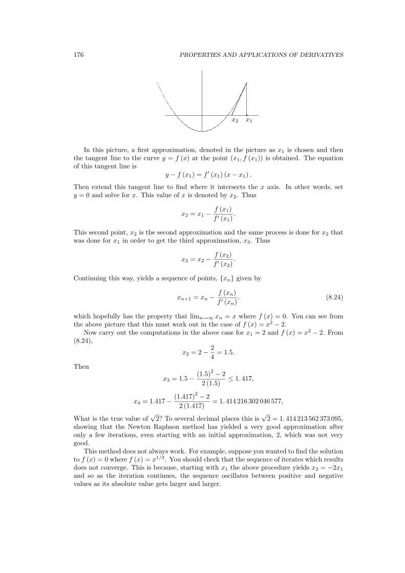
176 PROPERTIES AND APPLICATIONS OF DERIVATIVES
x1x2
In this picture, a first approximation, denoted in the picture as x1 is chosen and thenthe tangent line to the curve y = f (x) at the point (x1, f (x1)) is obtained. The equationof this tangent line is
y − f (x1) = f ′ (x1) (x− x1) .
Then extend this tangent line to find where it intersects the x axis. In other words, sety = 0 and solve for x. This value of x is denoted by x2. Thus
x2 = x1 − f (x1)f ′ (x1)
.
This second point, x2 is the second approximation and the same process is done for x2 thatwas done for x1 in order to get the third approximation, x3. Thus
x3 = x2 − f (x2)f ′ (x2)
.
Continuing this way, yields a sequence of points, xn given by
xn+1 = xn − f (xn)f ′ (xn)
. (8.24)
which hopefully has the property that limn→∞ xn = x where f (x) = 0. You can see fromthe above picture that this must work out in the case of f (x) = x2 − 2.
Now carry out the computations in the above case for x1 = 2 and f (x) = x2 − 2. From(8.24),
x2 = 2− 24
= 1.5.
Then
x3 = 1.5− (1.5)2 − 22 (1.5)
≤ 1. 417,
x4 = 1.417− (1.417)2 − 22 (1.417)
= 1. 414 216 302 046 577,
What is the true value of√
2? To several decimal places this is√
2 = 1. 414 213 562 373 095,showing that the Newton Raphson method has yielded a very good approximation afteronly a few iterations, even starting with an initial approximation, 2, which was not verygood.
This method does not always work. For example, suppose you wanted to find the solutionto f (x) = 0 where f (x) = x1/3. You should check that the sequence of iterates which resultsdoes not converge. This is because, starting with x1 the above procedure yields x2 = −2x1
and so as the iteration continues, the sequence oscillates between positive and negativevalues as its absolute value gets larger and larger.

8.15. EXERCISES 177
However, if f (x0) = 0 and f ′′ (x) > 0 for x near x0, you can draw a picture to show thatthe method will yield a sequence which converges to x0 provided the first approximation,x1 is taken sufficiently close to x0. Similarly, if f ′′ (x) < 0 for x near x0, then the methodproduces a sequence which converges to x0 provided x1 is close enough to x0.
8.15 Exercises
1. By drawing representative pictures, show convergence of the Newton Raphson methodin the cases described above where f ′′ (x) > 0 near x0 or f ′′ (x) < 0 near x0.
2. Draw some graphs to illustrate the Newton Raphson method does not yield a conver-gent sequence in the case where f (x) = x1/3.
3. Use the Newton Raphson method to approximate the first positive solution of x −tan x = 0. Hint: You may need to use a calculator to deal with tanx.
4. Use the Newton Raphson method to compute an approximation to√
3 which is within10−6 of the true value. Explain how you know you are this close.
5. Using the Newton Raphson method and an appropriate picture, discuss the con-vergence of the recursively defined sequence xn+1 =
((p− 1)xn + cx1−p
n
)/p where
x1, c > 0 and p > 1.

178 PROPERTIES AND APPLICATIONS OF DERIVATIVES

Antiderivatives And DifferentialEquations
A differential equation is an equation which involves an unknown function and its derivatives.Differential equations are the unifying idea in this chapter. Many interesting problems maybe solved by formulating them as solutions of a suitable differential equation with initialcondition called an initial value problem.
9.1 Initial Value Problems
The initial value problem is to find a function, y (x) for x ∈ [a, b] such that
y′ (x) = f (x, y (x)) , y (a) = y0.
Various assumptions are made on f (t, y) . At this time it is assumed that f does not dependon y and f is a given continuous defined [a, b] . Thus the initial value problem of interesthere is one of the form
y′ (x) = f (x) , y (a) = y0. (9.1)
Theorem 9.1.1 There is at most one solution to the initial value problem, (9.1) which iscontinuous on [a, b].
Proof: Suppose both A (x) and B (x) are solutions to this initial value problem forx ∈ (a, b). Then letting H (x) ≡ A (x) − B (x) , it follows that H (a) = 0 and H ′ (x) =A′ (x)−B′ (x) = f (x)− f (x) = 0. Therefore, from Corollary 6.8.4 on Page 133, it followsH (x) equals a constant on (a, b). By continuity of H, this constant must equal H (a) = 0.
The main difficulty in solving these initial value problems like (9.1) is in finding a functionwhose derivative equals the given function. This is in general a very hard problem, althoughtechniques for doing this are presented later which will cover many cases of interest. Thefunctions whose derivatives equal a given function, f (x) , are called antiderivatives andthere is a special notation used to denote them.
Definition 9.1.2 Let f be a function.∫
f (x) dx denotes the set of antiderivatives of f .Thus F ∈ ∫
f (x) dx means F ′ (x) = f (x). It is customary to refer to f (x) as the integrand.This symbol is also called the indefinite integral and sometimes is referred to as an integralalthough this last usage is not correct.
The reason this last usage is not correct is that the integral of a function is a singlenumber not a whole set of functions. Nevertheless, you can’t escape the fact that it iscommon usage to call that symbol an integral.
179

180 ANTIDERIVATIVES AND DIFFERENTIAL EQUATIONS
Lemma 9.1.3 Suppose F , G ∈ ∫f (x) dx for x ∈ (a, b). Then there exists a constant, C
such that for all x ∈ (a, b) , F (x) = G (x) + C.
Proof:F ′ (x)−G′ (x) = f (x)− f (x) = 0
for all x ∈ (a, b). Consequently, by Corollary 6.8.4 on Page 133, F (x) − G (x) = C. Thisproves the lemma.
There is another simple lemma about antiderivatives.
Lemma 9.1.4 If a and b are nonzero real numbers, and if∫
f (x) dx and∫
g (x) dx arenonempty, then
∫(af (x) + bg (x)) dx = a
∫f (x) dx + b
∫g (x) dx
Proof: The symbols on the two sides of the equation denote sets of functions. It isnecessary to verify the two sets of functions are the same. Suppose then that F ∈ ∫
f (x) dxand G ∈ ∫
g (x) dx. Then aF + bG is a typical function of the right side of the equation.Taking the derivative of this function, yields af (x) + bg (x) and so this shows the set offunctions on the right side is a subset of the set of functions on the left.
Now take H ∈ ∫(af (x) + bg (x)) dx and pick F ∈ ∫
f (x) dx. Then aF ∈ a∫
f (x) dxand
(H (x)− aF (x))′ = af (x) + bg (x)− af (x) = bg (x)
showing that
H − aF ∈∫
bg (x) dx = b
∫g (x) dx
because b 6= 0. Therefore
H ∈ aF + b
∫g (x) dx ⊆ a
∫f (x) dx + b
∫g (x) dx.
This has shown the two sets of functions are the same and proves the lemma.From Lemma 9.1.3 it follows that if F (x) ∈ ∫
f (x) dx, then every other function in∫f (x) dx is of the form F (x) + C for a suitable constant, C. Thus it is customary to write
∫f (x) dx = F (x) + C
where it is understood that C is an arbitrary constant, called a constant of integration.From the formulas for derivatives presented earlier, the following table of antiderivatives
follows.
f (x)∫
f (x) dx
xn, n 6= −1 xn
n+1 + C
x−1 ln |x|+ Ccos (x) sin (x) + Csin (x) − cos (x) + Cex ex + Ccosh (x) sinh (x) + Csinh (x) cosh (x) + C
1√1−x2 arcsin (x) + C1√
1+x2 arcsinh x + C

9.2. AREAS 181
The above table is a good starting point for other antiderivatives. For example,
Proposition 9.1.5 Let∑n
k=0 akxk be a polynomial. Then
∫ n∑
k=0
akxkdx =n∑
k=0
akxk+1
k + 1+ C
Proof: This follows from the above table and Lemma 9.1.4.
9.2 Areas
Consider the problem of finding the area between the graph of a function of one variableand the x axis as illustrated in the following picture.
xa
A(x)
@@
@x + h
¡¡
¡¡
¡¡
A(x + h)−A(x)
The curved line on the top represents the graph of the function y = f (x) and the symbol,A (x) represents the area between this curve and the x axis between the point, a and thepoint x as shown. The vertical line from the point, x + h up to the curve and the verticalline from x up to the curve define the area, A (x + h)−A (x) as indicated. You can see thatthis area is between hf (x) and hf (x + h). This happens because the function is decreasingnear x. In general, for continuous functions, f, Theorem 5.7.10 on Page 96 implies thereexists xM , xm ∈ [x, x + h] with the properties
f (xM ) ≡ max f (x) : x ∈ [x, x + h]
andf (xm) ≡ min f (x) : x ∈ [x, x + h]
Then,
f (xm) =hf (xm)
h≤ A (x + h)−A (x)
h≤ hf (xM )
h= f (xM ) .
Therefore, using the squeezing theorem, Theorem 5.9.5, and the continuity of f,
A′ (x) ≡ limh→0
A (x + h)−A (x)h
= f (x) .
The consideration of h < 0 is also straightforward. This discussion implies the followingtheorem.

182 ANTIDERIVATIVES AND DIFFERENTIAL EQUATIONS
Theorem 9.2.1 Let a < b and let f : [a, b] → [0,∞) be continuous. Then letting A (x)denote the area between a, x, the graph of the function, and the x axis,
A′ (x) = f (x) for x ∈ (a, b) , A (a) = 0. (9.2)
Also, A is continuous on [a, b].
The problem for A described in the above theorem is called an initial value problemand the equation, A′ (x) = f (x) is a differential equation. It is called this because it is anequation for an unknown function, A (x) written in terms of the derivative of this unknownfunction. The assertion that A should be continuous on [a, b] follows from the fact thatit has to be continuous on (a, b) because of the existence of its derivative and the aboveargument can also be used to obtain one sided derivatives for A at the end points, a and b,which yields continuity on [a, b].
Example 9.2.2 Let f (x) = x2 for x ∈ [1, 2]. Find the area between the graph of thefunction, the points 1 and 2, and the x axis.
The function, x3
3 + C has the property that its derivative gives x2. This is true for anyC. It only remains to choose C in such a way that the function equals zero at x = 1.Thus C = −1
3 . It follows that A (x) = x3
3 − 13 . Therefore, the area described equals
A (2) = 83 − 1
3 = 73 square units.
Example 9.2.3 Find the area between the graph of the function y = 1/x2 and the x axisfor x between 1/2 and 3.
The function − 1x + C has the property that its derivative equals 1/x2. Letting C = 2,
A (x) = − 1x +2 satisfies the appropriate initial value problem and so the area equals A (3) =
53 .
9.3 Area Between Graphs
It is a minor generalization to consider the area between the graphs of two functions. Con-sider the following picture.
f(x)
g(x)
x x + ha
A(x)
¡¡
¡¡
¡¡
A(x + h)−A(x)
You see that sometimes the function, f (x) is on top and sometimes the function, g (x)is on top. It is the length of the vertical line joining the two graphs which is of importance

9.3. AREA BETWEEN GRAPHS 183
and this length is always |f (x)− g (x)| regardless of which function is larger. By Theorem5.7.10 on Page 96 there exist xM , xm ∈ [x, x + h] satisfying
|f (xM )− g (xM )| ≡ max |f (x)− g (x)| : x ∈ [x, x + h]and
|f (xm)− g (xm)| ≡ min |f (x)− g (x)| : x ∈ [x, x + h] .
Then|f (xm)− g (xm)|h
h≤ A (x + h)−A (x)
h≤ |f (xM )− g (xM )|h
h,
and using the squeezing theorem, Theorem 5.9.5 on Page 100, as h → 0
A′ (x) = |f (x)− g (x)|Also A (a) = 0 as before. This yields the following theorem which generalizes the onepresented earlier because the x axis is the graph of the function, y = 0.
Theorem 9.3.1 Let a < b and let f, g : [a, b] → R be continuous. Then letting A (t) denotethe area between the graphs of the two functions for x ∈ [a, t] ,
A′ (t) = |f (t)− g (t)| for t ∈ (a, b) , A (a) = 0. (9.3)
Also, A is continuous on [a, b].
Example 9.3.2 Let f (x) = 8 − x2
2 and g (x) = x2
2 − 1. Find the area between the graphsof the two functions for x ∈ [−4, 3].
You should graph the two functions. The answer is A (3) where
A′ (x) = |f (x)− g (x)| = ∣∣9− x2∣∣ , A (−4) = 0.
Now ∣∣9− x2∣∣ =
x2 − 9 if x ∈ [−4,−3]9− x2 if x ∈ [−3, 3]
It follows that on (−4,−3) , A (x) = x3
3 − 9x + C where C is chosen so that A (−4) = 0.Thus
(−4)3
3− 9 (−4) + C = 0
and so C = − 443 . Therefore, for x ∈ (−4,−3) ,
A (x) =x3
3− 9x− 44
3
Also,
A (−3) =(−3)3
3− 9 (−3)− 44
3=
103
.
Now consider A (x) for x ∈ (−3, 3). It is necessary to have A continuous on the interval[−4, 3] because it is supposed to have a derivative. Hence
A′ (x) = 9− x2, A (−3) =103
for x ∈ (−3, 3). It follows that
A (x) = 9x− x3
3+ D

184 ANTIDERIVATIVES AND DIFFERENTIAL EQUATIONS
where
A (−3) = 9 (−3)− (−3)3
3+ D =
103
Thus D = 643 and A (x) = 9x− x3
3 + 643 for x ∈ (−3, 3). By continuity of A, the area, A (3) ,
is given by
A (3) = 9 (3)− (3)3
3+
643
=1183
.
This illustrates the following procedure which you can use to find areas.
Procedure 9.3.3 Suppose y = f (x) and y = g (x) are two functions defined for x ∈ [a, b] .Then to find the area between the two graphs of the functions, find an antiderivative of|f (x)− g (x)| , A (x). The desired area is then given by A (b)−A (a) .
Proof: Suppose B′ (x) = |f (x)− g (x)| , B (a) = 0. Then from the above explanation,B (b) is the desired area. From Lemma 9.1.3 there is some constant, C such that A (x) =B (x) + C. Therefore,
A (b)−A (a) = (B (b) + C)− (B (a) + C)= (B (b) + C)− C = B (b)
which is the desired area.A similar procedure holds for finding the area between two functions which are of the
form x = f (y) and x = g (y) for y ∈ [c, d] .More generally, consider the initial value problem
F ′ (x) = f (x) , F (a) = 0. (9.4)
Procedure 9.3.4 To solve the initial value problem, (9.4), find an antiderivative, G, suchthat G′ (x) = f (x) . If there is a solution to the initial value problem, (9.4) it will equalG (x)−G (a) .
Proof: Suppose F solves (9.4). Then by Lemma 9.1.3, there exists a constant, C suchthat F (x) = G (x)+C. Since F (a) = 0, it follows C = −G (a) and so F (x) = G (x)−G (a) .
Example 9.3.5 Find the area between x = 4− y2 and x = −3y.
First find where the two graphs intersect. 4− y2 = −3y. The solution is y = −1 and 4.For y in this interval, you can verify that 4−y2 > −3y and so
∣∣4− y2 − (−3y)∣∣ = 4−y2+3y.
An antiderivative is 4y − y3
3 + 3y2
2 and so the desired area is
4 (4)− (4)3
3+
3 (4)2
2−
(4 (−1)− (−1)3
3+
3 (−1)2
2
)=
1256
.
9.4 Exercises
1. Find the area between the graphs of the functions, y = x2 + 1 and y = 3x + 5.
2. Find the area between the graphs of the functions, y = 2x2 and y = 6x + 8.
3. Find the area between the graphs of y = 5x + 14 and y = x2.
4. Find the area between the graphs of the functions y = x + 1 and y = 2x for x ∈ [0, 3].

9.4. EXERCISES 185
5. Find the area between y = |x| and the x axis for x ∈ [−2, 2].
6. Find the area between the graphs of y = x and y = sin x for x ∈ [−π2 , π
].
7. Find the area between the graphs of x = y2 and y = 2− x.
8. Find the area between the x axis and the graph of the function 2x√
1 + x2 for x ∈ [0, 2].Hint: Recall the chain rule for derivatives.
9. Show that the area of a right triangle equals one half the product of two sides whichare not the hypotenuse.
10. Let A denote the region between the x axis and the graph of the function, f (x) =x−x2. For k ∈ (0, 1) , the line y = kx divides this region into two pieces. Explain whythere exists a number, k such that the area of these two pieces is exactly equal. Hint:This will likely involve the intermediate value theorem. Write an equation satisfied byk and then find an approximate value for k. Hint: You should draw plenty of picturesto do this last part.
11. Find the area between the graph of f (x) = 1/x for x ∈ [1, 2] and the x axis in termsof known functions.
12. Find the area between the graph of f (x) = 1/x2 for x ∈ [1, 2] and the x axis in termsof known functions.
13. Find the area between y = sin x and y = cos x for x ∈ [0, π
4
].
14. Find the area between ex and cos x for x ∈ [0, 2π] .
15. Find the area between y = ex and y = 2x + 1 for x > 0. In order to do this, you haveto find a solution to ex = 2x + 1 and this will require a numerical procedure such asNewton’s method or graphing and zooming on your calculator.
16. Find the area between y = ln x and y = sin x for x > 0. In order to do this, you haveto find a solution to ln x = sinx and this will require a numerical procedure such asNewton’s method or graphing and zooming on your calculator.
17. Let p > 1. An inequality which is of major importance is
ab ≤ ap
p+
bq
q
where here q is defined by 1/p + 1/q = 1. Establish this inequality by adding up areasin the following picture.
b
a
x
t
x = tp−1
t = xq−1
In the picture the right side of the inequality represents the sum of all the areas andthe left side is the area of the rectangle determined by (a, 0) and (0, b).

186 ANTIDERIVATIVES AND DIFFERENTIAL EQUATIONS
9.5 The Method Of Substitution
Finding areas can often be reduced to solving an initial value problem. The crucial step inthe solution of this initial value problem is to find an antiderivative for a given function.This is a hard problem if you insist on finding antiderivatives in terms of known functionsbut there are some general procedures for finding antiderivatives which are presented next.The method of substitution is based on the following formula which is merely a restatementof the chain rule.
∫f (g (x)) g′ (x) dx = F (x) + C, (9.5)
where F ′ (y) = f (y). Here are some other examples of the method of substitution.
Example 9.5.1 Find∫
sin (x) cos (x)√
3 + 2−1 sin2 (x) dx
Note it is of the form given in (9.5) with g (x) = 2−1 sin2 (x) and F (u) = 23
(√(3 + u)
)3
.Therefore,
∫sin (x) cos (x)
√3 + 2−1 sin2 (x) dx =
112
(√(12 + 2 sin2 x
))3
+ C.
Example 9.5.2 Find∫ (
1 + x2)6 2x dx.
This is a special case of (9.5) when g (x) = 1 + x2 and F (u) = u7/7. Therefore, theanswer is ∫ (
1 + x2)6
2x dx =(1 + x2
)7/7 + C.
Example 9.5.3 Find∫ (
1 + x2)6
x dx
This equals
12
∫ (1 + x2
)62x dx =
12
(1 + x2
)7
7+ C =
(1 + x2
)7
14+ C.
Actually, it is not necessary to recall (9.5) and massage things to get them in that form.There is a trick based on the Leibniz notation for the derivative which is very useful andillustrated in the following example.
Example 9.5.4 Find∫
cos (2x) sin2 (2x) dx.
Let u = sin (2x). Then dudx = 2 cos (2x). Now formally
du
2= cos (2x) dx.
Thus∫
cos (2x) sin2 (2x) dx =12
∫u2 du =
u3
6+ C
=(sin (2x))3
6+ C

9.5. THE METHOD OF SUBSTITUTION 187
The expression (1/2) du replaced the expression cos (2x) dx which occurs in the originalproblem and the resulting problem in terms of u was much easier. This was solved andfinally the original variable was replaced. When using this method, it is a good idea tocheck your answer to be sure you have not made a mistake. Thus in this example, the
chain rule implies(
(sin(2x))3
6
)′= cos (2x) sin2 (2x) which verifies the answer is right. Here
is another example.
Example 9.5.5 Find∫
3√
2x + 7x dx.
In this example u = 2x + 7 so that du = 2dx. Then
∫3√
2x + 7x dx =∫
3√
u
x︷ ︸︸ ︷u− 7
2
dx︷︸︸︷12
du
=∫ (
14u4/3 − 7
4u1/3
)du
=328
u7/3 − 2116
u4/3 + C
=328
(2x + 7)7/3 − 2116
(2x + 7)4/3 + C
Example 9.5.6 Find∫
x3x2dx
Let u = 3x2so that du
dx = 2x ln (3) 3x2and du
2 ln(3) = x3x2dx. Thus
∫x3x2
dx =1
2 ln (3)
∫du =
12 ln (3)
[u + C]
=1
2 ln (3)3x2
+(
12 ln (3)
)C
Since the constant is an arbitrary constant, this is written as
12 ln (3)
3x2+ C.
Example 9.5.7 Find∫
cos2 (x) dx
Recall that cos (2x) = cos2 (x)− sin2 (x) and 1 = cos2 (x) + sin2 (x). Then subtractingand solving for cos2 (x),
cos2 (x) =1 + cos (2x)
2.
Therefore, ∫cos2 (x) dx =
∫1 + cos (2x)
2dx
Now letting u = 2x, du = 2dx and so∫
cos2 (x) dx =∫
1 + cos (u)4
du
=14u +
14
sinu + C
=14
(2x + sin (2x)) + C.
188 ANTIDERIVATIVES AND DIFFERENTIAL EQUATIONS
Also ∫sin2 (x) dx = −1
2cosx sin x +
12x + C
which is left as an exercise.
Example 9.5.8 Find∫
tan (x) dx
Let u = cos x so that du = − sin (x) dx. Then writing the antiderivative in terms of u,this becomes
∫ −1u du. At this point, recall that (ln |u|)′ = 1/u. Thus this antiderivative is
− ln |u|+ C = ln∣∣u−1
∣∣ + C and so∫
tan (x) dx = ln |sec x|+ C.This illustrates a general procedure.
Procedure 9.5.9∫ f ′(x)
f(x) dx = ln |f (x)|+ C.
This follows from the chain rule.
Example 9.5.10 Find∫
sec (x) dx.
This is usually done by a trick. You write as∫ sec(x)(sec(x)+tan(x))
(sec(x)+tan(x)) dx and note thatthe numerator of the integrand is the derivative of the denominator. Thus
∫sec (x) dx =
ln |sec (x) + tan (x)|+ C.
Example 9.5.11 Find∫
csc (x) dx.
This is done like the antiderivatives for the secant. ddx csc (x) = − csc (x) cot (x) and
ddx cot (x) = − csc2 (x) . Write the integral as− ∫ − csc(x)(cot(x)+csc(x))
(cot(x)+csc(x)) dx = − ln |cot (x) + csc (x)|+C.
9.6 Exercises
1. Find the indicated antiderivatives.
(a)∫
x√2x−3
dx
(b)∫
x(3x2 + 6
)5dx
(c)∫
x sin(x2
)dx
(d)∫
sin3 (2x) cos (2x)
(e)∫
1√1+4x2 dx Hint: Remember the sinh−1 function and its derivative.
2. Find the indicated antiderivatives.
(a)∫
sec (3x) dx
(b)∫
sec2 (3x) tan (3x) dx
(c)∫
13+5x2 dx
(d)∫
1√5−4x2 dx
(e)∫
3x√
4x2−5dx
3. Find the indicated antiderivatives.
(a)∫
x cosh(x2 + 1
)dx

9.6. EXERCISES 189
(b)∫
x35x4dx
(c)∫
sin (x) 7cos(x) dx
(d)∫
x sin(x2
)dx
(e)∫
x5√
2x2 + 1 dx Hint: Let u = 2x2 + 1.
4. Find∫
sin2 (x) dx. Hint: Derive and use sin2 (x) = 1−cos(2x)2 .
5. Find the area between the graphs of y = sin (2x) and y = cos (2x) for x ∈ [0, 2π].
6. Find the area between the graphs of y = sin2 x, and the x axis, for x ∈ [0, 2π].
7. Find the area between the graphs of y = cos2 x and y = sin2 x for x ∈ [0, π/2].
8. Find the indicated antiderivatives.
(a)∫
ln xx dx
(b)∫
x3
3+x4 dx
(c)∫
1x2+2x+2 dx Hint: Complete the square in the denominator and then let u =
x + 1.
(d)∫
1√4−x2 dx
(e)∫
1x√
x2−9dx Hint: Let x = 3u.
(f)∫ ln(x2)
x dx
(g) Find∫
x3√(6x2+5)
dx
(h) Find∫
x 3√
(6x + 4) dx
9. Find the indicated antiderivatives.
(a)∫
x√
(2x + 4) dx
(b)∫
x√
(3x + 2) dx
(c)∫
1√(36−25x2)
dx
(d)∫
1x
√(3x + 5) dx
(e)∫
1√(9−4x2)
dx
(f)∫
1√(1+4x2)
dx
(g)∫
4 x√(3x−1)
dx
(h)∫
1x2
3√
(6x + 4) dx
(i)∫
4 x√(5x+1)
dx
(j)∫
1
x√
(9x2−4)dx
(k)∫
1
2√
(9+4x2)dx
10. Find the area between the graph of f (x) = x3/(2 + 3x4
)and the x axis for x ∈ [0, 4].
11. Find∫
1x1/3+x1/2 dx. Hint: Try letting x = u6 and use long division.

190 ANTIDERIVATIVES AND DIFFERENTIAL EQUATIONS
9.7 Integration By Parts
Another technique for finding antiderivatives is called integration by parts and is based onthe product rule. Recall the product rule. If u′ and v′ exist, then
(uv)′ (x) = u′ (x) v (x) + u (x) v′ (x) . (9.6)
Therefore,(uv)′ (x)− u′ (x) v (x) = u (x) v′ (x)
Proposition 9.7.1 Let u and v be differentiable functions for which∫
u (x) v′ (x) dx and∫u′ (x) v (x) dx are nonempty. Then
uv −∫
u′ (x) v (x) dx =∫
u (x) v′ (x) dx. (9.7)
Proof: Let F ∈ ∫u′ (x) v (x) dx. Then
(uv − F )′ = (uv)′ − F ′ = (uv)′ − u′v = uv′
by the chain rule. Therefore every function from the left in (9.7) is a function found in theright side of (9.7). Now let G ∈ ∫
u (x) v′ (x) dx. Then (uv −G)′ = −uv′ + (uv)′ = u′v bythe chain rule. It follows that uv −G ∈ ∫
u′ (x) v (x) dx and so G ∈ uv − ∫u′ (x) v (x) dx.
Thus every function from the right in (9.7) is a function from the left. This proves theproposition.
Example 9.7.2 Find∫
x sin (x) dx
Let u (x) = x and v′ (x) = sin (x). Then applying (9.7),∫
x sin (x) dx = (− cos (x))x−∫
(− cos (x)) dx
= −x cos (x) + sin (x) + C.
Example 9.7.3 Find∫
x ln (x) dx
Let u (x) = ln (x) and v′ (x) = x. Then from (9.7),∫
x ln (x) dx =x2
2ln (x)−
∫x2
2
(1x
)
=x2
2ln (x)−
∫x
2
=x2
2ln (x)− 1
4x2 + C
Example 9.7.4 Find∫
arctan (x) dx
Let u (x) = arctan (x) and v′ (x) = 1. Then from (9.7),∫
arctan (x) dx = x arctan (x)−∫
x
(1
1 + x2
)dx
= x arctan (x)− 12
∫2x
1 + x2dx
= x arctan (x)− 12
ln(1 + x2
)+ C.

9.8. EXERCISES 191
9.8 Exercises
1. Find the following antiderivatives.
(a)∫
xe−3x dx
(b)∫
1x(ln(|x|))2 dx
(c)∫
x√
2− x dx
(d)∫
(ln |x|)2 dx Hint: Let u (x) = (ln |x|)2 and v′ (x) = 1.
(e)∫
x3 cos(x2
)dx
2. Show that∫
sec3 (x) dx = 12 tan (x) sec (x) + 1
2 ln |sec x + tan x|+ C.
3. Consider the following argument. Integrate by parts, letting u (x) = x and v′ (x) = 1x2
to get∫
1x
dx =∫
x
(1x2
)dx =
(− 1
x
)x +
∫1x
dx
= −1 +∫
1x
dx.
Now subtracting∫
1x dx from both sides, 0 = −1. Is there anything wrong here? If so,
what?
4. Find the following antiderivatives.
(a)∫
x3 arctan (x) dx
(b)∫
x3 ln (x) dx
(c)∫
x2 sin (x) dx
(d)∫
x2 cos (x) dx
(e)∫
x arcsin (x) dx
(f)∫
cos (2x) sin (3x) dx
(g)∫
x3ex2dx
(h)∫
x3 cos(x2
)dx
5. Find the antiderivatives
(a)∫
x2 sin x dx
(b)∫
x2 sin x dx
(c)∫
x37x dx
(d)∫
x2 ln x dx
(e)∫
(x + 2)2 ex dx
(f)∫
x32x dx
(g)∫
sec3 (2x) tan (2x) dx
(h)∫
x27x dx
6. Try doing∫
sin2 x dx the obvious way. If you don’t make any mistakes, the processwill go in circles. Now do it by taking
∫sin2 x dx = x sin2 x − 2
∫x sin x cos x dx =
x sin2 x− ∫x sin (2x) dx.

192 ANTIDERIVATIVES AND DIFFERENTIAL EQUATIONS
9.9 Trig. Substitutions
Certain antiderivatives are easily obtained by making an auspicious substitution involvinga trig. function. The technique will be illustrated by presenting examples.
Example 9.9.1 Find∫
1(x2+2x+2)2
dx.
Complete the square as before and write∫
1(x2 + 2x + 2)2
dx =∫
1((x + 1)2 + 1
)2 dx
Use the following substitution next.
x + 1 = tan u (9.8)
so dx =(sec2 u
)du. Therefore, this last indefinite integral becomes
∫sec2 u(
tan2 u + 1)2 du =
∫ (cos2 u
)du
=∫
1 + cos 2u
2du
=u
2+
sin 2u
4+ C
=u
2+
2 sin u cosu
4+ C
Next write this in terms of x using the following device based on the following picture.
¡¡
¡¡
¡¡
¡¡
x + 1
1
√(x + 1)2 + 1
u
In this picture which is descriptive of (9.8), sin u = x+1√(x+1)2+1
and cos u = 1√(x+1)2+1
.
Therefore, putting in this information to change back to the x variable,∫
1(x2 + 2x + 2)2
dx
=12
arctan (x + 1) +12
x + 1√(x + 1)2 + 1
1√(x + 1)2 + 1
+ C
=12
arctan (x + 1) +12
x + 1(x + 1)2 + 1
+ C.

9.9. TRIG. SUBSTITUTIONS 193
Example 9.9.2 Find∫
1√x2+3
dx.
Let x =√
3 tan u so dx =√
3(sec2 u
)du. Making the substitution, consider
∫1√
3√
tan2 u + 1
√3
(sec2 u
)du
=∫
(secu) du = ln |sec u + tanu|+ C
Now the following diagram is descriptive of the above transformation.
¡¡
¡¡
¡¡
¡¡
x
√3
√3 + x2
u
Using the above diagram, sec u =√
3+x2√3
and tan u = x√3. Therefore, restoring the x
variable,
∫1√
x2 + 3dx = ln
∣∣∣∣∣
√3 + x2
√3
+x√3
∣∣∣∣∣ + C
= ln∣∣∣√
3 + x2 + x∣∣∣ + C.
Example 9.9.3 Find∫ (
4x2 + 3)1/2
dx.
Let 2x =√
3 tan u so 2dx =√
3 sec2 (u) du. Then making the substitution,
√3
∫ (tan2 u + 1
)1/2
√3
2sec2 (u) du
=32
∫sec3 (u) du. (9.9)
Now use integration by parts to obtain∫
sec3 (u) du =∫
sec2 (u) sec (u) du =
= tan (u) sec (u)−∫
tan2 (u) sec (u) du
= tan (u) sec (u)−∫ (
sec2 (u)− 1)sec (u) du
= tan (u) sec (u) +∫
sec (u) du−∫
sec3 (u) du
= tan (u) sec (u) + ln |sec (u) + tan (u)| −∫
sec3 (u) du

194 ANTIDERIVATIVES AND DIFFERENTIAL EQUATIONS
Therefore,
2∫
sec3 (u) du = tan (u) sec (u) + ln |sec (u) + tan (u)|+ C
and so ∫sec3 (u) du =
12
[tan (u) sec (u) + ln |sec (u) + tan (u)|] + C. (9.10)
Now it follows from (9.9) that in terms of u the set of antiderivatives is given by
34
[tan (u) sec (u) + ln |sec (u) + tan (u)|] + C
Use the following diagram to change back to the variable, x.
¡¡
¡¡
¡¡
¡¡
2x
√3
√3 + 4x2
u
From the diagram, tan (u) = 2x√3
and sec (u) =√
3+4x2√3
. Therefore,
∫ (4x2 + 3
)1/2dx =
34
[2x√
3
√3 + 4x2
√3
+ ln
∣∣∣∣∣
√3 + 4x2
√3
+2x√
3
∣∣∣∣∣
]+ C
=34
[2x√
3
√3 + 4x2
√3
+ ln
∣∣∣∣∣
√3 + 4x2
√3
+2x√
3
∣∣∣∣∣
]+ C
=12x√
(3 + 4x2) +34
ln∣∣∣√
3 + 4x2 + 2x∣∣∣ + C
Note that these examples involved something of the form(a2 + (bx)2
)and the trig
substitution,
bx = a tanu
was the right one to use. This is the auspicious substitution which often simplifies thesesorts of problems.
Example 9.9.4 Find∫ √
3− 5x2 dx
In this example, let√
5x =√
3 sin (u) so√
5dx =√
3 cos (u) du. The reason this mightbe a good idea is that it will get rid of the square root sign as shown below. Making the

9.9. TRIG. SUBSTITUTIONS 195
substitution,∫ √
3− 5x2 dx =√
3∫ √
1− sin2 (u)√
3√5
cos (u) du
=3√5
∫cos2 (u) du
=3√5
∫1 + cos 2u
2du
=3√5
(u
2+
sin 2u
4
)+ C
=3
2√
5u +
32√
5sin u cos u + C
The appropriate diagram is the following.
¡¡
¡¡
¡¡
¡¡
√5x
√3− 5x2
√3
u
From the diagram, sin (u) =√
5x√3
and cos (u) =√
3−5x2√3
. Therefore, changing back to x,∫ √
3− 5x2 dx =
32√
5arcsin
(√5x√3
)+
32√
5
√5x√3
√3− 5x2
√3
+ C
=310
√5 arcsin
(13
√15x
)+
12x√
(3− 5x2) + C
Example 9.9.5 Find∫ √
5x2 − 3 dx
In this example, let√
5x =√
3 sec (u) so√
5dx =√
3 sec (u) tan (u) du. Then changingthe variable, consider
√3
∫ √sec2 (u)− 1
√3√5
sec (u) tan (u) du
=3√5
∫tan2 (u) sec (u) du
=3√5
[∫sec3 (u) du−
∫sec (u) du
].
Now from (9.10), this equals
3√5
[12
[tan (u) sec (u) + ln |sec (u) + tan (u)|]− ln |tan (u) + sec (u)|]
+ C
=3
2√
5tan (u) sec (u)− 3
2√
5ln |sec (u) + tan (u)|+ C.

196 ANTIDERIVATIVES AND DIFFERENTIAL EQUATIONS
Now it is necessary to change back to x. The diagram is as follows.
¡¡
¡¡
¡¡
¡¡
√5x2 − 3
√3
√5x
u
Therefore, tan (u) =√
5x2−3√3
and sec (u) =√
5x√3
and so
∫ √5x2 − 3 dx =
=3
2√
5
√5x2 − 3√
3
√5x√3− 3
2√
5ln
∣∣∣∣∣
√5x√3
+√
5x2 − 3√3
∣∣∣∣∣ + C
=12
(√5x2 − 3
)x− 3
10
√5 ln
∣∣∣√
5x +√
(−3 + 5x2)∣∣∣ + C
To summarize, here is a short table of auspicious substitutions corresponding to certainexpressions.
Expression a2 + b2x2 a2 − b2x2 a2x2 − b2
Trig. substitution bx = a tan (u) bx = a sin (u) ax = b sec (u)
Of course there are no “magic bullets” but these substitutions will often simplify anexpression enough to allow you to find an antiderivative. These substitutions are oftenespecially useful when the expression is enclosed in a square root.
9.10 Exercises
1. Find the antiderivatives.
(a)∫
x√(4−x2)
dx
(b)∫
3√(36−25x2)
dx
(c)∫
3√(16−25x2)
dx
(d)∫
1√(4−9x2)
dx
(e)∫
1√(36−x2)
dx
(f)∫ (√
(9− 16x2))3
dx
(g)∫ (√
(16− x2))5
dx
(h)∫ √
(25− 36x2) dx

9.11. PARTIAL FRACTIONS 197
(i)∫ (√
(4− 9x2))3
dx
(j)∫ √
(1− 9x2) dx
2. Find the antiderivatives.
(a)∫ √
(36x2 − 25) dx
(b)∫ √
(x2 − 4) dx
(c)∫ (√
(16x2 − 9))3
dx
(d)∫ √
(25x2 − 16) dx
3. Find the antiderivatives.
(a)∫
126+x2−2x dx Hint: Complete the square.
(b)∫ √
(x2 + 9) dx
(c)∫ √
(4x2 + 25) dx
(d)∫
x√
4x4 + 9 dx
(e)∫
x3√
4x4 + 9 dx
(f)∫
1
(25+36(2x−3)2)2 dx
(g)∫
1
(16+25(x−3)2)2 dx
(h)∫
1261+25x2−150x dx Hint: Complete the square.
(i)∫ (√
(25x2 + 9))3
dx
(j)∫
125+16x2 dx
4. Find the antiderivatives. Hint: Complete the square.
(a)∫ √
(4x2 + 16x + 15) dx
(b)∫ √
(x2 + 6x) dx
(c)∫
3√(−32−9x2−36x)
dx
(d)∫
3√(−5−x2−6x)
dx
(e)∫
1√(9−16x2−32x)
dx
(f)∫ √
(4x2 + 16x + 7) dx
9.11 Partial Fractions
The main technique for finding antiderivatives in the case f (x) = p(x)q(x) for p and q poly-
nomials is the technique of partial fractions. Before presenting this technique, a few moreexamples are presented.
Example 9.11.1 Find∫
1x2+2x+2 dx.

198 ANTIDERIVATIVES AND DIFFERENTIAL EQUATIONS
To do this complete the square in the denominator to write∫
1x2 + 2x + 2
dx =∫
1(x + 1)2 + 1
dx
Now change the variable, letting u = x+1 so that du = dx. Then the last indefinite integralreduces to ∫
1u2 + 1
du = arctan u + C
and so ∫1
x2 + 2x + 2dx = arctan (x + 1) + C.
Example 9.11.2 Find∫
13x+5 dx.
Let u = 3x + 5 so du = 3dx and changing the variable,
13
∫1u
du =13
ln |u|+ C.
Therefore, ∫1
3x + 5dx =
13
ln |3x + 5|+ C.
Example 9.11.3 Find∫
3x+2x2+x+1 dx.
First complete the square in the denominator.∫
3x + 2x2 + x + 1
dx =∫
3x + 2x2 + x + 1
4 + 34
dx
=∫
3x + 2(x + 1
2
)2 + 34
dx.
Now let (x +
12
)2
=34u2
so that x + 12 =
√3
2 u. Therefore, dx =√
32 du and changing the variable,
43
∫ 3(√
32 u− 1
2
)+ 2
u2 + 1
√3
2du
=√
32
(2√
3∫
u
u2 + 1du− 2
3
∫1
u2 + 1du
)
=√
32
(√3
∫2u
u2 + 1du− 2
3
∫1
u2 + 1du
)
=32
ln(u2 + 1
)−√
33
arctanu + C
Therefore, ∫3x + 2
x2 + x + 1dx =
32
ln
((2√3
(x +
12
))2
+ 1
)−√
33
arctan(
2√3
(x +
12
))+ C.
The following simple but important Lemma is needed to continue.

9.11. PARTIAL FRACTIONS 199
Lemma 9.11.4 Let f (x) and g (x) be polynomials. Then there exists a polynomial, q (x)such that
f (x) = q (x) g (x) + r (x)
where the degree of r (x) < degree of g (x) or r (x) = 0.
Proof: Consider the polynomials of the form f (x) − g (x) l (x) and out of all thesepolynomials, pick the one which has the smallest degree. This can be done because of thewell ordering of the natural numbers discussed earlier. Let this take place when l (x) = q1 (x)and let r (x) = f (x)− g (x) q1 (x). It is required to show degree of r (x) < degree of g (x) orelse r (x) = 0. Suppose f (x)−g (x) l (x) is never equal to zero for any l (x). Then r (x) 6= 0.It is required to show the degree of r (x) is smaller than the degree of g (x) . If this doesn’thappen, then the degree of r ≥ the degree of g. Let
r (x) = bmxm + · · ·+ b1x + b0
g (x) = anxn + · · ·+ a1x + a0
where m ≥ n and bm and an are nonzero. Then letting
r1 (x) = r (x)− xm−nbm
ang (x)
= f (x)− g (x) q1 (x)− xm−nbm
ang (x)
= f (x)− g (x)(
q1 (x) +xm−nbm
an
),
it follows this is not zero by the assumption that f (x)− g (x) l (x) is never equal to zero forany l (x). Now the degree of r1 (x) < degree of r (x), a contradiction to the construction ofr (x). This proves the lemma.
Corollary 9.11.5 Let f (x) and g (x) be polynomials. Then there exists a polynomial, r (x)such that the degree of r (x) < degree of g (x) and a polynomial, q (x) such that
f (x)g (x)
= q (x) +r (x)g (x)
.
Example 9.11.6 Find∫ −x3+11x2+24x+14
(2x+3)(x+5)(x2+x+1) dx.
In this problem, first check to see if the degree of the numerator in the integrand isless than the degree of the denominator. In this case, this is so. If it is not so, use longdivision to write the integrand as the sum of a polynomial with a rational function in whichthe degree of the numerator is less than the degree of the denominator. See the precedingcorollary which guarantees this can be done. Now look for a partial fractions expansion forthe integrand which is in the following form.
a
2x + 3+
b
x + 5+
cx + d
x2 + x + 1
and try to find constants, a, b, c, and d so that the above rational functions sum to theintegrand. The reason cx + d is used in the numerator of the last expression is thatx2 + x + 1 cannot be factored using real polynomials. Thus the problem involves findinga, b, c, d, such that
−x3 + 11x2 + 24x + 14(2x + 3) (x + 5) (x2 + x + 1)
=a
2x + 3+
b
x + 5+
cx + d
x2 + x + 1

200 ANTIDERIVATIVES AND DIFFERENTIAL EQUATIONS
and so−x3 + 11x2 + 24x + 14 = a (x + 5)
(x2 + x + 1
)+
b (2x + 3)(x2 + x + 1
)+ (cx + d) (2x + 3) (x + 5) . (9.11)
Now these are two polynomials which are supposed to be equal. Therefore, they have thesame coefficients. Multiplying the right side out and collecting the terms,
−x3 + 11x2 + 24x + 14 =
(2b + 2c + a) x3 + (6a + 5b + 13c + 2d)x2 + (6a + 13d + 5b + 15c)x + 15d + 5a + 3b
and therefore, it is necessary to solve the equations,
2b + 2c + a = −16a + 5b + 13c + 2d = 116a + 13d + 5b + 15c = 24
15d + 5a + 3b = 14
The solution is c = 1, a = 1, b = −2, d = 1. Therefore,
−x3 + 11x2 + 24x + 14(2x + 3) (x + 5) (x2 + x + 1)
=1
2x + 3− 2
x + 5+
1 + x
x2 + x + 1.
This may look like a fairly formidable problem. In reality it is not that bad. First let x = −5in (9.11) and obtain a simple equation for finding b. Next let x = −3/2 to get a simpleequation for a. This reduces the above system to a more manageable size. Anyway, it isnow possible to find the antiderivative of the given function.
∫ −x3 + 11x2 + 24x + 14(2x + 3) (x + 5) (x2 + x + 1)
dx =
∫1
2x + 3dx−
∫2
x + 5dx +
∫1 + x
x2 + x + 1dx.
Now each of these indefinite integrals can be found using the techniques given above. Thusthe desired antiderivative equals
12
ln |2x + 3| − 2 ln |x + 5|+
12
ln(x2 + x + 1
)+
13
√3 arctan
(√3
3(2x + 1)
)+ C.
This was a long example. Here is an easier one.
Example 9.11.7 Find∫
3x5+7x2−1 dx.
In this case the degree of the numerator is larger than the degree of the denominatorand so long division must first be used. Thus
3x5 + 7x2 − 1
= 3x3 + 3x +7 + 3x
x2 − 1
Now look for a partial fractions expansion of the form
7 + 3x
x2 − 1=
a
(x− 1)+
b
(x + 1).

9.11. PARTIAL FRACTIONS 201
Therefore,7 + 3x = a (x + 1) + b (x− 1) .
Letting x = 1, a = 5. Then letting x = −1, it follows b = −2. Therefore,
7 + 3x
x2 − 1=
5x− 1
− 2x + 1
and so3x5 + 7x2 − 1
= 3x3 + 3x +5
x− 1− 2
x + 1.
therefore, ∫3x5 + 7x2 − 1
dx =34x4 +
32x2 + 5 ln (x− 1)− 2 ln (x + 1) + C.
What is done when the factors are repeated?
Example 9.11.8 Find∫
3x+7(x+2)2(x+3)
dx.
First observe that the degree of the numerator is less than the degree of the denominator.In this case the correct form of the partial fraction expansion is
a
(x + 2)+
b
(x + 2)2+
c
(x + 3).
The reason there are two terms devoted to (x + 2) is that this is squared. Computing theconstants yields
3x + 7(x + 2)2 (x + 3)
=1
(x + 2)2+
2x + 2
− 2x + 3
and therefore,∫
3x + 7(x + 2)2 (x + 3)
dx = − 1x + 2
+ 2 ln (x + 2)− 2 ln (x + 3) + C.
Example 9.11.9 Find the proper form for the partial fractions expansion of
x3 + 7x + 9(x2 + 2x + 2)3 (x + 2)2 (x + 1) (x2 + 1)
.
First check to see if the degree of the numerator is smaller than the degree of thedenominator. Since this is the case, look for a partial fractions decomposition in the followingform.
ax + b
(x2 + 2x + 2)+
cx + d
(x2 + 2x + 2)2+
ex + f
(x2 + 2x + 2)3+
A
(x + 2)+
B
(x + 2)2+
D
(x + 1)+
gx + h
x2 + 1.
These examples illustrate what to do when using the method of partial fractions. You firstcheck to be sure the degree of the numerator is less than the degree of the denominator. Ifthis is not so, do a long division. Then you factor the denominator into a product of factors,some linear of the form ax + b and others quadratic, ax2 + bx + c which cannot be factoredfurther. Next follow the procedure illustrated in the above examples.

202 ANTIDERIVATIVES AND DIFFERENTIAL EQUATIONS
9.12 Rational Functions Of Trig. Functions
Example 9.12.1 Find∫
cos θ1+cos θ dθ.
The integrand is an example of a rational function of cosines and sines. When such athing occurs there is a substitution which will reduce the integrand to a rational functionlike those above which can then be integrated using partial fractions. The substitution isu = tan
(θ2
). Thus in this example, du =
(1 + tan2
(θ2
))12dθ and so in terms of this new
variable, the indefinite integral is∫
2 cos (2 arctanu)(1 + cos (2 arctanu)) (1 + u2)
du.
You can evaluate cos (2 arctan u) exactly. This equals 2 cos2 (arctan u)−1. Setting up a littletriangle as above, cos (arctan u) equals 1/
√1 + u2 and so the integrand reduces to
2(2
(1/√
1 + u2)2 − 1
)(1 +
(2
(1/√
1 + u2)2 − 1
))(1 + u2)
=1− u2
1 + u2= −1 +
21 + u2
therefore, in terms of u the antiderivative equals −u + 2 arctan u. Now replace u to obtain
− tan(
θ
2
)+ 2arctan
(tan
(θ
2
))+ C.
When you use partial fractions, be sure you look for something which is of theright form. Otherwise you may be looking for something which is not there.
9.13 Exercises
1. Give a condition on a, b, and c such that ax2 + bx + c cannot be factored as a productof two polynomials which have real coefficients.
2. Find the partial fractions expansion of the following rational functions.
(a) 2x+7(x+1)2(x+2)
(b) 5x+1(x2+1)(2x+3)
(c) 5x+1(x2+1)2(2x+3)
(d) 5x4+10x2+3+4x3+6x(x+1)(x2+1)2
3. Find the antiderivatives
(a)∫
x5+4x4+5x3+2x2+2x+7(x+1)2(x+2)
dx
(b)∫
5x+1(x2+1)(2x+3) dx
(c)∫
5x+1(x2+1)2(2x+3)
4. Find∫
sin θ1+sin θ dθ. Hint: Use the above procedure of letting u = tan
(θ2
)and then
multiply both the top and the bottom by (1− sin θ) to see another way of doing it.
5. In finding∫
sec (x) dx, try the substitution u = sin (x) .

9.14. PRACTICE PROBLEMS FOR ANTIDERIVATIVES 203
6. In finding∫
csc (x) dx try the substitution u = cos (x) .
7. Find the antiderivatives.
(a)∫
17x−3(6x+1)(x−1) dx
(b)∫
50x4−95x3−20x2−3x+7(5x+3)(x−2)(2x−1) dx Hint: Notice the degree of the numerator is larger
than the degree of the denominator.
(c)∫
8x2+x−5(3x+1)(x−1)(2x−1) dx
(d)∫
3x+2(5x+3)(x+1) dx
8. Find the antiderivatives
(a)∫
52x2+68x+46+15x3
(x+1)2(5x2+10x+8)dx
(b)∫
9x2−42x+38(3x+2)(3x2−12x+14) dx
(c)∫
9x2−6x+19(3x+1)(3x2−6x+5) dx
9. Find the antiderivatives.
(a)∫
1(3x2+12x+13)2
dx
(b)∫
1(5x2+10x+7)2
dx
(c)∫
1(5x2−20x+23)2
dx
9.14 Practice Problems For Antiderivatives
Here are lots of practice problems for finding antiderivatives. Some of these are very hardbut you don’t have to do all of them if you don’t want to. However, the more you do, thebetter you will be at taking antiderivatives. Most of these problems are modifications ofproblems I found in a Russian calculus book. This book had some which were even harder.I shall give answers to these problems so you can see whether you have it right. Bewarethat sometimes you may get it right even though it looks different than the answer given.Also, there is no guarantee that my answers are right.

204 ANTIDERIVATIVES AND DIFFERENTIAL EQUATIONS
1. Find∫ √
2x+1x dx.
Answer:∫ √2x+1x dx = 2
√2√
x + ln x + C
2. Find∫
tet
(t+1)2dt Hint: Write this as
∫ ((1+t)et
(t+1)2− et
(1+t)2
)dt
=∫ (
et
(t+1) − et
(1+t)2
)dt.
Answer: et
t+1 + C
3. Find∫
5−2x2
5+2x2 dx.
Answer:∫5−2x2
5+2x2 dx = −x+√
10 arctan 15x√
10+C
4. Find∫ (
3− x5)2
dx.
Answer:∫ (3− x5
)2dx = 1
11x11 − x6 + 9x + C
5. Find∫
(2x + 3)−25dx.
Answer:∫(2x + 3)−25
dx = − 148(2x+3)24
+ C
6. Find∫
5x dx.
Answer:∫5x dx = 1
ln 55x + C
7. Find∫
cosh2 8x dx.
Answer:∫cosh2 8x dx = 1
16 cosh 8x sinh 8x+ 12x+
C
8. Find∫
tanh2 2x dx.
Answer:∫tanh2 2x dx =
− 12 tanh 2x− 1
4 ln (−1 + tanh 2x)
+ 14 ln (1 + tanh 2x) + C
9. Find∫
cosh (3x + 3) dx.
Answer:∫cosh (3x + 3) dx = 1
3 sinh (3x + 3) +C
10. Find∫
81+x dx.
Answer:∫81+x dx = 2
ln 223x + 23 ln 223x + C
11. Find∫ √(36+x2)+
√(36−x2)√
(1296−x4)dx.
Answer:∫ √(36+x2)+
√(36−x2)√
(1296−x4)dx =
∫1√
(36−x2)dx+
∫1√
(36+x2)dx = arcsin 1
6x+
ln(x +
√(36 + x2)
)+ C
12. Find∫
(7x + 1)30 dx.
Answer:∫(7x + 1)30 dx = 1
217 (7x + 1)31 + C
13. Find∫ √
(1 + sin 3x) dx.
Answer:∫ √(1 + sin 3x) dx =
23 (sin 3x− 1)
√(1+sin 3x)
cos 3x + C
14. Find∫ (√
(3 + 2x))5
dx.
Answer:∫ (√
(3 + 2x))5
dx = 17
(√(3 + 2x)
)7
+C
15. Find∫
149+4x2 dx.
Answer:∫1
49+4x2 dx = 114 arctan 2
7x + C
16. Find∫
1√(4x2−9)
dx.
Answer:∫1√
(4x2−9)dx =
12 ln
(2x +
√(4x2 − 9)
)+ C
17. Find∫
1sin2(2x+3)
dx.
Answer:∫1
sin2(2x+3)dx =
− 12 sin(2x+3) cos (2x + 3) + C
18. Find∫
11+cos 6x dx.
Answer:∫1
1+cos 6x dx =(tan 1
2
)x + C
19. Find∫
11+sin(3x) dx.
Answer:∫1
1+sin 3x dx = − 2
3(tan 32 x+1) + C

9.14. PRACTICE PROBLEMS FOR ANTIDERIVATIVES 205
20. Find∫
x2√
(4x3 + 2) dx.
Answer:∫
x2√
(4x3 + 2) dx =
118
(√(4x3 + 2)
)3
+ C
21. Find∫
x8(√
(3x9 + 2))5
dx.
Answer:∫
x8(√
(3x9 + 2))5
dx
= 2189
(√(3x9 + 2)
)7
+ C
22. Find∫
x3+8x4 dx.
Answer:∫
x3+8x4 dx =
124
√6 arctan
(23x2
√6)
+ C
23. Find∫
13(2+x)
√x
dx.
Answer:∫
13(2+x)
√x
dx =
19
√3√
6 arctan(
16
√3√
x√
6)
+ C
24. Find∫
1
x√
(25x2−9)dx.
Answer:
You could let 3 sec u = 5x so
(3 sec u tanu) du = 5 dx and then∫
1
x√
(25x2−9)dx = 1
3
∫du = u
3 + C.
Now restoring the original variables, thisyields 1
3 arcsec 53 |x|+ C.
25. Find∫
1√(x(3x−5))
dx.
Answer:∫
dx√(x(3x−5))
=
13
√3 ln
(√3
(x− 5
6
)+
√(3x2 − 5x)
)+
C
26. Find∫
1x cos(ln 4x) dx.
Answer:∫
1x cos(ln 4x) dx =
ln (sec (ln 4x) + tan (ln 4x)) + C
27. Find∫
x7ex8dx.
Answer:∫x7ex8
dx = 18ex8
+ C
28. Find∫
ln4 xx dx.
Answer:∫ln4 x
x dx = 15 ln5 x + C
29. Find∫
1x(2+ln 2x) dx.
Answer:∫1
x(2+ln 2x) dx =
ln (2 + ln 2x) + C
30. Find∫
sin 7x+cos 7x√(sin 7x−cos 7x)
dx.
Answer:∫sin 7x+cos 7x√(sin 7x−cos 7x)
dx =
27
√(sin 7x− cos 7x) + C
31. Find∫
csc 4x dx.
Answer:∫csc 4x dx =
14 ln |csc 4x− cot 4x|+ C
32. Find∫
arctan 5x1+25x2 dx.
Answer:∫arctan 5x1+25x2 dx = 1
10 arctan2 5x + C
33. Find∫
18(6+2x)(6−x) cos
(ln 6+2x
6−x
)dx.
Answer:∫18
(6+2x)(6−x) cos(ln 6+2x
6−x
)dx =
sin(ln 6+2x
6−x
)+ C
34. Find∫
x23(2− 6x12
)10dx
Answer:∫x23
(2− 6x12
)10dx =
15184
(2− 6x12
)12− 12376
(2− 6x12
)11 +C
35. Find∫
x5√(6−3x2)
dx.
Answer:∫x5√
(6−3x2)dx =
− 115x4
√(6− 3x2)− 8
45x2√
(6− 3x2)
− 3245
√(6− 3x2) + C

206 ANTIDERIVATIVES AND DIFFERENTIAL EQUATIONS
36. Find∫
cos3 3x sin12 3x dx.
Answer:∫
cos3 3x sin12 3x dx =
∫ (cos 3x
(1− sin2 3x
)sin
12 3x
)dx
= − 221 sin
72 3x + 2
9 sin32 3x + C
37. Find∫
1e2x+ex dx.
Answer:∫
1e2x+ex dx = −1−xex
ex +ln (ex + 1)+C
38. Find∫
1√(ex+1)
dx.
Answer:
Let u2 = ex so 2udu = exdx = au2dx.In terms of u this is
2∫
1u√
1+u2 du. Now let
u = tan θ so du =(sec2 θ
)dθ. Then the
indefinite integral becomes
2∫
sec2 θtan θ sec(θ) dθ = 2
∫csc θ dθ =
2 ln |csc θ − cot θ|+ C.
In terms of u this is
2 ln∣∣∣√
u2+1u − 1
u
∣∣∣ + C and in terms of x
this is
2 ln∣∣∣∣√
(ex+1)
e12 x
− e−12 x
∣∣∣∣ + C .
39. Find∫ arctan
√x√
x(1+x)dx.
Answer:∫ arctan
√x√
x(1+x)= arctan2
√x + C
40. Find∫ √(
1+x1−x
)dx.
Answer:
Multiply the fraction on the top andbottom by 1 + x to get∫
1+x√(1−x2)
dx. Now let x = sin θ so dx =
cos θ dθ. Then this is∫
1+sin θ√(1−sin2 θ)
cos θ dθ =∫
(1 + sin θ) dθ = θ − cos θ + C.
In terms of x this gives
arcsin x−√
(1− x2) + C.
41. Find∫ √(
x−2x+2
)dx.
Answer:
Multiply the fraction on the top and
bottom by x + 2 to get∫ √(x2−4)
x+2 dxNow let x = 2 sec θ so dx = 2 sec θ tan θ dθand in terms of θ the indefinite integralis
2∫ √sec2(θ)−1
sec θ+1 sec θ tan θ dθ =
2∫ tan2 θ sec(θ)
1+sec θ dθ
= 2∫
tan2 θ1+cos θ = 2
∫sec2 θ dθ−2
∫sec θ dθ =
2 tan θ−2 ln (sec θ + tan θ)+C. Now interms of x this is√
(x2 − 4)−2 ln
(12x + 1
2
√(x2 − 4)
)+ C.
42. Find∫
x2√(4+9x2)
dx.
Answer:∫x2√
(4+9x2)dx =
118x
√(4 + 9x2)−
227 ln
(3x +
√(4 + 9x2)
)+ C
43. Find∫
1√(x2+49)
dx.
Answer:∫1√
(x2+49)dx = ln
(x +
√(x2 + 49)
)+
C
44. Find∫
1√(x2−36)
dx.
Answer:∫1√
(x2−36)dx = ln
(x +
√(x2 − 36)
)+
C
45. Find∫
x ln (3x) dx.
Answer:∫x ln (3x) dx = 1
2x2 ln 3x− 14x2 + C
46. Find∫
x ln2 (6x) dx.
Answer:∫x ln2 6x dx = 1
2x2 ln2 6x− 12x2 ln 6x+
14x2 + C

9.14. PRACTICE PROBLEMS FOR ANTIDERIVATIVES 207
47. Find∫
x3ex2dx.
Answer:∫x3ex2
dx = 12x2ex2 − 1
2ex2+ C
48. Find∫
x2 sin 8x dx
Answer:∫x2 sin 8x dx =
− 18x2 cos 8x+ 1
256 cos 8x+ 132x sin 8x+C
49. Find∫
arcsin x dx
Answer:∫arcsin x dx
= x arcsinx +√
(1− x2) + C
50. Find∫
arctan x dx
Answer:∫arctanx dx
= x arctanx− 12 ln
(1 + x2
)+ C
51. Find∫
arctan 6xx3 dx
Answer:∫arctan 6x
x3 dx
= − 12x2 arctan 6x− 3
x−18 arctan 6x+C
52. Find∫
sin 4x ln (tan 4x) dx
Answer:
Integration by parts gives
− 14 cos 4x ln (tan 4x)+
14 ln (csc 4x− cot 4x) + C
53. Find∫
e2x√
(e4x + 1) dx.
Answer:∫e2x
√(e4x + 1) dx
= 14e2x
√(e4x + 1)+ 1
4 arcsinh(e2x
)+C
54. Find∫
cos (ln 7x) dx.
Answer:∫cos (ln 7x) dx = x cos (ln 7x)
+∫
x sin (ln (7x))(
1x
)dx
= x cos (ln 7x)+[x sin (ln 7x)− ∫
cos (ln (7x)) dx]and so∫
cos (ln 7x) dx =12 [x cos (ln 7x) + x sin (ln 7x)] + C
55. Find∫
sin (ln 7x) .
Answer:∫sin (ln 7x) dx
= 12 [x sin (ln 7x)− x cos (ln 7x)] + C
56. Find∫
e5x sin 3x dx.
Answer:∫e5x sin 3x dx
= − 334e5x cos 3x + 5
34e5x sin 3x + C
57. Find∫
e3x sin2 2x dx.
Answer:∫e3x sin2 2x dx
= 16e3x − 3
25e3x (cos 2) x− 425e3x (sin 2)
x + C
58. Find∫
3 x+4(x+3)2
dx.
Answer:∫3 x+4
(x+3)2dx =
3 ln (x + 3)− 3x+3 + C
59. Find∫
7x2+100x+347(x+2)(x+7)2
dx.
Answer:∫7x2+100x+347(x+2)(x+7)2
dx
= 7 ln (x + 2)− 2x+7 + C
60. Find∫
2 3x2+7x+8(x+2)(x2+2x+2) dx.
Answer:∫2 3x2+7x+8
(x+2)(x2+2x+2) dx
= 6 ln (x + 2) + 2 arctan (1 + x) + C
61. Find∫
2 4x2+65x+266(x+2)(x2+16x+66) dx.
Answer:∫2 4x2+65x+266
(x+2)(x2+16x+66) dx
= 8 ln (x + 2) +√2 arctan 1
4 (16 + 2x)√
2 + C
62. Find∫
1x3+8 dx.
Answer:∫1
x3+8 dx =112 ln (x + 2)− 1
24 ln(x2 − 2x + 4
)
+ 112
√3 arctan 1
6 (2x− 2)√
3 + C

208 ANTIDERIVATIVES AND DIFFERENTIAL EQUATIONS
63. Find∫
1x4+x2+1 dx.
Answer:∫1
x4+x2+1 dx =14 ln
(x2 + x + 1
)+
16
√3 arctan 1
3 (2x + 1)√
3
− 14 ln
(x2 − x + 1
)+
16
√3 arctan 1
3 (2x− 1)√
3 + C
64. Find∫
1x4+81 dx. Hint:
x4 + 81 =(x2 − 3x
√2 + 9
) (x2 + 3x
√2 + 9
).
Answer:
Now you can use partial fractions tofind∫
1x4+81 dx =
1216
√2 ln x2+3x
√2+3
x2−3x√
2+3+
1108
√2 arctan
(13x√
2 + 1)
+ 1108
√2 arctan
(13x√
2− 1)
+ C
65. Find∫
1x6+64 dx.
Answer:
First factor the denominator.
x6 + 64 =(x2 + 4
) ((x−√3
)2+ 1
)((x +
√3)2
+ 1)
.
1x6+64 = Ax+B
x2+4 + Cx+D
(x−√3)2+1
+ Ex+F
(x+√
3)2+1
and so after wading through much af-fliction, the partial fractions decompo-sition is
163x2+12+− 1
192
√3x+ 1
48
(x−√3)2+1
+1
192
√3x+ 1
48
(x+√
3)2+1
. There-
fore, the indefinite integral is∫ (
163x2+12 + − 1
192
√3x+ 1
48
(x−√3)2+1
+
+1
192
√3x+ 1
48
(x+√
3)2+1
)dx =
196 arctan 1
2x− 1384
√3 ln
(x2 − 2
√3x + 4
)
+ 1192 arctan
(x−√3
)+
1384
√3 ln
(x2 + 2
√3x + 4
)+
1192 arctan
(x +
√3)
+ C
66. Find∫
x2
(x−3)100dx.
Answer:∫
x2
(x−3)100dx
= 111(3−x)99
− 349(3−x)98
+ 197(3−x)97
+ C
67. Find∫
2 4+4x+3x2+x3
(x2+1)(x2+2x+5) dx.
Answer:∫
2 4+4x+3x2+x3
(x2+1)(x2+2x+5) dx
= 12 ln
(x2 + 1
)+ arctan x+
12 ln
(x2 + 2x + 5
)+ arctan
(12 + 1
2x)
+C
68. Find∫
1−x7
x(1+x7) dx
Answer:∫
1−x7
x(1+x7) dx
= ln x− 27 ln
(1 + x7
)+ C
69. Find∫
x2+1x4−2x2+1 dx
Answer:∫
x2+1x4−2x2+1 dx
= − 12(x−1) − 1
2(1+x) + C
70. Find∫
x5
x8+1 dx
Answer:
Let u = x2.∫
x5
x8+1 dx
=∫
u2
2u4+2 du. Now use partial fractions.∫
x5
x8+1 dx = 116
√2 ln x4−x2√2+1
x4+x2√
2+1
+ 18
√2 arctan
(x2√
2 + 1)
+ 18
√2 arctan
(x2√
2− 1)
+ C
71. Find∫
x2+4x6+64 dx.
Answer:∫
x2+4x6+64 dx =
− 196
√3 ln
(x2 − 2
√3x + 4
)+
116 arctan
(x−√3
)+
196
√3 ln
(x2 + 2
√3x + 4
)
+ 116 arctan
(x +
√3)
+ C
9.14. PRACTICE PROBLEMS FOR ANTIDERIVATIVES 209
72. Find∫
dx
x(2+3√
x+ 3√x) .
Answer:∫dx
x(2+3√
x+ 3√x) =∫
6u(2+3u3+u2) du =
3 ln u− 67 ln (1 + u)− 15
14 ln(3u2 − 2u + 2
)
− 335
√5 arctan 1
10 (6u− 2)√
5 + C
= 3 ln x1/6 − 67 ln
(1 + x1/6
)−1514 ln
(3x1/3 − 2x1/6 + 2
)−335
√5 arctan 1
10
(6x1/6 − 2
)√5 + C
73. Find∫ √(x+3)−
√(x−3)√
(x+3)+√
(x−3)dx.
Answer:∫ √(x+3)−
√(x−3)√
(x+3)+√
(x−3)dx =
16x2 − 1
6
√(x + 3)
(√(x− 3)
)3
− 12
√(x + 3)
√(x− 3)+
32
√((x−3)(x+3))√(x−3)
√(x+3)
ln(x +
√(x2 − 9)
)+C
74. Find∫
x2√x2+6x+13
dx.
Answer:∫x2√
x2+6x+13dx =
12x
√(x2 + 6x + 13)− 9
2
√(x2 + 6x + 13)+
7 ln(x + 3 +
√(x2 + 6x + 13)
)+ C
75. Find∫ √(x2+4x+5)
x dx.
Answer:∫ √(x2+4x+5)
x dx =√
(x2 + 4x + 5) + 2 arcsinh (x + 2)
−√5 arctanh 15 (5 + 2x)
√5√
(x2+4x+5)+C
You might try letting u = sinh−1 (x + 2) .
76. Find∫
1x3√
x2+9dx.
Answer:∫1
x3√
x2+9dx =
− 118x2
√(x2 + 9)+
154 arctanh 3√
(x2+9)+ C
You might try letting u = 1√x2+9
.
77. Find∫
dxx4√
x2−9.
Answer:∫dx
x4√
x2−9=
127x3
√(x2 − 9) + 2
243x
√(x2 − 9) + C
78. Find∫
sin6 (3x) dx.
Answer:∫sin6 (3x) dx =
− 12 sin5 x cos x− 5
8 sin3 x cos x
− 1516 cos x sin x + 5
16x + C
79. Find∫ sin3(x)
cos4(x) dx.
Answer:∫ sin3(x)cos4(x) dx =
13
sin4 xcos3 x − 1
3sin4 xcos x −
13 sin2 x cos x− 2
3 cosx + C
80. Find∫
tan5 (2x) dx.
Answer:∫tan5 (2x) dx =
− 14 tan2 2x + 1
8 tan4 2x
+ 14 ln
(2 + 2 tan2 2x
)+ C
81. Find∫
dx√tan(2x)
.
Answer:∫dx√
tan(2x)=
2 tan12 x
1+2 tan2 x + 2 tan52 x
1+2 tan2 x
−2 tan12 x + 1
4
√2 arctan 2
√2 tan
12 x
1−2 tan x
+ 14
√2 ln 2 tan x+2
√2 tan
12 x+1√
(1+2 tan2 x)+ C
You might try the substitution, u =tan (x) .
82. Find∫
dxcos x+3 sin x+4 .
Answer:∫dx
cos x+3 sin x+4 =13
√6 arctan 1
12
(6 tan 1
2x + 6)√
6 + C
Try the substitution, u = tan(
x2
).

210 ANTIDERIVATIVES AND DIFFERENTIAL EQUATIONS
9.15 Volumes
Imagine a building having height h and consider the intersection of the building with aplane which is parallel to the ground at height y. Let the area of this intersection, calledthe cross section at height y, equal A (y) . Then the volume of the building between the twoparallel planes at height y and height y + ∆y would be approximately ∆y (A (y)) . Writtenin terms of differentials dV = A (y) dy and so the total volume of the building between 0and y, V (y) , would satisfy the differential equation,
dV
dy= A (y) , V (0) = 0.
The volume of the building would be V (h) . You can use differential equations to computevolumes of other shapes as well.
Example 9.15.1 Consider a pyramid which sits on a square base of length 500 feet andsuppose the pyramid has height 300 feet. Find the volume of the pyramid in cubic feet.
At height, y, the length of one of the sides, x, would satisfy x300−y = 500
300 = 53and so
x = 53 (300− y) . Therefore,
dV
dy=
(53
(300− y))2
and so V (y) = − 15
(500− 5
3y)3 + C. Since V (0) = 0, the constant must equal 1
5 (500)3 .Therefore, the total volume of the pyramid would equal
−15
(500− 5
3300
)3
+15
(500)3 = 25, 000, 000 cubic feet.
Example 9.15.2 The base of a solid is a circle of radius 10 meters in the xy plane. Whenthis solid is cut with a plane which is perpendicular to the xy plane and the x axis at x, theresult is a square. Find the volume of the resulting solid.
Reasoning as above for the building and letting V (x) denote the volume between −10and x, yields
dV
dx= A (x) , V (−10) = 0
as an appropriate differential equation for this volume. Here A (x) is the area of the surfaceresulting from the intersection of the plane with the solid. The length of one side of thissurface is 2
√100− x2 because the equation of the circle which bounds the base is x2 + y2 =
100. Therefore, A (x) = 4(100− x2
)and so V (x) = 400x − 4
3x3 + C. To find C, useV (−10) = 0 and so C = −400 (−10) + 4
3 (−10)3 = 80003 . Therefore, the total volume is
V (10) = 400 (10)− 43
(10)3 +8000
3=
16 0003
Example 9.15.3 Find the volume of a sphere of radius R.
The sphere is obtained by revolving a disk of radius R about the y axis. Thus the radiusof a the cross section at height y would be
√R2 − y2 and so the area of this cross section
is π(R2 − y2
). Therefore,
dV
dy= π
(R2 − y2
), V (−R) = 0

9.15. VOLUMES 211
and so V (y) = π(R2y − 1
3y3)
+ C. Now since V (−R) = 0, C = π(−R3
3 + R3)
and so
V (R) = π
(R3 − 1
3(R)3
)+ π
(−R3
3+ R3
)=
43πR3
Example 9.15.4 The graph of the function, f (x) =√
x is revolved about the x axis. Findthe volume of the resulting shape between x = 0 and x = 8.
The cross sections perpendicular to the x axis for this shape are circles and the crosssection at x has radius
√x. Therefore, A (x) = πx and the appropriate differential equation
and initial value isdV
dx= πx, V (0) = 0
and the answer is V (8) . From the differential equation and initial condition, V (x) = π x2
2and so V (8) = π 64
2 = 32π.There is another way to find volumes without using cross sections. This method involves
the notion of shells. Consider the following picture of a circular shell.
In this picture the radius of the inner circle will be r and the radius of the outer circlewill be r + ∆r while the height of the shell is H. Therefore, the volume of the shell wouldbe the difference in the volumes of the two cylinders or
π(r + ∆r)2H − πr2h = 2πHr (∆r) + πH (∆r)2 . (9.12)
Now consider the problem of revolving the region between y = f (x) and y = g (x) forx ∈ [a, b] about the line x = c for c < a. The following picture is descriptive of the situation.
a bc x @@Ix + h
y = f(x)
y = g(x)

212 ANTIDERIVATIVES AND DIFFERENTIAL EQUATIONS
Let V (x) denote the volume of the solid which results from revolving the region betweenthe graphs of f and g above the interval, [a, x] about the line x = c. Thus V (x + h)−V (x)equals the volume which results from revolving the region between the graphs of f and gwhich is also between the two vertical lines shown in the above picture. This results in asolid which is very nearly a circular shell like the one shown in the previous picture and theapproximation gets better as let h decreases to zero. Therefore,
V ′ (x) = limh→0
V (x + h)− V (x)h
(9.13)
= limh→0
2π |f (x)− g (x)| (x− c) h + π |f (x)− g (x)|h2
h= 2π |f (x)− g (x)| (x− c) .
Also, V (a) = 0 and this means that to find the volume of revolution it suffices to solve theinitial value problem,
dV
dx= 2π |f (x)− g (x)| (x− c) , V (a) = 0 (9.14)
and the volume of revolution will equal V (b) . Note that in the above formula, it is notnecessary to worry about which is larger, f (x) or g (x) because it is expressed in terms ofthe absolute value of their difference. However, in doing the computations necessary to solvea given problem, you typically will have to worry about which is larger.
Example 9.15.5 Find the volume of the solid formed by revolving the region between y =sin (x) and the x axis for x ∈ [0, π] about the y axis.
In this example, c = 0 and since sin (x) ≥ 0 for x ∈ [0, π] , the initial value problem is
dV
dx= 2πx sin (x) , V (0) = 0.
Then using integration by parts,
V (x) = 2π (sinx− x cos x) + C
and from the initial condition, C = 0. Therefore, the volume is V (π) = 2π2.
Example 9.15.6 Find the volume of the solid formed by revolving the region between y =sin x, y = cos x and the x axis for x ∈ [0, π/4] about the line x = −4
In this example, cos x > sin x for x ∈ [0, π/4] and so the initial value problem is
dV
dx= 2π (x + 4) (cos x− sin x) , V (0) = 0.
Using integration by parts
V ∈∫
2π (x + 4) (cos x− sinx) dx = 2 (5 cos x + x sin x + 3 sin x + x cos x)π + C
and the initial condition gives C = −10π. Therefore, the volume is
V (π/4) = 2 (5 cos (π/4) + (π/4) sin (π/4) + 3 sin (π/4) + (π/4) cos (π/4)) π − 10π
= 2(
4√
2 +14π√
2)
π − 10π

9.16. EXERCISES 213
Example 9.15.7 Find the volume of a sphere of radius R using the method of shells.
In this case the volume of the sphere is obtained by revolving the region between y =√R2 − x2, y = −√R2 − x2 and the x axis for x ∈ [0, R] about the y axis. Thus this volume
satisfies the initial value problem
dV
dx= 2π
(2√
R2 − x2)
x, V (0) = 0.
Thus, using the method of substitution,∫
2π(2√
R2 − x2)
x dx = −43
(√(R2 − x2)
)3
π + C
and from the initial condition, C = 43R3π. Therefore,
V (x) = −43
(√(R2 − x2)
)3
π +43R3π
and so the volume of the sphere is V (R) = 43R3π, the same formula obtained earlier using
the method of cross sections to set up the differential equation.
9.16 Exercises
1. The equation of an ellipse is(
xa
)2+(
yb
)2 = 1. Sketch the graph of this in the case wherea = 2 and b = 3. You should get an oval shaped thing which looks like a squashedcircle. Now find the volume of the solid obtained by revolving this ellipse about they axis. What is the volume if it is revolved about the x axis? What is the volume ofthe solid obtained by revolving it about the line x = −2?
2. A sphere of radius R has a hole drilled through a diameter which is centered at thediameter and of radius r < R. Find the volume of what is left after the hole has beendrilled. How much material was taken out?
3. Show the volume of a right circular cone is (1/3)× area of the base × height.
4. Let R be a region in the xy plane of area A and consider the cone formed by fixing apoint in space h units above R and taking the union of all lines starting at this pointwhich end in R. Show that under these general conditions, the volume of the coneis (1/3)× A × h. Hint: The cross sections at height y look just like R but shrunk.Argue that the area at height y, denoted by A (y) is simply A (y) = A (h−y)2
h2 .
5. A circle of radius r in the xy plane is the base of a solid which has the property thatcross sections perpendicular to the x axis are equilateral triangles. Find the volumeof this solid.
6. A square having each side equal to r in the xy plane is the base of a solid which hasthe property that cross sections perpendicular to the x axis are equilateral triangles.Find the volume of this solid.
7. The bounded region between y = x2 and y = x is revolved about the x axis. Find thevolume of the solid which results.
8. The region between y = ln x, and the x axis for x ∈ [1, 3] is revolved about the y axis.What is the volume of the resulting solid?
9. The region between y = 2+sin 3x and the x axis for x ∈ [0, π/3] is revolved about theline x = −1. Find the volume of the solid which results.

214 ANTIDERIVATIVES AND DIFFERENTIAL EQUATIONS
9.17 Lengths And Areas Of Surfaces Of Revolution
The same techniques can be used to compute lengths of the graph of a function, y = f (x) .Consider the following picture.
¤¤¤¤¤¤
dx
dydl
which depicts a small right triangle attached as shown to the graph of a function, y = f (x)for x ∈ [a, b] . If the triangle is small enough, this shows the length of the curve joined by thehypotenuse of the right triangle is essentially equal to the length of the hypotenuse. Thus,(dl)2 = (dx)2 + (dy)2 and dividing by (dx)2 yields
dl
dx=
√1 +
(dy
dx
)2
=√
1 + f ′ (x)2, l (a) = 0
as an initial value problem for the function, l (x) which gives the length of this curve on[a, x] .
This definition gives the right answer for the length of a straight line. To see this,consider a straight line through the points (a, b) and (c, d) where a < c. Then the right
answer is given by the Pythagorean theorem or distance formula and is√
(a− c)2 + (b− c)2.What is obtained from the above initial value problem? The equation of the line is f (x) =b+
(d−bc−a
)(x− a) and so f ′ (x) =
(d−bc−a
). Therefore, letting l denote the arc length function,
dl
dx=
√1 +
(d− b
c− a
)2
, l (a) = 0.
Thus l (x) =
√1 +
(d−bc−a
)2
(x− a) and in particular, l (c) , the length of the line is given by√
1 +(
d− b
c− a
)2
(c− a) =√
(a− c)2 + (b− c)2
as hoped. Thus this differential equation gives the right answer in the familiar cases but italso can be used to find lengths for more general curves than straight lines. Here is anotherfamiliar example.
Example 9.17.1 Find the length of the part of the circle having radius r which is betweenthe points
(0,√
22 r
)and
(√2
2 r,√
22 r
).
Here the function is f (x) =√
r2 − x2 and so f ′ (x) = −x/√
r2 − x2. Therefore, ourdifferential equation is
dl
dx=
√1 +
x2
(r2 − x2)=
√r2
r2 − x2=
r√r2 − x2
.

9.17. LENGTHS AND AREAS OF SURFACES OF REVOLUTION 215
Therefore, l is an antiderivative of this last function. Using a trig substitution, x = r sin θ,it follows dx = r cos θdθ and so∫
r√r2 − x2
dx =∫
1√1− sin2 θ
r cos θ dθ
= r
∫dθ = rθ + C
Hence changing back to the variable x it follows l (x) = r arcsin(
xr
)+ C. It only remains
to find the constant. Plugging in x = 0 this gives 0 = C and l (x) = r arcsin(
xr
)so in
particular, the length of the desired arc is
l
(√2
2r
)= r arcsin
(√2
2
)= r
π
4.
Note this gives the length of one eighth of the circle and so from this the length of the wholecircle should be 2rπ. Here is another example
Example 9.17.2 Find the length of the graph of y = x2 between x = 0 and x = 1.
Here f ′ (x) = 2x and so the initial value problem to be solved is
dl
dx=
√1 + 4x2, l (0) = 0.
Thus, getting the exact answer depends on finding∫ √1 + 4x2 dx.
Use the trig. substitution, 2x = tan u so dx = 12
(sec2 u
)du. Therefore, making this substi-
tution and using (9.10) on Page 194,∫ √
1 + 4x2 dx =12
∫ (sec3 u
)du
=14
(tan u) (sec u) +14
ln |sec u + tan u|+ C
=14
(2x)(√
1 + 4x2)
+14
ln∣∣∣2x +
√1 + 4x2
∣∣∣ + C
and since l (0) = 0 it must be the case that C = 0 and so the desired length is
l (1) =12
√5 +
14
ln∣∣∣2 +
√5∣∣∣
Example 9.17.3 What is the equation of a hanging chain?
Consider the following picture of a portion of this chain.
¾
Á
q
qT0
T (x)
-
6
θ
T (x) cos θ
T (x) sin θ
?ρl(x)g

216 ANTIDERIVATIVES AND DIFFERENTIAL EQUATIONS
In this picture, ρ denotes the density of the chain which is assumed to be constant andg is the acceleration due to gravity. T (x) and T0 represent the magnitude of the tension inthe chain at x and at 0 respectively, as shown. Let the bottom of the chain be at the originas shown. If this chain does not move, then all these forces acting on it must balance. Inparticular,
T (x) sin θ = l (x) ρg, T (x) cos θ = T0.
Therefore, dividing these yields
sin θ
cos θ= l (x)
≡c︷ ︸︸ ︷ρg/T0.
Now letting y (x) denote the y coordinate of the hanging chain corresponding to x,
sin θ
cos θ= tan θ = y′ (x) .
Therefore, this yieldsy′ (x) = cl (x) .
Now differentiating both sides of the differential equation,
y′′ (x) = cl′ (x) = c
√1 + y′ (x)2
and soy′′ (x)√
1 + y′ (x)2= c.
Let z (x) = y′ (x) so the above differential equation becomes
z′ (x)√1 + z2
= c.
Therefore,∫ z′(x)√
1+z2 dx = cx + d. Change the variable in the antiderivative letting u = z (x)and this yields
∫z′ (x)√1 + z2
dx =∫
du√1 + u2
= sinh−1 (u) + C
= sinh−1 (z (x)) + C.
by (8.9) on Page 160. Therefore, combining the constants of integration,
sinh−1 (y′ (x)) = cx + d
and soy′ (x) = sinh (cx + d) .
Therefore,
y (x) =1c
cosh (cx + d) + k
where d and k are some constants and c = ρg/T0. Curves of this sort are called catenaries.Note these curves result from an assumption the only forces acting on the chain are asshown.
The problem of finding the surface area of a solid of revolution is closely related to thatof finding the length of a graph. First consider the following picture of the frustrum of a

9.17. LENGTHS AND AREAS OF SURFACES OF REVOLUTION 217
cone in which it is desired to find the lateral surface area. In this picture, the frustrum ofthe cone is the left part which has an l next to it and the lateral surface area is this part ofthe area of the cone.
HHHHHHHHHHHHHHH
©©©©©©©©©©©©©©©-r-R
l
l1
To do this, imagine painting the sides and rolling the shape on the floor for exactly onerevolution. The wet paint would make the following shape.
ll1
wet paint on floor2πR
2πr
What would be the area of this wet paint? Its area would be the difference between theareas of the two sectors shown, one having radius l1 and the other having radius l+ l1. Bothof these have the same central angle equal to
2πR
2π (l + l1)2π =
2πR
l + l1.
Therefore, by Theorem 3.8.2 on Page 66, this area is
(l + l1)2 πR
(l + l1)− l21
πR
(l + l1)= πRl
l + 2l1l + l1
The view from the side is

218 ANTIDERIVATIVES AND DIFFERENTIAL EQUATIONS
HHHHHHHHHH
©©©©©©©©©©
l1
lR− r
r
and so by similar triangles, l1 = lr/ (R− r) . Therefore, substituting this into the above, thearea of this frustrum is
πRll + 2
(lr
R−r
)
l +(
lrR−r
) = πl (R + r) = 2πl
(R + r
2
).
Now consider a function, f, defined on an interval, [a, b] and suppose it is desired to findthe area of the surface which results when the graph of this function is revolved about thex axis. Consider the following picture of a piece of this graph.
x + hxx axis
y = f(x)
Let A (x) denote the area which results from revolving the graph of the function restrictedto [a, x] . Then from the above formula for the area of a frustrum,
A (x + h)−A (x)h
≈ 2π1h
√h2 + (f (x + h)− f (x))2
(f (x + h) + f (x)
2
)
where ≈ denotes that these are close to being equal and the approximation gets increasinglygood as h → 0. Therefore, rewriting this a little yields
A (x + h)−A (x)h
≈ 2π
√1 +
(f (x + h)− f (x)
h
)2 (f (x + h) + f (x)
2
)
Therefore, taking the limit as h → 0, and using A (a) = 0, this yields the following initialvalue problem for A which can be used to find the area of a surface of revolution.
A′ (x) = 2πf (x)√
1 + f ′ (x)2, A (a) = 0.
Example 9.17.4 Find the surface area of the surface obtained by revolving the function,y = r for x ∈ [a, b] about the x axis. Of course this is just the cylinder of radius r and heightb − a so this area should equal 2πr (b− a) . (Imagine painting it and rolling it on the floorand then taking the area of the rectangle which results.)

9.18. EXERCISES 219
Using the above initial value problem, solve
A′ (x) = 2πr√
1 + 02, A (a) = 0.
The solution is A (x) = 2πr (x− a) . Therefore, A (b) = 2πr (b− a) as expected.
Example 9.17.5 Find the surface area of a sphere of radius r.
Here the function involved is f (x) =√
r2 − x2 for x ∈ [−r, r] and it is to be revolvedabout the x axis. In this case
f ′ (x) =−x√
r2 − x2
and so the initial value problem is of the form
A′ (x) = 2π
=r︷ ︸︸ ︷√
r2 − x2
√1 +
x2
r2 − x2, A (−r) = 0
Thus, simplifying the above yields A′ (x) = 2πr and so A (x) = 2πrx+C and since A (−r) =0, it follows that C = 2πr2. Therefore, the surface area equals A (r) = 2πr2 + 2πr2 = 4πr2.
9.18 Exercises
1. In the hanging chain problem the picture and the derivation involved an assumptionthat at its lowest point, the chain was horizontal. Imagine lifting the end higher andhigher and you will see this might not be the case in general. Can you modify theabove derivation for the hanging chain to show that even in this case the chain willbe in the form of a catenary?
2. Find the length of the graph of y = ln (cos x) for x ∈ [0, π/4] .
3. Find the length of the graph of y = x1/2 − x3/2
3 for x ∈ [0, 3] .
4. Find the length of y = cosh (x) for x ∈ [0, 1] .
5. For a a positive real number, find the length of y = ax2
2 − 14a ln x for x ∈ [1, 2] . Of
course your answer should depend on a.
6. The giant arch in St. Louis is in the form of an inverted catenary. Why?
7. The graph of the function, y = x2 for x ∈ [0, 1] is revolved about the x axis. Find thearea of the surface of revolution.
8. The graph of the function, y =√
x for x ∈ [0, 1] is revolved about the y axis. Findthe area of the surface of revolution. Hint: Switch x and y and then use the previousproblem.
9. The graph of the function, y = x1/2− x3/2
3 is revolved about the x axis. Find the areaof the surface of revolution if x ∈ [0, 2] .
10. The graph of the function, y = cosh x for x ∈ [0, 1] is revolved about the x axis. Findthe area of the surface of revolution.
11. The graph of the function, y = sinh x for x ∈ [0, 1] is revolved about the x axis. Findthe area of the surface of revolution.

220 ANTIDERIVATIVES AND DIFFERENTIAL EQUATIONS
12. The ellipse, x2
a2 + y2
b2 = 1 is revolved about the x axis. Find the area of the surface ofrevolution.
13. Separable differential equations are those which can be written in the form
dy
dx=
f (x)g (y)
.
The reason these are called separable is that if you formally cross multiply,
g (y) dy = f (x) dx
and the variables are “separated”. The x variables are on one side and the y variablesare on the other. Such an equation was encountered in the hanging chain problem.Recall z′ (x) /
√1 + z2 = c so dz
dx = c√
1 + z2. Now show that if G′ (y) = g (y) andF ′ (x) = f (x) , then if the equation, F (x) − G (y) = c specifies y as a differentiablefunction of x, then x → y (x) solves the separable differential equation. For thisreason the expression, F (x) − G (y) = c for c an arbitrary constant is regarded asan acceptable description of the solution of the differential equation. In short, thisindicates that to find the solutions of the equation, it suffices to take G (y) ∈ ∫
g (y) dy,F (x) ∈ ∫
f (x) dx, and obtain the solutions as F (x)−G (y) = c where c is a constant.Hint: Use implicit differentiation or the chain rule.
14. Find the solution to the initial value problem,
y′ =x
y2, y (0) = 1.
15. Find the solution to the initial value problem,
y′ = 1 + y2, y (0) = 0.
9.19 The Equation y′ + ay = 0
The homogeneous first order constant coefficient linear differential equation is a differentialequation of the form
y′ + ay = 0. (9.15)
It is arguably the most important differential equation in existence. Generalizations ofit include the entire subject of linear differential equations and even many of the mostimportant partial differential equations occurring in applications.
Here is how to find the solutions to this equation. Multiply both sides of the equationby eat. Then use the product and chain rules to verify that
eat (y′ + ay) =d
dt
(eaty
)= 0.
Therefore, since the derivative of the function t → eaty (t) equals zero, it follows this functionmust equal some constant, C. Consequently, yeat = C and so y (t) = Ce−at. This showsthat if there is a solution of the equation, y′ + ay = 0, then it must be of the form Ce−at
for some constant, C. You should verify that every function of the form, y (t) = Ce−at is asolution of the above differential equation, showing this yields all solutions. This proves thefollowing theorem.

9.20. EXERCISES 221
Theorem 9.19.1 The solutions to the equation, y′ + ay = 0 consist of all functions of theform, Ce−at where C is some constant.
Exercise 9.19.2 Radioactive substances decay in the following way. The rate of decay isproportional to the amount present. In other words, letting A (t) denote the amount of theradioactive substance at time t, A (t) satisfies the following initial value problem.
A′ (t) = −k2A (t) , A (0) = A0
where A0 is the initial amount of the substance. What is the solution to the initial valueproblem?
Write the differential equation as A′ (t)+k2A (t) = 0. From Theorem 9.19.1 the solutionis
A (t) = Ce−k2t
and it only remains to find C. Letting t = 0, it follows A0 = A (0) = C. Thus A (t) =A0 exp
(−k2t).
9.20 Exercises
1. For x sufficiently large, let f (x) = (ln x)ln x Find f ′ (x) . How big does x need to bein order for this to make sense. Hint: You should have lnx > 0.
2. Verify that for any constant, C, the function, y (t) = Ce−at solves the differentialequation, y′ + ay = 0.
3. Prove Theorem 9.19.1 by using Problem 13 on Page 220.
4. In Example 9.19.2 the half life is the time it takes for half of the original amount ofthe substance to decay. Find a formula for the half life assuming you know k2.
5. There are ten grams of a radioactive substance which is allowed to decay for five years.At the end of the five years there are 9.5 grams of the substance left. Find the half lifeof the substance. Hint: Use the given information to find k2 and then use Problem 4.
6. Sometimes banks compound interest continuously. They do so by letting the amountin the account satisfy the initial value problem,
A′ (t) = rA (t) , A (0) = A0
where here A (t) is the amount at time t measured in years, r is the interest rate peryear, and A0 is the initial amount. Find A (t) explicitly. If $100 is placed in an accountwhich is compounded continuously at 6% per year, how many years will it be beforethere is $200 in the account? Hint: In this case, r = .06.
7. A population is growing at the rate of 11% per year. This means it satisfies thedifferential equation, A′ = .11A. Find the time it takes for the population to double.
8. A substance is decaying at the rate of .0 1 per year. Find the half life of the substance.
9. The half live of a substance is 40 years. Find the rate of decay of the substance.
10. A sample of 4 grams of a radioactive substance has decayed to 2 grams in 5 days. Findthe half life of the substance. Give your answer in terms of logarithms.

222 ANTIDERIVATIVES AND DIFFERENTIAL EQUATIONS
11. $1000 is deposited in an account that earns interest at the rate of 5% per year com-pounded continuously. How much will be in the account after 10 years?
12. A sample of one ounce of water from a water supply is cultured in a Petri dish. Afterfour hours, there are 3000.0 bacteria present and after six hours there are 7000 bacteriapresent. How many were present in the original sample?
13. Carbon 14 is a radioactive isotope of carbon and it is produced at a more or lessconstant rate in the earth’s atmosphere by radiation from the sun. It also decays ata rate proportional to the amount present. Show this implies that, assuming this hasbeen going on for billions of years, it is reasonable to assume the amount of Carbon 14in the atmosphere is essentially constant over time. Hint: By assumption, if A is theamount of Carbon 14 in the atmosphere, dA
dt = −k2A + r where k2 is the constant ofdecay described above and r is the constant rate of production. Now differentiate bothsides and show A′ (t) = Ce−k2t. Conclude A (t) = D − (
C/k2)e−k2t. What happens
to this over a long period of time?
14. The method of carbon dating is based on the result of Problem 13. When an animalor plant is alive it absorbs carbon from the atmosphere and so when it is living ithas a known percentage of carbon 14. When it dies, it quits absorbing carbon andthe carbon 14 begins to decay. After some time, t, the amount of carbon 14 can bemeasured and on this basis, the time since the death of the animal or plant can beestimated. Given the half life of carbon 14 is 5730 years and the amount of carbon14 in a mummy is .3 what it was at the time of death, how long has it been sincethe mummy was alive? (To see how to come up with this figure for the half life, seeProblem 5. You do experiments and take measurements over a smaller period of time.)
15. The half life of carbon 14 is known to be 5730 years. A certain tree stump is knownto be 4000 years old. What percentage of the original carbon 14 should it contain?
16. One model for population growth is to assume the rate of growth is proportional toboth the population and the difference between some maximum sustainable populationand the population. The reason for this is that when the population gets large enough,there begin to be insufficient resources. Thus dA
dt = kA (M −A) , where k and M arepositive constants. Show this is a separable differential equation and its solutions areof the form
A (t) =M
1 + CMe−kMt
where C is a constant. Given three measurements of population at three equallyspaced times, show how to predict the maximum sustainable population1.
9.21 Force On A Dam And Work Of A Pump
Imagine you are a fish swimming in a lake behind a dam and you are interested in the totalforce acting on the dam. The following picture is what you would see.
1This has been done with the earth’s population and the maximum sustainable population has beenexceeded. Therefore, the model is far too simplistic for human population growth. However, it would worksomewhat better for predicting the growth of things like bacteria.
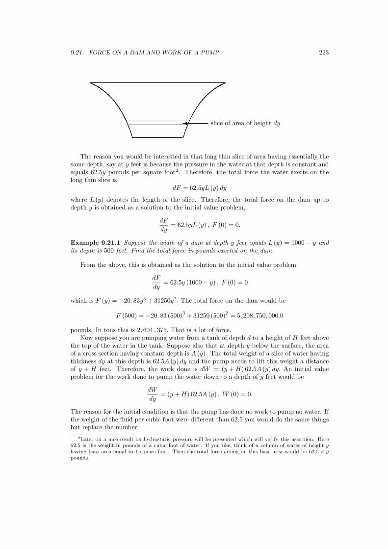
9.21. FORCE ON A DAM AND WORK OF A PUMP 223
¾ slice of area of height dy
The reason you would be interested in that long thin slice of area having essentially thesame depth, say at y feet is because the pressure in the water at that depth is constant andequals 62.5y pounds per square foot2. Therefore, the total force the water exerts on thelong thin slice is
dF = 62.5yL (y) dy
where L (y) denotes the length of the slice. Therefore, the total force on the dam up todepth y is obtained as a solution to the initial value problem,
dF
dy= 62.5yL (y) , F (0) = 0.
Example 9.21.1 Suppose the width of a dam at depth y feet equals L (y) = 1000 − y andits depth is 500 feet. Find the total force in pounds exerted on the dam.
From the above, this is obtained as the solution to the initial value problem
dF
dy= 62.5y (1000− y) , F (0) = 0
which is F (y) = −20. 83y3 + 31250y2. The total force on the dam would be
F (500) = −20. 83 (500)3 + 31250 (500)2 = 5, 208, 750, 000.0
pounds. In tons this is 2, 604 , 375. That is a lot of force.Now suppose you are pumping water from a tank of depth d to a height of H feet above
the top of the water in the tank. Suppose also that at depth y below the surface, the areaof a cross section having constant depth is A (y) . The total weight of a slice of water havingthickness dy at this depth is 62.5A (y) dy and the pump needs to lift this weight a distanceof y + H feet. Therefore, the work done is dW = (y + H) 62.5A (y) dy. An initial valueproblem for the work done to pump the water down to a depth of y feet would be
dW
dy= (y + H) 62.5A (y) , W (0) = 0.
The reason for the initial condition is that the pump has done no work to pump no water. Ifthe weight of the fluid per cubic foot were different than 62.5 you would do the same thingsbut replace the number.
2Later on a nice result on hydrostatic pressure will be presented which will verify this assertion. Here62.5 is the weight in pounds of a cubic foot of water. If you like, think of a column of water of height yhaving base area equal to 1 square foot. Then the total force acting on this base area would be 62.5 × ypounds.

224 ANTIDERIVATIVES AND DIFFERENTIAL EQUATIONS
Example 9.21.2 A spherical storage tank sitting on the ground having radius 30 feet ishalf filled with a fluid which weighs 50 pounds per cubic foot. How much work is done topump this fluid to a height of 100 feet?
Letting r denote the radius of a cross section y feet below the level of the fluid, r2 +y2 =900. Therefore,
r =√
900− y2.
It follows the area of the cross section at depth y is π(900− y2
). Here H = 70 and so the
initial value problem to solve is
dW
dy= (y + 70) 50π
(900− y2
), W (0) = 0.
Therefore, W (y) = 50π(− 1
4y4 − 703 y3 + 450y2 + 63 000y
)and the total work in foot pounds
equals
W (30) = 50π
(−1
4(30)4 − 70
3(30)3 + 450 (30)2 + 63 000 (30)
)= 73 , 125, 000π
9.22 Exercises
1. A cylindrical storage tank having radius 20 feet and length 40 feet is filled with a fluidwhich weighs 50 pounds per cubic foot. This tank is lying on its side on the ground.Find the total force acting on the ends of the tank by the fluid.
2. Suppose the tank in the above problem is filled to a depth of 8 feet. Find the workneeded to pump the fluid to a height of 50 feet.
3. A conical hole is filled with water. If the depth of the hole is 20 feet and the radius ofthe hole is 10 feet, how much work is needed to pump the water to a height of 10 feetabove the ground?
4. A dam 500 feet high has a width at depth y equal to 4000− 2y feet. What is the totalforce on the dam if it is filled?
5. When the bucket is filled with water it weighs 30 pounds and when empty it weighs2 pounds and the person on top of a 100 foot building exerts a constant force of 40pounds. The bucket is full at the bottom but leaks at the rate of .1 cubic feet persecond. How much work does the person on the top of the building do in lifting thebucket to the top? Will the bucket be empty when it reaches the top? You can useNewton’s law that force equals mass times acceleration.
6. In the situation of the above problem, suppose the person on the top maintains aconstant velocity of 1 foot per second. How much work does he do and is the bucketempty when it reaches the top?
7. A silo is 10 feet in diameter and at a height of 30 feet there is a hemispherical top.The silage weighs 10 pounds per cubic foot. How much work was done in filling it tothe very top?
8. A cylindrical storage tank having radius 10 feet is filled with water to a depth of 20feet. If the storage tank stands upright on its circular base, what is the total force thewater exerts on the sides of the tank? Hint: The pressure in the water at depth y is62.5y pounds per square foot.

9.22. EXERCISES 225
9. A spherical storage tank having radius 10 feet is filled with water. What is the totalforce the water exerts on the storage tank? Hint: The pressure in the water at depthy is 62.5y consider the area corresponding to a slice at height y. This is a surface ofrevolution and you know how to deal with these.

226 ANTIDERIVATIVES AND DIFFERENTIAL EQUATIONS

The Integral
The integral originated in attempts to find areas of various shapes and the ideas involvedin finding integrals are much older than the ideas related to finding derivatives. In fact,Archimedes1 was finding areas of various curved shapes about 250 B.C. The integral isneeded to remove some of the mathematical loose ends and also to enable the study of moregeneral problems involving differential equations. It will also be useful for formulating otherphysical models. The technique used for finding the area of a circular segment presentedearly in the book was essentially that employed by Archimedes and contains the essentialideas for the integral. The main difference is that here the triangles will be replaced withrectangles. You may be wondering what the fuss is about. Areas have already been foundas solutions of differential equations. However, there is a profound difference between whatis about to be presented and what has just been done. It is related to the fundamentalmathematical question of existence. As an illustration, consider the problem of finding thearea between y = ex2
and the x axis for x ∈ [0, 1] . As pointed out earlier, the area isobtained as a solution to the initial value problem,
A′ (x) = ex2, A (0) = 0.
So what is the solution to this initial value problem? By Theorem 9.1.1 there is at most onesolution, but what is the solution? Does it even exist? More generally, for which functions,f does there exist a solution to the initial value problem, y′ (x) = f (x) , y (0) = y0? Thesequestions are typical of mathematics. There are usually two aspects to a mathematicalconcept. One is the question of existence and the other is how to find that which exists.The two questions are often very different and one can have a good understanding of onewithout having any idea how to go about considering the other. However, both are absolutelyessential. In the preceding chapter the only thing considered was the second question.
10.1 Upper And Lower Sums
The Riemann integral pertains to bounded functions which are defined on a bounded in-terval. Let [a, b] be a closed interval. A set of points in [a, b], x0, · · ·, xn is a partitionif
a = x0 < x1 < · · · < xn = b.
1Archimedes 287-212 B.C. found areas of curved regions by stuffing them with simple shapes which heknew the area of and taking a limit. He also made fundamental contributions to physics. The story is toldabout how he determined that a gold smith had cheated the king by giving him a crown which was notsolid gold as had been claimed. He did this by finding the amount of water displaced by the crown andcomparing with the amount of water it should have displaced if it had been solid gold.
227

228 THE INTEGRAL
Such partitions are denoted by P or Q. For f a bounded function defined on [a, b] , let
Mi (f) ≡ supf (x) : x ∈ [xi−1, xi],mi (f) ≡ inff (x) : x ∈ [xi−1, xi].
Also let ∆xi ≡ xi − xi−1. Then define upper and lower sums as
U (f, P ) ≡n∑
i=1
Mi (f)∆xi and L (f, P ) ≡n∑
i=1
mi (f) ∆xi
respectively. The numbers, Mi (f) and mi (f) , are well defined real numbers because f isassumed to be bounded and R is complete. Thus the set S = f (x) : x ∈ [xi−1, xi] isbounded above and below. In the following picture, the sum of the areas of the rectanglesin the picture on the left is a lower sum for the function in the picture and the sum of theareas of the rectangles in the picture on the right is an upper sum for the same functionwhich uses the same partition.
y = f(x)
x0 x1 x2 x3 x0 x1 x2 x3
What happens when you add in more points in a partition? The following picturesillustrate in the context of the above example. In this example a single additional point,labeled z has been added in.
y = f(x)
x0 x1 x2 x3z x0 x1 x2 x3z
Note how the lower sum got larger by the amount of the area in the shaded rectangleand the upper sum got smaller by the amount in the rectangle shaded by dots. In generalthis is the way it works and this is shown in the following lemma.
Lemma 10.1.1 If P ⊆ Q then
U (f,Q) ≤ U (f, P ) , and L (f, P ) ≤ L (f,Q) .
Proof: This is verified by adding in one point at a time. Thus let P = x0, · · ·, xnand let Q = x0, · · ·, xk, y, xk+1, · · ·, xn. Thus exactly one point, y, is added between xk

10.1. UPPER AND LOWER SUMS 229
and xk+1. Now the term in the upper sum which corresponds to the interval [xk, xk+1] inU (f, P ) is
sup f (x) : x ∈ [xk, xk+1] (xk+1 − xk) (10.1)
and the term which corresponds to the interval [xk, xk+1] in U (f, Q) is
sup f (x) : x ∈ [xk, y] (y − xk) + sup f (x) : x ∈ [y, xk+1] (xk+1 − y) (10.2)≡ M1 (y − xk) + M2 (xk+1 − y) (10.3)
All the other terms in the two sums coincide. Now sup f (x) : x ∈ [xk, xk+1] ≥ max (M1, M2)and so the expression in (10.2) is no larger than
sup f (x) : x ∈ [xk, xk+1] (xk+1 − y) + sup f (x) : x ∈ [xk, xk+1] (y − xk)
= sup f (x) : x ∈ [xk, xk+1] (xk+1 − xk) ,
the term corresponding to the interval, [xk, xk+1] and U (f, P ) . This proves the first part ofthe lemma pertaining to upper sums because if Q ⊇ P, one can obtain Q from P by addingin one point at a time and each time a point is added, the corresponding upper sum eithergets smaller or stays the same. The second part is similar and is left as an exercise.
Lemma 10.1.2 If P and Q are two partitions, then
L (f, P ) ≤ U (f, Q) .
Proof: By Lemma 10.1.1,
L (f, P ) ≤ L (f, P ∪Q) ≤ U (f, P ∪Q) ≤ U (f, Q) .
Definition 10.1.3I ≡ infU (f,Q) where Q is a partitionI ≡ supL (f, P ) where P is a partition.
Note that I and I are well defined real numbers.
Theorem 10.1.4 I ≤ I.
Proof: From Lemma 10.1.2,
I = supL (f, P ) where P is a partition ≤ U (f,Q)
because U (f, Q) is an upper bound to the set of all lower sums and so it is no smaller thanthe least upper bound. Therefore, since Q is arbitrary,
I = supL (f, P ) where P is a partition≤ infU (f,Q) where Q is a partition ≡ I
where the inequality holds because it was just shown that I is a lower bound to the set ofall upper sums and so it is no larger than the greatest lower bound of this set. This provesthe theorem.
Definition 10.1.5 A bounded function f is Riemann integrable, written as
f ∈ R ([a, b])
ifI = I
and in this case, ∫ b
a
f (x) dx ≡ I = I.

230 THE INTEGRAL
Thus, in words, the Riemann integral is the unique number which lies between all uppersums and all lower sums if there is such a unique number.
Recall Proposition 2.14.3. It is stated here for ease of reference.
Proposition 10.1.6 Let S be a nonempty set and suppose sup (S) exists. Then for everyδ > 0,
S ∩ (sup (S)− δ, sup (S)] 6= ∅.If inf (S) exists, then for every δ > 0,
S ∩ [inf (S) , inf (S) + δ) 6= ∅.
This proposition implies the following theorem which is used to determine the questionof Riemann integrability.
Theorem 10.1.7 A bounded function f is Riemann integrable if and only if for all ε > 0,there exists a partition P such that
U (f, P )− L (f, P ) < ε. (10.4)
Proof: First assume f is Riemann integrable. Then let P and Q be two partitions suchthat
U (f,Q) < I + ε/2, L (f, P ) > I − ε/2.
Then since I = I,
U (f, Q ∪ P )− L (f, P ∪Q) ≤ U (f, Q)− L (f, P ) < I + ε/2− (I − ε/2) = ε.
Now suppose that for all ε > 0 there exists a partition such that (10.4) holds. Then forgiven ε and partition P corresponding to ε
I − I ≤ U (f, P )− L (f, P ) ≤ ε.
Since ε is arbitrary, this shows I = I and this proves the theorem.The condition described in the theorem is called the Riemann criterion .Not all bounded functions are Riemann integrable. For example, let
f (x) ≡
1 if x ∈ Q0 if x ∈ R \Q (10.5)
Then if [a, b] = [0, 1] all upper sums for f equal 1 while all lower sums for f equal 0. Thereforethe Riemann criterion is violated for ε = 1/2.
10.2 Exercises
1. Prove the second half of Lemma 10.1.1 about lower sums.
2. Verify that for f given in (10.5), the lower sums on the interval [0, 1] are all equal tozero while the upper sums are all equal to one.
3. Let f (x) = 1 + x2 for x ∈ [−1, 3] and let P =−1,− 1
3 , 0, 12 , 1, 2
. Find U (f, P ) and
L (f, P ) .

10.3. FUNCTIONS OF RIEMANN INTEGRABLE FUNCTIONS 231
4. Show that if f ∈ R ([a, b]), there exists a partition, x0, · · ·, xn such that for anyzk ∈ [xk, xk+1] , ∣∣∣∣∣
∫ b
a
f (x) dx−n∑
k=1
f (zk) (xk − xk−1)
∣∣∣∣∣ < ε
This sum,∑n
k=1 f (zk) (xk − xk−1) , is called a Riemann sum and this exercise showsthat the integral can always be approximated by a Riemann sum.
5. Let P =1, 1 1
4 , 112 , 13
4 , 2. Find upper and lower sums for the function, f (x) = 1
xusing this partition. What does this tell you about ln (2)?
6. If f ∈ R ([a, b]) and f is changed at finitely many points, show the new function isalso in R ([a, b]) .
7. Define a “left sum” asn∑
k=1
f (xk−1) (xk − xk−1)
and a “right sum”,n∑
k=1
f (xk) (xk − xk−1) .
Also suppose that all partitions have the property that xk − xk−1 equals a constant,(b− a) /n so the points in the partition are equally spaced, and define the integralto be the number these right and left sums get close to as n gets larger and larger.Show that for f given in (10.5),
∫ x
0f (t) dt = 1 if x is rational and
∫ x
0f (t) dt = 0 if
x is irrational. It turns out that the correct answer should always equal zero for thatfunction, regardless of whether x is rational. This is shown in more advanced courseswhen the Lebesgue integral is studied. This illustrates why this method of definingthe integral in terms of left and right sums is total nonsense.
10.3 Functions Of Riemann Integrable Functions
It is often necessary to consider functions of Riemann integrable functions and a naturalquestion is whether these are Riemann integrable. The following theorem gives a partialanswer to this question. This is not the most general theorem which will relate to thisquestion but it will be enough for the needs of this book.
Theorem 10.3.1 Let f, g be bounded functions and let f ([a, b]) ⊆ [c1, d1] and g ([a, b]) ⊆[c2, d2] . Let H : [c1, d1]× [c2, d2] → R satisfy,
|H (a1, b1)−H (a2, b2)| ≤ K [|a1 − a2|+ |b1 − b2|]
for some constant K. Then if f, g ∈ R ([a, b]) it follows that H (f, g) ∈ R ([a, b]) .
Proof: In the following claim, Mi (h) and mi (h) have the meanings assigned above withrespect to some partition of [a, b] for the function, h.
Claim: The following inequality holds.
|Mi (H (f, g))−mi (H (f, g))| ≤
K [|Mi (f)−mi (f)|+ |Mi (g)−mi (g)|] .

232 THE INTEGRAL
Proof of the claim: By the above proposition, there exist x1, x2 ∈ [xi−1, xi] be suchthat
H (f (x1) , g (x1)) + η > Mi (H (f, g)) ,
andH (f (x2) , g (x2))− η < mi (H (f, g)) .
Then|Mi (H (f, g))−mi (H (f, g))|
< 2η + |H (f (x1) , g (x1))−H (f (x2) , g (x2))|< 2η + K [|f (x1)− f (x2)|+ |g (x1)− g (x2)|]≤ 2η + K [|Mi (f)−mi (f)|+ |Mi (g)−mi (g)|] .
Since η > 0 is arbitrary, this proves the claim.Now continuing with the proof of the theorem, let P be such that
n∑
i=1
(Mi (f)−mi (f))∆xi <ε
2K,
n∑
i=1
(Mi (g)−mi (g))∆xi <ε
2K.
Then from the claim,
n∑
i=1
(Mi (H (f, g))−mi (H (f, g)))∆xi
<
n∑
i=1
K [|Mi (f)−mi (f)|+ |Mi (g)−mi (g)|]∆xi < ε.
Since ε > 0 is arbitrary, this shows H (f, g) satisfies the Riemann criterion and henceH (f, g) is Riemann integrable as claimed. This proves the theorem.
This theorem implies that if f, g are Riemann integrable, then so is af +bg, |f | , f2, alongwith infinitely many other such continuous combinations of Riemann integrable functions.For example, to see that |f | is Riemann integrable, let H (a, b) = |a| . Clearly this functionsatisfies the conditions of the above theorem and so |f | = H (f, f) ∈ R ([a, b]) as claimed.The following theorem gives an example of many functions which are Riemann integrable.
Theorem 10.3.2 Let f : [a, b] → R be either increasing or decreasing on [a, b]. Thenf ∈ R ([a, b]) .
Proof: Let ε > 0 be given and let
xi = a + i
(b− a
n
), i = 0, · · ·, n.
Then since f is increasing,
U (f, P )− L (f, P ) =n∑
i=1
(f (xi)− f (xi−1))(
b− a
n
)
= (f (b)− f (a))(
b− a
n
)< ε
whenever n is large enough. Thus the Riemann criterion is satisfied and so the function isRiemann integrable. The proof for decreasing f is similar.

10.4. PROPERTIES OF THE INTEGRAL 233
Corollary 10.3.3 Let [a, b] be a bounded closed interval and let φ : [a, b] → R be Lipschitzcontinuous. Then φ ∈ R ([a, b]) . Recall that a function, φ, is Lipschitz continuous if thereis a constant, K, such that for all x, y,
|φ (x)− φ (y)| < K |x− y| .
Proof: Let f (x) = x. Then by Theorem 10.3.2, f is Riemann integrable. Let H (a, b) ≡φ (a). Then by Theorem 10.3.1 H (f, f) = φ f = φ is also Riemann integrable. Thisproves the corollary.
In fact, it is enough to assume φ is continuous, although this is harder. This is thecontent of the next theorem which is where the difficult theorems about continuity anduniform continuity are used.
Theorem 10.3.4 Suppose f : [a, b] → R is continuous. Then f ∈ R ([a, b]) .
Proof: By Corollary 5.13.5 on Page 114, f is uniformly continuous on [a, b] . Therefore,if ε > 0 is given, there exists a δ > 0 such that if |xi − xi−1| < δ, then Mi −mi < ε
b−a . Let
P ≡ x0, · · ·, xn
be a partition with |xi − xi−1| < δ. Then
U (f, P )− L (f, P ) <
n∑
i=1
(Mi −mi) (xi − xi−1) <ε
b− a(b− a) = ε.
By the Riemann criterion, f ∈ R ([a, b]) . This proves the theorem.
10.4 Properties Of The Integral
The integral has many important algebraic properties. First here is a simple lemma.
Lemma 10.4.1 Let S be a nonempty set which is bounded above and below. Then if −S ≡−x : x ∈ S ,
sup (−S) = − inf (S) (10.6)
andinf (−S) = − sup (S) . (10.7)
Proof: Consider (10.6). Let x ∈ S. Then −x ≤ sup (−S) and so x ≥ − sup (−S) . Iffollows that − sup (−S) is a lower bound for S and therefore, − sup (−S) ≤ inf (S) . Thisimplies sup (−S) ≥ − inf (S) . Now let −x ∈ −S. Then x ∈ S and so x ≥ inf (S) whichimplies −x ≤ − inf (S) . Therefore, − inf (S) is an upper bound for −S and so − inf (S) ≥sup (−S) . This shows (10.6). Formula (10.7) is similar and is left as an exercise.
In particular, the above lemma implies that for Mi (f) and mi (f) defined above Mi (−f) =−mi (f) , and mi (−f) = −Mi (f) .
Lemma 10.4.2 If f ∈ R ([a, b]) then −f ∈ R ([a, b]) and
−∫ b
a
f (x) dx =∫ b
a
−f (x) dx.

234 THE INTEGRAL
Proof: The first part of the conclusion of this lemma follows from Theorem 10.3.2 sincethe function φ (y) ≡ −y is Lipschitz continuous. Now choose P such that
∫ b
a
−f (x) dx− L (−f, P ) < ε.
Then since mi (−f) = −Mi (f) ,
ε >
∫ b
a
−f (x) dx−n∑
i=1
mi (−f)∆xi =∫ b
a
−f (x) dx +n∑
i=1
Mi (f)∆xi
which implies
ε >
∫ b
a
−f (x) dx +n∑
i=1
Mi (f) ∆xi ≥∫ b
a
−f (x) dx +∫ b
a
f (x) dx.
Thus, since ε is arbitrary, ∫ b
a
−f (x) dx ≤ −∫ b
a
f (x) dx
whenever f ∈ R ([a, b]) . It follows
∫ b
a
−f (x) dx ≤ −∫ b
a
f (x) dx = −∫ b
a
− (−f (x)) dx ≤∫ b
a
−f (x) dx
and this proves the lemma.
Theorem 10.4.3 The integral is linear,∫ b
a
(αf + βg) (x) dx = α
∫ b
a
f (x) dx + β
∫ b
a
g (x) dx.
whenever f, g ∈ R ([a, b]) and α, β ∈ R.
Proof: First note that by Theorem 10.3.1, αf +βg ∈ R ([a, b]) . To begin with, considerthe claim that if f, g ∈ R ([a, b]) then
∫ b
a
(f + g) (x) dx =∫ b
a
f (x) dx +∫ b
a
g (x) dx. (10.8)
Let P1,Q1 be such that
U (f,Q1)− L (f,Q1) < ε/2, U (g, P1)− L (g, P1) < ε/2.
Then letting P ≡ P1 ∪Q1, Lemma 10.1.1 implies
U (f, P )− L (f, P ) < ε/2, and U (g, P )− U (g, P ) < ε/2.
Next note that
mi (f + g) ≥ mi (f) + mi (g) , Mi (f + g) ≤ Mi (f) + Mi (g) .
Therefore,
L (g + f, P ) ≥ L (f, P ) + L (g, P ) , U (g + f, P ) ≤ U (f, P ) + U (g, P ) .

10.4. PROPERTIES OF THE INTEGRAL 235
For this partition,
∫ b
a
(f + g) (x) dx ∈ [L (f + g, P ) , U (f + g, P )]
⊆ [L (f, P ) + L (g, P ) , U (f, P ) + U (g, P )]
and ∫ b
a
f (x) dx +∫ b
a
g (x) dx ∈ [L (f, P ) + L (g, P ) , U (f, P ) + U (g, P )] .
Therefore, ∣∣∣∣∣∫ b
a
(f + g) (x) dx−(∫ b
a
f (x) dx +∫ b
a
g (x) dx
)∣∣∣∣∣ ≤
U (f, P ) + U (g, P )− (L (f, P ) + L (g, P )) < ε/2 + ε/2 = ε.
This proves (10.8) since ε is arbitrary.It remains to show that
α
∫ b
a
f (x) dx =∫ b
a
αf (x) dx.
Suppose first that α ≥ 0. Then
∫ b
a
αf (x) dx ≡ supL (αf, P ) : P is a partition =
α supL (f, P ) : P is a partition ≡ α
∫ b
a
f (x) dx.
If α < 0, then this and Lemma 10.4.2 imply
∫ b
a
αf (x) dx =∫ b
a
(−α) (−f (x)) dx
= (−α)∫ b
a
(−f (x)) dx = α
∫ b
a
f (x) dx.
This proves the theorem.
Theorem 10.4.4 If f ∈ R ([a, b]) and f ∈ R ([b, c]) , then f ∈ R ([a, c]) and
∫ c
a
f (x) dx =∫ b
a
f (x) dx +∫ c
b
f (x) dx. (10.9)
Proof: Let P1 be a partition of [a, b] and P2 be a partition of [b, c] such that
U (f, Pi)− L (f, Pi) < ε/2, i = 1, 2.
Let P ≡ P1 ∪ P2. Then P is a partition of [a, c] and
U (f, P )− L (f, P )
= U (f, P1)− L (f, P1) + U (f, P2)− L (f, P2) < ε/2 + ε/2 = ε. (10.10)

236 THE INTEGRAL
Thus, f ∈ R ([a, c]) by the Riemann criterion and also for this partition,
∫ b
a
f (x) dx +∫ c
b
f (x) dx ∈ [L (f, P1) + L (f, P2) , U (f, P1) + U (f, P2)]
= [L (f, P ) , U (f, P )]
and ∫ c
a
f (x) dx ∈ [L (f, P ) , U (f, P )] .
Hence by (10.10),∣∣∣∣∣∫ c
a
f (x) dx−(∫ b
a
f (x) dx +∫ c
b
f (x) dx
)∣∣∣∣∣ < U (f, P )− L (f, P ) < ε
which shows that since ε is arbitrary, (10.9) holds. This proves the theorem.
Corollary 10.4.5 Let [a, b] be a closed and bounded interval and suppose that
a = y1 < y2 · ·· < yl = b
and that f is a bounded function defined on [a, b] which has the property that f is eitherincreasing on [yj , yj+1] or decreasing on [yj , yj+1] for j = 1, · · ·, l − 1. Then f ∈ R ([a, b]) .
Proof: This follows from Theorem 10.4.4 and Theorem 10.3.2.The symbol,
∫ b
af (x) dx when a > b has not yet been defined.
Definition 10.4.6 Let [a, b] be an interval and let f ∈ R ([a, b]) . Then
∫ a
b
f (x) dx ≡ −∫ b
a
f (x) dx.
Note that with this definition,∫ a
a
f (x) dx = −∫ a
a
f (x) dx
and so ∫ a
a
f (x) dx = 0.
Theorem 10.4.7 Assuming all the integrals make sense,
∫ b
a
f (x) dx +∫ c
b
f (x) dx =∫ c
a
f (x) dx.
Proof: This follows from Theorem 10.4.4 and Definition 10.4.6. For example, assume
c ∈ (a, b) .
Then from Theorem 10.4.4,
∫ c
a
f (x) dx +∫ b
c
f (x) dx =∫ b
a
f (x) dx

10.5. FUNDAMENTAL THEOREM OF CALCULUS 237
and so by Definition 10.4.6,∫ c
a
f (x) dx =∫ b
a
f (x) dx−∫ b
c
f (x) dx
=∫ b
a
f (x) dx +∫ c
b
f (x) dx.
The other cases are similar.The following properties of the integral have either been established or they follow quickly
from what has been shown so far.
If f ∈ R ([a, b]) then if c ∈ [a, b] , f ∈ R ([a, c]) , (10.11)∫ b
a
α dx = α (b− a) , (10.12)
∫ b
a
(αf + βg) (x) dx = α
∫ b
a
f (x) dx + β
∫ b
a
g (x) dx, (10.13)
∫ b
a
f (x) dx +∫ c
b
f (x) dx =∫ c
a
f (x) dx, (10.14)
∫ b
a
f (x) dx ≥ 0 if f (x) ≥ 0 and a < b, (10.15)∣∣∣∣∣∫ b
a
f (x) dx
∣∣∣∣∣ ≤∣∣∣∣∣∫ b
a
|f (x)| dx
∣∣∣∣∣ . (10.16)
The only one of these claims which may not be completely obvious is the last one. To showthis one, note that
|f (x)| − f (x) ≥ 0, |f (x)|+ f (x) ≥ 0.
Therefore, by (10.15) and (10.13), if a < b,∫ b
a
|f (x)| dx ≥∫ b
a
f (x) dx
and ∫ b
a
|f (x)| dx ≥ −∫ b
a
f (x) dx.
Therefore, ∫ b
a
|f (x)| dx ≥∣∣∣∣∣∫ b
a
f (x) dx
∣∣∣∣∣ .
If b < a then the above inequality holds with a and b switched. This implies (10.16).
10.5 Fundamental Theorem Of Calculus
With these properties, it is easy to prove the fundamental theorem of calculus2. Letf ∈ R ([a, b]) . Then by (10.11) f ∈ R ([a, x]) for each x ∈ [a, b] . The first version of thefundamental theorem of calculus is a statement about the derivative of the function
x →∫ x
a
f (t) dt.
2This theorem is why Newton and Liebnitz are credited with inventing calculus. The integral had beenaround for thousands of years and the derivative was by their time well known. However the connectionbetween these two ideas had not been fully made although Newton’s predecessor, Isaac Barrow had madesome progress in this direction.

238 THE INTEGRAL
Theorem 10.5.1 Let f ∈ R ([a, b]) and let
F (x) ≡∫ x
a
f (t) dt.
Then if f is continuous at x ∈ (a, b) ,
F ′ (x) = f (x) .
Proof: Let x ∈ (a, b) be a point of continuity of f and let h be small enough thatx + h ∈ [a, b] . Then by using (10.14),
h−1 (F (x + h)− F (x)) = h−1
∫ x+h
x
f (t) dt.
Also, using (10.12),
f (x) = h−1
∫ x+h
x
f (x) dt.
Therefore, by (10.16),
∣∣h−1 (F (x + h)− F (x))− f (x)∣∣ =
∣∣∣∣∣h−1
∫ x+h
x
(f (t)− f (x)) dt
∣∣∣∣∣
≤∣∣∣∣∣h−1
∫ x+h
x
|f (t)− f (x)| dt
∣∣∣∣∣ .
Let ε > 0 and let δ > 0 be small enough that if |t− x| < δ, then
|f (t)− f (x)| < ε.
Therefore, if |h| < δ, the above inequality and (10.12) shows that∣∣h−1 (F (x + h)− F (x))− f (x)
∣∣ ≤ |h|−1ε |h| = ε.
Since ε > 0 is arbitrary, this shows
limh→0
h−1 (F (x + h)− F (x)) = f (x)
and this proves the theorem.Note this gives existence for the initial value problem,
F ′ (x) = f (x) , F (a) = 0
whenever f is Riemann integrable and continuous.3
The next theorem is also called the fundamental theorem of calculus.
Theorem 10.5.2 Let f ∈ R ([a, b]) and suppose there exists an antiderivative for f,G, suchthat
G′ (x) = f (x)
for every point of (a, b) and G is continuous on [a, b] . Then∫ b
a
f (x) dx = G (b)−G (a) . (10.17)
3Of course it was proved that if f is continuous on a closed interval, [a, b] , then f ∈ R ([a, b]) but this isa hard theorem using the difficult result about uniform continuity.

10.5. FUNDAMENTAL THEOREM OF CALCULUS 239
Proof: Let P = x0, · · ·, xn be a partition satisfying
U (f, P )− L (f, P ) < ε.
Then
G (b)−G (a) = G (xn)−G (x0)
=n∑
i=1
G (xi)−G (xi−1) .
By the mean value theorem,
G (b)−G (a) =n∑
i=1
G′ (zi) (xi − xi−1)
=n∑
i=1
f (zi)∆xi
where zi is some point in [xi−1, xi] . It follows, since the above sum lies between the upperand lower sums, that
G (b)−G (a) ∈ [L (f, P ) , U (f, P )] ,
and also ∫ b
a
f (x) dx ∈ [L (f, P ) , U (f, P )] .
Therefore, ∣∣∣∣∣G (b)−G (a)−∫ b
a
f (x) dx
∣∣∣∣∣ < U (f, P )− L (f, P ) < ε.
Since ε > 0 is arbitrary, (10.17) holds. This proves the theorem.The following notation is often used in this context. Suppose F is an antiderivative of f
as just described with F continuous on [a, b] and F ′ = f on (a, b) . Then
∫ b
a
f (x) dx = F (b)− F (a) ≡ F (x) |ba.
Definition 10.5.3 Let f be a bounded function defined on a closed interval [a, b] and letP ≡ x0, · · ·, xn be a partition of the interval. Suppose zi ∈ [xi−1, xi] is chosen. Then thesum
n∑
i=1
f (zi) (xi − xi−1)
is known as a Riemann sum. Also,
||P || ≡ max |xi − xi−1| : i = 1, · · ·, n .
Proposition 10.5.4 Suppose f ∈ R ([a, b]) . Then there exists a partition, P ≡ x0, · · ·, xnwith the property that for any choice of zk ∈ [xk−1, xk] ,
∣∣∣∣∣∫ b
a
f (x) dx−n∑
k=1
f (zk) (xk − xk−1)
∣∣∣∣∣ < ε.

240 THE INTEGRAL
Proof: Choose P such that U (f, P ) − L (f, P ) < ε and then both∫ b
af (x) dx and∑n
k=1 f (zk) (xk − xk−1) are contained in [L (f, P ) , U (f, P )] and so the claimed inequalitymust hold. This proves the proposition.
It is significant because it gives a way of approximating the integral.The definition of Riemann integrability given in this chapter is also called Darboux
integrability and the integral defined as the unique number which lies between all uppersums and all lower sums which is given in this chapter is called the Darboux integral . Thedefinition of the Riemann integral in terms of Riemann sums is given next.
Definition 10.5.5 A bounded function, f defined on [a, b] is said to be Riemann integrableif there exists a number, I with the property that for every ε > 0, there exists δ > 0 suchthat if
P ≡ x0, x1, · · ·, xnis any partition having ||P || < δ, and zi ∈ [xi−1, xi] ,
∣∣∣∣∣I −n∑
i=1
f (zi) (xi − xi−1)
∣∣∣∣∣ < ε.
The number∫ b
af (x) dx is defined as I.
Thus, there are two definitions of the Riemann integral. It turns out they are equivalentwhich is the following theorem of Darboux.
Theorem 10.5.6 A bounded function defined on [a, b] is Riemann integrable in the senseof Definition 10.5.5 if and only if it is integrable in the sense of Darboux. Furthermore thetwo integrals coincide.
The proof of this theorem is left for the exercises in Problems 10 - 12. It isn’t essentialthat you understand this theorem so if it does not interest you, leave it out. Note that itimplies that given a Riemann integrable function f in either sense, it can be approximatedby Riemann sums whenever ||P || is sufficiently small. Both versions of the integral areobsolete but entirely adequate for most applications and as a point of departure for a moreup to date and satisfactory integral. The reason for using the Darboux approach to theintegral is that all the existence theorems are easier to prove in this context.
10.6 Exercises
1. Let F (x) =∫ x3
x2t5+7
t7+87t6+1 dt. Find F ′ (x) .
2. Let F (x) =∫ x
21
1+t4 dt. Sketch a graph of F and explain why it looks the way it does.
3. Let a and b be positive numbers and consider the function,
F (x) =∫ ax
0
1a2 + t2
dt +∫ a/x
b
1a2 + t2
dt.
Show that F is a constant.
4. Solve the following initial value problem from ordinary differential equations which isto find a function y such that
y′ (x) =x7 + 1
x6 + 97x5 + 7, y (10) = 5.

10.7. RETURN OF THE WILD ASSUMPTION 241
5. If F, G ∈ ∫f (x) dx for all x ∈ R, show F (x) = G (x) + C for some constant, C. Use
this to give a different proof of the fundamental theorem of calculus which has for itsconclusion
∫ b
af (t) dt = G (b)−G (a) where G′ (x) = f (x) .
6. Suppose f is Riemann integrable on [a, b] and continuous. (In fact continuous impliesRiemann integrable.) Show there exists c ∈ (a, b) such that
f (c) =1
b− a
∫ b
a
f (x) dx.
Hint: You might consider the function F (x) ≡ ∫ x
af (t) dt and use the mean value
theorem for derivatives and the fundamental theorem of calculus.
7. Suppose f and g are continuous functions on [a, b] and that g (x) 6= 0 on (a, b) . Showthere exists c ∈ (a, b) such that
f (c)∫ b
a
g (x) dx =∫ b
a
f (x) g (x) dx.
Hint: Define F (x) ≡ ∫ x
af (t) g (t) dt and let G (x) ≡ ∫ x
ag (t) dt. Then use the Cauchy
mean value theorem on these two functions.
8. Consider the function
f (x) ≡
sin(
1x
)if x 6= 0
0 if x = 0 .
Is f Riemann integrable? Explain why or why not.
9. Prove the second part of Theorem 10.3.2 about decreasing functions.
10. Suppose f is a bounded function defined on [a, b] and |f (x)| < M for all x ∈ [a, b] . Nowlet Q be a partition having n points, x∗0, · · ·, x∗n and let P be any other partition.Show that
|U (f, P )− L (f, P )| ≤ 2Mn ||P ||+ |U (f, Q)− L (f, Q)| .
Hint: Write the sum for U (f, P ) − L (f, P ) and split this sum into two sums, thesum of terms for which [xi−1, xi] contains at least one point of Q, and terms for which[xi−1, xi] does not contain any points of Q. In the latter case, [xi−1, xi] must becontained in some interval,
[x∗k−1, x
∗k
]. Therefore, the sum of these terms should be
no larger than |U (f, Q)− L (f, Q)| .11. ↑ If ε > 0 is given and f is a Darboux integrable function defined on [a, b], show there
exists δ > 0 such that whenever ||P || < δ, then
|U (f, P )− L (f, P )| < ε.
12. ↑ Prove Theorem 10.5.6.
10.7 Return Of The Wild Assumption
The entire treatment of exponential functions and logarithms up till this time has beenbased on the Wild Assumption on Page 143. This was a totally unjustified assumptionthat exponential functions existed and were differentiable. Some pictures were drawn by a

242 THE INTEGRAL
computer as evidence. Based on this outrageous wild assumption, logarithms were defined.It is now possible to establish Wild Assumption 7.3.1.
Define
L1 (x) ≡∫ x
1
1t
dt. (10.18)
There is no problem in writing this integral because the function, f (t) = 1/t is decreas-ing.
Theorem 10.7.1 The function, L1 : (0,∞) → R satisfies the following properties.
L1 (xy) = L1 (x) + L1 (y) , L1 (1) = 0, (10.19)
The function, L1 is one to one and onto, strictly increasing, and its graph is concave down-ward. In addition to this, whenever m
n ∈ Q
L1
(n√
xm)
=m
nL1 (x) . (10.20)
Proof: Fix y > 0 and let
f (x) = L1 (xy)− (L1 (x) + L1 (y))
Then by Theorem 6.2.6 on Page 122 and the Fundamental theorem of calculus, Theorem10.5.1,
f ′ (x) = y
(1xy
)− 1
x= 0.
Therefore, by Corollary 6.8.4 on Page 133, f (x) is a constant. However, f (1) = 0 and sothis proves (10.19).
From the Fundamental theorem of calculus, Theorem 10.5.1, L′1 (x) = 1x > 0 and so L1 is
a strictly increasing function and is therefore one to one. Also the second derivative equals
L′′1 (x) =−1x2
< 0
showing that the graph of L1 is concave down.Now consider the assertion that L1 is onto. First note that from the definition, L1 (2) > 0.
In fact,L1 (2) ≥ 1/2
as can be seen by looking at a lower sum for∫ 2
1(1/t) dt. Now if x > 0
L1 (x× x) = L1x + L1x = 2L1x.
Also,
L1 ((x) (x) (x)) = L1 ((x) (x)) + L1 (x)= L1 (x) + L1 (x) + L1 (x)= 3L1 (x) .
Continuing in this way it follows that for any positive integer, n,
L1 (xn) = nL1 (x) . (10.21)

10.7. RETURN OF THE WILD ASSUMPTION 243
Therefore, L1 (x) achieves arbitrarily large values as x gets increasingly large because youcan take x = 2 in (10.21) and use the definition of L1 to verify that L1 (2) > 0. Now if x > 0
0 = L1
=1︷ ︸︸ ︷(1x
)(x)
= L1
(1x
)+ L1 (x)
showing that
L1
(x−1
)= L1
(1x
)= −L1x. (10.22)
You see that(
12
)n can be made as close to zero as desired by taking n sufficiently large.Also, from (10.21),
L1
(12n
)= nL1
(12
)= −nL1 (2)
showing that L1 (x) gets arbitrarily large in the negative direction provided that x is asufficiently small positive number. Since L1 is continuous, the intermediate value theoremmay be used to fill in all the numbers in between. Thus the picture of the graph of L1 lookslike the following
where the graph approaches the y axis as x gets close to 0.It only remains to verify the claim about raising x to a rational power. From (10.21)
and (10.22), for any integer, n, positive or negative,
L1 (xn) = nL1 (x) .
Therefore, letting m,n be integers,
mL1 (x) = L1 (xm) = L1
((n√
xm)n)
= nL1
(n√
xm)
and som
nL1 (x) = L1
(n√
xm)
.
This proves the theorem.Now Wild Assumption 7.3.1 on Page 143 can be fully justified.
Definition 10.7.2 For b > 0 define
expb (x) ≡ L−11 (xL1 (b)) . (10.23)
Proposition 10.7.3 The function just defined in (10.23) satisfies all conditions of WildAssumption 7.3.1 on Page 143 and L1 (b) = ln b as defined on Page 143.

244 THE INTEGRAL
Proof: First let x = mn where m and n are integers. To verify that expb (m/n) = n
√bm,
expb
(m
n
)≡ L−1
1
(m
nL1 (b)
)= L−1
1
(L1
(n√
bm))
= n√
bm
by (10.20).That expb (x) > 0 follows immediately from the definition of the inverse function. (L1
is defined on positive real numbers and so L−11 has values in the positive real numbers.)
Consider the claim that if h 6= 0 and b 6= 1, then expb (h) 6= 1. Suppose then thatexpb (h) = 1. Then doing L1 to both sides, hL1 (b) = L1 (1) = 0. Hence either h = 0 orb = 1 which are both excluded.
What of the laws of exponents for arbitrary values of x and y? As part of Wild Assump-tion 7.3.1, these were assumed to hold.
L1 (expb (x + y)) = (x + y)L1 (b)
and
L1 (expb (x) expb (y)) = L1 (expb (x)) + L1 (expb (y))= xL1 (b) + yL1 (b) = (x + y)L1 (b) .
Since L1 is one to one, this shows the first law of exponents holds,
expb (x + y) = expb (x) expb (y) .
From the definition, expb (1) = b and expb (0) = 1. Therefore,
1 = expb (1 + (−1)) = expb (−1) expb (1) = expb (−1) b
showing that expb (−1) = b−1. Now
L1 (expab (x)) = xL1 (ab) = xL1 (a) + xL1 (b)
while
L1 (expa (x) expb (x)) = L1 (expa (x)) + L1 (expb (x))= xL1 (a) + xL1 (b) .
Again, since L1 is one to one, expab (x) = expa (x) expb (x) . Finally,
L1
(expexpb(x) (y)
)= yL1 (expb (x)) = yxL1 (b)
whileL1 (expb (xy)) = xyL1 (b)
and so since L1 is one to one, expexpb(x) (y) = expb (xy) . This establishes all the laws ofexponents for arbitrary real values of the exponent.
exp′b exists by Theorem 8.1.6 on Page 151. Therefore, expb defined in (10.23) satisfiesall the conditions of Wild Assumption 7.3.1.
It remains to consider the derivative of expb and verify L1 (b) = ln b. First,
L1
(L−1
1 (x))
= x
and soL′1
(L−1
1 (x)) (
L−11
)′(x) = 1.

10.8. EXERCISES 245
By (10.18), (L−1
1
)′(x)
L−11 (x)
= 1
showing that(L−1
1
)′(x) =
(L−1
1
)(x). Now by the chain rule,
exp′b (x) =(L−1
1
)′(xL1 (b))L1 (b)
= L−11 (xL1 (b)) L1 (b)
= expb (x) L1 (b) .
From the definition of ln b on Page 143, it follows ln = L1.
10.8 Exercises
1. Show ln 2 ∈ [.5, 1] .
2. There is a general procedure for estimating the integral of a function, f (x) = y onan interval, [a, b] . Form a uniform partition, P = x0, x1, · · ·, xn where for eachj, xj − xj−1 = h. Let fi = f (xi) and assuming f ≥ 0 on the interval [xi−1, xi] ,approximate the area above this interval and under the curve with the area of atrapezoid having vertical sides, fi−1, and fi as shown in the following picture.
f0f1
h
Thus 12
(fi+fi−1
2
)approximates the area under the curve. Show that adding these up
yieldsh
2[f0 + 2f1 + · · ·+ 2fn−1 + fn]
as an approximation to∫ b
af (x) dx. This is known as the trapezoidal rule. Verify that
if f (x) = mx + b, the trapezoidal rule gives the exact answer for the integral. Wouldthis be true of upper and lower sums for such a function? Can you show that in thecase of the function, f(t) = 1/t the trapezoidal rule will always yield an answer whichis too large for ln 2?
3. Apply the trapezoidal rule to estimate ln 2 in the case where h = 1/5. Now use acalculator or table to find the exact value of ln 2.

246 THE INTEGRAL
4. Suppose it is desired to find a function, L : (0,∞) → R which satisfies
L (xy) = Lx + Ly, L(1) = 0. (10.24)
Show the only differentiable solutions to this equation are functions of the formLk (x) =
∫ x
1kt dt. Hint: Fix x > 0 and differentiate both sides of the above equa-
tion with respect to y. Then let y = 1.
5. Recall that ln e = 1. In fact, this was how e was defined in Problem ?? on Page ??.Show that
limy→0+
(1 + yx)1/y = ex.
Hint: Consider ln (1 + yx)1/y = 1y ln (1 + yx) = 1
y
∫ 1+yx
11t dt, use upper and lower
sums and then the squeezing theorem to verify ln (1 + yx)1/y → x. Recall that x → ex
is continuous.
6. Let there be three equally spaced points, xi−1, xi−1 + h ≡ xi, and xi + 2h ≡ xi+1.Suppose also a function, f, has the value fi−1 at x, fi at x + h, and fi+1 at x + 2h.Then consider
gi (x) ≡ fi−1
2h2(x− xi) (x− xi+1)− fi
h2(x− xi−1) (x− xi+1)+
fi+1
2h2(x− xi−1) (x− xi) .
Check that this is a second degree polynomial which equals the values fi−1, fi, andfi+1 at the points xi−1, xi, and xi+1 respectively. The function, gi is an approximationto the function, f on the interval [xi−1, xi+1] . Also,
∫ xi+1
xi−1
gi (x) dx
is an approximation to∫ xi+1
xi−1f (x) dx. Show
∫ xi+1
xi−1gi (x) dx equals
hfi−1
3+
hfi43
+hfi+1
3.
Now suppose n is even and x0, x1, · · ·, xn is a partition of the interval, [a, b] andthe values of a function, f defined on this interval are fi = f (xi) . Adding theseapproximations for the integral of f on the succession of intervals,
[x0, x2] , [x2, x4] , · · ·, [xn−2, xn] ,
show that an approximation to∫ b
af (x) dx is
h
3[f0 + 4f1 + 2f2 + 4f3 + 2f2 + · · ·+ 4fn−1 + fn] .
This is called Simpson’s rule. Use Simpson’s rule to compute an approximation to ln 2letting n = 4. Compare with the answer from a calculator or computer.
7. Logarithms were invented before calculus, one of the inventors being Napier, a Scottishnobleman. His interest in logarithms was computational. Describe how one could uselogarithms to find 7th roots for example. Also describe how one could use logarithmsto do computations involving large numbers. Describe how you could construct atable for log10 x for x various numbers. Next, how do you suppose Napier did it?Remember, he did not have calculus. Hint: logb
(351/7
)= 1
7 logb (35) . You can findthe logarithm of the number you are after. If you had a table of logarithms to somebase, you could then see what number this corresponded to.

10.9. TECHNIQUES OF INTEGRATION 247
10.9 Techniques Of Integration
The techniques for finding antiderivatives may be used to find integrals.
10.9.1 The Method Of Substitution
Recall ∫f (g (x)) g′ (x) dx = F (x) + C, (10.25)
where F ′ (y) = f (y) .How does this relate to finding definite integrals? This is based on the following formula
in which all the functions are integrable and F ′ (y) = f (y) .
∫ b
a
f (g (x)) g′ (x) dx =∫ g(b)
g(a)
f (y) dy. (10.26)
This formula follows from the observation that, by the fundamental theorem of calculus,both sides equal F (g (b))− F (g (a)) .
How can you remember this? The easiest way is to use the Leibniz notation. In (10.26)let y = g (x) . Then
dy
dx= g′ (x)
and so formally dy = g′ (x) dx. Then making the substitution
∫ b
a
f(y)︷ ︸︸ ︷f (g (x))
dy︷ ︸︸ ︷g′ (x) dx =
∫ ?
?
f (y) dy.
What should go in as the top and bottom limits of the integral? The important thing toremember is that if you change the variable, you must change the limits! Whenx = a, it follows that y = g (a) to the bottom limit must equal g (a) . Similarly the top limitshould be g (b) .
Example 10.9.1 Find∫ 2
1x sin
(x2
)dx
Let u = x2 so du = 2x dx and so du2 = x dx. Therefore, changing the variables gives
∫ 2
1
x sin(x2
)dx =
12
∫ 4
1
sin (u) du = −12
cos (4) +12
cos (1)
Sometimes people prefer not to worry about the limits. This is fine provided you don’t writeanything which is false. The above problem can be done in the following way.
∫x sin
(x2
)dx = −1
2cos
(x2
)+ C
and so from an application of the fundamental theorem of calculus
∫ 2
1
x sin(x2
)dx = −1
2cos
(x2
) |21
= −12
cos (4) +12
cos (1) .

248 THE INTEGRAL
Example 10.9.2 Find the area of the ellipse,
(y − β)2
b2+
(x− α)2
a2= 1.
If you sketch the ellipse, you see that it suffices to find the area of the top right quarterfor y ≥ β and x ≥ α and multiply by 4 since the bottom half is just a reflection of the tophalf about the line, y = β and the left top quarter is just the reflection of the top rightquarter reflected about the line, x = α. Thus the area of the ellipse is
4∫ α+a
α
b
√1− (x− α)2
a2dx
Change the variables, letting u = x−αa . Then du = 1
a dx and so upon changing the limits tocorrespond to the new variables, this equals
4ba
π/4︷ ︸︸ ︷∫ 1
0
√1− u2 du = 4× ab× 1
4π = πab
because the integral in the above is just one quarter of the unit circle and so has area equalto π/4.
10.9.2 Integration By Parts
Recall the following proposition for finding antiderivative.
Proposition 10.9.3 Let u and v be differentiable functions for which∫
u (x) v′ (x) dx and∫u′ (x) v (x) dx are nonempty. Then
uv −∫
u′ (x) v (x) dx =∫
u (x) v′ (x) dx. (10.27)
In terms of integrals, this is stated in the following proposition.
Proposition 10.9.4 Let u and v be differentiable functions on [a, b] such that uv′, u′v ∈R ([a, b]) . Then ∫ b
a
u (x) v′ (x) dx = uv (x) |ba −∫ b
a
u′ (x) v (x) dx (10.28)
Proof: Use the product rule and properties of integrals to write∫ b
a
u (x) v′ (x) dx =∫ b
a
(uv)′ (x) dx−∫ b
a
u′ (x) v (x) dx
= uv (x) |ba −∫ b
a
u′ (x) v (x) dx.
This proves the proposition.
Example 10.9.5 Find∫ π
0x sin (x) dx
Let u (x) = x and v′ (x) = sin (x) . Then applying (10.27),∫ π
0
x sin (x) dx = (− cos (x)) x|π0 −∫ π
0
(− cos (x)) dx
= −π cos (π) = π.

10.10. EXERCISES 249
Example 10.9.6 Find∫ 1
0xe2x dx
Let u (x) = x and v′ (x) = e2x. Then from (10.28)
∫ 1
0
xe2x dx =e2x
2x|10 −
∫ 1
0
e2x
2dx
=e2x
2x|10 −
e2x
4|10
=e2
2−
(e2
4− 1
4
)
=e2
4+
14
10.10 Exercises
1. Find the integrals.
(a)∫ 4
0xe−3x dx
(b)∫ 3
21
x(ln(|x|))2 dx
(c)∫ 1
0x√
2− x dx
(d)∫ 3
2(ln |x|)2 dx Hint: Let u (x) = (ln |x|)2 and v′ (x) = 1.
(e)∫ π
0x3 cos
(x2
)dx
2. Find∫ 2
1x ln
(x2
)dx
3. Find∫ 1
0ex sin (x) dx
4. Find∫ 1
02x cos (x) dx
5. Find∫ 2
0x3 cos (x) dx
6. Find the integrals.
(a)∫ 6
5x√
2x−3dx
(b)∫ 4
2x
(3x2 + 6
)5dx
(c)∫ π
0x sin
(x2
)dx
(d)∫ π/4
0sin3 (2x) cos (2x)
(e)∫ 7
01√
1+4x2 dx Hint: Remember the sinh−1 function and its derivative.
7. Find the integrals.
(a)∫ π/9
0sec (3x) dx
(b)∫ π/9
0sec2 (3x) tan (3x) dx
(c)∫ 5
01
3+5x2 dx
(d)∫ 1
01√
5−4x2 dx

250 THE INTEGRAL
(e)∫ 6
23
x√
4x2−5dx
8. Find the integrals.
(a)∫ 3
0x cosh
(x2 + 1
)dx
(b)∫ 2
0x35x4
dx
(c)∫ π
−πsin (x) 7cos(x) dx
(d)∫ π
0x sin
(x2
)dx
(e)∫ 2
1x5√
2x2 + 1 dx Hint: Let u = 2x2 + 1.
9. Find∫ π/4
0sin2 (x) dx. Hint: Derive and use sin2 (x) = 1−cos(2x)
2 .
10. Find the area between the graphs of y = sin (2x) and y = cos (2x) for x ∈ [0, 2π] .
11. Find the following integrals.
(a)∫ π
1x2 sin
(x3
)dx
(b)∫ 6
1x
1+x2 dx
(c)∫ .5
01
1+4x2 dx
(d)∫ 4
1x2√
1 + x dx
12. The most important of all differential equations is the first order linear equation,y′ + p (t) y = f (t) . Show the solution to the initial value problem consisting of thisequation and the initial condition, y (a) = ya is
y (t) = e−P (t)ya + e−P (t)
∫ t
a
eP (s)f (s) ds,
where P (t) =∫ t
ap (s) ds. Give conditions under which everything is correct. Hint:
You use the integrating factor approach. Multiply both sides by eP (t), verify the leftside equals
d
dt
(eP (t)y (t)
),
and then take the integral,∫ t
aof both sides.
13. Suppose x0 ∈ (a, b) and that f is a function which has n+1 continuous derivatives onthis interval. Consider the following.
f (x) = f (x0) +∫ x
x0
f ′ (t) dt
= f (x0) + (t− x) f ′ (t) |xx0+
∫ x
x0
(x− t) f ′′ (t) dt
= f (x0) + f ′ (x0) (x− x0) +∫ x
x0
(x− t) f ′′ (t) dt.
Explain the above steps and continue the process to eventually obtain Taylor’s formula,
f (x) = f (x0) +n∑
k=1
f (k) (x0)k!
(x− x0)k +
1n!
∫ x
x0
(x− t)nf (n+1) (t) dt
where n! ≡ n (n− 1) · · · 3 · 2 · 1 if n ≥ 1 and 0! ≡ 1.

10.10. EXERCISES 251
14. In the above Taylor’s formula, use Problem 7 on Page 241 to obtain the existence ofsome z between x0 and x such that
f (x) = f (x0) +n∑
k=1
f (k) (x0)k!
(x− x0)k +
f (n+1) (z)(n + 1)!
(x− x0)n+1
.
Hint: You might consider two cases, the case when x > x0 and the case when x < x0.
15. There is a general procedure for constructing these methods of approximate integrationlike the trapezoidal rule and Simpson’s rule. Consider [0, 1] and divide this intervalinto n pieces using a uniform partition, x0, · · ·, xn where xi − xi−1 = 1/n for eachi. The approximate integration scheme for a function, f, will be of the form
(1n
) n∑
i=0
cifi ≈∫ 1
0
f (x) dx
where fi = f (xi) and the constants, ci are chosen in such a way that the above sumgives the exact answer for
∫ 1
0f (x) dx where f (x) = 1, x, x2, · · ·, xn. When this has
been done, change variables to write
∫ b
a
f (y) dy = (b− a)∫ 1
0
f (a + (b− a) x) dx
≈ b− a
n
n∑
i=1
cif
(a + (b− a)
(i
n
))
=b− a
n
n∑
i=1
cifi
where fi = f(a + (b− a)
(in
)). Consider the case where n = 1. It is necessary to find
constants c0 and c1 such that
c0 + c1 = 1 =∫ 1
01 dx
0c0 + c1 = 1/2 =∫ 1
0x dx.
Show that c0 = c1 = 1/2, and that this yields the trapezoidal rule. Next take n = 2and show the above procedure yields Simpson’s rule. Show also that if this integrationscheme is applied to any polynomial of degree 3 the result will be exact. That is,
12
(13f0 +
43f1 +
13f2
)=
∫ 1
0
f (x) dx
whenever f (x) is a polynomial of degree three. Show that if fi are the values of f ata, a+b
2 , and b with f1 = f(
a+b2
), it follows that the above formula gives
∫ b
af (x) dx
exactly whenever f is a polynomial of degree three. Obtain an integration scheme forn = 3.
16. Let f have four continuous derivatives on [xi−1, xi+1] where xi+1 = xi−1 + 2h andxi = xi−1 + h. Show using Problem 14, there exists a polynomial of degree three,p3 (x) , such that
f (x) = p3 (x) +14!
f (4) (ξ) (x− xi)4

252 THE INTEGRAL
Now use Problem 15 and Problem 6 on Page 246 to conclude∣∣∣∣∣∫ xi+1
xi−1
f (x) dx−(
hfi−1
3+
hfi43
+hfi+1
3
)∣∣∣∣∣ <M
4!2h5
5,
where M satisfies, M ≥ max∣∣f (4) (t)
∣∣ : t ∈ [xi−1, xi]
. Now let S (a, b, f, 2m) de-note the approximation to
∫ b
af (x) dx obtained from Simpson’s rule using 2m equally
spaced points. Show∣∣∣∣∣∫ b
a
f (x) dx− S (a, b, f, 2m)
∣∣∣∣∣ <M
1920(b− a)5
1m4
where M ≥ max∣∣f (4) (t)
∣∣ : t ∈ [a, b]
. Better estimates are available in numericalanalysis books. However, these also have the error in the form C
(1/m4
).
10.11 Improper Integrals
The integral is only defined for certain bounded functions which are defined on closed andbounded intervals. Nevertheless people do consider things like the following:
∫∞0
f (t) dt.Whenever things like this occur they require a special definition. In this section a few typesof improper integrals will be discussed.
Definition 10.11.1 The symbol∫∞
af (t) dt is defined to equal
limR→∞
∫ R
a
f (t) dt
whenever this limit exists. If limx→a+ f (t) = ±∞ but f is integrable on [a + δ, b] for allsmall δ, then ∫ b
a
f (t) dt ≡ limδ→0+
∫ b
a+δ
f (t) dt
whenever this limit exists. Similarly, if limx→b− f (t) = ±∞ but f is integrable on [a, b− δ]for all small δ, then ∫ b
a
f (t) dt ≡ limδ→0+
∫ b−δ
a
f (t) dt
whenever the limit exists. Finally, if limx→a+ f (t) = ±∞, then∫ ∞
a
f (t) dt ≡ limR→∞
∫ R
a
f (t) dt
where the improper integral,∫ R
af (t) dt is defined above as limδ→0+
∫ R
a+δf (t) dt.
You can probably construct other examples of improper integrals such as integrals of theform
∫ a
−∞ f (t) dt. The definitions are analogous to the above.
Example 10.11.2 Find∫∞0
e−t dt.
From the definition, this equals limR→∞∫ R
0e−t dt = limR→∞
(1− e−R
)= 1.
Example 10.11.3 Find∫ 1
01√x
dx.

10.11. IMPROPER INTEGRALS 253
From the definition this equals limδ→0+
∫ 1
δx−1/2 dx = limδ→0+
(2− 2
√δ)
= 2.
Sometimes you can argue the improper integral exists even though you can’t find it. Thefollowing theorem is about this question of existence.
Theorem 10.11.4 Suppose f (t) ≥ 0 for all t ∈ [a,∞) and that f ∈ R ([a + δ, R]) wheneverδ > 0 is small enough, for every R > a. Suppose also there exists a number, M such thatfor all R > a, the integral
∫ R
af (t) dt exists and
∫ R
a
f (t) dt ≤ M. (10.29)
Then∫∞
af (t) dt exists.
If f (t) ≥ 0 for all t ∈ (a, b] and there exists M such that∫ b
a+δ
f (t) dt ≤ M (10.30)
for all δ > 0, then∫ b
af (t) dt exists.
If f (t) ≥ 0 for all t ∈ [a, b) and there exists M such that∫ b−δ
a
f (t) dt ≤ M (10.31)
for all δ > 0, then∫ b
af (t) dt exists.
Proof: Suppose (10.29). Then I ≡ sup∫ R
af (t) dt : R > a
≤ M. It follows that if
ε > 0 is given, there exists R0 such that∫ R0
af (t) dt ∈ (I − ε, I]. Then, since f (t) ≥ 0, it
follows that for R ≥ R0, and small δ > 0,
∫ R
a+δ
f (t) dt =∫ R0
a+δ
f (t) dt +∫ R
R0
f (t) dt.
Letting δ → 0+,
∫ R
a
f (t) dt =∫ R0
a
f (t) dt +∫ R
R0
f (t) dt ≥∫ R0
a
f (t) dt.
Therefore, whenever R > R0,∣∣∣∫ R
af (t) dt− I
∣∣∣ < ε. Since ε is arbitrary, the conditions for
I = limR→∞
∫ R
a
f (t) dt
are satisfied and so I =∫∞
af (t) dt.
Now suppose (10.30). Then I ≡ sup∫ b
a+δf (t) dt : δ > 0
≤ M. It follows that if ε > 0
is given, there exists δ0 > 0 such that∫ b
a+δ0
f (t) dt ∈ (I − ε, I].
Therefore, if δ < δ0,
I − ε <
∫ b
a+δ0
f (t) dt ≤∫ b
a+δ
f (t) dt ≤ I

254 THE INTEGRAL
showing that for such δ,∣∣∣∫ b
a+δf (t) dt− I
∣∣∣ < ε. This is what is meant by the expression
limδ→0+
∫ b
a+δ
f (t) dt = I
and so I =∫ b
af (t) dt.
The last case is entirely similar to this one. This proves the theorem.
Example 10.11.5 Does∫ 1
01√sin x
dx exist?
I don’t know how to find an antiderivative for this function but the question of existencecan still be resolved. Since limx→0+
xsin x = 1, it follows that for x small enough, x
sin x < 32 ,
say for x < δ1. Then for such x, it follows
23x < sinx
and so if δ < δ1,
∫ 1
δ
1√sin x
dx ≤∫ δ1
δ
√32
1√x
dx +∫ 1
δ1
1√sin δ1
dx.
Now using the argument of Example 10.11.3, the first integral in the above is bounded aboveby
(√δ1 −
√δ)√
6. The second integral equals 1−δ1√sin δ1
. Therefore, the improper integral
exists because the conditions of Theorem 10.11.4 with M = 1−δ1√sin δ1
+(√
δ1 −√
δ)√
6.
Example 10.11.6 The gamma function is defined by Γ (α) ≡ ∫∞0
e−ttα−1 dt whenever α >0. Does the improper integral exist?
You should supply the details to the following estimate in which δ is a small positivenumber less than 1 and R is a large positive number.
∫ R
δ
e−ttα−1 dt ≤∫ k
δ
e−ttα−1 dt +∫ R
k
e−ttα−1 dt
≤∫ k
0
tα−1 dt +∫ ∞
k
e−t/2 dt.
Here k is chosen such that if t ≥ k,
e−ttα−1 < e−t/2.
Such a k exists because
limt→∞
e−ttα−1
e−t/2= 0.
Therefore, let M ≡ ∫ k
0tα−1 dt +
∫∞k
e−t/2 dt and this shows from the above theorem that
∫ R
0
e−ttα−1 dt ≤ M
for all large R and so∫∞0
e−ttα−1 dt exists.Sometimes the existence of the improper integral is a little more subtle. This is the case
when functions are not all the same sign for example.

10.12. EXERCISES 255
Example 10.11.7 Does∫∞0
sin xx dx exist?
You should verify∫ 1
0sin x
x dx exists and that
∫ R
0
sinx
xdx =
∫ 1
0
sin x
xdx +
∫ R
1
sin x
xdx
=∫ 1
0
sin x
xdx + cos 1− cosR
R−
∫ R
1
cosx
x2dx.
Thus the improper integral exists if it can be shown that∫∞1
cos xx2 dx exists. However,
∫ R
1
cosx
x2dx =
∫ R
1
cosx + |cos x|x2
dx−∫ R
1
(|cos x| − cosx)x2
dx (10.32)
and ∫ R
1
cos x + |cosx|x2
dx ≤∫ R
1
2x2
dx ≤∫ ∞
0
2x2
dx < ∞∫ R
1
(|cos x| − cos x)x2
dx ≤∫ R
1
2x2
dx ≤∫ ∞
0
2x2
dx < ∞.
Since both integrands are positive, Theorem 10.11.4 applies and the limits
limR→∞
∫ R
1
(|cosx| − cos x)x2
dx, limR→∞
∫ R
1
cosx + |cos x|x2
dx
both exist and so from (10.32) limR→∞∫ R
1cos xx2 dx also exists and so
∫∞0
sin xx dx exists.
This is an important example. There are at least two ways to show that∫∞0
sin xx dx =
12π. However, they involve techniques which will not be discussed in this book. It is astandard problem in the subject of complex analysis. The above argument is a special caseof the following corollary to Theorem 10.11.4.
Definition 10.11.8 Let f be a real valued function. Then f+ (t) ≡ |f(t)|+f(t)2 and f− (t) ≡
|f(t)|−f(t)2 . Thus |f (t)| = f+ (t) + f− (t) and f (t) = f+ (t) − f− (t) while both f+ and f−
are nonnegative functions.
Corollary 10.11.9 Suppose f is a real valued function and the conditions of Theorem10.11.4 hold for both f+ and f−. Then
∫∞0
f (t) dt exists.
Example 10.11.10 Does∫∞0
cos(x2
)dx exist?
This is called a Fresnel integral and it has also been evaluated exactly using techniquesfrom complex analysis. In fact
∫∞0
cos(x2
)dx = 1
4
√2√
π. The verification that this integralexists is left to you. First change the variable letting x2 = u and then integrate by parts.You will eventually get an integral of the form
∫∞0
sin uu3/2 du. Break it up into positive and
negative parts and use Corollary 10.11.9.
10.12 Exercises
1. Verify all the details in Example 10.11.6.
2. Verify all the details of Example 10.11.7.

256 THE INTEGRAL
3. Verify all the details of Example 10.11.10.
4. Show Γ (1) = 1 = Γ (2) . Next show Γ (α + 1) = αΓ (α) and prove that for n a non-negative integer, Γ (n + 1) = n!.
5. It can be shown that Γ(
12
)=√
π. Using this and Problem 4, find Γ(
52
). What is the
advantage of the gamma function over the notion of factorials? Hint: For what valuesof x is Γ (x) defined?
6. Prove∫∞0
sin(x2
)dx exists.
7. For α > 0 find∫ 1
0tα ln t dt if it exists and if it does not exist, explain why.
8. Prove that for every α > 0,∫ 1
0tα−1dt exists and find the answer.
9. Prove that for every α > 0,∫ 1
0(tan t)α−1
dt exists.
10. Prove that for every α > 0,∫ 1
0(sin t)α−1
dt exists.
11. Recall the area of the surface obtained by revolving the graph of y = f (x) about thex axis for x ∈ [a, b] for f a positive continuous function having continuous derivativeis given by
2π
∫ b
a
f (x)√
1 + (f ′ (x))2dx.
Also the volume of the solid obtained in the same way is given by the integral,
π
∫ b
a
(f (x))2 dx.
It seems reasonable to define the surface area and volume for x ∈ [a,∞) in terms of animproper integral. Try it on the function, f (x) = 1/x for x ≥ 1. Show the resultingsolid has finite volume but infinite surface area. Thus you could fill it but you couldn’tpaint it. Sometimes people call this Gabriel’s horn.
12. Show∫∞0
2x1+x2 dx does not exist but that limR→∞
∫ R
−R2x
1+x2 dx = 0. This last limit iscalled the Cauchy principle value integral. It is not a very respectable thing. Themethods of complex analysis typically give the Cauchy principle value. Try to showthe following: For every number, A, there exist sequences an, bn →∞ such that
limn→∞
∫ bn
−an
2x
1 + x2dx = A.
This is true and shows why such principle value integrals are somewhat disreputable.
13. Suppose f is a continuous function which is bounded and defined on R. Show∫ ∞
−∞
ε
π(ε2 + (x− x1)
2)dx = 1.
Next show that
limε→0+
∫ ∞
−∞
εf (x)
π(ε2 + (x− x1)
2)dx = f (x1) .

Infinite Series
11.1 Approximation By Taylor Polynomials
By now, you have noticed there are two sorts of functions, those which come from a formulalike f (x) = x2 + 2 which are easy to evaluate by following a simple procedure, and thosewhich come as short words; things like ln (x) or sin (x) . This latter type of function isnot so easy to evaluate. For example, what is sin 2? Can you get it by doing a simplesequence of operations like you can with f (x) = x2 + 2? How can you find sin 2? It turnsout there are many ways to do so. In this section, the method of Taylor polynomials isdiscussed. The following theorem is called Taylor’s theorem. Before presenting it, recall themeaning of n! for n a positive integer. Define 0! ≡ 1 = 1! and (n + 1)! ≡ (n + 1) n! so thatn! = n (n− 1) · · · 1. In particular, 2! = 2, 3! = 3× 2! = 6, 4! = 4× 3! = 24, etc.
Theorem 11.1.1 Suppose f has n + 1 derivatives on an interval, (a, b) and let c ∈ (a, b) .Then if x ∈ (a, b) , there exists ξ between c and x such that
f (x) = f (c) +n∑
k=1
f (k) (c)k!
(x− c)k +f (n+1) (ξ)(n + 1)!
.
(In this formula, the symbol∑0
k=1 ak will denote the number 0.)
Proof: Suppose first that n = 0. By the mean value theorem,
f (x)− f (c) = f ′ (ξ) (x− c)
for some ξ between c and x. Now assume the theorem holds for n. Then let
g (x) ≡ f (x)− f (c)−n+1∑
k=1
f (k) (c)k!
(x− c)k, h (x) = (x− c)n+2
so g (c) = h (c) = 0. By the Cauchy mean value theorem, Theorem 6.8.2 on Page 133, andthe observation that g (c) and h (c) both equal 0, there exists ξ between x and c such thath′ (ξ) g (x) = g′ (ξ) h (x) and so
(n + 2) (ξ − c)n+1
(f (x)− f (c)−
n+1∑
k=1
f (k) (c)k!
)=
(f ′ (ξ)−
n+1∑
k=1
f (k) (c)(k − 1)!
(ξ − c)k−1
)(x− c)n+2
. (11.1)
257

258 INFINITE SERIES
The induction hypothesis in (11.1) yields
f ′ (ξ)−n+1∑
k=1
f (k) (c)(k − 1)!
(ξ − c)k−1 = f ′ (ξ)− f ′ (c)−n∑
k=1
(f ′)(k) (c)k!
(ξ − c)k
=(f ′)(n+1) (ξ1)
(n + 1)!(ξ − c)n+1
for some ξ1 between ξ and c. Consequently,
(n + 2) (ξ − c)n+1
(f (x)− f (c)−
n+1∑
k=1
f (k) (c)k!
)=
((f ′)(n+1) (ξ1)
(n + 1)!(ξ − c)n+1
)(x− c)n+2
. (11.2)
and so, dividing by (n + 2) (ξ − c)n+1,
f (x)− f (c)−n+1∑
k=1
f (k) (c)k!
=(f ′)(n+1) (ξ1)
(n + 2)!(x− c)n+2
where ξ1 is between c and ξ while ξ is between c and x. Thus ξ1 is between c and x andthis proves the theorem.
The term f(n+1)(ξ)(n+1)! , is called the remainder and this particular form of the remainder is
called the Lagrange form of the remainder.
Example 11.1.2 Approximate sinx for x in some open interval containing 0.
Use Taylor’s formula just presented and let c = 0. Then for f (x) = sin x,
f ′ (x) = cosx, f ′′ (x) = − sin x, f ′′′ (x) = − cosx,
etc. Therefore, f (0) = 0, f ′ (0) = 1, f ′′ (0) = 0, f ′′′ (0) = −1, etc. Thus the Taylor polyno-mial for sin x is of the form
x− x3
3!+ · · · ± x2n+1
(2n + 1)!
while the remainder is of the formf (2n+2) (ξ)(2n + 2)!
for some ξ between 0 and x. For n = 2 in the above, the resulting polynomial is
x− x3
3!+
x5
5!
and the error between this polynomial and sin x must be measured by the remainder term.Therefore, ∣∣∣∣sin x−
(x− x3
3!+
x5
5!
)∣∣∣∣ ≤∣∣∣∣f (6) (ξ) x6
6!
∣∣∣∣ ≤x6
6!.

11.2. EXERCISES 259
For small x, this error is very small but if x is large, no such conclusion can be drawn. Thisis illustrated in the following picture.
–6
–4
–2
0
2
4
6
–4 –3 –2 –1 1 2 3 4x
¡¡¡ª
sin(x)
¡¡¡ª
x− x3
3! + x5
5!
You see from the picture that the polynomial is a very good approximation for thefunction, sin x as long as |x| is small but that if |x| gets very large, the approximation islousy. The above estimate indicates the good approximation holds as long as |x| is smalland it quantifies how good the approximation is. Suppose for example, you wanted to findsin (.5) . Then from the above error estimate,
∣∣∣∣∣sin (.5)−(
(.5)− (.5)3
3!+
(.5)5
5!
)∣∣∣∣∣ ≤(.5)6
6!=
146 080
so difference between the approximation and sin (.5) is less than 10−4. If this is used to findsin (.1) the polynomial approximation would be even closer.
11.2 Exercises
1. Let pn (x) = a0+∑n
k=1 ak (x− c)k. Show that if you require that pn (c) = f (c) , p′n (c) =
f ′ (c) , · · ·, p(n)n (c) = f (n) (c) , then this requirement is achieved if and only if a0 =
f (c) , a1 = f ′ (c) , · · ·, an = f(n)(c)n! . Thus the Taylor polynomial of degree n and its
first n derivatives agree with the function and its first n derivatives when x = c.
2. Find the Taylor polynomials for cos x for x near 0 along with a formula for the re-mainder. Use your approximate polynomial to compute cos (.5) to 3 decimal placesand prove your approximation is this good.
3. Find the Taylor polynomials for ln (1 + x) for x near 0.
4. Find the Taylor polynomials for ln (1− x) for x near 0.
5. Find a Taylor polynomial for ln(
1+x1−x
)and use it to compute ln 5 to three decimal
places.

260 INFINITE SERIES
6. Verify that limn→∞ Mn
n! = 0 whenever M is a positive real number. Hint: Prove byinduction that Mn/n! ≤ (2M)n
/ (√
n)n. Now consider what happens when
√n is
much larger than 2M.
7. Show that for every x ∈ R, sin (x) = limn→∞∑n
k=1 (−1)n−1 x2n−1
(2n−1)! . Hint: Use theformula for the error to conclude that
∣∣∣∣∣sin x−n∑
k=1
(−1)k−1 x2k−1
(2k − 1)!
∣∣∣∣∣ ≤|x|2n
(2n)!
and then use the result of Problem 6.
8. Show cos (x) = limn→∞∑n
k=1 (−1)n−1 x2n−2
(2n−2)! by finding a suitable formula for theremainder and then using an argument similar to that done in Problem 7.
9. Using Problem 6, show ex = limn→∞∑n
k=1xk
k! for all x ∈ R.
10. Find an such that arctan (x) = limn→∞∑n
k=0 akxk for some values of x. Find thevalues of x for which the limit is true and prove your result. Hint: It is a good ideato use
arctan (x) =∫ x
0
11 + t2
dt,
show1
1 + t2=
n∑
k=0
(−1)kt2k ± t2n+2
1 + t2,
and then integrate this finite sum from 0 to x. Thus the error would be no larger than
∣∣∣∣∫ x
0
t2n+2
1 + t2dt
∣∣∣∣ ≤∣∣∣∣∫ x
0
t2n+2 dt
∣∣∣∣ .
11. If you did Problem 10 correctly, you found
arctan x = limn→∞
n∑
k=1
(−1)k−1 x2k−1
2k − 1
and that this limit will hold for x ∈ [−1, 1] . Use this to verify that
π
4= lim
n→∞
n∑
k=1
(−1)k−1 12k − 1
.
12. Do for ln (1 + x) what was done for arctan (x) and find a formula of this sort for ln 2.Use
ln (1 + x) =∫ x
0
11 + t
dt.
13. Repeat 10 for the function ln (1− x) .

11.3. INFINITE SERIES OF NUMBERS 261
11.3 Infinite Series Of Numbers
11.3.1 Basic Considerations
Earlier in Definition 5.11.1 on Page 103 the notion of limit of a sequence was discussed.There is a very closely related concept called an infinite series which is dealt with in thissection.
Definition 11.3.1 Define∞∑
k=m
ak ≡ limn→∞
n∑
k=m
ak
whenever the limit exists and is finite. In this case the series is said to converge. If it doesnot converge, it is said to diverge. The sequence ∑n
k=m ak∞n=min the above is called the
sequence of partial sums.
From this definition, it should be clear that infinite sums do not always make sense.Sometimes they do and sometimes they don’t, depending on the behavior of the partialsums. As an example, consider
∑∞k=1 (−1)k. The partial sums corresponding to this symbol
alternate between −1 and 0. Therefore, there is no limit for the sequence of partial sums.It follows the symbol just written is meaningless and the infinite sum diverges.
Proposition 11.3.2 Let ak ≥ 0. Then ∑nk=m ak∞n=m
is an increasing sequence. If thissequence is bounded above, then
∑∞k=m ak converges and its value equals
sup
n∑
k=m
ak : n = m,m + 1, · · ·
.
When the sequence is not bounded above,∑∞
k=m ak diverges.
Proof: It follows ∑nk=m ak∞n=m is an increasing sequence because
n+1∑
k=m
ak −n∑
k=m
ak = an+1 ≥ 0.
If it is bounded above, then by the form of completeness found in Theorem 5.11.15 on Page107 it follows the sequence of partial sums converges to sup ∑n
k=m ak : n = m,m + 1, · · ·.If the sequence of partial sums is not bounded, then it is not a Cauchy sequence and so itdoes not converge. See Theorem 5.11.13 on Page 107. This proves the proposition.
In the case where ak ≥ 0, the above proposition shows there are only two alternativesavailable. Either the sequence of partial sums is bounded above or it is not bounded above.In the first case convergence occurs and in the second case, the infinite series diverges. Forthis reason, people will sometimes write
∑∞k=m ak < ∞ to denote the case where convergence
occurs and∑∞
k=m ak = ∞ for the case where divergence occurs. Be very careful you neverthink this way in the case where it is not true that all ak ≥ 0. For example, the partialsums of
∑∞k=1 (−1)k are bounded because they are all either −1 or 0 but the series does not
converge.One of the most important examples of a convergent series is the geometric series. This
series is∑∞
n=0 rn. The study of this series depends on simple High school algebra andTheorem 5.11.9 on Page 106. Let Sn ≡
∑nk=0 rk. Then
Sn =n∑
k=0
rk, rSn =n∑
k=0
rk+1 =n+1∑
k=1
rk.

262 INFINITE SERIES
Therefore, subtracting the second equation from the first yields
(1− r)Sn = 1− rn+1
and so a formula for Sn is available. In fact, if r 6= 1,
Sn =1− rn+1
1− r.
By Theorem 5.11.9, limn→∞ Sn = 11−r in the case when |r| < 1. Now if |r| ≥ 1, the limit
clearly does not exist because Sn fails to be a Cauchy sequence (Why?). This shows thefollowing.
Theorem 11.3.3 The geometric series,∑∞
n=0 rn converges and equals 11−r if |r| < 1 and
diverges if |r| ≥ 1.
If the series do converge, the following holds.
Theorem 11.3.4 If∑∞
k=m ak and∑∞
k=m bk both converge and x, y are numbers, then∞∑
k=m
ak =∞∑
k=m+j
ak−j (11.3)
∞∑
k=m
xak + ybk = x
∞∑
k=m
ak + y
∞∑
k=m
bk (11.4)
∣∣∣∣∣∞∑
k=m
ak
∣∣∣∣∣ ≤∞∑
k=m
|ak| (11.5)
where in the last inequality, the last sum equals +∞ if the partial sums are not boundedabove.
Proof: The above theorem is really only a restatement of Theorem 5.11.6 on Page 104and the above definitions of infinite series. Thus
∞∑
k=m
ak = limn→∞
n∑
k=m
ak = limn→∞
n+j∑
k=m+j
ak−j =∞∑
k=m+j
ak−j .
To establish (11.4), use Theorem 5.11.6 on Page 104 to write∞∑
k=m
xak + ybk = limn→∞
n∑
k=m
xak + ybk
= limn→∞
(x
n∑
k=m
ak + y
n∑
k=m
bk
)
= x
∞∑
k=m
ak + y
∞∑
k=m
bk.
Formula (11.5) follows from the observation that, from the triangle inequality,∣∣∣∣∣
n∑
k=m
ak
∣∣∣∣∣ ≤∞∑
k=m
|ak|
and so ∣∣∣∣∣∞∑
k=m
ak
∣∣∣∣∣ = limn→∞
∣∣∣∣∣n∑
k=m
ak
∣∣∣∣∣ ≤∞∑
k=m
|ak| .

11.3. INFINITE SERIES OF NUMBERS 263
Example 11.3.5 Find∑∞
n=0
(52n + 6
3n
).
From the above theorem and Theorem 11.3.3,∞∑
n=0
(52n
+63n
)= 5
∞∑n=0
12n
+ 6∞∑
n=0
13n
= 51
1− (1/2)+ 6
11− (1/3)
= 19.
The following criterion is useful in checking convergence.
Theorem 11.3.6 The sum∑∞
k=m ak converges if and only if for all ε > 0, there exists nε
such that if q ≥ p ≥ nε, then ∣∣∣∣∣∣
q∑
k=p
ak
∣∣∣∣∣∣< ε. (11.6)
Proof: Suppose first that the series converges. Then ∑nk=m ak∞n=m is a Cauchy se-
quence by Theorem 5.11.13 on Page 107. Therefore, there exists nε > m such that ifq ≥ p− 1 ≥ nε > m, ∣∣∣∣∣
q∑
k=m
ak −p−1∑
k=m
ak
∣∣∣∣∣ =
∣∣∣∣∣∣
q∑
k=p
ak
∣∣∣∣∣∣< ε. (11.7)
Next suppose (11.6) holds. Then from (11.7) it follows upon letting p be replaced withp + 1 that ∑n
k=m ak∞n=m is a Cauchy sequence and so, by the completeness axiom, itconverges. By the definition of infinite series, this shows the infinite sum converges asclaimed.
Definition 11.3.7 A series ∞∑
k=m
ak
is said to converge absolutely if∞∑
k=m
|ak|
converges. If the series does converge but does not converge absolutely, then it is said toconverge conditionally.
Theorem 11.3.8 If∑∞
k=m ak converges absolutely, then it converges.
Proof: Let ε > 0 be given. Then by assumption and Theorem 11.3.6, there exists nε
such that whenever q ≥ p ≥ nε,q∑
k=p
|ak| < ε.
Therefore, from the triangle inequality,
ε >
q∑
k=p
|ak| ≥∣∣∣∣∣∣
q∑
k=p
ak
∣∣∣∣∣∣.
By Theorem 11.3.6,∑∞
k=m ak converges and this proves the theorem.In fact, the above theorem is really another version of the completeness axiom. Thus its
validity implies completeness. You might try to show this.

264 INFINITE SERIES
Theorem 11.3.9 (comparison test) Suppose an and bn are sequences of non negativereal numbers and suppose for all n sufficiently large, an ≤ bn. Then
1. If∑∞
n=k bn converges, then∑∞
n=m an converges.
2. If∑∞
n=k an diverges, then∑∞
n=m bn diverges.
Proof: Consider the first claim. From the assumption there exists n∗ such that n∗ >max (k, m) and for all n ≥ n∗ bn ≥ an. Then if p ≥ n∗,
p∑n=m
an ≤n∗∑
n=m
an +k∑
n=n∗+1
bn
≤n∗∑
n=m
an +∞∑
n=k
bn.
Thus the sequence,∑pn=m an∞p=m
is bounded above and increasing. Therefore, it convergesby completeness. The second claim is left as an exercise.
Example 11.3.10 Determine the convergence of∑∞
n=11
n2 .
For n > 1,1n2
≤ 1n (n− 1)
.
Now
p∑n=2
1n (n− 1)
=p∑
n=2
[1
n− 1− 1
n
]
= 1− 1p→ 1
Therefore, letting an = 1n2 and bn = 1
n(n−1)
A convenient way to implement the comparison test is to use the limit comparison test.This is considered next.
Theorem 11.3.11 Let an, bn > 0 and suppose for all n large enough,
0 < a <an
bn≤ an
bn< b < ∞.
Then∑
an and∑
bn converge or diverge together.
Proof: Let n∗ be such that n ≥ n∗, then
an
bn> a and
an
bn< b
and so for all such n,
abn < an < bbn
and so the conclusion follows from the comparison test.
Example 11.3.12 Determine the convergence of∑∞
k=11√
n4+2n+7.
11.3. INFINITE SERIES OF NUMBERS 265
This series converges by the limit comparison test. Compare with the series of Example11.3.10.
limn→∞
(1
n2
)(
1√n4+2n+7
) = limn→∞
√n4 + 2n + 7
n2
= limn→∞
√1 +
2n3
+7n4
= 1.
Therefore, the series converges with the series of Example 11.3.10. How did I know what tocompare with? I noticed that
√n4 + 2n + 7 is essentially like
√n4 = n2 for large enough
n. You see, the higher order term, n4 dominates the other terms in n4 + 2n + 7. Therefore,reasoning that 1/
√n4 + 2n + 7 is a lot like 1/n2 for large n, it was easy to see what to
compare with. Of course this is not always easy and there is room for acquiring skillthrough practice.
To really exploit this limit comparison test, it is desirable to get lots of examples ofseries, some which converge and some which do not. The tool for obtaining these exampleshere will be the following wonderful theorem known as the Cauchy condensation test.
Theorem 11.3.13 Let an ≥ 0 and suppose the terms of the sequence an are decreasing.Thus an ≥ an+1 for all n. Then
∞∑n=1
an and∞∑
n=0
2na2n
converge or diverge together.
Proof: This follows from the inequality of the following claim.Claim:
n∑
k=1
2ka2k−1 ≥2n∑
k=1
ak ≥n∑
k=0
2k−1a2k .
Proof of the Claim: Note the claim is true for n = 1. Suppose the claim is true for n.Then, since 2n+1 − 2n = 2n, and the terms, an, are decreasing,
n+1∑
k=1
2ka2k−1 = 2n+1a2n +n∑
k=1
2ka2k−1 ≥ 2n+1a2n +2n∑
k=1
ak
≥2n+1∑
k=1
ak ≥ 2na2n+1 +2n∑
k=1
ak ≥ 2na2n+1 +n∑
k=0
2k−1a2k =n+1∑
k=0
2k−1a2k .
Example 11.3.14 Determine the convergence of∑∞
k=11kp where p is a positive number.
These are called the p series.
Let an = 1np . Then a2n =
(12p
)n. From the Cauchy condensation test the two series
∞∑n=1
1np
and∞∑
n=0
2n
(12p
)n
=∞∑
n=0
(2(1−p)
)n
converge or diverge together. If p > 1, the last series above is a geometric series havingcommon ratio less than 1 and so it converges. If p ≤ 1, it is still a geometric series but inthis case the common ratio is either 1 or greater than 1 so the series diverges. It followsthat the p series converges if p > 1 and diverges if p ≤ 1. In particular,
∑∞n=1 n−1 diverges
while∑∞
n=1 n−2 converges.

266 INFINITE SERIES
Example 11.3.15 Determine the convergence of∑∞
k=11√
n2+100n.
Use the limit comparison test.
limn→∞
(1n
)(
1√n2+100n
) = 1
and so this series diverges with∑∞
k=11k .
Example 11.3.16 Determine the convergence of∑∞
k=21
k ln k .
Use the Cauchy condensation test. The above series does the same thing in terms ofconvergence as the series
∞∑n=1
2n 12n ln (2n)
=∞∑
n=1
1n ln 2
and this series diverges by limit comparison with the series∑
1n .
Sometimes it is good to be able to say a series does not converge. The nth term testgives such a condition which is sufficient for this. It is really a corollary of Theorem 11.3.6.
Theorem 11.3.17 If∑∞
n=m an converges, then limn→∞ an = 0.
Proof: Apply Theorem 11.3.6 to conclude that
limn→∞
an = limn→∞
n∑
k=n
ak = 0.
It is very important to observe that this theorem goes only in one direction. That is,you cannot conclude the series converges if limn→∞ an = 0. If this happens, you don’tknow anything from this information. Recall limn→∞ n−1 = 0 but
∑∞n=1 n−1 diverges. The
following picture is descriptive of the situation.
∑an converges
lim an = 0
an = n−1
11.3.2 More Tests For Convergence
So far, the tests for convergence have been applied to non negative terms only. Sometimes,a series converges, not because the terms of the series get small fast enough, but because ofcancellation taking place between positive and negative terms. A discussion of this involvessome simple algebra.
Let an and bn be sequences and let
An ≡n∑
k=1
ak, A−1 ≡ A0 ≡ 0.

11.3. INFINITE SERIES OF NUMBERS 267
Then if p < q
q∑n=p
anbn =q∑
n=p
bn (An −An−1) =q∑
n=p
bnAn −q∑
n=p
bnAn−1
=q∑
n=p
bnAn −q−1∑
n=p−1
bn+1An = bqAq − bpAp−1 +q−1∑n=p
An (bn − bn+1)
This formula is called the partial summation formula. It is just like integration by parts.
Theorem 11.3.18 (Dirichlet’s test) Suppose An is bounded and limn→∞ bn = 0, with bn ≥bn+1. Then
∞∑n=1
anbn
converges.
Proof: This follows quickly from Theorem 11.3.6. Indeed, letting |An| ≤ C, and usingthe partial summation formula above along with the assumption that the bn are decreasing,
∣∣∣∣∣q∑
n=p
anbn
∣∣∣∣∣ =
∣∣∣∣∣bqAq − bpAp−1 +q−1∑n=p
An (bn − bn+1)
∣∣∣∣∣
≤ C (|bq|+ |bp|) + C
q−1∑n=p
(bn − bn+1)
= C (|bq|+ |bp|) + C (bp − bq)
and by assumption, this last expression is small whenever p and q are sufficiently large. Thisproves the theorem.
The following corollary is known as the alternating series test.
Corollary 11.3.19 If limn→∞ bn = 0, with bn ≥ bn+1, then∑∞
n=1 (−1)nbn converges.
A favorite test for convergence is the ratio test. This is discussed next.
Theorem 11.3.20 Suppose |an| > 0 for all n and suppose
limn→∞
|an+1||an| = r.
Then∞∑
n=1
an
diverges if r > 1converges absolutely if r < 1test fails if r = 1
.
Proof: Suppose r < 1. Then there exists n1 such that if n ≥ n1, then
0 <
∣∣∣∣an+1
an
∣∣∣∣ < R
where r < R < 1. Then|an+1| < R |an|

268 INFINITE SERIES
for all such n. Therefore,
|an1+p| < R |an1+p−1| < R2 |an1+p−2| < · · · < Rp |an1 | (11.8)
and so if m > n, then |am| < Rm−n1 |an1 | . By the comparison test and the theorem ongeometric series,
∑ |an| converges. This proves the convergence part of the theorem.To verify the divergence part, note that if r > 1, then (11.8) can be turned around for
some R > 1. Showing limn→∞ |an| = ∞. Since the nth term fails to converge to 0, it followsthe series diverges.
To see the test fails if r = 1, consider∑
n−1 and∑
n−2. The first series diverges whilethe second one converges but in both cases, r = 1. (Be sure to check this last claim.)
The ratio test is very useful for many different examples but it is somewhat unsatisfactorymathematically. One reason for this is the assumption that an > 0, necessitated by the needto divide by an, and the other reason is the possibility that the limit might not exist. Thenext test, called the root test removes both of these objections.
Theorem 11.3.21 Suppose |an|1/n< R < 1 for all n sufficiently large. Then
∞∑n=1
an converges absolutely.
If there are infinitely many values of n such that |an|1/n ≥ 1, then
∞∑n=1
an diverges.
Proof: Suppose first that |an|1/n< R < 1 for all n sufficiently large. Say this holds
for all n ≥ nR. Then for such n,n√|an| < R.
Therefore, for such n,|an| ≤ Rn
and so the comparison test with a geometric series applies and gives absolute convergenceas claimed.
Next suppose |an|1/n ≥ 1 for infinitely many values of n. Then for those values of n,|an| ≥ 1 and so the series fails to converge by the nth term test.
Corollary 11.3.22 Suppose limn→∞ |an|1/n exists and equals r. Then
∞∑
k=m
ak
converges absolutely if r < 1test fails if r = 1diverges if r > 1
Proof: The first and last alternatives follow from Theorem 11.3.21. To see the test failsif r = 1, consider the two series
∑∞n=1
1n and
∑∞n=1
1n2 both of which have r = 1 but having
different convergence properties.
Example 11.3.23 Show that for all x ∈ R,
ex =∞∑
k=0
xk
k!. (11.9)

11.3. INFINITE SERIES OF NUMBERS 269
By Taylor’s theorem
ex = 1 + x +x2
2!+ · · ·+ xn
n!+ eξn
xn+1
(n + 1)!
=n∑
k=0
xk
k!+ eξn
xn+1
(n + 1)!(11.10)
where |ξn| ≤ |x| . Now for any x ∈ R∣∣∣∣eξn
xn+1
(n + 1)!
∣∣∣∣ ≤ e|x||x|n+1
(n + 1)!
and an application of the ratio test shows
∞∑n=0
e|x||x|n+1
(n + 1)!< ∞.
Therefore, the nth term converges to zero by the nth term test and so for each x ∈ R,
limn→∞
eξnxn+1
(n + 1)!= 0.
Therefore, taking the limit in (11.10) it follows (11.9) holds.
11.3.3 Double Series
Sometimes it is required to consider double series which are of the form
∞∑
k=m
∞∑
j=m
ajk ≡∞∑
k=m
∞∑
j=m
ajk
.
In other words, first sum on j yielding something which depends on k and then sum these.The major consideration for these double series is the question of when
∞∑
k=m
∞∑
j=m
ajk =∞∑
j=m
∞∑
k=m
ajk.
In other words, when does it make no difference which subscript is summed over first? Inthe case of finite sums there is no issue here. You can always write
M∑
k=m
N∑
j=m
ajk =N∑
j=m
M∑
k=m
ajk
because addition is commutative. However, there are limits involved with infinite sums andthe interchange in order of summation involves taking limits in a different order. Therefore,it is not always true that it is permissible to interchange the two sums. A general rule ofthumb is this: If something involves changing the order in which two limits are taken, youmay not do it without agonizing over the question. In general, limits foul up algebra andalso introduce things which are counter intuitive. Here is an example. This example is alittle technical. It is placed here just to prove conclusively there is a question which needsto be considered.

270 INFINITE SERIES
Example 11.3.24 Consider the following picture which depicts some of the ordered pairs(m,n) where m,n are positive integers.
0 r
0 r
0 r
0 r
0 r
0 r
0 r
-c r
-c r
-c r
-c r
-c r
-c r
a r
c r
c r
c r
c r
c r
b r
0 r
0 r
0 r
0 r
0 r
0 r
0 r
0 r
0 r
0 r
0 r
0 r
0 r
0 r0 r
0 r
0 r
0 r
0 r
0 r
0 r
0 r
0 r
0 r
0 r
0 r
0 r
0 r
0 r
0 r
0 r
0 r
0 r
0 r
0 r
0 r
The numbers next to the point are the values of amn. You see ann = 0 for all n, a21 =a, a12 = b, amn = c for (m,n) on the line y = 1 + x whenever m > 1, and amn = −c for all(m,n) on the line y = x− 1 whenever m > 2.
Then∑∞
m=1 amn = a if n = 1,∑∞
m=1 amn = b− c if n = 2 and if n > 2,∑∞
m=1 amn = 0.Therefore,
∞∑n=1
∞∑m=1
amn = a + b− c.
Next observe that∑∞
n=1 amn = b if m = 1,∑∞
n=1 amn = a + c if m = 2, and∑∞
n=1 amn = 0if m > 2. Therefore,
∞∑m=1
∞∑n=1
amn = b + a + c
and so the two sums are different. Moreover, you can see that by assigning different valuesof a, b, and c, you can get an example for any two different numbers desired.
Don’t become upset by this. It happens because, as indicated above, limits are takenin two different orders. An infinite sum always involves a limit and this illustrates whyyou must always remember this. This example in no way violates the commutative law ofaddition which has nothing to do with limits. However, it turns out that if aij ≥ 0 for alli, j, then you can always interchange the order of summation. This is shown next and isbased on the following lemma. First, some notation should be discussed.

11.3. INFINITE SERIES OF NUMBERS 271
Definition 11.3.25 Let f (a, b) ∈ [−∞,∞] for a ∈ A and b ∈ B where A,B are sets whichmeans that f (a, b) is either a number, ∞, or −∞. The symbol, +∞ is interpreted as a pointout at the end of the number line which is larger than every real number. Of course there isno such number. That is why it is called ∞. The symbol, −∞ is interpreted similarly. Thensupa∈A f (a, b) means sup (Sb) where Sb ≡ f (a, b) : a ∈ A .
Unlike limits, you can take the sup in different orders.
Lemma 11.3.26 Let f (a, b) ∈ [−∞,∞] for a ∈ A and b ∈ B where A,B are sets. Then
supa∈A
supb∈B
f (a, b) = supb∈B
supa∈A
f (a, b) .
Proof: Note that for all a, b, f (a, b) ≤ supb∈B supa∈A f (a, b) and therefore, for all a,supb∈B f (a, b) ≤ supb∈B supa∈A f (a, b). Therefore,
supa∈A
supb∈B
f (a, b) ≤ supb∈B
supa∈A
f (a, b) .
Repeat the same argument interchanging a and b, to get the conclusion of the lemma.
Lemma 11.3.27 If An is an increasing sequence in [−∞,∞], then sup An = limn→∞An.
Proof: Let sup (An : n ∈ N) = r. In the first case, suppose r < ∞. Then letting ε > 0be given, there exists n such that An ∈ (r − ε, r]. Since An is increasing, it follows ifm > n, then r − ε < An ≤ Am ≤ r and so limn→∞An = r as claimed. In the case wherer = ∞, then if a is a real number, there exists n such that An > a. Since Ak is increasing,it follows that if m > n, Am > a. But this is what is meant by limn→∞An = ∞. The othercase is that r = −∞. But in this case, An = −∞ for all n and so limn→∞An = −∞.
Theorem 11.3.28 Let aij ≥ 0. Then∑∞
i=1
∑∞j=1 aij =
∑∞j=1
∑∞i=1 aij.
Proof: First note there is no trouble in defining these sums because the aij are allnonnegative. If a sum diverges, it only diverges to ∞ and so ∞ is the value of the sum.Next note that ∞∑
j=r
∞∑
i=r
aij ≥ supn
∞∑
j=r
n∑
i=r
aij
because for all j,∞∑
i=r
aij ≥n∑
i=r
aij .
Therefore,∞∑
j=r
∞∑
i=r
aij ≥ supn
∞∑
j=r
n∑
i=r
aij = supn
limm→∞
m∑
j=r
n∑
i=r
aij
= supn
limm→∞
n∑
i=r
m∑
j=r
aij = supn
n∑
i=r
limm→∞
m∑
j=r
aij
= supn
n∑
i=r
∞∑
j=r
aij = limn→∞
n∑
i=r
∞∑
j=r
aij =∞∑
i=r
∞∑
j=r
aij
Interchanging the i and j in the above argument proves the theorem.The following is the fundamental result on double sums.

272 INFINITE SERIES
Theorem 11.3.29 Let aij be a number and suppose∞∑
i=r
∞∑
j=r
|aij | < ∞ .
Then ∞∑
i=r
∞∑
j=r
aij =∞∑
j=r
∞∑
i=r
aij
and every infinite sum encountered in the above equation converges.
Proof: By Theorem 11.3.28∞∑
j=r
∞∑
i=r
|aij | =∞∑
i=r
∞∑
j=r
|aij | < ∞
Therefore, for each j,∑∞
i=r |aij | < ∞ and for each i,∑∞
j=r |aij | < ∞. By Theorem 11.3.8on Page 263,
∑∞i=r aij ,
∑∞j=r aij both converge, the first one for every j and the second for
every i. Also,∞∑
j=r
∣∣∣∣∣∞∑
i=r
aij
∣∣∣∣∣ ≤∞∑
j=r
∞∑
i=r
|aij | < ∞
and∞∑
i=r
∣∣∣∣∣∣
∞∑
j=r
aij
∣∣∣∣∣∣≤
∞∑
i=r
∞∑
j=r
|aij | < ∞
so by Theorem 11.3.8 again,∞∑
j=r
∞∑
i=r
aij ,
∞∑
i=r
∞∑
j=r
aij
both exist. It only remains to verify they are equal. Note 0 ≤ (|aij |+ aij) ≤ |aij | . Therefore,by Theorem 11.3.28 and Theorem 11.3.4 on Page 262
∞∑
j=r
∞∑
i=r
|aij |+∞∑
j=r
∞∑
i=r
aij =∞∑
j=r
∞∑
i=r
(|aij |+ aij)
=∞∑
i=r
∞∑
j=r
(|aij |+ aij)
=∞∑
i=r
∞∑
j=r
|aij |+∞∑
i=r
∞∑
j=r
aij
=∞∑
j=r
∞∑
i=r
|aij |+∞∑
i=r
∞∑
j=r
aij
and so∑∞
j=r
∑∞i=r aij =
∑∞i=r
∑∞j=r aij as claimed. This proves the theorem.
One of the most important applications of this theorem is to the problem of multiplicationof series.
Definition 11.3.30 Let∑∞
i=r ai and∑∞
i=r bi be two series. For n ≥ r, define
cn ≡n∑
k=r
akbn−k+r.
The series∑∞
n=r cn is called the Cauchy product of the two series.

11.3. INFINITE SERIES OF NUMBERS 273
It isn’t hard to see where this comes from. Formally write the following in the case r = 0:
(a0 + a1 + a2 + a3 · ··) (b0 + b1 + b2 + b3 · ··)and start multiplying in the usual way. This yields
a0b0 + (a0b1 + b0a1) + (a0b2 + a1b1 + a2b0) + · · ·and you see the expressions in parentheses above are just the cn for n = 0, 1, 2, ···. Therefore,it is reasonable to conjecture that
∞∑
i=r
ai
∞∑
j=r
bj =∞∑
n=r
cn
and of course there would be no problem with this in the case of finite sums but in thecase of infinite sums, it is necessary to prove a theorem. The following is a special case ofMerten’s theorem.
Theorem 11.3.31 Suppose∑∞
i=r ai and∑∞
j=r bj both converge absolutely1. Then( ∞∑
i=r
ai
)
∞∑
j=r
bj
=
∞∑n=r
cn
where
cn =n∑
k=r
akbn−k+r.
Proof: Let pnk = 1 if r ≤ k ≤ n and pnk = 0 if k > n. Then
cn =∞∑
k=r
pnkakbn−k+r.
Also,∞∑
k=r
∞∑n=r
pnk |ak| |bn−k+r| =∞∑
k=r
|ak|∞∑
n=r
pnk |bn−k+r|
=∞∑
k=r
|ak|∞∑
n=k
|bn−k+r|
=∞∑
k=r
|ak|∞∑
n=k
∣∣bn−(k−r)
∣∣
=∞∑
k=r
|ak|∞∑
m=r
|bm| < ∞.
Therefore, by Theorem 11.3.29∞∑
n=r
cn =∞∑
n=r
n∑
k=r
akbn−k+r =∞∑
n=r
∞∑
k=r
pnkakbn−k+r
=∞∑
k=r
ak
∞∑n=r
pnkbn−k+r =∞∑
k=r
ak
∞∑
n=k
bn−k+r
=∞∑
k=r
ak
∞∑m=r
bm
1Actually, it is only necessary to assume one of the series converges and the other converges absolutely.This is known as Merten’s theorem and may be read in the 1974 book by Apostol listed in the bibliography.

274 INFINITE SERIES
and this proves the theorem.
11.4 Exercises
1. Determine whether the following series converge absolutely, conditionally, or not atall and give reasons for your answers.
(a)∑∞
n=1 (−1)n 1√n2+n+1
(b)∑∞
n=1 (−1)n (√n + 1−√n
)
(c)∑∞
n=1 (−1)n (n!)2
(2n)!
(d)∑∞
n=1 (−1)n (2n)!
(n!)2
(e)∑∞
n=1(−1)n
2n+2
(f)∑∞
n=1 (−1)n(
nn+1
)n
(g)∑∞
n=1 (−1)n(
nn+1
)n2
2. Determine whether the following series converge absolutely, conditionally, or not atall and give reasons for your answers.
(a)∑∞
n=1 (−1)n ln(k5)k
(b)∑∞
n=1 (−1)n ln(k5)k1.01
(c)∑∞
n=1 (−1)n 10n
(1.01)n
(d)∑∞
n=1 (−1)n sin(
1n
)
(e)∑∞
n=1 (−1)n tan(
1n2
)
(f)∑∞
n=1 (−1)n cos(
1n2
)
3. Suppose∑∞
n=1 an converges absolutely, can the same thing be said about∑∞
n=1 a2n?
Explain.
4. A person says a series converges conditionally by the ratio test. Explain why hisstatement is total nonsense.
5. A person says a series diverges by the alternating series test. Explain why his statementis total nonsense.
6. Find a series which diverges using one test but converges using another if possible. Ifthis is not possible, tell why.
7. If∑∞
n=1 an and∑∞
n=1 bn both converge, can you conclude the sum,∑∞
n=1 anbn con-verges?
8. If∑∞
n=1 an converges absolutely, and bn is bounded, can you conclude∑∞
n=1 anbn
converges? What if it is only the case that∑∞
n=1 an converges?
9. The logarithm test states the following. Suppose ak 6= 0 for large k and that p =
limk→∞ln
(1|ak|
)
ln k exists. If p > 1, then∑∞
k=1 ak converges absolutely. If p < 1, thenthe series,
∑∞k=1 ak does not converge absolutely. Prove this theorem.

11.5. TAYLOR SERIES 275
10. For 1 ≥ x ≥ 0, and p ≥ 1, show that (1− x)p ≥ 1− px. Hint: This can be done usingthe mean value theorem from calculus. Define f (x) ≡ (1− x)p−1+px and show thatf (0) = 0 while f ′ (x) ≥ 0 for all x ∈ (0, 1) .
11. Using the result of Problem 10 establish Raabe’s Test, an interesting variation on theratio test. This test says the following. Suppose there exists a constant, C and anumber p such that ∣∣∣∣
ak+1
ak
∣∣∣∣ ≤ 1− p
k + C
for all k large enough. Then if p > 1, it follows that∑∞
k=1 ak converges absolutely.Hint: Let bk ≡ k− 1 + C and note that for all k large enough, bk > 1. Now concludethat there exists an integer, k0 such that bk0 > 1 and for all k ≥ k0 the given inequalityabove holds. Use Problem 10 to conclude that
∣∣∣∣ak+1
ak
∣∣∣∣ ≤ 1− p
k + C≤
(1− 1
k + C
)p
=(
bk
bk+1
)p
showing that |ak| bpk is decreasing for k ≥ k0. Thus |ak| ≤ C/bp
k = C/ (k − 1 + C)p.
Now use comparison theorems and the p series to obtain the conclusion of the theorem.
12. Consider the series∑∞
k=0 (−1)n 1√n+1
. Show this series converges and so it makes sense
to write(∑∞
k=0 (−1)n 1√n+1
)2
. What about the Cauchy product of this series? Doesit even converge? What does this mean about using algebra on infinite sums as thoughthey were finite sums?
13. Suppose f is a nonnegative continuous decreasing function defined on [1,∞). Show theimproper integral,
∫∞1
f (t) dt and the sum∑∞
k=1 f (k) converge or diverge together.This is called the integral test. Use this test to verify convergence of
∑∞k=1
1kα whenever
α > 1 and divergence whenever α ≤ 1.
14. For p a positive number, determine the convergence of∑∞
n=21
n(ln(n))p for various valuesof p.
15. Determine the convergence of the series∑∞
n=1
(∑nk=1
1k
)−n/2.
16. Verify Theorem 11.3.31 on the two series∑∞
k=0 2−k and∑∞
k=0 3−k.
11.5 Taylor Series
Earlier Taylor polynomials were used to approximate known functions such as sin x andln (1 + x) . A much more exciting idea is to use infinite series of known functions as definitionsof possibly new functions.
Definition 11.5.1 Let ak∞k=0 be a sequence of numbers. The expression,
∞∑
k=0
ak (x− a)k (11.11)
is called a Taylor series centered at a. This is also called a power series centered at a.

276 INFINITE SERIES
In the above definition, x is a variable. Thus you can put in various values of x and askwhether the resulting series of numbers converges. Defining, D to be the set of all values ofx such that the resulting series does converge, define a new function, f defined on D as
f (x) ≡∞∑
k=0
ak (x− a)k.
This might be a totally new function, one which has no name. Nevertheless, much can besaid about such functions. The following lemma is fundamental in considering the form ofD which always turns out to be an interval centered at a which may or may not containeither end point.
Lemma 11.5.2 Suppose z ∈ D. Then if |x− a| < |z − a| , then x ∈ D also and furthermore,the series
∑∞k=0 |ak| |x− a|k converges.
Proof: Let 1 > r = |x− a| / |z − a| . The nth term test implies
limn→∞
|an| |z − a|n = 0
and so for all n large enough,|an| |z − a|n < 1
so for such n,
|an| |x− a|n = |an| |z − a|n |x− a|n|z − a|n ≤ |x− a|n
|z − a|n < rn
Therefore,∑∞
k=0 |ak| |x− a|k converges by comparison with the geometric series,∑
rn.With this lemma, the following fundamental theorem is obtained.
Theorem 11.5.3 Let∑∞
k=0 ak (x− a)k be a Taylor series. Then there exists r ≤ ∞ suchthat the Taylor series converges absolutely if |x− a| < r. Furthermore, if |x− a| > r, theTaylor series diverges.
Proof: Letr ≡ sup |y − a| : y ∈ D .
Then if |x− a| < r, it follows there exists z ∈ D such that |z − a| > |x− a| since otherwise,r wouldn’t be as defined. In fact |x− a| would then be an upper bound to |y − a| : y ∈ D .
Therefore, by the above lemma∑∞
k=0 |ak| |x− a|k converges and this proves the first partof this theorem.
Now suppose |x− a| > r. If∑∞
k=0 ak (x− a)k converges then by the above lemma, r failsto be an upper bound to |y − a| : y ∈ D and so the Taylor series must diverge as claimed.This proves the theorem.
From now on D will be referred to as the interval of convergence and r of the abovetheorem as the radius of convergence. Determining which points of x : |x− a| = r arein D requires the use of specific convergence tests and can be quite hard. However, thedetermination of r tends to be pretty easy.
Example 11.5.4 Find the interval of convergence of the Taylor series∑∞
n=1xn
n .
Use Corollary 11.3.22.
limn→∞
( |x|nn
)1/n
= limn→∞
|x|n√
n= |x|
11.5. TAYLOR SERIES 277
because limn→∞ n√
n = 1 and so if |x| < 1 the series converges. The endpoints requirespecial attention. When x = 1 the series diverges because it reduces to
∑∞n=1
1n . At the
other endpoint, however, the series converges because it reduces to∑∞
n=1(−1)n
n and thealternating series test applies and gives convergence.
Example 11.5.5 Find the radius of convergence of∑∞
n=1nn
n! xn.
Apply the ratio test. Taking the ratio of the absolute values of the (n + 1)th and the nth
terms(n+1)(n+1)
(n+1)n! |x|n+1
nn
n! |x|n= (n + 1)n |x|n−n = |x|
(1 +
1n
)n
→ |x| e
Therefore the series converges absolutely if |x| e < 1 and diverges if |x| e > 1. Consequently,r = 1/e.
11.5.1 Operations On Power Series
It is desirable to be able to differentiate, integrate, and multiply power series. The followingtheorem says one can differentiate power series in the most natural way on the interval ofconvergence, just as you would differentiate a polynomial. This theorem may seem obvious,but it is a serious mistake to think this. You usually cannot differentiate an infinite serieswhose terms are functions even if the functions are themselves polynomials. The following isspecial and pertains to power series. It is another example of the interchange of two limits,in this case, the limit involved in taking the derivative and the limit of the sequence of finitesums.
Theorem 11.5.6 Let∑∞
n=0 an (x− a)n be a Taylor series having radius of convergencer > 0 and let
f (x) ≡∞∑
n=0
an (x− a)n (11.12)
for |x− a| < r. Then
f ′ (x) =∞∑
n=0
ann (x− a)n−1 =∞∑
n=1
ann (x− a)n−1 (11.13)
and this new differentiated power series, the derived series, has radius of convergence equalto r.
Proof: First it will be shown that the series on the right in (11.13) has the same radiusof convergence as the original series. Thus let |x− a| < r and pick y such that
|x− a| < |y − a| < r.
Thenlim
n→∞|an| |y − a|n−1 = lim
n→∞|an| |y − a|n = 0
because ∞∑n=0
|an| |y − a|n < ∞
and so, for n large enough,|an| |y − a|n−1
< 1.
278 INFINITE SERIES
Therefore, for large enough n,
|an|n |x− a|n−1 = |an| |y − a|n−1n
∣∣∣∣x− a
y − a
∣∣∣∣n−1
≤ n
∣∣∣∣x− a
y − a
∣∣∣∣n−1
and∞∑
n=1
n
∣∣∣∣x− a
y − a
∣∣∣∣n−1
converges by the ratio test. By the comparison test, it follows∑∞
n=1 ann (x− a)n−1 con-verges absolutely for any x satisfying |x− a| < r. Therefore, the radius of convergenceof the derived series is at least as large as that of the original series. On the other hand,if
∑∞n=1 |an|n |x− a|n−1 converges then by the comparison test,
∑∞n=1 |an| |x− a|n−1 and
therefore∑∞
n=1 |an| |x− a|n also converges which shows the radius of convergence of thederived series is no larger than that of the original series. It remains to verify the assertionabout the derivative.
Let |x− a| < r and let r1 < r be close enough to r that
x ∈ (a− r1, a + r1) ⊆ [a− r1, a + r1] ⊆ (a− r, a + r) .
Thus, letting r2 ∈ (r1, r) ,∞∑
n=0
|an| rn1 ,
∞∑n=0
|an| rn2 < ∞ (11.14)
Letting y be close enough to x, it follows both x and y are in [a− r1, a + r1] . Thenconsidering the difference quotient,
f (y)− f (x)y − x
=∞∑
n=0
an (y − x)−1 [(y − a)n − (x− a)n]
=∞∑
n=1
annzn−1n (11.15)
where the last equation follows from the mean value theorem and zn is some point betweenx− a and y − a. Therefore,
f (y)− f (x)y − x
=∞∑
n=1
annzn−1n =
=∞∑
n=1
ann(zn−1n − (x− a)n−1
)+
∞∑n=1
ann (x− a)n−1
=∞∑
n=2
ann (n− 1)wn−2n (zn − (x− a)) +
∞∑n=1
ann (x− a)n−1 (11.16)
where wn is between zn and x− a. Thus wn is between x− a and y − a and so
wn + a ∈ [a− r1, a + r1]

11.5. TAYLOR SERIES 279
which implies |wn| ≤ r1. The first sum on the right in (11.16) therefore satisfies∣∣∣∣∣∞∑
n=2
ann (n− 1)wn−2n (zn − (x− a))
∣∣∣∣∣ ≤ |y − x|∞∑
n=2
|an|n (n− 1) |wn|n−2
≤ |y − x|∞∑
n=2
|an|n (n− 1) rn−21
= |y − x|∞∑
n=2
|an| rn−22 n (n− 1)
(r1
r2
)n−2
Now from (11.14), |an| rn−22 < 1 for all n large enough. Therefore, for such n,
|an| rn−22 n (n− 1)
(r1
r2
)n−2
≤ n (n− 1)(
r1
r2
)n−2
and the series∑
n (n− 1)(
r1r2
)n−2
converges by the ratio test. Therefore, there exists aconstant, C independent of y such that
∞∑n=2
|an|n (n− 1) rn−21 = C < ∞
Consequently, from (11.16)∣∣∣∣∣f (y)− f (x)
y − x−
∞∑n=1
ann (x− a)n−1
∣∣∣∣∣ ≤ C |y − x| .
Taking the limit as y → x (11.13) follows. This proves the theorem.As an immediate corollary, it is possible to characterize the coefficients of a Taylor series.
Corollary 11.5.7 Let∑∞
n=0 an (x− a)n be a Taylor series with radius of convergence r > 0and let
f (x) ≡∞∑
n=0
an (x− a)n. (11.17)
Then
an =f (n) (a)
n!. (11.18)
Proof: From (11.17), f (a) = a0 ≡ f (0) (a) /0!. From Theorem 11.5.6,
f ′ (x) =∞∑
n=1
ann (x− a)n−1 = a1 +∞∑
n=2
ann (x− a)n−1.
Now let x = a and obtain that f ′ (a) = a1 = f ′ (a) /1!. Next use Theorem 11.5.6 again totake the second derivative and obtain
f ′′ (x) = 2a2 +∞∑
n=3
ann (n− 1) (x− a)n−2
let x = a in this equation and obtain a2 = f ′′ (a) /2 = f ′′ (a) /2!. Continuing this way provesthe corollary.

280 INFINITE SERIES
This also shows the coefficients of a Taylor series are unique. That is, if
∞∑
k=0
ak (x− a)k =∞∑
k=0
bk (x− a)k
for all x in some interval, then ak = bk for all k.
Example 11.5.8 Find the power series for sin (x) , and cos (x) centered at 0 and give theinterval of convergence.
First consider f (x) = sin (x) . Then f ′ (x) = cos (x) , f ′′ (x) = − sin (x) , f ′′′ (x) =− cos (x) etc. Therefore, from Taylor’s formula, Theorem 11.1.1 on Page 257,
f (x) = 0 + x + 0− x3
3!+ 0 +
x5
5!+ · · ·+ x2n+1
(2n + 1)!+
f (2n+2) (ξn)(2n + 2)!
where ξn is some number between 0 and x. Furthermore, this equals either ± sin (ξn) or± cos (ξn) and so its absolute value is no larger than 1. Thus
∣∣∣∣f (2n+2) (ξn)(2n + 2)!
∣∣∣∣ ≤1
(2n + 2)!.
By the ratio test, it follows that
∞∑n=0
1(2n + 2)!
< ∞
and so by the comparison test,
∞∑n=0
∣∣∣∣f (2n+2) (ξn)(2n + 2)!
∣∣∣∣ < ∞
also. Therefore, by the nth term test limn→∞f(2n+2)(ξn)
(2n+2)! = 0. This implies
sin (x) =n∑
k=0
(−1)k x2k+1
(2k + 1)!+
f (2n+2) (ξn)(2n + 2)!
and the last term converges to zero as n →∞ for any value of x and therefore,
sin (x) =∞∑
k=0
(−1)k x2k+1
(2k + 1)!
for all x ∈ R. By Theorem 11.5.6, you can differentiate both sides, doing the series term byterm and obtain
cos (x) =∞∑
k=0
(−1)k x2k
(2k)!
for all x ∈ R.
Example 11.5.9 Find the sum∑∞
k=1 k2−k.

11.5. TAYLOR SERIES 281
It may not be obvious what this sum equals but with the above theorem it is easy to find.From the formula for the sum of a geometric series, 1
1−t =∑∞
k=0 tk if |t| < 1. Differentiateboth sides to obtain
(1− t)−2 =∞∑
k=1
ktk−1
whenever |t| < 1. Let t = 1/2. Then
4 =1
(1− (1/2))2=
∞∑
k=1
k2−(k−1)
and so if you multiply both sides by 2−1,
2 =∞∑
k=1
k2−k.
The following is a very important example known as the binomial series.
Example 11.5.10 Find a Taylor series for the function (1 + x)α centered at 0 valid for|x| < 1.
Use Theorem 11.5.6 to do this. First note that if y (x) ≡ (1 + x)α, then y is a solution
of the following initial value problem.
y′ − α
(1 + x)y = 0, y (0) = 1. (11.19)
Next it is necessary to observe there is only one solution to this initial value problem. Tosee this, multiply both sides of the differential equation in (11.19) by (1 + x)−α
. When thisis done one obtains
d
dx
((1 + x)−α
y)
= (1 + x)−α
(y′ − α
(1 + x)y
)= 0. (11.20)
Therefore, from (11.20), there must exist a constant, C, such that
(1 + x)−αy = C.
However, y (0) = 1 and so it must be that C = 1. Therefore, there is exactly one solutionto the initial value problem in (11.19) and it is y (x) = (1 + x)α. The strategy for findingthe Taylor series of this function consists of finding a series which solves the initial valueproblem above. Let
y (x) ≡∞∑
n=0
anxn (11.21)
be a solution to (11.19). Of course it is not known at this time whether such a series exists.However, the process of finding it will demonstrate its existence. From Theorem 11.5.6 andthe initial value problem,
(1 + x)∞∑
n=0
annxn−1 −∞∑
n=0
αanxn = 0
and so ∞∑n=1
annxn−1 +∞∑
n=0
an (n− α) xn = 0

282 INFINITE SERIES
Changing the order variable of summation in the first sum,
∞∑n=0
an+1 (n + 1) xn +∞∑
n=0
an (n− α)xn = 0
and from Corollary 11.5.7 and the initial condition for (11.19) this requires
an+1 =an (α− n)
n + 1, a0 = 1. (11.22)
Therefore, from (11.22) and letting n = 0, a1 = α. Then using (11.22) again along with this
information, a2 = α(α−1)2 . Using the same process, a3 = (α(α−1)
2 )(α−2)
3 = α(α−1)(α−2)3! . By
now you can spot the pattern. In general,
an =
n of these factors︷ ︸︸ ︷α (α− 1) · · · (α− n + 1)
n!.
Therefore, our candidate for the Taylor series is
y (x) =∞∑
n=0
α (α− 1) · · · (α− n + 1)n!
xn.
Furthermore, the above discussion shows this series solves the initial value problem on itsinterval of convergence. It only remains to show the radius of convergence of this seriesequals 1. It will then follow that this series equals (1 + x)α because of uniqueness of theinitial value problem. To find the radius of convergence, use the ratio test. Thus the ratioof the absolute values of (n + 1)st term to the absolute value of the nth term is
∣∣∣α(α−1)···(α−n+1)(α−n)(n+1)n!
∣∣∣ |x|n+1
∣∣∣α(α−1)···(α−n+1)n!
∣∣∣ |x|n= |x| |α− n|
n + 1→ |x|
showing that the radius of convergence is 1 since the series converges if |x| < 1 and divergesif |x| > 1.
The expression, α(α−1)···(α−n+1)n! is often denoted as
(αn
). With this notation, the following
theorem has been established.
Theorem 11.5.11 Let α be a real number and let |x| < 1. Then
(1 + x)α =∞∑
n=0
(α
n
)xn.
There is a very interesting issue related to the above theorem which illustrates thelimitation of power series. The function f (x) = (1 + x)α makes sense for all x > −1 butone is only able to describe it with a power series on the interval (−1, 1) . Think about this.The above technique is a standard one for obtaining solutions of differential equations andthis example illustrates a deficiency in the method. To completely understand power series,it is necessary to take a course in complex analysis. You may have noticed the prominent roleplayed by geometric series. This is no accident. It turns out that the right way to considerTaylor series is through the use of geometric series and something called the Cauchy integralformula of complex analysis. However, these are topics for another course.
You can also integrate power series on their interval of convergence.

11.5. TAYLOR SERIES 283
Theorem 11.5.12 Let f (x) =∑∞
n=0 an (x− a)n and suppose the interval of convergenceis r > 0. Then if |y − a| < r,
∫ y
a
f (x) dx =∞∑
n=0
∫ y
a
an (x− a)ndx =
∞∑n=0
an (y − a)n+1
n + 1.
Proof: Define F (y) ≡ ∫ y
af (x) dx and G (y) ≡ ∑∞
n=0an(y−a)n+1
n+1 . By Theorem 11.5.6and the Fundamental theorem of calculus,
G′ (y) =∞∑
n=0
an (y − a)n = f (y) = F ′ (y) .
Therefore, G (y)−F (y) = C for some constant. But C = 0 because F (a)−G (a) = 0. Thisproves the theorem.
Next consider the problem of multiplying two power series.
Theorem 11.5.13 Let∑∞
n=0 an (x− a)n and∑∞
n=0 bn (x− a)n be two power series havingradii of convergence r1 and r2, both positive. Then
( ∞∑n=0
an (x− a)n
)( ∞∑n=0
bn (x− a)n
)=
∞∑n=0
(n∑
k=0
akbn−k
)(x− a)n
whenever |x− a| < r ≡ min (r1, r2) .
Proof: By Theorem 11.5.3 both series converge absolutely if |x− a| < r. Therefore, byTheorem 11.3.31 ( ∞∑
n=0
an (x− a)n
)( ∞∑n=0
bn (x− a)n
)=
∞∑n=0
n∑
k=0
ak (x− a)kbn−k (x− a)n−k =
∞∑n=0
(n∑
k=0
akbn−k
)(x− a)n
.
This proves the theorem.The significance of this theorem in terms of applications is that it states you can multiply
power series just as you would multiply polynomials and everything will be all right on thecommon interval of convergence.
This theorem can be used to find Taylor series which would perhaps be hard to findwithout it. Here is an example.
Example 11.5.14 Find the Taylor series for ex sin x centered at x = 0.
Using Problems 7 - 9 on Page 260 or Example 11.5.8 on Page 280, and Example 11.3.23on Page 268, all that is required is to multiply
ex
︷ ︸︸ ︷1 + x +
x2
2!+
x3
3!· ··
sin x︷ ︸︸ ︷x− x3
3!+
x5
5!+ · · ·
From the above theorem the result should be
x + x2 +(− 1
3!+
12!
)x3 + · · ·

284 INFINITE SERIES
= x + x2 +13x3 + · · ·
You can continue this way and get the following to a few more terms.
x + x2 +13x3 − 1
30x5 − 1
90x6 − 1
630x7 + · · ·
I don’t see a pattern in these coefficients but I can go on generating them as long as I want.(In practice this tends to not be very long.) I also know the resulting power series willconverge for all x because both the series for ex and the one for sinx converge for all x.
Example 11.5.15 Find the Taylor series for tan x centered at x = 0.
Lets suppose it has a Taylor series a0 + a1x + a2x2 + · · ·. Then
(a0 + a1x + a2x
2 + · · ·)
cos x︷ ︸︸ ︷1− x2
2+
x4
4!+ · · ·
=
(x− x3
3!+
x5
5!+ · · ·
).
Using the above, a0 = 0, a1x = x so a1 = 1,(0
(−12
)+ a2
)x2 = 0 so a2 = 0.
(a3 − a1
2
)x3 =
−13! x3 so a3 − 1
2 = − 16 so a3 = 1
3 . Clearly one can continue in this manner. Thus the firstseveral terms of the power series for tan are
tan x = x +13x3 + · · ·.
You can go on calculating these terms and find the next two yielding
tan x = x +13x3 +
215
x5 +17315
x7 + · · ·This is a very significant technique because, as you see, there does not appear to be a verysimple pattern for the coefficients of the power series for tan x. Of course there are someissues here about whether tan x even has a power series, but if it does, the above must beit. In fact, tan (x) will have a power series valid on some interval centered at 0 and thisbecomes completely obvious when one uses methods from complex analysis but it isn’t tooobvious at this point. If you are interested in this issue, read the last section of the chapter.Note also that what has been accomplished is to divide the power series for sin x by thepower series for cosx just like they were polynomials.
11.6 Exercises
1. Find the radius of convergence of the following.
(a)∑∞
k=1
(x2
)n
(b)∑∞
k=1 sin(
1n
)3nxn
(c)∑∞
k=0 k!xk
(d)∑∞
n=0(3n)n
(3n)! xn
(e)∑∞
n=0(2n)n
(2n)! xn
2. Find∑∞
k=1 k2−k.

11.6. EXERCISES 285
3. Find the power series centered at 0 for the function 1/(1 + x2
)and give the radius of
convergence.
4. Use the power series technique which was applied in Example 11.5.10 to consider theinitial value problem y′ = y, y (0) = 1. This yields another way to obtain the powerseries for ex.
5. Use the power series technique on the initial value problem y′ + y = 0, y (0) = 1.What is the solution to this initial value problem?
6. Use the power series technique to find solutions in terms of power series to the initialvalue problem
y′′ + xy = 0, y (0) = 0, y′ (0) = 1.
Tell where your solution gives a valid description of a solution for the initial valueproblem. Hint: This is a little different but you proceed the same way as in Example11.5.10. The main difference is you have to do two differentiations of the power seriesinstead of one.
7. Suppose the function, ex is defined in terms of a power series, ex ≡ ∑∞k=0
xk
k! . UseTheorem 11.3.31 on Page 273 to show directly the usual law of exponents,
ex+y = exey.
Be sure to check all the hypotheses.
8. Define the following function2:
f (x) ≡
e−(1/x2) if x 6= 00 if x = 0
.
Show that f (k) (x) exists for all k and for all x. Show also that f (k) (0) = 0 for allk ∈ N. Therefore, the power series for f (x) is of the form
∑∞k=0 0xk and it converges
for all values of x. However, it fails to converge to f (x) except at the single point,x = 0.
9. Let fn (x) ≡ (1n + x2
)1/2. Show that for all x,
||x| − fn (x)| ≤ 1√n
.
Now show f ′n (0) = 0 for all n and so f ′n (0) → 0. However, the function, f (x) ≡ |x|has no derivative at x = 0. Thus even though fn (x) → f (x) for all x, you cannot saythat f ′n (0) → f ′ (0) .
10. Let the functions, fn (x) be given in Problem 9 and consider
g1 (x) = f1 (x) , gn (x) = fn (x)− fn−1 (x) if n > 1.
2Surprisingly, this function is very important to those who use modern techniques to study differentialequations. One needs to consider test functions which have the property they have infinitely many derivativesbut vanish outside of some interval. The theory of complex variables can be used to show there are noexamples of such functions if they have a valid power series expansion. It even becomes a little questionablewhether such strange functions even exist at all. Nevertheless, they do, there are enough of them, and it isthis very example which is used to show this.

286 INFINITE SERIES
Show that for all x,∞∑
k=0
gk (x) = |x|
and that g′k (0) = 0 for all k. Therefore, you can’t differentiate the series term by termand get the right answer3.
11. Find the exact value of∑∞
n=1 n22−n.
12. Use the theorem about the binomial series to give a proof of the binomial theorem
(a + b)n =n∑
k=0
(n
k
)an−kbk
whenever n is a positive integer.
13. You know∫ x
01
t+1 dt = ln |1 + x| . Use this and Theorem 11.5.12 to find the powerseries for ln |1 + x| centered at 0. Where does this power series converge? Where doesit converge to the function, ln |1 + x|?
14. You know∫ x
01
t2+1 dt = arctanx. Use this and Theorem 11.5.12 to find the powerseries for arctan x centered at 0. Where does this power series converge? Where doesit converge to the function, arctanx?
15. Find the power series for sin(x2
)by plugging in x2 where ever there is an x in the
power series for sin x. How do you know this is the power series for sin(x2
)?
16. It is hard to find∫ 1
0ex2
dx because you don’t have a convenient antiderivative for theintegrand. Replace ex2
with an appropriate power series and estimate this integral.
17. Do the same as the previous problem for∫ 1
0sin
(x2
)dx.
18. Find limx→0tan(sin x)−sin(tan x)
x7 .4
11.7 Some Other Theorems
First recall Theorem 11.3.31 on Page 273. For convenience, the version of this theoremwhich is of interest here is listed below.
Theorem 11.7.1 Suppose∑∞
i=0 ai and∑∞
j=0 bj both converge absolutely. Then( ∞∑
i=0
ai
)
∞∑
j=0
bj
=
∞∑n=0
cn
where
cn =n∑
k=0
akbn−k.
Furthermore,∑∞
n=0 cn converges absolutely.3How bad can this get? It can be much worse than this. In fact, there are functions which are continuous
everywhere and differentiable nowhere. We typically don’t have names for them but they are there just thesame. Every such function can be written as an infinite sum of polynomials which of course have derivativesat every point. Thus it is nonsense to differentiate an infinite sum term by term without a theorem of somesort.
4This is a wonderful example. You should plug in small values of x using a calculator and see what youget using modern technology.

11.7. SOME OTHER THEOREMS 287
Proof: It only remains to verify the last series converges absolutely. By Theorem 11.3.28on Page 271 and letting pnk be as defined there,
∞∑n=0
|cn| =∞∑
n=0
∣∣∣∣∣n∑
k=0
akbn−k
∣∣∣∣∣
≤∞∑
n=0
n∑
k=0
|ak| |bn−k| =∞∑
n=0
∞∑
k=0
pnk |ak| |bn−k|
=∞∑
k=0
∞∑n=0
pnk |ak| |bn−k| =∞∑
k=0
∞∑
n=k
|ak| |bn−k|
=∞∑
k=0
|ak|∞∑
n=0
|bn| < ∞.
This proves the theorem.The theorem is about multiplying two series. What if you wanted to consider
( ∞∑n=0
an
)p
where p is a positive integer maybe larger than 2? Is there a similar theorem to the above?
Definition 11.7.2 Define ∑
k1+···+kp=m
ak1ak2 · · · akp
as follows. Consider all ordered lists of nonnegative integers k1, · · ·, kp which have theproperty that
∑pi=1 ki = m. For each such list of integers, form the product, ak1ak2 · · · akp
and then add all these products.
Note thatn∑
k=0
akan−k =∑
k1+k2=n
ak1ak2
Therefore, from the above theorem, if∑
ai converges absolutely, it follows
( ∞∑
i=0
ai
)2
=∞∑
n=0
( ∑
k1+k2=n
ak1ak2
).
It turns out a similar theorem holds for replacing 2 with p.
Theorem 11.7.3 Suppose∑∞
n=0 an converges absolutely. Then
( ∞∑n=0
an
)p
=∞∑
m=0
cmp
wherecmp ≡
∑
k1+···+kp=m
ak1 · · · akp .

288 INFINITE SERIES
Proof: First note this is obviously true if p = 1 and is also true if p = 2 from the abovetheorem. Now suppose this is true for p and consider (
∑∞n=0 an)p+1. By the induction
hypothesis and the above theorem on the Cauchy product,( ∞∑
n=0
an
)p+1
=
( ∞∑n=0
an
)p ( ∞∑n=0
an
)
=
( ∞∑m=0
cmp
)( ∞∑n=0
an
)
=∞∑
n=0
(n∑
k=0
ckpan−k
)
=∞∑
n=0
n∑
k=0
∑
k1+···+kp=k
ak1 · · · akpan−k
=∞∑
n=0
∑
k1+···+kp+1=n
ak1 · · · akp+1
and this proves the theorem.This theorem implies the following corollary for power series.
Corollary 11.7.4 Let∞∑
n=0
an (x− a)n
be a power series having radius of convergence, r > 0. Then if |x− a| < r,( ∞∑
n=0
an (x− a)n
)p
=∞∑
n=0
bnp (x− a)n
wherebnp ≡
∑
k1+···+kp=n
ak1 · · · akp .
Proof: Since |x− a| < r, the series,∑∞
n=0 an (x− a)n, converges absolutely. Therefore,
the above theorem applies and( ∞∑
n=0
an (x− a)n
)p
=
∞∑n=0
∑
k1+···+kp=n
ak1 (x− a)k1 · · · akp (x− a)kp
=
∞∑n=0
∑
k1+···+kp=n
ak1 · · · akp
(x− a)n
.
With this theorem it is possible to consider the question raised in Example 11.5.15 onPage 284 about the existence of the power series for tan x. This question is clearly includedin the more general question of when
( ∞∑n=0
an (x− a)n
)−1

11.7. SOME OTHER THEOREMS 289
has a power series.
Lemma 11.7.5 Let f (x) =∑∞
n=0 an (x− a)n, a power series having radius of convergencer > 0. Suppose also that f (a) = 1. Then there exists r1 > 0 and bn such that for all|x− a| < r1,
1f (x)
=∞∑
n=0
bn (x− a)n.
Proof: By continuity, there exists r1 > 0 such that if |x− a| < r1, then∞∑
n=1
|an| |x− a|n < 1.
Now pick such an x. Then
1f (x)
=1
1 +∑∞
n=1 an (x− a)n
=1
1 +∑∞
n=0 cn (x− a)n
where cn = an if n > 0 and c0 = 0. Then∣∣∣∣∣∞∑
n=1
an (x− a)n
∣∣∣∣∣ ≤∞∑
n=1
|an| |x− a|n < 1 (11.23)
and so from the formula for the sum of a geometric series,
1f (x)
=∞∑
p=0
( ∞∑n=0
cn (x− a)n
)p
.
By Corollary 11.7.4, this equals∞∑
p=0
∞∑n=0
bnp (x− a)n (11.24)
wherebnp =
∑
k1+···+kp=n
ck1 · · · ckp .
Thus |bnp| ≤∑
k1+···+kp=n |ck1 | · · ·∣∣ckp
∣∣ ≡ Bnp and so by Theorem 11.7.3,
∞∑p=0
∞∑n=0
|bnp| |x− a|n ≤∞∑
p=0
∞∑n=0
Bnp |x− a|n
=∞∑
p=0
( ∞∑n=0
|cn| |x− a|n)p
< ∞
by (11.23) and the formula for the sum of a geometric series. Since the series of (11.24)converges absolutely, Theorem 11.3.28 on Page 271 implies the series in (11.24) equals
∞∑n=0
( ∞∑p=0
bnp
)(x− a)n
and so, letting∑∞
p=0 bnp ≡ bn, this proves the lemma.With this lemma, the following theorem is easy to obtain.

290 INFINITE SERIES
Theorem 11.7.6 Let f (x) =∑∞
n=0 an (x− a)n, a power series having radius of conver-gence r > 0. Suppose also that f (a) 6= 0. Then there exists r1 > 0 and bn such that forall |x− a| < r1,
1f (x)
=∞∑
n=0
bn (x− a)n.
Proof: Let g (x) ≡ f (x) /f (a) so that g (x) satisfies the conditions of the above lemma.Then by that lemma, there exists r1 > 0 and a sequence, bn such that
f (a)f (x)
=∞∑
n=0
bn (x− a)n
for all |x− a| < r1. Then1
f (x)=
∞∑n=0
bn (x− a)n
where bn = bn/f (a) . This proves the theorem.There is a very interesting question related to r1 in this theorem. One might think that
if |x− a| < r, the radius of convergence of f (x) and if f (x) 6= 0 it should be possibleto write 1/f (x) as a power series centered at a. Unfortunately this is not true. Considerf (x) = 1 + x2. In this case r = ∞ but the power series for 1/f (x) converges only if |x| < 1.What happens is this, 1/f (x) will have a power series that will converge for |x− a| < r1
where r1 is the distance between a and the nearest singularity or zero of f (x) in the complexplane. In the case of f (x) = 1 + x2 this function has a zero at x = ±i. This is just anotherinstance of why the natural setting for the study of power series is the complex plane. Toread more on power series, you should see the book by Apostol [1] or any text on complexvariable.

Part III
Vector Valued Functions
291


Rn
The notation, Rn refers to the collection of ordered lists of n real numbers. More precisely,consider the following definition.
Definition 12.0.7 Define Rn ≡ (x1, · · ·, xn) : xj ∈ R for j = 1, · · ·, n . (x1, · · ·, xn) =(y1, · · ·, yn) if and only if for all j = 1, · · ·, n, xj = yj . When (x1, · · ·, xn) ∈ Rn, it isconventional to denote (x1, · · ·, xn) by the single bold face letter, x. The numbers, xj arecalled the coordinates. The set
(0, · · ·, 0, t, 0, · · ·, 0) : t ∈ R
for t in the ith slot is called the ith coordinate axis. The point 0 ≡ (0, · · ·, 0) is called theorigin.
Thus (1, 2, 4) ∈ R3 and (2, 1, 4) ∈ R3 but (1, 2, 4) 6= (2, 1, 4) because, even though thesame numbers are involved, they don’t match up. In particular, the first entries are notequal.
Why would anyone be interested in such a thing? First consider the case when n = 1.Then from the definition, R1 = R. Recall that R is identified with the points of a line.Look at the number line again. Observe that this amounts to identifying a point on thisline with a real number. In other words a real number determines where you are on thisline. Now suppose n = 2 and consider two lines which intersect each other at right anglesas shown in the following picture.
2
6 · (2, 6)
−8
3·(−8, 3)
Notice how you can identify a point shown in the plane with the ordered pair, (2, 6) .You go to the right a distance of 2 and then up a distance of 6. Similarly, you can identifyanother point in the plane with the ordered pair (−8, 3) . Go to the left a distance of 8 andthen up a distance of 3. The reason you go to the left is that there is a − sign on the eight.From this reasoning, every ordered pair determines a unique point in the plane. Conversely,taking a point in the plane, you could draw two lines through the point, one vertical and the
293

294 RN
other horizontal and determine unique points, x1 on the horizontal line in the above pictureand x2 on the vertical line in the above picture, such that the point of interest is identifiedwith the ordered pair, (x1, x2) . In short, points in the plane can be identified with orderedpairs similar to the way that points on the real line are identified with real numbers. Nowsuppose n = 3. As just explained, the first two coordinates determine a point in a plane.Letting the third component determine how far up or down you go, depending on whetherthis number is positive or negative, this determines a point in space. Thus, (1, 4,−5) wouldmean to determine the point in the plane that goes with (1, 4) and then to go below thisplane a distance of 5 to obtain a unique point in space. You see that the ordered triplescorrespond to points in space just as the ordered pairs correspond to points in a plane andsingle real numbers correspond to points on a line.
You can’t stop here and say that you are only interested in n ≤ 3. What if you wereinterested in the motion of two objects? You would need three coordinates to describewhere the first object is and you would need another three coordinates to describe wherethe other object is located. Therefore, you would need to be considering R6. If the twoobjects moved around, you would need a time coordinate as well. As another example,consider a hot object which is cooling and suppose you want the temperature of this object.How many coordinates would be needed? You would need one for the temperature, threefor the position of the point in the object and one more for the time. Thus you would needto be considering R5. Many other examples can be given. Sometimes n is very large. Thisis often the case in applications to business when they are trying to maximize profit subjectto constraints. It also occurs in numerical analysis when people try to solve hard problemson a computer.
There are other ways to identify points in space with three numbers but the one presentedis the most basic. In this case, the coordinates are known as Cartesian coordinates afterDescartes1 who invented this idea in the first half of the seventeenth century. I will oftennot bother to draw a distinction between the point in n dimensional space and its Cartesiancoordinates.
12.1 Algebra in Rn
There are two algebraic operations done with elements of Rn. One is addition and the otheris multiplication by numbers, called scalars.
Definition 12.1.1 If x ∈ Rn and a is a number, also called a scalar. Then ax ∈ Rn isdefined by
ax = a (x1, · · ·, xn) ≡ (ax1, · · ·, axn) . (12.1)
This is known as scalar multiplication. If x,y ∈ Rn then x + y ∈ Rn and is defined by
x + y = (x1, · · ·, xn) + (y1, · · ·, yn)≡ (x1 + y1, · · ·, xn + yn) (12.2)
With this definition, the algebraic properties satisfy the conclusions of the followingtheorem.
Theorem 12.1.2 For v,w ∈ Rn and α, β scalars, (real numbers), the following hold.
v + w = w + v, (12.3)1Rene Descartes 1596-1650 is often credited with inventing analytic geometry although it seems the ideas
were actually known much earlier. He was interested in many different subjects, physiology, chemistry, andphysics being some of them. He also wrote a large book in which he tried to explain the book of Genesisscientifically. Descartes ended up dying in Sweden.

12.2. EXERCISES 295
the commutative law of addition,
(v + w) + z = v+(w + z) , (12.4)
the associative law for addition,v + 0 = v, (12.5)
the existence of an additive identity,
v+(−v) = 0, (12.6)
the existence of an additive inverse, Also
α (v + w) = αv+αw, (12.7)
(α + β)v =αv+βv, (12.8)
α (βv) = αβ (v) , (12.9)
1v = v. (12.10)
In the above 0 = (0, · · ·, 0).
You should verify these properties all hold. For example, consider (12.7)
α (v + w) = α (v1 + w1, · · ·, vn + wn)= (α (v1 + w1) , · · ·, α (vn + wn))= (αv1 + αw1, · · ·, αvn + αwn)= (αv1, · · ·, αvn) + (αw1, · · ·, αwn)= αv + αw.
As usual subtraction is defined as x− y ≡ x+(−y) .
12.2 Exercises
1. Verify all the properties (12.3)-(12.10).
2. Compute 5 (1, 2, 3,−2) + 6 (2, 1,−2, 7) .
3. Draw a picture of the points in R2 which are determined by the following orderedpairs.
(a) (1, 2)
(b) (−2,−2)
(c) (−2, 3)
(d) (2,−5)
4. Does it make sense to write (1, 2) + (2, 3, 1)? Explain.
5. Draw a picture of the points in R3 which are determined by the following orderedtriples.
(a) (1, 2, 0)
(b) (−2,−2, 1)
(c) (−2, 3,−2)

296 RN
12.3 Distance in Rn
How is distance between two points in Rn defined?
Definition 12.3.1 Let x =(x1, · · ·, xn) and y = (y1, · · ·, yn) be two points in Rn. Then|x− y| to indicates the distance between these points and is defined as
distance between x and y ≡ |x− y| ≡(
n∑
k=1
|xk − yk|2)1/2
.
This is called the distance formula. The symbol, B (a, r) is defined by
B (a, r) ≡ x ∈ Rn : |x− a| < r .
This is called an open ball of radius r centered at a. It gives all the points in Rn which arecloser to a than r.
First of all note this is a generalization of the notion of distance in R. There the distancebetween two points, x and y was given by the absolute value of their difference. Thus |x− y|is equal to the distance between these two points on R. Now |x− y| =
((x− y)2
)1/2
wherethe square root is always the positive square root. Thus it is the same formula as the abovedefinition except there is only one term in the sum. Geometrically, this is the right way todefine distance which is seen from the Pythagorean theorem. Consider the following picturein the case that n = 2.
(x1, x2) (y1, x2)
(y1, y2)
There are two points in the plane whose Cartesian coordinates are (x1, x2) and (y1, y2)respectively. Then the solid line joining these two points is the hypotenuse of a right trianglewhich is half of the rectangle shown in dotted lines. What is its length? Note the lengthsof the sides of this triangle are |y1 − x1| and |y2 − x2| . Therefore, the Pythagorean theoremimplies the length of the hypotenuse equals
(|y1 − x1|2 + |y2 − x2|2
)1/2
=((y1 − x1)
2 + (y2 − x2)2)1/2
which is just the formula for the distance given above.Now suppose n = 3 and let (x1, x2, x3) and (y1, y2, y3) be two points in R3. Consider the
following picture in which one of the solid lines joins the two points and a dotted line joins

12.3. DISTANCE IN RN 297
the points (x1, x2, x3) and (y1, y2, x3) .
(x1, x2, x3) (y1, x2, x3)
(y1, y2, x3)
(y1, y2, y3)
By the Pythagorean theorem, the length of the dotted line joining (x1, x2, x3) and(y1, y2, x3) equals (
(y1 − x1)2 + (y2 − x2)
2)1/2
while the length of the line joining (y1, y2, x3) to (y1, y2, y3) is just |y3 − x3| . Therefore, bythe Pythagorean theorem again, the length of the line joining the points (x1, x2, x3) and(y1, y2, y3) equals
[((y1 − x1)
2 + (y2 − x2)2)1/2
]2
+ (y3 − x3)2
1/2
=((y1 − x1)
2 + (y2 − x2)2 + (y3 − x3)
2)1/2
,
which is again just the distance formula above.This completes the argument that the above definition is reasonable. Of course you
cannot continue drawing pictures in ever higher dimensions but there is not problem withthe formula for distance in any number of dimensions. Here is an example.
Example 12.3.2 Find the distance between the points in R4,a =(1, 2,−4, 6) and b =(2, 3,−1, 0)
Use the distance formula and write
|a− b|2 = (1− 2)2 + (2− 3)2 + (−4− (−1))2 + (6− 0)2 = 47
Therefore, |a− b| = √47.
All this amounts to defining the distance between two points as the length of a straightline joining these two points. However, there is nothing sacred about using straight lines.One could define the distance to be the length of some other sort of line joining these points.It won’t be done in this book but sometimes this sort of thing is done.
Another convention which is usually followed, especially in R2 and R3 is to denote thefirst component of a point in R2 by x and the second component by y. In R3 it is customaryto denote the first and second components as just described while the third component iscalled z.
Example 12.3.3 Describe the points which are at the same distance between (1, 2, 3) and(0, 1, 2) .

298 RN
Let (x, y, z) be such a point. Then√
(x− 1)2 + (y − 2)2 + (z − 3)2 =√
x2 + (y − 1)2 + (z − 2)2.
Squaring both sides
(x− 1)2 + (y − 2)2 + (z − 3)2 = x2 + (y − 1)2 + (z − 2)2
and sox2 − 2x + 14 + y2 − 4y + z2 − 6z = x2 + y2 − 2y + 5 + z2 − 4z
which implies−2x + 14− 4y − 6z = −2y + 5− 4z
and so2x + 2y + 2z = −9. (12.11)
Since these steps are reversible, the set of points which is at the same distance from the twogiven points consists of the points, (x, y, z) such that (12.11) holds.
The following lemma is fundamental. It is a form of the Cauchy Schwarz inequality.
Lemma 12.3.4 Let x =(x1, · · ·, xn) and y = (y1, · · ·, yn) be two points in Rn. Then∣∣∣∣∣
n∑
i=1
xiyi
∣∣∣∣∣ ≤ |x| |y| . (12.12)
Proof: Let θ be either 1 or −1 such that
θ
n∑
i=1
xiyi =n∑
i=1
xi (θyi) =
∣∣∣∣∣n∑
i=1
xiyi
∣∣∣∣∣
and consider p (t) ≡ ∑ni=1 (xi + tθyi)
2. Then for all t ∈ R,
0 ≤ p (t) =n∑
i=1
x2i + 2t
n∑
i=1
xiθyi + t2n∑
i=1
y2i
= |x|2 + 2t
n∑
i=1
xiθyi + t2 |y|2
If |y| = 0 then (12.12) is obviously true because both sides equal zero. Therefore, assume|y| 6= 0 and then p (t) is a polynomial of degree two whose graph opens up. Therefore, iteither has no zeroes, two zeros or one repeated zero. If it has two zeros, the above inequalitymust be violated because in this case the graph must dip below the x axis. Therefore, iteither has no zeros or exactly one. From the quadratic formula (see Problem 18 on Page44) this happens exactly when
4
(n∑
i=1
xiθyi
)2
− 4 |x|2 |y|2 ≤ 0
and son∑
i=1
xiθyi =
∣∣∣∣∣n∑
i=1
xiyi
∣∣∣∣∣ ≤ |x| |y|

12.4. EXERCISES 299
as claimed. This proves the inequality. In the next chapter a different proof is given.There are certain properties of the distance which are obvious. Two of them which follow
directly from the definition are|x− y| = |y − x| ,
|x− y| ≥ 0 and equals 0 only if y = x.
The third fundamental property of distance is known as the triangle inequality. Recall thatin any triangle the sum of the lengths of two sides is always at least as large as the thirdside. The following corollary is equivalent to this simple statement and this will be moreclear in the next chapter. The above lemma makes possible a completely algebraic proof ofthis inequality.
Corollary 12.3.5 Let x,y be points of Rn. Then
|x + y| ≤ |x|+ |y| .
Proof: Using the above lemma,
|x + y|2 ≡n∑
i=1
(xi + yi)2
=n∑
i=1
x2i + 2
n∑
i=1
xiyi +n∑
i=1
y2i
≤ |x|2 + 2 |x| |y| ≤ |y|2= (|x|+ |y|)2
and so upon taking square roots of both sides,
|x + y| ≤ |x|+ |y|
and this proves the corollary.
12.4 Exercises
1. You are given two points in R3, (4, 5,−4) and (2, 3, 0) . Show the distance from thepoint, (3, 4,−2) to the first of these points is the same as the distance from this pointto the second of the original pair of points. Note that 3 = 4+2
2 , 4 = 5+32 . Obtain a
theorem which will be valid for general pairs of points, (x, y, z) and (x1, y1, z1) andprove your theorem using the distance formula.
2. A sphere is the set of all points which are at a given distance from a single given point.Find an equation for the sphere which is the set of all points that are at a distance of4 from the point (1, 2, 3) in R3.
3. A sphere centered at the point (x0, y0, z0) ∈ R3 having radius r consists of all points,(x, y, z) whose distance to (x0, y0, z0) equals r. Write an equation for this sphere inR3.
4. Suppose the distance between (x, y) and (x′, y′) were defined to equal the larger of thetwo numbers |x− x′| and |y − y′| . Draw a picture of the sphere centered at the point,(0, 0) if this notion of distance is used.

300 RN
5. Repeat the same problem except this time let the distance between the two points be|x− x′|+ |y − y′| .
6. If (x1, y1, z1) and (x2, y2, z2) are two points such that |(xi, yi, zi)| = 1 for i = 1, 2, showthat in terms of the usual distance,
∣∣(x1+x22 , y1+y2
2 , z1+z22
)∣∣ < 1. What would happenif you used the way of measuring distance given in Problem 4 (|(x, y, z)| = maximumof |z| , |x| , |y| .)?
7. Give a simple description using the distance formula of the set of points which are atan equal distance between the two points (x1, y1, z1) and (x2, y2, z2) .
12.5 Lines in Rn
To begin with consider the case n = 1, 2. In the case where n = 1, the only line is justR1 = R. Therefore, if x1 and x2 are two different points in R, consider
x = x1 + t (x2 − x1)
where t ∈ R and the totality of all such points will give R. You see that you can alwayssolve the above equation for t, showing that every point on R is of this form. Now considerthe plane. Does a similar formula hold? Let (x1, y1) and (x2, y2) be two different pointsin R2 which are contained in a line, l. Suppose that x1 6= x2. Then if (x, y) is an arbitrarypoint on l,
¡¡
¡¡
¡¡
¡¡
¡¡
(x1, y1)
(x2, y2)(x, y)
Now by similar triangles,
m ≡ y2 − y1
x2 − x1=
y − y1
x− x1
and so the point slope form of the line, l, is given as
y − y1 = m (x− x1) .
If t is defined byx = x1 + t (x2 − x1) ,
you obtain this equation along with
y = y1 + mt (x2 − x1)= y1 + t (y2 − y1) .
Therefore,(x, y) = (x1, y1) + t (x2 − x1, y2 − y1) .

12.5. LINES IN RN 301
If x1 = x2, then in place of the point slope form above, x = x1. Since the two given pointsare different, y1 6= y2 and so you still obtain the above formula for the line. Because of this,the following is the definition of a line in Rn.
Definition 12.5.1 A line in Rn containing the two different points, x1 and x2 is the col-lection of points of the form
x = x1 + t(x2 − x1
)
where t ∈ R. This is known as a parametric equation and the variable t is called theparameter.
Often t denotes time in applications to Physics. Note this definition agrees with theusual notion of a line in two dimensions and so this is consistent with earlier concepts.
Lemma 12.5.2 Let a,b ∈ Rn with a 6= 0. Then x = ta + b, t ∈ R, is a line.
Proof: Let x1 = b and let x2−x1 = a so that x2 6= x1. Then ta + b = x1 + t(x2 − x1
)and so x = ta + b is a line containing the two different points, x1 and x2. This proves thelemma.
Definition 12.5.3 Let p and q be two points in Rn, p 6= q. The directed line segment fromp to q, denoted by −→pq, is defined to be the collection of points,
x = p + t (q− p) , t ∈ [0, 1]
with the direction corresponding to increasing t.
Think of −→pq as an arrow whose point is on q and whose base is at p as shown in thefollowing picture.
Á
q
p
This line segment is a part of a line from the above Definition.
Example 12.5.4 Find a parametric equation for the line through the points (1, 2, 0) and(2,−4, 6) .
Use the definition of a line given above to write
(x, y, z) = (1, 2, 0) + t (1,−6, 6) , t ∈ R.
The reason for the word, “a”, rather than the word, “the” is there are infinitely manydifferent parametric equations for the same line. To see this replace t with 3s. Then youobtain a parametric equation for the same line because the same set of points are obtained.The difference is they are obtained from different values of the parameter. What happensis this: The line is a set of points but the parametric description gives more informationthan that. It tells us how the set of points are obtained. Obviously, there are many ways totrace out a given set of points and each of these ways corresponds to a different parametricequation for the line.

302 RN
12.6 Exercises
1. Suppose you are given two points, (−a, 0) and (a, 0) in R2 and a number, r > 2a. Theset of points described by
(x, y) ∈ R2 : |(x, y)− (−a, 0)|+ |(x, y)− (a, 0)| = r
is known as an ellipse. The two given points are known as the focus points of the
ellipse. Simplify this to the form(
x−Aα
)2+
(yβ
)2
= 1. This is a nice exercise in messyalgebra.
2. Let (x1, y1) and (x2, y2) be two points in R2. Give a simple description using the dis-tance formula of the perpendicular bisector of the line segment joining these two points.Thus you want all points, (x, y) such that |(x, y)− (x1, y1)| = |(x, y)− (x2, y2)| .
3. Find a parametric equation for the line through the points (2, 3, 4, 5) and (−2, 3, 0, 1) .
4. Let (x, y) = (2 cos (t) , 2 sin (t)) where t ∈ [0, 2π] . Describe the set of points encoun-tered as t changes.
5. Let (x, y, z) = (2 cos (t) , 2 sin (t) , t) where t ∈ R. Describe the set of points encounteredas t changes.
12.7 Open And Closed Sets
Eventually, one must consider functions which are defined on subsets of Rn and their prop-erties. The next definition will end up being quite important. It describe a type of subsetof Rn with the property that if x is in this set, then so is y whenever y is close enough to x.
Definition 12.7.1 Let U ⊆ Rn. U is an open set if whenever x ∈ U, there exists r > 0 suchthat B (x, r) ⊆ U. More generally, if U is any subset of Rn, x ∈ U is an interior point ofU if there exists r > 0 such that x ∈ B (x, r) ⊆ U. In other words U is an open set exactlywhen every point of U is an interior point of U .
If there is something called an open set, surely there should be something called a closedset and here is the definition of one.
Definition 12.7.2 A subset, C, of Rn is called a closed set if Rn \ C is an open set.
To illustrate this definition, consider the following picture.
qx U
B(x, r)
You see in this picture how the edges are dotted. This is because an open set, can notinclude the edges or the set would fail to be open. For example, consider what would happen

12.7. OPEN AND CLOSED SETS 303
if you picked a point out on the edge of U in the above picture. Every open ball centeredat that point would have in it some points which are outside U . Therefore, such a pointwould violate the above definition. You also see the edges of B (x, r) dotted suggesting thatB (x, r) ought to be an open set. This is intuitively clear but does require a proof. This willbe done in the next theorem and will give examples of open sets. Also, you can see that ifx is close to the edge of U, you might have to take r to be very small.
It is roughly the case that open sets don’t have their skins while closed sets do. Here isa picture of a closed set, C.
B(x, r)xqC
Note that x /∈ C and since Rn \C is open, there exists a ball, B (x, r) contained entirelyin Rn \C. If you look at Rn \C, what would be its skin? It can’t be in Rn \C and so it mustbe in C. This is a rough heuristic explanation of what is going on with these definitions.Also note that Rn and ∅ are both open and closed. Here is why. If x ∈ ∅, then there mustbe a ball centered at x which is also contained in ∅. This must be considered to be truebecause there is nothing in ∅ so there can be no example to show it false2. Therefore, fromthe definition, it follows ∅ is open. It is also closed because if x /∈ ∅, then B (x, 1) is alsocontained in Rn \ ∅ = Rn. Therefore, ∅ is both open and closed. From this, it follows Rn isalso both open and closed.
Theorem 12.7.3 Let x ∈ Rn and let r ≥ 0. Then B (x, r) is an open set. Also,
D (x, r) ≡ y ∈ Rn : |y − x| ≤ ris a closed set.
Proof: Suppose y ∈ B (x,r) . It is necessary to show there exists r1 > 0 such thatB (y, r1) ⊆ B (x, r) . Define r1 ≡ r− |x− y| . Then if |z− y| < r1, it follows from the abovetriangle inequality that
|z− x| = |z− y + y − x|≤ |z− y|+ |y − x|< r1 + |y − x| = r − |x− y|+ |y − x| = r.
Note that if r = 0 then B (x, r) = ∅, the empty set. This is because if y ∈ Rn, |x− y| ≥ 0and so y /∈ B (x, 0) . Since ∅ has no points in it, it must be open because every point in it,(There are none.) satisfies the desired property of being an interior point.
2To a mathematician, the statment: Whenever a pig is born with wings it can fly must be taken as true.We do not consider biological or aerodynamic considerations in such statements. There is no such thing as awinged pig and therefore, all winged pigs must be superb flyers since there can be no example of one whichis not. On the other hand we would also consider the statement: Whenever a pig is born with wings it can’tpossibly fly, as equally true. The point is, you can say anything you want about the elements of the emptyset and no one can gainsay your statement. Therefore, such statements are considered as true by default.You may say this is a very strange way of thinking about truth and ultimately this is because mathematicsis not about truth. It is more about consistency and logic.

304 RN
Now suppose y /∈ D (x, r) . Then |x− y| > r and defining δ ≡ |x− y| − r, it follows thatif z ∈ B (y, δ) , then by the triangle inequality,
|x− z| ≥ |x− y| − |y − z| > |x− y| − δ
= |x− y| − (|x− y| − r) = r
and this shows that B (y, δ) ⊆ Rn \D (x, r) . Since y was an arbitrary point in Rn \D (x, r) ,it follows Rn\D (x, r) is an open set which shows from the definition that D (x, r) is a closedset as claimed.
A picture which is descriptive of the conclusion of the above theorem which also impliesthe manner of proof is the following.
yxqq
6
-r
r1
B(x, r)
yxqq
6
-r
r1
D(x, r)
Recall R2 consists of ordered pairs, (x, y) such that x ∈ R and y ∈ R. R2 is also written asR× R. In general, the Cartesian product of two sets, A×B, means (a, b) : a ∈ A, b ∈ B .Now suppose A ⊆ Rm and B ⊆ Rn. Then if (x,y) ∈ A × B, x = (x1, · · ·, xm) andy =(y1, · · ·, yn) . Therefore, the following identification will be made.
(x,y) = (x1, · · ·, xm, y1, · · ·, yn) ∈ Rn+m.
Similarly, starting with something in Rn+m, you can write it in the form (x,y) where x ∈ Rm
and y ∈ Rn. The following theorem has to do with the Cartesian product of two closed setsor two open sets. Also here is an important definition.
Definition 12.7.4 A set, A ⊆ Rn is said to be bounded if there exist finite intervals, [ai, bi]such that
A ⊆n∏
i=1
[ai, bi] .
Theorem 12.7.5 Let U be an open set in Rm and let V be an open set in Rn. Then U ×Vis an open set in Rn+m. If C is a closed set in Rm and H is a closed set in Rn, then C ×His a closed set in Rn+m. If C and H are bounded, then so is C ×H.
Proof: Let (x,y) ∈ U × V. Since U is open, there exists r1 > 0 such that B (x, r1) ⊆ U.Similarly, there exists r2 > 0 such that B (y, r2) ⊆ V . Now
B ((x,y) , δ) ≡(s, t) ∈ Rn+m :
m∑
k=1
|xk − sk|2 +n∑
j=1
|yj − tj |2 < δ2
Therefore, if δ ≡ min (r1, r2) and (s, t) ∈ B ((x,y) , δ) , then it follows that s ∈ B (x, r1) ⊆ Uand that t ∈ B (y, r2) ⊆ V which shows that B ((x,y) , δ) ⊆ U ×V. Hence U ×V is open asclaimed.
Next suppose (x,y) /∈ C × H. It is necessary to show there exists δ > 0 such thatB ((x,y) , δ) ⊆ Rn+m \ (C ×H) . Either x /∈ C or y /∈ H since otherwise (x,y) would be a

12.8. EXERCISES 305
point of C×H. Suppose therefore, that x /∈ C. Since C is closed, there exists r > 0 such thatB (x, r) ⊆ Rm \C. Consider B ((x,y) , r) . If (s, t) ∈ B ((x,y) , r) , it follows that s ∈ B (x, r)which is contained in Rm \C. Therefore, B ((x,y) , r) ⊆ Rn+m \ (C ×H) showing C ×H isclosed. A similar argument holds if y /∈ H.
If C is bounded, there exist [ai, bi] such that C ⊆ ∏mi=1 [ai, bi] and if H is bounded,
H ⊆ ∏m+ni=m+1 [ai, bi] for intervals [am+1, bm+1] , · · ·, [am+n, bm+n] . Therefore, C × H ⊆∏m+n
i=1 [ai, bi] and this establishes the last part of this theorem.
12.8 Exercises
1. Show carefully that Rn is both open and closed.
2. Show that every open set in Rn is the union of open balls contained in it.
3. Show the intersection of any two open sets is an open set.
12.9 Vectors
Suppose you push on something. What is important? There are really two things which areimportant, how hard you push and the direction you push. Vectors are used to model this.What was just described would be called a force vector. It has two essential ingredients,its magnitude and its direction. Geometrically think of vectors as directed line segments asshown in the following picture in which all the directed line segments are considered to bethe same vector because they have the same direction, the direction in which the arrowspoint, and the same magnitude (length).
££££±£
£££±
££££±
££££±
Because of this fact that only direction and magnitude are important, it is always possibleto put a vector in a certain particularly simple form. Let −→pq be a directed line segment orvector. Then from Definition 12.5.3 that −→pq consists of the points of the form
p + t (q− p)
where t ∈ [0, 1] . Subtract p from all these points to obtain the directed line segment con-sisting of the points
0 + t (q− p) , t ∈ [0, 1] .
The point in Rn,q− p, will represent the vector.Geometrically, the arrow, −→pq, was slid so it points in the same direction and the base is
at the origin, 0. For example, see the following picture.

306 RN
££££±
££££±
££££±
In this way vectors can be identified with elements of Rn.The magnitude of a vector determined by a directed line segment −→pq is just the distance
between the point p and the point q. By the distance formula this equals
(n∑
k=1
(qk − pk)2)1/2
= |p− q|
and for v any vector in Rn the magnitude of v equals(∑n
k=1 v2k
)1/2 = |v| .What is the geometric significance of scalar multiplication? If a represents the vector, v
in the sense that when it is slid to place its tail at the origin, the element of Rn at its pointis a, what is rv?
|rv| =(
n∑
k=1
(rai)2
)1/2
=
(n∑
k=1
r2 (ai)2
)1/2
=(r2
)1/2
(n∑
k=1
a2i
)1/2
= |r| |v| .
Thus the magnitude of rv equals |r| times the magnitude of v. If r is positive, then thevector represented by rv has the same direction as the vector, v because multiplying by thescalar, r, only has the effect of scaling all the distances. Thus the unit distance along anycoordinate axis now has length r and in this rescaled system the vector is represented by a.If r < 0 similar considerations apply except in this case all the ai also change sign. Fromnow on, a will be referred to as a vector instead of an element of Rn representing a vectoras just described. The following picture illustrates the effect of scalar multiplication.
£££±
v £££££±
2v ££
£££°
−2v
Note there are n special vectors which point along the coordinate axes. These are
ei ≡ (0, · · ·, 0, 1, 0, · · ·, 0)
where the 1 is in the ith slot and there are zeros in all the other spaces. See the picture inthe case of R3.
-ye2
6
z
e3
¡¡ª
x
e1
¡¡
¡¡
¡¡
¡

12.9. VECTORS 307
The direction of ei is referred to as the ith direction. Given a vector, v = (a1, · · ·, an) ,aiei is the ith component of the vector. Thus aiei = (0, · · ·, 0, ai, 0, · · ·, 0) and so thisvector gives something possibly nonzero only in the ith direction. Also, knowledge of the ith
component of the vector is equivalent to knowledge of the vector because it gives the entryin the ith slot and for v = (a1, · · ·, an) ,
v =n∑
k=1
aiei.
What does addition of vectors mean physically? Suppose two forces are applied to someobject. Each of these would be represented by a force vector and the two forces actingtogether would yield an overall force acting on the object which would also be a force vectorknown as the resultant. Suppose the two vectors are a =
∑nk=1 aiei and b =
∑nk=1 biei.
Then the vector, a involves a component in the ith direction, aiei while the component inthe ith direction of b is biei. Then it seems physically reasonable that the resultant vectorshould have a component in the ith direction equal to (ai + bi) ei. This is exactly what isobtained when the vectors, a and b are added.
a + b = (a1 + b1, · · ·, an + bn) .
=n∑
i=1
(ai + bi) ei.
Thus the addition of vectors according to the rules of addition in Rn, yields the appro-priate vector which duplicates the cumulative effect of all the vectors in the sum.
What is the geometric significance of vector addition? Suppose u,v are vectors,
u =(u1, · · ·, un) ,v =(v1, · · ·, vn)
Then u + v =(u1 + v1, · · ·, un + vn) . How can one obtain this geometrically? Consider thedirected line segment,
−→0u and then, starting at the end of this directed line segment, follow
the directed line segment−−−−−−→u (u + v) to its end, u + v. In other words, place the vector u in
standard position with its base at the origin and then slide the vector v till its base coincideswith the point of u. The point of this slid vector, determines u + v. To illustrate, see thefollowing picture
£££££££±
³³³³³³1
³³³³³³1
¡¡
¡¡
¡¡
¡¡µ
u
v
u + v
Note the vector u + v is the diagonal of a parallelogram determined from the two vec-tors u and v and that identifying u + v with the directed diagonal of the parallelogramdetermined by the vectors u and v amounts to the same thing as the above procedure.
An item of notation should be mentioned here. In the case of Rn where n ≤ 3, it isstandard notation to use i for e1, j for e2, and k for e3. Now here are some applications ofvector addition to some problems.
Example 12.9.1 There are three ropes attached to a car and three people pull on theseropes. The first exerts a force of 2i+3j−2k Newtons, the second exerts a force of 3i+5j + k

308 RN
Newtons and the third exerts a force of 5i− j+2k. Newtons. Find the total force in thedirection of i.
To find the total force add the vectors as described above. This gives 10i+7j + kNewtons. Therefore, the force in the i direction is 10 Newtons.
The Newton is a unit of force like pounds.
Example 12.9.2 An airplane flies North East at 100 miles per hour. Write this as avector.
A picture of this situation follows.
¡¡
¡¡
¡µ
The vector has length 100. Now using that vector as the hypotenuse of a right trianglehaving equal sides, the sides should be each of length 100/
√2. Therefore, the vector would
be 100/√
2i + 100/√
2j.
Example 12.9.3 An airplane is traveling at 100i + j + k kilometers per hour and at acertain instant of time its position is (1, 2, 1) . Here imagine a Cartesian coordinate systemin which the third component is altitude and the first and second components are measuredon a line from West to East and a line from South to North. Find the position of thisairplane one minute later.
Consider the vector (1, 2, 1) , is the initial position vector of the airplane. As it moves,the position vector changes. After one minute the airplane has moved in the i direction adistance of 100× 1
60 = 53 kilometer. In the j direction it has moved 1
60 kilometer during thissame time, while it moves 1
60 kilometer in the k direction. Therefore, the new displacementvector for the airplane is
(1, 2, 1) +(
53,
160
,160
)=
(83,12160
,12160
)
Example 12.9.4 A certain river is one half mile wide with a current flowing at 4 miles perhour from East to West. A man swims directly toward the opposite shore from the Southbank of the river at a speed of 3 miles per hour. How far down the river does he find himselfwhen he has swam across? How far does he end up swimming?
Consider the following picture.
¾ 4
6
3
You should write these vectors in terms of components. The velocity of the swimmer instill water would be 3j while the velocity of the river would be −4i. Therefore, the velocity

12.10. EXERCISES 309
of the swimmer is −4i+3j. Since the component of velocity in the direction across the riveris 3, it follows the trip takes 1/6 hour or 10 minutes. The speed at which he travels is√
42 + 32 = 5 miles per hour and so he travels 5 × 16 = 5
6 miles. Now to find the distancedownstream he finds himself, note that if x is this distance, x and 1/2 are two legs of aright triangle whose hypotenuse equals 5/6 miles. Therefore, by the Pythagorean theoremthe distance downstream is
√(5/6)2 − (1/2)2 =
23
miles.
12.10 Exercises
1. The wind blows from West to East at a speed of 50 kilometers per hour and an airplaneis heading North West at a speed of 300 Kilometers per hour. What is the velocityof the airplane relative to the ground? What is the component of this velocity in thedirection North?
2. In the situation of Problem 1 how many degrees to the West of North should theairplane head in order to fly exactly North. What will be the speed of the airplane?
3. In the situation of 2 suppose the airplane uses 34 gallons of fuel every hour at that airspeed and that it needs to fly North a distance of 600 miles. Will the airplane haveenough fuel to arrive at its destination given that it has 63 gallons of fuel?
4. A certain river is one half mile wide with a current flowing at 2 miles per hour fromEast to West. A man swims directly toward the opposite shore from the South bankof the river at a speed of 3 miles per hour. How far down the river does he find himselfwhen he has swam across? How far does he end up swimming?
5. A certain river is one half mile wide with a current flowing at 2 miles per hour fromEast to West. A man can swim at 3 miles per hour in still water. In what directionshould he swim in order to travel directly across the river? What would the answer tothis problem be if the river flowed at 3 miles per hour and the man could swim onlyat the rate of 2 miles per hour?
6. Three forces are applied to a point which does not move. Two of the forces are2i + j + 3k Newtons and i− 3j + 2k Newtons. Find the third force.
7. An airplane is flying due north at 150 miles per hour. A wind is pushing the airplanedue east at 40 miles per hour. After 1 hour, the plane starts flying 30 East of North.Assuming the plane starts at (0, 0) , where is it after 2 hours? Let North be thedirection of the positive y axis and let East be the direction of the positive x axis.
8. A bird flies from its nest 5 km. in the direction 60 north of east where it stops torest on a tree. It then flies 10 km. in the direction due southeast and lands atop atelephone pole. Place an xy coordinate system so that the origin is the bird’s nest,and the positive x axis points east and the positive y axis points north. Find thedisplacement vector from the nest to the telephone pole.

310 RN

Vector Products
13.1 The Dot Product
There are two ways of multiplying vectors which are of great importance in applications.The first of these is called the dot product, also called the scalar product and sometimesthe inner product.
Definition 13.1.1 Let a,b be two vectors in Rn define a · b as
a · b ≡n∑
k=1
akbk.
With this definition, there are several important properties satisfied by the dot product.In the statement of these properties, α and β will denote scalars and a,b, c will denotevectors.
Proposition 13.1.2 The dot product satisfies the following properties.
a · b = b · a (13.1)
a · a ≥ 0 and equals zero if and only if a = 0 (13.2)
(αa + βb) · c =α (a · c) + β (b · c) (13.3)
c · (αa + βb) = α (c · a) + β (c · b) (13.4)
|a|2 = a · a (13.5)
You should verify these properties. Also be sure you understand that (13.4) follows fromthe first three and is therefore redundant. It is listed here for the sake of convenience.
Example 13.1.3 Find (1, 2, 0,−1) · (0, 1, 2, 3) .
This equals 0 + 2 + 0 +−3 = −1.The dot product satisfies a fundamental inequality known as the Cauchy Schwartz in-
equality.
Theorem 13.1.4 The dot product satisfies the inequality
|a · b| ≤ |a| |b| . (13.6)
Furthermore equality is obtained if and only if one of a or b is a scalar multiple of the other.
311

312 VECTOR PRODUCTS
Proof: First note that if b = 0 both sides of (13.6) equal zero and so the inequalityholds in this case. Therefore, it will be assumed in what follows that b 6= 0.
Define a function of t ∈ Rf (t) = (a + tb) · (a + tb) .
Then by (13.2), f (t) ≥ 0 for all t ∈ R. Also from (13.3),(13.4),(13.1), and (13.5)
f (t) = a · (a + tb) + tb · (a + tb)
= a · a + t (a · b) + tb · a + t2b · b= |a|2 + 2t (a · b) + |b|2 t2.
Now
f (t) = |b|2(
t2 + 2ta · b|b|2 +
|a|2|b|2
)
= |b|2t2 + 2t
a · b|b|2 +
(a · b|b|2
)2
−(
a · b|b|2
)2
+|a|2|b|2
= |b|2
(t +
a · b|b|2
)2
+
|a|2|b|2 −
(a · b|b|2
)2
≥ 0
for all t ∈ R. In particular f (t) ≥ 0 when t = −(a · b/ |b|2
)which implies
|a|2|b|2 −
(a · b|b|2
)2
≥ 0. (13.7)
Multiplying both sides by |b|4,|a|2 |b|2 ≥ (a · b)2
which yields (13.6).From Theorem 13.1.4, equality holds in (13.6) whenever one of the vectors is a scalar
multiple of the other. It only remains to verify this is the only way equality can occur.If either vector equals zero, then equality is obtained in (13.6) so it can be assumed bothvectors are non zero and that equality is obtained in (13.7). This implies that f (t) = 0when t = −
(a · b/ |b|2
)and so from (13.2), it follows that for this value of t, a+tb = 0
showing a = −tb. This proves the theorem.You should note that the entire argument was based only on the properties of the dot
product listed in (13.1) - (13.5). This means that whenever something satisfies these prop-erties, the Cauchy Schwartz inequality holds. There are many other instances of theseproperties besides vectors in Rn.
The Cauchy Schwartz inequality allows a proof of the triangle inequality for distancesin Rn in much the same way as the triangle inequality for the absolute value.
Theorem 13.1.5 (Triangle inequality) For a,b ∈ Rn
|a + b| ≤ |a|+ |b| (13.8)
and equality holds if and only if one of the vectors is a nonnegative scalar multiple of theother. Also
||a| − |b|| ≤ |a− b| (13.9)

13.2. THE GEOMETRIC SIGNIFICANCE OF THE DOT PRODUCT 313
Proof : By properties of the dot product and the Cauchy Schwartz inequality,
|a + b|2 = (a + b) · (a + b)= (a · a) + (a · b) + (b · a) + (b · b)
= |a|2 + 2 (a · b) + |b|2
≤ |a|2 + 2 |a · b|+ |b|2
≤ |a|2 + 2 |a| |b|+ |b|2
= (|a|+ |b|)2 .
Taking square roots of both sides you obtain (13.8).It remains to consider when equality occurs. If either vector equals zero, then that
vector equals zero times the other vector and the claim about when equality occurs isverified. Therefore, it can be assumed both vectors are nonzero. To get equality in thesecond inequality above, Theorem 13.1.4 implies one of the vectors must be a multiple ofthe other. Say b = αa. If α < 0 then equality cannot occur in the first inequality becausein this case
(a · b) = α |a|2 < 0 < |α| |a|2 = |a · b|Therefore, α ≥ 0.
To get the other form of the triangle inequality,
a = a− b + b
so
|a| = |a− b + b|≤ |a− b|+ |b| .
Therefore,|a| − |b| ≤ |a− b| (13.10)
Similarly,|b| − |a| ≤ |b− a| = |a− b| . (13.11)
It follows from (13.10) and (13.11) that (13.9) holds. This is because ||a| − |b|| equals theleft side of either (13.10) or (13.11) and either way, ||a| − |b|| ≤ |a− b| . This proves thetheorem.
13.2 The Geometric Significance Of The Dot Product
13.2.1 The Angle Between Two Vectors
Given two vectors, a and b, the included angle is the angle between these two vectors whichis less than or equal to 180 degrees. The dot product can be used to determine the includedangle between two vectors. To see how to do this, consider the following picture.
©©©©©*
PPPPPPPPq
AAAAAU
AAAAAU
b
a
a− b
θ

314 VECTOR PRODUCTS
By the law of cosines,
|a− b|2 = |a|2 + |b|2 − 2 |a| |b| cos θ.
Also from the properties of the dot product,
|a− b|2 = (a− b) · (a− b)
= |a|2 + |b|2 − 2a · b
and so comparing the above two formulas,
a · b = |a| |b| cos θ. (13.12)
In words, the dot product of two vectors equals the product of the magnitude of the twovectors multiplied by the cosine of the included angle. Note this gives a geometric descriptionof the dot product which does not depend explicitly on the coordinates of the vectors.
Example 13.2.1 Find the angle between the vectors 2i + j− k and 3i + 4j + k.
The dot product of these two vectors equals 6+4−1 = 9 and the norms are√
4 + 1 + 1 =√6 and
√9 + 16 + 1 =
√26. Therefore, from (13.12) the cosine of the included angle equals
cos θ =9√
26√
6= . 720 58
Now the cosine is known, the angle can be determines by solving the equation, cos θ = .720 58. This will involve using a calculator or a table of trigonometric functions. The answeris θ = . 766 16 radians or in terms of degrees, θ = . 766 16× 360
2π = 43. 898. Recall how thislast computation is done. Set up a proportion, x
.76616 = 3602π because 360 corresponds to 2π
radians. However, in calculus, you should get used to thinking in terms of radians and notdegrees. This is because all the important calculus formulas are defined in terms of radians.
Example 13.2.2 Let u,v be two vectors whose magnitudes are equal to 3 and 4 respectivelyand such that if they are placed in standard position with their tails at the origin, the anglebetween u and the positive x axis equals 30 and the angle between v and the positive x axisis -30. Find u · v.
From the geometric description of the dot product in (13.12)
u · v = 3× 4× cos (60) = 3× 4× 1/2 = 6.
Observation 13.2.3 Two vectors are said to be perpendicular if the included angle is π/2radians (90). You can tell if two nonzero vectors are perpendicular by simply taking theirdot product. If the answer is zero, this means they are are perpendicular because cos θ = 0.
Example 13.2.4 Determine whether the two vectors, 2i + j− k and 1i + 3j + 5k are per-pendicular.
When you take this dot product you get 2 + 3 − 5 = 0 and so these two are indeedperpendicular.

13.2. THE GEOMETRIC SIGNIFICANCE OF THE DOT PRODUCT 315
13.2.2 Work And Projections
Our first application will be to the concept of work. The physical concept of work doesnot in any way correspond to the notion of work employed in ordinary conversation. Forexample, if you were to slide a 150 pound weight off a table which is three feet high andshuffle along the floor for 50 yards, sweating profusely and exerting all your strength to keepthe weight from falling on your feet, keeping the height always three feet and then depositthis weight on another three foot high table, the physical concept of work would indicatethat the force exerted by your arms did no work during this project even though the musclesin your hands and arms would likely be very tired. The reason for such an unusual definitionis that even though your arms exerted considerable force on the weight, enough to keep itfrom falling, the direction of motion was at right angles to the force they exerted. The onlypart of a force which does work in the sense of physics is the component of the force in thedirection of motion. The work is defined to be the magnitude of the component of this forcetimes the distance over which it acts in the case where this component of force points in thedirection of motion and (−1) times the magnitude of this component times the distance incase the force tends to impede the motion. Thus the work done by a force on an object asthe object moves from one point to another is a measure of the extent to which the forcecontributes to the motion. This is illustrated in the following picture in the case where thegiven force contributes to the motion.
»»»»»»»»»»»
¡¡
¡¡µ
»»»»»:CCCCO F
F||
F⊥q
qp2
p1
θ
In this picture the force, F is applied to an object which moves on the straight line fromp1 to p2. There are two vectors shown, F|| and F⊥ and the picture is intended to indicatethat when you add these two vectors you get F while F|| acts in the direction of motion andF⊥ acts perpendicular to the direction of motion. Only F|| contributes to the work done byF on the object as it moves from p1 to p2. From trigonometry, you see the magnitude ofF|| should equal |F| |cos θ| . Thus, since F|| points in the direction of the vector from p1 top2, the total work done should equal
|F| ∣∣−−−→p1p2
∣∣ cos θ = |F| |p2 − p1| cos θ
If the included angle had been obtuse, then the work done by the force, F on the objectwould have been negative because in this case, the force tends to impede the motion fromp1 to p2 but in this case, cos θ would also be negative and so it is still the case that thework done would be given by the above formula. Thus from the geometric description ofthe dot product given above, the work equals
|F| |p2 − p1| cos θ = F· (p2−p1) .
This explains the following definition.
Definition 13.2.5 Let F be a force acting on an object which moves from the point, p1 tothe point p2. Then the work done on the object by the given force equals F· (p2 − p1) .
The concept of writing a given vector, F in terms of two vectors, one which is parallelto a given vector, D and the other which is perpendicular can also be explained with noreliance on trigonometry, completely in terms of the algebraic properties of the dot product.

316 VECTOR PRODUCTS
As before, this is mathematically more significant than any approach involving geometry ortrigonometry because it extends to more interesting situations. This is done next.
Theorem 13.2.6 Let F and D be nonzero vectors. Then there exist unique vectors F|| andF⊥ such that
F = F|| + F⊥ (13.13)
where F|| is a scalar multiple of D, also referred to as
projD (F) ,
and F⊥ ·D = 0.
Proof: Suppose (13.13) and F|| = αD. Taking the dot product of both sides with Dand using F⊥ ·D = 0, this yields
F ·D = α |D|2
which requires α = F ·D/ |D|2 . Thus there can be no more than one vector, F||. It followsF⊥ must equal F− F||. This verifies there can be no more than one choice for both F|| andF⊥.
Now let
F|| ≡F ·D|D|2 D
and let
F⊥ = F− F|| = F−F ·D|D|2 D
Then F|| = α D where α = F·D|D|2 . It only remains to verify F⊥ ·D = 0. But
F⊥ ·D = F ·D−F ·D|D|2 D ·D
= F ·D− F ·D = 0.
This proves the theorem.
Example 13.2.7 Let F = 2i+7j−3k Newtons. Find the work done by this force in movingfrom the point (1, 2, 3) to the point (−9,−3, 4) where distances are measured in meters.
According to the definition, this work is
(2i+7j− 3k) · (−10i− 5j + k) = −20 + (−35) + (−3)= −58 Newton meters.
Note that if the force had been given in pounds and the distance had been given in feet,the units on the work would have been foot pounds. In general, work has units equal tounits of a force times units of a length. Instead of writing Newton meter, people write joulebecause a joule is by definition a Newton meter. That word is pronounced “jewel” and it isthe unit of work in the metric system of units. Also be sure you observe that the work doneby the force can be negative as in the above example. In fact, work can be either positive,negative, or zero. You just have to do the computations to find out.
Example 13.2.8 Find proju (v) if u = 2i + 3j− 4k and v = i− 2j + k.

13.2. THE GEOMETRIC SIGNIFICANCE OF THE DOT PRODUCT 317
From the above discussion in Theorem 13.2.6, this is just
14 + 9 + 16
(i− 2j + k) · (2i + 3j− 4k) (2i + 3j− 4k)
=−829
(2i + 3j− 4k) = −1629
i− 2429
j +3229
k.
Example 13.2.9 Suppose a, and b are vectors and b⊥ = b− proja (b) . What is the mag-nitude of b⊥ in terms of the included angle?
|b⊥|2 = (b− proja (b)) · (b− proja (b))
=
(b−b · a
|a|2 a
)·(
b−b · a|a|2 a
)
= |b|2 − 2(b · a)2
|a|2 +
(b · a|a|2
)2
|a|2
= |b|2(
1− (b · a)2
|a|2 |b|2)
= |b|2 (1− cos2 θ
)= |b|2 sin2 (θ)
where θ is the included angle between a and b which is less than π radians. Therefore,taking square roots,
|b⊥| = |b| sin θ.
13.2.3 The Parabolic Mirror
When light is reflected the angle of incidence is always equal to the angle of reflection. Thisis illustrated in the following picture in which a ray of light reflects off something like amirror.
?Angle of incidence
Angle of reflection Reflecting surface
An interesting problem is to design a curved mirror which has the property that it willdirect all rays of light coming from a long distance away (essentially parallel rays of light)to a single point. You might be interested in a reflecting telescope for example or somesort of scheme for achieving high temperatures by reflecting the rays of the sun to a smallarea. Turning things around, you could place a source of light at the single point and desireto have the mirror reflect this in a beam of light consisting of parallel rays. How can youdesign such a mirror?

318 VECTOR PRODUCTS
It turns out this is pretty easy given the above techniques for finding the angle betweenvectors. Consider the following picture.
?
Tangent to the curved mirror
(x, y(x))
r(0, p)
r6Piece of the curved mirror
It suffices to consider this in a plane for x > 0 and then let the mirror be obtained as asurface of revolution. In the above picture, let (0, p) be the special point at which all theparallel rays of light will be directed. This is set up so the rays of light are parallel to they axis. The two indicated angles will be equal and the equation of the indicated curve willbe y = y (x) while the reflection is taking place at the point (x, y (x)) as shown. To say thetwo angles are equal is to say their cosines are equal. Thus from the above,
(0, 1) · (1, y′ (x))√1 + y′ (x)2
=(−x, p− y) · (−1,−y′ (x))√x2 + (y − p)2
√1 + y′ (x)2
.
This follows because the vectors forming the sides of one of the angles are (0, 1) and (1, y′ (x))while the vectors forming the other angle are (−x, p− y) and (−1,−y′ (x)) . Therefore, thisyields the differential equation,
y′ (x) =−y′ (x) (p− y) + x√
x2 + (y − p)2
which is written more simply as(√
x2 + (y − p)2 + (p− y))
y′ = x
Now let y − p = xv so that y′ = xv′ + v. Then in terms of v the differential equation is
xv′ =1√
1 + v2 − v− v.
Using the technique for solving separable differential equations described in Problem 13 onPage 220 this reduces to (
1√1 + v2 − v
− v
)dv =
dx
x
To find∫ (
1√1+v2−v
− v)
dv use a trig. substitution, v = tan θ. Then in terms of θ, theantiderivative becomes
∫ (1
sec θ − tan θ− tan θ
)sec2 θ dθ =
∫sec θ dθ
= ln |sec θ + tan θ|+ C.

13.2. THE GEOMETRIC SIGNIFICANCE OF THE DOT PRODUCT 319
Now in terms of v, this isln
(v +
√1 + v2
)= ln x + c.
There is no loss of generality in letting c = ln C because ln maps onto R. Therefore, fromlaws of logarithms,
ln∣∣∣v +
√1 + v2
∣∣∣ = ln x + c = ln x + ln C
= ln Cx.
Therefore,v +
√1 + v2 = Cx
and so √1 + v2 = Cx− v.
Now square both sides to get
1 + v2 = C2x2 + v2 − 2Cxv
which shows1 = C2x2 − 2Cx
y − p
x= C2x2 − 2C (y − p) .
Solving this for y yields
y =C
2x2 +
(p− 1
2C
)
and for this to correspond to reflection as described above, it must be that C > 0. Asdescribed in an earlier section, this is just the equation of a parabola. Note it is possible tochoose C as desired adjusting the shape of the mirror.
13.2.4 The Equation Of A Plane
The dot product makes possible a description of planes. To find the equation of a plane,you need two things, a point contained in the plane and a vector normal to the plane. Letp0 = (x0, y0, z0) denote the position vector of a point in the plane, let p = (x, y, z) be theposition vector of an arbitrary point in the plane, and let n denote a vector normal to theplane. This means that
n· (p− p0) = 0
whenever p is the position vector of a point in the plane. The following picture illustratesthe geometry of this idea.
££££££££££
££££££££££
¡¡
¡¡
¡
µ p0
¢¢¢¢¢
¸p i¤¤¤¤ºn
P
Expressed equivalently, the plane is just the set of all points p such that the vector,p− p0 is perpendicular to the given normal vector, n.

320 VECTOR PRODUCTS
Example 13.2.10 Find the equation of the plane with normal vector, n =(1, 2, 3) contain-ing the point (2,−1, 5) .
From the above, the equation of this plane is just
(1, 2, 3) · (x− 2, y + 1, z − 3) = x− 9 + 2y + 3z = 0
Example 13.2.11 2x + 4y − 5z = 11 is the equation of a plane. Find the normal vectorand a point on this plane.
You can write this in the form 2(x− 11
2
)+ 4 (y − 0) + (−5) (z − 0) = 0. Therefore, a
normal vector to the plane is 2i + 4j− 5k and a point in this plane is(
112 , 0, 0
). Of course
there are many other points in the plane.
Definition 13.2.12 Suppose two planes intersect. The angle between the planes is definedto be the angle between their normal vectors.
13.3 Exercises
1. Use formula (13.12) to verify the Cauchy Schwartz inequality and to show that equalityoccurs if and only if one of the vectors is a scalar multiple of the other.
2. For u,v vectors in R3, define the product, u ∗ v ≡ u1v1 +2u2v3 +3u3v3. Show the ax-ioms for a dot product all hold for this funny product. Prove |u ∗ v| ≤ (u ∗ v)1/2 (v ∗ v)1/2
.Hint: Do not try to do this with methods from trigonometry.
3. Find the angle between the vectors 3i− j− k and i + 4j + 2k.
4. Find the angle between the vectors i− 2j + k and i + 2j− 7k.
5. If F is a force and D is a vector, show projD (F) = (|F| cos θ)u where u is the unitvector in the direction of D, u = D/ |D| and θ is the included angle between the twovectors, F and D.
6. A boy drags a sled for 100 feet along the ground by pulling on a rope which is 20degrees from the horizontal with a force of 10 pounds. How much work does this forcedo?
7. An object moves 10 meters in the direction of j. There are two forces acting on thisobject, F1 = i + j + 2k, and F2 = −5i + 2j−6k. Find the total work done on theobject by the two forces. Hint: You can take the work done by the resultant of thetwo forces or you can add the work done by each force.
8. An object moves 10 meters in the direction of j + i. There are two forces acting onthis object, F1 = i + 2j + 2k, and F2 = 5i + 2j−6k. Find the total work done on theobject by the two forces. Hint: You can take the work done by the resultant of thetwo forces or you can add the work done by each force.
9. An object moves 20 meters in the direction of k + j. There are two forces acting onthis object, F1 = i + j + 2k, and F2 = i + 2j−6k. Find the total work done on theobject by the two forces. Hint: You can take the work done by the resultant of thetwo forces or you can add the work done by each force.
10. If a,b, and c are vectors. Show that (b + c)⊥ = b⊥ + c⊥ where b⊥ = b− proja (b) .
13.4. THE CROSS PRODUCT 321
11. In the discussion of the reflecting mirror which directs all rays to a particular point,(0, p) . Show that for any choice of positive C this point is the focus of the parabolaand the directrix is y = p− 1
C .
12. Suppose you wanted to make a solar powered oven to cook food. Are there reasonsfor using a mirror which is not parabolic? Also describe how you would design a goodflash light with a beam which does not spread out too quickly.
13. Find (1, 2, 3, 4) · (2, 0, 1, 3) .
14. Show that (a · b) = 14
[|a + b|2 − |a− b|2
].
15. Prove from the axioms of the dot product the parallelogram identity, |a + b|2 +|a− b|2 = 2 |a|2 + 2 |b|2 .
16. Find the equation of the plane having a normal vector, 5i+2j−6k which contains thepoint (2, 1, 3) .
17. Find the equation of the plane having a normal vector, i + 2j−4k which contains thepoint (2, 0, 1) .
18. Find the equation of the plane having a normal vector, 2i + j−6k which contains thepoint (1, 1, 2) .
19. Find the equation of the plane having a normal vector, i + 2j−3k which contains thepoint (1, 0, 3) .
20. If (a, b, c) 6= (0, 0, 0) , show that ax+by+cz = d is the equation of a plane with normalvector ai + bj + ck.
21. Find the cosine of the angle between the two planes 2x+3y−z = 11 and 3x+y+2z = 9.
22. Find the cosine of the angle between the two planes x+3y−z = 11 and 2x+y+2z = 9.
23. Find the cosine of the angle between the two planes 2x+y−z = 11 and 3x+5y+2z = 9.
24. Find the cosine of the angle between the two planes x+3y+z = 11 and 3x+2y+2z = 9.
13.4 The Cross Product
The cross product is the other way of multiplying two vectors in R3. It is very differentfrom the dot product in many ways. First the geometric meaning is discussed and thena description in terms of coordinates is given. Both descriptions of the cross product areimportant. The geometric description is essential in order to understand the applicationsto physics and geometry while the coordinate description is the only way to practicallycompute the cross product.
Definition 13.4.1 Three vectors, a,b, c form a right handed system if when you extendthe fingers of your right hand along the vector, a and close them in the direction of b, thethumb points roughly in the direction of c.

322 VECTOR PRODUCTS
For an example of a right handed system of vectors, see the following picture.
XXXXXXy
©©©©¼
£££££££±
a
b
c
In this picture the vector c points upwards from the plane determined by the other twovectors. You should consider how a right hand system would differ from a left hand system.Try using your left hand and you will see that the vector, c would need to point in theopposite direction as it would for a right hand system.
From now on, the vectors, i, j,k will always form a right handed system. To repeat, ifyou extend the fingers of our right hand along i and close them in the direction j, the thumbpoints in the direction of k.
The following is the geometric description of the cross product. It gives both the directionand the magnitude and therefore specifies the vector.
Definition 13.4.2 Let a and b be two vectors in Rn. Then a× b is defined by the followingtwo rules.
1. |a× b| = |a| |b| sin θ where θ is the included angle.
2. a× b · a = 0, a× b · b = 0, and a,b,a× b forms a right hand system.
The cross product satisfies the following properties.
a× b = − (b× a) , a× a = 0, (13.14)
For α a scalar,(αa)×b = α (a× b) = a× (αb) , (13.15)
For a,b, and c vectors, one obtains the distributive laws,
a× (b + c) = a× b + a× c, (13.16)
(b + c)× a = b× a + c× a. (13.17)
Formula (13.14) follows immediately from the definition. The vectors a× b and b× ahave the same magnitude, |a| |b| sin θ, and an application of the right hand rule shows theyhave opposite direction. Formula (13.15) is also fairly clear. If α is a nonnegative scalar,the direction of (αa)×b is the same as the direction of a× b,α (a× b) and a× (αb) whilethe magnitude is just α times the magnitude of a× b which is the same as the magnitudeof α (a× b) and a× (αb) . Using this yields equality in (13.15). In the case where α < 0,everything works the same way except the vectors are all pointing in the opposite directionand you must multiply by |α| when comparing their magnitudes. The distributive laws aremuch harder to establish but the second follows from the first quite easily. Thus, assumingthe first, and using (13.14),
(b + c)× a = −a× (b + c)= − (a× b + a× c)= b× a + c× a.

13.4. THE CROSS PRODUCT 323
A proof of the distributive law is given in a later section for those who are interested.Now from the definition of the cross product,
i× j = k j× i = −kk× i = j i× k = −jj× k = i k× j = −i
With this information, the following gives the coordinate description of the cross product.
Proposition 13.4.3 Let a = a1i + a2j + a3k and b = b1i + b2j + b3k be two vectors. Then
a× b = (a2b3 − a3b2) i+(a3b1 − a1b3) j++ (a1b2 − a2b1)k. (13.18)
Proof: From the above table and the properties of the cross product listed,
(a1i + a2j + a3k)× (b1i + b2j + b3k) =
a1b2i× j + a1b3i× k + a2b1j× i + a2b3j× k+
+a3b1k× i + a3b2k× j
= a1b2k− a1b3j− a2b1k + a2b3i + a3b1j− a3b2i
= (a2b3 − a3b2) i+(a3b1 − a1b3) j+(a1b2 − a2b1)k (13.19)
This proves the proposition.It is probably impossible for most people to remember (13.18). Fortunately, there is
a somewhat easier way to remember it. This involves the notion of a determinant. Adeterminant is a single number assigned to a square array of numbers as follows.
det(
a bc d
)≡
∣∣∣∣a bc d
∣∣∣∣ = ad− bc.
This is the definition of the determinant of a square array of numbers having two rows andtwo columns. Now using this, the determinant of a square array of numbers in which thereare three rows and three columns is defined as follows.
det
a b cd e fh i j
≡ (−1)1+1
a
∣∣∣∣e fi j
∣∣∣∣
+(−1)1+2b
∣∣∣∣d fh j
∣∣∣∣ + (−1)1+3c
∣∣∣∣d eh i
∣∣∣∣ .
Take the first element in the top row, a, multiply by (−1) raised to the 1 + 1 since a isin the first row and the first column, and then multiply by the determinant obtained bycrossing out the row and the column in which a appears. Then add to this a similar numberobtained from the next element in the first row, b. This time multiply by (−1)1+2 becauseb is in the second column and the first row. When this is done do the same for c, the lastelement in the first row using a similar process. Using the definition of a determinant forsquare arrays of numbers having two columns and two rows, this equals
a (ej − if) + b (fh− dj) + c (di− eh) ,
an expression which, like the one for the cross product will be impossible to remember,although the process through which it is obtained is not too bad. It turns out these two

324 VECTOR PRODUCTS
impossible to remember expressions are linked through the process of finding a determinantwhich was just described. The easy way to remember the description of the cross productin terms of coordinates, is to write
a× b =
∣∣∣∣∣∣
i j ka1 a2 a3
b1 b2 b3
∣∣∣∣∣∣(13.20)
and then follow the same process which was just described for calculating determinantsabove. This yields
(a2b3 − a3b2) i− (a1b3 − a3b1) j+(a1b2 − a2b1)k (13.21)
which is the same as (13.19). Later in the book a complete discussion of determinants isgiven but this will suffice for now.
Example 13.4.4 Find (i− j + 2k)× (3i− 2j + k) .
Use (13.20) to compute this.∣∣∣∣∣∣
i j k1 −1 23 −2 1
∣∣∣∣∣∣=
∣∣∣∣−1 2−2 1
∣∣∣∣ i−∣∣∣∣
1 23 1
∣∣∣∣ j+∣∣∣∣
1 −13 −2
∣∣∣∣k
= 3i + 5j + k.
13.4.1 The Distributive Law For The Cross Product
This section gives a proof for (13.16), a fairly difficult topic. It is included here for theinterested student. If you are satisfied with taking the distributive law on faith, it is notnecessary to read this section. The proof given here is quite clever and follows the onegiven in [5]. Another approach, based on volumes of parallelepipeds is found in [16] and isdiscussed a little later.
Lemma 13.4.5 Let b and c be two vectors. Then b× c = b× c⊥ where c|| + c⊥ = c andc⊥ · b = 0.
Proof: Consider the following picture.
-b
¡¡¡µθ
c6c⊥
Now c⊥ = c− c· b|b|
b|b| and so c⊥ is in the plane determined by c and b. Therefore, from
the geometric definition of the cross product, b× c and b× c⊥ have the same direction.Now, referring to the picture,
|b× c⊥| = |b| |c⊥|= |b| |c| sin θ
= |b× c| .Therefore, b× c and b× c⊥ also have the same magnitude and so they are the same vector.
With this, the proof of the distributive law is in the following theorem.
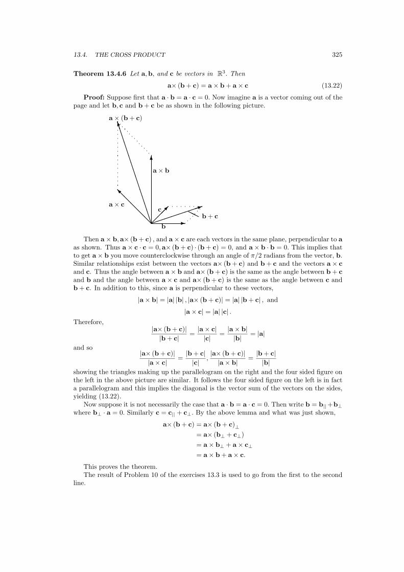
13.4. THE CROSS PRODUCT 325
Theorem 13.4.6 Let a,b, and c be vectors in R3. Then
a× (b + c) = a× b + a× c (13.22)
Proof: Suppose first that a · b = a · c = 0. Now imagine a is a vector coming out of thepage and let b, c and b + c be as shown in the following picture.
-b
¡¡¡µc
³³³³³³³³1b + cHH
6a× b
BB
BB
BB
BB
BB
BB
BB
BBMa× (b + c)
@@
@@
@Ia× c
Then a× b,a× (b + c) , and a× c are each vectors in the same plane, perpendicular to aas shown. Thus a× c · c = 0,a× (b + c) · (b + c) = 0, and a× b · b = 0. This implies thatto get a× b you move counterclockwise through an angle of π/2 radians from the vector, b.Similar relationships exist between the vectors a× (b + c) and b + c and the vectors a× cand c. Thus the angle between a× b and a× (b + c) is the same as the angle between b + cand b and the angle between a× c and a× (b + c) is the same as the angle between c andb + c. In addition to this, since a is perpendicular to these vectors,
|a× b| = |a| |b| , |a× (b + c)| = |a| |b + c| , and
|a× c| = |a| |c| .Therefore,
|a× (b + c)||b + c| =
|a× c||c| =
|a× b||b| = |a|
and so|a× (b + c)||a× c| =
|b + c||c| ,
|a× (b + c)||a× b| =
|b + c||b|
showing the triangles making up the parallelogram on the right and the four sided figure onthe left in the above picture are similar. It follows the four sided figure on the left is in facta parallelogram and this implies the diagonal is the vector sum of the vectors on the sides,yielding (13.22).
Now suppose it is not necessarily the case that a · b = a · c = 0. Then write b = b||+b⊥where b⊥ · a = 0. Similarly c = c|| + c⊥. By the above lemma and what was just shown,
a× (b + c) = a× (b + c)⊥= a× (b⊥ + c⊥)= a× b⊥ + a× c⊥= a× b + a× c.
This proves the theorem.The result of Problem 10 of the exercises 13.3 is used to go from the first to the second
line.

326 VECTOR PRODUCTS
13.4.2 Torque
Imagine you are using a wrench to loosen a nut. The idea is to turn the nut by applying aforce to the end of the wrench. If you push or pull the wrench directly toward or away fromthe nut, it should be obvious from experience that no progress will be made in turning thenut. The important thing is the component of force perpendicular to the wrench. It is thiscomponent of force which will cause the nut to turn. For example see the following picture.
©©©©©©©©©*£££££±
F
£££££±
©©©F
R
AA
AKF⊥ θ
θ
In the picture a force, F is applied at the end of a wrench represented by the positionvector, R and the angle between these two is θ. Then the tendency to turn will be |R| |F⊥| =|R| |F| sin θ, which you recognize as the magnitude of the cross product of R and F. If therewere just one force acting at one point whose position vector is R, perhaps this would besufficient, but what if there are numerous forces acting at many different points with neitherthe position vectors nor the force vectors in the same plane; what then? To keep track ofthis sort of thing, define for each R and F, the Torque vector,
τ ≡ R× F.
That way, if there are several forces acting at several points, the total torque can be obtainedby simply adding up the torques associated with the different forces and positions.
Example 13.4.7 Suppose R1 = 2i − j+3k,R2 = i+2j−6k meters and at the points de-termined by these vectors there are forces, F1 = i − j+2k and F2 = i − 5j + k Newtonsrespectively. Find the total torque about the origin produced by these forces acting at thegiven points.
It is necessary to take R1 × F1 + R2 × F2. Thus the total torque equals∣∣∣∣∣∣
i j k2 −1 31 −1 2
∣∣∣∣∣∣+
∣∣∣∣∣∣
i j k1 2 −61 −5 1
∣∣∣∣∣∣= −27i− 8j− 8k Newton meters
Example 13.4.8 Find if possible a single force vector, F which if applied at the pointi + j + k will produce the same torque as the above two forces acting at the given points.
This is fairly routine. The problem is to find F = F1i + F2j + F3k which produces theabove torque vector. Therefore,
∣∣∣∣∣∣
i j k1 1 1F1 F2 F3
∣∣∣∣∣∣= −27i− 8j− 8k
13.4. THE CROSS PRODUCT 327
which reduces to (F3 − F2) i+(F1 − F3) j+(F2 − F1)k =− 27i− 8j− 8k. This amounts tosolving the system of three equations in three unknowns, F1, F2, and F3,
F3 − F2 = −27F1 − F3 = −8F2 − F1 = −8
However, there is no solution to these three equations. (Why?) Therefore no single forceacting at the point i + j + k will produce the given torque.
The mass of an object is a measure of how much stuff there is in the object. An objecthas mass equal to one kilogram, a unit of mass in the metric system, if it would exactlybalance a known one kilogram object when placed on a balance. The known object is onekilogram by definition. The mass of an object does not depend on where the balance is used.It would be one kilogram on the moon as well as on the earth. The weight of an objectis something else. It is the force exerted on the object by gravity and has magnitude gmwhere g is a constant called the acceleration of gravity. Thus the weight of a one kilogramobject would be different on the moon which has much less gravity, smaller g, than on theearth. An important idea is that of the center of mass. This is the point at which an objectwill balance no matter how it is turned.
Definition 13.4.9 Let an object consist of p point masses, m1, · · ··,mp with the position ofthe kth of these at Rk. The center of mass of this object, R0 is the point satisfying
p∑
k=1
(Rk −R0)× gmku = 0
for all unit vectors, u.
The above definition indicates that no matter how the object is suspended, the totaltorque on it due to gravity is such that no rotation occurs. Using the properties of the crossproduct, (
p∑
k=1
Rkgmk −R0
p∑
k=1
gmk
)× u = 0 (13.23)
for any choice of unit vector, u. You should verify that if a× u = 0 for all u, then it mustbe the case that a = 0. Then the above formula requires that
p∑
k=1
Rkgmk −R0
p∑
k=1
gmk= 0.
dividing by g, and then by∑p
k=1 mk,
R0 =∑p
k=1 Rkmk∑pk=1 mk
. (13.24)
This is the formula for the center of mass of a collection of point masses. To consider thecenter of mass of a solid consisting of continuously distributed masses, you need the methodsof calculus.
Example 13.4.10 Let m1 = 5, m2 = 6, and m3 = 3 where the masses are in kilograms.Suppose m1 is located at 2i+3j+k, m2 is located at i−3j+2k and m3 is located at 2i−j+3k.Find the center of mass of these three masses.

328 VECTOR PRODUCTS
Using (13.24)
R0 =5 (2i + 3j + k) + 6 (i− 3j + 2k) + 3 (2i− j + 3k)
5 + 6 + 3
=117
i− 37j +
137
k
13.4.3 The Box Product
Definition 13.4.11 A parallelepiped determined by the three vectors, a,b, and c consistsof
ra+sb + tb : r, s, t ∈ [0, 1] .
That is, if you pick three numbers, r, s, and t each in [0, 1] and form ra+sb + tb, then thecollection of all such points is what is meant by the parallelepiped determined by these threevectors.
The following is a picture of such a thing.
©©©©©©*
c
a
b££££££££££±
-
££££££££££
££££££££££
©©©©©©
©©©©©©
¡¡
¡¡
¡¡
¡¡
¡¡
¡¡
¡µ
a× c
θ
You notice the area of the base of the parallelepiped, the parallelogram determined bythe vectors, a and c has area equal to |a× c| while the altitude of the parallelepiped is|b| cos θ where θ is the angle shown in the picture between b and a× c. Therefore, thevolume of this parallelepiped is the area of the base times the altitude which is just
|a× c| |b| cos θ = a× c · b.
This expression is known as the box product and is sometimes written as [a, c,b] . Youshould consider what happens if you interchange the b with the c or the a with the c. Youcan see geometrically from drawing pictures that this merely introduces a minus sign. In anycase the box product of three vectors always equals either the volume of the parallelepipeddetermined by the three vectors or else minus this volume.
Example 13.4.12 Find the volume of the parallelepiped determined by the vectors, i+2j−5k, i + 3j− 6k,3i + 2j + 3k.
According to the above discussion, pick any two of these, take the cross product andthen take the dot product of this with the third of these vectors. The result will be eitherthe desired volume or minus the desired volume.
(i + 2j− 5k)× (i + 3j− 6k) =
∣∣∣∣∣∣
i j k1 2 −51 3 −6
∣∣∣∣∣∣= 3i + j + k

13.5. EXERCISES 329
Now take the dot product of this vector with the third which yields
(3i + j + k) · (3i + 2j + 3k) = 9 + 2 + 3 = 14.
This shows the volume of this parallelepiped is 14 cubic units.Here is another proof of the distributive law for the cross product. From the above pic-
ture (a× b) ·c = a· (b× c) because both of these give either the volume of a parallelepipeddetermined by the vectors a,b, c or -1 times the volume of this parallelepiped. Now to provethe distributive law, let x be a vector. From the above observation,
x · a× (b + c) = (x× a) · (b + c)= (x× a) · b+(x× a) · c= x · a× b + x · a× c
= x· (a× b + a× c) .
Therefore,x· [a× (b + c)− (a× b + a× c)] = 0
for all x. In particular, this holds for x = a× (b + c) − (a× b + a× c) showing thata× (b + c) = a× b + a× c and this proves the distributive law for the cross product anotherway.
13.5 Exercises
1. Show that if a× u = 0 for all unit vectors, u, then a = 0.
2. If you only assume (13.23) holds for u = i, j,k, show that this implies (13.23) holdsfor all unit vectors, u.
3. Let m1 = 5,m2 = 1, and m3 = 4 where the masses are in kilograms and the distanceis in meters. Suppose m1 is located at 2i − 3j + k, m2 is located at i − 3j + 6k andm3 is located at 2i + j + 3k. Find the center of mass of these three masses.
4. Let m1 = 2,m2 = 3, and m3 = 1 where the masses are in kilograms and the distanceis in meters. Suppose m1 is located at 2i− j + k, m2 is located at i− 2j + k and m3
is located at 4i + j + 3k. Find the center of mass of these three masses.
5. Find the volume of the parallelepiped determined by the vectors, i− 7j− 5k, i− 2j−6k,3i + 2j + 3k.
6. Suppose a,b, and c are three vectors whose components are all integers. Can youconclude the volume of the parallelepiped determined from these three vectors willalways be an integer?
7. What does it mean geometrically if the box product of three vectors gives zero?
8. Suppose a =(a1, a2, a3) ,b =(b1, b2, b3) , and c =(c1, c2, c3) . Show the box product,[a,b, c] equals the determinant
∣∣∣∣∣∣
c1 c2 c3
a1 a2 a3
b1 b2 b3
∣∣∣∣∣∣.

330 VECTOR PRODUCTS
9. It is desired to find an equation of a plane containing the two vectors, a and b. UsingProblem 7, show an equation for this plane is
∣∣∣∣∣∣
x y za1 a2 a3
b1 b2 b3
∣∣∣∣∣∣= 0
That is, the set of all (x, y, z) such that the above expression equals zero.
10. Using the notion of the box product yielding either plus or minus the volume of theparallelepiped determined by the given three vectors, show that
(a× b) ·c = a· (b× c)
In other words, the dot and the cross can be switched as long as the order of thevectors remains the same. Hint: There are two ways to do this, by the coordinatedescription of the dot and cross product and by geometric reasoning.
11. Verify directly that the coordinate description of the cross product, a× b has theproperty that it is perpendicular to both a and b. Then show by direct computationthat this coordinate description satisfies
|a× b|2 = |a|2 |b|2 − (a · b)2
= |a|2 |b|2 (1− cos2 (θ)
)
where θ is the angle included between the two vectors. Explain why |a× b| has thecorrect magnitude. All that is missing is the material about the right hand rule.Verify directly from the coordinate description of the cross product that the rightthing happens with regards to the vectors i, j,k. Next verify that the distributive lawholds for the coordinate description of the cross product. This gives another way toapproach the cross product. First define it in terms of coordinates and then get thegeometric properties from this.
13.6 Vector Identities And Notation
There are two special symbols, δij and εijk which are very useful in dealing with vectoridentities. To begin with, here is the definition of these symbols.
Definition 13.6.1 The symbol, δij , called the Kroneker delta symbol is defined as follows.
δij ≡
1 if i = j0 if i 6= j
.
With the Kroneker symbol, i and j can equal any integer in 1, 2, · · ·, n for any n ∈ N.
Definition 13.6.2 For i, j, and k integers in the set, 1, 2, 3 , εijk is defined as follows.
εijk ≡
1 if (i, j, k) = (1, 2, 3) , (2, 3, 1) , or (3, 1, 2)−1 if (i, j, k) = (2, 1, 3) , (1, 3, 2) , or (3, 2, 1)0 if there are any repeated integers
.
The subscripts ijk and ij in the above are called indices. A single one is called an index.This symbol, εijk is also called the permutation symbol.

13.6. VECTOR IDENTITIES AND NOTATION 331
The way to think of εijk is that ε123 = 1 and if you switch any two of the numbers inthe list i, j, k, it changes the sign. Thus εijk = −εjik and εijk = −εkji etc. You shouldcheck that this rule reduces to the above definition. For example, it immediately impliesthat if there is a repeated index, the answer is zero. This follows because εiij = −εiij andso εiij = 0.
It is useful to use the Einstein summation convention when dealing with these symbols.Simply stated, the convention is that you sum over the repeated index. Thus aibi means∑
i aibi. Also, δijxj means∑
j δijxj = xi. When you use this convention, there is one veryimportant thing to never forget. It is this: Never have an index be repeated more than once.Thus aibi is all right but aiibi is not. The reason for this is that you end up getting confusedabout what is meant. If you want to write
∑i aibici it is best to simply use the summation
notation. There is a very important reduction identity connecting these two symbols.
Lemma 13.6.3 The following holds.
εijkεirs = (δjrδks − δkrδjs) .
Proof: If j, k 6= r, s then every term in the sum on the left must have either εijk
or εirs contains a repeated index. Therefore, the left side equals zero. The right side alsoequals zero in this case. To see this, note that if the two sets are not equal, then there isone of the indices in one of the sets which is not in the other set. For example, it could bethat j is not equal to either r or s. Then the right side equals zero.
Therefore, it can be assumed j, k = r, s . If i = r and j = s for s 6= r, then thereis exactly one term in the sum on the left and it equals 1. The right also reduces to 1 inthis case. If i = s and j = r, there is exactly one term in the sum on the left which isnonzero and it must equal -1. The right side also reduces to -1 in this case. If there isa repeated index in j, k , then every term in the sum on the left equals zero. The rightalso reduces to zero in this case because then j = k = r = s and so the right side becomes(1) (1)− (−1) (−1) = 0.
Proposition 13.6.4 Let u,v be vectors in Rn where the Cartesian coordinates of u are(u1, · · ·, un) and the Cartesian coordinates of v are (v1, · · ·, vn). Then u · v = uivi. If u,vare vectors in R3, then
(u× v)i = εijkujvk.
Also, δikak = ai.
Proof: The first claim is obvious from the definition of the dot product. The second isverified by simply checking it works. For example,
u× v ≡∣∣∣∣∣∣
i j ku1 u2 u3
v1 v2 v3
∣∣∣∣∣∣
and so(u× v)1 = (u2v3 − u3v2) .
From the above formula in the proposition,
ε1jkujvk ≡ u2v3 − u3v2,
the same thing. The cases for (u× v)2 and (u× v)3 are verified similarly. The last claimfollows directly from the definition.
With this notation, you can easily discover vector identities and simplify expressionswhich involve the cross product.
332 VECTOR PRODUCTS
Example 13.6.5 Discover a formula which simplifies (u× v)×w.
From the above reduction formula,
((u× v)×w)i = εijk (u× v)j wk
= εijkεjrsurvswk
= −εjikεjrsurvswk
= − (δirδks − δisδkr) urvswk
= − (uivkwk − ukviwk)= u ·wvi − v ·wui
= ((u ·w)v − (v ·w)u)i .
Since this holds for all i, it follows that
(u× v)×w =(u ·w)v − (v ·w)u.
This is good notation and it will be used in the rest of the book whenever convenient.Actually, this notation is a special case of something more elaborate in which the level ofthe indices is also important, but there is time for this more general notion later. You willsee it in advanced books on mechanics in physics and engineering. It also occurs in thesubject of differential geometry.
13.7 Exercises
1. Discover a vector identity for u× (v ×w) .
2. Discover a vector identity for (u× v) · (z×w) .
3. Discover a vector identity for (u× v)× (z×w) in terms of box products.
4. Simplify (u× v) · (v ×w)× (w × z) .
5. Simplify |u× v|2 + (u× v)2 − |u|2 |v|2 .
6. Prove that εijkεijr = 2δkr.

Functions
Vector valued functions have values in Rp where p is an integer at least as large as 1. Hereis a simple example which is obviously of interest.
Example 14.0.1 A rocket is launched from the rotating earth. You could define a functionhaving values in R3 as (r (t) , θ (t) , φ (t)) where r (t) is the distance of the center of mass ofthe rocket from the center of the earth, θ (t) is the longitude, and φ (t) is the latitude of therocket.
Example 14.0.2 Let f (x, y) =(sin xy, y3 + x, x4
). Then f is a function defined on R2
which has values in R3. For example, f (1, 2) = (sin 2, 9, 16).
As before, D (f) denotes the domain of the function, f which is written in bold facebecause it will possibly have values in Rp. When D (f) is not specified, it will be understoodthat the domain of f consists of those things for which f makes sense.
Example 14.0.3 Let f (x, y, z) =(
x+yz ,
√1− x2, y
). Then D (f) would consist of the set
of all (x, y, z) such that |x| ≤ 1 and z 6= 0.
There are many ways to make new functions from old ones.
Definition 14.0.4 Let f ,g be functions with values in Rp. Let a, b be elements of R(scalars). Then af + bg is the name of a function whose domain is D (f) ∩ D (g) whichis defined as
(af + bg) (x) = af (x) + bg (x) .
f · g or (f ,g) is the name of a function whose domain is D (f) ∩D (g) which is defined as
(f ,g) (x) ≡ f · g (x) ≡ f (x) · g (x) .
If f and g have values in R3, define a new function, f × g by
f × g (t) ≡ f (t)× g (t) .
If f : D (f) → X and g : X → Y, then g f is the name of a function whose domain is
x ∈ D (f) : f (x) ∈ D (g)
which is defined asg f (x) ≡ g (f (x)) .
This is called the composition of the two functions.
333
334 FUNCTIONS
You should note that f (x) is not a function. It is the value of the function at thepoint, x. The name of the function is f . Nevertheless, people often write f (x) to denote afunction and it doesn’t cause too many problems in beginning courses. When this is done,the variable, x should be considered as a generic variable free to be anything in D (f) . I willuse this slightly sloppy abuse of notation whenever convenient.
Example 14.0.5 Let f (t) ≡ (t, 1 + t, 2) and g (t) ≡ (t2, t, t
). Then f · g is the name of the
function satisfying
f · g (t) = f (t) · g (t) = t3 + t + t2 + 2t = t3 + t2 + 3t
Note that in this case is was assumed the domains of the functions consisted of all of Rbecause this was the set on which the two both made sense. Also note that f and g map Rinto R3 but f · g maps R into R.
Example 14.0.6 Suppose f (t) =(2t, 1 + t2
)and g:R2 → R is given by g (x, y) ≡ x + y.
Then g f : R→ R and
g f (t) = g (f (t)) = g(2t, 1 + t2
)= 1 + 2t + t2.
14.1 Exercises
1. Let f (t) =(t, t2 + 1, t
t+1
)and let g (t) =
(t + 1, 1, t
t2+1
). Find f · g.
2. Let f ,g be given in the previous problem. Find f × g.
3. Find D (f) if f (x, y, z, w) =(
xyzw ,
√6− x2y2
).
4. Let f (t) =(t, t2, t3
),g (t) =
(1, t, t2
), and h (t) = (sin t, t, 1) . Find the time rate of
change of the volume of the parallelepiped spanned by the vectors f ,g, and h.
14.2 Continuous Functions
What was done earlier for scalar functions is generalized here to include the case of a vectorvalued function.
Definition 14.2.1 A function f : D (f) ⊆ Rp → Rq is continuous at x ∈ D (f) if for eachε > 0 there exists δ > 0 such that whenever y ∈ D (f) and
|y − x| < δ
it follows that|f (x)− f (y)| < ε.
f is continuous if it is continuous at every point of D (f) .
Note the total similarity to the scalar valued case.

14.3. EXERCISES 335
14.2.1 Sufficient Conditions For Continuity
The next theorem is a fundamental result which will allow us to worry less about the ε δdefinition of continuity.
Theorem 14.2.2 The following assertions are valid.
1. The function, af + bg is continuous at x whenever f , g are continuous at x ∈ D (f)∩D (g) and a, b ∈ R.
2. If f is continuous at x, f (x) ∈ D (g) ⊆ Rp, and g is continuous at f (x) ,then g f iscontinuous at x.
3. If f = (f1, · · ·, fq) : D (f) → Rq, then f is continuous if and only if each fk is acontinuous real valued function.
4. The function f : Rp → R, given by f (x) = |x| is continuous.
The proof of this theorem is in the last section of this chapter. Its conclusions are notsurprising. For example the first claim says that (af + bg) (y) is close to (af + bg) (x) wheny is close to x provided the same can be said about f and g. For the second claim, if yis close to x, f (x) is close to f (y) and so by continuity of g at f (x), g (f (y)) is close tog (f (x)) . To see the third claim is likely, note that closeness in Rp is the same as closenessin each coordinate. The fourth claim is immediate from the triangle inequality.
For functions defined on Rn, there is a notion of polynomial just as there is for functionsdefined on R.
Definition 14.2.3 Let α be an n dimensional multi-index. This means
α = (α1, · · ·, αn)
where each αi is a natural number or zero. Also, let
|α| ≡n∑
i=1
|αi|
The symbol, xα,meansxα ≡ xα1
1 xα22 · · · xαn
3 .
An n dimensional polynomial of degree m is a function of the form
p (x) =∑
|α|≤m
dαxα.
where the dα are real numbers.
The above theorem implies that polynomials are all continuous.
14.3 Exercises
1. Let f (t) = (t, sin t) . Show f is continuous at every point t.
2. Suppose |f (x)− f (y)| ≤ K |x− y| where K is a constant. Show that f is everywherecontinuous. Functions satisfying such an inequality are called Lipschitz functions.

336 FUNCTIONS
3. Suppose |f (x)− f (y)| ≤ K |x− y|α where K is a constant and α ∈ (0, 1). Show thatf is everywhere continuous.
4. Suppose f : R3 → R is given by f (x) = 3x1x2 + 2x23. Use Theorem 14.2.2 to verify
that f is continuous. Hint: You should first verify that the function, πk : R3 → Rgiven by πk (x) = xk is a continuous function.
5. Generalize the previous problem to the case where f : Rq → R is a polynomial.
6. State and prove a theorem using Theorem 5.4.1 which involves quotients of functionsencountered in the previous problem.
14.4 Limits Of A Function
As in the case of scalar valued functions of one variable, a concept closely related to con-tinuity is that of the limit of a function. The notion of limit of a function makes sense atpoints, x, which are limit points of D (f) and this concept is defined next.
Definition 14.4.1 Let A ⊆ Rm be a set. A point, x, is a limit point of A if B (x, r)contains infinitely many points of A for every r > 0.
Definition 14.4.2 Let f : D (f) ⊆ Rp → Rq be a function and let x be a limit point ofD (f) . Then
limy→x
f (y) = L
if and only if the following condition holds. For all ε > 0 there exists δ > 0 such that if
0 < |y − x| < δ, and y ∈ D (f)
then,|L− f (y)| < ε.
Theorem 14.4.3 If limy→x f (y) = L and limy→x f (y) = L1, then L = L1.
Proof: Let ε > 0 be given. There exists δ > 0 such that if 0 < |y − x| < δ andy ∈ D (f) , then
|f (y)− L| < ε, |f (y)− L1| < ε.
Pick such a y. There exists one because x is a limit point of D (f) . Then
|L− L1| ≤ |L− f (y)|+ |f (y)− L1| < ε + ε = 2ε.
Since ε > 0 was arbitrary, this shows L = L1.
As in the case of functions of one variable, one can define what it means for limy→x f (x) =±∞.
Definition 14.4.4 If f (x) ∈ R, limy→x f (x) = ∞ if for every number l, there exists δ > 0such that whenever |y − x| < δ and y ∈ D (f) , then f (x) > l.
The following theorem is just like the one variable version presented earlier.

14.4. LIMITS OF A FUNCTION 337
Theorem 14.4.5 Suppose limy→x f (y) = L and limy→x g (y) = K where K,L ∈ Rq. Thenif a, b ∈ R,
limy→x
(af (y) + bg (y)) = aL + bK, (14.1)
limy→x
f · g (y) = LK (14.2)
and if g is scalar valued with limy→x g (y) = K 6= 0,
limy→x
f (y) g (y) = LK. (14.3)
Also, if h is a continuous function defined near L, then
limy→x
h f (y) = h (L) . (14.4)
Suppose limy→x f (y) = L. If |f (y)− b| ≤ r for all y sufficiently close to x, then |L− b| ≤ ralso.
Proof: The proof of (14.1) is left for you. It is like a corresponding theorem for con-tinuous functions. Now (14.2)is to be verified. Let ε > 0 be given. Then by the triangleinequality,
|f · g (y)− L ·K| ≤ |fg (y)− f (y) ·K|+ |f (y) ·K− L ·K|≤ |f (y)| |g (y)−K|+ |K| |f (y)− L| .
There exists δ1 such that if 0 < |y − x| < δ1 and y ∈ D (f) , then
|f (y)− L| < 1,
and so for such y, the triangle inequality implies, |f (y)| < 1 + |L| . Therefore, for 0 <|y − x| < δ1,
|f · g (y)− L ·K| ≤ (1 + |K|+ |L|) [|g (y)−K|+ |f (y)− L|] . (14.5)
Now let 0 < δ2 be such that if y ∈ D (f) and 0 < |x− y| < δ2,
|f (y)− L| < ε
2 (1 + |K|+ |L|) , |g (y)−K| < ε
2 (1 + |K|+ |L|) .
Then letting 0 < δ ≤ min (δ1, δ2) , it follows from (14.5) that
|f · g (y)− L ·K| < ε
and this proves (14.2).The proof of (14.3) is left to you.Consider (14.4). Since h is continuous near L, it follows that for ε > 0 given, there exists
η > 0 such that if |y − L| < η, then
|h (y)−h (L)| < ε
Now since limy→x f (y) = L, there exists δ > 0 such that if 0 < |y − x| < δ, then
|f (y)−L| < η.
Therefore, if 0 < |y − x| < δ,|h (f (y))−h (L)| < ε.

338 FUNCTIONS
It only remains to verify the last assertion. Assume |f (y)− b| ≤ r. It is required to showthat |L− b| ≤ r. If this is not true, then |L− b| > r. Consider B (L, |L− b| − r) . Since Lis the limit of f , it follows f (y) ∈ B (L, |L− b| − r) whenever y ∈ D (f) is close enough tox. Thus, by the triangle inequality,
|f (y)− L| < |L− b| − r
and so
r < |L− b| − |f (y)− L| ≤ ||b− L| − |f (y)− L||≤ |b− f (y)| ,
a contradiction to the assumption that |b− f (y)| ≤ r.
Theorem 14.4.6 For f : D (f) → Rq and x ∈ D (f) a limit point of D (f) , f is continuousat x if and only if
limy→x
f (y) = f (x) .
Proof: First suppose f is continuous at x a limit point of D (f) . Then for every ε > 0there exists δ > 0 such that if |y − x| < δ and y ∈ D (f) , then |f (x)− f (y)| < ε. Inparticular, this holds if 0 < |x− y| < δ and this is just the definition of the limit. Hencef (x) = limy→x f (y) .
Next suppose x is a limit point of D (f) and limy→x f (y) = f (x) . This means that if ε > 0there exists δ > 0 such that for 0 < |x− y| < δ and y ∈ D (f) , it follows |f (y)− f (x)| < ε.However, if y = x, then |f (y)− f (x)| = |f (x)− f (x)| = 0 and so whenever y ∈ D (f) and|x− y| < δ, it follows |f (x)− f (y)| < ε, showing f is continuous at x.
The following theorem is important.
Theorem 14.4.7 Suppose f : D (f) → Rq. Then for x a limit point of D (f) ,
limy→x
f (y) = L (14.6)
if and only iflimy→x
fk (y) = Lk (14.7)
where f (y) ≡ (f1 (y) , · · ·, fp (y)) and L ≡ (L1, · · ·, Lp) .
Proof: Suppose (14.6). Then letting ε > 0 be given there exists δ > 0 such that if0 < |y − x| < δ, it follows
|fk (y)− Lk| ≤ |f (y)− L| < ε
which verifies (14.7).Now suppose (14.7) holds. Then letting ε > 0 be given, there exists δk such that if
0 < |y − x| < δk, then|fk (y)− Lk| < ε√
p.
Let 0 < δ < min (δ1, · · ·, δp) . Then if 0 < |y − x| < δ, it follows
|f (y)− L| =
(p∑
k=1
|fk (y)− Lk|2)1/2
<
(p∑
k=1
ε2
p
)1/2
= ε.

14.5. EXERCISES 339
This proves the theorem.This theorem shows it suffices to consider the components of a vector valued function
when computing the limit.
Example 14.4.8 Find lim(x,y)→(3,1)
(x2−9x−3 , y
).
It is clear that lim(x,y)→(3,1)x2−9x−3 = 6 and lim(x,y)→(3,1) y = 1. Therefore, this limit
equals (6, 1) .
Example 14.4.9 Find lim(x,y)→(0,0)xy
x2+y2 .
First of all observe the domain of the function is R2 \ (0, 0) , every point in R2 exceptthe origin. Therefore, (0, 0) is a limit point of the domain of the function so it might makesense to take a limit. However, just as in the case of a function of one variable, the limitmay not exist. In fact, this is the case here. To see this, take points on the line y = 0.At these points, the value of the function equals 0. Now consider points on the line y = xwhere the value of the function equals 1/2. Since arbitrarily close to (0, 0) there are pointswhere the function equals 1/2 and points where the function has the value 0, it follows therecan be no limit. Just take ε = 1/10 for example. You can’t be within 1/10 of 1/2 and alsowithin 1/10 of 0 at the same time.
Note it is necessary to rely on the definition of the limit much more than in the case ofa function of one variable and it is the case there are no easy ways to do limit problemsfor functions of more than one variable. It is what it is and you will not deal with theseconcepts without agony.
14.5 Exercises
1. Find the following limits if possible
(a) lim(x,y)→(0,0)x2−y2
x2+y2
(b) lim(x,y)→(0,0)x(x2−y2)(x2+y2)
(c) lim(x,y)→(0,0)(x2−y4)2
(x2+y4)2Hint: Consider along y = 0 and along x = y2.
(d) lim(x,y)→(0,0) x sin(
1x2+y2
)
(e) lim(x,y)→(1,2)−2yx2+8yx+34y+3y3−18y2+6x2−13x−20−xy2−x3
−y2+4y−5−x2+2x . Hint: It might help towrite this in terms of the variables (s, t) = (x− 1, y − 2) .
2. In the definition of limit, why must x be a limit point of D (f)? Hint: If x were nota limit point of D (f), show there exists δ > 0 such that B (x, δ) contains no points ofD (f) other than possibly x itself. Argue that 33.3 is a limit and that so is 22 and 7and 11. In other words the concept is totally worthless.
14.6 The Limit Of A Sequence
As in the case of real numbers, one can consider the limit of a sequence of points in Rp.
340 FUNCTIONS
Definition 14.6.1 A sequence an∞n=1 converges to a, and write
limn→∞
an = a or an → a
if and only if for every ε > 0 there exists nε such that whenever n ≥ nε ,
|an−a| < ε.
In words the definition says that given any measure of closeness, ε, the terms of thesequence are eventually all this close to a. There is absolutely no difference between thisand the definition for sequences of numbers other than here bold face is used to indicate an
and a are points in Rp.
Theorem 14.6.2 If limn→∞ an = a and limn→∞ an = a1 then a1 = a.
Proof: Suppose a1 6= a. Then let 0 < ε < |a1−a| /2 in the definition of the limit. Itfollows there exists nε such that if n ≥ nε, then |an−a| < ε and |an−a1| < ε. Therefore,for such n,
|a1−a| ≤ |a1−an|+ |an−a|< ε + ε < |a1−a| /2 + |a1−a| /2 = |a1−a| ,
a contradiction.As in the case of a vector valued function, it suffices to consider the components. This
is the content of the next theorem.
Theorem 14.6.3 Let an =(an1 , · · ·, an
p
) ∈ Rp. Then limn→∞ an = a ≡ (a1, · · ·, ap) if andonly if for each k = 1, · · ·, p,
limn→∞
ank = ak. (14.8)
Proof: First suppose limn→∞ an = a. Then given ε > 0 there exists nε such that ifn > nε, then
|ank − ak| ≤ |an − a| < ε
which establishes (14.8).Now suppose (14.8) holds for each k. Then letting ε > 0 be given there exist nk such
that if n > nk,
|ank − ak| < ε/
√p.
Therefore, letting nε > max (n1, · · ·, np) , it follows that for n > nε,
|an − a| =(
n∑
k=1
|ank − ak|2
)1/2
<
(n∑
k=1
ε2
p
)1/2
= ε,
showing that limn→∞ an = a. This proves the theorem.
Example 14.6.4 Let an =(
1n2+1 , 1
n sin (n) , n2+33n2+5n
).
It suffices to consider the limits of the components according to the following theorem.Thus the limit is (0, 0, 1/3) .

14.6. THE LIMIT OF A SEQUENCE 341
Theorem 14.6.5 Suppose an and bn are sequences and that
limn→∞
an = a and limn→∞
bn = b.
Also suppose x and y are real numbers. Then
limn→∞
xan + ybn = xa + yb (14.9)
limn→∞
an · bn = a · b (14.10)
If bn ∈ R, thenanbn → ab.
Proof: The first of these claims is left for you to do. To do the second, let ε > 0 begiven and choose n1 such that if n ≥ n1 then
|an−a| < 1.
Then for such n, the triangle inequality and Cauchy Schwarz inequality imply
|an · bn−a · b| ≤ |an · bn−an · b|+ |an · b− a · b|≤ |an| |bn−b|+ |b| |an−a|≤ (|a|+ 1) |bn−b|+ |b| |an−a| .
Now let n2 be large enough that for n ≥ n2,
|bn−b| < ε
2 (|a|+ 1), and |an−a| < ε
2 (|b|+ 1).
Such a number exists because of the definition of limit. Therefore, let
nε > max (n1, n2) .
For n ≥ nε,
|an · bn−a · b| ≤ (|a|+ 1) |bn−b|+ |b| |an−a|< (|a|+ 1)
ε
2 (|a|+ 1)+ |b| ε
2 (|b|+ 1)≤ ε.
This proves (14.9). The proof of (14.10) is entirely similar and is left for you.
14.6.1 Sequences And Completeness
Recall the definition of a Cauchy sequence.
Definition 14.6.6 an is a Cauchy sequence if for all ε > 0, there exists nε such thatwhenever n,m ≥ nε,
|an−am| < ε.
A sequence is Cauchy means the terms are “bunching up to each other” as m,n getlarge.
Theorem 14.6.7 Let an∞n=1 be a Cauchy sequence in Rp. Then there exists a ∈ Rp suchthat an → a.

342 FUNCTIONS
Proof: Let an =(an1 , · · ·, an
p
). Then
|ank − am
k | ≤ |an − am|
which shows for each k = 1, · · ·, p, it follows ank∞n=1 is a Cauchy sequence. By completeness
of R, it follows there exists ak such that limn→∞ ank = ak. Letting a =(a1, · · ·, ap) , it follows
from Theorem 14.6.3 thatlim
n→∞an = a.
This proves the theorem.
Theorem 14.6.8 The set of terms in a Cauchy sequence in Rp is bounded in the sense thatfor all n, |an| < M for some M < ∞.
Proof: Let ε = 1 in the definition of a Cauchy sequence and let n > n1. Then from thedefinition,
|an−an1 | < 1.
It follows that for all n > n1,
|an| < 1 + |an1 | .Therefore, for all n,
|an| ≤ 1 + |an1 |+n1∑
k=1
|ak| .
This proves the theorem.
Theorem 14.6.9 If a sequence an in Rp converges, then the sequence is a Cauchy se-quence.
Proof: Let ε > 0 be given and suppose an→ a. Then from the definition of convergence,there exists nε such that if n > nε, it follows that
|an−a| < ε
2
Therefore, if m,n ≥ nε + 1, it follows that
|an−am| ≤ |an−a|+ |a− am| < ε
2+
ε
2= ε
showing that, since ε > 0 is arbitrary, an is a Cauchy sequence.
14.6.2 Continuity And The Limit Of A Sequence
Just as in the case of a function of one variable, there is a very useful way of thinking ofcontinuity in terms of limits of sequences found in the following theorem. In words, it saysa function is continuous if it takes convergent sequences to convergent sequences wheneverpossible.
Theorem 14.6.10 A function f : D (f)→ Rq is continuous at x ∈ D (f) if and only if,whenever xn→ x with xn ∈ D (f) , it follows f (xn) → f (x) .

14.7. PROPERTIES OF CONTINUOUS FUNCTIONS 343
Proof: Suppose first that f is continuous at x and let xn→ x. Let ε > 0 be given. Bycontinuity, there exists δ > 0 such that if |y − x| < δ, then |f (x)− f (y)| < ε. However,there exists nδ such that if n ≥ nδ, then |xn−x| < δ and so for all n this large,
|f (x)−f (xn)| < ε
which shows f (xn)→ f (x) .Now suppose the condition about taking convergent sequences to convergent sequences
holds at x. Suppose f fails to be continuous at x. Then there exists ε > 0 and xn ∈ D (f)such that |x− xn| < 1
n , yet|f (x)−f (xn)| ≥ ε.
But this is clearly a contradiction because, although xn→ x, f (xn) fails to converge to f (x) .It follows f must be continuous after all. This proves the theorem.
14.7 Properties Of Continuous Functions
Functions of p variables have many of the same properties as functions of one variable. Firstthere is a version of the extreme value theorem generalizing the one dimensional case.
Theorem 14.7.1 Let C be closed and bounded and let f : C → R be continuous. Then fachieves its maximum and its minimum on C. This means there exist, x1,x2 ∈ C such thatfor all x ∈ C,
f (x1) ≤ f (x) ≤ f (x2) .
There is also the long technical theorem about sums and products of continuous func-tions. These theorems are proved in the next section.
Theorem 14.7.2 The following assertions are valid
1. The function, af +bg is continuous at x when f , g are continuous at x ∈ D (f)∩D (g)and a, b ∈ R.
2. If and f and g are each real valued functions continuous at x, then fg is continuousat x. If, in addition to this, g (x) 6= 0, then f/g is continuous at x.
3. If f is continuous at x, f (x) ∈ D (g) ⊆ Rp, and g is continuous at f (x) ,then g f iscontinuous at x.
4. If f = (f1, · · ·, fq) : D (f) → Rq, then f is continuous if and only if each fk is acontinuous real valued function.
5. The function f : Rp → R, given by f (x) = |x| is continuous.
14.8 Exercises
1. f : D ⊆ Rp → Rq is Lipschitz continuous or just Lipschitz for short if there exists aconstant, K such that
|f (x)− f (y)| ≤ K |x− y|for all x,y ∈ D. Show every Lipschitz function is uniformly continuous which meansthat given ε > 0 there exists δ > 0 independent of x such that if |x− y| < δ, then|f (x)− f (y)| < ε.
2. If f is uniformly continuous, does it follow that |f | is also uniformly continuous? If |f | isuniformly continuous does it follow that f is uniformly continuous? Answer the samequestions with “uniformly continuous” replaced with “continuous”. Explain why.

344 FUNCTIONS
14.9 Some Advanced Calculus
This section contains the proofs of the theorems which were just stated without proof.
Theorem 14.9.1 The following assertions are valid
1. The function, af +bg is continuous at x when f , g are continuous at x ∈ D (f)∩D (g)and a, b ∈ R.
2. If and f and g are each real valued functions continuous at x, then fg is continuousat x. If, in addition to this, g (x) 6= 0, then f/g is continuous at x.
3. If f is continuous at x, f (x) ∈ D (g) ⊆ Rp, and g is continuous at f (x) ,then g f iscontinuous at x.
4. If f = (f1, · · ·, fq) : D (f) → Rq, then f is continuous if and only if each fk is acontinuous real valued function.
5. The function f : Rp → R, given by f (x) = |x| is continuous.
Proof: Begin with 1.) Let ε > 0 be given. By assumption, there exist δ1 > 0 suchthat whenever |x− y| < δ1, it follows |f (x)− f (y)| < ε
2(|a|+|b|+1) and there exists δ2 > 0such that whenever |x− y| < δ2, it follows that |g (x)− g (y)| < ε
2(|a|+|b|+1) . Then let0 < δ ≤ min (δ1, δ2) . If |x− y| < δ, then everything happens at once. Therefore, using thetriangle inequality
|af (x) + bf (x)− (ag (y) + bg (y))|
≤ |a| |f (x)− f (y)|+ |b| |g (x)− g (y)|
< |a|(
ε
2 (|a|+ |b|+ 1)
)+ |b|
(ε
2 (|a|+ |b|+ 1)
)< ε.
Now begin on 2.) There exists δ1 > 0 such that if |y − x| < δ1, then |f (x)− f (y)| < 1.Therefore, for such y,
|f (y)| < 1 + |f (x)| .It follows that for such y,
|fg (x)− fg (y)| ≤ |f (x) g (x)− g (x) f (y)|+ |g (x) f (y)− f (y) g (y)|
≤ |g (x)| |f (x)− f (y)|+ |f (y)| |g (x)− g (y)|≤ (1 + |g (x)|+ |f (y)|) [|g (x)− g (y)|+ |f (x)− f (y)|] .
Now let ε > 0 be given. There exists δ2 such that if |x− y| < δ2, then
|g (x)− g (y)| < ε
2 (1 + |g (x)|+ |f (y)|) ,
and there exists δ3 such that if |x− y| < δ3, then
|f (x)− f (y)| < ε
2 (1 + |g (x)|+ |f (y)|)Now let 0 < δ ≤ min (δ1, δ2, δ3) . Then if |x− y| < δ, all the above hold at once and
|fg (x)− fg (y)| ≤

14.9. SOME ADVANCED CALCULUS 345
(1 + |g (x)|+ |f (y)|) [|g (x)− g (y)|+ |f (x)− f (y)|]
< (1 + |g (x)|+ |f (y)|)(
ε
2 (1 + |g (x)|+ |f (y)|) +ε
2 (1 + |g (x)|+ |f (y)|))
= ε.
This proves the first part of 2.) To obtain the second part, let δ1 be as described above andlet δ0 > 0 be such that for |x− y| < δ0,
|g (x)− g (y)| < |g (x)| /2
and so by the triangle inequality,
− |g (x)| /2 ≤ |g (y)| − |g (x)| ≤ |g (x)| /2
which implies |g (y)| ≥ |g (x)| /2, and |g (y)| < 3 |g (x)| /2.Then if |x− y| < min (δ0, δ1) ,
∣∣∣∣f (x)g (x)
− f (y)g (y)
∣∣∣∣ =∣∣∣∣f (x) g (y)− f (y) g (x)
g (x) g (y)
∣∣∣∣
≤ |f (x) g (y)− f (y) g (x)|(|g(x)|2
2
)
=2 |f (x) g (y)− f (y) g (x)|
|g (x)|2
≤ 2|g (x)|2 [|f (x) g (y)− f (y) g (y) + f (y) g (y)− f (y) g (x)|]
≤ 2|g (x)|2 [|g (y)| |f (x)− f (y)|+ |f (y)| |g (y)− g (x)|]
≤ 2|g (x)|2
[32|g (x)| |f (x)− f (y)|+ (1 + |f (x)|) |g (y)− g (x)|
]
≤ 2|g (x)|2 (1 + 2 |f (x)|+ 2 |g (x)|) [|f (x)− f (y)|+ |g (y)− g (x)|]
≡ M [|f (x)− f (y)|+ |g (y)− g (x)|]
whereM ≡ 2
|g (x)|2 (1 + 2 |f (x)|+ 2 |g (x)|)
Now let δ2 be such that if |x− y| < δ2, then
|f (x)− f (y)| < ε
2M−1
and let δ3 be such that if |x− y| < δ3, then
|g (y)− g (x)| < ε
2M−1.
Then if 0 < δ ≤ min (δ0, δ1, δ2, δ3) , and |x− y| < δ, everything holds and∣∣∣∣f (x)g (x)
− f (y)g (y)
∣∣∣∣ ≤ M [|f (x)− f (y)|+ |g (y)− g (x)|]

346 FUNCTIONS
< M[ε
2M−1 +
ε
2M−1
]= ε.
This completes the proof of the second part of 2.) Note that in these proofs no effort ismade to find some sort of “best” δ. The problem is one which has a yes or a no answer.Either is it or it is not continuous.
Now begin on 3.). If f is continuous at x, f (x) ∈ D (g) ⊆ Rp, and g is continuousat f (x) ,then g f is continuous at x. Let ε > 0 be given. Then there exists η > 0 suchthat if |y − f (x)| < η and y ∈ D (g) , it follows that |g (y)− g (f (x))| < ε. It follows fromcontinuity of f at x that there exists δ > 0 such that if |x− z| < δ and z ∈ D (f) , then|f (z)− f (x)| < η. Then if |x− z| < δ and z ∈ D (g f) ⊆ D (f) , all the above hold and so
|g (f (z))− g (f (x))| < ε.
This proves part 3.)Part 4.) says: If f = (f1, · · ·, fq) : D (f) → Rq, then f is continuous if and only if each
fk is a continuous real valued function. Then
|fk (x)− fk (y)| ≤ |f (x)− f (y)|
≡(
q∑
i=1
|fi (x)− fi (y)|2)1/2
≤q∑
i=1
|fi (x)− fi (y)| . (14.11)
Suppose first that f is continuous at x. Then there exists δ > 0 such that if |x− y| < δ,then |f (x)− f (y)| < ε. The first part of the above inequality then shows that for eachk = 1, · · ·, q, |fk (x)− fk (y)| < ε. This shows the only if part. Now suppose each function,fk is continuous. Then if ε > 0 is given, there exists δk > 0 such that whenever |x− y| < δk
|fk (x)− fk (y)| < ε/q.
Now let 0 < δ ≤ min (δ1, · · ·, δq) . For |x− y| < δ, the above inequality holds for all k andso the last part of (14.11) implies
|f (x)− f (y)| ≤q∑
i=1
|fi (x)− fi (y)|
<
q∑
i=1
ε
q= ε.
This proves part 4.)To verify part 5.), let ε > 0 be given and let δ = ε. Then if |x− y| < δ, the triangle
inequality implies
|f (x)− f (y)| = ||x| − |y||≤ |x− y| < δ = ε.
This proves part 5.) and completes the proof of the theorem.Here is a multidimensional version of the nested interval lemma.
Lemma 14.9.2 Let Ik =∏p
i=1
[ak
i , bki
] ≡ x ∈ Rp : xi ∈
[ak
i , bki
]and suppose that for all
k = 1, 2, · · ·,Ik ⊇ Ik+1.
Then there exists a point, c ∈ Rp which is an element of every Ik.

14.9. SOME ADVANCED CALCULUS 347
Proof: Since Ik ⊇ Ik+1, it follows that for each i = 1, · · ·, p ,[ak
i , bki
] ⊇ [ak+1
i , bk+1i
].
This implies that for each i,ak
i ≤ ak+1i , bk
i ≥ bk+1i . (14.12)
Consequently, if k ≤ l,al
i ≤ bli ≤ bk
i . (14.13)
Now defineci ≡ sup
al
i : l = 1, 2, · · ·
By the first inequality in (14.12),
ci = supal
i : l = k, k + 1, · · · (14.14)
for each k = 1, 2 · · · . Therefore, picking any k,(14.13) shows that bki is an upper bound for
the set,al
i : l = k, k + 1, · · · and so it is at least as large as the least upper bound of thisset which is the definition of ci given in (14.14). Thus, for each i and each k,
aki ≤ ci ≤ bk
i .
Defining c ≡ (c1, · · ·, cp) , c ∈ Ik for all k. This proves the lemma.If you don’t like the proof, here is another one which follows directly from the one variable
nested interval lemma, Lemma 5.7.7 on Page 95.
Lemma 14.9.3 Let Ik =∏p
i=1
[ak
i , bki
] ≡ x ∈ Rp : xi ∈
[ak
i , bki
]and suppose that for all
k = 1, 2, · · ·,Ik ⊇ Ik+1.
Then there exists a point, c ∈ Rp which is an element of every Ik.
Proof: For each i = 1, · · ·, p,[ak
i , bki
] ⊇ [ak+1
i , bk+1i
]and so by the nested interval
theorem for one dimensional problems, there exists a point ci ∈[ak
i , bki
]for all k. Then
letting c ≡ (c1, · · ·, cp) it follows c ∈ Ik for all k. This proves the lemma.The following definition is similar to that given earlier. It defines what is meant by a
sequentially compact set in Rp.
Definition 14.9.4 A set, K ⊆ Rp is sequentially compact if and only if whenever xn∞n=1
is a sequence of points in K, there exists a point, x ∈ K and a subsequence, xnk∞k=1 such
that xnk→ x.
It turns out the sequentially compact sets in Rpare exactly those which are closed andbounded. Only half of this result will be needed in this book and this is proved next.
Theorem 14.9.5 Let C ⊆ Rp be closed and bounded. Then C is sequentially compact.
Proof: Let an ⊆ C, let C ⊆ ∏pi=1 [ai, bi] , and consider all sets of the form
∏pi=1 [ci, di]
where [ci, di] equals either[ai,
ai+bi
2
]or [ci, di] =
[ai+bi
2 , bi
]. Thus there are 2p of these sets
because there are two choices for the ith slot for i = 1, · · ·, p. Also, if x and y are two pointsin one of these sets,
|xi − yi| ≤ 2−1 |bi − ai| .
Therefore, letting D0 =(∑p
i=1 |bi − ai|2)1/2
,
|x− y| =(
p∑
i=1
|xi − yi|2)1/2
≤ 2−1
(p∑
i=1
|bi − ai|2)1/2
≡ 2−1D0.

348 FUNCTIONS
In particular, since d ≡ (d1, · · ·, dp) and c ≡ (c1, · · ·, cp) are two such points,
D1 ≡(
p∑
i=1
|di − ci|2)1/2
≤ 2−1D0
Denote by J1, · · ·, J2p these sets determined above. Since the union of these sets equalsall of I0, it follows
C = ∪2p
k=1Jk ∩ C.
Pick Jk such that an is contained in Jk ∩ C for infinitely many values of n. Let I1 ≡ Jk.Now do to I1 what was done to I0 to obtain I2 ⊆ I1 and for any two points, x,y ∈ I2
|x− y| ≤ 2−1D1 ≤ 2−2D0,
and I2 ∩C contains an for infinitely many values of n. Continue in this way obtaining sets,Ik such that Ik ⊇ Ik+1 and for any two points in Ik,x,y, it follows |x− y| ≤ 2−kD0, andIk ∩ C contains an for infinitely many values of n. By the nested interval lemma, thereexists a point, c which is contained in each Ik.
Claim: c ∈ C.
Proof of claim: Suppose c /∈ C. Since C is a closed set, there exists r > 0 such thatB (c, r) is contained completely in Rp \ C. In other words, B (c, r) contains no points of C.Let k be so large that D02−k < r. Then since c ∈ Ik, and any two points of Ik are closerthan D02−k, Ik must be contained in B (c, r) and so has no points of C in it, contrary tothe manner in which the Ik are defined in which Ik contains an for infinitely many valuesof n. Therefore, c ∈ C as claimed.
Now pick an1 ∈ I1 ∩ an∞n=1 . Having picked this, let an2 ∈ I2 ∩ an∞n=1 with n2 > n1.Having picked these two, let an3 ∈ I3 ∩ an∞n=1 with n3 > n2 and continue this way. Theresult is a subsequence of an∞n=1 which converges to c ∈ C because any two points in Ik
are within D02−k of each other. This proves the theorem.Here is a proof of the extreme value theorem.
Theorem 14.9.6 Let C be closed and bounded and let f : C → R be continuous. Then fachieves its maximum and its minimum on C. This means there exist, x1,x2 ∈ C such thatfor all x ∈ C,
f (x1) ≤ f (x) ≤ f (x2) .
Proof: Let M = sup f (x) : x ∈ C . Recall this means +∞ if f is not bounded aboveand it equals the least upper bound of these values of f if f is bounded above. Then thereexists a sequence, xn such that f (xn) → M. Since C is sequentially compact, there existsa subsequence, xnk
, and a point, x ∈ C such that xnk→ x. But then since f is continuous
at x, it follows from Theorem 14.6.10 on Page 342 that f (x) = limk→∞ f (xnk) = M. This
proves f achieves its maximum and also shows its maximum is less than ∞. Let x2 = x.The case of a minimum is handled similarly.
Recall that a function is uniformly continuous if the following definition holds.
Definition 14.9.7 Let f : D (f) → Rq. Then f is uniformly continuous if for every ε > 0there exists δ > 0 such that whenever |x− y| < δ, it follows |f (x)− f (y)| < ε.
Theorem 14.9.8 Let f :C → Rq be continuous where C is a closed and bounded set in Rp.Then f is uniformly continuous on C.

14.9. SOME ADVANCED CALCULUS 349
Proof: If this is not so, there exists ε > 0 and pairs of points, xn and yn satisfying|xn − yn| < 1/n but |f (xn)− f (yn)| ≥ ε. Since C is sequentially compact, there existsx ∈ C and a subsequence, xnk
satisfying xnk→ x. But |xnk
− ynk| < 1/k and so
ynk→ x also. Therefore, from Theorem 14.6.10 on Page 342,
ε ≤ limk→∞
|f (xnk)− f (ynk
)| = |f (x)− f (x)| = 0,
a contradiction. This proves the theorem.

350 FUNCTIONS
Limits And Derivatives
15.1 Limits Of A Vector Valued Function
The above discussion considered expressions like
f (t0 + h)− f (t0)h
and determined what they get close to as h gets small. In other words it is desired toconsider
limh→0
f (t0 + h)− f (t0)h
Specializing to functions of one variable, one can give a meaning to
lims→t+
f (s) , lims→t−
f (s) , lims→∞
f (s) ,
andlims−∞
f (s) .
Definition 15.1.1 In the case where D (f) is only assumed to satisfy D (f) ⊇ (t, t + r) ,
lims→t+
f (s) = L
if and only if for all ε > 0 there exists δ > 0 such that if
0 < s− t < δ,
then|f (s)− L| < ε.
In the case where D (f) is only assumed to satisfy D (f) ⊇ (t− r, t) ,
lims→t−
f (s) = L
if and only if for all ε > 0 there exists δ > 0 such that if
0 < t− s < δ,
then|f (s)− L| < ε.
351

352 LIMITS AND DERIVATIVES
One can also consider limits as a variable “approaches” infinity. Of course nothing is “close”to infinity and so this requires a slightly different definition.
limt→∞
f (t) = L
if for every ε > 0 there exists l such that whenever t > l,
|f (t)− L| < ε (15.1)
andlim
t→−∞f (t) = L
if for every ε > 0 there exists l such that whenever t < l, (15.1) holds.
Note that in all of this the definitions are identical to the case of scalar valued functions.The only difference is that here |·| refers to the norm or length in Rp where maybe p > 1.
Example 15.1.2 Let f (t) =(cos t, sin t, t2 + 1, ln (t)
). Find limt→π/2 f (t) .
Use Theorem 14.4.7 on Page 338 and the continuity of the functions to write this limitequals
(lim
t→π/2cos t, lim
t→π/2sin t, lim
t→π/2
(t2 + 1
), limt→π/2
ln (t))
=(
0, 1, ln(
π2
4+ 1
), ln
(π
2
)).
Example 15.1.3 Let f (t) =(
sin tt , t2, t + 1
). Find limt→0 f (t) .
Recall that limt→0sin t
t = 1. Then from Theorem 14.4.7 on Page 338, limt→0 f (t) =(1, 0, 1) .
15.2 The Derivative And Integral
The following definition is on the derivative and integral of a vector valued function of onevariable.
Definition 15.2.1 The derivative of a function, f ′ (t) , is defined as the following limitwhenever the limit exists. If the limit does not exist, then neither does f ′ (t) .
limh→0
f (t + h)− f (x)h
≡ f ′ (t)
The function of h on the left is called the difference quotient just as it was for a scalarvalued function. If f (t) = (f1 (t) , · · ·, fp (t)) and
∫ b
afi (t) dt exists for each i = 1, · · ·, p, then∫ b
af (t) dt is defined as the vector,
(∫ b
a
f1 (t) dt, · · ·,∫ b
a
fp (t) dt
).
This is what is meant by saying f ∈ R ([a, b]) .

15.2. THE DERIVATIVE AND INTEGRAL 353
This is exactly like the definition for a scalar valued function. As before,
f ′ (x) = limy→x
f (y)− f (x)y − x
.
As in the case of a scalar valued function, differentiability implies continuity but not theother way around.
Theorem 15.2.2 If f ′ (t) exists, then f is continuous at t.
Proof: Suppose ε > 0 is given and choose δ1 > 0 such that if |h| < δ1,∣∣∣∣f (t + h)− f (t)
h− f ′ (t)
∣∣∣∣ < 1.
then for such h, the triangle inequality implies
|f (t + h)− f (t)| < |h|+ |f ′ (t)| |h| .Now letting δ < min
(δ1,
ε1+|f ′(x)|
)it follows if |h| < δ, then
|f (t + h)− f (t)| < ε.
Letting y = h + t, this shows that if |y − t| < δ,
|f (y)− f (t)| < ε
which proves f is continuous at t. This proves the theorem.As in the scalar case, there is a fundamental theorem of calculus.
Theorem 15.2.3 If f ∈ R ([a, b]) and if f is continuous at t ∈ (a, b) , then
d
dt
(∫ t
a
f (s) ds
)= f (t) .
Proof: Say f (t) = (f1 (t) , · · ·, fp (t)) . Then it follows
1h
∫ t+h
a
f (s) ds− 1h
∫ t
a
f (s) ds =
(1h
∫ t+h
t
f1 (s) ds, · · ·, 1h
∫ t+h
t
fp (s) ds
)
and limh→01h
∫ t+h
tfi (s) ds = fi (t) for each i = 1, · · ·, p from the fundamental theorem of
calculus for scalar valued functions. Therefore,
limh→0
1h
∫ t+h
a
f (s) ds− 1h
∫ t
a
f (s) ds = (f1 (t) , · · ·, fp (t)) = f (t)
and this proves the claim.
Example 15.2.4 Let f (x) = c where c is a constant. Find f ′ (x) .
The difference quotient,
f (x + h)− f (x)h
=c− c
h= 0
Therefore,
limh→0
f (x + h)− f (x)h
= limh→0
0 = 0
Example 15.2.5 Let f (t) = (at, bt) where a, b are constants. Find f ′ (t) .
From the above discussion this derivative is just the vector valued functions whose com-ponents consist of the derivatives of the components of f . Thus f ′ (t) = (a, b) .

354 LIMITS AND DERIVATIVES
15.2.1 Geometric And Physical Significance Of The Derivative
Suppose r is a vector valued function of a parameter, t not necessarily time and considerthe following picture of the points traced out by r.
r³³³³³³³³³³³³³³³³r
©©©©©©©©©©©©©©r
rÃÃÃÃÃÃÃÃÃÃÃÃÃÃrr(t)
r(t + h)
-³³³³1©©©*:
In this picture there are unit vectors in the direction of the vector from r (t) to r (t + h) .You can see that it is reasonable to suppose these unit vectors, if they converge, convergeto a unit vector, T which is tangent to the curve at the point r (t) . Now each of these unitvectors is of the form
r (t + h)− r (t)|r (t + h)− r (t)| ≡ Th.
Thus Th → T, a unit tangent vector to the curve at the point r (t) . Therefore,
r′ (t) ≡ limh→0
r (t + h)− r (t)h
= limh→0
|r (t + h)− r (t)|h
r (t + h)− r (t)|r (t + h)− r (t)|
= limh→0
|r (t + h)− r (t)|h
Th = |r′ (t)|T.
In the case that t is time, the expression |r (t + h)− r (t)| is a good approximation forthe distance traveled by the object on the time interval [t, t + h] . The real distance wouldbe the length of the curve joining the two points but if h is very small, this is essentiallyequal to |r (t + h)− r (t)| as suggested by the picture below.
rrr(t)
r(t + h)
Therefore,|r (t + h)− r (t)|
hgives for small h, the approximate distance travelled on the time interval, [t, t + h] dividedby the length of time, h. Therefore, this expression is really the average speed of the objecton this small time interval and so the limit as h → 0, deserves to be called the instantaneousspeed of the object. Thus |r′ (t)|T represents the speed times a unit direction vector, Twhich defines the direction in which the object is moving. Thus r′ (t) is the velocity of theobject. This is the physical significance of the derivative when t is time.
How do you go about computing r′ (t)? Letting r (t) = (r1 (t) , · · ·, rq (t)) , the expression
r (t0 + h)− r (t0)h
(15.2)

15.2. THE DERIVATIVE AND INTEGRAL 355
is equal to (r1 (t0 + h)− r1 (t0)
h, · · ·, rq (t0 + h)− rq (t0)
h
).
Then as h converges to 0, (15.2) converges to
v ≡ (v1, · · ·, vq)
where vk = r′k (t) . This by Theorem 14.4.7 on Page 338, which says that the term in (15.2)gets close to a vector, v if and only if all the coordinate functions of the term in (15.2) getclose to the corresponding coordinate functions of v.
In the case where t is time, this simply says the velocity vector equals the vector whosecomponents are the derivatives of the components of the displacement vector, r (t) .
In any case, the vector, T determines a direction vector which is tangent to the curve atthe point, r (t) and so it is possible to find parametric equations for the line tangent to thecurve at various points.
Example 15.2.6 Let r (t) =(sin t, t2, t + 1
)for t ∈ [0, 5] . Find a tangent line to the curve
parameterized by r at the point r (2) .
From the above discussion, a direction vector has the same direction as r′ (2) . There-fore, it suffices to simply use r′ (2) as a direction vector for the line. r′ (2) = (cos 2, 4, 1) .Therefore, a parametric equation for the tangent line is
(sin 2, 4, 3) + t (cos 2, 4, 1) = (x, y, z) .
Example 15.2.7 Let r (t) =(sin t, t2, t + 1
)for t ∈ [0, 5] . Find the velocity vector when
t = 1.
From the above discussion, this is simply r′ (1) = (cos 1, 2, 1) .
15.2.2 Differentiation Rules
There are rules which relate the derivative to the various operations done with vectors suchas the dot product, the cross product, and vector addition and scalar multiplication.
Theorem 15.2.8 Let a, b ∈ R and suppose f ′ (t) and g′ (t) exist. Then the following for-mulas are obtained.
(af + bg)′ (t) = af ′ (t) + bg′ (t) . (15.3)
(f · g)′ (t) = f ′ (t) · g (t) + f (t) · g′ (t) (15.4)
If f ,g have values in R3, then
(f × g)′ (t) = f (t)× g′ (t) + f ′ (t)× g (t) (15.5)
The formulas, (15.4), and (15.5) are referred to as the product rule.

356 LIMITS AND DERIVATIVES
Proof: The first formula is left for you to prove. Consider the second, (15.4).
limh→0
f · g (t + h)− fg (t)h
= limh→0
f (t + h) · g (t + h)− f (t + h) · g (t)h
+f (t + h) · g (t)− f (t) · g (t)
h
= limh→0
(f (t + h) · (g (t + h)− g (t))
h+
(f (t + h)− f (t))h
· g (t))
= limh→0
n∑
k=1
fk (t + h)(gk (t + h)− gk (t))
h+
n∑
k=1
(fk (t + h)− fk (t))h
gk (t)
=n∑
k=1
fk (t) g′k (t) +n∑
k=1
f ′k (t) gk (t)
= f ′ (t) · g (t) + f (t) · g′ (t) .
Formula (15.5) is left as an exercise which follows from the product rule and the definitionof the cross product in terms of components given on Page 323.
Example 15.2.9 Letr (t) =
(t2, sin t, cos t
)
and let p (t) = (t, ln (t + 1) , 2t). Find (r (t)× p (t))′ .
From (15.5) this equals(2t, cos t,− sin t)×(t, ln (t + 1) , 2t)+(t2, sin t, cos t
)×(1, 1
t+1 , 2)
.
Example 15.2.10 Let r (t) =(t2, sin t, cos t
)Find
∫ π
0r (t) dt.
This equals(∫ π
0t2 dt,
∫ π
0sin t dt,
∫ π
0cos t dt
)=
(13π3, 2, 0
).
Example 15.2.11 An object has position r (t) =(t3, t
1+1 ,√
t2 + 2)kilometers where t is
given in hours. Find the velocity of the object in kilometers per hour when t = 1.
Recall the velocity at time t was r′ (t) . Therefore, find r′ (t) and plug in t = 1 to findthe velocity.
r′ (t) =
(3t2,
1 (1 + t)− t
(1 + t)2,12
(t2 + 2
)−1/22t
)
=
(3t2,
1(1 + t)2
,1√
(t2 + 2)t
)
When t = 1, the velocity is
r′ (1) =(
3,14,
1√3
)kilometers per hour.
Obviously, this can be continued. That is, you can consider the possibility of taking thederivative of the derivative and then the derivative of that and so forth. The main thing toconsider about this is the notation and it is exactly like it was in the case of a scalar valuedfunction presented earlier. Thus r′′ (t) denotes the second derivative.
When you are given a vector valued function of one variable, sometimes it is possible togive a simple description of the curve which results. Usually it is not possible to do this!
Example 15.2.12 Describe the curve which results from the vector valued function, r (t) =(cos 2t, sin 2t, t) where t ∈ R.

15.3. LEIBNIZ’S NOTATION 357
The first two components indicate that for r (t) = (x (t) , y (t) , z (t)) , the pair, (x (t) , y (t))traces out a circle. While it is doing so, z (t) is moving at a steady rate in the positive di-rection. Therefore, the curve which results is a cork skrew shaped thing called a helix.
As an application of the theorems for differentiating curves, here is an interesting appli-cation. It is also a situation where the curve can be identified as something familiar.
Example 15.2.13 Sound waves have the angle of incidence equal to the angle of reflection.Suppose you are in a large room and you make a sound. The sound waves spread out andyou would expect your sound to be inaudible very far away. But what if the room were shapedso that the sound is reflected off the wall toward a single point, possibly far away from you?Then you might have the interesting phenomenon of someone far away hearing what yousaid quite clearly. How should the room be designed?
Suppose you are located at the point P0 and the point where your sound is to be reflectedis P1. Consider a plane which contains the two points and let r (t) denote a parameterizationof the intersection of this plane with the walls of the room. Then the condition that the angleof reflection equals the angle of incidence reduces to saying the angle between P0−r (t) and−r′ (t) equals the angle between P1− r (t) and r′ (t) . Draw a picture to see this. Therefore,
(P0 − r (t)) · (−r′ (t))|P0 − r (t)| |r′ (t)| =
(P1 − r (t)) · (r′ (t))|P1 − r (t)| |r′ (t)| .
This reduces to(r (t)−P0) · (−r′ (t))
|r (t)−P0| =(r (t)−P1) · (r′ (t))
|r (t)−P1| (15.6)
Now(r (t)−P1) · (r′ (t))
|r (t)−P1| =d
dt|r (t)−P1|
and a similar formula holds for P1 replaced with P0. This is because
|r (t)−P1| =√
(r (t)−P1) · (r (t)−P1)
and so using the chain rule and product rule,
d
dt|r (t)−P1| =
12
((r (t)−P1) · (r (t)−P1))−1/2 2 ((r (t)−P1) · r′ (t))
=(r (t)−P1) · (r′ (t))
|r (t)−P1| .
Therefore, from (15.6),
d
dt(|r (t)−P1|) +
d
dt(|r (t)−P0|) = 0
showing that |r (t)−P1|+ |r (t)−P0| = C for some constant, C.This implies the curve ofintersection of the plane with the room is an ellipse having P0 and P1 as the foci.
15.3 Leibniz’s Notation
Leibniz’s notation also generalizes routinely. For example, dydt = y′ (t) with other similar
notations holding.

358 LIMITS AND DERIVATIVES
15.4 Exercises
1. Find the following limits if possible
(a) limx→0+
(|x|x , sin x/x, cosx
)
(b) limx→0+
(x|x| , sec x, ex
)
(c) limx→4
(x2−16x+4 , x + 7, tan 4x
5x
)
(d) limx→∞(
x1+x2 , x2
1+x2 , sin x2
x
)
2. Find limx→2
(x2−4x+2 , x2 + 2x− 1, x2−4
x−2
).
3. Prove from the definition that limx→a ( 3√
x, x + 1) = ( 3√
a, a + 1) for all a ∈ R. Hint:You might want to use the formula for the difference of two cubes,
a3 − b3 = (a− b)(a2 + ab + b2
).
4. Let r (t) =(4 + (t− 1)2 ,
√t2 + 1 (t− 1)3 , (t−1)3
t5
)describe the position of an object
in R3 as a function of t where t is measured in seconds and r (t) is measured in meters.Is the velocity of this object ever equal to zero? If so, find the value of t at which thisoccurs and the point in R3 at which the velocity is zero.
5. Let r (t) =(sin 2t, t2, 2t + 1
)for t ∈ [0, 4] . Find a tangent line to the curve parame-
terized by r at the point r (2) .
6. Let r (t) =(t, sin t2, t + 1
)for t ∈ [0, 5] . Find a tangent line to the curve parameterized
by r at the point r (2) .
7. Let r (t) =(sin t, t2, cos
(t2
))for t ∈ [0, 5] . Find a tangent line to the curve parame-
terized by r at the point r (2) .
8. Let r (t) =(sin t, cos
(t2
), t + 1
)for t ∈ [0, 5] . Find the velocity when t = 3.
9. Let r (t) =(sin t, t2, t + 1
)for t ∈ [0, 5] . Find the velocity when t = 3.
10. Let r (t) =(t, ln
(t2 + 1
), t + 1
)for t ∈ [0, 5] . Find the velocity when t = 3.
11. Suppose an object has position r (t) ∈ R3 where r is differentiable and suppose alsothat |r (t)| = c where c is a constant.
(a) Show first that this condition does not require r (t) to be a constant. Hint: Youcan do this either mathematically or by giving a physical example.
(b) Show that you can conclude that r′ (t) · r (t) = 0. That is, the velocity is alwaysperpendicular to the displacement.
12. Prove (15.5) from the component description of the cross product.
13. Prove (15.5) from the formula (f × g)i = εijkfjgk.
14. Prove (15.5) directly from the definition of the derivative without considering compo-nents.

15.5. NEWTON’S LAWS OF MOTION 359
15. A bezier curve in Rn is a vector valued function of the form
y (t) =n∑
k=0
(n
k
)xk (1− t)n−k
tk
where here the(nk
)are the binomial coefficients and xk are n + 1 points in Rn. Show
that y (0) = x0, y (1) = xn, and find y′ (0) and y′ (1) . Recall that(n0
)=
(nn
)= 1 and(
nn−1
)=
(n1
)= n. Curves of this sort are important in various computer programs.
16. Suppose r (t), s (t) , and p (t) are three differentiable functions of t which have valuesin R3. Find a formula for (r (t)× s (t) · p (t))′ .
17. If r′ (t) = 0 for all t ∈ (a, b), show there exists a constant vector, c such that r (t) = cfor all t ∈ (a, b) .
18. If F′ (t) = f (t) for all t ∈ (a, b) and F is continuous on [a, b] , show∫ b
af (t) dt =
F (b)− F (a) .
15.5 Newton’s Laws Of Motion
Definition 15.5.1 Let r (t) denote the position of an object. Then the acceleration of theobject is defined to be r′′ (t) .
Newton’s1 first law is: “Every body persists in its state of rest or of uniform motion ina straight line unless it is compelled to change that state by forces impressed on it.”
Newton’s second law is:F = ma (15.7)
where a is the acceleration and m is the mass of the object.Newton’s third law states: “To every action there is always opposed an equal reaction;
or, the mutual actions of two bodies upon each other are always equal, and directed tocontrary parts.”
Of these laws, only the second two are independent of each other, the first law beingimplied by the second. The third law says roughly that if you apply a force to something,the thing applies the same force back.
The second law is the one of most interest. Note that the statement of this law dependson the concept of the derivative because the acceleration is defined as a derivative. Newtonused calculus and these laws to solve profound problems involving the motion of the planetsand other problems in mechanics. The next example involves the concept that if you knowthe force along with the initial velocity and initial position, then you can determine theposition.
Example 15.5.2 Let r (t) denote the position of an object of mass 2 kilogram at time tand suppose the force acting on the object is given by F (t) =
(t, 1− t2, 2e−t
). Suppose
r (0) = (1, 0, 1) meters, and r′ (0) = (0, 1, 1) meters/sec. Find r (t) .
1Isaac Newton 1642-1727 is often credited with inventing calculus although this is not correct since mostof the ideas were in existence earlier. However, he made major contributions to the subject partly in orderto study physics and astronomy. He formulated the laws of gravity, made major contributions to optics, andstated the fundamental laws of mechanics listed here. He invented a version of the binomial theorem whenhe was only 23 years old and built a reflecting telescope. He showed that Kepler’s laws for the motion of theplanets came from calculus and his laws of gravitation. In 1686 he published an important book, Principia,in which many of his ideas are found. Newton was also very interested in theology and had strong views onthe nature of God which were based on his study of the Bible and early Christian writings. He finished hislife as Master of the Mint.

360 LIMITS AND DERIVATIVES
By Newton’s second law, 2r′′ (t) = F (t) =(t, 1− t2, 2e−t
)and so
r′′ (t) =(t/2,
(1− t2
)/2, e−t
).
Therefore the velocity is given by
r′ (t) =(
t2
4,t− t3/3
2,−e−t
)+ c
where c is a constant vector which must be determined from the initial condition given forthe velocity. Thus letting c =(c1, c2, c3) ,
(0, 1, 1) = (0, 0,−1) + (c1, c2, c3)
which requires c1 = 0, c2 = 1, and c3 = 2. Therefore, the velocity is found.
r′ (t) =(
t2
4,t− t3/3
2+ 1,−e−t + 2
).
Now from this, the displacement must equal
r (t) =(
t3
12,t2/2− t4/12
2+ t, e−t + 2t
)+ (C1, C2, C3)
where the constant vector, (C1, C2, C3) must be determined from the initial condition forthe displacement. Thus
r (0) = (1, 0, 1) = (0, 0, 1) + (C1, C2, C3)
which means C1 = 1, C2 = 0, and C3 = 0. Therefore, the displacement has also been found.
r (t) =(
t3
12+ 1,
t2/2− t4/122
+ t, e−t + 2t
)meters.
Actually, in applications of this sort of thing acceleration does not usually come to you as anice given function written in terms of simple functions you understand. Rather, it comes asmeasurements taken by instruments and the position is continuously being updated basedon this information. Another situation which often occurs is the case when the forces onthe object depend not just on time but also on the position or velocity of the object.
Example 15.5.3 An artillery piece is fired at ground level on a level plain. The angle ofelevation is π/6 radians and the speed of the shell is 400 meters per second. How far doesthe shell fly before hitting the ground?
Neglect air resistance in this problem. Also let the direction of flight be along the positivex axis. Thus the initial velocity is the vector, 400 cos (π/6) i + 400 sin (π/6) j while the onlyforce experienced by the shell after leaving the artillery piece is the force of gravity, −mgjwhere m is the mass of the shell. The acceleration of gravity equals 9.8 meters per sec2 andso the following needs to be solved.
mr′′ (t) = −mgj, r (0) = (0, 0) , r′ (0) = 400 cos (π/6) i + 400 sin (π/6) j.
Denoting r (t) as (x (t) , y (t)) ,
x′′ (t) = 0, y′′ (t) = −g.

15.5. NEWTON’S LAWS OF MOTION 361
Therefore, y′ (t) = −gt+C and from the information on the initial velocity, C = 400 sin (π/6) =200. Thus
y (t) = −4.9t2 + 200t + D.
D = 0 because the artillery piece is fired at ground level which requires both x and y toequal zero at this time. Similarly, x′ (t) = 400 cos (π/6) so x (t) = 400 cos (π/6) t = 200
√3t.
The shell hits the ground when y = 0 and this occurs when −4.9t2 +200t = 0. Thus t = 40.816 326 530 6 seconds and so at this time,
x = 200√
3 (40. 816 326 530 6) = 14139. 190 265 9 meters.
The next example is more complicated because it also takes in to account air resistance.
Example 15.5.4 A lump of “blue ice” escapes the lavatory of a jet flying at 600 milesper hour at an altitude of 30,000 feet. This blue ice weighs 64 pounds near the earth andexperiences a force of air resistance equal to (−.1) r′ (t) pounds. Find the position andvelocity of the blue ice as a function of time measured in seconds. Also find the velocitywhen the lump hits the ground. Such lumps have been known to surprise people on theground.
The first thing needed is to obtain information which involves consistent units. The blueice weighs 32 pounds near the earth. Thus 32 pounds is the force exerted by gravity on thelump and so its mass must be given by Newton’s second law as follows.
64 = m× 32.
Thus m = 2 slugs. The slug is the unit of mass in the system involving feet and pounds.The jet is flying at 600 miles per hour. I want to change this to feet per second. Thus itflies at
600× 528060× 60
= 880 feet per second.
The explanation for this is that there are 5280 feet in a mile and so it goes 600×5280 feetin one hour. There are 60× 60 seconds in an hour. The position of the lump of blue ice willbe computed from a point on the ground directly beneath the airplane at the instant theblue ice escapes and regard the airplane as moving in the direction of the positive x axis.Thus the initial displacement is
r (0) = (0, 30000) feet
and the initial velocity isr′ (0) = (880, 0) feet/sec.
The force of gravity is(0,−64) pounds
and the force due to air resistance is
(−.1) r′ (t) pounds.
Newtons second law yields the following initial value problem for r (t) = (r1 (t) , r2 (t)) .
2 (r′′1 (t) , r′′2 (t)) = (−.1) (r′1 (t) , r′2 (t)) + (0,−64) , (r1 (0) , r2 (0)) = (0, 30000) ,
(r′1 (0) , r′2 (0)) = (880, 0)

362 LIMITS AND DERIVATIVES
Therefore,2r′′1 (t) + (.1) r′1 (t) = 0
2r′′2 (t) + (.1) r′2 (t) = −64r1 (0) = 0
r2 (0) = 30000r′1 (0) = 880r′2 (0) = 0
(15.8)
To save on repetition solve
mr′′ + kr′ = c, r (0) = u, r′ (0) = v.
Divide the differential equation by m and get
r′′ + (k/m) r′ = c/m.
Now multiply both sides by e(k/m)t. You should check this gives
d
dt
(e(k/m)tr′
)= (c/m) e(k/m)t
Therefore,
e(k/m)tr′ =1k
ekm tc + C
and using the initial condition, v = c/k + C and so
r′ (t) = (c/k) + (v − (c/k)) e−km t
Now this implies
r (t) = (c/k) t− 1k
me−km t
(v − c
k
)+ D (15.9)
where D is a constant to be determined from the initial conditions. Thus
u = −m
k
(v − c
k
)+ D
and sor (t) = (c/k) t− 1
kme−
km t
(v − c
k
)+
(u +
m
k
(v − c
k
)).
Now apply this to the system (15.8) to find
r1 (t) = − 1(.1)
2(
exp(− (.1)
2t
))(880) +
(2
(.1)(880)
)
= −17600.0 exp (−.0 5t) + 17600.0
and
r2 (t) = (−64/ (.1)) t− 1(.1)
2(
exp(− (.1)
2t
))(64(.1)
)+
(30000 +
2(.1)
(64(.1)
))
= −640.0t− 12800.0 exp (−.0 5t) + 42800.0
This gives the coordinates of the position. What of the velocity? Using (15.9) in the sameway to obtain the velocity,
r′1 (t) = 880.0 exp (−.0 5t) ,
r′2 (t) = −640.0 + 640.0 exp (−.0 5t) . (15.10)

15.5. NEWTON’S LAWS OF MOTION 363
To determine the velocity when the blue ice hits the ground, it is necessary to find the valueof t when this event takes place and then to use (15.10) to determine the velocity. It hitsground when r2 (t) = 0. Thus it suffices to solve the equation,
0 = −640.0t− 12800.0 exp (−.0 5t) + 42800.0.
This is a fairly hard equation to solve using the methods of algebra. In fact, I do not havea good way to find this value of t using algebra. However if plugging in various values of tusing a calculator you eventually find that when t = 66.14,
−640.0 (66.14)− 12800.0 exp (−.0 5 (66.14)) + 42800.0 = 1.588 feet.
This is close enough to hitting the ground and so plugging in this value for t yields theapproximate velocity,
(880.0 exp (−.0 5 (66.14)) ,−640.0 + 640.0 exp (−.0 5 (66.14))) = (32. 23,−616. 56) .
Notice how because of air resistance the component of velocity in the horizontal directionis only about 32 feet per second even though this component started out at 880 feet persecond while the component in the vertical direction is -616 feet per second even though thiscomponent started off at 0 feet per second. You see that air resistance can be very importantso it is not enough to pretend, as is often done in beginning physics courses that everythingtakes place in a vacuum. Actually, this problem used several physical simplifications. It wasassumed the force acting on the lump of blue ice by gravity was constant. This is not reallytrue because it actually depends on the distance between the center of mass of the earth andthe center of mass of the lump. It was also assumed the air resistance is proportional to thevelocity. This is an over simplification when high speeds are involved. However, increasinglycorrect models can be studied in a systematic way as above.
15.5.1 Kinetic Energy
Newton’s second law is also the basis for the notion of kinetic energy. When a force isexerted on an object which causes the object to move, it follows that the force is doing workwhich manifests itself in a change of velocity of the object. How is the total work done onthe object by the force related to the final velocity of the object? By Newton’s second law,and letting v be the velocity,
F (t) = mv′ (t) .
Now in a small increment of time, (t, t + dt) , the work done on the object would be approx-imately equal to
dW = F (t) · v (t) dt. (15.11)
If no work has been done at time t = 0,then (15.11) implies
dW
dt= F · v, W (0) = 0.
Hence,dW
dt= mv′ (t) · v (t) =
m
2d
dt|v (t)|2 .
Therefore, the total work done up to time t would be W (t) = m2 |v (t)|2− m
2 |v0|2 where |v0|denotes the initial speed of the object. This difference represents the change in the kineticenergy.

364 LIMITS AND DERIVATIVES
15.5.2 Impulse And Momentum
Work and energy involve a force acting on an object for some distance. Impulse involves aforce which acts on an object for an interval of time.
Definition 15.5.5 Let F be a force which acts on an object during the time interval, [a, b] .The impulse of this force is ∫ b
a
F (t) dt.
This is defined as (∫ b
a
F1 (t) dt,
∫ b
a
F2 (t) dt,
∫ b
a
F3 (t) dt
).
The linear momentum of an object of mass m and velocity v is defined as
Linear momentum = mv.
The notion of impulse and momentum are related in the following theorem.
Theorem 15.5.6 Let F be a force acting on an object of mass m. Then the impulse equalsthe change in momentum. More precisely,
∫ b
a
F (t) dt = mv (b)−mv (a) .
Proof: This is really just the fundamental theorem of calculus and Newton’s second lawapplied to the components of F.
∫ b
a
F (t) dt =∫ b
a
mdvdt
dt = mv (b)−mv (a) (15.12)
Now suppose two point masses, A and B collide. Newton’s third law says the forceexerted by mass A on mass B is equal in magnitude but opposite in direction to the forceexerted by mass B on mass A. Letting the collision take place in the time interval, [a, b] anddenoting the two masses by mA and mB and their velocities by vA and vB it follows that
mAvA (b)−mAvA (a) =∫ b
a
(Force of B on A) dt
and
mBvB (b)−mBvB (a) =∫ b
a
(Force of A on B) dt
= −∫ b
a
(Force of B on A) dt
= − (mAvA (b)−mAvA (a))
and this showsmBvB (b) + mAvA (b) = mBvB (a) + mAvA (a) .
In other words, in a collision between two masses the total linear momentum before the colli-sion equals the total linear momentum after the collision. This is known as the conservationof linear momentum.

15.6. EXERCISES 365
15.6 Exercises
1. Show the solution to v′ + rv = c with the initial condition, v (0) = v0 is v (t) =(v0 − c
r
)e−rt + (c/r) . If v is velocity and r = k/m where k is a constant for air
resistance and m is the mass, and c = f/m, argue from Newton’s second law thatthis is the equation for finding the velocity, v of an object acted on by air resistanceproportional to the velocity and a constant force, f , possibly from gravity. Does thereexist a terminal velocity? What is it?
2. Verify Formula (15.12) carefully by considering the components.
3. Suppose that the air resistance is proportional to the velocity but it is desired to findthe constant of proportionality. Describe how you could find this constant.
4. Suppose an object having mass equal to 5 kilograms experiences a time dependentforce, F (t)=e−ti + cos (t) j + t2k meters per sec2. Suppose also that the object isat the point (0, 1, 1) meters at time t = 0 and that its initial velocity at this time isv = i + j− k meters per sec. Find the position of the object as a function of t.
5. Fill in the details for the derivation of kinetic energy. In particular verify that mv′ (t) ·v (t) = m
2ddt |v (t)|2. Also, why would dW = F (t) · v (t) dt?
6. Suppose the force acting on an object, F is always perpendicular to the velocity ofthe object. Thus F · v = 0. Show the Kinetic energy of the object is constant. Suchforces are sometimes called forces of constraint because they do not contribute to thespeed of the object, only its direction.
7. A cannon is fired at an angle, θ from ground level on a vast plain. The speed of the ballas it leaves the mouth of the cannon is known to be s meters per second. Neglecting airresistance, find a formula for how far the cannon ball goes before hitting the ground.Show the maximum range for the cannon ball is achieved when θ = π/4.
8. Suppose in the context of Problem 7 that the cannon ball has mass 10 kilograms andit experiences a force of air resistance which is .01v Newtons where v is the velocityin meters per second. The acceleration of gravity is 9.8 meters per sec2. Also supposethat the initial speed is 100 meters per second. Find a formula for the displacement,r (t) of the cannon ball. If the angle of elevation equals π/4, use a calculator or othermeans to estimate the time before the cannon ball hits the ground.
9. Show using Corollary 6.8.4 that Newton’s first law can be obtained from the secondlaw.
10. Show that if v′ (t) = 0, for all t ∈ (a, b) , then there exists a constant vector, zindependent of t such that v (t) = z for all t.
11. Suppose an object moves in three dimensional space in such a way that the only forceacting on the object is directed toward a single fixed point in three dimensional space.Verify that the motion of the object takes place in a plane. Hint: Let r (t) denote theposition vector of the object from the fixed point. Then the force acting on the objectmust be of the form g (r (t)) r (t) and by Newton’s second law, this equals mr′′ (t) .Therefore,
mr′′ × r = g (r) r× r = 0.
Now argue that r′′× r =(r′ × r)′ , showing that (r′ × r) must equal a constant vector,z. Therefore, what can be said about z and r?

366 LIMITS AND DERIVATIVES
12. Suppose the only forces acting on an object are the force of gravity, −mgk and a force,F which is perpendicular to the motion of the object. Thus F · v = 0. Show the totalenergy of the object,
E ≡ 12m |v|2 + mgz
is constant. Here v is the velocity and the first term is the kinetic energy while thesecond is the potential energy. Hint: Use Newton’s second law to show the timederivative of the above expression equals zero.
13. Using Problem 12, suppose an object slides down a frictionless inclined plane from aheight of 100 feet. When it reaches the bottom, how fast will it be going? Assume itstarts from rest.
14. The ballistic pendulum is an interesting device which is used to determine the speedof a bullet. It is a large massive block of wood hanging from a long string. A rifleis fired into the block of wood which then moves. The speed of the bullet can bedetermined from measuring how high the block of wood rises. Explain how this canbe done and why. Hint: Let v be the speed of the bullet which has mass m and let theblock of wood have mass M. By conservation of momentum mv = (m + M)V whereV is the speed of the block of wood immediately after the collision. Thus the energyis 1
2 (m + M)V 2 and this block of wood rises to a height of h. Now use Problem 12.
15. In the experiment of Problem 14, show the kinetic energy before the collision is greaterthan the kinetic energy after the collision. Thus linear momentum is conserved butenergy is not. Such a collision is called inelastic.
16. There is a popular toy consisting of identical steel balls suspended from strings ofequal length as illustrated in the following picture.
The ball at the right is lifted and allowed to swing. When it collides with the otherballs, the ball on the left is observed to swing away from the others with the samespeed the ball on the right had when it collided. Why does this happen? Why don’ttwo or more of the stationary balls start to move, perhaps at a slower speed? This isan example of an elastic collision because energy is conserved. Of course this couldchange if you fixed things so the balls would stick to each other.
15.7 Systems Of Ordinary Differential Equations
Newton’s laws of motion yield a system of ordinary differential equations. Many times theresulting system is so complex that it is impossible to solve in terms of known functions.Therefore, there is a natural question about whether there even exist solutions. This is

15.7. SYSTEMS OF ORDINARY DIFFERENTIAL EQUATIONS 367
a profound question which must ultimately be dealt with. This section contains a fairlygeneral result on existence and uniqueness for systems of ordinary differential equations.First of all, recall from Theorem 10.3.4 on Page 233, if f is continuous on [a, b] , thenf ∈ R ([a, b]) . Therefore, if f is a continuous vector valued function defined on [a, b] itfollows from Definition 15.2.1 on Page 352 that f ∈ R ([a, b]) . Also from this definition, onecan obtain the following simple lemma.
Lemma 15.7.1 Let f be a continuous function defined on [a, b] having values in Rn. Then|f | is also continuous and ∣∣∣∣∣
∫ b
a
f (t) dt
∣∣∣∣∣ ≤∫ b
a
|f | (t) dt.
Proof: By the triangle inequality,
||f (t)| − |f (s)|| ≤ |f (t)− f (s)| ≡(
n∑
i=1
|fi (t)− fi (s)|2)1/2
and since f is continuous, each fi is also and so lims→t |f (s)| = |f (t)| showing f is continuousat t. It only remains to prove the inequality. To do this, note that if u ∈ Rn, there exists avector, v such that |v| = 1 and u · v = |u| . In fact you may let v = u/ |u| if u 6= 0. If u = 0,let v = e1. Therefore, let v be such a unit vector with the property that
v·∫ b
a
f (t) dt =
∣∣∣∣∣∫ b
a
f (t) dt
∣∣∣∣∣ .
Then letting v = (v1, · · ·, vn) ,
v·∫ b
a
f (t) dt = v1
∫ b
a
f1 (t) dt + · · ·+ vn
∫ b
a
fn (t) dt
=∫ b
a
v · f (t) dt ≤∫ b
a
|f (t)| dt
by the Cauchy Schwarz inequality. This proves the lemma.
15.7.1 Picard Iteration
Suppose that f : [a, b]× Rn → Rn satisfies the following two conditions.
|f (t,x)− f (t,x1)| ≤ K |x− x1| , (15.13)
f is continuous and bounded. (15.14)
The first of these conditions is known as a Lipschitz condition.
Lemma 15.7.2 Suppose x : [a, b] → Rn is a continuous function and c ∈ [a, b]. Then x isa solution to the initial value problem,
x′ = f (t,x) , x (c) = x0 (15.15)
if and only if x is a solution to the integral equation,
x (t) = x0 +∫ t
c
f (s,x (s)) ds. (15.16)

368 LIMITS AND DERIVATIVES
Proof: If x solves (15.16), then since f is continuous,the fundamental theorem of cal-culus, Theorem 15.2.3 on Page 353 can be used to differentiate both sides and obtainx′ (t) = f (t,x (t)) . Also, letting t = c on both sides, gives x (c) = x0. Conversely, if xis a solution of the initial value problem, integrate both sides from c to t obtaining (15.16).This proves the lemma.
It follows from this lemma that the initial value problem, (15.15) is equivalent to theintegral equation (15.16) and so it suffices to study this integral equation. The most famoustechnique for studying this integral equation is the method of Picard iteration . In thismethod, you begin with an initial function, x0 (t) ≡ x0 and then iterate as follows.
x1 (t) ≡ x0 +∫ t
c
f (s,x0 (s)) ds
= x0 +∫ t
c
f (s,x0) ds,
x2 (t) ≡ x0 +∫ t
c
f (s,x1 (s)) ds,
and if xk−1 (s) has been determined,
xk (t) ≡ x0 +∫ t
c
f (s,xk−1 (s)) ds.
These definitions imply some simple estimates. Let
Mf ≡ max |f (s,x0)| : s ∈ [a, b] ,x ∈ Rn .
Then for any t ∈ [a, b] ,|x1 (t)− x0| ≤
∣∣∣∣∫ t
c
|f (s,x0)| ds
∣∣∣∣ ≤ Mf |t− c| . (15.17)
Now using this estimate and the Lipschitz condition for f ,
|x2 (t)− x1 (t)| ≤∣∣∣∣∫ t
c
|f (s,x1 (s))− f (s,x0)| ds
∣∣∣∣
≤∣∣∣∣∫ t
c
K |x1 (s)− x0| ds
∣∣∣∣ ≤
KMf
∣∣∣∣∫ t
c
|s− c| ds
∣∣∣∣ ≤ KMf|t− c|2
2. (15.18)
Continuing in this way leads to the following lemma.
Lemma 15.7.3 Let k ≥ 2. Then for any t ∈ [a, b] ,
|xk (t)− xk−1 (t)| ≤ MfKk−1 |t− c|k
k!. (15.19)
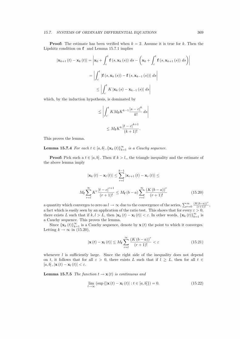
15.7. SYSTEMS OF ORDINARY DIFFERENTIAL EQUATIONS 369
Proof: The estimate has been verified when k = 2. Assume it is true for k. Then theLipshitz condition on f and Lemma 15.7.1 implies
|xk+1 (t)− xk (t)| =∣∣∣∣x0 +
∫ t
c
f (s,xk (s)) ds−(x0 +
∫ t
c
f (s,xk+1 (s)) ds
)∣∣∣∣
=∣∣∣∣∫ t
c
|f (s,xk (s))− f (s,xk−1 (s))| ds
∣∣∣∣
≤∣∣∣∣∫ t
c
K |xk (s)− xk−1 (s)| ds
∣∣∣∣which, by the induction hypothesis, is dominated by
≤∣∣∣∣∣∫ t
c
KMfKk−1 |s− c|k
k!ds
∣∣∣∣∣
≤ MfKk |t− c|k+1
(k + 1)!.
This proves the lemma.
Lemma 15.7.4 For each t ∈ [a, b] , xk (t)∞k=1 is a Cauchy sequence.
Proof: Pick such a t ∈ [a, b] . Then if k > l,, the triangle inequality and the estimate ofthe above lemma imply
|xk (t)− xl (t)| ≤k−1∑
r=l
|xr+1 (t)− xr (t)| ≤
Mf
∞∑
r=l
Kr |t− c|r+1
(r + 1)!≤ Mf (b− a)
∞∑
r=l
(K (b− a))r
(r + 1)!(15.20)
a quantity which converges to zero as l →∞ due to the convergence of the series,∑∞
r=0(K(b−a))r
(r+1)! ,
a fact which is easily seen by an application of the ratio test. This shows that for every ε > 0,there exists L such that if k, l > L, then |xk (t)− xl (t)| < ε. In other words, xk (t)∞k=1 isa Cauchy sequence. This proves the lemma.
Since xk (t)∞k=1 is a Cauchy sequence, denote by x (t) the point to which it converges.Letting k →∞ in (15.20),
|x (t)− xl (t)| ≤ Mf
∞∑
r=l
(K (b− a))r
(r + 1)!< ε (15.21)
whenever l is sufficiently large. Since the right side of the inequality does not dependon t, it follows that for all ε > 0, there exists L such that if l ≥ L, then for all t ∈[a, b] , |x (t)− xl (t)| < ε.
Lemma 15.7.5 The function t → x (t) is continuous and
liml→∞
(sup |x (t)− xl (t)| : t ∈ [a, b]) = 0. (15.22)

370 LIMITS AND DERIVATIVES
Proof: Formula (15.22) was established above in (15.21).Let ε > 0 be given and let t ∈ [a, b] . Then letting l be large enough that
liml→∞
(sup |x (t)− xl (t)| : t ∈ [a, b]) < ε/3,
|x (s)− x (t)| ≤|x (s)− xl (s)|+ |xl (s)− xl (t)|+ |xl (t)− x (t)|
≤ 2ε
3+ |xl (s)− xl (t)| .
By the continuity of xl,the last term is dominated by ε3 whenever |s− t| is small enough.
This verifies continuity of t → x (t) and proves the lemma.Letting l be large enough that
liml→∞
(sup |x (t)− xl (t)| : t ∈ [a, b]) <ε
K (b− a),
∣∣∣∣∫ t
c
f (s,xl (s)) ds−∫ t
c
f (s,x (s)) ds
∣∣∣∣
≤∣∣∣∣∫ t
c
|f (s,xl (s))− f (s,x (s))| ds
∣∣∣∣
≤∣∣∣∣∫ t
c
K |xl (s)− x (s)| ds
∣∣∣∣
< K (b− a)ε
K (b− a)= ε.
Since ε is arbitrary, this verifies that
liml→∞
∫ t
c
f (s,xl (s)) ds =∫ t
c
f (s,x (s)) ds.
It follows thatx (t) = lim
k→∞xk (t)
= limk→∞
(x0 +
∫ t
c
f (s,xk−1 (s)) ds
)
= x0 +∫ t
c
f (s,x (s)) ds
and so by Lemma 15.7.2, x is a solution to the initial value problem, (15.15). This provesthe existence part of the following theorem.
Theorem 15.7.6 Let f satisfy (15.13) and (15.14). Then there exists a unique solution tothe initial value problem, (15.15).
Proof: It only remains to verify the uniqueness assertion. Therefore, assume x and x1
are two solutions to the initial value problem. Then by Lemma 15.7.2 it follows that
x (t)− x1 (t) =∫ t
c
(f (s,x (s))− f (s,x1 (s))) ds.

15.7. SYSTEMS OF ORDINARY DIFFERENTIAL EQUATIONS 371
Suppose first that t < c. Then this equation implies that for all such t,
|x (t)− x1 (t)| ≤∫ c
t
|f (s,x (s))− f (s,x1 (s))|
≤∫ c
t
K |x (s)− x1 (s)| ds.
Letting g (t) =∫ c
t|x (s)− x1 (s)| ds, it follows that −g′ (t) = |x (t)− x1 (t)| and so
−g′ (t) ≤ Kg (t)
which implies 0 ≤ g′ (t) + Kg (t) and consequently,
0 ≤ (eKtg (t)
)′
which implies integration from t to c gives
0 ≤ eKcg (c)− eKtg (t) .
But g (c) = 0 and so 0 ≥ g (t) ≥ 0. Hence g (t) = 0 for all t ≤ c and so x (t) = x1 (t) forthese values of t.
Now suppose that t ≥ c. Then
|x (t)− x1 (t)| ≤∫ t
c
|f (s,x (s))− f (s,x1 (s))|
≤ K
∫ t
c
|x (s)− x1 (s)| ds.
Letting h (t) =∫ t
c|x (s)− x1 (s)| ds, it follows that
h′ (t) ≤ Kh (t)
and so (e−Kth (t)
)′ ≤ 0
which means e−Kth (t)− e−Kch (c) ≤ 0. But h (c) = 0 and so this requires
h (t) ≡∫ t
c
|x (s)− x1 (s)| ds ≤ 0
and so x (t) = x1 (t) whenever t ≥ c. Therefore, x1 = x. This proves uniqueness andestablishes the theorem.
15.7.2 Numerical Methods For Differential Equations
The above considers a fundamental philosophical question about existence of solutions tothe initial value problem. In principle, it yields a method for finding the solution as well butit is never used this way. There are much simpler and better ways to obtain approximatesolutions to differential equations than using Picard iteration. The most primitive way ofdoing this is the Euler method. Suppose you want to find the solution to the initial valueproblem,
x′ = f (t,x) , x (0) = x0,

372 LIMITS AND DERIVATIVES
for t ∈ [0, T ] , where f satisfies the conditions given above for existence. You split the timeinterval into n equal pieces, 0, T
n , 2Tn , · · ·, (n−1)T
n , nTn . Letting h = T
n and ti = ih, you thenreplace the derivative with a difference quotient as follows.
x (ti + h)− x (ti)h
= f (ti,x (ti)) , x (0) = x0. (15.23)
Noting that ti + h = ti+1, this can be written more simply as
x (ti+1) = x (ti) + hf (ti,x (ti)) , x (0) = x0. (15.24)
Now this can be used to find an approximate solution as follows. x0 is known because it isgiven. From (15.24) x (t1) = x0 + hf (0,x0) . Having found x (t1) , this can be substitutedback in to (15.24) to find x (t2) = x (t1) + hf (t1,x (t1)) . Using x (t2) one used (15.24) tofind x (t3) and you continue doing this till you get x (tn). For t ∈ (tk, tk+1) you define
x (t) ≡ (tk+1 − t)h
x (tk) +(t− tk)
hx (tk+1) .
This whole idea is based on approximating functions with their linear approximations locally.Therefore, the resulting function will be piecewise linear and hopefully will not be too faroff. It is customary to write xi instead of x (ti) .
How well does it work? In general, when you are working with numerical methods youtest them on known examples and see how well they perform. In the following example,Euler’s method will be applied to an initial value problem whose solution is known.
Example 15.7.7 Solve the initial value problem y′ = y, y (0) = 1 for t ∈ [0, 5] using Euler’smethod with a step size of .01 and a step size of .001.
The correct answer is y = ex. Thus y (5) = e5 = 148. 413 159 102 576 6. Now from Euler’smethod,
y1 = 1 + .01 (0) = 1
Nowy2 = 1 + (.01) 1 = 1.01.
Next,y3 = 1.01 + (.01) 1.01 = (1.01)2 .
Continuing this way, and using the pattern which is emerging,
y500 = (1.01)500 = 144. 77
and this is the value which Euler’s method gives for y (5) . If you used the step size .001,
you would have (1.001)5000 = 148. 042 which is pretty close.Of course this was an easy example because it led to a pattern which was easy to apply.
In general, there will be no pattern and you just have to iterate things till you get to theend. This is done by a computer.
You need a much better method than the Euler method if you want to solve ordinarydifferential equations. There are many methods and the detailed study of them is outsidethe scope of this book. One of the most famous is the Runge Kutta fourth order method.To solve x′ = f (t,x) , x (0) = x0, you do the following to go from tn to tn+1.
k1 ≡ hf (tn,xn)
k2 ≡ hf(
tn +12h,xn +
12k1
)
k3 ≡ hf(
tn +12h,xn +
12k2
)
k4 ≡ hf (tn + h,xn + k3) .

15.8. EXERCISES 373
Thenxn+1 ≡ xn +
16
(k1 + 2k2 + 2k3 + k4) .
This method is called fourth order because it can be shown that the difference between thetrue solution and this approximate solution is dominated by Ch4 where C is some constantindependent of the choice of h.
Even better schemes have been devised. The computer algebra system, Maple, uses onesuch system which is a fifth order method. The important thing for you to realize at thispoint is that the initial value problem for an ordinary differential equation is a significantproblem and it has been solved quite well.
15.8 Exercises
1. Consider the model problem y′ = y, y (0) = 1 on the interval [0, 1] . Solve it numericallyfor h = .2 using the Euler method and compare with the true solution. Now use theRunge Kutta method for h = .2 and compare with the true solution.
2. Show that if y′ = f (x) , y (0) = 0 so the differential equation does not depend on y,then the Runge Kutta method above reduces to Simpson’s rule for numerical integra-tion.
3. Show that in going from 0 to t1,the difference between the Euler solution and thetrue solution is less than a constant times h2. Assume anything you like about thesmoothness of the function, f. Now show how these errors add up and conclude theEuler method is of order 1. Thus the difference between the true solution and theEuler solution is less than Ch.
4. Work the above model problem using the following method known as a predictorcorrector method.
xn+1 = xn +h
2[f (tn,xn) + f
(tn+1,x∗n+1
)]
where here x∗n+1 = xn + hf (tn,xn) . This x∗n+1 is the prediction. Then xn+1 is thecorrection. Use h = .2 and compare with the true solution.

374 LIMITS AND DERIVATIVES

Line Integrals
The concept of the integral can be extended to functions which are not defined on an intervalof the real line but on some curve in Rn. This is done by defining things in such a way thatthe more general concept reduces to the earlier notion. First it is necessary to consider whatis meant by arc length.
16.1 Arc Length And Orientations
The application of the integral considered here is the concept of the length of a curve. C isa smooth curve in Rn if there exists an interval, [a, b] ⊆ R and functions xi : [a, b] → R suchthat the following conditions hold
1. xi is continuous on [a, b] .
2. x′i exists and is continuous and bounded on [a, b] , with x′i (a) defined as the derivativefrom the right,
limh→0+
xi (a + h)− xi (a)h
,
and x′i (b) defined similarly as the derivative from the left.
3. For p (t) ≡ (x1 (t) , · · ·, xn (t)) , t → p (t) is one to one on (a, b) .
4. |p′ (t)| ≡(∑n
i=1 |x′i (t)|2)1/2
6= 0 for all t ∈ [a, b] .
5. C = ∪(x1 (t) , · · ·, xn (t)) : t ∈ [a, b] .
The functions, xi (t) , defined above are giving the coordinates of a point in Rn and thelist of these functions is called a parameterization for the smooth curve. Note the naturaldirection of the interval also gives a direction for moving along the curve. Such a directionis called an orientation. The integral is used to define what is meant by the length of sucha smooth curve. The earlier treatment in terms of initial value problems will be made morerigorous here. Consider such a smooth curve having parameterization (x1, · · ·, xn) . Forminga partition of [a, b], a = t0 < · · · < tn = b and letting pi = ( x1 (ti), · · ·, xn (ti) ), you couldconsider the polygon formed by lines from p0 to p1 and from p1 to p2 and from p3 to p4
etc. to be an approximation to the curve, C. The following picture illustrates what is meantby this.
375

376 LINE INTEGRALS
¡¡
¡¡
¡¡
""
""
""
p0
p1
p2
p3
Now consider what happens when the partition is refined by including more points. Youcan see from the following picture that the polygonal approximation would appear to beeven better and that as more points are added in the partition, the sum of the lengths ofthe line segments seems to get close to something which deserves to be defined as the lengthof the curve, C.
p0
p1
p2
p3
Thus the length of the curve is approximated by
n∑
k=1
|p (tk)− p (tk−1)| .
Since the functions in the parameterization are differentiable, it is reasonable to expect thisto be close to
n∑
k=1
|p′ (tk−1)| (tk − tk−1)
which is seen to be a Riemann sum for the integral
∫ b
a
|p′ (t)| dt
and it is this integral which is defined as the length of the curve.Would the same length be obtained if another parameterization were used? This is a
very important question because the length of the curve should depend only on the curveitself and not on the method used to trace out the curve. The answer to this question isthat the length of the curve does not depend on parameterization. The proof is somewhattechnical so is given in the last section of this chapter.
Does the definition of length given above correspond to the usual definition of length inthe case when the curve is a line segment? It is easy to see that it does so by consideringtwo points in Rn, p and q. A parameterization for the line segment joining these two pointsis
fi (t) ≡ tpi + (1− t) qi, t ∈ [0, 1] .

16.1. ARC LENGTH AND ORIENTATIONS 377
Using the definition of length of a smooth curve just given, the length according to thisdefinition is
∫ 1
0
(n∑
i=1
(pi − qi)2
)1/2
dt = |p− q| .
Thus this new definition which is valid for smooth curves which may not be straight linesegments gives the usual length for straight line segments.
The proof that curve length is well defined for a smooth curve contains a result whichdeserves to be stated as a corollary. It is proved in Lemma 16.6.2 on Page 385 but the proofis mathematically fairly advanced so it is presented later.
Corollary 16.1.1 Let C be a smooth curve and let f : [a, b] → C and g : [c, d] → C betwo parameterizations satisfying 1 - 5. Then g−1 f is either strictly increasing or strictlydecreasing.
Definition 16.1.2 If g−1 f is increasing, then f and g are said to be equivalent param-eterizations and this is written as f ∼ g. It is also said that the two parameterization givethe same orientation for the curve when f ∼ g.
When the parameterizations are equivalent, they preserve the direction, of motion alongthe curve and this also shows there are exactly two orientations of the curve since eitherg−1 f is increasing or it is decreasing. This is not hard to believe. In simple language, themessage is that there are exactly two directions of motion along a curve.
Lemma 16.1.3 The following hold for ∼.
f ∼ f , (16.1)
If f ∼ g then g ∼ f , (16.2)
If f ∼ g and g ∼ h, then f ∼ h. (16.3)
Proof: Formula (16.1) is obvious because f−1 f (t) = t so it is clearly an increasingfunction. If f ∼ g then f−1 g is increasing. Now g−1 f must also be increasing because itis the inverse of f−1 g. This verifies (16.2). To see (16.3), f−1 h =
(f−1 g
) (g−1 h
)and so since both of these functions are increasing, it follows f−1 h is also increasing. Thisproves the lemma.
The symbol, ∼ is called an equivalence relation. If C is such a smooth curve justdescribed, and if f : [a, b] → C is a parameterization of C, consider g (t) ≡ f ((a + b)− t) ,also a parameterization of C. Now by Corollary 16.1.1, if h is a parameterization, then iff−1 h is not increasing, it must be the case that g−1 h is increasing. Consequently, eitherh ∼ g or h ∼ f . These parameterizations, h, which satisfy h ∼ f are called the equivalenceclass determined by f and those h ∼ g are called the equivalence class determined by g.These two classes are called orientations of C. They give the direction of motion on C. Yousee that going from f to g corresponds to tracing out the curve in the opposite direction.
Sometimes people wonder why it is required, in the definition of a smooth curve thatp′ (t) 6= 0. Imagine t is time and p (t) gives the location of a point in space. If p′ (t) is allowedto equal zero, the point can stop and change directions abruptly, producing a pointy placein C. Here is an example.
Example 16.1.4 Graph the curve(t3, t2
)for t ∈ [−1, 1] .

378 LINE INTEGRALS
In this case, t = x1/3 and so y = x2/3. Thus the graph of this curve looks like the picturebelow. Note the pointy place. Such a curve should not be considered smooth.
16.2 Line Integrals And Work
Let C be a smooth curve contained in Rp. A curve, C is an “oriented curve” if the onlyparameterizations considered are those which lie in exactly one of the two equivalence classes,each of which is called an “orientation”. In simple language, orientation specifies a directionover which motion along the curve is to take place. Thus, it specifies the order in which thepoints of C are encountered. The pair of concepts consisting of the set of points making upthe curve along with a direction of motion along the curve is called an oriented curve.
Definition 16.2.1 Suppose F (x) ∈ Rp is given for each x ∈ C where C is a smoothoriented curve and suppose x → F (x) is continuous. The mapping x → F (x) is called avector field. In the case that F (x) is a force, it is called a force field.
Next the concept of work done by a force field, F on an object as it moves along thecurve, C, in the direction determined by the given orientation of the curve will be defined.This is new. Earlier the work done by a force which acts on an object moving in a straightline was discussed but here the object moves over a curve. In order to define what is meantby the work, consider the following picture.
¡¡
¡¡
¡¡µ
x(t)
F(x(t))
x(t + h)
In this picture, the work done by a constant force, F on an object which moves from thepoint x (t) to the point x (t + h) along the straight line shown would equal F·(x (t + h)− x (t)) .It is reasonable to assume this would be a good approximation to the work done in movingalong the curve joining x (t) and x (t + h) provided h is small enough. Also, provided h issmall,
x (t + h)− x (t) ≈ x′ (t) h
where the wriggly equal sign indicates the two quantities are close. In the notation ofLeibniz, one writes dt for h and
dW = F (x (t)) · x′ (t) dt

16.2. LINE INTEGRALS AND WORK 379
or in other words,dW
dt= F (x (t)) · x′ (t) .
Defining the total work done by the force at t = 0, corresponding to the first endpoint ofthe curve, to equal zero, the work would satisfy the following initial value problem.
dW
dt= F (x (t)) · x′ (t) , W (a) = 0.
This motivates the following definition of work.
Definition 16.2.2 Let F (x) be given above. Then the work done by this force field on anobject moving over the curve C in the direction determined by the specified orientation isdefined as ∫
C
F · dR ≡∫ b
a
F (x (t)) · x′ (t) dt
where the function, x is one of the allowed parameterizations of C in the given orientationof C. In other words, there is an interval, [a, b] and as t goes from a to b, x (t) moves in thedirection determined from the given orientation of the curve.
Theorem 16.2.3 The symbol,∫
CF · dR, is well defined in the sense that every parameter-
ization in the given orientation of C gives the same value for∫
CF · dR.
Proof: Suppose g : [c, d] → C is another allowed parameterization. Thus g−1 f is anincreasing function, φ. Then since φ is increasing,
∫ d
c
F (g (s)) · g′ (s) ds =∫ b
a
F (g (φ (t))) · g′ (φ (t)) φ′ (t) dt
=∫ b
a
F (f (t)) · d
dt
(g
(g−1 f (t)
))dt =
∫ b
a
F (f (t)) · f ′ (t) dt.
This proves the theorem.Regardless the physical interpretation of F, this is called the line integral. When F is
interpreted as a force, the line integral measures the extent to which the motion over thecurve in the indicated direction is aided by the force. If the net effect of the force on theobject is to impede rather than to aid the motion, this will show up as the work beingnegative.
Does the concept of work as defined here coincide with the earlier concept of work whenthe object moves over a straight line when acted on by a constant force?
Let p and q be two points in Rn and suppose F is a constant force acting on an objectwhich moves from p to q along the straight line joining these points. Then the workdone is F · (q− p) . Is the same thing obtained from the above definition? Let x (t) ≡p+t (q− p) , t ∈ [0, 1] be a parameterization for this oriented curve, the straight line in thedirection from p to q. Then x′ (t) = q− p and F (x (t)) = F. Therefore, the above definitionyields ∫ 1
0
F · (q− p) dt = F · (q− p) .
Therefore, the new definition adds to but does not contradict the old one.

380 LINE INTEGRALS
Example 16.2.4 Suppose for t ∈ [0, π] the position of an object is given by r (t) = ti +cos (2t) j + sin (2t)k. Also suppose there is a force field defined on R3,F (x, y, z) ≡ 2xyi +x2j + k. Find ∫
C
F · dR
where C is the curve traced out by this object which has the orientation determined by thedirection of increasing t.
To find this line integral use the above definition and write∫
C
F · dR =∫ π
0
(2t (cos (2t)) ,t2,1
) ·
(1,−2 sin (2t) , 2 cos (2t)) dt
In evaluating this replace the x in the formula for F with t, the y in the formula for Fwith cos (2t) and the z in the formula for F with sin (2t) because these are the values ofthese variables which correspond to the value of t. Taking the dot product, this equals thefollowing integral. ∫ π
0
(2t cos 2t− 2 (sin 2t) t2 + 2 cos 2t
)dt = π2
16.3 Exercises
1. Suppose for t ∈ [0, 2π] the position of an object is given by r (t) = ti + cos (2t) j +sin (2t)k. Also suppose there is a force field defined on R3,F (x, y, z) ≡ 2xyi+
(x2 + 2zy
)j+
y2k. Find ∫
C
F · dR
where C is the curve traced out by this object which has the orientation determinedby the direction of increasing t.
2. Here is a vector field,(y, x + z2, 2yz
)and here is the parameterization of a curve, C.
R (t) = (cos 2t, 2 sin 2t, t) where t goes from 0 to π/4. Find∫
CF· dR.
3. If f and g are both increasing functions, show f g is an increasing function also.Assume anything you like about the domains of the functions.
4. Suppose for t ∈ [0, 3] the position of an object is given by r (t) = ti + tj + tk. Alsosuppose there is a force field defined on R3,F (x, y, z) ≡ yzi + xzj + xyk. Find
∫
C
F · dR
where C is the curve traced out by this object which has the orientation determinedby the direction of increasing t. Repeat the problem for r (t) = ti + t2j + tk.
5. Suppose for t ∈ [0, 1] the position of an object is given by r (t) = ti + tj + tk. Alsosuppose there is a force field defined on R3,F (x, y, z) ≡ zi + xzj + xyk. Find
∫
C
F · dR
where C is the curve traced out by this object which has the orientation determinedby the direction of increasing t. Repeat the problem for r (t) = ti + t2j + tk.

16.4. MOTION ON A SPACE CURVE 381
6. Let F (x, y, z) be a given force field and suppose it acts on an object having mass, mon a curve with parameterization, (x (t) , y (t) , z (t)) for t ∈ [a, b] . Show directly thatthe work done equals the difference in the kinetic energy. Hint:
∫ b
a
F (x (t) , y (t) , z (t)) · (x′ (t) , y′ (t) , z′ (t)) dt =
∫ b
a
m (x′′ (t) , y′′ (t) , z′′ (t)) · (x′ (t) , y′ (t) , z′ (t)) dt,
etc.
16.4 Motion On A Space Curve
A fly buzzing around the room, a person riding a roller coaster, and a satellite orbiting theearth all have something in common. They are moving over some sort of curve in threedimensions.
Denote by R (s) the function which takes s to a point on this curve where s is arc length.Thus R (s) equals the point on the curve which occurs when you have traveled a distance ofs along the curve from one end. This is known as the parameterization of the curve in termsof arc length. Note also that it incorporates an orientation on the curve because there areexactly two ends you could begin measuring length from. In this section, assume anythingabout smoothness and continuity to make the following manipulations valid. In particular,assume that R′ exists and is continuous.
Lemma 16.4.1 Define T (s) ≡ R′ (s) . Then |T (s)| = 1 and if T′ (s) 6= 0, then thereexists a unit vector, N (s) perpendicular to T (s) and a scalar valued function, κ (s) withT′ (s) = κ (s)N (s) .
Proof: First, s =∫ s
0|R′ (r)| dr because of the definition of arc length. Therefore,
from the fundamental theorem of calculus, 1 = |R′ (s)| = |T (s)| . Therefore, T ·T = 1and so upon differentiating this on both sides, yields T′ · T + T ·T′ = 0 which showsT ·T′ = 0. Therefore, the vector, T′ is perpendicular to the vector, T. In case T′ (s) 6= 0,
let N (s) = T′(s)|T′(s)| and so T′ (s) = |T′ (s)|N (s) , showing the scalar valued function is
κ (s) = |T′ (s)| . This proves the lemma.The radius of curvature is defined as ρ = 1
κ . Thus at points where there is a lot ofcurvature, the radius of curvature is small and at points where the curvature is small, theradius of curvature is large. The plane determined by the two vectors, T and N is calledthe osculating plane. It identifies a particular plane which is in a sense tangent to this spacecurve. In the case where |T′ (s)| = 0 near the point of interest, T (s) equals a constant andso the space curve is a straight line which it would be supposed has no curvature. Also, theprincipal normal is undefined in this case. This makes sense because if there is no curvinggoing on, there is no special direction normal to the curve at such points which could bedistinguished from any other direction normal to the curve. In the case where |T′ (s)| = 0,κ (s) = 0 and the radius of curvature would be considered infinite.
Definition 16.4.2 The vector, T (s) is called the unit tangent vector and the vector, N (s)is called the principal normal. The function, κ (s) in the above lemma is called the curva-ture.When T′ (s) 6= 0 so the principal normal is defined, the vector, B (s) ≡ T (s) ×N (s)is called the binormal.
The binormal is normal to the osculating plane and B′ tells how fast this vector changes.Thus it measures the rate at which the curve twists.
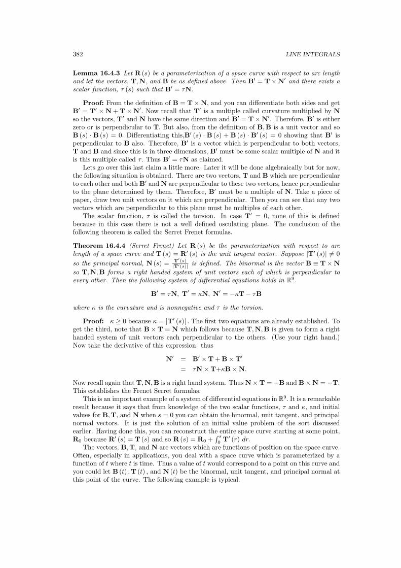
382 LINE INTEGRALS
Lemma 16.4.3 Let R (s) be a parameterization of a space curve with respect to arc lengthand let the vectors, T,N, and B be as defined above. Then B′ = T×N′ and there exists ascalar function, τ (s) such that B′ = τN.
Proof: From the definition of B = T×N, and you can differentiate both sides and getB′ = T′ ×N + T×N′. Now recall that T′ is a multiple called curvature multiplied by Nso the vectors, T′ and N have the same direction and B′ = T×N′. Therefore, B′ is eitherzero or is perpendicular to T. But also, from the definition of B,B is a unit vector and soB (s) · B (s) = 0. Differentiating this,B′ (s) · B (s) + B (s) · B′ (s) = 0 showing that B′ isperpendicular to B also. Therefore, B′ is a vector which is perpendicular to both vectors,T and B and since this is in three dimensions, B′ must be some scalar multiple of N and itis this multiple called τ . Thus B′ = τN as claimed.
Lets go over this last claim a little more. Later it will be done algebraically but for now,the following situation is obtained. There are two vectors, T and B which are perpendicularto each other and both B′ and N are perpendicular to these two vectors, hence perpendicularto the plane determined by them. Therefore, B′ must be a multiple of N. Take a piece ofpaper, draw two unit vectors on it which are perpendicular. Then you can see that any twovectors which are perpendicular to this plane must be multiples of each other.
The scalar function, τ is called the torsion. In case T′ = 0, none of this is definedbecause in this case there is not a well defined osculating plane. The conclusion of thefollowing theorem is called the Serret Frenet formulas.
Theorem 16.4.4 (Serret Frenet) Let R (s) be the parameterization with respect to arclength of a space curve and T (s) = R′ (s) is the unit tangent vector. Suppose |T′ (s)| 6= 0so the principal normal, N (s) = T′(s)
|T′(s)| is defined. The binormal is the vector B ≡ T×Nso T,N,B forms a right handed system of unit vectors each of which is perpendicular toevery other. Then the following system of differential equations holds in R9.
B′ = τN, T′ = κN, N′ = −κT− τB
where κ is the curvature and is nonnegative and τ is the torsion.
Proof: κ ≥ 0 because κ = |T′ (s)| . The first two equations are already established. Toget the third, note that B×T = N which follows because T,N,B is given to form a righthanded system of unit vectors each perpendicular to the others. (Use your right hand.)Now take the derivative of this expression. thus
N′ = B′ ×T + B×T′
= τN×T+κB×N.
Now recall again that T,N,B is a right hand system. Thus N×T = −B and B×N = −T.This establishes the Frenet Serret formulas.
This is an important example of a system of differential equations in R9. It is a remarkableresult because it says that from knowledge of the two scalar functions, τ and κ, and initialvalues for B,T, and N when s = 0 you can obtain the binormal, unit tangent, and principalnormal vectors. It is just the solution of an initial value problem of the sort discussedearlier. Having done this, you can reconstruct the entire space curve starting at some point,R0 because R′ (s) = T (s) and so R (s) = R0 +
∫ s
0T′ (r) dr.
The vectors, B,T, and N are vectors which are functions of position on the space curve.Often, especially in applications, you deal with a space curve which is parameterized by afunction of t where t is time. Thus a value of t would correspond to a point on this curve andyou could let B (t) ,T (t) , and N (t) be the binormal, unit tangent, and principal normal atthis point of the curve. The following example is typical.

16.4. MOTION ON A SPACE CURVE 383
Example 16.4.5 Given the circular helix, R (t) = (a cos t) i + (a sin t) j + (bt)k, find thearc length, s (t) ,the unit tangent vector, T (t) , the principal normal, N (t) , the binormal,B (t) , the curvature, κ (t) , and the torsion, τ (t) . Here t ∈ [0, T ] .
The arc length is s (t) =∫ t
0
(√a2 + b2
)dr =
(√a2 + b2
)t. Now the tangent vector is
obtained using the chain rule as
T =dRds
=dRdt
dt
ds=
1√a2 + b2
R′ (t)
=1√
a2 + b2((−a sin t) i + (a cos t) j + bk)
The principal normal:
dTds
=dTdt
dt
ds
=1
a2 + b2((−a cos t) i + (−a sin t) j + 0k)
and so
N =dTds
/
∣∣∣∣dTds
∣∣∣∣ = − ((cos t) i + (sin t) j)
The binormal:
B =1√
a2 + b2
∣∣∣∣∣∣
i j k−a sin t a cos t b− cos t − sin t 0
∣∣∣∣∣∣
=1√
a2 + b2((b sin t) i−b cos tj + ak)
Now the curvature, κ (t) =∣∣dT
ds
∣∣ =
√(a cos ta2+b2
)2
+(
a sin ta2+b2
)2
= aa2+b2 . Note the curvature
is constant in this example. The final task is to find the torsion. Recall that B′ = τN wherethe derivative on B is taken with respect to arc length. Therefore, remembering that t is afunction of s,
B′ (s) =1√
a2 + b2((b cos t) i+(b sin t) j)
dt
ds
=1
a2 + b2((b cos t) i+(b sin t) j)
= τ (− (cos t) i− (sin t) j) = τN
and it follows −b/(a2 + b2
)= τ .
An important application of the usefulness of these ideas involves the decomposition ofthe acceleration in terms of these vectors of an object moving over a space curve.
Corollary 16.4.6 Let R (t) be a space curve and denote by v (t) the velocity, v (t) = R′ (t)and let v (t) ≡ |v (t)| denote the speed and let a (t) denote the acceleration. Then v = vTand a =dv
dt T + κv2N.
Proof: T = dRds = dR
dtdtds = v dt
ds . Also, s =∫ t
0v (r) dr and so ds
dt = v which impliesdtds = 1
v . Therefore, T = v/v which implies v = vT as claimed.

384 LINE INTEGRALS
Now the acceleration is just the derivative of the velocity and so by the Serrat Frenetformulas,
a =dv
dtT + v
dTdt
=dv
dtT + v
dTds
v =dv
dtT + v2κN
Note how this decomposes the acceleration into a component tangent to the curve and one
which is normal to it. Also note that from the above, v |T′| T′(t)|T′| = v2κN and so |T′|
v = κ
and N =T′(t)|T′|
From this, it is possible to give an important formula from physics. Suppose an objectorbits a point at constant speed, v. What is the centripetal acceleration of this object? Youmay know from a physics class that the answer is v2/r where r is the radius. This followsfrom the above quite easily. The parameterization of the object which is as described is
R (t) =(r cos
(v
rt)
, r sin(v
rt))
.
Therefore, T =(− sin
(vr t
), cos
(vr t
))and T′ =
(−vr cos
(vr t
),−v
r sin(
vr t
)). Thus, κ = |T′ (t)| /v =
1r . It follows
a =dv
dtT + v2κN =
v2
rN.
The vector, N points from the object toward the center of the circle because it is a positivemultiple of the vector,
(−vr cos
(vr t
),−v
r sin(
vr t
)).
Sometimes curves don’t come to you parametrically. This is unfortunate when it occursbut you can sometimes find a parametric description of such curves.
Example 16.4.7 Find a parameterization for the intersection of the surfaces y + 3z =2x2 + 4 and y + 2z = x + 1.
You need to solve for x and y in terms of x. This yields
z = 2x2 − x + 3, y = −4x2 + 3x− 5.
Therefore, letting t = x, the parameterization is (x, y, z) =(t,−4t2 − 5 + 3t,−t + 3 + 2t2
).
Example 16.4.8 Find a parametrization for the straight line joining (3, 2, 4) and (1, 10, 5) .
(x, y, z) = (3, 2, 4) + t (−2, 8, 1) = (3− 2t, 2 + 8t, 4 + t) where t ∈ [0, 1] . Note where thiscame from. The vector, (−2, 8, 1) is obtained from (1, 10, 5) − (3, 2, 4) . Now you shouldcheck to see this works.
16.5 Exercises
1. Find a parametrization for the intersection of the planes 2x + y + 3z = −2 and3x− 2y + z = −4.
2. Find a parametrization for the intersection of the plane 3x + y + z = −3 and thecircular cylinder x2 + y2 = 1.
3. Find a parametrization for the intersection of the plane 4x + 2y + 3z = 2 and theelliptic cylinder x2 + 4z2 = 9.

16.6. INDEPENDENCE OF PARAMETERIZATION 385
4. Find a parametrization for the straight line joining (1, 2, 1) and (−1, 4, 4) .
5. Find a parametrization for the intersection of the surfaces 3y + 3z = 3x2 + 2 and3y + 2z = 3.
6. Let R (t) = (cos t) i+(cos t) j+(√
2 sin t)k. Find the arc length, s as a function of the
parameter, t, if t = 0 is taken to correspond to s = 0.
7. Let R (t) = 2i+(4t + 2) j+4tk. Find the arc length, s as a function of the parameter,t, if t = 0 is taken to correspond to s = 0.
8. Let R (t) = e5ti+e−5tj+5√
2tk. Find the arc length, s as a function of the parameter,t, if t = 0 is taken to correspond to s = 0.
9. An object moves along the x axis toward (0, 0) and then along the curve y = x2 inthe direction of increasing x at constant speed. Is the force acting on the object acontinuous function? Explain.
16.6 Independence Of Parameterization
Recall that if p (t) : t ∈ [a, b] was a parameterization of a smooth curve, C, the length of Cis defined as ∫ b
a
|p′ (t)| dt
If some other parameterization were used to trace out C, would the same answer be obtained?
Theorem 16.6.1 Let φ : [a, b] → [c, d] be one to one and suppose φ′ exists and is continuouson [a, b] . Then if f is a continuous function defined on [a, b] which is Riemann integrable1,
∫ d
c
f (s) ds =∫ b
a
f (φ (t))∣∣φ′ (t)∣∣ dt
Proof: Let F ′ (s) = f (s) . (For example, let F (s) =∫ s
af (r) dr.) Then the first integral
equals F (d)−F (c) by the fundamental theorem of calculus. By Lemma 5.7.4 on Page 94,φ is either strictly increasing or strictly decreasing. Suppose φ is strictly decreasing. Thenφ (a) = d and φ (b) = c. Therefore, φ′ ≤ 0 and the second integral equals
−∫ b
a
f (φ (t))φ′ (t) dt =∫ a
b
d
dt(F (φ (t))) dt
= F (φ (a))− F (φ (b)) = F (d)− F (c) .
The case when φ is increasing is similar. This proves the theorem.
Lemma 16.6.2 Let f : [a, b] → C, g : [c, d] → C be parameterizations of a smooth curvewhich satisfy conditions 1 - 5. Then φ (t) ≡ g−1 f (t) is 1 − 1 on (a, b) , continuous on[a, b] , and either strictly increasing or strictly decreasing on [a, b] .
Proof: It is obvious φ is 1 − 1 on (a, b) from the conditions f and g satisfy. It onlyremains to verify continuity on [a, b] because then the final claim follows from Lemma 5.15.3on Page 117. If φ is not continuous on [a, b] , then there exists a sequence, tn ⊆ [a, b]such that tn → t but φ (tn) fails to converge to φ (t) . Therefore, for some ε > 0 there
1Recall that all continuous functions of this sort are Riemann integrable.

386 LINE INTEGRALS
exists a subsequence, still denoted by n such that |φ (tn)− φ (t)| ≥ ε. Using the sequentialcompactness of [c, d] , (See Theorem 14.9.5 on Page 347.) there is a further subsequence,still denoted by n such that φ (tn) converges to a point, s, of [c, d] which is not equal toφ (t) . Thus g−1 f (tn) → s and still tn → t. Therefore, the continuity of f and g implyf (tn) → g (s) and f (tn) → f (t) . Therefore, g (s) = f (t) and so s = g−1 f (t) = φ (t) , acontradiction. Therefore, φ is continuous as claimed.
Theorem 16.6.3 The length of a smooth curve is not dependent on parameterization.
Proof: Let C be the curve and suppose f : [a, b] → C and g : [c, d] → C both satisfyconditions 1 - 5. Is it true that
∫ b
a|f ′ (t)| dt =
∫ d
c|g′ (s)| ds?
Let φ (t) ≡ g−1f (t) for t ∈ [a, b]. Then by the above lemma φ is either strictly increasingor strictly decreasing on [a, b] . Suppose for the sake of simplicity that it is strictly increasing.The decreasing case is handled similarly.
Let s0 ∈ φ ([a + δ, b− δ]) ⊂ (c, d) . Then by assumption 4, g′i (s0) 6= 0 for some i. Bycontinuity of g′i, it follows g′i (s) 6= 0 for all s ∈ I where I is an open interval containedin [c, d] which contains s0. It follows that on this interval, gi is either strictly increasingor strictly decreasing. Therefore, J ≡ gi (I) is also an open interval and you can define adifferentiable function, hi : J → I by
hi (gi (s)) = s.
As in Theorem 8.1.6 on Page 151, this implies that for s ∈ I,
h′i (gi (s)) =1
g′i (s). (16.4)
Now letting s = φ (t) for s ∈ I, it follows t ∈ J1, an open interval. Also, for s and t relatedthis way, f (t) = g (s) and so in particular, for s ∈ I,
gi (s) = fi (t) .
Consequently,s = hi (fi (t)) = φ (t)
and so, for t ∈ J1,
φ′ (t) = h′i (fi (t)) f ′i (t) = h′i (gi (s)) f ′i (t) =f ′i (t)
g′i (φ (t))(16.5)
which shows that φ′ exists and is continuous on J1, an open interval containing φ−1 (s0) .Since s0 is arbitrary, this shows φ′ exists on [a + δ, b− δ] and is continuous there.
Now f (t) = g (g−1 f
)(t) = g (φ (t)) and it was just shown that φ′ is a continuous
function on [a− δ, b + δ] . It follows
f ′ (t) = g′ (φ (t))φ′ (t)
and so, by Theorem 16.6.1,∫ φ(b−δ)
φ(a+δ)
|g′ (s)| ds =∫ b−δ
a+δ
|g′ (φ (t))|∣∣φ′ (t)
∣∣ dt
=∫ b−δ
a+δ
|f ′ (t)| dt.
Now using the continuity of φ,g′, and f ′ on [a, b] and letting δ → 0+ in the above, yields∫ d
c
|g′ (s)| ds =∫ b
a
|f ′ (t)| dt
and this proves the theorem.

The Circular Functions Again
The circular functions have already been discussed. You recall the important role of planegeometry in defining them. A major consideration was the careful definition of arc lengthof a circle and showing the radian measure of an angle is well defined. This involved similartriangles and such notions. On the other hand, the only thing necessary do calculus is theconcept of completeness and a way to measure distance, the distance formula. Is it possibleto define the circular functions beginning with these things instead of dragging in all thatplane geometry? Also, what are some things the circular functions are good for? Thischapter is devoted to these questions.
To begin with, there is a physical motivation for the circular functions. Consider a garagedoor spring. These springs exert a force which resists extension. Attach such a spring tothe ceiling and attach a mass, m, to the bottom end of the spring as shown in the followingpicture. Any mass will do. It does not have to be a small elephant.
m
The weight of this mass, mg, is a downward force which extends the spring, moving thebottom end of the spring downward a distance l where the upward force exerted by thespring exactly balances the downward force exerted on the mass by gravity. It has beenexperimentally observed that as long as the extension, z, of such a spring is not too great,the restoring force exerted by the spring is of the form kz where k is some constant whichdepends on the spring. (It would be different for a slinky than for a garage door spring.)This is known as Hooke’s law which is the simplest model for elastic materials. Therefore,mg = kl. Now let y be the displacement from this equilibrium position of the bottom of thespring with the positive direction being up. Thus the acceleration of the spring would bey′′. The extension of the spring in terms of y would be (l − y) . Then Newton’s second lawalong with Hooke’s law imply
my′′ = k (l − y)−mg
and since kl −mg = 0, this yields
my′′ + ky = 0.
387

388 THE CIRCULAR FUNCTIONS AGAIN
Dividing by m and letting ω2 = k/m yields the equation for undamped oscillation,
y′′ + ω2y = 0.
Based on physical reasoning just presented, there should be a solution to this equation. It isthe displacement of the bottom end of a spring from the equilibrium position. However, itis not enough to base questions of existence in mathematics on physical intuition, althoughit is sometimes done. The following theorem gives the necessary existence and uniquenessresults.
Theorem 17.0.4 There exists exactly one function, y, which satisfies the following initialvalue problem.
y′′ + ω2y = 0, y (a) = y0, y′ (a) = y1. (17.1)
Proof: First consider the question of uniqueness. Suppose both z and y are solutionsto the problem (17.1). Then let x = z− y and use Theorem 6.2.6 to conclude x satisfies thefollowing initial value problem.
x′′ + ω2x = 0, x (a) = x′ (a) = 0.
Now multiply both sides of the differential equation by x′ and use Theorem 6.2.6 again towrite
d
dt
((x′)2
2+
ω2 (x)2
2
)= 0.
By Corollary 6.8.4 on Page 133 the expression
(x′)2
2+
ω2 (x)2
2
must equal a constant. However this expression equals zero when t = a and so it mustbe zero for all t. Therefore, in particular, x (t) = 0 and so z (t) = y (t) . This proves theuniqueness part.
To establish the existence of a solution, let z (t) ≡ y (t + a) . Then y solves (17.1) if andonly if z solves
z′′ + ω2z = 0, z (0) = y0, z′ (0) = y1. (17.2)
Now let
C (t) ≡∞∑
n=0
(−1)n t2n
(2n!), S (t) ≡
∞∑n=0
(−1)n t2n+1
(2n + 1)!. (17.3)
Using the ratio test, you see both series in the above converge for all t ∈ R. (Of course youknow what these series are already but you don’t need to know this for the purposes of thispresentation. Remember, you can define functions in terms of power series.) Then you seeright away using the theorem about differentiation of power series that
S′ (t) = C (t) and C ′ (t) = −S (t) . (17.4)
Consider the function, z (t) = y0C (ωt) + y0ω S (ωt) . It follows from the chain rule and what
was just observed about S′ and C ′ that z solves (17.2). Therefore, our solution to (17.1) isthe function, y (t) ≡ z (t− a).
The quantity which is a constant in the above proof of uniqueness is sometimes referredto as the energy.
It follows immediately from (17.3) that C (t) satisfies the following initial value problems.
C ′′ + C = 0, C (0) = 1, C ′ (0) = 0.

389
In terms of the spring, this would have the spring constant, k equal in magnitude to themass, m and the function would be the displacements from equilibrium of the bottom of thespring when initially it is raised one unit above the equilibrium point and released with zerovelocity. The second of these functions, S (t) is the solution to the initial value problem
S′′ + S = 0, S (0) = 0, S′ (0) = 1.
In terms of the spring, the spring constant, k would be equal in magnitude to the mass, mand the function would be the displacements from equilibrium of the bottom of the springwhen initially it is at the equilibrium point and moving upward with unit speed. The nexttheorem is on properties of these functions, C and S. These properties will be obtaineddirectly from the initial value problems they satisfy. In addition, another proof is given ofProperty (17.4) which is based on the initial value problems satisfied by the functions ratherthan the differentiation theorem for power series.
Theorem 17.0.5 The functions C and S satisfy the following properties.
C2 (t) + S2 (t) = 1, (17.5)
S (−t) = −S (t) , C (−t) = C (t) , (17.6)
These conditions in (17.6) say that S is odd and C is even because the property of being oddor even is defined in terms of these equations.
S (x + y) = S (x)C (y) + C (x)S (y) , (17.7)
C (x− y) = C (x)C (y) + S (x)S (y) , (17.8)
For x ≥ 0,
x− x3
6≤ S (x) , (17.9)
1− x2
2≤ C (x) ≤ 1− x2
2+
x4
24. (17.10)
Proof: To verify (17.4) consider the function, y (x) = C ′ + S. Then
y′′ + y = C ′′′ + C ′ + S′′ + S = 0
andy (0) = C ′ (0) + S (0) = 0 + 0 = 0,
whiley′ (0) = C ′′ (0) + S′ (0) = −C (0) + C (0) = 0.
By the Theorem 17.0.4, y (x) = 0. The second half of (17.4) is proved similarly only thistime consider y (x) = S′ (x)− C (x) .
It will be shown that y solves the differential equation and the initial condition, y (0) =S′ (0)− C (0) = 1− 1 = 0. Thus by Theorem 17.0.4 again y (x) = 0.
To verify (17.5) use the initial value problem satisfied by C to write
C ′′ + C = 0.
Now multiply by C ′ and use Theorem 6.2.6 to obtain
d
dt
((C ′ (t))2
2+
(C (t))2
2
)= 0

390 THE CIRCULAR FUNCTIONS AGAIN
and so(C ′ (t))2
2+
(C (t))2
2= c
for some constant, c. Now the initial conditions for C imply this constant, c equals 1/2.Using C ′ = −S, yields (17.5).
Let y (t) = S (−t) + S (t) . Then by Theorem 6.2.6 y′ (t) = −S′ (−t) + S′ (t) and soy (0) = 0 and y′ (0) = −1 + 1 = 0. Also using Theorem 6.2.6 again, y′′ (t) = S′ (−t) + S′ (t)and so y′′ + y = 0. Then by Theorem 17.0.4, it follows y (t) = 0. This proves the first partof (17.6). The second part is similar.
To verify (17.7), fix y and let y (x) = S (x + y)− (S (x)C (y) + S (y)C (x)) . Then from(17.4),
y′ (x) = C (x + y)− (C (x) C (y)− S (y)S (x))
andy′′ (x) = −S (x + y)− (−S (x) C (y)− S (y) C (x))
soy′′ + y = 0.
Also y (0) = S (y)−S (y) = 0 and y′ (0) = C (y)−C (y) = 0. Therefore, by Theorem 17.0.4,it follows y (x) = 0 proving (17.7). The proof of (17.8) is completely similar and is left asan exercise.
This brings us to the estimates. Let w (x) = x− S (x) . Then w (0) = 0 and
w′ (x) = 1− C (x) ≥ 0.
By Corollary 6.8.5 on Page 133, it follows that w is increasing on [0,∞). Therefore, w (x) ≥ 0which shows that
x− S (x) ≥ 0.
Let z (x) = C (x)−(1− x2
2
). Then z (0) = 0 and
z′ (x) = −S (x) + x ≥ 0
so by Corollary 6.8.5on Page 133, it follows that z (x) = C (x)−(1− x2
2
)≥ 0 for all x ≥ 0,
proving the bottom half of (17.10). Now let y (x) = S (x)−(x− x3
6
). Then y (0) = 0 and
y′ (x) = C (x)−(
1− x2
2
)≥ 0
so by Corollary 6.8.5, it follows that y (x) = S (x)−(x− x3
6
)≥ 0 for all x ≥ 0. This proves
(17.9). Now let u (x) =(1− x2
2 + x4
24
)− C (x) . Then u (0) = 0 and
u′ (x) = −x +x3
6+ S (x) ≥ 0
by (17.9). Therefore, by Corollary 6.8.5, u (x) ≥ 0 for all x ≥ 0 and this shows the top halfof (17.10).
With (17.9) and (17.10) other properties of C and S related to their periodic behaviormay be obtained.

391
Theorem 17.0.6 There exists a positive number, P such that C (x) > 0 on [0, P2 ) and
C(
P2
)= 0. In addition to this, both C and S are periodic of period 2P. This means that for
all x ∈ R,C (x + 2P ) = C (x) , S (x + 2P ) = S (x) .
Also the function, r (t) ≡ (C (t) , S (t)) is one to one for t ∈ [0, 2P ) and C (t) = cos t whileS (t) = sin t for t given in radians and P = π where 2π is the circumference of the unitcircle.
Proof: From (17.10) that C (2) < 0 because C (2) ≤(1− 22
2 + 24
24
)= − 1
3 < 0. Recall,C (1) = 1 > 0. By the intermediate value theorem there exists a number, P/2 ∈ (0, 2) suchthat C (P/2) = 0. There is only one such number because for x ∈ (0, 2) ,
C ′ (x) = −S′ (x) ≤ −x +x3
6= (−x)
(1− x2
6
)< 0
showing that C is strictly decreasing on this interval because of Corollary 6.8.6. This provesthe first part of the theorem. S is increasing on (0, P/2) because S′ (x) = C (x) and C (x) > 0on (0, P/2) . Therefore, from (17.5), S (P/2) = 1. Also this shows that r (t) is one to one fort ∈ [0, P/2] . Now consider what happens on the interval, [P/2, P ] . Points on this intervalare of the form, x + P/2 where x ∈ [0, P/2] . From (17.6),(17.7), and (17.8),
C (x + P/2) = C (x)C (P/2)− S (x)S (P/2)= −S (x) ≤ 0, < 0 if x ∈ (0, P/2)
while
S (x + P/2) = S (x)C (P/2) + S (P/2) C (x)= C (x) ≥ 0, > 0 if x ∈ (0, P/2) .
Therefore, S is strictly decreasing on [P/2, P ] because its derivative, C is negative on(P/2, P ). Also C is strictly decreasing on this interval because its derivative, −S is negativeon (P/2, P ) . Since C is strictly decreasing on the interval [0, P ] it follows that r is one toone on [0, P ] . Furthermore,
S (P ) = S (P/2) C (P/2) + S (P/2)C (P/2) = 0C (P ) = C (P/2) C (P/2)− S (P/2)S (P/2) = −1.
In going from P to 3P/2, use similar arguments to verify that S is strictly decreasing andthat C is strictly increasing and that S (3P/2) = −1 while C (−3P/2) = 0. If r (t1) = r (t2)for t1 ∈ [0, P ] and t2 ∈ [P, 3P/2] , then C (t1) = C (t2) and S (t1) = S (t2) . Therefore,S (t2) ≤ 0 and so S (t1) ≤ 0. But S (t1) ≥ 0 and so t1 = P = t2. It follows that r isone to one on [0, 3P/2] . In going from 3P/2 to 2P, use the same arguments to verify thatC and S are strictly increasing and C (2P ) = 1 while S (2P ) = 0. Now if r (t1) = r (t2)for t2 ∈ (3P/2, 2p) and t1 ∈ [0, 3P/2] , C (t1) = C (t2) > 0 and so, t1 ∈ [0, P/2). NowS (t1) = S (t2) < 0 which can’t happen for t1 ∈ [0, P/2] . Therefore, r is one to one on[0, 2P ). It only remains to verify that C and S are periodic of period 2P, that P = π, andthat C = cos while S = sin.
First consider the claim that S and C are 2P periodic.
S (x + 2P ) = S (x + P ) C (P ) + C (x + P ) S (P )= −S (x + P )= − [S (x)C (P ) + C (x) S (P )] = S (x) .

392 THE CIRCULAR FUNCTIONS AGAIN
To verify the assertion about C,
C (x + 2P ) = C (x + P ) C (P )− S (x + P ) S (P )= −C (x + P )= − [C (x)C (P )− S (x) S (P )] = C (x) .
Now it remains to verify the other assertions. First note that by (17.5), r (t) = (C (t) , S (t))is a point on the unit circle. Since r is one to one on (0, 2P ) , the length of the path tracedout by r for t ∈ [0, s] is given by A (s) where A solves the initial value problem,
A′ (t) =√
(C ′ (t))2 + (S′ (t))2 =√
S2 (t) + C2 (t) = 1, A (0) = 0.
The solution to this is just A (t) = t and so the length of this path traced out by r is justs. In other words, (C (t) , S (t)) is the point on the unit circle which is at a distance of tmeasured along an arc which starts at (1, 0) and proceeds counter clock wise to this pointas shown in the following picture in which t denotes the length of the indicated arc of thecircle.
¡¡
¡¡
¡¡
t
(C(t), S(t))
Thus, drawing a right triangle with the radius of the circle as its hypotenuse and t theangle just described, C (t) = cos t and S (t) = sin t. Now the length of the curve traced outby r for t ∈ [0, 2P ] is just 2P but from the above discussion, this involves starting at (1, 0)and continuing around the unit circle till (1, 0) . Define 2π to be this length. Therefore,P = π. This proves the theorem.
Note that this finishes off all the trig identities as well thanks to the previous theorem,so this gives an alternate way of defining the circular functions. No reference was made toplane geometry, just the definition of distance along with the notion of arc length.
17.1 The Equations Of Undamped And Damped Oscil-lation
With the circular functions, the equation of undamped oscillation, y′′ + ω2y = 0 may besolved. This equation resulted from the oscillations of a heavy weight on a spring but itoccurs in many other physical contexts also.
Theorem 17.1.1 The initial value problem,
y′′ + ω2y = 0, y (0) = y0, y′ (0) = y1 (17.11)

17.1. THE EQUATIONS OF UNDAMPED AND DAMPED OSCILLATION 393
has a unique solution and this solution is
y (t) = y0 cos (ωt) +y1
ωsin (ωt) . (17.12)
Proof: You should verify that (17.12) does indeed provide a solution to the initialvalue problem (17.11). It follows from Theorem 17.0.4 that this is the only solution to thisproblem.
Now consider another sort of differential equation,
y′′ − a2y = 0, a > 0 (17.13)
To give the complete solution, let Dy ≡ y′. Then the differential equation may be writtenas
(D + a) (D − a) y = 0.
Let z = (D − a) y. Thus (D + a) z = 0 and so z (t) = C1e−at from Theorem 9.19.1 on Page
221. Therefore,(D − a) y ≡ y′ − ay = C1e
−at.
Multiply both sides of this last equation by e−at. By the product and chain rules,
d
dt
(e−aty
)= C1e
−2at.
Therefore,
e−aty =C1
−2ae−2at + C2
and soy =
C1
−2ae−at + C2e
at.
Now since C1 is arbitrary, it follows any solution of (17.13) is of the form y = C1e−at+C2e
at.Now you should verify that any expression of this form actually solves the equation, (17.13).This proves most of the following theorem.
Theorem 17.1.2 Every solution of the differential equation, y′′ − a2y = 0 is of the formC1e
−at +C2eat for some constants C1 and C2 provided a > 0. In the case when a = 0, every
solution of y′′ = 0 is of the form C1t + C2 for some constants, C1 and C2.
All that remains of the proof is to do the part when a = 0 which is left as an exerciseinvolving the mean value theorem.
Now consider the differential equation of damped oscillation. In the example of theobject bobbing on the end of a spring,
my′′ = −ky
where k was the spring constant and m was the mass of the object. Suppose the object isalso attached to a dash pot. This is a device which resists motion like a shock absorber ona car. You know how these work. If the car is just sitting still the shock absorber appliesno force to the car. It only gives a force in response to up and down motion of the car andyou assume this force is proportional to the velocity and opposite the velocity. Thus in ourspring example, you would have
my′′ = −ky − δ2y′
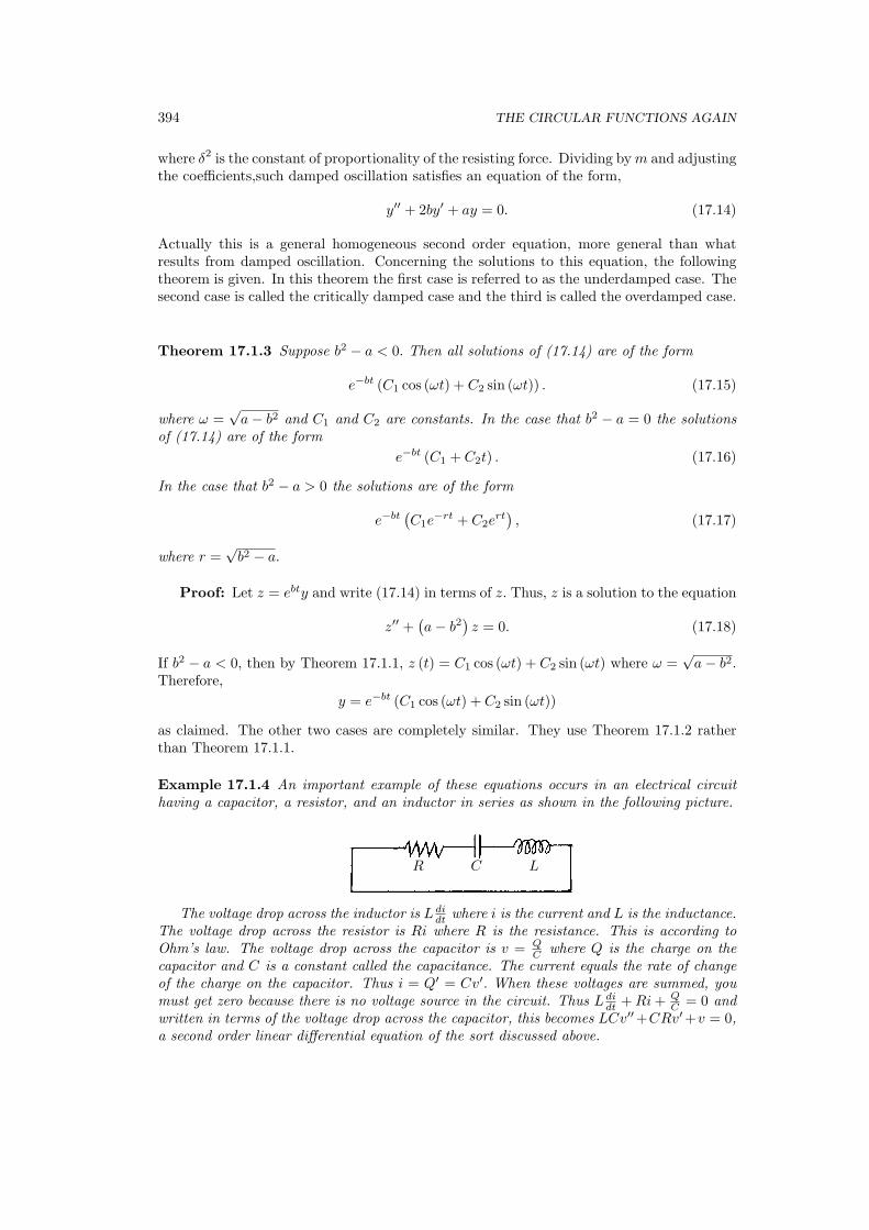
394 THE CIRCULAR FUNCTIONS AGAIN
where δ2 is the constant of proportionality of the resisting force. Dividing by m and adjustingthe coefficients,such damped oscillation satisfies an equation of the form,
y′′ + 2by′ + ay = 0. (17.14)
Actually this is a general homogeneous second order equation, more general than whatresults from damped oscillation. Concerning the solutions to this equation, the followingtheorem is given. In this theorem the first case is referred to as the underdamped case. Thesecond case is called the critically damped case and the third is called the overdamped case.
Theorem 17.1.3 Suppose b2 − a < 0. Then all solutions of (17.14) are of the form
e−bt (C1 cos (ωt) + C2 sin (ωt)) . (17.15)
where ω =√
a− b2 and C1 and C2 are constants. In the case that b2 − a = 0 the solutionsof (17.14) are of the form
e−bt (C1 + C2t) . (17.16)
In the case that b2 − a > 0 the solutions are of the form
e−bt(C1e
−rt + C2ert
), (17.17)
where r =√
b2 − a.
Proof: Let z = ebty and write (17.14) in terms of z. Thus, z is a solution to the equation
z′′ +(a− b2
)z = 0. (17.18)
If b2 − a < 0, then by Theorem 17.1.1, z (t) = C1 cos (ωt) + C2 sin (ωt) where ω =√
a− b2.Therefore,
y = e−bt (C1 cos (ωt) + C2 sin (ωt))
as claimed. The other two cases are completely similar. They use Theorem 17.1.2 ratherthan Theorem 17.1.1.
Example 17.1.4 An important example of these equations occurs in an electrical circuithaving a capacitor, a resistor, and an inductor in series as shown in the following picture.
R C L
The voltage drop across the inductor is L didt where i is the current and L is the inductance.
The voltage drop across the resistor is Ri where R is the resistance. This is according toOhm’s law. The voltage drop across the capacitor is v = Q
C where Q is the charge on thecapacitor and C is a constant called the capacitance. The current equals the rate of changeof the charge on the capacitor. Thus i = Q′ = Cv′. When these voltages are summed, youmust get zero because there is no voltage source in the circuit. Thus L di
dt + Ri + QC = 0 and
written in terms of the voltage drop across the capacitor, this becomes LCv′′+CRv′+v = 0,a second order linear differential equation of the sort discussed above.
17.2. EXERCISES 395
17.2 Exercises
1. Prove from the initial value problems satisfied by S and C the formula (17.8). Alsoverify the second half of (17.6).
2. Verify that y = C1e−at + C2e
at solves the differential equation, (17.13).
3. Verify (17.18).
4. Verify that all solutions to the differential equation, y′′ = 0 are of the form y =C1t + C2.
5. Show from Corollary 6.8.5 and Theorem 17.0.5 that for all x ≥ 0,
S (x) ≤ x− x3
6+
x5
120. (17.19)
6. Using Theorem 17.0.5 and Problem 5, estimate S (.1) and C (.1) . Give upper andlower bounds for these numbers.
7. Using Theorem 17.0.5 and Problem 5 and Theorem 5.9.5, establish the limit,
limx→0
S (x)x
= 1.
8. A mass of ten Kilograms is suspended from a spring attached to the ceiling. Thismass causes the end of the spring to be displaced a distance of 39. 2 cm. The massend of the spring is then pulled down a distance of one cm. and released. Find thedisplacement from the equilibrium position of the end of the spring as a function oftime. Assume the acceleration of gravity is 9.8m/ sec2 .
9. Keep everything the same in Problem 8 except suppose the suspended end of thespring is also attached to a dash pot which provides a force opposite the direction of thevelocity having magnitude 10
√19 |v| Newtons for |v| the speed. Give the displacement
as before.
10. In (17.14) consider the equation in which b = −1 and a = 3. Explain why this equationdescribes a physical system which has some dubious properties.
11. Solve the initial value problem, y′′ + 5y′ − y = 0, y (0) = 1, y′ (0) = 0.
12. Solve the initial value problem y′′ + 2y′ + 2y = 0, y (0) = 0, y′ (0) = 1.
13. In the case of undamped oscillation show the solution can be written in the formA cos (ωt− φ) where φ is some angle called a phase shift and a constant, A, called theamplitude.
14. Using Theorem 17.0.5 and Problem 5 and Theorem 5.9.5, establish the limit,
limx→0
1− C (x)x
= 0.
15. Is the derivative of a function always continuous? Hint: Consider
h (x) =
x2 sin(
1x
)if x 6= 0
0 if x = 0 .
Show h′ (0) = 0. What is h′ (x) for x 6= 0?

396 THE CIRCULAR FUNCTIONS AGAIN
16. Suppose f (t) = a cos ωt + b sin ωt. Show there exists φ such that
f (t) =√
a2 + b2 sin (ωt + φ) .
Hint: f (t) =√
a2 + b2(
a√a2+b2
cosωt + b√a2+b2
sin ωt)
and(
b√a2+b2
, a√a2+b2
)is a
point on the unit circle so it is of the form (cosφ, sin φ) . Now recall the formulas forthe sine and cosine of sums of angles.
17. For θ = 0, π/6, π/4, π/3, π/2, 2π/3,3π/4,5π/6,π,7π/6,5π/4,4π/3,3π/2,5π/3,
7π/4,11π/6,2π, show these angles on the unit circle and find the sine and cosine ofeach one. These are important examples. Do this without any reference to trianglesor plane geometry.

Curvilinear Coordinate Systems
18.1 Polar Cylindrical And Spherical Coordinates
So far points have been identified in terms of Cartesian coordinates but there are other waysof specifying points in two and three dimensional space. These other ways involve using a listof two or three numbers which have a totally different meaning than Cartesian coordinatesto specify a point in two or three dimensional space. In general these lists of numbers whichhave a different meaning than Cartesian coordinates are called Curvilinear coordinates.Probably the simplest curvilinear coordinate system is that of polar coordinates. The ideais suggested in the following picture.
x
y
¡¡
¡¡
¡¡
¡¡
¡¡•
θ
r
(x, y)
(r, θ)
You see in this picture, the number r identifies the distance of the point from the origin,(0, 0) while θ is the angle shown between the positive x axis and the line from the originto the point. This angle will always be given in radians and is in the interval [0, 2π). Thusthe given point, indicated by a small dot in the picture, can be described in terms of theCartesian coordinates, (x, y) or the polar coordinates, (r, θ) . How are the two coordinatessystems related? From the picture,
x = r cos (θ) , y = r sin (θ) . (18.1)
Example 18.1.1 The polar coordinates of a point in the plane are(5, π
6
). Find the Carte-
sian or rectangular coordinates of this point.
From (18.1), x = 5 cos(
π6
)= 5
2
√3 and y = 5 sin
(π6
)= 5
2 . Thus the Cartesian coordinatesare
(52
√3, 5
2
).
Example 18.1.2 Suppose the Cartesian coordinates of a point are (3, 4) . Find the polarcoordinates.
397

398 CURVILINEAR COORDINATE SYSTEMS
Recall that r is the distance form (0, 0) and so r = 5 =√
32 + 42. It remains to identifythe angle. Note the point is in the first quadrant, (Both the x and y values are positive.)Therefore, the angle is something between 0 and π/2 and also 3 = 5 cos (θ) , and 4 = 5 sin (θ) .Therefore, dividing yields tan (θ) = 4/3. At this point, use a calculator or a table oftrigonometric functions to find that at least approximately, θ = . 927 295 radians.
Now consider two three dimensional generalizations of polar coordinates. The followingpicture serves as motivation for the definition of these two other coordinate systems.
-
6
¡¡
¡¡
¡¡
¡ª
x1 (x1, y1, 0)
y1
(ρ, φ, θ)(r, θ, z1)(x1, y1, z1)
z1
ρ
rθ
φ
•
x
y
z
In this picture, ρ is the distance between the origin, the point whose Cartesian coor-dinates are (0, 0, 0) and the point indicated by a dot and labeled as (x1, y1, z1), (r, θ, z1) ,and (ρ, φ, θ) . The angle between the positive z axis and the line between the origin and thepoint indicated by a dot is denoted by φ, and θ, is the angle between the positive x axisand the line joining the origin to the point (x1, y1, 0) as shown, while r is the length of thisline. Thus r and θ determine a point in the plane determined by letting z = 0 and r andθ are the usual polar coordinates. Thus r ≥ 0 and θ ∈ [0, 2π). Letting z1 denote the usualz coordinate of a point in three dimensions, like the one shown as a dot, (r, θ, z1) are thecylindrical coordinates of the dotted point. The spherical coordinates are determined by(ρ, φ, θ) . When ρ is specified, this indicates that the point of interest is on some sphere ofradius ρ which is centered at the origin. Then when φ is given, the location of the pointis narrowed down to a circle and finally, θ determines which point is on this circle. Letφ ∈ [0, π], θ ∈ [0, 2π), and ρ ∈ [0,∞). The picture shows how to relate these new coordinatesystems to Cartesian coordinates. For Cylindrical coordinates,
x = r cos (θ) ,
y = r sin (θ) ,
z = z
and for spherical coordinates,
x = ρ sin (φ) cos (θ) ,
y = ρ sin (φ) sin (θ) ,
z = ρ cos (φ) .
Spherical coordinates should be especially interesting to you because you live on thesurface of a sphere. This has been known for several hundred years. You may also know

18.2. THE ACCELERATION IN POLAR COORDINATES 399
that the standard way to determine position on the earth is to give the longitude andlatitude. The latitude corresponds to φ and the longitude corresponds to θ.1
18.2 The Acceleration In Polar Coordinates
Sometimes you have information about forces which act not in the direction of the coordinateaxes but in some other direction. When this is the case, it is often useful to express things interms of different coordinates which are consistent with these directions. A good exampleof this is the force exerted by the sun on a planet. This force is always directed towardthe sun and so the force vector changes as the planet moves. To discuss this, consider thefollowing simple diagram in which two unit vectors, er and eθ are shown.
¡¡
¡¡
¡¡
¡µ@
@I¡
¡µereθ
θ
(r, θ)XXXy
The vector, er = (cos θ, sin θ) and the vector, eθ = (− sin θ, cos θ) . You should convinceyourself that the picture above corresponds to this definition of the two vectors. Note thater is a unit vector pointing away from 0 and
eθ =der
dθ, er = −deθ
dθ. (18.2)
Now consider the position vector from 0 of a point in the plane, r (t) .Then
r (t) = r (t) er (θ (t))
where r (t) = |r (t)| . Thus r (t) is just the distance from the origin, 0 to the point. What isthe velocity and acceleration? Using the chain rule,
der
dt=
der
dθθ′ (t) ,
deθ
dt=
deθ
dθθ′ (t)
and so from (18.2),der
dt= θ′ (t) eθ,
deθ
dt= −θ′ (t) er (18.3)
Using (18.3) as needed along with the product rule and the chain rule,
r′ (t) = r′ (t) er + r (t)d
dt(er (θ (t)))
= r′ (t) er + r (t) θ′ (t) eθ.
Next consider the acceleration.
r′′ (t) = r′′ (t) er + r′ (t)der
dt+ r′ (t) θ′ (t) eθ + r (t) θ′′ (t) eθ + r (t) θ′ (t)
d
dt(eθ)
= r′′ (t) er + 2r′ (t) θ′ (t) eθ + r (t) θ′′ (t) eθ + r (t) θ′ (t) (−er) θ′ (t)
=(r′′ (t)− r (t) θ′ (t)2
)er +
(2r′ (t) θ′ (t) + r (t) θ′′ (t)
)eθ. (18.4)
1Actually latitude is determined on maps and in navigation by measuring the angle from the equatorrather than the pole but it is essentially the same idea that we have presented here.

400 CURVILINEAR COORDINATE SYSTEMS
This is a very profound formula. Consider the following examples.
Example 18.2.1 Suppose an object of mass m moves at a uniform speed, s, around a circleof radius R. Find the force acting on the object.
By Newton’s second law, the force acting on the object is mr′′. In this case, r (t) = R, aconstant and since the speed is constant, θ′′ = 0. Therefore, the term in (18.4) correspondingto eθ equals zero and mr′′ = −Rθ′ (t)2 er. The speed of the object is s and so it moves s/Rradians in unit time. Thus θ′ (t) = s/R and so
mr′′ = −mR( s
R
)2
er = −ms2
Rer.
This is the familiar formula for centripetal force from elementary physics, obtained as a veryspecial case of (18.4).
Example 18.2.2 A platform rotates at a constant speed in the counter clockwise directionand an object of mass m moves from the center of the platform toward the edge at constantspeed. What forces act on this object?
Let v denote the constant speed of the object moving toward the edge of the platform.Then
r′ (t) = v, r′′ (t) = 0, θ′′ (t) = 0,
while θ′ (t) = ω, a positive constant. From (18.4)
mr′′ (t) = −mr (t)ω2er + m2vωeθ.
Thus the object experiences centripetal force from the first term and also a funny force fromthe second term which is in the direction of rotation of the platform. You can observe thisby experiment if you like. Go to a playground and have someone spin one of those merrygo rounds while you ride it and move from the center toward the edge. The term 2r′θ′ iscalled the Coriolis force.
Suppose at each point of space, r is associated a force, F (r) which a given object ofmass m will experience if its position vector is r. This is called a force field. a force fieldis a central force field if F (r) = g (r) er. Thus in a central force field, the force an objectexperiences will always be directed toward or away from the origin, 0. The following simplelemma is very interesting because it says that in a central force field, objects must move ina plane.
Lemma 18.2.3 Suppose an object moves in three dimensions in such a way that the onlyforce acting on the object is a central force. Then the motion of the object is in a plane.
Proof: Let r (t) denote the position vector of the object. Then from the definition of acentral force and Newton’s second law,
mr′′ = g (r) r.
Therefore, mr′′ × r = m (r′ × r)′ = g (r) r× r = 0. Therefore, (r′ × r) = n, a constantvector and sor · n = r· (r′ × r) = 0 showing that n is a normal vector to a plane whichcontains r (t) for all t. This proves the lemma.
The next example has as a special case one of Kepler’s laws, Kepler’s second law , theequal area law.

18.3. PLANETARY MOTION 401
Example 18.2.4 An object moves in three dimensions in such a way that the only forceacting on the object is a central force. Then the object moves in a plane and the radiusvector from the origin to the object sweeps out area at a constant rate.
The above lemma says the object moves in a plane. From the assumption that the forcefield is a central force field, it follows from (18.4) that
2r′ (t) θ′ (t) + r (t) θ′′ (t) = 0
Multiply both sides of this equation by r. This yields
2rr′θ′ + r2θ′′ =(r2θ′
)′= 0. (18.5)
Consequently,r2θ′ = c (18.6)
for some constant, C. Now consider the following picture.
ÃÃÃÃÃÃÃÃó³³³³³³³ dθ³³
In this picture, dθ is the indicated angle and the two lines determining this angle areposition vectors for the object at point t and point t + dt. The area of the circular sector,dA, is essentially r2dθ and so dA = 1
2r2dθ. Therefore,
dA
dt=
12r2 dθ
dt=
c
2. (18.7)
18.3 Planetary Motion
Kepler’s laws of planetary motion state that planets move around the sun along an ellipse,the equal area law described above holds, and there is a formula for the time it takes for theplanet to move around the sun. These laws, discovered by Kepler, were shown by Newtonto be consequences of his law of gravitation which states that the force acting on a mass, mby a mass, M is given by
F = −GMm
(1r3
)r =−GMm
(1r2
)er
where r is the distance between centers of mass and r is the position vector from M tom. Here G is the gravitation constant. This is called an inverse square law. Gravity actsaccording to this law and so does electrostatic force. The constant, G, is very small whenusual units are used and it has been computed using a very delicate experiment. It is nowaccepted to be
6.67× 10⁻¹¹ Newton meter2/kilogram2.
The experiment involved a light source shining on a mirror attached to a quartz fiber fromwhich was suspended a long rod with two equal masses at the ends which were attracted

402 CURVILINEAR COORDINATE SYSTEMS
by two larger masses. The gravitation force between the suspended masses and the twolarge masses caused the fibre to twist ever so slightly and this twisting was measured byobserving the deflection of the light reflected from the mirror on a scale placed some distancefrom the fibre. The constant was first measured successfully by Lord Cavendish in 1798and the present accepted value was obtained in 1942. Experiments like these are majoraccomplishments.
In the following argument, M is the mass of the sun and m is the mass of the planet.(It could also be a comet or an asteroid.)
Consider the first of Kepler’s laws, the one which states that planets move along ellipses.From Lemma 18.2.3, the motion is in a plane. Now from (18.4) and Newton’s second law,(r′′ (t)− r (t) θ′ (t)2
)er +
(2r′ (t) θ′ (t) + r (t) θ′′ (t)
)eθ = −GMm
m
(1r2
)er = −k
(1r2
)er
Thus k = GM and
r′′ (t)− r (t) θ′ (t)2 = −k
(1r2
), 2r′ (t) θ′ (t) + r (t) θ′′ (t) = 0. (18.8)
As in (18.5),(r2θ′
)′ = 0 and so there exists a constant, c, such that
r2θ′ = c. (18.9)
Therefore, also,2rr′θ′ + r2θ′′ = 0
and so
θ′′ =−2rr′θ′
r2=−2r′θ′
r=−2r
dr
dt
c
r2(18.10)
=−2c
r3
dr
dt(18.11)
Now consider the first of the above equations. The question of interest is to know how rdepends on θ. By the chain rule, regarding r as a function of θ and θ as a function of t,
dr
dθ
dθ
dt=
dr
dt(18.12)
and by (18.9),dr
dθ=
c
r2
dr
dt. (18.13)
Also, by (18.10) and (18.9),
d2θ
dt2=
−2c
r3
dr
dt=−2c
r3
(dr
dθ
dθ
dt
)
=−2c
r3
dr
dθ
( c
r2
)=−2c2
r5
dr
dθ
Differentiating (18.12) again with respect to t,
d2r
dt2=
d2r
dθ2
(dθ
dt
)2
+dr
dθ
d2θ
dt2
=d2r
dθ2
( c
r2
)2
+dr
dθ
(−2c2
r5
dr
dθ
)
=d2r
dθ2
( c
r2
)2
−(
dr
dθ
)2 (2c2
r5
).

18.3. PLANETARY MOTION 403
It follows that the first equation of (18.8) yields r′′ (t)− r (t) θ′ (t)2 = −k(
1r2
)
d2r
dθ2
( c
r2
)2
−(
dr
dθ
)2 (2c2
r5
)− r
( c
r2
)2
= −k
(1r2
)
which is a fairly messy looking differential equation. However, it can be simplified bymultiplying both sides by r4
c2 to get
d2r
dθ2 −(
dr
dθ
)2 (2r
)− r = − k
c2r2 (18.14)
Next consider the above equation in terms of ρ = r−1. Thus, from the chain rule,
r = ρ−1,dr
dθ= (−1) ρ−2 dρ
dθ,
d2r
dθ2 = 2ρ−3
(dρ
dθ
)2
− ρ−2 d2ρ
dθ2 .
substituting this in to (18.14),
= d2rdθ2︷ ︸︸ ︷
2ρ−3
(dρ
dθ
)2
− ρ−2 d2ρ
dθ2 −
= drdθ︷ ︸︸ ︷
(−1) ρ−2 dρ
dθ
2
(2ρ)− ρ−1 = − k
ρ2c2.
Now note that the first and third terms add to zero and so
−ρ−2 d2ρ
dθ2 − ρ−1 = − k
ρ2c2
Multiplying both sides by −ρ−2 yields the equation,
d2ρ
dθ2 + ρ =k
c2,
a much more manageable equation. Multiply both sides by dρdθ .
d2ρ
dθ2
dρ
dθ+ ρ
dρ
dθ=
k
c2
dρ
dθ
Then from the product rule,
12
d
dθ
((dρ
dθ
)2
+ ρ2
)=
k
c2
dρ
dθ.
Therefore, there exists a constant, c1 such that
12
((dρ
dθ
)2
+ ρ2
)− k
c2ρ = c1

404 CURVILINEAR COORDINATE SYSTEMS
and so(
dρ
dθ
)2
= 2c1 +k
c2ρ− ρ2
=(
k2
4c4+ 2c1
)−
(ρ− k
2c2
)2
≡ δ2 −(
ρ− k
2c2
)2
Now letting ρ1 = ρ− k2c2 ,
1δ2
(dρ1
dθ
)2
+(ρ1
δ
)2
= 1
which shows that(
1δ
dρ1dθ , ρ1
δ
)is a point on the unit circle. Therefore, there exists an angle,
α (θ) such thatdρ1
dθ= δ cos (α (θ)) , ρ1 = δ sin (α (θ)) .
Differentiating the second equation with respect to θ,
dρ1
dθ= α′ (θ) δ cos (α (θ))
and so α′ (θ) = 1. Therefore, α (θ) = θ + φ for some constant, φ. Redefining, θ if necessary,(Let θ = θ + φ) it can be assumed that φ = 0 so
ρ− k
2c2= ρ1 = δ sin θ.
Thusρ =
k
c2+ δ sin θ
and so
r =1
kc2 + δ sin θ
=c2/k
1 + (c2/k) δ sin θ
=pε
1 + ε sin θ(18.15)
whereε =
(c2/k
)δ and p = c2/kε. (18.16)
Here all these constants are nonnegative.Thus
r + εr sin θ = εp
and so r = (εp− εy) . Then squaring both sides,
x2 + y2 = (εp− εy)2 = ε2p2 − 2pε2y + ε2y2
And sox2 +
(1− ε2
)y2 = ε2p2 − 2pε2y. (18.17)
In case ε = 1, this reduces to the equation of a parabola. If ε < 1, this reduces to theequation of an ellipse and if ε > 1, this is called a hyperbola. This proves that objects which

18.3. PLANETARY MOTION 405
are acted on only by a force of the form given in the above example move along hyperbolas,ellipses or circles. The case where ε = 0 corresponds to a circle. The constant, ε is calledthe eccentricity. This is called Kepler’s first law in the case of a planet.
Kepler’s third law involves the time it takes for the planet to orbit the sun. From (18.17)you can complete the square and obtain
x2 +(1− ε2
)(y +
pε2
1− ε2
)2
= ε2p2 +p2ε4
(1− ε2)=
ε2p2
(1− ε2),
and this yields
x2/
(ε2p2
1− ε2
)+
(y +
pε2
1− ε2
)2
/
(ε2p2
(1− ε2)2
)= 1. (18.18)
Now note this is the equation of an ellipse and that the diameter of this ellipse is
2εp
(1− ε2)≡ 2a.
This follows becauseε2p2
(1− ε2)2≥ ε2p2
1− ε2.
Now let T denote the time it takes for the planet to make one revolution about the sun.Recall Example 10.9.2 on Page 248 which gives the area of an ellipse. Using this formula,and (18.7) the following equation must hold.
area of ellipse︷ ︸︸ ︷π
εp√1− ε2
εp
(1− ε2)= T
c
2
Therefore,
T =2c
πε2p2
(1− ε2)3/2
and so
T 2 =4π2ε4p4
c2 (1− ε2)3
Now using (18.16),
T 2 =4π2ε4p4
kεp (1− ε2)3=
4π2 (εp)3
k (1− ε2)3
=4π2a3
k=
4π2a3
GM.
Written more memorably, this has shown
T 2 =4π2
GM
(diameter of ellipse
2
)3
. (18.19)
This relationship is known as Kepler’s third law. Kepler’s second law, the equal area formula,holds for any central force, not just one which satisfies an inverse square law.

406 CURVILINEAR COORDINATE SYSTEMS
18.4 Exercises
1. In general it is a stupid idea to try to use algebra to invert and solve for a set ofcurvilinear coordinates such as polar or cylindrical coordinates in term of Cartesiancoordinates. Not only is it often very difficult or even impossible to do it, but alsoit takes you in entirely the wrong direction because the whole point of introducingthe new coordinates is to write everything in terms of these new coordinates and notin terms of Cartesian coordinates. However, sometimes this inversion can be done.Describe how to solve for r and θ in terms of x and y in polar coordinates.
2. A point has Cartesian coordinates, (1, 2, 3) . Find its spherical and cylindrical coordi-nates.
3. Describe the following surface in rectangular coordinates. φ = π/4 where φ is thepolar angle in spherical coordinates.
4. Describe the following surface in rectangular coordinates. θ = π/4 where θ is the anglemeasured from the postive x axis spherical coordinates.
5. Describe the following surface in rectangular coordinates. θ = π/4 where θ is the anglemeasured from the postive x axis cylindrical coordinates.
6. Describe the following surface in rectangular coordinates. r = 5 where r is one of thecylindrical coordinates.
7. Describe the following surface in rectangular coordinates. ρ = 4 where ρ is the distanceto the origin.
8. Give the cone, z =√
x2 + y2 in cylindrical coordinates and in spherical coordinates.
9. Write the following in spherical coordinates.
(a) z = x2 + y2.
(b) x2 − y2 = 1(c) z2 + x2 + y2 = 6
(d) z =√
x2 + y2
(e) y = x
(f) z = x
10. Write the following in cylindrical coordinates.
(a) z = x2 + y2.
(b) x2 − y2 = 1(c) z2 + x2 + y2 = 6
(d) z =√
x2 + y2
(e) y = x
(f) z = x
11. Suppose you know how the spherical coordinates of a moving point change as a functionof t. Can you figure out the velocity of the point? Specifically, suppose φ (t) = t, θ (t) =1+ t, and ρ (t) = t. Find the speed and the velocity of the object in terms of Cartesiancoordinates. Hint: You would need to find x′ (t) , y′ (t) , and z′ (t) . Then in terms ofCartesian coordinates, the velocity would be x′ (t) i + y′ (t) j + z′ (t)k.

18.4. EXERCISES 407
12. Explain why low pressure areas rotate counter clockwise in the Northern hemisphereand clockwise in the Southern hemisphere. Hint: Note that from the point of viewof an observer fixed in space, the low pressure area already has a counter clockwiserotation because of the rotation of the earth and its spherical shape. Now consider(18.6). In the low pressure area stuff will move toward the center so r gets smaller.How are things different in the Southern hemisphere?
13. What are some physical assumptions which are made in the above derivation of Keplerslaws from Newton’s laws of motion?
14. The orbit of the earth is pretty nearly circular and the distance from the sun to theearth is about 149×106 kilometers. Using (18.19) and the above value of the universalgravitation constant, determine the mass of the sun. The earth goes around it in 365days. (Actually it is 365.256 days.)
15. It is desired to place a satellite above the equator of the earth which will rotate aboutthe center of mass of the earth every 24 hours. Is it necessary that the orbit becircular? What if you want the satellite to stay above the same point on the earthat all times? If the orbit is to be circular and the satellite is to stay above the samepoint, at what distance from the center of mass of the earth should the satellite be?You may use that the mass of the earth is 5.98 × 1024 kilograms. Such a satellite iscalled geosynchronous.

408 CURVILINEAR COORDINATE SYSTEMS

Part IV
Functions Of More Than OneVariable
409


Linear Algebra
19.1 Matrices
A matrix is a rectangular array of numbers. Several of them are referred to as matrices.For example, here is a matrix.
1 2 3 45 2 8 76 −9 1 2
This matrix is a 3 × 4 matrix because there are three rows and four columns. The first
row is (1 2 3 4) , the second row is (5 2 8 7) and so forth. The first column is
156
. The
convention in dealing with matrices is to always list the rows first and then the columns.Also, you can remember the columns are like columns in a Greek temple. They stand upright while the rows just lay there like rows made by a tractor in a plowed field. Elements ofthe matrix are identified according to position in the matrix. For example, 8 is in position2, 3 because it is in the second row and the third column. The symbol, (aij) refers to amatrix in which the i denotes the row and the j denotes the column. Using this notationon the above matrix, a23 = 8, a32 = −9, a12 = 2, etc.
There are various operations which are done on matrices. They can sometimes be added,multiplied by a scalar and sometimes multiplied. To illustrate scalar multiplication, considerthe following example.
3
1 2 3 45 2 8 76 −9 1 2
=
3 6 9 1215 6 24 2118 −27 3 6
.
The new matrix is obtained by multiplying every entry of the original matrix by the givenscalar. If A is an m× n matrix, −A is defined to equal (−1)A.
Two matrices which are the same size can be added. When this is done, the result is thematrix which is obtained by adding corresponding entries. Thus
1 23 45 2
+
−1 42 86 −4
=
0 65 1211 −2
.
Two matrices are equal exactly when they are the same size and the corresponding entriesare identical.
Stated in a general form the rules for scalar multiplication and addition are these.
411

412 LINEAR ALGEBRA
Definition 19.1.1 Let A = (aij) and B = (bij) be two m× n matrices. Then A + B = Cwhere
C = (cij)
for cij = aij + bij . Also if x is a scalar,
xA = (cij)
where cij = xaij . The number Aij will typically refer to the ijth entry of the matrix, A. Thezero matrix, denoted by 0 will be the matrix consisting of all zeros.
Note there are 2× 3 zero matrices, 3× 4 zero matrices, etc. In fact for every size thereis a zero matrix.
With this definition, the following properties are all obvious but you should verify all ofthese properties valid for A, B, and C, m× n matrices and 0 an m× n zero matrix,
A + B = B + A, (19.1)
the commutative law of addition,
(A + B) + C = A + (B + C) , (19.2)
the associative law for addition,A + 0 = A, (19.3)
the existence of an additive identity,
A + (−A) = 0, (19.4)
the existence of an additive inverse. Also, for α, β scalars, the following also hold.
α (A + B) = αA + αB, (19.5)
(α + β)A = αA + βA, (19.6)
α (βA) = αβ (A) , (19.7)
1A = A. (19.8)
The above properties, (19.1) - (19.8) are known as the vector space axioms and the factthat the m×n matrices satisfy these axioms is what is meant by saying this set of matricesforms a vector space.
Definition 19.1.2 Let x ∈ Rn. Recall this means x is a list of n real numbers. From nowon, this list of numbers will be arranged vertically. Thus
x =
x1
...xn
.
These n×1 matrices are also called vectors, sometimes column vectors, while a 1×n matrixof the form (x1 · · · xn) is referred to as a row vector.

19.1. MATRICES 413
All the above is fine, but the real reason for considering matrices is that they can bemultiplied. This is where things quit being banal.
First consider the problem of multiplying an m × n matrix by an n × 1 column vector.Consider the following example
(1 2 34 5 6
)
789
=?
The way I like to remember this is as follows. Slide the vector, placing it on top the tworows as shown
71
82
93
74
85
96
,
multiply the numbers on the top by the numbers on the bottom and add them up to geta single number for each row of the matrix. These numbers are listed in the same ordergiving, in this case, a 2× 1 matrix. Thus
(1 2 34 5 6
)
789
=
(7× 1 + 8× 2 + 9× 37× 4 + 8× 5 + 9× 6
)=
(50122
).
In more general terms,
(a11 a12 a13
a21 a22 a23
)
x1
x2
x3
=
(a11x1 + a12x2 + a13x3
a21x1 + a22x2 + a23x3
).
Motivated by this example, here is the definition of how to multiply an m×n matrix by ann× 1 matrix. (vector)
Definition 19.1.3 Let A = Aij be an m× n matrix and let v be an n× 1 matrix,
v =
v1
...vn
Then Av is an m× 1 matrix and the ith component of this matrix is
(Av)i =n∑
j=1
Aijvj .
Thus
Av =
∑nj=1 A1jvj
...∑nj=1 Amjvj
.
Using the repeated index summation convention on Page 331,
(Av)i = Aijvj .
Note also that multiplication by an m×n matrix takes a vector in Rn, an n× 1 matrix, andproduces a vector in Rm, an m× 1 matrix.

414 LINEAR ALGEBRA
With this done, the next task is to multiply an m × n matrix times an n × p matrix.Before doing so, the following may be helpful.
(m×these must match
n) (n× p ) = m× p
If the two middle numbers don’t match, you can’t multiply the matrices.Let A be an m× n matrix and let B be an n× p matrix. Then B is of the form
B = (b1, · · ·,bp)
where bk is an n× 1 matrix. Then an m× p matrix, AB is defined as follows:
AB ≡ (Ab1, · · ·, Abp) (19.9)
where Abk is an m× 1 matrix. Hence AB as just defined is an m× p matrix.What is the ijth entry of AB? It would be the ith entry of the jth column of AB. Thus
it would be the ith entry of Abj . Now
bj =
B1j
...Bnj
and from the above definition, the ith entry is
n∑
k=1
AikBkj . (19.10)
This motivates the definition for matrix multiplication which identifies the ijth entries ofthe product.
Definition 19.1.4 Let A = (Aij) be an m×n matrix and let B = (Bij) be an n×p matrix.Then AB is an m× p matrix and
(AB)ij =n∑
k=1
AikBkj . (19.11)
In terms of the repeated summation convention, on Page 331,
(AB)ij = AikBkj . (19.12)
Two matrices, A and B are said to be conformable in a particular order if they can bemultiplied in that order. Thus if A is an r × s matrix and B is a s × p then A and B areconformable in the order, AB.
Example 19.1.5 Multiply if possible
1 23 12 6
(2 3 17 6 2
).
First check to see if this is possible. It is of the form (3× 2) (2× 3) and since the insidenumbers match, it must be possible to do this. The answer is of the form
1 23 12 6
(27
),
1 23 12 6
(36
),
1 23 12 6
(12
)

19.1. MATRICES 415
where the commas separate the columns in the resulting product. Thus the above productequals
16 15 513 15 546 42 14
,
a 3× 3 matrix as desired.
Example 19.1.6 Multiply if possible
1 23 12 6
2 3 17 6 20 0 0
.
This is not possible because it is of the form (3× 2) (3× 3) and the middle numbersdon’t match.
Example 19.1.7 Multiply if possible
2 3 17 6 20 0 0
1 23 12 6
.
This is possible because in this case it is of the form (3× 3) (3× 2) and the middlenumbers do match. When the multiplication is done it equals
13 1329 320 0
.
Note the above two examples show matrix multiplication is not commutative. In fact,it can happen that AB makes sense while BA does not make sense which was the case inthese examples. It seems natural to ask if the product of any two n×n matrices commutes.
Example 19.1.8 Compare(
1 23 4
)(0 11 0
)and
(0 11 0
)(1 23 4
).
The first product is (1 23 4
)(0 11 0
)=
(2 14 3
),
the second product is (0 11 0
)(1 23 4
)=
(3 41 2
),
and you see these are not equal. Therefore, you cannot conclude that AB = BA for matrixmultiplication. However, there are some properties which do hold.
Proposition 19.1.9 If all multiplications and additions make sense, the following hold formatrices and a, b scalars.
A (aB + bC) = a (AB) + b (AC) (19.13)
(B + C)A = BA + CA (19.14)
A (BC) = (AB) C (19.15)

416 LINEAR ALGEBRA
Proof: Using the repeated index summation convention and the above definition ofmatrix multiplication,
(A (aB + bC))ij = Aik (aB + bC)kj
= Aik (aBkj + bCkj)= aAikBkj + bAikCkj
= a (AB)ij + b (AC)ij
= (a (AB) + b (AC))ij
showing that A (B + C) = AB + AC as claimed. Formula (19.14) is entirely similar.Consider (19.15), the associative law of multiplication.
(A (BC))ij = Aik (BC)kj
= AikBklClj
= (AB)il Clj
= ((AB)C)ij .
This proves (19.15).Another important operation on matrices is that of taking the transpose. The following
example shows what is meant by this operation, denoted by placing a T as an exponent onthe matrix.
1 23 12 6
T
=(
1 3 22 1 6
)
What happened? The first column became the first row and the second column becamethe second row. Thus the 3 × 2 matrix became a 2 × 3 matrix. The number 3 was in thesecond row and the first column and it ended up in the first row and second column. Thismotivates the following definition of the transpose of a matrix.
Definition 19.1.10 Let A be an m× n matrix. Then AT denotes the n×m matrix whichis defined as follows. (
AT)ij
= Aji
The transpose of a matrix has the following important property.
Lemma 19.1.11 Let A be an m× n matrix and let B be a n× p matrix. Then
(AB)T = BT AT (19.16)
and if α and β are scalars,(αA + βB)T = αAT + βBT (19.17)
Proof: From the definition,((AB)T
)ij
= (AB)ji
= AjkBki
=(BT
)ik
(AT
)kj
=(BT AT
)ij
(19.17) is left as an exercise and this proves the lemma.

19.1. MATRICES 417
There is a special matrix called I and defined by
Iij = δij
where δij is the Kroneker symbol defined on Page 330. It is called the identity matrixbecause it is a multiplicative identity in the following sense.
Lemma 19.1.12 Suppose A is an m× n matrix and In is the n× n identity matrix. ThenAIn = A. If Im is the m×m identity matrix, it also follows that ImA = A.
Proof:
(AIn)ij = Aikδkj
= Aij
and so AIn = A. The other case is left as an exercise for you.
Definition 19.1.13 An n×n matrix, A has an inverse, A−1 if and only if AA−1 = A−1A =I where I = (δij) for
δij ≡
1 if i = j0 if i 6= j
19.1.1 Finding The Inverse Of A Matrix
A little later a formula is given for the inverse of a matrix. However, it is not a good way tofind the inverse for a matrix. It is also important to note that not all matrices have inverses.
Example 19.1.14 Let A =(
1 11 1
). Does A have an inverse?
One might think A would have an inverse because it does not equal zero. However,(
1 11 1
)( −11
)=
(00
)
and if A−1 existed, this could not happen because you could write(
00
)= A−1
((00
))= A−1
(A
( −11
))=
=(A−1A
) ( −11
)= I
( −11
)=
( −11
),
a contradiction. Thus the answer is that A does not have an inverse.
Example 19.1.15 Let A =(
1 11 2
). Show
(2 −1−1 1
)is the inverse of A.
To check this, multiply(
1 11 2
)(2 −1−1 1
)=
(1 00 1
)
and (2 −1−1 1
)(1 11 2
)=
(1 00 1
)

418 LINEAR ALGEBRA
showing that this matrix is indeed the inverse of A.
In the last example, how would you find A−1? You wish to find a matrix,(
x zy w
)
such that (1 11 2
) (x zy w
)=
(1 00 1
).
This requires the solution of the systems of equations,
x + y = 1, x + 2y = 0
andz + w = 0, z + 2w = 1.
Writing the augmented matrix for these two systems gives(
1 1 11 2 0
)(19.18)
for the first system and (1 1 01 2 1
)(19.19)
for the second. Lets solve the first system. Take (−1) times the first row and add to thesecond to get (
1 1 10 1 −1
)
Now take (−1) times the second row and add to the first to get(
1 0 20 1 −1
).
Putting in the variables, this says x = 2 and y = −1.Now solve the second system, (19.19) to find z and w. Take (−1) times the first row and
add to the second to get (1 1 00 1 1
).
Now take (−1) times the second row and add to the first to get(
1 0 −10 1 1
).
Putting in the variables, this says z = −1 and w = 1. Therefore, the inverse is(
2 −1−1 1
).
Didn’t the above seem rather repetitive? Note that exactly the same row operationswere used in both systems. In each case, the end result was something of the form (I|v)
where I is the identity and v gave a column of the inverse. In the above,(
xy
), the first
column of the inverse was obtained first and then the second column(
zw
).
This is the reason for the following simple procedure for finding the inverse of a matrix.

19.2. EXERCISES 419
Procedure 19.1.16 Suppose A is an n × n matrix. To find A−1 if it exists, form theaugmented n× 2n matrix,
(A|I)
and then do row operations until you obtain an n× 2n matrix of the form
(I|B) (19.20)
if possible. When this has been done, B = A−1. The matrix, A has no inverse exactly whenit is impossible to do row operations and end up with one like (19.20).
Example 19.1.17 Let A =
1 0 11 −1 11 1 −1
. Find A−1.
Form the augmented matrix,
1 0 1 1 0 01 −1 1 0 1 01 1 −1 0 0 1
.
Now do row operations until the n×n matrix on the left becomes the identity matrix. Thisyields after a some computations,
1 0 0 0 12
12
0 1 0 1 −1 00 0 1 1 − 1
2 − 12
and so the inverse of A is the matrix on the right,
0 12
12
1 −1 01 − 1
2 − 12
.
Checking the answer is easy. Just multiply the matrices and see if it works.
1 0 11 −1 11 1 −1
0 12
12
1 −1 01 − 1
2 − 12
=
1 0 00 1 00 0 1
.
19.2 Exercises
1. In (19.1) - (19.8) describe −A and 0.
2. Using only the properties (19.1) - (19.8) show −A is unique.
3. Using only the properties (19.1) - (19.8) show 0 is unique.
4. Using only the properties (19.1) - (19.8) show 0A = 0. Here the 0 on the left is thescalar 0 and the 0 on the right is the zero for m× n matrices.
5. Using only the properties (19.1) - (19.8) and previous problems show (−1)A = −A.
6. Prove (19.17).
7. Prove that ImA = A where A is an m× n matrix.

420 LINEAR ALGEBRA
8. Let A and be a real m × n matrix and let x ∈ Rn and y ∈ Rm. Show (Ax,y)Rm =(x,AT y
)Rn where (·, ·)Rk denotes the dot product in Rk.
9. Use the result of Problem 8 to verify directly that (AB)T = BT AT without makingany reference to subscripts.
10. Let x =(−1,−1, 1) and y =(0, 1, 2) . Find xT y and xyT if possible.
11. Give an example of matrices, A, B,C such that B 6= C, A 6= 0, and yet AB = AC.
12. Let A =
1 1−2 −11 2
, B =
(1 −1 −22 1 −2
), and C =
1 1 −3−1 2 0−3 −1 0
. Find
if possible.
(a) AB
(b) BA
(c) AC
(d) CA
(e) CB
(f) BC
13. Show that if A−1 exists for an n×n matrix, then it is unique. That is, if BA = I andAB = I, then B = A−1.
14. Show (AB)−1 = B−1A−1.
15. Give an example of a matrix, A such that A2 = I and yet A 6= I and A 6= −I.
16. Give an example of matrices, A,B such that neither A nor B equals zero and yetAB = 0.
17. Write
x1 − x2 + 2x3
2x3 + x1
3x3
3x4 + 3x2 + x1
in the form A
x1
x2
x3
x4
where A is an appropriate matrix.
18. Give another example other than the one given in this section of two square matrices,A and B such that AB 6= BA.
19. Suppose A and B are square matrices of the same size. Which of the following arecorrect?
(a) (A−B)2 = A2 − 2AB + C2
(b) (AB)2 = A2B2
(c) (A + B)2 = A2 + 2AB + C2
(d) (A + B)2 = A2 + AB + BA + B2
(e) A2B2 = A (AB)B
(f) (A + B)3 = A3 + 3A2B + 3AB2 + B3
(g) (A + B) (A−B) = A2 −B2
(h) None of the above. They are all wrong.

19.3. LINEAR TRANSFORMATIONS 421
(i) All of the above. They are all right.
20. Let A =( −1 −1
3 3
). Find all 2× 2 matrices, B such that AB = 0.
21. Prove that if A−1 exists and Ax = 0 then x = 0.
22. Let
A =
1 2 32 1 41 0 2
.
Find A−1 if possible. If A−1 does not exist, determine why.
19.3 Linear Transformations
By (19.13), if A is an m× n matrix, then for v,u vectors in Rn and a, b scalars,
A
∈Rn
︷ ︸︸ ︷au + bv
= aAu + bAv ∈ Rm (19.21)
Definition 19.3.1 A function, A : Rn → Rm is called a linear transformation if for allu,v ∈ Rn and a, b scalars, (19.21) holds.
From (19.21), matrix multiplication defines a linear transformation as just defined. Itturns out this is the only type of linear transformation available. Thus if A is a lineartransformation from Rn to Rm, there is always a matrix which produces A. Before showingthis, here is a simple definition.
Definition 19.3.2 A vector, ei ∈ Rn is defined as follows:
ei ≡
0...1...0
,
where the 1 is in the ith position and there are zeros everywhere else. Thus
ei = (0, · · ·, 0, 1, 0, · · ·, 0)T.
Of course the ei for a particular value of i in Rn would be different than the ei for thatsame value of i in Rm for m 6= n. One of them is longer than the other. However, whichone is meant will be determined by the context in which they occur.
These vectors have a significant property.
Lemma 19.3.3 Let v ∈ Rn. Thus v is a list of real numbers arranged vertically, v1, · · ·, vn.Then
eTi v = vi. (19.22)
Also, if A is an m× n matrix, then letting ei ∈ Rm and ej ∈ Rn,
eTi Aej = Aij (19.23)

422 LINEAR ALGEBRA
Proof: First note that eTi is a 1 × n matrix and v is an n × 1 matrix so the above
multiplication in (19.22) makes perfect sense. It equals
(0, · · ·, 1, · · ·0)
v1
...vi
...vn
= vi
as claimed.Consider (19.23). From the definition of matrix multiplication using the repeated index
summation convention, and noting that (ej)k = δkj
eTi Aej = eT
i
A1k (ej)k...
Aik (ej)k...
Amk (ej)k
= eTi
A1j
...Aij
...Amj
= Aij
by the first part of the lemma. This proves the lemma.
Theorem 19.3.4 Let L : Rn → Rm be a linear transformation. Then there exists a uniquem× n matrix, A such that
Ax = Lx
for all x ∈ Rn. The ikth entry of this matrix is given by
eTi Lek (19.24)
Proof: By the lemma,
(Lx)i = eTi Lx = eT
i xkLek =(eT
i Lek
)xk.
Let Aik = eTi Lek, to prove the existence part of the theorem.
To verify uniqueness, suppose Bx = Ax = Lx for all x ∈ Rn. Then in particular, this istrue for x = ej and then multiply on the left by eT
i to obtain
Bij = eTi Bej = eT
i Aej = Aij
showing A = B. This proves uniqueness.
Corollary 19.3.5 A linear transformation, L : Rn → Rm is completely determined by thevectors Le1, · · ·, Len .
Proof: This follows immediately from the above theorem. The unique matrix determin-ing the linear transformation which is given in (19.24) depends only on these vectors.
This theorem shows that any linear transformation defined on Rn can always be consid-ered as a matrix. Therefore, the terms “linear transformation” and “matrix” will be usedinterchangeably. For example, to say a matrix is one to one, means the linear transformationdetermined by the matrix is one to one.
Example 19.3.6 Find the linear transformation, L : R2 → R2 which has the property
that Le1 =(
21
)and Le2 =
(13
). From the above theorem and corollary, this linear
transformation is that determined by matrix multiplication by the matrix(
2 11 3
).

19.3. LINEAR TRANSFORMATIONS 423
19.3.1 Least Squares Problems
Definition 19.3.7 Let x1, · · ·,xk be a set of vectors in Rn. Define
span x1, · · ·,xk ≡
k∑
i=1
cixi : c1, · · ·, ck ∈ R
In words span x1, · · ·,xk consists of all vectors which can be obtained by adding up scalarstimes the vectors in the set x1, · · ·,xk. These sums are called linear combinations.
The following lemma is very significant, being a special case of something called theGram Schmidt procedure. Before reading further, you should review the dot product andits properties on Page 311. Also recall that
δij =
1 if i = j0 if i 6= j
.
Lemma 19.3.8 Let A be an m × n matrix, A 6= 0. Then there exist vectors, f1, · · ·, frsuch that fi · fj = δij and span f1, · · ·, fr = A (Rn) ≡ Ax : x ∈ Rn.
Proof: Letf1 =
Aei1
|Aei1 |where ei1 is the first vector in the list, e1, · · ·, en with the property that Aei 6= 0. Thus
span f1 = span Aei1 = span Ae1, · · ·, Aei1
because Aek = 0 for k < i1. Now suppose f1, · · ·, fk have been chosen in such a way thatfi · fj = δij and
span Aei1 , · · ·, Aeik = span Ae1, Ae2, · · ·, Aeik
= span f1, · · ·, fk .
This was just accomplished for k = 1. There are two cases to consider.First it could happen that Aej ∈ span f1, · · ·, fk for all j. In this case, stop and consider
span f1, · · ·, fk . For x ∈ Rn arbitrary,
Ax = A
(n∑
i=1
xiei
)=
k∑
i=1
xiAei
=n∑
i=1
xi
=Aei︷ ︸︸ ︷k∑
j=1
yijfj =k∑
j=1
(n∑
i=1
xiyij
)fj
∈ span f1, · · ·, fk
showing that span f1, · · ·, fk = A (Rn) .The other case is that Aej /∈ span f1, · · ·, fk for some j. (By construction, Aej is in
span f1, · · ·, fk for all j ≤ ik.) Let ik+1 be the smallest index larger than ik such thatAeik+1 /∈ span f1, · · ·, fk . Then define
fk+1 ≡Aeik+1 −
∑kj=1
(Aeik+1 · fj
)fj∣∣∣Aeik+1 −
∑kj=1
(Aeik+1 · fj
)fj
∣∣∣. (19.25)

424 LINEAR ALGEBRA
Note the denominator is non zero because of the assumption that Aeik+1 /∈ span f1, · · ·, fk .Then
span f1, · · ·, fk+1 = spanAei1 , · · ·, Aeik+1
= span
Ae1, · · ·, Aeik+1
(19.26)
Also, from the properties of the dot product on Page 311, for l < k + 1,
fk+1 · fl =Aeik+1 · fl −
∑kj=1
(Aeik+1 · fj
)δjl︷ ︸︸ ︷
fj · fl∣∣∣Aeik+1 −∑k
j=1
(Aeik+1 · fj
)fj
∣∣∣
=Aeik+1 · fl −Aeik+1 · fl∣∣∣Aeik+1 −
∑kj=1
(Aeik+1 · fj
)fj
∣∣∣= 0
Therefore, since |fk+1| = 1, it follows that f1, · · ·, fk+1 has the property that fi · fj = δij
and each fj ∈ A (Rn) . Continue until the first case is obtained. This must happen in nomore than n applications of the above process because for each j, ij < ij+1 and ij can’t beany larger than n. This proves the lemma.
The following is a fundamental existence theorem which is based on the above lemma.
Theorem 19.3.9 Let y ∈ Rm and let A be an m × n matrix. Then there exists x ∈ Rn
minimizing the function, |y−Ax|2 . Furthermore, x minimizes this function if and only if
(y−Ax) ·Aw = 0
for all w ∈ Rn.
Proof: Let f1, · · ·, fr be the vectors of Lemma 19.3.8 with span f1, · · ·, fr = A (Rn).Since A (Rn) = span f1, · · ·, fr , it follows that if you can find y1, · · ·, yr in such a way asto minimize ∣∣∣∣∣y−
r∑
k=1
ykfk
∣∣∣∣∣
2
,
then letting Ax =∑r
k=1 ykfk, it will follow that this x is the desired solution. Let y1, · · ·, yr
be a list of scalars. Then from the definition of |·| and the properties of the dot product,∣∣∣∣∣y−
r∑
k=1
ykfk
∣∣∣∣∣
2
=
(y−
r∑
k=1
ykfk
)·(
y−r∑
k=1
ykfk
)
= |y|2 − 2r∑
k=1
yk (y · fk) +∑
k
∑
l
ykyl
δkl︷ ︸︸ ︷fk · fl
= |y|2 − 2r∑
k=1
yk (y · fk) +r∑
k=1
y2k
= |y|2 +r∑
k=1
y2k − 2yk (y · fk)
Now complete the square to obtain
= |y|2 +r∑
k=1
(y2
k − 2yk (y · fk) + (y · fk)2)−
r∑
k=1
(y · fk)2
= |y|2 +r∑
k=1
(yk − (y · fk))2 −r∑
k=1
(y · fk)2 .

19.3. LINEAR TRANSFORMATIONS 425
This shows that the minimum is obtained when yk = (y · fk) . This proves the existencepart of the Theorem.
To verify the other part, let t ∈ R and consider
|y−A (x + tw)|2 = (y−Ax− tAw) · (y−Ax− tAw)
= |y−Ax|2 − 2t (y−Ax) ·Aw + t2 |Aw|2 .
Then from the above equation, |y−Ax|2 ≤ |y−Az|2 for all z ∈ Rn if and only if for allw ∈ Rn and t ∈ R
|y−Ax|2 − 2t (y−Ax) ·Aw + t2 |w|2 ≥ |y−Ax|2
and this happens if and only if for all t ∈ R and w ∈ Rn,
−2t (y−Ax) ·Aw + t2 |Aw|2 ≥ 0,
which occurs if and only if (y−Ax) · Aw = 0 for all w ∈ Rn. (Why?) This proves thetheorem.
Lemma 19.3.10 Let A be an m× n matrix. Then
Ax · y = x·AT y
Proof: This follows from the definition. Using the repeated index summation convention,
Ax · y = Aijxjyi
= xjATjiyi
= x·AT y.
19.3.2 The Least Squares Regression Line
As an important application of the above theorem is the problem of finding the least squaresregression line in statistics. Suppose you are given points in the plane, (xi, yi)n
i=1 and youwould like to find constants m and b such that the line y = mx + b goes through all thesepoints. Of course this will be impossible in general. Therefore, try to find m, b to get asclose as possible. The desired system is
y1
...yn
=
x1 1...
...xn 1
(mb
)
which is of the form y = Ax and it is desired to choose m and b to make∣∣∣∣∣∣∣A
(mb
)−
y1
...yn
∣∣∣∣∣∣∣
2
as small as possible. According to Theorem 19.3.9, the best values for m and b occur as thesolution to
AT A
(mb
)= AT
y1
...yn

426 LINEAR ALGEBRA
where
A =
x1 1...
...xn 1
.
Thus, computing AT A,
( ∑ni=1 x2
i
∑ni=1 xi∑n
i=1 xi n
)(mb
)=
( ∑ni=1 xiyi∑ni=1 yi
)
Solving this system of equations for m and b,
m =− (
∑ni=1 xi) (
∑ni=1 yi) + (
∑ni=1 xiyi) n
(∑n
i=1 x2i )n− (
∑ni=1 xi)
2
and
b =− (
∑ni=1 xi)
∑ni=1 xiyi + (
∑ni=1 yi)
∑ni=1 x2
i
(∑n
i=1 x2i ) n− (
∑ni=1 xi)
2 .
One could clearly do a least squares fit for curves of the form y = ax2 + bx + c in thesame way. In this case you want to solve as well as possible for a, b, and c the system
x21 x1 1...
......
x2n xn 1
abc
=
y1
...yn
and one would use the same technique as above. Many other similar problems are important,including many in higher dimensions and they are all solved the same way.
19.3.3 The Fredholm Alternative
The next major result is called the Fredholm alternative. It comes from Theorem 19.3.9and Lemma 19.3.10.
Theorem 19.3.11 Let A be an m× n matrix. Then there exists x ∈ Rn such that Ax = yif and only if whenever AT z = 0 it follows that z · y = 0.
Proof: First suppose that for some x ∈ Rn, Ax = y. Then letting AT z = 0 and usingthe above lemma,
y · z = Ax · z = x ·AT z = x · 0 = 0.
This proves half the theorem.To do the other half, suppose that whenever, AT z = 0 it follows that z · y = 0. It is
necessary to show there exists x ∈ Rn such that y = Ax. From Theorem 19.3.9 there existsx minimizing |y −Ax|2 which therefore satisfies
(y −Ax) ·Aw = 0 (19.27)
for all w ∈ Rn. Therefore, for all w ∈ Rn,
AT (y −Ax) ·w = 0
which shows that AT (y −Ax) = 0. (Why?) Therefore, by assumption,
(y −Ax) · y = 0.

19.4. EXERCISES 427
Now by (19.27) with w = x,
(y −Ax) · (y−Ax) = (y −Ax) · y− (y −Ax) ·Ax = 0
showing that y = Ax. This proves the theorem.The following corollary is also called the Fredholm alternative.
Corollary 19.3.12 Let A be an m× n matrix. Then A is onto if and only if AT is one toone.
Proof: Suppose first A is onto. Then by Theorem 19.3.11, it follows that for all y ∈ Rm,y · z = 0 whenever AT z = 0. Therefore, let y = z where AT z = 0 and conclude that z · z = 0whenever AT z = 0. If AT x = AT y, then AT (x− y)= 0 and so x− y = 0. Thus AT is oneto one.
Now let y ∈ Rm be given. y · z = 0 whenever AT z = 0 because, since AT is assumed tobe one to one, and 0 is a solution to this equation, it must be the only solution. Therefore,by Theorem 19.3.11 there exists x such that Ax = y therefore, A is onto.
19.4 Exercises
1. The proof of Theorem 19.3.9 concluded with the following observation. If −ta+t2b ≥ 0for all t ∈ R and b ≥ 0, then a = 0. Why is this so?
2. In the proof of Lemma 19.3.8 explain the assertion (19.26).
3. In the proof of Theorem 19.3.11 the following argument was used. If x ·w = 0 for allw ∈ Rn, then x = 0. Why is this so?
4. Suppose L : Rn → Rm is a linear transformation. Show the following are equivalent.
(a) Lx = 0 implies x = 0.
(b) L is one to one.
5. Using Corollary 19.3.12 and Problem 4, show that an m×n matrix is onto if and onlyif its transpose is one to one.
6. Suppose A is a 3× 2 matrix. Is it possible that AT is one to one? What does this sayabout A being onto? Prove your answer.
7. Explain why there always exists a solution to the equation, AT y = AT Ax and alsoexplain why this is called a least squares solution to the equation, y = Ax.
8. Referring to Problem 7, find the least squares solution to the following system.
x + 2y = 12x + 3y = 23x + 5y = 4
9. You are doing experiments and have obtained the ordered pairs, (0, 1) , (1, 2) , (2, 3.5) ,and (3, 4) . Find m and b such that y = mx + b approximates these four points as wellas possible. Now do the same thing for y = ax2 + bx + c, finding a, b, and c to givethe best approximation.

428 LINEAR ALGEBRA
10. Suppose you have several ordered triples, (xi, yi, zi) . Describe how to find a polyno-mial,
z = a + bx + cy + dxy + ex2 + fy2
for example giving the best fit to the given ordered triples. Is there any reason youhave to use a polynomial? Would similar approaches work for other combinations offunctions just as well?
19.5 Moving Coordinate Systems
The study of moving coordinate systems gives a non trivial example of the usefulness ofthe above ideas involving linear transformations and matrices. To begin with, here is theconcept of the product rule extended to matrix multiplication.
Definition 19.5.1 Let A (t) be an m × n matrix. Say A (t) = (Aij (t)) . Suppose also thatAij (t) is a differentiable function for all i, j. Then define A′ (t) ≡ (
A′ij (t)). That is, A′ (t)
is the matrix which consists of replacing each entry by its derivative. Such an m×n matrixin which the entries are differentiable functions is called a differentiable matrix.
The next lemma is just a version of the product rule.
Lemma 19.5.2 Let A (t) be an m × n matrix and let B (t) be an n × p matrix with theproperty that all the entries of these matrices are differentiable functions. Then
(A (t)B (t))′ = A′ (t)B (t) + A (t) B′ (t) .
Proof: (A (t) B (t))′ =(C ′ij (t)
)where Cij (t) = Aik (t)Bkj (t) and the repeated index
summation convention is being used. Therefore,
C ′ij (t) = A′ik (t) Bkj (t) + Aik (t) B′kj (t)
= (A′ (t)B (t))ij + (A (t)B′ (t))ij
= (A′ (t)B (t) + A (t) B′ (t))ij
Therefore, the ijth entry of A (t)B (t) equals the ijth entry of A′ (t)B (t) + A (t)B′ (t) andthis proves the lemma.
19.5.1 The Coriolis Acceleration
Imagine a point on the surface of the earth. Now consider unit vectors, one pointing South,one pointing East and one pointing directly away from the center of the earth.
¤¤¤¤²i
¾k HHHjj

19.5. MOVING COORDINATE SYSTEMS 429
Denote the first as i, the second as j and the third as k. If you are standing on the earthyou will consider these vectors as fixed, but of course they are not. As the earth turns, theychange direction and so each is in reality a function of t. Nevertheless, it is with respectto these apparently fixed vectors that you wish to understand acceleration, velocities, anddisplacements.
In general, let i∗, j∗,k∗ be the usual fixed vectors in space and let i (t) , j (t) ,k (t) be anorthonormal basis of vectors for each t, like the vectors described in the first paragraph.It is assumed these vectors are C1 functions of t. Letting the positive x axis extend in thedirection of i (t) , the positive y axis extend in the direction of j (t), and the positive z axisextend in the direction of k (t) , yields a moving coordinate system. Now let u be a vectorand let t0 be some reference time. For example you could let t0 = 0. Then define thecomponents of u with respect to these vectors, i, j,k at time t0 as
u ≡ u1i (t0) + u2j (t0) + u3k (t0) .
Let u (t) be defined as the vector which has the same components with respect to i, j,k butat time t. Thus
u (t) ≡ u1i (t) + u2j (t) + u3k (t) .
and the vector has changed although the components have not.This is exactly the situation in the case of the apparently fixed basis vectors on the earth
if u is a position vector from the given spot on the earth’s surface to a point regarded asfixed with the earth due to its keeping the same coordinates relative to the coordinate axeswhich are fixed with the earth. Now define a linear transformation Q (t) mapping R3 to R3
byQ (t)u ≡ u1i (t) + u2j (t) + u3k (t)
whereu ≡ u1i (t0) + u2j (t0) + u3k (t0)
Thus letting v be a vector defined in the same manner as u and α, β, scalars,
Q (t) (αu + βv) ≡ (αu1 + βv1
)i (t) +
(αu2 + βv2
)j (t) +
(αu3 + βv3
)k (t)
=(αu1i (t) + αu2j (t) + αu3k (t)
)+
(βv1i (t) + βv2j (t) + βv3k (t)
)
= α(u1i (t) + u2j (t) + u3k (t)
)+ β
(v1i (t) + v2j (t) + v3k (t)
)
≡ αQ (t)u + βQ (t)v
showing that Q (t) is a linear transformation. Also, Q (t) preserves all distances because,since the vectors, i (t) , j (t) ,k (t) form an orthonormal set,
|Q (t)u| =(
3∑
i=1
(ui
)2
)1/2
= |u| .
Lemma 19.5.3 Suppose Q (t) is a real, differentiable n × n matrix which preserves dis-tances. Then Q (t) Q (t)T = Q (t)T
Q (t) = I. Also, if u (t) ≡ Q (t)u, then there exists avector, Ω (t) such that
u′ (t) = Ω (t)× u (t) .

430 LINEAR ALGEBRA
Proof: Recall that (z ·w) = 14
(|z + w|2 − |z−w|2
). Therefore,
(Q (t)u·Q (t)w) =14
(|Q (t) (u + w)|2 − |Q (t) (u−w)|2
)
=14
(|u + w|2 − |u−w|2
)
= (u ·w) .
This implies (Q (t)T
Q (t)u ·w)
= (u ·w)
for all u,w. Therefore, Q (t)TQ (t)u = u and so Q (t)T
Q (t) = Q (t)Q (t)T = I. This provesthe first part of the lemma.
It follows from the product rule, Lemma 19.5.2 that
Q′ (t) Q (t)T + Q (t)Q′ (t)T = 0
and soQ′ (t)Q (t)T = −
(Q′ (t)Q (t)T
)T
. (19.28)
From the definition, Q (t)u = u (t) ,
u′ (t) = Q′ (t)u =Q′ (t)
=u︷ ︸︸ ︷Q (t)T u (t).
Then writing the matrix of Q′ (t) Q (t)T with respect to fixed in space orthonormal basisvectors, i∗, j∗,k∗, where these are the usual basis vectors for R3, it follows from (19.28) thatthe matrix of Q′ (t) Q (t)T is of the form
0 −ω3 (t) ω2 (t)ω3 (t) 0 −ω1 (t)−ω2 (t) ω1 (t) 0
for some time dependent scalars, ωi. Therefore,
u1
u2
u3
′
(t) =
0 −ω3 (t) ω2 (t)ω3 (t) 0 −ω1 (t)−ω2 (t) ω1 (t) 0
u1
u2
u3
(t)
=
w2 (t) u3 (t)− w3 (t)u2 (t)w3 (t) u1 (t)− w1 (t)u3 (t)w1 (t) u2 (t)− w2 (t)u1 (t)
where the ui are the components of the vector u (t) in terms of the fixed vectors i∗, j∗,k∗.Therefore,
u′ (t) = Ω (t)×u (t) = Q′ (t) Q (t)T u (t) (19.29)
whereΩ (t) = ω1 (t) i∗+ω2 (t) j∗+ω3 (t)k∗.
because
Ω (t)× u (t) ≡∣∣∣∣∣∣
i∗ j∗ k∗
w1 w2 w3
u1 u2 u3
∣∣∣∣∣∣≡
i∗(w2u
3 − w3u2)
+ j∗(w3u
1 − w1u3)
+ k∗(w1u
2 − w2u1).
This proves the lemma and yields the existence part of the following theorem.
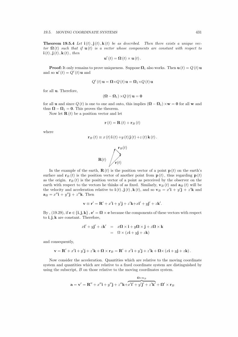
19.5. MOVING COORDINATE SYSTEMS 431
Theorem 19.5.4 Let i (t) , j (t) ,k (t) be as described. Then there exists a unique vec-tor Ω (t) such that if u (t) is a vector whose components are constant with respect toi (t) , j (t) ,k (t) , then
u′ (t) = Ω (t)× u (t) .
Proof: It only remains to prove uniqueness. Suppose Ω1 also works. Then u (t) = Q (t)uand so u′ (t) = Q′ (t)u and
Q′ (t)u = Ω×Q (t)u = Ω1×Q (t)u
for all u. Therefore,(Ω−Ω1)×Q (t)u = 0
for all u and since Q (t) is one to one and onto, this implies (Ω−Ω1)×w = 0 for all w andthus Ω−Ω1 = 0. This proves the theorem.
Now let R (t) be a position vector and let
r (t) = R (t) + rB (t)
whererB (t) ≡ x (t) i (t)+y (t) j (t)+z (t)k (t) .
£££££±
¡¡
¡µ
@@R
R(t)
rB(t)
r(t)
In the example of the earth, R (t) is the position vector of a point p (t) on the earth’ssurface and rB (t) is the position vector of another point from p (t) , thus regarding p (t)as the origin. rB (t) is the position vector of a point as perceived by the observer on theearth with respect to the vectors he thinks of as fixed. Similarly, vB (t) and aB (t) will bethe velocity and acceleration relative to i (t) , j (t) ,k (t), and so vB = x′i + y′j + z′k andaB = x′′i + y′′j + z′′k. Then
v ≡ r′ = R′ + x′i + y′j + z′k+xi′ + yj′ + zk′.
By , (19.29), if e ∈i, j,k , e′ = Ω× e because the components of these vectors with respectto i, j,k are constant. Therefore,
xi′ + yj′ + zk′ = xΩ× i + yΩ× j + zΩ× k
= Ω× (xi + yj + zk)
and consequently,
v = R′ + x′i + y′j + z′k + Ω× rB = R′ + x′i + y′j + z′k + Ω× (xi + yj + zk) .
Now consider the acceleration. Quantities which are relative to the moving coordinatesystem and quantities which are relative to a fixed coordinate system are distinguished byusing the subscript, B on those relative to the moving coordinates system.
a = v′ = R′′ + x′′i + y′′j + z′′k+
Ω×vB︷ ︸︸ ︷x′i′ + y′j′ + z′k′ + Ω′ × rB

432 LINEAR ALGEBRA
+Ω×
vB︷ ︸︸ ︷x′i + y′j + z′k+
Ω×rB(t)︷ ︸︸ ︷xi′ + yj′ + zk′
= R′′ + aB + Ω′ × rB + 2Ω× vB + Ω× (Ω× rB) .
The acceleration aB is that perceived by an observer who is moving with the moving coor-dinate system and for whom the moving coordinate system is fixed. The term Ω× (Ω× rB)is called the centripetal acceleration. Solving for aB ,
aB = a−R′′ −Ω′ × rB − 2Ω× vB −Ω× (Ω× rB) . (19.30)
Here the term − (Ω× (Ω× rB)) is called the centrifugal acceleration, it being an accelerationfelt by the observer relative to the moving coordinate system which he regards as fixed, andthe term −2Ω× vB is called the Coriolis acceleration, an acceleration experienced by theobserver as he moves relative to the moving coordinate system. The mass multiplied by theCoriolis acceleration defines the Coriolis force.
There is a ride found in some amusement parks in which the victims stand next toa circular wall covered with a carpet or some rough material. Then the whole circularroom begins to revolve faster and faster. At some point, the bottom drops out and thevictims are held in place by friction. The force they feel is called centrifugal force and itcauses centrifugal acceleration. It is not necessary to move relative to coordinates fixed withthe revolving wall in order to feel this force and it is pretty predictable. However, if thenauseated victim moves relative to the rotating wall, he will feel the effects of the Coriolisforce and this force is really strange. The difference between these forces is that the Coriolisforce is caused by movement relative to the moving coordinate system and the centrifugalforce is not.
19.5.2 The Coriolis Acceleration On The Rotating Earth
Now consider the earth. Let i∗, j∗,k∗, be the usual basis vectors attached to the rotatingearth. Thus k∗ is fixed in space with k∗ pointing in the direction of the north pole from thecenter of the earth while i∗ and j∗ point to fixed points on the survace of the earth. Thus i∗
and j∗ depend on t while k∗ does not. Let i, j,k be the unit vectors described earlier with ipointing South, j pointing East, and k pointing away from the center of the earth at somepoint of the rotating earth’s surface, p. Letting R (t) be the position vector of the point p,from the center of the earth, observe the coordinates of R (t) are constant with respect toi (t) , j (t) ,k (t) . Also, since the earth rotates from West to East and the speed of a point onthe surface of the earth relative to an observer fixed in space is ω |R| sin φ where ω is theangular speed of the earth about an axis through the poles, it follows from the geometricdefinition of the cross product that
R′ = ωk∗ ×R
Therefore, Ω = ωk∗ and so
R′′ =
=0︷ ︸︸ ︷Ω′ ×R+Ω×R′ = Ω× (Ω×R)
since Ω does not depend on t. Formula (19.30) implies
aB = a−Ω× (Ω×R)− 2Ω× vB −Ω× (Ω× rB) . (19.31)

19.5. MOVING COORDINATE SYSTEMS 433
In this formula, you can totally ignore the term Ω× (Ω× rB) because it is so small when-ever you are considering motion near some point on the earth’s surface. To see this, note
ω
seconds in a day︷ ︸︸ ︷(24) (3600) = 2π, and so ω = 7.2722 × 10⁻⁵ in radians per second. If you are using
seconds to measure time and feet to measure distance, this term is therefore, no larger than
(7.2722× 10⁻⁵
)2 |rB | .
Clearly this is not worth considering in the presence of the acceleration due to gravity whichis approximately 32 feet per second squared near the surface of the earth.
If the acceleration a, is due to gravity, then
aB = a−Ω× (Ω×R)− 2Ω× vB =
≡g︷ ︸︸ ︷−GM (R + rB)
|R + rB |3−Ω× (Ω×R)− 2Ω× vB ≡ g − 2Ω× vB.
Note thatΩ× (Ω×R) = (Ω ·R)Ω− |Ω|2 R
and so g, the acceleration relative to the moving coordinate system on the earth is notdirected exactly toward the center of the earth except at the poles and at the equator,although the components of acceleration which are in other directions are very small whencompared with the acceleration due to the force of gravity and are often neglected. There-fore, if the only force acting on an object is due to gravity, the following formula describesthe acceleration relative to a coordinate system moving with the earth’s surface.
aB = g−2 (Ω× vB)
While the vector, Ω is quite small, if the relative velocity, vB is large, the Coriolis ac-celeration could be significant. This is described in terms of the vectors i (t) , j (t) ,k (t)next.
Letting (ρ, θ, φ) be the usual spherical coordinates of the point p (t) on the surfacetaken with respect to i∗, j∗,k∗ the usual way with φ the polar angle, it follows the i∗, j∗,k∗
coordinates of this point are
ρ sin (φ) cos (θ)ρ sin (φ) sin (θ)
ρ cos (φ)
.
It follows,i =cos (φ) cos (θ) i∗ + cos (φ) sin (θ) j∗ − sin (φ)k∗
j = − sin (θ) i∗ + cos (θ) j∗ + 0k∗
andk =sin (φ) cos (θ) i∗ + sin (φ) sin (θ) j∗ + cos (φ)k∗.
It is necessary to obtain k∗ in terms of the vectors, i, j,k. Thus the following equationneeds to be solved for a, b, c to find k∗ = ai+bj+ck
k∗︷ ︸︸ ︷
001
=
cos (φ) cos (θ) − sin (θ) sin (φ) cos (θ)cos (φ) sin (θ) cos (θ) sin (φ) sin (θ)− sin (φ) 0 cos (φ)
abc
(19.32)

434 LINEAR ALGEBRA
The first column is i, the second is j and the third is k in the above matrix. The solutionis a = − sin (φ) , b = 0, and c = cos (φ) .
Now the Coriolis acceleration on the earth equals
2 (Ω× vB) = 2ω
k∗︷ ︸︸ ︷− sin (φ) i+0j+cos (φ)k
× (x′i+y′j+z′k) .
This equals2ω [(−y′ cosφ) i+ (x′ cos φ + z′ sin φ) j− (y′ sin φ)k] . (19.33)
Remember φ is fixed and pertains to the fixed point, p (t) on the earth’s surface. Therefore,if the acceleration, a is due to gravity,
aB = g−2ω [(−y′ cos φ) i+(x′ cos φ + z′ sin φ) j− (y′ sinφ)k]
where g = −GM(R+rB)
|R+rB |3 −Ω× (Ω×R) as explained above. The term Ω× (Ω×R) is prettysmall and so it will be neglected. However, the Coriolis force will not be neglected.
Example 19.5.5 Suppose a rock is dropped from a tall building. Where will it strike?
Assume a = −gk and the j component of aB is approximately
−2ω (x′ cos φ + z′ sin φ) .
The dominant term in this expression is clearly the second one because x′ will be small.Also, the i and k contributions will be very small. Therefore, the following equation isdescriptive of the situation.
aB = −gk−2z′ω sinφj.
z′ = −gt approximately. Therefore, considering the j component, this is
2gtω sin φ.
Two integrations give(ωgt3/3
)sinφ for the j component of the relative displacement at
time t.This shows the rock does not fall directly towards the center of the earth as expected
but slightly to the east.
Example 19.5.6 In 1851 Foucault set a pendulum vibrating and observed the earth rotateout from under it. It was a very long pendulum with a heavy weight at the end so that itwould vibrate for a long time without stopping1. This is what allowed him to observe theearth rotate out from under it. Clearly such a pendulum will take 24 hours for the plane ofvibration to appear to make one complete revolution at the north pole. It is also reasonableto expect that no such observed rotation would take place on the equator. Is it possible topredict what will take place at various latitudes?
Using (19.33), in (19.31),aB = a−Ω× (Ω×R)
−2ω [(−y′ cos φ) i+(x′ cos φ + z′ sin φ) j− (y′ sin φ)k] .
1There is such a pendulum in the Eyring building at BYU and to keep people from touching it, there isa little sign which says Warning! 1000 ohms.
19.5. MOVING COORDINATE SYSTEMS 435
Neglecting the small term, Ω× (Ω×R) , this becomes
= −gk + T/m−2ω [(−y′ cosφ) i+(x′ cosφ + z′ sin φ) j− (y′ sin φ)k]
where T, the tension in the string of the pendulum, is directed towards the point at whichthe pendulum is supported, and m is the mass of the pendulum bob. The pendulum can bethought of as the position vector from (0, 0, l) to the surface of the sphere x2+y2+(z − l)2 =l2. Therefore,
T = −Tx
li−T
y
lj+T
l − z
lk
and consequently, the differential equations of relative motion are
x′′ = −Tx
ml+ 2ωy′ cos φ
y′′ = −Ty
ml− 2ω (x′ cos φ + z′ sin φ)
andz′′ = T
l − z
ml− g + 2ωy′ sinφ.
If the vibrations of the pendulum are small so that for practical purposes, z′′ = z = 0, thelast equation may be solved for T to get
gm− 2ωy′ sin (φ) m = T.
Therefore, the first two equations become
x′′ = − (gm− 2ωmy′ sin φ)x
ml+ 2ωy′ cos φ
andy′′ = − (gm− 2ωmy′ sin φ)
y
ml− 2ω (x′ cos φ + z′ sin φ) .
All terms of the form xy′ or y′y can be neglected because it is assumed x and y remainsmall. Also, the pendulum is assumed to be long with a heavy weight so that x′ and y′ arealso small. With these simplifying assumptions, the equations of motion become
x′′ + gx
l= 2ωy′ cosφ
andy′′ + g
y
l= −2ωx′ cos φ.
These equations are of the form
x′′ + a2x = by′, y′′ + a2y = −bx′ (19.34)
where a2 = gl and b = 2ω cos φ. Then it is fairly tedious but routine to verify that for each
constant, c,
x = c sin(
bt
2
)sin
(√b2 + 4a2
2t
), y = c cos
(bt
2
)sin
(√b2 + 4a2
2t
)(19.35)
yields a solution to (19.34) along with the initial conditions,
x (0) = 0, y (0) = 0, x′ (0) = 0, y′ (0) =c√
b2 + 4a2
2. (19.36)

436 LINEAR ALGEBRA
It is clear from experiments with the pendulum that the earth does indeed rotate out fromunder it causing the plane of vibration of the pendulum to appear to rotate. The purposeof this discussion is not to establish these self evident facts but to predict how long it takesfor the plane of vibration to make one revolution. Therefore, there will be some instant intime at which the pendulum will be vibrating in a plane determined by k and j. (Recallk points away from the center of the earth and j points East. ) At this instant in time,defined as t = 0, the conditions of (19.36) will hold for some value of c and so the solutionto (19.34) having these initial conditions will be those of (19.35) by uniqueness of the initialvalue problem. Writing these solutions differently,
(x (t)y (t)
)= c
(sin
(bt2
)cos
(bt2
))
sin
(√b2 + 4a2
2t
)
This is very interesting! The vector, c
(sin
(bt2
)cos
(bt2
))
always has magnitude equal to |c|but its direction changes very slowly because b is very small. The plane of vibration isdetermined by this vector and the vector k. The term sin
(√b2+4a2
2 t)
changes relatively fastand takes values between −1 and 1. This is what describes the actual observed vibrationsof the pendulum. Thus the plane of vibration will have made one complete revolution whent = T for
bT
2≡ 2π.
Therefore, the time it takes for the earth to turn out from under the pendulum is
T =4π
2ω cosφ=
2π
ωsec φ.
Since ω is the angular speed of the rotating earth, it follows ω = 2π24 = π
12 in radians perhour. Therefore, the above formula implies
T = 24 sec φ.
I think this is really amazing. You could actually determine latitude, not by taking readingswith instruments using the North Star but by doing an experiment with a big pendulum.You would set it vibrating, observe T in hours, and then solve the above equation for φ.Also note the pendulum would not appear to change its plane of vibration at the equatorbecause limφ→π/2 sec φ = ∞.
The Coriolis acceleration is also responsible for the phenomenon of the next example.
Example 19.5.7 It is known that low pressure areas rotate counterclockwise as seen fromabove in the Northern hemisphere but clockwise in the Southern hemisphere. Why?
Neglect accelerations other than the Coriolis acceleration and the following accelerationwhich comes from an assumption that the point p (t) is the location of the lowest pressure.
a = −a (rB) rB
where rB = r will denote the distance from the fixed point p (t) on the earth’s surface whichis also the lowest pressure point. Of course the situation could be more complicated butthis will suffice to explain the above question. Then the acceleration observed by a personon the earth relative to the apparently fixed vectors, i,k, j, is
aB = −a (rB) (xi+yj+zk)− 2ω [−y′ cos (φ) i+(x′ cos (φ) + z′ sin (φ)) j− (y′ sin (φ)k)]

19.6. EXERCISES 437
Therefore, one obtains some differential equations from aB = x′′i + y′′j + z′′k by matchingthe components. These are
x′′ + a (rB)x = 2ωy′ cos φ
y′′ + a (rB) y = −2ωx′ cos φ− 2ωz′ sin (φ)z′′ + a (rB) z = 2ωy′ sin φ
Now remember, the vectors, i, j,k are fixed relative to the earth and so are constant vectors.Therefore, from the properties of the determinant and the above differential equations,
(r′B × rB)′ =
∣∣∣∣∣∣
i j kx′ y′ z′
x y z
∣∣∣∣∣∣
′
=
∣∣∣∣∣∣
i j kx′′ y′′ z′′
x y z
∣∣∣∣∣∣
=
∣∣∣∣∣∣
i j k−a (rB)x + 2ωy′ cosφ −a (rB) y − 2ωx′ cos φ− 2ωz′ sin (φ) −a (rB) z + 2ωy′ sinφ
x y z
∣∣∣∣∣∣
Then the kth component of this cross product equals
ω cos (φ)(y2 + x2
)′+ 2ωxz′ sin (φ) .
The first term will be negative because it is assumed p (t) is the location of low pressurecausing y2+x2 to be a decreasing function. If it is assumed there is not a substantial motionin the k direction, so that z is fairly constant and the last term can be neglected, then thekth component of (r′B × rB)′ is negative provided φ ∈ (
0, π2
)and positive if φ ∈ (
π2 , π
).
Beginning with a point at rest, this implies r′B×rB = 0 initially and then the above impliesits kth component is negative in the upper hemisphere when φ < π/2 and positive in thelower hemisphere when φ > π/2. Using the right hand and the geometric definition of thecross product, this shows clockwise rotation in the lower hemisphere and counter clockwiserotation in the upper hemisphere.
Note also that as φ gets close to π/2 near the equator, the above reasoning tends tobreak down because cos (φ) becomes close to zero. Therefore, the motion towards the lowpressure has to be more pronounced in comparison with the motion in the k direction inorder to draw this conclusion.
19.6 Exercises
1. Remember the Coriolis force was 2Ω× vB where Ω was a particular vector whichcame from the matrix, Q (t) as described above. Show that
Q (t) =
i (t) · i (t0) j (t) · i (t0) k (t) · i (t0)i (t) · j (t0) j (t) · j (t0) k (t) · j (t0)i (t) · k (t0) j (t) · k (t0) k (t) · k (t0)
.
There will be no Coriolis force exactly when Ω = 0 which corresponds to Q′ (t) = 0.When will Q′ (t) = 0?
2. An illustration used in many beginning physics books is that of firing a rifle hori-zontally and dropping an identical bullet from the same height above the perfectlyflat ground followed by an assertion that the two bullets will hit the ground at ex-actly the same time. Is this true on the rotating earth assuming the experiment
438 LINEAR ALGEBRA
takes place over a large perfectly flat field so the curvature of the earth is not anissue? Explain. What other irregularities will occur? Recall the Coriolis force is2ω [(−y′ cosφ) i+(x′ cosφ + z′ sinφ) j− (y′ sin φ)k] where k points away from the cen-ter of the earth, j points East, and i points South.
19.7 Determinants
Let A be an n × n matrix. The determinant of A, denoted as det (A) is a number. If thematrix is a 2×2 matrix, this number is very easy to find.
Definition 19.7.1 Let A =(
a bc d
). Then
det (A) ≡ ad− cb.
The determinant is also often denoted by enclosing the matrix with two vertical lines. Thus
det(
a bc d
)=
∣∣∣∣a bc d
∣∣∣∣ .
Example 19.7.2 Find det(
2 4−1 6
).
From the definition this is just (2) (6)− (−1) (4) = 16.Having defined what is meant by the determinant of a 2× 2 matrix, what about a 3× 3
matrix?
Example 19.7.3 Find the determinant of
1 2 34 3 23 2 1
.
Here is how it is done by “expanding along the first column”.
(−1)1+1 1∣∣∣∣
3 22 1
∣∣∣∣ + (−1)2+1 4∣∣∣∣
2 32 1
∣∣∣∣ + (−1)3+1 3∣∣∣∣
2 33 2
∣∣∣∣ = 0.
What is going on here? Take the 1 in the upper left corner and cross out the row and thecolumn containing the 1. Then take the determinant of the resulting 2 × 2 matrix. Nowmultiply this determinant by 1 and then multiply by (−1)1+1 because this 1 is in the firstrow and the first column. This gives the first term in the above sum. Now go to the 4.Cross out the row and the column which contain 4 and take the determinant of the 2 × 2matrix which remains. Multiply this by 4 and then by (−1)2+1 because the 4 is in the firstcolumn and the second row. Finally consider the 3 on the bottom of the first column. Crossout the row and column containing this 3 and take the determinant of what is left. Thenmultiply this by 3 and by (−1)3+1 because this 3 is in the third row and the first column.This is the pattern used to evaluate the determinant by expansion along the first column.
You could also expand the determinant along the second row as follows.
(−1)2+1 4∣∣∣∣
2 32 1
∣∣∣∣ + (−1)2+2 3∣∣∣∣
1 33 1
∣∣∣∣ + (−1)2+3 2∣∣∣∣
1 23 2
∣∣∣∣ = 0.
It follows exactly the same pattern and you see it gave the same answer. You pick a rowor column and corresponding to each number in that row or column, you cross out the row

19.7. DETERMINANTS 439
and column containing it, take the determinant of what is left, multiply this by the numberand by (−1)i+j assuming the number is in the ith row and the jth column. Then addingthese gives the value of the determinant.
What about a 4× 4 matrix?
Example 19.7.4 Find det (A) where
A =
1 2 3 45 4 2 31 3 4 53 4 3 2
As in the case of a 3 × 3 matrix, you can expand this along any row or column. Letspick the third column. det (A) =
3 (−1)1+3
∣∣∣∣∣∣
5 4 31 3 53 4 2
∣∣∣∣∣∣+ 2 (−1)2+3
∣∣∣∣∣∣
1 2 41 3 53 4 2
∣∣∣∣∣∣+
4 (−1)3+3
∣∣∣∣∣∣
1 2 45 4 33 4 2
∣∣∣∣∣∣+ 3 (−1)4+3
∣∣∣∣∣∣
1 2 45 4 31 3 5
∣∣∣∣∣∣.
Now you know how to expand each of these 3 × 3 matrices along a row or a column. Ifyou do so, you will get −12 assuming you make no mistakes. You could expand this matrixalong any row or any column and assuming you make no mistakes, you will always getthe same thing which is defined to be the determinant of the matrix, A. This method ofevaluating a determinant by expanding along a row or a column is called the method ofLaplace expansion.
Note that each of the four terms above involves three terms consisting of determinantsof 2×2 matrices and each of these will need 2 terms. Therefore, there will be 4×3×2 = 24terms to evaluate in order to find the determinant using the method of Laplace expansion.Suppose now you have a 10× 10 matrix. I hope you see that from the above pattern therewill be 10! = 3, 628 , 800 terms involved in the evaluation of such a determinant by Laplaceexpansion along a row or column. This is a lot of terms.
In addition to the difficulties just discussed, I think you should regard the above claimthat you always get the same answer by picking any row or column with considerableskepticism. It is incredible and not at all obvious. However, it requires a little effort toestablish it. This is done in the section on the theory of the determinant which follows. Theabove examples motivate the following incredible theorem and definition.
Definition 19.7.5 Let A = (aij) be an n×n matrix. Then a new matrix called the cofactormatrix, cof (A) is defined by cof (A) = (cij) where to obtain cij delete the ith row and thejth column of A, take the determinant of the (n− 1)× (n− 1) matrix which results, (Thisis called the ijth minor of A. ) and then multiply this number by (−1)i+j. To make theformulas easier to remember, cof (A)ij will denote the ijth entry of the cofactor matrix.
Theorem 19.7.6 Let A be an n× n matrix where n ≥ 2. Then
det (A) =n∑
j=1
aij cof (A)ij =n∑
i=1
aij cof (A)ij . (19.37)
The first formula consists of expanding the determinant along the ith row and the secondexpands the determinant along the jth column.

440 LINEAR ALGEBRA
Notwithstanding the difficulties involved in using the method of Laplace expansion,certain types of matrices are very easy to deal with.
Definition 19.7.7 A matrix M , is upper triangular if Mij = 0 whenever i > j. Thus sucha matrix equals zero below the main diagonal, the entries of the form Mii, as shown.
∗ ∗ · · · ∗0 ∗ . . .
......
. . . . . . ∗0 · · · 0 ∗
A lower triangular matrix is defined similarly as a matrix for which all entries above themain diagonal are equal to zero.
You should verify the following using the above theorem on Laplace expansion.
Corollary 19.7.8 Let M be an upper (lower) triangular matrix. Then det (M) is obtainedby taking the product of the entries on the main diagonal.
Example 19.7.9 Let
A =
1 2 3 770 2 6 70 0 3 33.70 0 0 −1
Find det (A) .
From the above corollary, it suffices to take the product of the diagonal elements. Thusdet (A) = 1 × 2 × 3 × −1 = −6. Without using the corollary, you could expand along thefirst column. This gives
1
∣∣∣∣∣∣
2 6 70 3 33.70 0 −1
∣∣∣∣∣∣and now expand this along the first column to get this equals
1× 2×∣∣∣∣
3 33.70 −1
∣∣∣∣
Next expand the last along the first column which reduces to the product of the maindiagonal elements as claimed. This example also demonstrates why the above corollary istrue.
There are many properties satisfied by determinants. Some of the most important arelisted in the following theorem.
Theorem 19.7.10 If two rows or two columns in an n × n matrix, A, are switched, thedeterminant of the resulting matrix equals (−1) times the determinant of the original matrix.If A is an n×n matrix in which two rows are equal or two columns are equal then det (A) = 0.Suppose the ith row of A equals (xa1 + yb1, · · ·, xan + ybn). Then
det (A) = xdet (A1) + y det (A2)
where the ith row of A1 is (a1, · · ·, an) and the ith row of A2 is (b1, · · ·, bn) , all other rowsof A1 and A2 coinciding with those of A. In other words, det is a linear function of each
19.7. DETERMINANTS 441
row A. The same is true with the word “row” replaced with the word “column”. In additionto this, if A and B are n× n matrices, then
det (AB) = det (A) det (B) ,
and if A is an n× n matrix, then
det (A) = det(AT
).
This theorem implies the following corollary which gives a way to find determinants. AsI pointed out above, the method of Laplace expansion will not be practical for any matrixof large size.
Corollary 19.7.11 Let A be an n×n matrix and let B be the matrix obtained by replacingthe ith row (column) of A with the sum of the ith row (column) added to a multiple of anotherrow (column). Then det (A) = det (B) . If B is the matrix obtained from A by replacing theith row (column) of A by a times the ith row (column) then a det (A) = det (B) .
Here is an example which shows how to use this corollary to find a determinant.
Example 19.7.12 Find the determinant of the matrix,
A =
1 2 3 45 1 2 34 5 4 32 2 −4 5
Replace the second row by (−5) times the first row added to it. Then replace the thirdrow by (−4) times the first row added to it. Finally, replace the fourth row by (−2) timesthe first row added to it. This yields the matrix,
B =
1 2 3 40 −9 −13 −170 −3 −8 −130 −2 −10 −3
and from the above corollary, it has the same determinant as A. Now using the corollarysome more, det (B) =
(−13
)det (C) where
C =
1 2 3 40 0 11 220 −3 −8 −130 6 30 9
.
The second row was replaced by (−3) times the third row added to the second row and thenthe last row was multiplied by (−3) . Now replace the last row with 2 times the third addedto it and then switch the third and second rows. Then det (C) = − det (D) where
D =
1 2 3 40 −3 −8 −130 0 11 220 0 14 −17

442 LINEAR ALGEBRA
You could do more row operations or you could note that this can be easily expanded alongthe first column followed by expanding the 3×3 matrix which results along its first column.Thus
det (D) = 1 (−3)∣∣∣∣
11 2214 −17
∣∣∣∣ = 1485
and so det (C) = −1485 and det (A) = det (B) =(−1
3
)(−1485) = 495.
The theorem about expanding a matrix along any row or column also provides a way togive a formula for the inverse of a matrix. Recall the definition of the inverse of a matrix inDefinition 19.1.13 on Page 417.
Theorem 19.7.13 A−1 exists if and only if det(A) 6= 0. If det(A) 6= 0, then A−1 =(a−1
ij
)where
a−1ij = det(A)−1 cof (A)ji
for cof (A)ij the ijth cofactor of A.
Proof: By Theorem 19.7.6 and letting (air) = A, if det (A) 6= 0,
n∑
i=1
air cof (A)ir det(A)−1 = det(A) det(A)−1 = 1.
Now considern∑
i=1
air cof (A)ik det(A)−1
when k 6= r. Replace the kth column with the rth column to obtain a matrix, Bk whosedeterminant equals zero by Theorem 19.7.10. However, expanding this matrix along the kth
column yields
0 = det (Bk) det (A)−1 =n∑
i=1
air cof (A)ik det (A)−1
Summarizing,n∑
i=1
air cof (A)ik det (A)−1 = δrk.
Nown∑
i=1
air cof (A)ik =n∑
i=1
air cof (A)Tki
which is the krth entry of cof (A)TA. Therefore,
cof (A)T
det (A)A = I. (19.38)
Using the other formula in Theorem 19.7.6, and similar reasoning,
n∑
j=1
arj cof (A)kj det (A)−1 = δrk
Nown∑
j=1
arj cof (A)kj =n∑
j=1
arj cof (A)Tjk

19.7. DETERMINANTS 443
which is the rkth entry of A cof (A)T. Therefore,
Acof (A)T
det (A)= I, (19.39)
and it follows from (19.38) and (19.39) that A−1 =(a−1
ij
), where
a−1ij = cof (A)ji det (A)−1
.
In other words,
A−1 =cof (A)T
det (A).
Now suppose A−1 exists. Then by Theorem 19.7.10,
1 = det (I) = det(AA−1
)= det (A) det
(A−1
)
so det (A) 6= 0. This proves the theorem.Theorem 19.7.13 says that to find the inverse, take the transpose of the cofactor matrix
and divide by the determinant. The transpose of the cofactor matrix is called the adjugateor sometimes the classical adjoint of the matrix A. It is an abomination to call it the adjointalthough you do sometimes see it referred to in this way. In words, A−1 is equal to one overthe determinant of A times the adjugate matrix of A.
Example 19.7.14 Find the inverse of the matrix,
A =
1 2 33 0 11 2 1
First find the determinant of this matrix. Using Corollary 19.7.11 on Page 441, thedeterminant of this matrix equals the determinant of the matrix,
1 2 30 −6 −80 0 −2
which equals 12. The cofactor matrix of A is−2 −2 64 −2 02 8 −6
.
Each entry of A was replaced by its cofactor. Therefore, from the above theorem, the inverseof A should equal
112
−2 −2 64 −2 02 8 −6
T
=
− 1
613
16
− 16 − 1
623
12 0 − 1
2
.
This way of finding inverses is especially useful in the case where it is desired to find theinverse of a matrix whose entries are functions.

444 LINEAR ALGEBRA
Example 19.7.15 Suppose
A (t) =
et 0 00 cos t sin t0 − sin t cos t
Find A (t)−1.
First note det (A (t)) = et. The cofactor matrix is
C (t) =
1 0 00 et cos t et sin t0 −et sin t et cos t
and so the inverse is
1et
1 0 00 et cos t et sin t0 −et sin t et cos t
T
=
e−t 0 00 cos t − sin t0 sin t cos t
.
This formula for the inverse also implies a famous procedure known as Cramer’s rule.Cramer’s rule gives a formula for the solutions, x, to a system of equations, Ax = y.
In case you are solving a system of equations, Ax = y for x, it follows that if A−1 exists,
x =(A−1A
)x = A−1 (Ax) = A−1y
thus solving the system. Now in the case that A−1 exists, there is a formula for A−1 givenabove. Using this formula,
xi =n∑
j=1
a−1ij yj =
n∑
j=1
1det (A)
cof (A)ji yj .
By the formula for the expansion of a determinant along a column,
xi =1
det (A)det
∗ · · · y1 · · · ∗...
......
∗ · · · yn · · · ∗
,
where here the ith column of A is replaced with the column vector, (y1 · · · ·, yn)T , and thedeterminant of this modified matrix is taken and divided by det (A). This formula is knownas Cramer’s rule.
Procedure 19.7.16 Suppose A is an n × n matrix and it is desired to solve the systemAx = y,y = (y1, · · ·, yn)T for x = (x1, · · ·, xn)T
. Then Cramer’s rule says
xi =detAi
detA
where Ai is obtained from A by replacing the ith column of A with the column (y1, · · ·, yn)T.
Definition 19.7.17 A submatrix of a matrix A is a rectangular array of numbers obtainedby deleting some rows and columns of A. Let A be an m× n matrix. The determinant rankof the matrix equals r where r is the largest number such that some r × r submatrix of Ahas a non zero determinant. A given row, as of a matrix, A is a linear combination of rowsai1 , · · ·,air if there are scalars, cj such that as =
∑rj=1 cjaij . The row rank of a matrix is the
smallest number, r such that every row is a linear combination of some r rows. The columnrank of a matrix is the smallest number, r, such that every column is a linear combinationof some r columns.

19.8. EXERCISES 445
The following theorem is proved in the section on the theory of the determinant. It saysthe row rank and column rank are both no larger than the determinant rank. In fact, it iseasy to see they are all equal once the theorem has been proved.
Theorem 19.7.18 If A has determinant rank, r, then there exist r rows of the matrix suchthat every other row is a linear combination of these r rows. There also exist r columnssuch that every column is a linear combination of these r columns.
The following theorem is of fundamental importance and ties together many of the ideaspresented above. It is proved in the next section.
Theorem 19.7.19 Let A be an n× n matrix. Then the following are equivalent.
1. A is one to one.
2. A is onto.
3. det (A) 6= 0.
It is a remarkable fact that for n × n matrices, one to one is equivalent to onto. Thisamazing result is proved in the next section but is stated here.
Corollary 19.7.20 Let A be an n × n matrix. Then A is one to one if and only if A isonto.
19.8 Exercises
1. Find the determinants of the following matrices.
(a)
1 2 33 2 20 9 8
(The answer is 31.)
(b)
4 3 21 7 83 −9 3
(The answer is 375.)
(c)
1 2 3 21 3 2 34 1 5 01 2 1 2
, (The answer is −2.)
2. A matrix is said to be orthogonal if AT A = I. Thus the inverse of an orthogonal matrixis just its transpose. What are the possible values of det (A) if A is an orthogonalmatrix?
3. If A−1 exist, what is the relationship between det (A) and det(A−1
). Explain your
answer.
4. Is it true that det (A + B) = det (A) + det (B)? If this is so, explain why it is so andif it is not so, give a counter example.
5. Let A be an r×r matrix and suppose there are r−1 rows (columns) such that all rows(columns) are linear combinations of these r − 1 rows (columns). Show det (A) = 0.

446 LINEAR ALGEBRA
6. ↑Theorem 19.7.18 showed that determinant rank is at least as large as column androw rank. Show they are all equal.
7. Show det (aA) = an det (A) where here A is an n× n matrix and a is a scalar.
8. Suppose A is an upper triangular matrix. Show that A−1 exists if and only if allelements of the main diagonal are non zero. Is it true that A−1 will also be uppertriangular? Explain. Is everything the same for lower triangular matrices?
9. Let A and B be two n× n matrices. A ∼ B (A is similar to B) means there exists aninvertible matrix, S such that A = S−1BS. Show that if A ∼ B, then B ∼ A. Showalso that A ∼ A and that if A ∼ B and B ∼ C, then A ∼ C.
10. In the context of Problem 9 show that if A ∼ B, then det (A) = det (B) .
11. Let A be an n× n matrix and let x be a nonzero vector such that Ax = λx for somescalar, λ. When this occurs, the vector, x is called an eigenvector and the scalar, λ iscalled an eigenvalue. It turns out that not every number is an eigenvalue. Only certainones are. Why? Hint: Show that if Ax = λx, then (λI −A)x = 0. Explain why thisshows that (λI −A) is not one to one and not onto. Now use Theorem 19.7.19 toargue det (λI −A) = 0. What sort of equation is this? How many solutions does ithave?
12. Suppose det (λI −A) = 0. Show using Theorem 19.7.19 there exists x 6= 0 such that(λI −A)x = 0.
13. Let F (t) = det(
a (t) b (t)c (t) d (t)
). Verify
F ′ (t) = det(
a′ (t) b′ (t)c (t) d (t)
)+ det
(a (t) b (t)c′ (t) d′ (t)
).
Now suppose
F (t) = det
a (t) b (t) c (t)d (t) e (t) f (t)g (t) h (t) i (t)
.
Use Laplace expansion and the first part to verify F ′ (t) =
det
a′ (t) b′ (t) c′ (t)d (t) e (t) f (t)g (t) h (t) i (t)
+ det
a (t) b (t) c (t)d′ (t) e′ (t) f ′ (t)g (t) h (t) i (t)
+
a (t) b (t) c (t)d (t) e (t) f (t)g′ (t) h′ (t) i′ (t)
.
Conjecture a general result valid for n × n matrices and explain why it will be true.Can a similar thing be done with the columns?
14. Use the formula for the inverse in terms of the cofactor matrix to find the inverse ofthe matrix,
A =
et 0 00 et cos t et sin t0 et cos t− et sin t et cos t + et sin t
.

19.9. THE MATHEMATICAL THEORY OF DETERMINANTS 447
15. Let A be an r×r matrix and let B be an m×m matrix such that r+m = n. Considerthe following n× n block matrix
C =(
A 0D B
).
where the D is an m× r matrix, and the 0 is a r ×m matrix. Letting Ik denote thek × k identity matrix, tell why
C =(
A 0D Im
)(Ir 00 B
).
Now explain why det (C) = det (A) det (B) . Hint: Part of this will require an expla-nation of why
det(
A 0D Im
)= det (A) .
See Corollary 19.7.11.
19.9 The Mathematical Theory Of Determinants
It is easiest to give a different definition of the determinant which is clearly well defined andthen prove the earlier one in terms of Laplace expansion. Let (i1, · · ·, in) be an ordered listof numbers from 1, · · ·, n . This means the order is important so (1, 2, 3) and (2, 1, 3) aredifferent. There will be some repetition between this section and the previous section forthe convenience of the reader.
The following Lemma will be essential in the definition of the determinant.
Lemma 19.9.1 There exists a unique function, sgnn which maps each list of numbers from1, · · ·, n to one of the three numbers, 0, 1, or −1 which also has the following properties.
sgnn (1, · · ·, n) = 1 (19.40)
sgnn (i1, · · ·, p, · · ·, q, · · ·, in) = − sgnn (i1, · · ·, q, · · ·, p, · · ·, in) (19.41)
In words, the second property states that if two of the numbers are switched, the value of thefunction is multiplied by −1. Also, in the case where n > 1 and i1, · · ·, in = 1, · · ·, n sothat every number from 1, · · ·, n appears in the ordered list, (i1, · · ·, in) ,
sgnn (i1, · · ·, iθ−1, n, iθ+1, · · ·, in) ≡
(−1)n−θ sgnn−1 (i1, · · ·, iθ−1, iθ+1, · · ·, in) (19.42)
where n = iθ in the ordered list, (i1, · · ·, in) .
Proof: To begin with, it is necessary to show the existence of such a function. This isclearly true if n = 1. Define sgn1 (1) ≡ 1 and observe that it works. No switching is possible.In the case where n = 2, it is also clearly true. Let sgn2 (1, 2) = 1 and sgn2 (2, 1) = 0 whilesgn2 (2, 2) = sgn2 (1, 1) = 0 and verify it works. Assuming such a function exists for n,sgnn+1 will be defined in terms of sgnn . If there are any repeated numbers in (i1, · · ·, in+1) ,sgnn+1 (i1, · · ·, in+1) ≡ 0. If there are no repeats, then n + 1 appears somewhere in theordered list. Let θ be the position of the number n + 1 in the list. Thus, the list is of theform (i1, · · ·, iθ−1, n + 1, iθ+1, · · ·, in+1) . From (19.42) it must be that
sgnn+1 (i1, · · ·, iθ−1, n + 1, iθ+1, · · ·, in+1) ≡

448 LINEAR ALGEBRA
(−1)n+1−θ sgnn (i1, · · ·, iθ−1, iθ+1, · · ·, in+1) .
It is necessary to verify this satisfies (19.40) and (19.41) with n replaced with n + 1. Thefirst of these is obviously true because
sgnn+1 (i1, · · ·, n, n + 1) ≡ (−1)n+1−(n+1) sgnn (i1, · · ·, n) = 1.
If there are repeated numbers in (i1, · · ·, in+1) , then it is obvious (19.41) holds because bothsides would equal zero from the above definition. It remains to verify (19.41) in the casewhere there are no numbers repeated in (i1, · · ·, in+1) . Consider
sgnn+1
(i1, · · ·, r
p, · · ·, sq, · · ·, in+1
),
where the r above the p indicates the number, p is in the rth position and the s above theq indicates that the number, q is in the sth position. Suppose first that r < θ < s. Then
sgnn+1
(i1, · · ·, r
p, · · ·, θn + 1, · · ·, s
q, · · ·, in+1
)≡
(−1)n+1−θ sgnn
(i1, · · ·, r
p, · · ·, s−1q , · · ·, in+1
)
while
sgnn+1
(i1, · · ·, r
q, · · ·, θn + 1, · · ·, s
p, · · ·, in+1
)=
(−1)n+1−θ sgnn
(i1, · · ·, r
q, · · ·, s−1p , · · ·, in+1
)
and so, by induction, a switch of p and q introduces a minus sign in the result. Similarly,if θ > s or if θ < r it also follows that (19.41) holds. The interesting case is when θ = r orθ = s. Consider the case where θ = r and note the other case is entirely similar.
sgnn+1
(i1, · · ·,
rn + 1, · · ·, s
q, · · ·, in+1
)=
(−1)n+1−r sgnn
(i1, · · ·, s−1
q , · · ·, in+1
)(19.43)
whilesgnn+1
(i1, · · ·, r
q, · · ·, sn + 1, · · ·, in+1
)=
(−1)n+1−s sgnn
(i1, · · ·, r
q, · · ·, in+1
). (19.44)
By making s− 1− r switches, move the q which is in the s− 1th position in (19.43) to therth position in (19.44). By induction, each of these switches introduces a factor of −1 andso
sgnn
(i1, · · ·, s−1
q , · · ·, in+1
)= (−1)s−1−r sgnn
(i1, · · ·, r
q, · · ·, in+1
).
Therefore,
sgnn+1
(i1, · · ·,
rn + 1, · · ·, s
q, · · ·, in+1
)= (−1)n+1−r sgnn
(i1, · · ·, s−1
q , · · ·, in+1
)
= (−1)n+1−r (−1)s−1−r sgnn
(i1, · · ·, r
q, · · ·, in+1
)
= (−1)n+s sgnn
(i1, · · ·, r
q, · · ·, in+1
)= (−1)2s−1 (−1)n+1−s sgnn
(i1, · · ·, r
q, · · ·, in+1
)

19.9. THE MATHEMATICAL THEORY OF DETERMINANTS 449
= − sgnn+1
(i1, · · ·, r
q, · · ·, sn + 1, · · ·, in+1
).
This proves the existence of the desired function.To see this function is unique, note that you can obtain any ordered list of distinct
numbers from a sequence of switches. If there exist two functions, f and g both satisfying(19.40) and (19.41), you could start with f (1, · · ·, n) = g (1, · · ·, n) and applying the samesequence of switches, eventually arrive at f (i1, · · ·, in) = g (i1, · · ·, in) . If any numbers arerepeated, then (19.41) gives both functions are equal to zero for that ordered list. Thisproves the lemma.
In what follows sgn will often be used rather than sgnn because the context supplies theappropriate n.
Definition 19.9.2 Let f be a real valued function which has the set of ordered lists ofnumbers from 1, · · ·, n as its domain. Define
∑
(k1,···,kn)
f (k1 · · · kn)
to be the sum of all the f (k1 · · · kn) for all possible choices of ordered lists (k1, · · ·, kn) ofnumbers of 1, · · ·, n . For example,
∑
(k1,k2)
f (k1, k2) = f (1, 2) + f (2, 1) + f (1, 1) + f (2, 2) .
Definition 19.9.3 Let (aij) = A denote an n× n matrix. The determinant of A, denotedby det (A) is defined by
det (A) ≡∑
(k1,···,kn)
sgn (k1, · · ·, kn) a1k1 · · · ankn
where the sum is taken over all ordered lists of numbers from 1, · · ·, n. Note it suffices totake the sum over only those ordered lists in which there are no repeats because if there are,sgn (k1, · · ·, kn) = 0 and so that term contributes 0 to the sum.
Let A be an n × n matrix, A = (aij) and let (r1, · · ·, rn) denote an ordered list of nnumbers from 1, · · ·, n. Let A (r1, · · ·, rn) denote the matrix whose kth row is the rk rowof the matrix, A. Thus
det (A (r1, · · ·, rn)) =∑
(k1,···,kn)
sgn (k1, · · ·, kn) ar1k1 · · · arnkn (19.45)
andA (1, · · ·, n) = A.
Proposition 19.9.4 Let(r1, · · ·, rn)
be an ordered list of numbers from 1, · · ·, n. Then
sgn (r1, · · ·, rn) det (A)
=∑
(k1,···,kn)
sgn (k1, · · ·, kn) ar1k1 · · · arnkn (19.46)
= det (A (r1, · · ·, rn)) . (19.47)

450 LINEAR ALGEBRA
Proof: Let (1, · · ·, n) = (1, · · ·, r, · · ·s, · · ·, n) so r < s.
det (A (1, · · ·, r, · · ·, s, · · ·, n)) = (19.48)
∑
(k1,···,kn)
sgn (k1, · · ·, kr, · · ·, ks, · · ·, kn) a1k1 · · · arkr· · · asks
· · · ankn,
and renaming the variables, calling ks, kr and kr, ks, this equals
=∑
(k1,···,kn)
sgn (k1, · · ·, ks, · · ·, kr, · · ·, kn) a1k1 · · · arks· · · askr
· · · ankn
=∑
(k1,···,kn)
− sgn
k1, · · ·,
These got switched︷ ︸︸ ︷kr, · · ·, ks , · · ·, kn
a1k1 · · · askr
· · · arks· · · ankn
= −det (A (1, · · ·, s, · · ·, r, · · ·, n)) . (19.49)
Consequently,det (A (1, · · ·, s, · · ·, r, · · ·, n)) =
− det (A (1, · · ·, r, · · ·, s, · · ·, n)) = − det (A)
Now letting A (1, · · ·, s, · · ·, r, · · ·, n) play the role of A, and continuing in this way, switchingpairs of numbers,
det (A (r1, · · ·, rn)) = (−1)p det (A)
where it took p switches to obtain(r1, · · ·, rn) from (1, · · ·, n). By Lemma 19.9.1, this implies
det (A (r1, · · ·, rn)) = (−1)p det (A) = sgn (r1, · · ·, rn) det (A)
and proves the proposition in the case when there are no repeated numbers in the orderedlist, (r1, · · ·, rn). However, if there is a repeat, say the rth row equals the sth row, then thereasoning of (19.48) -(19.49) shows that A (r1, · · ·, rn) = 0 and also sgn (r1, · · ·, rn) = 0 sothe formula holds in this case also.
Observation 19.9.5 There are n! ordered lists of distinct numbers from 1, · · ·, n .
To see this, consider n slots placed in order. There are n choices for the first slot. Foreach of these choices, there are n− 1 choices for the second. Thus there are n (n− 1) waysto fill the first two slots. Then for each of these ways there are n−2 choices left for the thirdslot. Continuing this way, there are n! ordered lists of distinct numbers from 1, · · ·, n asstated in the observation.
With the above, it is possible to give a more symmetric description of the determinantfrom which it will follow that det (A) = det
(AT
).
Corollary 19.9.6 The following formula for det (A) is valid.
det (A) =1n!·
∑
(r1,···,rn)
∑
(k1,···,kn)
sgn (r1, · · ·, rn) sgn (k1, · · ·, kn) ar1k1 · · · arnkn . (19.50)
And also det(AT
)= det (A) where AT is the transpose of A. (Recall that for AT =
(aT
ij
),
aTij = aji.)

19.9. THE MATHEMATICAL THEORY OF DETERMINANTS 451
Proof: From Proposition 19.9.4, if the ri are distinct,
det (A) =∑
(k1,···,kn)
sgn (r1, · · ·, rn) sgn (k1, · · ·, kn) ar1k1 · · · arnkn .
Summing over all ordered lists, (r1, · · ·, rn) where the ri are distinct, (If the ri are notdistinct, sgn (r1, · · ·, rn) = 0 and so there is no contribution to the sum.)
n! det (A) =∑
(r1,···,rn)
∑
(k1,···,kn)
sgn (r1, · · ·, rn) sgn (k1, · · ·, kn) ar1k1 · · · arnkn.
This proves the corollary since the formula gives the same number for A as it does for AT .
Corollary 19.9.7 If two rows or two columns in an n × n matrix, A, are switched, thedeterminant of the resulting matrix equals (−1) times the determinant of the original matrix.If A is an n×n matrix in which two rows are equal or two columns are equal then det (A) = 0.Suppose the ith row of A equals (xa1 + yb1, · · ·, xan + ybn). Then
det (A) = xdet (A1) + y det (A2)
where the ith row of A1 is (a1, · · ·, an) and the ith row of A2 is (b1, · · ·, bn) , all other rowsof A1 and A2 coinciding with those of A. In other words, det is a linear function of eachrow A. The same is true with the word “row” replaced with the word “column”.
Proof: By Proposition 19.9.4 when two rows are switched, the determinant of theresulting matrix is (−1) times the determinant of the original matrix. By Corollary 19.9.6 thesame holds for columns because the columns of the matrix equal the rows of the transposedmatrix. Thus if A1 is the matrix obtained from A by switching two columns,
det (A) = det(AT
)= − det
(AT
1
)= − det (A1) .
If A has two equal columns or two equal rows, then switching them results in the samematrix. Therefore, det (A) = −det (A) and so det (A) = 0.
It remains to verify the last assertion.
det (A) ≡∑
(k1,···,kn)
sgn (k1, · · ·, kn) a1k1 · · · (xaki + ybki) · · · ankn
= x∑
(k1,···,kn)
sgn (k1, · · ·, kn) a1k1 · · · aki · · · ankn
+y∑
(k1,···,kn)
sgn (k1, · · ·, kn) a1k1 · · · bki · · · ankn
≡ xdet (A1) + y det (A2) .
The same is true of columns because det(AT
)= det (A) and the rows of AT are the columns
of A.
Definition 19.9.8 We say a vector, w, is a linear combination of the vectors v1, · · ·,vrif there exists scalars, c1, · · ·cr such that w =
∑rk=1 ckvk. This is the same as saying w ∈
span v1, · · ·,vr .
The following corollary is also of great use.

452 LINEAR ALGEBRA
Corollary 19.9.9 Suppose A is an n × n matrix and some column (row) is a linear com-bination of r other columns (rows). Then det (A) = 0.
Proof: Let A =(
a1 · · · an
)be the columns of A and suppose the condition that
one column is a linear combination of r of the others is satisfied. Then by using Corollary19.9.7 we may rearrange the columns to have the nth column a linear combination of thefirst r columns. Thus an =
∑rk=1 ckak and so
det (A) = det(
a1 · · · ar · · · an−1
∑rk=1 ckak
).
By Corollary 19.9.7
det (A) =r∑
k=1
ck det(
a1 · · · ar · · · an−1 ak
)= 0.
The case for rows follows from the fact that det (A) = det(AT
). This proves the corollary.
Recall the following definition of matrix multiplication.
Definition 19.9.10 If A and B are n× n matrices, A = (aij) and B = (bij), AB = (cij)where
cij ≡n∑
k=1
aikbkj .
One of the most important rules about determinants is that the determinant of a productequals the product of the determinants.
Theorem 19.9.11 Let A and B be n× n matrices. Then
det (AB) = det (A) det (B) .
Proof: Let cij be the ijth entry of AB. Then by Proposition 19.9.4,
det (AB) =
∑
(k1,···,kn)
sgn (k1, · · ·, kn) c1k1 · · · cnkn
=∑
(k1,···,kn)
sgn (k1, · · ·, kn)
(∑r1
a1r1br1k1
)· · ·
(∑rn
anrnbrnkn
)
=∑
(r1···,rn)
∑
(k1,···,kn)
sgn (k1, · · ·, kn) br1k1 · · · brnkn (a1r1 · · · anrn)
=∑
(r1···,rn)
sgn (r1 · · · rn) a1r1 · · · anrn det (B) = det (A) det (B) .
This proves the theorem.
Lemma 19.9.12 Suppose a matrix is of the form
M =(
A ∗0 a
)(19.51)
or
M =(
A 0∗ a
)(19.52)

19.9. THE MATHEMATICAL THEORY OF DETERMINANTS 453
where a is a number and A is an (n− 1) × (n− 1) matrix and ∗ denotes either a columnor a row having length n − 1 and the 0 denotes either a column or a row of length n − 1consisting entirely of zeros. Then
det (M) = adet (A) .
Proof: Denote M by (mij) . Thus in the first case, mnn = a and mni = 0 if i 6= n whilein the second case, mnn = a and min = 0 if i 6= n. From the definition of the determinant,
det (M) ≡∑
(k1,···,kn)
sgnn (k1, · · ·, kn)m1k1 · · ·mnkn
Letting θ denote the position of n in the ordered list, (k1, · · ·, kn) then using the earlierconventions used to prove Lemma 19.9.1, det (M) equals
∑
(k1,···,kn)
(−1)n−θ sgnn−1
(k1, · · ·, kθ−1,
θ
kθ+1, · · ·,n−1
kn
)m1k1 · · ·mnkn
Now suppose (19.52). Then if kn 6= n, the term involving mnkn in the above expressionequals zero. Therefore, the only terms which survive are those for which θ = n or in otherwords, those for which kn = n. Therefore, the above expression reduces to
a∑
(k1,···,kn−1)
sgnn−1 (k1, · · ·kn−1)m1k1 · · ·m(n−1)kn−1 = adet (A) .
To get the assertion in the situation of (19.51) use Corollary 19.9.6 and (19.52) to write
det (M) = det(MT
)= det
((AT 0∗ a
))= a det
(AT
)= a det (A) .
This proves the lemma.In terms of the theory of determinants, arguably the most important idea is that of
Laplace expansion along a row or a column. This will follow from the above definition of adeterminant.
Definition 19.9.13 Let A = (aij) be an n × n matrix. Then a new matrix called thecofactor matrix, cof (A) is defined by cof (A) = (cij) where to obtain cij delete the ith rowand the jth column of A, take the determinant of the (n− 1)× (n− 1) matrix which results,(This is called the ijth minor of A. ) and then multiply this number by (−1)i+j. To makethe formulas easier to remember, cof (A)ij will denote the ijth entry of the cofactor matrix.
The following is the main result. Earlier this was given as a definition and the outrageoustotally unjustified assertion was made that the same number would be obtained by expandingthe determinant along any row or column. The following theorem proves this assertion.
Theorem 19.9.14 Let A be an n× n matrix where n ≥ 2. Then
det (A) =n∑
j=1
aij cof (A)ij =n∑
i=1
aij cof (A)ij . (19.53)
The first formula consists of expanding the determinant along the ith row and the secondexpands the determinant along the jth column.

454 LINEAR ALGEBRA
Proof: Let (ai1, · · ·, ain) be the ith row of A. Let Bj be the matrix obtained from Aby leaving every row the same except the ith row which in Bj equals (0, · · ·, 0, aij , 0, · · ·, 0) .Then by Corollary 19.9.7,
det (A) =n∑
j=1
det (Bj)
Denote by Aij the (n− 1) × (n− 1) matrix obtained by deleting the ith row and the jth
column of A. Thus cof (A)ij ≡ (−1)i+j det(Aij
). At this point, recall that from Proposition
19.9.4, when two rows or two columns in a matrix, M, are switched, this results in multi-plying the determinant of the old matrix by −1 to get the determinant of the new matrix.Therefore, by Lemma 19.9.12,
det (Bj) = (−1)n−j (−1)n−i det((
Aij ∗0 aij
))
= (−1)i+j det((
Aij ∗0 aij
))= aij cof (A)ij .
Therefore,
det (A) =n∑
j=1
aij cof (A)ij
which is the formula for expanding det (A) along the ith row. Also,
det (A) = det(AT
)=
n∑
j=1
aTij cof
(AT
)ij
=n∑
j=1
aji cof (A)ji
which is the formula for expanding det (A) along the ith column. This proves the theorem.Note that this gives an easy way to write a formula for the inverse of an n × n matrix.
Recall the definition of the inverse of a matrix in Definition 19.1.13 on Page 417.
Theorem 19.9.15 A−1 exists if and only if det(A) 6= 0. If det(A) 6= 0, then A−1 =(a−1
ij
)where
a−1ij = det(A)−1 cof (A)ji
for cof (A)ij the ijth cofactor of A.
Proof: By Theorem 19.9.14 and letting (air) = A, if det (A) 6= 0,
n∑
i=1
air cof (A)ir det(A)−1 = det(A) det(A)−1 = 1.
Now considern∑
i=1
air cof (A)ik det(A)−1
when k 6= r. Replace the kth column with the rth column to obtain a matrix, Bk whosedeterminant equals zero by Corollary 19.9.7. However, expanding this matrix along the kth
column yields
0 = det (Bk) det (A)−1 =n∑
i=1
air cof (A)ik det (A)−1

19.9. THE MATHEMATICAL THEORY OF DETERMINANTS 455
Summarizing,n∑
i=1
air cof (A)ik det (A)−1 = δrk.
Using the other formula in Theorem 19.9.14, and similar reasoning,n∑
j=1
arj cof (A)kj det (A)−1 = δrk
This proves that if det (A) 6= 0, then A−1 exists with A−1 =(a−1
ij
), where
a−1ij = cof (A)ji det (A)−1
.
Now suppose A−1 exists. Then by Theorem 19.9.11,
1 = det (I) = det(AA−1
)= det (A) det
(A−1
)
so det (A) 6= 0. This proves the theorem.The next corollary points out that if an n × n matrix, A has a right or a left inverse,
then it has an inverse.
Corollary 19.9.16 Let A be an n× n matrix and suppose there exists an n× n matrix, Bsuch that BA = I. Then A−1 exists and A−1 = B. Also, if there exists C an n× n matrixsuch that AC = I, then A−1 exists and A−1 = C.
Proof: Since BA = I, Theorem 19.9.11 implies
detB detA = 1
and so det A 6= 0. Therefore from Theorem 19.9.15, A−1 exists. Therefore,
A−1 = (BA)A−1 = B(AA−1
)= BI = B.
The case where CA = I is handled similarly.The conclusion of this corollary is that left inverses, right inverses and inverses are all
the same in the context of n× n matrices.Theorem 19.9.15 says that to find the inverse, take the transpose of the cofactor matrix
and divide by the determinant. The transpose of the cofactor matrix is called the adjugateor sometimes the classical adjoint of the matrix A. It is an abomination to call it the adjointalthough you do sometimes see it referred to in this way. In words, A−1 is equal to one overthe determinant of A times the adjugate matrix of A.
In case you are solving a system of equations, Ax = y for x, it follows that if A−1 exists,
x =(A−1A
)x = A−1 (Ax) = A−1y
thus solving the system. Now in the case that A−1 exists, there is a formula for A−1 givenabove. Using this formula,
xi =n∑
j=1
a−1ij yj =
n∑
j=1
1det (A)
cof (A)ji yj .
By the formula for the expansion of a determinant along a column,
xi =1
det (A)det
∗ · · · y1 · · · ∗...
......
∗ · · · yn · · · ∗
,

456 LINEAR ALGEBRA
where here the ith column of A is replaced with the column vector, (y1 · · · ·, yn)T , and thedeterminant of this modified matrix is taken and divided by det (A). This formula is knownas Cramer’s rule.
Definition 19.9.17 A matrix M , is upper triangular if Mij = 0 whenever i > j. Thussuch a matrix equals zero below the main diagonal, the entries of the form Mii as shown.
∗ ∗ · · · ∗0 ∗ . . .
......
. . . . . . ∗0 · · · 0 ∗
A lower triangular matrix is defined similarly as a matrix for which all entries above themain diagonal are equal to zero.
With this definition, here is a simple corollary of Theorem 19.9.14.
Corollary 19.9.18 Let M be an upper (lower) triangular matrix. Then det (M) is obtainedby taking the product of the entries on the main diagonal.
Recall the following definition of rank presented earlier.
Definition 19.9.19 A submatrix of a matrix A is a rectangular array of numbers obtainedby deleting some rows and columns of A. Let A be an m× n matrix. The determinant rankof the matrix equals r where r is the largest number such that some r × r submatrix of Ahas a non zero determinant. A given row, as of a matrix, A is a linear combination of rowsai1 , · · ·,air if there are scalars, cj such that as =
∑rj=1 cjaij . The row rank of a matrix is the
smallest number, r such that every row is a linear combination of some r rows. The columnrank of a matrix is the smallest number, r, such that every column is a linear combinationof some r columns.
Theorem 19.9.20 The determinant rank of A coincides with the row rank.
Proof: Suppose the determinant rank of A = (aij) equals r. If rows and columns areinterchanged, the determinant rank of the modified matrix is unchanged. Thus rows andcolumns can be interchanged to produce an r × r matrix in the upper left corner of thematrix which has non zero determinant. Now consider the r + 1× r + 1 matrix, M,
a11 · · · a1r a1p
......
...ar1 · · · arr arp
al1 · · · alr alp
where C will denote the r×r matrix in the upper left corner which has non zero determinant.I claim det (M) = 0.
There are two cases to consider in verifying this claim. First, suppose p > r. Then theclaim follows from the assumption that A has determinant rank r. On the other hand, ifp < r, then the determinant is zero because there are two identical columns. Expand thedeterminant along the last column and divide by det (C) to obtain
alp = −r∑
i=1
cof (M)ip
det (C)aip.

19.9. THE MATHEMATICAL THEORY OF DETERMINANTS 457
Now note that cof (M)ip does not depend on p. Therefore the above sum is of the form
alp =r∑
i=1
miaip
which shows the lth row is a linear combination of the first r rows of A. Since l is arbitrary,this proves that every row is a linear combination of the first r rows.
Now suppose for some k < r, there exist k rows such that every row is a linear combi-nation of these k rows. Then the matrix, C in the upper left corner must have determinantequal to zero because this matrix would be of the form
∑ki=1 c1
i vTi
...∑ki=1 cr
i vTi
where the rows arevT
i
k
i=1. By Corollary 19.9.7 on Page 451 the determinant of the above
matrix is of the form
∑
i1,···,ik
c1i1c
2i2 · · · ck
ikdet
vTi1...
vTik
where each matrix in the above sum has r rows. But there are only k choices for vectors tofill these rows and so there must be repeated rows resulting in the above sum equaling zeroas claimed. Therefore, k ≥ r after all and so the row rank of A equals r.
Corollary 19.9.21 The column rank of A coincides with the determinant rank of A.
Proof: This follows from the above theorem by considering AT . The rows of AT are thecolumns of A and the determinant rank of AT and A are the same by Corollary 19.9.6 onPage 450.
The following theorem is of fundamental importance and ties together many of the ideaspresented above.
Theorem 19.9.22 Let A be an n× n matrix. Then the following are equivalent.
1. det (A) = 0.
2. A,AT are not one to one.
3. A is not onto.
Proof: Suppose det (A) = 0. Then the determinant rank of A = r < n. Therefore,there exist r columns such that every other column is a linear combination of these columnsby Corollary 19.9.21. In particular, it follows that for some m, the mth column is a linearcombination of all the others. Thus letting A =
(a1 · · · am · · · an
)where the
columns are denoted by ai, there exists scalars, αi such that
am =∑
k 6=m
αkak.
Now consider the column vector, x ≡ (α1 · · · −1 · · · αn
)T . Then
Ax = −am +∑
k 6=m
αkak = 0.

458 LINEAR ALGEBRA
Since also A0 = 0, it follows A is not one to one. Similarly, AT is not one to one by thesame argument applied to AT . This verifies that 1.) implies 2.).
Now suppose 2.). Then since AT is not one to one, it follows there exists x 6= 0 such that
AT x = 0.
Taking the transpose of both sides yields
xT A = 0
where the 0 is a 1× n matrix or row vector. Now if Ay = x, then
|x|2 = xT (Ay) =(xT A
)y = 0y = 0
contrary to x 6= 0. Consequently there can be no y such that Ay = x and so A is not onto.This shows that 2.) implies 3.).
Finally, suppose 3.). If 1.) does not hold, then det (A) 6= 0 but then from Theorem19.9.15 on Page 454 A−1 exists and so for every y ∈ Rn there exists a unique x ∈ Rn suchthat Ax = y. In fact x = A−1y. Thus A would be onto contrary to 3.). This shows 3.)implies 1.) and proves the theorem.
Corollary 19.9.23 Let A be an n× n matrix. Then the following are equivalent.
1. det(A) 6= 0.
2. A and AT are one to one.
3. A is onto.
Proof: This follows immediately from the above theorem.
19.10 Exercises
1. Let m < n and let A be an m × n matrix. Show that A is not one to one. Hint:Consider the n× n matrix, A1 which is of the form
A1 ≡(
A0
)
where the 0 denotes an (n−m) × n matrix of zeros. Thus det A1 = 0 and so A1 isnot one to one. Now observe that A1x is the vector,
A1x =(
Ax0
)
which equals zero if and only if Ax = 0.
19.11 The Determinant And Volume
The determinant is the essential algebraic tool which provides a way to give a unified treat-ment of the concept of volume and it is this which is the most significant application ofdeterminants.

19.11. THE DETERMINANT AND VOLUME 459
Lemma 19.11.1 Suppose A is an m × n matrix where m > n. Then A does not map Rn
onto Rm.
Proof: Suppose A did map Rn onto Rm. Then consider the m×m matrix,
A1 ≡(
A 0)
where 0 refers to an n × (m− n) matrix. Thus A1 cannot be onto Rm because it has atleast one column of zeros and so its determinant equals zero. However, if y ∈ Rm and A isonto, then there exists x ∈ Rn such that Ax = y. Then
A1
(x0
)= Ax + 0 = Ax = y.
Since y was arbitrary, it follows A1 would have to be onto.The following proposition is a special case of a fundamental linear algebra result some-
times called the exchange theorem.
Proposition 19.11.2 Suppose v1, · · ·,vp are vectors in Rn and span v1, · · ·,vp = Rn.Then p ≥ n.
Proof: Define a linear transformation from Rp to Rn as follows.
Ax ≡p∑
i=1
xivi.
(Why is this a linear transformation?) Thus A (Rp) = span v1, · · ·,vp = Rn. Then fromthe above lemma, p ≥ n since if this is not so, A could not be onto.
Proposition 19.11.3 Suppose v1, · · ·,vp are vectors in Rn such that p < n. Then thereexist at least n−p vectors, wp+1, · · ·,wn such that wi ·wj = δij and wk ·vj = 0 for everyj = 1, · · ·,vp.
Proof: Let A : Rp → span v1, · · ·,vp be defined as in the above proposition so thatA (Rp) = span v1, · · ·,vp . Since p < n there exists zp+1 /∈ A (Rp) . Then by Lemma 19.3.8on Page 423 there exists xp+1 such that
(zp+1 − xp+1, Ay) = 0
for all y ∈ Rp. Let wp+1 ≡ (zp+1 − xp+1) / |zp+1 − xp+1| . Now if p + 1 = n, stop. wp+1is the desired list of vectors. Otherwise, do for span v1, · · ·,vp,wp+1 what was donefor span v1, · · ·,vp using Rp+1 instead of Rp and obtain wp+2 in this way such thatwp+2 ·wp+1 = 0 and wp+2 · vk = 0 for all k. Continue till a list of n− p vectors have beenfound.
Recall the geometric definition of the cross product of two vectors found on Page 322.As explained there, the magnitude of the cross product of two vectors was the area of theparallelogram determined by the two vectors. There was also a coordinate description of thecross product. In terms of the notation of Proposition 13.6.4 on Page 331 the ith coordinateof the cross product is given by
εijkujvk
where the two vectors are (u1, u2, u3) and (v1, v2, v3) . Therefore, using the reduction identityof Lemma 13.6.3 on Page 331
|u× v|2 = εijkujvkεirsurvs
= (δjrδks − δkrδjs)ujvkurvs
= ujvkujvk − ujvkukvj
= (u · u) (v · v)− (u · v)2

460 LINEAR ALGEBRA
which equals
det(
u · u u · vu · v v · v
).
Now recall the box product and how the box product was ± the volume of the parallelepipedspanned by the three vectors. From the definition of the box product
u× v ·w =
∣∣∣∣∣∣
i j ku1 u2 u3
v1 v2 v3
∣∣∣∣∣∣· (w1i + w2j + w3k)
= det
w1 w2 w3
u1 u2 u3
v1 v2 v3
.
Therefore,
|u× v ·w|2 = det
w1 w2 w3
u1 u2 u3
v1 v2 v3
2
which from the theory of determinants equals
det
u1 u2 u3
v1 v2 v3
w1 w2 w3
det
u1 v1 w1
u2 v2 w2
u3 v3 w3
=
det
u1 u2 u3
v1 v2 v3
w1 w2 w3
u1 v1 w1
u2 v2 w2
u3 v3 w3
=
det
u21 + u2
2 + u23 u1v1 + u2v2 + u3v3 u1w1 + u2w2 + u3w3
u1v1 + u2v2 + u3v3 v21 + v2
2 + v23 v1w1 + v2w2 + v3w3
u1w1 + u2w2 + u3w3 v1w1 + v2w2 + v3w3 w21 + w2
2 + w23
= det
u · u u · v u ·wu · v v · v v ·wu ·w v ·w w ·w
You see there is a definite pattern emerging here. These earlier cases were for a parallelepipeddetermined by either two or three vectors in R3. It makes sense to speak of a parallelepipedin any number of dimensions.
Definition 19.11.4 Let u1, · · ·,up be vectors in Rk. The parallelepiped determined by thesevectors will be denoted by P (u1, · · ·,up) and it is defined as
P (u1, · · ·,up) ≡
p∑
j=1
sjuj : sj ∈ [0, 1]
.
The volume of this parallelepiped is defined as
volume of P (u1, · · ·,up) ≡ (det (ui · uj))1/2
.
In this definition, ui ·uj is the ijth entry of a p×p matrix. Note this definition agrees withall earlier notions of area and volume for parallelepipeds and it makes sense in any numberof dimensions. However, it is important to verify the above determinant is nonnegative.After all, the above definition requires a square root of this determinant.
19.11. THE DETERMINANT AND VOLUME 461
Lemma 19.11.5 Let u1, · · ·,up be vectors in Rk for some k. Then det (ui · uj) ≥ 0.
Proof: Recall v ·w = vT w. Therefore, in terms of matrix multiplication, the matrix(ui · uj) is just the following
p×k︷ ︸︸ ︷
uT1...
uTp
k×p︷ ︸︸ ︷(u1 · · · up
)
which is of the formUT U.
First show det(UT U
) ≥ 0. By Proposition 19.11.3 there are vectors, wp+1, · · ·,wk such thatwi ·wj = δij and for all i = 1, · · ·, p, and l = p + 1, · · ·, k, wl · ui = 0. Then consider
U1 = (u1, · · ·,up,wp+1, · · ·,wk) ≡ (U W
)
where WT W = I. Then
UT1 U1 =
(UT
WT
) (U W
)=
(UT U 0
0 I
). (Why?)
Now using the cofactor expansion method, this last k × k matrix has determinant equalto det
(UT U
)(Why?) On the other hand this equals det
(UT
1 U1
)= det (U1) det
(UT
1
)=
det (U1)2 ≥ 0.
In the case where k < p, UT U has the form WWT where W = UT has more rows thancolumns. Thus you can define the p× p matrix,
W1 ≡(
W 0),
and in this case,
0 = det W1WT1 = det
(W 0
)(WT
0
)= det WWT = det UT U.
This proves the lemma and shows the definition of volume is well defined.Note it gives the right answer in the case where all the vectors are perpendicular. Here
is why. Suppose u1, · · ·,up are vectors which have the property that ui · uj = 0 if i 6= j.Thus P (u1, · · ·,up) is a box which has all p sides perpendicular. What should its volumebe? Shouldn’t it equal the product of the lengths of the sides? What does det (ui · uj) give?The matrix (ui · uj) is a diagonal matrix having the squares of the magnitudes of the sidesdown the diagonal. Therefore, det (ui · uj)
1/2 equals the product of the lengths of the sidesas it should. The matrix, (ui · uj) whose determinant gives the square of the volume ofthe parallelepiped spanned by the vectors, u1, · · ·,up is called the Grammian matrix andsometimes the metric tensor.
These considerations are of great significance because they allow the computation in asystematic manner of k dimensional volumes of parallelepipeds which happen to be in Rn forn 6= k. Think for example of a plane in R3 and the problem of finding the area of somethingon this plane.
Example 19.11.6 Find the equation of the plane containing the three points, (1, 2, 3) , (0, 2, 1) ,and (3, 1, 0) .

462 LINEAR ALGEBRA
These three points determine two vectors, the one from (0, 2, 1) to (1, 2, 3) , i + 0j + 2k,and the one from (0, 2, 1) to (3, 1, 0) , 3i + (−1) j+(−1)k. If (x, y, z) denotes a point in theplane, then the volume of the parallelepiped spanned by the vector from (0, 2, 1) to (x, y, z)and these other two vectors must be zero. Thus
det
x y − 2 z − 13 −1 −11 0 2
= 0
Therefore, −2x− 7y + 13 + z = 0 is the equation of the plane. You should check it containsall three points.
19.12 Exercises
1. Here are three vectors in R4 : (1, 2, 0, 3)T, (2, 1,−3, 2)T
, (0, 0, 1, 2)T . Find the volumeof the parallelepiped determined by these three vectors.
2. Here are two vectors in R4 : (1, 2, 0, 3)T, (2, 1,−3, 2)T . Find the volume of the paral-
lelepiped determined by these two vectors.
3. Here are three vectors in R2 : (1, 2)T, (2, 1)T
, (0, 1)T . Find the volume of the paral-lelepiped determined by these three vectors. Recall that from the above theorem, thisshould equal 0.
4. If there are n + 1 or more vectors in Rn, Lemma 19.11.5 implies the parallelepipeddetermined by these n + 1 vectors must have zero volume. What is the geometricsignificance of this assertion?
5. Find the equation of the plane through the three points (1, 2, 3) , (2,−3, 1) , (1, 1, 7) .
19.13 Linear Systems Of Ordinary Differential Equa-tions
Another important application of linear algebra is to linear systems of ordinary differentialequations. Consider for t ∈ [a, b] the system
x′ = A (t)x (t) + g (t) , x (c) = x0, (19.54)
where c ∈ [a, b] , A (t) is an n×n matrix whose entries are continuous functions of t, (aij (t))and g (t) is a vector whose components are continuous functions of t. It turns out that thissystem satisfies the conditions of Theorem 15.7.6 on Page 370 with f (t,x) ≡ A (t)x+g (t) .
Lemma 19.13.1 The system, (19.54) satisfies the hypotheses of Theorem 15.7.6 on Page370 with f (t,x) ≡ A (t)x + g (t) .
Proof: First note that if the ai are nonnegative numbers, then by the Cauchy Schwarzinequality,
n∑
i=1
ai =n∑
i=1
ai1 ≤(
n∑
i=1
a2i
)1/2 (n∑
i=1
1
)1/2
= n1/2
(n∑
i=1
a2i
)1/2

19.13. LINEAR SYSTEMS OF ORDINARY DIFFERENTIAL EQUATIONS 463
so squaring both sides, (n∑
i=1
ai
)2
≤ n
n∑
i=1
a2i .
Now let x = (x1, · · ·, xn)T and x1 = (x11, · · ·x1n)T. Then letting
M ≡ max |aij (t)| : t ∈ [a, b] , i, j ≤ n ,
it follows from the above inequality
|f (t,x)− f (t,x1)| = |A (t) (x− x1)|
=
∣∣∣∣∣∣∣∣
n∑
i=1
∣∣∣∣∣∣
n∑
j=1
aij (t) (xj − x1j)
∣∣∣∣∣∣
2
1/2∣∣∣∣∣∣∣∣
≤ M
∣∣∣∣∣∣∣∣
n∑
i=1
n∑
j=1
|xj − x1j |
2
1/2∣∣∣∣∣∣∣∣
≤ M
∣∣∣∣∣∣∣
n∑
i=1
n
n∑
j=1
|xj − x1j |2
1/2∣∣∣∣∣∣∣
= Mn
n∑
j=1
|xj − x1j |2
1/2
= Mn |x− x1| .
Therefore, let K = Mn.This lemma yields the following extremely important theorem.
Theorem 19.13.2 Let A (t) be a continuous n × n matrix and let g (t) be a continuousvector for t ∈ [a, b] and let c ∈ [a, b] and x0 ∈ Rn. Then there exists a unique solution to(19.54) valid for t ∈ [a, b] .
This theorem includes more examples of linear systems of equations than one typicallyencounters in any beginning course on differential equations. With this and the theory ofdeterminants and matrices, some fundamental theorems about the nature of solutions tolinear systems of equations become possible.
Definition 19.13.3 Let Φ(t) = (x1 (t) , · · ·,xn (t)) be an n × n matrix in which the ith
column is the vector, xi (t) . Then
Φ′ (t) ≡ (x′1 (t) , · · ·,x′n (t)) .
Φ(t) is called a fundamental matrix for the equation
x′ (t) = A (t)x (t) , (19.55)
on the interval [a, b] if for each i = 1, 2, · · ·, n,
x′i (t) = A (t)xi (t) ,
and for all t ∈ [a, b] ,Φ(t)−1 exists.

464 LINEAR ALGEBRA
A fundamental matrix consists of a matrix whose columns are solutions of (19.55). Thefollowing lemma is an amazing result about matrices of this form.
Lemma 19.13.4 Let Φ(t) be a matrix which has the property that its columns are solutionsof (19.55) where A (t) is a continuous n × n matrix defined on an interval, [a, b] . Then ifc is any constant vector, it follows that Φ(t) c is a solution of (19.55). Furthermore, thisgives all possible solutions to (19.55) if and only if det (Φ (t0)) 6= 0 for some t0 ∈ [a, b] .(When all solutions to (19.55) are obtained in the form Φ(t) c, Φ(t) c is called the generalsolution.) Finally, det (Φ (t)) either equals zero for all t ∈ [a, b] or det (Φ (t)) is never equalto zero for any t ∈ [a, b] .
Proof: Let Φ (t) = (x1 (t) , · · ·,xn (t)) . Then Φ (t) c =∑n
i=1 cixi (t) and so
(Φ (t) c)′ =
(n∑
i=1
cixi (t)
)′
=n∑
i=1
cix′i (t)
=n∑
i=1
ciA (t)xi (t) = A (t)
(n∑
i=1
cixi (t)
)= A (t) (Φ (t) c) .
This proves the first part, also called the principle of superposition.Suppose now that det (Φ (t0)) 6= 0 for some t0 ∈ [a, b] and let z be a solution of (19.55).
Choose a constant vector, c as follows.
c ≡ Φ(t0)−1 z (t0) .
Then Φ (t0) c = z (t0) and defining x (t) ≡ Φ(t) c, it follows x is a solution to (19.55) whichhas the property that at the single point, t0,x (t0) = z (t0) . Therefore, by the uniquenesspart of Theorem 19.13.2, x (t) = z (t) for all t ∈ [a, b] , showing that z (t) = Φ (t) c. Sincez is an arbitrary solution to (19.55) this proves all solutions to the equation, (19.55), areobtained as Φ (t) c if det (Φ (t0)) 6= 0 at some t0 ∈ [a, b] .
Now it is shown that if at some point, t0, det (Φ (t0)) = 0 then you do not obtain allsolutions in this form. Since det (Φ (t0)) = 0, it follows from Theorem 19.9.22 on Page 457that Φ (t0) cannot map Rn onto Rn and so there exists z0 ∈ Rn with the property that thereis no solution, c, to the equation
Φ (t0) c = z0.
From the existence part of Theorem 19.13.2, there does exist a solution, z, to the initialvalue problem
z′ (t) = A (t) z (t) , z (t0) = z0,
and this solution cannot equal Φ (t) c for any choice of c because if it did, you could plug int0 and find that Φ (t0) c = z0, a contradiction to how z0 was chosen.
It remains to verify the last amazing assertion. This follows from the following picturewhich summarizes the above conclusions which have been proved at this point. The graphin the picture represents det (Φ (t)) and shows it is impossible to have this function equalto zero at some point and yet nonzero at another.

19.13. LINEAR SYSTEMS OF ORDINARY DIFFERENTIAL EQUATIONS 465
ta b
f@@I
Φ(t)c not general solution
f Φ(t)c is general solution
Either Φ (t) c is the general solution or it is not. Therefore, the graph of det (Φ (t))cannot cross the t axis and this proves the lemma.
The function, t → det (Φ (t)) is known as the Wronskian2. and the above lemma issometimes called the Wronskian alternative.
Theorem 19.13.5 Let A (t) be a continuous n × n matrix and let c ∈ [a, b]. Then thereexists a fundamental matrix for the equation,
x′ (t) = A (t)x (t) ,
Φ(t) , which satisfies Φ(c) = I.
Proof: From Theorem 19.13.2 there exists xi satisfying (19.55) and the initial condition,xi (c) = ei. Now let Φ (t) = (x1 (t) , · · ·,xn (t)) . Thus Φ (c) = I and so det (Φ (t)) is neverequal to zero on [a, b] by the above lemma. Therefore, for all t ∈ [a, b] , Φ (t)−1 exists andconsequently, Φ (t) is a fundamental matrix. This proves the theorem.
The most important formula in the theory of differential equations is the variation ofconstants formula, sometimes called Green’s formula. This formula is concerned with thesolution to the system,
x′ = A (t)x (t) + g (t) , x (c) = x0, (19.56)
where c ∈ [a, b] , A (t) is an n×n matrix whose entries are continuous functions of t, (aij (t))and g (t) is a vector whose components are continuous functions of t. By Theorem 19.13.2there exists a unique solution to this initial value problem but that is all this theorem says.The variation of constants formula gives a representation of the solution to this problemin terms of the fundamental matrix for x′ = A (t)x. Look for a solution to (19.56) whichis of the form x (t) = Φ (t)v (t) ,v (t) = (v1 (t) , · · ·, vn (t))T
, where Φ (t) is a fundamentalmatrix which satisfies Φ (c) = I. Let Φ (t) = (x1 (t) , · · ·,xn (t)) . Then
Φ (t)v (t) =n∑
i=1
vi (t)xi (t)
and so by the product rule,
(Φ (t)v (t))′ =n∑
i=1
v′i (t)xi (t) + vix′i (t)
= Φ (t)v′ (t) + Φ′ (t)v (t) .
Therefore, x will be a solution to the differential equation in (19.56) if and only if
Φ (t)v′ (t) +
=A(t)Φ(t)v(t)︷ ︸︸ ︷Φ′ (t)v (t) = A (t) Φ (t)v (t) + g (t) .
2This is named after Wronski, a Polish mathematician who lived from 1778-1853.

466 LINEAR ALGEBRA
Since Φ (t) is a fundamental matrix, Φ′ (t) = A (t)Φ (t) and so this equation reduces to
Φ (t)v′ (t) = g (t) .
Now multiplying on both sides by Φ (t)−1 which exists because Φ (t) is a fundamental matrix,it follows that x will be a solution to (19.56) if and only if
v′ (t) = Φ (t)−1 g (t) .
From the formula for the inverse of a matrix, Φ (t)−1 has all continuous entries and so theright side of the above is continuous. Therefore, it makes sense to define
v (t) ≡∫ t
c
Φ(s)−1 g (s) ds + x0
and Φ (t)v (t) will be a solution to the differential equation of (19.56). Now consider
x (t) = Φ (t)v (t) = Φ (t)x0 + Φ(t)∫ t
c
Φ(s)−1 g (s) ds. (19.57)
From the above discussion, it solves the differential equation of (19.56). However, it alsosatisfies the initial condition because x (c) = Φ (c)x0+Φ (c)0 = Ix0. Therefore, by Theorem19.13.2 the formula given in (19.57) is the solution to the initial value problem (19.56). Itis (19.57) which is called the variation of constants formula.
19.14 Exercises
1. The differential equation of undamped oscillation is y′′+ω2y = 0 where ω 6= 0. Definea new variable, z = y′ and show this differential equation may be written as the firstorder system (
zy
)′=
(0 −ω2
1 0
) (zy
).
Now show a fundamental matrix for this equation is(
ω cos ωt −ω sinωtsin ωt cos ωt
).
Finally, show that all solutions of the equation, y′′+ω2y = 0 are of the form c1 cos ωt+c2 sin ωt.
2. Do the same thing for the equation y′′ − ω2y = 0 that was done in Problem 1.
3. Now suppose you have the equation, y′′ + 2by′ + 4cy = 0. Try to reduce this to oneof the above problems by changing the equation to one for the dependent variablez = eλty and choosing λ appropriately.
4. Show that any differential equation of the form y(n) +a1 (t) y(n−1) + · · ·+an−1 (t) y′+an (t) y = 0 can be written as a first order system using a technique similar to thatoutlined in Problem 1.
5. Show that if Φ (t) is a fundamental matrix for x′ = A (t)x and x′p = A (t)xp + f (t)then if z′ = A (t) z + f (t) , there exists c a constant vector such that xp + Φ (t) c = z.Thus the general solution for the equation x′ = A (t)x + f (t) is xp + Φ(t) c where cis an arbitrary constant vector. The solution, xp is called a particular solution.

19.14. EXERCISES 467
6. He has forgotten the continuous matrix, A (t) for t ∈ [−1, 1] used in the differentialequation x′ = A (t)x but remembers there were two solutions.
x1 (t) =(
sin tt2
)and x2 (t) =
(tet
t
)
Find the continuous matrix if possible. If not possible, tell why.

468 LINEAR ALGEBRA

Functions Of Many Variables
20.1 The Graph Of A Function Of Two Variables
With vector valued functions of many variables, it doesn’t take long before it is impossibleto draw meaningful pictures. This is because one needs more than three dimensions toaccomplish the task and we can only visualize things in three dimensions. Ultimately, oneof the main purposes of calculus is to free us from the tyranny of art. In calculus, we arepermitted and even required to think in a meaningful way about things which cannot bedrawn. However, it is certainly interesting to consider some things which can be visualizedand this will help to formulate and understand more general notions which make sense incontexts which cannot be visualized. One of these is the concept of a scalar valued functionof two variables.
Let f (x, y) denote a scalar valued function of two variables evaluated at the point (x, y) .Its graph consists of the set of points, (x, y, z) such that z = f (x, y) . How does one go aboutdepicting such a graph? The usual way is to fix one of the variables, say x and considerthe function z = f (x, y) where y is allowed to vary and x is fixed. Graphing this wouldgive a curve which lies in the surface to be depicted. Then do the same thing for othervalues of x and the result would depict the graph desired graph. Computers do this verywell. The following is the graph of the function z = cos (x) sin (2x + y) drawn using Maple,a computer algebra system.1.
Notice how elaborate this picture is. The lines in the drawing correspond to takingone of the variables constant and graphing the curve which results. The computer did thisdrawing in seconds but you couldn’t do it as well if you spent all day on it. I used a gridconsisting of 70 choices for x and 70 choices for y.
Sometimes attempts are made to understand three dimensional objects like the abovegraph by looking at contour graphs in two dimensions. The contour graph of the abovethree dimensional graph is below and comes from using the computer algebra system again.
1I used Maple and exported the graph as an eps. file which I then imported into this document.
469

470 FUNCTIONS OF MANY VARIABLES
–4
–2
0
2
4
y
–4 –2 2 4x
This is in two dimensions and the different lines in two dimensions correspond to pointson the three dimensional graph which have the same z value. If you have looked at a weathermap, these lines are called isotherms or isobars depending on whether the function involved istemperature or pressure. In a contour geographic map, the contour lines represent constantaltitude. If many contour lines are close to each other, this indicates rapid change in thealtitude, temperature, pressure, or whatever else may be measured.
A scalar function of three variables, cannot be visualized because four dimensions arerequired. However, some people like to try and visualize even these examples. This is doneby looking at level surfaces in R3 which are defined as surfaces where the function assumesa constant value. They play the role of contour lines for a function of two variables. As asimple example, consider f (x, y, z) = x2 + y2 + z2. The level surfaces of this function wouldbe concentric spheres centered at 0. (Why?) Another way to visualize objects in higherdimensions involves the use of color and animation. However, there really are limits to whatyou can accomplish in this direction. So much for art.
20.2 The Directional Derivative
The directional derivative is just what its name suggests. It is the derivative of a functionin a particular direction. The following picture illustrates the situation in the case of afunction of two variables.
©©©©©©©©*
6
-¡
¡¡
¡ªx
z
y
v(x0, y0)
z = f(x, y)

20.2. THE DIRECTIONAL DERIVATIVE 471
In this picture, v ≡ (v1, v2) is a unit vector in the xy plane and x0 ≡ (x0, y0) is a point inthe xy plane. When (x, y) moves in the direction of v, this results in a change in z = f (x, y)as shown in the picture. The directional derivative in this direction is defined as
limt→0
f (x0 + tv1, y0 + tv2)− f (x0, y0)t
.
It tells how fast z is changing in this direction. If you looked at it from the side, youwould be getting the slope of the indicated tangent line. A simple example of this is aperson climbing a mountain. He could go various directions, some steeper than others. Thedirectional derivative is just a measure of the steepness in a given direction. This motivatesthe following general definition of the directional derivative.
Definition 20.2.1 Let f : U → R where U is an open set in Rn and let v be a unit vector.For x ∈ U, define the directional derivative of f in the direction, v, at the point x as
Dvf (x) ≡ limt→0
f (x + tv)− f (x)t
.
Example 20.2.2 Find the directional derivative of the function, f (x, y) = x2y in the di-rection of i + j at the point (1, 2) .
First you need a unit vector which has the same direction as the given vector. This unitvector is v ≡
(1√2, 1√
2
). Then to find the directional derivative from the definition, write the
difference quotient described above. Thus f (x + tv) =(1 + t√
2
)2 (2 + t√
2
)and f (x) = 2.
Therefore,
f (x + tv)− f (x)t
=
(1 + t√
2
)2 (2 + t√
2
)− 2
t,
and to find the directional derivative, you take the limit of this as t → 0. However, thisdifference quotient equals 1
4
√2
(10 + 4t
√2 + t2
)and so, letting t → 0,
Dvf (1, 2) =(
52
√2)
.
There is something you must keep in mind about this. The direction vector must alwaysbe a unit vector2.
There are some special unit vectors which come to mind immediately. These are thevectors, ei where
ei = (0, · · ·, 0, 1, 0, · · ·0)T
and the 1 is in the ith position.
Definition 20.2.3 Let U be an open subset of Rn and let f : U → R. Then lettingx =(x1, · · ·, xn)T be a typical element of Rn,
∂f
∂xi(x) ≡ Deif (x) .
This is called the partial derivative of f. Thus,
∂f
∂xi(x) ≡ lim
t→0
f (x+tei)− f (x)t
= limt→0
f (x1, · · ·, xi + t, · · ·xn)− f (x1, · · ·, xi, · · ·xn)t
,
2Actually, there is a more general formulation of this known as the Gateaux derivative in which thelength of v is not considered but it will not be considered here.

472 FUNCTIONS OF MANY VARIABLES
and to find the partial derivative, differentiate with respect to the variable of interest andregard all the others as constants. Other notation for this partial derivative is fxi
, f,i, orDif. If y = f (x) , the partial derivative of f with respect to xi may also be denoted by
∂y
∂xior yxi .
Example 20.2.4 Find ∂f∂x , ∂f
∂y , and ∂f∂z if f (x, y) = y sin x + x2y + z.
From the definition above, ∂f∂x = y cos x+2xy, ∂f
∂y = sin x+x2, and ∂f∂z = 1. Having taken
one partial derivative, there is no reason to stop doing it. Thus, one could take the partialderivative with respect to y of the partial derivative with respect to x, denoted by ∂2f
∂y∂x orfxy. In the above example,
∂2f
∂y∂x= fxy = cos x + 2x.
Also observe that∂2f
∂x∂y= fyx = cos x + 2x.
Higher order partial derivatives are defined by analogy to the above. Thus in the aboveexample,
fyxx = − sinx + 2.
These partial derivatives, fxy are called mixed partial derivatives.The concept of a directional derivative for a vector valued function is also easy to define
although the geometric significance expressed in pictures is not.
Definition 20.2.5 Let f : U → Rp where U is an open set in Rn and let v be a unit vector.For x ∈ U, define the directional derivative of f in the direction, v, at the point x as
Dvf (x) ≡ limt→0
f (x + tv)− f (x)t
.
Example 20.2.6 Let f (x, y) =(xy2, yx
)T. Find the directional derivative in the direction
(1, 2)T at the point (x, y) .
First, a unit vector in this direction is(1/√
5, 2/√
5)T
and from the definition, the desiredlimit is
limt→0
((x + t
(1/√
5)) (
y + t(2/√
5))2 − xy2,
(x + t
(1/√
5)) (
y + t(2/√
5))− xy
)
t
= limt→0
(45xy√
5 +45xt +
15
√5y2 +
45ty +
425
t2√
5,25x√
5 +15y√
5 +25t
)
=(
45xy√
5 +15
√5y2,
25x√
5 +15y√
5)
.
You see from this example and the above definition that all you have to do is to formthe vector which is obtained by replacing each component of the vector with its directionalderivative. In particular, you can take partial derivatives of vector valued functions and usethe same notation.
Example 20.2.7 Find the partial derivative with respect to x of the function f (x, y, z, w) =(xy2, z sin (xy) , z3x
)T.
From the above definition, fx (x, y, z) = D1f (x, y, z) =(y2, zy cos (xy) , z3
)T.

20.3. EXERCISES 473
20.3 Exercises
1. Why must the vector in the definition of the directional derivative be a unit vector?Hint: Suppose not. Would the directional derivative be a correct manifestation ofsteepness?
2. Find ∂f∂x , ∂f
∂y , and ∂f∂z for f =
(a) x2y + cos (xy) + z3y
(b) ex2+y2z sin (x + y)
(c) z2 sin3(ex2+y3
)
(d) x2 cos(sin
(tan
(z2 + y2
)))
(e) xy2+z
3. Suppose
f (x, y) =
2xy+6x3+12xy2+18yx2+36y3+sin(x3)+tan(3y3)
3x2+6y2 if (x, y) 6= (0, 0)0 if (x, y) = (0, 0) .
Find ∂f∂x (0, 0) and ∂f
∂y (0, 0) .
4. Find fx, fy, fz, fxy, fyx, fxz,fzx, fzy, fyz for the following and form a conjecture aboutthe mixed partial derivatives.
(a) x2y3z4 + sin (xyz)
(b) sin (xyz) + x2yz
(c) z ln∣∣x2 + y2 + 1
∣∣
(d) ex2+y2+z2
(e) tan (xyz)
5. Suppose f : U → R where U is an open set and suppose that x ∈ U has the propertythat for all y near x, f (x) ≤ f (y) . Prove that if f has all of its partial derivatives atx, then fxi (x) = 0 for each xi. Hint: This is just a repeat of the similar one variabletheorem given earlier, Theorem 6.5.2 on Page 126. You just do this argument givenearlier for each variable to get the conclusion.
6. As an important application of Problem 5 consider the following. Experiments aredone at n times, t1, t2, · · ·, tn and at each time there results a collection of numericaloutcomes. Denote by (ti, xi)p
i=1 the set of all such pairs and try to find numbersa and b such that the line x = at + b approximates these ordered pairs as well aspossible in the sense that out of all choices of a and b,
∑pi=1 (ati + b− xi)
2 is assmall as possible. In other words, you want to minimize the function of two variables,f (a, b) ≡ ∑p
i=1 (ati + b− xi)2. Find a formula for a and b in terms of the given ordered
pairs. You will be finding the formula for the least squares regression line.

474 FUNCTIONS OF MANY VARIABLES
20.4 Mixed Partial Derivatives
Under certain conditions the mixed partial derivatives will always be equal. This astonishingfact is due to Euler in 1734.
Theorem 20.4.1 Suppose f : U ⊆ R2 → R where U is an open set on which fx, fy, fxy
and fyx exist. Then if fxy and fyx are continuous at the point (x, y) ∈ U , it follows
fxy (x, y) = fyx (x, y) .
Proof: Since U is open, there exists r > 0 such that B ((x, y) , r) ⊆ U. Now let |t| , |s| <r/2 and consider
∆ (s, t) ≡ 1st
h(t)︷ ︸︸ ︷f (x + t, y + s)− f (x + t, y)−
h(0)︷ ︸︸ ︷(f (x, y + s)− f (x, y)). (20.1)
Note that (x + t, y + s) ∈ U because
|(x + t, y + s)− (x, y)| = |(t, s)| = (t2 + s2
)1/2
≤(
r2
4+
r2
4
)1/2
=r√2
< r.
As implied above, h (t) ≡ f (x + t, y + s)−f (x + t, y). Therefore, by the mean value theoremfrom calculus and the (one variable) chain rule,
∆ (s, t) =1st
(h (t)− h (0)) =1st
h′ (αt) t
=1s
(fx (x + αt, y + s)− fx (x + αt, y))
for some α ∈ (0, 1) . Applying the mean value theorem again,
∆ (s, t) = fxy (x + αt, y + βs)
where α, β ∈ (0, 1).If the terms f (x + t, y) and f (x, y + s) are interchanged in (20.1), ∆ (s, t) is also un-
changed and the above argument shows there exist γ, δ ∈ (0, 1) such that
∆ (s, t) = fyx (x + γt, y + δs) .
Letting (s, t) → (0, 0) and using the continuity of fxy and fyx at (x, y) ,
lim(s,t)→(0,0)
∆(s, t) = fxy (x, y) = fyx (x, y) .
This proves the theorem.The following is obtained from the above by simply fixing all the variables except for the
two of interest.
Corollary 20.4.2 Suppose U is an open subset of Rn and f : U → R has the propertythat for two indices, k, l, fxk
, fxl, fxlxk
, and fxkxlexist on U and fxkxl
and fxlxkare both
continuous at x ∈ U. Then fxkxl(x) = fxlxk
(x) .
It is necessary to assume the mixed partial derivatives are continuous in order to assertthey are equal. The following is a well known example [1].

20.5. THE LIMIT OF A FUNCTION OF MANY VARIABLES 475
Example 20.4.3 Let
f (x, y) =
xy(x2−y2)
x2+y2 if (x, y) 6= (0, 0)0 if (x, y) = (0, 0)
From the definition of partial derivatives it follows immediately that fx (0, 0) = fy (0, 0) =0. Using the standard rules of differentiation, for (x, y) 6= (0, 0) ,
fx = yx4 − y4 + 4x2y2
(x2 + y2)2, fy = x
x4 − y4 − 4x2y2
(x2 + y2)2
Now
fxy (0, 0) ≡ limy→0
fx (0, y)− fx (0, 0)y
= limy→0
−y4
(y2)2= −1
while
fyx (0, 0) ≡ limx→0
fy (x, 0)− fy (0, 0)x
= limx→0
x4
(x2)2= 1
showing that although the mixed partial derivatives do exist at (0, 0) , they are not equalthere.
20.5 The Limit Of A Function Of Many Variables
Limits of scalar valued functions of one variable and later vector valued functions of onevariable were considered earlier. Now consider vector valued functions of many variables.When f : D (f) → Rq one can only consider in a meaningful way limits at limit points ofthe set, D (f) and this concept is defined next.
Definition 20.5.1 Let A denote a nonempty subset of Rp. A point, x is said to be a limitpoint of the set, A if for every r > 0, B (x, r) contains infinitely many points of A.
Lemma 20.5.2 If A is a nonempty open set in Rp, then every point of A is a limit pointof A.
Proof: Let x ∈ A and let B (x, r) be a ball as above. Since x ∈ A, an open set,B (x, r1) ⊆ A for some r1 > 0. Then letting δ = min (r1, r) , it follows B (x, δ) ⊆ A∩B (x, r) .Now every nonempty ball in Rp contains infinitely many points (Why?) and this proves thelemma.
The case where A is open will be the one of most interest but many other sets have limitpoints.
Definition 20.5.3 Let f : D (f) ⊆ Rp → Rq where q, p ≥ 1 be a function and let x be alimit point of D (f). Then
limy→x
f (y) = L

476 FUNCTIONS OF MANY VARIABLES
if and only if the following condition holds. For all ε > 0 there exists δ > 0 such that if
0 < |y − x| < δ and y ∈ D (f)
then,|L− f (y)| < ε.
Proposition 20.5.4 Let f : D (f) ⊆ Rp → Rq where q, p ≥ 1 be a function and let x be alimit point of D (f). Then if limy→x f (y) exists, it must be unique.
Proof: Suppose limy→x f (y) = L1 and limy→x f (y) = L2. Then for ε > 0 be given, letδi > 0 correspond to Li in the definition of the limit and let δ = min (δ1, δ2). Since x is alimit point, there exists y ∈ B (x, δ) ∩D (f) . Therefore,
|L1 − L2| ≤ |L1 − f (y)|+ |f (y)− L2|< ε + ε = 2ε.
Since ε > 0 is arbitrary, this shows L1 = L2.
Theorem 20.5.5 Suppose x is a limit point of D (f) and limy→x f (y) = L , limy→x g (y) =K where K and L are vectors in Rp for p ≥ 1. Then if a, b ∈ R,
limy→x
af (y) + bg (y) = aL + bK, (20.2)
limy→x
f · g (y) = L ·K (20.3)
Also, if h is a continuous function defined near L, then
limy→x
h f (y) = h (L) . (20.4)
For a vector valued function, f (y) = (f1 (y) , · · ·, fq (y)) , limy→x f (y) = L = (L1 · ··, Lk)T
if and only iflimy→x
fk (y) = Lk (20.5)
for each k = 1, · · ·, p.
Proof: The proof of (20.2) is left for you. It is like a corresponding theorem for contin-uous functions. Consider (20.3). Let ε > 0 be given. Then by the triangle inequality, theproperties of the dot product and the Cauchy Schwartz inequality,
|f · g (y)− L ·K| ≤ |f · g (y)− f (y) ·K|+ |f (y) ·K− L ·K|≤ |f (y)| |g (y)−K|+ |K| |f (y)− L| . (20.6)
There exists δ1 such that if 0 < |y − x| < δ1, then
|f (y)− L| < 1,
and so for such y, it follows from the triangle inequality that |f (y)| < 1 + |L| . Therefore,for 0 < |y − x| < δ1,
|f · g (y)− L ·K| ≤ (1 + |K|+ |L|) [|g (y)−K|+ |f (y)− L|] . (20.7)
Now let 0 < δ2 be such that for 0 < |x− y| < δ2,
|f (y)− L| < ε
2 (1 + |K|+ |L|) , |g (y)−K| < ε
2 (1 + |K|+ |L|) .

20.5. THE LIMIT OF A FUNCTION OF MANY VARIABLES 477
Then letting 0 < δ ≤ min (δ1, δ2) , it follows from (20.7) that
|f · g (y)− L ·K| < ε
and this proves (20.3).Consider (20.4). Since h is continuous near, L, it follows that for ε > 0 given, there
exists η > 0 such that if |y − L| < η, then
|h (y)− h (L)| < ε
Since limy→x f (y) = L, there exists δ > 0 such that if 0 < |y − x| < δ, then
|f (y)− L| < η.
Therefore, if 0 < |y − x| < δ, then
|h (f (y))− h (L)| < ε.
Consider (20.5). Suppose first that limy→x f (y) = L. Then if ε > 0 is given, there existsδ > 0 such that if |y − x| < δ,
|f (y)− L| < ε.
But for each k,
|fk (y)− Lk| ≤ |f (y)− L|and so if |y − x| < δ,
|fk (y)− Lk| ≤ |f (y)− L| < ε.
Next suppose limy→x fk (y) = Lk for each k. Then if ε > 0 is given, there exists δk suchthat if 0 < |y − x| < δk,
|fk (y)− Lk| < ε√q.
Then, letting 0 < δ ≤ min (δ1, · · ·, δq) , if follows that if 0 < |y − x| < δ,
|f (y)− L| ≡(
q∑
k=1
|fk (y)− Lk|2)1/2
<
(q∑
k=1
ε2
q
)1/2
= ε.
This proves the theorem.
Theorem 20.5.6 For f : D (f) → Rq and x ∈ D (f) such that x is a limit point of D (f) ,it follows f is continuous at x if and only if limy→x f (y) = f (x) .
Proof: It follows immediately that if f is continuous at x then for all ε > 0 there existsδ > 0 such that if |x− y| < δ and y ∈ D (f) , then |f (x)− f (y)| < ε. Therefore, since xis a limit point of D (f) , limy→x f (y) = f (x) . Suppose then that limy→x f (y) = f (x) andlet ε > 0 be given. From the definition of the limit, there exists δ > 0 such that whenevery ∈ D (f) and |y − x| < δ, it follows |f (y)− f (x)| < ε. Also, |f (x)− f (x)| < ε and so if|x− y| < δ, then |f (x)− f (y)| < ε.

478 FUNCTIONS OF MANY VARIABLES
20.6 Exercises
1. limy→x f (y) was only defined in the case where x was a limit point of D (f) . Why?
2. Suppose x is defined to be a limit point of a set, A if and only if for all r > 0, B (x, r)contains a point of A different than x. Show this is equivalent to the above definitionof limit point.
3. Let xknk=1 be any finite set of points in Rp. Show this set has no limit points.
4. Show that if f ,g :U → R3 where U is a nonempty subset of Rp and x is a limit pointof U, show if limy→x f (y) = L and limy→x g (y) = M, then limy→x f (y) × g (y) =L×M.
5. Let
f (x, y) ≡ xy
x2+y2 if (x, y) 6= (0, 0)0 if (x, y) = (0, 0)
.
Find lim(x,y)→(0,0) f (x, y) if it exists. If it does not exist, tell why it does not exist.
6. Find limx→0sin(|x|)|x| and prove your answer from the definition of limit.
7. Suppose g is a continuous vector valued function of one variable defined on [0,∞).Prove
limx→x0
g (|x|) = g (|x0|) .
8. Give some examples of limit problems for functions of many variables which havelimits and prove your assertions.
20.7 Approximation With A Tangent Plane
To begin with, suppose f is a function of one variable which has a derivative at the pointx0. Then the tangent line to the graph of the function, f at the point (x0, f (x0)) is givenby
y − f (x0) = f ′ (x0) (x− x0) (20.8)
and a picture of the situation is depicted below.
r
££££££££££
(x0, f(x0))
Thus from (20.8),y = f (x0) + f ′ (x0) (x− x0) .

20.7. APPROXIMATION WITH A TANGENT PLANE 479
How close y is to f (x)? Letting v = (x− x0) ,
f (x0 + v)− y =f (x0 + v)− f (x0)
v(v)− f ′ (x0) (v)
=
→0 as v→0︷ ︸︸ ︷f (x0 + v)− f (x0)
v− f ′ (x0)
v.
Now this showsf (x0 + v)− (f (x0) + f ′ (x0) v) = o (v)
where
limv→0
o (v)|v| = 0.
Therefore, for small v, f (x0) + f ′ (x0) v is a very good approximation to, f (x0 + v) .What of a function of two variables? Obviously such an approximation exists in one
direction if the function has a directional derivative in the given direction, but what aboutletting v be arbitrary and small? The idea similar to the above is an expression of the form
f ((x0, y0) + (v1, v2)) = f (x0, y0) + av1 + bv2 +
=o(v)︷ ︸︸ ︷o (v1, v2)
where
lim|v|→0
|o (v)||v| = 0. (20.9)
Theorem 20.7.1 Let U be an open subset of R2 and suppose f : U → R has the propertythat the partial derivatives fx and fy exist for (x, y) ∈ U and are continuous at the point(x0, y0) . Then
f ((x0, y0) + (v1, v2)) = f (x0, y0) +∂f
∂x(x0, y0) v1 +
∂f
∂x(x0, y0) v2 + o (v)
where o (v) satisfies (20.9).
Proof:
f ((x0, y0) + (v1, v2))−(
f (x0, y0) +∂f
∂x(x0, y0) v1 +
∂f
∂y(x0, y0) v2
)(20.10)
= (f (x0 + v1, y0 + v2)− f (x0, y0))−(
∂f
∂x(x0, y0) v1 +
∂f
∂y(x0, y0) v2
)
=
changes only in first component︷ ︸︸ ︷f (x0 + v1, y0 + v2)− f (x0, y0 + v2) +
changes only in second component︷ ︸︸ ︷f (x0, y0 + v2)− f (x0, y0)
−(
∂f
∂x(x0, y0) v1 +
∂f
∂y(x0, y0) v2
)
By the mean value theorem, there exist numbers s and t in [0, 1] such that this equals
=(
∂f
∂x(x0 + tv1, y0 + v2) v1 +
∂f
∂y(x0, y0 + sv2) v2
)

480 FUNCTIONS OF MANY VARIABLES
−(
∂f
∂x(x0, y0) v1 +
∂f
∂y(x0, y0) v2
)
=(
∂f
∂x(x0 + tv1, y0 + v2)− ∂f
∂x(x0, y0)
)v1 +
(∂f
∂y(x0, y0 + sv2)− ∂f
∂y(x0, y0)
)v2
Therefore, letting o (v) denote the expression in (20.10), and noticing that |v1| and |v2| areboth no larger than |v| ,
|o (v)| ≤(∣∣∣∣
∂f
∂x(x0 + tv1, y0 + v2)− ∂f
∂x(x0, y0)
∣∣∣∣ +∣∣∣∣∂f
∂y(x0, y0 + sv2)− ∂f
∂y(x0, y0)
∣∣∣∣)|v| .
It follows
|o (v)||v| ≤
∣∣∣∣∂f
∂x(x0 + tv1, y0 + v2)− ∂f
∂x(x0, y0)
∣∣∣∣ +∣∣∣∣∂f
∂y(x0, y0 + sv2)− ∂f
∂y(x0, y0)
∣∣∣∣
Therefore, limv→0|o(v)||v| = 0 because of the assumption that fx and fy are continuous at
the point (x0, y0) and this proves the theorem.Writing this in a different form, letting v ≡ (x− x0, y − y0) ,
f (x, y) = f (x0, y0) +∂f
∂x(x0, y0) (x− x0) +
∂f
∂x(x0, y0) (y − y0) + o (v)
The right side of the above, f (x0, y0) + ∂f∂x (x0, y0) (x− x0) + ∂f
∂x (x0, y0) (y − y0) = z is theequation of a plane tangent to the graph of f. The message of the above theorem is thatthe approximation is very good if both |x− x0| and |y − y0| are small.
Of course the above theorem has a generalization to any number of variables but for morethan two it is impossible to draw a meaningful picture. Nevertheless, there is a meaningfultheorem about approximating the function with one of a special form as above.
Theorem 20.7.2 Let U be an open subset of Rp for p ≥ 1 and suppose f : U → R has theproperty that the partial derivatives fxi exist for all x ∈ U and are continuous at the pointx0 ∈ U. Then
f (x0 + v) = f (x0) +p∑
i=1
∂f
∂xi(x0) vi + o (v) .
That is, f is differentiable at x0 and the derivative of f equals the linear transformationobtained by multiplying by the 1× p matrix,
(∂f
∂x1(x0) , · · ·, ∂f
∂xp(x0)
).
Proof: The proof is similar to the case of two variables. Letting v =(v1 · ··, vp)T
, denoteby θiv the vector
(0, · · ·, 0, vi, vi+1, · · ·, vp)T

20.7. APPROXIMATION WITH A TANGENT PLANE 481
Thus θ0v = v, θp−1 (v) = (0, · · ·, 0, vp)T
, and θpv = 0. Now
f (x0 + v)−(
f (x0) +p∑
i=1
∂f
∂xi(x0) vi
)(20.11)
=p∑
i=1
changes only in the ith position︷ ︸︸ ︷f (x0 + θi−1v)− f (x0 + θiv)
−
p∑
i=1
∂f
∂xi(x0) vi
Now by the mean value theorem there exist numbers si ∈ (0, 1) such that the above expres-sion equals
=p∑
i=1
∂f
∂xi(x0 + θiv+sivi) vi −
p∑
i=1
∂f
∂xi(x0) vi
and so letting o (v) equal the expression in (20.11),
|o (v)| ≤p∑
i=1
∣∣∣∣∂f
∂xi(x0 + θiv + sivi)− ∂f
∂xi(x0)
∣∣∣∣ |vi|
≤p∑
i=1
∣∣∣∣∂f
∂xi(x0 + θiv + sivi)− ∂f
∂xi(x0)
∣∣∣∣ |v|
and so
limv→0
|o (v)||v| ≤ lim
v→0
p∑
i=1
∣∣∣∣∂f
∂xi(x0 + θiv + sivi)− ∂f
∂xi(x0)
∣∣∣∣ = 0
because of continuity of the fxi at x0. This proves the theorem.As before, let x− x0 = v and write
f (x) = f (x0) +p∑
i=1
∂f
∂xi(x0) (xi − x0i) + o (v)
where o (v) satisfies (20.9). This is called the linear approximation of the function f at thepoint x0.
Definition 20.7.3 Let f :U → Rp where U is an open set in Rn. Then f is in C1 (U) ifall its partial derivatives exist and are continuous on U. Sometimes people use C1 as anadjective and say f is C1
Example 20.7.4 Suppose f (x, y, z) = xy + z2. Approximate f (x, y, z) for (x, y, z) near(1, 2, 3) .
Taking the partial derivatives of f, fx = y, fy = x, fz = 2z. Therefore, fx (1, 2, 3) =1, fy (1, 2, 3) = 2, and fz (1, 2, 3) = 6. Therefore, the desired approximation is
f (1, 2, 3) + 1 (x− 1) + 2 (y − 2) + 6 (z − 3)= 11 + 1 (x− 1) + 2 (y − 2) + 6 (z − 3) = −12 + x + 2y + 6z
What about the case where f has values in Rq rather than R? Is there a similar theoremabout linear approximations in this case also?

482 FUNCTIONS OF MANY VARIABLES
Theorem 20.7.5 Let U be an open subset of Rp for p ≥ 1 and suppose f : U → Rq has theproperty that the partial derivatives fxi
exist for all x ∈ U and are continuous at the pointx0 ∈ U, then
f (x0 + v) = f (x0) +p∑
i=1
∂f∂xi
(x0) vi + o (v) (20.12)
where o (v) satisfies (20.9).
Proof: Let f (x) ≡ (f1 (x) , · · ·, fq (x))T . From Theorem 20.7.2, the following holds foreach k = 1, · · ·, q.
fk (x) = fk (x0) +p∑
i=1
∂fk
∂xi(x0) vi + ok (v) .
Define o (v) ≡ (o1 (v) , · · ·, oq (v))T . Then (20.9) holds for o (v) because it holds for eachof the components of o (v) . Also, the above equation is then equivalent to (20.12). Lettingv = x− x0, this is equivalent to
f (x) = f (x0) +p∑
i=1
∂f∂xi
(x0) (xi − x0i) + o (x− x0) . (20.13)
When a formula like the above holds, the function must be continuous at x0. This is thecontent of the following important lemma.
Lemma 20.7.6 Let f : U → Rq where U is an open subset of Rp. If (20.13) holds, thenf is continuous at x0. Furthermore, if C ≥ max
∣∣∣ ∂f∂xi
(x0)∣∣∣ , i = 1, · · ·, p
, then whenever
|x− x0| is small enough,
|f (x)− f (x0)| ≤ (Cp + 1) |x− x0| (20.14)
Proof: Suppose (20.13) holds. Since o (v) satisfies (20.9), there exists δ1 > 0 such thatif |x− x0| < δ1, then |o (x− x0)| < |x− x0| . But also, by the triangle inequality, Corollary12.3.5 on Page 299,
∣∣∣∣∣p∑
i=1
∂f∂xi
(x0) (xi − x0i)
∣∣∣∣∣ ≤ C
p∑
i=1
|xi − x0i| ≤ Cp |x− x0|
Therefore, if |x− x0| < δ1,
|f (x)− f (x0)| ≤∣∣∣∣∣
p∑
i=1
∂f∂xi
(x0) (xi − x0i)
∣∣∣∣∣ + |x− x0|
< (Cp + 1) |x− x0|
which verifies (20.14). Now letting ε > 0 be given, let δ = min(δ1,
εCp+1
). Then for
|x− x0| < δ,
|f (x)− f (x0)| < (Cp + 1) |x− x0| < (Cp + 1)ε
Cp + 1= ε
showing f is continuous at x0.

20.7. APPROXIMATION WITH A TANGENT PLANE 483
Definition 20.7.7 A function, v → g (v) is o (v) if (20.9) holds for g (v) . That is,
limv→0
|g (v)||v| = 0.
Also, the symbol, o (v) , means o (·) is a function which satisfies (20.9). Thus it is permis-sible to write things like o (v) = 10o (v) or o (v) = o (v) + o (v) because if o (v) satisfies(20.9), then so does o (v) + o (v) and 10o (v) .
This is both imprecise and useful because it neglects everything which is not importantand directs our attention to that which really matters, namely (20.9). I find it helpful tothink of o (v) as an adjective rather than a precise definition.
Something more than existence of the partial derivatives at a point is necessary in orderto accomplish such a linear approximation. Here is an example.
f (x, y) ≡ xy
x2+y2 if (x, y) 6= (0, 0)0 if (x, y) = (0, 0)
Then
fx (0, 0) ≡ limt→0
f (t, 0)− f (0, 0)t
= limt→0
0t
= 0.
Similarly, fy (0, 0) = 0 so the partial derivatives do indeed exist. However, this functionis not even continuous at the point (0, 0) because for every δ > 0, f (δ/2, δ/2) = 1
2 whilef (0, δ/2) = 0. Thus B ((0, 0) , δ) contains points where the value of the function equals 1/2and also points where the value of the function equals 0. Consequently no limit can exist.(Why?) It follows from Theorem 20.5.6 on Page 477 that f is not continuous at (0, 0) .Therefore, from the above discussion, it is impossible to give the sort of approximation for fdescribed in Theorem 20.7.1 at the point (0, 0) . You might find the picture of this functionamusing.
You see the way it is pinched near the center. I think you should notice that from theabove discussion you see there is a problem and so it can be seen in the picture because itwas expected. However, it is likely the picture would never have revealed the truth. Thisillustrates the limitations of abandoning careful logical reasoning and definitions in favor ofpictures. I realize some of the above theorems and definitions are hard but they are theonly route to correct understanding of multivariable calculus.
Here is another picture. This time it is of the function,
f (x, y) ≡ (
x2−y4
x2+y4
)2
if (x, y) 6= (0, 0)1 if (x, y) = (0, 0)
(20.15)

484 FUNCTIONS OF MANY VARIABLES
This is a very interesting example which you will examine in the exercises.
20.8 Exercises
1. Show the function in (20.15) is not continuous at (0, 0) and yet it has directionalderivatives in every direction at (0, 0).
2. Find a linear approximation to the function f (x, y, z) = x 3√
yz2 near the point (1, 8, 1) .Use this approximation to estimate f (1.1, 7.9, 1.1) and then use a calculator to makea comparison.
3. In 1 Kings chapter 7 there is a description of the molten sea in Solomon’s temple.“And he made a molten sea, ten cubits from the one brim to the other: it was roundall about, and his height was five cubits: and a line of thirty cubits did compass itround about..... And it was an hand breadth thick.... It contained two thousandbaths.” Lets assume a hand breadth is 8 inches and a cubit is 1.5 feet. What wasthe approximate volume in cubic feet of the brass used in the molten sea. How manybaths of brass were used?
20.9 Differentiation And The Chain Rule
20.9.1 The Chain Rule
As in the case of a function of one variable, it is important to consider the derivative of acomposition of two functions. A function, g : U → Rp has a good linear approximation atx ∈ U if
g (x + v) = g (x) +n∑
i=1
∂g (x)∂xi
vi + o (v) . (20.16)
Lemma 20.9.1 Let g : U → Rp where U is an open set in Rn and suppose g has a goodlinear approximation at x ∈ U . Then o (g (x + v)− g (x)) = o (v) .
Proof: It is necessary to show
limv→0
|o (g (x + v)− g (x))||v| = 0. (20.17)
From (20.16), and Lemma 20.7.6, there exists δ > 0 such that if |v| < δ, then
|g (x + v)− g (x)| ≤ (Cn + 1) |v| . (20.18)
Now let ε > 0 be given. There exists η > 0 such that if |g (x + v)− g (x)| < η, then
|o (g (x + v)− g (x))| <(
ε
Cn + 1
)|g (x + v)− g (x)| (20.19)

20.9. DIFFERENTIATION AND THE CHAIN RULE 485
Let |v| < min(δ, η
Cn+1
). For such v, |g (x + v)− g (x)| ≤ η, which implies
|o (g (x + v)− g (x))| <
(ε
Cn + 1
)|g (x + v)− g (x)|
<
(ε
Cn + 1
)(Cn + 1) |v|
and so|o (g (x + v)− g (x))|
|v| < ε
which establishes (20.17). This proves the lemma.Recall the notation f g (x) ≡ f (g (x)) . Thus f g is the name of a function and this
function is defined by what was just written. The last assertion of the following theorem isknown as the chain rule.
Theorem 20.9.2 Let U be an open set in Rn, let V be an open set in Rp, let g : U → Rp
be such that g (U) ⊆ V, and let f : V → Rq. Suppose g has a good linear approximation atx ∈ U and that f has a good linear approximation at g (x) . Then f g has a good linearapproximation at x and furthermore,
f (g (x + v)) = f (g (x)) +n∑
j=1
(p∑
i=1
∂f (g (x))∂yi
∂gi (x)∂xj
)vj + o (v) . (20.20)
and∂ (f g) (x)
∂xj=
p∑
i=1
∂f (g (x))∂yi
∂gi (x)∂xj
. (20.21)
Proof: From the assumption that f has a good linear approximation at g (x) ,
f (g (x + v)) = f (g (x)) +p∑
i=1
∂f (g (x))∂yi
(gi (x + v)− gi (x)) + o (g (x + v)− g (x))
which by Lemma 20.9.1 equals
f (g (x + v)) = f (g (x)) +p∑
i=1
∂f (g (x))∂yi
(gi (x + v)− gi (x)) + o (v) .
Now since g has a good linear approximation at x, the above becomes
f (g (x + v)) = f (g (x)) +p∑
i=1
∂f (g (x))∂yi
n∑
j=1
∂gi (x)∂xj
vj + o (v)
+ o (v)
= f (g (x)) +p∑
i=1
∂f (g (x))∂yi
n∑
j=1
∂gi (x)∂xj
vj
+
p∑
i=1
∂f (g (x))∂yi
o (v) + o (v)
= f (g (x)) +n∑
j=1
(p∑
i=1
∂f (g (x))∂yi
∂gi (x)∂xj
)vj + o (v)

486 FUNCTIONS OF MANY VARIABLES
because∑p
i=1∂f(g(x))
∂yio (v) + o (v) = o (v) . This establishes (20.20). It only remains to
verify (20.21). Using the formula,
∂ (f g) (x)∂xk
= limt→0
f (g (x+tek))− f (g (x))t
= limt→0
1t
[(p∑
i=1
∂f (g (x))∂yi
∂gi (x)∂xk
)t + o (tek)
].
This follows from observing that for v = tek, vi = 0 unless i = k in which case vk = t. Now
limt→0
|o (tek)|t
= 0
and so, taking the limit yields
∂ (f g) (x)∂xk
=p∑
i=1
∂f (g (x))∂yi
∂gi (x)∂xk
as claimed.There is an easy way to remember this in terms of the repeated index summation con-
vention presented earlier. Let y = g (x) and z = f (y) . Then the above says
∂z∂yi
∂yi
∂xk=
∂z∂xk
.
Remember there is a sum on the repeated index.
Example 20.9.3 Let f (u, v) = sin (uv) and let u (x, y, t) = t sinx+cos y and v (x, y, t, s) =s tan x + y2 + ts. Letting z = f (u, v) where u, v are as just described, find ∂z
∂t and ∂z∂x .
From the above,
∂z
∂t=
∂z
∂u
∂u
∂t+
∂z
∂v
∂v
∂t= v cos (uv) sin (x) + us cos (uv) .
Also,∂z
∂x=
∂z
∂u
∂u
∂x+
∂z
∂v
∂v
∂x= v cos (uv) t cos (x) + us sec2 (x) cos (uv) .
Clearly you can continue in this way taking partial derivatives with respect to any of theother variables.
Example 20.9.4 Recall spherical coordinates are given by
x = ρ sin φ cos θ, y = ρ sinφ sin θ, z = ρ cos φ.
If an object moves in three dimensions, describe its acceleration in terms of spherical coor-dinates and the vectors,
eρ = (sin φ cos θ, sin φ sin θ, cos φ)T,
eθ = (−ρ sin φ sin θ, ρ sin φ cos θ, 0)T,
andeφ = (ρ cos φ cos θ, ρ cosφ sin θ,−ρ sin φ)T
.

20.9. DIFFERENTIATION AND THE CHAIN RULE 487
Why these vectors? Note how they were obtained. Let
r (ρ, θ, φ) = (ρ sin φ cos θ, ρ sin φ sin θ, ρ cos φ)T
and fix φ and θ, letting only ρ change, this gives a curve in the direction of increasing ρ.Thus it is a vector which points away from the origin. Letting only φ change and fixingθ and ρ, this gives a vector which is tangent to the sphere of radius ρ and points South.Similarly, letting θ change and fixing the other two gives a vector which points East and istangent to the sphere of radius ρ. It is thought by most people that we live on a large sphere.The giant turtle carrying the flat earth on its back as it proceeds through the universe is notusually accepted as a correct model. Given we live on a sphere, what directions would bemost meaningful? Wouldn’t it be the directions of the vectors just described?
Let r (t) denote the position vector of the object from the origin. Thus
r (t) = ρ (t) eρ (t) =((x (t) , y (t) , z (t))T
)
Now this implies the velocity is
r′ (t) = ρ′ (t) eρ (t) + ρ (t) (eρ (t))′ . (20.22)
You see, eρ = eρ (ρ, θ, φ) where each of these variables is a function of t.
∂eρ
∂φ= (cos φ cos θ, cos φ sin θ,− sin φ)T =
1ρeφ,
∂eρ
∂θ= (− sin φ sin θ, sin φ cos θ, 0)T =
1ρeθ,
and∂eρ
∂ρ= 0.
Therefore, by the chain rule,
deρ
dt=
∂eρ
∂φ
dφ
dt+
∂eρ
∂θ
dθ
dt
=1ρ
dφ
dteφ +
1ρ
dθ
dteθ.
By (20.22),
r′ = ρ′eρ +dφ
dteφ +
dθ
dteθ. (20.23)
Now things get interesting. This must be differentiated with respect to t. To do so,
∂eθ
∂θ= (−ρ sin φ cos θ,−ρ sin φ sin θ, 0)T =?
where it is desired to find a, b, c such that ? = aeθ + beφ + ceρ. Thus−ρ sin φ sin θ ρ cos φ cos θ sin φ cos θρ sin φ cos θ ρ cos φ sin θ sin φ sin θ
0 −ρ sin φ cosφ
abc
=
−ρ sin φ cos θ−ρ sin φ sin θ
0
Using Cramer’s rule, the solution is a = 0, b = − cos φ sin φ, and c = −ρ sin2 φ. Thus
∂eθ
∂θ= (−ρ sin φ cos θ,−ρ sin φ sin θ, 0)T
= (− cos φ sin φ) eφ +(−ρ sin2 φ
)eρ.

488 FUNCTIONS OF MANY VARIABLES
Also,∂eθ
∂φ= (−ρ cosφ sin θ, ρ cos φ cos θ, 0)T = (cot φ) eθ
and∂eθ
∂ρ= (− sin φ sin θ, sin φ cos θ, 0)T =
1ρeθ.
Now in (20.23) it is also necessary to consider eφ.
∂eφ
∂φ= (−ρ sin φ cos θ,−ρ sin φ sin θ,−ρ cosφ)T = −ρeρ
∂eφ
∂θ= (−ρ cosφ sin θ, ρ cos φ cos θ, 0)T
= (cot φ) eθ
and finally,∂eφ
∂ρ= (cos φ cos θ, cosφ sin θ,− sin φ)T =
1ρeφ.
With these formulas for various partial derivatives, the chain rule is used to obtain r′′ whichwill yield a formula for the acceleration in terms of the spherical coordinates and thesespecial vectors. By the chain rule,
d
dt(eρ) =
∂eρ
∂θθ′ +
∂eρ
∂φφ′ +
∂eρ
∂ρρ′
=θ′
ρeθ +
φ′
ρeφ
d
dt(eθ) =
∂eθ
∂θθ′ +
∂eθ
∂φφ′ +
∂eθ
∂ρρ′
= θ′((− cos φ sin φ) eφ +
(−ρ sin2 φ)eρ
)+ φ′ (cotφ) eθ +
ρ′
ρeθ
d
dt(eφ) =
∂eφ
∂θθ′ +
∂eφ
∂φφ′ +
∂eφ
∂ρρ′
=(θ′ cot φ
)eθ + φ′ (−ρeρ) +
(ρ′
ρeφ
)
By (20.23),r′′ = ρ′′eρ + φ′′eφ + θ′′eθ + ρ′ (eρ)
′ + φ′ (eφ)′ + θ′ (eθ)′
and from the above, this equals
ρ′′eρ + φ′′eφ + θ′′eθ + ρ′(
θ′
ρeθ +
φ′
ρeφ
)+
φ′((
θ′ cot φ)eθ + φ′ (−ρeρ) +
(ρ′
ρeφ
))+
θ′(
θ′((− cos φ sin φ) eφ +
(−ρ sin2 φ)eρ
)+ φ′ (cot φ) eθ +
ρ′
ρeθ
)
20.9. DIFFERENTIATION AND THE CHAIN RULE 489
and now all that remains is to collect the terms. Thus r′′ equals
r′′ =(ρ′′ − ρ
(φ′
)2 − ρ(θ′
)2 sin2 (φ))eρ +
(φ′′ +
2ρ′φ′
ρ− (
θ′)2 cos φ sin φ
)eφ +
+(
θ′′ +2θ′ρ′
ρ+ 2φ′θ′ cot (φ)
)eθ.
and this gives the acceleration in spherical coordinates. Note the prominent role playedby the chain rule. All of the above is done in books on mechanics for general curvilinearcoordinate systems and in the more general context, special theorems are developed whichmake things go much faster but these theorems are all exercises in the chain rule.
As an example of how this could be used, consider a rocket. Suppose for simplicity thatit experiences a force only in the direction of eρ, directly away from the earth. Of coursethis force produces a corresponding acceleration which can be computed as a function oftime. As the fuel is burned, the rocket becomes less massive and so the acceleration will bean increasing function of t. However, this would be a known function, say a (t). Supposeyou wanted to know the latitude and longitude of the rocket as a function of time. (Thereis no reason to think these will stay the same.) Then all that would be required would beto solve the system of differential equations3,
ρ′′ − ρ(φ′
)2 − ρ(θ′
)2 sin2 (φ) = a (t) ,
φ′′ +2ρ′φ′
ρ− (
θ′)2 cosφ sin φ = 0,
θ′′ +2θ′ρ′
ρ+ 2φ′θ′ cot (φ) = 0
along with initial conditions, ρ (0) = ρ0 (the distance from the launch site to the center ofthe earth.), ρ′ (0) = ρ1(the initial vertical component of velocity of the rocket, probably 0.)and then initial conditions for φ, φ′, θ, θ′. The initial value problems could then be solvednumerically and you would know the distance from the center of the earth as a function oft along with θ and φ. Thus you could predict where the booster shells would fall to earth soyou would know where to look for them. Of course there are many variations of this. Youmight want to specify forces in the eθ and eφ direction as well and attempt to control theposition of the rocket or rather its payload. The point is that if you are interested in doingall this in terms of φ, θ, and ρ, the above shows how to do it systematically and you see it isall an exercise in using the chain rule. More could be said here involving moving coordinatesystems and the Coriolis force.
20.9.2 Differentiation And The Derivative
By now, you may have suspected there should be a definition of something which will beequivalent to the assertion that a function has a good linear approximation. This is in factthe case.
Definition 20.9.5 Let f : U → Rp where U is an open set in Rn for n, p ≥ 1 and let x ∈ Ube given. Then f is defined to be differentiable at x ∈ U if and only if f has a good linearapproximation at x.
3You won’t be able to find the solution to equations like these in terms of simple functions. However, theycan be solved numerically. This means you determine the value of the various variables for various valuesof t without finding a neat formula involving known functions for the solution. This sort of computation isusually done by a computer.

490 FUNCTIONS OF MANY VARIABLES
Of course an obvious question arrises. What if n, p = 1. Is this new definition equivalentto the old one in this case? In the case where n, p = 1, suppose f ′ (x) exists. Then
lim|v|→0
|f (x + v)− f (x)− f ′ (x) v||v| = 0
because|f (x + v)− f (x)− f ′ (x) v|
|v| =∣∣∣∣f (x + v)− f (x)
v− f ′ (x)
∣∣∣∣
and f ′ (x) is defined as the limv→0f(x+v)−f(x)
v . It follows that
f (x + v)− f (x)− f ′ (x) v = o (v) .
Therefore, if f is differentiable in the old way, it is differentiable in the new way justdescribed.
Now suppose f is differentiable in the new way in terms of having a good linear approx-imation. Then
∣∣∣∣f (x + v)− f (x)
v− f ′ (x)
∣∣∣∣ =∣∣∣∣f ′ (x) v + o (v)
v− f ′ (x)
∣∣∣∣
=∣∣∣∣o (v)
v
∣∣∣∣
and this last expression converges to 0 by the definition of what it means to be o (v) .Therefore, f ′ (x) equals the limit of the difference quotient as before and this shows that iff is differentiable in the new way, then it is differentiable in the old way.
Why bother with a new definition if there is an old one which is already perfectly good?It is because in the case of a function of n variables, the old definition makes absolutely nosense because you can’t divide by a vector. This is the whole reason for the new way oflooking at things.
Now that a definition of what it means for a function to be differentiable has been given,an obvious question is: What is the derivative? In the case of a scalar function of onevariable,
f (x + v) = f (x) + f ′ (x) v + o (v) , (20.24)
where v ∈ R. Thus v → f ′ (x) v is a linear mapping from R to R, and f ′ (x) can be thoughtof as this linear mapping. Till now, it has been thought of as a number and this is what itis, but multiplication by it yields a linear transformation from R to R. In the more generalsetting described above, the derivative is the same thing, a linear transformation.
Let f : U → Rq where U is an open subset of Rp and f is differentiable. Recall thisimplies
f (x + v) = f (x) +p∑
j=1
∂f (x)∂xj
vj + o (v) .
Taking the ith coordinate of the above equation yields
fi (x + v) = fi (x) +p∑
j=1
∂fi (x)∂xj
vj + o (v)

20.9. DIFFERENTIATION AND THE CHAIN RULE 491
and it follows that the term with a sum is nothing more than the ith component of J (x)vwhere J (x) is the q × p matrix,
∂f1∂x1
∂f1∂x2
· · · ∂f1∂xp
∂f2∂x1
∂f2∂x2
· · · ∂f2∂xp
.... . .
∂fq
∂x1
∂fq
∂x2· · · ∂fq
∂xp
and thatf (x + v) = f (x) + J (x)v + o (v) . (20.25)
The linear transformation which results by multiplication by this q × p matrix is known asthe derivative. This linear transformation is also denoted by Df (x) or sometimes f ′ (x) tocorrespond completely with the earlier notation. Thus
J (x)v = Df (x)v = f ′ (x)v,
where the first of these terms means matrix multiplication in which v ∈ Rp and the secondtwo denote a linear transformation acting on the vector, v. There is no need to distinguishthese subtle issues at this time. Just think of them as different notations for the derivative.There is also a notion of partial derivative in this context.
Definition 20.9.6 Suppose U is an open set in Rn and V is an open set in Rp. Also supposef : U × V → Rq is in C1 (U × V ) . Define D1f (x,y) and D2f (x,y) as follows. D1f (x,y)is a linear transformation mapping Rn to Rq which satisfies
f (x + v,y) = f (x,y) + D1f (x,y)v + o (v) .
(See Problem 1) In other words, fix y and take the derivative of the resulting function of x.D2f (x,y) is defined similarly as the derivative of what is obtained when x is fixed and thevariable of interest is y. Generalization to more factors follows the same pattern.
In terms of matrices of partial derivatives,
D1f (x,y) =
∂f1(x,y)∂x1
∂f1(x,y)∂x2
· · · ∂f1(x,y)∂xn
∂f2(x,y)∂x1
∂f2(x,y)∂x2
· · · ∂f2(x,y)∂xn
.... . .
∂fq(x,y)∂x1
∂fq(x,y)∂x2
· · · ∂fq(x,y)∂xn
while
D2f (x,y) =
∂f1(x,y)∂y1
∂f1(x,y)∂y2
· · · ∂f1(x,y)∂yp
∂f2(x,y)∂y1
∂f2(x,y)∂y2
· · · ∂f2(x,y)∂yp
.... . .
∂fq(x,y)∂y1
∂fq(x,y)∂y2
· · · ∂fq(x,y)∂yp
.
There have been quite a few terms defined. First there was the concept of continuity.Next the concept of partial or directional derivative. Next there was the concept of differ-entiability and the derivative being a linear transformation determined by a certain matrix.Finally, it was shown that if a function is C1, then it has a derivative. To give a rough ideaof the relationships of these topics, here is a picture.

492 FUNCTIONS OF MANY VARIABLES
Continuous|x|+ |y|
Partial derivativesxy
x2+y2
derivative
C1
You might ask whether there are examples of functions which are differentiable but notC1. Of course there are. In fact, such an example exists even in one dimension. Consider
f (x) =
x2 sin(
1x
)if x 6= 0
0 if x = 0 . (20.26)
Then you should verify that f ′ (x) exists for all x ∈ R but f ′ fails to be continuous at x = 0.Thus the function is differentiable at every point of R but fails to be C1 at every point ofR.
20.10 Exercises
1. In more advanced treatments of differentiation the following is done. Let f : U → Rq
where U is an open set in Rp. f is differentiable at x ∈ U if there exists a lineartransformation, L such that
f (x + v) = f (x) + Lv + o (v) .
Show that defining L ≡ Df (x) , then Df (x) is well defined. That is, there can’t betwo different linear transformations which satisfy the above equation. Hint: Replacev with tv and use the above to write
f (x+tv)− f (x)t
= Liv+o (t)
t, i = 1, 2.
Now this implies L1v = L2v+o(t)t .
2. Suppose f : U → Rq and let x ∈ U and v be a unit vector. Show Dvf (x) = Df (x)v.
3. Now, using the definition in Problem 1, show that Jf (x) the above matrix of partialderivatives exists and Df (x)v = Lv = Jf (x)v.
4. Let
f (x, y) =
x if |y| > |x|−x if |y| ≤ |x| .
Show f is continuous at (0, 0) and that the partial derivatives exist at (0, 0) but thefunction is not differentiable at (0, 0) .
5. Let
f (x, y) =
(x2−y4)2
(x2+y4)2if (x, y) 6= (0, 0)
1 if (x, y) = (0, 0).
Show that all directional derivatives of f exist at (0, 0) , and are all equal to zero butthe function is not even continuous at (0, 0) .

20.11. THE GRADIENT 493
20.11 The Gradient
Let f : U → R where U is an open subset of Rn and suppose f is differentiable on U. Thusif x ∈ U,
f (x + v) = f (x) +n∑
j=1
∂f (x)∂xi
vi + o (v) . (20.27)
Definition 20.11.1 Define ∇f (x) ≡(
∂f∂x1
(x) , · · ·, ∂f∂xn
(x))T
. This vector is called thegradient vector.
This defines the gradient for a scalar valued function. There are ways to define thegradient for vector valued functions but this will not be attempted in this book.
It follows immediately from (20.27) that
f (x + v) = f (x) +∇f (x) · v + o (v) (20.28)
An important aspect of the gradient is its relation with the directional derivative. From(20.28), for v a unit vector,
f (x+tv)− f (x)t
= ∇f (x) · v+o (tv)
t
= ∇f (x) · v+o (t)
t.
Therefore, taking t → 0,Dvf (x) = ∇f (x) · v. (20.29)
Example 20.11.2 Let f (x, y, z) = x2+sin (xy)+z. Find Dvf (1, 0, 1) where v =(
1√3, 1√
3, 1√
3
).
Note this vector which is given is already a unit vector. Therefore, from the above, it isonly necessary to find∇f (1, 0, 1) and take the dot product. ∇f (x, y, z) = (2x, x cos (xy) , 1) .
Therefore,∇f (1, 0, 1) = (2, 1, 1) . Therefore, the directional derivative is (2, 1, 1)·(
1√3, 1√
3, 1√
3
)=
43
√3.Because of (20.29) it is easy to find the largest possible directional derivative and the
smallest possible directional derivative.
Proposition 20.11.3 Let f : U → R be a differentiable function and let x ∈ U. Then
max Dvf (x) : |v| = 1 = |∇f (x)| (20.30)
andmin Dvf (x) : |v| = 1 = − |∇f (x)| . (20.31)
Furthermore, the maximum in (20.30) occurs when v = ∇f (x) / |∇f (x)| and the minimumin (20.31) occurs when v = −∇f (x) / |∇f (x)| .
Proof: From (20.29) and the Cauchy Schwarz inequality,
|Dvf (x)| ≤ |∇f (x)|
and so for any choice of v with |v| = 1,
− |∇f (x)| ≤ Dvf (x) ≤ |∇f (x)| .

494 FUNCTIONS OF MANY VARIABLES
The proposition is proved by noting that if v = −∇f (x) / |∇f (x)| , then
Dvf (x) = ∇f (x) · (−∇f (x) / |∇f (x)|)= − |∇f (x)|2 / |∇f (x)| = − |∇f (x)|
while if v =∇f (x) / |∇f (x)| , then
Dvf (x) = ∇f (x) · (∇f (x) / |∇f (x)|)= |∇f (x)|2 / |∇f (x)| = |∇f (x)| .
The conclusion of the above proposition is important in many physical models. Forexample, consider some material which is at various temperatures depending on location.Because it has cool places and hot places, it is expected that the heat will flow from thehot places to the cool places. Consider a small surface having a unit normal, n. Thus n isa normal to this surface and has unit length. If it is desired to find the rate in calories persecond at which heat crosses this little surface in the direction of n it is defined as J · nAwhere A is the area of the surface and J is called the heat flux. It is reasonable to supposethe rate at which heat flows across this surface will be largest when n is in the direction ofgreatest rate of decrease of the temperature. In other words, heat flows most readily in thedirection which involves the maximum rate of decrease in temperature. This expectationwill be realized by taking J = −K∇u where K is a positive scalar function which candepend on a variety of things. The above relation between the heat flux and ∇u is usuallycalled the Fourier heat conduction law and the constant, K is known as the coefficient ofthermal conductivity. It is a material property, different for iron than for aluminum. Inmost applications, K is considered to be a constant but this is wrong. Experiments showthis scalar should depend on temperature. Nevertheless, things get very difficult if thisdependence is allowed. The constant can depend on position in the material or even ontime.
An identical relationship is usually postulated for the flow of a diffusing species. In thisproblem, something like a pollutant diffuses. It may be an insecticide in ground water forexample. Like heat, it tries to move from areas of high concentration toward areas of lowconcentration. In this case J = −K∇c where c is the concentration of the diffusing species.When applied to diffusion, this relationship is known as Fick’s law. Mathematically, it isindistinguishable from the problem of heat flow.
Note the importance of the gradient in formulating these models.The gradient has fundamental geometric significance illustrated by the following picture.
½½½>
JJ
JJ
¤¤¤¤º ∇f(x0, y0, z0)
x′1(t0)
x′2(s0)
In this picture, the surface is a piece of a level surface of a function of three vari-ables, f (x, y, z) . Thus the surface is defined by f (x, y, z) = c or more completely as(x, y, z) : f (x, y, z) = c . For example, if f (x, y, z) = x2 + y2 + z2, this would be a pieceof a sphere. There are two smooth curves in this picture which lie in the surface havingparameterizations, x1 (t) = (x1 (t) , y1 (t) , z1 (t)) and x2 (s) = (x2 (s) , y2 (s) , z2 (s)) whichintersect at the point, (x0, y0, z0) on this surface4. This intersection occurs when t = t0 ands = s0. Since the points, x1 (t) for t in an interval lie in the level surface, it follows
4Do there exist any smooth curves which lie in the level surface of f and pass through the point(x0, y0, z0)? It turns out there do if ∇f (x0, y0, z0) 6= 0 and if the function, f, is C1. However, this is a

20.12. EXERCISES 495
f (x1 (t) , y1 (t) , z1 (t)) = c
for all t in some interval. Therefore, taking the derivative of both sides and using the chainrule on the left,
∂f
∂x(x1 (t) , y1 (t) , z1 (t)) x′1 (t)+
∂f
∂y(x1 (t) , y1 (t) , z1 (t)) y′1 (t) +
∂f
∂z(x1 (t) , y1 (t) , z1 (t)) z′1 (t) = 0.
In terms of the gradient, this merely states
∇f (x1 (t) , y1 (t) , z1 (t)) · x′1 (t) = 0.
Similarly,∇f (x2 (s) , y2 (s) , z2 (s)) · x′2 (s) = 0.
Letting s = s0 and t = t0, it follows
∇f (x0, y0, z0) · x′1 (t0) = 0, ∇f (x0, y0, z0) · x′2 (s0) = 0.
It follows ∇f (x0, y0, z0) is perpendicular to both the direction vectors of the two indicatedcurves shown. Surely if things are as they should be, these two direction vectors woulddetermine a plane which deserves to be called the tangent plane to the level surface of f atthe point (x0, y0, z0) and that ∇f (x0, y0, z0) is perpendicular to this tangent plane at thepoint, (x0, y0, z0).
Example 20.11.4 Find the equation of the tangent plane to the level surface, f (x, y, z) = 6of the function, f (x, y, z) = x2 + 2y2 + 3z2 at the point (1, 1, 1) .
First note that (1, 1, 1) is a point on this level surface. Therefore, it suffices to find thenormal vector to the proposed plane. But ∇f (x, y, z) = (2x, 4y, 6z) and so ∇f (1, 1, 1) =(2, 4, 6) . Therefore, from this problem, the equation of the plane is
(2, 4, 6) · (x− 1, y − 1, z − 1) = 0
or in other words,
2x− 12 + 4y + 6z = 0.
20.12 Exercises
1. Find the gradients of f =
(a) x2y + z3 at (1, 1, 2)
(b) z sin(x2y
)+ 2x+y at (1, 1, 0)
(c) u ln(x + y + z2 + w
)at (x, y, z, w, u) = (1, 1, 1, 1, 2)
2. Find the directional derivatives of f at the indicated point in the direction,(
12 , 1
2 , 1√2
).
(a) x2y + z3 at (1, 1, 1)
consequence of the implicit function theorem, one of the greatest theorems in all mathematics and a topicfor an advanced calculus class.

496 FUNCTIONS OF MANY VARIABLES
(b) z sin(x2y
)+ 2x+y at (1, 1, 2)
(c) xy + z2 + w at (1, 2, 3)
3. Find the tangent plane to the indicated level surface at the indicated point.
(a) x2y + z3 = 2 at (1, 1, 1)
(b) z sin(x2y
)+ 2x+y = 2 sin 1 + 4 at (1, 1, 2)
(c) cos (x) + z sin (x + y) = 1 at(−π, 3π
2 , 2)
4. Explain why the displacement vector of an object moving in R3 is always perpendicularto the velocity vector if the object is always at a fixed distance from a given point.
5. The level surfaces x2 + y2 + z2 = 4 and z + x2 + y2 = 4 have the point(√
22 ,
√2
2 , 1)
inthe curve formed by the intersection of these surfaces. Find a direction vector for thiscurve at this point. Hint: Recall the gradients of the two surfaces are perpendicularto the corresponding surfaces at this point. A direction vector for the desired curveshould be perpendicular to both of these gradients.
6. In a slightly more general setting, suppose f1 (x, y, z) = 0 and f2 (x, y, z) = 0 are twolevel surfaces which intersect in a curve which has parameterization, (x (t) , y (t) , z (t)) .Find a differential equation for this curve.
20.13 Nonlinear Ordinary Differential Equations LocalExistence
Recall Definition 20.7.3. The following lemma applies to such functions.
Lemma 20.13.1 Let D (x0, r) ≡ x ∈ Rn : |x− x0| ≤ r and suppose U is an open setcontaining D (x0, r) such that f : U → Rn is C1 (U) . Then for K = Mn, where M denotesthe maximum of
∣∣∣ ∂f∂xi
(z)∣∣∣ for z ∈ D (x0, r) and i = 1, · · ·, n, it follows that for all x,y ∈
D (x0, r) ,|f (x)− f (y)| ≤ K |x− y| .
Proof: Let x,y ∈ D (x0, r) and consider the line segment joining these two points,x+t (y − x) for t ∈ [0, 1] as shown in the following picture.
D(x0, r)
rx0
r rx
y
Observe x+(0) (y − x) = x while x+(1) (y − x) = y and for t ∈ (0, 1) ,
|x+t (y − x)− x0| = |(1− t) (x− x0) + t (y − x0)|≤ (1− t) |x− x0|+ t |y − x0|≤ (1− t) r + tr = r

20.13. NONLINEAR ORDINARY DIFFERENTIAL EQUATIONS LOCAL EXISTENCE 497
showing that the points on the line segment x+t (y − x) for t ∈ [0, 1] are contained inD (x0, r) as claimed and as indicated in the picture.
If h (t) = f (x+t (y − x)) for t ∈ [0, 1] , then
f (y)− f (x) = h (1)− h (0) =∫ 1
0
h′ (t) dt.
Also, by the chain rule,
h′ (t) =n∑
i=1
∂f∂xi
(x+t (y − x)) (yi − xi) .
Therefore,|f (y)− f (x)| =
∣∣∣∣∣∫ 1
0
n∑
i=1
∂f∂xi
(x+t (y − x)) (yi − xi) dt
∣∣∣∣∣
≤∫ 1
0
n∑
i=1
∣∣∣∣∂f∂xi
(x+t (y − x))∣∣∣∣ |yi − xi| dt
≤ M
n∑
i=1
|yi − xi| ≤ Mn |x− y| .
Now consider the map, P which maps all of Rn to D (x0, r) given as follows. Forx ∈ D (x0, r) , Px = x. For x /∈D (x0, r) Px will be the closest point in D (x0, r) to x.
¡¡
¡¡¡µ
x
¾z
Px»»»»»9•
•x0
D(x0, r)
Lemma 20.13.2 For any pair of points, x,y ∈ Rn, |Px− Py| ≤ |x− y| .
Proof: From the above picture and z ∈ D (x0, r) arbitrary, the angle between the vectorsx−Px and z−Px is always greater than π/2 radians. Therefore, the cosine of this angle isalways negative. It follows that
(y−Py) · (Px−Py) ≤ 0
and(x−Px) · (Py−Px) ≤ 0.

498 FUNCTIONS OF MANY VARIABLES
Thus (x−Px) · (Px−Py) ≥ 0 and so if subtracting yields
(x−Px− (y−Py)) · (Px−Py) ≥ 0
which implies
(x− y) · (Px−Py) ≥ (Px−Py) · (Px−Py)
= |Px−Py|2 .
Now apply the Cauchy Schwarz inequality to the left side of the above inequality to obtain
|x− y| |Px−Py| ≥ |Px−Py|2
which yields the claim of the lemma.This implies the following local existence and uniqueness theorem.
Theorem 20.13.3 Let [a, b] be a closed interval and let U be an open subset of Rn. Letf : [a, b]×U → Rn be continuous and suppose that for each t ∈ [a, b] , the map x → ∂f
∂xi(t,x)
is continuous. Also let x0 ∈ U and c ∈ [a, b] . Then there exists an interval, I ⊆ [a, b] suchthat c ∈ I and there exists a unique solution to the initial value problem,
x′ = f (t,x) , x (c) = x0 (20.32)
valid for t ∈ I. If D (x0, r) is a closed ball as defined above which is contained in U, and if
M ≡ max |f (t,x)| : (t,x) ∈ [a, b]×D (x0, r) ,
then one can take I = [p, q] where p = max(a, c− r
M
)and q = min
(b, c + r
M
).
Proof: Consider the following picture.
U
D(x0, r)
The large dotted circle represents U and the little solid circle represents D (x0, r) asindicated. Here r is chosen so small that D (x0, r) is contained in U as shown. Now let Pdenote the projection map defined above. Consider the initial value problem
x′ = f (t, Px) , x (c) = x0. (20.33)
From Lemma 20.13.1 and the continuity of x → ∂f∂xi
(t,x) , there exists a constant, K suchthat if x,y ∈ D (x0, r) , then |f (t,x)− f (t,y)| ≤ K |x− y| for all t ∈ [a, b] . Therefore, byLemma 20.13.2,
|f (t, Px)− f (t, Py)| ≤ K |Px−Py| ≤ K |x− y| .

20.14. LAGRANGE MULTIPLIERS 499
It follows from Theorem 15.7.6 on Page 370 that (20.33) has a unique solution valid fort ∈ [a, b] . Since x is continuous, it follows that there exists an interval, I containing c suchthat for t ∈ I, x (t) ∈ B (x0, r) . Therefore, for these values of t, f (t, Px) = f (t,x) and sothere is a unique solution to (20.32) on I.
It remains to describe I.
|x (t)− x0| =∣∣∣∣∫ t
c
x′ (s) ds
∣∣∣∣ ≤∣∣∣∣∫ t
c
|x′ (s)| ds
∣∣∣∣ ≤ M |t− c|
and so, if |t− c| < rM , it follows x (t) ∈ D (x0, r) and so for [p, q] as given, if t ∈ [p, q] ,
Px (t) = x (t) and the solution to (20.33) is the solution to (20.32). This proves the theorem.There is a more general theorem which just gives existence.
Theorem 20.13.4 Let [a, b] be a closed interval and let U be an open subset of Rn. Letf : [a, b] × U → Rn be continuous. Also let x0 ∈ U and c ∈ [a, b] . Then there exists aninterval, I ⊆ [a, b] such that c ∈ I and there exists a solution to the initial value problem,
x′ = f (t,x) , x (c) = x0 (20.34)
valid for t ∈ I. If D (x0, r) is a closed ball which is contained in U, and if
M ≡ max |f (t,x)| : (t,x) ∈ [a, b]×D (x0, r) ,
then one can take I = [p, q] where p = max(a, c− r
M
)and q = min
(b, c + r
M
).
This is called the Peano (pronounced piano) existence theorem and it is one of the mostuseful results in certain areas of applied math. The proof is not particularly hard and maybe found as an exercise in [10] or [14]. However, it does involve the notion of compactnessin a space of continuous functions and this is a topic for an advanced calculus course.
20.14 Lagrange Multipliers
Lagrange multipliers are used to solve extremum problems for a function defined on a levelset of another function. For example, suppose you want to maximize xy given that x+y = 4.This is not too hard to do using methods developed earlier. Solve for one of the variables,say y, in the constraint equation, x+y = 4 to find y = 4−x. Then the function to maximizeis f (x) = x (4− x) and the answer is clearly x = 2. Thus the two numbers are x = y = 2.This was easy because you could easily solve the constraint equation for one of the variablesin terms of the other. Now what if you wanted to maximize f (x, y, z) = xyz subject tothe constraint that x2 + y2 + z2 = 4? It is still possible to do this using the techniques ofProblem 5 on Page 473. Solve for one of the variables in the constraint equation, say z,substitute it into f, and then find where the partial derivatives equal zero to find candidatesfor the extremum. However, it seems you might encounter many cases and it does look alittle fussy. However, sometimes you can’t solve the constraint equation for one variablein terms of the others. Also, what if you had many constraints. What if you wanted tomaximize f (x, y, z) subject to the constraints x2 + y2 = 4 and z = 2x + 3y2. Things areclearly getting more involved and messy. It turns out that at an extremum, there is a simplerelationship between the gradient of the function to be maximized and the gradient of theconstraint function. This relation can be seen geometrically as in the following picture.

500 FUNCTIONS OF MANY VARIABLES
¤¤¤¤¤¤¤¤º
q(x0, y0, z0)
¤¤¤¤²
p
½¤¤JJ¤¤
∇g(x0, y0, z0)
∇f(x0, y0, z0)
In the picture, the surface represents a piece of the level surface of g (x, y, z) = 0 andf (x, y, z) is the function of three variables which is being maximized or minimized on thelevel surface and suppose the extremum of f occurs at the point (x0, y0, z0) . As shownabove, ∇g (x0, y0, z0) is perpendicular to the surface or more precisely to the tangent plane.However, if x (t) = (x (t) , y (t) , z (t)) is a point on a smooth curve which passes through(x0, y0, z0) when t = t0, then the function, h (t) = f (x (t) , y (t) , z (t)) must have either amaximum or a minimum at the point, t = t0. Therefore, h′ (t0) = 0. But this means
0 = h′ (t0) = ∇f (x (t0) , y (t0) , z (t0)) · x′ (t0)= ∇f (x0, y0, z0) · x′ (t0)
and since this holds for any such smooth curve, ∇f (x0, y0, z0) is also perpendicular to thesurface. This picture represents a situation in three dimensions and you can see that it isintuitively clear that this implies ∇f (x0, y0, z0) is some scalar multiple of ∇g (x0, y0, z0).Thus
∇f (x0, y0, z0) = λ∇g (x0, y0, z0)
This λ is called a Lagrange multiplier after Lagrange who considered such problems in the1700’s.
Of course the above argument is at best only heuristic. It does not deal with the questionof existence of smooth curves lying in the constraint surface passing through (x0, y0, z0) .Nor does it consider all cases, being essentially confined to three dimensions. In addition tothis, it fails to consider the situation in which there are many constraints. However, I thinkit is likely a geometric notion like that presented above which led Lagrange to formulate themethod.
Example 20.14.1 Maximize xyz subject to x2 + y2 + z2 = 27.
Here f (x, y, z) = xyz while g (x, y, z) = x2+y2+z2−27. Then ∇g (x, y, z) = (2x, 2y, 2z)and ∇f (x, y, z) = (yz, xz, xy) . Then at the point which maximizes this function5,
(yz, xz, xy) = λ (2x, 2y, 2z) .
5There exists such a point because the sphere is closed and bounded.
20.14. LAGRANGE MULTIPLIERS 501
Therefore, each of 2λx2, 2λy2, 2λz2 equals xyz. It follows that at any point which maximizesxyz, |x| = |y| = |z| . Therefore, the only candidates for the point where the maximum occursare (3, 3, 3) , (−3,−3, 3) (−3, 3, 3) , etc. The maximum occurs at (3, 3, 3) which can be verifiedby plugging in to the function which is being maximized.
There are no magic bullets here. It was still required to solve a system of nonlinearequations to get the answer. However, it does often help to do it this way.
The above generalizes to a general procedure. First it is essential to have a special caseof the implicit function theorem.
Theorem 20.14.2 Let f : (a, b)× U → Rn where U is an open set in Rn and suppose D1fand D2f are both continuous on (a, b)× U. Suppose also that for t0 ∈ (a, b) and x0 ∈ U,
f (t0,x0) = 0,det (D2f (t0,x0)) 6= 0.
Then there exists (p, q) such that t0 ∈ (p, q) and a function, x : (p, q) → U such that
f (t,x (t)) = 0
for all t ∈ (p, q) .
Proof: By the Peano existence theorem6, Theorem 20.13.4 on Page 499 there exists anopen interval, (p, q) containing t0 and a solution, x to the initial value problem,
x′ (t) = −D2f (t,x (t))−1D1f (t,x (t)) , x (t0) = x0
for t ∈ (p, q) . This is because by assumption, the function, (t,x) → −D2f (t,x)−1D1f (t,x)
is continuous. Thus,D1f (t,x (t)) + D2f (t,x (t))x′ (t) = 0.
Then0 = f (t0,x0) (20.35)
and by the chain rule,
d
dt(f (t,x (t))) = D1f (t,x (t)) + D2f (t,x (t))x′ (t) = 0
Therefore, t → f (t,x (t)) must be a constant vector and this vector equals zero by (20.35).This proves the theorem.
Let f : U → R be a C1 function and let
gi (x) = 0, i = 1, · · ·, m (20.36)
be a collection of equality constraints with m < n. Now consider the system of nonlinearequations
f (x) = t
gi (x) = 0, i = 1, · · ·, m.
x0 is a local maximum if f (x0) ≥ f (x) for all x near x0 which also satisfies the constraints(20.36). A local minimum is defined similarly.
6I have not presented a proof of this important theorem so this part of the argument is technically incom-plete. However you can just assume in addition that the function (t,x) → −D2f (t,x (t))−1 D1f (t,x (t)) isC1 and then use the Theorem on the local existence for solutions to ordinary differential equations whichwas proved. Not much is lost in doing this because this extra regularity will be available in nearly everyconceivable example of any interest.

502 FUNCTIONS OF MANY VARIABLES
Now suppose x0 satisfies all the constraints and is a point where f has a local maximum.(The case of a local minimum is handled similarly.) Thus t0 ≡ f (x0) is the largest value ofany f (x) for x near x0 satisfying the constraints. Consider the m + 1× n matrix,
fx1 (x0) fx2 (x0) · · · fxn(x0)
g1x1 (x0) g1x2 (x0) · · · g1xn (x0)...
......
gmx1 (x0) gmx2 (x0) · · · gmxn(x0)
. (20.37)
It will be shown that this matrix has rank less than m + 1. This will be established byderiving a contradiction if the matrix has rank m + 1.
Suppose therefore, this matrix has rank m + 1 then by Definition 19.9.19 on Page456, some m + 1 × m + 1 submatrix has nonzero determinant. This determines m + 1variables, xi1 , · · ·, xim+1 corresponding to the columns used to get the m + 1×m + 1 matrixhaving nonzero determinant. For x ≡ (x1, · · ·, xn) , if j is not equal to one of the ik, replacethe variable, xj with the constant x0j where x0 ≡ (x01, · · ·, x0n) and let y ∈ Rm+1 bedefined as
y ≡ (y1, · · ·, ym+1) ≡(xi1 , · · ·, xim+1
)
and lety0 ≡ (y01, · · ·, y0m+1) ≡
(x0i1 , · · ·, x0im+1
).
Denote by W the set of points in Rm+1
W ≡ y ∈ Rm+1 : y =
(xi1 , · · ·, xim+1
)where x ∈ U.
Now let f1 (y) be defined as what is obtained from f (x) by replacing xj for j none of theik with x0j and xik
with yk and let gl (y) be defined similarly for l = 1, 2, · · ·,m. Therefore,
f1 (y0) = t0, gl (y0) = 0,
and for all y close enough to y0 with gl (y) = 0 for each l = 1, · · ·,m, t0 ≥ f1 (y) .Furthermore,
f1y1
(y0) f1y2
(y0) · · · f1ym+1
(y0)g1
y1(y0) g1
y2(y0) · · · g1
ym+1(y0)
......
...gm
y1(y0) gm
y2(y0) · · · gm
ym+1(y0)
has nonzero determinant. But this matrix equals D2F (t0,y0) where F : R×W → Rm+1 isdefined as
F (t,y) ≡
f1 (y)− tg1 (y)
...gm (y)
(20.38)
Therefore by Theorem 20.14.2 there is an open interval containing t0, (p, q) , and a functiony defined on this interval with the property that F (t,y (t)) = 0 for all t ∈ (p, q) . This is acontradiction because, as noted above, t0 is the largest value for all f1 (y) with y close to y0
such that gl (y) = 0. Therefore, the matrix of (20.37) has rank less than m + 1 as claimed.Suppose now the rank of the matrix,
g1x1 (x0) g1x2 (x0) · · · g1xn (x0)...
......
gmx1 (x0) gmx2 (x0) · · · gmxn (x0)
(20.39)

20.14. LAGRANGE MULTIPLIERS 503
equals m. This means there is an m×m submatrix which has nonzero determinant and sonone of the above rows can be a linear combination of the others. Therefore, by Theorem19.9.20 on Page 456 every row of the matrix of (20.37) is a linear combination of the rowsof the above matrix. In particular, there exist scalars,
λ1, · · ·, λm
such that
fx1 (x0)...
fxn(x0)
= λ1
g1x1 (x0)...
g1xn(x0)
+ · · ·+ λm
gmx1 (x0)...
gmxn(x0)
(20.40)
The λi are called the Lagrange multipliers. This proves the following theorem.
Theorem 20.14.3 Let U be an open subset of Rn and let f : U → R be a C1 function.Then if x0 ∈ U is either a local maximum or local minimum of f subject to the constraints(20.36), and if the rank of the matrix in (20.39) equals m, then there exist scalars, λ1, ···, λm
such that (20.40) holds.
To help remember how to use (20.40) it may be helpful to do the following. First writethe Lagrangian,
L = f (x)−m∑
i=1
λigi (x)
and then proceed to take derivatives with respect to each of the components of x and alsoderivatives with respect to each λi and set all of these equations equal to 0. The formula(20.40) is what results from taking the derivatives of L with respect to the components ofx. When you take the derivatives with respect to the Lagrange multipliers, and set whatresults equal to 0, you just pick up the constraint equations. This yields n + m equationsfor the n + m unknowns, x1, · · ·, xn, λ1, · · ·, λm. Then you proceed to look for solutions tothese equations. Of course these might be impossible to find using methods of algebra, butyou just do your best and hope it will work out.
Example 20.14.4 Minimize xyz subject to the constraints x2 +y2 +z2 = 4 and x−2y = 0.
Form the Lagrangian,
L = xyz − λ(x2 + y2 + z2 − 4
)− µ (x− 2y)
and proceed to take derivatives with respect to every possible variable, leading to the fol-lowing system of equations.
yz − 2λx− µ = 0xz − 2λy + 2µ = 0
xy − 2λz = 0x2 + y2 + z2 = 4
x− 2y = 0
Now you have to find the solutions to this system of equations. In general, this could bevery hard or even impossible. If λ = 0, then from the third equation, either x or y mustequal 0. Therefore, from the first two equations, µ = 0 also. If µ = 0 and λ 6= 0, then fromthe first two equations, xyz = 2λx2 and xyz = 2λy2 and so either x = y or x = −y, which

504 FUNCTIONS OF MANY VARIABLES
requires that both x and y equal zero thanks to the last equation. But then from the fourthequation, z = ±2 and now this contradicts the third equation. Thus µ and λ are either bothequal to zero or neither one is and the expression, xyz equals zero in this case. However, I
know this is not the best value for a minimizer because I can take x = 2√
35 , y =
√35 , and
z = −1. This satisfies the constraints and the product of these numbers equals a negativenumber. Therefore, both µ and λ must be non zero. Now use the last equation eliminate xand write the following system.
5y2 + z2 = 4y2 − λz = 0
yz − λy + µ = 0yz − 4λy − µ = 0
From the last equation, µ = (yz − 4λy) . Substitute this into the third and get
5y2 + z2 = 4y2 − λz = 0
yz − λy + yz − 4λy = 0
y = 0 will not yield the minimum value from the above example. Therefore, divide the lastequation by y and solve for λ to get λ = (2/5) z. Now put this in the second equation toconclude
5y2 + z2 = 4y2 − (2/5) z2 = 0 ,
a system which is easy to solve. Thus y2 = 8/15 and z2 = 4/3. Therefore, candidates for min-
ima are(2√
815 ,
√815 ,±
√43
), and
(−2
√815 ,−
√815 ,±
√43
), a choice of 4 points to check.
Clearly the one which gives the smallest value is(2√
815 ,
√815 ,−
√43
)or
(−2
√815 ,−
√815 ,−
√43
)
and the minimum value of the function subject to the constraints is − 25
√30− 2
3
√3.
You should rework this problem first solving the second easy constraint for x and thenproducing a simpler problem involving only the variables y and z.
20.15 Exercises
1. Maximize 2x + 3y − 6z subject to the constraint, x2 + 2y2 + 3z2 = 9.
2. Find the dimensions of the largest rectangle which can be inscribed in a circle of radiusr.
3. Find the points on y2x = 9 which are closest to (0, 0) .
4. Find points on xy = 4 farthest from (0, 0) if any exist. If none exist, tell why. Whatdoes this say about the method of Lagrange multipliers?
5. A can is supposed to have a volume of 36π cubic centimeters. Find the dimensions ofthe can which minimizes the surface area.
6. A can is supposed to have a volume of 36π cubic centimeters. The top and bottom ofthe can are made of tin costing 4 cents per square centimeter and the sides of the canare made of aluminum costing 5 cents per square centimeter. Find the dimensions ofthe can which minimizes the cost.

20.15. EXERCISES 505
7. Minimize∑n
j=1 xj subject to the constraint∑n
j=1 x2j = a2. Your answer should be
some function of a which you may assume is a positive number.
8. Find the point, (x, y, z) on the level surface, 4x2 + y2 − z2 = 1which is closest to(0, 0, 0) .
9. A curve is formed from the intersection of the plane, 2x + 3y + z = 3 and the cylinderx2 + y2 = 4. Find the point on this curve which is closest to (0, 0, 0) .
10. A curve is formed from the intersection of the plane, 2x + 3y + z = 3 and the spherex2 + y2 + z2 = 16. Find the point on this curve which is closest to (0, 0, 0) .
11. Find the point on the plane, 2x + 3y + z = 4 which is closest to the point (1, 2, 3) .
12. Let A = (Aij) be an n × n matrix which is symmetric. Thus Aij = Aji and recall(Ax)i = Aijxj where as usual sum over the repeated index. Show ∂
∂xi(Aijxjxi) =
2Aijxj . Show that when you use the method of Lagrange multipliers to maximizethe function, Aijxjxi subject to the constraint,
∑nj=1 x2
j = 1, the value of λ whichcorresponds to the maximum value of this functions is such that Aijxj = λxi. ThusAx = λx. This λ is called an eigenvalue of the matrix, A.
13. Here are two lines. x =(1 + 2t, 2 + t, 3 + t)T and x = (2 + s, 1 + 2s, 1 + 3s)T. Find
points p1 on the first line and p2 on the second with the property that |p1 − p2| is atleast as small as the distance between any other pair of points, one chosen on one lineand the other on the other line.
14. Find the dimensions of the largest triangle which can be inscribed in a circle of radiusr.
15. Find the point on the intersection of z = x2 + y2 and x + y + z = 1 which is closest to(0, 0, 0) .
16. Minimize 4x2 + y2 + 9z2 subject to x + y − z = 1 and x− 2y + z = 0.
17. Minimize xyz subject to the constraints x2 + y2 + z2 = r2 and x− y = 0.
18. Let n be a positive integer. Find n numbers whose sum is 8n and the sum of thesquares is as small as possible.
19. Find the point on the level surface, 2x2 + xy + z2 = 16 which is closest to (0, 0, 0) .
20. Find the point on x2
4 + y2
9 + z2 = 1 closest to the plane x + y + z = 10.
21. Let x1, · · ·, x5 be 5 positive numbers. Maximize their product subject to the constraintthat
x1 + 2x2 + 3x3 + 4x4 + 5x5 = 300.
22. Let f (x1, · · ·, xn) = xn1xn−1
2 · · · x1n. Then f achieves a maximum on the set,
S ≡
x ∈ Rn :n∑
i=1
ixi = 1 and each xi ≥ 0
.
If x ∈ S is the point where this maximum is achieved, find x1/xn.

506 FUNCTIONS OF MANY VARIABLES
23. Let (x, y) be a point on the ellipse, x2/a2 + y2/b2 = 1 which is in the first quadrant.Extend the tangent line through (x, y) till it intersects the x and y axes and let A (x, y)denote the area of the triangle formed by this line and the two coordinate axes. Findthe maximum value of the area of this triangle as a function of a and b.
24. Maximize∏n
i=1 x2i (≡ x2
1×x22×x2
3×· · ·×x2n) subject to the constraint,
∑ni=1 x2
i = r2.
Show the maximum is(r2/n
)n. Now show from this that
(n∏
i=1
x2i
)1/n
≤ 1n
n∑
i=1
x2i
and finally, conclude that if each number xi ≥ 0, then(
n∏
i=1
xi
)1/n
≤ 1n
n∑
i=1
xi
and there exist values of the xi for which equality holds. This says the “geometricmean” is always smaller than the arithmetic mean.
25. Maximize x2y2 subject to the constraint
x2p
p+
y2q
q= r2
where p, q are real numbers larger than 1 which have the property that
1p
+1q
= 1.
show the maximum is achieved when x2p = y2q and equals r2. Now conclude that ifx, y > 0, then
xy ≤ xp
p+
yq
q
and there are values of x and y where this inequality is an equation.
20.16 Taylor’s Formula For Functions Of Many Vari-ables
Let U be an open subset of Rp and let f : U → R be a Ck function. What is the analog ofTaylor’s formula for a function of one variable? To answer this question, let x ∈ U and letB (x, 2r) ⊆ U. Then if v ∈ Rp with |v| < r, it follows that x+ tv ∈ U whenever |t| ≤ 2. Theconsideration of this question involves the function
F (t) ≡ f (x + tv)
for t ∈ (0, 2) . This is a function of one variable and so the one variable Taylor’s formulaapplies to F provided F has derivatives. That this is the case is part of the next lemma.First a definition is convenient.
Definition 20.16.1 Let ∂i denote the partial derivative with respect to xi where x =(x1, · · ·, xp) . Thus
∂ig ≡ ∂g
∂xi.

20.16. TAYLOR’S FORMULA FOR FUNCTIONS OF MANY VARIABLES 507
Now for v = (v1, · · ·, vp) , a fixed vector, define the “differential operator”,∑p
i=1 vi∂i ac-cording to the rule
(p∑
i=1
vi∂i
)(g) ≡
p∑
i=1
vi (∂ig)
=p∑
i=1
vi∂g
∂xi.
The symbol, (∑p
i=1 vi∂i)2 is defined just as you might expect.
(p∑
i=1
vi∂i
)2
=∑
i,j
vivj∂i∂j
where ∑
i,j
vivj∂i∂j
(g) =
∑
i,j
vivj (∂i (∂jg)) .
Similarly,(
p∑
i=1
vi∂i
)3
=∑
i,j,k
vivjvk∂i∂j∂k
and more generally,
(p∑
i=1
vi∂i
)n
=∑
i1,···,in
vi1vi2 · · · vin∂i1∂i2 · · · ∂in
where the sum is taken over all choices of the indices, i1, · · ·, in in 1, · · ·, p .
Lemma 20.16.2 Let f and F be as above. Then F ∈ Ck (0, 2) and for each l ≤ k
F (l) (t) =
(p∑
i=1
vi∂i
)l
f (x + tv) .
Proof: From the chain rule,
F ′ (t) =p∑
i=1
vi∂if (x + tv) =
(p∑
i=1
vi∂i
)1
f (x + tv)
and this proves the lemma if l = 1. Now suppose this is true for l < k. Then
F (l) (t) =
(p∑
i=1
vi∂i
)l
f (x + tv)
=∑
i1,···,il
vi1vi2 · · · vil∂i1∂i2 · · · ∂il
f (x + tv)

508 FUNCTIONS OF MANY VARIABLES
Taking the derivative of this using the chain rule, yields
F (l+1) (t) =∑
i1,···,il
vi1vi2 · · · vil∂i1∂i2 · · · ∂il
p∑
il+1=1
vil+1∂il+1
f (x + tv)
=∑
i1,···,il+1
vi1vi2 · · · vil+1∂i1∂i2 · · · ∂il+1f (x + tv)
=
(p∑
i=1
vi∂i
)l+1
f (x + tv)
and this proves the lemma.By Taylor’s theorem, Theorem 11.1.1 on Page 257,
F (t) = F (0) + F ′ (0) t + · · ·+ F (k−1) (0) tk−1
(k − 1)!+
F (k) (st) tk
k!
for some st ∈ (0, t) . In particular, this formula holds for t = 1 since 1 < 2. Therefore, fromthe above lemma, there exists s ∈ (0, 1) such that
f (x + v) = f (x) +
(p∑
i=1
vi∂i
)f (x) + · · ·
· · ·+ 1(k − 1)!
(p∑
i=1
vi∂i
)k−1
f (x) +1k!
(p∑
i=1
vi∂i
)k
f (x + sv) (20.41)
and this is Taylor’s formula for a function of many variables. This proves the followingtheorem.
Theorem 20.16.3 Let U be an open set in Rp and let f : U → R be Ck. Then there existss ∈ (0, 1) such that (20.41) holds whenever |v| is sufficiently small.
20.16.1 Some Linear Algebra
If H is an n× n matrix with H = HT , it follows from Exercise 8 on Page 420
Hx · y = x·Hy =Hy · x. (20.42)
In case you didn’t work this exercise, here is a proof of this exercise.
Lemma 20.16.4 Let A be an m× n matrix. Then Ax · y = x·AT y.
Proof: Using the repeated index summation convention,
Ax · y = Aijxjyi = xjAijyi = xj
(AT
)ji
yi = x·AT y.
This lemma implies (20.42).
Theorem 20.16.5 Let H be a real n×n symmetric matrix and let S denote the vectors inRn which have unit length. Then there exists λ, µ such that
λ = min Hx · x : x ∈ S , µ = max Hx · x : x ∈ S .
If xλ is a point of S at which Hxλ · xλ = λ, then Hxλ = λxλ. Similarly, if xµ is a pointof S at which Hxµ · xµ = µ, then Hxµ = µxµ. In addition to this, if Hx =rx for some realnumber, r and x 6= 0, then λ ≤ r ≤ µ.

20.16. TAYLOR’S FORMULA FOR FUNCTIONS OF MANY VARIABLES 509
Proof: A vector in S determines a unique point, x which is at unit distance from 0.The set of such points, x is a closed and bounded set in Rn and so since x →Hx · x iscontinuous, it achieves a minimum value, λ and a maximum value, µ. It remains to show µand λ satisfy the given conditions. First note that if u is any nonzero vector in Rn,
Hu|u| ·
u|u| ≥ λ
and soHu · u ≥ λ |u|2 = λu · u
and so (Hu− λu) ·u ≥ 0 for all u 6= 0.Now let v ∈ Rn be an arbitrary vector. Then from what was just shown
H (xλ + tv) · (xλ + tv) ≥ λ (xλ + tv) · (xλ + tv)
and so from properties of dot products and (20.42),
Hxλ · xλ + 2tHxλ · v + t2Hv · v ≥=λ︷ ︸︸ ︷
λxλ · xλ + 2tλxλ · v + t2λv · v.
Since Hxλ · xλ = λ, subtract this from both sides and then divide both sides by t. If t isnegative this yields
2Hxλ · v + tHv · v ≤ 2λxλ · v + tλv · vNow let t → 0 to obtain
2Hxλ · v ≤ 2λxλ · v.
Letting t > 0 and doing the same thing leads to
2Hxλ · v ≥ 2λxλ · v.
Consequently, Hxλ · v = λxλ · v and so (H − λI)xλ · v = 0. Since this holds for any v, itholds in particular for v =(H − λI)xλ and therefore, (H − λI)xλ = 0. The claim aboutxµ and µ is completely similar.
Now suppose Hx = rx. This means H x|x| · x
|x| = r x|x| · x
|x| = r and so λ ≤ r ≤ µ by theway these two numbers are defined. This proves the theorem.
20.16.2 The Second Derivative Test
Let f : U → R where U is an open set in Rn and f is C2. What is the analog of the secondderivative test for functions of one variable? Let x be a point of U where Df (x)= 0. Thusall partial derivatives of f at this point equal zero. These points are called critical points.By Theorem 20.16.3 the following equation is valid for all v having |v| small enough.
f (x + v) = f (x) +12
(p∑
i=1
vi∂i
)2
f (x + sv)
= f (x) +12
∑
i,j
vivj∂i∂jf (x + sv)
= f (x) +12vT H (x + sv)v
= f (x) +12H (x + sv)v · v (20.43)

510 FUNCTIONS OF MANY VARIABLES
where
H (y) ≡
fx1x1 (y) fx1x2 (y) · · · fx1xn (y)fx2x1 (y) fx2x2 (y) · · · fx2xn
(y)...
.... . .
...fxnx1 (y) fxnx2 (y) · · · fxnxn (y)
and this is a symmetric matrix due to Theorem 20.4.1 on Page 474. This matrix is called theHessian matrix.By the assumption f is C2, all the entries of H (y) are continuous functionsof y. The following theorem is the second derivative test for a function of many variables.
Theorem 20.16.6 Let f : U → R for U an open set in Rn and let f be a C2 function andsuppose that at some x ∈ U, ∂if (x) = 0 for all i. Also let µ and λ be defined for H = H (x)as in Theorem 20.16.5. Thus
λ = min H (x)u · u : u ∈ S , µ = max H (x)u · u : u ∈ S .
If λ > 0 then f has a local minimum at x. If µ < 0 then f has a local maximum at x. Ifeither λ or µ equals zero, the test fails. If λ < 0 and µ > 0 there exists a direction in whichwhen f is evaluated on the line through the critical point having this direction, the resultingfunction of one variable has a local minimum and there exists a direction in which when fis evaluated on the line through the critical point having this direction, the resulting functionof one variable has a local maximum. This last case is called a saddle point.
Proof: Suppose first λ > 0. From (20.43),
f (x + v) = f (x) +12H (x)v · v+
12
(H (x + sv)−H (x))v · v (20.44)
By continuity of the entries of H (y) , it follows that if |v| is small enough,
|(H (x + sv)−H (x))v · v| ≤ λ
2|v|2
Therefore, for all v small enough,
f (x + v) ≥ f (x) +12H (x)
v|v| ·
v|v| |v|
2 +12
(−λ
2|v|2
)
≥ f (x) +λ
4|v|2
showing f has a local minimum at x.The case where µ < 0 is completely similar and is left as an exercise. It remains to verify
the test fails in case either µ or λ = 0. This is easily done by looking at f (x, y) = x4 + y4
in which f clearly has a local minimum at (0, 0) , f (x, y) = −x4− y4 in which f has a localmaximum at (0, 0) , and f (x, y) = x4− y4 in which (0, 0) is clearly neither a local minimumnor a local maximum for this function.
Finally consider the case where µ > 0 and λ < 0. By Theorem 20.16.5 there exists v suchthat H (x)v = µv. Thus H (x)v · v = µ |v|2 . The line through x having v as its directionvector is just x+tv and so from (20.44)
f (x+tv) = f (x) +t2
2H (x)v · v+
t2
2(H (x + sv)−H (x))v · v (20.45)
= f (x) +µt2
2|v|2 +
t2
2(H (x + sv)−H (x))v · v. (20.46)

20.16. TAYLOR’S FORMULA FOR FUNCTIONS OF MANY VARIABLES 511
Now consider the last term. From continuity of the partial derivatives,
|(H (x + sv)−H (x))v · v| ≤ µ
4|v|2
provided |v| is small enough. The line is unchanged if v is multiplied by a small scalar.therefore, for small enough |v| in a certain direction,
f (x+tv) = f (x) +µt2
2|v|2 +
t2
2(H (x + sv)−H (x))v · v
≥ f (x) +µt2
2|v|2−µ
4|v|2 = f (x) +
µt2
4|v|2 ,
showing that in that direction, f has a local minimum at the point, x. The case whereλ < 0 is similar.
How can you tell which case occurs? The way to do this is to recall Theorem 20.16.5 inwhich it was shown that Hxλ = λxλ and Hxµ = µxµ. In general, if Hx = λx and x 6= 0,then (λI −H)x = 0 even though x 6= 0. Therefore, the matrix (λI −H) must not have aninverse since if it did, you could multiply both sides of (λI −H)x = 0 by this inverse andconclude x = 0. Therefore,
det (λI −H) = 0.
It follows the numbers, λ and µ will be found among the solutions to the above equation,called the characteristic equation of the matrix. The number λ is the smallest solution tothis equation and the number µ is the largest. The solutions to this equation are calledeigenvalues of the matrix. Note this equation will always be an nth degree polynomialequation. As in the case of a function of one variable, there is a picture to help youremember the situation.
In the picture the plus signs denote all positive eigenvalues. This is the case λ > 0. Theminus signs denote all negative eigenvalues. This is the case µ < 0.
Example 20.16.7 Let f (x, y) = 2x4 − 4x3 + 14x2 + 12yx2 − 12yx − 12x + 2y2 + 4y + 2.Find the critical points and determine whether they are local minimums, local maximums,or saddle points.
fx (x, y) = 8x3 − 12x2 + 28x + 24yx− 12y− 12 and fy (x, y) = 12x2 − 12x + 4y + 4. Thepoints at which both fx and fy equal zero are
(12 ,− 1
4
), (0,−1) , and (1,−1) .
The Hessian matrix is(
24x2 + 28 + 24y − 24x 24x− 1224x− 12 4
).
and the thing to determine is the sign of its eigenvalues evaluated at the critical points.
First consider the point(
12 ,− 1
4
). This matrix is
(16 00 4
)and its eigenvalues are 16, 4
showing that this is a local minimum.
Next consider (0,−1) at this point the Hessian matrix is(
4 −12−12 4
)and the eigen-
values are 16,−8. Therefore, this point is a saddle point.

512 FUNCTIONS OF MANY VARIABLES
Finally consider the point (1,−1) . At this point the Hessian is(
4 1212 4
)and the
eigenvalues are 16,−8 so this point is also a saddle point.The geometric significance of a saddle point was explained above. In one direction it
looks like a local minimum while in another it looks like a local maximum. In fact, theydo look like a saddle. Here is a picture of the graph of the above function near the saddlepoint, (0,−1) .
–0.2–0.1
00.1
0.2
x
–1.2–1.1
–1–0.9
–0.8
y
–0.4–0.2
00.20.40.6
You see it is a lot like the place where you sit on a saddle. If you want to get a betterpicture, you could graph instead
f (x, y) = arctan(2x4 − 4x3 + 14x2 + 12yx2 − 12yx− 12x + 2y2 + 4y + 2
).
Since arctan is a strictly increasing function, it preserves all the information about whetherthe given function is increasing or decreasing in certain directions. Below is a graph of thisfunction which illustrates the behavior near the point (1,−1) .
–2–1
01
2
x
–2–1
01
2
y
–1.5–1
–0.50
0.51
1.5
Or course sometimes the second derivative test is inadequate to determine what is goingon. This should be no surprise since this was the case even for a function of one variable.For a function of two variables, a nice example is the Monkey saddle.
Example 20.16.8 Suppose f (x, y) = arctan(6xy2 − 2x3 − 3y4
). Show (0, 0) is a critical
point for which the second derivative test gives no information.
Before doing anything it might be interesting to look at the graph of this function of twovariables plotted using Maple.

20.17. EXERCISES 513
This picture should indicate why this is called a monkey saddle. It is because the monkeycan sit in the saddle and have a place for his tail. Now to see (0, 0) is a critical point, notethat
∂ (arctan (g (x, y)))∂x
=1
1 + g (x, y)2gx (x, y)
and that a similar formula holds for the partial derivative with respect to y. Therefore, itsuffices to verify that for
g (x, y) = 6xy2 − 2x3 − 3y4
gx (0, 0) = gy (0, 0) = 0.
gx (x, y) = 6y2 − 6x2, gy (x, y) = 12xy − 12y3
and clearly (0, 0) is a critical point. So are (1, 1) and (1,−1) . Now gxx (0, 0) = 0 and so doesgxy (0, 0) and gyy (0, 0) . This implies fxx, fxy, fyy are all equal to zero at (0, 0) also. (Why?)Therefore, the Hessian matrix is the zero matrix and clearly has only the zero eigenvalue.Therefore, the second derivative test is totally useless at this point.
However, suppose you took x = t and y = t and evaluated this function on this line.This reduces to h (t) = f (t, t) = arctan(4t3 − t4), which is strictly increasing near t = 0.This shows the critical point, (0, 0) of f is neither a local max. nor a local min. Next letx = 0 and y = t. Then p (t) ≡ f (0, t) = −3t4. Therefore, along the line, (0, t) , f has a localmaximum at (0, 0) .
20.17 Exercises
1. Finish the proof of Theorem 20.16.5.
2. Use the second derivative test on the critical points (1, 1) , and (1,−1) for Example20.16.8.
3. If H = HT and Hx = λx while Hx = µx for λ 6= µ, show x · y = 0.
4. Verify the claims made about the three examples in Theorem 20.16.6.
5. Show the points(
12 ,− 21
4
), (0,−4) , and (1,−4) are critical points of the following
function of three variables and classify them as local minimums, local maximums orsaddle points.

514 FUNCTIONS OF MANY VARIABLES
f (x, y) = −x4 + 2x3 + 39x2 + 10yx2 − 10yx− 40x− y2 − 8y − 16.
Answer:
The Hessian matrix is( −12x2 + 78 + 20y + 12x 20x− 10
20x− 10 −2
)
The eigenvalues must be checked at the critical points. First consider the point(12 ,− 21
4
). At this point, the Hessian is
( −24 00 −2
)
and its eigenvalues are −24,−2, both negative. Therefore, the function has a localmaximum at this point.
Next consider (0,−4) . At this point the Hessian matrix is
( −2 −10−10 −2
)
and the eigenvalues are 8,−12 so the function has a saddle point.
Finally consider the point (1,−4) . The Hessian equals
( −2 1010 −2
)
having eigenvalues: 8,−12 and so there is a saddle point here.
6. Show the points(
12 ,− 53
12
), (0,−4) , and (1,−4) are critical points of the following func-
tion of three variables and classify them according to whether they are local minimums,local maximums or saddle points.
f (x, y) = −3x4 + 6x3 + 37x2 + 10yx2 − 10yx− 40x− 3y2 − 24y − 48.
Answer:
The Hessian matrix is( −36x2 + 74 + 20y + 36x 20x− 10
20x− 10 −6
).
Check its eigenvalues at the critical points. First consider the point(
12 ,− 53
12
). At this
point the Hessian is
( − 163 0
0 −6
)
and its eigenvalues are − 163 ,−6 so there is a local maximum at this point. The same
analysis shows there are saddle points at the other two critical points.
7. Show the points(
12 , 37
20
), (0, 2) , and (1, 2) are critical points of the following function
of three variables and classify them according to whether they are local minimums,local maximums or saddle points.
f (x, y) = 5x4 − 10x3 + 17x2 − 6yx2 + 6yx− 12x + 5y2 − 20y + 20.
Answer:

20.17. EXERCISES 515
The Hessian matrix is(
60x2 + 34− 12y − 60x −12x + 6−12x + 6 10
).
Check its eigenvalues at the critical points. First consider the point(
12 , 37
20
). At this
point, the Hessian matrix is
( − 165 0
0 10
)
and its eigenvalues are − 165 , 10. Therefore, there is a saddle point.
Next consider (0, 2) at this point the Hessian matrix is
(10 66 10
)
and the eigenvalues are 16, 4. Therefore, there is a local minimum at this point. Thereis also a local minimum at the critical point, (1, 2) .
8. Show the points(
12 ,− 17
8
), (0,−2) , and (1,−2) are critical points of the following func-
tion of three variables and classify them according to whether they are local minimums,local maximums or saddle points.
f (x, y) = 4x4 − 8x3 − 4yx2 + 4yx + 8x− 4x2 + 4y2 + 16y + 16.
Answer:
The Hessian matrix is(
48x2 − 8− 8y − 48x −8x + 4−8x + 4 8
). Check its eigenvalues at
the critical points. First consider the point(
12 ,− 17
8
). This matrix is( −3 0
0 8
)and its eigenvalues are −3, 8.
Next consider (0,−2) at this point the Hessian matrix is(8 44 8
)and the eigenvalues are 12, 4. Finally consider the point (1,−2) .
(8 −4−4 8
), eigenvalues: 12, 4.
If the eigenvalues are both negative, then local max. If both positive, then local min.Otherwise the test fails.
9. Find the critical points of the following function of three variables and classify themaccording to whether they are local minimums, local maximums or saddle points.
f (x, y, z) = 13x2 + 32
3 x + 43 − 16
3 yx− 583 y − 4
3zx− 463 z + 1
3y2 − 43zy − 5
3z2.
Answer:
The critical point is at (−2, 3,−5) . The eigenvalues of the Hessian matrix at this pointare −6,−2, and 6.
10. Find the critical points of the following function of three variables and classify themaccording to whether they are local minimums, local maximums or saddle points.
f (x, y, z) = − 53x2 + 2
3x− 23 + 8
3yx + 23y + 14
3 zx− 283 z − 5
3y2 + 143 zy − 8
3z2.
Answer:
The eigenvalues are 4,−10, and −6 and the only critical point is (1, 1, 0) .

516 FUNCTIONS OF MANY VARIABLES
11. Find the critical points of the following function of three variables and classify themaccording to whether they are local minimums, local maximums or saddle points.
f (x, y, z) = − 113 x2 + 40
3 x− 563 + 8
3yx + 103 y − 4
3zx + 223 z − 11
3 y2 − 43zy − 5
3z2.
12. Find the critical points of the following function of three variables and classify themaccording to whether they are local minimums, local maximums or saddle points.
f (x, y, z) = − 23x2 + 28
3 x + 373 + 14
3 yx + 103 y − 4
3zx− 263 z − 2
3y2 − 43zy + 7
3z2.
13. Show that if f has a critical point and some eigenvalue of the Hessian matrix ispositive, then there exists a direction in which when f is evaluated on the line throughthe critical point having this direction, the resulting function of one variable has alocal minimum. State and prove a similar result in the case where some eigenvalue ofthe Hessian matrix is negative.
14. Suppose µ = 0 but there are negative eigenvalues of the Hessian at a critical point.Show by giving examples that the second derivative tests fails.
15. Show the points(
12 ,− 9
2
), (0,−5) , and (1,−5) are critical points of the following func-
tion of three variables and classify them as local minimums, local maximums or saddlepoints.
f (x, y) = 2x4 − 4x3 + 42x2 + 8yx2 − 8yx− 40x + 2y2 + 20y + 50.
16. Show the points(1,− 11
2
), (0,−5) , and (2,−5) are critical points of the following
function of three variables and classify them as local minimums, local maximums orsaddle points.
f (x, y) = 4x4 − 16x3 − 4x2 − 4yx2 + 8yx + 40x + 4y2 + 40y + 100.
17. Show the points(
32 , 27
20
), (0, 0) , and (3, 0) are critical points of the following function
of three variables and classify them as local minimums, local maximums or saddlepoints.
f (x, y) = 5x4 − 30x3 + 45x2 + 6yx2 − 18yx + 5y2.
18. Find the critical points of the following function of three variables and classify themas local minimums, local maximums or saddle points.
f (x, y, z) = 103 x2 − 44
3 x + 643 − 10
3 yx + 163 y + 2
3zx− 203 z + 10
3 y2 + 23zy + 4
3z2.
19. Find the critical points of the following function of three variables and classify themas local minimums, local maximums or saddle points.
f (x, y, z) = − 73x2 − 146
3 x + 833 + 16
3 yx + 43y − 14
3 zx + 943 z − 7
3y2 − 143 zy + 8
3z2.
20. Find the critical points of the following function of three variables and classify themas local minimums, local maximums or saddle points.
f (x, y, z) = 23x2 + 4x + 75− 14
3 yx− 38y − 83zx− 2z + 2
3y2 − 83zy − 1
3z2.
21. Find the critical points of the following function of three variables and classify themas local minimums, local maximums or saddle points.
f (x, y, z) = 4x2 − 30x + 510− 2yx + 60y − 2zx− 70z + 4y2 − 2zy + 4z2.
22. Show the critical points of the following function are points of the form, (x, y, z) =(t, 2t2 − 10t,−t2 + 5t
)for t ∈ R and classify them as local minimums, local maximums
or saddle points.

20.17. EXERCISES 517
f (x, y, z) = − 16x4 + 5
3x3 − 256 x2 + 10
3 yx2 − 503 yx + 19
3 zx2 − 953 zx− 5
3y2 − 103 zy − 1
6z2.
The verification that the critical points are of the indicated form is left for you.
The Hessian is
−2x2 + 10x− 25
3 + 203 y + 38
3 z 203 x− 50
3383 x− 95
3203 x− 50
3 − 103 − 10
3383 x− 95
3 − 103 − 1
3
at a critical point it is
− 4
3 t2 + 203 t− 25
3203 (t)− 50
3383 (t)− 95
3203 (t)− 50
3 − 103 − 10
3383 (t)− 95
3 − 103 − 1
3
.
The eigenvalues are
0,−23t2 +
103
t− 6 +23
√(t4 − 10t3 + 493t2 − 2340t + 2916),
and−2
3t2 +
103
t− 6− 23
√(t4 − 10t3 + 493t2 − 2340t + 2916).
If you graph these functions of t you find the second is always positive and the thirdis always negative. Therefore, all these critical points are saddle points.
23. Show the critical points of the following function are (0,−3, 0) , (2,−3, 0) , and(1,−3,− 1
3
)and classify them as local minimums, local maximums or saddle points.
f (x, y, z) = − 32x4 + 6x3 − 6x2 + zx2 − 2zx− 2y2 − 12y − 18− 3
2z2.
The Hessian is
−12 + 36x + 2z − 18x2 0 −2 + 2x
0 −4 0−2 + 2x 0 −3
Now consider the critical point,(1,−3,− 1
3
). At this point the Hessian matrix equals
163 0 00 −4 00 0 −3
,
The eigenvalues are 163 ,−3,−4 and so this point is a saddle point.
Next consider the critical point, (2,−3, 0) . At this point the Hessian matrix is
−12 0 20 −4 02 0 −3
The eigenvalues are −4,− 152 + 1
2
√97,− 15
2 − 12
√97, all negative so at this point there
is a local max.
Finally consider the critical point, (0,−3, 0) . At this point the Hessian is

518 FUNCTIONS OF MANY VARIABLES
−12 0 −20 −4 0−2 0 −3
and the eigenvalues are the same as the above, all negative. Therefore, there is a localmaximum at this point.
24. Show the critical points of the following function are points of the form, (x, y, z) =(t, 2t2 + 6t,−t2 − 3t
)for t ∈ R and classify them as local minimums, local maximums
or saddle points.
f (x, y, z) = −2yx2 − 6yx− 4zx2 − 12zx + y2 + 2yz.
25. Show the critical points of the following function are (0,−1, 0) , (4,−1, 0) , and (2,−1,−12)and classify them as local minimums, local maximums or saddle points.
f (x, y, z) = 12x4 − 4x3 + 8x2 − 3zx2 + 12zx + 2y2 + 4y + 2 + 1
2z2.

The Riemann Integral On Rn
21.1 Methods For Double Integrals
This chapter is on the Riemann integral for a function of n variables. It begins by introducingthe basic concepts and applications of the integral. The proofs of the theorems involved aredifficult and are left till the end. To begin with consider the problem of finding the volumeunder a surface of the form z = f (x, y) where f (x, y) ≥ 0 and f (x, y) = 0 for all (x, y)outside of some bounded set. To solve this problem, consider the following picture.
´´
QQQ
z = f(x, y)
In this picture, the volume of the little prism which lies above the rectangle Q and thegraph of the function would lie between MQ (f) v (Q) and mQ (f) v (Q) where
MQ (f) ≡ sup f (x) : x ∈ Q , mQ (f) ≡ inf f (x) : x ∈ Q , (21.1)
and v (Q) is defined as the area of Q. Now consider the following picture.
519

520 THE RIEMANN INTEGRAL ON RN
In this picture, it is assumed f equals zero outside the circle and f is a bounded nonneg-ative function. Then each of those little squares are the base of a prism of the sort in theprevious picture and the sum of the volumes of those prisms should be the volume underthe surface, z = f (x, y) . Therefore, the desired volume must lie between the two numbers,
∑
Q
MQ (f) v (Q) and∑
Q
mQ (f) v (Q)
where the notation,∑
Q MQ (f) v (Q) , means for each Q, take MQ (f) , multiply it by thearea of Q, v (Q) , and then add all these numbers together. Thus in
∑Q MQ (f) v (Q) , adds
numbers which are at least as large as what is desired while in∑
Q mQ (f) v (Q) numbersare added which are at least as small as what is desired. Note this is a finite sum becauseby assumption, f = 0 except for finitely many Q, namely those which intersect the circle.The sum,
∑Q MQ (f) v (Q) is called an upper sum,
∑Q mQ (f) v (Q) is a lower sum, and
the desired volume is caught between these upper and lower sums.None of this depends in any way on the function being nonnegative. It also does not
depend in any essential way on the function being defined on R2, although it is impossibleto draw meaningful pictures in higher dimensional cases. To define the Riemann integral, itis necessary to first give a description of something called a grid. First you must understandthat something like [a, b]× [c, d] is a rectangle in R2, having sides parallel to the axes. Thesituation is illustrated in the following picture.
c
d
a b
[a, b]× [c, d]
(x, y) ∈ [a, b] × [c, d] , means x ∈ [a, b] and also y ∈ [c, d] and the points which do this

21.1. METHODS FOR DOUBLE INTEGRALS 521
comprise the rectangle just as shown in the picture.
Definition 21.1.1 For i = 1, 2, letαi
k
∞k=−∞ be points on R which satisfy
limk→∞
αik = ∞, lim
k→−∞αi
k = −∞, αik < αi
k+1. (21.2)
For such sequences, define a grid on R2 denoted by G or F as the collection of rectangles ofthe form
Q =[α1
k, α1k+1
]× [α2
l , α2l+1
]. (21.3)
If G is a grid, another grid, F is a refinement of G if every box of G is the union of boxesof F .
For G a grid, the expression, ∑
Q∈GMQ (f) v (Q)
is called the upper sum associated with the grid, G as described above in the discussion ofthe volume under a surface. Again, this means to take a rectangle from G multiply MQ (f)defined in (21.1) by its area, v (Q) and sum all these products for every Q ∈ G. The symbol,
∑
Q∈GmQ (f) v (Q) ,
called a lower sum, is defined similarly. With this preparation it is time to give a definitionof the Riemann integral of a function of two variables.
Definition 21.1.2 Let f : R2 → R be a bounded function which equals zero for all (x, y)outside some bounded set. Then
∫f dV is defined to be the unique number which lies between
all upper sums and all lower sums. In the case of R2, it is common to replace the V with Aand write this symbol as
∫f dA where A stands for area.
This definition begs a difficult question. For which functions does there exist a uniquenumber between all the upper and lower sums? This interesting question is discussed inthe section on the theory of the Riemann integral. First consider the question: How canthe Riemann integral be computed? Consider the following picture in which f equals zerooutside the rectangle [a, b]× [c, d] .

522 THE RIEMANN INTEGRAL ON RN
It depicts a slice taken from the solid defined by (x, y) : 0 ≤ y ≤ f (x, y) . You see thesewhen you look at a loaf of bread. If you wanted to find the volume of the loaf of bread, andyou knew the volume of each slice of bread, you could find the volume of the whole loaf byadding the volumes of individual slices. It is the same here. If you could find the volumeof the slice represented in this picture, you could add these up and get the volume of thesolid. The slice in the picture corresponds to constant y and is assumed to be very thin,having thickness equal to h. Denote the volume of the solid under the graph of z = f (x, y)on [a, b]× [c, y] by V (y) . Then
V (y + h)− V (y) ≈ h
∫ b
a
f (x, y) dx
where the integral is obtained by fixing y and integrating with respect to x. It is hoped thatthe approximation would be increasingly good as h gets smaller. Thus, dividing by h andtaking a limit, it is expected that
V ′ (y) =∫ b
a
f (x, y) dx, V (c) = 0.
Therefore, the volume of the solid under the graph of z = f (x, y) is given by
∫ d
c
(∫ b
a
f (x, y) dx
)dy (21.4)
but this was also the result of∫
f dV. Therefore, it is expected that this is a way to evaluate∫f dV. Note what has been gained here. A hard problem, finding
∫f dV, is reduced to a
sequence of easier problems. First do∫ b
a
f (x, y) dx
getting a function of y, say F (y) and then do
∫ d
c
(∫ b
a
f (x, y) dx
)dy =
∫ d
c
F (y) dy.
Of course there is nothing special about fixing y first. The same thing should be obtainedfrom the integral, ∫ b
a
(∫ d
c
f (x, y) dy
)dx (21.5)
These expressions in (21.4) and (21.5) are called iterated integrals. They are tools forevaluating
∫f dV which would be hard to find otherwise. In practice, the parenthesis is
usually omitted in these expressions. Thus
∫ b
a
(∫ d
c
f (x, y) dy
)dx =
∫ b
a
∫ d
c
f (x, y) dy dx
and it is understood that you are to do the inside integral first and then when you havedone it, obtaining a function of x, you integrate this function of x.
I have presented this for the case where f (x, y) ≥ 0 and the integral represents a vol-ume, but there is no difference in the general case where f is not necessarily nonnegative.

21.1. METHODS FOR DOUBLE INTEGRALS 523
Throughout, I have been assuming the notion of volume has some sort of independent mean-ing. This assumption is nonsense and is one of many reasons the above explanation doesnot rise to the level of a proof. It is only intended to make things plausible. A carefulpresentation will be given later.
Another aspect of this is the notion of integrating a function which is defined on someset, not on all R2. For example, suppose f is defined on the set, S ⊆ R2. What is meant by∫
Sf dV ?
Definition 21.1.3 Let f : S → R where S is a subset of R2. Then denote by f1 the functiondefined by
f1 (x, y) ≡
f (x, y) if (x, y) ∈ S0 if (x, y) /∈ S
.
Then ∫
S
f dV ≡∫
f1 dV.
Example 21.1.4 Let f (x, y) = x2y + yx for (x, y) ∈ [0, 1]× [0, 2] ≡ R. Find∫
Rf dV.
This is done using iterated integrals like those defined above. Thus
∫
R
f dV =∫ 1
0
∫ 2
0
(x2y + yx
)dy dx.
The inside integral yields ∫ 2
0
(x2y + yx
)dy = 2x2 + 2x
and now the process is completed by doing∫ 1
0to what was just obtained. Thus
∫ 1
0
∫ 2
0
(x2y + yx
)dy dx =
∫ 1
0
(2x2 + 2x
)dx =
53.
If the integration is done in the opposite order, the same answer should be obtained.
∫ 2
0
∫ 1
0
(x2y + yx
)dx dy
∫ 1
0
(x2y + yx
)dx =
56y
Now ∫ 2
0
∫ 1
0
(x2y + yx
)dx dy =
∫ 2
0
(56y
)dy =
53.
If a different answer had been obtained it would have been a sign that a mistake had beenmade.
Example 21.1.5 Let f (x, y) = x2y + yx for (x, y) ∈ R where R is the triangular regiondefined to be in the first quadrant, below the line y = x and to the left of the line x = 4.Find
∫R
f dV.

524 THE RIEMANN INTEGRAL ON RN
x
y
¡¡
¡¡
¡¡
4
R
Now from the above discussion,∫
R
f dV =∫ 4
0
∫ x
0
(x2y + yx
)dy dx
The reason for this is that x goes from 0 to 4 and for each fixed x between 0 and 4, y goesfrom 0 to the slanted line, y = x. Thus y goes from 0 to x. This explains the inside integral.Now
∫ x
0
(x2y + yx
)dy = 1
2x4 + 12x3 and so
∫
R
f dV =∫ 4
0
(12x4 +
12x3
)dx =
6725
.
What of integration in a different order? Lets put the integral with respect to y on theoutside and the integral with respect to x on the inside. Then
∫
R
f dV =∫ 4
0
∫ 4
y
(x2y + yx
)dx dy
For each y between 0 and 4, the variable x, goes from y to 4.
∫ 4
y
(x2y + yx
)dx =
883
y − 13y4 − 1
2y3
Now ∫
R
f dV =∫ 4
0
(883
y − 13y4 − 1
2y3
)dy =
6725
.
Here is a similar example.
Example 21.1.6 Let f (x, y) = x2y for (x, y) ∈ R where R is the triangular region definedto be in the first quadrant, below the line y = 2x and to the left of the line x = 4. Find∫
Rf dV.
x
y
¢¢¢¢¢¢¢¢¢
4
R
Put the integral with respect to x on the outside first. Then∫
R
f dV =∫ 4
0
∫ 2x
0
(x2y
)dy dx

21.1. METHODS FOR DOUBLE INTEGRALS 525
because for each x ∈ [0, 4] , y goes from 0 to 2x. Then
∫ 2x
0
(x2y
)dy = 2x4
and so ∫
R
f dV =∫ 4
0
(2x4
)dx =
20485
Now do the integral in the other order. Here the integral with respect to y will be onthe outside. What are the limits of this integral? Look at the triangle and note that x goesfrom 0 to 4 and so 2x = y goes from 0 to 8. Now for fixed y between 0 and 8, where does xgo? It goes from the x coordinate on the line y = 2x which corresponds to this y to 4. Whatis the x coordinate on this line which goes with y? It is x = y/2. Therefore, the iteratedintegral is ∫ 8
0
∫ 4
y/2
(x2y
)dx dy.
Now ∫ 4
y/2
(x2y
)dx =
643
y − 124
y4
and so ∫
R
f dV =∫ 8
0
(643
y − 124
y4
)dy =
20485
the same answer.A few observations are in order here. In finding
∫S
f dV there is no problem in settingthings up if S is a rectangle. However, if S is not a rectangle, the procedure always isagonizing. A good rule of thumb is that if what you do is easy it will be wrong. Thereare no shortcuts! There are no quick fixes which require no thought! Pain and sufferingis inevitable and you must not expect it to be otherwise. Always draw a picture and thenbegin agonizing over the correct limits. Even when you are careful you will make lots ofmistakes until you get used to the process.
Sometimes an integral can be evaluated in one order but not in another.
Example 21.1.7 For R as shown below, find∫
Rsin
(y2
)dV.
x
8
¢¢¢¢¢¢¢¢¢
4
R
Setting this up to have the integral with respect to y on the inside yields∫ 4
0
∫ 8
2x
sin(y2
)dy dx.
Unfortunately, there is no antiderivative in terms of elementary functions for sin(y2
)so
there is an immediate problem in evaluating the inside integral. It doesn’t work out so the

526 THE RIEMANN INTEGRAL ON RN
next step is to do the integration in another order and see if some progress can be made.This yields ∫ 8
0
∫ y/2
0
sin(y2
)dx dy =
∫ 8
0
y
2sin
(y2
)dy
and∫ 8
0y2 sin
(y2
)dy = − 1
4 cos 64 + 14 which you can verify by making the substitution,
u = y2. Thus ∫
R
sin(y2
)dy = −1
4cos 64 +
14.
This illustrates an important idea. The integral∫
Rsin
(y2
)dV is defined as a number.
It is the unique number between all the upper sums and all the lower sums. Finding it isanother matter. In this case it was possible to find it using one order of integration butnot the other. The iterated integral in this other order also is defined as a number but itcan’t be found directly without interchanging the order of integration. Of course sometimesnothing you try will work out.
Consider a two dimensional material. Of course there is no such thing but a flat platemight be modeled as one. The density ρ is a function of position and is defined as follows.Consider a small chunk of area, dV located at the point whose Cartesian coordinates are(x, y) . Then the mass of this small chunk of material is given by ρ (x, y) dV. Thus if thematerial occupies a region in two dimensional space, U, the total mass of this material wouldbe ∫
U
ρ dV
In other words you integrate the density to get the mass. Now by letting ρ depend onposition, you can include the case where the material is not homogeneous. Here is anexample.
Example 21.1.8 Let ρ (x, y) denote the density of the plane region determined by the curves13x + y = 2, x = 3y2, and x = 9y. Find the total mass if ρ (x, y) = y.
You need to first draw a picture of the region, R. A rough sketch follows.
PPPPPPPP
ÃÃÃÃÃÃÃÃÃÃÃÃÃ
(3, 1)
(9/2, 1/2)
(0, 0)
x = y2 (1/3)x + y = 2
x = 9y
This region is in two pieces, one having the graph of x = 9y on the bottom and thegraph of x = 3y2 on the top and another piece having the graph of x = 9y on the bottomand the graph of 1
3x + y = 2 on the top. Therefore, in setting up the integrals, with theintegral with respect to x on the outside, the double integral equals the following sum ofiterated integrals.
has x=3y2 on top︷ ︸︸ ︷∫ 3
0
∫ √x/3
x/9
y dy dx +
has 13 x+y=2 on top︷ ︸︸ ︷∫ 9
2
3
∫ 2− 13 x
x/9
y dy dx

21.2. EXERCISES 527
You notice it is not necessary to have a perfect picture, just one which is good enough tofigure out what the limits should be. The dividing line between the two cases is x = 3 andthis was shown in the picture. Now it is only a matter of evaluating the iterated integralswhich in this case is routine and gives 1.
21.2 Exercises
1. Let ρ (x, y) denote the density of the plane region determined by the curves 14x + y =
6, x = 4y2, and x = 16y. Find the total mass if ρ (x, y) = y. Your answer should be116875 .
2. Let ρ (x, y) denote the density of the plane region determined by the curves 15x + y =
6, x = 5y2, and x = 25y. Find the total mass if ρ (x, y) = y + 2x. Your answer shouldbe 1735
3 .
3. Let ρ (x, y) denote the density of the plane region determined by the curves y = 3x, y =x, 3x + 3y = 9. Find the total mass if ρ (x, y) = y + 1. Your answer should be 81
32 .
4. Let ρ (x, y) denote the density of the plane region determined by the curves y = 3x, y =x, 4x + 2y = 8. Find the total mass if ρ (x, y) = y + 1.
5. Let ρ (x, y) denote the density of the plane region determined by the curves y = 3x, y =x, 2x + 2y = 4. Find the total mass if ρ (x, y) = x + 2y.
6. Let ρ (x, y) denote the density of the plane region determined by the curves y = 3x, y =x, 5x + 2y = 10. Find the total mass if ρ (x, y) = y + 1.
7. Find∫ 4
0
∫ 2
y/21xe2 y
x dx dy. Your answer should be e4−1. You might need to interchangethe order of integration.
8. Find∫ 8
0
∫ 4
y/21xe3 y
x dx dy.
9. Find∫ 8
0
∫ 4
y/21xe3 y
x dx dy.
10. Find∫ 4
0
∫ 2
y/21xe3 y
x dx dy.
11. Evaluate the iterated integral and then write the iterated integral with the order ofintegration reversed.
∫ 4
0
∫ 3y
0xy3 dx dy. Your answer for the iterated integral should be∫ 12
0
∫ 413 x
xy3 dy dx.
12. Evaluate the iterated integral and then write the iterated integral with the order ofintegration reversed.
∫ 3
0
∫ 3y
0xy3 dx dy.
13. Evaluate the iterated integral and then write the iterated integral with the order ofintegration reversed.
∫ 2
0
∫ 2y
0xy2 dx dy.
14. Evaluate the iterated integral and then write the iterated integral with the order ofintegration reversed.
∫ 3
0
∫ y
0xy3 dx dy.
15. Evaluate the iterated integral and then write the iterated integral with the order ofintegration reversed.
∫ 1
0
∫ y
0xy2 dx dy.
16. Evaluate the iterated integral and then write the iterated integral with the order ofintegration reversed.
∫ 5
0
∫ 3y
0xy2 dx dy.

528 THE RIEMANN INTEGRAL ON RN
17. Find∫ 1
3 π
0
∫ 13 π
xsin y
y dy dx. Your answer should be 12 .
18. Find∫ 1
2 π
0
∫ 12 π
xsin y
y dy dx.
19. Find∫ π
0
∫ π
xsin y
y dy dx
20. Evaluate the iterated integral and then write the iterated integral with the order ofintegration reversed.
∫ 3
−3
∫ x
−xx2 dy dx
Your answer for the iterated integral should be∫ 0
3
∫ −y
−3x2 dx dy +
∫ −3
0
∫ y
−3x2 dx dy +∫ 3
0
∫ 3
yx2 dx dy +
∫ 0
−3
∫ 3
−yx2 dx dy. This is a very interesting example which shows that
iterated integrals have a life of their own, not just as a method for evaluating doubleintegrals.
21. Evaluate the iterated integral and then write the iterated integral with the order ofintegration reversed.
∫ 2
−2
∫ x
−xx2 dy dx.
21.3 Methods For Triple Integrals
The integral of a function of three variables is defined similar to the integral of a functionof two variables.
Definition 21.3.1 For i = 1, 2, 3 letαi
k
∞k=−∞ be points on R which satisfy
limk→∞
αik = ∞, lim
k→−∞αi
k = −∞, αik < αi
k+1. (21.6)
For such sequences, define a grid on R3 denoted by G or F as the collection of boxes of theform
Q =[α1
k, α1k+1
]× [α2
l , α2l+1
]× [α3
p, α3p+1
]. (21.7)
If G is a grid, F is called a refinement of G if every box of G is the union of boxes of F .
For G a grid, ∑
Q∈GMQ (f) v (Q)
is the upper sum associated with the grid, G where
MQ (f) ≡ sup f (x) : x ∈ Qand if Q = [a, b]×[c, d]×[e, f ] , then v (Q) is the volume of Q given by (b− a) (d− c) (f − e) .Letting
mQ (f) ≡ inf f (x) : x ∈ Qthe lower sum associated with this partition is
∑
Q∈GmQ (f) v (Q) ,
With this preparation it is time to give a definition of the Riemann integral of a function ofthree variables. This definition is just like the one for a function of two variables.
Definition 21.3.2 Let f : R3 → R be a bounded function which equals zero outside of somebounded subset of R3.
∫f dV is defined as the unique number between all the upper sums
and lower sums.

21.3. METHODS FOR TRIPLE INTEGRALS 529
As in the case of a function of two variables there are all sorts of mathematical questionswhich are dealt with later.
The way to think of integrals is as follows. Located at a point x, there is an “infinites-imal” chunk of volume, dV. The integral involves taking this little chunk of volume, dV ,multiplying it by f (x) and then adding up all such products. Upper sums are too large andlower sums are too small but the unique number between all the lower and upper sums isjust right and corresponds to the notion of adding up all the f (x) dV. Even the notationis suggestive of this concept of sum. It is a long thin S denoting sum. This is the fun-damental concept for the integral in any number of dimensions and all the definitions andtechnicalities are designed to give precision and mathematical respectability to this notion.
To consider how to evaluate triple integrals, imagine a sum of the form∑
ijk aijk wherethere are only finitely many choices for i, j, and k and the symbol means you simply addup all the aijk. By the commutative law of addition, these may be added systematically inthe form,
∑k
∑j
∑i aijk. A similar process is used to evaluate triple integrals and since
integrals are like sums, you might expect it to be valid. Specifically,∫
f dV =∫ ∫ ∫
f (x, y, z) dx dy dz.
In words, sum with respect to x and then sum what you get with respect to y and finally,with respect to z. Of course this should hold in any other order such as
∫f dV =
∫ ∫ ∫f (x, y, z) dz dy dx.
Later this will be proved under appropriate conditions1.Having discussed double and triple integrals, the definition of the integral of a function
of n variables is accomplished in the same way. It is given in Definition 21.11.3 on Page 559.In this book most integrals will involve no more than three variables. However, this doesnot mean an integral of a function of more than three variables is unimportant. Therefore,I will begin to refer to the general case when theorems are stated.
Definition 21.3.3 For E ⊆ Rn,
XE (x) ≡
1 if x ∈ E0 if x /∈ E
.
Define∫
Ef dV ≡ ∫ XEf dV when fXE ∈ R (Rn) .
As an example of the use of triple integrals, consider a solid occupying a set of points,U ⊆ R3having density ρ. Thus ρ is a function of position and the total mass of the solidequals ∫
U
ρ dV.
This is just like the two dimensional case. The mass of an infinitesimal chunk of the solidlocated at x would be ρ (x) dV and so the total mass is just the sum of all these,
∫U
ρ (x) dV.
Example 21.3.4 Find∫ 3
2
∫ x
3
∫ x
3y(x− y) dz dy dx.
1All of these fundamental questions about integrals can be considered more easily in the context of theLebesgue integral. However, this integral is more abstract than the Riemann integral.

530 THE RIEMANN INTEGRAL ON RN
The inside integral yields∫ x
3y(x− y) dz = x2 − 4xy + 3y2. Next this must be integrated
with respect to y to give∫ x
3
(x2 − 4xy + 3y2
)dy = −3x2 + 18x − 27. Finally the third
integral gives
∫ 3
2
∫ x
3
∫ x
3y
(x− y) dz dy dx =∫ 3
2
(−3x2 + 18x− 27)
dx = −1.
Example 21.3.5 Find∫ π
0
∫ 3y
0
∫ y+z
0cos (x + y) dx dz dy.
The inside integral is∫ y+z
0cos (x + y) dx = 2 cos z sin y cos y+2 sin z cos2 y−sin z−sin y.
Now this has to be integrated.
∫ 3y
0
∫ y+z
0
cos (x + y) dx dz =∫ 3y
0
(2 cos z sin y cos y + 2 sin z cos2 y − sin z − sin y
)dz
= −1− 16 cos5 y + 20 cos3 y − 5 cos y − 3 (sin y) y + 2 cos2 y.
Finally, this last expression must be integrated from 0 to π. Thus
∫ π
0
∫ 3y
0
∫ y+z
0
cos (x + y) dx dz dy
=∫ π
0
(−1− 16 cos5 y + 20 cos3 y − 5 cos y − 3 (sin y) y + 2 cos2 y)
dy
= −3π
Example 21.3.6 Find the volume of R where R is the bounded region formed by the plane15x + y + 1
5z = 1 and the planes x = 0, y = 0, z = 0.
When z = 0, the plane becomes 15x + y = 1. Thus the intersection of this plane with the
xy plane is this line shown in the following picture.
``````````
1
5Therefore, the bounded region is between the triangle formed in the above picture by
the x axis, the y axis and the above line and the surface given by 15x + y + 1
5z = 1 orz = 5
(1− (
15x + y
))= 5− x− 5y. Therefore, an iterated integral which yields the volume
is ∫ 5
0
∫ 1− 15 x
0
∫ 5−x−5y
0
dz dy dx =256
.
Example 21.3.7 Find the mass of the bounded region, R formed by the plane 13x+ 1
3y+ 15z =
1 and the planes x = 0, y = 0, z = 0 if the density is ρ (x, y, z) = z.
This is done just like the previous example except in this case there is a function tointegrate. Thus the answer is
∫ 3
0
∫ 3−x
0
∫ 5− 53 x− 5
3 y
0
z dz dy dx =758
.

21.3. METHODS FOR TRIPLE INTEGRALS 531
Example 21.3.8 Here is an iterated integral:∫ 2
0
∫ 3− 32 x
0
∫ x2
0dz dy dx. Write as an iterated
integral in the order dz dx dy.
The inside integral is just a function of x and y. (In fact, only a function of x.) The orderof the last two integrals must be interchanged. Thus the iterated integral which needs to bedone in a different order is ∫ 2
0
∫ 3− 32 x
0
f (x, y) dy dx.
As usual, it is important to draw a picture and then go from there.
JJ
JJ
JJJ
3− 32x = y
3
2Thus this double integral equals
∫ 3
0
∫ 23 (3−y)
0
f (x, y) dx dy.
Now substituting in for f (x, y) ,
∫ 3
0
∫ 23 (3−y)
0
∫ x2
0
dz dx dy.
Example 21.3.9 Find the volume of the bounded region determined by 3y + 3z = 2, x =16− y2, y = 0, x = 0.
In the yz plane, the following picture corresponds to x = 0.
@@
@@
@@
3y + 3z = 2
23
23
Therefore, the outside integrals taken with respect to z and y are of the form∫ 2
30
∫ 23−y
0dz dy
and now for any choice of (y, z) in the above triangular region, x goes from 0 to 16 − y2.Therefore, the iterated integral is
∫ 23
0
∫ 23−y
0
∫ 16−y2
0
dx dz dy =860243
Example 21.3.10 Find the volume of the region determined by the intersection of the twocylinders, x2 + y2 ≤ 9 and y2 + z2 ≤ 9.
The first listed cylinder intersects the xy plane in the disk, x2 + y2 ≤ 9. What is thevolume of the three dimensional region which is between this disk and the two surfaces,z =
√9− y2 and z = −
√9− y2? An iterated integral for the volume is
∫ 3
−3
∫ √9−y2
−√
9−y2
∫ √9−y2
−√
9−y2dz dx dy = 144.

532 THE RIEMANN INTEGRAL ON RN
Note I drew no picture of the three dimensional region. If you are interested, here it is.
One of the cylinders is parallel to the z axis, x2 + y2 ≤ 9 and the other is parallel tothe x axis, y2 + z2 ≤ 9. I did not need to be able to draw such a nice picture in order towork this problem. This is the key to doing these. Draw pictures in two dimensions andreason from the two dimensional pictures rather than attempt to wax artistic and considerall three dimensions at once. These problems are hard enough without making them evenharder by attempting to be an artist.
Example 21.3.11 Find the total mass of the bounded solid determined by z = 9− x2 − y2
and x, y, z ≥ 0 if the mass is given by ρ (x, y, z) = z
When z = 0 the surface, z = 9 − x2 − y2 intersects the xy plane in a circle of radius 3centered at (0, 0) . Since x, y ≥ 0, it is only a quarter of a circle of interest, the part whereboth these variables are nonnegative. For each (x, y) inside this quarter circle, z goes from0 to 9− x2 − y2. Therefore, the iterated integral is of the form,
∫ 3
0
∫ √(9−x2)
0
∫ 9−x2−y2
0
z dz dy dx =2438
π
Example 21.3.12 Find the volume of the bounded region determined by x ≥ 0, y ≥ 0, z ≥ 0,and 1
7x + y + 14z = 1, and x + 1
7y + 14z = 1.
When z = 0, the plane 17x+y+ 1
4z = 1 intersects the xy plane in the line whose equationis
17x + y = 1
while the plane, x + 17y + 1
4z = 1 intersects the xy plane in the line whose equation is
x +17y = 1.
Furthermore, the two planes intersect when x = y as can be seen from the equations,x + 1
7y = 1 − z4 and 1
7x + y = 1− z4 which imply x = y. Thus the two dimensional picture
to look at is depicted in the following picture.

21.4. EXERCISES WITH ANSWERS 533
DDDDDDDDDDDDD
````````````
x + 17y + 1
4z = 1
y + 17x + 1
4z = 1
¡¡
¡¡
R1
R2
y = x
You see in this picture, the base of the region in the xy plane is the union of the twotriangles, R1 and R2. For (x, y) ∈ R1, z goes from 0 to what it needs to be to be on theplane, 1
7x+ y + 14z = 1. Thus z goes from 0 to 4
(1− 1
7x− y). Similarly, on R2, z goes from
0 to 4(1− 1
7y − x). Therefore, the integral needed is
∫
R1
∫ 4(1− 17 x−y)
0
dz dV +∫
R2
∫ 4(1− 17 y−x)
0
dz dV
and now it only remains to consider∫
R1dV and
∫R2
dV. The point of intersection of theselines shown in the above picture is
(78 , 7
8
)and so an iterated integral is
∫ 7/8
0
∫ 1− x7
x
∫ 4(1− 17 x−y)
0
dz dy dx +∫ 7/8
0
∫ 1− y7
y
∫ 4(1− 17 x−y)
0
dz dx dy =76.
21.4 Exercises With Answers
The evaluation of integrals by setting up appropriate iterated integrals and then evaluatingthese requires a lot of practice. Therefore, I have included exercises with answers. Each ofthese exercises corresponds to one which does not have answers in the next section.
1. Evaluate the integral∫ 7
4
∫ 3x
5
∫ x
5ydz dy dx
Answer:
− 34172
2. Find∫ 4
0
∫ 2−5x
0
∫ 4−2x−y
0(2x) dz dy dx
Answer:
− 24643
3. Find∫ 2
0
∫ 2−5x
0
∫ 1−4x−3y
0(2x) dz dy dx
Answer:
− 1963
4. Evaluate the integral∫ 8
5
∫ 3x
4
∫ x
4y(x− y) dz dy dx
Answer:114 607
8
534 THE RIEMANN INTEGRAL ON RN
5. Evaluate the integral∫ π
0
∫ 4y
0
∫ y+z
0cos (x + y) dx dz dy
Answer:
−4π
6. Evaluate the integral∫ π
0
∫ 2y
0
∫ y+z
0sin (x + y) dx dz dy
Answer:
− 194
7. Fill in the missing limits.∫ 1
0
∫ z
0
∫ z
0f (x, y, z) dx dy dz =
∫ ?
?
∫ ?
?
∫ ?
?f (x, y, z) dx dz dy,
∫ 1
0
∫ z
0
∫ 2z
0f (x, y, z) dx dy dz =
∫ ?
?
∫ ?
?
∫ ?
?f (x, y, z) dy dz dx,
∫ 1
0
∫ z
0
∫ z
0f (x, y, z) dx dy dz =
∫ ?
?
∫ ?
?
∫ ?
?f (x, y, z) dz dy dx,
∫ 1
0
∫√z
z/2
∫ y+z
0f (x, y, z) dx dy dz =
∫ ?
?
∫ ?
?
∫ ?
?f (x, y, z) dx dz dy,
∫ 7
5
∫ 5
2
∫ 3
0f (x, y, z) dx dy dz =
∫ ?
?
∫ ?
?
∫ ?
?f (x, y, z) dz dy dx.
Answer:∫ 1
0
∫ z
0
∫ z
0f (x, y, z) dx dy dz =
∫ 1
0
∫ 1
y
∫ z
0f (x, y, z) dx dz dy,
∫ 1
0
∫ z
0
∫ 2z
0f (x, y, z) dx dy dz =
∫ 2
0
∫ 1
x/2
∫ z
0f (x, y, z) dy dz dx,
∫ 1
0
∫ z
0
∫ z
0f (x, y, z) dx dy dz =
∫ 1
0
[∫ x
0
∫ 1
xf (x, y, z) dz dy +
∫ 1
x
∫ 1
yf (x, y, z) dz dy
]dx,
∫ 1
0
∫√z
z/2
∫ y+z
0f (x, y, z) dx dy dz =
∫ 1/2
0
∫ 2y
y2
∫ y+z
0f (x, y, z) dx dz dy +
∫ 1
1/2
∫ 1
y2
∫ y+z
0f (x, y, z) dx dz dy
∫ 7
5
∫ 5
2
∫ 3
0f (x, y, z) dx dy dz =
∫ 3
0
∫ 5
2
∫ 7
5f (x, y, z) dz dy dx
8. Find the volume of R where R is the bounded region formed by the plane 15x+y+ 1
4z =1 and the planes x = 0, y = 0, z = 0.
Answer:∫ 5
0
∫ 1− 15 x
0
∫ 4− 45 x−4y
0dz dy dx = 10
3
9. Find the volume of R where R is the bounded region formed by the plane 15x+ 1
2y+ 14z =
1 and the planes x = 0, y = 0, z = 0.
Answer:∫ 5
0
∫ 2− 25 x
0
∫ 4− 45 x−2y
0dz dy dx = 20
3
10. Find the mass of the bounded region, R formed by the plane 14x + 1
2y + 13z = 1 and
the planes x = 0, y = 0, z = 0 if the density is ρ (x, y, z) = y
Answer:∫ 4
0
∫ 2− 12 x
0
∫ 3− 34 x− 3
2 y
0(y) dz dy dx = 2
11. Find the mass of the bounded region, R formed by the plane 12x + 1
2y + 14z = 1 and
the planes x = 0, y = 0, z = 0 if the density is ρ (x, y, z) = z2
Answer:∫ 2
0
∫ 2−x
0
∫ 4−2x−2y
0
(z2
)dz dy dx = 64
15

21.4. EXERCISES WITH ANSWERS 535
12. Here is an iterated integral:∫ 3
0
∫ 3−x
0
∫ x2
0dz dy dx. Write as an iterated integral in the
following orders: dz dx dy, dx dz dy, dx dy dz, dy dx dz, dy dz dx.
Answer:∫ 3
0
∫ x2
0
∫ 3−x
0dy dz dx,
∫ 9
0
∫ 3√z
∫ 3−x
0dy dx dz,
∫ 9
0
∫ 3−√z
0
∫ 3−y√z
dx dy dz,∫ 3
0
∫ 3−y
0
∫ x2
0dz dx dy,
∫ 3
0
∫ (3−y)2
0
∫ 3−y√z
dx dz dy
13. Find the volume of the bounded region determined by 5y + 2z = 4, x = 4 − y2, y =0, x = 0.
Answer:∫ 45
0
∫ 2− 52 y
0
∫ 4−y2
0dx dz dy = 1168
375
14. Find the volume of the bounded region determined by 4y + 3z = 3, x = 4 − y2, y =0, x = 0.
Answer:∫ 34
0
∫ 1− 43 y
0
∫ 4−y2
0dx dz dy = 375
256
15. Find the volume of the bounded region determined by 3y + z = 3, x = 4 − y2, y =0, x = 0.
Answer:∫ 1
0
∫ 3−3y
0
∫ 4−y2
0dx dz dy = 23
4
16. Find the volume of the region bounded by x2 + y2 = 16, z = 3x, z = 0, and x ≥ 0.
Answer:∫ 4
0
∫√(16−x2)
−√
(16−x2)
∫ 3x
0dz dy dx = 128
17. Find the volume of the region bounded by x2 + y2 = 25, z = 2x, z = 0, and x ≥ 0.
Answer:∫ 5
0
∫√(25−x2)
−√
(25−x2)
∫ 2x
0dz dy dx = 500
3
18. Find the volume of the region determined by the intersection of the two cylinders,x2 + y2 ≤ 9 and y2 + z2 ≤ 9.
Answer:
8∫ 3
0
∫√(9−y2)
0
∫√(9−y2)
0dz dx dy = 144
19. Find the total mass of the bounded solid determined by z = a2−x2−y2 and x, y, z ≥ 0if the mass is given by ρ (x, y, z) = z
Answer:∫ 4
0
∫√(16−x2)
0
∫ 16−x2−y2
0(z) dz dy dx = 512
3 π
20. Find the total mass of the bounded solid determined by z = a2−x2−y2 and x, y, z ≥ 0if the mass is given by ρ (x, y, z) = x + 1
Answer:∫ 5
0
∫√(25−x2)
0
∫ 25−x2−y2
0(x + 1) dz dy dx = 625
8 π + 12503
21. Find the volume of the region bounded by x2 + y2 = 9, z = 0, z = 5− y
Answer:∫ 3
−3
∫√(9−x2)
−√
(9−x2)
∫ 5−y
0dz dy dx = 45π

536 THE RIEMANN INTEGRAL ON RN
22. Find the volume of the bounded region determined by x ≥ 0, y ≥ 0, z ≥ 0, and12x + y + 1
2z = 1, and x + 12y + 1
2z = 1.
Answer:∫ 23
0
∫ 1− 12 x
x
∫ 2−x−2y
0dz dy dx +
∫ 23
0
∫ 1− 12 y
y
∫ 2−2x−y
0dz dx dy = 4
9
23. Find the volume of the bounded region determined by x ≥ 0, y ≥ 0, z ≥ 0, and17x + y + 1
3z = 1, and x + 17y + 1
3z = 1.
Answer:∫ 78
0
∫ 1− 17 x
x
∫ 3− 37 x−3y
0dz dy dx +
∫ 78
0
∫ 1− 17 y
y
∫ 3−3x− 37 y
0dz dx dy = 7
8
24. Find the mass of the solid determined by 25x2 + 4y2 ≤ 9, z ≥ 0, and z = x + 2 if thedensity is ρ (x, y, z) = x.
Answer:∫ 3
5− 3
5
∫ 12
√(9−25x2)
− 12
√(9−25x2)
∫ x+2
0(x) dz dy dx = 81
1000π
25. Find∫ 1
0
∫ 35−5z
0
∫ 7−z15 x
(7− z) cos(y2
)dy dx dz.
Answer:You need to interchange the order of integration.
∫ 1
0
∫ 7−z
0
∫ 5y
0(7− z) cos
(y2
)dx dy dz =
54 cos 36− 5
4 cos 49
26. Find∫ 2
0
∫ 12−3z
0
∫ 4−z13 x
(4− z) exp(y2
)dy dx dz.
Answer:You need to interchange the order of integration.
∫ 2
0
∫ 4−z
0
∫ 3y
0(4− z) exp
(y2
)dx dy dz
= − 34e4 − 9 + 3
4e16
27. Find∫ 2
0
∫ 25−5z
0
∫ 5−z15 y
(5− z) exp(x2
)dx dy dz.
Answer:You need to interchange the order of integration.
∫ 2
0
∫ 5−z
0
∫ 5x
0
(5− z) exp(x2
)dy dx dz = −5
4e9 − 20 +
54e25
28. Find∫ 1
0
∫ 10−2z
0
∫ 5−z12 y
sin xx dx dy dz.
Answer:You need to interchange the order of integration.
∫ 1
0
∫ 5−z
0
∫ 2x
0
sin x
xdy dx dz =
−2 sin 1 cos 5 + 2 cos 1 sin 5 + 2− 2 sin 5
29. Find∫ 20
0
∫ 2
0
∫ 6−z15 y
sin xx dx dz dy +
∫ 30
20
∫ 6− 15 y
0
∫ 6−z15 y
sin xx dx dz dy.
Answer:You need to interchange the order of integration.
∫ 2
0
∫ 30−5z
0
∫ 6−z
15 y
sin x
xdx dy dz =
∫ 2
0
∫ 6−z
0
∫ 5x
0
sin x
xdy dx dz
= −5 sin 2 cos 6 + 5 cos 2 sin 6 + 10− 5 sin 6

21.5. EXERCISES 537
21.5 Exercises
1. Evaluate the integral∫ 4
2
∫ 2x
2
∫ x
2ydz dy dx
2. Find∫ 3
0
∫ 2−5x
0
∫ 2−x−2y
02x dz dy dx
3. Find∫ 2
0
∫ 1−3x
0
∫ 3−3x−2y
0x dz dy dx
4. Evaluate the integral∫ 5
2
∫ 3x
4
∫ x
4y(x− y) dz dy dx
5. Evaluate the integral∫ π
0
∫ 3y
0
∫ y+z
0cos (x + y) dx dz dy
6. Evaluate the integral∫ π
0
∫ 4y
0
∫ y+z
0sin (x + y) dx dz dy
7. Fill in the missing limits.∫ 1
0
∫ z
0
∫ z
0f (x, y, z) dx dy dz =
∫ ?
?
∫ ?
?
∫ ?
?f (x, y, z) dx dz dy,
∫ 1
0
∫ z
0
∫ 2z
0f (x, y, z) dx dy dz =
∫ ?
?
∫ ?
?
∫ ?
?f (x, y, z) dy dz dx,
∫ 1
0
∫ z
0
∫ z
0f (x, y, z) dx dy dz =
∫ ?
?
∫ ?
?
∫ ?
?f (x, y, z) dz dy dx,
∫ 1
0
∫√z
z/2
∫ y+z
0f (x, y, z) dx dy dz =
∫ ?
?
∫ ?
?
∫ ?
?f (x, y, z) dx dz dy,
∫ 6
4
∫ 6
2
∫ 4
0f (x, y, z) dx dy dz =
∫ ?
?
∫ ?
?
∫ ?
?f (x, y, z) dz dy dx.
8. Find the volume of R where R is the bounded region formed by the plane 15x+ 1
3y+ 14z =
1 and the planes x = 0, y = 0, z = 0.
9. Find the volume of R where R is the bounded region formed by the plane 14x+ 1
2y+ 14z =
1 and the planes x = 0, y = 0, z = 0.
10. Find the mass of the bounded region, R formed by the plane 14x + 1
3y + 12z = 1 and
the planes x = 0, y = 0, z = 0 if the density is ρ (x, y, z) = y + z
11. Find the mass of the bounded region, R formed by the plane 14x + 1
2y + 15z = 1 and
the planes x = 0, y = 0, z = 0 if the density is ρ (x, y, z) = y
12. Here is an iterated integral:∫ 2
0
∫ 1− 12 x
0
∫ x2
0dz dy dx. Write as an iterated integral in the
following orders: dz dx dy, dx dz dy, dx dy dz, dy dx dz, dy dz dx.
13. Find the volume of the bounded region determined by 2y + z = 3, x = 9 − y2, y =0, x = 0.
14. Find the volume of the bounded region determined by 3y + 2z = 5, x = 9 − y2, y =0, x = 0.
Your answer should be 11 525648
15. Find the volume of the bounded region determined by 5y + 2z = 3, x = 9 − y2, y =0, x = 0.
16. Find the volume of the region bounded by x2 + y2 = 25, z = x, z = 0, and x ≥ 0.
Your answer should be 2503 .
17. Find the volume of the region bounded by x2 + y2 = 9, z = 3x, z = 0, and x ≥ 0.
18. Find the volume of the region determined by the intersection of the two cylinders,x2 + y2 ≤ 16 and y2 + z2 ≤ 16.

538 THE RIEMANN INTEGRAL ON RN
19. Find the total mass of the bounded solid determined by z = 4−x2−y2 and x, y, z ≥ 0if the mass is given by ρ (x, y, z) = y
20. Find the total mass of the bounded solid determined by z = 9−x2−y2 and x, y, z ≥ 0if the mass is given by ρ (x, y, z) = z2
21. Find the volume of the region bounded by x2 + y2 = 4, z = 0, z = 5− y
22. Find the volume of the bounded region determined by x ≥ 0, y ≥ 0, z ≥ 0, and17x + 1
3y + 13z = 1, and 1
3x + 17y + 1
3z = 1.
23. Find the volume of the bounded region determined by x ≥ 0, y ≥ 0, z ≥ 0, and15x + 1
3y + z = 1, and 13x + 1
5y + z = 1.
24. Find the mass of the solid determined by 16x2 + 4y2 ≤ 9, z ≥ 0, and z = x + 2 if thedensity is ρ (x, y, z) = z.
25. Find∫ 2
0
∫ 6−2z
0
∫ 3−z12 x
(3− z) cos(y2
)dy dx dz.
26. Find∫ 1
0
∫ 18−3z
0
∫ 6−z13 x
(6− z) exp(y2
)dy dx dz.
27. Find∫ 2
0
∫ 24−4z
0
∫ 6−z14 y
(6− z) exp(x2
)dx dy dz.
28. Find∫ 1
0
∫ 12−4z
0
∫ 3−z14 y
sin xx dx dy dz.
29. Find∫ 20
0
∫ 1
0
∫ 5−z15 y
sin xx dx dz dy +
∫ 25
20
∫ 5− 15 y
0
∫ 5−z15 y
sin xx dx dz dy. Hint: You might try
doing it in the order, dy dx dz
21.6 Different Coordinates
As mentioned above, the fundamental concept of an integral is a sum of things of the formf (x) dV where dV is an “infinitesimal” chunk of volume located at the point, x. Up tonow, this infinitesimal chunk of volume has had the form of a box with sides dx1, · · ·, dxn sodV = dx1 dx2 · · · dxn but its form is not important. It could just as well be an infinitesimalparallelepiped for example. In what follows, this is what it will be.
First recall the following fundamental definition on Page 460.
Definition 21.6.1 Let u1, · · ·,up be vectors in Rk. The parallelepiped determined by thesevectors will be denoted by P (u1, · · ·,up) and it is defined as
P (u1, · · ·,up) ≡
p∑
j=1
sjuj : sj ∈ [0, 1]
.
Now define the volume of this parallelepiped.
volume of P (u1, · · ·,up) ≡ (det (ui · uj))1/2
.
The dot product is used to determine this volume of a parallelepiped spanned by thegiven vectors and you should note that it is only the dot product that matters. Now considerspherical coordinates, ρ, φ, and θ. Recall there is a relationship between these coordinatesand rectangular coordinates given by
x = ρ sin φ cos θ, y = ρ sinφ sin θ, z = ρ cos φ (21.8)

21.6. DIFFERENT COORDINATES 539
where φ ∈ [0, π], θ ∈ [0, 2π), and ρ > 0. Thus (ρ, φ, θ) is a point in R3, more specifically inthe set
U = (0,∞)× [0, π]× [0, 2π)
and corresponding to such a (ρ, φ, θ) ∈ U there exists a unique point, (x, y, z) ∈ V where Vconsists of all points of R3 other than the origin, (0, 0, 0) . This (x, y, z) determines a uniquepoint in three dimensional space as mentioned earlier. Suppose at the point (ρ0, φ0, θ0) ∈ U,there is an infinitesimal box having sides dρ, dφ, dθ. Then this little box would correspondto something in V. What? Consider the mapping from U to V defined by
x =
xyz
=
ρ sin φ cos θρ sin φ sin θ
ρ cos φ
= f (ρ, φ, θ) (21.9)
which takes a point, (ρ, φ, θ) in U and sends it to the point in V which is identified as(x, y, z)T ≡ x. What happens to an element of the infinitesimal box, located at (ρ0, φ0, θ0)?Such an element is of the form
(ρ0 + s1dρ, φ0 + s2 dφ, θ0 + s3dθ) ,
where si ≥ 0 and∑
i si ≤ 1. Also, from the definition of the derivative,
f (ρ0 + s1dρ, φ0 + s2dφ, θ0 + s3dθ)− f (ρ0, φ0, θ0) =
Df (ρ0, φ0, θ0)
s1dρs2dφs3dθ
+ o
s1dρs2dφs3dθ
where the last term may be taken equal to 0 because the vector, (s1dρ, s2dφ, s3dθ)T isinfinitesimal meaning nothing precise but conveying the idea that it is surpassingly small.Therefore, an element of this infinitesimal box is sent to the vector,
=Df(ρ0,φ0,θ0)︷ ︸︸ ︷(∂x (ρ0, φ0, θ0)
∂ρ,∂x (ρ0, φ0, θ0)
∂φ,∂x (ρ0, φ0, θ0)
∂θ
)
s1dρs2dφs3dθ
=
s1∂x (ρ0, φ0, θ0)
∂ρdρ + s2
∂x (ρ0, φ0, θ0)∂φ
dφ + s3∂x (ρ0, φ0, θ0)
∂θdθ
an element of the infinitesimal parallelepiped determined by the vectors
∂x (ρ0, φ0, θ0)∂ρ
dρ,∂x (ρ0, φ0, θ0)
∂φdφ,
∂x (ρ0, φ0, θ0)∂θ
dθ
.
The situation is no different for general coordinate systems. In general, x = f (u) whereu ∈ U, a subset of Rn and x is a point in V, a subset of n dimensional space. Thus, lettingthe Cartesian coordinates of x be given by x = (x1, · · ·, xn)T
, each xi being a function ofu, an infinitesimal box located at u0 corresponds to an infinitesimal parallelepiped locatedat f (u0) which is determined by the n vectors
∂x(u0)
∂uidui
n
i=1. From Definition 21.6.1, the
volume of this infinitesimal parallelepiped located at f (u0) is given by
det(
∂x (u0)∂ui
dui · ∂x (u0)∂uj
duj
)1/2
(21.10)

540 THE RIEMANN INTEGRAL ON RN
in which there is no sum on the repeated index. Now in general if there are n vectors in Rn,v1, · · ·,vn ,
det (vi · vj)1/2 = |det (v1, · · ·,vn)| (21.11)
where this last matrix is the n×n matrix which has the ith column equal to vi. The reasonfor this is that the matrix whose ijth entry is vi ·vj is just the product of the two matrices,
vT1...
vTn
(v1, · · ·,vn)
where the first on the left is the matrix having the ith row equal to vTi while the matrix
on the right is just the matrix having the ith column equal to vi. Therefore, since thedeterminant of a matrix equals the determinant of its transpose,
det (vi · vj) = det
vT1...
vTn
(v1, · · ·,vn)
= det (v1, · · ·,vn)2
and so taking square roots yields (21.11). Therefore, from the properties of determinants,(21.10) equals ∣∣∣∣det
(∂x (u0)
∂u1du1, · · ·, ∂x (u0)
∂undun
)∣∣∣∣ =
∣∣∣∣det(
∂x (u0)∂u1
, · · ·, ∂x (u0)∂un
)∣∣∣∣ du1 · · · dun
and this is the infinitesimal chunk of volume corresponding to the point f (u0) in V.
Definition 21.6.2 Let x = f (u) be as described above. Then the symbol, ∂(x1,···xn)∂(u1,···,un) , called
the Jacobian determinant, is defined by∣∣∣∣det
(∂x (u0)
∂u1, · · ·, ∂x (u0)
∂un
)∣∣∣∣ ≡∂ (x1, · · ·xn)∂ (u1, · · ·, un)
.
Also, the symbol,∣∣∣ ∂(x1,···xn)∂(u1,···,un)
∣∣∣ du1 · · · dun is called the volume element.
This has given motivation for the following fundamental procedure often called thechange of variables formula.
Procedure 21.6.3 Suppose U is a subset of Rn and suppose f : U → V is a C1 functionwhich is one to one.2Then if h : V → R,
∫
U
h (f (u))∂ (x1, · · ·xn)∂ (u1, · · ·, un)
dV =∫
V
h (x) dV.
2This will cause non overlapping infinitesimal boxes in U to be mapped to non overlapping infinitesimalparallelepipeds in V.
Also, in the context of the Riemann integral we should say more about the sets, U and V in any casethe function, h. These conditions are mainly technical however, and since a mathematically respectabletreatment will not be attempted for this theorem, I think it best to give a memorable version of it which isessentially correct in all examples of interest.

21.6. DIFFERENT COORDINATES 541
Now return to Spherical coordinates. In this case, it is necessary to find the absolutevalue of
det(
∂x (ρ0, φ0, θ0)∂ρ
,∂x (ρ0, φ0, θ0)
∂φ,∂x (ρ0, φ0, θ0)
∂θ
)
which equals
det
sin φ cos θ ρ cos φ cos θ −ρ sinφ sin θsin φ sin θ ρ cosφ sin θ ρ sin φ cos θ
cos φ −ρ sin φ 0
= ρ2 sin φ
which is positive because φ ∈ [0, π] .
Example 21.6.4 Find the volume of a ball, BR of radius R.
In this case, U = (0, R]× [0, π]× [0, 2π) and use spherical coordinates. Then (21.9) yieldsa set in R3 which clearly differs from the ball of radius R only by a set having volume equalto zero. It leaves out the point at the origin is all. Therefore, the volume of the ball is
∫
BR
1 dV =∫
U
ρ2 sin φdV
=∫ R
0
∫ π
0
∫ 2π
0
ρ2 sin φ dθ dφ dρ =43R3π.
The reason this was effortless, is that the ball, BR is realized as a box in terms of thespherical coordinates. Remember what was pointed out earlier about setting up iteratedintegrals over boxes.
Example 21.6.5 Find the volume element for cylindrical coordinates.
In cylindrical coordinates,
xyz
=
r cos θr sin θ
z
Therefore, the Jacobian determinant is
det
cos θ −r sin θ 0sin θ r cos θ 0
0 0 1
= r.
It follows the volume element in cylindrical coordinates is r dθ dr dz.
Example 21.6.6 This example uses spherical coordinates to verify an important conclusionabout gravitational force. Let the hollow sphere, H be defined by a2 ≤ x2 + y2 + z2 ≤ b2 andsuppose this hollow sphere has constant density taken to equal 1. Now place a unit mass atthe point (0, 0, z0) where |z0| ∈ [a, b] . Show the force of gravity acting on this unit mass is(
αG∫ ∫ ∫
H(z−z0)
[x2+y2+(z−z0)2]3/2 dV
)k and then show that if |z0| > b then the force of gravity
acting on this point mass is the same as if the entire mass of the hollow sphere were placedat the origin, while if |z0| < a, the total force acting on the point mass from gravity equalszero. Here G is the gravitation constant and α is the density. In particular, this shows thatthe force a planet exerts on an object is as though the entire mass of the planet were situatedat its center3.
3This was shown by Newton in 1685 and allowed him to assert his law of gravitation applied to theplanets as though they were point masses. It was a major accomplishment.

542 THE RIEMANN INTEGRAL ON RN
Without loss of generality, assume z0 > 0. Let dV be a little chunk of material locatedat the point (x, y, z) of H the hollow sphere. Then according to Newton’s law of gravity,the force this small chunk of material exerts on the given point mass equals
xi + yj + (z − z0)k|xi + yj + (z − z0)k|
1(x2 + y2 + (z − z0)
2)Gα dV =
(xi + yj + (z − z0)k)1
(x2 + y2 + (z − z0)
2)3/2
Gα dV
Therefore, the total force is∫ ∫ ∫
H
(xi + yj + (z − z0)k)1
(x2 + y2 + (z − z0)
2)3/2
Gα dV.
By the symmetry of the sphere, the i and j components will cancel out when the integral istaken. This is because there is the same amount of stuff for negative x and y as there is forpositive x and y. Hence what remains is
αGk∫ ∫ ∫
H
(z − z0)[x2 + y2 + (z − z0)
2]3/2
dV
as claimed. Now for the interesting part, the integral is evaluated. In spherical coordinatesthis integral is. ∫ 2π
0
∫ b
a
∫ π
0
(ρ cos φ− z0) ρ2 sinφ
(ρ2 + z20 − 2ρz0 cosφ)3/2
dφ dρ dθ. (21.12)
Rewrite the inside integral and use integration by parts to obtain this inside integral equals
12z0
∫ π
0
(ρ2 cos φ− ρz0
) (2z0ρ sin φ)
(ρ2 + z20 − 2ρz0 cosφ)3/2
dφ =
12z0
(−2
−ρ2 − ρz0√(ρ2 + z2
0 + 2ρz0)+ 2
ρ2 − ρz0√(ρ2 + z2
0 − 2ρz0)−
∫ π
0
2ρ2 sin φ√(ρ2 + z2
0 − 2ρz0 cosφ)dφ
).
(21.13)There are some cases to consider here.
First suppose z0 < a so the point is on the inside of the hollow sphere and it is alwaysthe case that ρ > z0. Then in this case, the two first terms reduce to
2ρ (ρ + z0)√(ρ + z0)
2+
2ρ (ρ− z0)√(ρ− z0)
2=
2ρ (ρ + z0)(ρ + z0)
+2ρ (ρ− z0)
ρ− z0= 4ρ
and so the expression in (21.13) equals
12z0
(4ρ−
∫ π
0
2ρ2 sin φ√(ρ2 + z2
0 − 2ρz0 cos φ)dφ
)
=1
2z0
(4ρ− 1
z0
∫ π
0
ρ2ρz0 sin φ√
(ρ2 + z20 − 2ρz0 cos φ)
dφ
)

21.7. EXERCISES WITH ANSWERS 543
=1
2z0
(4ρ− 2ρ
z0
(ρ2 + z2
0 − 2ρz0 cos φ)1/2 |π0
)
=1
2z0
(4ρ− 2ρ
z0[(ρ + z0)− (ρ− z0)]
)= 0.
Therefore, in this case the inner integral of (21.12) equals zero and so the original integralwill also be zero.
The other case is when z0 > b and so it is always the case that z0 > ρ. In this case thefirst two terms of (21.13) are
2ρ (ρ + z0)√(ρ + z0)
2+
2ρ (ρ− z0)√(ρ− z0)
2=
2ρ (ρ + z0)(ρ + z0)
+2ρ (ρ− z0)
z0 − ρ= 0.
Therefore in this case, (21.13) equals
12z0
(−
∫ π
0
2ρ2 sin φ√(ρ2 + z2
0 − 2ρz0 cosφ)dφ
)
=−ρ
2z20
(∫ π
0
2ρz0 sinφ√(ρ2 + z2
0 − 2ρz0 cos φ)dφ
)
which equals
−ρ
z20
((ρ2 + z2
0 − 2ρz0 cosφ)1/2 |π0
)
=−ρ
z20
[(ρ + z0)− (z0 − ρ)] = −2ρ2
z20
.
Thus the inner integral of (21.12) reduces to the above simple expression. Therefore, (21.12)equals ∫ 2π
0
∫ b
a
(− 2
z20
ρ2
)dρ dθ = −4
3π
b3 − a3
z20
and so
αGk∫ ∫ ∫
H
(z − z0)[x2 + y2 + (z − z0)
2]3/2
dV = αGk(−4
3π
b3 − a3
z20
)= −kG
total massz20
.
21.7 Exercises With Answers
1. Find the area of the bounded region, R, determined by 3x+3y = 1, 3x+3y = 8, y = 3x,and y = 4x.
Answer:
Let u = yx , v = 3x + 3y. Then solving these equations for x and y yields
x =
13
v
1 + u, y =
13u
v
1 + u
.
Now∂ (x, y)∂ (u, v)
= det
(− 1
3v
(1+u)21
3+3u13
v(1+u)2
13
u1+u
)= −1
9v
(1 + u)2.

544 THE RIEMANN INTEGRAL ON RN
Also, u ∈ [3, 4] while v ∈ [1, 8] . Therefore,
∫
R
dV =∫ 4
3
∫ 8
1
∣∣∣∣∣−19
v
(1 + u)2
∣∣∣∣∣ dv du =
∫ 4
3
∫ 8
1
19
v
(1 + u)2dv du =
740
2. Find the area of the bounded region, R, determined by 5x+ y = 1, 5x+ y = 9, y = 2x,and y = 5x.
Answer:
Let u = yx , v = 5x + y. Then solving these equations for x and y yields
x =
v
5 + u, y = u
v
5 + u
.
Now
∂ (x, y)∂ (u, v)
= det
(− v
(5+u)21
5+u
5 v(5+u)2
u5+u
)= − v
(5 + u)2.
Also, u ∈ [2, 5] while v ∈ [1, 9] . Therefore,
∫
R
dV =∫ 5
2
∫ 9
1
∣∣∣∣∣−v
(5 + u)2
∣∣∣∣∣ dv du =∫ 5
2
∫ 9
1
v
(5 + u)2dv du =
127
3. A solid, R is determined by 5x + 3y = 4, 5x + 3y = 9, y = 2x, and y = 5x and thedensity is ρ = x. Find the total mass of R.
Answer:
Let u = yx , v = 5x + 3y. Then solving these equations for x and y yields
x =
v
5 + 3u, y = u
v
5 + 3u
.
Now
∂ (x, y)∂ (u, v)
= det
(−3 v
(5+3u)21
5+3u
5 v(5+3u)2
u5+3u
)= − v
(5 + 3u)2.
Also, u ∈ [2, 5] while v ∈ [4, 9] . Therefore,
∫
R
ρ dV =∫ 5
2
∫ 9
4
v
5 + 3u
∣∣∣∣∣−v
(5 + 3u)2
∣∣∣∣∣ dv du =
∫ 5
2
∫ 9
4
(v
5 + 3u
) (v
(5 + 3u)2
)dv du =
412319 360
.

21.7. EXERCISES WITH ANSWERS 545
4. A solid, R is determined by 2x + 2y = 1, 2x + 2y = 10, y = 4x, and y = 5x and thedensity is ρ = x + 1. Find the total mass of R.
Answer:
Let u = yx , v = 2x + 2y. Then solving these equations for x and y yields
x =
12
v
1 + u, y =
12u
v
1 + u
.
Now
∂ (x, y)∂ (u, v)
= det
(− 1
2v
(1+u)21
2+2u12
v(1+u)2
12
u1+u
)= −1
4v
(1 + u)2.
Also, u ∈ [4, 5] while v ∈ [1, 10] . Therefore,
∫
R
ρ dV =∫ 5
4
∫ 10
1
(x + 1)
∣∣∣∣∣−14
v
(1 + u)2
∣∣∣∣∣ dv du
=∫ 5
4
∫ 10
1
(x + 1)
(14
v
(1 + u)2
)dv du
5. A solid, R is determined by 4x + 2y = 1, 4x + 2y = 9, y = x, and y = 6x and thedensity is ρ = y−1. Find the total mass of R.
Answer:
Let u = yx , v = 4x + 2y. Then solving these equations for x and y yields
x =
12
v
2 + u, y =
12u
v
2 + u
.
Now
∂ (x, y)∂ (u, v)
= det
(− 1
2v
(2+u)21
4+2uv
(2+u)212
u2+u
)= −1
4v
(2 + u)2.
Also, u ∈ [1, 6] while v ∈ [1, 9] . Therefore,
∫
R
ρ dV =∫ 6
1
∫ 9
1
(12u
v
2 + u
)−1∣∣∣∣∣−
14
v
(2 + u)2
∣∣∣∣∣ dv du = −4 ln 2 + 4 ln 3
6. Find the volume of the region, E, bounded by the ellipsoid, 14x2 + 1
9y2 + 149z2 = 1.
Answer:
Let u = 12x, v = 1
3y, w = 17z. Then (u, v, w) is a point in the unit ball, B. Therefore,
∫
B
∂ (x, y, z)∂ (u, v, w)
dV =∫
E
dV.
But ∂(x,y,z)∂(u,v,w) = 42 and so the answer is
(volume of B)× 42 =43π42 = 56π.

546 THE RIEMANN INTEGRAL ON RN
7. Here are three vectors. (4, 1, 4)T, (5, 0, 4)T
, and(3, 1, 5)T. These vectors determine a
parallelepiped, R, which is occupied by a solid having density ρ = x. Find the massof this solid.
Answer:
Let
4 5 31 0 14 4 5
uvw
=
xyz
. Then this maps the unit cube,
Q ≡ [0, 1]× [0, 1]× [0, 1]
onto R and
∂ (x, y, z)∂ (u, v, w)
=
∣∣∣∣∣∣det
4 5 31 0 14 4 5
∣∣∣∣∣∣= |−9| = 9
so the mass is
∫
R
x dV =∫
Q
(4u + 5v + 3w) (9) dV
=∫ 1
0
∫ 1
0
∫ 1
0
(4u + 5v + 3w) (9) du dv dw = 54
8. Here are three vectors. (3, 2, 6)T, (4, 1, 6)T
, and (2, 2, 7)T. These vectors determine a
parallelepiped, R, which is occupied by a solid having density ρ = y. Find the mass ofthis solid.
Answer:
Let
3 4 22 1 26 6 7
uvw
=
xyz
. Then this maps the unit cube,
Q ≡ [0, 1]× [0, 1]× [0, 1]
onto R and
∂ (x, y, z)∂ (u, v, w)
=
∣∣∣∣∣∣det
3 4 22 1 26 6 7
∣∣∣∣∣∣= |−11| = 11
and so the mass is
∫
R
x dV =∫
Q
(2u + v + 2w) (11) dV
=∫ 1
0
∫ 1
0
∫ 1
0
(2u + v + 2w) (11) du dv dw =552
.

21.7. EXERCISES WITH ANSWERS 547
9. Here are three vectors. (2, 2, 4)T, (3, 1, 4)T
, and (1, 2, 5)T. These vectors determine
a parallelepiped, R, which is occupied by a solid having density ρ = y + x. Find themass of this solid.
Answer:
Let
2 3 12 1 24 4 5
uvw
=
xyz
. Then this maps the unit cube,
Q ≡ [0, 1]× [0, 1]× [0, 1]
onto R and
∂ (x, y, z)∂ (u, v, w)
=
∣∣∣∣∣∣det
2 3 12 1 24 4 5
∣∣∣∣∣∣= |−8| = 8
and so the mass is 2u + 3v + w
∫
R
x dV =∫
Q
(4u + 4v + 3w) (8) dV
=∫ 1
0
∫ 1
0
∫ 1
0
(4u + 4v + 3w) (8) du dv dw = 44.
10. Let D =(x, y) : x2 + y2 ≤ 25
. Find
∫D
e36x2+36y2dx dy.
Answer:
This is easy in polar coordinates. x = r cos θ, y = r sin θ. Thus ∂(x,y)∂(r,θ) = r and in terms
of these new coordinates, the disk, D, is the rectangle,
R = (r, θ) ∈ [0, 5]× [0, 2π] .
Therefore,
∫
D
e36x2+36y2dV =
∫
R
e36r2r dV =
∫ 5
0
∫ 2π
0
e36r2r dθ dr =
136
π(e900 − 1
).
Note you wouldn’t get very far without changing the variables in this.
11. Let D =(x, y) : x2 + y2 ≤ 9
. Find
∫D
cos(36x2 + 36y2
)dx dy.
Answer:
This is easy in polar coordinates. x = r cos θ, y = r sin θ. Thus ∂(x,y)∂(r,θ) = r and in terms
of these new coordinates, the disk, D, is the rectangle,
R = (r, θ) ∈ [0, 3]× [0, 2π] .
Therefore,
∫
D
cos(36x2 + 36y2
)dV =
∫
R
cos(36r2
)r dV =

548 THE RIEMANN INTEGRAL ON RN
∫ 3
0
∫ 2π
0
cos(36r2
)r dθ dr =
136
(sin 324) π.
12. The ice cream in a sugar cone is described in spherical coordinates by ρ ∈ [0, 8] , φ ∈[0, 1
4π], θ ∈ [0, 2π] . If the units are in centimeters, find the total volume in cubic
centimeters of this ice cream.
Answer:
Remember that in spherical coordinates, the volume element is ρ2 sin φdV and so thetotal volume of this is
∫ 8
0
∫ 14 π
0
∫ 2π
0ρ2 sinφ dθ dφ dρ = − 512
3
√2π + 1024
3 π.
13. Find the volume between z = 5− x2 − y2 and z =√
(x2 + y2).
Answer:
Use cylindrical coordinates. In terms of these coordinates the shape is
h− r2 ≥ z ≥ r, r ∈[0,
12
√21− 1
2
], θ ∈ [0, 2π] .
Also, ∂(x,y,z)∂(r,θ,z) = r. Therefore, the volume is
∫ 2π
0
∫ 12
√21− 1
2
0
∫ 5−r2
0
r dz dr dθ =394
π +14π√
21
14. A ball of radius 12 is placed in a drill press and a hole of radius 4 is drilled out withthe center of the hole a diameter of the ball. What is the volume of the material whichremains?
Answer:
You know the formula for the volume of a sphere and so if you find out how much stuffis taken away, then it will be easy to find what is left. To find the volume of what isremoved, it is easiest to use cylindrical coordinates. This volume is
∫ 4
0
∫ 2π
0
∫ √(144−r2)
−√
(144−r2)
r dz dθ dr = −40963
√2π + 2304π.
Therefore, the volume of what remains is 43π (12)3 minus the above. Thus the volume
of what remains is4096
3
√2π.
15. A ball of radius 11 has density equal to√
x2 + y2 + z2 in rectangular coordinates.The top of this ball is sliced off by a plane of the form z = 1. What is the mass ofwhat remains?
Answer:
∫ 2π
0
∫ arcsin( 211
√30)
0
∫ sec φ
0
ρ3 sin φdρ dφ dθ +∫ 2π
0
∫ π
arcsin( 211
√30)
∫ 11
0
ρ3 sin φdρ dφ dθ
=24 623
3π

21.8. EXERCISES 549
16. Find∫ ∫
Syx dV where S is described in polar coordinates as 1 ≤ r ≤ 2 and 0 ≤ θ ≤ π/4.
Answer:
Use x = r cos θ and y = r sin θ. Then the integral in polar coordinates is∫ π/4
0
∫ 2
1
(r tan θ) dr dθ =34
ln 2.
17. Find∫ ∫
S
((yx
)2 + 1)
dV where S is given in polar coordinates as 1 ≤ r ≤ 2 and
0 ≤ θ ≤ 14π.
Answer:
Use x = r cos θ and y = r sin θ. Then the integral in polar coordinates is∫ 1
4 π
0
∫ 2
1
(1 + tan2 θ
)r dr dθ.
18. Use polar coordinates to evaluate the following integral. Here S is given in terms ofthe polar coordinates.
∫ ∫S
sin(4x2 + 4y2
)dV where r ≤ 2 and 0 ≤ θ ≤ 1
6π.
Answer:
∫ 16 π
0
∫ 2
0
sin(4r2
)r dr dθ.
19. Find∫ ∫
Se2x2+2y2
dV where S is given in terms of the polar coordinates, r ≤ 2 and0 ≤ θ ≤ 1
3π.
Answer:
The integral is ∫ 13 π
0
∫ 2
0
re2r2dr dθ =
112
π(e8 − 1
).
20. Compute the volume of a sphere of radius R using cylindrical coordinates.
Answer:
Using cylindrical coordinates, the integral is∫ 2π
0
∫ R
0
∫√R2−r2
−√R2−r2 r dz dr dθ = 43πR3.
21.8 Exercises
1. Find the area of the bounded region, R, determined by 5x+ y = 2, 5x+ y = 8, y = 2x,and y = 6x.
2. Find the area of the bounded region, R, determined by y+2x = 6, y+2x = 10, y = 3x,and y = 4x.
3. A solid, R is determined by 3x+y = 2, 3x+y = 4, y = 2x, and y = 6x and the densityis ρ = x. Find the total mass of R.
4. A solid, R is determined by 4x + 2y = 5, 4x + 2y = 6, y = 5x, and y = 7x and thedensity is ρ = y. Find the total mass of R.
5. A solid, R is determined by 3x + y = 3, 3x + y = 10, y = 3x, and y = 5x and thedensity is ρ = y−1. Find the total mass of R.

550 THE RIEMANN INTEGRAL ON RN
6. Find the volume of the region, E, bounded by the ellipsoid, 14x2 + y2 + z2 = 1.
7. Here are three vectors. (4, 1, 2)T, (5, 0, 2)T
, and (3, 1, 3)T. These vectors determine a
parallelepiped, R, which is occupied by a solid having density ρ = x. Find the massof this solid.
8. Here are three vectors. (5, 1, 6)T, (6, 0, 6)T
, and (4, 1, 7)T. These vectors determine a
parallelepiped, R, which is occupied by a solid having density ρ = y. Find the mass ofthis solid.
9. Here are three vectors. (5, 2, 9)T, (6, 1, 9)T
, and (4, 2, 10)T. These vectors determine
a parallelepiped, R, which is occupied by a solid having density ρ = y + x. Find themass of this solid.
10. Let D =(x, y) : x2 + y2 ≤ 25
. Find
∫D
e25x2+25y2dx dy.
11. Let D =(x, y) : x2 + y2 ≤ 16
. Find
∫D
cos(9x2 + 9y2
)dx dy.
12. The ice cream in a sugar cone is described in spherical coordinates by ρ ∈ [0, 10] , φ ∈[0, 1
3π], θ ∈ [0, 2π] . If the units are in centimeters, find the total volume in cubic
centimeters of this ice cream.
13. Find the volume between z = 5− x2 − y2 and z = 2√
(x2 + y2).
14. A ball of radius 3 is placed in a drill press and a hole of radius 2 is drilled out with thecenter of the hole a diameter of the ball. What is the volume of the material whichremains?
15. A ball of radius 9 has density equal to√
x2 + y2 + z2 in rectangular coordinates. Thetop of this ball is sliced off by a plane of the form z = 2. What is the mass of whatremains?
16. Find∫ ∫
Syx dV where S is described in polar coordinates as 1 ≤ r ≤ 2 and 0 ≤ θ ≤ π/4.
17. Find∫ ∫
S
((yx
)2 + 1)
dV where S is given in polar coordinates as 1 ≤ r ≤ 2 and
0 ≤ θ ≤ 16π.
18. Use polar coordinates to evaluate the following integral. Here S is given in terms ofthe polar coordinates.
∫ ∫S
sin(2x2 + 2y2
)dV where r ≤ 2 and 0 ≤ θ ≤ 3
2π.
19. Find∫ ∫
Se2x2+2y2
dV where S is given in terms of the polar coordinates, r ≤ 2 and0 ≤ θ ≤ π.
20. Compute the volume of a sphere of radius R using cylindrical coordinates.
21. In Example 21.6.6 on Page 541 check out all the details by working the integrals tobe sure the steps are right.
22. What if the hollow sphere in Example 21.6.6 were in two dimensions and everything,including Newton’s law still held? Would similar conclusions hold? Explain.
23. Fill in all details for the following argument that∫∞0
e−x2dx = 1
2
√π. Let I =
∫∞0
e−x2dx.
Then
I2 =∫ ∞
0
∫ ∞
0
e−(x2+y2)dx dy =∫ π/2
0
∫ ∞
0
re−r2dr dθ =
14π
from which the result follows.

21.9. THE MOMENT OF INERTIA 551
24. Show using Problem 23 Γ(
12
)=√
π, thus completing the discussion of the gammafunction in the exercises on Page 256.
25. Let p, q > 0 and define B (p, q) =∫ 1
0xp−1 (1− x)q−1. Show Γ (p) Γ (q) = B (p, q) Γ (p + q).
Hint: It is fairly routine if you start with the left side and proceed to change variables.
21.9 The Moment Of Inertia
In order to appreciate the importance of this concept, it is necessary to discuss its physicalsignificance.
21.9.1 The Spinning Top
To begin with consider a spinning top as illustrated in the following picture.
¡¡
¡¡
¡¡
¡x
y
z
R ¡¡
¡¡
¡¡µ Ωa
¡¡
¡¡
¡µ
@@
@@R
u
y
θ
α
For the purpose of this discussion, consider the top as a large number of point masses,mi, located at the positions, ri (t) for i = 1, 2, · · ·, N and these masses are symmetricallyarranged relative to the axis of the top. As the top spins, the axis of symmetry is observedto move around the z axis. This is called precession and you will see it occur whenever youspin a top. What is the speed of this precession? In other words, what is θ′?
Imagine a coordinate system which is fixed relative to the moving top. Thus in thiscoordinate system the points of the top are fixed. Let the standard unit vectors of thecoordinate system moving with the top be denoted by i (t) , j (t) ,k (t) where i (0) , j (0) ,k (0)are the standard unit vectors corresponding to the coordinate axes indicated in the picture,also denoted by i, j,k. Now take a vector, u and suppose at time 0,
u ≡ u1i (0) + u2j (0) + u3k (0) .

552 THE RIEMANN INTEGRAL ON RN
Let u (t) be defined as the vector which has the same components with respect to i (t) , j (t) ,k (t)but at time t. Thus
u (t) ≡ u1i (t) + u2j (t) + u3k (t) .
and the vector has changed although the components have not. Letting Q (t)u ≡ u (t) ,it follows Q (t) is a linear transformation which preserves lengths. Therefore, from Lemma19.5.3 on Page 429, There exists a vector Ω (t) such that
u′ (t) = Ω (t)× u (t) .
The vector Ωa shown in the picture is the vector for which
r′i (t) ≡ Ωa × ri (t)
is the velocity of the ith point mass due to rotation about the axis of the top. ThusΩ (t) = Ωa (t)+Ωp (t) and it is assumed Ωp (t) is very small relative to Ωa. In other words,it is assumed the axis of the top moves very slowly relative to the speed of the points in thetop which are spinning very fast around the axis of the top. The angular momentum, L isdefined by
L ≡N∑
i=1
ri ×mivi (21.14)
where vi equals the velocity of the ith point mass. Thus vi = Ω (t)× ri and from the aboveassumption, vi may be taken equal to Ωa × ri. Therefore, L is essentially given by
L ≡N∑
i=1
miri × (Ωa × ri)
=N∑
i=1
mi
(|ri|2 Ωa − (ri ·Ωa) ri
).
By symmetry of the top, this last expression equals a multiple of Ωa. Thus L is parallel toΩa. Also,
L · Ωa =N∑
i=1
miΩa · ri × (Ωa × ri)
=N∑
i=1
mi (Ωa × ri) · (Ωa × ri)
=N∑
i=1
mi |Ωa × ri|2 =N∑
i=1
mi |Ωa|2 |ri|2 sin2 (βi)
where βi denotes the angle between the position vector of the ith point mass and the axisof the top. Since this expression is positive, this also shows L has the same direction as Ωa.Let ω ≡ |Ωa| . Then the above expression is of the form
L ·Ωa = Iω2,
where
I ≡N∑
i=1
mi |ri|2 sin2 (βi) .

21.9. THE MOMENT OF INERTIA 553
Thus, to get I you take the mass of the ith point mass, multiply it by the square of itsdistance to the axis of the top and add all these up. This is defined as the moment of inertiaof the top about the axis of the top. Letting u denote a unit vector in the direction of theaxis of the top, this implies
L = Iωu. (21.15)
Note the simple description of the angular momentum in terms of the moment of inertia.Referring to the above picture, define the vector, y to be the projection of the vector, u onthe xy plane. Thus
y = u− (u · k)k
and(u · i) = (y · i) = sin α cos θ. (21.16)
Now also from (21.14),
dLdt
=N∑
i=1
mi
=0︷ ︸︸ ︷r′i × vi + ri ×miv′i
=N∑
i=1
ri ×miv′i = −N∑
i=1
ri ×migk
where g is the acceleration of gravity. From (21.15), (21.16), and the above,
dLdt· i = Iω
(dudt· i
)= Iω
(dydt· i
)
= (−Iω sin α sin θ) θ′ = −N∑
i=1
ri ×migk · i
= −N∑
i=1
migri · k× i =−N∑
i=1
migri · j. (21.17)
To simplify this further, recall the following definition of the center of mass.
Definition 21.9.1 Define the total mass, M by
M =N∑
i=1
mi
and the center of mass, r0 by
r0 ≡∑N
i=1 rimi
M. (21.18)
In terms of the center of mass, the last expression equals
−Mgr0 · j = −Mg (r0 − (r0 · k)k + (r0 · k)k) · j= −Mg (r0 − (r0 · k)k) · j= −Mg |r0 − (r0 · k)k| cos θ
= −Mg |r0| sin α cos(π
2− θ
).

554 THE RIEMANN INTEGRAL ON RN
Note that by symmetry, r0 (t) is on the axis of the top, is in the same direction as L,u, andΩa, and also |r0| is independent of t. Therefore, from the second line of (21.17),
(−Iω sin α sin θ) θ′ = −Mg |r0| sin α sin θ.
which shows
θ′ =Mg |r0|
Iω. (21.19)
From (21.19), the angular velocity of precession does not depend on α in the picture. Italso is slower when ω is large and I is large.
The above discussion is a considerable simplification of the problem of a spinning topobtained from an assumption that Ωa is approximately equal to Ω. It also leaves out allconsiderations of friction and the observation that the axis of symmetry wobbles. This iswobbling is called nutation. The full mathematical treatment of this problem involves theEuler angles and some fairly complicated differential equations obtained using techniquesdiscussed in advanced physics classes. Lagrange studied these types of problems back in the1700’s.
21.9.2 Kinetic Energy
The next problem is that of understanding the total kinetic energy of a collection of movingpoint masses. Consider a possibly large number of point masses, mi located at the positionsri for i = 1, 2, · · ·, N. Thus the velocity of the ith point mass is r′i = vi. The kinetic energyof the mass mi is defined by
12mi |r′i|2 .
(This is a very good time to review the presentation on kinetic energy given on Page 363.)The total kinetic energy of the collection of masses is then
E =N∑
i=1
12mi |r′i|2 . (21.20)
As these masses move about, so does the center of mass, r0. Thus r0 is a function of tjust as the other ri. From (21.20) the total kinetic energy is
E =N∑
i=1
12mi |r′i − r′0 + r′0|2
=N∑
i=1
12mi
[|r′i − r′0|2 + |r′0|2 + 2 (r′i − r′0 · r′0)
]. (21.21)
NowN∑
i=1
mi (r′i − r′0 · r′0) =
(N∑
i=1
mi (ri − r0)
)′
· r′0= 0
because from (21.18)
N∑
i=1
mi (ri − r0) =N∑
i=1
miri −N∑
i=1
mir0
=N∑
i=1
miri −N∑
i=1
mi
(∑Ni=1 rimi∑Ni=1 mi
)= 0.

21.9. THE MOMENT OF INERTIA 555
Let M ≡ ∑Ni=1 mi be the total mass. Then (21.21) reduces to
E =N∑
i=1
12mi
[|r′i − r′0|2 + |r′0|2
]
=12M |r′0|2 +
N∑
i=1
12mi |r′i − r′0|2 . (21.22)
The first term is just the kinetic energy of a point mass equal to the sum of all the massesinvolved, located at the center of mass of the system of masses while the second termrepresents kinetic energy which comes from the relative velocities of the masses taken withrespect to the center of mass. It is this term which is considered more carefully in the caseof rigid body motion.
Definition 21.9.2 The collection of masses, mi located at the positions, ri is said toundergo rigid body motion if whenever i 6= j, |ri (t)− rj (t)| is a constant which does notdepend on t. Thus the distance between any pair of these point masses does not change.
A fun experiment is to take a hard boiled egg and spin it and then take a raw egg andgive it a spin. You will certainly feel a big difference in the way the two eggs respond.Incidentally, this is a good way to tell whether the egg has been hard boiled or is raw andcan be used to prevent messiness which could occur if you think it is hard boiled and itreally isn’t.
Now let e1 (t) , e2 (t) , and e3 (t) be an orthonormal set of vectors which is fixed in thebody undergoing rigid body motion. This means that ri (t)− r0 (t) has components whichare constant in t with respect to the vectors, ei (t) . Now let Q (t) be a linear transformationdefined by
Q (t)u ≡ u1e1 (t) + u2e2 (t) + u3e3 (t)
whereu ≡ u1e1 (0) + u2e2 (0) + u3e3 (0) .
Thusri (t)− r0 (t) = Q (t) (ri (0)− r0 (0)) .
Then as in the discussion of the Coriolis force presented earlier, Lemma 19.5.3 on Page 429implies Q′ (t)Q (t)T is of the form
0 −ω3 (t) ω2 (t)ω3 (t) 0 −ω1 (t)−ω2 (t) ω1 (t) 0
and there exists a vector, Ω (t) which does not depend on i such that
r′i (t)− r′0 (t) = Ω (t)× (ri (t)− r0 (t)) .
Now using this in (21.22),
E =12M |r′0|2 +
N∑
i=1
12mi |Ω (t)× (ri (t)− r0 (t))|2
=12M |r′0|2 +
12
(N∑
i=1
mi |ri (t)− r0 (t)|2 sin2 θi
)|Ω (t)|2
=12M |r′0|2 +
12
(N∑
i=1
mi |ri (0)− r0 (0)|2 sin2 θi
)|Ω (t)|2

556 THE RIEMANN INTEGRAL ON RN
where θi is the angle between Ω (t) and the vector, ri (t)−r0 (t) . Therefore, |ri (t)− r0 (t)| sin θi
is the distance between the point mass, mi located at ri and a line through the center ofmass, r0 with direction, Ω as indicated in the following picture.
©©©©©©©©©©*
¡¡
¡¡
¡µrmi Ω(t)
ri(t)− r0(t) θi
Thus the expression,∑N
i=1 mi |ri (0)− r0 (0)|2 sin2 θi plays the role of a mass in thedefinition of kinetic energy except instead of the speed, substitute the angular speed, |Ω (t)| .It is this expression which is called the moment of inertia about the line whose direction isΩ (t) .
In both of these examples, the center of mass and the moment of inertia occurred in anatural way.
21.9.3 Finding The Moment Of Inertia And Center Of Mass
The methods used to evaluate multiple integrals make possible the determination of centersof mass and moments of inertia. In the case of a solid material rather than finitely manypoint masses, you replace the sums with integrals. The sums are essentially approximationsof the integrals which result.
Example 21.9.3 Let a solid occupy the three dimensional region R and suppose the densityis ρ. What is the moment of inertia of this solid about the z axis? What is the center ofmass?
Here the little masses would be of the form ρ (x) dV where x is a point of R. Therefore,the contribution of this mass to the moment of inertia would be
(x2 + y2
)ρ (x) dV
where the Cartesian coordinates of the point x are (x, y, z) . Then summing these up as anintegral, yields the following for the moment of inertia.
∫
R
(x2 + y2
)ρ (x) dV. (21.23)
To find the center of mass, sum up rρ dV for the points in R and divide by the totalmass. In Cartesian coordinates, where r =(x, y, z) , this means to sum up vectors of theform (xρ dV, yρ dV, zρ dV ) and divide by the total mass. Thus the Cartesian coordinates ofthe center of mass are
(∫R
xρ dV∫R
ρ dV,
∫R
yρ dV∫R
ρ dV,
∫R
zρ dV∫R
ρ dV
)≡
∫R
rρ dV∫R
ρ dV.
Here is a specific example.
Example 21.9.4 Find the moment of inertia about the z axis and center of mass of the solidwhich occupies the region, R defined by 9− (
x2 + y2) ≥ z ≥ 0 if the density is ρ (x, y, z) =√
x2 + y2.

21.10. EXERCISES 557
This moment of inertia is∫
R
(x2 + y2
)√x2 + y2 dV and the easiest way to find this
integral is to use cylindrical coordinates. Thus the answer is
∫ 2π
0
∫ 3
0
∫ 9−r2
0
r3r dz dr dθ =874835
π.
To find the center of mass, note the x and y coordinates of the center of mass,∫
Rxρ dV∫
Rρ dV
,
∫R
yρ dV∫R
ρ dV
both equal zero because the above shape is symmetric about the z axis and ρ is also sym-metric in its values. Thus xρ dV will cancel with −xρ dV and a similar conclusion will holdfor the y coordinate. It only remains to find the z coordinate of the center of mass, z. Inpolar coordinates, ρ = r and so,
z =
∫R
zρ dV∫R
ρ dV=
∫ 2π
0
∫ 3
0
∫ 9−r2
0zr2 dz dr dθ
∫ 2π
0
∫ 3
0
∫ 9−r2
0r2 dz dr dθ
=187
.
Thus the center of mass will be(0, 0, 18
7
).
21.10 Exercises
1. Let R denote the finite region bounded by z = 4− x2 − y2 and the xy plane. Find zc,the z coordinate of the center of mass if the density, σ is a constant.
2. Let B be a solid ball of constant density and radius R. Find the moment of inertiaabout a line through a diameter of the sphere. You should get 2
5R2M.
3. Let C be a solid cylinder of constant density and radius R. Find the moment of inertiaabout the axis of the cylinder
You should get 12R2M .
4. Let C be a solid cylinder of constant density and radius R and mass M and let B bea solid ball of radius R and mass M. The cylinder and the sphere are placed on thetop of an inclined plane and allowed to roll to the bottom. Which one will arrive firstand why?
5. Suppose a solid of mass M occupying the region, B has moment of inertia, Il about aline, l which passes through the center of mass of M and let l1 be another line parallelto l and at a distance of a from l. Then the parallel axis theorem states Il1 = Il +a2M.Prove the parallel axis theorem. Hint: Choose axes such that the z axis is l and l1passes through the point (a, 0) in the xy plane.
6. Using the parallel axis theorem find the moment of inertia of a solid ball of radius Rand mass M about an axis located at a distance of a from the center of the ball. Youranswer should be Ma2 + 2
5MR2.
7. Find the moment of inertia of a solid thin rod of length l, mass M, and constantdensity about an axis through the center of the rod perpendicular to the axis of therod. You should get 1
12 l2M.

558 THE RIEMANN INTEGRAL ON RN
8. Using the parallel axis theorem, find the moment of inertia of a solid thin rod of lengthl, mass M, and constant density about an axis through an end of the rod perpendicularto the axis of the rod. You should get 1
3 l2M.
9. Let the angle between the z axis and the sides of a right circular cone be α. Alsoassume the height of this cone is h. Find the z coordinate of the center of mass of thiscone assuming the density is constant. Hint: Use spherical coordinates. You shouldget (3/4) h.
10. Let R denote the part of the solid ball, x2 +y2 +z2 ≤ R2 which lies in the first octant.That is x, y, z ≥ 0. Find the coordinates of the center of mass if the density is constant.Your answer for one of the coordinates for the center of mass should be (3/8)R.
11. Show that in general for L angular momentum,
dLdt
= Γ
where Γ is the total torque,Γ ≡
∑ri × Fi
where Fi is the force on the ith point mass.
21.11 Theory Of The Riemann Integral
The definition of the Riemann integral of a function of n variables uses the following defini-tion.
Definition 21.11.1 For i = 1, · · ·, n, letαi
k
∞k=−∞ be points on R which satisfy
limk→∞
αik = ∞, lim
k→−∞αi
k = −∞, αik < αi
k+1. (21.24)
For such sequences, define a grid on Rn denoted by G or F as the collection of boxes of theform
Q =n∏
i=1
[αi
ji, αi
ji+1
]. (21.25)
If G is a grid, F is called a refinement of G if every box of G is the union of boxes of F .
Lemma 21.11.2 If G and F are two grids, they have a common refinement, denoted hereby G ∨ F .
Proof: Letαi
k
∞k=−∞ be the sequences used to construct G and let
βi
k
∞k=−∞ be
the sequence used to construct F . Now letγi
k
∞k=−∞ denote the union of
αi
k
∞k=−∞ and
βik
∞k=−∞. It is necessary to show that for each i these points can be arranged in order.
To do so, let γi0 ≡ αi
0. Now ifγi−j , · · ·, γi
0, · · ·, γij
have been chosen such that they are in order and all distinct, let γij+1 be the first element
of αi
k
∞k=−∞ ∪
βik
∞k=−∞ (21.26)

21.11. THEORY OF THE RIEMANN INTEGRAL 559
which is larger than γij and let γi
−(j+1) be the last element of (21.26) which is strictly smallerthan γi
−j . The assumption (21.24) insures such a first and last element exists. Now let thegrid G ∨ F consist of boxes of the form
Q ≡n∏
i=1
[γi
ji, γi
ji+1
].
The Riemann integral is only defined for functions, f which are bounded and are equalto zero out of some bounded set, D. In what follows f will always be such a function.
Definition 21.11.3 Let f be a bounded function which equals zero off a bounded set, D,and let G be a grid. For Q ∈ G, define
MQ (f) ≡ sup f (x) : x ∈Q , mQ (f) ≡ inf f (x) : x ∈Q . (21.27)
Also define for Q a box, the volume of Q, denoted by v (Q) by
v (Q) ≡n∏
i=1
(bi − ai) , Q ≡n∏
i=1
[ai, bi] .
Now define upper sums, UG (f) and lower sums, LG (f) with respect to the indicated grid,by the formulas
UG (f) ≡∑
Q∈GMQ (f) v (Q) , LG (f) ≡
∑
Q∈GmQ (f) v (Q) .
A function of n variables is Riemann integrable when there is a unique number between allthe upper and lower sums. This number is the value of the integral.
Note that in this definition, MQ (f) = mQ (f) = 0 for all but finitely many Q ∈ G sothere are no convergence questions to be considered here.
Lemma 21.11.4 If F is a refinement of G then
UG (f) ≥ UF (f) , LG (f) ≤ LF (f) .
Also if F and G are two grids,LG (f) ≤ UF (f) .
Proof: For P ∈ G let P denote the set,
Q ∈ F : Q ⊆ P .
Then P = ∪P and
LF (f) ≡∑
Q∈FmQ (f) v (Q) =
∑
P∈G
∑
Q∈P
mQ (f) v (Q)
≥∑
P∈GmP (f)
∑
Q∈P
v (Q) =∑
P∈GmP (f) v (P ) ≡ LG (f) .
Similarly, the other inequality for the upper sums is valid.To verify the last assertion of the lemma, use Lemma 21.11.2 to write
LG (f) ≤ LG∨F (f) ≤ UG∨F (f) ≤ UF (f) .
This proves the lemma.This lemma makes it possible to define the Riemann integral.

560 THE RIEMANN INTEGRAL ON RN
Definition 21.11.5 Define an upper and a lower integral as follows.
I (f) ≡ inf UG (f) : G is a grid ,
I (f) ≡ sup LG (f) : G is a grid .
Lemma 21.11.6 I (f) ≥ I (f) .
Proof: From Lemma 21.11.4 it follows for any two grids G and F ,
LG (f) ≤ UF (f) .
Therefore, taking the supremum for all grids on the left in this inequality,
I (f) ≤ UF (f)
for all grids F . Taking the infimum in this inequality, yields the conclusion of the lemma.
Definition 21.11.7 A bounded function, f which equals zero off a bounded set, D, is saidto be Riemann integrable, written as f ∈ R (Rn) exactly when I (f) = I (f) . In this casedefine ∫
f dV ≡∫
f dx = I (f) = I (f) .
As in the case of integration of functions of one variable, one obtains the Riemanncriterion which is stated as the following theorem.
Theorem 21.11.8 (Riemann criterion) f ∈ R (Rn) if and only if for all ε > 0 there existsa grid G such that
UG (f)− LG (f) < ε.
Proof: If f ∈ R (Rn), then I (f) = I (f) and so there exist grids G and F such that
UG (f)− LF (f) ≤ I (f) +ε
2−
(I (f)− ε
2
)= ε.
Then letting H = G ∨ F , Lemma 21.11.4 implies
UH (f)− LH (f) ≤ UG (f)− LF (f) < ε.
Conversely, if for all ε > 0 there exists G such that
UG (f)− LG (f) < ε,
thenI (f)− I (f) ≤ UG (f)− LG (f) < ε.
Since ε > 0 is arbitrary, this proves the theorem.
21.11.1 Basic Properties
It is important to know that certain combinations of Riemann integrable functions areRiemann integrable. The following theorem will include all the important cases.
Theorem 21.11.9 Let f, g ∈ R (Rn) and let φ : K → R be continuous where K is acompact set in R2 containing f (Rn)× g (Rn). Also suppose that φ (0, 0) = 0. Then defining
h (x) ≡ φ (f (x) , g (x)) ,
it follows that h is also in R (Rn).

21.11. THEORY OF THE RIEMANN INTEGRAL 561
Proof: Let ε > 0 and let δ1 > 0 be such that if (yi, zi) , i = 1, 2 are points in K, suchthat |z1 − z2| ≤ δ1 and |y1 − y2| ≤ δ1, then
|φ (y1, z1)− φ (y2, z2)| < ε.
Let 0 < δ < min (δ1, ε, 1) . Let G be a grid with the property that for Q ∈ G, the diameterof Q is less than δ and also for k = f, g,
UG (k)− LG (k) < δ2. (21.28)
Then defining for k = f, g,
Pk ≡ Q ∈ G : MQ (k)−mQ (k) > δ ,
it followsδ2 >
∑
Q∈G(MQ (k)−mQ (k)) v (Q) ≥
∑
Pk
(MQ (k)−mQ (k)) v (Q) ≥ δ∑
Pk
v (Q)
and so for k = f, g,
ε > δ >∑
Pk
v (Q) . (21.29)
Suppose for k = f, g,MQ (k)−mQ (k) ≤ δ.
Then if x1,x2 ∈ Q,
|f (x1)− f (x2)| < δ, and |g (x1)− g (x2)| < δ.
Therefore,|h (x1)− h (x2)| ≡ |φ (f (x1) , g (x1))− φ (f (x2) , g (x2))| < ε
and it follows that|MQ (h)−mQ (h)| ≤ ε.
Now letS ≡ Q ∈ G : 0 < MQ (k)−mQ (k) ≤ δ, k = f, g .
Thus the union of the boxes in S is contained in some large box, R, which depends onlyon f and g and also, from the assumption that φ (0, 0) = 0, MQ (h) −mQ (h) = 0 unlessQ ⊆ R. Then
UG (h)− LG (h) ≤∑
Q∈Pf
(MQ (h)−mQ (h)) v (Q)+
∑
Q∈Pg
(MQ (h)−mQ (h)) v (Q) +∑
Q∈Sδv (Q) .
Now since K is compact, it follows φ (K) is bounded and so there exists a constant, C,depending only on h and φ such that MQ (h)−mQ (h) < C. Therefore, the above inequalityimplies
UG (h)− LG (h) ≤ C∑
Q∈Pf
v (Q) + C∑
Q∈Pg
v (Q) +∑
Q∈Sδv (Q) ,
which by (21.29) implies
UG (h)− LG (h) ≤ 2Cε + δv (R) ≤ 2Cε + εv (R) .
Since ε is arbitrary, the Riemann criterion is satisfied and so h ∈ R (Rn).

562 THE RIEMANN INTEGRAL ON RN
Corollary 21.11.10 Let f, g ∈ R (Rn) and let a, b ∈ R. Then af + bg, fg, and |f | are allin R (Rn) . Also, ∫
Rn
(af + bg) dx = a
∫
Rn
f dx + b
∫
Rn
g dx, (21.30)
and ∫|f | dx ≥
∣∣∣∣∫
f dx
∣∣∣∣ . (21.31)
Proof: Each of the combinations of functions described above is Riemann integrable byTheorem 21.11.9. For example, to see af + bg ∈ R (Rn) consider φ (y, z) ≡ ay + bz. Thisis clearly a continuous function of (y, z) such that φ (0, 0) = 0. To obtain |f | ∈ R (Rn) , letφ (y, z) ≡ |y| . It remains to verify the formulas. To do so, let G be a grid with the propertythat for k = f, g, |f | and af + bg,
UG (k)− LG (k) < ε. (21.32)
Consider (21.30). For each Q ∈ G pick a point in Q, xQ. Then∑
Q∈Gk (xQ) v (Q) ∈ [LG (k) ,UG (k)]
and so ∣∣∣∣∣∣
∫k dx−
∑
Q∈Gk (xQ) v (Q)
∣∣∣∣∣∣< ε.
Consequently, since ∑
Q∈G(af + bg) (xQ) v (Q)
= a∑
Q∈Gf (xQ) v (Q) + b
∑
Q∈Gg (xQ) v (Q) ,
it follows ∣∣∣∣∫
(af + bg) dx− a
∫f dx− b
∫g dx
∣∣∣∣ ≤∣∣∣∣∣∣
∫(af + bg) dx−
∑
Q∈G(af + bg) (xQ) v (Q)
∣∣∣∣∣∣+
∣∣∣∣∣∣a
∑
Q∈Gf (xQ) v (Q)− a
∫f dx
∣∣∣∣∣∣+
∣∣∣∣∣∣b
∑
Q∈Gg (xQ) v (Q)− b
∫g dx
∣∣∣∣∣∣≤ ε + |a| ε + |b| ε.
Since ε is arbitrary, this establishes Formula (21.30) and shows the integral is linear.It remains to establish the inequality (21.31). By (21.32), and the triangle inequality for
sums, ∫|f | dx + ε ≥
∑
Q∈G|f (xQ)| v (Q) ≥
≥∣∣∣∣∣∣∑
Q∈Gf (xQ) v (Q)
∣∣∣∣∣∣≥
∣∣∣∣∫
f dx
∣∣∣∣− ε.
Then since ε is arbitrary, this establishes the desired inequality. This proves the corollary.Which functions are in R (Rn)? Begin with step functions defined below.

21.11. THEORY OF THE RIEMANN INTEGRAL 563
Definition 21.11.11 If
Q ≡n∏
i=1
[ai, bi]
is a box, define int (Q) as
int (Q) ≡n∏
i=1
(ai, bi) .
f is called a step function if there is a grid, G such that f is constant on int (Q) for eachQ ∈ G, f is bounded, and f (x) = 0 for all x outside some bounded set.
The next corollary states that step functions are in R (Rn) and shows the expectedformula for the integral is valid.
Corollary 21.11.12 Let G be a grid and let f be a step function such that f = fQ onint (Q) for each Q ∈ G. Then f ∈ R (Rn) and
∫f dx =
∑
Q∈GfQv (Q) .
Proof: Let Q be a box of G,
Q ≡n∏
i=1
[αi
ji, αi
ji+1
],
and suppose g is a bounded function, |g (x)| ≤ C, and g = 0 off Q, and g = 1 on int (Q) .Thus, g is the simplest sort of step function. Refine G by including the extra points,
αiji
+ η and αiji+1 − η
for each i = 1, · · ·, n. Here η is small enough that for each i, αiji
+ η < αiji+1 − η. Also let L
denote the largest of the lengths of the sides of Q. Let F be this refined grid and denote byQη the box
n∏
i=1
[αi
ji+ η, αi
ji+1 − η].
Now define the box, Bk by
Bk ≡ [α1
j1 , α1j1+1
]× · · · ×[αk−1
jk−1, αk−1
jk−1+1
]×
[αk
jk, αk
jk+ η
]×[αk+1
jk+1, αk+1
jk+1+1
]× · · · × [
αnjn
, αnjn+1
]
orBk ≡ [
α1j1 , α
1j1+1
]× · · · ×[αk−1
jk−1, αk−1
jk−1+1
]×
[αk
jk− η, αk
jk
]×[αk+1
jk+1, αk+1
jk+1+1
]× · · · × [
αnjn
, αnjn+1
].
In words, replace the closed interval in the kth slot used to define Q with a much thinnerclosed interval at one end or the other while leaving the other intervals used to define Q thesame. This is illustrated in the following picture.

564 THE RIEMANN INTEGRAL ON RN
Qη
Q
Bk Bk
The important thing to notice, is that every point of Q is either in Qη or one of the sets,Bk. Therefore,
LF (g) ≥ v (Qη)−n∑
k=1
2Cv (Bk) ≥ v (Qη)− 4CLn−1nη
= v (Qη)−Kη (21.33)
where K is a constant which does not depend on η. Similarly,
UF (g) ≤ v (Qη) + Kη. (21.34)
This implies UF (g)−LF (g) < 2Kη and since η is arbitrary, the Riemann criterion verifiesthat g ∈ R (Rn) . Formulas (21.33) and (21.34) also verify that
v (Qη) ∈ [UF (g)−Kη,LF (g) + Kη]
⊆ [LF (g)−Kη,UF (g) + Kη] .
But also ∫g dx ∈ [LF (g) ,UF (g)] ⊆ [LF (g)−Kη,UF (g) + Kη]
and so ∣∣∣∣∫
g dx− v (Qη)∣∣∣∣ ≤ 4Kη.
Now letting η → 0, yields∫
g dx = v (Q) .Now let f be as described in the statement of the Corollary. Let fQ be the value of f
on int (Q) , and let gQ be a function of the sort just considered which equals 1 on int (Q) .Then f is of the form
f =∑
Q∈GfQgQ
with all but finitely many of the fQ equal zero. Therefore, the above is really a finite sumand so by Corollary 21.11.10, f ∈ R (Rn) and
∫f dx =
∑
Q∈GfQ
∫gQ dx =
∑
Q∈GfQv (Q) .
There is a good deal of sloppiness inherent in the above description of a step functiondue to the fact that the boxes may be different but match up on an edge. It is convenientto be able to consider a more precise sort of function and this is done next.

21.11. THEORY OF THE RIEMANN INTEGRAL 565
For Q a box of the form
Q =k∏
i=1
[ai, bi] ,
define the half open box, Q′ by
Q′ =k∏
i=1
(ai, bi].
The reason for considering these sets is that if G is a grid, the sets, Q′ where Q ∈ G aredisjoint. Defining a step function, φ as
φ (x) ≡∑
Q∈GφQXQ′ (x) ,
the number, φQ is the value of φ on the set, Q′. As before, define
MQ′ (f) ≡ sup f (x) : x ∈ Q′ , mQ′ (f) ≡ inf f (x) : x ∈ Q′ .
The next lemma will be convenient a little later.
Lemma 21.11.13 Suppose f is a bounded function which equals zero off some bounded set.Then f ∈ R (Rn) if and only if for all ε > 0 there exists a grid, G such that
∑
Q∈G(MQ′ (f)−mQ′ (f)) v (Q) < ε. (21.35)
Proof: Since Q′ ⊆ Q,
MQ′ (f)−mQ′ (f) ≤ MQ (f)−mQ (f)
and therefore, the only if part of the equivalence is obvious.Conversely, let G be a grid such that (21.35) holds with ε replaced with ε
2 . It is necessaryto show there is a grid such that (21.35) holds with no primes on the Q. Let F be a refinementof G obtained by adding the points αi
k + ηk where ηk ≤ η and is also chosen so small thatfor each i = 1, · · ·, n,
αik + ηk < αi
k+1.
Then for
Q ≡n∏
i=1
[αi
ki, αi
ki+1
] ∈ G,
Let
Q ≡n∏
i=1
[αi
ki+ ηki
, αiki+1
]
and denote by G the collection of these smaller boxes. For each set, Q in G there is thesmaller set, Q along with n boxes, Bk, k = 1, · · ·, n, one of whose sides is of length ηk and theremainder of whose sides are shorter than the diameter of Q such that the set, Q is the unionof Q and these sets, Bk. Now suppose f equals zero off the ball B
(0,R
2
). Then without
loss of generality, you may assume the diameter of every box in G which has nonemptyintersection with B (0,R) is smaller than R
3 . (If this is not so, simply refine G to make it so,such a refinement leaving (21.35) valid.) Suppose there are P sets of G contained in B (0,R)and suppose that for all x, |f (x)| < C/2. Then
∑
Q∈F(MQ (f)−mQ (f)) v (Q) ≤
∑
Q∈G(MQ (f)−mQ (f)) v (Q)

566 THE RIEMANN INTEGRAL ON RN
+∑
Q∈F\G(MQ (f)−mQ (f)) v (Q)
≤ ε/2 + CPnRn−1η < ε
whenever η is small enough. Since ε is arbitrary, f ∈ R (Rn) as claimed.
Definition 21.11.14 A bounded set, E is a Jordan set in Rn or a contented set in Rn ifXE ∈ R (Rn). Also, for G a grid and E a set, denote by ∂G (E) those boxes of G which havenonempty intersection with both E and Rn \ E.
The next theorem is a characterization of those sets which are Jordan sets.
Theorem 21.11.15 A bounded set, E, is a Jordan set if and only if for every ε > 0 thereexists a grid, G, such that ∑
Q∈∂G(E)
v (Q) < ε.
Proof: If Q /∈ ∂G (E) , then
MQ (XE)−mQ (XE) = 0
and if Q ∈ ∂G (E) , thenMQ (XE)−mQ (XE) = 1.
It follows that UG (XE)−LG (XE) =∑
Q∈∂G(E) v (Q) and this implies the conclusion of thetheorem.
Note that if E is a Jordan set and if f ∈ R (Rn) , then by Corollary 21.11.10, XEf ∈R (Rn) .
Definition 21.11.16 For E a Jordan set and fXE ∈ R (Rn) .
∫
E
f dV ≡∫
Rn
XEf dV.
A bounded set, E, has Jordan content 0 or content 0 if for every ε > 0 there exists a grid,G such that ∑
Q∩E 6=∅v (Q) < ε.
This symbol says to sum the volumes of all boxes from G which have nonempty intersectionwith E.
Note that any finite union of sets having Jordan content 0 also has Jordan content 0.(Why?)
Definition 21.11.17 Let A be any subset of Rn. Then ∂A denotes those points, x with theproperty that if U is any open set containing x, then U contains points of A as well as pointsof AC .
Corollary 21.11.18 If a bounded set, E ⊆ Rn is contented, then ∂E has content 0.

21.11. THEORY OF THE RIEMANN INTEGRAL 567
Proof: Let ε > 0 be given and suppose E is contented. Then there exists a grid, G suchthat ∑
Q∈∂G(E)
v (Q) <ε
2n + 1. (21.36)
Now refine G if necessary to get a new grid, F such that all boxes from F which havenonempty intersection with ∂E have sides no larger than δ where δ is the smallest of all thesides of all the Q in the above sum. Recall that ∂G (E) consists of those boxes of G whichhave nonempty intersection with both E and Rn \ E.
Let x ∈ ∂E. Then since the dimension is n, there are at most 2n boxes from F whichcontain x. Furthermore, at least one of these boxes is in ∂F (E) and is therefore a subsetof a box from ∂G (E) . Here is why. If x is an interior point of some Q ∈ F , then there arepoints of both E and EC contained in Q and so x ∈ Q ∈ ∂F (E) and there are no otherboxes from F which contain x. If x is not an interior point of any Q ∈ F , then the interiorof the union of all the boxes from F which do contain x is an open set and therefore, mustcontain points of E and points from EC . If x ∈ E, then one of these boxes must containpoints which are not in E since otherwise, x would fail to be in ∂E. Pick that box. It is in∂F (E) and contains x. On the other hand, if x /∈ E, one of these boxes must contain pointsof E since otherwise, x would fail to be in ∂E. Pick that box. This shows that every setfrom F which contains a point of ∂E shares this point with a box of ∂G (E) . Let the boxesfrom ∂G (E) be P1, · · ·, Pm . Let S (Pi) denote those sets of F which contain a point of∂E in common with Pi. Then if Q ∈ S (Pi) , either Q ⊆ Pi or it intersects Pi on one of its2n faces. Therefore, the sum of the volumes of those boxes of S (Pi) which intersect Pi ona particular face of Pi is no larger than v (Pi) . Consequently,
∑
Q∈S(Pi)
v (Q) ≤ 2nv (Pi) + v (Pi)
and so for Q ∈ F ,
∑
Q∩∂E 6=∅v (Q) =
m∑
i=1
∑
Q∈S(Pi)
v (Q) ≤m∑
i=1
(2n + 1) v (Pi) < ε
from (21.36). This proves the corollary.
Theorem 21.11.19 If a bounded set, E, has Jordan content 0, then E is a Jordan set andif f is any bounded function defined on E, then fXE ∈ R (Rn) and
∫
E
f dV = 0.
Proof: Let ε > 0. Then let G be a grid such that∑
Q∩E 6=∅v (Q) < ε.
Then every set of ∂G (E) contains a point of E so∑
Q∈∂G(E)
v (Q) ≤∑
Q∩E 6=∅v (Q) < ε
and since ε was arbitrary, this shows from Theorem 21.11.15 that E is a Jordan set. Nowlet M be a positive number larger than all values of f , let m be a negative number smallerthan all values of f and let ε > 0 be given. Let G be a grid with
∑
Q∩E 6=∅v (Q) <
ε
1 + (M −m).

568 THE RIEMANN INTEGRAL ON RN
ThenUG (fXE) ≤
∑
Q∩E 6=∅Mv (Q) ≤ εM
1 + (M −m)
andLG (fXE) ≥
∑
Q∩E 6=∅mv (Q) ≥ εm
1 + (M −m)
and so
UG (fXE)− LG (fXE) ≤∑
Q∩E 6=∅Mv (Q)−
∑
Q∩E 6=∅mv (Q)
= (M −m)∑
Q∩E 6=∅v (Q) <
ε (m−N)1 + (M −m)
< ε.
This shows fXE ∈ R (Rn) . Now also,
mε ≤∫
fXE dV ≤ Mε
and since ε is arbitrary, this shows∫
E
f dV ≡∫
fXE dV = 0
and proves the theorem.
Corollary 21.11.20 If fXEi ∈ R (Rn) for i = 1, 2, · · ·, r and for all i 6= j, Ei ∩Ej is eitherthe empty set or a set of Jordan content 0, then letting F ≡ ∪r
i=1Ei, it follows fXF ∈ R (Rn)and ∫
fXF dV ≡∫
F
f dV =r∑
i=1
∫
Ei
f dV.
Proof: By Corollary 21.11.10, this is true if r = 1. Suppose it is true for r. It will beshown that it is true for r + 1. Let Fr = ∪r
i=1Ei and let Fr+1 be defined similarly. By theinduction hypothesis, fXFr ∈ R (Rn) . Also, since Fr is a finite union of the Ei, it followsthat Fr ∩ Er+1 is either empty or a set of Jordan content 0.
−fXFr∩Er+1 + fXFr + fXEr+1 = fXFr+1
and by Theorem 21.11.19 each function on the left is in R (Rn) and the first one on the lefthas integral equal to zero. Therefore,
∫fXFr+1 dV =
∫fXFr dV +
∫fXEr+1 dV
which by induction equals
r∑
i=1
∫
Ei
f dV +∫
Er+1
f dV =r+1∑
i=1
∫
Ei
f dV
and this proves the corollary.What functions in addition to step functions are integrable? As in the case of integrals
of functions of one variable, this is an important question. It turns out that the Riemannintegrable functions are characterized by being continuous except on a very small set. Tobegin with it is necessary to define the oscillation of a function.

21.11. THEORY OF THE RIEMANN INTEGRAL 569
Definition 21.11.21 Let f be a function defined on Rn and let
ωf,r (x) ≡ sup |f (z)− f (y)| : z,y ∈ B (x,r) .
This is called the oscillation of f on B (x,r) . Note that this function of r is decreasing inr. Define the oscillation of f as
ωf (x) ≡ limr→0+
ωf,r (x) .
Note that as r decreases, the function, ωf,r (x) decreases. It is also bounded below by0 and so the limit must exist and equals inf ωf,r (x) : r > 0 . (Why?) Then the followingsimple lemma whose proof follows directly from the definition of continuity gives the reasonfor this definition.
Lemma 21.11.22 A function, f, is continuous at x if and only if ωf (x) = 0.
This concept of oscillation gives a way to define how discontinuous a function is at apoint. The discussion will depend on the following fundamental lemma which gives theexistence of something called the Lebesgue number.
Definition 21.11.23 Let C be a set whose elements are sets of Rn and let K ⊆ Rn. Theset, C is called a cover of K if every point of K is contained in some set of C. If the elementsof C are open sets, it is called an open cover.
Lemma 21.11.24 Let K be sequentially compact and let C be an open cover of K. Thenthere exists r > 0 such that whenever x ∈ K, B(x, r) is contained in some set of C .
Proof: Suppose this is not so. Then letting rn = 1/n, there exists xn ∈ K such thatB (xn, rn) is not contained in any set of C. Since K is sequentially compact, there is asubsequence, xnk
which converges to a point, x ∈ K. But there exists δ > 0 such thatB (x, δ) ⊆ U for some U ∈ C. Let k be so large that 1/k < δ/2 and |xnk
− x| < δ/2 also.Then if z ∈ B (xnk
, rnk) , it follows
|z− x| ≤ |z− xnk|+ |xnk
− x| < δ
2+
δ
2= δ
and so B (xnk, rnk
) ⊆ U contrary to supposition. Therefore, the desired number exists afterall.
Theorem 21.11.25 Let f be a bounded function which equals zero off a bounded set andlet W denote the set of points where f fails to be continuous. Then f ∈ R (Rn) if W hascontent zero. That is, for all ε > 0 there exists a grid, G such that
∑
Q∈GW
v (Q) < ε (21.37)
whereGW ≡ Q ∈ G : Q ∩W 6= ∅ .
Proof: Let |f (x)| < C/2 for all x ∈ Rn, let ε > 0 be given, and let G be a grid whichsatisfies (21.37). Since f equals zero off some bounded set, there exists R such that f equalszero off of B
(0,R
2
). Thus W ⊆ B
(0,R
2
). Also note that if G is a grid for which (21.37)
holds, then this inequality continues to hold if G is replaced with a refined grid. Therefore,

570 THE RIEMANN INTEGRAL ON RN
you may assume the diameter of every box in G which intersects B (0, R) is less than R3 .
Since W is bounded, GW contains only finitely many boxes. Letting
Q ≡n∏
i=1
[ai, bi]
be one of these boxes, enlarge the box slightly as indicated in the following picture.
Q ¡¡¡
Q
The enlarged box is an open set of the form,
Q ≡n∏
i=1
(ai − ηi, bi + ηi)
where ηi is chosen small enough that if
n∏
i=1
( bi + ηi − (ai − ηi)) ≡ v(Q
),
then ∑
Q∈GW
v(Q
)< ε.
For each x ∈ Rn, let rx be such that
ωf,rx (x) < ε + ωf (x) . (21.38)
Now let C denote all intersections of the form Q∩B (x,rx) such that x ∈B (0,R) so that C isan open cover of the compact set, B (0,R). Let δ be a Lebesgue number for this open coverof B (0,R) and let F be a refinement of G such that every box in F has diameter less than δ.Now let F1 consist of those boxes of F which have nonempty intersection with B (0,R/2) .Thus all boxes of F1 are contained in B (0,R) and each one is contained in some set of C.Now let CW be those open sets of C, Q ∩ B (x,rx) , for which x ∈ W and let FW be thosesets of F1 which are subsets of some set of CW . Then
UF (f)− LF (f) =∑
Q∈FW
(MQ (f)−mQ (f)) v (Q)
+∑
Q∈F1\FW
(MQ (f)−mQ (f)) v (Q) .
If Q ∈ F1 \ FW , then Q must be a subset of some set of C \CW since it is not in any set ofCW . Therefore, from (21.38) and the observation that x /∈ W,
MQ (f)−mQ (f) ≤ ε.
Therefore,UF (f)− LF (f) ≤
∑
Q∈FW
Cv (Q) +∑
Q∈F1\FW
εv (Q)

21.11. THEORY OF THE RIEMANN INTEGRAL 571
≤ Cε + ε (2R)n.
Since ε is arbitrary, this proves the theorem.4
From Theorem 21.11.15 you get a pretty good idea of what constitutes a contented set.These sets are essentially those which have thin boundaries. Most sets you are likely tothink of will fall in this category. However, it is good to give specific examples of sets whichare contented.
Theorem 21.11.26 Suppose E is a bounded contented set in Rn and f, g : E → R are twofunctions satisfying f (x) ≥ g (x) for all x ∈ E and fXE and gXE are both in R (Rn) . Nowdefine
P ≡ (x,xn+1) : x ∈ E and g (x) ≤ xn+1 ≤ f (x) .
Then P is a contented set in Rn+1.
Proof: Let G be a grid such that for k = f, g,
UG (k)− LG (k) < ε/2. (21.39)
Let the boxes of G which have nonempty intersection with E be Q1, · · ·, Qm and letai∞i=−∞ be a sequence on R, ai < ai+1 for all i, which includes
MQj (fXE) ,MQj (gXE) ,mQj (fXE) ,mQj (gXE)
for all j = 1, · · ·,m. Now define a grid on Rn+1 as follows.
G′ ≡ Q× [ai, ai+1] : Q ∈ G, i ∈ Z
In words, this grid consists of all possible boxes of the form Q× [ai, ai+1] where Q ∈ G andai is a term of the sequence just described. It is necessary to verify that XP ∈ R (
Rn+1).
This is done by showing that UG′ (XP ) − LG′ (XP ) < ε and then noting that ε > 0 wasarbitrary. For G′ just described, denote by Q′ a box in G′. Thus Q′ = Q × [ai, ai+1] forsome i.
UG′ (XP )− LG′ (XP ) ≡∑
Q′∈G′(MQ′ (XP )−mQ′ (XP )) vn+1 (Q′)
=∞∑
i=−∞
m∑
j=1
(MQ′j (XP )−mQ′j (XP )
)vn (Qj) (ai+1 − ai)
and all sums are bounded because the functions, f and g are given to be bounded. Therefore,there are no limit considerations needed here. Thus
UG′ (XP )− LG′ (XP ) =
m∑
j=1
vn (Qj)∞∑
i=−∞
(MQj×[ai,ai+1] (XP )−mQj×[ai,ai+1] (XP )
)(ai+1 − ai) .
Consider the inside sum with the aid of the following picture.
4In fact one cannot do any better. It can be shown that if a function is Riemann integrable, then it mustbe the case that for all ε > 0, (21.37) is satisfied for some grid, G. This along with what was just shown isknown as Lebesgue’s theorem after Lebesgue who discovered it in the early years of the twentieth century.Actually, he also invented a far superior integral which has been the integral of serious mathematicians sincethat time.

572 THE RIEMANN INTEGRAL ON RN
MQj(g)mQj
(g)
qaQj
xn+1
xxn+1 = g(x) xn+1 = f(x)
0 0 0 0 0 0 0 0 0
In this picture, the little rectangles represent the boxes Qj×[ai, ai+1] for fixed j. The partof P having x contained in Qj is between the two surfaces, xn+1 = g (x) and xn+1 = f (x)and there is a zero placed in those boxes for which MQj×[ai,ai+1] (XP )−mQj×[ai,ai+1] (XP ) =0. You see, XP has either the value of 1 or the value of 0 depending on whether (x, y) is con-tained in P. For the boxes shown with 0 in them, either all of the box is contained in P or noneof the box is contained in P. Either way, MQj×[ai,ai+1] (XP )−mQj×[ai,ai+1] (XP ) = 0 on theseboxes. However, on the boxes intersected by the surfaces, the value of MQj×[ai,ai+1] (XP )−mQj×[ai,ai+1] (XP ) is 1 because there are points in this box which are not in P as wellas points which are in P. Because of the construction of G′ which included all values ofMQj (fXE) ,MQj (gXE) ,mQj (fXE) ,mQj (gXE) for all j = 1, · · ·,m,
∞∑
i=−∞
(MQj×[ai,ai+1] (XP )−mQj×[ai,ai+1] (XP )
)(ai+1 − ai) ≤
∑
i:mQj(g)≤ai<MQj
(g)1 (ai+1 − ai) +
∑
i:mQj(f)≤ai<MQj
(f)1 (ai+1 − ai)
=(MQj (g)−mQj (g)
)+
(MQj (f)−mQj (f)
).
(Note the inequality.) Therefore, by (21.39),
UG′ (XP )− LG′ (XP ) ≤m∑
j=1
vn (Qj)[(
MQj (g)−mQj (g))
+(MQj (f)−mQj (f)
)]
= UG (f)− LG (f) + UG (g)− LG (g) < ε/2 + ε/2 = ε.
Since ε > 0 is arbitrary, this proves the theorem.
Corollary 21.11.27 Suppose f and g are continuous functions defined on E, a contentedset in Rn and that g (x) ≤ f (x) for all x ∈ E. Then
P ≡ (x,xn+1) : x ∈ E and g (x) ≤ xn+1 ≤ f (x)
is a contented set in Rn.
Proof: Extend f and g to equal 0 off E. The set of discontinuities of f and g is containedin ∂E and Corollary 21.11.18 on Page 566 implies this is a set of content 0. Therefore,from Theorem 21.11.25, for k = f, g, it follows that kXE is in R (Rn) because the set ofdiscontinuities is contained in ∂E. The conclusion now follows from Theorem 21.11.26. Thisproves the corollary.

21.11. THEORY OF THE RIEMANN INTEGRAL 573
As an example of how this can be applied, it is obvious a closed interval is a contentedset in R. Therefore, if f, g are two continuous functions with f (x) ≥ g (x) for x ∈ [a, b] , itfollows from the above theorem or its corollary that the set,
P1 ≡ (x, y) : g (x) ≤ y ≤ f (x)
is a contented set in R2. Now using the theorem and corollary again, suppose f1 (x, y) ≥g1 (x, y) for (x, y) ∈ P1 and f, g are continuous. Then the set
P2 ≡ (x, y, z) : g1 (x, y) ≤ z ≤ f1 (x, y)
is a contented set in R3. Clearly you can continue this way obtaining examples of contentedsets.
Note that as a special case of Corollary 21.11.12 on Page 563, it follows that every boxis a contented set.
21.11.2 Iterated Integrals
To evaluate an n dimensional Riemann integral, one uses iterated integrals. Formally, aniterated integral is defined as follows. For f a function defined on Rn+m,
y → f (x,y)
is a function of y for each x ∈ Rn+m. Therefore, it might be possible to integrate thisfunction of y and write ∫
Rm
f (x,y) dVy.
Now the result is clearly a function of x and so, it might be possible to integrate this andwrite ∫
Rn
∫
Rm
f (x,y) dVy dVx.
This symbol is called an iterated integral, because it involves the iteration of two lowerdimensional integrations. Under what conditions are the two iterated integrals equal to theintegral ∫
Rn+m
f (z) dV ?
Definition 21.11.28 Let G be a grid on Rn+m defined by the n + m sequences,αi
k
∞k=−∞ i = 1, · · ·, n + m.
Let Gn be the grid on Rn obtained by considering only the first n of these sequences andlet Gm be the grid on Rm obtained by considering only the last m of the sequences. Thus atypical box in Gm would be
n+m∏
i=n+1
[αi
ki, αi
ki+1
], ki ≥ n + 1
and a box in Gn would be of the form
n∏
i=1
[αi
ki, αi
ki+1
], ki ≤ n.

574 THE RIEMANN INTEGRAL ON RN
Lemma 21.11.29 Let G, Gn, and Gmbe the grids defined above. Then
G = R× P : R ∈ Gn and P ∈ Gm .
Proof: If Q ∈ G, then Q is clearly of this form. On the other hand, if R × P is one ofthe sets described above, then from the above description of R and P, it follows R × P isone of the sets of G.
Now let G be a grid on Rn+m and suppose
φ (z) =∑
Q∈GφQXQ′ (z) (21.40)
where φQ equals zero for all but finitely many Q. Thus φ is a step function. Recall that for
Q =n+m∏
i=1
[ai, bi] , Q′ ≡n+m∏
i=1
(ai, bi]
Letting (x,y) = z, Lemma 21.11.29 implies
φ (z) = φ (x,y) =∑
R∈Gn
∑
P∈Gm
φR×PXR′×P ′ (x,y)
=∑
R∈Gn
∑
P∈Gm
φR×PXR′ (x)XP ′ (y) . (21.41)
For a function of two variables, h, denote by h (·,y) the function, x → h (x,y) andh (x, ·) the function y →h (x,y) . The following lemma is a preliminary version of Fubini’stheorem.
Lemma 21.11.30 Let φ be a step function as described in (21.40). Then
φ (x, ·) ∈ R (Rm) , (21.42)∫
Rm
φ (·,y) dVy ∈ R (Rn) , (21.43)
and ∫
Rn
∫
Rm
φ (x,y) dVy dVx =∫
Rn+m
φ (z) dV. (21.44)
Proof: To verify (21.42), note that φ (x, ·) is the step function
φ (x,y) =∑
P∈Gm
φR×PXP ′ (y) .
Where x ∈ R′. By Corollary 21.11.12, this verifies (21.42). From the description in (21.41)and this corollary,
∫
Rm
φ (x,y) dVy =∑
R∈Gn
∑
P∈Gm
φR×PXR′ (x) v (P )
=∑
R∈Gn
( ∑
P∈Gm
φR×P v (P )
)XR′ (x) , (21.45)

21.11. THEORY OF THE RIEMANN INTEGRAL 575
another step function. Therefore, Corollary 21.11.12 applies again to verify (21.43). Finally,(21.45) implies
∫
Rn
∫
Rm
φ (x,y) dVy dVx =∑
R∈Gn
∑
P∈Gm
φR×P v (P ) v (R)
=∑
Q∈GφQv (Q) =
∫
Rn+m
φ (z) dV.
and this proves the lemma.From (21.45),
MR′1
(∫
Rm
φ (·,y) dVy
)≡ sup
∑
R∈Gn
( ∑
P∈Gm
φR×P v (P )
)XR′ (x) : x ∈ R′1
=∑
P∈Gm
φR1×P v (P ) . (21.46)
Similarly,
mR′1
(∫
Rm
φ (·,y) dVy
)≡ inf
∑
R∈Gn
( ∑
P∈Gm
φR×P v (P )
)XR′ (x) : x ∈ R′1
=∑
P∈Gm
φR1×P v (P ) . (21.47)
Theorem 21.11.31 (Fubini) Let f ∈ R (Rn+m) and suppose also that f (x, ·) ∈ R (Rm)for each x. Then ∫
Rm
f (·,y) dVy ∈ R (Rn) (21.48)
and ∫
Rn+m
f (z) dV =∫
Rn
∫
Rm
f (x,y) dVy dVx. (21.49)
Proof: Let G be a grid such that UG (f)− LG (f) < ε and let Gn and Gm be as definedabove. Let
φ (z) ≡∑
Q∈GMQ′ (f)XQ′ (z) , ψ (z) ≡
∑
Q∈GmQ′ (f)XQ′ (z) .
By Corollary 21.11.12, and the observation that MQ′ (f) ≤ MQ (f) and mQ′ (f) ≥ mQ (f) ,
UG (f) ≥∫
φdV, LG (f) ≤∫
ψ dV.
Also f (z) ∈ (ψ (z) , φ (z)) for all z. Thus from (21.46),
MR′
(∫
Rm
f (·,y) dVy
)≤ MR′
(∫
Rm
φ (·,y) dVy
)=
∑
P∈Gm
MR′×P ′ (f) v (P )
and from (21.47),
mR′
(∫
Rm
f (·,y) dVy
)≥ mR′
(∫
Rm
ψ (·,y) dVy
)=
∑
P∈Gm
mR′×P ′ (f) v (P ) .

576 THE RIEMANN INTEGRAL ON RN
Therefore,
∑
R∈Gn
[MR′
(∫
Rm
f (·,y) dVy
)−mR′
(∫
Rm
f (·,y) dVy
)]v (R) ≤
∑
R∈Gn
∑
P∈Gm
[MR′×P ′ (f)−mR′×P ′ (f)] v (P ) v (R) ≤ UG (f)− LG (f) < ε.
This shows, from Lemma 21.11.13, that∫Rm f (·,y) dVy ∈ R (Rn) . It remains to verify
(21.49). First note ∫
Rn+m
f (z) dV ∈ [LG (f) ,UG (f) ] .
Next, by Lemma 21.11.30,
LG (f) ≤∫
Rn+m
ψ dV =∫
Rn
∫
Rm
ψ dVy dVx ≤∫
Rn
∫
Rm
f (x,y) dVy dVx
≤∫
Rn
∫
Rm
φ (x,y) dVy dVx =∫
Rn+m
φdV ≤ UG (f) .
Therefore, ∣∣∣∣∫
Rn
∫
Rm
f (x,y) dVy dVx −∫
Rn+m
f (z) dV
∣∣∣∣ ≤ ε
and since ε > 0 is arbitrary, this proves Fubini’s theorem5.
Corollary 21.11.32 Suppose E is a bounded contented set in Rn and let φ, ψ be continuousfunctions defined on E such that φ (x) ≥ ψ (x) . Also suppose f is a continuous boundedfunction defined on the set,
P ≡ (x, y) : ψ (x) ≤ y ≤ φ (x) ,
It follows fXP ∈ R (Rn+1
)and
∫
P
f dV =∫
E
∫ φ(x)
ψ(x)
f (x, y) dy dVx.
Proof: Since f is continuous, there is no problem in writing f (x, ·) ∈ R (R1
). Also,
fXP ∈ R (Rn+1
)because P is contented thanks to Corollary 21.11.27. Therefore, by
Fubini’s theorem∫
P
f dV =∫
Rn
∫
RfXP dy dVx
=∫
E
∫ φ(x)
ψ(x)
f (x, y) dy dVx
proving the corollary.Other versions of this corollary are immediate and should be obvious whenever encoun-
tered.5Actually, Fubini’s theorem usually refers to a much more profound result in the theory of Lebesgue
integration.

21.11. THEORY OF THE RIEMANN INTEGRAL 577
21.11.3 Some Observations
Some of the above material is very technical. This is because it gives complete answers tothe fundamental questions on existence of the integral and related theoretical considerations.It was realized early in the twentieth century that these difficulties occur because from thepoint of view of mathematics, this is not the right way to define an integral! Better results areobtained much more easily using the Lebesgue integral. Many of the technicalities relatedto Jordan content disappear almost magically when the right integral is used. However, theLebesgue integral is much more abstract than the Riemann integral and it is not traditionalto consider it in a beginning calculus course. If you are interested in the fundamentalproperties of the integral and the theory behind it, you should abandon the Riemann integralwhich is an antiquated relic and begin to study the integral of the last century. One of thebest introductions to it is in [14]. Another very good source is [8]. This advanced calculustext does everything in terms of the Lebesgue integral and never bothers to struggle withthe inferior Riemann integral. A more general treatment is found in [10], [11], [15], and [12].There is also a still more general integral called the generalized Riemann integral. A recentbook on this subject is [3].

578 THE RIEMANN INTEGRAL ON RN

The Integral On Other Sets
Consider the boundary of some three dimensional region such that a function, f is definedon this boundary. Imagine taking the value of this function at a point, multiplying this valueby the area of an infinitesimal chunk of area located at this point and then adding these up.This is just the notion of the integral presented earlier only now there is a difference becausethis infinitesimal chunk of area should be considered as two dimensional even though it isin three dimensions. However, it is not really all that different from what was done earlier.As before, it all depends on the following fundamental definition on Page 460.
Definition 22.0.33 Let u1, · · ·,up be vectors in Rn. The p dimensional parallelepiped de-termined by these vectors will be denoted by P (u1, · · ·,up) and it is defined as
P (u1, · · ·,up) ≡
p∑
j=1
sjuj : sj ∈ [0, 1]
.
Define the volume of this parallelepiped by
volume of P (u1, · · ·,up) ≡ (det (ui · uj))1/2
.
Suppose then that x = f (u) where u ∈ U, a subset of Rp and x is a point in V, a subsetof n dimensional space where n ≥ p. Thus, letting the Cartesian coordinates of x be givenby x = (x1, · · ·, xn)T
, each xi being a function of u, an infinitesimal box located at u0
corresponds to an infinitesimal parallelepiped located at f (u0) which is determined by the
p vectors
∂x(u0)∂ui
dui
p
i=1, each of which is tangent to the surface defined by x = f (u) .
(No sum on the repeated index.) From Definition 22.0.33, the volume of this infinitesimalparallelepiped located at f (u0) is given by
det(
∂x (u0)∂ui
dui · ∂x (u0)∂uj
duj
)1/2
. (22.1)
I like to think of this in the case where p = 2. In this case the infinitesimal parallelepipedis an infinitesimal parallelogram tangent to the surface defined by x = f (u) like a very smallscale on a lizard. This is the essence of the idea. To define the area of the lizard sum upareas of individual scales.
Now, continuing with the general case, the matrix in the above formula is a p×p matrix.Denoting
∂x (u0)∂ui
= x,i
579

580 THE INTEGRAL ON OTHER SETS
to save space, this matrix is of the form
p×p︷ ︸︸ ︷
du1 0 · · · 00 du2 · · · 0...
.... . .
...0 0 · · · dup
p×n︷ ︸︸ ︷
xT,1
xT,2...
xT,p
·
n×p︷ ︸︸ ︷(x,1 x,2 · · · x,p
)
p×p︷ ︸︸ ︷
du1 0 · · · 00 du2 · · · 0...
.... . .
...0 0 · · · dup
Therefore, by the theorem which says the determinant of a product equals the product of thedeterminants, Theorem 19.9.11 on Page 452, the determinant of the above product equals
det
du1 0 · · · 00 du2 · · · 0...
.... . .
...0 0 · · · dup
2
det
xT,1
xT,2...
xT,p
(x,1 x,2 · · · x,p
) =
det
xT,1
xT,2...
xT,p
(x,1 x,2 · · · x,p
) (du1du2 · · · dup)
2
and so taking the square root implies the volume of the infinitesimal parallelepiped atx = f (u0) is
det(
∂x (u0)∂ui
· ∂x (u0)∂uj
)1/2
du1 du2 · · · dup =
det(Df (u)T
Df (u))1/2
du1 du2 · · · dup
Definition 22.0.34 Let x = f (u) be as described above. Then the symbol, ∂(x1,···xn)∂(u1,···,up) , is
defined by
det(
∂x (u0)∂ui
· ∂x (u0)∂uj
)1/2
≡ ∂ (x1, · · ·xn)∂ (u1, · · ·, up)
.
Also, the symbol, dVp ≡ ∂(x1,···xn)∂(u1,···,up) du1 · · · dup is called the volume element or area ele-
ment.Note the use of the subscript, p. This indicates the p dimensional volume element.When p = 2 it is customary to write dA. Also, continue referring to ∂(x1,···xn)
∂(u1,···,up) as theJacobian.
This motivates the following fundamental procedure which I hope is extremely familiarfrom the earlier material.

581
Procedure 22.0.35 Suppose U is a subset of Rp and suppose f : U → f (U) ⊆ Rn is a oneto one and C1 function. Then if h : f (U) → R, define the p dimensional surface integral,∫f(U)
h (x) dVp according to the following formula.
∫
f(U)
h (x) dVp ≡∫
U
h (f (u))∂ (x1, · · ·xn)∂ (u1, · · ·, up)
dV.
Example 22.0.36 Find the area of the region labeled A in the following picture. The twocircles are of radius 1, one has center (0, 0) and the other has center (1, 0) .
Aπ/3
The circles bounding these disks are x2 +y2 = 1 and (x− 1)2 +y2 = x2 +y2−2x+1 = 1.Therefore, in polar coordinates these are of the form r = 1 and r = 2 cos θ.
The set A corresponds to the set U, in the (θ, r) plane determined by θ ∈ [−π3 , π
3
]and
for each value of θ in this interval, r goes from 1 up to 2 cos θ. Therefore, the area of thisregion is of the form,
∫
U
1 dV =∫ π/3
−π/3
∫ 2 cos θ
1
∂ (x1, x2)∂ (θ, r)
dr dθ.
It is necessary to find ∂(x1,x2)∂(θ,r) . The mapping f : U → R2 takes the form f (θ, r) = (r cos θ, r sin θ)T
and so
Df (θ, r) =( −r sin θ cos θ
r cos θ sin θ
)
and so
Df (θ, r)TDf (θ, r) =
(r2 00 1
)
which implies∂ (x1, x2)∂ (θ, r)
= det(Df (θ, r)T
Df (θ, r))1/2
= r.
Therefore, the area element is r dr dθ. It follows the desired area is
∫ π/3
−π/3
∫ 2 cos θ
1
r dr dθ =12
√3 +
13π.
Example 22.0.37 Consider the surface given by z = x2 for (x, y) ∈ [0, 1]× [0, 1] = U. Findthe surface area of this surface.

582 THE INTEGRAL ON OTHER SETS
The first step in using the above is to write this surface in the form x = f (u) . This iseasy to do if you let u =(x, y) . Then f (x, y) =
(x, y, x2
). If you like, let x = u1 and y = u2.
What is ∂(x1,x2,x3)∂(x,y) ?
Df (x, y) =
1 00 12x 0
and so
Df (x, y)T =(
1 0 2x0 1 0
)
Thus in this case,
Df (u)TDf (u) =
(1 + 4x2 0
0 1
)
and so the area element is√
1 + 4x2 dx dy and the surface area is obtained by integratingthe function, h (x) ≡ 1. Therefore, this area is
∫
U
dV =∫ 1
0
∫ 1
0
√1 + 4x2 dx dy =
12
√5− 1
4ln
(−2 +
√5)
which can be obtained by using the trig. substitution, 2x = tan θ on the inside integral.Note this all depends on being able to write the surface in the form, x = f (u) for
u ∈ U ⊆ Rp. Surfaces obtained in this form are called parametrically defined surfaces.These are best but sometimes you have some other description of a surface and in thesecases things can get pretty intractable. For example, you might have a level surface of theform 3x2 + 4y4 + z6 = 10. In this case, you could solve for z using methods of algebra.Thus z = 6
√10− 3x2 − 4y4 and a parametric description of part of this level surface is(
x, y, 6√
10− 3x2 − 4y4)
for (x, y) ∈ U where U =(x, y) : 3x2 + 4y4 ≤ 10
. But what if
the level surface was something like
sin(x2 + ln
(7 + y2 sin x
))+ sin (zx) ez = 11 sin (xyz)?
I really don’t see how to use methods of algebra to solve for some variable in terms ofthe others. It isn’t even clear to me whether there are any points (x, y, z) ∈ R3 satisfyingthis particular relation. However, if a point satisfying this relation can be identified, theimplicit function theorem from advanced calculus can usually be used to assert one of thevariables is a function of the others proving the existence of a parameterization at leastlocally. However, this theorem doesn’t give us the answer in terms of known functions sothis isn’t much help. Finding a parametric description of a surface is a hard problem andthere are no easy answers.
Example 22.0.38 Let U = [0, 12] × [0, 2π] and let f : U → R3 be given by f (t, s) ≡(2 cos t + cos s, 2 sin t + sin s, t)T
. Find a double integral for the surface area. A graph ofthis surface is drawn below.

583
It looks like something you would use to make sausages. Anyway,
Df (t, s) =
−2 sin t − sin s2 cos t cos s
1 0
and so
Df (t, s)TDf (t, s) =
(5 2 sin t sin s + 2 cos t cos s
2 sin t sin s + 2 cos t cos s 1
)
and
(∂ (x1, x2, x3)
∂ (t, s)
)2
= det(
5 2 sin t sin s + 2 cos t cos s2 sin t sin s + 2 cos t cos s 1
)
= 5− 4 sin2 t sin2 s− 8 sin t sin s cos t cos s− 4 cos2 t cos2 s
which implies the area equals
∫ 2π
0
∫ 12
0
√5− 4 sin2 t sin2 s− 8 sin t sin s cos t cos s− 4 cos2 t cos2 s dt ds.
If you really needed to find the number this equals, how would you go about finding it?This is an interesting question and there is no single right answer. You should think aboutthis. Here is an example for which you will be able to find the integrals.
Example 22.0.39 Let U = [0, 2π]× [0, 2π] and for (t, s) ∈ U, let
f (t, s) = (2 cos t + cos t cos s,−2 sin t− sin t cos s, sin s)T.
Find the area of f (U) . This is the surface of a donut shown below. The fancy name forthis shape is a torus.

584 THE INTEGRAL ON OTHER SETS
To find its area,
Df (t, s) =
−2 sin t− sin t cos s − cos t sin s−2 cos t− cos t cos s sin t sin s
0 cos s
and so
Df (t, s)TDf (t, s) =
(4 + 4 cos s + cos2 s 0
0 1
)
which implies the area element is
det(
4 + 4 cos s + cos2 s 00 1
)1/2
ds dt =(4 + 4 cos s + cos2 s
)1/2ds dt
= (cos s + 2) ds dt
and the area is ∫ 2π
0
∫ 2π
0
(cos s + 2) ds dt = 8π2
Example 22.0.40 Let U = [0, 2π]× [0, 2π] and for (t, s) ∈ U, let
f (t, s) = (2 cos t + cos t cos s,−2 sin t− sin t cos s, sin s)T.
Find ∫
f(U)
h dV
where h (x, y, z) = x2.
Everything is the same as the preceding example except this time it is an integral of afunction. The area element is (cos s + 2) ds dt and so the integral called for is
∫
f(U)
h dV =∫ 2π
0
∫ 2π
0
x on the surface︷ ︸︸ ︷2 cos t + cos t cos s
2
(cos s + 2) ds dt = 22π2
Example 22.0.41 Let U =(x, y, z) : x2 + y2 + z2 ≤ 4
and for (x, y, z) ∈ U let f (x, y, z) =
(x, y, x + y, z) . Find the three dimensional volume of f (U) .
585
Note there is no picture here because I am unable to draw one in four dimensions.Nevertheless it is a three dimensional volume which is being computed. Everything is donethe same as before.
Df (x, y, z) =
1 0 00 1 01 1 00 0 1
and so
Df (x, y, z)TDf (x, y, z) =
2 1 01 2 00 0 1
and so the volume element is 3 dx dy dz. Therefore, the volume of f (U) is
∫
U
3 dx dy dz = 3(
43π (8)
)= 32π.
The special case where a surface is in the form z = f (x, y) , (x, y) ∈ U, yields a simpleformula which is used most often in this situation. You write the surface parametrically inthe form f (x, y) = (x, y, f (x, y))T : (x, y) ∈ U. Then
Df (x, y) =
1 00 1fx fy
and so
Df (x, y, z)TDf (x, y, z) =
(1 + f2
x fxfy
fxfy 1 + f2y
).
Thus,
det(
1 + f2x fxfy
fxfy 1 + f2y
)= 1 + f2
y + f2x
and so the area element is √1 + f2
y + f2x dx dy.
When the surface of interest comes in this simple form, people generally use this area elementdirectly rather than worrying about a parameterization and taking determinants and findingmatrices.
In the case where the surface is of the form x = f (y, z) for (y, z) ∈ U, the area elementis obtained similarly and is √
1 + f2y + f2
z dy dz.
I think you can guess what the area element is if y = f (x, z) .
There is also a simple geometric description of these area elements. Consider the surfacez = f (x, y) . This is a level surface of the function of three variables z− f (x, y) . In fact thesurface is simply z−f (x, y) = 0. Now consider the gradient of this function of three variables.The gradient is perpendicular to the surface and the third component is positive in this case.This gradient is (−fx,−fy, 1) and so the unit upward normal is just 1√
1+f2x+f2
y
(−fx,−fy, 1) .
Now consider the following picture.

586 THE INTEGRAL ON OTHER SETS
³³³³³³³³³³B
BB
BBBM
6
kn θ
θ
dV
dxdy
In this picture, you are looking at a chunk of area on the surface seen on edge and so itseems reasonable to expect to have dx dy = dV cos θ. But it is easy to find cos θ from thepicture and the properties of the dot product.
cos θ =n · k|n| |k| =
1√1 + f2
x + f2y
.
Therefore, dV =√
1 + f2x + f2
y dx dy as claimed. In this context, the surface involved isreferred to as S because the vector valued function, f giving the parameterization will nothave been identified.
Example 22.0.42 Let z =√
x2 + y2 where (x, y) ∈ U for U =(x, y) : x2 + y2 ≤ 4
Find
∫
S
h dV
where h (x, y, z) = x + z and S is the surface described as(x, y,
√x2 + y2
)for (x, y) ∈ U.
Here you can see directly the angle in the above picture is π4 and so dV =
√2 dx dy. If
you don’t see this or if it is unclear, simply compute√
1 + f2x + f2
y and you will find it is√
2. Therefore, using polar coordinates,∫
S
h dV =∫
U
(x +
√x2 + y2
)√2 dV
=√
2∫ 2π
0
∫ 2
0
(r cos θ + r) r dr dθ
=163
√2π.
One other issue is worth mentioning. Suppose fi : Ui → Rn where Ui are sets in Rp andsuppose f1 (U1) intersects f2 (U2) along C where C = h (V ) for V ⊆ Rk for k < p. Thendefine integrals and areas over f1 (U1) ∪ f2 (U2) as follows.
∫
f1(U1)∪f2(U2)
g dVp ≡∫
f1(U1)
g dVp +∫
f2(U2)
g dVp.
Admittedly, the set C gets added in twice but this doesn’t matter because its p dimensionalvolume equals zero and therefore, the integrals over this set will also be zero. Why isthis? To find the p dimensional volume element on C, it is necessary to find a function, f ,mapping U ⊆ Rp to C. Let f (v, s1, · · ·, sp−k) ≡ h (v) . Then Df (v, s1, · · ·, sp−k) has at leastone column of zeros and so det
(DfT Df
)= 0 showing the p dimensional volume element is
zero and so this makes no contribution to the integral as claimed. Clearly something similarholds in the case of many surfaces joined in this way.

22.1. EXERCISES WITH ANSWERS 587
I have been purposely vague about precise mathematical conditions necessary for theabove procedures. This is because the precise mathematical conditions which are usuallycited are very technical and at the same time far too restrictive. The most general condi-tions under which these sorts of procedures are valid include things like Lipschitz functionsdefined on very general sets. These are functions satisfying a Lipschitz condition of theform |f (x)− f (y)| ≤ K |x− y| . For example, y = |x| is Lipschitz continuous. However,this function does not have a derivative at every point. So it is with Lipschitz functions.However, it turns out these functions have derivatives at enough points to push everythingthrough but this requires considerations involving the Lebesgue integral. Lipschitz functionsare also not the most general kind of function for which the above is valid.
22.1 Exercises With Answers
1. Find a parameterization for the intersection of the planes x + y + 2z = −3 and2x− y + z = −4.
Answer:
(x, y, z) =(−t− 7
3 ,−t− 23 , t
)
2. Find a parameterization for the intersection of the plane 4x + 2y + 4z = 0 and thecircular cylinder x2 + y2 = 16.
Answer:
The cylinder is of the form x = 4 cos t, y = 4 sin t and z = z. Therefore, from theequation of the plane, 16 cos t+8 sin t+4z = 0. Therefore, z = −16 cos t−8 sin t and thisshows the parameterization is of the form (x, y, z) = (4 cos t, 4 sin t,−16 cos t− 8 sin t)where t ∈ [0, 2π] .
3. Find a parameterization for the intersection of the plane 3x + 2y + z = 4 and theelliptic cylinder x2 + 4z2 = 1.
Answer:
The cylinder is of the form x = cos t, 2z = sin t and y = y. Therefore, from the equationof the plane, 3 cos t+2y+ 1
2 sin t = 4. Therefore, y = 2− 32 cos t− 1
4 sin t and this showsthe parameterization is of the form (x, y, z) =
(cos t, 2− 3
2 cos t− 14 sin t, 1
2 sin t)
wheret ∈ [0, 2π] .
4. Find a parameterization for the straight line joining (4, 3, 2) and (1, 7, 6) .
Answer:
(x, y, z) = (4, 3, 2) + t (−3, 4, 4) = (4− 3t, 3 + 4t, 2 + 4t) where t ∈ [0, 1] .
5. Find a parameterization for the intersection of the surfaces y + 3z = 4x2 + 4 and4y + 4z = 2x + 4.
Answer:
This is an application of Cramer’s rule. y = −2x2 − 12 + 3
4x, z = − 14x + 3
2 + 2x2.Therefore, the parameterization is (x, y, z) =
(t,−2t2 − 1
2 + 34 t,− 1
4 t + 32 + 2t2
).
6. Find the area of S if S is the part of the circular cylinder x2 + y2 = 16 which liesbetween z = 0 and z = 4 + y.
Answer:
Use the parameterization, x = 4 cos v, y = 4 sin v and z = u with the parameterdomain described as follows. The parameter, v goes from −π
2 to 3π2 and for each v in

588 THE INTEGRAL ON OTHER SETS
this interval, u should go from 0 to 4+4 sin v. To see this observe that the cylinder hasits axis parallel to the z axis and if you look at a side view of the surface you wouldsee something like this:
y
z
¡¡
¡¡
¡¡
¡¡
¡¡
The positive x axis is coming out of the paper toward you in the above picture andthe angle v is the usual angle measured from the positive x axis. Therefore, the areais just A =
∫ 3π/2
−π/2
∫ 4+4 sin v
04 du dv = 32π.
7. Find the area of S if S is the part of the cone x2 + y2 = 9z2 between z = 0 and z = h.
Answer:
When z = h , x2 + y2 = 9h2 which is the boundary of a circle of radius ah. Aparameterization of this surface is x = u, y = v, z = 1
3
√(u2 + v2) where (u, v) ∈
D, a disk centered at the origin having radius ha. Therefore, the volume is just∫ ∫
D
√1 + z2
u + z2v dA =
∫ ha
−ha
∫√(9h2−u2)
−√
(9h2−u2)
13
√10 dv du = 3πh2
√10
8. Parametrizing the cylinder x2 + y2 = 4 by x = 2 cos v, y = 2 sin v, z = u, show thatthe area element is dA = 2 du dv
Answer:
It is necessary to compute ∂(x,y,z)∂(u,v) = det
(DfT Df
).
Df (u, v) =
0 −2 sin v0 2 cos v1 0
and so DfT Df =(
1 00 4
)and so the area element is as described.
9. Find the area enclosed by the limacon r = 2 + cos θ.
Answer:
You can graph this region and you see it is sort of an oval shape and that θ ∈ [0, 2π]while r goes from 0 up to 2 + cos θ. Now x = r cos θ and y = r sin θ are the x andy coordinates corresponding to r and θ in the above parameter domain. Therefore,the area of the limacon equals
∫ ∫P
∣∣∣∂(x,y)∂(r,θ)
∣∣∣ dr dθ =∫ 2π
0
∫ 2+cos θ
0r dr dθ because the
Jacobian equals r in this case. Therefore, the area equals∫ 2π
0
∫ 2+cos θ
0r dr dθ = 9
2π.

22.1. EXERCISES WITH ANSWERS 589
10. Find the surface area of the paraboloid z = h(1− x2 − y2
)between z = 0 and z = h.
Answer:
Let R denote the unit circle. Then the area of the surface above this circle would be∫ ∫R
√1 + 4x2h2 + 4y2h2 dA. Changing to polar coordinates, this becomes
∫ 2π
0
∫ 1
0
√1 + 4h2r2r dr dθ = 1
6π
√(1+4h2)+4
√(1+4h2)h2−1
h2 .
11. Evaluate∫ ∫
S(1 + x) dA where S is the part of the plane 2x + 3y + 3z = 18 which is
in the first octant.
Answer:∫ 6
0
∫ 6− 23 x
0(1 + x) 1
3
√22 dy dx = 28
√22
12. Evaluate∫ ∫
S(1 + x) dA where S is the part of the cylinder x2 + y2 = 16 between
z = 0 and z = h.
Answer:
Parametrize the cylinder as x = 4 cos θ and y = 4 sin θ while z = t and the parameterdomain is just [0, 2π]× [0, h] . Then the integral to evaluate would be
∫ 2π
0
∫ h
0
(1 + 4 cos θ) 4 dt dθ = 8hπ.
Note how 4 cos θ was substituted for x and the area element is 4 dt dθ .
13. Evaluate∫ ∫
S(1 + x) dA where S is the hemisphere x2 + y2 + z2 = 16 between x = 0
and x = 4.
Answer:
Parametrize the sphere as x = 4 sin φ cos θ, y = 4 sin φ sin θ, and z = 4 cos φ andconsider the values of the parameters. Since it is referred to as a hemisphere andinvolves x > 0, θ ∈ [−π
2 , π2
]and φ ∈ [0, π] . Then the area element is
√a4 sin φdθ dφ
and so the integral to evaluate is
∫ π
0
∫ π/2
−π/2
(1 + 4 sin φ cos θ) 16 sin φdθ dφ = 96π
14. For (θ, α) ∈ [0, 2π]× [0, 2π] , let
f (θ, α) ≡ (cos θ (2 + cos α) ,− sin θ (2 + cos α) , sin α)T.
Find the area of f ([0, 2π]× [0, 2π]) .
Answer:
Df (θ, α) =
− sin (θ) (2 + cosα) − cos θ sin α− cos (θ) (2 + cos α) sin θ sin α
0 cos α
and so the area element is
det(DfT Df
)1/2dθ dα =
(4 + 4 cos α + cos2 α
)1/2dθ dα.
Therefore, the area is∫ 2π
0
∫ 2π
0
(4 + 4 cos α + cos2 α
)1/2dθ dα =
∫ 2π
0
∫ 2π
0
(2 + cos α) dθ dα = 8π2.

590 THE INTEGRAL ON OTHER SETS
15. For (θ, α) ∈ [0, 2π]× [0, 2π] , let
f (θ, α) ≡ (cos θ (4 + 2 cos α) ,− sin θ (4 + 2 cos α) , 2 sin α)T.
Also let h (x) = cos α where α is such that
x =(cos θ (4 + 2 cos α) ,− sin θ (4 + 2 cos α) , 2 sin α)T.
Find∫f([0,2π]×[0,2π])
h dV.
Answer:
Df (θ, α) =
− sin (θ) (4 + 2 cos α) −2 cos θ sin α− cos (θ) (4 + 2 cos α) 2 sin θ sin α
0 2 cos α
and so the area element is
det(DfT Df
)1/2dθ dα =
(64 + 64 cos α + 16 cos2 α
)1/2dθ dα.
Therefore, the desired integral is∫ 2π
0
∫ 2π
0
(cos α)(64 + 64 cos α + 16 cos2 α
)1/2dθ dα
=∫ 2π
0
∫ 2π
0
(cosα) (8 + 4 cos α) dθ dα = 8π2
16. For (θ, α) ∈ [0, 2π]× [0, 2π] , let
f (θ, α) ≡ (cos θ (3 + cos α) ,− sin θ (3 + cos α) , sin α)T.
Also let h (x) = cos2 θ where θ is such that
x =(cos θ (3 + cos α) ,− sin θ (3 + cos α) , sin α)T.
Find∫f([0,2π]×[0,2π])
h dV.
Answer:
Df (θ, α) =
− sin (θ) (3 + cosα) − cos θ sin α− cos (θ) (3 + cos α) sin θ sin α
0 cos α
and so the area element is
det(DfT Df
)1/2dθ dα =
(9 + 6 cos α + cos2 α
)1/2dθ dα.
Therefore, the desired integral is∫ 2π
0
∫ 2π
0
(cos2 θ
) (9 + 6 cos α + cos2 α
)1/2dθ dα
=∫ 2π
0
∫ 2π
0
(cos2 θ
)(3 + cos α) dθ dα = 6π2
17. For (θ, α) ∈ [0, 25]× [0, 2π] , let
f (θ, α) ≡ (cos θ (4 + 2 cos α) ,− sin θ (4 + 2 cos α) , 2 sin α + θ)T.

22.2. EXERCISES 591
Find a double integral which gives the area of f ([0, 25]× [0, 2π]) .
Answer:
In this case, Df (θ, α) =
− sin (θ) (4 + 2 cos α) −2 cos θ sin α− cos (θ) (4 + 2 cos α) 2 sin θ sin α
1 2 cos α
and so the area
element is
det(DfT Df
)dθ dα =
(68 + 64 cos α + 12 cos2 α
)1/2dθ dα and so the surface area is
∫ 2π
0
∫ 2π
0
(68 + 64 cos α + 12 cos2 α
)1/2dθ dα.
18. For (θ, α) ∈ [0, 2π]× [0, 2π] , and β a fixed real number, define f (θ, α) ≡
(cos θ (2 + cos α) ,− cosβ sin θ (2 + cos α) + sin β sinα, sin β sin θ (2 + cos α) + cos β sin α)T.
Find a double integral which gives the area of f ([0, 2π]× [0, 2π]) .
Answer:
Df =
− sin (2θ + θ cos α) − sinα cos θ−2 cos β cos θ − cosβ cos θ cosα cosβ sin θ sin α + sin β cosα2 sinβ cos θ + sin β cos θ cosα − sin (β sin θ sin α) + cos β cosα
and so after many
computations, the area element is(4 + 4 cos α + cos2 α
)1/2dθ dα. Therefore, the area
is∫ 2π
0
∫ 2π
0(2 + cos α) dθ dα = 8π2.
22.2 Exercises
1. Find a parameterization for the intersection of the planes 4x + 2y + 4z = 3 and6x− 2y = −1.
2. Find a parameterization for the intersection of the plane 3x+y+z = 1 and the circularcylinder x2 + y2 = 1.
3. Find a parameterization for the intersection of the plane 3x + 2y + 4z = 4 and theelliptic cylinder x2 + 4z2 = 16.
4. Find a parameterization for the straight line joining (1, 3, 1) and (−2, 5, 3) .
5. Find a parameterization for the intersection of the surfaces 4y + 3z = 3x2 + 2 and3y + 2z = −x + 3.
6. Find the area of S if S is the part of the circular cylinder x2 + y2 = 4 which liesbetween z = 0 and z = 2 + y.
7. Find the area of S if S is the part of the cone x2 +y2 = 16z2 between z = 0 and z = h.
8. Parametrizing the cylinder x2 + y2 = a2 by x = a cos v, y = a sin v, z = u, show thatthe area element is dA = a du dv
9. Find the area enclosed by the limacon r = 2 + cos θ.
10. Find the surface area of the paraboloid z = h(1− x2 − y2
)between z = 0 and z = h.
11. Evaluate∫ ∫
S(1 + x) dA where S is the part of the plane 4x + y + 3z = 12 which is
in the first octant.

592 THE INTEGRAL ON OTHER SETS
12. Evaluate∫ ∫
S(1 + x) dA where S is the part of the cylinder x2+y2 = 9 between z = 0
and z = h.
13. Evaluate∫ ∫
S(1 + x) dA where S is the hemisphere x2 + y2 + z2 = 4 between x = 0
and x = 2.
14. For (θ, α) ∈ [0, 2π]×[0, 2π] , let f (θ, α) ≡ (cos θ (4 + cos α) ,− sin θ (4 + cos α) , sin α)T.
Find the area of f ([0, 2π]× [0, 2π]) .
15. For (θ, α) ∈ [0, 2π]× [0, 2π] , let f (θ, α) ≡
(cos θ (3 + 2 cos α) ,− sin θ (3 + 2 cos α) , 2 sin α)T.
Also let h (x) = cos α where α is such that
x =(cos θ (3 + 2 cos α) ,− sin θ (3 + 2 cos α) , 2 sin α)T.
Find∫f([0,2π]×[0,2π])
h dV.
16. For (θ, α) ∈ [0, 2π]× [0, 2π] , let f (θ, α) ≡
(cos θ (4 + 3 cos α) ,− sin θ (4 + 3 cos α) , 3 sin α)T.
Also let h (x) = cos2 θ where θ is such that
x =(cos θ (4 + 3 cos α) ,− sin θ (4 + 3 cos α) , 3 sin α)T.
Find∫f([0,2π]×[0,2π])
h dV.
17. For (θ, α) ∈ [0, 28]× [0, 2π] , let f (θ, α) ≡
(cos θ (4 + 2 cos α) ,− sin θ (4 + 2 cos α) , 2 sin α + θ)T.
Find a double integral which gives the area of f ([0, 28]× [0, 2π]) .
18. For (θ, α) ∈ [0, 2π]× [0, 2π] , and β a fixed real number, define f (θ, α) ≡(
cos θ (3 + 2 cos α) ,− cos β sin θ (3 + 2 cos α)+2 sin β sin α, sin β sin θ (3 + 2 cos α) + 2 cos β sin α
)T
.
Find a double integral which gives the area of f ([0, 2π]× [0, 2π]) .
19. In the case where f : U → R3, show that
∂ (x, y, z)∂ (u1, u2)
= |fu1 × fu2 | .
Thus the area element is |fu1 × fu2 | du1 du2.
20. In spherical coordinates, φ = c, ρ ∈ [0, R] determines a cone. Find the area of thiscone without doing any work involving Jacobians and such.

Vector Calculus
23.1 Divergence And Curl Of A Vector Field
Imagine a region, U in R3 and at each point, x, of U there is associated a vector, f (x) .For example, this could be the force acting on a unit mass at the point, x. It could be thevelocity of a fluid moving through R3 at x, etc. Such a thing is called a vector field. Theprecise definition follows.
Definition 23.1.1 A function, f : U → Rp for U ⊆ Rp an open set is called a vector field.A scalar valued function is called a scalar field. It is called a Ck vector field if the function,f is a Ck function. For a C1 vector field, as just described ∇ · f (x) ≡ div f (x) known asthe divergence, is defined as
∇ · f (x) ≡ div f (x) ≡p∑
i=1
∂fi
∂xi(x) .
Using the repeated summation convention, this is often written as
fi,i (x) ≡ ∂ifi (x)
where the comma indicates a partial derivative is being taken with respect to the ith variableand ∂i denotes differentiation with respect to the ith variable. In words, the divergence isthe sum of the ith derivative of the ith component function of f for all values of i. If p = 3,the curl of the vector field yields another vector field and it is defined as follows.
(curl (f) (x))i ≡ (∇× f (x))i ≡ εijk∂jfk (x)
where here ∂j means the partial derivative with respect to xj and the subscript of i in(curl (f) (x))i means the ith Cartesian component of the vector, curl (f) (x) . Thus the curlis evaluated by expanding the following determinant along the top row.
∣∣∣∣∣∣
i j k∂∂x
∂∂y
∂∂z
f1 (x, y, z) f2 (x, y, z) f3 (x, y, z)
∣∣∣∣∣∣.
Note the similarity with the cross product. Sometimes the curl is called rot. (Short forrotation not decay.) Also
∇2f ≡ ∇ · (∇f) .
This last symbol is important enough that it is given a name, the Laplacian.It is also denotedby ∆. Thus ∇2f = ∆f. In addition for f a vector field, the symbol f · ∇ is defined as a
593

594 VECTOR CALCULUS
“differential operator” in the following way.
f · ∇ (g) ≡ f1 (x)∂g (x)∂x1
+ f2 (x)∂g (x)∂x2
+ · · ·+ fp (x)∂g (x)∂xp
.
Thus f · ∇ takes vector fields and makes them into new vector fields.
This definition is in terms of a given coordinate system but later coordinate free defini-tions of the curl and div are presented. For now, everything is defined in terms of a givenCartesian coordinate system. The divergence and curl have profound physical significanceand this will be discussed later. For now it is important to understand their definition interms of coordinates. Be sure you understand that for f a vector field, div f is a scalar fieldmeaning it is a scalar valued function of three variables. For a scalar field, f, ∇f is a vectorfield described earlier on Page 493. For f a vector field having values in R3, curl f is anothervector field.
Example 23.1.2 Let f (x) = xyi + (z − y) j + (sin (x) + z)k. Find div f and curl f .
First the divergence of f is
∂ (xy)∂x
+∂ (z − y)
∂y+
∂ (sin (x) + z)∂z
= y + (−1) + 1 = y.
Now curl f is obtained by evaluating
∣∣∣∣∣∣
i j k∂∂x
∂∂y
∂∂z
xy z − y sin (x) + z
∣∣∣∣∣∣=
i(
∂
∂y(sin (x) + z)− ∂
∂z(z − y)
)− j
(∂
∂x(sin (x) + z)− ∂
∂z(xy)
)+
k(
∂
∂x(z − y)− ∂
∂y(xy)
)= −i− cos (x) j− xk.
There are many interesting identities which relate the gradient, divergence and curl.
Theorem 23.1.3 Assuming f ,g are a C2 vector fields whenever necessary, the followingidentities are valid.
1. ∇ · (∇× f) = 0
2. ∇×∇φ = 0
3. ∇ × (∇× f) = ∇ (∇ · f) − ∇2f where ∇2f is a vector field whose ith component is∇2fi.
4. ∇ · (f × g) = g· (∇× f)− f · (∇× g)
5. ∇× (f × g) = (∇ · g) f− (∇ · f)g+(g·∇) f− (f ·∇)g

23.1. DIVERGENCE AND CURL OF A VECTOR FIELD 595
Proof: These are all easy to establish if you use the repeated index summation conven-tion and the reduction identities discussed on Page 331.
∇ · (∇× f) = ∂i (∇× f)i
= ∂i (εijk∂jfk)= εijk∂i (∂jfk)= εjik∂j (∂ifk)= −εijk∂j (∂ifk)= −εijk∂i (∂jfk)= −∇ · (∇× f) .
This establishes the first formula. The second formula is done similarly. Now consider thethird.
(∇× (∇× f))i = εijk∂j (∇× f)k
= εijk∂j (εkrs∂rfs)
==εijk︷︸︸︷εkij εkrs∂j (∂rfs)
= (δirδjs − δisδjr) ∂j (∂rfs)= ∂j (∂ifj)− ∂j (∂jfi)= ∂i (∂jfj)− ∂j (∂jfi)=
(∇ (∇ · f)−∇2f)i
This establishes the third identity.Consider the fourth identity.
∇ · (f × g) = ∂i (f × g)i
= ∂iεijkfjgk
= εijk (∂ifj) gk + εijkfj (∂igk)= (εkij∂ifj) gk − (εjik∂igk) fk
= ∇× f · g −∇× g · f .This proves the fourth identity.
Consider the fifth.
(∇× (f × g))i = εijk∂j (f × g)k
= εijk∂jεkrsfrgs
= εkijεkrs∂j (frgs)= (δirδjs − δisδjr) ∂j (frgs)= ∂j (figj)− ∂j (fjgi)= (∂jgj) fi + gj∂jfi − (∂jfj) gi − fj (∂jgi)= ((∇ · g) f + (g · ∇) (f)− (∇ · f)g − (f · ∇) (g))i
and this establishes the fifth identity.I think the important thing about the above is not that these identities can be proved and
are valid as much as the method by which they were proved. The reduction identities on Page331 were used to discover the identities. There is a difference between proving somethingsomeone tells you about and both discovering what should be proved and proving it. This

596 VECTOR CALCULUS
notation and the reduction identity make the discovery of vector identities fairly routineand this is why these things are of great significance.
One of the above identities says ∇ · (∇× f) = 0. Suppose now ∇ · g = 0. Does it followthat there exists f such that g =∇× f ? It turns out that this is usually the case and whensuch an f exists, it is called a vector potential. Here is one way to do it, assuming everythingis defined so the following formulas make sense.
f (x, y, z)=(∫ z
0
g2 (x, y, t) dt,−∫ z
0
g1 (x, y, t) dt +∫ x
0
g3 (t, y, 0) dt, 0)T
. (23.1)
In verifying this you need to use the following manipulation which will generally hold underreasonable conditions but which has not been carefully shown yet.
∂
∂x
∫ b
a
h (x, t) dt =∫ b
a
∂h
∂x(x, t) dt. (23.2)
The above formula seems plausible because the integral is a sort of a sum and the derivativeof a sum is the sum of the derivatives. However, this sort of sloppy reasoning will get youinto all sorts of trouble. The formula involves the interchange of two limit operations, theintegral and the limit of a difference quotient. Such an interchange can only be accomplishedthrough a theorem. The following gives the necessary result.
Lemma 23.1.4 Suppose h and ∂h∂x are continuous on the rectangle R = [c, d]× [a, b] . Then
(23.2) holds.
Proof: Let H (x) =∫ b
a∂h∂x (x, t) dt.
Claim: H is continuous.From Theorem 14.9.8 on Page 348, ∂h
∂x is uniformly continuous on R since R is a closedand bounded set. Therefore, letting ε > 0 be given, there exists δ > 0 such that if |x− x′| <δ, then ∣∣∣∣
∂h
∂x(x, t)− ∂h
∂x(x′, t)
∣∣∣∣ <ε
b− a + 1.
for all t ∈ [a, b] . Consequently,
|H (x)−H (x′)| =
∣∣∣∣∣∫ b
a
∂h
∂x(x, t) dt−
∫ b
a
∂h
∂x(x′, t) dt
∣∣∣∣∣
≤∫ b
a
∣∣∣∣∂h
∂x(x, t)− ∂h
∂x(x′, t)
∣∣∣∣ dt <ε
b− a + 1(b− a) < ε.
Since ε > 0 is arbitrary, this establishes the claim.Now by Fubini’s theorem,
∫ x
c
H (r) dr =∫ x
c
∫ b
a
∂h
∂x(r, t) dt dr
=∫ b
a
∫ x
c
∂h
∂x(r, t) dr dt
=∫ b
a
h (x, t) dt−∫ b
a
h (c, t) dt.
Using the fundamental theorem of calculus in the above formula, it follows
∂
∂x
(∫ b
a
h (x, t) dt−∫ b
a
h (c, t) dt
)

23.2. EXERCISES 597
exists and equals H (x) . Thus
H (x) ≡∫ b
a
∂h
∂x(x, t) dt =
∂
∂x
(∫ b
a
h (x, t) dt−∫ b
a
h (c, t) dt
)
=∂
∂x
(∫ b
a
h (x, t) dt
)
and this proves the lemma.The second formula of Theorem 23.1.3 states ∇×∇φ = 0. This suggests the following
question: Suppose ∇× f = 0, does it follow there exists φ, a scalar field such that ∇φ = f?The answer to this is often yes and a theorem will be given and proved after the presentationof Stoke’s theorem. This scalar field, φ, is called a scalar potential for f .
There is also a fundamental result having great significance which involves ∇2 called themaximum principle. This principle says that if ∇2u ≥ 0 on a bounded open set, U, then uachieves its maximum value on the boundary of U. You must understand the fundamentaladvanced calculus results involving compactness in order to read the proof of this theorem.
Theorem 23.1.5 Let U be a bounded open set in Rn and suppose u ∈ C2 (U) ∩ C(U
)
such that ∇2u ≥ 0 in U. Then letting ∂U = U \ U, it follows that maxu (x) : x ∈ U
=
max u (x) : x ∈ ∂U .
Proof: If this is not so, there exists x0 ∈ U such that u (x0) > max u (x) : x ∈ ∂U .
Since U is bounded there exists ε > 0 such that u (x) + ε |x|2 also has its maximum in Ubecause if this is not so, there exists a sequence, εn of positive numbers converging tozero and a point xεn ∈ ∂U such that u (xεn) + εn |xεn |2 ≥ u (x) + εn |x|2 for all x ∈ U.Then using compactness of ∂U, there exists a subsequence, still denoted by εn such thatxεn → x1 ∈ ∂U and so, taking the limit,
u (x1) ≥ u (x) for all x ∈ U,
contrary to what was assumed about x0.Now let x1 be the point in U at which u (x) + ε |x|2 achieves its maximum. As an
exercise you should show that ∇2 (f + g) = ∇2f +∇2g and therefore, ∇2(u (x) + ε |x|2
)=
∇2u (x) + 2nε. (Why?) Therefore,
0 ≥ ∇2u (x1) + 2nε ≥ 2nε,
a contradiction. This proves the theorem.
23.2 Exercises
1. Find div f and curl f where f is
(a)(xyz, x2 + ln (xy) , sinx2 + z
)T
(b) (sinx, sin y, sin z)T
(c) (f (x) , g (y) , h (z))T
(d) (x− 2, y − 3, z − 6)T
(e)(y2, 2xy, cos z
)T

598 VECTOR CALCULUS
(f) (f (y, z) , g (x, z) , h (y, z))T
2. Prove formula 2 of Theorem 23.1.3.
3. Simplify the expression f× (∇× g) + g× (∇× f) + (f · ∇)g+ (g · ∇) f .
4. Simplify ∇× (v × r) where r = (x, y, z)T = xi + yj + zk and v is a constant vector.
5. Discover a formula which simplifies ∇ · (v∇u).
6. Verify that ∇ · (u∇v)−∇ · (v∇u) = u∇2v − v∇2u.
7. Verify that ∇2 (uv) = v∇2u + 2 (∇u · ∇v) + u∇2v.
8. Functions, u, which satisfy ∇2u = 0 are called harmonic functions. Show the followingfunctions are harmonic whereever they are defined.
(a) 2xy
(b) x2 − y2
(c) sin x cosh y
(d) ln(x2 + y2
)
(e) 1/√
x2 + y2 + z2
9. Verify the formula given in (23.1) is a vector potential for g assuming that div g = 0.
10. Show that if∇2uk = 0 for each k = 1, 2, ···,m, and ck is a constant, then∇2 (∑m
k=1 ckuk) =0 also.
11. In Theorem 23.1.5 why is ∇2(ε |x|2
)= 2nε?
12. Using Theorem 23.1.5 prove the following: Let f ∈ C (∂U) (f is continuous on ∂U.)where U is a bounded open set. Then there exists at most one solution, u ∈ C2 (U)∩C
(U
)and ∇2u = 0 in U with u = f on ∂U. Hint: Suppose there are two solutions,
ui, i = 1, 2 and let w = u1 − u2. Then use the maximum principle.
13. Suppose B is a vector field and ∇×A = B. Thus A is a vector potential for B. Showthat A+∇φ is also a vector potential for B. Here φ is just a C2 scalar field. Thus thevector potential is not unique.
23.3 The Divergence Theorem
The divergence theorem relates an integral over a set to one on the boundary of the set. Itis also called Gauss’s theorem.
Definition 23.3.1 A subset, V of R3 is called cylindrical in the x direction if it is of theform
V = (x, y, z) : φ (y, z) ≤ x ≤ ψ (y, z) for (y, z) ∈ Dwhere D is a subset of the yz plane. V is cylindrical in the z direction if
V = (x, y, z) : φ (x, y) ≤ z ≤ ψ (x, y) for (x, y) ∈ Dwhere D is a subset of the xy plane, and V is cylindrical in the y direction if
V = (x, y, z) : φ (x, z) ≤ y ≤ ψ (x, z) for (x, z) ∈ D

23.3. THE DIVERGENCE THEOREM 599
where D is a subset of the xz plane. If V is cylindrical in the z direction, denote by ∂V theboundary of V defined to be the points of the form (x, y, φ (x, y)) , (x, y, ψ (x, y)) for (x, y) ∈D, along with points of the form (x, y, z) where (x, y) ∈ ∂D and φ (x, y) ≤ z ≤ ψ (x, y) .Points on ∂D are defined to be those for which every open ball contains points which are inD as well as points which are not in D. A similar definition holds for ∂V in the case thatV is cylindrical in one of the other directions.
The following picture illustrates the above definition in the case of V cylindrical in thez direction.
z = ψ(x, y)
z = φ(x, y)¡
¡¡
¡x
z
y
Of course, many three dimensional sets are cylindrical in each of the coordinate direc-tions. For example, a ball or a rectangle or a tetrahedron are all cylindrical in each direction.The following lemma allows the exchange of the volume integral of a partial derivative foran area integral in which the derivative is replaced with multiplication by an appropriatecomponent of the unit exterior normal.
Lemma 23.3.2 Suppose V is cylindrical in the z direction and that φ and ψ are the func-tions in the above definition. Assume φ and ψ are C1 functions and suppose F is a C1
function defined on V. Also, let n = (nx, ny, nz) be the unit exterior normal to ∂V. Then∫ ∫ ∫
V
∂F
∂z(x, y, z) dV =
∫ ∫
∂V
Fnz dA.
Proof: From the fundamental theorem of calculus,∫ ∫ ∫
V
∂F
∂z(x, y, z) dV =
∫ ∫
D
∫ ψ(x,y)
φ(x,y)
∂F
∂z(x, y, z) dz dx dy (23.3)
=∫ ∫
D
[F (x, y, ψ (x, y))− F (x, y, φ (x, y))] dx dy
Now the unit exterior normal on the top of V, the surface (x, y, ψ (x, y)) is
1√ψ2
x + ψ2y + 1
(−ψx,−ψy, 1).

600 VECTOR CALCULUS
This follows from the observation that the top surface is the level surface, z − ψ (x, y) = 0and so the gradient of this function of three variables is perpendicular to the level surface.It points in the correct direction because the z component is positive. Therefore, on the topsurface,
nz =1√
ψ2x + ψ2
y + 1
Similarly, the unit normal to the surface on the bottom is
1√φ2
x + φ2y + 1
(φx, φy,−1
)
and so on the bottom surface,
nz =−1√
φ2x + φ2
y + 1
Note that here the z component is negative because since it is the outer normal it mustpoint down. On the lateral surface, the one where (x, y) ∈ ∂D and z ∈ [φ (x, y) , ψ (x, y)] ,nz = 0.
The area element on the top surface is dA =√
ψ2x + ψ2
y + 1 dx dy while the area element
on the bottom surface is√
φ2x + φ2
y + 1 dx dy. Therefore, the last expression in (23.3) is ofthe form,
∫ ∫
D
F (x, y, ψ (x, y))
nz︷ ︸︸ ︷1√
ψ2x + ψ2
y + 1
dA︷ ︸︸ ︷√ψ2
x + ψ2y + 1 dx dy+
∫ ∫
D
F (x, y, φ (x, y))
nz︷ ︸︸ ︷ −1√
φ2x + φ2
y + 1
dA︷ ︸︸ ︷√φ2
x + φ2y + 1 dx dy
+∫ ∫
Lateral surface
Fnz dA,
the last term equaling zero because on the lateral surface, nz = 0. Therefore, this reducesto
∫ ∫∂V
Fnz dA as claimed.The following corollary is entirely similar to the above.
Corollary 23.3.3 If V is cylindrical in the y direction, then∫ ∫ ∫
V
∂F
∂ydV =
∫ ∫
∂V
Fny dA
and if V is cylindrical in the x direction, then∫ ∫ ∫
V
∂F
∂xdV =
∫ ∫
∂V
Fnx dA
With this corollary, here is a proof of the divergence theorem.
Theorem 23.3.4 Let V be cylindrical in each of the coordinate directions and let F be aC1 vector field defined on V. Then
∫ ∫ ∫
V
∇ · F dV =∫ ∫
∂V
F · n dA.

23.3. THE DIVERGENCE THEOREM 601
Proof: From the above lemma and corollary,∫ ∫ ∫
V
∇ · F dV =∫ ∫ ∫
V
∂F1
∂x+
∂F2
∂y+
∂F3
∂ydV
=∫ ∫
∂V
(F1nx + F2ny + F3nz) dA
=∫ ∫
∂V
F · n dA.
This proves the theorem.The divergence theorem holds for much more general regions than this. Suppose for
example you have a complicated region which is the union of finitely many disjoint regionsof the sort just described which are cylindrical in each of the coordinate directions. Thenthe volume integral over the union of these would equal the sum of the integrals over thedisjoint regions. If the boundaries of two of these regions intersect, then the area integralswill cancel out on the intersection because the unit exterior normals will point in oppositedirections. Therefore, the sum of the integrals over the boundaries of these disjoint regionswill reduce to an integral over the boundary of the union of these. Hence the divergencetheorem will continue to hold. For example, consider the following picture. If the divergencetheorem holds for each Vi in the following picture, then it holds for the union of these two.
V1 V2
General formulations of the divergence theorem involve Hausdorff measures and theLebesgue integral, a better integral than the old fashioned Riemann integral which has beenobsolete now for almost 100 years. When all is said and done, one finds that the conclusionof the divergence theorem is usually true and the theorem can be used with confidence.
This theorem also makes possible a coordinate free definition of the divergence.
Theorem 23.3.5 Let B (x, δ) be the ball centered at x having radius δ and let F be a C1
vector field. Then letting v (B (x, δ)) denote the volume of B (x, δ) given by∫
B(x,δ)
dV,
it follows
div F (x) = limδ→0+
1v (B (x, δ))
∫
∂B(x,δ)
F · n dA. (23.4)
Proof: The divergence theorem holds for balls because they are cylindrical in everydirection. Therefore,
1v (B (x, δ))
∫
∂B(x,δ)
F · n dA =1
v (B (x, δ))
∫
B(x,δ)
div F (y) dV.
Therefore, since div F (x) is a constant,∣∣∣∣∣div F (x)− 1
v (B (x, δ))
∫
∂B(x,δ)
F · n dA
∣∣∣∣∣

602 VECTOR CALCULUS
=
∣∣∣∣∣div F (x)− 1v (B (x, δ))
∫
B(x,δ)
div F (y) dV
∣∣∣∣∣
=
∣∣∣∣∣1
v (B (x, δ))
∫
B(x,δ)
(div F (x)− div F (y)) dV
∣∣∣∣∣
≤ 1v (B (x, δ))
∫
B(x,δ)
|div F (x)− div F (y)| dV
≤ 1v (B (x, δ))
∫
B(x,δ)
ε
2dV < ε
whenever ε is small enough due to the continuity of div F. Since ε is arbitrary, this shows(23.4).
How is this definition independent of coordinates? It only involves geometrical notionsof volume and dot product. This is why. Imagine rotating the coordinate axes, keepingall distances the same and expressing everything in terms of the new coordinates. Thedivergence would still have the same value because of this theorem.
23.4 Exercises
1. To prove the divergence theorem, it was shown first that the spacial partial deriva-tive in the volume integral could be exchanged for multiplication by an appropriatecomponent of the exterior normal. This problem starts with the divergence theoremand goes the other direction. Assuming the divergence theorem, holds for a region, V,show that
∫∂V
nu dA =∫
V∇u dV. Note this implies
∫V
∂u∂x dV =
∫∂V
n1u dA.
2. Let V be such that the divergence theorem holds. Show that∫
V∇ · (u∇v) dV =∫
∂Vu ∂v
∂n dA where n is the exterior normal and ∂v∂n denotes the directional derivative
of v in the direction n.
3. Let V be such that the divergence theorem holds. Show that∫ ∫ ∫
V
(v∇2u− u∇2v
)dV =∫ ∫
∂V
(v ∂u
∂n − u ∂v∂n
)dA where n is the exterior normal and ∂u
∂n is defined in Problem 2.
4. Let V be a ball and suppose ∇2u = f in V while u = g on ∂V. Show there is at mostone solution to this boundary value problem which is C2 in V and continuous on Vwith its boundary. Hint: You might consider w = u− v where u and v are solutionsto the problem. Then use the result of Problem 2 and the identity
w∇2w = ∇ · (w∇w)−∇w · ∇w
to conclude ∇w = 0. Then show this implies w must be a constant by consideringh (t) = w (tx+(1− t)y) and showing h is a constant. Alternatively, you might con-sider the maximum principle.
5. Show that∫
∂V∇×v · n dA = 0 where V is a region for which the divergence theorem
holds and v is a C2 vector field.
6. Let F (x, y, z) = (x, y, z) be a vector field in R3 and let V be a three dimensionalshape and let n = (n1, n2, n3). Show
∫∂V
(xn1 + yn2 + zn3) dA = 3× volume of V.
7. Does the divergence theorem hold for higher dimensions? If so, explain why it does.How about two dimensions?
8. Let F = xi + yj + zk and let V denote the tetrahedron formed by the planes, x =0, y = 0, z = 0, and 1
3x+ 13y + 1
5z = 1. Verify the divergence theorem for this example.

23.5. SOME APPLICATIONS OF THE DIVERGENCE THEOREM 603
23.5 Some Applications Of The Divergence Theorem
23.5.1 Hydrostatic Pressure
Imagine a fluid which does not move which is acted on by an acceleration, g. Of course theacceleration is usually the acceleration of gravity. Also let the density of the fluid be ρ, afunction of position. What can be said about the pressure, p, in the fluid? Let B (x, ε) be asmall ball centered at the point, x. Then the force the fluid exerts on this ball would equal
−∫
∂B(x,ε)
pn dA.
Here n is the unit exterior normal at a small piece of ∂B (x, ε) having area dA. By thedivergence theorem, (see Problem 1 on Page 602) this integral equals
−∫
B(x,ε)
∇p dV.
Also the force acting on this small ball of fluid is∫
B(x,ε)
ρg dV.
Since it is given that the fluid does not move, the sum of these forces must equal zero. Thus∫
B(x,ε)
ρg dV =∫
B(x,ε)
∇p dV.
Since this must hold for any ball in the fluid of any radius, it must be that
∇p = ρg. (23.5)
Earlier the topic of force on a dam was discussed where it was asserted that the pressureat depth z was equal to 62.5z. This is easy to see from (23.5). In this case, g = gk whereg = 32 feet/sec2. The weight of a cubic foot of water is 62.5 pounds. Therefore, the mass inslugs of this water is 62.5/32. Since it is a cubic foot, this is also the density of the water inslugs per cubic foot. Also, it is normally assumed that water is incompressible1. Therefore,this is the mass of water at any depth. Therefore,
∂p
∂xi+
∂p
∂yj+
∂p
∂zk =
62.532
× 32k.
and so p does not depend on x and y and is only a function of z. It follows p (0) = 0,and p′ (z) = 62.5. Therefore, p (x, y, z) = 62.5z. This establishes the earlier claim. This isinteresting but (23.5) is more interesting because it does not require ρ to be constant.
23.5.2 Archimedes Law Of Buoyancy
Archimedes principle states that when a solid body is immersed in a fluid the net force actingon the body by the fluid is directly up and equals the total weight of the fluid displaced.
Denote the set of points in three dimensions occupied by the body as V. Then for dAan increment of area on the surface of this body, the force acting on this increment of area
1There is no such thing as an incompressible fluid but this doesn’t stop people from making this assump-tion.

604 VECTOR CALCULUS
would equal −p dAn where n is the exterior unit normal. Therefore, since the fluid does notmove, ∫
∂V
−pn dA =∫
V
−∇p dV =∫
V
ρg dV k
Which equals the total weight of the displaced fluid and you note the force is directedupward as claimed. Here ρ is the density and (23.5) is being used. There is an interestingpoint in the above explanation. Why does the second equation hold? Imagine that V werefilled with fluid. Then the equation follows from (23.5) because in this equation g = −gk.
23.5.3 Equations Of Heat And Diffusion
Let x be a point in three dimensional space and let (x1, x2, x3) be Cartesian coordinates ofthis point. Let there be a three dimensional body having density, ρ = ρ (x, t).
The heat flux, J, in the body is defined as a vector which has the following property.
Rate at which heat crosses S =∫
S
J · n dA
where n is the unit normal in the desired direction. Thus if V is a three dimensional body,
Rate at which heat leaves V =∫
∂V
J · n dA
where n is the unit exterior normal.Fourier’s law of heat conduction states that the heat flux, J satisfies J = −k∇ (u) where
u is the temperature and k = k (u,x, t) is called the coefficient of thermal conductivity.This changes depending on the material. It also can be shown by experiment to changewith temperature. This equation for the heat flux states that the heat flows from hot placestoward colder places in the direction of greatest rate of decrease in temperature. Let c (x, t)denote the specific heat of the material in the body. This means the amount of heat withinV is given by the formula
∫ ∫ ∫V
ρ (x, t) c (x, t) u (x, t) dV. Suppose also there are sourcesfor the heat within the material given by f (x,u, t) . If f is positive, the heat is increasingwhile if f is negative the heat is decreasing. For example such sources could result froma chemical reaction taking place. Then the divergence theorem can be used to verify thefollowing equation for u. Such an equation is called a reaction diffusion equation.
∂
∂t(ρ (x, t) c (x, t)u (x, t)) = ∇ · (k (u,x, t)∇u (x, t)) + f (x, u, t) . (23.6)
Take an arbitrary V for which the divergence theorem holds. Then the time rate ofchange of the heat in V is
d
dt
∫
V
ρ (x, t) c (x, t) u (x, t) dV =∫
V
∂ (ρ (x, t) c (x, t)u (x, t))∂t
dV
where, as in the preceding example, this is a physical derivation so the consideration ofhard mathematics is not necessary. Therefore, from the Fourier law of heat conduction,ddt
∫V
ρ (x, t) c (x, t)u (x, t) dV =
∫
V
∂ (ρ (x, t) c (x, t)u (x, t))∂t
dV =
rate at which heat enters︷ ︸︸ ︷∫
∂V
−J · n dA +∫
V
f (x, u, t) dV
∫
∂V
k∇ (u) · n dA +∫
V
f (x, u, t) dV =∫ ∫ ∫
V
(∇ · (k∇ (u)) + f) dV.

23.5. SOME APPLICATIONS OF THE DIVERGENCE THEOREM 605
Since this holds for every sample volume, V it must be the case that the above reactiondiffusion equation, (23.6) holds. Note that more interesting equations can be obtained byletting more of the quantities in the equation depend on temperature. However, the aboveis a fairly hard equation and people usually assume the coefficient of thermal conductivitydepends only on x and that the reaction term, f depends only on x and t and that ρ and care constant. Then it reduces to the much easier equation,
∂
∂tu (x, t) =
1ρc∇ · (k (x)∇u (x, t)) + f (x,t) . (23.7)
This is often referred to as the heat equation. Sometimes there are modifications of thisin which k is not just a scalar but a matrix to account for different heat flow propertiesin different directions. However, they are not much harder than the above. The majormathematical difficulties result from allowing k to depend on temperature.
It is known that the heat equation is not correct even if the thermal conductivity didnot depend on u because it implies infinite speed of propagation of heat. However, this doesnot prevent people from using it.
23.5.4 Balance Of Mass
Let y be a point in three dimensional space and let (y1, y2, y3) be Cartesian coordinates ofthis point. Let V be a region in three dimensional space and suppose a fluid having density,ρ (y, t) and velocity, v (y,t) is flowing through this region. Then the mass of fluid leaving Vper unit time is given by the area integral,
∫∂V
ρ (y, t)v (y, t) · n dA while the total mass ofthe fluid enclosed in V at a given time is
∫V
ρ (y, t) dV. Also suppose mass originates at therate f (y, t) per cubic unit per unit time within this fluid. Then the conclusion which canbe drawn through the use of the divergence theorem is the following fundamental equationknown as the mass balance equation.
∂ρ
∂t+∇ · (ρv) = f (y, t) (23.8)
To see this is so, take an arbitrary V for which the divergence theorem holds. Then thetime rate of change of the mass in V is
∂
∂t
∫
V
ρ (y, t) dV =∫
V
∂ρ (y, t)∂t
dV
where the derivative was taken under the integral sign with respect to t. (This is a physicalderivation and therefore, it is not necessary to fuss with the hard mathematics related tothe change of limit operations. You should expect this to be true under fairly generalconditions because the integral is a sort of sum and the derivative of a sum is the sum ofthe derivatives.) Therefore, the rate of change of mass, ∂
∂t
∫V
ρ (y, t) dV, equals
∫
V
∂ρ (y, t)∂t
dV =
rate at which mass leaves︷ ︸︸ ︷∫
∂V
ρ (y, t)v (y, t) · n dA +∫
V
f (y, t) dV
=∫
V
(∇ · (ρ (y, t)v (y, t)) + f (y, t)) dV.
Since this holds for every sample volume, V it must be the case that the equation ofcontinuity holds. Again, there are interesting mathematical questions here which can beexplored but since it is a physical derivation, it is not necessary to dwell too much on them.

606 VECTOR CALCULUS
If all the functions involved are continuous, it is certainly true but it is true under far moregeneral conditions than that.
Also note this equation applies to many situations and f might depend on more thanjust y and t. In particular, f might depend also on temperature and the density, ρ. Thiswould be the case for example if you were considering the mass of some chemical and frepresented a chemical reaction. Mass balance is a general sort of equation valid in manycontexts.
23.5.5 Balance Of Momentum
This example is a little more substantial than the above. It concerns the balance of mo-mentum for a continuum. To see a full description of all the physics involved, you shouldconsult a book on continuum mechanics. The situation is of a material in three dimensionsand it deforms and moves about in three dimensions. This means this material is not a rigidbody. Let B0 denote an open set identifying a chunk of this material at time t = 0 and letBt be an open set which identifies the same chunk of material at time t > 0.
Let y (t,x) = (y1 (t,x) , y2 (t,x) , y3 (t,x)) denote the position with respect to Cartesiancoordinates at time t of the point whose position at time t = 0 is x = (x1, x2, x3) . Thecoordinates, x are sometimes called the reference coordinates and sometimes the materialcoordinates and sometimes the Lagrangian coordinates. The coordinates, y are called theEulerian coordinates or sometimes the spacial coordinates and the function, (t,x) → y (t,x)is called the motion. Thus
y (0,x) = x. (23.9)
The derivative,D2y (t,x)
is called the deformation gradient. Recall the notation means you fix t and consider the func-tion, x → y (t,x) , taking its derivative. Since it is a linear transformation, it is representedby the usual matrix, whose ijth entry is given by
Fij (x) =∂yi (t,x)
∂xj.
Let ρ (t,y) denote the density of the material at time t at the point, y and let ρ0 (x) denotethe density of the material at the point, x. Thus ρ0 (x) = ρ (0,x) = ρ (0, y (0,x)) . The firsttask is to consider the relationship between ρ (t,y) and ρ0 (x) .
Lemma 23.5.1 ρ0 (x) = ρ (t,y (t,x)) det (F ) and in any reasonable physical motion, det (F ) >0.
Proof: Let V0 represent a small chunk of material at t = 0 and let Vt represent the samechunk of material at time t. I will be a little sloppy and refer to V0 as the small chunk ofmaterial at time t = 0 and Vt as the chunk of material at time t rather than an open setrepresenting the chunk of material. Then by the change of variables formula for multipleintegrals, ∫
Vt
dV =∫
V0
|det (F )| dV.
If det (F ) = 0 for some t the above formula shows that the chunk of material went frompositive volume to zero volume and this is not physically possible. Therefore, it is impossiblethat det (F ) can equal zero. However, at t = 0, F = I, the identity because of (23.9).Therefore, det (F ) = 1 at t = 0 and if it is assumed t → det (F ) is continuous it followsby the intermediate value theorem that det (F ) > 0 for all t. Of course it is not known for

23.5. SOME APPLICATIONS OF THE DIVERGENCE THEOREM 607
sure this function is continuous but the above shows why it is at least reasonable to expectdet (F ) > 0.
Now using the change of variables formula,
mass of Vt =∫
Vt
ρ (t,y) dV =∫
V0
ρ (t,y (t,x)) det (F ) dV
= mass of V0 =∫
V0
ρ0 (x) dV.
Since V0 is arbitrary, it follows ρ0 (x) = ρ (t,y (t,x)) det (F ) as claimed. Note this showsthat det (F ) is a magnification factor for the density.
Now consider a small chunk of material, Bt at time t which corresponds to B0 at timet = 0. The total linear momentum of this material at time t is
∫
Bt
ρ (t,y)v (t,y) dV
where v is the velocity. By Newton’s second law, the time rate of change of this linearmomentum should equal the total force acting on the chunk of material. In the followingderivation, dV (y) will indicate the integration is taking place with respect to the variable,y. By Lemma 23.5.1 and the change of variables formula for multiple integrals
d
dt
(∫
Bt
ρ (t,y)v (t,y) dV (y))
=d
dt
(∫
B0
ρ (t,y (t,x))v (t,y (t,x)) det (F ) dV (x))
=d
dt
(∫
B0
ρ0 (x)v (t,y (t,x)) dV (x))
=∫
B0
ρ0 (x)[∂v∂t
+∂v∂yi
∂yi
∂t
]dV (x)
=∫
Bt
ρ (t,y) det (F )[∂v∂t
+∂v∂yi
∂yi
∂t
]1
det (F )dV (y)
=∫
Bt
ρ (t,y)[∂v∂t
+∂v∂yi
∂yi
∂t
]dV (y) .
Having taken the derivative of the total momentum, it is time to consider the total forceacting on the chunk of material.
The force comes from two sources, a body force, b and a force which act on the boundaryof the chunk of material called a traction force. Typically, the body force is something likegravity in which case, b = −gρk, assuming the Cartesian coordinate system has been chosenin the usual manner. The traction force is of the form
∫
∂Bt
s (t,y,n) dA
where n is the unit exterior normal. Thus the traction force depends on position, time, andthe orientation of the boundary of Bt. Cauchy showed the existence of a linear transfor-mation, T (t,y) such that T (t,y)n = s (t,y,n) . It follows there is a matrix, Tij (t,y) suchthat the ith component of s is given by si (t,y,n) = Tij (t,y)nj . Cauchy also showed thismatrix is symmetric, Tij = Tji. It is called the Cauchy stress. Using Newton’s second law toequate the time derivative of the total linear momentum with the applied forces and usingthe usual repeated index summation convention,
∫
Bt
ρ (t,y)[∂v∂t
+∂v∂yi
∂yi
∂t
]dV (y) =
∫
Bt
b (t,y) dV (y) +∫
∂Bt
Tij (t,y)nj dA.

608 VECTOR CALCULUS
Here is where the divergence theorem is used. In the last integral, the multiplication by nj
is exchanged for the jth partial derivative and an integral over Bt. Thus∫
Bt
ρ (t,y)[∂v∂t
+∂v∂yi
∂yi
∂t
]dV (y) =
∫
Bt
b (t,y) dV (y) +∫
Bt
∂ (Tij (t,y))∂yj
dV (y) .
Since Bt was arbitrary, it follows
ρ (t,y)[∂v∂t
+∂v∂yi
∂yi
∂t
]= b (t,y) +
∂ (Tij (t,y))∂yj
≡ b (t,y) + div (T )
where here div T is a vector whose ith component is given by
(div T )i =∂Tij
∂yj.
The term, ∂v∂t + ∂v
∂yi
∂yi
∂t , is the total derivative with respect to t of the velocity v. Thus youmight see this written as
ρv = b + div (T ) .
The above formulation of the balance of momentum involves the spatial coordinates, ybut people also like to formulate momentum balance in terms of the material coordinates,x. Of course this changes everything.
The momentum in terms of the material coordinates is∫
B0
ρ0 (x)v (t,x) dV
and so, since x does not depend on t,
d
dt
(∫
B0
ρ0 (x)v (t,x) dV
)=
∫
B0
ρ0 (x)vt (t,x) dV.
As indicated earlier, this is a physical derivation and so the mathematical questions relatedto interchange of limit operations are ignored. This must equal the total applied force. Thus
∫
B0
ρ0 (x)vt (t,x) dV =∫
B0
b0 (t,x) dV +∫
∂Bt
TijnjdA, (23.10)
the first term on the right being the contribution of the body force given per unit volumein the material coordinates and the last term being the traction force discussed earlier. Thetask is to write this last integral as one over ∂B0. For y ∈ ∂Bt there is a unit outer normal,n. Here y = y (t,x) for x ∈ ∂B0. Then define N to be the unit outer normal to B0 at thepoint, x. Near the point y ∈ ∂Bt the surface, ∂Bt is given parametrically in the formy = y (s, t) for (s, t) ∈ D ⊆ R2 and it can be assumed the unit normal to ∂Bt near thispoint is
n =ys (s, t)× yt (s, t)|ys (s, t)× yt (s, t)|
with the area element given by |ys (s, t)× yt (s, t)| ds dt. This is true for y ∈ Pt ⊆ ∂Bt, asmall piece of ∂Bt. Therefore, the last integral in (23.10) is the sum of integrals over smallpieces of the form ∫
Pt
TijnjdA (23.11)

23.5. SOME APPLICATIONS OF THE DIVERGENCE THEOREM 609
where Pt is parametrized by y (s, t) , (s, t) ∈ D. Thus the integral in (23.11) is of the form∫
D
Tij (y (s, t)) (ys (s, t)× yt (s, t))j ds dt.
By the chain rule this equals∫
D
Tij (y (s, t))(
∂y∂xα
∂xα
∂s× ∂y
∂xβ
∂xβ
∂t
)
j
ds dt.
Remember y = y (t,x) and it is always assumed the mapping x → y (t,x) is one to one andso, since on the surface ∂Bt near y, the points are functions of (s, t) , it follows x is also afunction of (s, t) . Now by the properties of the cross product, this last integral equals
∫
D
Tij (x (s, t))∂xα
∂s
∂xβ
∂t
(∂y∂xα
× ∂y∂xβ
)
j
ds dt (23.12)
where here x (s, t) is the point of ∂B0 which corresponds with y (s, t) ∈ ∂Bt. ThusTij (x (s, t)) = Tij (y (s, t)) . (Perhaps this is a slight abuse of notation because Tij is definedon ∂Bt, not on ∂B0, but it avoids introducing extra symbols.) Next (23.12) equals
∫
D
Tij (x (s, t))∂xα
∂s
∂xβ
∂tεjab
∂ya
∂xα
∂yb
∂xβds dt
=∫
D
Tij (x (s, t))∂xα
∂s
∂xβ
∂tεcabδjc
∂ya
∂xα
∂yb
∂xβds dt
=∫
D
Tij (x (s, t))∂xα
∂s
∂xβ
∂tεcab
=δjc︷ ︸︸ ︷∂yc
∂xp
∂xp
∂yj
∂ya
∂xα
∂yb
∂xβds dt
=∫
D
Tij (x (s, t))∂xα
∂s
∂xβ
∂t
∂xp
∂yj
=εpαβ det(F )︷ ︸︸ ︷εcab
∂yc
∂xp
∂ya
∂xα
∂yb
∂xβds dt
=∫
D
(det F )Tij (x (s, t)) εpαβ∂xα
∂s
∂xβ
∂t
∂xp
∂yjds dt.
Now ∂xp
∂yj= F−1
pj and also
εpαβ∂xα
∂s
∂xβ
∂t= (xs × xt)p
so the result just obtained is of the form∫
D
(detF )F−1pj Tij (x (s, t)) (xs × xt)p ds dt =
∫
D
(det F ) Tij (x (s, t))(F−T
)jp
(xs × xt)p ds dt.
This has transformed the integral over Pt to one over P0, the part of ∂B0 which correspondswith Pt. Thus the last integral is of the form
∫
P0
det (F )(F−T T
)ip
NpdA

610 VECTOR CALCULUS
Summing these up over the pieces of ∂Bt and ∂B0 yields the last integral in (23.10) equals∫
∂B0
det (F )(F−T T
)ip
NpdA
and so the balance of momentum in terms of the material coordinates becomes∫
B0
ρ0 (x)vt (t,x) dV =∫
B0
b0 (t,x) dV +∫
∂B0
det (F )(F−T T
)ip
NpdA
The matrix, det (F )(F−T T
)ip
is called the Piola Kirchhoff stress, S. An application of thedivergence theorem yields
∫
B0
ρ0 (x)vt (t,x) dV =∫
B0
b0 (t,x) dV +∫
B0
∂(det (F )
(F−T T
)ip
)
∂xpdV.
Since B0 is arbitrary, a balance law for momentum in terms of the material coordinates isobtained
ρ0 (x)vt (t,x) = b0 (t,x) +∂
(det (F )
(F−T T
)ip
)
∂xp
= b0 (t,x) + div(det (F )
(F−T T
))
= b0 (t,x) + div S. (23.13)
The main purpose of this presentation is to show how the divergence theorem is usedin a significant way to obtain balance laws and to indicate a very interesting direction forfurther study. To continue, one needs to specify T or S as an appropriate function of thingsrelated to the motion, y. Often the thing related to the motion is something called thestrain and such relationships between the stress and the strain are known as constitutivelaws. The proper formulation of constitutive laws involves more physical considerationssuch as frame indifference in which it is required the response of the system cannot dependon the manner in which the Cartesian coordinate system was chosen. There are also manyother physical properties which can be included and which require a certain form for theconstitutive equations. These considerations are outside the scope of this book and requirea considerable amount of linear algebra.
There are also balance laws for energy which you may study later but these are moreproblematic than the balance laws for mass and momentum. However, the divergence the-orem is used in these also.
23.5.6 The Wave Equation
As an example of how the balance law of momentum is used to obtain an important equationof mathematical physics, suppose S = kF where k is a constant and F is the deformationgradient and let u ≡ y − x. Thus u is the displacement. Then from (23.13) you can verifythe following holds.
ρ0 (x)utt (t,x) = b0 (t,x) + k∆u (t,x) (23.14)
In the case where ρ0 is a constant and b0 = 0, this yields
utt − c∆u = 0.
The wave equation is utt − c∆u = 0 and so the above gives three wave equations, one foreach component.

23.6. EXERCISES 611
23.5.7 A Negative Observation
Many of the above applications of the divergence theorem are based on the assumption thatmatter is continuously distributed in a way that the above arguments are correct. In otherwords, a continuum. However, there is no such thing as a continuum. It has been knownfor some time now that matter is composed of atoms. It is not continuously distributedthrough some region of space as it is in the above. Apologists for this contradiction withreality sometimes say to consider enough of the material in question that it is reasonable tothink of it as a continuum. This mystical reasoning is then violated as soon as they go fromthe integral form of the balance laws to the differential equations expressing the traditionalformulation of these laws. See Problem 1 below, for example. However, these laws continueto be used and seem to lead to useful physical models which have value in predicting thebehavior of physical systems. This is what justifies their use, not any fundamental truth.
23.6 Exercises
1. Suppose f : U → R is continuous where U is some open set and for all B ⊆ U whereB is a ball,
∫B
f (x) dV = 0. Show this implies f (x) = 0 for all x ∈ U.
2. Let U denote the box centered at (0, 0, 0) with sides parallel to the coordinate planeswhich has width 4, length 2 and height 3. Find the flux integral
∫ ∫∂U
F · n dS whereF = 〈x + 3, 2y, 3z〉. Hint: If you like, you might want to use the divergence theorem.
3. Verify (23.14) from (23.13) and the assumption that S = kF.
4. Fick’s law for diffusion states the flux of a diffusing species, J is proportional tothe gradient of the concentration, c. Write this law getting the sign right for theconstant of proportionality and derive an equation similar to the heat equation forthe concentration, c. Typically, c is the concentration of some sort of pollutant or achemical.
5. Show that if uk, k = 1, 2, · · ·, n each satisfies (23.7) then for any choice of constants,c1, · · ·, cn, so does
n∑
k=1
ckuk.
6. Suppose k (x) = k, a constant and f = 0. Then in one dimension, the heat equationis of the form ut = αuxx. Show u (x, t) = e−αn2t sin (nx) satisfies the heat equation2.
7. In a linear, viscous, incompressible fluid, the Cauchy stress is of the form
Tij (t,y) = λ
(vi,j (t,y) + vj,i (t,y)
2
)
where the comma followed by an index indicates the partial derivative with respect tothat variable and v is the velocity. Thus
vi,j =∂vi
∂yj
2Fourier, an officer in Napoleon’s army studied solutions to the heat equation back in 1813. He wasinterested in heat flow in cannons. He sought to find solutions by adding up infinitely many solutions ofthis form. Actually, it was a little more complicated because cannons are not one dimensional but it wasthe beginning of the study of Fourier series, a topic which fascinated mathematicians for the next 150 yearsand motivated the development of analysis.

612 VECTOR CALCULUS
Show, using the balance of mass equation that incompressible implies div v = 0. Nextshow the balance of momentum equation requires
ρv−λ
2∆v = ρ
[∂v∂t
+∂v∂yi
vi
]− λ
2∆v = b.
This is the famous Navier Stokes equation for incompressible viscous linear fluids.There are still open questions related to this equation, one of which is worth $1,000,000at this time.
23.7 Stokes Theorem
Stokes theorem relates an integral over the surface to one around the boundary. Considerthe following picture.
u
v
½½
½½
½½ -
(a, b)
½½
½=
(c, d)
6
(c, b)
DC1
C2
C3
q ¸
¾
C ′1C ′2
C ′3
£££££±
a££
n
-RS
The triangle on the left is the parameter domain, D, and the curved surface on theright is the image of this parameter domain, S, when D is mapped by R to R3. Notethe vertices of the triangle are labeled as (a, b) , (c, b) , and (c, d). The arrows indicatea direction. Thus moving in the counterclockwise direction around the triangle, R (u, v)moves in the indicated direction around the surface, S. Motion along C1, the bottom sideof the triangle, corresponds to motion along C ′1 in the indicated direction with similarconsiderations for the other sides of the parameter domain and S. The unit vector normalto the parameter domain is coming out of the paper toward you with the motion aroundthe edge of the parameter domain counterclockwise about this unit vector. Think of thefingers of the right hand wrapping in this direction and the thumb pointing in the directionof the unit normal. The unit vector, n on the surface, S has the same relation to motionaround the edge of S, denoted by ∂S. As in the case of the parameter domain, it is inthe direction in which the thumb points when the fingers of the right hand wrap in theindicated direction of motion around S. Note motion around the parameter domain in theopposite direction results in the unit normal on S pointing in the opposite direction tothe one indicated. It may be useful to imagine the parameter domain drawn on a sheetof rubber lying flat on a table and the surface, S as what results when one stretches therubber into a shape in three dimensions. To give a more quantitative description of the unitnormal on S, use the geometric description of the cross product and the observation thatRu (u, v) and Rv (u, v) are tangent vectors to the surface, S, at the point R (u, v) to concludethat n = Ru (u, v)×Rv (u, v) / |Ru (u, v)×Rv (u, v)| . Of course certain assumptions mustbe made on smoothness. Note first that the normal on S would not be well defined ifRu (u, v) ×Rv (u, v) = 0 and so assume that for all (u, v) ∈ D,Ru (u, v) ×Rv (u, v) 6= 0.It is assumed here that R is a C2 map meaning that all its first and second derivativesexist and are continuous and that R is one to one. To minimize confusion in the followingargument, R,1 will denote the partial derivative of R with respect to the first variable andR,2 denotes the partial derivative of R with respect to the second variable.

23.7. STOKES THEOREM 613
Lemma 23.7.1 The area element on S is of the form, dA = |Ru (u, v)×Rv (u, v)| du dv.
Proof: This follows from a simple computation. Letting
R (u, v) = (x1 (u, v) , x2 (u, v) , x3 (u, v)) ,
|Ru (u, v)×Rv (u, v)|2 = εijkxj,1xk,2εirsxr,1xs,2
= (δjrδks − δkrδjs)xj,1xk,2xr,1xs,2
= xj,1xk,2xj,1xk,2 − xj,1xk,2xk,1xj,2
= (Ru ·Ru) (Rv ·Rv)− (Ru ·Rv)2 .
On the other hand,
DRT DR =(
x1,1 x2,1 x3,1
x1,2 x2,2 x3,2
)
x1,1 x1,2
x2,1 x2,2
x3,1 x3,2
=(
x21,1 + x2
2,1 + x23,1 x1,1x1,2 + x2,1x2,2 + x3,1x3,2
x1,1x1,2 + x2,1x2,2 + x3,1x3,2 x21,2 + x2
2,2 + x23,2
)
and its determinant is (Ru ·Ru) (Rv ·Rv)− (Ru ·Rv)2 showing that
dA =((Ru ·Ru) (Rv ·Rv)− (Ru ·Rv)2
)1/2
du dv
= |Ru (u, v)×Rv (u, v)| du dv
as claimed.
Theorem 23.7.2 Let F be a C1 vector field defined near S where the assumptions on Sare as defined above. Then
∫ ∫
S
∇× F · n dA =∫
∂S
F· dR (23.15)
Proof: The proof is based on the following identity, whose proof is left till later.
∇× F (R (u, v)) ·R,1 (u, v)×R,2 (u, v) =
∂F (R (u, v))∂u
·R,2 (u, v)− ∂F (R (u, v))∂v
·R,1 (u, v) . (23.16)
Using this identity, begin with the left side of (23.15) and arrive at the right side. Note that
n dA = (Ru (u, v)×Rv (u, v) / |Ru (u, v)×Rv (u, v)|) |Ru (u, v)×Rv (u, v)| du dv
and so∇× F · n dA = ∇× F (R (u, v)) ·R,1 (u, v)×R,2 (u, v) du dv.
Therefore, from (23.16), ∫ ∫
S
∇× F · n dA =
∫ ∫
D
(∂F (R (u, v))
∂u·R,2 (u, v)− ∂F (R (u, v))
∂v·R,1 (u, v)
)du dv =

614 VECTOR CALCULUS
∫ d
b
∫ c
a+( c−ad−b )(v−b)
∂F (R (u, v))∂u
·R,2 (u, v) du dv (23.17)
−∫ c
a
∫ b+( d−bc−a )(u−a)
0
∂F (R (u, v))∂v
·R,1 (u, v) dv du. (23.18)
Integrate the integral of (23.17) by parts. This gives∫ d
b
F (R (u, v)) ·R,2 (u, v) |ca+( c−a
d−b )(v−b)dv−
∫ d
b
∫ c
a+( c−ad−b )(v−b)
F (R (u, v)) ·R,21 (u, v) du dv
(23.19)while the expression in (23.18) yields, upon integrating by parts, the following:
−∫ c
a
F (R (u, v))·R,1 (u, v) |b+( d−bc−a )(u−a)
0 +∫ c
a
∫ b+( d−bc−a )(u−a)
0
F (R (u, v))·R,12 (u, v) dv du.
(23.20)The last integrals in (23.19) and (23.20) are the same because of the assumption that R isC2. Therefore, this reduces to
∫ d
b
F (R (c, v)) ·R,2 (c, v) dv−
∫ d
b
F(R
(a +
(c− a
d− b
)(v − b) , v
))·R,2
(a +
(c− a
d− b
)(v − b) , v
)dv
−∫ c
a
F(R
(u, b +
(d− b
c− a
)(u− a)
))·
R,1
(u, b +
(d− b
c− a
)(u− a)
)du +
∫ c
a
F (R (u, 0)) ·R,1 (u, 0) du. (23.21)
It remains to recognize this as∫
∂SF · dR. The first integral above equals
∫C′2
F· dR andthe last integral equals
∫C′1
F· dR directly from the definition of these expressions. It onlyremains to identify the sum of the other two with
∫C3
F· dR. Change the variable in thefirst of these as v = d + t (b− d) and in the second by u = c + t (a− c) . Thus the −1 timesthe first equals,
(b− d)∫ 1
0
F (R (c + t (a− c) , d + t (b− d))) ·R,2 (c + t (a− c) , d + t (b− d)) dt,
while −1 times the second equals
(a− c)∫ 1
0
F (R (c + t (a− c) , d + t (b− d))) ·R,1 (c + t (a− c) , d + t (b− d)) dt.
Now letting R (t) ≡ R (c + t (a− c) , d + t (b− d)) for t ∈ [0, 1] , it follows that R is aparameterization for C ′3 and also the chain rule implies
R′ (t) = R,1 (c + t (a− c) , d + t (b− d)) (a− c) + R,2 (c + t (a− c) , d + t (b− d)) (b− d) .
Therefore, the sum of the two remaining terms reduces to∫ 1
0
F(R (t)
)· R′ (t) dt ≡
∫
C′3
F· dR

23.7. STOKES THEOREM 615
and this shows (23.21) reduces to∫
∂SF· dR. This proves Stoke’s theorem.
The above argument was based on a simple parameter domain but other parameterdomains work out the same way. In particular, other triangles work out the same. Nowconsider the following picture of a parameter domain which is made up of simple parameterdomains of the sort just considered.
½½
½½
½½ -
½½
½=6
ZZ
ZZ
ZZZ
ZZ
?-
¾Z
ZZ~
6D1 D2
D3
The union of the three triangles shown is considered the parameter domain and R mapsDi to Si with the direction of motion around ∂Si determined by the direction of motionaround Di as described above. Then
∫ ∫S∇×F · n dA equals the sum of the surface integrals
over each Si. Also,∫
∂SF· dR is equal to the sum of the integrals around ∂Si in the indicated
direction because the integrals along ∂Si ∩ ∂Sj cancel due to the fact these are taken inopposite directions. Therefore, knowledge of Stoke’s theorem on each piece of S impliesStoke’s theorem on all of S. The conclusion is that Stoke’s theorem holds under verygeneral conditions. As before, think of the parameter domain drawn on a piece of rubber.Stokes theorem will hold for surfaces obtained from the parameter domain by stretching therubber in three dimensions.
However, you should note that in the above discussion the surface for which Stoke’stheorem applies must have two sides. By specifying a direction around the surface, youcan let the fingers of your right hand wrap in that direction and the thumb determines thepositive side of the surface. Moving around the surface in the other direction yields theother side. Some surfaces have only one side and it is impossible to carry out any treatmentof Stoke’s theorem for these surfaces. A simple example is the Mobius band, illustrated inthe following picture. It is made by putting a twist in a strip of paper and gluing the endstogether. Also included is a sculpture depicting the same thing. If you follow the shadedpart and keep following it, you will go from the shaded to the unshaded and then back to theshaded and see there is only one side. These Mobius bands have some practical usefulness.In old machine shops where the equipment was run by a belt, they would put such a twistin the belt to spread the surface wear on the belt over twice the area.

616 VECTOR CALCULUS
Stokes theorem holds under far weaker smoothness assumptions than those presentedabove. The assumption that the map, R is C2 can be eliminated by approximation of lesssmooth surfaces with surfaces which are defined in terms of a parameterization, R whichis C2. Using the theory of the Lebesgue integral one can give very general versions of thistheorem. The main ideas involve orientation and being able to define surface area.
It remains to verify formula (23.16).The identity follows from the reduction identity of Lemma 13.6.3 on Page 331 along with
the repeated index summation convention discussed there.
∇× F ·R,1 ×R,2 = εijk (∂jFk) εirsRr,1Rs,2
= (δjrδks − δjsδkr) (∂jFk) Rr,1Rs,2
= (∂jFk)Rj,1Rk,2 − (∂jFk) Rk,1Rj,2
=∂F∂u
·R,2 − ∂F∂v
·R,1.
Recall the symbol, εijk is the permutation symbol which is defined by
εijk ≡
1 if (i, j, k) = (1, 2, 3) , (2, 3, 1) , or (3, 1, 2)−1 if (i, j, k) = (2, 1, 3) , (1, 3, 2) , or (3, 2, 1)0 if (i, j, k) has any repeated indices
and δij is the Kronecker symbol defined by δij = 1 if i = j and δij = 0 if i 6= j.
23.7.1 Green’s Theorem
If the surface, S, lies in the xy plane and if the vector field, F = P (x, y) i + Q (x, y) j,Stokes theorem reduces to Green’s theorem. In fact, Stoke’s theorem is sometimes provedby using Green’s theorem. For this approach, see Vector Analysis by Davis and Snider, [5].In Green’s theorem S ⊆ R2 and so the area element is dx dy. Also, for F given as above,∇×F =
(∂Q∂x − ∂P
∂y
)k and the unit normal to S is just k assuming the direction around S
is counter clockwise. Therefore, from Stoke’s theorem,∫ ∫
S
(∂Q
∂x− ∂P
∂y
)dx dx =
∫ ∫
S
∇× F · n dA =∫
∂S
F· dR.

23.8. GREEN’S THEOREM AGAIN 617
The ends of the above give us Green’s theorem. Actually, the line integral on the right isnormally written in differential form notation. To do this note that dR = dxi + dyj and so
∫
∂S
F· dR =∫
∂S
P dx + Qdy
but it means the same thing.
23.8 Green’s Theorem Again
In the above it was shown that Green’s theorem follows from Stoke’s theorem. You can alsogo the other way and begin with Green’s theorem. I will first establish Green’s theorem forregions of a particular sort and then show that the theorem holds for many other regionsalso. Suppose a region is of the form indicated in the following picture in which
U = (x, y) : x ∈ (a, b) and y ∈ (b (x) , t (x))= (x, y) : y ∈ (c, d) and x ∈ (l (y) , r (y)) .
9
z :
yq
q
q
q
q qq q
U x = r(y)x = l(y)
y = t(x)
y = b(x)c
d
a bI will refer to such a region as being convex in both the x and y directions.
Lemma 23.8.1 Let F (x, y) ≡ (P (x, y) , Q (x, y)) be a C1 vector field defined near U whereU is a region of the sort indicated in the above picture which is convex in both the x andy directions. Suppose also that the functions, r, l, t, and b in the above picture are all C1
functions and denote by ∂U the boundary of U oriented such that the direction of motion iscounter clockwise. (As you walk around U on ∂U , the points of U are on your left.) Then
∫
∂U
Pdx + Qdy ≡∫
∂U
F·dR =∫ ∫
U
(∂Q
∂x− ∂P
∂y
)dA. (23.22)
Proof: First consider the right side of (23.22).∫ ∫
U
(∂Q
∂x− ∂P
∂y
)dA
=∫ d
c
∫ r(y)
l(y)
∂Q
∂xdxdy −
∫ b
a
∫ t(x)
b(x)
∂P
∂ydydx
=∫ d
c
(Q (r (y) , y)−Q (l (y) , y)) dy +∫ b
a
(P (x, b (x)))− P (x, t (x)) dx. (23.23)
Now consider the left side of (23.22). Denote by V the vertical parts of ∂U and by H thehorizontal parts. ∫
∂U
F·dR =

618 VECTOR CALCULUS
=∫
∂U
(〈0, Q〉+ 〈P, 0〉) · dR
=∫ d
c
〈0, Q (r (s) , s)〉 · 〈r′ (s) , 1〉ds +∫
H
〈0, Q (r (s) , s)〉 · 〈±1, 0〉ds
−∫ d
c
〈0, Q (l (s) , s)〉 · 〈l′ (s) , 1〉ds +∫ b
a
〈P (s, b (s)) , 0〉 · 〈1, b′ (s)〉ds
+∫
V
〈P (s, b (s)) , 0〉 · 〈0,±1〉ds−∫ b
a
〈P (s, t (s)) , 0〉 · 〈1, t′ (s)〉ds
=∫ d
c
Q (r (s) , s) ds−∫ d
c
Q (l (s) , s) ds +∫ b
a
P (s, b (s)) ds−∫ b
a
P (s, t (s)) ds
which coincides with (23.23). This proves the lemma.
Corollary 23.8.2 Let everything be the same as in Lemma 23.8.1 but only assume thefunctions r, l, t, and b are continuous and piecewise C1 functions. Then the conclusion thislemma is still valid.
Proof: The details are left for you. All you have to do is to break up the various lineintegrals into the sum of integrals over sub intervals on which the function of interest is C1.
From this corollary, it follows (23.22) is valid for any triangle for example.Now suppose (23.22) holds for U1, U2, ···, Um and the open sets, Uk have the property that
no two have nonempty intersection and their boundaries intersect only in a finite number ofpiecewise smooth curves. Then (23.22) must hold for U ≡ ∪m
i=1Ui, the union of these sets.This is because ∫ ∫
U
(∂Q
∂x− ∂P
∂y
)dA =
=m∑
k=1
∫ ∫
Uk
(∂Q
∂x− ∂P
∂y
)dA
=m∑
k=1
∫
∂Uk
F · dR =∫
∂U
F · dR
because if Γ = ∂Uk ∩ ∂Uj , then its orientation as a part of ∂Uk is opposite to its orientationas a part of ∂Uj and consequently the line integrals over Γ will cancel, points of Γ also notbeing in ∂U. As an illustration, consider the following picture for two such Uk.
¡¡
@@
@@
@@
¡»»»»»»»»
¡µ
¾@
@@R
I
»»»»:ªµ
ªU1
U2
Similarly, if U ⊆ V and if also ∂U ⊆ V and both U and V are open sets for which (23.22)holds, then the open set, V \ (U ∪ ∂U) consisting of what is left in V after deleting U alongwith its boundary also satisfies (23.22). Roughly speaking, you can drill holes in a region forwhich (23.22) holds and get another region for which this continues to hold provided (23.22)holds for the holes. To see why this is so, consider the following picture which typifies thesituation just described.

23.9. STOKE’S THEOREM FROM GREEN’S THEOREM 619
V:
y 9
zU
9
z :
y
Then ∫
∂V
F·dR =∫ ∫
V
(∂Q
∂x− ∂P
∂y
)dA
=∫ ∫
U
(∂Q
∂x− ∂P
∂y
)dA +
∫ ∫
V \U
(∂Q
∂x− ∂P
∂y
)dA
=∫
∂U
F·dR +∫ ∫
V \U
(∂Q
∂x− ∂P
∂y
)dA
and so ∫ ∫
V \U
(∂Q
∂x− ∂P
∂y
)dA =
∫
∂V
F·dR−∫
∂U
F·dR
which equals ∫
∂(V \U)
F · dR
where ∂V is oriented as shown in the picture. (If you walk around the region, V \ U withthe area on the left, you get the indicated orientation for this curve.)
You can see that (23.22) is valid quite generally. This verifies the following theorem.
Theorem 23.8.3 (Green’s Theorem) Let U be an open set in the plane and let ∂U bepiecewise smooth and let F (x, y) = 〈P (x, y) , Q (x, y)〉 be a C1 vector field defined near U.Then it is often the case that
∫
∂U
F · dR =∫ ∫
U
(∂Q
∂x(x, y)− ∂P
∂y(x, y)
)dA.
23.9 Stoke’s Theorem From Green’s Theorem
Stoke’s theorem is a generalization of Green’s theorem which relates the integral over asurface to the integral around the boundary of the surface. These terms are a little differentfrom what occurs in R2. To describe this, consider a sock. The surface is the sock and itsboundary will be the edge of the opening of the sock in which you place your foot. Anotherway to think of this is to imagine a region in R2 of the sort discussed above for Green’stheorem. Suppose it is on a sheet of rubber and the sheet of rubber is stretched in threedimensions. The boundary of the resulting surface is the result of the stretching applied tothe boundary of the original region in R2. Here is a picture describing the situation.
∂S
R
I
S

620 VECTOR CALCULUS
Recall the following definition of the curl of a vector field.
Definition 23.9.1 Let
F (x, y, z) = 〈F1 (x, y, z) , F2 (x, y, z) , F3 (x, y, z)〉be a C1 vector field defined on an open set, V in R3. Then
∇× F ≡∣∣∣∣∣∣
i j k∂∂x
∂∂y
∂∂z
F1 F2 F3
∣∣∣∣∣∣
≡(
∂F3
∂y− ∂F2
∂z
)i+
(∂F1
∂z− ∂F3
∂x
)j+
(∂F2
∂x− ∂F1
∂y
)k.
This is also called curl (F) and written as indicated, ∇× F.
The following lemma gives the fundamental identity which will be used in the proof ofStoke’s theorem.
Lemma 23.9.2 Let R : U → V ⊆ R3 where U is an open subset of R2 and V is an opensubset of R3. Suppose R is C2 and let F be a C1 vector field defined in V.
(Ru ×Rv) · (∇× F) (R (u, v)) = ((F R)u ·Rv − (F R)v ·Ru) (u, v) . (23.24)
Proof: Start with the left side and let xi = Ri (u, v) for short.
(Ru ×Rv) · (∇× F) (R (u, v)) = εijkxjuxkvεirs∂Fs
∂xr
= (δjrδks − δjsδkr) xjuxkv∂Fs
∂xr
= xjuxkv∂Fk
∂xj− xjuxkv
∂Fj
∂xk
= Rv · ∂ (F R)∂u
−Ru · ∂ (F R)∂v
which proves (23.24).The proof of Stoke’s theorem given next follows [5]. First, it is convenient to give a
definition.
Definition 23.9.3 A vector valued function, R :U ⊆ Rm → Rn is said to be in Ck(U,Rn
)
if it is the restriction to U of a vector valued function which is defined on Rm and is Ck.That is this function has continuous partial derivatives up to order k.
Theorem 23.9.4 (Stoke’s Theorem) Let U be any region in R2 for which the conclu-sion of Green’s theorem holds and let R ∈ C2
(U,R3
)be a one to one function satisfying
|(Ru ×Rv) (u, v)| 6= 0 for all (u, v) ∈ U and let S denote the surface,
S ≡ R (u, v) : (u, v) ∈ U ,
∂S ≡ R (u, v) : (u, v) ∈ ∂Uwhere the orientation on ∂S is consistent with the counter clockwise orientation on ∂U (Uis on the left as you walk around ∂U). Then for F a C1 vector field defined near S,
∫
∂S
F · dR =∫ ∫
S
curl (F) · ndS

23.9. STOKE’S THEOREM FROM GREEN’S THEOREM 621
where n is the normal to S defined by
n ≡ Ru ×Rv
|Ru ×Rv| .
Proof: Letting C be an oriented part of ∂U having parametrization, r (t) ≡ (u (t) , v (t))for t ∈ [α, β] and letting R (C) denote the oriented part of ∂S corresponding to C,
∫
R(C)
F · dR =
=∫ β
α
F (R (u (t) , v (t))) · 〈Ruu′ (t) + Rvv′ (t)〉dt
=∫ β
α
F (R (u (t) , v (t)))Ru (u (t) , v (t))u′ (t) dt
+∫ β
α
F (R (u (t) , v (t)))Rv (u (t) , v (t)) v′ (t) dt
=∫
C
〈(F R) ·Ru, (F R) ·Rv〉 · dr.
Since this holds for each such piece of ∂U, it follows∫
∂S
F · dR =∫
∂U
〈(F R) ·Ru, (F R) ·Rv〉 · dr.
By the assumption that the conclusion of Green’s theorem holds for U , this equals∫ ∫
U
[((F R) ·Rv)u − ((F R) ·Ru)v] dA
=∫ ∫
U
[(F R)u ·Rv + (F R) ·Rvu − (F R) ·Ruv − (F R)v ·Ru] dA
=∫ ∫
U
[(F R)u ·Rv − (F R)v ·Ru] dA
the last step holding by equality of mixed partial derivatives, a result of the assumptionthat R is C2. Now by Lemma 23.9.2, this equals
∫ ∫
U
(Ru ×Rv) · (∇× F) dA
=∫ ∫
U
∇× F· (Ru ×Rv) dA
=∫ ∫
S
∇× F · ndS
because dS = |(Ru ×Rv)| dA and n = (Ru×Rv)|(Ru×Rv)| . Thus
(Ru ×Rv) dA =(Ru ×Rv)|(Ru ×Rv)| |(Ru ×Rv)| dA
= ndS.
This proves Stoke’s theorem.

622 VECTOR CALCULUS
23.9.1 Conservative Vector Fields
Definition 23.9.5 A vector field, F defined in a three dimensional region is said to beconservative3 if for every piecewise smooth closed curve, C, it follows
∫C
F· dR = 0.
Definition 23.9.6 Let (x,p1, · · ·,pn,y) be an ordered list of points in Rp. Let
p (x,p1, · · ·,pn,y)
denote the piecewise smooth curve consisting of a straight line segment from x to p1 andthen the straight line segment from p1 to p2 · ·· and finally the straight line segment frompn to y. This is called a polygonal curve. An open set in Rp, U, is said to be a region if ithas the property that for any two points, x,y ∈ U, there exists a polygonal curve joining thetwo points.
Conservative vector fields are important because of the following theorem.
Theorem 23.9.7 Let U be a region in Rp and let F : U → Rp be a continuous vector field.Then F is conservative if and only if there exists a scalar valued function of p variables, φsuch that F = ∇φ. Furthermore, if C is an oriented curve which goes from x to y in U, then
∫
C
F · dR = φ (y)− φ (x) . (23.25)
Thus the line integral is path independent in this case. This function, φ is called a scalarpotential for F.
Proof: To save space and fussing over things which are unimportant, denote by p (x0,x)a polygonal curve from x0 to x. Thus the orientation is such that it goes from x0 to x. Thecurve p (x,x0) denotes the same set of points but in the opposite order. Suppose first F isconservative. Fix x0 ∈ U and let
φ (x) ≡∫
p(x0,x)
F· dR.
This is well defined because if q (x0,x) is another polygonal curve joining x0 to x, Then thecurve obtained by following p (x0,x) from x0 to x and then from x to x0 along q (x,x0) isa closed piecewise smooth curve and so by assumption, the line integral along this closedcurve equals 0. However, this integral is just
∫
p(x0,x)
F· dR+∫
q(x,x0)
F· dR =∫
p(x0,x)
F· dR−∫
q(x0,x)
F· dR
which shows ∫
p(x0,x)
F· dR =∫
q(x0,x)
F· dR
and that φ is well defined. For small t,
φ (x + tei)− φ (x)t
=
∫p(x0,x+tei)
F · dR− ∫p(x0,x)
F · dRt
=
∫p(x0,x)
F · dR+∫p(x,x+tei)
F · dR− ∫p(x0,x)
F · dRt
.
3There is no such thing as a liberal vector field.

23.9. STOKE’S THEOREM FROM GREEN’S THEOREM 623
Since U is open, for small t, the ball of radius |t| centered at x is contained in U. There-fore, the line segment from x to x + tei is also contained in U and so one can takep (x,x + tei) (s) = x + s (tei) for s ∈ [0, 1]. Therefore, the above difference quotient re-duces to
1t
∫ 1
0
F (x + s (tei)) · tei ds =∫ 1
0
Fi (x + s (tei)) ds
= Fi (x + st (tei))
by the mean value theorem for integrals. Here st is some number between 0 and 1. Bycontinuity of F, this converges to Fi (x) as t → 0. Therefore, ∇φ = F as claimed.
Conversely, if ∇φ = F, then if R : [a, b] → Rp is any C1 curve joining x to y,
∫ b
a
F (R (t)) ·R′ (t) dt =∫ b
a
∇φ (R (t)) ·R′ (t) dt
=∫ b
a
d
dt(φ (R (t))) dt
= φ (R (b))− φ (R (a))= φ (y)− φ (x)
and this verifies (23.25) in the case where the curve joining the two points is smooth. Thegeneral case follows immediately from this by using this result on each of the pieces of thepiecewise smooth curve. For example if the curve goes from x to p and then from p to y,the above would imply the integral over the curve from x to p is φ (p)− φ (x) while from pto y the integral would yield φ (y) − φ (p) . Adding these gives φ (y) − φ (x) . The formula(23.25) implies the line integral over any closed curve equals zero because the starting andending points of such a curve are the same. This proves the theorem.
Example 23.9.8 Let F (x, y, z) = (cos x− yz sin (xz) , cos (xz) ,−yx sin (xz)) . Let C be apiecewise smooth curve which goes from (π, 1, 1) to
(π2 , 3, 2
). Find
∫C
F · dR.
The specifics of the curve are not given so the problem is nonsense unless the vector fieldis conservative. Therefore, it is reasonable to look for the function, φ satisfying ∇φ = F.Such a function satisfies
φx = cos x− y (sinxz) z
and so, assuming φ exists,
φ (x, y, z) = sin x + y cos (xz) + ψ (y, z) .
I have to add in the most general thing possible, ψ (y, z) to ensure possible solutions are notbeing thrown out. It wouldn’t be good at this point to add in a constant since the answercould involve a function of either or both of the other variables. Now from what was justobtained,
φy = cos (xz) + ψy = cos xz
and so it is possible to take ψy = 0. Consequently, φ, if it exists is of the form
φ (x, y, z) = sin x + y cos (xz) + ψ (z) .
Now differentiating this with respect to z gives
φz = −yx sin (xz) + ψz = −yx sin (xz)

624 VECTOR CALCULUS
and this shows ψ does not depend on z either. Therefore, it suffices to take ψ = 0 and
φ (x, y, z) = sin (x) + y cos (xz) .
Therefore, the desired line integral equals
sin(π
2
)+ 3 cos (π)− (sin (π) + cos (π)) = −1.
The above process for finding φ will not lead you astray in the case where there does notexist a scalar potential. As an example, consider the following.
Example 23.9.9 Let F (x, y, z) =(x, y2x, z
). Find a scalar potential for F if it exists.
If φ exists, then φx = x and so φ = x2
2 + ψ (y, z) . Then φy = ψy (y, z) = xy2 but thisis impossible because the left side depends only on y and z while the right side dependsalso on x. Therefore, this vector field is not conservative and there does not exist a scalarpotential.
Definition 23.9.10 A set of points in three dimensional space, V is simply connected ifevery piecewise smooth closed curve, C is the edge of a surface, S which is contained entirelywithin V in such a way that Stokes theorem holds for the surface, S and its edge, C.
C
R
I
S
This is like a sock. The surface is the sock and the curve, C goes around the opening ofthe sock.
As an application of Stoke’s theorem, here is a useful theorem which gives a way to checkwhether a vector field is conservative.
Theorem 23.9.11 For a three dimensional simply connected open set, V and F a C1 vectorfield defined in V, F is conservative if ∇× F = 0 in V.
Proof: If ∇×F = 0 then taking an arbitrary closed curve, C, and letting S be a surfacebounded by C which is contained in V, Stoke’s theorem implies
0 =∫
S
∇× F · n dA =∫
C
F· dR.
Thus F is conservative.

23.9. STOKE’S THEOREM FROM GREEN’S THEOREM 625
23.9.2 Maxwell’s Equations And The Wave Equation
Many of the ideas presented above are useful in analyzing Maxwell’s equations. Theseequations are derived in advanced physics courses. They are
∇×E +1c
∂B∂t
= 0 (23.26)
∇ ·E = 4πρ (23.27)
∇×B− 1c
∂E∂t
=4π
cf (23.28)
∇ ·B = 0 (23.29)
and it is assumed these hold on all of R3 to eliminate technical considerations having to dowith whether something is simply connected.
In these equations, E is the electrostatic field and B is the magnetic field while ρ andf are sources. By (23.29) B has a vector potential, A1 such that B = ∇×A1. Now go to(23.26) and write
∇×E+1c∇× ∂A1
∂t= 0
showing that
∇×(E +
1c
∂A1
∂t
)= 0
It follows E + 1c
∂A1∂t has a scalar potential, ψ1 satisfying
∇ψ1 = E +1c
∂A1
∂t. (23.30)
Now suppose φ is a time dependent scalar field satisfying
∇2φ− 1c2
∂2φ
∂t2=
1c
∂ψ1
∂t−∇ ·A1. (23.31)
Next defineA ≡ A1 +∇φ, ψ ≡ ψ1 +
1c
∂φ
∂t. (23.32)
Therefore, in terms of the new variables, (23.31) becomes
∇2φ− 1c2
∂2φ
∂t2=
1c
(∂ψ
∂t− 1
c
∂2φ
∂t2
)−∇ ·A +∇2φ
which yields
0 =∂ψ
∂t− c∇ ·A. (23.33)
Then it follows from Theorem 23.1.3 on Page 594 that A is also a vector potential for B.That is
∇×A = B. (23.34)
From (23.30)
∇(
ψ − 1c
∂φ
∂t
)= E +
1c
(∂A
∂t−∇∂φ
∂t
)
and so∇ψ = E +
1c
∂A∂t
. (23.35)

626 VECTOR CALCULUS
Using (23.28) and (23.35),
∇× (∇×A)− 1c
∂
∂t
(∇ψ − 1
c
∂A∂t
)=
4π
cf . (23.36)
Now from Theorem 23.1.3 on Page 594 this implies
∇ (∇ ·A)−∇2A−∇(
1c
∂ψ
∂t
)+
1c2
∂2A∂t2
=4π
cf
and using (23.33), this gives1c2
∂2A∂t2
−∇2A =4π
cf . (23.37)
Also from (23.35), (23.27), and (23.33),
∇2ψ = ∇ ·E+1c
∂
∂t(∇ ·A)
= 4πρ +1c2
∂2ψ
∂t2
and so1c2
∂2ψ
∂t2−∇2ψ = −4πρ. (23.38)
This is very interesting. If a solution to the wave equations, (23.38), and (23.37) can befound along with a solution to (23.33), then letting the magnetic field be given by (23.34)and letting E be given by (23.35) the result is a solution to Maxwells equations. This issignificant because wave equations are easier to think of than Maxwell’s equations. Note theabove argument also showed that it is always possible, by solving another wave equation,to get (23.33) to hold.
23.10 Exercises
1. Determine whether the vector field,(2xy3 sin z4, 3x2y2 sin z4 + 1, 4x2y3
(cos z4
)z3 + 1
)is conservative. If it is conservative, find a potential function.
2. Determine whether the vector field,(2xy3 sin z + y2 + z, 3x2y2 sin z + 2xy, x2y3 cos z + x
)is conservative. If it is conservative, find a potential function.
3. Determine whether the vector field,(2xy3 sin z + z, 3x2y2 sin z + 2xy, x2y3 cos z + x
)is conservative. If it is conservative, find a potential function.
4. Find scalar potentials for the following vector fields if it is possible to do so. If it isnot possible to do so, explain why.
(a)(y2, 2xy + sin z, 2z + y cos z
)
(b)(2z
(cos
(x2 + y2
))x, 2z
(cos
(x2 + y2
))y, sin
(x2 + y2
)+ 2z
)
(c) (f (x) , g (y) , h (z))
(d)(xy, z2, y3
)
(e)(z + 2 x
x2+y2+1 , 2 yx2+y2+1 , x + 3z2
)

23.10. EXERCISES 627
5. If a vector field is not conservative on the set U , is it possible the same vector fieldcould be conservative on some subset of U? Explain and give examples if it is possible.If it is not possible also explain why.
6. Prove that if a vector field, F has a scalar potential, then it has infinitely many scalarpotentials.
7. Here is a vector field: F ≡ (2xy, x2 − 5y4, 3z2
). Find
∫C
F·dR where C is a curvewhich goes from (1, 2, 3) to (4,−2, 1) .
8. Here is a vector field: F ≡ (2xy, x2 − 5y4, 3
(cos z3
)z2
). Find
∫C
F·dR where C is acurve which goes from (1, 0, 1) to (−4,−2, 1) .
9. Find∫
∂UF·dR where U is the set, (x, y) : 2 ≤ x ≤ 4, 0 ≤ y ≤ x and F (x, y) =
(x sin y, y sin x) .
10. Find∫
∂UF·dR where U is the set,
(x, y) : 2 ≤ x ≤ 3, 0 ≤ y ≤ x2
and F (x, y) =
(x cos y, y + x) .
11. Find∫
∂UF·dR where U is the set, (x, y) : 1 ≤ x ≤ 2, x ≤ y ≤ 3 and F (x, y) =
(x sin y, y sin x) .
12. Find∫
∂UF·dR where U is the set,
(x, y) : x2 + y2 ≤ 2
and F (x, y) =
(−y3, x3).
13. Show that for many open sets in R2, Area of U =∫
∂Uxdy, and Area of U =
∫∂U−ydx
and Area of U = 12
∫∂U−ydx + xdy. Hint: Use Green’s theorem.
14. Let P be a polygon with vertices (x1, y1) , (x2, y2) , · · ·, (xn, yn) , (x1, y1) encountered asyou move over the boundary of the polygon in the counter clockwise direction. UsingProblem 13, find a nice formula for the area of the polygon in terms of the vertices.
15. Two smooth oriented surfaces, S1 and S2 intersect in a piecewise smooth orientedclosed curve, C. Let F be a C1 vector field defined on R3. Explain why
∫ ∫S1
curl (F) ·n dS =
∫ ∫S2
curl (F) · n dS. Here n is the normal to the surface which corresponds tothe given orientation of the curve, C.
16. Parametric equations for one arch of a cycloid are given by x = a (t− sin t) andy = a (1− cos t) where here t ∈ [0, 2π] . Sketch a rough graph of this arch of a cycloidand then find the area between this arch and the x axis. Hint: This is very easy usingGreen’s theorem and the vector field, F =(−y, x) .
17. Consider the vector field,(
−y(x2+y2) ,
x(x2+y2) , 0
)= F. Show that ∇ × F = 0 but that
for the closed curve, whose parameterization is R (t) = (cos t, sin t, 0) for t ∈ [0, 2π] ,∫C
F· dR 6= 0. Therefore, the vector field is not conservative. Does this contradictTheorem 23.9.11? Explain.
18. The cylinder x2 + y2 = 4 is intersected with the plane x + y + z = 2. This yields aclosed curve, C. Orient this curve in the counter clockwise direction when viewed froma point high on the z axis. Let F =
(x2y, z + y, x2
). Find
∫C
F·dR.
19. The cylinder x2 + 4y2 = 4 is intersected with the plane x + 3y + 2z = 1. This yieldsa closed curve, C. Orient this curve in the counter clockwise direction when viewedfrom a point high on the z axis. Let F =
(y, z + y, x2
). Find
∫C
F·dR.

628 VECTOR CALCULUS
20. The cylinder x2 + y2 = 4 is intersected with the plane x + 3y + 2z = 1. This yields aclosed curve, C. Orient this curve in the clockwise direction when viewed from a pointhigh on the z axis. Let F =(y, z + y, x). Find
∫C
F·dR.
21. Let F =(xz, z2 (y + sin x) , z3y
). Find the surface integral,
∫ ∫S
curl (F) · ndA whereS is the surface, z = 4− (
x2 + y2), z ≥ 0.
22. Let F =(xz,
(y3 + x
), z3y
). Find the surface integral,
∫ ∫S
curl (F) · ndA where S isthe surface, z = 16− (
x2 + y2), z ≥ 0.
23. The cylinder z = y2 intersects the surface z = 8 − x2 − 4y2 in a curve, C whichis oriented in the counter clockwise direction when viewed high on the z axis. Find∫
CF·dR if F =
(z2
2 , xy, xz)
. Hint: This is not too hard if you show you can useStokes theorem on a domain in the xy plane.
24. Suppose solutions have been found to (23.38), (23.37), and (23.33). Then define Eand B using (23.35) and (23.34). Verify Maxwell’s equations hold for E and B.
25. Suppose now you have found solutions to (23.38) and (23.37), ψ1 and A1. Then goshow again that if φ satisfies (23.31) and ψ ≡ ψ1 + 1
c∂φ∂t , while A ≡ A1 + ∇φ, then
(23.33) holds for A and ψ.
26. Why consider Maxwell’s equations? Why not just consider (23.38), (23.37), and(23.33)?
27. Tell which open sets are simply connected.
(a) The inside of a car radiator.
(b) A donut.
(c) The solid part of a cannon ball which contains a void on the interior.
(d) The inside of a donut which has had a large bite taken out of it.
(e) All of R3 except the z axis.
(f) All of R3except the xy plane.

The Fundamental Theorem OfAlgebra
The fundamental theorem of algebra states that every non constant polynomial havingcoefficients in C has a zero in C. If C is replaced by R, this is not true because of theexample, x2 + 1 = 0. This theorem is a very remarkable result and notwithstanding itstitle, all the best proofs depend on either analysis or topology. It was first proved by Gaussin 1797. The proof given here follows Rudin [14]. See also Hardy [9] for a similar proof,more discussion and references. The best proof of this fundamental theorem is based onLiouville’s theorem and is found in nearly every book on complex analysis.
Lemma A.0.1 Let ak ∈ C for k = 1, ···, n and let p (z) ≡ ∑nk=1 akzk. Then p is continuous.
Proof:|azn − awn| ≤ |a| |z − w|
∣∣zn−1 + zn−2w + · · ·+ wn−1∣∣ .
Then for |z − w| < 1, the triangle inequality implies |w| < 1 + |z| and so if |z − w| < 1,
|azn − awn| ≤ |a| |z − w|n (1 + |z|)n.
If ε > 0 is given, let
δ < min(
1,ε
|a|n (1 + |z|)n
).
It follows from the above inequality that for |z − w| < δ, |azn − awn| < ε. The function ofthe lemma is just the sum of functions of this sort and so it follows that it is also continuous.
Theorem A.0.2 (Fundamental theorem of Algebra) Let p (z) be a non constant polynomial.Then there exists z ∈ C such that p (z) = 0.
Proof: Suppose not. Then
p (z) =n∑
k=0
akzk
where an 6= 0, n > 0. Then
|p (z)| ≥ |an| |z|n −n−1∑
k=0
|ak| |z|k
and solim|z|→∞
|p (z)| = ∞. (1.1)
629

630 THE FUNDAMENTAL THEOREM OF ALGEBRA
Now letλ ≡ inf |p (z)| : z ∈ C .
By (1.1), there exists an R > 0 such that if |z| > R, it follows that |p (z)| > λ+1. Therefore,
λ ≡ inf |p (z)| : z ∈ C = inf |p (z)| : |z| ≤ R .
The set z : |z| ≤ R is a closed and bounded set in R2 and so this infimum is achieved atsome point w with |w| ≤ R. If |p (w)| = 0, this is a contradiction so assume |p (w)| > 0.Then consider
q (z) ≡ p (z + w)p (w)
.
Since q (0) = 1, it follows q (z) is of the form
q (z) = 1 + ckzk + · · ·+ cnzn
where ck is the first coefficient which is nonzero. It is also true that |q (z)| ≥ 1 by theassumption that |p (w)| is the smallest value of |p (z)|.
Therefore,q (z) = 1 + zk (ck + d (z))
where limz→0 d (z) = 0. Now by De Moivre’s theorem, Theorem 4.0.4 on Page 74, thereexists zn such that
zkn =
ck
|ck|2(−1
n
).
Then by De Moivre’s theorem again, limn→∞ d (zn) = 0 and
q (zn) = 1− 1n
+
(ck
|ck|2(−1
n
)d (zn)
).
Therefore, for n large enough ∣∣∣∣∣ck
|ck|2d (zn)
∣∣∣∣∣ <12
and so for such n,
|q (zn)| ≤ 1− 1n
+12n
< 1,
a contradiction to |q (z)| ≥ 1.

Bibliography
[1] Apostol, T. M., Mathematical Analysis, Addison Wesley Publishing Co., 1974.
[2] Apostol, T. M., Calculus second edition, Wiley, 1967.
[3] Bartle R.G., A Modern Theory of Integration, Grad. Studies in Math., Amer. Math.Society, Providence, RI, 2000.
[4] Chahal J. S. , Historical Perspective of Mathematics 2000 B.C. - 2000 A.D.
[5] Davis H. and Snider A., Vector Analysis Wm. C. Brown 1995.
[6] Euclid, The Thirteen Books of the Elements, Dover, 1956.
[7] Fitzpatrick P. M., Advanced Calculus a course in Mathematical Analysis, PWS Pub-lishing Company 1996.
[8] Fleming W., Functions of Several Variables, Springer Verlag 1976.
[9] Hardy G., A Course Of Pure Mathematics, Tenth edition, Cambridge University Press1992.
[10] Kuttler K. L., Basic Analysis, Rinton
[11] Kuttler K.L., Modern Analysis CRC Press 1998.
[12] Lang S. Real and Functional analysis third edition Springer Verlag 1993. Press, 2001.
[13] Rose, David, A., The College Math Journal, vol. 22, No.2 March 1991.
[14] Rudin, W., Principles of mathematical analysis, McGraw Hill third edition 1976
[15] Rudin W., Real and Complex Analysis, third edition, McGraw-Hill, 1987.
[16] Salas S. and Hille E., Calculus One and Several Variables, Wiley 1990.
[17] Tierney John, Calculus and Analytic Geometry, fourth edition, Allyn and Bacon,Boston, 1969.
631

Index
∩, 21∪, 21∇2, 593nth term test, 266
absolute convergence, 263adjugate, 443, 455alternating series test, 267amplitude, 64, 142annuity
ordinary, 31antiderivatives, 179arc length, 375Archimedian property, 28area of a cone, 68arithmetic mean, 506augmented matrix, 38
balance of momentum, 606bezier curves, 359binomial series, 281binomial theorem, 32
capacitance, 394carbon dating, 222Cartesian coordinates, 294catenary, 216Cauchy, 88Cauchy condensation test, 265Cauchy mean value theorem, 133Cauchy product, 272Cauchy Schwartz inequality, 311Cauchy Schwarz, 298Cauchy sequence, 106, 341Cauchy stress, 607center of mass, 553central force field, 400centrifugal acceleration, 432centripetal acceleration, 432centripetal force, 400chain rule, 485change of variables formula, 540characteristic equation, 511
circular functions, 139circular shells, 211closed set, 302coefficient of thermal conductivity, 494cofactor, 439, 453column rank, 444, 456comparison test, 263completeness, 42completeness, 107completeness axiom, 42completing the square, 44complex conjugate, 73complex numbers, 73component, 307concave down, 135concave up, 135conformable, 414conservation of linear momentum, 364conservation of mass, 605conservative, 622constitutive laws, 610contented set, 566continuous function, 88, 334Coordinates, 293Coriolis acceleration, 432Coriolis acceleration
earth, 434Coriolis force, 400, 432Cramer’s rule, 444, 456critical points, 509curl, 593curvature, 381cycloid, 627
Darboux, 240Darboux integral, 240deformation gradient, 606dense, 29density of rationals, 29derivative
intermediate value property, 134mean value theorem, 132
632

INDEX 633
derivative of a function, 120, 352determinant, 449
product, 452transpose, 450
difference quotient, 120, 352differentiability and continuity, 121differentiable, 489differentiable matrix, 428differential equation, 182differentiation rules, 122, 355directrix, 70, 321Dirichlet function, 81Dirichlet test, 267discriminant, 44distance, 53distance formula, 296divergence, 593divergence theorem, 598domain, 81donut, 583dot product, 311
eigenvalue, 505eigenvalues, 511Einstein summation convention, 331ellipse, 70equality of mixed partial derivatives, 475Euclidean algorithm, 30Euler method, 371Eulerian coordinates, 606extreme value theorem, 96
Fermat’s principle, 173Fibonacci sequence, 85Fick’s law, 494, 611field axioms, 16first order linear differential euqations, 250focus, 70force field, 378, 400Foucalt pendulum, 434Fourier law of heat conduction, 494Fredholm alternative, 426frequency, 142frustrum of a cone, 216function
even, 131odd, 131uniformly continuous, 113
fundamental matrix, 465fundamental theorem of algebra, 629fundamental theorem of arithmetic, 34
fundamental theorem of calculus, 238future value of an annuity, 31
Gauss’s theorem, 598geometric mean, 506geometric series, 261gradient vector, 493Grammian, 461greatest common divisor, 33greatest lower bound, 42grids, 558
hanging chain, 215Heine Borel, 113Hessian matrix, 510Holder’s inequality, 175Hooke’s law, 387hyperbola, 71
implicit differentiation, 150implicit function theorem, 150improper integrals, 252inconsistent, 39indefinite integral, 179inductance, 394inflection point, 137initial value problem, 179, 182inner product, 311integral, 179integral test, 275integrand, 179integration by parts, 190, 248interior point, 302intermediate value theorem, 94, 112intervals, 22inverse function theorem, 150inverse image, 83inverses and determinants, 442, 454isoceles triangle, 55
Jacobian determinant, 540Jordan content, 566Jordan set, 566joule, 316
Kepler’s first law, 402Kepler’s laws, 400Kepler’s third law, 405kilogram, 327kinetic energy, 363Kroneker delta, 330

634 INDEX
Lagrange multipliers, 503Lagrange remainder, 258Lagrangian coordinates, 606Laplace expansion, 439, 453law of cosines, 54law of sines, 64least squares regression, 473least upper bound, 42Lebesgue’s theorem, 571length of smooth curve, 376limit comparison test, 264limit of a function, 97, 336, 351limit point, 475line integral, 379linear combination, 423, 444, 451, 456linear momentum, 364Lipschitz, 114, 335, 343Lipschitz condition, 367lizards
surface area, 579local maximum, 126local minimum, 126logarithmic differentiation, 155lower sum, 559
main diagonal, 440mass ballance, 605material coordinates, 606mathematical induction, 27matrix, 411
inverse, 417left inverse, 455lower triangular, 440, 456right inverse, 455upper triangular, 440, 456
max. min.theorem, 96mean value theorem
for integrals, 241Merten’s theorem, 273metric tensor, 461minor, 439, 453Mobius band, 615motion, 606moving coordinate system, 429
acceleration , 431multi-index, 335multinomial expansion, 44
natural logarithms, 147Navier, 612nested interval lemma, 95
Newton, 308second law, 359
Newton Raphson method, 175nonremovable discontinuity, 87
Ohm’s law, 394open set, 302order axioms, 20ordinary differential equations
existence and uniqueness, 370global existence, 370linear systems, 463local existence, 498
orientation, 378oriented curve, 378oscillation
critically damped, 394over damped, 394underdamped, 394
osculating plane, 381
p series, 265parabola, 69parametrization, 375partial derivative, 471partial fractions expansion, 199partial summation formula, 267particular solution, 466partition, 228Pathagorean theorem, 48Peano existence theorem, 499permutation symbol, 330permutations and combinations, 43phase shift, 64, 142Picard iteration, 368Piola Kirchhoff stress, 610polar form complex number, 74power series, 275precession of a top, 551present value of an annuity, 31prime number, 33principal normal, 381product rule, 122
cross product, 355dot product, 355matrices, 428
profit, 127properties of integral
properties, 237
quadratic formula, 44quotient rule, 122

INDEX 635
Raabe’s test, 275radius of curvature, 381range, 81rank of a matrix, 444, 456ratio test, 267rational function, 83rational root theorem, 34rationial function of cosines and sines, 202real numbers, 15recurrence relation, 85recursively defined sequence, 112recursively defined sequence, 85refinement of grids, 558regression line, 425relatively prime, 33removable discontinuity, 87resistance, 394resultant, 307Revenue, 127Riemann criterion, 230Riemann criterion, 560Riemann integrable, 229Riemann integral, 560rigid body motion, 555Rolle’s theorem, 132root test, 268rot, 593row operations, 38row rank, 444, 456
saddle point, 510scalar field, 593scalar potential, 622scalar product, 311scalars, 294separable differential equations, 220sequence of partial sums, 261sequences, 84sequential compactness, 113sequentially compact set, 347Simpson’s rule, 246, 251slope, 51smooth curve, 375Snell’s law, 173spacial coordinates, 606span, 423, 451spherical coordinates, 486squeezing theorem, 100squeezing theorem, 105Stokes, 612subtend, 56
superposition, 464
Taylor series, 275Taylor’s formula, 250, 257, 508torsion, 382torus, 583trapezoidal rule, 245, 251triangle inequality, 24, 299, 312trichotomy, 21trigonometric functions, 54
uniformly continuous, 113unit tangent vector, 381upper and lower sums, 228upper sum, 559
variation of constants formula, 465vector field, 378, 593vector potential, 596vector space, 412vector valued function
derivative, 352integral, 352
vectors, 305, 412volume element, 540, 580
Weierstrass, 88well ordered, 27work, 379Wronskian, 465