Calculus 1.1: Review of Trig/Precal

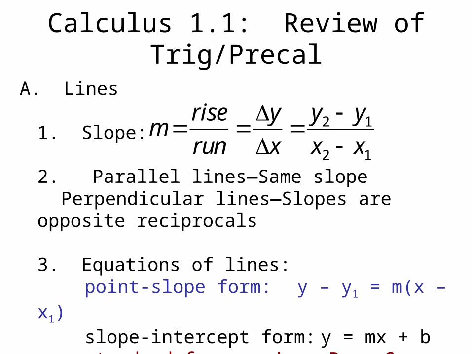
A. Lines

1. Slope:

2. Parallel lines—Same slopePerpendicular lines—Slopes are opposite

reciprocals

3. Equations of lines:point-slope form: y – y1 = m(x –

x1) slope-intercept form: y = mx + bstandard form: Ax + By = C

mrise

run

y

x

y y

x x

2 1

2 1

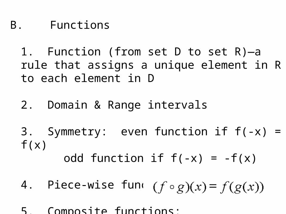
B. Functions

1. Function (from set D to set R)—a rule that assigns a unique element in R to each element in D

2. Domain & Range intervals

3. Symmetry: even function if f(-x) = f(x)odd function if f(-x) = -f(x)

4. Piece-wise functions

5. Composite functions:

f a f b whenever a b( ) ( )

C. Inverse functions:

1. f is one-to-one if <horizontal line test>

2.

3. Graphs of inverse functions are reflections across the line y = x

4. To find an inverse function, solve the equation y = f(x) for x in terms of y, then interchange x and y to write y = f-1(x)

f f x and f f x 1 1

D. Exponential & Logarithmic Functions

1. Exponential function:

2. Logarithmic function:

E. Properties of Logarithms:

f x a x( )

f x xa( ) log

1.log ( ) log loga a aXY X Y

2.log log loga a a

X

YX Y

3.log logar

aX r X

4. : logln

lnChange of base x

x

aa

5. : logremember y x a xay

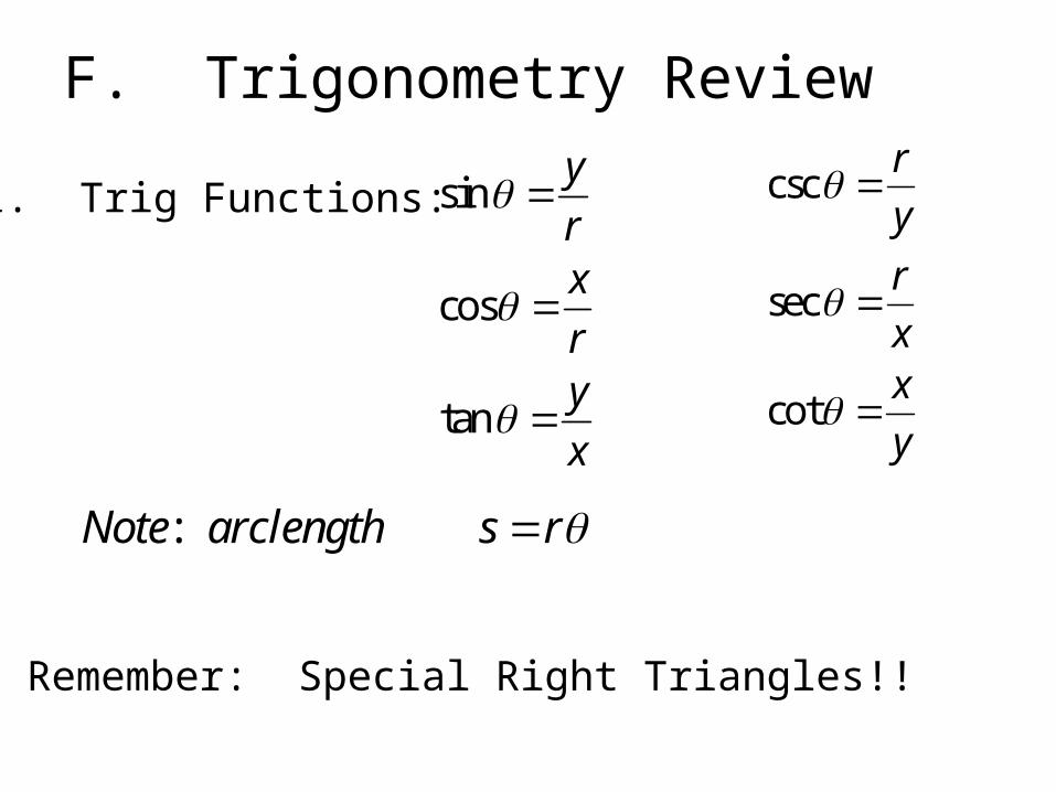
F. Trigonometry Review

sin

cos

tan

y

rx

ry

x

1. Trig Functions: csc

sec

cot

r

y

r

xx

y

Note arclength s r:

2. Remember: Special Right Triangles!!

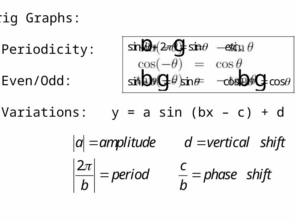
3. Trig Graphs:

a. Periodicity:

b. Even/Odd:

c. Variations: y = a sin (bx – c) + d

sin sin .

sin sin cos cos

2b g

bg bg

etc

a amplitude d vertical shift

bperiod

c

bphase shift

2

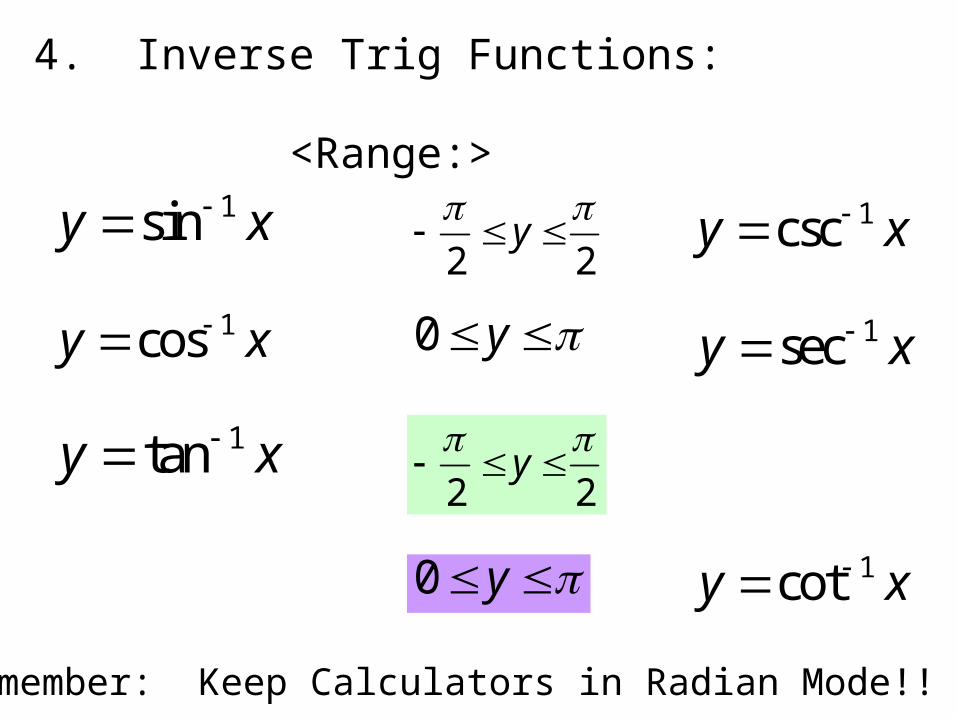
4. Inverse Trig Functions:

<Range:>

y x sin 1

y x cos 1 0 y

y x tan 1

2 2

y

2 2

y

y x csc 1

y x sec 1

y x cot 10 y

Remember: Keep Calculators in Radian Mode!!

Calculus 1.2: Limit of a Function

A. Definition: Limit:

“The limit of f(x), as x approaches a, equals L”—if we can make f(x) arbitrarily close to L by taking x sufficiently close to a (on either side of a) but not equal to a.

Ex 1: see fig 2 p.71 (Stewart)

x a

f x L

lim ( )

B. One-sided limits:

x a

f x L

lim ( ) (from the left)

x a

f x L

lim ( )

lim ( )x af x L

iff

x a x a

f x L f x

lim ( ) lim ( )

C. Estimating Limits using <calculators>

(from the right)

Note:

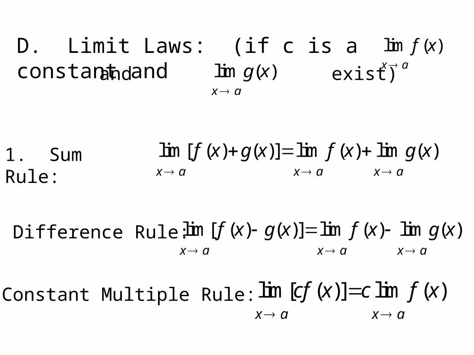
D. Limit Laws: (if c is a constant and lim ( )x a

f x

and exist) lim ( )x a

g x

1. Sum Rule: lim[ ( ) ( )] lim ( ) lim ( )x a x a x a

f x g x f x g x

2. Difference Rule: lim[ ( ) ( )] lim ( ) lim ( )x a x a x a

f x g x f x g x

3. Constant Multiple Rule: lim[ ( )] lim ( )x a x a

cf x c f x

4. Product Rule: lim[ ( ) ( )] lim ( ) lim ( )x a x a x a

f x g x f x g x

5. Quotient Rule: lim( )

( )

lim ( )

lim ( )x a

x a

x a

f x

g x

f x

g x

( ( ) )g x 0

6. Power Rule: lim[ ( )] [lim ( )]x a x a

f x n f x n

(n is a positive integer)

7. Root Rule: lim ( ) lim ( )x a

f x f xnn

x a

(n is a positive integer)

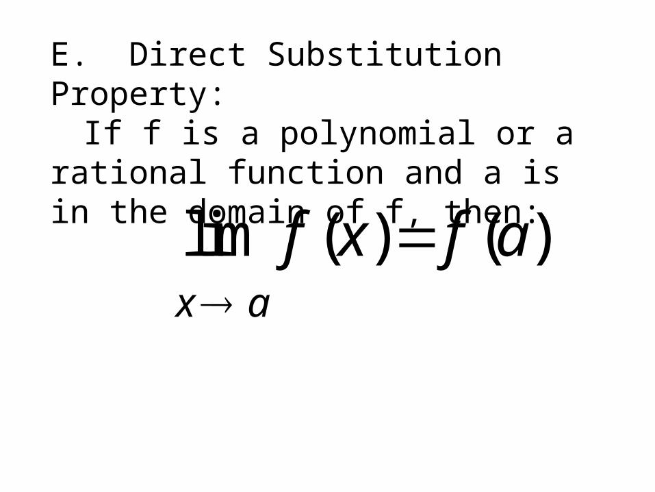
E. Direct Substitution Property:If f is a polynomial or a rational

function and a is in the domain of f, then:

lim ( ) ( )x a

f x f a

Calculus 1.3: Limits Involving Infinity

A. Definition: (Let f be a function defined on both sides of a) lim ( )

x af x

means that the values of f(x) can be made arbitrarily large by taking x sufficiently close to a (but not equal to a)

Note:

lim ( )x af x

arb. large negative

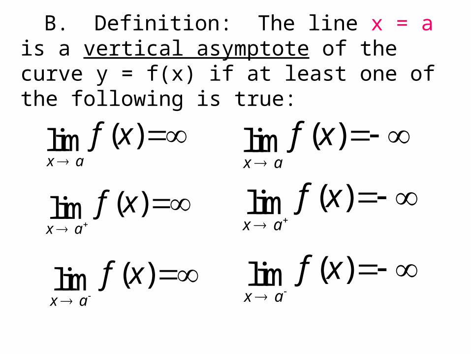
B. Definition: The line x = a is a vertical asymptote of the curve y = f(x) if at least one of the following is true:

x a

f x

lim ( )x a

f x

lim ( )

x a

f x

lim ( )x a

f x

lim ( )

x a

f x

lim ( )x a

f x

lim ( )

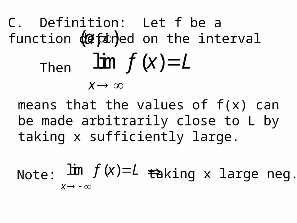
C. Definition: Let f be a function defined on the interval ( , )a

Then lim ( )x

f x L

means that the values of f(x) can be made arbitrarily close to L by taking x sufficiently large.

Note: lim ( )x

f x L

taking x large neg.

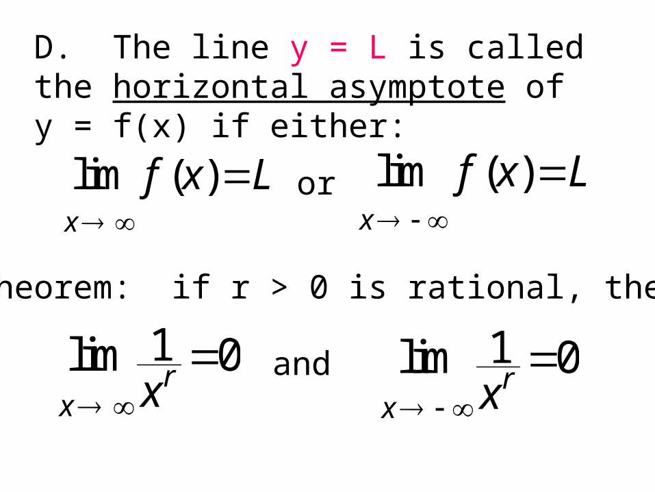
D. The line y = L is called the horizontal asymptote of y = f(x) if either:

lim ( )x

f x L

or lim ( )x

f x L

E. Theorem: if r > 0 is rational, then

limx

rx 1 0 lim

xrx 1 0and

F. Method for finding limits at infinity:

1. Divide top and bottom of rational function by the largest power of x in the denominator

2. Simplify using theorem in E above

Calculus 1.4: Continuity

A. DEF: A function f is continuous at a number a if

lim ( ) ( )x af x f a

(assuming f(a) is defined and lim ( ) )x af x exists

**Remember, this means:

lim ( ) lim ( ) lim ( ) ( )x a x a x af x f x f x f a

B. Types of Discontinuity

1. Removable

2. Infinite

3. Jump

4. Oscillating see fig 2.21 p. 80

<Geometrically, the graph of a continuous function can be drawn without removing your pen from the paper>

C. Continuous Functions

1. A function is continuous from the right at a if

2. A function is continuous on an interval [a,b] if it is continuous at every number on the interval

3. The following are continuous at every number in their domains:

polynomials, rational functions

root functions, trig functions

lim ( ) ( )x a

f x f a

D. Intermediate Value Theorem:

Suppose f is continuous on [a,b] and f(a) < N < f(b)

Then there exists a number c in (a,b) such that f(c) = N

Calculus 1.5: Rates of Change

A. Average Rates of Change

1. Average Rate of Change of a function over an interval – the amount of change divided by the length of the interval

2. Secant Line – a line through 2 points on a curve

f

x

f x f x

x x

( ) ( )2 1

2 1

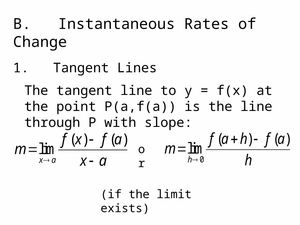
B. Instantaneous Rates of Change

1. Tangent Lines

The tangent line to y = f(x) at the point P(a,f(a)) is the line through P with slope:

mf x f a

x ax a

lim( ) ( )

mf a h f a

hh

lim

( ) ( )0

or

(if the limit exists)

2. Velocities

Instantaneous velocity v(a) at time t=a:

v af a h f a

hh( ) lim

( ) ( )

0

Calculus 1.6: Derivatives

A. Definitions:

1. Differential Calculus—the study of how one quantity changes in relation to another quantity.

2. The derivative of a function f at a number a:

f a

f a h f a

hh( ) lim

( ) ( )0

(if the limit exists), or

f af x f a

x ax a( ) lim

( ) ( )

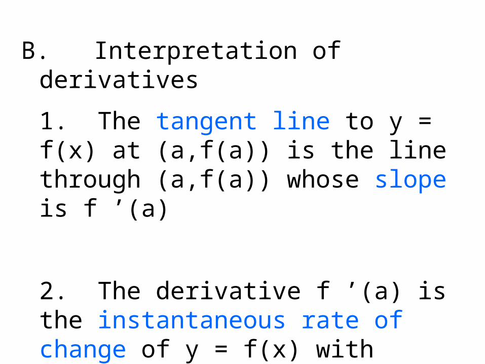
B. Interpretation of derivatives

1. The tangent line to y = f(x) at (a,f(a)) is the line through (a,f(a)) whose slope is f ’(a)

2. The derivative f ’(a) is the instantaneous rate of change of y = f(x) with respect to x when x = a

C. The Derivative as a Function

1. Definition of the derivative of f(x) as a function:

f x

f x h f x

hh( ) lim

( ) ( )0

Ex: Find f ‘ (x):

1 3. ( )f x x x

2 1. ( )f x x 3

1

2. ( )f x

x

x

Calculus 1.7: Differentiability

A. Other Notation for Derivatives:

f x ydy

dx

df

dx

d

dxf x Df x D f xx( ) ( ) ( ) ( )

B. DEF: A function f is differentiable at a if f ‘(a) exists. It is differentiable on (a,b) if it is differentiable at every number in (a,b).

Ex 1: y x

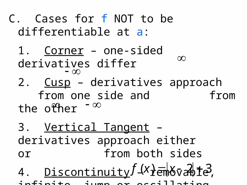
C. Cases for f NOT to be differentiable at a:

1. Corner – one-sided derivatives differ

2. Cusp – derivatives approach from one side and from the other

3. Vertical Tangent – derivatives approach either or from both sides

4. Discontinuity – removable, infinite, jump or oscillating

Ex 2: Find all points in the domain where f is not differentiable.

State which case each is:

f x x( ) 2 3

D. Graphs of f ’

1. Sketching f ’ when given the graph of f see Stewart p.135 fig

2

a. p. 106 #22 b. p. 105 #13-16c. p. 106-107 #24-26

2. Sketching f when given the graph of f ’

a. p. 107 #27,28

Calculus: Unit 1 Test

• Grademaster #1-40 (Name, Date, Subject, Period, Test Copy #)

• Do Not Write on Test! Show All Work on Scratch Paper!

• Label BONUS QUESTIONS Clearly on Notebook Paper. (If you have time)

• Find Something QUIET To Do When Finished!