calculation tool for the treatment of electrostatic...

Calculation tool for the treatment of

electrostatic precipitator ash in Metso’s

ash leaching process

Master’s Thesis within the Innovative and Sustainable Chemical Engineering programme

MALIN LARSSON

Department of Chemical and Biological Engineering

Forest Products and Chemical Engineering

CHALMERS UNIVERSITY OF TECHNOLOGY

Gothenburg, Sweden 2012

MASTER’S THESIS

Calculation tool for the treatment of electrostatic

precipitator ash in Metso’s ash leaching process


MALIN LARSSON

SUPERVISORS:

Kai Lüder

Martin Wimby

Therese Hedlund

EXAMINER

Hans Theliander



CHALMERS UNIVERSITY OF TECHNOLOGY


Calculation tool for the treatment of electrostatic precipitator ash in Metso’s ash leaching process


MALIN LARSSON

© MALIN LARSSON, 2012



Chalmers University of Technology

SE-412 96 Göteborg

Sweden

Telephone: + 46 (0)31-772 1000

Cover:

Simplified process flow diagram of an ash leaching process.

Chalmers Reproservice


I

Calculation tool for the treatment of electrostatic precipitator ash in Metso’s ash leaching process

Master’s Thesis in the Innovative and Sustainable Chemical Engineering programme

MALIN LARSSON



Chalmers University of Technology

ABSTRACT

Two different solubility models have been developed for Metso’s Ash Leach process. The backbone of

the models consists of mass balances describing the overall process and the individual components;

leaching tank and centrifuge. The difference between the models is the modeling of the dissolution of

the components included in the electrostatic precipitator ash in water. Electrostatic precipitator ash is

mainly composed of five components; Na+, K

+, Cl

-, SO4

2- and CO3

2-, which in solid phase leads to

formation of the salts Na2SO4, Na2CO3, NaCl, K2SO4, K2CO3 and KCl. The main components in the

ash are normally sodium and sulphate, but ashes consisting of high amounts of carbonate may also

occur. The first model, Model I, is a simple model based solely on mass balances and a fixed amount of

ash dissolved in a saturated solution. Na2SO4 is the only salt predicted to be present in the solid phase.

All other salts are assumed to be completely dissolved.

For the other model, regressions of literature data and experimental data from units in operation have

been used. The dissolution predicted by Model II is dependent on the system Na2SO2-K2SO4-Na2CO3

and its dependence on temperature. This system was used in order to investigate the possibility to use a

four component system when describing the solubility of a five component system. NaCl, KCl and

K2CO3 are assumed to be completely dissolved.

It is also important to consider the total amount of ash dissolved in a saturated solution. The amount of

dissolved ash in water is commonly considered to be between 29-33 wt% in a saturated solution for

units in operation. Three different amounts of ash in water have been investigated: One regression is

depending on the K/(K+Na) molar ratio in the slurry, and two fixed amounts of ash at 31 wt% and 32

wt% dissolved solids in the liquid phase. The predicted results using these settings are compared with

the predicted results using the amount of dissolved ash specified in the experimental data.

Finally, the efficiencies predicted by Models I and II are compared to simulations performed by

Chemcad including corrections done by Metso Power.

Both Models I and II predict the reject composition well for slurries containing low contents of

carbonate and potassium at an ash to water ratio in slurry of 800 g ash/ l water, if no recirculation is

used. When the ash to water ratio increases, both Model I and II predicts the concentration of

negatively charged ions well for a slurry containing a low amount carbonate. But the concentration

potassium and sodium are predicted to be higher respectively lower than the experimental data.

When recirculation is used, the predicted reject composition deviates from the experimental data. For

Mill 1, this probably depends on the fact that suspended solids are carried over to the liquid phase. In

reality suspended solids may be carried over to the liquid phase if the centrifuge is not working

properly. However, the recycled ash composition conforms well to the experimental data for Mill 1, but

for Mill 2 larger deviations occur due to the higher amounts of carbonate in the slurry and a lower

dryness of the recycled ash. The same result occurs when comparing efficiencies. For Mill 1 the

predicted efficiencies of both Models I and II conform relatively well to the efficiencies based on

experimental data and the efficiencies predicted by Chemcad. Only smaller deviations occur. For Mill 2

deviations occur from experimental data for all models including Chemcad. Model II produces the best

prediction of carbonate and sulphate efficiencies whereas Chemcad and Model I predict significantly

higher recovery efficiency than what is the case in reality.

II

It is concluded that all models provides good estimations of the reject composition for ashes containing

low carbonate and potassium contents when no liquid is recycled back to the leaching tank. But when

the carbonate content increases the deviations increase as well. In order to find correlations for systems

including larger amounts of potassium and carbonate a larger quantity and more accurate data are

needed. It may be necessary to develop a thermodynamic model in order to produce more accurate

predictions about such a system. When the recirculation ratio is increased an increased concentration

potassium and carbonate will be present in the liquid phase, which makes it important to have a model

that provides accurate predictions of the precipitation of burkeite and glaserite.

When modeling different specified amounts of ash that are dissolved in a saturated solution, deviations

occur when the results are compared with the predicted values using the specified amount of ash

dissolved in the reject. This indicates that an accurate amount of ash dissolved in a saturated solution is

needed to obtain accurate compositions in the liquid phase.

Key words:

Leaching, Chemical recovery, Non-process elements, Solubility, Electrostatic precipitator ash,

Chloride, Potassium, Sodium sulphate

Contents

NOTATIONS IV

1 INTRODUCTION 1

1.1 Purpose 2

1.2 Scope 2

2 BACKGROUND 3

2.1 Kraft Pulping 3

2.2 Recovery Boiler 4 2.2.1 ESP ash composition 4

2.3 Ash leaching principle and process 6

2.4 Solubility 8 2.4.1 Thermodynamics 8 2.4.2 Solubility in water 10

2.4.2.1 Solid phases 10 2.4.3 Solubility studies 11

2.4.3.1 Collocation of experimental data by Linke 11

2.4.3.2 Experimental data produced by Teeple 12

2.4.3.3 Experimental data produced by Jaretun 13

2.4.3.4 Experimental data produced by Goncalves 14

2.5 Computational programs 16 2.5.1 RBD 16 2.5.2 Chemcad 16

3 MASS BALANCES 17

3.1 Comparison between predicted and experimental data 19

3.2 Evaluation of model assumptions 19

4 MODELS 21

4.1 Model I 21 4.1.1 Input variables 22

4.2 Model II 22 4.2.1 Input variables 23 4.2.2 Investigation of the amount ash dissolved with composition 24

5 RESULTS AND DISCUSSION 25

5.1 Predictions without recirculation 25

5.2 Predictions with recirculation 27 5.2.1 Investigations of the ash amount dissolved 29 5.2.2 Temperature dependence of Model II 30

5.3 Comparison with Chemcad 31 5.3.1 Effect of recycling 33

II

6 CONCLUSIONS 34

7 FUTURE WORK 35

8 REFERENCES 36

APPENDIX A – SOLUBILITIES OF ANHYDROUS SALTS IN WATER 37

APPENDIX B – SOLUBILITY FOR MIXTURES 39

APPENDIX C – EXPERIMENTAL DATA FROM UNITS IN OPERATION 47

APPENDIX D – MASS BALANCES 55

APPENDIX E – EXCEL DATA SHEET, MODEL I 56

APPENDIX F – PREDICTIONS WITHOUT RECIRCULATION 57

APPENDIX G – TEMPERATURE DEPENDENCE BY MODEL II 58

Preface This report is a Master’s Thesis project for the degree of Master of Science in Chemical Engineering at

Chalmers University of Technology. The project has been performed at Metso Power in Gothenburg in

collaboration with the Department of Forest Products and Chemical Engineering at Chalmers

University of Technology during the spring and summer of 2012. The supervisors were Kai Lüder,

Martin Wimby and Therese Hedlund at Metso Power. The examiner at Chalmers University of

Technology was Hans Theliander.

First of all, I would especially like to thank my supervisors Kai Lüder, Martin Wimby and Therese

Hedlund for their commitment and assistance provided throughout the entire project. Major effort has

been put into discussions and commenting on the report.

I would also like to show my appreciation to all employees at Metso Power for their warm welcoming

and support, whenever I have had questions.

Lastly, I would like to thank my family and friends for being interested in my work and for supporting

me through setbacks. A special thanks to Simon who is always there for me and have supported and

encouraged me during the project.

Malin Larsson

Gothenburg, 2012

IV

Notations

Roman letters

Activity

Difference in Gibbs free energy

Enthalpy change

Mass flow

Number of molecules

Total pressure

Molar gas constant

Entropy change

Absolute temperatur

Molar fraction in liquid

Greek letters

Activity coefficient

Chemical potential

Standard chemical potential

Subscripts

Electrostatic precipitator ash to leaching

Aqueous solution

Purged liquid stream

Water to leaching

Any specie

Liquid stream rich in chloride and potassium

Suspended solids together with diluted solids before separation

Recycled reject

Abbreviations

Black liquor solids

Chloride

Carbonate

Dry solids

Dissolved solids

Electrostatic precipitator ash

Electrostatic precipitator

Potassium

Potassium chloride

Potassium carbonate

Potassium sulphate

Sodium

Sodium chloride

Sodium carbonate

Sodium sulphide

Sodium sulphate

Recovery Boiler Design

Sulphate

Suspended solids

1

1 Introduction

In pulp and paper industry there is a continuously ongoing work for closing processes where the main focus is

to save energy and chemicals (1). Saving energy and chemicals reduces the environmental impact and cost of

make-up chemicals. One way to reduce the usage of chemicals is to remove non-process elements, such as

chlorides and potassium, from the electrostatic precipitator ash. The electrostatic precipitator ash from the

recovery boiler contains five main components which result in different ionic alkali salts, for example

Na2SO4, Na2CO3, NaCl, K2SO4, K2CO3 and KCl (2). Since chlorides and potassium cause corrosion and

plugging in the recovery boiler they need to be separated from the process flow. Traditionally a part of the ash

flow has been dumped to avoid this problem. But since dumping also means losing valuable Na2SO4, different

processes for separating chlorides and potassium from the process flow have been developed. One of these is

the leaching process, where precipitator ash is leached with water (1).

In an ash leaching process the difference in water solubility of salts occurring in the precipitator ash is used in

order to separate chloride and potassium from sulphate. This separation leads to enhanced Na2SO4 recovery

and removal of non-process elements such as chlorides and potassium (3). The interaction between ions and

the solubility of different salts are therefore important parameters when modeling the leaching process. For

dimensioning of ash leaching plants today, Metso Power uses Chemcad to solve the component and mass

balances. The Pitzer electrolyte model available in Chemcad is applied to predict the solubility of precipitator

ash. The calculation procedure in Chemcad comprises several steps which are not discussed in this report. The

results are exported from Chemcad to Excel where important corrections must be made in the results due to

errors originating from weaknesses in the Chemcad model. Other issues with using Chemcad for this purpose

are that Metso Power has a limited number of licenses for Chemcad and the program is therefore not

accessible to everyone. In some situations the steady state calculations for the ash leaching system has

difficulties to converge, which seems to be a problem with new versions of the software. New versions might

also produce altered results when comparing with previous versions. Since Excel is already used for

corrections and processing of data, it would have been preferable to use this software throughout the entire

procedure.

In literature a limited number of models predicting the solubility of precipitator ash have been found. Two

models for the prediction of the solubility of precipitator ash have been published by Saturnino (4, 5).

Saturnino has modeled this dissolution in the OLI software (5) but also developed a regression model (4). The

aqueous model in the OLI electrolyte simulation software is an electrolyte thermodynamic model based on

published experimental data. The model uses data regression wherever possible and produce estimations and

extrapolations where required (6). According to Saturnino, the estimated solubilities of the ash conform well

with experimental data, but to somewhat lower predicted concentration of Cl- and higher predicted

concentration of Na+ (5). The regression model developed by Saturnino is based on experimental data. The

model equation consists of a third degree polynomial which depends on temperature, alkalinity (hydroxide

plus sulphide concentration in grams per litre), molar ratio of potassium over potassium and sodium in the ash

and compound parameters. The curves provide the solubility of the negatively charged ions (Cl-, CO3

2- and

SO42-

) provided that the solution is in equilibrium with the positively charged ions (K+, Na

+). The data cover a

temperature range from 50 to 100 ⁰C (7). Predictions compared to the experimental work performed by

Jaretun (8) give similar results for the extraction of the elements.

2

1.1 Purpose

The primary aim with the Master’s Thesis project is to develop a calculation tool for solubilities in Excel for

Metso’s Ash Leach Process in order to become more or less independent on Chemcad. An Excel data sheet

fitted with relevant equations to describe the equilibrium solubility of the different ions when the ash is

dissolved, should be developed and evaluated. The ambition is to implement and evaluate an accurate model

for the predictions of aqueous solubilities at equilibrium in the mass balance calculation. It is important to

keep the model as simple as possible in order to make it easy to follow and maintain. The major advantage

with an in-house software is that such a calculation tool is available to all Metso engineers. If one wish to

change the chemical model inside the calculation tool in the future it can be easily done, which is not the case

for a commercial program such as Chemcad.

1.2 Scope

This paragraph describes the limitations of the project.

The objective is to develop a model for a single step ash leaching process.

The components included in the models are Na+, K

+, Cl

-, SO4

2- and CO3

2- forming the salts NaCl,

KCl, Na2SO4, K2SO4, Na2CO3 and K2CO3.

The operating temperature of the ash leaching process is normally in the range of 70-90 ⁰C. The

models are based on experimental data in this range and are therefore only valid in this temperature

interval.

Separation in the centrifuge is assumed to be total, which means that no solids are discharged with

the reject, i.e. the liquid phase.

The fact that different ash composition affects the dryness of the outgoing ash is not considered in

the project.

Dynamic effects, for example time required to reach equilibrium between solid and liquid phase, is

not considered in this report. The residence time in the leaching tankt is long enough for the system

to reach steady state. This assumption is consistent with the experimental data performed by Jaretun

(8).

3

2 Background

A brief background to the Kraft pulping process is provided in this chapter. The setup of the ash leaching

process together with the section about solubilities provides the background to the developed models.

2.1 Kraft Pulping

The ash leaching principle can be used in the Kraft pulping process, which is the most common way of

manufacturing pulp in Sweden. The Kraft process can handle almost all species of softwood and hardwood,

provides strong pulp and is economically feasible due to high chemical recovery efficiency, about 97% (9). It

is an effective technology that provides recycling of pulping chemicals and generation of steam and electrical

power when black liquor is burnt (9). Sodium hydroxide and sodium sulphide are used as active cooking

chemicals, which removes lignin and hemicelluloses from cellulose. About fifty percent of the ingoing wood

is dissolved in the process together with the spent pulping chemicals, resulting in a stream called weak black

liquor, as can be seen in Figure 1. The weak black liquor is separated from the pulp and evaporated in order to

increase the concentration before entering the recovery boiler as heavy black liquor. When the black liquor is

burnt, a smelt bed mainly consisting of Na2CO3 and Na2S are formed in the lower part of the furnace (10).

The flue gas contains mainly of Na2SO4 but also other inorganic compounds such as cadmium, chlorides and

potassium which accumulate in the electrostatic precipitator (ESP) forming ESP ash.

Figure 1. The kraft chemical recovery cycle including the ash leaching process (9).

Since the ESP ash contains a large fraction Na2SO4, which is a valuable make-up chemical, it is favourable to

recycle it back to the process. The main part of the chlorides and potassium accumulate in the ESP ash, and

therefore this ash is treated in the ash leaching process. As mentioned in Chapter 1, the ash leaching system

utilises the differences in solubility of different compounds in order to separate them from each other. The

process is built on the fact that NaCl and KCl are more soluble in water than Na2SO4. This means that large

fractions of NaCl and KCl normally can be removed and disposed for water treatment, where Na2SO4 is

recycled back to the recovery cycle.

4

2.2 Recovery Boiler

The recovery boiler is one of the most important equipments in pulp mills since it recycles cooking chemicals

and produces energy. The chemical, physical and combustion properties vary among mills depending on

location, wood species, pulp yield, white liquor properties and ratio between wood and chemicals among

other factors (9).

Concentrated black liquor from the evaporation plant is sprayed into the recovery boiler and burnt in deficit of

oxygen leading to the reduction of Na2SO4 to Na2S. The inorganic sulphur and sodium can be recovered as a

molten ash smelt containing mostly Na2S and Na2CO3. The smelt is dissolved in water, forming green liquor,

before it is sent to the causticizing plant where Na2CO3 is converted to NaOH. A fraction of the burnt black

liquor in the recovery boiler will vaporize from the char bed, follow the flue gases, and accumulate in the ESP

as ESP ash (6).

2.2.1 ESP ash composition

The ESP ash consists of inorganic compounds which usually enter the mill with the wood and to a smaller

extent with the make-up chemicals and water (11). The amount of inorganic non-process elements entering

the mill depends on wood type, location of the mill and transportation route. ESP ash compositions from three

mills are presented in Table 1. These mills will be referred to as Mill 1, Mill 2 and Mill 3. The ash from Mill 1

is a low carbonate ash, whereas Mill 2 and Mill 3 produce ash with relatively high carbonate content. The

chloride content is similar for all mills and the potassium content is somewhat lower for Mill 2 and higher for

Mill 3.

Table 1. Average ESP ash composition from three different mills; Mill 1, Mill 2 and Mill 3. The composition

for each analysis in ash, reject, slurry and recycled ash is presented in Appendix C.

Average ash composition (wt% dry ash) Mill 1 Mill 2 Mill 3

Cl- 3,64% 3,79% 4,38%

K+ 4,37% 2,97% 5,19%

Na+ 29,68% 34,07% 34,21%

SO42- 62,08% 41,64% 30,12%

CO32- 0,23% 17,52% 26,10%

Na2SO4 84,48% 58,57% 40,89%

Na2CO3 0,38% 29,44% 42,32%

NaCl 5,52% 5,95% 6,63%

K2SO4 8,96% 3,69% 4,48%

K2CO3 0,04% 1,96% 4,92%

KCl 0,61% 0,39% 0,75%

Average ratio of ash to water in slurry

(g ash/l H2O) 1200 800 900

Temperature (ºC) 90 90 90

Chloride, potassium, cadmium, calcium and arsenic are examples of undesirable non-process elements.

Chlorides and potassium accumulate in the pulping liquors and have higher solubility than for example

cadmium (12). These non process elements accumulate until they reach a steady-state concentration

dependent on inputs, degree of mill closure and liquor sulphidity. When mills close up, which means that

they decrease the dumping of cooking chemicals, the input of chloride and potassium becomes increasingly

important. An increased closure can accumulate chloride and potassium up to 4-12 times greater than mills

which operate fairly open (13).

5

As mentioned earlier the chlorides and potassium accumulate in the black liquor, which is burnt in the

recovery boiler. KCl and NaCl have a higher vapor pressure than Na2S and will therefore volatilize from the

char bed in the recovery boiler and accumulate in the ESP ash (3). This means that the bed temperature in the

recovery boiler has a significant effect on the enrichment of chlorides and potassium in the ESP ash. The ESP

ash is mainly composed of five different ions; sodium, sulphate, potassium, chloride and carbonate which

mainly form Na2SO4, NaCl, Na2CO3, K2SO4, KCl and K2CO3. The melting point of the ESP ash is influenced

by the potassium and chloride concentrations in the fired black liquor (11). An increase in potassium or

chloride concentrations result in a lower melting point of the ash, leading to increased deposits and plugging

in the upper furnace sections which lead to the fact that consecutive downtime is required for washing the

boiler with water. The downtime needs to be minimized since it results in economical losses. Deposits are

sticky when 15-70% of the ash is in the molten state. The temperature when 15% of the ash particles have

melted is called the sticky temperature, which is denoted T15. The temperature when 70% is in molten state is

called the radical deformation temperature, denoted T70. Figure 2 shows the effect of chloride on T15 and T70

for a typical carry over deposit containing 5 mole% K+/(K

++Na

+) (13). An increase in chloride content lowers

both the sticky and the radical deformation temperature. The effect of potassium is similar to chloride, but not

as prominent (13, 14). At a low chloride concentration, potassium gives only a small effect on the sticky

temperature, illustrated in the picture to the right in Figure 2. But when the chloride concentration increases,

potassium has an increased effect on lowering the sticky temperature.

Figure 2. To the left, the sticky temperature is shown as a function of the molar ratio between chloride divided

by sodium and potassium for a typical carry over deposit containing 5 mole% K+/(K

++Na

+) (13, 15). The

sticky temperature dependence of potassium in the ash is shown in the right picture as a function of the molar

ratio Cl-/(Na

+ + K

+) (13). The plots are regressions of experimental data.

When particles stick to the walls and tubes of the recovery boiler it leads to lower heat transfer through the

surface and reduced temperature of the generated steam. The region of sticky ash for high and low

concentration of chlorides and potassium can be seen in Figure 3. High potassium and chloride concentrations

result in deposits in the upper part of the boiler, shown as the marked region in the left picture in Figure 3,

where the temperatures of the flue gases are lower. In this region the deposits have a tendency to harden and

are difficult to remove with sootblowers which leads to a increased risk of plugging (16).When the

concentration of chlorides and potassium are lower, the fouling occurs in the region marked in the right

picture of Figure 3. In this region the deposits are easier to remove with sootblowing and the downtime for

washing decreases.

6

Figure 3. The left picture shows the deposit area with a high concentration of chlorides and potassium. To the

right the deposit area for a low concentration chloride and potassium is shown (15).

Removal of potassium and chloride from the ESP ash is a very important issue in future chemical recovery

cycles, where the focus is to reduce the amount of chemicals used in the process. Ash leaching of ESP ash is

one way of decreasing the content of these two non-process elements (3). This is because of the enrichment in

the ash, but also since the ash is easier to handle in comparison to liquors. The purge of chloride and

potassium becomes more and more important due to the construction of new recovery boilers operating at

higher temperatures and steam pressures.

2.3 Ash leaching principle and process

The purpose of the ash leaching system is to decrease the concentration of chlorides and potassium in the

liquor cycle while Na2SO4 is recovered. Alternative ash treatment systems available are ion exchange,

evaporation/crystallisation and freeze crystallisation (3). These are all interesting processes but will not be

further discussed here.

The usage of an ash leaching plant reduces the environmental impact and cost for make-up chemicals

compared to purging of ESP ash. The ash leaching system keeps the major part of the heavy metals, such as

cadmium, in the solids that are brought back to the liquor cycle. The heavy metals can then be separated

elsewhere, for instance in filtering of the green liquor dregs. The amount of ESP ash to be treated in the

leaching plant in order to maintain the right chemical balance depends on the input of potassium and chlorides

to the mill. The leaching step is selective, meaning that most of the potassium and chlorides are dissolved in

the liquid phase while a large fraction of Na2SO4 remains solid and can be separated from the liquid phase and

returned to the liquor cycle. The dissolution principle of NaCl, KCl and Na2SO4 is by a simplified picture

shown in Figure 4. Initially the ash is mixed with water to form a suspension. When equilibrium is obtained

between the liquid and solid, almost all NaCl and KCl are dissolved while Na2SO4 stays in solid phase. The

last unit operation is separation of the liquid containing the dissolved salts from the solid fraction.

Figure 4. A simplified picture of the ash leaching principle (15). In reality, Na2SO4 is not the only component

in the solid phase.

7

In Figure 5 a simplified process flow diagram is shown for the ash leaching process. The ash is mixed with

warm water in an agitated leaching tank which results in the formation of a slurry. The slurry is a partly

diluted mixture which contains suspended solids and diluted solids in water. This initial step corresponds to

the mixing and equilibrium step shown in Figure 4. Most of the chlorides and potassium dissolve in the water

while the main part of Na2SO4 remains solid.

Figure 5. Simplified process flow diagram of an ash leaching process (10).

The slurry is transferred from the leaching tank to a centrifuge where liquid and solids are mechanically

separated by centrifugal forces. The fraction dissolved solids and suspended solids in slurry, reject and

recycled ash are principally shown in Figure 6. In an ideal separation step the separation between suspended

solids and reject is total, which means that no suspended solids are present in the reject.

Figure 6. Dissolved and suspended solids in the process streams entering and exiting the centrifuge.

In reality this separation depends on the centrifugal force, which include the density difference between solid

and liquid phase, viscosity, particle size and mechanical work of the centrifuge. A smaller particle size makes

it more difficult to dewater the recycled ash which results in a decreased dryness. When the dewatering

decreases a larger fraction of reject will be present in the recycled solids, which leads to a decreased

efficiency. The normal dryness of the recycled solids is 70-90% depending mainly on carbonate content and

type of centrifuge. The dryness of the treated ash should not be below 80 % to guarantee an efficient

separation step. If smaller particles are present, it will also increase the risk that particles are carried over to

the liquid phase which results in suspended solids in the reject.

The recycled ash containing Na2SO4 is mixed with virgin black liquor in the mix tank and returned to the

chemical recovery cycle. The liquid fraction contains the main part of the potassium and chloride. One part of

this liquid is discharged via the water treatment system and the remaining part is returned to the leaching tank,

as illustrated in Figure 5. By adjusting the amount of recycled reject, the selectivity of the removal efficiency

of Cl- and K

+ and the recovery efficiency of Na2SO4 is controlled. Figure 7 shows a typical correlation

between removal and recovery efficiency, based on units in operation. When the recycled fraction is

decreased the removal efficiency of chlorides and potassium will increase. On the other hand the recovery

efficiency of Na2SO4 will decrease. If instead the recovery of sodium and sulphate should be promoted the

H2O +

dissolved solids

H2O +

dissolved solids

H2O +

dissolved solids

suspended solids suspended solids

rejectrecycled ashslurry

8

amount of recycled liquid must be increased. This leads to a lower removal efficiency of chlorides and

potassium since the bleed flow is decreased. This means that it is impossible to obtain maximum removal of

chlorides and potassium at the same time as maximum recovery of Na2SO4.

Figure 7. The removal efficiency of Cl- and K

+ as a function of recovery efficiency of Na2SO4. The dots

represent experimental data from different mills and the curves are regressions of the experimental data (15).

2.4 Solubility

A brief introduction to the thermodynamics of the dissolution of compounds is outlined in section 2.4.1

below. The solubilities of different compounds and mixtures common in the ESP ash are presented in 2.4.2.

A limited number of studies have been done on concentrated inorganic salt mixtures common in forest

industrial applications (17), for example mixtures containing ESP ash. The most interesting work performed

by Goncalves, Jaretun, Linke and Teeple are presented in section 2.4.3.

2.4.1 Thermodynamics

The solubility of a compound in a solvent decides the number of compound molecules which can be dissolved

to form a saturated solution. A sufficient amount of molecules must be dissolved to obtain equilibrium

between the solvent and the undissolved solid. There are many different conditions which might affect the

solubility of a compound in a pure solvent or solution, for example temperature, pH and composition.

However, if one for example studies a two component system consisting of a partly soluble crystalline

compound in water some important effects can be highlighted. When the equilibrium state for the two

component system is obtained the dissolved compound molecules in the aqueous solution coexist with

compound molecules bound to each other in solid phase (crystal). The concentration of dissolved molecules

will then be unchanged with time. This means that the probability for a molecule to leave the solid state into

solution must be the same as the probability to bind one dissolved molecule to the crystal. One important

effect which contributes to the dissolution is the increased entropy when a molecule is mixed in the aqueous

solution. However, this might be counterbalanced by the binding energy between molecules in the crystal. If

the binding energy is large the probability for a molecule to leave the crystal is low resulting in low solubility.

If the binding energy is low the probability for a molecule to obtain enough energy from the system to

dissolve is much higher. If the temperature of the system is increased the available amount of energy increases

which generally increase the compound solubility.

The balance between energy and entropy for the solvation process can be expressed by the difference in Gibbs

free energy denoted between the aqueous phase and the crystal by expression:

(2.1)

where represents the enthalpy change and the entropy change for the solvation process at temperature

in degrees Kelvin. When equilibrium is obtained =0 and the net flow of molecules between the two

different phases becomes zero. A closely related property to Gibbs energy is the chemical potential which

9

for a compound i in a multiple system of j components at constant pressure and temperature can be expressed

as:

(2.2)

The chemical potential for a compound i can be related to a standard chemical potential at a hypothetical

standard state and the activity as:

(2.3)

where R is the gas constant. The activity relates to the molar fraction as:

(2.4)

Here is the activity coefficient which contains the information about the deviation from an ideal dilute

solution. When the concentration goes to zero the activity becomes equal to the molar ratio and the activity

coefficient becomes equal to one.

When an uncharged hydrophobic compound is dissolved in water the aqueous solubility is low and can

successfully be modelled by a simplified dissolution model based on an ideal dilute solution. It is assumed

that a dissolved molecule is totally surrounded by water molecules and do not interact with other dissolved

molecules. The molecular interactions within the crystal and the interactions between the solute and the water

molecules are considered. For electrolyte systems the long range columbic forces between all charged ions

must be considered already at very low concentration and will play a dominant role in the deviation from ideal

solubility. Strong multiple electrolyte systems are common in pulp and paper industry. These systems become

even more complex due to ion association, hydration, complex formation, and different precipitations taking

place which must be taken into account (18) for proper predictions. It is also important to take the common

ion effect in account. If a strong electrolyte is added to a solution with a weak electrolyte, where the strong

and weak electrolytes have one ion in common, the solubility of the weak electrolyte is decreased as a result

of the common ion effect (19). For example, when NaCl is present in aqueous solution, the solubility of

Na2SO4 is decreased, since both salts consists of Na+ (20). The short thermodynamic descriptions above must

be adjusted for electrolyte systems due to the charge of dissociated ions etc. However this theory will not be

further discussed in this thesis but good descriptions and summaries are found in literature (18).

10

2.4.2 Solubility in water

The solubilities of different salts normally present in precipitator ash dissolved in pure water are shown in

Figure 8. As can be seen the solubilities for K2SO4 and KCl increase with temperature. The solubility of NaCl

slightly increases with temperature (21). Na2SO4 and Na2CO3 solubilities increase rapidly between 0 – 40 ⁰C

but subsequently decreases between temperature of 40-100 °C. K2CO3 has a very high solubility between 50-

60 wt% in water which might indicate that it is unlikely to precipitate even in mixtures. The solubility for the

salts in pure water can be compared to the solubilities of the compounds in mixture discussed in section 2.4.3.

Figure 8. Solubilites of different anhydrous salts, common in the ESP ash, in pure water according to Perry,

1997 (21).

2.4.2.1 Solid phases

The desired composition of the ESP ash entering an ash leaching system is low content of potassium and

carbonate and high content of Na2SO4 which leads to the formation of a recycled ash mainly composed of

Na2SO4. This is not always the case since the ash composition might vary significantly between mills (11).

When the potassium content increases, K2SO4 starts to precipitate which leads to formation of the double salts

glaserite (3K2SO4·Na2SO4) (22). If the carbonate content increases, Na2CO3 will start to precipitate and form

crystals together with Na2SO4, resulting in a double salt called burkeite (2Na2SO4·Na2CO3). Glaserite is

formed when the potassium content of the slurry is high. K2SO4 precipitates together with Na2SO4 which leads

to a lower removal efficiency of potassium and lower recovery efficiency of sodium. Figure 9 shows the

transition between different solid phases depending on the potassium concentration and the molar ratio

K/(K+Na) in the liquid phase.

Figure 9. The transitions between different solid phases are shown in the figure, depending on the mass

fraction of potassium, based on dry solids (DS), as a function of the molar ratio K/(K+Na) in the liquid phase

(20). Data is taken for the system Na2SO4 – K2SO4 at 55 ºC and are published in the work by Linke, 1958.

11

The potassium concentration in the liquid phase is usually quite low which means that Na2SO4 and sometimes

glaserite are present in the solid phase. As shown in Figure 9 glaserite starts to precipitate at a concentration

of 7 wt% potassium (based on dry solids in the liquid phase) in a mixed system of Na2SO4 and K2SO4 (20).

The ash leaching process is usually operated with a potassium concentration between 0-12 wt% DS in the

liquid phase. This means that either only Na2SO4 or glaserite and Na2SO4 probably should be present in the

solid phase. By experience of the ash leaching plants the precipitation of potassium starts to become a

problem when 11 wt%, based on dry solids (DS), potassium is present in the reject (15). The removal

efficiency of potassium then decreases since it will precipitate as glaserite. Additional and more accurate data

would be desirable to evaluate at what concentration glaserite starts to precipitate in the five component

system Na+- K

+- Cl

-- SO4

2-- CO3

2-. The precipitation of glaserite in the ash leaching process can be avoided by

decreasing the recirculation and increasing the bleed until the concentration potassium is decreased in the

system.

Burkeite results in two kinds of problems. It forms solid particles with a sticky character which increases the

difficulties with dewatering the slurry suspension in the centrifuge. This leads to a lower removal efficiency

of chloride and potassium since the recycled ash has a high liquid content. It will also affect the removal

efficiency of sulphate, since burkeite will precipitate instead of the desired Na2SO4. From experience of units

in operation the carbonate limit in the ESP ash is around 5 wt%. When the fraction is higher, burkeite starts to

form and the result is a lower dry content in the recycled ash.

2.4.3 Solubility studies

In this section the most interesting studies published in literature are presented. It contains solubility

experiments performed by Teeple, Jaretun and Goncalves. Data from the collocation with solubility

experiments summarized by Linke is also presented.

2.4.3.1 Collocation of experimental data by Linke

The experimental data used in this project were gathered from the collocation of solubility experiments

summarized by Linke year 1958 (20). All published results were experimentally determined and assembled

for systems with no more than three components (20).

The most interesting systems for this thesis are Na2SO4 – NaCl, Na2SO4 - K2SO4 and Na2SO4 – Na2CO3,

which have a major importance in the five component system Na+- K

+- Cl

-- SO4

2-- CO3

2-. The systems

Na2SO4- K2SO4 and Na2SO4 – Na2CO3 contribute to formation of glaserite respectively burkeite in the solid

phase. As can be seen in Figure 10 and Figure 11, the solubility of different compounds change when other

compounds are present in solution. In Figure 10 the difference in solubility of the mixture Na2SO4 - K2SO4

compared to the solubility of the pure compounds in water is shown. The solubility of K2SO4 is drastically

decreased when Na2SO4 is added to the solution. Even for Na2SO4, the solubility is decreased in the mixture,

but not as much as for K2SO4. This is due to the common ion effect and the fact that Na2SO4 is more soluble

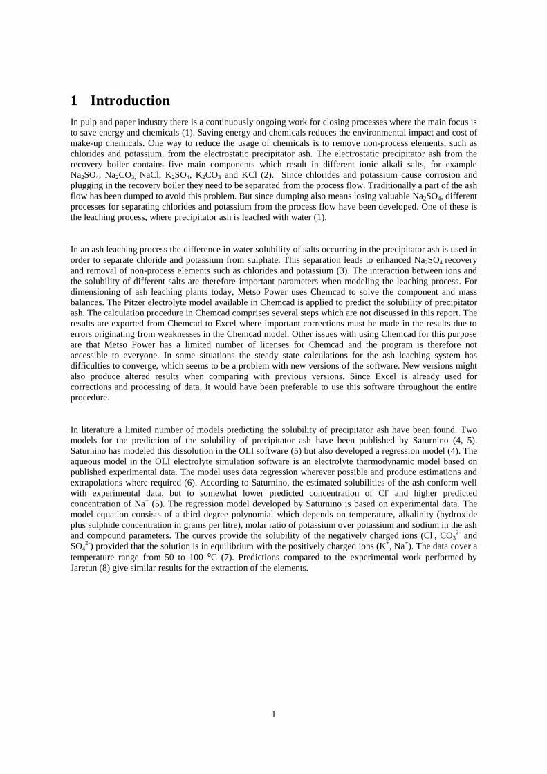
than K2SO4. A similar effect can be seen for the mixture of Na2CO3 and Na2SO4 where the solubility of

Na2CO3 is drastically decreased compared to the solubility of the pure salt in water.

Figure 10. Solubilites of Na2SO4 and K2SO4 in the saturated system Na2SO4 - K2SO4 in water depending on

temperature. The composition in the mixture is compared with the solubility of the pure compounds in water

(20).

12

Figure 11 shows the solubilities of the saturated system NaCl - Na2SO4 which are compared to the solubility

of the pure compounds in water. The solubility of both Na2SO4 and NaCl is decreased when mixed with each

other. At a temperature of 90ºC NaCl precipitates at a concentration of 24,1 wt% and Na2SO4 at a

concentration of 5,5 wt%. NaCl is more soluble than Na2SO4 and therefore the solubility of Na2SO4 decreases

due to the common ion effect. The NaCl concentration in the reject in an ash leaching process is normally

much lower than 24,1%, which means that the major part of the NaCl present will dissolve in solution.

Figure 11. Solubilities for the system Na2SO4 – NaCl. The solution is saturated and in equilibrium with the

solid phase consisting of Na2SO4 and NaCl. The solubilities for the pure compounds in water are shown for

comparative purposes (20).

2.4.3.2 Experimental data produced by Teeple

When digging for gold in 1862, potash and borax where found in Searles Lake, a dry lake basin located in

California. Later it was discovered that potash and borax were useful as detergents and for usage in cleaning

products. In the early 1900’s a separation plant was built in order to extract borax, potash, soda ash and

Na2SO4. In 1929, John Teeple wrote a book about the salts of Searls Lake, with the objective to evaluate and

improve the current plant. This was performed with experiments of the relative solubilities of the different

salts and the influence of salts on the solubility of others. Some of his experiments include the same

compounds as in precipitator ash, which makes his experiments interesting for this work (23).

Six interesting systems were investigated. One-five component and five four-component systems including

NaCl, Na2SO4, Na2CO3, KCl, K2SO4 and K2CO3 are presented in Appendix B. All systems were dissolved in

water and analysed at different temperatures. The five component systems were saturated with NaCl, which

differ from the ESP ash in the sense that ESP ash is more likely to be saturated with Na2SO4 in solution.

Since the operation temperature of the ash leaching process is around 80-90°C, the phase transitions at the

higher temperatures is the most interesting. One of the most interesting systems is system V, containing

Na2SO4, Na2CO3 and K2SO4 is presented in Figure 12. The solubilities of the three salts; Na2SO4, Na2CO3 and

K2SO4 decrease in mixture compared to the solubilities of the pure compounds in water. The common ion

effect makes burkeite and glaserite precipitate and the more soluble salt Na2SO4 dissolve in the solution. As

can be seen the solubilities of Na2SO4 decreases and the solubility of Na2CO3 and K2SO4 increase within the

temperature range of 50-75 ⁰C. When comparing the composition K2SO4 in the system Na2SO4 - K2SO4

according to Linke to the system Na2SO4 - Na2CO3 - K2SO4 according to Teeple, shown in Figure 13, it can be

seen that the data points conform relatively well. It can also be noticed that the linear trends in the mixtures is

similar to the linear trend for K2SO4 in pure water, but with a shift in solubility of approximately 10 wt%,

between the systems.

13

Figure 12. The solubility of individual salts (20, 21) and solubility of the mixture in the system Na2SO4 –

Na2CO3 - K2SO4. The saturated solution is in equilibrium with the solid phase consisting of Na2SO4¸ glaserite

and burkeite (23).

Figure 13. Solubility for K2SO4 in three different systems. The system of K2SO4 in pure water, the system

Na2SO4-K2SO4 according to Linke (20) in equilibrium with the solid phase Na2SO4 and glaserite and the

system Na2SO4 - Na2CO3-K2SO4 according to Teeple (23) in equilibrium with the solid phase Na2SO4,

glaserite and burkeite.

2.4.3.3 Experimental data produced by Jaretun

The solubility of the five component system Na+, K

+, SO4

2-, Cl

- and CO3

2- has been studied by Jaretun. One

purpose of this study was to determine the solubility and removal efficiencies of chloride and potassium.

Experiments using a synthetic precipitator ash were performed. The composition of the synthetic ash is shown

in Table 2. This ash contains a very high amount of NaCl compared to a typical ESP ash shown in Table 1.

The high concentration NaCl is chosen in order to determine the removal efficiency of chlorides at severe

conditions (8).

Table 2. Synthetic ash composition in weight percentage.

Ash composition Percentage (wt%)

Na2SO4 63

NaCl 29

Na2CO3 5

KCl 3

14

The setup of the experiment is shown in Figure 14. The temperature in the experiments has been varied

between 55-75 ⁰C. Results from the experiments are presented in Appendix B.

Figure 14. Schematic diagram showing the experimental setup used by Jaretun (8) and Goncalves (22).

The interesting results are that the temperature dependence for sodium and potassium seems to be negligible,

as shown in Figure 15. But a slight temperature dependence can be seen for chloride and carbonate. The

sulphate concentration decreases between 55 and 65 ⁰C but at higher temperatures it seems to be independent

of temperature. It is also noticed that the removal of chloride and potassium is high which gives a removal

efficiency of 90-100%.

Figure 15. The composition of the synthetic precipitator ash in saturated solution analysed by Jaretun is

shown in the figure. The ash content in the slurry are 1000 g ash /l water analysed in a temperature range of

55-75ºC (8).

2.4.3.4 Experimental data produced by Goncalves

A laboratory study was performed by Goncalves in order to examine the main factors affecting the removal

efficiency of chloride and potassium (22). The set up of the experiments was similar to the experiments

performed by Jaretun, shown in Figure 14. Six different ash samples from four different mills, presented in

Table 3 where investigated in the range of 60-100⁰C. This ash composition can be compared with the ash

composition in Mill 1, Mill 2 and Mill 3 presented in Table 1. It can be noticed that the carbonate content is

significantly higher in Mill 2 and Mill 3 than in the ash presented by Goncalves.

Table 3. Composition of different ESP ash samples used in solubility experiments performed by Goncalves.

Ash composition (wt%) Ash A Ash B Ash C Ash D Ash E Ash F

Na+ 29,30% 28,80% 31,50% 28,80% 27,80% 30,20%

K+ 5,60% 5,80% 5,20% 5,90% 6,70% 5,80%

Cl- 6,60% 5,90% 5,40% 1,10% 3,40% 8,30%

CO32- 1,20% 0,30% 12,40% 2,70% 0,10% 6,40%

SO42- 56,90% 58,70% 45,50% 61,50% 61,50% 48,80%

Amount dissolved

ash in liquid phase 30,07% 30,56% 29,87% 32,61% 32,80% 32,34%

15

The results showed that the removal efficiencies of chloride and potassium were directly proportional to the

concentration of chloride and potassium in the slurry. No significant temperature effect was observed in the

liquid composition of ash A as can be seen in Figure 16. The temperature dependence is slightly more linear

than for Jaretun, but these experiments are performed at a higher temperature, which may affect the solubility.

Figure 16. The temperature dependence of the composition in liquid phase (dry substance) of ash A, specified

in Table 3, and an ash content of 800 g ash/l H2O (22).

In Figure 17., the fraction of different ions is expressed as a function of the ratio ash to water in the slurry. As

can be seen the sulphate concentration decreases as the chloride concentration, potassium and carbonate

concentration increases. This means that higher ash content in the slurry increases the removal efficiency of

sulphate, since less sulphate will dissolve. Therefore it is important to have a relatively high ratio ash to water

in order to receive a high recovery efficiency of sulphate.

Figure 17. The liquid composition (dry substance) as a function of the ash to water ratio in the slurry of ash A

at 85 ⁰C (22).

16

2.5 Computational programs

This section gives a short description of the programs used during the thesis work. RBD is used for correction

the experimental data in order to achieve electroneutrality and to predict the salt composition. The results

predicted by Chemcad are used as a comparison with the developed models.

2.5.1 RBD

RBD (Recovery Boiler Design) is an in-house program developed by Metso Power, which is mainly used for

the design of recovery boilers. It contains a data bank of literature data. These data can be used to calculate

sticky temperature and composition of ashes containing sulphate, carbonate, chloride, potassium, sodium and

sulfur. By specifying the amount of chloride, potassium and carbonate the fraction of sodium and sulphate can

be calculated. The values are corrected in order to fulfill the criteria of electron neutrality. The composition of

Na2SO4, Na2CO3, K2SO4, K2CO3, NaCl and KCl can then be predicted by the program.

2.5.2 Chemcad

Chemcad is a commercially available chemical process simulation software. It is mainly used to simulate

chemical processes and can be used for both non electrolyte and electrolyte simulations. At Metso Power a

standard module is used to predict the solubility of the different salt in the precipitator ash in water. The Pitzer

electrolyte model is used to calculate the equilibrium of the salts in water. The model used assumes that only

Na2SO4 is present in the solid phase, and that all other salts are completely dissolved. The calculation

procedure starts by defining the ash composition (from RBD), water and ash flow. Then the amount recycled

liquid and dry substance in recycled solids are specified. Finally the composition in slurry, reject and recycled

ash is received.

17

3 Mass balances

The backbone of all of the models consists of mass balances describing the process and the individual

components; leaching tank and centrifuge. Mass balances are based on the setup of the ash leaching process

shown in Figure 18. Mass balances of the leaching tank are shown in equations 3.1 and 3.2. These balances

are used to calculate the slurry flow and the flow of each component in the slurry. Similar balances for the

centrifuge are shown in Appendix D, which gives the flow and composition of recycled ash.

(3.1)

(3.2)

Figure 18. Schematic figure of the Metso AshLeach single stage system (15).

When the slurry is formed in the leaching tank, a fraction of the ash will dissolve in water and form a

saturated solution. This means that the slurry consists of a saturated liquid phase which is in equilibrium with

the solid phase, the suspended solids. The sum of suspended and dissolved solids equals the total amount of

dry solids:

(3.3)

The total amount of ESP ash dissolved in water is commonly considered to be 29 – 33 wt% in a saturated

solution and depends among other factors on the ash composition. The amount of dissolved ash along with the

solubility of different compounds is specified in each model. The main difference between the models is the

prediction of the solubility of the compounds. The solubility is modeled using regression of experimental

data. These relations will be discussed for each model in Chapter 4.

The amount ash dissolved depends on the total amount water in the leaching tank, as can be seen in Equation

3.4. The total amount water in the leaching tank includes the pure water flow and the water content in the

recirculation flow.

(3.4)

is the dry solids content in a saturated solution, which by experience normally contains

approximately 29-33% dry solids, as mentioned before.

18

This means that the amount water available decides how much ash that will dissolve. If the amount water is

very high compared to the ash flow, it is possible to dissolve all ash present in the slurry. But since the aim is

to remove chloride and potassium and recover sodium and sulphate, it is preferable to use a lower amount of

water. This means that only a part of the ash will be dissolved whereas the rest will be present as suspended

solids. The amount of suspended solids, , can be calculated by using the total content of dry solids, DS, in

the slurry and the content dry solids in the saturated liquid phase:

(3.5)

The slurry is pumped to the centrifuge where the suspended solids are separated from the reject. For all

models it is assumed that all suspended solids will be present in the recycled ash, which means that the

separation in the centrifuge is total. The reject is consequently assumed to be a liquid without any suspended

solids, as shown in Figure 6. In a plant with a centrifuge that is working properly it is a good assumption.

Since it is difficult to separate all of the liquid from the solid phase in the centrifuge, the recycled ash will

contain some liquid. As mentioned in section 2.3 the particle size and the mechanical work of the centrifuge,

among other factors, affects the dryness of the recycled ash. The dryness of the ash is not investigated in this

work and therefore the amount of suspended solids in the recycled ash must be specified in the models.

The Excel solver is used to solve the total mass balance, equation 3.6 and the mass balances for each

compound, equation 3.7 over the process.

(3.6)

(3.7)

When the mass balances are solved the removal and recovery efficiencies can be calculated. The efficiencies

are calculated as the ratio of the amount of a compound in the recycled ash divided by the amount of the

compound in the incoming ash. Since the removal efficiency is mainly interesting for chlorides and potassium

it is calculated by subtracting the recovery efficiency from the maximum efficiency, of 100%.

(3.8)

(3.9)

(3.10)

(3.11)

(3.12)

19

3.1 Comparison between predicted and experimental data

In order to compare the predicted results from the models with the experimental data, adaptations have been

made. The calculation procedure is shown detail in Appendix D. These values have been calculated by using

mass balances with the measured slurry flow and recirculation ratio together with the analysed dry solids

content in slurry, reject and recycled solids. The recirculation ratio is defined as the ratio between the recycled

reject divided by the total reject stream, shown in Appendix D. When using experimental data performed by

Goncalves the provided ratio between ash and water in the slurry can be used in the model, since there is no

recirculation back to the leaching tank. No assumptions need to be made which makes this comparison more

robust.

A weakness with the accuracy and relevance of the experimental data from units in operation is the time for

sampling. The ESP ash, slurry, reject and recycled ash samples are taken at the same time without respect to

the residence time in the different units in the process. This error can be minimized by doing the leaching tests

in a laboratory when the exact composition of ESP ash is known.

3.2 Evaluation of model assumptions

To evaluate if the assumptions used in the model are valid, a total mass balance of the process has been

performed in order to calculate the composition in the liquid phase using experimental data. The water and

ingoing ash flow are the same values used as input values in the model and the calculation procedure for these

flows are shown in Appendix D. These balances gives also the flow of recycled ash. When using these flows

together with the experimental data of ingoing and recycled ash composition the bleed composition can be

calculated. This calculated composition in saturated solution will be referred to as calculated composition by

mass balances. This balance has been chosen due to the fact that the experimental of ingoing ash and recycled

ash probably are easier to analyse since the dry content is significantly higher than in the reject. The result is

shown in Figure 19 and Figure 20. As can be seen in the figures there is a difference between the

experimental and the calculated values by mass balances for all compounds in Mill 1, and mainly for chloride

and carbonate in Mill 2. This implies that there are errors in the experimental data or that the assumptions are

incorrect. Investigations about the assumption that no suspended solids are present in the reject needs to be

evaluated. If suspended solids are carried over to the reject, the fractions of sodium and sulphate will increase

whereas the fractions of chloride and potassium will decrease in the reject, which is the case in Mill 1. It

would also be preferable to use additional and more accurate experimental data, since systematic errors might

occur in the experimental work.

Figure 19. Comparison of reject composition when using experimental data and calculated composition by

mass balances from Mill 1. The composition is in wt% dry solids in reject. Bars are average values and the

error bars the standard deviation.

20

Figure 20. Comparison of reject composition when using experimental and calculated composition using mass

balances in Mill 2. The composition is in wt% dry solids in reject. Bars are average values and the error bars

are the standard deviation.

21

4 Models

The models have the same structure and are built mainly by mass balances presented in Chapter 3 and by

regressions of experimental data from units in operation and literature data by Teeple, Jaretun and Goncalves.

The main focus has been to find relationships of the solubility for the different compounds in ESP ash in

saturated solution. NaCl is assumed to be completely dissolved in saturated solution in both models.

4.1 Model I

A first model was developed, in order to investigate if a simple model could give an estimation of the

solubility and efficiencies for different components present in the ESP ash. This model is built by mass

balances of the process which is presented in Chapter 3 and in Appendix D. To model the solubility of the

components in the ESP ash two additional assumptions have been made. The first is that only Na2SO4 will be

present in the solid phase. All other salts are assumed to be completely dissolved and are therefore present in

the liquid phase. Since the operation temperature for the ash leaching system is 70-90 ⁰C and the solubilities

for example Na2SO4 and Na2CO3 changes drastically at temperatures below 40 ⁰C, the model is only valid for

temperatures above 60 ⁰C. According to Goncalves the system is independent of temperature in the

temperature interval of 70-90 ºC.

The second assumption is that a fixed amount of ash will be dissolved in water. The dissolved amount ash in

water is commonly considered to be between 29-33 wt% in a saturated solution for units in operation without

the addition of sulphuric acid to the leaching tank, shown in Figure 21. For the mills that add acid, the

solubility of the ash increases and is between 33-35 wt%.

Figure 21. Amount of dissolved ash (wt%) in a saturated solution for ashes without and with addition of

sulphuric acid, respectively. The experimental data is obtained from work performed by Goncalves and

Jaretun and from different units in operation.

The average amount of dissolved ash without addition of sulphuric acid is 31,2 wt% and therefore the amount

of dissolved ash in a saturated solution in the model will be fixed to 31 wt%. This means that the reject will

consist of 31 wt% dry solids. As mentioned earlier, chlorides, potassium and carbonate are assumed to be

completely dissolved. In order to add up to 31 wt% dissolved solids, sodium and sulphate are dissolved as

well. The remaining Na2SO4 is present in the solid phase. The temperature dependence is not investigated.

The Excel data sheet for calculations by Model I is shown in Appendix E

22

4.1.1 Input variables

The input variables used are ash and water flow, ash composition, recirculation ratio and amount of dry solids

in centrifuge, all of which are presented in Table 4. Ash compositions and amounts of dry solids in the

centrifuge are obtained from the experimental data and recirculation ratios from the process flows. In Model I

the composition of ions are used as input variables and the Na2SO4 composition in the solid phase is

calculated in the model by using molar weight for the different ions. Since only Na2SO4 is present in the solid

phase, it is straight forward to calculate this composition and it is therefore possible to use single ions instead

of salts as input values. Comparisons of experimental data from Goncalves, Mill 1, Mill 2 and Mill 3 are

performed. The values of sodium and sulphate are corrected using the RBD software to achieve

electroneutrality and a total amount of 100%, to make the experimental data possible to use in the model.

When using the literature data obtained from Goncalves, only the solubilities of different compounds in

saturated solution are predicted. According to the experimental setup, no liquid is recycled back to the

leaching tank.

Table 4. Example of input data. The table shows one sample each from Mill 1 and Mill 2 and another sample

performed by Goncalves. The experimental data is corrected in RBD in order to achieve electroneutrality.

Additional data is presented in Appendix C.

ESP ash composition from RBD

Sample (wt% DS) Mill 1

Ash sample 1

Mill 2

Ash sample 1

Goncalves

Ash A

Cl- 3,16% 4,24% 6,68%

K+ 4,30% 2,99% 4,92%

Na+ 29,63% 33,43% 29,32%

SO42- 62,90% 45,32% 57,86%

CO32- 0,01% 14,02% 1,22%

Suspended solids in

centrifuge (wt%) 85,20% 56,52% -

Recirculation ratio (%) 14,06% 27,32% 0%

Ash flow (kg/h) 5498 4808 800-1400

Water flow (kg/h) 4274 6438 1000

4.2 Model II

This model was developed in order to investigate if it is possible to use a system containing four components

when describing the solubility of the ESP ash. The system Na2SO4 – Na2CO3 – K2SO4 is used. This system is

chosen since the solubility of these salts is probably affected the most in the water and ash mixture. NaCl,

KCl and K2CO3 have a high solubility and are probably completely dissolved, if the ash does not contain an

abnormal content of these compounds. The assumption about the chlorides is made since the common ion

effect drastically lowers the solubility of Na2SO4, Na2CO3 and K2SO4 in favour for dissolution of NaCl and

KCl. The KCl concentration is usually quite low and will not exceed the limit when it starts to precipitate. The

concentration of NaCl is higher, but still low enough for NaCl to stay in solution. The assumption is based on

the system Na2SO4 – NaCl published by Linke. In this system, the solubility of NaCl is only slightly

decreased while the solubility of Na2SO4 is drastically decreased in mixture compared to the solubility of the

pure compounds in water. The same dependence is shown in the system containing KCl and K2SO4, where the

solubility of K2SO4 is significantly decreased when KCl is present in the solution. The available data for

K2CO3 is limited, but the salt has a very high solubility in water, between 50-60 wt% in a saturated solution. It

is therefore assumed to be completely dissolved. Linear regressions of literature data published by Teeple in

1929 of the mixture Na2SO4 – Na2CO3 – K2SO4 in a saturated water solution are used. The regressions are

functions of Na2CO3 and K2SO4, respectively, diluted in saturated solutions which are dependent on

temperature. This means that fixed amounts of Na2CO3 and K2SO4 are dissolved in water at a specified

temperature, and the remaining solids will be present in the solid phase.

23

The linear correlation used for K2SO4 is:

(4.1)

and for Na2CO3;

(4.2)

Where T is the temperature in degrees centigrade. For example at 90 ºC the Na2CO3fraction in the liquid

phase will be 5,3 wt% whereas the fraction K2SO4 will be 9,3 wt%.

NaCl, KCl and K2CO3 are assumed to be completely dissolved. The total amount dissolved ash are assumed to

be 31 wt%. This means that Na2SO4 is dissolved until this value is reached. Data was unfortunately only

available in the temperature range of 50-75 ºC, as shown in Appendix B. This regression is then extrapolated

to 85 ºC when comparing the model with Goncalves and to 90ºC when comparing with Mill 1, Mill 2 and Mill

3. To investigate how the model affects the reject composition at different temperatures, predictions at 60, 70,

80 and 90ºC have been performed for Mill 1 and Mill 2.

4.2.1 Input variables

For Model II and for Chemcad, the salt composition and not only the composition of single ions are used as

input values. Since more than one salt may be present in the solid phase it is important to know the amount of

each salt present in the ingoing ash. This is due to the fact that the salt composition cannot be easy predicted

in the model. As for Model I, ash and water flow, suspended solids in the centrifuge and recirculation ratio is

used for Mill 1, Mill 2 and Mill 3. For Goncalves only the water flow together with ash flow and composition

is specified in the models.

Table 5. Example of input variables. The table shows the ash compositions and process flows from literature

data performed by Goncalves and experimental data from Mill 1 and Mill 2, where the experimental data is

corrected in RBD in order to receive electroneutrality and to predict the composition of different salts in the

ash. Additional data is presented in Appendix C.

ESP ash composition from RBD

Mill 1

Ash sample 1

Mill 2

Ash sample 1

Goncalves

Ash A

Na2SO4 (wt%) 85,69% 63,67% 76,14%

Na2CO3 (wt%) 0,02% 23,53% 1,91%

NaCl (wt%) 4,80% 6,64% 9,78%

K2SO4 (wt%) 8,97% 4,11% 10,49%

K2CO3 (wt%) 0,00% 1,61% 0,28%

KCl (wt%) 0,52% 0,45% 1,40%

Suspended solids in

centrifuge (wt%) 85,20% 56,52% -

Recirculation ratio (%) 14,06% 27,32% 0%

Ash flow (kg) 5498 4808 800-1400

Water flow (kg) 4274 6438 1000

Temperature (ºC) 60-90 60-90 85

24

4.2.2 Investigation of the amount ash dissolved with composition

The solubility of the ash changes with the ash composition among other factors. Therefore different amounts

of ash dissolved in water have been used in Model II to predict the reject composition. This is done in order to

investigate the dependence of the amount of dissolved ash in water on the composition in liquid phase. If the

dissolved amount of ash in water is predicted to be too high, increased amount of Na2SO4 will dissolve which

leads to a lower predicted removal efficiency of Na2SO4. Three different amounts of ash in water have been

investigated: One regression is depending on the K/(K+Na) molar ratio in the slurry, shown in Figure 22, and

two fixed amounts of ash at 31 wt% and 32 wt% dissolved solids in the liquid phase. The regression is based

on literature data by Jaretun and Goncalves and it is a function of the amount of ash dissolved in water

depending on the molar ratio K/(K+Na) in the slurry. The value of the correlation coefficient (R2) is quite low

and therefore a more accurate correlation would be desirable.

Figure 22. Amount of ash dissolved in water as a function of the molar ratio K/(K+Na) present in the slurry.

Dots are experimental values according to Jaretun and Goncalves and the line is a linear regression of the

experimental values.

The predicted results received by using the regression, 31 wt% or 32 wt% ash dissolved in saturated solution

are compared to predicted values using the amount of dissolved ash specified in the experimental data. An

example is shown below:

(4.3)

The difference between the predicted values for each compound (Cl, Na, K, SO4 and CO3) is calculated for

each mill.

25

5 Results and discussion

The outline of this chapter is first a comparison between the models without using recirculation. Thereafter

the results when using recirculation are presented in section 5.2. In this section the temperature dependence by

Model II is investigated. Finally, a comparison of predicted efficiencies by Chemcad and the different models

are performed.

5.1 Predictions without recirculation

The ingoing ash composition together with the ratio ash to water in slurry according to Goncalves is used to

predict the solubility in the liquid phase (without using recirculation and separation in the centrifuge). For

both models an amount of dissolved ash in a saturated solution fixed to 31wt% has been used. As shown in

Figure 23, both models predict a similar composition of Ash B (defined in Table 3) in the liquid phase. When

comparing with the experimental data the chloride fractions are slightly larger and the potassium fractions are

slightly smaller than in the experiments. This ESP ash contains a large fraction of sulphate and a minor

fraction carbonate which makes it relatively straight forward to predict the composition in the liquid phase.

Since there is no recycling of reject, all potassium salts in the slurry will probably dissolve. The larger fraction

of potassium in the experiments compared to the predicted values is probably due to errors in the experiments,

since the potassium is predicted to dissolve completely in the models.

Figure 23.The composition in the liquid phase (wt% DS) for Ash B at 85ºC is shown for the experimental data

and compared with the predicted values with the different models. The amount of ash in slurry is 800 g ash/l

water. A fixed value of 31wt% dissolved solids is used for both models.

When using Ash C with an ash content in slurry of 500g ash/l water at a temperature of 85ºC to predict the

composition in the liquid phase, the result looks a bit different. The potassium and chlorides should be

completely dissolved according to the models in this case as well, but the experimental data shows a higher

chloride and potassium value than the predicted values. This is probably due to experimental errors. Model II

shows the best conformity with the experimental data for sodium, sulphate and carbonate, presented in Figure

24. Model I predicts larger fractions sodium and carbonate and smaller fraction sulphate when comparing

with the experimental results. The poorer results for this ash compared to Ash B probably depends on the

higher carbonate content present in the ESP ash which affects the composition in the solid phase and therefore

also the composition in the liquid phase.

26

Figure 24. The composition in the liquid phase (wt% DS) for Ash C at 85ºC is shown for the experimental

data and compared with the predicted values using three different models. The amount of ash in slurry is 800

g ash/l water. A fixed value of 31wt% dissolved solids is used for all models.

Experiments performed by Goncalves shows the variation in reject composition depending on the ratio of ash

to water in the slurry. The models are used to predict the liquid composition at different ratios of ash to water

in the slurry for Ash A. The predicted sodium and potassium fractions using Model I is shown in Figure 25.

The predicted sodium concentration is generally lower than the experimental values and the predicted

potassium concentration is generally higher than the experimental data. It can also be noticed that the

experimental values of sodium level out as the ash content in the slurry increases. The predicted sodium and

potassium concentration decreases respectively increases linearly and deviates more and more from the

experimental data. This is because potassium is predicted to be completely dissolved in the Model I, which is

not the case in reality. The fact that potassium is predicted to dissolve totally in the model leads to a lower

predicted solubility of sodium. The composition predicted by Model II shows the same trend as Model I,

which is shown in Appendix F. In Figure 26 the predicted concentration for different ratios of ash to water in

slurry is shown. As can be seen the predicted values conform well to the experimental data in all points.

Figure 25. The composition in liquid phase (wt% DS) of Ash A depending on the ash content in slurry is

shown in the figure. A comparison of the experimental data performed by Goncalves at 85ºC and the

predicted values using Model I, with a dissolved ash amount of 31wt% in saturated solution is performed.

27

Figure 26. The composition in liquid phase (wt% DS) of Ash A depending on the ash content in slurry is

shown in the figure. A comparison of the experimental data performed by Goncalves at 85ºC and the

predicted values using Model I, with a dissolved ash amount of 31wt% in saturated solution is performed.

5.2 Predictions with recirculation

To evaluate how well the models predict the composition in the reject using recirculation and separation in a

centrifuge, data from Mill 1 and Mill 2 have been utilised for predictions using Models I and II. As shown in

Figure 27 the experimental data are not consistent with the predicted reject composition in Mill 1, but more

consistent with the calculated composition using mass balances, defined in section 3.2 and Appendix D.

Figure 27. Reject composition in wt% dry substance of different ions present in the ash leaching process in

Mill 1. The experimental data are obtained at 90ºC. A dissolved ash amount of 31 wt% ESP ash in saturated

solution is used in the models. The bars show mean values of experimental data, calculated composition and

predictions. The error bars shows the standard deviation of the mean values.

The chloride and potassium concentration in the reject is higher in Model I and II than in the reject analysis

for Mill 1. But for both Models I and II the chloride fraction was consistent with the composition provided by

the adjusted analysis. The opposite scenarios are shown for sodium and sulphate, with high values in the

experimental data and lower values in the calculated reject data and predicted model results. The carbonate

and chloride concentrations are low which means that they probably are completely dissolved, which is

consistent with both models. In reality potassium may be present as glaserite which decreases the amount of

potassium in the liquid phase, as predicted by Model II, where the potassium concentration is lower than that

predicted by Model I. The fact that the composition of the reject obtained by the adjusted analysis is similar to

that predicted in Mill 1 can probably be explained by the assumption that no suspended solids will be present

in the reject. Suspended solids are carried over to the reject when the separation is performed in the

centrifuge. This leads to a higher amount of Na2SO4 present in the reject, which means that the percental

fractions of chloride and potassium will decrease in the reject.

28

The experimental data from Mill 2 shows that the amount of chloride is higher than the predicted values,

shown in Figure 28. This should be impossible, since all chlorides are predicted to be completely dissolved in

the model. This observation might therefore be due to uncertainties in the experimental data. However, when

comparing the predicted values with the calculated values using mass balances data it gives a more consistent

result.

Figure 28. Composition in the reject, dry substance, of different ions present in the ash leaching process at

Mill 2 at a temperature of 90ºC. The models assume that 31 wt% ash is dissolved in a saturated solution. Bars

show mean values from experimental data and predicted values. The error bars show the standard deviation of

the mean values.

The predicted and experimental data in the reject conform very well for potassium especially the values

predicted by Model I with a small deviation for Model II. The big differences in sulphate and carbonate

concentrations in the predicted values for Model I are due to the fact that only Na2SO4 is present as suspended

solids in the model. For Model II the predicted values show the opposite result, where the sulphate

concentration is very high in the reject compared to the experimental data and the carbonate concentration is

lower than in the experimental data. In reality a significant amount of the double salt burkeite precipitates,

but not as much as predicted by Model II. One of the ashes in Mill 2 had a carbonate concentration of 19,4

wt% DS. When carbonate content exceeds ~19 wt% DS in the slurry the predicted results by Model I becomes

none physical due to limitations in the model as no carbonate will precipitate. The same result was predicted

for Mill 3, where the carbonate concentration is even higher in the ash, 26,10 wt% DS. The result was a

negative flow of sulphate in the liquid phase in Model I, as for Mill 2. If one wants to use this model further,

the problem might be solved by letting Na2CO3 precipitate in order to add up for the Na2SO4 that could not

precipitate.

When comparing the reject composition determined by experiments with the data predicted by the models the

result conform very well for Mill 1, as can be seen in Figure 29. Since the incoming ash in Mill 1 mainly is

composed of Na2SO4, it will also be the main component present in the recycled ash. The result was a bit

different for Mill 2 compared to Mill 1, mainly due to the higher carbonate content in the ash. The results are

presented in Figure 30. This figure shows that the sulphate content is higher for Model I and lower for Model

II when compared to the experimental data. The opposite relation is shown for carbonate, where the predicted

carbonate content in the recycled solids is low for Model I and high for Model II compared to the

experimental data.

29

Figure 29. Comparison of experimental and predicted compositions of recycled ash in Mill 1. The

composition is given as dry solids. The bars show the mean values and the error bars denote the standard

deviations.

Figure 30. Composition in recycled ash presented as dry solids in Mill 2. Bars denote mean values whereas

error bars denote the standard deviations.

5.2.1 Investigations of the ash amount dissolved

The regression determined by the experimental data performed by Jaretun and Goncalves, shown in Figure

22, is compared with experimental data in the reject from Mill 1, Mill 2 and Mill 2 (Figure 31). The data

points are unevenly distributed and only one point coincide with the regression.

Figure 31. Experimental data of dry solids in liquid phase from Mill 1, Mill 2 and Mill 3. The straight line is a

regression from literature data performed by Jaretun (8) and Goncalves (2, 22).

30

The deviations between the predicted values using dry solids according to reject analysis and the predicted

compositions using 31 wt%, 32 wt% and the regression according to Jaretun and Goncalves is presented in

Table 6. The maximum average deviations are shown for each mill. Mill 3 shows the largest deviation,

which is because of the high dissolved ash amount in this mill, 32,6 wt% according to experimental data. The

result is a deviation that varies between 0,2-2,3 wt%. The regression gives slightly better predictions, but there

are still deviations. The same procedure has been performed for the efficiencies. It is consequently

investigated how much the dissolved ash amount in the liquid phase influences the efficiencies. As presented

in Table 7 the deviations between efficiencies vary from 0,5 to 9,2%. A deviation of 9,2 % shows that the

solubility of the ash may give a significant error on the efficiency of the plant.

Table 6. The table shows the maximum deviation from the predicted composition in the reject by using Model

II with a dissolved ash amount corresponding to the experimental data compared to predicted values using a

dissolved ash content in a saturated solution of 31 wt%, 32 wt% or by the regression according to Jaretun and

Goncalves.

31 wt% 32 wt%

Regression

Jaretun & Goncalves

Mill 1 ± 0,2 % ± 0,5 % ± 0,6 %

Mill 3 ± 2,3 % ± 0,8 % ± 1,6 %

Mill 2 ± 0,8 % ± 1,7 % ± 0,5 %

Table 7. The table shows the maximum deviation from the predicted efficiencies by using Model II with a

dissolved ash amount corresponding to the experimental data compared to predicted values using a dissolved

ash content in saturated solution of 31 wt%, 32wt% or by the regression according to Jaretun and Goncalves.

31 wt% 32 wt%

Regression

Jaretun & Goncalves

Mill 1 ± 0,5 % ± 1,2 % ± 1,3 %

Mill 3 ± 5,3 % ± 2,0 % ± 3,9 %

Mill 2 ± 5,5 % ± 9,2 % ± 1,0 %

Due to the deviations shown more effort should be put into finding a more accurate correlation of the amount

of dry solids dissolved in water. This correlation is only dependent on the molar ratio of K/(K+Na) in the

slurry which is an rough approximation. The synthetic ash used by Jaretun had low potassium content but

high content of chloride. Such high amounts chloride probably affected the solubility and resulted in a

dissolved ash amount of approximately 29 wt % in saturated solution, which might be lower than if lower

amounts of chloride would have been present.

5.2.2 Temperature dependence of Model II

The effect of the temperature dependence in Model II was investigated by making predictions of the reject

composition in Mill 1, Mill 2 and Mill 3 in a temperature range of 60-90ºC, using a fixed amount of 31 wt%

ash dissolved in a saturated solution. The predicted result for Mill 3 is shown in Figure 32 and can be

compared with the results published by Goncalves. According to Goncalves no temperature dependence can

be seen when predicting the reject composition using ash A, which is shown in Figure 16. The predictions

made by Model II diverge from the literature data presented by Goncalves since a slight temperature

dependence on sulphate and carbonate concentrations occurs, which is shown in Figure 32. The ESP ash

produced in Mill 3 contains high amounts of carbonate and therefore a temperature dependence of carbonate

can be seen, since a fixed amount carbonate is dissolved at a given temperature. The carbonate content

increases whereas the potassium content decreases with temperature. A similar dependence can be seen for

Mill 2, which also has high contents carbonate in the ash. A dependence on potassium and sodium can be seen

in the Mill 1 mill, shown in Appendix G. This depends on the higher amount of potassium present in the ESP

ash in Mill 1. This divergence from the literature data according to Goncalves and Jaretun, means that it

31

might be difficult to model the five components system Na – K – Cl - CO3 – SO4 by merely using a four

component system depending on temperature.

Figure 32. Temperature dependence predicted by Model II for Mill 3 in a temperature interval of 60-90ºC.

The model dissolves 31 wt% ash in a saturated solution.

5.3 Comparison with Chemcad

A comparison between Model I, Model II and Chemcad is performed. Simulations of the different ash

compositions from Mill 1, Mill 2 and the ash composition of Ash E according to Goncalves have been

performed in Chemcad and corrected by the Excel worksheet used by Metso Power. For the mills, the same

ESP ash composition and flow, water flow, recirculation ratio and suspended solids in the centrifuge as in the

models are used in the Chemcad module. Examples of input data for Mill 1 and Mill 2 are specified in Table

5. For ash E an amount of suspended solids of 26 wt% in the slurry and 80 wt% in recycled ash are specified.

The recirculation ratio are specified to 30, 50 and 70%.

The efficiencies calculated using the predicted composition in the recycled ash by Models I and II are

compared with the efficiencies calculated using the corrected Chemcad predictions. The calculated

efficiencies for Mill 1 are quite consistent with experimental data for both models, as shown in Figure 33. The

result from Chemcad shows a lower removal efficiency for potassium and higher recovery efficiency of

sodium, as presented in Figure 33.

Figure 33. Comparison of the efficiencies based on experimental values and values predicted by Models I and

II. The bars represent mean values from Mill 1. Chemcad simulations and predictions made using Model II

are performed at 90ºC.

For Mill 2 the efficiencies predicted by the models show a larger deviation from the efficiencies calculated by

the experimental data compared to the case of Mill 1. This deviation is conducted with the deviation between

the experimental data and predicted data of the recycled ash, since the compound flows in the ingoing ESP

32

ash together with the compound flows in the recycled ash gives the efficiency for each compound. The

differences in recovery efficiencies of sulphate and carbonate (Figure 34) comes from the fact that only

Na2SO4 is assumed to be present in the solid phase in Model I, as mentioned earlier. This makes the predicted

carbonate content much lower whereas the sulphate content becomes higher in the recycled ash compared to

the experimental data which is presented in Figure 34 for Mill 2. The opposite relation is shown for Model I.

Figure 34. Comparison of the efficiencies based on experimental values and predicted values by Model I and

II. The bars are average values from Mill 2. Chemcad simulations and predictions by Model II are performed

at 90ºC.

To show the efficiencies for an ash consisting of a relatively high fraction potassium, Ash E according to

Goncalves is used. Unfortunately no experimental data were available, but Model I and II have been

compared to the corrected Chemcad data. In Figure 35 the efficiencies calculated by Model I, II and corrected

Chemcad data are shown. It can be noticed that the recovery efficiency for potassium is low in the corrected

Chemcad data and predicted data by Model II since these models take the precipitation of glaserite in account.

This means that a increased amount of potassium will be present in the solid phase. In order to further

investigate the accuracy of the glaserite precipitation, it is necessary to compare the results with experimental

data.

Figure 35. Comparison of the predicted efficiencies by Model I and II with corrected data by Chemcad of Ash

E. A recirculation ratio of 50% and a suspended solids amount of 26 wt% in slurry have been used. The

amount of suspended solids in the recycled ash are fixed to 80 wt% Chemcad simulations and predictions by

Model II are performed at 90ºC.

33

5.3.1 Effect of recycling

When recirculation is used it affects the composition of the liquid phase and therefore also the composition of

the solid phase. By comparing predictions by Model I, II and corrected data from Chemcad, the variations of

potassium with recirculation ratio for Ash E can be seen in Figure 36. Three different recirculation ratios of

30, 50 and 70%, respectively, have been investigated. Ash E is as mentioned before an ash with relatively

high content potassium and when the recirculation ratio is increased, the effect of the fraction potassium in the

solid and liquid phase can be seen. For Model I, both the fraction potassium in liquid and solid phase

increases, since potassium is predicted to be completely dissolved. For Model II and Chemcad the fractions of

potassium in liquid phase are relatively constant whereas the fraction in solid phase increases. This is due to

formation of glaserite in solid phase, which is included in these models. Unfortunately no experimental data

was available for this ash.

Figure 36. The potassium fraction in reject and recycled ash for Ash E according to Goncalves are predicted

by Model I, II and corrected Chemcad predictions depending on the recirculation ratio. The recirculation ratio

are fixed to 30, 50 and 70% at a temperature of 90ºC. The water flow is adjusted in order to achieve 26 wt%

suspended solids in the slurry, which corresponds to ~50 wt% dry solids. The suspended solids in recycled

ash are fixed to 80 wt%. In Model I and II the amount of dissolved solids was fixed to 31 wt%.

34

6 Conclusions

The assumption that all chlorides are dissolved in water is likely to be valid. Therefore the separation of

chlorides are addicted to the dewatering of the recycled ash. More efforts are needed in order to determine the

solubilities of Na2SO4, K2SO4 and Na2CO3 in mixture of ESP ash.

It is concluded that Model I predicts the composition for low carbonate and potassium ashes relatively well.

But as the ash to water ratio or the carbonate content in slurry increase, the model deviates from the

experimental data.

It will probably be difficult to predict the solubility of a precipitator ash only by using experimental data from

the four component system Na2SO4 – K2SO4 – Na2CO3 dependent only on temperature, which is used in

Model II. It would be preferable to expand the data range with experiments at higher temperatures, at least to

90ºC. A relatively accurate prediction of the reject composition can be made for an ash with low potassium

and carbonate contents, but as these concentrations increase the results becomes more and more incorrect.

When using recirculation of reject back into the leaching tank, the predicted reject composition deviate from

the experimental data. The deviation occurs for all compounds in Mill 1 and a significant deviation is shown

for carbonate and sulphate content compared to experimental data obtained from Mill 2. When performing

mass balances of the system in order to evaluate if the experimental data and assumptions are valid, it result in

large deviations from the experimental data. These deviations likely depend on errors in the experimental data

together with the assumption that no suspended solids are estimated to be present in the reject using the

models. It is possible that carry over may occur in the centrifuge in reality, when the centrifuge does not work

properly, which affects the performance of the ash leaching process.

When modelling different specified amounts of ash that are dissolved in a saturated solution, deviations occur

when the results are compared with the predicted values using the specified amount of ash dissolved in the

reject. The regression done using the experimental data according to Jaretun and Goncalves provides the most

accurate results, but the results are not significantly better than in the case where the amount of dissolved ash

is 31 wt% for the ashes investigated in this work. It is therefore important to find a more accurate correlation

for the amount of dissolved ash in water.

It can also be concluded that the efficiencies predicted by Chemcad suffer from a quite similar deviation from

those efficiencies based on the experimental data, just like the efficiencies calculated using the models. When

studying the effect of recirculation ratio, both the corrected Chemcad data and predicted data by Model II

shows an increasing amount of potassium in solid phase as the recirculation ratio increases. To further

investigate the accuracy of these models, experimental data is needed for ashes containing a high content of

potassium.

35

7 Future work

A larger quantity and more accurate data are needed to further evaluate the models. This data could also be

used to evaluate the results predicted by Chemcad and when developing a thermodynamic model if this is

desirable. Experiments with varied parameters like ash composition and ratio of ash to water in slurry are

needed to further develop the models, in order to increase the accuracy. It may also be interesting to

investigate the temperature dependence for an increased number of ashes in order to verify the results

showing temperature independence according to Goncalves. Therefore it would be preferable to perform

experiments in lab scale, maybe as a new Master’s Thesis. Firstly, it should be advantageous to investigate the

solubility of the ash according to the experimental setup used by Jaretun and Goncalves, as can be seen in

Figure 14. Thereafter an ash leaching process in lab scale, consisting of a leaching tank and a centrifuge

should preferably be performed. This setup provides data on how the recirculation of the reject will affect the

composition in the recycled ash and reject. This setup may also provide an indication of which ash

compositions that are likely to lead to carry over in the centrifuge, which results in suspended solids in the

reject.

When using experimental data for calculations of process flows today, it is assumed that no suspended solids

are present in the reject. To abandon this assumption it might be possible to use a statistical evaluation method

such as the method of least squares predict the process flows. By using this kind of method it is also possible

to evaluate the accuracy of the experimental data.

It should also be very interesting to investigate how different ash compositions affect the amount of dissolved

ash and composition of different ions in a saturated solution. If more experimental data were available, the

regression determined by data according to Goncalves and Jaretun could be evaluated further.

One way to further develop these models is to investigate if it is possible to use a model based on the molar

ratio CO3/(CO3+SO4) or K/(K+Na) and the ratio ash to water in slurry to predict the composition of carbonate

or potassium in the reject. The ratio K/(K+Na) is also important for the precipitation of glaserite, and need

therefore to be investigated further.

The modelling of the dryness in the recycled ash coming from the centrifuge is not included in the developed

models. This is an important parameter to take in account, since it will affect the efficiencies of the leaching

process. Increased carbonate content results in formation of burkeite which decreases the particle size of the

crystals, leading to a decreased ability to dewater the slurry. It might therefore be possible to use the dryness

in the ash as a function of the carbonate content in the suspended solids to calculate the dryness in the

centrifuge.

36

8 References

1. Knutsson M, Eriksson M, Sartório L. Experiences from first start-up of an ash leaching system. TAPPI

Fall Conference & Trade Fair; San Diego, California, USA, 2002.

2. Saturnino D, Tran H. Prediction of the solubility of recovery boiler precipitator ash. TAPPI Journal. 2009.

3. Tran H, Earl P. Chloride and Potassium Removal Processes for Kraft Pulp Mills: A Technical Review.

International Chemical Recovery Conference TAPPI/PAPTAC; June 7-10; Charleston, South Carolina, USA,

2004

4. Saturnino D, Cardoso M, Oliveira É. Dissolution of chloride and potassium salts during leaching of

electrostatic precipitator ashes from kraft recover boilers. Appita Journal. 2009;62(1):52-9.

5. Saturnino D. The Solubility of Kraft Recovery Boiler Precipitator Ash. Toronto, Canada, : Graduate

Departent of Chemical Engineering and Applied Chemistry, University of Toronto, 2006.

6. OLI, Systems, inc. OLI Electrolyte Simulation. www.olisystems.com.

7. Saturnino D. Personal Communication. 2012.

8. Jaretun A. Utstötning av klorid och kalium genom lakning av elektrostatfilteraska. Lund, 1998.

9. Tran H, Vakkilainnen E. The Kraft Chemical Recovery Process. Toronto, Cananda: 2008.

10. Johansson U. Different Methods for the Purge of Chlorides and Potassium from Electrostatic Precipitator

Dust in the Kraft Mill. Stockholm, 2005.

11. Jordan J, Bryant P. Cluster Rule impact on recovery boiler operations : Chloride and potassium

concentrations in the kraft liquor cycle. . TAPPI Journal. 1996;79(12):108-16.

12. Dahlbom J. Effekter av PFG vid indunstning och förbränning av bioslam i ett massabruks sodapanna.

Stockhom.: Värmeforsk Service AB; 2003.

13. Minday M, Reid D, Burke M. An overview of various strategies for balancing saltcake, chloride and

potassium level in an EFC kraft mill. TAPPI Minimum Effluent Symposium Oct. 23-24; San Fransisco,

California, USA, 1997.

14. Ferreira L, Soares M, Egas A, Castro J. Selective removal of chloride and potassium in kraft pulp mills.

TAPPI Journal. 2003;2(4):21-5.

15. Metso Power. Internal material. 2012.

16. Jaretun A, Aly G. Leaching of Chloride and Potassium from Electrostatic Precipitator Catch.

International Chemical Recovery Conference, 1998.

17. Ahlroth M, Johansson U, Svedin K. Syntesrapport om kunskapsläget gällande löslighet och aktivitetsdata

för högkoncentrerade saltlösningar i skogsindustriella tillämpningar. Stockholm, : 2007.

18. Jaretun A. Thermodynamic Modelling of Electrolyte Solutions with Application to the Pulp and Paper

Industry. Alnarp: Förvaltningsavdelningens repro, SLU; 2000.

19. Mendham J, Denney RC, Barnes JD, Thomas MJK. Vogel's textbook of Quantitative Chemical Analysis

6th edition. Harlow, England: Pearson Education Limitied; 2000. 12-50 p.

20. Linke W. Solubilities, inorganic and metal organic compounds; a compilation of solubility data from the

periodical literature. Fourth ed. Washington D.C., USA: American Chemical Society; 1958.

21. Perry H. Perry's Chemical Engineers' Handbook. Seventh ed: McGraw-Hill; 1997.

22. Goncalves C, Tran H, Shenassa R. Factors affecting chloride and potassium removal efficiency of a

recovery boiler precipitator ash treament system. International Chemical Recovery Conference, PAPTAC &

TAPPI; May 29 - June 1; Quebec, Canada, 2007.

23. Teeple J, E. The Industrial Developement of Searles Lake Brines. New York: The Chemical Catalogue

Company; 1929.

http://www.olisystems.com/

37

Appendix A – Solubilities of anhydrous salts in water

Solubilities for single salts common in the ESP ash in pure water. Literature data according to Perry, 1997 and

Linke, 1958.

Table 8. Solubility data for the system NaCl- H2O at 0-100⁰C , Perry, 1997.

T (°C) g/100 g water g/100 g saturated solution Solid phase

0 35,7 26,3 NaCl

10 35,8 26,4 NaCl

20 36,0 26,5 NaCl

30 36,3 26,6 NaCl

40 36,6 26,8 NaCl

50 37,0 27,0 NaCl

60 37,3 27,2 NaCl

70 37,8 27,4 NaCl

80 38,4 27,8 NaCl

90 39,0 28,1 NaCl

100 39,8 28,5 NaCl

Table 9. Solubility data for the system Na2SO4- H2O at 35-100⁰C, Linke, 1958.

T (°C) g/100g water g/100g satutated

solution Solid phase

35 49,1 32,9 Na2SO4

40 48,1 32,5 Na2SO4

45 47,2 32,1 Na2SO4

50 46,4 31,7 Na2SO4

60 45,2 31,1 Na2SO4

70 44,2 30,7 Na2SO4

75 43,6 30,4 Na2SO4

80 43,2 30,2 Na2SO4

90 42,6 29,9 Na2SO4

100 42,2 29,7 Na2SO4

Table 10. Solubility data for the system Na2CO3 – H2O at 40-100⁰C, Linke, 1958.

T (°C) g/100g water g/100g satutated solution Solid phase

40 48,8 32,8 Na2CO3*H2O

50 47,5 32,2 Na2CO3*H2O

60 46,3 31,6 Na2CO3*H2O

70 45,6 31,3 Na2CO3*H2O

75 45,4 31,2 Na2CO3*H2O

80 45,2 31,1 Na2CO3*H2O

90 44,9 31,0 Na2CO3*H2O

100 44,7 30,9 Na2CO3*H2O

38

Table 11. Solubility data for the system KCl – H2O at 0-100⁰C (21).


0 27,6 21,6 KCl

10 31,0 23,7 KCl

20 34,0 25,4 KCl

30 37,0 27,0 KCl

40 40,0 28,6 KCl

50 42,6 29,9 KCl

60 45,5 31,3 KCl

70 48,3 32,6 KCl

80 51,1 33,8 KCl

90 54,0 35,1 KCl

100 56,7 36,2 KCl

Table 12. Solubility data for the system K2SO4 – H2O at 0-100⁰C, Perry, 1997.


0 7,4 6,9 K2SO4

10 9,2 8,4 K2SO4

20 11,1 10,0 K2SO4

30 13,0 11,5 K2SO4

40 14,8 12,9 K2SO4

50 16,5 14,2 K2SO4

60 18,2 15,4 K2SO4

70 19,8 16,5 K2SO4

80 21,4 17,6 K2SO4

90 22,8 18,6 K2SO4

100 24,1 19,4 K2SO4

Table 13. Solubility data for the system K2CO3 – H2O at 0-100⁰C, Perry, 1997.


0 105,5 51,3 K2CO3*2H2O

10 108,0 51,9 K2CO3*2H2O

20 110,5 52,5 K2CO3*2H2O

30 113,7 53,2 K2CO3*2H2O

40 116,9 53,9 K2CO3*2H2O

50 121,2 54,8 K2CO3*2H2O

60 126,8 55,9 K2CO3*2H2O

70 133,1 57,1 K2CO3*2H2O

80 139,8 58,3 K2CO3*2H2O

90 147,5 59,6 K2CO3*2H2O

100 155,7 60,9 K2CO3*2H2O

39

Appendix B – Solubility for mixtures

Solubilities for mixtures published by Linke, Teeple, Goncalves and Jaretun.

Linke

Table 14. Solubility data for the system NaCl – Na2SO4 – H2O at 50, 75 and 100⁰C, Linke, 1958.

g/100 g saturated solution

T (°C) NaCl Na2SO4 Solid phase Density

(kg/m3) Reference

50 7,9 20,8 Na2SO4 1247 Chretien, 1926

16,1 11,3 Na2SO4 1216 Chretien, 1926

24,1 5,5 Na2SO4, NaCl 1223 Chretien, 1926

25,4 2,6 NaCl 1203 Chretien, 1926

75 7,8 19,7 Na2SO4

Chretien, 1926

16,5 10,2 Na2SO4

Chretien, 1926


26,4 2,1 NaCl 1189 Chretien, 1926

100 7,7 18,6 Na2SO4

Chretien, 1926

18,4 8,8 Na2SO4

Chretien, 1926


27,2 1,8 NaCl 1777 Chretien, 1926

40

Table 15. Solubility data for the system Na2CO3 – Na2SO4 – H2O at 50, 75 and 100⁰C, Linke, 1958. With

solid phases C1=Na2CO3 H2O, 1 2 = Na2CO3 2Na2SO4 (burkeite), SS = solid solution.

g/100g saturated solution

T (°C) Na2CO3 Na2SO4 Solid phase Reference

50 28,6 5,4 Dawkins, 1922

28,5 5,9 Dawkins, 1922

25,7 7,5 Dawkins, 1922

19,4 12,9 Dawkins, 1922

12,6 20,4 Dawkins, 1922

10,5 22,5 Dawkins, 1922

10,2 23,1 Dawkins, 1922

5,1 27,3 Dawkins, 1922

32,2 0,0 C1 Caspari, 1924

29,7 5,5 C1, 1*2 Caspari, 1924

11,4 22,2 1*2, Na2SO4 Caspari, 1924

0,0 31,8 Caspari, 1924

75 31,5 0,0 C1

29,0 4,8 C1, 1*2

7,6 24,2 1*2, Na2SO4

0,0 30,4 Na2SO4

100 30,8 0,0 C1 Green and Frattali, 1946

29,6 2,1 C1 Green and Frattali, 1946

28,8 3,4 C1, SS Green and Frattali, 1946



24,8 5,4 SS Green and Frattali, 1946








4,2 26,4 SS, Na2SO4 Green and Frattali, 1946

2,9 28,0 Na2SO4 Green and Frattali, 1946



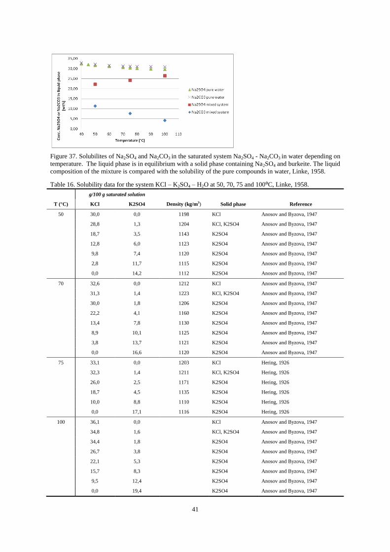
41

Figure 37. Solubilites of Na2SO4 and Na2CO3 in the saturated system Na2SO4 - Na2CO3 in water depending on

temperature. The liquid phase is in equilibrium with a solid phase containing Na2SO4 and burkeite. The liquid

composition of the mixture is compared with the solubility of the pure compounds in water, Linke, 1958.

Table 16. Solubility data for the system KCl – K2SO4 – H2O at 50, 70, 75 and 100⁰C, Linke, 1958.


T (°C) KCl K2SO4 Density (kg/m3) Solid phase Reference

50 30,0 0,0 1198 KCl Anosov and Byzova, 1947

28,8 1,3 1204 KCl, K2SO4 Anosov and Byzova, 1947

18,7 3,5 1143 K2SO4 Anosov and Byzova, 1947





70 32,6 0,0 1212 KCl Anosov and Byzova, 1947

31,3 1,4 1223 KCl, K2SO4 Anosov and Byzova, 1947







75 33,1 0,0 1203 KCl Hering, 1926

32,3 1,4 1211 KCl, K2SO4 Hering, 1926

26,0 2,5 1171 K2SO4 Hering, 1926

18,7 4,5 1135 K2SO4 Hering, 1926

10,0 8,8 1110 K2SO4 Hering, 1926

0,0 17,1 1116 K2SO4 Hering, 1926

100 36,1 0,0

KCl Anosov and Byzova, 1947

34,8 1,6

KCl, K2SO4 Anosov and Byzova, 1947

34,4 1,8

K2SO4 Anosov and Byzova, 1947

26,7 3,8


22,1 5,3


15,7 8,3


9,5 12,4


0,0 19,4


42

Table 17. Solubility data for the system Na2SO4 – K2SO4 – H2O at 50, 70, 75 and 100⁰C, Linke, 1958. The

formula of the solid phase glaserite is 3K2SO4 Na2SO4.


T (°C) Na2SO4 K2SO4

Density

(kg/m3) Solid phase Reference

55 0,0 15,0

K2SO4 Yanat'eva and Orlova, 1956

5,1 14,5


5,6 14,3


5,6 14,3

K2SO4

"new" solid solution Yanat'eva and Orlova, 1956

6,0 14,1


6,7 14,1


7,4 13,6

Glaserite Yanat'eva and Orlova, 1956

8,1 13,1


8,8 12,8


11,6 11,6


19,0 9,1


24,9 7,5


28,0 6,5


29,0 6,2

Glaserite, Na2SO4 Yanat'eva and Orlova, 1956

29,0 6,2

Glaserite, Na2SO4 Yanat'eva and Orlova, 1956

31,6 0,0

Na2SO4 Yanat'eva and Orlova, 1956

50 29,4 5,9 1339 Glaserite, Na2SO4 Coenec and Krombach, 1928-1929

5,68 13,8 1157 Glaserite, K2SO4 Coenec and Krombach, 1928-1929





Teeple

Table 18. Collocation of the systems investigated by Teeple, 1929.

System Salts Temperature (⁰C)

I NaCl, Na2SO4, Na2CO3 20, 35, 50, 75, 100

II KCl, K2SO4, K2CO3 35, 50, 75

III NaCl, Na2SO4, KCl, K2SO4 20, 35, 50, 75, 100

IV NaCl, Na2CO3, KCl, K2CO3 20, 35, 50, 75, 100

V Na2SO4, Na2CO3, K2SO4, K2CO3 35, 50, 75

VI NaCl (sat), Na2SO4, Na2CO3, KCl, K2SO4,K2CO3 20, 35, 50, 75, 100

43

Table 19. Solubility data for the system Na2CO3 – K2CO3 - Na2SO4 - K2SO4 – H2O at 35, 50 and 75⁰C,

Teeple, 1929. The solid phase glaserite have the molecular formula 3K2SO4 Na2SO4 and burkeite Na2CO3 2

Na2SO4.

g/100g H2O mole/1000 mole H2O

T

(°C) Na2CO3 K2CO3 Na2SO4 K2SO4 Na2CO3 K2CO3 Na2SO4 K2SO4 Solid phase

35 0,0 0,0 50,7 0,0 0,0 0,0 64,2 0,0 Na2SO4

0,0 0,0 0,0 14,1 0,0 0,0 0,0 14,5 K2SO4

48,8 0,0 0,0 0,0 82,9 0,0 0,0 0,0 Na2CO3*1H20

0,0 115,1 0,0 0,0 0,0 150,0 0,0 0,0 K2CO3*3/2H2

O

0,0 0,0 48,8 7,9 0,0 0,0 61,8 8,2 Na2SO4, Glaserite

0,0 0,0 7,2 15,0 0,0 0,0 9,2 15,5 K2SO4,

Glaserite

14,3 95,7 0,0 0,0 24,2 124,6 0,0 0,0 Na2CO3*1H20,

Na2CO3*K2C

O3

9,3 108,8 0,0 0,0 15,8 141,7 0,0 0,0 K2CO3*3/2H2

O,

Na2CO3*K2CO3

0,0 112,5 0,0 trace 0,0 146,5 0,0 trace K2CO3*3/2H2

O, K2SO4

45,8 0,0 6,9 0,0 77,8 0,0 8,7 0,0 Na2CO3*1H20,

Burkeite

18,5 0,0 34,3 0,0 31,3 0,0 43,5 0,0 Na2SO4, Burkeite

14,1 96,1 trace 0,0 24,0 125,2 trace 0,0 Na2CO3*1H20,

Na2CO3*K2CO3, K2SO4

9,1 108,9 trace 0,0 15,4 141,8 trace 0,0 K2CO3*3/2H2

O, Na2CO3*K2C

O3, K2SO4

17,0 0,0 31,8 6,9 28,8 0,0 40,3 7,2 Na2SO4, Burkeite,

Glaserite

32,1 32,7 0,8 0,0 54,5 42,6 1,0 0,0 Na2CO3*1H20, K2SO4,

Glaserite

40,5 7,8 8,4 0,0 68,8 10,1 10,7 0,0 Na2CO3*1H20, Burkeite,

Glaserite

50 0,0 0,0 46,6 0,0 0,0 0,0 59,1 0,0 Na2SO4

0,0 0,0 0,0 17,1 0,0 0,0 0,0 17,6 K2SO4

47,5 0,0 0,0 0,0 80,6 0,0 0,0 0,0 Na2CO3*1H20

0,0 121,2 0,0 0,0 0,0 157,9 0,0 0,0 K2CO3*3/2H2O

0,0 0,0 47,4 9,3 0,0 0,0 60,1 9,6 Na2SO4,

Glaserite

0,0 0,0 8,6 17,7 0,0 0,0 10,9 18,3 K2SO4,

Glaserite

15,8 95,2 0,0 0,0 26,8 124,0 0,0 0,0 Na2CO3*1H20, Na2CO3*K2C

O3

7,8 116,7 0,0 0,0 13,2 152,0 0,0 0,0 K2CO3*3/2H2O,

Na2CO3*K2C

O3

0,0 121,2 0,0 trace 0,0 157,9 0,0 trace K2CO3*3/2H2

O, K2SO4

44,4 0,0 6,3 0,0 75,4 0,0 8,0 0,0 Na2CO3*1H20, Burkeite

12,6 0,0 36,7 0,0 21,4 0,0 46,5 0,0 Na2SO4,

Burkeite


Na2CO3*K2C

44

O3, K2SO4

7,2 117,2 trace 0,0 12,3 152,6 trace 0,0 K2CO3*3/2H2

O, Na2CO3*K2C

O3, K2SO4

6,8 6,9 43,1 0,0 11,6 9,0 54,6 0,0 Na2SO4, Burkeite,

Glaserite

29,9 38,1 1,1 0,0 50,8 49,6 1,5 0,0 Na2CO3*1H20, K2SO4,

Glaserite

38,0 10,3 8,7 0,0 64,6 13,4 11,1 0,0 Na2CO3*1H20, Burkeite,

Glaserite

75 0,0 0,0 43,9 0,0 0,0 0,0 55,6 0,0 Na2SO4

0,0 0,0 0,0 20,6 0,0 0,0 0,0 21,3 K2SO4

45,3 0,0 0,0 0,0 77,0 0,0 0,0 0,0 Na2CO3*1H20

0,0 136,4 0,0 0,0 0,0 177,7 0,0 0,0 K2CO3*3/2H2O

0,0 0,0 44,4 11,7 0,0 0,0 56,3 12,0 Na2SO4,

Glaserite

0,0 0,0 8,1 21,8 0,0 0,0 10,3 22,6 K2SO4,

Glaserite

18,0 94,2 0,0 0,0 30,6 122,6 0,0 0,0 Na2CO3*1H20, Na2CO3*K2C

O3

5,1 133,5 0,0 0,0 8,6 173,9 0,0 0,0 K2CO3*3/2H2O,

Na2CO3*K2C

O3

0,0 135,8 0,0 trace 0,0 176,9 0,0 trace K2CO3*3/2H2

O, K2SO4

42,9 0,0 5,4 0,0 72,8 0,0 6,8 0,0 Na2CO3*1H20, Burkeite

7,9 0,0 39,0 0,0 13,4 0,0 49,4 0,0 Na2SO4,

Burkeite


Na2CO3*K2C

O3, K2SO4

4,8 133,5 trace 0,0 8,2 173,8 trace 0,0 K2CO3*3/2H2

O,

Na2CO3*K2CO3, K2SO4

8,2 0,0 37,6 11,6 13,9 0,0 47,6 11,9 Na2SO4,

Burkeite, Glaserite

28,0 42,9 1,8 0,0 47,5 55,9 2,2 0,0 Na2CO3*1H20,

K2SO4, Glaserite

34,1 16,0 8,2 0,0 58,0 20,8 10,3 0,0 Na2CO3*1H20,

Burkeite, Glaserite

45

Jaretun

Table 20. Original results from the leaching experiments according to Jaretun. The composition in liquid

phase in a temperature interval between 55-75ºC, dependent on the ingoing ratio of ash to water are shown.

Jaretun, 1998.

Ingoing phase ratio (g/l)

T (°C) Composition 600 800 1000 1200 1400

55 K+ (M) 0,234 0,254 0,302 0,402 0,442

Na+ (M) 5,550 5,464 5,732 5,680 5,620

Cl- (M) 3,040 3,720 4,520 4,780 4,880

CO32- (M) 0,352 0,434 0,494 0,540 0,482

SO4 2- (M) 1,174 0,746 0,476 0,508 0,492

Solution (g) 203,50 211,16 213,17 216,97 215,89

Diluted solids (g) 62,02 64,14 69,17 72,02 73,77

60 K+ (M) 0,218 0,294 0,346 0,394 0,468

Na+ (M) 5,298 5,716 6,046 5,660 5,520

Cl- (M) 2,980 4,020 4,960 5,040 5,020

CO32- (M) 0,372 0,496 0,510 0,392 0,378

SO4 2- (M) 1,166 0,822 0,516 0,468 0,468

Solution (g) 206,59 207,61 213,87 214,23 214,44

Diluted solids (g) 60,89 63,88 68,43 70,49 71,16

65 K+ (M) 0,210 0,274 0,336 0,402 0,450

Na+ (M) 4,916 5,298 5,568 5,706 5,480

Cl- (M) 2,740 3,680 4,520 4,900 5,140

CO32- (M) 0,316 0,408 0,410 0,348 0,316

SO4 2- (M) 1,034 0,730 0,508 0,438 0,492

Solution (g) 206,64 206,30 211,74 214,80 213,20

Diluted solids (g) 60,96 62,90 67,32 72,20 70,37

70 K+ (M) 0,210 0,278 0,336 0,390 0,482

Na+ (M) 4,984 5,402 5,532 5,638 5,360

Cl- (M) 2,900 3,840 4,640 5,100 5,160

CO32- (M) 0,342 0,442 0,434 0,344 0,252

SO4 2- (M) 1,104 0,760 0,516 0,438 0,484

Solution (g) 206,85 209,03 211,71 213,39 212,92

Diluted solids (g) 60,56 63,75 67,16 69,72 69,49

75 K+ (M) 0,218 0,276 0,332 0,400 0,488

Na+ (M) 5,064 5,290 5,716 5,680 5,560

Cl- (M) 2,900 3,820 4,740 5,260 5,220

CO32- (M) 0,350 0,422 0,374 0,286 0,246

SO4 2- (M) 1,020 0,738 0,508 0,438 0,436

Solution (g) 202,45 206,27 210,20 211,79 211,35

Diluted solids (g) 58,62 62,40 65,92 69,98 70,59

46

The assumptions that were made to make it possible to calculate the composition in g/l H2O was:

That the water is taken at 25°C, with a density of 1000 kg/m3.

The dissolved material is calculated as weight of solution – 150 g water.

The volume of solution can be calculated as;

Goncalves

Table 21. Composition of different ash samples, calculated in RBD in order to receive electroneutrality and to

calculate the composition of salts, Goncalves, 2007.

Ash

composition

(wt%)

Ash A Ash B Ash C Ash D Ash E Ash F

Cl 6,68% 5,97% 5,46% 1,12% 3,45% 8,40%

K 4,92% 5,09% 4,60% 5,18% 5,87% 5,11%

Na 29,32% 28,92% 31,65% 28,77% 27,95% 30,39%

SO4 57,86% 59,70% 45,76% 62,20% 62,62% 49,62%

CO3 1,22% 0,30% 12,54% 2,74% 0,10% 6,48%

Na2SO4 76,14% 78,14% 61,15% 81,20% 80,16% 65,30%

Na2CO3 1,91% 0,47% 19,97% 4,26% 0,15% 10,16%

NaCl 9,78% 8,70% 8,12% 1,62% 4,91% 12,30%

K2SO4 10,49% 11,30% 7,25% 12,01% 13,86% 8,99%

K2CO3 0,28% 0,07% 2,52% 0,67% 0,03% 1,49%

KCl 1,40% 1,31% 1,00% 0,25% 0,88% 1,76%

Table 22. Reject composition for experiments performed by Goncalves at 85ºC.

Ash

composition

(wt% DS)

Ash A Ash B Ash C

800g/l 1000 g/l 1200 g/l 1400 g/l 800g/l 500g/l

Cl 11,35% 16,40% 16,90% 20,00% 9,00% 8,10%

K 7,70% 9,70% 10,00% 11,10% 10,70% 7,30%

Na 28,65% 27,90% 27,90% 27,60% 25,90% 29,90%

SO4 49,40% 42,90% 41,30% 36,50% 53,50% 44,80%

CO3 2,85% 3,10% 3,90% 4,80% 0,90% 9,80%

47

Appendix C – Experimental data from units in operation

Mill 1

In this section the experimental data and corrected data by RBD for Mill 1 are presented. All samples are

taken at a temperature of 90ºC.

Table 23. Experimental data of ash composition at Mill 1.

Experimental data Ash composition (wt%)

Sample 1 2 3 4 5 6 7 8 9

Cl 3,16% 2,95% 3,30% 3,70% 4,00% 4,10% 3,81% 3,85% 3,88%

K 4,30% 4,50% 4,40% 4,30% 4,20% 4,60% 4,40% 4,40% 4,20%

Na 29,30% 31,20% 30,57% 29,78% 30,59% 30,80% 30,73% 30,80% 30,74%

SO4 62,97% 64,19% 63,91% 62,49% 61,38% 61,32% 60,09% 62,54% 62,22%

CO3 0,01% 0,01% 0,05% 0,12% 0,84% 0,67% 0,18% 0,05% 0,17%

Dry solids 99,97% 99,96% 99,97% 99,92% 99,89% 99,95% 99,94% 99,97% 99,96%

Table 24. Ash composition calculated by the Recovery Boiler Design program developed by Metso Power.

The experimental data of Cl, K and CO3 are used, and the composition of Na and SO4 are predicted by the

program. Thereafter the program predicts the composition of different salts.

Calculated from RBD Ash composition (wt%)

Sample 1 2 3 4 5 6 7 8 9

Cl 3,16% 2,95% 3,30% 3,70% 4,00% 4,10% 3,81% 3,85% 3,88%

K 4,30% 4,50% 4,40% 4,30% 4,20% 4,60% 4,40% 4,40% 4,20%

Na 29,63% 29,47% 29,59% 29,72% 29,96% 29,65% 29,67% 29,65% 29,82%

SO4 62,90% 63,07% 62,66% 62,16% 61,00% 60,98% 61,94% 62,05% 61,93%

CO3 0,01% 0,01% 0,05% 0,12% 0,84% 0,67% 0,18% 0,05% 0,17%

Na2SO4 85,69% 85,58% 85,21% 84,71% 83,33% 82,63% 84,24% 84,39% 84,57%

Na2CO3 0,02% 0,02% 0,08% 0,20% 1,37% 1,08% 0,29% 0,08% 0,28%

NaCl 4,80% 4,46% 5,00% 5,62% 6,09% 6,19% 5,78% 5,84% 5,91%

K2SO4 8,97% 9,43% 9,14% 8,84% 8,42% 9,25% 9,01% 9,03% 8,59%

K2CO3 0,00% 0,00% 0,01% 0,02% 0,15% 0,13% 0,03% 0,01% 0,03%

KCl 0,52% 0,51% 0,56% 0,61% 0,64% 0,72% 0,64% 0,65% 0,62%

48

Table 25. Experimental data of slurry composition. Dry solids is the amount of diluted and suspended solids

in the solution.

Experimental data Slurry composition (wt%)

Sample 1 2 3 4 5 6 7 8 9

Cl, % 3,06% 2,44% 3,01% 3,08% 4,01% 3,84% 4,06% 4,02% 3,74%

K, % 4,20% 4,50% 4,10% 4,60% 4,40% 4,80% 4,50% 5,00% 4,30%

Na, % 29,50% 29,40% 29,70% 29,80% 29,70% 29,50% 29,70% 29,40% 28,80%

SO4, % 63,74% 65,78% 64,03% 64,35% 63,28% 63,33% 62,72% 62,85% 64,22%

CO3, % 0,04% 0,02% 0,02% 0,03% 0,21% 0,43% 0,43% 0,33% 0,26%

Dry solids % 53,97% 54,93% 56,39% 54,62% 54,99% 53,53% 54,71% 54,92% 54,40%

Table 26. Slurry composition calculated by the Recovery Boiler Design program developed by Metso Power.

The experimental data of Cl, K and CO3 are used, and the composition of Na and SO4 are predicted by the


Calculated

from RBD Slurry composition (wt%)

Sample 1 2 3 4 5 6 7 8 9

Cl 3,06% 2,44% 3,01% 3,08% 4,01% 3,84% 4,06% 4,02% 3,74%

K 4,20% 4,50% 4,10% 4,60% 4,40% 4,80% 4,50% 5,00% 4,30%

Na 29,70% 29,41% 29,76% 29,41% 29,70% 29,43% 29,68% 29,29% 29,75%

SO4 63,00% 63,63% 63,11% 62,88% 61,68% 61,50% 61,33% 61,36% 61,95%

CO3 0,04% 0,02% 0,02% 0,03% 0,21% 0,43% 0,43% 0,33% 0,26%

Na2SO4 86,00% 86,32% 86,32% 85,15% 83,90% 82,98% 83,27% 82,45% 84,43%

Na2CO3 0,07% 0,03% 0,03% 0,05% 0,34% 0,69% 0,70% 0,53% 0,42%

NaCl 4,66% 3,69% 4,59% 4,65% 6,08% 5,78% 6,14% 6,02% 5,68%

K2SO4 8,77% 9,53% 8,58% 9,61% 8,97% 9,76% 9,11% 10,15% 8,80%

K2CO3 0,01% 0,00% 0,00% 0,01% 0,04% 0,09% 0,08% 0,07% 0,05%

KCl 0,49% 0,42% 0,47% 0,55% 0,68% 0,71% 0,70% 0,77% 0,62%

Table 27. Experimental data of recycled ash composition in Mill 1. Dry solids is the amount of diluted and

suspended solids in the solution.

Experimental data Recycled ash (Product)(wt%)

Sample 1 2 3 4 5 6 7 8 9

Cl 0,40% 0,36% 0,41% 0,32% 0,38% 0,48% 0,57% 0,56% 0,61%

K 0,70% 0,70% 0,70% 0,60% 0,60% 0,90% 0,90% 1,00% 0,90%

Na 33,20% 33,20% 33,00% 32,99% 33,24% 33,18% 33,07% 32,93% 32,27%

SO4 68,17% 68,08% 68,09% 66,39% 68,29% 67,53% 66,25% 67,60% 67,01%

CO3 0,01% 0,00% 0,00% 0,00% 0,02% 0,08% 0,09% 0,08% 0,06%

Dry solids 89,90% 90,80% 89,30% 90,80% 91,20% 87,98% 88,90% 89,10% 88,25%

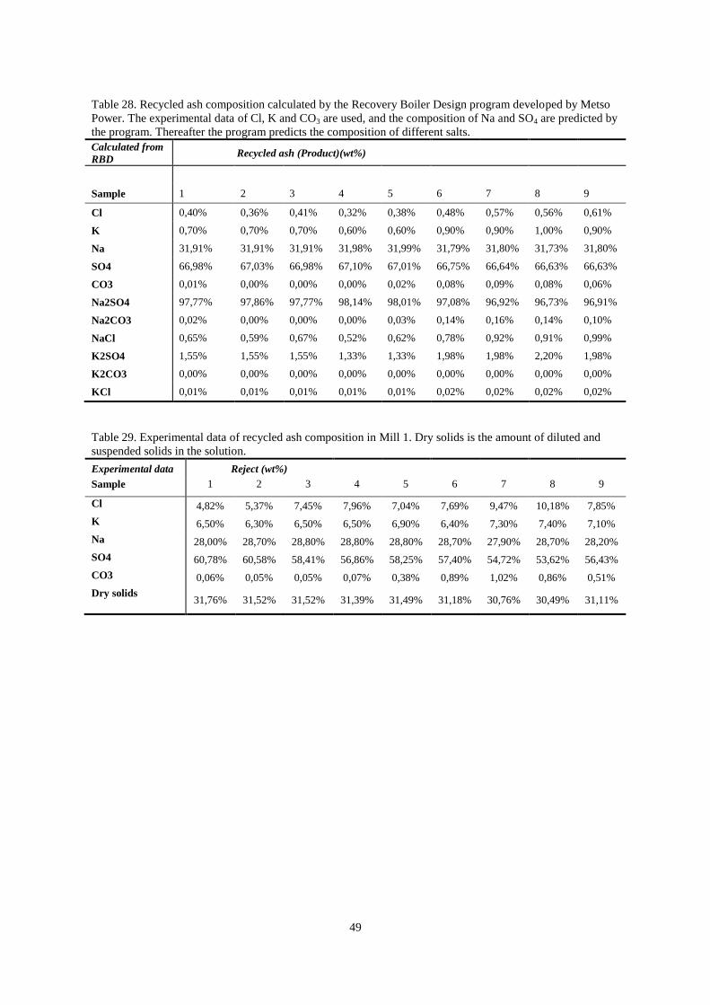
49

Table 28. Recycled ash composition calculated by the Recovery Boiler Design program developed by Metso

Power. The experimental data of Cl, K and CO3 are used, and the composition of Na and SO4 are predicted by

the program. Thereafter the program predicts the composition of different salts.

Calculated from

RBD Recycled ash (Product)(wt%)

Sample 1 2 3 4 5 6 7 8 9

Cl 0,40% 0,36% 0,41% 0,32% 0,38% 0,48% 0,57% 0,56% 0,61%

K 0,70% 0,70% 0,70% 0,60% 0,60% 0,90% 0,90% 1,00% 0,90%

Na 31,91% 31,91% 31,91% 31,98% 31,99% 31,79% 31,80% 31,73% 31,80%

SO4 66,98% 67,03% 66,98% 67,10% 67,01% 66,75% 66,64% 66,63% 66,63%

CO3 0,01% 0,00% 0,00% 0,00% 0,02% 0,08% 0,09% 0,08% 0,06%

Na2SO4 97,77% 97,86% 97,77% 98,14% 98,01% 97,08% 96,92% 96,73% 96,91%

Na2CO3 0,02% 0,00% 0,00% 0,00% 0,03% 0,14% 0,16% 0,14% 0,10%

NaCl 0,65% 0,59% 0,67% 0,52% 0,62% 0,78% 0,92% 0,91% 0,99%

K2SO4 1,55% 1,55% 1,55% 1,33% 1,33% 1,98% 1,98% 2,20% 1,98%

K2CO3 0,00% 0,00% 0,00% 0,00% 0,00% 0,00% 0,00% 0,00% 0,00%

KCl 0,01% 0,01% 0,01% 0,01% 0,01% 0,02% 0,02% 0,02% 0,02%



Experimental data Reject (wt%)

Sample 1 2 3 4 5 6 7 8 9

Cl 4,82% 5,37% 7,45% 7,96% 7,04% 7,69% 9,47% 10,18% 7,85%

K 6,50% 6,30% 6,50% 6,50% 6,90% 6,40% 7,30% 7,40% 7,10%

Na 28,00% 28,70% 28,80% 28,80% 28,80% 28,70% 27,90% 28,70% 28,20%

SO4 60,78% 60,58% 58,41% 56,86% 58,25% 57,40% 54,72% 53,62% 56,43%

CO3 0,06% 0,05% 0,05% 0,07% 0,38% 0,89% 1,02% 0,86% 0,51%

Dry solids 31,76% 31,52% 31,52% 31,39% 31,49% 31,18% 30,76% 30,49% 31,11%

50


Power. The experimental data of Cl, K and CO3 are used, and the composition of Na and SO4 are predicted by

the program. Thereafter the program predicts the composition of different salts.

From

RBD Reject (wt%)

Sample 1 2 3 4 5 6 7 8 9

Cl 4,82% 5,37% 7,45% 7,96% 7,04% 7,69% 9,47% 10,18% 7,85%

K 6,50% 6,30% 6,50% 6,50% 6,90% 6,40% 7,30% 7,40% 7,10%

Na 28,25% 28,45% 28,55% 28,61% 28,28% 28,81% 28,39% 28,37% 28,25%

SO4 60,37% 59,83% 57,45% 56,86% 57,40% 56,21% 53,82% 53,19% 56,29%

CO3 0,06% 0,05% 0,05% 0,07% 0,38% 0,89% 1,02% 0,86% 0,51%

Dry

solids 31,76% 31,52% 31,52% 31,39% 31,49% 31,18% 30,76% 30,49% 31,11%

Na2SO4 78,63% 78,27% 74,92% 74,17% 74,23% 73,51% 69,13% 68,19% 72,52%

Na2CO3 0,09% 0,08% 0,08% 0,11% 0,59% 1,39% 1,57% 1,32% 0,78%

NaCl 7,00% 7,83% 10,83% 11,58% 10,15% 11,21% 13,56% 14,55% 11,27%

K2SO4 13,05% 12,50% 12,31% 12,15% 13,07% 11,78% 12,82% 12,83% 13,15%

K2CO3 0,02% 0,01% 0,01% 0,02% 0,11% 0,24% 0,31% 0,26% 0,15%

KCl 1,21% 1,30% 1,85% 1,97% 1,86% 1,87% 2,62% 2,85% 2,13%

Table 31. Process flows measured at the point of sampling for analysis.

Experimental data Process flows

Sample 1 2 3 4 5 6 7 8 9

Slurry flow (kg/h) 10736 13031 13114 13951 13523 12705 12296 14841 13619

Recirculation ratio (%) 16,4% 13,8% 13,5% 12,5% 11,5% 11,7% 12,1% 9,6% 10,5%

Mill 2

In this section the experimental data and corrected data by RBD for Mill 2 are presented. All data are taken at

a temperature of 90ºC.

Table 32. Experimental data of ash composition at Mill 1.

Experimental

data Ash composition (wt%)

Sample 1 2 3 4 5

Cl 4,2% 3,3% 3,1% 3,4% 4,4%

K 3,0% 3,5% 3,0% 2,9% 3,0%

Na 33,8% 34,4% 34,0% 34,7% 34,7%

SO4 43,2% 42,2% 42,8% 42,7% 40,5%

CO3 14,0% 18,5% 17,7% 17,2% 18,3%

Dry solids 98,9% 98,9% 98,9% 98,9% 98,9%

51

Table 33. Ash composition calculated by the Recovery Boiler Design program developed by Metso Power.

The experimental data for Cl, K and CO3 are used, and the composition of Na and SO4 are predicted by the


Calculated

from RBD Ash composition (wt%)

Sample 1 2 3 4 5

Cl 4,2% 3,3% 3,1% 3,4% 4,4%

K 3,0% 3,5% 3,0% 2,9% 3,0%

Na 33,4% 33,8% 34,0% 34,0% 34,3%

SO4 45,3% 40,9% 42,2% 42,5% 40,1%

CO3 14,0% 18,5% 17,7% 17,2% 18,3%

Na2SO4 63,7% 57,0% 59,3% 59,8% 56,4%

Na2CO3 23,5% 30,8% 29,7% 29,0% 30,7%

NaCl 6,6% 5,2% 4,9% 5,3% 6,9%

K2SO4 4,1% 4,2% 3,8% 3,7% 3,5%

K2CO3 1,6% 2,4% 2,0% 1,9% 2,0%

KCl 0,5% 0,4% 0,3% 0,3% 0,5%

Table 34. Experimental data of slurry composition. Dry solids is the amount of diluted and suspended solids

in the solution.

Experimental

data Slurry composition (wt%)

Sample 1 2 3 4 5

Cl, % 4,40% 3,19% 1,57% 2,63% 2,50%

K, % 3,50% 1,50% 1,49% 1,49% 1,93%

Na, % 33,95% 35,46% 34,86% 35,35% 36,70%

SO4, % 42,92% 42,94% 46,46% 45,72% 43,32%

CO3, % 14,36% 17,43% 16,69% 16,59% 18,11%

Dry solids % 40,03% 47,01% 44,24% 43,79% 45,01%

52

Table 35. Slurry composition calculated by the Recovery Boiler Design program developed by Metso Power.

The experimental data for Cl, K and CO3 are used, and the composition of Na and SO4 are predicted by the

program.

Calculated

from RBD Slurry composition (wt%)

Sample 1 2 3 4 5

Cl 4,40% 3,19% 1,57% 2,63% 2,50%

K 3,50% 1,50% 1,49% 1,49% 1,93%

Na 33,14% 35,05% 34,72% 34,82% 34,79%

SO4 44,60% 42,83% 45,53% 44,47% 42,67%

CO3 14,36% 17,43% 16,69% 16,59% 18,11%

Na2SO4 62,09% 61,78% 65,66% 64,14% 61,10%

Na2CO3 23,88% 30,03% 28,75% 28,58% 30,98%

NaCl 6,83% 5,13% 2,52% 4,23% 3,99%

K2SO4 4,73% 1,91% 2,03% 1,98% 2,45%

K2CO3 1,93% 0,99% 0,95% 0,94% 1,32%

KCl 0,54% 0,16% 0,08% 0,14% 0,17%



Experimental

data Recycled ash (Product)(wt%)

Sample 1 2 3 4 5

Cl 2,10% 1,20% 0,96% 2,35% 1,62%

K 1,00% 1,00% 1,00% 1,00% 0,94%

Na 36,48% 36,82% 34,96% 34,95% 36,06%

SO4 48,11% 47,22% 48,25% 47,22% 48,87%

CO3 14,87% 16,75% 16,16% 16,15% 17,10%

Dry solids 70,55% 70,20% 73,24% 63,81% 70,33%


Power. The experimental data for Cl, K and CO3 are used, and the composition of Na and SO4 are predicted

by the program. Thereafter the program predicts the composition of different salts.

Calculated

from RBD Recycled ash (Product)(wt%)

Sample 1 2 3 4 5

Cl 2,10% 1,20% 0,96% 2,35% 1,62%

K 1,00% 1,00% 1,00% 1,00% 0,94%

Na 34,78% 35,04% 34,90% 35,06% 35,20%

SO4 47,25% 46,01% 46,98% 45,44% 45,14%

CO3 14,87% 16,75% 16,16% 16,15% 17,10%

Na2SO4 68,70% 66,90% 68,31% 66,08% 65,71%

Na2CO3 25,83% 29,10% 28,07% 28,05% 29,74%

NaCl 3,40% 1,95% 1,56% 3,81% 2,63%

K2SO4 1,42% 1,38% 1,41% 1,36% 1,27%

K2CO3 0,57% 0,64% 0,62% 0,61% 0,61%

KCl 0,07% 0,04% 0,03% 0,08% 0,05%

53



Experimental

data Reject (wt%)

Sample 1 2 3 4 5

Cl 10,28% 7,31% 6,72% 5,95% 8,55%

K 6,47% 2,49% 5,98% 4,48% 6,93%

Na 31,37% 32,92% 34,42% 31,13% 33,64%

SO4 36,20% 37,26% 37,29% 36,22% 32,92%

CO3 13,02% 18,19% 18,34% 17,83% 18,56%

Dry solids 29,28% 30,08% 30,30% 30,32% 30,67%


Power. The experimental data for Cl, K and CO3 are used, and the composition of Na and SO4 are predicted

by the program. Thereafter the program predicts the composition of different salts.

Calculated

from RBD Reject (wt%)

Sample 1 2 3 4 5

Cl 10,28% 7,31% 6,72% 5,95% 8,55%

K 6,47% 2,49% 5,98% 4,48% 6,93%

Na 31,42% 34,95% 32,40% 33,29% 31,96%

SO4 38,81% 37,06% 36,56% 38,45% 34,00%

CO3 13,02% 18,19% 18,34% 17,83% 18,56%

Na2SO4 51,19% 52,59% 48,77% 52,69% 44,59%

Na2CO3 20,51% 30,84% 29,22% 29,18% 29,08%

NaCl 15,12% 11,57% 9,99% 9,09% 12,50%

K2SO4 7,60% 2,70% 6,49% 5,11% 6,97%

K2CO3 3,24% 1,68% 4,14% 3,01% 4,83%

KCl 2,33% 0,62% 1,38% 0,92% 2,03%

Table 40. Process flows measured at the point of analysis.


Sample 1 2 3 4 5

Slurry (kg/h) 14093 14991 14994 15309 15498

Recirculation ratio (%) 27 10 10 40 25

54

Mill 3

Experimental data and data corrected by the program RBD are shown for the ESP ash, slurry, recycled solids

and reject.

Table 41. Experimental composition of ingoing ash, slurry, recycled ash and reject in Mill 3. Dry solids are

the amount of diluted and suspended solids in the solution.

Table 42. Composition of ingoing ash, slurry, recycled ash and reject calculated by the Recovery Boiler

Design program developed by Metso Power. The experimental data for Cl, K and CO3 are used, and the

composition of Na and SO4 are predicted by the program. Thereafter the program predicts the composition of

different salts.

From

RBD

Ash Slurry Solids Reject

Cl 4,38% 6,70% 1,40% 12,80%

K 5,19% 7,20% 1,70% 13,00%

Na 34,21% 33,22% 35,86% 31,48%

SO4 30,12% 25,78% 37,64% 6,62%

CO3 26,10% 27,10% 23,40% 36,10%

Na2SO4 40,89% 33,81% 54,15% 7,87%

Na2CO3 42,32% 42,45% 40,21% 51,31%

NaCl 6,63% 9,80% 2,25% 16,98%

K2SO4 4,48% 5,29% 1,85% 2,34%

K2CO3 4,92% 7,06% 1,46% 16,24%

KCl 0,75% 1,59% 0,08% 5,26%

Table 43. Process flows measured at the point of analysis.


Sample 1

Slurry (kg/h) 12985

Recirculation ratio (%) 50

Experimental

data

Ash Slurry Solids Reject

Cl 4,38% 6,70% 1,40% 12,80%

K 5,19% 7,20% 1,70% 13,00%

Na 33,80% 32,00% 34,80% 30,10%

SO4 31,40% 28,50% 33,00% 10,70%

CO3 26,10% 27,10% 23,40% 36,10%

Total weight,

%

100,87% 101,50% 94,30% 102,70%

Dry solids, % - 47,40% 82,40% 32,60%

55

Appendix D – Mass balances

Total balance

The total mass balance over the system can be seen below.

Recirculation

When the reject flow and recirculation ratio are known, the recycled flow can be calculated.

Balance over centrifuge

The balance over the centrifuge gives the flow of the recycled ash, with a known recirculation ratio.

Calculation procedure for ash and water flow

1. Amount suspended solids in slurry and recycled solids are calculated by using the dry solids content

in slurry, solids and reject assuming that no suspended solids are present in the reject.

2. The flow recycled solids and reject flow can then be calculated:

3. The recirculation ratio gives the recirculation and bleed flow:

4. The ash and water flow can now be calculated by a mass balance over the leaching tank.

56

Appendix E – Excel data sheet, Model I

Figure 38 The Excel calculation sheet is shown for Model I, with the predicted values for Ash 1 in Mill 1.

The values marked red are required input data.

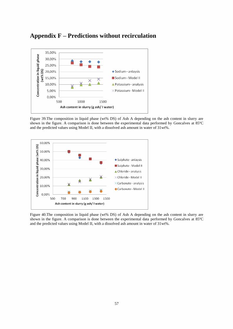
57

Appendix F – Predictions without recirculation

Figure 39.The composition in liquid phase (wt% DS) of Ash A depending on the ash content in slurry are

shown in the figure. A comparison is done between the experimental data performed by Goncalves at 85ºC

and the predicted values using Model II, with a dissolved ash amount in water of 31wt%.

Figure 40.The composition in liquid phase (wt% DS) of Ash A depending on the ash content in slurry are

shown in the figure. A comparison is done between the experimental data performed by Goncalves at 85ºC

and the predicted values using Model II, with a dissolved ash amount in water of 31wt%.

58

Appendix G – Temperature dependence by Model II

Below the figures for Mill 2 predicted by Model II.

Figure 41. Temperature dependence predicted by Model II for Mill 2. A dissolved ash amount of 31 wt% is

specified in the model.

Figure 42. Temperature dependence predicted by Model II for Mill 2. A dissolved ash amount of 31 wt% is

specified in the model.

calculation tool for the treatment of electrostatic...

Documents