calculation of the derived bouguer anomaly...
TRANSCRIPT
185
CALCULATION OF THE DERIVED BOUGUER ANOMALY USING THE EQUIVALENT SOURCE METHOD BASED ON
JOINT INVERSION OF GROUND GRAVITY AND AIRBORNE GRAVITY GRADIENT DATA
Novel technologies for greenfield explorationEdited by Pertti SaralaGeological Survey of Finland, Special Paper 57, 185–197, 2015
byHeikki Salmirinne1) and Markku Pirttijärvi2)
Salmirinne, H. & Pirttijärvi, M. 2015. Calculation of the derived Bouguer anom-aly using the equivalent source method based on joint inversion of ground gravity and airborne gravity gradient data. Geological Survey of Finland, Special Paper 57, 185−197, 11 figures.
Gravity gradient data measured in airborne surveys are not suitable for the direct determination of the absolute vertical gravity field or Bouguer anomaly. However, the deriving of traditional-like vertical Bouguer anomalies is important for better un-derstanding of airborne gravity gradient data and enabling comparisons and combina-tions of gradient and ground gravity surveys. The derived Bouguer anomaly can be calculated and integrated with ground grav-ity using either the Fourier transform method or the equivalent source method. In this paper, the equivalent source procedure using joint inversion of airborne gravity gradient data and sparsely sampled ground gravity data is described and applied for a Falcon AGG (Airborne Gravity Gradient) survey covering an area of 1000 km2 in Savukoski, northern Finland. The national regional gravity net of the Finnish Geo-detic Institute with a station spacing of 5 km was used as a source of ground gravity data. As a consequence of this station spacing, the smallest dimension of an airborne gradient survey in Finland should be at least 20 km in order to model long wavelength information from the national ground gravity data of Finland. The equivalent source method was tested and evaluated using 3D block modelling to combine the information contents of the longer wavelengths of the ground gravity with the shorter wavelengths of the gravity gradients. Because the equivalent model needs to explain both gravity and gradient data, the selection of the size and discre-tization of the initial model is important. The equivalent source method, in which AGG and ground gravity data are simultaneously optimized, proved to be feasible for the integration of ground gravity and airborne gradient data into the derived Bouguer anomaly comparable with traditional regional ground gravity data.
Keywords (GeoRef Thesaurus, AGI): geophysics, airborne methods, gradiometers, gravity methods, gravity anomalies, Bouguer anomalies, three-dimensional models, Savukoski, Pelkosenniemi, Finland
1) Geological Survey of Finland, P.O. Box 77, FI-96101 Rovaniemi, Finland E-mail: [email protected]
2) University of Oulu, Department of Physics, P.O. Box 3000, FI-90014 University of Oulu E-mail: [email protected]
186
Geological Survey of Finland, Special Paper 57Heikki Salmirinne and Markku Pirttijärvi
INTRODUCTION
Airborne gravity gradiometry has been commer-cially available for about 15 years. The method has been widely known for resource exploration due to its accuracy, which is several times greater than that of airborne gravimetry. Currently, there are three contractors (Bell Geospace, CGG and ARKEx) performing gravity gradiometry surveys for hydrocarbon and mineral exploration compa-nies and to a lesser degree for national research institutes. Gradiometry surveys are extremely valuable for mapping and exploration purposes. However, processing and interpretation proce-dures for airborne gradient data are dissimilar to those for traditional gravity data. Gravity tensor components measured in gradiometry surveys are not suitable for direct determination of the abso-lute value of the vertical gravity field or Bouguer anomaly. However, deriving traditional-like verti-cal Bouguer anomalies is important for better un-derstanding of the results and enabling compari-sons and combinations of gradient and ground gravity surveys.
There are two basic methods for the determina-tion of the derived Bouguer anomaly from gradi-ent surveys: the Fourier transform method and the equivalent source method. In order to tie airborne gradient data to gravity values at the ground level,
a sufficient density of ground gravity data is need-ed for both methods.
This paper focuses on the determination of the derived Bouguer anomaly using the equivalent source method and Falcon AGG (Airborne Grav-ity Gradient) survey measurements in the Savukos- ki area, northern Finland. Commercial programs for equivalent source modelling are not currently available. Therefore, we implemented the simulta-neous inversion of AGG and ground gravity data into the GRABLOX2 program developed by GTK and the University of Oulu (Pirttijärvi 2009). The equivalent source application by GRABLOX2 is based on the linearized Occam inversion of a 3D block model that consists of a single layer of ele-ments. The method was tested to find the balance between the information contents of the longer wavelengths of ground gravity and the shorter wavelengths of gravity gradients. The derived Bouguer anomaly was combined with GTK’s re-gional gravity data in Central Lapland. The work was carried out during 2012–2014 in the project Novel Technologies for Greenfield Exploration (NovTecEx) funded by the Tekes (Finnish Fund-ing Agency for Innovation) Green Mining Pro-gramme.
AIRBORNE GRAVITY GRADIOMETERS
The first airborne gravity gradiometer suitable for mineral exploration was developed by BHP Billi-ton and Lockheed Martin in the FALCON project between 1991 and 2000 (Lee 2001, Dransfield & Lee 2004). This gradiometer is called the Falcon AGG (Airborne Gravity Gradiometer). Bell Geo-space introduced the 3D FTG- gradiometer (Full Tensor Gradiometer) in 2003, based on the same Lockheed Martin gradiometer technology as the Falcon (Murphy 2004). The Falcon AGG and 3D FTG are currently the only two gradiometers used in airborne applications for hydrocarbon and min-eral exploration.
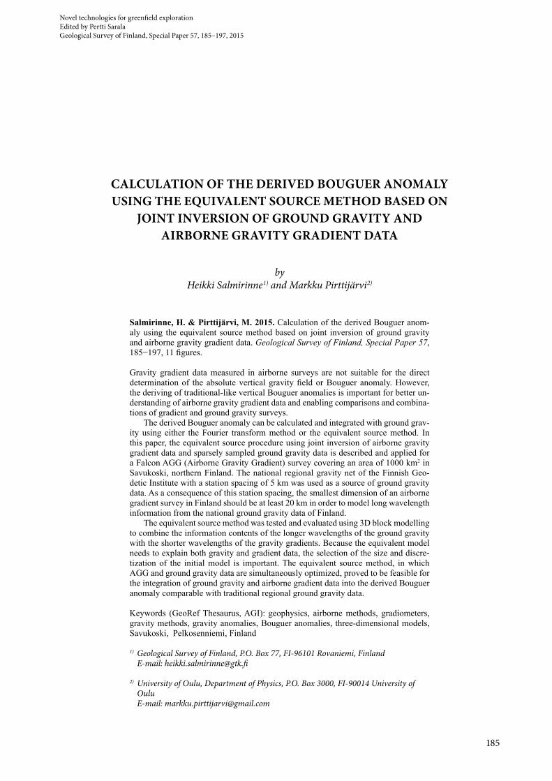
The basis for both the FTG and the AGG gra-diometers is the Gravity Gradient Instrument (GGI). The GGI consist of two pairs of opposing accelerometers mounted on a symmetrically rotat-ing disk (Fig. 1 A). FTG gradiometry comprises 3
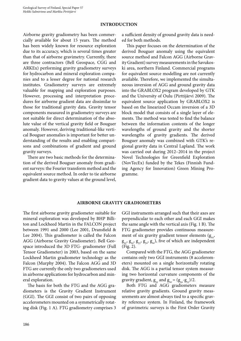
GGI instruments arranged such that their axes are perpendicular to each other and each GGI makes the same angle with the vertical axis (Fig. 1 B). The FTG gradiometer provides continuous measure-ment of six gravity gradient tensor elements (gxx, gxy, gxz, gyy, gyz, gzz), five of which are independent (Fig. 2).
Compared with the FTG, the AGG gradiometer contains only two GGI instruments (8 accelerom-eters) mounted on a single horizontally rotating disk. The AGG is a partial tensor system measur-ing two horizontal curvature components of the gravity gradient, gxy and guv = (gxx-gyy)/2.
Both FTG and AGG gradiometers measure relative gravity gradients. Ground gravity meas-urements are almost always tied to a specific grav-ity reference system. In Finland, the framework of gravimetric surveys is the First Order Gravity

187
Geological Survey of Finland, Special Paper 57Calculation of the derived Bouguer anomaly using the equivalent source method based on
joint inversion of ground gravity and airborne gravity gradient data
Fig. 1. A) The GGI instrument with two pairs of accelerometers mounted on a rotating disk. B) Three GGI instruments of the FTG system mounted on a stabilized platform. Images: Bell Geospace.
Fig. 2. Gravity vector components (gx, gy and gz) and nine diagonally symmetric components of the gravity tensor.
Net (FOGN), which is practically identical to the International Gravity Standardization Net 1971 (IGSN71) (Kiviniemi 1964, 1980, Kääriäinen & Mäkinen 1997). Although airborne gravity gradi-ent results are often applied as such, it is reasoned to transform them into traditional gravity anoma-lies and tie them to the gravity system to increase the understanding and compatibility of surveys. One important reason for the conformation is the different wavelength information contents of
ground gravity and airborne gradient data. Basi-cally, gradient surveys provide information on anomalies having a wavelength of about 0.3 to 10 km, the noise increasing as a function of the wave-length, whereas ground surveys include longer wavelengths more reliable (Dransfield 2013). Al-though methods and tools for conforming ground and airborne gradient surveys have been present-ed, they are not yet well established and require further development.
188
Geological Survey of Finland, Special Paper 57Heikki Salmirinne and Markku Pirttijärvi
METHODS FOR DERIVED BOUGUER CALCULATIONS
Fourier method
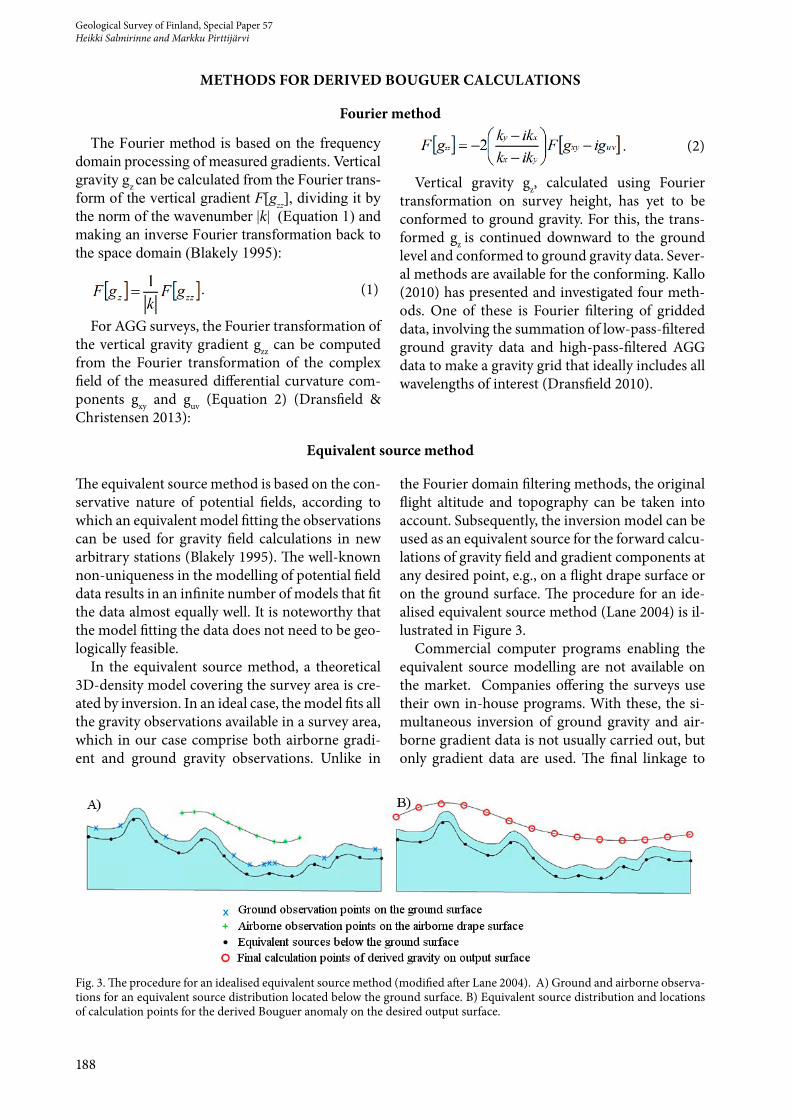
Fig. 3. The procedure for an idealised equivalent source method (modified after Lane 2004). A) Ground and airborne observa-tions for an equivalent source distribution located below the ground surface. B) Equivalent source distribution and locations of calculation points for the derived Bouguer anomaly on the desired output surface.
The Fourier method is based on the frequency domain processing of measured gradients. Vertical gravity gz can be calculated from the Fourier trans-form of the vertical gradient F[gzz], dividing it by the norm of the wavenumber |k| (Equation 1) and making an inverse Fourier transformation back to the space domain (Blakely 1995):
. (1)
For AGG surveys, the Fourier transformation of the vertical gravity gradient gzz can be computed from the Fourier transformation of the complex field of the measured differential curvature com-ponents gxy and guv (Equation 2) (Dransfield & Christensen 2013):
. (2)
Vertical gravity gz, calculated using Fourier transformation on survey height, has yet to be conformed to ground gravity. For this, the trans-formed gz is continued downward to the ground level and conformed to ground gravity data. Sever-al methods are available for the conforming. Kallo (2010) has presented and investigated four meth-ods. One of these is Fourier filtering of gridded data, involving the summation of low-pass-filtered ground gravity data and high-pass-filtered AGG data to make a gravity grid that ideally includes all wavelengths of interest (Dransfield 2010).
Equivalent source method
The equivalent source method is based on the con-servative nature of potential fields, according to which an equivalent model fitting the observations can be used for gravity field calculations in new arbitrary stations (Blakely 1995). The well-known non-uniqueness in the modelling of potential field data results in an infinite number of models that fit the data almost equally well. It is noteworthy that the model fitting the data does not need to be geo-logically feasible.
In the equivalent source method, a theoretical 3D-density model covering the survey area is cre-ated by inversion. In an ideal case, the model fits all the gravity observations available in a survey area, which in our case comprise both airborne gradi-ent and ground gravity observations. Unlike in
the Fourier domain filtering methods, the original flight altitude and topography can be taken into account. Subsequently, the inversion model can be used as an equivalent source for the forward calcu-lations of gravity field and gradient components at any desired point, e.g., on a flight drape surface or on the ground surface. The procedure for an ide-alised equivalent source method (Lane 2004) is il-lustrated in Figure 3.
Commercial computer programs enabling the equivalent source modelling are not available on the market. Companies offering the surveys use their own in-house programs. With these, the si-multaneous inversion of ground gravity and air-borne gradient data is not usually carried out, but only gradient data are used. The final linkage to
189
Geological Survey of Finland, Special Paper 57Calculation of the derived Bouguer anomaly using the equivalent source method based on
joint inversion of ground gravity and airborne gravity gradient data
ground gravity has been conducted using the Fou-rier filtering method, for example.
In this study, the equivalent source modelling was performed with the GRABLOX2 program de-veloped by the University of Oulu and GTK (Pirt-tijärvi 2009). The modelling is based on linearized Occam inversion, where the roughness of the 3D density model is minimized together with a data
misfit. Gravity field calculation is based on the an-alytical solution for a dipping prism (Hjelt 1974). Calculations of gradient components are based on Hjelt’s (1972) solution for the magnetic dip-ping prism, which is analogical to the calculation for gravity gradients. The GRABLOX2 program is freely downloadable from the URL address https://wiki.oulu.fi/x/jYU7AQ.
Equivalent modelling using GRABLOX2
The following text describes the steps required for preparing the derived Bouger anomaly using joint inversion of airborne gravity gradient data and (sparsely) sampled ground gravity data (Bouguer anomaly) using the program GRABLOX2.
Data preparation: Both the airborne and ground data have to be prepared for the formats required by GRABLOX2. If the original flight lines are not parallel to the map coordinate axis, coor-dinate transformation (rotation and shift) should be performed to reduce the number of elements in the block model. It is noteworthy that observed gradients (gradient tensor) also have to be rotated according to the new rotated coordinate system. However, Falcon AGG data always have to be modelled in the original survey coordinates, be-cause the two measured curvature components (gxy & guv) alone do not enable the rotation of the gradient tensor. The amount of original airborne gradient data is usually too large to be used as in-put data for practical inversion. Therefore, the data have to be resampled on a regular grid and then saved in column-formatted text files using third party software such as Geosoft Oasis montaj. Since the terrain topography has a considerable effect on the gravity gradient data (much greater than on gravity data), terrain-corrected gradient data must be used. Ground gravity data are used as such, and they should preferably include stations outside the gradient survey area. The drape surface and ground topography are used as elevation values for gradient and ground data, respectively.
Initial model creation: In GRABLOX2, the size and discretization of the 3D block model can be manually or automatically defined based on the area of the gradient data. Because the equivalent model needs to explain both gravity and gradient data, the top of the model must locate below the ground surface. The equivalent source model con-tains only one layer. The thickness of the layer has
to be set to a suitable value for the inversion. If it is too thick, the model will no longer be able to explain short wavelength anomalies. If the layer is too thin, large density contrasts are needed to ex-plain variations in the data. As a compromise, the layer thickness should be set equal to or smaller than the grid size. The discretization of the model should be based on the flight line spacing. The ele-ment size should be either equal to the line spac-ing (DY x DY) or rectangular so that the size along the flight lines is half the size across flight lines (DY/2 x DY). Margin elements have to be added to the model. The margin elements extend possible gravity effects of the density contrast between the model and the background density away from the study area. Since the density values of blocks do not need to be geologically feasible, background density can be set to zero (g/cm3). The minimum and maximum density limits should be checked and set large enough (e.g. from -20 g/cm3 to +20 g/cm3, or even more) to allow the generation of big gravity anomalies and rapid gravity gradients.
Inversion: After the initial model has been cre-ated, the gravity and gradient data can be read into the GRABLOX2 program. Before actual density inversion, the base anomaly (regional field) can be optimized for the gravity data and each gradi-ent component. Because gradient data should not contain any long wavelengths, the base anomaly should be a constant value. For gravity data, the base anomaly can be more complex, but for equiv-alent layer modelling it needs not be more com-plex than a second order polynomial. The base anomaly of gravity data can be optimized during the density inversion, which can improve the over-all data fit.
The final inversion is carried out with the Oc-cam density inversion method, which uses an it-erative conjugate gradient solver and stabilizes the inversion by minimizing the model roughness
190
Geological Survey of Finland, Special Paper 57Heikki Salmirinne and Markku Pirttijärvi
together with the data misfit. The Occam method uses a so-called Lagrange scaler (FOPT parameter in GRABLOX2) as a user-defined parameter to emphasize the smoothness of the model (FOPT > 1) at the expense of a poor data fit or the good-ness of the data fit (FOPT < 1) at the expense of a rugged density model. Because the objective is to find as a model that fits the gravity and gradi-ent data as well as possible, a quite small value (FOPT ≈ 0.1) or an automatic Lagrange scaler can be given. The automatic value is defined by giving FOPT a negative value. As the RMS of the data de-creases towards 1%, the automatic Lagrange scaler approaches the value |FOPT/10|. Thus, FOPT = -1 gives automatic Lagrange scaler values from 1 down to 0.1. Note that the smaller the Lagrange scaler is, the larger the density variations become, and hence the minimum and maximum density limits must be set adequately.
Since the model contains only a single layer of elements, the inversion is quite fast if the total number of elements, i.e., the size of the survey area, is not very large. The computation becomes slow if the model has more than 30 000 elements. Typically, 5–10 iterations are enough to obtain an RMS error less than 5%. User discretion based on data fit and model roughness is needed to assess the quality of the equivalent source inversion.
Derived Bouguer anomaly calculation: Af-ter the joint inversion of AGG and ground grav-ity data, the optimized equivalent source model is used in the forward calculation of the derived Bouguer anomaly. For this purpose, an apparent “fake” gravity dataset with the desired XYZ co-ordinates is read into the program. Usually, the computation is made at the XY coordinates of the gradient data and at the Z coordinates interpolated from digital elevation models.
EQUIVALENT MODELLING IN THE SAVUKOSKI AREA
Data
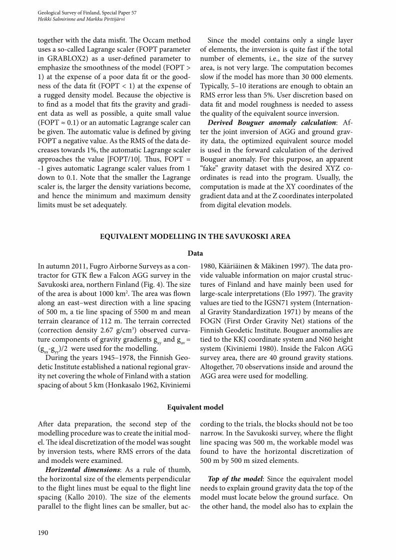
In autumn 2011, Fugro Airborne Surveys as a con-tractor for GTK flew a Falcon AGG survey in the Savukoski area, northern Finland (Fig. 4). The size of the area is about 1000 km2. The area was flown along an east–west direction with a line spacing of 500 m, a tie line spacing of 5500 m and mean terrain clearance of 112 m. The terrain corrected (correction density 2.67 g/cm3) observed curva-ture components of gravity gradients gxy and guv = (gxx-gyy)/2 were used for the modelling.
During the years 1945–1978, the Finnish Geo-detic Institute established a national regional grav-ity net covering the whole of Finland with a station spacing of about 5 km (Honkasalo 1962, Kiviniemi
1980, Kääriäinen & Mäkinen 1997). The data pro-vide valuable information on major crustal struc-tures of Finland and have mainly been used for large-scale interpretations (Elo 1997). The gravity values are tied to the IGSN71 system (Internation-al Gravity Standardization 1971) by means of the FOGN (First Order Gravity Net) stations of the Finnish Geodetic Institute. Bouguer anomalies are tied to the KKJ coordinate system and N60 height system (Kiviniemi 1980). Inside the Falcon AGG survey area, there are 40 ground gravity stations. Altogether, 70 observations inside and around the AGG area were used for modelling.
Equivalent model
After data preparation, the second step of the modelling procedure was to create the initial mod-el. The ideal discretization of the model was sought by inversion tests, where RMS errors of the data and models were examined.
Horizontal dimensions: As a rule of thumb, the horizontal size of the elements perpendicular to the flight lines must be equal to the flight line spacing (Kallo 2010). The size of the elements parallel to the flight lines can be smaller, but ac-
cording to the trials, the blocks should not be too narrow. In the Savukoski survey, where the flight line spacing was 500 m, the workable model was found to have the horizontal discretization of 500 m by 500 m sized elements.
Top of the model: Since the equivalent model needs to explain ground gravity data the top of the model must locate below the ground surface. On the other hand, the model also has to explain the
191
Geological Survey of Finland, Special Paper 57Calculation of the derived Bouguer anomaly using the equivalent source method based on
joint inversion of ground gravity and airborne gravity gradient data
Fig. 4. Savukoski Falcon AGG survey area in northern Finland, east–west flight lines, north–south tie lines and national ground gravity observation stations of the Finnish Geodetic Institute (red dots). Contains data from the National Land Survey of Finland Topographic Database 03/2013.
observed gradient data, which often change sharp-ly. For the best results, the depth to the top of the model should be more than half of the horizontal block size. In the Savukoski area, the top was set to a constant level of -247 m, 500 m below the aver-age flight height (253 m). The ground topography in the survey area ranges between 147–450 m.
Thickness of the layer: The thickness of the equivalent layer also requires some consideration. If it is too thick, the model cannot explain short wavelength anomalies in the gradient data. If the layer is too thin, large density contrasts are needed to explain ground gravity anomalies. In our case, the thickness of 250 m can give a very good fit for ground gravity data, but errors are larger for the gradients. For the final model, a thickness of 50 m
was found to give the best overall fit for both the gravity and gradient data.
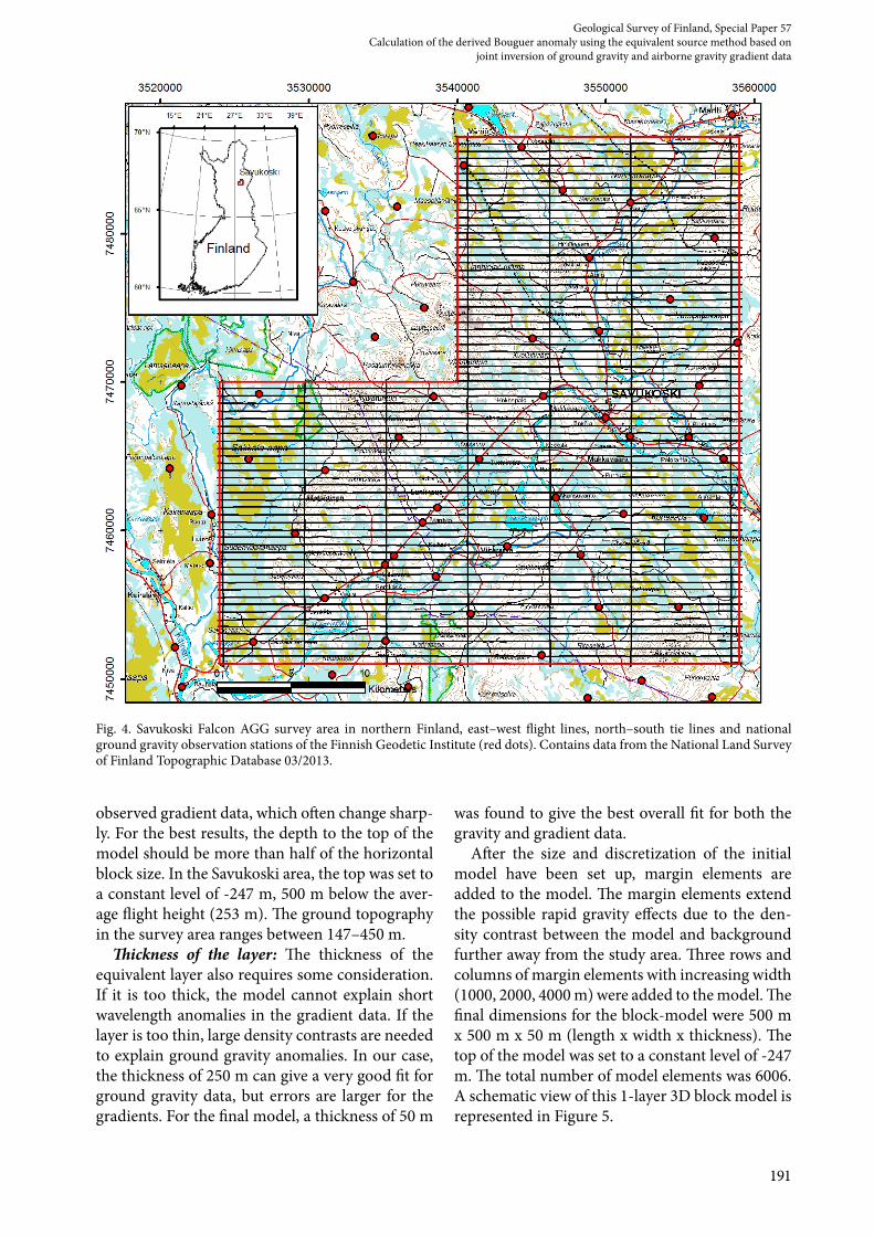
After the size and discretization of the initial model have been set up, margin elements are added to the model. The margin elements extend the possible rapid gravity effects due to the den-sity contrast between the model and background further away from the study area. Three rows and columns of margin elements with increasing width (1000, 2000, 4000 m) were added to the model. The final dimensions for the block-model were 500 m x 500 m x 50 m (length x width x thickness). The top of the model was set to a constant level of -247 m. The total number of model elements was 6006. A schematic view of this 1-layer 3D block model is represented in Figure 5.
192
Geological Survey of Finland, Special Paper 57Heikki Salmirinne and Markku Pirttijärvi
Fig. 5. Schematic view of the 1-layer 3D block model used for equivalent source modelling of the Savukoski AGG survey.
The final inversion was made using the model described above (6006 elements of size 500 m x 500 m x 50 m), similarly gridded Falcon AGG data (2 x 4024 data records) and 73 sparsely sampled ground gravity observations. The computation of 5 iterations took about 7.5 minutes with the GRA-
BLOX2 program on a PC with an Intel 3.3 GHz i5 processor. The forward computation of the derived Bouguer anomaly on a 500 m x 500 m station net on the ground surface using the resulting density model shown in Figure 5 took about 13 seconds.
RESULTS
Simultaneous inversion of densely sampled Falcon AGG data and the sparse ground gravity data of the Finnish Geodetic Institute using the joint in-version method described in the preceding chap-ter gaves the derived Bouguer anomaly presented in Figure 6 as the final result.
For comparison, the modelling was also car-ried out using a horizontally denser 250 m x 500 m model. The thickness (50 m) and depth to the top of the model (-247 m) were the same as before. Application of the denser model and data gridded at the same 250 x 500 m resolution did not appear to improve the result.
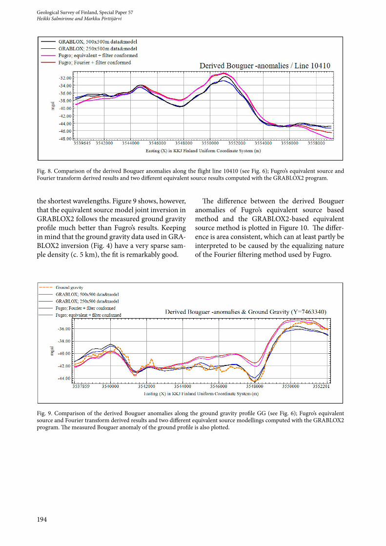
In Figures 7 and 8, the derived Bouguer anoma-lies computed by GRABLOX2 are compared with the results delivered to GTK by Fugro Airborne Surveys. The results are presented up to the profiles 10080 and 10410 shown in Figure 6. Fugro only used the gradient data in their equivalent source modelling, and the conforming with ground data was carried out using the Fourier domain filtering method. The equivalent model used by Fugro was composed of a thin flat layer of rectangular plates
sized 125 m x 125 m (email notification by Fugro). Although the results of GRABLOX and Fugro are not completely comparable due to the differ-ent modelling procedures applied, differences can particuarly be seen in relation to the long wave-lengths. These especially become visible on the eastern side of line 10080 and in the middle part of line 10410, where a clear level difference of the long wavelength is observed.
Figure 9 displays the Bouguer anomaly along the 14-km-long ground gravity profile GG (see Fig. 6), measured by GTK in 1990, and the de-rived Bouguer anomalies by Fugro and GRA-BLOX2. The ground gravity profile was measured with a station spacing of 20 m, resulting in more detailed (short wavelength anomalies) informa-tion than the Bouguer anomaly derived from the airborne gradient survey. This is due to the low-pass filtering of the gradient data to limit the ef-fect of noise. It has been evaluated that there are no anomalies shorter than 300 m wavelength in Falcon AGG data. Neither Fugro nor GRABLOX2 can reproduce the ground gravity anomalies with

193
Geological Survey of Finland, Special Paper 57Calculation of the derived Bouguer anomaly using the equivalent source method based on
joint inversion of ground gravity and airborne gravity gradient data
Fig. 6. The equivalent source method derived Bouguer anomaly of the Savukoski AGG survey with the difference between the derived Bouguer and ground gravity observations. The locations of the flight lines 10080 and 10410, and ground gravity profile GG measured in 1990, have also been plotted on the map.
Fig. 7. Comparison of the derived Bouguer anomalies along flight line 10080 (see Fig. 6); Fugro’s equivalent source and Fourier transform derived results and two different equivalent source results computed with the GRABLOX2 program.
194
Geological Survey of Finland, Special Paper 57Heikki Salmirinne and Markku Pirttijärvi
Fig. 8. Comparison of the derived Bouguer anomalies along the flight line 10410 (see Fig. 6); Fugro’s equivalent source and Fourier transform derived results and two different equivalent source results computed with the GRABLOX2 program.
the shortest wavelengths. Figure 9 shows, however, that the equivalent source model joint inversion in GRABLOX2 follows the measured ground gravity profile much better than Fugro’s results. Keeping in mind that the ground gravity data used in GRA-BLOX2 inversion (Fig. 4) have a very sparse sam-ple density (c. 5 km), the fit is remarkably good.
The difference between the derived Bouguer anomalies of Fugro’s equivalent source based method and the GRABLOX2-based equivalent source method is plotted in Figure 10. The differ-ence is area consistent, which can at least partly be interpreted to be caused by the equalizing nature of the Fourier filtering method used by Fugro.
Fig. 9. Comparison of the derived Bouguer anomalies along the ground gravity profile GG (see Fig. 6); Fugro’s equivalent source and Fourier transform derived results and two different equivalent source modellings computed with the GRABLOX2 program. The measured Bouguer anomaly of the ground profile is also plotted.

195
Geological Survey of Finland, Special Paper 57Calculation of the derived Bouguer anomaly using the equivalent source method based on
joint inversion of ground gravity and airborne gravity gradient data
Fig. 10. Difference between Fugro’s equivalent+filtered derived and GRABLOX2 equivalent derived Bouguer anomalies. The locations of profiles in Figures 7–9 are also plotted.
CONCLUSIONS
Gravity gradient data measured in airborne sur-veys are not suitable for the direct determination of the absolute vertical gravity field (or Bouguer anomaly). However, the derived Bouguer anom-aly can be calculated and integrated with ground gravity using either the Fourier transform method or the equivalent source method. In the equivalent source method, ground gravity data can success-fully be inverted simultaneously with airborne gradient data. Commercial computer programs enabling equivalent source modelling are not available on the market. In this study, equivalent source modelling using joint inversion of AGG and ground gravity data was carried out using
GRABLOX2 gravity interpretation and modelling software developed by the University of Oulu and GTK (Pirttijärvi 2009).
The discretization of the initial model depends on both the spatial coverage and resolution, as well as on the theoretical information content of the observations used in the modelling. This is mainly controlled by airborne gradient data due to their finer sampling compared with sparse ground grav-ity data. The flight line spacing gives the maximum width of the blocks perpendicular to the flight-line direction (Kallo 2010). Along flight lines, the dis-cretization should be no less than half of the flight-line spacing. Otherwise, the narrow elements create
196
Geological Survey of Finland, Special Paper 57Heikki Salmirinne and Markku Pirttijärvi
artefacts in the derived Bouguer anomaly. Because the equivalent model needs to explain both grav-ity and gradient data, the top of the model must locate below the ground surface. Choosing the thickness of blocks is a compromise between fitting the airborne gradient and ground gravity data. A thin layer of blocks gives a better fit for gradients, whereas a thick layer fits ground data better. In practice, a thin layer (less than half of the horizon-tal block size) appears to be better than thick layer (equal to or greater than the horizontal block size). A model in which the depth to the top of the blocks varies according to the drape survey does not im-prove the results. Therefore, the top of the blocks should be set at a constant level. In the Savukoski Falcon AGG survey area, the discretization of the 3D block model was 500 m x 500 m x 50 m (length x width x thickness). The top of the model was set to the level of -247 m (above sea level).
National ground gravity data of the Finnish Geo- detic Institute (station spacing 5 km) are suitable for simultaneous inversion with airborne gradient
data for equivalent modelling, when the size of the flight area is large enough. In order to model long wavelength information from the ground gravity data, the smallest dimension of the gradi-ent survey area should preferably be at least four times the station spacing of ground gravity. As a consequence, in Finland, the smallest dimension of a gradient survey should be at least 20 km. In the Savukoski survey, the smallest dimension is 19.3 km, which fulfils this requirement.
Although GRABLOX’s and Fugro’s results are not completely comparable due to the different modelling procedures, differences can especially be seen in relation to the long wavelengths. The simultaneous inversion of AGG and ground grav-ity data appears to reproduce the long wavelengths better, and hence, the results are more compatible with the ground gravity data.
It has been estimated that an airborne gradient survey flown with 500-m line spacing delivers infor-mation equivalent of ground gravity measurements performed with a station spacing 4 stations/km2
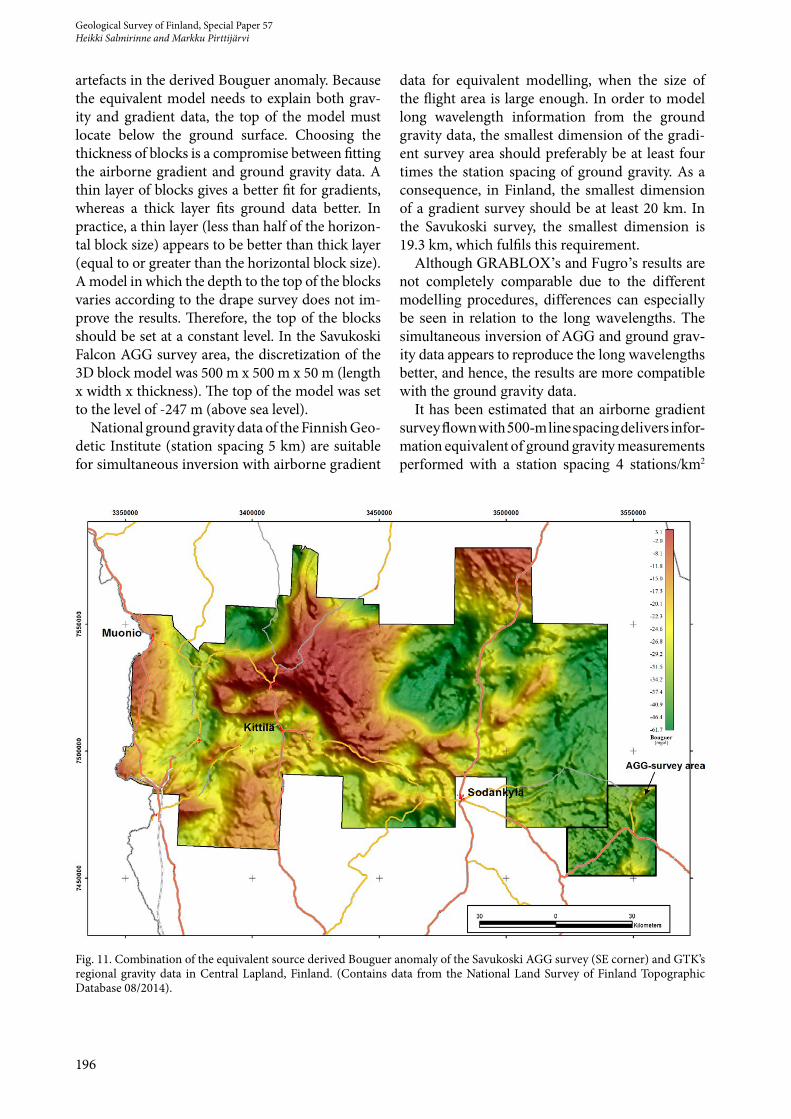
Fig. 11. Combination of the equivalent source derived Bouguer anomaly of the Savukoski AGG survey (SE corner) and GTK’s regional gravity data in Central Lapland, Finland. (Contains data from the National Land Survey of Finland Topographic Database 08/2014).
197
Geological Survey of Finland, Special Paper 57Calculation of the derived Bouguer anomaly using the equivalent source method based on
joint inversion of ground gravity and airborne gravity gradient data
(Dransfield 2013). The target sample density of GTK’s regional ground gravity surveys has been 4-6 stations/km2. The combination of the equiva-lent source derived Bouguer anomaly of the Sa-vukoski AGG survey and the Bouguer anomaly of GTK’s regional ground gravity data in Central Lapland is presented Figure 11. It can be seen that the derived Bouguer anomaly of the Savukoski AGG survey area matches well with the regional ground gravity in Central Lapland, where the data sample density varies between 1-6 stations/km2.
The equivalent source method, in which AGG and ground gravity data are simultaneously opti-mized, proved to be a feasible method for the in-tegration of ground gravity and airborne gradient data into the derived Bouguer anomaly and com-parable with the traditional regional ground gravity data. This type of integration should be an essen-tial part of a data processing flow if airborne grav-ity gradiometry technology is to be systematically applied to regional gravity mapping in the future.
ACKNOWLEDGEMENTS
This work was financed by the Finnish Fund-ing Agency for Innovation (TEKES) through the NovTecEx project (Green Mining programme). The authors would like to thank the Finnish Geo-
detic Institute for ground gravity data. Geophysi-cist Aimo Hattula is acknowledged for reviewing and his comments on improving the text.
REFERENCES
Blakely, R. J. 1995. Potential theory in gravity and magne-tic applications. Cambridge: Cambridge University Press. 441 p.
Dransfield, M. 2010. Conforming Falcon gravity and global gravity anomaly. Geophysical Prospecting 58, 469−483.
Dransfield, M. H. & Lee, J. B. 2004. The FALCON® airbor-ne gravity gradiometer systems. In: Lane, R. J. L. (ed.) Airborne Gravity 2004 − Abstracts from the ASEG-PESA Airborne Gravity 2004 Workshop. Geoscience Australia Record 2004/18, 15−19.
Dransfield, M. H. & Christensen, A. N. 2013. Performance of airborne gravity gradiometers. The Leading Edge, Au-gust 2013, 908−922.
Elo, S. 1997. Interpretations of the gravity anomaly map of Finland. In: The lithosphere in Finland − a geophysical perspective. Geophysica 33 (1), 51−80.
Hjelt, S.-E. 1972. Magnetostatic anomalies of dipping prisms. Geoexploration 10, 239−254.
Hjelt S.-E. 1974. The gravity anomaly of a dipping prism. Geoexploration 12, 29−39.
Honkasalo, T. 1962. Gravity surveys of Finland in years 1945-1960. Helsinki. 35 p., 3 maps.
Kääriäinen, J. & Mäkinen, J. 1997. The 1979-1996 gravity survey and results of the gravity survey of Finland 1945-1996. Suomen geodeettisen laitoksen julkaisuja 125. Kirkkonummi: Finnish Geodetic Institute. 24 p.
Kallo, M. 2010. Aerogravimetristen tensoriaineistojen yh-distäminen maanpinnan painovoima havaintoihin. Un-published M. Sc. thesis, University of Turku. 93 p. (in Finnish)
Kiviniemi, A. 1964. The First Order Gravity Net of Finland. Publications of the Finnish Geodetic Institute 59.
Kiviniemi, A. 1980. Gravity measurements in 1961-1978 and the results of the gravity survey of Finland in 1945-1978. Suomen geodeettisen laitoksen julkaisuja, 91. Fin-nish Geodetic Institute. 22 p.
Korhonen, J. V., Aaro, S., All, T., Elo, S., Haller, L. Å., Kääriäinen, J., Kulinich, A., Skilbrei, J. R., Solheim, D., Säävuori, H., Vaher, R., Zhdanova, L. & Koistinen, T. 2002. Bouguer anomaly map of the Fennoscandian Shield: IGSN 71 gravity system, GRS80 normal gravity formula. Bouguer density 2670 kg/m³, terrain correcti-on applied. Anomaly continued upwards to 500 m above ground; scale 1:2 000 000.
Lane, R. J. L. 2004. Integrating ground and airborne data into regional gravity compilations. In: Lane, R. J. L. (ed.) Airborne Gravity 2004 − Abstracts from the ASEG-PESA Airborne Gravity 2004 Workshop. Geoscience Australia Record 2004/18, 81−97.
Lee, J. B. 2001. FALCON gravity gradiometer technology. Exploration Geophysics 32, 247−250.
Murphy, C. A. 2004. The Air-FTG Airborne Gravity Gradio-meter System. In: Lane, R. (ed.) Airborne Gravity 2004 − Abstracts from the ASEG-PESA Airborne Gravity 2004 Workshop. Geoscience Australia Record 2004/18, 7−14.
Pirttijärvi, M. 2009. Grablox2 – Gravity interpretation and modelling software based on 3-D block models, user’s guide to version 2.0. Department of Physics, University of Oulu, 62. Available at: https://wiki.oulu.fi/download/attachments/20678029/Grablox2_manu.pdf