calculating eﬀective conductivity of heterogeneous soils ... · pdf filecalculating...

Archives of Hydro-Engineering and Environmental MechanicsVol. 52 (2005), No. 2, pp. 111–130

© IBW PAN, ISSN 1231–3726

Calculating Effective Conductivity of Heterogeneous Soils by

Homogenization

Adam Szymkiewicz

Institute of Hydro-Engineering of the Polish Academy of Sciences,

ul. Kościerska 7, 80-328 Gdańsk, Poland, e-mail: [email protected]

(Received March 07, 2005; revised May 23, 2005)

Abstract

The paper concerns effective conductivity of a heterogeneous soil composed of twomaterials characterized by different hydraulic conductivities. According to the homo-genization theory the effective conductivity is obtained from the solution of an el-liptic equation for a single representative elementary volume. A numerical algorithmto solve this equation is described. Examples of calculations for periodic media withinclusions of various shapes are presented. Influence of volumetric fraction, arrange-ment, continuity and conductivity ratio of the two materials on the effective conduct-ivity is investigated. Numerical results are compared with some analytical estimationsavailable in the literature.

Key words: effective conductivity, soil heterogeneity, groundwater flow, up-scaling,homogenization

1. Introduction

Water flow in soils is commonly described by the following generalized equation,holding for both saturated and unsaturated conditions (e.g. Bear 1972, Zaradny1993):

.C .h/ C cs S/@h

@t� r Ð .K .h/ r .h C x3// D 0; (1)

where C.h/ is the specific moisture capacity, cs the specific storage coefficient, S

saturation of the water phase, K(h/ the hydraulic conductivity tensor, h the waterpressure head (also known as suction head or capillary head in the unsaturatedzone), x3 the vertical coordinate. In the saturated zone h > 0, C D 0, S D 1 andK is independent of h. In unsaturated conditions h < 0, S < 1, the coefficients C

and K are nonlinear functions of h, and the term cs S is negligibly small comparedto C. Eq. (1) is valid on the assumption that the air phase filling pore space is atconstant atmospheric pressure.

112 A. Szymkiewicz

In practical applications one often has to deal with heterogeneous soils con-

taining shales, lenses or other inclusions, characterized by the hydraulic conductiv-

ity K2.h/ very different from the conductivity of the base material (matrix) K1.h/,

as shown in Fig. 1. If the modelled domain contains a large number of such in-

clusions, the local variability of K is difficult to account for in the solution of

Eq. (1). In such case it is convenient to describe the flow at macroscopic scale,

where the soil is considered to be homogeneous and characterized by effective

(macroscopic) capacity Ce f f .h/ and effective conductivity Ke f f .h/.

inclusions W2

conductivity K2

l

macroscopic scale local scale

L

REV (W)

matrix W1

conductivity K1

interface G

L >> l

Fig. 1. Observation scales in a heterogeneous soil

The macroscopic equations can be derived from the local-scale equations using

various mathematical techniques. One possible choice is the asymptotic homogen-

ization method (Bensoussan et al. 1978, Sanchez-Palencia 1980, Auriault 1991).

Application of this method to the problem of unsaturated flow in heterogeneous

soils is described in the papers by Lewandowska & Laurent (2001), Lewandowska

& Auriault (2004) and Lewandowska et al. (2004). These papers present mac-

roscopic equations and definitions of the effective conductivity Ke f f .h/ and the

effective capacity Ce f f .h/ for three different cases: (1) moderately heterogeneous

soil with local parameters of the same order, (2) soil with highly conductive inclu-

sions and (3) soil with weakly conductive inclusions. In each model the effective

conductivity coefficient is obtained from the solution of the local boundary value

problem for an elliptic equation in the domain of a single representative element-

ary volume (REV). The models were validated by comparison with the results

of “numerical experiments”, i.e. direct solution of the local scale equation in

heterogeneous domain (e.g. Lewandowska et al. 2004, Szymkiewicz 2004). Some

preliminary results concerning comparison with laboratory experiments are also

available (Lewandowska et al. 2005).

Calculating Effective Conductivity of Heterogeneous Soils by Homogenization 113

Apart from the derivation of a complete macroscopic description, a largeamount of research has been focused solely on the estimation of the effectiveconductivity Ke f f for heterogeneous media. From the point of view of the mac-roscopic description, such information is sufficient for steady flow. An overviewof the methods employed to calculate the effective hydraulic conductivity (orpermeability) is presented in the papers by Wen & Gomez-Hernandez (1996)and Renard & de Marsily (1997). The most popular approaches include directnumerical solution of the flow equation in a REV domain (Harter & Knudby2004), renormalization (King 1989) and self-consistent methods (Dagan 1989, Po-ley 1988). One should note that the problem of calculating the effective transportproperties concerns all physical processes described by equations similar to Eq.(1), e.g. thermal or electric conduction, diffusion, etc. – see for example, the worksof Markov (1999) or Berryman (1995).

This paper aims to present the numerical calculation of the effective conduct-ivity according to the asymptotic homogenization theory. The numerical resultsobtained for model soils of periodic structure with two- or three- dimensionalinclusions will be compared with some analytical estimations available in the lit-erature.

The following notation will be used throughout the paper. The conductivitiesof the two components are denoted by K1 and K2 (tensors) if the materials areanisotropic or K1 and K2 (scalars) if they are isotropic. The effective conductivity

tensor is denoted by Ke f f and its elements by Ke f fi j . If the effective conductivity

is isotropic it is denoted as scalar K e f f .

2. Analytical Estimations of the Effective Conductivity

Consider a heterogeneous soil composed of two isotropic materials with the con-ductivity of K1 and K2, and volumetric fractions f1 and f2, respectively. For anyspatial arrangement of the materials the elements of the effective conductivitytensor are bound in the following manner (e.g. Markov 1999):

�

f1 K�11 C f2 K�1

2

��1D Kh � K

e f fi j � Ka D f1 K1 C f2 K2: (2)

The bounds (2) are known as Wiener or Voigt-Reuss bounds. The upper andlower bounds correspond respectively to the weighted arithmetic mean Ka andweighted harmonic mean Kh of the components’ conductivities. These two means

are the exact values of Ke f fi j in perfectly layered soil, respectively for flow in

the direction parallel (Ka/ or orthogonal (Kh/ to the layers. Thus, a layered

arrangement of components shows the largest anisotropy. In all other cases Ke f fi j

is somewhere between the harmonic and arithmetic mean. Obviously, the largerthe difference between the components’ conductivities, the wider the range of theadmissible values of the effective conductivity.

114 A. Szymkiewicz

The effective conductivity of heterogeneous media is commonly estimated us-ing the effective medium theory. It focuses on the analysis of the perturbationof the potential field (pressure field in this case) caused by the presence of asingle inclusion of different conductivity in a homogeneous material. On this

basis, the effective conductivity for a material containing random dispersion ofinclusions is estimated. Different variants of the effective medium methods exist(e.g. self-consistent or differential approach). Their application is described, forexample, in the contributions of Markov (1999), Dagan (1989), Giordano (2003),Jones & Friedman (2000) or Fokker (2001).

One of the well-known results concerns macroscopically isotropic medium with3D spherical or 2D circular inclusions. The effective conductivity is given by thefollowing formula (e.g. Markov 1999):

K e f f D K1K2 C .D � 1/ K1 � .D � 1/ f2 .K2 � K1/

K2 C .D � 1/ K1 C f2 .K2 � K1/; (3)

where indices 1 and 2 denote matrix and inclusion parameters respectively andD is the number of dimensions (D = 2 or 3). Eq. (3) is known as Maxwell’sformula for D = 3 or Raleigh’s formula for D = 2 (different names are alsoused). Hashin & Shtrikman (1962) showed that, for a macroscopically isotropicmedium composed of two materials of the conductivity K1 and K2, arbitrarilyarranged in space, Eq. (3) provides the maximum value of K e f f when K1 > K2

and the minimum value of K e f f when K1 < K2. Thus, the values obtained fromEq. (3) are known as Hashin-Shtrikman bounds. The other bounding value foreach case mentioned can be obtained by interchanging K1 with K2 and f1 withf2 in Eq. (3).

The effective medium theory has also been applied to anisotropic media. Theeffective conductivity coefficient for a medium containing a dispersion of uniformlyaligned ellipsoids is given by the following formula (Berryman 1995, Giordano2003):

Ke f fi i D K1 C f2 .K2 � K1/

h

1 C f1 pi .K2 � K1/ .K1/�1i�1

; (4)

where pi is the depolarising factor in the direction i , assuming values from therange h0; 1i, while p1 C p2 + p3 = 1. Note that in this case the effective conduct-ivity is a diagonal tensor, the main anisotropy axes being parallel to the ellipsoids’axes. The depolarising factors depend on the shape of the ellipsoid and are definedby the following elliptic integral:

pi Da1a2a3

2

Z C1

0

du�

u C a2i

Ð

q

�

u C a21

Ð �

u C a22

Ð �

u C a23

Ð

i D 1; 2; 3; (5)


where a1, a2 and a3 denote the lengths of the ellipsoid axes parallel to the respect-

ive directions. The computation of the depolarising factors for various geometries

is presented in detail by Markov (1999) and Giordano (2003). For ellipses theycan be calculated from Eq. (5), assuming that a3 ! 1. In this case p1 + p2 =

1, while p3 = 0. For inclusions in the form of a circle (p1 D p2 D 1=2/ or sphere

(p1 D p2 D p3 D 1=3/ Eq. (4) reduces to Eq. (3). For inclusions in the form of lay-

ers orthogonal to p1 direction p1 D 1; p2 D p3 = 0 and Eq. (4) gives the harmonicmean of K1 and K2. One should note, however, that for anisotropic ellipses and

ellipsoids Eq. (4) does not define bounds of the effective conductivity, contrary to

Eq. (3).

Both presented formulae have been derived for the assumption that the volu-metric fraction of inclusions is small ( f2 − 1), and the interaction between inclu-

sions can be neglected. For larger volumetric fraction of inclusions one can use

Bruggemann’s formula in the following form (Berryman 1995, Giordano 2003):

f1 .K2 � K1/ .K1/�pi D�

K2 � Ke f fi i

� �

Ke f fi i

��pi

: (6)

In this case Ke f fi i is given implicitly and Eq. (6) has to be solved by a numerical

method.

3. Definition of the Effective Conductivity According to the

Homogenization Theory

Consider a soil composed of two materials (anisotropic in a general case) of theconductivities K1 and K2 and the volumetric fractions f1 and f2. The soil has

periodic structure. The REV (representative elementary volume, equivalent to

period) is denoted by �, its parts occupied by the two materials by �1 and �2,

respectively, and the interface between them by 0. The dimension of the REVis very small compared to the dimensions of the considered macroscopic domain

(Fig. 1), i.e. the following relation holds:

" Dl

L− 1; (7)

where " is scale parameter, l is the REV dimension, L is the dimension of the

macroscopic domain. Eq. (1) represents a necessary condition for the existenceof a macroscopic model. According to the homogenization theory the effective

conductivity of such medium is defined as (Lewandowska & Laurent 2001):

Ke f f D1

j�j

�Z

�1

�

K1r�

�I C y

��

d� CZ

�2

�

K2r�

�II C y

��

d�

½

; (8)

116 A. Szymkiewicz

where j�j is the REV volume, y = [y1, y2, y3] is the local spatial coordinateassociated with the REV and the vector function � = [�1, �2, �3] is the solutionof the following equation:

r Ð K1 r�

�I C y

Ð

D 0 in �1; (9a)

r Ð K2 r�

�I I C y

Ð

D 0 in �2; (9b)

with � D �I in �1 and � = �

I I in �2. At the interface 0 the function � and its“flux” Kr .� C y/ are continuous:

�I D �

I I on 0; (10)

K1 r�

�I C y

Ð

N D K2 r�

�I I C y

Ð

N on 0; (11)

where N is a unit vector normal to 0. The function � is y-periodic:

� .yi / D � .yi C li / ; (12)

where li is the REV dimension in the specific direction yi . For such boundaryproblem an infinite number of solutions exists, which differ by a constant value.In order to obtain a unique solution we assume that the average of function � in� is equal to zero:

1

j�j

Z

�

� d� D 0: (13)

Equations (9a, b) with the conditions (10)–(13) are known as the local bound-ary value problem. Its solution can be considered as equivalent to the solution ofsteady flow equation in a single REV with unit pressure gradient in directions y1,y2 and y3, respectively. In scalar notation one obtains three equations – one foreach component of �. If both materials are locally isotropic, the equations havethe following form:

@

@y1

�

K@�1

@y1C K

�

C@

@y2

�

K@�1

@y2

�

C@

@y3

�

K@�1

@y3

�

D 0; (14)

@

@y1

�

K@�2

@y1

�

C@

@y2

�

K@�2

@y2C K

�

C@

@y3

�

K@�2

@y3

�

D 0; (15)

@

@y1

�

K@�3

@y1

�

C@

@y2

�

K@�3

@y2

�

C@

@y3

�

K@�3

@y3C K

�

D 0; (16)

where K D K1, � D �I in �1 and K D K2, � D �

I I in �2. In this case the elementsof the conductivity tensor:


Ke f f D

2

6

6

6

6

4

Ke f f11 K

e f f12 K

e f f13

Ke f f21 K

e f f22 K

e f f23

Ke f f31 K

e f f32 K

e f f33

3

7

7

7

7

5

; (17)

are defined in the following manner:

Ke f fi j D

1

j�j

�Z

�1

�

K1@�i

@y jC K1

�

d� CZ

�2

�

K2@�i

@y jC K2

�

d�

½

i D j; (18)

Ke f fi j D

1

j�j

�Z

�1

�

K1@�i

@y j

�

d� CZ

�2

�

K2@�i

@y j

�

d�

½

i 6D j: (19)

The effective conductivity is a function of the conductivities of both materialsand of the local geometry. The influence of the REV geometry is representedby the function �. Note that for a perfectly layered soil analytical solution of the

problem (9)–(13) is possible, yielding Ke f fi j equal to the arithmetic or harmonic

mean of the components’ conductivities, which coincides with Eq. (2).The definition (8)–(13) was obtained under the assumption that the hydraulic

conductivities of the two materials K1 and K2 are of the same order (Lewandowska& Laurent 2001). However, it can be shown that the definition has a more generalcharacter and is applicable regardless of the local conductivity ratio (Szymkiewicz2004). It is valid for soils with inclusions, as well as for soils composed of twointerconnected materials. Similar definitions of the effective conductivity wereproposed by other authors for single-phase and two-phase flow, using asymptotichomogenization (e.g. Saez et al. 1989) or volume averaging (e.g. Quintard &Whitaker 1988).

For flow in partially saturated conditions K1 and K2 as well as Ke f f are func-tions of the pressure head h. A single point of the Ke f f .hi / function is obtainedassuming the same value of the pressure head hi in �1 and �2, and solving thelocal boundary value problem (9)–(13) with K1 = K1.hi / and K2 = K2.hi /. Re-peating this procedure for several values of hi one obtains the function Ke f f .h/

in tabularized form (Lewandowska & Laurent 2001).

4. Numerical Solution of the Local Boundary Value Problem

The results presented in this paper were obtained using a numerical code de-veloped by the author, based on the finite volume method (FVM). FVM is relat-ively simple in implementation and well suited for elliptic equations with discon-tinuous coefficients (Crumpton et al. 1995).

The REV domain � is divided into M D M1 ð M2 ð M3 uniform cuboids (fi-nite volumes or cells) of the dimensions 1y1 ð 1y2 ð 1y3 (Fig. 2). Each volume

118 A. Szymkiewicz

is characterized by a scalar hydraulic conductivity K1 or K2. The values of � are

sought for at the geometrical centres of the volumes. The solution procedure isoutlined on the example of Eq. (14) defining the component �1.

c1(i,j,k) c1(i+1,j,k)

c*Dy1

Dy3Dy2

l1

l2

l3

i = 1 i = M1

j = M2

k = M3

j = 1k = 1

K(i,j,k) K(i+1,j,k)

Fig. 2. Discretization of the REV domain for the solution of the local boundary value problem

According to the standard FVM procedure Eq. (14) can be written for eachfinite volume in the following conservative form:

Z

V

.r Ð K r .�1 C y1// dV DZ

S

.K r .�1 C y1// ndS DX6

lD1ql Al ; (20)

where K stands for either K1 or K2, V and S denote the volume and the externalsurface of the cell, n is a unit vector normal to S, ql is the „flux” at each of the 6

sides of the cell, and Al the side’s surface. At the sides orthogonal to the y1 axisq is equal to:

q D K@�1

@y1C K; (21)

while at the other sides:

q D K@�1

@yi; (22)

where i = 2 or 3. The fluxes ql are approximated using the continuity conditions

for the function �1 and its flux (10)–(11). For the flux q between the cells (i; j; k/

and (i + 1, j , k/ having (in a general case) different hydraulic conductivities K.i; j;k/

and K.iC1; j;k/ (Fig. 2) the continuity conditions yield:


K.i; j;k/

�Ł � �1.iC1; j;k/

121y1

C K.i; j;k/ D q D K.iC1; j;k/

�1.iC1; j;k/ � �Ł

121y1

C K.iC1; j;k/; (23)

where �* is the value of �1 at the side’s centre. The formula for q resulting from(23) is:

q D2K.i; j;k/ K.iC1; j;k/

K.i; j;k/ C K.iC1; j;k/

�.iC1; j;k/ � �.i; j;k/

1y1C

2K.i; j;k/ K.iC1; j;k/

K.i; j;k/ C K.iC1; j;k/

: (24)

As can be seen, the hydraulic conductivity at the cell’s side is equal to theharmonic mean of the neighbouring cells’ conductivities. The fluxes at the othersides of the cell are approximated in the same manner. For the cells adjacent to theexternal boundary of the domain � one makes use of the periodicity conditions.Consider, for example, the approximation of fluxes in y1 direction. The formulaanalogous to Eq. (24) written for the external sides of boundary cells (1, j , k/ and(M1, j , k/ would involve the values of �1.0; j;k/ and �1.M1C1; j;k/ corresponding to thefictional cells adjacent to the boundary, but lying outside the solution domain. Dueto periodicity conditions these values can be replaced by their counterparts fromthe opposite boundary: �1.0; j;k/ D �1.M1; j;k/ and �1.M1C1; j;k/ D �1.1; j;k/. Finally, inorder to obtain a unique solution of Eq. (14) (and to satisfy Eq. (13)) the value�1 = 0 should be specified at a single point of the solution domain.

Spatial discretization of Eq. (14) performed in the manner presented aboveleads to a system of linear algebraic equations with sparse and banded coefficientmatrix (the maximum number of non-zero elements in a single row is 5 for a 2Dproblem and 7 for a 3D problem). The system is solved using the conjugatedgradient method (Bjorck & Dahlquist 1974). Having obtained the values of �1.i; j;k/

one can compute the integrals (18) and (19). The gradients of �1 appearing inthe integrals are approximated numerically according to Eqs. (21)–(24).

5. Examples

5.1. Local Geometry and Numerical Parameters

The calculations were performed for soils of periodic structure. The representat-ive elementary volume (period) is a rectangle of dimensions l1 ð l2 or a cuboid ofdimensions l1 ð l2 ð l3. The soil is composed of the base material (matrix) with theconductivity of K1 and embedded inclusions with the conductivity of K2 (both ma-terials are locally isotropic). In three-dimensional case the inclusions have formsof cuboids, ellipsoids and octahedra (bipyramids) (Fig. 3). Their 2D analogues arerectangles, ellipses and rhombi. The inclusions are of uniform size and orientation,their dimensions in the directions y1, y2 and y3 being denoted by a1, a2 and a3.Two types of arrangements are studied (Fig. 3): simple arrangement (the centres

120 A. Szymkiewicz

of inclusions are placed in the corners of the REV) and centred arrangement (the

centres of inclusions are placed in the corners and in the centre of the REV).

The inclusions are allowed to overlap. Note that all geometries are symmetric

with respect to the coordinate axes (or planes). Thus, the effective conductivity

tensor has off-diagonal elements equal to zero. The effective conductivity does

not depend on the unit system, so in most of the examples dimensionless values

will be used.

a1

a2

a3

l3

l1

l2

simple arrangement centred arrangement

Fig. 3. Three-dimensional inclusion shapes (cuboids, ellipsoids and octahaedra) and arrangements(simple and centred) used in numerical examples

In order to minimize the numerical error and investigate the convergence of

the solution, numerical tests were carried out for different mesh densities. The

tests showed that for the geometries considered in this study sufficient accuracy of

the solution is obtained with 40 cells in each direction – the results presented in

the following sections were obtained for such numerical mesh. Further increasing

of the number of cells does not significantly influence the solution (relative errors

below 3%).

A typical example of the solution of the local boundary value problem for

a two-dimensional case is presented in Fig. 4. The figure shows distributions of

�1.y1,y2/ and �2.y1,y2/ functions for weakly conductive rectangular inclusions in

centred arrangement (K2/K1 = 10�4/. The periodicity and anti-symmetry of both

functions are clearly visible. Minimum and maximum values occur in the vicinity

of the parts of inclusion – matrix interface which are orthogonal to the respective

flow direction (y1 or y2/.


y1

y1

y2

y2

c2 (y1,y2)

c1 (y1,y2)

K1=1

K2=10-4

Fig. 4. Example of the distribution of �1 and �2 functions for a 2D geometry with weaklyconductive inclusions

5.2. Influence of the Local Conductivity Ratio

The influence of the components’ conductivity ratio on the effective conductiv-

ity of a heterogeneous soil is shown on two-dimensional examples. They concern

square inclusions in simple arrangement ( f2 = 0.49) and rectangular inclusions

in simple arrangement ( l1= l2 = 1, a1 = 0.9, a2 = 0.5, f2 = 0.45). The relation

between the effective conductivity and the inclusion conductivity K2 is shown in

Fig. 5. The values of both coefficients are calculated with respect to the matrix

conductivity K1. For rectangular inclusions both components of the effective con-

ductivity tensor are shown. The obtained functions have sigmoidal shape, reaching

constant values for large conductivity contrast. This means that for inclusions much

more or much less conductive than the matrix (K2/K1 < 10�3 or K2/K1 > 103/ the

effective conductivity becomes a linear function of the matrix conductivity. The

linear coefficient depends on the geometry of the medium. For smaller difference

of the components’ conductivities the effective conductivity depends on both K1

and K2. Similar results (not shown here) were obtained for three-dimensional

geometries.

122 A. Szymkiewicz

Fig. 5. Relation between the effective conductivity and the inclusion – matrix conductivity ratioK2/K1 for 2D inclusions

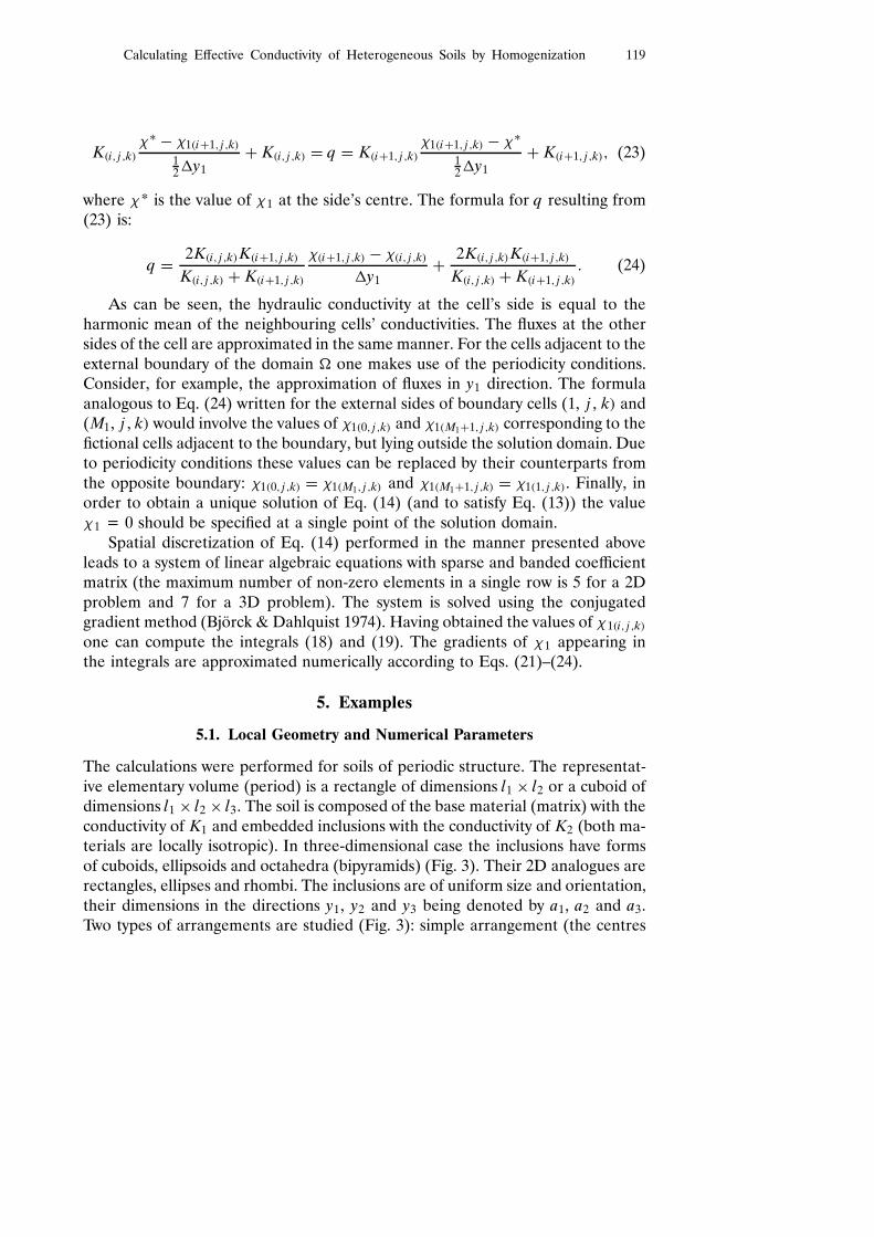
In partially saturated conditions the conductivities of both materials and their

ratio are highly non-linear functions of the water pressure head h. Consequently,the effective conductivity also depends on h. This relation is shown on the example

of a heterogeneous soil composed of loamy sand and silty clay. The calculationswere performed for a 2D isotropic geometry with square inclusions in simple

arrangement ( f2 = 0.49, a1/a2 D l1/l2 = 1, a1/l1 = 0.7). Parameters of the twomaterials are taken after (Carsel & Parrish 1988). The conductivity curves K.h/

of sand and clay cross and the parameter ratio varies in a wide range (Fig. 6). Theeffective conductivity function K e f f .h/ has been computed for two different cases:

loamy sand matrix with silty clay inclusions and silty clay matrix with loamy sandinclusions. As one can see, the functions differ substantially from each other,

since the effective conductivity strongly depends on the continuity of the mostconductive material. Both effective curves have a characteristic shape – for each

one two segments can be distinguished corresponding to the zones where theinclusion – matrix conductivity ratio is greater or less than one.

5.3. Influence of the Local Geometry – Isotropic Case

In this section the influence of the shape and volumetric fraction of inclusions on

the effective conductivity of an isotropic medium is investigated. The calculationshave been performed for 2D geometry (a1 D a2, l1 D l2/ and 3D geometry (a1 Da2 D a3, l1 D l2 = l3/. The inclusions were either much more conductive or muchless conductive than the matrix (K2/K1 = 104 or K2/K1 = 10�4/. The volumetric

fraction of inclusions f2 ranged from 0 to 1, i.e. overlapping of inclusions wasallowed. The limit value of f2, for which the inclusions become connected depends

on their shape and arrangement (Tabl. 1). In the two-dimensional case whenthe inclusions become connected the matrix loses its continuity, thus the two


Fig. 6. Effective conductivity of an heterogeneous soil as a function of the capillary pressure head

materials interchange their roles. In the three-dimensional case the matrix keepsits continuity even for overlapping inclusions. In this case the continuity of the

matrix is lost for f2 close or equal to 1 (minimum values are 0.83 for octahedra

in simple arrangement and 0.95 for ellipsoids in simple arrangement). For each

analyzed case the effective conductivity calculated from the formulae (2), (4) and(6) are also shown.

Table 1. Limit value of the volumetric fraction of inclusions f2 for which the inclusions become

connected

Arrangement

Shape simple centered

rectangle 1 1=2

ellipse ³=4 ³=4

rhombus 1=2 1

cuboid 1 1=4

ellipsoid ³=6 ³p

3=8

octahedron 1=6 1=3

For two-dimensional geometries (Fig. 7) K e f f calculated according to the ho-

mogenization theory are inside Wiener bounds (Eq. 2) and correspond to the

Hashin-Shtrikman bounds (Eq. 4) – upper bound for weakly conductive inclusions

and lower bound for highly conductive inclusions (note that for larger volumetricfraction f2 inclusions and matrix interchange their roles). Bruggemann’s equation

124 A. Szymkiewicz

(6) gives values of K e f f smaller for weakly conductive inclusions and larger for

highly conductive inclusions, as compared to the values obtained by homogeniz-

ation. Thus, Eq. (4) seems to be a better approximation of effective conductivity

for 2D periodic and isotropic geometries than Eq. (6). For small volumetric frac-tions of inclusions ( f2 < 0:3 or f2 > 0:8) Eqs. (4) and (5) give very similar values

of K e f f . The influence of shape and arrangement of inclusions on the effective

conductivity seems negligible. Note the symmetry of the K e f f . f2/ functions for

K2 > K1 and K2 < K1.

Fig. 7. Effective conductivity for 2D isotropic geometries as a function of volumetric fraction ofinclusions

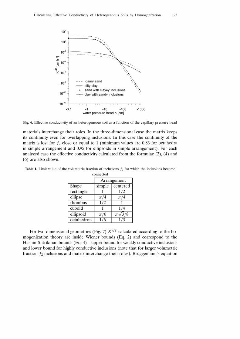
In the three-dimensional case (Fig. 8) a similarity of the results obtained fordifferent shapes and arrangements of inclusions and calculated from Eq. (4) can

be observed when one of the materials is discontinuous. However, there is no

symmetry between the results for K2 > K1 and K2 < K1. This is due to the fact

that when both materials are continuous, the effective conductivity depends on

the conductivity of the most permeable material. When the highly conductiveinclusions become interconnected, the effective conductivity increases rapidly by

several orders of magnitude. On the other hand, when the weakly conductive

inclusions become interconnected, the effective conductivity does not change sig-

nificantly as long as the most permeable material keeps its continuity. However,

in such situation the values of K e f f are somewhat smaller compared to the valuesobtained from Eq. (4). In this case Eq. (6) appears a better approximation, al-

though the influence of the shape and arrangement of inclusions is more visible.


All values calculated according to the homogenization theory are inside Wienerand Hashin-Shtrikman bounds. One can also notice, that for the same volumetricfraction f2 the effective conductivity is greater for three-dimensional geometry,than the two-dimensional one.

5.4. Influence of the Local Geometry – Anisotropic Case

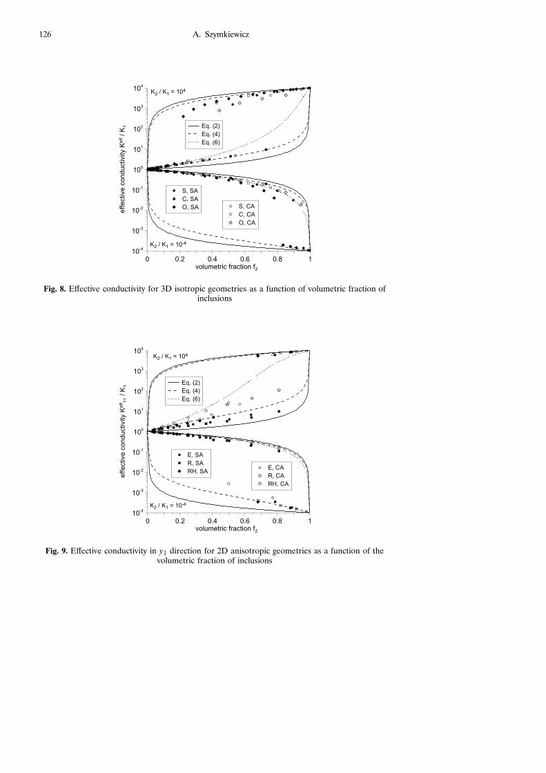
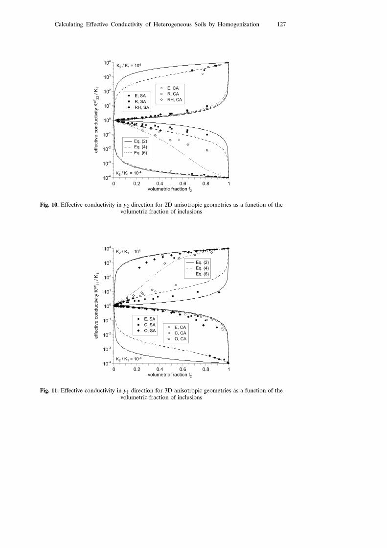
A similar series of calculations has been performed for anisotropic geometries,assuming a1=a2 D l1= l2 = 5 for the 2D case and a1=a3 D l1= l3 = 5, a2=a3 D l2= l3 =2 for 3D case. The depolarising factors are p1 = 0.167, p2 = 0.833 for 2D geometryand p1 = 0.090, p2 = 0.310, p3 = 0.600 for 3D geometry. The effective conductivityis given by a diagonal tensor. The results for two-dimensional case are presentedin Figs. 9 and 10. The figures show the effective conductivity in the direction of the

longer and shorter axis of the inclusions, respectively. The values of Ke f f11 for K2 >

K1 and the values of Ke f f22 for K2 < K1 obtained from homogenization are strongly

dependent on the shape and arrangement of inclusions. The difference betweenEqs. (4) and (6) is also significant in those cases. In other cases the analytical andnumerical approximations are very close. Thus, the effective conductivity seemsto be strongly related to the geometrical parameters if the flow is parallel tothe longest axis of highly conductive inclusions or parallel to the shortest axisof the weakly conductive inclusions. In both cases the transport properties ofthe composed medium are determined by the distance between the inclusions,measured along the longest axis. In the case of highly conductive inclusions itrepresents the minimum thickness of the weakly permeable layer which slowsdown the flow, while for weakly conductive inclusions it represents the maximumsize of highly conductive “gaps”, which enable faster flow. One can notice some

regularity of the results for different geometries. Ke f fi i is closer to the matrix

conductivity for simple arrangement compared to the centred arrangement. Foreach of the arrangements the values closest to the matrix conductivity correspondto rectangular inclusions, while the values closest to the inclusions conductivitycorrespond to rhombic inclusions. At the same volumetric fraction f2 rhombi havethe largest dimensions, while rectangles have the smallest dimensions. Similar tothe isotropic 2D geometries a symmetry between results for K2 > K1 and K2 < K1

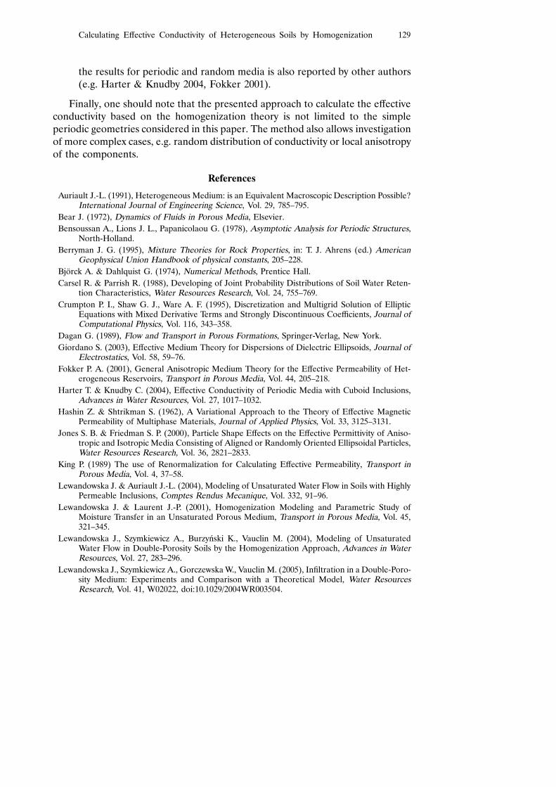
is observed for anisotropic 2D geometries.The results for three-dimensional geometries are presented in Figs. 11 and

12, showing the effective conductivity in y1 and y3 directions, respectively. Onecan observe similar differences between different shapes and arrangements ofinclusions as for the two-dimensional case. However, the results for K2 > K1 andK2 < K1 do not show symmetry, due to the continuity of the highly conductivematerial (as in the 3D isotropic case).

Although the relations between Ke f fi i and f2 described by the analytical formu-

lae (4) and (6) roughly correspond to the numerical results obtained for periodic

126 A. Szymkiewicz

Fig. 8. Effective conductivity for 3D isotropic geometries as a function of volumetric fraction ofinclusions

Fig. 9. Effective conductivity in y1 direction for 2D anisotropic geometries as a function of thevolumetric fraction of inclusions

128 A. Szymkiewicz


geometries, they do not fit exactly to any particular geometry in the anisotropiccase. In contrast to the isotropic case some values calculated numerically accordingto the homogenization theory fall outside the range defined by Eq. (4), howeverthey always satisfy Wiener bounds given by Eq. (2).

6. Summary and Conclusions

Although the presented analysis is far from being exhaustive, it allows us to drawsome conclusions on the effective conductivity of heterogeneous soils with peri-odically arranged inclusions:

ž When the inclusions are much more permeable or much less permeablethan the matrix, the effective conductivity becomes a linear function of thematrix conductivity, independent of the conductivity of the inclusions.

ž For macroscopically isotropic media with disconnected inclusions the ef-fective conductivity obtained for periodic geometries is very close to theeffective medium approximation (i.e. Hashin-Shtrikman bounds), regardlessof the shape and arrangement of the inclusions. It means that periodic andrandom media are equivalent in this case.

ž In the case of anisotropic media the results obtained for periodic geomet-ries show significant influence of the shape and arrangement of inclusionson the effective conductivity in some directions. None of the consideredperiodic geometries corresponds exactly to the effective medium approxim-ations, although some qualitative similarity can be observed. Discrepancy of


the results for periodic and random media is also reported by other authors(e.g. Harter & Knudby 2004, Fokker 2001).

Finally, one should note that the presented approach to calculate the effectiveconductivity based on the homogenization theory is not limited to the simpleperiodic geometries considered in this paper. The method also allows investigationof more complex cases, e.g. random distribution of conductivity or local anisotropyof the components.

References

Auriault J.-L. (1991), Heterogeneous Medium: is an Equivalent Macroscopic Description Possible?International Journal of Engineering Science, Vol. 29, 785–795.

Bear J. (1972), Dynamics of Fluids in Porous Media, Elsevier.

Bensoussan A., Lions J. L., Papanicolaou G. (1978), Asymptotic Analysis for Periodic Structures,North-Holland.

Berryman J. G. (1995), Mixture Theories for Rock Properties, in: T. J. Ahrens (ed.) AmericanGeophysical Union Handbook of physical constants, 205–228.

Bjorck A. & Dahlquist G. (1974), Numerical Methods, Prentice Hall.

Carsel R. & Parrish R. (1988), Developing of Joint Probability Distributions of Soil Water Reten-tion Characteristics, Water Resources Research, Vol. 24, 755–769.

Crumpton P. I., Shaw G. J., Ware A. F. (1995), Discretization and Multigrid Solution of EllipticEquations with Mixed Derivative Terms and Strongly Discontinuous Coefficients, Journal ofComputational Physics, Vol. 116, 343–358.

Dagan G. (1989), Flow and Transport in Porous Formations, Springer-Verlag, New York.

Giordano S. (2003), Effective Medium Theory for Dispersions of Dielectric Ellipsoids, Journal ofElectrostatics, Vol. 58, 59–76.

Fokker P. A. (2001), General Anisotropic Medium Theory for the Effective Permeability of Het-erogeneous Reservoirs, Transport in Porous Media, Vol. 44, 205–218.

Harter T. & Knudby C. (2004), Effective Conductivity of Periodic Media with Cuboid Inclusions,Advances in Water Resources, Vol. 27, 1017–1032.

Hashin Z. & Shtrikman S. (1962), A Variational Approach to the Theory of Effective MagneticPermeability of Multiphase Materials, Journal of Applied Physics, Vol. 33, 3125–3131.

Jones S. B. & Friedman S. P. (2000), Particle Shape Effects on the Effective Permittivity of Aniso-tropic and Isotropic Media Consisting of Aligned or Randomly Oriented Ellipsoidal Particles,Water Resources Research, Vol. 36, 2821–2833.

King P. (1989) The use of Renormalization for Calculating Effective Permeability, Transport inPorous Media, Vol. 4, 37–58.

Lewandowska J. & Auriault J.-L. (2004), Modeling of Unsaturated Water Flow in Soils with HighlyPermeable Inclusions, Comptes Rendus Mecanique, Vol. 332, 91–96.

Lewandowska J. & Laurent J.-P. (2001), Homogenization Modeling and Parametric Study ofMoisture Transfer in an Unsaturated Porous Medium, Transport in Porous Media, Vol. 45,321–345.

Lewandowska J., Szymkiewicz A., Burzyński K., Vauclin M. (2004), Modeling of UnsaturatedWater Flow in Double-Porosity Soils by the Homogenization Approach, Advances in WaterResources, Vol. 27, 283–296.

Lewandowska J., Szymkiewicz A., Gorczewska W., Vauclin M. (2005), Infiltration in a Double-Poro-sity Medium: Experiments and Comparison with a Theoretical Model, Water ResourcesResearch, Vol. 41, W02022, doi:10.1029/2004WR003504.

130 A. Szymkiewicz

Markov K. Z. (1999), Elementary Micromechanics of Heterogeneous Media, in: Markov K. Z. &Preziosi L. Heterogeneous Media: Modeling and Simulation, Birkhauser, Boston.

Poley A. D. (1988), Effective Permeability and Dispersion in Locally Heterogeneous Aquifers,Water Resources Research, Vol. 24, 1921–1926.

Quintard M. & Whitaker S. (1988), Two-Phase Flow in Heterogeneous Porous Media: The Methodof Large-Scale Averaging, Transport in Porous Media, Vol. 3, 357–413.

Renard P. & de Marsily G. (1997), Calculating Equivalent Permeability: a Review, Advances inWater Resources, Vol. 20, 253–278.

Saez A., Otero C., Rusinek I. (1989), The Effective Homogeneous Behavior of HeterogeneousPorous Medium, Transport in Porous Media, Vol. 4, 213–288.

Sanchez-Palencia E. (1980), Non-Homogeneous Media and Vibration Theory, Springer-Verlag.Berlin.

Szymkiewicz A. (2004), Modeling of Unsaturated Water Flow in Highly Heterogeneous Soils, PhDdissertation, Universite Joseph Fourier, Grenoble / Politechnika Gdańska, Gdańsk.

Wen X.-H. & Gomez-Hernandez J.-J. (1996), Upscaling Hydraulic Conductivities in Heterogen-eous Media: An overview, Journal of Hydrology, Vol. 183 (1–2), ix–xxxii.

Zaradny H. (1993), Groundwater Flow in Saturated and Unsaturated Soils, Balkema, Rotter-dam/Brookfield.

calculating eﬀective conductivity of heterogeneous soils ... · pdf filecalculating...

Documents