c reversible computing

48 CHAPTER II. PHYSICS OF COMPUTATION

C Reversible computing

C.1 Reversible computing as a solution

Notice that the key quantity FE in Eqn. II.1 depends on the energy dissipatedas heat.16 The 100kBT limit depends on the energy in the signal (necessaryto resist thermal fluctuation causing a bit flip). Although most commoncomputing operations must dissipate a minimum amount of energy (as givenby VNL), there is nothing that says that information processing has to bedone this way. If we do things di↵erently, there is no need to dissipate energy,and an arbitrarily large amount of it can be recovered for future operations(“arbitrary” in the sense that there is no inherent physical lower bound onthe energy that must be dissipated and cannot be recovered). Accomplishingthis becomes a matter of precise energy management: moving it around indi↵erent patterns, with as little dissipation as possible. Moreover, Esig can beincreased to improve reliability, provided we minimize dissipation of energy.This goal can be accomplished by making the computation logically reversible(i.e., each successor state has only one predecessor state).

All fundamental physical theories are Hamiltonian dynamical systems,and all such systems are time-reversible: if (t) is a solution, then so is (�t).That is, in general, physics is reversible. Therefore, physical informationcannot be lost, but we can lose track of it. This is entropy: “unknowninformation residing in the physical state.” Note how this is fundamentallya matter of information and knowledge: processes are irreversible becauseinformation becomes inaccessible. Entropy is ignorance.

To avoid dissipation, don’t erase information. The problem is to keeptrack of information that would otherwise be dissipated, to avoid squeezinginformation out of logical space (IBDF) into thermal space (NIBDF). This isaccomplished by making computation logically reversible (it is already phys-ically reversible). In e↵ect, computational information is rearranged andrecombined in place. (We will see lots of examples of how to do this.)

C.1.a Information Mechanics

In 1970s, Ed Fredkin, Tommaso To↵oli, and others at MIT formed the In-formation Mechanics group to the study the physics of information. As wewill see, Fredkin and To↵oli described computation with idealized, perfectly

16This section is based on Frank (2005b).

C. REVERSIBLE COMPUTING 49

elastic balls reflecting o↵ barriers. The balls have minimum dissipation andare propelled by (conserved) momentum. The model is unrealistic but illus-trates many ideas of reversible computing. Later we will look at it briefly(Sec. C.7). They also suggested a more realistic implementation involving“charge packets bouncing around along inductive paths between capacitors.”Richard Feynman (Caltech) had been interacting with the Information Me-chanics group, and developed “a full quantum model of a serial reversiblecomputer” (Feynman, 1986).

Charles Bennett (1973) (IBM) first showed how any computation could beembedded in an equivalent reversible computation. Rather than discardinginformation (and hence dissipating energy), it keeps it around so it can later“decompute” it back to its initial state. This was a theoretical proof based onTuring machines, and did not address the issue of physical implementation.

Bennett (1982) suggested Brownian computers (or Brownian motion ma-chines) as a possible physical implementation of reversible computation. Theidea is that rather than trying to avoid randomization of kinetic energy(transfer from mechanical modes to thermal modes), perhaps it can be ex-ploited. This is an example of respecting the medium in embodied computa-tion. A Brownian computer makes logical transitions as a result of thermalagitation. However, because it is operating at thermal equilibrium, it isabout as likely to go backward as forward; it is essentially conducting a ran-dom walk, and therefore can be expected to take ⇥(n2) time to advance n

steps from its initial state. A small energy input — a very weak externaldriving force — biases the process in the forward direction, so that it pre-cedes linearly, but still very slowly. This means we will need to look at therelation between energy and computation speed (Sec. C.1.b). DNA polymer-ization provides an example. We can compare its energy dissipation, about40kBT (⇠ 1 eV) per nucleotide, with its rate, about a thousand nucleotidesper second.

Bennett (1973) also described a chemical Turing machine, in which thetape is a large macromolecule analogous to RNA. An added group encodesthe state and head location, and for each transition rule there is a hypothet-ical enzyme that catalyzes the state transition. We will look at molecularcomputation in much more detail later (Ch. IV).

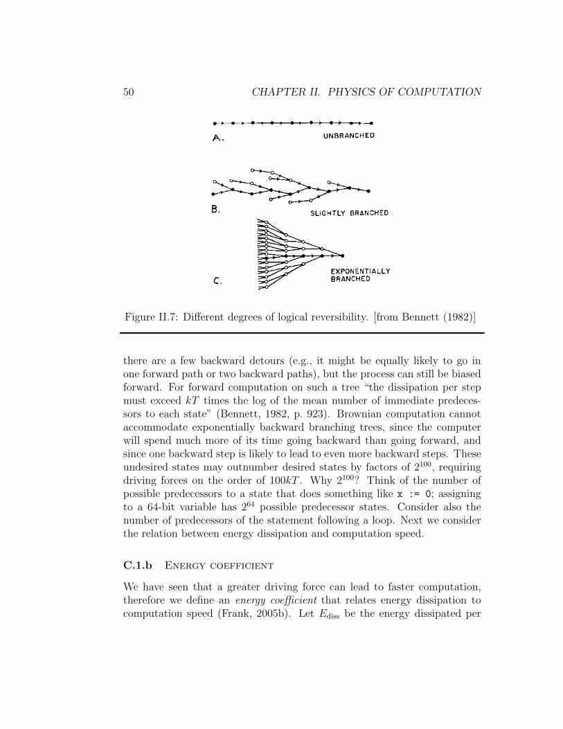
As in ballistic computing, Brownian computing needs logical reversibility.With no driving force, it is equally likely to move forward or backward, butany driving force will ensure forward movement. Brownian computing canaccommodate a small degree of irreversibility (see Fig. II.7). In these cases,


Figure II.7: Di↵erent degrees of logical reversibility. [from Bennett (1982)]

there are a few backward detours (e.g., it might be equally likely to go inone forward path or two backward paths), but the process can still be biasedforward. For forward computation on such a tree “the dissipation per stepmust exceed kT times the log of the mean number of immediate predeces-sors to each state” (Bennett, 1982, p. 923). Brownian computation cannotaccommodate exponentially backward branching trees, since the computerwill spend much more of its time going backward than going forward, andsince one backward step is likely to lead to even more backward steps. Theseundesired states may outnumber desired states by factors of 2100, requiringdriving forces on the order of 100kT . Why 2100? Think of the number ofpossible predecessors to a state that does something like x := 0; assigningto a 64-bit variable has 264 possible predecessor states. Consider also thenumber of predecessors of the statement following a loop. Next we considerthe relation between energy dissipation and computation speed.

C.1.b Energy coefficient

We have seen that a greater driving force can lead to faster computation,therefore we define an energy coe�cient that relates energy dissipation tocomputation speed (Frank, 2005b). Let Ediss be the energy dissipated per


operation and fop be the frequency of operations; then the energy coe�cientis defined:

cEdef= Ediss/fop.

For example, for DNA, cE ⇡ (40kT )/(1kHz) = 40⇥26 meV/kHz ⇡ 1 eV/kHz(since at room temperature, kBT ⇡ 26 meV: see Sec. A, p. 32). If our goal,however, is to operate at GHz frequencies (fop ⇡ 109) and energy dissipationbelow kBT (which is below VNL, but possible for reversible logic), then weneed energy coe�cients vastly lower than DNA. This is an issue, of course,for molecular computation.

C.1.c Adiabatic circuits

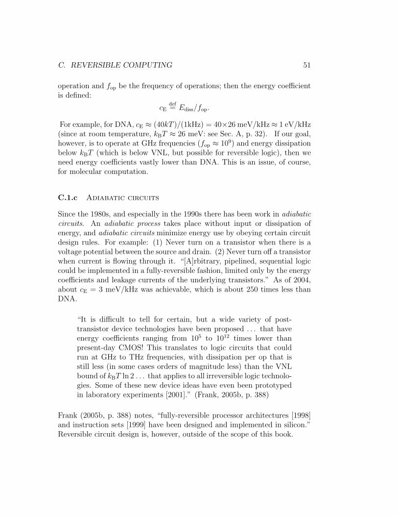
Since the 1980s, and especially in the 1990s there has been work in adiabaticcircuits. An adiabatic process takes place without input or dissipation ofenergy, and adiabatic circuits minimize energy use by obeying certain circuitdesign rules. For example: (1) Never turn on a transistor when there is avoltage potential between the source and drain. (2) Never turn o↵ a transistorwhen current is flowing through it. “[A]rbitrary, pipelined, sequential logiccould be implemented in a fully-reversible fashion, limited only by the energycoe�cients and leakage currents of the underlying transistors.” As of 2004,about cE = 3 meV/kHz was achievable, which is about 250 times less thanDNA.

“It is di�cult to tell for certain, but a wide variety of post-transistor device technologies have been proposed . . . that haveenergy coe�cients ranging from 105 to 1012 times lower thanpresent-day CMOS! This translates to logic circuits that couldrun at GHz to THz frequencies, with dissipation per op that isstill less (in some cases orders of magnitude less) than the VNLbound of kBT ln 2 . . . that applies to all irreversible logic technolo-gies. Some of these new device ideas have even been prototypedin laboratory experiments [2001].” (Frank, 2005b, p. 388)

Frank (2005b, p. 388) notes, “fully-reversible processor architectures [1998]and instruction sets [1999] have been designed and implemented in silicon.”Reversible circuit design is, however, outside of the scope of this book.


C.2 Foundations of Conservative Computation

If we want to avoid the von Neumann-Landauer limit, then we have to do re-versible computation (we cannot throw logical information away). Moreover,if we want to do fast, reliable computation, we need to use driving forcesand signal levels well above this limit, but this energy cannot be dissipatedinto the environment. Therefore, we need to investigate a conservative logicby which energy and other resources are conserved.17 What this means isthat the mechanical modes (computation) must be separated from the ther-mal modes (heat) to minimize damping and fluctuation and the consequentthermalization of information (recall Sec. B.2).

According to Fredkin & To↵oli (1982), “Computation is based on the stor-age, transmission, and processing of discrete signals.” They outline severalphysical principles implicit in the axioms of conventional dissipative logic:

P1 “The speed of propagation of information is bounded.” That is, thereis no action at a distance.

P2 “The amount of information which can be encoded in the state of afinite system is bounded.” This is ultimately a consequence of thermo-dynamics and quantum theory.

P3 “It is possible to construct macroscopic, dissipative physical deviceswhich perform in a recognizable and reliable way the logical functionsAND, NOT, and FAN-OUT.” This is a simple empirical fact (i.e., webuild these things).

Since only macroscopic systems are irreversible, as we go to the microscopiclevel, we need to understand reversible logic. This leads to new physicalprinciples of computing:

P4 “Identity of transmission and storage.” From a relativistic perspective,information storage in one reference frame may be information trans-mission in another. For an example, consider leaving a note on a tablein an airplane. In the reference frame of the airplane, it is informationstorage. If the airplane travels from one place to another, then in thereference plane of the earth it is information transmission.

17This section is based primarily on Fredkin & To↵oli (1982).


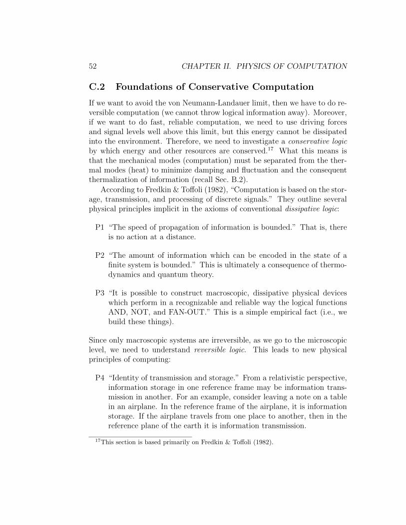
(where the superscript denotes the abstract "time" in which events take place in a discrete dynamical system), and is graphically represented as in Figure 1. The value that is present at a wire’s input at time t (and at its output at time t + 1) is called the state of the wire at time t.

From the unit wire one obtains by composition more general wires of arbitrary length. Thus, a wire of length i (i ! 1) represents a space-time signal path whose ends are separated by an interval of i time units. For the moment we shall not concern ourselves with the specific spatial layout of such a path (cf. constraint P8).

Observe that the unit wire is invertible, conservative (i.e., it conserves in the output the number of 0's and l's that are present at the input), and is mapped into its inverse by the transformation t -t.

2.4. Conservative-Logic Gates; The Fredkin Gate. Having introduced a primitive whose role is to represent signals, we now need primitives to represent in a stylized way physical computing events.

Figure 1. The unit wire.

A conservative-logic gate is any Boolean function that is invertible and conservative (cf. Assumptions P5 and P7 above). It is well known that, under the ordinary rules of function composition (where fan-out is allowed), the two-input NAND gate constitutes a universal primitive for the set of all Boolean functions. In conservative logic, an analogous role is played by a single signal-processing primitive, namely, the Fredkin gate, defined by the table

u x1 x2 v y1 y2 0 0 0 0 0 0 0 0 1 0 1 0 0 1 0 0 0 1 0 1 1 0 1 1 (2) 1 0 0 1 0 0 1 0 1 1 0 1 1 1 0 1 1 0 1 1 1 1 1 1

and graphically represented as in Figure 2a. This computing element can be visualized as a device that performs conditional crossover of two data signals according to the value of a control signal (Figure 2b). When this value is 1 the two data signals follow parallel paths; when 0, they cross over. Observe that the Fredkin gate is nonlinear and coincides with its own inverse.

Figure 2. (a) Symbol and (b) operation of the Fredkin gate.

In conservative logic, all signal processing is ultimately reduced to conditional routing of signals. Roughly speaking, signals are treated as unalterable objects that can be moved around in the course of a computation but never created or destroyed. For the physical significance of this approach, see Section 6.

2.5. Conservative-Logic Circuits. Finally, we shall introduce a scheme for connecting signals, represented by unit wires, with events, represented by conservative-logic gates.

Figure II.8: Symbol for unit wire. (Fredkin & To↵oli, 1982)

P5 “Reversibility.” This is because microscopic physics is reversible. There-fore, our computational primitives will need to be invertible.

P6 “One-to-one composition.” Physically, fan-out is not trivial (even inconventional logic), so we cannot assume that one function output canbe substituted for any number of input variables. Copying a signalcan be complicated (and, in some cases, impossible, as in quantumcomputing). We have to treat fan-out as a specific signal-processingelement.

P7 “Conservation of additive quantities.” It can be shown that in a re-versible systems there are a number of independent conserved quanti-ties, and in many systems they are additive over the subsystems, whichmakes them more useful. Emmy Noether (1882–1935) proved a famoustheorem: that any symmetry has a corresponding conservation law,and vice versa; that is, there is a one-to-one correspondence betweenphysical invariances and conserved quantities. In particular, time in-variance corresponds to conservation of energy, translational invariancecorresponds to conservation of linear momentum, and rotational invari-ance corresponds to conservation of angular momentum. Conservativelogic has to obey at least one additive conservation law.

P8 “The topology of space-time is locally Euclidean. “Intuitively, theamount of ‘room’ available as one moves away from a certain pointin space increases as a power (rather than as an exponential) of thedistance from that point, thus severely limiting the connectivity of acircuit.”

We will see that two primitive operations are su�cient for conservative logic:the unit wire and the Fredkin gate.


cab

ca'b'

0ab

0ab

1ab

1ba

(b)(a)

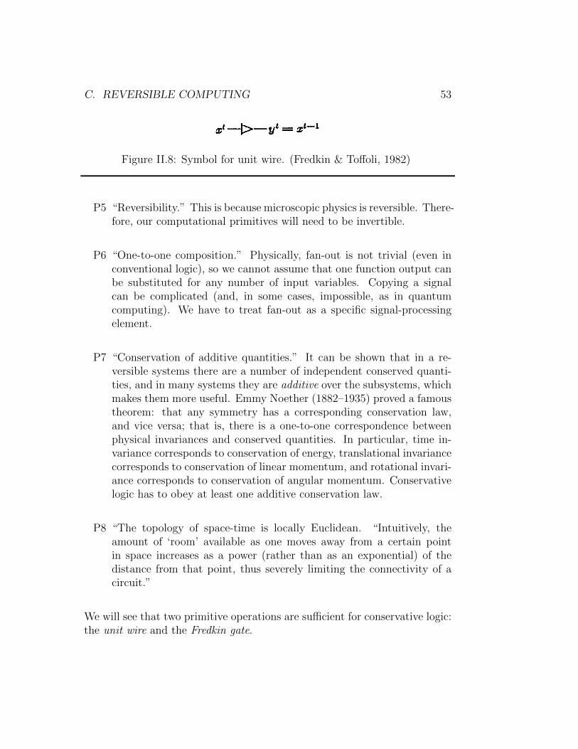
Figure II.9: Fredkin gate or CSWAP (conditional swap): (a) symbol and (b)operation.

C.2.a Unit wire

The basic operation of information storage/transmission is the unit wire,which moves one bit of information between two space-time points separatedby one unit of time (Fig. II.8). The input value at time t, which is consideredthe wire’s state at time t, becomes the output value at time t+ 1. The unitwire is reversible and conservative (since it conserves the number of 0s and 1sin its input). (Note that there are mathematically reversible functions thatare not conservative, e.g., Not.)

C.2.b Fredkin gate

A conservative logic gate is a Boolean function that is both invertible andconservative (preserves the number of 0s and 1s). Since the number of 1s and0s is conserved, conservative computing is essentially conditional rerouting,that is, the initial supply of 0s and 1s is rearranged. Conventional modelsof computation are based on rewriting (e.g., Turing machines, the lambdacalculus, register machines, term-rewriting systems, Post and Markov pro-ductions), but we have seen that overwriting dissipates energy (and is thusnon-conservative). In conservative logic we rearrange bits without creatingor destroying them. There is no infinite “bit supply” and no “bit bucket.”In the context of the physics of computation, these are physically real, notmetaphors!

A swap is the simplest operation on two bits, and the Fredkin gate, whichis a conditional swap operation (also called CSWAP), is an example of aconservative logic operation on three bits. It is defined:

(0, a, b) 7! (0, a, b),


c c c a a'ccc

c ca a a ba' a' a' b'b b bb' b' b'

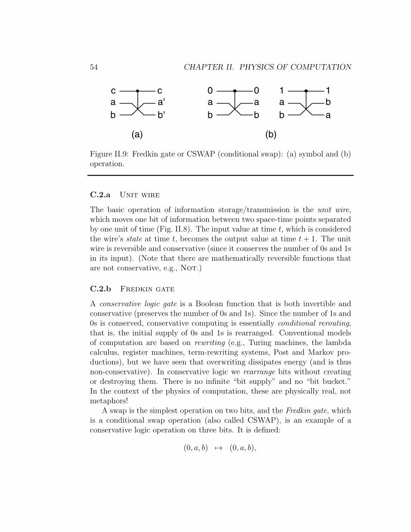
Figure II.10: Alternative notations for Fredkin gate.A conservative-logic circuit is a directed graph whose nodes are conservative-logic gates and whose arcs are wires of any length (cf. Figure 3).

Figure 3. (a) closed and (b) open conservative-logic circuits.

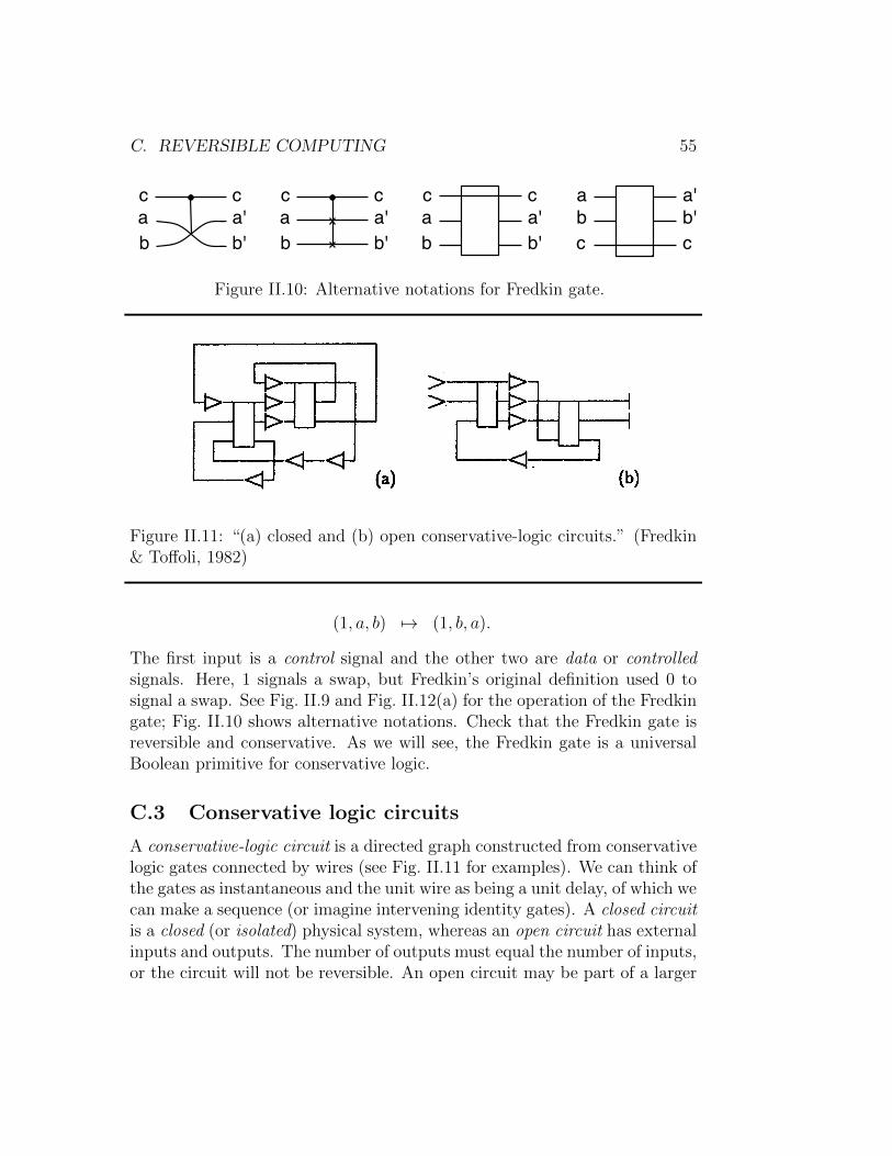
Any output of a gate can be connected only to the input of a wire, and sirnilarly any input of a gate only to the output of a wire. The interpretation of such a circuit in terms of conventional sequential computation is immediate, as the gate plays the role of an "instantaneous" combinational element and the wire that of a delay element embedded in an interconnection line. In a closed conservative-logic circuit, all inputs and outputs of any elements are connected within the circuit (Figure 3a). Such a circuit corresponds to what in physics is called a a closed (or isolated) system. An open conservative-logic circuit possesses a number of external input and output ports (Figure 3b). In isolation, such a circuit might be thought of as a transducer (typically, with memory) which, depending on its initial state, will respond with a particular Output sequence to any particular input sequence. However, usually such a circuit will be thought of as a portion of a larger circuit; thence the notation for input and output ports (Figure 3b), which is suggestive of, respectively, the trailing and the leading edge of a wire. Observe that in conservative-logic circuits the number of output ports always equals that of input ones.

The junction between two adjacent unit wires can be formally treated as a node consisting of a trivial conservative-logic gate, namely, the identity gate. Inwhat follows, whenever we speak of the realizability of a function in terms of a certain set of conservative-logic primitives, the unit wire and the identity gate will be tacitly assumed to be included in this set.

A conservative-logic circuit is a time-discrete dynamical system. The unit wires represent the system’s individual state variables, while the gates (including, of course, any occurrence of the identity gate) collectively represent the system’s transition function. The number N of unit wires that are present in the circuit may be thought of as the number of degrees of freedom of the system. Of these N wires, at any moment N1 will be in state 1, and the remaining N0 (= N - N1) will be in state 0. The quantity N1 is an additive function of the system’s state, i.e., is defined for any portion of the circuit and its value for the whole circuit is the sum of the individual contributions from all portions. Moreover, since both the unit wire and the gates return at their outputs as many l’s as are present at their inputs, the quantity N1 is an integral of the motion of the system, i.e., is constant along any trajectory. (Analogous considerations apply to the quantity N0, but, of course, N0 and N1 are not independent integrals of the motion.) It is from this "conservation principle" for the quantities in which signals are encoded that conservative logic derives its name.

It must be noted that reversibility (in the sense of mathematical invertibility) and conservation are independent properties, that is, there exist computing circuits that are reversible but not "bit-conserving," (Toffoli, 1980) and vice versa (Kinoshita, 1976).

Figure II.11: “(a) closed and (b) open conservative-logic circuits.” (Fredkin& To↵oli, 1982)

(1, a, b) 7! (1, b, a).

The first input is a control signal and the other two are data or controlledsignals. Here, 1 signals a swap, but Fredkin’s original definition used 0 tosignal a swap. See Fig. II.9 and Fig. II.12(a) for the operation of the Fredkingate; Fig. II.10 shows alternative notations. Check that the Fredkin gate isreversible and conservative. As we will see, the Fredkin gate is a universalBoolean primitive for conservative logic.

C.3 Conservative logic circuits

A conservative-logic circuit is a directed graph constructed from conservativelogic gates connected by wires (see Fig. II.11 for examples). We can think ofthe gates as instantaneous and the unit wire as being a unit delay, of which wecan make a sequence (or imagine intervening identity gates). A closed circuitis a closed (or isolated) physical system, whereas an open circuit has externalinputs and outputs. The number of outputs must equal the number of inputs,or the circuit will not be reversible. An open circuit may be part of a larger


uab

ua' = ūa+ub b' = ua+ūb

(a)

ab

0

a

ab

(b)āb

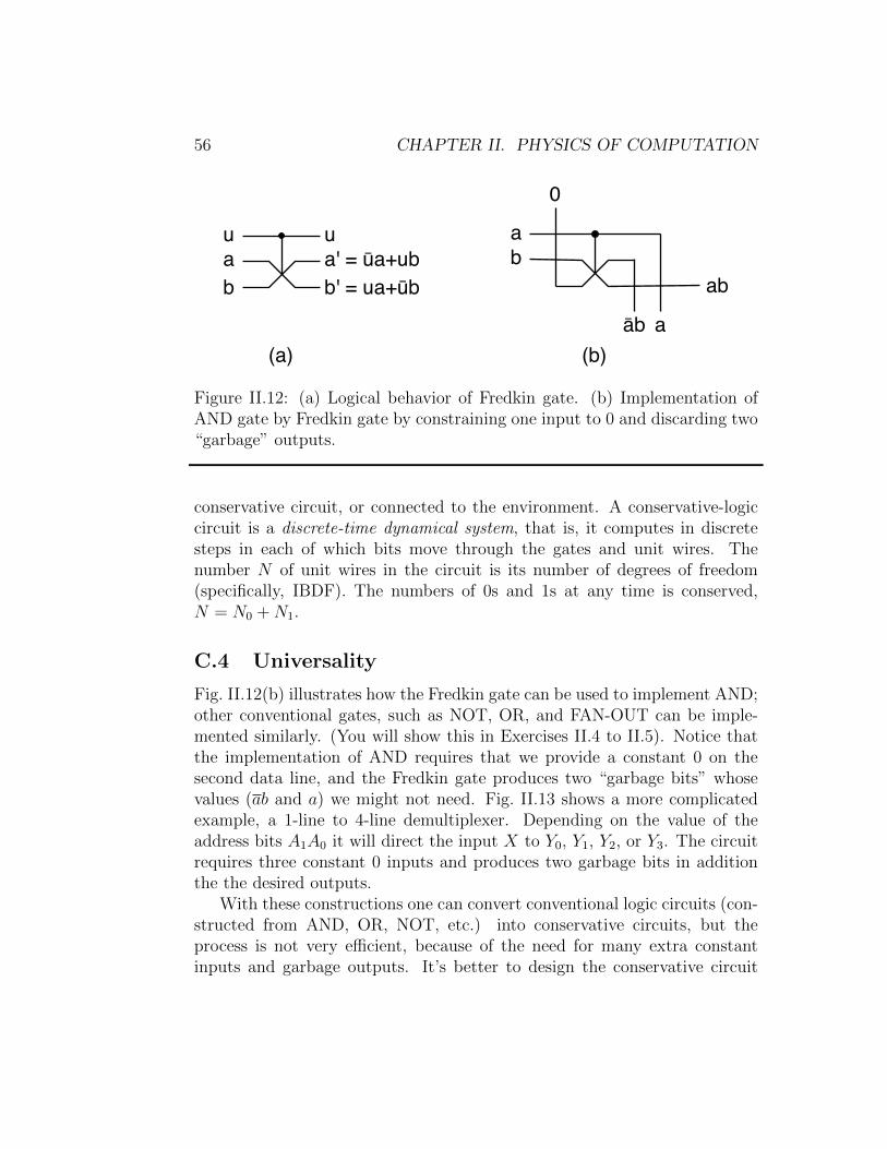
Figure II.12: (a) Logical behavior of Fredkin gate. (b) Implementation ofAND gate by Fredkin gate by constraining one input to 0 and discarding two“garbage” outputs.

conservative circuit, or connected to the environment. A conservative-logiccircuit is a discrete-time dynamical system, that is, it computes in discretesteps in each of which bits move through the gates and unit wires. Thenumber N of unit wires in the circuit is its number of degrees of freedom(specifically, IBDF). The numbers of 0s and 1s at any time is conserved,N = N0 +N1.

C.4 Universality

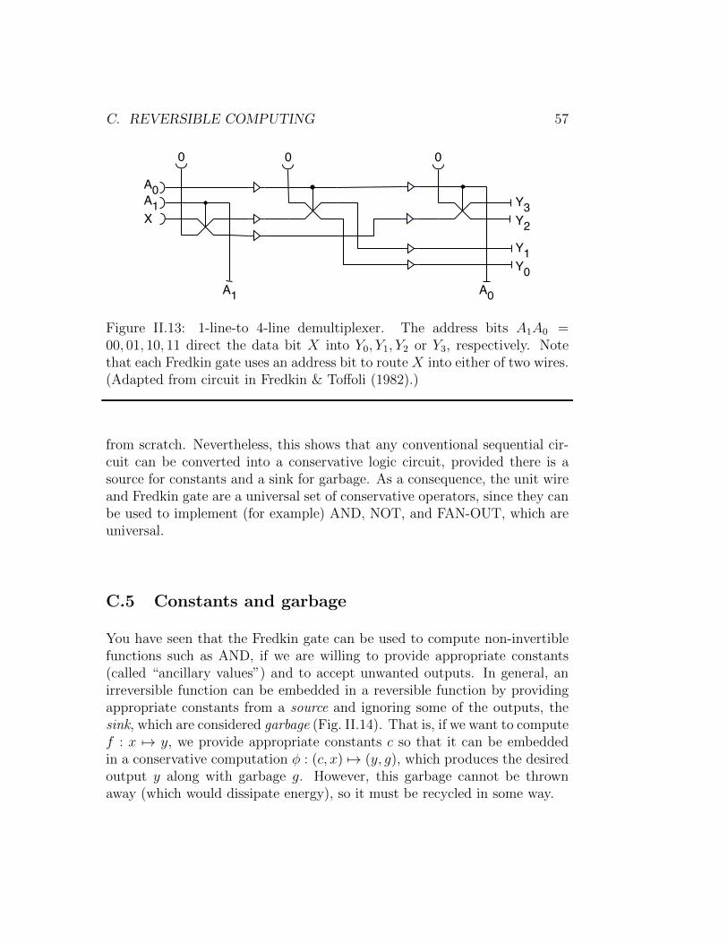
Fig. II.12(b) illustrates how the Fredkin gate can be used to implement AND;other conventional gates, such as NOT, OR, and FAN-OUT can be imple-mented similarly. (You will show this in Exercises II.4 to II.5). Notice thatthe implementation of AND requires that we provide a constant 0 on thesecond data line, and the Fredkin gate produces two “garbage bits” whosevalues (ab and a) we might not need. Fig. II.13 shows a more complicatedexample, a 1-line to 4-line demultiplexer. Depending on the value of theaddress bits A1A0 it will direct the input X to Y0, Y1, Y2, or Y3. The circuitrequires three constant 0 inputs and produces two garbage bits in additionthe the desired outputs.

With these constructions one can convert conventional logic circuits (con-structed from AND, OR, NOT, etc.) into conservative circuits, but theprocess is not very e�cient, because of the need for many extra constantinputs and garbage outputs. It’s better to design the conservative circuit


0 0 0

X

A0A1

A1 A0

Y0

Y1

Y2

Y3

Figure II.13: 1-line-to 4-line demultiplexer. The address bits A1A0 =00, 01, 10, 11 direct the data bit X into Y0, Y1, Y2 or Y3, respectively. Notethat each Fredkin gate uses an address bit to route X into either of two wires.(Adapted from circuit in Fredkin & To↵oli (1982).)

from scratch. Nevertheless, this shows that any conventional sequential cir-cuit can be converted into a conservative logic circuit, provided there is asource for constants and a sink for garbage. As a consequence, the unit wireand Fredkin gate are a universal set of conservative operators, since they canbe used to implement (for example) AND, NOT, and FAN-OUT, which areuniversal.

C.5 Constants and garbage

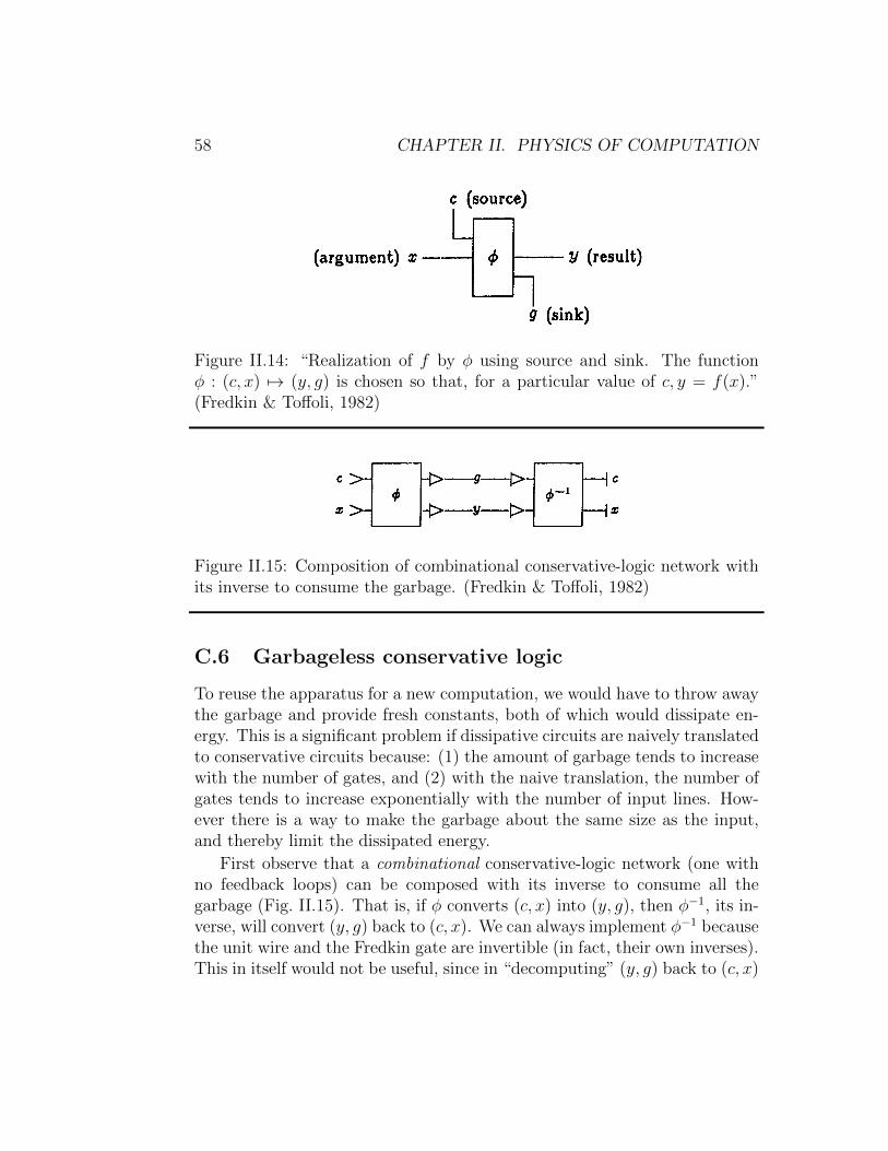
You have seen that the Fredkin gate can be used to compute non-invertiblefunctions such as AND, if we are willing to provide appropriate constants(called “ancillary values”) and to accept unwanted outputs. In general, anirreversible function can be embedded in a reversible function by providingappropriate constants from a source and ignoring some of the outputs, thesink, which are considered garbage (Fig. II.14). That is, if we want to computef : x 7! y, we provide appropriate constants c so that it can be embeddedin a conservative computation � : (c, x) 7! (y, g), which produces the desiredoutput y along with garbage g. However, this garbage cannot be thrownaway (which would dissipate energy), so it must be recycled in some way.


3. COMPUTATION IN CONSERVATIVE-LOGIC CIRCUITS; CONSTANTS AND GARBAGE In Figure 4a we have expressed the output variables of the Fredkin gate as explicit functions of the input variables. The overall functional relation-ship between input and output is, as we have seen, invertible. On the other hand, the functions that one is interested in computing are often noninvertible. Thus, special provisions must be made in the use of the Fredkin gate (or, for that matter, of any invertible function that is meant to be a general-purpose signal-processing primitive) in order to obtain adequate computing power.

Suppose, for instance, that one desires to compute the AND function, which is not invertible. In Figure 4b only inputs u and x1 are fed with arbitrary values a and b, while x2 is fed with the constant value 0. In this case, the y1 output will provide the desired value ab ("a AND b"), while the other two outputs v and y2 will yield the "unrequested" values a and ¬ab. Thus, intuitively, the AND function can be realized by means of the Fredkin gate as long as one is willing to supply "constants" to this gate alongside with the argument, and accept "garbage" from it alongside with the result. This situation is so common in computation with invertible primitives that it will be convenient to introduce some terminology in order to deal with it in a precise way.

Figure 4. Behavior of the Fredkin gate (a) with unconstrained inputs, and (b) with x2 constrained to the

value 0, thus realizing the AND function.

Figure 5. Realization of f by !using source and sink. The function : (c, x) (y, g) is chosen so that, for a

particular value of c, y = f(x).

Terminology: source, sink, constants, garbage. Given any finite function , one obtains a new function f "embedded" in it by assigning specified values to certain distinguished input lines (collectively called the source) and disregarding certain distinguished output lines (collectively called the sink). The remaining input lines will constitute the argument, and the remaining output lines, the result. This construction (Figure 5) is called a realization of f by means of !using source and sink. In realizing f by means of , the source lines will be fed with constant values, i.e., with values that do not depend on the argument. On the other hand, the sink lines in general will yield values that depend on the argument, and thus cannot be used as input constants for a new computation. Such values will be termed garbage. (Much as in ordinary life, this

Figure II.14: “Realization of f by � using source and sink. The function� : (c, x) 7! (y, g) is chosen so that, for a particular value of c, y = f(x).”(Fredkin & To↵oli, 1982)

Consider now the network -1,which is the inverse of (Figure 20b). If g and y are used as inputs for -1 this network will "undo" ’s computation and return c and x as outputs. By combining the two networks, as in Figure 21, we obtain a new network which obviously computes the identity function and thus looks, in terms of input-output behavior, just like a bundle of parallel wires. Not only the argument x but also the constants c are returned unchanged. Yet, buried in the middle of this network there appears the desired result y. Our next task will be to "observe" this value without disturbing the system.

In a conservative-logic circuit, consider an arbitrary internal line carrying the value a (Figure 22a). The "spy" device of Figure 22b, when fed with a 0 and a 1, allows one to extract from the circuit a copy of a, together with its complement, ¬a without interfering in any way with the ongoing computation. By applying this device to every individual line of the result y of Figure 21, we obtain the complete circuit shown in Figure 23. As before, the result y produced by !is passed on to -1 I; however, a copy of y (as well as its complement ¬y) is now available externally. The "price" for each of these copies is merely the supply of n new constants (where n is the width of the result).

Figure 20. (a) Computation of y = f(x) by means of a combinational conservative-logic network . (b) This

computation is "undone" by the inverse network, -1

Figure 21. The network obtained by combining and -1 'looks from the outside like a bundle of parallel

wires. The value y(=f(x)) is buried in the middle.

The remarkable achievements of this construction are discussed below with the help of the schematic representation of Figure 24. In this figure, it will be convenient to visualize the input registers as "magnetic bulletin boards," in which identical, undestroyable magnetic tokens can be moved on the board surface. A token at a given position on the board represents a 1, while the absence of a token at that position represents a 0. The capacity of a board is the maximum number of tokens that can be placed on it. Three such registers are sent through a "black box" F, which represents the conservative-logic circuit of Figure 23, and when they reappear some of the tokens may have been moved, but none taken away or added. Let us follow this process, register by register.

Figure 22. The value a carried by an arbitrary line (a) can be inspected in a nondestructive way by the "spy"

device in (b).

Figure II.15: Composition of combinational conservative-logic network withits inverse to consume the garbage. (Fredkin & To↵oli, 1982)

C.6 Garbageless conservative logic

To reuse the apparatus for a new computation, we would have to throw awaythe garbage and provide fresh constants, both of which would dissipate en-ergy. This is a significant problem if dissipative circuits are naively translatedto conservative circuits because: (1) the amount of garbage tends to increasewith the number of gates, and (2) with the naive translation, the number ofgates tends to increase exponentially with the number of input lines. How-ever there is a way to make the garbage about the same size as the input,and thereby limit the dissipated energy.

First observe that a combinational conservative-logic network (one withno feedback loops) can be composed with its inverse to consume all thegarbage (Fig. II.15). That is, if � converts (c, x) into (y, g), then ��1, its in-verse, will convert (y, g) back to (c, x). We can always implement ��1 becausethe unit wire and the Fredkin gate are invertible (in fact, their own inverses).This in itself would not be useful, since in “decomputing” (y, g) back to (c, x)


Consider now the network -1,which is the inverse of (Figure 20b). If g and y are used as inputs for -1 this network will "undo" ’s computation and return c and x as outputs. By combining the two networks, as in Figure 21, we obtain a new network which obviously computes the identity function and thus looks, in terms of input-output behavior, just like a bundle of parallel wires. Not only the argument x but also the constants c are returned unchanged. Yet, buried in the middle of this network there appears the desired result y. Our next task will be to "observe" this value without disturbing the system.

In a conservative-logic circuit, consider an arbitrary internal line carrying the value a (Figure 22a). The "spy" device of Figure 22b, when fed with a 0 and a 1, allows one to extract from the circuit a copy of a, together with its complement, ¬a without interfering in any way with the ongoing computation. By applying this device to every individual line of the result y of Figure 21, we obtain the complete circuit shown in Figure 23. As before, the result y produced by !is passed on to -1 I; however, a copy of y (as well as its complement ¬y) is now available externally. The "price" for each of these copies is merely the supply of n new constants (where n is the width of the result).

Figure 20. (a) Computation of y = f(x) by means of a combinational conservative-logic network . (b) This

computation is "undone" by the inverse network, -1

Figure 21. The network obtained by combining and -1 'looks from the outside like a bundle of parallel

wires. The value y(=f(x)) is buried in the middle.

The remarkable achievements of this construction are discussed below with the help of the schematic representation of Figure 24. In this figure, it will be convenient to visualize the input registers as "magnetic bulletin boards," in which identical, undestroyable magnetic tokens can be moved on the board surface. A token at a given position on the board represents a 1, while the absence of a token at that position represents a 0. The capacity of a board is the maximum number of tokens that can be placed on it. Three such registers are sent through a "black box" F, which represents the conservative-logic circuit of Figure 23, and when they reappear some of the tokens may have been moved, but none taken away or added. Let us follow this process, register by register.

Figure 22. The value a carried by an arbitrary line (a) can be inspected in a nondestructive way by the "spy"

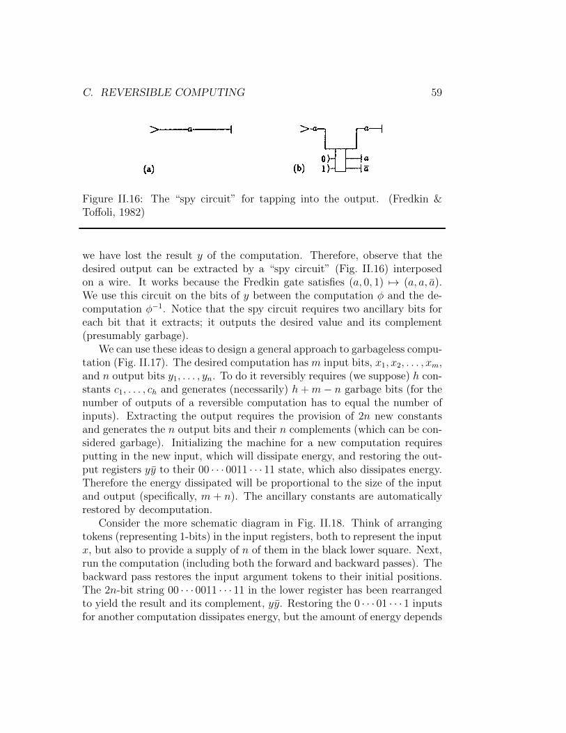
device in (b). Figure II.16: The “spy circuit” for tapping into the output. (Fredkin &To↵oli, 1982)

we have lost the result y of the computation. Therefore, observe that thedesired output can be extracted by a “spy circuit” (Fig. II.16) interposedon a wire. It works because the Fredkin gate satisfies (a, 0, 1) 7! (a, a, a).We use this circuit on the bits of y between the computation � and the de-computation ��1. Notice that the spy circuit requires two ancillary bits foreach bit that it extracts; it outputs the desired value and its complement(presumably garbage).

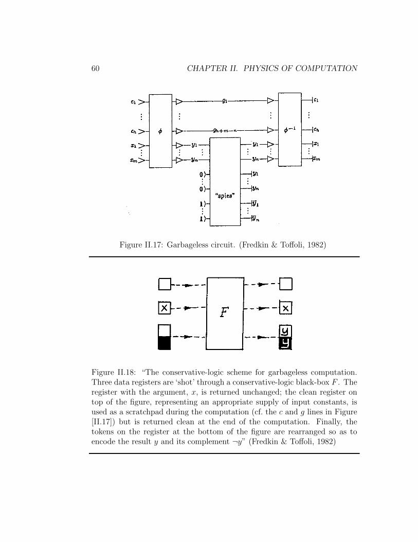
We can use these ideas to design a general approach to garbageless compu-tation (Fig. II.17). The desired computation has m input bits, x1, x2, . . . , xm,and n output bits y1, . . . , yn. To do it reversibly requires (we suppose) h con-stants c1, . . . , ch and generates (necessarily) h+m � n garbage bits (for thenumber of outputs of a reversible computation has to equal the number ofinputs). Extracting the output requires the provision of 2n new constantsand generates the n output bits and their n complements (which can be con-sidered garbage). Initializing the machine for a new computation requiresputting in the new input, which will dissipate energy, and restoring the out-put registers yy to their 00 · · · 0011 · · · 11 state, which also dissipates energy.Therefore the energy dissipated will be proportional to the size of the inputand output (specifically, m + n). The ancillary constants are automaticallyrestored by decomputation.

Consider the more schematic diagram in Fig. II.18. Think of arrangingtokens (representing 1-bits) in the input registers, both to represent the inputx, but also to provide a supply of n of them in the black lower square. Next,run the computation (including both the forward and backward passes). Thebackward pass restores the input argument tokens to their initial positions.The 2n-bit string 00 · · · 0011 · · · 11 in the lower register has been rearrangedto yield the result and its complement, yy. Restoring the 0 · · · 01 · · · 1 inputsfor another computation dissipates energy, but the amount of energy depends


Figure 23. A "garbageless" circuit for computing the function y = f(x). Inputs C1,..., Ch and X1,…., Xm are

returned unchanged, while the constants 0,...,0 and 1,..., 1 in the lower part of the circuits are replaced by the result, y1,...., yn and its complement, ¬y1,...., ¬yn

Figure 24. The conservative-logic scheme for garbageless computation. Three data registers are "shot" through a conservative-logic black-box F. The register with the argument, x, is returned unchanged; the

clean register on top of the figure, representing an appropriate supply of input constants, is used as a scratchpad during the computation (cf. the c and g lines in Figure 23) but is returned clean at the end of the

computation. Finally, the tokens on the register at the bottom of the figure are rearranged so as to encode the result y and its complement ¬y

(a) The "argument" register, containing a given arrangement of tokens x, is returned unchanged. The capacity of this register is m, i.e., the number of bits in x.

(b) A clean "scratchpad register" with a capacity of h tokens is supplied, and will be returned clean. (This is the main supply of constants-namely, c1, . . . , ch in Figure 23.) Note that a clean register means one with all 0's (i.e., no tokens), while we used both 0's and l's as constants, as needed, in the construction of Figure 10. However, a proof due to N. Margolus shows that all 0's can be used in this register without loss of generality. In other words, the essential function of this register is to provide the computation with spare room rather than tokens.

(c) Finally, we supply a clean "result" register of capacity 2n (where n is the number of bits in y). For this register, clean means that the top half is empty and the bottom half completely filled with tokens. The

Figure II.17: Garbageless circuit. (Fredkin & To↵oli, 1982)

Figure 23. A "garbageless" circuit for computing the function y = f(x). Inputs C1,..., Ch and X1,…., Xm are

returned unchanged, while the constants 0,...,0 and 1,..., 1 in the lower part of the circuits are replaced by the result, y1,...., yn and its complement, ¬y1,...., ¬yn

Figure 24. The conservative-logic scheme for garbageless computation. Three data registers are "shot" through a conservative-logic black-box F. The register with the argument, x, is returned unchanged; the

clean register on top of the figure, representing an appropriate supply of input constants, is used as a scratchpad during the computation (cf. the c and g lines in Figure 23) but is returned clean at the end of the

computation. Finally, the tokens on the register at the bottom of the figure are rearranged so as to encode the result y and its complement ¬y

(a) The "argument" register, containing a given arrangement of tokens x, is returned unchanged. The capacity of this register is m, i.e., the number of bits in x.

(b) A clean "scratchpad register" with a capacity of h tokens is supplied, and will be returned clean. (This is the main supply of constants-namely, c1, . . . , ch in Figure 23.) Note that a clean register means one with all 0's (i.e., no tokens), while we used both 0's and l's as constants, as needed, in the construction of Figure 10. However, a proof due to N. Margolus shows that all 0's can be used in this register without loss of generality. In other words, the essential function of this register is to provide the computation with spare room rather than tokens.

(c) Finally, we supply a clean "result" register of capacity 2n (where n is the number of bits in y). For this register, clean means that the top half is empty and the bottom half completely filled with tokens. The

Figure II.18: “The conservative-logic scheme for garbageless computation.Three data registers are ‘shot’ through a conservative-logic black-box F . Theregister with the argument, x, is returned unchanged; the clean register ontop of the figure, representing an appropriate supply of input constants, isused as a scratchpad during the computation (cf. the c and g lines in Figure[II.17]) but is returned clean at the end of the computation. Finally, thetokens on the register at the bottom of the figure are rearranged so as toencode the result y and its complement ¬y” (Fredkin & To↵oli, 1982)


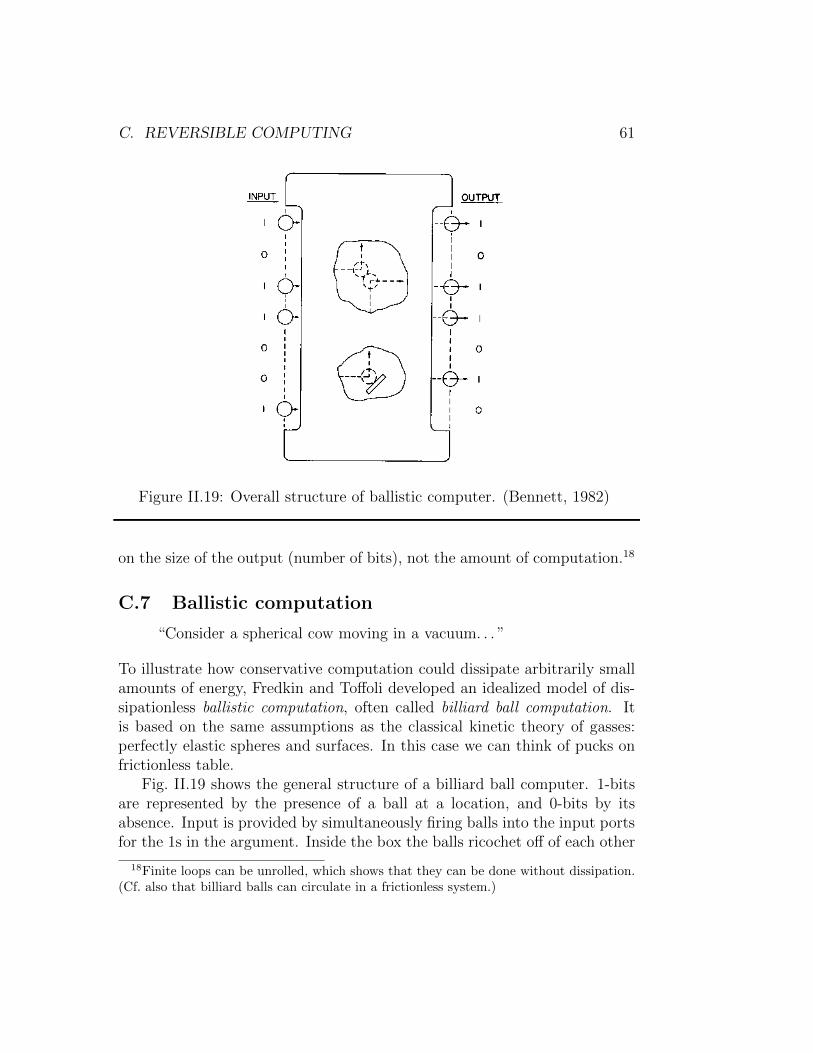
Figure II.19: Overall structure of ballistic computer. (Bennett, 1982)

on the size of the output (number of bits), not the amount of computation.18

C.7 Ballistic computation

“Consider a spherical cow moving in a vacuum. . . ”

To illustrate how conservative computation could dissipate arbitrarily smallamounts of energy, Fredkin and To↵oli developed an idealized model of dis-sipationless ballistic computation, often called billiard ball computation. Itis based on the same assumptions as the classical kinetic theory of gasses:perfectly elastic spheres and surfaces. In this case we can think of pucks onfrictionless table.

Fig. II.19 shows the general structure of a billiard ball computer. 1-bitsare represented by the presence of a ball at a location, and 0-bits by itsabsence. Input is provided by simultaneously firing balls into the input portsfor the 1s in the argument. Inside the box the balls ricochet o↵ of each other

18Finite loops can be unrolled, which shows that they can be done without dissipation.(Cf. also that billiard balls can circulate in a frictionless system.)


Figure 14 Billiard ball model realization of the interaction gate.

All of the above requirements are met by introducing, in addition to collisions between two balls, collisions between a ball and a fixed plane mirror. In this way, one can easily deflect the trajectory of a ball (Figure 15a), shift it sideways (Figure 15b), introduce a delay of an arbitrary number of time steps (Figure 1 Sc), and guarantee correct signal crossover (Figure 15d). Of course, no special precautions need be taken for trivial crossover, where the logic or the timing are such that two balls cannot possibly be present at the same moment at the crossover point (cf. Figure 18 or 12a). Thus, in the billiard ball model a conservative-logic wire is realized as a potential ball path, as determined by the mirrors.

Note that, since balls have finite diameter, both gates and wires require a certain clearance in order to function properly. As a consequence, the metric of the space in which the circuit is embedded (here, we are considering the Euclidean plane) is reflected in certain circuit-layout constraints (cf. P8, Section 2). Essentially, with polynomial packing (corresponding to the Abelian-group connectivity of Euclidean space) some wires may have to be made longer than with exponential packing (corresponding to an abstract space with free-group connectivity) (Toffoli, 1977).

Figure 15. The mirror (indicated by a solid dash) can be used to deflect a ball’s path (a), introduce a

sideways shift (b), introduce a delay (c), and realize nontrivial crossover (d).

Figure 16. The switch gate and its inverse. Input signal x is routed to one of two output paths depending on

the value of the control signal, C.

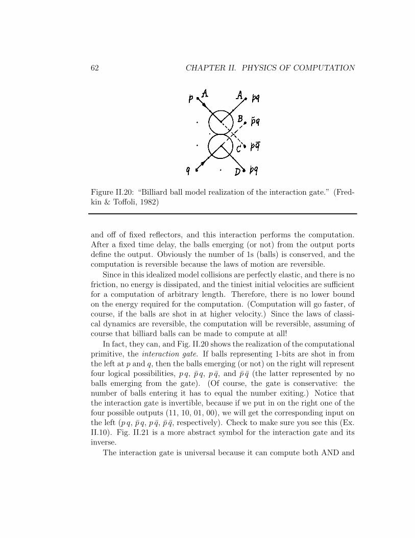
Figure II.20: “Billiard ball model realization of the interaction gate.” (Fred-kin & To↵oli, 1982)

and o↵ of fixed reflectors, and this interaction performs the computation.After a fixed time delay, the balls emerging (or not) from the output portsdefine the output. Obviously the number of 1s (balls) is conserved, and thecomputation is reversible because the laws of motion are reversible.

Since in this idealized model collisions are perfectly elastic, and there is nofriction, no energy is dissipated, and the tiniest initial velocities are su�cientfor a computation of arbitrary length. Therefore, there is no lower boundon the energy required for the computation. (Computation will go faster, ofcourse, if the balls are shot in at higher velocity.) Since the laws of classi-cal dynamics are reversible, the computation will be reversible, assuming ofcourse that billiard balls can be made to compute at all!

In fact, they can, and Fig. II.20 shows the realization of the computationalprimitive, the interaction gate. If balls representing 1-bits are shot in fromthe left at p and q, then the balls emerging (or not) on the right will representfour logical possibilities, p q, p q, p q, and p q (the latter represented by noballs emerging from the gate). (Of course, the gate is conservative: thenumber of balls entering it has to equal the number exiting.) Notice thatthe interaction gate is invertible, because if we put in on the right one of thefour possible outputs (11, 10, 01, 00), we will get the corresponding input onthe left (p q, p q, p q, p q, respectively). Check to make sure you see this (Ex.II.10). Fig. II.21 is a more abstract symbol for the interaction gate and itsinverse.

The interaction gate is universal because it can compute both AND and


Figure 12. (a) Balls of radius l/sqrt(2) traveling on a unit grid. (b) Right-angle elastic collision between two

balls.

Figure 13. (a) The interaction gate and (b) its inverse.

6.2. The Interaction Gate. The interaction gate is the conservative-logic primitive defined by Figure 13a, which also assigns its graphical representation.7

In the billiard ball model, the interaction gate is realized simply as the potential locus of collision of two balls. With reference to Figure 14, let p, q be the values at a certain instant of the binary variables associated with the two points P, Q, and consider the values-four time steps later in this particular example-of the variables associated with the four points A, B, C, D. It is clear that these values are, in the order shown in the figure, pq, ¬pq, p¬q; and pq. In other words, there will be a ball at A if and only if there was a ball at P and one at Q; similarly, there will be a ball at B if and only if there was a ball at Q and none at P; etc.

6.3. Interconnection; Timing and Crossover; The Mirror. Owing to its AND and NOT capabilities, the interaction gate is clearly a universal logic primitive (as explained in Section 5, we assume the availability of input constants). To verify that these capabilities are retained in the billiard ball model, one must make sure that one can realize the appropriate interconnections, i.e., that one can suitably route balls from one collision locus to another and maintain proper timing. In particular, since we are considering a planar grid, one must provide a way of performing signal crossover.

7 Note that the interaction gate has four output lines but only four (rather than 24) output states-in other words, the output variables are constrained. When one considers its inverse (Figure 13b), the same constraints appear on the input variables. In composing functions of this kind, one must exercise due care that the constraints are satisfied.

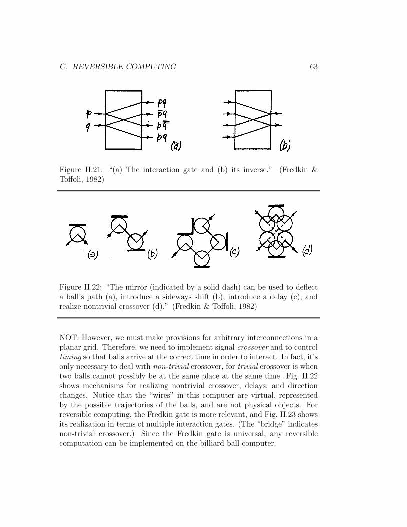
Figure II.21: “(a) The interaction gate and (b) its inverse.” (Fredkin &To↵oli, 1982)

Figure 14 Billiard ball model realization of the interaction gate.

All of the above requirements are met by introducing, in addition to collisions between two balls, collisions between a ball and a fixed plane mirror. In this way, one can easily deflect the trajectory of a ball (Figure 15a), shift it sideways (Figure 15b), introduce a delay of an arbitrary number of time steps (Figure 1 Sc), and guarantee correct signal crossover (Figure 15d). Of course, no special precautions need be taken for trivial crossover, where the logic or the timing are such that two balls cannot possibly be present at the same moment at the crossover point (cf. Figure 18 or 12a). Thus, in the billiard ball model a conservative-logic wire is realized as a potential ball path, as determined by the mirrors.

Note that, since balls have finite diameter, both gates and wires require a certain clearance in order to function properly. As a consequence, the metric of the space in which the circuit is embedded (here, we are considering the Euclidean plane) is reflected in certain circuit-layout constraints (cf. P8, Section 2). Essentially, with polynomial packing (corresponding to the Abelian-group connectivity of Euclidean space) some wires may have to be made longer than with exponential packing (corresponding to an abstract space with free-group connectivity) (Toffoli, 1977).

Figure 15. The mirror (indicated by a solid dash) can be used to deflect a ball’s path (a), introduce a

sideways shift (b), introduce a delay (c), and realize nontrivial crossover (d).

Figure 16. The switch gate and its inverse. Input signal x is routed to one of two output paths depending on

the value of the control signal, C.

Figure II.22: “The mirror (indicated by a solid dash) can be used to deflecta ball’s path (a), introduce a sideways shift (b), introduce a delay (c), andrealize nontrivial crossover (d).” (Fredkin & To↵oli, 1982)

NOT. However, we must make provisions for arbitrary interconnections in aplanar grid. Therefore, we need to implement signal crossover and to controltiming so that balls arrive at the correct time in order to interact. In fact, it’sonly necessary to deal with non-trivial crossover, for trivial crossover is whentwo balls cannot possibly be at the same place at the same time. Fig. II.22shows mechanisms for realizing nontrivial crossover, delays, and directionchanges. Notice that the “wires” in this computer are virtual, representedby the possible trajectories of the balls, and are not physical objects. Forreversible computing, the Fredkin gate is more relevant, and Fig. II.23 showsits realization in terms of multiple interaction gates. (The “bridge” indicatesnon-trivial crossover.) Since the Fredkin gate is universal, any reversiblecomputation can be implemented on the billiard ball computer.

64 CHAPTER II. PHYSICS OF COMPUTATION156 Introduction to computer science

!

"

#

!$

"$

#$

!

Figure 3.14. A simple billiard ball computer, with three input bits and three output bits, shown entering on the leftand leaving on the right, respectively. The presence or absence of a billiard ball indicates a 1 or a 0, respectively.Empty circles illustrate potential paths due to collisions. This particular computer implements the Fredkin classicalreversible logic gate, discussed in the text.

we will ignore the effects of noise on the billiard ball computer, and concentrate onunderstanding the essential elements of reversible computation.The billiard ball computer provides an elegant means for implementing a reversible

universal logic gate known as the Fredkin gate. Indeed, the properties of the Fredkin gateprovide an informative overview of the general principles of reversible logic gates andcircuits. The Fredkin gate has three input bits and three output bits, which we refer toas a, b, c and a�, b�, c�, respectively. The bit c is a control bit, whose value is not changedby the action of the Fredkin gate, that is, c� = c. The reason c is called the control bitis because it controls what happens to the other two bits, a and b. If c is set to 0 then aand b are left alone, a� = a, b� = b. If c is set to 1, a and b are swapped, a� = b, b� = a.The explicit truth table for the Fredkin gate is shown in Figure 3.15. It is easy to seethat the Fredkin gate is reversible, because given the output a�, b�, c�, we can determinethe inputs a, b, c. In fact, to recover the original inputs a, b and c we need only applyanother Fredkin gate to a�, b�, c�:

Exercise 3.29: (Fredkin gate is self-inverse) Show that applying two consecutiveFredkin gates gives the same outputs as inputs.

Examining the paths of the billiard balls in Figure 3.14, it is not difficult to verify thatthis billiard ball computer implements the Fredkin gate:

Exercise 3.30: Verify that the billiard ball computer in Figure 3.14 computes theFredkin gate.

In addition to reversibility, the Fredkin gate also has the interesting property thatthe number of 1s is conserved between the input and output. In terms of the billiardball computer, this corresponds to the number of billiard balls going into the Fredkingate being equal to the number coming out. Thus, it is sometimes referred to as beinga conservative reversible logic gate. Such reversibility and conservative properties areinteresting to a physicist because they can be motivated by fundamental physical princi-

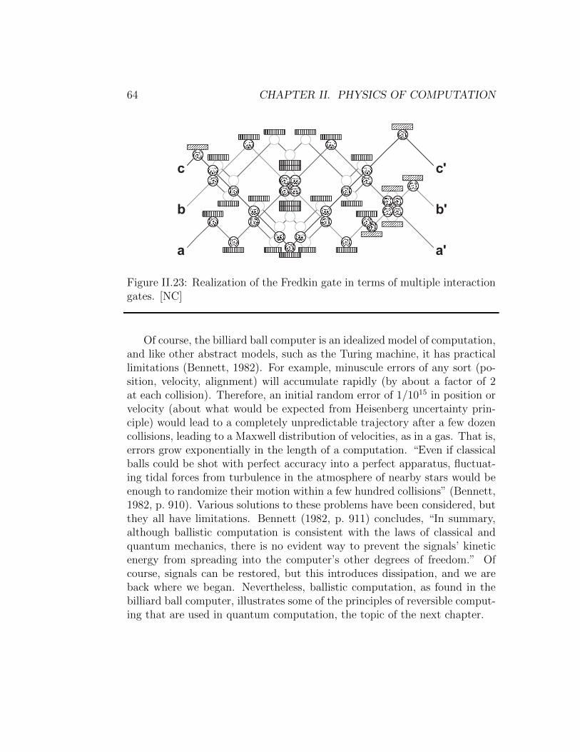
Figure II.23: Realization of the Fredkin gate in terms of multiple interactiongates. [NC]

Of course, the billiard ball computer is an idealized model of computation,and like other abstract models, such as the Turing machine, it has practicallimitations (Bennett, 1982). For example, minuscule errors of any sort (po-sition, velocity, alignment) will accumulate rapidly (by about a factor of 2at each collision). Therefore, an initial random error of 1/1015 in position orvelocity (about what would be expected from Heisenberg uncertainty prin-ciple) would lead to a completely unpredictable trajectory after a few dozencollisions, leading to a Maxwell distribution of velocities, as in a gas. That is,errors grow exponentially in the length of a computation. “Even if classicalballs could be shot with perfect accuracy into a perfect apparatus, fluctuat-ing tidal forces from turbulence in the atmosphere of nearby stars would beenough to randomize their motion within a few hundred collisions” (Bennett,1982, p. 910). Various solutions to these problems have been considered, butthey all have limitations. Bennett (1982, p. 911) concludes, “In summary,although ballistic computation is consistent with the laws of classical andquantum mechanics, there is no evident way to prevent the signals’ kineticenergy from spreading into the computer’s other degrees of freedom.” Ofcourse, signals can be restored, but this introduces dissipation, and we areback where we began. Nevertheless, ballistic computation, as found in thebilliard ball computer, illustrates some of the principles of reversible comput-ing that are used in quantum computation, the topic of the next chapter.

c reversible computing

Documents