C∞-algebraic geometry

with corners

Kelli L. Francis-Staite

St John’s College

The University of Oxford

A thesis submitted for the degree of

Doctor of Philosophy

Hilary 2019

Dedication

This thesis is dedicated to my Grandmother and in memory of my Gran for their endless

generosity, support and encouragement.

i

Acknowledgements

Thank-you to all the wonderful people that have contributed to a diverse and interesting

DPhil.

Thank-you to my supervisor, Professor Dominic Joyce, for all your guidance. For

sitting through one meeting a week, almost every week of the year, including several

months of Skype meetings while I was in Australia; and for your support during the time

when I was ill. For encouraging my application in the first place and for all your helpful

emails. For organising funding from QGM for my final year. For commitment to reading

my thesis long before it was a thesis. And for signing all those forms.

Thank-you to Cameron, for the cooking meals while I wrote this thesis, and bringing

so many things into my life that a university cannot. I am glad it is you by my side as we

watch episodes of Gardening Australia, or ride another 50 miles on a bicycle because we

want to leave Oxford for a day, or during the next unexpected hospital trip. Thank-you

for sharing your life with me, and for doing the dishes.

Thank-you to Cameron’s family and my family for their ever loving support, whether

via Skype or in Adelaide with hot meals, advice and gardening. Thank-you to my Adelaide

mathematics and non-mathematics friends, David, Laura, Brett, Steve, Michael, Annie,

Vincent, Lydia, Sally, Rachael, Jin, Hannah, and more, many of whom no longer live in

Adelaide nor even Australia, some whom have even crossed paths with me in England and

Europe, our random conversations and sporadic messages are invaluable to me.

Thank-you to my office mates Aurelio and Nick, for getting a Christmas tree in our

first year, covering it with origami, and not taking it down until we were moved out of the

office three years later. For asking ‘How are you?’, listening for an answer, and showing the

high levels of empathy many of our answers required. For giving me half an idea of what

mathematics you do, and listening to my attempts to explain my research to you. For

putting up with the forest of indoor plants I installed in our second year and watering them

(or forgetting to water them) when I was away. For many happy dinners, cakes, chocolate

and birthday cards, and generally contributing to a thriving working environment. To

ii

Eloise and Tom for sharing many of these experiences with us, and my love of gardening

and nature.

Thank-you to my college friends, and foremost Anna who made some truly horrible

times bearable and some good times excellent. You also knew all about England and all

the non-mathematical information I needed to know, which was invaluable. To Max for

your similar support and happy attitude, thank-you both for everything. To the many,

many others in college that taught me about the UK and other countries and cultures in

thousands of conversations mostly over lunch. Maria, Andrea, Gabija, Alex, Alina, Ed,

Angelika, Tunrayo, Seb, Olivia, Gwen, Andreas, Aravind, Miriam and more, thank-you,

we truly are a community and I cherish all the experiences we have shared together.

Thank-you to St John’s Hall, kitchen and buttery staff for catering to my dietary

requirements, and providing the lunch my friends and I have taken there almost every

day of the year. Thank-you to St John’s for both their monetary support for conferences

and books through Special Grants, The James Fund and Academic Grants, as well as

allowing me to be a part of their community and letting me wander through their ever

changing garden. I volunteered for three of the four St John’s MCR committees that held

office during my DPhil, all of which had a positive impact on my life through meeting

new friends and contributing to our college. I also appreciate taking part in the St John’s

Women’s Leadership Programs and Women’s Network.

Thank-you to QGM, the Centre for Quantum Geometry of Moduli Spaces, for their

funding support throughout my final year; for the travel support; for the opportunity

to meet William and many other friends in QGM; and for allowing me to learn new

mathematics at the QGM retreats and masterclasses.

Thank-you to the Mathematics Institute in Oxford, and thank-you to the students

that stood with me on the four CCG committees representing each year of my DPhil.

Particular thanks to Adam, Candy, and Luci, for what we have taught each other and

the friends we have become. Thank-you Sandy for always going above and beyond in her

administration role and supporting me through many challenging times. Thank-you to my

mentors, Sam and Frances, to the many students who attended courses, reading groups

and seminars with me, and to our geometry group for creating such a strong mathematical

community. Also, thank-you to MPLS and the Oxford Career’s Service for the courses,

events and advice.

Thank-you to The Queen’s College for the opportunity to teach Statistics, Probability

and Geometry with three cohorts of intelligent and lively mathematics students. Thank-

you all for teaching me as much as I hope I taught you.

iii

Thank-you to the School of Mathematical Sciences at the University of Adelaide, for

their support during several of my visits. To my masters supervisor Dr Thomas Leistner for

writing that paper with me and all your advice. Thank-you for the helpful conversations

that took place in Adelaide and the many people that were in them. Not least to Danny

Stevenson, David Roberts and Mike Eastwood for their mathematical help, as well as Ray

Vozzo, Michael Murrary, Nick Buchdahl and many others that have moved from mentors

and lecturers to colleagues and friends. Thank-you to the international Mathematics

community for several helpful conversations, including to Professor George Bergman who

answered my emails about his work. Thank-you as well to my two examiners for their

helpful comments.

Thank-you to The Rhodes Trust, for the funding and support, for the friends I made,

and for the opportunity to come here. Thank-you to the referees that supported my appli-

cation. Jacob, Carl, Amy, Rebecca, Danielle, Finn and others, thank-you for contributing

to an engaging Oxford experience.

iv

Abstract

C∞-schemes are a generalisation of manifolds that have nice properties such as the exis-

tence of fibre products. C∞-schemes have been used as a model for synthetic differential

geometry, as in Dubuc [21], Kock [55], and Moerdijk and Reyes [72], and for defining

derived differential geometry as in Lurie [62, §4.5], and Spivak [84].

Manifolds with corners are a generalisation of manifolds locally modelled on [0,∞)k ×Rn−k, and their smooth maps behave well with respect to the corners as in Melrose [68].

In particular, Joyce [47] describes a corner functor from the category of manifolds with

corners to the category of ‘interior’ manifolds with corners with mixed dimension.

C∞-algebraic geometry with corners is the study of C∞-rings and C∞-schemes with

corners, which we define in this thesis. We define (local/interior/firm) C∞-rings with

corners, and study categorical properties such as the existence of limits and colimits using

various adjoint functors. We describe a spectrum functor from C∞-rings with corners to

local C∞-ringed spaces with corners, and show this a right adjoint to a global sections

functor. We define C∞-schemes with corners using this spectrum functor.

We show there is a full and faithful embedding of the category of manifolds with

corners into the category of firm C∞-schemes with corners, and that fibre products of firm

C∞-schemes with corners exist. We show that manifolds with corners are affine under

geometric conditions. We define (b-)cotangent sheaves of C∞-schemes with corners and

show they correspond to the (b-)cotangent bundles of manifolds with corners of Joyce [47].

We describe the categories of interior local C∞-ringed spaces with corners and interior

firm C∞-schemes with corners. We construct corner functors for both of these categories,

which are right adjoint to the inclusion of these interior spaces/schemes into the non-

interior ones. We show that these corner functors correspond to the corner functor for

manifolds with corners.

We expect applications of this work in defining derived spaces with corners in derived

differential geometry, and we explore the connections of this work to log geometry and the

positive log differentiable spaces of Gillam and Molcho [28].

v

Statement of Originality

I declare that the work contained in this thesis is, to the best of my knowledge, original

and my own work, unless indicated otherwise. I declare that the work contained in this

thesis has not been submitted towards any other degree or award at this institution or at

any other institution.

Chapter 4 is based on joint work with Professor Dominic Joyce.

Kelli L. Francis-Staite

June 17, 2019

vi

Contents

Dedication i

Acknowledgements ii

Abstract v

Statement of Originality vi

1 Introduction 1

1.1 Motivation . . . . . . . . . . . . . . . . . . . . . . . . . . . . . . . . . . . . 2

1.1.1 The category of manifolds . . . . . . . . . . . . . . . . . . . . . . . . 2

1.1.2 C∞-rings and C∞-schemes . . . . . . . . . . . . . . . . . . . . . . . 3

1.1.3 Other generalisations of the category of manifolds . . . . . . . . . . 5

1.1.4 Derived geometry . . . . . . . . . . . . . . . . . . . . . . . . . . . . . 6

1.1.5 Manifolds with corners . . . . . . . . . . . . . . . . . . . . . . . . . . 7

1.1.6 Motivations from symplectic geometry . . . . . . . . . . . . . . . . . 8

1.2 What is in this thesis . . . . . . . . . . . . . . . . . . . . . . . . . . . . . . . 9

1.3 Summary of main results . . . . . . . . . . . . . . . . . . . . . . . . . . . . 11

1.3.1 C∞-rings and C∞-schemes with corners . . . . . . . . . . . . . . . . 11

1.3.2 Finite limits . . . . . . . . . . . . . . . . . . . . . . . . . . . . . . . . 12

1.3.3 Embedding manifolds (with corners) . . . . . . . . . . . . . . . . . . 13

1.3.4 Corner functors . . . . . . . . . . . . . . . . . . . . . . . . . . . . . . 13

1.4 Future work and applications of C∞-algebraic geometry with corners . . . . 14

2 Background on C∞-rings and C∞-schemes 16

2.1 Two definitions of C∞-ring . . . . . . . . . . . . . . . . . . . . . . . . . . . 17

2.2 Modules and cotangent modules of C∞-rings . . . . . . . . . . . . . . . . . 26

2.3 Sheaves on topological spaces . . . . . . . . . . . . . . . . . . . . . . . . . . 28

vii

2.4 C∞-ringed spaces and C∞-schemes . . . . . . . . . . . . . . . . . . . . . . . 32

2.4.1 Products of C∞-schemes . . . . . . . . . . . . . . . . . . . . . . . . . 39

2.5 Sheaves of OX -modules and cotangent modules . . . . . . . . . . . . . . . . 43

3 Background on manifolds with (g-)corners 45

3.1 Monoids and the local model . . . . . . . . . . . . . . . . . . . . . . . . . . 45

3.2 Smooth maps and manifolds with (g-)corners . . . . . . . . . . . . . . . . . 49

3.3 Boundaries and corners of manifolds with (g-)corners . . . . . . . . . . . . . 53

3.4 Tangent bundles and b-tangent bundles . . . . . . . . . . . . . . . . . . . . 56

4 C∞-rings with corners 60

4.1 Categorical pre C∞-rings with corners . . . . . . . . . . . . . . . . . . . . . 60

4.2 Pre C∞-rings with corners . . . . . . . . . . . . . . . . . . . . . . . . . . . . 63

4.3 C∞-rings with corners . . . . . . . . . . . . . . . . . . . . . . . . . . . . . . 73

4.4 Free C∞-rings with corners, generators and relations . . . . . . . . . . . . . 82

4.5 Special classes of C∞-rings with corners . . . . . . . . . . . . . . . . . . . . 88

4.6 Local C∞-rings with corners, and localisation . . . . . . . . . . . . . . . . . 93

4.7 Modules, and (b-)cotangent modules . . . . . . . . . . . . . . . . . . . . . . 103

5 C∞-schemes with corners 116

5.1 C∞-ringed spaces with corners . . . . . . . . . . . . . . . . . . . . . . . . . 116

5.1.1 Limits and colimits . . . . . . . . . . . . . . . . . . . . . . . . . . . . 120

5.2 Spectrum functor . . . . . . . . . . . . . . . . . . . . . . . . . . . . . . . . . 129

5.3 Semi-complete C∞-rings with corners . . . . . . . . . . . . . . . . . . . . . 134

5.4 C∞-schemes with corners . . . . . . . . . . . . . . . . . . . . . . . . . . . . 141

5.4.1 Limits and colimits . . . . . . . . . . . . . . . . . . . . . . . . . . . . 145

5.5 Relation to manifolds with corners . . . . . . . . . . . . . . . . . . . . . . . 152

5.6 Sheaves of OX -modules and cotangent modules . . . . . . . . . . . . . . . . 158

5.7 Corner functor for LC∞RSc . . . . . . . . . . . . . . . . . . . . . . . . . . 160

5.7.1 Boundary . . . . . . . . . . . . . . . . . . . . . . . . . . . . . . . . . 165

5.8 Corner functor for C∞Schcfi . . . . . . . . . . . . . . . . . . . . . . . . . . . 166

5.8.1 Boundary . . . . . . . . . . . . . . . . . . . . . . . . . . . . . . . . . 180

5.9 Log geometry and log schemes . . . . . . . . . . . . . . . . . . . . . . . . . 182

5.9.1 Comparison to C∞-algebraic geometry . . . . . . . . . . . . . . . . . 186

A Additional Material 193

A.1 Fibre products of manifolds . . . . . . . . . . . . . . . . . . . . . . . . . . . 193

viii

Bibliography 196

Glossary 203

ix

Chapter 1

Introduction

Algebraic Geometry was revolutionised in the 1960’s when Alexander Grothendieck in-

troduced the concept of a ‘scheme’ and encouraged the use of category theory to study

these objects. Schemes generalise ‘varieties’, which are the solution sets of polynomial

equations. While both concepts (locally) correspond to an algebraic object called a ‘com-

mutative ring’, schemes allow more general commutative rings. This means they hold

more algebraic information about the polynomials and more specific information about

the functions between these solution sets. Schemes reflected Grothendieck’s sentiment

that we should care less about the objects studied and more about the functions between

the objects.

Differential Geometry studies ‘nice’ solutions to differential equations and the geometry

of these solutions, which are the spaces known as manifolds. While schemes generalise

varieties using commutative rings, in a similar way manifolds can be generalised by C∞-

schemes using C∞-rings. This is known as C∞-algebraic geometry, and was originally

suggested by William Lawvere in the late 1960’s.

Recently, both Algebraic Geometry and Differential Geometry have been further gen-

eralised in Derived Geometry, which is based on the notions of schemes and C∞-schemes.

One of the motivations for Derived Geometry is to study the parameter spaces of solu-

tions to equations known as moduli spaces. Moduli spaces appear prolifically in all areas

of Geometry, and in Mathematics more generally. In many cases, these moduli spaces are

well behaved and we can deduce many facts about possible solutions from their geometry,

topology and algebra. However, poorly behaved moduli spaces are also of importance,

and one of the aims of Derived Geometry is to understand these more complicated moduli

spaces.

Poor behaviour of moduli spaces includes the appearance of boundaries and corners

1

in their geometry, particularly when considering the process of compactification. To

study these moduli spaces in Differential Geometry requires understanding manifolds with

boundary and corners, and suggests generalising to their corresponding C∞-rings and C∞-

schemes with corners.

This thesis defines these new concepts of C∞-rings and C∞-schemes with corners and

studies their properties. We call this the study of C∞-algebraic geometry with corners,

and we aim to provide the foundational material necessary to describe moduli spaces with

boundary and corners in Derived Geometry.

We now make all of this more precise. We first introduce and motivate the key concepts,

then describe the main results and layout of thesis, and finally describe future work and

potential applications of C∞-algebraic geometry with corners.

1.1 Motivation

We start by motivating why we should generalise manifolds using C∞-algebraic geometry,

then consider manifolds with corners.

1.1.1 The category of manifolds

The category of smooth manifolds with smooth morphisms does not have particularly nice

properties. Firstly, the space of morphisms between two manifolds is not a manifold, as

it is an infinite dimensional space, however it has many similar properties to a manifold.

Secondly, fibre products of manifolds do not always exist. Let us be more precise about

fibre products.

Take the smooth morphisms f : R → R and g : R → R such that f(x) = x2 and

g(y) = y2 for each x, y ∈ R. The fibre product of the diagram (1.1.1)

Rf

&&

Rg

xxR(1.1.1)

if it exists, is a manifold X with morphisms p1, p2 : X → R such that f p1 = g p2. It

satisfies a universal property, that is, if any other space X ′ comes equipped with morphisms

p′1, p′2 : X ′ → R with f p′1 = g p′2, then there is a unique map X ′ → X that commutes

with all the other morphisms. Intuitively, the universal property makes X into the smallest

manifold that has the right morphisms p1, p2.

Two pieces of information allow the calculation of fibre products of manifolds, with

further details in Appendix A.1. The first is that if the fibre product of manifolds exists,

2

its underlying set is equal to the fibre product of sets, which always exists and is well

known. Explicitly, for sets A,B,C with set maps α : A → C, and β : B → C, then the

fibre product is the following set

A×C B = (a, b) ∈ A×B|α(a) = β(b).

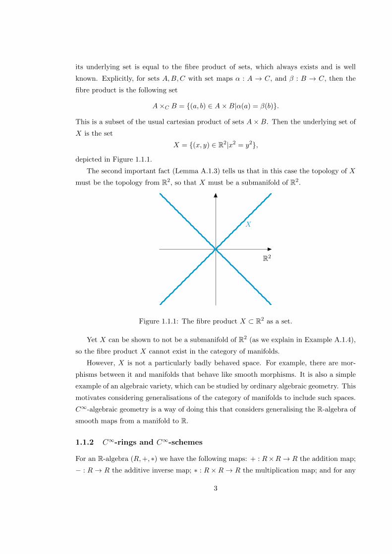
This is a subset of the usual cartesian product of sets A×B. Then the underlying set of

X is the set

X = (x, y) ∈ R2|x2 = y2,

depicted in Figure 1.1.1.

The second important fact (Lemma A.1.3) tells us that in this case the topology of X

must be the topology from R2, so that X must be a submanifold of R2.

R2

X

f

g

Figure 1.1.1: The fibre product X ⊂ R2 as a set.

Yet X can be shown to not be a submanifold of R2 (as we explain in Example A.1.4),

so the fibre product X cannot exist in the category of manifolds.

However, X is not a particularly badly behaved space. For example, there are mor-

phisms between it and manifolds that behave like smooth morphisms. It is also a simple

example of an algebraic variety, which can be studied by ordinary algebraic geometry. This

motivates considering generalisations of the category of manifolds to include such spaces.

C∞-algebraic geometry is a way of doing this that considers generalising the R-algebra of

smooth maps from a manifold to R.

1.1.2 C∞-rings and C∞-schemes

For an R-algebra (R,+, ∗) we have the following maps: + : R×R→ R the addition map;

− : R→ R the additive inverse map; ∗ : R ×R→ R the multiplication map; and for any

3

scalar λ ∈ R the scalar multiplication maps λ : R→ R, r 7→ λr. We also have two objects

0, 1, which can be written as maps R0 → R. These maps obey certain identities, and they

imply that all real polynomials p : Rn → R give operations Rn → R.

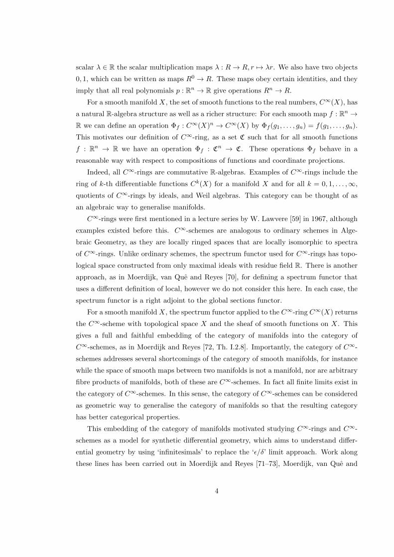
For a smooth manifold X, the set of smooth functions to the real numbers, C∞(X), has

a natural R-algebra structure as well as a richer structure: For each smooth map f : Rn →R we can define an operation Φf : C∞(X)n → C∞(X) by Φf (g1, . . . , gn) = f(g1, . . . , gn).

This motivates our definition of C∞-ring, as a set C such that for all smooth functions

f : Rn → R we have an operation Φf : Cn → C. These operations Φf behave in a

reasonable way with respect to compositions of functions and coordinate projections.

Indeed, all C∞-rings are commutative R-algebras. Examples of C∞-rings include the

ring of k-th differentiable functions Ck(X) for a manifold X and for all k = 0, 1, . . . ,∞,

quotients of C∞-rings by ideals, and Weil algebras. This category can be thought of as

an algebraic way to generalise manifolds.

C∞-rings were first mentioned in a lecture series by W. Lawvere [59] in 1967, although

examples existed before this. C∞-schemes are analogous to ordinary schemes in Alge-

braic Geometry, as they are locally ringed spaces that are locally isomorphic to spectra

of C∞-rings. Unlike ordinary schemes, the spectrum functor used for C∞-rings has topo-

logical space constructed from only maximal ideals with residue field R. There is another

approach, as in Moerdijk, van Que and Reyes [70], for defining a spectrum functor that

uses a different definition of local, however we do not consider this here. In each case, the

spectrum functor is a right adjoint to the global sections functor.

For a smooth manifold X, the spectrum functor applied to the C∞-ring C∞(X) returns

the C∞-scheme with topological space X and the sheaf of smooth functions on X. This

gives a full and faithful embedding of the category of manifolds into the category of

C∞-schemes, as in Moerdijk and Reyes [72, Th. I.2.8]. Importantly, the category of C∞-

schemes addresses several shortcomings of the category of smooth manifolds, for instance

while the space of smooth maps between two manifolds is not a manifold, nor are arbitrary

fibre products of manifolds, both of these are C∞-schemes. In fact all finite limits exist in

the category of C∞-schemes. In this sense, the category of C∞-schemes can be considered

as geometric way to generalise the category of manifolds so that the resulting category

has better categorical properties.

This embedding of the category of manifolds motivated studying C∞-rings and C∞-

schemes as a model for synthetic differential geometry, which aims to understand differ-

ential geometry by using ‘infinitesimals’ to replace the ‘ε/δ’ limit approach. Work along

these lines has been carried out in Moerdijk and Reyes [71–73], Moerdijk, van Que and

4

Reyes [70], Kock [55], and Dubuc [19–21].

The study of C∞-rings and C∞-schemes has been called C∞-algebraic geometry. Re-

cent motivation to study C∞-algebraic geometry is to develop a version of derived geom-

etry for Differential Geometry, as originally suggested in Lurie [62, §4.5], and developed

by Spivak [84]. This has led to further studies in derived geometry by Borisov [8], Borisov

and Noel [10], and the ‘d-manifolds’/‘d-orbifolds’ of Joyce [41], and further refinement

of C∞-algebraic geometry as in Joyce [40] and in Borisov [9]. Note that a d-manifold

is essentially a C∞-scheme that is isomorphic to the fibre product of manifolds, with an

extra sheaf structure. This motivates using a category that contains manifolds and their

fibre products.

1.1.3 Other generalisations of the category of manifolds

C∞-schemes can be viewed as starting with the maps C∞(X) and asking how can this

structure be generalised. This is an example of the ‘maps out’ generalisation of manifolds:

we generalise smooth maps out of the space X to R. There are several other ‘maps out’

approaches, such as those defined in Sikorski [81], and several papers by Spallek starting

with [83]. Many of the ‘maps out’ approaches are also summarised in great detail by

Buchner et al. [7].

One of the approaches by Spallek has been further studied in the book Navarro

Gonzalez and Sancho de Salas [76]. In this book, it is known as the category of C∞-

differentiable spaces, and this category also has all finite limits. C∞-differentiable spaces

are equivalent to a subcategory of C∞-schemes, specifically to C∞-schemes that are lo-

cally isomorphic to the spectrum of certain quotients of C∞(Rn) known as differentiable

algebras. Then the category of manifolds also embeds fully and faithfully into affine C∞-

differentiable spaces, and this embeds fully and faithfully into the category of C∞-schemes.

The spaces defined in Sikorski [81] are a nice subcategory of C∞-differentiable spaces, and

these have been expanded to a sheaf-theoretic version in Mostow [75], who also compares

these notions in more detail.

Reversing the viewpoint, there have been several ‘maps in’ approaches that generalise

the idea of smooth maps from a (subset of) a Euclidean space to the space X. These

approaches include the Diffeological Spaces of Souriau [82] described further in Iglesias-

Zemmour [36], and the various Chen spaces from Chen [12–15]. These notions work

particularly well for considering infinite dimensional spaces (as the morphisms Rn → X

capture information of finite dimensional subspaces), and to describe quotient spaces.

In each of these ‘maps in’ approaches, one begins by taking a set (or topological space)

5

and a collection of maps out of the space (often called plots) that satisfy certain conditions,

such as allowing composition with the usual smooth morphisms and requiring that if a

map is a plot locally, then it is a global plot. Stacey [85] compares these various different

notions, and their relations to Sikorski’s ‘maps out’ approach. However, while each of

these notions generalises smooth manifolds in ways to allow fibre products, they do not

do this by considering spectra of rings in ways similar to Algebraic Geometry, and this

approach is not well suited for derived geometry.

1.1.4 Derived geometry

We are motivated to develop the theory of C∞-algebraic geometry with corners so it can

be used in derived differential geometry as in Joyce [41]. Let us explain the origins of

derived geometry.

Derived geometry was initially conceptualised for algebraic geometry. The motivation

arose from trying to define invariants from moduli spaces that were very singular, as in

Kontsevich [56]. To say something is singular, usually one means either it has quotient

singularities or it has intersection singularities. On the level of spaces, schemes can handle

intersection singularities well and stacks can handle quotient singularities well, but coho-

mology theories do not necessarily behave well without additional assumptions. Here, the

usual notion of cotangent bundle is not sufficient to capture the singular nature of the

space, instead cotangent complexes are more appropriate.

Bertand Toen, Gabriele Vezzossi and Jacob Lurie developed many of the initial ideas

of Derived Algebraic Geometry, and the survey paper Toen [86] details the extensive

applications and further developments of this work in the wider mathematical community.

A more recent survey paper by Anel [4] also describes the ideas in derived geometry to

motivate its use. In Derived Algebraic Geometry, the cotangent complexes live naturally

and hold the information required about the singular nature of a space.

Lurie in [62] first described how to apply many of the ideas of Derived Algebraic

Geometry to differential geometry. Much of the foundational work was carried out by

Lurie’s student David Spivak in his thesis [84]. Further work has been undertaken by

Borisov [8], and Borisov and Noel [10], although their derived objects formed an ∞-

category. The derived differential geometry of Joyce [41] involves only a 2-category of

derived spaces. All of these approaches are built from C∞-rings, C∞-schemes and C∞-

stacks.

The motivation behind the ‘d-manifolds’ of [41] is also related to defining invariants

of certain moduli spaces. This results in requiring additional structure on the moduli

6

spaces, which may be spaces with corners. A manifold with corners is one such space with

corners. The thesis involves building a model of C∞-rings and C∞-schemes with corners

that describes manifolds with corners, not just manifolds. One can then define C∞-stacks

with corners and derived spaces with corners to capture the structure of these moduli

spaces with corners.

1.1.5 Manifolds with corners

The definition of manifold with corners involves generalising the local model of a manifold

from Rn to Rnk = [0,∞)k × Rn−k, and generalising the smooth maps between the local

models, for which there are several different approaches in the literature. We will use the

notion of smooth maps of manifolds with corners that are called ‘b-maps’ in Melrose [68].

These are also used in more recent work by Joyce as in [47]. These b-maps respect the

boundary and corners of a manifold with corners. This allows for a definition of a corner

functor, that takes manifolds to their ‘space of corners’, which is a manifold with corners

of mixed dimension.

Manifolds with corners have been studied in a variety of contexts, beginning with

Cerf [11] and Douady [18] in 1961, as natural ways to extend the notion of a manifold

with boundary. Their work was motivated by understanding questions from differential

topology, for example, to understand homotopy types of diffeomorphism groups of spheres

and other compact manifolds of dimension 3, and they gave many foundational results.

There have been a variety of applications from this work on manifolds with corners in

differential topology, including those of Janich [37]. Janich considered the classification

of manifolds with an O(n) action (called O(n)-manifolds) by decomposing into certain

‘parts’ that are often manifolds with corners. Previously, if such a manifold with corners

was obtained, the corners were often smoothed in some way, eliminating the need to study

manifolds with corners in general. However, Janich explains this approach is not helpful

for this decomposition, and uses the manifold with corners results of Cerf and Douady to

give a ‘classification by parts’ of certain O(n)-manifolds.

Other applications in differential topology include defining the cobordism category of

a manifold with corners as in Laures [58], and to define ‘extended topological quantum

field theories’, which are functors between cobordism categories and categories of vector

spaces as in Kerler [54].

Manifolds with corners arise naturally in many contexts. They can arise directly

such as when considering solutions to the partial differential equation that governs the

motion of a square drum when struck. They can also arise indirectly. For example, many

7

results work well for compact manifolds and such results may need to be extended to

non-compact manifolds by compactifying them. Upon compactifying, the manifold may

become a manifold with corners, so the results need to be generalised for manifolds with

corners. One example is from Monthubert and Nistor [74] who recently extended results

from index theory to non-compact manifolds using manifolds with corners.

For many such applications in analysis, fundamental theorems on the geometry and

analysis of manifolds and manifolds with boundary were extended to manifolds with cor-

ners, as in Melrose [68]. There have also been generalisations of manifolds with corners

along these lines, including the manifolds with analytic corners of Joyce [48].

Another generalisation of manifolds with corners is manifolds with g-corners, as in

Joyce [47]. These allow a more general local model and we will show that many of our

results on manifolds with corners extend to these manifolds with g-corners.

1.1.6 Motivations from symplectic geometry

Some of the specific invariants that have motived derived differential geometry have arisen

in symplectic geometry, as in Joyce [41].

In symplectic geometry, the objects of interest are symplectic manifolds, and classifying

these spaces involves understanding how maps, called J-holomorphic curves, into the

manifold behave. J-holomorphic curves, also known as pseudo-holomorphic curves, are

curves from a Riemann surface (often the Riemann sphere) to the symplectic manifold that

commute with the complex structure from the Riemann surface and an almost complex

structure (called J) on the symplectic manifold.

Recent research in symplectic geometry concerns defining invariants (e.g. numbers,

cohomology classes, categories) on a symplectic manifold using J-holomorphic curves.

Specifically, it aims to define invariants (akin to Gromov-Witten invariants) by ‘counting’

the moduli spaces of J-holomorphic curves arising from a symplectic manifold.

When the J-holomorphic curves are generic, they create families called moduli spaces,

M(J,A), that are parameterised by J and the integer homology classes A of the manifold

that this curve represents. In the nice cases, each family is in fact a finite dimensional

manifold and, while not necessarily compact, there are ways to define invariants such as

the Gromov-Witten invariants as described in McDuff and Salamon [65].

However, to define invariants on these moduli spaces of J-holomorphic curves in general

(for example for symplectic manifolds that are not weakly monotone), more structure

on the moduli spaces is needed. There are several proposed options for this structure:

Kuranishi spaces, polyfolds, and derived spaces. Kuranishi spaces were first defined in

8

Fukaya and Ono, [24], and expanded upon in Fukaya et al. [25]. While they have made a

lot of progress on this, their definition of Kuranishi space has issues, such as not having a

nice notion of morphism and relying on many arbitrary choices.

Polyfolds are an alternative theory to Kuranishi spaces. They were first defined by

Hofer, and developed in a series of papers by Hofer, Wysocki and Zehnder [35]. They

were proposed to solve several issues with Kuranishi spaces. While there has been much

work on foundations of this area, there is still progress to be made on the applications of

defining invariants.

Joyce has proposed ‘d-orbifolds with corners’ as the model for the moduli spaces of

J-holomorphic curves. This model first uses C∞-rings and C∞-schemes to describe C∞-

stacks, as in Joyce [40]. It then considers C∞-stacks that come from fibre products of

orbifolds, and adds an extra sheaf to become a d-orbifold. Then d-orbifolds form a 2-

category with nicely behaved morphisms. There is a provisional notion of corners structure

on a d-orbifold, which adds another sheaf to the d-orbifolds. Joyce [43] shows d-orbifolds

with such corners structure are equivalent to a version of Kuranishi spaces as a 2-category,

and that theseM(J,A) indeed have such a structure. However, this definition of ‘d-orbifold

with corners’ is provisional, as it currently has problems with identifying the correct corners

structure.

This thesis is motivated by ideas to refine the definition of d-orbifolds with corners (and

other derived spaces with corners). Instead of adding a sheaf at the end of the construction

that defines the corners, one should start with a C∞-schemes with corners structure (or

C∞-stack with corners structure). This should make the d-orbifolds with corners easier

to define for each M(J,A), and also describe properties between the C∞-schemes and the

corners precisely. It is intended by Joyce that final version of a d-orbifold with corners

will use the C∞-schemes with corners defined in this thesis.

1.2 What is in this thesis

This thesis defines C∞-rings with corners and C∞-schemes with corners. It explores several

properties of both ideas. It shows, under certain conditions, fibre products of C∞-schemes

with corners exist. It describes how the category of manifolds with corners can be fully and

faithfully embedded into this category. It also describes a corner functor, which returns

the space of corners associated to certain C∞-schemes with corners. Our C∞-schemes

with corners are related to log geometry, in the sense of ‘positive log differentiable spaces’

described in Gillam and Molcho [28], which extend the notion of C∞-differentiable space.

9

In Chapter 2, we recall background on C∞-rings and C∞-schemes; this section is

mostly a summary of background material found in Dubuc [21], Joyce [40, §2–§5] and

Moerdijk and Reyes [72]. We recall the two definitions of C∞-rings, and that the category

of C∞-rings is the category of algebras over an algebraic theory (in the sense of Adamek,

Rosicky and Vitale [3]) so it has all small limits, directed colimits, and small colimits.

We recall the definition of local C∞-rings and discuss their limits and colimits. We recall

the definition of C∞-scheme, and we describe a subcategory of C∞-rings called complete

C∞-rings for which there is an equivalence of categories with the category of affine C∞-

schemes. We use this to show that finite limits of C∞-schemes exist. Section 2.4.1 is new,

where we discuss infinite products of (affine) C∞-schemes.

Chapter 3 describes background on manifolds with corners, as in Joyce [39, 47], and

Melrose [68], and recalls important facts on monoids to describe manifolds with g-corners.

It defines smooth maps of manifolds with (g-)corners, the boundary and corners of a

manifold with (g-)corners, and the corner functor. It also describes their (co)tangent

bundles and, briefly, how their fibre products behave.

The content of Chapter 4 is mostly new and is joint work with Dominic Joyce. We

describe two notions of pre C∞-ring with corners, one as a functor from Euclidean spaces

with corners to sets, and one as a pair (C,Cex) where C is a C∞-ring and Cex is a monoid,

such that the pair behaves well under smooth maps of manifolds with corners. These

notions were first considered in the masters thesis by Kalashnikov [51]. Similar to C∞-

rings, pre C∞-rings with corners are also algebras over an algebraic theory and have all

small limits, directed colimits, and small colimits. We add an additional condition to

define C∞-rings with corners, and show that limits, directed colimits and small colimits

exist in this category too. We describe free C∞-rings with corners, and how to add

relations, and then give a notion of local C∞-rings with corners and localisations, which

we use to define C∞-schemes with corners in Chapter 5. We describe many functors and

their adjoints to study limits and colimits of these categories. We also describe modules

and (b-)cotangent modules of C∞-rings with corners, and prove that they are isomorphic

to the global sections of the (b-)cotangent bundles of both manifolds with corners and

manifolds with g-corners locally and, under certain conditions, globally.

Chapter 5 is new work and comprises of just under half the material in this thesis.

It introduces C∞-ringed spaces with corners and shows small colimits and small limits

exist in this category. We construct a spectrum functor that is right adjoint to a global

sections functor. We define C∞-schemes with corners and show that manifolds with (g-)

corners embed fully and faithfully into this category. We originally aimed to show that

10

all finite limits of C∞-schemes with corners exist, however, there are many interesting

differences between the category of C∞-schemes and C∞-schemes with corners that cre-

ated difficulties for this. Instead, we show that finite limits exist under a certain finitely

generated assumption (which we call firm), where manifolds with (g-)corners considered as

C∞-schemes with corners satisfy this assumption. We use the category of semi-complete

C∞-rings with corners to do this, and we study this category for this purpose.

In Chapter 5 we also define the subcategory of interior C∞-schemes with corners

and describe how all our categories relate with functors and their adjoints. We show

that there is a corner functor for firm C∞-rings with corners that is right adjoint to the

inclusion of interior firm C∞-schemes with corners into firm C∞-schemes with corners.

Similarly, we show there is a corner functor between interior and non-interior local C∞-

ringed spaces with corners, and we explain how these two corner functors relate. We

describe the boundary and corners of a C∞-scheme with corners, and match this with

the definitions of boundary and corners of a manifold with (g-)corners. Chapter 5 also

surveys log geometry, log schemes, and positive log differentiable spaces, and explains how

our C∞-schemes with corners relate to these.

1.3 Summary of main results

1.3.1 C∞-rings and C∞-schemes with corners

The new work of Chapter 4 is joint work with Dominic Joyce. We define pre C∞-rings

with corners and categorical pre C∞-rings with corners, which originally appeared in

Kalashnikov [51]. We show these are equivalent, so pre C∞-rings with corners can be

identified as the category of algebras over an algebraic theory. This gives results on

existence of small limits and colimits. We describe forgetful functors between pre C∞-

rings with corners and the category of C∞-rings, and describe adjoints to this. We add

an extra condition to define C∞-rings with corners, and give an adjoint functor from pre

C∞-rings with corners to describe how their limits and colimits relate. We also define

subcategories of C∞-rings with corners (interior, local, finitely generated, free, firm), and

explore whether these categories also have colimits and limits using adjoint functors.

We define localisations of C∞-rings with corners, and explicitly describe localising at

an ‘R-point’. This is important for defining a spectrum functor. We then define modules

over C∞-rings with corners and give notions of cotangent and b-cotangent modules.

The new work of Chapter 5 is in defining C∞-schemes with corners and their properties.

First we describe a suitable category of local C∞-ringed spaces with corners, and then a

11

spectrum functor for both C∞-rings with corners and interior C∞-rings with corners.

We show each spectrum functor is right adjoint to a global sections functor. The aim

was to show that finite limits in the category of C∞-schemes existed, but this was more

complicated than originally thought.

1.3.2 Finite limits

For an ordinary ring R, then Γ Spec(R) ∼= R where Spec is the spectrum functor in

ordinary algebraic geometry, and Γ is the global sections functor. Here Spec is right

adjoint to Γ considered as functors between ordinary rings and ordinary local ringed

spaces with corners. Then these functors give an equivalence of categories between the

(opposite) category of ordinary rings and ordinary affine schemes. As finite colimits exist

in the category of ordinary rings, then finite limits exist in the category of ordinary affine

schemes. One can then show finite limits of ordinary schemes exist, by either glueing

together the finite limits of affine neighbourhoods, or describing the finite limits of local

ringed spaces with corners and showing these are locally isomorphic to the finite limits of

affine neighbourhoods.

For C∞-ring C, then Γ SpecC C in general, where we are now using the spectrum

functor for C∞-rings. However, Spec is still a right adjoint to Γ considered as functors

between the (opposite) category of C∞-rings and local C∞-ringed spaces with corners, and

there is a canonical isomorphism Spec Γ SpecC ∼= SpecC. Using this isomorphism, we

can define ‘complete’ C∞-rings to be C∞-rings such that Γ SpecC ∼= C, and show there

is an equivalence of categories between complete C∞-rings and affine C∞-schemes as in

Joyce [40]. As complete C∞-rings have all finite colimits, then affine C∞-schemes have all

finite limits. Constructing limits of C∞-schemes in the category of local C∞-ringed spaces

and showing they are locally isomorphic to finite limits of affine C∞-schemes implies that

the category of C∞-schemes has all finite limits.

For a C∞-ring with corners (C,Cex), not only is Γc Specc(C,Cex) (C,Cex), but we

also have Specc Γc Specc(C,Cex) Specc(C,Cex) in general. Here Specc and Γc are the

spectrum and global section functors for C∞-rings with corners. We can still show that

Specc is right adjoint to Γc, however because Specc Γc Specc(C,Cex) Specc(C,Cex) in

general we do not expect an equivalence of categories between a (sub)category of C∞-rings

with corners and affine C∞-schemes with corners.

Instead we use the category of semi-complete C∞-rings with corners, and start by

showing that the category of local C∞-ringed spaces with corners has all finite limits.

Then we show that when a finitely generated condition on Cex holds, finite limits of

12

C∞-schemes with corners exist and are equal to finite limits in the category of local C∞-

ringed spaces with corners using these semi-complete C∞-rings with corners. This finitely

generated condition we call firm and manifolds with (g-)corners considered as C∞-schemes

with corners satisfy this condition. We also describe a similar result for interior C∞-ringed

spaces/schemes with corners.

1.3.3 Embedding manifolds (with corners)

As mentioned in the background of §2, the category of manifolds embeds fully and faith-

fully into the category of C∞-schemes, in fact into the category of affine C∞-schemes.

Transverse fibre products of manifolds exist in the category of manifolds and respect this

embedding. There is a cotangent module for each C∞-ring and cotangent bundle for each

C∞-scheme that correspond with the cotangent module and bundle of a manifold.

In this thesis, we show the category of manifolds with corners embeds fully and faith-

fully into the category of C∞-schemes with corners, but the image is only affine when

the manifolds with corners have faces, which is a nice geometric property. This geometric

property means ‘local behaviour comes from global behaviour’, which we explain further in

Theorem 5.5.2. Manifolds with g-corners also embed fully and faithfully into the category

of C∞-schemes with corners, however an equivalent geometric property to faces does not

imply that local behaviour comes from global behaviour, and the image is not affine in

general.

This issue extends to cotangent modules and bundles, where there is also another ver-

sion of this, the b-cotangent module and b-cotangent bundle. These b-cotangent modules

and bundles behave better with respect to the smooth maps of manifolds with corners.

We show the cotangent module and b-cotangent module are isomorphic to the global sec-

tions of the cotangent and b-cotangent bundles on coordinate charts of manifolds with

corners and manifolds with g-corners. If we consider manifolds with faces (with finitely

many boundary components), then this is true globally not just on coordinate charts,

but this does not apply for manifolds with g-corners. However, the cotangent sheaf and

b-cotangent sheaf do match the cotangent bundles and b-cotangent bundles of manifolds

with (g-)corners globally.

1.3.4 Corner functors

Manifolds with (g-)corners have a notion of corner functor as in Joyce [47], which takes

a manifold with (g-)corners to a manifold with corners of mixed dimension with interior

maps, and which behaves well when using the smooth maps (called b-maps) of Melrose

13

[66–68]. Manifolds with (g-)corners also have a boundary and k-corners as defined in §3.3.

We generalise this corners functor in §5.7 and §5.8. We show that there is a corner

functor C loc for local C∞-ringed spaces with corners, which is right adjoint to the inclusion

of interior local C∞-ringed spaces with corners into the category of C∞-ringed spaces

with corners. This means the inclusion preserves colimits and the corner functor preserves

limits. The corner functors are related to a description of boundary from Gillam and

Molcho [28] for positive log differentiable spaces.

We use a different definition of corner functor C for firm C∞-schemes with corners,

and show this is right adjoint to the inclusion of interior firm C∞-schemes with corners

into firm C∞-schemes with corners. We show C is equivalent to the restriction of C loc to

firm C∞-schemes with corners. To define C, we could have just restricted C loc to firm

C∞-schemes with corners and showed that its image lies in interior firm C∞-schemes with

corners, however with our definition of C the corners of the schemes can understood and

studied without needing to consider ringed spaces. We suspect this may be useful from a

derived geometry perspective.

We show that C loc applied to an arbitrary C∞-scheme with corners is not always a

C∞-scheme with corners, so we do not expect to be able to extend the notion of corners

to C∞-schemes with corners that are not firm. We define the boundary and k-corners

of firm C∞-schemes with corners and local C∞-ringed spaces with corners, then describe

how they match with the boundary and k-corners of manifolds with (g-)corners and how

they relate to the boundary defined in [28]. As a corollary we show the corners functors

of manifolds with (g-)corners are also right adjoints, and satisfy a universal property.

While we were motivated to study finite limits/fibre products from derived geometry,

the corner functor for firm C∞-schemes with corners is constructed from colimits of C∞-

schemes with corners and motivates studying how colimits behave too. We have done

this following colimit results from ordinary (locally) ringed spaces from Demazure and

Gabriel [17, Prop. I.1.1.6], and then describing colimits for C∞-schemes with corners.

1.4 Future work and applications of C∞-algebraic geometry

with corners

There are a few loose ends and potential extensions of C∞-algebraic geometry. For exam-

ple, in §4.5 we define various subcategories of C∞-rings with corners (e.g. toric, integral,

saturated), and we expect their corresponding C∞-schemes with corners to behave better

than arbitrary C∞-schemes with corners, and to have nice results about the corners and

14

boundary.

We would also like to prove that transverse fibre products of manifolds with (g-)

corners respect the embedding into C∞-schemes with corners. In Remark 5.5.5 we suggest

appropriate notions of transverse for manifolds with (g-)corners to do this. Some tentative

calculation suggests restricting to the category of toric C∞-rings/schemes with corners may

be required here.

Remark 5.4.9 discusses a left adjoint to a certain functor that would describe how

limits of C∞-schemes with corners behave and relate to C∞-schemes. There is an issue

with showing the existence of this adjoint with the current method we have, and further

insight on this would be appreciated.

Proposition 5.4.7 characterises interior firm C∞-schemes with corners as firm C∞-

schemes with corners that are interior C∞-ringed spaces with corners. It would be in-

teresting to see whether all C∞-schemes with corners that are interior C∞-ringed spaces

with corners are interior C∞-schemes with corners, as we mention in Remark 5.4.6.

In Proposition 5.4.10 we show fibre products of C∞-schemes with corners exist under

certain conditions. In Remark 5.4.11 we suggest a counterexample to the existence of fibre

products in general, which would be interesting to verify.

Originally C∞-rings and C∞-schemes were studied as a model for synthetic differential

geometry, and our (firm) C∞-rings with corners and C∞-schemes with corners could be

investigated as a model for synthetic differential geometry with corners.

The corner functor could possibly motivate a corner functor for log geometry, and some

of our ideas of boundary and corners could be translated over to this field.

We should be able to define and study C∞-stacks with corners and C∞-orbifolds with

corners, and then consider derived spaces with corners. We expect that only firm C∞-

schemes/stacks with corners will be necessary, which will mean fibre products exist and

there is a possibility of a corner functor for these derived spaces.

Along these lines, we expect a relationship between Kuranishi spaces and C∞-schemes

with corners. Joyce [43] describes a modification of the Kuranishi spaces (with corners) of

Fukaya and Ono [24], which has nice morphisms, and shows that there is an equivalence

of 2-categories between these modified Kuranishi spaces (with corners) and d-orbifolds

(with corners). The original notion of d-orbifold with corners in Joyce [43] was considered

without the definition of C∞-scheme with corners and Joyce is intending to refine this

notion using the work in this thesis, so that there are corner functors for these categories.

There is a truncation functor from d-orbifolds to C∞-schemes, and we expect that there

will be a truncation functor from d-orbifolds with corners to C∞-schemes with corners.

15

Chapter 2

Background on C∞-rings and

C∞-schemes

We begin with background material and results on C∞-rings and C∞-schemes, which we

will later generalise to C∞-rings with corners and C∞-schemes with corners. References

for this section include Dubuc [20, 21], Moerdijk and Reyes [72], and Kock [55], which all

have a view towards synthetic differential geometry, and Adamek, Rosicky and Vitale [3]

who consider algebraic theories and their algebras, which generalise C∞-rings from a

categorical perspective.

In this chapter, we follow closely the work of Joyce [40, §2–§5], particularly in notation.

First, we remark on the notation used from category theory.

Remark 2.0.1. We do not define basic notions of a category nor constructions such as

functors, adjoints, limits, colimits, fibre products etc. which can be found in standard texts

such as Mac Lane [63], Leinster [61] and Awodey [5]. However, we write the following for

notational purposes.

Limits of a diagram in a category, where they exist, are an object in the category

with a universal property, such that it has morphisms from the limit into each element

of the diagram. Colimits are similar with morphisms to the colimit from each element of

the diagram. When we say small limit or colimit, we mean a diagram whose collection

of objects and morphisms form sets. When we say finite limit or colimit we mean the

collection of objects in the diagram is finite.

(Co)products are (co)limits over a diagram that has no morphisms between each

element of the diagram. If the category has a final/terminal (or initial) object, then

(co)products are the same as (co)limits over the same diagram with added morphisms to

this final object (from this initial object). When we say fibre product, we mean a limit over

16

the diagram of the form A→ B ← C, which is a finite limit. If B is the terminal object,

then the fibre product is just the product of A and C. All finite limits exist if and only if

there is a terminal object and all fibre products exist in this category, as each finite limit

is an iterated number of fibre products over the terminal object. When we say pushout

we mean fibre coproduct, that is a colimit over the diagram of the form A← B → C, and

there are similar observations about existence with initial objects.

If a functor is a right adjoint, it preserves limits, and its corresponding left adjoint

preserves colimits. Adjoints are defined in several equivalent ways, using unit and counits,

using natural transformations, using initial and final objects, and we will make use of all

of them. These different definitions can be found for example in Leinster [61, Ch. 2].

2.1 Two definitions of C∞-ring

Here we recall two different notions of C∞-rings. This section follows results of Dubuc [21],

Joyce [40], and Moerdijk and Reyes [72]. Proposition 2.1.11 expands on details suggested

in [21, Prop. 5], but other than this, there is no new material and we keep notation similar

to [40].

We first define C∞-rings as functors using the category of Euclidean spaces, as in

Joyce [40].

Definition 2.1.1. Let Euc be the category of Euclidean spaces with objects Rn, for non-

negative n, and morphisms all smooth maps. Let Man be the category of manifolds with

smooth morphisms. Let Sets be the category of sets with set maps. The notions of finite

products in Euc and Sets are well defined, where Rm+n = Rm ×Rn is the product of Rn

and Rm, and A×B is the product of sets A,B.

A product-preserving functor F : Euc→ Sets is called a categorical C∞-ring . We

require that F preserves the empty product, so it maps R0 in Euc to the point ∗, the final

object in Sets.

A morphism η : F → G between categorical C∞-rings F,G : Euc→ Sets is a natural

transformation η : F ⇒ G. These will automatically preserve products. We use the

notation CC∞Rings for the category of categorical C∞-rings and these morphisms. C∞-

rings in this sense are an examples of algebras over the algebraic theory Euc in the sense

of Adamek, Rosicky and Vitale [3], and many categorical properties of C∞-rings follow

from [3].

Here is an alternative definition of C∞-rings as in classical algebra:

17

Definition 2.1.2. A C∞-ring is a set C that is equipped with operations

Φf : Cn =pn copies qC × · · · × C −→ C

for all non-negative integers n and all smooth maps f : Rn → R. We use the convention

that when n = 0, then C0 is the single point ∅. We require that these operations

satisfy the following composition and projection relations. For the composition relations,

take non-negative integers m,n, and smooth functions fi : Rn → R for i = 1, . . . ,m and

g : Rm → R. Let h be the composition

h(x1, . . . , xn) = g(f1(x1, . . . , xn), . . . , fm(x1, . . . , xn)

),

for all (x1, . . . , xn) ∈ Rn. For any (c1, . . . , cn) ∈ Cn we require

Φh(c1, . . . , cn) = Φg

(Φf1(c1, . . . , cn), . . . ,Φfm(c1, . . . , cn)

).

For the projection relations, let πj : Rn → R, πj : (x1, . . . , xn) 7→ xj be the j-th projection

map for each 1 6 j 6 n, then we require Φπj (c1, . . . , cn) = cj for all (c1, . . . , cn) ∈ Cn.

We call each Φf a C∞-operation. Usually we refer to C as the C∞-ring, and leave the

C∞-operations implicit.

A morphism between C∞-rings φ : C → D is a map of sets φ : C → D such that for

all smooth f : Rn → R and c1, . . . , cn ∈ C then Ψf

(φ(c1), . . . , φ(cn)

)= φ Φf (c1, . . . , cn),

where Φf and Ψf are the C∞-operations for C and D respectively. We will write C∞Rings

for the category of C∞-rings.

There is a forgetful functor Π : C∞Rings → Sets mapping a C∞-ring C to its

underlying set C, forgetting the C∞-operations.

Each C∞-ring C has the structure of a commutative R-algebra. Here, let f : R2 → Ris f(x, y) = x + y be the smooth addition map, then addition ‘+’ on C can be defined

by c + d = Φf (c, d) for c, d ∈ C. Similarly, the smooth multiplication map g : R2 → Ris g(x, y) = xy gives multiplication ‘ · ’ on C by c · d = Φg(c, d). For each λ ∈ R and

scalar multiplication map λ′ : R → R is λ′(x) = λx, we define scalar multiplication by

λc = Φλ′(c). Let 0′ : R0 → R be the zero map, then we can show that 0 = Φ0′(∅) gives

a zero element for C, and 1 = Φ1′(∅), for the unit map 1′ : ∅ 7→ 1, gives an identity

element for C. The projection and composition relations show this gives C the structure

of a commutative R-algebra.

Remark 2.1.3. There is an equivalence of categories CC∞Rings ∼= C∞Rings. Here,

F ∈ CC∞Rings is identified with a C ∈ C∞Rings such that F (R) = C, and for any

smooth f : Rn → R, then F (f) is identified with Φf .

18

The following example of smooth functions on a manifold motivates our definitions.

Example 2.1.4. Let X be a smooth manifold. Let C∞(X) be the set of smooth functions

c : X → R. For non-negative integers n and smooth f : Rn → R, define C∞-operations

Φf : C∞(X)n → C∞(X) by composition(Φf (c1, . . . , cn)

)(x) = f

(c1(x), . . . , cn(x)

), (2.1.1)

for all c1, . . . , cn ∈ C∞(X) and x ∈ X. The composition and projection relations follow

directly from the definition of Φf , so that C∞(X) forms a C∞-ring. If we consider the

R-algebra structure of C∞(X) as a C∞-ring, this is the canonical R-algebra structure

on C∞(X). If f : X → Y is a smooth map of manifolds, then f∗ : C∞(Y ) → C∞(X)

mapping c 7→ c f is a morphism of C∞-rings.

Define a functor FC∞RingsMan : Man → C∞Ringsop to map X 7→ C∞(X) on objects

and f 7→ f∗ on morphisms.

Moerdijk and Reyes show that FC∞RingsMan : Man→ C∞Ringsop is a full and faithful

functor [72, Th. I.2.8], and takes transverse fibre products in Man to fibre products in

C∞Ringsop.

There are many more C∞-rings than those that come from manifolds. For example,

given any k-differentiable manifold X of dimX > 0, then the set Cj(X) of j-differentiable

maps f : X → R is a C∞-ring with operations Φf defined as in (2.1.1), and each of these

C∞-rings is different for each integer 0 > j > k.

Example 2.1.5. Consider X = ∗ the point, so dimX = 0, then C∞(∗) = R = C0(X)

and Example 2.1.4 shows the C∞-operations Φf : Rn → R given by Φf (x1, . . . , xn) =

f(x1, . . . , xn) make R into a C∞-ring. This is the initial object in C∞Rings, and the

simplest nonzero example of a C∞-ring. The zero C∞-ring is the set 0 where all C∞-

operations Φf : 0 → 0 send 0 7→ 0, and this is the final object in C∞Rings.

By Moerdijk and Reyes [72, p. 21–22] and Adamek et al. [3, Prop. 1.21, Prop. 2.5 &

Th. 4.5] we have:

Proposition 2.1.6. The category C∞Rings of C∞-rings has all small limits and all

small colimits. The forgetful functor Π : C∞Rings→ Sets preserves limits and directed

colimits, and can be used to compute such (co)limits, however it does not preserve general

colimits such as pushouts.

This proposition is important for several reasons, including that a C∞-scheme is defined

in terms of sheaves of C∞-rings, which require (small) limits to exist. Also, for these

19

sheaves to be well behaved, a notion of stalk (which uses directed colimit) and a way

to sheafify (which uses small limits and colimits) is needed. We are also particularly

interested in fibre products, that is, finite limits of C∞-schemes, which require pushouts

to exist for C∞-rings.

For the pushout of morphisms φ : C→D, ψ : C→E in C∞Rings, we write Dqφ,C,ψ Eor D qC E. In the special case C =R the coproduct D qR E will be written as D ⊗∞ E.

Recall that coproduct of R-algebras A,B is the tensor product A⊗B, however D⊗∞ E is

usually different from their tensor product D⊗ E. For example, for non-negative integers

m,n, then C∞(Rm)⊗∞C∞(Rn) ∼= C∞(Rm+n) as in [72, p. 22], which contains the tensor

product C∞(Rm)⊗C∞(Rn) but is larger than this, as it includes elements such as exp(xy).

Definition 2.1.7. An ideal I in C is an ideal in C when C is considered as a commutative

R-algebra. We do not require it to be closed under all C∞-operations, as if we did and we

consider the smooth function exp : R→ R, then Φexp(0) = 1, and the ideal would have to

be the entire set C.

We can make the R-algebra quotient C/I into a C∞-ring using Hadamard’s Lemma.

That is, if f : Rn → R is smooth, define ΦIf : (C/I)n → C/I by(

ΦIf (c1 + I, . . . , cn + I)

)(x) = Φf

(c1(x), . . . , cn(x)

)+ I.

Then Hadamard’s Lemma says for any smooth function f : Rn → R, there exists gi :

R2n → R for i = 1, . . . , n, such that

f(x1, . . . , x2)− f(y1, . . . , yn) =n∑i=1

(xi − yi)gi(x1, . . . , xn, y1, . . . , yn).

If d1, . . . , dn are alternative choices for c1, . . . , cn, then ci−di ∈ I for each i = 1, . . . , n and

Φf (c1, . . . , cn)− Φf (d1, . . . , dn) =n∑i=1

(ci − di)Φf (c1, . . . , cn, d1, . . . , dn) ∈ I,

so ΦIf is independent of the choice of representatives c1, . . . , cn in C and is well defined.

We can consider the ideal of a C∞-ring C generated by a collection of elements ca ∈ C

with a ∈ A, in the sense of commutative R-algebras. We denote this (ca : a ∈ A), so that

(ca : a ∈ A) =∑n

i=1 cai · di : n > 0, a1, . . . , an ∈ A, d1, . . . , dn ∈ C.

Definition 2.1.8. Let C be a C∞-ring such that there are a finite number of elements

c1, . . . , cn in C that generate C under the C∞-operations, then C is called a finitely gener-

ated C∞-ring. Note that then every element of c ∈ C can be written as Φf (c1, . . . , cn) for

20

some ci ∈ C. Then C∞(R) is finitely generated as a C∞-ring but not as an R-algebra, so

this condition is much weaker than being a finitely generated R-algebra.

In fact, C∞(Rn) is the free C∞-ring with n generators, as in Kock [55, Prop. III.5.1].

As in Joyce [40], if C is finitely generated, then C ∼= C∞(Rn)/I where I is the kernel of

the map φ : C∞(Rn)→ C, φ(f) = Φf (c1, . . . , cn).

An ideal I in a C∞-ring C is called finitely generated if I = (ca : a ∈ A) for A a

finite set. A C∞-ring C is called finitely presented if there is a finitely generated ideal I in

C∞(Rn) such that C ∼= C∞(Rn)/I for some n > 0. Note that C∞(Rn) is not noetherian,

so ideals in a finitely generated C∞-ring may not be finitely generated themselves. This

implies finitely presented C∞-rings are a subcategory of finitely generated C∞-rings, in

contrast to ordinary algebraic geometry where they are equal.

Definition 2.1.9. Recall that a local R-algebra, R, is an R-algebra with a unique maximal

ideal m. The residue field of R is the field isomorphic to R/m. A C∞-ring C is called

local if, regarded as an R-algebra, C is a local R-algebra with residue field R. The quotient

morphism gives a (necessarily unique) morphism of C∞-rings π : C → R with the property

that c ∈ C is invertible if and only if π(c) 6= 0. Equivalently, if such a morphism π : C → Rexists with this property, then C is local with maximal ideal mC

∼= Ker(π).

Usually morphisms of local rings are required to send maximal ideals into maximal

ideals. However, if φ : C → D is any morphism of local C∞-rings, then because the

residue fields in both cases are R, then φ−1(mD) = mC , so there is no difference between

local morphisms and morphisms for C∞-rings. This also shows that morphisms of local

C∞-rings commute with the morphisms π : C → R.

Remark 2.1.10. We use the term ‘local C∞-ring’ following Dubuc [21, Def. 4] and Joyce

[40]. They are known by different names in other references, such as Archimedean local

C∞-rings in [70, §3], C∞-local rings in Dubuc [20, Def. 2.13], and pointed local C∞-rings

in [72, §I.3]. Moerdijk and Reyes [70–72] use ‘local C∞-ring’ to mean a C∞-ring which is

a local R-algebra, and require no restriction on its residue field.

Proposition 2.1.11. The category of local C∞-rings has all small colimits and small

limits. Small colimits commute with small colimits in C∞Rings, and there is a right

adjoint to the inclusion of local C∞-rings into C∞-rings. Small limits commute with

small limits in C∞Rings only in certain cases, outlined in the proof below, so there is no

left adjoint.

It is already known in the literature that finite colimits (for example, pushouts) of

local C∞-rings exist, for instance in Moerdijk and Reyes [72, §I.3], although their proof is

21

different to the following proof. This proof for colimits expands on the proof of Dubuc [21,

Prop. 5] for finite colimits.

Proof. We first consider pushouts of local C∞-rings.

Let C,D,E be local C∞-rings with morphisms C → D and C → E. Let F be their

pushout in C∞-rings, with maps q1 : D→ F and q2 : E→ F. By definition of pushout in

C∞-rings, we can show that F consists of elements of the form

Φg(q1(d1), . . . , q1(dm), q2(e1), . . . , q2(en))

for smooth g : Rm+n → R, with d1, . . . , dm ∈ C and e1, . . . , en ∈ D. As C,D,E are local,

there exists unique morphisms π1 : C → R, π2 : D → R, π3 : E → R, which define their

maximal ideals, and such that the diagram below commutes.

C

zz ## π1

ww

D

π2

q1

##

Eq2

π3

FtR

(2.1.2)

As F is the pushout, there must be a unique morphism t : F → R that makes the

diagram commute. Take f ∈ F such that t(f) 6= 0 ∈ R. We need to show f has an inverse

in F, so that t makes F into a local C∞-ring.

As f ∈ F, then f = Φg(p) for p = (p1, p2) with p1 = (q1(d1), . . . , q1(dn)) and p2 =

(q2(e1), . . . , q2(em)) for some smooth g : Rn+m → R, c1, . . . , cn ∈ C and d1, . . . , dm ∈ D.

Then

t(f) = g(π1(d1), . . . , π1(dn), π2(e1), . . . , π2(em)) 6= 0.

As g is non-zero at this point, then it must be non-zero in a neighbourhood of this point,

and there must be a function h 6= 0, h : Rn+m → R such that gh = 1 in an open

neighbourhood V of the point. We will show that Φh(p) is the inverse of f .

There are open sets U1 ⊂ Rn and U2 ⊂ Rm such that U1 × U2 ⊂ V , and functions

h1 : Rn → R, h2 : Rm → R such that h1, h2 are zero outside of U1 and U2 respectively, and

are equal to 1 in open balls about t(p1), t(p2) contained in U1 and U2 respectively. Hence

(gh− 1)h1h2 = 0 on Rn+m, which implies that

0 = Φ(gh−1)h1h2(p) = Φ(gh−1)(p)Φh1(p1)Φh2(p2).

22

As D and E are local, and h1 and h2 are non-zero at these points, which lie in U1

and U2, then Φh1(d1, . . . , dn) is invertible in D, and q1(Φh1(d1, . . . , dn)) = Φh1(p1) is

invertible in F, and similarly for h2. So we must have 0 = Φ(gh−1)(p), which implies that

Φg(p)Φh(p) = fΦh(p) = 1, and F is a local C∞-ring.

We have shown the category of local C∞-rings is closed under pushouts, and the

pushouts are exactly those in C∞Rings. As R is the initial object in local C∞-rings,

then all finite colimits can be written as a combination of (iterated) pushouts, which

shows that the category of local C∞-rings has all finite colimits.

To extend this to small colimits, consider that by Proposition 2.1.6, all small colimits

exist for C∞-rings. Again, we can show each element in the colimit is generated from

finitely many elements from the C∞-rings in the diagram, and if all C∞-rings in the

diagram are local, then there must be a unique morphism from the colimit to R. The

same method can then be applied to show that this element is invertible if and only if its

image in R is non-zero. Hence the small colimit of local C∞-rings exists and commutes

with small colimits in the category of C∞-rings.

One can then construct the right adjoint F to the inclusion of local C∞-rings into

C∞-rings by taking F (C) of a C∞-ring C to be the colimit of all the local C∞-rings D

that have morphisms D → C. For a morphism φ : C1 → C2 ∈ C∞Rings then F (φ)

is constructed using the universal property of colimits. The unit is the identity natural

transformation, and the counit is the unique morphism from the colimit to C, and it is

straightforward to see that they form an adjoint pair.

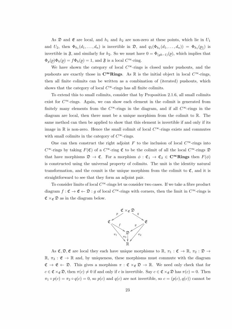
To consider limits of local C∞-rings let us consider two cases. If we take a fibre product

diagram f : C → E← D : g of local C∞-rings with corners, then the limit in C∞-rings is

C ×E D as in the diagram below.

C ×E Dp

yy

q

%%C

f

%%π1

Eg

yyπ2

Dπ3

R

As C,D,E are local they each have unique morphisms to R, π1 : C → R, π2 : D →R, π3 : E → R and, by uniqueness, these morphisms must commute with the diagram

C → E ← D. This gives a morphism π : C ×E D → R. We need only check that for

c ∈ C×ED, then π(c) 6= 0 if and only if c is invertible. Say c ∈ C×ED has π(c) = 0. Then

π1 p(c) = π2 q(c) = 0, so p(c) and q(c) are not invertible, so c = (p(c), q(c)) cannot be

23

invertible either. So C ×E D is local.

Consider now a pair of local C∞-rings C,D with no morphisms between them. Their

product in C∞-rings is C×D, which is not local as it has two distinct R-points. However,

if one instead takes the fibre product over their morphisms to R, that is over the diagram

C → R ← D, then the fibre product C ×R D in C∞-rings is local. It then follows that

this fibre product is actually the product in local C∞-rings: if any other local C∞-ring E

maps into both C and D, then it must commute with their morphisms to R by uniqueness

of its own morphism to R.

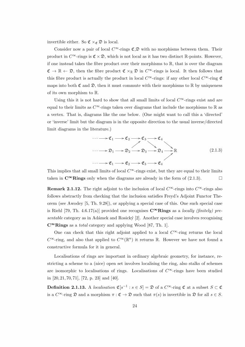
Using this it is not hard to show that all small limits of local C∞-rings exist and are

equal to their limits as C∞-rings taken over diagrams that include the morphisms to R as

a vertex. That is, diagrams like the one below. (One might want to call this a ‘directed’

or ‘inverse’ limit but the diagram is in the opposite direction to the usual inverse/directed

limit diagrams in the literature.)

· · · // C1// C2

// C3//

##

C4

""· · · // D1

// D2//

;;

D3// D4

// R

· · · // E1// E2

// E3// E4

<< (2.1.3)

This implies that all small limits of local C∞-rings exist, but they are equal to their limits

taken in C∞Rings only when the diagrams are already in the form of (2.1.3).

Remark 2.1.12. The right adjoint to the inclusion of local C∞-rings into C∞-rings also

follows abstractly from checking that the inclusion satisfies Freyd’s Adjoint Functor The-

orem (see Awodey [5, Th. 9.28]), or applying a special case of this. One such special case

is Riehl [79, Th. 4.6.17(a)] provided one recognises C∞Rings as a locally (finitely) pre-

sentable category as in Adamek and Rosicky [2]. Another special case involves recognising

C∞Rings as a total category and applying Wood [87, Th. 1].

One can check that this right adjoint applied to a local C∞-ring returns the local

C∞-ring, and also that applied to C∞(Rn) it returns R. However we have not found a

constructive formula for it in general.

Localisations of rings are important in ordinary algebraic geometry, for instance, re-

stricting a scheme to a (nice) open set involves localising the ring, also stalks of schemes

are isomorphic to localisations of rings. Localisations of C∞-rings have been studied

in [20,21,70,71], [72, p. 23] and [40].

Definition 2.1.13. A localisation C[s−1 : s ∈ S] = D of a C∞-ring C at a subset S ⊂ C

is a C∞-ring D and a morphism π : C → D such that π(s) is invertible in D for all s ∈ S.

24

We call π : C → D the localisation morphism for D. This has the universal property that

for any morphism of C∞-rings φ : C → E such that φ(s) is invertible in E for all s ∈ S,

then there is a unique morphism ψ : D→ E with φ = ψ π.

Adding an extra generator s−1 and extra relation s · s−1 − 1 = 0 for each s ∈ S to C,

then it can be shown that localisations C[s−1 : s ∈ S] always exist and are unique up to

unique isomorphism. When S = c then C[c−1] ∼= C ⊗∞ C∞(R)/I, where I is the ideal

generated by ι1(c) · ι2(x) − 1, x is the generator of C∞(R), and ι1, ι2 are the coproduct

morphisms ι1 : C → C ⊗∞ C∞(R), ι2 : C∞(R)→ C ⊗∞ C∞(R).

An example of this is that if f ∈ C∞(Rn) is a smooth function, and U = f−1(Rn \ 0),

then partitions of unity show that C∞(U) ∼= C∞(Rn)[f−1] as in [72, Prop. I.1.6].

The following definition is crucial for defining C∞-schemes.

Definition 2.1.14. A C∞-ring morphism x : C → R, where R is regarded as a C∞-ring

as in Example 2.1.5, is called an R-point . Note that a map x : C → R is a morphism of

C∞-rings whenever it is a morphism of the underlying R-algebras, as in [72, Prop. I.3.6].

We define Cx as the localisation Cx = C[s−1 : s ∈ C, x(s) 6= 0], and denote the projection

morphism πx : C → Cx. Importantly, [71, Lem. 1.1] shows Cx is a local C∞-ring.

There is a one to one correspondence between the R-points of C∞(Rn) and evaluation

at points x ∈ Rn. This also true for C∞(X) for any smooth manifold X, which is a

consequence of [72, Cor. I.3.7].

We can describe Cx explicitly as in Joyce [40, Prop. 2.14].

Proposition 2.1.15. Let x : C → R be an R-point of a C∞-ring C, and consider the

projection morphism πx : C → Cx. Then Cx ∼= C/Kerπx. This kernel is Kerπx = I where

I =c ∈ C : there exists d ∈ C with x(d) 6= 0 in R and c · d = 0 in C

. (2.1.4)

While this localisation morphism πx : C → Cx is surjective, general localisations of

C∞-rings do not have surjective localisation morphisms.

Example 2.1.16. Let C∞p (Rn) to be the set of germs of smooth functions c : Rn → Rat p ∈ Rn for n > 0 and p ∈ Rn. We can give C∞p (Rn) a C∞-ring structure by using

(2.1.1) on germs of functions. There are many equivalent ways to consider the set germs:

as a quotient of C∞(Rn) by an ideal, as a localisation, and as an equivalence class of

pairs as in Joyce [40, Ex. 2.15]. As set of germs [(c, U)] for c ∈ C∞(U) for some U ⊆ X

with p ∈ U , there is a unique maximal ideal mp =

[(c, U)] ∈ C∞p (Rn) : c(x) = 0

and

C∞p (Rn)/mp∼= R. Then C∞p (Rn) is a local C∞-ring.

25

2.2 Modules and cotangent modules of C∞-rings

The following is a summary of the theory of modules and cotangent modules for C∞-rings

as defined in Joyce [40, §5], with reference to Fermat Theories in Dubuc and Kock [23].

Definition 2.2.1. A module M over a C∞-ring C is a module over C as a commutative

R-algebra, and morphisms of C-modules are the usual morphisms of R-algebra modules.

Denote µM : C ×M → M the multiplication map, and write µM (c,m) = c ·m for c ∈ C

and m ∈M . The category C-mod of C-modules is an abelian category.

If a C-module M fits into an exact sequence C ⊗ Rn → M → 0 in C-mod then it is

finitely generated ; if it further fits into an exact sequence C ⊗ Rm → C ⊗ Rn → M → 0

it is finitely presented . This second condition is not automatic from the first as C∞-rings

are not generally noetherian.

For a morphism φ : C → D of C∞-rings and M ∈ C-mod then we have φ∗(M) =

M ⊗C D ∈ D-mod, which gives a functor φ∗ : C-mod → D-mod. For N ∈ D-mod there

is a corresponding C-module φ∗(N) = N where the C-action is defined by µφ∗(N)(c, n) =

µN (φ(c), n). This also defines a functor φ∗ : D-mod → C-mod. Here φ∗ respects the

finitely generated and finitely presented properties, however φ∗ does not.

Example 2.2.2. Let Γ∞(E) be the collection of smooth sections e of a vector bundle

E → X of a manifold X, so Γ∞(E) is a vector space and a module over C∞(X). If

λ : E → F is a morphism of vector bundles over X, then there is a morphism of C∞(X)-

modules λ∗ : Γ∞(E)→ Γ∞(F ) where λ∗ : e 7→ λ e.For each smooth map of manifolds f : X → Y there is a morphism of C∞-rings

f∗ : C∞(Y ) → C∞(X). Each vector bundle E → Y gives a vector bundle f∗(E) → X.

Using (f∗)∗ : C∞(Y )-mod→ C∞(X)-mod from Definition 2.2.1, then (f∗)∗(Γ∞(E)

)=

Γ∞(E)⊗C∞(Y ) C∞(X) is isomorphic to Γ∞

(f∗(E)

)in C∞(X)-mod.

Remark 2.2.3. Let E → X be a vector bundle over a manifold X. Then Γ∞(E) is finitely

presented. In fact, any manifold has a finite atlas of (disconnected) charts, see for example

Greub, Halperin and Valstone, [31, p. 20-21]. Using bump functions, one can extend local

bases for the sections of the vector bundle restricted to these charts to global spanning

sections e1, . . . , en ∈ Γ∞(E) for n 0. This gives a surjective morphism ψ : X ×Rn → E

of vector bundles. The kernel is also a vector bundle F .

For any other surjective morphism φ : X ×Rm → F , we then have the following exact

sequence of vector bundles

X × Rm φ // X × Rn ψ // E // 0.

26

Taking sections, we have an exact sequence of C∞(X)-modules

C∞(X)⊗R Rmφ∗ // C∞(X)⊗R Rn

ψ∗ // Γ∞(E) // 0.

This means Γ∞(E) is finitely presented as a C∞(X)-module.

The definition of C-module only used the commutative R-algebra structure of C, how-

ever the cotangent module ΩC of C does use the C∞-ring structure. It is related to the mod-

ule of Kahler differentials (or module of relative differential forms) as in Hartshorne [33,

p. 172]. In their language, there is a morphism of modules from the module of Kahler

differentials of C over R to the module ΩC that is surjective but not in general injective,

with further discussion on this available on the nLab page [77].

Cotangent modules are an example of a construction defined in Dubuc and Kock [23]

for Fermat Theories, which are types of algebraic theories that have derivatives, and so

this construction can be applied to C∞-rings.

Definition 2.2.4. Take a C∞-ring C and M ∈ C-mod, then a C∞-derivation is a map

d : C → M that is R-linear and satisfies the following: for any smooth f : Rn → R and

elements c1, . . . , cn ∈ C, then

dΦf (c1, . . . , cn) =n∑i=1

Φ ∂f∂xi

(c1, . . . , cn) · dci. (2.2.1)

The pair (M,d) is called a cotangent module for C if it is universal in the sense that for

any M ′ ∈ C-mod with C∞-derivation d′ : C → M ′, there exists a unique morphism of

C-modules λ : M → M ′ with d′ = λ d. Then a cotangent module is unique up to

unique isomorphism. We can explicitly construct a cotangent module for C by considering

the free C-module over the symbols dc and quotienting by relations dΦf (c1, . . . , cn) −∑ni=1 Φ ∂f

∂xi

(c1, . . . , cn) ·dci where we have smooth f : Rn → R and elements c1, . . . , cn ∈ C.

We call this construction ‘the’ cotangent module of C and write it as dC : C → ΩC

If we have a morphism of C∞-rings C → D then ΩD = φ∗(ΩD) can be considered as

a D-module with C∞-derivation dD φ : C → ΩD. The universal property of ΩC , gives

a unique morphism Ωφ : ΩC → ΩD of C-modules such that dD φ = Ωφ dC . From this

we have a morphism of D-modules (Ωφ)∗ : ΩC ⊗C D→ ΩD. If we have two morphisms of

C∞-rings φ : C → D, ψ : D→ E then uniqueness means Ωψφ = Ωψ Ωφ : ΩC → ΩE.

Example 2.2.5. As in Example 2.2.2 if X is a manifold, then its cotangent bundle T ∗X

is a vector bundle over X and its global sections Γ∞(T ∗X) are a C∞(X)-module, with

C∞-derivation d : C∞(X) → Γ∞(T ∗X), d : c 7→ dc the usual exterior derivative and

equation (2.2.1) following from the chain rule.

27

As in Remark 2.2.3, Γ∞(T ∗X) is a finitely presented module. One can then show

that (Γ∞(T ∗X),d) has the universal property in Definition 2.2.4, and so form a cotangent

module for C∞(X). Joyce [40, Ex. 5.4] states this result without proof for manifolds and,

while this result seems known in the literature, we cannot find a proof. We extend this

result to manifolds with corners and describe the proof precisely in Proposition 4.7.5 where

we consider cotangent modules for C∞-rings with corners.

If we have a smooth map of manifolds f : X → Y , then f∗(T ∗Y ), T ∗X are vector

bundles over X, and the derivative df : f∗(T ∗Y ) → T ∗X is a vector bundle morphism.

This induces a morphism of C∞(X)-modules (df)∗ : Γ∞(f∗(T ∗Y ))→ Γ∞(T ∗X), which is

identified with (Ωf∗)∗ from Definition 2.2.4 using that Γ∞(f∗(T ∗Y )) ∼= Γ∞(T ∗Y )⊗C∞(Y )

C∞(X).

This example shows that Definition 2.2.4 abstracts the notion of sections of a cotangent

bundle of a manifold to a concept that is well defined for any C∞-ring.

2.3 Sheaves on topological spaces

Here we consider the definitions of presheaves and sheaves. The standard definition of a

presheaf on a category C valued in a category A is a functor E : Cop → A, where Cop is

the opposite category of C (as in Kashiwara and Schapira [52, §17]).

For a topological space X, let Open(X) be the category of open subsets of X with

inclusion morphisms. In this thesis, we need only consider presheaves and sheaves E :

Cop → A where C = Open(X) for some topological space X, and A is some ‘nice’

category, such as the category of abelian groups, rings, C∞-rings, monoids etc. We will

call these (pre)sheaves of sets, groups, rings, C∞-rings, monoids etc. over X.

By ‘nice’ we mean categories that are complete, that is, having all (small) limits, and,

for this thesis, we will only consider categories A whose objects are sets with some extra

structure, so that there is a faithful functor from these categories to the category of sets

that takes each object to their underlying set. Abelian groups, rings, C∞-rings, monoids

etc are are all algebras over algebraic theories, so they satisfy this and their faithful functor

to sets respects limits and colimits, which is important in the definition of sheaf. In §4we define interior C∞-rings with corners, and while these are constructed from algebraic

theories and are ‘nice’ in the sense above, they are not algebras over algebraic theories

themselves and the functor(s) from interior C∞-rings with corners to their underlying

set(s) respect colimits but not limits, so their sheaves behave differently.

The above discussion gives the following definition, following Godement [30] and Mac

28

Lane and Moerdijk [64].

Definition 2.3.1. A presheaf E on a topological space X valued in A is a functor E :

Open(X)op → A. This equivalently means that E(U) ∈ A for every open set U ⊆ X,

and there is a morphism ρUV : E(U) → E(V ) in A called the restriction map for every

inclusion V ⊆ U ⊆ X of open sets, satisfying the conditions that

(i) ρUU = idE(U) : E(U)→ E(U) for all open U ⊆ X; and

(ii) ρUW = ρVW ρUV : E(U)→ E(W ) for all open W ⊆ V ⊆ U ⊆ X.

A presheaf E : Open(X)op → A is called a sheaf if for all open covers Uii∈I of

U ∈ Open(X), then

E(U)→∏i∈IE(Ui)⇒

∏i,j∈IE(Ui ∩ Uj)

forms an equaliser diagram in A. This implies

(iii) E(∅) = 0 where 0 is the final object in A.

If there is a faithful functor F : A → Sets taking an object of A to its underlying set that

preserves limits, then a presheaf E valued in A on X is sheaf if it equivalently satisfies the

following

(iv) (Uniqueness) If U ⊆ X is open, Vi : i ∈ I is an open cover of U , and s, t ∈ F (E(U))

with F (ρUVi)(s) = F (ρUVi)(t) in F (E(Vi)) for all i ∈ I, then s = t in F (E(U)); and

(v) (Glueing) If U ⊆ X is open, Vi : i ∈ I is an open cover of U , and we are given

elements si ∈ F (E(Vi)) for all i ∈ I such that F (ρVi(Vi∩Vj))(si) = F (ρVj(Vi∩Vj))(sj)

in F (E(Vi ∩ Vj)) for all i, j ∈ I, then there exists s ∈ F (E(U)) with F (ρUVi)(s) = si

for all i ∈ I.

Note that (iv) implies (iii) using the empty cover of the empty set. If s ∈ F (E(U)) and

open V ⊂ U , we write s|V = F (ρUV )(s).

If E ,F are presheaves or sheaves valued in A on X, then a morphism φ : E → F is

a natural transformation of functors E ⇒ F . That is, for each open U ⊆ X, it gives a

morphism in A φ(U) : E(U) → F(U) such that the following diagram commutes for all

open V ⊆ U ⊆ XE(U)

φ(U)//

ρUV

F(U)

ρ′UV E(V )

φ(V ) // F(V ),

where ρUV is the restriction map for E , and ρ′UV the restriction map for F . We define

Sh(X,A) as the category of sheaves on a topological space X valued in A.

29

This second equivalent definition applies for sheaves of C∞-rings and C∞-rings with

corners. The functor from interior C∞-rings with corners to sets (C,Cinq0) 7→ Cinq0does not respect limits (even though the functor Πin : (C,Cin q 0) 7→ Cin does respect

limits as in Theorem 4.3.7), so only the definition of sheaves in terms of equalisers makes

sense for this category.

It is often required in ordinary Algebraic Geometry for presheaves to satisfy (iii) as

in Hartshorne [33, §II.1]. However, this would imply sheaves of interior C∞-rings with

corners are not presheaves of C∞-rings with corners and create additional difficulties, so

we do not require this. We discuss this further in §5.1 and in Remark 5.1.5.

We now assume that A is also cocomplete, that is, it has small colimits and equalisers.

Abelian groups, rings, C∞-rings, monoids etc. all satisfy this, as will (interior) C∞-rings

with corners.

Definition 2.3.2. For E a presheaf valued in A on a topological space X, then we can

define the stalk E at a point x ∈ X to be the direct limit of the E(U) in A for all U ⊆ X

with x ∈ U , using the restriction maps ρUV .

If there is a faithful functor F : A → Sets taking an object of A to its underlying set

that preserves colimits, then explicitly it can be written as a set of equivalence classes of

sections s ∈ F (E(U)) for any open U which contains x, where the equivalence relation is

such that s1 ∼ s2 for s1 ∈ F (E(U)) and s2 ∈ F (E(V )) with x ∈ U, V if there is an open

set W ⊂ V ∩ U with x ∈W and s1|W = s2|W ∈ F (E(W )).

The stalk is also an element of A and the restriction morphisms give rise to morphisms

ρU,x : E(U)→ Ex. A morphism φ : E → F induces morphisms φx : Ex → Fx for all x ∈ X;

this is an isomorphism if and only if φx is an isomorphism for all x ∈ X.

Definition 2.3.3. There is a sheafification functor which takes the category of presheaves

over a topological space X valued in A and their natural transformations to Sh(X,A).

This is defined as a left adjoint to the inclusion of Sh(X,A) into the category of presheaves

over X. We say the image of a presheaf E over X is the sheaf E , and the adjoint property

gives a morphism π : E → E and a universal property: whenever we have a morphism

φ : E → F of presheaves of abelian groups on X and F is a sheaf, then there is a unique

morphism φ : E → F with φ = φ π. This implies sheafification is unique up to canonical

isomorphism.

The sheafification always exists for our categories A, and there is an isomorphism of

stalks Ex ∼= Ex. If there is a faithful functor F : A → Sets taking an object of A to

its underlying set that preserves colimits and limits, it can be constructed (as in [33,

30

Prop. II.1.2]) by defining E(U) as the subset of all functions t : U → qx∈UEx such that

for all x ∈ U , then t(x) = F (ρV,x)(s) ∈ Ex for some s ∈ F (E(V )) for open V ⊂ U , x ∈ V .

If f : X → Y is a continuous map of topological spaces, we can consider pushforwards

and pullbacks of sheaves by f . We will use both of these definitions when defining C∞-

schemes (with corners).

Definition 2.3.4. If f : X → Y is a continuous map of topological spaces, and E is

a sheaf valued in A on X, then the direct image (or pushforward) sheaf f∗(E) on Y is

defined by(f∗(E)

)(U) = E

(f−1(U)

)for all open U ⊆ V . Here, we have restriction maps

ρ′UV = ρf−1(U)f−1(V ) :(f∗(E)

)(U) →

(f∗(E)

)(V ) for all open V ⊆ U ⊆ Y so that f∗(E) is

a sheaf valued in A on Y .

For a morphism φ : E → F in Sh(X,A) we can define f∗(φ) : f∗(E) → f∗(F) by(f∗(φ)

)(U) = φ

(f−1(U)

)for all open U ⊆ Y . This gives a morphism f∗(φ) in Sh(Y,A),

and a functor f∗ : Sh(X,A) → Sh(Y,A). For two continuous maps of topological spaces,

f : X → Y , g : Y → Z, then (g f)∗ = g∗ f∗.

Definition 2.3.5. For a continuous map f : X → Y topological spaces and a sheaf Evalued in A on Y , then we define the pullback (inverse image) of E under f to be the

sheafification of the presheaf U 7→ limA⊇f(U) E(A) for open U ⊆ X, where the direct limit

is taken over all open A ⊆ Y containing f(U), using the restriction maps ρAB in E . We

write this sheaf as f−1(E).

If φ : E → F is a morphism in Sh(Y,A), then there is a pullback morphism f−1(φ) :

f−1(E)→ f−1(F).

Remark 2.3.6. (a) Pullbacks written f−1(E) as in Definition 2.3.5 are used for sheaves

of abelian groups or C∞-rings, however there are different notions f∗(E) or f∗(E) for

pullbacks of sheaves of OY -modules E that are more involved and discussed in §2.5.

(b) For a continuous map f : X → Y of topological spaces we have functors f∗ :

Sh(X,A) → Sh(Y,A), and f−1 : Sh(Y,A) → Sh(X,A). Hartshorne [33, Ex. II.1.18]

gives a natural bijection

HomX

(f−1(E),F

) ∼= HomY

(E , f∗(F)

)(2.3.1)

for all E ∈ Sh(Y,A) and F ∈ Sh(X,A), so that f∗ is right adjoint to f−1. This will be

important in many proofs we consider.

31

2.4 C∞-ringed spaces and C∞-schemes

We now define (local) C∞-ringed spaces and C∞-schemes and consider their properties.

New material includes the proof of Lemma 2.4.6, a discussion of limits and colimits in

Remark 2.4.16, and §2.4.1, which considers products of C∞-schemes.

Definition 2.4.1. A C∞-ringed space X = (X,OX) is a topological space X with a sheaf

OX of C∞-rings on X.

A morphism f = (f, f ]) : (X,OX) → (Y,OY ) of C∞ ringed spaces consists of a

continuous map f : X → Y and a morphism f ] : f−1(OY )→ OX of sheaves of C∞-rings

on X, for f−1(OY ) the inverse image sheaf as in Definition 2.3.5. From (2.3.1), we know

f∗ is right adjoint to f−1, so there is a natural bijection

HomX

(f−1(OY ),OX

) ∼= HomY

(OY , f∗(OX)

). (2.4.1)

We will write f] : OY → f∗(OX) for the morphism of sheaves of C∞-rings on Y corre-

sponding to the morphism of sheaves of C∞-rings on X f ] under (2.4.1), so that

f ] : f−1(OY ) −→ OX ! f] : OY −→ f∗(OX). (2.4.2)

Given two C∞-ringed space morphisms f : X → Y and g : Y → Z we can compose

them to form

g f =(g f, (g f)]

)=(g f, f ] f−1(g])

).

If we consider f] : OY → f∗(OX), then the composition is

(g f)] = g∗(f]) g] : OZ −→ (g f)∗(OX) = g∗ f∗(OX).

We call X = (X,OX) a local C∞-ringed space if it is C∞-ringed space for which

the stalks OX,x of OX at x are local C∞-rings for all x ∈ X. As in Definition 2.1.9,

since morphisms of local C∞-rings are automatically local morphisms, morphisms of local

C∞-ringed spaces (X,OX), (Y,OY ) are just morphisms of C∞-ringed spaces without any

additional locality condition. Local C∞-ringed spaces are called Archimedean C∞-spaces

in Moerdijk, van Que and Reyes [70, §3].

We will follow the notation of Joyce [40] and write C∞RS for the category of C∞-

ringed spaces, and LC∞RS for the full subcategory of local C∞-ringed spaces. We

write underlined upper case letters such as X,Y , Z, . . . to represent C∞-ringed spaces

(X,OX), (Y,OY ), (Z,OZ), . . . , and underlined lower case letters f, g, . . . to represent mor-

phisms of C∞-ringed spaces (f, f ]), (g, g]), . . . . When we write ‘x ∈ X’ we mean that

X = (X,OX) and x ∈ X. If we write ‘U is open in X’ we will mean that U = (U,OU )

and X = (X,OX) with U ⊆ X an open set and OU = OX |U .

32

Example 2.4.2. For a manifold X, we have a C∞-ringed space X = (X,OX) with

topological space X and its sheaf of smooth functions OX(U) = C∞(U) for each open

subset U ⊆ X, with C∞(U) defined in Example 2.1.4. If V ⊆ U ⊆ X then the restriction

morphisms ρUV : C∞(U) → C∞(V ) are the usual restriction of a function to an open

subset ρUV : c 7→ c|V .

Partitions of unity allow us to verify that OX is a sheaf of C∞-rings on X (not just

a presheaf), so X = (X,OX) is a C∞-ringed space. As the stalks OX,x at x ∈ X are

local C∞-rings, isomorphic to the ring of germs as in Example 2.1.16, then X is a local

C∞-ringed space.

For a smooth map of manifolds f : X → Y with corresponding local C∞-ringed

spaces (X,OX), (Y,OY ) as above we define f](U) : OY (U) = C∞(U) → OX(f−1(U)) =

C∞(f−1(U)) for each open U ⊆ Y by f](U) : c 7→ c f for all c ∈ C∞(U). This gives a

morphism f] : OY → f∗(OX) of sheaves of C∞-rings on Y . Then f = (f, f ]) : (X,OX)→(Y,OY ) is a morphism of (local) C∞-ringed spaces with f ] : f−1(OY )→ OX corresponding

to f] under (2.4.2)

Definition 2.4.3. Let C be a C∞-ring, and write XC for the set of all R-points x of

C, as in Definition 2.1.13. Write TC for the topology on XC that has basis of open sets

Uc =x ∈ XC : x(c) 6= 0

for all c ∈ C. For each c ∈ C define a map c∗ : XC → R such

that c∗ : x 7→ x(c).

For a morphism φ : C → D of C∞-rings, we can define fφ : XD → XC by fφ(x) = xφ,

which is continuous.

From Joyce [40, Lem. 4.15], this definition implies TC is the weakest topology on XC

such that the c∗ : XC → R are continuous for all c ∈ C, and it implies that (XC , TC) is a

regular, Hausdorff topological space.

Definition 2.4.4. For a C∞-ring C, we define the spectrum of C, and write it as SpecC.

Here, SpecC is a C∞-ringed space (X,OX), with X the topological space XC from Defini-

tion 2.4.3. For open U ⊆ X, then OX(U) is the set of functions s : U →∐x∈U Cx, where

we write sx for the image of x under s, such that around each point x ∈ U there is an

open subset x ∈W ⊆ U and element c ∈ C with sx = πx(c) ∈ Cx for all x ∈W . This is a

C∞-ring with the operations Φf on OX(U) defined using the operations Φf on Cx.

For s ∈ OX(U), the restriction map of functions s 7→ s|V for open V ⊆ U ⊆ X is

a morphism of C∞-rings, giving the restriction map ρUV : OX(U) → OX(V ). The stalk

OX,x at x ∈ X is isomorphic to Cx by Joyce [40, Lem. 4.18], which is a local C∞-ring.

Hence (X,OX) is a local C∞-ringed space.

33

For a morphism φ : C → D of C∞-rings, then we have an induced morphism of local

C∞-rings, φx : Cfφ(x) → Dx. If we let (X,OX) = SpecC, (Y,OY ) = SpecD, then for

open U ⊆ X define (fφ)](U) : OX(U) → OY (f−1φ (U)) by (fφ)](U)s : x 7→ φx(sfφ(x)).

This gives a morphism (fφ)] : OX → (fφ)∗(OY ) of sheaves of C∞-rings on X. Then

fφ = (fφ, f]φ) : (Y,OY ) → (X,OX) is a morphism of local C∞-ringed spaces, where f ]φ

corresponds to (fφ)] under (2.4.2). Then Spec is a functor C∞Ringsop → LC∞RS,

called the spectrum functor, where Specφ : SpecD→ SpecC is defined by Specφ = fφ.

Example 2.4.5. For a manifold X then SpecC∞(X) is isomorphic to the local C∞-ringed

space X constructed in Example 2.4.2.

The following lemma will be important for considering C∞-schemes with corners. As

the lemma is stated without proof in [40, Lem 4.28], we include a proof here.

Lemma 2.4.6. Take element c ∈ C in a C∞-ring C and let X = SpecC = (X,OX). If

we consider Uc = x ∈ X : x(c) 6= 0 as in Definition 2.4.3, then Uc ⊆ X is open and

X|Uc = (Uc,OX |Uc) ∼= SpecC[c−1].

Proof. Let φ : C → C[c−1] be the localisation morphism, and write Spec(C[c−1]) =

(Y,OY ) = Y . Consider the morphism Spec(φ) = (φ∗, φ]) : Y → X and the restric-

tion ρX,Uc : OX → OX |Uc . We will show that φ∗ : Y → X is an isomorphism onto its

image, Uc, and that φ] : OX → φ∗(OY ) is an isomorphism upon restriction to Uc, so that

Spec(φ) is an isomorphism onto its image X|Uc .Firstly, as φ : C → C[c−1] is a C∞-ring morphism, any R-point, x of C[c−1] corresponds

to a unique R-point, x, of C. If x ∈ X\Uc is an R-point of C, then x /∈ Uc, and the definition

of Uc means x(c) = 0. However, in C[c−1], c is invertible, so x cannot give a corresponding

an R-point of C[c−1].

For any x ∈ Uc, x(c) 6= 0, then the universal property of C[c−1] implies there is a

unique corresponding R-point x of C[c−1]. Hence Y is isomorphic as a set to Uc. Using

the definition of φ∗, then this correspondence is the continuous map φ∗ : Y → X with

image Uc. That is, any open set U ⊂ X, gives an open set U ∩ Uc in Y .

To see it is a homeomorphism, consider a base element of the topology Ud = y ∈Y : y(d) 6= 0 ⊂ Y ∼= Uc, for some d ∈ C[c−1]. We show that around any point y ∈ Ud,there is an open set Uk, with k ∈ φ(C), such that y ∈ Uk ⊂ Ud, so the topology is the

subset topology. Now d must be of the form Φf (a, c−1) for some a ∈ C and some smooth

f : R2 → R. Take y ∈ Ud, then y(d) = f(y(a), y(c−1)), with y(c−1) = y(c)−1 6= 0. Assume

r = y(c) > 0 without loss of generality. Then consider that y ∈ Y : y(c) ∈ ( r2 ,3r2 ) =

UΦg(c) is open in Y , where g : R → R is a smooth bump function with support ( r2 ,3r2 ),

34

and UΦg(c) contains y. Let h : R→ R be any smooth function with h(t) = 1t for t ∈ ( r2 ,

3r2 )

and positive elsewhere. Then for all y ∈ Ud ∩ UΦg(c), we have

0 6= y(d) = f(y(a), y(c−1)) = f(y(a), h(y(c))) = y(Φf(·,h(·))(a, c)) = y(b)

for b = Φf(·,h(·))(a, c) ∈ φ(C). So Ub ⊃ Ud ∩ UΦg(c) and it follows that

y ∈ UbΦg(c) = Ub ∩ UΦg(c) = Ud ∩ UΦg(c) ⊂ Ud

is open in Uc, with k = bΦg(c) ∈ φ(C), as required.

To show the map of sheaves φ] : OX → φ∗(OY ) is an isomorphism upon restriction to

Uc, we show it is an isomorphism on stalks, that is Cx and C[c−1]x are isomorphic for each

x ∈ Uc and corresponding x ∈ Y .

For x ∈ Uc, then the image of c under the map πx : C → Cx is invertible. By

the universal property of C[c−1], there is a unique map α1 : C[c−1] → Cx. The universal

property of Cx then gives a unique morphism α2 : Cx → C[c−1]x, and the universal property

of C[c−1]x then gives a unique morphism α3 : C[c−1]x → Cx. As the following diagram

commutes, these two maps must be inverses, and the localisations must be isomorphic.

Cφ //

πx

C[c−1]

πxα1

ssCx

α2 ..C[c−1]x

α3

mm

By definition, α3 is the stalk map φ]x, which implies Spec(φ) : Y → X is an isomorphism

onto its image X|Uc as required.

Definition 2.4.7. There is a global sections functor Γ : LC∞RS→ C∞Ringsop, which

takes (X,OX) to OX(X) and morphisms (f, f ]) : (X,OX) → (Y,OY ) to Γ : (f, f ]) 7→f](Y ), for f] relating f ] as in (2.4.2).

For each C∞-ring C we can define a morphism ΞC : C → Γ SpecC. Here, for c ∈ C

then ΞC(c) : XC →∐x∈XC

Cx is defined by ΞC(c)x = πx(c) ∈ Cx, so ΞC(c) ∈ OXC(XC) =

Γ SpecC. This ΞC is a C∞-ring morphism as it it composed of C∞-ring morphism

πx : C → Cx and the C∞-operations onOXC(XC) are defined pointwise in the Cx. In fact, it

defines a natural transformation Ξ : idC∞Rings ⇒ ΓSpec of functors idC∞Rings,ΓSpec :

C∞Rings→ C∞Rings.

Theorem 2.4.8. The functor Spec : C∞Ringsop → LC∞RS is right adjoint to Γ :

LC∞RS→ C∞Ringsop. Here, Ξ is the unit of the adjunction between Γ and Spec. This

implies Spec preserves limits as in [21, p. 687]. Hence if we have C∞-ring morphisms

35

φ : F → D, ψ : F → E in C∞Rings then their pushout C = D qF E has image that is

isomorphic to the fibre product SpecC ∼= SpecD×SpecF SpecE.

We extend this theorem to C∞-schemes with corners in §5.1.

Remark 2.4.9. The definition of spectrum functor follows Dubuc [21] and Joyce [40],

and it is called the Archimedean spectrum in Moerdijk et al. [70, §3]. They also show it is

a right adjoint to the global sections functor as above.

In [70, §1] they consider another definition of spectrum SpecC which uses ‘C∞-radical

prime ideals’ not R-points. This means they use a different, less restrictive, definition of

local C∞-ring. This is not an equivalent definition to our definition, as the image of the

functor is not contained in LC∞RS, but in a larger subcategory of C∞RS which they

call C∞-spaces. However, in [70, §3] they show there is a right adjoint to the inclusion

of LC∞RS into the category of C∞-spaces. Their definition of spectrum composed with

this right adjoint gives a right adjoint to our global sections functor. As right adjoints

are naturally isomorphic, then this composition is naturally isomorphic to our spectrum

functor.

Definition 2.4.10. Elements X ∈ LC∞RS that are isomorphic to SpecC for some

C ∈ C∞Rings are called affine C∞-schemes. Elements X ∈ LC∞RS that are locally

isomorphic to SpecC for some C ∈ C∞Rings (depending upon the open sets) are called

C∞-schemes. We define C∞Sch and AC∞Sch to be the full subcategories of C∞-schemes

and affine C∞-schemes in LC∞RS respectively.

Remark 2.4.11. Unlike ordinary algebraic geometry, affine C∞-schemes are very general

objects. All manifolds are affine, and all their fibre products are affine, suggesting that

the use of C∞-schemes in Derived Differential Geometry can (and usually is) confined to

only affine (finitely presentable) C∞-schemes. Contrary to this, we will need non-affine

C∞-schemes with corners in §5, which will require understanding non-affine C∞-schemes.

More generally, all second countable, metrizable C∞-schemes are affine, and it is nec-

essary that affine C∞-schemes are Hausdorff and regular. Joyce [40, Th. 4.41] shows that

a local C∞-ringed space that is Hausdorff, Lindelof and has smoothly generated topology

is an affine C∞-scheme. Here, X ∈ LC∞RS has smoothly generated topology if the sets

Uc = x ∈ X : π πx(c) 6= 0 ∈ R where c ∈ OX(X) form a basis for the topology of X.

As in Joyce [40, Prop. 4.34] we have the following crucial isomorphism that allows us

to define complete C∞-rings.

Proposition 2.4.12. For each C∞-ring C, Spec ΞC : Spec Γ SpecC → SpecC is an

isomorphism in LC∞RS.

36

Definition 2.4.13. A C∞-ring C is called complete if ΞC : C → Γ SpecC is an iso-

morphism. We define C∞Ringsco to be the full subcategory in C∞Rings of complete

C∞-rings.

Using Proposition 2.4.12 we see that complete C∞-rings are isomorphic to the image of

the functor Γ Spec : C∞Rings→ C∞Rings, which gives a left adjoint to the inclusion

of C∞Ringsco into C∞Rings. Let this left adjoint be the functor Rcoall : C∞Rings →

C∞Ringsco.

An example of a C∞-ring that is not complete is the quotient of C∞(Rn) by the ideal of

compactly supported functions, and Rcoall applied to this quotient returns the zero C∞-ring.

In ordinary algebraic geometry, we have a contravariant equivalence of categories be-

tween ordinary affine schemes and commutative rings. This is used to show all (finite)

limits of ordinary schemes exist. However, this is not true in the case of affine C∞-schemes;

in some sense, there are more C∞-rings than affine C∞-schemes, and Spec is not full nor

faithful on C∞Ringsop. The next theorem tells us that the category of complete C∞-rings

gives an equivalence of categories instead.

The following is a summary of results from [40, Prop. 4.11,Th. 4.25].

Theorem 2.4.14. (a) Spec |(C∞Ringsco)op : (C∞Ringsco)op → LC∞RS is full and

faithful, and an equivalence of categories Spec |··· : (C∞Ringsco)op → AC∞Sch.

(b) Let X be an affine C∞-scheme. Then X ∼= SpecOX(X), where OX(X) is a complete

C∞-ring.

(c) The functor Rcoall : C∞Rings → C∞Ringsco is left adjoint to the inclusion functor

inc : C∞Ringsco → C∞Rings. That is, Rcoall is a reflection functor.

(d) All small colimits exist in C∞Ringsco, although they may not coincide with the

corresponding small colimits in C∞Rings.

(e) Spec |(C∞Ringsco)op = Spec inc : (C∞Ringsco)op → LC∞RS is right adjoint to

Rcoall Γ : LC∞RS → (C∞Ringsco)op. Thus Spec |··· takes limits in (C∞Ringsco)op

(equivalently, colimits in C∞Ringsco) to limits in LC∞RS.

Using (a), that small limits exist in the category of C∞Rings, and that Γ : LC∞RS→C∞Rings is a left adjoint with image in (C∞Ringsco)op when restricted to AC∞Sch,

then small limits of C∞Ringsco exist and coincide with small limits in C∞Rings. As

we have an equivalence of categories, (C∞Ringsco)op → AC∞Sch, then AC∞Sch also

has all small colimits and small limits. As Spec is a right adjoint, then limits in AC∞Sch

coincide with limits in C∞Sch and LC∞RS, however it is not necessarily true that

colimits in AC∞Sch coincide with colimits in C∞Sch and LC∞RS.

37

We have the following theorem on limits in C∞RS and subcategories.

Theorem 2.4.15. (i) All finite limits exist in the category C∞RS.

(ii) The full subcategory LC∞RS is closed under finite limits in C∞RS.

(iii) The full subcategories AC∞Sch and C∞Sch of LC∞RS are closed under all finite

limits in LC∞RS. Hence fibre products and all finite limits exist in these categories.

Remark 2.4.16. In the previous Theorem, for (i) and (ii) refer to Joyce [40, Prop. 4.11,

Th. 4.25], and for (ii) refer to Dubuc [21, Prop. 7]. Note however that the proof of (iii)

relies on the existence of complete C∞-rings; this part of the theorem is mentioned in [40]

however the proof is not detailed.

One can prove this using the following: Theorem 2.4.14(a) shows all limits are exactly

those from colimits of complete C∞-rings, then Theorem 2.4.14(d) implies all small colimits

exist, and therefore all small limits exist in AC∞Sch. One then shows they coincide

with small limits in LC∞RS. Finite limits of C∞Sch in LC∞RS are then shown to

be locally affine, giving the result. Alternatively, following the standard proof in ordinary

algebraic geometry, see Hartshorne [33, Th. 3.3]), one could show that glueing C∞-schemes

together on affine neighbourhoods is a scheme, then glue the fibre products of the local

affine neighbourhoods, which gives the same result.

In Section 5, we have similar results for local C∞-ringed spaces with corners and C∞-

schemes with corners, where we describe the proofs in more detail. In fact, all small limits

exist in C∞RS and LC∞RS, we show this is true in §5.1.1 with our more general results

on C∞-ringed spaces with corners.

Demazure and Gabriel, [17, I §1 1.6] construct small colimits in the categories of

ordinary ringed and locally ringed spaces. This construction also applies for (local) C∞-

ringed spaces; the underlying topological space is the colimit of the underlying topological

spaces and the sheaf is essentially the limit of the sheaves. For locally ringed spaces, the

main issue is to show the stalks are local, where in the C∞-ring case, this follows from

Proposition 2.1.11. We describe this proof explicitly when we consider C∞-ringed spaces

with corners in §5.1.1.

Finally, we consider the embedding of manifolds into C∞-schemes and whether fibre

products respect this embedding. In the following theorem we summarise results found in

Dubuc [21, Th. 16], Moerdijk and Reyes [71, § II. Prop. 1.2], and Joyce [40, Cor. 4.27].

Theorem 2.4.17. There is a full and faithful functor FAC∞SchMan : Man→ AC∞Sch that

takes a manifold X to the affine C∞-scheme X = (X,OX), where OX(U) = C∞(U) is

38

the usual smooth sections on U . Here (X,OX) ∼= Spec(C∞(X)) and hence X is affine.

The functor FAC∞SchMan sends transverse fibre products of manifolds to fibre products of

C∞-schemes with corners.

2.4.1 Products of C∞-schemes

This section is new and we discuss products of C∞-schemes.

Remark 2.4.18. When considering infinite products of schemes we will need to consider

whether or not measurable cardinals exist. We will not define measurable cardinals, but

refer the reader to Jech [38, Ch. 10] and Gillman and Jerison [29, Ch. 12] for further

details. Measurable cardinals are a type of large cardinal number, that is, a cardinal

number that cannot be accessed by the standard arithmetic operations using ℵ0. This

means that ℵ0,ℵ1,ℵ2 . . ., 2ℵ0 , 22ℵ0 , . . . , 2ℵ1 , 22ℵ0 , . . . and many other cardinal numbers are

not measurable cardinals, (cf. [29, p. 161-166]). We say such non-measurable cardinals are

less than any measurable cardinal.

The existence of measurable cardinals is an axiom of set theory that is independent

from the usual ZFC axioms (Zermelo–Fraenkel set axioms and the Axiom of Choice), as in

Jech [38, p. 33, 77]. None of our examples or intended applications would need to assume

measurable cardinals exist, however the definitions of C∞-rings and C∞-rings with corners

do not preclude this assumption, so we note carefully where this assumption impacts the

theory.

The author would like to acknowledge assistance from Professor George Bergman for

details in the proof of the following lemma.

Lemma 2.4.19. Let I be a set and define C =∏i∈I R. Then any R-point x : C → R

factors through precisely one of the R in the product provided the cardinality of I is less

than any measurable cardinal.

Proof. This follows by considering Bergman and Nahlus [6, Th. 9], which implies that

whenever the cardinality of I is less than any measurable cardinal, then x : C → Rfactors as a R-algebra morphism through a product of finitely many of the R in C, say

Ri1 , . . . ,Rin . This means that there is an element c = (ci)i∈I ∈ C, with ci = 1 for i = ik

and zero otherwise, such that x(c) = 1.

Letting dik = (di)i∈I , with di = δiki , then∑k

i=1 dik = c, and x(c) = 1 =∑k

i=1 x(dik).

However, dik1· dik2

= 0, so x(dik1) · x(dik2

) = x(dik1· dik2

) = 0, so precisely one dik is such

that x(dik) = 1 with all others evaluating to 0. Then x must factor through only this

Rik .

39

Remark 2.4.20. One can deduce Lemma 2.4.19 using the language of ultrafilters (in the

sense of Comfort and Negrepontis [16]), which forms part of the reasoning behind [6, Th. 9].

First one shows that any such x : C → R gives an ultrafilter on I, and that factoring

through precisely one of the R in the product requires it to be a principal/fixed ultrafilter.

Showing that there are no ultrafilters that do not factor through one of the R in the product

requires showing there are no non-principal/free ultrafilters to come from such an x. In

Gillman and Jerison [29], this is a property called realcompact and they show in [29, p. 163]

that such an ultrafilter I only has this property if and only if it has cardinality less that

any measurable cardinal, giving the result.

Lemma 2.4.21. Let I be a set and C =∏i∈I Ci be a C∞-ring that is the product of the

C∞-rings Ci. If x : C → R factors through Ck then there is a canonical isomorphism

(Ck)x ∼= Cx.

Proof. Consider the following commutative diagram.∏i∈I Ci

πkww

x

++

πx

Ckπk,x

(Ck)x

''

(∏i∈I Ci)x

too

R

(2.4.3)

Here πk is the projection onto the k-th factor and πx, πk,x are the localisation projections,

which are surjective. Note that the dotted arrow t exists by the universal property of

localisation of C.

The map t : (∏i∈I Ci)x → (Ck)x sends πx((ci)i∈I) ∈ (

∏i∈I Ci)x to πk,x πin

x ((ci)i∈I) =

πk,x(ck) ∈ (Ck)x. This implies t is surjective. To show it is injective, say t(πx((ci)i∈I)) =

t(πx((di)i∈I)) ∈ (Ck)x, then πk,x(ck) = πk,x(dk), so by Proposition 2.1.15 there exists

a ∈ Ck with x(a) 6= 0 such that a · (ck − dk) = 0. Then define (ai)i∈I ∈∏i∈I Ci by ak = a

and ai = 0 for i 6= k. Then (ai)i∈I · ((ci)i∈I − (di)i∈I) and x((ai)i∈I) 6= 0, which implies

πx((ci)i∈I) = πx((di)i∈I) ∈ (∏i∈I Ci)x, so t is injective and must be an isomorphism.

Proposition 2.4.22. If I is a set with cardinality less than any measurable cardinal and

if Cii∈I is a collection of C∞-rings, then Spec(∏i∈I Ci)

∼=∐i∈I Spec(Ci). That is,

coproducts in C∞-schemes and affine C∞-schemes are the same.

Proof. Let X = Spec(∏i∈I Ci) and Y =

∐i∈I Spec(Ci). Firstly note that any R-point

yk : Ck → R, k ∈ I, gives a unique R-point x :∏i∈I Ci → R by x((ci)i∈I) 7→ yk(ck), so

there is an inclusion of sets Y → X.

40

Take x ∈ X, so that x :∏i∈I Ci → R is an R-point. We have an inclusion morphism

of C∞-rings i :∏i∈I Ri →

∏i∈I Ci, so that the composition x i :

∏i∈I Ri → R is an

R-point of∏i∈I R. By Lemma 2.4.19, this R-point factors through one of the R in the

product; denote this Rk. Then the element dk = (di)i∈I ∈∏i∈I R with di = δki maps

to a similarly described element in∏i∈I Ci and then maps to 1 under x. This gives a

morphism from Ck → R that commutes with the projection from∏i∈I Ci → Ck. However,

dk′ = (di)i∈I ∈∏i∈I R with di = δk

′i and k′ 6= k will map to a similarly described element

in∏i∈I Ci and then to 0 under x, so that x factors through Ck uniquely. Hence Y = X

as sets.

Take a basic open set Uc = x :∏i∈I Ci → R : x(c) 6= 0 ⊂ X for some c = (ci)i∈I ∈∏

i∈I Ci. Then each x ∈ Uc corresponds to an R-point yk : Ck → R for some k ∈ I, and

x(c) 6= 0 if and only if yk(ck) 6= 0. Then each Uc is in one-to-one correspondence with

disjoint unions of basic opens∐i∈I U

kck⊂ Y , where Ukck = yk : Ck → R : yk(ck) 6= 0. As

such disjoint unions of basic opens form a basis for the topology of Y then the topologies

are the same, and X = Y as topological spaces.

Taking Spec of the projections πk :∏i∈I Ci → Ck gives corresponding morphisms

Spec(πk) : Spec(Ck)→ Spec(∏i∈I Ci), which we can amalgamate to a morphism

f = (f, f ]) :∐i∈I

Spec(Ci)→ Spec(∏i∈I

Ci)

using the universal property of a coproduct. We have shown that f is an isomorphism

of topological spaces. Take yk ∈ Y and x = f(yk), then f ]yk : OX,x → OY,yk is the

isomorphism t in Lemma 2.4.21, so f is an isomorphism.

Remark 2.4.23. Proposition 2.4.22 is unlike the case of ordinary algebraic geometry,

which we discuss here. In ordinary algebraic geometry, if I is a set and Ai is a collection

of rings, then the projections∏i∈I Ai → Aj and the universal property of coproducts give

a canonical morphism φ :∐i∈I Spec(Ai)→ Spec(

∏i∈I Ai). This is an isomorphism if I is

finite. Let X = Spec(∏i∈I Ai), Xi = Spec(Ai) so φ = (φ, φ]) :

∐i∈I Xi → X.

If I is infinite (and enough of the Ai are non-zero) then φ is not an isomorphism, as

then the topological space of the target is larger than the topological space of the domain.

To see this, note first that the inclusion of each Xi in X is both open and closed. Here,

the prime ideal pi ⊂ Ai corresponds to a point pi ∈∐j∈I Xj , and under φ pi is sent to

prime ideal pi = (aj)j∈I ∈ X with aj = Aj for i 6= j and ai = pi. This means φ is a

bijection onto its image.

Take ideals in∏i∈I Ai defined as bj = (bi,j)i∈I with bj,j = Aj and bi,j = 0 the zero

ideal of Aj whenever i 6= j. Let V (bj) be the basic closed set in∏i∈I Ai corresponding to

41

bj (defined in Hartshorne [33, p. 70] as the set of all prime ideals that contain bj), then

its complement is equal to the image of Xi in X. Hence each image of Xi is open. Also

an ideal qi ⊂ Ai gives an open set Xi \ V (qi), and then

φ(Xi \ V (qi)) = φ(Xi) \ V (qi)

where qi = (cj)j∈I ∈ X with cj = Aj for i 6= j and ci = qi. This implies φ is a

homeomorphism onto its image.

Now take ideals dj = (di,j)i∈I ⊂∏i∈I Ai with dj,j = 0 the zero ideal of Ai and di,j = Ai

for all i 6= j. These define closed sets V (dj) that are equal to the image of each Xi in X,

so this image is also closed.

However, the direct sum∑

i∈I Ai (which contains all finite linear combinations of

elements of the Ai’s) is an ideal of∏i∈I Ai. It is equal to

∏i∈I Ai when I is finite.

However, when I is infinite it is not equal to∏i∈I Ai, so must be contained in a maximal

(prime) ideal that is not of the form pi for some pi. This prime ideal is not in the image

of φ, and hence φ is not an isomorphism.

We can examine the topology of X and∐i∈I Xi when I is infinite in more detail. We

see that

φ(∐i∈I

Xi) = ∪i∈Iφ(Xi) = ∪j∈I(X \ V (bj)) = X \ (∩j∈IV (bj)) = X \ V (∑j∈J

bj) ⊂ X,

where∑

j∈J bj is the direct sum of ideals. As V (∑

j∈J bj) is the complement of φ(∐i∈I Xi),

then all prime ideals of∏i∈I Ai either are equal to pi for some pi ⊂ XI and are in the

image of φ, or they contain the direct sum and are not in the image of φ. Then V (∑

j∈J bj)

is closed in X and not open, and φ(∐i∈I Xi) is open in X but not closed.

This is important because while X is an affine scheme,∐i∈I Xi is not affine for I

infinite. If it were affine, it would be quasi-compact, that is every open cover would have

a finite subcover. [This follows as, say Y \V (dj)j∈J is an open cover of an affine scheme

Y = Spec(B) for some ring B, then

Y = ∪j∈J(Y \ V (dj)) = Y \ ∪j∈JV (dj) = Y \ V (∑j∈J

dj)

implies the direct sum∑

j∈J dj = B, so there is a finite linear combination of the dj that

equals 1 ∈ B. The elements in this finite linear combination correspond to the subcover.

For more on quasi-compact, see Hartshorne [33, p. 80, 2.13(b)].] However, Xii∈I is an

open cover of∐i∈I Xi and it has no finite subcover, so

∐i∈I Xi is not affine.

We can also show that any open set of X that contains V (∑

j∈J bj) must contain all

but finitely many of the φ(Xi). Here an open set is of the form X \ V (K) for some ideal

42

K ⊂∏i∈I Ai. If V (

∑j∈J bj) ⊂ X \ V (K), then

∅ = V (K) ∩ V (∑j∈J

bj) = V (K +∑j∈J

bj),

so 1 ∈ K +∑

j∈J bj =∏i∈I Ai. Then K must contain an element that is equal to 1 in all

but finitely many of the entries, and the result follows.

We conclude that X is affine, it has (open and closed) affine subschemes φ(Xi) ∼= Xi,

and has the (non-affine when I is infinite) open subscheme φ(∐i∈I Xi). Hence, the image

of∐i∈I Xi under φ when I is infinite is open but does not cover X, so φ is not an

isomorphism when I is infinite.

2.5 Sheaves of OX-modules and cotangent modules

This section follows Joyce [40, §5.3], recalling their definition of cotangent sheaves.

Our definition of sheaf of OX -module is the usual definition of sheaf of modules on a

ringed space as in Hartshorne [33, §II.5] and Grothendieck [32, §0.4.1], using the underlying

R-algebra structure on our (sheaves of) C∞-rings.

Definition 2.5.1. For an element X ∈ C∞RS we define the category OX -mod. The

objects are sheaves of OX-modules (or simply OX -modules) E on X. Here, E is a functor

on open sets U ⊆ X such that E : U 7→ E(U) ∈ OX(U)-mod is a sheaf as in Definition 2.3.1.

This means we have linear restriction maps EUV : E(U)→ E(V ) for each inclusion of open

sets V ⊆ U ⊆ X, such that the following commutes

OX(U)× E(U)

ρUV ×EUV

// E(U)

EUV OX(V )× E(V ) // E(V ),

(2.5.1)

where the horizontal arrows are module multiplication.

Morphisms in OX -mod are natural transformations φ : E → F . An OX -module E is

called a vector bundle of rank n if it is locally free, that is, around every point there is an

open set U ⊆ X with E|U ∼= OX |U ⊗R Rn.

Definition 2.5.2. We define the pullback f∗(E) of a sheaf of modules E on Y by a

morphism f = (f, f ]) : X → Y of C∞-ringed spaces as f∗(E) = f−1(E) ⊗f−1(OY ) OX .

Here f−1(E) is as in Definition 2.3.5, so that f∗(E) is a sheaf of modules on X. Morphisms

of OY -modules φ : E → F give morphisms of OX -modules f∗(φ) = f−1(φ) ⊗ idOX :

f∗(E)→ f∗(F).

43

Definition 2.5.3. We define the cotangent sheaf PT ∗X of a C∞-ringed space X =

(X,OX) as follows. To each open U ⊆ X we define a presheaf by taking the cotangent

module ΩOX(U) of Definition 2.2.4, regarded as a module over the C∞-ring OX(U). Here,

for open sets V ⊆ U ⊆ X we have restriction morphisms ΩρUV : ΩOX(U) → ΩOX(V )

associated to the morphisms of C∞-rings ρUV : OX(U) → OX(V ) so that the following

commutes:

OX(U)× ΩOX(U)

ρUV ×ΩρUV

µOX (U)

// ΩOX(U)

ΩρUV OX(V )× ΩOX(V )

µOX (V ) // ΩOX(V ).

Definition 2.2.4 implies Ωψφ = Ωψ Ωφ so that this is a well defined presheaf of OX -

modules on X. The cotangent sheaf T ∗X of X is the sheafification of PT ∗X.

The universal property of sheafification shows that for open U ⊆ X we have an iso-

morphism of OX |U -modules

T ∗(U,OX |U ) ∼= T ∗X|U .

For a morphism f : X → Y ∈ C∞RS then f∗(T ∗Y ) = f−1(T ∗Y ) ⊗f−1(OY ) OX . The

universal properties of sheafification show that f∗(T ∗Y ) is the sheafification of the presheaf

P(f∗(T ∗Y )) where

U 7−→ P(f∗(T ∗Y ))(U) = limV⊇f(U) ΩOY (V ) ⊗OY (V ) OX(U).

This gives a morphism of presheaves PΩf : P(f∗(T ∗Y ))→ PT ∗X on X where

(PΩf )(U) = limV⊇f(U)(Ωρf−1(V )Uf](V ))∗.

Here, we have morphisms f](V ) : OY (V ) → OX(f−1(V )) from f] : OY → f∗(OX) corre-

sponding to f ] in f as in (2.4.2), and ρf−1(V )U : OX(f−1(V )) → OX(U) in OX so that

(Ωρf−1(V )Uf](V ))∗ : ΩOY (V ) ⊗OY (V ) OX(U) → ΩOX(U) = (PT ∗X)(U) is constructed as

in Definition 2.2.4. Then write Ωf : f∗(T ∗Y ) → T ∗X for the induced morphism of the

associated sheaves. This corresponds to the morphism df : f∗(T ∗Y ) → T ∗X of vector

bundles over manifold X and smooth map of manifolds f : X → Y as in Example 2.2.2.

44

Chapter 3

Background on manifolds with

(g-)corners

We now give some background material on manifolds with (g-)corners. While manifolds

with corners were originally studied in Cerf [11] and Douady [18] to generalise manifolds

with boundary, we will focus on the more recent work of Melrose [66–68] and Joyce [39,47],

who are of particular interest for their descriptions of smooth maps and the corner functor.

In particular, Joyce [47] studied ‘manifolds with generalised corners’, or ‘manifolds with

g-corners’ for short, a generalisation of manifolds with corners. Here we will present the

fundamental definitions of manifold with corners and manifolds with g-corners, and explain

how they relate to each other.

3.1 Monoids and the local model

While manifolds are locally modelled on Rn, manifolds with corners are more generally

modelled on Rnk = [0,∞)k ×Rn−k. Manifolds with g-corners are more general still, where

for any weakly toric commutative monoid P , we have a corresponding local model XP ,

and if P = Nk × Zn−k then XP∼= Rnk .

To make this precise, we start by recalling facts about monoids in the style of log

geometry. References for monoids include Ogus [78, §I], Gillam [26, §1–§2], and Gillam

and Molcho [28, §1]. The only thing new here is the definition of firm monoid.

Definition 3.1.1. A (commutative) monoid is a set P equipped with an associative com-

mutative binary operation + : P × P → P that has an identity element 0. All monoids

in this thesis will be commutative. A morphism of monoids P → Q is a morphism of

45

sets that respects the binary operation and sends identity to identity. Write Mon for the

category of monoids.

For any n ∈ N = 0, 1, . . . and p ∈ P we will write np = n · p =p n copies qp+ · · ·+ p, and

require 0 · p = 0.

A submonoid Q of a monoid P is a subset that is closed under the binary operation

and contains the identity element. We can form the quotient monoid P/Q which is the

set of all ∼-equivalence classes [p] of p ∈ P such that p ∼ p′ if there are q, q′ ∈ Q with

p + q = p′ + q′ ∈ P . It has an induced monoid structure from the monoid P . There is

a morphism π : P → P/Q. This quotient satisfies the following universal property: it is

a monoid P/Q with a morphism of monoids π : P → P/Q such that π(Q) = 0 and if

µ : P → R is a monoid morphism with µ(Q) = 0 then µ = ν π for a unique morphism

ν : P/Q→ R.

A unit in P is an element p ∈ P that has a (necessarily unique) inverse under the

binary operation, p′, so that p′ + p = 0. Write P× as the set of all units of P . It is a

submonoid of P , in fact it is an abelian group. A monoid is an abelian group if and only

if it is equal to its set of units.

An ideal I in a monoid P is a proper subset I ⊂ P such that if p ∈ P and i ∈ I then

ip ∈ I, so it is necessarily closed under P ’s binary operation. It must not contain any

units. An ideal I is called prime if whenever a + b ∈ I for a, b ∈ P then either a or b is

in P . We say the complement P \ I of a prime ideal I is a face which is automatically a

submonoid of P . If we have elements pj ∈ P for j in some indexing set J then we can

consider the ideal generated by the pj , which we write as 〈pj〉j∈J . It consists of all elements

in P of the form a+ pj for any a ∈ P and any j ∈ J . Note that if any of the pj are units

then the ‘ideal’ generated by these pj is a misnomer, as 〈pj〉j∈J is not an ideal and instead

equal to P . We do not usually consider the empty set to be an ideal.

For any monoid P there is an associated abelian group P gp and morphism πgp : P →P gp. This has the universal property that any morphism from P to an abelian group

factors through πgp, so P gp is unique up to canonical isomorphism. It can be shown to

be isomorphic to the quotient monoid (P × P )/∆P , where ∆P = (p, p) : p ∈ P is the

diagonal submonoid of P × P , and πgp : p 7→ [p, 0].

For a monoid P we have the following properties:

(i) If there is a surjective morphism Nk → P for some k > 0, we call P finitely gener-

ated. This morphism can be uniquely written as (n1, . . . , nk) 7→ n1p1 + · · ·nkpk for

some p1, . . . , pk ∈ P which we call the generators of P . This implies P gp is finitely

generated. If there is an isomorphism P ∼= Nk then P is called free.

46

(ii) If the group of units P× is only the identity element we call P sharp. Any monoid

has an associated sharpening P ] which is the sharp quotient monoid P/P× with

surjection π] : P → P ]. If the sharpening of P is finitely generated we call P firm,

so finitely generated P are firm.

(iii) If πgp : P → P gp is injective we call P integral or cancellative. This occurs if and

only if p+ p′ = p+ p′′ implies p′ = p′′ for all p, p′, p′′ ∈ P . Then P is isomorphic to

its image under πgp, so we can consider it a subset of P gp.

(iv) If P is integral and whenever p ∈ P gp with np ∈ P ⊂ P gp for some n > 1 implies

p ∈ P then we call P saturated.

(v) If P gp is a torsion free group, then we call P torsion free. That is, if there is n > 0

and p ∈ P gp such that np = 0 then p = 0.

(vi) If P is finitely generated, integral, saturated and torsion free then it is called weakly

toric, so weakly toric implies firm. It has rank rankP = dimR(P⊗NR). For a weakly

toric P then there is an isomorphism P× ∼= Zl and P ] is a toric monoid (defined

below). The exact sequence 0 → P× → P → P ] → 0 splits, so that P ∼= P ] × Zl.Then the rank of P is equal to rankP = rankP gp = rankP ] + l.

(vii) If P is a weakly toric monoid and is also sharp we call P toric (note that saturated

and sharp together imply torsion free.) For a toric monoid P its associated group

P gp is a finitely generated, torsion-free abelian group, so P gp ∼= Zk for k > 0. Then

the rank of P is rankP = k.

These definitions are not standard in the literature. For example, Ogus [78, p. 13], refer

to our weakly toric monoids as toric monoids, and to our toric monoids as sharp toric

monoids.

We will write Monfg,Monwt,Monto for the full subcategories of Mon that con-

tain finitely generated, weakly toric, and toric monoids, respectively, so that Monto ⊂Monwt ⊂Monfg ⊂Mon.

In many examples, we may use multiplication · instead of addition as the binary

operation with identity element 1. Such a monoid P may have an element 0 ∈ P such

that 0p = 0 for all p ∈ P which we call a zero element of P . Important examples for this

thesis are the following:

Example 3.1.2. (a) The most basic toric monoid is Nk under addition for k = 0, 1, . . . ,

with (Nk)gp ∼= Zk.

47

(b) Zk under addition is weakly toric, but not toric as it is not sharp with (Zk)× = Zk 6= 0.

An example of generators are (1, 0, . . . , 0), (0, 1, 0, . . . , 0), . . . , (0, . . . , 1), (−1,−1, . . . ,−1).

(c)([0,∞), ·, 1

)under multiplication is a monoid that is not finitely generated. It has

identity 1 and zero element 0. We have [0,∞)gp = 0, so [0,∞) is not integral, and

[0,∞)× = (0,∞), so [0,∞) is not sharp. However, the sharpening is isomorphic to 0and so it is firm. Similarly,

(R, ·, 1

)is not finitely generated, not integral and not sharp,

but it is firm and has zero element 0.

Definition 3.1.3. Let P be a weakly toric monoid (considered under addition). We

define XP = Hom(P, [0,∞)) as in Joyce [47, §3.2] to be the set of monoid morphisms

x : P → [0,∞) where the target is considered as a monoid under multiplication as in

Example 3.1.2(c). The interior of XP is defined to be XP = Hom(P, (0,∞)) where (0,∞)

is a submonoid of [0,∞), so that XP ⊂ XP .

For p ∈ P there is a corresponding function λp : XP → [0,∞) such that λp(x) = x(p).

For any p, q ∈ P then λp+q = λp · λq and λ0 = 1. Then we can define a topology on XP

to be the weakest topology such that each λp is continuous. Then XP is locally compact,

Hausdorff and XP is an open subset of XP . The interior U of an open set U ⊂ XP is

defined to be U ∩XP .

As P is weakly toric, then we can take a presentation for P with generators p1, . . . , pm

and relations

aj1p1 + · · ·+ ajmpm = bj1p1 + · · ·+ bjmpm in P for j = 1, . . . , k,

for aji , bji ∈ N, i = 1, . . . ,m and j = 1, . . . , k. Then we have a continuous function

λp1 × · · · × λpm : XP → [0,∞)m that is a homeomorphism onto its image

X ′P =

(x1, . . . , xm) ∈ [0,∞)m : xaj11 · · ·x

ajmm = x

bj11 · · ·x

bjmm , j = 1, . . . , k

,

which is closed subset of [0,∞)m.

Example 3.1.4. If P = Nk × Zm−k then P is weakly toric. We can take generators

p1 = (1, 0, . . . , 0), p2 = (0, 1, 0, . . . , 0), . . . , pm = (0, . . . , 0, 1), pm+1 = (0, . . . , 0,−1, . . . ,−1)

with pm+1 having −1 in the k + 1 to m + 1 entries, so that the only relation on P is

pk+1 + · · ·+ pm+1 = 0. Then XP is homeomorphic to

X ′P =

(x1, . . . , xm+1) ∈ [0,∞)m+1 : xk+1 · · ·xm+1 = 1.

This means that for (x1, . . . , xm+1) ∈ X ′P we have xk+1, . . . , xm+1 positive with x−1m+1 =

xk+1 · · ·xm. So there is a homeomorphism from XP to Rmk where (x1, . . . , xm+1) 7→(x1, . . . , xk, log(xk+1), . . . , log(xm)).

48

3.2 Smooth maps and manifolds with (g-)corners

We start by defining smooth maps with target and domain (open subsets of) Rnk , then

extend this to define smooth maps with target and domain (open subsets of) XP . We will

use the notion of smooth map from Melrose [66–68] who calls them b-maps.

Definition 3.2.1. Let f : U → R be a continuous map for open U ⊆ Rnk . We say that f

is smooth if all derivatives ∂a1+···+am

∂ua11 ···∂u

ammf(u1, . . . , um) : U → R exist and are continuous for

all a1, . . . , am > 0, including one-sided derivatives where ui = 0 for i = 1, . . . , k.

Let f : U → [0,∞) be a continuous map. We say that f is weakly smooth if if all

derivatives ∂a1+···+am

∂ua11 ···∂u

ammf(u1, . . . , um) : U → R exist and are continuous for all a1, . . . , am >

0, including one-sided derivatives where ui = 0 for i = 1, . . . , k. We say f is smooth

if it is weakly smooth and it is either identically 0, or for every point in U there is an

open neighbourhood in U containing this point such that f is of the form f(u1, . . . , un) =

ua11 · · ·u

akk F (u1, . . . , un) for a weakly smooth positive function F : U → (0,∞) and non-

negative integers a1, . . . , ak. In the latter case, f is called interior.

Let πi : Rnk → [0,∞) be the projection onto the i-th factor for i = 1, . . . , k and let

πi : Rnk → R be the projection onto the i-th factor for i = k + 1, . . . , n. For open sets

U ⊆ Rml and V ⊆ Rnk we say a continuous function f : U → V is weakly smooth if πi f is

weakly smooth for i = 1, . . . , k and smooth for i = k + 1, . . . , n. We say f is smooth if it

is weakly smooth and πi f is smooth for i = 1, . . . , k. We say f is interior if it is smooth

and no composition πi f is zero for i = 1, . . . , k, which implies f(U) ⊂ V . Then we

say f is a diffeomorphism if it is a smooth bijection with smooth inverse, which requires

n = m, k = l.

Let P be a weakly toric monoid and XP its corresponding topological space as in

Definition 3.1.3. Let P have generators p1, . . . , pm and take the homeomorphism λp1×· · ·×λpm : XP → X ′P ⊆ [0,∞)m. Let U be an open subset of XP , and U ′ = λp1×· · ·×λpm(U) ⊂X ′P . Then we say a continuous function f : U → R or f : U → [0,∞) is smooth if there

exists an open neighbourhood W ′ of U ′ in [0,∞)m and a smooth function g : W ′ → R or

g : W ′ → [0,∞) that is smooth in the sense above, such that f = g λp1 × · · ·×λpm . This

can be shown to be independent of the choice of generators of P , and if P = Nk × Zn−k

it matches with the definition above.

If Q is another weakly toric monoid and we consider open V ⊆ XQ and continuous

function f : U → V . Then f is smooth if λq f : U → [0,∞) is smooth for all q ∈ Q in the

sense above. We call f interior if f(U) ⊆ V , and a diffeomorphism if it bijective with

smooth inverse. Again if P = Nk × Zn−k this matches with the definitions above.

49

We now define charts and atlases to give the definitions of a manifold with corners and

a manifold with g-corners, as in Joyce [47, §3].

Definition 3.2.2. For a Hausdorff, second countable topological space X we define an

g-chart on X to be a triple (P,U, φ). Here, P is a weakly toric monoid, so it is a submonoid

of P gp ∼= Zn for some n > 0. We require U ⊂ XP to be open and φ : U → X to be a

homeomorphic onto its image in X. If rankP = m we call (P,U, φ) m-dimensional.

If (P,U, φ) and (Q,V, ψ) are m-dimensional g-charts on X then they are called com-

patible if we have a diffeomorphism ψ−1 φ : φ−1(φ(U) ∩ ψ(V )

)→ ψ−1

(φ(U) ∩ ψ(V )

)between open subsets of XP and XQ. A g-atlas on X is a family of pairwise compatible

charts with the same dimension where the union of the images of the φ in each chart

cover X. A maximal g-atlas on X is a g-atlas that is not properly contained in any other

g-atlas; each g-atlas is contained in a unique maximal g-atlas, which contains all g-charts

compatible with each chart in the g-atlas.

We call X a manifold with g-corners if it can be equipped with a maximal g-atlas. We

say X has dimension m if the g-atlas has dimension m. We say that X is a manifold with

corners if each g-chart (P,U, φ) of X then P ∼= Nk × Zm−k for some k = 1, . . . ,m. In this

case, the data of the g-chart (P,U, φ) is equivalent to the data of a chart (φ,U) for open

U ⊆ Rnk and φ : U → X a homeomorphism onto its image, as in [47, §2]. If k = 0 for each

g-chart, then X is a (smooth) manifold in the usual sense.

If X,Y are two manifolds with g-corners then a continuous map f : X → Y is smooth

(or interior) if for all g-charts (P,U, φ), (Q,V, ψ) then

ψ−1 f φ : (f φ)−1(ψ(V )) −→ V

is smooth (or interior) between open sets of XP and XQ. Then we let Mangc be the

category of manifolds with g-corners and their smooth maps, and Mangcin the non-full

subcategory of manifolds with g-corners and interior maps. We also have Manc the full

subcategory of Mangc of manifolds with corners, and Mancin the full subcategory of

Mangcin of manifolds with corners with interior maps.

We will also like to consider Hausdorff, second countable topological spaces that consist

of disjoint unions∐∞m=0Xm, where Xm is a manifold with g-corners of dimension m. We

write Mangc for the category with these objects (which we call of manifolds with g-corners

with mixed dimension), and morphisms that are continuous morphisms and restrict to

smooth morphisms of manifolds with g-corners on each m-dimensional pieces. That is,

continuous f :∐∞m=0Xm →

∐∞n=0 Yn, such that f |Xm∩f−1(Yn) : Xm ∩ f−1(Yn) → Yn is

smooth for all m,n > 0.

50

We write Mangcin ⊂ Mangc for the subcategory with the same objects, and morphisms

f with f |Xm∩f−1(Yn) interior for all m,n > 0. We write Manc for the full subcategory

of Mangc that consists of disjoint unions of manifolds with corners, and Mancin for the

full subcategory of Mangcin with objects in Manc. We call objects of Manc and Manc

in

manifolds with corners with mixed dimension.

For a manifold with (g-)corners (of possibly mixed dimension) we will write C∞(X)

to be the set of smooth functions from X to R, which is a C∞-ring and an R-algebra (in a

similar way to Example 2.1.4). We will write Ex(X) to be the set smooth functions from

X to [0,∞) and In(X) to be the set of interior functions from X to [0,∞), which are both

monoids, as in Definition 4.1.1 and discussed further in §4. Similarly to Example 2.1.16,

we will also consider the germs of these functions at a point x ∈ X, and write these sets

as C∞x (X), Exx(X), Inx(X).

Remark 3.2.3. We know that a weakly toric monoid P is isomorphic to P ] × Zl, where

P ] is toric and l is a non-negative integer. This implies XP∼= XP ] × XZl ∼= XP ] × Rl.

This means that manifolds with g-corners have local models XQ×Rl for toric monoids Q

and l > 0, where XNk∼= [0,∞)k.

Each toric monoid Q has a natural point δ0 ∈ XQ called the vertex of XQ, which acts by

taking 0 ∈ Q to 1 ∈ [0,∞) and all non-zero q ∈ Q to zero. Given a manifold with g-corners

X and a point x ∈ X, there is a neighbourhood of x and a toric monoid Q such that this

neighbourhood is modelled on XQ×Rl near (δ0, 0) ∈ XQ×Rl, where rankQ+ l = dimX.

From [47, Ex. 3.23] we have the simplest example of a manifold with g-corners that is

not a manifold with corners.

Example 3.2.4. Let P be the weakly toric monoid of rank 3 with

P =

(a, b, c) ∈ Z3 : a > 0, b > 0, a+ b > c > 0.

This has generators p1 = (1, 0, 0), p2 = (0, 1, 1), p3 = (0, 1, 0), and p4 = (1, 0, 1) and one

relation p1 + p2 = p3 + p4. The local model it induces is

XP∼= X ′P =

(x1, x2, x3, x4) ∈ [0,∞)4 : x1x2 = x3x4

. (3.2.1)

Figure 3.2.1 is a three dimensional sketch of X ′P as a square-based 3-dimensional in-

finite pyramid. From Remark 3.2.3, we can see X ′P has a vertex (0, 0, 0, 0) corresponding

to δ0 ∈ XP . It also has one-dimensional edges consisting of points (x1, 0, 0, 0), (0, x2, 0, 0),

(0, 0, x3, 0), (0, 0, 0, x4), and 2-dimensional faces of consisting of the points (x1, 0, x3, 0),

(x1, 0, 0, x4), (0, x2, x3, 0), (0, x2, 0, x4). Its interiorX ′P∼= R3 consists of points (x1, x2, x3, x4)

51

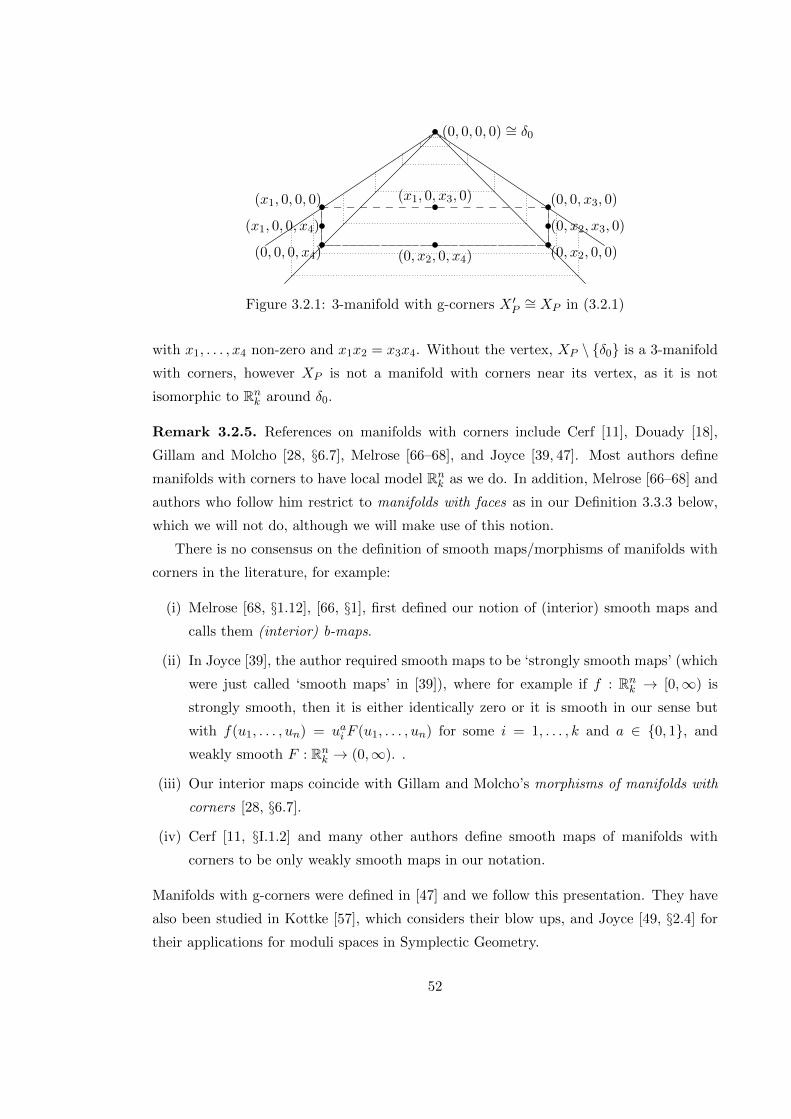
• (0, 0, 0, 0) ∼= δ0

•(x1, 0, 0, 0) •(0, 0, x3, 0)

•(0, 0, 0, x4)

•(0, x2, 0, 0)

•(0, x2, 0, x4)

•(x1, 0, x3, 0)

•(x1, 0, 0, x4) •(0, x2, x3, 0)

Figure 3.2.1: 3-manifold with g-corners X ′P∼= XP in (3.2.1)

with x1, . . . , x4 non-zero and x1x2 = x3x4. Without the vertex, XP \ δ0 is a 3-manifold

with corners, however XP is not a manifold with corners near its vertex, as it is not

isomorphic to Rnk around δ0.

Remark 3.2.5. References on manifolds with corners include Cerf [11], Douady [18],

Gillam and Molcho [28, §6.7], Melrose [66–68], and Joyce [39, 47]. Most authors define

manifolds with corners to have local model Rnk as we do. In addition, Melrose [66–68] and

authors who follow him restrict to manifolds with faces as in our Definition 3.3.3 below,

which we will not do, although we will make use of this notion.

There is no consensus on the definition of smooth maps/morphisms of manifolds with

corners in the literature, for example:

(i) Melrose [68, §1.12], [66, §1], first defined our notion of (interior) smooth maps and

calls them (interior) b-maps.

(ii) In Joyce [39], the author required smooth maps to be ‘strongly smooth maps’ (which

were just called ‘smooth maps’ in [39]), where for example if f : Rnk → [0,∞) is

strongly smooth, then it is either identically zero or it is smooth in our sense but

with f(u1, . . . , un) = uai F (u1, . . . , un) for some i = 1, . . . , k and a ∈ 0, 1, and

weakly smooth F : Rnk → (0,∞). .

(iii) Our interior maps coincide with Gillam and Molcho’s morphisms of manifolds with

corners [28, §6.7].

(iv) Cerf [11, §I.1.2] and many other authors define smooth maps of manifolds with

corners to be only weakly smooth maps in our notation.

Manifolds with g-corners were defined in [47] and we follow this presentation. They have

also been studied in Kottke [57], which considers their blow ups, and Joyce [49, §2.4] for

their applications for moduli spaces in Symplectic Geometry.

52

3.3 Boundaries and corners of manifolds with (g-)corners

The material of this section broadly follows Joyce [39], [47, §2.2 & §3.4]. In the following

definition we will consider the empty set and the whole set to be prime ideals of a monoid,

which we will not need to do later.

Definition 3.3.1. Take a weakly toric monoid P and corresponding topological space

XP . For each x ∈ XP define the support of x, suppXP x = p ∈ P : x(p) 6= 0. Then

suppXP x is a face of P . Define the depth of x to be depthXP x = rankP − rank suppXP x,

which is an integer valued in 0, . . . , rankP . Define the depth l stratrum of XP to be

Sl(XP ) =x ∈ XP : depthXP x = l

.

The interior of XP is S0(X).

For any face F ⊂ P there is an inclusion iPF : XF → XP where y ∈ XF maps to the

x ∈ XP such that x(p) = y(p) if p ∈ F and x(p) = 0 otherwise. Then iPF (XF ) = x ∈ XP :

suppXP x = F and this is isomorphic to RrankF , a manifold without boundary. Then we

see that

Sl(XP ) =∐F

iPF (XF ),

where this disjoint union is over the faces F of P that have rank(F ) + l = rank(P ). Also,

Sl(XP ) is a smooth manifold without boundary, and we see

rankP∐l=0

Sl(XP ) = XP

stratifies XP into manifolds without boundary.

We can restrict this stratification to open sets, U ⊂ XP , so that Sl(U) = U ∩ Sl(XP )

are the depth l elements of U , and

U =rankP∐l=0

Sl(U).

This is shown to be invariant under diffeomorphism in [47, §3.4].

For a manifold with g-corners, X, then for each x ∈ X we can choose a chart (P,U, φ)

with φ(u) = x for some u ∈ U and let the depth of x be the depth of u. As the depth is

invariant under diffeomorphisms, this is independent of the chart. Then we can similarly

define the stratification

Sl(X) =x ∈ X : depthX x = l

53

for l = 0, 1, . . . ,dimX. The disjoint union of the stratum is equal to X, and each stratum

is a manifold without boundary of codimension l.

For x ∈ Rnk the depth of x simplifies to the number of zeros of its coordinates. Then

for a manifold with corners X the depth of an element x ∈ X is the depth of its image

φ(x) ∈ U ⊆ Rnk in a coordinate chart (U, φ).

Definition 3.3.2. For a manifold with g-corners X of dimension n, take x ∈ X, and

k = 0, 1, . . . , n. Then we define a local k-corner component γ of X at x to be a local choice

of connected component of Sk(X) near x. More precisely, for any open neighbourhood

V of x in X that is small enough, then γ is a choice of connected component W of

V ∩Sk(X). So x is in the closure of W in X and if we chose another open neighbourhood

V ′ and connected component W ′ of V ′ ∩ Sk(X) then x ∈ W ∩W ′. The local 1-corner

components are called local boundary components of X.

We define the boundary and k-corners of X to be the sets

∂X =

(x, β) : x ∈ X, β is a local boundary component of X at x,

Ck(X) =

(x, γ) : x ∈ X, γ is a local k-corner component of X at x,

for k = 0, 1, . . . , n. This implies ∂X = C1(X) and C0(X) = X.

One can define charts on Ck(X) so that each are a manifold with g-corners of codi-

mension k. If X is a manifold with corners then Ck(X) is a manifold with corners for each

k = 0, . . . , n.

The corners of X is the manifold with (g-)corners with mixed dimension

C(X) =dimX∐k=0

Ck(X).

There are canonical smooth maps iX : Ck(X) → X where (x, β) 7→ x, which are not

interior and may also not be injective.

The property that iX is injective on connected components of ∂X is of particular

importance for manifolds with corners, although it is not considered for manifolds with

g-corners as discussed in Remark 4.7.10.

Definition 3.3.3. A manifold with corners X is called a manifold with faces if for each

connected component F of ∂X, the map iX |F : F → X is injective. Then the faces of X

are the connected components of ∂X, which can be regarded as subsets of X. In his work

on analysis on manifolds with corners, Melrose [66–68] restricts to manifolds with faces,

as some things can then be done globally.

54

Here is an example of a manifold with corners that does not have faces that is from [47,

Ex. 2.8].

Example 3.3.4. We define the teardrop as the subset T =

(x, y) ∈ R2 : x > 0, y2 6 x2−x4

. As shown in Figure 3.3.1, T is a manifold with corners of dimension 2. The teardrop

is not a manifold with faces as the boundary is diffeomorphic to [0, 1], and so is connected,

while the map iT : ∂T → T is not injective.

x

y

• //oo

OO

Figure 3.3.1: The teardrop T

We now show that the corners of X is in fact a functor in a specific sense by considering

how it acts on morphisms. The following is from [47, Lem. 3.33].

Lemma 3.3.5. A smooth map of manifolds with g-corners f : X → Y is compatible

with the depth stratifications X =∐k>0 S

k(X), Y =∐l>0 S

l(Y ) in Definition 3.3.1.

That is, if we take a connected subset ∅ 6= W ⊆ Sk(X) for some k > 0, then f(X) is

contained in some Sl(Y ) for a unique l > 0.

In general, a smooth f : X → Y does not induce a map ∂f : ∂X → ∂Y nor a map

Ck(f) : Ck(Y )→ Ck(Y ). This means that boundaries and k-corners do not give functors

on Manc by themselves. If we allow mixed dimension and the full corners C(X) =∐k>0Ck(X) from Definition 3.3.2, we can define a functor as in Joyce [47, Def. 3.34].

Definition 3.3.6. Take a smooth map f : X → Y of manifolds with corners, and let γ

be a local k-corner component at x ∈ X. For a small enough neighbourhood V of x in X,

then γ gives a connected component W of V ∩ Sk(X) with x in the closure of W . Then

Lemma 3.3.5 says there is an l > 0 such that f(W ) ⊆ Sl(Y ). Now f(W ) is connected as

f is continuous, and f(x) ∈ f(W ). This gives a unique l-corner component f∗(γ) of Y

at f(x), such that for a small enough neighbourhood V of f(x) in Y , then f∗(γ) has the

corresponding connected component W of V ∩ Sl(Y ) where W ∩ f(W ) 6= ∅. This f∗(γ) is

well defined as it is independent of the choice of sufficiently small V, V .

We define a map C(f) : C(X) → C(Y ) by C(f) : (x, γ) 7→ (f(x), f∗(γ)), which is

smooth by [47, Def. 2.10,Def. 3.34]. Then C(f) is a morphism in Manc and this defines

55

the functor C : Mangc → Mangc, and restriction to manifolds with corners defines a

functor C : Manc → Manc, both of which we call the corner functor.

By [47, Prop. 2.11, Prop. 3.36] C(f) is interior for each smooth map of manifolds with

(g-)corners f : X → Y . We can also consider taking the domain category to be Manc

and Mangc so that the corner functors can be extended to the functors C : Manc →Manc

in and C : Mangc → Mangcin . We will show these are right adjoint to the inclusions

Mancin → Manc and Mangc

in → Mangc in §5.8.

3.4 Tangent bundles and b-tangent bundles

We now discuss tangent bundles of manifolds with (g-)corners. For a manifold with corners

there are two relevant constructions: the (ordinary) tangent bundle which is a standard

generalisation of the tangent space of a manifold with corners, and the b-tangent bundle

defined in Melrose [67, §2.2], [68, §I.10], [66, §2]. Manifolds with g-corners do not have

well behaved (ordinary) tangent bundles in that the dimension of the tangent spaces is

not locally constant, however their b-tangent bundles are well behaved. The duals of

the tangent bundle and b-tangent bundle give the cotangent and b-cotangent bundles

respectively. We follow the presentation of Joyce [47, §2.3, §3.5].

Definition 3.4.1. For a manifold with corners X of dimension m we define the tangent

bundle π : TX → X of X. This is a natural vector bundle on X that is unique up to

canonical isomorphism. There are many equivalent ways to characterise TX, let us first

consider how to do this using coordinate charts.

For a chart (U, φ) on X, with U ⊆ Rmk open, then TX|φ(U) is the trivial bundle.

If (u1, . . . , um) are coordinates on U then TX|φ(U) has a basis of sections ∂∂u1

, . . . , ∂∂um

.

Then TX has a corresponding chart (TU, Tφ) where TU = U × Rm ⊆ R2mk . A point

(u1, . . . , um, q1, . . . , qm) ∈ TU can be represented by the vector q1∂∂u1

+ · · ·+ qm∂

∂umover

(u1, . . . , um) ∈ U or φ(u1, . . . , um) ∈ X.

Where two charts (U, φ) to (U , φ) of X overlap, we can consider their change of coor-

dinates (u1, . . . , um) (u1, . . . , um), which gives a corresponding change from (TU, Tφ)

to (TU, T φ) where (u1, . . . , um, q1, . . . , qm) (u1, . . . , um, q1, . . . , qm). This is given by∂∂ui

=∑m

j=1∂uj∂ui

(u1, . . . , um) · ∂∂uj

, which implies qj =∑m

i=1∂uj∂ui

(u1, . . . , um)qi.

We can also define TX intrinsically using the elements of Γ∞(TX) which are called

vector fields. For each x ∈ X the fibre of TX at x is denoted TxX and there is a canonical

isomorphism

TxX ∼=

linear maps v : C∞(X)→ R : v(fg) = v(f)g(x)+f(x)v(g) for all f, g ∈ C∞(X).

56

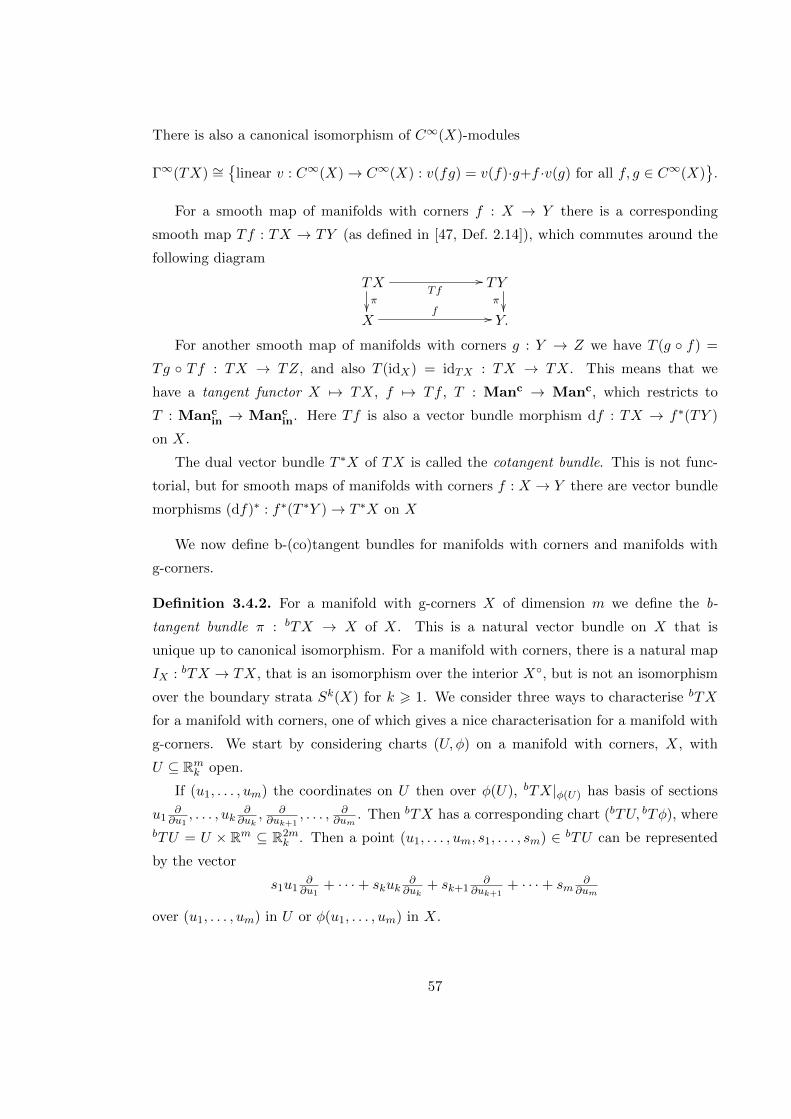
There is also a canonical isomorphism of C∞(X)-modules

Γ∞(TX) ∼=

linear v : C∞(X)→ C∞(X) : v(fg) = v(f)·g+f ·v(g) for all f, g ∈ C∞(X).

For a smooth map of manifolds with corners f : X → Y there is a corresponding

smooth map Tf : TX → TY (as defined in [47, Def. 2.14]), which commutes around the

following diagram

TXπ

Tf// TYπ

Xf // Y.

For another smooth map of manifolds with corners g : Y → Z we have T (g f) =

Tg Tf : TX → TZ, and also T (idX) = idTX : TX → TX. This means that we

have a tangent functor X 7→ TX, f 7→ Tf , T : Manc → Manc, which restricts to

T : Mancin → Manc

in. Here Tf is also a vector bundle morphism df : TX → f∗(TY )

on X.

The dual vector bundle T ∗X of TX is called the cotangent bundle. This is not func-

torial, but for smooth maps of manifolds with corners f : X → Y there are vector bundle

morphisms (df)∗ : f∗(T ∗Y )→ T ∗X on X

We now define b-(co)tangent bundles for manifolds with corners and manifolds with

g-corners.

Definition 3.4.2. For a manifold with g-corners X of dimension m we define the b-

tangent bundle π : bTX → X of X. This is a natural vector bundle on X that is

unique up to canonical isomorphism. For a manifold with corners, there is a natural map

IX : bTX → TX, that is an isomorphism over the interior X, but is not an isomorphism

over the boundary strata Sk(X) for k > 1. We consider three ways to characterise bTX

for a manifold with corners, one of which gives a nice characterisation for a manifold with

g-corners. We start by considering charts (U, φ) on a manifold with corners, X, with

U ⊆ Rmk open.

If (u1, . . . , um) the coordinates on U then over φ(U), bTX|φ(U) has basis of sections

u1∂∂u1

, . . . , uk∂∂uk

, ∂∂uk+1

, . . . , ∂∂um

. Then bTX has a corresponding chart (bTU, bTφ), where

bTU = U × Rm ⊆ R2mk . Then a point (u1, . . . , um, s1, . . . , sm) ∈ bTU can be represented

by the vector

s1u1∂∂u1

+ · · ·+ skuk∂∂uk

+ sk+1∂

∂uk+1+ · · ·+ sm

∂∂um

over (u1, . . . , um) in U or φ(u1, . . . , um) in X.

57

Where two charts (U, φ) and (U , φ) overlap we can consider their change of coordinates

(u1, . . . , um) (u1, . . . , um), which give a change of coordinates (bTU, bTφ) to (bTU, bT φ)

where (u1, . . . , um, s1, . . . , sm) (u1, . . . , um, s1, . . . , sm) with

sj =

∑k

i=1 u−1j ui

∂uj∂ui

si +∑m

i=k+1 u−1j

∂uj∂ui

si, j 6 k,∑ki=1 ui

∂uj∂ui

si +∑m

i=k+1∂uj∂ui

si, j > k.

In coordinate charts (bTU, bTφ), (TU, Tφ), IX : bTX → TX acts by

(u1, . . . , um, s1, . . . , sm) 7−→ (u1, . . . , um, u1s1, . . . , uksk, sk+1, . . . , sm).

A more intrinsic definition uses elements of Γ∞(bTX), which are called b-vector fields.

Then there is a canonical isomorphism of C∞(X)-modules

Γ∞(bTX) ∼=v ∈ Γ∞(TX) : v|Sk(X) is tangent to Sk(X) for all k

. (3.4.1)

This gives an inclusion of Γ∞(bTX) into Γ∞(TX), which corresponds to the morphism

IX : bTX → TX.

Finally, in terms of germs, there is a canonical isomorphism

bTxX ∼= (v, v′) : v : C∞x (X)→ R is a linear map ,

v′ : Exx(X)→ R is a morphism of monoids,

v([a][b]) = v([a]) ev(b) + v([b]) ev(a), for all [a], [b] ∈ C∞x (X),

v′ exp([a]) = v([a]), for all [a] ∈ C∞x (X),

v inc([b]) = ev([b])v′([b]), for all [b] ∈ C∞x (X)

Here ev([a]) = a(x) is evaluation at the point x ∈ X and inc : Exx(X) → C∞x (X) is the

natural inclusion. If the manifold with corners has faces then this can be extended to a

global definition but otherwise it cannot be. Then IX : bTX → TX for a manifold with

corners acts by (v, v′) 7→ v.

This last definition in terms of germs is also well behaved for a manifold with g-corners,

defining bTX for a manifold with g-corners as in [47, §3.5]. For the model spaces XP , we

have bTXP∼= XP × HomMon(P,R). Also, for a manifold with g-corners X and a point

x ∈ X then Remark 3.2.3 tells us that X near x is locally modelled on XQ×Rl near (δ0, 0)

for a toric monoid Q, which gives an isomorphism

bTxX ∼= HomMon(Q,R)× Rl.

58

For a smooth morphism of manifolds with (g-)corners that is interior there is a corre-

sponding interior map bTf : bTX → bTY as in [66, §2] that makes the following commute:

bTX

π

IX

''

bTf// bTY

IY

&&

π

TXπ

Tf // TYπ

Xf // Y.

In terms of germs, bTf : (x, v, v′) 7→ (f(x), v f, v′ f). This gives functors bT : Mancin →

Mancin, bT : Mangc

in → Mangcin called the tangent functor where X 7→ bTX, f 7→ bTf .

The maps IX : bTX → TX correspond to a natural transformations I : bT → T of functors

on Mancin and Mangc

in . The map bTf is also a vector bundle morphism bdf : bTX →f∗(bTY ) on X.

The dual vector bundle of bTX is called the b-cotangent bundle bT ∗X of X. This is

not functorial, although for an interior map f : X → Y of manifolds with (g-)corners we

have a vector bundle morphism (bdf)∗ : f∗(bT ∗Y )→ bT ∗X.

One reason for considering manifolds with g-corners is that they are specially well

behaved under fibre products, as the next result from [47, §4.3] shows:

Theorem 3.4.3. Let g : X → Z and h : Y → Z be interior maps of manifolds with

g-corners. Call g, h b-transverse if bTxg ⊕ bTyh : bTxX ⊕ bTyY → bTzZ is a surjective

linear map for all x ∈ X and y ∈ Y with g(x) = h(y) = z ∈ Z.

If g, h are b-transverse then the fibre product X ×g,Z,h Y exists in Mangcin .

The analogue is false for manifolds with corners, unless we impose complicated extra

restrictions on g, h over ∂jX, ∂kY, ∂lZ so that the maps are what is called sb-transverse

in Joyce [49]. Note that b-transverse fibre products of manifolds with corners in Mangcin

can be manifolds with g-corners, not corners. For example, from (3.2.1) we see that XP in

Example 3.2.4 may be written as [0,∞)2 ×g,[0,∞),h [0,∞)2, where g, h : [0,∞)2 → [0,∞)

given by g(x, y) = h(x, y) = xy are b-transverse. So manifolds with g-corners can be seen

as a type of completion of the category of manifolds with corners under fibre products

of b-transverse maps. We discuss fibre products of manifolds with (g-)corners further in

Remark 5.5.5.

59

Chapter 4

C∞-rings with corners

We now develop a theory of C∞-rings with corners, a generalisation of C∞-rings in which

manifolds are replaced by manifolds with corners, as in §3. This chapter is based on joint

work with Professor Dominic Joyce.

Some of these ideas were introduced in the MSc thesis of Kalashnikov [51], who studied

the category of (categorical) pre C∞-ring with corners PC∞Ringscin(CPC∞Ringsc

in) as

in §4.1 and §4.2, although they did not use the pre-fix ‘pre’. Apart from this, the author

knows of no previous work on this subject. However, the theory is related to ‘log geometry’

in algebraic geometry, as discussed in §5.9, and our C∞-rings with corners could in some

sense be regarded as ‘log C∞-rings’.

4.1 Categorical pre C∞-rings with corners

There is a natural generalisation of C∞-rings to the corners case. We will call these ‘pre

C∞-rings with corners’, as we will reserve the name ‘C∞-rings with corners’ for pre C∞-

rings with corners satisfying an additional condition given in §4.3. The name comes from

an analogy with ‘pre log rings’ and ‘log rings’ in log geometry, as in §5.9.

Definition 4.1.1. Let X be a manifold with corners (or with g-corners). Smooth maps

g : X → [0,∞) will be called exterior maps, to contrast them with interior maps. We

write In(X) for the set of interior maps g : X → [0,∞), and Ex(X) for the set of exterior

maps g : X → [0,∞). Thus, we have three sets:

(a) C∞(X) of smooth maps f : X → R;

(b) In(X) of interior maps g : X → [0,∞); and

(c) Ex(X) of exterior (smooth) maps g : X → [0,∞), with In(X) ⊆ Ex(X).

60

Much of this chapter concerns properties of these three sets.

In §2.1 we gave two equivalent definitions for C∞-rings. Similarly, we will give two

equivalent definitions for pre C∞-rings with corners. We start with the analogue of Defi-

nition 2.1.1.

Definition 4.1.2. Let Euc ⊂ Man and CC∞Rings be as in Definition 2.1.1. Write

Eucc,Euccin for the full subcategories of Manc,Manc

in with objects Rm × [0,∞)n for all

m,n > 0. Note that products are defined in Eucc,Euccin with(

Rk × [0,∞)l)×(Rm × [0,∞)n

)= Rk+m × [0,∞)l+n, (4.1.1)

where if the coordinates on Rk × [0,∞)l are (w1, . . . , wk, x1, . . . , xl) and on Rm × [0,∞)n

are (y1, . . . , ym, z1, . . . , zn), then the coordinates on Rk+m × [0,∞)l+n are

(w1, . . . , wk, y1, . . . , ym, x1, . . . , xl, z1, . . . , zn).

We have inclusions

Euc ⊂ Euccin ⊂ Eucc. (4.1.2)

Define a categorical pre C∞-ring with corners as in Kalashnikov [51, Def. 4.17] to be

a product-preserving functor F : Eucc → Sets. Here F should also preserve the empty

product, i.e. it maps R0 × [0,∞)0 = ∅ in Eucc to the terminal object in Sets, the

point ∗.If F,G : Eucc → Sets are categorical pre C∞-rings with corners, a morphism η : F →

G is a natural transformation η : F ⇒ G. Such natural transformations are automatically

product-preserving. We write CPC∞Ringsc for the category of categorical pre C∞-ring

with corners.

Define a categorical interior pre C∞-ring with corners to be a product-preserving

functor F : Euccin → Sets. These form a category CPC∞Ringsc

in, with morphisms

natural transformations.

Define functors ΠC∞cor ,Π

intcor,Π

C∞int in a commutative triangle

CPC∞Ringsc

ΠC∞

cor

//

Πintcor ,,

CC∞Rings

CPC∞Ringscin

ΠC∞

int

33(4.1.3)

by restriction to subcategories in (4.1.2), so that for example Πintcor maps F : Eucc → Sets

to F |Euccin

: Euccin → Sets.

Here is the motivating example.

61

Example 4.1.3. (a) Let X be a manifold with corners. Define a categorical pre C∞-ring

with corners F : Eucc → Sets by F = HomManc(X,−). That is, for objects Rm× [0,∞)n

in Eucc ⊂Manc we have

F(Rm × [0,∞)n

)= HomManc

(X,Rm × [0,∞)n

),

and for morphisms g : Rm × [0,∞)n → Rm′ × [0,∞)n′

in Eucc we have

F (g) = g : HomManc

(X,Rm × [0,∞)n

)−→ HomManc

(X,Rm

′ × [0,∞)n′)

mapping F (g) : h 7→ gh. Let f : X → Y be a smooth map of manifolds with corners, and

F,G : Eucc → Sets the functors corresponding to X,Y . Define a natural transformation

η : G⇒ F by

η(Rm × [0,∞)n

)= f : Hom

(Y,Rm × [0,∞)n

)−→ Hom

(X,Rm × [0,∞)n

)mapping η : h 7→ h f .

Define a functor FCPC∞Ringsc

Manc : Manc → (CPC∞Ringsc)op to map X 7→ F on

objects, and f 7→ η on morphisms, for X,Y, F,G, f, η as above.

All of this also works if X,Y are manifolds with g-corners, as in Definition 3.2.2, giving

a functor FCPC∞Ringsc

Mangc : Mangc → (CPC∞Ringsc)op.

(b) Similarly, if X is a manifold with corners, define a categorical interior pre C∞-ring with

corners F : Euccin → Sets by F = HomManc

in(X,−). This gives functors F

CPC∞Ringscin

Mancin

:

Mancin → (CPC∞Ringsc

in)op and FCPC∞Ringsc

in

Mangcin

: Mangcin → (CPC∞Ringsc

in)op.

In the language of Algebraic Theories, as in Adamek, Rosicky and Vitale [3], Euc,Eucc,

Euccin are examples of algebraic theories (that is, small categories with finite products),

and CC∞Rings,CPC∞Ringsc,CPC∞Ringscin are the corresponding categories of al-

gebras. Also the inclusions of subcategories (4.1.2) are morphisms of algebraic theories, and

the functors (4.1.3) the corresponding morphisms. So, as for Proposition 2.1.6, Adamek et

al. [3, Prop.s 1.21, 2.5, 9.3 & Th. 4.5] give important results on their categorical properties:

Theorem 4.1.4. (a) The categories CC∞Rings,CPC∞Ringsc,CPC∞Ringscin, have

all small limits and directed colimits and they may be computed objectwise in Euc,Eucc,

Euccin by taking the corresponding small limits/directed colimits in Sets.

(b) All small colimits exist in CC∞Rings,CPC∞Ringsc,CPC∞Ringscin, though in

general they are not computed objectwise in Euc,Eucc,Euccin by taking colimits in Sets.

(c) There are functors IcorC∞ , I

intC∞ , I

corint which are left adjoints of ΠC∞

cor ,ΠC∞int ,Π

intcor in (4.1.3).

As ΠC∞cor ,Π

C∞int ,Π

intcor are right adjoints, they preserve limits. Since Icor

C∞ , IintC∞ , I

corint are left

adjoints, they preserve colimits.

62

In (a), Adamek et al. prove that all sifted colimits exist in CC∞Rings, . . . and may be

computed objectwise in Euc, . . . by taking sifted colimits in Sets. Here sifted colimits [3,

§2] are a class of limits in categories which include filtered colimits and directed colimits.

We only mainly interested in directed colimits.

4.2 Pre C∞-rings with corners

We now give the analogue of §4.1 using an alternative definition of pre C∞-ring with

corners similar to Definition 2.1.2, as in Kalashnikov [51, Def. 4.18].

Definition 4.2.1. A pre C∞-ring with corners C assigns the data:

(a) Two sets C and Cex.

(b) Operations Φf : Cm × Cnex → C for all smooth maps f : Rm × [0,∞)n → R.

(c) Operations Ψg : Cm × Cnex → Cex for all exterior g : Rm × [0,∞)n → [0,∞).

Here we allow one or both of m,n to be zero, and consider S0 to be the single point ∅for any set S. These operations must satisfy the following relations:

(i) Suppose k, l,m, n > 0, and ei : Rk × [0,∞)l → R is smooth for i = 1, . . . ,m, and

fj : Rk × [0,∞)l → [0,∞) is exterior for j = 1, . . . , n, and g : Rm × [0,∞)n → R is

smooth. Define smooth h : Rk × [0,∞)l → R by

h(x1, . . . , xk, y1, . . . , yl) = g(e1(x1, . . . , yl), . . . , em(x1, . . . , yl),

f1(x1, . . . , yl), . . . , fn(x1, . . . , yl)).

(4.2.1)

Then for all (c1, . . . , ck, c′1, . . . , c

′l) ∈ Ck × Clex we have

Φh(c1, . . . , ck, c′1, . . . , c

′l) = Φg

(Φe1(c1, . . . , c

′l), . . . ,Φem(c1, . . . , c

′l),

Ψf1(c1, . . . , c′l), . . . ,Ψfn(c1, . . . , c

′l)).

(ii) Suppose k, l,m, n > 0, and ei : Rk × [0,∞)l → R is smooth for i = 1, . . . ,m, and

fj : Rk × [0,∞)l → [0,∞) is exterior for j = 1, . . . , n, and g : Rm× [0,∞)n → [0,∞)

is exterior. Define exterior h : Rk × [0,∞)l → [0,∞) by (4.2.1). Then for all

(c1, . . . , ck, c′1, . . . , c

′l) ∈ Ck × Clex we have

Ψh(c1, . . . , ck, c′1, . . . , c

′l) = Ψg

(Φe1(c1, . . . , c

′l), . . . ,Φem(c1, . . . , c

′l),

Ψf1(c1, . . . , c′l), . . . ,Ψfn(c1, . . . , c

′l)).

63

(iii) Write πi : Rm × [0,∞)n → R for projection to the ith coordinate of Rm for i =

1, . . . ,m, and π′j : Rm × [0,∞)n → [0,∞) for projection to the jth coordinate of

[0,∞)n for j = 1, . . . , n. Then for all (c1, . . . , cm, c′1, . . . , c

′n) in Cm × Cnex and all

i = 1, . . . ,m, j = 1, . . . , n we have

Φπi(c1, . . . , cm, c′1, . . . , c

′n) = ci, Ψπ′j

(c1, . . . , cm, c′1, . . . , c

′n) = c′j .

We will refer to the operations Φf ,Ψg as the C∞-operations, and we often write a pre

C∞-ring with corners as a pair C = (C,Cex), leaving the C∞ operations implicit. If c ∈ C

and c′ ∈ Cex, by a slight abuse of notation we will write c = (c, c′) ∈ C, which will be

useful for §5.

Let C = (C,Cex) and D = (D,Dex) be pre C∞-rings with corners. A morphism

φ : C →D is a pair φ = (φ, φex) of maps φ : C → D and φex : Cex → Dex, which commute

with all the operations Φf ,Ψg on C,D. That is, whenever f : Rm × [0,∞)n → R is

smooth, g : Rm × [0,∞)n → [0,∞) is exterior and (c1, . . . , cm, c′1, . . . , c

′n) ∈ Cm × Cnex we

have

φ Φf (c1, . . . , cm, c′1, . . . , c

′n) = Φf

(φ(c1), . . . , φ(cm), φex(c′1), . . . , φex(c′n)

),

φex Ψg(c1, . . . , cm, c′1, . . . , c

′n) = Ψg

(φ(c1), . . . , φ(cm), φex(c′1), . . . , φex(c′n)

).

Morphisms compose in the obvious way. Write PC∞Ringsc for the category of pre C∞-

rings with corners.

Define functors Πsm,Πex : PC∞Ringsc → Sets by Πsm : C 7→ C, Πex : C 7→ Cex on

objects, and Πsm : φ 7→ φ, Πex : φ 7→ φex on morphisms, where ‘sm’, ‘ex’ are short for

‘smooth’ and ‘exterior’.

As for ΠC∞cor in (4.1.3), there is a natural functor ΠC∞

cor : PC∞Ringsc → C∞Rings

acting on objects by C = (C,Cex) 7→ C, where C has the C∞-operations Φf : Cm → C from

smooth f : Rm → R in (b) above with n = 0, and on morphisms by φ = (φ, φex) 7→ φ.

Here is our motivating example.

Example 4.2.2. Let X be a manifold with corners. Define a pre C∞-ring with corners

C = (C,Cex) by C = C∞(X) and Cex = Ex(X), as sets. If f : Rm × [0,∞)n → R is

smooth, define the operation Φf : Cm × Cnex → C by

Φf (c1, . . . , cm, c′1, . . . , c

′n) : x 7−→ f

(c1(x), . . . , cm(x), c′1(x), . . . , c′n(x)

). (4.2.2)

If g : Rm × [0,∞)n → [0,∞) is exterior, define Ψg : Cm × Cnex → Cex by

Ψg(c1, . . . , cm, c′1, . . . , c

′n) : x 7−→ g

(c1(x), . . . , cm(x), c′1(x), . . . , c′n(x)

). (4.2.3)

64

This makes C into a pre C∞-ring with corners.

Suppose f : X → Y is a smooth map of manifolds with corners, and let C,D be the

pre C∞-rings with corners corresponding to X,Y . Write φ = (φ, φex), where φ : D → C

maps φ(d) = d f and φex : Dex → Cex maps φ(d′) = d′ f . Then φ : D → C is a

morphism of pre C∞-rings with corners.

Define a functor FPC∞Ringsc

Manc : Manc → (PC∞Ringsc)op to map X 7→ C on objects,

and f 7→ φ on morphisms, for X,Y,C,D, f,φ as above.

We will also write C∞(X) = FPC∞Ringsc

Manc (X), and write f∗ : C∞(Y ) → C∞(X)

for FPC∞Ringsc

Manc (f) : FPC∞Ringsc

Manc (Y )→ FPC∞Ringsc

Manc (X).

All of this also works if X,Y are manifolds with g-corners, as in Definition 3.2.2, giving

a functor FPC∞Ringsc

Mangc : Mangc → (PC∞Ringsc)op.

Remark 4.2.3. An important difference between ordinary manifolds, and manifolds with

corners, is that if X is a manifold with corners, gi : X → [0,∞) for i ∈ I are exterior (or

interior) maps, and ηi : i ∈ I is a smooth partition of unity on X, then∑

i∈I ηigi : X →[0,∞) is generally not exterior (or interior).

This means that the geometry of manifolds with corners is more global. If g : X →[0,∞) is an exterior map, then there is a locally constant map ng : ∂X → 0, 1, 2, . . . ,∞such that g vanishes to order ng along ∂X locally, and if x′, x′′ lie in the same connected

component of ∂X then ng(x′) = ng(x

′′) even if iX(x′), iX(x′′) are far away in X.

Recall the notion of ‘manifold with faces’ in Definition 3.3.3. If X is a manifold

with corners, but not a manifold with faces, then there are not enough exterior maps

g : X → [0,∞) to properly describe the local geometry of X. That is, X near some x is

locally modelled on Rn−k × [0,∞)k near 0 with coordinates (x1, . . . , xn−k, y1, . . . , yk), but

there do not exist exterior gi : X → [0,∞) locally modelled on yi : Rn−k×[0,∞)k → [0,∞)

for all i = 1, . . . , k. For example, the teardrop T in Example 3.3.4 is locally modelled

near (0, 0) on [0,∞)2, but we can only find exterior g : T → [0,∞) locally modelled on

ya1yb2 : [0,∞)2 → [0,∞) when a = b, as the multiplicities ng on the y1- and y2-axes must

be the same.

In the notation of §5, a manifold with corners X corresponds to a natural C∞-scheme

with corners X, but X is affine with X ∼= SpeccC∞(X) only if X is a manifold with

faces. If X does not have faces then X 6∼= SpeccC∞(X).

In fact FPC∞Ringsc

Manc : Manc → (PC∞Ringsc)op above is full and faithful. Despite

this, if X does not have faces then we regard C∞(X) as somehow ‘wrong’ (e.g. its local

C∞-rings with corners in §4.6 and b-cotangent modules in §4.7 do not behave as expected),

and we will not make much use of it.

65

This also means that results on C∞-schemes relying on partitions of unity should not

be expected to extend to C∞-schemes with corners.

Similar to Remark 2.1.3, we have the following equivalence.

Proposition 4.2.4. There is a natural equivalence of categories between CPC∞Ringsc

and PC∞Ringsc, which identifies F : Eucc → Sets in CPC∞Ringsc with C = (C,Cex)

in PC∞Ringsc such that F(Rm × [0,∞)n

)= Cm × Cnex for m,n > 0.

Under this equivalence, for a smooth function f : Rnk → R, we identify F (f) with Φf ,

and for an exterior function g : Rnk → [0,∞), we identify F (g) with Ψg. The proof of this

proposition then follows from F being a product preserving functor, and the definition of

C∞-ring with corners, similar to the discussion in Joyce [40, p. 7].

The operations Φf ,Ψg on a pre C∞-ring with corners C = (C,Cex) comprise a huge

amount of data. It is often helpful to work with a small subset of this structure. The next

definition explains this small subset. We use the theory of monoids from §3.1.

Definition 4.2.5. Let C = (C,Cex) be a pre C∞-ring with corners. Then C = ΠC∞cor (C)

is a C∞-ring, and thus a commutative R-algebra. The R-algebra structure makes C into a

monoid in two ways: under multiplication ‘·’ with identity 1, and under addition ‘+’ with

identity 0.

Define g : [0,∞)2 → [0,∞) by g(x, y) = xy. Then g induces Ψg : Cex × Cex → Cex.

Define multiplication · : Cex × Cex → Cex by c′ · c′′ = Ψg(c′, c′′). The map 1 : R0 → [0,∞)

gives an operation Ψ1 : ∅ → Cex. The identity in Cex is 1Cex = Ψ1(∅). This makes

(Cex, ·, 1Cex) into a monoid.

The functor Πex : PC∞Ringsc → Sets in Definition 4.2.1 extends to a functor Πex :

PC∞Ringsc → Mon mapping Πex : C 7→ Cex and Πex : φ 7→ φex, where Cex is now

regarded as a monoid.

The map 0 : R0 → [0,∞) gives an operation Ψ0 : ∅ → Cex. Thus we have a

distinguished element 0Cex = Ψ0(∅) in Cex, which is not the monoid identity element. It

is uniquely characterised by the property that c′ · 0Cex = 0Cex for all c′ ∈ Cex.

Write i : [0,∞) → R for the inclusion. Then we have a map Φi : Cex → C. This is a

monoid morphism, for C a monoid under multiplication.

The exterior map exp : R→ [0,∞) induces Ψexp : C → Cex. It is a monoid morphism,

for C a monoid under addition.

The smooth map exp : R→ R induces Φexp : C → C, with Φexp = Φi Ψexp.

To summarise, the following data in C = (C,Cex) are particularly important:

(a) C is a commutative R-algebra.

66

(b) Cex is a monoid. It has a special 0Cex ∈Cex with c′ · 0Cex =0Cex , all c′∈Cex.

(c) Φi : Cex → C is a monoid morphism, for C a monoid under multiplication.

(d) Ψexp : C → Cex is a monoid morphism, for C a monoid under addition.

(e) Φexp = Φi Ψexp : C → C.

Many of our definitions will use only the structures (a)–(e). When we write Φi,Ψexp,Φexp

without further explanation, we mean those in (c)–(e).

The monoid morphism Φi : Cex → C makes C into a prelog ring, in the sense of log

geometry discussed in §5.9. We will define C∞-rings with corners in §4.3 to be pre C∞-

rings with corners satisfying an additional condition similar to requiring Φi : Cex → C to

be a log ring.

Now we could define ‘interior pre C∞-rings with corners’ following Definition 4.2.1,

but replacing exterior maps by interior maps throughout. Instead we will do something

more complicated. The functor Icorint : CPC∞Ringsc

in → CPC∞Ringsc in Theorem

4.1.4(c) is faithful, and thus an equivalence from CPC∞Ringscin to a subcategory of

CPC∞Ringsc, the essential image of Icorint .

We will define PC∞Ringscin ⊂ PC∞Ringsc to be the subcategory corresponding to

the essential image of Icorint under the equivalence CPC∞Ringsc ∼= PC∞Ringsc from

Proposition 4.2.4. That is, we will define interior pre C∞-rings with corners as special

examples of pre C∞-rings with corners, and interior morphisms as special morphisms

between (interior) pre C∞-rings with corners.

The advantage of this is that rather than having two separate theories, we will be able

to work with both interior and non-interior (pre) C∞-rings with corners, and both interior

and non-interior morphisms, all in a single theory.

Definition 4.2.6. Let C = (C,Cex) be a pre C∞-ring with corners. Then Cex is a monoid

and 0Cex ∈ Cex with c′ · 0Cex = 0Cex for all c′ ∈ Cex.

We call C an interior pre C∞-ring with corners if 0Cex 6= 1Cex , and there do not exist

c′, c′′ ∈ Cex with c′ 6= 0Cex 6= c′′ and c′ ·c′′ = 0Cex . That is, Cex should have no zero divisors.

Write Cin = Cex \ 0Cex. Then Cex = Cin q 0Cex, where q is the disjoint union. Since

Cex has no zero divisors, Cin is closed under multiplication, and 1Cex ∈ Cin as 0Cex 6= 1Cex .

Thus Cin is a submonoid of Cex. We write 1Cin= 1Cex . This implies (C,Cex) is in the

essential image of Icorint considered as a subcategory of PC∞Ringsc.

Let C,D be interior pre C∞-rings with corners, and φ = (φ, φex) : C → D be

a morphism in PC∞Ringsc. We call φ interior if φex(Cin) ⊆ Din. Then we write

67

φin = φex|Cin: Cin → Din. Interior morphisms are closed under composition and include

the identity morphisms.

Write PC∞Ringscin for the (non-full) subcategory of PC∞Ringsc with objects inte-

rior pre C∞-rings with corners, and morphisms interior morphisms.

As in §4.1, define functors Πsm,Πin : PC∞Ringscin → Sets by Πsm : C 7→ C, Πin :

C 7→ Cin on objects, and Πsm : φ 7→ φ, Πin : φ 7→ φin on morphisms, where ‘sm’, ‘in’

are short for ‘smooth’ and ‘interior’. Also define Πin : PC∞Ringscin → Mon to map

Πin : C 7→ Cin, where Cin is regarded as a monoid.

Define ΠC∞int : PC∞Ringsc

in → C∞Rings to be the restriction of the functor ΠC∞cor :

PC∞Ringsc → C∞Rings in Definition 4.2.1 to PC∞Ringscin.

Example 4.2.7. Let X be a manifold with corners. Define an interior pre C∞-ring with

corners C = (C,Cex) by C = C∞(X) and Cex = In(X) q 0 the disjoint union, as sets,

where 0 is the zero function X → [0,∞).

If f : Rm × [0,∞)n → R is smooth and g : Rm × [0,∞)n → [0,∞) is exterior, define

Φf : Cm × Cnex → C and Ψg : Cm × Cnex → Cex by (4.2.2)–(4.2.3). Here to check that Ψg

does map to Cex ⊆ Ex(X), we verify that Ψg(c1, · · · , cm, c′1, . . . , c′n) : X → [0,∞) is either

interior or zero, since c′1, . . . , c′n are either interior or zero.

Suppose f : X → Y is an interior map of manifolds with corners, and let C,D be

the interior pre C∞-rings with corners corresponding to X,Y . Write φ = (φ, φex), where

φ : D→ C maps φ(d) = d f and φex : Dex → Cex maps φ(d′) = d′ f . Then φ : D→ C

is a morphism in PC∞Ringscin.

Define a functor FPC∞Ringsc

inManc

in: Manc

in → (PC∞Ringscin)op to map X 7→ C on

objects, and f 7→ φ on morphisms, for X,Y,C,D, f,φ as above.

If X is a manifold with corners, then FPC∞Ringsc

Manc (X) from Example 4.2.2 agrees with

FPC∞Ringsc

inManc

in(X) if and only if X is nonempty and connected, since then Ex(X) is the

disjoint union In(X)q 0.We will also write C∞in (X) = F

PC∞Ringscin

Mancin

(X), and write f∗in : C∞in (Y ) → C∞in (X)

for FPC∞Ringsc

inManc

in(f) : F

PC∞Ringscin

Mancin

(Y ) → FPC∞Ringsc

inManc

in(X). Thus C∞in (X) = C∞(X) if

and only if X is nonempty and connected.

This example also works if X,Y are manifolds with g-corners, as in Definition 3.2.2,

giving a functor FPC∞Ringsc

in

Mangcin

: Mangcin → (PC∞Ringsc

in)op.

Lemma 4.2.8. Let C = (C,Cex) be an interior pre C∞-ring with corners. Then C×ex ⊆Cin. If g : Rm× [0,∞)n → [0,∞) is interior, then Ψg : Cm×Cnex → Cex maps Cm×Cnin →Cin.

68

Proof. As 0Cex is not invertible, then 0Cex /∈ C×ex, and C×ex ⊆ Cex \ 0Cex = Cin. As g is

interior we may write

g(x1, . . . , xm, y1, . . . , yn) = ya11 · · · y

ann · exp h(x1, . . . , xm, y1, . . . , yn), (4.2.4)

for a1, . . . , an ∈ N and h : Rm × [0,∞)n → R smooth. Then for c1, . . . , cm ∈ C and

c′1, . . . , c′n ∈ Cin we have

Ψg

(c1, . . . , cm, c

′1, . . . , c

′n

)= c′a1

1 · · · c′ann ·Ψexp

[Φh

(c1, . . . , cm, c

′1, . . . , c

′n

)].

Here c′a11 · · · c′ann ∈ Cin as Cin is a submonoid of Cex, and Ψexp[· · · ] ∈ Cin as Ψexp maps to

C×ex ⊆ Cin ⊆ Cex. Thus Ψg

(c1, . . . , cm, c

′1, . . . , c

′n

)∈ Cin.

Here is the analogue of Remark 2.1.3 and Proposition 4.2.4.

Proposition 4.2.9. There is an equivalence CPC∞Ringscin∼= PC∞Ringsc

in, which

identifies F : Euccin → Sets in CPC∞Ringsc

in with C = (C,Cex) in PC∞Ringscin such

that F(Rm × [0,∞)n

)= Cm × Cnin for m,n > 0.

Proof. Let F : Euccin → Sets be a categorical interior pre C∞-ring with corners. Define

sets C = F (R), Cin = F ([0,∞)), and Cex = Cin q 0Cex, where q is the disjoint union.

Then F(Rm× [0,∞)n

)= Cm×Cnin, as F is product-preserving. Let f : Rm× [0,∞)n → R

and g : Rm × [0,∞)n → [0,∞) be smooth. We must define maps Φf : Cm × Cnex → C and

Ψg : Cm × Cnex → Cex.

Let c1, . . . , cm ∈ C and c′1, . . . , c′n ∈ Cex. Then some of c′1, . . . , c

′n lie in Cin and the

rest in 0Cex. For simplicity suppose that c′1, . . . , c′k ∈ Cin and c′k+1 = · · · = c′n = 0Cex for

0 6 k 6 n. Define smooth d : Rm × [0,∞)k → R, e : Rm × [0,∞)k → [0,∞) by

d(x1, . . . , xm, y1, . . . , yk) = f(x1, . . . , xm, y1, . . . , yk, 0, . . . , 0),

e(x1, . . . , xm, y1, . . . , yk) = g(x1, . . . , xm, y1, . . . , yk, 0, . . . , 0).(4.2.5)

Then F (d) maps Cm × Ckin → C. Set

Φf (c1, . . . , cm, c′1, . . . , c

′k, 0Cex , . . . , 0Cex) = F (d)(c1, . . . , cm, c

′1, . . . , c

′k).

Either e : Rm × [0,∞)k → [0,∞) is interior, or e = 0. If e is interior define

Ψg(c1, . . . , cm, c′1, . . . , c

′k, 0Cex , . . . , 0Cex) = F (e)(c1, . . . , cm, c

′1, . . . , c

′k).

If e = 0 set Ψg(c1, . . . , cm, c′1, . . . , c

′k, 0Cex , . . . , 0Cex) = 0Cex . This defines Φf ,Ψg, and makes

C = (C,Cex) into an interior pre C∞-ring with corners.

69

Conversely, let C = (C,Cex) be an interior pre C∞-ring with corners. Then Cex =

Cin q 0. As in the proof of Proposition 4.2.4 we define a product-preserving functor

F : Euccin → Sets with F

(Rm × [0,∞)n

)= Cm × Cnin, using the fact from Lemma 4.2.8

that Ψg : Cm × Cnex → Cex maps Cm × Cnin → Cin for g interior. The rest of the proof

follows that of Proposition 4.2.4.

We define analogues of the functors I intC∞ , I

corC∞ ,Π

intcor in Theorem 4.1.4.

Definition 4.2.10. Let C be a C∞-ring, and write Φ′e : Cn → C for the C∞-ring operations

on C for e : Rn → R smooth. Set Cex = C q 0Cex, where q is the disjoint union.

Let f : Rm × [0,∞)n → R be smooth. We must define Φf : Cm × Cnex → C. Let

c1, . . . , cm ∈ C and c′1, . . . , c′n ∈ Cex. Then some of c′1, . . . , c

′n lie in Cin = C and the rest

in 0Cex. For simplicity suppose that c′1, . . . , c′k ∈ C and c′k+1 = · · · = c′n = 0Cex for

0 6 k 6 n. Define smooth d : Rm+k → R by

d(x1, . . . , xm, y1, . . . , yk) = f(x1, . . . , xm, exp y1, . . . , exp yk, 0, . . . , 0),

and set Φf (c1, . . . , cm, c′1, . . . , c

′n) = Φ′d(c1, . . . , cm, c

′1, . . . , c

′k). This defines Φf .

Suppose g : Rm× [0,∞)n → [0,∞) is exterior. Let c1, . . . , cm ∈ C and c′1, . . . , c′n ∈ Cex,

and again for simplicity suppose that c′1, . . . , c′k ∈ C and c′k+1 = · · · = c′n = 0Cex . Define

exterior h : Rm × [0,∞)k → [0,∞) by

h(x1, . . . , xm, y1, . . . , yk) = g(x1, . . . , xm, y1, . . . , yk, 0, . . . , 0).

Then either h = 0 or h is interior. If h = 0 set Ψg(c1, . . . , cm, c′1, . . . , c

′n) = 0Cex . If h is

interior it maps Rm × (0,∞)k → (0,∞), so we define e : Rm+k → R by

e(x1, . . . , xm, y1, . . . , yk) = log(h(x1, . . . , xm, exp y1, . . . , exp yk)

).

Set Ψg(c1, . . . , cm, c′1, . . . , c

′n) = Φ′e(c1, . . . , cm, c

′1, . . . , c

′k). This defines Ψg.

These Φf ,Ψg make C = (C,Cex) into a pre C∞-ring with corners, which has ΠC∞cor (C) =

C. Also Cex has no zero divisors, so C is interior.

Define a functor I intC∞ : C∞Rings → PC∞Ringsc

in to map C 7→ C on objects, for C

as above, and to map morphisms φ : C → D in C∞Rings to φ = (φ, φex) : C → D in

PC∞Ringscin, where φex : Cq0Cex → Dq0Dex maps φex|C = φ and φex(0Cex) = 0Dex .

Define IcorC∞ : C∞Rings → PC∞Ringsc by Icor

C∞ = I intC∞ . Both I int

C∞ , IcorC∞ are full and

faithful.

70

Suppose now that C is a C∞-ring, and D an interior pre C∞-ring with corners, and

set C = I intC∞(C). Then we can define a 1-1 correspondence

HomC∞Rings

(C,ΠC∞

int (D))

= HomC∞Rings

(C,D

) ∼= HomPC∞Ringscin

(C,D)

= HomPC∞Ringscin

(I intC∞(C),D

),

identifying φ : C → D with φ = (φ, φex) : C → D, where φex : C q 0Cex → Dex is given

by φex|C = Ψexp φ and φex(0Cex) = 0Dex . This is functorial in C,D, and so shows that

I intC∞ is left adjoint to ΠC∞

int . The same proof shows that IcorC∞ is left adjoint to ΠC∞

cor . There

is also a right adjoint to ΠC∞cor , which we define for C∞-rings with corners in Theorem

4.3.9.

Definition 4.2.11. We define a functor Πintcor : PC∞Ringsc → PC∞Ringsc

in right

adjoint to inc : PC∞Ringscin → PC∞Ringsc. Let C = (C,Cex) be a pre C∞-ring

with corners. We will define an interior pre C∞-ring with corners C = (C, Cex) where

Cex = Cex q 0Cex, and set Πint

cor(C) = C. Here Cex already contains a zero element 0Cex ,

but we are adding an extra 0Cexwith 0Cex 6= 0Cex

.

Let f : Rm× [0,∞)n → R and g : Rm× [0,∞)n → [0,∞) be smooth, and write Φf ,Ψg

for the operations in C. We must define maps Φf : Cm×Cnex → C and Ψg : Cm×Cnex → Cex.

Let c1, . . . , cm ∈ C and c′1, . . . , c′n ∈ Cex. Then some of c′1, . . . , c

′n lie in Cex and the rest

in 0Cex. For simplicity suppose that c′1, . . . , c

′k ∈ Cex and c′k+1 = · · · = c′n = 0Cex

for

0 6 k 6 n. Define smooth d : Rm × [0,∞)k → R, e : Rm × [0,∞)k → [0,∞) by (4.2.5).

Set

Φf (c1, . . . , cm, c′1, . . . , c

′k, 0Cex

, . . . , 0Cex) = Φd(c1, . . . , cm, c

′1, . . . , c

′k).

Either e : Rm × [0,∞)k → [0,∞) is interior, or e = 0. If e is interior define

Ψg(c1, . . . , cm, c′1, . . . , c

′k, 0Cex

, . . . , 0Cex) = Ψe(c1, . . . , cm, c

′1, . . . , c

′k).

If e = 0 define Ψg(c1, . . . , cm, c′1, . . . , c

′k, 0Cex

, . . . , 0Cex) = 0Cex

. This defines the maps

Φf , Ψg. This makes C = (C, Cex) into an interior pre C∞-ring with corners.

Now let φ : C →D be a morphism in PC∞Ringsc, and define C, D as above. Define

φex : Cex → Dex by φex|Cex = φex and φex(0Cex) = 0Dex

. Then φ = (φ, φex) : C → D is a

morphism in PC∞Ringscin.

Define a functor Πintcor : PC∞Ringsc → PC∞Ringsc

in by Πintcor : C 7→ C on objects

and Πintcor : φ 7→ φ on morphisms, for C,D, C, D,φ, φ as above.

Suppose now that C,D are pre C∞-rings with corners with C interior. Then we can

71

define a 1-1 correspondence

HomPC∞Ringsc

(inc(C),D

)= HomPC∞Ringsc(C,D)

∼= HomPC∞Ringscin

(C,Πint

cor(D)),

identifying φ : inc(C) → D with φ : C → Πintcor(D), where φ = (φ, φex) and φ = (φ, φex)

with φex|Cin= φex|Cin

and φex(0Cex) = 0Dex. This is functorial in C,D, and so shows that

Πintcor is right adjoint to inc : PC∞Ringsc

in → PC∞Ringsc.

We have now given the analogue of all of §4.1 in terms of our new definitions. Remark

2.1.3, and Propositions 4.2.4 and 4.2.9 give equivalences

CC∞Rings ∼= C∞Rings, CPC∞Ringsc ∼= PC∞Ringsc,

CPC∞Ringscin∼= PC∞Ringsc

in.(4.2.6)

These identify ΠC∞cor ,Π

C∞int ,Π

intcor in (4.1.3) with ΠC∞

cor ,ΠC∞int ,Π

intcor in Definitions 4.2.6 and

4.2.11. Theorem 4.1.4(c) gives left adjoints IcorC∞ , I

intC∞ , I

corint for ΠC∞

cor ,ΠC∞int ,Π

intcor in (4.1.3).

Definitions 4.2.10 and 4.2.11 give left adjoints IcorC∞ , I

intC∞ and inc : PC∞Ringsc

in →PC∞Ringsc for ΠC∞

cor ,ΠC∞int ,Π

intcor above. Therefore (4.2.6) identifies Icor

C∞ , IintC∞ , I

corint in

§4.1 with IcorC∞ , I

intC∞ , inc above.

Thus from Theorem 4.1.4 we deduce:

Theorem 4.2.12. (a) In the categories PC∞Ringsc,PC∞Ringscin of (interior) pre

C∞-rings with corners, all small limits and all directed colimits exist. The functors

Πsm,Πex : PC∞Ringsc → Sets, Πex : PC∞Ringsc →Mon, Πsm,Πin : PC∞Ringscin →

Sets and Πin : PC∞Ringscin →Mon preserve limits and directed colimits, so these may

be used to compute such (co)limits.

(b) All small colimits exist in PC∞Ringsc,PC∞Ringscin, though in general they are not

preserved by Πsm,Πex, Πex and Πsm,Πin, Πin.

(c) The functors ΠC∞cor ,Π

C∞int ,Π

intcor described above are right adjoint to Icor

C∞ , IintC∞ and inc :

PC∞Ringscin → PC∞Ringsc. Since ΠC∞

cor ,ΠC∞int ,Π

intcor are right adjoints, they preserve

limits. Since IcorC∞ , I

intC∞ and inc : PC∞Ringsc

in → PC∞Ringsc are left adjoints, they

preserve colimits.

Remark 4.2.13. Kalashnikov [51, §4.6] also showed small colimits of pre C∞-rings with

corners exist using an argument similar to Moerdijk and Reyes proof that small colimits

of C∞-rings exist as in [72, p. 21-23].

72

Example 4.2.14. The inclusion inc : PC∞Ringscin → PC∞Ringsc in general does not

preserve limits, and therefore cannot have a left adjoint. Let J be a small category and

A : J → PC∞Ringscin be a functor. Then by Theorem 4.2.12(a), limits lim←−j∈JA(j) exist

in both PC∞Ringsc and PC∞Ringscin. But these limits may not be the same, and the

limit in PC∞Ringsc may not be an object in PC∞Ringscin.

We illustrate this for products in PC∞Ringsc and PC∞Ringscin. Suppose C,D are

interior pre C∞-rings with corners, and write E = C×D and F = C×inD for the products

in PC∞Ringsc and PC∞Ringscin. Then Theorem 4.2.12(a) implies that E = C × D,

Eex = Cex ×Dex, F = C ×D, Fin = Cin ×Din. Since Cex = Cin q 0Cex, etc., where q is

the disjoint union, this gives

Eex = (Cin ×Din)q (Cin × 0Dex)q (0Cex ×Din)q (0Cex × 0Dex),

Fex = (Cin ×Din)q (0Cex × 0Dex).

Thus E 6∼= F. Moreover in Eex we have (1Cex , 0Dex) · (0Cex , 1Dex) = (0Cex , 0Dex), so Eex has

zero divisors, and E is not an object in PC∞Ringscin.

Another way to see this is that the final object in the category of pre C∞-rings with

corners is (0, 0), however the final object in the category of interior pre C∞-rings with

corners is (0, 0, 1). Taking the product of two objects in interior pre C∞-rings with

corners is the same as taking the fibre product (in both PC∞Ringscin and PC∞Ringsc)

over these two objects and their unique morphisms to (0, 0, 1). This is different to

taking their product in pre C∞-rings with corners, which is a fibre product over these two

objects and their unique morphisms to (0, 0) in PC∞Ringsc only.

In contrast, the initial object in both categories is (R, [0,∞)), and their coproducts

are the same.

4.3 C∞-rings with corners

Here are some properties of Φi,Φexp in Definition 4.2.5(c),(e).

Proposition 4.3.1. (a) Let C be a C∞-ring. Then the C∞-ring operation Φexp : C → C

induced by exp : R→ R is injective.

(b) Let C = (C,Cex) be a pre C∞-ring with corners, and suppose c′ lies in the group

C×ex of invertible elements in the monoid Cex. Then there exists a unique c ∈ C such that

Φexp(c) = Φi(c′) in C, for i : [0,∞) → R the inclusion.

Proof. For (a), let a ∈ C with b = Φexp(a) ∈ C. Then Φexp(−a) is the inverse b−1 of b.

The map t 7→ exp(t)− exp(−t) is a diffeomorphism R→ R. Let e : R→ R be its inverse.

73

Define smooth f : R2 → R by f(x, y) = e(x − y). Then f(exp t, exp(−t)) = t. Hence in

the C∞-ring C we have

Φf (b, b−1) = Φf (Φexp(a),Φexp −(a)) = Φf(exp,exp −)(a) = Φid(a) = a.

But b determines b−1 uniquely, so Φf (b, b−1) = a implies that b = Φexp(a) determines a

uniquely, and Φexp : C → C is injective.

For (b), as c′ ∈ C×ex we have a unique inverse c′−1 ∈ C×ex. Define smooth g : [0,∞)2 → Rby g(x, y) = e(x− y), for e : R→ R as above. Observe that if (x, y) ∈ [0,∞)2 with xy = 1

then x = exp t, y = exp(−t) for t = log x, and so

exp g(x, y) = exp g(exp t, exp(−t)) = exp e(exp t− exp(−t)) = exp(t) = x.

Therefore there is a unique smooth function h : [0,∞)2 → R with

exp g(x, y)− x = h(x, y)(xy − 1). (4.3.1)

We have operations Φg,Φh : C2ex → C. Define c = Φg(c

′, c′−1). Then

Φexp(c)− Φi(c′) = Φexp g(x,y)−x(c′, c′−1) = Φh(x,y)(xy−1)(c

′, c′−1)

= Φh(c′, c′−1) · (Φi(c′ · c′−1)− 1C) = 0,

using Definition 4.1.2(i) in the first and third steps, and (4.3.1) in the second. Hence

Φexp(c) = Φi(c′). Uniqueness of c follows from part (a).

We can now define C∞-rings with corners.

Definition 4.3.2. Let C = (C,Cex) be a pre C∞-ring with corners. We call C a C∞-ring

with corners if any (hence all) of the following hold:

(i) Φi|C×ex: C×ex → C is injective.

(ii) Ψexp : C → C×ex is surjective.

(iii) Ψexp : C → C×ex is a bijection.

Here Proposition 4.3.1(b) implies that (i),(ii) are equivalent, and Definition 4.2.5(e) and

Proposition 4.3.1(a) imply that Ψexp : C → C×ex is injective, so (ii),(iii) are equivalent, and

therefore (i)–(iii) are equivalent. Write C∞Ringsc for the full subcategory of C∞-rings

with corners in PC∞Ringsc.

We call a C∞-ring with corners C interior if it is an interior pre C∞-ring with corners,

as in §4.2. Write C∞Ringscin ⊂ C∞Ringsc for the subcategory of interior C∞-rings with

corners, and interior morphisms between them.

74

Remark 4.3.3. We can interpret the condition that C = (C,Cex) be a C∞-ring with

corners as follows. Imagine there is some ‘space with corners’ X, such that C =

smooth

maps c : X → R

, and Cex =

exterior maps c′ : X → [0,∞)

. If c′ ∈ Cex is invertible

(that is, c′ ∈ C×ex) then c′ should map X → (0,∞), and we require that there should exist

smooth c = log c′ : X → R in C with c′ = exp c.

Example 4.3.4. The functors FPC∞Ringsc

Manc , FPC∞Ringsc

Mangc in Example 4.2.2 map to the

functors (C∞Ringsc)op ⊂ (PC∞Ringsc)op, and so we will write them as FC∞Ringsc

Manc ,

FC∞Ringsc

Mangc . To see this, note that if X is a manifold with corners and C = (C,Cex) =(C∞(X),Ex(X)

)as in Example 4.2.2, and c′ ∈ C×ex, then c′ : X → [0,∞) is smooth and

invertible, so c′ actually maps X → (0,∞). Thus c = log c′ : X → R is smooth and

lies in C = C∞(X), with Ψexp(c) = c′. Hence C is a C∞-ring with corners by Definition

4.3.2(ii). Similarly, FPC∞Ringsc

inManc

in, F

PC∞Ringscin

Mangcin

in Example 4.2.7 map to the functors

(C∞Ringscin)op ⊂ (PC∞Ringsc

in)op, and so we will write them as FC∞Ringsc

inManc

inand

FC∞Ringsc

in

Mangcin

.

Proposition 4.3.5. The inclusion functor inc : C∞Ringsc → PC∞Ringsc has a left

adjoint ΠC∞preC∞ : PC∞Ringsc → C∞Ringsc and a right adjoint ˜ΠC∞

preC∞. Their restric-

tions to PC∞Ringscin are left and right adjoints respectively for inc : C∞Ringsc

in →PC∞Ringsc

in, so the inclusion respects limits and colimits.

Proof. Let C = (C,Cex) be a pre C∞-ring with corners. We will define a C∞-ring with

corners C = (C, Cex). As a set, define Cex = Cex/∼, where ∼ is the equivalence relation

on Cex given by c′ ∼ c′′ if there exists c′′′ ∈ C×ex with Φi(c′′′) = 1 and c′ = c′′ · c′′′. That is,

Cex is the quotient of Cex by the group Ker(Φi|C×ex

)⊆ C×ex. There is a natural surjective

projection π : Cex → Cex.

If f : Rm × [0,∞)n → R is smooth and g : Rm × [0,∞)n → [0,∞) is exterior, then we

can show there exist unique maps Φf : Cm × Cnex → C and Ψg : Cm × Cnex → Cex making

the following diagrams commute:

Cm × Cnex Φf//

idm×πn

C

id

Cm × Cnex

Φf // C,

Cm × Cnex Ψg//

idm×πn

Cex

π Cm × Cnex

Ψg // Cex,

(4.3.2)

and these make C into a pre C∞-ring with corners. Also, C satisfies Definition 4.3.2(i).

Therefore C is a C∞-ring with corners.

Suppose φ = (φ, φex) : C →D is a morphism of pre C∞-rings with corners, and define

C, D as above. Then by a similar argument to (4.3.2), we find that there is a unique map

75

φex such that the following commutes:

Cex φex

//

π

Dex

π

Cex

φex // Dex,

and then φ = (φ, φex) : C → D is a morphism of C∞-rings with corners. Define a

functor ΠC∞preC∞ : PC∞Ringsc → C∞Ringsc to map C 7→ C on objects and φ 7→ φ on

morphisms.

Now let C be a pre C∞-ring with corners, D a C∞-ring with corners, and φ : C →D

a morphism. Then we have a morphism φ : C → D, as D = D, and φ ↔ φ gives a 1-1

correspondence

HomPC∞Ringsc

(C, inc(D)

)= HomPC∞Ringsc(C,D)

∼= HomC∞Ringsc

(ΠC∞

preC∞(C),D),(4.3.3)

which is functorial in C,D. Hence ΠC∞preC∞ is left adjoint to inc.

If C above is interior then C is interior, and if φ : C →D is interior then φ is interior,

so ΠC∞preC∞ restricts to ΠC∞

preC∞ : PC∞Ringscin → C∞Ringsc

in. The 1-1 correspondence

(4.3.3) restricts to a 1-1 correspondence on interior morphisms. Hence ΠC∞preC∞ is left

adjoint to inc : C∞Ringscin → PC∞Ringsc

in.

For the right adjoint, take (C,Cex) = C a pre C∞-ring with corners and consider

the C∞-ring with corners (C, Cex) = C where Cex is the submonoid of Cex generated by

Ψexp(C) and Cex \ C×ex. We see that Cex = Ψexp(C) ∪ (Cex \ C×ex) ⊂ Cex. To make this a

C∞-ring with corners, we take the C∞-operations on C corresponding to smooth maps

f : Rnk → R to be the restrictions of these C∞-operations on C to C.

Non-zero smooth maps f : Rnk → [0,∞) are of the form

f(x1, . . . , xn) = xa11 · · ·x

akk exp(g(x1, . . . , xn))

for a smooth function g : Rnk → R. Then we see that

Ψf (c′1, . . . , c′k, ck+1, . . . , cn) = c′1

a1 · · · c′kakΨexp(g(c′1, . . . , c

′k, ck+1, . . . , cn)))

is indeed an element of Ψexp(C) ∪ (Cex \ C×ex). This tells us that the images of the C∞-

operations corresponding to these f are already in Cex, so that C = ˜ΠC∞preC∞(C) is a well

defined sub pre C∞-ring with corners of C. As Ψexp : C → C×ex is now surjective, then C

is a C∞-ring with corners. (We could in fact define C to be the largest sub pre C∞-ring

with corners of C such that Ψexp : C → C×ex is surjective, so that C is a C∞-ring with

corners.)

76

If we have a pre C∞-rings with corners morphism φ : C → D then we can consider

the restriction φ|C . On the C∞-ring this is the identity, on the monoid we see that

elements of Ψexp(C) have image in Ψexp(D) as φex commutes with the C∞-operations,

however there may be non-invertible elements c′ that map into D× \Ψexp(D). We define

φ = ˜ΠC∞preC∞(φ) : C → D to be the restriction of φ to C except for elements c′ that

map into D× \Ψexp(D). These elements we define to map to their corresponding unique

d′ ∈ Ψexp(D) from Proposition 4.3.1(b) such that Φi(φex(c′)) = Φi(d′). It follows that φ

respects the C∞-operations and is a morphism of C∞-rings with corners.

To check that ˜ΠC∞preC∞ is right adjoint to inc : C∞Ringsc → PC∞Ringsc, we see that

the unit is the identity natural transformation and the counit is the inclusion morphism.

The compositions inc ⇒ inc ˜ΠC∞preC∞ inc ⇒ inc and ˜ΠC∞

preC∞ ⇒˜ΠC∞

preC∞ inc ˜ΠC∞preC∞ ⇒

˜ΠC∞preC∞ are the identity morphisms as ˜ΠC∞

preC∞ takes a C∞-ring with corners to itself.

If C above is interior then C and C are interior, and if φ : C →D is interior then φ and

φ are interior, so ΠC∞preC∞ and ˜ΠC∞

preC∞ restrict to functors PC∞Ringscin → C∞Ringsc

in,

and considering the proofs above we see that they are left and right adjoint respectively

to inc : C∞Ringscin → PC∞Ringsc

in.

Remark 4.3.6. Note that the Cex defined above is actually the pushout of monoids

Φexp(C)qΦ−1i (Φexp(C)) Cex, and we discuss this further in §5.9.1.

The categories C∞Ringsc,C∞Ringscin behave well under (co)limits.

Theorem 4.3.7. (a) C∞Ringsc,C∞Ringscin are closed under limits and colimits in

PC∞Ringsc,PC∞Ringscin, respectively. Thus, all small limits and small colimits exist

in C∞Ringsc,C∞Ringscin. The functors

Πsm,Πex : C∞Ringsc −→ Sets, Πex : C∞Ringsc −→Mon,

Πsm,Πin : C∞Ringscin −→ Sets, Πin : C∞Ringsc

in −→Mon,

preserve limits and directed colimits, and may be used to compute such (co)limits. The

inclusion inc : C∞Ringscin → C∞Ringsc has a right adjoint (C,Cex) 7→ (C,Cexq0ex),

and hence preserves colimits; it does not preserve limits, hence it does not have a left

adjoint.

Proof. This proof follows from applying Proposition 4.3.5 to Theorem 4.2.12. The same

proof from Example 4.2.14 shows inc : C∞Ringscin → C∞Ringsc does not preserve

limits, hence there is no left adjoint.

77

Remark 4.3.8. Theorem 4.3.7 is essential for sheaves of (interior) C∞-rings with corners

to be well behaved. In particular, to construct the sheafification OX of a presheaf of

C∞-rings with corners POX on X we need to take small limits in C∞Ringsc, and to

define the stalk OX,x of OX at x ∈ X we need to take a directed colimit in C∞Ringsc.

Theorem 4.3.9. The forgetful functor G : C∞Ringsc → C∞Rings has a left adjoint

Fexp : C∞Rings → C∞Ringsc. Hence G preserves limits. G also has a right adjoint,

F>0 : C∞Rings→ C∞Ringsc, hence G preserves colimits.

Proof. We construct Fexp on objects by C 7→ (C,Φexp(C) q 0) = (C,Cex), where q is

the disjoint union. Here Cex is a subset of C and Φi : Cex → C is the inclusion morphism,

and consequently injective. The C∞-operations are defined as follows. For elements

c′1, . . . , c′k ∈ Cex, ck+1, . . . , cn ∈ C and for a smooth function f : Rnk → R we have

Φf (c′1, . . . , c′k, ck+1, . . . , cn) = Φf (Φexp(c1), . . . ,Φexp(ck), ck+1, . . . , cn).

For a smooth function g : Rnk → [0,∞), if g = 0, then Ψg(c′1, . . . , c

′k, ck+1, . . . , cn) = 0 ∈

Cex.

Otherwise, we have g(x1, . . . , xn) = xa11 · · ·x

akk F (x1, . . . , x2) for a positive smooth func-

tion F : Rnk → (0,∞). Then F can be extended to a smooth positive function F : Rn → Rsuch that F |Rnk = i F . Then we define

Ψg(c′1, . . . , c

′k, ck+1, . . . , cn) = (c′1)a1 · · · (c′k)akΦF (c′1, . . . , c

′k, ck+1, . . . , cn),

which is independent of the choice of extension of F .

For a morphism φ : C → D, then we define Fexp(φ) : Fexp(C) → Fexp(D), such that

Fexp(φ)(Φexp(c)) = Φexp(Fexp(φ(c))) for all c ∈ C and Fexp(φ)(0) = 0. This is well defined

as φ respects the C∞-operations.

Then Fexp is a left adjoint to G, where the unit of the adjunction η : id ⇒ GFexp is

the identity natural transformation, as GFexp is the identity functor GFexp : C∞Rings→C∞Rings. The counit is ε : FexpG⇒ id, where for any C = (C,Cex) ∈ C∞Ringsc, then

εC : (C,Φexp(C) q 0) → C is the identity on the C∞-ring, and it is the injective map

Φexp(C)q0 3 Φexp(c) 7→ Ψexp(c) ∈ Cex, 0 7→ 0 on the monoid. Proposition 4.3.1 implies

this is well defined and forms a natural transformation.

The compositions Fexp ⇒ FexpGFexp ⇒ Fexp and G ⇒ GFexpG ⇒ G are the identity

natural transformations, and this gives the required adjunction. This also implies that

HomC∞Ringsc(Fexp(C),D) ∼= HomC∞Rings(C, G(D)),

78

for a C∞-ring C and a C∞-ring with corners D = (D,Dex). That is,

HomC∞Ringsc((C,Φexp(C)q 0), (D,Dex)) ∼= HomC∞Rings(C,D).

This adjunction is a different but equivalent construction to the left adjoint constructed

in Definition 4.2.10.

For the second part of the theorem, we begin by constructing F>0 on objects. Here

C 7→ (C,C>0) where C>0 is the subset of elements c of C that satisfy the following condition:

for all smooth f : Rn → R such that f |[0,∞)×Rn−1 = 0 and for d1, . . . , dn−1 ∈ C, then

Φf (c, d1, . . . , dn−1) = 0 ∈ C. Note that C>0 is non-empty, as it contains Φexp(C) q 0.Also, any C∞-ring with corners (C,Cex) has Φi(Cex) ⊆ C>0.

We need to show that (C,C>0) is a C∞-ring with corners. Take a smooth function

f : Rnk → [0,∞). Then there is a (non-unique) smooth extension g : Rn → R such that

g|Rnk = i f for i : [0,∞)→ R the inclusion function. We define

Ψf (c′1, . . . , c′k, ck+1, . . . , cn) = Φg(c

′1, . . . , c

′k, ck+1, . . . , cn)

for c′i ∈ C>0 and ci ∈ C. Then Φi : C>0 → C is the inclusion morphism.

To show this is well defined, say h is another such extension, then g − h|Rnk = 0. We

want to show that

Φg−h(c′1, . . . , c′k, ck+1, . . . , cn) = 0

for c′i ∈ C>0 and ci ∈ C. As g−h satisfies the hypothesis of Lemma 4.3.10, we can assume

g − h = f1 + · · ·+ fk with fi|Ri−1×[0,∞)×Rn−i−1 = 0. Then

Φg−h(c′1, . . . , c′k, ck+1, . . . , cn) = Φf1+···+fk(c′1, . . . , c

′k, ck+1, . . . , cn)

= Φf1(c′1, . . . , c′k, ck+1, . . . , cn) + · · ·

+ Φfk(c′1, . . . , c′k, ck+1, . . . , cn)

= 0 + · · ·+ 0

as c′i are in C>0. Therefore Ψf is a well defined C∞-operation. A similar approach shows

smooth functions f : Rnk → R give well defined C∞-operations. Hence (C,C>0) is a

C∞-ring with corners.

On morphisms, F>0 sends φ : C → D to (φ, φex) : (C,C>0) → (D,D>0) where φex =

φ|C>0. As φ respects the C∞-operations, then the image of C>0 under φ is contained in

D>0, so φex is well defined.

We describe the unit and counit of the adjunction to show that F>0 is right adjoint toG.

The counit is the identity natural transformation. The unit is the identity on the C∞-ring

79

and it is Φi on the monoid. It then follows that the compositions F>0 ⇒ F>0GF>0 ⇒ F>0

and G⇒ GF>0G⇒ G are the identity compositions, so F>0 is a right adjoint to G. This

also implies that

HomC∞Ringsc(C, F>0(D)) ∼= HomC∞Rings(G(C),D),

for a C∞-ring with corners C and a C∞-ring D.

Lemma 4.3.10. If f : Rn → R is smooth such that f |Rnk = 0, then there are smooth

fi : Rn → R for i = 1, . . . , k such that fi|Ri−1×[0,∞)×Rn−i−1 = 0 for i = 1, . . . , k, and

f = f1 + . . .+ fk.

Proof. Let f be as in the statement of the lemma. Consider the following open subset

U = Sk−1 \ (x1, . . . , xk) : xi > 0 of the dimension k− 1 unit sphere Sk−1 ⊂ Rk. Take an

open cover U1, . . . , Uk of U such that Ui = (x1, . . . , xk) ∈ U |xi < 0. Take a partition of

unity ρi : U → [0, 1] for i = 1, . . . , k, subordinate to U1, . . . , Un, with ρi having support

on Ui and∑k

i=1 ρi = 1.

Define the fi as follows

fi =

f(x1, . . . , xn)ρi

((x1,...,xk)|(x1,...,xk)|

), if xi < 0 for some i = 1, . . . , k,

0, otherwise,

where |(x1, . . . , xk)| is the length of the vector (x1, . . . , xk) ∈ Rk. These fi are smooth

where the ρi are defined. The ρi are not defined in the first quadrant of Rk, where all

xi > 0, however approaching the boundary of this quadrant, the ρi are all constant. As

f |Rnk = 0, then all derivatives of f are zero in this quadrant, so the fi are smooth on Rn

and identically zero on Rnk . In addition, fi|Ri−1×[0,∞)×Rn−i−1 = 0, as the ρi are zero outside

of Ui. Finally, as∑ρi = 1 and f |Rnk = 0, then f = f1 + . . .+ fk as required.

Remark 4.3.11. The definition of the left adjoint Fexp in Theorem 4.3.9 shows its im-

age actually lies in C∞Ringscin, and the first part of this theorem is then also true for

interior C∞-rings with corners. Also, F>0 composed with the right adjoint C∞Ringsc →C∞Ringsc

in defined in Theorem 4.3.7(b) gives a right adjoint to C∞Ringscin → C∞Rings,

and so the second part of Theorem 4.3.9 is also true for interior C∞-rings with corners.

In Section 4.6, we define local C∞-rings with corners, and, in this case, the functors

Fexp and F>0 restricted to local C∞-rings are also left and right adjoints respectively to

G restricted to local C∞-rings with corners. This implies G preserves limits and colimits

of local C∞-rings with corners.

80

Relating to log geometry, discussed in §5.9, if C is a C∞-ring, we could say that Fexp(C)

is the trivial corners structure on C, as it is the initial object in the category of C∞-rings

with corners that have C∞-ring C. Also, F>0(C) is the final object in this category.

We can summarise the adjoints from Definition 4.2.10, Definition 4.2.11, Theorem

4.2.12, Proposition 4.3.5, Theorem 4.3.7 and Theorem 4.3.9 in the following diagram.

PC∞RingscOO

?

a

//PC∞Ringsc

inOO

?

? _oo

C∞Ringsc

a

//a

a

C∞Ringscin

a

vv

? _oo

a

a

C∞Rings

a

OO

a

OO

a

66 66

The following lemma considers how localisations of C∞-rings (with corners) behave

with respect to F>0, and we use this in Remark 5.4.9. It also gives some intuition into

what elements of a C∞-ring C are in C>0. For example, it implies that c2 ∈ C>0 for all

c ∈ C.

Lemma 4.3.12. Let C be a C∞-ring. If g : Rn → R is smooth such that g(Rn) ⊆ [0,∞),

then Φg(c1, . . . , cn) ∈ C>0 for all ci ∈ C.

Proof. Let C be a C∞-ring and g : Rn → R smooth such that g(Rn) ⊆ [0,∞). Take any

c1, . . . , cn ∈ C. Take smooth f : Rm+1 → R such that f |[0,∞)×Rm = 0. We need to show

that for any d1, . . . , dm ∈ C then we have that Φf (Φg(c1, . . . , cn), d1, . . . , dm) = 0.

However

Φf (Φg(c1, . . . , cn), d1, . . . , dm) = Φh(c1, . . . , cn, d1, . . . , dm)

where h(x1, . . . , xn, y1, . . . , ym) = f(g(x1, . . . , xn), y1, . . . , ym) = 0 from the definition of f

and g. Hence Φf (Φg(c1, . . . , cn), d1, . . . , dm) = 0 as required.

Definition 4.3.13. A morphism φ : C → D in C∞Ringsc or PC∞Ringsc is called

injective, or surjective, if the maps of sets φ : C → D and φex : Cex → Dex are injective, or

surjective, respectively.

Let φ : C →D be a morphism, and define E = φ(C) ⊆ D and Eex = φex(Cex) ⊆ Dex. If

f : Rm× [0,∞)n → R is smooth and g : Rm× [0,∞)n → [0,∞) is exterior, then since φ, φex

commute with operations Φf ,Ψg, we see that Φf : Dm ×Dmex → D maps Em × Emex → E,

and Ψg : Dm×Dmex → Dex maps Em×Emex → Eex. Define Φ′f = Φf |··· : Em×Emex → E and

81

Ψ′g = Ψg|··· : Em×Emex → Eex. Then these operations Φ′f ,Ψ′g for all f, g make E = (E,Eex)

into a pre C∞-ring with corners, and a C∞-ring with corners if C,D are. We call E the

image of φ, and write it Imφ.

Write π = φ : C → E and πex = φex : Cex → Eex, and let ı : E → D, ıex : Eex → Dex

be the inclusions. Then π = (π, πex) : C → E and ı = (ı, ıex) : E → D are morphisms

of (pre) C∞-rings with corners, with π surjective and ı injective. This shows that every

morphism φ : C →D in C∞Ringsc or PC∞Ringsc fits into a commutative triangle

Cφ

//

π ))

D,

Imφı

44

with π surjective and ı injective, and this characterises Imφ,π, ı uniquely up to canonical

isomorphism.

If C,D,φ are interior, then Imφ,π, ı are also interior.

If φ : C →D is an injective morphism in C∞Ringsc or PC∞Ringsc with D interior,

then C is also interior, since φex : Cex → Dex maps zero divisors to zero divisors as it is

injective, but there are no zero divisors in Dex.

4.4 Free C∞-rings with corners, generators and relations

We define free C∞-rings with corners.

Definition 4.4.1. We defined categorical pre C∞-rings with corners as product-preserving

functors F : Eucc → Sets, so that we have a full embedding of C∞Ringsc ⊂ PC∞Ringsc

in the functor category Fun(Eucc,Sets). The Yoneda embedding Y : (Eucc)op →Fun(Eucc,Sets) maps to C∞Ringsc ⊂ Fun(Eucc,Sets), which gives a full embedding

(Eucc)op → C∞Ringsc. Explicitly, this embedding maps Rm × [0,∞)n in Eucc to

the C∞-ring with corners Fm,n := C∞(Rm × [0,∞)n

)from Example 4.2.2 with X =

Rm × [0,∞)n.

These C∞-rings with corners Fm,n corresponding to objects Rm× [0,∞)n in Eucc are

important from the point of view of Algebraic Theories [3], where they are called finitely

generated free algebras [3, Rem. 14.12], and Fm,n is the free C∞-ring with corners with

(m,n) generators in this 2-sorted case. Free C∞-rings with corners were considered in

Kalashnikov [51, Lem. 4.21].

It has the universal property that if C = (C,Cex) is any (pre) C∞-ring with corners

and c1, . . . , cm ∈ C, c′1, . . . , c′n ∈ Cex, then there is a unique morphism φ = (φ, φex) :

82

Fm,n → C such that φ(xi) = ci for i = 1, . . . ,m and φex(yj) = c′j for j = 1, . . . , n, where

(x1, . . . , xm, y1, . . . , yn) are the coordinates on Rm × [0,∞)n.

Explicitly, if f ∈ Fm,n, so that f : Rm × [0,∞)n → R is smooth, we define φ(f) =

Φf (c1, . . . , cm, c′1, . . . , c

′n) ∈ C, and if g ∈ Fm,nex , so that g : Rm × [0,∞)n → [0,∞) is

exterior, we set φex(g) = Ψg(c1, . . . , cm, c′1, . . . , c

′n) ∈ Cex.

More generally, if A,Aex are sets then by [3, Rem. 14.12] we can define the free C∞-

ring with corners FA,Aex = (FA,Aex ,FA,Aexex ) generated by (A,Aex). We may think of FA,Aex

as C∞(RA × [0,∞)Aex

), where RA =

(xa)a∈A : xa ∈ R

and [0,∞)Aex =

(ya′)a′∈Aex :

ya′ ∈ [0,∞)

. Explicitly, we define FA,Aex to be the set of maps c : RA × [0,∞)Aex → Rwhich depend smoothly on only finitely many variables xa, ya′ , and FA,Aex

ex to be the set of

maps c′ : RA× [0,∞)Aex → [0,∞) which depend smoothly on only finitely many variables

xa, ya′ , and operations Φf ,Ψg are defined as in (4.2.2)–(4.2.3). Regarding xa : RA → Rand ya′ : [0,∞)Aex → [0,∞) as functions for a ∈ A, a′ ∈ Aex, we have xa ∈ FA,Aex and

ya′ ∈ FA,Aexex , and we call xa, ya′ the generators of FA,Aex .

Then FA,Aex has the property that if C = (C,Cex) is any (pre) C∞-ring with corners

then a choice of maps α : A → C and αex : Aex → Cex uniquely determine a morphism

φ : FA,Aex → C with φ(xa) = α(a) for a ∈ A and φex(ya′) = αex(a′) for a′ ∈ Aex. We have

FA,Aex = Fm,n when A = 1, . . . ,m and Aex = 1, . . . , n.The analogue of all this also holds in C∞Ringsc

in ⊂ PC∞Ringscin, with the same

objects Fm,n and FA,Ain , which are interior C∞-rings with corners, and the difference that

(interior) morphisms Fm,n → C in PC∞Ringscin are uniquely determined by elements

c1, . . . , cm ∈ C and c′1, . . . , c′n ∈ Cin (rather than c′1, . . . , c

′n ∈ Cex), and similarly for FA,Ain

with αin : Ain → Cin.

As in Adamek et al. [3, §5, §11, §14], see in particular [3, Prop.s 11.26, 11.28, 11.30,

Cor. 11.33, & Rem. 14.14], every object in PC∞Ringsc,PC∞Ringscin can be built out

of free C∞-rings with corners, in a certain sense.

Proposition 4.4.2. (a) Every object C in PC∞Ringsc admits a surjective morphism φ :

FA,Aex → C from some free C∞-ring with corners FA,Aex. We call C finitely generated

if this holds with A,Aex finite sets.

(b) Every object C in PC∞Ringsc fits into a coequaliser diagram

FB,Bexα ..

β11 FA,Aex

φ // C, (4.4.1)

that is, C is the colimit of the diagram FB,Bex ⇒ FA,Aex in PC∞Ringsc, where φ :

FA,Aex → C is automatically surjective. We call C finitely presented if this holds with

A,Aex, B,Bex finite sets.

83

The analogues of (a) and (b) also hold in PC∞Ringscin.

In (b), if C ∈ C∞Ringsc then (4.4.1) is a coequaliser diagram in C∞Ringsc, since

ΠC∞cor preserves colimits, and similarly for C ∈ C∞Ringsc

in.

For C∞-rings in §2, we often wrote a C∞-ring C as a quotient C = C∞(Rm)/I for

I ⊆ C∞(Rm) an ideal. Suppose I is finitely generated by f1, . . . , fk ∈ C∞(Rm). Then we

have a coequaliser diagram in C∞Rings

C∞(Rk)(f1,...,fk)∗

..

0∗00 C∞(Rm) // C,

an analogue of (4.4.1). That is, C is the C∞-ring we get by imposing the relations f1 =

0, . . . , fk = 0 in C∞(Rm). This is the general finitely presented C∞-ring.

For C∞-rings with corners, things are more complicated in two ways. Firstly, we have

two kinds of generators, and two kinds of relations, corresponding to the two generating

objects R, [0,∞) of Eucc. And secondly, we must now write the [0,∞)-type relations in

the form gj = hj , rather than in the form fj = 0.

As in (4.4.1) the general finitely presented C∞-ring with corners C fits into a co-

equaliser diagram in C∞Ringsc

C∞(Rk × [0,∞)l)

(e1,...,ek,g1,...,gl)∗..

(f1,...,fk,h1,...,hl)∗00 C∞

(Rm × [0,∞)n

)// C,

where e1, . . . , ek, f1, . . . , fk lie in C∞(Rm × [0,∞)n

)and g1, . . . , gl, h1, . . . , hl in Ex

(Rm ×

[0,∞)n). That is, C has m generators x1 . . . , xm of type R and n generators y1, . . . , yn of

type [0,∞), where (x1, . . . , xm, y1, . . . , yn) are the coordinates on Rm× [0,∞)n, and these

generators satisfy k relations ej = fj in C of type R, and l relations gj = hj in Cex of type

[0,∞).

By replacing ei, fi by ei − fi, 0 we may suppose that f1 = · · · = fk = 0, and so write

the R type relations as e1 = 0, . . . , ek = 0 in C, as for ideals in C∞-rings. However, for the

[0,∞)-type relations gj = hj in Cex, we are not able to replace gj , hj by gj − hj , 0, since

gj − hj does not make sense in the monoid Ex(Rm × [0,∞)n

). Thus [0,∞) type relations

must be written as gj = hj .

We can also modify a given C∞-ring with corners C by adding extra generators and

relations. We will use the following notation for this:

Definition 4.4.3. Let C be a C∞-ring with corners, and A,Aex be sets. We will write

C(xa : a ∈ A)[ya′ : a′ ∈ Aex] for the C∞-ring with corners obtained by adding extra

84

generators xa for a ∈ A of type R and ya′ for a′ ∈ Aex of type [0,∞) to C. That is, by

definition

C(xa : a ∈ A)[ya′ : a′ ∈ Aex] := C ⊗∞ FA,Aex , (4.4.2)

where FA,Aex is the free C∞-ring with corners from Definition 4.4.1, with generators xa

for a ∈ A of type R and ya′ for a′ ∈ Aex of type [0,∞), and ⊗∞ is the coproduct in

C∞Ringsc. As coproducts are a type of colimit, Theorem 4.3.7(b) implies that C(xa :

a ∈ A)[ya′ : a′ ∈ Aex] is well defined. Since FA,Aex is interior, if C is interior then (4.4.2)

is a coproduct in both C∞Ringsc and C∞Ringscin, so C(xa : a ∈ A)[ya′ : a′ ∈ Aex] is

interior by Theorem 4.3.7(b).

By properties of coproducts and free C∞-rings with corners, morphisms φ : C(xa : a ∈A)[ya′ : a′ ∈ Aex]→D in C∞Ringsc are uniquely determined by a morphism ψ : C →D

and maps α : A→ D, αex : Aex → Dex. If C,D are interior and αex(Aex) ⊆ Din then φ is

interior.

Next suppose B,Bex are sets and fb ∈ C for b ∈ B, gb′ , hb′ ∈ Cex for b′ ∈ Bex. We will

write C/(fb = 0 : b ∈ B)[gb′ = hb′ : b′ ∈ Bex] for the C∞-ring with corners obtained by

imposing relations fb = 0, b ∈ B in C of type R, and gb′ = hb′ , b′ ∈ Bex in Cex of type

[0,∞). That is, we have a coequaliser diagram

FB,Bexα ,,

β

22 Cπ // C/(fb = 0 : b ∈ B)[gb′ = hb′ : b′ ∈ Bex], (4.4.3)

where α,β are determined uniquely by α(xb) = fb, αex(yb′) = gb′ , β(xb) = 0, βex(yb′) = hb′

for all b ∈ B and b′ ∈ Bex. As coequalisers are a type of colimit, Theorem 4.3.7(b) shows

that C/(fb = 0 : b ∈ B)[gb′ = hb′ : b′ ∈ Bex] is well defined. If C is interior and gb′ , hb′ ∈ Cin

for all b′ ∈ Bex (that is, gb′ , hb′ 6= 0Cex) then (4.4.2) is also a coequaliser in C∞Ringscin, so

Theorem 4.3.7(b) implies that C/(fb = 0 : b ∈ B)[gb′ = hb′ : b′ ∈ Bex] and π are interior.

Note that round brackets (· · · ) denote generators or relations of type R, and square

brackets [· · · ] generators or relations of type [0,∞). If we add generators or relations of

only one type, we use only these brackets.

We construct two explicit examples of quotients in C∞-rings with corners, which we

will use in §5.

Example 4.4.4. (a) Say we wish to quotient a C∞-ring with corners, (C,Cex) by an ideal

I in C. Quotienting the C∞-ring by the ideal will result in additional relations on the

monoid. While this quotient, (D,Dex) is the coequaliser of a diagram such as (4.4.3), it

is also equivalent to the following construction:

85

(*) The quotient is a C∞-ring with corners (D,Dex) with a morphism π = (π, πex) :

(C,Cex)→ (D,Dex) such that I is contained in the kernel of π, and is universal with respect

to this property. That is, if (E,Eex) is another C∞-ring with corners with morphism

π′ = (π′, π′ex) : (C,Cex) → (E,Eex) with I contained in the kernel of π′, then there is a

unique morphism p : (D,Dex)→ (E,Eex) such that p π = π′.

As a coequaliser is a colimit, by Theorem 4.3.9 we have D ∼= C/I, the quotient in C∞-

rings. For the monoid, we require that smooth f : R→ [0,∞) give well defined operations

Ψf : D → Dex. This means we require that if a − b ∈ I, then Ψf (a) ∼ Ψf (b) ∈ Cex, and

this needs to generate a monoid equivalence relation on Cex, so that a quotient by this

relation is well defined. If f : R→ [0,∞) is identically zero, this follows. If f : R→ [0,∞)

is non-zero and smooth this means that f is positive, and hence that f = exp log f is

well defined. By Hadamards lemma, if a− b ∈ I, then Φg(a)−Φg(b) ∈ I, for all g : R→ Rsmooth, and therefore Ψlog f (a) − Ψlog f (b) ∈ I. Hence in Cex we only require that if

a − b ∈ I, then Ψexp(a) ∼ Ψexp(b) ∈ Cex. The monoid equivalence relation that this

generates is equivalent to c′1 ∼I c′2 ∈ Cex if there exists d ∈ I such that c′1 = Ψexp(d) · c′2.

We claim that (C/I,Cex/∼I) is indeed the required C∞-ring with corners. If f :

[0,∞) → R is smooth, and c′1 ∼I c′2 ∈ Cex, then Φf (c′1) = Φf (Ψexp(d)c′2) ∈ C for some

d ∈ I. Then applying Hadamard’s lemma twice, we have

Φf (c′1)− Φf (c′2) =Φ(x−y)g(x,y)(Ψexp(d)c′2, c′2)

= Φi(c′2)(Φexp(d)− 1)Φg(Ψexp(d)c′2, c

′2)

= Φi(c′2)(d− 0)Φh(x,y)(d, 0)Φg(Ψexp(d)c′2, c

′2),

for smooth maps g, h : R2 → R. As d ∈ I, then Φf (c′1)−Φf (c′2) ∈ I, and Φf is well defined.

A similar proof shows all the C∞-operations are well defined, and so (C/I,Cex/∼I) is a

pre C∞-ring with corners.

We must show that Ψexp : C/I → Cex/∼I has image equal to (not just contained in)

the invertible elements (Cex/∼I)×. Say [c′1] ∈ (Cex/∼I)×, then there is [c′2] ∈ (Cex/∼I)×

such that [c′1][c′2] = [c′d′] = [1]. So there is d ∈ I such that c′1c′2 = Ψexp(d). However,

Ψexp(d) is invertible, so each of c′1, c′2 must be invertible in Cex, and using that Ψexp is

surjective onto invertible elements in C×ex gives the result. Thus (C/I,Cex/∼I) is a C∞-

ring with corners. The quotient morphisms C → C/I and Cex → Cex/∼I give the required

map π.

To show that this satisfies the required universal property of either (4.4.3) or (*), take

(E,Eex) another C∞-ring with corners with morphism π′ = (π′, π′ex) : (C,Cex)→ (E,Eex).

Then the unique morphism p : (D,Dex)→ (E,Eex) is defined by p([c], [c′]) = [π′(c), π′(c′)].

86

The requirement of (E,Eex) to factor through each diagram shows that this morphism is

well defined and unique, giving the result.

(b) Say we wish to quotient a C∞-ring with corners, (C,Cex) by an ideal P in the monoid

Cex. By this we mean quotient Cex by the equivalence relation c′1 ∼ c′2 if c′1 = c′2 or c′1, c′2 ∈

P . This is known as a Rees quotient of semigroups, see Rees [80, p. 389]. Quotienting

the monoid by this ideal will result in additional relations on both the monoid and the

C∞-ring, which we will now show. While this quotient, (D,Dex) is the coequaliser of a

diagram such as (4.4.3), it is also equivalent to the following construction:

(**) The quotient is a C∞-ring with corners (D,Dex) with a morphism π = (π, πex) :

(C,Cex) → (D,Dex) such that P is contained in the kernel of πex, and is universal with

respect to this property. That is, if (E,Eex) is another C∞-ring with corners with morphism

π′ = (π′, π′ex) : (C,Cex) → (E,Eex) with P contained in the kernel of π′ex, then there is a

unique morphism p : (D,Dex)→ (E,Eex) such that p π = π′.

Similar to part (a), we being with quotienting Cex by P , and then require that the C∞-

operations are well defined. As all smooth f : [0,∞) → R are equal to f i : [0,∞) → Rfor a smooth function f : R → R, we need only require that if c′1 ∼ c′2, then Φi(c

′1) ∼

Φi(c′2). This generates a C∞-ring equivalence relation on the C∞-ring C; such a C∞-ring

equivalence relation is the same data as giving an ideal I ⊂ C such that c1 ∼ c2 ∈ C

whenever c1 − c2 ∈ I. Here, this equivalence relation will be given by the ideal 〈Φi(P )〉,that is, the ideal generated by the image of P under Φi. Quotienting C by this ideal

generates a further condition on the monoid Cex, as in part (a), that is c′1 ∼ c′2 if there is

d ∈ 〈Φi(P )〉 such that c′1 = Ψexp(d)c′2.

The claim then is that we may take (D,Dex) equal to (C/〈Φi(P )〉,Cex/∼P ) where

c′1 ∼P c′2 if either c′1, c′2 ∈ P or there is d ∈ 〈Φi(P )〉 such that c′1 = Ψexp(d)(c′2). Similar

applications of Hadamard’s lemma as in (a) show that (D,Dex) is a C∞-ring with corners,

and similar discussions show that this is isomorphic to the quotient. We will use the

notation

(D,Dex) = (C,Cex)/∼P = (C/〈Φi(P )〉,Cex/∼P ) = (C/∼P ,Cex/∼P )

to refer to this quotient in §5.

Remark 4.4.5. Say φ : C →D is a morphism of C∞-rings with corners and we quotient

C by relations. If we quotient D by relations that include the image of all relations of

C under φ then there is a unique map from one quotient to the other that commutes

with φ and the projections to the quotients. For example, if we can take a prime ideal

P ⊂ Cex, such that φ(P ) ⊆ (Q) for some prime ideal Q ⊂ Dex, then the universal property

87

of quotients tells us there is a unique morphism φP : C/∼P → D/∼Q. We will use this

in §5.

Kalashnikov [51, §4.4] considered taking a pre C∞-rings with corners and considering

what conditions on an ideal of C, and a submonoid or monoidal equivalence relation in

Cex, allow a quotient to be defined without needing to add additional relations. Such pairs

of ideals and monoidal equivalences/submonoids they denoted corner equivalences. They

then considered similar results to Example 4.4.4 in [51, §4.6].

4.5 Special classes of C∞-rings with corners

We use the theory of monoids from §3.1 to give special classes of C∞-rings with corners.

The first definition is important for properties of C∞-schemes with corners.

Definition 4.5.1. We call a C∞-ring with corners, (C,Cex), firm if the sharpening C]ex is

a finitely generated monoid. We denote by C∞Ringscfi the full subcategory of C∞Ringsc

consisting of firm C∞-rings with corners.

Note that if (C,Cex) is a firm C∞-ring with corners, then there are ci ∈ Cex, for

i = 1, . . . , n such that the images of c′i under the quotient Cex → C]ex generate C]ex.

This implies each element in Cex can be written as Ψexp(c)ca11 · · · cann for some smooth

f : Rk+1k → [0,∞), c ∈ C, and non-negative integers ai.

Proposition 4.5.2. C∞Ringscfi is closed under finite colimits.

Proof. (R, [0,∞)) is an initial object in this category, where the sharpening of [0,∞) is

generated by 0. As our category has an initial object then all finite colimits are composed

of a finite number of (iterated) pushouts, hence we need only to show the category is closed

under pushouts. We show that the pushout of elements in C∞Ringscfi in the category of

C∞-rings with corners is an element of C∞Ringscfi and is therefore the pushout in this

full subcategory.

Take C,D,E ∈ C∞Ringscfi with morphisms C → D and C → E, and consider the

pushout DqC E, with its morphisms φ : D→DqC E and ψ : E→DqC E. Then every

element of (DqC E)ex is of the form

Ψf (φ(d1), . . . , φ(dn), ψ(e1), . . . , ψ(em), φex(d′1), . . . , φex(d′k), ψex(e′1), . . . , ψex(e′l)),

for f : Rm+nk+l → [0,∞), where di ∈ D, d′i ∈ Dex, ei ∈ E, e′i ∈ Eex, and d′i are generators of

the sharpening of Dex, and e′i generate the sharpening of Eex. We may write

f(x1, . . . , xm+n, y1, . . . , yk+l) = ya11 . . . y

ak+l

k+l F (x1, . . . , xm+n, y1, . . . , yk+l),

88

for F : [0,∞)n+m → (0,∞) smooth.

In the sharpening of (DqC E)ex, the above element corresponds to

φex(d′1)a1 . . . φex(d′k)akψex(e′1)ak+1 . . . ψex(e′l)

ak+l .

Hence every element (DqC E)]ex is the generated by the images of the generators of D]ex

and E]ex, and therefore (DqC E)]ex is finitely generated. Thus C∞Ringscfi is closed under

pushouts.

Remark 4.5.3. A finitely generated C∞-ring with corners is always firm, however the

reverse is not true. For example, take an infinitely generated C∞-ring, C, and apply the

functor Fexp from Theorem 4.3.9, to get a C∞-ring with corners (C,Φexp(C)q0), where

q is the disjoint union. The sharpening of Φexp(C) q 0 is 0 and therefore it is a firm

C∞-ring with corners, but it is not finitely generated. In other words, firm C∞-rings with

corners may have infinitely many generators of their C∞-ring, but finitely many generators

of the non-invertible elements of their monoid.

The difference between firm C∞-rings with corners and interior C∞-rings with corners

is that the former has finitely generated sharpening, whereas the latter has sharpening

with no zero-divisors.

We now use §3.1 to define some important classes of interior C∞-rings with corners:

Definition 4.5.4. Suppose C = (C,Cex) is an interior C∞-ring with corners, and let

Cin ⊆ Cex be the submonoid of §4.2. Then:

(i) We call C integral if Cin is an integral monoid.

(ii) We call C torsion-free if it is integral, and Cin is a torsion-free monoid.

(iii) We call C saturated if it is integral, and Cin is a saturated monoid. Note that C×in∼= C

as abelian groups since C is a C∞-ring with corners, so C×in is torsion-free. Therefore

C saturated implies that C is torsion-free.

(iv) We call C toric if it is saturated, and the sharpening C]in = Cin/C×in is a toric monoid.

This implies C is firm. Here C saturated implies C]in is integral, torsion-free, and

sharp. Thus C]in is toric if and only if it is saturated and finitely generated.

(v) We call C simplicial if it is saturated, and C]in∼= Nk for some k ∈ N. Simplicial

implies toric which implies firm.

We will write

C∞Ringsc∆ ⊂ C∞Ringsc

to⊂C∞Ringscsa⊂C∞Ringsc

tf ⊂C∞RingscZ ⊂ C∞Ringsc

in

89

for the full subcategories of simplicial, toric, saturated, torsion-free, and integral objects

in C∞Ringscin, respectively.

Example 4.5.5. Let X be a manifold with corners, and C∞in (X) be the interior C∞-ring

with corners from Example 4.2.7. Let S be the set of connected components of ∂X. For

each F ∈ S, we choose an interior map cF : X → [0,∞) which vanishes to order 1 on

F , and to order zero on ∂X \ F , such that cF = 1 outside a small neighbourhood UF of

iX(F ) in X, where we choose UF : F ∈ S to be locally finite in X. Then every interior

map g : X → [0,∞) may be written uniquely as g = exp(f) ·∏F∈S c

aFF , for f ∈ C∞(X)

and aF ∈ N, F ∈ S.

Hence as monoids we have In(X) ∼= C∞(X) × NS . Therefore C∞in (X) is integral,

torsion-free, and saturated, and it is simplicial and toric if and only if ∂X has finitely

many connected components. A more complicated proof shows that if X is a manifold

with g-corners then C∞in (X) is integral, torsion-free, and saturated, and it is toric if ∂X

has finitely many connected components.

The next proposition is proved as for Theorem 4.3.7(a), noting that writing Monsa ⊂Montf ⊂ MonZ for the full subcategories in Mon of saturated, torsion free, integral

monoids, and torsion free, integral monoids, and integral monoids, respectively, then

Monsa,Montf ,MonZ are closed under limits and directed colimits in Mon.

Proposition 4.5.6. C∞Ringscsa,C

∞Ringsctf and C∞Ringsc

Z are closed under limits

and under directed colimits in C∞Ringscin. Thus, all small limits and directed colimits

exist in C∞Ringscsa,C

∞Ringsctf ,C

∞RingscZ.

Recall that if D is a category and C ⊂ D a full subcategory, then C is a reflective subcat-

egory if the inclusion inc : C → D has a left adjoint Π : D → C, which is called a reflection

functor. Proposition 4.3.5 shows that C∞Ringsc ⊂ PC∞Ringsc and C∞Ringscin ⊂

PC∞Ringscin are reflective subcategories. We will show that C∞Ringsc

sa,C∞Ringsc

tf ,

C∞RingscZ ⊂ C∞Ringsc

in are too.

Theorem 4.5.7. There are reflection functors ΠZin,ΠtfZ ,Π

satf ,Π

sain in a diagram

C∞Ringscsa

inc// C∞Ringsc

tfinc//

Πsatfoo C∞Ringsc

Zinc//

ΠtfZoo C∞Ringsc

in,ΠZ

inoo

Πsain

pp

(4.5.1)

such that each of ΠZin,ΠtfZ ,Π

satf ,Π

sain is left adjoint to the corresponding inclusion functor inc.

90

Proof. Let C be an object in C∞Ringscin. We will construct an object D = ΠZin(C) in

C∞RingscZ and a projection π : C → D, with the property that if φ : C → E is a

morphism in C∞Ringscin with E ∈ C∞Ringsc

Z then φ = ψ π for a unique morphism

ψ : D→ E. Consider the diagram:

C = C0

π=π0

--

φ=φ0

//

α0// C1

α1//φ1

//

π1..

C2

α2//

φ2

--

· · · //D

ψ E.

(4.5.2)

Define C0 = C and φ0 = φ. By induction on n = 0, 1, . . . , if Cn,φn are defined,

define an object Cn+1 ∈ C∞Ringscin and morphisms αn : Cn → Cn+1, φn+1 : Cn+1 → E

as follows. We have a monoid Cnin, which as in §3.1 has an abelian group (Cnin)gp with

projection πgp : Cnin → (Cnin)gp, where Cnin,C

n are integral if πgp is injective. Using the

notation of Definition 4.4.3, we define

Cn+1 = Cn/[c′ = c′′ if c′, c′′ ∈ Cnin with πgp(c′) = πgp(c′′)

]. (4.5.3)

Write αn : Cn → Cn+1 for the natural surjective projection. Then Cn+1,αn are both

interior, since the relations c′ = c′′ in (4.5.3) are all interior.

We have a morphism φn : Cn → E with E integral, so by considering the diagram

with bottom morphism injective

Cnin πgp//

φnin

(Cnin)gp

(φnin)gp

Ein πgp

// (Ein)gp,

we see that if c′, c′′ ∈ Cnin with πgp(c′) = πgp(c′′) then φnin(c′) = φnin(c′′). Thus by the

universal property of (4.5.3), there is a unique morphism φn+1 : Cn+1 → E with φn =

φn+1 αn. This completes the inductive step, so we have defined Cn,αn,φn for all

n = 0, 1, . . . , where Cn,αn are independent of E,φ.

Now define D to be the directed colimit D = lim−→∞n=0C

n in C∞Ringscin, using the

morphisms αn : Cn → Cn+1. This exists by Theorem 4.3.7(a), and commutes with

Πin : C∞Ringscin →Mon. It has a natural projection π : C → D, and also projections

πn : Cn →D for all n. By the universal property of colimits, there is a unique morphism

ψ in C∞Ringscin making (4.5.2) commute.

The purpose of the quotient (4.5.3) is to modify Cn to make it integral, since if Cn

were integral then πgp(c′) = πgp(c′′) implies c′ = c′′. It is not obvious that Cn+1 in (4.5.3)

is integral, as the quotient modifies (Cnin)gp. However, the direct limit D is integral. To

91

see this, suppose d′, d′′ ∈ Din with πgp(d′) = πgp(d′′) in (Din)gp. Since Din = lim−→∞m=0C

min

in Mon, for m 0 we may write d′ = πmin (c′), d′′ = πmin (c′′) for c′, c′′ ∈ Cmin . As (Din)gp =

lim−→∞n=0(Cnin)gp and πgp(d′) = πgp(d′′), for some n m we have

πgp αn−1in · · · αmin(c′) = πgp αn−1

in · · · αmin(c′′) in (Cnin)gp.

But then (4.5.3) implies that αnin · · · αnin(c′) = αnin · · · αmin(c′′) in Cn+1in , so d′ = d′′.

Therefore πgp : Din → (Din)gp is injective, and D is integral.

Set ΠZin(C) = D. If ξ : C → C′ is a morphism in C∞Ringscin, by taking E = ΠZin(C′)

and φ = π′ ξ in (4.5.2) we see that there is a unique morphism ΠZin(ξ) in C∞RingscZ

making the following commute:

C

ξ

π// ΠZin(C)

ΠZin(ξ)

C′π′ // ΠZin(C′).

This defines the functor ΠZin. For any E ∈ C∞RingscZ, the correspondence between φ

and ψ in (4.5.2) implies that we have a natural bijection

HomC∞Ringscin

(C, inc(E)

) ∼= HomC∞RingscZ

(ΠZin(C),E

).

This is functorial in C,E, and so ΠZin is left adjoint to inc : C∞RingscZ → C∞Ringsc

in,

as we have to prove.

The constructions of ΠtfZ ,Π

satf are very similar. For Πtf

Z , if C is an object in C∞RingscZ,

the analogue of (4.5.3) is

Cn+1 = Cn/[c′ = c′′ if c′, c′′ ∈ Cnin with πtf(c′) = πtf(c′′)

],

where πtf : Cnin → (Cnin)gp/torsion is the natural projection. For Πsatf , if C is an object in

C∞Ringsctf , the analogue of (4.5.3) is

Cn+1 = Cn/(sc′ : c′ ∈ Cnin ⊆ (Cnin)gp and there exists c′′ ∈ (Cnin)gp \ Cninwith c′ = nc′ · c′′, n′c = 2, 3, . . .

)[nc′ · sc′ = c′, all c′, nc′ , sc′

].

Finally we set Πsain = Πsa

tf ΠtfZ ΠZin. This completes the proof.

Remark 4.5.8. One can prove Theorem 4.5.7 without constructing ΠZin,ΠtfZ ,Π

satf ,Π

sain ex-

plicitly, using Freyd’s Adjoint Functor Theorem, as in Mac Lane [63, Th. V.6.2]. This says

that given a functor F : C → D, if (i) C has all small limits, (ii) F preserves small limits,

and (iii) the ‘solution set condition’ holds, then F has a left adjoint G : D → C. For the

functors inc in (4.4.2), conditions (i),(ii) follow from Proposition 4.5.6.

92

Condition (iii) is set-theoretic. For ΠZin one can it check by considering the set of

surjective morphisms φ : C → D in C∞Ringscin with D ∈ C∞Ringsc

Z and D,Dex

the quotients of C,Cex by equivalence relations, and similarly for ΠtfZ . As in Adamek

and Rosicky [2, §6.D], if we assume the large-cardinal axiom in Set Theory known as

‘Vopenka’s Principle’, then the Adjoint Functor Theorem holds in this case without (iii),

so Proposition 4.5.6 implies Theorem 4.5.7.

As for Theorem 4.3.7(b), we deduce:

Corollary 4.5.9. Small colimits exist in C∞Ringscsa,C

∞Ringsctf ,C

∞RingscZ.

In Definition 4.4.3 we explained how to modify a C∞-ring with corners C by adding

generators C(xa : a ∈ A)[ya′ : a′ ∈ Aex] and imposing relations C/(fb = 0 : b ∈B)[gb′ = hb′ : b′ ∈ Bex]. This is just notation for certain small colimits in C∞Ringsc

or C∞Ringscin. Corollary 4.5.9 implies that we can also add generators and relations in

C∞Ringscsa,C

∞Ringsctf ,C

∞RingscZ, provided the relations gb′ = hb′ are interior, that

is, gb′ , hb′ 6= 0Cex .

Remark 4.5.10. We do not expect to have arbitary limits or colimits in C∞Ringsc∆,

C∞Ringscto or C∞Ringsc

fi, as the finitely generated conditions could not be expected to

hold for infinite limits or colimits. However, finite limits and finite colimits in C∞Ringscto

or C∞Ringscfi do exist. We can show finite colimits exist in C∞Ringsc

to by using a similar

proof to showing they exist in C∞Ringscfi as in Proposition 4.5.2. Finite limits can be

shown to exist by considering the finite limit in C∞Ringsc using Theorem 4.3.7(a), and

checking it is finitely generated, and then applying Proposition 4.5.6.

Finite products and coproducts exist in C∞Ringsc∆, however fibre products and fibre

coproducts do not exist in general. For example, the fibre product of N2 → N, (a, b) 7→a + b, and N2 → N, (c, d) 7→ c + d is the set (a, b, c, d) ∈ N4|a + b = c + d, which has

generators (1, 0, 1, 0), (1, 0, 0, 1), (0, 1, 1, 0), (0, 1, 0, 1) and relations between them. This is

not isomorphic to Nk for any non-negative integer k. This example relates to elements in

C∞Ringsc∆ where N2 correspond to the sharpening of the monoid part of C∞([0,∞)),

and the N to the sharpening of the monoid part ofC∞([0,∞)), and it is related to Example

3.2.4.

4.6 Local C∞-rings with corners, and localisation

Here is the corners analogue of local C∞-rings. To understand the first definition, recall

from Definition 2.1.9 that a C∞-ring C is local if and only if there exists a (necessarily

unique) R-algebra morphism π : C → R such that c ∈ C is invertible if and only if π(c) 6= 0.

93

Definition 4.6.1. Let C = (C,Cex) be a C∞-ring with corners. We say that C is local

if there exists a C∞-ring morphism (or equivalently, an R-algebra morphism) π : C → Rsuch that each c ∈ C is invertible in C if and only if π(c) 6= 0 in R, and each c′ ∈ Cex is

invertible in Cex if and only if π Φi(c′) 6= 0 in R, where Φi : Cex → C is induced by the

inclusion i : [0,∞) → R. Note that if C is local then π : C → R is determined uniquely

by Kerπ = c ∈ C : c is not invertible, and C is a local C∞-ring.

Alternatively, we could say C = (C,Cex) is a local C∞-ring with corners, if C is local,

and c′ ∈ Cex is invertible if and only if Φi(c′) ∈ C is invertible.

Remark 4.6.2. Let C = (C,Cex) and D = (D,Dex) be local C∞-rings with corners and

φ = (φ, φex) : C → D be a morphism of C∞-rings with corners. As in Definition 2.1.9,

φ : C → D is already a local morphism, which is equivalent to requiring that c ∈ C is

invertible if and only if φ(c) is invertible in D. The definition of local C∞-ring with corners

then ensures that c′ ∈ Cex is invertible if and only if φex(c′) is invertible in Dex. Thus

we do not define local morphisms of local C∞-rings with corners, as morphisms already

respect locality conditions.

Proposition 4.6.3. The category of (interior) local C∞-rings with corners has all small

colimits, and they commute with colimits in C∞Ringsc, and there is a right adjoint

functor to the inclusion of local C∞-rings with corners into non-local ones. The category

of (interior) local C∞-rings with corners has all small limits, and they commute with limits

in (interior) C∞Ringsc in certain cases. The forgetful functor from (interior) local C∞-

rings with corners to local C∞-rings, (C,Cex) 7→ C, has both a left and right adjoint, so it

respects colimits and limits.

This proof is similar to that of Proposition 2.1.11, and uses Theorem 4.3.9.

Proof. As in Proposition 2.1.11, we first consider pushouts of C∞-rings with corners.

Take C∞-rings with corners C,D,E and morphisms C →D and C → E, and let F =

(F,Fex) be the pushout in C∞-rings with corners, with morphisms p = (p, pex) : D → F

and q = (q, qex) : E → F. From Theorem 4.3.9, F is the pushout of the C∞-rings C,D

and E, and it is local by Proposition 2.1.11.

Elements of Fex are generated by elements of the form Ψf (p) for some smooth f :

Rm+nj+k → [0,∞), with

p = (p(d1), . . . , p(dm), q(e1), . . . , q(en), pex(d′1), . . . , pex(d′j), qex(e′1), . . . , qex(e′k)),

where d1, . . . , dm ∈ D, e1, . . . , em ∈ E, d′1, . . . , d′m ∈ Dex, e

′1, . . . , e

′m ∈ Eex. Therefore, all

elements of Fex are of this form.

94

Take w′ = Ψf (p) ∈ Fex such that Φi(w′) is invertible in F. We need to show that

w′ is invertible in Fex. We may write f = h1h2F for smooth h1 : [0,∞)j → [0,∞),

h2 : [0,∞)k → [0,∞), F : Rm+nj+k → (0,∞), where h1(x′1, . . . , x

′j) = x′a1

1 . . . x′ajj and

h2(y′1, . . . , y′k) = y′b11 . . . y′bkk . Then

w′ = Ψh1(pex(d′1), . . . , pex(d′j))Ψh2(qex(e′1), . . . , qex(e′k))ΨF (p).

As F is positive, it has an inverse G, and then ΨF (p) is invertible with inverse ΨG(p).

As Φi(w′) is invertible, the both Φih1(pex(d′1), . . . , pex(d′j)) and Φih2(qex(e′1), . . . , qex(e′k))

must be invertible.

Now Φih1(pex(d′1), . . . , pex(d′j)) = p(Φih1(d′1, . . . , d′j)). As p is a map of local C∞-rings,

then Φih1(d′1, . . . , d′j) is invertible in D. As D is a local C∞-ring with corners, this holds if

and only if Ψh1(d′1, . . . , d′n) is invertible in Dex. Applying p, then Ψh1(pex(d′1), . . . , pex(d′j))

must be invertible. The same argument applied to Φih2(qex(e′1), . . . , qex(e′k)) shows that

Ψh2(qex(e′1), . . . , qex(e′k)) is invertible. Therefore w′ is a product of three invertible elements

and is invertible itself.

Hence w′ is invertible in Fex, and local C∞-rings with corners are closed under pushouts

in C∞Ringsc. As pushouts in C∞Ringscin coincide with pushouts in C∞Ringsc, using

Theorem 4.3.7(b), then this is also true for interior local C∞-rings with corners.

As the initial object (R, [0,∞)) is local (and interior), then the category of (interior) lo-

cal C∞-rings with corners has all finite colimits, and the construction shows they commute

with colimits taken in C∞Ringsc.

For a small colimit of local C∞-rings with corners, again take the colimit in C∞-rings

with corners. The C∞-ring part is local by Theorem 4.3.9 and Proposition 2.1.11. We can

observe that every element in the monoid is again generated by finitely many elements

from the monoids in the diagram, and that there must be a unique morphism from the

colimit to R. Applying the same proof above shows that elements in the colimit are

invertible if and only if their image in R is non-zero, showing that the colimit is local, as

required. If the C∞-rings with corners in the diagram are also interior, Theorem 4.3.7(b)

shows that the colimit is also interior.

As in Proposition 2.1.11, one can construct a right adjoint F to the inclusion of local

C∞-rings with corners into C∞-rings with corners by taking F (C) to be the colimit of all

local C∞-rings with corners that have morphisms into C.

If one takes a diagram of local C∞-rings with corners in the form of (2.1.3), then the

limit in C∞-rings with corners exists and it is local by the same reasoning as Proposition

2.1.11, so this is the limit in local C∞-rings with corners. Theorem 4.3.9 shows its under-

lying C∞-ring is the limit of the underlying local C∞-rings. If the diagram is not of the

95

form of (2.1.3) we can add all the morphisms to R to form a vertex so that it is of the

form of (2.1.3) and then take the limit in C∞-rings with corners. This will be the limit

of the original diagram in the category of local C∞-rings with corners, so all small limits

exist in the category of local C∞-rings with corners, and they are equal to their limits in

C∞-rings with corners when their diagrams are of the form of (2.1.3).

If we take a diagram of interior local C∞-rings with corners, the same reasoning above

shows that the limit exists, and it commutes with limits in interior C∞-rings with corners

only when the diagram has the form of (2.1.3). For example, the product of interior local

C∞-rings with corners (C,Cex), (D,Dex) will be (C×RD,Cin×[0,∞) Dinq0). Note that

limits of interior C∞-rings with corners do not in general commute with limits of C∞-rings

with corners due to Theorem 4.3.7(b), so it is also not true that limits of interior local

C∞-rings with corners commute with limits of local C∞-rings with corners.

From Theorem 4.3.9, the forgetful functor from (interior) local C∞-rings with cor-

ners to local C∞-rings preserves both limits and colimits; then as in Theorem 4.3.9 the

left adjoint and right adjoints constructed in Theorem 4.3.9 are left and right adjoints

respectively when restricted to local C∞-rings. This completes the proof.

Definition 4.6.4. Let C = (C,Cex) be a C∞-ring with corners, and A ⊂ C, Aex ⊂ Cex

be subsets. A localisation C(a−1 : a ∈ A)[a′−1 : a′ ∈ Aex] of C at (A,Aex) is a C∞-ring

with corners D = C(a−1 : a ∈ A)[a′−1 : a′ ∈ Aex] and a morphism π : C → D such that

π(a) is invertible in D for all a ∈ A and πex(a′) is invertible in Dex for all a′ ∈ Aex, with

the universal property that if E = (E,Eex) is a C∞-ring with corners and φ : C → E

a morphism with φ(a) invertible in E for all a ∈ A and φex(a′) invertible in Eex for all

a′ ∈ Aex, then there is a unique morphism ψ : D→ E with φ = ψ π.

A localisation C(a−1 : a ∈ A)[a′−1 : a′ ∈ Aex] always exists (as proved in Kalashnikov

[51, §4.7] for localisations of pre C∞-rings with corners), and is unique up to unique

isomorphism. In the notation of Definition 4.4.3 we may write

C(a−1 : a ∈ A)[a′−1 : a′ ∈ Aex] =(C(xa : a ∈ A)[ya′ : a′ ∈ Aex]

)/(a · xa = 1 : a ∈ A

)[a′ · ya′ = 1 : a′ ∈ Aex

].

That is, we add an extra generator xa of type R and an extra relation a · xa = 1 of type

R for each a ∈ A, so that xa = a−1, and similarly for each a′ ∈ Aex.

If C is interior and Aex ⊆ Cin then C(a−1 : a ∈ A)[a′−1 : a′ ∈ Aex] makes sense and

exists in C∞Ringscin as well as in C∞Ringsc, and Theorem 4.3.7(b) implies that the two

localisations are the same.

The following lemma will be important in the theory of C∞-schemes with corners.

96

Lemma 4.6.5. Let C = (C,Cex) be a C∞-ring with corners and take c ∈ C. Let C(c−1) =

(D,Dex) be the localisation, then D ∼= C[c−1], the localisation of the C∞-ring.

Proof. As localisation is a colimit, this follows directly from Theorem 4.3.9. Explicitly, let

C = (C,Cex), c, and D = (D,Dex) be as in the statement. Then D = C(xc)/(c ·xc = 1) =

(C ⊗∞ C∞(R))/(c · xc = 1), where xc is the generator of C∞(R). Theorem 4.3.9 implies

the underlying C∞-ring of C ⊗∞ C∞(R) is equal to C ⊗∞ C∞(R). Example 4.4.4(a)

shows that the quotient (C ⊗∞ C∞(R))/(c · xc = 1) must have underlying C∞-ring,

C ⊗∞ C∞(R)/(c · xc = 1) = C[c−1] = D. In fact, we can conclude that D = (D,Dex) =

(C[c−1], (C ⊗∞ C∞(R))ex/∼I) where I is the ideal (c · xc = 1), using the notation of

Example 4.4.4(a).

Lemma 4.6.6. If C = (C,Cex) is a (pre) C∞-ring with corners and x : C → R a (pre)

C∞-ring morphism, then we have a morphism of (pre) C∞-rings with corners (x, xex) :

(C,Cex)→ (R, [0,∞)), where xex(c′) = x Φi(c′) for c′ ∈ Cex.

Proof. Let C = (C,Cex) and x : C → R be as in the statement. Take c′ ∈ Cex. To show

xex = x Φi : Cex → [0,∞) is well defined, assume for a contradiction that x Φi(c′) =

ε < 0 ∈ R. Let f : R → R be a smooth function such that f is the identity on [0,∞)

and it is zero on (−∞, ε/2). Then f i = i for i : [0,∞) → R the inclusion. So we have

0 > ε = xΦi(c′) = xΦf Φi(c

′) = f(xΦi(c′)) = f(ε) = 0, and xex = xΦi : Cex → [0,∞)

is well defined.

For (x, xex) to be a morphism of (pre) C∞-rings with corners, it must respect the

C∞-operations. For example, let f : [0,∞) → [0,∞) be smooth, then there is a smooth

function g : R → R that extends f , so that g i = i f . Then xex(Ψf (c′)) = x Φi(Ψf (c′)) = Φg(x Φi(c

′)) = Φg(xex(c′)) as required. A similar proof holds for the other

C∞-operations.

Definition 4.6.7. Let C = (C,Cex) be a C∞-ring with corners. An R-point x of C is a

C∞-ring morphism (or equivalently, an R-algebra morphism) x : C → R. Define Cx to be

the localisation

Cx = C(c−1 : c ∈ C, x(c) 6= 0

)[c′−1 : c′ ∈ Cex, x Φi(c

′) 6= 0], (4.6.1)

with projection πx : C → Cx. Lemma 4.6.6 shows x Φi(c′) > 0 so the localisation is well

defined.

If C is interior then Cx is interior by Definition 4.6.4. Theorem 4.6.8 shows Cx is local.

Part (c) of Theorem 4.6.8 is the analogue of Proposition 2.1.15. The point of the proof

97

is to give an alternative construction of Cx from C by imposing relations, but adding no

new generators.

Theorem 4.6.8. Let πx : C → Cx be as in Definition 4.6.7. Then:

(a) Cx is a local C∞-ring with corners.

(b) Cx = (Cx,Cx,ex) and πx = (πx, πx,ex), where πx : C → Cx is the local C∞-ring

associated to x : C → R in Definition 2.1.13.

(c) πx : C → Cx and πx,ex : Cex → Cx,ex are surjective.

Proof. Proposition 2.1.15 says that the local C∞-ring Cx is C/I, for I ⊂ C the ideal defined

in (2.1.4), with πx : C → Cx the projection C → C/I. Define

D = Cx = C/I and Dex = Cex/∼,

where ∼ is the equivalence relation on Cex given by c′ ∼ c′′ if there exists i ∈ I with

c′′ = Ψexp(i) · c′, and φ : C → D = C/I, φex : Cex → Dex = Cex/∼ to be the natural

surjective projections. Let f : Rm× [0,∞)n → R be smooth and g : Rm× [0,∞)n → [0,∞)

be exterior, and write Φf ,Ψg for the operations in C. Then as for (4.3.2), we can show

there exist unique maps Φ′f ,Ψ′g making the following diagrams commute:

Cm × Cnex Φf//

φm×φnex

C

φ

Dm ×Dnex

Φ′f // D,

Cm × Cnex Ψg//

φm×φnex

Cex

φex Dm ×Dn

ex

Ψ′g // Dex,

(4.6.2)

and these Φ′f ,Ψ′g make D = (D,Dex) into a C∞-ring with corners, and φ = (φ, φex) :

C →D into a surjective morphism.

Suppose that F is a C∞-ring with corners and χ = (χ, χex) : C → F a morphism such

that χ(c) is invertible in F for all c ∈ C with x(c) 6= 0. The definition D = Cx = C[c−1 : c ∈C, x(c) 6= 0] in C∞Rings in Definition 2.1.13 implies that χ : C → F factorises uniquely

as χ = ξ φ for ξ : D→ F a morphism in C∞Rings. Hence χ(i) = 0 in F for all i ∈ I, so

χex(Ψexp(i)) = 1Fexfor all i ∈ I. Thus if c′, c′′ ∈ Cex with c′′ = Ψexp(i) · c′ for i ∈ I then

χex(c′) = χex(c′′). Hence χex factorises uniquely as χex = ξex φex for ξex : Dex → Fex.

As χ,φ are morphisms in C∞Ringsc with φ surjective we see that ξ = (ξ, ξex) : D→F is a morphism. Therefore χ : C → F factorises uniquely as χ = ξ φ. Also φ(c) is

invertible in D = Cx for all c ∈ C with x(c) 6= 0, by definition of Cx in Definition 2.1.13.

Therefore we have a canonical isomorphism

D ∼= C(c−1 : c ∈ C, x(c) 6= 0

)98

identifying φ : C → D with the projection C → C(c−1 : c ∈ C, x(c) 6= 0

). Note that

x : C → R factorises as x = x φ for a unique morphism x : D→ R.

Next define

E = D = Cx and Eex = Dex/ ≈,

where ≈ is the monoidal equivalence relation on Dex generated by the conditions that

d′ ≈ d′′ whenever d′, d′′ ∈ Dex with Φ′i(d′) = Φ′i(d

′′) in D and x Φ′i(d′) 6= 0. Write

ψ = id : D → E, and let ψex : Dex → Eex be the natural surjective projection. Suppose

f : Rm × [0,∞)n → R is smooth and g : Rm × [0,∞)n → [0,∞) is exterior. Then as for

(4.6.2), we claim there are unique maps Φ′′f ,Ψ′′g making the following diagrams commute:

Dm ×Dnex Φ′f

//

ψm×ψnex

D

ψ

Em × Enex

Φ′′f // E,

Dm ×Dnex Ψ′g

//

ψm×ψnex

Dex

ψex Em × Enex

Ψ′′g // Eex.

(4.6.3)

To see that Φ′′f in (4.6.3) is well defined, note that as Φ′i : Dex → D is a monoid

morphism and ≈ is a monoidal equivalence relation generated by d′ ≈ d′′ when Φ′i(d′) =

Φ′i(d′′), we have a factorisation Φ′i = Φ′i ψex. We may extend f to smooth f : Rm+n → R,

and then Φ′f factorises as

Dm ×Dnex Φ′f

//

idmD ×(Φ′i)n ++

D.

Dm+n Φ′f

44

Using Φ′i = Φ′i ψex, we see that Φ′′f in (4.6.3) exists and is unique.

For Ψ′′g , if g = 0 then Ψ′′g = 0Eex = [0Dex ] in (4.6.3). Otherwise we may write g using

a1, . . . , an and h : Rm × [0,∞)n → R as in (4.2.4), and then

Ψg′(d1, . . . , dm, d′1, . . . , d

′n) = (d′1)a1 · · · (d′n)an ·Ψ′exp

[Φ′h(d1, . . . , dm, d

′1, . . . , d

′n)].

Since ψex : Dex → Eex is a monoid morphism, as it is a quotient by a monoidal equivalence

relation, we see from this and the previous argument applied to Φh(d1, . . . , dm, d′1, . . . , d

′n)

that Ψ′′g in (4.6.3) exists and is unique. These Φ′′f ,Ψ′′g make E = (E,Eex) into a C∞-ring

with corners, and ψ = (ψ,ψex) : D→ E into a surjective morphism.

We will show that there is a canonical isomorphism E ∼= Cx which identifies ψ φ :

C → E with πx : C → Cx. Firstly, suppose c ∈ C with x(c) 6= 0. Then ψ φ(c) is

invertible in E = Cx by definition of Cx in Definition 2.1.13. Secondly, suppose c′ ∈ Cex

with x Φi(c′) 6= 0. Set d′ = φex(c′). Then Φ′i(d

′) = φ Φi(c′) is invertible in D.

Now in the proof of Proposition 4.3.1(b), we do not actually need c′ to be invertible in

Cex, it is enough that Φi(c′) is invertible in C. Thus this proof shows that there exists

99

a unique d ∈ D with Φ′i(d′) = Φ′exp(d) = Φ′i Ψ′exp(d). But then d′ ≈ Ψ′exp(d), so

ψex(d′) = ψex Ψ′exp(d) = Ψ′′exp(ψ(d)). Hence ψex φex(c′) = ψex(d′) is invertible in Eex,

with inverse Ψ′′exp(−ψ(d)).

Thirdly, suppose that G is a C∞-ring with corners and ζ = (ζ, ζex) : C → G a

morphism such that ζ(c) is invertible in G for all c ∈ C with x(c) 6= 0 and ζex(c′) is

invertible in Gex for all c′ ∈ Cex with x Φi(c′) 6= 0. Then ζ = η φ for a unique

η : D → G, by the universal property of D. Since φex : Cex → Dex is surjective and

x = x φ we see that ηex(d′) is invertible in Gex for all d′ ∈ Dex with x Φ′i(d′) 6= 0.

Let d′, d′′ ∈ Dex with Φ′i(d′) = Φ′i(d

′′) in D and x Φ′i(d′) 6= 0, so that d′ ≈ d′′. Then

ηex(d′), ηex(d′′) are invertible in Gex with Φi ηex(d′) = Φi ηex(d′′) in G, so Definition

4.3.2(i) for G implies that ηex(d′) = ηex(d′′). Since ηex : Dex → Gex is a monoid morphism,

and ≈ is a monoidal equivalence relation, and ηex(d′) = ηex(d′′) for the generating relations

d′ ≈ d′′, we see that ηex factorises via Dex/ ≈. Thus there exists unique θex : Eex → Fex

with ηex = θex ψex. Set θ = η : E = D → G. Then η = θ ψ as ψ = idD. As ψ is

surjective we see that θ = (θ, θex) : E→ F is a morphism in C∞Ringsc, with η = θ ψ,

so that ζ = θ ψ φ.

This proves that ψ φ : C → E satisfies the universal property of πx : C → Cx from

the localisation (4.6.1), so E ∼= Cx as we claimed. Parts (b),(c) of the theorem are now

immediate, as E = Cx and φ,ψ are surjective. For (a), observe that x : C → R factorises

as π πx for π : Cx → R a morphism. If c ∈ Cx with π(c) 6= 0 then as πx : C → Cx

is surjective by (c) we have c = πx(c) with x(c) 6= 0, so c = πx(c) is invertible in Cx by

(4.6.1). Similarly, if c′ ∈ Cx,ex with π Φi(c′) 6= 0 then as πx,ex : Cex → Cx,ex is surjective

we find that c′ is invertible in Cx,ex. Hence Cx is a local C∞-ring with corners.

Note that the first equivalence relation in this proof is an example of the quotient from

Example 4.4.4(a), which enforces the correct invertibility condition (c ∈ Cx is invertible if

and only if x(c) 6= 0) on the C∞-ring. The second equivalence relation enforces the correct

invertibility condition (c′ ∈ Cx,ex is invertible if and only if x Φi(c′) 6= 0) on the monoid.

We can characterise the equivalence relations that define Cx,ex = Eex in the above proof

using the following lemma.

Lemma 4.6.9. Let C = (C,Cex) be a C∞-ring with corners and x : C → R an R-point of

C. Let πx : C → Cx be as in Definition 4.6.7, and I the ideal defined in (2.1.4). For any

c′1, c′2 ∈ Cex, then πx,ex(c′1) = πx,ex(c′2) if and only if there are elements a′, b′ ∈ Cex such

that Φi(a′) − Φi(b

′) ∈ I, x Φi(a′) 6= 0 and a′c′1 = b′c′2. Hence Cx = (C/I,Cex/∼) where

c′1 ∼ c′2 ∈ Cex if and only if there are elements a′, b′ ∈ Cex such that Φi(a′) − Φi(b

′) ∈ I,

x Φi(a′) 6= 0 and a′c′1 = b′c′2.

100

Proof. We first show that if πx,ex(c′1) = πx,ex(c′2), then there are a′, b′ satisfying the con-

ditions.

In Theorem 4.6.8, we constructed C∞-rings with corners D = (D,Dex) and E =

(E,Eex) and surjective morphisms φ = (φ, φex) : C →D, ψ = (ψ,ψex) : D→ E, where

E = D = Cx = C/I, Dex = Cex/∼ and Eex = Dex/ ≈,

and I ⊂ C is the ideal defined in (2.1.4), and ∼,≈ are explicit equivalence relations. Then

we showed that there is a unique isomorphism E ∼= Cx identifying ψ φ : C → E with

πx : C → Cx. As πx,ex(c′1) = πx,ex(c′2) we have ψex φex(c′1) = ψex φex(c′2) in Eex.

Thus φex(c′1) ≈ φex(c′2).

By definition ≈ is the monoidal equivalence relation on Dex generated by the condition

that d′ ≈ d′′ whenever d′, d′′ ∈ Dex with Φ′i(d′) = Φ′i(d

′′) in D and x Φ′i(d′) 6= 0, where

Φ′i : Dex → D is the C∞-ring operation from the inclusion i : [0,∞) → R, and x : C → Rfactorises as x = x φ for a unique morphism x : D → R. Hence φex(c′1) ≈ φex(c′2)

means that there is a finite sequence φex(c′1) = d′0, d′1, d′2, . . . , d

′n−1, d

′n = φex(c′2) in Dex,

and elements e′i, f′i , g′i ∈ Dex such that Φ′i(e

′i) = Φ′i(f

′i), x Φ′i(e

′i) 6= 0, and d′i−1 = e′i · g′i,

d′i = f ′i · g′i in Dex for i = 1, . . . , n.

As φex : Cex → Dex is surjective we can choose ei, fi, gi ∈ Cex with e′i = φex(ei),

f ′i = φex(fi), g′i = φex(gi) for i = 1, . . . , n. Then the conditions become

Φi(ei)− Φi(fi) ∈ I, x Φi(ei) 6= 0 ∈ R, i = 1, . . . , n,

c′1 ∼ e1 · g1, ei+1 · gi+1 ∼ fi · gi, i = 1, . . . , n− 1, c′2 ∼ fn · gn,(4.6.4)

since equality in Dex lifts to ∼-equivalence in Cex. By definition of ∼, this means that

there exist elements h0, h1, . . . , hn in the ideal I ⊂ C in (2.1.4) such that

c′1 = Ψexp(h0) · e1 · g1, c′2 = Ψexp(hn) · fn · gn,

and ei+1 · gi+1 = Ψexp(hi) · fi · gi, i = 1, . . . , n− 1.(4.6.5)

In fact, for any element h ∈ I, then the conditions Φi(ei)−Φi(fi) ∈ I and xΦi(ei) 6= 0 ∈ Rhold if and only if Φi(Ψexp(h)ei)− Φi(fi) ∈ I and x Φi(Ψexp(h)ei) 6= 0 ∈ R hold. So we

can remove the hi in (4.6.5). We have that πx,ex(c′1) = πx,ex(c′2) if and only if there are

elements ei, fi, gi ∈ Cex such that

c′1 = e1 · g1, c′2 = fn · gn,

ei+1 · gi+1 = fi · gi, i = 1, . . . , n− 1,

and x Φi(ei) 6= 0 ∈ R, i = 1, . . . , n.

(4.6.6)

101

We define a′ = f1 · f2 · . . . · fn and b′ = e1 · e2 · . . . · en. Then using (4.6.6), we see that

a′c′1 = b′c′2, Φi(a′)− Φi(b

′) ∈ I and x Φi(a′) 6= 0 as required.

For the reverse argument, say we have a′, b′ ∈ Cex with Φi(a′) − Φi(b

′) ∈ I and x Φi(a

′) 6= 0. Let n = 1, e1 = a′, g1 = 0 and f1 = b′ in (4.6.5) then we see that πx,ex(a′) =

πx,ex(b′). As x Φi(a′) 6= 0, then πx,ex(a′) is invertible in Cex. If we also have that

a′c′1 = b′c′2, then as πx,ex is a morphism, πx,ex(c′1) = πx,ex(c′2) and the result follows.

This lemma is important as it characterises localising at a point in the monoid as

a global condition, that is we have a global equality a′c′1 = b′c′2. In the C∞-ring, this

condition can be made local as a′, b′ can be described using bump functions, however

bump functions do not exist in the monoid in general. This creates interesting issues for

C∞-schemes with corners, discussed in §5.3.

Remark 4.6.10. Let (C,Cex) be a C∞-ring with a′, b′ ∈ Cex, and, such that for an R-

point x : C → R, we have x Φi(a′) 6= 0 and Φi(a

′) − Φi(b′) ∈ I. Then if we take c′ = a′

and d′ = b′ in Lemma 4.6.9 we have πx,ex(a′) = πx,ex(b′). That is, invertible elements in

Cex are equal in the stalk Cx,ex whenever their images under Φi are equal in Cx. This is

also a consequence of the definition of C∞-rings with corners, as Φi must be injective on

invertible elements of Cex, and Cx,ex.

Also, say c′ ∈ Cex such that πx,ex(c′) = 0. Then Lemma 4.6.9 implies there must be an

a′ ∈ Cex such that x Φi(a′) 6= 0, with a′c′ = 0. As x Φi(a

′) 6= 0 then a′ 6= 0. If c′ 6= 0,

then a′ and c′ must be a zero divisors.

Example 4.6.11. Let X be a manifold with corners (or with g-corners), and x ∈ X.

Define a C∞-ring with corners C = (C,Cex) such that C is the set of germs at x of smooth

functions c : X → R, and Cex is the set of germs at x of exterior functions c′ : X → [0,∞).

That is, elements of C are ∼-equivalence classes [U, c] of pairs (U, c), where U is an

open neighbourhood of x in X and c : U → R is smooth, and (U, c) ∼ (U , c) if there exists

an open neighbourhood U of x in U ∩ U with c|U = c|U . Similarly, elements of Cex are

equivalence classes [U, c′], where U is an open neighbourhood of x in X and c′ : U → [0,∞)

is exterior. The C∞-ring operations Φf ,Ψg are defined as in (4.2.2)–(4.2.3), but for germs.

As the set of germs only depends on the local behaviour, then the set of germs at x

of exterior functions is equal to the set of germs at x of interior functions and the zero

function. In particular, for an exterior function defined locally on an open set U of x, we

can shrink the open set around x until the function is either interior or zero in that set.

This implies that C is an interior C∞-ring with corners.

102

There is a morphism π : C → R mapping π : [U, c] 7→ c(x). If π([U, c]) 6= 0 then [U, c]

is invertible in C, and if π Φi([U, c′]) = c′(x) 6= 0 then [U, c′] is invertible in Cex. Hence

C is a local C∞-ring with corners. Write C∞x (X) = C. Then C∞x (X) depends only on an

arbitrarily small neighbourhood of x in X, so if X has corners then C∞x (X) ∼= C∞0(Rnk)

for n = dimX and 0 6 k 6 n.

In Remark 4.2.3 we noted that the C∞-ring with corners C∞(X) in Example 4.2.2

captures the geometric structure of X more faithfully if X is a manifold with faces. If X

has faces, then a smooth, exterior or interior function that is defined locally around a point

can be extended to a smooth, exterior or interior function defined globally. In particular,

for an exterior function defined locally on an open set U , we can shrink the open set until

the function is either interior or zero, and then extend it to an interior function or the

zero function respectively.

We conclude that if X has faces then

C∞x (X) ∼=(C∞(X)

)x∗∼=(C∞in (X)

)x∗ for all x ∈ X.

As in Definition 4.6.7, here (C∞(X))x∗ is the localisation of C∞(X) at x∗ : C∞(X)→ Rwhere for f ∈ C∞(X) then x∗(f) = f(x), and (C∞in (X)) is the localisation at x∗ ofC∞in (X),

the interior C∞-ring with corners of Example 4.2.7.

However, if X does not have faces then there is a point x ∈ X such that (C∞(X))x∗ (C∞x (X). That is, there are elements of the exterior germs in C∞x (X) that correspond

to exterior maps defined locally, but cannot be extended to global exterior maps. Again

recall the example of the teardrop T in Example 3.3.4. As in Remark 4.2.3, we noted

that exterior maps locally modelled near (0, 0) on ya1yb2 : [0,∞)2 → [0,∞) when a 6= b

cannot be extended to the entire teardrop. In this case, (C∞(T ))x∗ ( C∞x (T ) where

x∗ : C∞(T )→ R is the C∞-ring morphism which evaluates the function at x = (0, 0).

4.7 Modules, and (b-)cotangent modules

In §2.2 we discussed modules over C∞-rings. Here is the corners analogue:

Definition 4.7.1. Let C = (C,Cex) be a C∞-ring with corners. A module M over C, or

C-module, is a module over C regarded as a commutative R-algebra as in Definition 2.2.1,

and morphisms of C-modules are morphisms of R-algebra modules. Then C-modules form

an abelian category, which we write as C-mod.

The basic theory of §2.2 extends trivially to the corners case. So if φ = (φ, φex) : C →D is a morphism in C∞Ringsc then using φ : C → D we get functors φ∗ : C-mod →D-mod mapping M 7→M ⊗C D, and φ∗ : D-mod→ C-mod mapping N 7→ N .

103

One might expect that modules over C = (C,Cex) should also include some kind of

monoid module over Cex, but we do not do this.

Example 4.7.2. Let X be a manifold with corners (or g-corners) and E → X be a vector

bundle, and write Γ∞(E) for the vector space of smooth sections e of E. This is a module

over C∞(X), and hence over both the C∞-ring with corners C∞(X) from Example 4.2.2,

and also over the interior C∞-ring with corners C∞in (X) from Example 4.2.7.

Section 2.2 studied cotangent modules of C∞-rings, the analogues of (co)tangent bun-

dles of manifolds. As in §3.4 manifolds with corners X have (co)tangent bundles TX, T ∗X

which are functorial over smooth maps, and b-(co)tangent bundles bTX, bT ∗X, which are

functorial only over interior maps. In a similar way, for a C∞-ring with corners C we will

define the cotangent module ΩC , and if C is interior we will also define the b-cotangent

module bΩC .

Definition 4.7.3. Let C = (C,Cex) be a C∞-ring with corners. Define the cotangent

module ΩC of C to be the cotangent module ΩC of §2.2, regarded as a C-module. If

φ = (φ, φex) : C →D is a morphism in C∞Ringsc then from Ωφ in §2.2 we get functorial

morphisms Ωφ : ΩC → ΩD = φ∗(ΩD) in C-mod and (Ωφ)∗ : φ∗(ΩC) = ΩC ⊗C D→ ΩD in

D-mod.

Example 4.7.4. Let X be a manifold with corners. Then Γ∞(T ∗X) is a module over

the R-algebra C∞(X), and so over the C∞-rings with corners C∞(X) and C∞in (X) from

Examples 4.2.2 and 4.2.7. The exterior derivative d : C∞(X) → Γ∞(T ∗X) is a C∞-

derivation, and there is a unique morphism λ : ΩC∞(X) → Γ∞(T ∗X) such that d = λ d.

Proposition 4.7.5. Let X be a manifold with corners. Then Γ∞(T ∗X) is the cotangent

module of C∞(X). That is, λ from Example 4.7.4 is an isomorphism.

Proof. To show that Γ∞(T ∗X) is the cotangent module of both C∞(X) and C∞in (X), we

will first show that λ is surjective by exhibiting a finite set of globally generating sections

of Γ∞(T ∗X) of the form dc for some c ∈ C∞(X). By Melrose [68, Prop, 1.14.1], any man-

ifold with corners can be embedded into a manifold without boundary. As every manifold

without boundary admits a finite atlas (with charts having possibly disconnected, uncon-

tractable open sets, see for example Greub et al. [31, p. 20-21]), we can take coordinate

functions xi1, . . . , xin for each coordinate patch Ui, i = 1, . . . , k. On Ui, the dxi1, . . . ,dx

in

span the cotangent bundle restricted to this neighbourhood.

By Melrose [68, Lem. 1.6.1], we can take partitions of unity for manifolds with corners,

so we can take a partition of unity ρii=1,...,k subordinate to the open cover Uii=1,...,k.

104

Rescaling the ρi, we can assume that∑k

i=1 ρ2j = 1. Then we can extend the coordinate

functions to the entire manifold by taking xij = ρixij ∈ C∞(X) for each i = 1, . . . , k,

j = 1, . . . , n. Using the local relation

ρid(ρixij) = ρ2

i dxij + ρix

ijdρi

we deduce that

ρ2i dx

ij = ρid(ρix

ij)− ρixijdρi = ρidx

ij − xijdρi, (4.7.1)

where the right hand side is defined globally. We can then show that the collection of

global sections dxij , dρi span the cotangent bundle at each point, and therefore they

span the cotangent bundle. That is, if we have a one form φ ∈ Γ∞(T ∗X) such that

φ|Ui =∑n

j=1 fijdx

ij for f ij ∈ C∞(X), then

φ =k∑i=1

n∑j=1

ρ2i f

ijdx

ij =

k∑i=1

n∑j=1

f ij(ρidxij − xijdρi).

Hence Γ∞(T ∗X) is globally generated by sections of the form dc for some c ∈ C∞(X),

and so λ is surjective.

To show λ is injective, we first proceed by making a series of embeddings. From

Melrose [68, Prop. 1.14.1] we can embed X into a manifold without boundary U , and

we can use the Whitney Embedding Theorem to embed this first embedding into RN for

some N >> 0. We will then use, as in Lee [60, Th. 6.24, Prop. 6.25], that there is a

tubular open neighbourhood V ⊂ RN of U and a smooth submersion r : V → U that is a

retraction.

Now, take elements ai, bi ∈ C∞(X), i = 1, . . . , n such that∑

i aidbi ∈ ΩC∞(X) and

say that their image in Γ∞(T ∗X) under λ is 0, that is∑

i aidbi = 0 ∈ Γ∞(T ∗X). As X

can be embedded as a submanifold with corners of U , then these functions ai, bi can be

extended to functions on U using Seeley’s Extension theorem and Borel’s Lemma. While∑i aidbi = 0 on X it is not clear that this is true on U \X.

As U is a manifold, then, as in the previous part of the proof, there is a finite atlas

Ukk=1,...,m of U and we can take coordinate functions xk1, . . . , xkp for each coordinate

patch Uk, k = 1, . . . ,m. On Uk, the dxk1, . . . ,dxkn span the cotangent bundle restricted to

this neighbourhood. Take a partition of unity ρkk=1,...,m subordinate to the open cover

Uii=1,...,k and rescale the ρi so that∑m

k=1 ρ2k = 1. Then the ai and bi are functions of

105

these xkj locally, and we can use eq. (4.7.1) to write

∑i

aidbi =∑k

ρ2k

∑i

aidbi =∑i,j,k

ai|Uk∂bi|Uk∂xkj

ρ2kdx

kj

=∑i,j,k

ai|Uk∂bi|Uk∂xkj

(ρkdxkj − xkjdρk)

=∑i,j,k

(fi,j,kdxkj − gi,j,kdρk), (4.7.2)

where fi,j,k : U → R, gi,j,k : U → R are smooth functions with fi,j,k = ai|Uk∂bi|Uk∂xkj

ρk and

gi,j,k = ai|Uk∂bi|Uk∂xkj

xkj . These are both defined on all of U and are zero outside of Uk, and

for x ∈ X ∩ Uk, we have 0 =∑

i aidbi =∑

i,j,k ai|Uk∂bi|Uk∂xkj

dxkj . As dxkj are a basis of

Γ∞(T ∗Uk) then∑

i ai|Uk∂bi|Uk∂xkj

= 0 for x ∈ X ∩ Uk, which implies that fi,j,k, gi,j,k are also

zero on X ∩ Uk. In particular, fi,j,k, gi,j,k are zero on all of X. We have that∑i

aidbi −∑i,j,k

(fi,j,kdxkj − gi,j,kdρk) = 0

on U . Relabel and define aj , bj so that on U∑i

aidbi +∑j

ajdbj = 0,

where the bj correspond to the xkj , ρk, and the aj correspond to the fi,j,k, gi,j,k.

We can now pull back∑

i aidbi +∑

j aj bj = 0 ∈ Γ∞(T ∗U) to V using r so that we

have 0 =∑

i(ai r)d(bi r) +∑

j(aj r)d(bj r) ∈ Γ∞(T ∗V ). Take coordinate functions

x1, . . . , xN on RN , then ai r, bi r, aj r, bj r are functions of the xi restricted to V .

Take a smooth bump function ρ : RN → [0, 1] that is 1 near U and (the closure of) the

support is contained in V . Then define fi : RN → R by fi = ρ · ai r for each i = 1, . . . , n,

and fj : RN → R by fj = ρ · ai r for each j = 1, . . . , N . So we have fi|U = ai r|U = ai,

fi|U = ai r|U = ai, and we still have

0 =∑i

(fi|V )d(bi r) +∑j

(fj)|V d(bj r) ∈ Γ∞(T ∗V ).

Then take smooth bump functions ρi, ρj : RN → [0, 1] that are 1 in a neighbourhood

of the closed support of fi, fj respectively, and have closed support inside U , and define

gi = ρi · bi r : RN → R and gi = ρj · bi r. So gi|U = bi π, gi|U = bi π, and∑i fidgi +

∑j fidgi = 0, as this is zero outside of V by definition of gi, gj and zero inside

106

V by definition of fi, fj and gi, gj . This implies that

0 =∑i

fidgi +∑j

fidgi =∑i,j

fi∂gi∂xj

dxj +∑j,k

fj∂gj∂xk

dxk ∈ Γ∞(T ∗RN ),

with the sums over i = 1, . . . , n, j = 1, . . . , N, k = 1, . . . , N . As dx1, . . . ,dxN are a basis

for Γ∞(T ∗RN ), then this implies∑

i fi∂gi∂xk

+∑

j fj∂gj∂xk

= 0 for each k = 1, . . . , N .

Now, in ΩC∞(X) we have that∑i

aidbi +∑j

ajddj =∑i

Φfi(x1|X , . . . , xN |X)dΦgi(x1|X , . . . , xN |X)

+∑j

Φfi(x1|X , . . . , xN |X)dΦgi(x1|X , . . . , xN |X)

=∑i,j

Φfi(x1|X , . . . , xN |X)Φ ∂gi∂xj

(x1|X , . . . , xN |X)dxj |X

+∑j,k

Φfj((x1|X , . . . , xN |X)Φ ∂gj

∂xk

dxk|X

=∑k

Φ∑i fi

∂gi∂xk

+∑j fj

∂gj∂xk

(x1|X , . . . , xN |X)dxk|X

=∑k

Φ0(x1|X , . . . , xN |X)dxk|X = 0 ∈ ΩC∞(X).

However, aj |X : X → R are all identically zero, so that∑

j ajdbj = 0 ∈ ΩC∞(X). Hence

we have that∑

i aidbi = 0 ∈ ΩC∞(X) and λ is injective, so Γ∞(T ∗X) is the cotangent

module of both C∞(X) and C∞in (X), extending Joyce [40, Ex. 5.4]. Note that if X is a

manifold without boundary, we can skip the first part of the proof and just embed X in

RN with a tubular neighbourhood and use the retract as above.

Definition 4.7.6. Let C = (C,Cex) be an interior C∞-ring with corners, so that Cex =

Cin q 0Cex with Cin a monoid. Let M be a C-module. A b-derivation is a monoid

morphism din : Cin → M , where M is a monoid over addition, such that d = din Ψexp : C → M is a C∞-derivation in the sense of Definition 2.2.4 and we require that

din Ψexp(Φi(c′)) = Φi(c

′)dinc′ for all c′ ∈ Cin.

We call such a pair (M,din) a b-cotangent module for C if it has the universal property

that for any b-derivation d′in : Cin → M ′, there exists a unique morphism of C-modules

λ : M →M ′ with d′in = λ din.

There is a natural construction for a b-cotangent module: we take M to be the quotient

of the free C-module with basis of symbols dinc′ for c′ ∈ Cin by the C-submodule spanned

by all expressions of the form

(i) din(c′ · c′′)− dinc′ − dinc

′′ for all c′, c′′ ∈ Cin, and

107

(ii) din Ψexp f (c1, . . . , cn) −∑n

i=1 Φ ∂f∂xi

(c1, . . . , cn) · din Ψexp(ci) for all f : Rn → Rsmooth and c1, . . . , cn ∈ C.

(iii) din Ψexp(Φi(c′))− Φi(c

′)dinc′ for all c′ ∈ Cin.

Here (i) makes din : Cin →M a monoid morphism, and (ii) makes dinΨexp : C →M a C∞-

derivation. Thus b-cotangent modules exist, and are unique up to unique isomorphism.

When we speak of ‘the’ b-cotangent module, we mean that constructed above, and we

write it as dC,in : Cin → bΩC .

Since dC,in Ψexp : C → bΩC is a C∞-derivation, the universal property of ΩC = ΩC in

§2.2 implies that there is a unique C-module morphism IC : ΩC → bΩC with dC,in Ψexp =

IC dC : C → bΩC .

Let φ : C → D be a morphism in C∞Ringscin. Then we have a monoid morphism

φin : Cin → Din. Regarding bΩD as a C-module using φ : C → D, then dD,in φin : Cin →bΩD becomes a b-derivation. Thus by the universal property of bΩC , there exists a unique

C-module morphism bΩφ : bΩC → bΩD with dD,in φin = bΩφ dC,in. This then induces a

morphism of D-modules (bΩφ)∗ : φ∗(bΩC) = bΩC⊗CD→ bΩD. If φ : C →D, ψ : D→ E

are morphisms in C∞Ringscin then bΩψφ = bΩψ bΩφ : bΩC → bΩE.

Remark 4.7.7. In Definition 4.7.6 we could have omitted the condition that C be interior,

and considered monoid morphisms dex : Cex → M such that d = dex Ψexp : C → M is

a C∞-derivation and dex Ψexp(Φi(c′)) = Φi(c

′)dexc′ for all c′ ∈ Cex. However, since

c′ · 0Cex = 0Cex for all c′ ∈ Cex we would have dexc′ + dex0Cex = dex0Cex in M , so dexc

′ = 0,

and this modified definition would give bΩC = 0 for any C. To get a nontrivial definition

we took C to be interior, and defined din only on Cin = Cex \ 0Cex.If C lies in the image of the functor Πint

cor : C∞Ringsc → C∞Ringscin of Definition

4.2.11 then bΩC = 0, since Cin then contains a zero element 0Cinwith c′ · 0Cin

= 0Cinfor

all c′ ∈ Cin.

If din : Cin → M is a b-derivation then it is a morphism from a monoid to an abelian

group, and so factors through πgp : Cin → (Cin)gp. This suggests that b-cotangent modules

may be most interesting for integral C∞-rings with corners, as in §4.5, for which πgp :

Cin → (Cin)gp is injective.

Example 4.7.8. Let X be a manifold with corners (or g-corners), with b-cotangent bundle

bT ∗X as in §3.4. Example 4.2.7 defines a C∞-ring with corners C∞in (X) = C with Cin =

In(X), the monoid of interior maps c′ : X → [0,∞). We have a C∞(X)-module Γ∞(bT ∗X).

Define din : In(X)→ Γ∞(bT ∗X) by

din(c′) = c′−1 · bdc′ = bd(log c′), (4.7.3)

108

where bd = I∗X d is the composition of the exterior derivative d : C∞(X) → Γ∞(T ∗X)

with the projection I∗X : T ∗X → bT ∗X. Here (4.7.3) makes sense on the interior X where

c′ > 0, but has a unique smooth extension over X \X.We can now show that din : In(X) → Γ∞(bT ∗X) is a b-derivation in the sense of

Definition 4.7.6, so there is a unique morphism λ : bΩC∞(X) → Γ∞(bT ∗X) such that

din = λ din.

Proposition 4.7.9. If X is a manifold with faces with finitely many boundary components

then Γ∞(bT ∗X) is the b-cotangent module of C∞in (X). That is, λ from Example 4.7.8 is

an isomorphism.

Proof. Say X has dimension n and let C = (C∞(X), In(X) q 0). Each element of bΩC

is a linear combination of elements of the form dinc′ for some c′ ∈ In(X). On the other

hand, Γ∞(bT ∗X) contains elements that are locally spanned by dinc′ for some c′ ∈ In(X)

restricted to the local neighbourhood. As in Example 4.7.8, the universal property of bΩC

gives a morphism λ : bΩC → Γ∞(bT ∗X). We break this proof into two parts: showing λ

is surjective and injective.

To show λ is surjective, we need to show that there is a global spanning set for

Γ∞(bT ∗X) of elements of the form dinc′ for c′ ∈ In(X). We will not need to use that

X has finitely many boundary components for this part of the proof.

Firstly, using paracompactness of X, it can be shown that there are a countable num-

ber of boundary components. We label these boundary components Xi, i ∈ N, so that

∂X = ∪Xi. Take elements f1, . . . , fn ∈ In(X) such that in a neighbourhood of boundary

component Xi (away from any > 2-corners), then fj = xai,ji F for a smooth positive func-

tion F . Here xi is the coordinate corresponding to boundary component Xi. As X has

faces, we can prescribe the values of ai,j ∈ N independently, as we do below.

Near a k-corner, where boundaries Xi1 , . . . , Xik meet, fj = xai1,ji1

. . . xaik,jik

F ′ for a

positive smooth function F ′. Now,

din(fj) = ai1,j1

xi1dxi1 + . . .+ aik,j

1

xikdxik +

1

F

n∑t=1

∂F

∂xitdxit

near this k-corner.

From the proof of Proposition 4.7.5, we have elements xrl = ρrxrl ∈ C∞(X), where

ρr ∈ C∞(X) is a partition of unity for an open cover Urr=1,...,n. We see that dxrl =

din(exp xrl ) = bdxrl and dρr = din(exp ρr) = bdρr in Γ∞(bT ∗X). We will show that we

can pick the set (ai1,j , . . . , aik,j) : j = 1, . . . , n so that

dxrl ,dinfj , dρr : j = 1, . . . , n, r = 1, . . . , n+ 1, l = 1, . . . , n

109

spans Γ∞(bT ∗X). To do this, we first ensure that the set (ai1,j , . . . , aik,j) : j = 1, . . . , n is

linearly independent over R for all distinct selections of i1, . . . , ik ∈ N for all k = 1, . . . , n.

We assume, without loss of generality, that k = n.

Let ai,j = (i+ 1)j−1. Then linear dependence is equivalent to showing that for choice

of distinct i1, . . . , in ∈ N, there are non-zero b0, . . . , bn−1 such that b0 + b1(it + 1) + b2(it +

1)2 + . . .+bn−1(it+1)n−1 = 0 for each t = 1, . . . , n. However, this requires n distinct roots

to a non-zero degree n − 1 polynomial, giving a contradiction. Hence the coefficients are

linearly independent.

Then we have f1, . . . , fn, such that din(f1), . . . ,din(fn), locally span the b-cotangent

bundle’s ‘corner elements’ at each k-corner.

That is, if we take a point x ∈ X, and a coordinate neighbourhood Ux of x, such that

Ux ∼= Rnk , then an element s ∈ Γ∞(bT ∗X) is locally of the form s11x1

dx1 + . . . , sk1xk

dxk +

sk+1dxk+1+. . .+sndxn. Here si ∈ C∞(Ux) and x1, . . . , xn ∈ C∞(Ux) are coordinate charts

on Ux. From the proof of Proposition 4.7.5, we can write sk+1dxk+1+. . .+sndxn as a linear

combination of the dxrl ’s and dρr’s, with coefficients vlx,r ∈ C∞(Ux) and wrx ∈ C∞(Ux)

respectively. From the definition of the f ′js, we can write s11x1

dx1 + . . . , sk1xk

dxk as a

linear combination of dinfj ’s, with coefficients uxj ∈ C∞(Ux).

Take a cover Ux of X by coordinate patches, and a partition of unity φx sub-

ordinate to this cover. Then we can glue the coefficients vlx,r, wrx, u

xj ∈ C∞(X) together

to define vlr =∑

x vlx,rφx, wr =

∑xw

rxφx and uj =

∑x u

xjφx. Then s is a global linear

combination of the dxrl ’s, dρr’s and dinfj ’s with coefficients vlr, wr and uj respectively.

Hence, any element in Γ∞(bT ∗X) is generated by elements of the form din(c′) with

c′ ∈ In(X), and so λ : bΩC → Γ∞(bT ∗X) is surjective when X has faces.

To show that λ is injective, we follow a similar method to the proof of Proposition

4.7.5. Firstly, take X = Rnk and assume we have ai ∈ C∞(X) and bi ∈ In(X) such that∑i aidinbi ∈ bΩC but with image under λ such that

∑i aidinbi = 0 ∈ Γ∞(bT ∗X). Write

bi = xci11 . . . x

cikk exp(fi) for some smooth function fi : Rnk → R and non-negative integers

110

cij . We have din = bd log in Γ∞(bT ∗X), and using this we can write

0 =∑i

aidinbi =∑i

ai

k∑j=1

cijxj

bdxj +

n∑j=1

∂fi∂xj

bdxj

=∑i

ai

k∑j=1

(cijxj

+∂fi∂xj

)bdxj +n∑

j=k+1

∂fi∂xj

bdxj

=∑i

ai

k∑j=1

(cij + xj∂fi∂xj

)dinxj +n∑

j=k+1

∂fi∂xj

dinΨexp(xj)

.

Here the 1xj

make sense on the interior of Rnk and have unique smooth extension over the

boundary, and we use that bdxj = xjdinxj . As the dinxj and dinΨexp(xj) are a basis for

Γ∞(bT ∗X) then this implies∑

i ai(cij + xj

∂fi∂xj

) = 0 for each j = 1, . . . , k and∑

i ai∂fi∂xj

= 0

for each j = k + 1, . . . , n.

We note that each xj for j = 1, . . . , k are coordinate projections, so xj : Rnk → [0,∞) ∈In(X) and we have bi = x

ci11 . . . x

cikk Ψexp fi(Φi(x1), . . . ,Φi(xk), xk+1, . . . , xn). In bΩC we

use (i),(ii),(iii) from Definition 4.7.6 to write

∑i

aidinbi =∑i

ai

( k∑j=1

cijdinxj +

k∑j=1

Φi(xj)Φ ∂fi∂xj

(Φi(x1), . . . ,Φi(xk), xk+1, . . . , xn)dinxj

+n∑

j=k+1

Φ ∂fi∂xj

(Φi(x1), . . . ,Φi(xk), xk+1, . . . , xn)dinΨexp(xj))

=k∑j=1

(Φ∑i ai(c

ij+xj

∂fi∂xj

)(Φi(x1), . . . ,Φi(xk), xk+1, . . . , xn))dinxj

+n∑

j=k+1

Φ∑i ai(

∂fi∂xj

)(Φi(x1), . . . ,Φi(xk), xk+1, . . . , xn)dinΨexp(xj)

=

k∑j=1

(Φ0(Φi(x1), . . . ,Φi(xk), xk+1, . . . , xn))dinxj

+

n∑j=k+1

Φ0(Φi(x1), . . . ,Φi(xk), xk+1, . . . , xn)dinΨexp(xj) = 0.

So λ is injective for X = Rnk .

We now show λ is injective more generally. Let X be a manifold with corners with

faces with finitely many boundary components (∂X)ii=1,...,K . We will show X can

be embedded in RNK for some N > K and use this embedding to show λ is injective

for this X. In this ‘embedding’ the boundary and corners of X are embedded into the

boundary and corners of RNK , so that each boundary component of X is in a different

111

boundary component of RNK . (This means X is embedded as a ‘p-submanifold’ of RNK in

the language of Melrose [68, Def. 1.7.4].)

To do this, we see that by Melrose [68, Lem. 1.8.1] there are smooth functions ηi :

X → [0,∞) for i = 1, . . . ,K, such that if we take a coordinate chart V of X that

intersects boundary component iX((∂X)i) and let xi be the coordinate of V that is zero

along iX((∂X)i), then we have ηi(x) = xiHi(x) for some positive function Hi. In other

coordinate charts, ηi is strictly positive.

By Melrose [68, Prop. 1.14.1] we can embed X into a manifold without boundary U ,

and the Whitney embedding theorem says we can embed U into RM via w : U → RM

for some large M . Let g : X → U → RM be the composition of these embeddings. Then

define h : X → RNK by h(x) = (η1(x), . . . , ηK(x), g(x)) so that N = M + K. As g is an

embedding, then h is an embedding, and we have each different boundary component (∂X)i

embedding into a different boundary component of RNK , so X embeds as a p-submanifold

of RNK . In fact, this is an even stronger form of embedding where locally the target is

of the form X × RM for some large M , so that the b-tangent and b-cotangent spaces

also respect this decomposition. More details on this type of embedding can be found in

Joyce [47, Def. 4.8].

Lee [60, Th. 6.24, Prop. 6.25] tells us we can take a tubular neighbourhood T of w(U) in

RN−K , and this has a smooth retract r : T → w(U). Then our embedding of h : X → RNKbreaks into a series of embeddings along the bottom line of the commutative diagram

(4.7.4). Note that the upward arrows in the diagram are the canonical projections, and

that r is really w−1|w(U) r.

X n

h

88

# g

-- // U

w // T //

r

ii RN−K

[0,∞)K × U

OOOO

id×w // [0,∞)K × T

OOOO

// RNK

π

OOOO

(4.7.4)

Now assume we have ai ∈ C∞(X) and bi ∈ In(X) for i = 1, . . . ,m, such that∑i aidinbi ∈ bΩC but with image under λ such that

∑i aidinbi = 0 ∈ Γ∞(bT ∗X). For

a coordinate patch V ∼= Rnk in X with coordinates x1, . . . , xn, then bi(x1, . . . , xn) =

xci11 · · ·x

cikk Fi(x1, . . . , xn) for a positive smooth function Fi and non-negative integers cji .

Then for (global) coordinates y1, . . . , yN of RNK , we have bi g−1(y1, . . . , yN ) ∈ [0,∞)

for (y1, . . . , yN ) ∈ g(X) ⊂ Rnk . However, we know that ηi(x) = xiHi(x) for posi-

tive smooth function Hi and xi the coordinate on [0,∞), so xi = ηi(x)/Hi(x), so if

112

g(x1, . . . , xN ) = (y1, . . . , yN ) then xi = yi/Hi(x) and

bi g−1(y1, . . . , yN ) = xci11 · · ·x

cikk Fi(x1, . . . , xn)

=η1(x)

H1(x)

ci1· · · ηk(x)

Hk(x)

cikFi g−1(y1, . . . , yN )

= ycj11 · · · y

cikk Gi(y1, . . . , yN ),

for a positive smooth function Gi : g(V )→ [0,∞). Note that Gi is only defined locally on

the image of the coordinate patch V . Also, note that on the k-th boundary component,

for each i = 1, . . . ,m and j = 1, . . . ,K the cij are the same integer in any coordinate patch

V , so we can relabel the Gi to write

bi g−1(y1, . . . , yN ) = ycj11 · · · y

ciKK Gi(y1, . . . , yN )

with the same cij in each coordinate patch V of X. We can then take a partition of unity

on the coordinate patches of g(X) ⊂ RNK to glue the Gi so that we can globally write

bi g−1(y1, . . . , yN ) = ycj11 · · · y

ciKK Gi(y1, . . . , yN )

for a positive smooth function Gi : g(X)→ (0,∞) for each i = 1, . . . ,m. For j = 1, . . . ,K

we have

yj = ηj g−1 π(y1, . . . , yN ) = ηj(g−1(yK+1, . . . , yN ))

then each yj for j = 1, . . . ,K is dependent upon the other yj for j = K + 1, . . . , N so we

can consider Gi as a function of yj for j = K + 1, . . . , N only.

Similarly we can also see that ai g−1 : g(X) → R is smooth and we can consider

it as a function of the yK , . . . , yN only, and we have that∑

i ai g−1din(bi g−1) = 0 in

Γ∞(bT ∗g(X)). Relabel ai g−1 as ai and bi g−1 as bi.

As Gi and ai are functions of the yK+1, . . . , yN only, then we can use Seeley’s Extension

Theorem and Borel’s Lemma to extend them to functions on w(U), so that composing

with restriction implies they are functions on [0,∞)k × w(U).

Then∑

i aidinbi =∑

i,j aicijdinyj +

∑i aidinGi ∈ Γ∞(bT ∗[0,∞)k × w(U)). As in the

proof of Proposition 4.7.5, we have a finite atlas Ukk=1,...,p of w(U) and coordinate

functions xk1, . . . , xkn for each coordinate patch Uk, k = 1, . . . , p. We take ρkk=1,...,p a

partition of unity subordinate to this open cover that have been rescaled so that∑m

k=1 ρ2k =

1. On Uk, the din exp(xk1), . . . ,din exp(xkn) span the cotangent bundle of Uk. We see we

have an analogous relation to (4.7.1)

ρ2kdin exp(xkj ) = ρkdin exp(ρkx

kj )− ρkxikdin exp ρk

113

so that if xkj = ρkxkj the collection din exp xkj ,din exp ρkj=1,...,n,k=1,...,p span the cotan-

gent bundle of w(U). We can write, as in eq. (4.7.2),∑i

aidinbi =∑i,j

aicijdinyj +

∑i

aidinGi ∈ Γ∞(bT ∗[0,∞)k × w(U))

=∑i,j

aicijdinyj +

∑i,j,k

(fi,j,kdin exp xkj − gi,j,kdin exp ρk).

In the first sum, j sums from 1 to K. In the second sum, j sums from 1 to n. Here,

fi,j,k : U → R, gi,j,k : U → R are smooth functions with fi,j,k = ai|Uk∂ log(Gi)|Uk

∂xkjρk and

gi,j,k = ai|Uklog(Gi)|Uk

∂xkjykj . These are both defined on all of U and are zero outside of Uk,

and in g(X) ∩ Uk, we have

0 =∑i

aidbi =∑i,j

aicijdinyj +

∑i,j,k

ai|Uk∂ log(Gi)|Uk

∂ykjdin expxkj .

As dxkj are a basis of Γ∞(T ∗Uk) then∑

i ai|Uk∂ log(Gi)|Uk

∂ykj= 0 in g(X) ∩ Uk, which implies

that fi,j,k, gi,j,k are also zero in g(X)∩Uk. In particular, fi,j,k, gi,j,k are zero on all of g(X).

Hence, in Γ∞(bT ∗([0,∞)K × g(U))) have that∑i

aidinbi −∑i,j

aicijdinyj +

∑i,j,k

(fi,j,kdin exp xkj − gi,j,kdin exp ρk) = 0,

Relabel so that∑i

aidinbi +∑j

ajdin exp(bj) = 0 ∈ Γ∞(bT ∗([0,∞)K × U))

and the aj correspond to the fi,j,k, gi,j,k, and the bj correspond to the xkj and ρk which

are all smooth functions on g(U) only, and composition with restriction implying they are

smooth functions on [0,∞)k × g(U).

Consider now using the retraction r : T → U to pull back the ai, bi, aj , bj as we did in

Proposition 4.7.5, so that∑i

(ai r)din(bi r) +∑j

(aj r)din exp(bj r) = 0 ∈ Γ∞(bT ∗([0,∞)K × T )).

Note that here that by bi r we really mean composing with id×r : [0,∞)K × T →[0,∞)K × g(U). The rest of the proof follows using the method in Proposition 4.7.5 and

the relations we used to show λ is injective for X = Rnk .

Hence Γ∞(bT ∗X) is the cotangent module of C∞in (X) when X has faces and finitely

many boundary components.

114

Note that if X does not have faces, then there are not enough global elements to

generate Γ∞(bT ∗X) (as there will be restrictions on the powers ai,j), and if it does not

have finitely many boundary components we cannot use the embeddings in (4.7.4).

Remark 4.7.10. Note that a compact manifold with faces will have finitely many bound-

ary components and satisfy Proposition 4.7.9.

Let X be a manifold with g-corners. Say that for each connected component F of ∂X,

the map iX |F : F → X is injective. Here, iX : (x, β) 7→ x, where x ∈ X and β is a local

boundary component of X at x. If X is also a manifold with corners, then it would be a

manifold with faces and Exx(X) ∼= Ex(X)x∗ for all x ∈ X. However, for general manifolds

with g-corners satisfying this condition, it is not necessarily true that Exx(X) ∼= Ex(X)x∗ ,

as we show in Example 5.5.4.

This means that there are conditions on the powers ai,j for global sections and hence

there are not enough global sections of the form din(f) for f ∈ In(X) to show that

din : In(X) → Γ∞(bT ∗X) is the b-cotangent module. This suggests defining a manifold

with g-corners with faces to satisfy Exx(X) ∼= Ex(X)x∗ for all x ∈ X, a stronger condition

than injectivity of iX |F : F → X.

However, for XP , the local model for a manifold with g-corners, we will be able to show

both surjectivity and injectivity in an analogous proof to Proposition 4.7.9, so that the

b-cotangent modules of charts of a manifold with g-corners are isomorphic to the sections

of bT ∗X over g-charts.

Example 4.7.11. Suppose C = (C,Cex) is a C∞-ring with corners such that Cex =

C×ex q 0Cex, where q is the disjoint union. Then C is interior, with Cin = C×ex, and

lies in the essential image of I intC∞ : C∞Rings → C∞Ringsc

in in Definition 4.2.10, so C

holds only information from a C∞-ring. An example of this is when C = C∞(X) for X a

connected manifold without boundary.

Then Ψexp : C → Cin is a bijection, and setting din = dΨexp gives a 1-1 correspondence

between C∞-derivations d : C →M and b-derivations din : Cin →M , for C-modules M . It

follows that IC : ΩC → bΩC is an isomorphism, so the cotangent and b-cotangent modules

of C coincide.

115

Chapter 5

C∞-schemes with corners

We define and study C∞-schemes with corners, generalising the results of §2. We begin

with describing local C∞-ringed spaces with corners, and a corners version of a spectrum

functor.

5.1 C∞-ringed spaces with corners

Definition 5.1.1. A C∞-ringed space with corners X = (X,OX) is a topological space

X with a sheaf OX of C∞-rings with corners on X. That is, for each open set U ⊆ X, then

OX(U) = (OX(U),OexX (U)) is a C∞-ring with corners and OX satisfies the sheaf axioms

in §2.3. With a slight abuse of notation, we will write elements s ∈ OX(U), s′ ∈ OexX (U)

as s = (s, s′) ∈ OX(U).

A morphism f = (f,f ]) : (X,OX) → (Y,OY ) of C∞-ringed spaces with corners is a

continuous map f : X → Y and a morphism f ] = (f ], f ]ex) : f−1(OY )→ OX of sheaves of

C∞-rings with corners on X, for f−1(OY ) = (f−1(OY ), f−1(OexY )) as in Definition 2.3.5.

Note that f ] is adjoint to a morphism f ] = (f], fex] ) : OY → f∗(OX) on Y as in (2.4.2).

A local C∞-ringed space with corners X = (X,OX) is a C∞-ringed space for which

the stalks OX,x = (OX,x,OexX,x) of OX at x are local C∞-rings with corners for all

x ∈ X. As in Remark 4.6.2, we define morphisms of local C∞-ringed spaces with cor-

ners (X,OX), (Y,OY ) to be morphisms of C∞-ringed spaces with corners, without any

additional locality condition.

Write C∞RSc for the category of C∞-ringed spaces with corners, and LC∞RSc for

the full subcategory of local C∞-ringed spaces with corners.

For brevity, we will use the notation that bold upper case letters X,Y ,Z, . . . represent

C∞-ringed spaces with corners (X,OX), (Y,OY ), (Z,OZ), . . . , and bold lower case letters

116

f , g, . . . represent morphisms of C∞-ringed spaces with corners (f,f ]), (g, g]), . . . . When

we write ‘x ∈ X’ we mean that X = (X,OX) and x ∈ X. When we write ‘U is open

in X’ we mean that U = (U,OU ) and X = (X,OX) with U ⊆ X an open set and

OU = OX |U .

LetX = (X,OX ,OexX ) ∈ LC∞RSc, and let U be open inX. Take elements s ∈ OX(U)

and s′ ∈ OexX (U). Then s and s′ induce functions s : U → R, s′ : U → [0,∞), that at each

x ∈ U are the compositions

OX(U)ρX,x−−−→ OX,x

πx−→ R, and OexX (U)

ρexX,x−−−→ Oex

X,xπexx−−→ [0,∞).

Here, ρX,x, ρexX,x are the restriction morphism to the stalks, and πx, π

exx are the unique

morphisms that exist as OX,x is local for each x ∈ X, as in Definition 4.6.1 and Lemma

4.6.6. We denote s(x) and s′(x) the values of s : U → R and s′ : U → [0,∞) respectively

at the point x ∈ U . We denote sx ∈ OX,x and s′x ∈ OexX,x the values of s and s′ under the

restriction morphisms to the stalks ρX,x and ρexX,x respectively.

Lemma 5.1.2. The functions s : U → R and s′ : U → [0,∞) are continuous.

Proof. Let X, U , s and s′ be as in the statement. Assume for a contradiction that

s : U → R is not continuous. So there is an open set V ⊂ R such that s−1(V ) ⊂ U is not

open. Hence there is a u ∈ s−1(V ) such that for every open set U ′ ⊂ U with u ∈ U ′, then

there is a u′ ∈ U ′ with s(u′) /∈ V . Let ρ : R→ R be a smooth bump function with support

on V , and let s1 = Φρ(s) so that s1(u) = ρ(s(u)) 6= 0.

As OX,u is local and s1(u) = ρ(s(u)) 6= 0, then s1 is invertible in OX,u. So there is an

open set W ⊂ X with u ∈W and t ∈ OX(W ) such that ts1|W ′ = 1 ∈ OX(W ′) for an open

set W ′ ⊂ W ∩ U with u ∈ W ′. However, as s is not continuous, there is a u′ ∈ W ′ such

that s(u′) /∈ V , so s1(u′) = ρ(s(u′)) = 0. Then 1 = t(u)s1(u) = t(u′)s1(u′) = t(u′)0 = 0 ∈OX(W ′). However, as X has local stalks, then 0 6= 1 ∈ OX(W ′), which gives the required

contradiction.

For s′, note that s′ : U → [0,∞) is continuous if and only if Φi(s′) : U → R is

continuous, as s′−1([0, a)) = Φi(s′)−1((−∞, a)) for any element a > 0 ∈ R. Then Φi(s

′) :

U → R is continuous by the discussion above, so s′ : U → [0,∞) is continuous.

Definition 5.1.3. Let X = (X,OX) be a C∞-ringed space with corners. We call X an

interior C∞-ringed space with corners if one of the following equivalent conditions hold:

(a) For all open U ⊂ X and each s′ ∈ OexX (U), then Us′ = x ∈ U : s′x 6= 0 ∈ Oex

X,x,which is always closed in U , is open in U , and the stalks OX,x are interior C∞-rings

with corners.

117

(b) For all open U ⊂ X and each s′ ∈ OexX (U), then U \ Us′ = Us′ = x ∈ U : s′x = 0 ∈

OexX,x, which is always open in U , is closed in U , and the stalks OX,x are interior

C∞-rings with corners.

(c) OexX is the sheafification of a presheaf of the form Oin

X q 0, where OinX is a sheaf of

monoids, such that (OX(U),OinX(U) q 0) is an interior C∞-ring with corners for

each open U ⊂ X.

In each case, we can define a sheaf of monoids OinX , such that Oin

X(U) = s′ ∈ OexX (U)|s′x 6=

0 ∈ OexX,x for all x ∈ U.

We call X an interior local C∞-ringed space with corners if X is a local C∞-ringed

space with corners that is also an interior C∞-ringed space with corners.

If X,Y are interior (local) C∞-ringed spaces with corners, a morphism f : X →Y is called interior if the induced maps on stalks f ]x : OY,f(x) → OX,x are interior

morphisms of interior C∞-rings with corners for all x ∈ X. This gives a morphism of

sheaves f−1(OinY ) → Oin

X . Write C∞RScin ⊂ C∞RSc (and LC∞RSc

in ⊂ LC∞RSc) for

the non-full subcategories of interior (local) C∞-ringed spaces with corners and interior

morphisms.

Lemma 5.1.4. (a)-(c) in Definition 5.1.3 are equivalent.

Proof. (a) and (b) are equivalent by definition. The set Us′ is open, as the requirement

that an element is zero in the stalk is a local requirement. That is, s′x = 0 if and only if

s′|V = 0 ∈ OexX (V ) for some V ⊆ U .

Suppose (a) and (b) hold, then we will show they imply (c). Define OinX(U) = s′ ∈

OexX (U)|s′x 6= 0 ∈ Oex

X,x for all x ∈ U. If s′1, s′2 ∈ Oin

X(U) then s′1,x, s′2,x 6= 0, and as the

stalks are interior, then s′1,x · s′2,x 6= 0 ∈ OexX,x. So s′1 · s′2 ∈ Oin

X(U), and OinX is a monoid.

Then (OX(U),OinX(U) q 0) is a pre C∞-ring with corners, where the C∞-operations

come from restriction from OX(U). As the invertible elements of the monoid and the

C∞-rings of (OX(U),OinX(U)q0) are the same as those from OX(U), this is a C∞-ring

with corners. Let OexX be the sheafification of Oin

X q 0, which is a subsheaf of OexX . Note

that OinX(U) q 0 already satisfies uniqueness, so the sheafification process means Oex

X

now satisfies glueing. Then (OX , OexX ) is a sheaf of C∞-rings with corners.

There is a morphism (id, id], ι]ex) : (X,OX ,OexX ) → (X,OX , Oex

X ). This is the identity

on the topological spaces and the sheaves of C∞-rings. On the sheaves of monoids, we

have an inclusion ι]ex(U) : OexX (U)→ Oex

X (U). On stalks, any non-zero element of OexX,x is

an equivalence class represented by a section s′ ∈ OexX (U). As (a) is true, we can choose

U so that s′x 6= 0 for all x ∈ U . Then s′ ∈ OinX(U), so there is an element s′′ ∈ Oex

X (U)

118

that maps to s′ under ι]ex(U). Then s′′x 7→ s′x, and, as 0 7→ 0, then ι]ex is surjective on

stalks. As OexX is a subsheaf of Oex

X , then ι]ex is injective on stalks. Then (id, id], ι]ex) is an

isomorphism.

Suppose (c) holds, then we will show it implies (a), firstly if s′ ∈ OexX (U), where Oex

X

is the sheafification of OinX q 0, then if s′x 6= 0 ∈ Oex

X,x, then there is an open set V and

an element s′′ ∈ OinX(V ) that represents s′ on x ∈ V ⊂ U , and therefore s′x′ 6= 0 ∈ Oex

X,x′

for all x′ ∈ V , and the Us′ defined in (a) is open.

Now if s′1, s′2 ∈ Oex

X (U), and s′1,x, s′2,x 6= 0 ∈ Oex

X,x, then there is an open set V and

elements s′′1, s′′2 ∈ Oin

X(V ) that represent these s′1, s′2 upon restriction to Oex

X (V ). Then

s′′1,x · s′′2,x ∈ OinX,x /∈0, so the stalk OX,x = (OX,x,Oin

X,x q 0) is interior.

Remark 5.1.5. Note that, for an element X = (X,OX ,OexX ) ∈ LC∞RSc

in, then OX

is not a sheaf of interior C∞-rings with corners even if X is connected. For example,

OX(∅) = (0, 0) where (0, 0) is the final object in C∞-rings with corners, and it

is not equal to (0, 0, 1), the final object in interior C∞-rings with corners. This is

important for considering colimits and limits in both LC∞RSc and LC∞RScin, and for

defining the corner functors of §5.8.

In fact something more subtle occurs here: (OX ,OinX q 0) is a sheaf of interior C∞-

rings with corners in the sense of sheaves valued in arbitrary categories, not those valued

in the category of sets (as discussed in §2.3). The issue is that products (limits) of interior

C∞-rings with corners are not products of their underlying sets (as in Theorem 4.3.7(b)

and Example 4.2.14). This means the glueing condition (stated in Definition 2.3.1 for

abelian groups), which is formed by considering equalisers of products in Sets (or Abelian

groups), is different from considering such equalisers of products in interior C∞-rings with

corners. However, (OX ,OinXq0) is a presheaf of the underlying sets, so we can sheafify to

form OX , which is a sheaf of sets as well as a sheaf of C∞-rings with corners. Conditions

(a)-(c) characterise all sheaves of C∞-rings with corners that come from sheafifications of

sheaves of interior C∞-rings with corners.

Notably, conditions (a)-(c) are stronger than just requiring that the stalks are interior,

as we show in the following example. This is important as we would like sections of our

sheaves to identify the boundary and corners of the underlying spaces, so that the corner

functor studied in §5.8 is well behaved.

In particular, the boundary and corners of elements of LC∞RSc,LC∞RScin, should

result from points in the space where sections change from invertible to a non-invertible

in the stalks at these points. However, in the following example, adding a ‘bump function’

that changes from zero to non-zero to invertible in the interior of the topological space

119

suggests the topological space should have boundary in the interior. Imposing (a)-(c)

removes cases such as this for interior C∞-ringed spaces with corners. Note also that

when we define interior C∞-schemes with corners as spectra of interior C∞-rings with

corners, then (a)-(c) are already satisfied.

Example 5.1.6. Let X = R, and take K any non-empty closed subset of R. Define

a sheaf of C∞-rings with corners on X by OX(U) = C∞(U) and OexX (U) = In(U) q

constant functions U ∩K → 0, 0′ where 0, 0′ act as zeros with 0 ·0′ = 0. Any constant

function f : U ∩K → 0′, 0 is the zero function under Φi.

If U ∩K is empty, then OexX∼= In(U)q0 = Ex(U). At points x ∈ K, we have OX,x

∼=(C∞x (X),Exx(X) q 0′), and at points x ∈ X \ K we have OX,x

∼= (C∞x (X),Exx(X)).

These stalks are local C∞-rings with corners where the localisation morphism is evaluation

at x and 0′ evaluates to 0 ∈ R. There are no zero divisors so each stalk is interior. This

gives an interior local C∞-ringed space with corners.

Let s′ ∈ OexX (X) such that s′ = 0 for x ∈ X \K and s′ = 0′ for x ∈ K. Then the set

x ∈ X|s′x 6= 0 ∈ OexX,x = K is not open in X, so this is not an interior C∞-ringed space

with corners.

In particular, if we consider the corner functor C loc for LC∞RSc as defined in §5.7,

and apply it to (X,OX), it will have underlying set R qK, so this has extra boundary

over the set K.

5.1.1 Limits and colimits

Proposition 5.1.7. The categories C∞RSc, LC∞RSc, C∞RScin and LC∞RSc

in have

all small colimits.

Proof. This follows from the construction of small colimits of ordinary ringed and local

ringed spaces in Demazure and Gabriel, [17, I §1 1.6]. As in Remark 2.4.16, the hard part

of the proof for LC∞RSc and LC∞RScin involves showing that fibre products of local

C∞-rings with corners are local, which follows from Proposition 4.6.3.

One also needs to check that small colimits in C∞RScin and LC∞RSc

in constructed

in the same way are interior. We explain the details for the pushout W = (W,OW ,OexW )

of f = (f, f ], f ]ex) : X = (X,OX ,OexX ) → (Y,OY ,Oex

Y ) = Y and g = (g, g], g]ex) : X →(Z,OZ ,Oex

Z ) = Z as elements of LC∞RScin. We will construct morphisms p = (p, p], p]ex) :

Y → W and q = (q, q], q]ex) : Z → W for the morphisms from the definition of the

pushout, as in the diagram below.

120

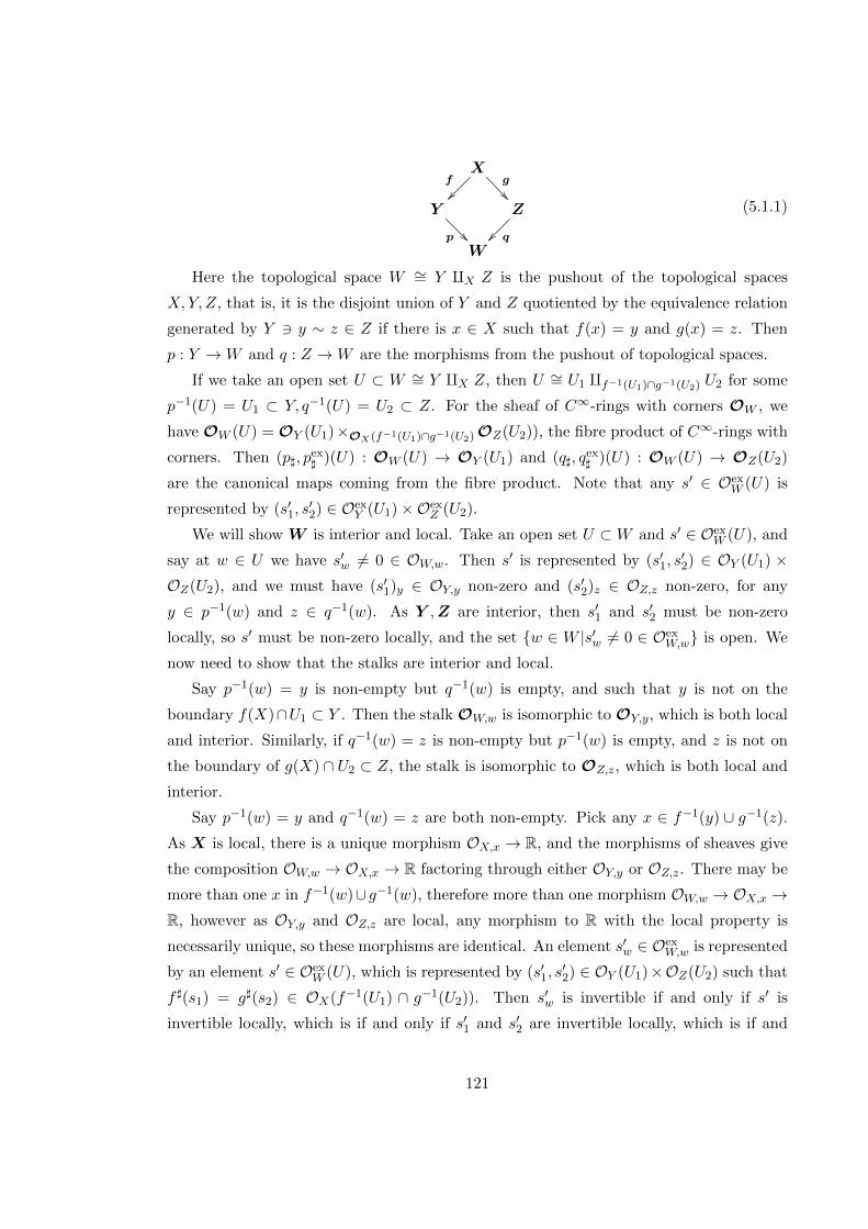
Xf

g

Y

p

Z

qW

(5.1.1)

Here the topological space W ∼= Y qX Z is the pushout of the topological spaces

X,Y, Z, that is, it is the disjoint union of Y and Z quotiented by the equivalence relation

generated by Y 3 y ∼ z ∈ Z if there is x ∈ X such that f(x) = y and g(x) = z. Then

p : Y →W and q : Z →W are the morphisms from the pushout of topological spaces.

If we take an open set U ⊂ W ∼= Y qX Z, then U ∼= U1 qf−1(U1)∩g−1(U2) U2 for some

p−1(U) = U1 ⊂ Y, q−1(U) = U2 ⊂ Z. For the sheaf of C∞-rings with corners OW , we

have OW (U) = OY (U1)×OX(f−1(U1)∩g−1(U2) OZ(U2)), the fibre product of C∞-rings with

corners. Then (p], pex] )(U) : OW (U) → OY (U1) and (q], q

ex] )(U) : OW (U) → OZ(U2)

are the canonical maps coming from the fibre product. Note that any s′ ∈ OexW (U) is

represented by (s′1, s′2) ∈ Oex

Y (U1)×OexZ (U2).

We will show W is interior and local. Take an open set U ⊂W and s′ ∈ OexW (U), and

say at w ∈ U we have s′w 6= 0 ∈ OW,w. Then s′ is represented by (s′1, s′2) ∈ OY (U1) ×

OZ(U2), and we must have (s′1)y ∈ OY,y non-zero and (s′2)z ∈ OZ,z non-zero, for any

y ∈ p−1(w) and z ∈ q−1(w). As Y ,Z are interior, then s′1 and s′2 must be non-zero

locally, so s′ must be non-zero locally, and the set w ∈ W |s′w 6= 0 ∈ OexW,w is open. We

now need to show that the stalks are interior and local.

Say p−1(w) = y is non-empty but q−1(w) is empty, and such that y is not on the

boundary f(X)∩U1 ⊂ Y . Then the stalk OW,w is isomorphic to OY,y, which is both local

and interior. Similarly, if q−1(w) = z is non-empty but p−1(w) is empty, and z is not on

the boundary of g(X) ∩ U2 ⊂ Z, the stalk is isomorphic to OZ,z, which is both local and

interior.

Say p−1(w) = y and q−1(w) = z are both non-empty. Pick any x ∈ f−1(y) ∪ g−1(z).

As X is local, there is a unique morphism OX,x → R, and the morphisms of sheaves give

the composition OW,w → OX,x → R factoring through either OY,y or OZ,z. There may be

more than one x in f−1(w)∪ g−1(w), therefore more than one morphism OW,w → OX,x →R, however as OY,y and OZ,z are local, any morphism to R with the local property is

necessarily unique, so these morphisms are identical. An element s′w ∈ OexW,w is represented

by an element s′ ∈ OexW (U), which is represented by (s′1, s

′2) ∈ OY (U1)×OZ(U2) such that

f ](s1) = g](s2) ∈ OX(f−1(U1) ∩ g−1(U2)). Then s′w is invertible if and only if s′ is

invertible locally, which is if and only if s′1 and s′2 are invertible locally, which is if and

121

only if the image of s′w under this unique morphism is non-zero, which makes OW,w into

a local C∞-ring with corners.

Additionally, if s′ ∈ OexW,w is a non-zero zero divisor, then it must be represented by

zero-divisor (s′1, s′2) ∈ Oex

Y,y×OZ,z, and requiring that it factor through to OX,x means that

both s′1, s′2 are non-zero. However, as OY,y and OZ,z are interior, the only zero divisors in

their product have one zero entry (as in Example 4.2.14), so s′ cannot be a zero divisor.

Hence OW,w is interior.

Here we have assumed there is only one element in both p−1(w) and q−1(w), how-

ever it is possible there is more than one element. In this case, we have several maps

OW,w → OY,yj → OX,xi → R and OW,w → OZ,zk → OX,xi → R for elements xi, yk, zk.

Each pair (yj , zk) are related by a finite number of relations such as f(x1) = yi, g(x1) =

g(x2), f(x2) = f(x3), g(x3) = g(x4), . . . , g(xn) = zj , and we get a diagram of maps as

below.

OW,w

ss ww '' ++ ,,OY,yi

&&

OZ,g(x1)

''

OY,f(x2)

''

OZ,g(x2)

''

OY,f(x3)

%%

. . .

OX,x1

''

OX,x2

OX,x3

ww

OX,x4

ss

. . .

rrR

However, the top rectangles commute by definition of the pushout, and the lower rectangles

commute by definition of local morphisms, so all these compositions are the same, and we

can again show these maps make OW,w into a local interior C∞-ring with corners.

Now consider p−1(w) = y but on the boundary of f(X) ∩ U1 ⊂ Y . There is still a

morphism from OW,w → OY,y → R, but we do not necessarily know that OW,w ∼= OY,y.However, this morphism is well defined, and sw ∈ OW,w is sent to s1,w ∈ OY,y which is

non-zero under the map to R if and only if s1,w is invertible and hence if and only if sw

is invertible, so OW,w is local. A similar proof shows OW,w is local, and a similar proof

as above shows OW,w is also interior. Hence W is an interior local C∞-ringed space with

corners.

Note that W satisfies the universal property of the pushout by using the universal

properties of the pushout of topological spaces and of the pullbacks of (interior/local)

C∞-rings with corners.

As C∞RSc, LC∞RSc, C∞RScin and LC∞RSc

in all have an initial object, (∅, 0, 0)the empty set with the zero C∞-ring with corners sheaf, and we can construct finite col-

122

imits as iterated pushouts using the initial objects. This shows that all finite colimits in

these categories exist. This result can be extended to show all small colimits exist by

showing small products exist. In this case, again the topological space is the coproduct of

the topological spaces, the sheaves are the product of the sheaves, local and interior follow

as above, and the universal properties follow from the universal properties of coproducts

and products.

Corollary 5.1.8. The inclusion and forgetful functors in the following diagram respect

small colimits.

LC∞RScin

// C∞RScin

LC∞RSc //

C∞RSc

LC∞RS // C∞RS // Top

Proposition 5.1.9. The forgetful functor LC∞RScin → LC∞RSc has a left adjoint,

therefore it preserves limits.

This proof uses the right adjoint to inc : C∞Ringscin → C∞Ringsc defined in Theo-

rem 4.3.7(b). We also show this forgetful functor preserves small limits directly in Theorem

5.1.10.

In contrast to Example 4.2.14, which shows that inc : C∞Ringscin → C∞Ringsc has

no left adjoint, in §5.8 we show that LC∞RScin → LC∞RSc also has a right adjoint,

and hence preserves colimits, extending Proposition 5.1.7. While interior local C∞-ringed

spaces with corners have interior stalks, they do not have sheaves of interior C∞-rings

with corners. This means this result does not contradict Example 4.2.14, as, from Propo-

sition 5.1.7, colimits of interior local C∞-ringed spaces with corners have stalks that are

constructed using only certain types of limits of interior C∞-rings with corners, which are

also interior.

Proof. A left adjoint can be constructed as follows. On objects, take (X,OX ,OexX ) ∈

LC∞RSc to (X,OX , OexX ) where Oex

X is the sheafification of the presheaf OexX q0ex, and

q is the disjoint union. Here 0ex becomes the new zero object. On connected components

U ⊂ X, OexX (U) ∼= Oex

X (U) q 0ex. This is an interior C∞-ring with corners, as it is the

image of OX(U) under the right adjoint to the inclusion inc : C∞Ringscin → C∞Ringsc

defined in Theorem 4.3.7(b).

A morphism (φ, φ], φ]ex) : X → Y in LC∞RSc is mapped to the morphism (φ, φ],ˆφ]ex),

whereˆφ]ex sends s′ ∈ φ−1(Oex

X )(U) to φ]ex(U)(s′) ∈ OexY (U), and 0ex to 0ex. This defines

123

ˆφ]ex on connected open sets U of X. The glueing property of sheaves then defines this on

all of X.

To show this is an adjoint, we construct the unit and counit at elementsX ∈ LC∞RSc

and Y ∈ LC∞RScin respectively. They are both the identity on the topological space and

the sheaves of C∞-rings. On the monoid scheaves, the unit sends OexX to Oex

X as sheaves

on X. On a connected component U ⊂ X, it does this by sending s′ ∈ OexX (U) to s′ and

0ex to 0, and the glueing property of sheaves defines this on all of X. The counit is defined

by the inclusion of OexY into Oex

Y as sheaves on Y . Checking that the unit and counit are

natural transformations and that they form an adjunction follows immediately from the

definitions.

Theorem 5.1.10. The categories C∞RSc, LC∞RSc, C∞RScin and LC∞RSc

in have

all small limits. Small limits commute with the inclusion and forgetful functors in the

following diagram, where Top is the category of topological spaces and continuous maps.

LC∞RScin

// C∞RScin

LC∞RSc //

C∞RSc

LC∞RSc // C∞RSc // Top

The proof is essentially the same as showing ordinary ringed spaces have all small limits,

however as this is not well known in the literature (see the discussion in the introduction

to Gillam [27]), we include the proof here. Note that limits in ordinary locally ringed

spaces are different from their limits as ordinary ringed spaces; this is due the fact that

pushouts of local rings are not always local. However pushouts of local C∞-rings (with

corners) are local, and so small limits of local C∞-ringed spaces (with corners) coincide

with small limits of C∞-ringed spaces (with corners).

Proof. We first show that all fibre products of (local) C∞-ringed spaces with corners exist;

as there is also a final object, (∗, (R, [0,∞)) the point with local C∞-ring with corners

(R, [0,∞)), then all finite limits exist. When then explain how to show all small products

exist, which shows all small limits exist.

Let X,Y ,Z be (local) C∞-ringed spaces with corners, and let there be morphisms

(f,f ]) = f : X → Z, (g, g]) = g : Y → Z. We will construct the fibre product

X ×f ,Z,g Y = W = (W,OW ) in LC∞RSc. We define W = X ×f,Z,g Y to be the

fibre product of the topological spaces of X,Y ,Z. At each point (x, y) ∈ W , where

124

f(x) = g(y) = z, we define the C∞-ring with corners Wx,y = OX,x qf]x,OZ,z ,g]yOY,y

to be the pushout of the stalks, with projections q1,(x,y) : OX,x → Wx,y and q2,(x,y) :

OY,y →Wx,y. Note that Wx,y is a local C∞-ring with corners if each stalk is also local,

by Proposition 4.6.3.

Let U be an open set in W . We define OW (U) = s : U →∐

(x,y)∈U Wx,y such that

for all s ∈ OW (U), for all (x, y) ∈ U , there are open sets V1 ⊂ X, V2 ⊂ Y , and V3 ⊂ Z,

with f(V1) ⊂ V3, g(V2) ⊂ V3, and (x, y) ∈ V1 ×V3 V2 ⊂ U such that s(x,y) = πx,y(w) for

some w in the pushout OX(V1) qOZ(V3) OY (V2) for all (x, y) ∈ V1 ×V3 V2. Here πx,y is

the unique map πx,y : OX(V1) qOZ(V3) OY (V2) → OX,x qOZ,zOY,y, which exists by the

universal property of the pushout in the domain.

We give OW (U) the structure of a C∞-ring with corners using the C∞-ring with

corners structure from the stalks Wx,y. For example, for a smooth function f : Rn → R,

then Φf (s)(x,y) = πx,y(Φf (w)). Then OW is a sheaf of (local) C∞-rings with corners on

W , with stalks Wx,y at points (x, y) ∈W .

We define maps (q1, q1]) = q1 : W → X and (q2, q2

]) = q2 : W → Y , where

q1 : W → X, (x, y) 7→ x and q2 : W → Y, (x, y) 7→ y are the usual projection maps defined

in the fibre product of topological spaces. On stalks, we have that q1,x] : OX,x → OW,(x,y)

is the map q1,(x,y), and similarly q2,y] = q2,(x,y). We need to show that these maps glue

to form maps q1] and q2

]. We describe this for q1,](U) : OX(U) → OW (q−11 (U)), where

q1,] corresponds to q1] by (2.4.2).

Take s ∈ OX(U), then, by definition of pushout, there is a map q1,U : OX(U) →OX(U)qOZ(Z) OY (Y ). This pushout is not necessarily isomorphic to OW (q−1

1 (U)), how-

ever we can define q1,](s)(x,y) = πx,y q1,U (s) for all (x, y) ∈ q−11 (U) = U ×Z Y , and this

is a well defined element of OW (q−11 (U)). Using the universal properties of pushouts, this

map at the level of stalks is the stalk map q1,(x,y), and that q1] : OX → f∗(OW ) is a well

behaved map of sheaves. A similar construction gives q2].

Finally, we must show the universal property holds for W . This follows from the

universal property of the fibre product X ×Z Y . Here, we again glue maps that result

from the universal properties from the pushouts of the stalks OX,xqf]x,OZ,z ,g]yOY,y, using

the universal properties from OX(V1)qOZ(V3) OY (V2) for open sets V1 ⊂ X, V2 ⊂ Y , and

V3 ⊂ Z, with f(V1) ⊂ V3, g(V2) ⊂ V3.

Hence (W,OW ) = X ×Z Y is the fibre product and all finite limits exist in the

categories C∞RSc and LC∞RSc. These fibre products commute with the forgetful

functor LC∞RSc → C∞RSc, as the pushout of local C∞-rings is local. The construction

of W shows that the limits in both C∞RSc and LC∞RSc commute with the forgetful

125

functor to topological spaces.

To show the same construction applies for fibre products in the categories of C∞RScin

and LC∞RScin, we need to check that the resulting sheaf is interior. From Proposition

4.6.3, we know the stalks are interior. Take an open set U ⊂W and s′ ∈ OexW (U). Say that

s′w16= 0 ∈ Oex

W,w1for some w1 ∈ U , we need to show that s′ is non-zero in every stalk in a

neighbourhood of w1. Now, in a neighbourhood V ⊂ U of w1, we have s′w = πexx,y(c

′) for

all w ∈ V , and some c′ in the monoid part of the pushout OX(V1)qOZ(V3) OY (V2), where

V1×V3 V2 = V . Then s′w16= 0 implies πex

x,y(c′) 6= 0 in the monoid part of OX,xqOZ,z

OY,y,

and that c′ 6= 0.

This means

c′ = Ψh(q1(a1), . . . , q1(am), q2(b1), . . . , q2(bn),

qex1 (a′1), . . . , qex

1 (a′k), qex2 (b′1), . . . , qex

2 (b′l))

for some smooth h : Rm+nk+l → [0,∞) where ai ∈ OX(V1), bi ∈ OY (V2), a′i ∈ Oex

X (V1)

and b′i ∈ OexY (V2). Here, q1 : OX(V1) → OX(V1) qOZ(V3) OY (V2) and q2 : OY (V2) →

OX(V1)qOZ(V3) OY (V2) are the inclusion morphisms coming from the fibre product.

Then

h(x1, . . . , xm+n, y1, . . . , yk+l) = yt11 · · · ytm+nn+mΨF (x1, . . . , xm+n, y1, . . . , yk+l)

with F : Rm+nk+l → [0,∞) smooth and positive, and ti non-negative integers. As πex

x,y

respects the C∞-operations, then applying it to c′, and given that the stalks are interior, we

see that πexx,y(c

′) 6= 0 if and only for all non-zero ti then πexx,yqex

1 (a′i) 6= 0 and πexx,yqex

2 (b′i) 6=0. This implies these a′i and b′i are non-zero in the stalks OX,x and OY,y. As X and Y are

interior, then these a′i and b′i must be non-zero in open neighbourhoods containing x and

y respectively.

As there are finitely many a′i and b′i, intersecting these open neighbourhoods, we must

have an open neighbourhood Vx ⊂ V1 of x and an open neighbourhood Vy ⊂ V2 of y

where these a′i and b′i are all non-zero in their respective neighbourhoods. Then c′ must

be non-zero in every stalk in the open neighbourhood Vx ×V3 Vy ⊂ W of w1, and so s′

must be non-zero in this open neighbourhood, as required. Therefore the fibre product of

interior (local) C∞-ringed spaces with corners is interior, and all fibre products exist in

C∞RScin and LC∞RSc

in.

We can extend this proof to small products. If Xii∈I is a collection of (local)

C∞-ringed spaces with corners, then we can construct the product X. Its underlying

topological space is the product of the Xi’s. Its stalks are the coproduct of the stalks, and

126

its sheaf of C∞-rings with corners is constructed in the same way as above. Proposition

4.6.3 again says that if theXi are local, thenX is local, and that if theXi are interior, the

stalks of X are interior. To show that X is interior follows as above, by understanding

that each element c′ in the monoid part of a coproduct is generated by finitely many

elements from the monoids in the coproduct. The universal properties follow directly

from the universal properties of C∞-ring with corners coproducts and topological space

products.

Definition 5.1.11. Let X = (X,OX) be a local C∞-ringed space with corners. We have

that OX = (OX ,OexX ), where OX is a sheaf of C∞-rings on X. We define a forgetful

functor τ : LC∞RSc → LC∞RS by sending objects X = (X,OX) 7→ (X,OX) and

morphisms f = (f,f ]) = (f, (f ], f ]ex)) 7→ (f, f ]). We define a forgetful functor τin :

LC∞RScin → LC∞RS by τin = τ |LC∞RSc

in.

Proposition 5.1.12. The forgetful functor τ : LC∞RSc → LC∞RS has a right adjoint,

hence it preserves colimits. It also has a left adjoint, so it preserves limits.

Proof. We begin by constructing the right adjoint on objects. Take (X,OX) ∈ LC∞RS

and construct OexX by sheafifying the following presheaf of monoids POex

X where, for an open

set U ⊂ X, then POexX (U) = Φexp(OX(U))q0ex, for q the disjoint union. The restriction

map on the presheaf is ρUV (s′) = Φexp(ρUV (s)) where s′ = Φexp(s), and zero otherwise.

Then (OX , OexX ) is a sheaf of C∞-rings with corners, as on connected components, it is

defined using the Fexp from Theorem 4.3.9. The right adjoint then sends (X,OX) ∈LC∞RS to (X,OX , Oex

X ).

A morphism (f, f ]) : (X,OX)→ (Y,OY )) naturally extends to a morphism (f, f ], f ]ex) :

(X,OX , OexX ) → (Y,OY , Oex

Y ). Here, on a connected component U ⊂ X, then s′ ∈f−1(Oex

Y )(U) is either in f−1(Φexp(OY ))(U) ∼= Φexp(f−1(OY ))(U) or is in f−1(0ex)(U) =

0ex. If it is in Φexp(f−1(OX))(U), then s′ = Φexp(s) 7→ Φexp(f ](s)) ∈ OexX (U) and other-

wise it maps to 0ex ∈ OexX (U).

This construction gives the right adjoint to the forgetful functor. The counit is the

identity, and the unit at the object (X,OX ,OexX ) ∈ LC∞RSc is the identity on the sheaves

of C∞-rings and on the topological spaces. On the sheaves of monoids, for a connected

component U ⊂ X, then s′ ∈ OexY (U) is either in Φexp(OX(U)) or it is equal to 0ex. In

the former case, the unit maps s′ to Ψexp(s′) ∈ OexX (U), and in the latter case it maps to

0 ∈ OexX (U).

As the forgetful functor is then a left adjoint, it preserves colimits.

Recalling in the proof of the existence of fibre products from Theorem 5.1.10, fibre

127

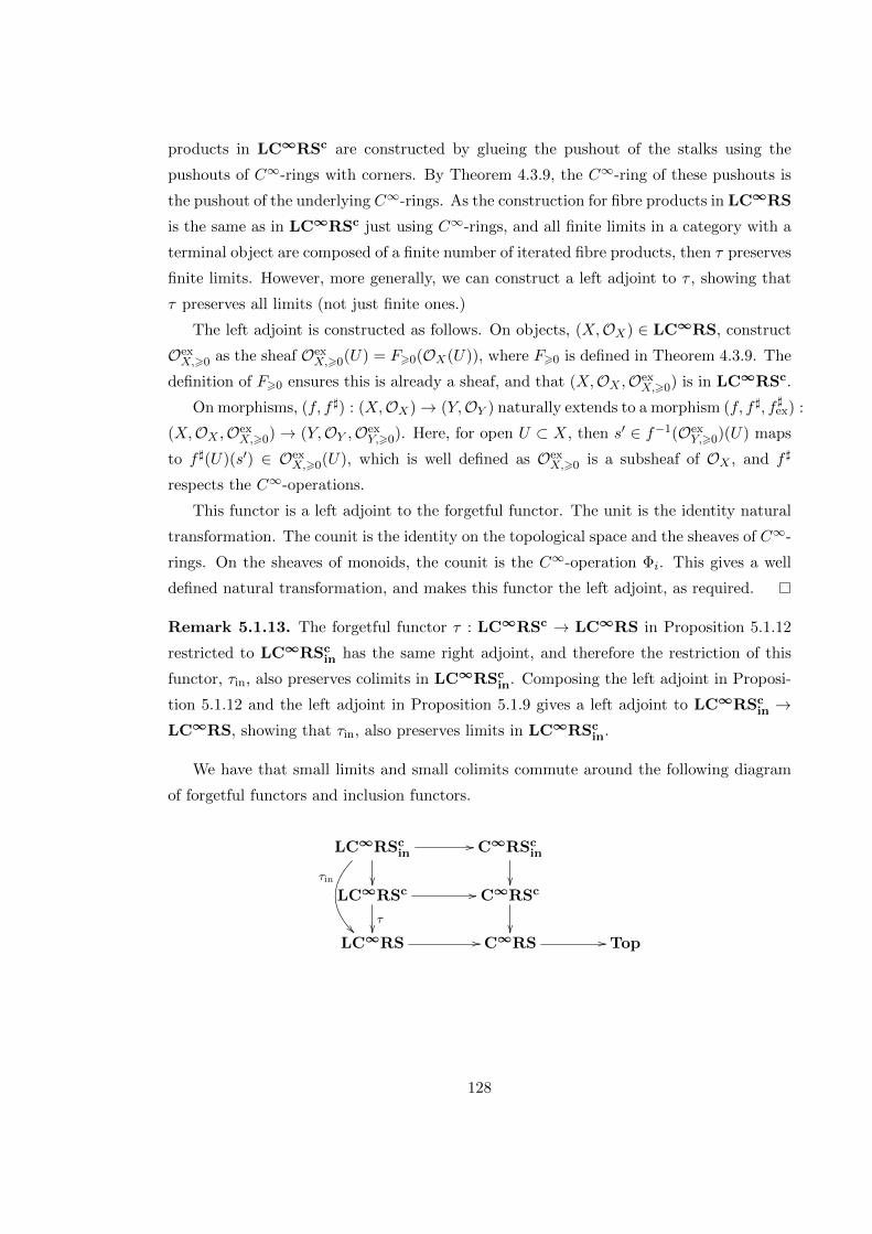
products in LC∞RSc are constructed by glueing the pushout of the stalks using the

pushouts of C∞-rings with corners. By Theorem 4.3.9, the C∞-ring of these pushouts is

the pushout of the underlying C∞-rings. As the construction for fibre products in LC∞RS

is the same as in LC∞RSc just using C∞-rings, and all finite limits in a category with a

terminal object are composed of a finite number of iterated fibre products, then τ preserves

finite limits. However, more generally, we can construct a left adjoint to τ , showing that

τ preserves all limits (not just finite ones.)

The left adjoint is constructed as follows. On objects, (X,OX) ∈ LC∞RS, construct

OexX,>0 as the sheaf Oex

X,>0(U) = F>0(OX(U)), where F>0 is defined in Theorem 4.3.9. The

definition of F>0 ensures this is already a sheaf, and that (X,OX ,OexX,>0) is in LC∞RSc.

On morphisms, (f, f ]) : (X,OX)→ (Y,OY ) naturally extends to a morphism (f, f ], f ]ex) :

(X,OX ,OexX,>0)→ (Y,OY ,Oex

Y,>0). Here, for open U ⊂ X, then s′ ∈ f−1(OexY,>0)(U) maps

to f ](U)(s′) ∈ OexX,>0(U), which is well defined as Oex

X,>0 is a subsheaf of OX , and f ]

respects the C∞-operations.

This functor is a left adjoint to the forgetful functor. The unit is the identity natural

transformation. The counit is the identity on the topological space and the sheaves of C∞-

rings. On the sheaves of monoids, the counit is the C∞-operation Φi. This gives a well

defined natural transformation, and makes this functor the left adjoint, as required.

Remark 5.1.13. The forgetful functor τ : LC∞RSc → LC∞RS in Proposition 5.1.12

restricted to LC∞RScin has the same right adjoint, and therefore the restriction of this

functor, τin, also preserves colimits in LC∞RScin. Composing the left adjoint in Proposi-

tion 5.1.12 and the left adjoint in Proposition 5.1.9 gives a left adjoint to LC∞RScin →

LC∞RS, showing that τin, also preserves limits in LC∞RScin.

We have that small limits and small colimits commute around the following diagram

of forgetful functors and inclusion functors.

LC∞RScin

τin

// C∞RScin

LC∞RSc

τ

// C∞RSc

LC∞RS // C∞RS // Top

128

5.2 Spectrum functor

Note that as in §5.1 we are using the notation that for a sheaf OX of local C∞-rings and

an element s ∈ OX(U) for open U ⊂ X, then sx is value of s in the stalk OX,x and s(x)

value of sx under the stalk map OX,x → R.

We now define a spectrum functor for C∞-rings with corners, in a similar way to

Definition 2.4.4.

Definition 5.2.1. Let C = (C,Cex) be a C∞-ring with corners, and use the notation from

Definition 4.6.7. As in Definition 2.4.3, write XC for the set of R-points of C with topology

TC . For each open U ⊆ XC , define OXC(U) = (OXC

(U),OexXC

(U)). Here OXC(U) is the

set of functions s : U →∐x∈U Cx (where we write sx for its value at the point x ∈ U)

such that sx ∈ Cx for all x ∈ U , and such that U may be covered by open W ⊆ U for

which there exist c ∈ C with sx = πx(c) in Cx for all x ∈W . Similarly, OexXC

(U) is the set

of s′ : U →∐x∈U Cx,ex with s′x ∈ Cx,ex for all x ∈ U , and such that U may be covered by

open W ⊆ U for which there exist c′ ∈ Cex with s′x = πx,ex(c′) in Cx,ex for all x ∈W .

Define operations Φf and Ψg on OXC(U) pointwise in x ∈ U using the operations Φf

and Ψg on Cx. This makes OXC(U) into a C∞-ring with corners. If V ⊆ U ⊆ XC are open,

the restriction maps ρUV = (ρUV , ρUV,ex) : OXC(U) → OXC

(V ) mapping ρUV : s 7→ s|Vand ρUV,ex : s′ 7→ s′|V are morphisms of C∞-rings with corners.

The local nature of the definition implies that OXC= (OXC

,OexXC

) is a sheaf of C∞-

rings with corners on XC . In fact, OXCis the sheaf of C∞-rings in Definition 2.4.4. By

Proposition 5.2.3 below, the stalk OXC ,x at x ∈ XC is naturally isomorphic to Cx, which is

a local C∞-ring with corners by Theorem 4.6.8(a). Hence (XC ,OXC) is a local C∞-ringed

space with corners, which we call the spectrum of C, and write as Specc C.

Now let φ = (φ, φex) : C → D be a morphism of C∞-rings with corners. As in

Definition 2.4.4, define the continuous function fφ : XD → XC by fφ(x) = x φ. For

U ⊆ XC open define (fφ)](U) : OXC(U) → OXD

(f−1φ (U)) by (fφ)](U)sx = φx(sfφ(x)),

where φx : Cfφ(x) → Dx is the induced morphism of local C∞-rings with corners and

s = (s, s′) ∈ OXC(U). Then (fφ)] : OXC

→ (fφ)∗(OXD) is a morphism of sheaves of

C∞-rings with corners on XC .

Let f ]φ : f−1φ (OXC

) → OXDbe the corresponding morphism of sheaves of C∞-rings

with corners on XD under (2.4.2). The stalk map f ]φ,x : OXC ,fφ(x) → OXD,x of f ]φ at

x ∈ XD is identified with φx : Cfφ(x) → Dx under the isomorphisms OXC ,fφ(x)∼= Cfφ(x),

OXD,x∼= Dx in Proposition 5.2.3. Then fφ = (fφ,f

]φ) : (XD,OXD

) → (XC ,OXC) is a

morphism of local C∞-ringed spaces with corners. Define Speccφ : Specc D → Specc C

129

by Speccφ = fφ. Then Specc is a functor (C∞Ringsc)op → LC∞RSc, the spectrum

functor.

Remark 5.2.2. Kalashnikov [51, §4.8] defined the real spectrum of a pre C∞-ring with

corners using the same topological space as our spectrum. However they required it to

have a sheaf of pre C∞-rings with corners that uses localisations of the pre C∞-ring with

corners on subsets that correspond to open sets. Lemma 5.4.4 and an argument using

universal properties will show the stalks are isomorphic in both definitions so that the real

spectrum is equivalent to our spectrum on C∞-rings with corners.

Proposition 5.2.3. In Definition 5.2.1, the stalk OXC ,x of OXCat x ∈ XC is naturally

isomorphic to Cx.

Proof. We have OXC ,x = (OXC ,x,OexXC ,x

) where elements [U, s] ∈ OXC ,x and [U, s′] ∈ OexXC ,x

are ∼-equivalence classes of pairs (U, s) and (U, s′), where U is an open neighbourhood of

x in XC and s ∈ OXC(U), s′ ∈ Oex

XC(U), and (U, s) ∼ (V, t), (U, s′) ∼ (V, t′) if there exists

open x ∈ W ⊆ U ∩ V with s|W = t|W in OXC(W ) and s′|W = t′|W in Oex

XC(W ). Define a

morphism of C∞-rings with corners Π = (Π,Πex) : OXC ,x → Cx by Π : [U, s] 7→ sx ∈ Cx

and Πex : [U, s′] 7→ s′x ∈ Cx,ex.

Suppose cx ∈ Cx and c′x ∈ Cx,ex. Then cx = πx(c) for c ∈ Cx and c′x = πx,ex(c′) for

c′ ∈ Cx,ex by Theorem 4.6.8(c). Define s : XC →∐y∈XC

Cy and s′ : XC →∐y∈XC

Cy,ex

by sy = πy(c) and s′y = πy,ex(c′). Then s ∈ OXC(XC), so that [XC , s] ∈ OXC ,x with

Π([XC , s]) = sx = πx(c) = cx, and similarly s′ ∈ OexXC

(XC) with Πex([XC , s′]) = c′x. Hence

Π : OXC ,x → Cx and Πex : OexXC ,x

→ Cx,ex are surjective.

Let [U1, s1], [U2, s2] ∈ OXC ,x with Π([U1, s1]) = s1,x = s2,x = Π([U2, s2]). Then by

definition of OXC(U1),OXC

(U2) there exists an open neighbourhood V of x in U1 ∩ U2

and c1, c2 ∈ C with s1,v = πv(c1) and s2,v = πv(c2) for all v ∈ V . Thus πx(c1) = πx(c2) as

s1,x = s2,x. Hence c1 − c2 lies in the ideal I in (2.1.4) by Proposition 2.1.15. Thus there

exists d ∈ C with x(d) 6= 0 ∈ R and d · (c1 − c2) = 0 ∈ C.

Making V smaller we can suppose that v(d) 6= 0 for all v ∈ V , as this is an open

condition. Then πv(c1) = πv(c2) ∈ Cv for v ∈ V , since πv(d) · πv(c1) = πv(d) · πv(c2) as

d · c1 = d · c2 and πv(d) is invertible in Cv. Thus s1,v = πv(c1) = πv(c2) = s2,v for v ∈ V ,

so s1|V = s2|V , and [U1, s1] = [V, s1|V ] = [V, s2|V ] = [U2, s2]. Therefore Π : OXC ,x → Cx is

injective, and an isomorphism.

Suppose [U1, s′1], [U2, s

′2] ∈ Oex

XC ,xwith Πex([U1, s

′1]) = s′1,x = s′2,x = Π([U2, s

′2]). As

above there exist an open neighbourhood V of x in U1 ∩ U2 and c′1, c′2 ∈ Cex with s′1,v =

πv,ex(c′1) and s′2,v = πv,ex(c′2) for all v ∈ V . At this point we can use Lemma 4.6.9, which

130

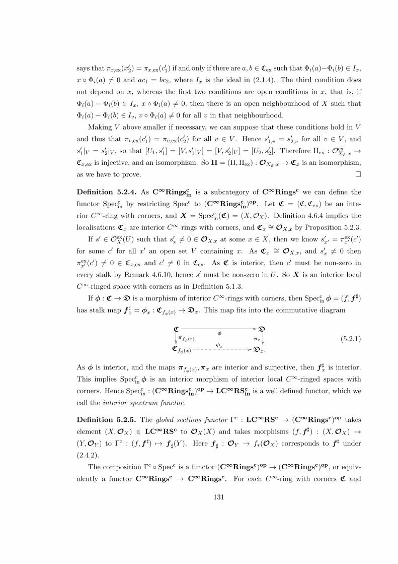
says that πx,ex(x′2) = πx,ex(c′1) if and only if there are a, b ∈ Cex such that Φi(a)−Φi(b) ∈ Ix,

x Φi(a) 6= 0 and ac1 = bc2, where Ix is the ideal in (2.1.4). The third condition does

not depend on x, whereas the first two conditions are open conditions in x, that is, if

Φi(a) − Φi(b) ∈ Ix, x Φi(a) 6= 0, then there is an open neighbourhood of X such that

Φi(a)− Φi(b) ∈ Iv, v Φi(a) 6= 0 for all v in that neighbourhood.

Making V above smaller if necessary, we can suppose that these conditions hold in V

and thus that πv,ex(c′1) = πv,ex(c′2) for all v ∈ V . Hence s′1,v = s′2,v for all v ∈ V , and

s′1|V = s′2|V , so that [U1, s′1] = [V, s′1|V ] = [V, s′2|V ] = [U2, s

′2]. Therefore Πex : Oex

XC ,x→

Cx,ex is injective, and an isomorphism. So Π = (Π,Πex) : OXC ,x → Cx is an isomorphism,

as we have to prove.

Definition 5.2.4. As C∞Ringscin is a subcategory of C∞Ringsc we can define the

functor Speccin by restricting Specc to (C∞Ringsc

in)op. Let C = (C,Cex) be an inte-

rior C∞-ring with corners, and X = Speccin(C) = (X,OX). Definition 4.6.4 implies the

localisations Cx are interior C∞-rings with corners, and Cx∼= OX,x by Proposition 5.2.3.

If s′ ∈ OexX (U) such that s′x 6= 0 ∈ OX,x at some x ∈ X, then we know s′x′ = πex

x′ (c′)

for some c′ for all x′ an open set V containing x. As Cx∼= OX,x, and s′x 6= 0 then

πexx′ (c

′) 6= 0 ∈ Cx,ex and c′ 6= 0 in Cex. As C is interior, then c′ must be non-zero in

every stalk by Remark 4.6.10, hence s′ must be non-zero in U . So X is an interior local

C∞-ringed space with corners as in Definition 5.1.3.

If φ : C →D is a morphism of interior C∞-rings with corners, then Speccinφ = (f,f ])

has stalk map f ]x = φx : Cfφ(x) →Dx. This map fits into the commutative diagram

Cπfφ(x)

φ//Dπx

Cfφ(x)φx //Dx.

(5.2.1)

As φ is interior, and the maps πfφ(x),πx are interior and surjective, then f ]x is interior.

This implies Speccinφ is an interior morphism of interior local C∞-ringed spaces with

corners. Hence Speccin : (C∞Ringsc

in)op → LC∞RScin is a well defined functor, which we

call the interior spectrum functor.

Definition 5.2.5. The global sections functor Γc : LC∞RSc → (C∞Ringsc)op takes

element (X,OX) ∈ LC∞RSc to OX(X) and takes morphisms (f,f ]) : (X,OX) →(Y,OY ) to Γc : (f,f ]) 7→ f ](Y ). Here f ] : OY → f∗(OX) corresponds to f ] under

(2.4.2).

The composition Γc Specc is a functor (C∞Ringsc)op → (C∞Ringsc)op, or equiv-

alently a functor C∞Ringsc → C∞Ringsc. For each C∞-ring with corners C and

131

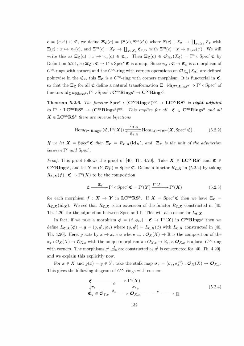
c = (c, c′) ∈ C, we define ΞC(c) = (Ξ(c),Ξex(c′)) where Ξ(c) : XC →∐x∈XC

Cx with

Ξ(c) : x 7→ πx(c), and Ξex(c) : XC →∐x∈XC

Cx,ex with Ξex(c) : x 7→ πx,ex(c′). We will

write this as ΞC(c) : x 7→ πx(c) ∈ Cx. Then ΞC(c) ∈ OXC(XC) = Γc Specc C by

Definition 5.2.1, so ΞC : C → Γc Specc C is a map. Since πx : C → Cx is a morphism of

C∞-rings with corners and the C∞-ring with corners operations on OXC(XC) are defined

pointwise in the Cx, this ΞC is a C∞-ring with corners morphism. It is functorial in C,

so that the ΞC for all C define a natural transformation Ξ : idC∞Ringsc ⇒ Γc Specc of

functors idC∞Ringsc ,Γc Specc : C∞Ringsc → C∞Ringsc.

Theorem 5.2.6. The functor Specc : (C∞Ringsc)op → LC∞RSc is right adjoint

to Γc : LC∞RSc → (C∞Ringsc)op. This implies for all C ∈ C∞Ringsc and all

X ∈ LC∞RSc there are inverse bijections

HomC∞Ringsc(C,Γc(X))LC,X // HomLC∞RSc(X,Specc C).RC,X

oo (5.2.2)

If we let X = Specc C then ΞC = RC,X(idX), and ΞC is the unit of the adjunction

between Γc and Specc.

Proof. This proof follows the proof of [40, Th. 4.20]. Take X ∈ LC∞RSc and C ∈C∞Ringsc, and let Y = (Y,OY ) = Specc C. Define a functor RC,X in (5.2.2) by taking

RC,X(f) : C → Γc(X) to be the composition

CΞC // Γc Specc C = Γc(Y )

Γc(f) // Γc(X) (5.2.3)

for each morphism f : X → Y in LC∞RSc. If X = Specc C then we have ΞC =

RC,X(idX). We see that RC,X is an extension of the functor RC,X constructed in [40,

Th. 4.20] for the adjunction between Spec and Γ. This will also occur for LC,X .

In fact, if we take a morphism φ = (φ, φex) : C → Γc(X) in C∞Ringsc then we

define LC,X(φ) = g = (g, g], g]ex) where (g, g]) = LC,X(φ) with LC,X constructed in [40,

Th. 4.20]. Here, g acts by x 7→ x∗ φ where x∗ : OX(X) → R is the composition of the

σx : OX(X)→ OX,x with the unique morphism π : OX,x → R, as OX,x is a local C∞-ring

with corners. The morphisms g], g]ex are constructed as g] is constructed for [40, Th. 4.20],

and we explain this explicitly now.

For x ∈ X and g(x) = y ∈ Y , take the stalk map σx = (σx, σexx ) : OX(X) → OX,x.

This gives the following diagram of C∞-rings with corners

Cπy

φ// Γc(X)

σx Cy∼= OY,y

φx // OX,xπ // R.

(5.2.4)

132

We know Cy∼= OY,y by Proposition 5.2.3 and π : OX,x → R is the unique local morphism.

If we have (c, c′) ∈ C with y(c) 6= 0, and y Φi(c′) 6= 0 then σx φ(c, c′) ∈ OX,x with

π[σx φ(c)] 6= 0 and

π[Φi σexx φex(c)] = π[σx φ Φi(c)] 6= 0.

As OX,x is a local C∞-ring with corners then σx φ(c, c′) is invertible in OX,x. The

universal property of πy : C → Cy gives a unique morphism φx : OY,y → OX,x that

makes (5.2.4) commute.

We define

g](V ) = (g](V ), gex] (V )) : OY (V )→ g∗(OX)(V ) = OX(U)

for each open V ⊆ Y with U = g−1(V ) ⊆ X by

g](V )(s)x 7→ φx(sg(x))

for s = (s, s′) ∈ OY (V ) and x ∈ U ⊆ X, which means g(x) ∈ V , sg(x) = (sg(x), s′g(x))

∈ OY,g(x), and φx(sg(x)) ∈ OX,x. We can identify elements, p, of OX(U) with maps

t = (t, t′) where t : U →∐x∈U OX,x and t : U →

∐x∈U Oex

X,x with tx = σx(p) ∈ OX,x and

t′x = σexx (p) ∈ Oex

X,x for x ∈ U . For s ∈ OY (V ) and x ∈ U ⊆ X, g(x) = y ∈ V ⊆ Y , then

Definition 5.2.1 tells us around y there is an open neighbourhood Wy in V and there is

(c, c′) ∈ C such that

sy′ = πy′(c, c′) ∈ Cy′

∼= OY,y′

for all y′ ∈Wy. This means

g](V )s(x′) = σx′(φ(c, c′))

for all x′ ∈ g−1(Wy), which is an open neighbourhood of x in U , by (5.2.4). These subsets

g−1(Wy) cover U so by Definition 2.3.1(v), g](V )s is a section of OX |U , and g](V ) is well

defined.

This defines a morphism g] : OY → g∗(OX) of sheaves of C∞-rings with corners on

Y , and g] : g−1(OY ) → OX is the corresponding morphism of sheaves of C∞-rings with

corners on X under (2.4.2). At a point x ∈ X such that g(x) = y ∈ Y , then the stalk map

is g]x : OY,y → OX,x is equal to φx. Then g = (g, g]) is a morphism in LC∞RSc, and

LC,X(φ) = g.

It now remains to show that these define natural bijections, but this follows very

similarly to [40, Th. 4.20].

133

Definition 5.2.7. We define the interior global sections functor Γcin : LC∞RSc

in →(C∞Ringsc

in)op to act on objects (X,OX) by Γcin : (X,OX) 7→ (C,Cex) where C = OX(X)

and Cex to be the set containing the zero element of OexX (X) and the elements of Oex

X (X)

that are non-zero in every stalk. That is,

Cex = c′ ∈ OexX (X) : c′ = 0 ∈ Oex

X (X), or σexx (c′) 6= 0 ∈ Oex

X,x ∀x ∈ X, (5.2.5)

where σexx is the stalk map σex

x : OexX → Oex

X,x. This is an interior C∞-ring with corners,

where the C∞-ring with corners structure is given by restriction from (OX(X),OexX (X)).

We define Γcin to act on morphisms (f,f ]) : (X,OX) → (Y,OY ) by Γc

in : (f,f ]) 7→f ](Y )|(C,Cex) for f ] : OY → f∗(OX) corresponding to f ] under (2.4.2).

In a similar way to Definition 5.2.5, for each interior C∞-ring with corners C, we can

define ΞinC (c) = (Ξin(c),Ξin

ex(c′)) for each element c = (c, c′) ∈ C where Ξin(c) : XC →∐x∈XC

Cx with Ξin(c) : x 7→ πx(c), and Ξinex(c) : XC →

∐x∈XC

Cx,ex with Ξinex(c) : x 7→

πx,ex(c′). We will write this as ΞinC (c) : x 7→ πx(c) ∈ Cx. We need to check that Ξin

ex(c′)

is an element of (5.2.5), that is, whether σexx (Ξin

ex(c′)) = πexx (c′) = 0 ∈ Cx,ex

∼= OexXC ,x

for

some c′ 6= 0 and for some x ∈ XC . However, as πx = (πx, πx,ex) : C → Cx is interior, then

this is immediate and hence ΞinC (c) is a well defined element of Γc

in Speccin(C).

As in Definition 5.2.5, ΞinC is a C∞-ring with corners morphism Ξin

C : C → Γcin

Speccin C, and it is functorial in C, so that the Ξin

C for all C define a natural transformation

Ξin : idC∞Ringscin⇒ Γc

in Speccin of functors idC∞Ringsc

in,Γc

in Speccin : C∞Ringsc

in →C∞Ringsc

in.

Theorem 5.2.8. The functor Speccin : (C∞Ringsc

in)op → LC∞RScin is right adjoint to

Γcin : LC∞RSc

in → (C∞Ringscin)op.

Proof. This proof is identical to that of Theorem 5.2.6. We need only check that the

definition of Γcin(X), which may not be equal to OX(X), gives well defined maps σin

x :

Γcin(X) → OX,x. As Γc

in(X) is a subobject of OX(X), these maps are the restriction of

the stalk maps σx : OX(X) → OX,x to Γcin(X). The definition of Γc

in(X) implies these

maps are interior.

5.3 Semi-complete C∞-rings with corners

There is an equivalence of categories between complete C∞-rings and affine C∞-schemes,

and one uses this equivalence to show that fibre products of C∞-schemes exist. Complete

C∞-rings C are such that Γ SpecC ∼= C, which form a particularly nice category due to

canonical isomorphisms Spec ΓSpecC ∼= SpecC for all C ∈ C∞Rings as in Proposition

134

2.4.12. These isomorphisms imply that Spec Γ is the identity functor on affine C∞-

schemes and other nice results listed in Theorem 2.4.14.

Using this, we see that

HomAC∞Sch(Spec Γ(X,OX),(Y,OY ))

∼= HomAC∞Sch(Spec Γ Spec Γ(X,OX), (Y,OY ))

∼= HomAC∞Sch(Spec Γ Spec Γ(X,OX),Spec Γ(Y,OY ))

∼= Hom(C∞Ringsco)op(Γ Spec Γ(X,OX),Γ(Y,OY ))

∼= HomLC∞RS((X,OX),Spec Γ(Y,OY ))

∼= HomLC∞RS((X,OX), (Y,OY ))

is functorial in both (X,OX) ∈ LC∞RS and (Y,OY ) ∈ AC∞Sch. Here the first iso-

morphism follows from Proposition 2.4.12, the second from Theorem 2.4.14(b), the third

from Theorem 2.4.14(a), the fourth from Theorem 2.4.14(e) and the fifth from Theorem

2.4.14(b). These isomorphisms imply that Spec Γ : LC∞RS→ AC∞Sch is left adjoint

to the inclusion AC∞Sch → LC∞RS, so this inclusion respects limits. An equivalent

result holds in ordinary algebraic geometry.

In this section we show that, unlike C∞-rings, it is not true that Specc Γc Specc C ∼=Specc C for all C∞-rings with corners C. This shows that C∞-schemes with corners will

not be as well behaved as C∞-schemes (or ordinary schemes), and that the inclusion of

(affine) C∞-schemes with corners into LC∞RSc may not respect limits. We then define

a category of ‘semi-complete’ C∞-rings with corners. In §5.4.1 we will use this category

to prove existence of fibre products (and finite limits) of C∞-schemes with corners under

certain conditions.

Remark 5.3.1. For C∞-rings, we have a canonical isomorphism Specφ : Spec Γ SpecC → SpecC ∼= (X,OX) for all C ∈ C∞Rings as in Proposition 2.4.12. This means

there is an isomorphism φx between the stalks of SpecC at R-points x : C → R and the

localisations of the global sections, OX(X) of SpecC at R-points x∗ : OX(X) → R, with

x corresponding to x∗ as in the proof of Theorem 5.2.6.

The following example describes a C∞-ring with corners C = (C,Cex) such that the

canonical morphism Specc(φ, φex) : Specc Γc Specc C → Specc C ∼= (X,OX ,OexX ) is not

an isomorphism. Explicitly, it describes a case where the lower triangle in the following

diagram does not commute for an x ∈ X, and hence φx,ex is not an isomorphism. Note

that we always have the outer rectangle commuting and the upper triangle commuting,

and φx,ex is injective but not necessarily surjective. This example says that if two elements

of OexX (X) agree locally, then while they have the same image in the stalk Oex

X,x they do

135

not necessarily have the same value in the localisation of OexX (X) at x∗, so φx,ex is not

always surjective.

Cexπx,ex //

φex

Cx,ex∼= Oex

X,x

φx,exOexX (X)

ρexX,x

22

πx,ex

// (OexX (X))x∗

(5.3.1)

Here (φ, φex) : (C,Cex)→ ΓcSpecc(C,Cex) ∼= (OX(X),OexX (X)) is the canonical morphism

taking c ∈ C to the section s ∈ OX(X) where sx = πx(c) for all x ∈ X, and similarly for

Cex. Also, ρX,x is the morphism that takes an element s ∈ OX(X) to its value in the stalk

OX,x, and similarly for ρexX,x.

One reason this diagram may not commute for the corners case is the following: for

two elements, c′, d′ ∈ Cex, equality in Cex,x requires a global equality. That is, there need

to be a′, b′ ∈ Cex such that a′c′ = b′d′ ∈ Cex with a′, b′ satisfying additional conditions as in

Lemma 4.6.9. In the C∞-ring C, this equality is only a local equality, as the a′ and b′ can

come from bump functions. However, in the monoid, bump functions do not necessarily

exist, meaning this condition is stronger and harder to satisfy.

In the following example, the C∞-ring with corners C is interior, and here Γcin(C) =

Γc(C), so the above discussion for C∞-rings with corners is also true for interior C∞-rings

with corners.

Example 5.3.2. Let X = R2 and C = (C∞(X),Cinq0ex). Here q is the disjoint union

of sets, and Cin is the monoid generated by Ex(X) and the bump functions c1, c2, c3, c4,

where each cj ∈ C∞(X) has support in the region Aj (defined in Figure 5.3.1) and zero

elsewhere. We have that c1cj = c2cj = c1c2 = 0 ∈ Ex(X) for j = 3, 4. Note that

Ex(X) 3 0 6= 0ex, so Cin q 0ex = Cex has no zero divisors.

We make C into a C∞-ring with corners using composition of functions. That is,

for a non-zero smooth function f : [0,∞)n × Rm → [0,∞), we define the C∞-operation

Ψf : Cnex × Cm → Cex by

Ψf (d1, . . . , dn, g1, . . . , gm) = f(d1, . . . , dn, g1, . . . , gm) ∈ Cin,

where di ∈ Cex and gj ∈ C. For the zero function 0 : [0,∞)n × Rm → [0,∞), we define

Ψ0(d1, . . . , dn, g1, . . . , gm) = 0ex.

If f : [0,∞)n × Rm → R is smooth, then we define the C∞-operation Φf : Cnex × Cm → C

by

Φf (d1, . . . , dn, g1, . . . , gm) = f(d1, . . . , dn, g1, . . . , gm).

136

As C×ex = Ex(X)× = In(X) and (C∞(X),Ex(X)) is a C∞-ring with corners, then C is a

C∞-ring with corners. As Cex has no zero divisors, then C is an interior C∞-ring with

corners.

A2

A1 A3

A4

x

y

Figure 5.3.1: Region of X = R2 with open sets Ai, and points x and y

By Proposition 5.2.3, we know OX,x is isomorphic to Cx, and we know (OX(X))x ∼=OX,x ∼= Cx for all x ∈ X. We will show that (Oex

X (X))x Cx,ex∼= OX,x, where x is a

point in R2 outside of the regions A1, A2, A3, A4, as in Figure 5.3.1. This will show that

Specc Γc Specc C Specc C. Note that R-points of OX(X) are in 1-1 correspondence

with elements of X by Example 2.4.5, so localising at x ∈ X makes sense.

Firstly, note that inOX,x, the elements cj under the map πx,ex : Cex → Cx,ex are distinct

for each j = 1, 2, 3, 4, using Lemma 4.6.9 and that if a ∈ Cex such that x Φi(a) 6= 0 then

a ∈ In(X). We can define the element s′1 ∈ OexX (X) such that s′1,x = πx,ex(c1) for all

x ∈ X. Now using Lemma 4.6.9, for any x ∈ A3 ∪ A4, we have that πx,ex(c1) = πx,ex(c2).

Using this and the locations of A1, A2, A3, A4 in Figure 5.3.1, then we can also define

s′2 ∈ OexX (X) such that s′2,x = πx,ex(c1) for all x outside of A3 ∪ A4, and s′2,x = πx,ex(c2)

for all x inside of A3 ∪A4, and s′2,x = πx,ex(c1) = πx,ex(c2) for all x ∈ A3 ∪A4.

The canonical map (OexX (X))x → Cex

∼= OX,x takes πx,ex(s′) 7→ πx,ex(c′) for s′ ∈OexX (X) where s′x = πx,ex(c′). This means that s′1 and s′2 have the same image under this

map. However, we will show that πx,ex(s′1) 6= πx,ex(s′2) despite s′1,x = s′2,x in an open

neighbourhood of x ∈ X.

If πx,ex(s′1) was equal to πx,ex(s′2), then by Lemma 4.6.9, there would be s′3, s′4 ∈ OX(X)

with s′3,x = s′4,x 6= 0 and s′3 = s′4 in an open neighbourhood of x, such that s′1s′3 = s′2s

′4. If

s′3,x = s′4,x 6= 0, then we have that s′3,x = πx,ex(e1) with e1 ∈ In(X), and s′4,x = πx,ex(e2)

137

with e2 ∈ In(X), for all x in a neighbourhood of x.

As s′1s′3 = s′2s

′4, then for x ∈ A4 we must have s′4(x) = 0 ∈ Ex(X). However, the only

way for s′4 to go from s′4,x = πx,ex(e2), which is invertible at x, to 0 in A4 would mean that

s′4,x = πx,ex(a3) for x ∈ A3 and s′4,x = πx,ex(a4) for all x ∈ A4, where a3 = cn3h1 for some

positive integer n and some h1 ∈ In(x), and a4 = cm4 h2 for some positive integer m and

some h2 ∈ In(x). In particular, this must be true at the point y in Figure 5.3.1, which lies

on the intersection of the boundaries of A3 and A4. However, Lemma 4.6.9 shows that

πx,ex(c3) 6= πx,ex(c4) and that πx,ex(a3) 6= πx,ex(a4) at this point, as there are no elements

of In(X) that are non-zero at y and zero in A3 \A4 and A4 \A3. So this s′4 cannot exist.

This means πx,ex(s′1) 6= πx,ex(s′2). Therefore, the canonical map (OexX (X))x → Cex,x

∼=OX,x is not injective. Hence Specc Γc Specc C Specc C.

If X is an affine C∞-scheme, then Joyce [40, Th. 4.36(a)] tells us that Spec(OX(X)) ∼=X. Also, [40, §4.6] tells us that C∞-rings that are isomorphic to OX(X) for some affine

C∞-scheme X are called complete C∞-rings and there is an equivalence of categories

between complete C∞-rings and affine C∞-schemes.

However, if X is an affine C∞-scheme with corners, then Example 5.3.2 shows that

Specc(OX(X)) X in general, as the sheaf of monoids may be different. This means we

do not expect there to be a subcategory of C∞-rings with corners that gives an equivalence

of categories to affine C∞-schemes with corners. However, we use the following lemma

to define semi-complete C∞-rings with corners, which have similar properties to complete

C∞-rings.

Lemma 5.3.3. Let (C,Cex) be a C∞-ring with corners and let X = (X,OX ,OexX ) =

Specc(C,Cex). Then there is a C∞-ring with corners (D,Dex) with D ∼= Γ Spec(C)

a complete C∞-ring, such that Specc(D,Dex) ∼= X and the canonical map (D,Dex) →Γ Specc(D,Dex) is an isomorphism on D, and injective on Dex. If (C,Cex) is firm, then

(D,Dex) is firm. If (C,Cex) is interior, then (D,Dex) is interior.

Note that Example 5.3.2 gives an example where no choice of Dex can make the canon-

ical map (D,Dex)→ Γ Specc(D,Dex) surjective on the monoids.

Proof. We define (D,Dex) such that D = Γ SpecC = OX(X), and let Dex be the sub-

monoid of OexX (X) generated by the invertible elements Ψexp(D) and the image φex(Cex).

One can check that the C∞-operations from (OX(X),OexX (X)) restrict to C∞-operations

on (D,Dex), and make (D,Dex) into a C∞-ring with corners. Let Y = Specc(D,Dex). If

(C,Cex) is firm, then (D,Dex) is firm, as the sharpening D]ex is the image of C]ex under

138

φex, hence the image of the generators generates D]ex. If (C,Cex) is interior, then (D,Dex)

is interior, as elements in both Ψexp(D) and φex(Cex) have no zero divisors.

Now the canonical morphism (φ, φex) : (C,Cex)→ Γ Specc(C,Cex) gives a morphism

(ψ,ψex) : (C,Cex) → (D,Dex) where ψ = φ, and ψex = φex with its image restricted to

the submonoid Dex of OX,ex(X). As D is complete, then Spec(D) ∼= Spec(C) ∼= (X,OX),

and Specc(ψ,ψex) : Y ∼= Specc(D,Dex) → Specc(C,Cex) ∼= X is an isomorphism on

the topological space and the sheaves of C∞-rings. To show that Specc(ψ,ψex) is an

isomorphism on the sheaves of monoids, we show ψex induces an isomorphism on the

stalks OexX,x∼= Cx,ex and Oex

Y,x∼= Dx,ex, for all R-points x ∈ X.

The stalk map corresponds to the morphism ψx,ex : Cx,ex → Dx,ex, which is defined

by ψx,ex(πx,ex(c′)) = πx,ex(ψex(c′)), where πx,ex : Cex → Cx,ex and πx,ex : Dex → Dx,ex

are the localisation morphisms. Now, as Specc(ψ,ψex) is an isomorphism on the sheaves

of C∞-rings, we know that ψx : Cx → Dx is an isomorphism, which implies we have an

isomorphism ψx,ex|C×x,ex: C×x,ex → D×x,ex of invertible elements in the monoids. This gives

the following commutative diagram of monoids.

Cexψex //

πx,ex

Dex ⊂ OexX (X)

πx,exC×x,ex

//∼= 11Cx,exψx,ex // Dx,ex D×x,ex

? _oo

(5.3.2)

To show ψx,ex is injective, first use that πx,ex is surjective so that for a′x, b′x ∈ Cx,ex, then

a′x = πx,ex(a′), b′x = πx,ex(b′) ∈ Cx,ex for a′, b′ ∈ Cex. Assume that ψx,ex(a′x) = ψx,ex(b′x).

Then we have

πx,ex(ψex(a′)) = ψx,ex(πx,ex(a′)) = ψx,ex(πx,ex(ab)) = πx,ex(ψex(b′)) ∈ Dx,ex,

so by Lemma 4.6.9, there are e′, f ′ ∈ D such that e′ψex(a′) = f ′ψex(b′) ∈ D, with Φi(e′)−

Φi(f′) ∈ I and xΦi(e

′) 6= 0. This implies πx,ex(e′) = πx,ex(f ′) ∈ D×x,ex, and as ψx,ex|C×x,ex:

C×x,ex → D×x,ex is an isomorphism and πx,ex is surjective, there must be e′′, f ′′ ∈ Cex such

that ψex(e′′) = e′ ∈ Dex and ψex(f ′′) = f ′ ∈ Dex, πx,ex(e′′) = πx,ex(f ′′) ∈ Cx,ex, and we

have ψex(e′′a′) = ψex(f ′′b′) ∈ Dex.

Recall that the map ψex sends c′ 7→ s′ ∈ Dex ⊂ OX,ex(X) where s′(x) = πx,ex(c′) for

all x ∈ X. So ψex(e′′a′) = ψex(f ′′b′) implies πx,ex(e′′a′) = πx,ex(f ′′b′) for all x ∈ X. At our

value of x ∈ X, we have that πx,ex(e′′) = πx,ex(f ′′) ∈ C×x,ex, hence we have a′x = πx,ex(a′) =

πx,ex(b′) = b′x, so the map is injective.

To show ψx,ex is surjective, take an element πx,ex(d′) = d′x ∈ Dx,ex for d′ ∈ D. Then

d′ = ψex(c′) · e′ where e′ ∈ Ψexp(D) is invertible, and c′ ∈ C. Then d′x = πx,ex(ψex(c′)) ·

139

πx,ex(e′). As e′ is invertible, then πx,ex(e′) ∈ Dx,ex is invertible. Then as ψx,ex|C×x,ex:

C×x,ex → D×x,ex is an isomorphism and πx,ex is surjective, there must be e′′ ∈ Cex such that

ψex(e′′) = e′, with ψx,ex(πx,ex(e′′)) = πx,ex(e′). Then ψx,ex πx,ex(e′c′) = πx,ex(d′) = d′x

and the map is surjective. Hence, ψx,ex is an isomorphism, and Specc(ψ,ψex) : Y ∼=Specc(D,Dex)→ Specc(C,Cex) ∼= X is an isomorphism.

Finally, as D is complete, we known that the canonical morphism (ϕ,ϕex) : (D,Dex)→Γ Specc(D,Dex) is an isomorphism on the C∞-rings. On the monoids, say d′1, d

′2 ∈ Dex

such that ϕex(d′1) = ϕex(d′2). Then ϕex(d′1), ϕex(d′2) are sections of OexY (Y ) and their

equality implies

πy,ex(d′1) = ϕex(d′1)y = ϕex(d′2)y = πy,ex(d′2) ∈ OY,y ∼= Dy,ex

for all y ∈ Y . We have d′1, d′2 ∈ Oex

X (X), so say that d′1,x = πx,ex(c′1) and d′2,x = πx,ex(c′2)

at a point x ∈ X. From the above, we know Dy,ex∼= Cx,ex where y ∈ Y corre-

sponds to x ∈ X via the isomorphism Specc(ψ,ψex). This isomorphism implies that

πy,ex(d′1) = ψx,ex(πx,ex(c′1)) and πy,ex(d′2) = ψx,ex(πx,ex(c′2)), so we have ψx,ex(πx,ex(c′1)) =

ψx,ex(πx,ex(c′2)). However, as ψx,ex is an isomorphism, we must have πx,ex(c′1) = πx,ex(c′2).

This means that d′1,x = d′2,x for all x ∈ X. As d′1, d′2 are sections of Oex

Y (Y ), then this is

only possible if d′1 = d′2. Hence ϕex is injective.

Definition 5.3.4. Let C = (C,Cex) be a C∞-ring with corners, and let (D,Dex) = D

be the C∞-ring with corners constructed in Lemma 5.3.3 corresponding to C. We call D

a semi-complete C∞-ring with corners, and the category of semi-complete C∞-rings with

corners, denoted C∞Ringscsc, is a full subcategory of C∞-rings with corners. The map

C 7→ D gives a functor Rscall : C∞Ringsc → C∞Ringsc

sc, which is left adjoint to the

inclusion functor C∞Ringscsc → C∞Ringsc. Here the counit is the identity morphism,

and the unit is the morphism (ψ,ψex) defined in the proof of Lemma 5.3.3.

Composing the functor Rscall with the forgetful functor C∞Ringsc → C∞Rings,

(C,Cex) 7→ C is the same as applying the forgetful functor first and then applying the

completion functor Rcoall for C∞-rings defined in Definition 2.4.13.

If C is a C∞-ring with corners and X = Specc C, Y = Specc Γc Specc C, then taking

Specc of the unit ΞC : C → Γc Specc C from Theorem 5.2.6 gives a morphism Y → X,

while the counit on X gives a morphism X → Y . The composition X → Y → X is the

identity, by definition of the counit. Applying the global sections functor Γc implies that

Γc Specc C is a semi-complete C∞-ring with corners for all C∞-rings with corners C.

However the composition Y →X → Y is not the identity in general, in particular if C

is the C∞-ring with corners from Example 5.3.2. Instead, this second composition gives a

140

morphism Y → Y that is not Speccφ for some morphism φ : Γc(X)→ Γc(X). What this

means is that, if we restrict Specc to C∞Ringscsc, then Specc is essentially surjective onto

the category of affine C∞-schemes with corners (AC∞Schc defined in Definition 5.4.1),

and it is faithful, but it is not full. So we do not have an equivalence of categories between

C∞Ringscsc and AC∞Schc.

Remark 5.3.5. To show the category of C∞-schemes has all fibre products, we first

take the fibre product of the C∞-schemes in LC∞RS using Theorem 2.4.15. We then

use the contravariant equivalence of categories between complete C∞-rings and affine C∞-

schemes on affine neighbourhoods from Theorem 2.4.14(a). This translates a fibre product

of affine C∞-schemes to a pushout of complete C∞-rings. As complete C∞-rings have all

pushouts (Theorem 2.4.14(d)), then the fibre product of the affine neighbourhoods of the

C∞-schemes exist, and can be shown to be isomorphic to open neighbourhoods of the fibre

product of the C∞-schemes. This means that the fibre product of the C∞-schemes exist

and are equal to the fibre product taken in LC∞RS, which we expect from the discussion

at the start of this section.

As there is no such equivalence of categories for affine C∞-schemes with corners, we

cannot use this proof for the corners case. Importantly, we cannot show that morphisms

between affine C∞-schemes with corners Specc(C,Cex) → Specc(D,Dex) give morphisms

(D,Dex)→ (C,Cex), even if the C∞-rings are semi-complete. However, in §5.4.1, we show

that we can do this under certain conditions on (D,Dex).

5.4 C∞-schemes with corners

We define the categories of C∞-schemes with corners and firm C∞-schemes with corners.

Firm C∞-schemes with corners have important properties that allow fibre products to

exist.

Definition 5.4.1. A local C∞-ringed space with corners that is isomorphic in LC∞RSc

to Specc C for some C∞-ring with corners C is called an affine C∞-scheme with corners.

We define the category AC∞Schc of affine C∞-schemes with corners to be the full sub-

category of affine C∞-schemes with corners in LC∞RSc. If X ∈ AC∞Schc is isomorphic

to Specc C for a firm C∞-ring with corners, C, we call X a firm affine C∞-scheme with

corners, and denote AC∞Schcfi the full subcategory of AC∞Schc of firm affine C∞-

schemes with corners.

Let X = (X,OX) be a local C∞-ringed space with corners. We call X a (firm) C∞-

scheme with corners if X can be covered by open sets U ⊆ X such that (U,OX |U ) is

141

a (firm) affine C∞-scheme with corners. We define the category (C∞Schcfi) C∞Schc of

(firm) C∞-schemes with corners to be the full sub-category of (firm) C∞-schemes with

corners in LC∞RSc. Then C∞Schcfi, AC∞Schc

fi and AC∞Schc are a full subcategories

of C∞Schc, and AC∞Schcfi is a full subcategory of C∞Schc

fi.

Remark 5.4.2. Kalashnikov [51, §4.8] defined a different notion of (affine) C∞-scheme

with corners using their ‘real spectrum’ functor (as in Remark 5.2.3). This definition is

more general than our definition as they use spectrums of pre C∞-rings with corners.

Definition 5.4.3. A local C∞-ringed space with corners that is isomorphic in LC∞RScin

to Speccin C for some interior C∞-ring with corners C is called an interior affine C∞-scheme

with corners. We define the category AC∞Schcin of interior affine C∞-schemes with

corners to be the full sub-category of interior affine C∞-schemes with corners in LC∞RScin,

so AC∞Schcin is a non-full subcategory of AC∞Schc. A firm interior affine C∞-scheme

with corners is an interior affine C∞-scheme with corners that is also a firm affine C∞-

scheme with corners. We denote AC∞Schcfi,in the full subcategory of AC∞Schc of firm

interior affine C∞-schemes with corners.

We call an object X ∈ LC∞RScin a (firm) interior C∞-scheme with corners if it

can be covered by open sets U ⊆ X such that (U,OX |U ) is a (firm) interior affine C∞-

scheme with corners. We define the category (C∞Schcfi,in) C∞Schc

in of (firm) interior

C∞-schemes with corners to be the full sub-category of (firm) interior C∞-schemes with

corners in LC∞RScin. This implies that (AC∞Schc

fi,in) AC∞Schcin is a full subcategory

of (C∞Schcfi,in) C∞Schc

in.

The following lemma will be useful when considering fibre products of C∞-schemes with

corners in this section. It also tells us that open subsets of (interior/firm) C∞-schemes

with corners are (interior/firm) C∞-schemes with corners.

Lemma 5.4.4. Let C be a C∞-ring with corners, and X = Specc C. For any element

c ∈ C, let Uc be as in Definition 2.4.4. Then X|Uc ∼= Specc(C[c−1]). Note that if C is

firm, then so is C[c−1]; if C is interior, then C[c−1] is also interior.

Proof. Write C[c−1] = (D,Dex). By Lemma 4.6.5, then D ∼= C[c−1]. By Lemma 2.4.6,

we need only show there is an isomorphism of stalks Cx,ex → Dx,ex. However, using

the universal properties of Cx, C[c−1] and C[c−1]x this follows by the same reasoning as

Lemma 2.4.6.

If C is firm, then so is C[c−1], as the sharpening of the monoid of C[c−1] is generated

by the image of C]ex under the morphism C → C[c−1]. If C is interior, then C[c−1] is also

interior, as otherwise zero-divisors would have to come from zero divisors in Cex.

142

In the following proposition, we find a sufficient condition for affine C∞-schemes with

corners that have interior stalks to be interior affine C∞-schemes with corners.

Proposition 5.4.5. Let (C,Cex) be a C∞-ring with corners and let (X,OX) = Specc(C,Cex)

be an affine C∞-scheme with corners such that all stalks are interior C∞-rings with cor-

ners. Then for each x ∈ X, if every zero-divisor c′ ∈ Cex has πx,ex(c′) ∈ Cx,ex either

invertible or zero, then (X,OX) is an interior affine C∞-scheme with corners.

Proof. Let (C,Cex) = C be a C∞-ring with corners such that the conditions in the propo-

sition hold. Let Z = c ∈ Cex : c 6= 0, dc = 0 for some d 6= 0, d ∈ C be the set of all zero

divisors in Cex. Then Z ∪ 0 is an ideal of Cex. Consider C′ex = Cex \ Z. We claim that

(C,C′ex) = C′ is a C∞-ring with corners and Specc(C,C′ex) = (X,OX).

We still have Φi : C′×ex → C injective, as it is a restriction and Z ∩ C×ex = ∅. If we

take a function f : Rnk → [0,∞), we must show that the image of C′exk × Cn−k under Ψf

is contained in C′ex. Assume f is non-zero, then f(x1, . . . , xn) = xa1 · · ·xakF (x1, . . . , xn)

where F : Rnk → (0,∞) and a1, . . . , ak ∈ N.

Assume for a contradiction that Ψf (c′1, . . . , c′k, ck+1, . . . , cn) ∈ Z, then

c′a11 · · · c

′akk ΨF (c′1, . . . , c

′k, ck+1, . . . , cn)d = 0

for some d ∈ Z. As F is non-zero at all points, it is invertible and hence so is element

ΨF (c′1, . . . , c′k, ck+1, . . . , cn). Then c′a1

1 . . . c′akk d = 0, and at least one ai must be non-zero.

But then the corresponding c′i is a zero-divisor. Hence, the image of C′exk × Cn−k under

Ψf is contained in C′ex and (C,C′ex) is a C∞-ring with corners.

We now show that the spectra are isomorphic. We have an inclusion (C,C′ex) →(C,Cex). Taking the spectrum of this morphism, we have an isomorphism on the topolog-

ical spaces and the sheaves of C∞-rings. On the sheaves of monoids, we show the stalks

are isomorphic. That is, we show that for any element z ∈ Z, then for each x ∈ X,

πx′,ex(z) = πx′,ex(c′) for some c′ ∈ C′ex for all x′ in some open neighbourhood around

x ∈ X.

Take z ∈ Z, then by assumption, we know πx,ex(z) is either invertible or zero. If it

is zero, then by Lemma 4.6.9, there is an element a ∈ Cex such that x Φi(a) 6= 0 and

az = 0. Then, by the definition of topology of X, there is an open set U ⊂ X such that

x′ Φi(a) 6= 0 in this neighbourhood. So again by Lemma 4.6.9, we have that πx′,ex(z) = 0

in this neighbourhood, as required.

If πx,ex(z) is invertible, then there is an element cx in the localisation Cx, such that

Ψexp(c) = πx,ex(z). As c ∈ Cx and πx : C → Cx is surjective, then there is an element c ∈ C

such that πx(c) = cx. So we have πx,ex(z) = Ψexp(πx(c)) = πx,ex(Ψexp(c)) and by Lemma

143

4.6.9, there are a, b ∈ Cex such that Φi(a) − Φi(b) ∈ I, x Φi(a) 6= 0 and aΨexp(c) = bz,

where I is as defined in (2.1.4). Now Φi(a) − Φi(b) ∈ I is a local condition, and so is

x Φi(a) 6= 0 by the previous paragraph, and aΨexp(c) = bz is a global condition, so we

have that πx,ex(z) = πx,ex(Ψexp(c)) locally as required.

Hence, Specc C = Specc C′ is an interior affine C∞-scheme with corners.

Remark 5.4.6. In this proposition, (C,Cex) may not be firm, however the resulting C∞-

ring with corners (C,C′ex) may be firm. Example 5.8.8 involves such a case.

This proposition uses that if πx,ex(c′) ∈ Cx,ex is either invertible or zero for zero divisors

c′ ∈ Cex then πx,ex(c′) is equal to πx,ex(d′) for some other element d′ ∈ Cex that is not a

zero divisor of Cex in every stalk. So it might be possible to generalise this proposition by

requiring that for all zero-divisors c′ ∈ Cex and all R-points x, then whenever πx,ex(c′) ∈Cx,ex is not invertible or zero, it must be equal to πx,ex(d′) for d′ ∈ Cex such that d′ is not

a zero-divisor.

It would be interesting to consider whether this is true for all C∞-rings with corners

C such that Specc(C) ∈ LC∞RScin; we show in the following proposition that this is true

at least locally for firm C∞-schemes with corners.

Proposition 5.4.7. Let X be a firm C∞-scheme with corners that is an interior C∞-

ringed space with corners. Then X is an interior firm C∞-scheme with corners.

Proof. Assume X ∼= Specc(C) is affine with C semi-complete and firm. Take a point

x ∈ X. We will construct an interior C∞-ring with corners D such that X|U ∼= Specc(D)

for some neighbourhood U ⊂ X with x ∈ U .

Take generators c′1, . . . , c′n in Cex that generate the sharpening. Assume, without loss

of generality, that πx,ex(c′k) 6= 0 ∈ Cx,ex for i = 1, . . . , k and πx,ex(c′k) = 0 ∈ Cx,ex for

i = k + 1, . . . , n for some integer 1 6 k 6 n. As X is an interior C∞-ringed space with

corners then the sets

Xc′i= x ∈ X : πx,ex(c′k) 6= 0 ∈ Cx,ex

and

X \Xc′i= Xc′i

= x ∈ X : πx,ex(c′k) = 0 ∈ Cx,ex

are both open and closed in X. If we consider V = (∩ki=1Xc′i) ∩ (∩ni=k+1Xc′i

), then x ∈ Vand V is open. As the topology on X is generated by basic open sets of the form Uc =

x ∈ X : x(c) 6= 0 for some c ∈ C, then there is a c ∈ C such that Uc ⊂ V with x ∈ Uc.Let D be the semi-complete C∞-ring with corners corresponding to C[c−1]. Then we

know X|Uc ∼= Specc(C[c−1]) ∼= Specc(D) by Lemma 5.4.4 and Definition 5.3.4. We claim

that D is an interior C∞-scheme with corners.

144

We need to show that there are no zero-divisors in Dex. Firstly, note that there is a

morphism C → D and that under this morphism, the ci also generate the sharpening of

Dex and so D is firm. So the candidates for zero-divisors in Dex are these generators. Now

if πx,ex(c′i) = 0 ∈ Cx,ex for all x ∈ Uc, we claim that the image of c′i is zero in Dex. This

follows as the morphism C →D induces a morphism Cx →Dx, which commutes with the

localisation morphisms Cex → Cx,ex and Dex → Dx,ex. This means that c′i is sent to zero

in Dx,ex whenever it is zero in Cx,ex. As D is semi complete we have that Dex ⊂ OX(Uc),

and if πx,ex(c′i) = 0 ∈ Dx,ex for all x ∈ Uc then it must be the zero section of OX(Uc) so it

must be zero in Dex, as required.

Similarly, if πx,ex(c′i) 6= 0 ∈ Cx,ex for some x ∈ Uc, then the image of c′i under this

morphism is non-zero. So the only candidates for zero-divisors of Dex are the c′i for

i = 1, . . . , k. These are all non-zero in each stalk in Dex. If they were zero-divisors, then

they would be zero-divisors in the stalks. However, we know X has interior stalks, so

these c′i cannot be zero-divisors. So there must be no zero divisors in Dex. Hence D is

interior and semi-complete, with X|Uc ∼= Specc(D). As we can do this around any point,

then X is an interior firm C∞-scheme with corners.

If X is not affine, we can do this on affine open covers and again show that X is an

interior firm C∞-scheme with corners.

5.4.1 Limits and colimits

Let us consider how limits and colimits behave in the category of C∞-schemes with corners.

We start by considering adjoints.

Proposition 5.4.8. There are right adjoints to the forgetful functors C∞Schc → C∞Sch,

AC∞Schc → AC∞Sch, C∞Schcin → C∞Sch and AC∞Schc

in → AC∞Sch hence the

forgetful functors preserve colimits.

This result uses the adjoints constructed in Proposition 5.1.12 and Theorem 4.3.9.

Proof. Let (X,OX) ∼= Spec(C), where C = OX(X) is complete. We show that the image

of (X,OX) under the right adjoint LC∞RS → LC∞RSc constructed in Proposition

5.1.12 ies in AC∞Schc, and its image is (X,OX , OexX ) ∼= Specc(Fexp(C)) where Fexp(C) =

(C,Φexp(C) q 0ex) is the left adjoint constructed in Theorem 4.3.9. This means that

Specc Fexp : (C∞Ringsco)op → AC∞Schc is the right adjoint under the equivalence of

categories AC∞Sch ∼= (C∞Ringsco)op from Theorem 2.4.14(b).

Note that for an R-point x : C → R, then we have Fexp(C)x ∼= Fexp(Cx), as all non-zero

elements of the monoid of Fexp(C) are already invertible. There is a canonical morphism

145

(X,OX , OexX ) → Specc(Fexp(C)), which is the identity on topological spaces and on C∞-

rings. We will define it on the sheaves of monoids, and show it is an isomorphism.

On the monoid sheaf, the section s′ : U → qx∈U (Φexp(Cx) q 0ex) is locally such

that s′(x) = Φexp(πx(c)) or s′(x) = 0ex. Then locally it is either 0ex or it is Φexp(s)

for some section s in the C∞-ring sheaf. Now if s′(x) = 0ex, it must be zero in the

connected component V of U that contains x. Otherwise, s′(x) is non-zero in the connected

component, and, using the glueing and uniqueness property of OX , it is equal to Φexp(s) on

V , for a unique element s ∈ OX(V ). This means that s′ corresponds to a unique element

of the sheafification of Φexp(OX)q0ex, which is the definition of OexX . So the morphism

of sheaves of monoids is well defined. Now if s′ ∈ OexX , we can run this argument in reverse

to see that s′ corresponds to a unique element of the monoid sheaf of Spec(Fexp(C)), giving

the result.

As AC∞Schcin is a subcategory of AC∞Schc and Fexp(C) is interior, then Specc Fexp :

C∞Ringsco)op → AC∞Schcin is the right adjoint to AC∞Schc

in → AC∞Sch.

For the right adjoint to C∞Schc → C∞Sch, take X = (X,OX) ∈ C∞Sch and let

U be an affine open set of X, so that X|U ∼= Specc(C) for C complete. Then, by the

discussion above, the right adjoint from Proposition 5.1.12 applied to X will be locally

isomorphic to Specc(Fexp(C)), and hence in C∞Schc. Again as C∞Schc is a full sub-

category of LC∞RSc, then this must be the right adjoint to C∞Schc → C∞Sch. The

same discussion describes the right adjoint to C∞Schcin → C∞Sch.

Remark 5.4.9. Ideally we would also like left adjoints to the functors C∞Schc →C∞Sch, AC∞Schc → AC∞Sch, C∞Schc

in → C∞Sch and AC∞Schcin → AC∞Sch,

as this would show that these functors preserve limits. This would be helpful in our un-

derstanding of fibre products of C∞-schemes with corners. A candidate for the left adjoint

to AC∞Schc → AC∞Sch is Spec(C) 7→ Specc(F>0(C)) where F>0(C) is the right adjoint

constructed in Theorem 4.3.9. We would like to proceed as follows:

There is a canonical morphism (X,OX ,OexX>0)→ Spec(F>0(C)). On topological spaces

and on the sheaves of C∞-rings, it is the identity morphism. On the sheaves of monoids,

if s′ ∈ OexX (U) is such that s′x = πex

x (c′) for all x ∈ V ⊂ U , and c′ ∈ C>0, then s′ comes

from an element s ∈ OX(U) with sx = πx(c′) as c′ ∈ C>0 ⊂ C. As c′ ∈ C>0, then if

s1, . . . , sn ∈ OX(U) and f : Rn+1 → R is smooth such that f |[0,∞)×Rn = 0, then

Φf (s, s1, . . . , sn)x = Φf (sx, s1,x, . . . , sn,x) = Φf (πx(c), s1,x), . . . , sn,x) = 0 ∈ C,

hence Φf (s, s1, . . . , sn) is locally 0, and the glueing property of sheaves says this is globally

0. Therefore s is an element in OexX>0, and this gives a well defined morphism of sheaves

146

OexX → Oex

X>0.

Considering the stalks of the map, we need to show for any R-point x : C → R, the

localisation (C,C>0)x is isomorphic to F>0(Cx) = (Cx, (Cx)>0). The universal property of

the localisation shows there exists a unique morphism (C,C>0)x → (Cx, (Cx)>0), which is

the stalk map of our morphism, and Theorem 4.6.8 says this is an isomorphism on the C∞-

rings. On the monoids, surjectivity of the localisation (πx, πexx ) : (C,C>0)→ (C,C>0)x says

elements in (C>0)x can be represented as πexx (c) for some c ∈ C>0. Then, for an element

c ∈ C>0, the monoid morphism sends (C>0)x 3 πexx (c)→ πx(c) ∈ (Cx)>0.

To show injectivity of this map, take c, d ∈ C such that πx(c) = πx(d) ∈ Cx are in

(Cx)>0. By Proposition 2.1.15, πx(c) = πx(d) if and only if there is a k ∈ C such that

k ·(c−d) = 0 ∈ C, with x(k) 6= 0. Then k2 ∈ C>0 by Lemma 4.3.12, and k2 ·c = k2 ·d ∈ C>0

with k2(x) > 0. Hence πexx (c) = πex

x (d) ∈ (C>0)x, and the map is injective.

However, we cannot at present show this map is surjective in general, although it is

surjective when X = Rn for example.

We now consider fibre products of C∞-schemes with corners.

Proposition 5.4.10. Let X → Z, Y → Z be morphisms of C∞-schemes with corners. If

Z is a firm C∞-scheme with corners, then the fibre product X×Z Y exists in the category

of C∞-schemes with corners, and is equal to the fibre product in the category LC∞RSc.

Similarly, if X → Z, Y → Z are morphisms of interior C∞-schemes with corners

and Z is a firm interior C∞-scheme with corners, then the fibre product X ×Z Y exists

in the category of interior C∞-schemes with corners, and is equal to the fibre product in

the category LC∞RScin.

Proof. Let f : X → Z, g : Y → Z be morphisms of C∞-schemes with corners, Z a firm

C∞-scheme with corners. Take the fibre product X ×Z Y ∈ LC∞RSc, constructed as in

Theorem 5.1.10.

Pick a point (x, y) ∈ X ×Z Y with f(x) = g(y) = z ∈ Z, and take affine open sets

x ∈ V1 ⊂ X, y ∈ V2 ⊂ Y , z ∈ V3 ⊂ Z with Z|V3 isomorphic to the spectrum of a firm

C∞-ring with corners. If necessary, use Lemma 5.4.4 to shrink V1 and V2 to affine open

sets so that f(V1) ⊂ V3 ⊃ g(V2). Then choosing C,D,E to be semi-complete C∞-rings

with corners (using Lemma 5.3.3 and Definition 5.3.4), we have Spec(C) = (V1,OX |V1),

SpecD = (V2,OY |V2), and SpecE = (V3,OZ |V3), with E firm, and the morphisms φ1 :

C → Γ Specc C ∼= OX(V1), φ2 : D → Γ Specc D ∼= Oy(V2), φ3 : E → Γ Specc E ∼=OZ(V3) are isomorphisms on their C∞-rings, and injective on their monoids.

The morphism f gives the morphism of C∞-rings with corners f ](V3) : OZ(V3) →OX(f−1(V3)) which we can compose with the restriction map ρf−1(V3),V1

to get a morphism

147

of C∞-rings with corners f : OZ(V3) ∼= ΓSpecc E→ ΓSpecc C ∼= OX(V1) and similarly

we can define a g for g. Now, we would like to find morphisms E → C, D → C that

have spectra f and g respectively. We can do this on the C∞-rings as φ1, φ2, φ3 are

isomorphisms. On the monoid Eex, the invertible elements are generated by Ψexp(E). As

E is firm, every element in Eex is of the form a′e1 . . . en where a ∈ Ψexp(E) is invertible,

and the image of the e1, . . . , en under the quotient morphism Eex → E]ex generate the

sharpening E]ex .

Now, for each i = 1, . . . , n, fex φex3 (ei) ∈ Oex

X (V1), but it may not ‘lift’ to Cex (by ‘lift’

we mean that it has an inverse image under φex1 ). However, locally around x we have that

fex φex3 (ei)x = πx,ex(c′) for all x in some open set x ∈ V i

1 ⊂ V1. Taking the intersection

V ′1 = ∩ni=1Vj

1 , we can restrict further to an open set x ∈ Uc ⊂ V ′1 for some c ∈ C, using

Lemma 5.4.4. Then each f φex3 (ei) ∈ Oex

X (Uc) does lift to an element of (C[c−1])ex. Then

every element a′e1 . . . en lifts in this neighbourhood Uc. This gives a well defined C∞-ring

with corners morphism from E to C[c−1]. Similarly, we have a well defined morphism

between E and D[d−1] for some element of d ∈ D. This gives a diagram of C∞-rings with

corners, and we can take the pushout C[c−1]qE D[d−1].

As Specc : (C∞Ringsc)op → LC∞RSc is a right adjoint, then it preserves limits, so

Specc(C[c−1] qE D[d−1]) ∼= X|Uc ×Z|V3Y |Ud . However, the construction of X ×Z Y in

Theorem 5.1.10 implies (X ×Z Y )|Uc×V3Ud∼= X|Uc ×Z|V3

Y |Ud , and hence X ×Z Y is a

C∞-scheme with corners. As C∞Schc is a full subcategory of LC∞RSc, then X ×Z Yis the fibre product in C∞Schc.

Similarly, if f : X → Z, g : Y → Z are morphisms of interior C∞-schemes with

corners, Z a firm interior C∞-scheme with corners, we can construct the fibre product as

above in the category of LC∞RScin. The same method will show that it is an interior C∞-

scheme with corners; one needs to check that if C is interior then C[c−1] in C∞Ringscin is

interior and matches with this localisation in C∞Ringsc, but this follows from Theorem

4.3.7(b) and Lemma 5.4.4.

Remark 5.4.11. If f : X → Z and g : Y → Z are morphisms of affine C∞-schemes with

corners where X ∼= Specc C, Y ∼= Specc D, Z ∼= Specc E, and such that f = Specc(φ :

E → D), g = Specc(ψ : E → C), then using that Specc is a right adjoint we can show

directly that the fibre product in both LC∞RSc and AC∞Schc exists and is isomorphic

to Specc(C qE D). In Proposition 5.4.10 we see that if Z if firm, then we call locally find

such φ and ψ for any morphisms f : X → Z and g : Y → Z.

However, as in Remark 5.3.5 and Definition 5.3.4, there is no equivalence of categories

between C∞-rings with corners and affine C∞-schemes with corners. This means mor-

148

phisms of affine C∞-schemes with corners may not correspond to morphisms of C∞-rings

with corners. So while we can take the fibre product of affine C∞-schemes with corners

in LC∞RSc, it is unclear if this should be the spectrum of a C∞-ring with corners.

Proposition 5.4.10 suggests fibre products of affine C∞-schemes with corners where

they exist may not even be affine, as it involves shrinking open neighbourhoods to find

affine neighbourhoods. Also, if the C∞-schemes are not firm then the neighbourhoods

may need to be shrunk to a set that is not longer open, which suggests that fibre products

of arbitrary C∞-schemes with corners may not exist.

We suspect a counterexample to the existence of arbitrary fibre products of (affine) C∞-

schemes with corners may be constructed using a version of Example 5.3.2. While the C∞-

ring with corners in this example is firm, potentially one could construct a counterexample

using some decreasing sequence of open sets and appropriate monoid generators (as in

Figure 5.3.1) around a particular point, which would create infinitely many generators in

the monoid. This would no longer be firm. Whether this does give a counter-example or

not we will not consider this here, as all the examples we would like to consider are firm.

Corollary 5.4.12. The subcategories C∞Schcfi and C∞Schc

fi,in are closed under finite

limits in LC∞RSc and LC∞RScin. Hence, fibre products and all finite limits exist in

these subcategories.

Proof. The proof of Proposition 5.4.10 shows that the fibre product in LC∞RSc is a C∞-

scheme with corners and is locally isomorphic to Specc(C[c−1]qED[d−1]). The application

of Lemma 5.3.3 allows C,D,E to be firm, then using Lemma 5.4.4 and Proposition 4.5.2,

shows C[c−1] qE D[d−1] is firm, so the fibre product is a firm C∞-scheme with corners.

As C∞Schcfi is a full subcategory of LC∞RSc, then this is the fibre product in C∞Schc

fi.

As C∞Schcfi has a final object Specc(R, [0,∞)), and all fibre products in a category

with a final object are (iterated) fibre products, then C∞Schcfi is closed under finite limits

in LC∞RSc, and all such fibre products and finite limits exist in C∞Schcfi. A similar

argument holds for C∞Schcfi,in.

Now we consider coproducts and colimits of C∞-schemes with corners. We will use∏

for the product of C∞-rings with corners and∏in for products of interior C∞-rings with

corners. We will refer to results in §2.4.1.

Remark 5.4.13. Firstly, some general colimits of C∞-schemes with corners exist. That

is, if we have a collection of C∞-schemes with corners such that there are isomorphisms

between open sets of the schemes, then we can ‘glue together’ to create another C∞-scheme

with corners.

149

This works as follows: Let Xii∈I be a collection of C∞-schemes with corners and

say there are open subsets U i,j for each i, j ∈ I with the induced C∞-scheme with corners

structure as in Lemma 5.4.4. Say we have isomorphisms of C∞-schemes with corners

φi,j : U i,j → U j,i, which are the identity morphism when i = j, and such that φi,j = φ−1j,i ,

φi,j(U i,j ∩U i,k) = U j,i ∩U j,k, and φi,j = φk,j φi,k. Then this gives a diagram of C∞-

schemes with corners with objects Xi,U i,ji,j∈I , and inclusion morphisms U i,j → Xi

and isomorphisms φi,j : U i,j → U j,k. By Proposition 5.1.7, we can take the colimit of this

diagram in local C∞-ringed spaces with corners. However, the construction of this colimit

is such that every point in the colimit has an open set isomorphic to an open subset of

one of the Xi, so this colimit is a C∞-scheme with corners.

For ordinary algebraic geometry the proof is the same, and this result appears in

Hartshorne [33, Ex. I.2.12]. This tells us, for example, if we take each U i,j to be the

empty set, that all coproducts of C∞-schemes with corners exist and are equal to their

products in LC∞RSc.

The following lemma extends Lemma 2.4.21.

Lemma 5.4.14. Let I be a set and C =∏i∈I(Ci,Ci,ex). If x : C → R factors through

Ck = (Ck,Ck,ex) then there is a canonical isomorphism (Ck)x ∼= Cx. If each Ci is interior,

and Cin =∏ini∈I(Ci,Ci,ex) then there is a canonical isomorphism (Ck)x ∼= Cx

∼= Cinx .

Proof. Consider the following commutative diagram, where the right hand side exists when

all Ci are interior. ∏i∈I Ci

πkww

x

++

πx

∏ini∈I Ci

? _oo

πinx

Ck

πk,x

(Ck)x

''

(∏i∈I Ci)x

too

(∏ini∈I Ci)x

poo

vvR

(5.4.1)

Here πk is the projection onto the k-th factor and πx,πinx ,πk,x are the localisation projec-

tions, which are surjective. Note that the dotted arrows exist by the universal properties

of localisations of C and Cin, and that if each Ci is interior, then t p is interior.

On the C∞-rings, the map t : (∏i∈I Ci)x → (Ck)x sends πx((ci)i∈I) ∈ (

∏i∈I Ci)x

to πk,x πinx ((ci)i∈I) = πk,x(ck) ∈ (Ck)x, and similarly on the monoids. This implies t

is surjective. To show it is injective, say t(πx((ci)i∈I)) = t(πx((di)i∈I)) ∈ (Ck)x, then

πk,x(ck) = πk,x(dk), so by Proposition 2.1.15 there exists a ∈ Ck with x(a) 6= 0 such that

150

a · (ck − dk) = 0. Then define (ai)i∈I ∈∏i∈I Ci by ak = a and ai = 0 for i 6= k. Then

(ai)i∈I · ((ci)i∈I − (di)i∈I) and x((ai)i∈I) 6= 0, which implies πx((ci)i∈I) = πx((di)i∈I) ∈(∏i∈I Ci)x, so t is injective on the C∞-rings. On the monoids similar reasoning gives the

same result showing t is an isomorphism.

We now consider the interior case. Note that p is the identity on the C∞-rings.

Say each Ci is interior so t p : (∏ini∈I Ci)x → (Ck)x is an interior morphism, then

(texpex)−1(0) = 0 ∈ (∏ini∈I Ci)x. So say texpex(πx,ex((c′i)i∈I)) = texpex(πx,ex((d′i)i∈I)) ∈

(Ck)x,ex where (c′i)i∈I , (d′i)i∈I ∈

∏ini∈I Ci are non-zero. Then Lemma 4.6.9 says there are

a, b ∈ Ck,ex such that x Φi(a) 6= 0 and ack = bdk, and there is e ∈ Ck such that

e(Φi(a) − Φi(b)) 6= 0 with x(e) 6= 0. Define (ai)i∈I in the monoid of∏ini∈I Ci such that

ak = a and ai = di for all i 6= k, define (bi)i∈I in the monoid of∏ini∈I Ci such that

bk = b and bi = ci for all i 6= k, and define (ei)i∈I ∈∏i∈I Ci with ek = e and ei = 0

for all i 6= k. Then we have x Φi((ai)i∈I)) 6= 0, (ai)i∈I(c′i)i∈I = (bi)i∈I(d

′i)i∈I , and

(ei)i∈I(Φi((ai)i∈I −Φi((bi)i∈I)) = 0, which implies that πx,ex((c′i)i∈I) = (πx,ex((d′i)i∈I)), so

that tex pex is injective. Hence t and t p are isomorphisms.

The following proposition extends Proposition 2.4.22 to C∞-schemes with corners.

Proposition 5.4.15. If I is a set with cardinality less than any measurable cardinal (c.f

Remark 2.4.18) and Cii∈I is a collection of C∞-rings with corners, then there is a

canonical isomorphism Specc(∏i∈I Ci) ∼=

∐i∈I Specc(Ci). If Cii∈I is a collection of

interior C∞-rings with corners, then

Specc(∏i∈I

inCi) ∼=

∐i∈I

Specc(Ci) ∼= Specc(∏i∈I

Ci).

Proof. As in the proof of Proposition 2.4.22, the projections πk :∏i∈I Ci → Ck give

morphisms Specc(πk) : Specc(Ck) → Specc(∏(in)i∈I Ci), which we can amalgamate to a

morphism f = (f, f ], f ]ex) :∐i∈I Spec(Ci) → Spec(

∏(in)i∈I Ci) using the universal property

of a coproduct. Proposition 2.4.22 shows that f is an isomorphism on the topological

spaces and the sheaves of C∞-rings, and Lemma 5.4.14 shows that the stalks of monoids

are isomorphic, so that f is an isomorphism of (interior) C∞-schemes with corners.

Remark 5.4.16. This proposition tells us that provided the cardinality of I is less than

any measurable cardinal, then the coproducts of interior and non-interior affine C∞-

schemes with corners are the same despite Theorem 4.3.7(b) telling us the interior and

non-interior products of interior C∞-rings with corners are different.

In addition, Joyce [40, Th. 4.41] gives a criterion for a C∞-scheme to be affine: the

sufficient conditions are Hausdorff, and Lindelof with smoothly generated topology. The

151

coproduct∐i∈I Specc(Ci) always has smoothly generated topology and is Hausdorff. How-

ever, it is not Lindelof unless I is countable, as otherwise it has an open cover Uii∈I such

that each Specc(Ci) is in exactly one of the Ui and does not intersect any of the others and

this open cover has no countable subcover if I has uncountable cardinality. This means

that if I has uncountable cardinality but has cardinality less than any measurable cardi-

nal, then the underlying C∞-scheme of∐i∈I Specc(Ci) is an example of an C∞-scheme

that does not satisfy the sufficient conditions, yet is affine nonetheless.

Finally, for any cardinality of I, if∐i∈I Specc(Ci) is affine, then its underlying C∞-

scheme must be isomorphic to the spectrum of its global sections, but its global sections

are∏i∈I Ci. This means that if I has measurable cardinality, we know that

∐i∈I Specc(Ci)

is not affine.

5.5 Relation to manifolds with corners

Here we describe how the category of manifolds with corners can be embedded into the

category of C∞-schemes with corners.

Definition 5.5.1. Define a functor FC∞Schc

fiManc : Manc → C∞Schc

fi that acts on ob-

jects X ∈ Manc by FC∞Schc

fiManc (X) = (X,OX), where we have OX(U) = C∞(U) =

(C∞(U),Ex(U)) for each open subset U ⊆ X. That is, C∞(U) is the C∞-ring of smooth

maps c : U → R and Ex(U) is the monoid of exterior (smooth) maps c′ : U → [0,∞), as

in Definition 4.1.1.

Example 4.3.4 shows that C∞(U) is a C∞-ring with corners for each open U . If

V ⊆ U ⊆ X are open we define ρUV = (ρUV , ρexUV ) : C∞(U)→ C∞(V ) by ρUV : c 7→ c|V

and ρexUV : c′ 7→ c′|V .

One can verify that OX is not just a presheaf but a sheaf of C∞-rings with corners

on X, so X = (X,OX) is a C∞-ringed space with corners. We show in Theorem 5.5.2(b)

that X is a firm C∞-scheme with corners, and it is also interior.

Let f : X → Y be a smooth map of manifolds with corners. Writing FC∞Schc

fiManc (X) =

(X,OX), and FC∞Schc

fiManc (Y ) = (Y,OY ), then for all open U ⊆ Y , we define

f ](U) : OY (U) = C∞(U)→ f∗(Ox)(U) = OX(f−1(U)) = C∞(f−1(U))

by f](U) : c 7→ c f for all c ∈ C∞(U) and f ex] (U) : c′ 7→ c′ f for all c′ ∈ Ex(U). Then

f ](U) is a morphism of C∞ rings with corners, and f ] : OY → f∗(OX) is a morphism

of sheaves of C∞-rings with corners on Y . Let f ] : f−1(OY ) → OX correspond to f ]

under (2.4.2). Then FC∞Schc

fiManc (f) = f = (f,f ]) : (X,OX) → (Y,OY ) is a morphism of

C∞-schemes with corners.

152

Define a functor FC∞Schc

fi,in

Mancin

: Mancin → C∞Schc

fi,in by restriction of FC∞Schc

fiManc to

Mancin.

Theorem 5.5.2. Let X be a manifold with corners and X = FC∞Schc

fiManc (X).

(a) If X has faces, then X is an affine C∞-scheme with corners, and is isomorphic

to Specc(C∞(X),Ex(X)). It is also an interior affine C∞-scheme with corners, with

X ∼= Speccin(C∞(X), In(X)q 0). Here q is the disjoint union.

(b) In general, X is a firm interior C∞-scheme with corners.

(c) The functors FC∞Schc

fiManc and F

C∞Schcfi,in

Mancin

are fully faithful.

Proof. For (a), let X be a manifold with corners and write X = FC∞Schc

fiManc (X) = (X,OX).

Note that Γc(X) = OX(X) = C∞(X) by the definition of OX . Consider the functor

LC,X in (5.2.2). In the notation of Theorem 5.2.6, if we let C = Γc(X) = C∞(X), then

LC∞(X),X is a bijection

LC∞(X),X : HomC∞Ringsc(C∞(X),C∞(X)) −→ HomLC∞RSc(X, SpeccC∞(X)).

Let idC∞(X) be the identity morphism in HomC∞Ringsc(C∞(X),C∞(X)) and define

(g, g]) = g = LC∞(X),X(idC∞(X)). We will show that g : X → SpeccC∞(X) is an

isomorphism in LC∞RSc when X is a manifold with faces.

Denote SpeccC∞(X) = Y , then the continuous map g : X → Y is defined in the

proof of Theorem 5.2.6 by g(x) = x∗ idX where idX : C∞(X) → C∞(X) is the identity

morphism and x∗ is the evaluation map at the point x ∈ X. This is a homeomorphism of

topological spaces, as shown in the proof of [40, Th. 4.41].

The map g] corresponds to g] by (2.4.2). For each open V ⊂ Y with U = g−1(V )

then g] is defined by g](V )(s)x 7→ i(sx∗), where s ∈ OY (V ), x ∈ U ⊆ X, and i is the

inclusion C∞-ring with corners morphism i : (C∞(X))x∗ → C∞x (X) for the localisation

(C∞(X))x∗ and the germs of functions C∞x (X) as defined in Example 4.6.11. On stalks,

we have g]x = i : (C∞(X))x∗ → C∞x (X). In Example 4.6.11, we showed that if X has

faces, then (C∞(X))x∗∼= C∞x (X) and then i is the identity map, which is indeed an

isomorphism of local C∞-rings with corners. This implies g] is an isomorphism on stalks,

so g is an isomorphism of local C∞-ringed spaces with corners. Hence X ∼= SpeccC∞(X)

is an affine C∞-scheme with corners.

Now let C∞in (X) = (C∞(X), In(X)q0), where q is the disjoint union. To show that

if X has faces, then X ∼= SpeccC∞in (X), we follow the same method above. Here we use

the bijection

LC∞in (X),X : HomC∞Ringsc(C∞in (X),C∞(X)) −→ HomLC∞RSc(X,SpeccC∞in (X))

153

from Theorem 5.2.6, and the result from Example 4.6.11, that if X has faces, then

C∞x (X) ∼=(C∞(X)

)x∗∼=(C∞in (X)

)x∗ .

The same reasoning above gives the result.

For (b), for any point x ∈ X, we can find a neighbourhood Ux of x such that Ux is a

manifold with faces. For example, Ux can be the coordinate neighbourhood of x, which

is diffeomorphic to Rnk for some n > k with k, n ∈ N. Then if CUx = (C∞(Ux),Ex(Ux)),

by the argument for part (a), we have X|Ux ∼= Specc CUx for each x ∈ X. That is, X is a

C∞-scheme with corners.

As Ux ∼= Rnk , it is connected and there are k connected components of the boundary

in Ux. From Example 4.5.5, we have that Ex(Ux) = In(Ux) q 0 ∼= C∞(X) × Nk q 0.Hence X is locally isomorphic to the spectrum of a firm interior C∞-ring with corners,

and is therefore a firm interior C∞-scheme with corners.

For (c), we know that FC∞Ringsc

Manc |Eucc : Eucc → (C∞Ringsc)op, as defined in Ex-

ample 4.3.4, is full and faithful as it is the Yoneda embedding. Note that the composition

Specc FC∞Ringsc

Manc is equal to FC∞Schc

fiManc when restricted to manifolds with faces, by the

proof of (a).

Let X and Y be manifolds with faces. Let X = FC∞Schc

fiManc (X) and Y = F

C∞Schcfi

Manc (Y ).

As above, we know Γc(X) = C∞(X) and Γc(Y ) = C∞(Y ), and (a) above shows that

SpeccC∞(X) is naturally isomorphic to X, and SpeccC∞(Y ) is naturally isomorphic to

Y . Using these isomorphisms, Theorem 5.2.6 gives a bijection

HomC∞Ringsc(C∞(Y ),C∞(X)) ∼= HomLC∞RSc(SpeccC∞(X),SpeccC∞(Y )).

This shows that Specc is full and faithful on the image of FC∞Ringsc

Manc restricted to manifolds

with faces, in particular when restricted to Euclidean spaces with corners, Eucc. We

conclude that Specc FC∞Ringsc

Manc |Eucc = FC∞Schc

fiManc |Eucc is full and faithful.

Now if f, g are smooth maps f, g : X → Y and (f,f ]) = FC∞Schc

fiManc (f) = F

C∞Schcfi

Manc (g) =

(g, g]), this directly implies f = g, so FC∞Schc

fiManc is faithful.

To show FC∞Schc

fiManc is full, let g = (g, g]) ∈ HomLC∞RSc(X,Y ). We want to show that

g : X → Y is smooth and g = FC∞Schc

fiManc (g). Let x ∈ X and say g(x) = y ∈ Y . As X and

Y are manifolds, there are coordinate neighbourhoods Ux ⊂ X of x and Vy ⊂ Y that are

isomorphic to Rnk ,Rml ⊂ Eucc for n = dimX,m = dimY .

Shrinking Ux and Vy if necessary, we can consider the restriction g|Ux : X|Ux → Y |Vy .As Ux and Vy are isomorphic to Euclidean spaces with corners, then as F

C∞Schcfi

Manc |Eucc is

full, then there is a smooth map hx : Ux → Vy such that FC∞Schc

fiManc |Eucc(hx) = (hx,hx

]) =

154

(g|Ux , g]|Ux) = g|Ux . That is, g|Ux = hx. So g is smooth in a neighbourhood of x for all

x ∈ X, so g is smooth on X.

Now FC∞Schc

fiManc (g)|Ux = F

C∞Schcfi

Manc (g|Ux) = g|Ux . As the morphisms FC∞Schc

fiManc (g) and g

agree on the open sets Ux for each x ∈ X, and Ux cover X, then the sheaf property of OX

and the definition of morphism of sheaves, implies that FC∞Schc

fiManc (g) and g are equal, as

required.

Remark 5.5.3. Note that if X is a manifold with faces then X = FC∞Schc

fiManc (X) is

isomorphic to Specc(C∞(X),Ex(X)) but (C∞(X),Ex(X)) is not firm unless X has finitely

many boundary components. This occurs, for example, when X is compact.

We can also consider the functors FC∞Schc

fiMangc : Mangc → C∞Schc

fi, X 7→ (X,OX)

with OX(U) = (C∞(U),Ex(U)), and FC∞Schc

fi,in

Mangcin

: Mangcin → C∞Schc

fi,in the restriction

of FC∞Schc

fiMangc to Mangc

in . We then can consider whether part (a) or (b) hold for X =

FC∞Schc

fiMangc (X). As a manifold with g-corners is Hausdorff and second countable, and the

topology is smoothly generated, we can apply [40, Th. 4.41] as in the proof, and we find

is that (a) is true for all open subsets U ⊂ XP for XP as in Definition 3.1.3, as on these

subsets can we guarantee that we have

C∞x (X) ∼=(C∞(X)

)x∗ . (5.5.1)

This means that part (b) above is then true for all manifolds with g-corners.

We would like to have some geometrical condition (such as ‘with faces’) that would

allow part (a) to be true more generally. That is, a geometric condition that ensures a

manifold with g-corners satisfies (5.5.1) at all points x ∈ X, so that it is an affine C∞-

scheme with corners. We could consider the following condition as a candidate: (*) the

map iX : ∂X → X is injective on connected components of the boundary map, as in

Definition 3.3.3. However, we will show below that (*) is not enough to guarantee that

part (a) above holds for all of manifolds with g-corners.

Example 5.5.4. Recall Example 3.2.4 of a manifold with g-corners that is not a manifold

with corners. We have

X ′P =

(x1, x2, x3, x4) ∈ [0,∞)4 : x1x2 = x3x4

. (5.5.2)

Figure 5.5.1 shows a three dimensional representation of this manifold as a square

based infinite pyramid such that the ‘faces of the pyramid’ are actually the 2-corners,

where two of the coordinates are zero. Consider compactifying this pyramid by attaching

another pyramid to the bottom as in Figure 5.5.2.

155

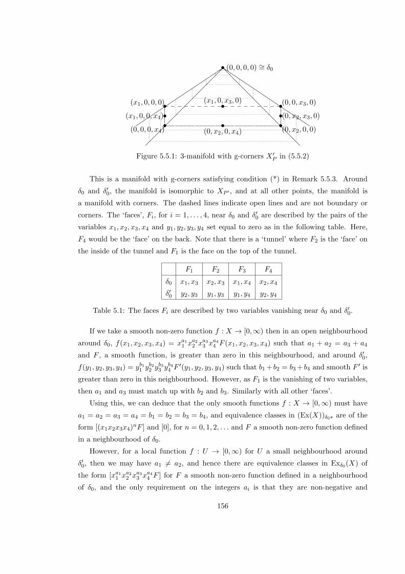
• (0, 0, 0, 0) ∼= δ0

•(x1, 0, 0, 0) •(0, 0, x3, 0)

•(0, 0, 0, x4)

•(0, x2, 0, 0)

•(0, x2, 0, x4)

•(x1, 0, x3, 0)

•(x1, 0, 0, x4) •(0, x2, x3, 0)

Figure 5.5.1: 3-manifold with g-corners X ′P in (5.5.2)

This is a manifold with g-corners satisfying condition (*) in Remark 5.5.3. Around

δ0 and δ′0, the manifold is isomorphic to XP ′ , and at all other points, the manifold is

a manifold with corners. The dashed lines indicate open lines and are not boundary or

corners. The ‘faces’, Fi, for i = 1, . . . , 4, near δ0 and δ′0 are described by the pairs of the

variables x1, x2, x3, x4 and y1, y2, y3, y4 set equal to zero as in the following table. Here,

F4 would be the ‘face’ on the back. Note that there is a ‘tunnel’ where F2 is the ‘face’ on

the inside of the tunnel and F1 is the face on the top of the tunnel.

F1 F2 F3 F4

δ0 x1, x3 x2, x3 x1, x4 x2, x4

δ′0 y2, y3 y1, y3 y1, y4 y2, y4

Table 5.1: The faces Fi are described by two variables vanishing near δ0 and δ′0.

If we take a smooth non-zero function f : X → [0,∞) then in an open neighbourhood

around δ0, f(x1, x2, x3, x4) = xa11 x

a22 x

a33 x

a44 F (x1, x2, x3, x4) such that a1 + a2 = a3 + a4

and F , a smooth function, is greater than zero in this neighbourhood, and around δ′0,

f(y1, y2, y3, y4) = yb11 yb22 y

b33 y

b44 F

′(y1, y2, y3, y4) such that b1 + b2 = b3 + b4 and smooth F ′ is

greater than zero in this neighbourhood. However, as F1 is the vanishing of two variables,

then a1 and a3 must match up with b2 and b3. Similarly with all other ‘faces’.

Using this, we can deduce that the only smooth functions f : X → [0,∞) must have

a1 = a2 = a3 = a4 = b1 = b2 = b3 = b4, and equivalence classes in (Ex(X))δ0∗ are of the

form [(x1x2x3x4)nF ] and [0], for n = 0, 1, 2, . . . and F a smooth non-zero function defined

in a neighbourhood of δ0.

However, for a local function f : U → [0,∞) for U a small neighbourhood around

δ′0, then we may have a1 6= a2, and hence there are equivalence classes in Exδ0(X) of

the form [xa11 x

a22 x

a33 x

a44 F ] for F a smooth non-zero function defined in a neighbourhood

of δ0, and the only requirement on the integers ai is that they are non-negative and

156

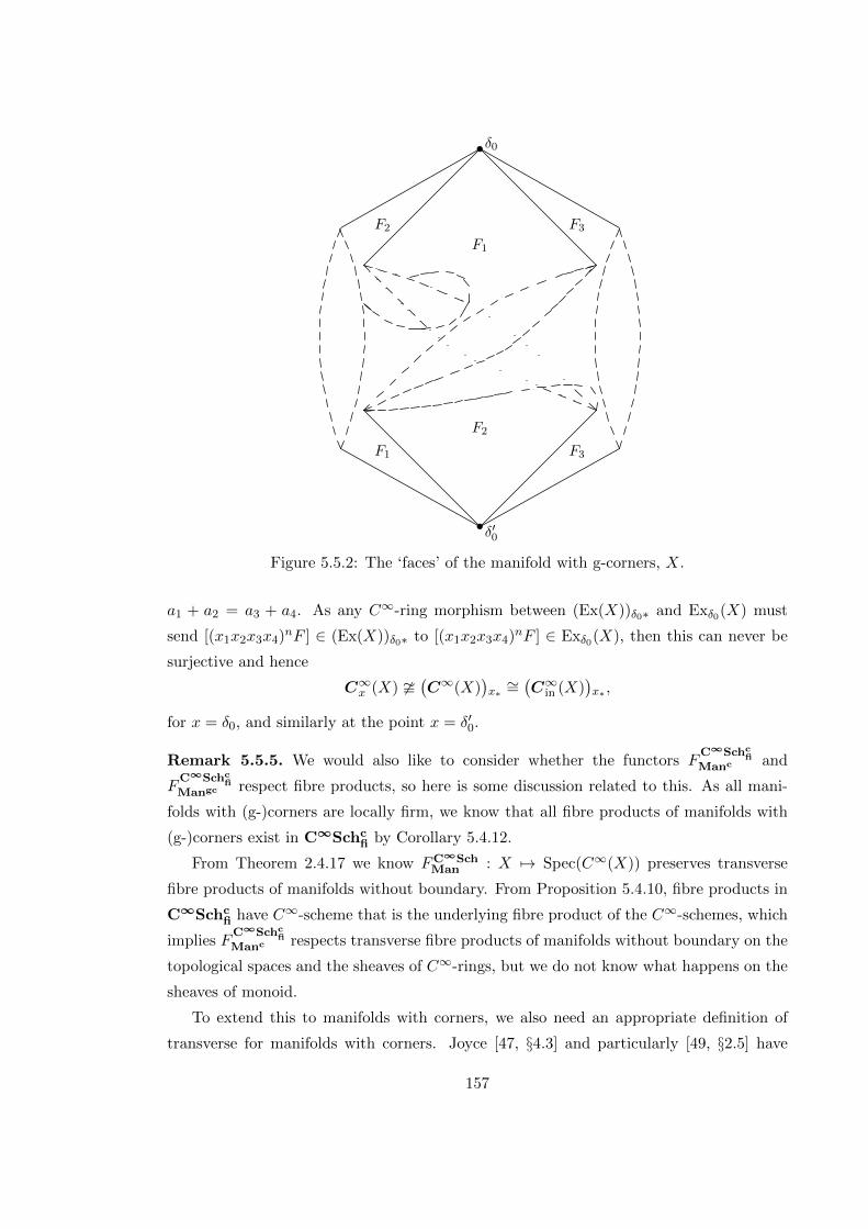
•δ0

F1

F2 F3

•δ′0

F2

F1 F3

Figure 5.5.2: The ‘faces’ of the manifold with g-corners, X.

a1 + a2 = a3 + a4. As any C∞-ring morphism between (Ex(X))δ0∗ and Exδ0(X) must

send [(x1x2x3x4)nF ] ∈ (Ex(X))δ0∗ to [(x1x2x3x4)nF ] ∈ Exδ0(X), then this can never be

surjective and hence

C∞x (X) (C∞(X)

)x∗∼=(C∞in (X)

)x∗ ,

for x = δ0, and similarly at the point x = δ′0.

Remark 5.5.5. We would also like to consider whether the functors FC∞Schc

fiManc and

FC∞Schc

fiMangc respect fibre products, so here is some discussion related to this. As all mani-

folds with (g-)corners are locally firm, we know that all fibre products of manifolds with

(g-)corners exist in C∞Schcfi by Corollary 5.4.12.

From Theorem 2.4.17 we know FC∞SchMan : X 7→ Spec(C∞(X)) preserves transverse

fibre products of manifolds without boundary. From Proposition 5.4.10, fibre products in

C∞Schcfi have C∞-scheme that is the underlying fibre product of the C∞-schemes, which

implies FC∞Schc

fiManc respects transverse fibre products of manifolds without boundary on the

topological spaces and the sheaves of C∞-rings, but we do not know what happens on the

sheaves of monoid.

To extend this to manifolds with corners, we also need an appropriate definition of

transverse for manifolds with corners. Joyce [47, §4.3] and particularly [49, §2.5] have

157

explored fibre products of manifolds with (g-)corners. Notably, manifolds with g-corners

enlarge the category of manifolds with corners under certain types of fibre products, but

in both cases, the fibre products may not exist in general, or they may exist but have

topological space that is not the fibre product of the topological spaces. They also may

not coincide with fibre products in the category of manifolds with (g-)corners and interior

maps.

In [49, §2.5.4] two definitions of transverse are given for manifolds with corners, sb-

transverse and the more restrictive sc-transverse. In [49, Th. 2.32, §2.5.4], we see that

only sc-transverse guarantees that the topological space of the fibre product is the fibre

product of the topological spaces. It is possible that FC∞Schc

fiManc respects sc-transverse fibre

products.

In [47, §4.3] and [49, §2.5] there are two corresponding definitions of transverse for

manifolds with g-corners, b-transverse (as in Theorem 3.4.3) and the more restrictive c-

transverse, and similarly only c-transverse guarantees that the topological space of the

fibre product is the fibre product of the topological spaces. It is possible that FC∞Schc

fiMangc

respects c-transverse fibre products.

Preliminary investigations of this suggests restricting to toric C∞-rings/C∞-schemes

with corners may be necessary to prevent torsion occurring in the fibre products.

5.6 Sheaves of OX-modules and cotangent modules

We define sheaves of OX -modules on a C∞-ringed space with corners, as in §2.5.

Definition 5.6.1. Let (X,OX) be a C∞-ringed space with corners. A sheaf of OX-

modules, or simply an OX -module, E on X, is a sheaf of OX -modules on X, as in Definition

2.5.1. A morphism of sheaves of OX-modules is a morphism of sheaves of OX -modules.

Then OX -modules form an abelian category, which we write as OX -mod.

An OX -module E is called a vector bundle of rank n if we may cover X by open U ⊆ Xwith E|U ∼= OX |U ⊗R Rn.

Pullback sheaves are defined analogously to Definition 2.5.2.

Definition 5.6.2. Let f = (f, f ], f ]ex) : (X,OX ,OexX ) → (Y,OY ,Oex

Y ) be a morphism of

C∞-ringed spaces with corners, and E be an OY -module. Define the pullback f∗(E) by

f∗(E) = f∗(E), the pullback in Definition 2.5.2 for f = (f, f ]) : (X,OX) → (Y,OY ). If

φ : E → F is a morphism of OY -modules we have a morphism of OX -modules f∗(φ) =

f∗(φ) = f−1(φ)⊗ idOX : f∗(E)→ f∗(F).

158

Definition 5.6.3. Let X = (X,OX) be a C∞-ringed space with corners, and X =

(X,OX) the underlying C∞-ringed space. Define the cotangent sheaf T ∗X of X to be

the cotangent sheaf T ∗X of X, as defined in Definition 2.5.3.

If U ⊆ X is open then we have an equality of sheaves of OX |U -modules

T ∗(U,OX |U ) = T ∗X|U .

Let f = (f, f ], f ]ex) : X → Y be a morphism of C∞-ringed spaces. Define Ωf :

f∗(T ∗Y ) → T ∗X to be a morphism of the cotangent sheaves by Ωf = Ωf , where f =

(f, f ]) : (X,OX)→ (Y,OY ).

Definition 5.6.4. Let X = (X,OX) be an interior local C∞-ringed space with corners.

For each open U ⊂ X, let dU,in : OinX(U)→ bΩCU be the b-cotangent module associated to

the interior C∞-ring with corners CU = (OX(U),OinX(U) q 0), where q is the disjoint

union. Here OinX(U) is the set of all elements of Oex

X (U) that are non-zero in each stalk

OexX,x for all x ∈ U . Note that Oin

X is a sheaf of monoids on X.

For each open U ⊂ X, the b-cotangent modules bΩCU define a presheaf PbT ∗X of

OX -modules, with restriction map bΩρUV : bΩCU → bΩCV defined as the unique map from

Definition 4.7.6. This exists by the universal property of bΩU as the b-cotangent module

associated to (OX(U),OinX(U)q 0), and makes the diagram in (2.5.1) commute for this

setup. Denote the sheafification of this presheaf the b-cotangent sheaf bT ∗X of X.

The definition of sheafification implies that, for each open set U , there is a canonical

morphism bΩCU → bT ∗X(U), and we have an equality of sheaves of OX |U -modules

bT ∗(U,OX |U ) = bT ∗X|U .

Also, for each x ∈ X, the stalk bT ∗X|x ∼= bΩOX,x, where bΩOX,x

is the b-cotangent module

of the interior C∞-ring with corners OX,x.

For a morphism f = (f, f ], f ]ex) : X → Y of interior local C∞-ringed spaces, then we

define the morphism of b-cotangent sheaves bΩf : f∗(bT ∗Y ) → bT ∗X by firstly noting

that f∗(bT ∗Y ) is the sheafification of the presheaf P(f∗(bT ∗Y )) acting by

U 7−→ P(f∗(bT ∗Y ))(U) = limV⊇f(U)bΩOY (V ) ⊗OY (V ) OX(U),

as in Definition 2.5.3. Then, following Definition 2.5.3, define a morphism of presheaves

PbΩf : P(f∗(bT ∗Y ))→ PT ∗X on X by

(PbΩf )(U) = limV⊇f(U)(bΩρf−1(V )Uf](V ))∗,

159

where (bΩρf−1(V )Uf](V ))∗ : bΩOY (V ) ⊗OY (V ) OX(U) → bΩOX(U) = (PbT ∗X)(U) is con-

structed as in Definition 2.2.4 from the C∞-ring with corners morphisms f ](V ) : OY (V )→OX(f−1(V )) from f ] : OY → f∗(OX) corresponding to f ] in f as in (2.4.2), and

ρf−1(V )U : OX(f−1(V )) → OX(U) in OX . Define bΩf : f∗(bT ∗Y ) → bT ∗X to be

the induced morphism of the associated sheaves.

Example 5.6.5. Let X be a manifold with (g-)corners and X the associated C∞-scheme

with corners. For each open set U ⊂ X we can show bT ∗X(U) ∼= Γ∞(bT ∗X,U) and

T ∗X(U) ∼= Γ∞(T ∗X,U). That is, as sheaves, bT ∗X ∼= Γ∞(bT ∗X,−) and T ∗X ∼=Γ∞(T ∗X,−). To do this, consider that for every open set U ⊂ X, there is a unique

map ψU : PbT ∗X(U) → Γ∞(bT ∗X,U) using the universal property of the b-cotangent

module as in Example 4.7.8.

If we shrink U to a coordinate patch, then U is a manifold with (g-)corners (with

faces) such that C∞x (U) = (C∞(U))x∗ for each x ∈ U , and corresponding R-point x∗ :

C∞(U) → R. Hence, by Proposition 4.7.9 (and Remark 4.7.10), there is an isomorphism

ψU : PbT ∗X(U) = bΩC∞(U) → Γ∞(bT ∗X,U). Using the uniqueness of ψU for each open

U ⊂ X, we can show that ψU extends to a map of presheaves ψ : PbT ∗X → Γ∞(bT ∗X,−)

that is an isomorphism on stalks.

As bT ∗X is the sheafification of PbT ∗X, there is a unique map of sheaves ψ′ : bT ∗X →Γ∞(bT ∗X,−) that is the same as ψ on stalks. Since ψ is an isomorphism on stalks, then

ψ′ is an isomorphism of sheaves as required. A similar proof shows T ∗X ∼= Γ∞(T ∗X,−)

for X a manifold with corners.

5.7 Corner functor for LC∞RSc

In this section, we define a corner functor, C loc, that describes the boundary and corners

of a local C∞-ringed space with corners. We show this is a right adjoint and show how it

relates to the definition of boundary in Gillam and Molcho [28, §4.4] if we consider a local

C∞-ringed space with corners to be a pre-log locally ringed space, as in §5.9.

Definition 5.7.1. Let X = (X,OX) be a local C∞-ringed space with corners. As a set,

we define

C loc(X) = (x, P ) : x ∈ X,P is a prime ideal in OexX,x.

There is a function of sets π : C loc(X)→ X, (x, P ) 7→ x.

We define a topology on C loc(X) to be the weakest topology such that π is continuous,

so π−1(U) is open for all U ⊂ X, and such that for all open U ⊂ X, for all elements

160

s′ ∈ OexX (U), then

Us′ = (x, P )|x ∈ U, s′x /∈ P ⊂ π−1(U)

is both open and closed in π−1(U). We denote Us′ = π−1(U) \ Us′ . Then π−1(U) = U0 =

U1, and ∅ = U1 = U0 for 0, 1 ∈ OexX (U). The collection Us′ , Us′ : open U ⊂ X, s′ ∈

OexX (U) is a subbase for the topology.

We can pullback the sheaves OX and OexX using π to get the sheaves π−1(OX) and

π−1(OexX ) on C loc(X). The identity morphisms induced from π, that is, π] : π−1(OX) →

π−1(OX) and π]ex : π−1(OexX ) → π−1(Oex

X ), give isomorphisms on stalks π]π(x,P ) : OX,x∼−→

(π−1(OX))(x,P ) and π]ex,π(x,P ) : OexX,x

∼−→ (π−1(OexX ))(x,P ). Then for each prime P in Oex

X,x,

we can identify

π−1(OexX )x ⊃ π]ex,π(x,P )(P ) ∼= P ⊂ Oex

X,x

and

π−1(OX)x ⊃ π]π(x,P )(〈Φi(P )〉) ∼= 〈Φi(P )〉 ⊂ OX,x.

Here 〈Φi(P )〉 is the ideal generated by the image of P under Φi : OexX,x → OX,x.

We define the sheaf of C∞-rings OCloc(X) to be the sheafification of the presheaf of

C∞-rings U 7→ π−1(OX)/I where

I(U) = s ∈ π−1(OX)(U) : s(x,P ) ∈ 〈Φi(P )〉 for all (x, P ) ∈ U.

Similarly, define OexCloc(X)

to be the sheafification of the presheaf U 7→ π−1(OexX )(U)/∼

where, for s′1, s′2 ∈ π−1(Oex

X )(U), then s′1 ∼ s′2 if for each (x, P ) ∈ U either s′1,x, s′2,x ∈ P ,

or there is p ∈ 〈Φi(P )〉 such that s′1,x = Ψexp(p)s′2,x. This is a similar process to quotienting

the C∞-ring with corners (π−1(OX)(U), π−1(OexX )(U)) by a prime ideal in π−1(Oex

X )(U),

which we described in Example 4.4.4(b), and creates a sheaf of C∞-rings with corners

OCloc(X) = (OCloc(X),OexCloc(X)

).

In Lemma 5.7.2 we show that OCloc(X) is interior and the stalks at the point (x, P )

are local C∞-rings with corners isomorphic to OX,x/∼P , using the notation of Example

4.4.4(b). This means that (C loc(X),OCloc(X),OexCloc(X)

) = C loc(X) is an interior local

C∞-ringed space with corners.

The continuous function π and the identity morphisms it induces (π], π]ex) : π−1(OX)→π−1(OX) can be used to define a canonical morphism in LC∞RSc, π : C loc(X) → X.

This is equal to π on the topological spaces, and, on the sheaves of C∞-rings with cor-

ners, then π](U) : π−1(OX)(U) → OCloc(X)(π−1(U)) sends s ∈ π−1(OX) to the image of

π](U)(s) ∈ π−1(OX)(π−1(U)) under the quotient map to OCloc(X)(π−1(U)), and similarly

for the sheaves of monoids map.

161

Let f = (f, f ], f ]ex) : X → Y be a morphism in LC∞RSc, we will define a morphism

C loc(f) : C loc(X) → C loc(Y ). On topological spaces, we define C loc(f) : C loc(X) →C loc(Y ) by (x, P ) 7→ (f(x), (f ]ex,x)−1(P )) where f ]ex,x : Oex

Y,f(x) → OexX,x is the stalk map

of f ]ex. This is continuous as if t ∈ OexY (U) for some open U ⊂ Y then C loc(f)−1(Ut) =

f−1(U)fex] (U)(t) is open, and similarly C loc(f)−1(Ut) = f−1(U)fex

] (U)(t) is open. It follows

that π C loc(f) = f π.

On sheaves, for s′ ∈ OexCloc(Y )

(V ), then as above, s can be represented by an element

s′′ ∈ π−1(OexX )(U), and an element s′′′ ∈ Oex

Y (U) for some open U ⊂ Y with U ⊃ π(V ).

Then we can map s′ → πex] (f−1(U)) f ex

] (U)(s′′′)|π−1(V ). (Note that this is really a map

of the presheaves π−1(OexY )/∼ → π−1(Oex

X )/∼ but definition of sheafification in Definition

2.3.3 and its universal property give the required morphisms of sheaves.) The restriction to

π−1(V ) means this map is independent of the choice of s′′′, and the definition ofOexCloc(Y )

(V )

as a quotient of π−1(OexX )(U) means this map is independent of the choice of s′′. This

gives a morphism OexCloc(Y )

(V ) → OexCloc(X)

(C loc(f)−1(V )). A similar definition gives a

morphism OCloc(Y )(V )→ OCloc(X)(f−1(V )). As both of these morphisms behave well with

restriction, this gives a morphism of sheaves C loc(f)] : OCloc(Y ) → C loc(f)∗(OCloc(X))

adjoint to C loc(f)] : C loc(f)−1(OCloc(Y )) → OCloc(X) as in (2.4.2), and a morphism in

LC∞RSc,

C loc(f) : C loc(X)→ C loc(Y ).

We see that π C loc(f) = f π.

On the stalks, we have C loc(f)](x,P ) : OY,f(x)/∼(f]ex,x)−1(P )→ OX,x/∼P . On the

monoid sheaf, if s′ 7→ 0 in the stalk, then s′ = [s′′] for some element s′′ ∈ OexY,f(x), and

f ]ex,(x,P )(s′′)x ∈ P . Then s′′f(x) ∈ (f ]ex,x)−1(P ), so s′′ ∼P 0 giving that s′ = 0. Therefore

C loc(f) is an interior morphism.

Then C loc(f) = (C loc(f), C loc(f)], C loc(f)]ex) : C loc(X) → C loc(Y ) is an interior

morphism of interior local C∞-ringed spaces with corners, where C loc(f)], C loc(f)]ex re-

late to the morphisms C loc(f)], Cloc(f)ex

] by (2.4.2). One can check that C loc(f g) =

C loc(f) C loc(g) and hence that C loc : LC∞RSc → LC∞RScin is a well defined functor.

If we now assume X is interior, then (x, (0)) : x ∈ X is contained in C loc(X), and

there is an inclusion of sets ιX : X → C loc(X), x 7→ (x, (0)). The image of X under

ιX : X → C loc(X) is closed in C loc(X), that is, for all open U ⊂ X, then

iX(U) = π−1(U) \ ∪s′∈OinX(U)Us′ = ∩s′∈Oin

X(U)Us′

is closed in π−1(U). Also, iX is continuous, as the definition of interior implies i−1X (Us′) =

x ∈ U : s′x 6= 0 ∈ OexX,x is open, and i−1

X (Us′) = x ∈ U : s′x = 0 ∈ OexX,x is open for all

s′ ∈ OexX (U).

162

Now any element s ∈ OX(U) gives an equivalence class in π−1(OX)(π−1(U)), which

gives an equivalence class in π−1(OX)(π−1(U))/∼, which gives an equivalence class in

OCloc(X)(π−1(U)), which gives an equivalence class in ι−1

X (OCloc(X))(U). So there is a map

OX(U) → ι−1X (OCloc(X))(U) and a similar map can be formed for elements in Oex

X (U).

These maps respect restriction and form morphisms of sheaves of C∞-rings with corners.

The stalks of ι−1X (OCloc(X)) are isomorphic to the stalks of OCloc(X), which are isomorphic

to OX,x/∼(0)∼= OX,x by Lemma 5.7.2. This means the inverse image sheaf ι−1

X (OCloc(X))

is canonically isomorphic to OX . So provided X is interior, this isomorphism gives a

morphism of local C∞-ringed spaces with corners ιX : X → C loc(X), which is essentially

the inclusion of X into (x, (0)) : x ∈ X ⊂ C loc(X) and the restriction of the sheaves to

this set. This is interior, as the stalk maps are isomorphisms. In addition, πX ιX = idX .

Lemma 5.7.2. The sheaf of C∞-rings with corners OCloc(X) described in Definition 5.7.1

is interior and the stalks at the point (x, P ) are local C∞-rings with corners isomorphic

to OX,x/∼P , using the notation of Example 4.4.4(b).

Proof. For each s′ ∈ OexCloc(X)

(U), consider the set

K = (x, P ) ∈ U : s′(x,P ) = 0 ∈ OexCloc(X),(x,P ).

Then there is an open cover Uii∈I of U such that s′|Ui corresponds to a ∼-equivalence

class [s′i] in π−1(OexX )(Ui), and we must have that s′i ∈ P at every point (x, P ) ∈ K∩Ui, and

s′i /∈ P for all (x, P ) ∈ (U \K)∩Ui. Now the definition of the inverse image sheaf implies

there is an open cover W ijj∈Ji of Ui such that s′i|Wi,j = [s′i,j ] for some s′i,j ∈ Oex

X (Vi,j)

where we have open Vi,j ⊂ X such that Vi,j ⊃ π(Wi,j). Now we must have s′i,j,x ∈ P for

all (x, P ) ∈ K ∩Wi,j , and s′i,j,x /∈ P for all (x, P ) ∈ (U \K) ∩Wi,j . Then

Wi,j ∩ (Vi,j)s′i,j = K ∩Wi,j

Wi,j ∩ (Vi,j)s′i,j = (U \K) ∩Wi,j

are both open in X. Taking the union over i ∈ I, j ∈ Ji, and using that ∪i∈I,j∈JiWi,j = U ,

we see that K and U \K are both open in U .

The stalks of (OCloc(X),OexCloc(X)

) at a point (x, P ) ∈ C loc(X) are isomorphic to

OX,x/〈Φi(P )〉 and OexX,x/∼P , where s′1 ∼P s′2 in Oex

X,x if s′1, s′2 ∈ P or there is a p ∈ 〈Φi(P )〉

such that Ψexp(p)s′1 = s′2, as in Example 4.4.4(b). To see this, consider that the definitions

give us the following diagram, where we will show the arrow t exists and is an isomorphism.

OX,x∼π]x

//

π−1(OX)(x,P )// // OCloc(X),(x,P )

OX,x/∼P t

55 55

(5.7.1)

163

To see that t exists at the point (x, P ), we use the universal property of OX,x/∼Pas in Example 4.4.4(b)(**). Let U be an open set in X and take s′ ∈ Oex

X (U) such that

s′x ∈ P . Then s′ maps to an equivalence class in OexCloc(X)

(π−1(U)). Consider the open set

U ′s = (x, P ) ∈ C(X) : x ∈ U, s′x ∈ P, then restricting to this open set, we see that our

(x, P ) is in U ′s ⊂ π−1(U) and so we can restrict the equivalence class of s′ to Us′ . In this

open set however, s′x ∈ P for all (x, P ) ∈ Us′ so s′ ∼ 0, and so s′ is in the kernel of the

composition of the top row of (5.7.1). Then the universal property of OX,x/∼P says that

t must exist and commute with the diagram. Also, t must be surjective as the top line is

surjective.

To see that t is injective is straightforward. For example, in the monoid case, if

[s′1,x], [s′2,x] ∈ OexX,x/∼P with representatives s′1, s

′2 ∈ Oex

X (U), and if tex([s′1,x]) = tex([s′2,x])

then s′1,x∼s′2,x for all (x, P ) ∈ V for some open V ⊂ π−1(U). This means at every (x, P ) ∈V then s′1,x ∼P s′2,x, so this must be true at our (x, P ), so that [s′1,x] = [s′2,x] ∈ Oex

X,x/∼Pas required.

Now OexX,x/∼P is interior as the complement of P ∈ Oex

X,x has no zero-divisors. It

is also local, as the unique morphism OX,x → R must have P in its kernel so it factors

through the morphism OX,x → OexX,x/∼P giving a unique morphism Oex

X,x/∼P → R with

the correct properties to be local.

This means that (C loc(X),OCloc(X),OexCloc(X)

) = C loc(X) is an interior local C∞-ringed

space with corners.

Theorem 5.7.3. The corner functor C loc : LC∞RSc → LC∞RScin is right adjoint

to the inclusion functor i : LC∞RScin → LC∞RSc. Thus we have natural, functorial

isomorphisms HomLC∞RScin

(C loc(X),Y ) ∼= HomLC∞RSc(X, i(Y )).

Proof. We describe the unit η : id ⇒ Ci and counit ε : iC ⇒ id of the adjunction. Here

εX = πX for X a C∞-scheme with corners, and ηX = ιX , for X an interior C∞-scheme

with corners. That ε is a natural transformation follows directly from the definition of

C(f) for each morphism of C∞-schemes with corners f .

To show η is a natural transformation, we need to show ηY f = Ci(f) ηX for all

f : X → Y ∈ C∞Schcin. On topological spaces we have x 7→ f(x) 7→ (f(x), (0)) under

ηY f , and x 7→ (x, (0)) 7→ (f(x), (f ]x,ex)−1(0)) under Ci(f) ηX . As f is interior, then

(f ]x,ex)−1(0) = (0) so we have equality on topological spaces.

On the sheaves of C∞-rings with corners, elements of OCloc(Y )(U) are equivalence

classes [[[s]]] where s ∈ OY (V ) for some open set V ⊃ π(U), [s] ∈ π−1(OY )(U), [[s]] ∈π−1(OY )(U)/∼ and [[[s]]] ∈ OCloc(Y )(U). The map ιY,](U) sends [[[s]]] to s|ι−1(U). So

ηY f sends [[[s]]] to f](ι−1(U))(s|ι−1(U)), and Ci(f) ηX sends [[[s]]] to [[[f](V )(s)]]] to

164

f](V )(s)|ι−1(U), which is equal to f](ι−1(U))(s|ι−1(U)) as required. (Again, this is actually

a map of the underlying presheaves, but the properties of the sheafification functor from

Definition 2.3.3 implies this gives a map of the corresponding sheaves.) The same occurs

for the sheaves of monoids, hence η is a natural transformation.

Finally, to show naturality, we need to show that C ⇒ CiC ⇒ C is the identity natural

transformation and i⇒ iCi⇒ i is the identity natural transformation. However, both of

these follow as πX ιX = idX .

Remark 5.7.4. If a functor F : C → D from a category C to a category D has a right

adjoint G : D → C, then one of the equivalent definitions of adjoint (cf. Awodey [5, §9])

says that for elements d ∈ D there is a morphism fd : FG(d)→ d, such that for all c ∈ Cand d ∈ D, and for all morphisms g : c 7→ G(d), there is a unique morphism h : c 7→ FG(d)

with fd h = g.

For the corner functor C loc : LC∞RSc → LC∞RScin, this means if X is a local

C∞-ringed space with corners, then we could instead define C loc(X) to be the (unique

up to isomorphism) interior local C∞-ringed space with corners with morphism πX :

C loc(X) → X that satisfies the following universal property: for all interior local C∞-

ringed spaces with corners Y and morphisms f : Y → X, there is a unique interior

morphism f : Y → C loc(X) such that πX f = f . For any morphism f : X → Y in

LC∞RSc, we can then define C loc(f) = f πX .

For all interior local C∞-ringed spaces with corners X, then the identity morphism

idX : X → X gives a unique interior morphism idX : X → C loc(X), such that πX idX = idX : X →X. We define ιX = idX , and by uniqueness we see f = C loc(f)ιX for

all morphisms f : Y →X for interior Y . This is consistent with our previous definition.

5.7.1 Boundary

We now consider defining a notion of boundary of local C∞-ringed spaces with corners.

For this, we need the following:

Definition 5.7.5. A prime ideal P in a non-trivial monoid M (under multiplication with

a zero element 0) is a minimal non-trivial prime ideal if P 6= 0 and there are no prime

ideals P ′ with P ′ ⊂ P .

Definition 5.7.6. If X is a local C∞-ringed space with corners, then the boundary ∂locX

of X is a sub-local C∞-ringed space with corners of C loc(X). It is the restriction of

C loc(X) to the set

∂locX = (x, P ) ∈ C loc(X) : x ∈ X,P is a minimal prime ideal of OexX,x.

165

That is, if we consider the inclusion of topological spaces ∂locX → C loc(X) then the inverse

image sheaf of OCloc(X) under this map gives the sheaf of C∞-rings with corners on ∂locX.

Note that we would not expect X 7→ ∂locX,X ∈ LC∞RSc to be a functor.

Remark 5.7.7. Gillam and Molcho [28, §4.4] define a notion of the boundary ∆X of

a pre-log locally ringed space X, discussed in §5.9. In Remark 5.9.4 we explain that

our local C∞-ringed spaces with corners are indeed pre-log locally ringed spaces. Then

for X ∈ LC∞RSc we can compare ∆X and ∂locX. Considering their definition of

boundary ∆X, we see the underlying sets of the topological spaces are identical, however

the topology on ∂locX is finer than the topology on ∆X, so there is a morphism of

topological spaces ∂locX → ∆X. Notably, the sets Us′ , Us′ defined in Definition 5.7.1

form a subbase for the topology on ∂locX, however only the sets Us′ form a base for the

topology on ∆X.

The sheaves on ∂locX,∆X are constructed in identical ways, so there is actually a

morphism ∂locX → ∆X of pre-log locally ringed spaces (in fact, both are local C∞-ringed

spaces with corners whenever X is), and the stalks are isomorphic. Then ∂locX → ∆X

is an isomorphism whenever the topology on ∆X is as fine as the topology on ∂locX.

5.8 Corner functor for C∞Schcfi

In this section, we define a corner functor for firm C∞-schemes with corners and compare

it to the corner functor for local C∞-ringed spaces with corners. We first consider the

prime ideals necessary for this construction.

Definition 5.8.1. For a C∞-ring with corners C, define the following two sets of prime

ideals

PrC = P ⊂ Cex|P is a prime ideal

and

Pr′C = P ⊂ Cex|P = π−1x,ex(P ′) for some x ∈ X for a prime ideal P ′ ⊂ Oex

X,x.

Here, πx,ex : Cex → Cx,ex is the surjective localisation morphism. While Pr′C ⊂ PrC ,

Example 5.8.3 shows these two sets are not always equal. In the following lemma we

will show some facts about prime ideals including that any P ∈ PrC \Pr′C are such that

Specc(C/∼P ) is the empty set with the zero-sheaf.

Lemma 5.8.2. (a) If we consider any R-point x : C → R and the localisation π : C → Cx,

then πx,ex takes prime ideals in Cex to prime ideals in Cx,ex (or to the entire monoid).

166

(b) For a C∞-ring with corners C if P ∈ PrC \Pr′C then Specc(C/∼P ) is the empty

set with the zero-sheaf. Also, an R-point x : C → R factors through C/∼P whenever

P ⊆ x−1(0), which implies πx,ex(P ) 6= Cex,x. So we have P ∈ PrC \Pr′C if and only if for

all R-points x : C → R then πx,ex(P ) = Cx,ex under the localisation π : C → Cx.

(c) If we have P ∈ PrC and an element c ∈ Cex such that c /∈ P then for each R-point

x : C → R we have πx,ex(c) ∈ πx,ex(P ) if and only if πx,ex(P ) = Cx,ex. This implies if we

have two prime ideals P1, P2 ∈ PrC with P1 ( P2, then for all x ∈ X, πx,ex(P1) ⊆ πx,ex(P2)

with equality only occurring when πx,ex(P1) = πx,ex(P2) = Cx,ex.

Proof. Firstly, if P is a prime ideal in Cex and we have a morphism of C∞-rings with

corners φ : D→ C then it follows that φ−1ex (P ) is a prime ideal in Dex. We now prove (a).

(a) Take a prime ideal P ⊂ Cex. To see that πx,ex(P ) take any c′x ∈ πx,ex(P ) then as

πx,ex is surjective there is c′ ∈ Cex is such that πx,ex(c′) = c′x and we have

c′xπx,ex(P ) = πx,ex(c)πx,ex(P ) = πx,ex(cP ) ⊂ πx,ex(P ).

Now say c′xd′x ∈ πx,ex(P ), then there are c′, d′ ∈ Cex such that πx,ex(c′) = c′x and πx,ex(d′) =

d′x. So πx,ex(c′d′) ∈ πx,ex(P ). So there are a′, b′ ∈ Cex such that a′c′d′ = b′p′ for some

p ∈ P , and with x Φi(a′) 6= 0 and Φi(a

′) − Φi(b′) ∈ I as in Lemma 4.6.9. However,

p′ ∈ P so b′p′ ∈ P and so a′c′d′ ∈ P . This means either c′d′ ∈ P , in which case, as P is

prime, then either c′ ∈ P or d′ ∈ P and so either c′x or d′x are in πx,ex(P ); or we have that

a′ ∈ P . However, this a′ ∈ P is such that x Φi(a′) 6= 0, which means that πx,ex(a′) ∈ Cex

is invertible, which would imply that πx,ex(a′) ∈ πx,ex(P ) = Cx,ex. In this case, both c′x

and d′x will be in πx,ex(P ). Hence πx,ex(P ) is either prime in Cx,ex or equal to all of Cx,ex.

(b) Take P ∈ PrC \Pr′C , this means that for all x : C → R then P ( π−1x,ex(πx,ex(P )).

So for each x there is a c′ ∈ Cex such that c′ /∈ P but πx,ex(c′) = πx,ex(p′) for some p′ ∈ P .

However, similar to the above, we must then have a′, b′ ∈ Cex with x Φi(a′) 6= 0 and

Φi(a′)− Φi(b

′) ∈ I and such that a′c′ = b′p′. As p′ ∈ P , then b′p′ ∈ P so a′c′ ∈ P and as

c′ /∈ P then a′ ∈ P . However, again πx,ex(a′) ∈ Cex is invertible, which would imply that

πx,ex(P ) = Cx,ex for all x : C → R. P ∈ PrC \Pr′C implies πx,ex(P ) = Cx,ex for all R-points

x. The reverse implication follows from the definition of Pr′C .

If πx,ex(P ) = Cx,ex for all R-points x then there are no R-points y : C/∼P → R, as if

there was such an R-point then composing it with the projection φ : C → C/∼P gives an

R-point x = y φ : C → R. Then taking the a′ corresponding to this R-point as in the

previous paragraph implies that x Φi(a′) 6= 0, however a′ ∈ P so φex(a′) = 0 ∈ Cex/∼P .

This gives

0 6= x Φi(a′) = y Φi φex(a′) = 0,

167

which is a contradiction to the existence of y.

Hence Specc(C/∼P ) is the empty set with the zero-sheaf. Notably, if C/∼P is not

the zero ring, then this will give an example of C∞-rings with corners that is not semi-

complete.

(c) If we have P ∈ PrC and an element c ∈ Cex such that c /∈ P and say we have

πx,ex(c) ∈ πx,ex(P ) for some R-point x : C → R. Then there is a p ∈ P such that

πx,ex(c) = πx,ex(p). Then, as above, there are a, b ∈ Cex satisfying certain conditions such

that ac = bp. However, as c /∈ P and P is prime, then a ∈ P . Yet πx,ex(a) is invertible in

Cx,ex, so πx,ex(P ) = Cx,ex for this R-point x.

Example 5.8.3. If C = C∞(RqRqR) then we will show PrC \Pr′C is non-empty. Label

each R as R1,R2,R3 then the prime ideals in Cex are

Pi = f : R1 q R2 q R3 → [0,∞) : f(Ri) = 0

for i = 1, 2, 3 and

P4 = 〈P1, P2〉, P5 = 〈P1, P3〉, P6 = 〈P2, P3〉, P7 = 〈P1, P2, P3〉.

If we take elements c′1, c′2, c′3 ∈ Cex such that c′i = 0 in Ri and c′i = 1 in Rj for j 6= i for

i, j = 1, 2, 3, then these prime ideals are finitely generated with

P1 = 〈c′1〉, P2 = 〈c′2〉, P3 = 〈c′3〉, P4 = 〈c′1, c′2〉, P5 = 〈c′2, c′3〉, P6 = 〈c′1, c′3〉, P7 = 〈c′1, c′2, c′3〉.

Then C/∼Pi ∼= C∞(Ri) is semi-complete for i = 1, 2, 3, and C/∼P7 = 0. In every stalk

πx,ex(Pi) = Cx,ex for i = 4, 5, 6, 7 for each x : C → R so the primes P4, P5, P6, P7 are in

PrC \Pr′C . As for example, c′3 maps to a non-zero element under the quotient morphism

C → C/∼P4 , the C/∼Pi for i = 4, 5, 6 are non-zero but are not semi-complete.

Proposition 5.8.4. Let X = Specc(C) with C a firm C∞-ring with corners. Then

Caff : X 7→∐P∈PrC

Specc(C/∼P ) is a functor Caff : AC∞Schcfi → C∞Schc

fi,in. The

points of the topological space of Caff(X) are in a one-to-one correspondence with pairs

(x, P ′), for some x ∈ X and prime ideal P ′ ⊂ Cx,ex. The stalks at a point (x, P ′) are

isomorphic to

Cx/∼P ′ ∼=(C/∼π−1

x,ex(P ′)

)x. (5.8.1)

Proof. Firstly, let C be any firm C∞-ring with corners and P ⊂ Cex prime. Let c′1, c′2 ∈ Cex

and [c′1], [c′2] be their equivalence classes in Cex/∼P . Then if [c′1][c′2] = 0 ∈ Cex/∼P , the

explicit description of quotient from Example 4.4.4(b) implies c′1c′2 ∈ P . As P is prime,

168

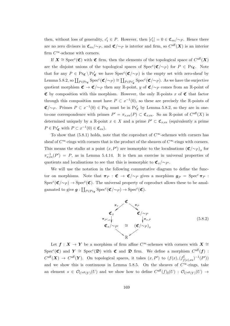
then, without loss of generality, c′1 ∈ P . However, then [c′1] = 0 ∈ Cex/∼P . Hence there

are no zero divisors in Cex/∼P , and C/∼P is interior and firm, so Caff(X) is an interior

firm C∞-scheme with corners.

If X ∼= Specc(C) with C firm, then the elements of the topological space of Caff(X)

are the disjoint unions of the topological spaces of Specc(C/∼P ) for P ∈ PrC . Note

that for any P ∈ PrC \Pr′C we have Specc(C/∼P ) is the empty set with zero-sheaf by

Lemma 5.8.2, so∐P∈PrC

Specc(C/∼P ) ∼=∐P∈Pr′C

Specc(C/∼P ). As we have the surjective

quotient morphism C → C/∼P then any R-point, y of C/∼P comes from an R-point of

C by composition with this morphism. However, the only R-points x of C that factor

through this composition must have P ⊂ x−1(0), so these are precisely the R-points of

C/∼P . Primes P ⊂ x−1(0) ∈ PrC must be in Pr′C by Lemma 5.8.2, so they are in one-

to-one correspondence with primes P ′ = πx,ex(P ) ⊂ Cx,ex. So an R-point of Caff(X) is

determined uniquely by a R-point x ∈ X and a prime P ′ ⊂ Cx,ex (equivalently a prime

P ∈ Pr′C with P ⊂ x−1(0) ∈ Cex).

To show that (5.8.1) holds, note that the coproduct of C∞-schemes with corners has

sheaf of C∞-rings with corners that is the product of the sheaves of C∞-rings with corners.

This means the stalks at a point (x, P ′) are isomorphic to the localisations (C/∼P )x for

π−1x,ex(P ′) = P , as in Lemma 5.4.14. It is then an exercise in universal properties of

quotients and localisations to see that this is isomorphic to Cx/∼P ′ .We will use the notation in the following commutative diagram to define the func-

tor on morphisms. Note that πP : C → C/∼P gives a morphism gP = Specc πP :

Specc(C/∼P )→ Specc(C). The universal property of coproduct allows these to be amal-

gamated to give g :∐P∈PrC

Specc(C/∼P )→ Specc(C).

Cπx

πP## ##

Cx

πP ′,x

C/∼Pπx,P

Cx/∼P ′

##

∼= (C/∼P )x

R

(5.8.2)

Let f : X → Y be a morphism of firm affine C∞-schemes with corners with X ∼=Specc(C) and Y ∼= Specc(D) with C and D firm. We define a morphism Caff(f) :

Caff(X) → Caff(Y ). On topological spaces, it takes (x, P ′) to (f(x), (f ]f(x),ex)−1(P ′))

and we show this is continuous in Lemma 5.8.5. On the sheaves of C∞-rings, take

an element s ∈ OCaff(Y )(U) and we show how to define Caff(f)](U) : OCaff(Y )(U) →

169

OCaff(X)(Caff(f)−1(U)) for open U ⊂ Caff(Y ). The same method will show how to define

Caff(f)ex] (U) for the sheaves of monoids.

For all points (y,Q) ∈ U , there is an open set Uy,Q ⊂ U such that s(y′, Q′) = πy′,Q′(dy)

for some dy ∈ D/∼Q and all (y′, Q′) ∈ Uy,Q. We can restrict this open set further around

(y,Q) by requiring Q′ = Q. Then there is an element dy ∈ D such that πQ(dy) = dy.

Then there is an sdy ∈ OY (Y ) such that sdy ,y′ = πy′(d) for all y′ ∈ Y . Then we can apply

f](Y ) to this element to get an element t ∈ OX(X).

Now we reverse the process: for all x′ ∈ X there is an open set Vx′ such that t(x) =

πx(cx′) for some cx′ ∈ C and all x ∈ Vx′ . Then we can define tx′,P ′ ∈ OC(X)(g−1(Vx))

by tx′,P ′(x, P ) = πx,P πP (cx′). On overlaps (x, P ) ∈ g−1(Vx′1) ∩ g−1(Vx′2), then πx,P πP (cx′1) = πP ′,x πx(cx′1) = πP ′,x πx(cx′2) = πx,P πP (cx′2), with the first and last equality

holding as diagram (5.8.2) is commutative, and the second equality from t being a well

defined element of OX(X). So tx′,P ′ agree on overlaps, and we can glue to an element

t ∈ OCaff(X)(Caff(X)).

Now this t was created from s restricted to an open set Uy,Q, so there is a t for each open

set Uy,Q and we need to restrict each t to Caff(f)−1(Uy,Q), to create a collection of sections

ty,Q ∈ OCaff(X)(Caff(f)−1(Uy,Q)). Finally we need to show that these agree on overlaps.

Say (x, P ) ∈ Caff(f)−1(Uy1,Q1)∩Caff(f)−1(Uy2,Q2), then Q1 = Q2 = Q = (f ]x,ex)−1(P ) and

Caff(f)(x, P ) = (y,Q) ∈ Uy1,Q ∩Uy2,Q. Then s(y,Q) = πy,Q(dy1) = πy,Q(dy2). We want to

show that in the stalks, we have g]g(x,P ) f]f(x)(sdy1

) = g]g(x,P ) f]f(x)(sdy2

). However, this

follows directly from Remark 4.4.5.

Finally, we can glue the sections ty,Q ∈ OCaff(X)(Caff(f)−1(Uy,Q)) to create a section

t ∈ OCaff(X)(Caff(f)−1(U)), which gives the map Caff(f)](U). By construction, it behaves

well with respect to restriction, so this defines Caff(f)]. The same construction on the

monoid sheaves gives Caff(f)ex] . This gives a morphism (Caff(f), Caff(f)], Caff(f)]ex) :

Caff(X) → Caff(Y ) using (2.4.2). This construction respects compositions of morphism,

so Caff is a functor from affine C∞-schemes with corners to interior C∞-schemes with

corners.

Lemma 5.8.5. The morphism Caff(f) : Caff(X)→ Caff(Y ), (x, P ) 7→ (f(x), (f ]x,ex)−1(P ))

in the previous proof is continuous provided f : X → Y is a morphism of firm affine C∞-

schemes with corners.

Proof. As in the proof of Proposition 5.8.4, we have f : X ∼= Specc(C)→ Y ∼= Specc(D)

a morphism of firm affine C∞-schemes with corners with C and D firm. We will use the

following commutative diagram, where we have prime ideals P ⊂ Cex, Q ⊂ Dex and points

170

x ∈ X, y = f(x) ∈ Y .

Cex/∼P Cex

πexPoo

πx,ex

))

Dex

πexQ //

πy,ex

uu

Dex/∼Q

OexX (X)

OexY (Y )

fex] (Y )

oo

Cx,ex

∼= OexX,x Oex

Y,y∼= Dy,ex

f]x,ex

oo

(5.8.3)

The topology of Caff(Y ) =∐P∈PrC

Specc(C/∼P ) is generated by open sets UπQ(d) ⊂Specc(D/∼Q) for d ∈ D and prime ideal Q ∈ PrD where

UπQ(d) = (y,Q′) : (y,Q′)(πQ(d)) = y(d) 6= 0, Q′ = πy,ex(Q).

To show Caff(f) is continuous then it is enough to show Caff(f)−1(UπQ(d)) is open in

Caff(X).

Firstly, we can consider f−1(Ud) where Ud is the basic open set of Specc(D) with

Ud = y : D→ R : y(d) 6= 0 ⊂ Specc(D).

We can then take open set

V = Specc(πP )−1(f−1(Ud)) ⊂ Specc(C/∼P ) ⊂ Caff(X)

for P a prime ideal of Cex that we need to determine. Here πP is as in (5.8.3).

Consider that

Caff(f)−1(UπQ(d)) = (x, P ′) : (f(x), (f ]x,ex)−1(P ′)) ∈ Ud

= (x, P ′) : f(x)(d) 6= 0, (f ]x,ex)−1(P ′) = πx,ex(Q).

So we need prime ideals P ′ ⊂ Cx,ex = OexX,x such that (f ]x,ex)−1(P ′) = πx,ex(Q). Fix

(x′, P ′) ∈ Caff(f)−1(UπQ(d)), let Caff(f)(x′, P ′) = (y′, Q′) ∈ UπQ(d), and let P = πx′,ex(P ′) ⊂Cex. We will show there is an open set W ⊂ Specc(C/∼P ) such that

W ∩ V ⊂ Specc(C/∼P ) ⊂ Caff(X)

contains (x′, P ′) and is contained in Caff(f)−1(UπQ(d)).

To do this, we need to use that D is firm. Take generators d1, . . . , dn ∈ Dex that

generate the sharpening D]ex. Order them so that d1, . . . , dk generate Q and dk+1, . . . , dn

are not in Q. Then πy′,ex(di) generate Q′ for i = 1, . . . , k and πy′,ex(di) /∈ Q′ by Lemma

5.8.2(c). As (f ]x′,ex)−1(P ′) = πx′,ex(Q) = Q′, then there are elements c1, . . . , cn ∈ Cex with

πx′,ex(c1), . . . , πx′,ex(ck) ∈ P ′ = πx′,ex(P ), and πx′,ex(ck+1), . . . , πx′,ex(cn) /∈ P ′ = πx′,ex(P ),

171

which implies c1, . . . , ck ∈ P and ck+1, . . . , cn /∈ P by Lemma 5.8.2(c), and are such that

f ]x′,ex(πy′,ex(di)) = πx′,ex(ci) for each i = 1, . . . , n.

Now take sections s1, . . . , sn ∈ OexX (X), t1, . . . , tn ∈ Oex

Y (Y ) such that (si)x = πx,ex(ci)

for all x ∈ X and (ti)x = πy′,ex(di) for all y ∈ Y . The previous paragraph implies that for

each i = 1, . . . , n,

f ex] (Y )(ti)x = f ]x,ex(πy,ex(di)) = πx,ex(ci) = (si)x (5.8.4)

when x = x′ ∈ X, and that this must be true for all x in an open neighbourhood Wi of x′

in X. Let

W ′ = ∩ki=1Wi ⊂ X, W ′′ = ∩ni=k+1Wi ⊂ X,

W = Specc(πP )−1(W ′ ∩W ′′) ⊂ Specc(C/∼P ) ⊂ Caff(X).

We see that x′ ∈W ′ ∩W ′′ so that (x′, P ′) ∈W .

We now show that W ∩V ⊂ Caff(f)−1(UπQ(d)). Take (x′′, P ′′) ∈W ∩V . As (x′′, P ′′) ∈V then f(x′′)(d) 6= 0 and P ′′ = πx′′,ex(P ), so P ′′ contains πx′′,ex(c1), . . . , πx′′,ex(c1) and does

not contain πx′′,ex(ck+1), . . . , πx′′,ex(cn). As (x′′, P ′′) ∈ W then x′′ ∈ W ′, which implies

that

(f ]x′′,ex)−1(P ′′) ⊃ (f ]x′′,ex)−1(πx′′,ex(ci)) 3 πy′′,ex(di) ∈ Q′

for all i = 1, . . . , k, and as these di generate Q, then πy′′,ex(Q) = Q′ ⊆ (f ]x′′,ex)−1(P ′′).

Now say that Q′ 6= (f ]x′′,ex)−1(P ′′), so that there is d ∈ Dex such that πy′′,ex(d) ∈(f ]x′′,ex)−1(P ′′) but πy′′,ex(d) /∈ Q′, which means d /∈ Q. Then d is a product of some

of the dj for j = k + 1, . . . , n, and as (f ]x′′,ex)−1(P ′′) is a prime ideal in Dx,ex then

π−1y,ex((f ]x′′,ex)−1(P ′′)) is prime in Dex, so a least one of the dj is such that πy′′,ex(dj) ∈

(f ]x′′,ex)−1(P ′′) but πy′′,ex(dj) /∈ Q′ for some j = k + 1, . . . , n. However, as (x′′, P ′′) ∈ Wthen x′′ ∈ W ′′, and we know that f ]x′′,ex(πy′′,ex(dj)) = πx′′,ex(cj) /∈ P ′′ by (5.8.4), which

implies a contradiction to the existence of such a d.

Hence πy′′,ex(Q) = Q′ = (f ]x′′,ex)−1(P ′′) for all (x′′, P ′′) ∈ W ∩ V , so W ∩ V ⊂Caff(f)−1(UπQ(d)) as required. So Caff(f)−1(UπQ(d)) is open, and Caff(f) is continuous.

Corollary 5.8.6. The image of Caff : AC∞Schcfi → C∞Schc

fi,in is an affine firm

C∞-scheme with corners, and we can consider it as a functor Caff : AC∞Schcfi →

AC∞Schcfi,in.

Proof. For any firm C∞-ring with corners C the prime ideals of Cex are finitely gener-

ated and there are finitely many of them. Then PrC has finite cardinality, so this is a

consequence of Proposition 5.4.15 and Proposition 5.8.4.

172

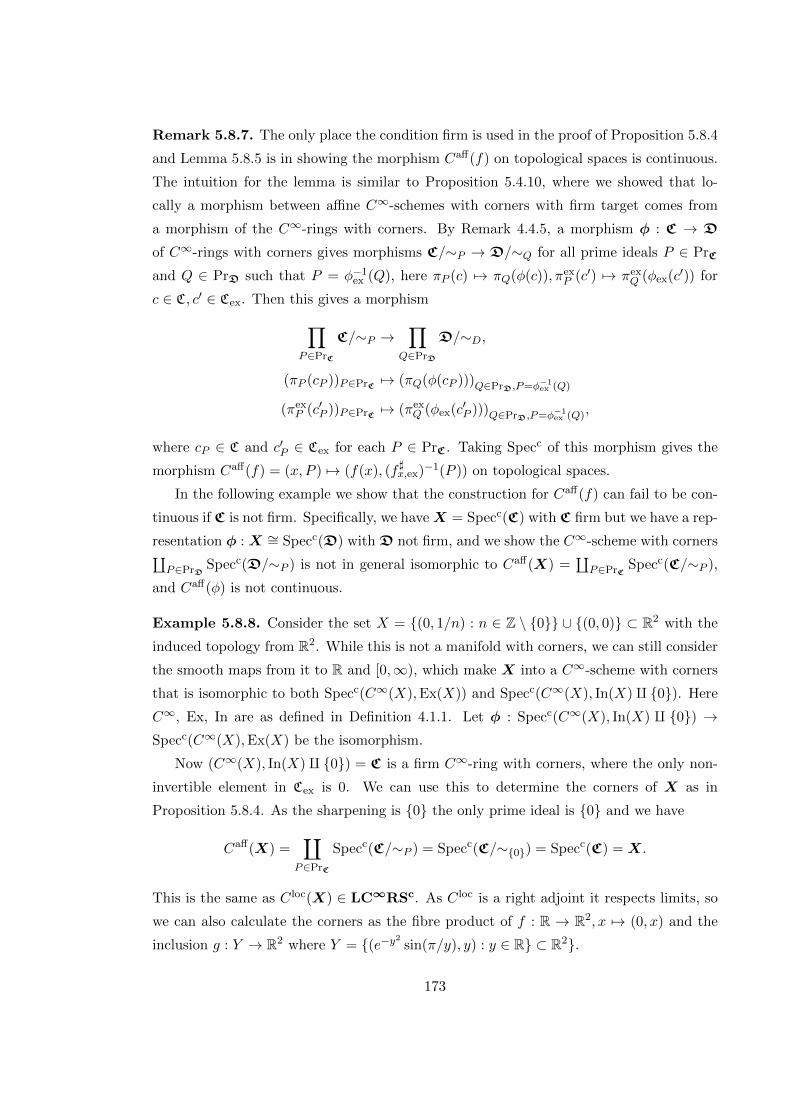
Remark 5.8.7. The only place the condition firm is used in the proof of Proposition 5.8.4

and Lemma 5.8.5 is in showing the morphism Caff(f) on topological spaces is continuous.

The intuition for the lemma is similar to Proposition 5.4.10, where we showed that lo-

cally a morphism between affine C∞-schemes with corners with firm target comes from

a morphism of the C∞-rings with corners. By Remark 4.4.5, a morphism φ : C → D

of C∞-rings with corners gives morphisms C/∼P → D/∼Q for all prime ideals P ∈ PrC

and Q ∈ PrD such that P = φ−1ex (Q), here πP (c) 7→ πQ(φ(c)), πex

P (c′) 7→ πexQ (φex(c′)) for

c ∈ C, c′ ∈ Cex. Then this gives a morphism∏P∈PrC

C/∼P →∏

Q∈PrD

D/∼D,

(πP (cP ))P∈PrC 7→ (πQ(φ(cP )))Q∈PrD,P=φ−1ex (Q)

(πexP (c′P ))P∈PrC 7→ (πex

Q (φex(c′P )))Q∈PrD,P=φ−1ex (Q),

where cP ∈ C and c′P ∈ Cex for each P ∈ PrC . Taking Specc of this morphism gives the

morphism Caff(f) = (x, P ) 7→ (f(x), (f ]x,ex)−1(P )) on topological spaces.

In the following example we show that the construction for Caff(f) can fail to be con-

tinuous if C is not firm. Specifically, we haveX = Specc(C) with C firm but we have a rep-

resentation φ : X ∼= Specc(D) with D not firm, and we show the C∞-scheme with corners∐P∈PrD

Specc(D/∼P ) is not in general isomorphic to Caff(X) =∐P∈PrC

Specc(C/∼P ),

and Caff(φ) is not continuous.

Example 5.8.8. Consider the set X = (0, 1/n) : n ∈ Z \ 0 ∪ (0, 0) ⊂ R2 with the

induced topology from R2. While this is not a manifold with corners, we can still consider

the smooth maps from it to R and [0,∞), which make X into a C∞-scheme with corners

that is isomorphic to both Specc(C∞(X),Ex(X)) and Specc(C∞(X), In(X) q 0). Here

C∞, Ex, In are as defined in Definition 4.1.1. Let φ : Specc(C∞(X), In(X) q 0) →Specc(C∞(X),Ex(X) be the isomorphism.

Now (C∞(X), In(X) q 0) = C is a firm C∞-ring with corners, where the only non-

invertible element in Cex is 0. We can use this to determine the corners of X as in

Proposition 5.8.4. As the sharpening is 0 the only prime ideal is 0 and we have

Caff(X) =∐

P∈PrC

Specc(C/∼P ) = Specc(C/∼0) = Specc(C) = X.

This is the same as C loc(X) ∈ LC∞RSc. As C loc is a right adjoint it respects limits, so

we can also calculate the corners as the fibre product of f : R → R2, x 7→ (0, x) and the

inclusion g : Y → R2 where Y = (e−y2sin(π/y), y) : y ∈ R ⊂ R2.

173

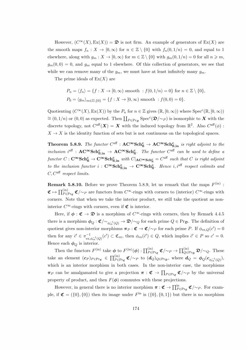
However, (C∞(X),Ex(X)) = D is not firm. An example of generators of Ex(X) are

the smooth maps fn : X → [0,∞) for n ∈ Z \ 0 with fn(0, 1/n) = 0, and equal to 1

elsewhere, along with gm : X → [0,∞) for m ∈ Z \ 0 with gm(0, 1/n) = 0 for all n > m,

gm(0, 0) = 0, and gm equal to 1 elsewhere. Of this collection of generators, we see that

while we can remove many of the gm, we must have at least infinitely many gm.

The prime ideals of Ex(X) are

Pn = 〈fn〉 = f : X → [0,∞) smooth : f(0, 1/n) = 0 for n ∈ Z \ 0,

P0 = 〈gm〉m∈Z\0 = f : X → [0,∞) smooth : f(0, 0) = 0.

Quotienting (C∞(X),Ex(X)) by the Pn for n ∈ Z gives (R, [0,∞)) where Specc(R, [0,∞))

∼= (0, 1/n) or (0, 0) as expected. Then∐P∈PrD

Specc(D/∼P ) is isomorphic to X with the

discrete topology, not Caff(X) = X with the induced topology from R2. Also Caff(φ) :

X → X is the identity function of sets but is not continuous on the topological spaces.

Theorem 5.8.9. The functor Caff : AC∞Schcfi → AC∞Schc

fi,in is right adjoint to the

inclusion iaff : AC∞Schcfi,in → AC∞Schc

fi. The functor Caff can be used to define a

functor C : C∞Schcfi → C∞Schc

fi,in with C|AC∞Schcfi

= Caff such that C is right adjoint

to the inclusion functor i : C∞Schcfi,in → C∞Schc

fi. Hence i, iaff respect colimits and

C,Caff respect limits.

Remark 5.8.10. Before we prove Theorem 5.8.9, let us remark that the maps F (in) :

C 7→∏(in)P∈PrC

C/∼P are functors from C∞-rings with corners to (interior) C∞-rings with

corners. Note that when we take the interior product, we still take the quotient as non-

interior C∞-rings with corners, even if C is interior.

Here, if φ : C → D is a morphism of C∞-rings with corners, then by Remark 4.4.5

there is a morphism φQ : C/∼φ−1ex (Q) →D/∼Q for each prime Q ∈ PrD. The definition of

quotient gives non-interior morphisms πP : C → C/∼P for each prime P . If φex,Q(c′) = 0

then for any c′ ∈ π−1

ex,φ−1ex (Q)

(c′) ⊂ Cex, then φex(c′) ∈ Q, which implies c′ ∈ P so c′ = 0.

Hence each φQ is interior.

Then the functors F (in) take φ to F (in)(φ) :∏(in)P∈PrC

C/∼P →∏(in)Q∈PrD

D/∼Q. These

take an element (cP )P∈PrC ∈∏(in)P∈PrC

C/∼P to (dQ)Q∈PrD , where dQ = φQ(cφ−1ex (Q)),

which is an interior morphism in both cases. In the non-interior case, the morphisms

πP can be amalgamated to give a projection π : C →∏P∈PrC

C/∼P by the universal

property of product, and then F (φ) commutes with these projections.

However, in general there is no interior morphism π : C →∏inP∈PrC

C/∼P . For exam-

ple, if C = (0, 0) then its image under F in is (0, 0, 1) but there is no morphism

174

from (0, 0) to (0, 0, 1). This is important as it means F in is not a left adjoint

to the forgetful functor i : C∞Ringscin → C∞Ringsc. Specifically, it means there is

no unit for the adjunction, so this does not contradict Theorem 4.3.7(b) which tells us a

left adjoint cannot exist. This discussion is the same if we restrict to firm C∞-rings with

corners.

Proof of Theorem 5.8.9. Let X = Specc(C) for C a firm C∞-ring with corners and take

Caff(X) =∐P∈PrC

Specc(C/∼P ). We have morphisms πX : Caff(X) → X, and ιX :

X → Caff(X) for interior X. Here we take gP = Specc(πP ) : Specc(C/∼P ) → Specc(C)

as in Proposition 5.8.4, and then amalgamate these maps using the universal property

of coproduct to get πX = g : Caff(X) =∐P∈PrC

Specc(C/∼P ) → X. If C is interior,

then 〈0〉 is a prime ideal of Cex and Specc(C/∼〈0〉) ∼= Specc(C), so there is an inclusion

ιX : X → Caff(X) =∐P∈PrC

Specc(C/∼P ).

In fact, as Caff(X) =∐P∈PrC

Specc(C/∼P ) ∼= Specc(∏P∈PrC

C/∼P ), then we can

write πX = Specc(C →∏P∈PrC

C/∼P ), and ιX = Specc(∏P∈PrC

C/∼P → C) where C

and X are interior for the latter. Showing these are natural transformations, commute

with morphisms f : X → Specc(D) ∼= Y and Caff(f) : Caff(X)→ Caff(Y ), and that these

form an adjoint pair follows from the definitions, where πX is the unit of the adjunction

and ιX is the counit.

Now, take X ∈ C∞Schcfi, so that there is a cover of X by open affines Uii∈I , with

X|Ui ∼= Specc(Ci) with Ci firm C∞-schemes with corners. Then Caff(X|Ui) makes sense

for each i. We would like to use Remark 5.4.13 to glue these together to define C(X), so

that C(X) is the colimit of all Caff(X|Ui) for U i = X|Ui affine in X. We will show that

Caff(X|Ui)|π−1i (Ui∩Uj)

∼= Caff(X|Uj )|π−1j (Ui∩Uj)

where πi : C(X|Ui) → X is the unit of the adjunction defined above, which will imply

that the properties in Remark 5.4.13 hold. To do this, we need only show that the

isomorphisms Specc(Ci)|V ∼= Specc(Cj)|V for open V ⊂ Ui ∩ Uj ⊂ X give isomorphisms

Caff(X|Ui)|π−1i (V )

∼= Caff(X|Uj )|π−1j (V ).

This is straightforward. In both cases the topological spaces are isomorphic to

(x, P ) : x ∈ V, P ⊂ OexX,x prime ideal,

where we use that OexX,x∼= Ci,ex,x

∼= Cj,ex,x. This creates a morphism of the topological

spaces. If s ∈ OCaff(Ui)(πi(V )) then sx = πx,P πP (c) for some c ∈ C. Then take s ∈OUi(V ) defined by sx = πx(c) for all c. Apply the isomorphism Specc(Ci)|V ∼= Specc(Cj)|V

175

to get an element of t ∈ OUj (V ). Then apply πj to this element. This gives a morphism of

the sheaves of C∞-rings, and a similar process gives a morphism of the sheaves of monoids.

To check these morphisms of sheaves are well defined, respect restrictions and do not

depend on choices follows similarly to the proof of the functor in Lemma 5.4.16, and

we see that we get a morphism Caff(X|Ui)|π−1i (V ) → Caff(X|Uj )|π−1

i (V ) that commutes

with each πi,πj . As Ci,ex,x∼= Cj,ex,x, then (Ci/∼Pi)(x,Pi)

∼= (Ci/∼Pj )(x,Pj), so this is an

isomorphism of sheaves of C∞-rings with corners. Hence these Caff(Ui) are isomorphic

on overlaps.

This means we can glue these Caff(Ui) to form C(X) using Remark 5.4.13. We now

show this is a functor. Take a morphism f : X → Y of firm C∞-schemes with corners.

Then take an open cover of Y by affine firm open sets Vii∈I . Then take an affine

firm open cover of f−1(Vi) in X, say Ui,jj∈J , so we have morphisms through f from

each U i,j to V i and then inclusions to Y . The functor Caff : AC∞Schcfi → C∞Schc

fi,in

gives morphisms Caff(U i,j) → Caff(V i) and the definition of colimit gives morphisms

Caff(V i)→ C(Y ). The universal property of C(X) as a colimit allows us to amalgamate

these morphisms to a unique morphism C(f) : C(X) → C(Y ) that commutes with all

the other morphisms. This defines C : C∞Schcfi → C∞Schc

fi,in on morphisms.

To show C : C∞Schcfi → C∞Schc

fi,in is a right adjoint to the inclusion i : C∞Schcfi,in →

C∞Schcfi, we use the πX and ιX defined above for affine firm C∞-schemes with corners

to give morphisms Caff(U) → X|U and X|U → C(X)|Caff(U) on affine firm neighbour-

hoods U . We again amalgamate these morphisms to πX and ιX defined on all of C(X)

and X, using that any firm C∞-scheme with corners is the colimit of any (firm) affine

cover and the definition of C(X) as a colimit of affine (firm) covers. That these are natural

transformations and the unit and counit of the adjunction follows from the definitions.

Remark 5.8.11. As in Remark 5.7.4 we can actually define the corners C(X) of a firm

C∞-scheme with corners X to be the unique (up to isomorphism) firm C∞-scheme with

corners with morphism πX : C(X) → X that satisifies the following universal property:

for all interior firm C∞-schemes with corners Y and morphisms f : Y → X, there is

a unique interior morphism f : Y → C(X) such that πX f = f . For any morphism

f : X → Y in C∞Schcfi, we can then define C(f) = f πX .

For all interior C∞-schemes with cornersX, then the identity morphism idX : X →X

gives a unique interior morphism idX : X → C(X), such that πX idX = idX : X →X. We define ιX = idX , and by uniqueness we see f = C(f) ιX for all morphisms

f : Y →X for interior Y . This is consistent with our previous definition.

Example 5.8.12. If X is a manifold without boundary, then there is an isomorphism

176

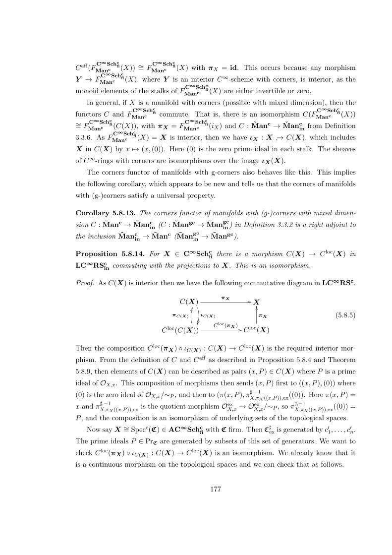
Caff(FC∞Schc

fiManc (X)) ∼= F

C∞Schcfi

Manc (X) with πX = id. This occurs because any morphism

Y → FC∞Schc

fiManc (X), where Y is an interior C∞-scheme with corners, is interior, as the

monoid elements of the stalks of FC∞Schc

fiManc (X) are either invertible or zero.

In general, if X is a manifold with corners (possible with mixed dimension), then the

functors C and FC∞Schc

fiManc commute. That is, there is an isomorphism C(F

C∞Schcfi

Manc (X))

∼= FC∞Schc

fiManc (C(X)), with πX = F

C∞Schcfi

Manc (iX) and C : Manc → Mancin from Definition

3.3.6. As FC∞Schc

fiManc (X) = X is interior, then we have ιX : X → C(X), which includes

X in C(X) by x 7→ (x, (0)). Here (0) is the zero prime ideal in each stalk. The sheaves

of C∞-rings with corners are isomorphisms over the image ιX(X).

The corners functor of manifolds with g-corners also behaves like this. This implies

the following corollary, which appears to be new and tells us that the corners of manifolds

with (g-)corners satisfy a universal property.

Corollary 5.8.13. The corners functor of manifolds with (g-)corners with mixed dimen-

sion C : Manc → Mancin (C : Mangc → Mangc

in ) in Definition 3.3.2 is a right adjoint to

the inclusion Mancin → Manc (Mangc

in → Mangc).

Proposition 5.8.14. For X ∈ C∞Schcfi there is a morphism C(X) → C loc(X) in

LC∞RScin commuting with the projections to X. This is an isomorphism.

Proof. As C(X) is interior then we have the following commutative diagram in LC∞RSc.

C(X)

ιC(X)

πX //X

C loc(C(X))Cloc(πX) //

πC(X)

JJ

C loc(X)

πX

OO

(5.8.5)

Then the composition C loc(πX) ιC(X) : C(X) → C loc(X) is the required interior mor-

phism. From the definition of C and Caff as described in Proposition 5.8.4 and Theorem

5.8.9, then elements of C(X) can be described as pairs (x, P ) ∈ C(X) where P is a prime

ideal of OX,x. This composition of morphisms then sends (x, P ) first to ((x, P ), (0)) where

(0) is the zero ideal of OX,x/∼P , and then to (π(x, P ), π],−1X,πX((x,P )),ex((0)). Here π(x, P ) =

x and π],−1X,πX((x,P )),ex is the quotient morphism Oex

X,x → OexX,x/∼P , so π],−1

X,πX((x,P )),ex((0)) =

P , and the composition is an isomorphism of underlying sets of the topological spaces.

Now sayX ∼= Specc(C) ∈ AC∞Schcfi with C firm. Then C]ex is generated by c′1, . . . , c

′n.

The prime ideals P ∈ PrC are generated by subsets of this set of generators. We want to

check C loc(πX) ιC(X) : C(X) → C loc(X) is an isomorphism. We already know that it

is a continuous morphism on the topological spaces and we can check that as follows.

177

First we have that π−1(U) in C loc(X) is isomorphic to π−1(U) in Caff(X). We will

show that for any (x, P ) ∈ Us′ there is an open set V ∈ Caff(X) with V ⊂ Us′ and

(x, P ) ∈ V . For (x′, P ′) ∈ Us′ , then s′x = πx,ex(c′) for some c′ ∈ Cex for all x ∈ W ⊂ U

with x′ ∈W , with πx′,ex(c′) /∈ P ′. Then πx,ex(c′) /∈ πx,ex(π−1x,ex(P ′)) for all x ∈ X. So

(x′, P ′) ∈ π−1(V ) ∩ Specc(C/∼π−1x,ex(P ′)) ⊂ Us′ .

Similarly, for (x′, P ′) ∈ Us′ , then

(x′, P ′) ∈ π−1(V ) ∩ Specc(C/∼π−1x,ex(P ′)) ⊂ Us′ .

As the underlying set of Specc(C/∼π−1x,ex(P ′)) is open in Caff(X), then these sets are open

in Caff(X). So we have a continuous map of topological spaces Caff(X) → C loc(X),

(x, P ) 7→ (x, P ). To show this a homeomorphism, we will use the firm assumption to

check that the inverse map is continuous.

Let U be an open set in C(X), so it is the union of open sets in Specc(C/∼P ) for some

P ∈ PrC . Pick a particular (x′, P ′) ∈ U . Then there is a basic open set

UπP (c) = (x, P ) ∈ Specc(C/∼π−1x,ex(P ′)) : (x, P )(πP (c)) 6= 0,

in Specc(C/∼P ) with UπP (c) ⊂ U and (x′, P ′) ∈ U . Here, we have projection πP : C →∈C/∼π−1

x,ex(P ′) and c ∈ C, so (x, P )(πP (c)) = x(c), and any (x, P ) ∈ UπP (c) must have

P = P ′. We must then have a basic open set

Uc = x ∈ X : x(c) 6= 0,

in X.

As P ′ is a prime ideal in Cx,ex it is finitely generated by subsets of the images of the

c′1, . . . , c′n under πx,ex : Cex → Cx,ex. Say the subset is c′1, . . . , c′k. Then in C loc(X) there

is an open set

V = π−1(Uc) ∩ (

k⋂i=1

(Uc)s′i) ∩ (

n⋂i=k+1

(Uc)s′i),

where s′i ∈ OX(UπP (c)) with s′i,x = πx,ex(c′i) for each i ∈ 1, . . . , n. Here, (Uc)s′i and (Uc)s′iare the open sets corresponding to Uc ⊂ X from Definition 5.7.1. As C is firm, each prime

ideal is finitely generated and the set V is an intersection of only finitely many open sets,

so it is open. Also V non-empty as it contains (x′, P ′). If (x, P ) ∈ V then P must contain

πx,ex(c′i) for i = 1, . . . , k and must not contain πx,ex(c′i) for i = k + 1, . . . , n, so P must

be equal to P ′. We must also have x ∈ Uc. This implies any (x, P ) ∈ V is also in U . As

we can do this for all point (x′, P ′) ∈ U then the image of U under Caff(X) → C loc(X),

178

(x, P ) 7→ (x, P ) is open so the inverse map is continuous and we have an isomorphism of

topological spaces.

Finally we check the morphisms of sheaves. However, we already know that the stalks

of the sheaves of Caff(X) and C loc(X) at the point (x, P ) are both isomorphic to OexX,x/∼P

and it is straightforward to check that the morphisms of the sheaves respect this isomor-

phism, so are isomorphisms themselves and C loc(πX) ιC(X) : C(X) → C loc(X) is an

isomorphism for firm affine C∞-schemes with corners.

For X ∈ C∞Schcfi, this result follows as C(X)|π−1(U) is isomorphic to Caff(X|U ) on

affine open subsets U of X.

In the following example, we will take an affine C∞-scheme with corners X and show

C loc(X) is not a C∞-scheme with corners.

Example 5.8.15. Take interior C∞-ring with corners C = (R,Cinq0) with Cin a subset

of the monoid (0,∞)× NN (with (0,∞) a monoid under multiplication and NN a monoid

under addition) such that all elements have only finite support. That is, if we write (δi)j∈N

for the element of NN with a 1 in the ith position and 0 elsewhere, then every element of

Cin is of the form a∑

i∈I⊂N(δi)j∈N for I a finite subset of N, a ∈ (0,∞).

The C∞-operations are defined as follows. For each smooth function f : Rnk → R,

then Φf (c′1, . . . , c′k, ck+1, . . . , cn) = f(a1 · 0

∑i∈I1

δi , . . . , ak · 0∑i∈Ik

δ′i , ck+1, . . . , cn), where

c′l = al∑

i∈Il(δi)j∈N. For each smooth function f : Rnk → [0,∞), then either f = 0

and Ψf = 0, or f is of the form f(x1, . . . , xn) = xb11 · · ·xbk1 F (x1, . . . , xn) with F strictly

positive, so that there is a smooth function g = log F : Rnk → R with F = exp g.

Then Ψf (c′1, . . . , c′k, ck+1, . . . , cn) = (c′1)b1 · · · (c′k)bkΨexp Φg(c

′1, . . . , c

′k, ck+1, . . . , cn) and

we define Ψexp(c) = exp(c) ∈ (0,∞) ⊂ Cin for any c ∈ C = R. This gives a C∞-ring with

corners with one R-point, so that X = Specc(C) ∼= (∗,OX ,OexX ) with OX(∗) = C.

The prime ideals in Cex are either the zero ideal 〈0〉 or of the form 〈(δi)j∈N〉i∈J⊂N for

any subset J ⊂ N, that is, they are generated by the (δi)j∈N. Then the topological space

of C loc(X) as a set is isomorphic to the collection of these prime ideals, but has a coarse

topology. For example, 〈0〉 is a closed point but it is not open. Its complement is the

union ∪i∈NU(δi)j∈N , which is open but not closed.

In fact, as a local C∞-ringed space with corners, C loc(X) is not a C∞-scheme with

corners. Suppose it were, then around every point, there must be an open set such C loc(X)

is affine on this open set. So by Joyce [40, Lem. 4.15] the topology must be Hausdorff on

this open set. Consider that any open set around the point 〈0〉 must contain the open set

Us′ = (∗, P ) : s′x /∈ P for some s′ ∈ OX(∗). So s′ = a∑

i∈I⊂N(δi)j∈N for I a finite subset

of N, a ∈ (0,∞). Consider that the prime ideals 〈(δi)j∈N〉i∈2N\I and 〈(δi)j∈N〉i∈2N+1\I are

179

contained in Us′ , however there are no open sets in X or in Us′ that separate these two

points. That is, Us′ is not Hausdorff, and no open set containing Us′ is Haursdorff. So

C loc(X) is not affine in a neighbourhood of 〈0〉 and is not a C∞-scheme with corners.

Note that if Cin = (0,∞) × NN, not just the finitely supported ones, C loc(X) can be

shown to be a C∞-scheme with corners.

5.8.1 Boundary

Finally we can consider the boundary of a firm C∞-scheme with corners, where we use

the definition of minimal prime ideal from §5.7.1.

Definition 5.8.16. IfX is a firm C∞-scheme with corners, then the boundary ∂X ofX is

a sub-C∞-scheme with corners of C(X). If locally X|U ∼= Specc C for an open set U ⊂ Xand C firm, then ∂X is locally isomorphic to

∐P Spec(C/∼P ) where the coproduct is

over prime ideals P such that there is an x ∈ X with πx,ex(P ) a minimal prime ideal in

OexX,x∼= Cx,ex.

Note that we would not expect X 7→ ∂X,X ∈ C∞Schcfi to be a functor.

This gives a corollary to Proposition 5.8.14 that the two notions of boundary, ∂X and

∂locX from §5.7.1 are the same for firm C∞-schemes with corners.

Corollary 5.8.17. If X is a firm C∞-scheme with corners, then ∂X ∼= ∂locX.

Proof. Proposition 5.8.14 explains that for any firm C∞-scheme with corners X there is

an isomorphism C(X)→ C loc(X). As X is firm, then ∂locX is an open subset and sub-

local C∞-ringed space with corners of C loc(X), and that the image of ∂X ⊂ C(X) under

the isomorphism lies in ∂locX. This gives a morphism p : ∂X → ∂locX. From Definition

5.7.1 and Proposition 5.8.4 we see that the topological spaces as sets are both isomorphic

to the collection of pairs

(x, P ) : x ∈ X,P minimal prime ideal in OexX,x,

and that p respects this. As C(X) → C loc(X) is an isomorphism, then p must be an

isomorphism.

Remark 5.8.18. For a firm C∞-scheme with corners X we can also compare ∂X to ∆X,

where the latter is Gillam and Molcho’s [28, §4.4] definition of boundary as in Remark 5.7.7.

Then there are morphisms ∂X → ∂locX → ∆X. The first morphism is an isomorphism

by Corollary 5.8.17.

180

The second can also be shown to be an isomorphism using a similar proof to Proposition

5.8.14. All that needs to be done is to show that the topology of ∆X is as fine as the

topologies of ∂X, ∂locX. To do this, if Specc(C) ∼= X|U for some open U ⊂ X and C firm,

then take c1, . . . , cn ∈ Cex that generate the sharpening of Cex. Take sections si ∈ OexX (U)

such that si(x) = πexx (ci) for i = 1, . . . , n. Then for a section s ∈ OX(U), around each

point x ∈ U we have that there is an open set V 3 x such that s = Fsa11 · · · sann for ai

non-negative integers. Let I be the subset of 1, . . . , n such that for i ∈ I then ai 6= 0,

and take J = 1, . . . , n \ I. Then consider that

Vs = (x, P ) : x ∈ V, P minimial non-trivial prime in OexX,x, s(x) /∈ P

is a basic open set in ∂X, ∂locX,∆X, however

Vs = (x, P ) : x ∈ V, P minimial non-trivial prime ideal in OexX,x, s(x) ∈ P

is a basic open set in ∂X, ∂locX but not in ∆X. However, we can show that

Vs = ∩j∈JVsj .

As J is a finite set, then Vs is open in ∆X. Using this, we can see that the topology on

∆X is as fine as ∂X, ∂locX so that ∂X → ∂locX → ∆X is an isomorphism.

Finally, we could also consider how our definitions of corners give a stratification that

aligns with the stratification of a manifold with (g-)corners from Definition 3.3.2. To do

this, let P× be the collection of non-units of a monoid P , which is a prime ideal.

Definition 5.8.19. Let P be a monoid. The dimension of a monoid is the maximal length

d (or ∞ if there is no maximum length) of a chain of prime ideals

∅ = Q0 ⊂ Q1 . . . ⊂ Qd = P×.

If Q is a prime ideal of P , then the codimension or height of Q is the maximal length d of

a chain of prime ideals

Q = Q0 ⊃ Q1 . . . ⊃ Qd = ∅.

If F is the corresponding face to Q, then the dimension of the quotient monoid P/F is

the same as the height of Q.

Then our boundary definitions correspond to the codimension 1 prime ideals, and

the stratification of C(X) and C loc(X) into the k-corners can occur by considering the

codimension k prime ideals in an analogous way to Definitions 5.8.16 and 5.7.6. For

181

example, if X is in the image of a manifold with corners under FC∞Schc

fiManc : Manc →

C∞Schcfi from Definition 5.5.1, then locally X ∼= Specc(C∞(Rnk),Ex(Rnk)). The prime

ideals in Ex(Rnk) are generated by different choices of the coordinate functions x1, . . . , xk :

Rnk → [0,∞). If we consider a prime ideal P = 〈xi1 , . . . , xim〉 which will have codimension

m 6 k where i1, . . . im are distinct integers in 1, . . . , k, then

(C∞(Rnk),Ex(Rnk))/∼P ∼= (C∞(Rn−mk−m),Ex(Rn−mk−m))

and taking Specc of this gives the appropriate m-corner component in Cm(X) (defined

in §3.3) locally. Hence, these k-corners will correspond to the images of the k-corners

(defined in §3.3) under FC∞Schc

fiManc .

5.9 Log geometry and log schemes

Log geometry was originally used to understand a certain type of cohomology theory

for schemes, such as in Kato [53], who was influenced by Fontaine and Illusie. It was

further developed to deal with issues of degeneration and non-compactness of schemes,

particularly when considering moduli spaces; Ogus [78] has a comprehensive introduction

to log geometry, and a survey paper by Abramovich et al. [1] details how it is used in the

context of moduli schemes.

Our C∞-schemes with corners in Section 5.1 are related to the ‘positive log differen-

tiable spaces’ of Gillam and Molcho [28].

We define pre-log rings as in Gillam [26], which form a category that are related to

the category of pre C∞-rings with corners. We then explain log rings, (pre-)log schemes,

log differentiable spaces and positive log differentiable spaces, and their relation to our

C∞-rings with corners and C∞-schemes with corners. In this section, we assume all rings

and monoids are commutative.

Definition 5.9.1. A pre-log ring (R,M,α), is a ring, (R,+, ·) and a monoid (M, ∗) with

a morphism of monoids α : M → R, where we consider R a monoid under the operation

‘ · ’. A morphism of pre-log rings (f, f ′) : (R1,M1, α1) → (R2,M2, α2) is a morphism of

rings f : R1 → R2 and a morphism of monoids f ′ : M1 → M2 such that α2 f ′ = f α1.

We call a pre-log ring (R,M,α) a pre-log structure on the ring R. Pre-log rings and their

morphisms form a category.

A pre-log ring (R,M,α) is a log ring if the morphism α induces an isomorphism

α−1(R×) ∼= R×, where R× is the group of units of R. If (R1,M1, α1) and (R2,M2, α2) are

log rings and (f, f ′) : (R1,M1, α1)→ (R2,M2, α2) is a morphism of pre-log rings, then we

182

call (f, f ′) a morphism of log rings. We call a log ring (M,R,α) a log structure on the ring

R. Log rings and their morphisms form a category.

Ogus [78, p. 274-275] uses ‘log-rings’ for our notion of pre-log rings. Note that

α−1(R×) ∼= R× implies that αi|M× : M× → R× is an isomorphism, but the converse

may not be true in general.

If R is a ring, then the trivial log structure on R is the log ring (R,R×, i) where i is the

inclusion map. This is the initial object in the category of log rings with ring R, and gives a

left adjoint to the forgetful functor (R,M,α)→ R. There is also a final object, (R,R, id),

which gives a right adjoint to the forgetful functor (R,M,α) → R. These adjoints imply

colimits and limits commute with the forgetful functor.

For any pre-log ring (R,M,α), there is a log ring associated to it (R,M ′, α′). Here,

M ′ is the monoid pushout M ′ = R× ⊕α,α−1(R×),iM and α′ : M ′ → R is defined using the

universal property of pushouts. This defines a left adjoint to the inclusion of the category

of log rings into pre-log rings.

Definition 5.9.2. A pre-log structure on a scheme (X,OX) is a sheaf of monoids MX

and a morphism of sheaves of monoids αX : MX → OX , where OX is considered a sheaf

of monoids under multiplication from the rings. We call (X,OX ,MX) a pre-log scheme.

A morphism of pre-log schemes (X1,OX1 ,MX1) and (X2,OX2 ,MX2) is a morphism of

schemes f = (f, f ]) : (X1,OX1) → (X2,OX2) with a morphism of sheaves of monoids

f [ : MX2 → f∗(MX1) such that

f ] αX2 = f∗(αX1) f [. (5.9.1)

A log structure on a scheme (X,OX) is a pre-log scheme

(X,OX ,MX) such that αX induces an isomorphism α−1X (O×X) ∼= O×X where O×X is the

sheaf of units of OX . Then (X,OX ,MX) is called a log scheme. Morphisms of log schemes

are morphisms of the underlying pre-log schemes.

The trivial log structure on a scheme (X,OX) is given by (X,OX ,O×X), with αX the

inclusion morphism. This is the final object in the category of log structures on a scheme

(X,OX). This induces an inclusion functor from the category of schemes to the category

of log schemes, right adjoint to the forgetful functor (X,OX ,O×X) → (X,OX), realising

schemes as a full subcategory of log schemes. The log scheme (X,OX ,OX), with αX the

identity morphism, is the initial object in the category of log structures on (X,OX), which

gives a left adjoint to the forgetful functor (X,OX ,O×X)→ (X,OX).

Definition 5.9.3. To any pre-log ring α : M → R, Ogus [78, p. 275] and Gillam [26,

p. 76] give a description of a spectrum functor Spec : (α : M → R) 7→ (X,OX ,MX)

183

where (X,OX) = Spec(R) is the usual spectrum of a ring, and MX is the log structure

associated to the pre-log structure M → OX which is induced by M → R. Precisely,

R ∼= OX(X) so restriction gives a morphism M → R ∼= OX(X) → OX(U) for each open

U ⊂ X. Then we define the presheaf of monoids MX such that MX(U) is the pushout

M ⊗α−1(OX(U)×) OX(U)×. Here OX(U)× is the group of invertible elements of OX(U).

Note that the presheaf restriction property is satisfied using the universal property of

pushouts, and that this universal property also gives morphisms MX(U)→ OX(U). Then

let MX be the sheafification of this presheaf, so we have that (X,OX ,MX) is a log scheme.

Here, universal properties show that MX,x is isomorphic to the pushout M⊗α−1(O×X,x)O×X,x.

This spectrum construction is very similar to the notion of a chart for a log scheme,

(see for example [28, p. 33]) where if (X,OX ,MX) is a log scheme, then a chart is a

morphism of monoids P → MX(X) such that the associated log structure, (X,OX , PX)

is isomorphic to (X,OX ,MX). Here PX is the sheafification of the presheaf PX where

PX(U) is the pushout P ⊗α−1(OX(U)×) OX(U)× using the composition P → MX(X) →OX(X) → OX(U). If α : M → R is a pre-log ring then M → MX(X) is a chart for

Spec(α : M → R) = (X,OX ,MX). In [28, p. 33] a log scheme is called quasi-coherent if

there exists charts locally. It is straight forward to show that a log scheme with a chart

(or with local charts) is locally the spectrum of a pre-log ring, however the notion of chart

applies more generally for log locally ringed spaces (as in the remark below) whereas the

spectrum functor does not.

Remark 5.9.4. In Definition 5.9.2, we can change the word ‘scheme’ to ‘locally ringed

space’ to define (pre-)log locally ringed spaces. Our local C∞-ringed spaces with corners

are examples of pre-log locally ringed spaces. Gillam and Molcho [28, §4.4] define a notion

of boundary on pre-log locally ringed spaces which related to our notions of corners, as

we discuss in §5.7.1.

There are some similarities in the definitions of C∞-schemes with corners and log

schemes. However, log schemes are based on ordinary schemes, not C∞-schemes. Also,

for a log scheme (X,OX ,MX) we have (X,OX) locally isomorphic to the spectrum of a

ring, however (X,OX ,MX) is not required to locally be isomorphic to the spectrum of

a log ring. In this sense, C∞-schemes with corners are analogous to quasi-coherent log

schemes.

The categories of differentiable spaces, log differentiable spaces, and positive log dif-

ferentiable spaces consider ways to construct log structures for manifolds and manifolds

with corners. These are based on the notion of a differentiable algebra, which we recall

the following definitions from Navarro Gonzalez and Sancho de Salas [76], and are closely

184

related to C∞-rings.

Definition 5.9.5. A differentiable algebra D is an R-algebra isomorphic to a quotient

of C∞(Rn) by an ideal a such that a is closed in the C∞-Whitney topology of C∞(Rn).

A reference for the C∞-Whitney topology can be found in [34, p. 35-36]. Morphisms of

differentiable algebras are morphisms of R-algebras.

A locally ringed R-space is a topological space X equipped with a sheaf OX of R-

algebras, such that the stalks are local rings. Morphisms of locally ringed R-spaces

(X,OX)→ (Y,OY ) are of the form (f, f ]) with f : X → Y a continuous map of topological

spaces, and f ] : f−1OY → OX a morphism of sheaves.

The spectrum, SpecD, of a differentiable algebra D, is a locally ringed R-space (X,OX).

The topological space X is the set of all maximal ideals m of D with residue field R ∼= D/m,

equipped with the Gelfand topology. This is the smallest topology such that for all d ∈ D,

the corresponding morphism d∗ : SpecD → R, that sends m ∈ SpecD to the value of d

under the isomorphism R ∼= D/m, is continuous.

The sheaf is defined by OX(U) = DU for open U ⊂ X. Here DU is the localisation

of D at U , that is, the R-algebra of (equivalence classes) of fractions d/m with d,m ∈ D,

and with m∗ non-zero on U .

An affine differentiable space is a locally ringed R-space that is isomorphic to SpecD

for some differentiable algebra D. A differentiable space is a locally ringed R-space (X,OX)

that is locally isomorphic to an affine differentiable space.

Morphisms of differentiable spaces are morphisms of locally ringed R-spaces.

The category of differentiable algebras has all finite colimits, and the category of differ-

entiable spaces has all finite limits, these commute with the forgetful functor to topological

spaces.

We now define log differentiable spaces and positive log differentiable spaces following

Gillam and Molcho [28].

Definition 5.9.6. A log differentiable space (X,OX ,MX) is a differentiable space (X,OX)

equipped with a log structure. That is, MX is a sheaf of monoids on X, and there is a

morphism of sheaves αX : MX → OX such that α induces an isomorphism α−1X (O×X) ∼= O×X .

A positive log differentiable space, (X,OX ,MX), is a differentiable space (X,OX), with

a sheaf of monoids MX on X, and a morphism of sheaves αX : MX → O>0X such that αX

induces an isomorphism α−1X (O>0

X ) ∼= O>0X . Here O>0

X and O>0X are the sheaves of monoids

such that for any open U ⊂ X, then

O>0X (U) = s ∈ OX(U) : s(x) > 0 ∈ R for all x ∈ U

185

and

O>0X (U) = s ∈ OX(U) : s(x) > 0 ∈ R for all x ∈ U.

In this definition, s(x) is the value of s under the composition of the following maps

OX(U)→ OX,x → OX,x/mx∼= R,

where mx is the maximal ideal in the local differentiable algebra OX,x.

Morphisms of (positive) log differentiable spaces are composed of a morphism of dif-

ferentiable spaces and a morphism of sheaves of monoids, such that the morphisms behave

well with respect to each α, as in (5.9.1).

A positive log differentiable space (X,OX ,MX) gives the data of a log differentiable

space (X,OX ,M∗X). We have that αX : MX → O>0X → OX is a morphism of sheaves, and

we can take the log structure associated to this morphism, which is given by the pushout

M∗X = MX qO>0XO×X , where O×X is the sheaf of invertible elements on X. In fact there

is an isomorphism to the coproduct M∗X∼= MX ⊗ Z/(2Z), where Z/(2Z) is the locally

constant sheaf with stalk Z/(2Z). This gives a faithful but not full functor from positive

log differentiable spaces to log differentiable spaces (c.f [28, p. 50]).

Similarly, a log differentiable space (X,OX ,MX) with morphism αX gives the data of

a positive log differentiable space (X,OX ,M>0X ) where M>0

X is the sheaf of monoids such

that

M>0X (U) = s′ ∈MX(U)|s′(x) > 0 ∈ R for all x ∈ U.

Here αX |M>0X

gives the required morphism. This is full but not faithful, and a left adjoint

to the previous functor. The composition of both of these functors is the identity functor

on positive log differentiable spaces, but not on log differentiable spaces.

The categories of log differentiable spaces and positive log differentiable spaces have

all finite limits and all coproducts.

5.9.1 Comparison to C∞-algebraic geometry

We now describe the relations of these logarithmic geometry constructions to C∞-algebraic

geometry.

A (pre) C∞-ring with corners (C,Cex) is a pre-log ring with morphism α = Φi : Cex →C. However, a C∞-ring with corners (C,Cex) is not a log ring, as our Definition 4.3.2,

does not mean that Φ−1i (C×) ∼= C×. In fact, it is never an isomorphism, as if we take a

C∞-ring with corners, (C,Cex), one can show that there is no element a ∈ C×ex such that

Φi(a) = −1C ∈ C×, where 1C is the identity element of C.

186

In the following Lemma and its corollaries, we see that for a semi-complete C∞-ring

with corners the invertible elements of Cex correspond only to the ‘positive’ elements of C.

Lemma 5.9.7. Let C be a complete C∞-ring. Then for each c ∈ C such that x c > 0

for each R-point x : C → R, there is d ∈ C such that Φexp(d) = c. Define the monoid

C>0 = c ∈ C : x(c) 6= 0 for each R-point x : C → R, then this is equal to Φexp(C) and

element is invertible.

Proof. Let C be complete and take c ∈ C such that x(c) > 0 for all R-points x : C → R.

Fix an R-point x, let εx = x(c) and take the open set Ux = x : C → R | x(c) > εx/2 3 xwhich is open in SpecC. Choose a smooth function fn : R → R such that fn(t) = log(t)

for t ∈ [1/n,∞). Then Φfn(c) exists for all n ∈ (0,∞). For each x take nx such that

nx > 2/εx.

Now, say x ∈ Ux for some R-point x. Then we claim Φexp Φfnx (c) is equal to c in the

stalk at x. As C is complete and Φexp is injective by Proposition 4.3.1(a), then this will

tell us the Φfnx (c) are equal in every stalk in appropriate Ux, and there is an element d

such that d|Ux = Φfnx (c)|Ux and Φexp(d) = c.

For this x we know that x c > 1/nx. So choose smooth g : R → R such that

g(t) = 0 for all t ∈ (−∞, 1/nx] and t > 0 otherwise, so that g(exp fnx(t) − id(t)) = 0

for all t ∈ R, and x (Φg(c)) = g(x(c)) 6= 0. Then letting e = Φg(c) we have that

e(Φexp Φfnx (c)−Φid(c)) = 0, so Proposition 2.1.15 implies Φexp Φfnx (c) is equal to c in

the stalk at x. So such an element d exists and we must have C>0 ⊆ Φexp(C).

Also, if d ∈ C then x Φexp(d) = exp(x(d)) > 0 for all x : C → R, so Φexp(C) = C>0.

In addition, elements of Φexp(C) are invertible, as Φexp(d) has inverse Φexp(−d) for all

d ∈ C.

Corollary 5.9.8. If C is semi-complete C∞-ring with corners, then Φi : Cex → C induces

an isomorphism Φi : C×ex → C>0 = Φexp(C).

Proof. If c ∈ C>0 then by Lemma 5.9.7 there is d ∈ C such that Φexp(d) = c. Then

Ψexp(d) ∈ C×ex and Φi Ψexp(d) = Φexp(d) = c. So there is a map

C>0 → C×ex,Φexp(d) 7→ Ψexp(d).

As Φexp is injective by Proposition 4.3.1(a) and Ψexp : C → C×ex is a bijection by Definition

4.3.2(iii), then C>0 → C×ex is a bijection, with inverse Φi|C×ex. Also if a, b ∈ C>0, a = Φexp(c),

b = Φexp(d) then ab = Φexp(c + d) 7→ Ψexp(cd) = Ψexp(c)Ψexp(d), so C>0 → C×ex is an

isomorphism of monoids (and in fact an isomorphism of abelian groups.)

187

Corollary 5.9.9. For C ∈ C∞Ringsc, Φi induces an isomorphism Φ−1i (C>0)→ C>0.

Proof. Corollary 5.9.8 implies there is canonical isomorphism of monoids (or groups)

Φi|C×ex: C×ex → C>0, so Φ−1

i (C>0) contains C×ex. As elements of Φ−1i (C>0) are isomorphic

to Φ−1i (Φexp(C)), then Φ−1

i (C>0) is equal to Ψexp(C), which is equal to C×ex by Definition

4.3.2(iii). This implies Φi|C×ex: C×ex → C>0 is equal to Φi|Φ−1

i (C>0) : Φ−1i (C×>0) → C>0 and

so the latter is an isomorphism.

Remark 5.9.10. In Lemma 5.9.7, we did not need to assume that C was a complete

C∞-ring, but we just needed to assume that C was some C∞-ring that is isomorphic to

(a subring of) OX(U) where OX is some sheaf of C∞-rings on a topological space X and

open U ⊂ X. This property is equivalent to the property of ‘germ determined’ defined in

Moerdijk and Reyes [72, Def. 4.1] for C∞-rings.

Similarly, in Corollary 5.9.8 and Corollary 5.9.9 we did not need to assume that (C,Cex)

is a semi-complete C∞-ring with corners, but that it is isomorphic to (a subring of)

OX(U) where OX is some sheaf of C∞-rings with corners on a topological space X and

open U ⊂ X. Joyce [40] defined a notion of fair C∞-ring, which is equivalent to germ

determined and finitely generated, and are called ‘C∞-rings of finite type presented by an

ideal of local character’ in Dubuc [20, 21]. Kalashnikov [51, §. 4.8] extended this notion

of fair to pre C∞-rings with corners, so C∞-rings with corners that satisfy Kalashnikov’s

notion of fair would be sufficient for these corollaries, although we can weaken this as we

do not need to require finitely generated.

We would like to compare the notions of spectrum of a log scheme to our notion of

spectrum of C∞-rings with corners. Consider the following definition along the lines of a

spectrum of (pre-)log rings as in [78], [26] and [28] but instead for C∞-rings with corners.

Definition 5.9.11. Let C be a C∞-ring with corners then define Specc(Φi : Cex → C)

to be the local C∞-ringed space with corners (X,OX ,M exX ) with (X,OX) ∼= Spec(C) an

affine C∞-scheme and M exX is the sheafification of the presheaf M ex

X , where for each U ⊂ Xwe let M ex

X (U) be the pushout Cex qΦ−1i (O>0

X (U)) O>0X (U).

We will show that this definition matches our definition of Specc in Definition 5.2.1.

This definition would also work for pre C∞-rings with corners, in which case this definition

of Specc would match our definition of Specc applied to ΠC∞preC∞(C) where ΠC∞

preC∞ is

defined in Proposition 4.3.5.

Proposition 5.9.12. If C = (C,Cex) is a C∞-ring with corners then Specc(Φi : Cex →C) = (X,OX ,MX) from Definition 5.9.11 is isomorphic to Specc C = (X,OX ,Oex

X ) in

Definition 5.2.1.

188

Proof. We can assume C is semi-complete by Lemma 5.3.3. By definition they are iso-

morphic on topological spaces and as sheaves of C∞-rings. Corollary 5.9.8 gives a map

O>0X (U)→ Oex

X (U) for each open U ⊂ X. As there is a map Cex → OexX (U), the universal

property of Cex qΦ−1i (O>0

X (U)) O>0X (U) gives a unique map MX(U) → Oex

X (U), which re-

spects restriction and descends to a morphism of stalks. So there is a morphism of sheaves

of monoids MX → OexX .

On the stalks, we can show we have isomorphisms MX,x∼= Cex qΦ−1

i (C>0x ) C

>0x∼= Cx,ex

using the universal properties of MX,x as a colimit, Cex qΦ−1i (C>0

x ) C>0x as a pushout, and

Cx,ex as a localisation. This means MX → OexX is an isomorphism on stalks. This gives

an isomorphism Specc C → Specc(Φi : Cex → C) which is the identity on the topological

spaces and the sheaves of C∞-rings, and an isomorphism on the sheaves of monoids.

This suggests that C∞-schemes with corners are related to quasi-coherent log schemes.

Gillam [26, p. 76] points out that it can be difficult to determine the log scheme correspond-

ing to Spec(M → R). This sentiment aligns with our observations: in general OexX (X) is

not isomorphic to Cex when X ∼= Specc C. We now see that our C∞-schemes with corners

are more closely related to positive log differentiable spaces.

The R-algebra structure of a differentiable algebra can be extended to a unique C∞-

ring structure by Definition 2.1.7. In particular, using the Whitney embedding theorem,

C∞(X) is a differentiable algebra for all manifolds X. Morphisms of differentiable al-

gebras are R-algebra morphisms, which respect the unique C∞-ring structures of the

differentiable algebras, as shown below in Lemma 5.9.13. This realises the category of

differentiable algebras as a full subcategory of C∞Rings, and similarly the category of

(affine) differentiable spaces is a full subcategory of (AC∞Sch) C∞Sch.

Lemma 5.9.13. Morphisms of differentiable algebras respect the C∞-operations from the

unique C∞-ring structures corresponding to the differentiable algebras. Hence morphisms

of differentiable spaces correspond to morphisms of C∞-schemes.

Proof. Let A = C∞(Rn)/a and B = C∞(Rm)/b be differentiable algebras, and φ : A→ B

a morphism of differentiable algebras, that is, an R-algebra morphism. Let τ1 : C∞(Rn)→A and τ2 : C∞(Rm) → B be the quotient maps. As a and b are closed in the Whitney

topology of C∞(Rn), then by Navarro Gonzalez and Sancho de Salas [76, Cor. 2.21], there

is a morphism of R-algebras ψ : C∞(Rn)→ C∞(Rm) such that τ2 ψ = φ τ1.

By Moerdijk and Reyes [72, Cor. 3.7], all R-algebra morphisms ψ : C∞(Rn)→ C∞(Rm)

come from smooth maps F : Rm → Rn, and by Moerdijk and Reyes [72, Th. 2.8], then ψ

is a morphism of C∞-rings. As quotient maps are C∞-ring morphisms and are surjective,

189

then φ is a C∞-ring morphism.

If we choose a different presentation of A ∼= C∞(Rn1)/a1, then because C∞(Rn1)/a1∼=

C∞(Rn)/a as R-algebras, the above implies they are isomorphic as C∞-rings. The same

holds for different choices of presentation for B. Hence, morphisms of differential spaces

are precisely morphisms of C∞-rings.

This result gives a partial answer to the question of whether C∞-ring morphisms are

just morphisms of the underlying R-algebras; if there are R-algebra morphisms of C∞-rings

that are not C∞-ring morphisms, at least one of the C∞-rings must not be isomorphic to

a differentiable algebra. Lemma 5.9.13 is also a corollary of Kainz et al. [50, Th. 2.4 (3)],

and Navarro Gonzalez and Sancho de Salas [76, Cor. 2.22].

Next we will show that a local C∞-ringed space with corners, (X,OX ,OexX ), for which

(X,OX) is a differentiable space, is a positive log differentiable space. In fact, there is a

containment of subcategories, as all positive log differentiable spaces can be considered as

local C∞-ringed spaces with corners.

Also, a C∞-scheme with corners (X,OX ,OexX ), for which (X,OX) a differentiable space,

is positive log differentiable space. However, there is no containment of subcategories here,

as not all C∞-schemes are differentiable spaces, and C∞-schemes are locally required to

be Specc C for a C∞-ring with corners, which is stronger than the definition of a positive

log differentiable space.

Proposition 5.9.14. A positive log differentiable space is equivalent to the data of a local

C∞-ringed space with corners, (X,OX ,OexX ), such that (X,OX) is a differentiable space.

Proof. Let (X,OX ,OexX ) be as in the statement of the proposition. We first want to show

this is a positive log differentiable space. To do this, we need only show that Φi induces an

isomorphism Φ−1i (O>0

X ) ∼= O>0X . However, for each open set U ⊂ X, then Remark 5.9.10

implies we can apply Corollary 5.9.9 to (OX(U),OexX (U)) to deduce this.

Now let (X,OX ,MX) be a positive log differentiable space, with morphism αX : MX →OX . We need to show that (OX ,MX) has a sheaf of C∞-rings with corners structure with

local stalks. To do this, we first show that the differentiable algebra and monoid structures

extend uniquely to a C∞-ring with corners structure.

Firstly, OX is a sheaf of differentiable algebras, so it extends to a unique C∞-ring

sheaf, with the usual C∞-operations. The operation Φi : MX → OX corresponds to αX .

Take open U ⊂ X and s′1, . . . , s′k ∈ MX(U) and sk+1, . . . , sn ∈ OX(U). For any smooth

f : Rnk → R, extend f to a smooth function f : Rn → R, and define

Φf (s′1, . . . , s′k, sk+1, . . . , sn) = Φf (αX(s′1), . . . , αX(s′k), sk+1, . . . , sn),

190

where the right hand side Φf is the operation on the C∞-ring OX(U). To check this is

well defined, let g be a different extension of f , then we need to check that

Φf−g(αX(s′1), . . . , αX(s′k), sk+1, . . . , sn) = 0.

We know that f− g|Rnk = 0. However, as OX(U) is a differentiable algebra, then OX(U) ∼=C∞(Rm)/a for some non-negative integer m. Then any s ∈ OX(U) is an equivalence

class represented by a function h ∈ C∞(Rm), and we can write h = Φh(π1, . . . , πm) for

πi : Rm → R the projection onto the ith factor. Then

Φf−g(αX(s′1), . . . , αX(s′k), sk+1, . . . , sn) = Φ(f−g)(h1,...,hn)([π1], . . . , [πm]),

where [πi] is the equivalence class of πi in OX(U) ∼= C∞(Rm)/a, and hi is the function

representing s′i for i = 1, . . . , k and si for i = k+1, . . . , n. As αX(s′1) are non-negative, then

hi are non-negative for i = 1, . . . , k. However as f − g|Rnk = 0, then (f − g)(h1, . . . , hn) = 0

and therefore

Φf−g(αX(s′1), . . . , αX(s′k), sk+1, . . . , sn) = 0,

as required.

Now define the operation Ψexp : OX(U) → MX(U) by Ψexp(s) = α−1X (Φexp(s))

for s ∈ OX(U). Note that Φexp(s) ∈ O>0X (U), and that αX induces an isomorphism

α−1X (O>0

X (U)) ∼= O>0X (U) ∼= M×X (U), so Ψexp is well defined.

For any non-zero smooth g : Rnk → [0,∞), then we have

g(x1, . . . , xn) = xa11 · · ·x

akk G(x1, . . . , xn)

where G : Rnk → (0,∞) is smooth and positive. Here ai are non-negative integers. Then

define

Ψg(s′1, . . . , s

′k,sk+1, . . . , sn) =

s′ak1 · · · s′akk Ψexp(Φlog G(αX(s′1), . . . , αX(s′k), sk+1, . . . , sn)).

Here s′aii means applying the monoid operation ai times to s′i. For the zero function,

0 : Rnk → [0,∞) then define Ψ0(s′1, . . . , s′k, sk+1, . . . , sn) = 0. A subtlety here is that

MX(U) may not have a zero, so we may need to add a zero to each MX(U) and then

sheafify to do this, and also extend αX to send 0 ∈MX to 0 in OX .

Direct calculation shows that this gives a pre C∞-ring with corners structure to

(OX(U),MX(U)). Also, Φi|M×X (U) : M×X (U)→ OX is injective as its image is O>0X (U), on

which is it an isomorphism as it is equal to αX . Hence (OX ,MX) is a sheaf of C∞-rings

191

with corners. Each stalk (OX,x,MX,x) is local, as we know OX.x is local, and that elements

in MX,x are invertible if and only if they are invertible under the morphism αX = Φi to

OX,x. Hence (X,OX ,MX) is a local C∞-ringed space with corners.

Gillam and Molcho [28] have a different notion of manifold with corners than we do,

“a positive log smooth differentiable space with free log structure”. If (X,OX ,MX) is a

positive log differentiable space then a free log structure means for all x ∈ X, there is an

open set U ⊂ X, such that the sharpening ofMX(U) is isomorphic to free finitely generated

monoid, that is, Nk for some non-negative integer k that may depend upon X and U . This

implies the sharpening of the stalk M ]X,x is also isomorphic to Nl for some non-negative

integer l. Here Nk,Nl are considered as monoids under addition. This condition does not

require the underlying topological space to be Hausdorff, nor of constant dimension, nor

second countable.

If X is a manifold with corners as in our Definition 3.2.2, then

(X,C∞(·)) = (X,C∞(·),Ex(·))

is a positive log differentiable space. As in Example 4.5.5, (X,C∞(·)) is such that for a

coordinate neighbourhood U ⊂ X, we have that

Ex(U) ∼= (Nk × C∞(U))q 0 ∼= In(U)q 0

for some non-negative integer k, where C∞(U) represents the invertible functions. Then

the sharpening is isomorphic to Nkq0. This means (X,C∞(·)) does not have a free log

structure, as we have an additional 0 appearing. However, while (X,C∞(·), In(·)) is not

a C∞-scheme with corners, it is a positive log smooth differentiable space with free log

structure, that is, we can remove the ‘0’ because a manifold with corners is an interior C∞-

scheme with corners. In this sense, manifold with corners from [28] correspond to interior

C∞-schemes with corners without the ‘0’, and our manifolds with corners correspond to

constant dimension, Hausdorff, second countable, positive log smooth differentiable spaces

with free log structure from [28] with the ‘0’.

192

Appendix A

Additional Material

A.1 Fibre products of manifolds

We describe the two facts needed for the details in the example of §1.1.1 where the fibre

product of manifolds does not exist. Here we will write |X| for the underlying set of a

manifold X. These results are referred to in Joyce [49, 2.37].

Lemma A.1.1. The fibre product of manifolds, if it exists, has set equal to the fibre

product of its underlying sets.

Proof. Take manifolds X,Y, Z with smooth maps g : X → Z and f : Y → Z. Assume the

fibre product exists in category of manifolds and denote it X ×Z Y . We know the fibre

products of sets exists and is equal to |X| ×|Z| |Y | = (x, y) : f(x) = g(y).Then the fibre product X ×Z Y induces the following isomorphism of sets

Hom(U,X ×Z Y ) ∼= Hom(U,X)×Hom(U,Z) Hom(U, Y ),

where U is a manifold, Hom(A,B) is the set of smooth maps from A to B, and the left

hand side is the fibre product of sets. If we consider U to be the 0-manifold ∗, then

the right hand side involves all maps from ∗ to X and Y that commute to Z, which is

equivalent to picking points x ∈ X, y ∈ Y with f(x) = g(y). So the right hand side is

isomorphic as a set to |X| ×|Z| |Y |. Any element of the left hand side is equivalent to

picking a point of X ×Z Y , so the left hand side is isomorphic as a set to |X ×Z Y |. This

implies |X| ×|Z| |Y | = |X ×Z Y | as required.

Lemma A.1.2. For manifolds X,Y, Z with smooth maps g : X → Z and f : Y → Z, then

the topology of their fibre product X ×Z Y is at least as coarse as the topology induced on

|X| ×|Z| |Y | = |X ×Y Z| coming from X × Y = |X| × |Y |.

193

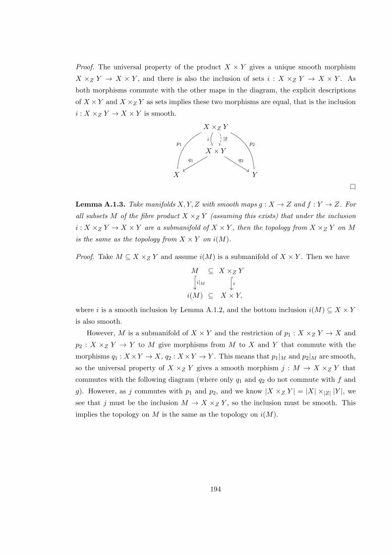
Proof. The universal property of the product X × Y gives a unique smooth morphism

X ×Z Y → X × Y , and there is also the inclusion of sets i : X ×Z Y → X × Y . As

both morphisms commute with the other maps in the diagram, the explicit descriptions

of X ×Y and X ×Z Y as sets implies these two morphisms are equal, that is the inclusion

i : X ×Z Y → X × Y is smooth.

X ×Z Y

X × Y

X Y

i ∃!p1

q1 q2

p2

Lemma A.1.3. Take manifolds X,Y, Z with smooth maps g : X → Z and f : Y → Z. For

all subsets M of the fibre product X ×Z Y (assuming this exists) that under the inclusion

i : X ×Z Y → X × Y are a submanifold of X × Y , then the topology from X ×Z Y on M

is the same as the topology from X × Y on i(M).

Proof. Take M ⊆ X ×Z Y and assume i(M) is a submanifold of X × Y . Then we have

M ⊆ X ×Z Y

i(M) ⊆ X × Y,

i|M i

where i is a smooth inclusion by Lemma A.1.2, and the bottom inclusion i(M) ⊆ X × Yis also smooth.

However, M is a submanifold of X × Y and the restriction of p1 : X ×Z Y → X and

p2 : X ×Z Y → Y to M give morphisms from M to X and Y that commute with the

morphisms q1 : X×Y → X, q2 : X×Y → Y . This means that p1|M and p2|M are smooth,

so the universal property of X ×Z Y gives a smooth morphism j : M → X ×Z Y that

commutes with the following diagram (where only q1 and q2 do not commute with f and

g). However, as j commutes with p1 and p2, and we know |X ×Z Y | = |X| ×|Z| |Y |, we

see that j must be the inclusion M → X ×Z Y , so the inclusion must be smooth. This

implies the topology on M is the same as the topology on i(M).

194

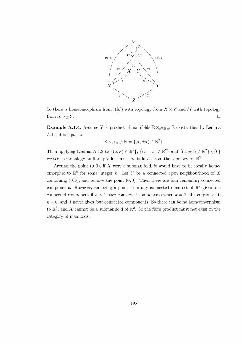
M

X ×Z Y

X × Y

X Y

Z

j

i

p1|M

p1

q1

p2

q2

p2|M

f g

So there is homeomorphism from i(M) with topology from X × Y and M with topology

from X ×Z Y .

Example A.1.4. Assume fibre product of manifolds R×x2,R,y2 R exists, then by Lemma

A.1.1 it is equal to

R×x2,R,y2 R = (x,±x) ∈ R2.

Then applying Lemma A.1.3 to (x, x) ∈ R2, (x,−x) ∈ R2 and (x,±x) ∈ R2 \ 0we see the topology on fibre product must be induced from the topology on R2.

Around the point (0, 0), if X were a submanifold, it would have to be locally home-

omorphic to Rk for some integer k. Let U be a connected open neighbourhood of X

containing (0, 0), and remove the point (0, 0). Then there are four remaining connected

components. However, removing a point from any connected open set of Rk gives one

connected component if k > 1, two connected components when k = 1, the empty set if

k = 0, and it never gives four connected components. So there can be no homeomorphism

to Rk, and X cannot be a submanifold of R2. So the fibre product must not exist in the

category of manifolds.

195

Bibliography

[1] D. Abramovich, Q. Chen, D. Gillam, Y. Huang, M. Olsson, M. Satriano, and S. Sun,

Logarithmic Geometry and Moduli, Handbook of Moduli. Vol. I, p. 1-61, Adv. Lec.

Math. (ALM), 24, International Press, Somerville, MA, 2013.

[2] A. Adamek and J. Rosicky, Locally presentable and accessible categories, L.M.S. Lec-

ture Notes 189, Cambridge University Press, 1994.

[3] A. Adamek, J. Rosicky and E.M. Vitale, Algebraic theories, Cambridge University

Press, 2010.

[4] M. Anel, The Geometry of Ambiguity, An introduction to the ideas of Derived Geom-

etry, February 2018, available at Anel - DerivedGeometry.pdf

[5] S. Awodey, Category Theory, Oxford Logic Guides 49, 2006.

[6] G. M. Bergman and N. Nahlus, Linear maps on kI , and homomorphic images of

infinite direct product algebras, Journal of Algebra 356, 2012, p. 257-274.

[7] K. Buchner, M. Heller, P. Multarzynski and W. Sasin, Literature on Differentiable

Spaces, Acta Cosmologica, Vol. 19, 1993.

[8] D. Borisov, Derived manifolds and d-manifolds, arXiv:1212.1153, 2012.

[9] D. Borisov, Topological characterization of various types of C∞-rings, in Communi-

cations in Analysis and Geometry, Volume 23, No. 2, p. 349-361, 2015.

[10] D. Borisov and J. Noel, Simplicial approach to derived differential manifolds,

arXiv:1112.0033, 2011.

[11] J. Cerf, Topologie de certains espaces de plongements, Bull. Soc. Math. France 89,

1961, p. 227-380.

196

[12] K. Chen, Iterated integrals of differential forms and loop space homology, Ann. of

Math. (2) 97, 1973, p. 217-246.

[13] K. Chen, Iterated integrals, fundamental groups and covering spaces, Trans. Amer.

Math. Soc. 206, 1975, p. 83-98.

[14] K. Chen, Iterated path integrals, Bull. Amer. Math. Soc. 83, 1977, no. 5, p. 831-879.

[15] K. Chen, On differentiable spaces, Categories in Continuum Physics (Buffalo, N.Y.,

1982), p. 38-42, Lecture Notes in Math., 1174, Springer, Berlin, 1986.

[16] W.W. Comfort and S. Negrepontis, The theory of ultrafilters, Springer-Verlag, Berlin

1974.

[17] M. Demazure and P. Gabriel, Groupes algebriques, North Holland Publishing Com-

pany, 1970.

[18] A. Douady, Varietes a bord anguleux et voisinages tubulaires, Seminaire Henri Cartan

14, 1961-2, exp. 1, p. 1-11.

[19] E.J. Dubuc, Sur les modeles de la geometrie differentielle synthetique, Cah. Topol.

Geom. Differ. Categ. 20, 1979, p. 231-279.

[20] E.J. Dubuc, Schemas C∞, Prepub. de la Universite de Montreal 80, 1980, Expose 3.

[21] E.J. Dubuc, C∞-schemes, Amer. J. Math. 103, 1981, p. 683-690.

[22] E.J. Dubuc, Open covers and infinitary operations in C∞-rings, Cah. Topol. Geom.

Differ. Categ. 22, 1981, p. 287-300.

[23] E.J. Dubuc and A. Kock, On 1-form classifiers, Comm. Alg. 12, 1984, p. 1471-1531.

[24] K. Fukaya and K. Ono, Arnold Conjecture and the Gromov-Witten Invariant, Topol-

ogy, Vol. 38, No. 5, p. 933-1048, 1999.

[25] K. Fukaya, Y.-G. Oh, H. Ohta and K. Ono, Lagrangian intersection Floer theory –

anomaly and obstruction, Parts I & II. AMS/IP Studies in Advanced Mathematics,

46.1 & 46.2, A.M.S./International Press, 2009.

[26] W.D. Gillam, Log geometry, preprint, 2009.

[27] W.D. Gillam, Localization of ringed spaces, Advances in Pure Mathematics, 2011, 1,

p. 250-263.

197

[28] W.D. Gillam and S. Molcho, Log differentiable spaces and manifolds with corners,

arXiv:1507.06752, 2015.

[29] L. Gillman and M. Jerison, Rings of continuous functions, D. Van Nostrand Company,

Canada, 1960.

[30] R. Godement, Topologie algebrique et theorie des faisceaux, Hermann, Paris, 1958.

[31] W. Greub, S. Halperin, and R. Vanstone. Connections, Curvature and Cohomology,

Volume I, Academic Press, New York and London, 1972.

[32] A. Grothendieck, Elements de geometrie algebrique I, Publ. Math. IHES 4, 1960.

[33] R. Hartshorne, Algebraic Geometry, Graduate Texts in Math. 52, Springer, New York,

1977.

[34] M. W. Hirsch, Differential Topology, Graduate Texts in Math. 33, Springer-Verlag,

1976.

[35] H. Hofer, K. Wysocki and E. Zehnder, A general Fredholm theory I: A splicing-

based Differential Geometry, JEMS, Volume 9, Issue 4, 2007, p. 841-876. A general

Fredholm theory II: Implicit function theorems, Geometric and Functional Analysis,

Volume 19, 2009, p. 206-293. A general Fredholm theory III: Fredholm functors and

polyfolds, Geometry & Topology 13, 2009, p. 2279-2387.

[36] P. Iglesias-Zemmour, Diffeology, Mathematical Surveys and Monographs, Volume 185,

American Mathematical Society, 2013.

[37] K. Janich, On the classification of O(n)-manifolds, Math. Ann. 176, p. 53-76, 1978.

[38] T. Jech, Set Theory, The Third Millennium Edition, revised and expanded, Springer,

2002, Springer monographs in Mathematics.

[39] D. Joyce, On manifolds with corners, p.225-258 in S. Janeczko, J. Li and D.H. Phong,

editors, Advances in Geometric Analysis, Advanced Lectures in Mathematics 21, In-

ternational Press, Boston, 2012. arXiv:0910.3518.

[40] D. Joyce, Algebraic Geometry over C∞-rings, arXiv:1001.0023, 2010.

[41] D. Joyce, An introduction to d-manifolds and derived differential geometry, p. 230-281

in L. Brambila-Paz, O. Garcia-Prada, P. Newstead and R.P. Thomas, editors, Moduli

spaces, L.M.S. Lecture Notes 411, Cambridge University Press, 2014. arXiv:1206.4207.

198

[42] D. Joyce, D-manifolds, d-orbifolds and derived differential geometry: a detailed sum-

mary, arXiv:1208.4948, 2012.

[43] D. Joyce, D-manifolds and d-orbifolds: a theory of derived differential geometry, to be

published by Oxford University Press, circa 2019. Preliminary version (2012) available

at http://people.maths.ox.ac.uk/∼joyce/dmanifolds.html.

[44] D. Joyce, A new definition of Kuranishi space, arXiv:1409.6908, 2014.

[45] D. Joyce, Some new homology and cohomology theories of manifolds,

arXiv:1509.05672, 2015.

[46] D. Joyce, Kuranishi spaces as a 2-category, arXiv:1510.07444, 2015.

[47] D. Joyce, A generalization of manifolds with corners, Adv. Math. 299, p. 760-862,

2016, pre-print at arXiv:1501.00401, 2015.

[48] D. Joyce, Manifolds with analytic corners, arXiv:1605.05913, 2016.

[49] D. Joyce, Kuranishi spaces and Symplectic Geometry Volume I. Basic theory of (m-)

Kuranishi spaces, preliminary version May 2017.

[50] G. Kainz, A. Kriegl and P. Michor, C∞-algebras from the functional analytic view

point, p. 89-107 in J. Pure Appl. Algebra, 46, North Holland, 1987.

[51] E. Kalashnikov, C∞-Algebraic Geometry, MSc thesis, University of Oxford, 2014.

[52] M. Kashiwara and P. Schapira, Categories and Sheaves, Springer, Grundlehren der

mathematischen Wissenschaften 332, A Series of Comprehensive Studies in Mathe-

matics, 2006.

[53] K. Kato, Logarithmic Structures of Fontaine-Illusie, In Jun-Ichi Igusa, editor, Alge-

braic Analysis, Geometry, and Number Theory, p. 191-224, Johns Hopkins University

Press, Baltimore and London, 1989.

[54] T. Kerler and V. V. Lyubashenko, Non-Semisimple Topological Quantum Field The-

ories for 3-Manifolds with Corners, Lecture Notes in Mathematics 1765, Springer-

Verlag, 2001.

[55] A. Kock, Synthetic differential geometry, second edition, L.M.S. Lecture Notes 333,

Cambridge University Press, 2006.

199

[56] M. Kontsevich, Enumeration of rational curves via torus actions, In R.H. Dijkgraaf,

C.F. Faber, G.B.M. van der Geer The moduli space of curves, Progress in Mathemat-

ics, vol 129. Birkhauser Boston, available at arXiv:hep-th/9405035, 1995.

[57] C. Kottke, Blow-up in manifolds with generalised corners, International Mathematics

Research Notices, Vol. 2018, No. 8, p. 2375-2415.

[58] G. Laures, On cobordism of manifolds with corners, Transactions of the American

Mathematical Society, Volume 352, Number 12, Pages 5667-5688, 2000.

[59] W. Lawvere, Categorical dynamics, 1967, Chicago Lectures, p. 1-28 in A. Kock Topos

Theoretic Methods in Geometry, Aarhus University Matematisk Institut, No. 30, 1979.

[60] J. M. Lee, Introduction to smooth manifolds, Second Edition, Graduate Texts in

Mathematics 218, Springer, 2013.

[61] T. Leinster, Basic Category Theory, Cambridge studies in Advanced Mathematics

143, Cambridge University Texts, 2014.

[62] J. Lurie, Derived Algebraic Geometry V: Structured spaces, arXiv:0905.0459, 2009.

[63] S. Mac Lane, Categories for the working mathematician, second edition, Springer-

Verlag, New York, 1998.

[64] S. Mac Lane and I. Moerdijk, Sheaves in Geometry and Logic: A first introduction to

topos theory, Springer, 1992.

[65] D. McDuff and D. Salamon, J-holomorphic curves and quantum cohomology, Univer-

sity Lecture Series, Volume: 6, 1994.

[66] R.B. Melrose, Calculus of conormal distributions on manifolds with corners, IMRN,

1992, p. 51-61.

[67] R.B. Melrose, The Atiyah–Patodi–Singer index theorem, A.K. Peters, Wellesley, MA,

1993.

[68] R.B. Melrose, Differential analysis on manifolds with corners, unfinished book avail-

able at http://math.mit.edu/∼rbm, 1996.

[69] D.S. Metzler, Topological and smooth stacks, math.DG/0306176, 2003.

200

[70] I. Moerdijk, N. van Que and G.E. Reyes, Rings of smooth functions and their lo-

calizations II, p. 277-300 in D.W. Kueker, E.G.K. Lopez-Escobar and C.H. Smith

(eds), Mathematical logic and theoretical computer science, Lecture Notes in Pure

and Applied Math. 106, Marcel Dekker, New York, 1987.

[71] I. Moerdijk and G.E. Reyes, Rings of smooth functions and their localizations I, J.

Algebra 99, 1986, p. 324-336.

[72] I. Moerdijk and G.E. Reyes, Models for smooth infinitesimal analysis, Springer-Verlag,

New York, 1991.

[73] I. Moerdijk and G. E. Reyes, A smooth version of the Zariski Topos, Advances in

Mathematics, 65, p. 229-253, 1987.

[74] B. Monthubert and V. Nistor, A topological index theorem for manifolds with corners,

Compositio Mathematica, Volume 148, Issue 2, March 2012 , p. 640-668, available at

monthube/articles/mn-final1.pdf

[75] M. A. Mostow, The differentiable space structures of Milnor classifying spaces, sim-

plicial complexes and geometric relations, J. Differ. Geom. 14, p. 255-293, 1979.

[76] J. A. Navarro Gonzalez and J. B. Sancho de Salas, C∞-Differentiable Spaces. Number

1824 in Lecture Notes in Mathematics. Springer-Verlag Berlin Heidelberg, 2003.

[77] nLab Authors, Kahler differential, available at http://ncatlab.org/nlab/show/K%

C3%A4hler%20differential, accessed February 2019

[78] A. Ogus, Lectures on Logarithmic Algebraic Geometry, Cambridge Studies in Ad-

vanced Mathematics 178, Cambridge University Press, 2018.

[79] E. Riehl, Category theory in context, Aurora: Dover Modern Math Originals, Dover

Publications, 2016

[80] D. Rees, On semi-groups, Math. Proc. Camb. Philos. Soc. 36 (4), 1940, p. 387-400.

[81] R. Sikorski, Abstract covariant derivative, Colloquium Mathematicum, XVIII, 1967.

[82] J. M. Souriau, Groupes differentiels in Differential geometrical methods in mathe-

matical physics (Proc. Conf., Aix-en-Provence/Salamanca, 1979), p. 91–128, Lecture

Notes in Math., 836, Springer, Berlin-New York, 1980.

[83] K. Spallek Differenzierbare und homomorphe auf analytischen Mengen, Math. Ann.

161, p. 143-162, 1965.

201

[84] D.I. Spivak, Derived smooth manifolds, Duke Mathematical Journal 153, 2010, p.

55-128. arXiv:0810.5174.

[85] A. Stacey, Comparative smootheology, Theory and Applications of Categories, Vol.

25, No. 4, 2011, p. 64-117.

[86] B. Toen, Derived Algebraic Geometry, EMS Surv. Math. Sci. 1, 2014, p. 153-240.

[87] R. J. Wood, Some remarks on total categories, Journal of Algebra, 75, 1982, p. 538-

585.

202

Glossary

Sets Sets, Definition 2.1.1

Euc Euclidean Spaces, Definition 2.1.1

Eucc Euclidean Spaces with corners, Definition 5.4.1

Euccin Euclidean Spaces with corners with interior maps, Definition 5.4.1

Man Manifolds, Definition 2.1.1

Manb Manifolds with boundary, Definition 5.4.1

Manc Manifolds with corners, Definition 5.4.1

Mangc Manifolds with g-corners, Definition 5.4.1

Mancin Manifolds with corners with interior maps, Definition 5.4.1

Mangcin Manifolds with g-corners with interior maps, Definition 5.4.1

Manc Manifolds with corners with mixed dimension, Definition 5.4.1

Mancin Manifolds with corners with mixed dimension with interior maps, Definition 5.4.1

Mangc Manifolds with g-corners with mixed dimension, Definition 5.4.1

Mangcin Manifolds with g-corners with mixed dimension with interior maps, Definition

5.4.1

Mon Monoids, Definition 5.4.1

C∞Rings C∞-rings Definition 2.1.2

CC∞Rings Categorical C∞-rings, Definition 2.1.1

C∞Ringsco Complete C∞-rings, Definition 2.4.13

203

CPC∞Ringsc Categorical pre C∞-rings with corners, Definition 4.1.2

CPC∞Ringscin Categorical interior pre C∞-rings with corners, Definition 4.1.2

PC∞Ringsc Pre C∞-rings with corners, Definition 4.2.1

PC∞Ringscin Interior pre C∞-rings with corners, Definition 4.2.6

C∞Ringsc C∞-rings with corners Definition 4.3.2

C∞Ringscin Interior C∞-rings with corners Definition 4.3.2

C∞Ringscsc Semi-complete C∞-rings with corners, Definition 5.3.4

C∞Ringscfi Firm C∞-rings with corners, Definition 4.5.1

C∞RS C∞-ringed spaces, Definition 2.4.1

LC∞RS Local C∞-ringed spaces, Definition 2.4.1

C∞RSc C∞-ringed spaces with corners, Definition 5.1.1

LC∞RSc Local C∞-ringed spaces with corners, Definition 5.1.1

C∞RScin Interior C∞-ringed spaces with corners,, Definition 5.1.3

LC∞RScin Interior local C∞-ringed spaces with corners, Definition 5.1.3

AC∞Sch Affine C∞-schemes, Definition 2.4.10

C∞Sch C∞-schemes, Definition 2.4.10

AC∞Schc Affine C∞-schemes with corners, Definition 5.4.1

AC∞Schcfi Firm affine C∞-schemes with corners, Definition 5.4.1

AC∞Schcin Interior affine C∞-schemes with corners, Definition 5.4.3

AC∞Schcfi,in Firm interior affine C∞-schemes with corners, Definition 5.4.3

C∞Schc C∞-schemes with corners, Definition 5.4.1

C∞Schcfi Firm C∞-schemes with corners, Definition 5.4.1

C∞Schcin Interior C∞-schemes with corners, Definition 5.4.1

C∞Schcfi,in Firm interior C∞-schemes with corners, Definition 5.4.1

204

Spec Spectrum for C∞-rings, Definition 2.4.4

Specc Spectrum for C∞-rings with corners, Definition 5.2.1

Speccin Spectrum for interior C∞-rings with corners, Definition 5.2.4

Γ Global sections of C∞-ringed spaces, Definition 2.4.7

Γc Global sections of C∞-ringed spaces with corners, Definition 5.2.5

Γcin Global sections of interior C∞-ringed spaces with corners, Definition 5.2.7

C-mod Modules over the C∞-ring C, Definition 2.2.1

C-mod Modules over the C∞-ring with corners C Definition 4.7.1

OX -mod Sheaves of modules over the sheaf of C∞-rings OX , Definition 2.5.1

OX -mod Sheaves of modules over the sheaf of C∞-rings with corners OX , Definition 5.6.2

ΩC Cotangent module of a C∞-ring C, Definition 2.2.4

ΩC Cotangent module of a C∞-ring with corners, Definition 4.7.3

bΩC b-cotangent module of a C∞-ring with corners, Definition 4.7.6

PrC Prime ideals in Cex of a C∞-ring with corners C = (C,Cex), Definition 5.8.1

C loc Corners functor for local C∞-ringed spaces with corners, Definition 5.7.1

Caff Corners functor for affine firm C∞-schemes with corners, Proposition 5.8.4

C Corners functor for firm C∞-schemes with corners, Theorem 5.8.9

Φi C∞-operation corresponding to the inclusion i : [0,∞)→ R, Definition 4.2.5

Ψexp C∞-operation corresponding to the exponential map exp : R → [0,∞), Definition

4.2.5

Φexp = Φi Ψexp C∞-operation corresponding to the exponential map exp : R→ R, Def-

inition 4.2.5

205