c copyright by daniel p´erez palomar 2003palomar/publications_files/phd_dissertation/... · daniel...
TRANSCRIPT

c© Copyright by Daniel Perez Palomar 2003
All Rights Reserved

The author has been awarded with the 2004 Young Author Best Paper Award
by the IEEE Signal Processing Society for the main publication of this dissertation:
Daniel P. Palomar, John M. Cioffi, and Miguel A. Lagunas, “Joint Tx-Rx Beamforming Design
for Multicarrier MIMO Channels: A Unified Framework for Convex Optimization,”
IEEE Transactions on Signal Processing, Vol. 51, No. 9, pp. 2381-2401, Sept. 2003.
This work has been awarded with the 2002/03 Rosina Ribalta first prize
for the best Doctoral Thesis project within the areas of Information Technologies and
Communications by the Epson Foundation.
This work has been awarded with the 2004 prize
for the best Doctoral Thesis in Advanced Mobile Communications
by the Vodafone Foundation and COIT.

Ph.D. committee:
Gregori Vazquez
Ana Perez-Neira
Sergio Barbarossa
Mats Bengtsson
Emilio Sanvicente
Technical University of Catalonia - UPC
Technical University of Catalonia - UPC
University of Rome “La Sapienza”
Royal Institute of Technology - KTH
Technical University of Catalonia - UPC
Qualification: Cum Laude

Abstract
MULTIPLE-INPUT MULTIPLE-OUTPUT (MIMO) CHANNELS constitute a unified way
of modeling a wide range of different physical communication channels, which can then
be handled with a compact and elegant vector-matrix notation. The two paradigmatic examples
are wireless multi-antenna channels and wireline Digital Subscriber Line (DSL) channels.
Research in antenna arrays (also known as smart antennas) dates back to the 1960’s. However,
the use of multiples antennas at both the transmitter and the receiver, which can be naturally
modeled as a MIMO channel, has been recently shown to offer a significant potential increase
in capacity. DSL has gained popularity as a broadband access technology capable of reliably
delivering high data rates over telephone subscriber lines. A DSL system can be modeled as a
communication through a MIMO channel by considering all the copper twisted pairs within a
binder as a whole rather than treating each twisted pair independently.
This dissertation considers arbitrary MIMO channels regardless of the physical nature of the
channels themselves; as a consequence, the obtained results apply to any communication system
that can be modeled as such. After an extensive overview of MIMO channels, both fundamental
limits and practical communication aspects of such channels are considered.
First, the fundamental limits of MIMO channels are studied. An information-theoretic ap-
proach is taken to obtain different notions of capacity as a function of the degree of channel
knowledge for both single-user and multiuser scenarios. Specifically, a game-theoretic framework
is adopted to obtain robust solutions under channel uncertainty.
Then, practical communication schemes for MIMO channels are derived for the single-user
case or, more exactly, for point-to-point communications (either single-user or multiuser when
coordination is possible at both sides of the link). In particular, a joint design of the transmit-
receive linear processing (or beamforming) is obtained (assuming a perfect channel knowledge)
for systems with either a power constraint or Quality of Service (QoS) constraints.
For power-constrained systems, a variety of measures of quality can be defined to optimize
the performance. For this purpose, a novel unified framework that generalizes the existing results
in the literature is developed based on majorization theory. In particular, the optimal struc-
ture of the transmitter and receiver is obtained for a wide family of objective functions that
i
ii
can be used to measure the quality of a communication system. Using this unified framework,
the original complicated nonconvex problem with matrix-valued variables simplifies into a much
simpler convex problem with scalar variables. With such a simplification, the design problem can
be then reformulated within the powerful framework of convex optimization theory, in which a
great number of interesting design criteria can be easily accommodated and efficiently solved even
though closed-form expressions may not exist. Among other results, a closed-form expression for
optimum beamforming in terms of minimum average bit error rate (BER) is obtained. For other
design criteria, either closed-form solutions are given or practical algorithms are derived within
the framework of convex optimization theory.
For QoS-constrained systems, although the original problem is a complicated nonconvex prob-
lem with matrix-valued variables, with the aid of majorization theory, the problem is reformulated
as a simple convex optimization problem with scalar variables. An efficient multi-level water-filling
algorithm is given to optimally solve the problem in practice.
Finally, the more realistic situation of imperfect channel knowledge due to channel estimation
errors is considered. The previous results on the joint transmit-receive design for MIMO channels
are then extended in this sense to obtain robust designs.

A mis padres,


Acknowledgements
I FEEL EXTREMELY LUCKY to have met all the people I have met during the intriguing
and appealing journey of my Ph.D.
Foremost, I would like to thank my advisor Prof. Miguel Angel Lagunas for his guidance
and support over the past four years. His office door has always been open, both literally and
metaphorically, and I could always talk to him no matter how busy he was. I can only feel
flattered for the confidence he has always shown in me. Fortunately, I have benefited from his
extraordinary motivation, great intuition, and technical insight. I just hope my thinking and
working attitudes have been shaped according to such outstanding qualities.
I wish to thank my mentor at Stanford University, Prof. John M. Cioffi, for he welcomed me
into his research group and treated me like another member of the group with no distinction,
making my stay at Stanford a pleasant and rewarding experience. He has always shown confidence
in me and has given me a continuous support which I appreciate. Very special and deep thanks
go to Joice DeBolt for being such a great human being always ready to listen and give advice.
My thanks also extend to Prof. Javier R. Fonollosa, for he guided my first steps as a Ph.D.
student and with whom I have had the pleasure of working in several European projects. I want
to thank him for the support he has always given to me.
I will always be indebted to the people who have boldly reviewed this dissertation: Toni
Pascual, Gonzalo Seco, Xavi Mestre, and Carlos Aldana. I appreciate very much the enormous
help of the people who, at some time or another, have reviewed some of my papers (in chronological
order): Dana Brooks, Laurent Schumacher, Carlos Aldana, Jerome Louveaux, Wonjong Rhee, Wei
Yu, Young-Han Kim, Jonathan Levin, Mats Bengtsson, George Ginis, and Jeannie Lee Fang. I
would also like to thank the people with whom I have had the pleasure to collaborate: John M.
Cioffi, Javier R. Fonollosa, Ana Perez Neira, Montse Najar, Toni Pascual, and Diego Bartolome.
Special thanks go to some people who I have encountered during my Ph.D. journey: Gonzalo
Seco for introducing me to the wonderful world of matrix theory at my early stage as a Ph.D.
student, Wei Yu and Wonjong Rhee for the encouraging and enthusiastic “wireless and convex”
discussions, and Mats Bengtsson for sharing with me the joy for convex optimization theory and
for his always interesting comments on my work.
v

vi
This long journey would have been nothing without all the people I have met. I want to
thank all my colleagues at UPC: Pau Fernandez, Ruben Villarino, Albert Guillen i Fabregas,
Christian Ibars, Xavi Mestre, Gonzalo Seco, Roger Gaspa, Toni Pascual, Diego Bartolome, Rene
Jativa, Alejandro Ramırez, Joel Sole, Carles Fernandez, Jaume Padrell, Joan Bas, Toni Castro,
Maribel Madueno, Helenca Duxans, Monica Caballero, Javier Ruiz Hidalgo, Hugo Durney, Pe-
dro Correa, Xavi Villares, Jose Antonio Lopez, Francesc Rey, Pere Pujol, Pablo Aguero, Ami
Wiesel, Ali Nassar, Camilo Chang, Carine Simon, Alex Heldring, Eduard Ubeda, Juan Rendon,
Pau Paches, Gustavo Hernandez Abrego, Carles Anton, Lluis Garrido, Sılvia Pujalte, Ramon
Morros, Alberto Sesma, David Font, David Urbano, and Carlos Lopez. I also want to thank
all the members and visitors of Cioffi’s diverse and friendly group at Stanford University: Amal
Ekbal, Ana Garcıa Armada, Ardavan Maleki-Tehrani, Atul Salvekar, Avneesh Agarwal, Carlos
Aldana, Chaohuang (Steve) Zeng, Christian Ibars, Dimitrios-Alexandros Toumpakaris, George
Ginis, Ghazi A. Al-rawi, Kazutomo Hasegawa (Hase), Jeannie Lee Fang, Jerome Louveaux, Jose
Tellado, Jungwon Lee, Kee-Bong Song, Marie-Laure Boucheret, Maxime Flament, Min Chuin
Hoo (Louise), Norihito Mihota, Seong Taek Chung, Susan C. Lin, Wei Yu, Wonjong Rhee, and
Prof. Yeheskel Bar-Ness. I could not possibly forget my good friends at Stanford: David Re-
bollo Monedero, Kevin Yarritu, Christian Ibars Casas, Ana Garcıa Armada, Gustavo Hernandez
Abrego, and Isabelle da Piedade. I also want to thank all my colleagues at CTTC: Alex Graell,
Ana Perez Neira, Antonio Mollfulleda, Carles Anton, Carlos Bader, Carolina Pinart, Diego Bar-
tolome, Herman Balların, Jordi Cebria, Jordi Mateu, Jordi Sorribes, Jose Lopez, Ju Liu, Marc
Realp, Marta Vallejo, Miquel Payaro, Monica Navarro, Patricia Gallart, Raul Munoz, Ricardo
Martınez, Toni Morell, Toni Pascual, and Xavi Mestre. I could not forget to thank my good
friends Xavi Martınez and Oscar Gonzalez, as well as my biking partner Rodolfo Guichon. Please
forgive me if your name should have been listed above and is missing.
Last, but not least, I would like to thank my parents, Laura, and my whole family for their
unconditional love and support.
Daniel Perez PalomarApril 2003
This work has been supported by the Catalan Government (DURSI) 1999FI 00588.

Contents
Notation xi
Acronyms xv
1 Introduction 1
1.1 Motivation . . . . . . . . . . . . . . . . . . . . . . . . . . . . . . . . . . . . . . . . 1
1.1.1 Wireless Multi-Antenna Channels . . . . . . . . . . . . . . . . . . . . . . . 1
1.1.2 Wireline DSL Channels . . . . . . . . . . . . . . . . . . . . . . . . . . . . . 2
1.1.3 A Generic Approach: MIMO Channels . . . . . . . . . . . . . . . . . . . . . 4
1.2 Outline of Dissertation . . . . . . . . . . . . . . . . . . . . . . . . . . . . . . . . . . 5
1.3 Research Contributions . . . . . . . . . . . . . . . . . . . . . . . . . . . . . . . . . 7
2 MIMO Channels: An Overview 11
2.1 Basic MIMO Channel Model . . . . . . . . . . . . . . . . . . . . . . . . . . . . . . 11
2.2 Examples of MIMO Channels . . . . . . . . . . . . . . . . . . . . . . . . . . . . . . 13
2.2.1 Frequency-Selective Channel . . . . . . . . . . . . . . . . . . . . . . . . . . 14
2.2.2 Multicarrier Channel . . . . . . . . . . . . . . . . . . . . . . . . . . . . . . . 17
2.2.3 Multi-Antenna Wireless Channel . . . . . . . . . . . . . . . . . . . . . . . . 19
2.2.4 Wireline DSL Channel . . . . . . . . . . . . . . . . . . . . . . . . . . . . . . 22
2.2.5 Fractional Sampling Equivalent Channel . . . . . . . . . . . . . . . . . . . . 24
2.2.6 CDMA Channel . . . . . . . . . . . . . . . . . . . . . . . . . . . . . . . . . 26
2.3 Gains and Properties of MIMO Channels . . . . . . . . . . . . . . . . . . . . . . . 26
2.3.1 Beamforming Gain . . . . . . . . . . . . . . . . . . . . . . . . . . . . . . . . 26
2.3.2 Diversity Gain . . . . . . . . . . . . . . . . . . . . . . . . . . . . . . . . . . 27
2.3.3 Multiplexing Gain . . . . . . . . . . . . . . . . . . . . . . . . . . . . . . . . 28
2.3.4 Tradeoffs Between Gains . . . . . . . . . . . . . . . . . . . . . . . . . . . . . 29
2.4 State-of-the-Art of Transmission Techniques for MIMO Channels . . . . . . . . . . 29
2.4.1 Transmission Techniques with no CSIT . . . . . . . . . . . . . . . . . . . . 32
2.4.2 Transmission Techniques with Perfect CSIT . . . . . . . . . . . . . . . . . . 34
2.4.3 Transmission Techniques with Partial CSIT . . . . . . . . . . . . . . . . . . 35
2.4.4 The Multiuser Case . . . . . . . . . . . . . . . . . . . . . . . . . . . . . . . 36
vii
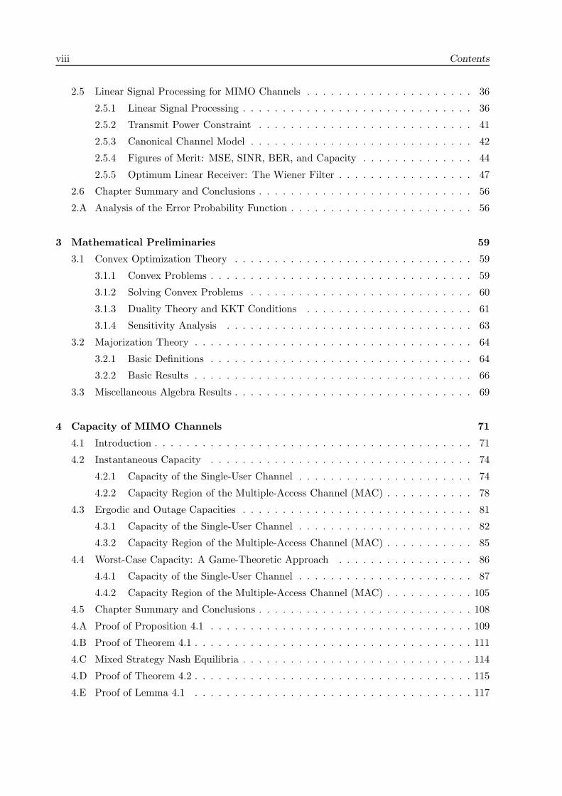
viii Contents
2.5 Linear Signal Processing for MIMO Channels . . . . . . . . . . . . . . . . . . . . . 36
2.5.1 Linear Signal Processing . . . . . . . . . . . . . . . . . . . . . . . . . . . . . 36
2.5.2 Transmit Power Constraint . . . . . . . . . . . . . . . . . . . . . . . . . . . 41
2.5.3 Canonical Channel Model . . . . . . . . . . . . . . . . . . . . . . . . . . . . 42
2.5.4 Figures of Merit: MSE, SINR, BER, and Capacity . . . . . . . . . . . . . . 44
2.5.5 Optimum Linear Receiver: The Wiener Filter . . . . . . . . . . . . . . . . . 47
2.6 Chapter Summary and Conclusions . . . . . . . . . . . . . . . . . . . . . . . . . . . 56
2.A Analysis of the Error Probability Function . . . . . . . . . . . . . . . . . . . . . . . 56
3 Mathematical Preliminaries 59
3.1 Convex Optimization Theory . . . . . . . . . . . . . . . . . . . . . . . . . . . . . . 59
3.1.1 Convex Problems . . . . . . . . . . . . . . . . . . . . . . . . . . . . . . . . . 59
3.1.2 Solving Convex Problems . . . . . . . . . . . . . . . . . . . . . . . . . . . . 60
3.1.3 Duality Theory and KKT Conditions . . . . . . . . . . . . . . . . . . . . . 61
3.1.4 Sensitivity Analysis . . . . . . . . . . . . . . . . . . . . . . . . . . . . . . . 63
3.2 Majorization Theory . . . . . . . . . . . . . . . . . . . . . . . . . . . . . . . . . . . 64
3.2.1 Basic Definitions . . . . . . . . . . . . . . . . . . . . . . . . . . . . . . . . . 64
3.2.2 Basic Results . . . . . . . . . . . . . . . . . . . . . . . . . . . . . . . . . . . 66
3.3 Miscellaneous Algebra Results . . . . . . . . . . . . . . . . . . . . . . . . . . . . . . 69
4 Capacity of MIMO Channels 71
4.1 Introduction . . . . . . . . . . . . . . . . . . . . . . . . . . . . . . . . . . . . . . . . 71
4.2 Instantaneous Capacity . . . . . . . . . . . . . . . . . . . . . . . . . . . . . . . . . 74
4.2.1 Capacity of the Single-User Channel . . . . . . . . . . . . . . . . . . . . . . 74
4.2.2 Capacity Region of the Multiple-Access Channel (MAC) . . . . . . . . . . . 78
4.3 Ergodic and Outage Capacities . . . . . . . . . . . . . . . . . . . . . . . . . . . . . 81
4.3.1 Capacity of the Single-User Channel . . . . . . . . . . . . . . . . . . . . . . 82
4.3.2 Capacity Region of the Multiple-Access Channel (MAC) . . . . . . . . . . . 85
4.4 Worst-Case Capacity: A Game-Theoretic Approach . . . . . . . . . . . . . . . . . 86
4.4.1 Capacity of the Single-User Channel . . . . . . . . . . . . . . . . . . . . . . 87
4.4.2 Capacity Region of the Multiple-Access Channel (MAC) . . . . . . . . . . . 105
4.5 Chapter Summary and Conclusions . . . . . . . . . . . . . . . . . . . . . . . . . . . 108
4.A Proof of Proposition 4.1 . . . . . . . . . . . . . . . . . . . . . . . . . . . . . . . . . 109
4.B Proof of Theorem 4.1 . . . . . . . . . . . . . . . . . . . . . . . . . . . . . . . . . . . 111
4.C Mixed Strategy Nash Equilibria . . . . . . . . . . . . . . . . . . . . . . . . . . . . . 114
4.D Proof of Theorem 4.2 . . . . . . . . . . . . . . . . . . . . . . . . . . . . . . . . . . . 115
4.E Proof of Lemma 4.1 . . . . . . . . . . . . . . . . . . . . . . . . . . . . . . . . . . . 117

Contents ix
5 Joint Design of Tx-Rx Linear Processing for MIMO Channels
with a Power Constraint: A Unified Framework 119
5.1 Introduction . . . . . . . . . . . . . . . . . . . . . . . . . . . . . . . . . . . . . . . . 120
5.2 Design Criterion . . . . . . . . . . . . . . . . . . . . . . . . . . . . . . . . . . . . . 123
5.3 Single Beamforming . . . . . . . . . . . . . . . . . . . . . . . . . . . . . . . . . . . 124
5.3.1 Single MIMO Channel . . . . . . . . . . . . . . . . . . . . . . . . . . . . . . 124
5.3.2 Multiple MIMO Channels . . . . . . . . . . . . . . . . . . . . . . . . . . . . 125
5.4 Multiple Beamforming . . . . . . . . . . . . . . . . . . . . . . . . . . . . . . . . . . 126
5.4.1 Single MIMO Channel . . . . . . . . . . . . . . . . . . . . . . . . . . . . . . 127
5.4.2 Multiple MIMO Channels . . . . . . . . . . . . . . . . . . . . . . . . . . . . 133
5.5 Analysis of Different Design Criteria: A Convex Optimization Approach . . . . . . 133
5.5.1 Minimization of the ARITH-MSE . . . . . . . . . . . . . . . . . . . . . . . 134
5.5.2 Minimization of the GEOM-MSE . . . . . . . . . . . . . . . . . . . . . . . . 136
5.5.3 Minimization of the Determinant of the MSE Matrix . . . . . . . . . . . . 137
5.5.4 Maximization of Mutual Information . . . . . . . . . . . . . . . . . . . . . . 138
5.5.5 Minimization of the MAX-MSE . . . . . . . . . . . . . . . . . . . . . . . . . 138
5.5.6 Maximization of the ARITH-SINR . . . . . . . . . . . . . . . . . . . . . . . 141
5.5.7 Maximization of the GEOM-SINR . . . . . . . . . . . . . . . . . . . . . . . 142
5.5.8 Maximization of the HARM-SINR . . . . . . . . . . . . . . . . . . . . . . . 143
5.5.9 Maximization of the PROD-(1+SINR) . . . . . . . . . . . . . . . . . . . . . 146
5.5.10 Maximization of the MIN-SINR . . . . . . . . . . . . . . . . . . . . . . . . . 147
5.5.11 Minimization of the ARITH-BER . . . . . . . . . . . . . . . . . . . . . . . 147
5.5.12 Minimization of the GEOM-BER . . . . . . . . . . . . . . . . . . . . . . . . 151
5.5.13 Minimization of the MAX-BER . . . . . . . . . . . . . . . . . . . . . . . . . 152
5.5.14 Including a ZF Constraint . . . . . . . . . . . . . . . . . . . . . . . . . . . . 152
5.6 Introducing Additional Constraints . . . . . . . . . . . . . . . . . . . . . . . . . . . 153
5.7 Simulation Results . . . . . . . . . . . . . . . . . . . . . . . . . . . . . . . . . . . . 155
5.8 Chapter Summary and Conclusions . . . . . . . . . . . . . . . . . . . . . . . . . . . 166
5.A Proof of Theorem 5.1 . . . . . . . . . . . . . . . . . . . . . . . . . . . . . . . . . . . 167
5.B Proof of Lemma 5.1 . . . . . . . . . . . . . . . . . . . . . . . . . . . . . . . . . . . 171
5.C Proof of Corollary 5.2 . . . . . . . . . . . . . . . . . . . . . . . . . . . . . . . . . . 171
5.D Proof of Schur-Convexity/Concavity Lemmas . . . . . . . . . . . . . . . . . . . . . 171
5.E Gradients and Hessians for the ARITH-BER . . . . . . . . . . . . . . . . . . . . . 173
5.F Proof of Water-Filling Results . . . . . . . . . . . . . . . . . . . . . . . . . . . . . . 175
6 Joint Design of Tx-Rx Linear Processing for MIMO Channels
with QoS Constraints 189
6.1 Introduction . . . . . . . . . . . . . . . . . . . . . . . . . . . . . . . . . . . . . . . . 189
6.2 QoS Requirements . . . . . . . . . . . . . . . . . . . . . . . . . . . . . . . . . . . . 192

x Contents
6.3 Single Beamforming . . . . . . . . . . . . . . . . . . . . . . . . . . . . . . . . . . . 194
6.3.1 Single MIMO Channel . . . . . . . . . . . . . . . . . . . . . . . . . . . . . . 194
6.3.2 Multiple MIMO Channels . . . . . . . . . . . . . . . . . . . . . . . . . . . . 195
6.4 Multiple Beamforming . . . . . . . . . . . . . . . . . . . . . . . . . . . . . . . . . . 195
6.4.1 Single MIMO Channel . . . . . . . . . . . . . . . . . . . . . . . . . . . . . . 196
6.4.2 Multiple MIMO Channels . . . . . . . . . . . . . . . . . . . . . . . . . . . . 203
6.5 Relaxation of the QoS Requirements . . . . . . . . . . . . . . . . . . . . . . . . . . 204
6.6 Simulation Results . . . . . . . . . . . . . . . . . . . . . . . . . . . . . . . . . . . . 205
6.6.1 Wireless Multi-Antenna Communication System . . . . . . . . . . . . . . . 205
6.6.2 Wireline (DSL) Communication System . . . . . . . . . . . . . . . . . . . . 209
6.7 Chapter Summary and Conclusions . . . . . . . . . . . . . . . . . . . . . . . . . . . 211
6.A Proof of Theorem 6.1 . . . . . . . . . . . . . . . . . . . . . . . . . . . . . . . . . . . 212
6.B Proof of Proposition 6.1 . . . . . . . . . . . . . . . . . . . . . . . . . . . . . . . . . 214
6.C Proof of Theorem 6.2 . . . . . . . . . . . . . . . . . . . . . . . . . . . . . . . . . . . 216
6.D Proof of Proposition 6.2 . . . . . . . . . . . . . . . . . . . . . . . . . . . . . . . . . 218
6.E Proof of Lemma 6.1 . . . . . . . . . . . . . . . . . . . . . . . . . . . . . . . . . . . 220
6.F Proof of Lemma 6.2 . . . . . . . . . . . . . . . . . . . . . . . . . . . . . . . . . . . 221
7 Robust Design against Channel Estimation Errors 223
7.1 Introduction . . . . . . . . . . . . . . . . . . . . . . . . . . . . . . . . . . . . . . . . 223
7.2 Worst-Case vs. Stochastic Robust Designs . . . . . . . . . . . . . . . . . . . . . . . 225
7.3 Worst-Case Robust Design . . . . . . . . . . . . . . . . . . . . . . . . . . . . . . . . 227
7.3.1 Error Modeling and Problem Formulation . . . . . . . . . . . . . . . . . . . 227
7.3.2 Power-Constrained Systems . . . . . . . . . . . . . . . . . . . . . . . . . . . 231
7.3.3 QoS-Constrained Systems . . . . . . . . . . . . . . . . . . . . . . . . . . . . 232
7.4 Stochastic Robust Design . . . . . . . . . . . . . . . . . . . . . . . . . . . . . . . . 233
7.4.1 Error Modeling and Problem Formulation . . . . . . . . . . . . . . . . . . . 234
7.4.2 Power-Constrained Systems . . . . . . . . . . . . . . . . . . . . . . . . . . . 238
7.4.3 QoS-Constrained Systems . . . . . . . . . . . . . . . . . . . . . . . . . . . . 238
7.5 Simulation Results . . . . . . . . . . . . . . . . . . . . . . . . . . . . . . . . . . . . 239
7.6 Chapter Summary and Conclusions . . . . . . . . . . . . . . . . . . . . . . . . . . . 245
7.A Proof of Lemma 7.1 . . . . . . . . . . . . . . . . . . . . . . . . . . . . . . . . . . . 246
7.B Proof of Lemma 7.2 . . . . . . . . . . . . . . . . . . . . . . . . . . . . . . . . . . . 247
8 Conclusions and Future Work 249
8.1 Conclusions . . . . . . . . . . . . . . . . . . . . . . . . . . . . . . . . . . . . . . . . 249
8.2 Future Work . . . . . . . . . . . . . . . . . . . . . . . . . . . . . . . . . . . . . . . 251
Bibliography

Notation
Boldface upper-case letters denote matrices, boldface lower-case letters denote column vectors,
and italics denote scalars.
XT , X∗, XH Transpose, complex conjugate, and conjugate transpose (Hermitian) of matrix
X, respectively.
(·) Optimal value.
X1/2 Hermitian square root of the Hermitian matrix X, i.e., X1/2X1/2 = X.
Px, P⊥x Projection matrix onto the subspace spanned by the columns of X and the
orthogonal subspace, respectively.
Tr (X) Trace of X.
|X| or det (X) Determinant of matrix X.
|x| Absolute value (modulus) of the scalar x.
‖·‖ A norm.
‖x‖2 Euclidean norm of vector x: ‖x‖2 =√
xHx.
‖X‖F Frobenius norm of matrix X: ‖X‖F =√
Tr (XHX).
d (X) Vector of diagonal elements of matrix X.
λ (X) Vector of eigenvalues of matrix X.
λmax (X), λi (X) Maximum eigenvalue and ith eigenvalue (in increasing or decreasing order),
respectively, of matrix X.
umax (X), ui (X) Eigenvector associated to the maximum and to the ith eigenvalue (in increasing
or decreasing order), respectively, of matrix X.
[X]i,j or [X]ij The (ith,jth) element of matrix X.
[X]:,j The jth column of matrix X.
diag (Dk) Block-diagonal matrix with diagonal blocks given by the set Dk. In partic-
ular, if the Dk’s are scalars, it reduces to a diagonal matrix.
xi

xii Notation
vec (·) Vec-operator: if X = [x1 · · ·xn], then vec (X) =[xT
1 · · · xTn
]T .
I Identity matrix. A subscript can be used to indicate the dimension.
ei Canonical vector with all the elements being zero except the ith one which is
equal to one.
A ≥ B A −B is positive semidefinite.
a ≥ b Elementwise relation ai ≥ bi.
a b a majorizes b or, equivalently, b is majorized by a.
a w b a weakly majorizes b or, equivalently, b is weakly majorized by a.
Defined as.
∝ Equal up to a scaling factor.
δkl Kronecker delta: δkl =
1
0
k = l
k = l.
[a, b], (a, b) Closed interval (a ≤ x ≤ b) and open interval (a < x < b), respectively.
[a, b), (a, b] Half-closed (or half-open) intervals a ≤ x < b and a < x ≤ b, respectively.
IR, IR+, IR++ The set of real, nonnegative real, and positive real numbers, respectively.
IRn×m, CI n×m The set of n×m matrices with real- and complex-valued entries, respectively.
Sn The set of Hermitian n × n matrices Sn X ∈CI n×n | X = XH
.
Sn+ The set of Hermitian positive semidefinite n × n matrices
Sn+ X ∈CI n×n | X = XH ≥ 0
.
Sn++ The set of Hermitian positive definite n × n matrices
Sn++
X ∈CI n×n | X = XH > 0
.
E [·] Statistical expectation. A subscript can be used to indicate the random vari-
able considered for the expectation.
∼ Distributed according to.
CN (m,C) Complex circularly symmetric Gaussian vector distribution with mean m and
covariance matrix C.1
log (·) Natural logarithm.
logb (·) Logarithm in base b.
Re [·], Im [·] Real and imaginary parts.1A complex Gaussian random vector z = x+jy is circularly symmetric (also termed proper Gaussian) if
E
[[x
y
] [xT yT
]]= 1
2
[A −B
B A
]so that E [zzH ] = A + jB [Nee93].

Notation xiii
sup, inf Supremum (lowest upper bound) and infimum (highest lower bound).⋂,⋃
Intersection and union.
(x)+ Positive part of x, i.e., max (0, x). For matrices it is defined elementwise.
g′ (a) Derivative of function g (x) evaluated at x = a.
∇xf (x) Gradient of function f (x) with respect to x.2
dom f Domain of function f .
2If x is a complex-valued vector and function f (x) is not analytic, the well-known definition of the complex
gradient operator is used, since it is very convenient, among other things, to determine the stationary points of a
real-valued scalar function of a complex vector [Bra83].

xiv Notation
Acronyms
1-D One-dimensional.
3GPP Third Generation Partnership Project.
A/D Analog-to-Digital.
ADSL Asymmetric DSL.
AWGN Additive White Gaussian Noise.
BER Bit Error Rate.
BLAST Bell-labs LAyered Space-Time.
bps Bits per second.
BPSK Binary Phase Shift Keying.
CDMA Code Division Multiple Access.
CO Central Office.
COFDM Coded Orthogonal Frequency Division Multiplexing.
CP Cyclic Prefix.
CPE Customer Premises Equipment.
CSI Channel State Information.
CSIR Channel State Information at the Receiver.
CSIT Channel State Information at the Transmitter.
D/A Digital-to-Analog.
DAB Digital Audio Broadcasting.
DF Decision-Feedback.
DFE Decision-Feedback Equalizer.
xv

xvi Acronyms
DFT Discrete Fourier Transform.
DLST Diagonal Layered Space-Time.
DMT Discrete Multi-Tone.
DSL Digital Subscriber Line.
DVB Digital Video Broadcasting.
ETSI European Telecommunications Standards Institute.
EVD Eigenvalue Decomposition.
FDD Frequency Division Duplex.
FDMA Frequency Division Multiple Access.
FEXT Far-End Crosstalk.
FFT Fast Fourier Transform.
FIR Finite Impulse Response.
HLST Horizontal Layered Space-Time.
IBI Inter-Block Interference.
IDFT Inverse Discrete Fourier Transform.
IEEE Institute of Electrical and Electronical Engineers.
IFFT Inverse Fast Fourier Transform.
i.i.d. Independent and Identically Distributed.
ISI Inter-Symbol Interference.
KKT Karush-Kuhn-Tucker.
LHS Left-Hand Side.
LMMSE Linear Minimum Mean Square Error.
LP Linear Program.
LST Layered Space-Time.
LTI Linear Time-Invariant.
LTV Linear Time-Varying.
MAC Multiple-Access Channel.
MC-CDMA Multicarrier CDMA.

Acronyms xvii
MIMO Multiple-Input Multiple-Output.
MISO Multiple-Input Single-Output.
ML Maximum Likelihood.
MLSE Maximum Likelihood Sequence Estimator.
MMSE Minimum Mean Square Error.
MSE Mean Square Error.
NEXT Near-End Crosstalk.
NLOS Non-Line-Of-Sight.
OFDM Orthogonal Frequency Division Multiplexing.
OFDMA Orthogonal Frequency Division Multiple Access.
P/S Parallel-to-Serial.
PAR Peak to Average Ratio.
pdf Probability Density Function.
PSD Power Spectral Density.
PSK Phase Shift Keying.
QAM Quadrature Amplitude Modulation.
QoS Quality of Service.
QP Quadratic Program.
QPSK Quadrature Phase Shift Keying.
RHS Right-Hand Side.
r.m.s. Root Mean Squared.
Rx Receiver.
S/P Serial-to-Parallel.
SIMO Single-Input Multiple-Output.
SINR Signal to Interference-plus-Noise Ratio.
SISO Single-Input Single-Output.
SNR Signal to Noise Ratio.
s.t. Subject To.

xviii Acronyms
STBC Space-Time Block Coding.
STC Space-Time Coding.
STTC Space-Time Trellis Coding.
SVD Singular Value Decomposition.
TDD Time Division Duplex.
TDMA Time Division Multiple Access.
Tx Transmitter.
UMTS Universal Mobile Telecommunications System.
UTRA UMTS Terrestrial Radio Access.
VDSL Very-high-bit-rate DSL.
w/ and w/o With and without, respectively.
WLAN Wireless Local Area Network.
w.l.o.g. Without Loss Of Generality.
ZF Zero-Forcing.
ZP Zero-Padding.

Chapter 1
Introduction
THE FOCUS OF THIS DISSERTATION is on communications through multiple-input
multiple-output (MIMO) channels. The interest of studying MIMO channels is because
many different types of real channels can be modeled as such. In other words, they represent a
unified way to model a wide variety of scenarios. In addition, MIMO channels can be naturally
handled with a convenient and elegant vector-matrix notation. The two paradigmatic examples
are wireless multi-antenna channels and wireline channels, although many other typical scenarios
are straightforwardly modeled as MIMO channels as well.
1.1 Motivation
1.1.1 Wireless Multi-Antenna Channels
The recent and anticipated growth of wireless communication systems has fueled research efforts
investigating methods to increase system capacity. Doubtlessly, the rapid advance in technology,
on the one hand, and the exploding demand for efficient high-quality services of digital wireless
communications, on the other hand, play a dramatic role in this trend. The demand for these
services is growing at an extremely rapid pace and these trends are likely to continue for several
years.
The radio spectrum available for wireless services is extremely scarce. As a consequence, a
prime issue in current wireless systems is the conflict between the increasing demand for wireless
services and the scarce electromagnetic spectrum. Spectral efficiency is therefore of primary con-
cern in the design of future wireless data communication systems with the omnipresent bandwidth
constraint.
The current need for increased capacity and interference protection in wireless multiuser
systems is at present treated through, among other techniques, limited microdiversity features
1
2 Chapter 1. Introduction
nT antennas
TRANSMITTER RECEIVER
nR antennas
s(t) y(t)
Scattering
medium
y1(t)
y2(t)
yn(t)R
s1(t)
s2(t)
sn(t)T
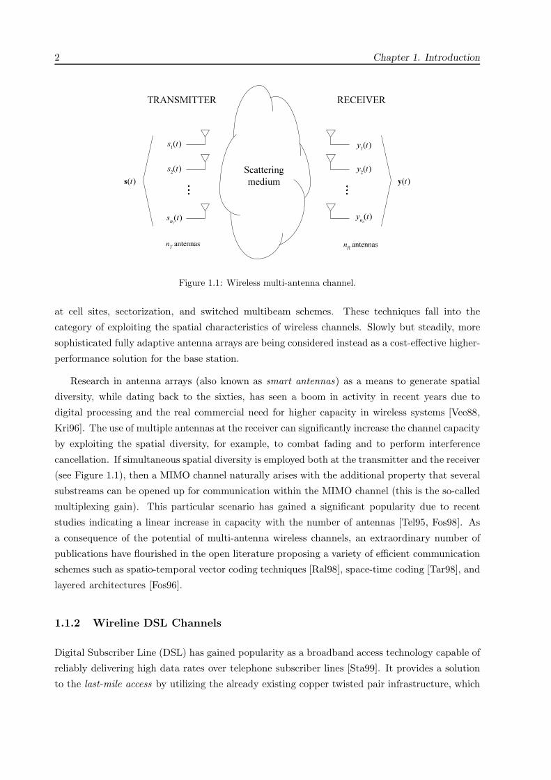
Figure 1.1: Wireless multi-antenna channel.
at cell sites, sectorization, and switched multibeam schemes. These techniques fall into the
category of exploiting the spatial characteristics of wireless channels. Slowly but steadily, more
sophisticated fully adaptive antenna arrays are being considered instead as a cost-effective higher-
performance solution for the base station.
Research in antenna arrays (also known as smart antennas) as a means to generate spatial
diversity, while dating back to the sixties, has seen a boom in activity in recent years due to
digital processing and the real commercial need for higher capacity in wireless systems [Vee88,
Kri96]. The use of multiple antennas at the receiver can significantly increase the channel capacity
by exploiting the spatial diversity, for example, to combat fading and to perform interference
cancellation. If simultaneous spatial diversity is employed both at the transmitter and the receiver
(see Figure 1.1), then a MIMO channel naturally arises with the additional property that several
substreams can be opened up for communication within the MIMO channel (this is the so-called
multiplexing gain). This particular scenario has gained a significant popularity due to recent
studies indicating a linear increase in capacity with the number of antennas [Tel95, Fos98]. As
a consequence of the potential of multi-antenna wireless channels, an extraordinary number of
publications have flourished in the open literature proposing a variety of efficient communication
schemes such as spatio-temporal vector coding techniques [Ral98], space-time coding [Tar98], and
layered architectures [Fos96].
1.1.2 Wireline DSL Channels
Digital Subscriber Line (DSL) has gained popularity as a broadband access technology capable of
reliably delivering high data rates over telephone subscriber lines [Sta99]. It provides a solution
to the last-mile access by utilizing the already existing copper twisted pair infrastructure, which

1.1. Motivation 3
Central
Office
other
users/services
user 1
user 2
user L
Single office
building Cabinet
Central
OfficeNEXTFEXT
Figure 1.2: Wireline DSL channel (scheme of a bundle of copper twisted pairs).
was originally built with the purpose of providing telephone service. Asymmetric DSL (ADSL)
systems have been successfully deployed, revealing the potential of this technology. Current efforts
focus on very-high-bit-rate DSL (VDSL) which allows the use of a bandwidth up to 20 MHz.
The dominant impairment in DSL systems is crosstalk arising from electromagnetic coupling
between neighboring twisted pairs. Near-end crosstalk (NEXT) comprises the signals originated
in the same side of the received signal (due to the existence of downstream and upstream trans-
mission) and far-end crosstalk (FEXT) includes the signal originated in the opposite side of the
received signal. The impact of NEXT is generally suppressed by employing frequency division
duplex (FDD) to separate downstream and upstream transmission. In addition to the crosstalk,
DSL channels are highly frequency-selective; as a consequence, multicarrier transmission schemes
are used in practice.
Modeling a DSL system as a MIMO channel presents many advantages with respect to treating
each twisted pair independently [Hon90, Gin02]. In fact, modeling a wireline channel as a MIMO
channel was done almost three decades ago [Lee76, Sal85]. A general scenario consists of a binder
group composed of a set of intended users in the same physical location plus some other users
that possibly belong to a different service provider and use different types of DSL systems (see
Figure 1.2). The MIMO channel represents the communication of the intended users while the
others are treated as interference.
In many situations, joint processing can be assumed at one side of the link, the Central Office
(CO), whereas the other side, corresponding to the Customer Premises Equipment (CPE), must
use independent processing per user since users are geographically distributed [Gin02]. In some
cases of practical interest, however, both ends of the MIMO system are each terminated in a
single physical location (see Figure 1.2), e.g., links between CO’s and Remote Terminals or links
between CO’s and private networks. This allows the utilization of joint processing at both sides
of the link [Hon90].
4 Chapter 1. Introduction
H
n
ysn
T
nR x n
T
nR
nR
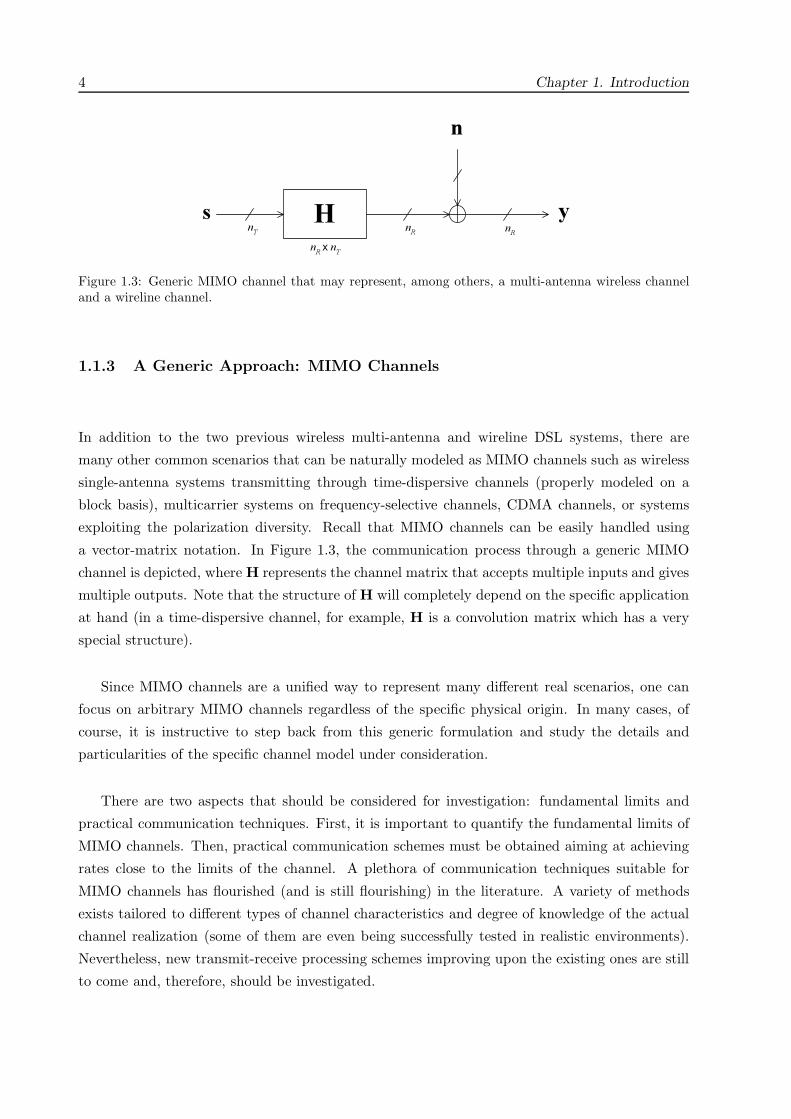
Figure 1.3: Generic MIMO channel that may represent, among others, a multi-antenna wireless channeland a wireline channel.
1.1.3 A Generic Approach: MIMO Channels
In addition to the two previous wireless multi-antenna and wireline DSL systems, there are
many other common scenarios that can be naturally modeled as MIMO channels such as wireless
single-antenna systems transmitting through time-dispersive channels (properly modeled on a
block basis), multicarrier systems on frequency-selective channels, CDMA channels, or systems
exploiting the polarization diversity. Recall that MIMO channels can be easily handled using
a vector-matrix notation. In Figure 1.3, the communication process through a generic MIMO
channel is depicted, where H represents the channel matrix that accepts multiple inputs and gives
multiple outputs. Note that the structure of H will completely depend on the specific application
at hand (in a time-dispersive channel, for example, H is a convolution matrix which has a very
special structure).
Since MIMO channels are a unified way to represent many different real scenarios, one can
focus on arbitrary MIMO channels regardless of the specific physical origin. In many cases, of
course, it is instructive to step back from this generic formulation and study the details and
particularities of the specific channel model under consideration.
There are two aspects that should be considered for investigation: fundamental limits and
practical communication techniques. First, it is important to quantify the fundamental limits of
MIMO channels. Then, practical communication schemes must be obtained aiming at achieving
rates close to the limits of the channel. A plethora of communication techniques suitable for
MIMO channels has flourished (and is still flourishing) in the literature. A variety of methods
exists tailored to different types of channel characteristics and degree of knowledge of the actual
channel realization (some of them are even being successfully tested in realistic environments).
Nevertheless, new transmit-receive processing schemes improving upon the existing ones are still
to come and, therefore, should be investigated.
1.2. Outline of Dissertation 5
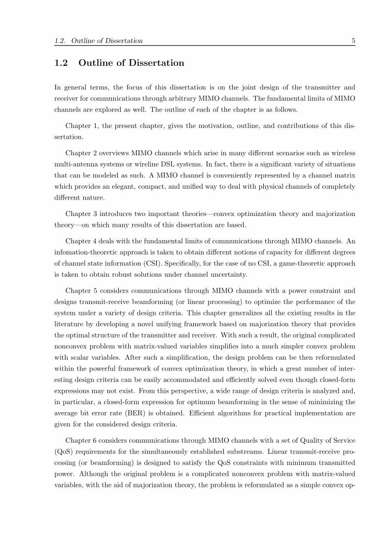
1.2 Outline of Dissertation
In general terms, the focus of this dissertation is on the joint design of the transmitter and
receiver for communications through arbitrary MIMO channels. The fundamental limits of MIMO
channels are explored as well. The outline of each of the chapter is as follows.
Chapter 1, the present chapter, gives the motivation, outline, and contributions of this dis-
sertation.
Chapter 2 overviews MIMO channels which arise in many different scenarios such as wireless
multi-antenna systems or wireline DSL systems. In fact, there is a significant variety of situations
that can be modeled as such. A MIMO channel is conveniently represented by a channel matrix
which provides an elegant, compact, and unified way to deal with physical channels of completely
different nature.
Chapter 3 introduces two important theories—convex optimization theory and majorization
theory—on which many results of this dissertation are based.
Chapter 4 deals with the fundamental limits of communications through MIMO channels. An
infomation-theoretic approach is taken to obtain different notions of capacity for different degrees
of channel state information (CSI). Specifically, for the case of no CSI, a game-theoretic approach
is taken to obtain robust solutions under channel uncertainty.
Chapter 5 considers communications through MIMO channels with a power constraint and
designs transmit-receive beamforming (or linear processing) to optimize the performance of the
system under a variety of design criteria. This chapter generalizes all the existing results in the
literature by developing a novel unifying framework based on majorization theory that provides
the optimal structure of the transmitter and receiver. With such a result, the original complicated
nonconvex problem with matrix-valued variables simplifies into a much simpler convex problem
with scalar variables. After such a simplification, the design problem can be then reformulated
within the powerful framework of convex optimization theory, in which a great number of inter-
esting design criteria can be easily accommodated and efficiently solved even though closed-form
expressions may not exist. From this perspective, a wide range of design criteria is analyzed and,
in particular, a closed-form expression for optimum beamforming in the sense of minimizing the
average bit error rate (BER) is obtained. Efficient algorithms for practical implementation are
given for the considered design criteria.
Chapter 6 considers communications through MIMO channels with a set of Quality of Service
(QoS) requirements for the simultaneously established substreams. Linear transmit-receive pro-
cessing (or beamforming) is designed to satisfy the QoS constraints with minimum transmitted
power. Although the original problem is a complicated nonconvex problem with matrix-valued
variables, with the aid of majorization theory, the problem is reformulated as a simple convex op-

6 Chapter 1. Introduction
Chapter 2:
“Overview of
MIMO Channels”
Chapter 3:
“Mathematical
Preliminaries”
Chapter 4:
“Capacity of
MIMO Channels”
Chapter 5:
“Joint Tx-Rx Design
with a Power Constraint”
Chapter 6:
“Joint Tx-Rx Design
with QoS Constraints”
Chapter 7:
“Robust Design”
Chapter 1:
“Introduction”
Chapter 8:
“Conclusions”Preceeding block is recommended
Preceeding block is required
Figure 1.4: Dependence among chapters.
1.3. Research Contributions 7
timization problem with scalar variables. An efficient multi-level water-filling algorithm is given
to optimally solve the problem in practice.
Chapter 7 extends the results of Chapters 5 and 6, in which perfect CSI was assumed, to
the more realistic situation of imperfect CSI accounting for channel estimation errors. Two
completely different philosophies are used to obtain robust designs: worst-case robustness and
stochastic (Bayesian) robustness.
Chapter 8 concludes the dissertation summarizing the main obtained results and enumerating
future lines of work.
The dependence among the chapters is illustrated in Figure 1.4. For example, before reading
Chapter 7, one should read first Chapters 5 and 6, for which one should first read Chapter 1 with
the recommendation of reading Chapters 2 and 3 as well.
1.3 Research Contributions
The main contribution of this dissertation is the development of a general unified framework
for the joint design of transmit-receive linear processing schemes for communications in MIMO
channels. Details of the research contributions in each chapter are as follows.
Chapter 4
The main result in this chapter is regarding the game-theoretic formulation of the communi-
cation problem published in one journal paper and one conference paper:
• D. P. Palomar, J. M. Cioffi, and M. A. Lagunas, “Uniform Power Allocation in MIMO
Channels: A Game-Theoretic Approach,” IEEE Trans. on Information Theory, Vol. 49,
No. 7, pp. 1707-1727, July 2003.
• D. P. Palomar, J. M. Cioffi, and M. A. Lagunas, “Uniform Power Allocation in MIMO
Channels: A Game-Theoretic Approach,” in Proc. IEEE 2003 International Symposium on
Information Theory (ISIT’03), p. 271, Pacifico, Yokohama, Japan, June 29-July 4, 2003.
Additional results have also been obtained for beamforming-constrained systems in realistic
multi-antenna correlated channels with perfect CSI in one journal paper and four conference
papers:
• D. P. Palomar and M. A. Lagunas, “Joint Transmit-Receive Space-Time Equalization in
Spatially Correlated MIMO channels: A Beamforming Approach,” IEEE Journal on Se-
lected Areas in Communications: Special Issue on MIMO Systems and Applications, Vol.
21, No. 5, pp. 730-743, June 2003.

8 Chapter 1. Introduction
• D. P. Palomar, J. R. Fonollosa, and M. A. Lagunas, “Capacity results on frequency-selective
Rayleigh MIMO channels,” in Proc. IST Mobile Communication Summit 2000, pp. 491-496,
Galway, Ireland, Oct. 1-4, 2000.
• D. P. Palomar, J. R. Fonollosa, and M. A. Lagunas, “Information-theoretic results for real-
istic UMTS MIMO channels,” in Proc. IST Mobile Communication Summit 2001, Sitges,
Barcelona, Spain, Sept. 9-12, 2001.
• D. P. Palomar, J. R. Fonollosa, and M. A. Lagunas, “Capacity results of spatially correlated
frequency-selective MIMO channels in UMTS,” in Proc. IEEE Vehicular Technology Conf.
Fall (VTC-Fall 2001), Atlantic City, NJ, Oct. 7-11, 2001.
• D. P. Palomar and M. A. Lagunas, “Capacity of spatially flattened frequency-selective
MIMO channels using linear processing techniques in transmission,” in Proc. 35th IEEE
Annual Conference on Information Sciences and Systems (CISS 2001), The John Hopkins
University, Baltimore, MD, March 21-23, 2001.
Chapter 5
The main results in this chapter involve the joint optimization of the transmitter and receiver
according to different criteria under a power constraint, for which a novel unified framework has
been developed. The results have been published in two journal papers and three conference
papers:
• D. P. Palomar, J. M. Cioffi, and M. A. Lagunas, “Joint Tx-Rx Beamforming Design for Mul-
ticarrier MIMO Channels: a Unified Framework for Convex Optimization,” IEEE Trans.
on Signal Processing, to appear in 2003 (submitted Feb. 2002, revised Dec. 2002).
• D. P. Palomar and M. A. Lagunas, “Joint Transmit-Receive Space-Time Equalization in
Spatially Correlated MIMO channels: A Beamforming Approach,” IEEE Journal on Se-
lected Areas in Communications: Special Issue on MIMO Systems and Applications, Vol.
21, No. 5, pp. 730-743, June 2003.1
• D. P. Palomar, M. A. Lagunas, A. P. Iserte, and A. P. Neira “Practical implementation of
jointly designed transmit-receive space-time IIR filters,” in Proc. 6th IEEE International
Symposium on Signal Processing and its Applications (ISSPA-2001), pp. 521-524, Kuala-
Lampur, Malaysia, Aug. 13-16, 2001.
• D. P. Palomar, M. A. Lagunas, and J. M. Cioffi, “On the Optimal Structure of Transmit-
Receive Linear Processing for MIMO Channels,” in Proc. 40th Annual Allerton Conference1Note that this paper has been previously listed in the publications of the capacity results for beamforming-
constrained systems corresponding to Chapter 4.
1.3. Research Contributions 9
on Communication, Control, and Computing, pp. 683-692, Allerton House, Monticello, IL,
Oct. 2-4, 2002.
• D. P. Palomar, J. M. Cioffi, M. A. Lagunas, and A. P. Iserte, “Convex Optimization Theory
Applied to Joint Beamforming Design in Multicarrier MIMO Channels,” in Proc. IEEE
2003 International Conference on Communications (ICC’03), Anchorage, Alaska, USA,
May 11-15, 2003.
Chapter 6
The main results in this chapter refer to the joint optimization of the transmitter and receiver
to satisfy a set of QoS constraints with minimum transmitted power. The results have been
published in one journal paper and one conference paper:
• D. P. Palomar, M. A. Lagunas, and J. M. Cioffi, “Optimum Linear Joint Transmit-Receive
Processing for MIMO Channels with QoS Constraints,” IEEE Trans. on Signal Processing,
to appear in 2003 (submitted May 2002, revised Feb. 2003).
• D. P. Palomar, M. A. Lagunas, and J. M. Cioffi, “Optimum Joint Transmit-Receive Linear
Processing for Vectored DSL Transmission with QoS Requirements,” in Proc. 36th Asilomar
Conference on Signals, Systems & Computers, pp. 388-392, Pacific Grove, CA, Nov. 3-6,
2002.
Chapter 7
The results in this chapter extend the previously obtained results for perfect CSI to the more
realistic case of imperfect CSI. Partial results were presented in one journal paper and additional
results are still to be submitted for publication:
• D. P. Palomar, M. A. Lagunas, and J. M. Cioffi, “Optimum Linear Joint Transmit-Receive
Processing for MIMO Channels with QoS Constraints,” IEEE Trans. on Signal Processing,
to appear in 2003 (submitted May 2002, revised Feb. 2003).2
Other contributions not presented in this dissertation
During the first and a half years of the author’s Ph.D. period, blind beamforming techniques
were developed for spread spectrum systems with multiple receive antennas. The results were
published in two journal papers and four conference papers:
2Note that this paper has been previously listed in the publications corresponding to Chapter 6.
10 Chapter 1. Introduction
• D. P. Palomar, M. Najar, and M. A. Lagunas “Self-reference Spatial Diversity Process-
ing for Spread Spectrum Communications,” AEU International Journal of Electronics and
Communications, Vol. 54, No. 5, pp. 267-276, Nov. 2000.
• D. P. Palomar and M. A. Lagunas “Temporal diversity on DS-CDMA communication sys-
tems for blind array signal processing,” EURASIP Signal Processing, Vol. 81, No. 8, pp.
1625-1640, Aug. 2001.
• D. P. Palomar and M. A. Lagunas “Blind beamforming for DS-CDMA systems,” in Proc. of
the Fifth Bayona Workshop on Emerging Technologies in Telecommunications, pp. 83-87,
Bayona, Spain, Sept. 6-8, 1999.
• D. P. Palomar, M. A. Lagunas, and M. Najar, “Self-reference Spatial Diversity Processing for
Spread Spectrum Communications,” in Proc. of International Symposium on Image/Video
Communications over Fixed and Mobile Networks (ISIVC’2000), Invited Presentation, Vol.
1, pp. 81-96, Rabat, Morocco, April 17-20, 2000.
• D. P. Palomar and M. A. Lagunas “Self-reference beamforming for DS-CDMA communi-
cation systems,” in Proc. IEEE International Conference on Acoustics, Speech, and Signal
Processing (ICASSP-2000), Vol. V, pp.3001-3004, Istanbul, Turkey, June 5-9, 2000.
• D. P. Palomar and M. A. Lagunas “Optimum Self-reference Spatial Diversity Processing
for FDSS and FH communication systems,” in Proc. EUSIPCO 2000, Vol. III, Tampere,
Finland, Sept. 4-8, 2000.
Some work was also done in the area of multiuser dectection in CDMA systems with results
published in one conference paper:
• D. P. Palomar, J. R. Fonollosa, and M. A. Lagunas, “MMSE Joint Detection in frequency-
selective wireless communication channels for DS-CDMA systems,” in Proc. IEEE Sixth
International Symposium on Spread Spectrum Techniques & Applications (ISSSTA 2000),
Vol. 2, pp. 530-534, Parsippany, NJ, Sept. 6-8, 2000.

Chapter 2
MIMO Channels: An Overview
MULTIPLE-INPUT MULTIPLE-OUTPUT (MIMO) CHANNELS arise in many different
scenarios such as wireline systems or multi-antenna wireless systems. There is a significant
variety of situations that can be modeled as a MIMO system or as a communication through a
MIMO channel. A MIMO channel can be represented by a channel matrix which provides an
elegant, compact, and unified way to deal with physical channels of completely different nature.
This chapter is organized as follows. After describing the basic MIMO channel model in
Section 2.1, a variety of illustrative examples of real communication systems that can be modeled
as MIMO channels is given in Section 2.2. To gain insight into MIMO communication systems,
Section 2.3 describes the basic characteristics and properties of MIMO channels. Section 2.4
gives an overview of the existing transmission techniques for MIMO channels and Section 2.5
focuses specifically on linear signal processing techniques which is the scope of this dissertation
(see Chapters 5 and 6).
2.1 Basic MIMO Channel Model
The signal model for a MIMO channel with nT transmit and nR receive dimensions (see Figure
2.1(a)) is1
y = Hs + n (2.1)
where s ∈ CI nT×1 is the transmitted vector, H ∈ CI nR×nT is the channel matrix, y ∈ CI nR×1 is the
received vector, and n ∈ CI nR×1 is a zero-mean circularly symmetric (also termed proper [Nee93])
complex Gaussian noise vector (which can also include other interference Gaussian signals) with
arbitrary covariance matrix Rn, i.e., n ∼CN (0,Rn). It is sometimes notationally convenient to
1Although a general MIMO channel may be nonlinear, we restrict to linear MIMO channels since the physical
process of propagation can be accurately modeled as a linear transformation.
11

12 Chapter 2. Overview of MIMO Channels
(a) Single MIMO channel
(b) Multiple MIMO channels
H
n
ysn
T
nR x n
T
nR
nR
Hk
sk
nT
nR x n
T
nR
nR
s1
sN
yk
y1
yN
nk
Figure 2.1: Scheme of a single MIMO channel and of a set of N parallel and independent MIMO channels.
utilize the whitened channel defined as
H R−1/2n H. (2.2)
Note that the whitened channel is useful when the received signal vector y is pre-processed with
the whitening matrix R−1/2n so that the pre-processed received signal vector R−1/2
n y = Hs + w
has a white noise w with a unitary covariance matrix, i.e., E [wwH ] = I.
The signal model of (2.1) represents a single transmission. A real communication is, of course,
composed of multiple transmissions. It suffices to index the signals in (2.1) with a time-discrete
index as y (n) = Hs (n) +n (n) (the channel can also be considered time-varying H (n)). For the
sake of notation, however, the discrete-time index is not used in the rest of the dissertation.
For the more general case of having a set of N parallel and independent MIMO channels
(multiple MIMO channels) with nT transmit and nR receive dimensions each2 (see Figure 2.12In general, one can consider that each MIMO channel has a different number of transmit and receive dimensions
nT,k and nR,k. For the sake of notation, however, we consider the same number of dimensions for all MIMO channels.
This is without loss of generality since one can always take nT = maxk nT,k and nR = maxknR,k and then fill
in each MIMO channel with zero elements as necessary so that it has dimensions nR × nT .
2.2. Examples of MIMO Channels 13
(b)), the signal model is
yk = Hksk + nk 1 ≤ k ≤ N (2.3)
where k denotes the channel index and sk, Hk, yk, and nk are defined as before for each MIMO
channel k (noise vectors corresponding to different MIMO channels are considered independent).
A natural example of this signal model is for vector transmission over frequency-selective chan-
nels using a multicarrier approach (assuming orthogonality among carriers) such as in a wireless
multi-antenna system (see §2.2.3) or in a wireline system (see §2.2.4). Another example of mul-
tiple MIMO channels is when multiple binders in wireline communications are considered for
transmission (assuming no crosstalk among binders).
The multiple MIMO channel model of (2.3) can be expressed as in (2.1) by defining the block-
diagonal matrix H = diag (Hk) and stacking the vectors as s =[sT1 · · · sT
N
]T , y =[yT
1 · · · yTN
]T ,
and n =[nT
1 · · · nTN
]T . Clearly, the model in (2.1) is more general (it can model, for example, a
multicarrier system with non-orthogonal carriers or intermodulation terms). However, the model
in (2.3) proves useful when each MIMO channel is independently processed as opposed to (2.1)
that treats all MIMO channels as a whole (c.f. §2.5.1.2).
When nT = 1, the MIMO channel reduces to a single-input multiple-output (SIMO) channel
(e.g., when having multiple antennas only at the receiver). Similarly, when nR = 1, the MIMO
channel reduces to a multiple-input single-output (MISO) (e.g., when having multiple antennas
only at the transmitter). When both nT = 1 and nR = 1, the MIMO channel simplifies to a
simple scalar or single-input single-output (SISO) channel.
2.2 Examples of MIMO Channels
This dissertation deals with MIMO channels as an abstract and convenient way to describe the
communication process. In real systems, each particular scenario has a specific type of MIMO
channel with a given structure. The results in this dissertation are completely general and do not
depend on the specific scenario that is modeled as a MIMO channel (of course, for the numerical
simulations of the proposed methods, a specific choice of the type of MIMO channel has to be
made).
This section is devoted to show how different communication systems can be expressed as
a communication over a MIMO channel. By doing this, a MIMO system is indeed seen as a
unified way to represent many different types of channels. Some of the characteristics that define
a channel are:
• the degree of frequency-selectivity: flat or narrowband channels vs. frequency-selective
channels (also termed time-dispersive, broadband, or wideband channels).
14 Chapter 2. Overview of MIMO Channels
Convolutional channel
MIMO representation
h(n)s(n) y(n)
y(-2)
y(-1)
y(0)
y(1)
y(2)
s(-2)
s(-1)
s(0)
s(1)
s(2)
h
h
h
h
h
h
h
h
= ·
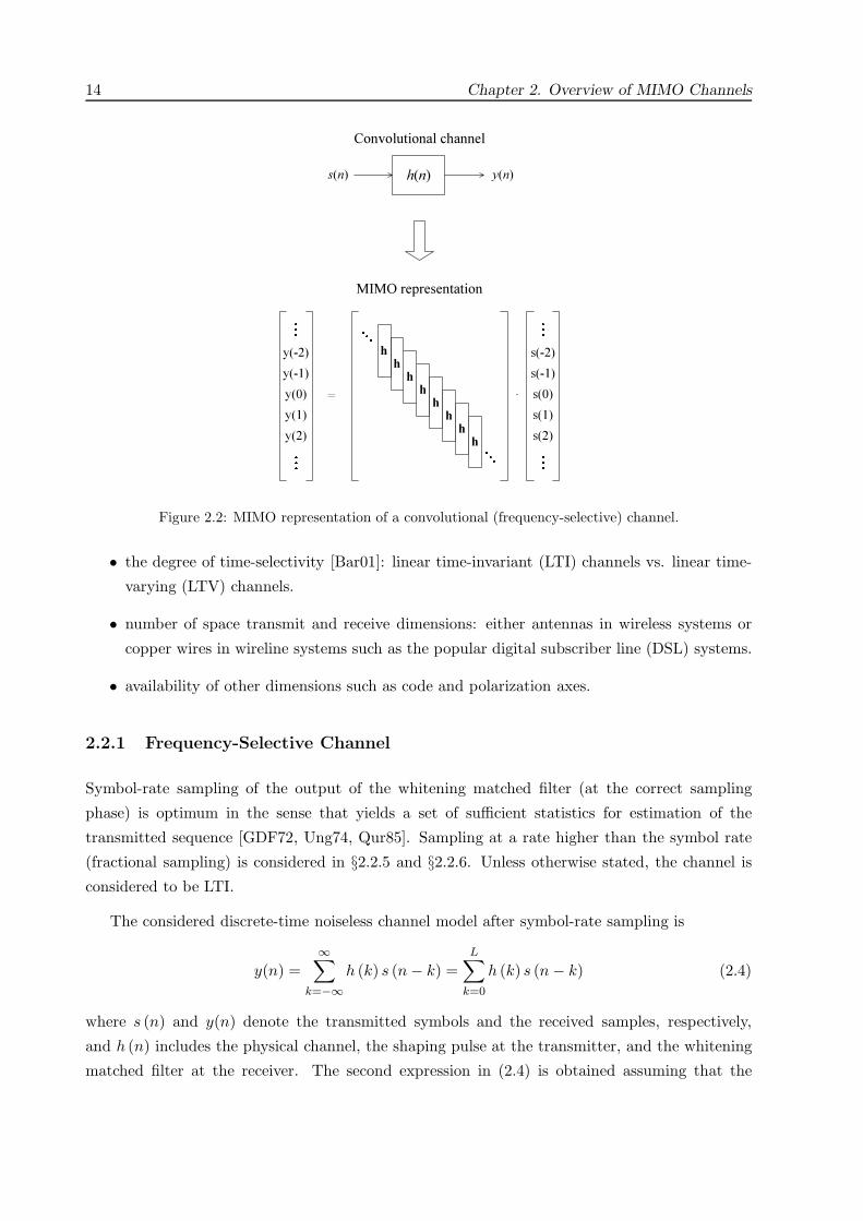
Figure 2.2: MIMO representation of a convolutional (frequency-selective) channel.
• the degree of time-selectivity [Bar01]: linear time-invariant (LTI) channels vs. linear time-
varying (LTV) channels.
• number of space transmit and receive dimensions: either antennas in wireless systems or
copper wires in wireline systems such as the popular digital subscriber line (DSL) systems.
• availability of other dimensions such as code and polarization axes.
2.2.1 Frequency-Selective Channel
Symbol-rate sampling of the output of the whitening matched filter (at the correct sampling
phase) is optimum in the sense that yields a set of sufficient statistics for estimation of the
transmitted sequence [GDF72, Ung74, Qur85]. Sampling at a rate higher than the symbol rate
(fractional sampling) is considered in §2.2.5 and §2.2.6. Unless otherwise stated, the channel is
considered to be LTI.
The considered discrete-time noiseless channel model after symbol-rate sampling is
y(n) =∞∑
k=−∞h (k) s (n − k) =
L∑k=0
h (k) s (n − k) (2.4)
where s (n) and y(n) denote the transmitted symbols and the received samples, respectively,
and h (n) includes the physical channel, the shaping pulse at the transmitter, and the whitening
matched filter at the receiver. The second expression in (2.4) is obtained assuming that the
2.2. Examples of MIMO Channels 15
channel is causal and of finite order L.3 Note that the main difficulty of dispersive channels is the
inter-symbol interference (ISI) due to the convolution of the symbols with the channel impulse
response.
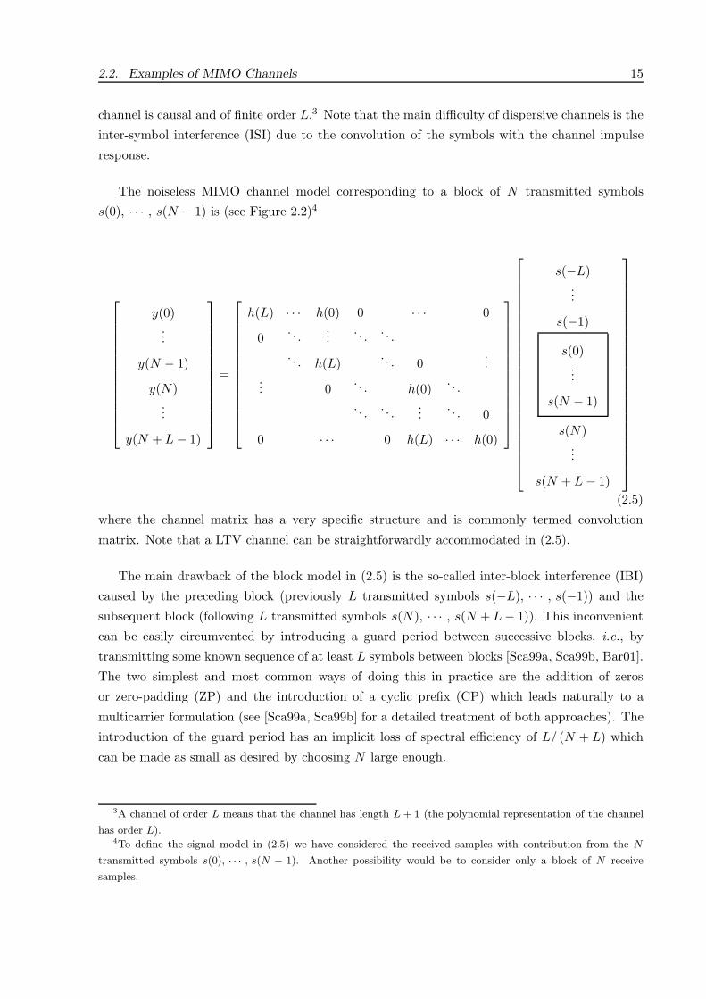
The noiseless MIMO channel model corresponding to a block of N transmitted symbols
s(0), · · · , s(N − 1) is (see Figure 2.2)4
y(0)...
y(N − 1)
y(N)...
y(N + L − 1)
=
h(L) · · · h(0) 0 · · · 0
0. . .
.... . . . . .
. . . h(L). . . 0
...... 0
. . . h(0). . .
. . . . . ....
. . . 0
0 · · · 0 h(L) · · · h(0)
s(−L)...
s(−1)
s(0)...
s(N − 1)
s(N)...
s(N + L − 1)
(2.5)
where the channel matrix has a very specific structure and is commonly termed convolution
matrix. Note that a LTV channel can be straightforwardly accommodated in (2.5).
The main drawback of the block model in (2.5) is the so-called inter-block interference (IBI)
caused by the preceding block (previously L transmitted symbols s(−L), · · · , s(−1)) and the
subsequent block (following L transmitted symbols s(N), · · · , s(N + L − 1)). This inconvenient
can be easily circumvented by introducing a guard period between successive blocks, i.e., by
transmitting some known sequence of at least L symbols between blocks [Sca99a, Sca99b, Bar01].
The two simplest and most common ways of doing this in practice are the addition of zeros
or zero-padding (ZP) and the introduction of a cyclic prefix (CP) which leads naturally to a
multicarrier formulation (see [Sca99a, Sca99b] for a detailed treatment of both approaches). The
introduction of the guard period has an implicit loss of spectral efficiency of L/ (N + L) which
can be made as small as desired by choosing N large enough.
3A channel of order L means that the channel has length L + 1 (the polynomial representation of the channel
has order L).4To define the signal model in (2.5) we have considered the received samples with contribution from the N
transmitted symbols s(0), · · · , s(N − 1). Another possibility would be to consider only a block of N receive
samples.

16 Chapter 2. Overview of MIMO Channels
(a) (b)
Original channel Effective channel
zero-padding
0
0
0
Original channel Effective channel
cyclic prefix
CP
CP
CP
DISCARD
DISCARD
DISCARD
Figure 2.3: Simplification of the channel matrix (removal of IBI) after: (a) zero-padding and (b) theutilization of the cyclic prefix.
2.2.1.1 Zero-Padding
The channel model in (2.5) is greatly simplified if at least L zeros are padded between blocks, in
which case the signal model simplifies to (see Figure 2.3(a))
y(0)...
y(N − 1)
y(N)...
y(N + L − 1)
=
h(0) 0 · · · 0...
. . . . . ....
h(L). . . 0
0. . . h(0)
.... . . . . .
...
0 · · · 0 h(L)
s(0)...
s(N − 1)
(2.6)
where the IBI has been effectively removed. In this case, a LTV channel can be readily incorpo-
rated in (2.6).
2.2.1.2 Cyclic Prefix
Another possibility to simplify the channel model in (2.5) is to introduce a cyclic prefix of at
least L symbols consisting on the last L symbols of the block. To be more specific, the trans-
mitter pre-appends the last L symbols of the block to finally transmit s(N − L), · · · , s(N −1), s(0), · · · , s(N − 1) and the receiver discards the last L received samples. The signal model
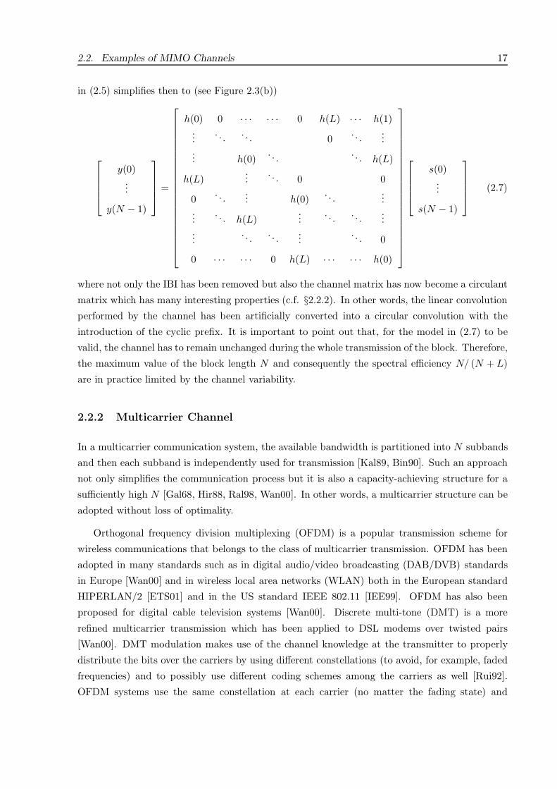
2.2. Examples of MIMO Channels 17
in (2.5) simplifies then to (see Figure 2.3(b))
y(0)...
y(N − 1)
=
h(0) 0 · · · · · · 0 h(L) · · · h(1)...
. . . . . . 0. . .
...... h(0)
. . . . . . h(L)
h(L)...
. . . 0 0
0. . .
... h(0). . .
......
. . . h(L)...
. . . . . ....
.... . . . . .
.... . . 0
0 · · · · · · 0 h(L) · · · · · · h(0)
s(0)...
s(N − 1)
(2.7)
where not only the IBI has been removed but also the channel matrix has now become a circulant
matrix which has many interesting properties (c.f. §2.2.2). In other words, the linear convolution
performed by the channel has been artificially converted into a circular convolution with the
introduction of the cyclic prefix. It is important to point out that, for the model in (2.7) to be
valid, the channel has to remain unchanged during the whole transmission of the block. Therefore,
the maximum value of the block length N and consequently the spectral efficiency N/ (N + L)
are in practice limited by the channel variability.
2.2.2 Multicarrier Channel
In a multicarrier communication system, the available bandwidth is partitioned into N subbands
and then each subband is independently used for transmission [Kal89, Bin90]. Such an approach
not only simplifies the communication process but it is also a capacity-achieving structure for a
sufficiently high N [Gal68, Hir88, Ral98, Wan00]. In other words, a multicarrier structure can be
adopted without loss of optimality.
Orthogonal frequency division multiplexing (OFDM) is a popular transmission scheme for
wireless communications that belongs to the class of multicarrier transmission. OFDM has been
adopted in many standards such as in digital audio/video broadcasting (DAB/DVB) standards
in Europe [Wan00] and in wireless local area networks (WLAN) both in the European standard
HIPERLAN/2 [ETS01] and in the US standard IEEE 802.11 [IEE99]. OFDM has also been
proposed for digital cable television systems [Wan00]. Discrete multi-tone (DMT) is a more
refined multicarrier transmission which has been applied to DSL modems over twisted pairs
[Wan00]. DMT modulation makes use of the channel knowledge at the transmitter to properly
distribute the bits over the carriers by using different constellations (to avoid, for example, faded
frequencies) and to possibly use different coding schemes among the carriers as well [Rui92].
OFDM systems use the same constellation at each carrier (no matter the fading state) and

18 Chapter 2. Overview of MIMO Channels
s(n)
S/PIFFT
(add CP)h(n)
“noise”
(discard CP)
FFT
H(2 n/N)s(n)+ “noise”
P/S S/P P/SN N+L NN+L
Figure 2.4: Classical scheme of an OFDM communication system.
therefore can be used for communications in which the transmitter does not know the channel (in
practice, of course, OFDM is always combined with coding schemes to combat the detrimental
effect of faded carriers on the performance of the system, yielding the so-called coded-OFDM
(COFDM) [Wan00]). In the multicarrier literature, however, the difference between OFDM and
DMT is sometimes overlooked and they are both interchangeably used to refer to the same scheme.
Multicarrier transmission is easily derived from the MIMO channel model of (2.7) obtained
with the utilization of the cyclic prefix. Thanks to the introduction of the cyclic prefix at the
transmitter and its removal at the receiver, the resulting channel matrix in (2.7) is a circulant
matrix whose rows are composed of cyclically shifted versions of a sequence [Hor85]. Circulant
matrices have a very interesting and useful property [Lan69, Gra72]: the eigenvectors are inde-
pendent of the specific channel coefficients and are always given by complex exponentials. To be
more precise, the eigenvalue decomposition (EVD) of the circulant channel matrix in (2.7) is
h(0) 0 · · · · · · 0 h(L) · · · h(1)...
. . . . . . 0. . .
...... h(0)
. . . . . . h(L)
h(L)...
. . . 0 0
0. . .
... h(0). . .
......
. . . h(L)...
. . . . . ....
.... . . . . .
.... . . 0
0 · · · · · · 0 h(L) · · · · · · h(0)
= FHDHF (2.8)
where F = [f0, · · · , fN−1] is the unitary discrete Fourier transform (DFT) (with fk 1√N
[1, e−j 2πN
k, e−j 2πN
2k, · · · , e−j 2πN
(N−1)k]T ) and DH = diag(H (2πk/N)N−1
k=0
)(with H (w) =∑L
n=0 h(n)e−jwn being the channel transfer function) is a diagonal matrix with the DFT coeffi-
cients as diagonal elements [Lan69, Gra72]. Note that the eigenvectors of the circulant matrix
are given by f∗k for 0 ≤ k ≤ N − 1.
As a consequence of the simple EVD of a circulant matrix, such a channel can be easily
diagonalized by performing the inverse DFT (IDFT) at the transmitter s = FHs (s contains the
temporal transmitted samples) and the DFT at the receiver y = Fy (y contains the temporal

2.2. Examples of MIMO Channels 19
received samples). In practice, the inverse fast Fourier transform (IFFT) and the fast Fourier
transform (FFT) are used (see Figure 2.4 for a scheme of the whole communication process).
As a consequence of the diagonalization of the channel matrix, the communication is effectively
performed over a set of N parallel and independent subchannels with gains H (2πk/N)N−1k=0 :
y(k) = H (2πk/N) s(k) + n(k) 0 ≤ k ≤ N − 1 (2.9)
or in matrix form
y = DHs + n (2.10)
where y =[y(0), · · · , y(N − 1)]T , s = [s(0), · · · , s(N − 1)]T , and n = [n(0), · · · , n(N − 1)]T .
It is remarkable that with a multicarrier approach, the original frequency-selective channel
with ISI and IBI is transformed into a set of parallel flat subchannels that can be straightforwardly
equalized. In addition, the different carriers can be used for multiplexing several users such as
in Orthogonal Frequency Division Multiple Access (OFDMA), where different users are assigned
different non-overlapping carriers, and in multicarrier CDMA (MC-CDMA), where each user
spreads its signal over all the carriers by means of a spreading code [Wan00].
As a final comment, it is worth pointing out that a multicarrier system need not be imple-
mented following the described block approach using the FFT and the IFFT. Instead, it can be
implemented using banks of orthogonal filters [Aka98].
2.2.3 Multi-Antenna Wireless Channel
Among the scenarios that lead to MIMO representations, perhaps the most popular is that
of wireless communications when multiple antennas are used at both the transmitter and the
receiver (see Figure 2.5). The popularity of this particular scenario is mainly due to recent
studies indicating a linear increase of capacity with the number of antennas [Tel95, Fos98] (see
also [Shi98, Shi00, Chu02]).
To exploit antenna arrays in wireless communication, it is necessary to obtain an accurate, yet
tractable, modeling of the MIMO channel. Existing models represent two extreme approaches.
On the one hand is the statistical modeling which is a tractable and idealized abstraction of spatial
propagation characteristics [Tel95, Fos98]. On the other hand are the parametric physical models
which explicitly relate the scattering environment to the channel coefficients and dictate their
statistics but are less tractable due to the nonlinearity in the spatial angles [Say02]. Some attempts
at bridging the gap between the two modeling philosophies are [Say02, Ges02, Shi00, Ral98].

20 Chapter 2. Overview of MIMO Channels
nT antennas
TRANSMITTER RECEIVER
nR antennas
s(t) y(t)
Scattering
medium
y1(t)
y2(t)
yn(t)R
s1(t)
s2(t)
sn(t)T
Figure 2.5: Example of a MIMO channel arising in wireless communications when multiple antennas areused at both the transmitter and the receiver.
2.2.3.1 Flat Multi-Antenna Wireless Channel
For the case of a flat channel, the MIMO channel model of (2.1) y = Hs + n is readily obtained
defining the channel matrix as
H =
h11 h12 · · · h1nT
h21. . .
......
. . ....
hnR1 · · · · · · hnRnT
(2.11)
where hij is the fading coefficient between the jth transmit antenna and the ith receive one. In
this case, the channel matrix H is in general a full matrix with no structure. Note that the
channel matrix may or may not vary at each transmission.
2.2.3.2 Frequency-Selective Multi-Antenna Wireless Channel
For the frequency-selective case, a discrete-time convolution with channel matrix coefficient is
obtained (similarly to (2.4)):
y(n) =L∑
k=0
H (k) s (n − k) + n(n) (2.12)
2.2. Examples of MIMO Channels 21
sk H(t)
n1(t)
IFFT(add CP)
Antenna 1
Antenna nT
nT
(discard CP)
FFT
nR
yk
Carrier k Carrier k
nn(t)R
nR x n
T
Antenna 1
Antenna nR
IFFT(add CP)
(discard CP)
FFT
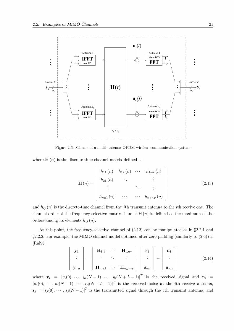
Figure 2.6: Scheme of a multi-antenna OFDM wireless communication system.
where H (n) is the discrete-time channel matrix defined as
H (n) =
h11 (n) h12 (n) · · · h1nT(n)
h21 (n). . .
......
. . ....
hnR1 (n) · · · · · · hnRnT(n)
(2.13)
and hij (n) is the discrete-time channel from the jth transmit antenna to the ith receive one. The
channel order of the frequency-selective matrix channel H (n) is defined as the maximum of the
orders among its elements hij (n).
At this point, the frequency-selective channel of (2.12) can be manipulated as in §2.2.1 and
§2.2.2. For example, the MIMO channel model obtained after zero-padding (similarly to (2.6)) is
[Ral98]
y1
...
ynR
=
H1,1 · · · H1,nT
.... . .
...
HnR,1 · · · HnR,nT
s1
...
snT
+
n1
...
nnR
(2.14)
where yi = [yi(0), · · · , yi(N − 1), · · · , yi(N + L − 1)]T is the received signal and ni =
[ni(0), · · · , ni(N − 1), · · · , ni(N + L − 1)]T is the received noise at the ith receive antenna,
sj = [sj(0), · · · , sj(N − 1)]T is the transmitted signal through the jth transmit antenna, and
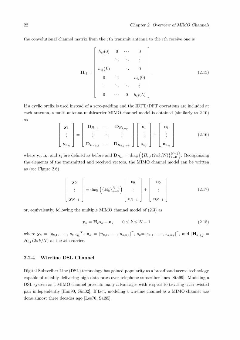
22 Chapter 2. Overview of MIMO Channels
the convolutional channel matrix from the jth transmit antenna to the ith receive one is
Hij =
hij(0) 0 · · · 0...
. . . . . ....
hij(L). . . 0
0. . . hij(0)
.... . . . . .
...
0 · · · 0 hij(L)
. (2.15)
If a cyclic prefix is used instead of a zero-padding and the IDFT/DFT operations are included at
each antenna, a multi-antenna multicarrier MIMO channel model is obtained (similarly to 2.10)
as
y1
...
ynR
=
DH1,1 · · · DH1,nT
.... . .
...
DHnR,1 · · · DHnR,nT
s1
...
snT
+
n1
...
nnR
(2.16)
where yi, ni, and sj are defined as before and DHi,j = diag(Hi,j (2πk/N)N−1
k=0
). Reorganizing
the elements of the transmitted and received vectors, the MIMO channel model can be written
as (see Figure 2.6)
y0
...
yN−1
= diag
(HkN−1
k=0
)
s0
...
sN−1
+
n0
...
nN−1
(2.17)
or, equivalently, following the multiple MIMO channel model of (2.3) as
yk = Hksk + nk 0 ≤ k ≤ N − 1 (2.18)
where yk = [yk,1, · · · , yk,nR]T , nk = [nk,1, · · · , nk,nR
]T , sk= [sk,1, · · · , sk,nT]T , and [Hk]i,j =
Hi,j (2πk/N) at the kth carrier.
2.2.4 Wireline DSL Channel
Digital Subscriber Line (DSL) technology has gained popularity as a broadband access technology
capable of reliably delivering high data rates over telephone subscriber lines [Sta99]. Modeling a
DSL system as a MIMO channel presents many advantages with respect to treating each twisted
pair independently [Hon90, Gin02]. If fact, modeling a wireline channel as a MIMO channel was
done almost three decades ago [Lee76, Sal85].

2.2. Examples of MIMO Channels 23
Central
Office
other
users/services
user 1
user 2
user L
Single office
building Cabinet
Central
OfficeNEXTFEXT
Figure 2.7: Scheme of a bundle of twisted pairs of a DSL system.
In many situations, joint processing can be assumed at one side of the link, the Central Office
(CO), whereas the other side, corresponding to the Customer Premises Equipment (CPE), must
use independent processing per user since users are geographically distributed [Gin02]. In some
cases of practical interest, however, both ends of the MIMO system are each terminated in a
single physical location, e.g., links between CO’s and Remote Terminals or links between CO’s
and private networks. This allows the utilization of joint processing at both sides of the link
[Hon90].
The dominant impairment in DSL systems is crosstalk arising from electromagnetic coupling
between neighboring twisted-pairs. Near-end crosstalk (NEXT) comprises the signals originated
in the same side of the received signal (due to the existence of downstream and upstream trans-
mission) and far-end crosstalk (FEXT) includes the signal originated in the opposite side of the
received signal. The impact of NEXT is generally suppressed by employing frequency division
duplex (FDD) to separate downstream and upstream transmission.
The general case under analysis consists of a binder group composed of L users in the same
physical location plus some other users that possibly belong to a different service provider and use
different types of DSL systems (see Figure 2.7). The MIMO channel represents the communication
of the L intended users while the others are treated as interference.
DSL channels are highly frequency-selective; as a consequence, practical communication sys-
tems are based on DMT modulations, i.e., multicarrier schemes. The channel model of such a
system is exactly as the obtained for the frequency-selective multi-antenna system considered in
§2.2.3 given by
yk = Hksk + nk 0 ≤ k ≤ N − 1 (2.19)
where yk = [yk,1, · · · , yk,L]T , nk = [nk,1, · · · , nk,L]T , sk=[sk,1, · · · , sk,L]T , and Hk is now an

24 Chapter 2. Overview of MIMO Channels
Multirate scalar convolution
Vector convolution
h(n)s(n) y(n) P
h(n)s(n) y(n)P
P x 1
Figure 2.8: Equivalence between a multirate scalar convolution and a vector convolution.
L × L square matrix in which the diagonal elements represents the channel transfer function of
each of the twisted pairs and the nondiagonal elements represent the FEXT.
2.2.5 Fractional Sampling Equivalent Channel
Excess-bandwidth systems (the majority of practical systems) utilize a transmit bandwidth higher
than the minimum (Nyquist) bandwidth. Examples are systems using spreading codes (c.f. §2.2.6)and systems using a root-raised cosine transmit shaping pulse (with a nonzero rolloff factor) for
which the baseband transmit spectrum is then band-limited to |f | ≤ (1 + β) 1/2T , where β ∈ [0, 1]
is the rolloff factor which determines the excess bandwidth [Pro95]. Although in such cases the
sampling theorem requires a sampling rate higher than the symbol rate for perfect reconstruction,
symbol-rate sampling of the output of the whitening matched filter (at the correct sampling phase)
is optimum in the sense that yields a set of sufficient statistics for estimation of the transmitted
sequence [GDF72, Ung74, Qur85].
Fractional-rate sampling (sampling at a rate higher than the symbol rate), however, has sig-
nificant practical advantages compared to symbol-rate sampling such as the insensitivity with
respect to the sampling phase and the possibility to implement in discrete time many of the
operations performed at the receiver such as the matched-filtering operation (as opposed to the
analog matched-filtering required for the symbol-rate sampling), timing recovery, frequency re-
covery, and phase recovery (c.f. [Qur85]). Fractionally-sampled systems can be modeled as a
multirate convolution which can be easily converted into the more convenient vector convolution
as we now show.
The received continuous-time noiseless signal is
yc(t) =∞∑
k=−∞s (k)hc (t − kT ) (2.20)

2.2. Examples of MIMO Channels 25
where T is the symbol period, the subscript c is used to denote continuous time signals, and hc (t)
includes the physical channel, the shaping pulse at the transmitter, and the bandpass filter at
the receiver. Note that the discrete-time signal model after sampling at the symbol rate of (2.4)
is readily obtained by defining y (n) yc(nT ) and h (n) hc (nT ).
The resulting discrete-time signal after fractional sampling every T/P seconds is given by the
multirate convolution
yc(nT/P ) =∞∑
k=−∞s (k) hc ((n − kP )T/P )
or, more compactly,
y (n) =∞∑
k=−∞s (k)h (n − kP ) (2.21)
where we have defined y (n) yc(nT/P ) and h (n) hc (nT/P ). Note that the multirate
convolution of (2.21) can be seen as the classical convolution of the channel and the upsam-
pled version of s (n) (see Figure 2.8). As is usually done in multirate theory, by stacking y (n)
and h (n) in vectors of length P as y(n) [y (nP ) , y (nP + 1) , · · · , y (nP + (P − 1))]T and
h(n) [h (nP ) , h (nP + 1) , · · · , h (nP + (P − 1))]T , the following vector discrete-time convolu-
tion signal model is obtained (see Figure 2.8):
y (n) =∞∑
k=−∞s (k)h (n − k) .
Assuming now that the oversampled channel h (n) has a finite support given by the interval
0 ≤ n < (L + 1) P , the final model is (similarly to (2.4))
y (n) =L∑
k=0
h (k) s (n − k) (2.22)
At this point, the MIMO representation can be easily obtained as was done for the scalar
discrete-time convolution signal model in §2.2.1. For example, the MIMO channel model obtained
after zero-padding is (similarly to (2.6))
y(0)...
y(N − 1)
y(N)...
y(N + L − 1)
=
h(0) 0 · · · 0...
. . . . . ....
h(L). . . 0
0. . . h(0)
.... . . . . .
...
0 · · · 0 h(L)
s(0)...
s(N − 1)
. (2.23)

26 Chapter 2. Overview of MIMO Channels
2.2.6 CDMA Channel
In a code division multiple access (CDMA) system, multiple users transmit overlapping in time
and frequency but using different signature waveforms or spreading codes (which are excess-
bandwidth shaping pulses). The discrete-time model for such systems is commonly obtained
following a matched filtering approach by sampling at the symbol rate the output of a bank
of filters where each filter is matched to one of the signature waveforms [Ver98]. An alternative
derivation of the discrete-time model for CDMA systems is based on a fractionally-sampled scheme
[Tsa96] (see also [Kle96, Jun95]) as we now briefly describe.
The signal model obtained for the fractional-rate sampling in §2.2.5 is valid for each of the users
of the CDMA system. In particular, the noiseless received continuous-time signal corresponding
to just one user is directly given by (2.20). After fractional sampling at the proper sampling rate,
the vector discrete-time convolution signal model of (2.22) is obtained. Adding up the effects of
K users, the final noiseless discrete-time signal model is
y (n) =K∑
k=1
L∑l=0
hk (l) sk (n − l) (2.24)
where each user is indexed by the index k.
At this point, the MIMO representation can be easily obtained as was done for the scalar
discrete-time convolution signal model in §2.2.1. For example, the MIMO channel model obtained
after zero-padding is obtained similarly to (2.23) but adding up the effect of all K users.
2.3 Gains and Properties of MIMO Channels
MIMO channels have a number of advantages over traditional SISO channels such as the beam-
forming (or array) gain, the diversity gain, and the multiplexing gain. The beamforming and
diversity gains are no exclusive of MIMO channels and also exist in SIMO and MISO channels.
The multiplexing gain, however, is a unique characteristic of MIMO channels. Some gains can be
simultaneously achieved while others compete and establish a tradeoff as is explained later. An
excellent overview of the gains of MIMO channels is given in [Bol02].
In a nutshell, the use of multiple dimensions at both ends of a communication link offers
significant improvements in terms of spectral efficiency and link reliability.
2.3.1 Beamforming Gain
Beamforming or array gain is the improvement in SINR obtained by coherently combining the
signals on multiple transmit or multiple receive dimensions. If the BER of a communication

2.3. Gains and Properties of MIMO Channels 27
system is plotted with respect to the transmitted power or the received power per antenna (using
a logarithmic scale), the beamforming gain is easily characterized as a shift of the curve due to
the gain in SINR.
Beamforming is a term traditionally associated with array processing or smart antennas in
wireless communications where an array of antennas exists either at the transmitter or at the
receiver [Vee88, Kri96]. We consider the concept of beamforming over any arbitrary dimension,
generalizing the traditional meaning that refers only to the space dimension.
For illustration purposes, consider a SIMO channel with the received signal given by y = hx+n
where h is the channel or signature of the desired signal and n is a white noise E [nnH ] = σ2I.
The receiver can now use a beamvector w to combine all the elements of y in a coherent way as
z = wHy. If the beamvector matches the channel, i.e., if w = h, the SINR is maximized and
given by SINR = ‖h‖2 /σ2 which clearly shows the increase of SINR with respect to using a single
receive dimension SINR = |h|2 /σ2.
2.3.2 Diversity Gain
Diversity gain is the improvement in link reliability obtained by receiving replicas of the informa-
tion signal through independently fading links, branches, or dimensions. This type of diversity is
clearly related to the random nature of the channel and is closely connected to the specific chan-
nel statistics. If the BER of a communication system is plotted with respect to the transmitted
power or the received power per antenna (using a logarithmic scale), the diversity gain is easily
characterized as the increase of the slope of the curve in the low BER region.
The basic idea is that with high probability, at least one or more of these links will not be in a
fade at any given instant. In other words, the use of multiple dimensions reduces the fluctuations
of the received signal and eliminates the deep fades [Bol02]. Clearly, this concept is suited for
wireless communications where fading exists due to multipath effects (this concept may not be
useful for wireline communications where the fading effect does not exist).
The three main forms of diversity traditionally exploited in wireless communications systems
are temporal diversity, frequency diversity, and spatial diversity [Bol02]. Other forms of diversity
include, for example, code diversity and polarization diversity [Nab02].
Transmit diversity is more difficult to exploit than receive diversity since it requires spe-
cial modulation and coding schemes, whereas receive diversity simply needs the multiple receive
dimensions to fade independently without requiring any specific modulation or coding scheme.

28 Chapter 2. Overview of MIMO Channels
2.3.3 Multiplexing Gain
Multiplexing gain is the increase of rate, at no additional power consumption, obtained through
the use of multiple dimensions at both sides of the communication link [Bol02]. While the
beamforming and the diversity gains can be obtained when multiple dimensions are present at
either the transmit or the receive side, multiplexing gain requires multiple dimensions at both
ends of the link.
The basic idea is to exploit the multiple dimensions to open up several parallel subchannels
within the MIMO channel, also termed channel eigenmodes, which lead to a linear increase in
capacity. The multiplexing property allows the transmission of several symbols simultaneously
or, in other words, the establishment of several substreams for communication (c.f. Chapters 5
and 6).
Channel Eigenmodes, Parallel Subchannels, and Established Substreams
It is important to remark that, in principle, the concepts of parallel subchannels (or channel
eigenmodes) and established substreams have a completely different meaning. Of course, they
are closely related and in many cases their meaning coincide. By parallel subchannels or channel
eigenmodes we refer to the parallel and orthogonal subchannels that the channel provides which
can be obtained via the singular value decomposition (SVD) of the channel H or via the eigenvalue
decomposition (EVD) of the squared channel HHH. The amplitude gains of the subchannels are
therefore given by the singular values of the channel and, equivalently, the power gains are given
by the eigenvalues of the squared channel, hence the name channel eigenmodes. The number of
available parallel subchannels is rank (H) or, equivalently, rank(HHH
).
By established substreams, we refer to the number of simultaneously transmitted symbols
which may or may not interfere with each other depending on whether the channel matrix is
diagonalized or not. If an orthogonality constraint is imposed over the established substreams to
obtain a set of parallel non-interfering links (diagonalized channel matrix), then the substreams
have to be established over the channel eigenmodes. In that case, both concepts become equivalent
and, as a consequence, the maximum number of substreams is clearly limited by the channel
rank. However, if we allow the established substreams not to be exactly orthogonal (not perfectly
separable), both concepts are completely different; in fact, the maximum number of substreams
is not directly limited anymore by the rank of the channel (although care has to be taken to
guarantee a certain level of performance due to the non-perfect separation of the substreams). In
Chapters 5 and 6, the possibility of establishing substreams over the channel eigenmodes both in
parallel and non-parallel fashions are explored in depth.

2.4. Transmission Techniques for MIMO Channels 29
2.3.4 Tradeoffs Between Gains
Beamforming and Diversity Gains
Beamforming gain is a concept that refers to the combination of multiple copies of the same
signal for a specific channel realization regardless of the channel statistics. Diversity gain, however,
is directly connected to the statistical behavior of the channel. With multiple receive dimensions,
both gains can be simultaneously achieved by a coherent combination of the received signals
and there is no tradeoff between them. With multiple transmit dimensions, beamforming gain
requires channel knowledge at the transmitter whereas diversity gain can be achieved even when
the channel is unknown.
Beamforming and Multiplexing Gains
Maximum beamforming gain on a MIMO channel implies that only the maximum singular
value of the channel should be used [And00] (c.f. § 5.3.1). In terms of multiplexing gain, however,
the optimum strategy is to use a subset of the channel singular values according to a water-filling
strategy [Tel95] (c.f. §5.5.4). In other words, maximum beamforming gain requires establishing
a single substream for communication, whereas maximum multiplexing gain requires, in general,
establishing several simultaneous substreams (c.f. Chapter 5).
Diversity and Multiplexing Gains
Traditionally, the design of systems has been focused on either extracting maximum diver-
sity gain or maximum multiplexing gain. Nevertheless, both gains can in fact be simultaneously
achieved, but there is a fundamental tradeoff between how much of each type of gain any commu-
nication scheme can extract as was shown in the excellent groundbreaking paper [Zhe03]. Note
that, since the diversity gain is related to the BER (it is the slope of the BER curve in the high
SINR region) and the multiplexing gain is related to the achieved rate, the diversity-multiplexing
tradeoff is essentially the tradeoff between the error probability and the data rate of a system.
2.4 State-of-the-Art of Transmission Techniques for
MIMO Channels
A plethora of communication techniques exists for transmission over MIMO channels which we
briefly review in this section. They basically depend on the degree of channel state information
(CSI) available at the transmitter and at the receiver. Clearly, the more channel information, the
better the performance of the system.
CSI at the receiver (CSIR) is traditionally acquired via the transmission of a training sequence
(pilot symbols) that allows the estimation of the channel. It is also possible to use blind methods
that do not require any training symbols but exploit knowledge of the structure of the transmitted
30 Chapter 2. Overview of MIMO Channels
signal or of the channel [Mou95, Liu96, Tsa97] (see also [Pal00, Pal01b] and references therein).
CSI at the transmitter (CSIT) cannot be directly obtained as happened with CSIR. One possible
way to achieve CSIT is to have a feedback channel from the receiver to the transmitter to send
back the channel state as side information (this technique requires the channel to be sufficiently
slowly varying and has a loss in spectral efficiency due to the utilization of part of the bandwidth
to transmit the channel state). Another traditional way to acquire CSIT is to infer knowledge
about the transmit channel from previous receive measurements [Ben01]. In general, the transmit
and receive channels may be uncorrelated since they may be separated in time and/or frequency.
In particular, in a time division duplex (TDD) system, the transmit and receive channels share
the same frequency using different time slots. Similarly, in a frequency division duplex (FDD)
system, the transmit and receive channels share the same time slot using different frequencies.
Whenever the time/frequency separation is small compared to the time/frequency coherence of
the channel, the reciprocity principle of electromagnetics implies that the instantaneous transmit
and receive channels are identical. Otherwise, even when the channel reciprocity property does
not hold, the transmit and receive channels still may show some statistical dependence which can
be exploited [Ben01].
MIMO channel modeling has attracted a significant attention in two main practical scenarios:
DSL channels and multi-antenna wireless channels. Before considering communication methods
for MIMO channels, we give a glimpse of communication techniques for systems with multiple
dimensions only at one side of the link, i.e., multiple-input single-output (MISO) and single-
input multiple-output (SIMO) channels. Transmitter diversity has traditionally been viewed more
difficult to exploit than receiver diversity and, as a consequence, processing methods for reception
clearly outnumber those for transmission. This is mainly because the transmitter is permitted
to generate a different signal at each transmit dimension (with the consequent challenging signal
design problem), whereas the receiver can only combine the copies of the received signal to achieve
a performance gain. A review of space-time processing techniques up to 1997 can be found in
[Pau97].
Regarding diversity only at the receiver, a wide variety of methods exists [Vee88, Kri96]. In
[Bal92], for example, space-time filters were designed in the frequency domain using the minimum
mean square error (MMSE) and the zero-forcing (ZF) criteria (a generalization of the classical
temporal-only case [Qur85, GDF91]). In [Win94], receive diversity with optimum combining is
shown to increase the capacity of a multiuser system. In [Cio95a, Cio95b], a comprehensive
analysis of MMSE decision feedback (MMSE-DF) space-time filters for reception is given. A
remarkable unified vision of design of space-time receive filters under the MMSE and ZF criteria
can be found in [Ari99]. In [Lag00], an array combiner in conjunction with maximum likelihood
sequence estimation (MLSE) was derived. The multiuser case has also been widely studied
[Lup89, Mos96, Jun95].

2.4. Transmission Techniques for MIMO Channels 31
No CSIT Partial CSIT Perfect CSIT
Perfect
CSIR
DifferentialSTC
Space-TimeCodes
BLAST
AntennaSelection
HybridSTC+Beamforming
RobustBeamforming
Partial
CSIR
No
CSIR
Beamforming
RobustMultiple
Beamforming
MultipleBeamforming
Figure 2.9: Classification of different communication methods as a function of the CSI at the transmitterand at the receiver.
Concerning methods with only transmit diversity, classical beamforming techniques can be
used to obtain the array gain when perfect CSIT is available [Pau97]. With partial CSIT, beam-
forming techniques can also be used [Nar98]. For the case of no CSIT, the transmit diversity
can be exploited either indirectly or directly. Indirect transmit diversity schemes convert spatial
diversity into time or frequency diversity which can then be readily exploited by the receiver
[Wit91, Ses94, Win98, Hir92]. Space-time coding (STC) techniques exploit the spatial diversity
in a direct way [Ala98, Tar98].
The more general and appealing case of simultaneous transmit and receive diversity (i.e.,
MIMO systems) is being extensively addressed since recent studies on wireless multi-antenna
MIMO channels showed a linear increase of capacity with the number of antennas [Tel95, Fos98].
It is generally assumed that perfect CSI is available at the receiver. Nevertheless, the case of no
CSI at any side of the link has also been considered using the so-called unitary and differential STC
[Hoc00a, Hoc00b]. Regarding the CSIT, there are two main families of transmission methods that
consider either no CSIT, for which STC techniques can be used, or perfect CSIT, for which linear
precoders and beamforming techniques can be designed (c.f. §2.4.1 and §2.4.2, respectively). In
practice, however, it may be more realistic to consider partial CSIT yielding robust designs (c.f.
§2.4.3). In Figure 2.9, a variety of communication techniques for MIMO channels are positioned
in a chart as a function of the required level of CSIT and CSIR.

32 Chapter 2. Overview of MIMO Channels
antenna 1
DEMUX
1:ndata bits
Channel
Encoder
antenna 2
antenna n
n
Figure 2.10: General scheme of space-time coding (STC).
2.4.1 Transmission Techniques with no CSIT
Transmission techniques that do not require CSIT can be encompassed within two main philoso-
phies: space-time coding and layered architectures. Space-time coding generalizes the classical
concept of coding on the temporal domain [Cal98] to coding on both spatial and temporal di-
mensions [Tar98]. Layered architectures refer to a particular case of a space-time coding when
a separate coding scheme is used for each spatial branch [Fos96]. This constraint on the cod-
ing scheme represents a significant reduction of complexity at the receiver. Recently, hybrid
schemes combining layered architectures with constituent space-time codes have been proposed
as a reasonable tradeoff between performance and complexity [Ari00].
2.4.1.1 Space-Time Coding
The idea of space-time coding is that the transmitter does not have CSIT (see Figure 2.9) but
introduces redundancy in the transmitted signal, both over space and time, that allows the receiver
to recover the signal even in difficult propagation situations. To be more specific, the symbols
are first encoded and then the encoded data is split into n substreams that are simultaneously
transmitted using n transmit antennas (see Figure 2.10). The received signal is decoded using a
maximum likelihood (ML) decoder. STC is indeed very effective as it combines the benefits of
forward error correction coding and diversity transmission to provide considerable performance
gains.
There are two main types of space-time coding techniques: space-time trellis coding (STTC)
and space-time block coding (STBC). The key development of the STC concept was originally
revealed in [Tar98] in the form of STTC. STTC may not be practical or cost-effective due to
the high complexity of the ML detector. In an attempt to reduce complexity, orthogonal STBC
that can be optimally decoded with a simple linear processing at the receiver were introduced
and analyzed in [Ala98, Tar99a] (see also [Gan00b, Gan01a]). In fact, the orthogonal STBC
designed for two transmit antennas in [Ala98] is so simple and useful that it has been included in
the technical specifications for the UMTS Terrestrial Radio Access (UTRA) system of the third
generation of mobile communication systems [3GP99].
It has to be noted that since 1998, an extraordinary number of publications (which we do not

2.4. Transmission Techniques for MIMO Channels 33
Encoder 1 antenna 1C3
C2
C1
C0
DEMUX
1:ndata bits
C3
C2
C1
C0
antenna 2
C2
antenna n
Encoder 2
Encoder n C1
C0
C3
...
...
...
C2
C1
C0
C2
C1
C0
C0
C1
C2
...
...
...
antenna 1
antenna 2
antenna n
HLST
DLST
Figure 2.11: General scheme of the horizontal and diagonal layered space-time (HLST and DLST) archi-tectures (also known as BLAST).
reference here) have flourished in the open literature dealing with the design of space-time codes
under different performance criteria for different scenarios such as spatially correlated channels
(see §2.4.3 for hybrids schemes combining STC with beamforming).
2.4.1.2 Layered Space-Time Architecture
Layered architectures, also known as layered space-time (LST) codes, are constructed by assem-
bling one-dimensional (1-D) constituent codes (see Figure 2.11). The original data stream is
demultiplexed into n data streams and then each data stream is encoded in such a way that
the encoders can proceed without sharing any information with each other, i.e., independent
encoding. Note that CSIT is not required (see Figure 2.9). At the receiver, with the use of
interference suppression and interference cancellation, these constituent codes can be separated
and then decoded using conventional decoding algorithms developed for 1-D codes, leading to a
much lower decoding complexity compared to ML decoding.
A diagonal LST (DLST) architecture was originally proposed by Foschini in 1996 [Fos96] (see
Figure 2.11). In [Fos99], the less complex horizontal LST (HLST)5 architecture was considered
and the name BLAST was coined standing for Bell-labs LAyered Space-Time architecture (see
Figure 2.11). In [Shi99], the layered architecture was further analyzed, giving error probability
expressions and considering different types of constituent codes.
Hybrids strategies that combine layered architectures with space-time processing techniques
5The horizontal LST architecture is sometimes in the literature referred to as vertical LST architecture.

34 Chapter 2. Overview of MIMO Channels
constitute a very promising solution in systems with many antennas to reduce complexity while
keeping performance. In [Tar99b], space-time codes were used as constituent codes of a layered
architecture for systems with a large number of transmit antennas to keep complexity at a reason-
able level. In [Ari00], the hybrid scheme went one step further by encompassing turbo space-time
processing within the layered architecture.
2.4.2 Transmission Techniques with Perfect CSIT
When perfect CSIT is available, the transmission can be adapted to each channel realization using
signal processing techniques (c.f. §2.5.1). Historically speaking, there are two main scenarios
that have motivated the development of communication methods for MIMO channels with CSIT:
wireline channels and wireless channels.
The initial motivation to design techniques for communication over MIMO channels was
originated in wireline systems by treating all the links within a bundle of cables as a whole [Lee76,
Sal85, Hon90, Yan94b, Yan94a]. In [Kas90], a vector coding technique consisting on partitioning
a frequency-selective SISO channel into an independent set of parallel ISI-free channels by means
of the channel eigenvectors was developed. Optimal bit allocation and energy distribution over
the set of parallel subchannels, where coset codes were applied, was also given. In [Rui92], the
channel eigenvectors were replaced by the discrete multiple tones of the IDFT, leading to a lower
complexity scheme. The idea of partitioning can be seen as a generalization and optimization
of multitone methods traceable back to at least 1964 (Holsinger). In [AD96, Gin02], a decision-
feedback equalizer (DFE) was considered at the receiver and also at the transmitter in the form
of a precoder in [Gin02].
Another more recent source of motivation to design methods for communication over MIMO
channels can be found in multi-antenna wireless systems [Ral98, And00, AD00, Sam01, Sca02].
In [Ral98], a spatio-temporal vector coding architecture was introduced for burst transmission
over MIMO channels. To reduce complexity a simplified version called discrete matrix multi-
tone space-frequency coding structure was also proposed. Transmit and receive linear processing
(equivalently, multiple beamforming) was jointly designed in [Sam01, Sca02]. In [AD00], finite-
length transmit and receive filters were derived assuming a DFE at the receiver. In [And00], the
flat multi-antenna MIMO case was considered providing useful insights from the point of view
of beamforming. For the case of single beamforming, a low-complexity transmission method was
proposed in which knowledge of the whole channel matrix is not necessary at any side of the link
(see Figure 2.9). In [Sca99a, Sca99b], a frequency-selective SISO channel was transformed into a
MIMO channel by means of a multirate filterbank scheme.

2.4. Transmission Techniques for MIMO Channels 35
2.4.3 Transmission Techniques with Partial CSIT
As previously mentioned, it is more reasonable in practice to consider partial CSIT. We now
describe two existing techniques to cope with this situation.
2.4.3.1 Hybrid Schemes
The basic idea is to enhance the performance of a space-time code, for which no CSIT is required,
by combining it with some type of beamforming or linear precoding, for which the existing
(possibly partial) CSIT can be exploited (see Figure 2.9).
In [Neg99], the combination of beamforming and space-time codes in a system with multiple
antennas at both sides of the link was considered aiming at maximizing the average SNR for
scenarios with partial CSIT. The appealing combination of beamforming and space-time codes
with partial CSIT was also taken in [Jon02] from a statistical viewpoint to minimize the pairwise
error probability for different degrees of CSIT (from no CSIT to perfect CSIT). In [Hon03] a
space-time code was combined with a linear precoding matrix to use the statistical knowledge
on the channel. A virtual representation of the MIMO channel was used in [Liu02] to adapt
space-time codes to the channel realization to cope with the channel correlation.
2.4.3.2 Robust Beamforming under Channel Estimation Errors
Since perfect CSIT is never available in practice, it is always necessary to quantify the degradation
due to channel estimation errors of any system that assumes perfect CSIT (the degradation due to
imperfect CSIR should also be quantified, e.g., [Gan01b]). However, it is always better to obtain
robust solutions by directly taking into account the existence of channel estimation errors when
designing the system (see Figure 2.9). There have been some attempts to obtain robust solutions
as we now mention (see also Chapter 7 to see how to take into account channel estimation errors
in the beamforming schemes proposed in Chapters 5 and 6).
In [Cox87, Bel00, Vor03], robust designs were obtained in the context of classical receive
beamforming. Robust designs of transmit beamforming with imperfect CSIT have been consid-
ered according to different criteria such as error probability [Wit95], SNR [Nar98], and mutual
information [Nar98, Vis01]. In [Vis01], robust transmission schemes were obtained for imperfect
CSIT in the form of either the mean or the covariance matrix of the channel distribution function
(see also [Jaf01] for the case of multiple transmit and receive antennas). In [Nar98], imperfect
CSIT was considered not only stemming from channel estimation errors but also from the effect
of quantizing the channel estimate at the receiver to be fed back as side information.
Partial CSI for the design of single-antenna systems modeled as MIMO channels was consid-
ered in [Bar01], where a design maximizing the average SNR was adopted. A stochastic robust

36 Chapter 2. Overview of MIMO Channels
design for MIMO channels was obtained in [Mil00] to minimize the sum of MSE’s with imper-
fect CSIT and perfect CSIR (a ZF receiver was assumed). In [Rey02], a robust solution to
the minimization of the sum of the MSE’s was derived for multi-antenna multicarrier systems
with imperfect CSIT and CSIR. In [Ise03], a robust minimum BER solution was designed for
single-antenna multicarrier systems with imperfect CSIT and perfect CSIR. In [Ben99, Ben01],
a worst-case robust approach was taken in the context of multiuser communications between
several mobiles and a multi-antenna base station.
2.4.4 The Multiuser Case
The more general case of multiuser communications has also been studied in the literature al-
though to a lesser extent. Interestingly, beamforming happens to be optimal for multiuser MIMO
systems provided that the number of users is sufficiently high [Rhe01b].
In [RF98a, RF98b, Vis99a], beamforming techniques were derived for uplink and down-
link communications in multiuser systems with multiple antennas only at the base station. In
[Ben99, Ben01], a more general scenario including robustness under channel estimation errors was
considered.
In [Vis02], an interesting downlink transmission scheme was proposed based on opportunistic
beamforming by transmitting at each time to a single user.
2.5 Linear Signal Processing for MIMO Channels
2.5.1 Linear Signal Processing
In a communication system, the optimal receiver is given by the Maximum Likelihood (ML)
detector, also known as Maximum Likelihood Sequence Estimation (MLSE) [Pro95]. The ML
detector is a nonlinear signal processing method and has an exponential complexity in the number
of channel dimensions or transmitted symbols. If the structure of the channel matrix is adequate,
i.e., if it can be modeled as a hidden Markov model, the MLSE can be efficiently implemented
with the Viterbi algorithm [Pro95]. To further reduce the complexity, other suboptimal nonlinear
signal processing techniques can be used such as the popular Decision-Feedback (DF) scheme
[Qur85, GDF91, Yan94a, Cio95a, Cio95b, Ari99] whose main drawback is the error propagation
due to the feedback mainly at low SNR. A more pragmatic solution is the utilization of linear
signal processing techniques which have low complexity and no error feedback problems at the
expense of a worse performance. We now focus on linear transmit-receive processing schemes
for MIMO systems. The meaning of the term beamforming, initially used for smart antennas6
6By smart antennas we refer to the classical scenario in which only one side of the communication link has
multiple antennas.
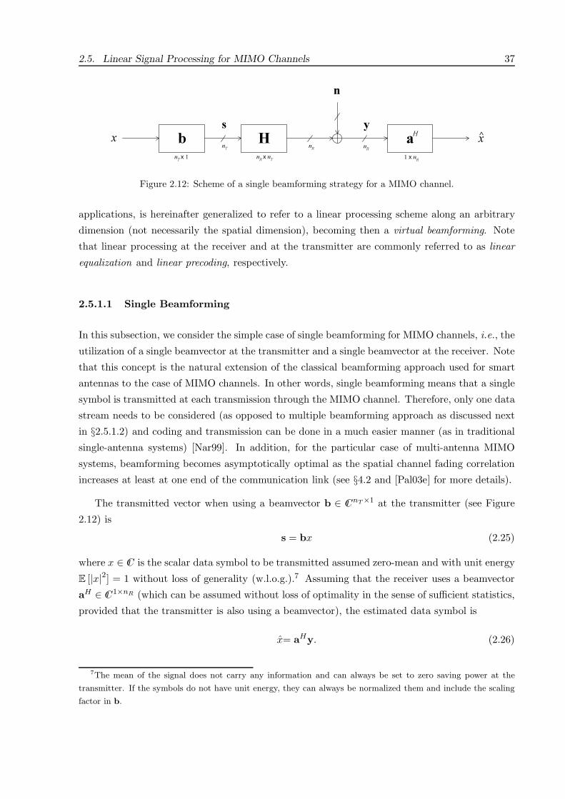
2.5. Linear Signal Processing for MIMO Channels 37
Hx b aH
n
ys
x^
nT x 1
nT
nR x n
T
nR
nR
1 x nR
Figure 2.12: Scheme of a single beamforming strategy for a MIMO channel.
applications, is hereinafter generalized to refer to a linear processing scheme along an arbitrary
dimension (not necessarily the spatial dimension), becoming then a virtual beamforming. Note
that linear processing at the receiver and at the transmitter are commonly referred to as linear
equalization and linear precoding, respectively.
2.5.1.1 Single Beamforming
In this subsection, we consider the simple case of single beamforming for MIMO channels, i.e., the
utilization of a single beamvector at the transmitter and a single beamvector at the receiver. Note
that this concept is the natural extension of the classical beamforming approach used for smart
antennas to the case of MIMO channels. In other words, single beamforming means that a single
symbol is transmitted at each transmission through the MIMO channel. Therefore, only one data
stream needs to be considered (as opposed to multiple beamforming approach as discussed next
in §2.5.1.2) and coding and transmission can be done in a much easier manner (as in traditional
single-antenna systems) [Nar99]. In addition, for the particular case of multi-antenna MIMO
systems, beamforming becomes asymptotically optimal as the spatial channel fading correlation
increases at least at one end of the communication link (see §4.2 and [Pal03e] for more details).
The transmitted vector when using a beamvector b ∈ CI nT ×1 at the transmitter (see Figure
2.12) is
s = bx (2.25)
where x ∈ CI is the scalar data symbol to be transmitted assumed zero-mean and with unit energy
E [|x|2] = 1 without loss of generality (w.l.o.g.).7 Assuming that the receiver uses a beamvector
aH ∈ CI 1×nR (which can be assumed without loss of optimality in the sense of sufficient statistics,
provided that the transmitter is also using a beamvector), the estimated data symbol is
x= aHy. (2.26)
7The mean of the signal does not carry any information and can always be set to zero saving power at the
transmitter. If the symbols do not have unit energy, they can always be normalized them and include the scaling
factor in b.
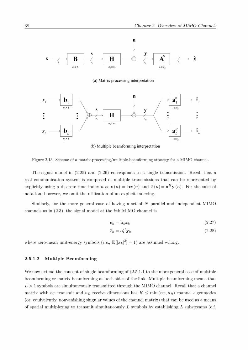
38 Chapter 2. Overview of MIMO Channels
H
nR x n
T
x B
nT x L
A
L x nR
H
x^
H
nR x n
T
na1
H
b1
x1
bL
xL
nT x 1
aL
H
x1
nT
nR
y
xL
n
nR
y
nTL L
(a) Matrix processing interpretation
(b) Multiple beamforming interpretation
1 x nR
s
s
^
^
nT x 1 1 x n
R
Figure 2.13: Scheme of a matrix-processing/multiple-beamforming strategy for a MIMO channel.
The signal model in (2.25) and (2.26) corresponds to a single transmission. Recall that a
real communication system is composed of multiple transmissions that can be represented by
explicitly using a discrete-time index n as s (n) = bx (n) and x (n)= aHy (n). For the sake of
notation, however, we omit the utilization of an explicit indexing.
Similarly, for the more general case of having a set of N parallel and independent MIMO
channels as in (2.3), the signal model at the kth MIMO channel is
sk = bkxk (2.27)
xk = aHk yk (2.28)
where zero-mean unit-energy symbols (i.e., E [|xk|2] = 1) are assumed w.l.o.g.
2.5.1.2 Multiple Beamforming
We now extend the concept of single beamforming of §2.5.1.1 to the more general case of multiple
beamforming or matrix beamforming at both sides of the link. Multiple beamforming means that
L > 1 symbols are simultaneously transmitted through the MIMO channel. Recall that a channel
matrix with nT transmit and nR receive dimensions has K ≤ min (nT , nR) channel eigenmodes
(or, equivalently, nonvanishing singular values of the channel matrix) that can be used as a means
of spatial multiplexing to transmit simultaneously L symbols by establishing L substreams (c.f.

2.5. Linear Signal Processing for MIMO Channels 39
Hk
xk B
kA
k
H
nk
yk
L L
sk
x1
xN
xk
^
x1
^
xN
^
nT x L
nT
nR x n
T
nR
nR
L x nR
Figure 2.14: Scheme of a non-cooperative multiple beamforming strategy for a set of N parallel MIMOchannels.
§2.3.3). For generality, we allow for arbitrary values of L; in a practical system we will typically
have L ≤ K to have an acceptable performance.
The transmitted vector when using a transmit linear processing matrix B ∈ CI nT×L (see Figure
2.13(a)) is
s = Bx =L∑
i=1
bixi (2.29)
where x = [x1 · · · xL]T ∈ CI L×1 is the vector of L data symbols assumed zero-mean, with unit
energy, and uncorrelated (white) 8E [xxH ] = IL w.l.o.g. Vector bi is the ith column of matrix
B and can be regarded as the beamvector associated to the ith data symbol xi, i.e., a multiple
beamforming architecture (see Figure 2.13(b)). Assuming that the receiver uses the receive linear
processing matrix AH ∈ CI L×nR , the estimated data vector is
x = AHy. (2.30)
Consider now the more general case of having a set of N parallel and independent MIMO
channels as in (2.3). To take into account the possibility of transmitting a different number of
symbols through each MIMO channel, we consider that Lk symbols are transmitted at the kth
MIMO channel and, therefore, a total of LT =∑N
k=1 Lk symbols are transmitted. Note that the
total number of transmit and receive dimensions is now nT N and nRN , respectively. Regarding
the linear processing at the transmitter and at the receiver, two different cases are considered as
we now describe [Pal03c]:
• Noncooperative scheme: this is when an independent signal processing per MIMO channel
is used such as in a multi-antenna muticarrier system with independent processing at each8White symbols account, for example, to having independent bit streams. In case of having colored symbols
due, for example, to a coded transmission [GDF91], a prewhitening operation can be performed prior to precoding
at the transmitter and the corresponding inverse operation can be performed after the equalizer at the receiver.
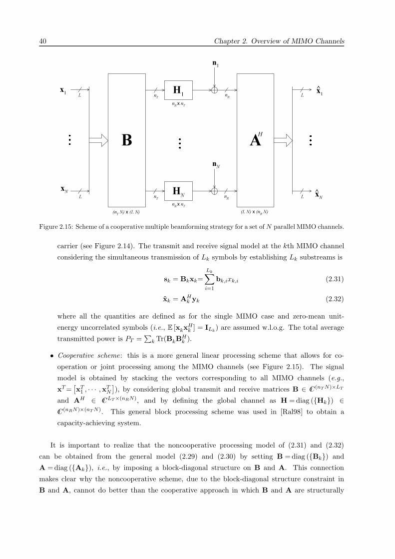
40 Chapter 2. Overview of MIMO Channels
x1
B
nN
L
xN H
N
A
xN
^
x1
(nT N) x (L N)
nR x n
T
n1
H1
L
L
L
H
nT
nT
nR
nR
nR x n
T
(L N) x (nR N)
Figure 2.15: Scheme of a cooperative multiple beamforming strategy for a set of N parallel MIMO channels.
carrier (see Figure 2.14). The transmit and receive signal model at the kth MIMO channel
considering the simultaneous transmission of Lk symbols by establishing Lk substreams is
sk = Bkxk=Lk∑i=1
bk,ixk,i (2.31)
xk = AHk yk (2.32)
where all the quantities are defined as for the single MIMO case and zero-mean unit-
energy uncorrelated symbols (i.e., E [xkxHk ] = ILk
) are assumed w.l.o.g. The total average
transmitted power is PT =∑
k Tr(BkBHk ).
• Cooperative scheme: this is a more general linear processing scheme that allows for co-
operation or joint processing among the MIMO channels (see Figure 2.15). The signal
model is obtained by stacking the vectors corresponding to all MIMO channels (e.g.,
xT =[xT
1 , · · · ,xTN
]), by considering global transmit and receive matrices B ∈ CI (nT N)×LT
and AH ∈ CI LT×(nRN), and by defining the global channel as H = diag (Hk) ∈CI (nRN)×(nT N). This general block processing scheme was used in [Ral98] to obtain a
capacity-achieving system.
It is important to realize that the noncooperative processing model of (2.31) and (2.32)
can be obtained from the general model (2.29) and (2.30) by setting B = diag (Bk) and
A =diag (Ak), i.e., by imposing a block-diagonal structure on B and A. This connection
makes clear why the noncooperative scheme, due to the block-diagonal structure constraint in
B and A, cannot do better than the cooperative approach in which B and A are structurally

2.5. Linear Signal Processing for MIMO Channels 41
unconstrained. Intuitively, the reason why the cooperative approach (see Figure 2.15) has poten-
tially a better performance is that it can reallocate the symbols among the MIMO channels in
an intelligent way (e.g., if one MIMO channel is a bad channel, it will try to use other MIMO
channels instead), whereas the noncooperative scheme (see Figure 2.14) will always transmit Lk
symbols through the kth MIMO channel no matter the channel state.
2.5.2 Transmit Power Constraint
In this dissertation, we consider systems limited in the average total transmitted power. In
particular, a constraint on the average power utilized to transmit the N -symbol (or block of
symbols) in the single beamforming case is
N∑k=1
E [ ‖sk‖22 ] =
N∑k=1
‖bk‖22 ≤ PT (2.33)
where PT is power in units of energy per transmission (the power in units of energy per second
is Ps = PT /Ts where Ts is the duration of a transmission). Similarly, a constraint on the average
power utilized to transmit the LT -symbol (or block of symbols) in the multiple beamforming case
isN∑
k=1
E [ ‖sk‖22 ] =
N∑k=1
‖Bk‖2F =
N∑k=1
Tr(BkB
Hk
) ≤ PT . (2.34)
Note that the power constraint for the case of a single MIMO channel is readily obtained partic-
ularizing for N = 1.
Whenever the channel is random, the previous power constraint (either (2.33) or (2.34))
corresponds to a short-term power constraint in the sense that for each set of transmit matrices
(in general designed as a function of the channel state), the power averaged over the possible
transmitted symbols is constrained by PT . On the other hand, a long-term power constraint
can be considered by further averaging over all channel states. Such a constraint allows the
transmitted power to exceed PT for some channel states as long as it is compensated for some
other channel states so that the power averaged over all channel states does not exceed PT
[Cai99b, Big01]. More generally, the power constraint can be averaged over NT transmissions
which contains as particular cases the short-term power constraint (for NT = 1) and the long-
term power constraint (for NT → ∞). The higher the value of NT , the less restrictive is the
power constraint (the long-term power constraint is clearly the least restrictive). A general case
of NT > 1, however, requires knowledge of some future realizations of the channel (or of the
channel statistics for NT → ∞) [Bar01]. Note that the case of a finite NT > 1 can be easily
included in the short-term power constraint of (2.33)-(2.34) by defining a block-diagonal channel
matrix that contains along the main diagonal the channel matrices corresponding to the NT
transmissions. In the limiting case of NT → ∞ a similar approach can be taken if the probability
density function (pdf) of the channel eigenvalues is known [Gol97, Bar01].
42 Chapter 2. Overview of MIMO Channels
For completeness, we now list other possible types of power constraints that may be interesting
depending on the specific scenario:
• Power constraint per MIMO channel. This only applies to the case of multiple MIMO
channels and consists on further constraining the power used in each MIMO channel:
‖Bk‖2F ≤ Pk.
• Power constraint per dimension. Similarly, the power used in the ith dimension can be
constrained:∑N
k=1 E [ |sk,i|2] =∑N
k=1 ‖ [Bk]i,: ‖22 ≤ Pi (this constraint will be considered
in Chapter 5 in the context of multi-antenna systems to control the dynamic range of the
signal transmitted by each antenna).
• Peak power constraint per MIMO channel. Noting that maxi |sk,i|2 ≤ sHk sk =
xHk BH
k Bkxk ≤ λmax
(BH
k Bk
) ‖xk‖22, the average peak power can be controlled by con-
straining the maximum eigenvalue of the squared transmit matrix: E [maxi |sk,i|2] ≤λmax
(BH
k Bk
)Lk ≤ P peak
k [Gan00a, Sca02] (this constraint is briefly considered in Chapter
5).
• Peak power constraint. Similarly to the peak power constraint per MIMO channel, this
one constrains the maximum eigenvalue of all MIMO channels: maxk
λmax
(BH
k Bk
)Lk
≤P peak
T .
• Peak average power constraint. This variation of the eigenvalue constraint is useful
for multicarrier systems where the signals corresponding to different MIMO channel are
added together: maxi∑N
k=1 E [ |sk,i|2] ≤∑N
k=1 E [xHk BH
k Bkxk] ≤∑N
k=1 λmax
(BH
k Bk
)Lk ≤
P peak-aveT .
• Instantaneous power constraint. This is in fact a family of power constraints based on
constraining the system for each realization of the data symbols xk instead of averag-
ing them. For example, an instantaneous total power constraint would be∑N
k=1 ‖sk‖22 =∑N
k=1 xHk BH
k Bkxk ≤ P instT . This type of constraints is very difficult to handle.
• Worst-case power constraint. The instantaneous power constraint can be simplified by
considering that for each channel state, the transmitter has to be designed so that the
constraint is satisfied for all possible xk’s: maxxk∑N
k=1 xHk BH
k Bkxk ≤ PwcT .
2.5.3 Canonical Channel Model
The canonical channel model is a reduction of the original channel model in which extraneous
dimensions are eliminated and which have other nice properties such as having a positive definite
Hermitian channel matrix and a noise with covariance matrix identical to the canonical channel
(see [Cio97] for a detailed treatment of the canonical channel model). The canonical channel

2.5. Linear Signal Processing for MIMO Channels 43
Hx B
n
y
nT x L n
R x n
T
nR
nR
Rn
-1/2
nRx n
R
B H Rn
-1/2
L x nR
HH
noise-whitening matched filter
canonical channel model
x Hcan
ncan
Hcan
= BHHHRnHB, E[n
canncan
] = Hcan
-1
ycan
H
ycan
Figure 2.16: Scheme of the canonical channel model.
model is known to produce sufficient statistics for the estimation of the transmitted symbols
[Sch91, Ch. 3][Cio97] and to be capacity-lossless from an information-theoretic point of view
[Cio97].
It is obtained by a series of information-lossless linear transformations on the channel out-
put y. The first transformation consists of a noise-whitening stage R−1/2n producing the global
channel C = R−1/2n HB. Assume for the moment that L ≤ rank (C). The principle of the suf-
ficiency of matched filtering may be now applied and the second stage is the matched filter
CH = BHHHR−1/2n . The canonical output signal after these two stages is
ycan = Hcanx + ncan (2.35)
where Hcan = BHHHR−1n HB is the canonical channel and E [ncann
Hcan] = Hcan is the covariance
matrix of the canonical noise (see Figure 2.16).
For the particular case of single beamforming, the canonical channel reduces to a scalar channel
hcan = bHHHR−1n Hb with a scalar noise ncan with covariance equal to the canonical channel
E [|ncan|2] = hcan.
Consider now the case L > rank (C) and define the effective number of transmit dimensions
as L = min (L, rank (C)). It is clear that the component of x that lies in the right null space
(kernel) of C, i.e., P⊥c x where P⊥
c is the projection onto the kernel, may be disregarded since it
is undetectable. In other words, the output signal depends only on the effective input xeff= Pcx

44 Chapter 2. Overview of MIMO Channels
and, therefore, only xeff can convey information (note that this does not mean that more than
L symbols cannot be transmitted, although they will not be perfectly separable9 ). To be more
exact, using the singular value decomposition (SVD) C = UΣVH , the output at the receiver
depends only on xeff= V1VH1 x where V1 contains the right singular vectors of C associated with
nonzero singular values.
2.5.4 Figures of Merit: MSE, SINR, BER, and Capacity
We now describe the four common measures of the performance of a communication system:
MSE, SINR, BER, and capacity. The MSE, SINR, and BER arise naturally from a estimation
framework. The notion of channel capacity, however, comes from a rather different information-
theoretic perspective.
2.5.4.1 Average vs. Outage Quantities
Regardless of the specific measure that is used to quantify the performance of a system, when
the channel is deterministic or when it changes at a very slow pace (such as in some wireline
systems), the measurement is given by a single value. However, when the channel is random, due
for example to fading in wireless channels [Pro95], the measurement becomes a random quantity.
To properly characterize the system performance in such cases, the pdf of the measurement
should be obtained. In practice, however, it is more convenient to characterize a system with a
single value rather than with the whole pdf. The two most common ways of doing it is with the
average value and with the outage value of the measurement whose choice depends on whether
the scenario is ergodic or non-ergodic.
The ergodic scenario arises in communications without delay constraints in which the trans-
mission duration is long enough to reveal the long-term ergodic properties of the fading channel
(assuming that the channel is an ergodic process in time). In such cases, average values such as
the average BER or the average capacity (also termed ergodic capacity) are useful measures.
The ergodicity assumption, however, is not necessarily satisfied in practical communication
system with stringent delay constraints operating on fading channels, because no significant
channel variability may occur during the whole transmission. In these circumstances, outage
values are more appropriate and meaningful than average values which give more conservative
9As a simple illustrative example, consider the following transmission of 101 symbols through 100 parallel SISO
channels with unit gain: transmit 100 symbols independently on each of the 100 SISO channels and the last symbol
simultaneously through all SISO channel (scaled down by a properly chosen factor) in a CDMA fashion. The first
100 symbols will see a slight increase of noise and the last symbol using matched filter receiver in a CDMA fashion
will benefit from the processing gain.
2.5. Linear Signal Processing for MIMO Channels 45
and unrealistic quantities. The outage value of a random variable is defined as the best value10
that can be achieved with a high probability of (1 − Pout) or, in other words, the best value that
is not achieved only with a small probability of Pout (termed outage probability). Parameterizing
the outage value with respect to the outage probability yields a whole curve of performance vs.
outage (the outage value at some given outage probability is just one point of this curve).
Practical wireless systems are in general non-ergodic scenarios and therefore outage values
are more realistic than average ones.
2.5.4.2 MSE
The mean square error (MSE) corresponding to the estimation x of the transmitted symbol x is
defined as
MSE E [|x − x|2] (2.36)
and is bounded by 0 < MSE ≤ 1. The upper bound can always be achieved by setting x = 0
(recall that E [|x|2] = 1) which means no effective communication.11 The lower bound cannot be
achieved unless the noise variance is zero (noiseless channel), which is never the case in any real
system (note that a zero MSE implies that an infinite amount of information can be transmitted).
The smaller the MSE the better the system, since the estimation matches more closely the
desired value. Hence, any reasonable system has to be designed to have a low MSE.
2.5.4.3 SINR
The signal to interference-plus-noise ratio (SINR) corresponding to the received signal y = αx+n
is defined as the ratio between the desired component and the undesired component (assuming
normalized symbols E [|x|2] = 1 and σ2n E [|n|2]):
SINR |α|2σ2
n
(2.37)
and is bounded by 0 < SINR < ∞. The upper bound cannot be achieved unless the channel is
noiseless and, similarly, the lower bound cannot be achieved unless the signal component is zero
which is never the case unless the transmitter stops the transmission. A closely related measure
is the Eb/N0 defined as the SINR per bit (assuming that N0 includes all the interfering signals).
The higher the SINR the better the system, since it implies a higher ratio of the desired to
undesired components. Hence, any reasonable system has to be designed to have a high SINR.10Note that depending on the specific measure, the best value may be the maximum value (SINR and capacity)
or the minimum value (MSE and BER).11In principle, it is possible to obtain values of the MSE higher than one simply by using a terrible receiver (for
example, by setting the estimation to x = 837). However, we focus on reasonable systems.
46 Chapter 2. Overview of MIMO Channels
2.5.4.4 BER
The ultimate performance of a digital communication system is given in terms of symbol error
probability (fraction of symbols in error) or bit error probability (fraction of bits in error). We
define the bit error rate (BER) as the bit error probability.12
Assuming that the interference-plus-noise component is Gaussian distributed,13 the symbol
error probability Pe can be analytically expressed as a function of the SINR [Pro95]:
Pe = αQ(√
β SINR)
(2.38)
where α and β are constants that depend on the signal constellation (see Appendix 2.A for more
details) and Q is the Q-function defined as Q (x) = 1√2π
∫∞x e−λ2/2dλ [Pro95].14
It is sometimes convenient to use the Chernoff upper bound of the tail of the Gaussian
distribution function Q (x) ≤ 12e−x2/2 [Ver98] to approximate the symbol error probability (which
becomes a reasonable approximation for high values of the SINR) as
Pe ≈ 12α e−β/2 SINR. (2.39)
The BER can be approximately obtained from the symbol error probability (assuming that a
Gray encoding is used to map the bits into the constellation points) as
BER ≈ Pe/k (2.40)
where k = log2 M is the number of bits per symbol and M is the constellation size. The BER is
bounded by 0 < BER ≤ 0.5. The lower bound cannot be achieved unless the channel is noiseless
and the upper bound can always be achieved by randomly choosing the estimated bit which
means no effective communication.15 In [Cho02] a more exact approximation of the BER than
that obtained combining (2.38) and (2.40) can be found.
The lower the BER the better the system, since it means that less errors are made when
estimating the transmitted bits. Hence, any reasonable system has to be designed to have a low
BER.12When dealing with coded systems, the ultimate measure is the coded BER as opposed to the uncoded BER
(obtained without using any coding). However, the coded BER is strongly related to the uncoded BER (in fact,
for codes based on hard decisions, both quantities are strictly related). Therefore, it is in general sufficient to focus
on the uncoded BER when optimizing the uncoded part of a communication system (keep in mind, however, that
with soft-input decoding, it may not be good enough to deal just with the uncoded BER).13The Gaussian assumption is a reasonable approximation even when each of the interfering signals is not
Gaussian distributed as long as the number of interfering signals is sufficiently high (since the total interference
contribution tends to have a Gaussian distribution as the number of interfering signals grows due to the central
limit theorem).14The Q-function and the complementary error function erfc are related as erfc (x) = 2Q (√2x
).
15In principle, as happened with the upper bound of the MSE, it is possible to obtain values of the BER higher
than 0.5 simply by using a terrible receiver (for example, by flipping the binary output of any properly designed
system). However, we focus on reasonable systems.
2.5. Linear Signal Processing for MIMO Channels 47
2.5.4.5 Capacity
The notion of capacity comes from an information-theoretic point of view. The capacity of a
channel is defined as the maximum rate of information that can be reliably transmitted [Sha48].
The adjective reliably means that the probability of error can be made as small as desired by
using a sufficiently long transmission block.
To achieve the capacity of a channel, the transmitter has to be carefully designed by using an
adequate power allocation and sufficiently long Gaussian-distributed codewords (c.f. Chapter 4).
At the receiver, the optimal maximum likelihood (ML) estimation of the transmitted codewords
is generally assumed. Interestingly, the receiver admits any transformation of the received signal
without any loss of capacity as long as it is information-lossless [Cov91b].
Clearly, the higher the information rate the better the system, since it means that more
information can be transmitted. Hence, any reasonable system has to be designed to have a high
information rate (as close as possible to the channel capacity).
2.5.5 Optimum Linear Receiver: The Wiener Filter
We now obtain the optimum linear receiver to optimize the performance of the system in terms
of either MSE, SINR, BER, and capacity (the design of the transmitter is far more involved and
is the scope of Chapters 5 and 6).
It suffices to focus on the case of a single MIMO channel since for multiple MIMO channels
the derivation can be done independently for each MIMO channel (recall that the MIMO channels
do not interfere with each other).
2.5.5.1 Optimum Linear Receiver in Terms of MSE
Consider first the single beamforming signal model given by (2.1), (2.25), and (2.26), i.e., x =
aH (Hbx + n). The MSE is
MSE (b,a) = |aHHb− 1|2 + aHRna (2.41)
= aH(HbbHHH + Rn
)a + 1 − aHHb− bHHHa. (2.42)
Given b, the optimum receive beamvector a is easily found by setting the gradient of the MSE

48 Chapter 2. Overview of MIMO Channels
to zero,16 obtaining the solution
a =(HbbHHH + Rn
)−1Hb (2.43)
= R−1n Hb
11 + bHHHR−1
n Hb(2.44)
where the second expression is obtained after applying the matrix inversion lemma (see §3.3).17Using the optimum receive beamvector (2.43), the MSE expression (2.42) reduces to
MSE (b) MSE (b,a)
=1
1 + bHHHR−1n Hb
. (2.45)
Now consider the multiple beamforming signal model given by (2.1), (2.29), and (2.30), i.e.,
x = AH (HBx + n). The MSE matrix E is defined as the covariance matrix of the error vector
(given by e x − x):
E (B,A) E [ (x − x) (x− x)H ]
=(AHHB− I
) (BHHHA− I
)+ AHRnA
= AH(HBBHHH + Rn
)A + I − AHHB − BHHHA (2.46)
from which the MSE of the ith substream is given by the ith diagonal element of matrix E:
MSEi (B,ai) = [E]ii
= aHi
(HBBHHH + Rn
)ai + 1−aH
i Hbi − bHi HHai
= aHi
(Hbib
Hi HH + Rni
)ai + 1−aH
i Hbi − bHi HHai (2.47)
where ai and bi are the ith columns of A and B, respectively, and Rni HBBHHH + Rn −Hbib
Hi HH is the noise covariance matrix seen by the ith substream. Note that (2.47) is identical
in form to (2.42) in the single beamforming case.
The derivation of the receive beamvectors ai’s can be independently done for each of the
substreams since the choice of the receive beamvector for one substream does not affect the
others as can be seen from (2.47). The optimum receive beamvectors are given similarly to (2.43)
by ai =(Hbib
Hi HH + Rni
)−1 Hbi which can be compactly written as the receive matrix
A =(HBBHHH + Rn
)−1HB (2.48)
= R−1n HB
(I + BHHHR−1
n HB)−1
. (2.49)
16Since the considered function (2.42) is not analytic, we use the well-known definition of the complex gradient
operator which is very convenient, among other things, to determine the stationary points of a real-valued scalar
function of a complex vector/matrix [Bra83]. The same applies verbatim to all the non-analytic functions considered
in this dissertation.17In practice, it is simpler to implement (2.43) than (2.44), because (2.43) requires knowledge of the covariance
matrix of the received signal (which can be easily estimated) rather than of the noise covariance matrix as in (2.44).

2.5. Linear Signal Processing for MIMO Channels 49
Expression (2.48) (as well as (2.43)) is the linear minimum MSE (LMMSE) filter or Wiener filter
[Kay93] and minimizes simultaneously all the diagonal elements of the MSE matrix E as can be
checked by “completing the squares” as follows (from (2.46)):
E (B,A) = (A− (HBBHHH + Rn)−1HB)H(HBBHHH + Rn)(A − (HBBHHH + Rn)−1HB)
+ I −BHHH(HBBHHH + Rn
)−1HB
≥ I − BHHH(HBBHHH + Rn
)−1HB (2.50)
where we have used the fact that X + Y ≥ X when Y is positive semidefinite. The lower bound
is clearly achieved by (2.48). The concentrated MSE matrix is obtained by plugging (2.48) into
(2.46) (or directly from (2.50)) as
E (B) E (B,A)
= I − BHHH(HBBHHH + Rn
)−1HB
= I − BHHHR−1n HB
(I + BHHHR−1
n HB)−1
=(I + BHHHR−1
n HB)−1
(2.51)
where we have used the matrix inversion lemma (see §3.3). From (2.51), the MSE at the ith
substream is
MSEi (B) MSEi (B,ai )
= 1−bHi HH
(Hbib
Hi HH + Rni
)−1Hbi
=1
1 + bHi HHR−1
ni Hbi
(2.52)
where the second expression is obtained after applying the matrix inversion lemma (see §3.3).Note that (2.52) is identical in form to the equivalent expression (2.45) in the single beamforming
case. It is interesting to note from the fact that MSEi (B) = [E (B)]ii (combining (2.51) and
(2.52)) the following relation:
[(I + BHHHR−1
n HB)−1]ii
=1
1 + bHi HHR−1
ni Hbi
.
As can be seen from the optimum receive matrix in (2.49) A =
R−1n HB
(I + BHHHR−1
n HB)−1 (and also from (2.44) in the single beamforming case),
the receive processing AH can be decomposed as the concatenation of a noise-whitening stage
R−1/2n , a matched filter stage BHHHR−1/2
n , and an MSE stage E =(I + BHHHR−1
n HB)−1.
The first two stages simplify the channel model significantly without any loss of performance
into the canonical channel model18. Therefore, the global communication process (including the
18Strictly speaking this is only true if BHHHR−1n HB is nonsingular (in particular, this implies L ≤ rank (H)).

50 Chapter 2. Overview of MIMO Channels
pre- and post-processing) can be nicely related to the canonical channel combining (2.49) and
(2.51) as
x = AH (HBx + n) (2.53)
= E (Hcanx + ncan) (2.54)
where Hcan and ncan are defined as in §2.5.3. Note that both E and Hcan depend on the transmit
matrix B which have to be properly designed (see Chapters 5 and 6).
2.5.5.2 Optimum Linear Receiver in Terms of SINR
Consider first the single beamforming signal model given by (2.1), (2.25), and (2.26), i.e., x =
aH (Hbx + n). The SINR is
SINR(b,a) ∣∣aHHb
∣∣2aHRna
=aH(HbbHHH
)a
aHRna. (2.55)
We can now obtain the optimum receive beamvector that maximizes the SINR. Expression
(2.55) is a generalized Rayleigh quotient that is maximized by the generalized eigenvector of
the matrix pencil(HbbHHH ,Rn
)corresponding to the maximum generalized eigenvalue of(
HbbHHH)a =λRna [Gol96], i.e.,
a = αR−1n Hb (2.56)
where α is an arbitrary scaling factor that does not affect the SINR. Alternatively, the SINR in
(2.55) can be upper-bounded as
∣∣aHHb∣∣2
aHRna≤ bHHHR−1
n Hb (2.57)
simply by using Cauchy-Schwarz’s inequality (see §3.3) with vectors (R−1/2n Hb) and (R1/2
n a):
|(aHR1/2n ) (R−1/2
n Hb)|2 ≤ (aHRnaH) (bHHHR−1n Hb).
The upper bound in (2.57) is achieved when R1/2n a ∝ R−1/2
n Hb or, equivalently, by (2.56). It is
important to remark that (2.56) is identical to (2.44) up to a scaling factor, i.e., the Wiener filter
is also optimal in terms of maximizing the SINR. Using the optimal receive beamvector (2.56),
the SINR in (2.55) reduces to
SINR(b) SINR (b,a) = bHHHR−1n Hb. (2.58)
For the multiple beamforming case, the SINR is similarly defined as
SINRi (B,ai) ∣∣aH
i Hbi
∣∣2aH
i Rniai(2.59)

2.5. Linear Signal Processing for MIMO Channels 51
where Rni is the noise covariance matrix seen by the ith substream. The derivation of the receive
beamvectors ai’s can be independently done for each of the substreams since the choice of the
receive beamvector for one substream does not affect the others. The optimal solution is again
given by the Wiener filter (up to a scaling factor)
ai = αi R−1
niHbi (2.60)
and the resulting SINR by
SINRi (B) SINRi (B,ai ) = bH
i HHR−1ni
Hbi. (2.61)
Comparing now (2.61) with (2.52) (also (2.58) with (2.45)), it is clear that the SINR and the
MSE are related by
SINRi =1
MSEi− 1. (2.62)
Note that the SINR in (2.62) is a convex decreasing function of the MSE (clearly, minimizing the
MSE is tantamount to maximizing the SINR).
2.5.5.3 Optimum Linear Receiver in Terms of BER
To design a system directly in terms of BER, it is convenient to relate the BER with the SINR
and with the MSE.
BER vs. SINR
Both the exact BER function and the Chernoff upper bound are convex decreasing functions
of the SINR as proved in Appendix 2.A. Since the BER is decreasing in the SINR, it follows
that the Wiener filter minimizes the BER (in the multiple beamforming case, the BER of each
substream depends only on its corresponding SINR).
BER vs. MSE
Using (2.62) in (2.38), the error probability can be alternatively expressed as a function of
the MSE
Pe = αQ(√
β(MSE−1 −1
)). (2.63)
Both the exact BER function and the Chernoff upper bound happen to be convex increasing
functions of the MSE for sufficiently small values of the argument (for BPSK and QPSK con-
stellations, this is true for any value of the argument) as can be observed from Figure 2.17 (see
Appendix 2.A for a formal proof). As a rule-of-thumb, the exact BER function and the Chernoff
upper bound are indeed convex in the MSE for a BER less than 2 × 10⁻² (recall that for BPSK
and QPSK constellations, this is true for any value of the BER). Note that this is a mild assump-
tion since any realistic system must have an uncoded BER19 of less than 2 × 10⁻². Therefore,19Given an uncoded bit error probability of at most 10−2 and using a proper coding scheme, coded bit error
probabilities with acceptable low values such as 10−6 can be obtained.

52 Chapter 2. Overview of MIMO Channels
0 0.02 0.04 0.06 0.08 0.1 0.12 0.14 0.16 0.18 0.20
0.002
0.004
0.006
0.008
0.01
0.012
0.014
0.016
0.018
0.02BER(MSE)
MSE
BE
R
QPSK
16−QAM
64−QAM
32−PSK
8−PSK
16−PSK
Figure 2.17: Convexity of the BER as a function of the MSE for the range of BER ≤ 2 × 10⁻².
for practical purposes, we can assume the exact BER and the Chernoff upper bound as convex
functions of the MSE.
Since the BER is increasing in the MSE, minimizing the BER is tantamount to minimizing the
MSE and it then follows that the Wiener filter minimizes the BER (in the multiple beamforming
case, the BER of each substream depends only on its corresponding MSE).
2.5.5.4 Optimum Linear Receiver in Terms of Capacity
Recall that the optimum receiver in terms of capacity is the ML receiver. The Wiener filter,
however, is an invertible transformation of the received signal and is, therefore, capacity-lossless
[Cio97]. As a consequence, we can consider the Wiener filter as the front-end stage of the receiver
without loss of generality.
2.5.5.5 A Summary of the Wiener filter
As has been shown in the previous subsections, the Wiener filter (equivalently, the LMMSE
receiver) is the optimal linear receiver in the sense that each of the MSE’s is minimized, each
of the SINR’s is maximized, and each of the BER’s is minimized. In terms of capacity, the

2.5. Linear Signal Processing for MIMO Channels 53
Wiener filter is capacity-lossless and simplifies the signal model by possibly eliminating useless
dimensions.
In addition, the Wiener filter is in fact the MMSE estimator (without imposing a linear
structure) if the symbols to be estimated are Gaussian distributed (note that this is necessary to
achieve capacity). In such a case, the linear structure of the receiver is without loss of optimality
[Kay93].
2.5.5.6 Optimum Linear Receiver under a ZF Constraint
It is very common in the literature of equalization to include a zero-forcing (ZF) constraint in
the design [Qur85, GDF91]. According to the channel model in (2.1), the ZF constraint (perfect
equalization) is
AHHB = I. (2.64)
Note that for a solution to exist it must be that L ≤ rank (H).
The design of the transmit and receive matrices can now be based (as before) on the opti-
mization of the MSE’s, SINR’s, or BER’s but this time subject to the ZF constraint of (2.64). In
that case, the MSE matrix in (2.46) reduces to EZF = AHRnA (due to the perfect equalization
of the channel) or, equivalently, MSEZFi = aH
i Rnai. The SINR simplifies to SINRZFi = 1
aHi Rnai
which implies the following relation
SINRZFi =
1MSEZF
i
. (2.65)
As a consequence, the optimization of the MSE’s, SINR’s, or BER’s subject to the ZF constraint
is uniquely expressed as
minai
aHi Rnai
s.t. aHi HB = eH
i .(2.66)
The associated Lagrangian is
L = aHi Rnai + Re
(aH
i HB− eHi
)λR + Im
(aH
i HB− eHi
)λI . (2.67)
Setting the gradient of the Lagrangian to zero and solving for the Lagrange multipliers, the
solution aZFi = R−1
n HB(BHHHR−1
n HB)−1 ei is obtained. More compactly, the optimal receiver
matrix is
AZF = R−1n HB
(BHHHR−1
n HB)−1
. (2.68)

54 Chapter 2. Overview of MIMO Channels
Using (2.68), the resulting MSE matrix, MSE’s, and SINR’s are given by
EZF (B) =(BHHHR−1
n HB)−1
, (2.69)
MSEZFi (B) =
[(BHHHR−1
n HB)−1]ii
, and (2.70)
SINRZFi (B) =
1[(BHHHR−1
n HB)−1]ii
. (2.71)
It may be useful for Chapters 5 and 6 to consider the following heuristic and intuitively
appealing asymptotic derivation of the ZF solution. Define the following extended MSE matrix:
E(γ) (B,A) γ(AHHB − I
) (BHHHA− I
)+ AHRnA. (2.72)
Note that the only difference with respect to the regular MSE matrix (2.46) is the scal-
ing factor γ. It is important to realize that, for γ → ∞, the importance of the term(AHHB − I
) (BHHHA − I
)increases with respect to the term AHRnA. As a consequence,
a design based on the minimization of the diagonal elements of (2.72) for γ → ∞ will produce(AHHB − I
) (BHHHA − I
)with zero diagonal elements or, equivalently,
(AHHB − I
)= 0.
Therefore, a design including the ZF constraint is easily obtained by using the extended MSE
matrix of (2.72) and then letting γ → ∞ in the solution.
Solving as for the unconstrained case but including the scaling factor γ we obtain (similarly
to (2.48)-(2.49))
A(γ) =(HBBHHH +
1γRn
)−1
HB (2.73)
= R−1n HB
(1γI + BHHHR−1
n HB)−1
. (2.74)
Note that expression (2.73) may not exist in the limit of γ → ∞ since HBBHHH may be singular.
Expression (2.74) always exists provided that L ≤ rank (H), which is a necessary condition to
guarantee the existence of the ZF constraint as previously discussed. The resulting MSE matrix
is (similarly to (2.51))
E(γ) (B) = γ
(I − BHHH
(HBBHHH +
1γRn
)−1
HB
)
=(
1γI + BHHHR−1
n HB)−1
(2.75)
and the MSE’s (similarly to (2.52))
MSE(γ)i (B) =
[(1γI + BHHHR−1
n HB)−1]
ii
=1
1γ + bH
i HHR(γ) −1ni Hbi
(2.76)
2.5. Linear Signal Processing for MIMO Channels 55
where R(γ)ni HBBHHH − Hbib
Hi HH + 1
γRn is an extended definition of the noise covariance
matrix.
Similarly, an extended SINR can be defined as
SINR(γ)i
∣∣aHi Hbi
∣∣2aH
i R(γ)ni ai
.
Using the optimal receive matrix given by (2.68), the resulting SINR expression is
SINR(γ)i = bH
i HHR(γ) −1ni
Hbi. (2.77)
The extended SINR can be related to the extended MSE as
SINR(γ)i =
1
MSE(γ)i
− 1γ
(2.78)
which includes as special cases the ZF-constrained case of (2.65) for γ → ∞ and the unconstrained
case of (2.62) for γ = 1.
The interest of the heuristic derivation based on the definition of the extended MSE matrix
and SINR is that in the limit of γ → ∞, the extended quantities tend to the ones obtained with
the ZF constraint:
A(γ) −→ AZF,
E(γ) −→ EZF,
MSE(γ)i −→ MSEZF
i , and
SINR(γ)i −→ SINRZF
i .
Thus, in order to obtain the transmit matrix B under the ZF constraint, one can either use
directly the ZF expressions (2.69)-(2.71) or use the extended expressions (2.75)-(2.77) and then
let γ → ∞.
Alternatively, the ZF constraint can be similarly imposed (with the same results) on different
versions of the channel:
• the whitened channel H = R−1/2n H: AHHB = I where A = R−1/2
n A
• the whitened and matched-filtered channel Hwmf = HHR−1n H: AHHwmfB = I where
A = R−1n HA
• the canonical channel Hcan= BHHHR−1n HB: AHHcanB = I where A = R−1
n HBA
56 Chapter 2. Overview of MIMO Channels
2.6 Chapter Summary and Conclusions
In this chapter, we have given an overview of MIMO channels. After introducing the basic
MIMO channel model, we have shown how many different real communication systems can be
conveniently modeled as such. The basic gains of MIMO channels—beamforming, diversity, and
multiplexing gains—have been described, followed by an overview of the existing communication
methods that try to achieve such gains. In particular, linear processing methods have been
considered in detail since they constitute the basis of Chapters 5-7.
No new material has been presented in this chapter, although the exposition of the subject
has followed a personal perspective.
Appendix 2.A Analysis of the Error Probability Function
In this appendix, we prove that the BER function and also the corresponding Chernoff upper
bound are convex decreasing functions of the SINR and convex increasing functions of the MSE
(for sufficiently small values of the MSE).
Before proceeding, recall that the symbol error probability can be analytically expressed as
a function of the SINR as Pe = αQ (√β SINR). As an example, for M-ary PAM, M-ary QAM,
and M-ary PSK constellations this relation is specifically given by
PPAMe
∼= 2(
1 − 1M
)Q(√
3M2 − 1
SINR
),
PQAMe
∼= 4(
1 − 1√M
)Q(√
3M − 1
SINR
), and
PPSKe
∼= 2Q(√
2 sin2( π
M
)SINR
)for M ≥ 4.
Note that α ≥ 1 and β ≤ 1. See Table 2.1 for specific values of the parameters (recall that M is
the constellation size and k = log2 M the number of bits per symbol).
BER as a function of the SINR
To prove that the BER function is convex decreasing in the SINR, it suffices to show that
the first and second derivatives of Q (√β x)
are negative and positive, respectively (note that a
positive scaling factor preserves monotonicity and convexity):
∂Q (√β x)
∂x= −√
β
8πe−βx/2x−1/2 < 0 0 < x < ∞
∂2Q (√β x)
∂x2=
12
√β
8πe−βx/2x−1/2
(1x
+ β
)> 0 0 < x < ∞.
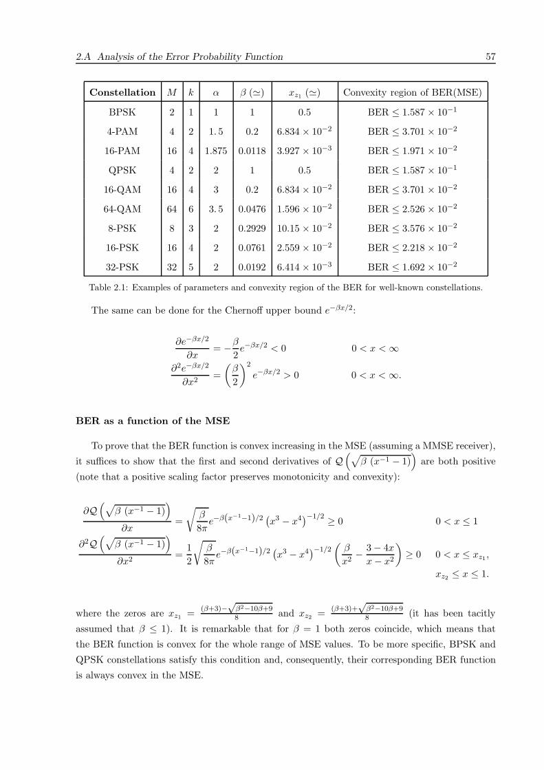
2.A Analysis of the Error Probability Function 57
Constellation M k α β () xz1 () Convexity region of BER(MSE)
BPSK 2 1 1 1 0.5 BER ≤ 1.587 × 10⁻¹
4-PAM 4 2 1. 5 0.2 6.834 × 10⁻² BER ≤ 3.701 × 10⁻²
16-PAM 16 4 1.875 0.0118 3.927 × 10⁻³ BER ≤ 1.971 × 10⁻²
QPSK 4 2 2 1 0.5 BER ≤ 1.587 × 10⁻¹
16-QAM 16 4 3 0.2 6.834 × 10⁻² BER ≤ 3.701 × 10⁻²
64-QAM 64 6 3. 5 0.0476 1.596 × 10⁻² BER ≤ 2.526 × 10⁻²
8-PSK 8 3 2 0.2929 10.15 × 10⁻² BER ≤ 3.576 × 10⁻²
16-PSK 16 4 2 0.0761 2.559 × 10⁻² BER ≤ 2.218 × 10⁻²
32-PSK 32 5 2 0.0192 6.414 × 10⁻³ BER ≤ 1.692 × 10⁻²
Table 2.1: Examples of parameters and convexity region of the BER for well-known constellations.
The same can be done for the Chernoff upper bound e−βx/2:
∂e−βx/2
∂x= −β
2e−βx/2 < 0 0 < x < ∞
∂2e−βx/2
∂x2=(
β
2
)2
e−βx/2 > 0 0 < x < ∞.
BER as a function of the MSE
To prove that the BER function is convex increasing in the MSE (assuming a MMSE receiver),
it suffices to show that the first and second derivatives of Q(√
β (x−1 − 1))
are both positive
(note that a positive scaling factor preserves monotonicity and convexity):
∂Q(√
β (x−1 − 1))
∂x=
√β
8πe−β(x−1−1)/2
(x3 − x4
)−1/2 ≥ 0 0 < x ≤ 1
∂2Q(√
β (x−1 − 1))
∂x2=
12
√β
8πe−β(x−1−1)/2
(x3 − x4
)−1/2(
β
x2− 3 − 4x
x − x2
)≥ 0 0 < x ≤ xz1,
xz2 ≤ x ≤ 1.
where the zeros are xz1 = (β+3)−√
β2−10β+98 and xz2 = (β+3)+
√β2−10β+98 (it has been tacitly
assumed that β ≤ 1). It is remarkable that for β = 1 both zeros coincide, which means that
the BER function is convex for the whole range of MSE values. To be more specific, BPSK and
QPSK constellations satisfy this condition and, consequently, their corresponding BER function
is always convex in the MSE.

58 Chapter 2. Overview of MIMO Channels
Consider now the Chernoff upper bound e−β(x−1−1)/2:
∂e−β(x−1−1)/2
∂x=
β
2e−β(x−1−1)/2x−2 > 0 0 < x < ∞
∂2e−β(x−1−1)/2
∂x2=
β
2e−β(x−1−1)/2x−4
(β
2− 2x
)≥ 0 0 < x ≤ β
4.
The Chernoff upper bound is then convex increasing in the MSE for MSE ≤ β/4 (see Table 2.1
for specific values).
The same analysis can be performed for a ZF receiver, obtaining that the BER function
Q(√
β MSE−1)
is convex increasing in the MSE for MSE ≤ β/3 and that the Chernoff upper
bound e−β MSE−1 /2 is convex increasing in the MSE for MSE ≤ β/4 (exactly the same result as
with the MMSE receiver).
Concluding, as a rule-of-thumb, both the exact BER function and the Chernoff upper bound
are convex increasing functions of the MSE for a BER ≤ 2 × 10⁻² (see Table 2.1).

Chapter 3
Mathematical Preliminaries
AN OVERVIEW OF TWO IMPORTANT THEORIES —convex optimization theory and
majorization theory—on which many results of this dissertation are based is given in this
chapter.
3.1 Convex Optimization Theory
Most problems of practical interest can be appropriately formulated as constrained optimization
problems. In some cases, possibly after some mathematical manipulations, the problems can be
expressed in convex form. For these type of problems, there is a well developed body of theory
and practice. In a nutshell, convex problems can be optimally solved very efficiently in practice.
As a consequence, roughly speaking, one can say that once a problem has been expressed in
convex form, it has been solved.
The two main mathematical references on the subject are [Lue69] and [Roc70]. An excellent
reference from a practical implementation perspective with engineering applications is [Boy00].
3.1.1 Convex Problems
A convex optimization problem (convex program) is of the form [Lue69, Roc70, Boy00]:
minx
f0(x)
s.t. fi(x) ≤ 0 1 ≤ i ≤ m,
hi(x) = 0 1 ≤ i ≤ p,
(3.1)
59
60 Chapter 3. Mathematical Preliminaries
where x ∈ IRn is the optimization variable, f0, · · · , fm are convex functions,1 and h1, · · · , hp
are linear functions (more exactly affine functions). The function f0 is the objective function
or cost function. The inequalities fi(x) ≤ 0 are called inequality constraints and the equations
hi(x) = 0 are called equality constraints. If there are no constraints, we say that the problem is
unconstrained.
The set of points for which the objective and all constraint functions are defined, i.e.,
D =m⋂
i=0
dom fi ∩p⋂
i=1
dom hi
is called the domain of the optimization problem (3.1). A point x ∈ D is feasible if it satisfies
all the constraints fi(x) ≤ 0 and hi(x) = 0. Problem (3.1) is said to be feasible if there exists at
least one feasible point and infeasible otherwise. The optimal value (minimal value) is denoted
by f (if the problem is infeasible, it is commonly denoted by f = +∞) and is achieved at an
optimal solution x, i.e., f = f0(x).
When the functions fi and hi in (3.1) are linear (affine), the problem is called a linear program
(LP) and is much simpler to solve. If the objective function is quadratic and the constraint
functions are linear (affine), the convex optimization problem (3.1) is called a quadratic program
(QP).
Many analysis and design problems arising in engineering can be cast (or recast) in the form
of a convex optimization problem. In general, some manipulations are required to convert the
problem into a convex one (unfortunately, this is not always possible). The interest of expressing
a problem in convex form is that, although an analytical solution may not exist and the problem
may seem difficult to solve (it may have hundreds of variables and a nonlinear, nondifferentiable
objective function), it can still be solved (numerically) very efficiently both in theory and practice
[Boy00]. Another interesting feature of expressing the problem in convex form is that additional
constraints can be straightforwardly added as long as they are convex.
Convex programming has been used in related areas such as FIR filter design [Wu96, Dav02],
antenna array pattern synthesis [Leb97], power control for interference-limited wireless networks
[Kan02], and beamforming design in a multiuser scenario with a multi-antenna base station
[Ben99, Ben01].
3.1.2 Solving Convex Problems
In some cases, convex optimization problems can be analytically solved using duality theory
and closed-form expressions can be obtained. In general, however, one must resort to iterative
methods [Lue69, Boy00].1A function f : IRn −→ IR is convex if, for all x, y ∈ dom f and θ ∈ [0, 1], θx+(1−θ)y ∈ dom f (i.e., the domain
is a convex set) and f (θx + (1 − θ)y) ≤ θf (x) + (1 − θ)f (y).

3.1. Convex Optimization Theory 61
In the last ten years, there has been considerable progress and development of efficient al-
gorithms for solving wide classes of convex optimization problems. Recently developed interior-
point methods can be used to iteratively solve convex problems efficiently in practice. This was
an important breakthrough achieved by Nesterov and Nemirovsky in 1988. They showed that
interior-point methods (initially proposed only for linear programming by Karmarkar in 1984)
can, in principle, be generalized to all convex optimization problems. In [Nes94], a very general
framework was developed for solving convex optimization problems using interior-point meth-
ods. In addition, the difference between the objective value at each iteration and the optimum
value can be upper-bounded using duality theory [Lue69, Boy00]. This allows the utilization of
nonheuristic stopping criteria based on checking whether some prespecified resolution has been
reached.
Interior-point methods solve constrained problems by solving a sequence of smooth (contin-
uous second derivatives are assumed) unconstrained problems, usually using Newton’s method
[Lue69, Boy00]. The solutions at each iteration are all strictly feasible (they are in the interior of
the domain), hence the name interior-point methods. They are also called barrier methods since
at each iteration a barrier function is used to guarantee that the solution obtained is strictly
feasible.
Alternatively, cutting-plane methods can be used [Boy00]. They use a completely different
philosophy and do not require differentiability of the objective and constraint functions. They
start with the feasible space and iteratively divide it into two halfspaces to reject the one that
is known not to contain any optimal solution. Ellipsoid methods are related to cutting-plane
methods in that they sequentially reduce an ellipsoid known to contain an optimal solution. In
general, cutting-plane methods are less efficient for problems to which interior-point methods
apply. See [Boy00] for details of implementation.
3.1.3 Duality Theory and KKT Conditions
The basic idea in Lagrangian duality is to take the constraints in (3.1) into account by augmenting
the objective function with a weighted sum of the constraint functions. We define the Lagrangian
associated with the problem (3.1) (not necessarily convex) as
L (x,λ,ν) = f0(x) +m∑
i=1
λifi(x) +p∑
i=1
νihi(x) (3.2)
where λi is the Lagrange multiplier associated with the ith inequality constraint fi(x) ≤ 0 and
νi the Lagrange multiplier associated with the ith equality constraint hi(x) = 0.
The optimization variable x is called primal variable and the vectors λ and ν are called the
dual variables or Lagrange multiplier vectors associated with the problem (3.1). The original
objective function f0(x) is termed the primal objective or primal function. The dual objective or
62 Chapter 3. Mathematical Preliminaries
dual function g (λ,ν) is defined as the minimum value of the Lagrangian over x, i.e., for λ ∈ IRm
and ν ∈ IRp,
g (λ,ν) = infx∈D
L (x,λ,ν) , (3.3)
which is concave even if the original problem is not convex because it is the pointwise infimum
of a family of affine functions of (λ,ν). We say that (λ,ν) are dual feasible if λ ≥ 0 and
g (λ,ν) > −∞.
The dual function g (λ,ν) is a lower bound on the optimal value f of the problem (3.1). For
any feasible (x,λ,ν):
f0(x) ≥ f0(x) +m∑
i=1
λifi(x) +p∑
i=1
νihi(x) (3.4)
≥ infz∈D
(f0(z) +
m∑i=1
λifi(z) +p∑
i=1
νihi(z)
)(3.5)
= g (λ,ν) (3.6)
where we have used the fact that fi(x) ≤ 0 and hi(x) = 0 for any feasible x and λi ≥ 0 for any
feasible λi in the first inequality. Thus, for the set of feasible (x,λ,ν), it follows that
minx
f0(x) ≥ maxλ,ν
g (λ,ν) (3.7)
which holds even if the original problem is not convex. The difference between the primal objective
f0(x) and the dual objective g (λ,ν) is called the duality gap. If (3.7) is satisfied with strict
inequality we say that weak duality holds; if (3.7) is achieved with equality we say that strong
duality holds.
A central result in convex analysis [Lue69, Roc70, Boy00] is that when the problem is convex,
under some technical conditions (called constraint qualifications), the duality gap reduces to zero
at the optimal (strong duality holds), i.e., (3.7) is achieved with equality for some (x,λ,ν).
Therefore, one way to solve the original problem is to solve its associated dual problem:
maxλ,ν
g (λ,ν)
s.t. λ ≥ 0,
(3.8)
which is always a convex optimization problem even if the original problem is not convex (the
objective to be maximized g (λ,ν) is concave and the constraint is convex). It is interesting to
note that a primal-dual feasible pair (x, (λ,ν)) localizes the optimal value of the primal (and
dual) problem in an interval:
f ∈ [g (λ,ν) , f0(x)]
the width of which is the duality gap. If the duality gap is zero, i.e., if g (λ,ν) = f0(x), then
x is primal optimal and (λ,ν) is dual optimal. These observations can be used in optimization
algorithms to provide nonheuristic stopping criteria.

3.1. Convex Optimization Theory 63
Let x and (λ,ν) be the primal and dual variables at the optimum. If we substitute them
in the chain of inequalities (3.4)-(3.6), we see that each of the inequalities must be satisfied with
equality (assuming that strong duality holds). To have equality in (3.4), it must be that λifi(x) =
0 (this is the so-called complementary slackness condition). Moreover, since the inequality in (3.5)
must also be satisfied with equality, the infimum is achieved at x; in other words, the gradient of
the Lagrangian with respect to x must be zero at (x,λ,ν), i.e., ∇xL (x,λ,ν) = 0. These
two results, together with the constraints on the primal and dual variables, form the Karush-
Kuhn-Tucker (KKT) conditions:
hi(x) = 0, fi(x) ≤ 0, (3.9)
λi ≥ 0, (3.10)
∇xf0(x) +m∑
i=1
λi∇xfi(x) +
p∑i=1
νi ∇xhi(x) = 0, (3.11)
λi fi(x) = 0. (3.12)
Under some technical conditions (called constraint qualifications), the KKT conditions are nec-
essary and sufficient for optimality. One simple version of the constraint qualifications is Slater’s
condition, which is satisfied when there exists x such that fi(x) < 0, 1 ≤ i ≤ m and
hi(x) = 0, 1 ≤ i ≤ p (such a point is sometimes called strictly feasible since the inequality
constraints hold with strict inequalities) [Roc70, Boy00].
In practice, the KKT conditions are very useful to obtain optimal solutions analytically (when-
ever this is possible).
3.1.4 Sensitivity Analysis
The optimal dual variables (Lagrange multipliers) of a convex optimization problem give useful
information about the sensitivity of the optimal value with respect to perturbations of the con-
straints [Lue69, Boy00]. Consider the following perturbed version of the original convex problem
(3.1):
minx
f0(x)
s.t. fi(x) ≤ ui 1 ≤ i ≤ m,
hi(x) = vi 1 ≤ i ≤ p.
(3.13)
This problem coincides with the original problem (3.1) if ui = 0 and vi = 0. When ui is positive
it means that we have relaxed the ith inequality constraint; when ui is negative, it means that we
have tightened the constraint. We define f (u,v) as the optimal value of the perturbed problem
with the perturbations u and v. Note that f (0,0) = f.
Suppose that f (u,v) is differentiable at u = 0, v = 0. Then, provided that strong duality
holds, the optimal dual variables λ,ν are related to the gradient of f (u,v) at u = 0, v = 0

64 Chapter 3. Mathematical Preliminaries
by [Boy00]
λi = −∂f (0,0)
∂ui, ν
i = −∂f (0,0)∂vi
. (3.14)
This means that tightening the ith constraint a small amount (i.e., taking ui small and negative)
yields an increase in f of approximately −λi ui and, similarly, loosening the ith constraint a
small amount (i.e., taking ui small and positive) yields a decrease in f of approximately λi ui.
The sensitivity result of (3.14) allows us to assign a numerical value to how active a constraint
is at the optimum x. If fi(x) < 0, then the constraint is inactive and it follows that the
constraint can be tightened or loosened a small amount without affecting the optimal value (this
agrees with the fact that λi must be zero by the complementary slackness condition). Suppose
now that fi(x) = 0, i.e., the ith constraint is active at the optimum. The ith optimal Lagrange
multiplier tells us how active the constraint is: if λi is small, it means that the constraint can be
loosened or tightened a small amount without much effect on the optimal value; if λi is large, it
means that if the constraint is loosened or tightened a small amount, the effect on the optimal
value will be great.
3.2 Majorization Theory
Many of the problems addressed in this dissertation result in complicated nonconvex constrained
optimization problems that involve matrix-valued variables. Majorization theory is a key tool
that will allow us to convert these problems into simple convex problems with scalar variables
that can be optimally solved.
In this section, we introduce the basic notion of majorization and state some basic results
that will be needed in the sequel. A complete reference on the subject is [Mar79].
3.2.1 Basic Definitions
Majorization makes precise the vague notion that the components of a vector x are “less spread
out” or “more nearly equal” than the components of a vector y.
Definition 3.1 [Mar79] For any x ∈ IRn, let
x[1] ≥ · · · ≥ x[n]
denote the components of vector x in decreasing order, and let
x(1) ≤ · · · ≤ x(n)
denote the components of vector x in increasing order.

3.2. Majorization Theory 65
Definition 3.2 [Mar79, 1.A.1] For any x,y ∈ IRn, x is majorized by y (or y majorizes x) if
k∑i=1
x[i] ≤k∑
i=1
y[i] 1 ≤ k ≤ n − 1
n∑i=1
x[i] =n∑
i=1
y[i]
and it is denoted by x ≺ y or, equivalently, by y x.
Alternatively, the previous conditions can be rewritten as
k∑i=1
x(i) ≥k∑
i=1
y(i) 1 ≤ k ≤ n − 1
n∑i=1
x(i) =n∑
i=1
y(i).
Definition 3.3 [Mar79, 1.A.2] For any x,y ∈ IRn, x is weakly majorized by y (or y weakly
majorizes x) ifk∑
i=1
x(i) ≥k∑
i=1
y(i) 1 ≤ k ≤ n
and it is denoted by x ≺w y or, equivalently, by y wx.2
Note that x ≺ y implies x ≺w y; in other words, majorization is a more restrictive definition
than weakly majorization.
Definition 3.4 [Mar79, 3.A.1] A real-valued function φ defined on a set A ⊆ IRn is said to be
Schur-convex on A if
x ≺ y on A ⇒ φ (x) ≤ φ (y) .
Similarly, φ is said to be Schur-concave on A if
x ≺ y on A ⇒ φ (x) ≥ φ (y) .
As a consequence, if φ is Schur-convex on A then −φ is Schur-concave on A and vice-versa.
It is important to remark that the sets of Schur-concave and Schur-convex functions do no
form a partition of the set of all functions from A ⊆ IRn to IR. In fact, neither are the two
sets disjoint (the intersection is not empty), nor do they cover the entire set of all functions (see
Figure 3.1). We now give some illustrative examples.
2More specifically, x is said to be weakly supermajorized by y (as opposed to the submajorization relation
denoted by x ≺w y [Mar79, 1.A.2]).
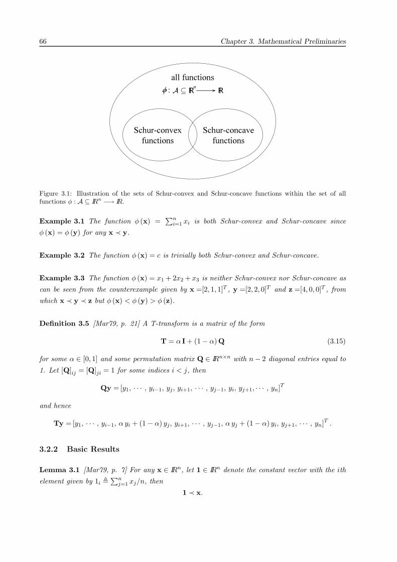
66 Chapter 3. Mathematical Preliminaries
all functions
Schur-convex
functions
Schur-concave
functions
Rn
R
Figure 3.1: Illustration of the sets of Schur-convex and Schur-concave functions within the set of allfunctions φ : A ⊆ IRn −→ IR.
Example 3.1 The function φ (x) =∑n
i=1 xi is both Schur-convex and Schur-concave since
φ (x) = φ (y) for any x ≺ y.
Example 3.2 The function φ (x) = c is trivially both Schur-convex and Schur-concave.
Example 3.3 The function φ (x) = x1 + 2x2 + x3 is neither Schur-convex nor Schur-concave as
can be seen from the counterexample given by x =[2, 1, 1]T , y =[2, 2, 0]T and z =[4, 0, 0]T , from
which x ≺ y ≺ z but φ (x) < φ (y) > φ (z).
Definition 3.5 [Mar79, p. 21] A T-transform is a matrix of the form
T = α I + (1 − α)Q (3.15)
for some α ∈ [0, 1] and some permutation matrix Q ∈ IRn×n with n − 2 diagonal entries equal to
1. Let [Q]ij = [Q]ji = 1 for some indices i < j, then
Qy =[y1, · · · , yi−1, yj, yi+1, · · · , yj−1, yi, yj+1, · · · , yn]T
and hence
Ty = [y1, · · · , yi−1, α yi + (1 − α) yj, yi+1, · · · , yj−1, α yj + (1 − α) yi, yj+1, · · · , yn]T .
3.2.2 Basic Results
Lemma 3.1 [Mar79, p. 7] For any x ∈ IRn, let 1 ∈ IRn denote the constant vector with the ith
element given by 1i ∑n
j=1 xj/n, then
1 ≺ x.

3.2. Majorization Theory 67
Lemma 3.1 is simply stating the obvious fact that a vector of equal components has the “least
spread out” or the “most equal” components.
Lemma 3.2 [Mar79, 3.B.1] An increasing function of a Schur-convex (Schur-concave) function
is Schur-convex (Schur-concave). Similarly, a decreasing function of a Schur-convex (Schur-
concave) function is Schur-concave (Schur-convex).
Lemma 3.3 [Mar79, 3.H.2] Let φ(x) =∑
i gi (xi) where xi ≥ xi+1 and each gi is differentiable.
Then φ is Schur-convex if and only if
g′i (a) ≥ g′i+1 (b) whenever a ≥ b, i = 1, . . . , n − 1.
Corollary 3.1 Let φ(x) =∑
i g (xi) where g is convex. Then φ is Schur-convex.
Lemma 3.4 [Mar79, 5.A.9.a] For any x,y ∈ IRn satisfying y w x, there exists a vector u such
that
u ≤ x and y u.
The following lemma is a fundamental result of majorization theory.
Lemma 3.5 [Mar79, 2.B.1] For any x,y ∈ IRn satisfying x ≺ y, there exists a sequence of
T-transforms T(1), · · · ,T(K) such that x = T(K) · · ·T(1)y and K < n.
We now give an algorithm to obtain such a sequence of T-transforms from [Mar79, 2.B.1].
Algorithm 3.1 [Mar79, 2.B.1] Algorithm to obtain a sequence of T-transforms such that x =
T(K) · · ·T(1)y.
Input: Vectors x,y ∈ IRn satisfying x ≺ y (it is assumed that the components of x and y are
in decreasing order and that x = y).
Output: Set of T-transforms T(1), · · · ,T(K).
0. Let y(0) = y and k = 1 be the iteration index.
1. Find the largest index i such that y(k−1)i > xi and the smallest index j greater than i such
that y(k−1)j < xj.
2. Let δ = min(xj − y
(k−1)j , y
(k−1)i − xi
)and α = 1 − δ/
(y
(k−1)i − y
(k−1)j
).
3. Use α to compute T(k) as in (3.15) and let y(k) = T(k)y(k−1).
4. If y(k) = x, then set k = k + 1 and go to step 1; otherwise, finish.
68 Chapter 3. Mathematical Preliminaries
Lemma 3.6 [Mar79, 9.B.1] Let R be an n×n Hermitian matrix with diagonal elements denoted
by the vector d and eigenvalues denoted by the vector λ, then
λ d.
Lemma 3.7 [Mar79, 9.B.2] For any x,y ∈ IRn satisfying x ≺ y, there exists a real symmetric
(and therefore Hermitian) matrix with diagonal elements given by x and eigenvalues given by y.
Lemma 3.7 is the converse of Lemma 3.6 (in fact it is stronger than the converse since it
guarantees the existence of a real symmetric matrix instead of just a Hermitian matrix). A
recursive algorithm to obtain a matrix with a given vector of eigenvalues and vector of diagonal
elements is indicated in [Mar79, 9.B.2] and [Vis99b, Section IV-A]. We consider the practical and
simple method obtained in [Vis99b, Section IV-A] and reproduce it here for completeness.
Algorithm 3.2 [Vis99b, Section IV-A] Algorithm to obtain a real symmetric matrix R with
diagonal values given by x and eigenvalues given by y provided that x ≺ y.
Input: Vectors x,y ∈ IRn satisfying x ≺ y (it is assumed that the components of x and y are
in decreasing order and that x = y).
Output: Matrix R.
1. Using Algorithm 3.1, obtain a sequence of T-transforms such that x = T(K) · · ·T(1)y.
2. Define the Givens rotation U(k) as[U(k)]ij
=
√[T(k)]ij
−√[
T(k)]ij
for i < j
otherwise.
3. Let R(0) = diag (y) and R(k) = U(k)T R(k−1)U(k). The desired matrix is given by R = R(K).Alternatively, define the unitary matrix Q = U(1) · · ·U(K) and the desired matrix is given
by R = QT diag (y)Q.
Corollary 3.2 For any λ ∈ IRn, there exists a real symmetric (and therefore Hermitian) matrix
with equal diagonal elements and eigenvalues given by λ.
Proof. The proof is straightforward from Lemmas 3.1 and 3.7.
As before, such matrix can be obtained using Algorithm 3.2. However, for this particular case
and allowing the desired matrix to be complex, it is easy to see that any unitary matrix Q satis-
fying the condition |[Q]ik| = |[Q]il| ∀i, k, l provides a valid solution given by R = QH diag (y)Q.
As an example, the unitary Discrete Fourier Transform (DFT) matrix and the Hadamard matrix
(when the dimensions are appropriate such as a power of two [Ver98, p.66][Pet78, Sec.5.6]) satisfy
this condition. Nevertheless, Algorithm 3.2 has the nice property that the obtained matrix Q is

3.3. Miscellaneous Algebra Results 69
real-valued and can be naturally decomposed (by construction) as the product of Givens rotations
(where each term performs a single rotation [Sod89]). This simple structure plays a key role for
practical implementation. Interestingly, an iterative approach to construct a matrix with equal
diagonal elements and with a given set of eigenvalues was obtained in [Mul76], based also on a
sequence of rotations.
3.3 Miscellaneous Algebra Results
In this section, we include for convenience a few basic algebra results that are standard fare in
most textbooks (e.g., [Hor85, Mag99, Sod89, Kay93, Sch91]) and that will be repeatedly used
throughout this dissertation.
Basic results on the trace and determinant
The following relation, commonly referred to as the circularity of the trace, is widely used:
Tr (AB) = Tr (BA) .
The following is a basic result on the determinant for conformable matrices [Mag99, Sod89]:
|I + AB| = |I + BA| .
Another useful result is
A ≥ B ⇒ |A| ≥ |B| .
Matrix Inversion Lemma
The general expression of the matrix inversion lemma is [Kay93, Sch91, Sod89, Hor85]
(A + BCD)−1 = A−1 − A−1B(DA−1B + C−1
)−1 DA−1.
A particular case is the Woodbury’s Identity:
(R + γ2ccH
)−1= R−1 − γ2
1 + γ2cHR−1cR−1ccHR−1.
Cauchy-Schwarz’s inequality
The Cauchy-Schwarz’s inequality in vector form is [Mag99, Hor85]
∣∣yHx∣∣ ≤ ‖y‖2 ‖x‖2
with equality if and only if y =αx, i.e., if y and x are linearly dependent.
Hadamard’s inequality
Given an n × n positive semidefinite matrix R, the following holds [Cov91b, Mag99, Hor85]:

70 Chapter 3. Mathematical Preliminaries
|R| ≤n∏
i=1
[R]ii
with equality if and only if matrix R is diagonal (except in the trivial case in which R is singular).
Jensen’s inequality [Boy00, Cov91b]
If f is a convex function, x1, · · · , xk ∈ dom f , and θ1, · · · , θk ≥ 0 with θ1 + · · · + θk = 1, then
f (θ1x1 + · · · + θkxk) ≤ θ1f (x1) + · · · + θkf (xk) .
Moreover, if f is strictly convex, then equality implies that the xi’s for which θi > 0 are equal.
The inequality extends to infinite sums, integrals, and expected values. For example, if x is a
random variable such that x ∈ dom f with probability one and f is convex, then
f (E [x]) ≤ E [f (x)] ,
provided the expectations exist. Moreover, if f is strictly convex, then equality implies that x is
a constant.
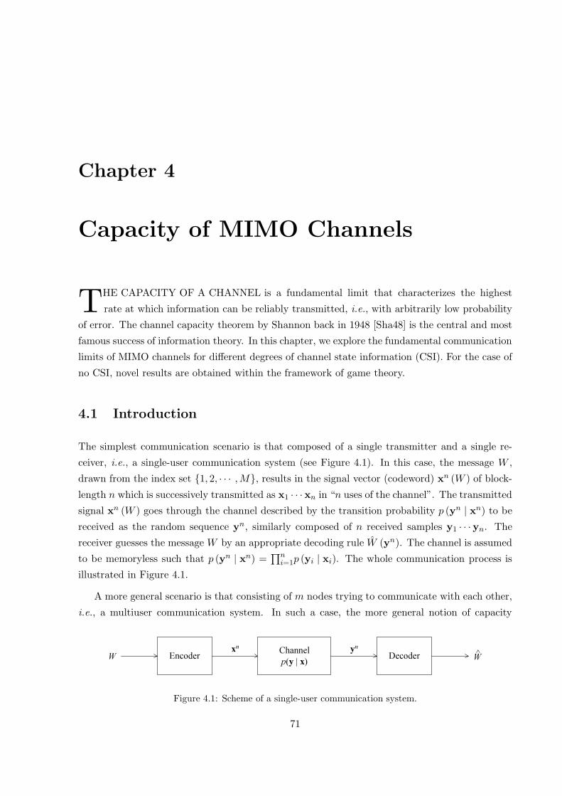
Chapter 4
Capacity of MIMO Channels
THE CAPACITY OF A CHANNEL is a fundamental limit that characterizes the highest
rate at which information can be reliably transmitted, i.e., with arbitrarily low probability
of error. The channel capacity theorem by Shannon back in 1948 [Sha48] is the central and most
famous success of information theory. In this chapter, we explore the fundamental communication
limits of MIMO channels for different degrees of channel state information (CSI). For the case of
no CSI, novel results are obtained within the framework of game theory.
4.1 Introduction
The simplest communication scenario is that composed of a single transmitter and a single re-
ceiver, i.e., a single-user communication system (see Figure 4.1). In this case, the message W ,
drawn from the index set 1, 2, · · · ,M, results in the signal vector (codeword) xn (W ) of block-
length n which is successively transmitted as x1 · · · xn in “n uses of the channel”. The transmitted
signal xn (W ) goes through the channel described by the transition probability p (yn | xn) to be
received as the random sequence yn, similarly composed of n received samples y1 · · · yn. The
receiver guesses the message W by an appropriate decoding rule W (yn). The channel is assumed
to be memoryless such that p (yn | xn) =∏n
i=1p (yi | xi). The whole communication process is
illustrated in Figure 4.1.
A more general scenario is that consisting of m nodes trying to communicate with each other,
i.e., a multiuser communication system. In such a case, the more general notion of capacity
EncoderChannel
p(y | x)DecoderW
xn
yn
W
Figure 4.1: Scheme of a single-user communication system.
71
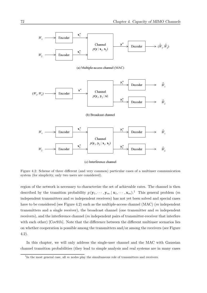
72 Chapter 4. Capacity of MIMO Channels
Encoder
Channel
p(y | x1, x
2)
Decoder
x1
x2
Encoder
W1
W2
y
(a) Multiple-access channel (MAC)
EncoderChannel
p(y1, y
2| x)
Decoder
x
(b) Broadcast channel
y1
(W1,W
2)
W1
^
Decodery2
W2
^
Channel
p(y1, y
2| x
1, x
2)
Decoder
(c) Interference channel
y1
W1
^
Decodery2
W2
^
Encoderx1
x2
Encoder
W1
W2
n
n
n
n
n
n
n
n
n
n
(W1,W
2)
^^
Figure 4.2: Scheme of three different (and very common) particular cases of a multiuser communicationsystem (for simplicity, only two users are considered).
region of the network is necessary to characterize the set of achievable rates. The channel is then
described by the transition probability p (y1, · · · ,ym | x1, · · · ,xm).1 This general problem (m
independent transmitters and m independent receivers) has not yet been solved and special cases
have to be considered (see Figure 4.2) such as the multiple-access channel (MAC) (m independent
transmitters and a single receiver), the broadcast channel (one transmitter and m independent
receivers), and the interference channel (m independent pairs of transmitter-receiver that interfere
with each other) [Cov91b]. Note that the difference between the different multiuser scenarios lies
on whether cooperation is possible among the transmitters and/or among the receivers (see Figure
4.2).
In this chapter, we will only address the single-user channel and the MAC with Gaussian
channel transition probabilities (they lead to simple analysis and real systems are in many cases
1In the most general case, all m nodes play the simultaneous role of transmitters and receivers.

4.1. Introduction 73
accurately modeled with a Gaussian channel transition probability because the noise is Gaussian).
For completeness, we recall the signal model for the single-user channel with nT transmit and nR
receive (finite) dimensions
y = Hx + n (4.1)
where x ∈ CI nT ×1 is the transmitted vector, H ∈ CI nR×nT is the channel matrix, y ∈ CI nR×1 is
the received vector, and n ∈ CI nR×1 is a proper complex Gaussian noise vector n ∼CN (0,Rn).2
For future reference, recall that H R−1/2n H is the whitened channel matrix as was defined in
(2.2). The covariance matrix of the transmitted vector signal is Q = E [xxH ] and the transmitter
is constrained in its average transmit power as Tr (Q)≤PT (c.f. §2.5.2). By uniform power
allocation we mean Q = PT /nT InT, which also implies an independent signaling over the transmit
dimensions if a Gaussian code is used. Another interesting constraint is the maximum eigenvalue
constraint λmax (Q) ≤ α (c.f. §2.5.2) which will be revisited in Section 4.4. Note that λmax (Q)
is an upper-bound on the average transmitted power at each transmit dimension E [ |xi|2] ≤λmax (Q).
Similarly, the signal model for the multiple-access channel with K users, each one transmitting
over nk dimensions with a (possibly different) power constraint Tr (Qk) ≤ Pk and with channel
Hk ∈ CI nR×nk , is
y =K∑
k=1
Hkxk + n. (4.2)
Different types of capacities are obtained depending on the characteristics of the communi-
cation system such as the deterministic/random nature of the channel, the degree of CSI at the
transmitter (CSIT) and at the receiver (CSIR), and the delay constraints [Big98]. Perfect (instan-
taneous) CSIR is considered throughout this chapter under the reasonable assumption that the
receiver may obtain sufficiently good channel estimates (c.f. §2.4). In fact, it is not necessary to
assume an a priori perfect CSIR; provided that the channel remains fixed during a sufficiently long
time, the capacity does not depend on whether the channel state is available or not at the receiver
[Big98].3 Regarding the transmitter, when perfect CSIT is available, the instantaneous capacity
(also termed deterministic capacity) at each channel state is a meaningful measure. This situation
may arise either when the channel is fixed and deterministic or when it is a fading channel with
a sufficiently slow fading so that the channel can be estimated and fed back to the transmitter
(c.f. §2.4). In many situations, however, the transmitter may not have an instantaneous CSI. In
such cases, provided that the channel statistics are known at the transmitter (statistical CSIT),
2Recall that, for a given H and since the noise is Gaussian distributed, the channel transition probability is
Gaussian: p (y | x) = 1π nR |Rn|e
−(y−Hx)HR−1n (y−Hx).
3The intuitive explanation of this effect is that, since the channel state remains fixed for the transmission of
the whole codeword, for sufficiently long codes, it can be estimated at the receiver by transmitting, for example, a
training sequence with length proportional to√
n at no cost of rate as n → ∞ [Wol78]. In fact, the channel state
is not at all required at the receiver with the utilization of universal decoders [Lap98].

74 Chapter 4. Capacity of MIMO Channels
the notions of ergodic and outage capacities (depending on the delay constraints of the system)
provide meaningful measures as will be further discussed. It may also be interesting to consider
the most pessimistic scenario in which not even the statistics of the channel are known at the
transmitter (no CSIT), implying the necessity of a robust communication scheme under channel
uncertainty. In such a case, as will be analyzed in detail, the notion of worst-case capacity (also
termed compound capacity) arises naturally and can be formulated as a game with two players:
the transmitter and a malicious nature that controls the channel state and the noise statistics.
The main contribution of this chapter is the characterization of the worst-case capacity within
the framework of game theory, obtaining the interesting novel result that a uniform power allo-
cation (transmitting in all directions) is the best thing to do when nothing is known about the
channel (under a mild isotropy condition). Interestingly, this result holds for the MAC as well.
This chapter is structured as follows. First, the instantaneous capacity as well as the er-
godic/outage capacity are briefly described in Sections 4.2 and 4.3, respectively. After that, the
worst-case capacity is extensively analyzed in Section 4.4, providing original results.
The results in this chapter regarding the instantaneous capacity in beamforming-constrained
systems and the worst-case capacity under a game-theoretic framework have been published in
[Pal01c, Pal03e] and [Pal03a, Pal03d], respectively.
4.2 Instantaneous Capacity
The notion of instantaneous capacity is meaningful only when instantaneous CSI is available at
both sides of the link, which happens either when the channel remains basically fixed such as
in DSL systems or when it changes sufficiently slow so that it can be considered fixed during
the sufficient number of transmissions. In such a case, capacity is achieved by adapting the
transmitted signal to the specific channel realization as we now review.
4.2.1 Capacity of the Single-User Channel
For the single-user channel, the optimum signaling to achieve rates up to the channel capacity is
well known [Bra74, Cov91b, Tel95]. The capacity of a channel is the maximum mutual information
between the transmitted and the received signals I (x;y) over all possible input distributions
satisfying the power constraint [Bla87, Cov91b]:
C = maxp(x):E‖x‖2≤PT
I (x;y) . (4.3)
For the vector Gaussian channel under consideration, it is well known that the maximum
mutual information is achieved with Gaussian inputs x ∼CN (0,Q) (i.e., when a Gaussian code

4.2. Instantaneous Capacity 75
P1
subchannel
-1
-1-1
-1
-1
-1
-1
P2
P3
P4
P5
water-level
power
Figure 4.3: Illustration of the water-filling power allocation Pi =(µ − λ−1
i
)+.
is used for transmission), where Q is the covariance matrix of the transmitted vector x, and the
mutual information is then [Cov91b, Tel95]
I (x;y) = log det(InR
+ R−1n HQHH
)(4.4)
where the units are nats/transmission since the natural logarithm has been used (note that any
other base can be chosen affecting only the units of the mutual information). The channel capacity
for each channel state H is given by the maximum mutual information over all Q verifying the
power constraint:
C (H) = maxQ:Tr(Q)≤PT ,
Q=QH≥0
log det(InR
+ R−1n HQHH
)(4.5)
where we have made explicit the dependence of the capacity on each particular channel state. This
maximization problem has a well-known solution based on diagonalizing the whitened channel
H = R−1/2n H and then distributing the available power over the channel eigenmodes in a water-
filling fashion. To be more specific, the capacity-achieving solution is [Bra74, Cov91b, Ral98,
Tel95, Sca99a]
Q = URHDQUH
RH(4.6)
where URHcontains the eigenvectors of RH = HHR−1
n H (whose EVD is given by RH =
URHDRH
UHRH
) and DQ is a diagonal matrix with diagonal elements λQ,i given by the water-
filling solution
λQ,i =(µ − λ−1
RH ,i
)+ 1 ≤ i ≤ nT (4.7)
where (x)+ max (0, x) and µ is the water-level chosen to satisfy the power constraint with
equality∑
i λQ,i = PT . This optimal power allocation has the appealing interpretation based on
considering the available power as water which is poured over a surface inversely proportional
to the channel gain, hence the name water-filling or water-pouring (see Figure 4.3) [Cov91b]. In
particular, this implies that eigenmodes with higher gain receive higher power and vice-versa; in

76 Chapter 4. Capacity of MIMO Channels
addition, there is a threshold under which no power is allocated to an eigenmode (for a given
channel, the number of used eigenmodes depends on the available power at the transmitter PT ).
The capacity can be then written as
C (H) =∑
i
log (1 + λQ,i λRH ,i) (4.8)
=∑
i
(log (µ λRH ,i))+ (4.9)
from which the channel capacity is achieved by properly using the constituent channel eigenmodes.
It will be convenient in the sequel to express the mutual information between x and y explicitly
as a function of Q and H (assuming a Gaussian code) as in [Tel95]:
Ψ(Q, H
)= log det
(InR
+ HQHH)
(4.10)
= log det(InT
+ QHHH)
(4.11)
Beamforming-Constrained Systems
We now consider the capacity of a channel when the transmitter is constrained to use a
beamvector (termed single beamforming in §2.5.1). Such a scheme is preferred in terms of com-
plexity because only one data stream needs to be considered and coding and transmission can be
done in a much easier manner (as in single antenna systems) [Nar99]. However, the utilization
of a beamvector at the transmitter implies a rank-one transmit covariance matrix which may not
be optimum. It is therefore necessary to analyze when such a communication structure does not
incur any loss of optimality [Pal01c, Pal01a, Pal03e].
The capacity expression when the communication system is constrained to use a rank-one
transmit covariance matrix (beamforming) is (similarly to (4.8)) given by [Pal01c, Pal03e]
Cbf (H) = log (1 + PT λRH ,max) (4.12)
where only the best channel eigenmode is used for transmission. Such a beamforming scheme is,
in principle, suboptimum because it uses only one channel eigenmode (compare (4.12) with (4.8)).
To be exact, beamforming is optimum if and only if PT ≤ λ−1RH ,2 − λ−1
RH ,1 where the λRH ,i’s are
assumed in decreasing order. This condition is satisfied if a sufficiently small value of transmit
power is used (provided that λRH ,1 = λRH ,2).
In wireless multi-antenna MIMO systems, for example, the optimality conditions are satisfied
for some situations with high spatial correlation. In particular, beamforming is asymptotically
optimum (in the sense of achieving capacity) as the spatial channel fading correlation increases at
least at one end of the link because the channel matrix becomes rank-one: H → hRhHT [Pal03e].
In [Jaf01, Sim03], the optimality of beamforming was analyzed for different degrees of chan-
nel feedback quality. In [Ivr03], different transmission strategies were considered (including a

4.2. Instantaneous Capacity 77
0 10 20 30 40 50 60 70 80 900
2
4
6
8
10
12
14
16
18
Outage Capacity (Pout
= 5%) of a MIMO (4,4) VEH−A channel (SNR = 16.00 dB)
Angle Spread (degrees)
Cap
acity
(bp
s/H
z)
w/ CSIT w/o CSIT
MIMO part−corr
MIMO corr
MIMO part−corr(beamforming)
range of optimalityof beamforming
MIMO uncorr
Figure 4.4: Outage capacity (at an outage probability of 5%) of a 4 × 4 MIMO Vehicular-A channel(SNR=16dB) as a function of the angle spread (part-corr) with CSIT (w/ CSIT), without CSIT (w/oCSIT), and when beamforming is used. In addition, the capacities with and without CSIT correspond-ing to fully uncorrelated (uncorr) and completely correlated (corr) MIMO channels are also plotted forcomparison.
beamforming approach) depending on the degree of channel knowledge at the transmitter and
the spatial correlation.
Numerical Example
We now evaluate numerically the range of optimality of beamforming in a typical wireless
multi-antenna MIMO channel (in particular, we consider 4 transmit and 4 receive antennas).
The transmitter (mobile unit) is assumed to be immersed in a rich scattering environment
and has an almost uncorrelated fading among the antennas. The receiver (base station), however,
is assumed to be on top of a building, receiving the signal from a mean direction of arrival with a
given angle spread. The spatial fading correlation was obtained using the closed-form expression
derived in [Sal94] (where a uniform-shaped angular distribution was assumed4) along with the
procedure explained in [Ped00] to include the corresponding spatial correlation into the generated
MIMO channel. The generated channel is frequency-selective following a Vehicular power delay
profile as specified by ETSI [ETS98b]. The noise covariance matrix was assumed white and
the signal was received with an average SNR of 16dB. For a more detailed description of the
4Depending on the exact shape of the considered angular ray distribution, different spatial correlation are
obtained. In general, however, this is just a minor detail and the conclusions derived under different ray distributions
should be roughly the same.

78 Chapter 4. Capacity of MIMO Channels
simulation scenario and for additional plots, the reader is referred to [Pal03e].
In Figure 4.4, the capacity5 is plotted as a function of the angle spread (partially correlated
channel) for the following situations: with instantaneous CSIT (w/ CSIT) according to the water-
filling solution, without CSIT (w/o CSIT) using a uniform power allocation among all the transmit
dimensions, and when beamforming is used (for which instantaneous CSIT is required). In
addition, the capacities with and without CSIT corresponding to fully uncorrelated (uncorr) and
completely correlated (corr) MIMO channels are also plotted for comparison. For the particular
scenario under consideration, we can infer that for an angle spread on the order of 4-8 degrees,
the loss in capacity of the beamforming scheme is negligible.6
4.2.2 Capacity Region of the Multiple-Access Channel (MAC)
In the multiple-access channel, we do not deal anymore with a single capacity measure but with
a capacity region, which is the set of achievable rates R1, · · · , RK (recall that, in the MAC,
the users transmit independently, whereas the receiver can perform a joint detection). For the
vector Gaussian MAC, it is well known that all the boundaries defining the achievable region
are maximized when Gaussian codes are used for transmission (in other words, the rate region
corresponding to a Gaussian signaling contains the rate region of other signaling distributions).
The achievable rate region corresponding to a set of channel states Hk and a set of covariance
matrices Qk (assuming Gaussian codes) is [Cov91b, Ver89]
R (Qk , Hk) =
(R1, · · · , RK) :
0 ≤∑k∈S
Rk ≤ log det(InR
+∑k∈S
R−1n HkQkH
Hk
),∀S ⊆ 1, · · · ,K
.
(4.13)
Recall that a joint detection is necessary in general to obtain all the rates within the region;
otherwise, if an independent detection is used for all the users, the interference channel model as
previously described (see Figure 4.2) would be more appropriate.
Assuming that the transmit covariance matrices are constrained in their average transmit
5To be more exact, we plot the capacity at an outage probability of 5% (i.e., the capacity that is achieved in
95% of the cases). In this case, however, the transmitter has instantaneous CSIT which is a fundamental difference
with respect to the outage capacity considered in §4.3 where only statistical CSIT is assumed.6Note that the curve for partial correlation in Figure 4.4 is not monotonic on the angle spread. This is due
to the specific model of the ray distribution (uniform-shaped angular distribution) used to compute the fading
correlation [Sal94]. For other distribution models, slightly different curves are obtained but the underlying trend
is always the same.
4.2. Instantaneous Capacity 79
power, the capacity region is [Ver89, Yu01b]
C (Hk) =⋃
Tr(Qk)≤Pk,Qk=QH
k ≥0
R (Qk , Hk) . (4.14)
Note that the convex closure operation usually needed [Cov91b] is unnecessary in this case because
the region is already closed and convex as shown in [Ver89, Yu01b].
Although the capacity region has been fully characterized in (4.14), it is not obvious how to
obtain in practice the boundary points defining the region. Since (4.14) is a convex region, its
boundary points can be found by maximizing the weighted sum of the data rates (different set of
weights µk give different points of the boundary)
maxRk
∑k µk Rk
s.t. Rk ∈ C (Hk)(4.15)
which is a convex optimization problem and therefore can be efficiently solved in practice (see
§3.1). This problem was extensively treated in [Yu01b].
A simple measure of particular interest in multiple-access channels is the sum capacity, which
is a single performance parameter as opposed to the capacity region. The sum capacity represents
the maximum total rate∑
k Rk that can be achieved by the system and is obtained as the solution
to the following convex optimization problem:
maxQk
log det(InR
+K∑
k=1
R−1n HkQkH
Hk
)
s.t. Tr (Qk) ≤ Pk, 1 ≤ k ≤ K
Qk = QHk ≥ 0.
(4.16)
This problem turns out to be easily solved by the iterative water-filling algorithm proposed in
[Yu01b], which solves, for each of the users and in a sequential manner, the single-user water-
filling solution when the rest of the users are considered as noise, i.e., when each user k considers
the interference-plus-noise covariance matrix Rn,k =∑l =k
HlQlHHl +Rn [Yu01b]. As was found in
[Yu01b], at an optimal point, each user must water-fill the rest of the users considered as noise.
Beamforming-Constrained Systems
We can also consider a beamforming-constrained system for the vector Gaussian MAC where
each user transmit using beamforming. The optimality conditions obtained for the single-user
case (sufficiently low transmit power and/or sufficiently high spatial correlation in a multi-antenna
system) are also valid for the MAC. In this scenario, however, the beamforming approach turns
out to be asymptotically optimal with the number of users regardless of the channel correlation
and of the transmit power as shown in [Rhe01b]. To be more exact, the number of users must be

80 Chapter 4. Capacity of MIMO Channels
sufficiently large compared to the number of receive dimensions (or antennas in a multi-antenna
system) [Rhe01b]. The underlying idea is that the multiplexing gain of a MIMO channel is
fully utilized on a multiuser level (by having many users doing beamforming) rather than on the
individual level.
Utilizing beamforming implies rank-one transmit covariance matrices, i.e., rank (Qk) = 1. The
definition of the capacity region corresponding to such a constrained system is straightforward
by including the rank-one constraint in the region defined in (4.14). The computation of such
a capacity region, however, turns out to be a very complicated problem because the rank-one
constraint is nonconvex and so is the whole problem (even the computation of the sum capacity is a
nonconvex problem). It is useful to parameterize the transmit covariance matrices as Qk = bkbHk
where bk is the beamvector of the kth user (this parameterization is also very appropriate to
describe CDMA systems where the beamvector denotes the code in time [Ulu01]). The sum
capacity is then characterized as the following nonconvex problem:
maxbk
log det(InR
+K∑
k=1
R−1n Hkbkb
Hk HH
k
)
s.t. bHk bk ≤ Pk, 1 ≤ k ≤ K.
(4.17)
As in the rank-unconstrained case, we can try to solve this maximization problem using an
iterative algorithm such that, at each iteration, the kth user’s beamvector is updated as bk =√Pk umax(HH
k R−1n,kHk) where Rn,k =
∑l =k
HlblbHl HH
l +Rn. This iterative algorithm, however, is
not guaranteed to converge to a global optimal solution due to the nonconvexity of the problem
(see [Ulu01] and references therein where this problem was considered in the CDMA context). For
illustrative purposes, we give a very simple counter-example which shows that such an iterative
approach does not converge.
Counter-Example7
Consider the following two-user channel
y =
2 0
0 1
x1 +
1 0
0 2
x2 + n
where Rn = I and the power constraint is given by P1 = P2 = 10. The optimal solution with
the rank-one constraint is given using the best of the two subchannels for each user, i.e., by
b1 =[√
10, 0]T
and b2 =[0,
√10]T
(in fact, this is the optimal solution even if the rank-one
constraint is removed, since each user water-fills the other user treated as noise). However, if
the starting point is b1 =[0,
√10]T
and b2 =[√
10, 0]T
, then the iterative algorithm cannot
escape from such a suboptimal point and fails to converge to the optimum.
7To the author’s knowledge, this counter-example is due to Prof. Zhi-Quan (Tom) Luo.

4.3. Ergodic and Outage Capacities 81
4.3 Ergodic and Outage Capacities
As we have seen, with perfect CSIT, it is possible to adapt Q to each channel state to achieve
the instantaneous capacity. However, obtaining CSI at the transmitter requires either a feedback
channel or the application of the channel reciprocity property when transmission and reception
operate at the same carrier frequency and the time variation of the channel is sufficiently slow (c.f.
§2.4). In many cases, the channel estimate at the transmitter may become significantly inaccurate,
mainly due to a fast time-varying nature of the channel. In fact, many practical communication
systems assume no CSI at the transmitter (see §2.4). For these situations, it becomes necessary
to utilize transmission techniques (and in particular a transmit power allocation) independent of
the current channel realization. The channel is therefore treated as a random quantity drawn
according to some known probability density function (pdf) pH(H). We now introduce the notions
of ergodic and outage capacities for the single-user case (for the multiuser case, the same ideas
apply).
The natural extension of the capacity (provided that there are no delay constraints in the
communication system) when the channel fading state is a random quantity is given by the
ergodic capacity obtained as the maximum mutual information averaged over all channel states
[Tel95]. The ergodic capacity is a useful measure of the achievable bit rate when the transmission
duration is so long as to reveal the long-term ergodic properties of the fading process, which is
assumed to be an ergodic process in time [Tel95, Big98]. The mutual information for a given
transmit covariance matrix Q is
Ierg (Q) = EH log det(InR
+ R−1n HQHH
). (4.18)
The ergodicity assumption, however, is not necessarily satisfied in practical communication
systems operating on fading channels because no significant channel variability may occur during
the whole transmission for applications with stringent delay constraints such as speech trans-
mission. In these cases, the Shannon capacity may be zero [Big98], i.e., there may be a non-
negligible probability that the value of the actual transmitted rate (no matter how small) exceeds
the instantaneous mutual information provided by the channel. It is then useful to associate an
outage probability to any given rate, i.e., the probability that the channel cannot support the
rate [Oza94, Big98]. An appropriate measure is then the outage capacity defined as the rate
that cannot be satisfied only with a small outage probability ε (also known as ε-achievable rate
[Cai99b, Big01]) [Oza94, Big98, Tel95, Cai99b]. The mutual information with outage probability
ε for a given transmit covariance matrix Q is
Ioutε (Q) = sup
R
R : Pr
log det
(InR
+ R−1n HQHH
) ≤ R ≤ ε
. (4.19)
Since the pdf or the statistics of the channel are a priori known, an optimal fixed power
allocation (independent of the actual channel realization) can be precomputed to maximize either

82 Chapter 4. Capacity of MIMO Channels
Ierg (Q) or Ioutε (Q) over the set of Q satisfying the power constraint to obtain the ergodic capacity
Cerg or the outage capacity Coutε , respectively. The same ideas are easily extended to the multiuser
case.
In the following, we will mainly treat the ergodic capacity since it is simpler to analyze than
the outage capacity, because it results in a convex optimization problem unlike the outage capacity
formulation (which will be briefly considered as well in the single-user case).
4.3.1 Capacity of the Single-User Channel
First of all, it is instructive to realize that the formulation of the ergodic capacity results in a
convex optimization problem (by the concavity of the logdet function and using the fact that the
expectation operator is linear):
maxQ
EH log det(InR
+ R−1n HQHH
)s.t. Tr (Q) ≤ PT ,
Q = QH ≥ 0.
(4.20)
In [Tel95], the ergodic capacity problem was solved for the particular case of a Gaussian-
distributed channel with i.i.d. entries, obtaining the uniform power allocation Q = PT /nT InTas
the optimal solution. The proof follows easily from the concavity of the logdet function and the
invariance under rotation (isotropy property) of the Gaussian random channel H ∼ HU where
U is a fixed unitary matrix [Tel95]. In fact, the optimality of the uniform power allocation holds
not just for the Gaussian-distributed channel matrix H but for any channel matrix satisfying
the isotropy property H ∼ HU. The uniform power distribution has also been shown optimum
for some particular cases of interest such as frequency-selective SISO channels [Oza94, Cai99a]
and the dual case of flat time-varying SISO channels [Cai99b]. (In case that the channel matrix
entries are correlated, it is possible to improve upon the uniform power allocation by using some
statistical knowledge of the channel, e.g., using a stochastic water-filling solution as proposed in
[Shi98].) We now extend the results to the more general case of arbitrary channel distributions
(not necessarily Gaussian or satisfying the isotropic condition H ∼ HU) having i.i.d. entries with
symmetric pdf.
Proposition 4.1 The ergodic capacity of the vector Gaussian memoryless channel (4.1) where
the channel state H ∈ CI nR×nT is a random matrix with i.i.d. entries drawn from a symmetric
pdf, phij(ν) = phij
(−ν), subject to a transmit power constraint PT is (assuming instantaneous
CSIR and statistical CSIT)
Cerg = EH log det(InR
+ PT /nT R−1n HHH
). (4.21)

4.3. Ergodic and Outage Capacities 83
The capacity-achieving solution is given by a Gaussian code with a uniform power allocation
Q = PT /nT InT, i.e., by x ∼ CN (0, PT /nT InT
).
Proof. See Appendix 4.A.
The characterization of the outage capacity is a significantly more difficult problem since
its formulation results in a nonconvex (combinatorial) optimization problem. In [Fos98], the
capacity of a MIMO channel with no CSIT was obtained assuming a uniform power allocation
over the transmit antennas. The choice of the uniform distribution was based on the symmetry
of the problem, i.e., the fact that the fading between each transmit-receive pair of antennas
is identically distributed and uncorrelated with the fading between any other pair of antennas
(spatially uncorrelated channel). In [Tel95], it was conjectured that, for the Gaussian-distributed
channel H with i.i.d. entries, the optimal solution is a uniform power allocation only over a subset
of the transmit dimensions. The problem can be formulated from two different points of view
(although equivalent in essence): given an outage probability obtain the corresponding rate or
given a desired rate obtain the corresponding outage probability.8 Consider the latter formulation
for a desired rate R:minQ
Prlog det
(InR
+ R−1n HQHH
) ≤ R
s.t. Tr (Q) ≤ PT ,
Q = QH ≥ 0.
(4.22)
Unfortunately, the problem is nonconvex due to the nonconvexity of the outage probability as a
function of Q. In fact, this is a well-known open problem. Even in the simple case of a Gaussian-
distributed channel H with i.i.d. entries, the problem remains unsolved [Tel95]. We will now
show how this problem can be relaxed to make it convex (solving the relaxed problem will yield
upper and lower bounds on the optimal solution).
For practical purposes, we can approximate the set of channels by a finite set with an approx-
imation error as small as desired. In other words, the set of channels can be quantized with the
sufficient number of points. Denoting the finite set of N channels by Hi and the probability of
the ith channel Hi by pi, the problem can be rewritten as
minQ,ti
∑Ni=1 pi ti
s.t. log det(InR
+ R−1n HiQHH
i
) ≥ R (1 − ti) 1 ≤ i ≤ N,
ti ∈ 0, 1 ,
Tr (Q) ≤ PT ,
Q = QH ≥ 0,
(4.23)
where the variables ti’s are indicators of whether a channel Hi generates an outage event (ti = 1)
or not (ti = 0) for a given Q. The problem is not convex due to the constraint ti ∈ 0, 1 which8In fact, the full characterization of the outage capacity is the whole curve of outage probability vs. rate.

84 Chapter 4. Capacity of MIMO Channels
−10 −5 0 5 10 15 20 25 300
5
10
15
20
25Ergodic and outage capacities (Pout=1.00%) in a MIMO(4,4) channel
SNR (dB)
Rat
e (b
its/tr
ansm
issi
on)
ergodic capacity outage capac − upper boundoutage capac − lower bound
Figure 4.5: Lower and upper bounds of the outage capacity (at an outage probability of 1%) along withthe ergodic capacity.
makes the problem a combinatorial one. Note that if we fix the set of channels corresponding to
an outage event, i.e., if we fix the set ti, then the problem is convex. It is possible, however,
to convexify problem (4.23) by relaxing the “hard” constraints ti ∈ 0, 1 to ti ∈ [0, 1] (i.e.,
0 ≤ ti ≤ 1):
minQ
∑Ni=1 pi ti
s.t. log det(InR
+ R−1n HiQHH
i
) ≥ R (1 − ti) 1 ≤ i ≤ N,
0 ≤ ti ≤ 1,
Tr (Q) ≤ PT ,
Q = QH ≥ 0.
(4.24)
The relaxed problem allows to obtain upper and lower bounds on the outage probability (equiv-
alently, on the outage capacity) and can be solved in practice since it is a convex problem (c.f.
§3.1). The minimum objective value of the relaxed problem (4.24) gives a lower bound on the
outage probability of the original (discretized) problem (4.23) and the upper bound can be readily
obtained by plugging the optimum transmit covariance matrix of the relaxed problem (4.24) into
(4.23) and solving for the ti’s.
As a final comment, it is important to remark that the tradeoff between rate and outage
probability is closely related to the tradeoff between multiplexing and diversity gains which has

4.3. Ergodic and Outage Capacities 85
been recently characterized in [Zhe03].9 In terms of diversity, the uniform power allocation has
been shown to be asymptotically optimal for a sufficiently high SNR [Zhe03].
Numerical Example
For illustration purposes, we plot in Figure 4.5 the upper and lower bounds obtained from
solving numerically the relaxed problem (4.24) using an interior-point method (see §3.1) for the
specific case of a real Gaussian 4 × 4 MIMO channel matrix with i.i.d. unit-variance entries.
4.3.2 Capacity Region of the Multiple-Access Channel (MAC)
The ergodic capacity region of the multiple-access channel has a simple characterization similar
to that in (4.13)-(4.14). The achievable rate region corresponding to a set of transmit covariance
matrices Qk (assuming that a Gaussian signaling is used) is [Tel01, Rhe01a]
Rerg (Qk) =
(R1, · · · , RK) :
0 ≤∑k∈S
Rk ≤ EH log det(InR
+∑k∈S
R−1n HkQkH
Hk
),∀S ⊆ 1, · · · ,K
.
(4.25)
The capacity region when the transmit covariance matrices are constrained in their average trans-
mit power is [Tel01, Rhe01a]
Cerg =⋃
Tr(Qk)≤Pk,Qk=QH
k ≥0
Rerg (Qk) .
Note that the concept of ergodic capacity when the transmitter has instantaneous CSI can also
be considered [Tse98].
For the specific case of Gaussian-distributed channel matrices with i.i.d. entries, the uniform
power allocation for each of the users, Qk = Pk/nk Ink∀k, was proved to be optimal in terms
of ergodic capacity in [Tel01, Rhe01a] (the proof is the natural extension of that of the single-
user case given in [Tel95] based on the concavity of the logdet function applied to each of the
constraints defining the rate region). The ergodic capacity region is then
Cerg =
(R1, · · · , RK) :
0 ≤∑k∈S
Rk ≤ EH log det(InR
+∑k∈S
Pk/nk R−1n HkH
Hk
),∀S ⊆ 1, · · · ,K
. (4.26)
9As defined in [Zhe03], the diversity gain is basically the exponent of the outage probability or, in other words,
the slope of the curve of outage probability vs. SNR for high SNR in a log-log scale. The multiplexing gain is
defined in [Zhe03] as the slope of the curve of rate vs. SNR in dB for high SNR.

86 Chapter 4. Capacity of MIMO Channels
This result also holds for more general channel distributions (not necessarily Gaussian or satisfying
the isotropic condition Hk∼ HkUk) that have i.i.d. entries with symmetric pdf as obtained in
Proposition 4.1 for the single-user case (the proof for the MAC is straightforward using the result
of Proposition 4.1 and is therefore not included).
4.4 Worst-Case Capacity: A Game-Theoretic Approach
This section considers the case in which not even the channel statistics are known at the transmit-
ter, obtaining therefore a robust power allocation under channel uncertainty. We formulate the
problem within a game-theoretic framework [Osb94, Fud92], in which the payoff function of the
game is the mutual information and the players are the transmitter and a malicious nature. The
formulation of the problem as a game allows a better characterization of the problem (different
types of games are considered such as a strategic game, a Stackelberg game, and a mixed-strategy
strategic game). Mathematically, this is formulated as a maximin problem that is known to lead
to robust solutions [Kas85]. Well-known examples of robust maximin and minimax formulations
are universal source coding and universal portfolio [Cov91b, Cov91a]. The problem turns out to
be the characterization of the capacity of a compound vector Gaussian channel [Lap98, Wol78].
Interestingly, the uniform power allocation is obtained as the solution of the game in terms of
capacity (under the mild condition that the set of channels is isotropically unconstrained, mean-
ing that the transmission “directions” are unconstrained). Note that well-known communication
schemes, such as space-time codes and layered architectures (e.g., BLAST) (c.f. §2.4), use indeed
a uniform power allocation. The results are easily extended to ergodic and outage capacities. The
loss in terms of capacity of the robust power allocation with respect to the optimal one (adapted
to the specific channel realization) is analyzed using the concept of duality gap arising in convex
optimization theory [Lue69, Boy00]. The robustness of the uniform power allocation from a max-
imin viewpoint also holds for the more interesting and general case of a multiple-access channel.
In particular, the worst-case rate region corresponding to the uniform power distribution is shown
to contain the worst-case rate region of any other possible power allocation strategy. In other
words, the capacity region of the compound vector MAC is achieved when each of the users is
using a uniform power allocation.
Channel Model
In wireless communications, the channel may undergo slow and/or fast fading due to shad-
owing and Doppler effects. Essentially, matrix H is not fixed and changes in time. One possible
way to deal with this is by considering the channel as a random variable with a known pdf pH(H)
which naturally leads to the notions of ergodic capacity and outage capacity as considered in
§4.3. In this section, we are interested in a robust design obtained by including uncertainty about
the channel at both the transmitter and the receiver. There is a significant variety of channel

4.4. Worst-Case Capacity: A Game-Theoretic Approach 87
models that can be used to model channel uncertainty (see [Lap98] for a great overview of re-
liable communication under channel uncertainty). If the fading is sufficiently slow (the channel
coherence time is much higher than the duration of a transmission), the system can be modeled
as a compound channel, where the channel state remains unchanged during the course of a trans-
mission and it is assumed to belong to a set of possible channel states but otherwise unknown
[Wol78, Csi81, Lap98, Big98] (the capacity of the compound vector Gaussian channel was obtained
in [Roo68]). For fast fading, however, the compound channel is no longer appropriate and other
models such as a compound finite-state channel (FSC) [Lap98] or an arbitrarily varying channel
(AVC) [Wol78, Csi81, Lap98] may be necessary. In the AVC, the channel state can arbitrarily
change from symbol to symbol during the course of a transmission (see [Hug88] for results on the
vector Gaussian AVC). Recall that, in situations where the unknown channel remains unchanged
over multiple transmissions, the utilization of a training sequence to estimate the channel at the
receiver is particularly attractive. The reader is referred to [Lap98] for a detailed discussion on
the applicability of each model.
We consider that the fading is slow enough so that the compound channel model is valid
(see [Roo68], for example, where the compound channel was used to model a wireless MIMO
system). In other words, we assume that the transmission duration is sufficiently long so that
the information-theoretic coding arguments are valid and sufficiently short so that the channel
remains effectively unchanged during a transmission (c.f. [Fos98, Big01]). This type of channel
is usually referred to as block-fading channel [Big98, Big01].
4.4.1 Capacity of the Single-User Channel
In this subsection, the problem of obtaining a robust transmit power allocation when the trans-
mitter does not even know the channel statistics is formulated within the framework of game
theory [Osb94, Fud92]. The idea of robustness implies being able to function in all possible sce-
narios and, in particular, the worst-case scenario. This concept fits naturally into the context of
game theory.
4.4.1.1 Game-Theoretic Formulation
We will consider a game in which the payoff function (by which the result of the game is measured)
is the mutual information and the players are: the transmitter that selects the best signaling
scheme p (x) and a malicious nature that chooses the worst communication conditions or channel
transition probability p (y | x). It is interesting to note that the formulation of the communication
process explicitly as a game was first proposed more than 40 years ago by Blachman [Bla57]
using a mutual information payoff. We constrain our search to Gaussian-distributed signal and
noise since it is well known that they constitute a robust solution (a saddle point) to a mutual

88 Chapter 4. Capacity of MIMO Channels
Hx
n
yn
Tn
R
nR x n
T
Player 1/2
"Transmitter"
Player 2/1
"Nature"
Figure 4.6: Communication interpreted as a two-player game.
information game for the memoryless vector channel [Bor85, Dig01].10 In this case, p (y | x) is
a vector Gaussian distribution parameterized with the channel state (H,Rn). In the sequel, by
“channel” we will simply refer to the whitened channel state H = R−1/2n H and not to the channel
transition probability p (y | x). The two-player game is illustrated in Figure 4.6.
With the previous considerations, the unknowns of the game are the transmit covariance
matrix Q and the whitened channel H (which implicitly includes the noise covariance matrix Rn
and the original channel H). The payoff function of the game is then the mutual information given
by Ψ(Q, H
)in (4.10). The game would be meaningless and trivial unless we placed restrictions on
the players. Therefore, we suppose that the channel H must belong to a set of possible channels
H and, similarly, Q must belong to a set of possible covariance matrices Q. It is important to
bear in mind that, for simplicity of notation, we write H ∈ H instead of (H,Rn)∈H ×Rn with
no loss of generality (one can always define H as the set of matrices H that can be parameterized
as H = R−1/2n H for some (H,Rn)∈H ×Rn). The set Q considered in this section is defined by
the average transmit power constraint
Q Q : Tr (Q)≤PT , Q = QH ≥ 0
. (4.27)
We remark that the results of this section still hold if the eigenvalue constraint λmax (Q) ≤ α is
utilized instead to define Q. Regarding the set H, since we are interested in finding a robust Q for
all possible channels, we would like not to impose any constraint on the allowable set of channels.
However, this would be a poor choice because the trivial solution H = 0 would be obtained. To
avoid this effect, we are forced to introduce some artificial constraints (unlike the constraint used
to define Q which is very natural). But this may have the side effect that the solution to the game
formulation may depend on the particular constraints chosen. Fortunately, as proved in §4.4.1.2,the solution to the game formulation is independent of the particular channel constraints under
the mild condition that the constraints guarantee an isotropy property in H or H (c.f. §4.4.1.2).10For complex-valued signals, the saddle-point property holds for proper complex Gaussian distributions [Nee93].
4.4. Worst-Case Capacity: A Game-Theoretic Approach 89
As has been previously argued, to take into account the effect of channel uncertainty, we con-
sider that the channel is known to belong to a set of possible channels H but otherwise unknown.
The worst-case channel for a given Q is given by the minimizing solution to infH∈H Ψ(Q, H
).
The transmitter will maximize the worst-case mutual information over the set Q, yielding the
following maximin formulation of the problem:11
supQ∈Q
infH∈H
Ψ(Q, H
). (4.28)
At this point, it is interesting to recall that a compound channel is precisely a channel that
is known to belong to a set of possible channels (unchanged during the course of a transmission)
but otherwise unknown [Wol78, Csi81, Lap98]. As discussed at the beginning of this section, this
type of channel may be useful to model communication under channel uncertainty for sufficiently
slow fading. The capacity of the compound channel (the capacity that can be guaranteed for
the set of possible channels H) was extensively treated in [Wol78] where an expression similar to
(4.28) was shown to be the capacity of the compound discrete memoryless channel. In [Roo68],
the vector Gaussian channel was specifically considered and (4.28) was indeed shown to be the
capacity of the compound vector Gaussian channel when the actual channel state is unknown at
both the transmitter and the receiver (under the mild assumption that H is bounded). Note that
knowledge of the channel state at the receiver does not increase the compound channel capacity
[Wol78],3 although the receiver may be simpler to implement with this knowledge. Clearly, the
capacity of the compound channel cannot exceed the capacity of any channel in the family. In
principle, it may not even be equal to the infimum of the capacities of the individual channels in
the family (this is because codes and their decoding sets must be found, not just to give small
error probability in the worst channel, but uniformly across the class of channels, which is a more
stringent condition) [Roo68, Lap98].
Alternatively, we can consider the compound channel when the transmitter knows the channel
state (as in the previous case, it is indifferent whether the receiver knows the channel state or
not [Wol78]). In this case, in principle, a different coding-decoding strategy can be used for
each channel realization and the capacity of such a compound channel is given by the following
minimax formulation:
infH∈H
supQ∈Q
Ψ(Q, H
)(4.29)
i.e., the infimum of the capacities of the family of channels H.
From a game-theoretic perspective, the problem can be viewed as a two-player zero-sum
(players with diametrically opposed preferences) game, also known as strictly competitive game
(the transmitter is the maximizing player and nature is the minimizing player) [Osb94] (see Figure
11For the particular sets Q and H considered in this chapter, the formulation sup-inf reduces to max-min. For
the sake of generality, however, we stick to the sup-inf notation throughout the chapter.
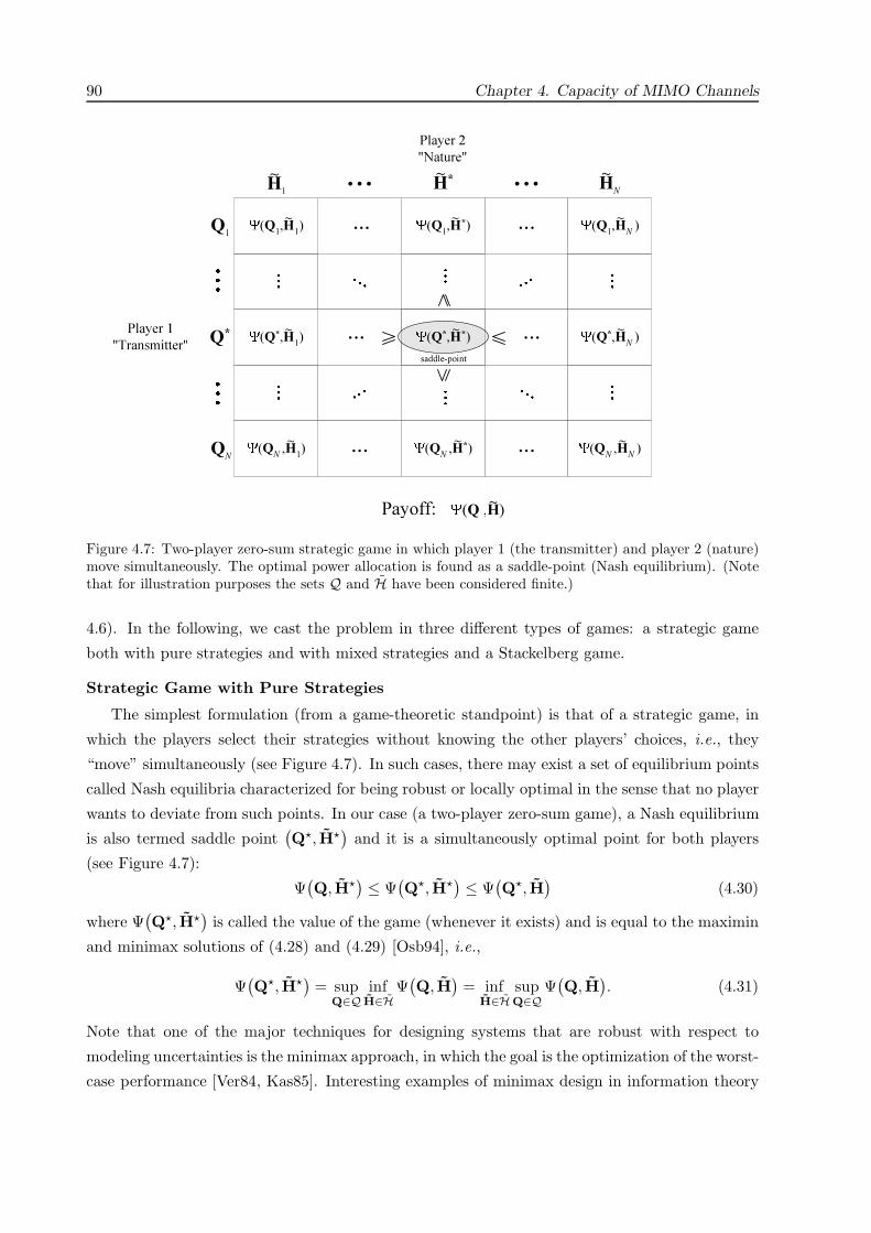
90 Chapter 4. Capacity of MIMO Channels
(Q1,H*)Q
1
Q*
QN
H1
H* HN
(QN
,H*)
(Q*,HN
)(Q*,H1) ......
(Q1,H
1)
(Q*,H*)
saddle-point
(QN
,H1)
(Q1,H
N )
(QN
,HN
)
... ...
... ...
Player 1
"Transmitter"
Player 2
"Nature"
Payoff: (Q ,H)
... ...
~ ~ ~
~ ~ ~
~~ ~
~~ ~
~
Figure 4.7: Two-player zero-sum strategic game in which player 1 (the transmitter) and player 2 (nature)move simultaneously. The optimal power allocation is found as a saddle-point (Nash equilibrium). (Notethat for illustration purposes the sets Q and H have been considered finite.)
4.6). In the following, we cast the problem in three different types of games: a strategic game
both with pure strategies and with mixed strategies and a Stackelberg game.
Strategic Game with Pure Strategies
The simplest formulation (from a game-theoretic standpoint) is that of a strategic game, in
which the players select their strategies without knowing the other players’ choices, i.e., they
“move” simultaneously (see Figure 4.7). In such cases, there may exist a set of equilibrium points
called Nash equilibria characterized for being robust or locally optimal in the sense that no player
wants to deviate from such points. In our case (a two-player zero-sum game), a Nash equilibrium
is also termed saddle point(Q, H
)and it is a simultaneously optimal point for both players
(see Figure 4.7):
Ψ(Q, H
) ≤ Ψ(Q, H
) ≤ Ψ(Q, H
)(4.30)
where Ψ(Q, H
)is called the value of the game (whenever it exists) and is equal to the maximin
and minimax solutions of (4.28) and (4.29) [Osb94], i.e.,
Ψ(Q, H
)= sup
Q∈Qinf
H∈HΨ(Q, H
)= inf
H∈HsupQ∈Q
Ψ(Q, H
). (4.31)
Note that one of the major techniques for designing systems that are robust with respect to
modeling uncertainties is the minimax approach, in which the goal is the optimization of the worst-
case performance [Ver84, Kas85]. Interesting examples of minimax design in information theory
4.4. Worst-Case Capacity: A Game-Theoretic Approach 91
are the problem of source coding or data compression when the data distribution is completely
unknown and the problem of portfolio investment when nothing is known about the stock market
[Cov91b, Cov91a]. Both problems can be formulated as a game in which two players compete:
the source encoding scheme vs. the data distribution and the portfolio investor vs. the market.
Strategic Game with Mixed Strategies
The function Ψ(Q, H
)may or may not have any saddle point depending on the particular set
H (c.f. §4.4.1.2). However, so far we have only considered pure strategies, i.e., strategies given by
a single fixed (deterministic) pair(Q, H
). The game can be extended to include mixed strategies,
i.e., the possibility of choosing a randomization over a set of pure strategies (the randomizations
of the different players is independent) [Osb94]. In this case, the payoff is the average of Ψ(Q, H
)over the mixed strategies, EpQp
HΨ(Q, H
), and the saddle point is similarly defined as
EpQpH
Ψ(Q, H
) ≤ EpQp
HΨ(Q, H
) ≤ EpQp
HΨ(Q, H
). (4.32)
It is well known that a strategic game always has a mixed strategy Nash equilibrium under
the assumption that each set of pure strategies is closed, bounded, and convex [Osb94]. In
fact, for our specific problem, even if we allow more general sets (which need not be closed,
bounded, and convex) such as the set H defined by λmax
(HHH
) ≥ β (which is nonconvex and
unbounded), it can be shown that the problem always has an infinite set of Nash equilibria (c.f.
§4.4.1.2). One can interpret mixed strategies in different ways. In this problem, perhaps, the
most relevant interpretation is to consider the mixed strategy Nash equilibrium as a steady state
of an environment in which players act repeatedly, learning other players’ mixed strategies (see
[Osb94] for other interpretations).
Stackelberg Game
Alternatively, instead of modeling our problem as a strategic game (which, in general, does not
have a pure strategy Nash equilibrium), we can formulate it in a more general way as an extensive
game12 in which the selected strategy of a user may depend on the previously selected strategy
of another user13 (as opposed to the previous strategic interpretation in which both players move
simultaneously) [Osb94, Fud92]. For the specific case of a two-player zero-sum game, in the
parlance of game theory, such an extensive game is called Stackelberg game [Osb94, Fud92].
Consider the case in which the transmitter moves first and then nature moves aware of the
transmitter’s move (see Figure 4.8). In such a case, the maximin solution of (4.28) is always
a pure strategy Nash equilibrium. In fact, such a solution is a subgame perfect equilibrium
(called in this case Stackelberg equilibrium) which is a more refined definition of equilibrium14
12An extensive game is an explicit description of the sequential structure of the decision problems encountered
by the players in a strategic situation [Osb94].13By extensive game we always refer to those with perfect information (imperfect information can also be con-
sidered) [Osb94].14The solution concept of Nash equilibrium is unsatisfactory in extensive games since it ignores the sequential

92 Chapter 4. Capacity of MIMO Channels
Player 1
"Transmitter"
Player 2
"Nature"
Q1
H1(Q*)
H*(Q*)
HN
(Q*)
Payoff: (Q,H(Q))
H1(Q
N ) H
N (Q
N )H
1(Q
1) H
N (Q
1)
H*(Q1) H*(Q
N)
Q*
QN
saddle-point
(Q*,H*(Q*))
(QN ,H
1(Q
N )) (Q
N ,H
N (Q
N ))
(QN ,H*(Q
N ))
(Q*,H1(Q*)) (Q*,H
N (Q*))(Q
1,H
1(Q
1))
(Q1,H*(Q
1))
(Q1,H
N (Q
1))
~
~
~ ~ ~
~~
~ ~~
~ ~ ~
~ ~ ~ ~ ~ ~
Figure 4.8: Two-player zero-sum extensive game in which player 1 (the transmitter) moves first and thenplayer 2 (nature) moves aware of player 1’s move, i.e., Stackelberg game. The optimal power allocationis found as a saddle-point (subgame perfect equilibrium which is also a Nash equilibrium). (Note that forillustration purposes the sets Q and H have been considered finite.)
[Osb94, Fud92]. In this case, a saddle point(Q, H (Q)
)is characterized by
Ψ(Q, H (Q)
) ≤ Ψ(Q, H (Q)
) ≤ Ψ(Q, H (Q)
). (4.33)
Similarly, we can also consider the opposite formulation of the Stackelberg game in which nature
moves first and then the transmitter moves aware of nature’s move with saddle point given by
Ψ(Q(H), H) ≤ Ψ
(Q(H), H) ≤ Ψ
(Q(H), H). (4.34)
Note that the saddle points of (4.33) and (4.34) are always satisfied by the solutions to problems
(4.28) and (4.29), respectively.
Existing Results
A significant part of the literature that has modeled communication as a game has dealt with
the characterization of saddle points satisfying (4.30), i.e., implicitly adopting a formulation of
the problem as a strategic game. Reference [Bla57] is one of the earliest papers dealing with such
a problem using a mutual information payoff. (Note that other payoff functions have also been
considered, such as the mean square error in [Bas83] to deal with communication over a channel
structure of the decision problem; as a consequence, more refined definitions of equilibrium have been proposed
[Osb94].

4.4. Worst-Case Capacity: A Game-Theoretic Approach 93
with an intelligent jammer.) A two-player zero-sum game was explicitly adopted in [Bor85]
obtaining the Gaussian distribution as a saddle point. In [Sta88], m-dimensional strategies were
considered in a game-theoretic formulation of communication over channels with block memory,
where it was found that memoryless jamming and memoryless coding constitute a saddle point. In
[Yan93], a two-player zero-sum game was explicitly formulated for communication in the presence
of jamming using a power constraint for both players. In [Dig01], communication under the worst
additive noise under a covariance constraint was analyzed (the Gaussian distribution was obtained
as a saddle-point solution) with emphasis on covariances satisfying correlation constraints at
different lags. The vector Gaussian AVC was considered in [Hug88] obtaining a saddle point
given by a water-filling solution for the jammer and for the coder. In [Chi01], the maximin and
minimax problems of (4.28) and (4.29) in a multi-antenna wireless scenario were solved for a
specific set of channels H defined by Tr(HHH
) ≥ β, i.e., the two Stackelberg games previously
formulated were implicitly considered.
The rest of the section focuses mainly on finding a robust power allocation when the channel is
unknown, i.e., in solving the maximin problem of (4.28). Such a solution has many interpretations.
Under some conditions (obtained in §4.4.1.2), it constitutes a saddle point of the strategic game
formulation of (4.30) with the inherent properties of robustness. In any case, if mixed strategies
are allowed in the strategic game, the solution to (4.28) always forms a saddle point defined by
(4.32) (c.f. §4.4.1.2). Finally, even if we restrict the game to pure strategies, the solution to (4.28)
always constitutes a saddle point as defined in (4.33) corresponding to a Stackelberg game. (The
opposite minimax problem formulation of (4.29) is briefly considered in §4.4.1.2.3 as well.)
4.4.1.2 Worst-Case Capacity and Robust Power Allocation
The main purpose of this subsection is to solve the maximin formulation of (4.28) and to charac-
terize the conditions under which the solution forms a saddle point in the strategic formulation
of the game (with pure strategies and mixed strategies).
As pointed out in §4.4.1.1, we have to define some artificial constraint on the channel to avoid
the trivial solution. Noting from (4.10)-(4.11) that the payoff function Ψ(Q, H
)depends on H
through HHH (the left singular vectors of H are irrelevant), it is convenient to define H as
H H : RH HHH = HHR−1
n H ∈RH
. (4.35)
To define the set RH we consider any kind of spectral (eigenvalue) constraint given by
RH RH : λi (RH) ∈ LRH (4.36)
where LRHdenotes an arbitrary eigenvalue constraint (in §4.4.1.2.1 some specific eigenvalue
constraints are considered). (Clearly, the set LRHcannot contain the all-zero vector that would
94 Chapter 4. Capacity of MIMO Channels
correspond to H = 0.) In defining the set RH as in (4.36), we are deliberately leaving the
eigenvectors of RH (equivalently, the right singular vectors of H) totally unconstrained. This is
so that no preference is given to any signaling direction,15 i.e., to guarantee the isotropy of RH
(any direction is possible).
Definition 4.1 A set of matrices H is isotropically unconstrained if the right singular vectors of
the elements of the set are unconstrained, i.e., if for each H ∈H then HU ∈H for any unitary
matrix U.
Clearly, the set H (defined according to (4.35) and (4.36)) is isotropically unconstrained.
We remark that the results in this subsection are valid regardless of the particular eigenvalue
constraint chosen to define the set LRH.
We now obtain the uniform power allocation as the maximin solution of (4.28), i.e., as the
capacity-achieving solution of the compound vector Gaussian channel. Note that this could be
proved in a shorter way by contradiction, i.e., by showing that, for any given power allocation,
we can always find some channel that yields a lower capacity than the minimum capacity cor-
responding to the uniform power allocation (indeed, this is the technique used in §4.4.2 for the
multiple-access channel). Nevertheless, we obtain a more complete proof by characterizing the
“shape” of the worst channel for any given power allocation and then we give some examples in
order to gain insight into the problem.
Before proceeding to the main result, recall that the capacity of the compound vector Gaussian
memoryless channel when the channel state is unknown was obtained in [Roo68]16 as
C(H) = supQ∈Q
infH∈H
log det(InR
+ HQHH)
(4.37)
under the mild assumption that H is bounded (if not, we can simply bound H by adding the
constraint λmax
(HHH
) ≤ c for a sufficiently large value of c, which can be done without loss of
generality based on physical interpretations of the channel H). The achievability was proved in
[Roo68] by showing the existence of a code (along with the decoding sets). Therefore, in theory,
one can always find a code to achieve rates arbitrarily close to capacity and then use a universal
decoder that decodes the received word according to the decoding set it belongs to (note that no
knowledge of the channel state is required).
Theorem 4.1 The capacity of the compound vector Gaussian memoryless channel with power
constraint PT , nT transmit dimensions, and nR receive dimensions (with no CSI) is
C(H) = infH∈H
log det(InR
+ PT /nT HHH)
(4.38)
15For a flat multi-antenna system, the term “direction” means literally spatial direction.16The extension to the complex-valued case is straightforward using the results of [Nee93].

4.4. Worst-Case Capacity: A Game-Theoretic Approach 95
where the class of channels H is an isotropically unconstrained set defined by (4.35)-(4.36) (uncon-
strained right singular vectors). The capacity-achieving solution of (4.38) is given by a Gaussian
code with a uniform power allocation
Q = PT /nT InT(4.39)
which implies an independent signaling over the transmit dimensions.
Proof. Intuitively speaking, due to the symmetry of the problem, if the transmitter does not use
a uniform power distribution, the channel will do an “inverse water-filling”, i.e., it will redistribute
its singular values so that the highest ones align with the lowest eigenvalues of Q (see Lemma 4.3
in Appendix 4.B). Therefore, maximizing the lowest eigenvalues of Q seems to be appropriate to
avoid such a behavior. Indeed, this is achieved by the uniform power allocation.
See Appendix 4.B for a formal proof.
Note that the worst-case capacity expression (4.38) obtained in Theorem 4.1 can be simplified
as
infH∈H
log det(InR
+ PT /nT HHH)
= infλRH,i∈LRH
nT∑i=1
log (1 + PT /nT λRH ,i) . (4.40)
Theorem 4.1 is basically saying that when the channel state is unknown but known to belong
to a set of possible channels H, the optimum solution in the sense of providing the best worst-case
performance is given by the uniform power allocation of (4.39). In other words, it is the solution
to the problem formulation as a Stackelberg game in which the transmitter moves first as depicted
in Figure 4.8. Note that if we had used instead the eigenvalue constraint λQ,max ≤ α to define
the set Q, it would have immediately followed λQ,i = α ∀i, i.e., a uniform solution as well.
The uniform power allocation and the corresponding minimizing channel always constitute a
saddle point of the Stackelberg game as defined in (4.33). Depending on the specific definition of
the set of channels H, they will also form a saddle point of the strategic game as given in (4.30).
The following corollary gives the exact conditions.
Corollary 4.1 The uniform power allocation Q = PT /nT InTobtained in Theorem 4.1 and the
corresponding minimizing channel form a saddle point of the strategic game given by (4.30) if
and only if the minimizing channel satisfies λRH ,i = β ∀i (in particular this implies nR ≥ nT ).
Proof. Since the right inequality of (4.30) is satisfied by any solution to (4.28), it suffices to
find the conditions under which the left inequality is satisfied, i.e., Ψ(Q, H
) ≤ Ψ(PT /nT I, H
)where H H (PT /nT I) is the minimizing channel of Theorem 4.1 corresponding to the uniform
power allocation. Recalling that Ψ(Q, H
)is maximized when the eigenvectors of Q align with
the right singular vectors of H and when the eigenvalues of Q water-fill the eigenvalues of HHH
[Tel95], it must be that HHH is a diagonal matrix and has equal eigenvalues. Thus, it must be
that HHH = β I or, equivalently, λRH ,i = β ∀i for some β.

96 Chapter 4. Capacity of MIMO Channels
In the next subsection, specific definitions of H are considered and Corollary 4.1 will be
invoked to show in which cases the uniform power allocation constitutes a saddle point of the
strategic game.
In [Dig01], the existence of a saddle point as defined in (4.30) was proved for any set of
channels H such that H = I and Rn∈Rn where Rn is closed, bounded, and convex. With the
additional constraint that Rn be isotropically unconstrained, the existence result of [Dig01] can
be combined with Theorem 4.1 and Corollary 4.1 to conclude that in such a case, the uniform
solution for both the transmitter and the noise always constitute a saddle point of the strategic
game as given in (4.30). We state this in the following corollary for further reference.
Corollary 4.2 Consider the set of channels H defined such that H = I (nT = nR) and Rn∈Rn
where Rn is closed, bounded, convex, and isotropically unconstrained (i.e., unconstrained eigen-
vectors). It then follows that the uniform power allocation Q = PT /nT I and the noise Rn = σ2n I
always form a saddle point of the strategic game given by (4.30).
Many papers have obtained the uniform solution for both the transmitter and the noise
(or jammer) as mutual information saddle points for the set of noise covariances with power
constraint given by Tr (Rn)≤Pn, e.g., [Bla57, Sta88, Yan93] (also [Hug88]17 for the particular
case in which the background noise is removed). Corollary 4.2 generalizes such a result to an
arbitrary set of noise covariances Rn (provided it is closed, bounded, convex, and isotropically
unconstrained). Note that a constraint on the channel eigenvalues λRH ,i can be alternatively
expressed (whenever nT = nR) as a constraint of the form H = I and Rn∈Rn as considered in
Corollary 4.2 since we can write λi (Rn) = λnT −i+1 (RH)−1.
As mentioned in §4.4.1.1, even when the strategic game does not have a saddle point or
Nash equilibrium, if mixed strategies are allowed the game has then an infinite set of saddle
points or Nash equilibria as defined in (4.32) (see Appendix 4.C). In particular, as proved in
Appendix 4.C, the mixed-strategy Nash equilibria are given by a pure strategy for the transmitter
Q = PT /nT InT(uniform power allocation) and a mixed strategy for nature that, for example,
puts equal probability on each element of the setH = U
HΣ
HPVH
H: P ∈ Π
where Σ
Hcontains
in the main diagonal the optimum (worst-case) singular values corresponding to Q = PT /nT InT
(as in Theorem 4.1), UH and VH are two arbitrary unitary matrices, and Π is the set of the nT !
different permutation matrices of size nT × nT (see Appendix 4.C for a proof).
4.4.1.2.1 Examples of Channel Constraints
To gain further insight into the problem, we now analyze in detail some particular constraints
to define the set of channels H. In principle, for each of the different constraints, it is possible
to directly solve the corresponding maximin problem of (4.28). Using the result obtained in17Although [Hug88] deals with the vector Gaussian AVC, the final problem formulation is also given by maximin
and minimax mathematical problems.
4.4. Worst-Case Capacity: A Game-Theoretic Approach 97
Theorem 4.1, however, we already know (provided that the set H is isotropically unconstrained)
that the optimal solution is the uniform power allocation Q = PT /nT InTand that the worst-
case channel is given by the minimizing solution to (4.40). It is important to remark that, to find
the worst-case channel, it is not necessary to solve the minimization for an arbitrary set λQ,ito obtain λ
RH ,i (λQ,i); it suffices to consider directly the uniform solution λQ,i = PT /nT ∀i
as in (4.40) and obtain λRH ,i (PT /nT ), which is a great simplification.
General Individual Channel Eigenvalue Constraint: λRH ,i ≥ βiConsider a general and individual constraint on each channel eigenvalue λRH ,i ≥ βi, where
it is assumed that βi ≥ βi+1 ≥ 0 and that all eigenvalues have a corresponding βi without loss
of generality (if not, one can always set βi = βi−1 or βi = 0 as appropriate). The minimizing
channel of (4.40) is easily obtained by minimizing each of the terms of the RHS of (4.40) as
λRH ,i = βi 1 ≤ i ≤ nT . (4.41)
This solution is in general non-uniform and, by Corollary 4.1, is not a saddle point of the strategic
game as given in (4.30). Note that Corollary 4.2 cannot be invoked to prove the existence of a
saddle point (for H = I) since the constraints expressed in terms of noise eigenvalues λn,i =
λ−1RH ,nT−i+1 ≤ β−1
nT −i+1 in general define a nonconvex and unbounded region for the set Rn.
Consider now a constraint just on the maximum channel eigenvalue λRH ,max ≥ β. This specific
constraint has a special interest since the maximum eigenvalue of RH= HHH is an upper-bound
on the elements of RH and, in particular, on the received power corresponding to the ith transmit
dimension, [RH ]ii = ‖hi‖2, where hi is the ith column of the channel matrix H. The minimizing
channel is given by λ
RH ,max = β
λRH ,i = 0 2 ≤ i ≤ nT .
(4.42)
It is also of interest to consider a constraint just on the minimum channel eigenvalue λRH ,min ≥β. The minimizing channel is now
λRH ,i = β 1 ≤ i ≤ nT . (4.43)
For this particular case, the minimizing channel is uniform and then, by Corollary 4.1, the uniform
power allocation forms a saddle point of the strategic game as given in (4.30). Alternatively,
Corollary 4.2 could have been invoked to show the existence of a saddle point (for H = I) since
the constraints expressed in terms of noise eigenvalues λn,max ≤ β−1 form a closed, bounded,
convex, and isotropically unconstrained set Rn.
Channel Trace Constraint: Tr (RH) =∑
i λRH ,i ≥ β
The channel trace constraint is probably the most reasonable constraint from a physical
standpoint since it represents the total channel energy ‖H‖2
F = Tr (RH). In [Chi01], this channel
constraint was considered, obtaining the same results.

98 Chapter 4. Capacity of MIMO Channels
Since function f(x) =∑n
i=1 log (1 + xi α) is Schur-concave (−f(x) is Schur-convex) [Mar79,
3.H.2] and any eigenvalue distribution is majorized by (∑
i λRH ,i, 0, · · · , 0) [Mar79, p.7] (see the
proof of Lemma 4.4 for a similar reasoning), it follows that its minimum value is achieved by
λ
RH ,max = β
λRH ,i = 0 2 ≤ i ≤ nT .
(4.44)
This solution is clearly non-uniform and, by Corollary 4.1, does not constitute a saddle point
of the strategic game as given in (4.30). Note that Corollary 4.2 cannot be invoked either to
prove the existence of a saddle point (for H = I) since the constraint expressed in terms of noise
eigenvalues∑
i λ−1n,i ≥ β defines a nonconvex and unbounded region for the set Rn.
Maximum Noise Eigenvalue Constraint: λn,max ≤ σ2
This constraint is identical to the minimum channel eigenvalue constraint with solution given
by (4.43).
Noise Trace Constraint: Tr (Rn) =∑
i λn,i ≤ σ2
This is the constraint considered in most publications since it is a very natural constraint
when the noise is interpreted as a jammer constrained in its average transmit power (as is the
intended transmitter). See, for example, [Bla57, Sta88, Yan93] and also [Hug88] for the particular
case in which the background noise is removed.
For this particular constraint, we can directly invoke Corollary 4.2 to show that the worst-case
noise is given by
λn,i = σ2/nR 1 ≤ i ≤ nR (4.45)
and that the uniform power allocation constitutes a saddle point of the strategic game as given
in (4.30).
Banded Noise Covariance Constraint
In [Dig01, Sec. III], a banded noise covariance constraint (a noise with correlation constraints
at different lags) was analyzed in detail. Such a constraint is not isotropically unconstrained
and, consequently, the results of this paper do not apply. Therefore, we cannot conclude that
the uniform power allocation is the maximin solution to the mutual information game. In fact,
the saddle-point solution was obtained in [Dig01, Sec. III] to be given by the maximum-entropy
extension for the noise and by a water-filling solution for the transmitter which in general is
non-uniform.
4.4.1.2.2 On the Specific Choice of the Channel Constraints
As has been shown in Theorem 4.1, the uniform power allocation is the solution to the maximin
problem of (4.28). In other words, it is a robust solution under channel uncertainty.

4.4. Worst-Case Capacity: A Game-Theoretic Approach 99
Other aspects and observations of the solution, such as whether it is better to have many
antennas or just a few in a multi-antenna system, depend on the particular choice of constraints
that define the set of channels H which have to be tailored to each specific application. To
illustrate this effect, we now consider some heuristic choices as examples (for simplicity, we assume
Rn = I).
Inspired by a communication system with multiple transmit and receive antennas with a unit-
energy channel in the sense of expected value E [| [H]i,j |2] = 1 (which implies E [Tr(HHH
)] =
nT nR), we can similarly consider a worst-case problem formulation with the trace constraint
defined as
Tr(HHH
) ≥ α nT nR
where α is a scaling factor that, for example, guarantees that the constraint is satisfied with a
certain probability (if the constraint is not satisfied, an outage event is declared). In this case,
using the results of §4.4.1.2.1, the worst-case capacity is given by
log (1 + α PT nR)
from which we can conclude that, while adding transmit antennas does not increase the worst-case
capacity when the channel state is unknown, adding receive antennas is always beneficial.
Inspired by a set of parallel subchannels, each with unit gain, we can instead define the trace
constraint as (assuming nT ≤ nR)
Tr(HHH
) ≥ α nT .
In this case, the worst-case capacity is given by
log (1 + α PT )
from which we can conclude that the worst-case performance is independent of the number of
transmit and receive antennas when the channel state is unknown. However, for this scenario cor-
responding to a set of parallel subchannels, it may be more appropriate to consider the minimum
channel eigenvalue constraint (assuming nT ≤ nR)
λmin
(HHH
) ≥ α,
obtaining a worst-case capacity (using the result in §4.4.1.2.1) given by the increasing function
of nT
nT log (1 + α PT /nT ) −→nT→∞ αPT
from which it is always beneficial to add transmit and also receive antennas.
A Numerical Example
In Figure 4.9, the capacity of the uniform power allocation is compared to that of a non-
uniform allocation (simply chosen according to the distribution λQ = [0.6, 0.2, 0.1, 0.1]T PT )

100 Chapter 4. Capacity of MIMO Channels
−5 0 5 10 15 20 25 300
5
10
15
20
25
30
Capacity with uniform and non−uniform power allocation ( Tr( H HH ) = nT n
R )
SNR (dB)
Cap
acity
(bi
ts /
tran
smis
sion
)
uniform power allocation non−uniform power allocation
arbitrary channels
worst−case channel
Figure 4.9: Capacity of the uniform and a non-uniform (according to the distribution λQ =[0.6, 0.2, 0.1, 0.1]T PT ) power allocations vs. the SNR for two arbitrary channels and for the worst channelof the set defined by Tr
(HHH
)= nT nR and Rn = σ2
n I.
as a function of the SNR defined as Tr (Q) /σ2n, where the noise covariance matrix was fixed
to Rn = σ2n I and the set of channels H was constrained using the channel trace constraint
Tr(HHH
)= nT nR for nT = nR = 4 (equivalently, H is defined by Tr
(HHH
)= nT nR/σ2
n).
The capacities corresponding to two arbitrary channels and to the worst channel adapted to each
power distribution are plotted. As expected, the capacity of the uniform distribution is always
the best for the worst-case channel (note that in general, for an arbitrary channel, this may or
may not be the case).
4.4.1.2.3 Opposite Problem Formulation: Nature Moves First
For completeness, we now briefly consider the opposite problem formulation, i.e., the minimax
problem of (4.29). A solution to (4.29) will always be a saddle point as defined in (4.34) corre-
sponding to the Stackelberg game in which nature moves first and then the transmitter moves
aware of natures’s move. In some cases, it will also form a saddle point of the strategic game as
defined in (4.30).
It is well known that Ψ(Q, H
)is maximized when the eigenvectors of Q align with the right
singular vectors of H and when the eigenvalues of Q water-fill the eigenvalues of RH= HHH

4.4. Worst-Case Capacity: A Game-Theoretic Approach 101
[Tel95]. The minimax problem of (4.29) reduces then to
minλRH,i
∑nTi=1 log
(1 + λ
Q,i (λRH ,i) λRH ,i
)s.t. λRH ,i ∈ LRH
(4.46)
where λQ,i (λRH ,i) =
(ν − λ−1
RH ,i
)+ is the water-filling solution and ν is the water-level chosen
to satisfy the power constraint of (4.27) with equality. Clearly, we can relabel the λRH ,i’s so that
they are in decreasing order without loss of generality and, as a consequence of the water-filling
solution, the λQ,i’s will also be in decreasing order.
For the cases considered in §4.4.1.2.1 where saddle points were obtained (minimum channel
eigenvalue constraint, maximum noise eigenvalue constraint, noise trace constraint, banded noise
covariance constraint), we already know that the same solutions are obtained when nature moves
first simply by the definition of saddle point in (4.30).
For the case of a general individual channel eigenvalue constraint λRH ,i ≥ βi, the worst-case
channel is simply obtained as in (4.41) (although in this case, the eigenvalues of Q water-fill those
of RH).
The channel trace constraint was considered in [Chi01], where it was found that for low
values of the SNR defined as PT β/σ2n (the noise covariance matrix was assumed fixed and given
by Rn = σ2n I) the worst channel is given by λ
RH ,i = β/min (nT , nR) ∀i and for high values of
the SNR the worst channel is similarly given except that a dominant eigenvalue arises.
4.4.1.2.4 Extension to Ergodic and Outage Capacities
In addition to analyzing robustness in terms of instantaneous capacity (which implies a fixed
channel state H), it is also interesting to consider other statistics of the capacity such as average
and outage values as described in §4.3. Whereas channel pdf was assumed known and fixed in
§4.3, we now consider the case in which it is known to belong to a class of pdf’s but otherwise
unknown.
In this sense, the maximin formulation is as in (4.28) but now the payoff function is given
either by Ierg (Q) or Ioutε (Q) (see (4.18) and (4.19)) and the minimization is over the set of
possible channel pdf’s pH∈PH in which the channel singular vectors are unconstrained (isotropic
property), e.g., E[λmax
(HHH
)] ≥ β. Without going into details, we justify why the uniform
power allocation is also obtained as a robust solution in terms of ergodic and outage capacities.
Simply note that pH
can always be chosen as a function of the utilized Q to put positive probability
only on channel states H with the singular vectors chosen to perform an “inverse water-filling”
on Q (c.f. Theorem 4.1), against which the best solution for the transmitter is a uniform power
allocation. Therefore, it is an optimal solution for every choice of H and hence for other capacity
statistics such as the average and the outage values.
102 Chapter 4. Capacity of MIMO Channels
It is interesting to point out that if pH
does a randomization over a set of channel states in Has defined in the previous subsections (this need not be in a general case), the ergodic capacity
problem then results in a mixed-strategy formulation of a game in which the pure strategies are
defined by H and, therefore, the previously obtained results on mixed strategy Nash equilibria
apply (c.f. Appendix 4.C).
It is important to bear in mind that the optimality of the uniform power allocation in terms
of ergodic and outage capacities is in the worst-case sense, i.e., when pH
is known to belong to a
set PH but otherwise unknown. Therefore, it cannot be concluded from the obtained results that
the uniform power allocation is optimum in terms of outage capacity for the case, for example,
of a random H with i.i.d. Gaussian entries which is a well-known open problem as discussed in
[Tel95] (where it was conjectured that the uniform power allocation could be the optimal solution,
but only over a certain number of transmit dimensions). It is interesting, however, to remark
that, by definition, the worst-case instantaneous capacity for a set of channels H as previously
considered happens to be the zero-outage capacity (also termed delay-limited capacity [Big98,
Cai99b, Big01]) for any pH that puts non-zero probability on each member of H. Unfortunately,
this result is not very useful for the case of a random channel H with i.i.d. CN (0, 1) entries, since
it has a zero worst-case capacity [Big01].18
Note that if one considers that nature can only control the channel eigenvalues but not the
eigenvectors, then the optimality of the uniform power allocation need not hold.
4.4.1.2.5 Cost of Robustness
Robustness is a desirable property that comes with a price. For a given channel state H,
one can explicitly compute the loss in performance of the robust uniform power distribution
with respect to the optimum allocation (obtained with a perfect instantaneous knowledge of the
channel state). However, it is also interesting to know the worst-case loss of performance for a
given class of channels H. In this section, the cost of robustness for a family of channels H (or,
equivalently, RH) is analyzed using the concept of duality gap arising in convex optimization
theory (see §3.1 and [Lue69, Roc70, Boy00]) following the approach proposed in [Yu01a].
Assuming for the moment a fixed channel state given by λRH ,i, the maximization of the
mutual information can be expressed in convex form (we use in this section logarithms in base 2
and natural logarithms denoted by log2 and ln, respectively) as
min f0(x) = −∑ni=1 log2 (1 + xi λRH ,i)
s.t.∑
i xi ≤ P,
xi ≥ 0 1 ≤ i ≤ n.
(4.47)
18The worst-case capacity studied in this paper is equivalent to the delay-limited capacity considered in [Big01]
under a short-term power constraint (in [Big01], however, perfect CSI was assumed).
4.4. Worst-Case Capacity: A Game-Theoretic Approach 103
(note that Slater’s condition is satisfied and, therefore, strong duality holds) and the Lagrangian
is
L (x, (λ,µ)) = −n∑
i=1
log2 (1 + xi λRH ,i) + λ
(∑i
xi − P
)−
n∑i=1
µi xi. (4.48)
The dual objective, g (λ,µ), is obtained by setting ∂L∂xi
= 0, which gives the water-filling solution
xi +1
λRH ,i=
1(λ − µi)
1log 2
. (4.49)
If we now evaluate the duality gap (see §3.1) denoted by Γ (x, (λ,µ)) at any x and with µ chosen
so that the water-filling condition (4.49) is satisfied, then the duality gap is
Γ (x, λ) = − 1log 2
n∑i=1
xi λRH ,i
1 + xi λRH ,i+ λP. (4.50)
(Note that a better choice of the Lagrange multipliers to obtain a smaller gap could be made,
however this choice produces a simple closed-form expression.) Using the smallest possible value
for λ (such that all the Lagrange multipliers λ and µi’s are non-negative)
λ =1
log 2max
i
(λRH ,i
1 + xi λRH ,i
)(4.51)
and assuming that the power constraint is satisfied with equality∑
i xi = P , we can write the
duality gap as
Γ (x) =1
log 2
n∑i=1
xi
(max
j
(λRH ,j
1 + xj λRH ,j
)− λRH ,i
1 + xi λRH ,i
). (4.52)
Finally, evaluating the gap for a uniform power allocation xi = P/n, we obtain
Γuni (λRH) Γ (xi = P/n) =
1log 2
n∑i=2
(P/n λRH ,max
1 + P/n λRH ,max− P/n λRH ,i
1 + P/n λRH ,i
)(4.53)
where we have made explicit the dependence of the gap on the channel eigenvalues λRH ,i which
are assumed in decreasing order. For a channel with equal eigenvalues, λRH ,i = κ, the uniform
power allocation is optimum and the gap becomes zero as expected. Note that for P → ∞ (with
positive λRH ,i’s) the gap also tends to zero, i.e., for high SNR the uniform distribution tends to
be optimal (this observation was empirically made in [Cho93] and further analyzed in [Yu01a]).
Now we can use the closed-form expression in (4.53) to easily obtain an upper bound on
the worst-case loss of performance for the class of channels RH . For example, if we consider a
maximum channel eigenvalue constraint λRH ,max ≥ β, the gap is
Γuni =n − 1log 2
P/n λRH ,max
1 + P/n λRH ,max−→
λRH,max→∞n − 1log 2
. (4.54)
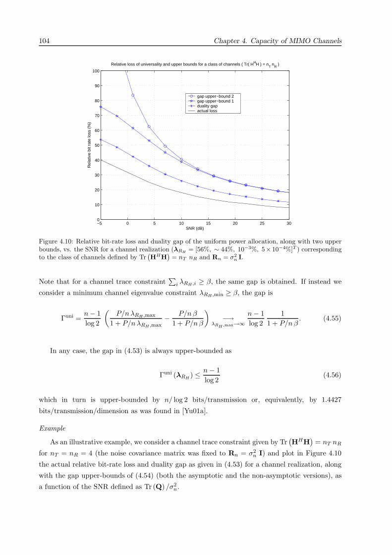
104 Chapter 4. Capacity of MIMO Channels
−5 0 5 10 15 20 25 300
10
20
30
40
50
60
70
80
90
100
Relative loss of universality and upper bounds for a class of channels ( Tr( H HH ) = nT n
R )
SNR (dB)
Rel
ativ
e bi
t rat
e lo
ss (
%)
gap upper−bound 2 gap upper−bound 1 duality gap actual loss
Figure 4.10: Relative bit-rate loss and duality gap of the uniform power allocation, along with two upperbounds, vs. the SNR for a channel realization (λRH = [56%, ∼ 44%, 10−3%, 5× 10⁻⁴%]T ) correspondingto the class of channels defined by Tr
(HHH
)= nT nR and Rn = σ2
n I.
Note that for a channel trace constraint∑
i λRH ,i ≥ β, the same gap is obtained. If instead we
consider a minimum channel eigenvalue constraint λRH ,min ≥ β, the gap is
Γuni =n − 1log 2
(P/n λRH ,max
1 + P/n λRH ,max− P/n β
1 + P/n β
)−→
λRH,max→∞n − 1log 2
11 + P/n β
. (4.55)
In any case, the gap in (4.53) is always upper-bounded as
Γuni (λRH) ≤ n − 1
log 2(4.56)
which in turn is upper-bounded by n/ log 2 bits/transmission or, equivalently, by 1.4427
bits/transmission/dimension as was found in [Yu01a].
Example
As an illustrative example, we consider a channel trace constraint given by Tr(HHH
)= nT nR
for nT = nR = 4 (the noise covariance matrix was fixed to Rn = σ2n I) and plot in Figure 4.10
the actual relative bit-rate loss and duality gap as given in (4.53) for a channel realization, along
with the gap upper-bounds of (4.54) (both the asymptotic and the non-asymptotic versions), as
a function of the SNR defined as Tr (Q) /σ2n.
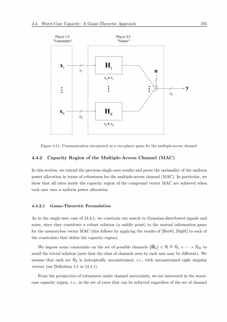
4.4. Worst-Case Capacity: A Game-Theoretic Approach 105
H1
x1
n
y
n1
nR
nR
x n1
Player 1/2
"Transmitter"
Player 2/1
"Nature"
HK
xK
nK
nR
x nK
Figure 4.11: Communication interpreted as a two-player game for the multiple-access channel.
4.4.2 Capacity Region of the Multiple-Access Channel (MAC)
In this section, we extend the previous single-user results and prove the optimality of the uniform
power allocation in terms of robustness for the multiple-access channel (MAC). In particular, we
show that all rates inside the capacity region of the compound vector MAC are achieved when
each user uses a uniform power allocation.
4.4.2.1 Game-Theoretic Formulation
As in the single-user case of §4.4.1, we constrain our search to Gaussian-distributed signals and
noise, since they constitute a robust solution (a saddle point) to the mutual information game
for the memoryless vector MAC (this follows by applying the results of [Bor85, Dig01] to each of
the constraints that define the capacity region).
We impose some constraints on the set of possible channels Hk ∈ H H1 × · · · × HK to
avoid the trivial solution (note that the class of channels seen by each user may be different). We
assume that each set Hk is isotropically unconstrained, i.e., with unconstrained right singular
vectors (see Definition 4.1 in §4.4.1).
From the perspective of robustness under channel uncertainty, we are interested in the worst-
case capacity region, i.e., in the set of rates that can be achieved regardless of the set of channel

106 Chapter 4. Capacity of MIMO Channels
states chosen from the set of possible channels Hk ∈ H. This can be formulated as a game
(see Figure 4.11) where the first player is the transmitter and the second player, who controls the
whole set of channels Hk and is aware of the first player’s move, is nature.
4.4.2.2 Worst-Case Capacity Region and Robust Power Allocation
The worst-case capacity region is in fact the notion of capacity region of the compound MAC
[Ver89, Lap98] (see also [Csi81, p. 288]). Mathematically, the worst-case region of the set of
achievable rates for a fixed set of transmit covariance matrices Qk is expressed (similarly to
the maximin formulation of the single-user case in (4.28)) as the following intersection:
R( Qk , H) =⋂
Hk∈HR( Qk , Hk
)(4.57)
which is closed and convex because it is the intersection of closed and convex sets. Recall that
R( Qk , Hk)
is the set of achievable sets for the set of channel states Hk as given in
(4.13). Assuming that the transmit covariance matrices are constrained in their average transmit
power, the worst-case capacity region (capacity region of the compound vector Gaussian MAC)
is [Ver89]19
C(H) =⋃
Tr(Qk)≤Pk,Qk=QH
k ≥0
R( Qk , H) (4.58)
which also happens to be closed and convex as shown in Theorem 4.2. In [Han98], an expression
similar to (4.58) was obtained as the delay-limited MAC capacity region (although the case of
perfect CSIT was considered therein). The worst-case capacity region is formally characterized
in the following theorem.
Theorem 4.2 The capacity region of the compound vector Gaussian memoryless multiple-access
channel (MAC) composed of K users with power constraints Pk, number of transmit dimensions
nk, and nR receive dimensions (with no CSI) is
C(H) =
(R1, · · · , RK) :
0 ≤∑k∈S
Rk ≤ infHk∈H
log det(InR
+∑k∈S
Pk/nk HkHHk
),∀S ⊆ 1, · · · ,K
(4.59)
where the class of channels H is an isotropically unconstrained set (unconstrained right singular
vectors). All set of rates within the region of (4.59) are achieved when each user utilizes a19As argued in [Ver89], achievability follows easily using randomized codes and the converse is established since
reliable communication has to be guaranteed no matter what channel state is in effect. Similarly to the single-user
case, the capacity region remains the same if the receiver is uninformed of the channel state [Csi81, p. 293].
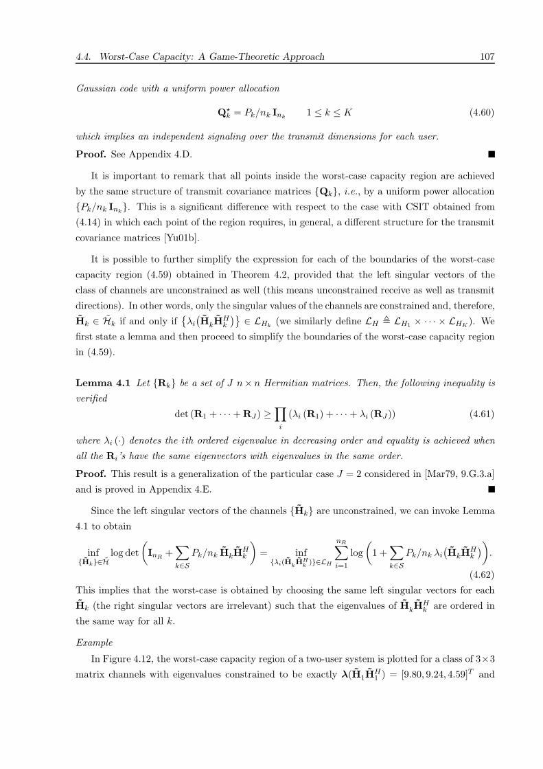
4.4. Worst-Case Capacity: A Game-Theoretic Approach 107
Gaussian code with a uniform power allocation
Qk = Pk/nk Ink
1 ≤ k ≤ K (4.60)
which implies an independent signaling over the transmit dimensions for each user.
Proof. See Appendix 4.D.
It is important to remark that all points inside the worst-case capacity region are achieved
by the same structure of transmit covariance matrices Qk, i.e., by a uniform power allocation
Pk/nk Ink. This is a significant difference with respect to the case with CSIT obtained from
(4.14) in which each point of the region requires, in general, a different structure for the transmit
covariance matrices [Yu01b].
It is possible to further simplify the expression for each of the boundaries of the worst-case
capacity region (4.59) obtained in Theorem 4.2, provided that the left singular vectors of the
class of channels are unconstrained as well (this means unconstrained receive as well as transmit
directions). In other words, only the singular values of the channels are constrained and, therefore,
Hk ∈ Hk if and only ifλi
(HkH
Hk
) ∈ LHk(we similarly define LH LH1 × · · · × LHK
). We
first state a lemma and then proceed to simplify the boundaries of the worst-case capacity region
in (4.59).
Lemma 4.1 Let Rk be a set of J n× n Hermitian matrices. Then, the following inequality is
verified
det (R1 + · · · + RJ) ≥∏
i
(λi (R1) + · · · + λi (RJ )) (4.61)
where λi (·) denotes the ith ordered eigenvalue in decreasing order and equality is achieved when
all the Ri’s have the same eigenvectors with eigenvalues in the same order.
Proof. This result is a generalization of the particular case J = 2 considered in [Mar79, 9.G.3.a]
and is proved in Appendix 4.E.
Since the left singular vectors of the channels Hk are unconstrained, we can invoke Lemma
4.1 to obtain
infHk∈H
log det(InR
+∑k∈S
Pk/nk HkHHk
)= inf
λi(HkHHk )∈LH
nR∑i=1
log(
1 +∑k∈S
Pk/nk λi
(HkH
Hk
)).
(4.62)
This implies that the worst-case is obtained by choosing the same left singular vectors for each
Hk (the right singular vectors are irrelevant) such that the eigenvalues of HkHHk are ordered in
the same way for all k.
Example
In Figure 4.12, the worst-case capacity region of a two-user system is plotted for a class of 3×3
matrix channels with eigenvalues constrained to be exactly λ(H1HH1 ) = [9.80, 9.24, 4.59]T and
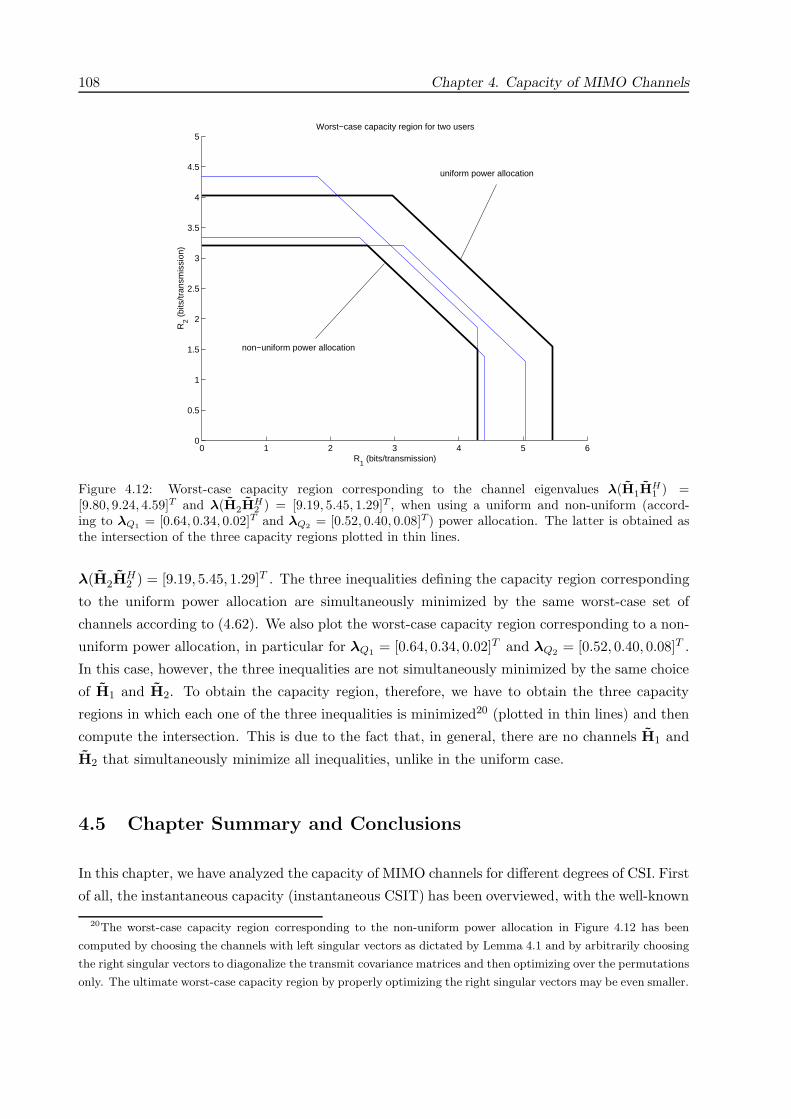
108 Chapter 4. Capacity of MIMO Channels
0 1 2 3 4 5 60
0.5
1
1.5
2
2.5
3
3.5
4
4.5
5Worst−case capacity region for two users
R1 (bits/transmission)
R2 (
bits
/tran
smis
sion
)uniform power allocation
non−uniform power allocation
Figure 4.12: Worst-case capacity region corresponding to the channel eigenvalues λ(H1HH1 ) =
[9.80, 9.24, 4.59]T and λ(H2HH2 ) = [9.19, 5.45, 1.29]T , when using a uniform and non-uniform (accord-
ing to λQ1 = [0.64, 0.34, 0.02]T and λQ2 = [0.52, 0.40, 0.08]T) power allocation. The latter is obtained asthe intersection of the three capacity regions plotted in thin lines.
λ(H2HH2 ) = [9.19, 5.45, 1.29]T . The three inequalities defining the capacity region corresponding
to the uniform power allocation are simultaneously minimized by the same worst-case set of
channels according to (4.62). We also plot the worst-case capacity region corresponding to a non-
uniform power allocation, in particular for λQ1 = [0.64, 0.34, 0.02]T and λQ2 = [0.52, 0.40, 0.08]T .
In this case, however, the three inequalities are not simultaneously minimized by the same choice
of H1 and H2. To obtain the capacity region, therefore, we have to obtain the three capacity
regions in which each one of the three inequalities is minimized20 (plotted in thin lines) and then
compute the intersection. This is due to the fact that, in general, there are no channels H1 and
H2 that simultaneously minimize all inequalities, unlike in the uniform case.
4.5 Chapter Summary and Conclusions
In this chapter, we have analyzed the capacity of MIMO channels for different degrees of CSI. First
of all, the instantaneous capacity (instantaneous CSIT) has been overviewed, with the well-known
20The worst-case capacity region corresponding to the non-uniform power allocation in Figure 4.12 has been
computed by choosing the channels with left singular vectors as dictated by Lemma 4.1 and by arbitrarily choosing
the right singular vectors to diagonalize the transmit covariance matrices and then optimizing over the permutations
only. The ultimate worst-case capacity region by properly optimizing the right singular vectors may be even smaller.

4.A Proof of Proposition 4.1 109
solution based on diagonalizing the channel matrix and distributing the power over the channel
eigenmodes in a water-filling fashion. The particular case of practical interest corresponding to
beamforming-constrained systems has been specifically addressed. Next, the ergodic and outage
capacities (statistical CSIT) have been reviewed. Finally and more extensively, the case in which
not even the channel statistics are known (no CSIT) has been investigated in great detail to
obtain robust solutions under channel uncertainty.
To be specific, the problem with no CSIT has been formulated within the framework of game
theory in which the payoff function of the game is the mutual information and the players are
the transmitter and a malicious nature. Mathematically, this has been expressed as a maximin
problem, obtaining a robust power allocation under channel uncertainty. This problem charac-
terizes the capacity of the compound vector Gaussian channel. Interestingly, the uniform power
allocation has been obtained as a robust solution to the game for the class of isotropically un-
constrained channels (unconstrained “directions”). The loss of capacity when using the uniform
power allocation has been analytically bounded, showing that for high SNR the loss is small.
For the more interesting and general case of a multiple-access channel (MAC), a uniform
power allocation for each of the users also constitutes a robust solution. To be more specific,
the worst-case rate region corresponding to the uniform power distribution has been shown to
contain the worst-case rate region of any other possible power allocation strategy. In other words,
the capacity region of the compound vector Gaussian MAC is achieved when each of the users is
using a uniform power allocation.
The main contribution of this chapter is the characterization of the worst-case capacity of
MIMO channels, in which both the channel and the noise covariance matrix are unknown, and
its formulation as different types of games within the framework of game theory (Section 4.4),
obtaining the interesting result that a uniform power allocation (transmitting in all directions)
is the best solution when nothing is known about the channel. Of course, the extension to the
MAC is even more interesting than the single-user case. Other small contributions of this chapter
include: the explicit consideration of beamforming-constrained systems (both in the single-user
and multiuser cases), the characterization of the optimum transmit strategy in terms of ergodic
capacity for a random channel matrix with i.i.d. entries drawn from a symmetric pdf (not
necessarily Gaussian or isotropic), the explicit formulation of the outage capacity problem as
a nonconvex problem and its relaxation to obtain upper and lower bounds, and the personal
treatment and exposition of the subject.
Appendix 4.A Proof of Proposition 4.1
We first obtain a lemma and then proceed to prove Proposition 4.1.
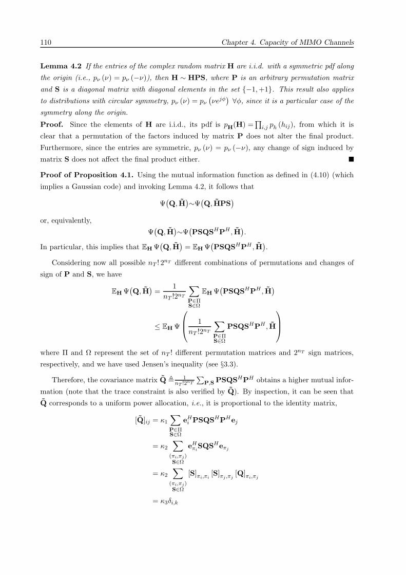
110 Chapter 4. Capacity of MIMO Channels
Lemma 4.2 If the entries of the complex random matrix H are i.i.d. with a symmetric pdf along
the origin (i.e., pν (ν) = pν (−ν)), then H ∼ HPS, where P is an arbitrary permutation matrix
and S is a diagonal matrix with diagonal elements in the set −1,+1. This result also applies
to distributions with circular symmetry, pν (ν) = pν
(νejφ) ∀φ, since it is a particular case of the
symmetry along the origin.
Proof. Since the elements of H are i.i.d., its pdf is pH(H) =∏
i,j ph (hij), from which it is
clear that a permutation of the factors induced by matrix P does not alter the final product.
Furthermore, since the entries are symmetric, pν (ν) = pν (−ν), any change of sign induced by
matrix S does not affect the final product either.
Proof of Proposition 4.1. Using the mutual information function as defined in (4.10) (which
implies a Gaussian code) and invoking Lemma 4.2, it follows that
Ψ(Q, H
)∼Ψ(Q, HPS
)or, equivalently,
Ψ(Q, H
)∼Ψ(PSQSHPH , H
).
In particular, this implies that EH Ψ(Q, H
)= EH Ψ
(PSQSHPH , H
).
Considering now all possible nT ! 2nT different combinations of permutations and changes of
sign of P and S, we have
EH Ψ(Q, H
)=
1nT !2nT
∑P∈ΠS∈Ω
EH Ψ(PSQSHPH , H
)
≤ EH Ψ
1
nT !2nT
∑P∈ΠS∈Ω
PSQSHPH , H
where Π and Ω represent the set of nT ! different permutation matrices and 2nT sign matrices,
respectively, and we have used Jensen’s inequality (see §3.3).Therefore, the covariance matrix Q 1
nT !2nT
∑P,S PSQSHPH obtains a higher mutual infor-
mation (note that the trace constraint is also verified by Q). By inspection, it can be seen that
Q corresponds to a uniform power allocation, i.e., it is proportional to the identity matrix,
[Q]ij = κ1
∑P∈ΠS∈Ω
eHi PSQSHPHej
= κ2
∑(πi,πj)S∈Ω
eHπi
SQSHeπj
= κ2
∑(πi,πj)S∈Ω
[S]πi,πi[S]πj ,πj
[Q]πi,πj
= κ3δi,k

4.B Proof of Theorem 4.1 111
where ei is the ith unit vector (all zeros except a one in the ith position). The domain of the per-
mutation indexes (πi, πj) is given by πi = πj ∈ 1, · · · , nT for i = j, and πi ∈ 1, · · · , nT , πj ∈1, · · · , nT − πi for i = j. The last equality is clear for i = j, because
∣∣ [S]πi,πi
∣∣2 = 1. For the
case i = j, it follows from the fact that for each pair (πi, πj) (note that πi = πj), half of the terms
of the summation over S ∈Ω have a positive sign and the other half a negative sign.
Thus, the uniform power allocation Q = PT /nT InTalways give an upper bound on the ergodic
mutual information and the ergodic capacity is then
EH Ψ(Pt/nT InT
, H)
= EH log det(InR
+ Pt/nT R−1n HHH
).
Appendix 4.B Proof of Theorem 4.1
We first present a couple of lemmas and then proceed to prove Theorem 4.1.
Lemma 4.3 Given two positive semidefinite n × n Hermitian matrices A and B, the following
holds
log det (I + AB) ≥n∑
i=1
log (1 + λA,i λB,n−i+1) , (4.63)
where λA,i and λB,i denote the eigenvalues in decreasing order (λi ≥ λi+1) of A and B, respec-
tively. Equality in (4.63) is achieved for UA = UBJ, where UA and UB contain the eigenvectors
corresponding to the eigenvalues in decreasing order of A and B, respectively, and J is the “back-
ward identity” permutation matrix [Hor85] defined as
J =
0 0 · · · 0 1
0. . . 1 0
.... . .
...
0 1. . . 0
1 0 · · · 0 0
.
Proof. Consider the EVD A = UADAUHA and B = UBDBUH
B , where DA = diag (λA,i) and
DB = diag (λB,i) (we assume eigenvalues in decreasing order). It follows that
det (I + AB) = det(I + DAUHDBU
)where U = U
HBUA. If A has n − k zero eigenvalues, we can write
DA =
DA,1 0
0 0
, DA,1 ∈ CI k×k (nonsingular)
U =[
U1 U2
], U1 ∈ CI n×k
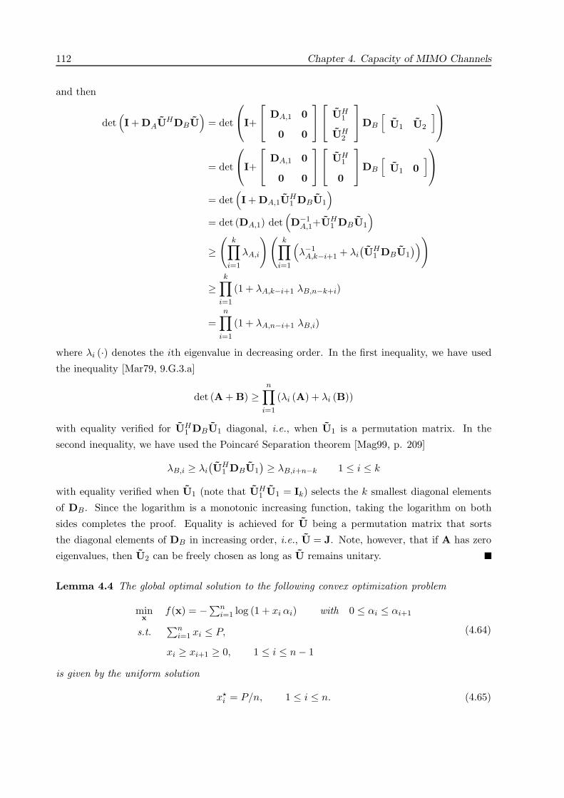
112 Chapter 4. Capacity of MIMO Channels
and then
det(I + DAUHDBU
)= det
I+
DA,1 0
0 0
UH
1
UH2
DB
[U1 U2
]
= det
I+
DA,1 0
0 0
UH
1
0
DB
[U1 0
]= det
(I + DA,1UH
1 DBU1
)= det (DA,1) det
(D−1
A,1+UH1 DBU1
)
≥(
k∏i=1
λA,i
)(k∏
i=1
(λ−1
A,k−i+1 + λi
(UH
1 DBU1
)))
≥k∏
i=1
(1 + λA,k−i+1 λB,n−k+i)
=n∏
i=1
(1 + λA,n−i+1 λB,i)
where λi (·) denotes the ith eigenvalue in decreasing order. In the first inequality, we have used
the inequality [Mar79, 9.G.3.a]
det (A + B) ≥n∏
i=1
(λi (A) + λi (B))
with equality verified for UH1 DBU1 diagonal, i.e., when U1 is a permutation matrix. In the
second inequality, we have used the Poincare Separation theorem [Mag99, p. 209]
λB,i ≥ λi
(UH
1 DBU1
) ≥ λB,i+n−k 1 ≤ i ≤ k
with equality verified when U1 (note that UH1 U1 = Ik) selects the k smallest diagonal elements
of DB . Since the logarithm is a monotonic increasing function, taking the logarithm on both
sides completes the proof. Equality is achieved for U being a permutation matrix that sorts
the diagonal elements of DB in increasing order, i.e., U = J. Note, however, that if A has zero
eigenvalues, then U2 can be freely chosen as long as U remains unitary.
Lemma 4.4 The global optimal solution to the following convex optimization problem
minx
f(x) = −∑ni=1 log (1 + xi αi) with 0 ≤ αi ≤ αi+1
s.t.∑n
i=1 xi ≤ P,
xi ≥ xi+1 ≥ 0, 1 ≤ i ≤ n − 1
(4.64)
is given by the uniform solution
xi = P/n, 1 ≤ i ≤ n. (4.65)

4.C Mixed Strategy Nash Equilibria 113
Proof. From an intuitive viewpoint, we can see that without the constraint xi ≥ xi+1, the
solution would be a water-filling, which would imply xi ≤ xi+1. With the additional constraint,
however, the solution will try to water-fill but always verifying the constraint xi ≥ xi+1, resulting
in xi = xi+1.
This result can be straightforwardly proved in a formal way using majorization theory [Mar79].
First, rewrite the objective function as f(x) =∑n
i=1 gi (xi) where gi (x) = − log (1 + xαi). Since
g′i (a) ≥ g′i+1 (b) whenever a ≥ b, function f(x) is Schur-convex [Mar79, 3.H.2]. Now, from
the definition of Schur-convexity [Mar79, 3.A.1] and using the fact that the uniform solution is
majorized by any other solution [Mar79, p.7], it follows that the minimum of f(x) is attained by
the uniform solution of (4.65). This result can be alternatively proved using convex optimization
theory [Lue69, Boy00].
Proof of Theorem 4.1. We use the relation (4.10)-(4.11) and the fact that the eigenvectors of
RH= HHR−1n H are unconstrained (see (4.36)) to simplify the inner minimization of (4.37) for a
given Q:
infRH∈RH
log det (I + QRH) = infλRH,i∈LRH
nT∑i=1
log (1 + λQ,i λRH ,nT−i+1)
=nT∑i=1
log(1 + λQ,i λ
RH ,nT−i+1 (λQ,i)
)
where Lemma 4.3 has been used (the minimizing eigenvectors are chosen according to URH=
UQJ) and λRH ,i (λQ,i) denote the minimizing eigenvalues of RH as a function of λQ,i,
which depend on the particular constraint used to define the set LRH(in §4.4.1.2.1, some specific
examples of LRHare considered).
The outer maximization of (4.37) can be now written as
maxλQ,i
∑nTi=1 log
(1 + λQ,i λ
RH ,nT−i+1 (λQ,i)
)s.t.
∑i λQ,i ≤ PT ,
λQ,i ≥ λQ,i+1 ≥ 0 1 ≤ i ≤ nT − 1
with solution given by λQ,i = PT /nT ∀i. To show this, we just have to apply Lemma 4.4:
nT∑i=1
log(1 + λQ,i λ
RH ,nT−i+1 (PT /nT )
) ≤ nT∑i=1
log(1 + PT /nT λ
RH ,nT −i+1 (PT /nT ))
and then the obvious relation
infλRH ,i∈LRH
nT∑i=1
log (1 + λQ,i λRH ,nT−i+1) ≤nT∑i=1
log(1 + λQ,i λ
RH ,nT−i+1 (PT /nT )
)

114 Chapter 4. Capacity of MIMO Channels
to finally obtain
nT∑i=1
log(1 + λQ,i λ
RH ,nT−i+1 (λQ,i)
) ≤ nT∑i=1
log(1 + PT /nT λ
RH ,nT−i+1 (PT /nT )).
Thus, the maximizing solution is given by λQ,i = PT /nT ∀i, i.e., a uniform power allocation
Q = PT /nT InT.
Appendix 4.C Mixed Strategy Nash Equilibria
In this appendix, we characterize the solutions to the mixed-strategy saddle point given by (4.32).
By the saddle-point property of (4.32), it must be that
EpH
EpQΨ(Q, H
) ≥ EpHΨ(Ep
QQ, H
).
However, by the concavity of the logdet function [Hor85], it holds that EpQΨ(Q, H
) ≤Ψ(EpQ
Q, H). Therefore, it must be the case that
EpQΨ(Q, H
)= Ψ(Ep
QQ, H
) ∀ H : pH
(H)
> 0
which, by the strict concavity of the logdet function [Hor85] and (4.10), implies that
HQ1HH = HQ2H
H ∀Q1,Q2, H : pQ (Q1) > 0, p
Q (Q2) > 0, pH
(H)
> 0.
Thus, we can conclude that Q1 = Q2 for ∀ Q1,Q2 : pQ (Q1) > 0, p
Q (Q2) > 0 (note that if the
set of used H’s have a common null space, by the nature of the saddle point in (4.32), all the used
Q’s will be orthogonal to that subspace). In other words, the optimal mixed strategy pQ reduces to
a pure strategy Q. We can now invoke Theorem 4.1: if Q was not the uniform power allocation,
the set of optimal H’s would align their largest singular values with the smallest eigenvalues of
Q, and the best solution is then given by the uniform power allocation Q = PT /nT I.
The problem now is to find a mixed strategy pH
so that the saddle-point conditions are
satisfied:
EpQpH
Ψ(Q, H
) ≤ EpHΨ(PT /nT I, H
) ≤ EpHΨ(PT /nT I, H
).
Recall that the mixed strategy pH
must satisfy Ψ(PT /nT I, H1
)= Ψ
(PT /nT I, H2
)for
∀ H1, H2 : pH
(H1
)> 0, p
H
(H2
)> 0 [Osb94]. Function Ψ
(PT /nT I, H
)only depends on H
through its singular values and it is minimized by some optimal set σH,i
. Therefore, any pH
that puts positive probability on channels H’s with singular values given by σH,i
and arbitrary
right and left singular vectors satisfies the right inequality of the saddle point. We just have to
find the appropriate pH
such that the left inequality of the saddle point is also satisfied. An
example of such an optimal mixed strategy pH
is one that puts equal probability on each element
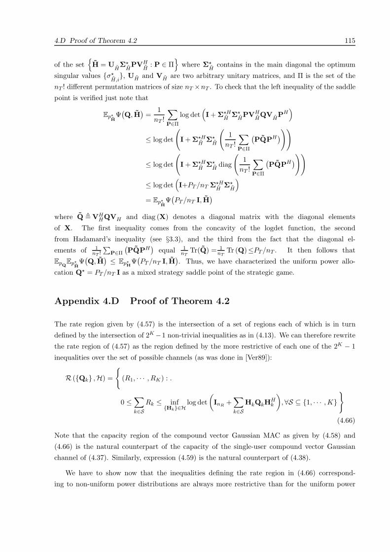
4.D Proof of Theorem 4.2 115
of the setH = U
HΣ
HPVH
H: P ∈ Π
where Σ
Hcontains in the main diagonal the optimum
singular values σH,i
, UH and VH are two arbitrary unitary matrices, and Π is the set of the
nT ! different permutation matrices of size nT ×nT . To check that the left inequality of the saddle
point is verified just note that
EpH
Ψ(Q, H
)=
1nT !
∑P∈Π
log det(I + ΣH
HΣ
HPVH
HQV
HPH)
≤ log det
(I + ΣH
HΣ
H
(1
nT !
∑P∈Π
(PQPH
)))
≤ log det
(I + ΣH
HΣ
Hdiag
(1
nT !
∑P∈Π
(PQPH
)))
≤ log det(I+PT /nT ΣH
HΣ
H
)= Ep
HΨ(PT /nT I, H
)where Q VH
HQVH and diag (X) denotes a diagonal matrix with the diagonal elements
of X. The first inequality comes from the concavity of the logdet function, the second
from Hadamard’s inequality (see §3.3), and the third from the fact that the diagonal el-
ements of 1nT !
∑P∈Π
(PQPH
)equal 1
nTTr(Q) = 1
nTTr (Q)≤PT /nT . It then follows that
EpQEp
HΨ(Q, H
) ≤ EpH
Ψ(PT /nT I, H
). Thus, we have characterized the uniform power allo-
cation Q = PT /nT I as a mixed strategy saddle point of the strategic game.
Appendix 4.D Proof of Theorem 4.2
The rate region given by (4.57) is the intersection of a set of regions each of which is in turn
defined by the intersection of 2K −1 non-trivial inequalities as in (4.13). We can therefore rewrite
the rate region of (4.57) as the region defined by the more restrictive of each one of the 2K − 1
inequalities over the set of possible channels (as was done in [Ver89]):
R (Qk ,H) =
(R1, · · · , RK) : .
0 ≤∑k∈S
Rk ≤ infHk∈H
log det(InR
+∑k∈S
HkQkHHk
),∀S ⊆ 1, · · · ,K
(4.66)
Note that the capacity region of the compound vector Gaussian MAC as given by (4.58) and
(4.66) is the natural counterpart of the capacity of the single-user compound vector Gaussian
channel of (4.37). Similarly, expression (4.59) is the natural counterpart of (4.38).
We have to show now that the inequalities defining the rate region in (4.66) correspond-
ing to non-uniform power distributions are always more restrictive than for the uniform power

116 Chapter 4. Capacity of MIMO Channels
distribution, i.e.,
infHk∈H
log det
(InR
+∑k∈S
HkQkHHk
)≤ inf
Hk∈Hlog det
(InR
+∑k∈S
Pk/nk HkHHk
)(4.67)
∀S ⊆ 1, · · · ,K∀Qk : Tr (Qk) ≤ Pk,Qk = QH
k ≥ 0 1 ≤ k ≤ K.
This has the important consequence that the worst-case rate region of the uniform power allo-
cation contains the worst-case rate region corresponding to any other power allocation strategy,
i.e.,
R (Qk ,H) ⊆ R (Pk/nk Ink ,H) ∀Qk : Tr (Qk) ≤ Pk,Qk = QH
k ≥ 0 1 ≤ k ≤ K.
Therefore, the expression of the worst-case capacity region in (4.58) reduces to
C (H) = R (Pk/nk Ink ,H)
which, together with (4.66), gives the desired result of (4.59). Now that (4.58) has been rewritten
as (4.59), it is clear that it is a closed and convex region.
We now focus on proving the inequalities of (4.67). We first consider a single user in the set
S and show that with a uniform power distribution the boundary can never decrease. Then, we
apply the same idea for the rest of the users in S. Consider the minimization of the boundary
with respect to the channel Hl of the lth user in S; for any given set of channels Hkk =l, we
have
infHl∈Hl
log det
(InR
+∑k∈S
HkQkHHk
)= inf
Hl∈Hl
log det(Rnl
+ HlQlHHl
)= inf
Hl∈Hl
log det(InT
+ QlHHl R−1
nlHl
)+ log det (Rnl
)
≤ infHl∈Hl
log det(InT
+ Pl/nl HHl R−1
nlHl
)+ log det (Rnl
)
= infHl∈Hl
log det
InR
+ Pl/nl HlHHl +∑k∈Sk =l
HkQkHHk
where Rnl
InR
+∑k∈Sk =l
HkQkHHk
is the interference-plus-noise covariance matrix seen by the
lth user and the inequality comes from invoking Lemmas 4.3 and 4.4 as was done when proving
Theorem 4.1 in Appendix 4.B for the single-user case. The previous reasoning can be sequentially
applied to each of the users in the set S to finally obtain
infHk∈H
log det
(InR
+∑k∈S
HkQkHHk
)≤ inf
Hk∈Hlog det
(InR
+∑k∈S
Pk/nk HkHHk
).
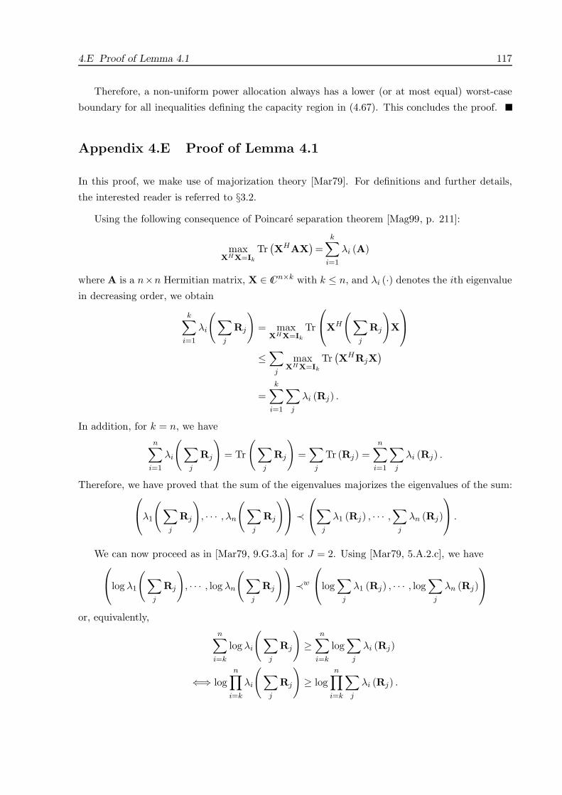
4.E Proof of Lemma 4.1 117
Therefore, a non-uniform power allocation always has a lower (or at most equal) worst-case
boundary for all inequalities defining the capacity region in (4.67). This concludes the proof.
Appendix 4.E Proof of Lemma 4.1
In this proof, we make use of majorization theory [Mar79]. For definitions and further details,
the interested reader is referred to §3.2.Using the following consequence of Poincare separation theorem [Mag99, p. 211]:
maxXHX=Ik
Tr(XHAX
)=
k∑i=1
λi (A)
where A is a n×n Hermitian matrix, X ∈ CI n×k with k ≤ n, and λi (·) denotes the ith eigenvalue
in decreasing order, we obtain
k∑i=1
λi
(∑j
Rj
)= max
XHX=Ik
Tr
XH
(∑j
Rj
)X
≤∑
j
maxXHX=Ik
Tr(XHRjX
)
=k∑
i=1
∑j
λi (Rj) .
In addition, for k = n, we haven∑
i=1
λi
(∑j
Rj
)= Tr
(∑j
Rj
)=∑
j
Tr (Rj) =n∑
i=1
∑j
λi (Rj) .
Therefore, we have proved that the sum of the eigenvalues majorizes the eigenvalues of the sum:λ1
(∑j
Rj
), · · · , λn
(∑j
Rj
) ≺∑
j
λ1 (Rj) , · · · ,∑
j
λn (Rj)
.
We can now proceed as in [Mar79, 9.G.3.a] for J = 2. Using [Mar79, 5.A.2.c], we havelog λ1
(∑j
Rj
), · · · , log λn
(∑j
Rj
) ≺w
log
∑j
λ1 (Rj) , · · · , log∑
j
λn (Rj)
or, equivalently,n∑
i=k
log λi
(∑j
Rj
)≥
n∑i=k
log∑
j
λi (Rj)
⇐⇒ logn∏
i=k
λi
(∑j
Rj
)≥ log
n∏i=k
∑j
λi (Rj) .
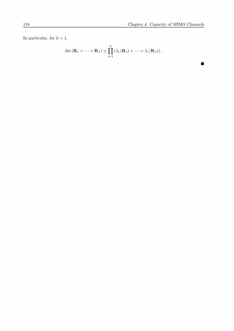
118 Chapter 4. Capacity of MIMO Channels
In particular, for k = 1,
det (R1 + · · · + RJ ) ≥n∏
i=1
(λi (R1) + · · · + λi (RJ)) .
Chapter 5
Joint Design of Tx-Rx Linear
Processing for MIMO Channels
with a Power Constraint:
A Unified Framework
THE DESIGN OF A COMMUNICATION SYSTEM requires the definition of an objective
function to measure the performance of the system. This chapter considers communication
through MIMO channels and designs transmit-receive beamforming or linear processing (also
termed linear precoder at the transmitter and linear equalizer at the receiver) to optimize the
performance of the system under a variety of design criteria subject to a power constraint. A
variety of interesting design criteria can be adopted depending on the specific application of
interest. The common way of proceeding is to choose a specific design criterion and then design
the system accordingly. This chapter generalizes all the existing results in the literature by
developing a novel unifying framework that provides the optimal structure of the transmitter
and receiver. With such a result, the original complicated nonconvex problem with matrix-
valued variables simplifies and then the design problem can be reformulated within the powerful
framework of convex optimization theory, in which a great number of interesting design criteria
can be easily accommodated and efficiently solved even though closed-form expressions may not
exist. From this perspective, a wide range of design criteria is analyzed and, in particular,
optimum beamforming in the sense of minimizing the average bit error rate (BER) is obtained.
Efficient algorithms for practical implementation are given for the considered design criteria.
Numerical results from simulations are given to support the mathematical development of the
problem.
119

120 Chapter 5. Joint Tx-Rx Processing: A Unified Framework
5.1 Introduction
Communications over multiple-input multiple-output (MIMO) channels have recently gained con-
siderable attention [Hon90, Yan94b, Fos96, Ral98, Sca99b]. They arise in many different scenarios
such as when a bundle of twisted pairs in digital subscriber lines (DSL) is treated as a whole
[Hon90], when multiple antennas are used at both sides of a wireless link [Fos96, Ral98], or sim-
ply when a frequency-selective channel is properly modeled by using, for example, transmit and
receive filterbanks [Sca99b] (c.f. §2.2). In particular, MIMO channels arising from the use of
multiple antennas at both the transmitter and the receiver have attracted a significant interest
because they provide an important increase in capacity over single-input single-output (SISO)
channels under some uncorrelation conditions [Tel95, Fos98]. The use of multiple antennas at
both ends of a wireless link provides significant improvement not only in terms of spectral effi-
ciency (multiplexing gain) [Tel95, Fos98] but also in terms of link reliability (beamforming and
diversity gains) [Bol02] (c.f. §2.3).
Communication techniques for MIMO systems fall into two main categories depending on
whether channel state information (CSI) is available at the transmitter (CSIT) (note that CSI at
the receiver (CSIR) is in general assumed) (c.f. §2.4). With no CSIT, popular space-time coding
techniques independent of the channel realization can be readily used [Fos96, Ala98, Tar98]. With
perfect CSIT, the transmission can be adapted to each channel realization using signal processing
techniques [Yan94b, Ral98, Sca99b]. In this chapter, we focus on the latter (i.e., when CSI is
available at both sides of the link) and in particular when linear processing is utilized for the sake
of complexity. Note that it is also possible to consider intermediate situations such as combining
space-time codes and signal processing when having partial CSI [Neg99, Jon02] (see Chapter 7 to
see how to take into account channel estimation errors). For the sake of complexity and perhaps
with some loss of optimality, we focus on linear processing techniques as opposed to nonlinear
techniques such as maximum likelihood (ML) detection1 or decision feedback (DF) schemes (see
§2.5.1 for more details).
In order to design a communication system, it is necessary to have an objective function
to measure the performance (c.f. §2.5.4). The system can be then optimized in the sense of
improving the performance as given by the objective function while the transmitter is assumed
to be constrained in its average transmitted power to limit the interference level of the system.
A variety of criteria can be used to design transmit and receive signal processing techniques for
MIMO channels. Alternatively, it is possible to formulate the problem from the opposite point of
view, i.e., to minimize the transmitted power subject to some Quality of Service (QoS) constraints
to guarantee a certain level of performance in the communication process (this approach is treated
in detail in Chapter 6).1In some very specific cases, the ML detector may happen to be linear such as in orthogonal space-time block
coding [Ala98, Tar99a, Gan01a].

5.1. Introduction 121
The capacity of a channel is the fundamental bound on the maximum reliably achievable data
rate. Therefore, in terms of spectral efficiency, a system should be designed to approach the
capacity of the channel [Cov91b, Ral98, Sca99a]. A capacity-achieving design dictates that the
channel matrix must be diagonalized and then a water-filling power allocation must be used on
the channel eigenmodes [Cov91b, Ral98, Sca99a]. In theory, this solution has the implication that
an ideal Gaussian code should be used on each channel eigenmode according to its allocated power
[Cov91b]. In practice, however, each Gaussian code is substituted by a simple (and suboptimal)
signal constellation and a practical (and suboptimal) coding scheme (if any). Hence, the resulting
system may be far from optimum. The complexity of such a solution is still significative since each
channel eigenmode requires a different combination of signal constellation and code depending
on the allocated power. To further reduce the complexity, the system can be constrained to
use the same constellation and code in all channel eigenmodes (possibly optimizing the set of
used eigenmodes to transmit only over those with a sufficiently high gain), i.e., an equal-rate
transmission. Examples of this pragmatic and simple solution are found in the European standard
HIPERLAN/2 [ETS01] and in the US standard IEEE 802.11 [IEE99] for wireless local area
networks (WLAN) that use a multicarrier approach with the same constellation on each carrier.
Consider now that the specific signal constellations and coding schemes for all the established
substreams have been selected either after some bit distribution method or simply by taking
a uniform bit distribution. It is then possible to further optimize the system to improve the
quality of each of the established substreams. In particular, we consider the joint design of linear
processing at both ends of the link (commonly referred to as linear precoding at the transmitter
and equalization at the receiver) according to a variety of criteria as we now review. In [Lee76,
Sal85, Yan94b, Sca99b], the sum of the mean square error (MSE) of all channel substreams (the
trace of the MSE matrix) was used as the objective to minimize. This criterion was generalized by
using a weighted sum (weighted trace) in [Sam01]. In [Sca99b], a maximum signal to interference-
plus-noise ratio (SINR) criterion with a zero-forcing (ZF) constraint was also considered. For
these criteria, the original complicated design problem is greatly simplified because the channel
turns out to be diagonalized by the transmit-receive processing. In [Yan94a], the determinant of
the MSE matrix was minimized and the diagonal structure was found to be optimal as well. In
[Sca02], the results were extended to the case of a peak power constraint (maximum eigenvalue
constraint) with similar results.
At this point, it is important to step back for a second and realize that the problem of designing
jointly the transmit and receive linear processing is an old one; in fact, it dates back to the sixties.
In [Ber67] (and references therein), transmit-receive filters for frequency-selective SISO channels
were jointly designed to minimize the MSE, where an iterative water-filling algorithm was found
for optimum energy distribution. In [Ami84], the solution was extended to 2×2 MIMO channels.
Decision feedback schemes were considered in [Kav85]. The first generalization to N ×N matrix
channels was obtained in [Sal85]. In [Hon92], the case was generalized to an arbitrary M × N

122 Chapter 5. Joint Tx-Rx Processing: A Unified Framework
matrix channel with correlated data symbols, colored noise, both near- and far-end crosstalk,
and excess bandwidth (although a closed-form expression was not provided, an iterative solution
was presented). In [Yan94b, Yan94a], joint transmit-receive filters were derived using an elegant
notation for a general framework including excess bandwidth and decision feedback systems.
Remarkably, the joint transmit-receive design for MIMO systems was already solved in 1976 for
flat channels [Lee76]. In [And00], the flat multi-antenna MIMO case was considered providing
useful insights from the point of view of beamforming.
Going back to the design of transmit and receive processing under different criteria, we remark
that the channel-diagonalizing property is of paramount importance in order to be able to solve
the problem.
The main interest of the diagonalizing structure is that it allows a scalarization of the prob-
lem (meaning that all matrix equations are substituted with scalar ones) with the consequent
great simplification. In light of the optimality of the channel-diagonalizing structure in all the
aforementioned examples (including the capacity-achieving solution), one may wonder whether
the same holds for other criteria. Examples of other reasonable criteria to design a communica-
tion system are the minimization of the maximum bit error rate (BER) of the substreams, the
minimization of the average BER, or the maximization of the minimum SINR of the substreams.
In these cases, it is not clear whether one can assume a diagonal structure as was obtained in
the previous cases. In fact, as will be shown, the diagonal structure is not optimal for these and
other criteria. Of course, a simple solution is to impose such a structure to simplify the design,
but doing so may be far from optimum such as in [Ong03], where the average BER (and also of
the Chernoff upper bound) was minimized imposing a diagonal structure, and in [Sam01], where
the minimum of the SINR’s was maximized imposing a diagonal structure.
In this chapter, we consider different design criteria based on optimizing the MSE’s, the
SINR’s, and also the BER’s directly. Instead of considering each design criterion separately, we
develop a unifying framework and generalize the existing results by considering two families of
objective functions that embrace most reasonable criteria to design a communication system:
Schur-concave and Schur-convex functions (these types of functions arise in majorization theory
[Mar79]). For Schur-concave objective functions, the channel-diagonalizing structure is always
optimal, whereas for Schur-convex functions, an optimal solution diagonalizes the channel only
after a very specific rotation of the transmitted symbols. Once the optimal structure of the
transmit-receive processing is known, the design problem simplifies and can be formulated within
the powerful framework of convex optimization theory, in which a great number of interesting
design criteria can be easily accommodated and efficiently solved even though closed-form expres-
sions may not exist (see §3.1 for details on convex optimization theory). We analyze a variety of
criteria and, in particular, we derive optimal beamvectors in the sense of having minimum aver-
age BER. Additional constraints on the Peak-to-Average Ratio (PAR) or on the signal dynamic

5.2. Design Criterion 123
range of the transmitted signal are easily included in the design within the convex optimization
framework. We propose two multi-level water-filling practical solutions that perform very close
to the optimal in terms of average BER with a low implementation complexity. Interestingly, the
optimal solution in the sense of minimum average BER can be obtained in closed-form.
This chapter is organized as follows. Section 5.3 considers the case of single beamforming,
which refers to the transmission of a single symbol through the MIMO channel by using transmit
and receive beamvectors. Section 5.4 extends the results to the more general case of multiple
beamforming or matrix beamforming, which refers to the simultaneous transmission of L symbols
through the MIMO channel by using transmit and receive multiple beamvectors or, equivalently,
transmit and receive beam-matrices. It is in this case of designing transmit and receive matrices
where the main result is obtained, i.e., the optimal transmit-receive structure for Schur-concave
and Schur-convex objective functions. In both sections, the transmission over a single MIMO
channel is considered first and then extended to the case of having multiple MIMO channels
which can model, for example, a multicarrier system. Once the optimal structure of the solution
is found, the problem simplifies and a variety of design criteria are considered and formulated
in Section 5.5 under the powerful framework of convex optimization theory. In Section 5.6,
additional constraints to control the dynamic range of the power amplifier and the PAR of the
transmitted signal are included in the design. In Section 5.7, numerical results for the proposed
methods are obtained from simulations using realistic channel models. Finally, in Section 5.8, a
summary of the chapter is given along with the final conclusions.
The problem formulation under the framework of convex optimization theory for the
single beamforming and multiple beamforming cases have been published in [Pal03b] and
[Pal02a, Pal03c], respectively.
5.2 Design Criterion
In order to design the system, we consider a general design criterion based on an arbitrary
objective function of any the three basic figures of merit that measure the performance of the
system as described in §2.5.4: the MSE, the SINR, and the BER.
The objective function is an indicator of how well the system performs. As an example, if
two MIMO systems are identical except in one of the substreams for which one of the systems
outperforms the other, any reasonable function should properly reflect this difference. Therefore,
it suffices to consider only these reasonable functions.2 Mathematically, this is equivalent to
saying that the objective function must be monotonic in each of its arguments while having the
rest fixed. To be more specific, a reasonable function of the MSE’s or of the BER’s must be2Given an unreasonable objective function, it is always possible to redefine it in a reasonable way so that it
better reflects the system performance.

124 Chapter 5. Joint Tx-Rx Processing: A Unified Framework
increasing in each variable and a reasonable function of the SINR’s must be decreasing in each
variable.
The optimum linear signal processing at the receiver was obtained in §2.5.5 as the classical
LMMSE receiver or Wiener filter given by ak =(Hkbkb
Hk HH
k + Rnk
)−1 Hkbk in the single
beamforming case and by Ak =(HkBkB
Hk HH
k + Rnk
)−1 HkBk in the multiple beamforming
case (see (2.43) and (2.48)). As shown in §2.5.5, the Wiener filter is optimal in the sense that
each of the MSE’s is minimized, each of the SINR’s is maximized, and each of the BER’s is
minimized. Therefore, it only remains to obtain the optimum linear signal processing at the
transmitter.
It is extremely important to remark that any objective function of the SINR’s can be al-
ternatively expressed as a function of the MSE’s by means of the relation in (2.62) SINRk,i =
MSE−1k,i −1. Similarly, any objective function of the BER’s can be expressed as a function of the
SINR’s by using the Q-function as in (2.38) and (2.40). Thus, it suffices to consider objective
functions of the MSE’s f0 (MSEk,i) increasing in each variable without loss of generality.
For the sake of notation, we define the squared whitened channel matrix RH HHR−1n H
(note that the eigenvectors and eigenvalues of RH are the right singular vectors and the squared
singular values, respectively, of the whitened channel R−1/2n H) with maximum eigenvalue and
corresponding eigenvector given by λH,max λmax (RH) and uH,max umax (RH), respectively.
For multiple MIMO channels, we similarly define RHk HH
k R−1nk
Hk, λHk,max λmax (RHk), and
uHk,max umax (RHk).
5.3 Single Beamforming
In this section, the simple case of single beamforming for MIMO channels as formulated in §2.5.1.1is considered. First, the simple case of a single MIMO channel is analyzed in §6.3.1 and then
the result is extended in § 6.3.2 to the case of multiple MIMO channels (typical of multicarrier
systems).
In [Ise01, Ise02, Pal03b], a variety of design criteria were considered for single beamforming
transmission in multicarrier applications. A convex optimization approach was explicitly adopted
in [Pal03b].
5.3.1 Single MIMO Channel
Single beamforming on a single MIMO channel is a trivial case and has a simple solution. It will
serve as a reference when dealing with the more general case of having a set of parallel MIMO
channels.
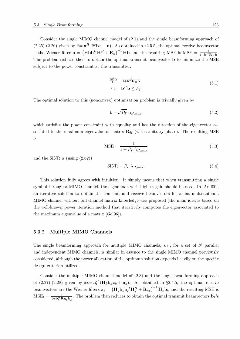
5.3. Single Beamforming 125
Consider the single MIMO channel model of (2.1) and the single beamforming approach of
(2.25)-(2.26) given by x= aH (Hbx + n). As obtained in §2.5.5, the optimal receive beamvector
is the Wiener filter a =(HbbHHH + Rn
)−1Hb and the resulting MSE is MSE = 1
1+bHRHb.
The problem reduces then to obtain the optimal transmit beamvector b to minimize the MSE
subject to the power constraint at the transmitter:
minb
11+bHRHb
s.t. bHb ≤ PT .(5.1)
The optimal solution to this (nonconvex) optimization problem is trivially given by
b =√
PT uH,max. (5.2)
which satisfies the power constraint with equality and has the direction of the eigenvector as-
sociated to the maximum eigenvalue of matrix RH (with arbitrary phase). The resulting MSE
is
MSE =1
1 + PT λH,max(5.3)
and the SINR is (using (2.62))
SINR = PT λH,max. (5.4)
This solution fully agrees with intuition. It simply means that when transmitting a single
symbol through a MIMO channel, the eigenmode with highest gain should be used. In [And00],
an iterative solution to obtain the transmit and receive beamvectors for a flat multi-antenna
MIMO channel without full channel matrix knowledge was proposed (the main idea is based on
the well-known power iteration method that iteratively computes the eigenvector associated to
the maximum eigenvalue of a matrix [Gol96]).
5.3.2 Multiple MIMO Channels
The single beamforming approach for multiple MIMO channels, i.e., for a set of N parallel
and independent MIMO channels, is similar in essence to the single MIMO channel previously
considered, although the power allocation of the optimum solution depends heavily on the specific
design criterion utilized.
Consider the multiple MIMO channel model of (2.3) and the single beamforming approach
of (2.27)-(2.28) given by xk= aHk (Hkbkxk + nk). As obtained in §2.5.5, the optimal receive
beamvectors are the Wiener filters ak =(Hkbkb
Hk HH
k + Rnk
)−1 Hkbk and the resulting MSE is
MSEk = 11+bH
k RHkbk
. The problem then reduces to obtain the optimal transmit beamvectors bk’s
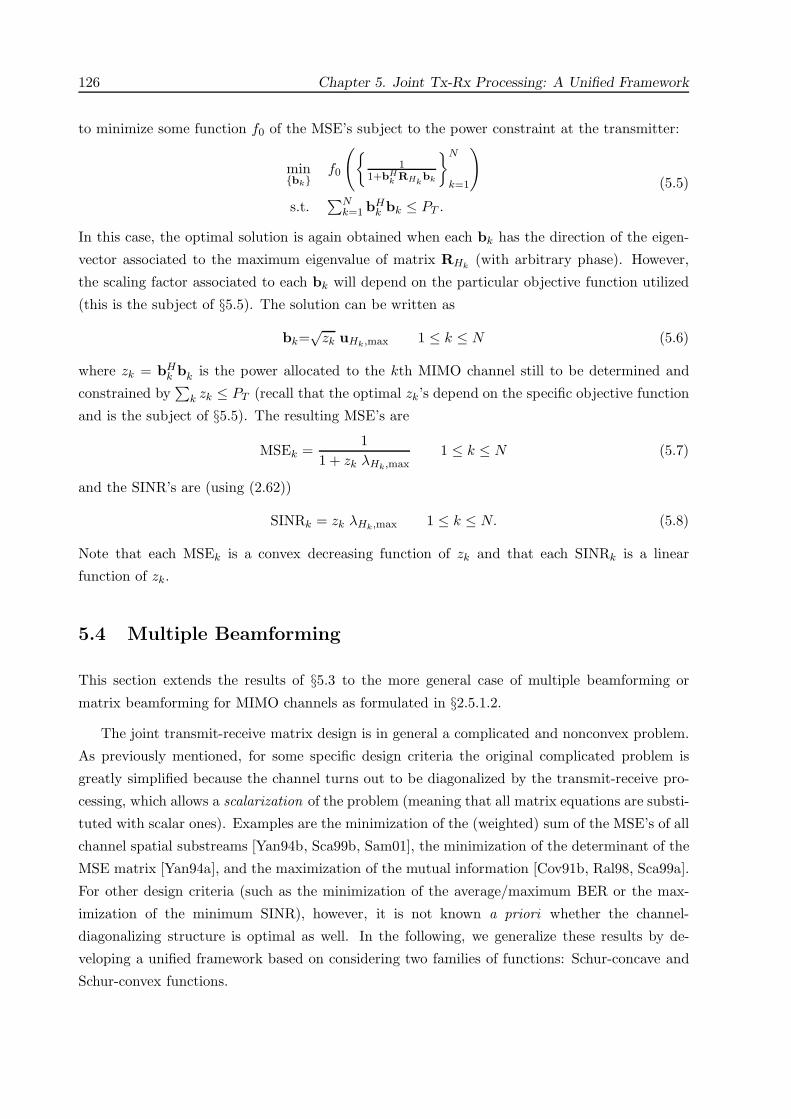
126 Chapter 5. Joint Tx-Rx Processing: A Unified Framework
to minimize some function f0 of the MSE’s subject to the power constraint at the transmitter:
minbk
f0
(1
1+bHk RHk
bk
N
k=1
)
s.t.∑N
k=1 bHk bk ≤ PT .
(5.5)
In this case, the optimal solution is again obtained when each bk has the direction of the eigen-
vector associated to the maximum eigenvalue of matrix RHk(with arbitrary phase). However,
the scaling factor associated to each bk will depend on the particular objective function utilized
(this is the subject of §5.5). The solution can be written as
bk=√
zk uHk ,max 1 ≤ k ≤ N (5.6)
where zk = bHk bk is the power allocated to the kth MIMO channel still to be determined and
constrained by∑
k zk ≤ PT (recall that the optimal zk’s depend on the specific objective function
and is the subject of §5.5). The resulting MSE’s are
MSEk =1
1 + zk λHk,max1 ≤ k ≤ N (5.7)
and the SINR’s are (using (2.62))
SINRk = zk λHk,max 1 ≤ k ≤ N. (5.8)
Note that each MSEk is a convex decreasing function of zk and that each SINRk is a linear
function of zk.
5.4 Multiple Beamforming
This section extends the results of §5.3 to the more general case of multiple beamforming or
matrix beamforming for MIMO channels as formulated in §2.5.1.2.The joint transmit-receive matrix design is in general a complicated and nonconvex problem.
As previously mentioned, for some specific design criteria the original complicated problem is
greatly simplified because the channel turns out to be diagonalized by the transmit-receive pro-
cessing, which allows a scalarization of the problem (meaning that all matrix equations are substi-
tuted with scalar ones). Examples are the minimization of the (weighted) sum of the MSE’s of all
channel spatial substreams [Yan94b, Sca99b, Sam01], the minimization of the determinant of the
MSE matrix [Yan94a], and the maximization of the mutual information [Cov91b, Ral98, Sca99a].
For other design criteria (such as the minimization of the average/maximum BER or the max-
imization of the minimum SINR), however, it is not known a priori whether the channel-
diagonalizing structure is optimal as well. In the following, we generalize these results by de-
veloping a unified framework based on considering two families of functions: Schur-concave and
Schur-convex functions.

5.4. Multiple Beamforming 127
It is important to recall here the difference between established substreams and channel eigen-
modes (c.f. §2.3.3). The established substreams are the scalar channels that are generated over
the matrix channel which may or may not be parallel and orthogonal; in other words, it refers
to the number of simultaneous symbols transmitted. The channel eigenmodes are the paral-
lel and orthogonal scalar channels existing within the matrix channel with gain given by the
channel eigenvalues. In general, the number of substreams is different to the number of channel
eigenmodes (preferably smaller, although not necessarily). When a diagonal structure is used
for transmission, each substream is established through a channel eigenmode and both concepts
coincide.
First, in §5.4.1, we deal with the case of a single MIMO channel, for which the main result
of this chapter is obtained. In particular, Theorem 5.1 develops a unified framework and obtains
the optimal transmit-receive structure for any Schur-concave or Schur-convex objective function,
generalizing the existing results in the literature. In §5.4.2, we then extend the results to the case
of multiple MIMO channels (typical of multicarrier systems). The results in this section were
obtained in [Pal03c] and [Pal02a].
5.4.1 Single MIMO Channel
Consider the single MIMO channel model of (2.1) and the matrix processing model of (2.29)-(2.30)
given by x = AH (HBx + n). As obtained in §2.5.5, the optimal receive matrix is the Wiener
filter A =(HBBHHH + Rn
)−1HB and the resulting MSE matrix is E =
(I + BHRHB
)−1.
The problem reduces then to obtain the optimal transmit matrix B to minimize some function
f0 of the MSE’s (diagonal elements of the MSE matrix) subject to the power constraint at the
transmitter:
minB
f0
([(I + BHRHB
)−1]ii
L
i=1
)s.t. Tr
(BBH
) ≤ PT .
(5.9)
Such a constrained nonconvex optimization problem is nontrivial and requires previous simplifi-
cation.
We first solve the problem in an optimal way in §5.4.1.1 by developing a unified framework,
which constitutes the main result of the chapter, and then consider a simple suboptimal approach
in §5.4.1.2 based on imposing a diagonality constraint on the MSE matrix.
5.4.1.1 Optimum Solution
To simplify the design of the system, we now show that for Schur-concave and Schur-convex ob-
jective functions [Mar79] (see §3.2), the problem can be scalarized, meaning that the complicated

128 Chapter 5. Joint Tx-Rx Processing: A Unified Framework
(c) Diagonalized (up to a rotation) system
(a) Original system
(b) Fully diagonalized system
x1
VB
VB
H
xL
x1
xL
w1
wL
x1
xL
x1
xL
H
nR x n
T
x B
nT x L
A
L x nR
H
n
nR
y
nT
L L
^
^
^
x1
xL
~
~
x1
~
xL
~
^
^
x^
w1
wL
1/2
H,1
1/2
H,L
1/2
H,1
1/2
H,L
B,1
B,L
B,1
B,L
*
A,1
*
A,1
*
A,L
*
A,L
Figure 5.1: Original matrix system, fully diagonalized system, and diagonalized (up to a rotation) system.
matrix function[(
I + BHRHB)−1]ii
can be simplified to a set of simple scalar expressions with-
out matrices involved. In particular, for Schur-concave functions the system is fully diagonalized,
whereas for Schur-convex functions it is diagonalized up to a rotation matrix (see Figure 5.1).
This is the main result of this chapter and is formally stated in the following theorem.
Theorem 5.1 Consider the following constrained optimization problem:
minB
f0 (d(E (B) ))
s.t. Tr(BBH
) ≤ PT
where matrix B ∈ CI nT×L is the optimization variable, d(E (B)) is the vector of diagonal elements

5.4. Multiple Beamforming 129
of the MSE matrix E (B) =(I + BHRHB
)−1 (the diagonal elements of E (B) are assumed in
decreasing order w.l.o.g.), RH ∈ CI nT×nT is a positive semidefinite Hermitian matrix, and f0 :
IRL −→ IR is an arbitrary objective function (increasing in each variable). It then follows that
there is an optimal solution B of at most rank L min (L, rank (RH)) with the following structure:
• If f0 is Schur-concave, then
B = UH,1ΣB,1 (5.10)
where UH,1 ∈ CI nT×L has as columns the eigenvectors of RH corresponding to the L largest
eigenvalues in increasing order and ΣB,1 = [0 diag (σB,i)] ∈ CI L×L has zero elements
except along the rightmost main diagonal (which can be assumed real w.l.o.g.).
• If f0 is Schur-convex, then
B = UH,1ΣB,1VHB (5.11)
where UH,1 and ΣB,1 are defined as before, and VB ∈ CI L×L is a unitary matrix (rotation)
such that(I + BHRHB
)−1 has identical diagonal elements. This rotation can be computed
using Algorithm 3.2 (reproduced from [Vis99b, Section IV-A]) or with any rotation matrix Q
that satisfies |[Q]ik| = |[Q]il| ∀i, k, l such as the Discrete Fourier Transform (DFT) matrix
or the Hadamard matrix when the dimensions are appropriate such as a power of two (see
§3.2 for more details).Proof. See Appendix 5.A.
For the single beamforming case L = 1, Theorem 5.1 simplifies and the diagonal structure
simply means that the channel eigenmode with highest gain is used (this is indeed the result
obtained in §5.3).We now give some interesting remarks and corollaries of Theorem 5.1.
Remark 5.1 For Schur-concave objective functions, the global communication process including
pre- and post-processing AHHB is fully diagonalized (see Figure 5.1(b)) as well as the MSE
matrix E. Note that the canonical channel Hcan = BHRHB (as defined in §2.5.3) is also fully
diagonalized.
Among the L established substreams, only L are associated to nonzero channel eigenvalues whereas
the remainder L0 = L − L are associated to zero eigenvalues. The global communication process
is3
x =(I + ΣH
B,1DH,1ΣB,1
)−1ΣH
B,1D1/2H,1
(D1/2
H,1ΣB,1x + w)
or, equivalently,
xi =
0σ2
B,(i−L0)λH,(i−L0)
1+σ2B,(i−L0)
λH,(i−L0)xi +
σB,(i−L0) λ1/2H,(i−L0)
1+σ2B,(i−L0)
λH,(i−L0)wi
1 ≤ i ≤ L0
L0 < i ≤ L
3Note that A =(HBBHHH + Rn
)−1HB = R−1
n HB(I + BHHHR−1
n HB)−1
.

130 Chapter 5. Joint Tx-Rx Processing: A Unified Framework
where DH,1 = diag(λH,iL
k=1
), the λH,i’s are the L largest eigenvalues of RH in increasing order,
w is a normalized equivalent white noise, and σB,i is the ith diagonal element of the rightmost
main diagonal of ΣB,1. The MSE matrix is E =(I + ΣH
B,1DH,1ΣB,1
)−1 and the corresponding
MSE’s are given by
MSEi =
1
11+σ2
B,(i−L0)λH,(i−L0)
1 ≤ i ≤ L0
L0 < i ≤ L.(5.12)
Similarly, the SINR’s are given using (2.62) by
SINRi =
0
σ2B,(i−L0) λH,(i−L0)
1 ≤ i ≤ L0
L0 < i ≤ L.(5.13)
It is clear from (5.12) or from (5.13), that if we try to establish more substreams (equivalently,
transmit more symbols) than the rank of the channel or the number of nonvanishing channel
eigenmodes (i.e., if L > rank (RH) or, equivalently, L0 > 0), then the system fails since some
substreams will have an MSE equal to 1 or, equivalently, a BER equal to 0.5. Therefore, for Schur-
concave objective functions, a communication system should be designed such that L ≤ rank (RH)
in order to have an acceptable performance. In case that L > rank (RH), the substreams associated
to zero eigenvalues can be simply ignored in the optimization methods of §5.5.
Remark 5.2 For Schur-convex objective functions, the global communication process including
pre- and post-processing AHHB is diagonalized only up to a very specific rotation of the data
symbols (see Figure 5.1(c)) and the MSE matrix E is nondiagonal with equal diagonal elements
(equal MSE’s).
In particular, assuming a pre-rotation of the data symbols at the transmitter x = VHBx and a
post-rotation of the estimates at the receiver ˜x = VHB x the same diagonalizing results of Schur-
concave functions apply (see Figure 5.1(c)). Since the diagonal elements of the MSE matrix
E =(I + BHRHB
)−1 are equal whenever the appropriate rotation is included, the MSE’s are
identical and given by
MSEi =1L
Tr (E) =1L
L0 +
L∑j=1
11 + σ2
B,j λH,j
1 ≤ i ≤ L. (5.14)
Similarly, the SINR’s are given using (2.62) by
SINRi =L
L0 +∑L
j=11
1+σ2B,j λH,j
− 1 1 ≤ i ≤ L. (5.15)
Note that, during the design process, the rotation matrix can be initially ignored since the
minimization can be based directly on the MSE expression in (5.14). The rotation can be computed
at a later stage of the design as explained in Theorem 5.1. Observe that for Schur-convex functions

5.4. Multiple Beamforming 131
(unlike for Schur-concave ones), it is possible to have L > rank (RH) (equivalently, L0 > 0) and
still obtain an acceptable performance. This is because the L symbols are transmitted over the L
nonzero eigenvalues in a distributed way (as opposed to the parallel and independent transmission
of the symbols for fully diagonalized systems); in other words, each substream is established using
several channel eigenmodes.
In both cases of Schur-concave and Schur-convex objective functions, the expressions of the
MSE’s of (5.12) and (5.14) have been scalarized in the sense that the original complicated matrix
expressions have been reduced to simple scalar expressions. For Schur-concave functions, the
specific power distribution among the channel eigenmodes will depend on the particular objective
function f0. Interestingly, for Schur-convex functions, the power distribution is independent of
the specific choice of f0 as formally stated in the following corollary.
Corollary 5.1 For Schur-convex objective functions, the optimal solution of the constrained op-
timization problem stated in Theorem 5.1 happens to be independent of the particular objective
function f0 chosen and can always be found by first minimizing Tr (E) and then obtaining the
appropriate rotation matrix as indicated in Theorem 5.1.
Proof. The proof is straightforward since for Schur-convex functions, the MSE expression to be
minimized given by (5.14) and the rotation matrix to make the diagonal elements of the MSE
matrix equal are completely independent of the particular choice of f0.
In other words, among the infinite solutions that minimize Tr (E), only that which yields
equal diagonal elements in E is the optimal solution for a Schur-convex objective function.
Corollary 5.2 If a function f0 is both Schur-concave and Schur-convex (c.f. §3.2), then it is
invariant with respect to post-rotations of B (i.e., it admits an arbitrary post-rotation in the
solution) and vice-versa.
Proof. See Appendix 5.B.
As an example, the function Tr (E) is clearly both Schur-concave and Schur-convex and con-
sequently it is invariant with respect to post-rotations of B, which on the other hand is obvious
from the circularity of the trace (see §3.3).
Remark 5.3 Theorem 5.1 still holds if a peak power constraint or maximum eigenvalue con-
straint λmax
(BBH
) ≤ Ppeak (c.f. [Sca02]) is used instead of the average power constraint or
trace constraint Tr(BBH
) ≤ PT . Furthermore, the optimal power allocation is trivially given by
ΣB,1 =√
Ppeak
[0L×(L−L) IL×L
] ∈ CI L×L regardless of the specific choice of f0, i.e., all the L
eigenmodes are used with the maximum peak power. The proof of Theorem 5.1 is still valid except
when invoking Lemma 5.11 (which is not valid anymore). Instead, it is not difficult to show that
given that BHRHB is diagonal, it is never worse to use B =√
Ppeak UH,1 [0 I].

132 Chapter 5. Joint Tx-Rx Processing: A Unified Framework
5.4.1.2 Suboptimum Solution: a Simple Approach Imposing Diagonality
At this point, it is interesting to consider a suboptimal but very simple solution to the considered
problem. The simplicity of the solution comes from imposing a diagonality constraint in the MSE
matrix, i.e., from forcing E =(I + BHRHB
)−1 to have a diagonal structure. This in turn implies
the diagonality of the canonical channel Hcan = BHRHB as defined in §2.5.3 and of the global
channel including the pre- and post-processing AHHB (see (2.53) and (2.54)). Imposing such
a structure implies that the transmission is performed in a parallel fashion through the channel
eigenmodes. In Lemma 5.1, we formally state such a simple solution.
Lemma 5.1 Consider the following constrained optimization problem:
minB
f0
(d((
I + BHRHB)−1))
s.t. Tr(BBH
) ≤ PT
BHRHB diagonal
where matrix B ∈ CI nT×L is the optimization variable, RH ∈ CI nT ×nT is a positive semidefinite
Hermitian matrix, d((I + BHRHB
)−1 ) is the vector of diagonal elements of the MSE matrix
E =(I + BHRHB
)−1 (the diagonal elements of E are assumed in decreasing order w.l.o.g.),
and f0 : IRL −→ IR is an arbitrary objective function (increasing in each variable). The opti-
mal solution is of the form B = UH,1ΣB,1 and has at most rank L min (L, rank (RH)) where
UH,1 ∈ CI nT×L has as columns the eigenvectors of RH corresponding to the L largest eigenval-
ues in increasing order and ΣB,1 = [0 diag (σB,i)] ∈ CI L×L has zero elements except along the
rightmost main diagonal (which can be assumed real w.l.o.g.).Proof. See Appendix 5.C.
Bear in mind that the optimal solution obtained in Lemma 5.1 under the diagonality constraint
need not be the optimal solution of the original problem considered in Theorem 5.1 without the
diagonality constraint. For Schur-concave functions, however, the solution of Lemma 5.1 happens
to be the optimal solution of the original problem in Theorem 5.1 since the diagonal structure is
without loss of optimality.
As happened with Schur-concave objective functions, the global communication process in-
cluding pre- and post-processing AHHB is fully diagonalized as well as the MSE matrix E.
Therefore, the system should be designed such that L ≤ rank (RH) in order to have an accept-
able performance. The global communication process is then (assuming L ≤ rank (RH))
xi =σ2
B,i λH,i
1 + σ2B,i λH,i
xi +σB,i λ
1/2H,i
1 + σ2B,i λH,i
wi 1 ≤ i ≤ L.
The corresponding MSE’s are
MSEi =1
1 + σ2B,i λH,i
1 ≤ i ≤ L (5.16)
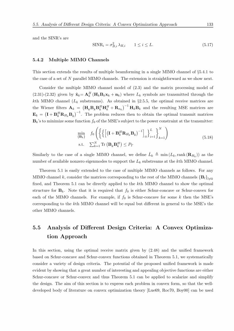
5.5. Analysis of Different Design Criteria: A Convex Optimization Approach 133
and the SINR’s are
SINRi = σ2B,i λH,i 1 ≤ i ≤ L. (5.17)
5.4.2 Multiple MIMO Channels
This section extends the results of multiple beamforming in a single MIMO channel of §5.4.1 to
the case of a set of N parallel MIMO channels. The extension is straightforward as we show next.
Consider the multiple MIMO channel model of (2.3) and the matrix processing model of
(2.31)-(2.32) given by xk= AHk (HkBkxk + nk) where Lk symbols are transmitted through the
kth MIMO channel (Lk substreams). As obtained in §2.5.5, the optimal receive matrices are
the Wiener filters Ak =(HkBkB
Hk HH
k + Rnk
)−1 HkBk and the resulting MSE matrices are
Ek =(I + BH
k RHkBk
)−1. The problem reduces then to obtain the optimal transmit matrices
Bk’s to minimize some function f0 of the MSE’s subject to the power constraint at the transmitter:
minBk
f0
([(I + BH
k RHkBk
)−1]ii
L
i=1
N
k=1
)
s.t.∑N
k=1 Tr(BkB
Hk
) ≤ PT
(5.18)
Similarly to the case of a single MIMO channel, we define Lk min (Lk, rank (RHk)) as the
number of available nonzero eigenmodes to support the Lk substreams at the kth MIMO channel.
Theorem 5.1 is easily extended to the case of multiple MIMO channels as follows. For any
MIMO channel k, consider the matrices corresponding to the rest of the MIMO channels Bll =k
fixed, and Theorem 5.1 can be directly applied to the kth MIMO channel to show the optimal
structure for Bk. Note that it is required that f0 is either Schur-concave or Schur-convex for
each of the MIMO channels. For example, if f0 is Schur-concave for some k then the MSE’s
corresponding to the kth MIMO channel will be equal but different in general to the MSE’s the
other MIMO channels.
5.5 Analysis of Different Design Criteria: A Convex Optimiza-
tion Approach
In this section, using the optimal receive matrix given by (2.48) and the unified framework
based on Schur-concave and Schur-convex functions obtained in Theorem 5.1, we systematically
consider a variety of design criteria. The potential of the proposed unified framework is made
evident by showing that a great number of interesting and appealing objective functions are either
Schur-concave or Schur-convex and thus Theorem 5.1 can be applied to scalarize and simplify
the design. The aim of this section is to express each problem in convex form, so that the well-
developed body of literature on convex optimization theory [Lue69, Roc70, Boy00] can be used

134 Chapter 5. Joint Tx-Rx Processing: A Unified Framework
to obtain optimal solutions very efficiently in practice using, for example, interior-point methods
(c.f. §3.1). In fact, it is possible in many cases to obtain simple closed-form solutions by means of
the Karush-Kuhn-Tucker (KKT) optimality conditions that can be easily implemented in practice
with low-complexity algorithms.
The following results were obtained in [Pal03c, Pal02a] for the multiple beamforming case and
in [Pal03b] for the single beamforming case.
For simplicity of notation we define zk,i σ2Bk ,i and λk,i λHk,i (k indexes the MIMO channels
and i the channel eigenmodes). Recall that whenever the fully diagonal structure is used (optimal
solution for Schur-concave functions and suboptimal solution for Schur-convex functions), in case
that Lk > rank (RHk), then the Lk − Lk substreams associated to zero eigenvalues are simply
ignored in the optimization process.
5.5.1 Minimization of the ARITH-MSE
The minimization of the (weighted) arithmetic mean of the MSE’s (ARITH-MSE) was considered
in [Yan94b, Sca99b, Sam01]. We deal with the weighted version as was extended in [Sam01] under
the unified framework of Theorem 5.1. The objective function is
f0 (MSEk,i) =∑k,i
(wk,i MSEk,i) . (5.19)
Lemma 5.2 The function f0 (xi) =∑
i (wi xi) (assuming xi ≥ xi+1) is minimized when the
weights are in increasing order wi ≤ wi+1 and it is then a Schur-concave function.
Proof. See Appendix 5.D.
By Lemma 5.2, the objective function (5.19) is Schur-concave on each MIMO channel k.
Therefore, by Theorem 5.1, the diagonal structure is optimal and the MSE’s are given by (5.12).
The problem in convex form (the objective is convex and the constraints linear) is4
minzk,i
∑k,i wk,i
11+λk,izk,i
s.t.∑
k,i zk,i ≤ PT ,
zk,i ≥ 0 1 ≤ k ≤ N, 1 ≤ i ≤ Lk.
(5.20)
4Note that it is not necessary to explicitly include the constraints corresponding to xi ≥ xi+1 of Lemma 5.2 in
the convex problem formulation of (5.20) since an optimal solution always satisfies these constraints (if xi < xj
for i < j, then those terms could be swapped so that xi ≥ xj is satisfied, but this would imply λk,i > λk,j which
cannot be optimal by Lemma 5.11).

5.5. Analysis of Different Design Criteria: A Convex Optimization Approach 135
As formally stated in Proposition 5.1, this problem can be solved very efficiently in practice
with Algorithm 5.1 that obtains the water-filling solution5
zk,i =(µ−1/2 w
1/2k,i λ
−1/2k,i − λ−1
k,i
)+(5.21)
where (x)+ max (0, x) and µ−1/2 is the water-level chosen to satisfy the power constraint with
equality. Since the optimal solution (5.21) does not distinguish between the two types of indexes
k and i, Algorithm 5.1 uses a single index for the sake of notation w.l.o.g.
Proposition 5.1 The following convex optimization problem:
minzk
∑Li=1 wi
11+λizi
s.t.∑L
i=1 zi ≤ PT ,
zi ≥ 0 1 ≤ i ≤ L,
is optimally solved by the water-filling solution zi =(µ−1/2 w
1/2i λ
−1/2i − λ−1
i
)+(it is tacitly
assumed that all the λi’s are strictly positive) where the water-level µ−1/2 is chosen such that∑Li=1 zi = PT .
Furthermore, the optimal water-filling solution can be efficiently obtained in practice with
Algorithm 5.1 in no more than L iterations (worst-case complexity).Proof. See Appendix 5.F.
Algorithm 5.1 Modified weighted water-filling algorithm (see Proposition 5.1).
Input: Number of available positive eigenvalues L, set of weights wi, set of eigenvalues λi,and maximum power PT .
Output: Set of allocated powers zi and water-level µ−1/2.
0. Reorder the set of pairs of weights and eigenvalues (wi, λi) so that the terms (wi λi) are
in decreasing order (define wL+1λL+1 0). Set L = L.
1. Set µ = wL λL (if wLλL = wL+1λL+1, then set L = L − 1 and go to step 1).
2. If µ−1/2 ≥ PT +∑L
i=1 λ−1i∑L
i=1 w1/2i λ
−1/2i
, then set L = L − 1 and go to step 1.
Otherwise, obtain the definitive water-level µ−1/2 and allocated powers as
µ−1/2 =PT +
∑Li=1 λ−1
i∑Li=1 w
1/2i λ
−1/2i
and
zi =(µ−1/2 w
1/2i λ
−1/2i − λ−1
i
)+,
undo the reordering done at step 0, and finish.5To be exact, this is a modified water-filling solution as opposed to the classical water-filling solution of the
form zk =(µ−1 − λ−1
k
)+.
136 Chapter 5. Joint Tx-Rx Processing: A Unified Framework
5.5.2 Minimization of the GEOM-MSE
The objective function corresponding to the minimization of the weighted geometric mean of the
MSE’s (GEOM-MSE) is
f0 (MSEk,i) =∏k,i
(MSEk,i)wk,i . (5.22)
Lemma 5.3 The function f0 (xi) =∏
i xwii (assuming xi ≥ xi+1 > 0) is minimized when the
weights are in increasing order wi ≤ wi+1 and it is then a Schur-concave function.
Proof. See Appendix 5.D.
By Lemma 5.3, the objective function (5.22) is Schur-concave on each MIMO channel k.
Therefore, by Theorem 5.1, the diagonal structure is optimal and the MSE’s are given by (5.12).
The problem in convex form (since the objective is log-convex, it is also convex [Boy00]) is6
minzk,i
∏k,i
(1
1+λk,izk,i
)wk,i
s.t.∑
k,i zk,i ≤ PT ,
zk,i ≥ 0 1 ≤ k ≤ N, 1 ≤ i ≤ Lk.
(5.23)
This problem, however, is more tractable if the logarithm of the objective is used as objective.
As formally stated in Proposition 5.2, this problem can be solved very efficiently in practice
with Algorithm 5.2 that obtains the water-filling solution
zk,i =(µ−1 wk,i − λ−1
k,i
)+(5.24)
where µ−1 is the water-level chosen to satisfy the power constraint with equality. Since the
optimal solution (5.24) does not distinguish between the two types of indexes k and i, Algorithm
5.2 uses a single index for simplicity w.l.o.g. Note that for the unweighted case wk,i = 1, (5.24)
becomes the classical capacity-achieving water-filling solution7 [Cov91b, Ral98].
Proposition 5.2 The following convex optimization problem:
minzi
∑Li=1 wi log
(1
1+λizi
)s.t.
∑Li=1 zi ≤ PT ,
zi ≥ 0 1 ≤ i ≤ L,
is optimally solved by the water-filling solution zi =(µ−1 wi − λ−1
i
)+ (it is tacitly assumed that
all the λi’s are strictly positive) where the water-level µ−1 is chosen such that∑L
i=1 zi = PT .6Again, it is not necessary to explicitly include the constraints corresponding to xi ≥ xi+1 of Lemma 5.3 in the
convex problem formulation of (5.23), since an optimal solution always satisfies these constraints.7Under the constraint of using Lk eigenmodes on the kth MIMO channel.

5.5. Analysis of Different Design Criteria: A Convex Optimization Approach 137
Furthermore, the optimal water-filling solution can be efficiently obtained in practice with
Algorithm 5.2 in no more than L iterations (worst-case complexity).
Proof. See Appendix 5.F.
Algorithm 5.2 Classical weighted water-filling algorithm (see Proposition 5.2).
Input: Number of available positive eigenvalues L, set of weights wi, set of eigenvalues λi,and maximum power PT .
Output: Set of allocated powers zi and water-level µ−1.
0. Reorder the set of pairs of weights and eigenmode gains (wi, λi) so that the terms (wi λi)
are in decreasing order (define wL+1λL+1 0). Set L = L.
1. Set µ = wL λL (if wLλL = wL+1λL+1, then set L = L − 1 and go to step 1).
2. If µ−1 ≥ PT +∑L
i=1 λ−1i∑L
i=1 wi
, then set L = L − 1 and go to step 1.
Otherwise, obtain the definitive water-level µ−1 and allocated powers as
µ−1 =PT +
∑Li=1 λ−1
i∑Li=1 wi
and
zi =(µ−1 wi − λ−1
i
)+,
undo the reordering of step 0, and finish.
5.5.3 Minimization of the Determinant of the MSE Matrix
The minimization of the determinant of the MSE matrix was considered in [Yan94a]. We now
show how this particular criterion is easily accommodated in our framework as a Schur-concave
function of the diagonal elements of the MSE matrix E. (For multiple MIMO channels with a
noncooperative scheme, the same reasoning applies for each MIMO channel.)
Using the fact that X ≥ Y ⇒|X| ≥ |Y|, it follows that the |E| is minimized for the choice
of the receive matrix given by (2.48). From the expression of the E in (2.51), it is clear that
|E| does not change if the transmit matrix B is post-multiplied by a unitary matrix (a rotation).
Therefore, we can always choose a rotation matrix so that E is diagonal without loss of optimality
(as we already knew from [Yan94a]) and then
|E| =∏j
λj (E) =∏j
[E]jj . (5.25)
Therefore, the minimization of |E| is equivalent to the minimization of the (unweighted) product
of the MSE’s treated in §5.5.2.

138 Chapter 5. Joint Tx-Rx Processing: A Unified Framework
5.5.4 Maximization of Mutual Information
The maximization of the mutual information can be used to obtain a capacity-achieving solution
[Cov91b]:
maxQ
I = log∣∣I + R−1
n HQHH∣∣ (5.26)
where Q is the transmit covariance matrix. Using the fact that |I + XY| = |I + YX| and that
Q = BBH (from (2.29)), the mutual information can be written as I = log∣∣I + BHHHR−1
n HB∣∣.
Comparing this with (2.51), it follows that the mutual information can be expressed (see [Cio97]
for detailed connections between the mutual information and the MSE matrix) as
I = − log |E| (5.27)
and, therefore, the maximization of I is equivalent to the minimization of |E| treated in §5.5.3.
Hence, the minimization of the unweighted product of the MSE’s, the minimization of the
determinant of the MSE matrix, and the maximization of the mutual information are all equiva-
lent criteria with solution given by a channel-diagonalizing structure and the classical capacity-
achieving water-filling for the power allocation:
zk,i =(µ−1 − λ−1
k,i
)+. (5.28)
5.5.5 Minimization of the MAX-MSE
In general, the overall performance (average BER) is dominated by the substream with highest
MSE. It makes sense then to minimize the maximum of the MSE’s (MAX-MSE) [Pal02a]. In
fact, as will be seen in the numerical results of §5.7, this criterion happens to perform very well
in practice in terms of average BER. The objective function is
f0 (MSEk,i) = maxk,i
MSEk,i . (5.29)
Lemma 5.4 The function f0 (xi) = maxi xi is a Schur-convex function.
Proof. See Appendix 5.D.
By Lemma 5.4, the objective function (5.29) is Schur-convex on each MIMO channel k. There-
fore, by Theorem 5.1, the optimal solution has a nondiagonal MSE matrix Ek.
5.5.5.1 Suboptimum Solution: A Simple Approach Imposing Diagonality
Although suboptimal, it is always interesting to solve the problem imposing a diagonal structure
by using the transmit matrix Bk= UHk,1ΣBk,1. The MSE’s are given by (5.16) and the problem
5.5. Analysis of Different Design Criteria: A Convex Optimization Approach 139
in convex form (the objective is linear and the constraints are all convex) is
mint,zk,i
t
s.t. t ≥ 11+λk,izk,i∑
k,i zk,i ≤ PT ,
zk,i ≥ 0
1 ≤ k ≤ N, 1 ≤ i ≤ Lk
1 ≤ k ≤ N, 1 ≤ i ≤ Lk.
(5.30)
It is straightforward to see that an optimal solution must satisfy all constraints on t with equality
t−1 = 1 + λk,izk,i ∀k, i (if the constraint was not satisfied with equality for some indexes k and i,
then zk,i could be decreased saving some power that could be redistributed among all eigenmodes,
which means that t could be further reduced and therefore it was not an optimal solution). The
solution has a simple closed-form expression given by
zk,i = λ−1k,i
PT∑l,j λ−1
l,j
. (5.31)
The same solution is obtained if one minimizes the maximum eigenvalue of the MSE matrix (or,
equivalently, if one maximizes the minimum eigenvalue of the SINR matrix defined as Γ E−1−I)
[Sca02].
5.5.5.2 Optimum Solution
Consider now the optimal solution with a nondiagonal MSE matrix Ek with equal diagonal
elements. The MSE’s are given by (5.14) which have to be minimized (scalarized problem).
Recall that after minimizing the MSE’s, it remains to obtain the optimal rotation matrix at
each MIMO channel such that the diagonal elements of each MSE matrix Ek are identical. The
scalarized problem in convex form (the objective is linear and the constraints are all convex) is
mint,zk,i
t
s.t. t ≥ 1Lk
((Lk − Lk
)+∑Lk
i=11
1+λk,izk,i
)∑
k,i zk,i ≤ PT ,
zk,i ≥ 0
1 ≤ k ≤ N,
1 ≤ k ≤ N, 1 ≤ i ≤ Lk.
(5.32)
It is also possible to consider the weighted version of the problem by including some weights in
(5.29). In such a case, although more involved, the problem can still be reformulated in convex
form and, therefore, optimally solved. Before attempting to solve the nontrivial problem (5.32),
let us consider two important particular cases.
For the case of single beamforming [Ise02, Pal03b] (i.e., Lk = 1) problem (5.32) simplifies to
one similar to (5.30) with solution (as (5.31))
zk = λ−1k
PT∑l λ
−1l
. (5.33)
140 Chapter 5. Joint Tx-Rx Processing: A Unified Framework
For the case of a single MIMO channel (or multiple MIMO channels with a cooperative ap-
proach), problem (5.32) simplifies to the minimization of the unweighted ARITH-MSE considered
in §5.5.1 (see also Proposition 5.1) as expected from the result in Corollary 5.1.
In the general case, as formally stated in Proposition 5.3, the problem can be solved very
efficiently in practice with Algorithm 5.3 that obtains the multi-level water-filling solution
zk,i =(µ
1/2k λ
−1/2k,i − λ−1
k,i
)+(5.34)
where µ1/2k are multiple water-levels chosen to satisfy the constraints on t and the power con-
straint all with equality.
Proposition 5.3 The following convex optimization problem:
mint,zk,i
t
s.t. t ≥ 1Lk
((Lk − Lk
)+∑Lk
i=11
1+λk,izk,i
)∑
k,i zk,i ≤ PT ,
zk,i ≥ 0
1 ≤ k ≤ N,
1 ≤ k ≤ N, 1 ≤ i ≤ Lk,
is optimally solved by the multi-level water-filling solution (it is tacitly assumed that all the λi’s
are strictly positive)
zk,i =(µ
1/2k λ
−1/2k,i − λ−1
k,i
)+
where the multiple water-levels µ1/2k are chosen positive such that the constraints on t and the
power constraint are satisfied with equality:
t = 1Lk
((Lk − Lk
)+∑Lk
i=11
1+λk,izk,i
)1 ≤ k ≤ N,∑
k,i zk,i = PT .
Furthermore, the optimal multi-level water-filling solution can be efficiently obtained in prac-
tice with Algorithm 5.3 in no more than LT ∑N
k=1 Lk iterations (worst-case complexity).
Proof. See Appendix 5.F.
Algorithm 5.3 Multi-level water-filling algorithm for the MAX-MSE criterion (see Proposition
5.3).
Input: Number of channels N , number of substreams per channel Lk, number of available
positive eigenvalues per channelLk
, set of eigenvalues λk,i, and maximum power PT .
Output: Set of allocated powers zk,i and set of water-levels µ1/2k .
0. Reorder the set λk,iLki=1 in decreasing order (define λk,Lk+1 0) and set Lk = Lk for
1 ≤ k ≤ N .

5.5. Analysis of Different Design Criteria: A Convex Optimization Approach 141
1. Set tmax - lb = max1≤k≤N
1
Lk
((Lk − Lk
)+ λ
1/2
k,Lk+1
∑Lki=1 λ
−1/2k,i
)and
tmin - ub = min1≤k≤N
1
Lk
((Lk − Lk
)+ λ
1/2
k,Lk
∑Lki=1 λ
−1/2k,i
)(denote the minimizing k by kmin).
2. If tmax - lb < tmin -ub and∑N
k=1
(∑Lki=1 λ
−1/2k,i
)2Lk tmin - ub−(Lk−Lk)
< PT +∑N
k=1
∑Lki=1 λ−1
k,i , then accept the
hypothesis and go to step 3.
Otherwise reject the hypothesis, set Lkmin= Lkmin
− 1, and go to step 1.
3. Obtain the definitive t, water-levels, and allocated powers as
t :N∑
k=1
(∑Lki=1 λ
−1/2k,i
)2
Lk t − (Lk − Lk
) = PT +N∑
k=1
Lk∑i=1
λ−1k,i ,
(recall that t ∈ [tmax - lb, tmin -ub))
µ1/2k =
∑Lki=1 λ
−1/2k,i
Lk t − (Lk − Lk
) , and
zk,i =(µ
1/2k λ
−1/2k,i − λ−1
k,i
)+,
undo the reordering done at step 0, and finish.
5.5.6 Maximization of the ARITH-SINR
The objective function to be minimized for the maximization of the (weighted) arithmetic mean
of the SINR’s (ARITH-SINR) is
f0 (SINRk,i) = −∑k,i
(wk,i SINRk,i) (5.35)
which can be expressed as a function of the MSE’s using (2.62) as
f0 (MSEk,i) = f0(MSE−1i,k −1) = −
∑k,i
wk,i (MSE−1i,k −1). (5.36)
Lemma 5.5 The function f0 (xi) = −∑i wi
(x−1
i − 1)
(assuming xi ≥ xi+1 > 0) is minimized
when the weights are in increasing order wi ≤ wi+1 and it is then a Schur-concave function.
Proof. See Appendix 5.D.
By Lemma 5.5, the objective function (5.36) is Schur-concave on each MIMO channel k.
Therefore, by Theorem 5.1, the diagonal structure is optimal and the SINR’s are given by (5.13).
142 Chapter 5. Joint Tx-Rx Processing: A Unified Framework
The problem expressed in convex form (it is actually an LP since the objective and the constraints
are all linear) is8
maxzk,i
∑k,i (wk,i λk,i) zk,i
s.t.∑
k,i zk,i ≤ PT ,
zk,i ≥ 0 1 ≤ k ≤ N, 1 ≤ i ≤ Lk.
(5.37)
The optimal solution is to allocate all the available power to the eigenmode with maximum
weighted gain (wk,i λk,i) (otherwise the objective value could be increased by transferring power
from other eigenmodes to this eigenmode). Although this solution maximizes indeed the weighted
sum of the SINR’s, it is a terrible solution in practice due to the extremely poor spectral efficiency
(only one substream would be conveying information). This criterion gives a pathological solution
and should not be used.
5.5.7 Maximization of the GEOM-SINR
The objective function to be minimized for the maximization of the (weighted) geometric mean
of the SINR’s (GEOM-SINR) is
f0 (SINRk,i) = −∏k,i
(SINRk,i)wk,i (5.38)
which can be expressed as a function of the MSE’s using (2.62) as
f0 (MSEk,i) = f0(MSE−1k,i −1) = −
∏k,i
(MSE−1k,i −1)wk,i . (5.39)
Note that the maximization of the product of the SINR’s is equivalent to the maximization of
the sum of the SINR’s expressed in dB.
Lemma 5.6 The function f0 (xi) = −∏i
(x−1
i − 1)wi (assuming 0.5 ≥ xi ≥ xi+1 > 0) is
minimized when the weights are in increasing order wi ≤ wi+1 and it is then a Schur-concave
function.
Proof. See Appendix 5.D.
By Lemma 5.6, the objective function (5.39) is Schur-concave on each MIMO channel k
provided that MSEk,i ≤ 0.5 ∀k, i (this is a mild assumption since a MSE greater than 0.5 is
unreasonable for a practical communication system). Therefore, by Theorem 5.1, the diagonal
8Note that it is not necessary to explicitly include the constraints corresponding to SINRk,i ≤ SINRk,i+1 in the
convex problem formulation (xi ≥ xi+1 in Lemma 5.5) since an optimal solution always satisfies them.
.

5.5. Analysis of Different Design Criteria: A Convex Optimization Approach 143
structure is optimal and the SINR’s are given by (5.13). The problem expressed in convex form
(the weighted geometric mean is a concave function9 [Roc70, Boy00]) is10
maxzk,i
∏k,i (λk,i zk,i)
wk,i
s.t.∑
k,i zk,i ≤ PT ,
zk,i ≥ 0, 1 ≤ k ≤ N, 1 ≤ i ≤ Lk,
(5.40)
where wk,i = wk,i/(∑
l,j wl,j
)(recall that λk,i > 0 ∀k, i, otherwise the problem has trivial solution
zk,i = 0 ∀k, i).
For the unweighted case wk,i = 1, the problem can be rewritten as the maximization of the
geometric mean subject to the arithmetic mean:
maxzk,i
∏k,i z
1/LT
k,i
s.t. 1/LT∑
k,i zk,i ≤ PT /LT ,
zk,i ≥ 0,
(5.41)
where LT ∑N
k=1 Lk. From the arithmetic-geometric mean inequality (∏
k xk)1/N ≤ 1
N
∑k xk
(with equality if and only if xk = xl ∀k, l) [Mag99, p.202][Hor85], it follows that the optimal
solution is the uniform power allocation
zk,i = PT /LT . (5.42)
Note that the uniform power distribution is commonly used due to its simplicity, e.g., [Won01].
For the general case, problem (5.40) can be easily solved by forming the Lagrangian and then
solving the KKT conditions (see §3.1) obtaining the optimal solution
zk,i = wk,i PT . (5.43)
5.5.8 Maximization of the HARM-SINR
The maximization of the harmonic mean of the SINR’s (HARM-SINR) was considered in [Ise02]
for the case of single beamforming. Using the unified framework of Theorem 5.1, we can extend
this result to the case of multiple beamforming. The objective function to be minimized is
f0 (SINRk,i) =∑k,i
1SINRk,i
(5.44)
9The concavity of the geometric mean is easily verified by showing that the Hessian matrix is positive semi-
definite for positive values of the arguments. The extension to include boundary points (points with zero-valued
arguments) is straightforward either by using a continuity argument to show that f (θx + (1 − θ)y) ≥ θf (x)+(1−θ)f (y) for 0 ≤ θ ≤ 1 or by considering the epigraph of the function and using [Lue69, Prop. 2.7.4].
10Again, it is not necessary to explicitly include the constraints corresponding to SINRk,i ≤ SINRk,i+1 (xi ≥ xi+1
in Lemma 5.6).
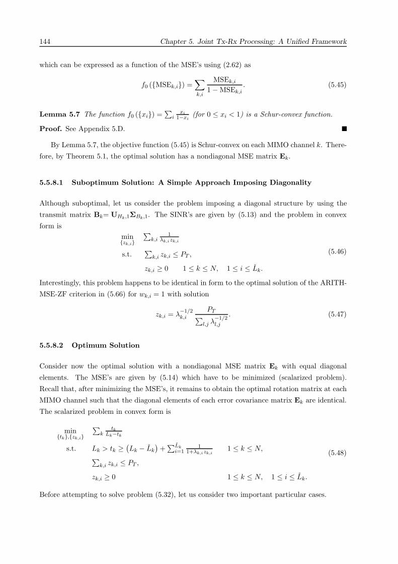
144 Chapter 5. Joint Tx-Rx Processing: A Unified Framework
which can be expressed as a function of the MSE’s using (2.62) as
f0 (MSEk,i) =∑k,i
MSEk,i
1 − MSEk,i. (5.45)
Lemma 5.7 The function f0 (xi) =∑
ixi
1−xi(for 0 ≤ xi < 1) is a Schur-convex function.
Proof. See Appendix 5.D.
By Lemma 5.7, the objective function (5.45) is Schur-convex on each MIMO channel k. There-
fore, by Theorem 5.1, the optimal solution has a nondiagonal MSE matrix Ek.
5.5.8.1 Suboptimum Solution: A Simple Approach Imposing Diagonality
Although suboptimal, let us consider the problem imposing a diagonal structure by using the
transmit matrix Bk= UHk,1ΣBk,1. The SINR’s are given by (5.13) and the problem in convex
form isminzk,i
∑k,i
1λk,izk,i
s.t.∑
k,i zk,i ≤ PT ,
zk,i ≥ 0 1 ≤ k ≤ N, 1 ≤ i ≤ Lk.
(5.46)
Interestingly, this problem happens to be identical in form to the optimal solution of the ARITH-
MSE-ZF criterion in (5.66) for wk,i = 1 with solution
zk,i = λ−1/2k,i
PT∑l,j λ
−1/2l,j
. (5.47)
5.5.8.2 Optimum Solution
Consider now the optimal solution with a nondiagonal MSE matrix Ek with equal diagonal
elements. The MSE’s are given by (5.14) which have to be minimized (scalarized problem).
Recall that, after minimizing the MSE’s, it remains to obtain the optimal rotation matrix at each
MIMO channel such that the diagonal elements of each error covariance matrix Ek are identical.
The scalarized problem in convex form is
mintk,zk,i
∑k
tkLk−tk
s.t. Lk > tk ≥ (Lk − Lk
)+∑Lk
i=11
1+λk,izk,i∑k,i zk,i ≤ PT ,
zk,i ≥ 0
1 ≤ k ≤ N,
1 ≤ k ≤ N, 1 ≤ i ≤ Lk.
(5.48)
Before attempting to solve problem (5.32), let us consider two important particular cases.

5.5. Analysis of Different Design Criteria: A Convex Optimization Approach 145
For the case of single beamforming [Ise02] (i.e., Lk = 1), the problem simplifies to (similarly
to (5.46))
minzk
∑k
1λk zk
s.t.∑
k zk ≤ PT ,
zk ≥ 0 1 ≤ k ≤ N
(5.49)
with solution
zk = λ−1/2k
PT∑l λ
−1/2l
. (5.50)
For the case of a single MIMO channel (or multiple MIMO channels with a cooperative
approach), problem (5.48) simplifies to the minimization of the ARITH-MSE considered in §5.5.1(see also Proposition 5.1) as expected from the result in Corollary 5.1.
In the general case, as formally stated in Proposition 5.4, the problem can be solved very
efficiently in practice with Algorithm 5.4 that obtains the multi-level water-filling solution
zk,i =(µ
1/2k λ
−1/2k,i − λ−1
k,i
)+(5.51)
where µ1/2k are multiple water-levels.
Proposition 5.4 The following convex optimization problem:
mintk,zk,i
∑Nk=1
tkLk−tk
s.t. Lk > tk ≥ (Lk − Lk
)+∑Lk
i=11
1+λk,izk,i∑k,i zk,i ≤ PT ,
zk,i ≥ 0
1 ≤ k ≤ N,
1 ≤ k ≤ N, 1 ≤ i ≤ Lk
is optimally solved by the multi-level water-filling solution (it is tacitly assumed that all the λi’s
are strictly positive)
zk,i =(µ
1/2k λ
−1/2k,i − λ−1
k,i
)+
where the multiple water-levels µ1/2k are chosen positive such that (ν is a positive parameter)
tk =(Lk − Lk
)+∑Lk
i=11
1+λk,izk,i1 ≤ k ≤ N,
µ1/2k = ν
L1/2k
Lk−tk,∑
k,i zk,i = PT .
Furthermore, the optimal multi-level water-filling solution can be efficiently obtained in prac-
tice with Algorithm 5.4 in no more than LT ∑N
k=1 Lk iterations (worst-case complexity).
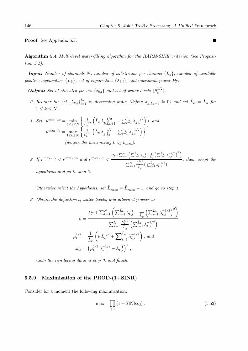
146 Chapter 5. Joint Tx-Rx Processing: A Unified Framework
Proof. See Appendix 5.F.
Algorithm 5.4 Multi-level water-filling algorithm for the HARM-SINR criterion (see Proposi-
tion 5.4).
Input: Number of channels N , number of substreams per channel Lk, number of available
positive eigenvaluesLk
, set of eigenvalues λk,i, and maximum power PT .
Output: Set of allocated powers zk,i and set of water-levels µ1/2k .
0. Reorder the set λk,iLki=1 in decreasing order (define λk,Lk+1 0) and set Lk = Lk for
1 ≤ k ≤ N .
1. Set νmin -ub = min1≤k≤N
1
L1/2k
(Lk λ
−1/2
k,Lk+1−∑Lk
i=1 λ−1/2k,i
)and
νmax - lb = max1≤k≤N
1
L1/2k
(Lk λ
−1/2
k,Lk−∑Lk
i=1 λ−1/2k,i
)(denote the maximizing k by kmax).
2. If νmax - lb < νmin -ub and νmax - lb <PT +
∑Nk=1
(∑Lki=1 λ−1
k,i− 1
Lk
(∑Lki=1 λ
−1/2k,i
)2)∑N
k=1
L1/2k
Lk
(∑Lki=1 λ
−1/2k,i
) , then accept the
hypothesis and go to step 3.
Otherwise reject the hypothesis, set Lkmax = Lkmax − 1, and go to step 1.
3. Obtain the definitive t, water-levels, and allocated powers as
ν =PT +
∑Nk=1
(∑Lki=1 λ−1
k,i − 1
Lk
(∑Lki=1 λ
−1/2k,i
)2)
∑Nk=1
L1/2k
Lk
(∑Lki=1 λ
−1/2k,i
)µ
1/2k =
1Lk
(ν L
1/2k +
∑Lk
i=1λ−1/2k,i
), and
zk,i =(µ
1/2k λ
−1/2k,i − λ−1
k,i
)+,
undo the reordering done at step 0, and finish.
5.5.9 Maximization of the PROD-(1+SINR)
Consider for a moment the following maximization:
max∏k,i
(1 + SINRk,i) . (5.52)

5.5. Analysis of Different Design Criteria: A Convex Optimization Approach 147
Using the relation between the MSE and the SINR in (2.62), this maximization can be equivalently
expressed as the following minimization:
min∏k,i
MSEk,i (5.53)
which is equivalent to the unweighted MAX-MSE criterion of (5.22), to the minimization of the
determinant of the MSE matrix in §5.5.3, and to the maximization of the mutual information
in §5.5.4 with solution given by the capacity-achieving expression (5.28). This result is com-
pletely natural since maximizing the logarithm of (5.52) is tantamount to maximizing the mutual
information I =∑
k,i log (1 + SINRk,i).
5.5.10 Maximization of the MIN-SINR
The objective function to be minimized for the maximization of the minimum of the SINR’s
(MIN-SINR) is
f0 (SINRk,i) = −mink,i
SINRk,i (5.54)
which can be expressed as a function of the MSE’s using (2.62) as
f0 (MSEk,i) = f0(MSE−1k,i −1) = −min
k,iMSE−1
k,i −1. (5.55)
Since the SINR is a monotonic decreasing function of the MSE, the minimization of (5.55) is
equivalent to the minimization of the maximum of the MSE’s maxk,i MSEk,i which was treated
with detail in §5.5.5. In [Sam01], the same criterion was used imposing a channel diagonal
structure.
5.5.11 Minimization of the ARITH-BER
The ultimate measure of a digital communication system is the BER (c.f. § 2.5.4). In practice,
MIMO communication systems use some type of coding over all the dimensions and possibly over
multiple transmissions to reduce the BER (usually some orders of magnitude). The ultimate
measure is then the coded BER as opposed to the uncoded BER (obtained without using any
coding). However, the coded BER is strongly related to the uncoded BER (in fact, for codes
based on hard decisions, both quantities are strictly related). Therefore, it suffices to focus on
the uncoded BER when designing the uncoded part of a communication system.
Under the Gaussian assumption, the uncoded BER can be analytically expressed as a function
of the SINR using the Q-function (c.f. §2.5.4.4). Recall that the Gaussian assumption, which
refers to the distribution of the global interference-plus-noise component, does not necessarily
imply that each interfering signal is Gaussian distributed. In fact, as long as the number of

148 Chapter 5. Joint Tx-Rx Processing: A Unified Framework
H
nR x n
T
B
nT x L L x n
R
n
nR
y
nT
(a) Independent (parallel) detection
(b) Joint ML detection
sDetector
Detector
A
x1
xL
⋅
⋅
H
x1
xL
H
nR x n
T
B
nT x L L x n
R
n
nR
y
nT
s
AH ML
DetectorL
x ⋅x1
xL
Figure 5.2: Scheme of a vector transmission using a transmit-receive linear processing with either anindependent or a joint detection of the established substreams.
interfering signals is sufficiently high, it is a reasonable assumption even when each of them
is not Gaussian distributed (since the total interference contribution tends to have a Gaussian
distribution as the number of interfering signals grows due to the central limit theorem).
Assuming that after the linear processing at the receiver each substream is detected indepen-
dently (see Figure 5.2(a)), the BER of the MIMO system is given by the average BER of the
established substreams or, equivalently, by the arithmetic mean of the BER’s (ARITH-BER). In
principle, a joint detection of all the substreams using an ML detector (see Figure 5.2(b)) is the
optimum receiver and outperforms the previously mentioned independent detection, for which the
minimization of the maximum eigenvalue of the MSE matrix11 may be an interesting criterion
[Sca02]. For complexity reasons, however, we assume an independent detection in the following.
The problem of minimizing the average BER in MIMO systems has recently been receiving
a considerable attention. In [Ong03], the problem was treated in detail imposing a diagonal
structure in the transmission (the approximation of the BER by the Chernoff upper bound was
also considered). The minimum BER solution without imposing any structural constraint has
been independently obtained in [Din02, Cha02a, Din03a] and in [Pal02a, Pal03c], where it has
been shown that the optimal solution consists of a nondiagonal transmission (nondiagonal MSE
matrix). In [Din03b], the minimum BER solution was used to improve the performance of a DMT
transmission using different constellations.
11Minimizing the maximum eigenvalue of the MSE matrix E =(I + BHHHR−1
n HB)−1
is equivalent to maxi-
mizing the minimum eigenvalue of the SINR matrix defined as Γ BHHHR−1n HB [Sca02].

5.5. Analysis of Different Design Criteria: A Convex Optimization Approach 149
The objective function to minimize is
f0 (BERk,i) =∑k,i
BERk,i (5.56)
which can be expressed as a function of the MSE’s using (2.62) and (2.38)-(2.40) (or the Chernoff
upper bound (2.39)) as
f0 (MSEk,i) =∑k,i
BER(MSE−1
k,i −1)
. (5.57)
Lemma 5.8 The function f0 (xi) =∑
i BER(x−1
i − 1)
(assuming θ ≥ xi > 0, for sufficiently
small θ such that BER(x−1
i − 1) ≤ 2 × 10⁻² ∀i) is a Schur-convex function.
Proof. See Appendix 5.D.
By Lemma 5.8, the objective function (5.57) is Schur-convex on each MIMO channel k (assum-
ing the same constellation/coding on all substreams of channel k) provided that BERk,i ≤ 2×10⁻²
(for BPSK and QPSK constellations, this is true for any value of the BER). Note that this is a
mild assumption since a practical system generally has an uncoded BER12 less than 2 × 10⁻².
Therefore, by Theorem 5.1, we can assume that for practical purposes the optimal solution has a
nondiagonal MSE matrix Ek.
5.5.11.1 Suboptimum Solution: A Simple Approach Imposing Diagonality
Consider first a suboptimal solution obtained by imposing a diagonal structure with
Bk= UHk,1ΣBk,1 (this case was extensively treated in [Ong03]). The SINR’s are given by (5.13)
and the problem in convex form is (recall that the BER function is convex decreasing on the
SINR as shown in §2.5.4.4) is
minzk,i
∑k,i αk,iQ
(√βk,iλk,izk,i
)s.t.
∑k,i zk,i ≤ PT ,
zk,i ≥ 0 1 ≤ k ≤ N, 1 ≤ i ≤ Lk.
(5.58)
This problem does not have a closed-form solution and one has to resort to general purpose
methods such as interior-point methods (see §3.1). For completeness we give the gradient and
the Hessian of the BER function and of the Chernoff approximation in Appendix 5.E.
12Given an uncoded BER of at most 10−2 and using a proper coding scheme, a coded BER with acceptable low
values such as 10−6 can be obtained. Note, however, that it is possible to design a system with an uncoded BER
higher than 10−2 for example with the utilization of low-density parity-check codes.

150 Chapter 5. Joint Tx-Rx Processing: A Unified Framework
5.5.11.2 Optimum Solution
Consider now the optimal solution with a nondiagonal MSE matrix Ek with equal diagonal
elements. The MSE’s are given by (5.14) which have to be minimized (scalarized problem).
Recall that after minimizing the MSE’s, it remains to obtain the optimal rotation matrix at
each MIMO channel such that the diagonal elements of each MSE matrix Ek are identical. The
scalarized problem in convex form is13
mintk,zk,i
∑k αkQ
(√βk
(t−1k − 1
))
s.t. θ ≥ tk ≥ 1Lk
((Lk − Lk
)+∑Lk
i=11
1+λk,izk,i
)∑
k,i zk,i ≤ PT ,
zk,i ≥ 0,
1 ≤ k ≤ N,
1 ≤ k ≤ N, 1 ≤ i ≤ Lk.
(5.59)
Note that we have explicitly included the upper bound θ on the MSE’s to guarantee the convexity
of the BER function and therefore of the whole problem.
The problem in convex form when using the Chernoff approximation is similarly given by
mintk,zk,i
∑k αkeβk(t−1
k −1)/2
s.t. θ ≥ tk ≥ 1Lk
((Lk − Lk
)+∑Lk
i=11
1+λk,izk,i
)∑
k,i zk,i ≤ PT ,
zk,i ≥ 0,
1 ≤ k ≤ N,
1 ≤ k ≤ N, 1 ≤ i ≤ Lk.
(5.60)
For a general case with N > 1 and Lk > 1, problems (5.59) and (5.60) do not have a simple
closed-form solution and one has to resort to general purpose methods such as interior-point
methods (see §3.1). For completeness, we give in Appendix 5.E the gradients and the Hessians
of the objective functions of (5.59) and (5.60) and of the log-barrier functions corresponding to
the constraints on the tk’s: tk ≥ 1Lk
((Lk − Lk
)+∑Lk
i=11
1+λk,izk,i
).
For the case of single beamforming (i.e., Lk = 1), problem (5.59) simplifies to that in (5.58).
For the case of a single MIMO channel (or multiple MIMO channels with a cooperative approach),
problems (5.59) and (5.60) have a closed-form solution as is stated below.
Remark 5.4 The minimization of the average BER (assuming the same constellation on all
substreams) of a vector transmission through a single MIMO channel (this also includes mul-
tiple MIMO channels with a cooperative approach) can be obtained by first minimizing Tr (E)
(method ARITH-MSE considered in §5.5.1) and then including the appropriate rotation matrix13We are implicitly assuming the same constellation and code on the substreams corresponding to each MIMO
channel k.

5.5. Analysis of Different Design Criteria: A Convex Optimization Approach 151
Q as indicated in Theorem 5.1 (such as the unitary DFT matrix) to make the diagonal ele-
ments of the MSE matrix equal. The solution can be then written in closed form, following the
notation of Theorem 5.1, as B = UH,1ΣB,1Q, where the squared-diagonal elements of ΣB,1, de-
noted by zi, are given by zi = PT λ−1/2i /
∑j λ
−1/2j if a ZF receiver is used (see (5.68)) and by
zi =(µ−1/2 λ
−1/2i − λ−1
i
)+if a MMSE receiver is used (see (5.21), for which Algorithm 5.1 can
be conveniently used in practice).
The previous remark is just a particularization of Corollary 5.1.
5.5.12 Minimization of the GEOM-BER
Although in terms of BER the minimization of the arithmetic mean is the soundest criterion from
a coding perspective, let us briefly consider the minimization of the geometric mean of the BER’s
(GEOM-BER) for completeness. The objective function is
f0 (BERk,i) =∏k,i
BERk,i (5.61)
which can be expressed as a function of the MSE’s using (2.62) and (2.38)-(2.40) (or the Chernoff
upper bound (2.39)) as
f0 (MSEk,i) =∏k,i
BER(MSE−1
k,i −1)
. (5.62)
Lemma 5.9 The function f0 (xi) =∏
i BER(x−1
i − 1)
is a Schur-concave function for θ ≥xi > 0 with θ such that
(∂ BER(x−1−1)
∂x
)2
≥ BER(x−1 − 1
) ∂2 BER(x−1−1)∂x2 for θ ≥ x > 0.
Proof. See Appendix 5.D.
By Lemma 5.9, the objective function (5.62) is Schur-concave on each MIMO channel k
(assuming the same constellation/coding on all substreams of channel k) provided that MSEk,i ≤ θ
∀k, i. This condition is trivially satisfied by the Chernoff approximation for any value of θ and
by the exact BER function for high values of θ in general around 0.8 (this is a mild assumption
since a MSE greater than 0.5 is unreasonable for a practical communication system). Therefore,
by Theorem 5.1, we can assume that for practical purposes that the diagonal structure is optimal
and the MSE’s are given by (5.12). For simplicity, we consider the formulation of the problem in
convex form using the Chernoff bound (it is actually an LP since the objective and the constraints
are all linear):
maxzk,i
∑k,i (βkλk,i) zk,i
s.t.∑
k,i zk,i ≤ PT ,
zk,i ≥ 0, 1 ≤ k ≤ N, 1 ≤ i ≤ Lk.
(5.63)

152 Chapter 5. Joint Tx-Rx Processing: A Unified Framework
Problem (5.63) is exactly identical to the one appearing in the maximization of the ARITH-SINR
with solution given by allocating all the available power to the eigenmode with maximum gain
(βkλk,i). Although this solution maximizes indeed the product of the BER’s, it is a terrible
solution in practice due to the extremely poor spectral efficiency (only one substream would be
conveying information). This criterion gives a pathological solution and should not be used.
5.5.13 Minimization of the MAX-BER
The objective function for the minimization of the maximum of the BER’s (MAX-BER) is
f0 (BERk,i) = maxk,i
BERk,i (5.64)
which can be expressed as a function of the MSE’s using (2.62), (2.38) and (2.40) as
f0 (MSEk,i) = maxk,i
BER
(MSE−1
k,i −1)
. (5.65)
The minimization of (5.65) is equivalent to the minimization of the maximum of the MSE’s14
maxk,i MSEk,i which was treated with detail in §5.5.5.
5.5.14 Including a ZF Constraint
It is interesting at this point to see how easily the ZF constraint can be imposed in the design
of the transmitter. Two different approaches can be taken. One is based on using the extended
MSE matrix in (2.75) to obtain the solution and then taking the asymptotic result for γ → ∞.
The other approach is based on using directly the limiting MSE matrix in (2.69). In any case,
Theorem 5.1 still holds. We consider three illustrative examples, but the same approach can be
applied to any other criteria.
5.5.14.1 ARITH-MSE-ZF
Consider the criterion ARITH-MSE treated in §5.5.1, but using instead the extended MSE matrix
defined in (2.75) (or, equivalently, the MSE’s given in (2.76)). The problem in convex form is
minzk,i
∑k,i wk,i
11γ+λk,izk,i
s.t.∑
k,i zk,i ≤ PT ,
zk,i ≥ 0 1 ≤ k ≤ N, 1 ≤ i ≤ Lk.
(5.66)
with solution
zk,i =(
µ−1/2 w1/2k,i λ
−1/2k,i − 1
γλ−1
k,i
)+
−→ µ−1/2 w1/2k,i λ
−1/2k,i (5.67)
14We are implicitly assuming the same constellation and code on all the substreams.
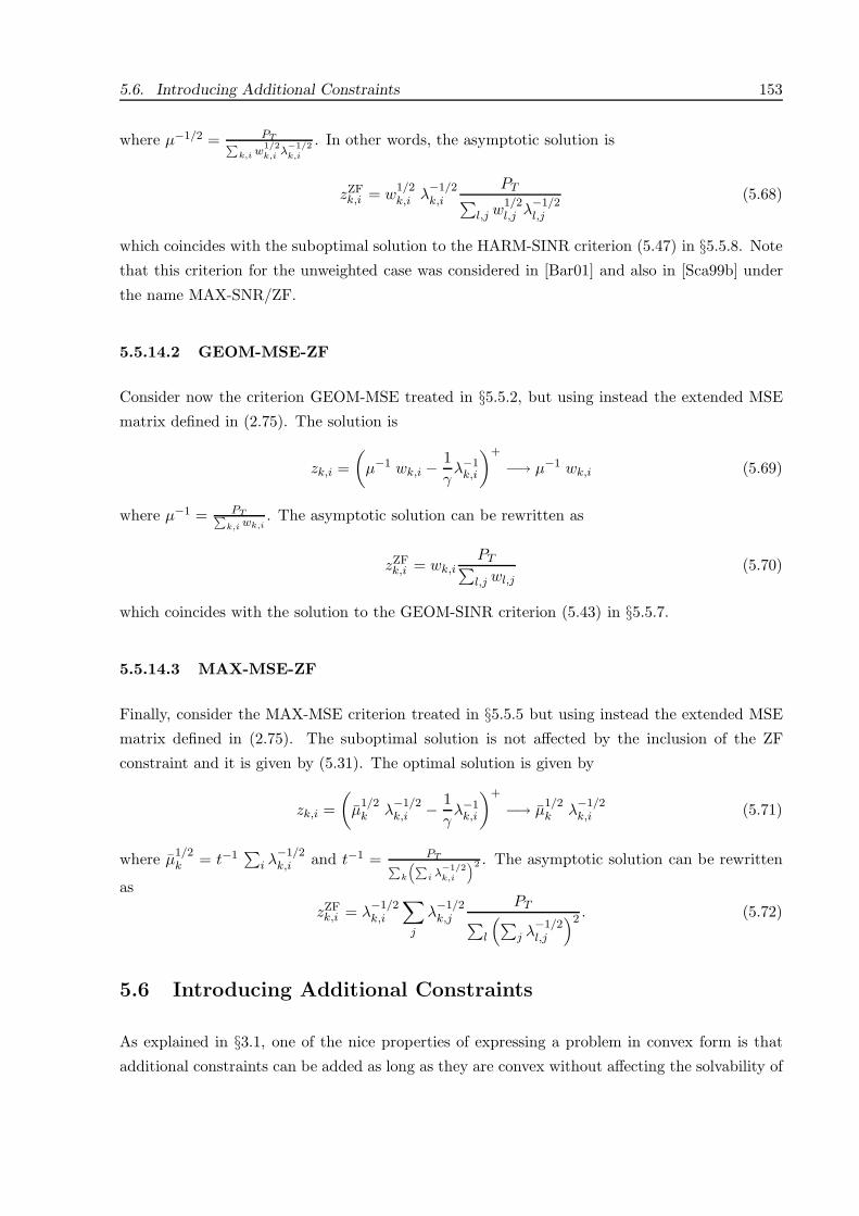
5.6. Introducing Additional Constraints 153
where µ−1/2 = PT∑k,i w
1/2k,i λ
−1/2k,i
. In other words, the asymptotic solution is
zZFk,i = w
1/2k,i λ
−1/2k,i
PT∑l,j w
1/2l,j λ
−1/2l,j
(5.68)
which coincides with the suboptimal solution to the HARM-SINR criterion (5.47) in §5.5.8. Note
that this criterion for the unweighted case was considered in [Bar01] and also in [Sca99b] under
the name MAX-SNR/ZF.
5.5.14.2 GEOM-MSE-ZF
Consider now the criterion GEOM-MSE treated in §5.5.2, but using instead the extended MSE
matrix defined in (2.75). The solution is
zk,i =(
µ−1 wk,i − 1γ
λ−1k,i
)+
−→ µ−1 wk,i (5.69)
where µ−1 = PT∑k,i wk,i
. The asymptotic solution can be rewritten as
zZFk,i = wk,i
PT∑l,j wl,j
(5.70)
which coincides with the solution to the GEOM-SINR criterion (5.43) in §5.5.7.
5.5.14.3 MAX-MSE-ZF
Finally, consider the MAX-MSE criterion treated in §5.5.5 but using instead the extended MSE
matrix defined in (2.75). The suboptimal solution is not affected by the inclusion of the ZF
constraint and it is given by (5.31). The optimal solution is given by
zk,i =(
µ1/2k λ
−1/2k,i − 1
γλ−1
k,i
)+
−→ µ1/2k λ
−1/2k,i (5.71)
where µ1/2k = t−1
∑i λ
−1/2k,i and t−1 = PT∑
k
(∑i λ
−1/2k,i
)2 . The asymptotic solution can be rewritten
as
zZFk,i = λ
−1/2k,i
∑j
λ−1/2k,j
PT∑l
(∑j λ
−1/2l,j
)2 . (5.72)
5.6 Introducing Additional Constraints
As explained in §3.1, one of the nice properties of expressing a problem in convex form is that
additional constraints can be added as long as they are convex without affecting the solvability of

154 Chapter 5. Joint Tx-Rx Processing: A Unified Framework
the problem. As an example, we now consider two additional constraints that may be interesting
to impose in a multicarrier multi-antenna communication system with N carriers and nT trans-
mit antennas. Of course, with the additional constraints, the closed-form solutions previously
obtained in §5.5 are not valid any more and have to be properly modified.
Recall that the transmitted vector signals in a multi-antenna multicarrier system are given
by sk = Bkxk 1 ≤ k ≤ N and the transmitted sequence by the ith antenna is then si (n) =1√N
∑Nk=1 sk,i e
−j 2πN
(k−1)(n−1) 1 ≤ n ≤ N . Therefore, the average transmitted power by the ith
antenna is Pi E [|si (n)|2] = 1N
∑Nk=1 E [|sk,i|2].
Dynamic Range of Power Amplifier
We can easily add constraints on the dynamic range of the power amplifier at each transmit
antenna element as was done in [Ben01]. Consider a Schur-concave objective function and assume
for simplicity Lk = Lk = L ∀k. From the optimal structure in (5.10) Bk = UHk ,1ΣBk,1, the total
average transmitted power (in units of energy per symbol period) by the ith antenna is
Pi =1N
N∑k=1
L∑l=1
∣∣ [Bk]i,l∣∣2 =
1N
N∑k=1
L∑l=1
σ2Bk,l
∣∣ [UHk,1]i,l∣∣2 (5.73)
which is linear in the variables σ2Bk,i. (For the carrier-cooperative scheme, Pi =
1N
∑Nk=1
∑NLl=1
∣∣ [B]i+(k−1)nT ,l
∣∣2.) Therefore, the following constraints are linear
αLi ≤ Pi ≤ αU
i 1 ≤ i ≤ nT
where αLi and αU
i are the lower and upper bounds for the ith antenna. Similarly, it is straight-
forward to set limits on the relative dynamic range of a single element in comparison to the total
power for the whole array [Ben01]:
ρLi Parray ≤ Pi ≤ ρU
i Parray 1 ≤ i ≤ nT
where ρLi and ρU
i are the relative bounds, and Parray =∑nT
i=1 Pi is the total power also linear in
σ2Bk ,i.
Peak to Average Ratio (PAR)
One of the main practical problems that OFDM systems face is the PAR. Indeed, multicarrier
signals exhibit Gaussian-like time-domain waveforms with relatively high PAR, i.e., they exhibit
large amplitude spikes when several frequency components add in-phase. These spikes may have a
serious impact on the design complexity and feasibility of the transceiver’s analog front-end (i.e.,
high resolution of D/A-A/D15 converters and power amplifiers with a linear behavior over a large
dynamic range). In practice, the transmitted signal has to be clipped when it exceeds a certain
threshold which has detrimental effects on the BER. A variety of techniques have been devised
to deal with the PAR [Mes96, Tel98, Tel00]. In this section we show how the PAR can be taken15D/A: Digital to Analog. A/D: Analog to Digital.

5.7. Simulation Results 155
into account into the design of the beamvectors using a convex optimization framework. Note
that the already existing techniques to cope with the PAR and this approach are not exclusive
and can be simultaneously used.
The PAR is defined as
PAR max0≤t≤Ts
A2(t)σ2
(5.74)
where Ts is the symbol period, A(t) is the zero-mean transmitted signal, and σ2 = E[A2(t)
].
Since the number of carriers is usually large (N ≥ 64), A(t) can be accurately modeled as a
Gaussian random process (central-limit theorem) with zero mean and variance σ2 [Mes96]. Using
this assumption, the probability that the PAR exceeds certain threshold or, equivalently, the
probability that the instantaneous amplitude exceeds a clipping value Aclip is
Pr |A(t)| > Aclip = 2 Q(
Aclip
σ
)(5.75)
where Q is the Q-function defined as Q (x) = 1√2π
∫∞x e−λ2/2dλ [Pro95]. The clipping probability
of an OFDM symbol is then [Mes96]
Pclip(σ) = 1 −(
1 − 2 Q(
Aclip
σ
))2N
. (5.76)
In other words, in order to have a clipping probability lower than P with respect to the maximum
instantaneous amplitude Aclip, the average signal power must satisfy
σ ≤ σclip(P ) =Aclip
Q−1(
1−(1−P )1/(2N)
2
) . (5.77)
When using multiple antennas for transmission, the previous equation has to be satisfied for all
transmit antennas. Those constraints can be easily incorporated in any of the convex designs
derived in §5.5 with a Schur-concave objective function. Using (5.73) the constraint is
1N
N∑k=1
L∑l=1
σ2Bk,l
∣∣ [UHk,1]i,l∣∣2 ≤ σ2
clip 1 ≤ i ≤ nT (5.78)
which is linear in the optimization variables σ2Bk,i. Such a constraint has two effects in the
solution: (i) the power distribution over the carriers changes with respect to the distribution
without the constraint, and (ii) the total transmitted power drops as necessary.
5.7 Simulation Results
For the numerical results, we consider a multi-antenna wireless channel. In particular, we have
chosen the European standard HIPERLAN/2 for WLAN [ETS01]. It is based on the multi-
carrier modulation OFDM (64 carriers are used in the simulations). We consider multiple an-
tennas at both the transmitter and the receiver, obtaining therefore the MIMO model used

156 Chapter 5. Joint Tx-Rx Processing: A Unified Framework
(a) (b)
1.0000 0.4154 0.2057 0.1997
0.4154 1.0000 0.3336 0.3453
0.2057 0.3336 1.0000 0.5226
0.1997 0.3453 0.5226 1.0000
RBS
=
1.0000 0.3644 0.0685 0.3566
0.3644 1.0000 0.3245 0.1848
0.0685 0.3245 1.0000 0.3093
0.3566 0.1848 0.3093 1.0000
RMS
=
0
10
20
30
50
80
110
140
180
230
280
330
400
490
600
730
880
1050
-3.3
-3.6
-3.9
-4.2
0.0
-0.9
-1.7
-2.6
-1.5
-3.0
-4.4
-5.9
-5.3
-7.9
-9.4
-13.2
-16.3
-21.2
Delay (ns)Average relative
power (dB)
Figure 5.3: (a) Power delay profile type C for HIPERLAN/2. (b) Envelope correlation matrices at thebase station (BS) and at the mobile station (MS) in the Nokia environment.
throughout the chapter (either multiple MIMO channels or a single MIMO channel depending on
whether a carrier-noncooperative approach or a carrier-cooperative approach is used as described
in §2.5.1.2). Perfect CSI is assumed at both sides of the communication link (channel estimation
errors are considered in Chapter 7).
The frequency selectivity of the channel is modeled using the power delay profile type C for
HIPERLAN/2 as specified in [ETS98a] (see Figure 5.3(a)), which corresponds to a typical large
open space indoor environment for NLOS conditions with 150ns average r.m.s. delay spread and
1050ns maximum delay (the sampling period is 50ns ) [ETS01]. The spatial correlation of the
MIMO channel is modeled according to the Nokia model defined in [Sch01] (which corresponds
to a reception hall) specified by the correlation matrices of the envelope of the channel fading at
the transmit and receive side given in Figure 5.3(b) where the base station is the receiver (uplink)
(see [Sch01] for details of the model). It models a large open indoor environment with two floors,
which could easily illustrate a conference hall or a shopping galleria scenario. The matrix channel
generated was normalized so that∑
n E [| [H(n)]ij |]2 = 1. The SNR is defined as the transmitted
power normalized with the noise variance.
For the numerical simulations, the following design criteria have been considered: ARITH-
MSE, GEOM-MSE, MAX-MSE (equivalently, MIN-SINR or MAX-BER), GEOM-SINR, HARM-
SINR, and ARITH-BER (benchmark). The utilization of the Chernoff upper bound instead of the
exact BER function gives indistinguishable results and is therefore not presented in the simulation
results. The constellations used for transmission are fixed and are not involved in the optimization

5.7. Simulation Results 157
−5 0 5 10 1510
−5
10−4
10−3
10−2
10−1
100
Outage BER (QPSK) in a MIMO(2,2) channel
SNR (dB)
BE
R
GEOM−MSEGEOM−SINRARITH−MSEHARM−SINRMAX−MSEARITH−BER
Figure 5.4: BER (at an outage probability of 5%) vs. SNR when using QPSK in a 2 × 2 MIMO channelwith L = 1 for the GEOM-MSE, GEOM-SINR, ARITH-MSE, HARM-SINR, MAX-MSE, and ARITH-BER criteria (without carrier cooperation).
process, regardless of whether some channel eigenmodes are not allocated any power (due to the
water-filling nature of many of the solutions) for fair comparisons. Unless otherwise specified,
a carrier-noncooperative approach is considered. The performance is given in terms of outage
BER (averaged over the channel substreams), i.e., the BER that can be guaranteed with some
probability or, equivalently, the BER that is not achieved with some small outage probability. In
particular, we consider the BER with an outage probability of 5%. Note that for typical systems
with delay constraints, the outage BER is a more realistic measure than the commonly used
mean BER that only makes sense when the transmission coding block is long enough to reveal
the long-term ergodic properties of the fading process (no delay constraints).
Single Beamforming
First we show some results when using a single channel spatial substream (Lk = 1 ∀k). In
Figure 5.4, the BER is plotted vs. the SNR for a 2×2 MIMO channel using QPSK constellations.
Clearly, the ARITH-BER criterion has the lowest BER because it was designed for that. The
MAX-MSE criterion performs really close to the ARITH-BER and can be considered the second
best criterion. The HARM-SINR and also the ARITH-MSE perform reasonably well (in fact, for
values of the BER higher than 10−2 they outperform the MAX-MSE). The GEOM-MSE and the
GEOM-SINR criteria perform really bad in terms of BER and should not be used. In Figure 5.5,
the same results are shown for a 4× 2 MIMO channel using 16-QAM constellations and the same
observations hold.

158 Chapter 5. Joint Tx-Rx Processing: A Unified Framework
−2 0 2 4 6 8 10 12 14 16 1810
−5
10−4
10−3
10−2
10−1
100
Outage BER (16−QAM) in a MIMO(4,2) channel
SNR (dB)
BE
RGEOM−MSEGEOM−SINRARITH−MSEHARM−SINRMAX−MSEARITH−BER
Figure 5.5: BER (at an outage probability of 5%) vs. SNR when using 16-QAM in a 4 × 2 MIMOchannel (2 transmit and 4 receive antennas) with L = 1 for the GEOM-MSE, GEOM-SINR, ARITH-MSE,HARM-SINR, MAX-MSE, and ARITH-BER criteria (without carrier cooperation).
Therefore, the best criteria are (in order): ARITH-BER, MAX-MSE, HARM-SINR, and
ARITH-MSE.
Including PAR Constraints
We now consider the introduction of PAR constraints as described in §5.6. We parameterize
the clipping amplitude with respect to µ as Aclip = µ√
PTnT
to make the results independent of the
total transmitted power PT . In Figure 5.6, the probability of clipping along with the BER (when
using QPSK constellations) is shown for the ARITH-MSE criterion in a 2 × 2 MIMO channel
both with PAR constraints (Pclip = 10−2) and without them. In 5.6(a), the results are shown as a
function of µ. It can be observed how the design with the PAR constraints always has a clipping
probability no greater than the prespecified value 10−2 as expected. The BER, however, can be
severely affected if a very low clipping probability is imposed due to power back-offs. From Figure
5.6(a), a choice of µ = 4 seems reasonable. In Figure 5.6(b), the results are shown as a function
of the SNR for µ = 4. For the design with PAR constraints, the BER is slightly higher due to
the additional constraint. However, the system is guaranteed to have a clipping probability of at
most 10−2 unlike in the unconstrained case where nothing can be guaranteed. Recall that in a
practical system, the final BER increases due to the clipping.
Including a ZF Constraint
We now consider the effect of introducing a ZF constraint. Clearly, since the design has
additional constraints, the performance will decrease with respect to the design without the ZF
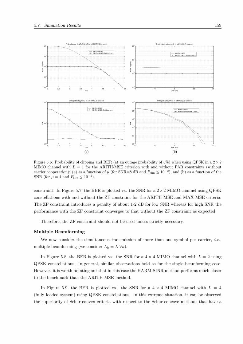
5.7. Simulation Results 159
2 2.5 3 3.5 4 4.5 5 5.510
−4
10−3
10−2
10−1
100
Prob. clipping (SNR=8.00 dB) in a MIMO(2,2) channel
mu
Pro
b. c
lippi
ng
ARITH−MSE ARITH−MSE (PAR const.)
2 2.5 3 3.5 4 4.5 5 5.510
−3
10−2
10−1
Outage BER (QPSK) in a MIMO(2,2) channel
mu
BE
R
ARITH−MSE ARITH−MSE (PAR const.)
−5 0 5 10 1510
−3
10−2
10−1
100
Prob. clipping (mu=4.0) in a MIMO(2,2) channel
SNR (dB)
Pro
b. c
lippi
ng
ARITH−MSE ARITH−MSE (PAR const.)
−5 0 5 10 1510
−5
10−4
10−3
10−2
10−1
100
Outage BER (QPSK) in a MIMO(2,2) channel
SNR (dB)
BE
R
ARITH−MSE ARITH−MSE (PAR const.)
(a) (b)
Figure 5.6: Probability of clipping and BER (at an outage probability of 5%) when using QPSK in a 2× 2MIMO channel with L = 1 for the ARITH-MSE criterion with and without PAR constraints (withoutcarrier cooperation): (a) as a function of µ (for SNR=8 dB and Pclip ≤ 10−2), and (b) as a function of theSNR (for µ = 4 and Pclip ≤ 10−2).
constraint. In Figure 5.7, the BER is plotted vs. the SNR for a 2×2 MIMO channel using QPSK
constellations with and without the ZF constraint for the ARITH-MSE and MAX-MSE criteria.
The ZF constraint introduces a penalty of about 1-2 dB for low SNR whereas for high SNR the
performance with the ZF constraint converges to that without the ZF constraint as expected.
Therefore, the ZF constraint should not be used unless strictly necessary.
Multiple Beamforming
We now consider the simultaneous transmission of more than one symbol per carrier, i.e.,
multiple beamforming (we consider Lk = L ∀k).
In Figure 5.8, the BER is plotted vs. the SNR for a 4 × 4 MIMO channel with L = 2 using
QPSK constellations. In general, similar observations hold as for the single beamforming case.
However, it is worth pointing out that in this case the HARM-SINR method performs much closer
to the benchmark than the ARITH-MSE method.
In Figure 5.9, the BER is plotted vs. the SNR for a 4 × 4 MIMO channel with L = 4
(fully loaded system) using QPSK constellations. In this extreme situation, it can be observed
the superiority of Schur-convex criteria with respect to the Schur-concave methods that have a
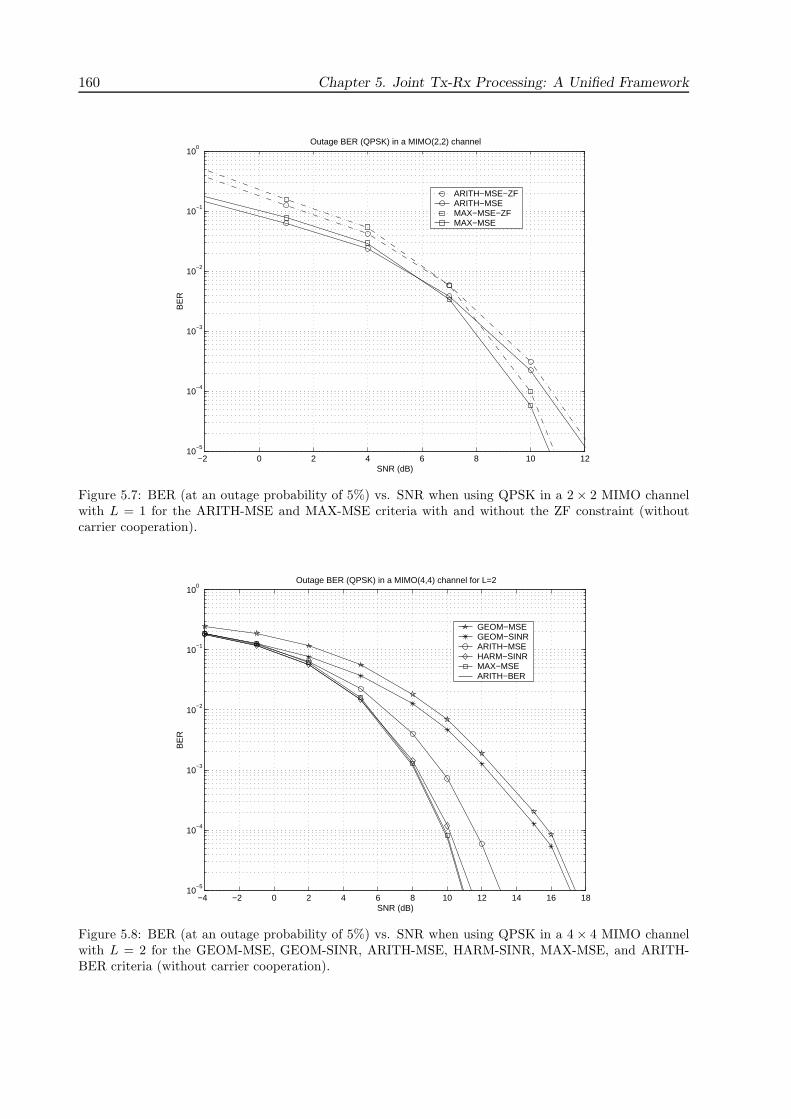
160 Chapter 5. Joint Tx-Rx Processing: A Unified Framework
−2 0 2 4 6 8 10 1210
−5
10−4
10−3
10−2
10−1
100
Outage BER (QPSK) in a MIMO(2,2) channel
SNR (dB)
BE
R
ARITH−MSE−ZFARITH−MSEMAX−MSE−ZFMAX−MSE
Figure 5.7: BER (at an outage probability of 5%) vs. SNR when using QPSK in a 2 × 2 MIMO channelwith L = 1 for the ARITH-MSE and MAX-MSE criteria with and without the ZF constraint (withoutcarrier cooperation).
−4 −2 0 2 4 6 8 10 12 14 16 1810
−5
10−4
10−3
10−2
10−1
100
Outage BER (QPSK) in a MIMO(4,4) channel for L=2
SNR (dB)
BE
R
GEOM−MSEGEOM−SINRARITH−MSEHARM−SINRMAX−MSEARITH−BER
Figure 5.8: BER (at an outage probability of 5%) vs. SNR when using QPSK in a 4 × 4 MIMO channelwith L = 2 for the GEOM-MSE, GEOM-SINR, ARITH-MSE, HARM-SINR, MAX-MSE, and ARITH-BER criteria (without carrier cooperation).
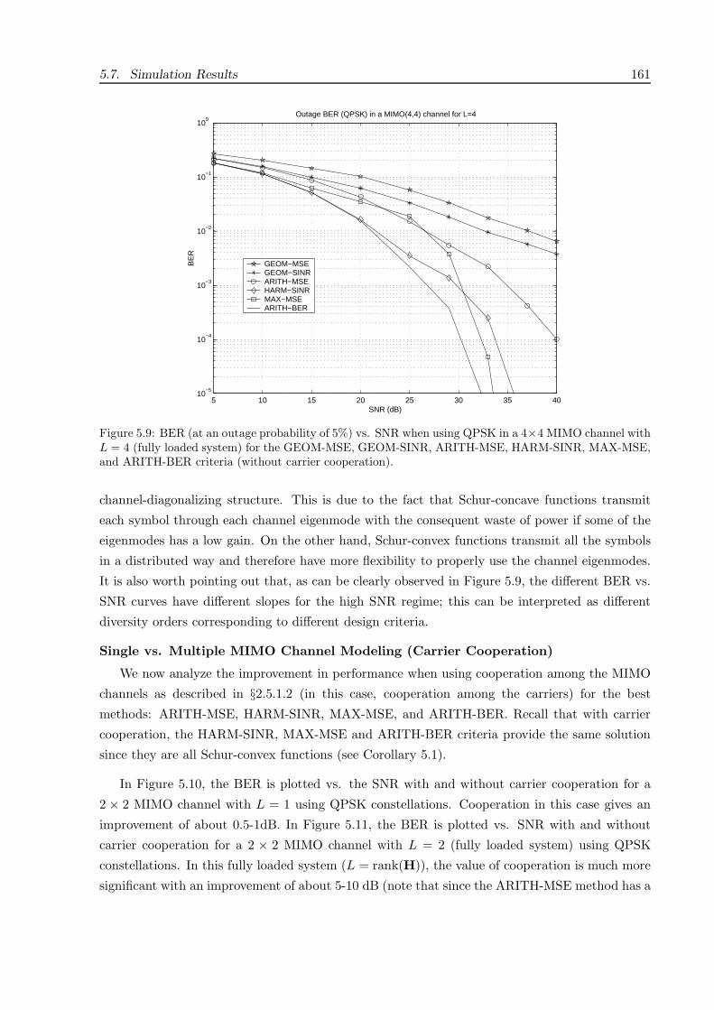
5.7. Simulation Results 161
5 10 15 20 25 30 35 4010
−5
10−4
10−3
10−2
10−1
100
Outage BER (QPSK) in a MIMO(4,4) channel for L=4
SNR (dB)
BE
R
GEOM−MSEGEOM−SINRARITH−MSEHARM−SINRMAX−MSEARITH−BER
Figure 5.9: BER (at an outage probability of 5%) vs. SNR when using QPSK in a 4×4 MIMO channel withL = 4 (fully loaded system) for the GEOM-MSE, GEOM-SINR, ARITH-MSE, HARM-SINR, MAX-MSE,and ARITH-BER criteria (without carrier cooperation).
channel-diagonalizing structure. This is due to the fact that Schur-concave functions transmit
each symbol through each channel eigenmode with the consequent waste of power if some of the
eigenmodes has a low gain. On the other hand, Schur-convex functions transmit all the symbols
in a distributed way and therefore have more flexibility to properly use the channel eigenmodes.
It is also worth pointing out that, as can be clearly observed in Figure 5.9, the different BER vs.
SNR curves have different slopes for the high SNR regime; this can be interpreted as different
diversity orders corresponding to different design criteria.
Single vs. Multiple MIMO Channel Modeling (Carrier Cooperation)
We now analyze the improvement in performance when using cooperation among the MIMO
channels as described in §2.5.1.2 (in this case, cooperation among the carriers) for the best
methods: ARITH-MSE, HARM-SINR, MAX-MSE, and ARITH-BER. Recall that with carrier
cooperation, the HARM-SINR, MAX-MSE and ARITH-BER criteria provide the same solution
since they are all Schur-convex functions (see Corollary 5.1).
In Figure 5.10, the BER is plotted vs. the SNR with and without carrier cooperation for a
2 × 2 MIMO channel with L = 1 using QPSK constellations. Cooperation in this case gives an
improvement of about 0.5-1dB. In Figure 5.11, the BER is plotted vs. SNR with and without
carrier cooperation for a 2 × 2 MIMO channel with L = 2 (fully loaded system) using QPSK
constellations. In this fully loaded system (L = rank(H)), the value of cooperation is much more
significant with an improvement of about 5-10 dB (note that since the ARITH-MSE method has a

162 Chapter 5. Joint Tx-Rx Processing: A Unified Framework
3 4 5 6 7 8 9 10 11 12 1310
−5
10−4
10−3
10−2
10−1
Outage BER (QPSK) in a MIMO(2,2) channel for L=1
SNR (dB)
BE
RARITH−MSE−noncoopARITH−MSE−coopHARM−SINR−noncoopHARM−SINR−coopMAX−MSE−noncoopMAX−MSE−coopARITH−BER−noncoopARITH−BER−coop
Figure 5.10: BER (at an outage probability of 5%) vs. SNR when using QPSK in a 2× 2 MIMO channelwith L = 1 for the ARITH-MSE, HARM-SINR, MAX-MSE, and ARITH-BER criteria with and withoutcarrier cooperation.
5 10 15 20 25 30 3510
−5
10−4
10−3
10−2
10−1
100
Outage BER (QPSK) in a MIMO(2,2) channel for L=2
SNR (dB)
BE
R
ARITH−MSE−noncoopARITH−MSE−coopHARM−SINR−noncoopHARM−SINR−coopMAX−MSE−noncoopMAX−MSE−coopARITH−BER−noncoopARITH−BER−coop
Figure 5.11: BER (at an outage probability of 5%) vs. SNR when using QPSK in a 2× 2 MIMO channelwith L = 2 (fully loaded system) for the ARITH-MSE, HARM-SINR, MAX-MSE, and ARITH-BERcriteria with and without carrier cooperation.

5.7. Simulation Results 163
2 4 6 8 10 12 14 16 18 2010
−5
10−4
10−3
10−2
10−1
100
Outage BER (QPSK) in a MIMO(4,4) channel for L=3
SNR (dB)
BE
R
MAX−MSE−suboptMAX−MSE−noncoopMAX−MSE−coop
Figure 5.12: BER (at an outage probability of 5%) vs. SNR when using QPSK in a 4× 4 MIMO channelwith L = 3 for the MAX-MSE criterion (optimal solution with and without carrier cooperation andsuboptimal solution).
channel-diagonalizing structure and all channel eigenmodes are used, both the carrier-cooperative
and the carrier-noncooperative approaches are equivalent).
Therefore, whereas cooperation among carriers may give a small improvement in underloaded
systems, for high loaded systems the difference becomes important and cooperation should be
used.
Optimum vs. Suboptimum (Imposing Diagonality) Design for Schur-Convex Criteria
We now compare the difference in performance between the optimal and suboptimal solutions
of a Schur-convex function: the MAX-MSE criterion. In Figure 5.12, the BER is plotted vs.
the SNR for a 4 × 4 MIMO channel with L = 3 using QPSK constellations. The optimal
cooperative method only shows a small improvement of about 0.5 dB with respect the optimal
noncooperative approach. The suboptimal approach (imposing the diagonal structure) has a
significant performance degradation of about 3 dB. In Figure 5.13, the BER is plotted vs. the
SNR for a 4 × 4 MIMO channel for L = 4. In this case, the system is fully loaded and the
difference of performance is much more significant. The optimal cooperative method is about
7 dB better than the optimal noncooperative approach and the suboptimal solution has an
additional degradation of another 7 dB. In fact, as previously seen in Figure 5.9, methods with
a diagonal structure fail for fully loaded systems.
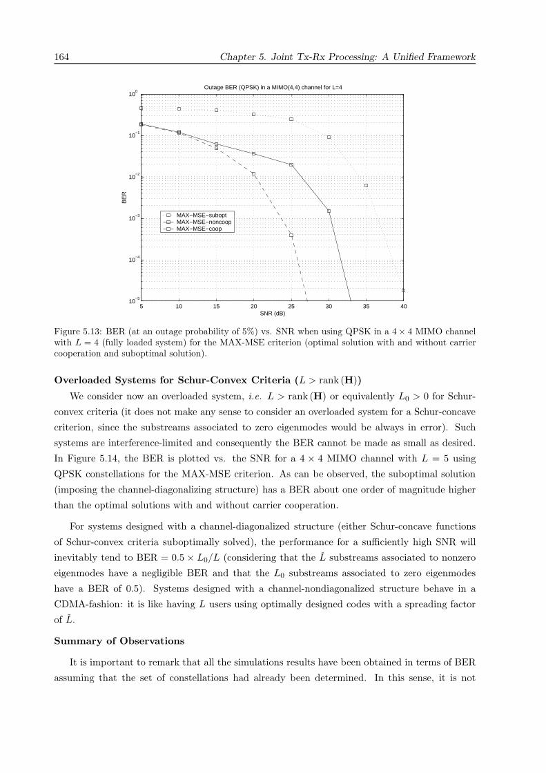
164 Chapter 5. Joint Tx-Rx Processing: A Unified Framework
5 10 15 20 25 30 35 4010
−5
10−4
10−3
10−2
10−1
100
Outage BER (QPSK) in a MIMO(4,4) channel for L=4
SNR (dB)
BE
R
MAX−MSE−suboptMAX−MSE−noncoopMAX−MSE−coop
Figure 5.13: BER (at an outage probability of 5%) vs. SNR when using QPSK in a 4× 4 MIMO channelwith L = 4 (fully loaded system) for the MAX-MSE criterion (optimal solution with and without carriercooperation and suboptimal solution).
Overloaded Systems for Schur-Convex Criteria (L > rank (H))
We consider now an overloaded system, i.e. L > rank (H) or equivalently L0 > 0 for Schur-
convex criteria (it does not make any sense to consider an overloaded system for a Schur-concave
criterion, since the substreams associated to zero eigenmodes would be always in error). Such
systems are interference-limited and consequently the BER cannot be made as small as desired.
In Figure 5.14, the BER is plotted vs. the SNR for a 4 × 4 MIMO channel with L = 5 using
QPSK constellations for the MAX-MSE criterion. As can be observed, the suboptimal solution
(imposing the channel-diagonalizing structure) has a BER about one order of magnitude higher
than the optimal solutions with and without carrier cooperation.
For systems designed with a channel-diagonalized structure (either Schur-concave functions
of Schur-convex criteria suboptimally solved), the performance for a sufficiently high SNR will
inevitably tend to BER = 0.5 × L0/L (considering that the L substreams associated to nonzero
eigenmodes have a negligible BER and that the L0 substreams associated to zero eigenmodes
have a BER of 0.5). Systems designed with a channel-nondiagonalized structure behave in a
CDMA-fashion: it is like having L users using optimally designed codes with a spreading factor
of L.
Summary of Observations
It is important to remark that all the simulations results have been obtained in terms of BER
assuming that the set of constellations had already been determined. In this sense, it is not

5.7. Simulation Results 165
5 10 15 20 25 30 35 40 45 5010
−2
10−1
100
Outage BER (QPSK) in a MIMO(4,4) channel for L=5
SNR (dB)
BE
R
MAX−MSE−suboptMAX−MSE−noncoopMAX−MSE−coop
Figure 5.14: BER (at an outage probability of 5%) vs. SNR when using QPSK in a 4× 4 MIMO channelwith L = 5 (overloaded system) for the MAX-MSE criterion (optimal solution with and without carriercooperation and suboptimal solution).
surprising that the maximization of the mutual information performs very poorly as a means to
improve the BER performance for a given set of practical constellations (such a criterion only
makes sense when optimizing the constellations).
We now summarize the observations made from the numerical simulations:
• Schur-convex criteria are in general superior to Schur-concave criteria in terms of BER
performance (the superiority is evident for highly loaded systems). In fact, the weakness
of Schur-concave functions is the diagonal structure that forces the transmission of each
symbol through each channel eigenmode with the consequent waste of power if some of the
eigenmodes has a low gain. On the other hand, Schur-convex functions transmit all the
symbols in a distributed way and therefore have more flexibility to properly use the channel
eigenmodes.
• Schur-convex criteria optimally solved are significantly better than when suboptimally
solved imposing a diagonal structure (the difference is higher for highly loaded systems).
The reason again is the lack of robustness inherent to the diagonal structure.
• Carrier cooperation always improves the performance. The difference becomes significative
for highly loaded systems.
• It is very common in the literature of equalization to include a ZF constraint in the design.
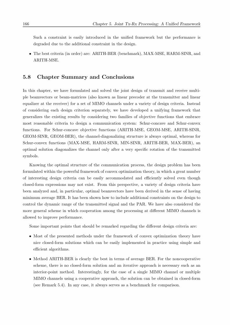
166 Chapter 5. Joint Tx-Rx Processing: A Unified Framework
Such a constraint is easily introduced in the unified framework but the performance is
degraded due to the additional constraint in the design.
• The best criteria (in order) are: ARITH-BER (benchmark), MAX-MSE, HARM-SINR, and
ARITH-MSE.
5.8 Chapter Summary and Conclusions
In this chapter, we have formulated and solved the joint design of transmit and receive multi-
ple beamvectors or beam-matrices (also known as linear precoder at the transmitter and linear
equalizer at the receiver) for a set of MIMO channels under a variety of design criteria. Instead
of considering each design criterion separately, we have developed a unifying framework that
generalizes the existing results by considering two families of objective functions that embrace
most reasonable criteria to design a communication system: Schur-concave and Schur-convex
functions. For Schur-concave objective functions (ARITH-MSE, GEOM-MSE, ARITH-SINR,
GEOM-SINR, GEOM-BER), the channel-diagonalizing structure is always optimal, whereas for
Schur-convex functions (MAX-MSE, HARM-SINR, MIN-SINR, ARITH-BER, MAX-BER), an
optimal solution diagonalizes the channel only after a very specific rotation of the transmitted
symbols.
Knowing the optimal structure of the communication process, the design problem has been
formulated within the powerful framework of convex optimization theory, in which a great number
of interesting design criteria can be easily accommodated and efficiently solved even though
closed-form expressions may not exist. From this perspective, a variety of design criteria have
been analyzed and, in particular, optimal beamvectors have been derived in the sense of having
minimum average BER. It has been shown how to include additional constraints on the design to
control the dynamic range of the transmitted signal and the PAR. We have also considered the
more general scheme in which cooperation among the processing at different MIMO channels is
allowed to improve performance.
Some important points that should be remarked regarding the different design criteria are:
• Most of the presented methods under the framework of convex optimization theory have
nice closed-form solutions which can be easily implemented in practice using simple and
efficient algorithms.
• Method ARITH-BER is clearly the best in terms of average BER. For the noncooperative
scheme, there is no closed-form solution and an iterative approach is necessary such as an
interior-point method. Interestingly, for the case of a single MIMO channel or multiple
MIMO channels using a cooperative approach, the solution can be obtained in closed-form
(see Remark 5.4). In any case, it always serves as a benchmark for comparison.

5.A Proof of Theorem 5.1 167
• The utilization of the Chernoff approximation instead of the exact BER function gives
indistinguishable results.
• Methods ARITH-MSE, HARM-SINR, and MAX-MSE have very simple solutions and per-
form really close to the benchmark given by ARITH-BER. These methods should therefore
be considered for practical purposes.
• Two novel multi-level water-filling solutions (with the corresponding practical implementa-
tion algorithms) have been obtained for the MAX-MSE and the HARM-SINR criteria.
• Cooperation among different MIMO channels improves performance without significant
increase on the complexity (each MIMO channel can be diagonalized independently and
then the largest eigenmodes are selected).
• A striking result is that, for single MIMO channels or multiple MIMO channels with coop-
eration, all criteria with Schur-convex objective functions (e.g., MAX-MSE, HARM-SINR,
MIN-SINR, ARITH-BER, and MAX-BER) have the same optimal solution. Hence, the
best performance in terms of average BER (given by the ARITH-BER criterion with coop-
eration among the MIMO channels) can be achieved in practice with low complexity using
the simple water-filling solution of the ARITH-MSE criterion plus the computation of the
rotation matrix (see Remark 5.4).
All the material presented in this chapter, which is strongly based on majorization theory and
convex optimization theory, is a novel contribution of this dissertation.
Appendix 5.A Proof of Theorem 5.1
We first present a couple of lemmas and then proceed to the proof of Theorem 5.1.
Lemma 5.10 If A and B are n × n positive semidefinite Hermitian matrices, then
Tr (AB) ≥n∑
i=1
λA,i λB,n−i+1
where λA,i and λB,i are the eigenvalues of A and B, respectively, in decreasing order.
Proof. The proof can be found in [Mar79, 9.H.1.h]. However, due to its simplicity using basic
results of majorization theory, we rewrite it here. Given the EVD of A and B, A = UADAUHA
and B = UBDBUHB , we have
Tr (AB) = Tr(DBUH
B AUB
)=
n∑i=1
λB,i
[UH
BAUB
]ii
.
168 Chapter 5. Joint Tx-Rx Processing: A Unified Framework
Since the function∑
i wi xi (with xi in decreasing order) is minimized when wi are in increasing
order and it is then a Schur-concave function (see Lemma 5.2), the minimum is achieved by an ex-
treme point (i.e., a vector that majorizes any other). Recalling that the vector of eigenvalues ma-
jorizes the vector of diagonal elements (Lemma 3.6), it follows that Tr (AB) ≥∑ni=1 λB,n−i+1 λA,i
where λA,i and λB,i are in decreasing order.
Lemma 5.11 Given a matrix B ∈ CI nT ×L and a positive semidefinite Hermitian matrix RH ∈CI nT×nT such that BHRHB is a diagonal matrix with diagonal elements in increasing order (pos-
sibly with some zero diagonal elements), it is always possible to find another matrix of the form
B = UH,1ΣB,1 of at most rank L min (L, rank (RH)) that satisfies BHRHB= BHRHB with
Tr(BBH
)≤Tr(BBH
), where UH,1 ∈ CI nT×L has as columns the eigenvectors of RH correspond-
ing to the L largest eigenvalues in increasing order and ΣB,1 =[0L×(L−L) diag (σB,i)L×L
] ∈CI L×L has zero elements except along the rightmost main diagonal (which can be assumed real
w.l.o.g.).
Proof. Although the basic idea follows easily from the application of Lemma 5.10, the formal
proof for arbitrary values of nT , L, and rank (RH) becomes notationally involved.
Since BHRHB ∈ CI L×L (recall that RH ∈ CI nT×nT ) is diagonal with diagonal elements in
increasing order, we can write
BHRHB = D =
0 0
0 D
where D is a square diagonal matrix (with real diagonal elements) of dimension L min (L, rank (RH)). Using the SVD [Hor85], we can then write R1/2
H B = QΣ where Q ∈ CI nT ×nT
is a unitary matrix whose columns are the left singular vectors, the right singular vectors (eigen-
vectors of D) are the canonical vectors, and matrix Σ ∈ CI nT ×L is composed of zero elements and
contains D1/2 in its top-right block so that ΣHΣ = D. In particular, if nT ≥ L, then D = D
and Σ =
D1/2
0
, and if nT < L, then Σ =
[0 D1/2
](note that the position of matrix D1/2
within Σ is different to the classical definition of the SVD [Hor85] because the diagonal elements
of BHRHB are assumed in increasing order).
Assuming that matrix RH is nonsingular with EVD given by RH = UHDHUHH , we can write
B = R−1/2H QΣ = UHD−1/2
H UHHQΣ. (5.79)
In case that RH is singular, clearly B must be orthogonal to the null space of RH , otherwise this
component could be made zero without changing the value of BHRHB and decreasing Tr(BBH
).
Knowing that B must be orthogonal to the null space of RH , expression (5.79) is still valid using
the pseudo-inverse of RH instead of the inverse.
5.A Proof of Theorem 5.1 169
The idea now is to find another matrix B by changing the unitary matrix Q in (5.79) with
the lowest possible value of Tr(BBH
)(note that any matrix B obtained from (5.79) satisfies by
definition the desired constraint BHRHB = D). Using Lemma 5.10, Tr(BBH
)can be lower-
bounded as follows:
Tr(BBH
)= Tr
(ΣΣHUHD−1
H U)
≥L∑
i=1
di λ−1H,i
where U UHHQ, di is the ith diagonal element of D in increasing order and λH,iL
i=1 are the L
largest eigenvalues of RH in increasing order. If the di’s are different, the lower bound is achieved
by matrix U being a permutation matrix. For subsets of equal di’s, the corresponding subblock
in U can be any rotation matrix. Therefore, if U is chosen as a permutation matrix P that selects
the L largest eigenvalues of RH in the same ordering as the di’s, the lower bound is achieved.
From (5.79), we obtain that the optimal B (in the sense of minimizing the value of Tr(BBH
))
has at most rank L and is of the form B = UHD−1/2H PΣ = UH,1ΣB,1 where UH,1 ∈ CI nT×L has
as columns the eigenvectors of RH corresponding to the L largest eigenvalues in increasing order
and ΣB,1 =[0L×(L−L) diag (σB,i)L×L
] ∈ CI L×L has zero elements except along the rightmost
main diagonal (which can be assumed real w.l.o.g.).
Proof of Theorem 5.1. The constrained optimization problem to be solved is
minB
f0 (d(E (B) ))
s.t. Tr(BBH
) ≤ PT
where d(E) is the vector of diagonal elements of the MSE matrix E (B) =(I + BHRHB
)−1.
It is mathematically convenient to assume the diagonal elements of E (B) in decreasing order,
i.e., di(E) ≥ di+1(E), without loss of generality. In fact, most reasonable objective functions (in
particular, all the objective functions considered in §5.5) have a fixed preferred ordering of the ar-
guments, i.e., the value of the function is minimized with a very specific ordering of the arguments.
In such cases, it suffices to relabel the arguments so that the preferred ordering is decreasing. In
a more general case, however, a function may not have a fixed preferred ordering since it may de-
pend on the specific value of the arguments. In such a case, since we are interested in minimizing
the objective function, we can define and use instead the function f0 (x) = minP∈Π
f0 (Px), where P
is a permutation matrix and Π is the set of the L! different permutation matrices. The original
minimization of f0 without the ordering constraint is equivalent to the minimization of f0 with
the ordering constraint. Therefore, we can always assume that the function to be minimized has
been properly defined so that the ordering constraint can be included without loss of generality
(c.f. §5.5).

170 Chapter 5. Joint Tx-Rx Processing: A Unified Framework
If f0 is Schur-concave, using the definition of Schur-concavity (Definition 3.4) and the relation
d ≺ λ (Lemma 3.6), it follows that f0 (λ(E)) ≤ f0 (d(E)) where λ(E) is the vector of eigen-
values of E =(I + BHRHB
)−1in decreasing order. The lower bound f0 (λ(E)) is achieved if
matrix(I + BHRHB
)−1 is diagonal with diagonal elements in decreasing order or, equivalently,
if BHRHB is diagonal with diagonal elements in increasing order. Furthermore, for any given
B, one can always find a rotation matrix Q so that QH(BHRHB
)Q becomes diagonal and
use instead the transmit matrix B = BQ (the sum of diagonal elements of E remains the same
regardless of Q) improving the performance (by this rotation the utilized power remains the same
Tr(BBH
)= Tr
(BBH
)). This implies that for Schur-concave functions, there is an optimal B
with a structure such that BHRHB is diagonal with diagonal elements in increasing order.
If f0 is Schur-convex, the opposite happens. From the definition of Schur-convexity (Definition
3.4) and the relation 1 ≺ d (Lemma 3.1), it follows that f0 (d(E)) is minimized when E has
equal diagonal elements. Furthermore, for any given B, one can always find (see Corollary 3.2) a
rotation matrix Q so that QH(I + BHRHB
)−1Q has identical diagonal elements and use instead
the transmit matrix B = BQ (the sum of diagonal elements of E remains the same regardless of
Q) improving the performance (the transmit power remains the same). Therefore, for an optimal
B we have that[(
I + BHRHB)−1]ii
= 1L Tr
(I + BHRHB
)−1. Interestingly, regardless of the
specific function f0, the optimal B can be found by first minimizing Tr(I + BHRHB
)−1(without
imposing the constraint that the diagonal elements be equal) and then including the rotation to
make the diagonal elements identical. The rotation can be found using Algorithm 3.2 (reproduced
from [Vis99b, Section IV-A]) or with any rotation matrix that satisfies |[Q]ik| = |[Q]il| ∀i, k, l such
as the Discrete Fourier Transform (DFT) matrix or the Hadamard matrix when the dimensions
are appropriate such as a power of two (see §3.2 for more details). Regarding the minimization
of Tr(I + BHRHB
)−1, since it is a Schur-concave function of the diagonal elements (f0 (d) =∑Li=1 di), the previous result can be applied to show that there is an optimal B (excluding for the
moment the rotation) such that BHRHB is diagonal with diagonal elements in increasing order.
Given that BHRHB is diagonal, it follows from Lemma 5.11 that B has at most rank L min (L, rank (RH)) and can be written as B = UH,1ΣB,1 where UH,1 ∈ CI nT ×L has as columns
the eigenvectors of RH corresponding to the L largest eigenvalues in increasing order and ΣB,1 =[0 diag (σB,i)
] ∈ CI L×L has zero elements except along the rightmost main diagonal.
Hence, we can write an optimal B as
B =
UH,1ΣB,1
UH,1ΣB,1VHB
for f0 Schur-concave
for f0 Schur-convex
where UH,1 and ΣB,1 are defined as before and VB ∈ CI L×L is the rotation to make the diagonal
elements of(I + BHRHB
)−1 identical.

5.D Proof of Schur-Convexity/Concavity Lemmas 171
Appendix 5.B Proof of Lemma 5.1
The proof is straightforward from Lemma 5.11. Since the diagonal elements of(I + BHRHB
)−1
can be assumed in decreasing ordering w.l.o.g. (c.f. proof of Theorem 5.1 in Appendix 5.A) and
BHRHB is diagonal, it follows from Lemma 5.11 that an optimal solution can be expressed as
B = UH,1ΣB,1 where UH,1 ∈ CI nT×L has as columns the eigenvectors of RH corresponding to the
L min (L, rank (RH)) largest eigenvalues in increasing order and ΣB,1 = [0 diag (σB,i)] ∈CI L×L has zero elements except along the rightmost main diagonal (assumed real w.l.o.g.).
Appendix 5.C Proof of Corollary 5.2
The proof in one direction is very similar to that of Theorem 5.1. First, note that the vector of
eigenvalues λ(E (B) ) (obtained when the channel is fully diagonalized with VB = I) majorizes
any vector of diagonal elements d(E (B) ) (obtained when an arbitrary rotation VB is used)
which in turn majorizes the vector of equal elements 1(E (B) ) (obtained when a very specific
rotation VB is used as described in Theorem 5.1 for Schur-convex functions). Since the function
is Schur-concave, it must be that f0 (λ) ≤ f0 (d) ≤ f0 (1). At the same time, since the function
is Schur-convex, it must be that f0 (λ) ≥ f0 (d) ≥ f0 (1). Therefore, it follows that f0 (λ) =
f0 (d) = f0 (1). The opposite direction is trivial since if the function is invariant with respect
post-rotations of B, it then follows that in particular f0 (d1) = f0 (d2) for d1 d2.
Appendix 5.D Proof of Schur-Convexity/Concavity Lemmas
Proof of Lemma 5.2 (f0 (x) =∑
i (wi xi))
Since the xi’s are in decreasing order xi ≥ xi+1, the function f0 (x) =∑
i (wi xi) is minimized
with the weights in increasing order wi ≤ wi+1. To show this assume for a moment that for
i < j (xi ≥ xj) the weights are such that wi > wj . It follows that the term (wi xi + wj xj) can be
minimized by simply swapping the weights:
wi (xi − xj) ≥ wj (xi − xj)
⇐⇒ wi xi + wj xj ≥ wi xj + wj xi.
To prove that the function f0 is Schur-concave (see Definition 3.4), define φ(x) −f0 (x) =∑i gi (xi) where gi (x) = −wi x. Function φ is Schur-convex because g′i (a) ≥ g′i+1 (b) whenever
a ≥ b (see Lemma 3.3) and, therefore, f0 is Schur-concave (see Definition 3.4).

172 Chapter 5. Joint Tx-Rx Processing: A Unified Framework
Proof of Lemma 5.3 (f0 (x) =∏
i xwii )
Since the xi’s are strictly positive and in decreasing order xi ≥ xi+1 > 0, the function
f0 (x) =∏
i xwii is minimized with the weights in increasing order wi ≤ wi+1. To show this
assume for a moment that for i < j (xi ≥ xj) the weights are so that wi > wj. It follows that the
term (xwii x
wj
j ) can be minimized by simply swapping the weights:
wi log(
xi
xj
)≥ wj log
(xi
xj
)
⇐⇒(
xi
xj
)wi
≥(
xi
xj
)wj
⇐⇒ xwii x
wj
j ≥ xwj
i xwij .
To prove that the function f0 is Schur-concave (see Definition 3.4), define φ(x) − log f0 (x) =∑i gi (xi) where gi (x) = −wi log x. Function φ is Schur-convex because g′i (a) ≥ g′i+1 (b) whenever
a ≥ b (see Lemma 3.3). Since f0 (x) = e−φ(x) and function e−x is decreasing in x, f0 is Schur-
concave by Lemma 3.2.
Proof of Lemma 5.4 (f0 (x) = maxi xi)From Definition 3.1, it follows that f0 (x) = maxi xi = x[1]. If x ≺ y it must be that
x[1] ≤ y[1] (from Definition 3.2) and, therefore, f0 (x) ≤ f0 (y). This means that f0 is Schur-
convex by Definition 3.4.
Proof of Lemma 5.5 (f0 (x) = −∑i
(wi
(x−1
i − 1))
)
Since the xi’s are strictly positive and in decreasing order xi ≥ xi+1 > 0, the function
f0 (x) = −∑i
(wi
(x−1
i − 1))
is minimized with the weights in increasing order wi ≤ wi+1 (this
can be similarly proved as was done in the proof of Lemma 5.2).
To prove that the function f0 is Schur-concave (see Definition 3.4), define φ(x) −f0 (x) =∑i gi (xi) where gi (x) = wi
(x−1 − 1
). Function φ is Schur-convex because g′i (a) ≥ g′i+1 (b)
whenever a ≥ b (see Lemma 3.3) and, therefore, f0 is Schur-concave by Definition 3.4.
Proof of Lemma 5.6 (f0 (x) = −∏i
(x−1
i − 1)wi)
Since the xi’s are strictly positive and in decreasing order xi ≥ xi+1 > 0, it follows that
f0 (x) = −∏i
(x−1
i − 1)wi is minimized with the weights in increasing order wi ≤ wi+1 (this can
be similarly proved as was done in the proof of Lemma 5.3).
To prove that the function f0 is Schur-concave for xi ≤ 0.5 (see Definition 3.4), define φ(x) log (−f0 (x)) =
∑i gi (xi) where gi (x) = wi log
(x−1 − 1
). Function φ is Schur-convex because
g′i (a) ≥ g′i+1 (b) whenever 0.5 ≥ a ≥ b 16 (see Lemma 3.3). Since f0 (x) = −eφ(x) and function
−ex is decreasing in x, f0 is Schur-concave by Lemma 3.2.
16Function (1 − x)x is increasing in x for 0 ≤ x ≤ 0.5.

5.E Gradients and Hessians for the ARITH-BER 173
Proof of Lemma 5.7 (f0 (x) =∑
ixi
1−xi)
To prove that the function f0 (x) =∑
ixi
1−xiis Schur-convex, rewrite it as f0 (x) =
∑i g (xi)
where g (x) = x1−x . Since function g is convex, it follows that f0 is Schur-convex by Corollary 3.3.
Proof of Lemma 5.8 (f0 (x) =∑
i BER(x−1
i − 1))
To prove that the function f0 (x) =∑
i BER(x−1
i − 1)
is Schur-convex for θ ≥ xi > 0 (for
sufficiently small θ such that BER(x−1
i − 1) ≤ 10−2 ∀i), write f0 (x) =
∑i g (xi) where g (x) =
BER(x−1 − 1
). Since function g is convex within the range (0, θ] (see §2.5.4.4), it follows that
f0 is Schur-convex by Corollary 3.1.
Proof of Lemma 5.9 (f0 (x) =∏
i BER(x−1
i − 1))
To prove that the function f0 (x) =∏
i BER(x−1
i − 1)
is Schur-concave for θ ≥ xi > 0 with
θ such that(
∂ BER(x−1−1)∂x
)2
≥ BER(x−1 − 1
) ∂2 BER(x−1−1)∂x2 for θ ≥ x > 0, define φ(x)
− log f0 (x) =∑
i g (xi) where g (x) = − log BER(x−1 − 1
). Function g is convex for θ ≥ x > 0
because ∂2g(x)∂x2 = 1
(BER(x−1−1))2
((∂ BER(x−1−1)
∂x
)2
− BER(x−1 − 1
) ∂2 BER(x−1−1)∂x2
)≥ 0 and φ is
Schur-convex by Corollary 3.1. Since f0 (x) = e−φ(x) and function e−x is decreasing in x, f0 is
Schur-concave by Lemma 3.2.
Appendix 5.E Gradients and Hessians for the ARITH-BER
Suboptimal Problem Formulation of (5.58)
• Gradient and the Hessian of the exact BER function f (x) =∑N
k=1 αkQ(√
βkxk
)where
βk = βkλk (see Appendix 5.A):
∇f (x) = −√
18π
α1 β1/21 e−β1x1/2x
−1/21
...
αN β1/2N e−βNxN /2x
−1/2N
Hf (x) =12
√18π
diag(
αk β1/2k e−βkxk/2x
−1/2k
(x−1
k + βk
)N
k=1
),
and of the Chernoff approximation f (x) =∑N
k=112αke−βkxk/2 (see Appendix 5.A):
∇f (x) = −14
α1 β1e−β1x1/2
...
αN βN e−βN xN/2
Hf (x) =18
diag(
αk β2ke−βkxk/2
).

174 Chapter 5. Joint Tx-Rx Processing: A Unified Framework
Optimal Problem Formulation of (5.59)
• Gradient and the Hessian of the exact BER function f (x) =∑N
k=1 αkQ(√
βk
(x−1
k − 1))
(see Appendix 5.A):
∇f (x) =
√18π
α1β1/21 e−β1(x−1
1 −1)/2(x3
1 − x41
)−1/2
...
αN β1/2N e−βN(x−1
N −1)/2(x3
N − x4N
)−1/2
Hf (x) =12
√18π
diag
(αkβ
1/2k e−βk(x−1
k −1)/2(x3
k − x4k
)−1/2(
βk
x2k
− 3 − 4xk
xk − x2k
)N
k=1
),
and of the Chernoff approximation f (x) =∑N
k=112αke−βk(x−1
k −1)/2 (see Appendix 5.A):
∇f (x) =14
α1β1e−β1(x−11 −1)/2x−2
1
...
αN βN e−βN(x−1N −1)/2x−2
N
Hf (x) =14
diag(
αkβke−βk(x−1k −1)/2x−4
k (βk/2 − 2xk)N
k=1
).
• Gradient and the Hessian of the log-barrier function f (x) = −1T log (b− Ax) correspond-
ing to the linear constraints Ax ≤ b [Boy00]:
∇f (x) = AT diag (1/ (b− Ax))1
Hf (x) = AT diag(1/ (Ax − b)2
)A.
• Gradient and the Hessian of the log-barrier function f (x) =
− log(t − 1
L
(L0 +
∑Li=1
11+λixi
))(we define x [t, x1,··· ,xL]T ) corresponding to the
constraints on the tk’s tk ≥ 1Lk
((Lk − Lk
)+∑Lk
i=11
1+λk,ixk,i
):
∇f (x) = − 1D
1
1L
λ1
(1+λ1x1)2
...
1L
λL(1+λL xL)2
Hf (x) =
1
1L
λ1
(1+λ1x1)2
...
1L
λL(1+λLxL)2
1D2
[1 1
Lλ1
(1+λ1x1)2 · · · 1
LλL
(1+λLxL)2
]
+2D
diag
(0,
1L
λ2i
(1 + λixi)3
L
i=1
)

5.F Proof of Water-Filling Results 175
where D t − 1L
(L0 +
∑Li=1
11+λixi
).
Appendix 5.F Proof of Water-Filling Results
Proof of Proposition 5.1 (Modified weighted water-filling.)
Since the problem is convex, an optimal solution can be obtained based on convex optimization
theory (the reader is referred to §3.1 and [Lue69, Roc70, Boy00] for details and definitions).
We first obtain the closed-form optimal solution to the problem and then proceed to prove the
optimality of Algorithm 5.1.
Optimal Solution. The Lagrangian corresponding to the constrained convex problem is
L =L∑
i=1
wi1
1 + λizi+ µ
L∑
i=1
zi − PT
−
L∑i=1
γizi (5.80)
where µ and γi are the dual variables or Lagrange multipliers. The water-filling solution is
easily found from the sufficient and necessary KKT optimality conditions (the problem satisfies
the Slater’s condition and therefore strong duality holds):
L∑i=1
zi ≤ PT ,
µ ≥ 0,
µ = wiλi
(1+λizi)2 + γi,
µ
(L∑
i=1zi − PT
)= 0,
zi ≥ 0,
γi ≥ 0,
γizi = 0.
(5.81)
It is assumed that there is at least one λi > 0; otherwise the problem has trivial solution given
by zi = 0 ∀i. If µ = 0, then γi = −wiλi
(1+λizi)2 , which cannot be (since γi ≥ 0). Therefore,
at an optimal solution µ > 0 and consequently (by the complementary slackness condition)
the power constraint must be satisfied with equality. Note that if λi = 0 for some i, then
γi = µ > 0 ⇒ zi = 0, i.e., no power is allocated to eigenmodes with zero gain (as expected).
From now on, we consider that all zero-valued λi’s have been removed.
If zi > 0, then γi = 0 (by the complementary slackness condition), µ = wiλi
(1+λizi)2 (note that
µ < wiλi), and zi = µ−1/2 w1/2i λ
−1/2i − λ−1
i (note that if λi = 0, then γi = µ > 0 and zi = 0 as
expected). If zi = 0, then µ = wiλi + γi (note that µ ≥ wiλi). Equivalently,
zi =
µ−1/2 w
1/2i λ
−1/2i − λ−1
i > 0
0
if µ < wiλi
if µ ≥ wiλi
176 Chapter 5. Joint Tx-Rx Processing: A Unified Framework
or, more compactly,
zi =(µ−1/2 w
1/2i λ
−1/2i − λ−1
i
)+(5.82)
where µ−1/2 is the water-level chosen so that∑L
i=1 zi = PT . Note that this solution satisfies all
KKT conditions and is therefore optimal.
Optimal Algorithm. Algorithm 5.1 is based on hypothesis testing. It first makes the assump-
tion that all L eigenmodes are active (zi > 0 for 1 ≤ i ≤ L) and then checks whether the
maximum power is exceeded, in which case the hypothesis is rejected, a new hypothesis with one
less active eigenmode is made, and so forth.
In more detail, Algorithm 5.1 first reorders the positive eigenmodes so that the terms (wiλi)
are in decreasing order. With this ordering, since λi zi =(µ−1/2 (wi λi)
1/2 − 1)+
, a hypothesis
is completely described by the set of active eigenmodes L (such that zi > 0 for 1 ≤ i ≤ L and
zero otherwise). This allows a reduction of the total number of hypotheses from 2L to L. The
initial hypothesis chooses the highest number of active eigenmodes L = L.
For each hypothesis, the water-level µ1/2 must be such that the considered L eigenmodes are
indeed active while the rest remain inactive: µ−1/2 w
1/2i λ
−1/2i − λ−1
i > 0
µ−1/2 w1/2i λ
−1/2i − λ−1
i ≤ 0
1 ≤ i ≤ L
L < i ≤ L
or, more compactly, (wLλL
)−1/2< µ−1/2 ≤ (wL+1λL+1
)−1/2
where we define wL+1λL+1 0 for simplicity of notation. Assuming that wLλL = wL+1λL+1
(otherwise, the hypothesis is clearly rejected since the set of possible water-levels is empty), the
algorithm checks whether the power constraint cannot be satisfied with the minimum water-level
in the limiting case, i.e., µ = wLλL. Note that for this limiting value, the eigenmode L becomes
inactive which corresponds to a different hypothesis. Therefore, the current hypothesis is rejected
when∑L
i=1 zi ≥ PT for µ = wLλL or, equivalently, when µ−1/2 ≥ PT +∑L
i=1 λ−1i∑L
i=1 w1/2i λ
−1/2i
. In such a case,
the zi’s must be decreased or, equivalently, the water-level µ−1/2 must be decreased and the
eigenmode L becomes inactive which corresponds to the new hypothesis. Otherwise, the current
hypothesis (the current set of active eigenmodes 1 ≤ i ≤ L) is accepted since removing more
active eigenmodes (decreasing the water-level) would further increase the objective function and
the addition of more active eigenmodes has already been tested and rejected (for exceeding the
maximum power). This reasoning can be applied as many times as needed for each remaining set
of active eigenmodes. Once the optimal set of active eigenmodes is known, the value of the active
zi’s is then increased to satisfy the power constraint with equality. The definitive water-level is
then
µ−1/2 =PT +
∑Li=1 λ−1
i∑Li=1 w
1/2i λ
−1/2i
. (5.83)

5.F Proof of Water-Filling Results 177
By the nature of the algorithm, the maximum number of iterations (worst-case complexity) is L.
Proof of Proposition 5.2 (Classical weighted water-filling.)
This proof very similar to that of Proposition 5.1 and, therefore, we simply give a sketch of the
proof.
Optimal Solution. The Lagrangian corresponding to the constrained convex problem is
L =L∑
i=1
−wi log (1 + λizi) + µ
L∑
i=1
zi − PT
−
L∑i=1
γizi (5.84)
where µ and γi are the dual variables or Lagrange multipliers. The water-filling solution is
easily found from the sufficient and necessary KKT optimality conditions (the problem satisfies
the Slater’s condition and therefore strong duality holds):
L∑i=1
zi ≤ PT ,
µ ≥ 0,
µ = wiλi
1+λizi+ γi,
µ
(L∑
i=1zi − PT
)= 0,
zi ≥ 0,
γi ≥ 0,
γizi = 0.
(5.85)
It is assumed that there is at least one λi > 0; otherwise the problem has trivial solution given by
zi = 0 ∀i. As in the proof of Proposition 5.1, it follows that µ > 0 and, consequently, the power
constraint must be satisfied with equality. It is simple to obtain the water-filling solution
zi =(µ−1wi − λ−1
i
)+ (5.86)
where µ−1 is the water-level chosen so that∑L
i=1 zi = PT .
Optimal Algorithm. The optimality of Algorithm 5.1 is proved as in the proof of Proposition
5.1. In this case, however, the comparison∑L
i=1 zi ≥ PT is given by µ−1 ≥ PT +∑L
i=1 λ−1i∑L
i=1 wi
.
Proof of Proposition 5.3 (Multi-level water-filling for the MAX-
MSE criterion.)
Since the problem is convex, the optimal solution can be found using convex optimization theory
(the reader is referred to §3.1 and [Lue69, Roc70, Boy00] for details and definitions). We first

178 Chapter 5. Joint Tx-Rx Processing: A Unified Framework
obtain the closed-form optimal solution to the problem and then proceed to prove the optimality
of Algorithm 5.3.
Optimal Solution. The Lagrangian corresponding to the constrained convex problem is
L = t +N∑
k=1
µk
1
Lk
(Lk − Lk
)+
Lk∑i=1
11 + λk,izk,i
− t
+ µ0
N∑
k=1
Lk∑i=1
zk,i − PT
−
N∑k=1
Lk∑i=1
γk,izk,i (5.87)
where µ0, µk, and γk,i are the dual variables or Lagrange multipliers. The multi-level water-
filling solution is found from the sufficient and necessary KKT optimality conditions (the problem
satisfies the Slater’s condition and therefore strong duality holds):
t ≥ 1Lk
((Lk − Lk
)+∑i
11+λk,izk,i
),
µk ≥ 0,
µ0 = µk/Lkλk,i
(1+λk,izk,i)2 + γk,i,
µk
(1
Lk
((Lk − Lk
)+∑i
11+λk,izk,i
)− t
)= 0,
∑k,i
zk,i ≤ PT ,
µ0 ≥ 0,
µ0
(∑k,i
zk,i − PT
)= 0,
zk,i ≥ 0,
γk,i ≥ 0,∑k
µk = 1,
γk,izk,i = 0.
(5.88)
It is assumed that for each k there is at least one eigenmode with nonzero gain λk,i > 0 (otherwise
the problem has trivial solution given by t = 1 and zk,i = 0 ∀k, i).
First of all, we show that µ0 and µk must be positive values and consequently (by the com-
plementary slackness conditions) the constraints on t and the power constraint must be satisfied
with equality (this can also be concluded from a direct inspection of the problem formulation). If
µ0 = 0, then γk,i = −µk/Lkλk,i
(1+λk,izk,i)2 . This clearly implies γk,i = 0 ∀k, i and since for each k it
is assumed that λk,i > 0 for some i, it also implies µk = 0 ∀k, which cannot possibly be because
of the constraint∑
k µk = 1 and consequently µ0 > 0. Note that in case λk,i = 0 for some k and
i, then γk,i = µ0 > 0 ⇒ zk,i = 0, i.e., no power is allocated to eigenmodes with zero gain (as ex-
pected). From now on, we consider that all zero-valued λk,i’s have been removed. Now, if µk = 0
for some k, then γk,i = µ0 > 0 ∀i ⇒ zk,i = 0 ∀i, and t ≥ 1Lk
((Lk − Lk
)+∑i
11+λk,izk,i
)= 1.
Consider now that µl > 0 for some l = k, this implies that t = 1Ll
((Ll − Ll
)+∑i
11+λl,izl,i
)(by the complementary slackness condition) which can be if only if t = 1 and zl,i = 0 ∀i. As a
consequence, if µk = 0 for some k, it would then follow that zk,i = 0 ∀k, i which does not agree
with constraint∑k,i
zk,i = PT . Therefore, it must be that µk > 0 ∀k.
If zk,i > 0, then γk,i = 0 (by the complementary slackness condition), µ0 = µk/Lkλk,i
(1+λk,izk,i)2
(note that µ0 < µk/Lkλk,i), and zk,i = (µk/(Lkµ0))1/2 λ−1/2k,i − λ−1
k,i . If zk,i = 0, then µ0 =
5.F Proof of Water-Filling Results 179
µk/Lkλk,i + γk,i (note that µ0 ≥ µk/Lkλk,i). Equivalently,
zk,i =
(µk/(Lkµ0))1/2 λ
−1/2k,i − λ−1
k,i
0
if µ0 < µk/Lkλk,i
if µ0 ≥ µk/Lkλk,i
or, more compactly,
zk,i =((µk/(Lkµ0))1/2 λ
−1/2k,i − λ−1
k,i
)+
where µ0 and µk are positive values so that the constraints on t and the power constraint are
satisfied with equality and∑
k µk = 1.
Defining µk µk/(Lkµ0) (note that given µk one can always find µ0 and µk as µk =
Lkµ0 µk and µ0 = 1/∑
k (Lk µk)), the optimal solution can be finally expressed as
zk,i =(µ
1/2k λ
−1/2k,i − λ−1
k,i
)+(5.89)
where µ1/2k are positive water-levels chosen to satisfy
t = 1Lk
((Lk − Lk
)+∑Lk
i=11
1+λk,izk,i
)1 ≤ k ≤ N,∑
k,i zk,i = PT .(5.90)
Note that this solution satisfies all KKT conditions and is therefore optimal.
Optimal Algorithm. Algorithm 5.3 is based on hypothesis testing. It first makes the hypothesis
that all LT =∑
k Lk eigenmodes are active (zk,i > 0 ∀k, i), imposes the equality constraints on
t, and then checks whether the maximum power is exceeded, in which case the hypothesis is
rejected, a new hypothesis is made with one less active eigenmode, and so forth.
To formally derive Algorithm 5.3, we first simplify the problem by properly defining the
hypotheses. If the eigenmodes are ordered in decreasing order for each k (i.e., λk,i ≥ λk,i+1)
and since λk,i zk,i =(µ
1/2k λ
1/2k,i − 1
)+, a hypothesis is completely described by the set of active
eigenmodes Lk (such that zk,i > 0 for 1 ≤ k ≤ N, 1 ≤ i ≤ Lk and zero otherwise). This
ordering of the eigenmodes, which we assume in the derivation of the algorithm, allows a reduc-
tion of the total number of hypotheses from∏
k 2Lk = 2∑
k Lk to∏
k Lk. Using the fact that∑Lki=1
11+λk,izk,i
=(Lk − Lk
)+ µ
−1/2k
∑Lki=1 λ
−1/2k,i , the constraints on t can be rewritten as
t =1Lk
(Lk − Lk
)+ µ
−1/2k
Lk∑i=1
λ−1/2k,i
1 ≤ k ≤ N (5.91)
and the constraints of the original problem (5.90) can be rewritten by parameterizing the water-
levels µ1/2k with respect to t as
µ1/2k =
∑Lki=1 λ
−1/2k,i
tLk−(Lk−Lk)1 ≤ k ≤ N,∑
k,i zk,i = PT .
(5.92)
180 Chapter 5. Joint Tx-Rx Processing: A Unified Framework
Note that the first constraint of (5.92) is nontrivial since each water-level µ1/2k is obtained as a
function of the parameter t and also of Lk, but at the same time Lk depends on the water-level
µ1/2k .
Consider a hypothesis given by Lk. The water-levels for such a hypothesis must be such
that the considered Lk eigenmodes are indeed active while the rest remain inactive: µ
1/2k λ
−1/2k,i − λ−1
k,i > 0
µ1/2k λ
−1/2k,i − λ−1
k,i ≤ 0
1 ≤ k ≤ N, 1 ≤ i ≤ Lk
1 ≤ k ≤ N, Lk < i ≤ Lk
⇐⇒ λ1/2
k,Lk+1≤ µ
−1/2k < λ
1/2
k,Lk1 ≤ k ≤ N (5.93)
where we define λk,Lk+1 0 ∀k for simplicity of notation. These constraints on the water-levels
implicitly constrain the parameter t. Combining (5.93) and (5.91), the range of possible values
for t is given by
tlbk(Lk
) ≤ t < tubk
(Lk
)1 ≤ k ≤ N (5.94)
or, equivalently,
t ∈N⋂
k=1
[tlbk(Lk
), tub
k
(Lk
))(5.95)
where tlbk(Lk
)= 1
Lk
((Lk − Lk
)+ λ
1/2
k,Lk+1
∑Lki=1 λ
−1/2k,i
)and tub
k
(Lk
)=
1Lk
((Lk − Lk
)+ λ
1/2
k,Lk
∑Lki=1 λ
−1/2k,i
). More compactly, we can write
t ∈[tmax - lb
(Lk
), tmin - ub
(Lk
))(5.96)
where tmax - lb(
Lk
)= max
1≤k≤N
tlbk(Lk
)and tmin - ub
(Lk
)= min
1≤k≤N
tubk
(Lk
). Denote the
maximizing k by kmax and the minimizing k by kmin. It is also important to notice that tubk
(Lk +
1)
= tlbk(Lk
)which implies that the different hypotheses partition the whole range of possible
values of t for a given k:
⋃Lk
Lk=1
[tlbk(Lk
), tub
k
(Lk
))=[tlbk(Lk
), tub
k (1))
=[(
1 − Lk/Lk
), 1)
[tlbk(L
(1)k
), tub
k
(L
(1)k
))⋂[tlbk(L
(2)k
), tub
k
(L
(2)k
))= ∅ L
(1)k = L
(2)k .
In other words, the partitioning of the interval[(
1 − Lk/Lk
), 1)
is given by (see Figure 5.15)
. . .[tlbk(Lk + 1
), tub
k
(Lk + 1
)),[tlbk(Lk
), tub
k
(Lk
)),[tlbk(Lk − 1
), tub
k
(Lk − 1
)), . . . (5.97)
We are now ready to derive an efficient optimal algorithm which starts with the smallest
possible value of t (highest values of the Lk’s) and then increases it until the power constraint is
satisfied. In more detail, Algorithm 5.3 first reorders the positive eigenmodes in decreasing order
for each k by setting Lk = Lk for 1 ≤ k ≤ N to obtain the initial hypothesis.

5.F Proof of Water-Filling Results 181
)[0
)[ )[ )[...
ub (1)ktlb (1)kt
ub (2)ktlb (2)kt
t
11 /k kL L−
lb ( )k kt L ub ( )k kt L
Figure 5.15: Illustrative scheme of the partition of the domain of t for a given index k.
At this point, if tmax - lb(
Lk
) ≥ tmin - ub(
Lk
), then the considered hypothesis can-
not satisfy the optimality conditions by (5.96) and must be rejected. Otherwise, if
tmax - lb(
Lk
)< tmin - ub
(Lk
), then we still have to check whether there is some value of
t ∈[tmax - lb
(Lk
), tmin - ub
(Lk
))such that the power constraint is satisfied, which can be
done simply by checking if with tmin - ub(
Lk
)the power constraint is strictly satisfied (since
higher values of t require less power). From µ1/2k =
∑Lki=1 λ
−1/2k,i
tLk−(Lk−Lk)and zk,i =
(µ
1/2k λ
−1/2k,i − λ−1
k,i
)+,
the strict power constraint condition∑N
k=1
∑Lki=1 zk,i < PT can be written as
N∑k=1
(∑Lki=1 λ
−1/2k,i
)2
tLk −(Lk − Lk
) < PT +N∑
k=1
Lk∑i=1
λ−1k,i . (5.98)
If the power constraint is not satisfied for t = tmin - ub(
Lk
), the hypothesis cannot satisfy the
optimality conditions and must be rejected. Otherwise, the hypothesis is accepted (as is later
shown, such a hypothesis is in fact the optimal) and the water-levels are recomputed to satisfy
the power constraint with equality, i.e.,
t :N∑
k=1
(∑Lki=1 λ
−1/2k,i
)2
Lk t − (Lk − Lk
) = PT +N∑
k=1
Lk∑i=1
λ−1k,i , (5.99)
(recall that t ∈ [tmax - lb
(Lk
), tmin - ub
(Lk
)])µ
1/2k =
∑Lki=1 λ
−1/2k,i
Lk t − (Lk − Lk
) , and (5.100)
zk,i =(µ
1/2k λ
−1/2k,i − λ−1
k,i
)+. (5.101)
After a hypothesis has been rejected, a new one has to be made. We now show by induction
how to do it in an efficient way such that the total number of hypotheses is reduced from∏
k Lk
to∑
k Lk (recall that the initial number of hypotheses was 2∑
k Lk). Assume that hypothesis Lkhas been rejected and that the optimal hypothesis (the one that contains the optimal t) is known
not to contain higher values for any of the Lk’s (this clearly holds for the initial hypothesis since
the values of the Lk’s are chosen as the highest possible). As a consequence, a new hypothesis
can be made only by decreasing some of the Lk’s. Noting that if any of the Lk’s is decreased to
some value Lnewk then tlbk
(Lnew
k
) ≥ tubk
(Lk
)(from (5.97)) and also that tub
k
(Lk
) ≥ tubkmin
(Lkmin
)(by
definition of kmin), it follows that tlbk(Lnew
k
) ≥ tubkmin
(Lkmin
). This means that if a new hypothesis
is made by decreasing some of the Lk’s for k = kmin, then the range of possible values for t will be

182 Chapter 5. Joint Tx-Rx Processing: A Unified Framework
empty since[tlbkmin
(Lkmin
), tub
kmin
(Lkmin
))⋂[tlbk(Lnew
k
), tub
k
(Lnew
k
))= ∅. Thus, we can guarantee
that the optimal hypothesis must have a lower value for Lkminof at most Lkmin
− 1, which is
taken as the next hypothesis to evaluate. Since it was assumed that the optimal hypothesis
was known not to contain higher values for any of the Lk’s of the original hypothesis, the new
hypothesis also satisfies this condition (since it only differs in Lkminand we have just shown that
the optimal hypothesis has a value of Lkminof at most Lkmin
− 1). Therefore, by induction (recall
that the initial hypothesis also satisfies this condition), the previous mechanism to generate new
hypotheses can be repeatedly applied.
It is simple to see that the accepted hypothesis must be the optimal one since removing more
active eigenmodes (decreasing water-levels and increasing t) would further increase t which is the
objective to minimize and adding more active eigenmodes has already been checked and rejected.
By the nature of the algorithm, the maximum number of iterations (worst-case complexity)
is∑
k Lk.
Proof of Proposition 5.4 (Multi-level water-filling for the HARM-
SINR criterion.)
Since the problem is convex, the optimal solution can be found using convex optimization theory
(the reader is referred to §3.1 and [Lue69, Roc70, Boy00] for details and definitions). We first
obtain the closed-form optimal solution to the problem and then proceed to prove the optimality
of Algorithm 5.4.
Optimal Solution. The Lagrangian corresponding to the constrained convex problem is
L =N∑
k=1
tkLk − tk
+N∑
k=1
µk
(Lk − Lk
)+
Lk∑i=1
11 + λk,izk,i
− tk
+
N∑k=1
αk (tk − Lk)
+ µ0
N∑
k=1
Lk∑i=1
zk,i − PT
−
N∑k=1
Lk∑i=1
γk,izk,i (5.102)
where µ0, µk, αk, and γk,i are the dual variables or Lagrange multipliers. The multi-level
water-filling solution is found from the sufficient and necessary KKT optimality conditions (the
5.F Proof of Water-Filling Results 183
problem satisfies the Slater’s condition and therefore strong duality holds):
tk ≥ (Lk − Lk
)+∑i
11+λk,izk,i
,
µk ≥ 0,
tk ≤ Lk,
αk ≥ 0,
∑k,i
zk,i ≤ PT ,
µ0 ≥ 0,
zk,i ≥ 0,
γk,i ≥ 0,
µ0 = µkλk,i
(1+λk,izk,i)2 + γk,i, µk = Lk
(Lk−tk)2+ αk,
µk
((Lk − Lk
)+∑i
11+λk,izk,i
− tk
)= 0, αk (tk − Lk) = 0,
µ0
(∑k,i
zk,i − PT
)= 0, γk,izk,i = 0.
(5.103)
Note that although the problem formulation allows tk = Lk, this will never happen at an optimal
solution since the objective would become infinite. Therefore, tk < Lk ∀k (and consequently
αk = 0 ∀k). It is assumed that for each k there is at least one eigenmode with a nonzero gain
Lk > 0 (otherwise the problem has trivial solution given by tk = Lk and zk,i = 0 ∀k, i).
First, we show that µ0 and µk must be positive values and consequently the lower constraints
on the tk’s and the power constraint must be satisfied with equality. From the KKT conditions,
µk = Lk
(Lk−tk)2+ αk ≥ Lk
(Lk−tk)2≥ 1
Lk> 0 ∀k and µ0 = µk
λk,i
(1+λk,izk,i)2 + γk,i ≥ µkλk,i
(1+λk,izk,i)2 > 0
at least for some (k, i) for which λk,i > 0. Note that if λk,i = 0 for some k and i, then γk,i = µ0 >
0 ⇒ zk,i = 0, i.e., no power is allocated to eigenmodes with zero gain (as expected). From now
on, we consider that all zero-valued λk,i’s have been removed.
If zk,i > 0, then γk,i = 0 (by the complementary slackness condition), µ0 = µkλk,i
(1+λk,izk,i)2
(note that µ0 < µkλk,i), and zk,i = (µk/µ0)1/2 λ−1/2k,i − λ−1
k,i . If zk,i = 0, then µ0 = µkλk,i + γk,i
(note that µ0 ≥ µkλk,i). Equivalently,
zk,i =
(µk/µ0)1/2 λ
−1/2k,i − λ−1
k,i
0
if µ0 < µkλk,i
if µ0 ≥ µkλk,i
or, more compactly
zk,i =((µk/µ0)1/2 λ
−1/2k,i − λ−1
k,i
)+
where µ0 and µk are positive values so that the lower constraints on the tk’s and the power
constraint are satisfied with equality, and µk = Lk
(Lk−tk)2.
Defining µk µk/µ0 and ν µ−1/20 , the optimal solution can be finally expressed as
zk,i =(µ
1/2k λ
−1/2k,i − λ−1
k,i
)+(5.104)
where ν is a positive parameter and µ1/2k are positive water-levels chosen to satisfy:
tk =(Lk − Lk
)+∑Lk
i=11
1+λk,izk,i1 ≤ k ≤ N,
µ1/2k = ν
L1/2k
Lk−tk,∑
k,i zk,i = PT .
(5.105)
184 Chapter 5. Joint Tx-Rx Processing: A Unified Framework
Note that this solution satisfy all KKT conditions and is therefore optimal.
Optimal Algorithm. Algorithm 5.4 is based on hypothesis testing. It first makes the assump-
tion that all LT =∑
k Lk eigenmodes are active (zk,i > 0 ∀k, i), imposes the two first constraints
of (5.105), and then checks whether the maximum power is exceeded, in which case the hypothesis
is rejected, a new hypothesis is made with one less active eigenmode, and so forth. The derivation
of Algorithm 5.4 is very similar to that of Algorithm 5.3 obtained in the proof of Proposition 5.3.
To formally derive Algorithm 5.4, we first simplify the problem by properly defining the
hypotheses. If the eigenmodes are ordered in decreasing order for each k (i.e., λk,i ≥ λk,i+1)
and since λk,i zk,i =(µ
1/2k λ
1/2k,i − 1
)+, a hypothesis is completely described by the set of active
eigenmodes Lk (such that zk,i > 0 for 1 ≤ k ≤ N, 1 ≤ i ≤ Lk and zero otherwise). This
ordering of the eigenmodes, which we assume in the derivation of the algorithm, allows a reduction
of the total number of hypotheses from∏
k 2Lk = 2∑
k Lk to∏
k Lk. The two first constraints of
(5.105) can be rewritten as
tk =(Lk − Lk
)+ µ
−1/2k
∑Lki=1 λ
−1/2k,i
tk = Lk − ν L1/2k µ
−1/2k
1 ≤ k ≤ N
from which the following constraints on ν are obtained:
ν =1
L1/2k
Lk µ
1/2k −
Lk∑i=1
λ−1/2k,i
1 ≤ k ≤ N. (5.106)
The constraints of the original problem (5.105) can be rewritten in a simpler way by parameter-
izing the water-levels µ1/2k with respect to ν as
µ1/2k = 1
Lk
(ν L
1/2k +
∑Lki=1 λ
−1/2k,i
)1 ≤ k ≤ N,∑
k,i zk,i = PT .(5.107)
Note that the first constraint of (5.107) is nontrivial since each water-level µ1/2k is obtained as a
function of the parameter ν and also of Lk, but at the same time Lk depends on the water-level
µ1/2k . It is important to notice that any solution satisfying the simplified problem given by (5.107)
and (5.104) also satisfies the original problem given by (5.105) and (5.104). Consequently, any
solution satisfying (5.107) and (5.104) is optimal since satisfies all KKT conditions (to see this
simply undo the steps taken to go from (5.105) to (5.107)).
Consider a hypothesis given by Lk. The water-levels for such a hypothesis must be such
that the considered Lk eigenmodes are indeed active while the rest remain inactive (see (5.93)):
λ−1/2
k,Lk+1≥ µ
1/2k > λ
−1/2
k,Lk1 ≤ k ≤ N (5.108)
5.F Proof of Water-Filling Results 185
](0
]( ]( ]( v
lb (1)kv ub (1)kv lb (2)kv ub (2)kv...
lb ( )k kv L ub ( )k kv L
Figure 5.16: Illustrative scheme of the partition of the domain of ν for a given index k.
where we define λk,Lk+1 0 ∀k for simplicity of notation. These constraints on the water-levels
implicitly constrain the parameter ν. Combining (5.108) and (5.106), the range of possible values
for ν is given by
ν lbk
(Lk
)< ν ≤ νub
k
(Lk
)1 ≤ k ≤ N (5.109)
where the lower bound is ν lbk
(Lk
)= 1
L1/2k
(Lk λ
−1/2
k,Lk−∑Lk
i=1 λ−1/2k,i
)and the upper bound
νubk
(Lk
)= 1
L1/2k
(Lk λ
−1/2
k,Lk+1−∑Lk
i=1 λ−1/2k,i
). More compactly, we can write
ν ∈(νmax - lb
(Lk
), νmin - ub
(Lk
)](5.110)
where νmax - lb(
Lk
)= max
1≤k≤N
ν lb
k
(Lk
)and νmin - ub
(Lk
)= min
1≤k≤N
νub
k
(Lk
). Denote the
maximizing k by kmax and the minimizing k by kmin. It is also important to notice that νubk
(Lk
)=
ν lbk
(Lk+1
)which implies that the different hypotheses partition the whole range of possible values
of ν for a given k (similarly to (5.97)):
⋃Lk
Lk=1
(ν lb
k
(Lk
), νub
k
(Lk
)]=(ν lb
k (1), νubk
(Lk
)]= (0, ∞](
ν lbk
(L
(1)k
), νub
k
(L
(1)k
)]⋂(ν lb
k
(L
(2)k
), νub
k
(L
(2)k
)]= ∅ L
(1)k = L
(2)k .
In other words, the partitioning of the interval (0, ∞] is given by (see Figure 5.16)
. . .(ν lb
k
(Lk − 1
), νub
k
(Lk − 1
)],(ν lb
k
(Lk
), νub
k
(Lk
)],(ν lb
k
(Lk + 1
), νub
k
(Lk + 1
)], . . . (5.111)
We are now ready to derive an efficient optimal algorithm which starts with the highest
possible value of ν (highest values of the Lk’s) and then decreases it until the power constraint is
satisfied. In more detail, Algorithm 5.4 first reorders the positive eigenmodes in decreasing order
for each k by setting Lk = Lk for 1 ≤ k ≤ N to obtain the initial hypothesis.
At this point, if νmax - lb(
Lk
) ≥ νmin - ub(
Lk
), then the considered hypothesis can-
not satisfy the optimality conditions by (5.110) and must be rejected. Otherwise, if
νmax - lb(
Lk
)< νmin - ub
(Lk
), then we still have to check whether there is some value
of ν ∈(νmax - lb
(Lk
), νmin - ub
(Lk
)]such that the power constraint is satisfied, which
can be done simply by checking if with νmax - lb(
Lk
)the power constraint is strictly sat-
isfied (since lower values of ν means lower water-levels which require less power). From
µ1/2k = 1
Lk
(ν L
1/2k +
∑Lki=1 λ
−1/2k,i
)and zk,i =
(µ
1/2k λ
−1/2k,i − λ−1
k,i
)+, the strict power constraint

186 Chapter 5. Joint Tx-Rx Processing: A Unified Framework
condition∑N
k=1
∑Lki=1 zk,i < PT can be written as
ν <
PT +∑N
k=1
(∑Lki=1 λ−1
k,i − 1
Lk
(∑Lki=1 λ
−1/2k,i
)2)
∑Nk=1
L1/2k
Lk
(∑Lki=1 λ
−1/2k,i
) . (5.112)
If the power constraint is not satisfied for ν = νmax - lb(
Lk
), the hypothesis cannot satisfy the
optimality conditions and must be rejected. Otherwise, the hypothesis is accepted (as is later
shown, such a hypothesis is in fact the optimal) and the water-levels are recomputed to satisfy
the power constraint with equality, i.e.,
ν =PT +
∑Nk=1
(∑Lki=1 λ−1
k,i − 1
Lk
(∑Lki=1 λ
−1/2k,i
)2)
∑Nk=1
L1/2k
Lk
(∑Lki=1 λ
−1/2k,i
) (5.113)
µ1/2k =
1Lk
(ν L
1/2k +
∑Lk
i=1λ−1/2k,i
), and (5.114)
zk,i =(µ
1/2k λ
−1/2k,i − λ−1
k,i
)+. (5.115)
After a hypothesis has been rejected, a new one has to be made. We now show by induction
how to do it in an efficient way so that the total number of hypotheses is reduced from∏
k Lk to∑k Lk (recall that the initial number of hypotheses was 2
∑k Lk). Assume that hypothesis Lk
has been rejected and that the optimal hypothesis (the one that contains the optimal ν) is known
not to contain higher values for any of the Lk’s (this clearly holds for the initial hypothesis since
the values of the Lk’s are chosen as the highest possible). As a consequence, a new hypothesis
can be made only by decreasing some of the Lk’s. Noting that if any of the Lk’s is decreased to
some value Lnewk then νub
k
(Lnew
k
) ≤ ν lbk
(Lk
)(from (5.111)) and also that ν lb
k
(Lk
) ≤ ν lbkmax
(Lkmax
)(by definition of kmax), it follows that νub
k
(Lnew
k
) ≤ ν lbkmax
(Lkmax
). This means that if a new
hypothesis is made by decreasing some of the Lk’s for k = kmax, then the range of possible
values for ν will be empty since[ν lb
k
(Lnew
k
), νub
k
(Lnew
k
))⋂[ν lb
kmax
(Lkmax
), νub
kmax
(Lkmax
))= ∅.
Thus, we can guarantee that the optimal hypothesis must have a lower value for Lkmax of at most
Lkmax−1, which is taken as the next hypothesis to evaluate. Since it was assumed that the optimal
hypothesis was known not to contain higher values for any of the Lk’s of the original hypothesis,
the new hypothesis also satisfies this condition (since it only differs in Lkmax and we have just
shown that the optimal hypothesis has a value of Lkmax of at most Lkmax − 1). Therefore, by
induction (recall that the initial hypothesis also satisfies this condition), the previous mechanism
to generate new hypotheses can be repeatedly applied.
It is simple to see that the accepted hypothesis must be the optimal one since removing more
active eigenmodes would further increase the objective to minimize (removing active eigenmodes
implies decreasing water-levels, increasing the tk’s, and increasing the terms tkLk−tk
) and adding
more active eigenmodes has already been checked and rejected.

5.F Proof of Water-Filling Results 187
By the nature of the algorithm, the maximum number of iterations (worst-case complexity)
is∑
k Lk.

188 Chapter 5. Joint Tx-Rx Processing: A Unified Framework
Chapter 6
Joint Design of Tx-Rx Linear
Processing for MIMO Channels
with QoS Constraints
THIS CHAPTER CONSIDERS COMMUNICATIONS THROUGH MIMO channels with a
set of Quality of Service (QoS) requirements for the simultaneously established substreams
in terms of MSE, SINR, or BER. Linear transmit-receive processing (also termed linear precoder
at the transmitter and linear equalizer at the receiver) is designed to satisfy the QoS constraints
with minimum transmitted power (the exact conditions under which the problem becomes un-
feasible are given). Although the original problem is a complicated nonconvex problem with
matrix-valued variables, with the aid of majorization theory, we reformulate it as a simple convex
optimization problem with scalar variables. We then propose a practical and efficient multi-level
water-filling algorithm to optimally solve the problem for the general case of different QoS re-
quirements. The optimal transmit-receive processing is shown to diagonalize the channel matrix
only after a very specific pre-rotation of the data symbols. For situations in which the resulting
transmit power is too large, we give the precise way to relax the QoS constraints in order to
reduce the required power based on a perturbation analysis. Numerical results from simulations
are also given to support the mathematical development of the problem.
6.1 Introduction
Communications over multiple-input multiple-output (MIMO) channels have recently gained con-
siderable attention [Hon90, Yan94b, Fos96, Ral98, Sca99b]. They arise in many different scenarios
such as when a bundle of twisted pair copper wires in digital subscriber lines (DSL) is treated as
a whole [Hon90], when multiple antennas are used at both sides of a wireless link [Fos96, Ral98],
189

190 Chapter 6. Joint Tx-Rx Processing with QoS Constraints
or simply when a time-dispersive or frequency-selective channel is properly modeled for block
transmission by using, for example, transmit and receive filterbanks [Sca99b] (c.f. §2.2). In par-
ticular, MIMO channels arising from the use of multiple antennas at both the transmitter and the
receiver have recently attracted a significant interest because they provide an important increase
in capacity over single-input single-output (SISO) channels under some uncorrelation conditions
[Tel95, Fos98].
The transmitter and the receiver may or may not have channel state information (CSI) (c.f.
§2.4). For slowly varying channels, it is generally assumed perfect CSI at the receiver (CSIR).
Regarding CSI at the transmitter (CSIT), a significant part of the publications deal with the
case of no CSIT such as the popular space-time coding techniques [Fos96, Ala98, Tar98], whereas
another great block of research has been devoted to the situation with perfect CSIT [Yan94b,
Ral98, Sca99b, Sam01]. We focus on the latter and, in particular, when linear processing is
utilized for the sake of complexity.
In many situations, the transmitter is constrained on its average transmit power to limit the
interference level of the system and the transmit-receive processing is designed to maximize the
quality of the communication according to some criterion as was considered in Chapter 5.
In other situations, however, the approach of maximizing the quality subject to a transmit
power constraint may not be the desired objective as argued next. From a system level point of
view, it may be interesting to consider the opposite formulation of the problem. Given that several
substreams are to be established through the MIMO channel and that each substream requires a
(possibly different) Quality of Service (QoS), the communication system wishes to satisfy these
QoS constraints with minimum transmitted power. This type of design has been considered in
the literature mainly for multiuser scenarios, in which multiple distributed users coexist and joint
multiuser processing cannot be assumed at one side of the link since the users are geographically
distributed. In [RF98a], a multiuser scenario with a multi-element base station was considered
and optimal beamvectors and power allocation were obtained for the uplink and downlink under
QoS constraints in terms of SINR. In [Ben99, Ben01], the same problem was solved under the
powerful framework of convex optimization theory which allows the introduction of additional
constraints (for example to control the dynamic range of the transmitted signal or to increase
the robustness against channel estimation errors). In [Cha02b], the problem was generalized to
the case of having multiple antennas at both sides of the link, although a global optimal solution
was not found due to the nonconvexity of the problem (a suboptimal iterative optimization
approach was taken). A similar signal model arising from a single-antenna multiuser multicarrier
CDMA system was treated in [Lok00] (with QoS constraints in term of SINR as well), in which
a suboptimal (due to the nonconvexity of the problem) gradient-type algorithm was used. In
[Vis99c], a single-antenna multiuser CDMA system was characterized in terms of user capacity
by optimally designing the CDMA codes of the users with SINR requirements.

6.1. Introduction 191
The approach in this chapter is similar to the aforementioned examples in that we deal with
the optimization of a system subject to QoS requirements and different in that it is assumed that
joint processing is possible at both the transmitter and the receiver. Of course, the previously
considered multiuser scenario in which the users are geographically distributed is not valid any-
more1 (note that the considered model does not correspond to a multiple-access channel since
both sides of the link are allowed to cooperate). Hence, the considered scenario is just a point-
to-point communication system2 where more than one substreams are simultaneously established
with (possibly different) QoS requirements.3 In fact, this situation happens naturally in spec-
trally efficient systems which are designed to approach the capacity of the MIMO channel as we
now describe.
The capacity-achieving solution dictates that the channel matrix has to be diagonalized and
that the power at the transmitter has to be allocated following a water-filling distribution on the
channel eigenmodes [Cov91b, Ral98, Sca99a]. In theory, this solution has the implication that an
ideal Gaussian code should be used on each channel eigenmode according to its allocated power
[Cov91b]. In practice, however, Gaussian codes are substituted with simple (and suboptimal)
signal constellations and practical (and suboptimal) coding schemes (if any). Therefore, the
uncoded part of a practical system basically transmits a set of (possibly different) constellations
simultaneously through the MIMO channel. In light of these observations, an interesting way to
design the uncoded part of a communication system is based on the gap approximation [Sta99,
p. 206], which gives the optimal bit distribution (following a water-filling allocation similar to
that of the capacity-achieving solution) under the assumption that practical constellations such
as QAM of different sizes are used. Of course, in order to reduce the complexity of a system
employing different constellations and codes, it can be constrained to use the same constellation
and code in all channel eigenmodes (possibly optimizing the utilized bandwidth to transmit only
over those eigenmodes with a sufficiently high gain), i.e., an equal-rate transmission. Examples
of this pragmatic and simple solution are found in the European standard HIPERLAN/2 [ETS01]
and in the US standard IEEE 802.11 [IEE99] for wireless local area networks (WLAN). In any
case, once the constellations to be used at each of the substreams are known, the system can be
further optimized such that each established substream satisfies, for example, a given BER.
Hence, this chapter considers the transmission of a vector of data symbols through a channel
1Some very specific multiuser scenarios allow for cooperation at both sides of the link such as in DSL systems
where both ends of the MIMO system are each terminated in a single physical location, e.g., links between central
offices and remote terminals (and also private networks) [Hon90] (see also [Pal02b]).2For the more general case of a multiuser scenario, each user with multiple transmit and receive dimensions, the
results of this chapter are not optimal, although they can still be applied iteratively for each of the users, obtaining
good solutions in practice [Ben02].3A very simple example of a single-user communication with several established substreams, each with a different
QoS requirement, arises when the user wants to transmit simultaneously different services such as audio and video
(since video typically requires a higher SINR than audio).
192 Chapter 6. Joint Tx-Rx Processing with QoS Constraints
matrix subject to (possibly different) QoS constraints given in terms of MSE, SINR, or BER. The
coding and modulation schemes used on the different substreams are assumed given and are not
involved in the optimization process (therefore, different services can employ different signal con-
stellations and different error control coding schemes yielding a general multirate communication
system). Linear transmit-receive processing is designed to satisfy the QoS constraints with min-
imum transmitted power (the exact conditions under which the problem becomes unfeasible are
given). The original formulation of the problem is a complicated nonconvex optimization problem
with matrix-valued variables. With the aid of majorization theory, however, the problem can be
reformulated as a simple convex problem with scalar variables. We propose then a practical and
efficient multi-level water-filling algorithm that obtains an optimal solution for the general case
of different QoS requirements among the established substreams. The optimal solution is shown
to diagonalize the channel matrix only after a very specific pre-rotation of the data symbols.
In some situations, when the transmit power required to satisfy the QoS constraints results too
large, it may be desirable to relax some QoS requirements. By using a sensitivity analysis of the
perturbed system, we obtain the precise way to relax the QoS constraints in order to reduce the
power needed.
This chapter is structured as follows. Section 6.3 considers the case of single beamforming,
which refers to the transmission of a single symbol through the MIMO channel by using transmit
and receive beamvectors. Section 6.4 extends the results to the more general case of multiple
beamforming, which refers to the simultaneous transmission of L symbols through the MIMO
channel by using transmit and receive multiple beamvectors or, equivalently, transmit and receive
matrices (or beam-matrices). In this section, the main result of the paper is obtained, i.e., the op-
timal transmit-receive linear processing for a communication with equal and different MSE-based
QoS requirements (as well as a simple and suboptimal transmit-receive scheme of interest that
will serve as a benchmark for comparison). In Section 6.5, the relaxation of the QoS requirements
is considered with application in practical systems. Numerical results obtained from simulations
are given in Section 6.6. Finally, in Section 6.7, a summary of the chapter is given along with the
final conclusions.
The results in this chapter have been published in [Pal02b, Pal03f].
6.2 QoS Requirements
The problem formulation of Chapter 5 was based on the optimization of some global measure
of the system quality subject to a power constraint. The opposite formulation of the problem is
the minimization of the transmitted power subject to a constraint on the system quality. The
analysis of such a formulation is straightforward using the results of Chapter 5. In particular,
the main result stated in Theorem 5.1 can be directly invoked and the practical algorithms

6.2. QoS Requirements 193
obtained in §5.5 for different measures of quality can be easily modified (in fact, the algorithms of
§5.5 can be directly used by iteratively fixing some transmit power, optimizing the quality with
the corresponding algorithm of §5.5, and then adjusting the power so that the achieved quality
approaches the desired value on an iterative fashion). In this chapter, however, we consider
a different problem in that we fix the quality of each of the substreams independently rather
than a single global measure of quality of the whole system. It is important to point out that
the particular case of constraining the BER averaged over a set of substreams using the same
constellation is equivalent to constraining each substream independently to the same BER (c.f.
§5.5.11 and [Pal03c]).
To design the system, we consider that each of the established substreams has a (possibly
different) QoS requirement expressed in terms of either the MSE’s
MSEk,i E[ |xk,i − xk,i|2] ≤ ρk,i 1 ≤ i ≤ L, 1 ≤ k ≤ N, (6.1)
the SINR’s
SINRk,i ∣∣aH
k,iHkbk,i
∣∣2aH
k,iRnk,iak,i
≥ γk,i 1 ≤ i ≤ L, 1 ≤ k ≤ N, (6.2)
or the BER’s
BERk,i BER (SINRk,i) ≤ pk,i 1 ≤ i ≤ L, 1 ≤ k ≤ N, (6.3)
where BER (SINR) is the BER function assuming a Gaussian-distributed interference-plus-noise
component (c.f. §2.5.4.4). As in Chapter 5, we only consider the uncoded part of the communi-
cation system and, therefore, the BER always refers to the uncoded BER (recall that, in practice,
an outer code should always be used on top of the uncoded part).
The optimum signal processing at the receiver was obtained in §2.5.5 as the classical LMMSE
filter or Wiener filter given by ak =(Hkbkb
Hk HH
k + Rnk
)−1 Hkbk in the single beamforming case
and by Ak =(HkBkB
Hk HH
k + Rnk
)−1 HkBk in the multiple beamforming case (see (2.43) and
(2.48)). As shown in §2.5.5, the Wiener filter is optimal in the sense that each of the MSE’s is
minimized, each of the SINR’s is maximized, and each of the BER’s is minimized. Therefore, for
any given feasible transmit matrix Bk (a Bk such that there exists some Ak with which the QoS
constraints can be satisfied), the Wiener filter will always give a feasible solution (clearly, if the
Wiener filter does not satisfy some of the QoS constraints, no other Ak will).4
The rest of the chapter is devoted to obtaining the optimal transmitter in terms of minimum
power that satisfies the QoS requirements (the exact conditions under which the problem becomes
unfeasible are derived). No matter whether the QoS requirements of the system are specified in
terms of MSE, SINR, or BER, the problem can always be formulated in terms of MSE constraints4To be exact, if some QoS constraints are satisfied with strict inequality for a given transmit matrix Bk and
the corresponding Wiener filter at the receiver, there must exist some other feasible receive matrix Ak. However,
we stick to the Wiener filter since it guarantees that for any feasible Bk it will always yield a feasible solution.

194 Chapter 6. Joint Tx-Rx Processing with QoS Constraints
as we consider in the rest of the paper without loss of generality (this is straightforward using
the relation between the SINR and the MSE in (2.62) and the relation between the BER and the
SINR in (2.38)-(2.40)).
For the sake of notation, we define the squared whitened channel matrix RH HHR−1n H
(note that the eigenvectors and eigenvalues of RH are the right singular vectors and the squared
singular values, respectively, of the whitened channel R−1/2n H). For multiple MIMO channels,
we similarly define RHk HH
k R−1nk
Hk.
The results in this section were obtained in [Pal02b, Pal03f].
6.3 Single Beamforming
In this section, the simple case of single beamforming for MIMO channels as formulated in §2.5.1.1is considered. First, the simple case of a single MIMO channel is analyzed in §6.3.1 and then
the result is extended in §6.3.2 to the case of multiple MIMO channels (typical of multicarrier
systems).
6.3.1 Single MIMO Channel
Single beamforming on a single MIMO channel is a trivial case and has a simple solution. It will
serve as a reference when dealing with the more general case of having a set of parallel MIMO
channels.
Consider the single MIMO channel model of (2.1) and the single beamforming approach of
(2.25)-(2.26) given by x= aH (Hbx + n). As obtained in §2.5.5, the optimal receive beamvector is
the Wiener filter a =(HbbHHH + Rn
)−1Hb and the resulting MSE is MSE = 1
1+bHRHb. The
problem then reduces to obtain the optimal transmit beamvector b to minimize the transmitted
power subject to a MSE QoS constraint:
minb
bHb
s.t. 11+bHRHb
≤ ρ.(6.4)
The optimal solution to this (nonconvex) optimization problem (similarly to that obtained in
§5.3.1) is trivially given by
b =√
λ−1H,max (ρ−1 − 1) uH,max (6.5)
where λH,max λmax (RH) and uH,max umax (RH). The optimal b satisfies the MSE constraint
with equality and has the direction of the eigenvector associated to the maximum eigenvalue of
matrix RH (with arbitrary phase). The minimum required power at the transmitter is
PT = λ−1H,max
(ρ−1 − 1
). (6.6)
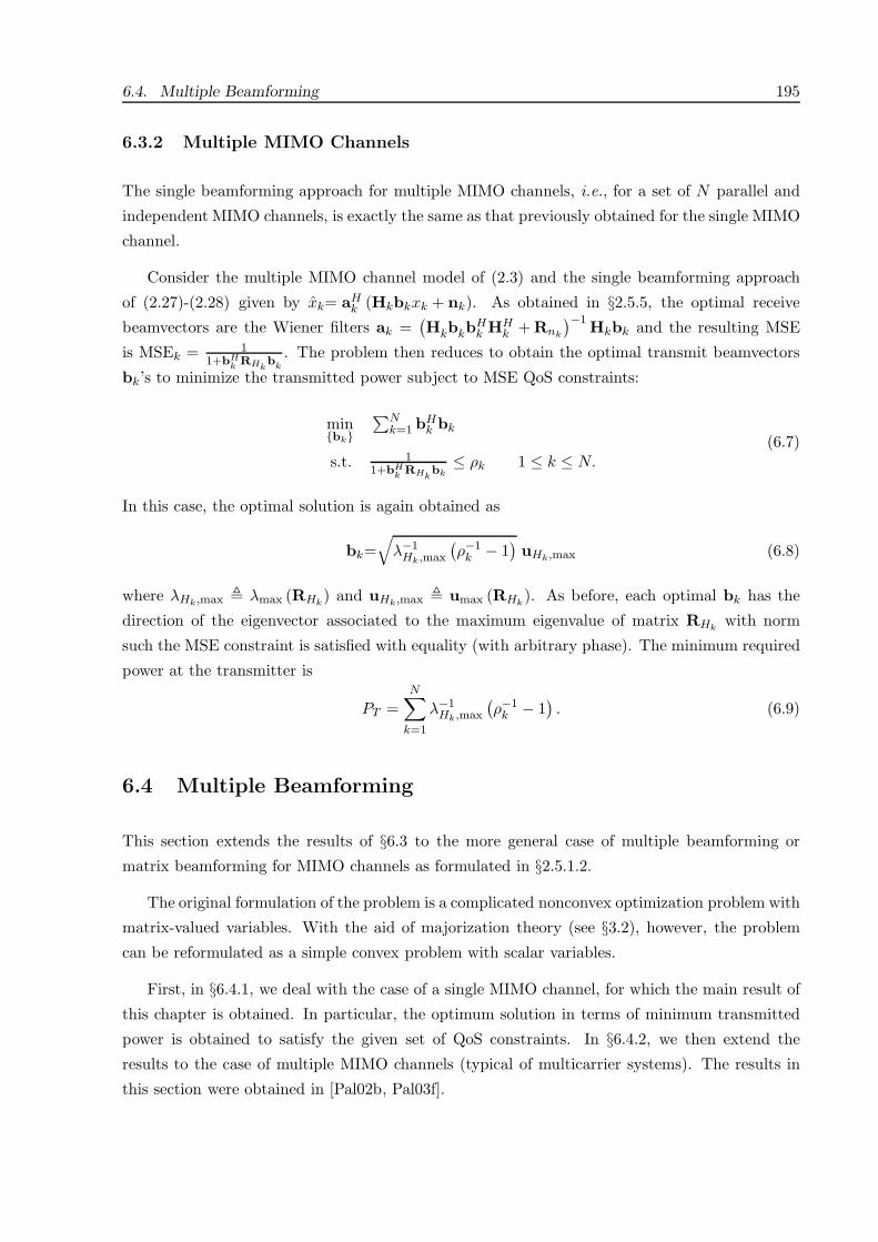
6.4. Multiple Beamforming 195
6.3.2 Multiple MIMO Channels
The single beamforming approach for multiple MIMO channels, i.e., for a set of N parallel and
independent MIMO channels, is exactly the same as that previously obtained for the single MIMO
channel.
Consider the multiple MIMO channel model of (2.3) and the single beamforming approach
of (2.27)-(2.28) given by xk= aHk (Hkbkxk + nk). As obtained in §2.5.5, the optimal receive
beamvectors are the Wiener filters ak =(Hkbkb
Hk HH
k + Rnk
)−1 Hkbk and the resulting MSE
is MSEk = 11+bH
k RHkbk
. The problem then reduces to obtain the optimal transmit beamvectors
bk’s to minimize the transmitted power subject to MSE QoS constraints:
minbk
∑Nk=1 bH
k bk
s.t. 11+bH
k RHkbk
≤ ρk 1 ≤ k ≤ N.(6.7)
In this case, the optimal solution is again obtained as
bk=√
λ−1Hk,max
(ρ−1
k − 1)uHk,max (6.8)
where λHk,max λmax (RHk) and uHk,max umax (RHk
). As before, each optimal bk has the
direction of the eigenvector associated to the maximum eigenvalue of matrix RHkwith norm
such the MSE constraint is satisfied with equality (with arbitrary phase). The minimum required
power at the transmitter is
PT =N∑
k=1
λ−1Hk,max
(ρ−1
k − 1). (6.9)
6.4 Multiple Beamforming
This section extends the results of §6.3 to the more general case of multiple beamforming or
matrix beamforming for MIMO channels as formulated in §2.5.1.2.
The original formulation of the problem is a complicated nonconvex optimization problem with
matrix-valued variables. With the aid of majorization theory (see §3.2), however, the problem
can be reformulated as a simple convex problem with scalar variables.
First, in §6.4.1, we deal with the case of a single MIMO channel, for which the main result of
this chapter is obtained. In particular, the optimum solution in terms of minimum transmitted
power is obtained to satisfy the given set of QoS constraints. In §6.4.2, we then extend the
results to the case of multiple MIMO channels (typical of multicarrier systems). The results in
this section were obtained in [Pal02b, Pal03f].

196 Chapter 6. Joint Tx-Rx Processing with QoS Constraints
6.4.1 Single MIMO Channel
Consider the single MIMO channel model of (2.1) and the matrix processing model of (2.29)-(2.30)
given by x = AH (HBx + n). As obtained in §2.5.5, the optimal receive matrix is the Wiener
filter A =(HBBHHH + Rn
)−1HB and the resulting MSE matrix is E =
(I + BHRHB
)−1.
The problem reduces then to obtain the optimal transmit matrix B to minimize the transmitted
power subject to a set of MSE QoS constraints:
minB
Tr(BBH
)s.t.
[(I + BHRHB
)−1]ii≤ ρi 1 ≤ i ≤ L.
(6.10)
Such a constrained optimization problem is nonconvex and requires previous manipulations (even
in the simple scalar and real case, 11+b2r ≤ ρ is a nonconvex region in b). Although (6.10) seems
at first a formidable problem to solve, with the aid of majorization theory (see §3.2) it can be
reformulated as a simple convex problem with scalar variables that can be optimally solved.
We first consider the simpler case with equal MSE QoS constraints in §6.4.1.1 and then extend
the solution to the more general (and complicated) case with different MSE QoS constraints in
§6.4.1.2 (in both cases, efficient algorithms are given for practical implementations). We then
consider a simple and suboptimum approach in §6.4.1.3 based on imposing a diagonality constraint
on the MSE matrix (such a constraint implies that the channel matrix is diagonalized and then
each symbol is transmitted through a different channel eigenmode).
6.4.1.1 Optimum Solution for Equal MSE QoS Constraints
The optimal solution for equal MSE QoS constraints ρi = ρ ∀i (along with the feasibility condi-
tion) is formally stated in the following theorem.
Theorem 6.1 The following nonconvex optimization problem subject to equal MSE QoS con-
straints:
minB
Tr(BBH
)s.t.
[(I + BHRHB
)−1]ii≤ ρ 1 ≤ i ≤ L,
(6.11)
can be optimally solved by first solving the simple convex optimization problem:
minzi
∑Li=1 zi
s.t. 1L
(L0 +
∑Li=1
11+ziλH,i
)≤ ρ,
zi ≥ 0, 1 ≤ i ≤ L
(6.12)

6.4. Multiple Beamforming 197
where L is the number of established links, L min (L, rank (RH)) is the number of effective
channel eigenvalues used, L0 L − L is the number of links associated to zero eigenvalues, and
the set λH,iLi=1 contains the L largest eigenvalues of RH in increasing order.
The optimal solution to (6.11) satisfies all QoS constraints with equality and is given by
B = UH,1ΣB,1Q where UH,1 ∈ CI nT ×L has as columns the eigenvectors of RH corresponding to
the L largest eigenvalues in increasing order, ΣB,1 = [0 diag (σB,i)] ∈ CI L×L has zero elements
except along the rightmost main diagonal (assumed real w.l.o.g.) which are given by σ2B,i = zi, 1 ≤
i ≤ L (the zi’s are the solution to the convex problem (6.12)), and Q is a unitary matrix such
that the diagonal elements of(I + BHRHB
)−1are equal. This rotation matrix can be computed
using Algorithm 3.2 (reproduced from [Vis99b, Section IV-A]) or with any rotation matrix Q that
satisfies |[Q]ik| = |[Q]il| ∀i, k, l such as the Discrete Fourier Transform (DFT) matrix or the
Hadamard matrix when the dimensions are appropriate (see §3.2 for more details). The problem
is feasible if and only if ρ > L0/L.
Proof. See Appendix 6.A.
Now that the original nonconvex problem has been reformulated as a simple convex problem,
we know that a global optimal solution can be obtained in practice by using, for example, interior-
point methods (see §3.1). Nevertheless, the particular convex problem (6.12) obtained in Theorem
6.1 can be optimally solved by a simple water-filling algorithm (Algorithm 6.1) as stated in the
following proposition (by setting ρ = ρL − L0 ).
Proposition 6.1 The optimal solution to the following convex optimization problem:
minzi
∑Li=1 zi
s.t.∑L
i=11
1+ziλi≤ ρ,
zi ≥ 0, 1 ≤ i ≤ L,
is given (if feasible) by the water-filling solution zi =(µ1/2 λ
−1/2i − λ−1
i
)+(it is tacitly assumed
that all the λi’s are strictly positive) where µ1/2 is the water-level chosen such that the MSE
constraint is satisfied with equality:∑L
i=11
1+ziλi= ρ.
Furthermore, the optimal water-filling solution can be efficiently obtained in practice with
Algorithm 6.1 in no more than L iterations (worst-case complexity). (It is assumed that ρ < L,
otherwise the optimal solution is trivially given by zi = 0 ∀i, i.e., by not transmitting anything.)
Proof. See Appendix 6.B.
Algorithm 6.1 Practical water-filling algorithm to solve the convex problem corresponding to
the design with equal MSE QoS requirements of Theorem 6.1.

198 Chapter 6. Joint Tx-Rx Processing with QoS Constraints
Input: Number of available positive eigenvalues L, set of eigenvalues λiLi=1, and MSE con-
straint ρ.
Output: Set of allocated powers ziLi=1 and water-level µ1/2.
0. Reorder the λi’s in decreasing order (define λL+1 0). Set L = L.
1. Set µ = λ−1L
(if λL = λL+1, then set L = L − 1 and go to step 1).
2. If µ1/2 ≥∑L
i=1 λ−1/2i
ρ−(L−L), then set L = L − 1 and go to step 1.
Otherwise, obtain the definitive water-level µ1/2 and allocated powers as
µ1/2 =∑L
i=1 λ−1/2i
ρ − (L − L) and
zi =(µ1/2 λ
−1/2i − λ−1
i
)+,
undo the reordering done at step 0, and finish.
Thus, the problem of finding a transmit matrix B that minimizes the required transmit power
subject to equal MSE QoS requirements has been completely solved in a practical and optimal
way. It is remarkable that, in general, the optimal solution does not consist on transmitting each
symbol through a channel eigenmode in a parallel fashion (diagonal transmission); instead, the
symbols are transmitted in a distributed way over all the channel eigenmodes.
6.4.1.2 Optimum Solution for Different MSE QoS Constraints
This section generalizes the results obtained in §6.4.1.1 by allowing different QoS constraints in
terms of MSE. This problem is more general and far more complicated than the one with equal
MSE constraints. Nevertheless, using majorization theory (see §3.2) we can still reformulate the
original complicated nonconvex problem as a simple convex optimization problem that can be
optimally solved as is formally stated in the following theorem (the feasibility condition of the
problem is also given).
Theorem 6.2 The following nonconvex optimization problem subject to different MSE QoS con-
straints (assumed in decreasing order ρi ≥ ρi+1 w.l.o.g.):
minB
Tr(BBH
)s.t.
[(I + BHRHB
)−1]ii≤ ρi 1 ≤ i ≤ L,
(6.13)

6.4. Multiple Beamforming 199
can be optimally solved by first solving the simple convex optimization problem:
minzi
∑Li=1 zi
s.t.∑L
i=k1
1+ziλH,i≤∑L
i=k+L0ρi∑L
i=11
1+ziλH,i≤∑L
i=1 ρi − L0,
zk ≥ 0,
1 ≤ k ≤ L,
1 ≤ k ≤ L
(6.14)
where L is the number of established links, L min (L, rank (RH)) is the number of effective
channel eigenvalues used, L0 L − L is the number of links associated to zero eigenvalues, and
the set λH,iLi=1 contains the L largest eigenvalues of RH in increasing order.
The optimal solution to (6.13) satisfies all QoS constraints with equality and is given by
B = UH,1ΣB,1Q where UH,1 ∈ CI nT ×L has as columns the eigenvectors of RH corresponding to
the L largest eigenvalues in increasing order, ΣB,1 = [0 diag (σB,i)] ∈ CI L×L has zero elements
except along the rightmost main diagonal (assumed real w.l.o.g.) which are given by σ2B,i = zi, 1 ≤
i ≤ L (the zi’s are the solution to the convex problem (6.14)), and Q is a unitary matrix such that[(I + BHRHB
)−1]ii
= ρi, 1 ≤ k ≤ L which can be computed using Algorithm 3.2 (reproduced
from [Vis99b, Section IV-A]). The problem is feasible if and only if∑L
i=1 ρi > L0 (a simple
sufficient condition for the feasibility of the problem is the rule of thumb: L ≤ rank (H) 5).
Proof. See Appendix 6.C.
Noting that∑L
i=1 ρi − L0 <∑L
i=1+L0ρi (recall that ρi < 1), problem (6.14) can be rewritten
more compactly as
minzi
∑Li=1 zi
s.t.∑L
i=k1
1+ziλH,i≤∑L
i=k ρi,
zk ≥ 0,
1 ≤ k ≤ L, (6.15)
where ρi
∑L0+1
k=1 ρk − L0
ρi+L0
for i = 1
for 1 < i ≤ L(note that the resulting ρi’s need not be in
decreasing ordering as the ρi’s).
By Theorem 6.2, the original formidable problem has been reformulated as a convex problem
which can always be solved in practice using, for example, interior-point methods (see §3.1).However, as happened with the case of equal MSE QoS requirements in §6.4.1.1, this problem
can be solved with a multi-level water-filling algorithm (Algorithms 6.2 and 6.3) as shown next.
5In a practical situation, a threshold should be considered in the rank determination to avoid extremelly small
eigenvalues to artificially increase the rank.

200 Chapter 6. Joint Tx-Rx Processing with QoS Constraints
Proposition 6.2 The optimal solution to the following convex optimization problem:
minzi
∑Li=1 zi
s.t.∑L
i=k1
1+ziλi≤∑L
i=k ρi,
zk ≥ 0,
1 ≤ k ≤ L,
is given (if feasible) by the multi-level water-filling solution zi =(µ
1/2i λ
−1/2i − λ−1
i
)+(it is tacitly
assumed that all the λi’s are strictly positive) where the multiple water-levels µ1/2i ’s are chosen to
satisfy: ∑Li=k
11+ziλi
≤∑Li=k ρi 1 < k ≤ L∑L
i=11
1+ziλi=∑L
i=1 ρi
µk ≥ µk−1 (µ0 0)
(µk − µk−1)(∑L
i=k1
1+ziλi−∑L
i=k ρi
)= 0.
Furthermore, the optimal multi-level water-filling solution can be efficiently obtained in prac-
tice with Algorithm 6.2 (or with the equivalent Algorithm 6.3) in no more (worst-case complexity)
than L(L + 1
)/2 inner iterations (simple water-fillings) or, more exactly, L2
(L + 1
)/6 basic it-
erations (iterations within each simple water-filling). (It is assumed that ρi < 1, otherwise the
optimal solution is trivially given by zi = 0 ∀i, i.e., by not transmitting anything.)
Proof. See Appendix 6.D.
Algorithm 6.2 Practical multi-level water-filling algorithm to solve the convex problem corre-
sponding to the design with different MSE QoS requirements of Theorem 6.2. Version 1. (See
Figure 6.1 for an illustrative example of the application of the algorithm.)
Input: Number of available positive eigenvalues L, set of eigenvalues λiLi=1, and set of MSE
constraints ρiLi=1 (note that the appropriate ordering of the λi’s and of the ρi’s is independent
of this algorithm).
Output: Set of allocated powers ziLi=1 and set of water-levels µ1/2
i Li=1.
0. Set L = L.
1. Perform an outer iteration.
2. If k0 = 1, then finish. Otherwise set L = k0 − 1 and go to step 1.
Outer iteration:
0. Set k0 = 1.

6.4. Multiple Beamforming 201
= constraint satisfied with strict inequality
= constraint satisfied with equality
= constraint not satisfied
Outer iteration #1 Final solution
k=1
k=5
k=12
([12,17])
Outer iteration #2 Outer iteration #3
k=17
([5,11])
([1,4])
Figure 6.1: Example of the execution of Algorithm 6.2 to solve the problem with different QoS requirements.
1. Perform an inner iteration: solve the equal MSE QoS constrained problem in[k0, L
]using
Algorithm 6.1 with the set of L − k0 + 1 eigenvalues λiLi=k0
and with the MSE constraint
given by ρ =∑L
i=k0ρi.
2. If all intermediate constraints are also satisfied (i.e., if∑L
i=k1
1+ziλi≤∑L
i=k ρi, k0 < k ≤ L),
then finish.
Otherwise, set k0 equal to the smallest index whose constraint is not satisfied and go to step
1.
Note that each outer iteration implicitly computes the water-level for the set[k0, L
]denoted
by µ1/2([
k0, L])
; in other words, µk = µ([
k0, L])
, k0 ≤ k ≤ L.
Algorithm 6.2 was conveniently written to prove its optimality. For a practical implementa-
tion, however, it can be rewritten in a much simpler way as in Algorithm 6.3.
Algorithm 6.3 Practical multi-level water-filling algorithm to solve the convex problem corre-
sponding to the design with different MSE QoS requirements of Theorem 6.2. Version 2.
Input: Number of available positive eigenvalues L, set of eigenvalues λiLi=1, and set of MSE
constraints ρiLi=1 (note that the appropriate ordering of the λi’s and of the ρi’s is independent
of this algorithm).
Output: Set of allocated powers ziLi=1 and set of water-levels µ1/2
i Li=1.
0. Set k0 = 1 and L = L.
1. Solve the equal MSE QoS constrained problem in[k0, L
]using Algorithm 6.1 with the set
of L − k0 + 1 eigenvalues λiLi=k0
and with the MSE constraint given by ρ =∑L
i=k0ρi.

202 Chapter 6. Joint Tx-Rx Processing with QoS Constraints
2. If any intermediate constraint (∑L
i=k1
1+ziλi≤ ∑L
i=k ρi, k0 < k ≤ L) is not satisfied,
then set k0 equal to the smallest index whose constraint is not satisfied and go to step 1.
Otherwise, if k0 = 1 finish and if k0 > 1 set L = k0 − 1, k0 = 1, and go to step 1.
This section has obtained the main result of the chapter: an efficient and optimal way to solve
in practice the problem of finding a transmit matrix B that minimizes the required transmit power
while satisfying different MSE QoS requirements. It suffices to use the multi-level water-filling
algorithm (Algorithm 6.3) and then to find the proper rotation matrix Q as described in Theorem
6.2.
As happened in the case of equal MSE QoS constraints, the optimal solution does not generally
consist on transmitting each symbol through a channel eigenmode in a parallel fashion (diagonal
transmission); instead, the symbols are transmitted in a distributed way over all the channel
eigenmodes.
6.4.1.3 Suboptimum Solution: A Simple Approach Imposing Diagonality
At this point, it is interesting to consider a suboptimum but very simple solution to the considered
problem. The simplicity of the solution comes from imposing a diagonality constraint in the MSE
matrix, i.e., from forcing E =(I + BHRHB
)−1 to have a diagonal structure. Imposing such a
structure implies that the transmission is performed in a parallel fashion through the channel
eigenmodes. In Lemma 6.1, we obtain such a simple solution and give the feasibility condition.
Then, in Lemma 6.2, we state the exact conditions under which such a constrained solution
happens to be the optimum solution to the original problem considered in Theorem 6.2.
Lemma 6.1 The following nonconvex optimization problem subject to different MSE QoS con-
straints (assumed in decreasing order ρi ≥ ρi+1 w.l.o.g. and bounded by 0 < ρi < 1):
minB
Tr(BBH
)s.t.
[(I + BHRHB
)−1]ii≤ ρi 1 ≤ i ≤ L,
BHRHB diagonal
is feasible if and only if the number of established links L satisfy L ≤ rank (RH) and the optimal
solution is then given by B = UH,1ΣB,1, where UH,1 ∈ CI nT×L has as columns the eigenvectors
of RH corresponding to the L largest eigenvalues in increasing order, denoted by λH,i, and
ΣB,1 ∈ CI L×L is a diagonal matrix with squared-diagonal elements given by
zi = λ−1H,i
(ρ−1
i − 1)
1 ≤ i ≤ L.
Proof. See Appendix 6.E.

6.4. Multiple Beamforming 203
Lemma 6.2 The optimal solution obtained in Lemma 6.1 under the diagonality constraint of the
MSE matrix E =(I + BHRHB
)−1 is the optimal solution to the problem considered in Theorem
6.2 without the diagonality constraint on E if and only if
λH,i ρ2i ≥ λH,i+1 ρ2
i+1 1 ≤ i < L (6.16)
where the ρi’s are in decreasing order and the λH,i’s are the L largest eigenvalues of RH in
increasing order. Note that this condition implies the feasibility condition L ≤ rank (RH).
The conditions in (6.16) can be stated in words by saying that the singular values of the
whitened channel λ1/2H,i have to increase at a slower rate than the decrease of the MSE constraints
ρi.
Proof. See Appendix 6.F.
As an example, the conditions of Lemma 6.2 are always satisfied for channels with equal
singular values (this corresponds to a diagonal squared channel matrix RH) and, consequently, a
parallel transmission is always the optimum structure for such channels.
Another interesting example arises for systems with equal MSE constraints as treated in
Theorem 6.1, for which the conditions in (6.16) are never satisfied (unless the squared-channel
has equal eigenvalues).
6.4.2 Multiple MIMO Channels
This section extends the results of multiple beamforming in a single MIMO channel of §6.4.1 to
the case of a set of N parallel MIMO channels. The extension is straightforward as we show next.
Consider the multiple MIMO channel model of (2.3) and the matrix processing model of
(2.31)-(2.32) given by xk= AHk (HkBkxk + nk) where Lk symbols are transmitted through the
kth MIMO channel (Lk substreams). As obtained in §2.5.5, the optimal receive matrices are
the Wiener filters Ak =(HkBkB
Hk HH
k + Rnk
)−1 HkBk and the resulting MSE matrices are
Ek =(I + BH
k RHkBk
)−1. The problem reduces then to obtain the optimal transmit matrices
Bk’s to minimize the transmitted power subject to a set of MSE QoS constraints:
minBk
∑Nk=1 Tr
(BkB
Hk
)s.t.
[(I + BH
k RHkBk
)−1]ii≤ ρk,i 1 ≤ i ≤ L, 1 ≤ k ≤ N.
(6.17)
This problem is clearly separable in each of the N MIMO channels. Therefore, the results
previously obtained in §6.4.1 are directly applicable to each of the MIMO channels.

204 Chapter 6. Joint Tx-Rx Processing with QoS Constraints
6.5 Relaxation of the QoS Requirements
In situations where the problem is feasible but the required transmit power exceeds some pre-
specified maximum level, the system may be forced to relax some QoS requirements so that
the required power is reduced. For that purpose, we identify which QoS constraints produce the
largest reduction in transmit power when relaxed by means of a perturbation analysis (see §3.1.4).The questions of whether and when these relaxations are necessary is a high-level decision6 that
may depend on factors as disparate as the energy left on the batteries at the transmitter or the
number of services/users requesting a link. Such high-level decisions are out of the scope of this
chapter.
It is well known from convex optimization theory (see §3.1) that the optimal dual variables
(Lagrange multipliers) of a convex optimization problem give useful information about the sen-
sitivity of the optimal objective value with respect to perturbations of the constraints. Consider
the following relaxation of the original QoS constraints of (6.1):
MSEi ≤ ρi + ui (δi) (6.18)
where ui (δi) : IR+ −→ IR+ is a positive differentiable function parameterized with δi such that
ui (δi) −→δi→0+
0. By Theorem 6.2, the relaxed problem in convex form is (for simplicity of exposition
and w.l.o.g., we focus on the multiple beamforming architecture in a single MIMO channel and
consider L ≤ rank (H) in (6.14)):
minzi
∑Li=1 zi
s.t.∑L
i=k1
1+ziλH,i≤∑L
i=k ρi + uk (δ) 1 ≤ k ≤ L,
zk ≥ 0.
where uk (δ) ∑L
i=k ui (δi) and δ=[δ1, · · · , δL]T . Defining p (u) as the optimal objective value
of the relaxed problem as a function of u = [u1, · · · , uL]T , the following local sensitivity result
given in (3.14) holds (note that the problem satisfies the Slater’s condition and therefore strong
duality holds, c.f. §3.1):µ
k = − ∂p
∂uk
∣∣∣∣δ=0
(6.19)
where µk is the Lagrange multiplier of the Lagrangian of the relaxed problem (similar to (6.26))
at an optimal point. Using the chain rule for differentiation ∂p
∂δi=∑L
k=1∂p
∂uk
∂uk∂δi
, noting that
∂uk(δ)∂δi
=
ui (δi)
0
i ≥ k
otherwise, and using (6.19), it follows that
∂p
∂δi
∣∣∣∣δ=0
= −µi
∂ui (δi)∂δi
∣∣∣∣δ=0
(6.20)
6Advanced communication systems are envisioned to exploit cross-layer signaling to further control the perfor-
mance of the whole system.

6.6. Simulation Results 205
where we have defined µi ∑i
k=1 µk.
The largest value of −∂p
∂δi
∣∣∣δ=0
for 1 ≤ i ≤ L indicates the QoS constraint that should be
relaxed in order to get the largest reduction of the required transmitted power. Note that the
optimal µi’s used in (6.20) are readily given by the water-levels implicitly obtained in Algorithms
6.2 and 6.3: for each subblock [k1, k2] of the partition on [1, L], choose µk = µ ([k1, k2]) k1 ≤ k ≤k2. The term ∂ui(δi)
∂δi
∣∣∣δ=0
in (6.20) depends on the particular cost function that relates the QoS in
terms of MSE as used in the problem formulation and the QoS as seen by the service/user which
can be in terms of MSE, SINR, or BER. We consider now a few examples.
Example 1 : MSEi ≤ ρi + δi
In this case, it follows that ∂ui(δi)∂δi
= 1 and therefore ∂p
∂δi
∣∣∣δ=0
= −µi . The largest µ
i is given
by µL (or any other µ
i belonging to the same water-filling subblock as obtained in Appendix
6.D). This means that the best way to relax the constraints in this case is by relaxing the tightest
constraint.
Example 2 : MSEi ≤ BER−1 (pi (1 + δi))
In this example, the QoS are given in terms of BER. The relaxation can be expressed as
MSEi ≤ ρi + ui (δi) by defining ρi BER−1 (pi) and ui (δi) BER−1 (pi (1 + δi)) − BER−1 (pi).
It follows that ∂ui(δi)∂δi
= ∂ BER−1(pi(1+δi))∂δi
.
As a final remark, note that the previous sensitivity analysis is local and, therefore, the
relaxation of the QoS constraints has to be performed in sufficiently small steps (recall that the
decreasing order of the ρi’s must be kept at each step).
6.6 Simulation Results
We now present numerical results obtained from simulations using realistic channel models for a
wireless multi-antenna communication system and for a wireline (DSL) communication system.
6.6.1 Wireless Multi-Antenna Communication System
We consider a wireless communication system with multiple antennas at both sides of the link
as was used for the numerical simulations in Chapter 5 (in particular 4 transmit and 4 re-
ceive antennas are considered). Perfect CSI is assumed at both sides of the communication
system (channel estimation errors are considered in Chapter 7). The channel model includes
the frequency-selectivity and the spatial correlation as measured in real scenarios. The MIMO
channels were generated using the parameters of the WLAN European standard HIPERLAN/2
[ETS01], which is based on the multicarrier modulation OFDM (64 carriers were used in the sim-
ulations). The frequency selectivity of the channel was modeled using the power delay profile type

206 Chapter 6. Joint Tx-Rx Processing with QoS Constraints
C for HIPERLAN/2 as specified in [ETS98a] (see Figure 5.3(a)), which corresponds to a typical
large open space indoor environment for NLOS conditions with 150ns average r.m.s. delay spread
and 1050ns maximum delay (the sampling period is 50ns [ETS01]). The spatial correlation of the
MIMO channel was modeled according to the Nokia model defined in [Sch01] (for the uplink) as
specified by the correlation matrices of the envelope of the channel fading at the transmit and
receive side (see Figure 5.3(b)). It models a large open indoor environment with two floors, which
could easily illustrate a conference hall or a shopping galleria scenario (see [Sch01] for details of
the model). The matrix channel generated was normalized so that∑
n E [| [H(n)]ij |2] = 1.
The results are given in terms of required transmit power at some outage probability Pout, i.e.,
the transmit power that will not suffice to satisfy the QoS constraints with a small probability
Pout (it will suffice for (1 − Pout) of the time). In particular, we consider an outage probability
of 5%. The reason of using the outage power instead of the average power is that, for typical
wireless systems with delay constraints, the former is more realistic than the latter which only
makes sense when the transmission coding block is long enough to reveal the long-term ergodic
properties of the fading process (no delay constraints). Instead of plotting absolute values of the
required transmit power, we plot relative values of the transmitted power normalized with the
noise spectral density N0. We call this normalized transmitted power SNR which is defined as
SNR = Tr(BBH
)/ (N N0) 7 where N is the number of carriers. Note that the plots are valid
only for the channel normalization used.
In the following, numerical results for the proposed methods obtained in this chapter are
given (Algorithm 6.1 for equal MSE QoS requirements and Algorithm 6.3 for different MSE
QoS requirements). As a means of comparison, the simple benchmark obtained by imposing
the diagonality of the MSE matrix as obtained in §6.4.1.3 is also considered. We consider two
multicarrier approaches as described in §2.5.1.2: the carrier-noncooperative scheme (optimizing
each carrier independently) and the carrier-cooperative scheme (treating all carriers as a single
MIMO channel). Note that the total number of established substreams is LN where L denotes
the number of spatial dimensions used per carrier.
Equal QoS Constraints
We now consider equal QoS requirements in terms of BER which correspond to equal QoS
requirements in terms of MSE because the same constellation (QPSK) is used on all the sub-
streams.
In Figure 6.2, the SNR per spatial dimension SNR/L is plotted as a function of L subject to
equal QoS requirements given by BER = 10−3. For L = 3, the gain over the benchmark is about
2dB. For L = 4, the gain is of 7dB for the carrier-noncooperative scheme and of 12dB for the
carrier-cooperative scheme. The required power for L = 4 increases significantly with respect to
7Note that such an SNR definition is a measure of the total transmitted power per symbol (normalized with
N0) and does not correspond to the SNR at each receive antenna.

6.6. Simulation Results 207
1 2 3 40
5
10
15
20
25
30
Outage SNR/L (Pout
=5%) vs. L for QPSK (nT=4, n
R=4, BER=1.00e−003)
L
SN
R/L
(dB
)
Benchmark carrier−noncooperative methodBenchmark carrier−cooperative method Optimal carrier−noncooperative method Optimal carrier−cooperative method
Figure 6.2: Outage SNR per spatial dimension vs. the number of spatial dimensions utilized L when usingQPSK in a multicarrier 4× 4 MIMO channel with an equal QoS for all substreams given by BER≤ 10−3.
L = 3 and therefore we choose the latter for the rest of the simulations.
In Figure 6.3, the SNR is given as a function of the (equal) QoS constraints in terms of BER
for L = 3. It can be observed that the gain over the benchmark is about 2-3dB and constant
for all range of the BER. Cooperation among carriers improves the performance in no more than
0.5dB. Given that the carrier-noncooperative scheme has an attractive parallel implementation
(since each carrier is independently processed), it may be an interesting solution for a practical
and efficient implementation.
Different QoS Constraints
We now generalize the set-up by considering different QoS constraints both in terms of BER
and MSE (since the same constellations are used on all the substreams).
In Figure 6.4, the SNR is plotted as a function of the nominal QoS corresponding to the first
substream (the QoS constraints for the others substreams are obtained by scaling this nominal
QoS constraint with the factors 0.5 and 0.1). Similar observations to those corresponding to
Figure 6.3 hold in this case.
Relaxation of the QoS Requirements
In Figure 6.5, an example of a relaxed system is given (as explained in §6.5). The relaxed-I
case consists of 10 relaxations per carrier with δ = 0.1 of the form MSEi ≤ BER−1(pi 10δi
)(note that an extreme case of this series of relaxations amounts to increasing the BER of a single

208 Chapter 6. Joint Tx-Rx Processing with QoS Constraints
10−5
10−4
10−3
10−2
10−1
5
10
15
20
Outage SNR (Pout
=5%) vs. BER for QPSK (L=3, nT=4, n
R=4)
BER
SN
R (
dB)
Benchmark carrier−noncooperative methodBenchmark carrier−cooperative method Optimal carrier−noncooperative method Optimal carrier−cooperative method
Figure 6.3: Outage SNR vs. the equal QoS constraints given in terms of BER when using QPSK in amulticarrier 4 × 4 MIMO channel with L = 3.
10−5
10−4
10−3
10−2
10−1
8
10
12
14
16
18
20
Outage SNR (Pout
=5%) vs. BER for QPSK (L=3, nT=4, n
R=4)
BER1 (factors: 1.00 0.50 0.10 )
SN
R (
dB)
Benchmark carrier−noncooperative methodBenchmark carrier−cooperative method Optimal carrier−noncooperative method Optimal carrier−cooperative method
Figure 6.4: Outage SNR vs. the different QoS constraints given in terms of BER when using QPSK in amulticarrier 4× 4 MIMO channel with L = 3. (The BER of the first substream is along the x-axis and theBER of the second and third substreams are given by scaling with the factors 0.5 and 0.1.)

6.6. Simulation Results 209
10−5
10−4
10−3
10−2
10−1
−4
−2
0
2
4
6
8
10
12
14
16
18
Outage SNR (Pout
=5%) vs. BER for QPSK (L=3, nT=4, n
R=4)
BER1 (factors: 1.00 0.50 0.10 )
SN
R (
dB)
Original Relaxed−I Relaxed−II
Figure 6.5: Outage SNR vs. the different QoS constraints given in terms of BER for the original carrier-cooperative method and for two succesive series of relaxations when using QPSK in a multicarrier 4 × 4MIMO channel with L = 3. (The BER of the first substream is along the x-axis and the BER of thesecond and third substreams are given by scaling with the factors 0.5 and 0.1.)
substream one order of magnitude) and the relaxed-II case consists of 10 additional relaxations
of the same type. As is observed, a significant reduction of the required transmit power can be
achieved at the expense of the relaxation of some QoS requirements (recall that these relaxations
are done in an optimal way).
6.6.2 Wireline (DSL) Communication System
We consider a VDSL system with typical parameters and DMT specifications: 4096 carriers on a
bandwidth of 17.664 MHz, 26-gauge cable (AWG 26), background noise with a flat PSD at -140
dBm/Hz. We simulate a bundle with a total of 25 copper pairs, 20 of which are the intended
users that can perform joint processing and the other 5 are considered as interference (no alien
interference was included).
The MIMO DSL channel includes wide-scale frequency variations with statistics determined
from measured FEXT transfer functions (see [Fan02] for details on the model). For illustrative
purposes, a few realizations of the crosstalk are plotted in Figure 6.6.
The results are given in terms of required transmit power (since the channel is basically
deterministic it is not necessary to take outage values as in the wireless case).
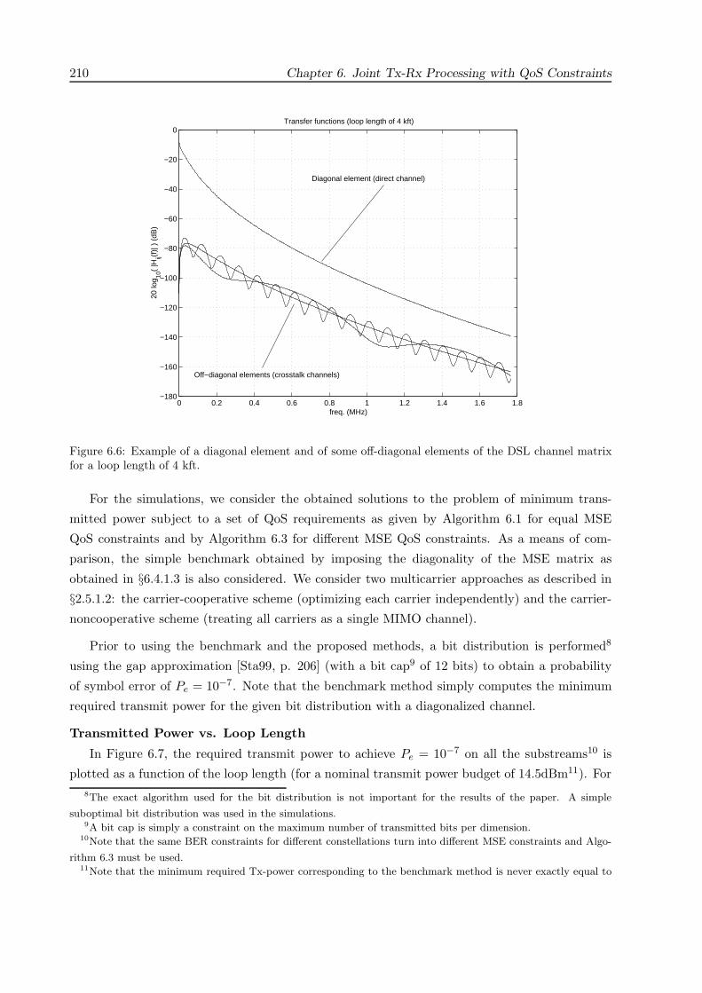
210 Chapter 6. Joint Tx-Rx Processing with QoS Constraints
0 0.2 0.4 0.6 0.8 1 1.2 1.4 1.6 1.8−180
−160
−140
−120
−100
−80
−60
−40
−20
0Transfer functions (loop length of 4 kft)
freq. (MHz)
20 lo
g 10(
|Hij(f
)| )
(dB
)
Diagonal element (direct channel)
Off−diagonal elements (crosstalk channels)
Figure 6.6: Example of a diagonal element and of some off-diagonal elements of the DSL channel matrixfor a loop length of 4 kft.
For the simulations, we consider the obtained solutions to the problem of minimum trans-
mitted power subject to a set of QoS requirements as given by Algorithm 6.1 for equal MSE
QoS constraints and by Algorithm 6.3 for different MSE QoS constraints. As a means of com-
parison, the simple benchmark obtained by imposing the diagonality of the MSE matrix as
obtained in §6.4.1.3 is also considered. We consider two multicarrier approaches as described in
§2.5.1.2: the carrier-cooperative scheme (optimizing each carrier independently) and the carrier-
noncooperative scheme (treating all carriers as a single MIMO channel).
Prior to using the benchmark and the proposed methods, a bit distribution is performed8
using the gap approximation [Sta99, p. 206] (with a bit cap9 of 12 bits) to obtain a probability
of symbol error of Pe = 10−7. Note that the benchmark method simply computes the minimum
required transmit power for the given bit distribution with a diagonalized channel.
Transmitted Power vs. Loop Length
In Figure 6.7, the required transmit power to achieve Pe = 10−7 on all the substreams10 is
plotted as a function of the loop length (for a nominal transmit power budget of 14.5dBm11). For8The exact algorithm used for the bit distribution is not important for the results of the paper. A simple
suboptimal bit distribution was used in the simulations.9A bit cap is simply a constraint on the maximum number of transmitted bits per dimension.
10Note that the same BER constraints for different constellations turn into different MSE constraints and Algo-
rithm 6.3 must be used.11Note that the minimum required Tx-power corresponding to the benchmark method is never exactly equal to
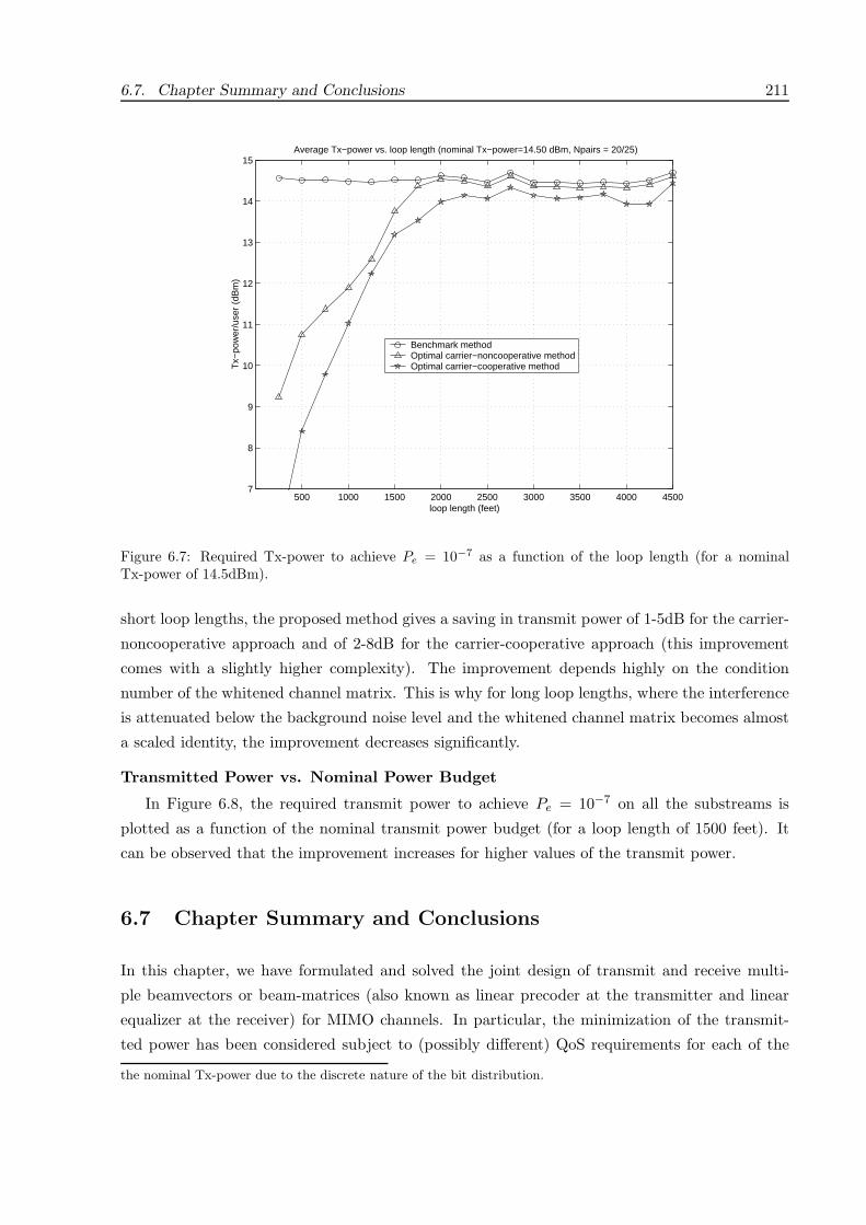
6.7. Chapter Summary and Conclusions 211
500 1000 1500 2000 2500 3000 3500 4000 45007
8
9
10
11
12
13
14
15Average Tx−power vs. loop length (nominal Tx−power=14.50 dBm, Npairs = 20/25)
loop length (feet)
Tx−
pow
er/u
ser
(dB
m)
Benchmark method Optimal carrier−noncooperative methodOptimal carrier−cooperative method
Figure 6.7: Required Tx-power to achieve Pe = 10−7 as a function of the loop length (for a nominalTx-power of 14.5dBm).
short loop lengths, the proposed method gives a saving in transmit power of 1-5dB for the carrier-
noncooperative approach and of 2-8dB for the carrier-cooperative approach (this improvement
comes with a slightly higher complexity). The improvement depends highly on the condition
number of the whitened channel matrix. This is why for long loop lengths, where the interference
is attenuated below the background noise level and the whitened channel matrix becomes almost
a scaled identity, the improvement decreases significantly.
Transmitted Power vs. Nominal Power Budget
In Figure 6.8, the required transmit power to achieve Pe = 10−7 on all the substreams is
plotted as a function of the nominal transmit power budget (for a loop length of 1500 feet). It
can be observed that the improvement increases for higher values of the transmit power.
6.7 Chapter Summary and Conclusions
In this chapter, we have formulated and solved the joint design of transmit and receive multi-
ple beamvectors or beam-matrices (also known as linear precoder at the transmitter and linear
equalizer at the receiver) for MIMO channels. In particular, the minimization of the transmit-
ted power has been considered subject to (possibly different) QoS requirements for each of the
the nominal Tx-power due to the discrete nature of the bit distribution.

212 Chapter 6. Joint Tx-Rx Processing with QoS Constraints
11 12 13 14 15 16 17 189
10
11
12
13
14
15
16
17
18Average Tx−power vs. nominal Tx−power (loop length = 1500 feet, Npairs = 20/25)
nominal Tx−power/user (dBm)
Tx−
pow
er/u
ser
(dB
m)
Benchmark method Optimal carrier−noncooperative methodOptimal carrier−cooperative method
Figure 6.8: Required Tx-power to achieve Pe = 10−7 as a function of the nominal Tx-power (for a looplength of 1500 feet).
established substreams in terms of MSE, SINR, and BER. Although the original problem formu-
lation is a complicated nonconvex problem with matrix-valued variables, by using majorization
theory we have been able to reformulate it as a simple convex optimization problem with scalar
variables. To optimally solve the convex problem in practice, we have proposed a practical and
efficient multi-level water-filling algorithm. For situations in which the required power results too
large, a perturbation analysis has been conducted to obtain the optimal way in which the QoS
requirements should be relaxed in order to reduce the power needed.
All the material presented in this chapter, which is strongly based on majorization theory and
convex optimization theory, is a novel contribution of this dissertation.
Appendix 6.A Proof of Theorem 6.1
First rewrite the original problem as
minB
Tr(BBH
)s.t. max
i
[(I + BHRHB
)−1]ii≤ ρ.
Note that this problem is exactly the opposite formulation of one of the design criteria considered
in §5.5.5 (the MAX-MSE criterion) where maxi
[(I + BHRHB
)−1]ii
was minimized subject to

6.A Proof of Theorem 6.1 213
a power constraint Tr(BBH
) ≤ PT .12 We claim that matrix E =(I + BHRHB
)−1 must have
equal diagonal elements at an optimal point and that the QoS constraints must be all satisfied
with equality. Otherwise, by Corollary 3.2, we could find a unitary matrix Q with QHEQ having
identical diagonal elements equal to 1L Tr (E) (this amounts to using BQ as transmit matrix
instead of B). Since 1L Tr (E) ≤ maxi [E]ii with equality if and only if all diagonal elements of
E are equal, using BQ would satisfy all QoS constraints with strict inequality and the objective
value could be further minimized by scaling down the whole transmit matrix. Therefore, the
problem can be rewritten as
minB
Tr(BBH
)s.t.
(I + BHRHB
)−1 with equal diag. elements
1L Tr
(I + BHRHB
)−1 ≤ ρ.
By Corollary 3.2, it follows that for any given B we can always find a unitary matrix Q such that
QH(I + BHRHB
)−1Q has equal diagonal elements. Therefore, we can simplify the problem by
decomposing B as B = BQ and imposing BHRHB to be diagonal w.l.o.g. It is important to
remark that imposing a diagonal structure on BHRHB does not affect the problem since the
objective value remains the same Tr(BBH) = Tr(BBH
)and the QoS constraint also remains
unchanged Tr(I + BHRHB
)−1 = Tr(I+BHRHB
)−1. In addition, since BHRHB is diagonal,
the unitary matrix Q such that QH(I+BHRHB
)−1Q has equal diagonal elements can be found
using Algorithm 3.2 (reproduced from [Vis99b, Section IV-A]) or with any rotation matrix that
satisfies |[Q]ik| = |[Q]il| ∀i, k, l such as the DFT matrix or the Hadamard matrix when the
dimensions are appropriate (see §3.2 for more details).
The problem can be finally written as
minB
Tr(BBH
)s.t. BHRHB diagonal
1L Tr
(I+BHRHB
)−1 ≤ ρ.
Since BHRHB is diagonal, B can be assumed without loss of optimality (by Lemma 5.11) of the
form B = UH,1ΣB,1 where UH,1 ∈ CI nT×L has as columns the eigenvectors of RH corresponding to
the L min (L, rank (RH)) largest eigenvalues in increasing order and ΣB,1 = [0 diag (σB,i)] ∈CI L×L has zero elements except along the rightmost main diagonal (assumed real w.l.o.g.). The
problem formulation of (6.12) follows by defining zi σ2B,i and denoting with the set λH,iL
i=1
the L largest eigenvalues of RH in increasing order. Note that the term L0 L − L in (6.12)
arises from the zero diagonal elements of BHRHB.12Both problems are equivalent in the sense that they both describe the same curve of required power PT for a
given MSE constraint ρ (in the considered case the curve is parameterized with respect to ρ, PT (ρ), and in [Pal03c]
the curve is parameterized with respect to PT , ρ (PT )).
214 Chapter 6. Joint Tx-Rx Processing with QoS Constraints
Rewriting the MSE constraint in (6.12) as∑L
i=11
1+ziλH,i≤ ρL − L0, it becomes clear that
it can be satisfied for sufficiently large values of the zi’s (equivalently, the problem is feasible) if
and only if ρ > L0/L.
Appendix 6.B Proof of Proposition 6.1
We first obtain the closed-form solution to the problem using convex optimization theory (see
§3.1) and then proceed to prove the optimality of Algorithm 6.1.
Optimal Solution. The Lagrangian corresponding to the constrained convex problem is
L =L∑
i=1
zi + µ
L∑
i=1
11 + ziλi
− ρ
−
L∑i=1
γi zi,
where µ and the γi’s are the dual variables or Lagrange multipliers. The water-filling solution is
easily found from the sufficient and necessary KKT optimality conditions (the problem satisfies
the Slater’s condition and therefore strong duality holds):
∑L
i=1
11 + ziλi
≤ ρ, zi ≥ 0 (6.21)
µ ≥ 0, γi ≥ 0 (6.22)
µλi
(1 + ziλi)2 + γi = 1 (6.23)
µ
(∑L
i=1
11 + ziλi
− ρ
)= 0, γizi = 0. (6.24)
Note that if µ = 0, then γi = 1 ∀i and zi = 0 ∀i, which cannot be since the MSE constraint
would not be satisfied because it was assumed that ρ < L. If zi > 0, then γi = 0 (by the
complementary slackness condition γizi = 0), µ λi
(1+ziλi)2 = 1 (note that µ λi > 1), and zi =
µ1/2 λ−1/2i − λ−1
i . If zi = 0, then µ λi + γi = 1 (note that µ λi ≤ 1). Equivalently,
zi =
µ1/2 λ
−1/2i − λ−1
i
0
if µλi > 1
if µλi ≤ 1
or, more compactly,
zi =(µ1/2 λ
−1/2i − λ−1
i
)+
where µ1/2 is the water-level chosen such that∑L
i=11
1+zi λi= ρ. This solution satisfies all KKT
conditions and is therefore optimal.
Optimal Algorithm. Algorithm 6.1 is based on hypothesis testing. It first makes the assump-
tion that all L eigenmodes are active (zi > 0 for 1 ≤ i ≤ L) and then checks whether the MSE
6.C Proof of Theorem 6.2 215
constraint could be satisfied with less power, in which case the current hypothesis is rejected, a
new hypothesis with one less active eigenmode is made, and so forth.
In more detail, Algorithm 6.1 first reorders the eigenvalues in decreasing order. With this
ordering, since λi zi =(µ1/2 λ
1/2i − 1
)+, a hypothesis is completely described by the set of active
eigenmodes L (such that zi > 0 for 1 ≤ i ≤ L and zero otherwise). This allows a reduction of the
total number of hypotheses from 2L to L. The initial hypothesis chooses the highest number of
active eigenmodes L = L.
For each hypothesis, the water-level µ1/2 must be such that the considered L eigenmodes are
indeed active while the rest remain inactive:
µ1/2 λ
−1/2i − λ−1
i > 0
µ1/2 λ−1/2i − λ−1
i ≤ 0
1 ≤ i ≤ L
L < i ≤ L
or, more compactly,
λ−1/2
L< µ1/2 ≤ λ
−1/2
L+1
where we define λL+1 0 for simplicity of notation. Assuming that λL = λL+1 (otherwise,
the hypothesis is clearly rejected since the set of possible water-levels is empty), the algorithm
checks whether the QoS constraint can be satisfied with the highest water-level of the subsequent
hypothesis µ1/2 = λ−1/2
L, in which case the current hypothesis is rejected since the QoS constraint
can be satisfied with a lower water-level and, equivalently, with lower zi’s (a reduced power). To
be more precise, the algorithm checks whether∑L
i=11
1+zi λi=(L − L
)+ λ
1/2
L
∑Li=1 λ
−1/2i ≤ ρ or,
equivalently, whether λ−1/2
L≥∑L
i=1 λ−1/2i
ρ−(L−L).
If the current hypothesis is rejected, the algorithm forms a new hypothesis by decreasing L to
account for the decrease of the water-level. Otherwise, the current hypothesis is accepted since it
contains the optimum water-level that satisfies the QoS constraint with equality (removing more
active eigenmodes would keep the QoS constraint away of being satisfied and the addition of more
active eigenmodes has already been tested and rejected for requiring a higher power to satisfy
the QoS constraint). This reasoning can be applied as many times as needed for each remaining
set of active eigenmodes. Once the optimal set of active eigenmodes is known, the active zi’s are
obtained such that the QoS constraint is satisfied with equality and the definitive water-level is
then
µ1/2 =∑L
i=1 λ−1/2i
ρ − (L − L) .
By the nature of the algorithm, the maximum number of iterations (worst-case complexity) is L.

216 Chapter 6. Joint Tx-Rx Processing with QoS Constraints
Appendix 6.C Proof of Theorem 6.2
We prove the theorem in two steps. First, we show the equivalence of the original complicated
problem and a simpler problem and, then, we solve the simple problem.
The original problem in (6.13) (problem P1) is equivalent to the following problem (problem
P2):
minB
Tr(BBH
)s.t. BHRHB diagonal
d((
I+BHRHB)−1)w ρ.
Intuitively, the second constraint will guarantee the existence of a unitary matrix Q such that
d(QH(I+BHRHB
)−1Q)
≤ ρ (note the difference with respect to the case with equal MSE
constraints for which there always exists Q such that E has equal diagonal elements by Corollary
3.2). To prove the equivalence of both problems, it suffices to show that for any feasible point B
of problem P1 (i.e., a point that satisfies the constraints of the problem) there is a corresponding
feasible point B in problem P2 with the same objective value, i.e., Tr(BBH
)= Tr
(BBH
), and
vice-versa. Therefore, solving one problem is tantamount to solving the other problem.
We prove first one direction. Let B be a feasible point of problem P1 with objective value
Tr(BBH
). Define λBλ
((I + BHRHB
)−1)
and dB d((
I + BHRHB)−1). Since B is fea-
sible, dB ≤ ρ and, therefore, dB w ρ (see Definition 3.3). It then follows by Lemma 3.6 that
λB w ρ (λB dB ⇒ λB w dB). Find a unitary matrix Q that diagonalizes BHRHB and
define B = BQ. It is straightforward to check that B is a feasible point of problem P2 (clearly
BHRHB is diagonal by selection of Q and, therefore, dB = λB = λB w ρ) with the same
objective value (Tr(BBH
)= Tr
(BBH
)).
We prove now the other direction. Let B be a feasible point of problem P2. Since λB =
dB w ρ, by Lemma 3.4, there exists a vector ρ such that ρ ≤ ρ and λB ρ. We can now invoke
Lemma 3.7 to show that there exists a unitary matrix Q such that d(QH(I+BHRHB
)−1Q)
=
ρ ≤ ρ. Defining B = BQ (choosing Q such that the diagonal elements of(I + BHRHB
)−1 are
in decreasing order), we have that B is a feasible point of problem P1 (d((
I + BHRHB)−1)≤ ρ
or, equivalently,[(
I + BHRHB)−1]ii≤ ρi). Note that if B is such that dB ρ, then B will
satisfy the constraints of problem P1 with equality and vice-versa.
Now that problems P1 and P2 have been shown to be equivalent, we focus on solving problem
P2 which is much simpler than problem P1. Since in problem P2 matrix BHRHB is diagonal
with diagonal elements in increasing order (recall that the diagonal elements of(I+BHRHB
)−1
are considered in decreasing order because the ρi’s are in decreasing order by definition), Lemma
5.11 can be invoked to show that B can be assumed without loss of optimality of the form
6.D Proof of Proposition 6.2 217
B = UH,1ΣB,1 where UH,1 ∈ CI nT×L has as columns the eigenvectors of RH corresponding to the
L min (L, rank (RH)) largest eigenvalues in increasing order and ΣB,1 = [0 diag (σB,i)] ∈CI L×L has zero elements except along the rightmost main diagonal (assumed real w.l.o.g.). Writing
the weakly majorization constraint of problem P2 explicitly according to Definition 3.3 (note that∑ki=1 ρ(i) =
∑Li=L−k+1 ρi because the ρi’s and the ρ(i)’s are in decreasing and increasing ordering,
respectively, and the same applies to the diagonal elements of(I + BHRHB
)−1), defining zi σ2
B,i, and denoting with the set λH,iLi=1 the L largest eigenvalues of RH in increasing order, the
problem reduces to
minzi
∑Li=1 zi
s.t.∑L
i=k−L0
11+ziλH,i
≤∑Li=k ρi L0 < k ≤ L,
(L0 − k + 1) +∑L
i=11
1+ziλH,i≤∑L
i=k ρi 1 ≤ k ≤ L0,
zk ≥ 0,
Note that the term L0 L − L for the range 1 ≤ k ≤ L0 arises from the zero diagonal elements
of BHRHB.
To be exact, the explicit weakly majorization constraint should also include the ordering
constraints:1
1 + zk λH,k≥ 1
1 + zk+1 λH,k+11 ≤ k < L. (6.25)
Note that the remaining ordering constraints are trivially verified since 1 ≥ 11+zkλH,k
. However,
it is not necessary to include such ordering constraints since an optimal solution always satisfies
them. Otherwise, we could reorder the terms (zi λH,i)’s to satisfy (6.25) and the solution obtained
this way would still satisfy the other constraints of the convex problem with the same objective
value. At this point, however, the λH,i’s would not be in increasing order and by, Lemma 5.11,
this is not an optimal solution since the terms (zi λH,i)’s could be put back in increasing order
with a lower objective value.
The problem formulation of (6.14) follows by noting that, since ρi < 1, the constraints for
1 ≤ k ≤ L0 imply and are implied by the constraint for k = 1:∑L
i=11
1+ziλH,i≤ ∑L
i=1 ρi − L0.
This constraint can be satisfied for sufficiently large values of the zi’s (equivalently, the problem
is feasible) if and only if∑L
i=1 ρi > L0 (the constraints for L0 < k ≤ L can always be satisfied).
It is straightforward to see that∑L
i=11
1+ziλH,i≤∑L
i=1 ρi −L0 must be satisfied with equality
at an optimal point. Otherwise, z1 could be decreased until it is satisfied with equality or z1
becomes zero (in which case, the same reasoning applies to z2 and so forth). This means that an
optimal solution to problem P2 must satisfy d((
I+BHRHB)−1) ρ, which in turn implies that
the QoS constraints in problem P1 must be satisfied with equality:[(
I + BHRHB)−1]ii
= ρi.

218 Chapter 6. Joint Tx-Rx Processing with QoS Constraints
Appendix 6.D Proof of Proposition 6.2
We first present a lemma and then proceed to prove Proposition 6.2.
Lemma 6.3 In Algorithm 6.2 (for different QoS constraints), the water-level of each outer iter-
ation (if more than one) is strictly lower than that of the previous iteration.
Proof. Let µ ([k1, k2]) denote the squared water-level when applying the single water-filling of
Algorithm 6.1 on [k1, k2].
For any outer iteration that has more than one inner iteration (by inner iteration we refer to
one execution of steps 1 and 2 of the outer iteration), after the first inner iteration we obtain k0
which is the smallest index whose constraint∑L
i=k0
11+ziλi
≤∑Li=k0
ρi is not satisfied. It follows
that µ([1, L]) < µ([k0, L]) because the squared water-level obtained in the first inner iteration
µ([1, L]) was not high enough to satisfy the constraint at k0 and has to be strictly increased. It
also follows that µ([k, L]) ≤ µ([1, L]) for 1 < k ≤ k0 since the water-filling over [1, L] also satisfies
the constraints for 1 < k < k0. Therefore, we have that µ([k, L]) < µ([k0, L]) for 1 ≤ k < k0.
The same reasoning applies to all subsequent inner iterations. Thus, after each outer iteration
on [1, L], we have that µ([k, L]) < µ([k0, L]) for 1 ≤ k < k0.
The following outer iteration (if any) is on [1, k0 − 1]. Any water-filling performed in this outer
iteration verifies µ ([k, k0 − 1]) < µ([k, L]) for 1 ≤ k ≤ k0 − 1 as we now show. Using µ([k, L]) on
[k, L] implies that the constraint is satisfied with equality∑L
i=k1
1+ziλi=∑L
i=k ρi. We have shown
before that µ([k0, L]) > µ([k, L]) for 1 ≤ k < k0; therefore, using µ([k, L]) only on [k, k0 − 1] and
µ([k0, L]) on [k0, L] the constraint is satisfied with strict inequality,∑L
i=k1
1+ziλi<∑L
i=k ρi which
can be rewritten as∑k0−1
i=k1
1+ziλi<∑k0−1
i=k ρi (recalling that∑L
i=k0
11+ziλi
=∑L
i=k0ρi since we
are using µ([k0, L]) in that range). Since using µ([k, L]) only on [k, k0 − 1] implies∑k0−1
i=k1
1+ziλi<∑k0−1
i=k ρi and using µ ([k, k0 − 1]) implies∑k0−1
i=k1
1+ziλi=∑k0−1
i=k ρi (by definition), it follows that
µ([k, L]) > µ ([k, k0 − 1]).
Finally, since µ ([k, k0 − 1]) < µ([k, L]) and µ([k, L]) < µ([k0, L]), it follows that
µ ([k, k0 − 1]) < µ([k0, L]) for 1 ≤ k < k0. In other words, the water-level of each outer iter-
ation is strictly lower than that of the previous one.
Proof of Proposition 6.2. We, first, obtain the closed-form solution to the problem using
convex optimization theory (see §3.1) and, then, proceed to prove the optimality of Algorithm
6.2.
Optimal Solution. The Lagrangian corresponding to the constrained convex problem is
L =L∑
k=1
zk +L∑
k=1
µk
L∑
i=k
11 + ziλi
−L∑
i=k
ρi
−
L∑k=1
γk zk, (6.26)

6.D Proof of Proposition 6.2 219
where the µk’s and the γk’s are the dual variables or Lagrange multipliers. The water-filling
solution is easily found from the sufficient and necessary KKT optimality conditions (the problem
satisfies the Slater’s condition and therefore strong duality holds):∑L
i=k
11 + ziλi
≤∑L
i=kρi, zk ≥ 0 (6.27)
µk ≥ 0, γk ≥ 0 (6.28)(∑k
i=1µi
)λk
(1 + zkλk)2 + γk = 1 (6.29)
µk
(∑L
i=k
11 + ziλi
−∑L
i=kρi
)= 0, γk zk = 0. (6.30)
It is important to point out here that µ1 cannot be zero at an optimal solution as we now
shown. If µ1 = 0, then γ1 = 1 and z1 = 0. It follows then, from the inequality∑L
i=11
1+zi λi≤∑L
i=1 ρi and using the trivial assumption that ρ1 < 1, that∑L
i=21
1+zi λi<∑L
i=2 ρi (note the
strict inequality), which in turn implies that µ2 = 0. This reasoning can be repeatedly applied
for k = 2, · · · , L to show that if µ1 = 0 then µk = 0 ∀k, but this cannot be since it would
imply that zk = 0 ∀k and then the constraints∑L
i=k1
1+zi λi≤∑L
i=k ρi 1 ≤ k ≤ L would not be
satisfied. Thus, it must be that µ1 > 0 which implies that∑L
i=11
1+ziλi=∑L
i=1 ρi.
By defining µk ∑k
i=1 µi, the KKT conditions involving the µk’s can be more compactly
rewritten as (define µ0 0):
µk ≥ µk−1 1 ≤ k ≤ L
µkλk
(1+zk λk)2+ γk = 1
(µk − µk−1)(∑L
i=k1
1+ziλi−∑L
i=k ρi
)= 0.
(6.31)
If zk > 0, then γk = 0 (by the complementary slackness condition γk zk = 0), µkλk
(1+zkλk)2= 1
(note that µk λk > 1), and zk = µ1/2k λ
−1/2k − λ−1
k . If zk = 0, then µk λk + γk = 1 (note that
µk λk ≤ 1). Equivalently,
zk =
µ
1/2k λ
−1/2k − λ−1
k
0
if µkλk > 1
if µkλk ≤ 1
or, more compactly,
zk =(µ
1/2k λ
−1/2k − λ−1
k
)+
where the water-levels µ1/2k ’s are chosen to satisfy the remaining KKT conditions:
∑Li=k
11+ziλi
≤∑Li=k ρi 1 < k ≤ L∑L
i=11
1+ziλi=∑L
i=1 ρi
µk ≥ µk−1 (µ0 0)
(µk − µk−1)(∑L
i=k1
1+ziλi−∑L
i=k ρi
)= 0.

220 Chapter 6. Joint Tx-Rx Processing with QoS Constraints
This solution satisfies all KKT conditions and is therefore optimal.
Optimal Algorithm. We now prove the optimality of the solution given by Algorithm 6.2 (and
also of the equivalent Algorithm 6.3) by showing that the solution it gives satisfies the KKT
conditions (6.27)-(6.30). Note that after running Algorithm 6.2, the set[1, L]
is partitioned into
subsets, each one solved by a single water-filling given by Algorithm 6.1. By the construction of
the algorithm, the constraints∑L
i=k1
1+ziλi≤ ∑L
i=k ρi are clearly satisfied. Since the algorithm
produces a partition on the set[1, L]
(each subset solved by a single water-filling) the following
conditions are necessarily satisfied (from (6.21), (6.22) and (6.24)):
zk ≥ 0, γk ≥ 0, and γkzk = 0.
The remaining conditions are given by (6.31). If for each subblock of the partition on[1, L],
[k1, k2], we choose µk = µ ([k1, k2]) k1 ≤ k ≤ k2, it can be readily checked that they are satisfied.
From Lemma 6.3, it follows that µk ≥ µk−1 is verified. Also, µkλk
(1+zkλk)2+ γk = 1 is satisfied by
the nature of the single water-filling solution (see (6.23)). Finally, since on each subblock [k1, k2]
the water-level is fixed, it follows that (µk − µk−1) = 0 for k1 < k ≤ k2 and that∑k2
i=k1
11+ziλi
=∑k2i=k1
ρi; hence, condition (µk − µk−1)(∑L
i=k1
1+ziλi−∑L
i=k ρi
)= 0 is satisfied for k1 ≤ k ≤ k2.
The worst-case number of outer iterations in Algorithm 6.2 is L and the worst-case number
of inner iterations (simple water-fillings) for an outer iteration on[1, L]
is L; consequently, the
worst-case number of total inner iterations is L(L+1
)/2. If, instead, we evaluate the complexity
in terms of basic iterations (iterations within each simple water-filling), the worst-case number of
these basic iterations is approximately equal to L2(L + 1
)/6.
Appendix 6.E Proof of Lemma 6.1
Since the MSE matrix E =(I + BHRHB
)−1 is constrained to be diagonal (recall that by def-
inition the ρi’s are in decreasing order and the diagonal elements of E can be assumed in de-
creasing order w.l.o.g.), it follows from Lemma 5.11 that an optimal solution can be expressed
as B = UH,1ΣB,1 where UH,1 ∈ CI nT×L has as columns the eigenvectors of RH corresponding to
the L min (L, rank (RH)) largest eigenvalues in increasing order (L0 L − L is the number
of zero eigenvalues used) and ΣB,1 = [0 diag (σB,i)] ∈ CI L×L has zero elements except along
the rightmost main diagonal (assumed real w.l.o.g.). Defining zi σ2B,i and denoting with the
set λH,iLi=1 the L largest eigenvalues of RH in increasing order, the original problem is then
6.F Proof of Lemma 6.2 221
simplified to the convex problem
minzi
∑Li=1 zi
s.t. 11+ziλH,i
≤ ρi+L0
1 ≤ ρi
zi ≥ 0.
1 ≤ i ≤ L,
L < i ≤ L,
The problem is clearly feasible if and only if ρi ≥ 1 for L < i ≤ L, but this cannot be since
by definition we know that ρi < 1. Therefore, the problem is feasible if and only if L = L or,
equivalently, L ≤ rank (RH). In such a case, the optimal solution to the problem is trivially given
by
zi = λ−1H,i
(ρ−1
i − 1).
Appendix 6.F Proof of Lemma 6.2
To study the optimality of the solution obtained in Lemma 6.1 (under the diagonality constraint
of the MSE matrix) with respect the original problem in Theorem 6.2 (without the diagonality
constraint), it suffices to check under which conditions the solution obtained in Lemma 6.1 satisfies
the KKT conditions obtained in the proof of Proposition 6.2 (which solves the convex problem
obtained in Theorem 6.2).
Since zi > 0 for 1 ≤ i ≤ L , it must be that γi = 0 for 1 ≤ i ≤ L and, therefore, µiλi
(1+ziλi)2 =
1 =⇒ µi = (1+ziλi)2
λi= 1
λiρ2i
(recall that λi λH,i). At this point, all KKT conditions (6.27)-(6.30)
are clearly satisfied except µi ≥ µi−1 1 < i ≤ L which is satisfied if and only if:
λi ρ2i ≥ λi+1 ρ2
i+1 1 ≤ i < L
which clearly cannot be satisfied if L > rank (RH) since the λi’s are in increasing order.

222 Chapter 6. Joint Tx-Rx Processing with QoS Constraints

Chapter 7
Robust Design
against Channel Estimation Errors
THIS CHAPTER PROPOSES SEVERAL WAYS TO INCLUDE ROBUSTNESS in the so-
lutions previously obtained in Chapters 5 and 6, where perfect Channel State Information
(CSI) was assumed. Two different philosophies are considered for robust designs: the worst-case
and the stochastic (Bayesian) approaches. The ultimate goal of this chapter is to obtain simple
robust solutions that can be readily implemented in practice. The problem of robust design,
however, deserves a more in-depth treatment (rather than merely a chapter) and several lines for
future research are pointed out.
7.1 Introduction
A common problem in practical communication systems arises from channel estimation errors
(see [Cox87] and references therein) which cause imperfect Channel State Information (CSI). For
a given communication channel, the best spectral efficiency is obviously achieved when perfect
CSI is available at both sides of the link. In a realistic wireless environment, however, CSI has
to be periodically estimated due to the random nature of the channel and, because of channel
estimation errors, only non-perfect CSI can be obtained [Ben01] (see Figure 7.1). This effect is
of paramount importance in practical implementations and should be taken into account when
designing a system.
CSI at the receiver (CSIR) is traditionally acquired via the transmission of a training sequence
(pilot symbols) that allows the estimation of the channel (it is also possible to use blind methods
that exploit the structure of the transmitted signal or of the channel (c.f. §2.4)). CSI at the
transmitter (CSIT) can be obtained either by means of a feedback channel from the receiver to
the transmitter or from previous receive measurements thanks to the channel reciprocity property
223

224 Chapter 7. Robust Design against Channel Estimation Errors
H
nR x n
T
x B(H)
nT x L
A(H)
L x nR
H
n
y
nRL Ln
T
sx^
nR
^ ^
H
Figure 7.1: Scheme of a MIMO communication system in which the transmitter B and receiver A areexplicitly designed as a function of the channel estimation H rather than the real channel H.
(c.f. §2.4). See [Ben01] for a description of channel estimation strategies in real systems. Whereas
a sufficiently accurate CSIR can be assumed in many cases, CSIT will be far from perfect in any
realistic situation. Hence, as a first approximation, one can assume perfect CSIR and imperfect
CSIT, although it would be more exact to consider imperfect CSIR as well.
To design properly the transmit and receive processing matrices B and A, it is necessary to
obtain CSI, which not only includes knowledge of the propagation channel H, but also of the
receive noise covariance matrix Rn. If, however, the receiver has imperfect CSI given by H and
Rn, then a robust design should be used for the derivation of the transmit and/or the receive
matrices. There are two basic schemes for the joint design of the transmitter and the receiver as
we now describe (see Figure 7.2 for a classification).
On the one hand, the receiver can acquire CSIR, design both A and B, and then feed B back
to the transmitter. In this case, there are two basic possibilities to analyze (see Figure 7.2):
• perfect CSI (treated in Chapters 5 and 6), and
• imperfect CSI which affects the design of both A and B.
On the other hand, the receiver may acquire CSIR and design only A, whereas the transmitter
should obtain CSIT (either by using a feedback channel from the receiver or using the channel
reciprocity property1) and design B. In this case, there are three basic possibilities to study (see
Figure 7.2):2
• perfect CSIR and perfect CSIT (treated in Chapters 5 and 6),
• perfect CSIR and imperfect CSIT (recall that this is a first approximation to the problem
of channel estimation errors, since we can assume that the receiver can estimate the channel1In this case, the noise covariance matrix still has to be fed back to the transmitter or assumed white.2From a physical standpoint, CSIR is generally better than CSIT. We do not consider the case of perfect CSIT
and imperfect CSIR due to its relatively rare occurrence in the real world [Big98].

7.2. Worst-Case vs. Stochastic Robust Designs 225
Design of
B and A
Rx designs
both B and A
Rx designs A
and
Tx designs B
Perfect CSI
Imperfect CSI
Perfect CSIT
(and also perfect CSIR)
Imperfect CSIT
Classical design
of Chapters 5 and 6
Classical design
of Chapters 5 and 6
Imperfect CSIR
Perfect CSIR
Robust design
Robust design
A(H), B(H)
A(H), B(H)
Robust design
A(H), B(H)^
A(H), B(H)^ ^
A(H), B(H)^ ^
Figure 7.2: Classification of the classical (naive) vs. robust approaches for: i) the case in which the receiverestimates the channel, designs both A and B, and feeds B back to the transmitter, and ii) the case inwhich the receiver estimates the channel and designs A and, independently, the transmitter obtains achannel estimate and designs B.
with a sufficient accuracy whereas the transmitter will always have some error in the channel
estimation due to the time-varying nature of the channel), and
• imperfect CSIR and imperfect CSIT.
In this chapter, for the sake of notation, we consider L ≤ rank (H)3 (although the results are
valid for other values of L as well) and we formulate the robust design using the signal model
for the case of multiple beamforming (single beamforming is just a particular case) in a single
MIMO channel (the case of multiple MIMO channels can be readily obtained).
Part of the results of this chapter were obtained in [Pal03f].
7.2 Worst-Case vs. Stochastic Robust Designs
There are two main approaches to deal with imperfect CSI: the worst-case and the stochastic
(Bayesian) viewpoints [Boy00].3Recall that L is the number of transmitted symbols or, equivalently, the number of established substreams.
226 Chapter 7. Robust Design against Channel Estimation Errors
On the one hand, the worst-case design guarantees a certain system performance for any
possible channel sufficiently close to the estimated one, provided that the estimation error is
bounded as expected (in a real situation, this assumption will be satisfied with some high prob-
ability, declaring an outage otherwise). This approach is extremely pessimistic (in most cases
unnecessarily), which translates into a significant increase of the required transmit power.
In [Cox87], a worst-case robust approach was taken in the context of classical beamforming
design at the receiver, obtaining the nice result that the heuristic approach of adding a small scaled
identity matrix to the noise covariance matrix is optimum when a white noise gain constraint is
imposed (see also [Vor03]). In [Ben99, Ben01], a worst-case robust approach was considered in
the context of multiuser communications between several mobile users and a multi-antenna base
station.
On the other hand, the stochastic design only guarantees a certain system performance aver-
aged over the channels that could have caused the current estimated channel. It follows a Bayesian
philosophy by considering the distribution function of the actual channel conditioned on the ob-
tained estimation. In other words, it optimizes the average performance given the estimation of
the channel. In this sense, nothing can be said for a given realization of the actual and estimated
channels. The stochastic approach avoids the high pessimism inherent to the worst-case design
with the consequent saving in transmit power.
Regarding the stochastic robustness, the main concern has been with respect to imperfect
CSIT while assuming perfect CSIR (although the classical beamforming scenario with multiples
antennas only at the receiver has also been analyzed from a Bayesian perspective [Bel00]). Robust
designs of transmit beamforming with imperfect CSIT have been considered according to different
criteria such as error probability [Wit95], SNR [Nar98], and mutual information [Nar98, Vis01].
In [Vis01], robust transmission schemes were obtained for imperfect CSIT in the form of either
the mean or the covariance matrix of the channel distribution function (see also [Jaf01] for the
case of multiple transmit and receive antennas). In [Nar98], imperfect CSIT was considered
not only stemming from channel estimation errors but also from the effect of quantizing the
channel estimate at the receiver to be fed back as side information. Partial CSI for the design
of single-antenna systems modeled as MIMO channels was considered in [Bar01], where a design
maximizing the average SNR was adopted. A stochastic robust design for MIMO channels was
obtained in [Mil00] to minimize the sum of MSE’s with imperfect CSIT and perfect CSIR (a
ZF receiver was assumed). In [Rey02], a robust solution to the minimization of the sum of the
MSE’s was derived for multi-antenna multicarrier systems with imperfect CSIT and CSIR. Robust
minimum BER solutions for multicarrier systems with imperfect CSIT and perfect CSIR were
designed in [Ise03] and [Rey03] for the single-antenna and multi-antenna cases, respectively.
In [Neg99], the combination of beamforming and space-time codes in a system with multiple
antennas at both sides of the link was considered aiming at maximizing the average SNR with
partial CSIT (modeled from a physical perspective). The appealing combination of beamforming
7.3. Worst-Case Robust Design 227
and space-time codes with partial CSIT was also taken in [Jon02] from a statistical viewpoint to
minimize the pairwise error probability for different degrees of CSIT (from no CSIT to perfect
CSIT).
In the rest of the chapter, we formulate the worst-case and the stochastic robust designs of the
transmitter and receiver for MIMO channels under the general framework considered in Chapters
5 and 6.
7.3 Worst-Case Robust Design
The underlying idea of a worst-case robust design against parameter estimation errors is to assume
that the actual parameter can be expressed as the estimated value plus some error bounded with
some norm. The design is then based on the worst error that satisfies the bound, hence the name
worst-case robust design. In the framework of communication systems, such a robust approach is
in general pessimistic, but guarantees the system performance under all possible channels under
the previous assumption of a bounded error.
We consider the case of imperfect CSIT and perfect CSIR and also the more realistic case of
imperfect CSIT and imperfect CSIR. Part of the results in this section were obtained in [Pal03f].
7.3.1 Error Modeling and Problem Formulation
Channel and Noise Estimation Errors
Instead of taking the channel estimate H as perfect (naive approach), the worst-case robust
approach assumes that the actual channel H can be written as
H = H + H∆ (7.1)
where H∆ represents the channel estimation error bounded as ‖H∆‖ ≤ εH [Ben99, Ben01] or as
‖H∆‖ /‖H‖ ≤ ε for some small εH or ε (both constraints are equivalent if εH ε‖H‖).The same idea applies to the estimated noise covariance matrix Rn, i.e., we assume that the
actual Rn can be written as
Rn = Rn + Rn,∆ (7.2)
where Rn,∆ represents the estimation error bounded as ‖Rn,∆‖ ≤ εn.
We now state a lemma that will prove very useful in the sequel.
Lemma 7.1 Given the matrices X ∈CI n×m and Y ∈CI n×m, it follows that
XYH + YXH ≤ 2σmax (X) σmax (Y) In
and, in particular, that
XXH ≤ λmax
(XXH
)In.
228 Chapter 7. Robust Design against Channel Estimation Errors
Proof. See Appendix 7.A.
Problem Formulation with Perfect CSIR and Imperfect CSIT
Under the assumption of perfect CSIR, the optimum receive matrix A for a given transmit
matrix B is given by the Wiener filter A =(HBBHHH + Rn
)−1HB as obtained in §2.5.5 and
the instantaneous MSE matrix is then E =(I + BHHHR−1
n HB)−1 as in (2.51).
Both the power-constrained problem formulation of Chapter 5 and the QoS-constrained prob-
lem formulation of Chapter 6 depend on the channel H and the noise covariance matrix Rn
through the squared whitened channel matrix RH = HHR−1n H (see, for example, (5.9) and
(6.10)). Therefore, we need to obtain the worst-case error induced in RH .
We can easily deal with the estimation error of the noise covariance matrix by considering
the norm on Sn++ (where Sn
++ is the set of Hermitian positive definite n × n matrices) induced
by the Euclidean norm on CI n, i.e., the spectral norm, leading to λmax (Rn,∆) ≤ εn. The spectral
norm implies that Rn,∆ ≤ εnI. It then follows from (7.2) that Rn ≤ Rn Rn + εnI and, using
the fact that X ≥ Y ⇒ X−1 ≤ Y−1 (for invertible matrices), we finally have that
RH ≥ HH R
−1
n H. (7.3)
To deal with the estimation error of the channel, consider again the norm on CI n×m induced
by the Euclidean norm on CI n, i.e., the spectral norm, leading to σmax (H∆) ≤ εH . Assuming for
the moment only channel estimation errors, we can decompose RH as RH = RH + RH,∆, where
RH HHR−1n H and RH,∆ HHR−1
n H∆ + HH∆R−1
n H + HH∆R−1
n H∆. It follows (using Lemma
7.1) that RH,∆ is bounded as
∣∣∣∣λi (RH,∆) − ε2H
λmin(Rn)
∣∣∣∣ ≤ 2εH σmax(H)λmin(Rn)
.
Since εH σmax(H), we can ignore the quadratic term and finally write:
RH = RH + RH,∆ |λi (RH,∆)| ≤ εR,
RH = RHH ≥ 0,
(7.4)
where εR 2 εH σmax(H)λmin(Rn) and we have made explicit the inherent constraints on RH,∆ to guarantee
the positive semidefiniteness of RH . (If the Frobenius norm is used instead of the maximum-
singular-value norm, similar bounds on λi (RH,∆) are obtained.) From (7.4) and using the eigen-
decomposition RH = UHDHUHH , the eigenvalues of RH can be shown to be lower-bounded
7.3. Worst-Case Robust Design 229
asλmin
(RH + RH,∆
) ≥ (λmin(RH) − εR
)+...
λi
(RH + RH,∆
) ≥ (λi(RH) − εR
)+...
λ1
(RH + RH,∆
) ≥ (λ1(RH) − εR
)+where λi (·) is the ith eigenvalue in decreasing order. The lower bounds λi (RH) ≥ (λi(RH)−εR
)+can be compactly expressed as
RH ≥ UH
(DH − εRI
)+UHH . (7.5)
Combining now the lower bounds on RH due to the noise covariance error (7.3) (obtained by
using the upper bound Rn = Rn + εnI as the noise covariance matrix) and due to the channel
error (7.5), we can finally bound the squared whitened channel matrix as
RH ≥ RH UH,n
(DH,n − εR,nI
)+UHH,n (7.6)
where HH R
−1
n H = UH,nDH,nUHH,n is the eigendecomposition of RH when using the upper bound
Rn instead of Rn and εR,n 2 εH σmax(H)
λmin(Rn)+εn. Note that the lower bound on RH (7.6) implies the
following upper bound on the MSE matrix:
E ≤ E
(I + BHRHB
)−1 (7.7)
where E is the worst-case MSE matrix.
Thus, a worst-case robust design with imperfect CSIT and perfect CSIR can be obtained
in practice simply by using the lower bound RH in lieu of RH (c.f. §7.3.2 and §7.3.3). This
reduces to adding a small scaled identity matrix to the noise covariance matrix (commonly termed
“diagonal loading” [Cox87, Car88, Vor03]) and then slightly decreasing the eigenvalues of the
squared whitened channel matrix.
Problem Formulation with Imperfect CSIR and Imperfect CSIT
In case of imperfect CSIR, the receiver has to be designed in a robust way as well. The MSE
matrix (2.46) is
E =(AHHB − I
) (BHHHA − I
)+ AHRnA
where H and Rn have an estimation error as in (7.1) and (7.2), respectively. The noise component
is easily bounded as before (using the spectral norm) AHRnA ≤ AH RnA where
Rn Rn + εnI.
The remaining component can be bounded as(AHHB− I
) (BHHHA− I
)=((
AHHB− I)
+ AHH∆B)((
BHHHA− I)
+ BHHH∆A)
≤ (AHHB − I)(
BHHHA− I)
+ εAB AHA

230 Chapter 7. Robust Design against Channel Estimation Errors
where εAB = ε2H λmax
(BBH
)+ 2εH σmax(H)λmax
(BBH
)+ 2εH σmax(B)/σmin(A) (note that the
first term can be ignored since εH σmax(H)) and we have used the following bounds (obtained
using Lemma 7.1 and assuming that A, which is a tall matrix, is full rank):
AHH∆BBHHH∆A≤ ε2
H λmax
(BBH
)AHA
AHHBBHHH∆A + AHH∆BBHHHA≤ 2εH σmax(H)λmax
(BBH
)AHA
AHH∆B + BHHH∆A≥ −2εH
σmax(B)σmin(A)
AHA.
The MSE matrix can be finally upper-bounded as
E ≤ E AH
(HBBHHH + Rn + ξ I
)A + I − AHHB − BHHHA (7.8)
where ξ = εn + 2εH
(σmax(H)λmax
(BBH
)+ λ
1/2max
(BBH
)/λ
1/2min
(AHA
))4 and
E is the worst-
case MSE matrix. Although the scalar ξ depends on B and A, this can be circumvented by
approximating the values of λmax
(BBH
)and λmin
(AHA
)with the average value of past realiza-
tions. In practice, however, the exact value of ξ should be obtained from numerical simulations
to avoid the high pessimism inherent in each of the bounds used (c.f. §7.5). The optimum receive
matrix that minimizes the diagonal elements of the worst-case MSE matrix E is easily obtained
(similarly to the Wiener filter in §2.5.5) as
Aξ =(HBBHHH + Rn + ξ I
)−1HB (7.9)
and the resulting MSE matrix is then
E =
(I + BHHH(Rn + ξ I)−1HB
)−1. (7.10)
Thus, a worst-case robust design with imperfect CSIT and CSIR can be obtained in practice
simply by diagonal loading, i.e., by adding a small scaled identity matrix to the noise covariance
matrix [Cox87, Car88, Vor03].
In the following subsections, the robust design is formulated for power-constrained and QoS-
constrained systems (extending the results of Chapters 5 and 6, respectively). With imperfect
CSIR, the receiver can only use the fixed receive matrix of (7.9) for the given estimated channel
and noise covariance matrix. With perfect CSIR, however, the receive matrix is assumed to be
optimally designed for each possible channel and noise covariance matrix.
4Since A is a tall matrix, it follows that σmin(A) = λ1/2min
(AHA
).

7.3. Worst-Case Robust Design 231
7.3.2 Power-Constrained Systems
Perfect CSIR and Imperfect CSIT
The worst-case power-constrained design, with perfect CSIR and imperfect CSIT, can be
formulated (similarly to (5.9)) as
minB
maxH,Rn
f0
([(I + BHHHR−1
n HB)−1]ii
L
i=1
)s.t. Tr
(BBH
) ≤ PT ,
H = H + H∆
Rn = Rn + Rn,∆
H∆ : ‖H∆‖ ≤ εH ,
Rn,∆ : ‖Rn,∆‖ ≤ εn,
Rn = RHn > 0,
(7.11)
or, more compactly, as
minB
maxRH
f0
([(I + BHRHB
)−1]ii
L
i=1
)s.t. Tr
(BBH
) ≤ PT ,
RH = RH + RH,∆ RH,∆ : |λi (RH,∆)| ≤ εR,n,
RH = RHH ≥ 0.
(7.12)
Now, since f0 (xi) is nondecreasing in each xi by definition (see §5.2 for details), we can use
the upper bound on the MSE matrix of (7.7) to finally write the problem as
minB
f0
([(I + BHRHB
)−1]ii
L
i=1
)s.t. Tr
(BBH
) ≤ PT ,
(7.13)
where the only difference with respect to the non-robust design of (5.9) is the use of RH instead
of RH .
Imperfect CSIR and Imperfect CSIT
For the case of imperfect CSIR and CSIT, the worst-case power-constrained design can be
formulated (similarly to (5.9)) as
minB,A
maxH,Rn
f0
([AH(HBBHHH + Rn
)A + I −AHHB− BHHHA
]ii
L
i=1
)s.t. Tr
(BBH
) ≤ PT ,
H = H + H∆
Rn = Rn + Rn,∆
H∆ : ‖H∆‖ ≤ εH ,
Rn,∆ : ‖Rn,∆‖ ≤ εn,
Rn = RHn > 0.
(7.14)
232 Chapter 7. Robust Design against Channel Estimation Errors
Since f0 (xi) is nondecreasing in each xi by definition (c.f. §5.2), we can use the upper
bound on the MSE matrix of (7.8) and the problem reduces then to
minB,A
f0
([AH(HBBHHH + Rn + ξ I
)A + I −AHHB− BHHHA
]ii
L
i=1
)s.t. Tr
(BBH
) ≤ PT ,
(7.15)
from which the optimum A is given by (7.9) and the upper bound on the MSE matrix reduces
to (7.10). The problem can be finally written as
minB
f0
([(I + BHHH(Rn + ξ I)−1HB
)−1]ii
L
i=1
)s.t. Tr
(BBH
) ≤ PT ,
(7.16)
where the only difference with respect to the non-robust design of (5.9) is the use of Rn + ξ I
instead of Rn.
7.3.3 QoS-Constrained Systems
Perfect CSIR and Imperfect CSIT
The worst-case QoS-constrained design, with perfect CSIR and imperfect CSIT, can be for-
mulated (similarly to (6.10)) as
minB
Tr(BBH
)s.t. max
H,Rn
[(I + BHHHR−1
n HB)−1]ii≤ ρi, 1 ≤ i ≤ L,
H = H + H∆
Rn = Rn + Rn,∆
H∆ : ‖H∆‖ ≤ εH ,
Rn,∆ : ‖Rn,∆‖ ≤ εn,
Rn = RHn > 0,
(7.17)
or, more compactly, as
minB
Tr(BBH
)s.t. max
RH
[(I + BHRHB
)−1]ii≤ ρi, 1 ≤ i ≤ L,
RH = RH + RH,∆ RH,∆ : |λi (RH,∆)| ≤ εR,n,
RH = RHH ≥ 0.
(7.18)
We can now use the upper bound on the MSE matrix of (7.7) to finally write the problem as
minB
Tr(BBH
)s.t.
[(I + BHRHB
)−1]ii≤ ρi, 1 ≤ i ≤ L,
(7.19)
7.4. Stochastic Robust Design 233
where, again, the only difference with respect to the non-robust design of (6.10) is the use of RH
instead of RH .
Imperfect CSIR and Imperfect CSIT
For the case of imperfect CSIR and CSIT, the worst-case QoS-constrained design can be
formulated (similarly to (6.10)) as
minB,A
Tr(BBH
)s.t. max
H,Rn
[AH(HBBHHH + Rn
)A + I − AHHB −BHHHA
]ii≤ ρi, 1 ≤ i ≤ L,
H = H + H∆
Rn = Rn + Rn,∆
H∆ : ‖H∆‖ ≤ εH ,
Rn,∆ : ‖Rn,∆‖ ≤ εn,
Rn = RHn > 0.
(7.20)
We can now use the upper bound on the MSE matrix of (7.8) and the problem reduces then to
minB,A
Tr(BBH
)s.t.
[AH(HBBHHH + Rn + ξ I
)A + I − AHHB − BHHHA
]ii≤ ρi, 1 ≤ i ≤ L,
(7.21)
from which the optimum A is obtained as in (7.9). The problem can be finally written as
minB,A
Tr(BBH
)s.t.
[(I + BHHH(Rn + ξ I)−1HB
)−1]ii≤ ρi, 1 ≤ i ≤ L,
(7.22)
where, again, the only difference with respect to the non-robust design of (6.10) is the use of
Rn + ξ I instead of Rn.
7.4 Stochastic Robust Design
An alternative to the pessimistic worst-case robust design is the stochastic approach that has a
completely different philosophy. The underlying idea is to model the pdf of the actual parameter
given the estimation and then consider the average performance over all possible parameters that
could have caused the estimated value (see for example [Goe99, Jon02]).
We consider in this section the case of imperfect CSIT and perfect CSIR and also the more
realistic case of imperfect CSIT and imperfect CSIR. The robust design problem is formulated in
a rather general framework. However, simple results are obtained only for some particular cases.

234 Chapter 7. Robust Design against Channel Estimation Errors
7.4.1 Error Modeling and Problem Formulation
Instead of utilizing the instantaneous value of the MSE matrix E, we have to consider averaged
values of functions of E with respect to the conditional pdf pH,Rn|H,Rn(H,Rn | H, Rn), i.e., the
pdf of the actual channel and noise covariance matrix conditioned on the estimated values.
Assuming that the errors in the estimation of the channel and the noise covariance matrix
are independent, the pdf can be factored as pH|H(H | H) pRn|Rn(Rn | Rn). In terms of expected
values, this reduces to EH,Rn|H,Rn[·] = ERn|Rn
EH|H [·].Channel Estimation Errors
First, we consider channel estimation errors. Given the actual channel H, we model the
estimated channel as
H = H + H∆ (7.23)
where the actual channel and the estimation error (equivalently, the actual and estimated
channels) are jointly Gaussian distributed [Jon02]. More specifically, defining h vec (H) and
h vec(H), we have that h
h
∼ CN
mh
mh
,
Chh Chh
Chh Chh
where mh and mh are the means of h and h, respectively, Chh and Chh are the covariance
matrices of h and h, respectively, and Chh is the cross-covariance matrix of h and h. It is well
known [Kay93] that the distribution of the actual channel h conditioned on the estimated one h
is also Gaussian distributed h | h ∼ CN (mh|h,Ch|h), i.e.,
ph|h(h | h) =1
π(nT nR)∣∣Ch|h
∣∣e−(h−mh|h)HC−1
h|h(h−mh|h)
where mh|h and Ch|h are the mean and covariance matrices of the actual channel h conditioned
on the estimation h. Assuming that the estimation error H∆ is independent of the channel
realization H (Chh∆= 0), it follows that5
mh|h = mh + Chh
(Chh + Ch∆h∆
)−1(h −mh
)Ch|h =
(C−1
hh + C−1h∆h∆
)−1.
If we further assume that the actual and estimated channels have zero means, mh = 0 and
mh = 0, and that Ch∆h∆ Chh, we can approximate mh|h and Ch|h as
mh|h h (7.24)
Ch|h Ch∆h∆. (7.25)
5Using mh|h = mh + Chh
C−1
hh(h − mh), Ch|h = Chh −C
hhC−1
hhC
hh, and applying the matrix inversion lemma
(see §3.3) in the latter.

7.4. Stochastic Robust Design 235
The expressions for the conditional mean and covariance matrix in (7.24)-(7.25) have the appeal-
ing intuitive interpretation that the actual channel h given the estimated channel h is on average
the estimated value h plus a zero-mean Gaussian error with covariance matrix given by Ch∆h∆.
A consequence of (7.24)-(7.25) is that EH|Hf (H) = EH∆f(H + H∆) for any function f .
At this point it would be possible to include some structure in the covariance matrix of the
estimation error Ch∆h∆based on physical interpretations. This way, the error could be modeled
more accurately and the system would be more robust to that particular error model. For
simplicity, however, we assume an unstructured error and consider Ch∆h∆= σ2
H I(nT nR).
It is worth mentioning that another interesting model of the channel estimation errors arises
when the channel singular vectors are perfectly known and the uncertainty is only with respect to
the singular values [Bar01]. This situation typically happens in time-invariant frequency-selective
channels with the utilization of the cyclic prefix (c.f. §2.2.1), because the singular vectors are
complex exponentials.6
Noise Estimation Errors
The noise covariance matrix Rn = E[nnH
]can be readily estimated using the sample covari-
ance matrix (zero mean is assumed) from a collection of N samples of the noise as 1N
∑Nk=1 nkn
Hk .
Assuming that the number of samples is high compared to the observation dimension, i.e.,
N nR, the strong law of the large numbers can be invoked to show that
limN→∞
1N
N∑k=1
nknHk = Rn
with probability one (simply note that each of the elements is a sum of random variables with the
corresponding element of Rn as the mean and bounded variance). Therefore, for a sufficiently
large N , the noise covariance matrix is well approximated by the sample mean:
Rn 1N
N∑k=1
nknHk .
To be exact, the sample covariance matrix (without the normalization factor) is a random matrix
that follows a central complex Wishart distribution (assuming that the noise samples nk are i.i.d.)
[Mui82].
In practice, however, the receiver may only be able to obtain a corrupted version of the noise
samples. For example, the receiver may estimate the channel using a training sequence and then
subtract the component of the received signal corresponding to the training sequence to obtain
an estimation of the noise samples. In such a case, we can model an estimated noise sample n as
n = n + n∆ (7.26)6The same happens in time-varying flat channels, because the channel singular vectors are the canonical vectors
(in such a case, the channel matrix is a diagonal matrix with diagonal elements given by the channel gain at each
instant).
236 Chapter 7. Robust Design against Channel Estimation Errors
where n∆ is the estimation error. The estimated noise covariance matrix is then
Rn =1N
N∑k=1
nknHk .
Proceeding now in the same way as in the previous analysis of channel estimation errors, we
assume that the noise realization n and the noise estimation n are jointly Gaussian distributed.
The actual noise n conditioned on the estimated noise n follows a Gaussian distribution n | n∼ CN (mn|n,Cn|n
)where mn|n n and Cn|n Cn∆n∆
. Assuming an unstructured noise error
covariance matrix Cn∆n∆= σ2
n InR, it is straightforward to obtain the following:
En|n [Rn] En|n
[1N
N∑k=1
nknHk
]
= En|n
[1N
N∑k=1
nknHk
]+ En|n
[1N
N∑k=1
(nk − nk) (nk − nk)H
]
= Rn + σ2n I.
With some abuse of notation, we denote En|n [·] by ERn|Rn[·] and, then, we can finally write
ERn|Rn[Rn] Rn + σ2
n I. (7.27)
Problem Formulation with Perfect CSIR and Imperfect CSIT
In the case of perfect CSIR, for each of the possible channels H that could have caused
the estimation H, the receiver can use the optimum receive matrix given by the Wiener filter
A =(HBBHHH + Rn
)−1HB (as obtained in §2.5.5) and the instantaneous MSE matrix is then
E =(I + BHHHR−1
n HB)−1as in (2.51).
Problem Formulation with Imperfect CSIR and Imperfect CSIT
In the case of imperfect CSIR, the receiver cannot use the optimum receive matrix for each of
the possible channels H that could have caused the estimation H and the only possibility is to use
a fixed receive matrix for each channel estimation H. In the same way that the optimal receive
matrix was obtained in §2.5.5 such that each MSE (diagonal element of E) was independently
minimized, we take here the same approach but considering the minimization of the averaged
MSE with respect to the pdf pH,Rn|H,Rn(H,Rn | H, Rn). We first state the following lemma.
Lemma 7.2 Let h vec (H) be a Gaussian-distributed random vector with mean and covariance
matrix conditioned on h vec(H) given by mh|h = h and Ch|h = σ2H I, respectively. It then
follows that
EH|H[HBBHHH
]= HBBHHH+σ2
H Tr(BBH
)I.
7.4. Stochastic Robust Design 237
Proof. See Appendix 7.B.
The conditional averaged MSE matrix is7
E =ERn|RnEH|H [E] . (7.28)
Consider first the expectation with respect to the channel matrix:
EH|H [E] = EH|H[AH(HBBHHH + Rn
)A + I − AHHB −BHHHA
]= AH
(HBBHHH + Rn + σ2
H Tr(BBH
)I)A + I − AHHB − BHHHA (7.29)
where we have used EH|H [H] = H (from (7.24)) and Lemma 7.2. Including now the expectation
with respect to the noise covariance matrix, we finally obtain
E = ERn|RnEH|H [E] = AH
(HBBHHH + Rn + ξ I
)A + I − AHHB − BHHHA (7.30)
where ξ = σ2H Tr
(BBH
)+ σ2
n. Note that the scalar ξ depends on Tr(BBH
). For power-
constrained systems, we have that Tr(BBH
)= PT and, therefore, ξ = σ2
H PT + σ2n. For QoS-
constrained system, ξ depends on the objective value which still has to be found. To avoid such a
dependence, Tr(BBH
)can be approximated, for example, by its expected value or by its averaged
value over the past realizations (recall that the values of σ2H and σ2
n have to be approximated as
well and, therefore, they can absorb any error in the a priori approximated value of Tr(BBH
)).
As a consequence, for practical purposes, ξ can be taken as a constant value.
The optimum receive matrix that minimizes the diagonal elements of the averaged MSE matrix
in (7.30) is easily obtained (similarly to the Wiener filter in §2.5.5) as
Aξ =(HBBHHH + Rn + ξ I
)−1HB. (7.31)
Thus, the optimum robust receive matrix (7.31) is easily obtained in practice simply by
adding a small scaled identity matrix to the noise covariance matrix. This result has been
obtained elsewhere [Cox87, Car88, Vor03] and is in fact a well-known trick commonly referred to
as “diagonal loading”.
In the following subsections, the robust design is formulated for power-constrained and QoS-
constrained systems (extending the results of Chapters 5 and 6, respectively) in a rather general
way. Specific solutions, however, are only obtained for some particular cases. With imperfect
CSIR, the receiver can only use the fixed receive matrix of (7.31) for the given estimated channel
and noise covariance matrix. With perfect CSIR, however, the receive matrix is assumed to
be optimally designed for each channel and noise covariance matrix that could have caused the
estimated ones.7Note that minimizing the conditional averaged MSE matrix as in (7.28) is tantamount to minimizing the joint
average EH,H,Rn,Rn[E].
238 Chapter 7. Robust Design against Channel Estimation Errors
7.4.2 Power-Constrained Systems
The stochastic power-constrained design can be formulated (similarly to (5.9)) for the case of
perfect CSIR and imperfect CSIT as
minB
EH,Rn|H,Rnf0
([(I + BHHHR−1
n HB)−1]ii
L
i=1
)s.t. Tr
(BBH
) ≤ PT ,
(7.32)
and for the case of imperfect CSIR and imperfect CSIT as
minB
EH,Rn|H,Rnf0
([AH
ξ
(HBBHHH + Rn
)Aξ+I − AH
ξ HB− BHHHAξ
]ii
L
i=1
)s.t. Tr
(BBH
) ≤ PT .
(7.33)
Example: Minimization of Tr (E) with Imperfect CSIR and CSITSince both the trace and the expectation operators are linear, they can be interchanged
without affecting the problem. Using the conditional expectation of the MSE matrix E of (7.30)
and plugging in the expression of the optimum robust receive matrix Aξ of (7.31), the problem
formulation reduces to
minB
Tr(I + BHHH
(Rn + ξ I
)−1HB)−1
s.t. Tr(BBH
) ≤ PT ,(7.34)
which falls exactly within the framework developed in Chapter 5 but using H and Rn+ξ I instead
of H and Rn, respectively. Interestingly, to obtain the optimum robust transmit matrix B, it
suffices to add a small scaled identity matrix to the noise covariance matrix (i.e., diagonal loading)
as obtained elsewhere [Cox87, Car88, Vor03] (although a different result would be obtained if some
structure was introduced in the estimation errors by means of Ch∆h∆and Cn∆n∆
).
7.4.3 QoS-Constrained Systems
The stochastic QoS-constrained design can be formulated (similarly to (6.10)) for the case of
perfect CSIR and imperfect CSIT as
minB
Tr(BBH
)s.t. EH,Rn|H,Rn
fi
([(I + BHHHR−1
n HB)−1]ii
)≤ fi (ρi) , 1 ≤ i ≤ L,
(7.35)
and for the case of imperfect CSIR and imperfect CSIT as
minB
Tr(BBH
)s.t. EH,Rn|H,Rn
fi
([AH
ξ
(HBBHHH + Rn
)Aξ+I− AH
ξ HB − BHHHAξ
]ii
)≤ fi (ρi) ,
1 ≤ i ≤ L.
(7.36)

7.5. Simulation Results 239
Example: MSE-QoS Constraints with Imperfect CSIR and CSIT
MSE-QoS constraints translate into the functions fi (x) = x. Since the fi’s and the expectation
operator are linear, they can be interchanged without affecting the problem. Using the conditional
expectation of the MSE matrix E of (7.30) and plugging in the expression of the optimum robust
receive matrix Aξ of (7.31), the problem formulation reduces to
minB
Tr(BBH
)s.t.
[(I + BHHH(Rn + ξ I)−1HB
)−1]ii≤ ρi, 1 ≤ i ≤ L,
(7.37)
which fits the case considered in Chapter 6 but using H and Rn + ξ I instead of H and Rn. As
happened in the minimization of Tr (E) with imperfect CSIR and CSIT, to obtain the optimum
robust transmit matrix B, it suffices to add a small scaled identity matrix to the noise covariance
matrix (i.e., diagonal loading) as obtained elsewhere [Cox87, Car88, Vor03] (recall that this result
has been obtained assuming unstructured estimation errors, i.e., Ch∆h∆= I and Cn∆n∆
= I).
7.5 Simulation Results
Illustrative Example
In this illustrative example, we compare in a qualitative way the structural difference between
the simple robust solutions based on decreasing the channel eigenvalues and diagonal loading
of the noise covariance matrix. The former is obtained in (7.5) for the worst-case design with
perfect CSIR and imperfect CSIT. The latter is obtained in (7.8) for the worst-case design with
imperfect CSIR and CSIT and in (7.30) for the stochastic design with imperfect CSIR and
CSIT. For simplicity, we only consider channel estimation errors and the interference-plus-noise
covariance matrix is assumed perfectly known.
In Figure 7.3, the response of different transmit beamvectors is depicted for a simple scenario
with 6 transmit and 6 receive antennas with a QoS constraint. In particular, we consider a phased
array design (which does not take into account the interference structure), a naive design (which
assumes the estimated channel as perfect), a worst-case robust design based on decreasing the
channel eigenvalues (c.f. §7.3), and a stochastic robust design based on diagonal loading (c.f.
§7.4). The channel has two propagation rays with departure angles of 0 and 60 and arrival
angles of 0 and 60 (with gains of 0dB and -0.9dB, respectively). The noise covariance matrix
contains a strong directive interference signal with an arrival angle of 5 plus white noise (with
an interference to noise ratio of 26dB).
As can be observed from Figure 7.3, the phased array design ignores the directional interference
and points towards the two transmit directions of the channel rays at 0 and 60. The naive design
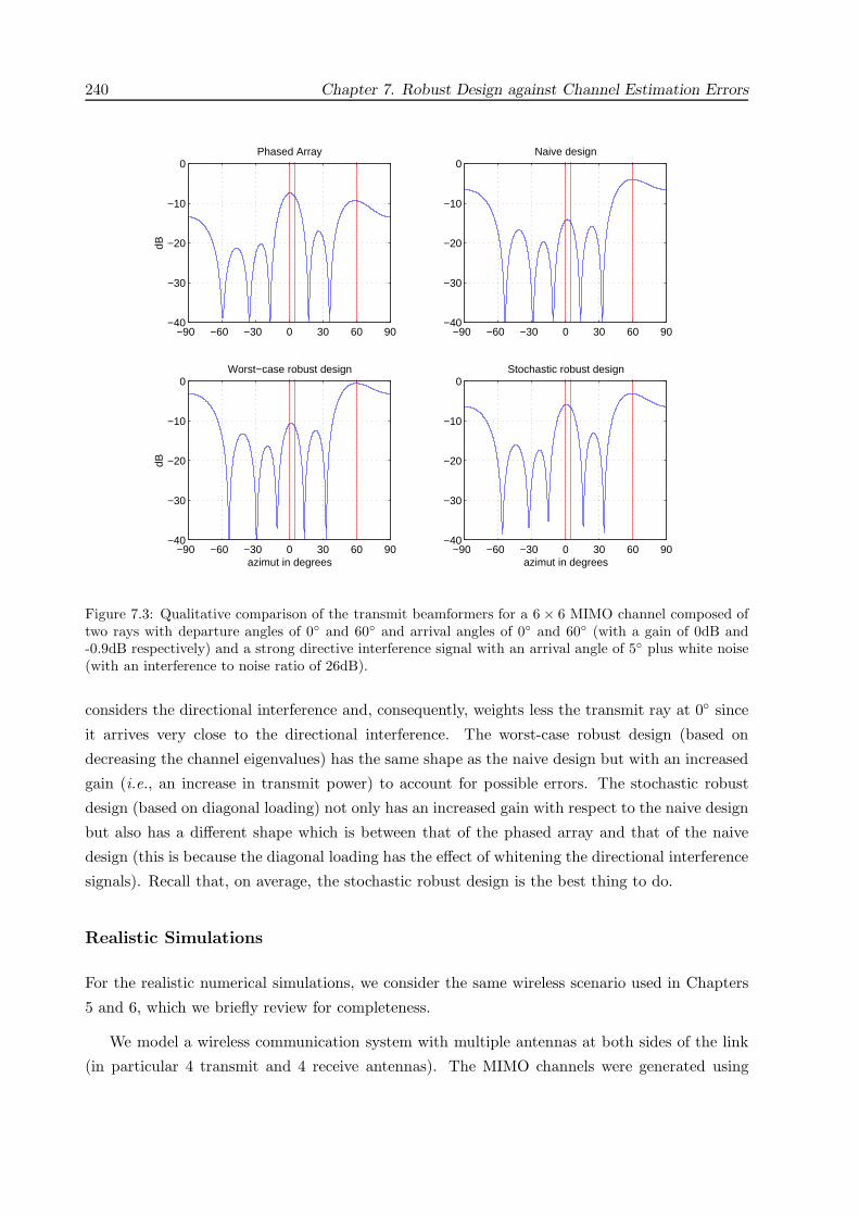
240 Chapter 7. Robust Design against Channel Estimation Errors
−90 −60 −30 0 30 60 90−40
−30
−20
−10
0Phased Array
dB
−90 −60 −30 0 30 60 90−40
−30
−20
−10
0Naive design
−90 −60 −30 0 30 60 90−40
−30
−20
−10
0Worst−case robust design
azimut in degrees
dB
−90 −60 −30 0 30 60 90−40
−30
−20
−10
0Stochastic robust design
azimut in degrees
Figure 7.3: Qualitative comparison of the transmit beamformers for a 6 × 6 MIMO channel composed oftwo rays with departure angles of 0 and 60 and arrival angles of 0 and 60 (with a gain of 0dB and-0.9dB respectively) and a strong directive interference signal with an arrival angle of 5 plus white noise(with an interference to noise ratio of 26dB).
considers the directional interference and, consequently, weights less the transmit ray at 0 since
it arrives very close to the directional interference. The worst-case robust design (based on
decreasing the channel eigenvalues) has the same shape as the naive design but with an increased
gain (i.e., an increase in transmit power) to account for possible errors. The stochastic robust
design (based on diagonal loading) not only has an increased gain with respect to the naive design
but also has a different shape which is between that of the phased array and that of the naive
design (this is because the diagonal loading has the effect of whitening the directional interference
signals). Recall that, on average, the stochastic robust design is the best thing to do.
Realistic Simulations
For the realistic numerical simulations, we consider the same wireless scenario used in Chapters
5 and 6, which we briefly review for completeness.
We model a wireless communication system with multiple antennas at both sides of the link
(in particular 4 transmit and 4 receive antennas). The MIMO channels were generated using

7.5. Simulation Results 241
the parameters of the European standard HIPERLAN/2 [ETS01] for wireless local area networks
(WLAN), which is based on the multicarrier modulation OFDM (64 carriers are used in the
simulations). The channel model includes the frequency-selectivity and the spatial correlation
as measured in real scenarios. In particular, the frequency selectivity of the channel is modeled
using the power delay profile type C for HIPERLAN/2 as specified in [ETS98a] and the spatial
correlation of the MIMO channel is modeled according to the Nokia model defined in [Sch01].
The matrix channel generated was normalized so that∑
n E [| [H(n)]ij |2] = 1. The SNR is defined
as the transmitted power normalized with the noise spectral density N0.
The estimated channel matrix contains a random estimation error drawn according to a
Gaussian pdf with zero mean and uncorrelated elements with variance σ2H = 0.01 (note that
the real channel matrix at each carrier follows a Gaussian pdf with zero-mean elements with unit
variance). The noise covariance matrix is assumed white and perfectly known.
For the worst-case robust design, the upper bound on the norm of the channel estimation
error (see (7.1)) should be chosen in a real system such that it is satisfied with high probability;
otherwise an outage event is declared.8 For an outage probability of 5%, the upper bound on the
norm should be chosen as εH √
14.6645 × σ2H for the case of 4 transmit and 4 receive antennas.
In practice, however, this value results unnecessarily high due to the pessimism inherent in all
bounds used in §7.3 to derive the worst-case design. Therefore, to overcome such excessive
pessimism, it is necessary to include in εH an additional factor αH which has to be found by
numerical simulations (its value is in general on the order of 10−3 ∼ 10−2).
Whenever the methods are evaluated for several independent realizations of the channel ma-
trix, the results are given in terms of outage values as in Chapters 5 and 6 (c.f. §2.5.4). To be
more specific, outage values of the BER refer to the BER that is guaranteed only for (1 − Pout) of
the time and outage values of the SNR refer to the SNR required in (1 − Pout) of the time (i.e.,
the SNR that will not suffice with probability Pout).
Worst-Case Robust Design with Perfect CSIR and Imperfect CSIT
In this example, we design a robust system with minimum transmit power subject to a set
of different QoS constraints in terms of BER (a carrier-noncooperative approach is taken to deal
with the multicarrier channel model). We make the approximation that perfect CSIR is available
and design a worst-case robust solution to cope with imperfect CSIT as obtained in §7.3.3. To be
specific, we consider the problem formulation of (7.19) in which a lower bound of RH (obtained
by decreasing its eigenvalues) is utilized.
In Figure 7.4, the required SNR and the obtained BER are plotted as a function of the desired
BER given as a QoS constraint for three different cases: exact design with perfect CSIT, naive
design with imperfect CSIT, and worst-case robust design against imperfect CSIT. As previously
8The worst-case performance is measured only when an outage event is not declared.
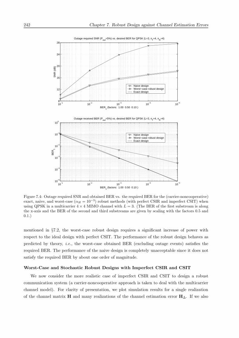
242 Chapter 7. Robust Design against Channel Estimation Errors
10−5
10−4
10−3
10−2
10−1
8
12
16
20
24
28
Outage required SNR (Pout
=5%) vs. desired BER for QPSK (L=3, nT=4, n
R=4)
BER1 (factors: 1.00 0.50 0.10 )
SN
R (
dB)
Naive design Worst−case robust designExact design
10−5
10−4
10−3
10−2
10−1
10−5
10−4
10−3
10−2
10−1
100
Outage received BER (Pout
=5%) vs. desired BER for QPSK (L=3, nT=4, n
R=4)
BER1 (factors: 1.00 0.50 0.10 )
BE
R1
Naive design Worst−case robust designExact design
Figure 7.4: Outage required SNR and obtained BER vs. the required BER for the (carrier-noncooperative)exact, naive, and worst-case (αH = 10−3) robust methods (with perfect CSIR and imperfect CSIT) whenusing QPSK in a multicarrier 4× 4 MIMO channel with L = 3. (The BER of the first substream is alongthe x-axis and the BER of the second and third substreams are given by scaling with the factors 0.5 and0.1.)
mentioned in §7.2, the worst-case robust design requires a significant increase of power with
respect to the ideal design with perfect CSIT. The performance of the robust design behaves as
predicted by theory, i.e., the worst-case obtained BER (excluding outage events) satisfies the
required BER. The performance of the naive design is completely unacceptable since it does not
satisfy the required BER by about one order of magnitude.
Worst-Case and Stochastic Robust Designs with Imperfect CSIR and CSIT
We now consider the more realistic case of imperfect CSIR and CSIT to design a robust
communication system (a carrier-noncooperative approach is taken to deal with the multicarrier
channel model). For clarity of presentation, we plot simulation results for a single realization
of the channel matrix H and many realizations of the channel estimation error H∆. If we also

7.5. Simulation Results 243
15 20 25 30 35 400
0.05
0.1
0.15
0.2
0.25
0.3
0.35
0.4
Average ARITH−MSE vs. SNR (L=3, nT=4, n
R=4)
SNR (dB)
MS
E
Naive design Stochastic (Bayesian) robust designWorst−case robust design Exact design
15 20 25 30 35 400
0.1
0.2
0.3
0.4
0.5
0.6
Worst−case ARITH−MSE vs. SNR (L=3, nT=4, n
R=4)
SNR (dB)
MS
E
Naive design Stochastic (Bayesian) robust designWorst−case robust design Exact design
Figure 7.5: Average and worst-case obtained ARITH-MSE vs. the desired MSE for the (carrier-noncooperative) exact, naive, worst-case robust (αH = 10−2), and stochastic robust methods (with imper-fect CSIR and CSIT) in a multicarrier 4 × 4 MIMO channel with L = 3.
consider many realizations of H and plot the results in terms of outage values, very similar curves
are obtained. Note that, for both the worst-case and the stochastic robust designs, the solution
is obtained by diagonal loading; the difference lies on the determination of the scaling factor ξ.9
We first consider a power-constrained system in which the objective function to minimize is
the MSE averaged over the carriers and substreams (ARITH-MSE method in §5.5.1). We derive
worst-case and stochastic robust solutions according to the problem formulation in (7.16) and
(7.34), respectively.
In Figure 7.5, the average and outage values of the ARITH-MSE are plotted as a function
9In both the worst-case and stochastic robust solutions, the value of ξ depends on B and A (in particular,
it depends on σmax (B) and σmin (A) in the worst-case design and on Tr(BBH
)in the stochastic design). This
dependence can be avoided in practice by approximating ξ using the solutions B and A obtained in the previous
block.

244 Chapter 7. Robust Design against Channel Estimation Errors
0.05 0.1 0.15 0.2 0.25 0.3 0.35 0.40
5
10
15
20
25
30
35
40
45
Required SNR vs. desired MSE (L=3, nT=4, n
R=4)
MSE
SN
R (
dB)
Naive design Stochastic (Bayesian) robust designWorst−case robust design Exact design
0.05 0.1 0.15 0.2 0.25 0.3 0.35 0.40.05
0.1
0.15
0.2
0.25
0.3
0.35
0.4
Average obtained MSE vs. desired MSE (L=3, nT=4, n
R=4)
MSE
MS
E
Naive design Stochastic (Bayesian) robust designWorst−case robust design Exact design
0.05 0.1 0.15 0.2 0.25 0.3 0.35 0.40.05
0.1
0.15
0.2
0.25
0.3
0.35
0.4
Worst−case obtained MSE vs. desired MSE (L=3, nT=4, n
R=4)
MSE
MS
E
Naive design Stochastic (Bayesian) robust designWorst−case robust design Exact design
Figure 7.6: Required SNR, average obtained MSE, and worst-case obtained MSE vs. the desired MSE forthe (carrier-noncooperative) exact, naive, worst-case robust (αH = 10−2), and stochastic robust methods(with imperfect CSIR and CSIT) in a multicarrier 4 × 4 MIMO channel with L = 3.
7.6. Chapter Summary and Conclusions 245
of the SNR for four different cases: exact design, naive design, worst-case robust design, and
stochastic robust design. We can observe that the stochastic robust design has the best average
performance, as expected, among the three methods with imperfect CSIT and CSIR. The best
worst-case performance, as predicted by theory, is obtained by the worst-case robust design.
However, the worst-case robust approach requires the determination of the additional factor αH
for a fine tuning of the scaling factor ξ used in the diagonal loading. If ξ is not well chosen,
the performance degrades significantly. Hence, the worst-case approach is not recommended in
practice.
It is also worth pointing out that all methods with imperfect CSI suffer from an MSE floor as
can be observed in Figure 7.5, unlike the exact design with perfect CSI whose performance can
be as good as desired by increasing the transmit power. For the stochastic robust design, it is
straightforward to obtain the value of the average MSE floor as E → Efl (I+ 1
σ2HBHHHHB
)−1
as PT → ∞, where B is the normalized transmit matrix defined as B = B/√
Tr(BBH
). The
optimal B is obtained as the solution to the minimization of Tr(Efl
)subject to Tr
(BBH) ≤ 1.
We then consider a QoS-constrained system with minimum transmit power subject to a set
of QoS requirements in terms of MSE. We derive worst-case and stochastic robust solutions
according to the problem formulation in (7.22) and (7.37), respectively.
In Figure 7.6, the required SNR, the obtained average MSE, and the obtained worst-case MSE
are plotted as a function of the desired MSE for four different cases: exact design, naive design,
worst-case robust design, and stochastic robust design. We can observe that the stochastic robust
design needs, in general, less than 3dB more transmit power than the exact design with perfect
CSI. The worst-case robust design, however, requires significantly much more power. The MSE
achieved by the stochastic robust design is, on average, the desired MSE as expected from the
analytical derivations; however, nothing can be guaranteed for the worst-case MSE. As predicted
by theory, the worst-case MSE is satisfied by the worst-case robust design (provided that the
scaling factor ξ used in the diagonal loading is properly chosen by numerical simulations). The
worst-case approach, however, is not recommended for practical purposes due to its sensitivity to
the exact value of ξ and to the excessive increase of required transmit power.
7.6 Chapter Summary and Conclusions
This chapter has considered the omnipresent problem of channel estimation errors in practical
communication systems. The problem formulation of Chapters 5 and 6, where perfect CSI was
assumed, has been extended to account for imperfect CSI, obtaining robust designs. Two different
philosophies have been considered: the worst-case and the stochastic (Bayesian) robust designs.
In particular, a robust formulation of the joint transmit-receive design for power-constrained

246 Chapter 7. Robust Design against Channel Estimation Errors
and QoS-constrained systems has been given under both philosophies. For the worst-case robust
approach, the problem has been easily formulated by using some bounds on the channel and
the noise covariance matrices. For the stochastic robust design, the general problem has been
formulated in a rather general framework, although simple results have been obtained only for
some particular cases such as when the trace of the MSE matrix is the objective to minimize or
when QoS constraints in terms of MSE are imposed. In both cases, the stochastic robust design
translates into the well-known trick of adding a small scaled identity matrix to the estimated
noise covariance matrix (although a different result would be obtained if a structured estimation
error was considered).
The analytical derivations have been checked by numerical simulations using realistic channel
models. The robust designs manage to perform well under channel estimation errors due to their
robustness (although they also show a limited performance). For power-constrained systems,
the robust solutions perform better than the naive solution with the same transmit power. For
QoS-constrained systems, the robust solutions satisfy the QoS requirements at the expense of an
increased transmit power with respect to the exact design with perfect CSI, which is the price to
be paid for robustness. In general terms, the worst-case philosophy has been found impractical
due to its sensitivity with respect to exact choice of its parameters and, therefore, the stochastic
philosophy is considered as the most appropriate solution in practice.
The contribution of this chapter has been the application of the well-known worst-case and
stochastic philosophies to obtain robust designs within the framework used in Chapters 5 and 6.
Appendix 7.A Proof of Lemma 7.1
The inequality XXH ≤ λmax
(XXH
)In is straightforward from the definition of maximum eigen-
value as we now show. Consider that cHXXHc >λmax
(XXH
)cHc for some c. This would imply
that λmax
(XXH
)< cHXXHc/cHc which cannot be since the maximum eigenvalue is defined as
λmax
(XXH
)= max
ccHXXHc/cHc.
The inequality XYH + YXH ≤ 2σmax (X) σmax (Y) In can be proved by showing that
cH(XYH + YXH
)c ≤ 2σmax (X) σmax (Y) cHc ∀c.

7.B Proof of Lemma 7.2 247
We can now establish the following chain of inequalities:
cH(XYH + YXH
)c = 2Re
[cHXYHc
]≤ 2∣∣cHXYHc
∣∣≤ 2∥∥XHc
∥∥2
∥∥YHc∥∥
2
= 2√
cHXXHc√
cHYYHc
≤ 2λ1/2max
(XXH
)λ1/2
max
(YYH
)cHc
= 2σmax (X)σmax (Y) cHc
where the second inequality follows from the Cauchy-Schwarz’s inequality (see §3.3) and the third
inequality from XXH ≤ λmax
(XXH
)In and YYH ≤ λmax
(YYH
)In.
Appendix 7.B Proof of Lemma 7.2
We first obtain a lemma and then proceed to prove Lemma 7.2.
Lemma 7.3 Let H ∈CI n×m be a random matrix with i.i.d. proper Gaussian-distributed entries
with zero mean and variance σ2, i.e., [H]ij ∼CN (0, σ2). Then, for any fixed unitary matrix
U ∈CI m×m, the distribution of HU is the same as the distribution of H, i.e., HU ∼ H.
Proof. Let G = HU. Since the rows of H are independent, the rows of G are also independent.
It remains to check that each row of G has the same distribution as that of H. Since the rows
of H are proper complex Gaussian vectors, so are those of G. Therefore, only the first and
second moments have to be compared. Let gHi and hH
i be the ith row of G and H, respectively
(gHi = hH
i U). It is clear that the first moment is equal: E [gi] = UHE [hi] = 0. The second
moment follows easily as well: E[gig
Hi
]= UH
E[hih
Hi
]U = UHU = I.
Proof of Lemma 7.2. First of all, note that
EH|H[HBBHHH
]= EH∆
[(H + H∆)BBH(H + H∆)H ]
= HBBHHH+EH∆
[H∆BBHHH
∆
]
where h∆ vec (H∆) has zero mean E [h∆] = 0 and covariance matrix E[h∆hH
∆
]= σ2
H I. It
remains to show that EH∆
[H∆BBHHH
∆
]= σ2
H Tr(BBH
)I.
248 Chapter 7. Robust Design against Channel Estimation Errors
From Lemma 7.3 and using the eigendecomposition BBH = UDBUH , it follows that
EH∆
[H∆BBHHH
∆
]= EH∆
[H∆DBHH
∆
]. We then have that
[EH∆
[H∆DBHH
∆
]]ij
=∑
k
λB,k EH∆
[[H∆]i,k
[HH
∆
]k,j
]= 0 for i = j
[EH∆
[H∆DBHH
∆
]]ii
=∑
k
λB,k EH∆
[∣∣ [H∆]i,k∣∣2]
= σ2H
∑k
λB,k
= σ2H Tr
(BBH
).
Chapter 8
Conclusions and Future Work
THIS DISSERTATION HAS CONSIDERED communications through MIMO channels
which includes many specific scenarios such as wireless multi-antenna systems and wireline
DSL systems. Both information-theoretic and practical communications aspects of MIMO
channels have been analyzed. For the former, the fundamental limits of MIMO channels with
different degrees of CSI have been studied; specifically, for the case of no CSI, a game-theoretic
approach was adopted to obtain robust solutions under channel uncertainty. For the latter,
an optimal joint design of the transmitter and receiver has been analyzed in detail. First,
power-constrained systems were considered and a unified framework was developed to obtain the
optimal transmit-receive structure for a wide family of design criteria. Then, QoS-constrained
systems were studied and the optimal design with minimum transmitted power was obtained.
These results, which were initially obtained for the case of perfect CSI, were later extended to
account for imperfect CSI due, for example, to channel estimation errors.
8.1 Conclusions
After giving the motivation of the dissertation in Chapter 1, an overview of MIMO channels has
been given in Chapter 2 and two important theories on which many results of this dissertation are
based, namely, convex optimization theory and majorization theory, have been briefly described
in Chapter 3.
Chapter 4 has focused on the information-theoretic analysis of MIMO channels with different
degrees of CSI for the single-user and mutiuser (multiple-access channel) cases. After reviewing
the well-known cases of instantaneous and statistic CSI (beamforming-constrained systems were
specifically addressed), the case in which not even the channel statistics are known was investi-
gated in great detail to obtain robust solutions under channel uncertainty. To be specific, the
problem was formulated within the framework of game theory in which the payoff function of
249
250 Chapter 8. Conclusions and Future Work
the game is the mutual information and the players are the transmitter and a malicious nature.
This problem characterizes the capacity of the compound vector Gaussian channel. The uniform
power allocation was obtained as a robust solution to the game in terms of capacity for the class
of isotropically unconstrained channels (unconstrained transmit “directions”). Interestingly, for
the multiple-access channel, the uniform power allocation for each of the users also constitutes a
robust solution (the worst-case rate region corresponding to the uniform power distribution was
shown to contain the worst-case rate region of any other possible power allocation strategy). In
other words, the capacity region of the compound vector Gaussian MAC is achieved when each
of the users is using a uniform power allocation.
Chapter 5 has formulated and solved the joint design of transmit and receive linear processing
(also termed multiple beamvectors or beam-matrices) for MIMO channels (only point-to-point
communications were considered) under a variety of design criteria subject to a power constraint.
Instead of considering each design criterion separately, a unifying framework that generalizes the
existing results in the literature was developed by considering two families of objective functions
that embrace most reasonable criteria to design a communication system: Schur-concave and
Schur-convex functions. Under such a framework, the optimal structure of the transmitter and
receiver is readily obtained and the problem can be then formulated within the powerful frame-
work of convex optimization theory, in which solutions can be efficiently obtained even though
closed-form expressions may not exist. From this perspective, different design criteria were ana-
lyzed and, in particular, a closed-form optimal solution in terms of minimum BER was obtained.
Efficient algorithms for practical implementation were given for the considered design criteria.
Chapter 6 has formulated and solved the joint design of transmit and receive linear pro-
cessing for MIMO channels (only point-to-point communications were considered) in terms of
minimum transmitted power subject to QoS constraints for each of the established substreams.
Although the original problem formulation was a complicated nonconvex problem with matrix-
valued variables, by using majorization theory, the problem was reformulated as a simple convex
optimization problem with scalar variables. To solve optimally the convex problem in practice, a
practical and efficient multi-level water-filling algorithm was obtained.
Chapter 7 has extended the results of Chapters 5 and 6, in which perfect CSI was assumed,
to the more realistic situation of imperfect CSI due to channel estimation errors. Two different
philosophies were used to obtain robust designs: worst-case robustness and stochastic (Bayesian)
robustness.
Summarizing, the main results obtained in this dissertation are:
• the game-theoretic formulation of the communication process, obtaining the uniform power
allocation as a robust solution under channel uncertainty,
• the unifying framework for the joint transmit-receive design that generalizes the existing re-
8.2. Future Work 251
sults in the literature by considering two families of functions that embrace most reasonable
design criteria (and, in particular, the closed-form solution in terms of minimum BER), and
• the optimum solution in terms of minimum transmitted power subject to a set of QoS
constraints.
8.2 Future Work
As a result of the work undertaken during the elaboration of the present dissertation, several lines
for future research have been singled out to extend the obtained results as we now mention.
Regarding the capacity results of Chapter 4, some open problems are:
• Obtaining an iterative method (similar to the iterative water-filling algorithm [Yu01b]) to
solve the maximization of the sum rate of the beamforming-constrained MAC of (4.17).
• Obtaining a simple iterative method to maximize an arbitrary weighted sum of the rates
(generalizing the iterative water-filling algorithm that maximizes the sum rate of (4.16) as
obtained in [Yu01b]).
• Characterizing the optimal transmit covariance matrix in terms of outage capacity for the
simple case of a Gaussian-distributed channel matrix with i.i.d. elements.
With respect to the joint transmit-receive design for MIMO channels, some interesting prob-
lems are:
• Extending the ARITH-BER method of §5.5.11 to include different constellations.
• Generalizing the unified framework of Theorem 5.1 to include a DF scheme and/or a peak-
power constraint.
• Performing an analytic characterization of the performance of the different criteria of Chap-
ter 5 (rather than using numerical simulations as a means of assessment and comparison).
• Further investigation along the line of Chapter 7 to obtain robust designs; in particular, an
analytical characterization of the performance under channel estimation errors.
• Extension of the obtained results in the joint transmit-receive design to the multiuser case.
The downlink of a multiuser wireless system (broadcast channel) not only requires the
design of the transmit and receive matrices for all the users but also has to allocate the total
available power among the users. This is currently an open problem in the literature since it
is a highly nonconvex and complicated problem. The uplink of a multiuser wireless system

252 Chapter 8. Conclusions and Future Work
(multiple-access channel) may be solved in a centralized way as the downlink. It seems
more natural, however, to consider distributed solutions that do not require a significant
user cooperation. Such an approach fits naturally within the framework of game theory in
which each user could be considered as a player in a game with multiple players. In any
case, both centralized and distributed problem formulations are currently open problems.
Bibliography
[3GP99] 3GPP, “Physical layer procedures (TDD),” 3G TS 25.224 (v3.1.1), TSGR,http://www.3gpp.org , Dec. 1999.
[AD96] N. Al-Dhahir and J. M. Cioffi, “Block transmission over dispersive channels: Transmitfilter optimization and realization, and MMSE-DFE receiver performance,” IEEETrans. on Information Theory , vol. 42, no. 1, pp. 137–160, Jan. 1996.
[AD00] N. Al-Dhahir and A. H. Sayed, “The finite-length multi-input multi-output MMSE-DFE,” IEEE Trans. on Signal Processing , vol. 48, no. 10, pp. 2921–2936, Oct. 2000.
[Aka98] A. N. Akansu, P. Duhamel, X. Lin, and M. de Courville, “Orthogonal transmultiplexersin communication: A review,” IEEE Trans. on Signal Processing , vol. 46, no. 4, pp.979–995, April 1998.
[Ala98] S. M. Alamouti, “A simple transmit diversity technique for wireless communications,”IEEE Journal on Selected Areas in Communications, vol. 16, no. 8, pp. 1451–1458,Oct. 1998.
[Ami84] N. Amitay and J. Salz, “Linear equalization theory in digital data transmission overdually polarized fading radio channels,” At&T Bell Labs. Technical Journal , vol. 63,no. 10, pp. 2215–2259, Dec. 1984.
[And00] J. B. Andersen, “Array gain and capacity for known random channels with multipleelement arrays at both ends,” IEEE Journal on Selected Areas in Communications,vol. 18, no. 11, pp. 2172–2178, Nov. 2000.
[Ari99] S. L. Ariyavisitakul, J. H. Winters, and I. Lee, “Optimum space-time processors withdispersive interference: Unified analysis and required filter span,” IEEE Trans. onCommunications, vol. 47, no. 7, pp. 1073–1083, July 1999.
[Ari00] S. L. Ariyavisitakul, “Turbo space-time processing to improve wireless channel capac-ity,” IEEE Trans. on Communications, vol. 48, no. 8, pp. 1347–1359, Aug. 2000.
[Bal92] P. Balaban and J. Salz, “Optimum diversity combining and equalization in digital datatransmission with applications to cellular mobile radio. Part I: Theoretical considera-tions, and Part II: Numerical results,” IEEE Trans. on Communications, vol. 40, no.5, pp. 885–894, 895–907, May 1992.
[Bar01] S. Barbarossa and A. Scaglione, “Time-varying fading channels,” in Signal ProcessingAdvances in Wireless and Mobile Communications - Volume II: Trends in Single- andMulti-User Systems, G. Giannakis, Y. Hua, P. Stoica, and L. Tong, Eds., chapter 1.Prentice Hall, Inc., Upper Saddle River, NJ, 2001.
253

254 Bibliography
[Bas83] T. Basar, “The Gaussian test channel with an intelligent jammer,” IEEE Trans. onInformation Theory , vol. IT-29, no. 1, pp. 152–157, Jan. 1983.
[Bel00] K. L. Bell, Y. Ephraim, and H. L. V. Trees, “A Bayesian approach to robust adaptivebeamforming,” IEEE Trans. on Signal Processing , vol. 48, no. 2, pp. 386–398, Feb.2000.
[Ben99] M. Bengtsson and B. Ottersten, “Optimal downlink beamforming using semidefiniteoptimization,” in Proc. 37th Annual Allerton Conference on Communication, Control,and Computing , pp. 987–996, Allerton House, Monticello, IL, Sept. 22-24, 1999.
[Ben01] M. Bengtsson and B. Ottersten, “Optimal and suboptimal transmit beamforming,” inHandbook of Antennas in Wireless Communications, L. C. Godara, Ed. CRC Press,2001.
[Ben02] M. Bengtsson, “A pragmatic approach to multi-user spatial multiplexing,” in Proc.2nd IEEE Sensor Array and Multichannel Signal Processing Workshop (SAM-2002),Rosslyn, VA, Aug. 4-6, 2002.
[Ber67] T. Berger and D. W. Tufts, “Optimum pulse amplitude modulation. Part I:Transmitter-receiver design and bounds from information theory,” IEEE Trans. onInformation Theory , vol. IT-13, no. 2, pp. 196–208, April 1967.
[Big98] E. Biglieri, J. Proakis, and S. Shamai, “Fading channels: Information-theoretic andcommunications aspects,” IEEE Trans. on Information Theory , vol. 44, no. 6, pp.2619–2691, Oct. 1998.
[Big01] E. Biglieri, G. Caire, and G. Taricco, “Limiting performance of block-fading channelswith multiple antennas,” IEEE Trans. on Information Theory , vol. 47, no. 4, pp.1273–1289, May 2001.
[Bin90] J. A. C. Bingham, “Multicarrier modulation for data transmission: An idea whosetime has come,” IEEE Communication Magazine, vol. 28, no. 5, pp. 5–14, May 1990.
[Bol02] H. Bolcskei and A. J. Paulraj, “Multiple-input multiple-output (MIMO) wireless sys-tems,” in The Communications Handbook , J. Gibson, Ed., pp. 90.1–90.14. CRC Press,2nd edition, 2002.
[Bla57] N. M. Blachman, “Communication as a game,” in Proc. IRE WESCON Conference,pp. 61–66, Aug. 1957.
[Bla87] R. E. Blahut, Principles and Practice of Information Theory, Addison-Wesley, Read-ing, MA, 1987.
[Bor85] J. M. Borden, D. M. Mason, and R. J. McEliece, “Some information theoretic saddle-points,” SIAM J. Control and Optimization, vol. 23, no. 1, pp. 129–143, Jan. 1985.
[Boy00] S. Boyd and L. Vandenberghe, Introduction to Convex Optimization with Engineer-ing Applications, Course Notes (available at http://www.stanford.edu/class/ee364).Stanford University, 2000.
[Bra74] L. H. Brandenburg and A. D. Wyner, “Capacity of the Gaussian channel with memory:The multivariate case,” The Bell System Technical Journal , vol. 53, no. 5, pp. 745–778,May-June 1974.

Bibliography 255
[Bra83] D. H. Brandwood, “A complex gradient operator and its application in adaptive arraytheory,” IEE Proc., vol. 130, no. 1, pp. 11–16, Feb. 1983.
[Cai99a] G. Caire and S. Shamai, “On the capacity of some channels with channel state infor-mation,” IEEE Trans. on Information Theory , vol. 45, no. 6, pp. 2007–2019, Sept.1999.
[Cai99b] G. Caire, G. Taricco, and E. Biglieri, “Optimum power control over fading channels,”IEEE Trans. on Information Theory , vol. 45, no. 5, pp. 1468–1489, July 1999.
[Cal98] A. R. Calderbank, “The art of signaling: Fifty years of coding theory,” IEEE Trans.on Information Theory , vol. 44, no. 6, pp. 2561–2595, Oct. 1998.
[Car88] B. D. Carlson, “Covariance matrix estimation errors and diagonal loading in adaptivearrays,” IEEE Trans. on Aerospace and Electronic Systems, vol. 24, no. 4, pp. 397–401,July 1988.
[Cha02a] S. S. Chan, T. N. Davidson, and K. M. Wong, “Asymptotically minimum bit errorrate block precoders for minimum mean square error equalization,” in Proc. 2nd IEEESensor Array and Multichannel Signal Processing Workshop (SAM-2002), pp. 140–144,Rosslyn, VA, Aug. 4-6, 2002.
[Cha02b] J.-H. Chang, L. Tassiulas, and F. Rashid-Farrokhi, “Joint transmitter receiver diversityfor efficient space division multiaccess,” IEEE Trans. on Wireless Communications,vol. 1, no. 1, pp. 16–27, Jan. 2002.
[Chi01] N. Chiurtu, B. Rimoldi, and E. Telatar, “On the capacity of multi-antenna Gaus-sian channels,” in Proc. IEEE International Symposium on Information Theory (ISIT2001), p. 53, Washington, DC, June 24-29, 2001.
[Cho93] P. S. Chow, “Bandwidth optimized digital transmission techniques for spectrallyshaped channels with impulse noise,” Ph.D. dissertation, Stanford University, Stanford,CA, May 1993.
[Cho02] K. Cho and D. Yoon, “On the general BER expression of one- and two-dimensionalamplitude modulations,” IEEE Trans. on Communications, vol. 50, no. 7, pp. 1074–1080, July 2002.
[Chu02] C.-N. Chuah, D. Tse, J. M. Kahn, and R. A. Valenzuela, “Capacity scaling in dual-antenna-array wireless systems,” IEEE Trans. on Information Theory , vol. 48, pp.637–650, March 2002.
[Cio95a] J. M. Cioffi, G. P. Dudevoir, M. V. Eyuboglu, and G. D. Forney, “MMSE decision-feedback equalizers and coding - Part I: Equalization results,” IEEE Trans. on Com-munications, vol. 43, no. 10, pp. 2582–2594, Oct. 1995.
[Cio95b] J. M. Cioffi, G. P. Dudevoir, M. V. Eyuboglu, and G. D. Forney, “MMSE decision-feedback equalizers and coding - Part II: Coding results,” IEEE Trans. on Communi-cations, vol. 43, no. 10, pp. 2595–2604, Oct. 1995.
[Cio97] J. M. Cioffi and G. D. Forney, “Generalized decision-feedback equalization for packettransmission with ISI and Gaussian noise,” in Communications, Computation, Con-trol and Signal Processing , A. Paulraj, V. Roychowdhury, and C. D. Schaper, Eds.,chapter 4. Kluwer Academic Publishers, Boston, MA, 1997.

256 Bibliography
[Cov91a] T. Cover, “Universal portfolios,” Mathematical Finance, vol. 1, no. 1, pp. 1–29, Jan.1991.
[Cov91b] T. M. Cover and J. A. Thomas, Elements of Information Theory , Wiley, New York,1991.
[Cox87] H. Cox, R. M. Zeskind, and M. M. Owen, “Robust adaptive beamforming,” IEEETrans. on Acoustics, Speech, and Signal Processing , vol. ASSP-35, no. 10, pp. 1365–1376, Oct. 1987.
[Csi81] I. Csiszar and J. Korner, Information Theory: Coding Theorems for Discrete Memo-ryless Systems, Academic Press, New York, 1981.
[Dav02] T. N. Davidson, Z.-Q. Luo, and J. F. Sturm, “Linear matrix inequality formulationof spectral mask constraints with applications to FIR filter design,” IEEE Trans. onSignal Processing , vol. 50, no. 11, pp. 2702–2715, Nov. 2002.
[Dig01] S. N. Diggavi and T. M. Cover, “The worst additive noise under a covariance con-straint,” IEEE Trans. on Information Theory , vol. 47, no. 7, pp. 3072–3081, Nov.2001.
[Din02] Y. Ding, T. N. Davidson, J.-K. Zhang, Z.-Q. Luo, and K. M. Wong, “Minimum BERprecoders for zero-forcing equalization,” in Proc. 2002 IEEE Int. Conf. on Acoustics,Speech, and Signal Proc. (ICASSP’02), Orlando, Florida, May 2002.
[Din03a] Y. Ding, T. N. Davidson, Z.-Q. Luo, and K. M. Wong, “Minimum BER block precodersfor zero-forcing equalization,” IEEE Trans. on Signal Processing , to appear 2003.
[Din03b] Y. Ding, T. N. Davidson, and K. M. Wong, “On improving the BER performance ofrate-adaptive block-by-block transceivers with applications to DMT,” in Proc. IEEE2003 Global Communications Conference (GLOBECOM-2003), San Francisco, CA,submitted, Dec. 1-5, 2003.
[ETS98a] ETSI, “Channel models for HIPERLAN/2 in different indoor scenarios,” ETSI EPBRAN 3ERI085B , pp. 1–8, March 1998.
[ETS98b] ETSI, “Selection Procedures for the Choice of Radio Transmission Technologies of theUMTS (UMTS 30.03),” Tech. Rep. TR101 112, v3.2.0,ETSI , 1998.
[ETS01] ETSI, “Broadband radio access networks (BRAN); HIPERLAN type 2; physical (PHY)layer,” ETSI TS 101 475 V1.2.2 , pp. 1–41, Feb. 2001.
[Fan02] J. L. Fang, “Modeling and characterization of copper access systems,” Ph.D. disser-tation, Stanford University, Stanford, CA, Dec. 2002.
[Fos96] G. J. Foschini, “Layered space-time architecture for wireless communication in a fadingenvironment when using multi-element antennas,” Bell Labs Technical Journal , vol. 1,no. 2, pp. 41–59, Autumn 1996.
[Fos98] G. Foschini and M. Gans, “On limits of wireless communications in a fading environ-ment when using multiple antennas,” Wireless Personal Communications, vol. 6, pp.311–335, 1998.

Bibliography 257
[Fos99] G. J. Foschini, G. D. Golden, R. A. Valenzuela, and P. W. Wolniansky, “Simplifiedprocessing for high spectral efficiency wireless communication employing multi-elementarrays,” IEEE Journal on Selected Areas in Comm., vol. 17, no. 11, pp. 1841–1852,Nov. 1999.
[Fud92] D. Fudenberg and J. Tirole, Game Theory , MIT Press, Cambridge, MA, 1992.
[Gal68] R. G. Gallager, Information Theory and Reliable Communication, John Wiley & Sons,Inc., USA, 1968.
[Gan00a] G. Ganesan and P. Stoica, “Space-time diversity,” in Signal Processing Advances inCommunication, G. Giannakis, Y. Hua, P. Stoica, and L. Tong, Eds., pp. 79–127.Prentice Hall, Upper Saddle River, NJ, 2000.
[Gan00b] G. Ganesan and P. Stoica, “Space-time diversity using orthogonal and amicable or-thogonal designs,” in Proc. 2000 IEEE Int. Conf. on Acoustics, Speech, and SignalProc. (ICASSP’00), vol. 5, pp. 2561–2564, Istanbul, Turkey, June 5-9, 2000.
[Gan01a] G. Ganesan and P. Stoica, “Space-time block codes: A maximum SNR approach,”IEEE Trans. on Information Theory , vol. 47, no. 4, pp. 1650–1656, May 2001.
[Gan01b] G. Ganesan and P. Stoica, “Utilizing space-time diversity for wireless communications,”Wireless Personal Communications, vol. 18, pp. 149–163, 2001.
[GDF72] J. G. David Forney, “Maximum-likelihood sequence estimation of digital sequence inthe presence of intersymbol interference,” IEEE Trans. on Information Theory , vol.IT-18, no. 3, pp. 363–378, May 1972.
[GDF91] J. G. David Forney and M. V. Eyuboglu, “Combined equalization and coding usingprecoding,” IEEE Communications Magazine, vol. 29, no. 12, pp. 25–34, Dec. 1991.
[Ges02] D. Gesbert, H. Bolcskei, D. A. Gore, and A. J. Paulraj, “Outdoor MIMO wirelesschannels: Models and performance prediction,” IEEE Trans. on Communications,vol. 50, no. 12, pp. 1926–1934, Dec. 2002.
[Gin02] G. Ginis and J. Cioffi, “Vectored transmission for digital subscriber line systems,”IEEE Journal on Selected Areas in Communications (special issue on Twisted PairTransmission), vol. 20, no. 5, pp. 1085–1104, June 2002.
[Goe99] D. L. Goeckel, “Adaptive coding for time-varying channels using outdated fadingestimates,” IEEE Trans. on Communications, vol. 47, no. 6, pp. 844–855, June 1999.
[Gol96] G. H. Golub and C. F. V. Loan, Matrix Computations, The Johns Hopkins UniversityPress, Baltimore, MD, 1996.
[Gol97] A. J. Goldsmith and P. P. Varaiya, “Capacity of fading channels with channel sideinformation,” IEEE Trans. on Information Theory , vol. 43, no. 6, pp. 1986–1992, Nov.1997.
[Gra72] R. M. Gray, “On the asymptotic eigenvalue distribution of Toeplitz matrices,” IEEETrans. on Information Theory , vol. IT-18, no. 6, pp. 725–730, Nov. 1972.
[Han98] S. V. Hanly and D. N. C. Tse, “Multiaccess fading channels - Part II: Delay-limitedcapacities,” IEEE Trans. on Information Theory , vol. 44, no. 7, pp. 2816–2831, Nov.1998.

258 Bibliography
[Hir88] W. Hirt and J. L. Massey, “Capacity of the discrete-time gaussian channel with inter-symbol interference,” IEEE Trans. on Information Theory , vol. 34, no. 3, pp. 380–388,May 1988.
[Hir92] A. Hiroike, F. Adachi, and N. Nakajima, “Combined effects of phase sweeping trans-mitter diversity and channel coding,” IEEE Trans. on Vehicular Technology , vol. 41,no. 2, pp. 170–176, May 1992.
[Hoc00a] B. M. Hochwald and T. L. Marzetta, “Unitary space-time modulation for multiple-antenna communications in rayleigh flat fading,” IEEE Trans. on Information Theory ,vol. 46, no. 2, pp. 543–564, March 2000.
[Hoc00b] B. M. Hochwald and W. Sweldens, “Differential unitary space-time modulation,” IEEETrans. on Communications, vol. 48, no. 12, pp. 2041–2052, Dec. 2000.
[Hon90] M. L. Honig, K. Steiglitz, and B. Gopinath, “Multichannel signal processing for datacommunications in the presence of crosstalk,” IEEE Trans. on Communications, vol.38, no. 4, pp. 551–558, April 1990.
[Hon92] M. L. Honig, P. Crespo, and K. Steiglitz, “Suppression of near- and far-end crosstalkby linear pre- and post-filtering,” IEEE Journal on Selected Areas in Communications,vol. 10, no. 3, pp. 614–629, April 1992.
[Hon03] Z. Hong, K. Liu, R. H. Jr, and A. Sayeed, “Spatial multiplexing in correlated fadingvia the virtual channel representation,” IEEE Journal on Selected Areas in Communi-cations: Special Issue on MIMO Systems and Applications, vol. 21, no. 5, pp. 856–866,June 2003.
[Hor85] R. A. Horn and C. R. Johnson, Matrix Analysis, Cambridge University Press, NewYork, 1985.
[Hug88] B. Hughes and P. Narayan, “The capacity of a vector Gaussian arbitrarily varyingchannel,” IEEE Trans. on Information Theory , vol. 34, no. 5, pp. 995–1003, Sept.1988.
[IEE99] IEEE, “Part 11: wireless LAN medium access control (MAC) and physical layer(PHY),” IEEE Std 802.11a, Dec. 1999.
[Ise01] A. P. Iserte, A. I. Perez-Neira, and M. A. Lagunas, “Pre- and post-beamforming inMIMO channels applied to HIPERLAN/2 and OFDM,” in Proc. IST Mobile Commu-nications Summit , pp. 3–8, Barcelona, Spain, Sept. 2001.
[Ise02] A. P. Iserte, A. I. Perez-Neira, and M. A. Lagunas, “Joint beamforming strategies inOFDM-MIMO systems,” in Proc. IEEE Int. Conf. on Acoustics, Speech and SignalProcessing (ICASSP 2002), Orlando, Florida, May 2002.
[Ise03] A. P. Iserte, M. A. Lagunas, and A. I. Perez-Neira, “Robust power allocation for min-imum BER in a SISO-OFDM system,” in Proc. IEEE 2003 International Conferenceon Communications (ICC 2003), vol. 2, pp. 1263–1267, Anchorage, AK, May 11-15,2003.
[Ivr03] M. T. Ivrlac, W. Utschick, and J. A. Nossek, “Fading correlations in wireless MIMOcommunication systems,” IEEE Journal on Selected Areas in Communications: SpecialIssue on MIMO Systems and Applications, vol. 21, no. 5, June 2003.
Bibliography 259
[Jaf01] S. A. Jafar and A. Goldsmith, “On optimality of beamforming for multiple antennasystems with imperfect feedback,” in Proc. IEEE International Symposium on Infor-mation Theory (ISIT 2001), p. 321, Washington, DC, June 24-29, 2001.
[Jon02] G. Jongren, M. Skoglund, and B. Ottersen, “Combining beamforming and orthogonalspace-time block coding,” IEEE Trans. on Information Theory , vol. 48, no. 3, pp.611–627, March 2002.
[Jun95] P. Jung and J. Blanz, “Joint detection with coherent receiver antenna diversity inCDMA mobile radio systems,” IEEE Trans. on Vehicular Technology , vol. 44, no. 1,pp. 76–88, Feb. 1995.
[Kal89] I. Kalet, “The multitone channel,” IEEE Trans. on Communications, vol. 37, no. 2,pp. 119–124, Feb. 1989.
[Kan02] S. Kandukuri and S. Boyd, “Optimal power control in interference-limited fading wire-less channels with outage-probability specifications,” IEEE Transactions on WirelessCommunications, vol. 1, no. 1, pp. 46–55, Jan. 2002.
[Kas85] S. A. Kassam and V. Poor, “Robust techniques for signal processing: A survey,” Proc.of the IEEE , vol. 73, no. 3, pp. 433–481, March 1985.
[Kas90] S. Kasturia, J. T. Aslanis, and J. M. Cioffi, “Vector coding for partial response chan-nels,” IEEE Trans. on Information Theory , vol. 36, no. 4, pp. 741–762, July 1990.
[Kav85] M. Kavehrad and J. Salz, “Cross-polarization cancellation and equalization in dig-ital transmission over dually polarized multipath fading channels,” At&T TechnicalJournal , vol. 64, no. 10, pp. 2211–2245, Dec. 1985.
[Kay93] S. M. Kay, Fundamentals of Statistical Signal Processing: Estimation Theory, PrenticeHall International, Inc., Englewood Cliffs, NJ, 1993.
[Kle96] A. Klein, G. K. Kaleh, and P. W. Baier, “Zero forcing and minimum mean-square-errorequalization for multiuser detection in code-division multiple-access channels,” IEEETrans. on Vehicular Technology , vol. 45, no. 2, pp. 276–287, May 1996.
[Kri96] H. Krim and M. Viberg, “Two decades of array signal processing research,” IEEESignal Processing Magazine, vol. 13, no. 4, pp. 67–94, July 1996.
[Lag00] M. A. Lagunas, J. Vidal, and A. Perez-Neira, “Joint array combining and MLSEfor single-user receivers in multipath Gaussian multiuser channels,” IEEE Journal onSelected Areas in Communications, vol. 18, no. 11, pp. 2252–2259, Nov. 2000.
[Lan69] P. Lancaster, Theory of Matrices, Academic Press, New York, 1969.
[Lap98] A. Lapidoth and P. Narayan, “Reliable communication under channel uncertainty,”IEEE Trans. on Information Theory , vol. 44, no. 6, pp. 2148–2177, Oct. 1998.
[Leb97] H. Lebret and S. Boyd, “Antenna array pattern synthesis via convex optimization,”IEEE Trans. on Signal Processing , vol. 45, no. 3, pp. 526–532, March 1997.
[Lee76] K. H. Lee and D. P. Petersen, “Optimal linear coding for vector channels,” IEEETrans. on Communications, vol. COM-24, no. 12, pp. 1283–1290, Dec. 1976.

260 Bibliography
[Liu96] H. Liu, G. Xu, L. Tong, and T. Kailath, “Recent developments in blind channelequalization: From cyclostationarity to subspaces,” Signal Processing , vol. 50, no. 1-2,pp. 83–99, April 1996.
[Liu02] K. Liu and A. M. Sayeed, “Space-time D-block codes via the virtual MIMO channelrepresentation,” IEEE Trans. on Wireless Communications, submitted, Nov. 2002.
[Lok00] T. M. Lok and T. F. Wong, “Transmitter and receiver optimization in multicarrierCDMA systems,” IEEE Trans. on Communications, vol. 48, no. 7, pp. 1197–1207,July 2000.
[Lue69] D. G. Luenberger, Optimization by Vector Space Methods, Wiley, New York, 1969.
[Lup89] R. Lupas and S. Verdu, “Linear multiuser detectors for synchronous code-divisionmultiple access channels,” IEEE Trans. on Information Theory , vol. 35, no. 1, pp.123–136, Jan. 1989.
[Mag99] J. R. Magnus and H. Neudecker, Matrix Differential Calculus with Applications inStatistics and Econometrics, Wiley, New York, 1999.
[Mar79] A. W. Marshall and I. Olkin, Inequalities: Theory of Majorization and Its Applications,Academic Press, New York, 1979.
[Mes96] D. J. G. Mestdagh and P. M. P. Spruyt, “A method to reduce the probability ofclipping in DMT-based transceivers,” IEEE Trans. on Communications, vol. 44, no.10, pp. 1234–1238, Oct. 1996.
[Mil00] J. Milanovic, T. N. Davidson, Z.-Q. Luo, and K. M. Wong, “Design of robust redun-dant precoding filter banks with zero-forcing equalizers for unknown frequency-selectivechannels,” in Proc. 2000 International Conference on Acoustics, Speech, and SignalProcessing (ICASSP-2000), vol. V, pp. 2761–2764, Istanbul, Turkey, June 2000.
[Mos96] S. Moshavi, “Multi-user detection for DS-CDMA communications,” IEEE Communi-cations Magazine: Topics in Personal Communications, vol. 34, no. 10, pp. 124–136,Oct. 1996.
[Mou95] E. Moulines, P. Dehamel, J.-F. Cardoso, and S. Mayrargue, “Subspace methods for theblind identification of multichannel FIR filters,” IEEE Trans. on Signal Processing ,vol. 43, no. 2, pp. 516–525, Feb. 1995.
[Mui82] R. J. Muirhead, Aspects of Multivariate Statistical Theory , Wiley, New York, 1982.
[Mul76] C. T. Mullis and R. A. Roberts, “Synthesis of minimum roundoff noise fixed pointdigital filters,” IEEE Trans. on Circuits and Systems, vol. CAS-23, no. 9, pp. 551–562,Sept. 1976.
[Nab02] R. U. Nabar, H. Bolcskei, V. Erceg, D. Gesbert, and A. J. Paulraj, “Performance ofmulti-antenna signaling techniques in the presence of polarization diversity,” IEEETrans. on Signal Processing , vol. 50, no. 10, pp. 2553–2562, Oct. 2002.
[Nar98] A. Narula, M. J. Lopez, M. D. Trott, and G. W. Wornell, “Efficient use of side infor-mation in multiple-antenna data transmission over fading channels,” IEEE Journal onSel. Areas in communications, vol. 16, no. 8, pp. 1423–1435, Oct. 1998.

Bibliography 261
[Nar99] A. Narula, M. D. Trott, and G. W. Wornell, “Performance limits of coded diversitymethods for transmitter antenna arrays,” IEEE Trans. on Information Theory , vol.45, no. 7, pp. 2418–2432, Nov. 1999.
[Nee93] F. D. Neeser and J. L. Massey, “Proper complex random processes with applicationsto information theory,” IEEE Trans. on Information Theory , vol. 39, no. 4, pp. 1293–1302, July 1993.
[Neg99] R. Negi, A. M. Tehrani, and J. Cioffi, “Adaptive antennas for space-time codingover block-time invariant multi-path fading channels,” in Proc. 49th IEEE VehicularTechnology Conference (VTC’99), pp. 70–74, Houston, Texas, May 16-20, 1999.
[Nes94] Y. Nesterov and A. Nemirovsky, “Interior-point polynomial methods for convex pro-gramming,” Studies in Applied Mathematics, SIAM , vol. 13, 1994.
[Ong03] E. N. Onggosanusi, A. M. Sayeed, and B. D. V. Veen, “Efficient signaling schemes forwideband space-time wireless channels using channel state information,” IEEE Trans.on Vehicular Technology , vol. 52, no. 1, pp. 1–13, Jan. 2003.
[Osb94] M. Osborne and A. Rubinstein, A Course in Game Theory , MIT Press, Cambridge,MA, 1994.
[Oza94] L. H. Ozarow, S. Shamai, and A. D. Wyner, “Information theoretic considerations forcellular mobile radio,” IEEE Trans. Vehicular Technology , vol. 43, pp. 359–378, May1994.
[Pal00] D. P. Palomar, M. Najar, and M. A. Lagunas, “Self-reference spatial diversity process-ing for spread spectrum communications,” AEU International Journal of Electronicsand Communications, vol. 54, no. 5, pp. 267–276, Nov. 2000.
[Pal01a] D. P. Palomar, J. R. Fonollosa, and M. A. Lagunas, “Capacity results of spatiallycorrelated frequency-selective MIMO channels in UMTS,” in Proc. IEEE VehicularTechnology Conf. Fall (VTC-Fall 2001), Atlantic City, NJ, Oct. 7-11, 2001.
[Pal01b] D. P. Palomar and M. A. Lagunas, “Temporal diversity on DS-CDMA communicationsystems for blind array signal processing,” EURASIP Signal Processing , vol. 81, no.8, pp. 1625–1640, Aug. 2001.
[Pal01c] D. P. Palomar and M. A. Lagunas, “Capacity of spatially flattened frequency-selectiveMIMO channels using linear processing techniques in transmission,” in Proc. 35thIEEE Annual Conference on Information Sciences and Systems (CISS-2001), The JohnHopkins University, Baltimore, MD, March 21-23, 2001.
[Pal02a] D. P. Palomar, M. A. Lagunas, and J. M. Cioffi, “On the optimal structure of transmit-receive linear processing for MIMO systems,” in Proc. 40th Annual Allerton Conferenceon Communication, Control, and Computing , pp. 683–692, Allerton House, Monticello,Illinois, Oct. 2-4, 2002.
[Pal02b] D. P. Palomar, M. A. Lagunas, and J. M. Cioffi, “Optimum joint transmit-receivelinear processing for vectored DSL transmission with QoS requirements,” in Proc.36th Asilomar Conference on Signals, Systems and Computers, pp. 388–392, PacificGrove, CA, Nov. 3-6, 2002.

262 Bibliography
[Pal03a] D. P. Palomar, J. M. Cioffi, and M. A. Lagunas, “Uniform power allocation in MIMOchannels: A game-theoretic approach,” IEEE Trans. on Information Theory , vol. 49,no. 7, pp. 1707–1727, July 2003.
[Pal03b] D. P. Palomar, J. M. Cioffi, M. A. Lagunas, and A. P. Iserte, “Convex optimizationtheory applied to joint beamforming design in multicarrier MIMO channels,” in Proc.IEEE 2003 International Conference on Communications (ICC 2003), vol. 4, pp. 2974–2978, Anchorage, AK, May 11-15, 2003.
[Pal03c] D. P. Palomar, J. M. Cioffi, and M. A. Lagunas, “Joint Tx-Rx beamforming designfor multicarrier MIMO channels: A unified framework for convex optimization,” IEEETrans. on Signal Processing , (submitted Feb. 2002, revised Dec. 2002) to appear 2003.
[Pal03d] D. P. Palomar, J. M. Cioffi, and M. A. Lagunas, “Uniform power allocation in MIMOchannels: A game-theoretic approach,” in Proc. IEEE 2003 International Symposiumon Information Theory (ISIT’03), p. 271, Pacifico, Yokohama, Japan, June 29-July 4,2003.
[Pal03e] D. P. Palomar and M. A. Lagunas, “Simplified joint transmit-receive space-time equal-ization on spatially correlated MIMO channels: A beamforming approach,” IEEEJournal on Selected Areas in Communications: Special Issue on MIMO Systems andApplications, vol. 21, no. 5, pp. 730–743, June 2003.
[Pal03f] D. P. Palomar, M. A. Lagunas, and J. M. Cioffi, “Optimum linear joint transmit-receive processing for MIMO channels with QoS constraints,” IEEE Trans. on SignalProcessing , (submitted May 2002, revised March 2003) to appear 2003.
[Pau97] A. J. Paulraj and C. B. Papadias, “Space-time processing for wireless communications,”IEEE Signal Processing Magazine, vol. 14, no. 6, pp. 49–83, Nov. 1997.
[Ped00] K. I. Pedersen, J. B. Andersen, J. P. Kermoal, and P. E. Mogensen, “A stochasticmultiple-input-multiple-output radio channel model for evaluation of space-time codingalgorithms,” in Proc. IEEE Vehicular Technology Conference VTC-2000 Fall , Vol. 2,pp. 893–897, Boston, MA, Sept. 2000.
[Pet78] W. W. Peterson and J. E. J. Weldon, Error-correcting codes, The MIT Press, Cam-bridge, Massachusetts, and London, England, second edition, 1978.
[Pro95] J. G. Proakis, Digital Communications, McGraw-Hill, 3rd edition, 1995.
[Qur85] S. U. H. Qureshi, “Adaptive equalization,” Proceedings of the IEEE , vol. 73, no. 9,pp. 1349–1387, Sept. 1985.
[Ral98] G. G. Raleigh and J. M. Cioffi, “Spatio-temporal coding for wireless communication,”IEEE Trans. on Communications, vol. 46, no. 3, pp. 357–366, March 1998.
[Rey02] F. Rey, M. Lamarca, and G. Vazquez, “Optimal power allocation with partial chan-nel knowledge for MIMO multicarrier systems,” in Proc. 56th Vehicular TechnologyConference (VTC’02-Fall), Vancouver, Canada, Sept. 2002.
[Rey03] F. Rey, M. Lamarca, and G. Vazquez, “Transmit filter optimization based on partialcsi knowledge for wireless applications,” in Proc. IEEE 2003 International Conferenceon Communications (ICC 2003), vol. 4, pp. 2567 –2571, Anchorage, AK, May 11-15,2003.

Bibliography 263
[RF98a] F. Rashid-Farrokhi, K. R. Liu, and L. Tassiulas, “Transmit beamforming and powercontrol for cellular wireless systems,” IEEE Journal on Selected Areas in Communica-tions, vol. 16, no. 8, pp. 1437–1450, Oct. 1998.
[RF98b] F. Rashid-Farrokhi, L. Tassiulas, and K. R. Liu, “Joint optimal power control andbeamforming in wireless networks using antenna arrays,” IEEE Trans. on Communi-cations, vol. 46, no. 10, pp. 1313–1324, Oct. 1998.
[Rhe01a] W. Rhee and J. M. Cioffi, “Ergodic capacity of multi-antenna Gaussian multiple accesschannels,” in Proc. 35th Asilomar Conference on Signals, Systems and Computers,Pacific Grove, CA, Nov. 4-7, 2001.
[Rhe01b] W. Rhee, W. Yu, and J. M. Cioffi, “The optimality of beam-forming in uplink multiuserwireless systems,” IEEE Trans. on Wireless Communications, to appear 2003. (See also“On the Asymptotic Optimality of Beam-forming in Multi-antenna Gaussian MultipleAccess Channels” in Proc. IEEE Globecomm, San Antonio, TX, Nov. 25-29, 2001).
[Roc70] R. T. Rockafellar, Convex Analysis, Princeton Univ. Press, Princeton, NJ, 2nd edition,1970.
[Roo68] W. L. Root and P. P. Varaiya, “Capacity of classes of Gaussian channels,” SIAM J.Appl. Math., vol. 16, no. 6, pp. 1350–1393, Nov. 1968.
[Rui92] A. Ruiz, J. Cioffi, and S. Kasturia, “Discrete multiple tone modulation with cosetcoding for the spectrally shaped channel,” IEEE Trans. on Communications, vol. 40,no. 6, pp. 1012–1029, June 1992.
[Sal85] J. Salz, “Digital transmission over cross-coupled linear channels,” At&T TechnicalJournal , vol. 64, no. 6, pp. 1147–1159, July-Aug. 1985.
[Sal94] J. Salz and J. H. Winters, “Effect of fading correlation on adaptive arrays in digitalmobile radio,” IEEE Trans. on Vehicular Technology , vol. 43, no. 4, pp. 1049–1057,Nov. 1994.
[Sam01] H. Sampath, P. Stoica, and A. Paulraj, “Generalized linear precoder and decoderdesign for MIMO channels using the weighted MMSE criterion,” IEEE Trans. onCommunications, vol. 49, no. 12, pp. 2198–2206, Dec. 2001.
[Say02] A. M. Sayeed, “Deconstructing multiantenna fading channels,” IEEE Trans. on SignalProcessing , vol. 50, no. 10, pp. 2563–2579, Oct. 2002.
[Sca99a] A. Scaglione, S. Barbarossa, and G. B. Giannakis, “Filterbank transceivers optimizinginformation rate in block transmissions over dispersive channels,” IEEE Trans. onInformation Theory , vol. 45, no. 3, pp. 1019–1032, April 1999.
[Sca99b] A. Scaglione, G. B. Giannakis, and S. Barbarossa, “Redundant filterbank precoders andequalizers Part I: Unification and optimal designs,” IEEE Trans. on Signal Processing ,vol. 47, no. 7, pp. 1988–2006, July 1999.
[Sca02] A. Scaglione, P. Stoica, S. Barbarossa, G. B. Giannakis, and H. Sampath, “Optimal de-signs for space-time linear precoders and decoders,” IEEE Trans. on Signal Processing ,vol. 50, no. 5, pp. 1051–1064, May 2002.

264 Bibliography
[Sch91] L. L. Scharf, Statistical Signal Processing: Detection, Estimation, and Time SeriesAnalysis, Addison-Wesley Publishing Company, Inc., 1991.
[Sch01] L. Schumacher, J. P. Kermoal, F. Frederiksen, K. I. Pedersen, A. Algans, and P. E.Mogensen, “MIMO channel characterisation,” Deliverable D2 V1.1 of IST-1999-11729METRA project (available at http://www.ist-metra.org), pp. 1–57, Feb. 2001.
[Sod89] T. Soderstrom and P. Stoica, System Identification, Prentice Hall International, Lon-don, UK, 1989.
[Ses94] N. Seshadri and J. H. Winters, “Two signaling schemes for improving the error per-formance of frequency division duplex (FDD) transmission systems using transmitterantenna diversity,” Int. J. Wireless Inform. Networks, vol. 1, no. 1, pp. 49–60, Jan.1994.
[Sha48] C. E. Shannon, “A mathematical theory of communication,” The Bell System TechnicalJournal , vol. 27, pp. 379–423, 623–656, July-Oct. 1948.
[Shi98] D. Shiu and J. M. Kahn, “Power allocation strategies for wireless systems with multipletransmit antennas,” Internal report of the University of California, Berkley and LucentTechnologies, July 1998.
[Shi99] D. Shiu and J. M. Kahn, “Design of high-throughput codes for multiple-antennawireless systems,” submitted to IEEE Trans. on Information Theory , Jan. 1999.
[Shi00] D. Shiu, G. J. Foschini, M. J. Gans, and J. M. Kahn, “Fading correlation and its effecton the capacity of multi-element antenna systems,” IEEE Trans. on Communications,vol. 48, no. 3, pp. 502–513, March 2000.
[Sim03] S. H. Simon and A. L. Moustakas, “Optimizing MIMO antenna systems with channelcovariance feedback,” IEEE Journal on Selected Areas in Communications: SpecialIssue on MIMO Systems and Applications, vol. 21, no. 3, pp. 406–417, April 2003.
[Sta88] W. E. Stark and R. J. McEliece, “On the capacity of channels with block memory,”IEEE Trans. on Information Theory , vol. 34, no. 2, pp. 1273–1289, March 1988.
[Sta99] T. Starr, J. M. Cioffi, and P. J. Silverman, Understanding Digital Subscriber LineTechnology , Prentice Hall, Upper Saddle River, NJ, 1999.
[Tar98] V. Tarokh, N. Seshadri, and A. R. Calderbank, “Space-time codes for high data ratewireless communications: Performance criterion and code construction,” IEEE Trans.on Information Theory , vol. 44, no. 2, pp. 744–765, March 1998.
[Tar99a] V. Tarokh, H. Jafarkhani, and A. R. Calderbank, “Space-time block codes from or-thogonal designs,” IEEE Trans. on Information Theory , vol. 45, no. 5, pp. 1456–1467,July 1999.
[Tar99b] V. Tarokh, A. Naguib, N. Seshadri, and A. R. Calderbank, “Combined array processingand space-time coding,” IEEE Trans. on Information Theory , vol. 45, no. 4, pp. 1121–1128, May 1999.
[Tel95] I. E. Telatar, “Capacity of multi-antenna Gaussian channels,” European Trans. onTelecommunications (ETT), vol. 10, no. 6, pp. 585–595, Nov.-Dec. 1999. (See also aprevious version of the paper in AT&T Bell Labs Internal Tech. Memo, June 1995.).
Bibliography 265
[Tel98] J. Tellado and J. M. Cioffi, “Efficient algorithms for reducing PAR in multicarriersystems,” in Proc. IEEE International Symposium on Information Theory (ISIT’98),Cambridge, MA, Aug. 1998.
[Tel00] J. Tellado, Multicarrier Modulation With Low PAR: Applications to DSL and Wireless,Kluwer Academic Publishers, 2000.
[Tel01] I. E. Telatar, “Multi-user multi-antenna Gaussian noise fading channels,” PrivateCommunication, 2001.
[Tsa96] M. K. Tsatsanis and G. B. Giannakis, “Optimal decorrelating receivers for DS-CDMAsystems: a signal processing framework,” IEEE Trans. on Signal Processing , vol. 44,no. 12, pp. 3044–3055, Dec. 1996.
[Tsa97] M. K. Tsatsanis and G. B. Giannakis, “Transmitter induced cyclostationarity for blindchannel equalization,” IEEE Trans. on Signal Processing , vol. 45, no. 7, pp. 1785–1794,July 1997.
[Tse98] D. N. C. Tse and S. V. Hanly, “Multiaccess fading channels - Part I: Polymatroidstructure, optimal resource allocation and throughput capacities,” IEEE Trans. onInformation Theory , vol. 44, no. 7, pp. 2796–2815, Nov. 1998.
[Ulu01] S. Ulukus and R. D. Yates, “Iterative construction of optimum signature sequence setsin synchronous CDMA systems,” IEEE Trans. on Information Theory , vol. 47, no. 5,pp. 1989–1998, July 2001.
[Ung74] G. Ungerboeck, “Adaptive maximum-likelihood receiver for carrier-modulated data-transmission systems,” IEEE Trans. on Communications, vol. COMM-22, no. 5, pp.624–636, May 1974.
[Vee88] B. D. V. Veen and K. M. Buckley, “Beamforming: A versatile approach to spatialfiltering,” IEEE ASSP Magazine, vol. 5, no. 2, pp. 4–24, April 1988.
[Ver84] S. Verdu and V. Poor, “On minimax robustness: A general approach and applications,”IEEE Trans. on Information Theory , vol. IT-30, no. 2, pp. 328–340, March 1984.
[Ver89] S. Verdu, “The capacity region of the symbol-asynchronous Gaussian multiple-accesschannel,” IEEE Trans. on Information Theory , vol. 35, no. 4, pp. 733–751, July 1989.
[Ver98] S. Verdu, Multiuser Detection, Cambridge University Press, New York, 1998.
[Vis99a] E. Visotsky and U. Madhow, “Optimum beamforming using transmit antenna arrays,”in Proc. IEEE 49th Vehicular Technology Conference (VTC’99), vol. 1, pp. 851–856,Houston, TX, May 1999.
[Vis99b] P. Viswanath and V. Anantharam, “Optimal sequences and sum capacity of syn-chronous CDMA systems,” IEEE Trans. on Information Theory , vol. 45, no. 6, pp.1984–1991, Sept. 1999.
[Vis99c] P. Viswanath, V. Anantharam, and D. N. C. Tse, “Optimal sequences, power con-trol, and user capacity of synchronous CDMA systems with linear MMSE multiuserreceivers,” IEEE Trans. on Information Theory , vol. 45, no. 6, pp. 1968–1983, Sept.1999.
266 Bibliography
[Vis01] E. Visotsky and U. Madhow, “Space-time transmit precoding with imperfect feedback,”IEEE Trans. on Information Theory , vol. 47, no. 6, pp. 2632–2639, Sept. 2001.
[Vis02] P. Viswanath, D. N. C. Tse, and R. Laroia, “Opportunistic beamforming using dumbantennas,” IEEE Trans. on Information Theory , vol. 48, no. 6, pp. 1277–1294, June2002.
[Vor03] S. A. Vorobyov, A. B. Gershman, and Z.-Q. Luo, “Robust adaptive beamforming usingworst-case performance optimization: a solution to the signal mismatch problem,”IEEE Trans. on Signal Processing , vol. 51, no. 2, pp. 313–324, Feb. 2003.
[Wan00] Z. Wang and G. B. Giannakis, “Wireless multicarrier communications: Where Fouriermeets Shannon,” IEEE Signal Processing Magazine, vol. 17, no. 3, pp. 29–48, May2000.
[Win94] J. H. Winters, J. Salz, and R. D. Gitlin, “The impact of antenna diversity on thecapacity of wireless communication systems,” IEEE Trans. on Communications, vol.42, no. 2/3/4, pp. 1740–1751, Feb./March/April 1994.
[Win98] J. H. Winters, “The diversity gain of transmit diversity in wireless systems withrayleigh fading,” IEEE Trans. on Vehicular Technology , vol. 47, no. 1, pp. 119–123,Feb. 1998.
[Wit91] A. Wittneben, “Base station modulation diversity for digital SIMULCAST,” in Proc.I41st IEEE Vehicular Technology Conf., pp. 848–853, 1991.
[Wit95] A. Wittneben, “Optimal predictive Tx combining diversity in correlated fading formicrocellular mobile radio applications,” in Proc. IEEE Global TelecommunicationsConf., pp. 48–54, 1995.
[Wol78] J. Wolfowitz, Coding Theorems of Information Theory , Springer-Verlag, Berlin, Ger-many, 3rd edition, 1978.
[Won01] K. K. Wong, R. S. K. Cheng, K. B. Letaief, and R. D. Murch, “Adaptive anten-nas at the mobile and base stations in an OFDM/TDMA system,” IEEE Trans. onCommunications, vol. 49, no. 1, pp. 195–206, Jan. 2001.
[Wu96] S.-P. Wu, S. Boyd, and L. Vandenberghe, “FIR filter design via semidefinite program-ming and spectral factorization,” in Proc. IEEE Conf. on Decision and Control , pp.271–276, Dec. 1996.
[Yan93] K. Yanagi, “Optimal mutual information for coders and jammers in mismatched com-munication channels,” SIAM J. Control and Optimization, vol. 31, no. 1, pp. 41–51,Jan. 1993.
[Yan94a] J. Yang and S. Roy, “Joint transmitter-receiver optimization for multi-input multi-output systems with decision feedback,” IEEE Trans. on Information Theory , vol. 40,no. 5, pp. 1334–1347, Sept. 1994.
[Yan94b] J. Yang and S. Roy, “On joint transmitter and receiver optimization for multiple-input-multiple-output (MIMO) transmission systems,” IEEE Trans. on Communications,vol. 42, no. 12, pp. 3221–3231, Dec. 1994.

Bibliography 267
[Yu01a] W. Yu and J. M. Cioffi, “On constant-power water-filling,” in Proc. IEEE InternationalConference on Communications (ICC 2001), vol. 6, pp. 1665–1669, Helsinki, Finland,June 11-14, 2001.
[Yu01b] W. Yu, W. Rhee, S. Boyd, and J. M. Cioffi, “Iterative water-filling for Gaussian vectormultiple access channels,” IEEE Trans. on Information Theory , to appear 2003. (Seealso “Iterative Water-filling for Gaussian Vector Multiple Access Channels” in Proc.IEEE International Symposium on Information Theory, Washington, DC, June 24-29,2001.).
[Zhe03] L. Zheng and D. N. C. Tse, “Diversity and multiplexing: A fundamental tradeoff inmultiple antenna channels,” IEEE Trans. on Information Theory , vol. 49, no. 5, pp.1073–1096, May 2003.