c 2016 by shiyu wang. all rights reserved
TRANSCRIPT

c© 2016 by Shiyu Wang. All rights reserved.

SOME THEORETICAL AND APPLIED DEVELOPMENTS TO SUPPORTCOGNITIVE LEARNING AND ADAPTIVE TESTING
BY
SHIYU WANG
DISSERTATION
Submitted in partial fulfillment of the requirementsfor the degree of Doctor of Philosophy in Statistics
in the Graduate College of theUniversity of Illinois at Urbana-Champaign, 2016
Urbana, Illinois
Doctoral Committee:
Professor Jeff A. Douglas, ChairProfessor Hua-Hua ChangAssistant Professor Steven A. CulpepperAssistant Professor Georgios FellourisAssociate Professor Jinming Zhang

Abstract
Cognitive diagnostic Modeling (CDM) and Computerized Adaptive Testing (CAT) are two useful tools to
measure subjects’ latent abilities from two different aspects. CDM plays a very important role in the fine-
grained assessment, where the primary purpose is to accurately classify subjects according to the skills or
attributes they possess, while CAT is a useful tool for coarse-grained assessment, which provides a single
number to indicate the student’s overall ability. This thesis discusses and solves several theoretical and
applied issues related to these two areas.
The first problem we investigate related to a nonparametric classifier in Cognitive Diagnosis. Latent
class models for cognitive diagnosis have been developed to classify examinees into one of the 2K attribute
profiles arising from a K-dimensional vector of binary skill indicators. These models recognize that response
patterns tend to deviate from the ideal responses that would arise if skills and items generated item responses
through a purely deterministic conjunctive process. An alternative to employing these latent class models
is to minimize the distance between observed item response patterns and ideal response patterns, in a
nonparametric fashion that utilizes no stochastic terms for these deviations. Theorems are presented that
show the consistency of this approach, when the true model is one of several common latent class models for
cognitive diagnosis. Consistency of classification is independent of sample size, because no model parameters
need to be estimated. Simultaneous consistency for a large group of subjects can also be shown given some
conditions on how sample size and test length grow with one another.
The second issue we consider is still within CDM framework, however our focus is about the model
misspecification. The maximum likelihood classification rule is a standard method to classify examinee
attribute profiles in cognitive diagnosis models. Its asymptotic behavior is well understood when the model
is assumed to be correct, but has not been explored in the case of misspecified latent class models. We
investigate the consequences of using a simple model when the true model is different. In general, when a
CDM is misspecified as a conjunctive model, the MLE for attribute profiles is not necessarily consistent. A
sufficient condition for the MLE to be a consistent estimator under a misspecified DINA model is found.
The true model can be any conjunctive models or even a compensatory model. Two examples are provided
ii

to show the consistency and inconsistency of the MLE under a misspecified DINA model. A Robust DINA
MLE technique is proposed to overcome the inconsistency issue, and theorems are presented to show that it
is a consistent estimator for attribute profile as long as the true model is a conjunctive model. Simulation
results indicate that when the true model is a conjunctive model, the Robust DINA MLE and the DINA
MLE based on the simulated item parameters can result in relatively good classification results even when
the test length is short. These findings demonstrate that simple models can be fitted without severely
affecting classification accuracy in some cases.
The last one discusses and solves a controversial issue related to CAT. In Computerized Adaptive Testing
(CAT), items are selected in real time and are adjusted to the test-taker’s ability. A long debated question
related to CAT is that they do not allow test-takers to review and revise their responses. The last chapter
of this thesis presents a CAT design that preserves the efficiency of a conventional CAT, but allows test-
takers to revise their previous answers at any time during the test, and the only imposed restriction is on
the number of revisions to the same item. The proposed method relies on a polytomous Item Response
Theory model that is used to describe the first response to each item, as well as any subsequent revisions
to it. The test-taker’s ability is updated on-line with the maximizer of a partial likelihood function. I have
established the strong consistency and asymptotic normality of the final ability estimator under minimal
conditions on the test-taker’s revision behavior. Simulation results also indicated this proposed design can
reduce measurement error and is robust against several well-known test-taking strategies.
iii

To my parents, Liping Jiang and Xuehong Wang
iv

Acknowledgments
I would never have been able to finish my dissertation without the support of many people. First of all, I want
to show my greatest gratitude to my two advisors, Professor Jeff Douglas and Professor Hua-Hua Chang.
I am thankful for Professor Jeff Douglas’s generous guidance and support, starting from the first semester
of my Ph.D study. My very first research, first presentation, and first job hunting, all were motivated and
encouraged by him. His generosity in sharing research ideas, warm personality and kind encouragements
have great influence to my attitude towards research and mentoring students. Also, thanks to Professor
Hua-Hua Chang, who has helped me prepare my future career by teaching me from writing research papers
and dealing with hard review comments, helping me improve both oral and written communication skills,
and always creating many opportunities for me to present my research work everywhere. His enthusiasm ,
positive attitude and determination encouraged me whenever I a hard time in my graduate study.
In addition, I wish to thank the members of my thesis committee. Thanks to Professor Georgios Fel-
louris, who has provided countless hours of assistance and guidance throughout my dissertation work, which
contributed to the Chapter 3 of my thesis. I would like to express my sincere appreciation to Professor
Steven Culpepper and Professor Jinming Zhang for their insightful suggestions and constant support. I
also thank the faculty of the Statistics Department at the University of Illinois. Each of them has had an
influence on my education, particularly many thanks to Professors Xiaofeng Shao and Professor Annie Qu,
who have generously offered their helpful discussions on my work and guidance to my future career.
Thanks also goes to the fellow students in the Statistics Department, who have helped me a lot during
my five-year study. Special thanks to Chung Eun Lee, Peibei Shi, Yeonjoo Park, Xianyang Zhang, Jin Wang,
Jianjun Hu, Srijan Sengupta, Xuan Bi, Xiwei Tang, Xueying Zheng, Christopher Kinson and many others.
Thank you very much for taking courses with me, sharing memories and experiences with me. I also owe
special thanks to Haiyan Lin, who is my friend and also my internship mentor at ACT, and Xin Li, my friend
at ACT, for their helpful discussions of research work and suggestions for my career development. Many
thanks also goes to my friends, Yan Yang and Yiling Hu, for their generosity of sharing and supporting to
my research work.
v

Lastly, I would like to show my tremendous gratitude to my beloved parents and husband. Special
thanks to my father, Xuehong Wang, who has gave me greatest treasure of personalities like grit, zest and
self-motivation, and without whom, I could not have the chance to go to college. I also want to thank my
dearest mother, Liping Jiang, who raises me to become a person with optimism, gratitude and curiosity.
Those characteristics walk me through various difficulties in my life. I can never come so close to my dream
without you. I also want to express my sincere thanks to my husband, Houping Xiao, for his unconditional
love and support in this long journey.
vi

Table of Contents
List of Tables . . . . . . . . . . . . . . . . . . . . . . . . . . . . . . . . . . . . . . . . . . . . . . ix
List of Figures . . . . . . . . . . . . . . . . . . . . . . . . . . . . . . . . . . . . . . . . . . . . . . x
Chapter 1 Consistency of Nonparametric Classification in Cognitive Diagnosis . . . . . 11.1 Introduction . . . . . . . . . . . . . . . . . . . . . . . . . . . . . . . . . . . . . . . . . . . . . . 1
1.1.1 Cognitive Diagnostic Models . . . . . . . . . . . . . . . . . . . . . . . . . . . . . . . . 11.1.2 Nonparametric Classification for Cognitive Diagnosis . . . . . . . . . . . . . . . . . . . 3
1.2 Consistent Classification Theory . . . . . . . . . . . . . . . . . . . . . . . . . . . . . . . . . . 51.2.1 Assumptions and Conditions . . . . . . . . . . . . . . . . . . . . . . . . . . . . . . . . 51.2.2 Asymptotic Results . . . . . . . . . . . . . . . . . . . . . . . . . . . . . . . . . . . . . 6
1.3 Numerical Studies . . . . . . . . . . . . . . . . . . . . . . . . . . . . . . . . . . . . . . . . . . 151.3.1 Study Design . . . . . . . . . . . . . . . . . . . . . . . . . . . . . . . . . . . . . . . . . 151.3.2 Results . . . . . . . . . . . . . . . . . . . . . . . . . . . . . . . . . . . . . . . . . . . . 161.3.3 Discussion . . . . . . . . . . . . . . . . . . . . . . . . . . . . . . . . . . . . . . . . . . . 18
Chapter 2 Model Misspecification in Cognitive Diagnosis . . . . . . . . . . . . . . . . . . 202.1 Introduction . . . . . . . . . . . . . . . . . . . . . . . . . . . . . . . . . . . . . . . . . . . . . . 202.2 Behavior of MLE in Misspecified Models . . . . . . . . . . . . . . . . . . . . . . . . . . . . . 21
2.2.1 Problem Formulation . . . . . . . . . . . . . . . . . . . . . . . . . . . . . . . . . . . . 212.2.2 The asymptotic behavior of MLE under misspecified conjunctive CDMs . . . . . . . . 232.2.3 Examples of the MLE under a misspecified DINA model . . . . . . . . . . . . . . . . . 32
2.3 Robust Estimation . . . . . . . . . . . . . . . . . . . . . . . . . . . . . . . . . . . . . . . . . . 332.3.1 Robust DINA MLE . . . . . . . . . . . . . . . . . . . . . . . . . . . . . . . . . . . . . 342.3.2 Asymptotic behavior of the Robust DINA MLE . . . . . . . . . . . . . . . . . . . . . . 35
2.4 Simulation . . . . . . . . . . . . . . . . . . . . . . . . . . . . . . . . . . . . . . . . . . . . . . . 392.4.1 Simulation 1 . . . . . . . . . . . . . . . . . . . . . . . . . . . . . . . . . . . . . . . . . 392.4.2 Simulation 2 . . . . . . . . . . . . . . . . . . . . . . . . . . . . . . . . . . . . . . . . . 40
2.5 Real data analysis . . . . . . . . . . . . . . . . . . . . . . . . . . . . . . . . . . . . . . . . . . 482.6 Discussion . . . . . . . . . . . . . . . . . . . . . . . . . . . . . . . . . . . . . . . . . . . . . . . 49
Chapter 3 Computerized Adaptive Testing that Allows for Response Revision . . . . . . 513.1 Introduction . . . . . . . . . . . . . . . . . . . . . . . . . . . . . . . . . . . . . . . . . . . . . . 513.2 Nominal Response Model . . . . . . . . . . . . . . . . . . . . . . . . . . . . . . . . . . . . . . 543.3 Standard CAT with Nominal Response Model . . . . . . . . . . . . . . . . . . . . . . . . . . . 59
3.3.1 Problem formulation . . . . . . . . . . . . . . . . . . . . . . . . . . . . . . . . . . . . . 593.3.2 Asymptotic analysis . . . . . . . . . . . . . . . . . . . . . . . . . . . . . . . . . . . . . 613.3.3 Discussion of the design . . . . . . . . . . . . . . . . . . . . . . . . . . . . . . . . . . . 66
3.4 CAT with response revision . . . . . . . . . . . . . . . . . . . . . . . . . . . . . . . . . . . . . 673.4.1 A novel CAT . . . . . . . . . . . . . . . . . . . . . . . . . . . . . . . . . . . . . . . . . 673.4.2 The proposed design . . . . . . . . . . . . . . . . . . . . . . . . . . . . . . . . . . . . . 683.4.3 Discussion of the proposed design . . . . . . . . . . . . . . . . . . . . . . . . . . . . . . 71
vii

3.4.4 Asymptotic properties . . . . . . . . . . . . . . . . . . . . . . . . . . . . . . . . . . . . 713.5 Numerical Examples . . . . . . . . . . . . . . . . . . . . . . . . . . . . . . . . . . . . . . . . . 79
3.5.1 An idealized item pool . . . . . . . . . . . . . . . . . . . . . . . . . . . . . . . . . . . 803.5.2 A discrete item pool . . . . . . . . . . . . . . . . . . . . . . . . . . . . . . . . . . . . . 81
3.6 Two test-taking strategies in CAT . . . . . . . . . . . . . . . . . . . . . . . . . . . . . . . . . 833.7 Simulation Studies Regarding Three test-taking behaviors . . . . . . . . . . . . . . . . . . . . 84
3.7.1 Correcting careless errors. . . . . . . . . . . . . . . . . . . . . . . . . . . . . . . . . . . 843.7.2 The Wainer Strategy . . . . . . . . . . . . . . . . . . . . . . . . . . . . . . . . . . . . . 873.7.3 The GK Strategy . . . . . . . . . . . . . . . . . . . . . . . . . . . . . . . . . . . . . . . 88
3.8 Conclusion and Discussion . . . . . . . . . . . . . . . . . . . . . . . . . . . . . . . . . . . . . . 89
References . . . . . . . . . . . . . . . . . . . . . . . . . . . . . . . . . . . . . . . . . . . . . . . . 92
viii

List of Tables
1.1 Q-matrices for test of 20 items . . . . . . . . . . . . . . . . . . . . . . . . . . . . . . . . . . . 161.2 Classification rates for the nonparametric method with DINA data . . . . . . . . . . . . . . 161.3 Classification rates for the nonparametric method with NIDA data . . . . . . . . . . . . . . . 171.4 Classification results for the nonparametric methods with DINA data and a uniform distri-
bution on α when Q is misspecified . . . . . . . . . . . . . . . . . . . . . . . . . . . . . . . . 181.5 Classification results for the nonparametric method with NIDA data and a uniform distribu-
tion on α when Q is misspecified . . . . . . . . . . . . . . . . . . . . . . . . . . . . . . . . . . 18
2.1 Attributes and Item Parameters . . . . . . . . . . . . . . . . . . . . . . . . . . . . . . . . . . 242.2 Asymptotic form of the upper bound . . . . . . . . . . . . . . . . . . . . . . . . . . . . . . . . 302.3 Q matrix, K = 3 . . . . . . . . . . . . . . . . . . . . . . . . . . . . . . . . . . . . . . . . . . . 422.4 Q matrix, K = 5 . . . . . . . . . . . . . . . . . . . . . . . . . . . . . . . . . . . . . . . . . . . 422.5 Classification rates for three methods with DINA data . . . . . . . . . . . . . . . . . . . . . 452.6 Classification rates for three methods with Reduced RUM data . . . . . . . . . . . . . . . . . 462.7 Classification rates for three methods with NIDA data . . . . . . . . . . . . . . . . . . . . . . 472.8 Q matrix for square root operation . . . . . . . . . . . . . . . . . . . . . . . . . . . . . . . . . 482.9 The Equivalence Classification Agreement Among Five Methods . . . . . . . . . . . . . . . . 49
3.1 RMSE in CAT and RCAT in an idealized item pool . . . . . . . . . . . . . . . . . . . . . . . 803.2 RMSE of CAT and RCAT in a realistic item pool . . . . . . . . . . . . . . . . . . . . . . . . 833.3 The conditional bias from the three designs . . . . . . . . . . . . . . . . . . . . . . . . . . . . 853.4 Four types of CAT designs that allow for response revision . . . . . . . . . . . . . . . . . . . . 883.5 The bias from five designs under the GK strategy . . . . . . . . . . . . . . . . . . . . . . . . . 89
ix

List of Figures
2.1 Inconsistency of MLE under model misspecification . . . . . . . . . . . . . . . . . . . . . . . . 322.2 Consistency of MLE under model misspecification . . . . . . . . . . . . . . . . . . . . . . . . 332.3 Consistency of Robust DINA MLE . . . . . . . . . . . . . . . . . . . . . . . . . . . . . . . . 402.4 True Model: DINA . . . . . . . . . . . . . . . . . . . . . . . . . . . . . . . . . . . . . . . . . . 432.5 True Model: Reduced RUM . . . . . . . . . . . . . . . . . . . . . . . . . . . . . . . . . . . . . 442.6 True Model: NIDA . . . . . . . . . . . . . . . . . . . . . . . . . . . . . . . . . . . . . . . . . . 44
3.1 Decomposition of the Fisher information. The solid line represents the evolution of the nor-malized accumulated Fisher information, {It(θt)/ft, 1 ≤ t ≤ τn}, in a CAT with responserevision. The dashed line with squares (diamonds) represents the corresponding informationfrom first responses (revisions). The horizontal line represents the maximal Fisher informa-tion, J∗(θ). The true ability value is θ = −2. . . . . . . . . . . . . . . . . . . . . . . . . . . . 81
3.2 95% Confidence Intervals. The left-hand side presents 95% confidence intervals, θi ± 1.96 ·(Ii(θi))
−1/2, 1 ≤ i ≤ n, in a standard CAT. The right-hand side presents the corresponding
intervals θτi ± 1.96 · (Iτi(θτi))−1/2, 1 ≤ i ≤ n in the proposed RCAT design that allows forresponse revision. In both cases, the true value of θ is −3. . . . . . . . . . . . . . . . . . . . . 81
3.3 Calibrated item parameters of the nominal response model in a pool with 134 items, eachhaving m = 4 categories. . . . . . . . . . . . . . . . . . . . . . . . . . . . . . . . . . . . . . . . 82
3.4 The conditional RMSEs at different scenarios for number of errors . . . . . . . . . . . . . . . 863.5 . The conditional biases and RMSEs under the Wainer strategy . . . . . . . . . . . . . . . . . 873.6 The conditional RMSEs from six designs under the GK strategy . . . . . . . . . . . . . . . . 89
x

Chapter 1
Consistency of NonparametricClassification in Cognitive Diagnosis
1.1 Introduction
Interest in cognitive diagnostic models (CDMs) which allow for the profiling of subjects according to a
variety of latent characteristics has been observed since the 1990s. Especially, motivated by the No Child
Left Behind Act of 2001 (Law, 2002), most developments and applications of CDMs have taken place in
educational contexts, where CDMs aim to provide students with information concerning whether or not they
have mastered each of a group of specific skills, which are often generically referred to as attributes. At the
same time, CDMs have also been widely applied outside of the field of education. For example, CDMs were
used as a tool for providing diagnosis of psychological disorders (Jaeger et al., 2006; Templin and Henson,
2006; De La Torre et al., 2015). Some researchers have also referred to CDMs as diagnostic classification
models (DCMs; Rupp and Templin (2008b); Rupp et al. (2010)) for greater generality of the applications of
CDMs.
The first chapter provides a theoretical foundation for a nonparametric method of cognitive diagnosis
studied in Chiu and Douglas (2013). We begin with a review of latent class models for cognitive diagnosis,
focusing on three particular models that play a role in assumptions of consistency theorems.
1.1.1 Cognitive Diagnostic Models
Latent class models for cognitive diagnosis are generally restricted to reflect some assumptions about the
underlying process by which examinees respond to items. We focus on a few such models that assume a
conjunctive response process, and a more thorough review of cognitive diagnostic models can be found in
Rupp and Templin (2007).
An important feature in the models we consider is a Q matrix (Tatsuoka,1985). This matrix records which
attributes or skills are required to correctly respond to each item. Suppose that there are N subjects, J
items and K attributes to classify. Entry qjk in the J×K matrix Q indicates whether item j requires the kth
attribute. Let Y1,Y2, ...,YN be random item response vectors of N subjects, where Yi = (Yi1, Yi2, ..., YiJ)′.
1

Let αi denote the attribute pattern for subject i, where αi = (αi1, αi2, ..., αiK)′ and each αik takes values
of either 0 or 1 for k = 1, 2, ...,K. Specifically αik is an indicator of whether the ith subject possesses the
kth attribute.
Conjunctive latent class models for cognitive diagnosis express the notion that all attributes specified
in Q for an item should be required to answer the item correctly, but allow for slips and guesses in ways
that distinguish the models from one another. The DINA model, an extension of the two-class model of
Macready and Dayton (1977), and named in Junker and Sijtsma (2001), is one such example. Consider ideal
response patterns, patterns that would arise if attribute possession entirely determined responses. Denote
this ideal response pattern by ηi = (ηi1, ηi2, ..., ηiJ)′, where ηij =∏Kk=1 α
qjkik . It denotes whether subject
i has mastered all the attributes required by item j. The DINA allows for deviations from this pattern
according to slipping parameters for each item, sj = P (Yij = 0|ηij = 1), and guessing parameters for each
item, gj = P (Yij = 1|ηij = 0). The item response function of the DINA model is then
P (Yij = 1|αi, s,g) = (1− sj)ηijg(1−ηij)j ,
and a likelihood function may be constructed from these item response functions together with an assumption
of independence of Yi given the attribute vector αi. Though it is a simple and practical model, the DINA
has some strong restrictions (Roussos et al., 2007). In particular, it assumes that the probability of a correct
item response, given non-mastery on at least one skill, does not depend on the number and type of required
skills that are not mastered. The next model we consider differs in this regard, but has some restrictions of
its own.
The NIDA model, introduced in Maris (1999), treats the slips and guesses at the subtask level. The
ideal response patterns remain the same, but a subtask response ηijk = 0 indicates whether subject i
correctly applied attribute k to answer item j. In this model, sk = P (ηijk = 0|αik = 1, qjk = 1), gk =
P (ηijk = 1|αik = 0, qjk = 1), and Yij = 1 only if all subtasks are correctly completed. By convention, let
P (ηijk = 1|αik = a, qjk = 0) = 1, no matter the value of αik. Then the item response function of the NIDA
model is
P (Yij = 1|αi, s,g) =∏Kk=1 P (ηijk = 1|αik, sk, gk) =
∏Kk=1[(1− sk)αikg1−αikk ]qjk .
A restriction of the NIDA model is that it implies items requiring the same set of attributes must have
precisely the same item response functions. This can be viewed as a desired property in certain situations
when the theory of the cognitive attributes is indeed correct, and the Q matrix describes the cognitive
processes to solve items of a certain type sufficiently well. It is also parsimonious, which is helpful for small
data sets that may not afford estimation of a more general parametric model (Roussos, Templin & Henson,
2

2007). However, in many situations it can readily be seen to conflict with data, because it implies such strict
conditions on observed proportion correct values of the items. For instance, the model implies that any two
items with the same entry in Q must have the same expected proportion correct. A generalization of this that
allows slipping and guessing probabilities to vary across items is a reduced version of the Reparameterized
Unified Model (Hartz and Roussos, 2008). In this model, the item response function is
P (Yij = 1|αi, π∗, r) = π∗j∏Kk=1 r
∗qjk(1−αk)jk .
Here π∗j is the probability a subject who possesses all of the required attributes answers item j correctly,
and r∗jk can be viewed as a penalty parameter for not possessing the kth attribute, and is between 0 and 1.
These three specific models will be considered in the classification consistency theory of the next section.
However, more general cognitive diagnostic models have been developed including conjunctive, disjunctive,
and compensatory models. For example, see the G-DINA framework (De La Torre, 2011), the log-linear
cognitive diagnostic model (Henson et al., 2009), and the general diagnostic model (Davier, 2008).
1.1.2 Nonparametric Classification for Cognitive Diagnosis
The restricted latent class models described above have become popular in cognitive diagnostic research.
However, there are alternatives that do not assume any particular probability model. The rule space method-
ology (Tatsuoka, 1983, 1985) is a widely-known and early approach to diagnostic testing, that combines
parametric modeling with the notion of an ideal response pattern. The idea behind rule space is to use
Boolean descriptive functions to establish the relationship between the examinee’s attribute pattern and the
observed response pattern through the Q-matrix, after adjusting for a fitted item response model. Building
on this method, but in a more nonparametric fashion, Barnes (2010) developed hill-climbing algorithms to
build the Q-matrix and examinee classifications in a purely exploratory approach. Some recent research has
attempted to classify attribute patterns by utilizing cluster analysis. Willse et al. (2007), for example, apply
K-means clustering to cognitive diagnosis data generated by the reduced Reparameterized Unified Model
(RUM). Ayers et al. (2008), test the performance of various common clustering methods in classifying exam-
inees. Chiu et al. (2009), conducted a theoretical and empirical evaluation of hierarchical agglomerative and
K-means clustering for grouping examinees into clusters having similar attribute patterns. They established
conditions for clusters to match perfectly with corresponding latent classes with probability approaching 1
as test length increases. Park and Lee (2011), also examined a method of clustering attributes required to
solve mathematics problems on the TIMSS by mapping item responses to an attribute matrix, and then
conducting K-means and hierarchical agglomerative cluster analysis.
3

A direct approach to nonparametric classification is to match observed item response patterns to the
nearest ideal response pattern. Chiu and Douglas (2013), studied this method, and found that accurate
classification can be achieved when the true model is DINA and NIDA with slip and guess parameters
considerably greater than 0. A step of the rule space method (Tastuoka, 1983), is quite similar. However,
rule space first requires calibration of the ability parameter based on an item response model, and cannot be
viewed as a wholly nonparametric method. Rule space attempts to reduce the dimensionality of observed
response patterns and the ideal response scores by mapping to a pair of new variables (θ, η) in a Cartesian
product space,then calculates a Mahalanobis distance between the two patterns to identify the attribute
pattern for each subject. By contrast, the Chiu and Douglas (2013) method requires fewer steps. The
estimator of α in this method would be perfect if all slip and guess parameters were 0, but still performs
with good relative efficiency even when this is not the case. To formally define the estimator, first recall that
Y1,Y2, ...,YN are random item response vectors of N subjects to J items, where Yi = (Yi1, Yi2, ..., YiJ)′.
Define ηij =∏Kk=1 α
qjkik to be the jth component of the ideal response pattern from the ith subject, and let
η denote this pattern. Then all possible ideal response patterns, η1,η2, ...,η2K , can be constructed from all
2K possible values for αi. Because the ηi is determined by αi, we define the distance between the observed
item response vector for the ith subject yi and the ideal response pattern under attribute profile αm to be
D(yi,αm), for m = 1, 2, ..., 2K .
The nonparametric classification estimator α arises by minimizing some measure of distance over all
possible ideal response vectors, and determining the α associated with the nearest ideal response vector. It
is natural to use Hamming distance for clustering with binary data, which simply counts the components of
yi and ηm that disagree,
D(yi,αm) =
J∑j=1
|yij − ηmj | =J∑j=1
dij(αm). (1.1)
Minimizing this distance over all possible values of the latent attribute vector produces the estimator,
αi = arg minm∈{1,2,...,2K}
D(yi,αm). (1.2)
This estimator can result in ties, especially in short exams. The probability of a tie converges to 0 as exam
length increases, so ties play no role in the theory of the estimator. However, in practice one must decide how
to break ties. This can be done by randomly choosing among the tied values, or by implementing a weighted
version Hamming distance to reduce their frequency. The next section considers the asymptotic theory for
α, and consistency theorems are given when the true model is the DINA, NIDA, or Reparameterized Unified
4

model.
1.2 Consistent Classification Theory
Though the nonparametric classifier based on minimizing Hamming distance to ideal response patterns
is clearly consistent when slipping and guessing parameters are 0 and data are ideal response patterns,
we show it also yields consistent classification under a variety of models when the stochastic terms differ
considerably from 0. Chiu and Douglas (2013) gave a heuristic justification for the theoretical underpinnings
of the classifier, and a formal analysis is given below. First we provide the assumptions and conditions for
consistency under different latent class models, along with their justifications.
1.2.1 Assumptions and Conditions
First we make the standard assumptions of independent subjects and conditional independence.
Assumption 1: The item response vectors Y1,Y2, ...,YN for subjects 1, 2, ..., N are statistically indepen-
dent.
Assumption 2: For subject i, the item response Yi1, Yi2, ..., YiJ are statistically independent conditional
on attribute vector αi.
Let qjk be the j, k element of the Q matrix, and define Bj = {k|qjk = 1}.
For some number δ ∈ (0, .5) we have the following conditions on parameters of the possible true model:
Condition (a.1): When data arise from the DINA model, parameters gj and sj satisfy that gj < 0.5− δ
and sj < 0.5− δ.
Condition (a.2): When data arise from the NIDA model, gk < 0.5− δ, for k = 1, 2, ...,K, and∏k∈Bj (1−
sk) > 0.5 + δ, for j = 1, 2, ..., J .
Condition (a.3): When data arise from the Reduced RUM model, π∗j > 0.5 + δ for every j, and for some
k ∈ Bj , r∗jk < 0.5− δ.
Condition (b): Define Am,m′ = {j|ηmj 6= ηm′ j}, where m and m′
index different attribute patterns
among the 2K possible patterns. Card(Am,m′ )→∞ as J →∞.
Condition (c): The number of subjects and the test length satisfy the relationship that ∀ε > 0, Ne−2Jε2 →
0 as J →∞.
Conditions (a.1) and (a.2) bound slipping and guessing parameters in the DINA and NIDA models away
from 0.5. These are reasonable assumptions for a valid model, because the probability of a subject answering
an item correctly should be at least primarily determined by possession or nonpossession of the required
5

attributes. If such assumptions are not met, diagnostic modeling will not be as useful, either with the
nonparametric classifier or with the parametric model. The condition essentially says that the most likely
response for someone who has mastered the attributes is 1, and the most likely response for someone who
has not mastered the required attributes is 0. Certainly masters of the attributes should have a higher
probability of success, though requiring it is at least 0.5 does make the conditional somewhat restrictive.
Condition (a.3) expresses the same notion for the Reduced RUM model, which can be rewritten as a NIDA
model in which slipping and guessing parameters can vary with the item. Condition (b) guarantees that for
each pair of attribute patterns, there is an infinite amount of information to separate them as the number
of items grows to infinity. Finally Condition (c) is established in order to get the simultaneous consistent
classification of a whole sample of subjects, and is unnecessary when considering the consistent classification
of a single subject.
1.2.2 Asymptotic Results
In this section, three propositions will be introduced first in order to prove the consistency results for a single
subject and a sample of subjects.
Proposition 1 Under Assumptions 1, 2, Conditions (a.1), (a.2), (a.3) and (b), for every i ∈ {1, 2, ..., N},
the true attribute pattern will minimize E[D(Yi,αm)] (m = 1, 2, ..., 2K), that is
α0 = argminαm
E [D(Yi,αm)] .
Proof. Suppose the real attribute pattern for a fixed item response vector Yi is α1. Let α2 be another
attribute pattern. Because E[D(Yi,αm)] =∑Jj=1E|Yij − ηmj |, we just need to compare E(|Yij − η1j |)
and E(|Yij − η2j |) for every j. Note that if α1 6= α2, there must be some j such that η1j 6= η2j . Let
A1,2 = {j|η1j 6= η2j}. Then for every j ∈ A1,2, we have
η1j = 1, η2j = 0, E(|Yij − η1j |)− E(|Yij − η2j |) = 1− 2P (Yij = 1);
η1j = 0, η2j = 1, E(|Yij − η1j |)− E(|Yij − η2j | = 2P (Yij = 1)− 1.
The problem then turns out to be deriving the specific P (Yij = 1) under different models.
(1) When data arise from DINA model, P (Yij = 1) = (1− sj)ηj ∗ g1−ηjj .
When η1j = 1 and η2j = 0,
E (|Yij − η1j |)− E(|Yij − η2j |) = 2sj − 1.
6

When η1j = 0 and η2j = 1,
E(|Yij − η1j |)− E(|Yij − η2j | = 2gj − 1.
From Condition (a.1) we know that gj < 0.5− δ, sj < 0.5− δ for some positive number δ. So we can get
E(|Yij − η1j |) < E(|Yij − η2j |) under the DINA model.
(2) When data arise from the NIDA model, P (Yij = 1) =∏Kk=1
[(1− sk)αkg1−αkk
]qjkWhen η1j = 1 and η2j = 0,
E(|Yij − η1j |)− E(|Yij − η2j |) = 1− 2∏k∈Bj
(1− sk).
When η1j = 0 and η2j = 1,
E(|Yij − η1j |)− E(|Yij − η2j | = 2 ∗∏k∈Bj
g1−αkk (1− sk)αk − 1.
According to Condition (a.2), for some positive number δ,∏k∈Bj (1−sk) > 0.5+δ, so 1−2
∏k∈Bj (1−sk) <
0. Furthermore, when η1j = 0, there must be some k′ ∈ Bj such that αk′ = 0 . Then gk′ < 0.5 − δ < 0.5,
we can get 2 ∗∏k∈Bj g
1−αkk (1 − sk)αk − 1 < 0. So E(|yij − η1j |) < E(|yij − η2j |) is also correct under the
NIDA model.
(3) When data arise from the Reduced RUM model, P (Yij = 1) = π∗j∏Kk=1 r
∗qjk(1−αk)jk .
When η1j = 1 and η2j = 0,
E(|Yij − η1j |)− E(|Yij − η2j |) = 1− 2π∗j .
When η1j = 0 and η2j = 1,
E(|Yij − η1j |)− E(|Yij − η2j |) = 2 ∗ π∗j∏k∈Bj
r∗(1−αk)jk − 1.
Similar to the argument for the NIDA model, there must be some k′ ∈ Bj such that αk′ = 0. With
Condition (a.3) that π∗j > 0.5 + δ for each j, we can get 1 − 2π∗j < 0. And rjk′ < 0.5 − δ, then
π∗j∏k∈Bj r
∗(1−αk)jk = rjk′π
∗j
∏k∈Bj ,k 6=k′ r
∗jk < 0.5
From the above argument,we can see that no matter which of the models is true, E(|Yij − η1j |) <
E(|Yij − η2j |), when j ∈ A1,2. Otherwise, for every j ∈ AC1,2, E(|Yij − η1j |) = E(|Yij − η2j |). Then we can
7

see that:
E
J∑j=1
|Yij − η1j |
< E
J∑j=1
|Yij − η2j |
.♦
The next proposition states that the true attribute pattern will be well separated from one another as
test length goes to infinity.
Proposition 2 Under the assumptions and conditions of Proposition 1, in addition to Condition(b), and
suppose α1 is the true attribute profile, α2 is another different attribute profile,
limJ→∞
E [D(Yi,α2)]− E [D(Yi,α1)] =∞.
Proof. Note that the difference between E[D(Yi,α1)] and E[D(Yi,α2)] is only determined by the values
when j ∈ A1,2. We first prove this proposition under the DINA model.
limJ→∞
E[D(Yi,α2)]− E[D(Yi,α1)] = limJ→∞
∑j∈J1
1− 2gj + limJ→∞
∑j∈J2
1− 2sj
> limJ→∞
∑j∈J1
δ + limJ→∞
∑j∈J2
δ =∞
Here J1 = {j ∈ A1,2|η1j = 0, η2j = 1}, J2 = {j ∈ A1,2|η1j = 1, η2j=0}, and the infinite sum results from the
cardinality of J1 and J2 going to infinity, as guaranteed by Condition (b).
The same argument can be applied to the NIDA model and the Reduced RUM.
♦
The third proposition investigates the relationship between the average of dij(αm) and its expectation
E[dij(αm)], for fixed i and every m ∈ {1, 2, ..., 2K} , when the test length goes to infinity.
Proposition 3 Under Assumptions 1 and 2, ∀ε > 0 and a fixed i ∈ {1, 2, ..., N}, define
Bε(J) =
maxm∈{1,2,...,2K}
| 1J
J∑j=1
(dij(αm)− E[dij(αm)])| ≥ ε
.
Then
limJ→∞
P (Bε(J)) = 0.
In order to prove Proposition 3, we need to apply the Hoeffding’s Inequality as it is stated below:
8
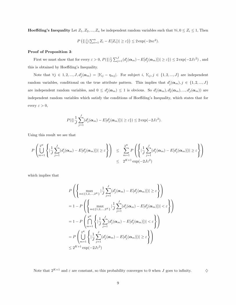
Hoeffding’s Inequality Let Z1, Z2, ..., Zn be independent random variables such that ∀i, 0 ≤ Zi ≤ 1, Then
P({| 1n (
∑ni=1 Zi − E[Zi])| ≥ ε}
)≤ 2 exp(−2nε2).
Proof of Proposition 3:
First we must show that for every ε > 0, P ({| 1J∑Jj=1(dij(αm)−E[dij(αm)])| ≥ ε}) ≤ 2 exp(−2Jε2) , and
this is obtained by Hoeffding’s Inequality.
Note that ∀j ∈ 1, 2, ..., J, dij(αm) = |Yij − ηmj |. For subject i, Yij , j ∈ {1, 2, ..., J} are independent
random variables, conditional on the true attribute pattern. This implies that dij(αm), j ∈ {1, 2, ..., J}
are independent random variables, and 0 ≤ dij(αm) ≤ 1 is obvious. So di1(αm), di2(αm), ..., diJ(αm)) are
independent random variables which satisfy the conditions of Hoeffding’s Inequality, which states that for
every ε > 0,
P ({| 1J
J∑j=1
(dij(αm)− E[dij(αm)])| ≥ ε}) ≤ 2 exp(−2Jε2).
Using this result we see that
P
2K⋃m=1
| 1JJ∑j=1
(dij(αm)− E[dij(αm)])| ≥ ε
≤
2K∑m=1
P
| 1JJ∑j=1
(dij(αm)− E[dij(αm)])| ≥ ε
≤ 2K+1 exp(−2Jε2)
which implies that
P
maxm∈{1,2,...,2K}
| 1J
J∑j=1
(dij(αm)− E[dij(αm)])| ≥ ε
= 1− P
maxm∈{1,2,...,2K}
| 1J
J∑j=1
(dij(αm)− E[dij(αm)])| < ε
= 1− P
2K⋂m=1
| 1JJ∑j=1
(dij(αm)− E[dij(αm)])| < ε
= P
2K⋃m=1
| 1JJ∑j=1
(dij(αm)− E[dij(αm)])| ≥ ε
≤ 2K+1 exp(−2Jε2)
Note that 2K+1 and ε are constant, so this probability converges to 0 when J goes to infinity. ♦
9

The preceding propositions are now used to prove Theorem 1 , along with a corollary to show that for
a single subject, the estimate of α by the nonparametric method will converge to the true attribute vector
almost surely when test length goes to infinity.
Theorem 1. For a particular subject i with true attribute pattern αi, under Assumptions 1 and 2 and
Conditions (a.1), (a.2), (a.3) and (b), the estimator αi derived from the nonparametric method of equation
2 is a consistent estimator of αi, provided one of the DINA model, NIDA model or Reduced RUM holds.
Specifically,
limJ→∞
P (αi = αi) = 1.
Proof. For fixed subject i, ∀ε > 0, let event Aε(J) = {|αi − αi| > ε}, and Bε(J) as defined in Proposition
3. Then we show that Aε(J) ⊂ Bε(J). In order to prove this, we can prove Bε(J)C ⊂ Aε(J)C .
Suppose Bε(J)C is true, that is ∀m ∈ {1, 2, ..., 2K},∀ε > 0
∣∣∣∣∣∣ 1JJ∑j=1
(dij(αm)− E[dij(αm)]
)∣∣∣∣∣∣ < ε
Then we can get that
1
J
J∑j=1
E[dij(αm)]− ε < 1
J
J∑j=1
dij(αm) <1
J
J∑j=1
E[dij(αm)] + ε.
If αi 6= αi, then∑Jj=1 d
ij(αi) <
∑Jj=1 d
ij(αi) and 1
J
∑Jj=1 d
ij(αi) <
1J
∑Jj=1 d
ij(αi). These inequalities imply
that
1
J
J∑j=1
E[dij(αi)]− ε <1
J
J∑j=1
dij(αi) <1
J
J∑j=1
dij(αi) <1
JE[dij(αi)] + ε, ∀ε > 0.
Thus for small enough ε we have
J∑j=1
E[dij(αi)] <
J∑j=1
E[dij(αi)].
This is contradictory to Proposition 1 that shows the true attribute pattern will minimize E[D(Yi,αm)],
and Proposition 2 that when J →∞ ,the difference of the expectation of the distance defined by (1) under
the wrong attribute pattern with that of under the true attribute pattern will go to infinity. So we may
conclude that Bε(J)C ⊂ Aε(J)C , and equivalently Aε(J) ⊂ Bε(J).
10

By the above claim and Proposition 3, we have ∀ε > 0
P (|αi −αi| > ε) ≤ P (Bε(J)) ≤ 2K+1 exp(−2Jε2)→ 0, as J →∞
Thus we have proved that if Assumptions 1 and 2 and Conditions (a.1), (a.2), (a.3) and (b) are satisfied,
limJ→∞ P (αi = αi) = 1 ♦
Corollary 1. Under Assumptions 1 and 2 and Conditions (a.1), (a.2), (a.3) and (b),
limJ→∞
P (|αi −αi| > ε, i.o) = 0.
Proof. We only need to prove that: ∑∞J=1 P (Bε(J)) <∞
and the result will follow from the Borel-Cantelli Theorem. Note that
∞∑J=1
P (Bε(J)) <
∞∑J=1
2K+1 exp(−2Jε2)
= 2K+1∞∑J=1
exp(−2Jε2).
Define f(J) = exp(−2Jε2).
According to the convergence rule of series,
limJ→∞
f(J + 1)
f(J)= lim
J→∞
exp(−2(J + 1)ε2)
exp(−2Jε2)
= exp(−2ε2) < 1
Then we have ∑∞J=1 P (Aε(J)) <
∑∞J=1 P (Bε(J)) <∞
which completes the proof of the corollary.
♦
11

Finally we investigate the joint consistency of a sample of N subjects. Essentially the same results hold,
but there must be some control on the relative sizes of N and J as both go to infinity.
Theorem 2. Under Assumptions 1 and 2 and Condition (a.1), (a.2), (a.3),(b)and (c)in section 2.1.1,
provided one of the DINA model, NIDA model or Reduced RUM holds,
limJ→∞
P
(N⋂i=1
{αi = αi}
)= 1.
Proof. Note that the only difference between Theorem 1 and Theorem 2 is that Theorem 2 has
sample size N but Theorem 1 has only one subject. So Proposition 1 and Proposition 2 still
hold for every subject in Theorem 2. For Proposition 3, ∀ε > 0, we can define Bε(N, J) =
{maxi∈{1,2,...,N}{maxm∈{1,2,...,2K} | 1J∑Jj=1(dij(αm) − Edij(αm))| ≥ ε}}. Then under Condition (c) we can
show that
limJ→∞
P (Bε(N, J)) = 0.
For every i ∈ {1, 2, ..., N}, P({∣∣∣ 1J ∑J
j=1(dij(αm)− E[dij(αm)])∣∣∣ ≥ ε}) ≤ 2 exp(−2Jε2) holds, so we see
that,
P
N⋃i=1
2K⋃m=1
| 1JJ∑j=1
(dJj (αm)− E[dij(αm)])| ≥ ε
≤N∑i=1
2K∑m=1
P
∣∣∣∣∣∣ 1J
J∑j=1
(dij(αm)− E[dij(αm)])
∣∣∣∣∣∣ ≥ ε
≤ 2K+1N exp(−2Jε2).
12

=⇒
P
maxi∈{1,2,...,N}
maxm∈{1,2,...,2K}
∣∣∣∣∣∣ 1JJ∑j=1
(dij(αm)− E[dij(αm)])
∣∣∣∣∣∣ ≥ ε
= 1− P
maxi∈{1,2,...,N}
maxm∈{1,2,...,2K}
∣∣∣∣∣∣ 1JJ∑j=1
(dij(αm)− E[dij(αm)])
∣∣∣∣∣∣ < ε
= 1− P
N⋂i=1
2K⋂m=1
| 1JJ∑j=1
(dij(αm)− E[dij(αm)])| < ε
= P
N⋃i=1
2K⋃m=1
| 1JJ∑j=1
(dij(αm)− E[dij(αm)])| ≥ ε
≤ 2K+1N exp(−2Jε2).
Note that 2K+1 is constant, so this probability converges to 0 provided the sample size and test length
have the relationship Ne−2Jε2 → 0 as J →∞ (Condition (c)).
Now define Aε(N, J) ={
maxi∈{1,2,...,N} |αi −αi| > ε}
, with the same argument as that in the proof of
Theorem 1, we can prove that Aε(N, J) ⊂ Bε(N, J). Then we can get that:
P
(N⋃i=1
{|αi −αi| > ε}
)≤ P
maxi∈{1,2,...,N}
maxm∈{1,2,...,2K}
∣∣∣∣∣∣ 1JJ∑j=1
(dij(αm)− E[dij(αm)])
∣∣∣∣∣∣ ≥ ε
≤ 2K+1N exp(−2Jε2) −→ 0,
provided that N exp(−2Jε2)→ 0 as J →∞. This completes the proof of Theorem 2. ♦
Corollary 2. Under Assumptions 1 and 2 and Conditions (a.1), (a.2), (a.3), (b), and (c), if the test length
J and sample size N satisfy the relationship that:
Jn1 ≤ N < Jn2 , 1 < n1 < n2 <∞.
Then
limJ→∞
P
(N⋃i=1
{αi 6= αi} , i.o
)= 0.
Proof. We only need to prove that: ∑Jn2
N=1
∑∞J=1 P (Bε(N, J)) <∞,
13

and the result will follow from the Borel-Cantelli Theorem like in Corollary 1. Note that
Jn2∑N=1
∞∑J=1
P (Bε(N, J)) <
Jn2∑N=1
∞∑J=1
2KN exp(−2Jε2)
= 2K∞∑J=1
(
Jn2∑N=1
N) exp(−2Jε2)
= 2K∞∑J=1
1 + Jn2
2exp(−2Jε2)
Define f(J) = 1+Jn2
2 exp(−2Jε2). According to the convergence rule of series,
limJ→∞
f(J + 1)
f(J)= lim
J→∞
1+(1+J)n2
2 exp(−2(J + 1))ε2
1+Jn2
2 exp(−2Jε2)
= limJ→∞
1 + (J + 1)n2
1 + Jn2exp(−2ε2)
= exp(−2ε2) < 1.
⇒∑∞J=1
1+Jn2
2 exp(−2Jε2) <∞.
Then we have
∑Jn2
N=1
∑∞J=1 P (Aε(N, J)) <
∑Jn2
N=1
∑∞J=1 P (Bε(N, J)) <∞
and the proof is complete. ♦
These theorems for consistency of the nonparametric method, assume that one of several possible true
models hold, and we have focused on some of the common latent class models for cognitive diagnosis. The
purpose was to show that the simple nonparametric method may be used without calibrating a model, no
matter which of those models hold. However, essentially the same general condition was used in the proof of
each particular model, and here we focus on the most general condition that any cognitive diagnosis model
must satisfy for the nonparametric technique to yield consistent classification. The key steps for the proofs
of consistency require that Proposition 1, Proposition 2 and Proposition 3 hold, under proper regularity
conditions. If we replace the conditions for the model parameters (Conditions (a.1), (a.2) and (a.3)) with
the more general condition that involves no model parameters,
Condition (a′): P (Yj = 1|ηj = 1) > 0.5 + δ , P (Yj = 1|ηj = 0) < 0.5− δ, for some positive number δ > 0,
the three propositions still hold. This means that the consistency results (Theorem 1, Corollary 1, Theorem
2 and Corollary 2) still hold for any models which satisfy the Condition (a′). The theory of the previous
14

results essentially utilized this condition, but phrased it in terms of what it required of model parameters.
More generally, these conditions on model parameters can be replaced by Condition (a′).
1.3 Numerical Studies
1.3.1 Study Design
In this section, we report simulated examples to illustrate finite test length behavior. The simulation
conditions are similar to those in Chiu & Douglas (2013) and were formed by crossing test length, the
data generation model, and the expected departure from ideal response patterns. For each condition, 1000
subjects were simulated using either DINA or NIDA model. For each data set, K = 3 attributes were
required and response profiles consisting of J = 20 or 40 items were generated. For a much more thorough
simulation study that covers more conditions and compares with competing parametric approaches, see Chiu
& Douglas (2013).
Two methods were used to generate the attribute profiles. The first sampled attribute patterns, α,
from a uniform distribution on the 2K possible values. The second approach utilized a multivariate normal
threshold method. Discrete α were linked to an underlying multivariate normal distribution, MVN(0K ,Σ),
with covariance matrix, Σ, structured as
Σ =
1 · · · ρ
.... . .
...
ρ · · · 1
,
with ρ = 0.5. Let θi = (θi1, θi2, ..., θiK)′
denote the K-dimensional vector of latent continuous scores for
subject i. The attribute pattern αi = (αi1, αi2, ..., αiK)′
was determined by
αik =
1, if θik ≥ Φ−1( kK+1 );
0, otherwise.
The item parameters for the DINA and NIDA models were generated from uniform distributions with
left endpoints of 0 and right endpoints, denoted as max(s, g), either 0.1, 0.3 or 0.5.
The Q-matrices for tests of 20 items with K = 3 were designed as in Table 1, and those for tests
of 40 items were obtained by doubling the length of the Q matrix in Table 1. For the simulation with
misspecified Q-matrices, 10% or 20% of misspecified Q entries were randomly arranged in the Q-matrix for
15

each replication.
Table 1.1: Q-matrices for test of 20 items
AttributeItem
1 2 3 4 5 6 7 8 9 10 11 12 13 14 15 16 17 18 19 20
1 1 0 0 1 1 0 1 0 0 1 1 0 1 0 0 1 1 0 1 12 0 1 0 1 0 1 0 1 0 1 0 1 0 1 0 1 0 1 1 13 0 0 1 0 1 1 0 0 1 0 1 1 0 0 1 0 1 1 1 1
1.3.2 Results
Results are summarized by an index called pattern-wise agreement rate (PAR), denoting the proportion of
attribute patterns accurately estimated according to PAR =∑Ni=1
I|αi=αi|N . The nonparametric estimator
based on minimizing Hamming distance can result in some ties, and these ties were randomly broken, though
there might be room for developing a more sophisticated technique.
In the first example, we investigate the impact of the model parameters and test length on the PAR of
the nonparametric method based on Hamming distance, when actual data were generated from the DINA
model and the NIDA model.
Table 1.2: Classification rates for the nonparametric method with DINA data
max(s, g) J = 20 J = 40
Uniform Attribute Patterns K = 3
0.1 0.9925 1.000
0.3 0.9200 0.9825
0.5 0.8100 0.8850
Multivariate Normal Attribute Patterns K = 3
0.1 0.9900 0.9975
0.3 0.9500 0.9950
0.5 0.7050 0.8675
Table 1.2 documents the effectiveness of the nonparametric method when applied to responses gener-
ated from the DINA model. In support of the theoretical results, this approach produces nearly perfect
classifications when the slipping and guessing parameter are less than 0.1. As the item parameters become
close to 0.5, the classification become worse, but much better than random assignment, which would have
an expected classification rate of 0.125 when K = 3. Consistent with the asymptotic theory, classification
16

rates clearly improve as test length increases. Table 1.3 below presents the results when the responses were
generated from the NIDA model. Note that the conditions for consistency are somewhat different for the
NIDA (Condition (a.2)), and could be violated for several items, in the case where s and g parameters are
allowed to be as large as 0.5.
Table 1.3: Classification rates for the nonparametric method with NIDA data
max(s, g) J = 20 J = 40
Uniform Attribute Patterns K = 3
0.1 0.9950 1.000
0.3 0.8225 0.8725
0.5 0.6775 0.8023
Multivariate Normal Attribute Patterns K = 3
0.1 0.9925 0.9990
0.3 0.8900 0.9125
0.5 0.4650 0.4800
Next we consider the robustness of the nonparametric method when several entries of Q-matrix are
misspecified. In each replication, 10% or 20% of the entries in a given Q-matrix were randomly changed.
The misspecified Q-matrix was used for classifying examinees with the nonparametric method. Table 1.4
reports the results for the DINA data with attribute patterns generated from a uniform distribution.(The
results when the attribute patterns generated from multivariate normal distribution have similar patterns
thus omit here.) Table 1.4 shows that classification agreement decreases with the rate of misspecification.
However, as the test length increases, the correct classification rate still increases. In all cases, classification
rates are well above random assignment. Table 1.5 show the similar results for NIDA data. Though it
requires theoretical proof, we speculate that for a certain range of the misspecified percent of entries in
Q-matrix, the consistency theories may still hold.
17

Table 1.4: Classification results for the nonparametric methods with DINA data and a uniform distributionon α when Q is misspecified
max(s, g) J = 20 J = 40
10% misspecified q entries K = 3
0.1 0.9125 0.9650
0.3 0.7825 0.8775
0.5 0.4625 0.8021
20% misspecified q entries K = 3
0.1 0.7231 0.8024
0.3 0.6621 0.7642
0.5 0.4321 0.5861
Table 1.5: Classification results for the nonparametric method with NIDA data and a uniform distributionon α when Q is misspecified
max(s, g) J = 20 J = 40
10% misspecified q entries K = 3
0.1 0.9125 0.9550
0.3 0.7123 0.8275
0.5 0.4232 0.4532
20% misspecified q entries K = 3
0.1 0.7135 0.7824
0.3 0.6213 0.6120
0.5 0.3346 0.4032
1.3.3 Discussion
The consistency results of the previous section demonstrate that nonparametric classification can be effective
under a variety of underlying conjunctive models. This can greatly expand potential applications, by allowing
for conducting cognitive diagnosis when calibration of a parametric model is not feasible. Nonparametric
classification based on minimizing Hamming distance to ideal response patterns is simple and fast and can
be used with a large number of attributes. One advantage over parametric modeling is that no model
calibration is needed, and it can be performed with a sample size as small as 1. Requiring no large samples
18

or calibration allows for small scale implementation, such as in the classroom setting, where diagnosis can
be most important.
The appealing property of the nonparametric method, is that it is consistent under a variety of possible
true parametric models, and can be viewed as robust in that sense. Here we studied the properties of the
classifier under the DINA, NIDA, and RED-RUM models, but consistency is not be restricted to them, as
a conjunctive response process and knowledge of the Q matrix are the critical assumptions. As discussed
following the theoretical results, the only general condition required of the underlying item response func-
tions, is that the probability of a correct response for masters of the attributes is bounded above 0.5 for
each item, and the probability for non-masters is bounded below 0.5. If the true model satisfies these simple
conditions, nonparametric classification will be consistent as the test length increases.
Though consistency results were demonstrated, Chiu and Douglas (2013) show that maximum likelihood
estimation with the correct parametric model is more efficient, which can be expected. Other advantages
of using parametric statistical models is that one can use general statistical techniques for goodness-of-fit,
model selection, and gain a sense of variability and the chance of errors. For instance, classification using
parametric latent class models for cognitive diagnosis allows one to compute posterior probabilities for any
attribute pattern, which cannot be done with the nonparametric classifier.
Nevertheless, the impressive relative efficiency (Chiu and Douglas, 2013) of the nonparametric classifier
and its consistency properties suggest that the approach may be a useful alternative when calibration of
a parametric model is not feasible. This approach can be implemented as soon as an item bank with
a corresponding Q matrix has been developed, and the computational simplicity allows one to construct
reliable computer programs for classification that amount to exhaustively searching through all possible
patterns, which is guaranteed to identify an optimal solution. Some promising directions for future research
in nonparametric classification include development of fit indices and algorithms for computerized adaptive
testing. Another ongoing issue for future research is identifying or validating the correct specification of the
Q matrix. In the numerical study we see the effect of misspecification rate on performance. Incorrect Q
matrix entries affect both parametric and nonparametric techniques, and suggest that robust methods could
be a fruitful area of research.
19

Chapter 2
Model Misspecification in CognitiveDiagnosis
2.1 Introduction
In cognitive diagnosis, many models have been developed to provide a profile defining mastery or non-
mastery of a set of predefined skills or attributes. Based on the assumptions about how attributes influence
test performance, CDMs can be categorized as noncompensatory models or compensatory models. Chapter
1.1.1 reviews several common conjunctive models, which express the notion that all attributes specified in the
attribute-by-item Q matrix for an item should be required to answer the item correctly, but allow for slips
and guesses in ways that distinguish the models from one another. Disjunctive models define the probability
of a correct response such that mastering a subset of the attributes is sufficient to have high probability of
a correct response. An example is the Deterministic Input, Noisy “Or” gate model (DINO; Templin and
Henson (2006)). Unlike noncompensatory models, compensatory models allow an individual to compensate
for what is lacked in some measured skills by having mastered other skills. Some representatives are the
General Diagnostic Model (GDM; Davier (2005)) and a special case of the GDM called the compensatory
RUM (Hartz (2002)). Encompassing the traditional categories of the reduced CDMs, several general models
based on different link functions (e.g., G-DINA; De La Torre (2011) and log-linear CDM; Henson et al.
(2009)) have been developed to include many of the common compensatory and noncompensatory models.
Starting the analysis with a general model obviates the need to identify the specific form of the CDM,
and a general model also has better model fit compared with other reduced models. However, specific and
simple models may be preferred under some circumstances for several reasons. First, simple models have
more straightforward interpretations (De La Torre et al., 2015). Second, they require smaller sample sizes
to be estimated accurately (Rupp and Templin, 2008b). Finally, appropriate reduced models can sometimes
provide better classification rates than general models, particularly when the sample size is small (Rojas et al.
(2012)). This phenomenon is essentially the bias-variance tradeoff, and is familiar in regression when we can
sometimes used a small but biased model for more efficient prediction, for example. When selecting a model,
which is surely never the true model, a natural question to consider is how accurately the misspecified model
20

can classify examinees, which is the ultimate objective. In particular, we are concerned with the behavior
of the maximum likelihood estimator, when the likelihood is computed assuming an incorrect model.
The objective of this chapter is to investigate the consequences of using a simple but incorrect model.
We are interested in the impact of model misspecification to the classification accuracy, which can be
investigated by analyzing the asymptotic behavior of the MLE for attribute profiles under misspecified
CDMs. The asymptotic behavior of the MLE under misspecified models associated with parameters in a
continuous space has been studied for nearly 50 years (Huber, 1967; Berk et al., 1966; White, 1982; Wainer
and Wright, 1980). However, CDMs are in a discrete classification space, and the theory for estimation of
discrete attribute profiles is different from that of the estimation of a parameter in a continuous parameter
space. In the CDM framework, several empirical studies have been conducted to investigate the effect of
model misspecification or Q matrix misspecification on parameter estimation and classification accuracy
(Rupp and Templin, 2008a; Chen et al., 2013). However, no theory of the asymptotic behavior of the MLE
for attribute profile under misspecified CDMs has been developed.
Specifically, our research questions include: 1) What is the behavior of MLE for attribute profile when
the true model and misspecified model both are conjunctive models? 2) Under what conditions is the MLE
for attribute profiles a consistent estimator, when the true model satisfying certain conditions, including
both conjunctive models and compensatory models, is misspecified as a DINA model? 3) If the MLE is
not consistent, can a robust estimation procedure be developed to solve the inconsistency issue under a
misspecified DINA model? Investigating these questions can provide practitioners some guidelines about in
what situations they can choose a simple model without severely affecting the classification accuracy.
2.2 Behavior of MLE in Misspecified Models
In this section, we investigate whether the MLE of attribute profiles can provide consistent classification
when the model is misspecified as a conjunctive model. Two examples about the behavior of MLE under a
misspecified DINA model are given.
2.2.1 Problem Formulation
Throughout this section, we focus on the case of a single examinee with true attribute profile denoted as α∗.
Suppose this examinee finishes a test with J items which measure K attributes. Let Y = (Y1, Y2, ..., YJ)T
be the examinee’s item response vector. The true attribute pattern in this case can be written as α∗ =
(α∗1, α∗2, ..., α
∗K)T , and each α∗k takes a value of either 0 or 1 for k = 1, 2, ...,K. Specifically, α∗k is an indicator
21

of whether this examinee possesses the kth attribute.
We assume that the Q matrix is the same for the true model and the misspecified model, which is a J×K
matrix with entry qjk to indicate whether item j requires the kth attribute. Define ηj(α∗) =
∏Kk=1(α∗k)qjk to
be the jth component of the ideal response pattern for this examinee, and let η(α∗) = (η1(α∗), ..., ηJ(α∗))T
denote this pattern. For an attribute pattern α, we denote the true item response function as π∗j (α),
j = 1, 2, ..., J . Based on the true model, the correct response probability for item j given any attribute
profile α can be written as:
π∗j (α) = P ∗(Yj = 1|α) =
π∗j1(α), if ηj(α) = 1;
π∗j2(α), if ηj(α) = 0.
In reality, the true model is not known, and after we collect data and we believe the responses come
from a conjunctive process, then an appropriate conjunctive model needs to be selected. Denote πj(α) as
the item response function for the model we choose, and different conjunctive models are defined through
different forms of πj(α). Three types of conjunctive models are introduced here.
Example 1 (The DINA model). The DINA model is the simplest conjunctive model, and the item response
function is totally determined by ηj(α). Thus there are only two types of correct response probabilities for
each item under the DINA model. ∀α,
πj(α) = P (Yj = 1|α) =
πj1(α) = πj1 = 1− sj , if ηj(α) = 1;
πj2(α) = πj2 = gj , if ηj(α) = 0.
Example 2 (The NIDA model). Different from the DINA model, the slipping and guessing parameters for
the NIDA model are defined through the attribute levels. Define Hj = {k|qjk = 1}, for the NIDA model,
πj(α) = P (Yj = 1|α) =
πj1(α) = πj1 =∏k∈Hj (1− sk) , if ηj(α) = 1;
πj2(α) =∏k∈Hj (1− sk)αkg1−αkk , if ηj(α) = 0.
Example 3 (The Reduced RUM model). The Reduced RUM model can be generalized from the NIDA model
with the item response function defined as:
πj(α) = P (Yj = 1|α) =
πj1(α) = πj1 = πj , if ηj(α) = 1;
πj2(α) = πj∏k∈Hj (r
∗jk)1−αk , if ηj(α) = 0.
Note that for the NIDA model and the Reduced RUM model, πj1 is the same for different α such that
22

ηj(α) = 1, however πj2(α) can be different for different α. Unlike the DINA model, for each item there can
be more than two types of correct response probabilities if K ≥ 1.
With the assumption of conditional independence, the likelihood function of α constructed from the
chosen model based on J questions is:
L(J)(α) =
J∏j=1
(πj(α))Yj (1− πj(α))(1−Yj).
Note that the superscript (J) indicates the corresponding function depends on J , and we will use such
notation from now on. The corresponding log-likelihood function can be written as:
l(J)(α) = log(LJ(α)) =
J∑j=1
[Yj log(πj(α)) + (1− Yj) log(1− πj(α))] .
When our selected model is different from the true model, we wish to investigate whether the MLE for α∗
arising from the wrong model is consistent. Let A = {αh 6= α∗, h = 1, 2, ..., 2K − 1} denote the set of the
2K − 1 alternative attribute patterns. Our problem is to consider if
limJ→∞
P(
maxαh∈A
l(J)(αh) < l(J)(α∗))
= 1. (2.1)
To investigate whether (2.1) can hold in the model misspecification case, we use a condition on the
identifiability of attribute patterns afforded by the Q-matrix, to eliminate a trivial cause for inconsistency.
Condition (I): Define Am,m′ ={j|ηj(αm) 6= ηj(α
m′
)}
, where m and m′
index different attribute
patterns among the 2K possible patterns. Then lim infJ→∞Card(A
m,m′ )
J > 0.
This condition guarantees that as the test length grows, more and more information becomes available
to distinguish attribute patterns from one another. Though the actual rate need not be as the same order
of J , a condition of this nature would be needed for consistency, even when using the true model.
To simplify the argument in the next section, we use the notation an � bn to denote that sequences {an}
and {bn} have the same order. This means that there exists constants 0 < m < M < ∞ and an integer n0
such that for all n > n0, m < |anbn | < M .
2.2.2 The asymptotic behavior of MLE under misspecified conjunctive CDMs
In this section, we first discuss the behavior of MLE when the true model and misspecified model both
belong to conjunctive categories by using a simple case when the number of attributes K = 1. Then we
extend the analysis to the general case where K ≥ 1 and when the true model can be any CDM satisfying
23

some necessary conditions and is misspecified as a DINA model.
A simple case when K = 1
Now let’s assume the true model and the misspecified model both are conjunctive models, and there is
only one attribute (K = 1) associated with J items. The corresponding Q matrix is simply a vector with
all elements equal to 1. Suppose the true attribute is α∗ for this examinee, and the set A only has one
element α1. Because only 1 attribute is required for each item, there are only two types of correct response
probabilities for each item no matter what the true conjunctive model is. The possible values for α and the
corresponding correct response probabilities for each item under the true model and the misspecified model
are summarized in Table 2.1 below:
Table 2.1: Attributes and Item Parameters
Correct Response Probability
Attribute Profile True Model Misspecified Model
α π∗j (α) πj(α)
0 π∗2j π2j
1 π∗1j π1j
The MLE for the attribute pattern under the misspecified model is
αMLE = arg maxα∈{0,1}
l(J)(α).
Furthermore, let E∗ denote the expectation under the true model, and define
∆(J) = E∗[l(J)(α∗)− l(J)(α1)].
∆(J) quantifies the expected distance between the log-likelihood value of the true attribute profile and
that of the alternative attribute profile under the probability measure from the true model.
For conjunctive models, it is natural to assume that the correct response probability for each item when
the examinee masters all the required attributes will be greater than when the examinee does not. So we
assume that there exists two positive numbers δ∗ > 0 and δ1 > 0, and for any attribute profile αh and αh′
such that η(αh) = 1 and η(αh′
) = 0, the true conjunctive model satisfies,
Condition (T) : π∗j1(αh)− π∗j2(αh′
) > δ∗,
24

and the misspecified conjunctive model satisfies,
Condition (M) : πj1(αh)− πj2(αh′
) > δ1.
Besides these two conditions, we assume that for the misspecified model, the two types of correct response
probabilities are bounded away from 0 and 1. The following theorem describes the behavior αMLE in this
simplest case.
Theorem 3. When K = 1, for one examinee with true attribute profile α∗ , suppose both the true model
and misspecified model are conjunctive models and satisfy Condition (T) and Condition (M) respectively,
and the correctly specified Q-matrix satisfies Condition (I) as the exam length increases. If 0 < ∆(J) � J ,
limJ→∞ P (l(J)(α∗) > l(J)(α1)) = 1. If 0 > ∆(J) � J , limJ→∞ P (l(J)(α1) > l(J)(α∗)) = 1.
Proof. First rewrite the probability in another format,
P(l(J)(α1)− l(J)(α∗) > 0
)= P
(l(J)(α1)− l(J)(α∗)− E∗[l(J)(α1)− l(J)(α∗)] > −E∗[l(J)(α1)− l(J)(α∗)]
)= P
(l(J)(α1)− l(J)(α∗)− (−∆(J)) > ∆(J)
).
Note that when K = 1, there are only two possible situations for the values of α∗ and α1: α∗ = 0,α1 = 1
and α∗ = 1,α1 = 0. We prove the theorem under the two cases respectively.
When α∗ = 0, α1 = 1, and recall that ∆(J) = E∗[l(J)(α∗)− l(J)(α1)], then it’s easy to verify that
l(J)(α1)− l(J)(α∗)− (−∆(J)) =
J∑j=1
(Yj − π∗j2)
(log
(πj1πj2
1− πj21− πj1
)).
Now define Zj = (Yj − π∗j2), then 0 < |Zj | < 1. Based on the conditional independence assumption,
we have Z1, Z2, ..., Zj are independent and E∗[Zj ] = 0, j = 1, 2, ..., J . Let Cj := log(πj1πj2
1−πj21−πj1 ). Based on
Condition (M), ∀j, Cj is positive and bounded away from 0. Suppose the upper bound is a positive number
C.
Then we have
P(l(J)(α1)− l(J)(α∗) > 0
)= P
( J∑j=1
ZjCj > ∆(J)).
To investigate the value of the above equation when J →∞, we need to discuss the behavior of ∆(J) in the
following two situations.
(a) If 0 < ∆J � J , then for large enough J , there exists a constant m0 > 0 such that ∆(J) = m0J . Then
25

by Hoeffding’s inequality we have
P(l(J)(α1) > l(J)(α0)
)< exp(−2(∆(J))2
JC2) ∼ exp(−2Jε),
where ε =m2
0
C2 > 0. Then (2.1) holds in this situation, and the MLE using the misspecified model is
consistent.
(b) If ∆(J) � J but ∆(J) < 0, then
P(l(J)(α1) > l(α0)
)= P
( J∑j=1
(−ZjCj) < −∆(J))
= 1− P (
J∑j=1
(−ZjCj) > −∆(J)).
By using Hoeffiding’s inequality again,
P (
J∑j=1
(−ZjCj) > −∆(J)) ≤ exp(−Jε)→ 0, as J →∞
Then
limJ→∞
P (l(J)(α1) > l(J)(α0)) = 1.
Similarly, when α∗ = 1 and α1 = 0, repeat the above analysis, and we can get the exact same conclusion.
Thus when ∆(J) < 0 and has the same order of J , αMLE = α1 with probability approaching 1, and is not
a consistent estimator of α∗. ♦
Theorem 3 indicates that whether the consistency of αMLE holds under model misspefication depends
heavily on the quantity ∆(J) = E∗[l(J)(α∗)− l(J)(α1)]. If 0 < ∆(J) � J , then the consistency of MLE under
model misspecification can hold. If ∆(J) < 0 and has the same order of J , αMLE = α1 with probability
approaching 1, and is not a consistent estimator of α∗. To see more directly how ∆(J) is related to the
parameters of the true and the misspecified model, and in what situations ∆(J) can guarantee the consistent
estimator under a misspecified model, consider the case when α∗ = 0 and α1 = 1. Now with this specific
example, it’s easy to verify that
∆(J) =
J∑j=1
(1− π∗j2) log
(1− πj21− πj1
)+ π∗j2 log
(πj2πj1
)=
J∑j=1
∆j .
Let’s consider two cases,
A. When πj2 ≥ π∗j2, because of Condition (M) for the misspecified model we have log(πj2πj1
) < 0 and
26

log(1−πj21−πj1 ) > 0, and they imply that
∆(J) ≥J∑j=1
[(1− πj2) log
(1− πj21− πj1
)+ πj2 log
(πj2πj1
)]=
J∑j=1
KL (πj2||πj1) > 0,
where KL(πj2||πj1) is the K-L divergence between πj2 and πj1, and will be strictly positive as long as
πj2 6= πj1. In this case, 0 < ∆(J) � J and consistency holds.
B. When πj2 < π∗j2, then each component of ∆(J) can be either negative or positive. For example, when
π∗j1 = 0.6, π∗j2 = 0.4, πj1 = 0.7, if πj2 = 0.1, then ∆j = −0.119 < 0, if πj2 = 0.3, then ∆j = 0.169 > 0.
So, in this case ∆(J) > 0 and whther it has the same order of J can not always be guaranteed. This
means that the MLE under the misspecified model may not be a consistent estimator for α∗.
Similarly, if α∗ = 1 and α1 = 0, we can conclude that if π∗1 ≥ π1, then the consistency for MLE holds,
otherwise, the MLE may not be consistent. By using this simple example we can see that when the true
model and the misspecified model are both conjunctive models, the MLE of attribute profile under such
model misspecification is not necessarily a consistent estimator.
General Situation
In the general situation where there are K ≥ 1 attributes associated with test, the analysis of the MLE under
misspecified conjunctive models is more complicated. However, if the true model is a model which satisfies
condition (T) and is misspecified as a DINA model which satisfies condition (M), a sufficient condition for
the consistency of the MLE can be found in this situation.
Theorem 4. When K ≥ 1, for an examinee with true attribute profile α∗, suppose the true model satisfies
Condition (T), and we misspecify it as a DINA model which satisfies condition (M). Let the Q-matrix be
correctly specified and satisfy Condition (I) as the exam length increases. Furthermore, if the correct response
probability under the true model and the misspecified model satisfy: Condition (S): ∀j, 0 < π∗j2(α∗) ≤ πj2 <
πj1 ≤ π∗j1(α∗), then the MLE for α∗ is a consistent estimator.
Proof. Suppose the response vector for a particular examinee is Y = (Y1, Y2, ..., YJ). Let the true attribute
pattern for this examinee be α∗, and denote the ideal response pattern under α∗ as η(α∗). Let A = {αh, h =
1, 2, ..., 2K − 1} denote the set of the 2K − 1 alternative attribute patterns.
Define Bm(α) = {j|ηj(α) = m},m ∈ {0, 1}. The DINA log-likelihood can be written as:
l(J)(α) =∑
j∈B1(α)
lj(α|ηj(α) = 1) +∑
j∈B0(αh)
lj(α|ηj(α) = 0),
27

we need to prove
limJ→∞
P
(maxαh∈A
l(J)(αh) < l(J)(α∗)
)= 1. (2.2)
Note that
P
maxαh∈A
l(J)(αh) < l(J)(α∗))≥ 1−
∑αh∈A
P({l(J)(αh) > l(J)(α∗)}
.
In order to prove equation (2.2), it is equivalent to prove:
limJ→∞
∑αh∈A
P({l(J)(αh) > l(J)(α∗)}
)= 0.
Because |A| <∞, it can be further simplified to prove that for any αh ∈ A,
limJ→∞
P({l(J)(αh) > l(J)(α∗)}
)= 0.
Define set Bmd(αh) = {j|ηj(α∗) = m, ηj(α
h) = d},m ∈ {0, 1}, d ∈ {0, 1}. The relationship of Bm(αh)
and Bmd(αh) is:
Bm(α∗) =⋃
d∈{0,1}
Bmd(αh),m ∈ {0, 1}; , Bd(α
h) =⋃
m∈{0,1}
Bmd(αh), d ∈ {0, 1}.
Then
l(J)(αh)− l(J)(α∗) =∑
j∈B01(αh)
[Yj log
(πj1(1− πj2)
(1− πj1)πj2
)− log
(1− πj2
1− πj1
)]
+∑
j∈B10(αh)
[Yj log
(πj2(1− πj2)
(1− πj2)πj1
)− log
(1− πj1
1− πj2
)]= I
(J)1 + I
(J)2
We need to prove that
limJ→∞
P(I(J)1 + I
(J)2 > 0
)= 0. (2.3)
Define J1(αh) = |B01(αh)| and J2(αh) = |B10(αh)|. The next step is to prove the above equation in three
different situations.
28

Based on Condition (I) that lim inf J1(αh)+J2(αh)J > 0, there are three possible cases J1(αh) and J2(αh).
(1.1) limJ→∞ J1(αh) =∞ and limJ→∞ J2(αh) =∞.
(1.2) limJ→∞ J1(αh) =∞ and limJ→∞ J2(αh) <∞.
(1.3)limJ→∞ J1(αh) <∞ and limJ→∞ J2(αh) =∞.
Proof of (1.1)
P(I(J)1 + I
(J)2 > 0
)≤ P
(I(J)1 > 0) + P (I
(J)2 > 0
)
Then we only need to prove
limJ→∞
P(I(J)1 > 0
)= 0, and lim
J→∞P(I(J)2 > 0
)= 0.
Using similar techniques as in the proof of Theorem 3, we have
P(I(J)1 > 0
)= P
(I(J)1 − E∗[I(J)1 ] > −E∗[I(J)1 ]
).
Note that, for j ∈ B01(αh), E∗(Yj) = P ∗(Yj = 1|ηj(α∗) = 0) = π∗j2(α∗). Then we can get that
P(I(J)1 > 0
)= P
( ∑j∈B01
(Yj − π∗j2(α∗))(log
(πj1
πj2
1− πj2
1− πj1
))> −E∗[I(J)
1 ]
),
where −E∗[I(J)1 ] =∑j∈B01(αh)(1− π∗j2(α∗)) log(
1−πj21−πj1 ) + π∗j2(α∗) log(
πj2πj1
).
Using a similar argument as in the prove of Theorem3, let Cj = log(πj1πj2
1−πj21−πj1 )) and because πj1, πj2
are bounded away from 0 and 1, then Cj is a finite number and assume the upper bound is C. In order to
use Hoeffding’s inequality, we only need to guarantee that −E∗[I(J)1 ] is positive and has the same order as
J1(αh). Note that because π∗j2(α∗) ≤ πj2 and πj2 < πj1,
−E∗[I(J)1 ] =
∑j∈B01(αh)
(1− π∗j2(α)) log
(1− πj2
1− πj1
)+ π∗j2(α) log
(πj2
πj1
)
≥∑
j∈B01(αh)
(1− πj2) log
(1− πj2
1− πj1
)+ πj2 log
(πj2
πj1
)=
∑j∈B01(αh)
KL (πj2||πj1) .
29

Based on the condition that limJ→∞ J1(αh) =∞, and by Hoeffiding’s inequality we have that
P(I(J)1 > 0
)≤ P
∑j∈B01
(Yj − π∗j2(α))C >∑
j∈B01(αh)
KL(πj2||πj1)
≤ exp
−2(∑
j∈B01(αh)KL(πj2||πj1))2
J1(αh)C2
∼ exp(−2J1(αh)ε
),
where ε > 0. Thus limJ→∞ P(I(J)1 > 0
)= 0. Similarly, we can get that
P(I(J)2 > 0
)≤ exp
−2(∑
j∈B10(αh)KL(πj1||πj2))2
J2(αh)C2
∼ exp(−2J2(αh)ε
),
and this completes the proof of (1.1)
Proofs of (1.2) and (1.3)
Here we only discuss (1.2) in detail and the conclusion for (1.3) is found by precisely the same argument.
In situation (1.2), J2(αh) <∞, so
limJ→∞
I(J)2 = lim
J→∞
∑j∈B10(αh)
[Yj log
(πj2(1− πj2)
(1− πj2)πj1
)− log
(1− πj11− πj2
)]
≤ limJ→∞
∑j∈B10(αh)
[log
(πj2(1− πj2)
(1− πj2)πj1
)− log
(1− πj11− πj2
)]<∞.
So in order to prove (2.3), we only need to prove limJ→∞ P(I(J)1 > 0
)= 0. The proof is this case is the
same as that in (1.1).
Similarly in situation (1.3), when J → ∞, I(J)1 will be a finite number and in order to prove (2.3), we
only need to prove limJ→∞ P(I(J)2 > 0
)= 0. To summarize, for some positive constant ε1, an upper bound
for P(l(J)(αh) > l(J)(α∗)
)can be simplified according to Table 3.8 below:
Table 2.2: Asymptotic form of the upper bound
Asymptotic Behavior Form of upper bound
limJ→∞ J1(αh) =∞, limJ→∞ J2(αh)(αh) =∞ exp(−2J1(αh)ε) + exp(−2J2(αh)ε)
limJ→∞ J1(αh) =∞, limJ→∞ J2(αh) <∞ exp(−2J1(αh)ε)
limJ→∞ J1(αh) <∞, limJ→∞ J2(αh) =∞ exp(−2J2(αh)ε)
1The constant in the different exponential bound are different, for simplicity, we just use ε to stand for that positive constantin each bound.
30

Note that at least one of J1(αh) and J2(αh) will have the same order as J . Thus, we can summarize the
upper bound as exp(−2J∗(αh)ε
), where J∗(αh) � J and ε > 0. ♦
Condition (T) is a natural assumption for conjunctive models, and Condition (S) is less intuitive, and
expresses that consistency will hold if the assumed discrimination of the item is no greater than the true
discrimination.
Though Theorem 4 is expressed for conjuctive models, the results can apply more generally. Note that
it’s also reasonable to assume Condition (T) applies to some compensatory models. For example, when the
Compensatory RUM model is the true model, the item response function is:
P ∗ (Yj = 1|α) =exp
(∑Kk=1 rjkαjkqjk − pj
)1 + exp
(∑Kk=1 rjkαjkqjk − pj
) ,where rjk > 0.
Define fj(α) =∑Kk=1 rjkαkqjk − pj . For α1 and α2 such that ηj(α
1) = 1, ηj(α2) = 0, the positive
coefficients rjk result in the relationship that : fj(α1) > fj(α
2). Because G(x) = exp(x)1+exp(x) is an increasing
function, we have π∗j1(α1) > π∗j2(α2).
However, if the true model is a disjunctive model, and is misspecified as a DINA model, we can not get
consistent classification. For example, if the DINO model is used, the item response function is determined
by
ωj = 1−K∏k=1
(1− αk)qjk ,
where ωj = 1 denotes that the examinee has mastered at least one of the required attributes for the jth item,
while ωj = 0 denotes that one has not mastered any of the required attributes. Given ωj , the probability of
a correct response is defined as
P ∗ (Yj = 1|ωj) = (1− sj)ωj g1−ωjj .
Suppose K = 3, for item j, qj = c(0, 1, 1), α1 = c(0, 1, 1), α2 = c(0, 0, 1). Then ηj(α1) = 1, ηj(α
2) = 0.
However, ωj(α1) = ωj(α
2) = 1, which means π∗j1(α1) = π∗j2(α2). Because of such equality, when data arise
from a disjunctive model, Conditions (T) cannot be satisfied. Thus, the consistency theorem cannot hold.
31

2.2.3 Examples of the MLE under a misspecified DINA model
In this section, we provide two examples for the MLE of attribute profile under a misspecified DINA model.
Example 1 shows the inconsistency of the MLE when the true model is a DINA model and is misspecified as
a DINA model with different item parameters. Example 2 shows the consistency of the MLE when the true
model is a compensatory RUM model and is misspecified as a DINA model. In both examples, the consistency
is measured by the pattern-wise agreement rate (PAR), which is defined as PAR =∑Ni=1
I|αi=αi|N to denote
the proportion of accurately estimated attribute patterns.
Example 1. Inconsistency of MLE under a misspecified DINA model. In this example, the number of
attributes K = 3 . The true model is a DINA model with fixed slipping and guessing parameters for each
item: st = 0.4, gt = 0.4. In particular, for ∀j, π∗j1 = 1 − 0.4 = 0.6, π∗j2 = 0.4. For the misspecified
DINA model, the guessing and slipping parameters are fixed at sm = 0.3, gm = 0.1 for each item, violating
Condition (S). That is, ∀j, πj1 = 1 − 0.3 = 0.7, πj2 = 0.1. To inspect the consistency, a sample of 1000
examinees with true attribute profiles simulated from a uniform distribution for each of 9 levels of test length:
J = 20, 40, 100, 200, 300, 400, 500, 600, 700. When test length equaled 20 items, a Q matrix which contains
12 items each measuring a single attribute, 6 items each measuring 2 attributes and 2 items each measuring
3 attributes was used. The Q matrices for longer tests were obtained by replicating this Q matrix. For each
condition, the examinees’ responses were simulated based on the true model, and their attribute profiles
were estimated based on the true DINA model and the misspecified DINA model. Results are summarized
by the Figure 2.1 below:
20 40 100 200 300 400 500 600 700
Test Length
PAR
%
020
4060
8010
0
Misspecified modelTrue Model
Figure 2.1: Inconsistency of MLE under model misspecification
From Figure 2.1 we can see that, under the misspecified DINA model, the pattern-wise agreement rate
decreases as the test length increases, which indicates the MLE is not a consistent estimator in this case.
32

Example 2: Consistency of the MLE under a misspecified DINA model. In this example, K = 3 and the
item parameters for the true model, a compensatory RUM model, were generated from uniform distributions
on appropriate intervals. In order to make the item parameters satisfy condition (T), the lower bound for
pj is controlled by 0.3 and the upper bound for rjk is controlled by 0.8. A sample of 1000 examinees was
generated with true attribute profiles simulated from a uniform distribution for each of the 5 levels of test
length: J = 20, 40, 100, 200, 300. For each condition, the Q matrix is constructed in the same way as that
in Example 1, and the examinees’ responses were simulated based on the true model. A DINA model is
calibrated by the “CDM” package (Robitzsch et al. (2014) ) in R based on the examinees responses in each
condition. The results in terms of PAR were summarized in Figure 2.2 below. We can see that, with the
increase of the test length, the PAR grows slowly to 100%, which indicates the MLE is a consistent estimator.
20 40 100 200 300
Test Length
PAR
%
020
4060
8010
0
Figure 2.2: Consistency of MLE under model misspecification
2.3 Robust Estimation
In the previous section, we discuss the inconsistency of the MLE for the attribute vector under misspecified
conjunctive models. Although a sufficient condition for consistency under a misspecified DINA model has
been found, it is difficult to verify whether the calibrated item parameters from a DINA model satisfy
Condition (S) or not. This is because one cannot know π∗j (α∗), thus suggesting a need to develop a robust
estimator that guarantees consistency of attribute vector classification under model misidentification.
The discussion in Section 2 indicates that the problematic part under model misspecification is that
we can not guarantee that E∗[l(J)(α∗) − l(J)(αh)], ∀αh ∈ A is positive and of order J . If some concave
function can be incorporated into the log-likelihood function to compensate for this problematic part, then
the modified log-likelihood function may guarantee the unique maximum is α∗. One solution is to utilize
33

the loss function of the nonparametric estimation method of Chiu and Douglas (2013), that was shown by
Wang and Douglas (2015) to be consistent for the attribute profile under very general conditions. Following
some regularity conditions, the loss function for nonparametric estimation method is strictly convex with an
expected value that has a unique minimum at α∗. Thus, by incorporating a multiple of this loss function
with the negative log-likelihood, a robust classifier is defined that has desirable consistency properties, and
is more efficient than simply using the nonparametric technique. The nonparametric estimation method can
be found in section 1.
2.3.1 Robust DINA MLE
One can regard the MLE as the minimizer of a loss function, which is the negative log-likelihood function.
The idea of the Robust DINA MLE is to shrink this loss function towards the distance function of the
consistent nonparametric estimation method to ensure consistency while obtaining greater efficiency than
using the nonparametric method alone. Suppose now the model is misspecified as a DINA model with the
item parameters:
πj1 = 1− sj , πj2 = gj .
For any attribute pattern α, the robust likelihood under α is
L(J)r (α) =
J∏j=1
(πj(α))Yj (1− πj(α))1−Yj exp (−λj(α)|Yj − ηj(α)|) ,
where
λj(α) =
log(πj1πj2
) if , ηj(α) = 1;
log(1−πj21−πj1 ) if , ηj(α) = 0.
Then the Robust DINA MLE estimator is :
αRMLE = argmaxαh∈A∪{α∗}
L(J)r (α) (2.4)
Note that any conjunctive model could be used for the parametric term, and the DINA is merely chosen
for its simplicity. The item response function is totally determined by the ideal response pattern and the
slipping and guessing parameters for each item. The item response functions are more complicated for other
conjunctive models, with item parameters that are generally more difficult to calibrate. As demonstrated
34

below, the Robust DINA MLE has good statistical properties, and applying the simple DINA model, can
always yield relatively efficient classifications of attribute patterns under a wide class of underlying true
models. There are some choices for calibrating the slipping and guessing parameters in DINA portion of
the model. Based on the consistency theorem discussed in the next section, those parameters can either be
randomly simulated from a reasonable interval or calibrated from the original DINA log-likelihood function
by using existing software. This greatly simplifies the item parameter calibration procedure. Next, we
provide theory to show the consistency of the Robust DINA MLE estimator under model misspecification.
2.3.2 Asymptotic behavior of the Robust DINA MLE
In this section, we first provide the regularity conditions required for consistency, then state and prove the
main consistency result for a single examinee, using the Robust DINA MLE. Then we extend the consistency
result to a finite sample of subjects.
The true model must satisfy the following conditions: for some known positive small number δ0,
Condition (T.1) 0.5 + δ0 < π∗j1(α) ≤ 1,
Condition (T.2) 0 ≤ π∗j2(α) < 0.5− δ0.
The corresponding two conditions are required for the misspecified DINA model: there exists positive
small numbers δ1, δ′
1 such that
Condition (M.1) πj1 − πj2 > δ1 > 0
Condition (M.2) δ′
1 < πj1, πj2 < 1− δ′1.
We also make the usual assumption that independence of the item response vector given the attribute
vector holds for the true model, and item response vectors of different examinees are independent.
Theorem 5. For an examinee with true attribute vector α∗, suppose the true CDM satisfies Conditions
(T.1) and (T.2). If a misspecified DINA model is used which satisfies Conditions (M.1) and (M.2), and we
correctly specify a Q-matrix that satisfies Condition (I) as the exam length increases, then the Robust DINA
MLE estimator is a consistent estimator of α∗. Specifically,
limJ→∞
P
(maxαh∈A
L(J)r (αh) < L(J)
r (α∗)
)= 1. (2.5)
Proof. The proof of Theorem 2.3.2 using exactly same techniques as those in the proof of Theorem 4, but
the structure of the robust log-likelihood is different. Note that the Robust DINA log-likelihood can be
35

written as:
l(J)r (α) = log(L(J)r (α)) =
J∑j=1
lrj (α)
=∑
j∈B1(α)
lrj (α|ηj(α) = 1) +∑
j∈B0(αh)
lrj (α|ηj(α) = 0) ,
where
lrj (α|ηj(α) = 1) = Yj log(πj1) + (1− Yj) log(1− πj1)− log
(πj1πj2
)(1− Yj);
lrj (α|ηj(α) = 0) = Yj log(πj2) + (1− Yj) log(1− πj2)− log
(1− πj21− πj1
)Yj .
♦
Following the same argument as those in the proof of Theorem 4, we can have that
l(J)r (αh)− l(J)r (α∗) =∑j∈B01
lrj (αh|η(αh) = 1)−
∑j∈B01
lrj (α∗|η(α∗) = 0)
+∑j∈B10
lrj (αh|η(αh) = 0)−
∑j∈B10
lrj (α∗|η(α∗) = 1)
= I(J)1 + I
(J)2 .
In order to prove Theorem , we only need to prove that
limJ→∞
P(I(J)1 + I
(J)2 > 0
)= 0. (2.6)
Again, using the same notations as the cardinalities defined in Theorem 4, we need to discuss (2.6) in three
situations.
Proof of (1.1)
P (I(J)1 + I
(J)2 > 0) ≤ P (I
(J)1 > 0) + P (I
(J)2 > 0).
Then we only need to prove
limJ→∞
P (I(J)1 > 0) = 0, and, lim
J→∞P (I
(J)2 > 0) = 0.
36

Using similar techniques as in the proof of Theorem 3, we have
P(I(J)1 > 0
)= P
(I(J)1 − E∗[IJ1 ] > −E∗[IJ1 ]
).
Note that for j ∈ B01(αh), E∗(Yj) = P ∗(Yj = 1|ηj(α∗) = 0) = π∗j2(α∗). Then we can get that
P(I(J)1 > 0
)= P
( ∑j∈B01
(Yj − π∗j2(α∗))2 log
(πj1πj2
1− πj21− πj1
)> −E∗[I(J)1 ]
),
where −E∗[I(J)1 ] =∑j∈B01(αh)
[(1− 2π∗j2(α∗)) log
(πj1πj2
1−πj21−πj1
)].
If we treat Zj = 2(Yj − π∗j2(α∗)) log(πj1πj2
1−πj21−πj1 ) as the new random variable, then
0 ≤ |Zj | ≤ 2 log
(πj1πj2
1− πj21− πj1
)≤ log
((
1
δ′1
)2)≤ ∞.
Furthermore,
(1− 2π∗j2(α∗)) log
(πj1πj2
1− πj21− πj1
)> 2δ0 log
((1 + δ1
1+δ′1
)2)
= ε1 > 0.
Define ε2 = log(( 1δ′1
)2), then we can apply Hoeffding’s inequality to obtain an upper bound for P (I(J)1 > 0).
P (I(J)1 > 0) < P
∑j∈B01(αh)
(Yj − π∗j2(α∗))ε2 > J1(αh)ε1
≤ exp
(−2(J1(αh)ε1)2
J1(α)ε22
)= exp(−2J1(αh)ε),
where ε =ε21ε22> 0. Thus P
(I(J)1 > 0
)→ 0, as J →∞.
Similarly,
P(I(J)2 > 0
)= P
(I(J)2 − E∗[I(J)2 ] > −E∗[I(J)2 ]
)= P
∑j∈B10(αh)
(Yj − π∗j1(α∗))2 log
(πj2πj1
1− πj11− πj2
)> −E∗[I(J)2 ]
,
where E∗[I(J)2 ] =
∑j∈B10(αh)(2π
∗j1(α∗)− 1) log
(πj1πj2
1−πj21−πj1
). Note that ∀j ∈ B10(αh),
(2π∗j1(α∗)− 1
)log
(πj1πj2
1− πj21− πj1
)> 2δ0 log
((1 +
δ11 + δ
′1
)2)
= ε1 > 0,∣∣∣∣log
(πj2πj1
1− πj11− πj2
)∣∣∣∣ < ε2.
37

Applying Hoeffdoing’s inequality again we see that
P(I(J)2 > 0
)< P
∑j∈B10(αh)
(Yj − π∗j1(α∗)) log
(πj2πj1
1− πj11− πj2
)> J2(αh)ε1
≤ exp
(−2(J2(αh)ε1)2
J2(α)ε22
)= exp
(−2J2(αh)ε
).
Thus P(I(J)2 > 0
)→ 0, as J →∞.
Proofs of (1.2) and (1.3)
Here we only discuss (1.2) in detail and the conclusion for (1.3) is found by precisely the same argument.
In situation (1.2), J2(αh) <∞, log(πj2(1−πj1)(1−πj2)πj1
)< 0, log
(1−πj21−πj1
πj1πj2
)> 0,
I(J)2 =
∑j∈B10(αh)
[Yj ∗ 2 log
(πj2(1− πj1)
(1− πj2)πj1
)+ log
(1− πj21− πj1
)]
≤∑
j∈B10(αh)
log
(1− πj21− πj1
πj1πj2
)<
∑j∈B10(αh)
2 log
(1
δ′1
)
≤ limJ→∞
J2(αh)2 log
(1
δ′1
)= C1 <∞
Then we only need to discuss P(I(J)1 > 0
)when J → ∞. Using the same technique as in the proof of
Theorem 4 we have,
P (I(J)1 > 0) ∼ exp(−2J1(αh)ε),
where ε > 0 is the same form as that in (1.1). So we conclude that P(I(J)1 + I
(J)2 > 0
)will converge to 0
as J →∞.
In situation (1.3), define C2 = limJ→∞ 2J1(αh)2 log(
1δ′1
)<∞, we have
P(I(J)1 + I
(J)2 > 0
)∼ exp
(−2J2(αh)ε
).
To summarize, we can get the exact same upper bounds for P(l(J)r (αh) > l
(J)r (α∗)
)as those in Table
3.8.
Theorem 6. For a sample of N subjects, suppose the true CDM satisfies Conditions (T.1) and (T.2). If
we use a possibly misspecified model which satisfies Conditions (M.1) and (M.2), and a correctly specified
38

Q-matrix that satisfies Condition (I) as the exam length increases, then
limJ→∞
P
(N⋂i=1
{maxαh∈A
L(J)r (αh) < L(J)
r (α∗i )
})= 1
Proof. With the same techniques as those used for Theorem 2.3.2, it is equivalent to prove that
limJ→∞
P
N⋃i=1
⋃αh∈A
{l(J)r (αh) > l(J)r (α∗i )
} ≤ limJ→∞
N∑i=1
∑αh∈A
P({l(J)r (αh) > l(J)r (α∗i )
})= 0
Because N is a finite sample size, not increasing with J , the above equation is always true based on a
direct application of Theorem 2.3.2. ♦
Remark 1. Note that the upper bound for P(L(J)r (αh) > L
(J)r (α∗)
)converges to 0 exponentially fast, thus
a strong consistency result can easily be achieved by applying the Borel-Cantelli Lemma.
The proof of Theorem 2.3.2 indicates that conditions (T.1) and (T.2) are the key factors to guarantee
the consistency of the Robust DINA MLE. For conjunctive models, the probability of a correct response
when subjects have mastered all the required attributes will always be larger than that when they have not.
If the true model satisfies conditions (T.1) and (T.2), and the misspecified DINA model satisfies conditions
(M.1) and (M.2), the standard independence assumption and the condition for the identifiability of Q matrix
guarantee that we can always get a consistent classification result by using the Robust DINA MLE. With
similar arguments as those in Section 2.2.2, the consistency may sill hold if the true model is a compensatory
model, but the 0.5 boundary may be too restrictive for most compensatory models. If the true model is a
disjunctive model, this theorem will not hold.
2.4 Simulation
2.4.1 Simulation 1
To illustrate how the proposed Robust DINA MLE can solve the inconsistency problem for the MLE under a
misspecified DINA model, a simulation based on the Example 1 in Section 2.2.3 was conducted. The Robust
DINA log-likelihood was constructed based on the same wrong parameters for the misspecified model as
were given in the inconsistency example. We summarize the PAR of those two methods under each test
length.
39

20 40 100 200 300 400 500 600 700
Test Length
PAR%
020
4060
8010
0
Misspecified MLERobust DINA MLE
Figure 2.3: Consistency of Robust DINA MLE
From Figure 2.3 we can see that the PAR from the Robust DINA MLE converges to 100% as the test
length increases. This indicates the Robust DINA MLE is a consistent estimator in this case.
2.4.2 Simulation 2
Because the nonparametric classifier is also a consistent estimator for the attribute profile, we can compare
the robust DINA MLE with it in terms of the estimation efficiency. Furthermore, although there is an
example which shows the MLE estimator under a misspecified DINA model is not necessarily consistent, it
is still worthwhile to investigate the behavior of the MLE in some model misspecification cases.
Simulation Design
The simulation conditions were formed by crossing test length, the data generation model, and the deviation
of πj1(α∗) and πj2(α∗) from 0.5 (denoted as δ0). The DINA, the NIDA, and the Reduced-RUM models were
chosen as the true models to generate examinees’ responses. Responses were simulated using the DINA, the
NIDA, and the Reduced-RUM. For each dataset, K = 3 or K = 5 attributes were required and response
profiles consisting of J = 20, 40, 100 or 200 items were sampled for N = 1000 subjects. The first two test
lengths were chosen to study the behavior under common conditions, and the larger two test lengths were
included to provide an empirical examination of whether consistency appears to hold. The attribute pattern
α∗i for i = 1, 2, ..., 1000 were determined based on a multivariate normal threshold model (Chiu and Douglas,
2013) to mimic a realistic situation where attributes are correlated and of unequal prevalence. Specifically,
the discrete α were linked to an underlying multivariate normal distribution, MVN(0K ,Σ), with covariance
40
matrix,
Σ =
1 · · · ρ
.... . .
...
ρ · · · 1
, and ρ = 0.5. Let θi = (θi1, θi2, ..., θiK)
′denote the K- dimensional vector of latent continuous scores for
examinee i. The attribute pattern αi = (αi1, αi2, ..., αiK) was determined by
αik =
1, if θik ≥ Φ−1( k
K+1 );
0, otherwise.
The item parameters for the three models were generated from uniform distributions on appropriate
intervals. The 0.5 boundary for πj1(α∗) and πj2(α∗) is the key condition to get the consistency results for
robust DINA MLE estimation and the non-parametric estimation method under model misspecification. As
two types of correct response probabilities grow in distance from 0.5, quantified by δ0, we expect greater
efficiency in classification. Here we regard relative efficiency as how correct classification rates compare
across two methods or two conditions. To investigate the performance with different δ0 values, we simulated
the item parameters from 3 different true models and control δ0 as “small”, “medium” and “large”. For the
DINA model, the three types of values for δ0 can be achieved by setting the upper bound of sj and gj as
0.5, 0.3, and 0.1. For the Reduced RUM model, we control the upper bound of r∗jk as 0.3, and let the lower
bound of πj vary from 0.5, 0.7 and 0.9. For the NIDA model, the lower bound for gk is controlled by 0.5. To
guarantee π∗j1(α) > 0.5, for any α, (1 − sk)K should be at least greater than 0.5. Because of this product
effect, the lower bound of sk varies from 0.2, 0.15, and 0.1 when K = 3, and 0.12, 0.07 and 0.09 when K = 5
to represent δ0 as “small”,“medium” and “large”.
No matter what the true model is, for parametric estimation methods, the DINA model is always used
to estimate the attribute pattern. Two methods were used to obtain the DINA item parameters. One was
to use “CDM” package in R to calibrate DINA item parameters, the other was to randomly simulate the
guessing and slipping parameters for each item from a uniform distribution with lower bound as 0.01 and
upper bound as 0.3.
The Q-matrices for tests of 20 items with K = 3 and 5 were designed as in Table 2.3 and Table 2.4, and
for those for tests of 40, 100 or 200 items were obtained by replicating the Q matrix in Table 2.3 and Table
2.4.
41

Table 2.3: Q matrix, K = 3
Item
Attribute 1 2 3 4 5 6 7 8 9 10 11 12 13 14 15 16 17 18 19 20
1 1 0 0 1 1 0 1 0 1 1 1 0 1 1 0 1 1 0 1 1
2 0 1 0 1 0 1 1 1 0 1 0 1 1 1 1 1 0 1 1 1
3 0 0 1 0 1 1 0 1 1 0 1 1 1 0 1 0 1 1 1 1
Table 2.4: Q matrix, K = 5
Item
Attribute 1 2 3 4 5 6 7 8 9 10 11 12 13 14 15 16 17 18 19 20
1 0 0 0 1 0 0 1 1 0 1 1 0 1 0 1 0 0 0 1 1
2 0 0 0 0 1 1 0 1 0 0 0 1 0 1 0 1 1 1 1 1
3 0 1 0 0 0 1 1 1 1 1 0 1 1 0 0 1 0 0 0 1
4 0 0 1 0 0 1 1 0 1 1 0 0 0 0 1 0 1 0 0 1
5 1 0 0 0 0 0 0 1 1 1 1 1 0 1 1 0 1 0 1 0
Results
Results are summarized by pattern-wise agreement rate (PAR) and attribute-wise agreement rate (AAR)
to reflect the agreement between estimated attribute profiles and the known true attribute profiles. PAR
is defined as PAR =∑Ni=1
I|αi=αi|N to denote the proportion of accurately estimated attribute patterns.
AAR refers the proportion of individual attributes that were classified correctly, and is defined as AAR =∑Ni=1
∑Kk=1
I[αik=αik]NK . The nonparametric estimator based on minimizing Hamming distance can result
in some ties, and these ties were randomly broken, though there might be room for developing a more
sophisticated technique. In order to see a clear trend, we first present the results for PAR when K = 5.
The barplot in Figure 2.4 documents PARs from the MLE, the robust DINA MLE and the non-parametric
estimation method when the data were generated from the DINA model. Conditioning on the same deviation
δ0, the PARs from the three methods both increase with test length. The larger the two correct response
probabilities deviate from 0.5, the higher the classification rates for the three methods under the same test
length. Besides those general trends, several interesting results can be concluded from Figure 2.4: 1) When
test length equaled 20 or 40, the robust DINA MLE method performed very well in most situations, with
classification rates nearly indistinguishable from the calibrated DINA model. 2) For the DINA MLE method,
the results based on the simulated item parameters were quite comparable to those based on the calibrated
42

item parameters. For the Robust DINA MLE method, results based on the simulated item parameters were
slighter worse than those based on the calibrated item parameters. 3) When the test length was long enough
(100 or 200), all three methods had similar performance and the PARs were all close to 100%. Especially, for
the two parametric methods, the results based on the calibrated item parameters and simulated parameters
had similar performances.
J=20 J=40 J=100 J=200
Small deviation
test length
PAR
020
4060
8010
0
MLE_cMLE_simRMLE_cRMLE_simNP
J=20 J=40 J=100 J=200
Medium deviation
test length
PAR
020
4060
8010
0
MLE_cMLE_simRMLE_cRMLE_simNP
J=20 J=40 J=100 J=200
Large deviation
test length
PAR
020
4060
8010
0
MLE_cMLE_simRMLE_cRMLE_simNP
Figure 2.4: True Model: DINA
MLEc: DINA MLE using calibrated item parameters; MLEsim: DINA MLE using simulated item parameter; RMLEc: Ro-bust DINA MLE using calibrated item parameters; RMLEsim:Robust DINA MLE using simulated item parameters; NP: thenonparametric estimation method
Figure 2.5 and Figure 2.6 document the classification results in terms of PAR of the three methods when
the data were generated from the Reduced-RUM model and the NIDA model. Note that, instead of fitting
the corresponding right model, we used the true model parameters to obtain the MLE for the attribute
profile as a baseline (the results were denoted as “Real” in those figures). Similar conclusions as those
from Figure 2.4 can be seen. However, the Robust DINA MLE displays a significant advantage over the
DINA MLE in many cases. An additional conclusion is that when test length is long enough (100 or 200),
the parametric methods based on a DINA model, no matter whether using calibrated item parameters or
simulated item parameters, had a similar but slightly worse performance as the MLE obtained by using the
true model parameters.
43

J=20 J=40 J=100 J=200
Small deviation
test length
PAR
020
4060
8010
0
MLE_cMLE_simRMLE_cRMLE_simNPReal
J=20 J=40 J=100 J=200
Medium deviation
test length
PAR
020
4060
8010
0
MLE_cMLE_simRMLE_cRMLE_simNPReal
J=20 J=40 J=100 J=200
Large deviation
test length
PAR
020
4060
8010
0
MLE_cMLE_simRMLE_cRMLE_simNPReal
Figure 2.5: True Model: Reduced RUM
MLEc: DINA MLE using calibrated item parameters; MLEsim: DINA MLE using simulated item parameter; RMLEc: Ro-bust DINA MLE using calibrated item parameters; RMLEsim:Robust DINA MLE using simulated item parameters; NP: thenonparametric estimation method; Real: MLE obtained using true reduced RUM model parameters
J=20 J=40 J=100 J=200
Small deviation
test length
PAR
020
4060
8010
0
MLE_cMLE_simRMLE_cRMLE_simNPReal
J=20 J=40 J=100 J=200
Medium deviation
test length
PAR
020
4060
8010
0
MLE_cMLE_simRMLE_cRMLE_simNPReal
J=20 J=40 J=100 J=200
Large deviation
test length
PAR
020
4060
8010
0
MLE_cMLE_simRMLE_cRMLE_simNPReal
Figure 2.6: True Model: NIDA
MLEc: DINA MLE using calibrated item parameters; MLEsim: DINA MLE using simulated item parameter; RMLEc: Ro-bust DINA MLE using calibrated item parameters; RMLEsim:Robust DINA MLE using simulated item parameters; NP: thenonparametric estimation method; Real: MLE obtained using true NIDA model parameters
Finally, the classification results when K = 3 are summarized in Table 2.5 to Table 2.7. The general
44

trends were the same as those when K = 5. The only difference is that now the Robust DINA MLE had a
similar performance as the DINA MLE when the test length equaled 20 or 40.
Table 2.5: Classification rates for three methods with DINA data
K = 3
PAR AAR
Test Length Test Length
δ0 Estimation Item Calibration 20 40 100 200 20 40 100 200
MLE Calibration 72.7 78.2 98.5 98 87.4 90.3 99.5 99.3
Simulation 73.2 65.6 90.2 91.5 88.7 82.9 95.9 97.0
small RMLE Calibration 73.4 78.9 97.3 97.7 87.9 90.9 99.1 98.8
Simulation 73.1 70.1 92.1 92.5 88.8 86.3 97.1 97.4
NP - 71.1 73.8 96.7 96.5 87.4 88.2 98.8 98.5
MLE Calibration 79.0 90.5 98.6 99.9 90.8 96.4 99.5 100
Simulation 73.7 82.2 98.0 99.6 88.5 92.9 99.3 99.9
medium RMLE Calibration 73.8 90.7 98.2 99.8 87.6 96.5 99.3 100
Simulation 76.4 83.4 97.8 99.6 90.1 93.6 99.2 99.9
NP - 74.5 85.2 98.3 99.7 96.7 97.7 99.9 100
MLE Calibration 91.3 94.6 99.9 100 96.0 98.1 100 100
Simulation 93.1 94.4 99.9 100 97.2 97.9 100 100
large RMLE Calibration 90.8 93.6 99.9 100 95.7 97.7 100 100
Simulation 93.1 94.1 99.9 100 97.2 97.8 99.9 100
NP - 92.4 93.5 99.9 100 96.7 97.6 99.9 100
45

Table 2.6: Classification rates for three methods with Reduced RUM data
K = 3
PAR AAR
Test Length Test Length
δ0 Estimation Item Calibration 20 40 100 200 20 40 100 200
MLE Calibration 88.8 93.9 97.2 99.2 95.7 97.6 99.1 99.7
Simulation 83.9 89.8 95.2 95.1 93.2 96.2 98.3 98.3
small RMLE Calibration 88.9 93.0 98.6 99.1 95.7 97.5 99.5 99.7
Simulation 83.0 88.8 96.7 97.9 92.5 95.8 98.9 99.0
NP - 86.7 90.8 98.4 97.9 94.5 96.5 99.4 99.3
R-RUM - 88.0 96.8 99.4 100 95.2 98.6 99.8 100
MLE Calibration 87.9 90.9 98.2 100 95.4 96.5 99.3 100
Simulation 85.1 90.0 98.0 99.6 93.8 96.3 99.2 99.9
medium RMLE Calibration 87.8 89.9 97.9 99.9 95.4 96.2 99.2 100
Simulation 85.1 90.4 98.1 99.8 93.8 96.5 99.3 99.9
NP - 86.2 88.9 98.1 99.8 94.4 94.7 99.6 100
R-RUM - 87.9 96.2 99.3 100 95.1 98.6 99.8 100
MLE Calibration 82.0 90.0 99.1 100 92.1 96.0 99.7 100
Simulation 83.5 85.7 99.1 100 93.2 94.5 99.7 100
large RMLE Calibration 82.7 86.0 99.1 100 92.6 94.2 99.7 100
Simulation 85.3 87.5 99.2 100 94.3 95.0 99.7 100
NP - 84.2 86.3 99.0 100 93.6 94.7 99.6 100
R-RUM - 87.1 94.4 99.7 100 94.8 97.8 99.9 100
46

Table 2.7: Classification rates for three methods with NIDA data
K = 3
PAR AAR
Test Length Test Length
δ0 Estimation Item Calibration 20 40 100 200 20 40 100 200
MLE Calibration 78.8 95.3 96.6 99.6 90.3 98.3 98.9 99.9
Simulation 74.6 92.2 92.1 98.7 89.1 96.7 97.1 99.6
small RMLE Calibration 79.7 89.4 96.1 99.5 90.9 96.2 98.6 99.8
Simulation 78.7 88.3 94.0 98.9 92.0 95.3 97.8 99.6
NP - 80.1 90.3 96.1 99.4 91.2 96.5 98.6 99.8
NIDA - 86.2 95.8 98.6 100 94.7 98.5 99.5 100
MLE Calibration 82.1 96.0 99.7 99.6 91.4 98.5 99.9 99.8
Simulation 84.9 90.6 98.6 99.2 93.5 96.3 99.5 99.7
medium RMLE Calibration 82.3 92.5 98.5 99.2 91.5 97.3 99.5 99.7
Simulation 82.6 90.2 98.0 99.0 91.8 96.1 99.3 99.7
NP - 84.6 91.8 98.5 99.3 93.2 96.9 99.5 99.7
NIDA - 85.2 96.9 99.9 100 93.7 98.8 100 100
MLE Calibration 88.6 97.5 99.8 100 95.5 98.8 99.9 100
Simulation 80.2 92.0 98.3 99.2 90.9 97.1 99.4 99.7
large RMLE Calibration 86.1 91.2 98.3 99.5 94.9 96.8 99.4 100
Simulation 83.2 91.2 98.2 99.6 92.7 96.7 99.4 100
NP - 82.6 92.3 98.3 99.4 92.5 97.2 99.4 100
NIDA - 89.3 98.5 99.9 100 95.6 99.4 100 100
To summarize, the consistency pattern for the DINA MLE, the Robust DINA MLE and the nonparamet-
ric classifier can be observed no matter whether the data were generated from the DINA model, the Reduced
RUM model or the NIDA model. Although we have generated an example to show the inconsistency of the
MLE under a misspecified conjunctive model, the simulation results indicate that the MLE estimator can
still be consistent. This can be explained mathematically. Although there might be negative and positive
terms in ∆(J), this sum is still positive and of order J when the true item parameters are uniformly dis-
tributed. A very interesting finding is that if the true conjunctive model satisfies δ0 > δ, when using the
parametric methods to estimate attribute profiles, there is no need to calibrate the DINA item parameters.
Simulating the DINA item parameters from a reasonable bounded uniform distribution may guarantee good
classification results, especially when test length is long.
47

2.5 Real data analysis
In this section, we compare the classification results from the MLE, the Robust DINA MLE and the Non-
parametric classifier based on a real data set. This data set contains responses to 34 items involving the
square root operation from 5348 second year students in a primary school in Beijing. The Q matrix for this
data set is in Table 6 below, assuming 6 attributes are required to do the square root operation. They are:
(1) know the concept of square root, (2) square the number, (3) simplify the equation, (4) multiplication
and division skills, (5) addition and subtraction skills, and (6) arithmetic ability.
Table 2.8: Q matrix for square root operation
Item
Attribute 1 2 3 4 5 6 7 8 9 10 11 12 13 14 15 16 17
1 1 1 1 1 0 0 0 0 0 0 0 0 0 0 0 1 1
2 0 0 0 0 0 0 0 0 0 0 0 0 0 0 0 0 0
3 0 0 0 0 1 1 1 1 0 0 1 1 1 1 1 0 0
4 0 0 0 0 0 0 0 0 1 1 1 1 0 0 0 0 0
5 0 0 0 0 0 0 0 0 0 0 0 0 1 1 1 0 0
6 0 0 0 0 0 0 0 0 0 0 0 0 0 0 0 0 0
Item
Attribute 18 19 20 21 22 23 24 25 26 27 28 29 30 31 32 33 34
1 1 0 0 0 0 0 0 0 0 0 0 0 0 0 0 0 0
2 0 1 1 1 1 0 0 0 0 0 0 0 0 0 1 0 1
3 0 0 0 0 0 0 1 1 1 1 1 1 1 1 0 1 0
4 0 0 0 0 0 1 1 1 1 1 0 0 0 1 1 1 1
5 0 0 0 0 0 0 0 0 0 0 1 1 1 1 1 0 0
6 0 0 0 0 0 0 0 0 0 0 0 0 0 1 1 1 1
In this analysis, a DINA model was used for the parametric estimation methods and the item parameters
were either calibrated by the “CDM” package or simulated from a uniform distribution on (0.01, 0.3). All
the calibrated parameters satisfy 1− sj − gj > 0. The total possible attribute profiles is 2K = 64. However,
they were classified into 36 equivalence classes because the Q matrix is not complete. The α which has the
same ideal response pattern belongs to one equivalence class. The five estimation methods: DINA MLE
based on calibrated item parameters, DINA MLE based on simulated item parameters, Robust DINA MLE
48

based on calibrated item parameters, Robust DINA MLE based on simulated item parameters and the
nonparametric estimation method were used, and pairwise equivalent class agreement rates between the 5
estimation methods are summarized by Table 2.9 below:
Table 2.9: The Equivalence Classification Agreement Among Five Methods
1 2 3 4 5
1 100% 49.4% 47.1% 47.0% 46.4%
2 - 100% 77.7% 91.0% 79.6%
3 - - 100% 78.9% 80.8%
4 - - - 100% 80.4%
5 - - - - 100%
1: DINA MLE based on calibrated item parameters
2: DINA MLE based on simulated item parameters
3: Robust DINA MLE based on calibrated item parameters
4: Robust DINA MLE based on simulated item parameters
5: Nonparametric estimation method
From the results we can see that the DINA MLE with calibrated item parameters had relatively low
agreement with other methods, and the other four methods had relatively high pairwise agreement, especially
for the DINA MLE with simulated item parameters and the Robust DINA MLE with simulated item
parameters.
2.6 Discussion
We have examined the consequences of model misspecification in the cognitive diagnosis framework when
using maximum likelihood classification of attribute profiles. Several interesting and even surprsing findings
were observed. First, in general, when a CDM is misspecified as a conjunctive model, the MLE for attribute
profiles is not necessarily consistent. An example was used to show that the MLE is not consistent when the
true model is a DINA model and is misspecified as a DINA model with different item parameters. Second, we
found a sufficient condition for the MLE to be a consistent estimator under a misspecified DINA model. The
true model can be any conjunctive models or even a compensatory model that satisfies these conditions. We
have provided another example to show that the MLE of attribute profile under a misspecified DINA model
can be a consistent estimator even when the true model is a compensatory RUM model. Third, a Robust
49

DINA MLE technique was proposed to overcome the inconsistency issue, and theorems were presented to
show that it is a consistent estimator for attribute profiles as long as the true model is a conjunctive model.
Finally, simulation results indicated that when the true model is a conjunctive model, the robust DINA
MLE and the DINA MLE based on the simulated item parameters can result in relatively good classification
result even when the test length is short.
Those findings give some insights when using cognitive diagnosis models to estimate attribute profiles:
simple and interpretable models can be fitted without severely affecting the classification accuracy. This is
especially valuable when practitioners believe the response data come from a conjunctive process. In such
cases, a simple DINA model can be used to get a relative good classification result. Surprisingly, according
to the simulation results, one can use simulated item parameters instead of calibrated item parameters to
get a good classification result.
Using a simple model can save much effort and expense on model calibration and offers a simple inter-
pretation. However, the worry is that this may result in inflated missclassification. For the DINA model,
the item response function is totally determined by the ideal response pattern, and if the Q matrix is not
complete and the test length is short, many attribute patterns may result in the exactly the same ideal re-
sponse pattern. This results in attribute patterns forming equivalence classes within which patterns may not
be distinguished from one another. If at this time we have further information about the attribute patterns,
not assuming they are independent, like the partially ordered set model (POSET) proposed by Tatsuoka
(2002), all the attribute patterns can be identified. Particularly, by using Bayesian analysis techniques in
Tatsuoka and Ferguson (2003), such POSET models can recognize confounding and equivalence classes in
classifications. However, to use such methods one needs to have prior information on the distributions of
the attribute profiles.
There is always a tradeoff between using a simple model and a complicated model. A complicated model
may result in more accurate classification results, but one needs to devote more effort on model calibrations
and result interpretations. A simple model can be easily implemented to analyze the data, but sometimes
may cause some unnecessary loss of accuracy. This paper discusses the consequences of using a simple model,
and gives some guidance for practitioners in what situations they can choose a simple model.
50

Chapter 3
Computerized Adaptive Testing thatAllows for Response Revision
3.1 Introduction
A main goal in educational assessment is the accurate estimation of the test-taker’s ability. In a conventional
paper-pencil test, this estimation is based on the examinee’s responses to a preassembled set of items. On the
other hand, in Computerized Adaptive Testing (CAT), as it was originally conceived by Lord (1971), items
are selected in real time and can be tailored to the examinee’s ability, which is learned as the test progresses.
This feature is especially important for examinees at the two extreme ends of the ability distribution, who
may otherwise receive items that are either too difficult or too easy.
The design of CAT is based on Item Response Theory (IRT) models for the probability of a correct answer
given the examinee’s ability and the item itself. The simplest IRT model is the Rasch model (Rasch (1993)),
in which the probability of a correct answer is equal to H(θ−b), where H is the cdf of the logistic distribution,
θ is a scalar parameter that represents the ability of the examinee and b is the difficulty parameter of the
item. A generalization of the Rasch model is the three parameter logistic model (3PL) model, in which
the probability of a correct answer is equal to c + (1 − c)H(a(θ − b)), where c ∈ (0, 1) is a parameter that
captures the probability of guessing the right answer and a is the discrimination parameter of the item. An
intermediate model, the two parameter logistic model (2PL), arises when we set c = 0.
A standard approach for item selection in CAT, proposed by Lord (Lord, 1980), is to select the item
with the maximum Fisher information at each step. In the case of the Rasch model, this means that item
i should be selected so that its difficulty parameter bi is equal to θ. Since θ is unknown, this suggests
setting bi equal to an estimate of θ based on the first i − 1 observations. For the adaptive estimation of
θ, Lord (1971) proposed the Stochastic Approximation algorithm of Robbins and Monro (1951). However,
this non-parametric approach can be very inefficient with binary data, as it was shown by Lai and Robbins
(1979). For this reason, Wu (1985, 1986) suggested using the Maximum Likelihood Estimator (MLE) of θ
based on the first i − 1 observations. Following this approach, coupled with the information maximizing
item selection strategy, Ying and Wu (1997) established the strong consistency and asymptotic normality of
51
the resulting estimator under the Rasch model, whereas Chang and Ying (2009) extended these results to
the case of the 2PL and 3PL model.
Thanks to the above statistical advances, as well as the rapid development of modern technology, CAT
has become popular for many kinds of measurement tasks, such as educational testing, patient reported
outcomes, and quality of life measurement. Examples of large-scale CATs include the Graduate Management
Admission Test (GMAT), the National Council Licensure Examination (NCLEX) for nurses, and the Armed
Services Vocational Aptitude Battery (ASVAB) (Chang and Ying, 2007). Moreover, beyond the problem
of ability estimation, CAT has been applied to mastery testing (Sie et al., 2015; Bartroff et al., 2008) and
cognitive diagnosis (Liu et al. (2015)). However, in none of the currently operational CAT programs are the
examinees allowed to revise their responses to previously administered items during the test (Vispoel et al.
(1999)) and this is one of the reasons that some testing programs have decided to switch to other modes of
testing (Luecht and Nungester, 1998).
The main argument against response revision among practitioners and researchers who oppose this feature
is that it violates the adaptive nature of CAT. Specifically, it has been argued that allowing for response
revision decreases estimation efficiency and increases bias (Stocking, 1997; Vispoel et al., 1999), as well as
that it gives the opportunity to disingenuous examinees to artificially inflate their test scores by adopting
deceptive test-taking strategies (Wainer, 1993; Kingsbury, 1996; Wise et al., 1999). On the other hand, it has
been argued that response revision in CAT may lead to more accurate inference, by minimizing measurement
error, and to a friendlier testing environment, by lowering the anxiety of the examinees (Wise, 1996; Vispoel
et al., 2000). Indeed, it has been reported that examinees would favor the response revision feature in CAT
(Vispoel and Coffman, 1992), whereas the desire for review opportunities has also been verified in other
studies of computerized tests, e.g., (Schmidt et al., 1978).
Overall, the absence of the opportunity to revise in CAT has been a main concern for both examinees
and testing companies and a number of modified CAT designs have been proposed in order to incorporate
this feature (Stocking, 1997; Vispoel et al., 2000; Han, 2013). In order to prevent the potential dangers of
revision, these designs have postulated quite limited revision rules. For example, they may impose an upper
bound on the number of items that can be revised, or they may allow the test-taker to revise only at specific
times during the test. Under such rules and restrictions, it has been reported that response revision does
not impact the estimation accuracy and efficiency of CAT. However, these conclusions were based only on
simulation experiments and were not supported theoretically.
In this chapter, we propose and analyze a novel CAT design whose goal is to preserve the advantages
of conventional CAT with respect to estimation efficiency, but at the same time to allow examinees to
52

revise their answers at any time during the test. The only restriction is on the number of revisions to the
same item. Thus, we impose significantly more relaxed revision constraints on the examinees in comparison
to alternative CAT designs that have been proposed to allow for response revision. In order to achieve
this, we use a different modeling framework than that of a typical CAT design. Indeed, although most
operational CAT programs employ multiple-choice items, they model them in a dichotomous way, specifying
the probability of each response being either right or wrong. On the contrary, we use a polytomous IRT
model, the nominal response model proposed by Bock (1972), and specify the probability that the examinee
selects each category of a given item. Based on this model, we postulate a joint probability model for the
first answer to each item and any subsequent revisions to it and we update the ability parameter after each
response with the maximizer of the likelihood of all responses, first answers and revisions. However, we do
not make any modeling assumptions for the decision of the examinee to revise or not at each step. Finally,
whenever the examinee asks for a new item, we select the one with the maximum Fisher information at the
current estimate of the ability level.
We provide an asymptotic analysis of the proposed method, which to our knowledge is the first rigorous
theoretical analysis of a CAT design that allows for response revision. First, we show that the resulting
estimator is strongly consistent as the number of administered items goes to infinity (Theorem 3.4.1). Then,
we show that it is asymptotically normal under a stability assumption on the cumulative Fisher information
that is satisfied when the number of revisions is small relative to the number of items (Theorem 3.4.2).
Moreover, we consider separately the case of a conventional CAT (that does not allow for response
revision) that is based on the nominal response model. To our knowledge, there has not been any theoretical
analysis of a standard CAT that is based on a polytomous model, therefore the corresponding consistency
(Theorem 3.3.1) and asymptotic normality (Theorem 3.3.2) results are new and of independent interest.
Most importantly, they help us illustrate the conceptual and technical differences between the traditional
CAT setup, where the number of observed responses coincides with the number administered items at any
time during the test, and the proposed setup in which the number of responses and items are in general
different.
The theoretical analysis of our design does not rely on any assumptions about the examinee’s revision
strategies, i.e., nothing was assumed regarding when and which items the examinee chooses to revise. How-
ever, before this design is implemented in practice, it is important to understand how it behaves under
various test-taking strategies that may even violate some of its underlying modeling assumptions. Thus we
also investigate the proposed design under different revision strategies. First, in order to illustrate that this
design can reduce measurement error, we consider examinees that only correct careless mistakes caused by
53

misreading the items or temporary lapses in memory. It is reasonable to expect that correcting such mistakes
can yield scores that represent more accurately the examinee’s skill level Vispoel (1998). Second, in order to
address the issue of cheating, which is a main concern for researchers and practitioners regarding response
revision in CAT Wise (1996), we consider examinees that adopt test-taking strategies which take advantage
of the response revision feature, such as the Wainer strategy and the generalized Kingsbury strategy (Wainer,
1993; Green et al., 1984; Wise et al., 1999).
Throughout the paper, we focus on a single examinee whose ability is quantified by an unknown, scalar
parameter θ ∈ R and we denote by Pθ/Eθ/Varθ the corresponding probability measure/expectation/variance.
3.2 Nominal Response Model
Let X be the response to a generic multiple-choice item with m ≥ 2 categories. We write X = k when the
examinee chooses category k and we assume that
Pθ(X = k) =exp(akθ + ck)∑mh=1 exp(ahθ + ch)
, 1 ≤ k ≤ m, (3.1)
where {ak, ck}1≤k≤m are known, item-specific real numbers that satisfy
m∑k=1
|ak| 6= 0 and
m∑k=1
|ck| 6= 0 (3.2)
and the identifiability conditions that∑mk=1 ak =
∑mk=1 ck = 0.
Thus, the distribution of X is specified by the ability of the examinee, θ, and the item-specific vector
b = (a2, . . . , am, c2, . . . , cm) and we write
pk(θ; b) := Pθ(X = k), 1 ≤ k ≤ m, (3.3)
whereas we use the following notation for the corresponding log-likelihood, score function and Fisher infor-
mation
`(θ; b, X) := logPθ(X) =
m∑k=1
log(pk(θ; b)
)1{X=k},
s(θ; b, X) :=d
dθ`(θ; b, X), J(θ; b) := Varθ[s(θ; b, X)].
(3.4)
54

Remark: In the special case of binary data (m = 2), a1 = −a2, c1 = −c2,
p2(θ; b) = 1− p1(θ; b) =exp(2a2θ + 2c2)
1 + exp(2a2θ + 2c2), (3.5)
thus, we recover the 2PL model with discrimination parameter 2|a1| and difficulty parameter −c2/a2.
For a given item with parameter vector b, we denote by a∗(b) and a∗(b) the maximum and minimum
of the ak’s respectively, i.e.,
a∗(b) := max1≤k≤m
ak and a∗(b) := min1≤k≤m
ak.
Furthermore, we denote by k∗(b) and k∗(b) the category with the largest and smallest a-value, respectively,
i.e.,
k∗(b) := argmax1≤k≤m
ak and k∗(b) := argmin1≤k≤m
ak. (3.6)
For simplicity and without loss of generality, we assume that the categories are ordered, so that k∗(b) = m
and k∗(b) = 1. We assume that b takes values in some compact set B ⊂ R2m−2 that represents the underlying
item bank/pool. Then, we denote by p∗(θ) (resp. p∗(θ)) the maximum probability of selecting the category
with the largest (resp. smallest) a-value, i.e.,
p∗(θ) := supb∈B
pk∗(b)(θ; b) and p∗(θ) := supb∈B
pk∗(b)(θ; b), (3.7)
and by J∗(θ) (resp. J∗(θ)) the maximal (resp. minimal) Fisher information in the pool, i.e.,
J∗(θ) := infb∈B
J(θ; b) and J∗(θ) := supb∈B
J(θ; b). (3.8)
The next two lemmas will be used throughout the paper.
Lemma 1. If g : R× B→ R is a jointly continuous function, then
(i) supb∈B g(·,b) and infb∈B g(·,b) are also continuous functions.
55

(ii) If xn → x0, then
lim supn
supb∈B
g(xn; b) ≤ supb∈B
g(x0; b)
lim infn
infb∈B
g(xn; b) ≥ infb∈B
g(x0; b)
and supb∈B |g(xn,b)− g(x0,b)| → 0.
Proof. Part (i) follows from the so-called Maximum Theorem (see, e.g., Sundaram, R. K. (1996), p. 239),
so we will only prove (ii). In order to do so, we will first prove that for every x0 ∈ R we have
lim supn
supb∈B
g(xn; b) ≤ supb∈B
g(x0; b). (3.9)
For any given b ∈ B and ρ > 0 define the function:
φ(x,b, ρ) := sup{g(x; b′); b′ ∈ S(b, ρ)}, x ∈ R,
where S(b, ρ) := {b′ ∈ B : ||b′ − b|| < ρ} is an open ball with center b and radius ρ and S(b, ρ) its closure.
From (i) it follows that φ(·,b, ρ) is a continuous function.
For every x, g(x; ·) is continuous, thus, upper semi-continuous, therefore we have
lim supρ→0
φ(x; b, ρ) ≤ g(x; b).
Thus, if we fix some ε > 0, for any b ∈ B we can find some ρb > 0 small enough so that
φ(x; b, ρb) ≤ g(x; b) + ε. (3.10)
Since {S(b, ρb)}b∈B is an open cover of B and B is compact, there is a finite set {b1, . . . ,bJ} ⊂ B so that
{S(bj , ρbj}1≤j≤J is also a cover of B. This means that for some arbitrary b ∈ B there exists a j ∈ {1, . . . , J}
so that b ∈ S(bj , ρbj ) and, consequently,
g(xn; b) ≤ φ(xn; bj , ρbj ) ≤ max1≤j≤J
φ(xn; bj , ρbj )
56

Since the right-hand side is free of b, we have
supb∈B
g(xn; b) ≤ max1≤j≤J
φ(xn; bj , ρbj ). (3.11)
Since xn → x0 and φ(·,b, ρ) is a continuous function, we have φ(xn; bj , ρbj ) → φ(x0,bj , ρbj ) for every
1 ≤ j ≤ J and, consequently,
max1≤j≤J
φ(xn; bj , ρbj )→ max1≤j≤J
φ(x0,bj , ρbj ). (3.12)
From (3.11) and (3.12) we conclude that
lim supn
supb∈B
g(xn; b) ≤ max1≤j≤J
φ(x0; bj , ρbj ). (3.13)
However, from the definition of the ρb’s in (3.10) we have
max1≤j≤J
φ(x; bj , ρbj ) ≤ max1≤j≤J
g(x0; bj) + ε ≤ supb∈B
g(x0; b) + ε (3.14)
From (3.13) and (3.14) we conclude that
lim supn
supb∈B
g(xn; b) ≤ supb∈B
g(x0; b) + ε (3.15)
Since ε is arbitrary, this proves (3.9). Now, in order to prove (ii), let us assume that g(x0; b) = 0 for every
b ∈ B. This can be done without any loss of generality, since we may otherwise work with g(xn,b)−g(x0,b).
Then, we simply need to show that
lim supn
supb∈B|g(xn; b)| = lim sup
nmax{sup
b∈Bg(xn; b) , sup
b∈B−g(xn; b)}
= 0.
(3.16)
Applying (3.9) with −g implies that
lim supn
supb∈B−g(xn; b) ≤ 0. (3.17)
Combining (3.9) and (3.17) proves (3.16).
♦
57

Lemma 2. (i) Fix b ∈ B. Then,
s(θ; b, X) :=
m∑k=1
[ak − a(θ; b)
]1{X=k}, (3.18)
J(θ; b) :=
m∑k=1
(ak − a(θ; b)
)2pk(θ; b); (3.19)
where a(θ; b) is the following weighted average of the ak’s:
a(θ; b) :=
m∑h=1
ah ph(θ; b), (3.20)
Moreover, the derivative of s(θ; b, X) with respect to θ does not depend on X. Specifically,
s′(θ; b) :=d
dθs(θ; b, X)
∣∣∣θ=θ
= −J(θ; b). (3.21)
(ii) Fix b ∈ B. Then, a(θ; b)→ a∗(b), pk∗(b)(θ; b)→ 1 as θ → −∞, a(θ; b)→ a∗(b) and pk∗(b)(θ; b)→ 1
as θ → +∞. Moreover,
lim|θ|→∞
J(θ; b) = 0. (3.22)
(iii) The functions θ → J∗(θ) and θ → J∗(θ) are continuous.
(iv) For any ability level θ, p∗(θ) < 1, p∗(θ) < 1, and for any X we have |s(θ; b,X)| ≤ K, 0 < J∗(θ) ≤
J∗(θ) ≤ K, where K is a constant that does not depend on θ or b.
Proof. Parts (i) and (ii) follow from direct computation. Part (iii) follows from Lemma 1, since J(θ; b) is
jointly continuous and B compact. Finally, for part (iv), for any θ and b we have
|s(θ; b,X)| ≤ max1≤k≤m
|ak − a(θ; b)| ≤ 2a∗(b) ≤ 2 supb∈B
a∗(b).
Moreover,
0 < J(θ; b) ≤m∑k=1
a2k pk(θ; b) ≤ m (a∗(b))2 ≤ m sup
b∈B(a∗(b))
2,
where the first inequality holds because the ak’s cannot be identical, due to (2.2) and the identification
condition, and the second follows from (2.10). The upper bound does not depend on b or θ, therefore it is
a bound for J∗(θ). On the other hand, since J∗ is continuous and B compact, we have J∗(θ) > 0.
♦
58

3.3 Standard CAT with Nominal Response Model
In this section, we consider the design of a CAT that is based on the nominal response model, but is
conventional in that it does not allow for response revision.
3.3.1 Problem formulation
Let n be the total number of items that will be administered to the examinee and let Xi denote the response
to item i, where 1 ≤ i ≤ n. In order to lighten the notation, we assume that each item has m ≥ 2 categories
and we write Xi = k if the examinee chooses category k in item i, where 1 ≤ k ≤ m and 1 ≤ i ≤ n. The
responses are assumed to be governed by the nominal response model (3.1)-(3.3), so that
Pθ(Xi = k) := pk(θ; bi), 1 ≤ k ≤ m, 1 ≤ i ≤ n, (3.23)
where θ is the scalar parameter of interest that represents the ability of the examinee and bi :=
(ai2, . . . , aim, ci2, . . . , cim) is vector that characterizes item i, satisfies (3.2) and takes values in the com-
pact set B ⊂ R2m−2. Note that in practice each bi can not take any value in B, because there is only a
finite number of items in a given item bank and there are further restrictions on the exposure rate of the
items (Chang and Ying (1999)). Nevertheless, this assumption will allows us to obtain a benchmark for the
large-sample performance that this method can attain in practice.
We assume that the responses are conditionally independent given the selected items, in the sense that
Pθ(X1:i|b1:i) =
i∏j=1
Pθ(Xj |bj), 1 ≤ i ≤ n, (3.24)
where X1:i ≡ (X1, . . . , Xi) and b1:i ≡ (b1, . . . ,bi). In a paper-pencil test, the selected items are fixed in
advance, thus, the corresponding item parameters, b1:n, are deterministic. However, this is not the case in
CAT, where items are determined in real time based on the already observed responses. Specifically, if we
denote by FXi the information contained in the first i responses, i.e., FXi := σ(X1, ...., Xi), then bi must
be a FXi−1-measurable, B-valued random vector for every 2 ≤ i ≤ n, whereas b1 is arbitrary. As a result,
despite assumption (3.24), the responses are far from independent and, in fact, they may have a complex
dependence structure.
The problem in a standard CAT design is to find an ability estimator, θn, at the end of the test, i.e.,
an FXn -measurable estimator of θ, and an item selection strategy, (bi)2≤i≤n, so that the accuracy of θn can
be optimized. We suggest selecting the items in order to maximize the Fisher information at the current
59

estimate of the ability level, i.e., item i+ 1 should be selected so that
bi+1 = argmaxb∈B
J(θi; b), 1 ≤ i ≤ n− 1, (3.25)
where J is the Fisher information function of the nominal response model given by (3.19) and θi is an
estimate of θ based on the first i responses, i.e, an Fi-measurable statistic. Thus, we need to estimate θ not
only at the end of the test, but after each response. Therefore, in order to implement the item selection
strategy (3.25), we need to estimate the test-taker’s ability in an on-line fashion.
We will define the proposed adaptive ability estimator for an arbitrary item selection strategy , not
necessarily (3.25). To be more specific, due to (3.23) and (3.24), the conditional log-likelihood and score
function of the first i responses given arbitrary selected items b1:i take the form
Li(θ) := logPθ(X1:i | b1:i) =
i∑j=1
`(θ; bj , Xj),
Si(θ) :=d
dθLi(θ) =
i∑j=1
s(θ; bj , Xj),
(3.26)
where `(θ; bj , Xj) and s(θ; bj , Xj) are the log-likelihood and score, respectively, of the jth response, defined
in (3.4). Then, our estimate of θ based on the first i observations is the root of Si(θ), which exists and is
unique as long as at least one of the first i responses does not correspond to the category with the largest
a-value or to the category with the smallest a-value, that is as long as i > n0, where
n0 := max{i ∈ {1, . . . , n} : Xj = k∗(bj) ∀j ≤ i or Xj = k∗(bj) ∀j ≤ i
}
(recall the definition of k∗(b) and k∗(b) in (3.6)). For example, if we have items with m = 4 categories
in which the largest (resp. smallest) a-value is associated with category 4 (resp. 1), we have n0 = 3 in a
sequence of responses 1, 1, 1, 3, . . ..
For i ≤ n0, we need an alternative ability estimator, such as the Bayesian estimator in Bock and Aitkin
(1981). Alternatively, for i ≤ n0 we may set θ0 = 0 and θi = θi−1 + d (resp. θi = θi−1 − d) if the initial
responses have the largest (resp. smallest) a-value, where d is some predetermined constant. In any case,
the following lemma shows that, for large n, the final ability estimator, θn, is the root of the score function
with probability 1.
Lemma 3. Pθ(Sn(θn) = 0 for all large n) = 1.
60

Proof. The final ability estimator, θn, is not a root of Sn(θ) on the event An ∪Bn, where
An = {X1 = k∗(b1), . . . , Xn = k∗(bn)},
Bn = {X1 = k∗(b1), . . . , Xn = k∗(bn)}.
Thus, it suffices to show that Pθ(lim supnAn) = 0 and Pθ(lim supnBn) = 0. We will prove only the first
identity, since the second can be shown in a similar way. Indeed, Pθ(An) = Eθ [Pθ (An |b1:n)] and
Pθ (An |b1:n) =
n∏i=1
pk∗(bi)(θ; bi) ≤ (p∗(θ))n,
where the equality follows the assumption of conditional independence (3.2) and the inequality from the
definition of p∗(θ) in (2.7). Since p∗(θ) < 1 (recall Lemma 2(iv)), we have∑∞n=1 Pθ(An) <∞ and from the
Borel-Cantelli lemma we obtain Pθ(lim supnAn) = 0, which completes the proof.
♦
3.3.2 Asymptotic analysis
In this section, we assume that (3.23) and (3.24) hold and we establish the asymptotic properties of the final
ability estimator, θn. Specifically, we establish its strong consistency for an arbitrary item selection strategy
and its asymptotic normality when the information-maximizing item selection strategy (3.25) is adopted.
First of all, in Lemma 4 we show that for an arbitrary item selection strategy, (bi)1≤i≤n, the corresponding
score function Sn(θ) is a martingale with mean 0 and predictable variation equal to the conditional Fisher
information
In(θ) :=
n∑i=1
J(θ; bi), (3.27)
where J(θ; bi) is the Fisher information of the ith item given by (3.19). Note also that from (3.21) it follows
that
S′
n(θ) :=d
dθSn(θ)
∣∣∣θ=θ
=
n∑i=1
−J(θ; bi) = −In(θ). (3.28)
Lemma 4. For any item selection strategy, the score function {Sn(θ)}n∈N is a {Fn}-martingale under Pθ,
61

with bounded increments, mean 0 and predictable variation
〈S(θ)〉n :=
n∑i=1
Eθ[(Si(θ)− Si−1(θ)
)2 | Fi−1] = In(θ).
Proof. Fix n ∈ N. Then,
Sn(θ)− Sn−1(θ) = s(θ; bn, Xn)
and from Lemma 2 (iv) it follows that |Sn(θ)−Sn−1(θ)| ≤ K. Moreover, since bn is Fn−1-measurable, from
representation (2.9) it follows that
Eθ[Sn(θ)− Sn−1(θ)|Fn−1] = Eθ[s(θ; bn, Xn)|Fn−1] = 0,
which proves the martingale property of Sn(θ). Next, from (2.10) it follows that
Eθ[(Sn(θ)− Sn−1(θ))2|Fn−1] = Eθ[s2(θ; bn, Xn)|Fn−1] = J(θ; bn),
which proves that 〈S(θ)〉n =∑ni=1 J(θ; bi).
♦
The following theorem establishes the strong consistency of θn.
Theorem 3.3.1. For any item selection strategy, as n→∞ we have Pθ(θn → θ) = 1 and
In(θn)
In(θ)→ 1 Pθ − a.s. (3.29)
Proof. Let (bn)n∈N be an arbitrary item selection strategy. From Lemma 4 it follows that Sn(θ) is a Pθ-
martingale with mean 0 and predictable variation In(θ) ≥ nJ∗(θ) → ∞, since J∗(θ) > 0. Then, from the
Martingale Strong Law of Large Numbers (see, e.g., Williams, D. (1991), p. 124), it follows that as n→∞
Sn(θ)
In(θ)→ 0 Pθ − a.s. (3.30)
From a Taylor expansion of Sn(θ) around θn it follows that there exists some θn that lies between θn and θ
so that
0 = Sn(θn) = Sn(θ) + S′
n(θn)(θn − θ)
= Sn(θ)− In(θn)(θn − θ) Pθ − a.s.
(3.31)
62

where the second equality follows from (3.6). From (3.30) and (3.40) we then obtain
In(θn)
In(θ)(θn − θ)→ 0 Pθ − a.s.
The strong consistency of θn will then follow as long as we can guarantee that the fraction in the last
relationship remains bounded away from 0 as n→∞. However, for every n we have
In(θn)
In(θ)=
∑ni=1 J(θn; bi)∑ni=1 J(θ; bi)
≥ nJ∗(θn)
nJ∗(θ)=J∗(θn)
J∗(θ).
Since J∗(θ) > 0, it suffices to show that Pθ(lim infn J∗(θn) > 0) = 1. Since J∗(θ) is continuous, positive and
bounded away from 0 when |θ| is bounded away from infinity (recall (2.13)) and θn lies between θn and θ,
it suffices to show that
Pθ(lim supn|θn| =∞) = 0. (3.32)
In order to prove (3.32), we observe first of all that since Sn(θn) = 0 for large n, (3.30) can be rewritten as
follows:
Sn(θ)− Sn(θn)
In(θ)→ 0 Pθ − a.s. (3.33)
But for every n we have In(θ) ≤ nJ∗(θ) and
Sn(θ)− Sn(θn) =
n∑i=1
[s(θ; bi, Xi)− s(θn; bi, Xi)
]=
n∑i=1
[a(θn; bi)− a(θ; bi)
]≥ n inf
b∈B
[a(θn; b)− a(θ; b)
],
therefore we obtain
Sn(θ)− Sn(θn)
In(θ)≥
infb∈B
[a(θn; b)− a(θ; b)
]J∗(θ)
. (3.34)
On the event {lim supn θn = ∞} there exists a subsequence (θnj ) of (θn) such that θnj → ∞. Conse-
quently, for any b ∈ B we have
limnj→∞
[a(θnj ; b)− a(θ; b)
]= a∗(b)− a(θ; b) > 0 (3.35)
63

and from Lemma 2 we obtain
lim infnj→∞
infb∈B
[a(θnj ; b)− a(θ; b)
]≥ inf
b∈B[a∗(b)− a(θ; b)] > 0. (3.36)
From (3.34) and (3.36) it follows that
lim infnj→∞
Snj (θ)− Snj (θnj )Inj (θ)
> 0
and comparing with (3.33) we conclude that Pθ(lim supn θn = ∞) = 0. In an identical way we can show
that Pθ(lim infn θn = −∞) = 0, which establishes (3.32) and completes the proof of the strong consistency
of θn. In order to prove (3.7), we observe that
|In(θn)− In(θ)|In(θ)
≤ 1
nJ∗(θ)
n∑i=1
|J(θn; bi)− J(θ; bi)|
≤ 1
J∗(θ)supb∈B|J(θn; b)− J(θ; b)|.
But since J(θ; b) is jointly continuous and θn strongly consistent, from Lemma 1 it follows that
supb∈B|J(θn; b)− J(θ; b)| → 0 Pθ − a.s. (3.37)
which completes the proof.
♦
It is interesting to note that (3.29) remains valid for any strongly consistent estimator of θ and that the
strong consistency of θn is established for any item selection strategy. This is due to the compactness of
the item parameter space, B. If this is not the case, the resulting estimator may fail to be consistent ( see
Chang and Ying (2009) for a counterexample ). On the other hand, as we show in the following theorem, the
information-maximizing item selection strategy (3.25) guarantees the asymptotic normality and efficiency of
θn.
Theorem 3.3.2. If In(θ)/n converges in probability to some positive constant under Pθ, then as n→∞ we
have
√In(θn) (θn − θ) −→ N (0, 1). (3.38)
This is in particular the case when the information-maximizing item selection strategy (3.25) is adopted, in
64

which case
√n(θn − θ)→ N
(0, [J∗(θ)]−1
). (3.39)
Proof. From Lemma 4 we know that {Sn(θ)}n∈N is a martingale with bounded increments, mean 0 and
predictable variation In(θ). Then, if In(θ)/n converges in probability to some positive constant under Pθ,
we can apply the Martingale Central Limit Theorem (see, e.g., Billingsley (2008), Ex. 35.19, p. 481) and
obtain
Sn(θ)√In(θ)
−→ N (0, 1).
From Lemma 3 and a Taylor expansion of Sn(θ) around θn it follows that there exists some θn that lies
between θn and θ so that
0 = Sn(θn) = Sn(θ) + S′
n(θn)(θn − θ)
= Sn(θ)− In(θn)(θn − θ) Pθ − a.s..
(3.40)
where the second equality follows from (3.28). Then we have
In(θn)
In(θ)
√In(θ) (θn − θ)→ N (0, 1),
where θn lies between θn and θ. But, similarly to (3.29) we can show that
In(θn)
In(θ)→ 1 Pθ − a.s.,
thus, from an application of Slutsky’s theorem we obtain
√In(θ) (θn − θ) −→ N (0, 1). (3.41)
From (3.41) and (3.29) and another application of Slutsky’s theorem we then obtain (3.38).
In order to prove the second part of this theorem, it suffices to show that
1
nIn(θ) =
1
n
n∑i=1
J(θ; bi)→ J∗(θ) Pθ − a.s, (3.42)
where (bi)1≤i≤n are the item parameters selected according to the information-maximizing strategy (3.25).
In order to prove (3.42) it suffices to show that J(θ; bn)→ J∗(θ) Pθ-a.s. Since J(θ; b) is jointly continuous
65

and θn strongly consistent, from Lemma 1 it follows that
supb∈B|J(θn; b)− J(θ; b)| → 0 Pθ − a.s. (3.43)
and, consequently,
|J(θn; bn)− J(θ; bn)| ≤ supb∈B|J(θn; b)− J(θ; b)| → 0 Pθ − a.s.,
which means that it suffices to show that
J(θn; bn)→ J∗(θ) Pθ − a.s.
But from the definition of (bn) in (3.25) we have J(θn−1; bn) = J∗(θn−1), therefore from the triangle
inequality we obtain:
|J(θn; bn)− J∗(θ)| ≤ |J(θn; bn)− J(θn−1; bn)|+ |J∗(θn−1)− J∗(θ)|
≤ supb∈B|J(θn; b)− J(θn−1; b)|+ |J∗(θn−1)− J∗(θ)|.
From (3.43) it follows that the first term in the upper bound goes to 0 Pθ − a.s.. Moreover, from the
continuity of J∗ (recall Lemma 2) and the strong consistency of θn it follows that the second term in the
upper bound goes to 0, which completes the proof.
♦
Remark: The resulting estimator is asymptotically efficient in the sense that if we could employ an oracle
item selection method and select each item i so that J(θ; bi) = J∗(θ), where J∗(θ) is the maximum Fisher
information an item can achieve at the true ability level θ, the asymptotic distribution of the MLE of θ
would be the same as (3.39).
3.3.3 Discussion of the design
The proposed design for a CAT based on the nominal response model is similar but not identical to that
of Chang and Ying (2009) for CAT based on dichotomous logistic models. It is interesting to point out
these differences in the special case of binary items (m = 2) in which the nominal response model reduces to
the dichotomous 2PL model (recall (3.5)) and each item is characterized by two parameters, the difficulty
parameter and the discrimination parameter.
66
Thus, for a CAT based on the 2PL model, Chang and Ying (2009) select only the difficulty parameter in
order to maximize the Fisher information. Moreover, while they assume that the discrimination parameter
is bounded, they allow the difficulty parameter to take any value in the real line. This is a convenient but
not very realistic assumption, as items are drawn from a given bank and it is not possible to have items
of arbitrary difficulty. Finally, their asymptotic analysis relies on a closed-form expression for the difficulty
parameter.
On the other hand, in our approach we assume that all components of the item parameter vector are
bounded and we establish the consistency of the resulting estimator for an arbitrary item selection strategy.
Moreover, in the proposed information-maximizing item selection strategy (3.25), we select all components
of the item parameter vector to maximize the Fisher information function. Finally, in our analysis we do
not use a closed-form expression for the item parameters defined by (3.25).
3.4 CAT with response revision
3.4.1 A novel CAT
In this section we propose and analyze a novel CAT design in which examinees are allowed to revise their
previous answers. As in the case of the conventional CAT presented in the previous section, we consider
multiple-choice items with m categories and we assume that the total number of items that will be admin-
istered, n, is fixed. However, after each response the examinee now decides whether to revise the answer to
a previous item or to proceed to a new item. The only restriction that we impose is that each item can be
revised at most m − 2 times during the test. As a result, we now need to restrict ourselves to items with
m ≥ 3 categories, unlike the previous section where the case of binary items (m = 2) was also included.
(Note that by “revision” we strictly mean a change of a previous answer).
In order to formalize this setup, let us consider the time during the test at which the examinee has
completed t responses and let ft be the number of distinct items that have been administered until then.
Then, the number of revisions until this time is t − ft. For each item i ∈ {1, . . . , ft}, we denote git as the
number of responses that have been given so far and correspond to this particular item. Since each item
can be revised up to m− 2 times, we have 1 ≤ git ≤ m− 1. Then, if we let Ct be the set of items that can
still be revised at this time, we have Ct = {i ∈ {1, . . . , ft} : git < m− 1} and the decision of the examinee is
67

described by the following random variable:
dt :=
0, the t+ 1th response corresponds to a new item
i, the t+ 1th response is a revision of item i ∈ Ct.
For each item i ∈ {1, . . . , ft}, we denote by Xij the category that was chosen at the jth attempt on this item
and by Xi1:j := (Xi
1, . . . , Xij) the set of all distinct answers that have been chosen in the first j attempts on
this item, where 1 ≤ j ≤ git. Thus, we write Xij = k if category k /∈ Xi
1:j−1 was chosen on the jth attempt
on item i, where 1 ≤ j ≤ git.
It is important to stress that, in this kind of CAT, information is coming not only from the content of
the responses, but also from the decisions of the examinee to revise or not, as well as from the identity of the
items that are chosen for revision. Specifically, Gt := σ (ds, 1 ≤ s ≤ t) . is the σ-algebra that contains the first
t decisions of the examinee regarding revision, whereas FXt := σ(Xi
1:git, 1 ≤ i ≤ ft
)is the σ-algebra that
contains the first t responses, first answers and revisions. Then, Ft := Gt∨FXt is the σ-algebra that contains
all available information after t responses. Note that the number of items that have been administered until
this time, ft, is Gt−1-measurable, since it can be fully recovered by d1, . . . , dt−1.
For each i ∈ {1, . . . , n− 1}, item i+ 1 needs to be selected at the time that the examinee has answered
i distinct items and does not want or is not allowed to revise any more items, that is at the {Gt}-stopping
time
τi := min{t ≥ 1 : ft = i and dt = 0}.
Since the total number of items that will be administered is n, the test stops at the random time τn, which
is determined by the test-taker’s revision strategy, (dt)1≤t≤τn . Our goal is to propose a design that will
guarantee the reliable estimation of the test-taker’s ability for any revision strategy, that is no matter when
and what the test-taker chooses to revise. Thus, we will not in general make any modeling assumptions
about the revision strategy, (dt)1≤t≤τn . Instead, we will postulate a statistical model for the responses of
the test-taker, i.e., the first answer to each item and any subsequent revisions.
3.4.2 The proposed design
As in the previous section, we assume that the first response to each item is governed by the nominal response
model, so that for every item i ∈ {1, . . . , n} we have
Pθ(Xi1 = k |bi) = pk(θ; bi), 1 ≤ k ≤ m, (3.44)
68

where pk is the pmf of the nominal response model defined by (3.1) - (3.3), θ an unknown scalar parameter
that represents the ability of the test-taker and bi := (aik, cik)2≤k≤m a B-valued vector that characterizes
item i. The item parameter bi+1 needs to be selected at time τi based on all the available information until
this time. Thus, we will say that (bi)2≤i≤n is an item selection strategy if bi+1 is a B-valued, Fτi -measurable
random vector for every 1 ≤ i ≤ n− 1. The ultimate goal is to obtain a good ability estimator at the end of
the test, i.e., an Fτn -measurable statistic θn that will be close to the true ability θ under minimal assumptions
on the behavior of the examinee.
With respect to item selection in this novel CAT, we propose the same, information-maximizing approach
as in the conventional CAT of the previous section. That is, we suggest that item i + 1 should be selected
so that
bi+1 = argmaxb∈B
J(θτi ; b), (3.45)
where J is the Fisher information function of the nominal response model given by (3.19) and θτi is an
estimate of θ that is based on all the available information up to the time of selection, i.e., an Fτi -measurable
statistic. Therefore, the item selection method (3.45) requires an estimate of θ at all the times that items
are selected, (τi)1≤i≤n.
For the adaptive estimation of θ we will use the maximizer of the partial likelihood of all observed
responses conditionally on the selected items and the revision decisions of the examinee. We will describe
the proposed estimator for an arbitrary item selection strategy, not necessarily (3.45), and at every time t,
not only at (τi)1≤i≤n. Thus, for any revision strategy (dt)1≤t≤τn and any item selection strategy (bi)1≤i≤n,
we suggest updating the ability of the examinee after t responses with the maximizer of
Lt(θ) := logPθ(Xi
1:git, 1 ≤ i ≤ ft
∣∣∣ Gt,b1:ft
). (3.46)
As in the case of a traditional CAT, we assume that responses coming from different items are condi-
tionally independent so that
Pθ(Xi
1:git, 1 ≤ i ≤ ft
∣∣∣ Gt,b1:ft
)=
ft∏i=1
Pθ(Xi
1:git| Gt,bi
). (3.47)
Moreover, we assume that the responses on a given item are independent of the revision strategy of the
69

examinee, in the sense that for every item i ∈ {1, . . . , ft} we have
Pθ(Xi
1:git| Gt,bi
)= Pθ
(Xi
1:git|bi)
(3.48)
= Pθ(Xi1 |bi) ·
git∏j=2
Pθ(Xij |Xi
1:j−1,bi).
The second equality follows from the definition of conditional probability and it is understood that the second
factor in the right-hand side is equal to 1 whenever git = 1. Each probability Pθ(Xi1 |bi) is determined by
(3.44), according to which the first answer to each item is governed by the nominal response model. Thus,
it remains to specify the contribution of the revised answers. We assume that the nominal response model
also determines revisions, in the sense that
Pθ(Xij = k |Xi
1:j−1,bi)
=pk(θ; bi)∑
h/∈Xi1:j−1ph(θ; bi)
, k /∈ Xi1:j−1. (3.49)
Assumptions (3.44), (3.47), (3.48) and (3.49) imply that the conditional log-likelihood function, Lt(θ), takes
the form
Lt(θ) =
ft∑i=1
[`(θ; bi, X
i1
)+ 1{git≥2}
git∑j=2
`(θ; bi, Xij |Xi
1:j−1)], (3.50)
where `(θ; bi, Xi1) is defined according to (3.4) and for every 2 ≤ j ≤ git we set
`(θ; bi, Xij |Xi
1:j−1) := logPθ(Xij |Xi
1:j−1,bi).
The corresponding score function takes the form
St(θ) :=d
dθLt(θ) =
ft∑i=1
[s(θ; bi, X
i1
)+ 1{git≥2}
git∑j=2
s(θ; bi, X
ij |Xi
1:j−1)], (3.51)
where s(θ; bi, Xi1) is defined according to (3.18) and for every 2 ≤ j ≤ git we have
s(θ; bi, Xij |Xi
1:j−1) :=d
dθ`(θ; bi, X
ij | Xi
1:j−1). (3.52)
Our estimate for θ after t responses, θt, will be the root of the score function St(θ). Similarly to the case
of the convention CAT, the root exists and is unique for every t that is larger than some random time and
a preliminary estimation procedure is needed until this time. However, similarly to Lemma 3, we can show
70

that θτn is the root of Sτn(θ) for all large n with probability 1.
3.4.3 Discussion of the proposed design
Assumptions (3.44) - (3.47) are analogous to (3.23) - (3.24) in the context of a conventional CAT. The
additional modeling assumptions that we impose in the novel CAT are (3.48) and (3.49). Assumption (3.48)
states that the responses on any given item do not depend on the decisions of the examinee regarding revision.
As a result, the statistical model for the revised answer does not depend on when the test-taker chooses to
revise. Assumption (3.49) is the statistical model for the revised answers. It implies that an examinee of
high ability is more likely to revise in the right direction than an examinee of low ability. However, its main
advantage is that it does not introduce any additional item parameters to the ones that would be used in
the conventional CAT of the previous section.
Contrary to previous CAT designs that allow for response revision, the proposed method takes into
account all responses of the examinee on a given item during the test, not only the last one. Therefore, while
examinees will benefit by revising wrong answers, they have to be cautious with revisions, as they cannot
switch back to a previous answer during the test.
While we model and incorporate the content of revised answers in our estimation method, the decisions
of the examinee regarding revision are not incorporated in the estimator. That is, we do not make any
assumption regarding when and what items the test-taker chooses to revise. Incorporating such information
could lead to alternative estimators and item selection methods. However, it would make the design much
more vulnerable to model mispecification, as it is not at all clear how to specify universal models for
the behavior of the examinee. Moreover, it could introduce additional parameters that would have to be
calibrated in a pretesting period, complicating the implementation of this modified CAT design in practice.
Overall, the proposed design preserves the complexity of a conventional CAT that is based on the nominal
response model, as it does not require any additional calibration effort, which is a very desirable property
for practical implementation. Our next goal is to show that it also preserves the statistical efficiency of a
conventional CAT under minimal assumptions on the revision strategy.
3.4.4 Asymptotic properties
In this section, we assume that assumptions (3.44), (3.47), (3.48) and (3.49) hold and we study the asymptotic
behavior of the final ability estimator. Specifically, we establish its strong consistency for any item selection
strategy and revision behavior and its asymptotic normality when the items are selected according to (3.45)
and the total number of revisions is small relative to the total number of distinct items.
71

First, in Lemma 5 we show that the conditional score function, St(θ), is a martingale with predictable
variation equal to the conditional Fisher information
It(θ) :=
ft∑i=1
J(θ; bi) + 1{git≥2}
git∑j=2
J(θ; bi |Xi
1:j−1) =
d
dθSt(θ), (3.53)
where J(θ; bi) is defined as in (3.27) and, for every 2 ≤ j ≤ git, we set
J(θ; bi |Xi
1:j−1)
:= Varθ[s(θ; bi, X
ij |Xi
1:j−1)], (3.54)
where s(θ; bi, Xij |Xi
1:j−1) is defined in (3.52).
Lemma 5. For any item selection strategy and any revision strategy,
(i) {St(θ)}t∈N is a {Ft}t∈N-martingale under Pθ with bounded increments, mean zero and predictable
variation
〈S(θ)〉t :=
t∑s=1
Eθ[(Ss(θ)− Ss−1(θ))
2 |Fs−1]
= It(θ).
(ii) {Sτn(θ)}n∈N is a {Fτn}n∈N-martingale with mean 0 and predictable variation {Iτn(θ)}n∈N.
Proof. (i) After t − 1 responses, the examinee either proceeds to a new item or revises a previous item.
Therefore, the difference St(θ)− St−1(θ) admits the following decomposition:
s(θ; bft , X
ft1
)1{dt−1=0} +
∑i∈Ct−1
s(θ; bi, X
igit|Xi
1:git−1
)1{dt−1=i}, (3.55)
where the sum in the second term is understood to be 0 when Ct−1 is the empty set. Since dt−1, Ct−1 are
Ft−1-measurable, taking conditional expectations with respect to Ft−1 we obtain
Eθ[St(θ)− St−1(θ)|Ft−1] = Eθ[s(θ; bft , X
ft1
) ∣∣∣Ft−1] 1{dt−1=0}
+∑
i∈Ct−1
Eθ[s(θ; bi, X
igit|Xi
1:git−1
) ∣∣∣Ft−1] 1{dt−1=i}.
Since ft and git are Ft−1-measurable, it follows that
Eθ[s(θ; bft , X
ft1
) ∣∣∣Ft−1] = 0 = Eθ[s(θ; bi, X
igit|Xi
1:git−1
) ∣∣∣Ft−1] ,
72

which proves that St(θ) is a zero-mean Ft-martingale under Pθ. From (3.55) we also have
Eθ[(St(θ)− St−1(θ))2 |Ft−1]
= J(θ; bft)1{dt−1=0} +∑
i∈Ct−1
J(θ; bi|Xi
1:git−1
)1{dt−1=i}
and, consequently, the predictable variation of St(θ) will be
〈S(θ)〉t :=
t∑s=1
Eθ[(Ss(θ)− Ss−1(θ))
2 |Fs−1]
=
t∑s=1
J(θ; bfs)1{ds−1=0} +∑
j∈Cs−1
J
(θ; bj |Xj
1:gjs−1
)1{ds−1=j}
.= It.
(ii) This follows from the Optional Sampling Theorem and the fact that (τn)n∈N is a strictly increasing
sequence of {Ft}t∈N-stopping times that are bounded, since τn ≤ (m− 1)n for every n ∈ N.
♦
In the next lemma, we collect the main properties of the conditional score function and the conditional
Fisher information that will be needed in our analysis.
Lemma 6. Fix bi ∈ B, j ∈ {2, . . . ,m− 1}, and Xi1:j−1 and let
a(θ; bi|Xi1:j−1) :=
∑k/∈Xi1:j−1
aki Pθ(Xij = k |Xi
1:j−1,bi).
(i) The conditional score in (3.52) and the conditional Fisher information (3.54) admit the following
representations
s(θ; bi, Xij = k |Xi
1:j−1) = aki − a(θ; bi|Xi1:j−1), k /∈ Xi
1:j−1
J(θ; bi |Xi
1:j−1)
=∑
k/∈Xi1:j−1
(ak − a(θ; bi |Xi
1:j−1))2
Pθ(Xij = k |Xi
1:j−1,bi).
Moreover, they are both bounded by a constant that does not depend on θ or bi.
(ii) a(θ; bi|Xi1:j−1)→ a∗(bi) as θ → −∞ and a(θ; bi|Xi
1:j−1)→ a∗(bi) as θ → +∞.
The proof of Lemma 6 follows by direct computation. We can now establish the strong consistency of
θτn as n→∞ without any conditions on the item selection or the revision strategy.
73

Theorem 3.4.1. For any item selection method and any revision strategy, as n→∞ we have
θτn → θ andIτn(θτn)
Iτn(θ)→ 1 Pθ-a.s. (3.56)
Proof. From Lemma 5 we have that Sτn(θ) is a {Fτn}-martingale with predictable variation Iτn(θ). Moreover,
from (4.10) we have Iτn(θ) ≥ nJ∗(θ)→∞ and from the Martingale Strong Law of Large Numbers (Williams,
D. (1991), p. 124 ) it follows that
Sτn(θ)
Iτn(θ)→ 0 Pθ − a.s. (3.57)
Since Sτn(θτn) = 0 for large enough n with probability 1, with a Taylor expansion around θ we have
0 = Sτn(θτn) = Sτn(θ) + S′
τn(θτn)(θτn − θ)
= Sτn(θ)− Iτn(θτn)(θτn − θ) Pθ − a.s.
(3.58)
where θτn lies between θτn and θ, and (3.57) takes the form
Iτn(θτn)
Iτn(θ)(θτn − θ)→ 0 Pθ − a.s.
However, since τn ≤ (m− 1)n and J∗(θ)ft ≤ It(θ) ≤ Kt for every t, we have
Iτn(θτn)
Iτn(θ)≥ nJ∗(θτn)
τnK≥ 1
(m− 1)KJ∗(θτn)
and it suffices to show that
lim supn|θτn | <∞ Pθ − a.s. (3.59)
For large n we have Sτn(θτn) = 0 and (3.57) can be rewritten as follows
Sτn(θ)− Sτn(θτn)
Iτn(θ)→ 0 Pθ − a.s. (3.60)
74

But from the definition of the score function in (4.8) it follows that
Sτn(θ)− Sτn(θτn)
=
n∑i=1
(s(θ; bi)− s(θτn ; bi))
+
giτn∑j=2
(s(θ; bi, X
ij |Xi
1:j−1)− s(θτn ; bi, Xij |Xi
1:j−1))
=
n∑i=1
(α(θτn ; bi)− α(θ; bi))
+
giτn∑j=2
(α(θτn ; bi|Xi
1:j−1)− α(θ; bi|Xi1:j−1)
)≥ n inf
b∈B
[α(θτn ; b)− α(θ; b)
]+ (τn − n) min
2≤j≤m−1minX1:j−1
infb∈B
[α(θτn ; b |X1:j−1)− α(θ; b|X1:j−1)
],
where X1:j−1 := (X1, . . . , Xj−1) is a vector of j− 1 distinct responses on an item with parameter b. On the
other hand, Iτn(θ) ≤ τnK, which implies that
Sτn(θ)− Sτn(θτn)
Iτn(θ)≥ 1
Kinfb∈B
[α(θτn ; b)− α(θ; b)]
+1
Kmin
2≤j≤m−1minX1:j−1
infb∈B
[α(θτn ; b |X1:j−1)− α(θ; b|X1:j−1)
].
On the event {lim supn θτn → ∞} there is a subsequence (θτnj ) of (θτn) so that θτnj → ∞ and from (3.36)
we have
lim infnj→∞
infb∈B
[α(θτnj ; b)− α(θ; b)
]> 0.
Similarly, due to Lemma 6 (ii), for any 2 ≤ j ≤ m− 1 and X1:j−1 we have
lim infnj→∞
infb∈B
[α(θτnj ; b |X1:j−1)− α(θ; b |X1:j−1)
]≥ 0.
Therefore,
lim infnj
Sτnj (θ)− Sτnj (θτnj )
Iτnj (θ)> 0
and comparing with (3.60) we conclude that P(lim supn θτn = ∞) = 0. Similarly we can show that
P(lim supn θτn = −∞) = 0, which proves (3.59) and, consequently, the strong consistency of θτn . In or-
75

der to prove the second claim of the theorem, we need to show that
|Iτn(θτn)− Iτn(θ)|Iτn(θ)
→ 0 Pθ − a.s. (3.61)
But Iτn(θ) ≥ nJ∗(θ), whereas |Iτn(θτn)− Iτn(θ)| is bounded above by
n∑i=1
|J(θτn ; bi)− J(θ; bi)|+n∑i=1
giτn∑j=2
∣∣∣J(θτn ; bi|Xi1:j−1)− J(θ; bi|Xi
1:j−1)∣∣∣
≤ n supb∈B|J(θτn ; b)− J(θ; b)|
+ (τn − n) max2≤j≤m−1
maxX1:j−1
supb∈B
∣∣∣J(θτn ; b|X1:j−1)− J(θ; b|X1:j−1)∣∣∣,
where again X1:j−1 := (X1, . . . , Xj−1) is a vector of j − 1 distinct responses on an item with parameter b.
Therefore, the ratio in (3.61) is bounded above by
1
J∗(θ)supb∈B|J(θτn ; b)− J(θ; b)|
+m− 2
J∗(θ)max
2≤j≤m−1maxX1:j−1
supb∈B
∣∣∣J(θτn ; b|X1:j−1)− J(θ; b|X1:j−1)∣∣∣.
But similarly to (3.37) we can show that
supb∈B|J(θτn ; b)− J(θ; b)| → 0 Pθ − a.s.
as well as that for every 2 ≤ j ≤ m− 1 and X1:j−1 we have
supb∈B|J(θτn ; b |X1:j−1)− J(θ; b |X1:j−1)| → 0 Pθ − a.s.
which completes the proof. ♦
In the following theorem we establish the asymptotic normality of the proposed estimator under a stability
condition on the Fisher information that is satisfied when we select each item according to (3.45) and the
total number of revisions is small relative to the number of distinct items.
Theorem 3.4.2. If Iτn(θ)/n converges in probability to a positive number, then
√Iτn(θτn) (θτn − θ)→ N (0, 1). (3.62)
76

This is true in particular when items are selected according to the information-maximizing item selection
strategy (3.45) and the number of revisions is much smaller than the number of items, in the sense that
τn − n = op(n), in which case we also have
√n(θτn − θ)→ N
(0, [J∗(θ)]−1
). (3.63)
Proof. Let us assume for the moment that as n→∞
Sτn(θ)√Iτn(θ)
→ N (0, 1). (3.64)
Since Sτn(θτn) = 0 for large enough n with probability 1, with a Taylor expansion around θ we have
0 = Sτn(θτn) = Sτn(θ) + S′
τn(θτn)(θτn − θ)
= Sτn(θ)− Iτn(θτn)(θτn − θ) Pθ − a.s.
(3.65)
where θτn lies between θτn and θ. From (3.64) and (3.65) we obtain
Iτn(θτn)
Iτn(θ)
√Iτn(θ) (θτn − θ)→ N (0, 1).
Thus, from (3.56) it follows that the ratio in the left-hand side goes to 1 almost surely and from Slutsky’s
theorem we obtain (3.62). Therefore, in order to prove the first part of the theorem, it suffices to show that
if Iτn(θ)/n converges in probability to some positive number, then (3.64) holds. In order to do so, we define
the martingale-difference array
Ynt :=St(θ)− St−1(θ)√
n1{t≤τn}, t ∈ N, n ∈ N.
Indeed, since {St(θ)} is an {Ft}-martingale and τn an {Ft}-stopping time, then {t ≤ τn} = {τn ≤ t− 1}c ∈
Ft−1 and, consequently, we have
Eθ[Ynt|Ft−1] =1{t≤Tn}√
nEθ[St(θ)− St−1(θ) | Ft−1] = 0.
Moreover, the increments of {St(θ)}t∈N are uniformly bounded, which implies that for every ε > 0 we have
77

as n→∞
∞∑t=1
Eθ[Y2nt 1{|Ynt|>ε}]→ 0. (3.66)
Therefore, from the Martingale Central Limit Theorem (see, e.g. Theorem 35.12 in Billingsley (2008)) and
Slutsky’s theorem it follows that if∑∞t=1 Eθ[Y
2nt | Ft−1] converges in probability to a positive number, then
√n
Iτn(θ)
∞∑t=1
Ynt −→ N (0, 1).
But
∞∑t=1
Eθ[Y2nt | Ft−1] =
1
n
τn∑t=1
Eθ[(St(θ)− St−1(θ))2 | Ft−1
]=Iτn(θ)
n
and
√n
Iτn(θ)
∞∑t=1
Ynt =1√Iτn(θ)
τn∑t=1
[St(θ)− St−1(θ)] =Sτn(θ)√Iτn(θ)
,
which completes the proof of the first part of the theorem. In order to prove the second part, it suffices to
show that
Iτn(θ)
n→ J∗(θ)
in probability as n→∞. Recall from (3.53) that the Fisher information function can be decomposed in the
following way:
Iτn(θ) =
n∑i=1
J(θ; bi) + IRτn(θ),
where IRτn(θ) is the part of the information coming from revisions, i.e.,
IRτn(θ) :=
n∑i=1
1{giτn≥2}
giτn∑j=2
J(θ; bi |Xi
1:j−1). (3.67)
Let (bi)2≤i≤n the information maximizing item selection strategy defined in (3.45). Then, from (3.42) we
78

have
1
n
n∑i=1
J(θ, bi)→ J∗(θ) Pθ − a.s.
whereas from (3.67) we can see that for any revision strategy we have
1
nIRτn(θ) ≤ Kτn − n
n,
where K is some constant that does not depend on θ. The upper bound goes to 0 in probability when
τn − n = op(n), which completes the proof.
♦
3.5 Numerical Examples
In this section, we present the results of two simulation studies in which we compare the proposed CAT
design that allows for response revision, to which we refer as RCAT, with that of a conventional CAT that
does not allow for response revision, when both designs are based on the nominal response model (3.1).
Specifically, in the first study we illustrate our asymptotic results, whereas in the second study we compare
the two designs in a realistic setup.
For both studies, when revision is allowed we assume that at most n1 items can be revised during the
test and that the examinee decides to revise a previous answer after the tth response with probability pt that
satisfies the following recursion
pt+1 = pt − 0.5/n1, p1 = 0.5.
For n1, we consider the following cases: n1/n = 0.1, 0.5, 1. Moreover, whenever the examinee decides to
revise, we assume that each of the previous items which can still be revised at time t are equally likely to be
selected for revision. The revised responses were simulated according to the conditional probability model
(3.49), which implies that examinees may revise either from a wrong answer to the correct one, or from the
correct answer to a wrong one, depending on their true ability. We replicated the two studies for ability
values in {−3,−2,−1, 0, 1, 2, 3}. For each scenario, we computed the root mean square error (RMSE) of the
final ability estimator, that is
√Eθ[(θn − θ))2
]and
√Eθ[(θτn − θ))2
]for CAT and RCAT respectively, on
the basis of 1, 000 simulation runs (examinees).
79

3.5.1 An idealized item pool
In the first study we considered an idealized item pool of items that was simulated based on Passos et al.
(2007). Each item has m = 3 categories, which means that each item can be revised at most once whenever
revision is allowed. The parameters of the nominal response model are restricted in the following intervals
a2 ∈ [−0.18, 4.15], a3 ∈ [0.17, 3.93], c2 ∈ [−8.27, 6.38] and c3 ∈ [−7.00, 8.24], whereas a1 = c1 = 0. The test
length was n = 50 items and items were selected according to the information-maximizing item selection
strategies (3.25) and (3.45) for CAT and RCAT, respectively.
The results are summarized in Table 3.1. We observe that the RMSE in RCAT is, typically, slightly
smaller than that in CAT and slightly larger than the quantity that is suggested by our asymptotic analysis,
(√nJ∗(θ))−1. The RMSE in RCAT seems to slightly outperform this benchmark in the case θ = −2 when
the number of revisions is large. For an examinee from this case, we plot in Figure 3.1 the evolution of
the normalized total information It(θ)/ft, as well as the corresponding information from first responses,∑fti=1 J(θ; bi)/ft and revisions, IRt (θ)/ft, where 1 ≤ t ≤ τn.
In Figure 3.2 we compare the approximate 95% confidence intervals, θi ± 1.96 · (Ii(θi))−1/2 and θτi ±
1.96 · (Iτi(θτi))−1/2 that are obtained after i distinct items have been answered with a CAT and RCAT,
respectively, where 1 ≤ i ≤ n, when the ability parameter is θ = −3. Our asymptotic results guarantee the
validity of the final confidence interval (i = n) when n is large. The graph indicates that revision improves
the estimation of θ.
Table 3.1: RMSE in CAT and RCAT in an idealized item pool
θ (√nJ∗(θ))−1
CAT RCATExpected Number of Revision
4 18 26
-3 .097 .104 .105 .107 .100-2 .071 .075 .073 .070 .070-1 .068 .072 .072 .072 .0710 .068 .074 .072 .072 .0721 .068 .077 .072 .069 .0702 .068 .075 .072 .070 .0703 .071 .079 .076 .073 .072
80

● ● ● ●
● ● ●
●
●
●
● ●
●● ●
●●
●
●
●● ●
●● ●
● ●●
●●
● ●●
●● ●
●● ●
●● ●
●●
●● ●
● ● ●● ●
● ● ● ● ● ● ● ● ● ● ● ● ● ● ● ● ● ● ● ● ● ● ● ● ● ●
0 20 40 60 80
01
23
4
The Decomposition of Fisher Information
Number of Response data points Tn
Fish
er In
form
atio
n/n
● Total InforFirst Response InforRevision Infor
Figure 3.1: Decomposition of the Fisher information. The solid line represents the evolution of the normalizedaccumulated Fisher information, {It(θt)/ft, 1 ≤ t ≤ τn}, in a CAT with response revision. The dashed linewith squares (diamonds) represents the corresponding information from first responses (revisions). Thehorizontal line represents the maximal Fisher information, J∗(θ). The true ability value is θ = −2.
10 20 30 40 50
1.5
2.0
2.5
3.0
3.5
CAT,θ=3
test length
ML
E o
fθ
●
●
●
●
●
●
● ●●
● ●●
●● ● ●
● ● ● ● ● ● ●
10 20 30 40 50
1.5
2.0
2.5
3.0
3.5
RCAT,θ=3
test length
ML
E o
fθ
● ●
●● ●
● ● ● ●●
● ●● ● ● ● ● ● ● ● ● ● ●
Figure 3.2: 95% Confidence Intervals. The left-hand side presents 95% confidence intervals, θi ± 1.96 ·(Ii(θi))
−1/2, 1 ≤ i ≤ n, in a standard CAT. The right-hand side presents the corresponding intervals
θτi ± 1.96 · (Iτi(θτi))−1/2, 1 ≤ i ≤ n in the proposed RCAT design that allows for response revision. In bothcases, the true value of θ is −3.
3.5.2 A discrete item pool
In the second study, we consider an item pool with 135 items that was constructed from a large scale
standardized test in China. The item parameters were calibrated based on 10,000 examinees’ responses. The
MULTILOG (Thissen (1991)) was used to calibrate the item parameters of the nominal response model,
which are described by Figure 3.3 of the supplementary material. Each item has m = 4 categories, which
means that each item can be revised at most twice when revision is allowed. As before, for both designs we
81

select the item that has the maximum Fisher information, but now items are selected without replacement
for each examinee, i.e. no item will be administered to the same examinee twice. We considered 3 levels for
the test length, n, and 3 levels for the maximum number of items that can be revised, to which were referred
as “small”,“medium” and “large”. Specifically, the following cases were considered n = 20 (n1 = 5, 10, 20),
30 (n1 = 5, 15, 30) and 40 (n1 = 5, 20, 40). The results are documented in Table 3.2 and show that the
positive effect of revisions in the ability estimation is much more intense than in the case of an idealized
item pool, especially when the number of revisions is large. However, as expected due to the discreteness of
item pool, the RMSEs from both designs were much larger than (√nJ∗(θ))−1.
parameter c1
items
Fre
quen
cy
−4 0 2 4 6 8
010
2030
4050
60
parameter c2
items
Fre
quen
cy
−8 −4 0 2 4
010
2030
40
parameter c3
items
Fre
quen
cy
−4 −2 0 2 4
010
2030
40
parameter c4
items
Fre
quen
cy
−2 0 1 2 3
05
1020
30
parameter a1
items
Fre
quen
cy
−2 0 1 2 3 4
010
2030
40
parameter a2
items
Fre
quen
cy
−4 −2 0 1 2
010
2030
40
parameter a3
items
Fre
quen
cy
−2 −1 0 1 2
010
2030
40
parameter a4
items
Fre
quen
cy
−1.5 −0.5 0.5 1.5
010
2030
4050
60
Figure 3.3: Calibrated item parameters of the nominal response model in a pool with 134 items, each havingm = 4 categories.
82

Table 3.2: RMSE of CAT and RCAT in a realistic item pool
θ -3 -2 -1 0 1 2 3
n=20 Design Condition
(√nJ∗(θ))−1 .084 .059 .059 .080 .081 .107 .165
CAT .283 .230 .301 .346 .338 .300 .333
small .264 .211 .258 .342 .324 .276 .315
RCAT medium 267 .194 .278 .342 .328 .276 .292
large .248 .181 .259 .333 .320 .250 .289
n=30 Design Condition
(√nJ∗(θ))−1 .068 .048 .048 .065 .066 .087 .135
CAT .256 .200 .236 .303 .291 .265 .314
small .246 .178 .227 .296 .287 .253 .300
RCAT medium .232 .181 .221 .276 .278 .224 .274
large .222 .159 .205 .283 .275 .217 .267
n=40 Design Condition
(√nJ∗(θ))−1 .059 .042 .042 .057 .058 .075 .117
CAT .243 .178 .213 .279 .289 .260 .309
small .247 .173 .208 .269 .277 .257 .300
RCAT medium 209 .149 .190 .260 .253 .215 .271
large .206 .145 .186 .257 .251 .202 .247
3.6 Two test-taking strategies in CAT
We now discuss two famous test-taking strategies that can take advantage of the feature of response revision
in CAT. For both of them, examinees are assumed to know the adaptive design mechanism, which is the
general principle that a correct response leads to a more difficult item, whereas a wrong response leads to
an easier item.
The Wainer strategy was originally proposed by Wainer (1993), and later reformulated by Stocking
(1997).Its main idea is that examinees can intentionally design an easier test by first answering all items
incorrectly on purpose and then trying to correct their answers at the end of the test. Although Stocking
(1997) described this strategy as an ”unrealistic worst-case model”, lots of simulation studies and real
experiments have been conducted to evaluate modified CAT designs that allow for response revision when
the examinees are simulated or trained to adopt the Wainer strategy (Bowles and Pommerich, 2001; Gershon
and Bergstrom, 1995; Stocking, 1997; Vispoel et al., 1999; Wang and Wingersky, 1992).
The Kingsbury strategy (K) was proposed by Green et al. (1984) and was later extended by Wise et al.
83

(1999) to the so-called generalized Kingsbury Strategy (GK). The main idea of both strategies is that an
examinee may choose to revise his/her answer to the previous item if he/she feels that the currently received
item is much easier than the previous one. Like Wainer’s strategy, these two strategies have also been
evaluated extensively through a series of simulation studies and real testing experiments (Kingsbury, 1996;
Vispoel et al., 2002). For a more detailed discussion we refer to Han (2013).
3.7 Simulation Studies Regarding Three test-taking behaviors
Three simulation studies were conducted to investigate the performance of the proposed CAT design, which
from now on will be called RCAT. Recall that in RCAT, all responses to a certain item during the test
contribute to the ability estimation, i.e., the first answer to this item as well as any subsequent revisions.
A modification of the RCAT design in which only the most recent answer to each item is used for ability
estimation is also studied. We refer to this design as RCAT-Naive. In the first study, we simulate a scenario
in which the examinee revises only a number of careless errors. In the second and third study, we simulate
a scenario in which the examinee adopts the Wainer strategy and the GK strategy, respectively. All studies
were based on a realistic item pool presented in 3.5.2. For simplicity, none of the three studies incorporated
item exposure control or non-statistical constraints in the item selection algorithm. Definitely, these factors
will be included in a future study. The test length was fixed at 40 items. For each simulation condition,
a sample of 5000 examinees was simulated at 13 θ nodes from -3 to 3 with step size 0.5. The evaluation
criteria were bias and the root mean square error (RMSE).
3.7.1 Correcting careless errors.
The goal of this simulation study is to evaluate whether the RCAT design reduces the measurement error
that is caused by careless mistakes, such as typing errors, by allowing the examinees to correct these errors.
In order to do so, we selected a small number of items to which the response of the examinee was simulated
to be incorrect. The incorrect answer was equally likely to be one of the three distracters of this item. Each
of these items was not selected at random, but was chosen so that the probability of a correct answer to
this item is high, according to the Nominal Response Model item response function. We refer to the errors
to these particular items as “typing errors”. The responses to all other items were simulated according to
the Nominal Response Model item response function. Two types of CAT designs were simulated. The first
is a standard CAT where response revisions are not allowed. The second is the RCAT design and in which
examinees were simulated to revise only the above typing errors, but not the responses to any other items.
84

Table 3.3: The conditional bias from the three designs
Ability
Number of Typos1 3 5
CAT RCAT CAT RCAT CAT RCATI II I II I II
-3 -.10 -.03 -.04 -.25 -.08 -.07 -.35 -.10 -.10-2.5 -.08 -.05 -.05 -.23 -.08 -.09 -.36 -.12 -.13-2 -.08 -.05 -.05 -.18 -.10 -.10 -.27 -.14 -.14
-1.5 -.12 -.09 -.09 -.25 -.19 -.20 -.36 -.26 -.26-1 -.12 -.10 -.09 -.31 -.25 -.26 -.46 -.36 -.38
-0.5 -.12 -.09 -.09 -.37 -.30 -.32 -.58 -.45 -.510 -.13 -.10 -.11 -.44 -.37 -.39 -.74 -.55 -.67
0.5 -.14 -.11 -.10 -.49 -.41 -.44 -.90 -.65 -.821 -.12 -.08 -.08 -.43 -.33 -.35 -.90 -.58 -.79
1.5 -.08 -.04 -.04 -.28 -.17 -.20 -.66 -.35 -.522 -.07 -.02 -.03 -.22 -.10 -.11 -.44 -.22 -.27
2.5 -.10 -.04 -.04 -.24 -.12 -.13 -.43 -.20 -.253 -.14 -.10 -.10 -.36 -.23 -.24 -.53 -.32 -.36
Moreover, two cases were considered for the time of this revision. In the first one, examinees were simulated
to correct each typing error as soon as possible during the test. This is denoted as RCAT- I. In the second
one, examinees were simulated to correct all typing errors at the end of the test. This is denoted as RCAT-II.
The number of errors each examinee made was set to 1, 3 and 5 respectively.
The bias for the three designs at each of the 13 θ nodes is documented in Table 3.3. The bias of the
RCAT-I and RCAT-II designs is smaller than that of the regular CAT design at all nodes, even when there is
only 1 typing error in the 40 items. As expected, the reduction in the bias becomes more substantial as the
number of typing errors increases. This suggests that when the examinees correct their careless mistakes,
the RCAT design reduces measurement error and increases test validity, even though the original typing
errors are not completely erased. The RCAT-I design had slightly smaller bias than the RCAT-II design
at most of the nodes. This indicates that examinees can benefit more by correcting their errors as soon
as possible after they realize them than correcting them at the end of the test. Moreover, it provides an
argument against the hypothesis that revision should only take place at the end and not during the test.
The corresponding RMSEs are documented in Figure 3.4. The RCAT-I design has the smallest RMSEs at
each of the nodes, and is followed by the RCAT-II design. The regular CAT design where response revisions
are not allowed always has the largest RMSE. This again supports the hypothesis that allowing for response
revision according to the RCAT design can reduce measurement error.
85

Figure 3.4: The conditional RMSEs at different scenarios for number of errors
86

Figure 3.5: . The conditional biases and RMSEs under the Wainer strategy
3.7.2 The Wainer Strategy
The goal of this simulation study is to compare the performance of the proposed RCAT design and the RCAT-
Naive design when the examinee adopts the Wainer strategy. To be comparable with earlier researches, this
study mimics the ”unrealistic worst case” scenario used in Stocking (1997). Therefore, the examinee was
simulated to randomly select one of the three distracters in each of the 40 items and then to go back and re-
do each question based on the conditional probability in equation (3.49). The RCAT-Naive design estimates
each examinee’s ability using only the 40 revised responses, whereas the RCAT design includes in the ability
estimation the first 40 wrong answers, in addition to the 40 revisions. Note here that the examinee receives
exactly the same items in both designs. Finally, for comparison purposes, a standard CAT design that does
not allow for response revision, and in which the examinee cannot follow the Wainer strategy, is simulated
as the baseline.
The conditional bias and the conditional root mean square error (RMSE) of the three designs are sum-
marized in Figure 3.5. We can see that in the RCAT-Naive design where the first attempt to each item is
ignored, examinees with ability levels from -3 to 1 can achieve a positive bias. On the other hand, in the
proposed RCAT design where all incorrect responses of the first round are taken into account, all examinees
receive much lower scores compared to their true abilities. Moreover, this negative bias increases with the
ability level. In fact, even if the examinee was able to correct all the wrong answers in the second round,
his/her final score at the end of the test would still be much lower than the true ability level. Thus, the
proposed RCAT design penalizes the Wainer strategy, unlike the RCAT-Naive design that is quite vulnerable
to it.
87

3.7.3 The GK Strategy
The purpose of this study is to investigate the performance of the proposed RCAT design, as well as to
compare it with the RCAT-Naive design and a regular CAT design, when the examinee adopts the GK
strategy. The idea of the GK strategy is that if the examinee realizes that the current item is less difficult
than the previous one, then he/she might go back to change his/her answer to the previous item. In order
to simulate the GK strategy, we assume that there is a parameter that describes the difficulty of each item.
Then, following Wise Wise et al. (1999) we simulate the GK strategy as follows: if the examinee receives
a new item whose difficulty parameter is lower than that of the previous administered item by a certain
amount, say x , then he/she goes back to change his/her answer to the previous item with some probability
y . Following Wise et al. (1999), we set x = 0.5 and y = 0.73 . For the revised responses, we consider
two models. In the first one, revisions are simulated according to the conditional probability (3.49). In the
second one, the revised answer is selected randomly among the remaining three options. Thus, two versions
for RCAT and RCAT-Naive Design are considered in this study and are summarized in Table 3.4 below:
Table 3.4: Four types of CAT designs that allow for response revision
Design Model for revised answer Name
RCATConditional Probability (7) RCAT-C
Random Guess RCAT-R
RCAT-NaiveConditional Probability (7) RCAT-NC
Random Guess RCAT-NR
Unlike the logistic dichotomous models, the polytomous Nominal Response Model, on which all the above
designs are based, does not have a natural difficulty parameter. For this reason, the difficulty index for each
item was developed according to the nonparametric transformation based on the correct proportion and the
point-biseral correlation (Richardson, 1936; Tucker, 1946). Note that this difficulty index is used only in
order to simulate the examinee’s revision strategy, and it is not used in the ability estimation algorithm.
The bias of the five designs is documented in Table 3.5. For the two RCAT-Naive designs, some low
ability examinees were underestimated, while some medium to high ability examinees were overestimated.
This means that if the first attempts are not included in the ability estimation, an examinee with a relatively
high ability may benefit by adopting the GK strategy. On the other hand, the bias of the RCAT designs
is almost 0 at all nodes, similarly to the standard CAT design. This indicates that the proposed RCAT
design, unlike the RCAT-Naive modification, is robust against the GK strategy. The RMSEs from all designs
88

Figure 3.6: The conditional RMSEs from six designs under the GK strategy
are presented in Figure 3.6. Again, the two RCAT-Naive designs have larger RMSEs for examinees whose
abilities fall into the range of -1.5 to 1.5. The RMSEs of the two RCAT designs are quite similar to those of
the standard CAT design.
Table 3.5: The bias from five designs under the GK strategy
Designθ
-3 -2.5 -2 -1.5 -1 -0.5 0 0.5 1 1.5 2 2.5 3
RCAT-NC .06 -.02 -.08 -.16 -.11 -.04 .16 .33 .31 .21 .10 .03 -.03
RCAT-NR .09 -.02 -.09 -.17 -.14 .00 .23 .39 .37 .27 .14 .01 -.11
RCAT-C -.02 -.01 .00 .01 .01 .02 .02 .00 -.01 -.01 -.01 .02 .02
RCAT-R .03 -.03 -.01 -.02 -.01 .00 .03 .04 .05 .04 .03 .01 -.05
CAT -.02 -.01 .00 .01 .01 .02 .02 .00 -.01 -.01 .01 .02 .02
3.8 Conclusion and Discussion
In Computerized Adaptive Testing (CAT), the administered items are taylored to the examinee’s ability,
which is learned on-line as the test progresses. However, unlike in a traditional paper-pencil test, examinees
are not allowed to revise their answers. Response revision is widely believed to harm statistical efficiency
and, for this reason, modified CAT designs that have been proposed in order to incorporate this feature
postulate quite restrictive revision rules.
In this work, we have proposed a novel CAT design whose goal is to mitigate the clash between adaptivity
89

and flexibility, preserving the statistical efficiency of the traditional CAT, while allowing the examinees to
revise their previous answers at any time during the test. In order to do so, the proposed design relies on a
polytomous IRT model, unlike the majority of CAT designs that are based on dichotomous models. Thus,
we are able to postulate a joint probability model for all responses on an item, the first answer and any
subsequent revisions, which are all used for the update of the ability parameter. On the other hand, we
do not model the decision of the examinee to revise or not and we propose exactly the same item selection
method as in the corresponding conventional CAT: selecting the item with the maximum Fisher information
at the current estimate of the ability parameter.
We performed a rigorous asymptotic analysis of the proposed method, which to our knowledge is the first
in the literature of CAT designs that allow for response revision. We showed that the resulting estimator is
strongly consistent and, under a stability assumption on the cumulative Fisher information, asymptotically
normal. This assumption is satisfied when the number of revisions is much smaller than the number of
distinct items, in which case the asymptotic variance of the resulting estimator is the same as the one that
is obtained by the corresponding conventional CAT. However, as our simulation study corroborated, a large
number of revisions can lead to more efficient estimation.
The only restriction that we impose on the examinee is that any given item with m > 2 categories can
be revised at most m − 2 times during the test. However, the examinee does not recover the freedom of
a paper-pencil test, as all responses on an item, and not only the last one, contribute to the estimation of
the ability parameter. This is a feature that helps protect the resulting ability estimator against cheating
strategies, which is an issue that we explore in our current research.
The most desirable feature of our approach from a practical point of view is that it does not require any
additional calibration effort to the one that is needed by the corresponding conventional CAT that is based
on the nominal response model. Thus, a traditional CAT system that is based on the nominal response
model can be very easily modified to allow response revision.
The results of three simulation studies regarding three test-taking strategies provide important insight to
our proposed design. First of all, it was observed that examinees who only correct careless errors during the
test have the chance to improve their scores. Moreover, in this scenario, the estimation bias is smaller and
the estimation accuracy higher than that in a standard CAT design where the examinees do not have the
opportunity to correct such mistakes. Moreover, it was observed that it is more beneficial for the examinee,
as well as for the accuracy of the test, to correct these errors immediately than at the end of the test. This
reveals an additional benefit of allowing the examinees can revise at any time during the test, and not only
at the end.
90

Second, it was observed that examinees who adopt the Wainer strategy have a very high risk of getting
a much lower score than the one that corresponds to their true ability levels. This is the case because in
the proposed design all responses during the test contribute to the ability estimation. On the other hand, if
the design is modified so that only the last answer to each item contributes to the ability estimation, then
it was show that examinees of low and medium ability can artificially inflate their scores by adopting the
Wainer strategy.
Third, it was shown from simulation studies that examinees do not seem to gain anything by adopting
the generalized Kingsbury strategy, as their ability estimates are very similar to those that they would obtain
in a standard CAT where they could not change their answers. On the other hand, if the design is modified
so that only the last answer to each item contributes to the ability estimation, then examinees of high ability
can improve their scores by adopting the generalized Kingsbury strategy.
Our work opens a number of research directions. First of all, since items in reality are drawn without
replacement, this may call for modifications of the item selection strategy in the spirit of Chang and Ying
(1999). Moreover, more empirical and theoretical work is required in order to understand the effect of
different revision behaviors to the final ability estimation, which is another issue under investigation. In
fact, it would be beneficial to model and incorporate in the ability estimation and the item selection the
decisions of the examinee to revise or not at each step. However, obtaining reliable, universal models for
the behavior of the examinee is a challenge that can be better addressed as soon as the proposed design is
implemented in practice and relevant data can be obtained. Another interesting direction is to take the point
of the test-taker and understand if there is an optimal revision strategy that could be employed. Finally, it
remains an open problem to incorporate response revision in a CAT that is based on binary items, where a
dichotomous IRT model must be used and our approach is not applicable.
91

References
Ayers, E., Nugent, R., and Dean, N. (2008). Skill set profile clustering based on student capability vectorscomputed from online tutoring data. Educational Data Mining 2008, page 210.
Barnes, T. (2010). Novel derivation and application of skill matrices: The q-matrix method. Handbook oneducational data mining, pages 159–172.
Bartroff, J., Finkelman, M., and Lai, T. L. (2008). Modern sequential analysis and its applications tocomputerized adaptive testing. Psychometrika, 73(3):473–486.
Berk, R. H. et al. (1966). Limiting behavior of posterior distributions when the model is incorrect. TheAnnals of Mathematical Statistics, 37(1):51–58.
Billingsley, P. (2008). Probability and measure. John Wiley & Sons.
Bock, R. D. (1972). Estimating item parameters and latent ability when responses are scored in two or morenominal categories. Psychometrika, 37(1):29–51.
Bock, R. D. and Aitkin, M. (1981). Marginal maximum likelihood estimation of item parameters: Applicationof an em algorithm. Psychometrika, 46(4):443–459.
Bowles, R. and Pommerich, M. (2001). An examination of item review on a cat using the specific informationitem selection algorithm.
Chang, H.-H. and Ying, Z. (1999). A-stratified multistage computerized adaptive testing. Applied Psycho-logical Measurement, 23(3):211–222.
Chang, H.-H. and Ying, Z. (2007). Computerized adaptive testing. The Sage Encyclopedia of Measurementand Statistics, 1:170–173.
Chang, H.-H. and Ying, Z. (2009). Nonlinear sequential designs for logistic item response theory modelswith applications to computerized adaptive tests. The Annals of Statistics, 37(3):1466–1488.
Chen, J., Torre, J., and Zhang, Z. (2013). Relative and absolute fit evaluation in cognitive diagnosis modeling.Journal of Educational Measurement, 50(2):123–140.
Chiu, C.-Y. and Douglas, J. (2013). A nonparametric approach to cognitive diagnosis by proximity to idealresponse patterns. Journal of Classification, 30(2):225–250.
Chiu, C.-Y., Douglas, J. A., and Li, X. (2009). Cluster analysis for cognitive diagnosis: Theory and appli-cations. Psychometrika, 74(4):633–665.
Davier, M. (2005). A general diagnostic model applied to language testing data. ETS Research ReportSeries, 2005(2):i–35.
Davier, M. (2008). A general diagnostic model applied to language testing data. British Journal of Mathe-matical and Statistical Psychology, 61(2):287–307.
De La Torre, J. (2011). The generalized dina model framework. Psychometrika, 76(2):179–199.
92
De La Torre, J., van der Ark, L. A., and Rossi, G. (2015). Analysis of clinical data from cognitive diagnosismodeling framework. Measurement and Evaluation in Counseling and Development.
Gershon, R. and Bergstrom, B. (1995). Does cheating on cat pay: Not! In American Educational ResearchAssociation Annual Meeting, volume 1995.
Green, B. F., Bock, R. D., Humphreys, L. G., Linn, R. L., and Reckase, M. D. (1984). Technical guidelinesfor assessing computerized adaptive tests. Journal of Educational Measurement, 21(4):347–360.
Han, K. T. (2013). Item pocket method to allow response review and change in computerized adaptivetesting. Applied Psychological Measurement, 37(4):259–275.
Hartz, S. (2002). A bayesian framework for the unified model for assessing cognitive abilities: lending theorywith practicality. Unpublished doctoral dissertation.
Hartz, S. and Roussos, L. (2008). The fusion model for skills diagnosis: Blending theory with practicality.ETS Research Report Series, 2008(2):i–57.
Henson, R. A., Templin, J. L., and Willse, J. T. (2009). Defining a family of cognitive diagnosis modelsusing log-linear models with latent variables. Psychometrika, 74(2):191–210.
Huber, P. J. (1967). The behavior of maximum likelihood estimates under nonstandard conditions. InProceedings of the fifth Berkeley symposium on mathematical statistics and probability, volume 1, pages221–233.
Jaeger, J., Tatsuoka, C., Berns, S., Varadi, F., Czobor, P., and Uzelac, S. (2006). Associating functionalrecovery with neurocognitive profiles identified using partially ordered classification models. Schizophreniaresearch, 85(1):40–48.
Junker, B. W. and Sijtsma, K. (2001). Cognitive assessment models with few assumptions, and connectionswith nonparametric item response theory. Applied Psychological Measurement, 25(3):258–272.
Kingsbury, G. (1996). Item review and adaptive testing. In Annual Meeting of the National Council onMeasurement in Education, New York, NY.
Lai, T. L. and Robbins, H. (1979). Adaptive design and stochastic approximation. The Annals of Statistics,7(6):1196–1221.
Law, P. (2002). No child left behind act of 2001. Public Law, 107:110.
Liu, J., Ying, Z., and Zhang, S. (2015). A rate function approach to computerized adaptive testing forcognitive diagnosis. Psychometrika, (2):468–490.
Lord, F. M. (1971). Robbins-monro procedures for tailored testing. Educational and Psychological Measure-ment, 31(1):3–31.
Lord, F. M. (1980). Applications of item response theory to practical testing problems. Routledge.
Luecht, R. M. and Nungester, R. J. (1998). Some practical examples of computer-adaptive sequential testing.Journal of Educational Measurement, 35(3):229–249.
Macready, G. B. and Dayton, C. M. (1977). The use of probabilistic models in the assessment of mastery.Journal of Educational and Behavioral Statistics, 2(2):99–120.
Maris, E. (1999). Estimating multiple classification latent class models. Psychometrika, 64(2):187–212.
Park, Y. and Lee, Y. (2011). Diagnostic cluster analysis of mathematics skills. IERI monograph series:Issues and methodologies in large-scale assessments, 4:75–107.
Passos, V. L., Berger, M. P., and Tan, F. E. (2007). Test design optimization in cat early stage with thenominal response model. Applied Psychological Measurement, 31(3):213–232.
93

Rasch, G. (1993). Probabilistic models for some intelligence and attainment tests. ERIC.
Richardson, M. W. (1936). The relation between the difficulty and the differential validity of a test. Psy-chometrika, 1(2):33–49.
Robbins, H. and Monro, S. (1951). A stochastic approximation method. The Annals of MathematicalStatistics, 22(3):400–407.
Robitzsch, A., Kiefer, T., George, A. C., Uenlue, A., and Robitzsch, M. A. (2014). Package cdm.
Rojas, G., de la Torre, J., and Olea, J. (2012). Choosing between general and specific cognitive diagnosismodels when the sample size is small. Paper presented at the Annual Meeting of the Natioanl Council onMeasurement in Education,Vancouver, British Columbia,Canada.
Roussos, L. A., Templin, J. L., and Henson, R. A. (2007). Skills diagnosis using irt-based latent class models.Journal of Educational Measurement, 44(4):293–311.
Rupp, A., Templin, J., and Henson, R. (2010). Diagnostic measurement. Theory, methods and applications.New York, NY: The Guilford Publication Inc.
Rupp, A. A. and Templin, J. (2008a). The effects of q-matrix misspecification on parameter estimates andclassification accuracy in the dina model. Educational and Psychological Measurement, 68(1):78–96.
Rupp, A. A. and Templin, J. L. (2007). Unique characteristics of cognitive diagnosis models. In The AnnualMeeting of the National Council for Measurement in Education, Chicago.
Rupp, A. A. and Templin, J. L. (2008b). Unique characteristics of diagnostic classification models: Acomprehensive review of the current state-of-the-art. Measurement, 6(4):219–262.
Schmidt, F. L., Urry, V. W., and Gugel, J. F. (1978). Computer assisted tailored testing: Examinee reactionsand evaluations. Educational and Psychological Measurement, 38(2):265–273.
Sie, H., Finkelman, M. D., Bartroff, J., and Thompson, N. A. (2015). Stochastic curtailment in adaptivemastery testing improving the efficiency of confidence interval–based stopping rules. Applied PsychologicalMeasurement, 39(4):278–292.
Stocking, M. L. (1997). Revising item responses in computerized adaptive tests: A comparison of threemodels. Applied Psychological Measurement, 21(2):129–142.
Tatsuoka, C. (2002). Data analytic methods for latent partially ordered classification models. Journal of theRoyal Statistical Society: Series C (Applied Statistics), 51(3):337–350.
Tatsuoka, C. and Ferguson, T. (2003). Sequential classification on partially ordered sets. Journal of theRoyal Statistical Society: Series B (Statistical Methodology), 65(1):143–157.
Tatsuoka, K. K. (1983). Rule space: An approach for dealing with misconceptions based on item responsetheory. Journal of Educational Measurement, 20(4):345–354.
Tatsuoka, K. K. (1985). A probabilistic model for diagnosing misconceptions by the pattern classificationapproach. Journal of Educational and Behavioral Statistics, 10(1):55–73.
Templin, J. L. and Henson, R. A. (2006). Measurement of psychological disorders using cognitive diagnosismodels. Psychological methods, 11(3):287.
Thissen, D. (1991). MULTILOG user’s guide: Multiple, categorical item analysis and test scoring using itemresponse theory. Scientific Software International.
Tucker, L. R. (1946). Maximum validity of a test with equivalent items. Psychometrika, 11(1):1–13.
Vispoel, W. P. (1998). Reviewing and changing answers on computer-adaptive and self-adaptive vocabularytests. Journal of educational measurement, 35(4):328–345.
94

Vispoel, W. P., Clough, S. J., Bleiler, T., Hendrickson, A. B., and Ihrig, D. (2002). Can examinees usejudgments of item difficulty to improve proficiency estimates on computerized adaptive vocabulary tests?Journal of Educational Measurement, 39(4):311–330.
Vispoel, W. P. and Coffman, D. D. (1992). Computerized adaptive testing of music-related skills. Bulletinof the Council for Research in Music Education, (112):29–49.
Vispoel, W. P., Hendrickson, A. B., and Bleiler, T. (2000). Limiting answer review and change on computer-ized adaptive vocabulary tests: Psychometric and attitudinal results. Journal of Educational Measurement,37(1):21–38.
Vispoel, W. P., Rocklin, T. R., Wang, T., and Bleiler, T. (1999). Can examinees use a review option to obtainpositively biased ability estimates on a computerized adaptive test? Journal of Educational Measurement,36(2):141–157.
Wainer, H. (1993). Some practical considerations when converting a linearly administered test to an adaptiveformat. Educational Measurement: Issues and Practice, 12(1):15–20.
Wainer, H. and Wright, B. D. (1980). Robust estimation of ability in the rasch model. Psychometrika,45(3):373–391.
Wang, M. and Wingersky, M. (1992). Incorporating post-administration item response revision into cat. Inannual meeting of the American Educational Research Association, San Francisco, CA.
Wang, S. and Douglas, J. (2015). Consistency of nonparametric classification in cognitive diagnosis. Psy-chometrika, 80(1):85–100.
White, H. (1982). Maximum likelihood estimation of misspecified models. Econometrica: Journal of theEconometric Society, pages 1–25.
Willse, J., Hensen, R., and Templin, J. (2007). Using sum scores or irt in place of cognitive diagnosis models:can existing or more familiar models do the job? In The Annual Meeting of the National Council forMeasurement in Education, Chicago.
Wise, S. L. (1996). A critical analysis of the arguments for and against item review in computerized adaptivetesting. In Annual Meeting of the National Council on Measurement in Education (NCME), volume 1996.
Wise, S. L., Finney, S. J., Enders, C. K., Freeman, S. A., and Severance, D. D. (1999). Examinee judgmentsof changes in item difficulty: Implications for item review in computerized adaptive testing. AppliedMeasurement in Education, 12(2):185–198.
Wu, C. J. (1985). Efficient sequential designs with binary data. Journal of the American Statistical Associ-ation, 80(392):974–984.
Wu, C. J. (1986). Maximum likelihood recursion and stochastic approximation in sequential designs. LectureNotes-Monograph Series, 8:298–313.
Ying, Z. and Wu, C. J. (1997). An asymptotic theory of sequential designs based on maximum likelihoodrecursions. Statistica Sinica, 7(1):75–91.
95