c© 2013 Jonathan J. Ponniah

A CLEAN SLATE APPROACH TO SECURE WIRELESS NETWORKING

BY

JONATHAN J. PONNIAH

DISSERTATION

Submitted in partial fulfillment of the requirementsfor the degree of Doctor of Philosophy in Electrical and Computer Engineering

in the Graduate College of theUniversity of Illinois at Urbana-Champaign, 2013

Urbana, Illinois

Doctoral Committee:

Professor P. R. Kumar, ChairProfessor Rayadurgam SrikantProfessor Nitin VaidyaAssociate Professor Yih-Chun Hu

ABSTRACT

Traditionally, wireless network protocols have been developed for perfor-

mance. Subsequently, as attacks are identified, patches or defenses have

been developed. This has led to an “arms race,” where one is never con-

fident about what other vulnerabilities may be exposed in the future. We

seek to reverse this process. We identify a set of axioms describing a model,

under which we develop a secure utility optimized network. Our results rest

on the axioms, and can be attacked only to the extent that the axioms can

be challenged. We present a complete suite of protocols, taking a wireless

network all the way from startup to optimality. These protocols are not just

individually secure; they are holistically secure, that is, there are no gaps

between them that can be attacked.

The approach considers a group of wireless nodes some of which are “good,”

and the rest, “bad.” The good nodes seek to form a functioning wireless net-

work, operating at a high level of utility. The bad nodes know the identities

of the good nodes but not conversely. Moreover, unlike their good counter-

parts, the bad nodes are capable of full centralized cooperation and collusion.

On the other hand, the good nodes arrive on the scene unsynchronized, un-

coordinated and ignorant of the others’ intentions.

We introduce a distributed protocol suite that enables the good nodes

to proceed all the way from birth to a min-max utility optimal network,

where the minimization is over all bad behaviors of the bad nodes, and the

maximization is over all protocols followed by the good nodes. That is, the

good nodes form a functioning, reliable network from startup, in the face

of any sustained cooperative attack mounted by the bad nodes. We show

that the protocol overhead occupies an arbitrarily small fraction of the total

operating lifetime. We prove that our protocol realizes a nearly optimal level

of utility.

Our protocol supersedes a considerable amount of previous work that deals

ii

with several classes of attacks such as the following: man-in-the-middle,

wormholes, dropping packets, Byzantine behaviors, disruption of timing events,

presenting false topologies, etc. More importantly, this protocol suite obvi-

ates the need to identify all of the other types attacks that can potentially

be carried out by colluding malicious nodes, for there are many. Instead,

under this protocol, the malicious nodes cannot reduce the utility of the net-

work any further than they could by either just jamming and/or cooperating

with the protocol. At a broader level, our approach presents a model-based

approach to secure protocol development, as an alternative to an arms race

type of approach.

iii

I dedicate this thesis to my family: Mom, Dad, Lisa and Christina

iv

ACKNOWLEDGMENTS

I would like to acknowledge all of the wonderful and interesting people I’ve

met during the past four-and-a-half years. Gerald, Erica, Marianne, Ruth,

Bridget, Jon, Kevin, Darin, Daniel, Pastor Terry, DP, Jason, Leah, the

Frahms, and all my friends at Stone Creek Church. Thank you for the

delicious Thanksgiving and Easter dinners and for treating me with such

generous hospitality. Nick, Hemant, Jay, Anand, Adnan, Sreeram, the coffee

and communications group, and all my colleagues who graduated before me.

I have fond memories of the office conversations, movies, volleyball, followed

by trips to Jupiter’s and Crane Alley. Wint, Bill, Geoff, Tom, Dale and

Margie, and my friends at the Immanuel Memorial Episcopal Church. I am

so grateful to you for inviting me to your homes, giving me rides to church,

and making me feel welcome. Prof. Layton, thank you for lending an ear

when I needed it; your teaching of the New Testament changed my life for

the better. Harrison and Pastor Karen and my friends at the Community

United Church of Christ, thanks for always including the newcomer in your

activities. Christopher, Finny, Shawn, Vineet, Benny, Tom, and my friends

from Toronto, you were the highlight of my visits back home. Thanks for

your calls to Champaign, and your sustained friendship even after long pe-

riods of separation. Reeba, you always checked to see how I was doing and

that meant a lot to me. Jim and the crew from Carbon, it was great fun

playing soccer with you guys and thanks for rides to practice. Miles, Colin,

Or, Joe, Matt, Thomas, and all my friends from CSL and Talbot, we shared

some unforgettable experiences: barbecues, discussions, The Barcrawl, the

rooftop on Talbot, dinner and Game of Thrones, Whiskey Wednesdays, Old

School night at High Dive followed by the after-party at Colin’s, trips to

Chicago, Savoy 16, and the late late late nights spent in room 139. You

guys made it all worthwhile. My advisor Prof. Kumar, it was a tremendous

privilege to be your student. Thank you for your counsel and support, and

v

for being a source of inspiration for me.

Finally, I would like to acknowledge my family: mom, dad, Lisa and

Christina. I may have been the source of some stress and worry, but this

thesis would not have been possible without you. I love you all.

vi

TABLE OF CONTENTS

CHAPTER 1 INTRODUCTION . . . . . . . . . . . . . . . . . . . . 11.1 Outline of Model and Results . . . . . . . . . . . . . . . . . . 6

CHAPTER 2 AN OVERVIEW OF THE PROTOCOL . . . . . . . . 132.1 The Main Ideas . . . . . . . . . . . . . . . . . . . . . . . . . . 142.2 The Problem of Forging Consensus . . . . . . . . . . . . . . . 162.3 The Problem of Inconsistency . . . . . . . . . . . . . . . . . . 182.4 The Model . . . . . . . . . . . . . . . . . . . . . . . . . . . . . 212.5 The Protocol Phases . . . . . . . . . . . . . . . . . . . . . . . 24

CHAPTER 3 THE ORTHOGONAL MAC CODE . . . . . . . . . . . 303.1 Construction of the Orthogonal MAC Code . . . . . . . . . . 333.2 Analysis of the Orthogonal MAC Code Construction . . . . . 383.3 Analysis of the Orthogonal MAC Code Complexity . . . . . . 69

CHAPTER 4 SECURE CLOCK SYNCHRONIZATION . . . . . . . 714.1 Problem Framework and Assumptions . . . . . . . . . . . . . 734.2 The Consistency Check . . . . . . . . . . . . . . . . . . . . . . 754.3 The Chain Network . . . . . . . . . . . . . . . . . . . . . . . . 774.4 The General Network and Other Extensions . . . . . . . . . . 86

CHAPTER 5 THE PROTOCOL FOR BOUNDED BIRTH TIMES . 895.1 The Main Result . . . . . . . . . . . . . . . . . . . . . . . . . 905.2 The Phases of the Protocol Suite . . . . . . . . . . . . . . . . 925.3 Feasibility of Protocol and Its Optimality . . . . . . . . . . . . 104

CHAPTER 6 THE PROTOCOL FOR UNBOUNDEDBIRTH TIMES . . . . . . . . . . . . . . . . . . . . . . . . . . . . . 1086.1 Overview of the UBTM Protocol . . . . . . . . . . . . . . . . 1106.2 The Initial Neighbor Discovery Phase . . . . . . . . . . . . . . 1146.3 The Initial Network Discovery Phase . . . . . . . . . . . . . . 1146.4 The Recurrent Neighbor Discovery Phase . . . . . . . . . . . . 1146.5 The Recurrent Network Discovery Phase . . . . . . . . . . . . 1166.6 The Scheduling, Data Transfer, and Verification Phases . . . . 1176.7 The Coma Phase . . . . . . . . . . . . . . . . . . . . . . . . . 117

vii

6.8 The Sentinel Phase . . . . . . . . . . . . . . . . . . . . . . . . 1186.9 Feasibility of the Protocol and Its Optimality . . . . . . . . . 120

CHAPTER 7 POSSIBLE FUTURE RESEARCH TOPICS . . . . . . 128

REFERENCES . . . . . . . . . . . . . . . . . . . . . . . . . . . . . . . 130

viii

CHAPTER 1

INTRODUCTION

The purpose of this thesis is to develop a clean-slate system theoretic ap-

proach to security of ad hoc multi-hop wireless networks. Traditionally,

protocols in this area have been developed for performance, not security.

Subsequently, they have evolved as an arms race, i.e., a sequence of attacks

interlaced by protocol patches responding to specific attacks, but without

any provable holistic guarantees. Our goal is to provide a model-based, sys-

tem theoretic approach to this field, which results in a complete protocol

suite that is not only provably secure, but also provably attains min-max

performance.

Our focus is on ad-hoc, multi-hop, wireless networks. These are a class of

wireless networks distinguished by their ability to form and configure them-

selves without any external assistance or pre-existing wireless infrastructure;

hence the name “ad hoc.” Packets in these networks are relayed from one

node to another in order to reach their destinations; hence the name “multi-

hop.” These networks can be used in a diverse variety of situations. Peace-

time applications include disaster scenarios such as Hurricane Katrina [1],

vehicular networks [2], or any other scenario where a group of nodes with

wireless capabilities wish to form a spontaneous network.

Since these networks lack a centralized controller, all the decisions on op-

erating the network are made by the nodes themselves. Some examples

include which packet a node should transmit, when to transmit it, and at

what power level, as well as when to generate packets for acknowledgment

or control, such as request-to-send (RTS) or clear-to-send (CTS), etc. Typi-

cally these decisions are distributed, and are made by each node based on the

limited information available to them. To create such networks and operate

them therefore requires a number of protocols constituting a protocol suite.

The protocols in such a suite have traditionally been organized into cate-

gories such as routing protocols, medium access protocols, power control pro-

1

tocols, auto-configuration protocols etc. Medium access protocols, such as

ALOHA or IEEE 802.11 [3] aim to resolve contention for the shared wireless

medium and thus provide nodes with the ability to access the medium. The

protocol IEEE 802.11 for example, can be configured in an ad-hoc mode for

use in such wireless networks. In this mode the nodes employ an RTS-CTS-

DATA-ACK handshake to avoid packet collisions between nearby transmis-

sions. Power control protocols decide the power levels at which packets are

broadcast [4]. Routing protocols determine the multi-hop path that packets

must follow in order to reach their destinations [5]. Transport protocols reg-

ulate the rate at which packets are injected into the network to avoid causing

excessive congestion, as well as provide end-to-end acknowledgments so that

dropped packets are resent [6]. These protocols operate at different layers

of the OSI stack, and interact with each other in intended, or, sometimes,

unintended ways.

Of all the categories mentioned, the set of routing protocols is the largest.

Routing protocols can be further classified as pro-active [7] or on-demand

[8]. Pro-active routing protocols use control packets to discover and main-

tain routes between source-destination pairs. The resulting overhead can be

costly in environments where the network topology (and hence the source-

destination routes) frequently change. On-demand protocols avoid this over-

head by only attempting to discover a route when it is needed, a strategy that

is advantageous in mobile networks and networks with time-varying links.

Routing protocols can also be classified as distance-vector based [9] or link-

state based [7]. Distance-vector routing protocols maintain at each node the

minimum number of hops needed to reach each of the remaining nodes in the

network, and the corresponding “next” node on a minimum-hop path. These

hop counts represent the cost-to-go in a dynamic programming problem.

The distributed Bellman-Ford algorithm or some variant is used to update

the distance-vector of each node after it receives the distance vectors of its

neighbors. Link-state protocols, on the other hand, require each node to

maintain the graph of the network, that is the state of all links in the entire

network. The link states are updated whenever new information is received

from a neighbor.

Protocols for power control [10], [11], [4] are likely to have a cross-layer

effect on network operation. For example, power levels affect the medium

access layer, because high-powered transmissions interfere with neighboring

2

transmissions and lead to packet collisions. High-powered transmissions also

create links between nodes that are far apart, thus enabling shorter routes in

the network, directly affecting the network layer. The quantity and quality

of these routes determine the amount of congestion in the network, which

also affect the transport layer. The COMPOW protocol [11] is an example

of a power-control protocol that operates on multiple layers of the OSI stack.

Protocols, in the form of scheduling policies, can also be chosen to maxi-

mize the network utility, where utility is a measure of the benefit the system

derives when the nodes operate at certain rates. Network utility maximiza-

tion was first developed by Kelly [12], [13], [14] for wireline networks, and

later generalized to static wireless networks with multipath routing by Lin,

Shroff, and Srikant [15], [16], and [17], following the work of Tassiulas and

Ephemides on throughput optimality [18].

This diverse collection of protocols illustrates the complexity in forming a

functioning network out of a collection of distributed wireless nodes. Yet, we

still have not even considered the operating challenges of networks infiltrated

with malicious nodes. The protocols described so far assume that all of the

nodes in the network are “good.” That is, that all the nodes in the network

faithfully follow the published protocol. However, the network may consist

of “bad” nodes that do not share the same obligation, but instead attempt

to sabotage the protocol by any available means, in collusion with the other

bad nodes. Moreover, since the entire operation is composed of numerous

interdependent subtasks, a bad node can potentially cause disproportionate

damage to the network.

The efforts to protect the network against such threats have made wireless

security a research area in its own right. Some of the “canonical” attacks

that have been identified include the Wormhole [19], which occurs when a

bad node surreptitiously sets up a link between unsuspecting and otherwise

unconnected nodes in the network. If this link remains consistent and sta-

ble, then no harm is done. However, the bad node may then seek to route

as much of the traffic as possible through the compromised link under its

control, and attempt to destabilize the network by inducing congestion or

redirecting traffic in suboptimal ways. Another attack called SYBIL occurs

when a collection of bad nodes adopt multiple forged identities, populating

the network with pseudonymous entities and using them to gain influence

in the network operation [20]. The “rushing” attack [21] occurs when an

3

attacker floods the network with route requests to maximize the number of

routes that travel through it and no other node. Route requests that may

arrive later via different routes are naively dropped by the receiving nodes

that have already processed the route requests from the attacker. As a result,

a malicious node ends up with control over a large fraction of the network

traffic. The “partial deafness” attack against 802.11 [22] occurs when an

attacker artificially reduces its link quality to draw more network resources.

Other attacks include the routing loop attack in which an attacker generates

forged routing packets causing data packets to cycle endlessly, the routing

black hole attack in which an attacker drops all packets it receives, and the

network partition attack in which an attacker injects forged routing packets

to prevent one set of nodes from reaching another [23]. All these attacks are

examples of a Denial of Service (DoS) attacks where a bad node is able to

exercise a disproportionate level of influence over the network operation.

In response to each attack, a corresponding fix or software patch has been

proposed. For example, temporal and geographical packet leashes [19, 24]

prevent wormhole attacks; network discovery chains prevent rushing attacks;

and queue regulation at the access point prevents partial deafness attacks.

The routing loop attack, the routing black hole attack, and the network

partition attack are all countered in the Ariadne protocol [23] by the joint

use of routing chains, encryption, and packet leashes. Some protocols such

as Watchdog and Pathrater [25] try to preempt any attacks by maintaining a

blacklist that tracks malicious behavior, but the effort backfires if an attacker

maligns a good node, causing other good nodes to add that node to their

blacklists.

The perpetual back-and-forth between discovering attacks and building

defenses is partially due to the fact that the dominating factor in the de-

sign of first generation wireless protocols was performance, and security was

an afterthought. In addition, wireless protocols are often built on the un-

derlying architecture of previous generations, especially of those that are in

widespread use. Given the original bias for performance, the result has been

a process in which protocols are hardened on an attack by attack basis. Even

after a protocol has been hardened to a specific attack, there may be other

attacks that have yet to be uncovered. Hence, at no point in this process

is it possible to authoritatively claim that a protocol is secure. Instead, one

only has a perpetual arms race between attacks and fixes.

4

The purpose of this thesis is to create a theoretical framework for the

design of secure wireless protocols. It is important to emphasize that by

security, we are not referring to privacy or “equivocation” in the Shannon [26]

sense of protecting a message from an eavesdropper, but to the integrity and

reliability of the network itself. There is another sense in which our work is

different from an information-theoretic approach. We employ cryptography,

which relies on the computation complexity of decoding, even though that

paradigm is not information-theoretically secure. We would like to establish

fundamental limits on what can and cannot be done, and replace the arms-

race driven system with one that offers more direction and certainty to the

design process. More precisely, we would like to establish a model-based

approach to secure wireless protocols, in which a specific attack is viewed as

a “policy,” a mapping from observations to actions that is consistent with the

model assumptions. Our goal is create a protocol that can provide guarantees

against all policies that can be carried out by a group of attackers, and not

just a protocol that is secure against an individual policy. Of course, we also

need an appropriate notion of performance, such as throughput, since without

it a network can be perfectly secured by shutting down all communication.

Our goal therefore is to design a protocol that is completely secure and

optimized for performance, while ensuring that security is not compromised;

an approach exactly opposite to the one in use today. Given this motivation,

we do not adopt the protocols in place already. Rather, we start with a clean

slate and design a fresh new protocol suite. We hope that the result that

emerges from this line of inquiry can provide some guidance and insight into

the architectures of the future. At the least, our results can be regarded as an

existence theorem on optimal performance in a certifiably secure framework.

A key objective in such a program of research is to establish a model of

the system that can support such a theory of wireless security. We will

address the problem by considering the behavior of adversarial nodes in the

context of utility maximization. In this framework, the good nodes seek to

maximize the overall utility of the network, measured by some function of

the operating rate vector, whereas the bad nodes employ whatever strategy

minimizes this utility. We have, in game-theory parlance, a zero-sum game

between protocols and attackers.

5

1.1 Outline of Model and Results

The description of the system model can be organized into five categories:

network utility, attacker capabilities, the physical model, encryption, and

clocks. We will discuss each of these categories in turn, starting with network

utility.

Suppose that the network is composed of good nodes that follow the es-

tablished protocol, and bad nodes that may not. Furthermore, suppose that

the bad nodes, unlike the good nodes, know a priori which nodes among

them are bad and can fully coordinate their activities. We will allow the

bad nodes to act in any way that minimizes the network utility. They might

for instance, advertise a wrong topology, drop packets that need to be re-

layed, refrain from acknowledging packets that are received, jam while others

transmit, or any combination of the above. In some cases, a bad node may

even choose to conform to the protocol, if doing so causes more damage to

the network utility than other malicious actions (and we will show in the

sequel how cooperation can hurt!). Collectively, these activities can be said

to constitute “Byzantine” behavior [27]. In short, the bad nodes can choose

any cooperative causal policy that minimizes network utility.

Concerning the physical limitations of the network we will assume that

each node, good or bad, has a maximum transmission power level. We will

also assume that nodes can transmit to each other at a finite set of rates that

depend on other transmissions that are currently being made, thus modeling,

for example, an SNR determined rate with a finite set of modulation schemes.

In addition, we will assume that any transmissions at rates below the SNR

determined rate are error-free. That is, the success of a transmission is

deterministic not probabilistic, which is an admittedly limiting assumption.

It is convenient to consider the notion of a “concurrent transmission set,”

as well as the notion of a “resulting rate vector.” The first point to note

is that the wireless medium is a shared medium. That is, interference can

occur at a receiver due to the transmission of nearby nodes. We will model

this phenomena by supposing that at any given instant, a subset of nodes

can transmit, with each node choosing a modulation rate, power level, and

other such choices as may be available to it. We will call this a “concurrent

transmission set.” The remaining non-transmitting nodes can listen to the

wireless medium. Depending on their proximities to transmitters, they may

6

be able to decode certain transmissions. We will describe what they can suc-

cessfully decode by a “rate vector,” which is a vector where each component

specifies the rate at which a node can decode another node. Some of these

components may be zero, as for example happens when it is not listening if

it is a half-duplex node, or if a transmission from another node is too weak

in comparison to the sum of all other interferences and noise, i.e., its signal-

to-interference-ratio is too low. We will denote this vector by x, just as we

have done earlier for the vector of source-destination throughputs realized by

the protocol, since both have the same dimension.

We will suppose that the graph formed out of those edges where two nodes

can directly communicate at the lowest rate modulation scheme even when

all other nodes are jamming, i.e., transmitting noise at the maximum power

level, is connected.

We will assume the complete set of cryptographic capabilities. That is, we

will suppose that each node has a private key and a public key. Information

that is encrypted by a private key can only be decoded with the public

key. An encrypted packet cannot be forged, altered or tampered with. The

encryption incurs a fraction of the overhead, which must be accounted for

when computing optimality.

The final category, clocks, merits additional explanation because the no-

tion of time is not frequently used in wireless network protocols. Most of

the work in scheduling for utility maximization and security is either event

driven or assumes universal access to a centralized reference clock. In prac-

tice however, wireless nodes have only their local clocks which are subject

to skew and offset. Incorporating these features into a clock model has sev-

eral implications. First of all, unsynchronized transmissions can result in

primary conflicts that fail, since half-duplex nodes cannot transmit and re-

ceive simultaneously. Secondly, clocks also affect the length of the operating

lifetime, commonly assumed to be infinite. Since timing data can only be

exchanged and transmitted in packets of finite length, either the operating

lifetime must be finite or the clocks must reset. Both options present their

own set of difficulties. The former prevents the network from reaping any

asymptotic benefits and the latter opens the network to replay attacks by way

of rebroadcasting stale packets that have embedded and signed timestamps.

Finally, unsynchronized clocks create security problems for the network, the

most significant being that any two nodes separated by more than one hop

7

must synchronize through intermediaries. If one or more of these intermedi-

aries are malicious, the timing data they provide may be false or inconsistent.

Even more insidiously, a bad node could malign a good node by rendering

it impossible for the network to infer which node is lying. We will devote

Chapter 4 to resolving this problem. It turns out that the bad nodes are

able to inject a certain amount of uncertainty into the clock estimates of the

good nodes, even if the good nodes form a connected subcomponent.

Returning to the clock model, we assume that each node has an affine

clock. That is, it ticks at a constant multiple (known as the skew) of some

standard reference clock. The relative skew between two nodes is the ratio

of their respective skews. We will assume that the relative skew between

any pair of two good nodes is uniformly bounded away from zero, and from

above by a constant known to all nodes a priori. At startup, we will assume

that the clocks are not synchronized, and that each clock has a finite lifetime

after which it resets. Moreover, the nodes must start up within a bounded

time of each other. We will later relax this assumption in Chapter 6 to admit

unbounded startup times; doing so introduces major challenges.

It may be recalled that each concurrent transmission set realizes a cer-

tain rate-vector, where each component corresponds to a single link, and so

we can call this a vector of link rates. By time sharing between concurrent

transmission sets, one can obtain a weighted average of rate vectors, i.e., a

weighted average of the link rates, where the weighted averaging is over the

proportion of time that the system allocates to each concurrent transmis-

sion set. As emphasized above, these are the results of direct links between

neighboring nodes. By employing routing and forwarding packets, one can

obtain a vector of throughputs between all the possible end-points; where

each component in the vector now denotes an end-to-end rate. This results

in a throughput vector x. We will only consider throughput vectors that are

achievable by protocols that time-share over concurrent transmission sets.

Such a throughput vector in turn provides a utility U(x). We will assume

that this utility function is monotone in the components of x, and that it is

continuous. Subsequently we will restrict the vector x to only contain those

nodes that are not in a separate connected component from the good nodes.

We now consider the game where the bad nodes wish to minimize this util-

ity over all the Byzantine behaviors, while the good nodes wish to maximize

it. Suppose that the bad nodes decide to “disable” one or more concurrent

8

transmission sets in order to reduce the set of feasible throughput vectors.

A concurrent transmission set is disabled by definition, if any destination

node in the set does not receive a scheduled packet. There are many reasons

why such a packet failed to arrive: the bad nodes could have jammed, re-

fused to transmit, or deployed more sophisticated attacks. We will lump all

these possibilities under the rubric of Byzantine attacks. We assign a label

“non-functional” to each such disabled concurrent transmission set. Let N

denote the set of concurrent transmission sets labeled “non-functional.” To

obtain an upper bound on utility, suppose that the bad nodes even reveal

which concurrent transmission sets have been disabled. Then the network

can operate over a time-sharing over the concurrent transmission sets that

have not been disabled. For each rate vector of such a concurrent transmis-

sion set πi, let γi denote the proportion of time allocated to πi, where γi ≥ 0

and∑i 6∈N

γi = 1. The vector γ represents a time-share of the non-disabled

concurrent transmission sets. Therefore, from this the vector of link level

rates z can be determined using the formula z =∑i 6∈N

γiπi.

Suppose now that yp denotes the throughput carried by a source-destination

path, and let yp denote the set of throughputs that can be carried over the

various source-destination paths. (Note that a single source-destination pair

(si, di) may be served by several paths with the same end-points). For each

link (n,m), {yp} must satisfy∑

p:(n,m)∈p

yp = zn,m for all p. That is, the sum

of throughput rates that use link (n,m) cannot exceed the capacity of the

link. The total throughput xsi,di for the source-destination pair (si, di) is

xsi,di =∑

p:p∈(si,di)

yp. The disabling of certain concurrent transmission sets

may split the graph into several components. However, all the good nodes

will be in the same component, by the assumption made earlier that the good

nodes are connected even under worst case jamming. Consider the source-

destination pairs restricted to this component. Let us maximize the utility

realized by these source-destination pairs over the choice of yp satisfying the

above constraints induced by γ and denote the maximum by U(N, γ); it is

a function of the labeling of concurrent transmission sets N , and the time-

share vector γ. The good nodes do not know who the bad nodes are, except

those that are not a part of this component. So U(N, γ) denotes the utility

perceived to be accrued by the nodes that appear to be good. Now let us

9

consider:

minbad nodes labeling of

concurrent transmission setsN

maxgood nodes time-sharing

of concurrent transmission setsγ

U(N, γ). (1.1)

The reason that (1.1) is an upper bound is because it corresponds to a situa-

tion where the bad nodes first announce which concurrent transmission sets

are disabled and with that knowledge, the good nodes optimally time share

over the rest of the non-disabled concurrent transmission sets.

We will show that there is a protocol under which the good nodes have a

common perception of the utility being accrued by the nodes that appear to

be conforming that is greater than:

(1− ε) minbad nodes labeling of

concurrent transmission setsN

maxgood nodes time-sharing

of concurrent transmission setsγ

U(N, γ),

where ε > 0 be arbitrarily small. That is, the good nodes all know the

throughputs that they are getting, and the remainder of the throughputs

appear to be as reported by the bad nodes. Clearly no higher value of

perceived utility than (1.1) is guaranteeable.

The utility in (1.1) reveals several important properties. First, the bad

nodes are unable to benefit from having a priori knowledge of the protocol.

Second, the bad nodes are effectively limited to jamming and/or cooperat-

ing in a concurrent transmission set. These two strategies when carried out

consistently are impossible to stop. However, the protocol is unable to force

the bad nodes to choose the same strategy across all concurrent transmission

sets. Rather, a bad node has the option to jam or cooperate in each con-

current transmission set, and in some cases, do both simultaneously. Third,

the protocol achieves (1.1) for any utility function U(x) (as noted earlier, the

utility function is assumed to be monotone increasing in each throughput,

and continuous).

In view of the properties discussed so far, the utility in (1.1) has the “flavor”

of optimality; it is able to bring a collection of nodes from primordial birth

to a fully functioning network operating at the perceived utility in (1.1),

regardless of what the attackers do. That is, the protocol is immune to all

attacks that are consistent with the model.

10

A counterpoint to the model-based framework is that the protocol can still

be attacked by challenging the model assumptions. For example, the results

no longer hold if receptions are probabilistic, or encryption can be broken.

However, now the design process has shifted so that protocols are tailored

to models not specific attacks. We argue that this is a more coherent and

sound basis for protocol design.

In the second part of this thesis, the model is extended to allow unbounded

birth times. The biggest complication from this extension is the formation

of multiple sub-components, each consisting of nodes born simultaneously or

within a certain bounded time of each other. To accommodate this change we

need to include additional functionality in the protocol that enables adjacent

components to merge. Furthermore, the protocol must also ensure that this

additional functionality is itself robust against malicious efforts to undermine

it. Since the birth times are unbounded but the operating lifetime is fixed,

the performance of the network can only be sensibly evaluated from the most

recent birth time of a good node. We develop a protocol that forms a fully

functioning network, and over the operating lifetime of the network from the

birth time of the last good node, achieves the utility in (1.1).

Our approach to wireless security weaves together holistically several tra-

ditionally independent topics: scheduling, network utility maximization, pro-

tocol security, and clock synchronization, and further does so in a guaranteed

security context with performance measured by a utility function. In the con-

text of secure wireless protocol design, these topics are deeply interrelated,

but are usually treated separately. Such separate treatment can leave open

vulnerabilities that cross the boundaries of separation. For instance, an at-

tacker can damage network utility by targeting clock synchronization and

disrupting coordinated action. An attacker might also be able to disrupt the

network by generating false data or not cooperating with the schedule. This

thesis is a holistic approach to protocol development for wireless networks

that by considering the problem in its entirety provides guaranteed security

within the model considered.

The rest of this thesis is organized as follows. In Chapter 2, we give an

overview of the protocol for a specific type of model in which the birth times

of the nodes are bounded. We give an intuitive proof for why the protocol is

able to achieve the results that are claimed. In Chapter 3 we introduce an

orthogonal MAC scheme that enables two unsynchronized half-duplex nodes

11

to exchange messages within a bounded time. The orthogonal MAC code

is used by the protocol in the initial stages of network formation, when the

nodes are newly born and trying to discover their neighborhood. In Chapter

4, we investigate the problem of clock synchronization in a network infiltrated

with hostile nodes. The presence of attackers injects some uncertainty into

the accuracy of clock parameters. We quantify this uncertainty. In Chapter

5 we examine the case in which the nodes are all born within a bounded

time. We describe the protocol, and show that it achieves the utility in (1.1).

In Chapter 6 we repeat the process for the case in which the nodes have

unbounded birth times. Chapter 7 offers some directions for future research.

12

CHAPTER 2

AN OVERVIEW OF THE PROTOCOL

The wireless ad-hoc network requires a complex execution of many inter-

dependent tasks in order to operate successfully. These “moving parts” offer

hidden malicious nodes lots of different ways in which to disrupt the network.

When seen in this light, the claims of this thesis may appear sweeping. To

wit, we claim that there exists a protocol which over the operating lifetime,

achieves an effective rate vector that is min-max optimal regardless of the

attacks carried out by malicious nodes. Moreover, the malicious nodes can

do no better than jam and/or cooperate in each concurrent transmission set.

In this chapter we attempt to provide an intuitive understanding of why

and how our protocol justifies these claims. First, it is important to clarify

the type of attacks that are the focus of this thesis. We are not offering

new ways to preserve the privacy of data packets in the tradition of Shan-

non. Throughout this thesis we will assume perfect encryption. Rather, our

concern is with the operation of the network; whether it can reliably trans-

port data while there are colluding malicious nodes participating in all of the

complex interactions that make the network “work.”

Given this scenario, the preceding claims provoke some natural questions.

For instance, how can the network behave as a cohesive unit if there are

bad nodes that cooperate only sporadically? What if these bad nodes defer

their bad behavior until much later in the network operation? How does

the network know at any moment which nodes are participating and which

nodes are misbehaving? Another set of questions pertains to the activity

of the bad nodes. We claim that the bad nodes are effectively limited to

jamming and/or cooperating, even if they have the ability to carry out far

more sophisticated attacks. We make the claim for a model of the good

and bad capabilities of the nodes without attempting to characterize the full

portfolio of attacks that are available to the colluding bad nodes. How do we

justify this claim? These questions will be at the forefront of our discussion

13

of the protocol operation.

2.1 The Main Ideas

There are several ideas that underpin our approach. First, we limit our anal-

ysis to throughput vectors that can be achieved by time-sharing concurrent

transmission (CT) sets, that is, a set of nodes that transmit simultaneously at

a specific throughput vector. This rate region is smaller than the information

theoretic capacity region, but using it makes the problem more tractable.

Next, given a schedule we note that any “attack,” no matter how complex

or sophisticated, has only one of the two following effects on a CT set: either

it disables the CT set or it does not. Since there are a finite number of CT

sets, all of which are known, the full portfolio of attacker strategies affects

the network in a way that can be completely characterized, even if some of

the strategies in the portfolio are unknown.

Moreover, any CT set that requires the cooperation of a bad node will

always be disabled if the bad node does not so cooperate. So without loss

of generality, we will reduce the portfolio of attacker strategies to those that

disable or enable CT sets by jamming or cooperating respectively.

Third, we note that a disabled CT set in a schedule will always be detected

by the node that fails to receive a scheduled packet. If alerted by this node,

the network can delete the disabled CT set from the collection of feasible CT

sets considered in the future, and then choose a new schedule.

The iterative pruning of CT sets is a key feature of the protocol. Since

there are only a finite number of CT sets, the number of disabled CT sets

must be finite.

Suppose that after each iteration the network chooses a schedule that

achieves the utility-optimal rate vector over the non-disabled (or feasible)

CT sets. Given a sufficiently long operating period, the colluding bad nodes

must eventually settle on a collection of disabled CT sets that represent

steady-state behavior. Let Θ be that set. Let C denote the set of all possi-

ble concurrent transmission sets. The effective operating rate vector of the

14

10 bits/s5 bits/s1 bits/s

A

B

C

D

Unlimited backdoor communication between bad nodes

Jamming signal

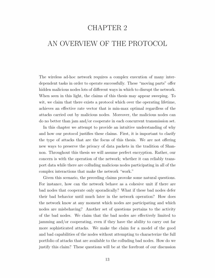
Figure 2.1: An example of an attacker that can jam and cooperate with aconcurrent transmission set.

network is:

maxprotocols

that time-shareover C\Θ

U(x). (2.1)

However, Θ can be equivalently represented as the set of actions in which

an attacker jams and/or cooperates with each CT set. It might not be clear

how an attacker can both jam and cooperate in the same CT set. Consider

Figure 2.1 composed of the source destination pairs (A, C) and (B, D) while

A and C are bad nodes and B and D are good. Now while node A jams, node

B can claim to have received all the scheduled packets, since by assumption,

the attackers fully cooperate. Hence node A effectively jams and cooperates

within the CT set. Therefore, the effective rate vector in (2.1) satisfies:

minbad nodes disable

a concurrenttransmission set

maxall protocols

that time-shareover concurrent

transmission sets

U(x). (2.2)

Note that the network arrives at this rate vector without ever having to

15

identify which nodes are good or bad. Instead, the network assumes that

any node contained in a feasible CT set must be good. This assumption may

not always be true, but it is falsified at most a finite number of times. Each

time, the assumption is false the corresponding CT set fails, is then detected,

removed from the feasible set, and never used again.

When averaged over a sufficiently large number of iterations, the rate loss

incurred by erroneously assuming cooperation can be made arbitrarily small.

To recapitulate, the achievable rate vector ensures that bad nodes are effec-

tively limited to jamming and/or cooperating with the protocol, and gain no

advantage by knowing the protocol a priori.

2.2 The Problem of Forging Consensus

The discussion so far has treated the “network” as though it were a single

cohesive unit, able to act in a coordinated manner, consistently detect and

identify disabled concurrent transmission sets, and uniformly decide on a

schedule after each iteration. In reality, the network is composed of good

and bad nodes. The good nodes are not initially synchronized; in fact they

are a distributed system. Moreover, they do not know a priori which nodes

are good or bad. On the other hand, the bad nodes do know which nodes are

good or bad, and in addition are capable of fully cooperating with each other,

i.e., they are a centralized system. Therefore all actions and decisions of the

good nodes occur in a distributed system and must be made by exchanging

and passing messages. The challenge is that bad nodes might selectively drop

messages to influence the outcome of any decisions. Since the good nodes

do not know which nodes are good or bad, they also do not know if their

messages are received or not. This problem was first proposed in a paper as

the Byzantine Generals Dilemma, which we will briefly describe now.

Consider an army encamped against an enemy city. The army, represent-

ing the Byzantine Empire, is divided into several divisions and arrayed on

opposing sides of the city. However, some of the divisions are led by treach-

erous generals. (Historically, the leadership of the Byzantine Empire, which

succeeded the Roman Empire, had a reputation for constant infighting and

backstabbing.) The loyal generals wish to decide on a common plan of action,

but they can only communicate by messenger. Suppose that in this arrange-

16

ment, two loyal generals A and B are separated by a traitor. General A sends

a message to General B requesting a joint attack. However, General A does

not know whether the message arrived or was intercepted. Suppose General

B receives the message and responds with an acknowledgment. Now General

B does not know whether his acknowledgment was received, and General A

does not know whether General B knows that his acknowledgment was re-

ceived. This recursive sequence of uncertainties carries on ad infinitum. A

fundamental result of this problem is that the loyal Byzantine generals will

never be able to decide on a common plan without an additional assumption;

namely, that the subgraph of loyal Byzantine generals is connected. It is not

obvious that this assumption is sufficient for the loyal Byzantine generals to

arrive at a consensus. The traitors might be able pass themselves off as loyal

and smear loyal generals as traitors. The solution to this problem is called

the Byzantine General’s Algorithm (BGA).

In the BGA, each user first broadcasts a message containing the infor-

mation it wishes to disseminate to all the other users in its neighborhood.

Next, each user broadcasts the messages from its neighbors’ neighbors to its

neighbors. This process is repeated n times over until each user has received

a message that has made k +m hops, where k is the number of good nodes

and m is the number of bad nodes that have behaved like good nodes, while

n is the total number of all nodes. It can be shown that after n rounds, the

good users will have the same set of messages if the subgraph of good users is

connected. Therefore, since they all obtain the same information, the good

nodes can make the same decision.

Another important caveat to the BGA is that the users must be syn-

chronous. In the network model we use, the good nodes do not have access

to a centralized reference clock. Instead, the good nodes have local clocks

that are relatively affine and the relative clock parameters (the skew and

offset) are unknown a priori. The protocol includes a series of steps that

allow the good nodes to learn their relative clock parameters, designate a

clock as a reference, and estimate the reading of the designated reference

clock. Clearly after this process is complete, the network is effectively syn-

chronized. But getting to this point requires the good nodes to arrive at

a common view of the network topology and the relative clock parameters.

Therefore we have a “chicken-or-egg” circular dependency where the BGA is

needed to synchronize the network, but a synchronized network is needed to

17

execute the BGA. To resolve it, we make use of two features of the network

model: a bounded relative clock skew between any pair of good nodes, and

bounded birth times for all nodes. Invoking these two properties, we can

assign (increasingly larger) time intervals of known size to each stage of the

BGA and guarantee that the transmissions in one stage will not overlap with

the transmissions in another stage.

An additional challenge the network must overcome prior to clock synchro-

nization is uncoordinated communication between half-duplex nodes. Any

pair of half-duplex good nodes seeking to exchange messages without a com-

mon schedule or reference clock must do so with the expectation that an

attempted transmission may result in a primary conflict. Recall that a pri-

mary conflict occurs when a source node attempts to transmit a packet to

a destination node that is also in transmit mode; the transmitted packet

fails to arrive. To guarantee communication between a source and destina-

tion node, we construct an orthogonal MAC code that dictates when a node

should transmit or receive according to its local clock. The code works as

long as the local clocks are relatively affine, even if they are unsynchronized.

In Chapter 3 we describe the construction of the orthogonal MAC code in

detail.

Using the orthogonal MAC code, the protocol is able to carry out a coor-

dinated execution of the BGA prior to clock synchronization, but with the

overhead of multiple retransmissions and large dead times separating trans-

mission intervals. We use an implementation of the Byzantine General’s

algorithm called the Exponential Information Gathering (EIG) algorithm.

2.3 The Problem of Inconsistency

The BGA enables the good nodes to obtain a common view of the topology

and the relative clock parameters (RCPs), even if there are malicious nodes

participating in the network. However, a common view is not enough for

the good nodes to establish an accurate estimate of a designated reference

clock. The data must also be consistent. Before expanding on this point, we

need to introduce some definitions. Given two nodes i and j, let t denote the

reading on node j’s continuous time clock, and let τ ij(t) denote the reading of

node i’s continuous time clock with respect to t. Let aij denote the relative

18

1 2 3 n-2 n-1 n

. . .1,2a

2,3a 2,1 nna 1,nna

Node i-1‘s clock

Node i ‘s clock

t

ti

i 1

1,iia

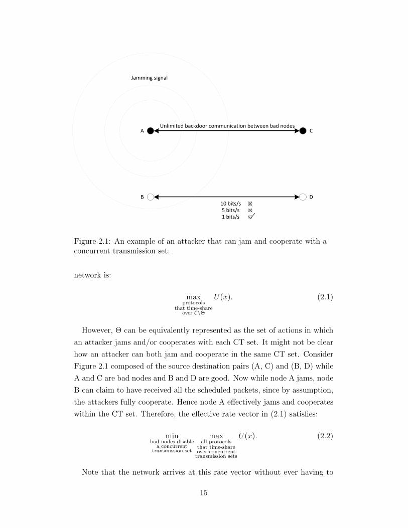
Figure 2.2: A chain network of nodes where the relative skew betweenadjacent nodes is known.

skew between node i and j. We will assume for simplicity and the purpose

of this example that all relative offsets are zero. That is, τ ij(t) = aijt. Now

consider the chain of nodes 1, . . . , n in Figure 2.2. The adjacent nodes in the

chain are able to measure their relative skews by exchanging timing packets.

Moreover, let us designate node n as the reference node. In order for the

chain network to behave as a coordinated unit, all nodes must estimate node

n’s clock with respect to their own. That is, each node k, for k = 1, . . . , n−2,

must determine τnk (t), where τnk (t) = an,kt. Since nodes k and n do not share

a direct link, their relative skew an,k cannot be measured via an exchange of

timing packets. Instead, node k can compute an,k using the relative skews of

adjacent nodes:

an,k =n∏

j=k+1

ak,k−1.

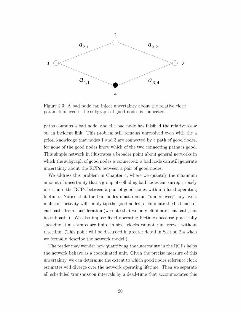
Now we can explain how a common view of the topology and the relative

skews between adjacent nodes does not prevent a bad node from injecting

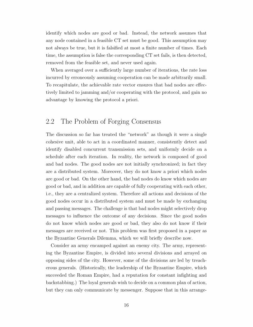
uncertainty into the data. Consider the network of Figure 2.3 where nodes 1,

2, and 3 are good nodes, but node 4 is a bad node. The good nodes share a

common view of the topology and the relative skews between adjacent nodes.

That is, all good nodes know the relative skews (a2,1, a3,2, a3,4, a3,1). However,

since nodes 1 and 3 do not share a direct link the relative skew a3,1 cannot

be directly measured via an exchange of packets. Instead, the network must

compute a3,1 using the known relative skews. However, in Figure 2.3 there

are two paths between nodes 1 and 3. Therefore we must have a3,1 = a3,2a2,1

along the top path and a3,1 = a4,1a4,3 along the bottom path. Suppose that

the estimate along path 123 does not agree with the estimate along 143. That

is, a3,2a2,1 6= a3,4a4,1. Clearly, the discord implies that at least one of the two

19

1 3

2

4

1,2a 2,3a

4,3a1,4a

Figure 2.3: A bad node can inject uncertainty about the relative clockparameters even if the subgraph of good nodes is connected.

paths contains a bad node, and the bad node has falsified the relative skew

on an incident link. This problem still remains unresolved even with the a

priori knowledge that nodes 1 and 3 are connected by a path of good nodes,

for none of the good nodes know which of the two connecting paths is good.

This simple network in illustrates a broader point about general networks in

which the subgraph of good nodes is connected: a bad node can still generate

uncertainty about the RCPs between a pair of good nodes.

We address this problem in Chapter 4, where we quantify the maximum

amount of uncertainty that a group of colluding bad nodes can surreptitiously

insert into the RCPs between a pair of good nodes within a fixed operating

lifetime. Notice that the bad nodes must remain “undercover;” any overt

malicious activity will simply tip the good nodes to eliminate the bad end-to-

end paths from consideration (we note that we only eliminate that path, not

its subpaths). We also impose fixed operating lifetimes because practically

speaking, timestamps are finite in size; clocks cannot run forever without

resetting. (This point will be discussed in greater detail in Section 2.4 when

we formally describe the network model.)

The reader may wonder how quantifying the uncertainty in the RCPs helps

the network behave as a coordinated unit. Given the precise measure of this

uncertainty, we can determine the extent to which good nodes reference clock

estimates will diverge over the network operating lifetime. Then we separate

all scheduled transmission intervals by a dead-time that accommodates this

20

divergence. Hence the good nodes in the network, having a common sched-

ule and consistent estimates of a designated reference clock, will act in a

coordinated manner and can be treated as a unified entity.

In this chapter we have provided an intuitive understanding into how a net-

work of good and bad nodes can simultaneously operate at a min-max utility

optimal rate vector through the iterative pruning of concurrent transmission

sets, and restrict the portfolio of attacker strategies to either jamming and/or

cooperating. We have also argued why a disparate collection of good and bad

nodes can behave as a coordinated unit in the first place. We will now dis-

cuss some aspects of the network model, before and subsequently terminate

the chapter with an in depth look of the individual phases that compose the

protocol.

2.4 The Model

The model-based approach to secure protocol design is one in which a pro-

tocol is tailored to a specific model of the network instead of individual

attacks. The central dogma of this thesis is that a model-based approach of-

fers a more sound and coherent framework for protocol design than an arms

race between patches and attacks. In this section, we formally describe the

model and provide an explanation for some selected features. As mentioned

in the introduction, the network model can be divided into five categories:

the model for network utility (U), the physical model (P), node capabilities

(N), clock behavior (CL), and cryptographic capabilities (CR).

There is already a significant body of literature that addresses the topic of

utility maximization in communication networks. In addition, much of the

research published in the area of distributed systems is focused on networks

composed of good and bad nodes. However, to the best of our knowledge,

this thesis contains the first attempt, in the context of security, to model

the dynamics of such a network formation and operation as a zero-sum game

between good and bad nodes. Suppose that the ith good source destination

pair (si, di) obtains a throughput rate xsi,di . We assume that (U1) there

exists a utility function U(x), and the total utility to the network derived by

serving all N good pairs is U(xs1,d1 , . . . , xsN ,dN ). However, since the network

does not know which nodes are good or bad, each node evaluates the utility

21

over all N “conforming” node pairs, where a node is defined as conforming

if it is represented in a feasible concurrent transmission set.

We now describe the physical model in more detail. We assume that: (P1)

there are n immobile nodes, (P2) the n wireless nodes exist in a bounded

domain, with the distance between every pair of nodes exceeding a mini-

mum distance dmin > 0, and power path loss decreasing monotonically with

distance. Furthermore, (P3) the receivers of the good nodes are subject to

noise, and the maximum achievable data rate is a monotonically decreasing

function of the SINR. This function could possibly be the Shannon formulaB2

log (1 + SINR) where B denotes bandwidth, or any other monotonically

decreasing function of SINR. We assume: (P4) the wireless nodes have a

maximum power constraint. In addition: (P5) the good nodes have a finite

number of modulation schemes, and (P6) any transmissions at rates below

the SINR-determined rate are error free. The lowest rate for which all nodes

have a modulation scheme, referred to as the base communication rate, oc-

curs at SINRthreshold. We also assume that (P7) the subgraph of good nodes

is connected in the following graph: there is an edge between each pair of

good nodes (i, j) for which SINRi,j and SINRj,i, respectively, both exceed

SINRthreshold when all nodes, except j or i, respectively, transmit at max

power.

A noteworthy feature of the physical model is that packets receptions are

deterministic; a packet transmitted at a rate below the SINR-based rate is

guaranteed to arrive as long as no primary conflicts occur. In the wireless

medium, probabilistic receptions model the system dynamics more realisti-

cally, but we will defer that model for future work.

We now move on to the set of model assumptions that describe the capa-

bilities and behaviors of the good nodes and the bad nodes. We assume that:

(N1) the network is composed of good nodes that conform to the protocol,

and bad nodes that may undermine it. Moreover: (N2) the good nodes are

half-duplex; they cannot transmit and receive simultaneously. On the other

hand, the bad nodes have no constraints on their ability to jointly transmit

and receive. We also assume that: (N3) the bad nodes are able to fully

coordinate their actions and fully aware of their collective states (equivalent

to unlimited bandwidth between all pairs of bad nodes). The bad nodes thus

also know the identities of the good and bad nodes a priori. In addition, the

bad nodes can execute any causal cooperative policy that undermines the

22

network. We assume that: (N4) the good nodes are all initially powered off,

and that they all turn on within U0 time units of the first good node that

turns on.

The next set of assumptions characterizes the clock model. As mentioned

in the introduction, clocks are not typically used in wireless protocols, where

all coordinated activity is event based. However, distributed clock synchro-

nization with hostile nodes is a well-studied topic in distributed systems.

Most of the assumptions of our model are consistent with the literature. We

assume that: (CL1) each good node initializes its own clock to zero when it

turns on, and (CL2) each good node i has a local continuous-time clock τ i(t)

that is affine with respect to the time t ≥ 0. That is, τ i(t) = ait+ bi where ai

and bi denote the skew and offset respectively of node i’s local clock. With-

out loss of generality for timekeeping in the statements and proofs we will

assume that: (CL3) the time t above and in (N4) is equal to the clock of the

first good node to turn on. We denote the relative skew and offset between

nodes i and j by aij and bij respectively, where aij := aiaj

and bij := bi−aijbj.We also denote by τ ij(s) = aijs + bij the time at node i’s continuous-time

clock with respect to the time s at node j’s continuous-time clock. We as-

sume that: (CL4) the relative clock skew aij between any two nodes i and

j is bounded by 0 < aij ≤ amax. It can be shown as a corollary of (N4),

(CL1) and (CL4) that: (CL5) the offset is bounded by |bij| ≤ amaxU0, since

τ i(U0) ≥ 0. We assume that: (CL6) the good nodes do not know their skew

parameters a priori.

Finally we describe the cryptographic aspects of the model. We assume

that: (CR1) each node is assigned a public key and a private key. The

private key is never revealed by a good node to any node, and information

encrypted by a private key can only be decoded with the corresponding public

key. However, possession of this key does not enable an attacker to forge,

alter, or tamper with an encrypted packet generated with the corresponding

private key. We assume that: (CR2) each node possesses the public key of

a central authority. Furthermore: (CR3) each node possesses an identity

certificate; a signed message from the central authority containing node i’s

public key and ID number. The certificate binds node i’s public key to its

identity. Finally, we assume that: (CR4) each node possesses a list of all

the other node IDs in the network.

An encryption scheme is information theoretically secure if the cipher text

23

Scheduling Phase

Data Transfer

Phase

Verification Phase

Neighbor Discovery

Phase

Network Discovery

Phase

Primordial Birth

Operating time expired?

No

TerminateYes

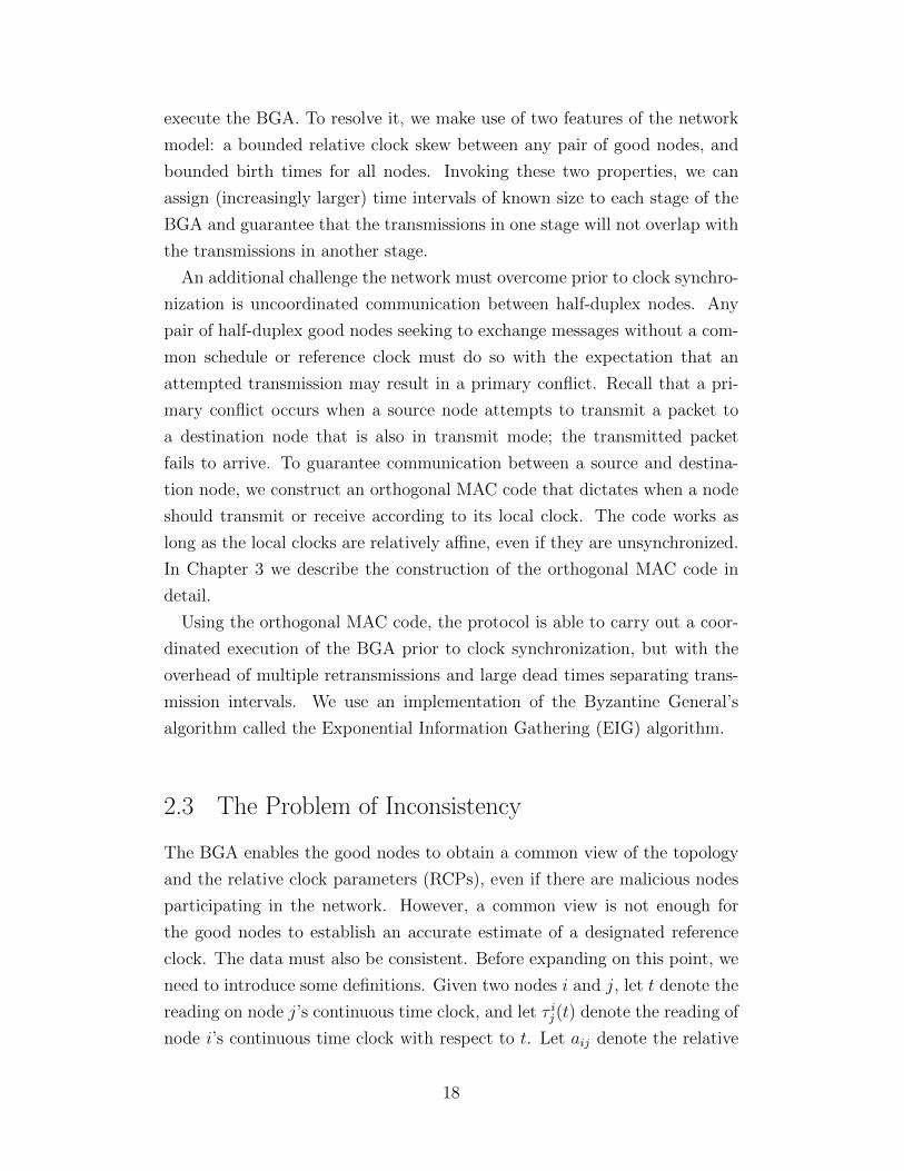
Figure 2.4: The protocol state diagram for the bounded-birth time model.

provides no information to an attacker about the message without the key.

It was shown by Shannon [26] that the one-time pad is the only scheme

that achieves this level of security. Our model reflects the reality that other

encryption schemes achieve a high enough level of secrecy, based on being

currently regarded as computationally complex, to justify treating encrypted

messages as private. Moreover, the focus of this thesis is not on preserving

secrecy but on ensuring a stable and reliable network in the face of malicious

behavior by participating nodes, though of course the ability to authenticate

or sign depends on the security of the cryptography.

2.5 The Protocol Phases

In this last section we discuss in more detail the individual phases that com-

pose the protocol. At the onset of this chapter, we argued that the network

could operate in a reliable and utility-optimal manner through the itera-

tive pruning of concurrent transmission sets. The protocol state diagram in

Figure 2.4 briefly summarizes how this task is implemented.

The protocol suite is composed of five phases: the neighbor discovery

phase, the network discovery phase, the scheduling phase, the data trans-

fer phase, and the verification phase. The first two phases form a tentative

network out of a collection of unsynchronized half-duplex nodes, infiltrated

with colluding attackers. At the conclusion of the network discovery phase,

the good nodes have a common topological view and a consistent estimate

of a reference clock. The last three phases are where the iterative pruning

of CT sets occurs. The network (now behaving as a coordinated unit) cycles

through these phases, constantly pruning failed CTs, until steady state is

24

reached. In the scheduling phase, the network determines a schedule based

on the most recently updated set of feasible CT sets. This schedule is imple-

mented in the data transfer phase. Wherever malicious activity prevents a

scheduled packet from arriving, the corresponding CT set is disabled in the

verification phase. This process is then repeated a sufficiently large number

of times.

2.5.1 The Neighbor Discovery Phase

The neighbor discovery phase is the initial step in the larger process of dis-

covering all the nodes and synchronizing all the clocks. It starts with each

node identifying its immediate neighbors and computing the corresponding

clock parameters. In the first move, each node attempts a handshake with a

neighbor by broadcasting a probe packet and waiting for an acknowledgment.

Each node then attempts to estimate its neighbor’s clock parameters via an

exchange of timing packets.

However these initial tentative steps are complicated by the fact that they

occur prior to synchronization and the nodes have a half-duplex constraint.

Moreover, the nodes begin this phase at different times because they start-

up at different times. As a result, any communication between two nodes

is uncoordinated and susceptible to mutual packet collisions. To circumvent

this problem we design an orthogonal MAC code that guarantees successful

two-way communication between any adjacent nodes, provided the relative

clock skew is bounded. The construction of the orthogonal MAC code is

provided in Chapter 3.

Another synchronization related problem is that some nodes may complete

these steps faster than their neighbors, in fact, so much faster that the slower

neighbors may fail to complete handshakes with their speedier compatriots.

In response we allocate increasingly large time intervals for each step so that

even in the worst case, with maximum skew drift and delay, the steps can be

completed in the time allotted.

Although the clock skews, delays and offsets are real-valued quantities,

the arrival times can only be measured in discrete-time, thus subjecting the

computed skew to some quantization error. This error is a fundamental

problem since it cannot be eliminated and will ultimately cause the clock

25

estimates to drift apart as time elapses. Moreover, we can expect malicious

nodes to exploit this drift and undermine network coordination. The only

option available is to reduce the skew error and separate the timing packets

by a large number of clock counts ka. However, we show that it is possible

with a joint selection of ka and the network lifetime Tlife, to completely

account for the skew drift without jeopardizing the goal of ε optimality.

A fundamental result of [28], [29] shows that only the sum of the offset

and delay (but not their individual values) can be determined by exchanging

timing packets. However, unlike the skew error, these quantities do not

cause the clock estimates to diverge indefinitely. Rather, the induced error

is bounded.

In the upcoming network discovery phase, the clock estimates obtained be-

tween adjacent nodes will be used to form clock estimates between arbitrary

nodes. We encounter a special vulnerability that enables malicious nodes

to distort these multi-hop clock estimates by manipulating the one-hop skew

computations. We force each node to vouch for the skew estimates made with

its neighbors by signing a link certificate containing the packets exchanged

during this phase. Any node that generates timing data not consistent with

its declared skews, at any point in the protocol, is self-evidently malicious.

2.5.2 The Network Discovery Phase

In the network discovery phase, each node discovers the topology of the net-

work by obtaining the link certificates of its neighbors, its neighbors’ neigh-

bors, and so forth. However, yet again, the network encounters the familiar

obstacle of unsynchronized nodes, uncoordinated transmissions, and some

nodes completing steps faster than others. Moreover, unlike the previous

phase, the interactions in each step of the network discovery phase must

occur in the same time interval at all nodes, regardless of how poorly syn-

chronized the clocks are. To solve this problem, we allocate increasingly large

intervals to each step, and force all transmissions associated with that step

to begin well into the interval and use the orthogonal MAC code.

Another major challenge is that malicious nodes may selectively drop pack-

ets, preventing the good nodes from having a common view of the topology.

We solve this problem using the Byzantine General’s algorithm [30]. The al-

26

gorithm ensures a packet between any pair of nodes goes through every path

between these nodes. We show that since the good nodes form a connected

component, they will form a common topological view.

Upon completion of the algorithm, each node is able to infer the topology

of the network and estimate the clock of any other node by taking the skew

product along the path. However, a problem occurs if there are multiple paths

to a node, and the skew products along each path differ by more than the

maximum skew error. Such a node belongs to an inconsistent cycle, defined

as a cycle in which the skew product differs from unity by more than the

maximum skew error. In such an inconsistent cycle, at least one malicious

node advertises a false clock to one of its neighbors (but not the other).

The neighbors could even be colluding in this endeavor. Unfortunately, it

is impossible to determine who is lying and who is telling the truth from

the clock skew parameters alone. As a result, it is necessary to remove at

least one link in the cycle with a bad endpoint so that every pair of nodes

will have a unique path and consistent clock estimates. Consistent estimates

are mandatory to ensure that all nodes are operating by roughly the same

reference time.

We propose a consistency check to identify at least one bad link in the

cycle. First the nodes wait for a long period of time, during which the gap

between the actual time and the estimated time diverges. Then a designated

node in the cycle, called the leader, initiates a timing packet that traverses

the cycle. Each node is forced to satisfy the delay condition; it is required to

forward the packet within one clock count of receiving it. We show that since

the false clock estimate has diverged so extensively from the actual clock, at

least one of the malicious nodes will not be able to both simultaneously

generate timestamps consistent with its declared skew as well as meet the

delay condition. This test is performed on every inconsistent cycle. If an

inconsistent cycle manages to pass the consistency check, then by deduction

the cycle leader must be a malicious node.

The consistency check is performed prior to synchronization and all the

related issues (uncoordinated nodes, completion of protocol steps at different

times) are still in play. We choose increasing time intervals for each step of

the consistency check and show that all nodes, fast or slow, properly complete

the test.

The core idea of the consistency check is that excessive skew error will,

27

after a sufficiently large amount of time, force the clock estimate to diverge

from the actual clock by a detectable amount. Smaller skew errors require

much larger wait-times. A key obstacle is achieving two competing goals: the

wait-time must be small enough to occupy a negligible fraction of the total

operating lifetime; and the skew error must be small enough to minimize the

clock drift over the total operating lifetime.

After the inconsistent cycles have been tested, the network disseminates

the timing data using the Byzantine General’s algorithm. The problem of

unsynchronized clocks is still in force, so we allocate increasing intervals of

time to each step and use the orthogonal MAC code for transmissions.

After the algorithm has finished, the nodes have a common view of the

timing data and can remove the malicious links from each inconsistent cycle.

At the conclusion of this phase, all the nodes in the network have a common

topological view, and a common estimate of all clocks. For the remainder of

the protocol, the network effectively operates by a common reference clock.

2.5.3 The Scheduling Phase

The purpose of the scheduling phase is to obtain a schedule over the set

of feasible concurrent transmission sets, whose corresponding effective end-

to-end rate vector maximizes the utility function. The schedule specifies

the concurrent transmission sets, the intervals in which they occur, and the

number of data packets to be transmitted in each interval.

The main problem in the scheduling phase is accounting for the diver-

gence in the estimates of the reference clock due to the uncertainty injected

into the relative clock parameters by the bad nodes. Clearly the concurrent

transmission sets must be separated by some bands to prevent any overlap.

However, choosing a large band exacerbates the clock divergence in future

transmission intervals thus causing overlap, while choosing a small band may

not prevent the immediate overlap caused by existing clock divergence. We

explicitly compute a suitable dead-time band in Chapter 4.

28

2.5.4 The Data Transfer Phase

The purpose of the data transfer phase is to carry out the schedule chosen

in the previous phase.

The main challenge to this phase comes from “sleeper cells” of malicious

nodes that have stayed undetected by cooperating with the protocol. At

any point in the data transfer phase, these nodes may suddenly sabotage

a concurrent transmission set by either jamming or dropping packets. To

counter this problem, each node keeps a record of any packet that failed to

arrive as scheduled. This information (or a subset of it) will be disseminated

to the rest of the network during the verification phase and never used again.

Moreover, we show that these types of attacks can only occur a finite number

of times, since there are a finite number of concurrent transmission sets and

each set can only be disabled once.

2.5.5 The Verification Phase

The purpose of the verification phase is to inform the network of concurrent

transmission sets that failed to transmit all of the packets assigned in the

schedule. As in the data transfer phase, some malicious nodes may choose

not to cooperate with the protocol and prevent the network from obtaining

a common view of the CT sets. The network uses the Byzantine General’s

algorithm to ensure that any knowledge of these failed sets is shared by all

the good nodes.

Two other issues need to be addressed as well. First, the transmission

intervals are separated by a dead-time D to account for the divergence in the

estimates of a reference clock. Second, the list of packets that failed to arrive

during the data transfer phase may be prohibitively and unpredictably large

to transmit. Instead we propose the following solution: let each node dissem-

inate the smallest ID in the list of failed packets. Then the network observes

the scheduled path of this packet and removes the concurrent transmission

set where it first failed.

In the next chapter we will provide a detailed description of the orthogonal

MAC code that plays such an important role in the neighbor and network

discovery phases.

29

CHAPTER 3

THE ORTHOGONAL MAC CODE

The distributed real-time operation of wireless networks requires the interac-

tion of many protocols, each of which addresses a unique functional require-

ment for the network to work reliably. In this chapter, we examine one of

the most basic requirements; the ability of adjacent nodes to communicate

with each other prior to clock synchronization.

The orthogonal MAC protocol that provides the above functionality is an

essential component of the larger protocol suite with a more comprehensive

goal. Given a set of nodes, some of which are malicious, how can the good

nodes form an operating and indeed optimized wireless network? In order

to even begin to achieve this larger goal, the nodes must first have the fun-

damental capability to communicate with each other, even before knowing

each others clock skew rates, and do so within a bounded time.

Wireless transceivers are generally half-duplex; they cannot transmit and

receive at the same time due to the physical limitations of the circuitry in

their receivers. There is recent work on developing full duplex radios, but en-

dowing a network of only half-duplex nodes to achieve communication capa-

bility allows a larger class of networks to operate reliably. Hence, we consider

nodes with radios where simultaneous transmissions by a transmitter and its

intended recipient effectively result in “primary conflicts,” a reference to the

loss of any messages that arrive while the recipient itself is in “transmit”

mode not “receive” mode. A communication scheme that attempts to solve

this problem is the orthogonal MAC Gold code [31]. This protocol provides

each node with a unique square-pulse waveform, where a pulse defines a time

interval in which the node should be in transmit mode. The Gold code has

the property that any two waveforms share a non-overlapping pulse during

which any transmitted messages will arrive collision-free. However, orthog-

onal MAC codes are designed under the assumption that the local clocks

in the network run at the same speed, even if they are not synchronized.

30

This assumption is not satisfied in practice because distributed clocks are

generally subject to skew and offset. Clock skew has the effect of stretching

or compressing transmitted signals, a distortion that invalidates the non-

overlapping pulse property of the Gold code. The same can be said of any

family of waveforms periodic with respect to a single pulse; under compres-

sion or stretching the pulses of one waveform can be made to overlap with

the pulses of another waveform. In this chapter, we solve this problem by de-

signing an orthogonal MAC code based on a family of two-pulse waveforms,

in which the spacing between the two pulses in each period is sufficiently

asymmetric to ensure that any two linearly distorted waveforms will share a

non-overlapping pulse.

A network that lacks a coordinated scheme for communication will likely

end up with multiple nodes transmitting messages simultaneously. The above

strategy works well to resolve primary conflicts, it does nothing to address a

different sort of conflict called “secondary conflict” that occurs when two or

more nodes attempt to simultaneously communicate with the same intended

recipient. This secondary conflict is also often called a “packet collision.”

Several protocols have been developed to avoid this from happening in un-

synchronized networks. For example ALOHA random access [32], directs a

wireless node to back off for an exponentially distributed amount of time

whenever a collision is detected, and retransmit after this time has expired.

However, the probability of repeat collisions within a bounded time-interval,

though small, is still nonzero and this uncertainty complicates the design of

wireless networks that require guaranteed success.

We overcome the secondary conflict too by dividing the time, as measured

by the local clock of each node, into slots, and assigning these slots for com-

municating to other nodes. A node may only transmit a given message during

the time-slot assigned to the corresponding destination. Furthermore, within

a time-slot a message can only be transmitted during the windows defined

by the orthogonal MAC code pulses. Similarly, any given message must be

received during the time-slot assigned to the corresponding source, and out-

side of the transmission windows defined by the orthogonal MAC code pulses.

The orthogonal MAC code presented in this chapter ensures that within a

bounded time, any source-destination pair will share a non-overlapping pulse

during which the source and destination will be paying attention to each

other. We will choose the sizes of the slots, the spacing between the pulses,

31

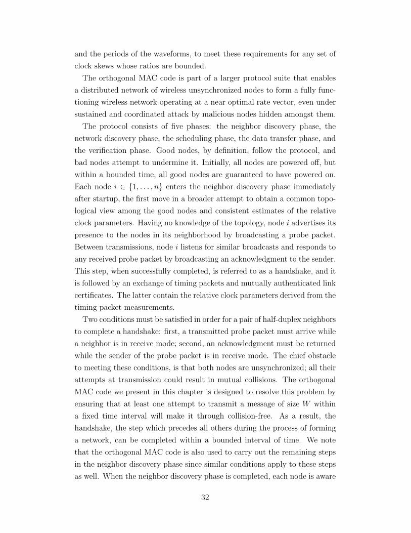
and the periods of the waveforms, to meet these requirements for any set of

clock skews whose ratios are bounded.

The orthogonal MAC code is part of a larger protocol suite that enables

a distributed network of wireless unsynchronized nodes to form a fully func-

tioning wireless network operating at a near optimal rate vector, even under

sustained and coordinated attack by malicious nodes hidden amongst them.

The protocol consists of five phases: the neighbor discovery phase, the

network discovery phase, the scheduling phase, the data transfer phase, and

the verification phase. Good nodes, by definition, follow the protocol, and

bad nodes attempt to undermine it. Initially, all nodes are powered off, but

within a bounded time, all good nodes are guaranteed to have powered on.

Each node i ∈ {1, . . . , n} enters the neighbor discovery phase immediately

after startup, the first move in a broader attempt to obtain a common topo-

logical view among the good nodes and consistent estimates of the relative

clock parameters. Having no knowledge of the topology, node i advertises its

presence to the nodes in its neighborhood by broadcasting a probe packet.

Between transmissions, node i listens for similar broadcasts and responds to

any received probe packet by broadcasting an acknowledgment to the sender.

This step, when successfully completed, is referred to as a handshake, and it

is followed by an exchange of timing packets and mutually authenticated link

certificates. The latter contain the relative clock parameters derived from the

timing packet measurements.

Two conditions must be satisfied in order for a pair of half-duplex neighbors

to complete a handshake: first, a transmitted probe packet must arrive while

a neighbor is in receive mode; second, an acknowledgment must be returned

while the sender of the probe packet is in receive mode. The chief obstacle

to meeting these conditions, is that both nodes are unsynchronized; all their

attempts at transmission could result in mutual collisions. The orthogonal

MAC code we present in this chapter is designed to resolve this problem by

ensuring that at least one attempt to transmit a message of size W within

a fixed time interval will make it through collision-free. As a result, the

handshake, the step which precedes all others during the process of forming

a network, can be completed within a bounded interval of time. We note

that the orthogonal MAC code is also used to carry out the remaining steps

in the neighbor discovery phase since similar conditions apply to these steps

as well. When the neighbor discovery phase is completed, each node is aware

32

of the IDs and relative clock parameters of its neighboring nodes.

The next stage of the protocol occurs during the network discovery phase,

in which the nodes disseminate their lists of neighbors among themselves

and infer a common topological view. However, the behavior of the bad

nodes in the network complicates matters. Bad nodes may choose to not

cooperate with the protocol, spread false information, or carry out other

malicious acts. The protocol uses the Byzantine General’s algorithm and a

skew consistency test to ensure that the good nodes share the same view of

the network topology and have consistent estimates of all the relative clock

parameters. Each of these steps are subject to the same conditions as the

handshake, and are carried out using the orthogonal MAC code. At the

conclusion of the network discovery phase, the nodes are able to schedule

their actions based on a sufficiently accurate estimate of a common reference

clock. The orthogonal MAC code is no longer needed since the network is

able to operate synchronously and schedule collision free transmissions.

Node i then iteratively cycles through the scheduling, data transfer, and

verification phases repeatedly, gradually eliminating infeasible concurrent

transmission sets until an optimal feasible rate vector is obtained. An im-

portant achievement of the protocol is that the rate loss due to overhead,

such as the time spent in the neighbor and network discovery phases, can be

made arbitrarily small by choosing the duration of each phase appropriately.

This result is due to the fact that the length of the orthogonal MAC code is

bounded.

This chapter is focused on the specific problem of uncoordinated com-

munication between half-duplex nodes during the initial stages of network

formation, a critical component of the overall protocol suite.

3.1 Construction of the Orthogonal MAC Code

Consider a collection of n wireless nodes. Each node i is equipped with a

local clock τ i(t) that is affine with respect to some global reference clock t.

That is, τ i(t) = ait + bi where the parameters ai and bi denote the clock

skew and offset respectively. Let aij > 0 and bij denote the relative skew

and relative offset of node i with respect to node j, where aij := aiaj

and

bij := bi−aijbj. Let τ ij(t) denote node i’s clock with respect to node j’s clock

33

)(

0

i

iTc

W W

WTc i

i

)(

0

)(

0

iT

)()(

1 tM i

1

t

Figure 3.1: A graph of M(i)1 (t). Note that M

(i)2 (t) = M

(n−i+1)1 (t).

t:

τ ij(t) := aijt+ bij.

We will assume that aij ≤ amax for all nodes i and j. The orthogonal MAC

code for each node i is composed of two fundamental two-pulse waveforms

M(i)1 (t) and M

(i)2 (t), which are designed to work when the relative skew ex-

pands (aij ≤ 1) or contracts (aij > 1), respectively, the transmitted signals

received at node j. The periods of the waveforms M(i)1 (t) and M

(i)2 (t) are

denoted by T(i)0 and T

(n−i+1)0 respectively, where T

(i)0 is defined below:

T0 := 32Wna2max, (3.1)

T(i)0 := iT0. (3.2)

The waveforms M(i)1 (t) and M

(i)2 (t) contain two-pulses of width W that

are separated by a distance unique to node i. We call the first pulse of the

waveform the primary pulse, and the second pulse, the secondary pulse. We

use the parameter ci to define the position of the secondary pulse in the

waveform, where:

ci :=1

amax(5n− i).

34

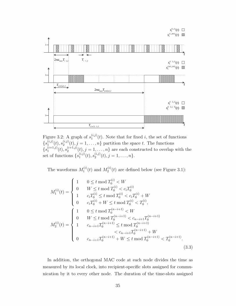
1

t

1

t

1

t

)(),(

1 ts ji

2,1iT2,1max2 iTna

2,1)1(iT

2,1)1(max2 iTna

2,1)2( iT

)()1,(

1 ts ji

)(),1(

1 ts ji

)()1,1(

1 ts ji

)(),2(

1 ts ji

)()1,2(

1 ts ji

Figure 3.2: A graph of s(i,j)1 (t). Note that for fixed i, the set of functions

{s(i,j)1 (t), s

(i,j)2 (t), j = 1, . . . , n} partition the space t. The functions

{s(i+1,j)1 (t), s

(i+1,j)2 (t), j = 1, . . . , n} are each constructed to overlap with the

set of functions {s(i,j)1 (t), s

(i,j)2 (t), j = 1, . . . , n}.

The waveforms M(i)1 (t) and M

(i)2 (t) are defined below (see Figure 3.1):

M(i)1 (t) =

1 0 ≤ t mod T

(i)0 < W

0 W ≤ t mod T(i)0 < ciT

(i)0

1 ciT(i)0 ≤ t mod T

(i)0 < ciT

(i)0 +W

0 ciT(i)0 +W ≤ t mod T

(i)0 < T

(i)0 ,

M(i)2 (t) =

1 0 ≤ t mod T(n−i+1)0 < W

0 W ≤ t mod T(n−i+1)0 < cn−i+1T

(n−i+1)0

1 cn−i+1T(n−i+1)0 ≤ t mod T

(n−i+1)0

< cn−i+1T(n−i+1)0 +W

0 cn−i+1T(n−i+1)0 +W ≤ t mod T

(n−i+1)0 < T

(n−i+1)0 .

(3.3)

In addition, the orthogonal MAC code at each node divides the time as

measured by its local clock, into recipient-specific slots assigned for commu-

nication by it to every other node. The duration of the time-slots assigned

35

by node i is denoted by Ti,2,

T0,2 := 2(dnamaxe+ 2)T(n)0 , (3.4)

Ti,2 := 2amaxnTi−1,2. (3.5)

In each time slot, node i either uses the signal M(i)1 (t) or M

(i)2 (t). We use

the functions s(i,j)1 (t) and s

(i,j)2 (t) to define a time-slot associated with the

signal M(i)1 (t) or M

(i)2 (t) respectively, that has been assigned by node i to

node j. The functions s(i,j)1 (t) and s

(i,j)2 (t) are defined below (see Figure 3.2):

s(i,j)1 (t) =

1 (j − 2)Ti−1,2 ≤ t mod 2(n− 1)Ti−1,2

< (j − 1)Ti−1,2, i < j

1 (j − 1)Ti−1,2 ≤ t mod 2(n− 1)Ti−1,2

< jTi−1,2, i > j

0 else,

(3.6)

s(i,j)2 (t) =

1 (n− 1)Ti−1,2 + (j − 2)Ti−1,2 ≤ t mod 2(n− 1)Ti−1,2

< (n− 1)Ti−1,2 + (j − 1)Ti−1,2, i < j

1 (n− 1)Ti−1,2 + (j − 1)Ti−1,2 ≤ t mod 2(n− 1)Ti−1,2

< (n− 1)Ti−1,2 + jTi−1,2, i > j

0 else.

(3.7)

Now suppose that node i wishes to transmit a message of size W to

node j during the interval [ts, ts + TMAC(W )), where TMAC(W ) := Tn,2 and

τ ji (ts) > 0. To accomplish this task, node i transmits its message during

the time intervals of size W , where both s(i,j)k (t) = 1 and M

(i)k (t) = 1. The

function s(i,j)k (t), when equal to 1, indicates that node i is “paying attention”

to node j. That is, node i is either transmitting or listening to node j. The

function M(i)k (t), when equal to 1 or 0, determines whether or not node i

is transmitting or listening. Taken together, both functions determine when

node i is transmitting to node j. Therefore, to be precise, node i transmits

its message to node j during every interval [t1, t1 +W ) ⊂ [ts, ts +TMAC(W ))

that satisfies one of the following condition for all t ∈ [t1, t1 +W ) and some

36

2,1)1(2 iTn

)(),(

1 ts ji

1

t

1

Wa ji

wt

)()(

1 tM i

))((),(

2 ts j

i

ij

))(()(

1 tM j

i

j

)(

0

iT

2,1)1(2 jji Tna

)(

0

j

jiTa

t

Wtt ww ,Node i

Node j

Figure 3.3: The interval [tw, tw +W ) satisfies both conditions that arenecessary for node i to successfully transmit a message of size W to node j.For all t ∈ [tw, tw +W ), M

(i)1 (t)s

(i,j)1 (t) = 1 and

M(i)1 (τ ji (t))s

(i,j)1 (τ ji (t)) + s

(i,j)1 (τ ji (t)) = 1.

k ∈ {1, 2}:

M(i)1 (t)s

(i,j)1 (t) = 1. (3.8)

Suppose that node j wishes to receive this message of size W from node

i during the interval [τ ji (ts), τji (ts) + TMAC(W )), where TMAC(W ) := Tn,2.

Node j listens for this message during the time intervals where s(j,i)k (t) = 1

and M(j)k (t) = 0. As before, the function s

(j,i)k (t), when equal to 1, indicates

that node j is “paying attention” to node i. That is, node j is either trans-

mitting or listening to node i. Similarly, the function M(j)k (t), when equal

to 1 or 0, determines whether or not node j is transmitting or listening.

Taken together, both functions determine when node j is listening to node i.

Therefore to be precise, node j listens for the message during every interval

[t1, t2) ⊂ [τ ji (ts), τji (ts) + TMAC(W )) that satisfies the following condition for

all t ∈ [t1, t2) and some k ∈ {1, 2}:

M(i)1 (t)s

(i,j)1 (t) + s

(i,j)1 (t) = 1. (3.9)

The described process is depicted in Figure 3.3. The following theorem shows

that node j will indeed successfully receive the message.

37

Theorem 3.1.1. Suppose node i transmits a message of size W to node

j using the orthogonal MAC code described above. Node j is guaranteed

to successfully receive the message transmitted from node i. That is, there

exists an interval [tw, tw + W ) that satisfies the following conditions for all

t ∈ [tw, tw +W ) and some k ∈ {1, 2}:

(i) M(i)k (t)s

(i,j)k (t) = 1,

(ii) M(j)k (τ ji (t))s

(j,i)k (τ ji (t)) + s

(j,i)k (τ ji (t)) = 1.

It can be shown that the duration of the orthogonal MAC code satisfies

TMAC(W ) ≤ cW where c := (2namax)9n. That is, the duration of the orthog-

onal MAC code is doubly exponential in the number of nodes. Clearly, this

level of efficiency is quite poor. However, as mentioned previously the or-

thogonal MAC code is designed as part of a larger protocol suite that allows

a collection of distributed nodes to form a fully functioning network oper-

ating at an optimal rate vector. Since the parameters n and amax are fixed

constants, the effect of the orthogonal MAC code on the protocol overhead

can be mitigated by choosing a sufficiently long data transfer phase which,

in large networks, might require very large time scales. In theory at least,

we do not pay a penalty for the relatively poor efficiency of the orthogonal

MAC code, but this property will likely require further improvement before

the code can be practically implemented.

3.2 Analysis of the Orthogonal MAC Code

Construction

In order to prove that node j can indeed successfully transmit a message to

node i, we first need to show that there exists an interval of time in which the

two nodes are paying attention to each other; the slot allocated to node i by

node j overlaps the slot allocated to node j by node i. Then, we need to show

that somewhere in the intersection of these two time-slots there is a pulse

generated by one of the fundamental waveforms {M (j)k (t), k = 1, 2} that does

not collide with a pulse generated by the corresponding waveform M(i)k (τ ij(t))

(shown in Figure 3.3). To do this, we locate the first primary pulse generated

by M(j)k (t) that occurs in the intersection of the time slots. If this pulse is

38

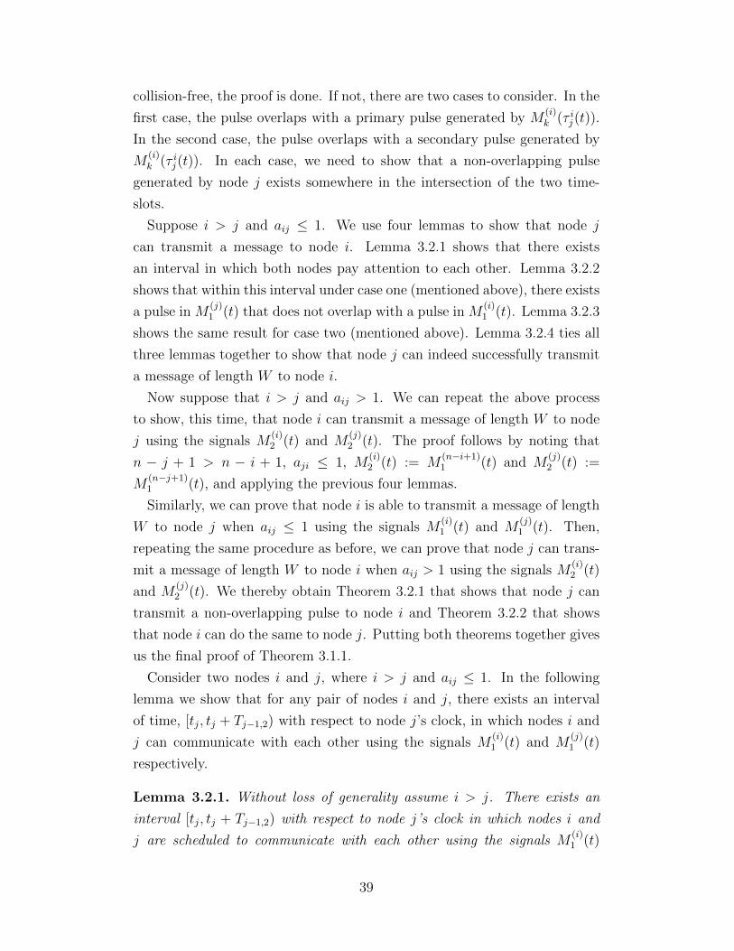
collision-free, the proof is done. If not, there are two cases to consider. In the

first case, the pulse overlaps with a primary pulse generated by M(i)k (τ ij(t)).

In the second case, the pulse overlaps with a secondary pulse generated by

M(i)k (τ ij(t)). In each case, we need to show that a non-overlapping pulse

generated by node j exists somewhere in the intersection of the two time-

slots.

Suppose i > j and aij ≤ 1. We use four lemmas to show that node j

can transmit a message to node i. Lemma 3.2.1 shows that there exists

an interval in which both nodes pay attention to each other. Lemma 3.2.2

shows that within this interval under case one (mentioned above), there exists

a pulse in M(j)1 (t) that does not overlap with a pulse in M

(i)1 (t). Lemma 3.2.3

shows the same result for case two (mentioned above). Lemma 3.2.4 ties all

three lemmas together to show that node j can indeed successfully transmit

a message of length W to node i.

Now suppose that i > j and aij > 1. We can repeat the above process

to show, this time, that node i can transmit a message of length W to node

j using the signals M(i)2 (t) and M

(j)2 (t). The proof follows by noting that

n − j + 1 > n − i + 1, aji ≤ 1, M(i)2 (t) := M

(n−i+1)1 (t) and M

(j)2 (t) :=

M(n−j+1)1 (t), and applying the previous four lemmas.

Similarly, we can prove that node i is able to transmit a message of length

W to node j when aij ≤ 1 using the signals M(i)1 (t) and M

(j)1 (t). Then,

repeating the same procedure as before, we can prove that node j can trans-

mit a message of length W to node i when aij > 1 using the signals M(i)2 (t)

and M(j)2 (t). We thereby obtain Theorem 3.2.1 that shows that node j can

transmit a non-overlapping pulse to node i and Theorem 3.2.2 that shows

that node i can do the same to node j. Putting both theorems together gives

us the final proof of Theorem 3.1.1.

Consider two nodes i and j, where i > j and aij ≤ 1. In the following

lemma we show that for any pair of nodes i and j, there exists an interval

of time, [tj, tj + Tj−1,2) with respect to node j’s clock, in which nodes i and

j can communicate with each other using the signals M(i)1 (t) and M

(j)1 (t)

respectively.

Lemma 3.2.1. Without loss of generality assume i > j. There exists an

interval [tj, tj + Tj−1,2) with respect to node j’s clock in which nodes i and

j are scheduled to communicate with each other using the signals M(i)1 (t)

39

and M(j)1 (t) respectively. That is, given t1 such that τ ij(t1) ≥ 0, the interval

[tj, tj + Tj−1,2) satisfies the following conditions:

[tj, tj + Tj−1,2) ⊂ [t1, t1 + Tn,2), (3.10)

τ ij([tj, tj + Tj−1,2)) ⊂ [τ ij(t1), τ ij(t1) + Tn,2), (3.11)

s(i,j)1 (τ ij(t)) = 1, ∀t ∈ [tj, tj + Tj−1,2), (3.12)

s(j,i)1 (t) = 1, ∀t ∈ [tj, tj + Tj−1,2). (3.13)

Proof. First we show that there exists an interval [ti, ti+Ti−1,2) ⊂ [τ ij(t1), τ ij(t1)+

Tn,2) with respect to node i’s clock in which node i pays attention to node j.

That is, s(i,j)1 (τ (i,j)(t)) = 1 for all t ∈ τ ji ([ti, ti + Ti−1,2)).

Since 0 ≤ τ ij(t1) mod 2(n− 1)Ti−1,2 < 2(n− 1)Ti−1,2, there exists some ta,

0 ≤ ta < 2(n−1)Ti−1,2 such that (τ ij(t1)+ta) mod 2(n−1)Ti−1,2 = (j−1)Ti−1,2

if 2 ≤ j ≤ n. Let ti := τ ij(t1) + ta. It follows from the definition in (3.6)

that node i is paying attention to node j during the interval [ti, ti + Ti−1,2)).

Moreover, we have:

ti + Ti−1,2 = τ ij(t1) + ta + Ti−1,2

< τ ij(t1) + 2(n− 1)Ti−1,2 + Ti−1,2 (3.14)

< τ ij(t1) + 2nTi−1,2

≤ τ ij(t1) + Ti,2 (3.15)

≤ τ ij(t1) + Tn,2, (3.16)

where (3.14) follows from the fact that ta < 2(n−1)Ti−1,2, and (3.15) follows

from the definition of Ti,2. Therefore it follows from (3.16) that the interval

[ti, ti +Ti−1,2) is contained in one complete run of the orthogonal MAC code.

That is, [ti, ti + Ti−1,2) ⊂ [τ ij(t1), τ ij(t1) + Tn,2).

Next we show that there exists a subinterval [tj, tj + Tj−1,2), with respect

to node j’s clock, of [ti, ti + Ti−1,2), in which node j pays attention to node

i. That is, τ ij([tj, tj + Tj−1,2)) ⊂ [ti, ti + Ti−1,2) and sj,i1 (t) = 1 for all t ∈[tj, tj + Tj−1,2).

Now since 0 ≤ τ ji (ti) mod 2(n − 1)Tj−1,2 < 2(n − 1)Tj−1,2, there exists

some tb, 0 ≤ tb < 2(n− 1)Tj−1,2 such that (τ ji (ti) + tb) mod 2(n− 1)Tj−1,2 =

(i−2)Tj−1,2 if 2 ≤ i ≤ n. Let tj := τ ji (ti)+tb. It follows from the definition of

(3.6) that node j pays attention to node i during the interval [tj, tj +Tj−1,2).

40

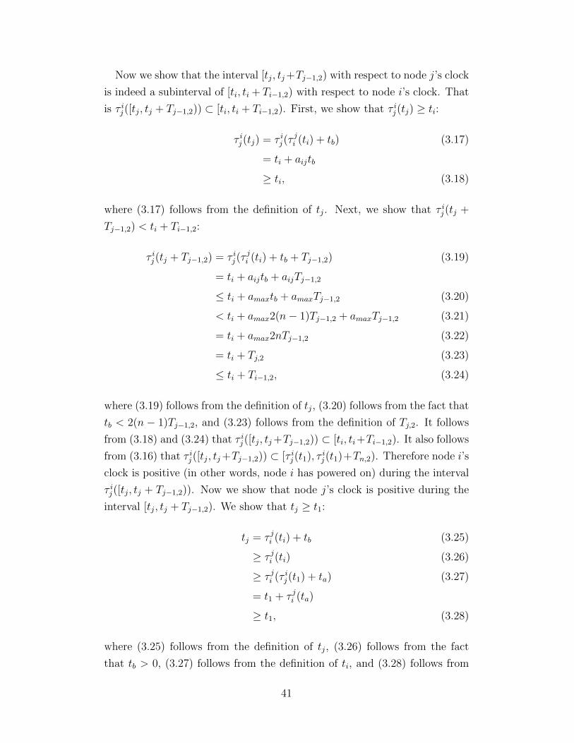
Now we show that the interval [tj, tj+Tj−1,2) with respect to node j’s clock

is indeed a subinterval of [ti, ti + Ti−1,2) with respect to node i’s clock. That

is τ ij([tj, tj + Tj−1,2)) ⊂ [ti, ti + Ti−1,2). First, we show that τ ij(tj) ≥ ti:

τ ij(tj) = τ ij(τji (ti) + tb) (3.17)

= ti + aijtb

≥ ti, (3.18)

where (3.17) follows from the definition of tj. Next, we show that τ ij(tj +

Tj−1,2) < ti + Ti−1,2:

τ ij(tj + Tj−1,2) = τ ij(τji (ti) + tb + Tj−1,2) (3.19)

= ti + aijtb + aijTj−1,2

≤ ti + amaxtb + amaxTj−1,2 (3.20)

< ti + amax2(n− 1)Tj−1,2 + amaxTj−1,2 (3.21)

= ti + amax2nTj−1,2 (3.22)

= ti + Tj,2 (3.23)

≤ ti + Ti−1,2, (3.24)

where (3.19) follows from the definition of tj, (3.20) follows from the fact that

tb < 2(n − 1)Tj−1,2, and (3.23) follows from the definition of Tj,2. It follows

from (3.18) and (3.24) that τ ij([tj, tj+Tj−1,2)) ⊂ [ti, ti+Ti−1,2). It also follows

from (3.16) that τ ij([tj, tj+Tj−1,2)) ⊂ [τ ij(t1), τ ij(t1)+Tn,2). Therefore node i’s

clock is positive (in other words, node i has powered on) during the interval

τ ij([tj, tj + Tj−1,2)). Now we show that node j’s clock is positive during the

interval [tj, tj + Tj−1,2). We show that tj ≥ t1:

tj = τ ji (ti) + tb (3.25)

≥ τ ji (ti) (3.26)

≥ τ ji (τ ij(t1) + ta) (3.27)

= t1 + τ ji (ta)

≥ t1, (3.28)

where (3.25) follows from the definition of tj, (3.26) follows from the fact

that tb > 0, (3.27) follows from the definition of ti, and (3.28) follows from

41

the fact that ta > 0. Next we show that tj + Tj−1,2 < t1 + Tn,2:

tj + Tj−1,2 = τ ji (ti) + tb + Tj−1,2 (3.29)

= τ ji (τ ij(t1) + ta) + tb + Tj−1,2 (3.30)

= t1 + ajita + tb + Tj−1,2

< t1 + aji2(n− 1)Ti−1,2 + 2(n− 1)Tj−1,2 + Tj−1,2 (3.31)

< t1 + aji2(n− 1)Ti−1,2 + amax2nTj−1,2

< t1 + aji2(n− 1)Ti−1,2 + Tj,2 (3.32)

< t1 + aji2(n− 1)Ti−1,2 + Ti−1,2 (3.33)

< t1 + amax2nTi−1,2

= t1 + Ti,2 (3.34)

≤ t1 + Tn,2, (3.35)

where (3.29) follows from the definition of tj, (3.30) follows from the definition

of ti, (3.31) follows from the fact that ta < 2(n − 1)Ti−1,2 and tb < 2(n −1)Tj−1,2, (3.32) follows from the definition of Tj−1,2, (3.33) follows from the

fact that i > j, and (3.34) follows from the definition of Ti,2.

It follows from (3.28) and (3.35) that the interval [tj, tj + Tj−1,2) occurs

in one iteration of the orthogonal MAC code. That is, [tj, tj + Tj−1,2) ⊂[t1, t1 + Tn,2). Therefore conditions (3.10)-(3.13) are satisfied for the interval

[tj, tj + Tj−1,2).

Now we will consider separately the two cases mentioned earlier. First, we

consider case one in which a primary pulse generated by node j collides with

a primary pulse generated by node i. We show that there exists a pulse of

length W generated by node j that does not collide with node i.

Lemma 3.2.2. Assume i > j and aij ≤ 1. Let I2 := [t2, t2+W ) be a primary

pulse of M(j)1 (t) with respect to node j’s clock and let I3 := [t3, t3 + W ) be

a primary pulse of M(i)1 (t) with respect to node i’s clock. Suppose the two

pulses overlap. That is, [t2, t2 +W )∩ τ ji ([t3, t3 +W )) 6= ∅. Then there exists

a pulse at tw := t2 +kT(j)0 with respect to node j’s clock that does not overlap

with any pulse of M(i)1 (τ ij(t)), where k :=

⌊1aij

(ij

)− W

T(j)0

− W

aijT(j)0

− cj⌋

.

Proof. We will prove the following in sequence:

(i) k ≥ 1,

42

(ii) [tw, tw +W ) ⊂ τ ji

([t3 + ciT

(i)0 +W, t3 + T

(i)0 ))

,

(iii) M(j)1 (t) = 1 and M

(i)1 (τ ij(t)) = 0 for all t ∈ [tw, tw +W ).

If the primary pulse of node j at time t2 (wrt to node j’s clock) collides (in

other words, the pulses overlap in time) with the primary pulse of node i,

we show that there exists a primary pulse that does not collide with node

i at time tw := t2 + kT(j)0 with respect to node j’s clock, where k is an

integer defined above. Clearly our selection of k cannot be zero because

otherwise tw = t2, which points to the same pulse that caused the collision

in the first place. We show that k as defined in the lemma is always strictly

positive. (i) We show that the parameters of the orthogonal MAC code,

selected at the onset, guarantees that k is strictly positive. Now by definition

T0 := 32Wna2max. Therefore, we prove that k ≥ 1 due to the following series

of inequalities:

T0 ≥ 8Wna2max,

⇒ 14namax

≥ 2WamaxT0

,

⇒ 1naij− cn ≥ 2W

aijT0,

⇒ [(n−j+1)−(n−i+1)]jaij

− cj ≥ 2WjaijT0

,

⇒ [(n−j+1)−(n−i+1)]jaij

− WjT0− W

jaijT0− cj ≥ 0,

⇒ 1aij

+ [(n−j+1)−(n−i+1)]jaij

− WjT0− W

jaijT0− cj ≥ 1,

⇒⌊

1aij

(ij

)− W

T(j)0

− W

aijT(j)0

− cj⌋≥ 1,

⇒ k ≥ 1.

(ii) Now we show that the pulse generated by node j at tw does not overlap

with any pulse generated by node i. That is,

[tw, tw +W ) ⊂ τ ji

([t3 + ciT

(i)0 +W, t3 + T

(i)0 )).

As before, we show that our choice of parameters for the orthogonal MAC

code guarantee this property. First we show that our choice of T0 := 32Wna2max

guarantees that tw ≥ τ ji (t3 + ciT(i)0 + W ) due to the following sequence of

inequalities:

T0 ≥ 8Wamax,

⇒ T0 ≥ 8Wamax2amax−1

,

43

⇒ T0 ≥ 4W1− 2n

4namax

,

⇒ T0 ≥ 4W1−2ncn

,

⇒ T0 ≥ 4W1−ici−jcj ,

⇒ T0 ≥ 4W(i−j)−ci(i−j)−jaij(ci+cj) ,

⇒ 1− ci + (1−ci)(i−j)jaij

≥ 1 + cj + 4WjaijT0

,

⇒ 1−ciaij

+ (1−ci)(i−j)jaij

≥ 1 + cj + 4WjaijT0

,

⇒ 1−ciaij

+ (1−ci)(i−j)jaij

≥ 1 + cj + 2WjT0

+ 2WjaijT0

,

⇒ 1aij

(ij

)− W

jT0− W

jaijT0− cj − 1 ≥ W

jT0+ ci

aij

(ij

)+ W

jaijT0,

⇒⌊

1aij

(ij

)− W

T(j)0

− W

aijT(j)0

− cj⌋≥ W

T(j)0

+ ciaij

(ij

)+ W

aijT(j)0

,

⇒ k ≥ W

T(j)0

+ ciaij

(ij

)+ W

aijT(j)0

,

⇒ kT(j)0 ≥ t2 +W − t2 +

ciT(i)0

aij+ W

aij,

⇒ kT(j)0 ≥ τ ji (t3)− t2 +

ciT(i)0

aij+ W

aij,

⇒ t2 + kT(j)0 ≥ τ ji (t3) +

ciT(i)0

aij+ W

aij,

⇒ tw ≥ τ ji (t3 + ciT(i)0 +W ).

Next we show that the choice of parameter cj := 1amax(5n−j) guarantees that

tw +W < τ ji (t3 + T(i)0 ) due to the following sequence of inequalities:

cj > 0,

⇒ 1aij

(ij

)− W

jT0− W

jaijT0− cj < 1

aij

(ij

)− W

jT0− W

jaijT0,

⇒⌊

1aij

(ij

)− W

jT0− W

jaijT0− cj

⌋< 1

aij

(ij

)− W

jT0− W

jaijT0,

⇒ k < 1aij

(T

(i)0

T(j)0

)− W

T(j)0

− W

aijT(j)0

,

⇒ kT(j)0 < τ ji (t3)− τ ji (t3)− W

aij+

T(i)0

aij−W,

⇒ kT(j)0 < τ ji (t3)− τ ji (t3 +W ) + T (i)

aij−W,

⇒ kT(j)0 < τ ji (t3)− t2 +

T(i)0

aij−W,

⇒ t2 + kT(j)0 +W < τ ji (t3) +

T(i)0

aij,

⇒ tw +W < τ ji (t3 + T(i)0 ).

It follows that [tw, tw + W ) ⊂ τ ji

([t3 + ciT

(i)0 +W, t3 + T

(i)0 ))

. (iii) Now

we use part (ii) to show that node j transmits and node i is silent during

the interval [tw, tw +W ) with respect to node j’s clock. Let t ∈ [tw, tw +W ).

44

From the fact that k is a positive integer and the definitions of t2, tw we have:

0 = tw mod T(j)0

≤ tw mod T(j)0 + (t− tw) mod T

(j)0

= tw mod T(j)0 +W

= W.

Therefore 0 ≤ tw mod T(j)0 + (t − tw) mod T

(j)0 ≤ W . Since by definition

W < T(j)0 , it follows that:

0 ≤ tw mod T(j)0 + (t− tw) mod T

(j)0

= [tw mod T(j)0 + (t− tw) mod T

(j)0 ] mod T

(j)0

= t mod T(j)0

< W.

By the inequality 0 ≤ t mod T(j)0 < W for all t ∈ [tw, tw + W ) shown above,

and the definition of M(j)1 (t), it follows that M

(j)1 (t) = 1 for all t ∈ [t2, t2+W ).

So we have proven that node j transmits during the interval [tw, tw + W ).

Now we need to show that node i is silent.

We have t ∈ [τ ji (t3 + ciT(i)0 +W ), τ ji (t3 +T

(i)0 )) since[tw, tw +W ) ⊂ [τ ji (t3 +

ciT(i)0 +W ), τ ji (t3 + T

(i))0 ). Then τ ij(t) ∈ [t3 + ciT

(i)0 +W, t3 + T

(i)0 ). Therefore

we have:

ciT(i)0 +W = (t3 + ciT

(i)0 +W ) mod T

(i)0

≤ (t3 + ciT(i)0 +W ) mod T

(i)0 + (τ ij(t)− (t3 + ciT

(i)0 +W )) mod T

(i)0

< (t3 + ciT(i)0 +W ) mod T

(i)0 + (t3 + T

(i)0 − (t3 + ciT

(i)0 +W )) mod T

(i)0

= T(i)0 .

Therefore

ciT(i)0 +W ≤ (t3+ciT

(i)0 +W ) mod T

(i)0 +(τ ij(t)−(t3+ciT

(i)0 +W )) mod T

(i)0 < T

(i)0 .

It follows that:

ciT(i)0 +W

45

≤ (t3 + ciT(i)0 +W ) mod T

(i)0 + (τ ij(t)− (t3 + ciT

(i)0 +W )) mod T

(i)0

= [(t3 + ciT(i)0 +W ) mod T

(i)0 + (τ ij(t)− (t3 + ciT

(i)0 +W )) mod T

(i)0 ] mod T

(i)0

= τ ij(t) mod T(i)0

< T(i)0 .

From the inequality ciT(i)0 +W ≤ τ ij(t) mod T

(i)0 < T

(i)0 proven above and the

definition of M(i)1 (t), it follows that M

(i)1 (τ ij(t)) = 0 for all t ∈ [t2, t2 + W ).

We have proven that node i is silent during the interval [tw, tw +W ) (wrt to

node j’s clock). Therefore there exists a collision-free pulse from node j to

node i of length W at [tw, tw +W ) all with respect to node j’s clock.

Now consider case two in which the primary pulse generated by node i

collides with a secondary pulse generated by node j. We show that there

exists a pulse of length W generated by node j that does not collide with

node i.

Lemma 3.2.3. Assume i > j and aij ≤ 1. Let I2 := [t2, t2+W ) be a primary

pulse of M(j)1 (t) with respect to node j’s clock and let I3 := [t3, t3 + W ) be

a secondary pulse of M(i)1 (t) with respect to node i’s clock. Suppose the two

pulses overlap. That is, [t2, t2 + W ) ∩ τ ji ([t3, t3 + W )) 6= ∅. There exists a

pulse at tw := t2 + cjT(j)0 with respect to node j’s clock that does not overlap

with any pulse of M(i)1 (τ ij(t)).

Proof. We will show:

(i) [tw, tw +W ) ⊂ τ ji ([t3 +W, t3 + (1− ci)T (i)0 )),

(ii) M(j)1 (t) = 1 and M

(i)1 (τ ij(t)) = 0 for all t ∈ [tw, tw +W ).

If the primary pulse of node j collides with the secondary pulse of node i

at time t2 (wrt to node j’s clock) we show that there exists a secondary

pulse that does not collide with node i at tw := t2 + cjT(j)0 with respect to

node j’s clock. To prove this, we only need to show that [tw, tw + W ) ⊂τ ji

([t3 +W, t3 + (1− ci)T (i)

0 ))

. (i) We show that the parameters of the or-

thogonal MAC code guarantee this property. Given the definition of cj we

first show that tw ≥ τ ji (t3 + (1 − ci)T(i)0 ) due to the following sequence of

inequalities:

16n ≥ 5n− j ∀j ∈ {1, . . . , n},

46

⇒ 1(5n−j)amax ≥

116namax

,

⇒ cj ≥ 116namax

,

⇒ cj ≥ 2Wamax32Wna2max

,

⇒ cj ≥ 2WamaxjT0

,

⇒ cj ≥ W

T(j)0

+ W

aijT(j)0

,

⇒ cjT(j)0 ≥ W + W

aij,

⇒ cjT(j)0 ≥ t2 +W − t2 + W

aij,

⇒ cjT(j)0 ≥ τ ji (t3)− t2 + W

aij,

⇒ t2 + cjT(j)0 ≥ τ ji (t3) + W

aij,

⇒ tw ≥ τ ji (t3 +W ).

It follows that tw ≥ τ ji (t3 + W ). Next we show that our choice of cj :=1

amax(5n−j) guarantees that tw +W < τ ji (t3 + (1− ci)T (i)0 ) due to the following

sequence of inequalities:

cj = 1(5n−j)amax ,

⇒ cj <11n2amax16n2amax

,

⇒ cj < 1 + 1n− 1

4namax− 1

4n2amax− 1

16namax,

⇒ cj < 1− cn + 1−cnn− 1

16namax,

⇒ cj < (1− cn) + 1−cnj− 2W

jaij(32Wna2max),

⇒ cj <1−cnaij

+ 1−cnjaij− 2W

jaijT0,

⇒ cj <1−cnaij

+ [(n−j+1)−(n−i+1)](1−cn)jaij

− 2WjaijT0

,

⇒ cj <(1−cn)aij

(ij

)− 2W

jaijT0,

⇒ cj <(1−cn)T

(i)0

aijT(j)0

− 2W

aijT(j)0

,

⇒ cj <(1−ci)T

(i)0

aijT(j)0

− W

aijT(j)0

− W

T(j)0

,

⇒ cjT(j)0 <

(1−ci)T(i)0

aij− W

aij−W,

⇒ cjT(j)0 < τ ji (t3)− τ ji (t3 +W ) +

(1−ci)T(i)0

aij−W,

⇒ cjT(j)0 < τ ji (t3)− t2 +

(1−ci)T(i)0

aij−W,

⇒ t2 + cjT(j)0 +W < τ ji (t3) +

(1−ci)T(i)0

aij,

⇒ tw +W < τ ij(t3 + (1− ci)T (i)0 ).

It follows that [tw, tw +W ) ⊂ [τ ji (t3 +W ), τ ji (t3 + (1− ci)T (i)0 )).

(ii) Now use part (i) to show that node j transmits during the interval

[tw, tw + W ) with respect to node j’s clock while node i is silent. Let t ∈

47

[tw, tw +W ). From the definition of T(j)0 we have |[tw, tw +W )| < T

(j)0 . Now

let t ∈ [tw, tw +W ). From the definition of t2 and tw we have:

cjT(j)0 = tw mod T

(j)0

≤ tw mod T(j)0 + (t− tw) mod T

(j)0

< tw mod T(j)0 + (tw +W − tw) mod T

(j)0

= cjT(j)0 +W.

Therefore cjT(j)0 ≤ tw mod T

(j)0 + (t − tw) mod T

(j)0 < cjT

(j)0 + W . It follows

from this inequality that:

cjT(j)0 ≤ tw mod T

(j)0 + (t− tw) mod T

(j)0

= [tw mod T(j)0 + (t− tw) mod T

(j)0 ] mod T

(j)0

= t mod T(j)0

< cjT(j)0 +W.

From the inequality cjT(j)0 ≤ t mod T

(j)0 < cjT

(j)0 +W proven above, and the

definition of M(j)1 (t), it follows that M

(j)1 (t) = 1 for all t ∈ [tw, tw+W ). So we

have proven that node j transmits during the interval [tw, tw +W ). Now we

need to show that node i is silent. We have t ∈ τ ji(

[t3 +W, t3 + (1− ci)T (i)0 ))

since [tw, tw + W ) ⊂ τ ji

([t3 +W, t3 + (1− ci)T (i)

0 ))

. Therefore τ ij(t) ∈ [t3 +

W, t3 + (1− ci)T (i)0 ). Clearly, |[t3 +W, t3 + (1− ci)T (i)

0 )| < T(i)0 . We have:

W + ciT(i)0 = (t3 +W ) mod T

(i)0

≤ (t3 +W ) mod T(i)0 + (τ ij(t)− (t3 +W )) mod T

(i)0

< (t3 +W ) mod T(i)0 + (t3 + (1− ci)T (i)

0 − (t3 +W )) mod T(i)0

= W + ciT(i)0 + (1− ci)T (i)

0 −W

= T(i)0 .

Therefore W+ciT(i)0 ≤ (t3 +W ) mod T

(i)0 +(τ ij(t)−(t3 +W )) mod T

(i)0 < T

(i)0 .

It follows that:

W + ciT(i)0 ≤ (t3 +W ) mod T

(i)0 + (τ ij(t)− (t3 +W )) mod T

(i)0

=≤ [(t3 +W ) mod T(i)0 + (τ ij(t)− (t3 +W )) mod T

(i)0 ] mod T

(i)0

48

= τ ij(t) mod T(i)0

< T(i)0 .

From the inequality ciT(i)0 +W ≤ τ ij(t) mod T

(i)0 < T

(i)0 proven above and the

definition of M(i)1 (t), it follows that M

(i)1 (τ ij(t)) = 0 for all t ∈ [t2, t2 + W ).

We have proven that node i is silent during the interval [tw, tw + W ) (wrt

to node j’s clock). Therefore there exists a collision-free pulse from node

j to node i of length W at the interval [tw, tw + W ) measured by node j’s

clock.

Now we prove that node j can successfully transmit a message of length

W to node i. We show, using the previous three lemmas, that within the

interval [tj, tj + Tj−1,2) there exists a pulse of length W generated by node j

that does not collide with a pulse generated by node i.

Lemma 3.2.4. Suppose aij ≤ 1 and i > j. Given t1 such that τ ij(t) ≥ 0,

there exists an interval [tw, tw +W ) that satisfies the following conditions for

all t ∈ [tw, tw +W ):

(i) [tw, tw +W ) ⊂ [t1, t1 + Tn,2),

(ii) [τ ij(tw), τ ij(tw +W )) ⊂ [τ ij(t1), τ ij(t1) + Tn,2),

(iii) M(j)1 (t)s

(j,i)1 (t) = 1,

(iv) M(i)1 (τ ij(t))s

(i,j)1 (τ ij(t))) + s

(i,j)1 (τ ij(t)) = 1.

Proof. From Lemma 3.2.1 there exists an interval [tj, tj+Tj−1,2) that satisfies

(3.10)-(3.13). Now |[tj, tj + Tj−1,2)| < Tj−1,2. Moreover,

Tj−1,2 ≥ T0,2

= 2Tn,1

= 2(dnamaxe+ 2)T(n)0

≥ 2(dnamaxe+ 2)T(j)0 .

It follows from the last inequality that there exists an interval I2 := [t2, t2 +

W ) ⊂ [tj, tj + Tj−1,2) that satisfies the following conditions:

(i) 0 ≤ t mod T(j)0 < W ,

49

(ii) 0 ≤ t2 − tj < T(j)0 .

There are three cases that may occur: Case 1: M(i)1 (τ ij(t)) = 0, for all

[t2, t2 + W ). In this case, set tw := t2. It follows from condition (i) and the

definition of M(j)1 (t), that for all t ∈ [t2, t2 +W ) we have,

M(j)1 (t) = 1,

M(i)1 (τ ij(t)) = 0.

In addition, we clearly have [tw, tw+W ) ⊂ [tj, tj+Tj−1,2). Case 2: M(i)1 (τ ij(t)) 6=

0 for all t ∈ [t2, t2 + W ). More specifically, there exists an interval I3 :=

[t3, t3 + W ) such that 0 ≤ t mod T(i)0 < W for all t ∈ I3 and [t2, t2 + W ) ∩

[τ ji (t3), τ ji (t3 +W )) 6= ∅.

In this case, let k =

⌊1aij

(ij

)− W

T(j)0

− W

aijT(j)0

− cj⌋

, and let tw := t2 +kT(j)0 .

It follows from Lemma 3.2.2 that for all t ∈ [tw, tw +W ):

M(j)1 (t) = 1,

M(i)1 (τ ij(t)) = 0.

Clearly tw ≥ tj since tw ≥ t2 ≥ tj. We also can show that tw+W < tj+Tj−1,2

due to the following sequence of inequalities:

tw +W ≤ t2 + kT(j)0 +W

≤ tj + T(j)0 + kT

(j)0 +W

< tj + T(j)0 + kT

(j)0 + T

(j)0

= tj + (k + 2)T(j)0

< tj + (k + 2)T(n)0

≤ tj + (dnamaxe+ 2)T(n)0

= tj + Tn,1

< tj + Tj−1,2.

Therefore [tw, tw + W ) ⊂ [tj, tj + Tj−1,2). Case 3: M(i)1 (τ ij(t)) 6= 0 for all

t ∈ [t2, t2 + W ). More specifically, there exists an interval I3 := [t3, t3 + W )

such that ciT(i)0 ≤ t mod T

(i)0 < ciT

(j)0 + W for all t ∈ I3 and [t2, t2 + W ) ∩

[τ ji (t3), τ ji (t3 + W )) 6= ∅. In this case let tw := t2 + cjT(j)0 . It follows from

50

Lemma 3.2.3 that for all t ∈ [tw, tw +W ):

M(j)1 (t) = 1,

M(i)1 (τ ij(t)) = 0.

Clearly tw ≥ tj since tw ≥ t2 ≥ tj. We also can show that tw+W < tj+Tj−1,2

due to the following sequence of inequalities:

tw +W = t2 + cjT(j)0 +W

≤ tj + T(j)0 +W

< tj + 2T(j)0

< tj + 2T(n)0

< tj + (dnamaxe+ 2)T(n)0

= tj + Tn,1

< tj + T0,2

≤ tj + Tj−1,2.

Therefore [tw, tw + W ) ⊂ [tj, tj + Tj−1,2). It follows that [tw, tw + W ) ⊂[tj, tj + Tj−1,2) in all cases and for all t ∈ [tw, tw +W ) we have:

M(j)1 (t) = 1,

M(i)1 (τ ij(t)) = 0,

s(j,i)1 (t) = 1,

s(i,j)1 (τ ij(t)) = 1.

where the latter two equalities follow from Lemma 3.2.1 cited at the onset of

the proof. Therefore for all t ∈ [tw, tw +W ) we have:

M(j)1 (t)s

(j,i)1 (t) = 1,

M(i)1 (τ ij(t))s

(i,j)1 (τ 1

j (t)) + s(i,j)1 (τ ij(t)) = 1.

Now we repeat the process when aij > 1. In the following lemma we

show that for any pair of nodes i and j, there exists an interval of time,

[tj, tj + Tj−1,2) with respect to node j’s clock, in which nodes i and j are

51

scheduled to communicate with each other using the signals M(i)2 (t) and

M(j)2 (t) respectively.

Lemma 3.2.5. Without loss of generality assume i > j. There exists an

interval [tj, tj + Tj−1,2) with respect to node j’s clock in which node i and

j are scheduled to communicate with each other using the signals M(i)2 (t)

and M(j)2 (t) respectively. That is, given t1 such that τ ij(t1) ≥ 0, the interval

[tj, tj + Tj−1,2) satisfies the following conditions:

[tj, tj + Tj−1,2) ⊂ [t1, t1 + Tn,2),

τ ij([tj, tj + Tj−1,2)) ⊂ [τ ij(t1), τ ij(t1) + Tn,2),

s(i,j)2 (τ ij(t)) = 1, ∀t ∈ [tj, tj + Tj−1,2),

s(j,i)2 (t) = 1, ∀t ∈ [tj, tj + Tj−1,2).

Proof. The proof of this lemma is very similar to the proof of Lemma 3.2.1.

First, we consider case one in which a primary pulse generated by node j

collides with a primary pulse generated by node i. We show that there exists

a pulse of length W generated by node j that does not collide with node i.

Lemma 3.2.6. Assume i > j and aij > 1. Let I3 := [t3, t3+W ) be a primary

pulse of M(i)2 (t) with respect to node i’s clock and let I2 := [t2, t2 + W ) be

a primary pulse of M(j)2 (t) with respect to node j’s clock. Suppose the two

pulses overlap. That is, [t2, t2 + W ) ∩ τ ji ([t3, t3 + W )) 6= ∅. There exists a

pulse at tw := t2 + cn−j+1T(n−j+1)0 with respect to node j’s clock that does not

overlap with any pulse of M(i)2 (τ ij(t)).

Proof. Let i := n − i + 1 and j := n − j + 1. Then I3 is a primary pulse

of M(i)1 (t) and I2 is a primary pulse of M

(j)1 (t). Set aij := aij. Therefore

aji ≤ 1. We need to show that there exists a pulse at tw := t2 + cjT(j)0 with

respect to node j’s clock that does not overlap with any pulse of M(i)1 (τ i

j(t)).

This result will be shown in Lemma 3.2.10.

Now we consider case two in which a primary pulse generated by node j

collides with a secondary pulse generated by node i. We show that there

exists a pulse of length W generated by node j that does not collide with

node i.

52

Lemma 3.2.7. Assume i > j and aij > 1. Let I3 := [t3, t3 + W ) be a

secondary pulse of M(i)2 (t) with respect to node i’s clock, and let I2 := [t2, t2 +

W ) be a primary pulse of M(j)2 (t) with respect to node j’s clock. Suppose the

two pulses overlap. That is, [t2, t2 +W ) ∩ τ ji ([t3, t3 +W )) 6= ∅. There exists

a pulse at tw := t2 + cn−j+1T(n−j+1)0 with respect to node j’s clock that does

not overlap with any pulse of M(i)2 (τ ij(t)).

Proof. Let i := n − i + 1 and j := n − j + 1. Then I3 is a secondary pulse

of M(i)1 (t) and I2 is a primary pulse of M

(j)1 (t). Set aij := aij. Therefore

aji ≤ 1. We need to show that there exists a pulse at tw := t2 + cjT(j)0 with

respect to node j’s clock that does not overlap with any pulse of M(i)1 (τ i

j(t)).

This result will be shown in Lemma 3.2.11.

Now we prove that node j can successfully transmit a message of length W

to node i when aij > 1. We show, using the previous three lemmas, Lemma

3.2.5, Lemma 3.2.7, and Lemma 3.2.6, that within the interval [tj, tj +Tj−1,2)

there exists a pulse of length W generated by node j that does not collide

with a pulse generated by node i.

Lemma 3.2.8. Suppose aij > 1 and i > j. Given t1 such that τ ij(t1) ≥ 0,

there exists an interval [tw, tw +W ) that satisfies the following conditions for

all t ∈ [tw, tw +W ):

(i) [tw, tw +W ) ⊂ [t1, t1 + Tn,2),

(ii) [τ ij(tw), τ ij(tw + Tn,2)) ⊂ [τ ij(t1), τ ij(t1) + Tn,2),

(iii) M(j)2 (t)s

(j,i)2 (t) = 1,

(iv) M(i)2 (τ ij(t))s

(i,j)2 (τ ij(t)) + s

(i,j)2 (τ ij(t)) = 1.

Proof. The proof of this lemma is similar to the proof of Lemma 3.2.4.

We have proved that node j can transmit a message of length W to node

i if aij ≤ 1 and if aij > 1. Putting both cases together gives us our first

theorem; the orthogonal MAC code enables node j to successfully transmit

a message of length W units to node i within a finite time TMAC(W ) := Tn,2

as long as the relative skew aij ≤ amax.

Theorem 3.2.1. Without loss of generality, assume i > j. Assume there

exists t1 such that τ ij(t1) > 0. There exists an interval [tw, tw + W ) that

satisfies the following conditions for all t ∈ [tw, tw+W ) and some k ∈ {1, 2}:

53

(i) [tw, tw +W ) ⊂ [t1, t1 + Tn,2),

(ii) [τ ij(tw), τ ij(tw +W )) ⊂ [τ ij(t1), τ ij(t1) + Tn,2),

(iii) M(i)k (τ ij(t))s

(i,j)k (τ ij(t)) + s

(i,j)k (τ ij(t)) = 1,

(iv) M(j)k (t)s

(j,i)k (t) = 1.

Proof. There are two cases to consider: Case 1: aij ≤ 1. It follows from

Lemma 3.2.4 that there exists an interval [tw, tw + W ) that satisfies the

following conditions for all t ∈ [tw, tw +W ):

(i) [tw, tw +W ) ⊂ [t1, t1 + Tn,2),

(ii) [τ ij(tw), τ ij(tw +W )) ⊂ [τ ij(t1), τ ij(t1) + Tn,2),

(iii) M(i)1 (τ ij(t))s

(i,j)1 (τ ij(t)) + s

(i,j)1 (τ ij(t)) = 1,

(iv) M(j)1 (t)s

(j,i)1 (t) = 1.

Case 2: aij > 1. It follows from Lemma 3.2.8 that there exists an interval

[tw, tw +W ) that satisfies the following conditions for all t ∈ [tw, tw +W ):

(i) [tw, tw +W ) ⊂ [t1, t1 + Tn,2),

(ii) [τ ij(tw), τ ij(tw +W )) ⊂ [τ ij(t1), τ ij(t1) + Tn,2),

(iii) M(i)2 (τ ij(t))s

(i,j)2 (τ ij(t)) + s

(i,j)2 (τ ij(t)) = 1,

(iv) M(j)2 (t)s

(j,i)2 (t) = 1.

We now show that node i can transmit a message of size W to node j.

Suppose i > j and aij ≤ 1. Consider two nodes i and j, where i > j and

aij ≤ 1. In the following lemma we show that for any two pairs of nodes i

and j, there exists an interval of time, [ti, ti + Ti), with respect to node i’s

clock, in which nodes i and j are scheduled to communicate with each other

using the signals M(i)1 (t) and M

(j)1 (t) respectively.

54

Lemma 3.2.9. Suppose i > j. Given t1 such that τ ji (t1) ≥ 0, there exists an

interval [ti, ti+Ti) that satisfies the following conditions for all t ∈ [ti, ti+Ti):

[ti, ti + Ti) ⊂ [t1, t1 + Tn,2), (3.36)

τ ji ([ti, ti + Ti)) ⊂ [τ ji (t1), τ ji (t1) + Tn,2), (3.37)

s(j,i)1 (τ ji (t)) = 1, (3.38)

s(i,j)1 (t) = 1. (3.39)

Proof. Since 0 ≤ t1 mod 2(n− 1)Ti−1,2 < 2(n− 1)Ti−1,2, there exists some ta,

0 ≤ ta < 2(n− 1)Ti−1,2 such that (t1 + ta) mod 2(n− 1)Ti−1,2 = (j − 1)Ti−1,2

if 1 ≤ j ≤ n− 1. Let ti := t1 + ta. It follows from the definition of s(i,j)1 (t) in

(3.6) that (3.39) is satisfied for all t ∈ [ti, ti + Ti−1,2).

Now since 0 ≤ τ ji (ti) mod 2(n − 1)Tj−1,2 < 2(n − 1)Tj−1,2, there exists

some tb, 0 ≤ tb < 2(n− 1)Tj−1,2 such that (τ ji (ti) + tb) mod 2(n− 1)Tj−1,2 =

(i− 2)Tj−1,2, if 2 ≤ i ≤ n. Set tj := τ ji (ti) + tb. It follows from the definition

of s(j,i)1 (t) that (3.38) is satisfied for all t ∈ [τ ij(tj), τ

ij(tj + Tj−1,2)). We will

prove (3.36) and show that [ti, ti + Ti) ⊂ [t1, t1 + Tn,2). Now set ti := τ ij(tj),

and let Ti := τ ij(tj + Tj−1,2)− τ ij(tj) = aijTj−1,2. First we show that ti ≥ t1:

ti := τ ij(tj)

= τ ij(τji (ti) + tb)

= τ ij(τji (t1 + ta) + tb)

= t1 + ta + aijtb

≥ t1.

Next we show that ti + Ti < t1 + Tn,2:

ti + Ti = t1 + ta + aijtb + Ti

< t1 + 2(n− 1)Ti−1,2 + aij2(n− 1)Tj−1,2 + aijTj−1,2

= t1 + 2(n− 1)Ti−1,2 + aij2nTj−1,2

= t1 + 2(n− 1)Ti−1,2 + Tj,2

≤ t1 + 2(n− 1)Ti−1,2 + Ti−1,2

≤ t1 + 2nTi−1,2

≤ t1 + Ti,2

55

≤ t1 + Tn,2.

It follows from both inequalities that [ti, ti+Ti) ⊂ [t1, t1 +Tn,2). Therefore

(3.36) is proved. Now we prove (3.37) and show that [τ ji (ti), τji (ti + Ti)) ⊂

[τ ji (t1), τ ji (t1) + Tn,2). First we show that τ ji (ti) ≥ τ ji (t1) due to the following

series of inequalities:

τ ji (ti) = τ ji (τ ij(tj))

= tj

= τ ji (ti) + tb

= τ ji (t1 + ta) + tb

= τ ji (t1) + ajita + tb

≥ τ ji (t1).

Next we show that τ ji (ti + Ti) < τ ji (t1) + Tn,2 due to the following series of

inequalities:

τ ji (ti + Ti) = τ ji (ti) + ajiTi

= τ ji (t1) + ajita + tb + aji(aijTj−1,2)

< τ ji (t1) + amax2(n− 1)Ti−1,2 + 2(n− 1)Tj−1,2 + Tj−1,2

= τ ji (t1) + amax2(n− 1)Ti−1,2 + 2nTj−1,2

≤ τ ji (t1) + amax2(n− 1)Ti−1,2 + Tj,2

≤ τ ji (t1) + amax2(n− 1)Ti−1,2 + Ti−1,2

≤ τ ji (t1) + amax2nTi−1,2

= τ ji (t1) + Ti,2

≤ τ ji (t1) + Tn,2.

It follows that [τ ji (ti), τji (ti +Ti)) ⊂ [τ ji (t1), τ ji (t1) +Tn,2). Therefore (3.37)

is satisfied.

Now we again consider two separate cases. First, we consider case one

in which a primary pulse generated by node i collides with a primary pulse

generated by node j. We show that there exists a pulse of length W generated

56

by node i that does not collide with node j.

Lemma 3.2.10. Assume i > j and aij ≤ 1. Let I2 := [t2, t2 + W ) be a

primary pulse of M(j)1 (t) with respect to node j’s clock and let I3 := [t3, t3+W )

be a primary pulse of M(i)1 (t) with respect to node i’s clock. Suppose the two

pulses overlap. That is, [t3, t3 + W ) ∩ τ ij([t2, t2 + W )) 6= ∅. There exists a

pulse at tw := t3 + ciT(i)0 with respect to node i’s clock that does not overlap

with any pulse of M(j)1 (τ ji (t)).

Proof. We will show:

(i) [tw, tw +W ) ⊂ τ ij([t2 + cjT(j)0 +W, t2 + T

(j)0 )),

(ii) M(i)1 (t) = 1 and M

(j)1 (τ ji (t)) = 0 for all t ∈ [tw, tw +W ).

If the primary pulse of node i collides with the primary pulse of node j at

time t3 (wrt to node i’s clock) we show that there exists a secondary pulse

that does not collide with node i at time tw := t3 + ciT(i)0 . We will first show

that [tw, tw + W ) ⊂ τ ij

([t2 + cjT

(j)0 +W ), t2 + T

(j)0 ))

and then show in (ii)

that this condition proves existence of a collision-free secondary pulse.

(i) We show that the parameters of the orthogonal MAC code selected

at the onset guarantee that [tw, tw + W ) ⊂ τ ij

([t2 + cjT

(j)0 +W, t2 + T

(j)0 ))

.

First we show that our selection of T0 := 32Wna2max guarantees that tw ≥

τ ij(t2 + cjT(j)0 +W ) due to the following sequence of inequalities:

T0 ≥ 10nWamax,

⇒ T05n≥ 2Wamax,

⇒ T05n≥ W

aij+W,

⇒(

5n(5n)(5n)

)T0 ≥ W

aij+W,

⇒(

5n(5n−i)(5n−j)

)T0 ≥ W

aij+W,

⇒(

5n(i−j)(5n−i)(5n−j)

)T0 ≥ W

aij+W,

⇒(

5ni−ij−5nj+ij(5n−i)(5n−j)

)T0 ≥ W

aij+W,

⇒(i(5n−j)−j(5n−i)

(5n−i)(5n−j)

)T0 ≥ W

aij+W,

⇒(

i5n−i −

j5n−j

)T0 ≥ W

aij+W,

⇒ (ici − jcj)T0 ≥ Waij

+W,

⇒ ciiT0 − cjjT0 ≥ Waij

+W,

⇒ ciT(i)0 − cjT

(j)0 ≥ W

aij+W,

57

⇒ ciT(i)0

aij− cjT (j)

0 ≥ Waij

+W,

⇒ ciT(i)0 − aijcjT

(j)0 ≥ W + aijW,

⇒ ciT(i)0 − aijcjT

(j)0 ≥ τ ij(t2)− t3 + aijW,

⇒ t3 + ciT(i)0 ≥ τ ij(t2) + aijcjT

(j)0 + aijW,

⇒ tw ≥ τ ij(t2) + aijcjT(j)0 + aijW,

⇒ tw ≥ τ ij(t2 + cjT(j)0 +W ).

Next we show that our choice cj and T(j)0 guarantees that τ ji (tw + W ) <

t2 + T(j)0 due to the following sequence of inequalities:

1 < i4amax

⇒ 2Wamax < i8Wa2max,

⇒ 2Wamax < i(32Wna2max)

(1

4n

),

⇒ 2Wamax < T(i)0

(4n−1

4n

),

⇒ 2Waij

< T(i)0

(1− amax

4namax

),

⇒ 2Waij

< T(i)0

(1− 1

4namax

(1aij

)),

⇒ 2Waij

< T(i)0

(1− cn

aij

),

⇒ W + Waij

< T(i)0

(1− ci

aij

),

⇒ W + Waij

< T(i)0 −

ciT(i)0

aij,

⇒ W + Waij

< T(j)0 −

ciT(i)0

aij,

⇒ aijW +W < aijT(j)0 − ciT

(i)0 ,

⇒ τ ij(t2 +W )− τ ij(t2) +W < aijT(j)0 − ciT

(i)0 ,

⇒ t3 − τ ij(t2) +W < aijT(j)0 − ciT

(i)0 ,

⇒ t3 + ciT(i)0 +W < τ ij(t2) + aijT

(i)0 ,

⇒ tw +W < τ ij(t2) + aijT(j)0 ),

⇒ tw +W < τ ij(t2 + T(i)0 ).

It follows from both series of inequalities that

[tw, tw +W ) ⊂ τ ij

([t2 + cjT

(j)0 +W, t2 + T

(j)0 )).

(ii) Now use part (i) to show that node i transmits during the interval

[tw, tw + W ) with respect to node i’s clock while node j is silent. Let t ∈[tw, tw +W ). From the definition of t3 and tw we have:

ciT(i)0 = tw mod T

(i)0

58

≤ tw mod T(i)0 + (t− tw) mod T

(i)0

< ciT(i)0 + (t3 + ciT

(i)0 +W − (t3 + ciT

(i)0 )) mod T

(i)0

= ciT(i)0 +W.

Therefore ciT(i)0 ≤ tw mod T

(i)0 + (t − tw) mod T

(i)0 < ciT

(i)0 + W . It follows

from this inequality that:

ciT(i)0 ≤ tw mod T

(i)0 + (t− tw) mod T

(i)0

= [tw mod T(i)0 + (t− tw) mod T

(i)0 ] mod T

(i)0

= t mod T(i)0

< ciT(i)0 +W.

Therefore ciT(i)0 ≤ t mod T

(i)0 < ciT

(i)0 +W for all t ∈ [tw, tw +W ). It follows

from this inequality and the definition of M(i)1 (t), that M

(i)1 (t) = 1 for all

t ∈ [tw, tw +W ). So we have shown that node i transmits during the interval

[tw, tw +W ). It now remains to show that node j is silent.

We have τ ji (t) ∈ [t2 + cjT(j)0 +W, t2 + T

(j)0 ) since τ ji ([tw, tw +W )) ⊂ [t2 +

cjT(j)0 +W, t2 + T

(j)0 ). It follows from the definition of t2 that:

cjT(j)0 +W = (t2 + cjT

(j)0 +W ) mod T

(j)0

≤ (t2 + cjT(j)0 +W ) mod T

(j)0 + (τ ji (t)− (t2 + cjT

(j)0 +W )) mod T

(j)0

< cjT(j)0 +W + (t2 + T

(j)0 − (t2 + cjT

(j)0 +W ))

= T(j)0 .

Therefore

cjT(j)0 +W ≤ (t2+cjT

(j)0 +W ) mod T

(j)0 +(τ ji (t)−(t2+cjT

(j)0 +W )) mod T

(j)0 < T

(j)0 .

It follows from this inequality that:

cjT(j)0 +W

≤ (t2 + cjT(j)0 +W ) mod T

(j)0 + (τ ji (t)− (t2 + cjT

(j)0 +W )) mod T

(j)0

= [(t2 + cjT(j)0 +W ) mod T

(j)0 + (τ ji (t)− (t2 + cjT

(j)0 +W )) mod T

(j)0 ] mod T

(j)0

= τ ji (t) mod T(j)0

< T(j)0 .

59

Therefore cjT(j)0 + W ≤ τ ji (t) < T

(j)0 for all t ∈ [tw, tw + W ). It follows

from this fact, and the definition of M(j)1 (t), that M

(j)1 (τ ji (t)) = 0 for all

t ∈ [tw, tw +W ).

Next we consider case two in which a primary pulse generated by node i

collides with a secondary pulse generated by node j. We show that there

exists a pulse of length W that does not collide with node j.

Lemma 3.2.11. Assume i > j and aij ≤ 1. Let I2 := [t2, t2 + W ) be a

primary pulse of M(j)1 (t) with respect to node j’s clock and let I3 := [t3, t3+W )

be a secondary pulse of M(i)1 (t) with respect to node i’s clock. Suppose the

two pulses overlap. That is, [t3, t3 + W ) ∩ τ ij([t2, t2 + W )) 6= ∅. Then there

exists a pulse at tw := t3 + ciT(i)0 with respect to node i’s clock that does not

overlap with any pulse of M(j)1 (τ ji (t)).

Proof. We will show that:

(i) [tw, tw +W ) ⊂ τ ij([t2 +W, t2 + (1− cj)T (j)0 )),

(ii) M(i)1 (t) = 1 and M

(j)1 (τ ji (t)) = 0 for all t ∈ [tw, tw +W ).

If the primary pulse of node i collides with the secondary pulse of node j at

time t3 (wrt to node i’s clock) we show that there exists a secondary pulse

that does not collide with node j at time tw := t3 + ciT(i)0 . We will first show

that [tw, tw + W ) ⊂ [τ ij(t2 + W ), τ ij(t2 + (1− cj)T (j)0 )), and then show in (ii)

that this condition proves the existence of a collision-free secondary pulse.

(i) We show that the parameters of the orthogonal MAC code selected at

the onset guarantee that [tw, tw + W ) ⊂ [τ ij(t2 + W ), τ ij(t2 + (1 − cj)T (j)0 )).

First we show that our selection of ci and T(i)0 guarantees tw ≥ τ ij(t2 + W )

due to the following sequence of inequalities:

2a2max ≥ 1,

⇒ 4Wa2max ≥ 2W,

⇒(

18n

)(32Wna2

max) ≥ 2W,

⇒(

i5n−i

)T0 ≥ 2W,

⇒ ciT(i)0 ≥ 2W,

⇒ ciT(i)0

aij≥ 2W

aij,

⇒ ciT(i)0

aij≥ W

aij+W,

⇒ ciT(i)0 ≥ W + aijW,

60

⇒ τ ji (t3) +ciT

(i)0

aij≥ t2 +W,

⇒ ciT(i)0 ≥ t3 +W − t3 + aijW,

⇒ ciT(i)0 ≥ τ ij(t2)− t3 + aijW,

⇒ t3 + ciT(i)0 ≥ τ ij(t2) + aijW,

⇒ tw ≥ τ ij(t2 +W ).

Therefore tw ≥ τ ij(t2 +W ). Next, we show that our selection of cj and T(j)0

guarantees that tw +W < τ ij(t2 + (1− ci)T (j)0 ) due to the following sequence

of inequalities:

1 < 8namax

⇒ 2Wamax < 16Wna2max

⇒ 2Wamax <T02

⇒ 2Wamax <(

1− 2namax4namax

)T0

⇒ 2Waij

< (1− 2ncnamax)T0

⇒ 2Waij

<(j − jcj+ici

aij

)T0

⇒ 2Waij

<(j(1− cj)− ici

aij

)T0

⇒ 2Waij

< j(1− cj)T0 − iciT0aij

⇒ 2Waij

< (1− cj)T (j)0 −

ciT(i)0

aij

⇒ W + Waij

< (1− cj)T (j)0 −

ciT(i)0

aij

⇒ aijW +W < aij(1− cj)T (j)0 − ciT

(i)0

⇒ τ ij(t2) + aijW − τ ij(t2) +W < aij(1− cj)T (j)0 − ciT

(i)0

⇒ τ ij(t2 +W )− τ ij(t2) +W < aij(1− cj)T (j)0 − ciT

(i)0

⇒ t3 − τ ij(t2) +W < aij(1− cj)T (j)0 − ciT

(i)0

⇒ τ ji (t3) +ciT

(i)0 +W

aij< t2 + (1− cj)T (j)

0

⇒ t3 + ciT(i)0 +W < τ ij(t2) + aij(1− cj)T (j)

0

⇒ tw +W < τ ij(t2 + (1− cj)T (j)0 ).

It follows from the previous two series of inequalities that [tw, tw + W ) ⊂[τ ij(t2 + W ), τ ij(t2 + (1 − ci)T (j)

0 )). (ii) Now use part (i) to show that node

i transmits during the interval [tw, tw + W ) while node j is silent. Let t ∈[tw, tw +W ). From the definition of t3 and tw we have:

ciT(i)0 = tw mod T

(i)0

≤ tw mod T(i)0 + (t− tw) mod T

(i)0

61

< tw mod T(i)0 + (tw +W − tw) mod T

(i)0

= tw mod T(i)0 +W mod T

(i)0

= tw mod T(i)0 +W

= ciT(i)0 +W.

Therefore ciT(i)0 ≤ tw mod T

(i)0 +(t−tw) mod T

(i)0 < ciT

(i)0 +W for all [tw, tw+

W ). It follows from this inequality that:

ciT(i)0 ≤ tw mod T

(i)0 + (t− tw) mod T

(i)0

= [tw mod T(i)0 + (t− tw) mod T

(i)0 ] mod T

(i)0

= t mod T(i)0

< ciT(i)0 +W.

Therefore ciT(i)0 ≤ t mod T

(i)0 < ciT

(i)0 +W for all t ∈ [tw, tw +W ). It follows

from this inequality and the definition of M(i)1 (t) that M

(i)1 (t) = 1 for all

t ∈ [t3 + ciT(i)0 , t3 + ciT

(i)0 + W ). So we have shown that node i transmits

during the interval [tw, tw + W ). It now remains to show that node j is

silent. We have τ ji (t) ∈ [t2 + W, t2 + (1 − ci)T (j)0 ) since τ ji ([tw, tw +W )) ⊂

[t2 + w, t2 + (1− cj)T (j)0 ). It follows from the definition of t2 that:

cjT(j)0 +W = (t2 +W ) mod T

(j)0

≤ (t2 +W ) mod T(j)0 + (τ ji (t)− (t2 +W )) mod T

(j)0

< (t2 +W ) mod T(j)0 + (t2 + (1− cj)T (j)

0 − (t2 +W )) mod T(j)0

= cjT(j)0 +W + (1− cj)T (j)

0 −W

= T(j)0 .

Therefore cjT(j)0 +W ≤ (t2+W ) mod T

(j)0 +(τ ji (t)−(t2+W )) mod T

(j)0 < T

(j)0

for all [tw, tw +W ). It follows from this fact that:

cjT(j)0 +W ≤ (t2 +W ) mod T

(j)0 + (τ ji (t)− (t2 +W )) mod T

(j)0

= [(t2 +W ) mod T(j)0 + (τ ji (t)− (t2 +W )) mod T

(j)0 ] mod T

(j)0

= τ ji (t) mod T(j)0

< T(j)0 .

Therefore cjT(j)0 +W ≤ τ ji (t) mod T

(j)0 < T

(j)0 for all [tw, tw +W ). It follows

62

from this fact and the definition of M(j)1 (t) that M

(j)1 (τ ji (t)) = 0 for all

t ∈ [tw, tw +W ).

Now we prove that node i can successfully transmit a message of length

W to node j when aij ≤ 1. We show, using the previous three lemmas that

within the interval [ti, ti + Ti) there exists a pulse of length W generated by

node i that does not collide with a pulse generated by node j.

Lemma 3.2.12. Suppose aij ≤ 1 and i > j. Given t1 such that τ ij(t1) ≥ 0,

there exists an interval [tw, tw +W ) that satisfies the following conditions for

all t ∈ [tw, tw +W ):

(i) [tw, tw +W ) ⊂ [t1, t1 + Tn,2),

(ii) [τ ji (tw), τ ji (tw +W )) ⊂ [τ ij(t1), τ ij(t1) + Tn,2),

(iii) M(i)1 (t)s

(i,j)1 (t) = 1,

(iv) M(j)1 (τ ji (t))s

(j,i)1 (τ ji (t)) + s

(j,i)1 (τ ji (t)) = 1.

Proof. It follows from Lemma 3.2.9 that there exists an interval [ti, ti + Ti)

that satisfies the following:

(i) [ti, ti + Ti) ⊂ [t1, t1 + Tn,2),

(ii) [τ ji (ti), τji (ti + Ti)) ⊂ [τ ji (t1), τ ji (t1) + Tn,2),

(iii) s(i,j)1 (t) = 1,

(iv) s(j,i)1 (τ ji (t)) = 1.

Moreover,

|[ti, ti + Ti)| = Ti

= aijTj−1,2

≥ aijT0,2

= aij2Tn,1

= aij2(dnamaxe+ 2)T(n)0

≥ 2

(dnamaxe+ 2

amax

)T

(i)0

≥ 2nT(i)0 .

63

It follows from the inequality |[ti, ti + Ti)| ≥ 2nT(i)0 that there exists an

interval I3 := [t3, t3 +W ) ⊂ [ti, ti+Ti) that satisfies the following conditions:

(i) 0 ≤ t mod T(i)0 < W ,

(ii) 0 ≤ t3 − ti < T(i)0 .

There are three cases that may occur: Case 1: M(j)1 (τ ji (t)) = 0, for all

[t3, t3 + W ). In this case, set tw := t3. It follows from condition (i) that for

all t ∈ [tw, tw +W ) we have,

M(j)1 (τ ji (t)) = 0,

M(i)1 (t) = 1.

In addition, we clearly have [tw, tw+W ) ⊂ [ti, ti+Ti). Case 2: M(j)1 (τ ji (t)) 6=

0 for some t ∈ [t3, t3 + W ). More specifically, there exists an interval I2 :=

[t2, t2 + W ) such that 0 ≤ t mod T(j)0 < W for all t ∈ I2 and [t2, t2 + W ) ∩

[τ ji (t3), τ ji (t3 +W )) 6= ∅.In this case, let tw := t3 + ciT

(i)0 . It follows from Lemma 3.2.10 that for all

t ∈ [τ ji (tw), τ ji (tw +W ):

M(i)1 (t) = 1,

M(j)1 (τ ji (t)) = 0.

Clearly tw ≥ t3 ≥ ti. We also can show that tw + W < ti + Ti due to the

following sequence of inequalities:

tw +W = t3 + ciT(i)0 +W

= ti + T(i)0 + ciT

(i)0 +W

< ti + T(i)0 + T

(i)0

= ti + 2T(i)0

< ti + 2T(n)0

< ti + 2dnamaxe+ 2

amaxT

(n)0

= ti +2Tn,1amax

= ti +T0,2

amax

64

≤ ti + aijT0,2

≤ ti + aijTj−1,2

≤ ti + Ti.

Therefore [tw, tw + W ) ⊂ [ti, ti + Ti). Case 3: M(j)1 (τ ji (t)) 6= 0 for all

t ∈ [t3, t3 + W ). More specifically, there exists an interval I2 := [t2, t2 + W )

such that cjT(j)0 ≤ t mod T

(j)0 < cjT

(j)0 + W for all t ∈ I2 and [τ ij(t2), τ ij(t2 +

W )) ∩ [t3, t3 +W ) 6= ∅.In this case let tw := t3 + ciT

(i)0 . It follows from Lemma 3.2.11 that for all

t ∈ [tw, tw +W ):

M(i)1 (t) = 1,

M(j)1 (τ ji (t)) = 0.

Clearly tw ≥ t3 ≥ ti. We also can show that tw + W < ti + Ti due to the

following sequence of inequalities:

tw +W = t3 + ciT(i)0 +W

≤ ti + T(i)0 + ciT

(i)0 +W

< ti + 2T(i)0

= ti + 2T(n)0

= ti + 2dnamaxe+ 2

amaxT

(n)0

= ti +2Tn,1amax

= ti +T0,2

amax

≤ ti + aijT0,2

≤ ti + aijTj−1,2

= ti + Ti.

Therefore [tw, tw +W ) ⊂ [ti, ti+Ti). It follows that [tw, tw +W ) ⊂ [ti, ti+Ti)

65

in all cases and for all t ∈ [tw, tw +W ) we have:

M(i)1 (t) = 1,

M(j)1 (τ ji (t)) = 0,

s(i,j)1 (t) = 1,

s(j,i)1 (τ ji (t)) = 1.

Therefore for all t ∈ [tw, tw +W ) we have:

M(i)1 (t)s

(i,j)1 (t) = 1,

M(j)1 (τ ji (t))s

(j,i)1 (τ ji (t)) + s

(j,i)1 (τ ji (t)) = 1.

Now we repeat the process when aij > 1. In the following lemma we

show that for any two pairs of nodes i and j, there exists an interval of

time, [ti, ti + Ti) with respect to node i’s clock, in which nodes i and j

are scheduled to communicate with each other using the signals M(i)2 (t) and

M(j)2 (t) respectively.

Lemma 3.2.13. Suppose i > j. Given t1 such that τ ji (t1) ≥ 0, there exists an

interval [ti, ti+Ti) that satisfies the following conditions for all t ∈ [ti, ti+Ti):

[ti, ti + Ti) ⊂ [t1, t1 + Tn,2),

[τ ji (ti), τji (ti + Ti)) ⊂ [τ ji (t1), τ ji (t1) + Tn,2),

s(j,i)2 (τ ji (t)) = 1,

s(i,j)2 (t) = 1.

Proof. The proof of this lemma is very similar to the proof of Lemma 3.2.9.

First, we consider case one in which a primary pulse generated by node i

collides with a primary pulse generated by node j. We show that there exists

a pulse of length W generated by node i that does not collide with node i.

Lemma 3.2.14. Assume i > j and aij > 1. Let I3 := [t3, t3 + W ) be a

primary pulse of M(i)2 (t) with respect to node i’s clock and let I2 := [t2, t2+W )

be a primary pulse of M(j)2 (t) with respect to node j’s clock. Suppose the two

66

pulses overlap. That is, [t3, t3 + W ) ∩ τ ij([t2, t2 + W )) 6= ∅. Then there

exists a pulse at tw := t3 + kT(n−i+1)0 with respect to node i’s clock, where

k =

⌊1aji

(n−j+1n−i+1

)− W

T(n−i+1)0

− W

ajiT(n−i+1)0

− cn−i+1

⌋, that does not overlap with

any pulse of M(j)2 (τ ji (t)).

Proof. Let i := n − i + 1 and j := n − j + 1. Then I3 is a primary pulse

of M(i)1 (t) and I2 is a primary pulse of M

(j)1 (t). Set aij := aij. Therefore

aji ≤ 1. We need to show that there exists a pulse at tw := t3 + kT(i)0 with

respect to node i’s clock that does not overlap with any pulse of M(j)1 (τ j

i(t)).

This result was already shown in Lemma 3.2.2.

Next we consider case two in which a primary pulse generated by node i

collides with a secondary pulse generated by node j. We show that there

exists a pulse of length W generated by node i that does not collide with

node j.

Lemma 3.2.15. Assume i > j and aij > 1. Let I3 := [t3, t3 + W ) be

a secondary pulse of M(i)2 (t) with respect to node i’s clock and let I2 :=

[t2, t2 + W ) be a primary pulse of M(j)2 (t) with respect to node j’s clock.

Suppose the two pulses overlap. That is, [t2, t2 + W ) ∩ τ ji ([t3, t3 + W )) 6= ∅.Then there exists a pulse at tw := t3 + cn−i+1T

(n−i+1)0 with respect to node i’s

clock that does not overlap with any pulse of M(j)2 (τ ji (t)).

Proof. Let i := n − i + 1 and j := n − j + 1. Then I3 is a primary pulse

of M(i)1 (t) and I2 is a primary pulse of M

(j)1 (t). Set aij := aij. Therefore

aji ≤ 1. We need to show that there exists a pulse at tw := t3 + ciT(i)0 with

respect to node i’s clock that does not overlap with any pulse of M(j)1 (τ j

i(t)).

This result was already shown in Lemma 3.2.3.

Now we prove that node i can successfully transmit a message of length

W to node i when aij < 1. We show, using the previous three lemmas, that

within the interval [ti, ti + Ti) there exists a pulse of length W generated by

node i that does not collide with a pulse generated by node j.

Lemma 3.2.16. Suppose aij > 1 and i > j. Given t1 such that τ ji (t1) ≥ 0,

there exists an interval [tw, tw +W ) that satisfies the following conditions for

all t ∈ [tw, tw +W ):

(i) [tw, tw +W ) ⊂ [t1, t1 + Tn,2),

67

(ii) [τ ji (tw), τ ji (tw + Tn,2)) ⊂ [τ ji (t1) + Tn,2),

(iii) M(i)2 (t)s

(i,j)2 (t) = 1,

(iv) M(j)2 (τ ji (t))s

(j,i)2 (τ ji (t)) + s

(j,i)2 (τ ji (t)) = 1.

Proof. The proof of this lemma is similar to the proof of Lemma 3.2.12.

We have proved that node i can communicate with node j if aij ≤ 1 and

if aij > 1. Putting both cases together gives us our second theorem; the

orthogonal MAC code enables node i to successfully transmit a message of

length W units to node j within a finite time TMAC(W ) := Tn,2 as long as

the relative skew aij ≤ amax.

Theorem 3.2.2. Without loss of generality, assume i > j. Assume there

exists t1 such that τ ji (t1) > 0. There exists an interval [tw, tw + W ) that

satisfies the following conditions for all t ∈ [tw, tw+W ) and some k ∈ {1, 2}:

(i) [tw, tw +W ) ⊂ [t1, t1 + Tn,2),

(ii) [τ ji (tw), τ ji (tw +W )) ⊂ [τ ji (t1), τ ji (t1) + Tn,2),

(iii) M(i)k (t)s

(i,j)k (t) = 1,

(iv) M(j)k (τ ji (t))s

(j,i)k (τ ji (t)) + s

(j,i)k (τ ji (t)) = 1.

Proof. There are two cases to consider: Case 1: aij ≤ 1. It follows from

Lemma 3.2.12 that there exists an interval [tw, tw + W ) that satisfies the

following conditions for all t ∈ [tw, tw +W ):

(i) [tw, tw +W ) ⊂ [t1, t1 + Tn,2),

(ii) [τ ji (tw), τ ji (tw +W )) ⊂ [τ ji (t1), τ ji (t1) + Tn,2),

(iii) M(i)1 (t)s

(i,j)1 (t) = 1,

(iv) M(j)1 (τ ji (t))s

(j,i)1 (τ ji (t)) + s

(j,i)1 (τ ji (t)) = 1.

Case 2: aij > 1. It follows from Lemma 3.2.16 that there exists an interval

[tw, tw +W ) that satisfies the following conditions for all t ∈ [tw, tw +W ):

(i) [tw, tw +W ) ⊂ [t1, t1 + Tn,2),

(ii) [τ ji (tw), τ ji (tw +W )) ⊂ [τ ji (t1), τ ji (t1) + Tn,2),

68

(iii) M(i)2 (t)s

(i,j)2 (t) = 1,

(iv) M(j)2 (τ ji (t))s

(j,i)2 (τ ji (t)) + s

(j,i)2 (τ ji (t)) = 1.

The proof of Theorem 3.1.1 follows from Theorem 3.2.2 and Theorem 3.2.1.

3.3 Analysis of the Orthogonal MAC Code Complexity

In this section we analyze the length of the orthogonal MAC code with re-

spect to the size of the message W , the number of nodes n, and the maximum

relative skew amax. The following lemma determines the length of the orthog-

onal MAC code for message of size W .

Lemma 3.3.1. The length of the orthogonal MAC code for a message of size

W is at most TMAC(W ), where TMAC(W ) := (2namax)9nW and the length is

measured with respect to the local clock.

Proof. The length of the orthogonal MAC code is Tn,2 where Tn,2 is recur-

sively defined in (3.5) by:

Ti,2 := 2amaxnTi−1,2,

where by (3.4),

T0,2 := 2(dnamaxe+ 2)n(32Wn(amax)2).

It follows that for all i ≤ n:

Ti,2 := (2amaxn)iT0,2

= (2amaxn)i2(dnamaxe+ 2)n(32Wn(amax)2)

≤ (2amaxn)i2(3namax)n(32Wn(amax)2)

≤ 192(2amaxn)i(namax)3W

≤ (2namax)8(2namax)

iW

≤ (2namax)i+8W

≤ (2namax)9nW.

69

Therefore Tn,2 ≤ (2namax)9nW and the lemma is proved.

The length of the orthogonal MAC code is doubly exponential in the num-

ber of nodes n; a property that makes this code infeasible to implement for

large values of n. However, in the context of the larger protocol suite de-

scribed in the introduction, the overhead of the orthogonal MAC code can

be mitigated by choosing a data transfer phase on a much larger time-scale.

Hence the orthogonal MAC code plays a critical role in obtaining a theo-

retical result; the existance of a protocol suite that enables a network of

asynchronous nodes to form a fully functioning network operating at near

optimal utility.

In practice, we cannot rely on arbitrarily large data data transfer phases

to hide the overhead of the orthogonal MAC code, so it is worth examining

ways to reduce the code complexity. The construction of s(i,j)k (t), which

determines the intervals in which node i corresponds with node j, is designed

to guarantee that an interval in which s(i,j)k (t) = 1 overlaps with an interval

in which s(j,i)k (τ ji (t)) = 1 for all node pairs i and j. We adopted the obvious

approach and made the pulse of s(i,j)k (t) more than namax times larger than

the pulse of s(j,i)k (t), where i > j. This approach however, leads to the

recursive definition of Ti,2 that is ultimately doubly exponential in n. Any

reduction in the code complexity requires a new and less obvious design of

s(i,j)k (t).

In the next chapter we examine another aspect of network formation; ob-

taining an internally consistent view of the clock parameters of each good

node, in a network infiltrated with bad nodes.

70

CHAPTER 4

SECURE CLOCK SYNCHRONIZATION

Distributed systems are becoming increasingly ubiquitous due to advances

in wireless technology. In many applications, including even the basic prob-

lem of medium access, these types of systems are required to operate in a

coordinated and timely manner, with the assumption that some reference

clock exists and can be universally accessed. However, in important classes

of distributed systems such as wireless ad-hoc networks, no such reference

clock exists. Instead, each individual node has an affine local clock that is

subject to skew and offset. Furthermore, these clock parameters are usually

unknown and can only be determined by an exchange of timing packets with

a neighbor. Previous work has shown to what extent relative clock param-

eters of adjacent nodes can be used to estimate the clock of a connected

reference node, thus providing every node in the network with an estimate

of a “virtual” reference clock.

In this paper, we consider the problem of clock synchronization in dis-

tributed wireless ad-hoc networks infiltrated with hostile wireless nodes. An

important feature of such networks is that a source node typically requires

the assistance of intermediate nodes to relay and forward a message to a

destination. This feature is especially pertinent in clock synchronization; a

pair of non-adjacent nodes depend on the integrity of the intermediate nodes

connecting them along a path to obtain their relative clock parameters (such

as skew and offset). As a result, malicious nodes have the opportunity to

sabotage network coordination by generating false timing data and relative

clock parameters. This destructive behavior is difficult to pre-empt, particu-

larly when the bad nodes can fully cooperate with each other while the good

nodes do not even know which nodes are good or bad a priori. For example, a

bad node could distort its relative clock parameters ever so slightly, but still

enough to cause the clock estimates to drift causing eventual loss of network

coordination. Similarly, a group of colluding bad nodes could evade detec-

71

tion by falsifying their clock parameters in a manner that causes cumulative

damage to the accuracy of the clock estimate, without betraying themselves.

We develop a protocol called consistency check that allows the good nodes

in wireless type of networks to obtain consistent estimates of their relative

clock skews and offsets to within an arbitrary ε, regardless of what the ma-

licious nodes conspire to do. The key idea is to wait for a sufficiently large

period of time, during which a clock diverges from its estimate. We then

force each node to timestamp and forward a packet within a fixed number

of clock counts, a task that will turn out to be an impossibility if a node has

manipulated or lied about its clock parameters. In addition, we will show

that no amount of collusion between the malicious nodes will prevent at least

one malicious node from being detected.

There is a significant body of published research work concerning the topic

of clock synchronization in the process of Byzantine faults. Both Lamport

[33] and Lundelius [34] present algorithms that work without authentication,

when the number of faulty processes is less than one third the total. It was

shown by Dolev [35] that it is impossible to achieve synchronization without

authentication when more than one third of the processes are faulty. Halpern

[36] presents a clock synchronization algorithm that only requires the non-

faulty processes to be connected. All of these algorithms assume periodic

clock updates from non-faulty processes. In this paper, the network will

obtain the relative clock parameters of the good nodes, thus avoiding the

overhead of periodic resynchronization.

The consistency check is part of a larger protocol suite (not presented in

this paper due to its considerable scope and length) that enables a distributed

network of wireless unsynchronized nodes to form a fully functioning wireless

network operating at a near optimal rate vector, while under sustained and

coordinated attack by the malicious nodes hidden amongst them. This pa-

per is more narrowly focused on the problem of clock synchronization during

the intial stages of network formation, a critical component of the overall

protocol suite. In the next section we describe the problem framework and

assumptions. Subsequently, we present the main result, namely that consis-

tency check allows the network to obtain a uniform and consistent estimate

of a reference clock, to within an arbitrary ε.

72

4.1 Problem Framework and Assumptions

Consider a collection of n wireless nodes, some good and some bad. Each

good wireless node is equipped with a affine local clock, subject to skew and

offset. The good nodes wish to obtain consistent and accurate estimates of

their relative clock parameters, for the purpose of coordinating future activity

according to a reference clock. The focus of this paper is on obtaining reliable

clock parameter estimates between nodes that are not adjacent, and thus

vulnerable to the manipulations of intermediate malicious nodes.

We impose four sets of assumptions concerning the capabilities of all the

wireless nodes in the network. The first set of assumptions characterizes the

physical model of the network. We assume that there is a base communi-

cation rate at which all good nodes can transmit. This communication is

half-duplex, i.e., a node cannot receive and transmit at the same time. Two

nodes are neighbors by definition, if they can decode each others transmis-

sions at base rate while all other nodes are transmitting. We assume that

the sub-graph of good nodes is connected using this definition.

The next set of assumptions describes the clock model. We assume that

associated with each good node i is a local continuous-time clock τ i(t) that

is affine with respect to some global reference time t. That is, τ i(t) = ait +

bi. The parameters ai and bi are called the clock skew and clock offset

respectively.

We also impose a set of assumptions that govern the identities of the good

nodes and bad nodes. We assume that the good nodes do not know a priori

the identities of the good nodes and bad nodes. By contrast, the bad nodes do

know which nodes are good and bad a priori, and are able to fully coordinate

all of their actions without any half-duplex or rate constraints.

The final set of assumptions characterizes the cryptographic capabilities of

the network. We will assume that each node has a private key and a public

key, and the public keys are known to everyone. An encrypted packet cannot

be forged, altered, or tampered with, even if the attacker can decode the

message with the corresponding public key.

Now let aij and bij denote the relative skew and relative offset respectively

of node i with respect to node j, where aij := aiaj

and bij := bi − aijbj. Let

73

τ ij(t) denote node i’s clock with respect to node j’s clock t:

τ ij(t) = aijt+ bij.

The relative clock parameters between any connected pair of nodes can be

computed using the corresponding parameters between neighboring nodes on

the connecting path. More precisely, on a path 1, . . . , n, the relative skew

and relative offset between the endpoints an,1 can be computed:

an,1 =n∏i=2

ai,i−1 (4.1)

bn,1 =n∑i=2

an,ibi,i−1. (4.2)

Suppose that the good nodes are able to directly measure the relative clock

parameters of their neighbors via an exchange of timing packets. In addition,

suppose that each node is able to disseminate its set of measured relative

clock parameters to the rest of the network. This process also non-trivial, is

described in Chapter 5, and requires a combination of the orthogonal MAC

code and the Byzantine General’s Algorithm. Then we can assume that all

of the good nodes have a common topological view, and the same set of

estimates of relative clock parameters between adjacent nodes. Now given a

path 1, . . . , n and the estimates of the relative clock parameters of adjacent

nodes {ai,i−1, bi,i−1} we can estimate the relative skew and offset between

the endpoints, an,1 and bn,1 respectively, using the equations (4.1) and (4.2)

respectively.

Although each good node is connected to every other good node by a path

of good nodes, and each good node has obtained the same set of relative clock

parameters between adjacent nodes, the good nodes still do not have enough

information to obtain accurate estimates of their clocks. A pair of good nodes

may be connected by several paths, of which some may contain bad nodes.

Moreover, bad nodes can generate false clock parameters. The good nodes do

not know a priori which nodes are good or bad and cannot distinguish good

paths from bad paths by the relative clock parameters alone. As a result,

the clock parameter estimates computed along each path connecting a pair

of nodes may differ significantly from one another, without giving any hint

74

as to which estimate is correct. We call a clock parameter estimate between

any pair of nodes inconsistent if there exists another path connecting the

same pair of nodes, that gives an estimate that gives a different estimate.

The canonical network that captures this fundamental problem is called an

inconsistent cycle. The two paths of an inconsistent cycle between any pair

of nodes generate clock parameter estimates that differ. As already stated,

it is impossible to determine which path is correct from the set {ai,i−1, bi,i−1}alone. The focus of this paper is on resolving this fundamental problem

that prevents a pair of nodes from reliably estimating their relative clock

parameters.

4.2 The Consistency Check

We use a test called the consistency check to remove from the network topol-

ogy at least one link incident to a malicious node in every inconsistent cycle.

Consequently, the paths between any pair of nodes in the new topology will

not generate estimates that differ by more than εa. The key idea of the test is

to wait until the false declared clocks and the “actual” clocks have diverged

so extensively, that a malicious node cannot satisfy a delay bound condition

without contradicting a neighbor. We can expect that two good neighbors

will not contradict each other since their relative clock parameters have been

accurately measured and declared. The test is constructed as follows:

Step 1. Each node in the network orders the inconsistent cycles by size

and by node ID (malicious nodes can use any order they choose to, and more

generally a similar exception applies in all the steps below).

Step 2. The network waits for a sufficiently long period of time during

which the gap between the “false” clocks and actual clocks diverge.

Step 3. Without loss of generality, suppose the first cycle in the ordering

consists of the ordered set of nodes 1, . . . , n. Then the leader of the first cycle

designated as the node with the smallest ID, in this case node 1, initiates a

timing packet that traverses the cycle once.

Step 4. Each node i is required to append receive and send timestamps,

ri−1,i and si,i+1 respectively, to the packet before forwarding it to the next

node in the cycle, node i+ 1.

Step 5. Repeat steps 3 and 4 for each inconsistent cycle.

75

Step 6. After all inconsistent cycles have been tested, each node broad-

casts to the rest of the network, using the Byzantine General’s algorithm,

the complete set of timing packets that it has forwarded.

Step 7. Each node verifies that every timestamp satisfies two conditions.

The first condition, skew consistency, is that the timestamps {si,i+1, ri−1,i}satisfy the following for i = 2, . . . , n:

ri−1,i = ai,i−1si−1,i + bi,i−1.

This condition ensures that the timestamps generated by each pair of neigh-

bors are consistent with their declared relative clock skews and offsets. The

second condition, a delay bound, is that K and the timestamps {si,i+1, ri−1,i}satisfy the following for i = 2, . . . , n:

si,i+1 − ri−1,i ≤ K. (4.3)

This condition guarantees that each node forwards the timing packet within

K clock counts of receiving it. Any link that does not satisfy both conditions

is removed from the topology.

We will show that given a suitably large enough consistency check start

time, at least one of the two previous conditions will be violated in every

inconsistent cycle. Given a cycle of nodes i1, . . . , im, let εa denote the error

of the cycle skew product, and εb denote the error of the cycle offset. That

is,

εa :=

∣∣∣∣∣a1,im

(m∏j=2

aij ,ij−1

)− 1

∣∣∣∣∣εb :=

∣∣∣∣∣m∑j=2

ai1,ij bij ,ij−1

∣∣∣∣∣We will prove the following theorem:

Theorem 4.2.1. Let Tj be the start-time of the consistency check for the

jth inconsistent cycle, consisting of nodes i1, . . . , im. At least one malicious

node in cycle j will violate a consistency check condition, if Tj satisfies the

76

following inequality:

Tj >aim,i∗(m+ 1)K + εb

εa, (4.4)

where i∗ is the node with the smallest skew product ai∗,i1.

The inequality (4.4) in Theorem 4.2.1 shows that to obtain a small maxi-

mum skew error εa induced by malicious nodes, the network must wait pro-

portionally longer. It is impossible to completely eliminate the induced skew

error within a finite time. An unbounded maximum offset error εb is also

similarly impossible to eliminate. We begin by first proving Theorem 4.2.1

for a chain network with two good endpoint nodes.

4.3 The Chain Network

Consider a chain network of n nodes 1, . . . , n, where the endpoints of the

chain, node 1 and node n are good, and the intermediate nodes 2, . . . , n− 1

are bad. Note that this network can also be reduced to a cycle of size n− 1

by making both endpoints the same node. We will assume that the two good

endpoints do not know whether or not any of the intermediate nodes are bad.

Now suppose that each pair of adjacent nodes (i, i − 1) for i = 2, . . . , n

has declared a set of relative skews and offsets {ai,i−1, bi,i−1}, and that each

node in the chain knows this set. The two good nodes wish to determine

whether the declared skews are accurate, that is whether an,1 =n∏i=2

ai,i−1.

Unfortunately, the good nodes have no way of directly measuring an,1. The

estimate of an,1 is obtained from the skew product itself, which is the very

thing that needs to be verified. So, instead, the good nodes carry out the

consistency check described earlier. After waiting a sufficiently long time,

node 1 initiates a timing packet that traverses the chain from left to right.

Each node in the chain is obligated to forward the packet after appending

receive and timestamps that satisfy the skew consistency and delay bound

conditions.

In order to defeat this test, the bad nodes, having collectively declared

a false set of relative skews and offsets, must support two sets of clocks for

each node i ∈ {2, . . . , n}: a “left” clock τ i,l(t) to generate receive timestamps,

77

and a “right” clock τ i,r(t) to generate send-time stamps. Unlike the clocks

of the good nodes, the left and right clocks of the bad nodes need not be

affine with respect to the global reference clock. In fact, the bad nodes are

free to jointly select any set of clocks {τ i,l(t), τ i,r(t), ∀i = 2, . . . , n − 1} that

are arbitrary functions of t, a much larger set than the affine clocks being

emulated. However, we will show that if node 1 waits sufficiently long enough,

there is no set of clocks {τ i,l(t), τ i,r(t), i = 2, . . . , n − 1} that can generate

timestamps which satisfy both conditions of the consistency check.

We will prove the following theorem:

Theorem 4.3.1. Let Ts be the start-time of the consistency check for the

chain network, consisting of nodes 1, . . . , n. At least one malicious node

in the chain will violate a consistency check condition, if Ts satisfies the

following inequality:

Ts >a1,i∗nK + |bn,1 − bn,1|

an,1 − an,1, (4.5)

where i∗ is the node with the smallest skew product ai∗,1.

Note the similarity between Theorem 4.2.1 and Theorem 4.3.1. In both

theorems a smaller desired skew error requires a proportionally longer wait

time in the consistency check.

4.3.1 Proof of the Consistency Check for the Chain Network

Let ri,i−1 and si,i+1 denote the receive and send timestamps generated by a

bad node i with respect to the left and right clocks τ i,l(t) and τ i,r(t) respec-

tively. Let ti,l and ti,r denote the time with respect to the global reference

clock at which the receive and send timestamps respectively are generated

at node i. We have:

ri−1,i := τ i,l(ti,l),

si,i+1 := τ i,r(ti,r).

Let t1 and tn denote the time with respect to the global reference clock at

which the timing packet was transmitted by node 1 and received by node n

78

respectively. We have:

s1,2 := τ 1(t1),

rn−1,n := τn(tn).

To simplify notation we will define left and right clocks at the endpoints so

that:

t1,r := t1,

tn,l := tn,

and,

τ 1,r(t1,r) := τ 1(t1),

τn,l(tn,l) := τn(tn).

In order to prove that both conditions of the consistency check cannot be

satisifed by any set of clocks {τ i,l(t), τ i,r(t), i = 2, . . . , n− 1}, we will assume

that the first condition is satisfied, and show that second must fail. Therefore,

the clocks must satisfy the following for all i = 2, . . . , n:

τ i,l(ti,l) = ai,i−1τi−1,r(ti−1,r) + bi,i−1. (4.6)

In addition, by virtue of causality, we also have:

τ i,l(ti,l) ≤ τ i,r(ti,r). (4.7)

We will prove that the delay bound condition must be violated if node 1

waits for a sufficiently large period of time before before initiating the tim-

ing packet. That is if τ 1(t1) is sufficiently large, then for some i, we have

τ i,r(ti,r)− τ i,l(ti,l) > K. More precisely, we will show that

n−1∑i=2

(τ i,r(ti,r)− τ i,l(ti,l)

)> nK, (4.8)

which implies that at least one node has violated the delay bound condition.

79

The sumn−1∑i=2

(τ i,r(ti,r)− τ i,l(ti,l)

)cannot be directly evaluated because the

left and right clocks {τ i,l(t), τ i,r(t)} are arbitrary functions of t. However, we

have the following equality by repeated addition and subtraction:

τn,l(tn,l) = τ 1,r(t1,r) +n∑i=2

(τ i,l(ti,l)− τ i−1,r(ti−1,r)

)+

n−1∑i=2

(τ i,l(ti,l)− τ i−1,r(ti−1,r)

)= τ 1,r(t1,r) + S1 + S2, (4.9)

where

S1 :=n∑i=2

(τ i,l(ti,l)− τ i−1,r(ti−1,r)

),

S2 :=n−1∑i=2

(τ i,l(ti,l)− τ i−1,r(ti−1,r)

).

The value S2 is the sum of the forwarding delays. We will use (4.6) and (4.7)

to obtain an upper bound on S1. Inserting this upper bound in (4.9) and

using the fact that τn,l(t) and τ 1,r(t) are both affine functions of t, will allow

us to obtain a lower bound on S2. The proof will then follow easily. In the

following lemma, we obtain an upper bound on S1 in the special case where

the forward skew product

j∏i=2

ai,i−1, is greater than 1 for all j ≥ 2.

Lemma 4.3.1. Suppose

j∏i=2

ai,i−1 ≥ 1 for all 2 ≤ i ≤ n. Then the following

inequality holds:

n∑i=2

(τ i,l(ti,l)− τ i−1,r(ti−1,r)) ≤(an,1 − 1

an,1

)τn,l(tn,l) +

n∑i=2

bi,i−1

ai,1. (4.10)

Proof. We have by definition τn+1,l(tn,l) := an+1,nτn,r(tn,r) + bn+1,n. For

n = 2, we have:

τ 2,l(t2,l)− τ 1,r(t1,r) =

(a2,1 − 1

a2,1

)τ 2,l(t2,l) +

b2,1

a2,1

. (4.11)

80

Now assume the lemma is true for n. We will show that it also holds for

n+ 1:

n+1∑i=2

(τ i,l(ti,l)− τ i−1,r(ti−1,r))

=n∑i=2

(τ i,l(ti,l)− τ i−1,r(ti−1,r)) + τn+1,l(tn+1,l)− τn,r(tn,r)

≤(an,1 − 1

an,1

)τn,l(tn,l) +

n∑i=2

bi,i−1

ai,1+ τn+1,l(tn+1,l)− τn,r(tn,r) (4.12)

≤(an,1 − 1

an,1

)τn,r(tn,r) +

n∑i=2

bi,i−1

ai,1+ τn+1,l(tn+1,l)− τn,r(tn,r) (4.13)

=

(an,1 − 1

an,1

)(τn+1,l(tn+1,l)− bn+1,n

an+1,n

)+

n∑i=2

bi,i−1

ai,1

+

(an+1,n − 1

an+1,n

)τn+1,l(tn+1,l) +

bn+1,n

an+1,n

(4.14)

=

(an+1,1 − 1

an+1,1

)τn+1,l(tn+1,l) +

n+1∑i=2

bi,i−1

ai,1, (4.15)

where (4.12) follows from the induction hypothesis in (4.10), (4.13) follows

from the fact that τn,r(tn,r) ≥ τn,l(tn,l) and ai,1 ≥ 1 for all 2 ≤ i ≤ n + 1

(that is, the coefficient ai,1− 1 is negative), (4.14) follows by straightforward

substitution, and (4.15) follows by simplification.

We now obtain an upperbound on S1 in the special case where the reverse

skew product

j∏i=1

an−(i−1),n−i is less than 1 for all j ≥ 1.

Lemma 4.3.2. Suppose

j∏i=1

an−(i−1),n−i ≤ 1 for all 2 ≤ j ≤ n− 1. Then the

following inequality holds:

j∑i=1

(τn−(i−1),l(tn−(i−1),l)− τn−i,r(tn−i,r)) ≤ (an,n−j − 1) τn−j,r(tn−j,r) + bn,n−1

+n−1∑

i=n−j+1

an,ibi,i−1. (4.16)

Proof. We have by definition τn−(k−1),l(tn−(k−1),l) := an−(k−1),n−kτn−k,r(tn−k,r)+

81

bn−(k−1),n−k. For j = 1, we have:

τn,l(tn,l)− τn−1,r(tn−1,r) = (an,n−1 − 1)τn−1,r(tn−1,r) + bn,n−1.

Now assume the lemma holds for j. We will show that it must hold for j+ 1:

j+1∑k=1

(τn−(k−1),l(tn−(k−1),l)− τn−k,r(tn−k,r))

=

j∑k=1

(τn−(k−1),l(tn−(k−1),l)− τn−k,r(tn−k,r)) + τn−j,l(tn−j,l)

− τn−(j+1),r(tn−(j+1),r)

≤ (an,n−j − 1)τn−j,r(tn−j,r) + bn,n−1 +n−1∑

k=n−j+1

an,kbk,k−1 + τn−j,l(tn−j,l)

− τn−(j+1),r(tn−(j+1),r) (4.17)

≤ (an,n−j − 1)τn−j,l(tn−j,l) + bn,n−1 +n−1∑

k=n−j+1

an,kbk,k−1 + τn−j,l(tn−j,l)

− τn−(j+1),r(tn−(j+1),r) (4.18)

= (an,n−j − 1)(an−j,n−(j+1)τ

n−(j+1),r(tn−(j+1),r) + bn−j,n−(j+1)

)+ bn,n−1

+n−1∑k=n−j

an,n−kbk,k−1 + (an−j,n−(j+1) − 1)τn−(j+1),r(tn−(j+1),r)

+ bn−j,n−(j+1) (4.19)

≤ (an,n−(j+1) − 1)τn−(j+1),r(tn−(j+1),r) + bn,n−1 +n−1∑k=n−j

an,kbk,k−1, (4.20)

where (4.17) follows from the induction hypothesis (4.16), (4.18) follows from

the fact that τ i,l(ti,l) ≤ τ i,r(ti,r) and an,n−j ≤ 1 for all 1 ≤ j ≤ n − 1

(that is, the coefficient an,n−j − 1 is negative), (4.19) from substitution into

τn−j,l(tn−j,l), and (4.20) from simplification.

We will combine both special cases in Lemma 4.3.1 and Lemma 4.3.2 to

obtain an upper bound on S1. First we define i∗ as the node with the smallest

skew product ai∗,1 in the chain network, that is less than one. That is,

ai∗,1 = minkak,1 and ai∗,1 ≤ 1. If no such node exists, set i∗ = 1.

Now we consider an arbitrary set of skews {ai,i−1, i = 2, . . . , n}. In the

82

following lemma, we show that if i∗ ≥ 2 then the forward skew product

starting from node i∗ is always greater than 1, and the reverse skew product

starting from node i∗ − 1 is always less than one.

Lemma 4.3.3. If i∗ ≥ 2 then aj,i∗ ≥ 1 for all i∗+1 ≤ j ≤ n and ai∗,i∗−k+1 ≤ 1

for all 1 ≤ k ≤ i∗. Otherwise, aj,1 ≥ 1 for all 2 ≤ j ≤ n.

Proof. Consider the case when i∗ ≥ 2, and suppose the first part of the

assertion is false. That is, for some j′ we have aj′i∗ < 1. It follows that

aj′1 = aj′i∗ ai∗1 ≤ ai∗1. But then j′ is a node with a smaller skew product aj1

than node i∗, which contradicts the definition of i∗. Now suppose that the

second part of the assertion is false. That is, for some j′ we have ai∗j′ > 1.

It follows that ai∗1 = ai∗j′ aj′1 ≥ aj′1. But then j′ is a node with a smaller

skew product than node i∗, which again contradicts the definition of i∗. Now

consider the case when i∗ = 1. Then by definition of i∗ it follows that aj1 ≥ 1

for all 2 ≤ j ≤ n.

We are now ready to obtain an upper bound on S1 for an arbitrary set of

skews.

Lemma 4.3.4. Suppose i∗ ≥ 2. We have the following inequality:

n∑j=2

τ j,l(tj,l)− τ j−1,r(tj−1,r) ≤ (ai∗,1 − 1)τ 1,r(t1,r) +

(an,i∗ − 1

an,i∗

)τn,l(tn,l) +

bn,1an,i∗

.

83

Proof.

n∑j=2

τ j,l(tj,l)− τ j−1,r(tj−1,r)

=i∗∑j=2

τ j,l(tj,l)− τ j−1,r(tj−1,r) +n∑

j=i∗+1

τ j,l(tj,l)− τ j−1,r(tj−1,r) (4.21)

= (ai∗,1 − 1)τ 1,r(t1,r) + bi∗,i∗−1 +i∗∑j=2

ai∗,j bj,j−1 +

(an,i∗ − 1

an,i∗

)τn,l(tn,l)

+n∑

i=i∗+1

bi,i−1

ai,i∗(4.22)

= (ai∗,1 − 1)τ 1,r(t1,r) +

(an,i∗ − 1

an,i∗

)τn,l(tn,l) +

n∑j=2

an,j bj,j−1

an,i∗(4.23)

= (ai∗,1 − 1)τ 1,r(t1,r) +

(an,i∗ − 1

an,i∗

)τn,l(tn,l) +

bn,1an,i∗

, (4.24)

where (4.22) follows by applying Lemma 4.3.2 and Lemma 4.3.1 to the first

and second sums respectively in the right-hand side of (4.21), (4.23) follows

by multiplying the terms in each summation byan,i∗

an,i∗and simplifying, and

(4.24) follows from the definitions of bij and d(i)ji .

Now that we have an upper bound on S1, we can use (4.9) to obtain a

lower bound on S2, the sum of the forwarding delays. The following lemma

gives the lower bound on S2:

Lemma 4.3.5. The sum of the forwarding delays in the chain network sat-

isfies the following inequality:

n−1∑j=2

(τ j,l(tj,l)− τ j,r(tj,r)

)≥ (an,1 − an,1)

an,i∗τ 1,r(t1,r) +

(bn,1 − bn,1)

an,i∗.

84

Proof.

n−1∑j=2

(τ j,l(tj,l)− τ j,r(tj,r)

)= τn,l(tn,l)− τn,r(tn,r)−

n∑j=2

τ j,l(tj,l)− τ j−1,r(tj−1,r) (4.25)

≥ τn,l(tn,l)− τn,r(tn,r)− (ai∗,1 − 1)τ 1,r(t1,r)−(an,i∗ − 1

an,i∗

)τn,l(tn,l)

− bn,1an,i∗

(4.26)

=τn,l(tn,l)

an,i∗− ai∗,1τ 1,r(t1,r)−

bn,1an,i∗

(4.27)

≥ τn,l(t1,r)

an,i∗− ai∗,1τ 1,r(t1,r)−

bn,1an,i∗

(4.28)

=an,1τ

1,r(t1,r) + bn,1an,i∗

− ai∗,1τ 1,r(t1,r)−bn,1an,i∗

(4.29)

=(an,1 − an,1)

an,i∗τ 1,r(t1,r) +

(bn,1 − bn,1)

an,i∗, (4.30)

where (4.25) follows by noting from repeated addition and subtraction that

τn,l(tn,l) = τ 1,r(t1,r)+n∑j=2

(τ j,l(tj,l)− τ j−1,r(tj−1,r)

)+n−1∑j=2

(τ j,l(tj,l)− τ j,r(tj,r)

),

(4.26) follows by applying Lemma 4.3.4 to the sum on the right-hand side

of (4.25), (4.27) follows from simplification, (4.28) follows from the fact that

tn,l ≥ t1,r since node n could not have received the timing packet before

node 1 transmitted it, (4.29) follows from the assumption that node n’s

clock is relatively affine with respect to node 1’s clock, and (4.30) follows by

simplification.

We are now ready to complete the proof of the consistency check for a

chain network. We show that if the start time of the consistency check is

sufficiently large, and the set of left and right clocks {τ i,l(ti,l), τ i,r(ti,r)} satisfy

the parameter consistency condition, then at least one node will violate the

delay bound condition. Hence there is no set of left and right clocks that can

pass both conditions of the consistency check if the start time is large.

Proof. We will assume that node 1 is a good node. Now it follows directly

85

from rearranging (4.5) that:

(an,1 − an,1)

an,i∗τ 1,r(t1,r) +

(bn,1 − bn,1)

an,i∗> nK. (4.31)

But by Lemma 4.3.5 the LHS of the inequality above is the lower bound

of the sum of the delays in the chain,n∑j=2

(τ j,l(tj,l)− τ j,r(tj,r)

). By direct

substitution into (4.31), it follows that:

n∑j=2

(τ j,l(tj,l)− τ j,r(tj,r)

)> nK. (4.32)

It follows from (4.32) that for some malicious node j ∈ {2, . . . , n} we have

τ j,l(tj,l)− τ j,r(tj,r) > K which violates the delay bound condition.

4.4 The General Network and Other Extensions

We now extend the proof of Theorem 4.3.1 for the chain network to Theorem

4.2.1 for the cycle. By assumption, the subgraph of good nodes in the network

is connected, so that every pair of good nodes is connected by a path of good

nodes. Any pair of nodes with two inconsistent paths corresponds directly

to an inconsistent cycle. Moreover, a cycle is just a special case of a chain

network with the same node for both endpoints. As a result, the proof of

Theorem 4.2.1 follows naturally from Theorem 4.3.1 by setting node 1 equal

to node n and noting that bn,1 = 0 (the relative offset of a clock with respect

to itself is zero) and an,1 = 1 (the relative skew of a clock with respect

to itself is one). If we remove a link incident to a malicious node from

every inconsistent cycle, then the resulting topology will only contain paths

that generate unique or consistent estimates of the relative clock parameters

between any pair of good nodes. Since each pair of good nodes is connected

by a path of good nodes, these parameter estimates will be correct, which

is the desired result. In this broader context, it is also unnecessary to make

any assumptions about the integrity of the cycle leader; a consistency check

that fails to detect a malicious node in an inconsistent cycle, by reverse

implication, exposes the leader of the cycle as a malicious node.

There are several other generalizations that could be made. In our analysis

86

we neglected to account for the effect of transmission and processing delays

on the packet arrival times. Fortunately, this delay can be easily included in

the model with an additional term. If d(i)ji is the packet delay from node j to

node i with respect to node i’s clock, then we have:

rji = aijsji + bij + d(i)ji ,

where rji and sji are the receive and send times respectively of a packet

transmitted from node j to node i. It is clear that the packet delay behaves

like an offset. Carrying through with the computations in the consistency

check proof adds an extra term in the numerator of (4.4).

Another topic that deserves clarification is the computation of the rela-

tive clock parameters {aij, bij} between adjacent nodes i and j. We have so

far assumed that these parameters could be measured by exchanging times-

tamps. However, a fundamental result of clock synchronization dictates that

the relative offset bij cannot always be measured precisely in this manner.

We can avoid having to deal with this problem if the relative skew and offset

between adjacent nodes is uniformly bounded. Under these circumstances,

the expression εb in theorem 4.2.1 is also bounded. The proof of the consis-

tency check continues to hold with a slight modification; we simply check the

parameter consistency condition with the declared skew aij and any relative

offset bij that satisfies the bound.

We did not address the issue of packet size in our analysis. The clock

parameters {ai, bi} and the global reference clock t, are all assumed to be

continuous-valued quantities. In practice though, timestamps and timing

packets are of finite size, and clocks produce discrete quantized readings. As

a result, the measured relative skew and offset will be subject to quantization

error. Fortunately, this error does not disturb the consistency check, which

in any case can only verify relative skews to within an ε. We can reduce the

quantization error to within ε, by expanding the period of time over which

the relative clock parameters are measured. As a result, the consistency

check can be sucessfully implemented with packets of finite size.

Finally, there remains the problem of implementing the consistency check

prior to clock synchronization. To carry out the test, each node in an incon-

sistent cycle must forward a timing packet in coordination with its neighbors,

but without access to a common reference time. The only way to complete

87

this task is by assigning increasingly larger intervals to each stage of the

test. If the maximum relative skew and offset between any pair of nodes are

bounded, then an appropriate choice of interval will ensure that enough time

has been allocated to complete a given stage of the consistency check. We

use such a schedule in Chapter 5, to enable a collection of unsynchronized,

half-duplex nodes infiltrated by attackers to establish a common reference

clock.

88

CHAPTER 5

THE PROTOCOL FOR BOUNDED BIRTHTIMES

In this chapter we provide a framework for a comprehensive approach to

security. One of the goals in this chapter is to develop protocols for wireless

networks that are secure in a model describing the capabilities of the hostile

adversary nodes. In fact one would like to aim even higher and additionally

achieve optimal performance in this guaranteed security context. By doing

so, one can take into consideration a throughput-based utility function for

the conforming source-destination pairs, and consider a zero-sum game where

the hostile nodes attempt to minimize the utility accruing to the conforming

nodes, while the good nodes attempt to maximize it. Another goal of this

chapter is to obtain an ε-optimal performance in this setting.

We recall that we start with a set of nodes, some good and some bad, where

the good nodes do not know which are the bad nodes, while the bad nodes

know everything. We describe the complete suite of protocols required for

the entire lifetime of the network, beginning with the primordial birth of the

nodes, and ending with a fully functioning network carrying data and thereby

providing utility. The good nodes follow the specified protocols, while the

bad nodes can attempt to disrupt anything and everything, including both

the network formation process as well as its functioning, by taking any ac-

tions within their capabilities. The bad nodes can, for example, refrain from

relaying a packet, advertise a wrong hop count, advertise a wrong logical

topology, cause packet collisions, behave uncooperatively vis-a-vis medium

access, disrupt attempts at cooperative scheduling, drop an ACK refuse to

acknowledge a neighbor’s handshake, behave inconsistently, or jam, by which

we mean use their transmit power to emit noise, etc. We further assume that

the bad nodes are capable of perfect collaboration. Thus one can view the

problem as a zero-sum game, where the maximization of the utility function

takes place over the suite of protocols that are followed by the good nodes,

while the bad nodes attempt to minimize the utility over all, what may be

89

called, Byzantine behaviors. In such games, since the protocol announce-

ment takes place first, one seeks the“Max-Min” of the utility function. We

will show the stronger result that we can nearly achieve the “Min-Max” util-

ity, i.e., there is a saddle-point. In fact, we show an even stronger result,

that the bad nodes may just as well restrict their actions to jamming and/or

conforming to the protocol on each concurrent transmission set, and other

Byzantine behaviors do not further reduce the accrued utility. By implica-

tion, our protocol is immune to the wormhole attack, the rushing attack,

the “partial deafness” attack, the routing loop attack, the routing black hole

attack, the network partition attack, and the blacklist attack mentioned at

the onset of thie section, as well as any other attacks that conform to our

model but have yet to be discovered.

Our approach is based on the model formally laid out in Chapter 2, describ-

ing the capabilities of good and bad nodes, and the wireless communication

system. Within this framework, we develop the security and performance

optimality results described above. The results are therefore only valid if

the assumptions underlying the model are valid. By introducing capabilities

outside the model, one can attack our protocols. However, the arms race

process would have shifted from specific attacks and patches to models and

capabilities, which is a sounder and more comprehensive and satisfactory

approach to security. Nevertheless, the modeling assumptions can indeed be

attacked, and in the Chapter 6 we specifically bring attention to assumptions

that we would like to generalize. We now describe the main results.

5.1 The Main Result

Denote by xsi,di the throughput obtained by an apparently “good” source-

destination pair (si, di). Suppose that when there are N such pairs, the

derived utility to the network is U(xs1,d1 , . . . , xsN ,dN ), where U is a continuous

function. This utility is only evaluated over the source-destination pairs that

are not detected by any good node as not conforming to the protocol. The

objective of the protocol is to maximize the utility over the feasible rate

vectors (xs1,d1 , xs2,d2 , . . . , xsn,dn) that the network can sustain.

We now consider the game where the bad nodes wish to minimize this util-

ity over all the Byzantine behaviors, while the good nodes wish to maximize

90

it over all the protocols. Suppose that the bad nodes decide to “disable” one

or more concurrent transmission sets in order to reduce the set of feasible

throughput vectors. A concurrent transmission set is disabled by definition,

if any destination node in the set does not receive a scheduled packet. There

are many reasons why such a packet failed to arrive: the bad nodes could

have jammed, refused to transmit, or deployed more sophisticated attacks.

We will lump all these possibilities under the rubric of Byzantine attacks.

We assign a label “non-functional” to each disabled concurrent transmission

set. Let N denote the set of concurrent transmission sets labeled “non-

functional.” For each rate vector of a concurrent transmission set πi, let γi

denote the proportion of time allocated to πi, where γi ≥ 0 and∑i 6∈N

γi = 1.

The vector γ represents a time-share of the concurrent transmission sets.

Therefore the vector of link level rates z can be determined using the formula∑i 6∈N

γiπi = z. Let yp denote the throughput carried by a source-destination

path. For each link (n,m), {yp} must satisfy∑

p:(n,m)∈p

yp = zn,m. That is, the

sum of throughput rates that use link (n,m) cannot exceed the capacity of

the link. The total throughput xsi,di for the source-destination pair (si, di)

is xsi,di =∑

p:p∈(si,di)

yp. Now the utility function U(x) can be rewritten as

U(N, γ); a function of the labeling of concurrent transmission sets N , and

the time-share vector γ.

We will show that the protocol suite achieves to within a factor (1− ε):

minbad nodes labeling of

concurrent transmission setsN

maxgood nodes time-sharing

of concurrent transmission setsγ

U(N, γ). (5.1)

Our main result, elaborated on in Theorem 5.3.2, is:

Theorem 5.1.1. Consider a network that satisfies the assumptions (P), (N),

(CL) and (CR). Given an arbitrary ε, where 0 < ε < 1, the protocol described

in Section 5.2 achieves, to within a factor (1− ε), the utility (5.1).

The reader may wonder: Why do we even need a notion of “time”? The

answer is twofold. First, without a notion of time, we cannot even speak of

throughput, and the utility functions we consider are based on the through-

puts of source-destination pairs. Second, the strategy we adopt uses local

91

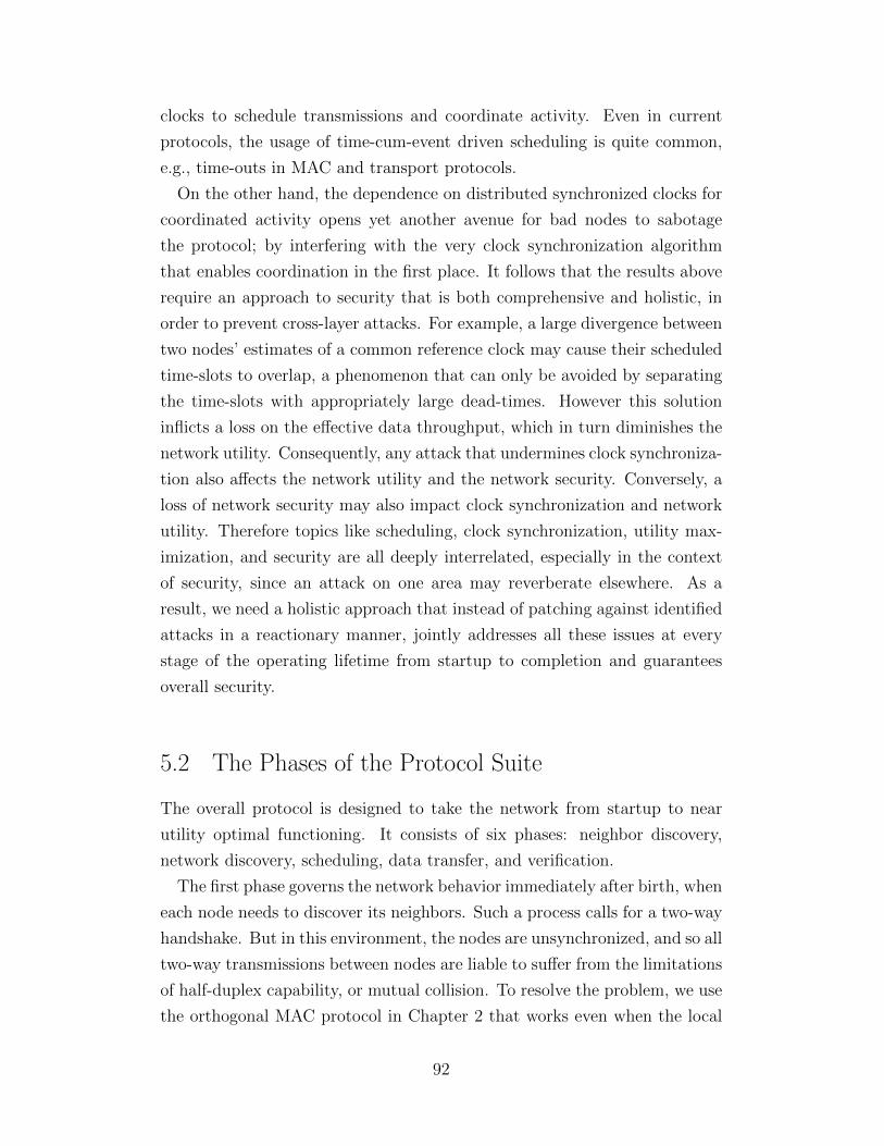
clocks to schedule transmissions and coordinate activity. Even in current

protocols, the usage of time-cum-event driven scheduling is quite common,

e.g., time-outs in MAC and transport protocols.

On the other hand, the dependence on distributed synchronized clocks for

coordinated activity opens yet another avenue for bad nodes to sabotage

the protocol; by interfering with the very clock synchronization algorithm

that enables coordination in the first place. It follows that the results above

require an approach to security that is both comprehensive and holistic, in

order to prevent cross-layer attacks. For example, a large divergence between

two nodes’ estimates of a common reference clock may cause their scheduled

time-slots to overlap, a phenomenon that can only be avoided by separating

the time-slots with appropriately large dead-times. However this solution

inflicts a loss on the effective data throughput, which in turn diminishes the

network utility. Consequently, any attack that undermines clock synchroniza-

tion also affects the network utility and the network security. Conversely, a

loss of network security may also impact clock synchronization and network

utility. Therefore topics like scheduling, clock synchronization, utility max-

imization, and security are all deeply interrelated, especially in the context

of security, since an attack on one area may reverberate elsewhere. As a

result, we need a holistic approach that instead of patching against identified

attacks in a reactionary manner, jointly addresses all these issues at every

stage of the operating lifetime from startup to completion and guarantees

overall security.

5.2 The Phases of the Protocol Suite

The overall protocol is designed to take the network from startup to near

utility optimal functioning. It consists of six phases: neighbor discovery,

network discovery, scheduling, data transfer, and verification.

The first phase governs the network behavior immediately after birth, when

each node needs to discover its neighbors. Such a process calls for a two-way

handshake. But in this environment, the nodes are unsynchronized, and so all

two-way transmissions between nodes are liable to suffer from the limitations

of half-duplex capability, or mutual collision. To resolve the problem, we use

the orthogonal MAC protocol in Chapter 2 that works even when the local

92

clocks tick at different and unknown rates.

After the two-way handshake, the nodes attempt to learn their relative

clock parameters. However, here we encounter fundamental limitations to

clock synchronization [28], [37], [29], namely that the nodes cannot distin-

guish clock offsets from delays. Our protocol will work within this restrictive

environment.

In the next phase, the nodes attempt to form a network in the presence of

malicious nodes with Byzantine behavior. We develop a protocol that enables

the good nodes to form a common topological view, regardless of whether

the bad nodes lie about their neighborhood or otherwise attempt to sabotage

the process. The good nodes are also able to decide on a common view of

the reference time, again in the face of coordinated attacks and inconsistent

or false timing data generated by the malicious nodes.

Having synchronized to a common reference time, and decided on a com-

mon topology, the nodes then determine a schedule for data transmission.

A schedule simply specifies which set of nodes should concurrently transmit,

or more precisely which set of links should be simultaneously active, at any

given time, i.e., time-indexed concurrent transmission sets. At this point,

some of the attackers who seemingly cooperated in the initial phases, may

choose to stop cooperating and/or actively undermine the transfer of data.

To counter this behavior the protocol enables the good nodes to reliably

broadcast any recorded failures to the rest of the network. The schedule is

then modified appropriately and the network begins data transfer anew.

We design the protocol to ensure that the loss of failed data transfer phases

can be amortized over the entire finite network operating lifetime and made

arbitrarily small. As the network repeatedly iterates through the scheduling-

data-verification phases, the clock estimates begin to drift. This drift poses

problems of its own and must be taken into account when determining the

schedule and computing the achieved utility. We choose tolerance bands

around each scheduled action of sufficient length to prevent collisions but

ensure ε optimality.

93

5.2.1 The Orthogonal MAC Code

For convenience, we summarize here the relevant conclusions from Chapter 3

concerning the orthogonal MAC code. The network consists of asynchronous,

half-duplex wireless nodes. Given any pair of nodes, the orthogonal MAC

code specifies the time intervals with respect to their local clocks, in which

each node should transmit or listen to the other node. It guarantees that

within a fixed-time time interval the condition for successful communication

between half-duplex nodes is satisfied.

The orthogonal MAC code for each node i is composed of two funda-

mental two-pulse waveforms, a “primary” pulse M(i)1 (t) and a “secondary”

pulse M(i)2 (t) which, given another node j, are designed to guarantee non-

overlapping transmit slots for both nodes when node i’s clock is relatively

slower (aij ≤ 1) or faster (aij > 1) than node j’s clock respectively. The

period of each waveform M(i)1 (t) and M

(i)2 (t) is denoted by T

(i)0 and T

(n−i+1)0

respectively, where T(i)0 are defined by T0 := 32Wna2

max, and T(i)0 := iT0.

The waveforms M(i)1 (t) and M

(i)2 (t) contain two pulses of width W that are

separated by a distance unique to node i. We use the parameter ci to define

the position of the secondary pulse in the waveform, where ci := 1amax(5n−i) .

They are defined by

M(i)1 (t) :=

1 0 ≤ t mod T

(i)0 < W

0 W ≤ t mod T(i)0 < ciT

(i)0

1 ciT(i)0 ≤ t mod T

(i)0 < ciT

(i)0 +W

0 ciT(i)0 +W ≤ t mod T

(i)0 < T

(i)0 ,

M(i)2 (t) := M

(n−i+1)1 (t).

In addition, the orthogonal MAC code partitions time (as measured by

each node’s local clock), into communication slots, two of which are assigned

to every other node in the network. The length of the communication slots

created by node i is denoted by Ti−1,2, where T0,2 := 2(dnamaxe+ 2)T(n)0 , and

Ti,2 := 2amaxnTi−1,2. In each communication slot, node i uses one of the two

square-pulse waveforms M(i)1 (t) or M

(i)2 (t) to determine the mode (transmit

or receive) at time t. The square-pulse function s(i,j)k (t), k = 1, 2, indicates

to node i whether at local time t it is currently in the communication slot

94

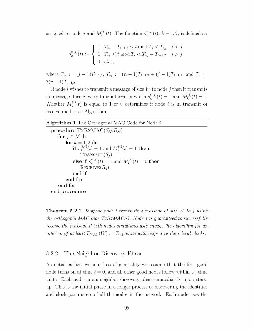
assigned to node j and M(i)k (t). The function s

(i,j)k (t), k = 1, 2, is defined as

s(i,j)k (t) :=

1 Tsk − Ti−1,2 ≤ t mod Ts < Tsk , i < j

1 Tsk ≤ t mod Ts < Tsk + Ti−1,2, i > j

0 else,

where Ts1 := (j − 1)Ti−1,2, Ts2 := (n − 1)Ti−1,2 + (j − 1)Ti−1,2, and Ts :=

2(n− 1)Ti−1,2.

If node i wishes to transmit a message of size W to node j then it transmits

its message during every time interval in which s(i,j)k (t) = 1 and M

(i)k (t) = 1.

Whether M(i)k (t) is equal to 1 or 0 determines if node i is in transmit or

receive mode; see Algorithm 1.

Algorithm 1 The Orthogonal MAC Code for Node i

procedure TxRxMAC(SN ,RN )for j ∈ N do

for k = 1, 2 doif s

(i,j)k (t) = 1 and M

(i)k (t) = 1 then

Transmit(Sj)

else if s(i,j)k (t) = 1 and M

(i)k (t) = 0 then

Receive(Rj)end if

end forend for

end procedure

Theorem 5.2.1. Suppose node i transmits a message of size W to j using

the orthogonal MAC code TxRxMAC(·). Node j is guaranteed to successfully

receive the message if both nodes simultaneously engage the algorithm for an

interval of at least TMAC(W ) := Tn,2 units with respect to their local clocks.

5.2.2 The Neighbor Discovery Phase

As noted earlier, without loss of generality we assume that the first good

node turns on at time t = 0, and all other good nodes follow within U0 time

units. Each node enters neighbor discovery phase immediately upon start-

up. This is the initial phase in a longer process of discovering the identities

and clock parameters of all the nodes in the network. Each node uses the

95

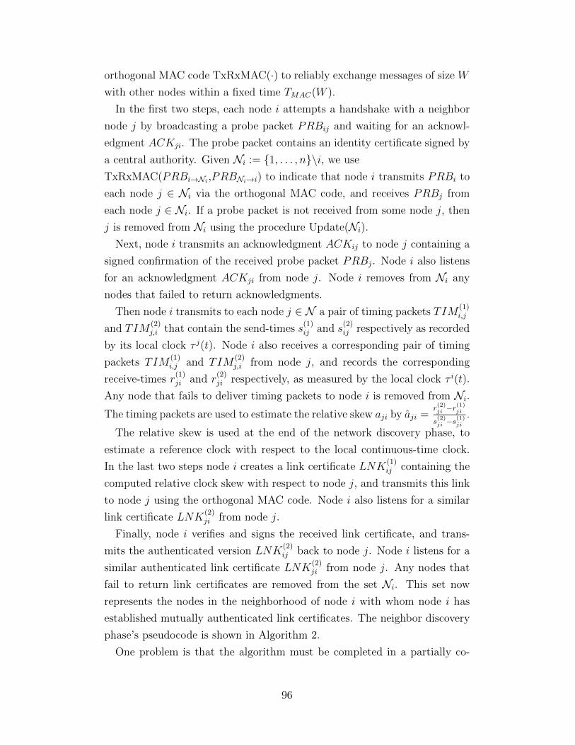
orthogonal MAC code TxRxMAC(·) to reliably exchange messages of size W

with other nodes within a fixed time TMAC(W ).

In the first two steps, each node i attempts a handshake with a neighbor

node j by broadcasting a probe packet PRBij and waiting for an acknowl-

edgment ACKji. The probe packet contains an identity certificate signed by

a central authority. Given Ni := {1, . . . , n}\i, we use

TxRxMAC(PRBi→Ni ,PRBNi→i) to indicate that node i transmits PRBi to

each node j ∈ Ni via the orthogonal MAC code, and receives PRBj from

each node j ∈ Ni. If a probe packet is not received from some node j, then

j is removed from Ni using the procedure Update(Ni).Next, node i transmits an acknowledgment ACKij to node j containing a

signed confirmation of the received probe packet PRBj. Node i also listens

for an acknowledgment ACKji from node j. Node i removes from Ni any

nodes that failed to return acknowledgments.

Then node i transmits to each node j ∈ N a pair of timing packets TIM(1)i,j

and TIM(2)j,i that contain the send-times s

(1)ij and s

(2)ij respectively as recorded

by its local clock τ j(t). Node i also receives a corresponding pair of timing

packets TIM(1)i,j and TIM

(2)j,i from node j, and records the corresponding

receive-times r(1)ji and r

(2)ji respectively, as measured by the local clock τ i(t).

Any node that fails to deliver timing packets to node i is removed from Ni.The timing packets are used to estimate the relative skew aji by aji =

r(2)ji −r

(1)ji

s(2)ji −s

(1)ji

.

The relative skew is used at the end of the network discovery phase, to

estimate a reference clock with respect to the local continuous-time clock.

In the last two steps node i creates a link certificate LNK(1)ij containing the

computed relative clock skew with respect to node j, and transmits this link

to node j using the orthogonal MAC code. Node i also listens for a similar

link certificate LNK(2)ji from node j.

Finally, node i verifies and signs the received link certificate, and trans-

mits the authenticated version LNK(2)ij back to node j. Node i listens for a

similar authenticated link certificate LNK(2)ji from node j. Any nodes that

fail to return link certificates are removed from the set Ni. This set now

represents the nodes in the neighborhood of node i with whom node i has

established mutually authenticated link certificates. The neighbor discovery

phase’s pseudocode is shown in Algorithm 2.

One problem is that the algorithm must be completed in a partially co-

96

ordinated manner even the nodes are asynchronous; the completion of any

stage depends on the successful completion of the previous stages by all

other good nodes. Consequently, we assign increasingly larger intervals

Sk := [tk, tk+1), k = 1, . . . 6 to each successive protocol stage; see Section 5.3.

At the conclusion of the neighbor discovery phase, node i has determined

the identity and relative clock parameters of each node in Ni, and included

this data in a mutually authenticated link certificate.

Algorithm 2 The Neighbor Discovery Phase

procedure NeighborDiscoveryNi := {1, . . . , n} \ iwhile t ∈ S1 do

TxRxMAC(PRBi→Ni ,PRBNi→i)Update(Ni)

end whilewhile t ∈ S2 do

TxRxMAC(ACKi→Ni ,ACKNi→i)end whilewhile t ∈ S3 do

TxRxMAC(TIM(1)i→Ni ,TIM

(1)Ni→i)

Update(Ni)end whilewhile t ∈ S4 do

TxRxMAC(TIM(2)i→Ni ,TIM

(2)Ni→i)

Update(Ni)end whilewhile t ∈ S5 do

TxRxMAC(LNK(1)i→Ni ,LNK

(1)Ni→i)

Update(Ni)end whilewhile t ∈ S6 do

TxRxMAC(LNK(2)i→Ni ,LNK

(2)Ni→i)

Update(Ni)end while

end procedure

5.2.3 The Network Discovery Phase

The purpose of this next phase is to allow the good nodes to obtain a common

view of the network topology and consistent estimates of all the other clock

97

parameters. To accomplish this, the good nodes must broadcast their lists

of neighbors to the rest of the network, and decide on the same view of

the topology. The difficulty of this endeavor is that the good nodes do not

know a priori which of the other nodes are good or bad. Consequently, bad

nodes have the opportunity to selectively drop lists or introduce false lists

with the aim of preventing consensus. We resolve this problem by using a

version of the Byzantine General’s algorithm of [38]. This requires an EIG

tree data structure. Let Ti denote node i’s EIG tree, which by construction

has depth n. The root of Ti is labeled with node i’s neighborhood, that is,

the nodes in Ni and the corresponding collection of link certificates. First

node i transmits to every node j ∈ Nj in its neighborhood, the list of nodes

in Ni and corresponding link certificates, while receiving similar lists from

each node in Nj. Node i updates its EIG tree with the newly received lists

from its neighbors, by assigning each received list to a unique child vertex

of the root of Ti. Node i then transmits the set of level 1 vertices of Ti to

every node in its neighborhood, receiving a set of level 1 vertcies from each

neighbor in turn. The EIG tree Ti is updated again. This process continues

through all n levels of the EIG tree. All communication is via the orthogonal

MAC code.

The notation T(k)i in Algorithm 3 indicates the k-level vertices of the EIG

tree Ti. The notation TxRxMAC(T(k)i→Ni , T

(k)Ni→i) indicates that, using the

orthogonal MAC code, node i transmits T(k)i to each node j ∈ Ni, and

receives T(k)j from each node j ∈ Ni.

We use the procedure UPDATE(Ti), to update the EIG tree Ti after the

arrival of new information, and the procedure DECIDE(Ti) to infer the net-

work topology based on the EIG tree. The n-stage EIG algorithm guarantees

that if the subgraph of good nodes is connected, then each good node will

decide on the same topological view.

5.2.4 The Consistency Check Phase

For convenience, we summarize here the results of Chapter 4 concerning

the consistency check protocol. We recall that the fundamental difficulty

is that any malicious nodes along the path 1, . . . , n may have generated

false timestamps in the neighbor discovery phase, and thus corrupted the

98

Algorithm 3 The EIG Byzantine General’s Algorithm

procedure EIGByzMAC(Ni)T

(0)i := Ni

for k = 1, . . . n dowhile t ∈ S6+k do

TxRxMAC(T(k)i→Ni , T

(k)Ni→i)

Update(Ti)end while

end forDecide(Ti)

end procedure

measured relative skews between adjacent nodes. Although, by assumption,

every pair of good nodes (i, j) in the network is connected by at least one

path of good nodes, there may be other connecting paths infiltrated by bad

nodes that generate different values for the relative skew. It is impossible to

determine the correct path from the relative skews alone. A pair of paths that

generate different relative skews between the same pair of nodes corresponds

to an inconsistent cycle; a cycle in which the skew product is not equal to

one. We use the Consistency Check algorithm to identify the path that has

generated the correct relative skew.

The consistency check works by circling a timing packet around every cycle

in which the skew product differs from one by more than εa, where εa is the

desired maximum skew error caused by malicious nodes. At the conclusion of

the test, at least one link with a malicious endpoint will be removed from the

cycle, thereby eliminating a connecting path. During the test, each node in

such a cycle is obliged to append a receive timestamp and a send timestamp

generated by the local clock before forwarding the packet to the next node.

These timestamps must satisfy a delay bound condition; the send time and

receive time cannot differ by more than 1 clock count. A node fails the

consistency check if its send and receive timestamps differ by more than one

clock count, or if its timestamps do not agree with its declared relative skew.

The key idea is that if the test starts after a sufficiently large amount of time

has elapsed, the clock estimates based on the faulty relative skews will have

diverged so extensively from the actual clocks that at least one malicious

node in the cycle will find it impossible to generate timestamps that are

consistent with its declared relative clock skew, and satisfy the delay bound

99

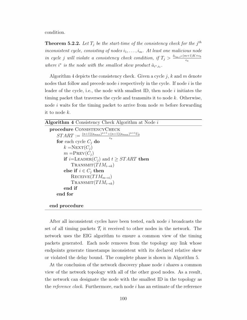
condition.

Theorem 5.2.2. Let Tj be the start-time of the consistency check for the jth

inconsistent cycle, consisting of nodes i1, . . . , im. At least one malicious node

in cycle j will violate a consistency check condition, if Tj >aim,i∗ (m+1)K+εb

εa

where i∗ is the node with the smallest skew product ai∗,i1.

Algorithm 4 depicts the consistency check. Given a cycle j, k and m denote

nodes that follow and precede node i respectively in the cycle. If node i is the

leader of the cycle, i.e., the node with smallest ID, then node i initiates the

timing packet that traverses the cycle and transmits it to node k. Otherwise,

node i waits for the timing packet to arrive from node m before forwarding

it to node k.

Algorithm 4 Consistency Check Algorithm at Node i

procedure ConsistencyCheck

START := (n+1)(amax)n+1+(n+1)(amax)n+1U0

εafor each cycle Cj do

k =Next(Cj)m =Prev(Cj)if i=Leader(Cj) and t ≥ START then

Transmit(TIMi→k)else if i ∈ Cj then

Receive(TIMm→i)Transmit(TIMi→k)

end ifend for

end procedure

After all inconsistent cycles have been tested, each node i broadcasts the

set of all timing packets Ti it received to other nodes in the network. The

network uses the EIG algorithm to ensure a common view of the timing

packets generated. Each node removes from the topology any link whose

endpoints generate timestamps inconsistent with its declared relative skew

or violated the delay bound. The complete phase is shown in Algorithm 5.

At the conclusion of the network discovery phase node i shares a common

view of the network topology with all of the other good nodes. As a result,

the network can designate the node with the smallest ID in the topology as

the reference clock. Furthermore, each node i has an estimate of the reference

100

Algorithm 5 The Network Discovery Phase at Node i

procedure NetworkDiscoveryEIGByzMAC(Ni)ConsistencyCheckEIGByzMAC(Ti)

end procedure

clock τ ri (t) with respect to its local clock t using the formula τ ri (t) := arit,

where the estimated relative skew ari and the actual relative skew ari differ

by at most εa.

5.2.5 The Scheduling Phase

In the scheduling phase the good nodes in the network obtain a common

schedule governing the transmission and reception of data packets. Funda-

mental to our scheduling is the notion of “concurrent transmission set.” This

is a set of nodes that transmit at the same time, each using a certain power

level and modulation schedule, akin to an “independent set” or “conflict-free

set.” A “schedule” is a sequence of such concurrent transmission sets, each

with specified start and end times. Each node i divides the data transfer

phase into time-slots, and assigns a concurrent transmission slot and corre-

sponding rate vector to each time-slot so that the effective rate vector over

all time-slots is optimal over an allowed set of concurrent transmission sets C,i.e., it achieves max

P(C)U where P(C) denotes the set of protocols using concur-

rent transmission sets in C. All the good nodes independently arrive at the

same schedule since they independently optimize the same utility function

over the same C (ties broken lexicographically).

The good nodes must conform to a common schedule even though they

do not share the same clock. To resolve this, each node i generates a local

estimate of the reference clock τ ri (t) with respect to its local clock t as de-

scribed in the network discovery phase. However, this estimate may not be

perfectly accurate; the computed relative skew between the local clock and

the reference clock depends on the declared skews between adjacent nodes

on the connecting path. As described in Section 5.2.4, some of the nodes

on this path may be malicious and can introduce an error of at most εa into

the computed relative skew. To address this, the time-slots are separated

101

by a dead-time of size D, where given any pair of nodes (i, j), D is cho-

sen to be larger than difference in their reference clock estimates. That is

|τ ri (t)− τ rj (τ ji (t))| ≤ D.

Finally, we choose enough time-slots to guarantee that every pair of nodes

can communicate once in either direction, via multi-hop routing, during the

data transfer phase. There are n(n − 1) ordered pairs, with connecting

paths of at most n nodes, so we use n2(n − 1) time-slots. The algorithm

UtilityMaximization(C) for the scheduling phase is depicted in Algorithm 6.

At the end of the scheduling phase, node i shares a common utility maxi-

mizing schedule with other good nodes.

Algorithm 6 The Scheduling Phase at Node i

procedure SchedulingUtilityMaximization(C)

end procedure

5.2.6 The Data Transfer Phase

In this phase the nodes exchange data packets using the generated schedule.

It is divided into time-slots with each time-slot assigned a concurrent trans-

mission set, a rate vector, and set of packets for each transmitter in the set.

To prevent collisions resulting from two nodes assigning themselves to differ-

ent time-slots due to timing error, node i begins transmission D time-units

after the start of the time-slot. The transmitted packet is then guaranteed

to arrive at the receiver in the same time slot, for appropriate choice of D

and time-slot size Bslot.

Algorithm 7 defines this phase, with mk denoting a message to be transmit-

ted or received by node i in the kth slot, Tstart the start time of the phase mea-

sured by the local estimate of the reference clock τ ri (t)), Sk = [tk, tk+1), k =

1, . . . , N the time-slots of the phase with N = n2(n − 1), t1 = Tstart, and

tk+1 := tk +Bslot + 2D, and TX(k) and RX(k) the concurrent transmission

set, and receiving nodes during slot k.

102

Algorithm 7 The Data Transfer Phase at Node i

procedure DataTransfer(Tstart)for k=1,. . . ,N do

if t ∈ Sk and t ≥ tk +D and i ∈ TX(k) thenTransmit(mk)

else if t ∈ Sk and i ∈ RX(k) thenReceive(mk)

end ifend for

end procedure

5.2.7 The Verification Phase

However, malicious nodes may not cooperate in data transfer phase, and so

some packets may not be received successfully. Whenever such a scheduled

packet fails to arrive at node j, it adds the offending concurrent transmission

set and associated packet number to a list, and distributes the list to the rest

of the network in the verification phase using the EIG Byzantine General’s

algorithm. These sets are then permanently removed from the collection

of feasible concurrent transmission sets C. With Lk denoting the list of

concurrent transmission sets that failed during the kth iteration of the data

transfer phase, the set Ck of feasible concurrent transmission sets during the

kth iteration of the scheduling phase is updated by intersecting it with Lck in

Algorithm 8.

We note that the nodes need not use the orthogonal MAC code, since they

have an estimate of the reference clock; all communication can be scheduled

into slots separated by a dead-time of 2D. Within each of the n stages of

EIG Byzantine General’s algorithm, there are n(n − 1) pairs of nodes that

may communicate, and at most n nodes on the connecting path. Therefore,

the total number of time-slots required is n3(n− 1).

At the conclusion of the phase, the good nodes share a common view of

the set of feasible concurrent transmission sets for the next iteration of the

scheduling phase.

103

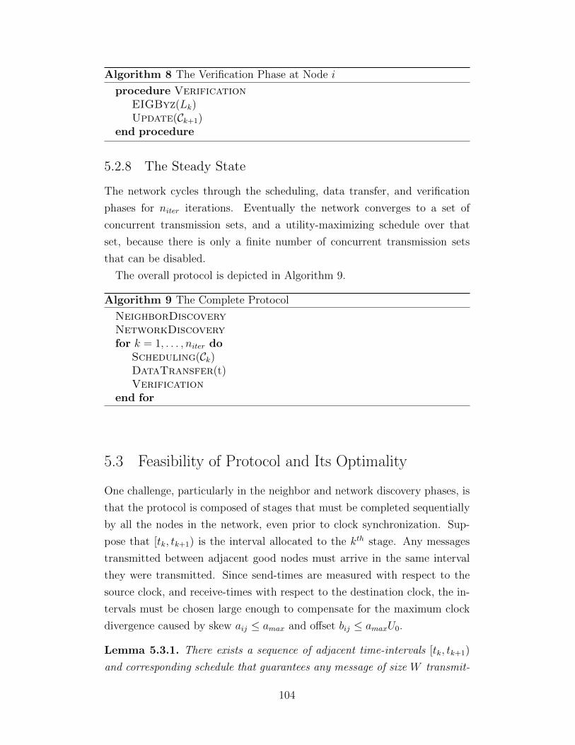
Algorithm 8 The Verification Phase at Node i

procedure VerificationEIGByz(Lk)Update(Ck+1)

end procedure

5.2.8 The Steady State

The network cycles through the scheduling, data transfer, and verification

phases for niter iterations. Eventually the network converges to a set of

concurrent transmission sets, and a utility-maximizing schedule over that

set, because there is only a finite number of concurrent transmission sets

that can be disabled.

The overall protocol is depicted in Algorithm 9.

Algorithm 9 The Complete Protocol

NeighborDiscoveryNetworkDiscoveryfor k = 1, . . . , niter do

Scheduling(Ck)DataTransfer(t)Verification

end for

5.3 Feasibility of Protocol and Its Optimality

One challenge, particularly in the neighbor and network discovery phases, is

that the protocol is composed of stages that must be completed sequentially

by all the nodes in the network, even prior to clock synchronization. Sup-

pose that [tk, tk+1) is the interval allocated to the kth stage. Any messages

transmitted between adjacent good nodes must arrive in the same interval

they were transmitted. Since send-times are measured with respect to the

source clock, and receive-times with respect to the destination clock, the in-

tervals must be chosen large enough to compensate for the maximum clock

divergence caused by skew aij ≤ amax and offset bij ≤ amaxU0.

Lemma 5.3.1. There exists a sequence of adjacent time-intervals [tk, tk+1)

and corresponding schedule that guarantees any message of size W transmit-

104

ted (via the orthogonal MAC code) by node i in the interval [tk, tk+1) (as

measured by node i’s clock) will be received by node j in the same interval as

measured by node j’s clock.

Proof. Set tk+1 := (amax)2tk + 2(amax)

3U0 + (amax)3TMAC(W ). Suppose that

a message from node i to node j during the interval [tk, tk+1) is transmitted

(via the orthogonal MAC code) at ts := amaxtk + (amax)2U0 with respect to

node i’s clock. By substitution and simplification it follows that τ ji (ts) ≥ tk

and τ ji (ts + TMAC(W )) < tk+1. Hence τ ji ([ts, ts + TMAC(W ))) ⊂ [tk, tk+1),

and so node j receives this message during the same interval with respect to

node j’s clock.

Consequently, we have:

Theorem 5.3.1. At the conclusion of the network discovery phase the good

nodes will have a common view of the topology and consistent estimates (to

within εa) of the skew of the reference clock.

Proof. From Lemma 5.3.1 all good nodes will proceed through each stage of

the Neighbor and network discovery phases together, and therefore establish

link certificates with their good neighbors. Since they form a connected

component, the good nodes obtain a common view of their link certificates

using the EIGByzMAC algorithm and the schedule in Lemma 5.3.1. The

good nodes can therefore infer the network topology and the relative skews

of all adjacent nodes based upon the collection of link certificates. Using

the consistency check, the good nodes can eliminate paths along which bad

nodes have provided false skew data. The good nodes can disseminate this

information to each other using the EIGByzMAC algorithm and Lemma 5.3.1

and thus obtain consistent estimates of the reference clock to within εa.

We have the following corollary to Lemma 5.3.1:

Lemma 5.3.2. The sequence of adjacent intervals [tj, tj+1), j = 0, . . . , k is

contained in [t0, c1t0 + c2W ) where constants c1 and c2 depend on amax, k,

U0, and n.

Proof. It is straightforward that the duration of the orthogonal MAC code

TMAC(W ) ≤ cW , where constant c depends on amax, and n. The result for

k = 1 follows from definition of tk, and substitution of cW into TMAC(W ),

and for general k by induction and definition of tk.

105

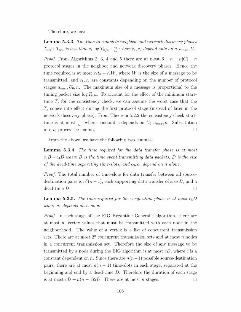
Therefore, we have:

Lemma 5.3.3. The time to complete neighbor and network discovery phases

Tnei+Tnet is less than c1 log Tlife+ c2εa

where c1, c2 depend only on n, amax, U0.

Proof. From Algorithms 2, 3, 4 and 5 there are at most 6 + n + n|C| + n

protocol stages in the neighbor and network discovery phases. Hence the

time required is at most c1t0 + c2W , where W is the size of a message to be

transmitted, and c1, c2 are constants depending on the number of protocol

stages amax, U0, n. The maximum size of a message is proportional to the

timing packet size log Tlife. To account for the effect of the minimum start-

time Ts for the consistency check, we can assume the worst case that the

Ts comes into effect during the first protocol stage (instead of later in the

network discovery phase). From Theorem 5.2.2 the consistency check start-

time is at most cεa

, where constant c depends on U0, amax, n. Substitution

into t0 proves the lemma.

From the above, we have the following two lemmas:

Lemma 5.3.4. The time required for the data transfer phase is at most

c3B+ c4D where B is the time spent transmitting data packets, D is the size

of the dead-time separating time-slots, and c3, c4 depend on n alone.

Proof. The total number of time-slots for data transfer between all source-

destination pairs is n2(n− 1), each supporting data transfer of size Bs and a

dead-time D.

Lemma 5.3.5. The time required for the verification phase is at most c5D

where c5 depends on n alone.

Proof. In each stage of the EIG Byzantine General’s algorithm, there are

at most n! vertex values that must be transmitted with each node in the

neighborhood. The value of a vertex is a list of concurrent transmission

sets. There are at most 2n concurrent transmission sets and at most n nodes

in a concurrent transmission set. Therefore the size of any message to be

transmitted by a node during the EIG algorithm is at most cD, where c is a

constant dependent on n. Since there are n(n−1) possible source-destination

pairs, there are at most n(n − 1) time-slots in each stage, separated at the

beginning and end by a dead-time D. Therefore the duration of each stage

is at most cD + n(n− 1)2D. There are at most n stages.

106

We now prove the main theorem of this chapter:

Theorem 5.3.2. The protocol ensures that a network of n nodes proceeds

from startup to a functioning network carrying data. There exists a selection

of parameters niter, D, B, εa and Tlife that achieves a utility equal to min-

max U(x) to within a factor ε, where the min is over all policies of the bad

nodes that can only adopt one of two actions in each concurrent transmission

set: conform to the protocol, or jam. Since no protocol can prevent a bad node

from doing so, the achieved utility is ε-optimal.

Proof. We begin by choosing parameters so that the protocol overhead, which

includes neighbor discovery, network discovery, verification phases, all dead-

times, and the iterations converging to the final rate vector, is an arbitrarily

small fraction of the total operating lifetime. With τ ri (t) := arit the estimate

of reference clock r with respect to the local clock at node i, the maxi-

mum difference in nodal estimates is bounded as |τ ri (τ i(t))− τ rk (τ ki (τ i(t)))| ≤2(amax)

2εaTlife + (amax)2U0. Given the number of rate vectors in the rate re-

gion, kr, we can choose niter, D, B, εa and Tlife to satisfy: niterniter+2nkr

≥ 1− εl,B

c1 log Tlife+c2εa

+B+c3D+c4D≥ 1−εd, niter((c1 log Tlife+

c2εa

+B+c3D+c4D) ≤ Tlife,

2(amax)2εaTlife + (amax)

2U0 ≤ D. These ensure, successively, that the rate

loss due to failed concurrent transmission sets is arbitrarily small, the time

spent transmitting data is an arbitrarily large fraction of the duration of

that iteration, the operating lifetime is large enough to support niter proto-

col iterations, and the dead-time D is large enough to tolerate the maximum

divergence in clock estimates caused by skew error εa.

Let {Θ(t)} be the non-increasing sequence of disabled concurrent trans-

mission sets, with limit θ attained at some finite time T , and C the set of

all concurrent transmission sets. Suppose rate vector x achieves maxP(C/θ)

U(x).

Our protocol obtains an effective data rate x(1 − εd)(1 − εl). Given a col-

lection of concurrent transmission sets C ′ ⊂ C, let P(C) denote the set of

protocols whose schedules map to C ′. The result follows, since for fixed Θ′,

any collection of disabled concurrent transmission sets, no protocol can do

better than maxP(C\Θ′) U .

107

CHAPTER 6

THE PROTOCOL FOR UNBOUNDEDBIRTH TIMES

The Unbounded Birth Time Model (UBTM) does not impose a bound

on the birth-times of the participating nodes. As a result, separate sub-

networks independently form, where the nodes in each subnetwork share

near-simultaneous birth-times. These subnetworks though operating inde-

pendently of each other might be adjacent. The UBTM protocol described

in this chapter enables adjacent subnetworks to detect each other and merge.

There are three major obstacles to overcome for the protocol to succeed.

First, the two subnetworks have to detect each other. Since both are initially

operating independently, there is no guarantee that a node in one subnet-

work will pick up the transmissions of a node in the other subnetwork; both

nodes could be transmitting simultaneously or listening to someone else. So

each subnetwork must set aside a dedicated period of time to listen for adja-

cent subnetworks in the area. Second, the two subnetworks have to merge.

Once a subnetwork has detected a neighbor, it must interrupt its “normal”

steady-state operation, change its reference clock, predict when the detected

subnetwork will be entering a neighbor discovery phase, and schedule a co-

inciding neighbor discovery phase. Of course, this procedure itself can be

hijacked by bad nodes seeking to repeatedly drive the subnetwork into spu-

rious merges. The entire process, both the sentinel phase and the merge is

temporally expensive, requiring at least two protocol cycles to carry out. As

a result, the sentinel phase can only be carried out infrequently, which im-

plies that an adjacent subnetwork might remain undetected for a long period

of time before a merge occurs. During this time, the entire network be-

ing unnecessarily partitioned is operating suboptimally. The corresponding

throughput loss, to be rendered negligible, must be suitably amortized over

a long enough operating period. This entire process applies on a per merge

basis. Over the course of the total operating lifetime, the subnetwork might

have to carry out numerous merges. Our goal is to obtain optimal operation

108

over the protocol lifetime from the instant the last good node was born. But

good nodes can be born at any time. Therefore, to operate optimally from

the instant the last good node was born, each subnetwork must at a minimum

be able to reset its clocks after a new node joins and continue operating for

a protocol lifetime. However, a clock reset implies the reuse of timestamps,

a potentially hazardous scenario that opens the door to “replay attacks.”

These attacks, in which bad nodes retransmit “stale” packets timestamped

from an earlier era, are impossible to detect. Hence, a subnetwork must also

change encryption before its clocks are reset in order to prevent stale packets

from corrupting the operation.

The third obstacle is that this clock reset procedure only works if every

good node is born within an operating lifetime of the last good node, an out-

come which need not be the case in the UBTM. Hence, a subnetwork might

run out the clock before another node joins. To avoid this, the subnetwork

enters a coma phase before the clock runs out, and executes a clock freeze.

The subnetwork stays in the coma phase until the broadcasts of an adjacent

subnetwork are detected, subsequently leaving the coma phase and restarting

the clock to attempt a merge.

The key idea underwriting much of the proof is that there are only a

finite number of times bad nodes can instigate a spurious merge or prevent

a merge from occurring. Whenever a merge is attempted, each node keeps

a record of both subnetworks and the connecting link that instigated the

merge. This merge “triple” is only allowed to fail a finite number of times

before it is deposited into the used-up collection and never used again. There

are also a finite number of these “merge triples.” We need to choose a large

enough operating lifetime to amortize the rate loss from all failed merges over

all merge triples. In addition, the protocol must provide functionality that

allows subnetworks to recognize when a merge has failed and guarantees a

consistent view of the failed merge triples among the affected good nodes.

In the next section we give a more detailed run-through of the protocol

operation.

109

6.1 Overview of the UBTM Protocol

For the moment let us adopt the perspective of an individual node i. Imme-

diately after its primordial birth, node i enters the initial neighbor discovery

phase followed by the initial network discovery phase. Both phases are iden-

tical to those in the BBTM protocol. Node i emerges from the initial network

discovery phase as part of a subnetwork Si of nodes that were all born simul-

taneously. The good nodes in this subnetwork have a common topological

view, and a consistent view of a common reference clock. Let us assume for

now that Si is a unified entity that behaves in a consistent manner.

As in the BBTM, Si cycles through the scheduling phase, the data transfer

phase, and the verification phase, successively pruning concurrent transmis-

sion sets that are either infeasible or have been disabled by malicious nodes.

However, Si also cycles through a recurrent neighbor discovery phase and

network discovery phase to “pick-up” adjacent subnetworks that are seeking

to merge. We will now describe this process in more detail.

Every nsent cycles, Si enters a “sentinel” phase. We use the word sentinel

to describe a node that refrains from transmitting for the express purpose

of receiving unscheduled transmissions from nodes in the neighborhood. In

general, a sentinel attempts to detect nodes that have not been previously

detected. These undetected nodes obviously do not share a common schedule

with the sentinel, and as a result their transmissions, from the perspective of

the sentinel, are completely unpredictable. Hence, in order to avoid primary

conflicts, the sentinel stays silent during this period of its duty.

The purpose of the sentinel phase is to detect adjacent subnetworks that

may have formed after Si left the initial neighbor and network discovery

phase. After initially broadcasting probe packets to advertise its presence,

Si quiets down to listen for any probe packets broadcasted by adjacent sub-

networks. The sentinel phase stretches over 2damaxe protocol cycles to ensure

complete overlap with the recurrent neighbor discovery phase of an adjacent

subnetwork.

Now suppose Si detects an adjacent subnetwork Sj. Being the subnetwork

initiating the merge, Si must change its reference clock to Sj, and predict

when Sj next enters the recurrent neighbor discovery phase. In the mean-

time, Si stays idle. Associated with each merge attempt is a merge “pair,”

consisting of the initiating subnetwork and the detected subnetwork. Fur-

110

thermore, there are rules in place to ensure that Sj does not initiate a merge

with Si, thereby causing both Si and Sj to “miss” each other. However, Sj

might initiate a merge with some other subnetwork in the interm, causing Sis

merge attempt to fail. The rules are designed to ensure that merge attempts

fail a finite number of times.

Returning to the original scenario, Si enters the recurrent neighbor dis-

covery phase at the time Sj was predicted to do the same. After proceeding

through the recurrent neighbor and network discovery phase, node i finally

has the opportunity to evaluate whether the attempted merge was success-

ful. Each node in the new post-merge subnetwork, call it Si, does the same

evaluation. Node i declares the merge successful if Sj ∪ Si ⊂ Si, that is,

Si contains the detected subnetwork Sj, the initiating subnetwork Si, and

possibly other nodes as well. If the merge succeeds, the node i adds the as-

sociated merge triple to the “used-up collection.” The merge triple is never

used again. However if the merge fails, the situation becomes more complex.

There are two reasons why a merge between Si and Sj could fail. The

first is that Si and/or Sj are infiltrated with bad nodes. The second is that

Sj attempted a merge with another subnetwork before Si could execute the

one it was planning. How many times could this happen? Let m be the

order of Si. There are at most 2m possible chains of ordered subnetworks

in which each subnetwork in the chain attempts to merge with its higher-

ordered neighbor. Therefore the total number of failures granted to the merge

pair (Si, Sj) is 2m where m is the order of Si. If the merge pair exceeds this

number, then it too is added to the used-up collection and never used again.

Hence failed merges will only happen a finite number of times.

Suppose the merge between Si and Sj is successful. Then the new sub-

network Si changes its encryption, resets its clocks, and proceeds to the

scheduling phase. In the scheduling phase, Si chooses a schedule that maxi-

mizes the utility function over the space of feasible concurrent transmission

sets. In the aftermath of a successful merge, this space is the entire space

of concurrent transmission sets for Si. The schedule is executed in the data

transfer phase, and failed concurrent transmission sets are pruned in the ver-

ification phase, resulting in a new feasible set. Next Si cycles through the

recurrent neighbor discovery phase and network discovery phase, the schedul-

ing phase, the data transfer phase, and the verification phase. The first two

phases allow Si to advertise its presence to adjacent subnetworks in a regular

111

Initial Neighbor Discovery

Phase

Initial Network Discovery

Phase

Scheduling Phase

Recurrent Network Discovery

Phase

Recurrent Neighbor Discovery

Phase

Sentinel Phase

Coma Phase

Data Transfer

Phase

Verification Phase

Enter Sentinel Phase?

Successful Merge?

Reset Clocks/Change

Encryption

Primordial Birth

Operating Time Expired?

New Component Detected?

No

New Component Detected?

Prepare for Merge

Yes

Yes

No

Yes

No

Yes

Yes

No

No

Figure 6.1: The state diagram of the UBTM protocol.

and predictable way. Some of these subnetworks may initiate merges with

Si, which if successful, will be picked up in the recurrent neighbor and net-

work discovery phases. The new subnetwork will then change its encryption,

reset its clocks and start the scheduling phase with a new space of feasible

concurrent transmission sets.

Eventually after repeatedly cycling through the protocol phases, Si will

arrive at a schedule that is utility optimal over the space of feasible concurrent

transmission sets for its topology. Moreover, Si will be operating at an

effective throughput vector that is utility optimal. After niter cycles have

expired, Si checks whether there are still nodes that have yet to join. If

so, then Si enters the coma phase and executes a clock freeze. During the

coma phase Si listens for any broadcasts from adjacent subnetworks, and if

received, will initiate a merge with the detected subnetwork. A successful

merge results in a change of encryption and clock reset, but a failed merge

will return Si to the coma phase.

The protocol state diagram is shown in Figure 6.1.

In the following sections we will describe some of the phases in more detail.

112

Algorithm 10 The Complete Protocol

InitialNeighborDiscoveryInitialNetworkDiscoverywhile coma or exit trigger not activated do

if k mod nsentinel = 0 thenSentinelPhasek := k + d3amaxeif new component is detected in the sentinel phase then

ChangeReferenceClock(SKEW,OFFSET)while the neighbor discovery phase of the detected component

has yet to occur doIdle

end whileend if

elseRecurrentNeighborDiscoveryPhaseRecurrentNetworkDiscoveryPhaseUpdateUsedTriplesif a successful merge has occurred then

ChangeEncryptionResetClocks k=1;

end ifif k ≥ niter and there are undetected nodes then ActivateCom-

maTriggerelse if k ≥ niter then ActivateExitTriggerelse

SchedulingPhaseDataTransferPhaseVerificationPhasek := k + 1

end ifend if

end whilewhile coma trigger is activated do

ComaPhaseif new component is detected in the coma phase then

ChangeReferenceClock(SKEW,OFFSET)while the neighbor discovery phase of the detected component has

yet to occur doIdle

end whileDeActivateComaTrigger

end ifend while

113

6.2 The Initial Neighbor Discovery Phase

The initial neighbor discovery (INeiD) phase is similar to the neighbor dis-

covery phase for the BBT model, with the exception that in the former, node

i also computes an estimate of the relative offset between each neighbor, and

includes the relative offset in the corresponding link certificate. A fundamen-

tal result of clock synchronization is that the relative clock offset between

a pair of nodes cannot be exactly computed from any exchange of timing

packets. Therefore, the estimated relative offset between adjacent pairs of

nodes can only be accurate to within amaxdmax clock counts, where dmax is

the maximum packet delay. At the conclusion of the post-birth neighbor

discovery phase, node i has generated a collection of link certificates for the

subset of its neighboring nodes that were born within a bounded time of

itself.

6.3 The Initial Network Discovery Phase

The initial network discovery (INetD) phase is also similar to the network dis-

covery phase for the BBT model. The difference again lies in the treatment of

the clock offset parameters. Whereas in the BBT model the clock offset was

ignored, the INetD phase verifies the consistency of the relative offsets in ad-

dition to the relative skews. An inconsistent cycle occurs when the computed

skew around the cycle differs from unity by more than εa, or the relative off-

set around the cycle differs from zero by more than εb. Since the computed

relative skew between adjacent nodes has an accuracy of amaxdmax, the com-

puted relative skew around a cycle is accurate to within (n+1)(amax)n+1dmax.

Therefore εb ≥ (n + 1)(amax)n+1dmax, and the start time of the consistency

check must satisfy Ts ≥ (n+1)(amax)n+1+(n+1)(amax)n+1dmaxεa

. At the conclusion of

the PBnetD phase, node i belongs to a subcomponent that has a consistent

view of a reference clock and a common view of the network topology.

6.4 The Recurrent Neighbor Discovery Phase

The recurrent neighbor discovery (RNeiD) phase repeats itself indefinitely

after the primordial formation of a subnetwork. Hence, Si, the subnetwork

114

that contains node i, already has a common view of the network topology and

a consistent view of a reference clock. As a result, the time intervals allocated

to each stage need not get progressively larger as in the initial neighbor

discovery phase. Instead, each interval is of fixed length and separated by a

band of length 2B, and the constituent nodes use the reference clock estimate

to schedule their transmissions and receptions. The purpose of the RNeiD

phase is fourfold. First, it allows Si to broadcast its presence to an adjacent

subnetwork that can subsequently estimate the reference clock of Si and

schedule a neighbor discovery phase that coincides with that of Si. Secondly,

it enables the nodes in Si to create link certificates with neighbors belonging

to an adjacent subnetwork that is attempting to merge with Si. Third, it

allows the nodes in Si to create link certificates with neighbors in an adjacent

subnetwork that was detected in preceding sentinel or coma phases. Finally,

it allows Si to recalculate the relative clock skew and offset after a successful

merge and clock reset.

In order to support all four goals, the RNeiD phase differs from the IN-

eiD phase in some important ways. First, all transmitted packets are time-

stamped with respect to the reference clock of Si. In addition, the probe

packets contain an ID that uniquely identifies the subnetwork Si. Hence,

any external sentinel nodes, i.e., the nodes acting as sentinels for the adjacent

subnetworks, which receive these probe packets can estimate the reference

clock of Si and infer the constituent nodes in Si. The external sentinel nodes

then use this information to predict when the next neighbor discovery of Si

will occur, and generate a merge triple containing the ID and reference clock

parameters of Si, and the unique ID of their own subnetwork. The merge

triple is then disseminated to the other nodes in that subnetwork. Second,

if Si is attempting to merge with another subnetwork by scheduling a coin-

ciding RNeiD phase, it includes the corresponding merge triple in its probe

packets so that that other subnetwork is alerted to the attempted merge.

This feature is important, because the nodes in the merged subnetwork must

be able to evaluate whether or not the merge was successful before triggering

a clock reset.

The component Si can only attempt a merge by scheduling a coinciding

RNeiD phase after detecting another component in a preceding sentinel or

coma phase. These latter two phases differ in a key area of consequence.

In the sentinel phase, the activity is always coordinated according to the

115

estimate of the reference clock of Si. In the coma phase, the nodes in Si

execute a coordinated clock freeze to begin the coma phase, but end the

coma phase with a cascading clock restart that increases the spread of the

estimates of the reference clock. The band size B that separates each phase

of the RNeiD phase must account for this increased spread.

At the conclusion of the RNeiD phase, node i will have generated link

certificates with all the adjacent nodes containing updated relative clock

parameters. Node i will also know if some of these adjacent nodes belong to

another component that is attempting a merge.

6.5 The Recurrent Network Discovery Phase

The recurrent network discovery (RNetD) phase follows the recurrent neigh-

bor discovery phase and its purpose, like the INetD phase, is to confer a

common view of the network topology of Si to all its constituent nodes, and

consistent estimates of the reference clock of Si. Moreover, in the event of a

successful merge between two components, an event that will be evident by

the inclusion of the corresponding merge triple, the INetD phase will trigger

a clock reset and change of encryption in order to prevent the clock from

running out.

The RNetD phase differs from the INetD phase in that the component is

already assumed to have a consistent view of a reference clock and common

view of the network topology. As in the RNeiD phase, the time intervals

allocated to each stage are of fixed size and separated by a band of length

2B. In addition, the RNetD phase evaluates whether or not an attempted

merge was successful. A merge is labeled successful if all the nodes in both

components are present in the unified network at the conclusion of the RNetD

phase. A merge triple is added to the used-up collection maintained by each

node if the corresponding merge is successful or if the merge has failed an

excessive number of times.

At the conclusion of the RNetD phase: node i is part of a subnetwork

at that stage that has a common view of the network topology, consistent

estimates of a reference clock, and awareness of whether it is the product of

a successful merge.

116

6.6 The Scheduling, Data Transfer, and Verification

Phases

These phases are similar to their counterparts in the BBT model.

6.7 The Coma Phase

The purpose of the coma phase is to tentatively end the system if no fu-

ture nodes are detected. (Note that a set of nodes never knows that it has

definitely reached the end unless all nodes are part of the network). This

tentative end must therefore have two properties. If no new nodes are ever

detected in the future, then the accrued utility must be nearly optimal. How-

ever, if new nodes are detected in the future, then the network needs to grow.

In the coma phase, the nodes in subnetwork Si freeze their clocks after

niter protocol cycles have expired and there are still nodes that have yet to

be encountered. The clocks stay frozen until some node, say node i, receives

a probe packet from a previously undiscovered subnetwork. First node i

estimates the skew and offset of the reference clock of the newly detected

subnetwork. The offset can only be accurate to within dmax. Then node i

generates a merge triple Mi containing the ID of the detected subnetwork,

the estimated skew and offset of the detected subnetwork, and the ID of Si.

If the merge triple has not already been added to the used-up collection of

triples, node i restarts its clock and broadcasts the merge triple to the rest

of the subnetwork Si using the Byzantine General’s algorithm.

An alternative scenario occurs if other nodes in Si generate merge triples

and broadcast the triples using the Byzantine General’s algorithm. When

node i receives these messages, it first verifies that each of them have not been

previously added to the used-up collection. If so, node i restarts its clock and

forwards the messages as per the Byzantine General’s algorithm. Otherwise

the messages are discarded. In addition, if the messages are received before

node i generates its own merge triple Mi, then node i discards Mi.

Since the clocks of each node in Si have been frozen, the nodes will have

to restart their clocks as they receive the message packets and re-estimate

the offsets. In addition, the transmission slots for the EIG algorithm are

separated by buffers large enough to accommodate the delay induced by the

117

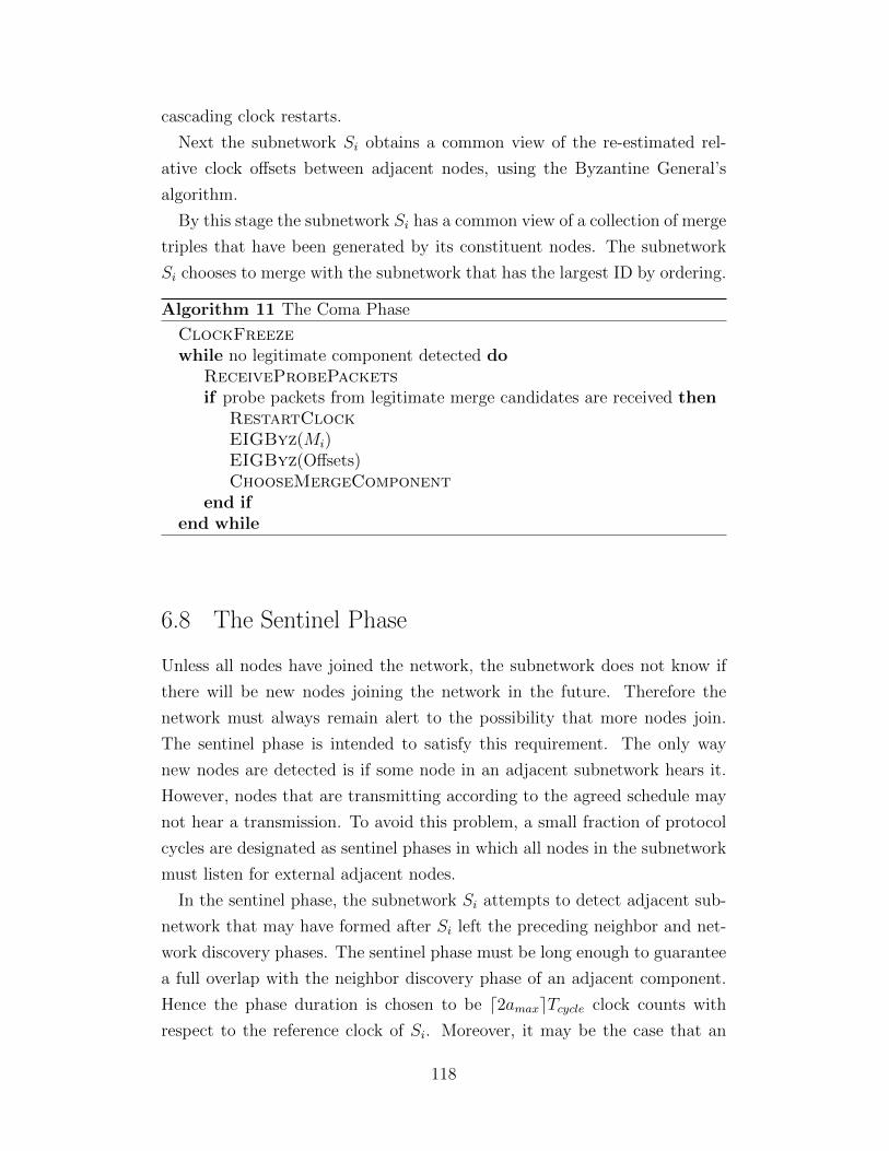
cascading clock restarts.

Next the subnetwork Si obtains a common view of the re-estimated rel-

ative clock offsets between adjacent nodes, using the Byzantine General’s

algorithm.

By this stage the subnetwork Si has a common view of a collection of merge

triples that have been generated by its constituent nodes. The subnetwork

Si chooses to merge with the subnetwork that has the largest ID by ordering.

Algorithm 11 The Coma Phase

ClockFreezewhile no legitimate component detected do

ReceiveProbePacketsif probe packets from legitimate merge candidates are received then

RestartClockEIGByz(Mi)EIGByz(Offsets)ChooseMergeComponent

end ifend while

6.8 The Sentinel Phase

Unless all nodes have joined the network, the subnetwork does not know if

there will be new nodes joining the network in the future. Therefore the

network must always remain alert to the possibility that more nodes join.

The sentinel phase is intended to satisfy this requirement. The only way

new nodes are detected is if some node in an adjacent subnetwork hears it.

However, nodes that are transmitting according to the agreed schedule may

not hear a transmission. To avoid this problem, a small fraction of protocol

cycles are designated as sentinel phases in which all nodes in the subnetwork

must listen for external adjacent nodes.

In the sentinel phase, the subnetwork Si attempts to detect adjacent sub-

network that may have formed after Si left the preceding neighbor and net-

work discovery phases. The sentinel phase must be long enough to guarantee

a full overlap with the neighbor discovery phase of an adjacent component.

Hence the phase duration is chosen to be d2amaxeTcycle clock counts with

respect to the reference clock of Si. Moreover, it may be the case that an

118

adjacent component concurrently enters the sentinel phase with Si. There-

fore, the sentinel phase must include a period of broadcasting probe packets

to ensure that two adjacent components do not stay mutually unaware of the

other’s presence. During the remaining time in the sentinel phase Si listens

for probe packets.

If node i detects the probe packets of an adjacent subnetwork it first es-

timates the relative skew and offset of the node that generated the probe

packets. The offset can only be estimated up to an accuracy of dmax. The

skew and offset are included in a corresponding merge candidate Mi contain-

ing the ID of the detected subnetwork, the received probe packets, and the

ID of the current subnetwork Si. Once the sentinel phase expires, node i

distributes the entire collection of generated merge candidates Mi to other

nodes in Si using the Byzantine General’s algorithm. At this stage, Si has a

common view of all the merge candidates generated by the constituent nodes.

Next Si chooses which subnetwork to merge with (if any) using the following

decision rules. First it eliminates any merge candidates that have already

been assigned to the used-up collection, since these merge candidates have

already been successfully used or have failed an excessive number of times.

Then it considers the collection of merge candidates corresponding to de-

tected subnetworks not in their sentinel phases. Choose the merge candidate

with the highest (by ordering) detected subnetwork ID. If no such merge can-

didates exist then consider the collection of merge candidates corresponding

to detected subnetworks in the sentinel phase and whose IDs are larger (by

ordering) then Si. Choose the subnetwork with the largest ID. If no such

subnetwork exists, then Si does not attempt any merges.

The reason that subnetwork Si does not attempt to schedule a merge

with lower-ordered subnetworks that are detected in their sentinel phases is

because those subnetworks may have also detected Si and may attempt to

schedule a merge of their own. We need to avoid the scenario where two

adjacent subnetworks attempt to schedule merges with each other, since if

each subnetwork reschedules its neighbor discovery phase to overlap with the

other, the attempted merge will fail.

119

Algorithm 12 The Sentinel Phase

ts := τ ri (τ i(t))for k = 1, . . . , d2amaxe do

RecurrentNeighborDiscoveryPhasewhile τ ri (τ i(t)) ≤ ts + kTcycle do

ReceiveProbePacketsend while

end forEIGByz(Mi)ChooseMergeSubnetwork

6.9 Feasibility of the Protocol and Its Optimality

In this section we will prove that there exists a choice of protocol parameters

that enables the network to obtain the utility in the BBT model, over the

network operating lifetime starting from the time the last good node was

born. The relevant parameters are the number of protocol cycles niter, the

time allocated to data transfer B, the dead-time between transmission inter-

vals D, and the operating lifetime Tlife. First, we obtain an upper bound on

the difference between the estimates of a reference clock by a pair of good

nodes.

Lemma 6.9.1. Given a skew error εa and an offset error εb, the maximum

difference between the estimate of the reference clock made by node i and

node j is at most 2εaamaxTlife + 2εb.

Proof.

|τ ri (τ i(t))− τ rj (τ j(t))| = |τ ri (τ i(t))− τ rj (τ ji (τ i(t)))|

= |ariτ i(t)− bri − arj(ajiτ i(t) + bji)a− brj|

≤ |ariτ i(t) + bri − (arj − εa)(ajiτ i(t) + bji)− brj|

= |ariτ i(t) + bri − arjbji − brj + εaτj(t)|

≤ |εaτ i(t) + εaτj(t) + bri + εb − arjbji − brj + εb|

= |εaτ i(t) + εaτj(t) + 2εb|

≤ 2εaamaxTlife + 2εb

We now show that a subnetwork of good nodes can form after a primordial

120

birth, if they are born within a bounded time b0 of the first node with respect

to the clock of the first node. The nodes in a subnetwork by definition have

the same topological view and consistent estimates of their relative skews

and offsets. Therefore the good nodes must be able to obtain both without

without initially having either. First we show that newly born good nodes

can sequentially exchange messages of finite size with each other a finite

number of times, within a bounded time frame. This exchange occurs prior

to any clock synchronization, under half-duplex constraints.

Lemma 6.9.2. There exists a sequence of adjacent time-intervals [tk, tk+1)

and corresponding schedule that guarantees any message of size W transmit-

ted (via the Orthogonal MAC Code) by node i in the interval [tk, tk+1) (as

measured by node i’s clock) will be received by node j in the same interval as

measured by node j’s clock.

Proof. Set tk+1 := (amax)2tk + 2(amax)

3b0 + (amax)3TMAC(W ). Suppose that

a message from node i to node j during the interval [tk, tk+1) is transmitted

(via the Orthogonal MAC Code) at ts := amaxtk + (amax)2b0 with respect to

node i’s clock. Then,

τ ji (ts) = τ ji (amaxtk + (amax)2b0)

= aji(amaxtk + (amax)2b0) + bji

≥ tk + amaxb0 + bji

≥ tk.

The inequalities above follow from substitution and simplification, and the

fact that 0 ≥ b0 ≥ −amaxb0. Similarly, we can show that τ ji (ts+TMAC(W )) <

tk+1:

τ ji (ts + TMAC(W )) ≤ aji(amaxtk + (amax)2b0 + TMAC(W )) + bji

≤ (amax)2tk + 2(amax)

3b0 + amaxTMAC(W ).

Hence τ ji ([ts, ts+TMAC(W ))) ⊂ [tk, tk+1), and so node j receives this message

during the same interval with respect to node j’s clock.

Consequently, we have:

Theorem 6.9.1. At the conclusion of the network discovery phase the good

121

nodes will have a common view of the topology and consistent estimates (to

within εa) of the skew of the reference clock.

Proof. From Lemma 6.9.2 all good nodes will proceed through each stage of

the Neighbor and Network Discovery Phases together, and therefore establish

link certificates with their good neighbors. Since they form a connected

component, the good nodes obtain a common view of their link certificates

using the EIGByzMAC algorithm and the schedule in Lemma 6.9.2. The

good nodes can therefore infer the network topology and the relative skews

of all adjacent nodes based upon the collection of link certificates. Using

Consistency Check, the good nodes can eliminate paths along which bad

nodes have provided false skew data. The good nodes can disseminate this

information to each other using the EIGByzMAC algorithm and Lemma 6.9.2

and thus obtain consistent estimates of the reference clock to within εa.

We have the following corollary to Lemma 6.9.2:

Lemma 6.9.3. The sequence of adjacent intervals [tj, tj+1), j = 0, . . . , k is

contained in [t0, c1t0 + c2W ), where constants c1 and c2 depend on amax, k,

b0, and n.

Proof. It is straightforward that the duration of the Orthogonal MAC Code

TMAC(W ) ≤ cW , where constant c depends on amax, and n. The result for

k = 1 follows from the definition of tk, and substitution of cW into TMAC(W ).

The result for general k follows by induction and definition of tk.

Therefore, we have:

Lemma 6.9.4. The time to complete Neighbor and Network Discovery Phases

Tnei+Tnet is less than c1 log Tlife+ c2εa

where c1, c2 depend only on n, amax, U0.

Proof. There are at most 6+n+n|C|+n protocol stages in the Neighbor and

Network Discovery Phases. Hence the time required is at most c1t0 + c2W ,

where W is the size of a message to be transmitted, and c1, c2 are constants

depending on the number of protocol stages amax, U0, n. The maximum size

of a message is proportional to the timing packet size log Tlife. To account

for the effect of the minimum start-time Ts for the consistency check, we

can assume the worst case that the Ts comes into effect during the first

protocol stage (instead of later in the Network Discovery Phase). Moreover,

122

the consistency check start-time is at most cεa

, where constant c depends on

amax, n. Substitution into t0 proves the lemma.

We can now show that:

Lemma 6.9.5. The time to complete initial neighbor and initial network

discovery Phases TINeiD + TINetD is less than cT,IND log Tlife,+cε,INDεa

where

cT,IND and cε,IND depend only on n, amax, U0.

Proof. In each stage of the EIG Byzantine General’s algorithm, there are

at most n! vertex values that must be transmitted with each node in the

neighborhood. The value of a vertex is a list of concurrent transmission

sets. There are at most 2n concurrent transmission sets and at most n nodes

in a concurrent transmission set. Therefore the size of any message to be

transmitted by a node during the EIG algorithm is at most cD, where c is a

constant dependent on n. Since there are n(n−1) possible source-destination

pairs, there are at most n(n − 1) time-slots in each stage, separated at the

beginning and end by a dead-time D. Therefore the duration of each stage

is at most cD + n(n− 1)2D. There are at most n such stages.

We can also show that:

Lemma 6.9.6. The time required for the data transfer phase is at most

cB,dataB + cD,dataD + cdata,T log Tlife, where B is the time spent transmit-

ting data packets, D is the size of the dead-time separating time-slots, and

cB,data, cD,data, andcT,data depend on n alone.

Proof. The total number of time-slots for data transfer between all source-

destination pairs is n2(n− 1), each supporting data transfer of size Bs and a

dead-time D.

Lemma 6.9.7. The time required for the verification phase is at most cD,verD+

cT,ver log Tlife where cD,ver and cT,ver depend on n alone.

Proof. The verification phase requires the network to exchange packets con-

taining timestamps of size log Tlife. Therefore the maximum packet size can

be expressed as a constant multiple of the time stamp size c log Tlife, where

c is dependent on the network size n alone. The packets are exchanged over

a fixed number of intervals that are separated by a dead-time D.

123

The proof of the next three lemmas are similar to the preceding proof.

The non-data transfer phases are all proportional in duration to the size of

the timing packets log Tlife, the dead-times separating transmission intervals,

and in the case of the network discovery phase, εa to carry out the consistency

check.

Lemma 6.9.8. The time required to complete the initial neighbor discovery

phase is at most cT,INeiD log Tlife + cD,INeiDD.

Lemma 6.9.9. The time required to complete the initial network discovery

phase is at most cINetD,T log Tlife + cINetD,DD +cSNetD,ε

εa.

Lemma 6.9.10. The time required to complete the coma phase is at most

cT,coma log Tlife.

We can now determine an upperbound on the duration of a protocol cycle.

Lemma 6.9.11. The time required to complete one cycle of the protocol

phase is at most cT,cycle log Tlife +cε,cycleεa

+ cD,cycleD + cB,cycleB, where the

constants cT,cycle, cε,cycle, cD,cycle, and cB,cycle depend only on n and amax.

Proof.

Tcycle ≤ TRNeiD + TRNetD + TRNeiD + TRNetD + Tdata + Tver

≤ (cT,IND + cT,INeiD + cT,INetD + cT,data + cT,ver + cT,coma) log Tlife

+cε,IND + cε,INetD

εa+ cB,dataB + (cD,INeiD + cD,INetD + cD,data + cD,ver)D

≤ cT,cycle log Tlife +cε,cycleεa

+ cD,cycleD + cB,cycleB.

We are now ready to prove the main theorem concerning unbounded birth

times. We note that optimality can only be measured since the last time

that a node was born.

Theorem 6.9.2. The protocol ensures that a network of n nodes proceeds

from startup to a functioning network carrying data. There exists a selection

of parameters niter, D, B, εa, and Tlife that achieves a utility equal to Min-

max U(x) to within a factor (1− ε) from the instant the last good node was

born, where the “Min” is over all policies of the bad nodes that can only jam

and/or cooperate during a concurrent transmission set.

124

Proof. We show that the protocol achieves an effective rate vector x that is

near utility-optimal over the protocol lifetime from the instant that the last

good node was born. Let εl be the fraction of the operating lifetime that

the network spends pruning concurrent transmission sets and transitioning

from separate adjacent components to a merge. The operating lifetime is

evaluated from the time the last good node was born. Consider the case in

which two adjacent components are both in normal protocol operation, that

is, out of the coma phase. Since at most 22n−1 sentinel phases will pass be-

fore any two adjacent components will merge, there are nsent cycles between

sentinel phases, and each sentinel phase lasts for at most d3amaxe cycles, it

follows that at most d3amaxe22n−1nsent cycles are required for two adjacent

good components to merge after primordial birth. Now consider the case in

which one of the components is in the coma phase. Then at most 22n−1 pro-

tocol cycles will be required for the two components to merge, since a node

in the coma phase is effectively on sentinel duty, the other component will

be cycling through the neighbor discovery phase, and there are at most 22n−1

possible failed merges between two adjacent good components. In addition,

a component spends at most 2nkr cycles pruning infeasible concurrent trans-

mission sets. Therefore the total number of protocol cycles must satisfy the

following inequality:

1− εl ≤niter

niter + d3amaxe22n−1nsent + 22n−1 + 2nkr, (6.1)

and the total number of sentinel phases nsent satisfies:

nsent ≥ 22n−1.

Let εd denote the fraction of time within a cycle that is spent in overhead,

that is, in the neighbor discovery phase, the network discovery phase, the

verification phase, or in the dead time between intervals. The amount of

time spent in data transfer must satisfy the following inequality:

1− εd ≤B

cT,cycle log Tlife + cB,cycleB +cε,cycleεa

+ cD,cycleD. (6.2)

Let Tlife denote the maximum operating lifetime of the protocol between

125

clock resets. The maximum operating lifetime of the protocol satisfies:

Tlife ≤ niter(cT,cycle log Tlife + cB,cycleB +cε,cycleεa

+ cD,cycleD)

+ 22n−1cT,coma log Tlife. (6.3)

Finally, from Lemma 6.9.1 the dead time satisfies the following inequality:

D ≥ 2εaamaxTlife + 2εb, (6.4)

where the maximum error in the relative offset satisfies:

εb ≤ (n+ 1)(amax)n+1dmax.

We need to find a set of parameters D, Tlife, B, niter, and εa that satisfies

inequalities (6.1), (6.2), (6.3), and (6.4), for a fixed εd, εl, cT,cycle, cB,cycleB,

cε,cycle, and cD,cycle. Rearranging (6.1) gives:

niter =(1− εl)(d3amaxe22n−1nsent + 22n−1 + 2nkr

εl.

Similarly, rearranging (6.2) gives:

B =(1− εd)(cT,cycle log Tlife +B +

cε,cycleεa

+ cD,cycleD)

εd.

Now if we substitute the previous two equations and (6.4) into (6.3) we

obtain:

Tlife ≥ c1 log Tlife +c2

εa+ c3εaTlife + c4,

where c1, c2, c3, and c4 depend on the fixed parameters εd, εl, cT,cycle, cB,cycle,

cε,cycle, and cD,cycle.

The inequality above can be solved by first choosing an εa so that εac3 < 1.

126

We can then choose Tlife large enough so that:

Tlife ≥c1 log Tlife + c2

εa+ c4

(1− c3εa).

The effective rate vector x satisfies x = (1−εd)(1−εl)xopt, where xopt is the

vector that is utility optimal over the set of feasible concurrent transmission

sets.

127

CHAPTER 7

POSSIBLE FUTURE RESEARCH TOPICS

The axiomatic approach to wireless network security is a principled approach

to combating vulnerabilities in the system. Under this approach, protocols

are designed to completely protect the network from any behavior that satis-

fies axiomatic conditions. Although the protocol is vulnerable to any attack

that exceeds the axiomatic bounds, these vulnerabilities are in some sense

precisely stated and can be addressed in a principled manner by relaxing the

axioms appropriately.

The work in this thesis opens several avenues that can be further explored.

They include relaxing the axioms that set the boundaries on attacker capa-

bility, and reducing the space of attack options by adding extra functionality

to the protocol.

The protocol currently allows bad nodes to jam and/or cooperate in each

concurrent transmission set as long as they behave consistently with respect

to that concurrent transmission set. A bad node may choose to jam in one

concurrent transmission set and cooperate in another, and in some concur-

rent transmission sets it could jam but still claim to be cooperating since it

is not feasible to verify that it is not cooperating. A possible improvement

would be to enable the protocol to detect nodes that participate in the net-

work but periodically jam during concurrent transmission sets that do not

include them. To counter this attack, the protocol could organize random

coordinated surprise tests on nodes to see if they are transmitting when they

should be silent. By preventing nodes that participate in the network from

jamming during other concurrent transmission sets, we can reduce the space

of strategies for an attacker and improve the utility attained.

Also of interest is the choice of utility function that best maximizes net-

work performance in the presence of adversarial nodes. Some measures of

utility, like proportional fairness for instance, appear especially vulnerable to

malicious behavior. An attacker with a weak connection to a good node could

128

opt to reduce the utility of the good nodes by participating in the network

and consuming a large share of the available time-slots. In a proportionally

fair scheme, the damage to the utility might be larger than that caused by

jamming, particularly, if the attacker is located far away. A possible research

topic is to investigate utility functions that are inherently more robust to

attacks of this type than others.

Another problem of interest is how to improve the transient behavior of

the protocols. Our approach and result on optimality is over a long time

horizon. We will examine how to make the protocols more efficient in the

transient phase without sacrificing security. In this way, we come full circle:

we approach performance, in this case transient performance, after designing

for security, and with security as a binding constraint. This is the reverse of

the usual approach.

The physical model that was adopted in Chapter 2, can also be extended

to include the probabilistic nature of packet receptions in wireless networks.

Our model of deterministic packet receptions enabled us to unequivocally

guarantee the security and performance of the protocol. However, in a net-

work where packet receptions are probabilistic, these guarantees no longer

apply. Instead, we could explore whether our claims hold with high proba-

bility if not with certainty.

This thesis might also extend to networks with mobile nodes. The oper-

ational challenge in such networks is that the topology undergoes constant

change while the nodes are moving. To address this challenge we could adopt

a quasi-static approach whereby the network is able to reach steady-state

within a short enough time period to assume a stable topology. Clearly, such

an approach depends on the efficiency of the transient behavior, an area of

future work that has already been mentioned.

Finally, there is also the issue of whether the rates supported by our proto-

col can eventually include the information theoretic capacity region. On this

point, there is far less clarity. First of all, it has yet to be determined if the

tactic of “iterative pruning” adopted for concurrent transmission sets, can

work equally well with information theoretic coding schemes and result in a

min-max formulation of utility. Second, the encryption tools that we have

adopted use computational complexity as a method for ensuring authenticity.

This paradigm is explicitly rejected in an information theoretic framework.

So the goal of adopting such a framework still remains a distant dream.

129

REFERENCES

[1] “Community wireless networks: Cutting edge technology for Internetaccess,” Center for Neighborhood Technology, IL, Tech. Rep.,Nov. 2006. [Online]. Available: http://www.cnt.org/repository/WCN-AllReports.pdf

[2] H. Hartenstein and K. Laberteaux, “A tutorial survey on vehicular adhoc networks,” Communications Magazine, IEEE, vol. 46, no. 6, pp.164–171, 2008.

[3] IEEE Protocol 802.11, “Draft standard for wireless LAN: Medium accesscontrol (MAC) and physical layer (PHY) specifications,” IEEE, July1996.

[4] V. Kawadia and P. R. Kumar, “Principles and protocols for power con-trol in wireless ad-hoc networks,” IEEE Journal on Selected Areas inCommunications, vol. 23, pp. 76–88, 2005.

[5] “Internet protocol,” RFC 791, Sep. 1981.

[6] “Requirements for Internet hosts — Communication layers,” RFC 1122,Oct. 1989.

[7] T. Clausen and P. Jacquet, “Optimized link state routingprotocol (OLSR),” RFC 3626, Oct. 2003. [Online]. Available:http://www.ietf.org/rfc/rfc3626.txt

[8] C. Perkins, E. Belding-Royer, and S. Das, “Ad hoc on demand distancevector (aodv) routing,” RFC 3561, July 2003. [Online]. Available:https://tools.ietf.org/html/rfc3561

[9] C. E. Perkins and P. Bhagwat, “Highly dynamic destination-sequenceddistance-vector routing,” in SIGCOMM, London, UK, Aug. 1994, pp.234–244.

[10] V. Kawadia and P. R. Kumar, “Power control and clustering in ad hocnetworks,” in Proc. IEEE Infocom’99, 2003, pp. 459–469.

130

[11] S. Narayanaswamy, V. Kawadia, R. S. Sreenivas, and P. R. Kumar,“Power control in ad-hoc networks: Theory, architecture, algorithm andimplementation of the COMPOW protocol,” in in European WirelessConference, 2002, pp. 156–162.

[12] F. Kelly, “Charging and rate control for elastic traffic,” European Trans-actions on Telecommunications, vol. 8, pp. 33–37, 1997.

[13] F. Kelly, A. K. Maulloo, and D. K. H. Tan, “Rate control in commu-nication networks: Shadow prices, proportional fairness and stability,”Journal of the Operational Research Society, vol. 49, pp. 237–252, 1998.

[14] F. Kelly, “Models for a self-managed Internet,” Philosophical Transac-tions of the Royal Society, vol. 358, no. 1773, pp. 1244–1245, Aug. 2000.

[15] X. Lin and N. Shroff, “Utility maximization for communication net-works with multipath routing,” IEEE Transactions on Automatic Con-trol, vol. 51, no. 5, pp. 766–781, May 2006.

[16] M. Neely, E. Modiano, and C. Rohrs, “Dynamic power allocation androuting for time-varying wireless networks,” IEEE Journal on SelectedAreas in Communications, vol. 23, no. 1, pp. 89–103, Jan. 2005.

[17] X. Lin, N. Shroff, and R. Srikant, “A tutorial on cross-layer optimizationin wireless networks,” IEEE Journal on Selected Areas in Communica-tions, vol. 24, no. 8, pp. 1452–1463, Aug. 2006.

[18] L. Tassiulas and A. Ephremides, “Stability properties of constrainedqueueing systems and scheduling policies for maximum throughput inmultihop radio networks,” IEEE Transactions on Automatic Control,vol. 37, no. 12, pp. 1936–1948, Dec. 1992.

[19] Y.-C. Hu, A. Perrig, and D. Johnson, “Packet leashes: a defense againstwormhole attacks in wireless networks,” in Infocom, vol. 3, Apr. 2003,pp. 1976–1986 vol.3.

[20] J. R. Douceur, “The SYBIL attack,” in IPTPS, 2002, pp. 251–260.

[21] Y.-C. Hu, A. Perrig, and D. B. Johnson, “Rushing attacks and defense inwireless ad hoc network routing protocols,” in WiSec, 2003, pp. 30–40.

[22] J. Choi, J. T. Chiang, D. Kim, and Y.-C. Hu, “Partial deafness: A noveldenial-of-service attack in 802.11 networks,” in Security and Privacy inCommunication Networks, ser. Lecture Notes of the Institute for Com-puter Sciences, Social Informatics and Telecommunications Engineering.Springer Berlin Heidelberg, 2010, vol. 50, pp. 235–252.

131

[23] Y.-C. Hu, A. Perrig, and D. B. Johnson, “Ariadne: A secure on-demandrouting protocol for ad hoc networks,” Wirel. Netw., vol. 11, no. 1-2,pp. 21–38, Jan. 2005.

[24] M. Poturalski, P. Papadimitratos, and J.-P. Hubaux, “Secure neighbordiscovery in wireless networks: formal investigation of possibility,” inASIACCS. New York, NY, USA: ACM, 2008. [Online]. Available:http://doi.acm.org/10.1145/1368310.1368338 pp. 189–200.

[25] S. Marti, T. J. Giuli, K. Lai, and M. Baker, “Mitigating routing misbe-havior in mobile ad hoc networks,” in MobiCom, 2000.

[26] C. Shannon, “Communication theory of secrecy systems,” Bell SystemTechnical Journal, vol. 28, pp. 656–715, Oct. 1949.

[27] R. Perlman, “Network layer protocols with Byzan-tine robustness,” Ph.D. dissertation, Massachusetts Insti-tute of Technology, Massachusetts, 1988. [Online]. Available:http://hdl.handle.net/1721.1/14403

[28] S. Graham and P. R. Kumar, “Time in general-purpose control systems:The control time protocol and an experimental evaluation,” in IEEECDC, vol. 4, Dec. 2004, pp. 4004–4009.

[29] N. M. Freris, S. R. Graham, and P. R. Kumar, “Fundamental limits onsynchronizing clocks over networks,” IEEE Transactions on AutomaticControl, vol. 56, no. 6, pp. 1352–1364, June 2011.

[30] N. Lynch, Distributed Algorithms. Waltham, MA: Morgan Kaufmann,1996.

[31] R. Gold, “Optimal binary sequences for spread spectrum multiplexing(corresp.),” Information Theory, IEEE Transactions on, vol. 13, no. 4,pp. 619–621, October 1967.

[32] N. Abramson, “The ALOHA system: Another alternative forcomputer communications,” in Proceedings of the November 17-19, 1970, Fall Joint Computer Conference, ser. AFIPS ’70(Fall). New York, NY, USA: ACM, 1970. [Online]. Available:http://doi.acm.org/10.1145/1478462.1478502 pp. 281–285.

[33] L. Lamport and P. M. Melliar-Smith, “Byzantine clock synchroniza-tion,” in Proceedings of the Third Annual ACM Symposium on Principlesof Distributed Computing, ser. PODC ’84. New York, NY, USA: ACM,1984. [Online]. Available: http://doi.acm.org/10.1145/800222.806737pp. 68–74.

132

[34] J. Lundelius and N. Lynch, “A new fault-tolerant algorithm forclock synchronization,” in Proceedings of the Third Annual ACMSymposium on Principles of Distributed Computing, ser. PODC’84. New York, NY, USA: ACM, 1984. [Online]. Available:http://doi.acm.org/10.1145/800222.806738 pp. 75–88.

[35] D. Dolev, J. Halpern, and H. R. Strong, “On the possibility andimpossibility of achieving clock synchronization,” in STOC, New York,1984. [Online]. Available: http://doi.acm.org/10.1145/800057.808720pp. 504–511.

[36] J. Y. Halpern, B. Simons, R. Strong, and D. Dolev, “Fault-tolerant clock synchronization,” in Proceedings of the Third AnnualACM Symposium on Principles of Distributed Computing, ser.PODC ’84. New York, NY, USA: ACM, 1984. [Online]. Available:http://doi.acm.org/10.1145/800222.806739 pp. 89–102.

[37] N. M. Freris and P. R. Kumar, “Fundamental limits on synchronizationof affine clocks in networks,” in 2007 46th IEEE Conference on Decisionand Control, Dec. 2007, pp. 921–926.

[38] A. Bar-Noy, D. Dolev, C. Dwork, and H. R. Strong, “Shifting gears:Changing algorithms on the fly to expedite Byzantine agreement,” inPODC. New York, NY, USA: ACM, 1987, pp. 42–51.

133