c 2012, julie bumbaugh - tdl

A Dynamical System Study of the Hodgkin-Huxley Model of Nerve Membranes

by

Julie Bumbaugh, B.S.

A Thesis

In

Mathematics and Statistics

Submitted to the Graduate Facultyof Texas Tech University in

Partial Fulfillment ofthe Requirements for the Degree of

Master of Science

Approved

Lih-Ing Roegerco-Chair

Sophia Jangco-Chair

Peggy Gordon MillerDean of the Graduate School

August, 2012

Texas Tech University, Julie Bumbaugh, August, 2012

ACKNOWLEDGEMENTS

I wish to acknowledge the help and support of Dr. Lih-Ing Roeger and Dr.

Sophia Jang. Their encouragement and advice since August of 2011 has made all of

this work possible for me. I also wish to thank my principal, Angie Inklebarger, for

being kind enough to allow me extra time when I needed it to work on this thesis.

She also allowed me to be away from the high school campus every Thursday during

my conference in order to meet some of the research requirements. I owe Dr. Jerry

Dwyer many thanks for being kind enough several years ago to be my mentor when

I first began to study the work of Hodgkin and Huxley. Finally, I could not have

accomplished what I have without the love and support of my husband, Alan

Bumbaugh.

ii


TABLE OF CONTENTS

Acknowledgements . . . . . . . . . . . . . . . . . . . . . . . . . . . . . . . ii

Abstract . . . . . . . . . . . . . . . . . . . . . . . . . . . . . . . . . . . . . v

List of Tables . . . . . . . . . . . . . . . . . . . . . . . . . . . . . . . . . . vi

List of Figures . . . . . . . . . . . . . . . . . . . . . . . . . . . . . . . . . . vii

1. Introduction . . . . . . . . . . . . . . . . . . . . . . . . . . . . . . . . . 1

2. Membrane current for Hodgkin-Huxley model . . . . . . . . . . . . . . . 3

2.1 The membrane current equation . . . . . . . . . . . . . . . . . 3

2.2 Modeling potassium conductance . . . . . . . . . . . . . . . . 4

2.3 Modeling sodium conductance . . . . . . . . . . . . . . . . . . 9

3. Solving the Hodgkin-Huxley space clamp model . . . . . . . . . . . . . 14

4. Modern techniques to analyzing dynamical systems . . . . . . . . . . . . 17

4.1 One-dimensional models . . . . . . . . . . . . . . . . . . . . . 17

4.1.1 Stability of equilibria . . . . . . . . . . . . . . . . . . . . . 18

4.1.2 Bifurcations . . . . . . . . . . . . . . . . . . . . . . . . . . 20

4.2 Two-dimensional models . . . . . . . . . . . . . . . . . . . . . 21

4.2.1 Nullclines . . . . . . . . . . . . . . . . . . . . . . . . . . . 22

4.2.2 Stability in 2-dimensions . . . . . . . . . . . . . . . . . . . 23

4.2.3 Limit cycles . . . . . . . . . . . . . . . . . . . . . . . . . . 27

4.2.4 Bifurcations in 2-dimensions . . . . . . . . . . . . . . . . . 27

4.2.5 Stable and unstable manifolds . . . . . . . . . . . . . . . . 29

4.2.6 Hodgkin-Huxley reduced model . . . . . . . . . . . . . . . 29

5. Problems for study and analysis . . . . . . . . . . . . . . . . . . . . . . 34

5.1 Proposed problems for study . . . . . . . . . . . . . . . . . . . 34

5.1.1 Problem 1- Derive Boltzmann’s function . . . . . . . . . . 34

5.1.2 Problem 2- Prove instability and stability of equilibria . . . 35

5.1.3 Problem 3- Find equilibrium and determine its stability . . 36

5.1.4 Problem 4- Demonstrate excitation block . . . . . . . . . . 36

5.1.5 Problem 5- Choose appropriate power for an activation vari-

able . . . . . . . . . . . . . . . . . . . . . . . . . . . . . . 36

iii


5.1.6 Problem 6- Derive the formula Hodgkin and Huxley used

for n . . . . . . . . . . . . . . . . . . . . . . . . . . . . . . 37

5.2 Solutions to the problems for study and analysis . . . . . . . . 37

5.2.1 Solution to problem 1 . . . . . . . . . . . . . . . . . . . . . 37






Bibliography . . . . . . . . . . . . . . . . . . . . . . . . . . . . . . . . . . 43

Appendix A . . . . . . . . . . . . . . . . . . . . . . . . . . . . . . . . . . . 44

Appendix B . . . . . . . . . . . . . . . . . . . . . . . . . . . . . . . . . . . 46

Appendix C . . . . . . . . . . . . . . . . . . . . . . . . . . . . . . . . . . . 48

Appendix D . . . . . . . . . . . . . . . . . . . . . . . . . . . . . . . . . . . 50

iv


ABSTRACT

Equations of the Hodgkin and Huxley model of action potentials in squid giant

axons have been studied and described in this thesis. Explanation of the

development of the space clamp model that won its authors the Nobel Prize for

Physiology and Medicine in 1963 is provided since it is still one of the key

mathematical models in the study of neural communications today. A numerical

approach was used to obtain solutions to their model. The computer code used will

be provided. More modern approaches to analyzing these models will be explored

and discussed as a study of dynamical systems. A reduced Hodgkin-Huxley model

will be explained and analyzed using modern methods. A set of problems will be

included for those who wish to be guided through parts of the development of the

models.

v


LIST OF TABLES

2.1 Computations for αn’s and βn’s . . . . . . . . . . . . . . . . . . . . . 8

3.1 List of variables and parameters for the Hodgkin-Huxley model . . . 15

4.1 Parameters for persistent sodium model . . . . . . . . . . . . . . . . 18

4.2 Parameters for 1-dimensional potassium model . . . . . . . . . . . . 21

4.3 Parameters for low-threshold INa,p + IK model . . . . . . . . . . . . 22

5.1 Parameters for high-threshold INa,p + IK model . . . . . . . . . . . . 35

vi


LIST OF FIGURES

2.1 Hodgkin-Huxley potassium vs. time for fixed membrane potential . . 7

3.1 Action potentials in squid giant axons . . . . . . . . . . . . . . . . . . 16

4.1 Persistent sodium model graphs . . . . . . . . . . . . . . . . . . . . . 19

4.2 Failure to generate “all or nothing” spikes . . . . . . . . . . . . . . . 23

4.3 Failure to have fixed threshold potential . . . . . . . . . . . . . . . . 24

4.4 Bifurcations in high threshold INa,p + IK model . . . . . . . . . . . . 25

4.5 Nullclines for high threshold INa,p + IK model . . . . . . . . . . . . . 25

4.6 A stable limit cycle . . . . . . . . . . . . . . . . . . . . . . . . . . . . 27

4.7 Low threshold INa,p + IK traces leading to excitation block . . . . . . 28

4.8 Bistability in high threshold INa,p + IK model. . . . . . . . . . . . . . 30

4.9 Hodgkin-Huxley model reduced to 2 variables with I = 0. . . . . . . . 32

4.10 Hodgkin-Huxley model reduced to 2 variables with I = 12. . . . . . . 32

5.1 Boltzmann’s function . . . . . . . . . . . . . . . . . . . . . . . . . . . 35

5.2 The intersection of nullclines . . . . . . . . . . . . . . . . . . . . . . . 39

5.3 Excitation block in the low-threshold INa,p + IK model. . . . . . . . 40

vii


CHAPTER 1

INTRODUCTION

The seminal and classical work of Alan Lloyd Hodgkin and Andrew Fielding

Huxley, from 1942 to 1952, of developing a mathematical model that would yield

membrane potential vs. time following a perturbation from the resting state of

membrane potential in squid giant axons continues to be the biophysically accurate

model that influences the development of such models today:

−dVdt

= gkn4(V − Vk) + gNam

3h(vV − VNa) + gl(V − Vl), (1.1)

dn

dt= αn(1− n)− βn · n, (1.2)

dm

dt= αm(1−m)− βm ·m, (1.3)

dh

dt= αh(1− h)− βh · h, (1.4)

αn =1

10

[110

(V + 10)

e110

(V+10) − 1

], (1.5)

βn =1

8eV80 , (1.6)

αm =0.1(V + 25)

e0.1(V+25) − 1, (1.7)

βm = 4eV18 , (1.8)

αh = 0.07eV20 , (1.9)

βh =1

eV+30

10 + 1. (1.10)

The first goal of this thesis is to fully understand and explain the work done by

Hodgkin and Huxley in connection with their “voltage clamp” model in order to

more fully understand and appreciate the modern techniques used today. The

second goal in this thesis is to demonstrate some of the modern forms of analysis

used in the study of dynamical systems and to apply some of them to the

Hodgkin-Huxley model. Hodgkin and Huxley published a series of 5 papers

describing their work. The first paper dealt with their experimental method and the

1


membrane in a normal ionic environment. The second paper describes their

technique of changing the sodium concentrations in the medium surrounding the

membrane which allowed them to resolve the ionic current into sodium and

potassium currents. Their third paper dealt with the effect that sudden changes in

membrane potential had on the ionic conductances. The fourth paper explained the

inactivation process which reduces sodium permeability during the falling phase of

the action potential. Their final paper concluded the series and revealed their

mathematical model of membrane current and specifically of the membrane’s ability

to generate action potentials. The development of the model will be explained in

this thesis. Curves from various particular solutions to the model along with the

Matlab program used are provided. Some modern methods used in the study of

dynamical systems in neuroscience today are also described in this thesis. The

Hodgkin-Huxley model was an important breakthrough in the study of neural

communication. Its historical significance aside; the review of just how this model

was arrived at would be valuable to students wanting to experience how

mathematical models are developed; therefore, a set of problems including the

derivation of one part of the models used today and some analysis of models using

more modern techniques will be included. The solutions to the set of problems will

be included.

2


CHAPTER 2

MEMBRANE CURRENT FOR HODGKIN-HUXLEY MODEL

2.1 The membrane current equation

The measure of the change in electric charge across the membrane of a neuron,

nerve cell, is called the membrane potential or potential difference, and the unit of

measure is called voltage, V . Hodgkin and Huxley used “space-clamp” or

“voltage-clamp” experiments holding the voltage across the membrane fixed at a

constant value, Vc. These experiments revealed that ionic movements through

excitable tissues were associated with perturbations of membrane potential [2].

Their work involved experiments with squid giant axons threaded with two fine

silver electrodes down the axis of the axons to both short circuit currents that arise

within the membrane and to inject a current proportional to the difference, Vc − V ,

allowing dVdt

= V = 0 [7]. One electrode measured the membrane’s potential and the

ionic current during a space-clamp experiment. The second electrode was used to

inject current to maintain a constant membrane potential equal to a stepped

potential. The required current injected to maintain this potential provided a way

of measuring the ionic currents which were initiated by the perturbation from the

resting potential.

They found that the ionic current could be broken down primarily into a

movement of sodium ions and a potassium current each of which varied with

permeability of the membrane to each ion and with the membrane potential. To

determine which portion of the currents were due to sodium and which were due to

potassium, Hodgkin and Huxley pioneered some techniques involving controlling the

medium surrounding the tissue. If 90% of the sodium in the extracellular seawater

were replaced with choline (enough to significantly reduce the amount of sodium

but not enough to render the squid axon inexcitable), there could be little inflow of

sodium and they would know the currents they were measuring were mostly due to

potassium. Then from their current measurements using normal seawater in the

surrounding medium, they could separate the potassium from the sodium currents.

3


For specific fixed values of membrane potential, they recorded ionic currents and

membrane potential measured against time. Their results showed that when they

depolarized the membrane and kept its potential constant in normal sea water,

sodium ions would flood into the cell first and then later would flow out. Potassium

was shown to flow outward during the later phase as well. Hodgkin and Huxley were

the first to assume that the ionic conductances might not all behave the same way

and developed a model that allowed each ion to have its own specific conductance.

The total membrane current equals membrane capacity current plus ionic currents:

I = CMdVdt

+ Ii. The ionic current is the sum of the potassium, sodium and other

leaking ion currents whose conductances are not dependent on membrane potential:

Ii = Ik + INa + Il. Ionic currents equal the product of conductance and potential

difference between the membrane’s potential and the resting potential for the ion:

Ii = Ik + INa + Il = gk(E − Ek) + gNa(E − ENa) + gl(E − El).

Note: V = (E − Er) and VNa = (ENa − ER) so (E − ENa) = (V − VNa).This allows the formula for the ionic currents to be:

Ii = gk(V − Vk) + gNa(V − VNa) + gl(V − Vl).

Hence the total membrane current equation is:

I = CMdV

dt+ gk(V − Vk) + gNa(V − VNa) + gl(V − Vl).

2.2 Modeling potassium conductance

In order to find a useful and relatively simple model of best fit, Hodgkin and

Huxley determined the potassium conductance to be proportional to the 4th power

of a variable that obeys a first order differential equation. Two factors are related to

the ability to excite the neurons to produce action potentials, the membrane

potential and the concentrations of the ions on either side of the membrane. The

variable n was chosen to represent the portion of particles inside the membrane

involved with the transfer of potassium to the outside and 1− n represents the

portion of particles outside affecting the transfer of potassium to the inside.

4


Another set of reasonable definitions for n and 1− n is that they represent the

probability that gates for the transfer of potassium to the outside and inside,

respectively, are open. Perhaps they are easier to understand as the portion that

such gates are open. Hodgkin and Huxley had no way of knowing the actual

physical makeup of the membrane. Next, the rate of change of the portion of said

particles would equal the rate in minus the rate out. They chose to let αn and βn be

the voltage dependent rate constants (constant with respect to time) for the

potassium ions to enter and leave the membrane. Hence,

dn

dt= αn(1− n)− βnn.

A solution to such a differential equation has the form n = C1 − C2e−C3t. Hodgkin

and Huxley used 1− e−t as a simplified model to determine an appropriate power of

n. We can analyze this function and powers of it to understand how they selected

the appropriate power. The first power is obviously inappropriate due to the fact

that the rise of potassium has a sigmoid shape with a single inflection point and

1− e−t has no inflection point. Studying various powers of 1− e−t reveals that the

point of inflection of (1− e−t)p will be located at t = ln(p) for p > 1. Hodgkin and

Huxley had very limited computing capabilities and it took them a great deal of

time to test these models using the calculators that they had available. They

decided to use the 4th power of n and mentioned that the 5th or 6th power might be

an improvement, but they did not feel the improvement would be sizeable enough to

make it worth the extra computational effort. We can note that the larger the value

of p, the less difference there is between ln(p) and ln(p+ 1). If we do think of n as

being a probability that a gate is open or what fraction that gate is open, and if to

model the behavior of ion transfer through the membrane requires the fouth power

of n, then it would seem that there are 4 gates in the channel that must all be open

to some degree for the ions to pass through the membrane. In other words, n is the

fraction that each of 4 required gates are open. Hodgkin and Huxley therefore used

the maximum conductance for potassium times the probability for conductance

through 4 gates at a given membrane potential, gk = gk · n4, to represent the voltage

dependent conductance of potassium. To date, it is held that there are 4 gates for

the transfer of potassium through this membrane. Next is the matter of the rate

5


constants αn and βn. While they are constant with respect to time, they are voltage

dependent. Since n was to represent the portion of particles inside the membrane

associated with transfer of potassium ions to the outside, Hodgkin and Huxley let

the ratio of rate inrate in + rate out

represent the limiting value of n for the corresponding

value of membrane potential associated with those rates, n∞ = αnαn+βn

. At time

t = 0, they assigned n = n0 = α0

α0+β0. They also assigned τn to be the ratio 1

αn+βn.

With these assignments, we can find the solution to

dn

dt= αn(1− n)− βnn (2.1)

is

n = n∞ − (n∞ − n0)e−tτn . (2.2)

They ultimately needed to find a formula for potassium conductance in terms of

membrane potential, but all of their measurements were against time at fixed

membrane potentials. So, they first derive their equation for potassium conductanc,

gK , for fixed membrane potential values as a function of time.

gK = gK · n4, (2.3)

gK = ( 4√gKn)4, (2.4)

(gK∞)14 = (gK)

14n∞, (2.5)

(gK0)14 = (gK)

14n0, (2.6)

gK = ( 4√gK · (n∞ − (n∞ − n0)e−

tτn ))4, (2.7)

gK = ( 4√gKn∞ − ( 4

√gKn∞ − 4

√gKn0)e−

tτn )4, (2.8)

gK = ((gK∞)14 − ((gK∞)

14 − (gK0)

14 )e−

tτn )4. (2.9)

See Figure 2.1 for the graph of this function. Next, Hodgkin and Huxley had to find

values for gk∞ , gko and τn (or for αn and βn) at different values of V . Potassium

conductance vs. time curves were plotted for different values of V . For each curve,

gk0 and gk∞ were recorded and corresponding values for τn were chosen for each

curve such that the conductance equations would fit the data best.

(Assuming n = 1 at the asymptote of the conductance curves, they chose to let gk

be a value which was 20% higher than the values of gk∞ when V = −100mV since

6


Figure 2.1. Hodgkin and Huxley’s potassium conductance vs. time curve using pa-rameters of gK0 = .09, gK∞ = 7.06, and τn = .75 for 5s of rise and then gK0 = 7.06,gK∞ = .09, and τn = 1.1 for 5s of the falling phase of conductance. V was heldat −25mv for the first 5s and at 0mv for the next 5s. This graph is plotted usingequation (2.9) for gK with fixed value of V .

they were not concerned with depolarizations greater than 110mV .) So,

20.26 · (1.20) = gk · (n∞)4 = gk · (1) = gk = 24.31. Using their values for gk∞’s, gk0’s,

and τn’s at each V , they calculated corresponding values for αn and βn using the

relationships:

gk∞ = gk · (n∞)4

to solve for n∞’s and then

n∞ =αn

αn + βn= αn · τn

to solve for the αn’s and then

τn =1

αn + βn

to solve for the βn’s.

Next, they plotted curves of αn vs. V , βn vs. V , and τn vs. V in order to see their

shapes and try to find functions in terms of V to fit each of them. Hodgkin and

Huxley made reference to using a function involving “movements of charged

particles in a constant field” from a paper by Goldman to represent their graph of

7


Table 2.1. Computations for αn’s and βn’s

Curve V (mV ) gk∞(m.mh0/cm2) τn n∞ αn βn—– (−∞) 24.31 —–

B −100 20.26 1.10 .955 .869 0.040

C −88 18.60 1.25 .935 .748 .052

D −76 17.00 1.50 .914 .610 .057

E −63 15.30 1.70 .891 .524 .064

F −51 13.27 2.05 .860 .419 .069

G −38 10.29 2.60 .807 .310 .074

H −32 8.62 3.20 .772 .241 .071

I −26 6.84 3.80 .728 .192 .071

J −19 5.00 4.50 .673 .150 .073

K −10 1.47 5.25 .496 .094 .096

L −6 0.98 5.25 .448 .085 .105

—– (0) (0.24) —– .315

αn vs. V . There is an equation 17 in the Goldman paper [1] on page 53 of that

paper which is referred to as a constant case. The equation is

J =∆V Λ+ − Λ−e

−β∆V

1− e−β∆V

where Λ+ and Λ− are limiting conductance values for large potentials in one

direction or the other. If we split this equation into

J =∆V Λ+

1− e−β∆V− ∆V Λ−e

−β∆V

1− e−β∆V=

∆V Λ+

1− e−β∆V− ∆V Λ−eβ∆V − 1

The second term of the Goldman formula: ∆V Λ−eβ∆V −1

resembles the function Hodgkin

and Huxley used to define αn. This term, from Goldman, describes movements in

one direction through the membrane and the factor Λ− is a conductance limiting

value, like gk, so the rest of that term involves the rate that the limiting value is

applied which is what αn does. If we take the Goldman term without Λ−, ∆Veβ∆V −1

,

and modify it by letting β = 1, vertically shrink it by a factor of 110

, horizontally

dilate it by a factor of 10, and finally translate it 10 units left, we arrive at Hodgkin

8


and Huxley’s formula for αn,

∆V

eβ∆V − 1⇒ αn =

1

10

[110

(V + 10)

e110

(V+10) − 1

].

We know they were relying on Goldman’s work and that they were tweaking

parameters to get curves to fit their data. It seems reasonable that this is how they

arrived at their formula for αn. Hodgkin and Huxley found a simple exponential

curve to describe βn. They explained that the data values for βn were so much

smaller than those for αn that all they could assertain from the curves was that they

appeared to be simple exponentials. They said they did not worry too much about

whether that was the appropriate choice. Together, these two formulas,

αn =1

10

[110

(V + 10)

e110

(V+10) − 1

],

βn =1

8eV80 ,

along withdn

dt= αn(1− n)− βn · n,

and

gk = gk · n4,

complete the Hodgkin-Huxley definition for potassium conductance in terms of

membrane potential V and the activation variable n.

2.3 Modeling sodium conductance

The conductance of sodium is considerably different than that of potassium due

to its transient nature meaning that it seems to have both activation and

inactivation gates. Activation gates open to let sodium ions in and later inactivation

gates open to let it out. Potassium conductance rises to a limiting value and stays

there unless the membrane is repolarized. Sodium conductance, on the other hand,

rises and falls again during a maintained depolarization of the membrane. Hodgkin

and Huxley could only speculate as to what was causing this transient behavior, but

9


they knew their model for sodium would need to include a factor that would cause

the conductance to return to resting values during long depolarizations. We need

first to see how they determined what power the activation variable and inactivation

variable should each be raised to. They used a similar form for sodium conductance

as they did for potassium: gNa = gNamphq. They named the activation variable

responsible for activating the carrying in of sodium, m, and the inactivation variable

responsible for shutting down the inflow of sodium and restoring the resting levels,

h. Similarly to potassium, they named the limiting value for the conductance

inward of sodium gNa. The rates of change of the activation and inactivation

variables have the same form as the potassium activation variable, n.

dm

dt= αm(1−m)− βm ·m

dh

dt= αh(1− h)− βh · h

αm and βh are rate constants (voltage dependent, but time constant) responsible for

the carrying of sodium ions into the membrane. βm and αh are the rate constants

resposible for the carrying of sodium ions to the outside of the membrane. Hodgkin

and Huxley did not know the physical makeup of the membrane, so their rationale

was that m could represent the portion of some particles on the inside associated

with the carrying of sodium ions to the outside and (1−m) would then be the

portion of the same type of particles on the outside associated with the carrying of

sodium ions to the inside during the rise of sodium conductance. Likewise, they

used h to represent the portion of some particle on the outside of the membrane

assosciated with the carrying of sodium ions to the inside and (1− h) as the

remaining portion of the same particle on the inside associated with the carrying of

sodium ions to the outside during the decline of sodium conductance. Solutions to

these differential equations have the same form as potassium’s activation variable.

m = m∞ − (m∞ −m0)e−tτm ,

h = h∞ − (h∞ − h0)e− tτh .

10


Just as with n,

m∞ =αm

αm + βmand h∞ =

αhαh + βh

,

τm =1

αm + βmand τh =

1

αh + βh.

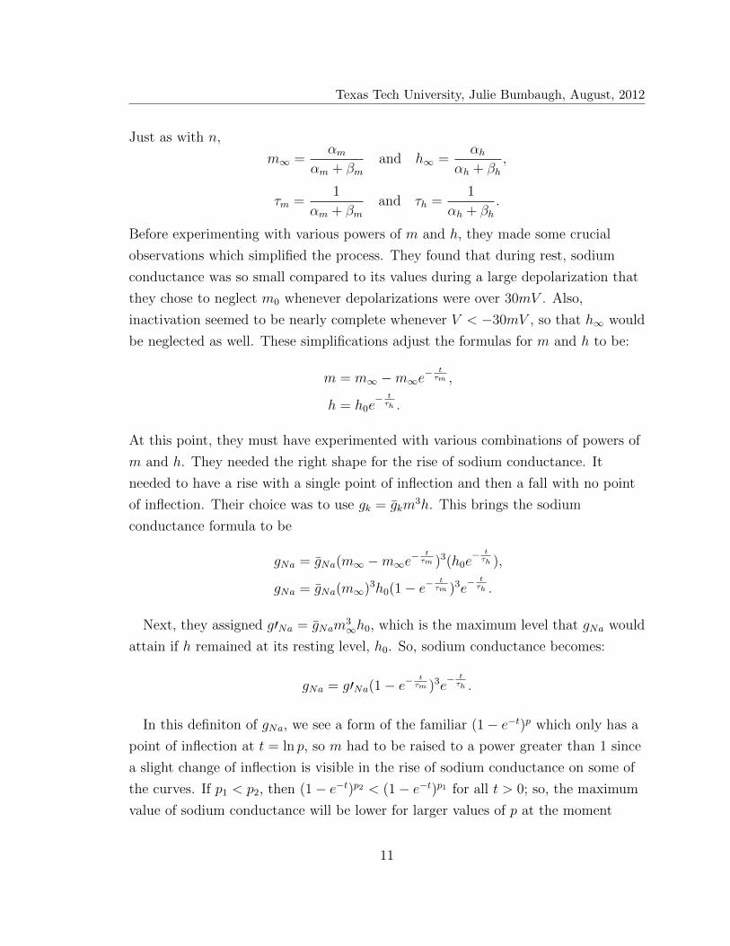
Before experimenting with various powers of m and h, they made some crucial

observations which simplified the process. They found that during rest, sodium

conductance was so small compared to its values during a large depolarization that

they chose to neglect m0 whenever depolarizations were over 30mV . Also,

inactivation seemed to be nearly complete whenever V < −30mV , so that h∞ would

be neglected as well. These simplifications adjust the formulas for m and h to be:

m = m∞ −m∞e−tτm ,

h = h0e− tτh .

At this point, they must have experimented with various combinations of powers of

m and h. They needed the right shape for the rise of sodium conductance. It

needed to have a rise with a single point of inflection and then a fall with no point

of inflection. Their choice was to use gk = gkm3h. This brings the sodium

conductance formula to be

gNa = gNa(m∞ −m∞e−tτm )3(h0e

− tτh ),

gNa = gNa(m∞)3h0(1− e−tτm )3e

− tτh .

Next, they assigned g′Na = gNam3∞h0, which is the maximum level that gNa would

attain if h remained at its resting level, h0. So, sodium conductance becomes:

gNa = g′Na(1− e−tτm )3e

− tτh .

In this definiton of gNa, we see a form of the familiar (1− e−t)p which only has a

point of inflection at t = ln p, so m had to be raised to a power greater than 1 since

a slight change of inflection is visible in the rise of sodium conductance on some of

the curves. If p1 < p2, then (1− e−t)p2 < (1− e−t)p1 for all t > 0; so, the maximum

value of sodium conductance will be lower for larger values of p at the moment

11


sodium conductance starts to fall. It is assumed here that the 3rd power provided

the optimum shape needed to fit the data. Hodgkin and Huxley then plotted a

family of curves for gNa = g′Na(1− e−tτm )3e

− tτh each with a different ratio for τm to

τh in order to best fit each of their gNa vs. t sets of data plots. Each plot is

associated with a different depolarization, so the voltage dependent time constants

had to be adjusted for each curve. This gave them τm’s and τh’s for each V to be

used with the measured g′Na’s to calculate the corresponding αm’s and βm’s. From

the formula, m∞ = αmαm+βm

, we can get:

αm =m∞τm

and βm =1−m∞τm

.

From the maximum level of gNa = g′Nam3∞h0, each m∞ was obtained by using

3√g′Na and the assumption that gNa approaches 1 for large depolarizations. Now,

they had a set of data for αm’s and βm’s and needed a function to fit them. The

function of V that Hodgkin and Huxley used to define αm was again a

transformation of the curve y = VeV −1

, from Goldman’s work, which is asymptotic to

y = 0 and decreases with a shape very close to the shape of the αm vs. V data. This

is the same parent function used to define αn. This time they horizontally dilated

the parent curve by a factor of 10 and translated it 25 units left to arrive at

αm =0.1(V + 25)

e0.1(V+25) − 1.

Another simple exponential was used to define the βm’s:

βm = 4eV18 .

One can also test these formulas by graphing the measured values for m∞’s against

the curve m∞ = αmαm+βm

and see that it is a reasonable fit. To obtain inactivation

rate constants, αh and βh, Hodgkin and Huxley calculated values for them using:

αh =h∞τh

and βh =1− h∞τh

.

12


The values were plotted against V and the following curves were used to fit them:

αh = 0.07eV20 and βh =

1

eV+30

10 + 1.

One can again test these formulas by plotting the measured h∞’s with the curve for

h∞ = αhαh+βh

and seeing that it too is a reasonable fit. Now we have the sodium

conductance well defined by the equations:

αm =0.1(V + 25)

e0.1(V+25) − 1, βm = 4e

V18 ,

αh = 0.07eV20 , βh =

1

eV+30

10 + 1,

dm

dt= αm(1−m)− βm ·m,

dh

dt= αh(1− h)− βh · h,

and gNa = gNam3h.

13


CHAPTER 3

SOLVING THE HODGKIN-HUXLEY SPACE CLAMP MODEL

Remember that the total membrane current was defined as:

I = CMdV

dt+ gk(V − Vk) + gNa(V − VNa) + gl(V − Vl).

Now that we have the ionic concuctances well defined, we can give the final form of

this equation along with all of the other necessary defining equations all of which

are functions of V and t:

I = CMdV

dt+ gkn

4(V − Vk) + gNam3h(V − VNa) + gl(V − Vl), (3.1)

dn

dt= αn(1− n)− βn · n, (3.2)

dm

dt= αm(1−m)− βm ·m, (3.3)

dh

dt= αh(1− h)− βh · h, (3.4)

αn =1

10

[110

(V + 10)

e110

(V+10) − 1

], (3.5)

βn =1

8eV80 , (3.6)

αm =0.1(V + 25)

e0.1(V+25) − 1, (3.7)

βm = 4eV18 , (3.8)

αh = 0.07eV20 , (3.9)

βh =1

eV+30

10 + 1. (3.10)

During a “voltage clamp” experiment where membrane potential is held at a

constant value, dVdt

= 0 and the one-way conductance rates, α’s and β’s, which are

voltage dependent, should then also be constant. At time, t = 0, I = 0, V = 0, m,

n, and h will begin at their resting or, steady state, values of m0, n0, and h0. The

last term of the total current equation, current due to “leaking ions”, has a rate

constant that is not dependent on membrane potential. Hodgkin and Huxley

14


created a term here that causes the resting potential of the membrane to be zero for

convenience. With the capacitance, C, of the membrane equal to 1 µF/cm2 and the

total current = 0, we can rewrite equation (3.1) as:

−dVdt

= gkn4(V − Vk) + gNam

3h(vV − VNa) + gl(V − Vl). (3.11)

To solve the system of equations (3.2) through (3.11) we will apply Euler’s method

to obtain successive values of the four variables, V , n, m, and h and then plot

curves of V vs. t for different depolarizations on the membrane. Table 3.1 holds the

constants needed for the calculations and the matlab program for solving the system

can be found in the Appendix A. Graphs of various membrane potential vs time

solutions to the Hodgkin-Huxley model for squid giant axons which were generated

by the Matlab program and are shown in Figure 3.1.

Table 3.1. List of variables and parameters for the Hodgkin-Huxley modelI Membrane Current Density (0A/cm2 during space clamp)

CM Membrane Capacitance (1 µF/cm2)

V Membrane Potential (mV )

t time (ms)

gk maximal conductance for potassium (36 m.mho/cm2)

n Proportion of particles in neuron involved with opening of potassium gate

Vk Resting Potential of potassium (12mV)

gna maximal conductance for sodium (120 m.mho/cm2)

m proportion of particles in neuron affecting opening of sodium gate

h proportion of particles outside of neuron affecting closing of “2nd” sodium gate

Vna Resting potential for Sodium (−115 mV)

gl maximal conductance for “leaking” ions (0.3 m.mho/cm2)

Vl Resting potential for “leaking” ions (−10.613 mV)

αn Voltage dependent rate for potassium ions to enter the cell per ms

βn Voltage dependent rate for potassium ions to exit the cell per ms

αm Voltage dependent rate for sodium to enter the cell per ms via the “1st” gate

βm Voltage dependent rate for sodium to exit the cell per ms via the “1st” gate

αh Voltage dependent rate for sodium to exit the cell per ms via the “2nd” gate

βh Voltage dependent rate for sodium to enter the cell per ms via the “2nd” gate

15


Figure 3.1. Membrane action potentials in squid giant axons: the upper left graphis of membrane potential vs. time with the initial condition V (0) = 20mV . In theupper right graph, V (0) = −20mV . Lower left graph uses V (0) = 2.9mV and thelower left graph uses V (0) = 1mV .

16


CHAPTER 4

MODERN TECHNIQUES TO ANALYZING DYNAMICAL SYSTEMS

Much progress has been made in the study of spike generation since the work of

Hodgkin and Huxley. Working without the knowledge of the membrane structure,

scientists tried to build models of a neuron by adjusting parameters that were

measured and not necessarily from the same neuron. The study of dynamical

systems today asks and tries to answer the questions of why two seemingly similar

neurons can behave so differently under the same conditions. A dynamical system

consists of a set of variables that describe its state and a law that describes the

evolution of the state variables with time [7].

The Hodgkin Huxley model is a dynamical system consisting of the state

variables V , n, m, and h with a four-dimensional system of ordinary differential

equations governing the evolution of the state variables. We will see that the

Hodgkin Huxley model can be reduced to a two-dimensional model and still produce

the same action potentials. Then we will perform analysis on the reduced model to

explain some of the dynamics of the squid giant axons. We begin by seeing how

other models are analyzed.

4.1 One-dimensional models

An example of a one-dimensional system is the persistent sodium model,

CV = I − gL(V − EL)− gNam∞(V )(V − ENa)

with m∞(V ) =1

1 + e(V1/2−V )/k.

This formula for m∞(V ) is much easier to find parameters for than the way

Hodgkin and Huxley did it from formulas for αm’s and βm’s. We show the

derivation of this Boltzmann function and how to get the parameters in chapter 5.

The state of this model is described by the membrane potential V . Using the

following experimental parameter values, we can plot the I − V , steady state

current-voltage relations and the voltage vs. time relations to better understand

17


this system. The parameters used are shown in Table 4.1.

Table 4.1. Parameters for persistent sodium model

C = 10µF I = 0pA gL = 19ms EL = −67mVgNa = 74ms V1/2 = 1.5mV k = 16mV ENa = 60mV

4.1.1 Stability of equilibria

Finding equilibria and determining their stability is an important step in

analyzing a dynamical system. The graph of V vs. V in Figure 4.1.1 shows that the

persistent sodium model has 3 equilibria due to the fact that V = 0 for 3 values of

V .

The smallest potential for which the membrane is in a state of equilibrium is a

stable equilibrium since small perturbations to the left of it would place the

potential in a region where V is positive and would thus send the potential back to

the right to the equilibrium point. Small perturbations to the right of it would place

the potential in a region where V is negative and would send the potential back to

the left towards the equilibrium.

The signs of V on either side of the middle equilibrium point show that it is

unstable. Small perturbations of the membrane potential from this equilibrium

point would send the potential into regions where V would send the potential in the

opposite direction towards one of the other two equilibria. The same argument

applies to the largest equilibrium point making it also a stable equilibrium. The

smallest of the stable points holds the potential at a resting value, while the larger

one holds it in an excited state.

We can conclude, in the one-dimensional system, that when the slope of the V

vs. V is negative at an equilibrium, it will be stable and when the slope is postive at

an equilibrium, it will be unstable. If we define V = F (V ), then for steady state,

F (V ) = 0. When F ′(V ) < 0, the equilibrium is stable and when F ′(V ) > 0, the

18


Figure 4.1. Graphs of persistent sodium model - Upper Left: Bistability trajectorieswith initial current I = 0. Upper Right: Monostabilty trajectories with initial currentI = 60. Lower Left: V vs. V . Lower Right: Steady State I − V relation (Currentvs. Membrane Potential).

equilibrium is unstable. We define the pararmeter, λ, the simplest eigenvalue for an

equilibrium, as

λ = F ′(V ). (V is an equilibrium)

If λ < 0, the equilibrium is stable. If λ > 0, the equilibrium is unstable. We will see

the same relationship between eigenvalues and equilibria with two-dimensional

systems.

19


Equivalently, if the slopes of the steady-state I − V curve are positive at an

equilibrium, the equilibrium would be stable due to the fact that the signs of the

steady-state I − V curve and the V vs. V curve are opposite of each other. When

V 6= 0, then the sign of V at a particular value of V is an indication of flow of

current in a particular direction. To maintain a steady-state at that same value of

membrane potential, V , there would need to be an injected current flowing in the

opposite direction. Therefore, the signs of the graphs of steady state I − V and V

vs. V would be opposite and their zeros would be at the same membrane potential

values.

4.1.2 Bifurcations

Determining the parameter values that can change a system’s phase portrait

qualitatively is another important step in analyzing a dynamical system. The

parameter which affects whether the phase portrait contains one or two stable

equilibria is I, the injected current. There are values of I for which the phase

portrait changes from 3 to 2 to 1 equilibrium. When the phase portrait changes

qualitatively like this, the system is said to undergo a bifurcation.

The graphs in Figure 4.1.1 depicting Bistability and Monostability of the

persistent sodium model are easily explained since the case of Bistability occurred

with an injected current, I = 0pA, which has been shown to have 2 stable equilibria.

If a current of I = 60pA were to be injected into the membrane, the steady state

curve would be translated up 60pA and would then have only 2 zeros corresponding

to one unstable equilibrium and the excited state stable equilibrium. It is not likely

that the membrane could stay at the unstable equilibrium potential since small

perturbations are very common and would send the potential to the excited state.

The 2 graphs depicting monostability and bistability of Figure 4.1.1 depict 2

qualitatively different phase portraits. The type of bifurcation depicted by the

persistent sodium model is known as a saddle-node bifurcation which is one in

which the system can change from having one stable resting equilibrium, one

unstable equilibrium and one stable excited state to a system with only one stable

excited state.

20


The one-dimensional potassium model, IK-model,

CV = −gL(V − EL)− gKm4∞(V )(V − EK)

does not have a saddle-node bifurcation. It is relatively easy to establish that it

cannot have a saddle-node bifurcation for V > EK . The parameters for this model

are found in Table 4.2. In order to have a saddle-node bifurcation when V > EK ,

Table 4.2. Parameters for 1-dimensional potassium model

C = 1 gL = 1 EL = −80 gK = 1 EK = −90 k = 15

the V vs. V graph would have to have an N-shaped curve and, if V = F (V ), then

F ′(V ) must equal zero more than once when V > EK . For this model,

F ′(V ) =dF

dV= −gL − gK(m4

∞(V )− 4gkm3∞(V )(V − EK).

If V > EK , then all of the terms of this derivative have a negative sign. Therefore,

F ′(V ) < 0 for all V > EK . So, F (V ), or V , is monotonic when V > EK and cannot

equal zero more than once on that interval; therefore, the model does not have a

saddle-node bifurcation when V > EK .

4.2 Two-dimensional models

Let us consider the 2-dimensional persistent sodium + potassium model denoted

as: INa,p + IK .

CV = I − gL(V − EL)− gNam∞(V )(V − ENa)− gKn(V − EK), (4.1)

n = (n∞(V )− n)/τ(V ), (4.2)

n∞(V ) =1

1 + exp(V1/2 − V )/k, (4.3)

m∞(V ) =1

1 + exp(V1/2 − V )/k. (4.4)

The state of this system is a 2-dimensional vector (V, n) on the phase plane R2

21


since the Na+ current has instantaneous activation kinetics, such that its

conductance may be considered to be maximal, m∞, over most all of the time

interval. The activation kinetics for n are much slower and so it must be defined by

its derivative. Parameters for this low-threshold model are given in table (4.3)

Table 4.3. Parameters for low-threshold INa,p + IK modelC = 1 I = 0 EL = −78mV gL = 8 gNa = 20gK = 10 m∞has V1/2 = −20 k = 15 n∞has V1/2 = −45 k = 5τV = 1 ENa = 60mV EK = −90mV

4.2.1 Nullclines

We first need to establish the equilibrium points by studying the null clines of the

state variables. A nullcline is all of the locations in the phase plane where a state

variable is at rest. In this system, that would be when V = 0 and when n = 0. The

equation for the V nullcline is:

0 = I − gL(V − EL)− gNam∞(V )(V − ENa)− gKn(V − EK),

n =I − gL(V − EL)− gNam∞(V )(V − ENa)

gK(V − EK),

where m∞(V ) =1

1 + e(V1/2−V )/K.

The n nullcline is:0 = n∞(V )− n,

n = n∞(V ) =1

1 + e(V1/2−V )/K.

The intersections of these nullclines will be the points where neither of the state

variables is changing, so the membrane is at equilibrium. In Figure 4.2, we see the

cubic-shaped nullcline for V in red and the sigmoid-shaped nullcline for n in green.

Their intersection is the equilibrium for this model.

This figure also is demonstrating that some models fail to have “all or nothing

spikes”. We can see trajectories of the phase plane which have varying initial values

for membrane potential but the same initial value for the potassium activation

22


variable, “n”. It is apparent that some trajectories follow a subthreshold path to the

equilibrium and others take a longer excursion with greater values of membrane

potential. So, there are varying amplitudes of action potentials, not “all or nothing”

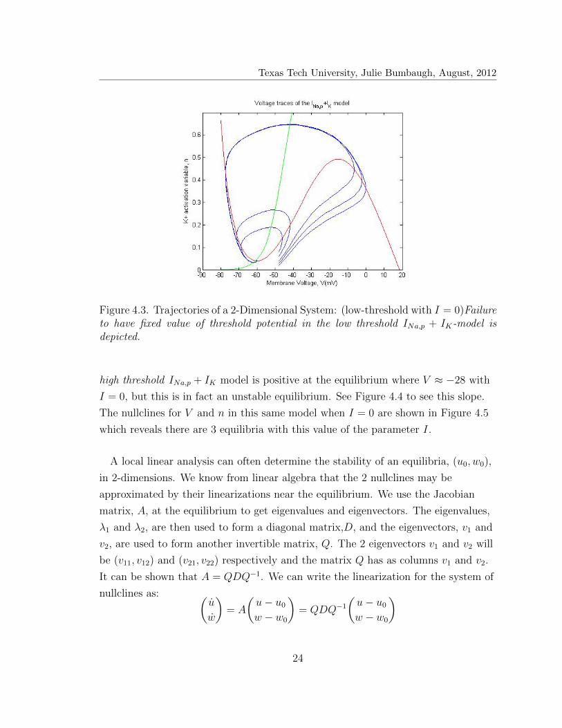
spikes. In Figure 4.3, we observe the INa,p + IK low threshold system has

trajectories all starting with the same initial membrane potential of −48mV , but

varying values of initial K+ activation variable “n”. Some trajectories depict full

action potentials and some make small excursions and return to equilibrium with

subthreshold spikes. We can see that this model has no fixed threshold of membrane

potential. All of the action potentials exhibited in Figures 4.2 and 4.3 are transient;

they all return to equilibrium values.

Figure 4.2. Trajectories of a 2-dimensional system: I = 0. (low-threshold) INa,p + IKmodel: Failure to generate all-or-nothing action potentials is depicted.

4.2.2 Stability in 2-dimensions

Now we need to address how we can determine the stability of the equilibrium. If

at least one trajectory diverges from the equilibrium, then it is said to be unstable.

Unlike the one-dimensional systems, stability can not be determined from the slope

of the V vs. V curve. For example, the slope of the steady-state I − V curve for the

23


Figure 4.3. Trajectories of a 2-Dimensional System: (low-threshold with I = 0)Failureto have fixed value of threshold potential in the low threshold INa,p + IK-model isdepicted.

high threshold INa,p + IK model is positive at the equilibrium where V ≈ −28 with

I = 0, but this is in fact an unstable equilibrium. See Figure 4.4 to see this slope.

The nullclines for V and n in this same model when I = 0 are shown in Figure 4.5

which reveals there are 3 equilibria with this value of the parameter I.

A local linear analysis can often determine the stability of an equilibria, (u0, w0),

in 2-dimensions. We know from linear algebra that the 2 nullclines may be

approximated by their linearizations near the equilibrium. We use the Jacobian

matrix, A, at the equilibrium to get eigenvalues and eigenvectors. The eigenvalues,

λ1 and λ2, are then used to form a diagonal matrix,D, and the eigenvectors, v1 and

v2, are used to form another invertible matrix, Q. The 2 eigenvectors v1 and v2 will

be (v11, v12) and (v21, v22) respectively and the matrix Q has as columns v1 and v2.

It can be shown that A = QDQ−1. We can write the linearization for the system of

nullclines as: (u

w

)= A

(u− u0

w − w0

)= QDQ−1

(u− u0

w − w0

)

24


Figure 4.4. Bifurcations for high threshold INa,p + IK model. It appears that whenI = 4.5 and I = −85.5 the state of this neuron changes from 3 equilibria betweenthese two values of injected current to 2 and then 1 equilibria.

Figure 4.5. Nullclines for high threshold INa,p + IK model with I = 0: Red curve isnullcline for V and Green curve is nullcline for activation variable n. Curves appearto have equilibria at approximately: V = −66, V = −56, and at V = −28.

25


Multiplying through by Q−1 on the left sides yields

Q−1

(u

w

)= Q−1A

(u− u0

w − w0

)= DQ−1

(u− u0

w − w0

).

Now, let y = Q−1(u−u0

w−w0

). This makes dy

dt= Q−1

(uw

). So, dy

dt= Dy. Solving for y will

lead us to finding a function of time to represent the magnitude of the deviations

from the equilibrium: (dy1

dtdy2

dt

)=

(λ1y1

λ2y2

),(

y1

y2

)=

(C1e

λ1t

C2eλ2t

).

Now that we have y, since y was defined to be Q−1(u−u0

w−w0

), we have(

u− u0

w − w0

)= Q · y,

=

(v11 v21

v12 v22

)·

(c1e

λ1t

c2eλ2t,

)

=

(v11c1e

λ1t + v21c2eλ2t

v12c1eλ1t + v22c2e

λ2t

)= (v11c1e

λ1t, v12c1eλ1t) + (v21c2e

λ2t, v22c2eλ2t)

= C1v1eλ1t + C2v2e

λ2t.

So, for any 2-dimensional system, if the eigenvalues are both negative or have

negative real parts, then as t→∞, the vector(u−u0

w−w0

)→(

00

)meaning that

deviations from the equilibrium will go to 0 making (u0, w0) stable. It is enough in

some cases, therefore, to find the λ’s to determine the stability of equilibria in

2-dimensional systems. Recall that an eigenvalue in one dimensional systems was

simply the slope of the V vs. V curve at the equilibrium and, if it was negative, it

meant the equilibrium was stable. (Equivalently, as explained earlier, if the slope of

the I − V curve is positive at equilibrium, it is stable because the signs of the V vs.

V curve and the I − V curve are opposite and their slopes would be opposite as

well.) Now, we know that negative eigenvalues also imply stability in 2-dimensions.

26


4.2.3 Limit cycles

In 2 dimensions, it is possible to have trajectories that follow a repeating cycle. A

trajectory that forms a closed loop is called a periodic trajectory. An isolated

periodic trajectory is called a limit cycle. When a neuronal model exhibits a limit

cycle, it means the neuron would be firing repetitive action potentials in this state.

Figure 4.6 illustrates the low-threshold INa,p + IK model with I = 40 this time

rather than 0. With this change of the parameter, I, the trajectories follow such a

limit cycle. When I was zero, in this model, the eigenvalues at the intersection of

the nullclines were negative, indicating stability. With I = 40, the eigenvalues are

positive. The Figure 4.7 shows us snapshots of the limit cycle’s appearance and

disappearance between the values I = 0 and I = 400. As the injected current

continues to be raised, we see the amplitude of the limit cycle shrinks and

eventually the limit cycle vanishes and is replaced by a stable excited equilibrium.

Figure 4.6. The stable limit cycle of the persistent INa,p + IK (low-threshold) modelwith I=40. The equilibrium at the intersection of the nullclines is not stable.

4.2.4 Bifurcations in 2-dimensions

A zero eigenvalue arises when the equilibrium undergoes a bifurcation [7]. That

makes sense, since negative eigenvalues ensure stability and positive ensure

unstability. Naturally, if an eigenvalue’s real part is zero, the system must be

undergoing some sort of qualitative change. To study the bifurcation(s) a system

may have, we can analyze models where we change a parameter that leads to a

27


Figure 4.7. Low threshold INa,p + IK traces leading to excitation block

bifurcation. We will look at the steady-state I − V curve for the system to see

where such bifurcations exist. Where the curve has a change in direction, is a

bifurcation since the number of equilibrium values of V which correspond to this

value of the current changes as we raise or lower the value of I from this location.

In Figure 4.4, we saw that the bifurcations for that model occur at approximately

I = 5 and I = −85. By determining potential values where the difference between

the two nullclines is zero near these bifurcation currents, we have found that when

28


I = 4.496, the difference in nullclines is very close to zero, (we are near an

equlibrium and close a bifurcation), when V = −60.63398. Using I = −85.607, the

difference between the nullclines is very close to zero for V = −36.17021. We can

obtain corresponding values for n for these potentials and injected current values

and then compute each equilibrium’s eigenvalues to determine the stability of the

equilibria. At these equilibria, the eigenvalues are negative, indicating stability.

Trying again, with a slightly higher potential than the first one, V = −58.5, the

eigenvalues are positive indicating instability. What this means is that the equilibria

left of the left knee in the steady-state I − V curve are stable and right of it are

unstable. As the injected current approaches 5 from below, the equilibria are

getting closer together and when they become one, one of the eigenvalues will be

zero. The stable node and the unstable saddle coelesce to form the saddle-node

which is stable on one side and unstable on the other. If we now examine the

dynamics near the right knee of the steady state curve, the eigenvalues at the

bifurcation value of I are positive. This equilibrium is unstable.

4.2.5 Stable and unstable manifolds

It is of interest to examine at least two trajectories. The first being of an initial

potential, V , between the stable and middle unstable equilibria when I = 3 with

τ = 0.152. The second consists of an initial potential, V to the right of the middle

equilibria. See Figure 4.8. This figure demonstrates that there is a region, known as

a manifold which is the attraction domain for a stable limit cycle. It is also

apparent that the region outside of this manifold, (the unstable manifold) is the

attraction domain for the resting state at the leftmost equilibrium which is stable.

4.2.6 Hodgkin-Huxley reduced model

Finally, in this chapter on 2-dimensional systems, we address the fact that the

Hodgkin Huxley Model may be reduced to a two-dimensional model by replacing

one of its state variables having fast kinetics with its maximal value since it achieves

this value almost instantaneously. The other variable can be substituted by a

function of one of the remaining state variables. In order to successfully minimalize

a neuronal model, it must be able to still produce a spiking limit cycle. In order to

29


Figure 4.8. The trajectories of the persistent sodium + potassium (high threshold)model with I = 3 and τ = 0.152. Bistability is exhibited with a resting equilitbriumwhich 3 of the trajectories shown in light blue end at and a spiking state shown bythe staable limit cyde which is the trajectory in yellow. The dark blue curve is thenullcline for V and the red is the nullcline for n.

do this, the model must have one amplifying and one resonant variable. One to

amplify a depolarization and one to restore or reset values so that another action

potential can occur.

In the case of the Hodgkin-Huxley model with its 4 state variables, m, n, h, and

V , an amazing near linear relationship was found between the variables h and n by

Krinskii and Kokoz in 1973 [7]. If these variables are plotted in the (n, h) plane, the

curve is seen to be very close to the line h = 0.89− 1.1n. This discovery along with

the determination that the action kinetics for sodium are practically instantaneous,

such that m may be replaced with m∞(V ), reduces the Hodgkin-Huxley model to 2

dimensions. See equations (4.5) and (4.6).

Some modern conventions have been applied here. Hodgkin and Huxley’s model

used (V − VK) rather than (V − EK) because it was what they could measure.

30


Their model also used the opposite signs for membrane potentials. The ions’ Nernst

potentials are used today, EK , ENa, and El which have the opposite values to the

values of VK , VNa, and Vl used in the older model. This reflects the V vs. t curves

over the t axis. Modern convention to correct the signs of the potential also involve

changing (V − 10) to (10− v), (V − 25) to (25− V ),(V − 30) to (30− V ) and V to

−V in equations (3.5) through (3.10).

CV = I − gKn4(V − EK)− gNa(m∞(V ))3(0.89− 1.1n)(V − ENa)−

gL(V − EL), (4.5)

n =(n∞(V )− n)

τn(V ). (4.6)

This definition for n is equivalent to equation (3.2) using the definitions for τn and

n∞ stated earlier. (Note: the Hodgkin-Huxley formula for n∞ is not as easy to work

with as using the Boltzmann function.) To analyze this minimalized model of the

Hodgkin-Huxley model, we first find the intersections of its nullclines to find the

equilibria. The V nullcline must satisfy:

n = 4

√I − gNam3

∞(V )(V − ENa)− gL(V − EL)

gK(V − EK). (4.7)

The n nullcline must satisfy:

n = n∞(V ). (4.8)

We will see that there is one equilibrium and that it is stable when I = 0 but

becomes unstable as seen when I = 12. See figures 4.9 and 4.10.

Calculations of the eigenvalues for each of the equilibria of the Hodgkin-Huxley

models, with I = 0 and I = 12 are negative and positive respectively, confirming

what we see geometrically, that the equilibrium is stable when I = 0 and unstable

when I = 12. See chapter 5 for these calculations. There is an Andronov-Hopf

bifurcation somewhere between these 2 values of I which means that the unique

equilibrium is stable for small values of I but becomes unstable when I increases

31


Figure 4.9. Hodgkin-Huxley space-clamp model reduced to 2 variables with I = 0.The intersection of the nullclines and 2 traces show that the equilibrium appears tobe stable.

Figure 4.10. Hodgkin-Huxley space-clamp model reduced to 2 variables with I = 12.The intersection of the nullclines and 2 traces show that the equilibrium appears tobe unstable. A stable limit cycle appears somewhere between I = 0 and I = 12.

32


past 12 giving birth to a limit cycle attractor [7].

It can be shown that, in models like the Hodgkin-Huxley model, as I continues to

increase, the amplitude of the stable limit cycle decreases until the excitation state,

ability to produce action potentials, is blocked. See the next chapter for simulations

and analysis to justify these claims.

33


CHAPTER 5

PROBLEMS FOR STUDY AND ANALYSIS

Modeling the real world with mathematical equations is one of the greatest

reasons we study mathematics. Students of Mathematics may follow the directions

below to practice some of the modern techniques to studying dynamical systems

and some of the mathematical steps that Hodgkin and Huxley used to derive their

model of action potentials in squid giant axons.

5.1 Proposed problems for study

5.1.1 Problem 1- Derive Boltzmann’s function

Today, the Boltzmann function is used to describe the steady-state activation

variables m∞, n∞, and inactivation variable h∞. To derive this formula, we note

that the shape of the curves from measured values of m,n and h resemble logistics

curves with their sigmoid shape. Boltzmann’s function also has the form of a

logistics curve with the asymptote at y = 1:

m∞ =1

1 + e−1k

(V−V1/2).

The limiting value for all of these curves is 1 because these variables represent the

ratio of these activation variables in membrane at each value of V . The maximum

ratio would be 1. Plotted curves of measured values for m,n, and h vs. V are used

to find the slopes of the curves at the inflection points to determine the parameter

C1. Solve the logistics Differential equation (5.1) for m∞(V ) to derive Boltmann’s

function:dm∞dV

= C1(m∞)(1− m∞C2

). (5.1)

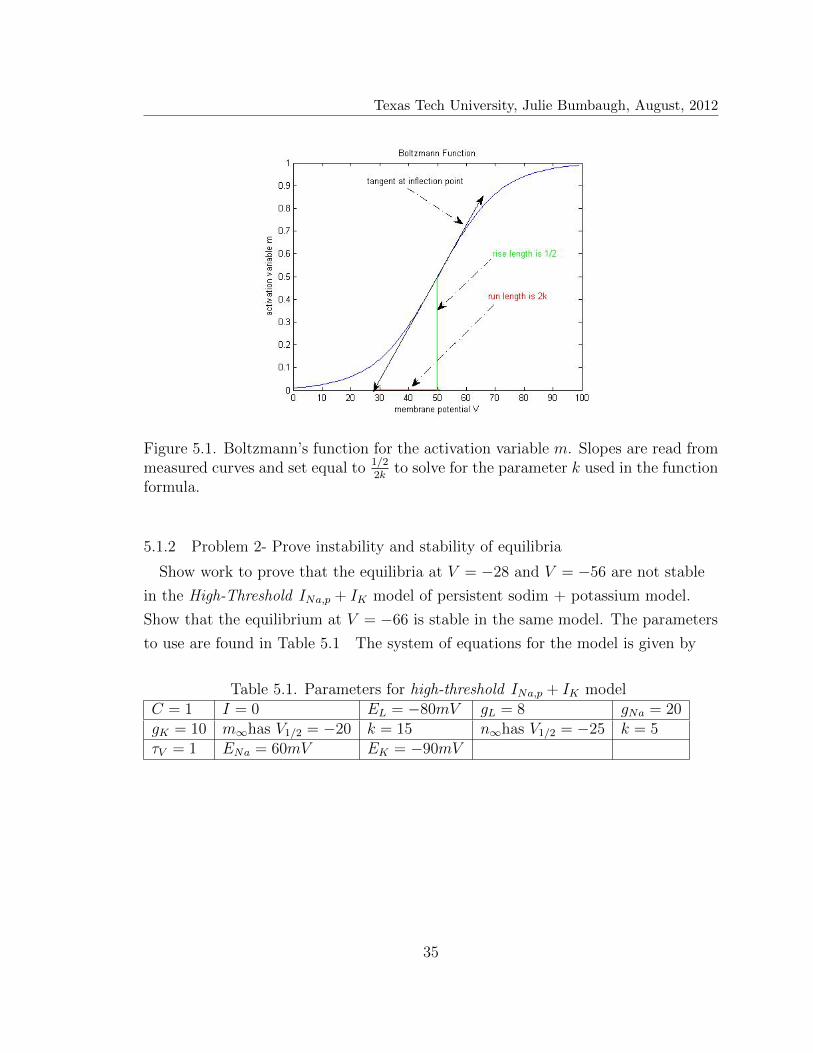
Use C2 = 1 as the limiting value and call the tangent slope at the inflection point1/22k

since we know the vertical location of an inflection point on a logistics curve

occurs at half the limiting value. They represented the run as 2k for a nicer looking

result. See Figure 5.1 to understand how 2k is obtained from the graphs. V1/2

represents the value of the membrane potential at the inflection point which is

where the value of the activation/inactivation variable is 1/2.

34


Figure 5.1. Boltzmann’s function for the activation variable m. Slopes are read frommeasured curves and set equal to 1/2

2kto solve for the parameter k used in the function

formula.

5.1.2 Problem 2- Prove instability and stability of equilibria

Show work to prove that the equilibria at V = −28 and V = −56 are not stable

in the High-Threshold INa,p + IK model of persistent sodim + potassium model.

Show that the equilibrium at V = −66 is stable in the same model. The parameters

to use are found in Table 5.1 The system of equations for the model is given by

Table 5.1. Parameters for high-threshold INa,p + IK modelC = 1 I = 0 EL = −80mV gL = 8 gNa = 20gK = 10 m∞has V1/2 = −20 k = 15 n∞has V1/2 = −25 k = 5τV = 1 ENa = 60mV EK = −90mV

35


equations (5.2) to (5.5).

CV = I − gL(V − EL)− gNam∞(V )(V − ENa)− gKn(V − EK), (5.2)

n = (n∞(V )− n)/τV , (5.3)

n∞(V ) =1

1 + e(V1/2−V )/k, (5.4)

m∞(V ) =1

1 + e(V1/2−V )/k. (5.5)

5.1.3 Problem 3- Find equilibrium and determine its stability

Use the Hodgkin-Huxley 2-dimensional reduced model parameters in Table 3.1

with I = 12 to write a program that will locate the value of V at the equilibrium of

the model with this injected current. The equations for the nullclines of this model

are (4.7) and (4.8). Then find the corresponding value for n. Finally, determine the

stability of this equilibrium. Finding the partial derivatives at the equilibrium is

quite complex for this model. Writing a program to perform the numerous

calculations would be very helpful.

5.1.4 Problem 4- Demonstrate excitation block

Show that as the injected current increases in the low threshold INa,p + IK model,

that an excitation block occurs which decreases the amplitude of the action

potentials until the limit cycle vanishes. See equations (4.1) through (4.4) and Table

4.3 for the equations defining this model and its parameters.

5.1.5 Problem 5- Choose appropriate power for an activation variable

Hodgkin and Huxley chose the 4th power of the activation variable n in their

model for potassium conductance. They were using the fact that 1− e−t is a

particular solution to the differential equation describing the rate of change of

potassium. Show/explain why the first power of this solution does not work as a

good model and theorize why it is reasonable that they would have stopped and

been satisfied with the 4th power of this solution.

36


5.1.6 Problem 6- Derive the formula Hodgkin and Huxley used for n

Show how Hodgkin and Huxley arrived at the formula for n, in equation (2.2)

from the differential equation (2.1).

5.2 Solutions to the problems for study and analysis

5.2.1 Solution to problem 1

We start with the fact that the limiting value, C2, will be 1 and solve the logistics

differential equation (5.1).

First, we separate the variables:

dm∞m∞(1−m∞)

= (C1)dV.

Integrate and use inflection point coordinates (V1/2,12) and slope 1/2

2kto finish finding

the particular solution.∫(

1

m∞+

1

1−m∞)dm∞ =

∫C1dV,

lnm∞ − ln(1−m∞) = C1V + C3,

lnm∞

1−m∞= C1V + C3,

m∞1−m∞

= C4eC1V ,

m∞ =C4e

C1V

C4eC1V + 1,

m∞ =1

1 + C5e−C1V.

Using dm∞dV

= 1/22k

in the differential equation yields 1k

= C1.

Using (V,m∞) = (V1/2,12) in the general solution yields C5 = e

1kV1/2 . So, the

particular solution is :

m∞ =1

1 + e1kV1/2e−

1kV

or

m∞ =1

1 + e−1k

(V−V1/2).

37



The partial derivatives needed for the Jacobian matrix elements are as follows:

∂V

∂V=

1

C(−gL − gNa ·m∞(V )− gNa(V − ENa)(−1)(1 + e(V1/2−V )/k)−2·

(e(V1/2−V )/k)(−1

k)− gK · n),

∂V

∂n=− gK(V − EK),

∂n

∂V=

1

τV(1 + e(V1/2−V )/k)−2(e(V1/2−V )/k)(

1

k),

∂n

∂n=− 1

τV.

The corresponding values for n can be calculated using the values of V at each

equilibria in the equation (5.3). The coordinates of the equilibria are (−28, .3543),

(−56, .002025), and (−66, .00027458). Here are the Jacobian matrices for V = −28,

V = −56, and V = −66 respectively: A =

(8.40466 −620

.0457568 −1

),

A =

(2.1104 −340

.00040424 −1

), and A =

(−1.74898 −240

.0000549 −1

). We calculate the trace

and determinant of each matrix. For V = −28, Tr(A) = 7.40466 and

|A| = 19.964556. When V = −56, Tr(A) = 1.1104 and |A| = −1.9729584. When

V = −66, Tr(A) = −2.74898 and |A| = 1.762156. Finally we compute the

eigenvalues for each equilibrium usingTr(A)±

√(Tr(A))2−4det(A)

2. The eigenvalues for

V = −28 are 3.70233±√−25.029234

2. When V = −56 the eigenvalues are 2.065566 and

−.955165. The eigenvalues for V = −66 are −1.018026 and −1.7309543. These

results tell us that the equilibrium at V = −28 is not stable, the equilibrium at

V = −56 is a saddle since one eigenvalue is positive and the other is negative. The

equilibrium at V = −66 is indeed stable since both eigenvalues are negative.


See a computer code in appendix B that locates the value of V at the equilibrium.

Figure 5.2 shows that the equilibrium is at a value of V = 22.357 to the nearest

thousandth. Now we can now determine the corresponding value of n using

38


Figure 5.2. Location of intersection of nullclines is at the zero of difference betweennullclines for HH reduced model. The plot shows this to be nearest to V = 22.357

equation (4.7). This yields n = 0.2998158738. Next, we find the Jacobian matrix.

Another program can be found in appendix C that aids in finding the partial

derivatives of V and n. Jacobian matrix, A =(1628.6135 −1162.5718

.0052275 −.2687

).

The Tr(A) = 1628.3448 and the determinant |A| = −431.5311034. The eigenvalues

areTr(A)+

√(Tr(A))2−4det(A)

2= 1628.609769 and

Tr(A)−√

(Tr(A))2−4det(A)

2= 1.000614876.

Since both eigenvalues are positive, this equilibrium is unstable.


We simply need to write a program to plot V vs. I for this model. See Appendix

D for possible programs. The following figure demonstrates the results of one such

program.

39


Figure 5.3. Excitation block in the low-threshold INa,p + IK model.


The particular solution 1− e−t to the differential equation,dndt

= αn(1− n)− βn · n does not have an inflection point since

d

dt(1− e−t) = e−t

andd2(1− e−t)

dt2= −e−t < 0.

The second derivative of this solution is always negative; hence, no inflection point.

The data collected showed a sigmoid shaped curve which has an inflection point. If

we raise this solution to any integral power p > 1, there will be an inflection point

at t = ln(p). Let y = (1− e−t)p. Then

dy

dt= p(1− e−t)p−1(e−t),

40


d2y

dt2= p(p− 1)(1− e−t)p−2 · e−2t − p(1− e−t)p−1 · e−t,

= p(1− e−t)p−2 · e−2t((p− 1)− (1− e−t · et)),

= p(1− e−t)p−2 · e−2t(p− et),

= 0 only when p− et = 0.

p− et = 0 when t = ln p.

Due to the slow rise of the natural log function, we know that the greater the value

of p, the smaller the difference is between ln p and ln (p+ 1). By raising the value of

p, we move the inflection point further and further to the right in our curve, but it

moves smaller and smaller amounts to the right such that eventually, there is no

practical benefit of using a higher power.

ln 2 ≈ .693 ln 3 ≈ 1.0986 ln 4 ≈ 1.386 ln 5 ≈ 1.609 ln 6 ≈ 1.792

Choosing 3rd power over 2nd pushes the inflection point ≈ .4 units further to the

right. Choosing 4th power over 3nd moves it an additional ≈ .3 units. 5th power

would have moved it another ≈ .2 units and 6th power would have moved it another

≈ .18 units. It must have been the case that the 4th power placed the inflection

point within ≈ .2unit of where it needed to be such that using higher powers

became unnecessary. They did make comment in their paper that they were

choosing a power to compensate for the “delayed rise of potassium”. We assume

here that they are referring to the point at which the rate of change in the rise of

the curve changes, the inflection point.


First, we separate the variables:

dn

αn − n(αn + betan)= dt.

Next we integrate:

− 1

αn + βnln |αn − n(αn + βn)| = t+ C.

41


Substitute for their definition of τn and continue solving for n:

−τn · ln |αn − n(αn + βn)| = t+ C,

ln |αn − n(αn + βn)| = − 1

τn· t+− 1

τn· C.

Apply the initial condition that when t = 0, n = n0 :

ln |αn − n0(αn + βn)| = − 1

τn· C,

−τn · ln |αn − n0(αn + βn)| = C.

Now we substitute this value of C back into the general solution:

ln |αn − n(αn + βn)| = −tτn− 1

τn· −τn · ln |αn − n0(αn + βn)|,

=−tτn

+ ln |αn − n0(αn + βn)|,

αn − n(αn + βn) = e−tτn · eln |αn−n0(αn+βn)|,

αn − n(αn + βn) = e−tτn · (αn − n0(αn + βn)).

Now, finish solving for n and make substitutions for n∞ = αnαn+βn

:

n · (αn + βn) = αn − (αn − n0(αn + βn)) · e−tτn ,

n =αn

(αn + βn)−(

αn(αn + βn)

− n0

)· e−

tτn ,

n = n∞ − (n∞ − n0) · e−tτn .

42


BIBLIOGRAPHY

[1] D. E. Goldman,Potential, Impedence, and Rectification in Membranes, J. Gen.Physiology, 26(1943), pp. 37-60.

[2] A. L. Hodgkin and A. F. Huxley, A Quantitative Description of MembraneCurrent and its Application to Conduction and Excitation in Nerve, J.Physiology, 117(1952), pp. 500–544.

[3] A. L. Hodgkin, A. F. Huxley, and B. Katz, Measurement of Current-VoltageRelations in the Membrane of the Giant Axon of Loligo, J. Physiology,116(1952), pp. 424-448.

[4] A. L. Hodgkin and A. F. Huxley, Currents Carried by Sodium and PotassiumIons through the Membrane of the Giant Axon of Loligo, J. Physiology,116(1952), pp. 449-472.

[5] A. L. Hodgkin and A. F. Huxley,The Components of Membrane Conductancein the Giant Axon of Loligo, J. Physiology, 116(1952), pp. 473-496.

[6] A. L. Hodgkin and A. F. Huxley,The Dual Effect of Membrane Potential onSodium Conductance in the Giant Axon of Loligo, J. Physiology, 116(1952),pp. 497-506.

[7] E. M. Izhikevich, Dynamical Systems in Neuroscience: The Geometry ofExcitability and Bursting, Cambridge, Massachusetts, 2007.

[8] J. D. Murray, Mathematical Biology, Springer-Verlag, Berlin, Heidelberg, 1993.

43


APPENDIX A

COMPUTER CODE FOR HODGKIN-HUXLEY MODEL

This matlab program uses Euler’s method to plot Action Potentials in “Voltage

Clamp” experiments:

1. % This program plots Voltage vs. Time of an action potential

%of a neuron.

2. % Input necessary constant values.

3. % This program should be run multiple times using different

% initial values for membrane potential.

4. Vna = -115;

5. Vk = 12;

6. Vl = -10.613;

7. gna = 120;

8. gk = 36;

9. gl = 0.3;

10. V=20;

11. %Calculate needed initial values from the constants.

12. an = 0.01*(V+10)/(exp(1+0.1*V)-1);

13. bn = 0.125*exp(V/80.0);

14. am = 0.1*(V+25)/(exp(0.1*V+2.5)-1);

15. bm = 4.0*exp(V/18.0);

16. ah = 0.07*exp(V/20.0);

17. bh = 1.0/(exp(3+0.1*V)+1);

18. % Initialize values for n,m,h, & V.

19. n = an/(an + bn);

20. m=am/(am + bm);

21. h = ah/(ah + bh);

22. V(1) = V;

23. t(1) = 0;

24. nn(1) = n;

25. mm(1) = m;

44


26. hh(1) = h;

27. ann(1) = an;

28. bnn(1) = bn;

29. ninf(1) = an/(an + bn);

30. %Use Euler’s method to get the next 1000 values of the

%variables using a step size of 0.01.

31. for i = 1:1000

32. an = 0.01*(V(i)+10)/(exp(1+0.1*V(i))-1);

33. bn = 0.125*exp(V(i)/90.0);

34. am = 0.1*(v(i)+25)/(exp(0.1*V(i)+2.5)-1);

35. bm = 4.0*exp(V(i)/18.0);

36. ah = 0.07*exp(V(i)/20.0);

37. bh = 1.0/(exp(3+0.1*V(i))+1);

38. dmdt = am*(1-m)-bm*m;

39. dndt = an*(1-n)-bn*n;

40. dhdt = ah*(1-h)-bh*h;

41. m = m + dmdt&0.01;

42. n = n+dndt*0.01;

43. h = h+dhdt*0.01;

44. dvdt = -gk*n^4*(V(i)-Vk)-gna*m^3*h*(V(i)-Vna)-gl*(V(i)-Vl);

45. V(i+1) = (V(i) + dvdt*0.01);

46. t(i+1) = (i)*0.01;

47. nn(i+1) = n;

48. mm(i+1) = m;

49. hh(i+1) = h;

50. ann(i+1) = an;

51. bnn(i+1) = bn;

52. ninf(i+1) = an/(an+bn);

53. end

54. % One could now plot alphas and betas versus V or

%could plot Membrane potential, Versus Time, t.

55. plot (t,-V)

45


APPENDIX B

COMPUTER CODE FOR FINDING INTERSECTION OF NULLCLINES

This matlab program finds intersections of nullclines by locating the zero of their

difference.

%This program will plot differences in the nullclines for n and V

%of the reduced HH model to help locate the equilibrium for

%given values of injected current I.

1. I=12;

2. gna=120;

3. Ena=120;

4. gl=.3;

5. El=10.6;

6. gk=36;

7. Ek=-12;

8. h=.00001;

9. N=1000;

10. V=22.35;

11. for i=1:N

12. v(i)= V;

13. a(i)=.1*(25-v(i))/(exp((25-v(i))/10)-1);

14. b(i)= 4*exp(-1*v(i)/18);

15. minf(i)=a(i)/(a(i)+b(i));

16. Vnull(i)=((I-gna*(minf(i))^3*(v-Ena)-gl*(v-El))/

(gk*(v-Ek)))^(.25);

17. nnull(i)=.01*(10-v)/(exp((10-v)/10)-1)/(.01*(10-v)/

((exp((10-v)/10)-1)+1/8*exp(-v/80)));

18. D(i)=Vnull(i)-nnull(i);

19. V = V+h;

20. end

21. plot(v,D,’r’)

22. hold on

23. plot(v,0)

24. xlabel(’V (mv)’)

46


25. ylabel(’Difference in nullclines’)

26. title(’Locating zero for difference in nullclines of reduced HH’)

27. axis([22.35 22.36 -.001 .001])

47


APPENDIX C

COMPUTER CODE FOR CALCULATING PARTIAL DERIVATIVES AT

EQUILIBRIUM

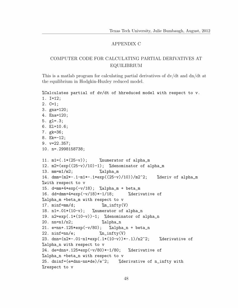
This is a matlab program for calculating partial derivatives of dv/dt and dn/dt atthe equilibrium in Hodgkin-Huxley reduced model.

%Calculates partial of dv/dt of hhreduced model with respect to v.

1. I=12;

2. C=1;

3. gna=120;

4. Ena=120;

5. gl=.3;

6. El=10.6;

7. gk=36;

8. Ek=-12;

9. v=22.357;

10. n=.2998158738;

11. m1=(.1*(25-v)); %numerator of alpha_m

12. m2=(exp((25-v)/10)-1); %denominator of alpha_m

13. mm=m1/m2; %alpha_m

14. dmm=(m2*-.1-m1*-.1*exp((25-v)/10))/m2^2; %deriv of alpha_m

%with respect to v

15. d=mm+4*exp(-v/18); %alpha_m + beta_m

16. dd=dmm+4*exp(-v/18)*-1/18; %derivative of

%alpha_m +beta_m with respect to v

17. minf=mm/d; %m_infty(V)

18. n1=.01*(10-v); %numerator of alpha_n

19. n2=exp(.1*(10-v))-1; %denominator of alpha_n

20. nn=n1/n2; %alpha_n

21. e=nn+.125*exp(-v/80); %alpha_n + beta_n

22. ninf=nn/e; %n_infty(V)

23. dnn=(n2*-.01-n1*exp(.1*(10-v))*-.1)/n2^2; %derivative of

%alpha_n with respect to v

24. de=dnn+.125*exp(-v/80)*-1/80; %derivative of

%alpha_n +beta_n with respect to v

25. dninf=(e*dnn-nn*de)/e^2; %derivative of n_infty with

%respect to v

48


26. dminf=(d*dmm-mm*dd)*d^2; %derivative of m_infty(V)

% with respect to v

%dminf is derivative of m_infty(V) with respect to V

27. w=1/C*(-gk*n^4-gna*minf^3*(.89-1.1*n)-gna*(v-Ena)

*(.89-1.1*n)*3*minf^2*dminf-gl);

%w is partial of dv/dt with respect to V

28. x=1/C*(-gk*(v-Ek)*4*n^3-gna*minf^3*(-1.1)*(v-Ena))

%x is partial of dv/dt with respect to n.

29. y=(1-n)*dnn-n*.125*exp(-v/80)*-1/80;

%y is partial of dn/dt with respect to v

30. z=-nn-.125*exp(-v/80); %partial of dn/dt with respect to n

31. h=.1

32. a=1

33. for i=1:10

34. q(i)=a

35. L(i)=z

36. a=a+h

37. end

38. plot(q,L)

39. axis([1 2 -.269 -.2685])

%Calculates the partial of dn/dt with respect to n.

49


APPENDIX D

COMPUTER CODE TO PLOT EXAMPLES OF EXCITATION BLOCK

The following program(s) will allow one to plot geometric proof of excitation block

when currents are ramped up in some models.

%This program is to plot low-threshold persistent sodium

%+potassium model’s potential vs. time graph with increasing

% injected current.

1. [t,y]=ode45(’my_lowthresholdtrajectoryfn’,[0 10000],[-75 .2 40]);

2. plot(t,y(:,1),’b’)

3. xlabel(’Time, t(ms)’)

4. ylabel(’Membrane potential, V(mv)’)

5. title(’V vs. t in I_{Na,p}+I_K low threshold model with

increasing values of I’)

6. axis([0 100 -75 0])

%% This program is to be used with the previous one.

% function dydt=my_highthresholdtrajectoryfn(t,y)

1. dydt=zeros(size(y));

2. C=1; I=0; El=-78; gl=8; gNa=20; gk=10; mV=-20; mk=15;

nV=-45; nk=5; Tau=1;

3. Ena=60; Ek=-90;

4. A=y(1)

5. B=y(2)

6. D=y(3)

50


7. dydt(1)=(1/C)*(D-gl*(A-El)-gNa*(1/(1+exp((mV-A)/mk)))*(A-Ena)-

gk*B*(A-Ek));

8. dydt(2)=(1/(1+exp((nV-A)/nk))-B)/Tau;

9. dydt(3)=3.6;

%%The next two programs go together to plot traces of n vs. V of

% the same model with fixed values of I.

%This program is to plot Traces of low-threshold

%persistent sodium +potassium model.

%Plots n vs. V graphs with different values for I.

1. [t,y]=ode45(’my_lowthresholdtrajectoryfn2’,[0 500],[-60 .1]);

2. h = 1

3. g = -89

4. for i=1:109

5. k(i)= g

6. j(i)= (300-8*(g+78)-20*

(1/(1+exp((-20-g)/15)))*(g-60))/(10*(g+90))

7. l(i) = 1/(1+exp((-45-g)/5))

8. g = g+h

9. end

10. plot(y(:,1),y(:,2),’b’)

11. hold on

12. plot(k,j,’r’)

13. hold on

14. plot(k,l,’g’)

15. hold off

16. xlabel(’Membrane potential, V(mv)’)

17. ylabel(’K+ activation variable, n’)

18. title(’n vs. V in I_{Na,p}+I_K low threshold model with I=0’)

19. axis([-89 20 0 1.2])

%% to be used with the program above.

1. function dydt=my_highthresholdtrajectoryfn(t,y)

2. dydt=zeros(size(y));

51


3. C=1; I=300; El=-78; gl=8; gNa=20; gk=10; mV=-20; mk=15; nV=-45;

4. nk=5; Tau=1;

5.Ena=60; Ek=-90;

6. A=y(1)

7. B=y(2)

8. dydt(1)=(1/C)*(I-gl*(A-El)-gNa*(1/(1+exp((mV-A)/mk)))*(A-Ena)-

gk*B*(A-Ek));

9. dydt(2)=(1/(1+exp((nV-A)/nk))-B)/Tau;

52

c 2012, julie bumbaugh - tdl

Documents