THE VALUE OF BRANDING IN TWO-SIDED PLATFORMS

by

Yutec Sun

A thesis submitted in conformity with the requirementsfor the degree of Doctor of Philosophy

Joseph L. Rotman School of ManagementUniversity of Toronto

c© Copyright 2013 by Yutec Sun

Abstract

The Value of Branding in Two-Sided Platforms

Yutec Sun

Doctor of Philosophy

Joseph L. Rotman School of Management

University of Toronto

2013

This thesis studies the value of branding in the smartphone market. Measuring brand value with data avail-

able at product level potentially entails computational and econometric challenges due to data constraints.

These issues motivate the three studies of the thesis.

Chapter 2 studies the smartphone market to understand how operating system platform providers can

grow one of the most important intangible assets, i.e., brand value, by leveraging the indirect network

between two user groups in a two-sided platform. The main finding is that iPhone achieved the greatest

brand value growth by opening its platform to the participation of third-party developers, thereby indirectly

connecting the consumers and the developers via its app store effectively. Without the open app store, I find

that iPhone would have lost its brand value by becoming a two-sided platform. Hence these findings provide

an important lesson that open platform strategy is vital to the success of building platform brands.

Chapter 3 solves a computational challenge in structural estimation of aggregate demand. I develop a

computationally efficient MCMC algorithm for the GMM estimation framework developed by Berry, Levin-

sohn and Pakes (1995) and Gowrisankaran and Rysman (forthcoming). I combine the MCMC method with

the classical approach by transforming the GMM into a Laplace type estimation framework, therefore avoid-

ing the need to formulate a likelihood model. The proposed algorithm solves the two fixed point problems,

i.e., the market share inversion and the dynamic programming, incrementally with MCMC iteration. Hence

the proposed approach achieves computational efficiency without compromising the advantages of the con-

ventional GMM approach.

Chapter 4 reviews recently developed econometric methods to control for endogeneity bias when the ran-

dom slope coefficient is correlated with treatment variables. I examine how standard instrumental variables

and control function approaches can solve the slope endogeneity problem under two general frameworks

commonly used in the literature.

ii

Acknowledgements

I have been blessed to have Avi Goldfarb as my supervisor during my Ph.D. study. This research would not

have started without his help and inspiration. Furthermore, he provided all of my needs and taught the

qualities that I lacked.

I thank Ron Borkovsky and Victor Aguirregabiria for providing excellent advice and support. I wish I

could have more time to work with them. I would also like to thank Andrew Ching for his constant care and

attention. He has been another source of inspiration for my research.

I would also like to thank my former and present colleagues in the Ph.D. program for participating in

my seminars. In particular, I acknowledge Masakazu Ishihara for his help and support for Chapter 3 of my

thesis.

I was able to complete this thesis thanks to love, trust, and encouragement of my beloved wife and son,

Jisun and Samuel.

This thesis is dedicated to the One whose name is I am, who have sustained and led me through the

darkest hours.

iii

Contents

1 Introduction 1

1.1 Overview . . . . . . . . . . . . . . . . . . . . . . . . . . . . . . . . . . . . . . . . . . . . . . . 1

2 The Value of Branding in Two-Sided Platforms 3

2.1 Introduction . . . . . . . . . . . . . . . . . . . . . . . . . . . . . . . . . . . . . . . . . . . . . . 3

2.2 Related Literature . . . . . . . . . . . . . . . . . . . . . . . . . . . . . . . . . . . . . . . . . . . 5

2.3 Data . . . . . . . . . . . . . . . . . . . . . . . . . . . . . . . . . . . . . . . . . . . . . . . . . . 7

2.3.1 Description . . . . . . . . . . . . . . . . . . . . . . . . . . . . . . . . . . . . . . . . . . 7

2.3.2 Smartphone Industry . . . . . . . . . . . . . . . . . . . . . . . . . . . . . . . . . . . . . 8

2.4 The Model of Two-Sided Platforms . . . . . . . . . . . . . . . . . . . . . . . . . . . . . . . . . 11

2.4.1 Consumer Demand of Smartphones . . . . . . . . . . . . . . . . . . . . . . . . . . . . . 11

2.4.2 Application Supply . . . . . . . . . . . . . . . . . . . . . . . . . . . . . . . . . . . . . . 13

2.4.3 User Installed Base . . . . . . . . . . . . . . . . . . . . . . . . . . . . . . . . . . . . . . 14

2.5 Estimating the Model of Two-Sided Platforms . . . . . . . . . . . . . . . . . . . . . . . . . . . 14

2.5.1 Identification . . . . . . . . . . . . . . . . . . . . . . . . . . . . . . . . . . . . . . . . . 15

2.5.2 Estimation Method . . . . . . . . . . . . . . . . . . . . . . . . . . . . . . . . . . . . . . 16

2.6 Measuring the Brand Value of Two-Sided Platforms . . . . . . . . . . . . . . . . . . . . . . . . 17

2.6.1 Framework . . . . . . . . . . . . . . . . . . . . . . . . . . . . . . . . . . . . . . . . . . 17

2.6.2 Measurement Procedure . . . . . . . . . . . . . . . . . . . . . . . . . . . . . . . . . . . 19

2.7 Estimation Results . . . . . . . . . . . . . . . . . . . . . . . . . . . . . . . . . . . . . . . . . . 19

2.7.1 Consumer Demand . . . . . . . . . . . . . . . . . . . . . . . . . . . . . . . . . . . . . . 19

2.7.2 Application Supply . . . . . . . . . . . . . . . . . . . . . . . . . . . . . . . . . . . . . . 21

2.8 Analysis of Brand Values . . . . . . . . . . . . . . . . . . . . . . . . . . . . . . . . . . . . . . . 23

iv

2.8.1 Brand Values . . . . . . . . . . . . . . . . . . . . . . . . . . . . . . . . . . . . . . . . . 23

2.8.2 Impact of App Stores on Brand Values . . . . . . . . . . . . . . . . . . . . . . . . . . . 26

2.8.3 Do App Stores Always Increase Brand Values? . . . . . . . . . . . . . . . . . . . . . . . 29

2.9 Limitations and Future Research . . . . . . . . . . . . . . . . . . . . . . . . . . . . . . . . . . 31

2.10 Conclusion . . . . . . . . . . . . . . . . . . . . . . . . . . . . . . . . . . . . . . . . . . . . . . 31

3 A Computationally Efficient Fixed Point Approach to Structural Estimation of Aggregate De-

mand 33

3.1 Introduction . . . . . . . . . . . . . . . . . . . . . . . . . . . . . . . . . . . . . . . . . . . . . . 33

3.2 Estimation of Dynamic Aggregate Demand . . . . . . . . . . . . . . . . . . . . . . . . . . . . . 35

3.2.1 Consumer Adoption Model . . . . . . . . . . . . . . . . . . . . . . . . . . . . . . . . . 35

3.2.2 GMM and Laplace Type Estimators . . . . . . . . . . . . . . . . . . . . . . . . . . . . . 37

3.3 Fixed Point Algorithms . . . . . . . . . . . . . . . . . . . . . . . . . . . . . . . . . . . . . . . . 38

3.3.1 Nested Fixed Point Approach . . . . . . . . . . . . . . . . . . . . . . . . . . . . . . . . 38

3.3.2 Pseudo Fixed Point Approach . . . . . . . . . . . . . . . . . . . . . . . . . . . . . . . . 40

3.4 Theoretical Results . . . . . . . . . . . . . . . . . . . . . . . . . . . . . . . . . . . . . . . . . . 42

3.5 Monte Carlo Studies . . . . . . . . . . . . . . . . . . . . . . . . . . . . . . . . . . . . . . . . . 45

3.5.1 Static Demand Estimation . . . . . . . . . . . . . . . . . . . . . . . . . . . . . . . . . . 45

3.5.2 Dynamic Demand Estimation . . . . . . . . . . . . . . . . . . . . . . . . . . . . . . . . 47

3.6 Discussion and Conclusion . . . . . . . . . . . . . . . . . . . . . . . . . . . . . . . . . . . . . . 50

4 Instrumental Variables and Control Function Methods in Models with Slope Endogeneity 52

4.1 Introduction . . . . . . . . . . . . . . . . . . . . . . . . . . . . . . . . . . . . . . . . . . . . . . 52

4.2 Models with Slope Endogeneity . . . . . . . . . . . . . . . . . . . . . . . . . . . . . . . . . . . 54

4.2.1 Correlated Heterogeneity . . . . . . . . . . . . . . . . . . . . . . . . . . . . . . . . . . 54

4.2.2 Independent Heterogeneity . . . . . . . . . . . . . . . . . . . . . . . . . . . . . . . . . 57

4.3 Discussion and Conclusion . . . . . . . . . . . . . . . . . . . . . . . . . . . . . . . . . . . . . . 59

Appendices 60

A Appendix to Chapter 2 61

A.1 Computation of Marginal Costs . . . . . . . . . . . . . . . . . . . . . . . . . . . . . . . . . . . 61

A.2 First-Stage Regression Results . . . . . . . . . . . . . . . . . . . . . . . . . . . . . . . . . . . . 62

v

A.3 Fixed Point Algorithm for Equilibrium Application Supply . . . . . . . . . . . . . . . . . . . . 63

A.4 Full Estimation Results of Table 2.2 . . . . . . . . . . . . . . . . . . . . . . . . . . . . . . . . . 65

A.5 Estimation Results for Alternative Specifications . . . . . . . . . . . . . . . . . . . . . . . . . . 65

A.6 Alternative Specification of Application Demand . . . . . . . . . . . . . . . . . . . . . . . . . . 67

B Appendix to Chapter 3 68

B.1 The MCMC Procedures . . . . . . . . . . . . . . . . . . . . . . . . . . . . . . . . . . . . . . . . 68

B.1.1 Quasi-Posterior . . . . . . . . . . . . . . . . . . . . . . . . . . . . . . . . . . . . . . . . 68

B.1.2 M-H Algorithm for Static Demand Estimation . . . . . . . . . . . . . . . . . . . . . . . 68

B.1.3 M-H Algorithm for Dynamic Demand Estimation . . . . . . . . . . . . . . . . . . . . . 69

B.2 The Data-Generating Process for Synthetic Data . . . . . . . . . . . . . . . . . . . . . . . . . . 70

B.2.1 Static Demand . . . . . . . . . . . . . . . . . . . . . . . . . . . . . . . . . . . . . . . . 70

B.2.2 Dynamic Demand . . . . . . . . . . . . . . . . . . . . . . . . . . . . . . . . . . . . . . . 70

B.3 Convergence of Pseudo Fixed Point . . . . . . . . . . . . . . . . . . . . . . . . . . . . . . . . . 71

B.4 MCMC for Static Demand Estimation . . . . . . . . . . . . . . . . . . . . . . . . . . . . . . . . 76

Bibliography 78

vi

List of Tables

2.1 Descriptive statistics of handset-level data . . . . . . . . . . . . . . . . . . . . . . . . . . . . . 8

2.2 Estimation of logit models of smartphone handset demand . . . . . . . . . . . . . . . . . . . . 20

2.3 Estimation of application supply model . . . . . . . . . . . . . . . . . . . . . . . . . . . . . . . 22

2.4 The growth of brand values since the adoption of the app stores (in millions of dollars/year) . 25

2.5 The contribution of app stores to brand values (in millions of dollars/year) . . . . . . . . . . . 29

2.6 The contribution of app stores to brand values when iPhone has the same fixed cost as Black-

Berry (in millions of dollars/year) . . . . . . . . . . . . . . . . . . . . . . . . . . . . . . . . . . 30

3.1 Comparison of the fixed point algorithms in static demand estimation . . . . . . . . . . . . . . 46

3.2 Comparison of CPU times in static demand estimation . . . . . . . . . . . . . . . . . . . . . . 46

3.3 Comparison of the fixed point algorithms in dynamic demand estimation . . . . . . . . . . . . 48

3.4 Comparison of CPU times in dynamic demand estimation . . . . . . . . . . . . . . . . . . . . . 49

A.1 First-stage regression results for smartphone demand estimation . . . . . . . . . . . . . . . . . 62

A.2 First-stage regression results for application supply estimation . . . . . . . . . . . . . . . . . . 63

A.3 Estimation of logit models of smartphone handset demand . . . . . . . . . . . . . . . . . . . . 65

A.4 Estimation of alternative models of smartphone handset demand . . . . . . . . . . . . . . . . 66

A.5 Smartphone demand estimation with alternative application demand function . . . . . . . . . 67

vii

List of Figures

2.1 Three-month moving average unit sales of platforms as a share of total mobile phone sales . . 9

2.2 Log of total available applications for each platform . . . . . . . . . . . . . . . . . . . . . . . . 10

2.3 The value of iPhone brand . . . . . . . . . . . . . . . . . . . . . . . . . . . . . . . . . . . . . . 23

2.4 The value of BlackBerry brand . . . . . . . . . . . . . . . . . . . . . . . . . . . . . . . . . . . . 24

2.5 The value of Android brand . . . . . . . . . . . . . . . . . . . . . . . . . . . . . . . . . . . . . 24

2.6 App stores’ impact on iPhone’s brand value . . . . . . . . . . . . . . . . . . . . . . . . . . . . . 26

2.7 App stores’ impact on BlackBerry’s brand value . . . . . . . . . . . . . . . . . . . . . . . . . . 27

2.8 App stores’ impact on Android’s brand value . . . . . . . . . . . . . . . . . . . . . . . . . . . . 28

3.1 MCMC samples for σα, γ0, and α . . . . . . . . . . . . . . . . . . . . . . . . . . . . . . . . . . 49

B.1 MCMC plots for σβ1 , σα, and α with starting values of (σβ1x, σα) = (0.1, 0.1) . . . . . . . . . . . 76

B.2 MCMC samples for γ0 and β with starting values of (σβ1x, σα) = (0.1, 0.1) . . . . . . . . . . . . 77

viii

Chapter 1

Introduction

1.1 Overview

This thesis consists of three independent studies on marketing and econometric problems related to mea-

suring the economic value of brand in the smartphone market. The first study explores the change in brand

value of smartphone operating system platforms catalyzed by the entry of third-party application develop-

ers. Structural estimation of consumer preference for the smartphone hardware and software systems entails

computational and econometric problems due to the data constraints of the product panel data. These issues

motivate the second and the third chapters of the thesis.

Chapter 2 explores how mobile applications changed the value of branding in the early smartphone mar-

ket. As the app stores became widely adopted by smartphone operating systems, the competition between

the previously self-contained operating systems became a race for building a two-sided platform serving

consumers and third-party developers. I examine whether the value of branding has been affected by the

transition to the platform-based market, in which attracting a large number of developers can be more impor-

tant driver of growth than building a strong consumer brand. Based on an equilibrium model of aggregate

smartphone demand and application supply, I analyze the impact of the app stores on the brand value of

three smartphone operating system platforms: iPhone, BlackBerry, and Android. The key findings are that 1)

the app stores contributed to the growth in the value of the three platform brands and 2) platform openness

to developer participation was a critical factor for achieving brand value growth in the market transition to

two-sided platforms.

In Chapter 3, I develop a computationally efficient approach to structural estimation of static and dynamic

1

demand for differentiated products using product-level data in collaboration with Masakazu Ishihara at New

York University. The conventional generalized method of moments (GMM) estimator widely used in the

literature relies on two computationally intensive nested fixed point algorithms developed by Rust (1987)

and Berry, Levinsohn and Pakes (1995). I transform the GMM estimator into a quasi-Bayesian (Laplace type)

framework and develop a new Markov Chain Monte Carlo (MCMC) approach based on the algorithm of Imai,

Jain and Ching (2009) that incrementally solves the fixed point problems simultaneously with the simulation

of Markov chain. The proposed approach has two main advantages. First, it reduces the computational

burden involved with the nested fixed point approach. In doing so, the proposed algorithm does not sacrifice

the rich consumer heterogeneity. Second, the proposed estimation approach requires only the GMM moment

condition to form the posterior, therefore avoiding the risk of misspecification bias particularly in complex

equilibrium frameworks. This contrasts with alternative approaches such as simulated maximum likelihood,

control function, and Bayesian methods that require explicitly specified likelihood model.

Chapter 4 reviews standard instrumental variables and control function approaches in models with slope

endogeneity, i.e., models where firms make marketing decisions with at least partial knowledge of the con-

sumer’s heterogeneous response to marketing-mix variables. In these models the treatment variables are

correlated with the random slope coefficients, which leads to the slope endogeneity. In the previous litera-

ture, the slope endogeneity has been known to cause a type of endogeneity bias for the standard instrumental

variables (IV) method, which is analogous to the conventional endogeneity bias for the ordinary least squares

estimator. I examine a general sufficient condition under which the standard IV estimator is consistent based

on two canonical examples with the slope endogeneity. In addition, I compare the difference in the con-

ditions under which the recently developed control function approaches can address the slope endogeneity

problem.

Overall, the three chapters make distinct contributions to the literature. The first study fills the gap in

the understanding of the brand value in two-sided platforms; the second provides a solution to the compu-

tational problem frequently encountered in structural demand estimation using product-level data; the last

study summarizes the conditions under which each different estimation strategy can correct for the slope

endogeneity problem. Although the last two chapters do not have immediate implication to the first study

on the smartphone market, they provide a potentially useful tool for future empirical studies of the rele-

vant markets. Therefore, this thesis is my first step toward the ultimate goal of advancing knowledge on

innovations in the information technology industries.

2

Chapter 2

The Value of Branding in Two-Sided

Platforms

2.1 Introduction

This chapter explores how the adoption of mobile application stores (app stores) changed the value of

branding in the early smartphone industry. The app store, first introduced to the iPhone operating system

(OS) in 2008, fundamentally changed how the OS platforms compete in the smartphone market (Menn,

2009; VisionMobile, 2011). The app stores transformed the previously self-contained OSs into a two-sided

marketplace platform that directly connects smartphone end users and third-party developers.1 This app

store business model was widely adopted by the existing operating system providers, as it has become

increasingly difficult to compete without the support of a large developer base even for the established

brands that previously dominated the smartphone market.

The new emphasis on mobile applications raises a question about the importance of branding in two-

sided platforms.2 In markets characterized by hardware/software systems, relevant theories suggest that

regardless of the difference in intrinsic benefits (e.g., brand or product quality), a platform attracting more

developers can become dominant through a positive feedback mechanism, by which both hardware demand

1The two-sided platform in this chapter refers to the operating system platforms as a market intermediary between consumers andthird-party software developers. While there may be a disagreement among researchers as to whether a market is two-sided or not, itis generally determined by a platform’s decision rather than an intrinsic market characteristic (Rysman, 2009).

2The terms brand equity and brand value are strictly distinguished in this chapter. I follow the convention of Goldfarb, Lu andMoorthy (2009); brand equity refers to the intangible utility of a product associated with a brand name for consumers, and brand valuedenotes the incremental profit attributable to the brand name for firms, generated by the brand equity.

3

and software supply fuel the growth of each other simultaneously (Chou and Shy, 1990; Church and Gandal,

1992). The positive feedback may increase the value of branding for platforms adopting an app store because

branding in a two-sided platform not only would directly contribute to increased consumer demand but

also would indirectly do so by encouraging developer participation. On the other hand, numerous empirical

studies on platform competition have found that brands without sufficient supply of complementary software

lost their customers to the rivals despite offering a superior intrinsic value (Ohashi, 2003; Liu, 2010; Dubé,

Hitsch and Chintagunta, 2010), which likely reduced the return on brand investment for firms making a

less successful transition to two-sided platforms. Hence, the prior literature is ambiguous about how the

transition to two-sided platforms affected the value of platform brands in the smartphone market.

This chapter fills this gap by analyzing the impact of app store adoptions on the value of the OS brands

for smartphone vendors by using product-level data in the U.S. market from January 2007 to December

2009. This period encompasses the launch of app stores in five OS platforms including iPhone, Android,

BlackBerry, Windows Mobile, and WebOS. Observing the periods before and after the app store openings

helps identifying the impact that the app stores had on the value of each OS platform brands.

The brand value measurement in this chapter follows the approach of Goldfarb, Lu and Moorthy (2009).

They propose an equilibrium framework in which brand value is defined as profit increment generated by a

brand over and above the quality of search attributes, which are observable to consumers prior to purchase.

This measurement approach involves simulation of a counterfactual experiment in which a focal platform

loses its brand equity, i.e., the product quality that cannot be attributed to the search attributes. To account

for the impact of the brand equity loss on both consumers and developers, I adopt the equilibrium framework

of application demand and supply developed by Church and Gandal (1993) and Nair, Chintagunta and Dubé

(2004). It allows me to capture the indirect network effects between consumers and developers without

observing individual-level data on applications or developers.

This chapter analyzes the brand values of three main platforms: iPhone, BlackBerry, and Android. It

finds that app stores contributed to the growth of brand values for all three platforms. However, it also finds

that the contribution of the app stores varied across the platforms depending on two important platform

characteristics: platform openness to the participation of developers and consumer preference for platform

brands. iPhone’s app store grew the brand value most effectively by leveraging its openness to developers

even though its brand equity, i.e., consumer preference for its brand, was not yet commensurate with the

traditional smartphone brands at the time. In contrast, while BlackBerry was estimated to be the most

preferred brand among consumers, the app store’s contribution to its brand value was the lowest due to the

4

lack of openness to developers. On the contrary, despite having the lowest brand equity, Android’s app store

had an intermediate impact on the brand value relative to the other two platforms by virtue of its openness

to developers. Hence, these findings suggest that platform openness was a critical factor for the brand value

growth in the market transition to two-sided platforms.

The smartphone market offers a unique opportunity to explore the implication of the market transition

to two-sided platforms, which sharply contrasts with other markets studied in the prior literature that were

established originally as a two-sided market. Overall, my results suggest that brand equity of a one-sided

platform can be leveraged by indirectly connecting existing customers with a new user group in a two-sided

platform.

The outline of the chapter is as follows. The next section discusses relevant studies on branding and

indirect network effects. Section 3 provides a description of the data and a background on the smartphone

market. Sections 4 and 5 discuss the model and the estimation strategy. Section 6 develops an approach to

measuring the brand values of two-sided platforms. Section 7 presents the estimation results, and Section 8

provides an analysis of the brand values of the two-sided platforms. I discuss some limitations in Section 9

and then conclude in Section 10.

2.2 Related Literature

This chapter contributes to the literature on two-sided platforms, indirect network effects, and branding.

Despite the long history of research on indirect network effects and branding, there has been ambiguity

about the value of branding in two-sided software platforms, which exhibit positive indirect network effects

between both sides of the platform participants, namely consumers and developers. Some researchers have

suggested that there is substitution between branding and apps in theoretical analyses of duopoly markets

with indirect network effects. They found that markets with strong indirect network effects tend to standard-

ize on a single platform regardless of horizontal differentiation (Church and Gandal, 1992; Chou and Shy,

1990) or vertical differentiation (Zhu and Iansiti, 2012; Sun and Tse, 2007). Numerous empirical studies

have also attributed market concentration to indirect network effects in various two-sided markets such as

personal computer operating systems (Shapiro and Varian, 1999, p.177), personal digital assistants (Nair,

Chintagunta and Dubé, 2004), video cassette recorders (Ohashi, 2003), and video game consoles (Dubé,

Hitsch and Chintagunta, 2010; Liu, 2010; Lee, 2011; Corts and Lederman, 2009).

On the other hand, there exist a few studies that provide evidence that indirect network effects may

5

complement the value of branding, although their focus is not on branding per se. Nair, Chintagunta and

Dubé (2004) observe that improvements in product quality can increase consumer demand via two channels:

directly through increased consumer utility and indirectly through developers’ enhanced profitability, which

encourages software development. In a theoretical analysis of two-sided platform competition, Zhu and

Iansiti (2012) find that if indirect network effects are moderate, superior quality is more important than

larger user base for winning a dominant market share. Furthermore, the market dominance by a superior

quality platform may be strengthened as indirect network effects become stronger. These findings suggest

that branding may have become more valuable as the smartphone operating systems have changed from

one-sided to two-sided platforms.

However, the impact of a platform’s decision to become two-sided on the value of branding and platform

competition is an open issue. This topic is closely related to the openness strategy in Rysman’s (2009) survey

of the literature on two-sided markets. The openness strategy discussed in his survey involves the choice

of either compatibility between platforms or the number of sides of a platform (e.g., one-sided or multi-

sided). While platform compatibility has attracted significant interest (Chen, Doraszelski and Harrington,

2009; Corts and Lederman, 2009; Lee, 2010), the latter issue has remained unexplored to the best of my

knowledge. Moreover, branding studies have been scarce in the literature on two-sided markets. Technology

products, particularly those exhibiting indirect network effects, have received less attention in the branding

research compared to consumer packaged goods. Nevertheless, there is a rich literature on the measurement

of brand equity that can be extended to the context of two-sided platforms.

Researchers have proposed various approaches to measuring the value of brands in markets of differ-

entiated products. Keller and Lehmann (2006) categorize them by three distinct perspectives: customer

based, financial market based, and company based approaches.3 This chapter employs the company-based

perspective in measuring the value of the smartphone OS brands. The company-based view focuses on the

value of a brand to firms and measures contemporaneous revenue or profit outcomes. Various measures

under this perspective have been proposed: a price premium by Sullivan (1998), a revenue premium by

Ailawadi, Lehmann and Neslin (2003), and a profit premium by Goldfarb, Lu and Moorthy (2009). The

revenue-premium measure has an advantage over the method based on a price premium because it captures

the trade-off between price premiums and market shares. The profit-premium method proposed by Goldfarb,

3The customer-based approach aims to evaluate brand equity based on consumer’s perceived values. Among the examples of thisapproach are Kamakura and Russell (1993) and Sriram, Balachander and Kalwani (2007), both of whom estimated brand equity asan intangible value of a product offering for consumers based on actual purchase data. The financial-market based perspective viewsbrand as a firm’s asset that can be traded in financial markets and thus considers brand’s long-term future performances as well ascontemporaneous financial impact (Mizik, 2009).

6

Lu and Moorthy (2009) differs from Ailawadi, Lehmann and Neslin (2003) in that they adopt a structural

modeling approach and consider marginal costs in estimating profit premiums.

This chapter follows Goldfarb, Lu and Moorthy’s (2009) profit-premium approach that views brand value

as the extra profit that accrues to a firm due to its brand, which would not accrue otherwise. In other

words, their brand value metric measures the difference in profits between an existing branded product and

its hypothetical unbranded equivalent. For the unbranded product, they simulate a counterfactual scenario

that manufacturers lose the brand equity down to the level of a reference brand. Using this approach, they

measure the value of brands to retailers and manufacturers based on product-market data in an equilibrium

framework. The measure of brand value encompasses drivers of brand equity discussed in the cognitive

psychology (Keller, 1993) and the information economics literature (Wernerfelt, 1988; Erdem and Swait,

1998).

To extend Goldfarb, Lu and Moorthy’s (2009) measurement approach to the context of two-sided plat-

forms, I incorporate the two-sided platform framework developed by Nair, Chintagunta and Dubé (2004).

They derive an equilibrium model of aggregate software demand and supply, assuming monopolistic compe-

tition in the software market and free-entry of application developers. This has the advantage of summarizing

the value of applications in a simple index, i.e., the number of applications available for each platform.

2.3 Data

2.3.1 Description

The data on smartphone handset demand were obtained from NPD group’s monthly survey of smartphone

and mobile phone consumers in the U.S. from January 2007 to December 2009. The data contained market

shares and average selling prices to consumers at the handset-carrier-month level. Total 171 product models

were observed during the 36-month period, yielding 3,045 observations. To represent the U.S. population

properly, NPD weighted the survey samples based on a number of demographics including age, gender,

region, and income. Total 13 handset makers produced smartphone models for six platforms: iPhone,

Android, BlackBerry, Symbian, Windows Mobile, and Palm.4 Observations for smartphones older than three

years since launch were dropped because of the extremely small sales of these models. Furthermore, eight

smartphone models with missing CPU speed information were excluded from the data. As a result, the final

4Maemo and other Linux-based platforms were not included due to the small number of observations.

7

dataset contained total 2,737 observations for 152 smartphone models.

Platform Handset- Avg Share Avg Share Avg Price Avg Apps Total No.Months (Platform) (Handset) ($) of Handsets

iPhone 87 0.0384 0.0137 276 25,372 7Android 46 0.0184 0.0064 175 13,156 9BlackBerry 965 0.0643 0.0024 142 730 28Windows Mobile 1,108 0.0370 0.0012 154 31 70Symbian 202 0.0035 0.0006 209 0 27Palm 329 0.0134 0.0015 179 10 11

Total 2,737 152

Table 2.1: Descriptive statistics of handset-level data

The statistics on the third-party applications were found in reports from various online media.5 Specifi-

cally, these reports provided the monthly number of applications available for iPhone, Android, BlackBerry,

Windows Mobile, and Palm.6 This resulted in total 52 platform-month observations. Although the count

measure does not take into account the quality of individual applications, I argue that it is likely to be

correlated with the aggregate quality.

The dataset was supplemented with handset characteristics, consumer price index, and market size in-

formation. The information on the handset characteristics was collected from pdadb.net, phonescoop.com,

gsmarena.com, and manufacturers’ websites. The consumer price index was used to deflate the price to the

level of January 2007. Market size information was obtained from the Semi-Annual Wireless Industry Sur-

vey by Cellular Telecommunications Internet Association (CTIA). It reports the estimate of total U.S. mobile

subscribers biannually, which was used as total market size in the analysis.

2.3.2 Smartphone Industry

Operating System Platforms

In the beginning of 2007, the smartphone market was dominated by four incumbent platforms: Research in

Motion (RIM)’s BlackBerry, Microsoft’s Windows Mobile, Palm Inc.’s Palm OS, and Nokia’s Symbian. Figure

2.1 shows the unit sales of each platform as a share of total mobile phone sales averaged using three-month

windows in the U.S. market.7

Apple entered the smartphone market by launching iPhone in June 2007. Google released its first Android

5The sources include the websites tracking the app stores (e.g., 148Apps.biz, AndroLib.com, webOS Nation, and Distimo) and thetechnology news media (e.g., PC World, Bloomberg, and Wired).

6Symbian’s application store was excluded because the app store did not launch in the U.S. until the last period of the data.7In Figure 2.1, the exact figures were smoothed by the three-month moving averages due to the confidentiality agreement with the

data provider.

8

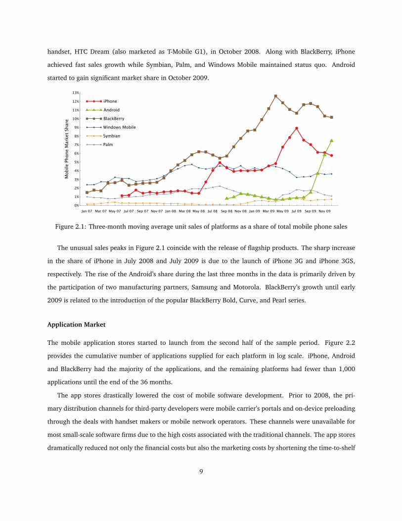
handset, HTC Dream (also marketed as T-Mobile G1), in October 2008. Along with BlackBerry, iPhone

achieved fast sales growth while Symbian, Palm, and Windows Mobile maintained status quo. Android

started to gain significant market share in October 2009.

Jan 07 Mar 07 May 07 Jul 07 Sep 07 Nov 07 Jan 08 Mar 08 May 08 Jul 08 Sep 08 Nov 08 Jan 09 Mar 09 May 09 Jul 09 Sep 09 Nov 09

13%

0%

1%

2%

3%

4%

5%

6%

7%

8%

9%

10%

11%

12%

Mob

ile P

hone

Mar

ket S

hare

iPhone

Android

BlackBerry

Windows Mobile

Symbian

Palm

Figure 2.1: Three-month moving average unit sales of platforms as a share of total mobile phone sales

The unusual sales peaks in Figure 2.1 coincide with the release of flagship products. The sharp increase

in the share of iPhone in July 2008 and July 2009 is due to the launch of iPhone 3G and iPhone 3GS,

respectively. The rise of the Android’s share during the last three months in the data is primarily driven by

the participation of two manufacturing partners, Samsung and Motorola. BlackBerry’s growth until early

2009 is related to the introduction of the popular BlackBerry Bold, Curve, and Pearl series.

Application Market

The mobile application stores started to launch from the second half of the sample period. Figure 2.2

provides the cumulative number of applications supplied for each platform in log scale. iPhone, Android

and BlackBerry had the majority of the applications, and the remaining platforms had fewer than 1,000

applications until the end of the 36 months.

The app stores drastically lowered the cost of mobile software development. Prior to 2008, the pri-

mary distribution channels for third-party developers were mobile carrier’s portals and on-device preloading

through the deals with handset makers or mobile network operators. These channels were unavailable for

most small-scale software firms due to the high costs associated with the traditional channels. The app stores

dramatically reduced not only the financial costs but also the marketing costs by shortening the time-to-shelf

9

Mar 07 Jun 07 Sep 07 Dec 07 Mar 08 Jun 08 Sep 08 Dec 08 Mar 09 Jun 09 Sep 09 Dec 09

12

0

1

2

3

4

5

6

7

8

9

10

11

log

(App

s) Palm

Windows Mobile

BlackBerry

Android

iPhone

Figure 2.2: Log of total available applications for each platform

from 68 days to 22 days and the time-to-payment from 82 days to 36 days on average (VisionMobile, 2010,

pp.19-20).8 By lowering the development costs, the app stores became a catalyst for the massive entry of

third-party developers; according to a report of a mobile application directory service, there were about

55,000 mobile developers for iPhone, iPad, and Android combined as of July 2010 (AppStoreHQ, 2010).

The same report also found that a relatively limited number of developers were publishing apps for mul-

tiple platforms. Of the 55,000 developers, the multihoming developers were about 3.2% of iOS developers9

and 13.8% of Android developers as of July 2010.

Another important feature of the application market is the consumer’s preference for variety. The top

five genres of applications ranked by total downloads were games, books, entertainment, education, and

lifestyle in iTunes App Store, which accounted for over 50% of the total downloads in May 2011 (Malik,

2011). Since consumers tend to have widely varying personal needs for these genres, large variety would be

desirable as in other software markets such as video game software and online music stores. AppStoreHQ’s

report also suggests that a wide variety of apps were consumed by the smartphone users. It found that

among the total 246,000 app installations for 5,000 randomly sampled Android users, there were 20,100

different applications (AppStoreHQ, 2011). Hence, I argue that the total number of applications in my data

is informative about how the variety of available applications affected consumer demand for smartphones.

8Apple charges $99 a year for application certification and distribution, and Android collects a one-time registration fee of $25.BlackBerry used to charge $200 as a registration fee, and additional $200 for submitting 10 apps to its app store, but it later announcedit would waive both fees in 2010.

9iOS refers to a unified family of operating systems for iPhone, iPod Touch, and iPad.

10

2.4 The Model of Two-Sided Platforms

This section describes the equilibrium framework of consumer demand, application supply, and smartphone

pricing. Given this framework, a reduced-form model will be derived so that key model parameters can be

estimated using the aggregate-level data on smartphone demand and application supply.10 I assume that in

each time period the game of smartphone pricing and app development/pricing is played in the following

sequence:

1. Smartphone firms set prices under Bertrand competition.

2. App developers make a decision on developing software for smartphone OS platforms.

3. App developers set prices under monopolistic competition.

4. Consumers receive utility from their choice of a smartphone or an outside option; smartphone firms

receive profits; app developers earn zero profit.

The smartphone firms observe all the factors determining the developers’ decisions and set the smart-

phone prices that maximize their own profits given the competitors’ prices and the developers’ best responses.

The developers are assumed to incur fixed costs for software development in each period and earn zero eco-

nomic profit in equilibrium under free entry.11 The developers choose the price of apps that maximizes their

own profits under monopolistic competition given the total number of users in each platform.

2.4.1 Consumer Demand of Smartphones

In each time period indexed by t, each consumer chooses a product j among Jt + 1 alternatives, where j

indexes a smartphone if 1 ≤ j ≤ Jt and a traditional mobile phone if j = 0. The consumer is a subscriber of

mobile phone service who owns either a traditional mobile phone or a smartphone. The consumer considers

only the presently available smartphones and their applications when making a purchase decision, not taking

into account future change in smartphone offerings and application supply.

Let Uijt represent consumer i’s utility of smartphone handset j at time t, and let gj denote the OS of

smartphone j. Then Uijt is specified as

Uijt = βgj + ~x′jtθi + USWijt + ξjt + εijt, (2.1)

10Recall that smartphone demand data is given at product level and the app supply data is at platform level.11Clements and Ohashi (2005), Nair, Chintagunta and Dubé (2004), and Dubé, Hitsch and Chintagunta (2010) used similar assump-

tions on the software market to derive a reduced-form model of application supply.

11

where βgj represents consumer-perceived brand equity of platform gj , ~xjt is the vector of product character-

istics of handset j at time t, ξjt is handset j’s time-varying product quality unobserved to the econometrician

at time t, and εijt is consumer i’s idiosyncratic taste for handset j at time t, which is assumed to follow an

extreme value distribution. USWijt is the direct utility of third-party software applications available for hand-

set j in platform gj . θi is a vector of random coefficients following a normal distribution, which allows the

researcher to account for the consumer’s unobserved heterogeneous tastes for ~xjt. Combining the random

coefficients with extreme-value distributed εijt leads to a random coefficients logit specification.

It is important to note that ~xjt includes only the product attributes searchable to consumers prior to

purchase, namely the search attributes. This allows the parameter of platform brand equity βgj to capture the

utility component that is not associated with the searchable product attributes, which would be recognized

by consumers only through the brand name associated with OS gj . Hence βgj represents overall experience

quality of OS gj such as reliability, ease of use, and security of the smartphone OS.

I specify the application utility USWijt by adopting the representative consumer approach following the

previous literature (Chou and Shy, 1990; Church and Gandal, 1992, 1993; Nair, Chintagunta and Dubé,

2004). Specifically, I use a constant elasticity of substitution (CES) utility function as

USWijt (x1gt, ..., xNgtgt, zit) =

Ngt∑k=1

(xkgt

)ab

+ zit, a ∈ (0, 1], b ∈ (0, 1), (2.2)

where g is the index of the platform of smartphone j, Ngt is the cumulative number of applications available

on platform g at time t, xkgt is the demand for software k on platform g at time t, and zit is a numéraire

capturing the value of non-software purchases. This is the utility that representative consumer i would

receive from consuming the variety of apps, (x1gt, ..., xNgtgt). The aggregate demand obtained by this CES

utility of the representative consumer is equivalent to the one generated by a discrete choice model of

individual consumers (Anderson, de Palma and Thisse, 1992, Proposition 3.8).

The representative consumer consumes xkgtNgtk=1 that maximizes the CES utility under a budget con-

straint. Hence, equilibrium application demand x∗kgtNgtk=1 maximizes

maxxkgt

Ngtk=1

USWijt (x1gt, ..., xNgtgt, zit) s.t.Ngt∑k=1

ρktxkgt + zit = yi − pjt,

where ρkt is the price of application k, yi is the income of consumer i, and pjt is the price of smartphone j at

time t. Then by the equilibrium assumption between application demand and supply, the indirect utility of

12

apps is derived as V SWijt = yi − pjt +Nγgt, where γ ∈ (0, 1).12 Instead of Nγ

gt, I use a log specification in order

to incorporate heterogeneity in the consumer preference for the applications.13

After combining all the utility components and normalizing with respect to the income and the logit error

scale, I obtain the indirect utility of smartphone j on platform gj as

Vijt = βgj + ~x′jtθi − αpjt +[γ log(Ngj ,t)− σ

]Ijt + ξjt + εijt, (2.3)

where Ijt = 1 if an app store is installed in handset j at time t and zero otherwise, and σ is a parameter that

modulates the curvature of the log function of Ngj ,t. The indirect utility of the outside option is Vi0t = εi0t.

2.4.2 Application Supply

In each period, the developers first decide whether to develop applications for each platform. Once they

choose to develop for a given platform, they set the price of each application under monopolistic competition,

taking as given the total number of users in each platform. Let ΠSWkgt be the developer’s profit from application

k on platform g at time t. Then ρ∗kt is the equilibrium price of application k at time t that maximizes the

following profit function:

ΠSWkgt =

(ρkt − cSW

)Bgtx

∗kgt − FCgt,

where ρkt is the price of application k at time t, cSW is marginal cost,14 Bgt is the user installed base (i.e., the

total current owners) of platform g at time t, x∗kgt is the equilibrium demand for application k on platform

g at time t, and FCgt is the developer’s fixed cost for providing an application which varies across platform-

months. The fixed cost is decomposed as FCgt = eFgζtηgt , where the platform-specific fixed cost Fg includes

financial and procedural costs that the developer incurs when developing and marketing applications on

platform g. Hence Fg captures the degree of platform g’s openness to the developer’s participation. ζt and

ηgt are common and platform-specific costs that vary over time, respectively.

Given the equilibrium prices ρ∗kt and the free-entry assumption, equilibrium app supply N∗gt is determined

12For details on derivation, refer to Nair, Chintagunta and Dubé (2004).13The power function specification yielded similar estimation results but with poor model fit relative to the log specification estimated

in Section 7. The full estimation result is available in the online appendix.14The marginal cost of application development is assumed to be homogeneous for lack of individual-level data on the developers,

which greatly simplifies the equilibrium price ρ∗k and thus the equilibrium app demand x∗kgt as well. The simplifying assumption isconsidered to be a reasonable approximation because the biggest source of the marginal cost was the royalty paid to the platforms,which was homogeneous across the platforms.

13

as15

logN∗gt = κ+ φ logBgt − Fg − ζt − ηgt. (2.4)

In this equation, the user installed base Bgt is a function of N∗gt in equilibrium because the developers take

into account the contemporaneous demand for the smartphones on platform g when making a development

decision. Hence Equation 4.1 is an implicit function of the equilibrium app supply N∗gt.

2.4.3 User Installed Base

To complete the specification of the application supply model, the installed base Bgt in Equation 2.4 needs

to be defined since the data on the installed bases are unavailable to the researcher. Let Mt be the size

of total mobile subscribers. To account for the replacement handset demand, I assume a homogeneous

replacement cycle of T = 24 months.16 Then the timing of smartphone replacement can be assumed to follow

an exponential distribution with mean 1/24. By the memoryless property of the exponential distribution,

the replacement rate is constant over time, and its value is r ≡ P (T ≤ 1) = 1−e−1/24 ≈ 0.04. Then platform

g’s installed base at time t is

Bgt = (1− r)Bgt−1 + rMtsgt, (2.5)

where sgt is the total market share of all smartphone handsets with OS g at time t.

2.5 Estimating the Model of Two-Sided Platforms

The previous section developed the equilibrium model of two-sided platforms, i.e., the model of smartphone

demand and application supply. In this section, I will describe empirical strategies to estimate the key

parameters of the model. The discussion of smartphone pricing is reserved for the next section where I

present the framework of brand value measurement.

15Details on the derivation are provided in Nair, Chintagunta and Dubé (2004) and Dubé, Hitsch and Chintagunta (2010).16The industry estimates the cycle to be between 18-24 months.

14

2.5.1 Identification

There are two main challenges for identifying the parameters of indirect network effects: γ in Equation 2.3

and φ in Equation 2.4. First, identifying the causal relationship can be difficult due to simultaneity between

smartphone demand and application supply, which is likely to cause endogeneity bias. To control for the

endogeneity of the application demand in Equation 2.3, I instrument for the number of apps, logNgt, with

the average product attributes in own and rival platforms that are expected to be correlated with app supply

through handset sales. The instruments are i) the average number of bluetooth-enabled devices in own

platform, ii) the average number of app-enabled devices and average camera pixels in rival platforms, and

iii) the log of average memory size in own platform interacted with a time trend and an app store dummy. I

assume that these instruments are uncorrelated with unobserved product quality ξjt following Berry (1994)

and Berry, Levinsohn and Pakes (1995). As instruments for user installed base Bgt in the app supply model

(Equation 2.4), I use the age of the latest OS versions and its quadratic term for each platform. This is

because the maturity of OS is likely to be positively correlated with user installed bases but uncorrelated

with unobserved app development costs, ζt and ηgt. However, if development costs have been declining in

the mobile software industry, they might be negatively correlated with these instruments. I address this issue

by including a time trend in the app supply model to control for the unobserved costs that are potentially

serially correlated.

The second identification issue arises because correlated unobservables may cause a potential correla-

tion between smartphone demand and application supply. Without addressing this issue, I may spuriously

find indirect network effects between smartphone demand and application supply (Gowrisankaran, Park and

Rysman, 2011). The unobservables potentially causing this spurious correlation problem include i) improve-

ments of brand equity (βg) and unobserved product quality (ξjt) in smartphone demand (Equation 2.3), and

ii) declines of unobserved app development costs (ζt and ηgt) in app supply (Equation 2.4). However, the

first drivers of the spurious correlation are unlikely to cause an identification problem for the smartphone

demand model. The parameters of indirect network effects are identified because the applications have a

universal impact on smartphone demand while the scope of the change in brand equity and unobserved

quality is limited to a single platform or a single product. Likewise, platform-specific cost changes are also

unlikely to cause the identification problem because the developer’s response to the size of user installed

bases is universal across all the platforms in the app supply model.

Nevertheless, the estimation strategy may still have a risk of spurious correlation if there is a universal

15

change in either unobserved smartphone qualities or unobserved app development costs across all products

and platforms. To address this concern, I include a time trend both in the smartphone demand and the app

supply models. Yet a change in a platform’s brand equity may contribute to the spurious correlation bias to a

certain extent if the improvement of the brand equity is highly correlated with the growth of its app supply.

To alleviate this concern, I include fixed effects for OS revisions to account for the improvement of platform

brand equities.

The price coefficient in the demand model may be biased if potential price endogeneity is ignored. I use

the instruments proposed by Berry, Levinsohn and Pakes (1995), which include the sum of handset ages and

the total number of app-enabled devices for a given firm. I also include a cost-related instrument, which is

an indicator variable for whether each smartphone is sold via a corresponding mobile carrier’s distribution

channel. This is a proxy for mobile network carrier’s subsidy, which is unobserved to the researcher.

Finally, the price coefficient may be biased if consumers’ forward-looking behavior is ignored.17 To ac-

count for the consumer dynamics, I adopt a simple reduced-form approach rather than developing a fully

structural model.18 Specifically I use handset age (the number of months elapsed since launch) as a proxy

variable to capture the option value of waiting for future products.19 Approximating the future utility com-

ponent with a simple reduced-form function has been proposed in the previous literature.20 Though it is not

perfect, Lou, Prentice and Yin (2011) found that this simple approach reduced the bias in the static demand

model.

2.5.2 Estimation Method

I estimate the smartphone demand and the app supply models separately following Nair, Chintagunta and

Dubé (2004) and Song (2011). I estimate the smartphone demand using Berry, Levinsohn and Pakes’s

(1995) instrumental variables method based on the generalized method of moments (GMM) approach. The

variables in the demand model include platform brand dummies, hardware attributes including price, fixed

effects for network carriers and OS revisions, a time trend, and the age of handsets since launch.21 The

17The assumption of static consumer demand may be violated for two reasons. First, the consumer’s dynamic purchase behavior mayarise from the durable-good nature of smartphones and rapid technological innovations. Second, potential smartphone buyers are likelyto compare the trade-off between purchasing a currently available product in the present and waiting for lowered price or improvedquality that will become available in the future.

18Full-structural modeling approach would require information on ownership changes across all platforms over time. Without thisinformation, identification will have to rely on strong assumptions on the replacement behavior.

19While more accurate proxy for the option value would also involve each age of all available handsets, including them all wouldbe infeasible due to the large number of handsets. Hence I assume that the the age of a firm’s own handset is a reasonable first-orderapproximation to the option value of waiting.

20See Geweke and Keane (2000), Carranza (2010), Lou, Prentice and Yin (2011), and Ching, Erdem and Keane (2011).21Fixed effects for smartphone hardware manufacturers were estimated insignificant and thus are not reported in the chapter.

16

unobserved time-varying quality ξjt is assumed to be mean independent of these characteristics, such that

GMM moment condition can be constructed as G(θ0) = E[Zjtξjt] = 0, where Zjt is the vector of price and

application instruments for handset j at time t, and θ0 is the vector of true model parameters.

I obtain the GMM estimator by minimizing the objective function g(θ)′Wg(θ), where g(θ) is the sample

analog of G(θ), and W is an optimal GMM weight matrix. The estimation is done in a nested procedure.

In the inner loop, the estimate of ξ = ξjtj,t is obtained for a given θ by matching each product’s market

share predicted at given parameter values with the observed share. The outer loop algorithm searches over θ

that minimizes the objective function evaluated in the inner loop.22 I use 200 Halton draws for Monte Carlo

integration to compute the predicted market shares. For the weight matrix W , I use the heteroscedasticity

and autocorrelation robust covariance estimator of Newey and West (1987).

2.6 Measuring the Brand Value of Two-Sided Platforms

2.6.1 Framework

This section outlines the framework for measuring the brand value of two-sided platforms from the per-

spective of smartphone handset producers. As mentioned in Section 4, the smartphone producers set prices

under Bertrand competition, taking into account the subsequent response of the app developers. Hence the

smartphone vendors internalize the response of developers to their pricing decision.

To specify the smartphone producer’s profit function, suppose the firm produces a single product indexed

by j among J alternatives. Let pj denote the price of handset j, Ng the total number of applications supplied

to platform g among G operating systems, cj the marginal cost of handset j, and βg the brand equity of

OS platform g built into product j. β and N are G-dimensional vectors of brand equities and app supplies,

respectively, and p is a J -dimensional vector of prices. Let Dj(β,p,N) be the demand for product j as a

function of brand equities, prices, and app supplies.23 Then the producer of handset j chooses price pj to

maximize a per-period profit specified as

Πj(β,p,N(β,p)) = (pj − cj)Dj(β, pj ,p−j ,N(β,p)), (2.6)

given brand equities β and prices of competing handsets p−j . It is worth noting that the app supply itself is

22The convergence threshold for the inner and the outer loops are 10−13 and 10−8, respectively.23Other product characteristics are omitted deliberately to simplify the notation.

17

a function of brand equities and prices in equilibrium, i.e., N = N(β,p).

The two-sided market framework requires that the app supply is in an equilibrium relationship with

the handset demand. Hence equilibrium pair (p∗,N∗) satisfies not only that p∗ simultaneously maximizes

Equation 2.6 for all j = 1, ..., J , but also that N∗ satisfies the equilibrium condition in Equation 2.4 given

p∗.

Suppose product j is the only product available in platform g. Then brand value can be expressed as

Πj(βg,β−g,p∗,N∗)−Πj(0,β−g, p

∗, N∗),

where (p∗,N∗) is the observed market equilibrium of prices and application supplies, and (p∗, N∗) is a new

equilibrium pair under the counterfactual scenario that platform g’s brand equity is lost (βg = 0). The loss of

brand equity in the two-sided market causes not only the firms to adjust their prices but also the developers

to respond accordingly, resulting in the new equilibrium pair (p∗, N∗). The brand value measure therefore

represents the profit premium for handset maker j in equilibrium that can be attributed solely to platform

g’s brand equity. Hence the brand value measure takes into account the changes in not only consumers’

brand choices but also smartphone producers’ pricing strategies and the developers’ application supplies in

equilibrium.

The reaction of the application developers is the characteristic that distinguishes the platform-centric

smartphone market from the traditional one-sided smartphone market prior to the arrival of the app stores.

I measure the impact of the transition from one-sided to two-sided platforms on brand values by taking the

following difference:

[Πj(βg,β−g,p

∗,N∗)−Πj(0,β−g, p∗, N

∗)]−[Πj(βg,β−g,p

∗0,N

∗0 = 0)−Πj(0,β−g, p

∗0, N

∗0 = 0)

].

In the above expression, (p∗,N∗) and (p∗, N∗) are the equilibrium pairs with all the app stores present, and

(p∗0,N∗0) and (p∗0, N

∗0) are the equilibrium pairs under the counterfactual scenario that eliminates the entire

app suppliers from all platforms. Hence the first bracketed term captures the brand value for a two-sided

platform, while the second bracket represents the counterfactual brand value for a one-sided platform that

has no applications. With this measurement approach, I evaluate the app stores’ impact on the value of the

platform brands.

18

2.6.2 Measurement Procedure

Once the parameters in the model of two-sided platforms are estimated, the next step in measuring brand

values is to compute the marginal cost cj in the smartphone producer’s profit function (Equation 2.6). Nevo

(2001) and Goldfarb, Lu and Moorthy (2009) use the first-order condition to recover the marginal costs. I

apply their approach to the setting of two-sided platforms by taking into account the simultaneity between

smartphone prices and application supplies.

Given knowledge of the demand system D(·) and the marginal costs, I solve for equilibrium prices and

application supplies under counterfactual brand equity β. Because the equilibrium price-application pair can

only be expressed as implicit functions, I develop a nested fixed point algorithm to solve for the equilibrium

prices and application supplies simultaneously. The technical details of computing the marginal costs and

the equilibrium solutions are provided in the online appendix.

2.7 Estimation Results

2.7.1 Consumer Demand

Table 2.2 presents the estimation results of the smartphone demand model in Equation 2.3. The first column

(Logit) and the second column (Logit-IV) estimate the same simple logit model using ordinary least squares

and instrumental variables regressions, respectively. From the second column to the last, I control for the

endogeneity of prices and log(apps) using the same set of instruments throughout the columns.24 Prices

are normalized by Consumer Price Index to the hundreds of dollars in January 2007. From the third to the

fifth columns (RCL I–III), I estimate random coefficients logit models instrumenting for prices and log(apps).

In Columns RCL II and RCL III, I include fixed effects for major OS revisions. The coefficient estimates for

searchable product attributes are not reported in the table but are available in the appendix.

The first two columns, Logit and Logit-IV, yield different coefficient estimates for price and log(apps).

Both coefficients become smaller as the potential endogeneity is controlled for in the Logit-IV column. This

result is consistent with the concern that prices and apps may be positively correlated with unobserved

product quality. On the other hand, the coefficient estimate for app store dummy (σ) indicates that having

excessively small collection of apps may hurt smartphone sales.

Columns RCL I–III include random coefficients for two product attributes: touchscreen and app store

24For this reason, Column Logit-IV may have rejected the test of overidentifying restrictions.

19

Logit Logit-IV RCL I RCL II RCL IIIObservations = 2,737 Estimate s.e. Estimate s.e. Estimate s.e. Estimate s.e. Estimate s.e.

Price / CPI ($100) -0.0005*** 0.0001 -0.0046*** 0.0006 -1.4441*** 0.3508 -1.4105*** 0.3554 -1.3091*** 0.3258log(Apps) 0.0016*** 0.0002 0.0012*** 0.0003 0.5712** 0.2221 0.4472** 0.2248 0.3931 0.2472Appstore enabled (σ) 0.0100*** 0.0012 0.0068*** 0.0022 6.4193*** 2.3050 5.7081** 2.2676 4.9551** 2.5094

Brand EquitiesiPhone 0.0018*** 0.0010 0.0123*** 0.0021 -6.4259*** 1.0473 -7.0806*** 1.0845 -6.9478*** 1.0662Android -0.0098*** 0.0011 -0.0058*** 0.0018 -8.8064*** 0.8023 -8.4591*** 0.8353 -8.4195*** 0.8249BlackBerry 0.0020*** 0.0005 0.0067*** 0.0010 -6.0773*** 0.5016 -6.0114*** 0.5278 -6.1351*** 0.4994Windows 0.0003 0.0005 0.0045*** 0.0010 -6.6524*** 0.5333 -6.5931*** 0.5589 -6.7356*** 0.5195Symbian -0.0008 0.0006 0.0060*** 0.0013 -6.8822*** 0.7036 -7.7181*** 0.6174 -7.7898*** 0.5562Palm 0.0005 0.0005 0.0061*** 0.0012 -5.8483*** 0.6533 -5.8406*** 0.6710 -6.0588*** 0.6251

OS Version Fixed EffectsiPhone 3.0 1.5949** 0.6352 1.4221** 0.5922Android 2.0 0.0057 0.7621BlackBerry 4.2+ -0.0534 0.2044BlackBerry 5.0 -0.7684* 0.4576Windows 6.1 -0.2692 0.2556Windows 6.5 -0.7433 0.6299Symbian 9 1.0567* 0.6094 0.8589 0.5705Palm WebOS 0.2984 0.9458

Standard Deviation of Random CoefficientsTouchscreen 3.3643*** 0.8504 4.0574*** 0.8855 3.8063*** 0.8836Appstore enabled 4.3522*** 1.0446 4.5568*** 1.0440 4.1204*** 1.1297

R2 0.5861 0.2527F 174.7265 96.9013nχ2 54.906 4.267 4.780 6.893p-value <0.001 0.234 0.188 0.075

***: p < 0.01; **: p < 0.05; *: p < 0.1.Utility for traditional mobile phones is normalized to zero up to logit error.

Table 2.2: Estimation of logit models of smartphone handset demand

dummy. I exclude the random coefficient for price because its estimate was negligible and insignificant.25

Including the random coefficients changes the ordering of the brand equity estimates obtained in the Logit-IV

column; while iPhone has higher brand equity than BlackBerry in Logit-IV, the rank of iPhone’s brand equity

falls to the third place in RCL I. The change in the iPhone brand equity suggests that it had relatively more

sales than other platforms from those consumers with high valuation of a touchscreen and an app store.

On the other hand, with the inclusion of the random coefficients, all the signs of the brand equities become

negative. However, this does not imply that the brand equities are nonexistent because they are identified

only up to relative levels and the mean utility for outside option is normalized to zero.

Column RCL II adds fixed effects for two major OS revisions, iPhone OS 3.0 and Symbian 9, in order

to address the spurious correlation problem driven by unobserved OS quality improvements. The estimates

of both fixed effects are large and significant at 10% level while they decrease iPhone’s brand equity from

-6.42 to -7.08 and Symbian’s from -6.88 to -7.71. This indicates that both iPhone and Symbian considerably

improved their brand equities by releasing major OS software upgrades, which appears to be consistent with

25Estimation results with the random coefficient for price are available in the online appendix.

20

the growth of their market shares as shown in Figure 2.1. Despite the change in brand equities, the brand

equity ranking remains unchanged among the three platforms in focus; BlackBerry has the highest brand

equity while Android has the lowest, and iPhone is ranked in between the two.

In addition, the inclusion of the OS revision fixed effects reduces the coefficient of log(apps) from 0.571

to 0.447 in the RCL II column although it remains significant. The decrease in the log(apps) coefficient

implies that if the model fails to account for the OS quality improvements, it would attribute their effects

on smartphone demand to the consumer’s valuation of apps, leading to the overestimation of the log(apps)

coefficient.

The brand equity estimates in the RCL II column are robust to the inclusion of additional OS revision fixed

effects in RCL III. Even though I include six additional fixed effects for major revisions of other platforms,

they do not significantly alter the brand equity estimates obtained in the RCL II column. The RCL III result

also shows that although the added fixed effects decrease the log(apps) coefficient further from 0.447 to

0.393, all of their estimates are insignificant, and the model rejects the test of overidentifying restrictions at

10% level (p = 0.075). This contrasts with the RCL II result, which has the p-value of 0.188. Hence I use the

brand equity estimates in RCL II to compute the brand values in Section 8.

2.7.2 Application Supply

Table 2.3 reports the estimation results for the application supply model in Equation 2.4. The development

cost for iPhone is normalized to zero. The first and the second columns estimate the app supply model by

ordinary least squares (OLS I–II), and the third column (IV) uses instrumental variables regression to control

for the endogeneity in log(installed base).

In the OLS I column, the estimates for the log fixed costs of application development are high for Windows

Mobile and BlackBerry, low for Android, and moderate for Palm. While Android has only slightly higher

fixed cost than iPhone, the difference is insignificant. The positive and significant coefficient estimate of

log(installed base) confirms the developers’ positive valuation of the size of user installed bases. The strongly

positive coefficient of the time trend, Month, is consistent with the conjecture that application development

costs may have been in decline in the industry as the time trend variable captures the negative time-varying

costs of application development.

In OLS II, dropping Android’s fixed cost improves the precision of the installed base coefficient estimate

considerably (from 0.341 to 0.068) while it slightly reduces the log(installed base) coefficient. Without

21

OLS I OLS II IVDep. Var: log(apps) Parameter Std. Error Parameter Std. Error Parameter Std. Error

log(Installed Base) 1.506*** 0.341 1.224*** 0.068 1.330*** 0.103Month 0.130*** 0.033 0.161*** 0.014 0.153*** 0.018Constant -16.899*** 4.459 -13.382*** 1.005 -14.690*** 1.274

log(Fixed Cost of App Development)Android 0.610 0.726BlackBerry 4.464*** 0.224 4.343*** 0.142 4.505*** 0.198Windows Mobile 5.213*** 0.236 5.421*** 0.154 5.469*** 0.172Palm 2.413** 1.004 3.234*** 0.287 3.045*** 0.320

Observations 52 52 52Instruments No No YesOverid test (p-value) – – 0.574R2 0.972 0.971 0.969F 326.79 363.58 249.89

***: p <0.01; **: p <0.05; *: p <0.1.iPhone’s development cost is normalized to zero.

Table 2.3: Estimation of application supply model

Android’s fixed cost, all the parameters become significant at 1% level, but the fixed costs for other platforms

are similar to those in the OLS I column.

The IV regression in the IV column yields fixed cost estimates similar to those obtained in the OLS II

column. However, I obtain a slightly higher coefficient estimate for log(installed base) than the one in the

OLS II column. This result is counterintuitive because the coefficient would be overestimated under potential

endogeneity. One possible explanation is that as the observed factors explain most of the variation in the

application supply as seen in the high R2, the potential omitted-variable bias may not be as significant as

in the smartphone demand estimation. Nonetheless, the IV regression yields similar fixed cost estimates as

obtained in the OLS II column and does not reject the test of overidentifying restrictions at 10% level.

The overall estimation results of the application supply model show that iPhone and Android were the

most open to developer participation while BlackBerry and Windows Mobile were the least accessible plat-

forms. Palm was relatively favorable to developer participation although not as much as the two leading

platforms. Given the estimates, the next section analyzes how consumer brand equities and app develop-

ment costs contributed to generating different outcomes for the brand values of iPhone, BlackBerry, and

Android.

22

2.8 Analysis of Brand Values

2.8.1 Brand Values

In this section, I estimate the brand values of iPhone, BlackBerry, and Android. As described in Section

6, I measure the brand values by taking the difference in profits between the observed equilibrium and a

counterfactual equilibrium under the scenario that the brand equity is lost to the level of a baseline brand.

Nokia’s Symbian is chosen as the baseline brand for the analysis because its lowest brand equity (excluding

Android) offers a natural benchmark for the brand value measurement. This requires a different approach

to measuring Android’s brand value, which is discussed later in this section.

Jan07 Mar07 May07 Jul07 Sep07 Nov07 Jan08 Mar08 May08 Jul08 Sep08 Nov08 Jan09 Mar09 May09 Jul09 Sep09 Nov09

180

0

20

40

60

80

100

120

140

160

Month

$ m

illio

n

Profit attributable to brand equity

Profit without brand equity

App Store Launch

Figure 2.3: The value of iPhone brand

Figure 2.3 displays two profit curves; the upper curve is the original profit estimate for Apple in the

observed equilibrium, and the lower curve is the counterfactual profit with iPhone’s brand equity replaced

by the reference brand’s. The gap between the two curves represents iPhone’s brand value, i.e., the profits

generated by iPhone’s brand equity over time. With the arrival of the app store in July 2008, iPhone’s brand

value starts to grow over time both in absolute size and in relative proportion to the original profit. This

result suggests that iPhone’s app store may have had a positive impact on its brand value.

The same plot is obtained for BlackBerry in Figure 2.4. First, the overall size of the brand value is larger

than iPhone’s, whether in absolute size or in relative proportion to total profits. This result is not surprising

because BlackBerry has the highest brand equity among the three platforms. The second key difference

from the previous figure is that BlackBerry’s brand value appears to be relatively unaffected by the app

23

Jan07 Mar07 May07 Jul07 Sep07 Nov07 Jan08 Mar08 May08 Jul08 Sep08 Nov08 Jan09 Mar09 May09 Jul09 Sep09 Nov09

180

0

20

40

60

80

100

120

140

160

Month

$ m

illio

n

Profit attributable to brand equity

Profit without brand equity

App Store Launch

Figure 2.4: The value of BlackBerry brand

store although there is marginal growth in the brand value after the app store launch. Considering the high

development cost for the BlackBerry apps, their contribution to the brand value may have been limited by

the platform’s lack of accessibility for the BlackBerry developers.

In contrast to the two platforms, Android’s brand value needs to be computed in a different way because

its brand equity estimate is even lower than the benchmark brand’s. Hence I increase Android’s brand equity

to the level of Symbian’s because there is no such alternative reference as a generic brand in the consumer

packaged goods market. Even though measuring Android’s brand value needs a counterintuitive approach,

it still deals with the same question of how much consumer brand equity is worth to Android smartphone

producers, for brand value is fundamentally a relative construct.

Jan07 Mar07 May07 Jul07 Sep07 Nov07 Jan08 Mar08 May08 Jul08 Sep08 Nov08 Jan09 Mar09 May09 Jul09 Sep09 Nov09

180

0

20

40

60

80

100

120

140

160

Month

$ m

illio

n

App Store Launch

Profit attributable to (counterfactual) brand equity

Original profit

Figure 2.5: The value of Android brand

24

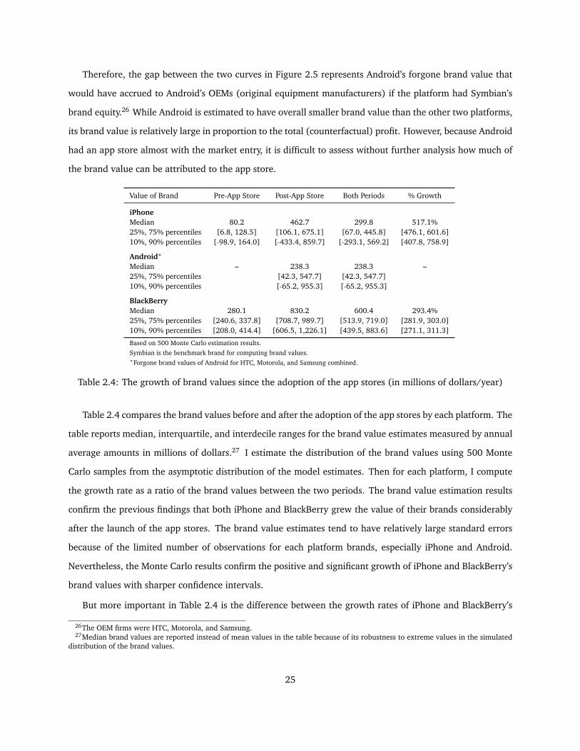
Therefore, the gap between the two curves in Figure 2.5 represents Android’s forgone brand value that

would have accrued to Android’s OEMs (original equipment manufacturers) if the platform had Symbian’s

brand equity.26 While Android is estimated to have overall smaller brand value than the other two platforms,

its brand value is relatively large in proportion to the total (counterfactual) profit. However, because Android

had an app store almost with the market entry, it is difficult to assess without further analysis how much of

the brand value can be attributed to the app store.

Value of Brand Pre-App Store Post-App Store Both Periods % Growth

iPhoneMedian 80.2 462.7 299.8 517.1%25%, 75% percentiles [6.8, 128.5] [106.1, 675.1] [67.0, 445.8] [476.1, 601.6]10%, 90% percentiles [-98.9, 164.0] [-433.4, 859.7] [-293.1, 569.2] [407.8, 758.9]

Android∗

Median – 238.3 238.3 –25%, 75% percentiles [42.3, 547.7] [42.3, 547.7]10%, 90% percentiles [-65.2, 955.3] [-65.2, 955.3]

BlackBerryMedian 280.1 830.2 600.4 293.4%25%, 75% percentiles [240.6, 337.8] [708.7, 989.7] [513.9, 719.0] [281.9, 303.0]10%, 90% percentiles [208.0, 414.4] [606.5, 1,226.1] [439.5, 883.6] [271.1, 311.3]

Based on 500 Monte Carlo estimation results.Symbian is the benchmark brand for computing brand values.∗Forgone brand values of Android for HTC, Motorola, and Samsung combined.

Table 2.4: The growth of brand values since the adoption of the app stores (in millions of dollars/year)

Table 2.4 compares the brand values before and after the adoption of the app stores by each platform. The

table reports median, interquartile, and interdecile ranges for the brand value estimates measured by annual

average amounts in millions of dollars.27 I estimate the distribution of the brand values using 500 Monte

Carlo samples from the asymptotic distribution of the model estimates. Then for each platform, I compute

the growth rate as a ratio of the brand values between the two periods. The brand value estimation results

confirm the previous findings that both iPhone and BlackBerry grew the value of their brands considerably

after the launch of the app stores. The brand value estimates tend to have relatively large standard errors

because of the limited number of observations for each platform brands, especially iPhone and Android.

Nevertheless, the Monte Carlo results confirm the positive and significant growth of iPhone and BlackBerry’s

brand values with sharper confidence intervals.

But more important in Table 2.4 is the difference between the growth rates of iPhone and BlackBerry’s

26The OEM firms were HTC, Motorola, and Samsung.27Median brand values are reported instead of mean values in the table because of its robustness to extreme values in the simulated

distribution of the brand values.

25

brand values. iPhone, despite having smaller brand value than BlackBerry, achieved 517% growth while

BlackBerry’s brand value grew only 293%. Considering the low development cost of the iPhone apps, this

result suggests that platform openness to developers may have been the key factor for the brand value growth

since the adoption of the app stores.

The value of the Android brand in Table 2.4 represents the forgone brand value combined across all the

OEMs. Android had only one month of sales prior to the app store opening, which is omitted in the table

because Android’s first-month sales do not appear to have been of a full month in the data judging from the

negligible volume.

2.8.2 Impact of App Stores on Brand Values

Given the brand value estimates, I examine the impact of the app stores on the brand values by conducting

a counterfactual experiment in which none of the platforms adopted an app store.

Jan07 Mar07 May07 Jul07 Sep07 Nov07 Jan08 Mar08 May08 Jul08 Sep08 Nov08 Jan09 Mar09 May09 Jul09 Sep09 Nov09

120

0

10

20

30

40

50

60

70

80

90

100

110

Month

$ m

illio

n

App Store Launch

Brand value attributable to app stores

Brand value without app stores

Figure 2.6: App stores’ impact on iPhone’s brand value

Figure 2.6 compares iPhone’s brand values in two market equilibria. The upper curve represents iPhone’s

brand value in the observed equilibrium, and the lower curve corresponds to the brand value in a counter-

factual equilibrium where there exists none of the app stores in the market. Hence the area between the two

curves captures iPhone’s brand value that can be attributed to the app store.

Immediately after the launch of iPhone’s app store, it has a slightly negative impact on the brand value

because the consumers had negative valuation of the app store that had few apps available. Nonetheless,

after a couple of months, the app store begins to contribute to the brand value substantially, both in absolute

26

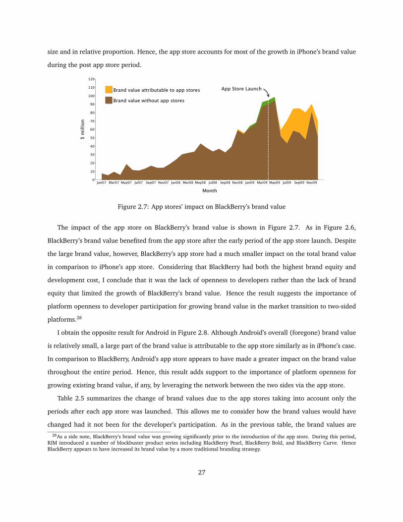
size and in relative proportion. Hence, the app store accounts for most of the growth in iPhone’s brand value

during the post app store period.

Jan07 Mar07 May07 Jul07 Sep07 Nov07 Jan08 Mar08 May08 Jul08 Sep08 Nov08 Jan09 Mar09 May09 Jul09 Sep09 Nov09

120

0

10

20

30

40

50

60

70

80

90

100

110

Month

$ m

illio

nBrand value attributable to app stores

Brand value without app stores

App Store Launch

Figure 2.7: App stores’ impact on BlackBerry’s brand value

The impact of the app store on BlackBerry’s brand value is shown in Figure 2.7. As in Figure 2.6,

BlackBerry’s brand value benefited from the app store after the early period of the app store launch. Despite

the large brand value, however, BlackBerry’s app store had a much smaller impact on the total brand value

in comparison to iPhone’s app store. Considering that BlackBerry had both the highest brand equity and

development cost, I conclude that it was the lack of openness to developers rather than the lack of brand

equity that limited the growth of BlackBerry’s brand value. Hence the result suggests the importance of

platform openness to developer participation for growing brand value in the market transition to two-sided

platforms.28

I obtain the opposite result for Android in Figure 2.8. Although Android’s overall (foregone) brand value

is relatively small, a large part of the brand value is attributable to the app store similarly as in iPhone’s case.

In comparison to BlackBerry, Android’s app store appears to have made a greater impact on the brand value

throughout the entire period. Hence, this result adds support to the importance of platform openness for

growing existing brand value, if any, by leveraging the network between the two sides via the app store.

Table 2.5 summarizes the change of brand values due to the app stores taking into account only the

periods after each app store was launched. This allows me to consider how the brand values would have

changed had it not been for the developer’s participation. As in the previous table, the brand values are28As a side note, BlackBerry’s brand value was growing significantly prior to the introduction of the app store. During this period,

RIM introduced a number of blockbuster product series including BlackBerry Pearl, BlackBerry Bold, and BlackBerry Curve. HenceBlackBerry appears to have increased its brand value by a more traditional branding strategy.

27

Jan07 Mar07 May07 Jul07 Sep07 Nov07 Jan08 Mar08 May08 Jul08 Sep08 Nov08 Jan09 Mar09 May09 Jul09 Sep09 Nov09

120

0

10

20

30

40

50

60

70

80

90

100

110

Month

$ m

illio

n

Brand value attributable to app stores

Brand value without app store

App Store Launch

Figure 2.8: App stores’ impact on Android’s brand value

converted into annual average amounts in millions of dollars, and Android’s brand values represent the

forgone brand values for the three handset manufacturers.

The results in Table 2.5 are consistent with the previous figures. First, the app stores helped growing

the brand values for all three platforms. The growth rate of the brand values ranges from 15.9% to 96.0%.

This result provides supporting evidence for the positive effect of the app stores for all three brands. Second,

iPhone increased its brand value by virtue of the app store substantially more than BlackBerry did, despite

having much less brand equity than BlackBerry. iPhone’s app store accounts for 96% of the brand value

growth ($173 million), which is considerably higher than the 15.9% growth ($110 million) for BlackBerry’s

brand value. Although BlackBerry possessed the most valuable brand worth $712 million even without the

apps, the high development cost for the BlackBerry developers limited the growth of BlackBerry’s brand

value. Hence platform openness, rather than consumer brand equity, was a more critical factor in leveraging

the two-sided network for growing brand value. This finding is further confirmed by the growth rate of

Android’s brand value, which was only 48.2% but still higher than BlackBerry’s. On the other hand, this

result also implies that Android would not have lost the opportunity to achieve substantial growth in brand

value with its open platform if only it had brand equity at least on par with the reference brand’s. Hence,

the result demonstrates that leveraging the two-sided network in a platform is likely to be successful only if

it has established a certain level of brand equity on the consumer side.

28

Brand Value Brand Value Change of % Increase ofw/o App Stores w/ App Stores Brand Value Brand Value

iPhoneMedian 195.4 462.7 173.7 96.0%25%, 75% percentiles [18.1, 378.1] [106.1, 675.1] [27.0, 319.7] [37.2, 181.7]10%, 90% percentiles [-222.5, 556.7] [-433.4, 859.7] [-224.1, 461.9] [0.4, 270.3]

Android∗

Median 155.3 238.3 58.6 48.2%25%, 75% percentiles [31.0, 327.2] [42.3, 547.7] [-0.2, 204.0] [14.8, 92.3]10%, 90% percentiles [-47.5, 524.9] [-65.2, 955.3] [-16.4, 497.0] [-2.6, 146.8]

BlackBerryMedian 712.4 830.2 110.3 15.9%25%, 75% percentiles [602.9, 871.5] [708.7, 989.7] [75.0, 150.9] [10.2, 21.6]10%, 90% percentiles [519.0, 1,048.9] [606.5, 1,226.1] [30.9, 192.1] [4.4, 26.9]

Symbian is the benchmark brand for computing brand values.∗Forgone brand values of Android for HTC, Motorola, and Samsung combined.

Table 2.5: The contribution of app stores to brand values (in millions of dollars/year)

2.8.3 Do App Stores Always Increase Brand Values?

Through the analysis of the brand values so far, I have reached two main conclusions: 1) the app stores

benefited the value of all three platform brands, and 2) platform openness to developers was a critical factor

in brand value growth for the platforms adopting the app stores. The second conclusion would be invalid if

a demand-side factor, namely the heterogeneity in consumer preference for apps between different platform

users, caused the difference in the app stores’ contribution to the brand values. For example, if the iPhone

users valued smartphone apps more than the BlackBerry users did, I would have still obtained the same

results as shown in Table 2.5. To test this alternative explanation, I estimate various smartphone demand

models that allow heterogeneous preference for apps across different platform users. However, the results

indicate that the data does not support the heterogeneity across the platform users at least at the aggregate

level.29

On the other hand, the first conclusion would be trivial if the consumers’ positive valuation of the applica-

tions simply implies the apps’ beneficial effect on the brand values. Hence I conduct another counterfactual

experiment to explore whether different implementation of the app stores could have resulted in a different

outcome. Specifically I simulate a scenario that iPhone had the same high development cost as BlackBerry

by increasing iPhone’s fixed cost Fg in Equation 2.4 up to the level of BlackBerry’s. This experiment can also

be considered as a robustness test for the second conclusion because if the different brand value growth was

driven by the factors other than the development costs in Table 2.5, the result should remain the same under

29The estimation results are available in the appendix.

29

the counterfactual scenario.

Brand Value Brand Value Change of % Increase ofw/o App Stores w/ App Stores Brand Value Brand Value

iPhoneMedian 194.6 56.5 -99.4 -45.3%25%, 75% percentiles [19.1, 379.8] [-33.9, 228.5] [-145.5, -37.4] [-72.1, -21.2]10%, 90% percentiles [-216.5, 561.3] [-174.8, 438.9] [-191.0, 53.0] [-105.3, 1.0]

Android∗

Median 153.8 258.6 69.2 71.0%25%, 75% percentiles [28.6, 326.2] [21.6, 665.4] [-19.7, 240.0] [19.1, 121.9]10%, 90% percentiles [-49.1, 523.5] [-101.0, 976.3] [–72.8, 507.2] [-23.5, 202.0]

BlackBerryMedian 717.6 872.6 153.2 21.4%25%, 75% percentiles [605.9, 876.5] [735.8, 1,063.9] [111.5, 204.5] [16.0, 27.3]10%, 90% percentiles [520.9, 1,050.4] [626.3, 1,279.3] [72.1, 264.2] [10.6, 33.2]

Symbian is the benchmark brand for computing brand values.∗Forgone brand values of Android for HTC, Motorola, and Samsung combined.

Table 2.6: The contribution of app stores to brand values when iPhone has the same fixed cost as BlackBerry(in millions of dollars/year)

Table 2.6 shows that iPhone’s app store, if without the developer’s easy access to the platform, could have

been detrimental to its brand value. The model predicts that given the high cost of app supply, iPhone would

have attracted only a small number of apps and the poor app collection would have reduced the sales of its

smartphones, resulting in the decline of the brand value by 45.3% compared to its brand value without the

app stores. At the same time, the consumers would have chosen the two rival platforms instead of iPhone,

boosting their brand values even further compared to the original brand values in Table 2.5; if iPhone lost

its openness, Android’s brand value would have increased from $238 million to $258 million, and Black-

Berry’s brand value from $830 million to $872 million. Hence, without providing the developers easy access,

iPhone’s app store would have lost attractiveness to the developers, thus losing the brand value as well. On

the contrary, it is worth noting that BlackBerry was still able to gain additional brand value even with the

same closed app store. Because BlackBerry has already established a large user base, the developers still

found BlackBerry’s software market sufficiently attractive despite its cost disadvantage. However, because

iPhone was a relatively new entrant without having such a large installed base, it would have been difficult

for the developers to justify the high cost for the iPhone app development.

30

2.9 Limitations and Future Research

Some of the limitations in this chapter can be addressed with richer data. More flexible consumer hetero-

geneity in the preference for apps can be incorporated in the model if data on consumer demographics or

individual-level purchase history are available. Likewise, the simplifying assumptions on the developer’s

profit function can be relaxed if individual-level data on the developers become available.

I chose to impose a static pricing assumption on the competition between the smartphone vendors due

to the lack of data on smartphone marginal costs. Without such information, estimating margins and brand

values would be infeasible in a dynamic-pricing game framework because there are no first-order conditions

to exploit as in the Bertrand competition.30 On the other hand, violation of the static-pricing assumption has

ambiguous implications on the marginal cost estimates. Consumer heterogeneity provides an incentive for

firms to engage in intertemporal price discrimination while network effects create an incentive for penetra-

tion pricing. However, unless each platform has a different incentive for the two pricing strategies, the main

result, which is about the app stores’ contribution to the brand values, is likely to remain unchanged.

This chapter does not take into account the market’s expectation about the long-run outcomes of the

competition. Forward-looking consumers and developers may join the most popular platform that is expected

to attract the largest installed bases in the future. If this is the case, then app stores’ impact on brand value

may have been underestimated for the iPhone platform. This is because the brand equity loss of a market-

leading platform may result in losing dominance in the developer side as well due to brand equity’s second

order effect on brand value via market expectations. However, the implication for other platforms is unclear

and warrants future research.

2.10 Conclusion

This chapter examines the impact of app stores on the value of three OS platform brands: iPhone, Android,

and Blackberry. The results suggest that the app stores significantly contributed to the growth in brand values

of all three platforms, while there exists a substantial variation in the degree of brand value growth. Despite

possessing lower consumer brand equity than BlackBerry, iPhone was able to increase the brand value more30To account for the dynamic pricing, other researchers used external information sources to fit a marginal cost function separately

(Liu, 2010) or included a time trend in the profit function to capture the time-varying marginal cost parsimoniously (Dubé, Hitschand Chintagunta, 2010). While Liu (2010) had to collect the marginal cost information for only two products, this study requirestracking over 150 products. Moreover, it would be impossible to identify the time-varying product-specific marginal costs withoutstrong assumption driving the result. Although the difficulty of estimating the marginal cost can be alleviated by assuming constantmarginal costs, this assumption would be too restrictive, considering the rapidly declining trend of the costs over time in the smartphonemarket. Therefore, I chose to use the static framework for modeling the pricing strategy.

31

effectively than BlackBerry by virtue of its openness to developers. Conversely, BlackBerry achieved only

limited brand value growth even with the largest consumer brand equity due to the lack of openness. In

contrast, because Android had little brand equity established in the consumer side, it had to forgo the

opportunity to grow the brand value considerably, which was made available by its open app store. These

core findings can be summarized as follows: providing developers with an open platform is the key to growing

brand value by leveraging the two-sided network in a platform, but only if it has built brand equity enough to

attract consumers. Finally, this chapter also shows that the beneficial effect of the app stores is not trivial, for

iPhone would have lost the brand value by becoming a two-sided platform without the openness of its app

store.

By studying the smartphone market, this chapter answers how the value of the OS brands was influenced

by the market transition from one-sided to two-sided platforms. It provides a balanced view of the impor-

tance of the consumer’s and the developer’s participation for building the value of platform brands. In this

sense, my findings are consistent with Shapiro and Varian’s (1999) view that “a superior technology is not

enough to win.” The lesson from the findings is that open platform strategy is vital to the success of platform

branding, especially for those new entrants that do not possess large user bases. Hence this study contributes

to the understanding of how a two-sided platform strategy contributed to the rise of the new OS brands in

the early smartphone market.

32

Chapter 3

A Computationally Efficient Fixed Point

Approach to Structural Estimation of

Aggregate Demand

This chapter solves an estimation problem that is likely to arise when the static framework of consumer

demand in Chapter 2 is extended to incorporate dynamics. Estimating dynamic demand models can be

computationally challenging, especially if data is available only at an aggregate level. Hence, this chapter

develops a computational approach that will be useful for measuring brand values in dynamic frameworks.1

3.1 Introduction

In the structural demand estimation literature, there is a growing demand for a more computationally ef-

ficient strategy for estimating dynamic structural models of aggregate demand. Since the seminal work of

Melnikov (2001), the model structure has become increasingly complex as the subsequent literature has

developed to account for unobserved consumer heterogeneity and price endogeneity.

As a strategy to address the issues in dynamic aggregate demand estimation, Gowrisankaran and Rysman

(2012) propose a nested fixed point (NFP) approach to estimate a random coefficients logit model. The NFP

approach embeds Rust’s (1987) dynamic programming algorithm as a subroutine under Berry, Levinsohn

1This chapter is based on the collaboration with Masakazu Ishihara at New York University.

33

and Pakes’s (1995) market share inversion procedure, also known as BLP contraction mapping. By incor-

porating these two fixed point algorithms within a generalized method of moments (GMM) framework, the

NFP approach estimates random coefficients logit models without specifying either the distribution of unob-

servables or the reduced form function of endogenous variables. However, it faces a heavy computational

burden due to the need to solve the dynamic programming problem repeatedly at every step of parameter

searching and BLP contraction mapping. Hence, the heavy computational cost has limited the use of the

random coefficients specification in empirical studies.

To overcome the limitation of the NFP approach, we develop a new fixed point approach based Imai,

Jain and Ching’s (2009) Bayesian dynamic programming algorithm (henceforth IJC algorithm). They solve

the Bellman equation incrementally with MCMC iteration, instead of finding exact solution at every itera-

tion. This incremental approach motivates our fixed point computation for both the BLP and the Bellman

procedures. We call it pseudo fixed point (PFP) algorithm because the algorithm uses partially solved fixed

points to simulate a Markov chain. The partial solutions need less iteration of the fixed point mappings

while they converge to the exact fixed points under standard MCMC procedures. Hence, by replacing the

computationally intensive fixed point computation with the partial solution procedure, the PFP algorithm

can significantly reduce the computational burden of the NFP approach.

However, there exist tradeoffs for employing the MCMC method in structural demand estimation. One

of the main criticisms of Bayesian structural estimation is aimed at the potential bias that may arise due

to misspecified likelihood models.2 Equilibrium frameworks may yield ambiguous endogenous outcomes,

providing less information than needed for fully specifying the likelihood functions. Furthermore, Bayesian

approach needs to numerically compute a Jacobian matrix in most cases, which itself is time-consuming.

Hence, these tradeoffs may offset the advantages of our MCMC approach.

We incorporate the PFP algorithm in a classical estimation setting to circumvent these tradeoffs. We adopt

a quasi-Bayesian approach that transforms the GMM objective function into a quasi-posterior distribution.

Our quasi-Bayesian approach is based on Chernozhukov and Hong’s (2003) Laplace type (LT) estimation

framework, which needs only a statistical criterion function instead of a likelihood to form a quasi-posterior.

Hence, the LT framework allows us to compute the GMM estimator using MCMC methods with only minimal

modification; this implies that our PFP approach achieves computational efficiency without the tradeoffs of

additional modeling assumptions. This contrasts with alternative approaches such as simulated maximum

2See the comments of Bajari (2003), Berry (2003), and Dubé and Chintagunta (2003) on Yang, Chen and Allenby’s (2003) Bayesiandemand estimation.

34

likelihood, control function, and Bayesian methods that need to specify either the joint or the conditional

distribution of endogenous prices and unobservables.

This chapter contributes to the growing literature on structural demand estimation. Dubé, Fox and Su

(2012) propose to recast classical extremum estimation problems into a mathematical program with equi-

librium constraints (MPEC). Dubé, Fox and Su (2012) demonstrate that the MPEC approach offers a numer-

ically efficient and reliable alternative to Gowrisankaran and Rysman’s (2012) NFP algorithm. However, in

dense optimization problems where the number of products is large and the number of markets is small, the

MPEC may lose its computational advantage over the NFP algorithm (Dubé, Fox and Su, 2012).3 In contrast,

the PFP algorithm performs faster than the NFP algorithm regardless of the scale of estimation problem.

The chapter also adds to the BLP type static demand estimation literature. Jiang, Manchanda and Rossi

(2009) develop a Bayesian approach using a limited information likelihood function. Romeo (2007) con-

structs a Bayesian GMM estimator by assuming a parametric distribution for the GMM moment. Hence, both

are subject to the same criticisms of the likelihood-based approaches; furthermore, they tend to have heavier

computational burden than Berry, Levinsohn and Pakes’s (1995) GMM approach.

The rest of the paper proceeds as follows. The next section provides a brief background on the LT

estimators for a simple dynamic structural model of consumer’s new product adoption. Section 3 describes

the PFP approach, and Section 4 presents theoretical results on the convergence of the pseudo fixed points.

In Section 5, we compare the empirical performance between the NFP and the PFP algorithms through Monte

Carlo experiments. We discuss alternative approach and conclude in the final section.

3.2 Estimation of Dynamic Aggregate Demand

3.2.1 Consumer Adoption Model

To illustrate our proposed fixed point approach, we consider a new product adoption problem of forward-

looking consumers in an infinite time horizon. Each period t, consumers indexed by i = 1, ..., N make a

choice between purchasing a product and delaying purchase to the next period. The products are indexed

by j = 1, ..., J , and the no purchase option is denoted by j = 0. We assume that when consumer i purchases

3In an example of two markets with the number of products ranging from 25 to 1,000, Dubé, Fox and Su (2012) find that the MPECapproach shows a similar performance as the NFP algorithm in BLP static demand estimation.

35

product j at time t, he receives a lifetime utility

Uijt = γ0 − αipjt + ξjt + εijt, j = 1, ..., J, (3.1)

where γ0 denotes common product quality, pjt is price, ξjt is time-varying product quality or demand shock

unobserved to the econometrician, and εijt is a random preference shock. If the consumer chooses not to

purchase, he receives a single-period utility Ui0t = εi0t. We assume that εijt is independently and identically

distributed as an extreme value distribution, i.e., εijt ∼ EV (0, 1) across all i,j, and t.

Let ωit ∈ Ω be consumer i’s information about the market at time t, which includes prices and attributes

of all products. We assume that ωit follows a Markov process F (ωit+1|ωit) with a density f(ωit+1|ωit). Let

Vi(ωit, εit) be the value of optimal decision given information ωit and random taste shocks εit = [εi0t, ..., εiJt].

Then the consumer’s dynamic optimization problem can be expressed recursively by the Bellman equation

Vi(ωit, εit) = maxεi0t + βV Eωit+1

[Vi(ωit+1, εit+1)|ωit

], maxj=1,...,J

Uijt

,

where βV is a common discount factor. Then the above equation can be integrated with respect to εit on

both sides to obtain the expected value function

Vi(ωit) ≡ Eεit Vi(ωit, εit) = log

[exp

(βV Eωit+1

[Vi(ωit+1)|ωit

])+

J∑j=1

exp(γ0 − αipjt + ξjt

)].

We specify αi as αi = α + σανi, where νi ∼ i.i.d.Fν . Then the conditional probability that consumer i

chooses product j at time t given no adoption prior to t is derived as

πijt =exp

(δjt − µijt

)exp

(βV Eωit+1

[Vi(ωit+1)|ωit

])+∑Jk=1 exp

(δkt − µikt

) ,where δjt = γ0 − αpjt + ξjt, and µijt = σανipjt. Let hit be the market participation rate of consumer i at

time t. We assume that hi0 = 1 for all i and the subsequent participation rates are updated as

hit = hit−1

[1−

J∑j=1

πijt−1

].

Then consumer i’s unconditional choice probability of product j at time t is πijthit, which is then aggregated

36

across consumers to yield the market share of product j:

Sjt(δ, V, σα) =

∫πijt(δ, Vi, σα)hit Fν(dνi). (3.2)

This market share function takes as inputs δ = [δ11, ..., δJT ] and V = [V1, ..., VN ]. The GMM estimator solves

for δ and V that match the above market share function with the observed shares at each step of parameter

search, which is the most computationally intensive part in the NFP algorithm.

Finally, following Gowrisankaran and Rysman (2012), we assume that the information ωit is fully char-

acterized by the logit inclusive value

ωit = log

[ J∑j=1

exp(δjt − µijt

)], (3.3)

and that the consumer’s expectation is consistent with true state transition process.4 Given this dynamic

consumer adoption model, we now turn to the description of the GMM and the LT estimation approaches.

3.2.2 GMM and Laplace Type Estimators

Suppose that we focus on estimating the structural parameters θ = [γ0, α, σα].5 The typical GMM population

moment takes the form as G(θ0) ≡ EZ ′ξ(θ0) = 0, where θ0 is a true parameter, and Z is matrix of price

instruments. Then the GMM objective function is given as

Ln(θ) = −n2gn(θ)′Wn(θ)gn(θ),

where gn is the sample analog of G, and Wn is the consistent estimator of GMM weight matrix W . While the

GMM estimator maximizes Ln(θ), the LT estimator is obtained from the mean of the quasi-posterior pn(θ)

defined as

pn(θ) =eLn(θ)π(θ)∫eLn(θ′)π(θ′) dθ′

,

4The logit inclusive value assumption has been used by Melnikov (2001), Hendel and Nevo (2006), and Gowrisankaran and Rysman(2012). While we assume the inclusive value sufficiency to demonstrate our proposed approach, it is not an essential part of ouralgorithm.

5The parameters of F (ωit+1|ωit) and βV are omitted from θ to simplify the discussion.

37

where π(θ) is a prior distribution. Therefore, while the quasi-posterior is analogous to the Bayesian posterior,

it needs only the criterion function Ln(θ) instead of the likelihood to form the posterior. The exact form of

the likelihood function may be unknown to the researcher or may not even exist in a complex equilibrium

framework. In these cases, the LT estimator can avoid a misspecification bias that may be caused by using

an arbitrary reduced form model.

Another important property of the LT estimator is that it is asymptotically equivalent to the GMM estima-

tor under mild conditions (Chernozhukov and Hong, 2003), i.e.,

√n(θ − θ0)

d−→ N

(0,[[∇θG(θ0)]′W (θ0)[∇θG(θ0)]

]−1).

Hence, the LT approach can use standard MCMC techniques for computing the GMM type estimator

without the explicitly specified likelihood function. However, the LT estimation is unlikely to lower the

computational cost if it still employs the same computationally intensive NFP algorithm. Hence in the next

section, we develop an alternative fixed point algorithm for the LT estimator.

3.3 Fixed Point Algorithms

To compute the LT estimator, we can use conventional MCMC algorithms to simulate the quasi-posterior.

However, this approach will face the same computation bottleneck as the GMM estimation if it relies on the

same NFP algorithm that repeatedly solves for the two fixed points: the value function V and the mean utility

δ that match observed and predicted market shares. Hence, we develop the PFP algorithm to overcome this

problem. Before describing our proposed PFP algorithm, we review the NFP algorithm first.

3.3.1 Nested Fixed Point Approach

The NFP approach consists of three loops. The middle and the inner loops are identical for computing both

the GMM and the LT estimators. The GMM and the LT estimators differ only in the outer loop where the

GMM estimator searches for the parameters that maximize Ln(θ) while the LT estimator computes the mean

of the quasi-posterior pn(θ). For convenience, we illustrate the NFP algorithm under the LT framework. In

the later section, we will use the LT estimator to compare the finite sample performance of the NFP and the

PFP algorithms. To simplify the notation, we suppress the time index t whenever appropriate.

In the middle loop, the NFP approach solves for δ by iterating the BLP fixed point operator recursively.

38

The BLP operator TV : C (Θ)→ C (Θ) is a mapping on the Banach space C (Θ) of continuous functions in Θ

with L∞-norm defined as

TV (δ)(θ) ≡ δ(θ) + log s− logS(δ, V, θ), θ ∈ Θ,

where s is the vector of observed market shares, V is the vector of value functions [V1, ..., VN ] that correspond

to (δ, θ), and S(δ, V, θ) is the vector of the market share functions in Equation 3.2.

For B = Ω × C (Θ) × Θ, define a Banach space C (B) of continuous and bounded functions on B with

L∞-norm. For a given (δ, θ) ∈ C (Θ)×Θ, we solve for Vi in the inner loop by recursively iterating the Bellman

operator Γ : C (B)→ C (B) defined as

Γ(Vi)(ω; δ, θ) ≡ log

[exp

(βV Eω′

[Vi(ω

′; δ, θ)|ω])

+ exp(ω)

], ω ∈ Ω.

It is worth noting that the Bellman operator Γ depends on δ and θ. This is because δ, together with θ,

determines not only the state variable ω but also the state transition distribution F (ω′|ω).

BLP Procedure (Middle Loop) Suppose the MCMC algorithm is at the r-th iteration. Given a candidate

parameter θ∗r drawn from a proposal distribution, the NFP algorithm iterates the BLP fixed point operator

to obtain the fixed point at θ∗r satisfying

δ(θ∗r) = TV (δ)(θ∗r).

Applying the operator TV recursively until convergence yields the mean utility δ that satisfies Sjt(δ, V, θ∗r) =

sjt for ∀j, t. Since each iteration of the middle loop takes as input the value functions Vii, the NFP approach

solves for them using the following recursive procedure in the inner loop.

Bellman Procedure (Inner Loop) For a given input of (δ, θ∗r) in the BLP iteration, the NFP algorithm

computes value functions Vii by iterating the Bellman operator Γ until it satisfies

Vi(ω; δ, θ) = Γ(Vi)(ω; δ, θ), ω ∈ Ω for i = 1, ..., N. (3.4)

This inner loop is called every time the BLP operator is executed in the middle loop. Since convergence must

be achieved in the inner loop at each iteration of the BLP operator for all simulated draws i = 1, ..., N , the

39

two procedures constitute the most computationally intensive part of the NFP algorithm.

Outer Loop We can use standard Metropolis-Hastings (M-H) algorithm to draw MCMC samples from the

quasi-posterior.6 For example, we can draw θ∗r from a random-walk transition kernel q(θ∗r|θr−1) and accept

it by letting θr = θ∗r with acceptance probability

λ(θr−1, θ∗r) = min

π(θ∗r)eLn(θ∗r)q(θr−1|θ∗r)π(θr−1)eLn(θr−1)q(θ∗r|θr−1)

, 1

. (3.5)

On the other hand, the conventional GMM estimation involves an optimization routine in the outer loop

instead of the M-H procedure. Usually each element of the parameters is perturbed to find a direction of the

algorithm path to proceed at each iteration. Compared to the optimization approach, MCMC simulation usu-

ally has higher computational burden because it involves more frequent evaluation of the computationally

intensive nested loops.7

3.3.2 Pseudo Fixed Point Approach

The PFP approach proposes to replace the middle and the inner loops each with a partial solution procedure.

In the BLP procedure, we partially solve for the fixed point by iterating the BLP operator only once during

each MCMC step. Even though we obtain only partial solutions of the BLP fixed point problem, they converge

to the exact solution as the MCMC algorithm proceeds. This approach is analogous to the IJC algorithm,

which incrementally solves for the value function via a one-step iteration of the Bellman operator.

In the Bellman step, we modify the IJC algorithm by obtaining a partial solution within a loose conver-

gence threshold. We incrementally tighten this threshold such that the pseudo value function will converge

to the exact fixed point. This can be understood as a hybrid approach between Rust’s (1987) full solution and

Imai, Jain and Ching’s (2009) partial solution methods. We impose this restriction to ensure the convergence

of the BLP operator.

Let δr and V r denote the pseudo fixed points of the BLP and the Bellman steps corresponding to the

r-th MCMC iteration, respectively. We retain the history Hr of most recent samples of size N(r) and their

corresponding pseudo fixed points; specifically, Hr = (θ∗s, δs, V s) : s = r −N(r), ..., r − 1. Given θ∗r and

Hr, we obtain δr and V r from the following steps.

6We provide more details on the PFP algorithm in the appendix.7Jiang, Manchanda and Rossi (2009) find that their Bayesian MCMC algorithm takes about three times longer than the standard

GMM approach in a static demand setting.

40

Modified BLP Step First, we define the pseudo BLP operator TV r : C (Θ)→ C (Θ) as

TV r (δ)(θ) ≡ δ(θ) + log s− logS(δ, V r, θ),

where V r is the pseudo value function obtained in the modified Bellman step. Then we compute the pseudo

BLP fixed point δr via a one-step iteration of TV r as

δr(θ∗r) = TV r (δr)(θ∗r), (3.6)

where the input δr is an approximation of δ at θ∗r. We compute δr by taking a weighted average over the

past pseudo fixed points stored in the history Hr. Specifically, its value at θ is given by

δr(θ) =

r−1∑s=r−N(r)

δs(θ∗s)Ws(θ), (3.7)

where Ws(θ) is a weight function that assigns more weight to δss closer to θ. The choice of weights varies by

different approximation methods.8 By growing the size of past history N(r) as r increases, we obtain better

approximation of δ, i.e., the convergence of δr to δ. After the modified BLP step, the output δr is stored in

Hr+1 for the approximation in the subsequent MCMC iterations.

Modified Bellman Step The modified BLP step requires the pseudo value function V r as input. Given δr

and θ∗r, the pseudo value function V r is obtained by iterating the corresponding Bellman operator multiple

times until it is within some error bound. Specifically,

V ri (ω; δr, θ∗r) = ΓK(V ri )(ω; δr, θ∗r), ω ∈ Ω for i = 1, ..., N,

for some K ∈ N such that ‖V − V r‖ < ε(r), where the input value function V ri is an approximation of the

value function at θ∗r, which is defined as

V ri (ω; δr, θ) =

r−1∑s=r−N(r)

V si (ω; δs, θ∗s)Ws(θ). (3.8)

8Imai, Jain and Ching (2009) use a Gaussian kernel while Norets (2009) uses a nearest neighbor method.

41

The convergence threshold ε(r) is a sequence decreasing toward zero as r → ∞. This ensures the conver-

gence of the pseudo value function V r to V and thus the convergence of the modified BLP operator TV r

to TV as well. On the other hand, setting loose error bound accelerates the modified Bellman step during

the burn-in sampling period of the Markov chain. Even though the error bound eventually is tightened, the

modified Bellman step still needs less iteration than the NFP procedure because the Bellman operator input

V r converges to V .

This completes the PFP algorithm for the LT estimator. In summary, the PFP algorithm achieves com-

putational gain by replacing the NFP procedure with single- and multiple-step operations that yield partial

solutions to the fixed point problems. The PFP algorithm generates a sequence of pseudo fixed points that

converges to the exact solution simultaneously as it grows the number of historical pseudo fixed points used

for subsequent approximations while simulating the Markov chain.

3.4 Theoretical Results

In this section, we prove that the pseudo BLP fixed point converges to the true fixed point under the model

described in Section 3.2.1. Although we consider the simple example in this section, the result easily extends

to more complex models as long as the BLP operator is a contraction mapping. We show the convergence

result for Norets’s (2009) extension of the IJC algorithm, which greatly simplifies the proof. In the following,

we suppress the indices, j and t, to simplify the notations. We make the following assumptions for the main

result in Theorem 1.

Assumption 3.1.

(i) The parameter space Θ and the state space Ω are compact.

(ii) The value function Vi(ω; δ, θ) satisfying Equation 3.4 is continuous in (ω, δ, θ) ∈ (Ω,C (Θ),Θ).

Assumption (i) is standard in the literature. The continuity of value function in Assumption (ii) is usually

satisfied in most applications including the one in Section 3.1.9 If the state variable ω is continuous in θ,

which is satisfied by the inclusive value sufficiency condition in our example, the continuity of the BLP fixed

point δ(θ) follows from the continuity of its inverse mapping S(δ, V, θ) in Equation 3.2.10

9Norets (2010) provides a sufficient condition for Assumption (ii).10Its existence is proved in Berry (1994).

42

Assumption 3.2. For the solution V of the Bellman equation 3.4, the BLP fixed point operator TV (δ)(θ) =

δ(θ) + log s− logS(δ, V, θ) is a contraction mapping with modulus βδ ∈ (0, 1): ‖TV (δ)− TV (δ′)‖ ≤ βδ‖δ − δ′‖

in some domain of C (Θ).

This condition is prerequisite for both the NFP and the PFP approaches. Berry, Levinsohn and Pakes

(1995) and Carranza (2010) provide a sufficient condition for Assumption 3.2 in static and dynamic demand

models, respectively.11 However, this condition tends to hold in a local neighborhood of δ ∈ C (Θ) in the

BLP type models, and there exists no universal way to verify the contraction mapping condition a priori

except through numerically estimating the modulus parameter, which is infeasible in practice. If the fixed

point algorithm encounters a neighborhood where Assumption 3.2 fails, one can use a tuning approach as

Gowrisankaran and Rysman (2012). Hence, without loss of generality, we will assume in this section that

the BLP fixed point operator is a global contraction mapping.

Assumption 3.3. Let B = Ω× C (Θ)×Θ. Then for any Borel set C ⊂ Θ, there exists ε > 0 such that

P (θ∗r ∈ C |(θs, θ∗s, δs, V s) : s = 1, ..., r − 1) ≥ εν(C)

for any given history (θs, θ∗s, δs, V s) ∈ Θ×Θ× C (Θ)× C (B) : s = 1, ..., r − 1 at the r-th MCMC iteration.

This is the key assumption for the convergence of the pseudo fixed point in Imai, Jain and Ching (2009)

and Norets (2009). It implies that the Markov chain has a strictly positive probability of jumping to the

neighborhood of any point in the parameter space. This condition holds for most standard MCMC methods

by the compactness condition in Assumption 3.1. Hence we can achieve a desired level of precision for the

pseudo fixed point δr at θ∗r by simulating the Markov chain long enough to obtain many samples in the

neighborhood of θ∗r.

Now we specify the weight function Ws(θ) in Equations 3.7 and 3.8. Norets’s (2009) nearest neighbor

method formulates a simple weight function. Among the past N(r) MCMC samples, we choose N(r) nearest

neighbors of θ∗r from the history Hr defined in the previous section. Let ki denote the index for the i-th

nearest neighbor, i.e.,

k1 = arg minj∈r−N(r),...,r−1

∥∥θ − θ∗j∥∥,11Carranza (2010) characterizes a sufficient condition of Assumption 3.2 for models of consumer adoption, which is slightly stronger

than that of Berry et al. (1995). However, no sufficient condition is known for models of dynamic replacement demand (Gowrisankaranand Rysman, 2012).

43

ki = arg minj∈r−N(r),...,r−1\k1,...,ki−1

∥∥θ − θ∗j∥∥, i = 2, ..., N(r).

The nearest neighbor method assigns nonzero weights only to the N(r) nearest neighbors selected above.

Then δr in Equation 3.7 is obtained by

δr(θ) =

N(r)∑i=1

δki(θ∗ki)Wki,r(θ), (3.9)

where Wki,r(θ) satisfies that Wki,r(θ) ∈ [0, 1] and∑N(r)i=1 Wki,r(θ) = 1. In the same way, for given (δr, θ), we

obtain V r in Equation 3.8 as

V r(ω; δr, θ) =

N(r)∑i=1

V ki(ω; δki , θ∗ki)Wki,r(θ).

The error threshold ε(r) for the pseudo value function needs to be tightened as r increases in order to

achieve the convergence of the pseudo fixed point δr. Although tighter threshold is desirable, we show in

the appendix that the approximation error in the value function affects the precision of δr only with the

same order of magnitude.12 Likewise, Kim and Park (2010) show that the approximation error in the BLP

contraction mapping does not propagate into the GMM estimates for BLP models. Hence, a reasonably small

ε(r) is likely to be sufficient.13

Assumption 3.4. ε(r)→ 0 as r →∞.

Finally, we make the following assumption for the length of history N(r) and the number of neighbors

N(r).

Assumption 3.5. Let 0 ≤ γ2 < γ1 < γ0 < 1, N(r) = btγ1c, and N(r) = btγ2c, where bxc is a floor function of

x.

Theorem 1. Under Assumptions 3.1–3.5, the pseudo fixed point δr in Equation 3.6 converges almost surely to

the exact fixed point δ uniformly in θ ∈ Θ. In other words,

supθ∈Θ

∥∥δ(θ)− δr(θ)∥∥→ 0 almost surely as r →∞.

Proof. The proof is provided in the appendix.12See Proposition 2 in the appendix.13Dubé, Fox and Su (2012) show that the approximation error can increase with the modulus parameters. Hence, tightening the

threshold in proportion to the inverse of βV is recommended when the discount factor is high.

44

Theorem 1 completes the proof for the convergence of the PFP algorithm. It is trivial to show that

Theorem 1 holds in the models of BLP’s static demand and Gowrisankaran and Rysman’s (2012) dynamic

demand with replacement. Based on Theorem 1, the convergence of the Markov chain can be shown using

similar argument as in the proof for Theorem 2 of Imai, Jain and Ching (2009).

While we established the theoretical result for the convergence of the PFP algorithm, the convergence

rate of its Markov chain remains as an empirical question since it also depends on specific parametrization

of the model. Hence, we conduct Monte Carlo experiments to measure the potential computational gain of

the PFP algorithm relative to the NFP algorithm.

3.5 Monte Carlo Studies

We conduct two Monte Carlo experiments to compare the finite sample properties of the two fixed point (NFP

and PFP) approaches in static and dynamic demand models. The comparison focuses on the convergence

rate of the Markov chain and the computation time for simulating the Markov chain. In both experiments,

we simulate synthetic data from a random coefficients logit model and estimate the structural parameters

using the LT estimator.

3.5.1 Static Demand Estimation

In the first study, we consider an example of static demand estimation. To simulate the data, we follow the

data-generating process of Dubé, Fox and Su (2012) with a change in the number of random coefficients.

We assume that consumer i’s utility of product j at market t is represented by

Uijt = γ0 + βixj − αipjt + ξjt + εijt,

where xj contains three product attributes [x1j , x2j , x3j ], pjt is price, ξjt is unobserved product quality, and

εijt is idiosyncratic taste drawn independently from an extreme value distribution. The utility of no purchase

is normalized to Ui0t = εi0t. We further assume that only x1j and pjt have random coefficients, distributed

as β1i ∼ N(β1, σ2β) and αi ∼ N(α, σ2

α), respectively. We use 200 Halton draws to obtain market shares via

Monte Carlo integration. In total we generate 100 replicated datasets, each of which contains 50 markets

with 25 products. The details on the construction of the variables are available in the appendix.

We run 10,000 MCMC iterations using a random-walk M-H algorithm and retain the last 5,000 samples

45

for inference. We start the Markov chains from below the true value. The figures of the MCMC draws are

available in the appendix. To estimate the parameters that enter the utility function linearly, we use the least

squares method following Nevo (2000). We use 10−10 as the convergence threshold for the BLP contraction

mapping.

(1) (2) (3)BLP fixed point Pseudo fixed point Pseudo fixed point

Nmax=500 Nmax=1,000Parameter True value Estimate RMSE Estimate RMSE Estimate RMSE

Linear parametersγ0 2.00 1.721 0.295 1.716 0.297 1.694 0.296β1 1.50 1.464 0.142 1.464 0.139 1.462 0.138β2 1.50 1.461 0.136 1.461 0.135 1.460 0.134β3 0.50 0.473 0.088 0.472 0.087 0.471 0.087α -3.00 -2.908 0.193 -2.919 0.202 -2.901 0.197

Std. dev. parametersσβ1 0.50 0.697 0.073 0.699 0.073 0.697 0.073σα 0.20 0.423 0.072 0.427 0.074 0.420 0.072

Total 10,000 MCMC iterations with 5,000 burn-in samples.The LT estimates are obtained from 100 Monte Carlo experiments using a diffuse prior.T=50 markets, J=25 products, N=200 simulation draws.

Table 3.1: Comparison of the fixed point algorithms in static demand estimation

Table 3.1 presents the mean and the root mean squared error (RMSE)14 of the LT estimates obtained

from the 100 Monte Carlo experiments. The second column of the table provides the true parameter values.

Column 1 displays the result for the NFP approach. In Columns 2 and 3, we obtain the results for the PFP

algorithm using two different sizes of history. Specifically, we allow the size of history, N(r), to grow up

to Nmax=500 and 1,000 for each result. In all three columns, we obtain similar parameter estimates and

the RMSEs. We also find a moderate amount of bias in the estimates of σβ1 and σα. Considering that the

estimates are robust with respect to the fixed point algorithms, the source of the bias appears to be the

limited number of samples in the simulated data, rather than the problem in the PFP algorithm.

CPU time (seconds)Mean Median Min Max Std. Dev.

Nested fixed point 4,905.18 3,890.14 845.78 19,724.94 3,650.00Pseudo fixed point 115.43 115.39 115.25 116.09 0.14

CPU times based on 100 Monte Carlo results.

Table 3.2: Comparison of CPU times in static demand estimation

While both the NFP and the PFP approaches yield almost identical estimation results, the PFP approach

14It is defined as the square root of the sum of squared deviations from the mean.

46

improves the computation speed significantly. Table 3.2 reports summary statistics of the total computation

time for the MCMC algorithms based on the 100 Monte Carlo results.15 As expected, the NFP algorithm

takes much longer CPU time than the PFP algorithm throughout the Monte Carlo results. Even in the best

case for the NFP algorithm, the PFP algorithm saves the CPU time by approximately 86.3%. But what we

find more important is the computational stability of the PFP algorithm. The PFP algorithm has the size of

standard deviation about 3.8 · 10−5 times smaller than that of the NFP algorithm. Considering that the NFP

algorithm often takes multiple times longer computation time than the average, the PFP algorithm appears

to provide not only computationally efficient but also numerically stable alternative to the NFP algorithm.

In the appendix, Figures B.1 and B.2 display the Markov chains simulated by the three methods in one

Monte Carlo experiment. Except a slightly higher fluctuation during the first few hundred iterations, the PFP

algorithm exhibits similar convergence rates as the NFP algorithm. Therefore, albeit in a limited scope of

the experiment, the Monte Carlo study result provides evidence for a relatively fast convergence of the PFP

algorithm.

3.5.2 Dynamic Demand Estimation

In the second Monte Carlo study, we estimate the dynamic consumer adoption model in Section 3.2.1. We

simulate data containing 100 products for 100 time periods. We use 50 Halton draws for integrating out

the unobserved consumer heterogeneity in both simulation and estimation. We simulate the prices from the

following equation:

pjt = γ0 + γzzjt + γwwjt + γξξjt + ujt. (3.10)

zjt is observed price/cost shifter evolving over time as zjt = ρ0 + ρzzjt−1 + ηjt. wjt is observed factor

independent across time, and ujt and ηjt are unobserved shocks. We parametrize the pricing equation

such that the prices of all products gradually decline over time. For the specification of the state transition

distribution, we assume a first order autoregressive process: ωit = λ0i + λiωit−1 +ψit. To evaluate the value

function for each consumer, we discretize the state space into 50 grid points and solve for the value function

at each location. We use 0.99 as the discount factor for data simulation and assume that it is known in the

estimation. We estimate the modulus of the BLP contraction mapping by measuring the distance between

each fixed point iteration. We discuss more details on the data simulation in the appendix.

15We report only the CPU time for Column 3 in Table 3.1 because the CPU times for both PFP algorithms were almost identical.

47

As in the previous experiment, we use a random walk M-H algorithm. To ensure the convergence of the

pseudo fixed points, we simulate longer Markov chain (130,000 samples) for the PFP approach relative to

the NFP approach (11,000 samples). Then we retain the last 10,000 MCMC samples for inference. We use

the least squares method to estimate γ0 and α in Equation 3.1. We start the Markov chains from σα = 0. For

the convergence threshold for the NFP algorithm, we use 10−6 for the middle loop and 10−8 for the inner

loop.

We optimize the NFP algorithm in order to provide a conservative estimate of the computational gain of

the PFP algorithm. Specifically, we use the nearest neighbor method to find a starting point for the fixed point

algorithms that is closer to the solution. This greatly reduced the computation time for the NFP algorithm,

which made the Monte Carlo experiment far more feasible for the NFP algorithm.

(1) (2)Nested fixed point Pseudo fixed point

Parameter True value Mean RMSE Mean RMSE

Linear parametersγ0 5.00 5.171 0.376 5.201 0.385α 2.00 2.003 0.111 2.001 0.111

Std. dev. parameterσα 0.50 0.585 0.080 0.582 0.079

Total MCMC iterations 11,000 130,000

The LT estimates based on the last 10,000 samples from 100 Monte Carlo experiments.Diffuse prior is used.BLP modulus: βδ=0.917; discount factor: βV =0.99.T=100 periods, J=100 products, N=50 simulation draws.

Table 3.3: Comparison of the fixed point algorithms in dynamic demand estimation

Table 3.3 summarizes 100 Monte Carlo estimation results for γ0, α, and σα using the NFP and the PFP

approaches. We use the history of 500 past solutions for the PFP algorithm. The estimation result confirms

that both algorithms recover the true parameter values well. Although we find a moderate bias in the

estimate of σα, this is expected to improve with more samples.16

Figure 3.1 shows the MCMC draws obtained from one Monte Carlo experiment. The horizontal lines

represent the true parameter values. The Markov chains of the PFP algorithm converge relatively quickly

to the true values, although they take longer iteration than those of the NFP algorithm; the Markov chains

of the PFP stabilize after about 15,000 iterations while the chains of the NFP converge almost immediately

after the start. This is consistent with the theory that the pseudo fixed points require many MCMC samples

for convergence.

16The smaller bias compared to the previous section appears to be due to the larger number of products.

48

0 2000 4000 6000 8000 10000

0.2

0.4

0.6

Iteration

σ αNested fixed point

0 20000 40000 60000 80000 100000 120000

0.2

0.4

0.6

Iteration

σ α

Pseudo fixed point

0 2000 4000 6000 8000 10000

3.0

4.0

5.0

6.0

Iteration

γ 0

0 20000 40000 60000 80000 100000 120000

3.0

4.0

5.0

6.0

Iteration

γ 0

0 2000 4000 6000 8000 10000

1.6

2.0

Iteration

α

0 20000 40000 60000 80000 100000 120000

1.6

2.0

Iteration

α

Figure 3.1: MCMC samples for σα, γ0, and α

Despite the fact that the PFP algorithm needs to simulate longer Markov chains, it takes less time for

each MCMC iteration. Hence, we compare the total computation time of the two algorithms in Table 3.4.

We measure the CPU time by the time for completing the entire MCMC sampling for a single Markov chain.

The BLP modulus βδ shows relatively high variation across the simulated datasets, causing high fluctuation

in the CPU time for the NFP algorithm. However, the PFP algorithm is relatively more robust to the variation

in the contraction mapping parameter.

We find that the PFP algorithm takes about 1 hour and 16 minutes on average for MCMC sampling while

the NFP algorithm requires about 25 hours and 57 minutes. Hence despite the longer Markov chain, the PFP

CPU time (seconds)Mean Median Min Max Std. Dev.

Nested fixed point 93,408.20 85,484.01 32,539.93 270,805.06 43,969.87Pseudo fixed point 4,578.57 4,511.08 3,562.23 8,466.64 531.04

CPU times based on 100 Monte Carlo experiments.Total MCMC samples: 11,000 for the NFP algorithm and 130,000 for the PFP algorithm.BLP modulus: βδ=0.917; discount factor: βV =0.99.

Table 3.4: Comparison of CPU times in dynamic demand estimation

49

approach can save the overall computation time by approximately 95% on average.17 It is worth noting that

although the conventional MCMC is known to have a higher computational cost than the classical estimation

approach, our implementation of the NFP algorithm yields more comparable performance by minimizing

the fixed point iterations. Hence, this Monte Carlo study suggests that the PFP approach may provide

substantial computational advantage over the conventional NFP approach in estimating dynamic structural

demand models.

3.6 Discussion and Conclusion

Recently the MPEC approach has shown promise in improving the numerical performance of the GMM

estimation. Dubé, Fox and Su (2012) recast the GMM estimation into a constrained optimization problem

and eliminate the middle and the inner loops of the NFP approach using modern numerical optimization

algorithm. The performance of the MPEC critically depends on the sparsity structure of the optimization

problem. This implies that for example, the computational advantage of the MPEC approach is maximized

when there are many independent markets. On the contrary, if we have only a small number of markets with

many products, the MPEC approach may lose its computational advantage over the NFP approach (Dubé et

al., 2012). This case is unlikely to arise in static demand estimation because we either have cross-sectional

data on multiple markets or consider time series as a realization of independent markets.

However, the optimization problem becomes much denser in dynamic framework due to the interde-

pendent consumer choices across time. Furthermore, in many empirical studies of durable good markets,

the data are available at aggregate market level with large number of products.18 In these cases, the op-

timization problem is not only dense but also extremely large scale. Hence, in estimation problems with

large-scale product panel in a small number of markets, we conjecture that the PFP algorithm may be a

better alternative.19

As a summary, we develop a computationally efficient fixed point algorithm for structural estimation of

aggregate demand in random coefficients logit framework. In order to reduce the computational burden

of the NFP algorithm, we develop the PFP algorithm to solve the BLP and the Bellman fixed points incre-

mentally with MCMC iteration. Then we embed the PFP algorithm within Chernozhukov and Hong’s (2003)

17The minimum saving of the CPU time is about 89%.18For example, BLP (1995) analyzed total 997 automobile models in the U.S. market, and Gowrisankaran and Rysman’s (2012)

studied 343 digital camcorder models available in the U.S.19Because the MPEC yields point estimate while the PFP simulates the entire distribution, the computation time depends on the

researcher’s needs as well as estimation problems. Hence direct comparison of the two methods is beyond the scope of this paper.

50

Laplace type framework to avoid the usual criticisms of the conventional Bayesian estimation. We show that

the pseudo fixed points generated by the PFP algorithm converge to the true fixed points under standard

conditions. We conduct Monte Carlo experiments to evaluate the empirical performance of our proposed

approach in static and dynamic demand estimations. We find that our approach yields consistent estimates

while reducing the computation time of the NFP approach by more than 86% in the static demand estimation

and by more than 89% in the dynamic demand estimation. Furthermore, we find that the PFP algorithm

also reduces the variation of the computation time across the simulated experiments. These results add sup-

port to the computational efficiency and the numerical stability of the PFP approach while it requires only

minimal modification of the conventional GMM–NFP estimation procedure.

A few caveats are in order. This paper mainly focused on the class of models that permit the use of

the BLP contraction mapping. Without the contraction mapping property, alternatives such as the MPEC

approach may have a better performance than our approach. The usual criticism against the choice of a

diffuse prior applies to the proposed algorithm as well. Nevertheless, we believe that the new opportunities

afforded by the proposed algorithm far outweigh the potential shortcomings.

51

Chapter 4

Instrumental Variables and Control

Function Methods in Models with Slope

Endogeneity

Slope endogeneity is a potential source of bias in demand estimation in Chapter 2. If the third-party soft-

ware applications are correlated with consumer’s heterogeneous application preference unobserved to the

econometrician, the mean preference for applications may be biased.1 Hence, Chapter 4 surveys various

estimation approaches that deal with this slope endogeneity problem.

4.1 Introduction

This chapter reviews standard instrumental variables (IV) and control function approaches in models with

slope endogeneity, i.e., models where firms make marketing decisions with at least partial knowledge of

consumers’ heterogeneous responses to the firms’ actions. For example, consider the following model

yi = βixi + ξi, (4.1)

1The slope endogeneity is relatively less problematic in Chapter 2 because most of the variation in application supply is explainedby observed variables.

52

where yi is consumer i’s response to a treatment xi, ξi is the consumer’s intrinsic preference/response, and

βi is consumer i’s responsiveness to xi, which is specified as a random coefficient βi = β + νi. Suppose

that the treatment variable xi is correlated with νi as well as ξi, and both of them are observed by market

participants but are unobserved to the researcher. In addition, assume that the researcher’s goal is to obtain

a consistent estimate of the average treatment effect α. Then even though an exogenous instrument zi exists

such that the unobservables are mean independent of zi, i.e., E[(νi, ξi)|zi] = 0, the standard IV estimator

βIV = β +Cov(zi, νixi + ξi)

Cov(zi, xi)(4.2)

is biased because Cov(zi, νixi) 6= 0.

This problem has been studied in the literature in different contexts; it is known as slope endogeneity

in the marketing literature (Kuksov and Villas-Boas, 2008; Luan and Sudhir, 2010; Park and Gupta, 2012),

correlated random coefficients in models of continuous treatment (Wooldridge, 1997; Heckman and Vytlacil,

1998; Wooldridge, 2003), essential heterogeneity in models of discrete treatment (Heckman, Urzua and Vyt-

lacil, 2006), and nonseparable demand in discrete choice models of demand for differentiated products (Kim

and Petrin, 2010; Gandhi, Kim and Petrin, 2011). While the researchers have proposed various solutions to

the slope endogeneity problem, there are cases where standard IV approach can effectively deal with the

slope endogeneity as well (Wooldridge, 1997, 2003).

This chapter examines how the standard IV approach performs in various models with slope endogeneity.

Then I compare different estimation approaches and the sufficient conditions for their consistency in partic-

ular examples. To manage the scope of this chapter, I focus on the control function literature, which includes

the work of Luan and Sudhir (2010), Kim and Petrin (2010), and Gandhi, Kim and Petrin (2011). The stan-

dard IV estimator is consistent if the reduced form of endogenous regressor is additively separable between

the instrument and the unobservable while the instruments are uncorrelated with the second moment of

the unobservable. On the other hand, while the control function approach of Luan and Sudhir (2010) and

Kim and Petrin (2010) does not rely on the additive separability condition, it requires the reduced form

function to be monotone in the unobservable. Gandhi, Kim and Petrin (2011) develop an approach based on

nonparametric control function that can address the slope endogeneity problem even when the additive sep-

arability and the monotonicity conditions fail to hold. However, their approach requires the control function

to preserve the information provided by instruments and control variables.

53

4.2 Models with Slope Endogeneity

This section examines two types of slope endogeneity. The key differentiator is whether the random slope

coefficient is correlated with the unobserved intercept. This determines whether Equation 4.1 has single or

multiple unobservables that are correlated with endogenous covariates.

For expositional purpose, I will consider slope endogeneity in models where individual consumers re-

spond to firm’s marketing actions. However, the implication of the slope endogeneity problem extends to

other contexts where a treatment is determined by the agent at least partially observing heterogeneous

treatment effects across agents.

4.2.1 Correlated Heterogeneity

Correlated heterogeneity arises when heterogeneous responsiveness is correlated with unobserved intercept

in Equation 4.1, i.e., Cov(βi, ξi) 6= 0. This type of slope endogeneity has been explored by Heckman and

Vytlacil (1998), Heckman, Urzua and Vytlacil (2006), Luan and Sudhir (2010), Kim and Petrin (2010), and

Gandhi, Kim and Petrin (2011).

The following conditions are assumed for Equation 4.1 in the setup of Luan and Sudhir (2010), which

encompasses the formulations of Heckman and Vytlacil (1998) and Kim and Petrin (2010).

Assumption 4.1. The reduced form of endogenous regressor is additively separable in instrument zi and unob-

served disturbance ηi: xi = f(zi, θz) + ηi.

Assumption 4.2. The unobservables in both Equation 4.1 and the reduced form of the endogenous variable xi

are mean independent of instrument: E[(ηi, νi, ξi)|zi] = 0

Assumption 4.3. E[ξi|ηi] = φηi, E[νi|ηi] = γηi.

The additive separability in Assumption 4.1 is usually assumed when control variable ηi is estimated using

a linear regression.2 The mean independence in Assumption 4.2 is a standard exclusion restriction condition.

Assumption 4.3 specifies the control functions in a simple linear form for the two disturbances that cause

endogeneity bias for both the intercept and the slope estimates.3 This assumption implies the correlation

between ξi and νi and thus excludes the case where the two unobservables are mutually independent.

2The examples include Train (2003), Petrin and Train (2010) and Luan and Sudhir (2010).3Intercept endogeneity is the traditional endogeneity that arises when xi and ξi are correlated.

54

Control Function Approaches Under Assumptions 4.1–4.3, Luan and Sudhir (2010) and Kim and Petrin

(2010) develop similar control function approaches to address the slope endogeneity problem. First, they

obtain an estimate for the control variable ηi and then replace the unobservables ξi and νi in Equation

4.1 with control functions E[ξi|ηi] = φηi and E[νi|ηi] = γηi, respectively. This approach can control for

endogeneity because the endogenous regressor is no longer correlated with the residuals once conditioned

on ηi, which constitutes the control functions.

However, this approach relies on additive separability condition (Assumption 4.1). Following the control

function literature, they estimate the control variable ηi by assuming ηi = xi − E[xi|zi]. Luan and Sudhir

(2010) explicitly specify a linear form for the function f(zi, θi), and Kim and Petrin (2010) consider a more

flexible reduced form function using second-order polynomials. These approaches cannot be extended to the

more general case where the reduced form is nonseparable, i.e., xi = f(zi, ηi).

To overcome the limitation, Kim and Petrin (2010) also consider an alternative control function method

following Imbens and Newey (2009). They replace Assumption 4.1 with the following:

Assumption 4.4. The reduced form xi = f(zi, ηi) is a monotone function of ηi almost surely in zi.

They further assume that ξi and νi are independent of zi, which is stronger than Assumption 4.2. Then

it can be shown that Fη(ηi) = Fx|z(xi|zi), which is a conditional distribution of xi given zi, and xi is

independent of (ξi, νi) conditional on Fη(ηi), therefore qualifying Fη(ηi) as a valid control function. However,

because cumulative distribution function Fη is uniform on [0, 1], it may be difficult to justify the linear control

function specification in Assumption 4.3 if the distribution of ξi does not have a compact support.

Gandhi, Kim and Petrin (2011) develop a different approach that requires neither additive separability

nor monotonicity. They replace ξi and νi in Equation 4.1 with a nonparametric control function defined as

f(zi, Vi) = E[ξi|(zi, Vi)]. They define the control variable Vi by letting Vi = xi−E[xi|zi] such that xi is uncor-

related with ξi and νi conditional on f(zi, Vi). Then they use the control function to construct conditional

moment restrictions in a similar way as Berry, Levinsohn and Pakes (1995). The key difference with the

control function approach of Luan and Sudhir (2010) and Kim and Petrin (2010) is that the control vari-

able Vi does not have to be uncorrelated with zi. Hence, their approach allows the researcher to control for

slope endogeneity even when true function of endogenous variable is nonlinear and nonseparable. However,

Gandhi, Kim and Petrin’s (2011) approach has a requirement that the σ-field generated by f(zi, Vi) must be

equal to that generated by (zi, Vi).4 To see this, consider the following simple example in which the reduced

4This is achieved if f is invertible for instance.

55

form of the endogenous regressor is

xi = zi + ξ2i .

Then the control variable becomes Vi = xi − E[xi|zi] = ξ2i − E[ξ2

i |zi], and the control function is f(zi, Vi) =

E[ξi|(zi, ξ

2i − E[ξ2

i |zi])]

. Suppose that ξi has a symmetric distribution and is independent of zi. Then

f(zi, Vi) = 0 for all (zi, Vi), which does not provide any information on the value of ξ2i and hence fails

to satisfy the control function (CF) condition of Gandhi, Kim and Petrin (2011); i.e., xi is still correlated

with ξi even after conditioning on f(zi, Vi).

Standard IV Approach In the introduction, I showed how the standard IV approach can yield inconsis-

tent estimate if slope endogeneity exists. However, the standard IV estimator can still be consistent under

Assumptions 4.1–4.3 if instruments are uncorrelated with the second moment of the disturbance, η2i , in the

reduced form equation. To see this, consider the IV estimator in Equation 4.2. The slope endogeneity bias of

this estimator is proportional to

Cov(zi, νixi) = Cov(zi, νif(zi, θ)) + Cov(zi, νiηi)

= Cov(zi, νiηi)

= γCov(zi, η2i ).

(4.3)

The first equality follows from Assumption 4.1. The second equality is obtained by taking conditional expec-

tations iteratively and utilizing Assumption 4.2. The last equality follows from Assumption 4.3. This shows

that in order for the IV estimator to be inconsistent, Cov(zi, η2i ) needs to be nonzero. However, the covari-

ance will become zero if for instance, a chosen instrument is exogenous to the unobserved shock ηi.5 Hence,

as long as the instrument is uncorrelated with the variance of the disturbance in reduced form functions, the

standard IV method will yield consistent estimate of the average treatment effect β.

It is worth noting that the zero covariance condition is similar to the assumption of conditional ho-

moscedasticity of covariance in Heckman and Vytlacil’s (1998) model.6 Conditional homoscedasticity re-

quires E[νiηi|zi] = E[νiηi] a.s. in zi and thus is a slightly stronger assumption than the zero covariance

5The exogeneity here refers to the notion of strict exogeneity in Engle, Hendry and Richard (1983), which is the independence ofobserved variable with unobserved disturbance in the current setup.

6Wooldridge (1997) and Wooldridge (2003) also consider similar sufficient conditions for the consistency of two stage least squaresestimation in a different context discussed in the next section.

56

condition. They show that identification by the conditional covariance condition extends to models where

the reduced form function f(zi, θz) is nonlinear in Assumption 4.1. However, if the reduced form function is

nonseparable, then the first equality in Equation 4.3 no longer holds, and therefore the IV approach would

fail even with exogenous instrument regardless of conditional homoscedasticity or zero covariance.

4.2.2 Independent Heterogeneity

Another type of slope endogeneity can arise when the random slope coefficient βi in Equation 4.1 is inde-

pendent of the unobserved shock ξi. This setup is considered in Park and Gupta (2012), Gandhi, Kim and

Petrin (2011), Wooldridge (1997), and Wooldridge (2003). Formally the following assumption is imposed

in place of Assumption 4.3.

Assumption 4.5. The random slope coefficient βi is independent of the unobservable ξi in Equation 4.1 while

E[βi|ηi] 6= 0 and E[ξi|ηi] 6= 0.

Assumption 4.5 is common in discrete choice models of consumer demand with unobserved heterogeneity

(e.g., Berry (1994) and Berry, Levinsohn and Pakes (1995)). To illustrate, consider an example where

consumer i’s utility of product j at market t is represented by

uijt = β − αitpjt + ξjt + εijt, (4.4)

where pjt is price of product j at market t, ξjt is product quality unobserved to the researcher, and εijt is

idiosyncratic random taste following an extreme value distribution. The consumer’s marginal utility of in-

come, αit, is heterogeneous across individuals and markets. In addition, assume that αit can be decomposed

as αit = α+νit where νit = αt+νi where νi is now independent and identically distributed as νi ∼ N(0, σ2ν).

Suppose that the index i in Assumptions 4.2, 4.1, 4.3, and 4.5 is replaced with the combination of j and t

where appropriate. Then under Assumption 4.5, the market-specific αt is independent of ξjt. Suppose that

the researcher has no information on (αt, ξjt) and is only interested in identifying the mean coefficient α.

Then the independence assumption implies that pjt is endogenous to multiple independent omitted variables

in Equation 4.4. This can be seen by expanding the above equation to

uijt = β − αitpjt + ξjt + εijt = β − αpjt + (ξjt − αtpjt) + εijt − νipjt, (4.5)

where ξjt and αtpjt give rise to intercept and slope endogeneity, respectively.

57

Even though the two unobservables, αt and ξjt, are mutually independent, the previously discussed con-

trol function approaches may still apply with some modifications. Despite the independence assumption, the

same reduced form disturbance ηjt may contain information for both αt and ξjt. Then with a more flexible

form of control functions, one may be able to control for the dependence of pjt on αt and ξjt simultane-

ously. On the other hand, the standard IV estimator can still be consistent as long as the instruments are

uncorrelated with the unobservables αt and ξjt, although it may be more difficult to find such instruments.

Another difficulty arises when the researcher needs to apply these approaches to nonlinear equilibrium

models. For example, suppose that firms are Bertrand-Nash players with marginal cost cjt of product j

at time t and set prices with at least partial information on ξjt and αt. Then equilibrium prices can be

characterized by the first order condition

pjt = cjt +sjt

|∂sjt/∂pjt|

= cjt +

∫sijtFν(dνi)∫

αitsijt(1− sijt)Fν(dνi),

(4.6)

where Fν is the distribution of νi, and sijt is individual i’s choice probability

sijt ≡exp(β − αpjt + ζjt − νipjt)

1 +∑k exp(β − αpkt + ζkt − νipkt)

, (4.7)

where ζjt = ξjt−αtpjt. This FOC does not yield a reduced form function corresponding to that in Assumption

4.1 or Assumption 4.4 because the disturbance αt cannot be separated from the endogenous price pjt. Hence

it is impossible to find a control variable as defined in Imbens and Newey (2009). This problem would not

arise in the special case of correlated heterogeneity in which both the slope endogeneity and the intercept

endogeneity arise from the same source, i.e., αt = ξjt. In this case, the reduced form function can be

obtained as

pjt = f(zjt, ηjt), (4.8)

where instrument zjt includes demand and cost shifters, and f is a nonseparable function. Even in this

stylized example, the reduced form function f may not be globally monotone in ξjt, and Kim and Petrin

(2010) characterize a sufficient condition for the monotonicity of the pricing function.

When the sufficient condition fails to hold, one can adopt Gandhi, Kim and Petrin’s (2011) approach

58

by obtaining a control variable Vjt = pjt − E[pjt|zjt] via a consistent nonparametric estimator E[pjt|zjt].

Then this control variable can be used to construct a control function E[ξjt|(zjt, Vjt)]. The validity of this

control function will depend on whether it provides the same amount of information as (zjt, Vjt), which is

determined by the relationship between ξjt and Vjt. However, this is an open issue that needs to be explored

in the future.

4.3 Discussion and Conclusion

I reviewed the standard IV and the control function approaches and examined sufficient conditions for their

consistency in models with slope endogeneity based on two canonical examples. The IV approach is con-

sistent when reduced form function of endogenous regressor is additively separable and its instruments are

uncorrelated with the second moment of the reduced form disturbance. This implies that both approaches

based on a separable reduced form should yield identical estimates, provided that the instruments are ex-

ogenous to the reduced form disturbance. This conclusion is consistent with Kim and Petrin’s (2010) similar

estimation results obtained by both methods. However, the control function approach can deal with non-

separable reduced form functions if they are monotone in control variable. If no one-to-one relationship

exists between control variable and endogenous regressor, then Gandhi, Kim and Petrin (2011) provide a

more flexible approach that can deal with the situation, but it requires the control function to preserve all

the information contained in their specially constructed control variable, and the conditions satisfying this

requirement are yet to be explored.

This chapter concludes that in linear reduced form models, the standard IV approach may still be valid

given the exogeneity of instruments. This implies that the standard IV estimation results in the past stud-

ies need not be invalidated unconditionally due to the concern for slope endogeneity. By examining the

conditions of slope endogeneity problem, this thesis contributes to the understanding of various estimation

strategies for models exhibiting slope endogeneity that may arise in different contexts.

59

Appendices

60

Appendix A

Appendix to Chapter 2

A.1 Computation of Marginal Costs

Let gj be the OS platform of handset j ∈ J , Agj = k ∈ J : gk = gj be the set of all handsets in the platform

of handset j, and Agj = k ∈ J : gk = gj , Ngk > 0 be the subset of Agj that contains only the handsets with

a positive number of apps. For a firm owning a set of handsets F , the profit function is specified as

π =∑k∈F

(pk − ck)sk.

Then the marginal cost is derived from the FOC:

∂π

∂pj= sj +

∑k∈F

(pk − ck)dskdpj

= 0, wheredskdpj

=

∫∂sik∂pj

+∑g

∂sik∂ logNg

∂ logNg∂pj

F (dνi).

Note that

∂sik∂ logNg

=

γsik(1−

∑l∈Ag sil) if k ∈ Ag,

−γsik∑l∈Ag sil if k /∈ Ag,

and∂ logNg∂pj

=φ∂ logBg∂pj

=φrM

Bg

∑l∈Ag

∂sl∂pj

.

The second term is obtained from the application supply equation logNg = κ + φ logBg − logFg and the

installed base equation Bgt = rMt

∑l∈Ag slt + (1− r)Bgt−1, where slt =

∫siltF (dνi).

Define matrices dS/dN and dN/dP such that

[dS/dN

]k,g

= γ(sk 1k ∈ Ag −

∑l∈Ag

∫siksil

),[dN/dP

]g,j

=φrM

Bg

∑l∈Ag

∂sl∂pj

.

Then the marginal cost is c = p + (Ω1 + Ω2)′−1

S, where S is the vector of market shares, Ω2 = dS/dN ·

61

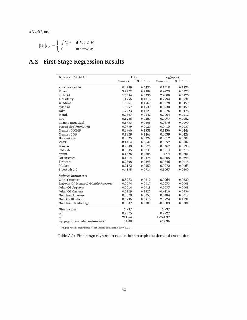
dN/dP , and

[Ω1]k,g =

∫∂sik∂pj

if k, g ∈ F,0 otherwise.

A.2 First-Stage Regression Results

Dependent Variable: Price log(Apps)Parameter Std. Error Parameter Std. Error

Appstore enabled -0.4399 0.6420 0.1918 0.1879iPhone 3.2272 0.2982 0.4429 0.0873Android 1.3334 0.3336 2.4800 0.0976BlackBerry 1.1756 0.1816 0.2294 0.0531Windows 1.3961 0.1569 -0.0578 0.0459Symbian 1.8957 0.1539 0.0230 0.0450Palm 1.7923 0.1628 -0.0076 0.0476Month -0.0607 0.0042 0.0064 0.0012CPU 0.1286 0.0280 -0.0097 0.0082Camera megapixel 0.1733 0.0308 0.0376 0.0090Screen size*Resolution 0.0739 0.0126 -0.0415 0.0037Memory 500MB 0.2966 0.1531 0.1156 0.0448Memory 1GB 0.1329 0.1468 0.0539 0.0429Handset age 0.0025 0.0029 -0.0012 0.0008AT&T -0.1414 0.0647 0.0057 0.0189Verizon -0.2648 0.0676 -0.0467 0.0198T-Mobile 0.0645 0.0745 0.0014 0.0218Sprint 0.1526 0.0686 1e-4 0.0201Touchscreen 0.1414 0.2376 0.2305 0.0695Keyboard 0.2508 0.0395 0.0546 0.01163G data 0.2172 0.0559 0.0272 0.0163Bluetooth 2.0 0.4135 0.0714 -0.1067 0.0209

Excluded InstrumentsCarrier support -0.5273 0.0819 -0.0264 0.0239log(own OS Memory)*Month*Appstore -0.0054 0.0017 0.0273 0.0005Other OS Appstore -0.0014 0.0018 -0.0037 0.0005Other OS Camera 0.3229 0.1825 -0.4110 0.0534Own firm Appstore 0.0078 0.0058 0.0484 0.0017Own OS Bluetooth 0.3296 0.5916 2.3724 0.1731Own firm Handset age 0.0007 0.0003 -0.0003 0.0001

Observations 2,737 2,737R2 0.7575 0.9927F 291.64 12741.37F6,2710 on excluded instruments+ 14.09 677.36

+ Angrist-Pischike multivariate F -test (Angrist and Pischke, 2009, p.217).

Table A.1: First-stage regression results for smartphone demand estimation

62

Dependent variable: log(Installed Base)

(N=52) Coefficient Std. Error t p-value

Age of OS 0.394 0.069 5.67 <0.001(Age of OS)2 -0.010 0.002 -3.58 0.001BlackBerry 0.011 0.429 0.03 0.979Windows -0.896 0.405 -2.21 0.032Palm -0.579 0.222 -2.61 0.012Month 0.029 0.020 1.46 0.150Constant 11.675 0.762 15.32 <0.001

R2 0.76F 276.91p-value (Hansen’s test) 0.574

iPhone’s development cost is normalized to zero.

Robust estimate of the standard error is used.

Table A.2: First-stage regression results for application supply estimation

A.3 Fixed Point Algorithm for Equilibrium Application Supply

In the outer optimization loop, I obtain the equilibrium prices by finding iteratively the best response of each

firm to the prices of rival’s handsets. For optimization, I use the Broyden-Fletcher-Goldfarb-Shanno (BFGS)

method, which is one of the widely used quasi-Newton methods. At each hill-climbing step of the outer loop,

I solve for the equilibrium application supply for all the platforms by finding a fixed point of Equation 2.4.

The following proposition is useful for implementing the fixed point iteration.

Proposition 1. Let X be a subset of RG such that Xg = (κ + φ logBg − logF, κ + φ log Bg − logF ) forg = 1, ..., G, where Bg and Bg are the lower and the upper bounds of platform g’s installed base Bg, i.e., Bg = 0

and Bg = M . Let T : X → X be a G-dimensional operator with T = (T1, ..., TG) such that Tg(logN) =

κ+φ logBg(logN)− logFg, where logN = (logN1, ..., logNG). If φγ < 1, then T has a unique fixed point inX and is a contraction mapping of modulus β < 1.

Recall that γ and φ are the parameters that capture the indirect network effects on the consumer and the

developer sides, respectively. Hence the proposition implies that the sequence of Ng generated by applying

the operator T recursively will converge to a unique fixed point, unless the indirect network effects are

strong to the extent that a change in application demand or supply is multiplied by the response of the other

side of the platform.

Proof. It suffices to show that ‖Tg(N) − Tg(N ′)‖ < β‖Ng − N ′g‖ for β ∈ (0, 1). Suppose Ng ≥ N ′g for all

g = 1, ..., G without loss of generality. Then by definition,

‖Tg(N)− Tg(N ′)‖ = ‖φ logBg(N)− φ logBg(N′)‖

= φ

∥∥∥∥∥∫ N

N ′

∑k

∂

∂NklogBg(ν)dν

∥∥∥∥∥≤ φ

∫ N

N ′

∥∥∥∥∥∑k

∂

∂NklogBg(ν)

∥∥∥∥∥dν.

63

Since

∂

∂NklogBg(N) =

1

Bg

∂

∂NkM[rSg + (1− r)Bgt−1

]=Mr

Bg

∑j∈Ag

∂sj∂Nk

=

MrBgγ∑j∈Ag sj(1−

∑l∈Ag sl) k = g

−MrBgγ∑j∈Ag sj

∑l∈Ak sl k 6= g

=

Mrγsg(1− sg)/Bg k = g

−Mrγsgsk/Bg k 6= g,

∑k

∂

∂NklogBg(N) =

Mrγ

Bg

(sg(1− sg)−

∑k 6=g

sgsk

)=Mrγ

Bgsg

(1−

∑k

sk

)≤ γ rMsg

Bg≤ γ.

Hence,

‖Tg(N)− Tg(N ′)‖ ≤ φγ‖N −N ′‖,

which implies that Tg is a contraction mapping of modulus β < 1 if φγ < 1. Since the operator T maps X to

itself, it has a fixed point in X. The uniqueness follows from the fact that T is a contraction mapping with

β < 1.

64

A.4 Full Estimation Results of Table 2.2

Logit Logit-IV RCL I RCL II RCL IIIObservations = 2,737 Estimate s.e. Estimate s.e. Estimate s.e. Estimate s.e. Estimate s.e.

Price / CPI ($100) -0.0005*** 0.0001 -0.0046*** 0.0006 -1.4441*** 0.3508 -1.4105*** 0.3554 -1.3091*** 0.3258log(Apps) 0.0016*** 0.0002 0.0012*** 0.0003 0.5712** 0.2221 0.4472** 0.2248 0.3931 0.2472Appstore enabled (σ) 0.0100*** 0.0012 0.0068*** 0.0022 6.4193*** 2.3050 5.7081** 2.2676 4.9551** 2.5094

Brand EquitiesiPhone 0.0018*** 0.0010 0.0123*** 0.0021 -6.4259*** 1.0473 -7.0806*** 1.0845 -6.9478*** 1.0662Android -0.0098*** 0.0011 -0.0058*** 0.0018 -8.8064*** 0.8023 -8.4591*** 0.8353 -8.4195*** 0.8249BlackBerry 0.0020*** 0.0005 0.0067*** 0.0010 -6.0773*** 0.5016 -6.0114*** 0.5278 -6.1351*** 0.4994Windows 0.0003 0.0005 0.0045*** 0.0010 -6.6524*** 0.5333 -6.5931*** 0.5589 -6.7356*** 0.5195Symbian -0.0008 0.0006 0.0060*** 0.0013 -6.8822*** 0.7036 -7.7181*** 0.6174 -7.7898*** 0.5562Palm 0.0005 0.0005 0.0061*** 0.0012 -5.8483*** 0.6533 -5.8406*** 0.6710 -6.0588*** 0.6251

Product Attributes Searchable to ConsumersCPU (GHz) -0.0009*** 0.0001 -0.0005*** 0.0002 -0.1214 0.0811 -0.1370* 0.0790 -0.1290 0.0792Camera megapixel 0.0010*** 0.0001 0.0020*** 0.0002 0.6189*** 0.1140 0.5976*** 0.1116 0.5747*** 0.1054Screen size * Resolution 0.0001*** 0.0000 0.0004*** 0.0001 0.1228*** 0.0419 0.1268*** 0.0436 0.1376*** 0.0442Memory 500MB 0.0005 0.0006 0.0026*** 0.0009 0.4278 0.5499 0.4441 0.5410 0.2848 0.5027Memory 1GB 0.0016*** 0.0006 0.0023*** 0.0008 0.5008 0.4108 0.4847 0.4119 0.4755 0.3831Handset age -4E-5*** 1E-5 -3E-5** 1E-5 -0.0261*** 0.0066 -0.0251*** 0.0067 -0.029*** 0.0072AT&T 0.0021*** 0.0002 0.0008* 0.0004 0.8894*** 0.1942 0.9137*** 0.1916 0.9658*** 0.1764Verizon 0.0018*** 0.0003 0.0004 0.0004 0.5185** 0.2113 0.5442*** 0.2084 0.5981*** 0.1960T-Mobile 0.0017*** 0.0003 0.0015*** 0.0004 1.1267*** 0.1766 1.122*** 0.1750 1.1671*** 0.1647Sprint 0.0012*** 0.0003 0.0014*** 0.0004 0.9797*** 0.1608 0.9952*** 0.1594 0.991*** 0.1485Touchscreen 0.0112*** 0.0008 0.0113*** 0.0012 -0.2680 0.8464 -0.7352 0.8900 -0.8827 0.9073Keyboard 0.0011*** 0.0002 0.0023*** 0.0003 0.6021*** 0.1384 0.5827*** 0.1385 0.5341*** 0.13173G data 0.0015*** 0.0002 0.0019*** 0.0003 0.5712*** 0.1321 0.5569*** 0.1299 0.5504*** 0.1213Bluetooth 2.0 -0.0005** 0.0003 0.0008* 0.0005 0.5175** 0.2347 0.4619** 0.2276 0.3987* 0.2157Month 1E-5 1E-5 -0.0003*** 3E-5 -0.0748*** 0.0216 -0.0743*** 0.0225 -0.0651*** 0.0215

OS Version Fixed EffectsiPhone 3.0 1.5949** 0.6352 1.4221** 0.5922Android 2.0 0.0057 0.7621BlackBerry 4.2+ -0.0534 0.2044BlackBerry 5.0 -0.7684* 0.4576Windows 6.1 -0.2692 0.2556Windows 6.5 -0.7433 0.6299Symbian 9 1.0567* 0.6094 0.8589 0.5705Palm WebOS 0.2984 0.9458

Standard Deviation of Random CoefficientsTouchscreen 3.3643*** 0.8504 4.0574*** 0.8855 3.8063*** 0.8836Appstore enabled 4.3522*** 1.0446 4.5568*** 1.0440 4.1204*** 1.1297

R2 0.5861 0.2527F 174.7265 96.9013nχ2 54.906 4.267 4.780 6.893p-value <0.001 0.234 0.188 0.075

***: p < 0.01; **: p < 0.05; *: p < 0.1.Utility for traditional mobile phones is normalized to zero up to logit error.

Table A.3: Estimation of logit models of smartphone handset demand

A.5 Estimation Results for Alternative Specifications

Table A.4 provides estimation results for alternative specifications based on the random coefficients logit

model in Table 2.2. Column I adds the random coefficient for price to the specification of RCL II in Table

2.2. The standard deviation of the price random coefficient has high standard error, and Column I rejects

the test of overidentifying restrictions at 10% level (p-value=0.091). From Column II to Column IV, I al-

low the coefficient of log(Apps) to vary by the three platforms: BlackBerry, Android, and iPhone. When I

65

I II III IVObservations = 2,737 Est. s.e. Est. s.e. Est. s.e. Est. s.e.

Price / CPI ($100) -1.414 0.888 -1.330 1.253 -1.332 1.089 -1.308 1.999log(Apps) 0.447 0.225 -0.005 0.987 0.043 0.834 -0.218 0.992Appstore enabled (σ) 5.712 2.355 1.439 8.631 2.098 7.699 -0.391 7.396log(Apps)*iPhone -0.005 0.863log(Apps)*Android 0.275 0.276 0.165 0.304log(Apps)*BlackBerry 0.074 0.303 0.056 0.271 0.139 0.268

Product Attributes Searchable to ConsumersCPU (GHz) -0.137 0.088 -0.164 0.076 -0.163 0.081 -0.170 0.073Camera megapixel 0.598 0.114 0.602 0.120 0.597 0.112 0.599 0.112Screen size * Resolution 0.127 0.044 0.115 0.042 0.114 0.043 0.114 0.046Memory 500MB 0.443 0.634 0.470 0.569 0.473 0.611 0.476 0.560Memory 1GB 0.485 0.412 0.497 0.433 0.552 0.424 0.536 0.438Handset age -0.025 0.007 -0.026 0.007 -0.026 0.007 -0.026 0.007AT&T 0.913 0.194 0.952 0.196 0.956 0.190 0.968 0.212Verizon 0.544 0.211 0.584 0.207 0.575 0.211 0.600 0.204T-Mobile 1.122 0.183 1.135 0.177 1.150 0.181 1.154 0.170Sprint 0.995 0.164 0.999 0.168 0.995 0.162 0.996 0.159Touchscreen -0.716 4.153 0.259 4.409 -0.144 4.359 1.235 3.727Keyboard 0.583 0.139 0.583 0.159 0.592 0.146 0.584 0.1363G data 0.557 0.138 0.556 0.157 0.569 0.156 0.563 0.141Bluetooth 2.0 0.462 0.239 0.381 0.246 0.385 0.238 0.360 0.275Month -0.074 0.023 -0.069 0.022 -0.069 0.022 -0.067 0.024

Brand EquitiesiPhone -7.078 1.212 -5.079 6.509 -5.684 5.421 -3.751 2.077Android -8.459 0.866 -7.349 3.383 -9.937 4.853 -8.087 3.669BlackBerry -6.009 0.835 -6.026 0.776 -6.045 0.824 -6.044 0.651Windows -6.591 0.797 -6.683 0.721 -6.699 0.769 -6.713 0.700Symbian -7.717 0.668 -7.775 0.642 -7.785 0.651 -7.800 0.682Palm -5.838 0.907 -5.980 0.850 -5.987 0.892 -6.027 0.827

OS Version Fixed EffectsiPhone 3.0 1.594 0.642 1.479 1.610 1.848 1.499 1.221 3.391Symbian 9 1.058 0.631 0.960 0.648 0.963 0.629 0.937 0.620

Standard Deviation of Random CoefficientsTouchscreen 4.032 5.076 2.391 7.588 2.977 6.156 -0.032 98.968Appstore enabled 4.564 1.846 2.807 4.919 3.327 4.771 1.984 4.667Price 0.027 5.199 -0.006 22.808 -0.011 13.036 -0.001 66.072

nχ2 4.773 6.869 6.711 7.437p-value 0.091 0.032 0.034 0.024

Utility for traditional mobile phones is normalized to zero up to logit error.

Table A.4: Estimation of alternative models of smartphone handset demand

include BlackBerry-specific log(Apps) coefficient in Column II, the coefficients of log(Apps) and app store

dummy become smaller in magnitude and lose significance. Furthermore, the brand equities of iPhone and

Android as well as all the random coefficients become highly insignificant, and the model strongly rejects the

overidentification test. I find similar results when I subsequently include additional indirect network effects

parameters that are Android- and iPhone-specific in Column III and Column IV. As expected, the estimation

results in Columns II–IV appear to be consistent with the observation that the data lack the variation needed

for identifying the heterogeneous indirect network effects.

66

A.6 Alternative Specification of Application Demand

Observations = 2,737 Estimate s.e.

Price / CPI ($100) -1.257 0.339(Apps)γ 0.006 0.006γ 0.574 0.086

Product Attributes Searchable to ConsumersCPU (GHz) -0.179 0.069Camera megapixel 0.602 0.104Screen size * Resolution 0.086 0.035Memory 500MB 0.363 0.503Memory 1GB 0.584 0.370Handset age -0.026 0.006AT&T 1.000 0.180Verizon 0.598 0.203T-Mobile 1.179 0.173Sprint 0.976 0.151Touchscreen -4.704 2.054Keyboard 0.595 0.129Wifi 0.009 0.1643G data 0.603 0.138Bluetooth 2.0 0.349 0.190Month -0.066 0.021

Brand EquitiesiPhone -7.457 1.174Android -8.335 0.720BlackBerry -6.095 0.550Windows -6.791 0.542Symbian -7.125 0.709Palm -6.094 0.665

Standard Deviation of Random CoefficientTouchscreen 6.374 1.709

nχ2 10.039p-value 0.039

Table A.5: Smartphone demand estimation with alternative application demand function

67

Appendix B

Appendix to Chapter 3

B.1 The MCMC Procedures

B.1.1 Quasi-Posterior

Let the parameters of the random coefficient distribution be denoted by θ2. We denote the parameters that

enter the utility function linearly by θ1 = (γ0, β, α). The GMM-type sample moment for the LT estimator is

gn(θ) = Z ′ξ(θ) = Z ′(δ(θ2)−X ′θ1

).

Define the sample weight matrix Wn as Wn = [gn(θ)gn(θ)′]−1. Then the objective function is

Ln(θ) = −n2gn(θ)′Wngn(θ),

and the quasi-posterior is proportional to

p(θ) ∝ eLn(θ)π(θ).

B.1.2 M-H Algorithm for Static Demand Estimation

At the r-th MCMC iteration, the proposed M-H algorithm draws a candidate parameter, θ∗r, and accepts it

with probability λ(θr−1, θ∗r). θr−1 is the parameter accepted at the previous M-H step.

1. Draw a candidate parameter from a transition kernel: θ∗r ∼ q(θ∗r|θr−1).

2. Compute δr at given θ∗r using the nearest neighbor method:

δr(θ∗r) = δk1(θ∗k1),

where θ∗k1 is the closest neighboring parameter to θ∗r among the N(r) previous candidates, i.e.,

θ∗s, s = r −N(r), ..., r − 1, and δk1 is the past pseudo fixed point associated with θ∗k1 .

68

3. Evaluate the GMM moment Ln(θ∗r) = −n2 ξ′ZWnZ

′ξ, where ξ = δr(θ∗r) − X ′θ1, X is the covariate

matrix, and θ1 is the least squares estimate of θ1 given δr(θ∗r).

4. Accept θ∗r with probability λ(θr−1, θ∗r) in Equation 3.5. We use a flat prior for θ, i.e., π(θ) = 1.

5. Iterate the BLP contraction mapping once:

δr(θ∗r) = δr(θ∗r) + log s− logS(θ∗r, δr

).

6. Store history Hr =⋃r−1s=r−N(r)θ∗s, δs.

7. Repeat steps 1–6.

B.1.3 M-H Algorithm for Dynamic Demand Estimation

At the r-th MCMC iteration:

1. Draw a candidate parameter θ∗r.

2. Approximate mean utility at the nearest neighboring parameter value:

δr(θ∗r) = δk1(θk1),

where k1 is the index for the nearest neighbor of θ∗r among the past N(r) pseudo fixed points, and δk1

is the past pseudo fixed point associated with θ∗k1 .

3. Evaluate the GMM moment Ln(θ∗r) = −n2 ξ′ZWnZ

′ξ, where ξ = δr(θ∗r) − X ′θ1, X is the covariate

matrix, and θ1 is the least squares estimate of θ1 given δr(θ∗r).

4. Accept θ∗r with probability λ(θr−1, θ∗r) in Equation 3.5.

5. Compute logit inclusive values, ωit = log[∑

j≥1 exp(δrjt(θ

∗r)− σ∗rα νipjt)]

, and estimate the transition

distribution F (ωit+1|ωit).

6. Iterate the following pseudo Bellman operator until∥∥Vi − V ri ∥∥ < ε(r) for all i:

Γ(V ri )(ωit; δr, θ∗r) = log

[exp

(βV E[V ri (ωit+1; δr, θ∗r)|ωit]

)+ exp(ωit)

],

where E[V ri (ωit+1; δr, θ∗r)|ωit] =∑s V

k1i (ωs;δr,θ∗r)f(ωs|ωit)∑

s f(ωs|ωit) is the expected value of V k1i , i.e., the past

pseudo value function associated with the nearest neighbor indexed by k1. The expectation is evaluated

on a set of grid points ωs.

7. Iterate the pseudo BLP fixed point operator by one step:

δr(θ∗r) = δr(θ∗r) + log s− logS(θ∗r, δr, V r

).

8. Store history Hr =⋃r−1s=r−N(r)

θ∗s, δs, V si i

.

69

9. Repeat steps 1–8.

B.2 The Data-Generating Process for Synthetic Data

B.2.1 Static Demand

The variables in the consumer utility, xj and ξjt, are generated as

xj =

x1j

x2j

x3j

∼ i.i.d.N

0

0

0

, 1 −0.8 0.3

−0.8 1 0.3

0.3 0.3 1

, ξjt ∼ i.i.d.N(0, 1),

and prices are obtained from pjt = 3 +∑3k=1 xkj + 1.5 · ξjt + ujt, where ujt ∼ U(0, 5). Six price instruments

are generated as zjtd = (∑k xkj + ujt)/4 + ejt for d = 1, ..., 6, where ejt ∼ U(0, 1). Additional instruments

are obtained from the higher-order polynomials of zjt and xj , yielding total 42 moment conditions.

B.2.2 Dynamic Demand

We simulate the dynamic demand from Equation 3.1 with γ0 = 5, α = 2, and σα = 0.5. The prices are

obtained from Equation 3.10 with γ0 = 1, γz = 1, γw = 0.2, γξ = 0.8, and σu = 0.01. The parameters for the

AR(1) process of zjt is ρ0 = 0.1, ρz = 0.95, and ση = 0.1. We set the initial prices, pj0 = 8 for all j. We draw

ξ from N(0, 1.52) and (w, u, η) from N(0, 1). In the estimation, we use (zjt, wjt) for price instruments.

For each consumer’s value function in data simulation and estimation, we construct the state space to

cover 20% larger space than the observed range of the inclusive values and discretize the state space by 50

grid points evenly.

70

B.3 Convergence of Pseudo Fixed Point

In order to prove Theorem 1, we first prove the following lemma.

Lemma 1. For any given θ ∈ Θ, ‖δ(θ)− δr(θ)‖ → 0 almost surely as r →∞.

Proof. First we decompose the approximation error into the following three parts:∥∥δ(θ)− δr(θ)∥∥ =∥∥(TV δ)(θ)− (TV r δ

r)(θ)∥∥

≤∥∥(TV δ)(θ)− (TV δ

r)(θ)∥∥+

∥∥(TV δr)(θ)− (TV r δ

r)(θ)∥∥

≤ βδ∥∥δ(θ)− δr(θ)∥∥+Ar3(θ) (by Assumption 3.2)

= βδ

∥∥∥∥δ(θ)− N(r)∑i=1

δki(θ∗ki)Wki,r(θ)

∥∥∥∥+Ar3(θ)

≤ βδ

[∥∥∥∥ N(r)∑i=1

[δ(θ)− δ(θ∗ki)

]Wki,r(θ)

∥∥∥∥+

∥∥∥∥ N(r)∑i=1

[δ(θ∗ki)− δki(θ∗ki)

]Wki,r(θ)

∥∥∥∥]

+Ar3(θ)

= βδ[Ar1(θ) +Ar2(θ)

]+Ar3(θ),

where Ar3(θ) =∥∥(TV δ

r)(θ)− (TV r δr)(θ)

∥∥, and

Ar1(θ) =

∥∥∥∥ N(r)∑i=1

[δ(θ)− δ(θ∗ki)

]Wki,r(θ)

∥∥∥∥, Ar2(θ) =

∥∥∥∥ N(r)∑i=1

[δ(θ∗ki)− δki(θ∗ki)

]Wki,r(θ)

∥∥∥∥.In the following, we show that each of the three parts converges to zero almost surely as r →∞ for any given

θ. The convergence ofAr3(θ) follows from Assumption 3.4 and the continuity of S(δ, V, θ) in V . Lemmas 2 and

3 establish the convergence of Ar1(θ) and Ar2(θ), respectively. Hence, the proof of Lemma 1 is complete.

Lemma 2. For any ε > 0, there exist δ1 > 0 and T ∈ N such that for all r ≥ T ,

P

(∥∥∥∥ N(r)∑i=1

[δ(θ)− δ(θ∗ki)

]Wki,r(θ)

∥∥∥∥ > ε

)≤ e−δ1(N(r)−N(r)) ≤ e−r

γ1/2.

Proof. We show that as we draw more MCMC samples, the nearest neighbors θ∗ki become closer to θ, such

that the approximation error converges toward zero.

P

(∥∥∥∥ N(r)∑i=1

[δ(θ)− δ(θ∗ki)

]Wki,r(θ)

∥∥∥∥ > ε

)≤ P

(N(r)∑i=1

∥∥δ(θ)− δ(θ∗ki)∥∥Wki,r(θ) > ε

)

≤ P

(N(r)⋃i=1

∥∥δ(θ)− δ(θ∗ki)∥∥ > ε)

,

since Wki,r(θ), i = 1, ..., N(r) are the positive weights that sum to 1, i.e.,Wki,r(θ) ∈ [0, 1] and∑N(r)i=1 Wki,r(θ) =

1. By the continuity of δ(θ), there exists δε > 0 such that if ‖θ − θ′‖ < δε, then ‖δ(θ)− δ(θ′)‖ < ε. Therefore,

71

we have

P

(N(r)⋃i=1

∥∥δ(θ)− δ(θ∗ki)∥∥ > ε)≤ P

(N(r)⋃i=1

∥∥θ − θ∗ki∥∥ > δε

).

Since ∃ki :

∥∥θ − θ∗ki∥∥ > δε

⊂∀j ∈ r −N(r), ..., r − 1 \ k1, ..., kN(r) :

∥∥θ − θ∗ki∥∥ > δε

⊂

⋃(j1,...,jN(r)−N(r))∈JN(r)−N(r)

N(r)−N(r)⋂i=1

∥∥θ − θ∗ji∥∥ > δε

,

where JN(r)−N(r) =

(j1, ..., jN(r)−N(r)) : ji ∈ r −N(r), ..., r − 1, ji < jk if i < k, ∀i, k

, we have

P

(N(r)⋃i=1

∥∥θ − θ∗ki∥∥ > δε

)≤

∑(j1,...,jN(r)−N(r))∈JN(r)−N(r)

P

(N(r)−N(r)⋂

i=1

θ∗ji ∈ Bcδε(θ)

). (B.1)

Let δ1 = − 12 log

[1− εν

(Bδε(θ)

)]. Then for any given N ≥ 1,

P

(N⋂i=1

θ∗ji ∈ Bcδε(θ)

)=

∫Bc×···×Bc

∫P(θ∗jN ∈ Bc

∣∣HjN−1)P(dHjN−1

∣∣θ∗jN−1 , ..., θ∗j1)

× dP(θ∗jN−1 , ..., θ∗j1)

≤[1− εν

(Bδε(θ)

)] ∫Bc×···×Bc

dP(θ∗jN−1 , ..., θ∗j1)

by Assumption 3.3

≤ · · · ≤[1− εν

(Bδε(θ)

)]N−1∫

P(θ∗j1 ∈ Bcδε

∣∣Hj1−1)P(dHj1−1

)≤[1− εν

(Bδε(θ)

)]N= e−2δ1N .

Hence it follows from the above inequality that

RHS of (B.1) =N(r)!

N(r)!(N(r)− N(r)

)!

exp[− 2δ1

(N(r)− N(r)

)]≤ exp

[− δ1

(N(r)− N(r)

)], ∀r ≥ T1,

for sufficiently large T1 ∈ N. The last inequality follows from Proposition 7 of Norets (2009). Since N(r) −N(r) = brγ1c − brγ2c ≥ rγ1 − 1− rγ2 ≥ rγ1/2, ∀r ≥ T2 for sufficiently large T2 ∈ N by Assumption 3.5, the

proof of Lemma 2 is complete.

Lemma 3. For ε > 0, there exists δ > 0 and T ∈ N such that for all r ≥ T and all θ ∈ Θ,

P

(∥∥∥∥ N(r)∑i=1

[δ(θ∗ki)− δki(θ∗ki)

]Wki,r(θ)

∥∥∥∥ > ε

)≤ e−δ2r

γ0γ1.

72

Proof. First, we find an upper bound of the above approximation error.

Ar2(θ) ≤N(r)∑i=1

∥∥∥δ(θ∗ki)− δki(θ∗ki)∥∥∥Wki,r(θ)

≤N(r)∑i=1

[βδ(Aki1 (θ∗ki) +Aki2 (θ∗ki)

)+Aki3 (θ∗ki)

]Wki,r(θ)

≤ βδ maxi=r−N(r),r−1

Ai1(θ∗i) + βδ maxi=r−N(r),r−1

Ai2(θ∗i) + maxi=r−N(r),r−1

Ai3(θ∗i),

(B.2)

where the second inequality uses the relation∥∥δ(θ) − δr(θ)∥∥ ≤ βδ

[Ar1(θ) + Ar2(θ)

]+ Ar3(θ) in the proof of

Lemma 1.

Following Imai, Jain and Ching (2009) and Norets (2009), our strategy is to apply the above inequality

recursively to show the convergence of the right hand side. Define M(r, 0) = r and M(r, k) = M(r, k − 1)−N(M(r, k − 1)). Then for any given m ∈ N,

RHS of (B.2) ≤m∑k=1

βkδ maxi=M(r,k),r−k

Ai1(θ∗i) + βmδ maxi=M(r,m),r−m

Ai2(θ∗i) + maxi=r−N(r),r−1

Ai3(θ∗i)

≤ βδ1− βδ

maxi=r−mN(r),r−1

Ai1(θ∗i) + βmδ maxi=r−mN(r),r−1

Ai2(θ∗i) + maxi=r−N(r),r−1

Ai3(θ∗i).

We use the fact that Ai2(·) is bounded above by some A2 < ∞, which follows from its continuity in the

compact space Θ. Let m(r) = b(r − rγ0)/N(r)c. Then since maxi=r−N(r),r−1Ai3(θ∗i) converges to zero as

r →∞ by Assumption 3.4, for any given ε > 0, we have ε1, ε2 > 0 and T1 ∈ N such that

P(Ar2(θ) > ε

)≤ P

(βδ

1− βδmax

i=r−m(r)N(r),r−1Ai1(θ∗i) + β

m(r)δ max

i=r−m(r)N(r),r−1Ai2(θ∗i) > ε1

), ∀r ≥ T1,

≤ P(

βδ1− βδ

maxi=r−m(r)N(r),r−1

Ai1(θ∗i) > ε1/2

)+ P(βm(r)δ A2 > ε1/2

)≤

r−1∑i=r−m(r)N(r)

P(Ai1(θ∗i) > ε2

), ∀r ≥ max(T1, T2), for sufficiently large T2 ∈ N,

≤r−1∑

i=r−m(r)N(r)

e−δ2(N(i)−N(i)) (by Lemma 2)

≤ e−δ2rγ0γ1

, ∀r ≥ max(T1, T2, T3), for sufficiently large T3 ∈ N.

The third inequality holds since m(r) → ∞ as r → ∞ by construction. The last inequality follows from

Proposition 8 of Norets (2009).

Theorem 1. Under Assumptions 3.1–3.5, the pseudo fixed point δr converges almost surely to the exact fixedpoint δ uniformly in θ ∈ Θ. In other words,

supθ∈Θ

∥∥δ(θ)− δr(θ)∥∥→ 0 a.s. as r →∞.

73

Proof. Let Xr(θ) = δ(θ) − δr(θ). Since Xr(θ) is continuous in Θ, for ε > 0, ∃δ > 0 such that ‖θ − θ′‖ <δ ⇒ ‖Xr(θ) − Xr(θ

′)‖ < ε/2. Define Bδ(θi) = θ : ‖θ − θi‖ < δ. Then there exists M(ε) ∈ N such that

Θ ⊆⋃M(ε)i=1 Bδ(θi) by the compactness of Θ. Then we have

supθ ‖Xr(θ)‖ > ε

⊆⋃M(ε)i=1

‖Xr(θi)‖ > ε/2

.

Hence,

P(

supθ‖Xr(θ)‖ > ε

)≤M(ε)∑i=1

P(‖Xr(θi)‖ > ε/2

)≤M(ε) sup

i=1,...,M(ε)

P(‖Xr(θi)‖ > ε/2

)≤M(ε)

[sup

i=1,...,M(ε)

P(Ar1(θi) ≥

ε

4βδ

)+ supi=1,...,M(ε)

P(Ar2(θi) ≥

ε

4βδ

)]≤M(ε)

[exp

[− δ1

(N(r)− N(r)

)]+ exp(−δ2rγ0γ1)

].

Therefore we obtain

∞∑t=1

P

(supθ∈Θ

∥∥δ(θ)− δr(θ)∥∥ > ε

)<∞,

and Theorem 1 follows from the Borel-Cantelli lemma.

Proposition 2. For given δr and θ, let ε ≡ supi∈1,...,N supω∈Ω |Vi(ω; δr, θ) − V ri (ω; δr, θ)|. Then given themodel described in Section 3.2.1, we have

∥∥TV (δr)(θ)− TV r (δr)(θ)∥∥ = o(ε).

Proof. Suppose V ′ = V + ε1, where 1 is the column vector of dimension N . Then the market share function

Sjt(δ, V′, θ) in Equation 3.2 is

Sjt(δ, V′, θ) =

∫exp

(δjt − θνipjt

)exp

(βV E

[V ′i (ω′)|ωit

])+ exp(ωit)

hit Fν(dνi)

=

∫exp

(δjt − θνipjt

)exp

(βV E

[Vi(ω′)|ωit

]+ βV ε

)+ exp(ωit)

hit Fν(dνi).

For given (j, t), let F (ε) = Sjt(δ, V + ε1, θ). Then the partial derivative with respect to ε is

F ′(ε) = − βVF (ε)

∫exp

(δjt − θνipjt

)exp

(βV E

[Vi(ω

′)|ωit]

+ βV ε)[

exp(βV E

[Vi(ω′)|ωit

]+ βV ε

)+ exp(ωit)

]2 hit Fν(dνi).

74

Since F (ε) is continuous, we can expand the function around 0 as

F (ε) = F (0) + F ′(0)ε+ o(ε)

= F (0)− βV ε

F (0)

∫πijt

(1−

J∑k=1

πikt

)hitFν(dνi) + o(ε).

Then,

|F (ε)− F (0)| ≤ βV ε

F (0)

∫πijt

(1−

J∑k=1

πikt

)hitFν(dνi) + o(ε)

≤ βV ε

F (0)F (0) + o(ε) = o(ε).

The above holds for arbitrary (δ, θ) and (j, t). Hence Proposition 2 follows from the definition of TV and TV r .

75

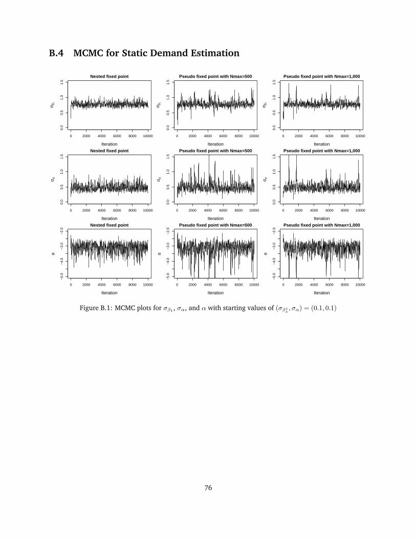
B.4 MCMC for Static Demand Estimation

0 2000 4000 6000 8000 10000

0.0

0.5

1.0

1.5

Nested fixed point

Iteration

σ β1

0 2000 4000 6000 8000 10000

0.0

0.5

1.0

1.5

Pseudo fixed point with Nmax=500

Iteration

σ β1

0 2000 4000 6000 8000 10000

0.0

0.5

1.0

1.5

Pseudo fixed point with Nmax=1,000

Iteration

σ β1

0 2000 4000 6000 8000 10000

0.0

0.5

1.0

1.5

Nested fixed point

Iteration

σ α

0 2000 4000 6000 8000 10000

0.0

0.5

1.0

1.5

Pseudo fixed point with Nmax=500

Iteration

σ α

0 2000 4000 6000 8000 10000

0.0

0.5

1.0

1.5

Pseudo fixed point with Nmax=1,000

Iteration

σ α

0 2000 4000 6000 8000 10000

−5.

0−

4.0

−3.

0−

2.0

Nested fixed point

Iteration

α

0 2000 4000 6000 8000 10000

−5.

0−

4.0

−3.

0−

2.0

Pseudo fixed point with Nmax=500

Iteration

α

0 2000 4000 6000 8000 10000

−5.

0−

4.0

−3.

0−

2.0

Pseudo fixed point with Nmax=1,000

Iteration

α

Figure B.1: MCMC plots for σβ1 , σα, and α with starting values of (σβ1x, σα) = (0.1, 0.1)

76

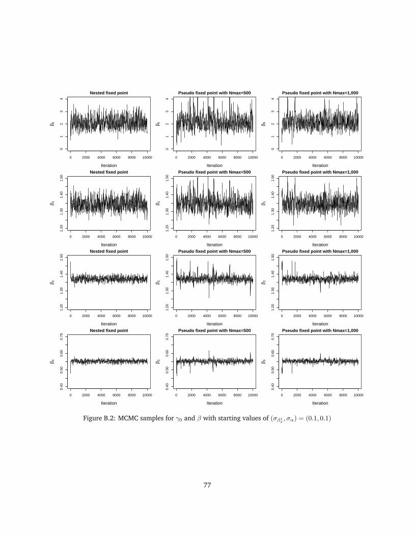
0 2000 4000 6000 8000 10000

01

23

4

Nested fixed point

Iteration

β 0

0 2000 4000 6000 8000 10000

01

23

4

Pseudo fixed point with Nmax=500

Iteration

β 00 2000 4000 6000 8000 10000

01

23

4

Pseudo fixed point with Nmax=1,000

Iteration

β 0

0 2000 4000 6000 8000 10000

1.20

1.30

1.40

1.50

Nested fixed point

Iteration

β 1

0 2000 4000 6000 8000 10000

1.20

1.30

1.40

1.50

Pseudo fixed point with Nmax=500

Iteration

β 1

0 2000 4000 6000 8000 10000

1.20

1.30

1.40

1.50

Pseudo fixed point with Nmax=1,000

Iteration

β 1

0 2000 4000 6000 8000 10000

1.20

1.30

1.40

1.50

Nested fixed point

Iteration

β 2

0 2000 4000 6000 8000 10000

1.20

1.30

1.40

1.50

Pseudo fixed point with Nmax=500

Iteration

β 2

0 2000 4000 6000 8000 10000

1.20

1.30

1.40

1.50

Pseudo fixed point with Nmax=1,000

Iteration

β 2

0 2000 4000 6000 8000 10000

0.40

0.50

0.60

0.70

Nested fixed point

Iteration

β 3

0 2000 4000 6000 8000 10000

0.40

0.50

0.60

0.70

Pseudo fixed point with Nmax=500

Iteration

β 3

0 2000 4000 6000 8000 10000

0.40

0.50

0.60

0.70

Pseudo fixed point with Nmax=1,000

Iteration

β 3

Figure B.2: MCMC samples for γ0 and β with starting values of (σβ1x, σα) = (0.1, 0.1)

77

Bibliography

Ailawadi, Kusum L., Donald R. Lehmann, and Scott A. Neslin, “Revenue Premium as an Outcome Measure

of Brand Equity,” Journal of Marketing, 2003, 67 (4), 1–17.

Anderson, Simon P., André de Palma, and Jacques-François Thisse, Discrete Choice Thoery of Product

Differentiation, The MIT Press, 1992.

Angrist, Joshua D. and Jörn-Steffen Pischke, Mostly Harmless Econometrics: An Empiricist’s Companion,

Princeton Univ Press, 2009.

AppStoreHQ, “iOS vs Android? Over 1,000 Developers (Including Some Top Names)

Are Having It Both Ways,” July 2010. http://blog.appstorehq.com/post/760323632/

ios-vs-android-over-1-000-developers-including-some.

, “It’s the Apps, Stupid!,” June 2011. http://blog.appstorehq.com/post/6590466369/

its-the-apps-stupid.

Bajari, Patrick, “Comment,” Quantitative Marketing and Economics, 2003, 1 (3), 277–283.

Berry, Steven, “Comment,” Quantitative Marketing and Economics, 2003, 1 (3), 285–291.

, James Levinsohn, and Ariel Pakes, “Automobile Prices in Market Equilibrium,” Econometrica, July

1995, 63 (4), 841–90.

Berry, Steven T., “Estimating Discrete-Choice Models of Product Differentiation,” RAND Journal of Eco-

nomics, Summer 1994, 25 (2), 242–262.

Carranza, Juan Esteban, “Product Innovation and Adoption in Market Equilibrium: The Case of Digital

Cameras,” International Journal of Industrial Organization, 2010, 28 (6), 604–618.

78

Chen, Jiawei, Ulrich Doraszelski, and Joseph E. Harrington Jr., “Avoiding Market Dominance: Product

Compatibility in Markets with Network Effects,” RAND Journal of Economics, 2009, 40 (3), 455–485.

Chernozhukov, Victor and Han Hong, “An MCMC Approach to Classical Estimation,” Journal of Economet-

rics, 2003, 115 (2), 293–346.

Ching, Andrew T., T’ulin Erdem, and Michael P. Keane, “Learning Models: An Assessment of Progress,

Challenges and New Developments,” Working Paper, 2011.

Chou, Chienfu and Oz Shy, “Network Effects Without Network Externalities,” International Journal of In-

dustrial Organization, 1990, 8 (2), 259–270.

Church, Jeffrey and Neil Gandal, “Network Effects, Software Provision, and Standardization,” The Journal

of Industrial Economics, 1992, 40 (1), 85–103.

and , “Complementary Network Externalities and Technological Adoption,” International Journal of

Industrial Organization, 1993, 11 (2), 239–260.

Clements, Matthew T. and Hiroshi Ohashi, “Indirect network effects and the product cycle: Video games

in the US, 1994-2002,” The Journal of Industrial Economics, 2005, 53 (4), 515–542.

Corts, Kenneth S. and Mara Lederman, “Software Exclusivity and the Scope of Indirect Network Effects in

the US Home Video Game Market,” International Journal of Industrial Organization, 2009, 27 (2), 121–

136.

Dubé, Jean-Pierre and Pradeep K. Chintagunta, “Comment,” Quantitative Marketing and Economics, 2003,

1 (3), 293–298.

Dubé, Jean-Pierre H., Günter J. Hitsch, and Pradeep K. Chintagunta, “Tipping and Concentration in

Markets with Indirect Network Effects,” Marketing Science, 2010, 29 (2), 216–249.

, Jeremy T. Fox, and Che-Lin Su, “Improving the Numerical Performance of BLP Static and Dynamic

Discrete Choice Random Coefficients Demand Estimation,” Econometrica, 2012, 80 (5), 2231–2267.

Engle, Robert F., David F. Hendry, and Jean-Francois Richard, “Exogeneity,” Econometrica, 1983, 51 (2),

277–304.

Erdem, Tülin and Joffre Swait, “Brand Equity as a Signaling Phenomenon,” Journal of Consumer Psychology,

1998, 7 (2), 131–157.

79

Gandhi, Amit, Kyooil Kim, and Amil Petrin, “Identification and Estimation in Discrete Choice Demand

Models When Endogenous Variables Interact with the Error,” Working Paper, 2011.

Geweke, John F. and Michael P. Keane, Bayesian Inference for Dynamic Discrete Choice Models without the

Need for Dynamic Programming, Cambridge University Press, 2000.

Goldfarb, Avi, Quiang Lu, and Sridhar Moorthy, “Measuring Brand Value in an Equilibrium Framework,”

Marketing Science, 2009, 28 (1), 69–86.

Gowrisankaran, Gautam and Marc Rysman, “Dynamics of Consumer Demand for New Durable Goods,”

Working Paper, 2012.

, Minsoo Park, and Marc Rysman, “Measuring Network Effects in a Dynamic Environment,” Working

Paper, 2011.

Heckman, James J. and Edward Vytlacil, “Instrumental Variables Methods for the Correlated Random

Coefficient Model: Estimating the Average Rate of Return to Schooling When the Return is Correlated

with Schooling,” Journal of Human Resources, 1998, 33 (4), 974–987.

, Sergio Urzua, and Edward Vytlacil, “Understanding Instrumental Variables in Models with Essential

Heterogeneity,” The Review of Economics and Statistics, 2006, 88 (3), 389–432.

Hendel, Igal and Aviv Nevo, “Measuring The Implications of Sales and Consumer Inventory Behavior,”

Econometrica, 2006, 74 (6), 1637–1673.

Imai, Susumu, Neelam Jain, and Andrew Ching, “Bayesian Estimation of Dynamic Discrete Choice Mod-

els,” Econometrica, 2009, 77 (6), 1865–1899.

Imbens, Guido W. and Whitney K. Newey, “Identification and Estimation of Triangular Simultaneous Equa-

tions Models Without Additivity,” Econometrica, 2009, 77 (5), 1481–1512.

Jiang, Renna, Puneet Manchanda, and Peter E. Rossi, “Bayesian Analysis of Random Coefficient Logit

Models Using Aggregate Data,” Journal of Econometrics, 2009, 149 (2), 136–148.

Kamakura, Wagner A. and Gary J. Russell, “Measuring Brand Value with Scanner Data,” International

Journal of Research in Marketing, 1993, 10 (1), 9–22.

Keller, Kevin Lane, “Conceptualizing, Measuring, and Managing Customer-Based Brand Equity,” The Journal

of Marketing, 1993, 57 (1), 1–22.

80

and Donald R. Lehmann, “Brands and Branding: Research Findings and Future Priorities,” Marketing

Science, 2006, 25 (6), 740.

Kim, Kyooil and Amil Petrin, “Control Function Corrections for Unobserved Factors in Differentiated Prod-

uct Models,” Working Paper, 2010.

and Minjung Park, “Approximation Error in the Nested Fixed Point Algorithm for BLP Model Estimation,”

Working Paper, 2010.

Kuksov, Dmitri and J. Miguel Villas-Boas, “Endogeneity and Individual Consumer Choice,” Journal of

Marketing Research, December 2008, XLV (6), 702–714.

Lee, Robin S., “Vertical Integration and Exclusivity in Platform and Two-Sided Markets,” Working Paper,

2010.

, “Dynamic Demand Estimation in Platform and Two-Sided Markets: The Welfare Cost of Software Incom-

patibility,” Working Paper, 2011.

Liu, Hongju, “Dynamics of Pricing in the Video Game Console Market: Skimming or Penetration?,” Journal

of Marketing Research, 2010, 47 (3), 428–443.

Lou, Weifang, David Prentice, and Xiangkang Yin, “What Difference Does Dynamics Make? The Case of

Digital Cameras,” International Journal of Industrical Organization, 2011.

Luan, Y. Jackie and K. Sudhir, “Forecasting Marketing-Mix Responsiveness for New Products,” Journal of

Marketing Research, 2010, 47 (3), 444–457.

Malik, Om, “Infographic: Apple App StoreâAZs March to 500,000 Apps,” GigaOM, May 2011. http://

gigaom.com/apple/infographic-apple-app-stores-march-to-500000-apps.

Melnikov, Oleg, “Demand for Differentiated Durable Products: The Case of the U.S. Computer Printer Mar-

ket,” Working Paper, 2001.

Menn, Joseph, “Store Set to Be Apple of Master’s Eye,” Financial Times, December 2009. http://www.ft.

com/cms/s/2/8bbd4b80-ed8b-11de-ba12-00144feab49a.html#axzz1RrncWMb7.

Mizik, Natalie, “Assessing the Total Financial Performance Impact of Marketing Assets with Limited Time-

Series Data: A Method and an Application to Brand Equity Research,” Marketing Science Institute Working

Paper, 2009. Report No. 09-116.

81

Nair, Harikesh, Pradeep Chintagunta, and Jean-Pierre Dubé, “Empirical Analysis of Indirect Network

Effects in the Market for Personal Digital Assistants,” Quantitative Marketing and Economics, 2004, 2, 23–

58.

Nevo, Aviv, “A Practitioner’s Guide to Estimation of Random-Coefficients Logit Models of Demand,” Journal

of Economics & Management Strategy, December 2000, 9 (4), 513–548.

, “Measuring Market Power in the Ready-To-Eat Cereal Industry,” Econometrica, March 2001, 69 (2), 307–

342.

Newey, Whitney K. and Kenneth D. West, “A Simple, Positive Semi-Definite, Heteroskedasticity and Auto-

correlation Consistent Covariance Matrix,” Econometrica, 1987, 55 (3), 703–708.

Norets, Andriy, “Inference in Dynamic Discrete Choice Models with Serially Correlated Unobserved State

Variables,” Econometrica, September 2009, 77 (5), 1665–1682.

, “Continuity and Differentiability of Expected Value Functions in Dynamic Discrete Choice Models,” Quan-

titative Economics, 2010, 1 (2), 305–322.

Ohashi, Hiroshi, “The Role of Network Effects in the US VCR Market, 1978–1986,” Journal of Economics &

Management Strategy, 2003, 12 (4), 447–494.

Park, Sungho and Sachin Gupta, “Handling Endogenous Regressors by Joint Estimation Using Copulas,”

Marketing Science, 2012, 31 (4), 567–586.

Petrin, Amil and Kenneth Train, “A Control Function Approach to Endogeneity in Consumer Choice Mod-

els,” Journal of Marketing Research, 2010, 57 (1), 3–13.

Romeo, Charles J., “A Gibbs Sampler for Mixed Logit Analysis of Differentiated Product Markets Using

Aggregate Data,” Computational Economics, 2007, 29 (1), 33–68.

Rust, John, “Optimal Replacement of GMC Bus Engines: An Empirical Model of Harold Zurcher,” Economet-

rica, 1987, 55 (5), 999–1033.

Rysman, Marc, “The Economics of Two-Sided Markets,” The Journal of Economic Perspectives, 2009, 23 (3),

125–143.

Shapiro, Carl and Hal R. Varian, Information Ruels: A Strategic Guide to the Network Economy, Harvard

Business School Press, 1999.

82

Song, Minjae, “Estimating Platform Market Power in Two-Sided Markets with an Application to Magazine

Advertising,” Unpublished Manuscript, 2011.

Sriram, S., Subramanian Balachander, and Manohar U. Kalwani, “Monitoring the Dynamics of Brand

Equity Using Store-Level Data,” Journal of Marketing, 2007, 71 (2), 61–78.

Sullivan, Mary W., “How Brand Names Affect the Demand for Twin Automobiles,” Journal of Marketing

Research, 1998, 35 (2), 154–165.

Sun, Mingchun and Edison Tse, “When Does the Winner Take All in Two-Sided Markets?,” Review of Net-

work Economics, 2007, 6 (1), 2.

Train, Kenneth, Discrete Choice Methods with Simulation, Cambridge University Press, January 2003.

VisionMobile, “Mobile Developer Economics 2010 and Beyond,” July 2010. http://www.visionmobile.

com/rsc/researchreports/Mobile%20Developer%20Economics%202010%20Report%20FINAL.pdf.

, “Mobile Developer Economics 2011,” June 2011. http://www.visionmobile.com/rsc/

researchreports/VisionMobile-Developer_Economics_2011.pdf.

Wernerfelt, Birger, “Umbrella Branding as a Signal of New Product Quality: An Example of Signalling by

Posting a Bond,” The Rand Journal of Economics, 1988, 19 (3), 458–466.

Wooldridge, Jeffrey M., “On Two Stage Least Squares Estimation of the Average Treatment Effect in a

Random Coefficient Model,” Economics Letters, 1997, 56 (2), 129–133.

, “Further Results on Instrumental Variables Estimation of Average Treatment Effects in the Correlated

Random Coefficient Model,” Economics Letters, 2003, 79 (2), 185–191.

Yang, Sha, Yuxin Chen, and Greg M. Allenby, “Bayesian Analysis of Simultaneous Demand and Supply,”

Quantitative Marketing and Economics, 2003, 1, 251–275.

Zhu, Feng and Marco Iansiti, “Entry into Platform-Based Markets,” Strategic Management Journal, 2012,

33 (1), 88–106.

83