by robert e. dumais, jr., teizi henmi, jeffrey passner ... · a mesoscale modeling system developed...

A Mesoscale Modeling System Developed for the

U.S. Army

By Robert E. Dumais, Jr., Teizi Henmi, Jeffrey Passner, Terry Jameson, Pat Haines, and David Knapp

ARL-TR-3183 April 2004 Approved for public release; distribution is unlimited.

NOTICES Disclaimers

The findings in this report are not to be construed as an official Department of the Army position, unless so designated by other authorized documents. Citation of manufacturers’ or trade names does not constitute an official endorsement or approval of the use thereof.

Army Research Laboratory White Sands Missile Range, NM 88002-5501

ARL-TR-3183 April 2004

A Mesoscale Modeling System Developed for the U.S. Army

Robert E. Dumais, Jr., Teizi Henmi,

Jeffrey Passner, Terry Jameson, Pat Haines, and David Knapp Computational Information Sciences Directorate, ARL

Approved for public release; distribution is unlimited.

REPORT DOCUMENTATION PAGE Form Approved OMB No. 0704-0188

Public reporting burden for this collection of information is estimated to average 1 hour per response, including the time for reviewing instructions, searching existing data sources, gathering and maintaining the data needed, and completing and reviewing the collection information. Send comments regarding this burden estimate or any other aspect of this collection of information, including suggestions for reducing the burden, to Department of Defense, Washington Headquarters Services, Directorate for Information Operations and Reports (0704-0188), 1215 Jefferson Davis Highway, Suite 1204, Arlington, VA 22202-4302. Respondents should be aware that notwithstanding any other provision of law, no person shall be subject to any penalty for failing to comply with a collection of information if it does not display a currently valid OMB control number. PLEASE DO NOT RETURN YOUR FORM TO THE ABOVE ADDRESS.1. REPORT DATE (DD-MM-YYYY)

April 2004 2. REPORT TYPE

Final 3. DATES COVERED (From - To)

5a. CONTRACT NUMBER

5b. GRANT NUMBER

4. TITLE AND SUBTITLE

A Mesoscale Modeling System Developed for the U.S. Army

5c. PROGRAM ELEMENT NUMBER

5d. PROJECT NUMBER

5e. TASK NUMBER

6. AUTHOR(S)

Robert E. Dumais, Jr; Teizi Henmi; Jeffrey Passner; Terry Jameson; Pat Haines; David Knapp

5f. WORK UNIT NUMBER

7. PERFORMING ORGANIZATION NAME(S) AND ADDRESS(ES)

U.S. Army Research Laboratory Computational Information Sciences Directorate Battlefield Environment Division (ATTN: AMSRL-CI-EB) White Sands Missile Range, NM 88002-5501

8. PERFORMING ORGANIZATION REPORT NUMBER

ARL-TR-3183

10. SPONSOR/MONITOR'S ACRONYM(S) ARLEB

9. SPONSORING/MONITORING AGENCY NAME(S) AND ADDRESS(ES)

U.S. Army Research Laboratory 2800 Powder Mill Road Adelphi, MD 20783-1145

11. SPONSOR/MONITOR'S REPORT NUMBER(S)

ARL-TR-3183 12. DISTRIBUTION/AVAILABILITY STATEMENT

Approved for public release; distribution is unlimited.

13. SUPPLEMENTARY NOTES

14. ABSTRACT

The U.S. Army Battlescale Forecast Model (BFM) is a short-range forecasting tool designed to run on a workstation in a tactical environment. The model is hydrostatic and remains computationally stable at large time steps due to alternating-direction implicit finite differencing. The model assimilates data using Newtonian relaxation to incorporate observations and time-tendencies of forecast variables from a previously run numerical model. The U.S. Army uses the BFM to produce real-time, short-range mesoscale forecasts either as input to tactical weather decision aids or to produce more precise firing solutions in artillery. Using a timely and accurate four-dimensional gridded database of meteorological information, a battlefield commander can receive critical guidance that can assist in determining appropriate courses of action in a rapidly changing battlefield weather environment. Standard statistical measures and a few case studies demonstrate the model’s merits.

15. SUBJECT TERMS

BFM, Mesoscale, Numerical, Model, Short-Range, Forecast, Army, Tactical

16. SECURITY CLASSIFICATION OF: 19a. NAME OF RESPONSIBLE PERSON Robert E. Dumais, Jr

a. REPORT

U b. ABSTRACT

U c. THIS PAGE

U

17. LIMITATION OF

ABSTRACT

U

18. NUMBER OF PAGES

50 19b. TELEPHONE NUMBER (Include area code) 505-678-4650

Standard Form 298 (Rev. 8/98) Prescribed by ANSI Std. Z39.18

ii

Preface

The U.S. Army Battlescale Forecast Model (BFM) is a mesoscale short-range forecasting tool designed to run on a single-processor workstation in a data-restricted tactical environment. Operated at resolutions between 2 and 10 km, the model is hydrostatic and can remain computationally stable at relatively large time steps due to its use of alternating-direction implicit finite differencing. In addition, the model assimilates data using Newtonian relaxation to incorporate both observations and the time-tendencies of forecast variables from a previously run, larger-scale numerical model. The BFM is currently being used by the U.S. Army to produce real-time, short-range mesoscale forecasts that can be used either to provide input for tactical weather decision aids or to assist in more precise firing solutions in artillery. Mean absolute error statistics derived from a small sample study show that the model can successfully assimilate forecast data from a global or regional numerical model, while also providing additional forecast resolution within the boundary layer. A few case studies provide examples of how the BFM can simulate low-level diurnal circulations forced by terrain inhomogeneities and surface radiation/heating gradients when low-level synoptic forcing is weak. By maintaining a timely and accurate four-dimensional gridded database of meteorological information, a battlefield commander can receive critical guidance that can assist in determining the appropriate courses of action while in a rapidly changing battlefield weather environment.

Acknowledgments

The authors would like to acknowledge the U.S. Naval Research Laboratory for the development of the operational global model (NOGAPS) that plays such an important role in the BFM; the Air Resources Laboratory for the use of several of their figures; and both the University of Utah and the Kennedy Space Center for access to Mesonet surface data used for BFM validation.

iii

INTENTIONALLY LEFT BLANK

Contents

Preface iii

Acknowledgments iii

List of Figures vi

List of Tables vii

Summary 1

Introduction................................................................................................................................1

1. Introduction 2

2. Model Configuration and Initialization 3

2.1 Model Configuration............................................................................................................3

2.2 Objective Analysis ...............................................................................................................4

2.3 Initialization .........................................................................................................................6

2.4 Post-Processing....................................................................................................................6

2.5 CAAM BFM ........................................................................................................................8

3. Newtonian Relaxation and Data Assimilation 11

4. Numerics and Physics 12

5. Forecast Examples and Statistics 13

5.1 Radiationally Driven Flows Under Weak Synoptic Forcing .............................................13 5.1.1 Case Study of Florida Sea Breeze ........................................................................13 5.1.2 Case Study of Great Salt Lake Breeze .................................................................17

5.2 Statistical Results over the United States: Continental U.S. Study from 27 to 31 March 1998 .....................................................................................................20

6. Possible Improvements and Considerations 30

v

7. Summary and Discussion 30

8. References 31

Acronyms and Abbreviations 34

Distribution List 36

List of Figures

Figure 1. Sample GUI for the BFM execution used on IMETS. .................................................................. 4

Figure 2. Data flow from AFWA OWS hub to IMETS, with Mbps rates for the continental U.S............... 6

Figure 3. ASP post-processed surface visibility field using the 9-h BFM forecast valid at 2100 UTC, 25 February 1999. .................................................................................................................................. 8

Figure 4. Actual and simulated SADARM impact points........................................................................... 10

Figure 5. Cape Canaveral sounding data valid at 1200 UTC, 23 June 1999. ............................................. 14

Figure 6. Forecast (7 h) of surface winds (m/s) near Cape Canaveral, valid at 1900 UTC, 23 July 1999. BFM resolution is 2 km. Contours of terrain elevation every 1 m. ............................................ 15

Figure 7. EDAS surface winds valid at 0000 UTC, 24 July 1999. Maximum vector is 9 m/s. ................. 16

Figure 8. Surface wind observations (m/s) from the Kennedy Space Center Mesonet valid at 1900 UTC, 23 July 1999. Contours of terrain at every 6 m. ......................................................................... 17

Figure 9. Salt Lake City radiosonde sounding data valid at 1200 UTC, 27 May 1999. ............................. 18

Figure 10. Forecast (7 h) of surface winds (m/s) near Salt Lake City, valid at 1900 UTC, 27 May 1999. BFM resolution is 2 km. Contours of terrain elevation every 200 m. ........................................ 19

Figure 11. Surface wind observations (m/s) obtained from Utah MesoWest valid at 1900 UTC, 27 May 1999. Contours of terrain elevation every 250 m......................................................................... 20

Figure 12. EDAS analysis of 500-hPa heights and winds valid at 1200 UTC, 27 March 1998. Solid lines are geopotential heights in DM; maximum wind vector = 47.5 m/s............................................ 21



Figure 15. EDAS analysis of 925-hPa wind vectors valid at 0000 UTC, 29 March 1998. Maximum wind vector = 26.0 m/s over southeast Massachusetts. ........................................................................ 26

vi

List of Tables

Table 1. MRMD summary for the RDAP and LUT SADARM missions. ................................................. 10

Table 2. Mean absolute BFM windspeed errors (m/s) by grid region from 27–30 March 1998. Errors are for 12/24-h forecasts, and SFC refers to 10-magl level. ................................................................. 24

Table 3. Mean absolute errors of NOGAPS point 41°N, 73°W compared with OKX sounding in New York grid area....................................................................................................................................... 25

Table 4. Mean absolute errors of NOGAPS point 42°N, 70°W compared with CHH sounding in New York grid area....................................................................................................................................... 25

Table 5. Mean absolute errors of NOGAPS point 43°N, 74°W compared with ALB sounding in New York grid area....................................................................................................................................... 25

Table 6. Mean absolute BFM temperature errors (°C) by grid region from 27–30 March 1998. Errors are for 12/24 h forecasts, and SFC refers to 2-magl level. ................................................................... 27

Table 7. Mean absolute BFM u-component wind errors (m/s) by grid region from 27–30 March 1998. Errors are for 12/24-h forecasts, and SFC refers to 10-magl level. ...................................................... 27

Table 8. Mean absolute BFM v-component wind errors (m/s) by grid region from 27–30 March 1998. Errors are for 12/24-h forecasts, and SFC refers to 10-magl level. ...................................................... 28

Table 9. Mean absolute BFM dewpoint errors (°C) by grid region from 27–30 March 1998. Errors are for 12/24-h forecasts, and SFC refers to 2-magl level.......................................................................... 28

Table 10. Composite mean absolute error/correlation coefficient over all regions and times for selected parameters and levels.............................................................................................................. 29

vii

INTENTIONALLY LEFT BLANK

1

Summary

Introduction

The U.S. Army Battlescale Forecast Model (BFM) is a short-range numerical weather prediction (NWP) tool designed specifically for tactical operations, and for communication and data restricted environments. Featuring a simplified graphical user interface (GUI), operators can use the model with minimal numerical modeling expertise. This model allows the Staff Weather Officer (SWO) to view meteorological output results in a variety of graphical forms. Furthermore, operators can generate on demand specifically tailored Tactical Decision Aids (TDAs) or weather hazard products for battlefield execution and missing planning. The model has been modified and simplified for operational utility in tactical environments, aiming for a compromise between model sophistication and timeliness. This report will demonstrate that the BFM is capable of producing reliable and timely mesoscale, short-range forecast guidance under most typical atmospheric conditions.

This report describes the BFM from many perspectives, including physics, numerics, tactical application, and mesoscale forecast ability. Additionally, specific case studies illustrate the model’s ability to simulate local mesoscale circulations, which are often missed by the coarser-resolution models run at the various operational modeling centers.

The BFM is a mesoscale NWP software system, designed to be globally relocatable, as well as robust and efficient in a tactical operation setting. The model is able to initialize coarser-resolution NWP model output supplied from U.S. Air Force and U.S. Navy operational centers. The system is also capable of a four-dimensional data assimilation (4DDA), based on the method of Newtonian relaxation, or nudging. Output from the BFM is post-processed by an external algorithm called the Atmospheric Sounding Program (ASP), and then is stored as four-dimensional gridded data in a relational database. Once in the database, the meteorological forecast grids can be rapidly accessed by application software critical to tactical operation decisionmaking, such as weather hazards algorithms, weather visualization tools, and TDAs.

1. Introduction

The Battlescale Forecast Model (BFM) is a tailored version of the Higher Order Turbulence Model for Atmospheric Circulation, developed at Los Alamos National Laboratory, New Mexico. The BFM was selected by the U.S. Army for its ability to simulate boundary layer flows in complex terrain (Yamada, 1981), to assimilate observational and larger-scale numerical model data (Yamada and Bunker, 1989), and to run efficiently on low-cost workstations and personal computers (Knapp, 1998). Boundary layer meteorological phenomena that can be resolved by the model fall between the meso-β and meso-γ classification of Orlanski (1975).

Hydrostatic equilibrium and the Boussinesq approximation are assumed, and detailed parameterizations for both surface radiation (Kondrat’yev, 1977) and boundary layer turbulence (Mellor and Yamada, 1982) exist. The model is also capable of treating vegetative canopy effects (Yamada, 1982) and includes a grid-nesting option (Yamada and Bunker, 1988), although they are not used in the current BFM. The technique of Newtonian relaxation (Hoke and Anthes, 1976; Yamada and Bunker, 1989) is used to assimilate both observational data and forecast parameter tendencies (from a previously run global or regional numerical model) into the prognostic BFM forecast.

The U.S. Army Integrated Meteorological System (IMETS) and the Computer Assisted Artillery Meteorology (CAAM) software suite are U.S. Army systems that have adopted the BFM for real-time tactical operations. Due to the highly transient nature of the atmosphere, short-range mesoscale forecasting is essential to mission planning for global U.S. Army operations that require detailed knowledge of both the current and future three-dimensional meteorological state. Many of these operations are anchored close to the earth’s surface and involve areas of interest no more than 500 by 500 km in size. These operations may be airborne (ballistics, munitions, rotorcraft, fixed wing), ground-based (troop and vehicle mobility, supply and transport, gunnery, surveillance, soldier heat stress), or strategically placed for readiness against nuclear, chemical, and biological releases. Given that time scales of mesoscale phenomena operate on the order of minutes to hours, numerical forecasts that provide high-frequency, gridded output are critical in supplying meteorological guidance for short-range U.S. Army mission planning at below-corps echelons.

This report describes the BFM and discusses its applications to the U.S. Army, examining the model’s strengths and weaknesses under different large-scale flow patterns and regional topographies. Included is a summary of the model configuration (terrain ingest, objective analysis, and initialization), a discussion of the application of Newtonian relaxation, a small-sample statistical evaluation, and a few brief case studies. Significant features of the BFM,

2

particularly the assimilation of global model forecast tendencies and the capability to simulate diurnal mesoscale boundary layer circulations, are shown. All references to the BFM in this report relate to the version currently operational on the IMETS, with the exception of a somewhat different configuration used by the CAAM, described in section 2.5.

2. Model Configuration and Initialization

2.1 Model Configuration

Operating on workstations or personal computers that have been selected as U.S. Army common hardware, the BFM is designed to generate up to a 24-h forecast depending upon the availability of larger-scale numerical model guidance. Before initiating a forecast, a user must specify the model domain grid center, grid dimensions, horizontal grid spacing, and initialization base time from a graphical user interface (GUI) window (figure 1). Once executed, the BFM module queries the IMETS meteorological database for available upper-air radiosonde and numerical model data for objective analysis, within an expanded region surrounding the model domain (valid for the initialization time). This region is a 161 by 161 grid, spaced at the horizontal resolution selected by the user (for instance, a 10-km resolution generates a 1600 by 1600 km square domain); however, surface observations are collected only from within the designated BFM model domain. Once the input meteorological data has been retrieved, model terrain data is generated and model execution initiated. Upon completion and post processing, the output data is inserted into a relational gridded meteorological database (GMDB), after which the user can select from a variety of visual display GUIs. At this point, BFM output can be displayed or plotted in a number of ways (contours, cross sections, vertical point soundings, tabular format, SkewT-LogP) on any available IMETS map backgrounds.

3

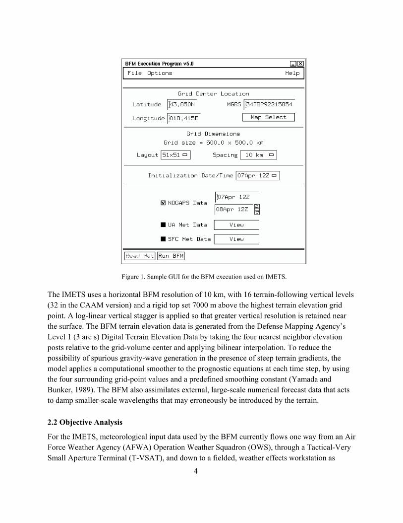
Figure 1. Sample GUI for the BFM execution used on IMETS.

The IMETS uses a horizontal BFM resolution of 10 km, with 16 terrain-following vertical levels (32 in the CAAM version) and a rigid top set 7000 m above the highest terrain elevation grid point. A log-linear vertical stagger is applied so that greater vertical resolution is retained near the surface. The BFM terrain elevation data is generated from the Defense Mapping Agency’s Level 1 (3 arc s) Digital Terrain Elevation Data by taking the four nearest neighbor elevation posts relative to the grid-volume center and applying bilinear interpolation. To reduce the possibility of spurious gravity-wave generation in the presence of steep terrain gradients, the model applies a computational smoother to the prognostic equations at each time step, by using the four surrounding grid-point values and a predefined smoothing constant (Yamada and Bunker, 1989). The BFM also assimilates external, large-scale numerical forecast data that acts to damp smaller-scale wavelengths that may erroneously be introduced by the terrain.

2.2 Objective Analysis

For the IMETS, meteorological input data used by the BFM currently flows one way from an Air Force Weather Agency (AFWA) Operation Weather Squadron (OWS), through a Tactical-Very Small Aperture Terminal (T-VSAT), and down to a fielded, weather effects workstation as

4

depicted in figure 2. Raw upper-air radiosonde and surface observations, along with gridded numerical model output produced by the Naval Operational Global Atmospheric Prediction System (NOGAPS), are currently received. Details of NOGAPS can be found in Hogan and Rosmond (1991).

When entering the BFM, all collected radiosonde data is subjected to gross and hypsometric checks to assure quality control. Then an objective analysis is executed to produce meteorological fields for both initialization and time-dependent data assimilation (using NOGAPS background forecasts). First, the radiosonde data is interpolated on predefined Cartesian height surfaces, after which spatial interpolation to the BFM grid-point locations is accomplished using an inverse-distance weighting function. Then the data is reinterpolated vertically from the Cartesian surfaces to the model, terrain-following coordinate surfaces defined by eq 1:

z Hz zH zg

*=−−

g (1)

where

= transformed vertical coordinate z *

= Cartesian vertical coordinate z

= ground elevation above mean sea level zg

H = material surface top of the model

H = corresponding height in Cartesian coordinates

For simplicity, H is defined in eq 2 as

H H zg= + max (2)

where is the maximum value of on the grid. zg max zg

NOGAPS forecast data is analyzed in a similar fashion, with the exception that a two-pass, successive corrections scheme (Barnes, 1964) is used to horizontally interpolate from NOGAPS to the BFM grid-point locations. When both radiosonde and NOGAPS data are available, a similar successive corrections approach is used to combine the analyzed first-guess background field (NOGAPS) with the radiosonde observations. Weighting in the compositing scheme has been modified slightly from that described previously in Henmi and Dumais (1998) in order to allow radiosonde data to have greater influence at grid points nearest to the observation location.

5

6

Figure 2. Data flow from AFWA OWS hub to IMETS, with Mbps rates for the continental U.S.

2.3 Initialization

The BFM execution cycle begins 3 h prior to initialization base time in order to dynamically “spin up” the model fields. Nudging is applied to the analyzed fields at all interior BFM grid points, and at the start of the preforecast cycle, a simple logarithmic wind profile is assumed that satisfies the condition of mass consistency. Surface temperature, wind, and dewpoint observations are also assimilated into the lowest model levels, using a form of observational nudging and a weighting scheme somewhat different from that used for the three-dimensional nudging of the analyses. This weighting is based on both model resolution and grid-point distance from the surface observation site (Henmi and Dumais, 1998).

2.4 Post-Processing

Upon forecast completion, the BFM produces a number of model-state parameters, such as the u and v horizontal wind vector components, potential temperature, and water vapor mixing ratio. While these prognostic parameters are useful for U.S. Army operations, it is necessary to place more specific weather information into the GMDB for tactical software, such as the Integrated Weather Effects Decision Aid (IWEDA). The IWEDA uses this output to provide

detailed information in terms of why, when, and how weather affects weapon systems (as well as their subsystems and components) and operations (Sauter, 1996). However, the IWEDA requires data not directly supported by the BFM, such as turbulence and surface visibility. In order to meet this data requirement a post-processing module, the Atmospheric Sounding Program (ASP), was developed to read the BFM output data and derive additional meteorological parameters for the GMDB. Most of these derived parameters are used in U.S. Army aviation, such parameters as turbulence, icing, cloud heights and amounts, surface visibility, fog, and thunderstorm probabilities.

Operational forecasting decisions must be made quickly, and it helps to apply artificial intelligence (AI) techniques. Although the ASP is not truly an AI program, the module applies elements of statistical methods, conventional computer programming, and basic meteorological principles. After diagnostic computations are complete, the operator should use the “if-then” rules in the code to check the consistency of the forecasts.

Since the post-processed products must be applicable at any point in the world, the modules are designed to cover weather events at any location, regardless of terrain, elevation, season, time of day, or climate zone. For example, Knapp (1996) collected 2790 surface observations from 80 continental U.S. locations from July 1994 to April 1995 and at all hours of the day. Using the surface elevation, temperature, dewpoint, relative humidity, windspeed, ceiling height, and precipitation, Knapp implemented screening regression techniques using stepwise procedures to determine the predictor values for his equations. Once the best-correlated predictor was found, other predictors were included to achieve optimal statistical results. For instance, eq 3 is formulated using observations with derived ceilings:

VISIBILITY=8.06+ (0.0003*SFC ELEVATION) -(0.0456*RH)+(0.0058*CEILING HEIGHT) (3)

where

VISIBILITY ≡ integer value category (categories in miles)

SFC ELEVATION ≡ surface elevation in meters above mean sea level

RH ≡ relative humidity in percent

CEILING HEIGHT ≡ feet above ground level

Figure 3 shows a plot of the ASP-produced surface visibility over the Midwestern United States, based on a 9-h BFM forecast valid at 2100 universal time coordinated (UTC), 25 February 1999. A more detailed discussion of the ASP is included in Passner (1999).

7

Figure 3. ASP post-processed surface visibility field using the 9-h BFM forecast valid at 2100 UTC,

25 February 1999.

2.5 CAAM BFM

CAAM is a software system designed to enhance the accuracy of meteorological (Met) input to artillery aiming calculations. All effective artillery firings must include aiming adjustments that are based upon Met information to compensate for variations in atmospheric wind, temperature, and density along the artillery shell trajectory. A recent study of the component errors for the Extended-Range 155-mm artillery round concluded that for a trajectory length of 28 km, 42 percent of the range error (down-range along the initial firing azimuth) and 56 percent of the deflection error (cross-range perpendicular to the initial firing azimuth) was attributable to inaccuracies in the Met data (Reichelderfer and Barker, 1993). Most of the remaining firing errors are due to muzzle velocity and occasion-to-occasion inaccuracies. Therefore, reducing the

8

Met errors in the data used for the firing calculations can significantly improve the aiming accuracy of the artillery rounds.

The CAAM BFM was used to generate forecast computer meteorological messages (FCMMs) that were then compared against those derived from radiosonde computer meteorological messages (RCMMs). Because the CAAM BFM forecasts data rather than measures it, the model predicts Met conditions at desired points in space and time and has the potential of more accurately representing the atmosphere, thus allowing for more precise artillery aiming. Since radiosonde data can contain inherent inaccuracies (such as balloon drift) for artillery aiming purposes, an alternate approach was employed for comparison that makes no initial assumption about the accuracy of the data. Met analysis was performed on data collected during Sense and Destroy Armor (SADARM) artillery live firings that occurred at Yuma Proving Ground, AZ (YPG). Actual submunition impact data were compared against predicted impacts derived from a trajectory simulation program. Two types of Met data were input to the trajectory simulator (RCMMs and FCMMs), in order to test which type of data most accurately represented the “real” atmosphere.

A series of SADARM artillery firings were simulated using General Trajectory Model 3 (GTRAJ3) simulations from the Armament Research Development and Engineering Centers Firing Tables Branch. The simulations were run first using a RCMM, and then using a FCMM. The specific input conditions for a particular firing (SADARM ballistic and aerodynamic parameters, gun azimuth/elevation angle, measured muzzle) were held identical from each GTRAJ3 run and were compared to the actual impact submunition coordinates obtained at the SADARM Reliability Determination and Assurance Program (RDAP) and the Limited User Test (LUT) conducted at YPG during January, April, and May 2000. The SADARM rounds experienced and responded to the “true” atmospheric conditions. Consequently, the GTRAJ3 simulation that resulted in the closest impact to the actual impact location(s) was the one using Met data most representative of the “true” atmosphere. The RCMMs were approximately 3-h old during the RDAP (i.e., the radiosonde used for the Met message to aim the gun was taken about 3 h before the firing). The FCMMs were 3-h forecasts, valid at the time of the firing. During the LUT, the RCMMs were only about 1.5-h old and the FCMMs were 5-h forecasts.

9

Figure 4 shows the actual and simulated impact points for one of the guns participating in the final LUT mission. The SADARM rounds came in from the northeast (from the upper right toward the lower left in the plot, as indicated by the diagonal arrow). Each of the rounds (labeled “Actuals”) impacted within the confines of the target array. The “+” symbol indicates where the GTRAJ3 simulation hit, using a 1.5 h-old RCMM and gun 1’s aiming data. When GTRAJ3 was rerun using identical aiming data but substituting the FCMM (a 5-h forecast RCMM that was valid at the firing time), the impact is depicted by the diamond symbol. As shown, the GTRAJ3 simulation using Met data from the CAAM BFM impacted closer to the actual live rounds,

indicating that the CAAM BFM, even when forecasting 5 h into the future, more accurately represented the true atmospheric conditions along the trajectories at the time of the firing than did a radiosonde only 1.5-h old.

02 MAY 00 LUT- GUN 1

3,647,000

3,647,100

3,647,200

3,647,300

3,647,400

3,647,500

3,647,600

233,400 233,600 233,800 234,000 234,200 234,400

X COORDINATE (meters)

Y C

OO

RD

INA

TE (m

eter

s)

TARGETS

ACTUALS

RCMM/1.5-h

FCMM/5.0-hN

Figure 4. Actual and simulated SADARM impact points.

Many of the other RDAP and LUT firings produced similar results. Each SADARM round contains 2 submunition canisters, thus the 12 rounds fired during the RDAP resulted in 24 ground impacts against which the simulated impacts were compared. On each of four LUT mission days, 24 rounds were fired, resulting 192 total impacts. In some cases, it was difficult to visually assess which simulation was closest to the live impacts. In order to quantify the results, the straight-line distance, or radial miss distance, was determined from every submunition impact coordinate to the RCMM-GTRAJ3 and FCMM-GTRAJ3 simulated impact points. Mean radial miss distance (MRMD) values were then calculated for the two RDAP mission days and the four LUT mission days. Table 1 summarizes the MRMD results (values are in meters):

Table 1. MRMD summary for the RDAP and LUT SADARM missions.

RCMM FCMM RDAP-1 256 222 RDAP-2 123 48 LUT-1 235 188 LUT-2 261 306 LUT-3 178 178 LUT-4 223 141

10

As per table 1, the FCMM-based MRMD values were smaller for 4 of the 6 mission days, indicating that the FCMMs more accurately represented the atmosphere than did the RCMMs for a majority of the missions. The results were almost identical for LUT-3 (when rounded to the nearest meter). During LUT-2 (18 Apr 2000), a disturbance in the upper atmosphere caused strong winds (exceeding 50 ms-1 near the apogee of the SADARM rounds) that changed direction significantly shortly before the firing. In this case, the RCMM (1.5-h old) was a more accurate representation of the firing conditions than the 5-h FCMM forecast.

3. Newtonian Relaxation and Data Assimilation

Newtonian relaxation (nudging) is accomplished by introducing an additional non-physical term to the prognostic equation for a variable α, such as in eq 4, that acts to “steer” the mesoscale model solution towards an observation(s) or large-scale model forecast for α (Yamada and Bunker, 1988; Hoke and Anthes, 1976; Harms et al., 1992). The model’s physical forcing terms are included in F, and α0 is the observation or large-scale numerical model value. Although, in the case of winds, α0 in the BFM is actually a target wind discussed by Yamada and Bunker (1989). The coefficient Gα is used to determine the strength of the nudging (Pielke, 1984), and this value in mesoscale models is somewhat arbitrary and is a function of the synoptic situation, meteorological parameters, and the magnitude of other model forcing terms. Stauffer and Seaman (1990) select Gα so that the time scale of the slowest physical adjustment process in the model and the nudging term are similar, and MESO (1993) shows that a value of Gα = 3 × 10-4 implies an exponential decay towards observation with an e-folding time of 0.93 h when no model physical forcing terms are present.

∂α / ∂t = F(α,x,t) + Gα * (α0 - α) (4)

For the BFM, the magnitude of Gα is dynamic and is set strong enough to effectively suppress undesirable phase and amplitude errors and correctly assimilate NOGAPS fields in space and time. Conversely, the nudging is not so strong as to significantly inhibit realistic boundary layer mesoscale circulations from developing within the model. Values of Gα in the BFM range from 1 × 10-4 to 3 × 10-4, although when nudging surface observations, larger values are used due to the stronger contributions from the forcing terms in the prognostic equations (care must be taken when nudging surface temperature, otherwise the model’s simulated boundary layer development may be stunted). Values of Gα in the BFM are determined separately for the prognostic variables representing wind, perturbation virtual potential temperature, and total water vapor mixing ratio. These values are periodically adjusted within the BFM (for each

11

parameter) during the model forecast cycle and are functions of the height above ground, time of day, BFM boundary layer lapse rate forecast, and degree of synoptic forcing forecast by NOGAPS. For example, an estimation of the degree of synoptic forcing is made using such identifiers as the low-level windspeed and the surface to 5000-magl temperature advection.

In conditions of weak forcing where the terrain can be expected to have a strong local influence, the magnitude of Gα is generally reduced. Local flow fields forced by surface temperature gradients over sloped surfaces (drainage/upslope wind) or along land/water boundaries (lake/sea breeze) can be well simulated at 2 to 10 km resolution when synoptic flow is weak (Doran and Horst, 1982; McNider, 1982; Mahrer and Pielke, 1976). Many BFM successes have been documented under such conditions (Yamada, 1981, 1983; Yamada and Bunker, 1989; Pielke and Pearce, 1994).

Three-dimensional, hourly gridded “nudging” files are created by linear interpolation between successive 6-h NOGAPS forecasts. Although the spatial resolution ratio between the 1º NOGAPS and the BFM is poor, it is an improvement over the previously used 2.5º-resolution NOGAPS grids. A study of the present BFM version versus a non-hydrostatic mesoscale model used for operational purposes (Henmi, 2000) indicates that comparable and often improved surface forecasts can be obtained by the “nested” BFM.

4. Numerics and Physics

A typical 24-h BFM forecast executes in 45 to 60 min on a single processor 350 MHz workstation (51×51×16 grid points). The model is computationally fast due to the use of an alternating direction implicit (ADI) solution technique (Peaceman and Rachford, 1955) in three-dimensions (allowing for larger time steps), in addition to a lack of explicit moist microphysics and a cumulus parameterization. The ADI method is second-order accurate for both space and time derivatives and is unconditionally stable (Kao and Yamada, 1989). Nevertheless, special treatment of updating values at intermediate time steps is required to apply this technique in three dimensions (Richtmeyer and Morton, 1967). By using the ADI method, the model is able to reduce the speed of fast external gravity waves, significantly increasing the maximum time step allowable under the Courant-Friedrich-Lewy (CFL) numerical stability condition. A planar Universe Transverse Mercator grid is used along with a staggered C grid (Arakawa and Lamb, 1977) for the prognostic calculations.

The pressure gradient in the planetary boundary layer (PBL) is computed by first assuming that the geostrophic winds at the PBL top (assumed 1500 magl) and at levels above are equivalent to the NOGAPS forecasted wind values. Below the PBL top, the geostrophic winds are computed

12

using a simplified thermal wind relationship similar to the approximations used by Yamada (1981). An advantage of this method is that realistic boundary layer pressure gradients can be calculated with less likelihood of large computational errors due to steep model terrain. However, in the free atmosphere this method retards the possibility of the BFM generating its own pressure gradient. This is currently not so problematic since relatively strong nudging is applied and the current BFM lacks both explicit moist physics and a cumulus parameterization.

The vertical wind component is determined diagnostically by assuming a condition of mass continuity and no vertical motion at both the top of the model domain and the earth’s surface. Finally, the model has complete parameterizations for surface radiation (Kondrat’yev, 1977), turbulence (Mellor and Yamada, 1982), stratus cloud radiation (Hanson and Derr, 1987), and stable precipitation (Sundqvist et al., 1989). A more complete description of the model physics and numerics can be found in Henmi and Dumais (1998) or Yamada and Bunker (1989).

5. Forecast Examples and Statistics

5.1 Radiationally Driven Flows Under Weak Synoptic Forcing

The following subsection discussed an example of a BFM forecast made during the summer in a weakly forced synoptic environment. This case was selected to illustrate how the BFM can simulate boundary layer flows that are primarily forced by strong surface radiational heating differences (such as sea breezes, nocturnal drainage flows, etc.). Also included is a brief mention of a second forecast example produced in the vicinity of the Great Salt Lake, UT.

5.1.1 Case Study of Florida Sea Breeze

For this 12-h simulation of a sea breeze circulation, a 100 by 100 km grid of 2-km, horizontal resolution was selected; centered near Cape Canaveral, FL (28.47°N, 80.53°W), and initialized at 1200 UTC on 23 July 1999. Since the synoptic forcing on this day was weak and the large-scale environmental conditions invariant during the study period, archived NOGAPS model output was not used for analysis nudging—model prognostic equations were instead nudged throughout the simulation to the initial fields using a uniform nudging coefficient value of 3 × 10-4. As seen by the 1200 UTC station XMR (Cape Canaveral radiosonde) sounding in figure 5, the ambient low-level pressure gradient was quite weak with southwesterly flow below 950 hPa and easterly flow above 950 hPa, with environmental windspeed values less than 5 m/s below 550 hPa.

13

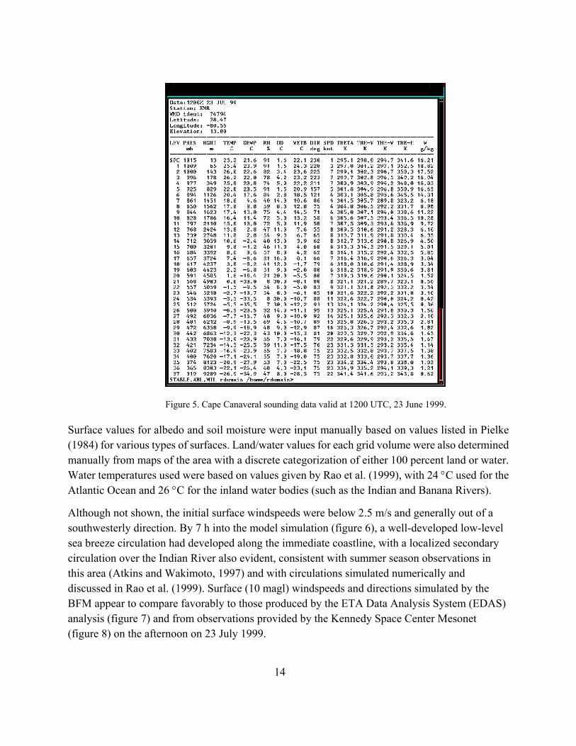
Figure 5. Cape Canaveral sounding data valid at 1200 UTC, 23 June 1999.

Surface values for albedo and soil moisture were input manually based on values listed in Pielke (1984) for various types of surfaces. Land/water values for each grid volume were also determined manually from maps of the area with a discrete categorization of either 100 percent land or water. Water temperatures used were based on values given by Rao et al. (1999), with 24 °C used for the Atlantic Ocean and 26 °C for the inland water bodies (such as the Indian and Banana Rivers).

Although not shown, the initial surface windspeeds were below 2.5 m/s and generally out of a southwesterly direction. By 7 h into the model simulation (figure 6), a well-developed low-level sea breeze circulation had developed along the immediate coastline, with a localized secondary circulation over the Indian River also evident, consistent with summer season observations in this area (Atkins and Wakimoto, 1997) and with circulations simulated numerically and discussed in Rao et al. (1999). Surface (10 magl) windspeeds and directions simulated by the BFM appear to compare favorably to those produced by the ETA Data Analysis System (EDAS) analysis (figure 7) and from observations provided by the Kennedy Space Center Mesonet (figure 8) on the afternoon on 23 July 1999.

14

Figure 6. Forecast (7 h) of surface winds (m/s) near Cape Canaveral, valid at 1900 UTC, 23 July 1999. BFM resolution is 2 km. Contours of terrain elevation every 1 m.

15

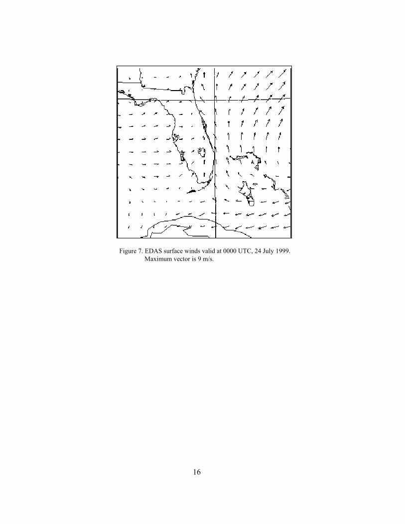
Figure 7. EDAS surface winds valid at 0000 UTC, 24 July 1999. Maximum vector is 9 m/s.

16

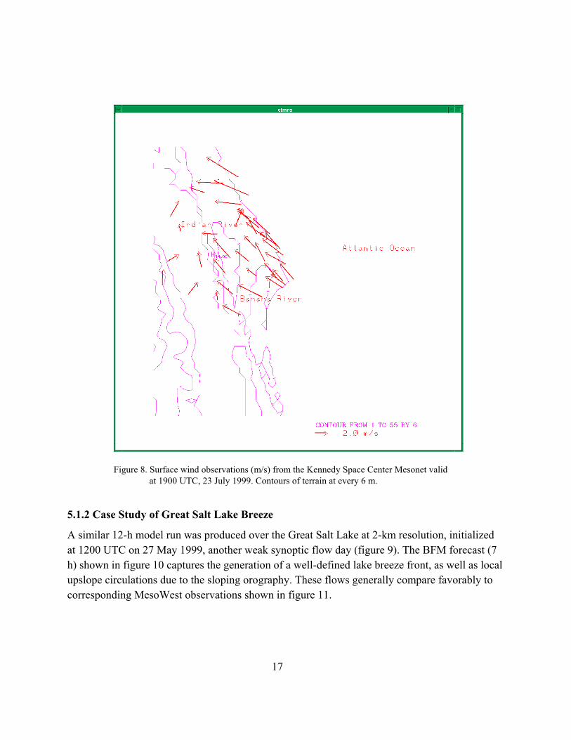
Figure 8. Surface wind observations (m/s) from the Kennedy Space Center Mesonet valid at 1900 UTC, 23 July 1999. Contours of terrain at every 6 m.

5.1.2 Case Study of Great Salt Lake Breeze

A similar 12-h model run was produced over the Great Salt Lake at 2-km resolution, initialized at 1200 UTC on 27 May 1999, another weak synoptic flow day (figure 9). The BFM forecast (7 h) shown in figure 10 captures the generation of a well-defined lake breeze front, as well as local upslope circulations due to the sloping orography. These flows generally compare favorably to corresponding MesoWest observations shown in figure 11.

17

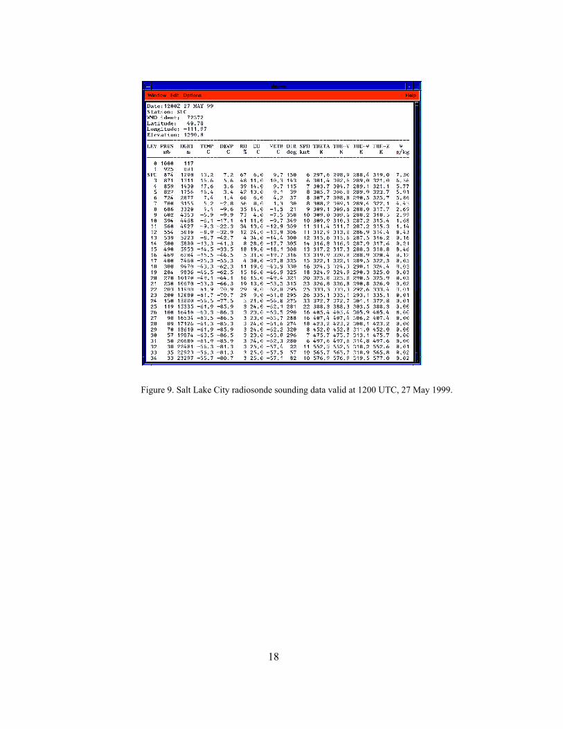
Figure 9. Salt Lake City radiosonde sounding data valid at 1200 UTC, 27 May 1999.

18

Figure 10. Forecast (7 h) of surface winds (m/s) near Salt Lake City, valid at 1900 UTC, 27 May 1999. BFM resolution is 2 km. Contours of terrain elevation every 200 m.

19

Figure 11. Surface wind observations (m/s) obtained from Utah MesoWest valid at 1900 UTC, 27 May 1999. Contours of terrain elevation every 250 m.

5.2 Statistical Results over the United States: Continental U.S. Study from 27 to 31 March 1998

The purpose of the study was to examine the BFM performance for a variety of geographical locations during an active synoptic period. The following 13 pressure levels of NOGAPS data were used to create analysis fields for nudging: 1000, 975, 925, 900, 850, 700, 500, 400, 300, 250, 200, 150, and 100 hPa. A total of 7 BFM forecasts were made for 9 locations within the continental U.S. from 27 to 31 March 1998, with a fixed domain size of 500 by 500 km and at a horizontal resolution of 10 km. Each forecast was 24 h in duration, and a statistical analysis of the data was generated every 6 h for surface and 12 h for upper-air parameters.

20

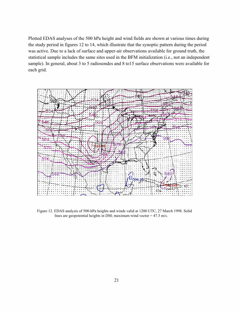
Plotted EDAS analyses of the 500 hPa height and wind fields are shown at various times during the study period in figures 12 to 14, which illustrate that the synoptic pattern during the period was active. Due to a lack of surface and upper-air observations available for ground truth, the statistical sample includes the same sites used in the BFM initialization (i.e., not an independent sample). In general, about 3 to 5 radiosondes and 8 to15 surface observations were available for each grid.

Figure 12. EDAS analysis of 500-hPa heights and winds valid at 1200 UTC, 27 March 1998. Solid lines are geopotential heights in DM; maximum wind vector = 47.5 m/s.

21



22

The statistical parameters produced are the mean absolute error, root-mean square error, correlation coefficient, standard deviation, and bias; for brevity, only the mean absolute error is extensively discussed in this section.

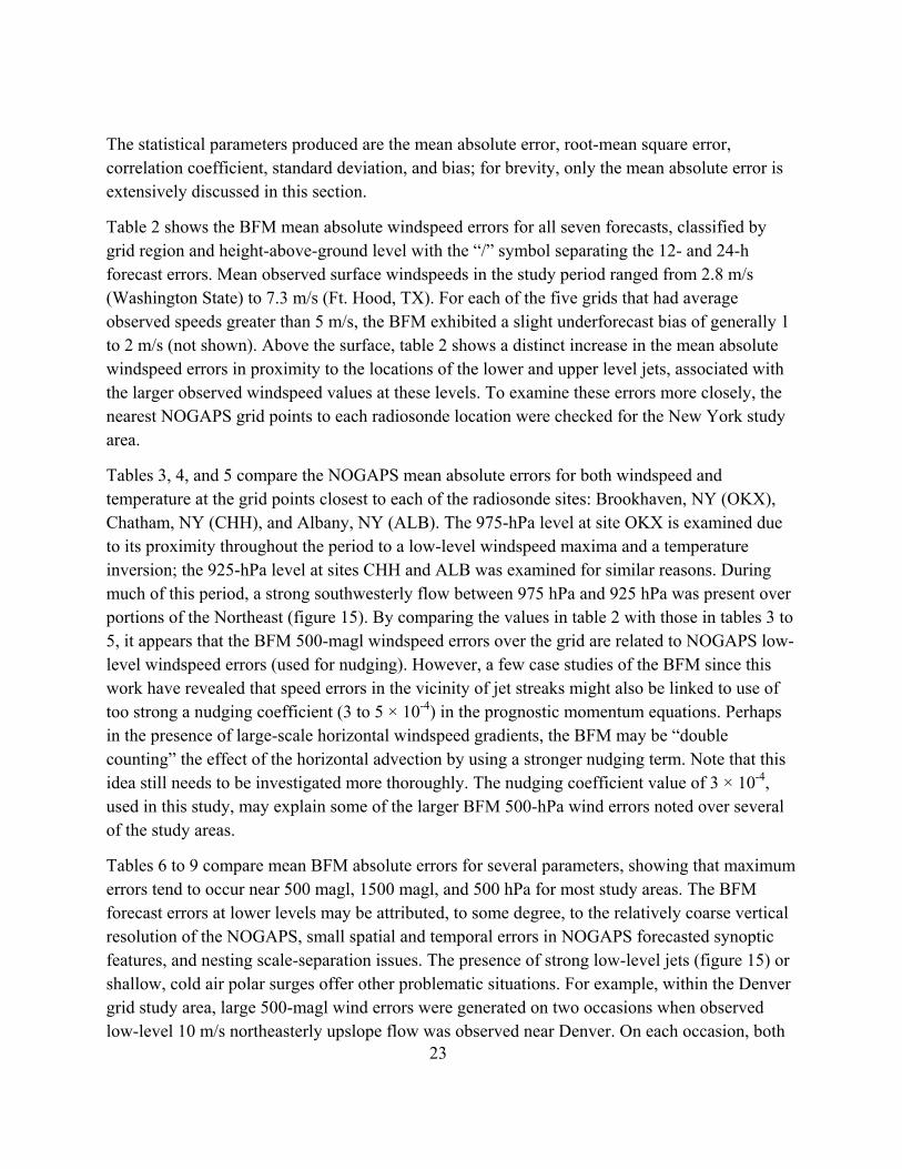
Table 2 shows the BFM mean absolute windspeed errors for all seven forecasts, classified by grid region and height-above-ground level with the “/” symbol separating the 12- and 24-h forecast errors. Mean observed surface windspeeds in the study period ranged from 2.8 m/s (Washington State) to 7.3 m/s (Ft. Hood, TX). For each of the five grids that had average observed speeds greater than 5 m/s, the BFM exhibited a slight underforecast bias of generally 1 to 2 m/s (not shown). Above the surface, table 2 shows a distinct increase in the mean absolute windspeed errors in proximity to the locations of the lower and upper level jets, associated with the larger observed windspeed values at these levels. To examine these errors more closely, the nearest NOGAPS grid points to each radiosonde location were checked for the New York study area.

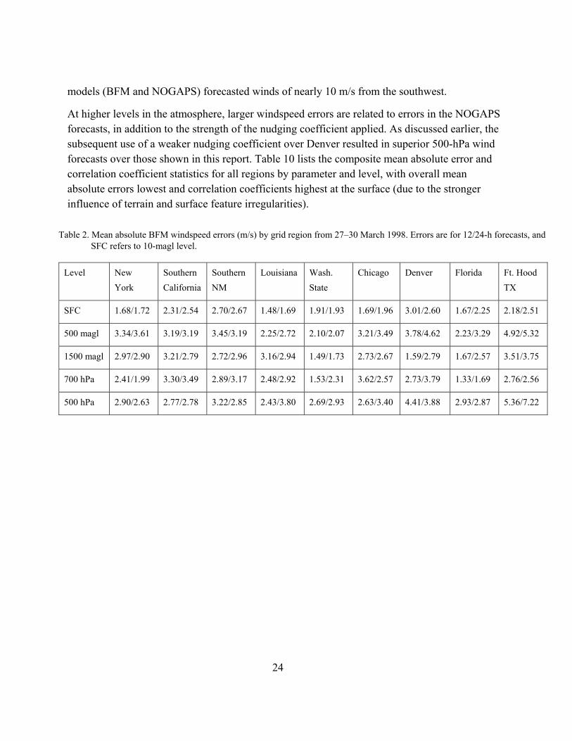
Tables 3, 4, and 5 compare the NOGAPS mean absolute errors for both windspeed and temperature at the grid points closest to each of the radiosonde sites: Brookhaven, NY (OKX), Chatham, NY (CHH), and Albany, NY (ALB). The 975-hPa level at site OKX is examined due to its proximity throughout the period to a low-level windspeed maxima and a temperature inversion; the 925-hPa level at sites CHH and ALB was examined for similar reasons. During much of this period, a strong southwesterly flow between 975 hPa and 925 hPa was present over portions of the Northeast (figure 15). By comparing the values in table 2 with those in tables 3 to 5, it appears that the BFM 500-magl windspeed errors over the grid are related to NOGAPS low-level windspeed errors (used for nudging). However, a few case studies of the BFM since this work have revealed that speed errors in the vicinity of jet streaks might also be linked to use of too strong a nudging coefficient (3 to 5 × 10-4) in the prognostic momentum equations. Perhaps in the presence of large-scale horizontal windspeed gradients, the BFM may be “double counting” the effect of the horizontal advection by using a stronger nudging term. Note that this idea still needs to be investigated more thoroughly. The nudging coefficient value of 3 × 10-4, used in this study, may explain some of the larger BFM 500-hPa wind errors noted over several of the study areas.

23

Tables 6 to 9 compare mean BFM absolute errors for several parameters, showing that maximum errors tend to occur near 500 magl, 1500 magl, and 500 hPa for most study areas. The BFM forecast errors at lower levels may be attributed, to some degree, to the relatively coarse vertical resolution of the NOGAPS, small spatial and temporal errors in NOGAPS forecasted synoptic features, and nesting scale-separation issues. The presence of strong low-level jets (figure 15) or shallow, cold air polar surges offer other problematic situations. For example, within the Denver grid study area, large 500-magl wind errors were generated on two occasions when observed low-level 10 m/s northeasterly upslope flow was observed near Denver. On each occasion, both

models (BFM and NOGAPS) forecasted winds of nearly 10 m/s from the southwest.

At higher levels in the atmosphere, larger windspeed errors are related to errors in the NOGAPS forecasts, in addition to the strength of the nudging coefficient applied. As discussed earlier, the subsequent use of a weaker nudging coefficient over Denver resulted in superior 500-hPa wind forecasts over those shown in this report. Table 10 lists the composite mean absolute error and correlation coefficient statistics for all regions by parameter and level, with overall mean absolute errors lowest and correlation coefficients highest at the surface (due to the stronger influence of terrain and surface feature irregularities).

Table 2. Mean absolute BFM windspeed errors (m/s) by grid region from 27–30 March 1998. Errors are for 12/24-h forecasts, and SFC refers to 10-magl level.

Level New York

Southern California

Southern NM

Louisiana Wash. State

Chicago Denver Florida Ft. Hood TX

SFC 1.68/1.72 2.31/2.54 2.70/2.67 1.48/1.69 1.91/1.93 1.69/1.96 3.01/2.60 1.67/2.25 2.18/2.51

500 magl 3.34/3.61 3.19/3.19 3.45/3.19 2.25/2.72 2.10/2.07 3.21/3.49 3.78/4.62 2.23/3.29 4.92/5.32

1500 magl 2.97/2.90 3.21/2.79 2.72/2.96 3.16/2.94 1.49/1.73 2.73/2.67 1.59/2.79 1.67/2.57 3.51/3.75

700 hPa 2.41/1.99 3.30/3.49 2.89/3.17 2.48/2.92 1.53/2.31 3.62/2.57 2.73/3.79 1.33/1.69 2.76/2.56

500 hPa 2.90/2.63 2.77/2.78 3.22/2.85 2.43/3.80 2.69/2.93 2.63/3.40 4.41/3.88 2.93/2.87 5.36/7.22

24

Table 3. Mean absolute errors of NOGAPS point 41°N, 73°W compared with OKX sounding in New York grid area.

Level Wind speed (m/s) Temperature (°C)

975 hPa 6.35/5.48 4.57/5.23

850 hPa 1.99/0.90 1.83/2.49

700 hPa 2.94/2.50 1.21/2.08

500 hPa 2.09/2.35 0.87/1.08

Table 4. Mean absolute errors of NOGAPS point 42°N, 70°W compared with CHH sounding in New York grid area.


925 hPa 2.40/2.73 2.65/3.85

850 hPa 2.61/2.22 2.23/2.13

700 hPa 2.36/2.74 0.62/1.03

500 hPa 3.52/1.75 0.95/1.17

Table 5. Mean absolute errors of NOGAPS point 43°N, 74°W compared with ALB sounding in New York grid area.


925 hPa 3.31/3.76 4.04/4.44

850 hPa 4.25/5.94 2.16/2.69

700 hPa 3.17/2.61 1.09/1.23

500 hPa 3.04/3.15 1.05/1.43

25

Figure 15. EDAS analysis of 925-hPa wind vectors valid at 0000 UTC, 29 March 1998. Maximum wind vector = 26.0 m/s over southeast Massachusetts.

26

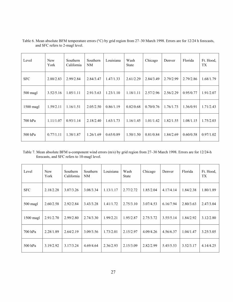
Table 6. Mean absolute BFM temperature errors (°C) by grid region from 27–30 March 1998. Errors are for 12/24 h forecasts, and SFC refers to 2-magl level.

Level New York

Southern California

Southern NM

Louisiana Wash State

Chicago Denver Florida Ft. Hood, TX

SFC 2.88/2.83 2.99/2.84 2.84/3.47 1.47/1.33 2.61/2.29 2.84/3.49 2.79/2.99 2.79/2.86 1.68/1.79

500 magl 3.52/5.16 1.05/1.11 2.91/3.63 1.23/1.10 1.18/1.11 2.57/2.96 2.56/2.29 0.95/0.77 1.91/2.07

1500 magl 1.59/2.11 1.16/1.51 2.05/2.50 0.86/1.19 0.82/0.68 0.70/0.76 1.76/1.73 1.36/0.91 1.71/2.43

700 hPa 1.11/1.07 0.93/1.14 2.18/2.40 1.63/1.73 1.16/1.45 1.01/1.42 1.82/1.55 1.08/1.15 1.75/2.03

500 hPa 0.77/1.11 1.38/1.87 1.26/1.69 0.65/0.89 1.50/1.50 0.81/0.84 1.84/2.69 0.60/0.58 0.97/1.02

Table 7. Mean absolute BFM u-component wind errors (m/s) by grid region from 27–30 March 1998. Errors are for 12/24-h forecasts, and SFC refers to 10-magl level.

Level New York

Southern California

Southern NM



SFC 2.18/2.28 3.07/3.26 3.08/3.34 1.13/1.17 2.77/2.72 1.85/2.04 4.17/4.14 1.84/2.38 1.80/1.89

500 magl 2.60/2.58 2.92/2.84 3.43/3.28 1.41/1.72 2.75/3.10 3.07/4.53 6.16/7.94 2.80/3.63 2.47/3.04

1500 magl 2.91/2.70 2.99/2.80 2.74/3.30 1.99/2.21 1.95/2.87 2.75/3.72 3.55/5.14 1.84/2.92 3.12/2.80

700 hPa 2.28/1.89 2.64/2.19 3.09/3.56 1.73/2.01 2.15/2.97 4.09/4.26 4.56/6.37 1.04/1.47 3.25/3.05

500 hPa 3.19/2.92 3.17/3.24 4.69/4.64 2.36/2.93 2.15/3.09 2.82/2.99 5.45/5.53 3.52/3.17 4.14/4.25

27

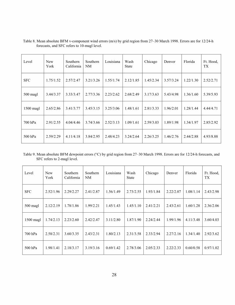
Table 8. Mean absolute BFM v-component wind errors (m/s) by grid region from 27–30 March 1998. Errors are for 12/24-h forecasts, and SFC refers to 10-magl level.

Level New York

Southern California

Southern NM



SFC 1.75/1.52 2.57/2.47 3.21/3.26 1.55/1.74 2.12/1.85 1.45/2.34 3.57/3.24 1.22/1.30 2.52/2.71

500 magl 3.44/3.37 3.33/3.47 2.77/3.36 2.23/2.62 2.68/2.49 3.17/3.63 5.43/4.98 1.36/1.60 5.39/5.93

1500 magl 2.65/2.86 3.41/3.77 3.45/3.15 3.25/3.06 1.48/1.61 2.81/3.33 1.96/2.01 1.28/1.44 4.44/4.71

700 hPa 2.91/2.55 4.04/4.46 3.74/3.66 2.52/3.13 1.09/1.61 2.59/3.03 1.89/1.98 1.34/1.97 2.85/2.92

500 hPa 2.59/2.29 4.11/4.18 3.84/2.95 2.48/4.23 3.24/2.64 2.26/3.25 1.46/2.76 2.44/2.88 4.93/8.88

Table 9. Mean absolute BFM dewpoint errors (°C) by grid region from 27–30 March 1998. Errors are for 12/24-h forecasts, and SFC refers to 2-magl level.

Level New York

Southern California

Southern NM



SFC 2.52/1.96 2.29/2.27 2.41/2.87 1.56/1.49 2.73/2.55 1.93/1.84 2.22/2.07 1.08/1.14 2.43/2.98

500 magl 2.12/2.19 1.78/1.86 1.99/2.21 1.45/1.43 1.45/1.10 2.41/2.21 2.43/2.61 1.60/1.28 2.36/2.06

1500 magl 1.74/2.13 2.23/2.60 2.42/2.47 3.11/2.80 1.87/1.90 2.24/2.44 1.99/1.96 4.11/3.48 3.60/4.03

700 hPa 2.58/2.31 3.60/3.35 2.43/2.31 1.80/2.13 2.31/3.58 2.33/2.94 2.27/2.16 1.34/1.40 2.92/3.62

500 hPa 1.98/1.41 2.18/3.17 3.19/3.16 0.69/1.42 2.78/3.06 2.05/2.33 2.22/2.33 0.60/0.58 0.97/1.02

28

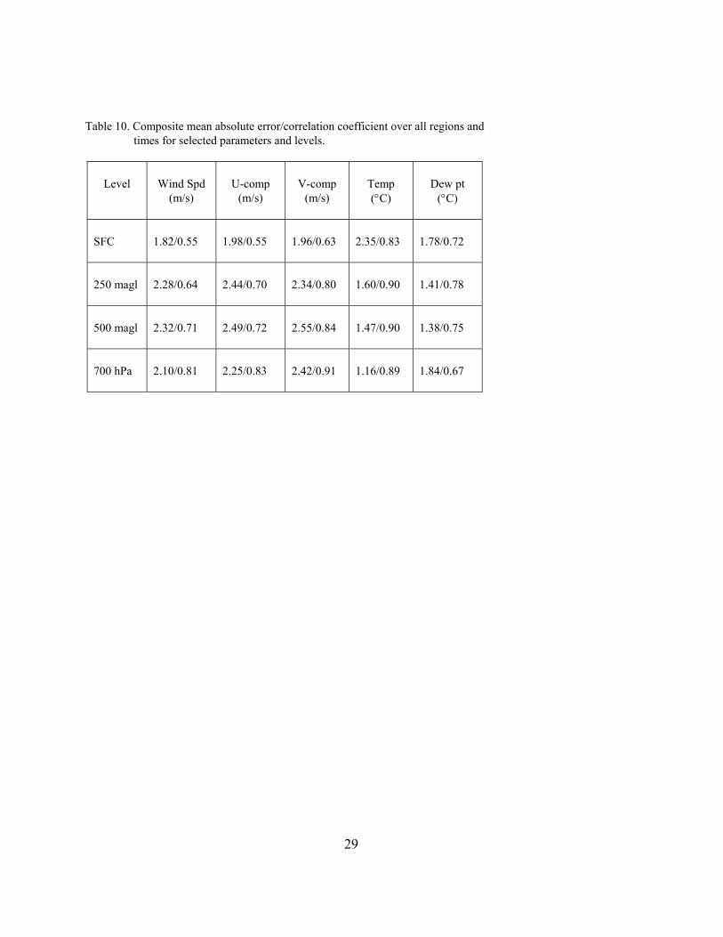
Table 10. Composite mean absolute error/correlation coefficient over all regions and times for selected parameters and levels.

Level Wind Spd (m/s)

U-comp (m/s)

V-comp (m/s)

Temp (°C)

Dew pt (°C)

SFC 1.82/0.55 1.98/0.55 1.96/0.63 2.35/0.83 1.78/0.72

250 magl 2.28/0.64 2.44/0.70 2.34/0.80 1.60/0.90 1.41/0.78

500 magl 2.32/0.71 2.49/0.72 2.55/0.84 1.47/0.90 1.38/0.75

700 hPa 2.10/0.81 2.25/0.83 2.42/0.91 1.16/0.89 1.84/0.67

29

6. Possible Improvements and Considerations

Several features of the current BFM could be examined for improvements and modifications—such as the use of the Mesoscale Modeling System V (MM5) of the Pennsylvania State University/National Center for Atmospheric Research (Grell et al., 1994) for obtaining nudging input files. AFWA is now operationally running the MM5 at a 45-km horizontal resolution, offering the potential to reduce the scale-separation nesting ratio for nudging to 4.5-to-1, a significant improvement from the current configuration ratio using NOGAPS. Other possible improvements might involve a better treatment of clouds and radiation, an elevation-dependent weighting for determining the surface nudging coefficients, a higher resolution and heterogeneous surface state input, and a cumulus parameterization option (Sun and Haines, 1996).

7. Summary and Discussion

The BFM is a useful short-range, operational forecasting and planning tool for the tactical Army, despite its limitations (i.e., localized summer convection, nonhydrostatic forcing, sharp frontal boundaries, etc.). The use of Newtonian relaxation provides an ability to fully assimilate forecast tendencies from a larger-scale numerical model. In benign synoptic regimes, successful simulations of local boundary layer flows forced by surface inhomogeneities in terrain and radiation are possible. If, for example, the AFWA MM5 were to be used to obtain BFM nudging guidance (replacing NOGAPS), the horizontal resolution nesting ratio could be reduced to about 4-to-1 or greater. This would reduce the scale separation and resolution consistency problems discussed by Warner et al. (1997). Nonetheless, previous results have shown that the present BFM can still provide useful forecasts in the lower boundary layer (Haines, 1999), which can guide tactical weather decision aids and other weather-dependent components of the Intelligent Planning of the Battlefield process.

30

8. References

Arakawa, A.; Lamb, V. R. Computational Design of the Basic Dynamical Processes of the UCLA General Circulation Model. Meth. Comp. Phys. 1977, 17, 174–264.

Atkins, N. T.; Wakimoto, R. M. Influence of the Synoptic-Scale Flow on Sea Breezes Observed During Cape. Mon. Wea. Rev. 1997, 125, 2112–2130.

Barnes, S. L. A Technique for Maximizing Details in Numerical Weather Map Analysis. J. Appl. Meteor. 1964, 3, 396–409.

Doran, J. C.; Horst, T. W. Observations and Models of Simple Nocturnal Slope Flows. J. Atmos. Sci. 1982, 40, 708–717.

Grell, G. A.; Dudhia, J.; Stauffer, D. R. A Description of the Fifth Generation Penn State/NCAR Mesoscale Model (MM5); NCAR/TN 398+STR; 1994,138 pp.

Hanson, H. P.; Derr, V. E. Parameterization of Radiative Flux Profiles within Layer Clouds. J. Appl. Meteor 1987, 26, 1511–1521.

Harms, D. E.; Sashegyi, K. D.; Madala, R. V.; Raman, S. Four-Dimensional Data Assimilation of Gale Data Using a Multivariate Analysis Scheme and a Mesoscale Model with Diabatic Initialization; NRL/MR/4223-92-7147; Naval Research Laboratory, 1992, 236 pp.

Haines, P. I. Validation of Short-Term Battlescale Forecast Model Forecasts with Profiler and Upper-Air Data Collected over Oklahoma. Preprints of the Eighth Conference on Aviation, Range, and Aerospace Meteorology, American Meteorological Society, Dallas, Texas, Jan 10-15, 1999, pp 599–603.

Henmi, T.; Dumais, Jr., R. E. Description of the Battlescale Forecast Model; ARL-TR-1032; U.S. Army Research Laboratory, 1998, 148 pp.

Henmi, T. Comparison and Evaluation of Operational Mesoscale MM5 and BFM over WSMR; ARL-TR-1476; U.S. Army Research Laboratory, 2000, 60 pp.

Hogan, T. F.; Rosmond, T. E. The Description of the Navy Operational Global Atmospheric Prediction System’s Spectral Forecast Model. Mon. Wea. Rev. 1991, 119, 1786–1815.

Hoke, J. E.; Anthes, R. A. The Initialization of Numerical Models by a Dynamic-Initialization Technique. Mon. Wea. Rev. 1976, 104, 1551–1556.

31

Kao, C-Y. J. Yamada, T. Numerical Simulations of a Stratocumulus-Capped Boundary Layer

Observed over Land. J. Atmos. Sci. 1989, 46, 832–848.

Knapp, D. I. Development of a Surface Visibility Algorithm for Worldwide Use with Mesoscale Model Output. 15th Conference of Weather Analysis and Forecasting, Amer. Meteor. Soc. 1996, 83–86.

Knapp, D. I. Battlescale Forecast Model (BFM) Target Area Wind Speed Validation over WSMR, NM Initial Results; ARL-TR-1730; U.S. Army Research Laboratory, 1998, 33 pp.

Kondrat’yev, K. Y. Radiative Regime on Inclined Surface. WMO Technical Note No. 15; Secretariat of the World Meteorological Organization, Geneva, Switzerland, 1977, 82 pp.

McNider, R. T. A Note on Velocity Fluctuations in Drainage Flows. J. Atmos. Sci. 1982, 39, 1658–1660.

Mahrer, Y.; Pielke, R. A. Numerical Simulation of Airflow over Barbados. Mon. Wea. Rev. 1976, 104, 1392–1402.

Mellor, G. L.; Yamada, T. Development of a Turbulence Closure Model for Geophysical Fluid Problems. Rev. Geophys. Space Phys. 1982, 20, 851–875.

MESO. MASS Version 5.5 Reference Manual. Available from MESO, Inc., 185 Jordan Road, Troy NY, 12180, 1993, 118 pp.

Orlanski, I. A Rational Subdivision of Scales for Atmospheric Processes. Bull. Am. Meteor. Soc. 1975, 56, 527–530.

Passner, J. E. The Atmospheric Sounding Program: An Analysis and Forecasting Tool for Weather Hazards on the Battlefield; ARL-TR-1883; U.S. Army Research Laboratory, 1999, 68 pp.

Peaceman, D. W. Rachford, Jr., H. H. The Numerical Solution of Parabolic and Elliptic Differential Equations. SIAM J. Appli. Math. 1955, 3, 28–41.

Pielke, R. A. Mesoscale Meteorological Modeling; Academic Press: New York, 1984, 612 pp.

Pielke, R. A.;Pearce, R. P. Mesoscale Modeling of the Atmosphere. Meteorological Monographs. Amer. Meteor. Soc. 1994, 25, 167 pp.

Rao, P. A.; Fuelberg, H. E.; Droegemeier, K. K. High-Resolution Modeling of the Cape Canaveral Land-Water Circulations and Associated Features. Mon. Wea. Rev. 1999, 127, 1808–1821.

32

Reichelderfer, M.; Barker, C. 155-mm Howitzer Accuracy and Effectiveness Analyses; AMSAA

Ground Warfare Division; Division Note No. DN-G-32; U.S. Army Materiel Systems Analyses Activity, Aberdeen Proving Ground, MD, December 1993.

Richtmeyer, R. D.; Morton, K. W. Difference Methods for Initial-Value Problems; 2nd ed.; Wiley-Interscience, 1967, 405 pp.

Sauter, David P. The Integrated Weather Effects Decision Aid (IWEDA): Status and Future Plans. Proceedings of the 1996 Battlespace Atmospherics Conference, Naval Command, Control and Ocean Surveillance Center, RDT&E Division, San Diego, CA, Dec 3-5, 1996, pp 75–81.

Stauffer, D. R.; Seaman, N. L. Use of Four-Dimensional Data Assimilation in a Limited-Area Mesoscale Model. Part I: Experiments with Synoptic-Scale Data. Mon. Wea. Rev. 1990, 118, 1250–1277.

Sun, W-Y.; Haines, P. A. Semi-Prognostic Tests of a New Cumulus Parameterization Scheme for Mesoscale Modeling. Tellus 1996, 48A, 272–289.

Sundqvist, H.; Berge, E.; Kristja’nsson, J. E. Condensation and Cloud Parameterization Studies with a Mesoscale Numerical Weather Prediction Model. Mon. Wea. Rev. 1989, 117, 1641–1657.

Yamada, T. A Numerical Simulation of Nocturnal Drainage Flow. J. Meteor. Soc. Japan 1981, 59, 108–122.

Yamada, T. A Numerical Model Study of Turbulent Airflow In and Above a Forest Canopy. J. Meteor. Soc. Japan 1982, 60, 439–454.

Yamada, T. Simulations of Nocturnal Drainage Flows by a q2l Turbulence Closure Model. J. Atmos. Sci. 1983, 40, 91–106.

Yamada, T.; Bunker, S. Development of a Nested Grid, Second Moment Turbulence Closure Model and Application to the 1982 ASCOT Brush Creek Data Simulation. J. Appli. Met. 1988, 27, 562–578.

Yamada, T. A Numerical Model Study of Nocturnal Drainage Flows with Strong Wind and Temperature Gradients. J. Appli. Met. 1989, 28, 545–554.

Warner, T. T.; Peterson, R. A.; Trendon, R. E. A Tutorial on Lateral Boundary Conditions as a Basic and Potentially Serious Limitation to Regional Numerical Weather Prediction. Bull. Amer. Meteor. Soc. 1997, 78, 2599–2617.

33

Acronyms and Abbreviations

ADI alternating direction implicit

AFWA Air Force Weather Agency

AI artificial intelligence

ALB Albany radiosonde

ASP Atmospheric Sounding Program

BFM Battlescale Forecast Model

CAAM Computer Assisted Artillery Meteorology

CHH Chatham radiosonde

CFL Courant-Friedrich-Lewy

EDAS ETA Data Analysis System

FCMM forecast computer meteorological messages

GMDB gridded meteorological database

GTRAJ3 General Trajectory Model 3

GUI graphical user interface

IMETS Integrated Meteorological System

IWEDA Integrated Weather Effects Decision Aid

LUT Limited User Test

Met meteorological

MM5 Mesoscale Modeling System V

MRMD mean radial miss distance

NOGAPS Naval Operational Global Atmospheric Prediction System

NWP numerical weather prediction

34

OKX Brookhaven radiosonde

OWS Operational Weather Squadron

PBL planetary boundary layer

RCMM radiosonde computer meteorological messages

RDAP Reliability Determination and Assurance Program

SADARM Sense and Destroy Armor

TDAs Tactical Decision Aids

T-VSAT Tactical-Very Small Aperture Terminal

UTC universal time coordinated

XMR Cape Canaveral radiosonde

YPG Yuma Proving Ground

4DDA four-dimensional data assimilation

35

Distribution List

Copies Copies

NCAR LIBRARY SERIALS 1 NASA SPACE FLT CTR 1

NATL CTR FOR ATMOS RSCH ATMOSPHERIC SCIENCES DIV

PO BOX 3000 CODE ED 41 1

BOULDER CO 80307-3000 HUNTSVILLE AL 35812

HEADQUARTERS DEPT OF ARMY 1 US ARMY MISSILE CMND 1

DAMI-POB (WEATHER TEAM) REDSTONE SCI INFO CTR

1000 ARMY PENTAGON, ROOM 2E383 AMSMI RD CS R DOC

WASHINGTON DC 20310-1067 REDSTONE ARSENAL AL 35898-5241

HQ AFWA/DNX 1 PACIFIC MISSILE TEST CTR 1

106 PEACEKEEPER DR STE 2N3 GEOPHYSICS DIV

OFFUTT AFB NE 68113-4039 ATTN: CODE 3250

POINT MUGU CA 93042-5000

AFRL/VSBL 1

29 RANDOLPH RD ATMOSPHERIC PROPAGATION

BRANCH 1 HANSCOM AFB MA 01731

SPAWARSYSCEN SAN DIEGO D858

ARL CHEMICAL BIOLOGY 1 49170 PROPAGATION PATH

NUC EFFECTS DIV SAN DIEGO CA 92152-7385

AMSRL SL CO

APG MD 21010-5423 METEOROLOGIST IN CHARGE 1

KWAJALEIN MISSILE RANGE

PO BOX 67

APO SAN FRANCISCO CA 96555

36

Copies Copies

US ARMY RSRC OFC 1 US ARMY MATERIEL SYST 1

ATTN: AMSRL-RO-EN ANALYSIS ACTIVITY

PO BOX 12211 AMSXY

RTP NC 27009 APG MD 21005-5071

US ARMY CECRL 1 US ARMY RESEARCH LABORATORY 1

CRREL-GP AMSRL D

ATTN: DR DETSCH 2800 POWDER MILL ROAD

HANOVER NH 03755-1290 ADELPHI MD 20783-1145

ARMY DUGWAY PROVING GRD 1 US ARMY RESEARCH LABORATORY 1

STEDP MT DA L 3 AMSRL CI-OK-TL

DUGWAY UT 84022-5000 2800 POWDER MILL ROAD

ADELPHI MD 20783-1197

ARMY DUGWAY PROVING GRD 1

STEDP MT M US ARMY RESEARCH LABORATORY 1

ATTN: MR BOWERS AMSRL SE-EE

DUGWAY UT 84022-5000 ATTN: DR SZTANKAY

2800 POWDER MILL ROAD

USAF ROME LAB TECH 1 ADELPHI MD 20783-1145

CORRIDOR W STE 262 RL SUL

26 ELECTR PKWY BLD 106 US ARMY RESEARCH LABORATORY 1

GRIFFISS AFB ROME, NY 13441-4514 AMSRL CI

ATTN: J GANTT

US ARMY FIELD ARTILLERY SCHOOL 1 2800 POWDER MILL ROAD

ATSF TSM TA ADELPHI MD 20783-1197

FT SILL OK 73503-5600

37

Copies Copies

US ARMY TRADOC ANALYSIS CMND 1 NAVAL SURFACE WEAPONS CTR 1

ATRC WSS R CODE G63

WSMR NM 88002-5502 DAHLGREN VA 22448-5000

US ARMY RESEARCH LABORATORY 1 US ARMY OEC 1

AMSRL CI E CSTE EFS

COMP & INFO SCI DIR PARK CENTER IV

WSMR NM 88002-5501 4501 FORD AVE

ALEXANDRIA VA 22302-1458

US ARMY DUGWAY PROVING GRD 1

STEDP3 US ARMY CORPS OF ENGRS 1

DUGWAY UT 84022-5000 ENGR TOPOGRAPHICS LAB

ATTN: CETEC-TR-G PF KRAUSE

WSMR TECH LIBRARY BR 1 ALEXANDRIA, VA 2215-3864

STEWS IM IT

WSMR NM 88002 US ARMY TOPO ENGR CTR 1

CETEC ZC 1

US ARMY RESEARCH LAB 1 FT BELVOIR VA 22060-5546

AMSRD-ARL-O DR D SMITH

2800 POWDER MILL RD SCI AND TECHNOLOGY 1

ADELPHI MD 20783-1197 101 RESEARCH DRIVE

HAMPTON VA 23666-1340

US ARMY CECOM 1

USATRADOC 1 INFORMATION & INTELLIGENCE

WARFARE DIRECTORATE ATCD FA

ATTN: AMSEL RD IW IP FT MONROE VA 23651-5170

FORT MONMOUTH NJ 07703-5211

38

Copies Copies

ARL LIBRARY 2 NAVAL RESEARCH LABORATORY 1

US ARMY RESEARCH LABORATORY MARINE METEOROLOGY DIVISION

AMSRD-CI-OK-TL 7 GRACE HOPPER AVENUE, STOP 2

ATTN: KATHLEEN RAPKA MONTEREY, CA 93943-5502

2800 POWDER MILL ROAD

ADELPHI, MD 20783-1197 US ARMY RESEARCH LABORATORY 1

ATTN SFAE-C3T-IE-II, ROBERT DICKENSHIED

US ARMY RESEARCH LABORATORY 3 WSMR, NM 88002

CISD BED

ATTN: MR ROBERT E DUMAIS JR DTIC 1 ELECTRONIC COPY AMSRD ARL CI EB

WSMR NM 88002-5501 DEFENSE TECHNICAL INFO CTR DTIC OCA US ARMY RESEARCH LABORATORY 4 ATTN: JOYCE CHIRAS CISD BED 8725 JOHN J KINGMAN RD STE 0944 ATTN: DR PATRICK A HAINES FT BELVOIR VA 22060-6218 DR TEIZI HENMI MR JEFFREY E PASSNER MAIL & RECORDS MANAGEMENT

ADELPHI 1 MR TERRY C JAMESON

AMSRD ARL CI EB US ARMY RESEARCH LABORATORY WSMR NM 88002-5501 ATTN: AMSRL CI IS R (A SMITH) MAIL & RECORDS MGMT

ADELPHI MD 20783-1197

39

Copies

US ARMY RESEARCH LABORATORY 1

CISD BED

ATTN: MR DAVID KNAPP

AMSRD ARL CI EM

WSMR NM 88002-5501

TOTAL 47

40

by robert e. dumais, jr., teizi henmi, jeffrey passner ... · a mesoscale modeling system developed...

Documents