by pedro jorge campos ferrinha tese de mestrado em economia
TRANSCRIPT

Monetary Policy and International Capital Flows:
The Recent Experience
by
Pedro Jorge Campos Ferrinha
Tese de Mestrado em Economia
Supervised by: Manuel Duarte Rocha
2014/2015


i
Born on April, 16, 1991, in Lisbon, the student started his education in São João da
Madeira where he completed the High School. Then, in September, 2009, he moved to
Porto to study Economics at Faculdade de Economia do Porto, faculty from which he
graduated in 2013.
Following his interesting in macroeconomics and monetary economics, he started his
Master’s Degree in Economics in the same institution in 2013. In the third quarter of
2014 he started to work at PricewaterhouseCoopers & Associados as assurance
associate.

ii
Even though this document is the result of one year of hard work and it will be used to
compete for a Master’s degree, it would not be complete if it were not for my family
support. This is the reason why the first appreciation goes to my parents. The full
support that I received from them during the last year in which I had to combine a
professional career with the ambition of finishing my Master’s made it possible for me
to totally focus on my goals. Mr. Fernando Ferrinha and Mrs. Anabela Campos, this
work is also yours.
The second reference goes to my brother, Mr. Nuno Ferrinha, who, although from the
other side of the World, made himself present and demonstrated his support every time
it was needed. As the first reader of my work, I give you my gratitude. This work is also
yours.
For my friends who in one way or another understood the challenge I was facing and
encouraged me to fight for it, I am grateful to you; for those who assigned part of their
time on reading this document and contributed with precious comments, I am grateful to
you.
Last, but not the least, I want to demonstrate my gratefulness to Professor Manuel
Duarte Rocha who, during the last year, played a crucial role: his assertive comments,
his experience as researcher and his full disposition to contribute to the conclusion of
this work was priceless. As far as this experience goes, the lessons I took from him go
much further than the result of the work here documented.

iii
Abstract: This work investigates the main determinants of capital flows to advanced
and non-advanced economies in the last decade and assesses whether and how
unconventional monetary policies played a role as an additional determinant in
explaining capital flows in this recent experience. We contribute to the literature by
using an alternative measure of capital flows that allow us to distinguish the investment
from the disinvestment component of the balance of payments. Our main findings are:
first, the determinants of capital flows in the pre-crisis period were also significant in
explaining the capital flows in the post-crisis period, both for advanced and non-
advanced economies. Second, unconventional monetary policies are one additional
determinant of capital inflows to advanced and non-advanced economies. Finally, we
find that unconventional monetary policies pushed capital flows to non-advanced
economies in form of new investment from foreign agents and pulled away capital
inflows in form repatriation of capital.
Resumo: O objeto de estudo deste trabalho foca-se nos determinantes dos fluxos de
capitais para economias avançadas e não avançadas durante a última década e de que
forma é que as políticas monetárias não convencionais contribuíram como fator
explicativo adicional. A nossa contribuição para a literatura que nos é próxima está
relacionada com a utilização de uma medida alternativa dos fluxos de capitais que
permitem distinguir a componente de investimento e de desinvestimento da balança de
pagamentos. Os nossos resultados são: primeiro, os determinantes dos fluxos de capitais
para economias avançadas e não avançadas do período pré-crise mantiveram-se
significativos no período pós-crise. Em segundo lugar, os resultados suportam a
hipótese de que as políticas monetárias não convencionais agiram como um
determinante adicional dos fluxos de capital para as economias avançadas e não-
avançadas. Por último, os resultados permitem-nos concluir que as políticas monetárias
não convencionais surtiram efeito nos fluxos de capital para economias não-avançadas
através do aumento das decisões de investimento para essas economias ao mesmo
tempo que contribuíram para a diminuição da repatriação de capital por parte dos
agentes domésticos.

iv
Index
Chapter 1 – Introduction 1
Chapter 2 – Recent experience on capital flows 4
Chapter 3 – Literature review on monetary policy and capital flows 9
Section 3.1 – Implementation of monetary policy 9
Section 3.2 – Monetary policies 15
Section 3.3 – Capital flows 22
Section 3.4 – Did the global financial crisis cause a shift on the drivers of capital
flows? 33
Section 3.5 – The effect of unconventional monetary policies on capital flows -
empirical results 35
Section 3.6 – Monetary policy normalization 39
Section 3.7 – How should capital flows be measured? 42
Chapter 4 – Modeling capital flows 45
Section 4.1 – Common determinants of capital flows 45
Section 4.2 – Baseline model and methodologic considerations 47
Section 4.3 – Data 52
Chapter 5 – Estimation results 54
Section 5.1 – Benchmark model 54
Section 5.2 – Did the determinants of capital flows change from the pre-crisis to
the post-crisis period? 59
Section 5.3 – Did unconventional monetary policies pushed capital flows to
certain economies? 64
Section 5.4 – The four-way decomposition 71
Section 5.5 – Robustness check 73
Chapter 6 – Conclusion 79
References 82
Annex 93

v
Figures
1. Capital inflows to emerging economies 6
2. Capital outflows from advanced economies 7
A1. Capital inflows to Emerging Asia 93
A2. Capital inflows to Latin America 93
A3. Capital inflows to Europe, Middle East, and Africa 94
A4. Transmission mechanism of monetary policy 94
vi
Tables
1. Hausman test for non-advanced economies 48
2. Hausman test for advanced economies 48
3. Benchmark results for non-advanced economies 55
4. Benchmark results for all the economies 56
5. Benchmark results for advanced economies 57
6. Pre and post-crisis regressions for non-advanced economies’ net inflows 60
7. Pre and post-crisis regressions for non-advanced economies’ gross inflows 61
8. Pre and post-crisis regressions for advanced economies’ net inflows 62
9. Pre and post-crisis regressions for advanced economies’ gross inflows 63
10. UMP effects on net inflows to non-advanced economies 64
11. UMP effects on gross inflows to non-advanced economies 65
12. UMP effects on net inflows to advanced economies 66
13. UMP effects on gross inflows to advanced economies 67
14. UMP effects on net inflows to all the economies 68
15. UMP effects on gross inflows to all the economies 69
16. Benchmark results for the four-way elements regarding non-advanced
economies 74
17. UMP results for the four-way elements regarding non-advanced economies 75
A1. Summary description of the variables 95
A2. List of Federal Reserve monetary actions' announcements with impact on the
balance sheet 97
A3. List of European Central Bank monetary actions' announcements with impact
on the balance sheet 99
A4. List of Bank of England monetary actions' announcements with impact on the
balance sheet 100
A5. List of Bank of Japan monetary actions' announcements with impact on the
balance sheet 101
A6. Sample 103
A7. Pre and post-crisis regressions for all the economies’ net inflows 104

vii
A8. Pre and post-crisis regressions for all the economies’ gross inflows 105
A9. Net and gross inflows to non-advanced economies controlling for the Federal
Reserve announcements 106
A10. Net and gross inflows to advanced economies controlling for the Federal
Reserve announcements 107
A11. Net and gross inflows to all the economies controlling for the Federal Reserve
announcements 108
A12. Benchmark results for the four-way elements regarding all the economies 109
A13. UMP results for the four-way elements regarding all the economies 110
A14. Benchmark results for the four-way elements regarding the advanced
economies 111
A.15. UMP results for the four-way elements regarding advanced economies 112
A.16. Robustness check: relative expansion of G4 balance sheet regarding non-
advanced economies’ net and gross inflows 113
A.17. Robustness check: relative expansion of G4 balance sheet regarding non-
advanced economies’ four-way elements 114
A.18. Robustness check: relative expansion of G4 balance sheet regarding advanced
economies’ net and gross inflows 115
A19. Robustness check: relative expansion of G4 balance sheet regarding advanced
economies’ four-way elements 116
A20. Robustness check: benchmark results not controlling for seasonal effects
regarding non-advanced economies’ net and gross inflows 117
A.21. Robustness check: benchmark results not controlling for seasonal effects
regarding advanced economies’ net and gross inflows 118
A.22. Robustness check: UMP results without controlling for seasonal effects
regarding non-advanced economies’ net inflows 119
A.23. Robustness check: UMP results without controlling for seasonal effects
regarding non-advanced economies’ gross inflows 120
A24. Robustness check: UMP results not controlling for seasonal effects regarding
advanced economies’ net inflows 121

viii
A25. Robustness check: UMP results not controlling for seasonal effects regarding
advanced economies’ gross inflows 122
A.26. Robustness check: benchmark model applied to non-advanced economies’
four-way elements not controlling for seasonal effects 123
A.27. Robustness check: benchmark model applied to advanced economies’ four-
way elements not controlling for seasonal effects 124
A.28. Robustness check: UMP results regarding non-advanced economies’ four-way
elements not controlling for seasonal effects 125
A.29. Robustness check: UMP results regarding advanced economies’ four-way
elements not controlling for seasonal effects 126
A.30. Robustness check: estimation of the benchmark model regarding non-
advanced using random effects 127
A.31. Robustness check: estimation of the benchmark model regarding advanced
using random effects 128
A.32. Robustness check: estimation of the UMP model regarding non-advanced
economies’ net inflows using random effects 129
A.33. Robustness check: estimation of the UMP model regarding non-advanced
economies’ gross inflows using random effects 130
A.34. Robustness check: estimation of the UMP model regarding advanced
economies’ net inflows using random effects 131
A.35. Robustness check: estimation of the UMP model regarding advanced
economies’ gross inflows using random effects 132
A.36. Robustness check: estimation of non-advanced economies’ four-way elements
using random effects 133
A.37. Robustness check: estimation of advanced economies’ four-way elements
using random effects 134
A.38. Robustness check: estimation of the UMP model regarding the non-advanced
economies’ four-way elements using random effects 135
A.39. Robustness check: estimation of the UMP model regarding the non-advanced
economies’ four-way elements using random effects 136

1
1. Introduction
The global financial crisis (GFC) triggered unusual actions from the major central
banks as interest rates were successively cut and reached the zero-lower bound. In order
to boost weak asset markets and stimulate real economic activity, the G41 central banks
initiated unconventional monetary policies (UMP), which culminated in an outstanding
expansion of their balance sheets (Fawley & Neely, 2013). The impacts of such UMP
measures have become increasingly controversial.
Advanced economies (AE) argue that unusual expansionary monetary policy
stabilized financial markets and promoted growth; therefore, its global effects must be
regarded as positive. Even if necessary under certain conditions to boost high-income
countries, low interest rates during prolonged periods of time may threaten financial
stability as low risk-free yields could induce a change in the asset allocation of investors
to non-advanced economies (NAE)2 rather than AE (IMF, 2010a and IMF, 2011b).
Moreover, NAEs’ policy makers made their suspicion about these policies’ negative
spillovers very clear. When put together with domestic factors, such as growth
prospects or appreciated currencies, the UMP was feared to create an environment that
could would affect capital flows, exchange rates, asset prices (Cho & Rhee, 2013),
generating a decrease in the robustness of their financial systems (Chen, Mancini-
Griffoni, & Sahay, 2014), leading to the expansion of domestic liquidity and potential
set off credit bubbles, a build-up of imbalances, including the drive up of asset prices to
unsustainable levels and overheating of the economies, and possible external shocks in
the form of sudden stops (IMF, 2010a, IMF, 2011b and Powell, 2010).3
There is literature that already assessed similar questions: Fratzscher, Lo Duca, &
Straub (2013), Ahmed & Zlate (2014), and Burns et al. (2014) concluded for a positive
effect of UMP on capital inflows both to AE and NAE beyond the global and domestic
1 We will follow the work of Cerutti, Claessens & Ratnovski (2014), Nier, Sedik, & Mondino (2014) and
Burns, Kida, Lim, Mohapatra, & Stocker (2014) and consider United States, Euro Area, United Kingdom,
and Japan as the G4 economies. 2 Non-advanced economies refers to emerging and developing countries.
3 The mechanisms by which capital inflows affect variables as asset prices (see e.g. Kim & Yang , 2011,
and Taguchi, Sahoo, & Natara, 2015), house price (see e.g. Tillmann, 2013, Aizenman & Jinjarak, 2009,
and Jinjarak & Sheffrin, 2011), and credit growth (see e.g. Lane & McQuade, 2013, and Arslan & Taskin,
2014) is object of an extensive literature.

2
conditions, even though these works employed different measures of UMP. The
contribution of our work to this literature is on the use of the four-way decomposition,
an alternative measure of capital inflows proposed by Janus & Riera-Crichton (2013).
This measure intends to distinguish the investment and disinvestment components of
the balance of payments. By doing so, it could help to correctly classify disinvestments
as outflows rather than negative inflows and consequently help policymakers design
and monitor effective capital controls (Janus & Riera-Crichton, 2013). Additionally,
this decomposition increases the ability to predict financial crises comparing with the
study of financial crises through net and gross capital flows (Janus & Riera-Crichton,
2013) as well as is helpful to understand which components affect output growth the
most during financial crises (Janus & Riera-Crichton, 2014).
This work aims to answer the following three questions (i) Which factors influenced
capital to flow to economies during the last decade? (ii) Did the determinants that
explain the capital flows in the pre-crisis period also explain the capital flows in the
post-crisis period? (iii) To which extent are unusual monetary policies influencing
capital flows?
Revealing some results, our study allowed us to conclude that for NAE the
determinants of net inflows are similar to the determinants of gross inflows.
Additionally, our results support the idea that the recent experience of AE and NAE was
different. However, proceeding with an estimation of the model including the two
groups does not allow the model to capture both experiences in the most adequate way.
In addition, we found empirical support for the hypothesis that UMP pushed capital to
flow to NAE, with capital flowing to those economies through the increase of
investment decisions of foreign agents. However, the four-way decomposition produces
results that allow us to conclude that UMP pulled capital inflows in form of capital
repatriation from national agents.
The rest of our work is organized in the following way: chapter 2 presents a succinct
exposition of capital flow’s recent experience; chapter 3 presents the literature review
regarding monetary policy and the determinants of capital flows; chapter 4 will deal
with the definition of the econometric model and other methodological considerations;

3
on chapter 5 we will present the results, discuss them, and briefly point to some
robustness exercises we have done; chapter 6 concludes the work.

4
2. Recent experience on capital flows
Based on what captured the attention of policymakers and on the focus institutions
that support policymakers’ decisions, we will follow IMF (2011a), and compute and
analyze the capital inflows for the most representative economies of Asia, Latin
America, Emerging Europe, Middle East, and Africa (EMEA) as well as gross capital
outflows for AE.
Regarding NAE, this option tends to be close to Ahmed & Zlate (2014) who
selected the largest capital inflows recipients in Latin America and Asia for their
sample, excluding world financial centers as Hong Kong and Singapore. The main
difference is related with the inclusion of EMEA’s countries: Ahmed & Zlate (2014)
argue their focus on concerns such as real exchange rate appreciation pressures, and
spillover effects of AE’ expansionary policies do not apply to emerging Europe
economies. However, this region captured attention in the literature regarding the
potential vulnerabilities due to the type of flows that flooded the region – mainly bank
and portfolio flows – which are more prone to raise a scenario in which investors
quickly reverse them (IMF, 2011b). Therefore, taking into account the latter argument
we will proceed to include EMEA economies.
In a different way, IMF (2014e) focus on the top eight receivers4 of net capital flows
which account for almost 90% of capital inflows (or 75% of gross capital inflows) to
emerging economies in the 2010Q1 – 2012Q4 period. From these emerging economies,
we do not include China due to data restrictions. The remaining economies are part of
our sample. 5
Figure 16 presents the gross capital inflows for the selected NAE during the period
2005Q1-2014Q4. One can see four different phases: i) a sharp reduction in the last
quarter of 2008; ii) a recovery stage during the beginning of 2009; iii) a reduction in the
4 Brazil, China, India, Indonesia, Mexico, Peru, Poland, and Turkey.
5 Brazil, Chile, Colombia, Hungary, India, Indonesia, Israel, Korea, Malaysia, Mexico, Peru, Phillipines,
Poland, Romania, Russian Federation, South Africa, Thailand and Turkey. 6 Figures 1 to 2 and A1 to A3 represent the gross capital inflows to non-advanced economies and gross
outflows from the advanced economies in % of the GDP, which are calculated with data extracted from
table A1.

5
last two quarters of 2011; and finally iv) a substantial decline during the first two
quarters of 2013.
Following the global financial crisis in the third quarter of 2008 tight financial
conditions around the world triggered an increase in risk aversion around the globe
leading to a retrenchment in private capital flows and a repatriation of funds to mature
markets (ECB, 2009). This effect was amplified by the decrease of growth prospects in
NAEs given the transmission, through the financial and trade channels, of the economic
performance of U.S. economy as well as European and advanced Asian (IMF, 2009a).
In conclusion, a sharp reduction of capital inflows to emerging and developing
economies prevailed in the last quarter of 2008 and the first quarter of 2009 (figure A1
to A3 in annex) reflecting market concerns regarding both internal and external
macroeconomic vulnerabilities of NAE, namely currency mismatches, weak risk
management and fast credit growth (IMF, 2009a & IMF, 2009b). This decrease was
driven mainly by both portfolio and other inflows and affected emerging Asian
economies more severely and Latin American and EMEA economies in a lower degree.
In all the referred cases, portfolio and bank flows drove the behavior of capital flows,
reflecting favorable conditions for carry-trade activity such as better economic
prospects (ECB, 2010b). On the contrary, foreign direct investment inflows remained
stable during the turmoil.
After the sharp decrease in the last quarter of 2008, the subsequent period registered
a recovery of capital inflows to NAE as a consequence of the improvement in these
economies prospects’, the reduction in interest rates in AE and the increase in investors’
risk appetite (IMF, 2010b). These factors were feared to create a harmful environment
which would drive capital flows to emerging and developing economies and could lead
to asset price bubbles, asset price appreciation, and surges in inflows when external
conditions are tightened (IMF, 2010b, IMF, 2010c). Beyond the possible damage these
flows could inflict to those economies, persistent private inflows could also have strong
potential consequences on global financial markets (ECB, 2011). In the last quarter of
2009, gross capital flows to Latin America, Emerging Asia, and EMEA accounted for
almost the double of the values of the retrenchment episode and close to the values

6
registered during the period from 2005 to 2008. The investor’s portfolio reallocation
into NAE was driven by portfolio and other flows principally on Asia and Latin
America. This reallocation occurred while growth and yield differentials remained large
enough to influence investor’s decisions (IMF, 2011b).
International spillovers from the Eurozone crisis regarding the concerns related with
the interaction between sovereign and financial sector risks (ECB, 2011) affected the
behavior of capital flows to NAE during the last two quarters of 2011 (Ahmed & Zlate,
2014). Asia and EMEA economies were the ones where greater reductions of capital
flows were registered, namely related with bank flows and latterly portfolio flows. Latin
American economies registered a smoother reduction, which was a consequence of a
sudden stop of portfolio flows for this region.
Regarding the fourth phase, it occurred as the market reacted to the possibility of
tapering by the FED raised by its chairman Ben Bernanke which induced an increase of
long-term interest rates both on U.S. and other AE (IMF, 2013b). This action interacted
with internal and external vulnerabilities in NAE, which investors overlooked during
-7%
-5%
-3%
-1%
1%
3%
5%
7%
9%
11%
200
5 Q
12
00
5 Q
22
00
5 Q
32
00
5 Q
42
00
6 Q
12
00
6 Q
22
00
6 Q
32
00
6 Q
42
00
7 Q
12
00
7 Q
22
00
7 Q
32
00
7 Q
42
00
8 Q
12
00
8 Q
22
00
8 Q
32
00
8 Q
42
00
9 Q
12
00
9 Q
22
00
9 Q
32
00
9 Q
42
01
0 Q
12
01
0 Q
22
01
0 Q
32
01
0 Q
42
01
1 Q
12
01
1 Q
22
01
1 Q
32
01
1 Q
42
01
2 Q
12
01
2 Q
22
01
2 Q
32
01
2 Q
42
01
3 Q
12
01
3 Q
22
01
3 Q
32
01
3 Q
42
01
4 Q
12
01
4 Q
22
01
4 Q
32
01
4 Q
4
% o
f G
DP
Figure 1 - Capital inflows to non-advanced economies
Direct investment Other investment Portfolio investment Gross capital inflows

7
the period of better growth performance when comparing with AE and higher risk
appetite (IMF, 2014a, IMF, 2014b), and provoked adjustments in capital flows, asset
prices, and national currencies (IMF, 2014e). Even if the adjustment did not configure a
sustainable reversal of capital flows during the following period, it could be interpreted
as a signal that investors would rebalance their portfolios on a scenario of higher
interest rates in AE and higher volatility of capital flows (IMF, 2013c). Smoother
decreases of capital inflows were registered in both Latin America and Asia contrasting
with the pronounced reduction in the case of EMEA.
In addition to describing the recent experience of NAE, we analyze the gross capital
outflows from the AE. We follow Fratzscher (2012) and analyze the capital outflows
from AE through figure 2.7 One can see four different phases: i) a sharp reduction of
capital outflows during 2008; ii) a recovery stage during the beginning of 2009; iii) a
reduction in the last two quarters of 2011; and finally iv) a decline during the first two
quarters of 2013.
This group of economies experienced a sharp decline in gross capital outflows
during 2008, with other investment accounting for the greatest of this behavior. In the
last quarter of 2008, gross capital outflows from AE registered -6.87% of the GDP.
7 Canada, Euro Area, Japan, United Kingdom, and Unites States.
-10%
-5%
0%
5%
10%
15%
200
5 Q
12
00
5 Q
22
00
5 Q
32
00
5 Q
42
00
6 Q
12
00
6 Q
22
00
6 Q
32
00
6 Q
42
00
7 Q
12
00
7 Q
22
00
7 Q
32
00
7 Q
42
00
8 Q
12
00
8 Q
22
00
8 Q
32
00
8 Q
42
00
9 Q
12
00
9 Q
22
00
9 Q
32
00
9 Q
42
01
0 Q
12
01
0 Q
22
01
0 Q
32
01
0 Q
42
01
1 Q
12
01
1 Q
22
01
1 Q
32
01
1 Q
42
01
2 Q
12
01
2 Q
22
01
2 Q
32
01
2 Q
42
01
3 Q
12
01
3 Q
22
01
3 Q
32
01
3 Q
42
01
4 Q
12
01
4 Q
22
01
4 Q
32
01
4 Q
4% o
f G
DP
Figure 2 - Capital Outflows from Advanced Economies
Direct investment Other investment
Portfolio investment Gross capital outflows
8
The sharp contraction in the last quarter of 2008 was followed by a recovery of
gross capital outflows in the subsequent periods accounting for 3.6% of GDP in the
second quarter of 2010. The recovery was a consequence of the consecutive increase in
portfolio investment and other investment outflows. During 2008, FDI outflows
remained quite stable, being the only component that recorded positive outflows
throughout the period of decline in capital outflows.
During 2009 and 2010, the capital outflows in AE recorded an increase namely
regarding portfolio and other investment. This behavior of capital outflows of AE
mirrored the increase of capital inflows to NAE. During the last two quarters of 2011
and the last two quarters of 2013, gross capital outflows from AE decreased as result of
the Eurozone crisis and the tapering talk by the Federal Reserve (Fed), respectively.

9
3. Literature review on monetary policy and capital flows
3.1 Implementation of monetary policy
Prior to the GFC, monetary policy was conducted in a relatively predictable and
systematic way (IMF, 2013a), following a wide variety of macroeconomic indicators
that could be transformed in the Taylor rule (Jayce, Miles, Scott, & Vayanos, 2012).
During that period, although several studies were undertaken towards improve our
understanding about the channels by which monetary policy operates, the process by
which these policies affect the economy was long, variable and included several
uncertain lags (ECB, 2000). Thus, the precise effects of monetary policy were difficult
to predict (ECB, 2000).
[Figure A4]
As a monopolist of base money, the central bank can fully determine the official
interest rates. Generally, “monetary policy mainly acts by setting a target for the
overnight interest rate in the interbank money market and adjusting the supply of central
bank money to that target through open market operations.” (Smaghi, 2009). The
manipulation of short-term interest rate affects initially financial market conditions as
changes of the policy interest rate affect the money market interest rate, asset prices,
exchange rate, general liquidity and credit conditions in the economy (ECB, 2000). In a
later moment, changes in financial conditions lead to changes in nominal spending by
households and firms (ECB, 2000). Additionally, when central banks affect short-term
interest rates the policy affects market expectations regarding longer-term interest rates
as long-term interest rates depend in part on market expectations about the future course
of short-term rates (ECB, 2000). Moreover, monetary policy may also influence the
actual behavior of economic agents: consumption and investment decisions in general
take into account the expectations of future inflation and general economic
developments. Because the manipulation of short-term interest rate affects the general
price level in the long-run, it will consequently affect the conditions in which agents
decide their consumption and investment (ECB, 2000).
However, this way of conducting monetary policy is limited by the zero lower
bound: the successive reductions in interest rate can, potentially, lead the central bank to

10
a scenario where it “can no longer stimulate aggregate demand by further interest-rate
reductions and must rely instead on non-standard policy alternatives” (Bernanke,
Reinhart, & Sack, 2004). In such a scenario, reserves at central bank and short term
assets are nearly perfect substitutes which means the central bank’s monetary policies
through those instruments are nearly irrelevant (IMF, 2013a).
When the zero lower bound is reached, and consequently the manipulation of short
term rates is severely limited, there are policy alternatives so central banks are still able
to provide additional monetary stimulus (Bernanke et al., 2004). Following Bernanke &
Reinhart (2004), it is possible to group the non-standard measures into three distinct
groups: 1) shape of public expectations through communication regarding the future
path of interest rates, 2) changes in the composition of the central bank’s balance sheet;
and 3) increases of the central bank’s balance sheet. Even if these measures are different
in their nature, their main goal is common: to improve financing conditions beyond the
manipulation of short-term interest rates by targeting the cost and supply of external
finance to banks, households, and non-financial companies (Smaghi, 2009). The details
of these non-standard measures, especially the increase of central bank’s balance sheet,
vary across central banks and depend, naturally, on the structures and characteristics of
the respective economies and the motivations of each action (Fawley & Neely, 2013).
Exploring the different ways by which central banks could increase their balance
sheets, we will follow Smaghi (2009) and distinct the forms central banks could expand
their balances:
Quantitative easing: describes the set of policies that aim to increase the magnitude
of central bank’s liabilities (Neely, 2010). When doing so, central banks can purchase
any type of assets from anybody; traditionally, quantitative easing focuses on buying
longer-term government bonds. There are two main reasons for this: the first one is that
sovereign yields are used by the private sector as a benchmark to the issuance of
securities. If the acquisition of bonds succeeds in lowering sovereign yields, it would be
expected yields of private securities to decrease. The second reason is that if long-term
yields decrease, that could affect long-term agents’ decisions, namely long-term
investment (Smaghi, 2009).

11
This type of expansion of the balance sheet is highly dependent on the action of the
private sector after they sell the assets they possess. If the additional liquidity is remains
within the financial sector, quantitative easing may be ineffective (Smaghi, 2009).
Credit easing: is intended to repair liquidity shortages in specific market segments
through a mix of loans, not only for financial institutions but also for the household and
the business sectors, and the acquisition of assets. The effectiveness of the operations
depend on the importance of those market segments in financing households and the
business sector, which is a specific characteristic of each economy, and on how those
monetary actions will improve the functioning of private credit markets.
Indirect Quantitative easing/Credit easing (Enhanced credit support): an alternative
way to increase the balance sheet, which does not imply the central bank to hold the
assets until maturity, is lending directly to banks at increased maturities against
collateral that includes assets whose markets are temporarily impaired. If these
operations are able to satisfy banks’ financing needs, it could happen that each action
affects directly the yield curve over the action horizon, particularly if the operations are
conducted at a fixed rate, full allotment. It should be noted that the monetary base is
determined endogenously by the banking system depending on the banks’ preference
for liquidity. Additionally, by enlarging the accepted collateral, the financing conditions
by banks to those sectors are facilitated as is also facilitated the creation and trading of
the assets whose market is impaired.
But which are the channels through which UMP works? To assess this question I
refer to the work of Bowdler & Radia (2012). Regarding this question, they explore
three main channels: portfolio rebalancing, liquidity, and policy signaling.
Portfolio rebalancing: by acquiring assets from the private sector, the central bank
affects the portfolio decisions of those who sell the assets, giving them money in
exchange of the assets. If the assets the private sector sells and the money received are
viewed as perfect substitutes, the transmission mechanism ends here because the
portfolio balance remains and agents will not need to rebalance it. Because at the zero
lower bound money and short-term bonds are perfect substitutes, central banks focus on
buying other assets that are less substitutes for money. And this is where the portfolio

12
rebalancing channel enters. If two assets are imperfect substitutes, changes in the
outstanding amounts of both will induce agents to rebalance their portfolio with that
action having consequences on asset prices. On a zero lower bound scenario, the
objective is that agents rebalance their portfolios into assets with longer maturities in
order to decrease the price of those assets. The effectiveness of this channel is surely
dependent on the degree of substitutability between assets: the higher the
substitutability, the less effective the mechanism will be.
There is some literature regarding the effect of the balance sheet expansion on long-
term yields. D’Amico & King (2013) study the effect of the first round of the large
scale asset purchase (LSAP) program on the US Treasury yield curve and concluded the
program contributed to a persistent decline of 30 basis points of the yield curve and a
temporarily reduction of 3.5 basis points in the sector where the purchases are made,
both effects concentrated on medium term maturities. Wu (2014) examines the
mechanisms through which unconventional measures affect long-term interest rates and
concludes LSAP programs lowered long-term yields. However, the effectiveness is not
the same in all the programs, being similar during the first round of quantitative easing
(QE), the second round of QE, and Operation Twist and decreasing during the third
round of QE. This article also contributes to the literature regarding the portfolio
rebalancing channel by concluding that continuing LSAP programs enhanced the
credibility of forward guidance.
Despite the fact that generally the literature focuses on US programs, there are some
studies on the effects of the policies of other central banks, such as the ECB (ECB).
Szczerbowicz (2012) assesses the effects of ECB’s UMP between 2007 and 2012 on
bank and government borrowing costs through an event-based regression. The
Securities Market Programme (SMP) proved to be the most efficient tool in order to
lower sovereign spreads with its effects going from 35 basis points (Italy) to 476
(Greece), hitting more effectively the peripheral euro-area economies. Furthermore,
Eser & Schwaab (2013) found a lower but significant impact of SMP on 5-year maturity
bond yields from 1 to 21 basis points, with Greece being the country that benefited the

13
most. The precise impact, the authors concluded, depends on the size and market
conditions as well as on the default risk.
Even if the main literature regarding quantitative easing’s portfolio rebalancing
channel concentrates on bond yields, Jarrow & Li (2012) purpose is to estimate the
impact of quantitative easing on U.S. interest rate term structure. Their main
conclusions is that short and medium term forward rates up to 12 years decreased, with
the magnitude of the effect decreasing as the maturity increases. Contrary to the Fed’s
intentions, the long term structure was not affected. Finally, the results regarding the
effect of 2008-2011 monetary policy on bond yields are consistent with those presented
in the existing literature as D’Amico & King (2013) and Krishnamurthy & Vissing-
Jorgensen (2011): the actions from the Fed caused a persistent decrease in bond yields
at all the maturities.
Liquidity channel: during times of financial stress, agents could ask for a liquidity
premium to compensate for the risk of holding assets that could not have an active
market where the assets could be transacted. Theoretically, asset purchases by central
banks are intended to reduce the liquidity premium. The impact should be higher as less
liquid is the market. We present the work of Gagnon, Raskin, Remache, & Sack (2011)
and Krishnamurthy & Vissing-Jorgensen (2011) as empirical studies regarding this
specific channel: on the one hand, the first study concludes that the actions from the Fed
improved liquidity in mortgage-backed securities market by providing a consistent
source of demand; on the other hand, the latter work concludes the same actions
lowered credit risk premium in corporate bond markets.
Signaling channel: revealing information about the future path of monetary policy
could influence long-term interest rates, as the monetary authority signals the market
that it expects policy rates to remain lower for a certain period of time. When combined
with asset purchases, this channel may help the authority to demonstrate its
commitments. Neely (2010) studies the possibility that LSAP announcements affected
US long-term interest rates concluding for a substantial reduction of interest rates in the
period following the announcements. Krishnamurthy & Vissing-Jorgensen (2011)
conclude QE operates through the signaling channel, with larger effects on medium

14
term than long-term yields. During QE1, the signaling channel contributed to a
reduction of 20 to 40 basis points on 5 to 10 years yield bonds. When looking to the
second action of QE, signaling channel is found to have lowered 5 years bond yields by
11 to 16 basis points and lowered 10 years yield bonds by 7 to 11 basis points. Bauer &
Rudebusch (2014) provide evidence that this channel had positive and statistically
significant effects on the first FED’s LSAP program by lowering the long term interest
rates. These findings concur with those of Wu (2014), who contributes by concluding
that continuing LSAP programs enhance the credibility of forward guidance.
However, there is also literature on possible perverse effects of signaling channel on
monetary policy’s efficiency. If agents put too much trust on the announcements and
ignore other relevant information that might influence the future path of interest rates,
those announcements could be interpreted within an herding and overreaction
environment (Kool & Thornton, 2012).

15
3.2 Monetary policies
In this section we will summarize the differences on the monetary actions8 in the
post-crisis period carried out by the central banks of the G4.9 The objective is to reflect
why we argue that it may be adequate to capture those actions by the variation of the
balance sheet.
The four central banks adapted their UMP to the structure of their economies
(Fawley & Neely, 2013). Even if the objective was to provide liquidity and support the
financial system, the framework of each action and its implementation reflected the
different specificities of the economy. Briefly, it can be said that both the program of
the Fed and that of the BoE (BoE) differed from those of the ECB and that of the BoJ
(BoJ) given the importance of the bond market in financing the economy in the former
group comparing with the importance banking system in the latter group (Fawley &
Neely, 2013).
Following the Lehman Brother’s bankruptcy in September 2008, monetary
institutions promptly faced a scenario of illiquidity and increase in risk premium. The
first action on September, 18, was the expansion of the foreign exchange swap lines by
the Fed – that was carried out on October, 13, in coordination with the ECB, the BoE
and the BoJ among others – with the objective of supplying foreign currencies to US
institutions and providing US dollars to external institutions. This action was latterly
revised and changed in order to accommodate any quantity of funds demanded. In the
same period, the Federal Reserve created the Asset-Backed Commercial Paper (ABCP),
the Money Market Mutual Fund Liquidity Facility, which lent money to banks for the
purpose of purchasing high-quality ABCP. Additionally, the Commercial Paper
Funding Facility was created with the objective of acquiring high-quality commercial
paper and so was the Term Auction Facility with the objective of providing liquidity to
8 The announcements referred during this chapter can be consulted on table A2 to A5. In footnote will be
referenced announcements that complement those presented on the tables with additional information. 9 We focus on these four economies for several motives: firstly, these economies play a central role on the
direction of capital flows as they act as financial centers, intermediating funds globally. Additionally,
since G4 financial systems intermediate much of the global credit, monetary actions in these economies
with impact on funding conditions will affect funding conditions globally. Furthermore, the central banks
of these economies are among the ones which pursued the most accommodative monetary policies in the
post-crisis period as we review here. Finally, these economies represent four of the five largest economies
in the world, considering by monetary zone.

16
depository institutions in exchange for a broader set of collateral in times at which
interbank markets were under stress. On November 25, 2008, the Federal Reserve
announced that it would start to purchase $100 billion in government-sponsored
enterprise (GSE) debt and $500 billion in mortgage-backed securities (MBS) issued by
GSEs. The objective was said to reduce the cost of credit and, at the same time, increase
the availability of credit for those who intended to purchase houses, which would
consequently improve housing market and financial markets in a broader (Fawley &
Neely, 2013).
During the same period, on October 15, 2008, the ECB implemented the Fixed Rate
Full-Allotment program in order to provide liquidity to the European banking system
against a broader set of eligible collateral. This action differed from the previous way of
conducting monetary policy that was intended to offer funds at rates determined by the
bidding process. Despite the Fixed Rate Full-Allotment, the interbank market
continued to face concerns regarding the counterparty risk by early 2009 (Fawley &
Neely, 2013). On May 7, 2009, the ECB reduced its main refinancing rate to 1%,
introduced 12-month long-term refinancing operations, and introduced the Covered
Bond Purchase Program. Regarding to the latter action, it must be said that given its
characteristics “Issuing long-maturity covered bonds helps banks to alleviate the
maturity mismatch they usually face between the long-term loans they hold as assets
and the on-demand deposits they hold as liabilities.” (Fawley & Neely, 2013). Given the
stress this market registered following the bankruptcy of the Lehman Brothers and the
importance of the market on funding the European banking system, the ECB announced
the purchase of €60 billion of covered bonds.
In order to counteract the worsening of the financial conditions that small and large
firms faced during the last quarter of 2008, the BoJ announced on December 2, 2008,
that it would start to provide unlimited credit to banks at the uncollateralized overnight
call rate - which at that time was 0.3%. Additionally, the Bank eased the quality of
corporate debt accepted as collateral from “A-rated or higher” to “BBB-rated or
higher”. Like the Fixed Rate Full-Allotment program carried out by the ECB, these
actions emphasize the importance of the banking system in financing the Japanese

17
economy. Additionally, on December 19, 2008, the BoJ decided to decrease the
overnight rate to 0.1% as well as to expand the outright purchases of Japanese
government bonds and introduce additional measures to facilitate corporate financing.
On January 22 and February 19, the BoJ announced reverse-action purchases of ¥3
trillion in commercial paper and ¥1 trillion in corporate bonds, respectively.
On January 19, 2009, Her Majesty’s Treasury announced the Asset Purchase
Facility that was intended to be operated by the BoE. This facility was designed to
achieve two distinct objectives: to increase the availability of corporate credit, by
reducing the illiquidity of the underlying instruments and to provide monetary stimulus
in order to achieve the inflation target. Because the £50 billion purchase of high quality
private sector assets was financed by the issuance of Treasury bills, these actions did
not increase the monetary base. On March 5, the BoE announced that the Asset
Purchase Facility would start to be financed by central bank reserves rather than by the
issuance of treasury bills and that the increase in the monetary base would be £75
billion and later of £200 billion. The Bank directed the purchase of assets to medium
and long-term assets of illiquid markets.
Summarizing, although each of the central banks announced the outright asset
purchases in the post-crisis period, the ECB and the BoJ only acquired a small amount
of a particular asset (Fawley & Neely, 2013). These central banks acted mainly through
loans to their banking system; on the contrary, the Fed and the BoE implemented large
acquisitions of assets. The improvement of market conditions led central banks to phase
out their programs (Fawley & Neely, 2013).
However, the European sovereign debt crisis and deflationary trends in the US, the
UK and Japan revived the necessity to employ UMPs. In May 2010, the evolution of the
sovereign debt crisis disrupted European financial markets. In order to ensure the depth
and the liquidity of public and private debt securities markets, the ECB announced on
May 10, 2009, the Securities Market Programme. The objective of this action was to
ensure the adequate functioning of the monetary policy transmission mechanism and
consequently ensure that the ECB was able to achieve the goal of price stability by
acquiring government debt in the secondary market. Those purchases were intended to

18
be sterilized which prevented the program to increase the monetary base. On October 6,
2011, a second round of the Covered Bond Purchase Program and additional 12-month
long-term refinancing operations were announced. Later, on December 8, the ECB
announced that it would conduct for the first time long-term refinancing operations with
maturity of 36 months in order to support bank lending and liquidity in the money
market. On September 6, 2012, the ECB announced the Outright Monetary Transactions
to replace the Securities Market Programme. The new program was still intended to
work through the sterilized acquisition of sovereign debt in the secondary market but it
became conditional to a European Financial Stability Facility/European Stability
Mechanism program. In order to support bank lending to households and non-financial
institutions, the ECB announced on June 5, 2014, targeted longer-term refinancing
operations with a maturity of nearly 4 years. Additionally, it was announced that
sterilizations of the operations under the Securities Market Programme were suspended.
Three months later, on September 4, 2014, the ECB reflected the importance of the
asset-backed securities’ market on financing the European economy and announced an
asset-backed securities purchase program. And a third edition of the covered bond
purchase programme was also announced. At that announcement the measures were
said to be expected to have a sizeable impact on the balance sheet of the central bank.
Regarding the BoJ, on December 1, 2009, it was announced that the Fixed-Rate
Operations would replace the Special Funds Supplying Operations. The main
differences between the two actions lay on the fixed amount of available loans on the
announced program and the broader class of eligible collateral (Fawley & Neely, 2013).
The objective of this action was to promote a reduction of long-term interest rates in
order to support Japan’s growth and avoid the deflationary trend. Additionally, on June
15, 2010, the BoJ announced the full details of the Fund-Provisioning Measure to
Support Strengthening the Foundations for Economic Growth program. 10
The objective
of the program was to make long-term funds available at low rates to those private
financial institutions that would be looking forward to lend those amounts to the
corporate sector. On June 14, 2011, and March 13, 2012, the BoJ decided to expand this
10
The announcement could be seen at http://www.boj.or.jp/en/announcements/release_2010/k100615.pdf

19
program given the positive impact of the previous action in promoting investment with
capacity to increase the potential growth. The total amount available for private
financial institutions increased from ¥3 billion in the first program to ¥5.5 billion in the
latter. Furthermore, the BoJ announced additional purchases of ¥60 trillion in Japanese
governmental bonds and Treasury bills and ¥1 trillion in private assets as part of its
APP. On January 22, 2013, the BoJ decided to implement a price stability target at 2%
in terms of the year-on-year rate of change in the consumer price index. In order to
achieve this objective as soon as possible the BoJ announced that it would pursue
aggressive monetary easing. This program was denominated Quantitative and
Qualitative Monetary Easing and was oriented to increase the monetary base at an
annual pace of ¥60 to ¥70 billion and to acquire Japanese governmental bonds at an
annual pace of ¥50 billion and Japan real estate investment trusts at the amount of ¥30
billion per year.
Slower recovery in output and employment and subdued inflation trends induced the
Federal Reserve to act on August 10, 2010, by maintaining the size of the balance sheet
and reinvesting the principal payments of the long-term asset purchases. On September
21, 2010, the Federal Reserve enhanced its intention to reinvest the principal payments
due to expectation that inflation would remain subdued for a long period of time.
Additionally, on November 3, 2010, it was announced that the Federal Reserve would
acquire $600 billion of long-term Treasury bills in order to support the real activity and
to drive inflation to the stability path consistent with its mandate. These actions were
designed to achieve its objectives through the reduction of long-term interest rates. On
the second semester of 2011, economic growth on the U.S. remained slow with the
overall labor market conditions continuing to be weak. In order to seek maximum
employment, the Federal Reserve announced, on September 21, what has been called
the “Operation Twist”: it would purchase $400 billion of Treasury securities with
remaining maturities of 6 years to 30 years and would sell the same amount of
Treasuries securities in its possession with remaining maturities of 3 years or less. This
action was intended to enhance the decrease of long-term interest rates as well as ease
broader financial market conditions. On June 20, 2012, the Federal Reserve announced

20
that it would enhance the acquisition of long-term Treasury assets at the same time that
would sell the same amount of short-term Treasury assets. On September 13, the
Federal Reserve made clear that economic growth would not be strong enough to
generate sustained improvement in labor market conditions without further policy
accommodation. Additionally, the strains in global financial markets were said to
continue to retard world economic growth. In order to boost economic growth and help
ensure that inflation would be consistent with its mandate, the Federal Reserve
announced further easing of monetary policy by purchasing additional agency
mortgage-backed securities at a pace of $40 billion per month. This detail is the main
difference regarding the previous programs: the Federal Reserve committed itself to a
pace of monthly purchases rather than a total amount of purchases (Fawley & Neely,
2013). The purchases were to be undertaken as long as the conditions of the labor
market would not improve substantially. For instance, this action would be reversed
when the economic activity as well as the unemployment would recover consistently –
that is what was firstly announced on December 18, 2013, and was systematically
communicated until December 2014. The consistent improvement in economic activity
and labor market conditions were sufficient to decrease the monthly purchase of
mortgage-backed securities from $40 to $5 and the monthly acquisition of long-term
Treasury securities from $45 billion to $10 billion.
Regarding the BoE, the apprehension that the inflation target would not be achieved
instigated the Bank to react by announcing on October 6, 2011, an increase from £200
billion to £275 billion on the asset purchases as part of the Asset Purchase Facility. On
February 9 and July 5, 2012, the BoE further increased the amount of purchases to £325
and £375, respectively. Additionally, in order to ease the flow of credit through the
banking system, which remained impaired in 2012, the BoE announced on July 13,
2012, and expanded on April 24, 2013, the Funding Lending Scheme. The objective of
this action was to reduce the price at which financial institutions finance themselves,
and therefore reduce the price at which those institutions finance households and the
corporate sector.

21
To sum up, from 2008 to 2014 there were two distinct phases during which central
banks carried out UMPs. Firstly, in order to calm and increase the liquidity in financial
markets, from 2008 until 2010 and after the zero lower bound was reached, these central
banks acted through the purchase of assets, with this policy being more important in the
case of the Federal Reserve and of the BoE, and through the increase of the available
amounts to lend to the financial institutions, namely in the case of the ECB and the BoJ.
Secondly, from 2010 until 2014, the central banks carried out UMPs for different
reasons. It is possible to categorize these reasons in two different groups: actions that
aimed to deal with the Eurozone crisis and actions aiming to support economic growth
and ensuring that inflation meets the defined target. The ECB focused on restoring the
functioning of securities market and supporting the banking system given its importance
in financing the economy. The Federal Reserve, the BoJ and BoE eased their monetary
policy in order to prevent disinflationary trends and support economic growth.
Even if those policies were conducted with different motives, they generally
resulted on the expansion of the central banks’ balance sheet as demonstrated by
Gambacorta, Hofmann & Peersman (2014) and Kozicki, Santor, & Suchanek (2011).
During this period, the increase of the balance sheet replaced short-term interest rates as
the main monetary policy instrument. As argued by Gambacorta et al. (2014), given the
evolution of the central banks’ balance sheet after short-term interest rates reached the
zero lower bound and the strong cross-country commonality of central banks from AE
in conducting the monetary policy after the global financial crisis through balance
sheets, we consider that it is adequate to capture those policies on a broader way
through the evolution of the aggregate balance sheet of these central banks.

22
3.3 Capital flows
The free movement of capital across countries is beneficial as it promotes the
productivity and growth of those who receive those flows and allows countries to
anticipate future increases on GDP (Epstein, 2009), contributing for a possible
acceleration of the convergence between capital-poor countries and capital-rich
countries (Lucas, 1990), and concedes the opportunity to apply the surplus of saving on
countries with higher return on capital (Kose, Prasad, Roggof, & Wei, 2009). At a
micro economic level, capital flows might be able to enhance the efficiency of resource
allocation and the competitiveness of the domestic financial system (IMF, 2012).
Moreover, opening the capital account may act as a way to discipline policymakers and
their actions regarding macroeconomic policies as the liberalization influences
sovereign risk premium when fiscal policies tend to be unsustainable (Montiel, 2014).
Nonetheless, the literature broadly agrees that large capital flows can be the starting
point for excessive risk taking by financial institutions and for macroeconomic
imbalances, including increase of macroeconomic volatility, and additional
vulnerability to crises (IMF, 2012).
The study of the determinants of capital flows and its volatility is essential so
policymakers can understand and evaluate the negative effects of international capital
mobility (Alfaro, Kalemli-Ozcan, & Volosovych, 2007). In any situation, policymakers
should evaluate the country’s specific vulnerabilities and examine what the potential
policy response to a tightening of global financial conditions should be. Countries with
strong fundamentals and investors’ confidence “(…) may be able to rely on market
mechanisms, countercyclical macroeconomic and prudential policies to deal with a
retrenchment of foreign capital” (Burns et al., 2014). Contrarily, countries that carry
weaker fundamentals and external imbalances may be forced to tighten their fiscal and
monetary policies in order to reduce their financing needs.
There is a continuing debate in the literature about the driving forces of capital
flows, with this discussion being one of the most important issues in the international
macroeconomics literature (Alfaro et al., 2007). Generally, the literature distinguishes
two groups of factors: push factors, which relate to economic and financial conditions

23
outside the receiving country, such as global interest rates or the growth of world GDP,
and pull factors, which include economic and financial conditions in the receiving
country. The study of those factors is relevant for policymakers, both in AE and NAE,
that face challenges related with the impact of capital flows on the stability of the
financial system and domestic economy. These studies can be useful for the
implementation of macroeconomic prudential reforms.
There is no general agreement on whether capital flows are mainly driven by push
factors or by pull factors. As stated by Alfaro et al. (2007), the fact that there is no
consensus about this issue is due to differences on the sample, different time periods,
and differences regarding the forms of capital flows studied. In the early 1990s,
evidence suggested that the push factors supplanted pull factors (IMF, 2011a). Since the
early 2000s, the literature has been focusing on the influence of pull factors on
determining capital flows. The main conclusion is that both push and pull factors matter
in driving capital flows (Montiel, 2014).
Chuhan, Claessens, & Mamingi (1998) study whether the capital flows to Asian and
Latin American economies from 1988 until 1992 were driven by push factors or by pull
factors. They conclude that both drivers are important in order to explain the flows.
However, its importance varies across regions and components. Global factors are,
indeed, more important to explain capital flows to Latin American economies while, on
the contrary, country-specific factors are much important in explaining capital flows to
Asian economies.
Fostel & Kaminsky (2008) examined which factors were relevant in explaining
Latin American economies’ access to international financial markets between 1980 and
2005. Their work focuses on gross issuance of bonds, equity, and syndicated loans and
its goal is to understand if the access to international financial markets is mainly driven
by domestic factors - good behavior - or external factors - global liquidity. Overall, the
external factors explain the access of Latin American economies to a higher degree than
domestic factors do. Apparently, “the boom-bust pattern in international issuance has
been mainly driven by fluctuations in global liquidity and investors’ changing risk
behavior” (Fostel & Kaminsky, 2008).

24
In addition, Förster, Jorra, & Tillmann (2014) examine the degree of co-movement
of gross capital inflows using a dynamic hierarchical factor model to decompose gross
capital inflows into global factors, factors specific to a particular type of capital inflows,
regional factors, and country-specific factors. Overall, the latter set of factors is the one
that contributes the most to explain the driving forces behind capital flows, accounting
for 60% to 80% of the dynamics. Furthermore, the results allow the authors to conclude
that regional factors explain about 5% to 20% of capital flow’s fluctuations. Finally, the
authors conclude that global factors only explain a residual portion of the overall
variation.
Besides the distinction of the influence of push and pull factors, the literature has
been focusing on the importance of individual variables in explaining capital flows.
The size of the economy, whether measured by GDP per capita or total GDP, is
usually used as a determinant of capital flows in order to test the hypothesis that bigger
economies attract higher levels of capital flows. This effect is found to significantly and
positively affect capital flows: Faria & Mauro (2009) and Alfaro, Kalemli-Ozcan, &
Volosovych (2008) for instance confirm this effect. However, other studies, as Alfaro et
al. (2007), found no evidence of this effect. When the literature switches its attention to
the GDP growth, whether per capita or not, in order to capture the difference in growth
prospects and possible cyclical differences between GDP growth of the domestic
economy and that of a foreign economy, or a group of economies, the results are even
more unequivocal in confirming the positive correlation between GDP growth and
capital flows – Milesi-Ferretti & Tille (2011), Mercado & Park (2011), Cerutti et al.
(2014), and Förster et al. (2014) support this hypothesis.
Among the broad array of factors that the literature pines down as explaining capital
flows is the interest rate differential between the domestic and the foreign economy,
usually the USA, or an aggregate of economies (e.g. see Mercado & Park, 2011 for the
former and Nier et al., 2014 for the latter). This variable’s objective is to capture the
Mundell-Fleming’s capital mobility effect due to differences in interest rates (Mark,
2000). Taylor & Sarno (1997) argue that falls of interest rates in the United States
encouraged investors to shift their investment decisions to Latin America and Asian

25
economies in pursuit of high-yield investments during the period 1988-1992.
Accounting for portfolio flows, the authors find that a rise in external interest rates
influences both short-term equity and debt portfolio inflows. Additionally, Nier et al.
(2014) found a significant positive effect of the short-term interest rate differential on
gross inflows excluding FDI as a share of GDP, when controlling for a series of other
variables. When controlling for fewer variables, the differential is not significant.
However, Mercado & Park (2011) found no evidence that total inflows were
significantly affected, either for emerging economies or for developing Asian
economies, during the period 1980-2009. This conclusion holds even when looking at
subcomponents of the financial account, such as FDI, portfolio investment, or other
investment. Carlson & Hernandéz (2002) find evidence of the same effect regarding the
largest recipients of capital flows during the 1990s: capital inflows received by these
economies were not affected by the interest rate differential. Again, this result holds
even when studying the subcomponents of the financial account. Finally, Cerutti et al.
(2014) concluded that the interest rate differentials are not significant in explaining
cross-border bank flows during 1990-2012.
Theoretically, the literature argues that trade openness to be positively related with
capital flows, as international trade may imply the transaction of financial instruments
in order to finance the trade flow or hedge any type of risk, such as foreign exchange
risk or interest rate. Additionally, Martin & Rey (2006) argue that trade openness
increases the resilience to financial crises: countries with a higher degree of
international trade have profits and dividends that are less dependent on local income.
Given so, an exogenous reduction in the national income will have a lower impact on
the price of financial assets and capital flows because trade openness will counteract the
initial effect. Cavallo & Frankel (2008) find that trade openness make economies less
vulnerable to sudden stops and currency crashes arguing that higher ratios of trade in %
of GDP decreases the required adjustment when international financing is cut-off.
In the theoretical model of Heckscher-Ohlin with two countries with identical
technologies, differing factors endowments and free trade in goods, but not factors,
trade and capital flows are perfect substitutes: factor prices are equalized in the two

26
economies after trade (Feenstra, 2003). The fact that trade openness is a perfect
substitute for capital flows would result in a negative relation between the two variables
(Antràs & Caballero, 2009). Additionally, Mundell (1957) treats the substitutability
between trade and capital differently: in a world with two economies, both with a
homogeneous production function, with only two possible products that can be
produced with each of the products requiring a greater portion of one factor than the
other commodity at any factor prices and with no possible specialization due to factor
endowments, impediments imposed to trade increase factor movements and
impediments imposed to factors increase trade movements. Finally, there is a vast
literature that assesses the importance of trade linkage as a mechanism of propagation of
financial crises. Forbes & Warnock (2012) assess the importance of the trade channel
on identifying episodes of surges, stops, flights and retrenchment of capital flows
concluding for an important role of trade linkage explaining crises contagion. While
Faria & Mauro (2009) and Fostel & Kaminsky (2008) have found a positive relation
between trade openness and capital flows, several studies rejected that relation between
trade openness and capital – see, e.g., Mercado & Park (2011), Okada (2013), Alfaro et
al. (2007) and Förster et al. (2014).
Another well-explored idea is the hypothesis that human capital affects capital
flows. This hypothesis was first introduced in order to try to explain the Luca’s
Paradox: why does capital not flow from rich to poor countries as the neoclassic theory
predicts? Lucas (1990) argues the paradox can be partly eliminated by considering
differences in human capital, as the incorporation of this factor in the neoclassic model
decreases significantly differences in rates of return between rich and poor economies.
However, differences subsist large enough to become a paradox as the incorporation of
human capital does not explain completely why capital does not flow to countries with
higher rates of return. Alfaro et al. (2007) find evidence that human capital is highly
significant in explaining equity and debt inflows per capita – as significant as GDP or
institutional quality. Faria & Mauro (2009) confirm the effect of human capital on
equity components of capital flows and give new insights regarding the effect: the level
of human capital affects the composition of capital flows. Countries with higher levels

27
of human capital tend to present external liabilities structures with higher shares of
equity flows. Borensztein, De Gregorio & Lee (1998), studying possible relations
between FDI and output growth, placed special attention in the role of human capital. It
was found that the FDI’s effect on GDP growth is dependent on the level of human
capital – the higher the level of human capital, measured by the level of educational
attainment, the higher the contribution of FDI to economic growth. The authors
conclude human capital enhances the efficiency of FDI on promoting GDP growth.
Noorbakhsh, Paloni, & Youssef (2001) study the hypothesis that educational policies
with the objective of raising the level of human capital might enhance the country’s FDI
attractiveness. The authors, following Lall (1998), conclude that countries which rely on
low-cost human capital are less able to attract high added-value FDI, slowing the
potential effect of FDI on output growth.
Similarly to corporate finance literature, there is a growing literature that relates the
role of institutions with a country’s structure of external debt. Albuquerque (2003)
models capital flows under a scenario where international financing contracts lack the
proper mechanisms to enforce payment and inalienability of FDI. The former is argued
to create financing constraints, proxied by increases in credit risk, and the latter implies
that to expropriate FDI is not advantageous relatively to other capital flows. Faria &
Mauro (2009) dedicated special attention to the role of institutions. Looking at total
equity, portfolio equity, and FDI, the authors conclude institutional quality, measured
by the Worldwide Governance Indicators index constructed by Kaufmann & Mastruzzi
(2004), is significantly and positively associated with total equity, portfolio equity and
FDI. The results support the idea that the higher is the institutional quality the more the
capital structure of a country tends to move in favor of FDI over debt: in other words,
the higher the institutional quality of a country the higher is the share of FDI on the
attracted flows and the fewer is the portion of debt. Alfaro et al. (2008) revisit Luca’s
paradox and raise the possibility that institutions, through the protection of private
property and by preventing the blocking of the adoption of new technologies, affect
productivity and market returns and consequently the economic growth and capital
flows. These results are in line with those obtained by Papaioannou (2009) regarding

28
the influence of institutional quality in explaining the Luca’s paradox: institutions can
explain part of Lucas’ paradox. Even if individualy it is not found to be significant,
Okada (2013) found that institutional quality has expressive interaction effects with
financial openness: the effect of institutions on capital flows increases with financial
openness.
Besides institutional quality, the growth of monetary aggregates was also used on
models that assessed the determinants of capital flows, as a proxy of global liquidity.
The hypothesis the literature tests is based on the possible positive effects of increases
of global liquidity on capital flows. Mercado & Park (2014), using the growth of broad
money (M2) weighted for the GDP of the 20 largest economies, reject this hypothesis
for the case of total inflows to emerging economies from 1980 to 2009. Additionally,
Cerutti et al. (2014) find evidence of a positive and significant relation between the
growth of money aggregates in the G4 economies (Euro Area, Japan, US, and UK) and
bank flows to AE and NAE. Rodrik & Verdasco (1999) assessing which factors
contribute to explaining the maturity structure of debt found M2 in % of GDP to have a
consistent and robust effect over the ratio of short-term debt to total debt. However,
Lim, Mohapatra, & Stocker (2014) proxy the global liquidity by the level of the U.S.
M2 finding that this effect on gross inflows to developing countries is indistinguishable
from zero. Regarding FDI inflows, foreign portfolio investment inflows, or even other
investment inflows the hypothesis is also rejected by Mercado & Park (2014).
Another well-established effect on capital flows is that of global risk aversion,
usually proxied by the VIX.11
Theoretically, swings in investment sentiment – between
risk-on and risk-off – are expected to influence the rebalancing of portfolios as increases
in uncertainty and risk aversion tend to decrease the agents’ investment decisions
(Powell, 2010). Fratzscher (2012) finds the VIX to be highly significant regarding net
portfolio inflows for emerging economies, both before and after the 2008 crisis, and
regarding bond portfolio flows, both for advanced and emerging economies. However,
this relation does not hold for equity portfolio flows, for which the VIX is only found to
be significant for AE. Ahmed & Zlate (2014) obtain results in line with those of
11
The VIX measures the implied volatility of S&P 500 index options.

29
Fratzscher (2012): they concluded that total portfolio flows was significantly affected
by the VIX during the entire period of 2002-2012; while total net inflows are not found
to be correlated with the VIX. Burns et al. (2014) and Lim et al. (2014) are also in line
with these results: the VIX was found to be significant regarding portfolio and debt
inflows. Additionally, those authors find that it was also correlated with gross financial
inflows for the 2000-2013 period. Nier et al. (2014) made their contribution regarding
this topic focusing particularly on the effect of the global financial cycle measured by
the VIX on capital flows and the relation between the VIX and other macroeconomic
variables. The results provide new insights about this subject, raising the possibility that
the VIX affects capital flows non-linearly. When the VIX is low, fundamentals are the
most important variables explaining the flow of capitals. Contrarily, the higher the VIX
the higher its importance in explaining capital flows, supplanting fundamentals. Here,
the interest rate differential is the exception. Additionally, the effect of the VIX on
capital flows is positively related with the degree of capital mobility. Dividing the
sample in a pre and post-crisis period, the results follow the hypothesis of the VIX’s
nonlinearity. In fact, the VIX is larger on the post-crisis period which is consistent with
the interaction model presented by the authors: the higher the VIX the higher its
importance in explaining capital flows.
Based on Ando & Modigliani (1963), De Santis & Lürhmann (2006) test the
hypothesis that differences in country’s demographic structure drive capital flows since
economies with younger and older demographic structures are characterized by having
lower saving rates. Furthermore, those countries tend to have a higher investment
demand, as shown by Higgins (1998). In financially integrated markets, countries’
demographic differences create an incentive to capital flow to younger and older
economies if they offer a higher premium. The authors find that increases, in short and
medium term, in youth-age and old-age in percentage of total population relative to the
world average are positively associated with increases in net equity inflows; when
focusing on net debt flows, this association does not hold, as demographic structure
does not appear as significant.
30
Besides the usual attention the literature places on the volume of capital flows, there
is an increasing trend in the literature with the objective to assess which factors explain
the volatility of capital flows. Usually, studies on this field try to raise new insights
regarding four distinct questions: i) Is there any difference on volatility depending on
the type of economy considered, ii) Is volatility driven by global or local factors, iii)
Among global and local factors, which is the most significant in explaining volatility
and, finally, iv) Are the determinants of the volatility of capital flows the same among
the components of the financial account?
To begin with, the literature tends to accept the idea that capital flows are more
volatile in emerging economies than in advanced ones. Broner & Rigobon (2004) show
that the standard deviation of capital inflows to emerging economies is almost 80%
higher than in AE. The authors argue that this happens due to the fact that capital flows
to emerging economies are more subject to large negative shocks, that these shocks are
characterized by a contagion effect, and finally that these shocks are more persistent
than when they occur in AE. The conclusions of Levchenko & Mauro (2007) are in line
with those of Broner & Rigobon (2004): the cross-country median of the standard
deviation of the financial account is found to be 55% higher in emerging and
developing countries in comparison with AE. However, there is some literature that
contradicts these conclusions: for instance, Bluedorn, Duttagupta, Guajardo, &
Topalova (2013) conclude that the volatility of both gross inflows and outflows is
higher in AE, for the diverse components of the financial account.
Regarding whether the volatility of capital flows is driven by global or local factors,
Broto, Díaz-Cassou, & Erce (2008) find no evidence that FDI volatility is affected by
global factors, contrary to domestic macroeconomic variables such as GDP per capita,
reserves, and institutional development. However, push factors are robustly correlated
with portfolio investments’ volatility: higher levels of world GDP as well as monetary
easing conditions are positively associated with increasing levels of volatility. The
authors argue the first effect may correspond to competition among agents for funds and
the second effect may be consistent with the increase in speculative activities as global
liquidity increases. Broto, Díaz-Cassou, & Erce (2011) concluded that during 2000-
31
2006 global drivers were the prominent factors affecting emerging market capital flows’
volatility, reporting a homogenous increasing importance of these drivers in explaining
capital flows’ volatility since the 2000s. Contrastingly, local factors are rejected to have
similar effects on the different components of financial account, possibly affecting the
components in opposite ways. This characteristic of capital flow’s volatility might
increase the complexity of recommendations for economic policy: besides the possible
distinct effects, local factors may only be significant regarding one component. In this
case, policy recommendations could vary with the component’s volatility policymakers
may desire to manage.
Regarding which characteristics affect capital flows’ volatility, Mercado & Park
(2011) study which factors explain how volatility varies across categories of capital
flows – trade openness increases the volatility of all categories; at the same time,
changes in stock market capital only affect portfolio inflows. In addition, the same
factor might affect different categories distinctively: financial openness is found to
affect FDI positively inflows and portfolio inflows negatively; this conclusion
reinforces the conclusion of Broto, Díaz-Cassou, & Erce (2011). Economies with better
institutions were found, by Neumann, Penl, & Tanku (2009) and Broner & Rigobon
(2004), to be positively associated with a lower degree of volatility, having improved
the ability to avoid adverse effects of larger capital flows due to capital liberalization.
Additionally, Neumann et al. (2009) found that the effects of financial liberalization on
the volatility of net capital flows are not clear: even though the findings reveal that the
standard deviation of FDI and portfolio flows increase with liberalization, the
significance of the coefficient does not hold regularly. The conclusions of Bogdanov
(2014) are in line with those of Neumann et al. (2009) as the author finds that the
estimated effects of capital account liberalization on net capital flows’ volatility is close
to zero and not statistically significant, arguing that capital account policies do not have
a considerable effect on cooling off the volatility of the financial account. Broto et al.
(2011) conclude for a significant U-shape relation between economic development and
FDI volatility. Additionally, the authors find a quadric relation between economic
development and bank flows’ volatility.

32
Last, but not the least, FDI is generally found to be the most stable component of
the financial account, as concluded by Alfaro et al. (2007) and Mercado & Park (2011).
Nevertheless, some argue that FDI is not as stable as the literature generally concludes
(Brukoff & Rother, 2007). These authors argue that literature’s conclusions are biased
by the way FDI data is compiled, being less accurate in capturing posterior capital
transactions than in capturing the initial interaction between agents. Furthermore, FDI
could mislead literature since data does not capture situations in which agents incur in
financial engineering to bypassing capital controls or decreasing taxation significantly.

33
3.4 Did the global financial crisis cause a shift on the drivers of capital flows?
Some authors explored the idea of a shift on the determinants of capital flows after
the GFC. The motivation is to obtain an answer to the following question: did the global
GFC cause a shift on the drivers of capital flows?
Milesi-Ferretti & Tille (2011) analyze, with different countries, the drivers of capital
flows during the collapse phase (2008:Q4 – 2009:Q1) and the recovery stage (2009:Q2
- 2009:Q4). The main goal was to determine the stylized facts and main drivers of the
collapse in the international capital flows in the period following the GFC.
Regarding the collapse stage, the results indicate that the reverse in capital inflows
was more severe for countries with larger gross debt positions and larger net liabilities
regarding debt instruments. The results also allow the authors to conclude that the
collapse was more severe in countries that experienced a faster GDP prior to the GFC
and with higher GDP per capita. When looking at the recovery stage, the authors find
the results to be generally consistent with the pre-crisis period: countries with larger
gross debt positions and slower growth in trading partners experienced slower increases
on capital inflows. Overall, the retrenchment of capital flows can be linked to the
international financial exposure and, to a lower degree, to macroeconomic variables,
especially the performance of trading partners. Countries with higher degree of financial
integration and with larger net liabilities positions regarding debt instruments suffered
sharper declines in capital flows. With greater difficulty, the retrenchment can be linked
to some pre-crisis macroeconomic conditions as pre-crisis GDP growth, GDP per
capita, and growth of trading partners.
Fratzscher (2012) studies the causes of the collapse of capital flows in 2008 and the
subsequent surge, focusing on the importance of push and pull factors. The author
focuses on whether there was a significant change on the determinants of capital flows
from the pre to the post-crisis period. The object of study was the portfolio investment
flow between October 2005 and November 2010. Countries’ external exposure before
the GFC, namely through trade and finance, is found to have played a minor role in
accounting for the transmission of global shocks. By contrast, fundamentals and
institutions contributed to isolate financial markets from adverse and idiosyncratic

34
shocks during the GFC. One of the main findings of the paper is that global common
factors are, during the sample, as important as country-specific factors in explaining net
capital flows. Nonetheless, differences are found within region and period of time.
Common factors are more important in explaining net capital flows during the crisis,
while pull factors seem to be more important in the period after 2009.
Finally, Ahmed & Zlate (2014) separately estimated their model for the pre-crisis
and post-crisis period in order to assess if there was any change on the determinants of
net inflows and portfolio inflows for the major emerging economies. For net capital
inflows, the authors do not find many differences between the two distinct periods as
the main determinants are the growth and policy rate differentials; on the contrary, risk
aversion only has a significant negative effect in the post-crisis period. Regarding
portfolio inflows, the growth differential is not significant in both periods, while the
policy rate and the VIX are significant in both periods: the former is positively related
with portfolio inflows while the latter is negatively associated. Considering structural
break tests for these dependent variables, the authors conclude for a structural change in
the sensitivity of flows to policy rate differentials, especially for portfolio inflows.

35
3.5 The effect of unconventional monetary policies on capital flows - empirical
results
Seven years after the GFC, the monetary tsunami continues to flood the world
economy. Monetary accommodation remains critical to support the real economy and to
encourage economic risk taking in AE, with the objective to increase real spending by
households and to encourage businesses to invest and hire (IMF, 2014c).
Even if UMPs successfully stimulated economy, “(…) market and liquidity risks
have increased to levels that could compromise financial stability if left unaddressed.”
(IMF, 2014c). This built up of risks can compromise financial stability and affect
economic fundamentals. The available evidence seems to suggest that unconventional
policies have increased the leverage of the corporate sector (IMF, 2014b). The effects of
these actions on NAE could have been disguised by their fundamentals in the post-crisis
period. In recent years, the cooling down of the fundamentals in NAE may have
emerged the risks built up by the response of the major central banks of the AE.
When the major central banks started to implement UMPs, the literature
reconsidered its main purpose and began to assess whether UMPs accelerated or not
capital flows to NAE; in the presence of a positive answer, literature questioned if those
policies impacted equally the components of the financial account. As presented in the
previous sections, literature supports the hypothesis that UMP decreased interest rates in
AE. It was argued that the decrease of short and long-term interest rates in AE induced
capital to flow to countries with higher returns (IMF, 2013d). Additionally, it was
argued that UMP created an excess of global liquidity which, together with low interest
rates in AE and better growth prospects in NAE, pulled capital to flow to NAE by
increasing investors’ risk taking (IMF, 2014c).
Fratzscher et al. (2013) analyzed the global spillovers of Fed’s UMP measures both
in the US and other AE as well as in NAE. The objective of the study is to investigate
the effects of the UMP measures on asset prices and on portfolio decisions, focusing on
equity portfolio flows and on bond portfolio flows from January 2007 to December
2010. Regarding the way UMP is captured, two measures are used:

36
1) Dummies to capture the effects of the announcements related to Q1 and Q2
policies. As generally accepted in the literature regarding the announcements of the Fed,
twelve episodes are taken into consideration.
2) The specific market interventions by the Fed are measured by the weekly
changes of the amounts of the following operations: liquidity support measures for the
financial sector, purchases of long term Treasury bonds, and purchases of long term
mortgage backed securities and government-sponsored enterprise agency debts.
One of the major findings is that LSAP announcements had smaller effects on
portfolio allocation than the effective implementation of the measures. Another finding
is that US QE measures only explain a small portion of equity and bond portfolio flows
between 2007 and 2010. However, UMP measures introduced an additional pro-cycle
effect on portfolio flows to NAE.
Ahmed & Zlate (2014) assessed the primary drivers of private capital flows to NAE.
Additionally, the work also seeks to raise a contribution on whether there has been a
significant change on the behavior of capital flows after the GFC, comparing with the
prior period, and whether UMPs triggered capital flows into NAE. Their work focuses
on total and portfolio flows using a sample of seven Asian economies and five Latin
American economies with quarterly data from 2002 to 2012. To capture the effects of
UMPs, the authors use several measures: firstly, they use a dummy variable to assess if
the capital flows to emerging markets reacted to the announcements of monetary
actions; secondly, the 10-year US Treasury bond yield is used; finally, the net asset
purchases are used to more directly capture the effect of UMP. The authors conclude,
from the estimations they made, that the dummy variable for the announcements is not
statistically significant for total net inflows, but is positive and statistically significant
for portfolio net inflows. Regarding the statistical significance, the same result is
obtained for the 10-year US Treasury bond yield, with the difference that the effect on
portfolio flows is negative. Finally, the measure of LSAP is found to negatively
influence portfolio inflows, even though it is not significant regarding total net inflows.
Contrarily to the previous studies, that focused on quantitative observed effects of
monetary actions on capital flows, Lim et al. (2014) contributed to literature by
37
studying whether there are any additional unobserved effects of UMP after taking into
account changes in the observable channels on gross capital inflows to developing
countries since 2000Q1 until 2013Q2 with a sample of 60 emerging economies. The
specification used on the paper does not include an explicit measure of quantitative
easing due to the intention to capture UMPs’ unobservable effects. For instance, the
authors test the hypothesis that unconventional monetary actions operated through an
unobserved channel by using a dummy variable for each QE round. The results are as
follows: the transmission of the UMPs occurs through liquidity, portfolio rebalancing,
and confidence channels. Additionally, heterogeneous effects were found regarding the
way the components of the financial account reacted to quantitative easing – captured
by the dummy variable. The results support the idea that portfolio flows are the
component that was most affected by those policies with FDI remaining largely
insensitive to QE-related channels.
Burns et al. (2014) followed the preceding work and studied the pattern of capital
flows to NAE and the effects of UMP on those flows. The sample covers 60 developing
countries from 2000:Q1 to 2013:Q2 and assesses the hypothesis that non-conventional
monetary actions affected capital flows to emerging and developing economies through
unobserved channels beyond the known monetary transmission mechanisms. Given so,
quantitative measures of QE actions are not used. Instead, the authors use dummy
variables to capture whether the extraordinary monetary measures have had an unusual
effect on capital flows; these dummies are expected to capture the possibility that UMPs
operated through unobservable channels. For robustness check, the authors present a
continuous QE intervention measure based on the evolution of G412
central banks’
balance sheet.
The study concludes that both push and pull factors appear to be relevant to explain
the flow of capitals to emerging markets in post-crisis period. Additionally, the increase
in capital flows registered after the 2009 is explained by the accommodative monetary
policies followed by the G4 central banks, suggesting that capital flows were higher
than they would be given the levels of other variables. Notwithstanding, there is
12
Fed, ECB, BoE and BoJ constitute the G4 group.

38
evidence that the impact on capital flows diminishes with the successive episodes of
quantitative easing.
Differently from the previous studies, Ree & Choi (2014) investigate how Korea’s
capital flows reacted to UMPs. The focus on Korea is explained by the fact that Korea
is in border line between AE and EME and capital flows to this economy may somehow
follow a safe haven behavior: in risk aversion moments, agents may allocate their
resources in Korea. The base model uses data from January 2008 until June 2013 and
focuses on portfolio flows, both equity and bond, and banking flows.
The authors conclude that portfolio equity flows to Korea are negatively related
with the VIX. Contrarily, partially confirming the safe haven behavior, portfolio bond
flows are positively related with VIX until risk aversion reaches a threshold. Once the
threshold is breached, flows tend to react negatively to increases of risk aversion.
Regarding the observable effect of UMP’s operations or monetary policy
announcements, neither equity portfolio nor bond portfolios were found to have been
significant directly affected by these variables. The only component affected by UMP
was cross-border banking capital flows, essentially through the mortgage-backed
securities purchase program. However, the authors present the idea that UMP actions
influenced capital flows indirectly through a negative effect on the VIX and on global
liquidity.
Overall, literature tends to agree that UMP acted as an additional determinant of
capital inflows to NAE. This conclusion holds for different specifications of the UMP,
as well as for different measures of capital inflows.

39
3.6 Monetary policy normalization
Understanding if UMPs pushed capital flows to certain economies will allow us to
understand which are the economies that may be more vulnerable to the effects of the
normalization of the monetary policy and the potential occurrence of sudden stops.13
For instance, the reversal of UMP may prompt several problems in those economies
with weaker fundamentals and external imbalances by increasing borrowing costs and
making the financing of fiscal deficits more difficult (World Bank, 2012). One first
event that could provide some indications as to what might happen when the
normalization of monetary policy begins is the announcement, in May 2013, of the
possibility of Fed’s intention to gradually reduce their large scale asset purchase
program.
In the final days of May 2013, Fed’s chairman Ben Bernanke raised the possibility
of slowing down the pace of monthly acquisition of securities purchases from the
prevailing $85 billion monthly rate to a lower quantity anticipating a complete phasing
out (Bernanke, 2013). While this type of policies was not predicted by investors to last
during a long period of time, the raise of the possibility of UMPs’ unwind surprised
markets (Mishra, Moriyaman, N’Diaye, & Nguyen, 2014). The market reaction to the
announcement was sharp and understood by literature as surprisingly large. However,
the impact was heterogeneous among emerging economies (Eichengreen & Gupta,
2014). Asset prices and currencies decreased, raising questions about NAE’s growth
prospects in an environment of uncertainty (IMF, 2014e).
This reaction to tapering talk was analyzed by the literature. The main objective was
to understand which economies were affected and what drove capital flows in the period
following the announcement, so a light could be raised towards understanding the
possible effects of monetary policy normalization when the accommodative strategy
was to be removed by monetary authorities. Eichengreen & Gupta (2014) analyze
which countries were hit and why, focusing on the change in the exchange rate, foreign
reserves and equity prices between April 2013 and August 2013. The authors conclude
13 For a detailed discussion on the transition from the unconventional monetary policy to a less
accommodative monetary policy stance, one can see IMF (2014b), IMF (2014c), and IMF (2015).

40
there is no evidence that countries with stronger fundamentals experienced smaller falls
in exchange rates, foreign reserves, and stock prices. The key factor was the size of
financial markets: countries with deeper markets experienced larger adjustments. The
possible explanation provided by the authors is that investors concentrated their actions
in large and liquid financial markets where they could rebalance their portfolios,
contrasting with small and illiquid markets where portfolio rebalancing was limited.
Additionally, the authors found that countries that allowed the exchange rate to
appreciate and that experienced greater current account deficits in the post-crisis period
to experience the sharpest exchange rate depreciation, reserve losses, and stock market
declines after the tapering talk.
Aizenman, Binici, & Hutchison (2014) assess a similar question of the previous
work by focusing on the immediate impact of tapering talk on three asset prices: stock
market, exchange rate, and CDS spreads. To do so, the authors use daily data from
November 27, 2012, until October 3, 2013. The study is conducted for 26 emerging
countries. When the estimation takes into account the full sample, Bernanke’s news are
found to be associated with falls in stock prices and exchange rate depreciations, but
show no significant impact on sovereign spreads, indicating the expectation of a
retrenchment of capital flows and carry-trade to emerging markets. When the authors
take into account the fundamental position of the different economies in the sample,
dividing the sample between robust and fragile economies, the results reveal
asymmetric adjustments: both groups experienced exchange rate depreciations by the
time of Bernanke’s tapering announcements, with this depreciation being more than
three times larger for the robust group comparing with the fragile group. Furthermore,
the tapering talking increased substantially CDS spreads for countries with robust
fundamentals while having negligible effects in countries with weaker fundamentals.
Additionally, the stock price reacted negatively to the announcements. However, even
though the sign is equal for both groups, the reduction is more than two times larger for
the countries belonging to the robust group.
To sum up, the results of Aizenman et al. (2014) imply that Bernanke’s
announcement hit the group of economies with stronger fundamentals more severely.

41
The authors provide a possible explanation for the results: countries with stronger
economies may be the ones that received higher capital flows in the earlier period of
quantitative easing, which, in times of retrenchment of those flows, could imply that
they these are the ones experiencing higher adjustments.
However, there is some literature that provides empirical results that point in the
opposite direction the previous works point. Mishra et al. (2014) analyze the market
reaction around the dates of FOMC announcements from January, 1, 2013, to January,
22, 2014 and explore the factors that might have influenced those reactions. The model
presented controls for macroeconomic fundamentals, such as the current account
balance, the fiscal balance, inflation, financial depth, trade linkages with China, capital
flows measures, and macro prudential policies.
The results are challenging in the sense they oppose the findings of Eichengreen &
Gupta (2014) and Aizenman et al. (2014): market pressures are found to be reduced
impact on countries with stronger fundamentals, deeper financial markets, better growth
prospects, and a greater degree of financial integration. Countries with stronger
fundamentals experienced lower pressure around each negative event.
Additionally, IMF (2014e), in line with the findings of Mishra et al. (2014), also
found evidence that countries with stronger fundamentals and deeper financial markets
subdued market pressures during the period between May and August 2013. In
particular, current account and fiscal surpluses, lower inflation, higher GDP growth, and
more reserves were associated with lower exchange rate depreciation, reductions in
asset prices, and lower increases in bond yields.
Ahmed, Coulibaly, & Zlate (2015) assess “the importance of economic
fundamentals in the transmission of international shocks to financial markets in various
emerging markets (…)” particularly during the period of tapering talk. Consistent with
the findings of Mishra et al. (2014) and IMF (2014e), they found emerging economies
with better fundamentals to experience a smoother deterioration in exchange rates and
increases in bond yields.

42
3.7 How should capital flows be measured?
During the 1990s net capital inflows mirrored gross capital inflows very closely. For
this reason, gross capital flows could, generally, be ignored in earlier studies (Forbes &
Warnock, 2011). As the size and volatility of gross capital flows expanded, the relation
between net capital inflows and gross capital flows began to be disturbed because net
capital flows remained somehow stable (Forbes & Warnock, 2011).
When deciding which of them should be the object of study, the question under
investigation should be kept in mind. Net capital flows are the counterpart of the current
account. If the economy is absorbing excessive net inflows, that might be an indicator
of persistent current account deficits (De Gregorio, 2013). It could be said that that
current account is what matters when focusing on the exchange rate, in particular real
exchange rate. If the question under scrutiny is related with financial stability and the
way EME’s financial system are able to manage flows, gross capital flows are the ones
which must be taken into account (Ahmed & Zlate, 2014).
Beyond the most used measures of capital flows, Janus & Riera-Crichton (2013) and
Janus & Riera-Crichton (2014) proposed a four-way decomposition in order to answer
to the fact that a considerable percentage of Balance of Payments changes on assets
(liabilities) are actually negative (positive). The starting point for the decomposition is
the balance of payments identity:
Net Capital Inflow = Gross Capital Inflow − Gross Capital outflow ⇔
⇔ Net Capital Inflow = ∆Stock of Liabilities − ∆Stock of Assets
As emphasised by Janus & Riera-Crichton (2013), both the variation of the stock of
liabilities and of the stock of assets could actually register positive and negative values.
This way, it is possible to re-write the equation:
Net Capital Inflow = ∆Stock of Liabilities − ∆Stock of Assets ⇔
⇔ Net Capital Inflow = (L+ − L−) − (A+ − A−)
43
𝐿+ represents positive liability changes resulting from foreign investment in the
economy;
𝐿− represents the absolute value of negative liability changes resulting from foreign
disinvestment in the economy, i.e., an outflow from the economy;
𝐴+ represents positive asset changes resulting from domestic investment in foreign
economies;
𝐴− represents the absolute value of negative asset resulting from domestic
disinvestment in foreign economies, i.e., an inflow to the economy;
The objective of this decomposition is to distinguish the investment and
disinvestment components that gross capital inflow and gross capital outflow fail to.
Exemplifying, consider a hypothetical scenario where the stock of assets due to FDI
decreased by $1000. At the same time, portfolio investment on foreign economies
increased by $500 and other investment assets increased as well by $500. Traditionally,
the standard decomposition of capital outflows would record ∆𝐴 = 0 . However,
following the four-way decomposition, we should record ∆𝐴+ = 1000 and ∆𝐴− =
1000.
Regarding the effectiveness of the four-way decomposition, Janus & Riera-Crichton
(2013) concluded that it is possible to improve the prediction of sudden stop crises if
literature would change its focus from the two way decomposition to the four-way one.
Additionally, Janus & Riera-Crichton (2014), based on the previous decomposition,
focus on capital reversals and its effects on output. The authors’ findings suggest that
gross foreign investment reversals have a negative output effect allowing them to
conclude “(…) that the composition of the current account and not just its level or rate
of change, can have a first-order output effect.”. The authors also argue that these
results could change the understanding of the literature regarding capital controls, as the
more adverse output effect of reversals on the disinvestment component of liabilities,
𝐿− , during financial crisis comparing with domestic outflows, via 𝐴+ , should push
capital controls to limit the former but not the latter. Additionally, if the repatriation of
capital, 𝐴−, is found to have stronger effects on the output than foreign inflows, 𝐿+, as

44
national investors tend to be better informed than foreign investors policymakers could
have incentive to stimulate the former but not the latter.

45
4. Modeling capital flows
4.1 Common determinants of capital flows
We model capital flows following the literature reviewed on the previous chapter, as
our purpose is not to present a new model to assess the determinants of capital flows.
Contrariwise, our objective is to raise an econometric model that follows the general
trend in the literature regarding the drivers of capital flows so we are able to analyze the
questions we proposed to regarding the determinants of capital flows and whether there
was a change on the determinants of the capital flows from the pre to the post-crisis. On
the basis of that model, we will extend the benchmark model and introduce the UMP
variables and the four-way decomposition.
Regarding the global conditions, it is usual to include a GDP growth differential
between the domestic economy and the US (see e.g. Burns et al., 2014) or, an aggregate
of AE, such as the G4 (see e.g. Ahmed & Zlate (2014) and Nier et al., 2014). When a
group of economies is considered, it is widely accepted to weigh the growth rates by
GDP.
In order to capture Mundel-Flemings’ capital mobility effect due to differences in
interest rates, the interest rate differential is used in the literature, in which, apart from
the country, or group of countries, with which the differential is built, different
possibilities regarding the maturity of the interest rate used should be taken into
consideration. Even though the literature usually focuses on U.S. monetary policies and
consequently on US interest rates as proxy of global interest rates (Ahmed & Zlate,
2014) it is possible to compute an aggregate interest rate (Nier et al. , 2014).
Additionally, the literature considers measures of global risk aversion (see e.g.
Ahmed & Zlate, 2014, and Nier et al., 2014), inflation, as in Fostel & Kaminsky (2008),
and global money supply – Cerutti et al. (2014) and Burns et al. (2014). While not
recurrent, there is also some literature which takes in account the yield curve of a
country, or a group of countries, and the global growth expectation, measured by the
Purchasing Managers' Index.
It seems to be generally accepted to include trade openness as an explanatory
variable, as argued by Montiel (2014) and exemplified by Mercado & Park (2011) and

46
Okada (2013). Measures of institutional quality are also common, differing on the index
used – usually the choice lays in the index constructed by Kaufman & Mastruzzi (2004)
and used by Mercado & Park (2011) and Faria & Mauro (2009).14
As described in chapter 2, the study of how monetary actions in the post-crisis
affected capital flows depends on what effect the researcher wants to capture. The
literature provides three different options:
i) Capturing qualitative effects of specific events through the use of dummy
variables. We can distinguish two different options: the use of dummy variables in order
to capture the effect of monetary announcements (see e.g. Ahmed & Zlate (2014) or
Fratzscher et al. (2013)) or the effective implementation of those announcements (e.g.
Burns et al. (2014) or Lim et al. (2014));
ii) Controlling for the well-accepted channels by which monetary policy works
literature presents the possibility of using a dummy variable to test the hypothesis UMP
affected capital flows through unobserved channels beyond the usual transmission
mechanisms (see e.g. Burns et al. (2014) or Lim et al. (2014)); and
iii) Assessing the quantitative effects of UMP on capital flows whether of a specific
policy, such as the net asset purchases by the Federal Reserve (Ahmed & Zlate, 2014),
the weekly changes of liquidity support measures or the purchases of long-term assets
by the Federal Reserve (Fratzscher et al., 2013), or a more broader quantitative
measure, as the continuous expansion in the size of the central banks' balance sheet
(Burns et al., 2014), which reflects the direction and the intensity of the monetary
policy.
14
There are, however, other possible choices as the Freedom House (Noorbakhsh et al., 2001), the
International Country Risk Guide (ICRG), as proved by Papaioannou (2009), Alfaro et al. (2007), and
Alfaro et al. (2008), or the Business Environmental Risk Intelligence (BERI) which was used by
Globerman & Shapiro (2002).

47
4.2 Baseline model and methodological considerations
We use a panel data with the following specification:
𝐶𝐹𝑖𝑡 =∝ +𝛽1𝑋𝑖𝑡 + 𝛽2𝑉𝐼𝑋𝑡 + 𝛾𝑈𝑀𝑃𝑡 + 𝜇𝑖 + 𝜈𝑖𝑡.
𝐶𝐹𝑖𝑡 represents the capital flows to country i in the quarter t – whether on its net,
gross or four-way form- expressed as a percentage of GDP. 𝑋𝑖𝑡 is the set of time variant
and cross-country variables, 𝑉𝐼𝑋𝑡 represents the only time-variant variable that is
common to all the economies, and 𝑈𝑀𝑃𝑡 represents the variables that try to capture
unconventional monetary measures. 𝛼, 𝛽1, 𝛽2, and 𝛾 are the parameters to be estimated,
𝜇𝑖 represents the unobservable country-specific effect, and 𝜈𝑖𝑡 is the error term. We
estimate the model including seasonal dummies. A more extensive analysis of this
specification will be conducted in the following paragraphs.15
In the literature, many paths were taken regarding model estimation. Before we opt
for one, we will present the several options. Even if the literature on capital flows seems
to generally agree on the use of panel data fixed effects in order to capture the
unobserved heterogeneity among countries by takin into account all time-invariant
country specific factors (e.g. see Fratzscher et al., 2013, Ahmed & Zlate, 2014, Burns et
al., 2014, and Lim et al., 2014). Nier et al. (2014) discuss the pertinence of using
random effects as produces proper estimates regarding variables that do not vary
significantly through time and differences are due mainly from cross-country
differences. Ahmed & Zlate (2014) argue that fixed effects could be properly employed
when the previous differences are constant over time but differ from country to country
as this model is adequate to capture long-term factors.
Besides the discussion between fixed and random effects, which constitute the most
common choices, other articles present distinct choices: i) Förster et al. (2014) use a
dynamic hierarchical factor model as their objective is to estimate the pyramid structure
that affects capital flows; ii) Fratzscher (2012) use a factor model; finally iii) Carlson &
15
A brief description of each variable and where the data was retrieved from is provided in table A1 on
the annex.

48
Hernandéz (2002) employ a seemingly unrelated regression technique, and iv) Ree &
Choi (2014) estimate the panel data model by pooled OLS.
We carry out the Hausman test for the benchmark model regarding NAE and AE in
order to test which would be the most appropriate model to employ between fixed and
random effects.
Table 1 – Hausman test for non-advanced economies
Dependent variable: Net inflows Gross inflows
Sample: Non advanced economies Non advanced economies
Period: 2005Q1-2014Q4 2005Q1-2014Q4
Equation: (1) (2)
Chi-Sq. Statistic 23.7795 38.4529
Prob. 0.0002 0.0000
Note: Dependent variable in % of GDP.
Table 2 – Hausman test for advanced economies
Dependent variable: Net inflows Gross inflows
Sample: Advanced economies Advanced economies
Period: 2005Q1-2014Q4 2005Q1-2014Q4
Equation: (3) (4)
Chi-Sq. Statistic 10.7243 12.4566
Prob. 0.0571 0.0290
Note: Dependent variable in % of GDP.
The results support the rejection of the null hypothesis, i.e., the use of fixed effects
over random effects. This is also the most common choice in the literature as pointed
anteriorly. Consequently, we will test our model using cross-section fixed effects.
Nonetheless, we will, on section 5.6, discuss how the results would change if we would
have opted for random effects.
𝐶𝐹𝑖𝑡 represent the different measures of capital inflows:

49
Capital flows
Net capital flows are defined as the difference between gross capital flows – the
variation of the stock of liabilities registered in a certain period - and gross capital
outflows – the variation of the stock of assets registered in a certain period. These
variables are well-known and attract the majority of the attention from literature.
Additionally, we will use the four-way decomposition in order to measure capital flows
as discussed in section 3.7.
All of these capital flows are measured relative to the GDP in US dollars. Because
GDP is only available seasonally adjusted for 17 economies, the majority of the
advanced ones, we should take in consideration possible seasonal effects. This is the
reason why we include seasonal dummies in order to account for this effect.
𝑋𝑖𝑡 and 𝑍𝑡 represent the set of determinants likely to influence capital flows:
Growth differential
This variable intends to capture the difference in growth prospects and possible
cyclical differences between the real GDP growth in the i economy and the weighted
average of the G4 economies: United States, Euro Area, Japan and United Kingdom.
Similarly to the nominal GDP used to calculate the dependent variable, only the AE
have seasonally adjusted data. Given so, we will avoid possible seasonal effects by
calculating the real GDP growth over the homologous period.
Interest rate differential
The interest rate differential aims to capture the possible effect regarding the
difference of returns in agents’ decisions of rebalance their portfolios. For instance,
when central banks from AE ease their monetary policies it is expected that their
interest rates decline and that induces agents to rebalance their portfolio favoring assets
with higher returns giving the same level of risk.
From this point of view, we should use a measure that proxies, given countries’
differences regarding the financial system, a short-term indicator of investors’

50
possibility of investment and it is homogeneous across all the countries in the sample.
This is the usual option in the literature, as exemplified by Fratzscher (2012), Nier et al.
(2014), and Burns et al. (2014). Given these aspects we use a 3-month money market
interest rate that represents banks’ marginal cost of funding (Coeuré, 2012). We build
the G4 variable weighting the average of the G4’s interest rates with GDP.
VIX
In line with the existing literature, the VIX is used as a measure of global risk
aversion.16
Theoretically, agent’s decisions are influenced by swings in investment
sentiment. In periods of higher risk aversion agents tend to rebalance their portfolios
towards safer and more liquid assets (Jevčák, Setzer & Suardi, 2010); the VIX measures
the implied volatility of the Standard & Poor’s (S&P) 500 index options. We will
follow Nier et al. (2014) and compute the log of the VIX.
Trade Openness
The variable is constructed summing the imports and the exports of a country and
dividing it by the GDP in US dollars. This variable follows Alfaro et al. (2008),
Mercado & Park (2011), and Okada (2013).
Institutional Quality
We proxy institutional quality using the index constructed by Kauffman et al.
(2004), such as Faria & Mauro (2009) did. This index reflects six dimensions of
governance: voice and accountability, political stability and absence of violence,
government effectiveness, regulatory quality, rule of law, and control of corruption.
UMPs are intended to be captured by variables included in 𝑈𝑀𝑃𝑡:
16 There are, however, other alternatives as the Credit Suisse’s Global Risk Appetite Index (Ahmed &
Zlate, 2014), the VXD and the VXN (Abutaleb & Hamad, 2012 and Wong & Fong, 2013).

51
Announcements from monetary authorities:
As Fratzscher (2013) and Ahmed & Zlate (2014), we also intend to capture the
possible effect of announcements of UMPs on capital flows. Because our study includes
more than one central bank, contrarily to the previous works, we will follow Lim et al.
(2014) and Burns et al. (2014) and their episode indicator in the sense that we will
define the dummy variable as taking the value of one if there are two or more monetary
announcements from the G4 central banks in the quarter and zero if that does not occur.
We should note however that the episode indicator from Lim et al. (2014) and Burns et
al. (2014) is related with the effective implementation of QE policies rather than its
announcement, as it is our intention.
Our announcements follow the work of Fawley & Neely (2013) that we expand
beyond 2012.17
To do so, we followed authors’ rational and categorized monetary
authorities’ announcements as related with UMPs if the action increased the central
bank liabilities. To do so, we reviewed the monetary policy announcements of each of
the four central banks.
Balance sheet expansion:
As argued in section 3.2, we will quantitatively measure the different monetary
policies by the expansion of the balance sheet of the G4 central banks. Based on Burns
et al. (2014) and Lim et al. (2014) we will construct our variable by weighting the
quarterly balance sheet variation of G4 central banks by the GDP.
17
The list of announcements could be consulted in table A2 to A5.

52
4.3 Data
We use quarterly data on direct investment, portfolio investment and other
investment from January of 2005 to December of 2014, available in the IMF’s database
Balance of Payment Statistics, for 54 economies.18
This period correspond to the full
period available regarding the most recent Balance of Payments Manual, the 6th
. From
the same database we obtain nominal GDP. International Financial Statistics, on its
turn, provides us data of real GDP, exchange rates, and import and export of goods and
services. Additionally, the VIX was obtained from the Chicago Board Options
Exchange (CBOE). The measure of institutional quality was obtained from the World
Governance Indicators’ database which is produced by Daniel Kaufmann, Aart Kraay
and Massimo Mastruzzi. Finally, data regarding central banks’ balance sheet is
collected from each of the central banks’ databases.
Regarding the sample of countries and given that our aim is to study the
determinants of capital flows both to AE and NAE, we will follow Fratzscher et al.
(2013).19
For instance, regarding emerging economies the sample contains the most
representative countries for each region that has been focusing by policy-making
literature – Latin America, Asia, Emerging Europe, Middle East and Africa - as
discussed in chapter 2. Additionally, because Fratzscher et al. (2013) is the only study
that assesses similar questions to ours using AE follow this sample as a benchmark
allows us to incorporate AE.
However, given data restriction regarding the explained variable it is not possible to
follow completely the original sample. Kazakhstan, Kuwait, Nigeria, Pakistan, Saudi
Arabia, Taiwan and Venezuela are dropped off the sample because of data restriction.
Additionally, statistical analysis was employed to identify the countries that consistently
stood out from the other countries in a cross section way.20
Because the experience of
18
The countries included in the sample are listed in table A6. 19
Studies about capital flows focus mainly on emerging and developing economies. There is, however,
some literature that groups in the same sample AE and NAE as Choi, Sharma & Strömqvist, Reinhart &
Reinhart (2008), Milesi-Ferretti & Tille (2011), or Fratzscher (2012). Generally, when that is the option,
the results are presented in the three ways: for all the economies, for the advanced, and for the non-
advanced economies. 20
An observation was considered an outlier if it outside the range determined by the average for quarter t
plus (minus) three times the standard deviation of the observations in that quarter.

53
the countries regarding the behaviors of the variables may differ with the classification
of the country between advanced and non-advanced group of economies, this statistical
analysis was carried out taking that in consideration by employing the analysis after the
sample was divided between AE and NAE. From this analysis Ireland, Hong Kong, and
Singapore appear as outliers regarding the dependent variables.
Regarding Ireland, there is not any work other than Fratzscher et al. (2013) that is
close to ours and considers AE. Even though, we should note that Milesi-Ferretti &
Tille (2011), on their study about the drivers of capital flows during the collapse phase
(2008:Q4 – 2009:Q1) and the recovery stage (2009:Q2 - 2009:Q4), excluded Ireland as
it registered extreme values given reflecting the country’s role as international financial
intermediaries. This decision is in line with the results of our analysis. Consequently,
we will remove the country from our sample. Regarding the removal of Hong Kong
and Singapore, Ahmed & Zlate (2014), Burns et al. (2014), and Lim et al. (2014) do not
take those countries in consideration. Additionally, Milesi-Ferretti & Tille (2011) do not
take them as well into consideration given its extreme values. These countries are part
of the set of international financial centers, reason why their capital inflows are extreme
comparing with the rest of the sample. This way, we will drop them from our sample.

54
5. Estimation results
5.1 Benchmark model
Through the estimation of the benchmark model we intend to assess the
determinants of capital flows during the period from 2005Q1 to 2014Q4. Additionally,
these estimations allow us to evaluate the performance of the benchmark model in our
sample by comparing the results with the literature. Finally, the results will allow us to
establish a base model from which we will extend to the UMP variables and to the four-
way decomposition.
Table 3 presents us results for NAE. Both measures of capital flows are negatively
related with the VIX, which confirms the hypothesis that agents tend to reduce their
exposure to NAE in periods of higher risk aversion. Additionally, the growth of real
GDP is positively related with both net and gross capital inflows, suggesting that agents
tend to balance their portfolios towards NAE with higher growth. Moreover, trade
openness is found to have a negative effect on capital flows which supports the
hypothesis that external agents evaluate trade openness as a possible transmission
channel of financial crises, decreasing the investment decisions to economies with
higher degree of trade linkages (Förster et al., 2012).21
Finally, the result shows that
institutional quality affects positively capital flows.
These results are in line with those presented by Ahmed & Zlate (2014) and Burns
et al. (2014) that conclude that generally both push and pull factors are important
determinants of capital flows to emerging economies – the VIX, the growth differential
and institutional quality seem to be the variables that are consistently significant in
explaining capital inflows to NAE; contrarily, the interest rate differential is not
significant regarding capital inflows
21
For further discussion on how currency crises propagate through the trade channel see Glick & Rose
(1999), Haile & Pozo (2008) and Haidar (2012) for example.

55
Table 3 - Benchmark results for non-advanced economies
Dependent variable: Net inflows Gross inflows
Model: Fixed effects Fixed effects
Sample: Non advanced economies Non advanced economies
Period: 2005Q1-2014Q4 2005Q1-2014Q4
Equation: (5) (6)
VIX -0.0243
(0.0076)***
-0.0591
(0.0162)***
Growth differential 0.6268
(0.0882)***
0.9139
(0.1281)***
Interest rate differential -0.0048
(0.0688)
0.5621
(0.4066)
Trade openness -0.1599
(0.0273)***
-0.1911
(0.0459)***
Institutional quality 0.0743
(0.0302)**
0.1362
(0.0488)***
Seasonally controlled Yes Yes Observations 867 867
R-squared 0.337 0.286 Note: White robust standard errors in parenthesis. Dependent variable in % of GDP. * significant at 10%, **
significant at 5%, *** significant at 1%.
At this point, we should try to understand how the results change if, as Fratzscher et
al. (2013) did, we consider AE and NAE in the same sample. Following the results
presented in table 4, for net capital inflows, only trade openness and institutional quality
are significant with the same sign as previously discussed for NAE. Given the
insignificance of both growth differential and the VIX comparing with the results
previously presented for non-advanced results we are able to conclude that this is a
signal that the model could fail to distinguish possible different experiences such as the
advanced and non-advanced. Regarding gross capital flows the results are similar to the
results presented in equation 6; the only difference lays on the insignificance of growth
differential in equation 8 which was significant in equation 6.

56
Table 4 - Benchmark results for all the economies
Dependent variable: Net inflows Gross inflows
Model: Fixed effects Fixed effects
Sample: All the economies All the economies
Period: 2005Q1-2014Q4 2005Q1-2014Q4
Equation: (7) (8)
VIX 0.0031
(0.0060)
-0.1108
(0.0178)***
Growth differential 0.0129
(0.0749)
0.2330
(0.1756)
Interest rate differential -0.0729
(0.0905)
0.5271
(0.3596)
Trade openness -0.0953
(0.0246)***
-0.2190
(0.0578)***
Institutional quality 0.1133
(0.0244)***
0.2523
(0.0638)***
Seasonal controlled Yes Yes
Observations 1605 1605
R-squared 0.298 0.151 Note: White robust standard errors in parenthesis. Dependent variable in % of GDP. * significant at 10%, **
significant at 5%, *** significant at 1%.
In order to understand how putting together economies with possible different
experiences may affect the results, we present in table 5 the results of net and gross
capital flows when considering only AE. For net capital inflows, market sentiment is
significant with positive coefficient, which constitutes a striking difference with the
results previously presented, both for non-advanced and for all the economies in the
same sample. This result may suggest that AE are perceived as safe-haven currencies.22
In other words, when the risk aversion decreases, investors tend to flow their capital to
NAE, which reflects the higher perceived riskiness of those economies (Bluedorn et al.,
2013). However, the coefficient of VIX changes when looking to gross inflows as it
becomes negative. Bluedorn et al. (2013) argue that in periods of low risk aversion
gross inflows increase less than gross outflows, suggesting that residents’ investing
abroad is higher than foreigners’ investment inwards AE.
22 The literature usually emphasizes Switzerland and Japan as the countries to which this status is
assigned the most. One could read Botman, Filho, and Lam (2013), Habib & Stracca (2013), or Ranaldo
& Söderlind (2010) for further discussion on this subject.

57
Additionally, net inflows are positively related with interest rate differential, which
confirms the hypothesis that economies with higher interest rates capture higher levels
of net inflows. Trade openness registers a significant and negative coefficient, even
when looking at gross inflows, which may confirm the hypothesis that agents perceive
trade linkages as a channel of propagation of financial crises, decreasing the volume of
capital to economies with higher trade openness. Finally, institutional quality has a
positive coefficient regarding net and gross inflows.
Table 5 - Benchmark results for advanced economies
Dependent variable: Net inflows Gross inflows
Model: Fixed effects Fixed effects
Sample: Advanced economies Advanced economies
Period: 2005Q1-2014Q4 2005Q1-2014Q4
Equation: (9) (10)
VIX 0.0298
(0.0099)***
-0.1585
(0.0321)***
Growth differential -0.0441
(0.1690)
1.1330
(0.4650)**
Interest rate differential 0.6296
(0.2798)*
0.1395
(0.8990)
Trade openness -0.0346
(0.0398)
-0.2830
(0.1658)*
Institutional quality 0.1005
(0.0430)**
0.2903
(0.1498)*
Seasonally controlled Yes Yes
Observations 719 719
R-squared 0.305 0.166
Note: White robust standard errors in parenthesis. Dependent variable in % of GDP. * significant at 10%,
** significant at 5%, *** significant at 1%.
Overall, from the results we can see that including in the same sample AE and NAE
in the same regression causes the model to produce results that are not consistent with
the results of the different groups when estimated separately. This effect is noticeable
significant when comparing NAE’s determinants of net capital inflows with the
determinants of net capital inflows to all the economies. Moreover, we are able to
conclude that VIX is a significant determinant of gross inflows both for NAE and AE.

58
Nonetheless, we should note that the VIX presented opposite signals regarding net
inflows: the negative signal regarding NAE contrasts with the positive signal obtain for
AE. Additionally, institutional quality was found to have a positive effect on capital
inflows for the two groups, independently of the measure of the flows. Finally, growth
differential is only relevant regarding inflows to NAE and gross inflows to AE.
59
5.2 Did the determinants of capital flows change from the pre-crisis period to
the post-crisis period?
We will now study whether the determinants of capital flows in the pre-crisis period
remained significant in the post-crisis period. By analyzing the pre and post-crisis
periods separately we aim to identify potential differences regarding the determinants of
capital flows in these two periods.23
This analysis follows the work of Fratzscher (2012)
and Ahmed & Zlate (2014) that assessed a similar question.
Before doing so, we need to define the pre-crisis and the post-crisis periods. We
will follow the literature and define the bankruptcy of the Lehman Brothers in
September 2008 as the episode that originated the GFC (e.g. Fawley & Neely, 2013).
Therefore, we define the pre-crisis period from 2005Q1 until 2008Q3 and the post-crisis
period from 2008Q4 until 20014Q4.
For NAE there is not a significant difference between the two periods regarding net
inflows, as both growth differential and institutional quality are significant with a
positive coefficient. As can be concluded from the results presented in equation 11 and
12, the only difference is related with trade openness which is not significant in the pre-
crisis period but displays a statistically significant negative coefficient in the post-crisis
period. The VIX, which was significant in the whole period, is not significant when the
period is divided in the pre and post-crisis period. These results differ, in part, from
those of Ahmed & Zlate (2014) who conclude for a structural change from pre-crisis to
post-crisis period especially regarding the sensitivity of capital flows to policy rate
differentials. We should note, however, that Ahmed & Zlate (2014) raised their
conclusions based structural break tests. In a different way, our work is based on the
estimation of the two sub-periods separately.
When we turn our attention to gross inflows we are able to conclude that there is no
difference between the two periods: growth differential has a positive significant
coefficient in the two distinct periods, while the interest rate differential is significant in
23
The results regarding all the economies reveal the same problem that we discussed in the previous
section. This way, even though we will not discuss the results, they may be consulted in tables A7 and
A8.

60
the pre-crisis period but loses its significance in the post-crisis period. As in the case of
net inflows, the VIX is not significant in each of the sub-periods.
Table 6 - Pre and post-crisis regressions for non-advanced economies’ net inflows
Dependent variable: Net inflows Net inflows
Model: Fixed effects Fixed effects
Sample: Non advanced economies Non advanced economies
Period: 2005Q1-2008Q3 2008Q4-2014Q4
Equation: (11) (12)
VIX 0.0152
(0.0117)
-0.0143
(0.0109)
Growth differential 0.5333
(0.1614)***
0.2253
(0.1155)**
Interest rate differential -0.0066
(0.0492)
-0.1960
(0.2764)
Trade openness -0.1019
(0.0654)
-0.1097
(0.0349)***
Institutional quality 0.1458
(0.0807)*
0.1084
(0.0548)**
Seasonally controlled Yes Yes
Observations 348 519
R-squared 0.563 0.301 Note: White robust standard errors in parenthesis. Dependent variable in % of GDP. * significant at 10%, **
significant at 5%, *** significant at 1%.
If we shift our attention from NAE to AE we can see on table 8 that, regarding net
capital inflows, the experiences in the pre and post-crisis period were different: in the
former period VIX was the only significant variable with a positive coefficient
suggesting the same effect obtained to the whole period. When looking to the post-crisis
the VIX results holds again – which could be an indication that during times of high risk
aversion advanced economies were viewed as safe-haven by agents; additionally, trade
openness and institutional quality were also significant in the post-crisis period, but not
on the pre-crisis, with a negative and a positive coefficient, respectively.
For gross inflows, the determinants do not differ when comparing the two sub-
periods: the VIX is significantly negative in both sets; the only difference lies on the
negative significance of trade openness in the pots-crisis period. However, it should be

61
said that the results differ when we compare them with those obtained for the full period
as growth differential and institutional quality lose their explanatory value.
Table 7 – Pre and post-crisis regressions for non-advanced economies’ gross inflows
Dependent variable: Gross inflows Gross inflows
Model: Fixed effects Fixed effects
Sample: Non-advanced economies Non-advanced economies
Period: 2005Q1-2008Q3 2008Q4-2014Q4
Equation: (13) (14)
VIX -0.0006
(0.0202)
-0.0251
(0.0185)
Growth differential 0.5395
(0.3265)*
0.2987
(0.1619)*
Interest rate differential 0.6695
(0.3255)**
0.0701
(0.5136)
Trade openness 0.0146
(0.1047)
-0.0519
(0.0624)
Institutional quality 0.0205
(0.0972)
0.1382
(0.1110)
Seasonally controlled Yes Yes
Observations 351 512
R-squared 0.609 0.16 Note: White robust standard errors in parenthesis. Dependent variable in % of GDP. * significant at 10%, **
significant at 5%, *** significant at 1%.
To sum up, our results differ from those of Ahmed & Zlate (2014) regarding NAE
as we did not conclude for a change on the determinants of capital flows from one
period to the other. In other words, the determinants of the capital flows in the pre-crisis
period were generally found as the determinants of the capital flows in the post-crisis
period. In addition, we also conclude for the inexistence of a change on the
determinants of capital flows for the experience of AE’ gross inflows. AE’ net inflows
appear as the only variable which registers a significant change on its determinants
between the two periods.
Finally, we should note that the when dividing the sample on the two periods, some
results reveal less statistically significant variables that the equivalent equations on table

62
3 and 5. We suspect that this happens given the fewer number of observations taking
into account by the model.
Table 8 – Pre and post-crisis regressions for advanced economies’ net inflows
Dependent variable: Net inflows Net inflows
Model: Fixed effects Fixed effects
Sample: Advanced economies Advanced economies
Period: 2005Q1-2008Q3 2008Q4-2014Q4
Equation: (15) (16)
VIX 0.0365
(0.0139)***
0.0404
(0.0150)***
Growth differential -0.2023
(0.2788)
-0.1497
(0.2405)
Interest rate differential 0.2103
(0.4448)
-0.2946
(0.7641)
Trade openness -0.0140
(0.0374)
-0.1514
(0.0730)**
Institutional quality 0.0144
(0.0657)
0.2934
(0.0902)***
Seasonally controlled Yes Yes
Observations 300 419
R-squared 0.62 0.282 Note: White robust standard errors in parenthesis. Dependent variable in % of GDP. * significant at 10%, **
significant at 5%, *** significant at 1%.
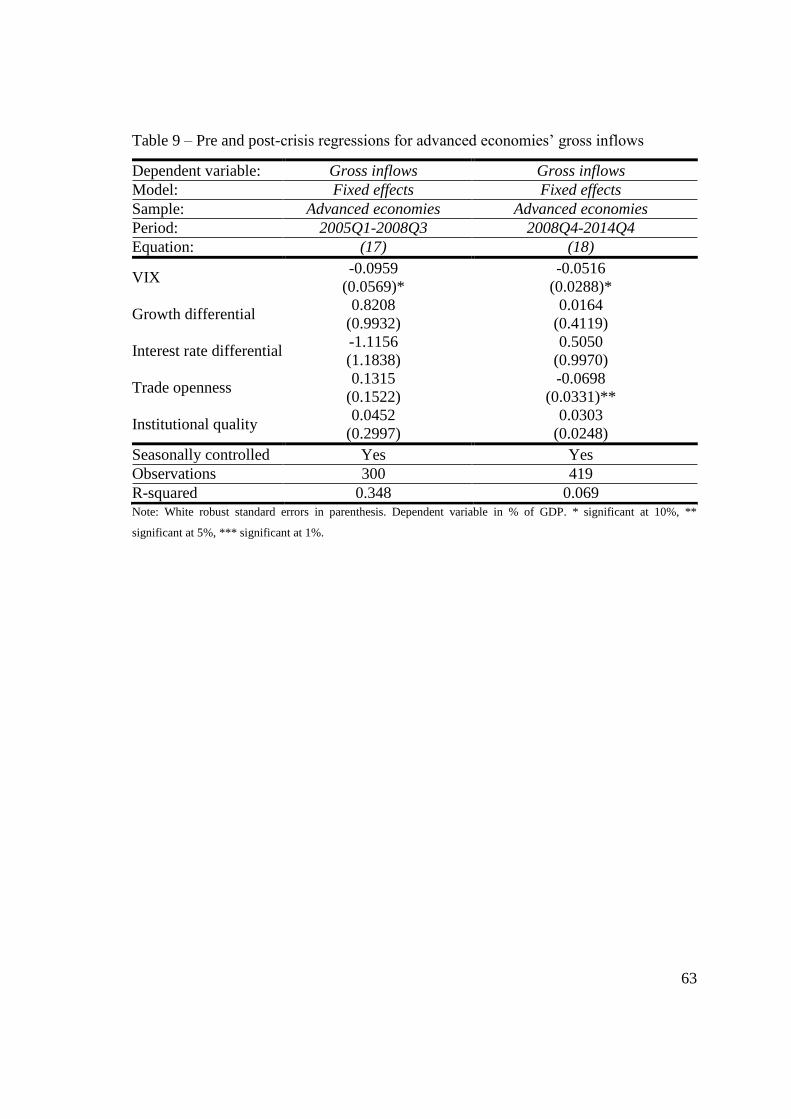
63
Table 9 – Pre and post-crisis regressions for advanced economies’ gross inflows
Dependent variable: Gross inflows Gross inflows
Model: Fixed effects Fixed effects
Sample: Advanced economies Advanced economies Period: 2005Q1-2008Q3 2008Q4-2014Q4
Equation: (17) (18)
VIX -0.0959
(0.0569)*
-0.0516
(0.0288)*
Growth differential 0.8208
(0.9932)
0.0164
(0.4119)
Interest rate differential -1.1156
(1.1838)
0.5050
(0.9970)
Trade openness 0.1315
(0.1522)
-0.0698
(0.0331)**
Institutional quality 0.0452
(0.2997)
0.0303
(0.0248)
Seasonally controlled Yes Yes
Observations 300 419
R-squared 0.348 0.069 Note: White robust standard errors in parenthesis. Dependent variable in % of GDP. * significant at 10%, **
significant at 5%, *** significant at 1%.
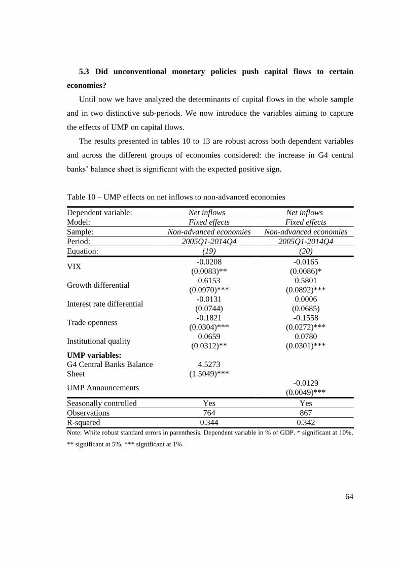
64
5.3 Did unconventional monetary policies push capital flows to certain
economies?
Until now we have analyzed the determinants of capital flows in the whole sample
and in two distinctive sub-periods. We now introduce the variables aiming to capture
the effects of UMP on capital flows.
The results presented in tables 10 to 13 are robust across both dependent variables
and across the different groups of economies considered: the increase in G4 central
banks’ balance sheet is significant with the expected positive sign.
Table 10 – UMP effects on net inflows to non-advanced economies
Dependent variable: Net inflows Net inflows
Model: Fixed effects Fixed effects
Sample: Non-advanced economies Non-advanced economies Period: 2005Q1-2014Q4 2005Q1-2014Q4
Equation: (19) (20)
VIX -0.0208
(0.0083)**
-0.0165
(0.0086)*
Growth differential 0.6153
(0.0970)***
0.5801
(0.0892)***
Interest rate differential -0.0131
(0.0744)
0.0006
(0.0685)
Trade openness -0.1821
(0.0304)***
-0.1558
(0.0272)***
Institutional quality 0.0659
(0.0312)**
0.0780
(0.0301)***
UMP variables:
G4 Central Banks Balance
Sheet
4.5273
(1.5049)***
UMP Announcements -0.0129
(0.0049)***
Seasonally controlled Yes Yes
Observations 764 867
R-squared 0.344 0.342
Note: White robust standard errors in parenthesis. Dependent variable in % of GDP. * significant at 10%,
** significant at 5%, *** significant at 1%.

65
Table 11 – UMP effects on gross inflows to non-advanced economies
Dependent variable: Gross inflows Gross inflows
Model: Fixed effects Fixed effects
Sample: Non-advanced economies Non-advanced economies Period: 2005Q1-2014Q4 2005Q1-2014Q4
Equation: (21) (22)
VIX -0.0479
(0.0176)***
-0.0354
(0.0170)**
Growth differential 0.8669
(0.1404)***
0.8014
(0.1330)***
Interest rate differential 0.6077
(0.4090)
0.5710
(0.3899)
Trade openness -0.2092
(0.0515)***
-0.1828
(0.0455)***
Institutional quality 0.1917
(0.0616)***
0.1443
(0.0490)***
UMP variables:
G4 Central Banks Balance
Sheet
10.8288
(2.7226)***
UMP Announcements -0.0348
(0.0090)***
Seasonally controlled Yes Yes
Observations 764 867
R-squared 0.297 0.299
Note: White robust standard errors in parenthesis. Dependent variable in % of GDP. * significant at 10%,
** significant at 5%, *** significant at 1%.
Focusing on the balance sheet variable, the results support the hypothesis that UMP
pushed capital flows to NAE in the post-crisis period. This result is consistent for both
net and gross inflows and points to the same direction of Fratzscher et al. (2013),
Ahmed & Zlate (2014), Burns et al. (2014), and Lim et al. (2014). We should highlight
that our result is important to literature as points in the direction of the previous studies
using a different sample and a different measure of UMP.
However, our results bring to the discussion another finding: UMP did not only
affect non-advanced markets as it also affected gross inflows to AE. The closest result
produced before by the literature is the one of Fratzscher et al. (2013) that supports the
idea that FED’s liquidity operations induced equity portfolio inflows to AE as well the
acquisition of mortgage-backed securities and government-sponsored enterprise debt

66
induced bond portfolio flows to the same economies. However, Fratzscher et al. (2013)
conclude some UMP induced bond portfolios outflows from the AE, namely the
acquisition of long term treasury bonds. This difference should take into consideration
that our quantitative measure of UMP is broader since it includes four distinct central
banks and, therefore, does not distinguishes individual countries’ policies.
Table 12 – UMP effects on net inflows to advanced economies
Dependent variable: Net inflows Net inflows
Model: Fixed effects Fixed effects
Sample: Advanced economies Advanced economies Period: 2005Q1-2014Q4 2005Q1-2014Q4
Equation: (23) (24)
VIX 0.0326
(0.0107)***
0.0331
(0.0112)***
Growth differential -0.0179
(0.1777)
-0.0649
(0.1702)
Interest rate differential 0.3100
(0.2920)
0.6248
(0.2804)**
Trade openness -0.0700
(0.0537)
-0.0338
(0.0397)
Institutional quality 0.1068
(0.0517)**
0.0982
(0.0437)**
UMP variables:
G4 Central Banks Balance
Sheet
0.8586
(1.8423)
UMP Announcements -0.0048
(0.0068)
Seasonally controlled Yes Yes
Observations 619 719
R-squared 0.276 0.305
Note: White robust standard errors in parenthesis. Dependent variable in % of GDP. * significant at 10%,
** significant at 5%, *** significant at 1%.
Additionally, it should be noted in table 14 and 15 that when the sample includes
both AE and NAE, the conclusions do not change. Fratzscher et al. (2013) find,
however, that the change in the amount outstanding of long term Treasury bonds related
to the long scale asset purchase affected equity and bond inflows negatively when
considering AE and NAE at the same time.

67
Table 13 – UMP effects on gross inflows to advanced economies
Dependent variable: Gross inflows Gross inflows
Model: Fixed effects Fixed effects
Sample: Advanced economies Advanced economies Period: 2005Q1-2014Q4 2005Q1-2014Q4
Equation: (25) (26)
VIX -0.0787
(0.0339)**
-0.1078
(0.0360)***
Growth differential 0.8363
(0.4932)*
0.8145
(0.4690)*
Interest rate differential -0.2067
(1.0167)
0.0670
(0.8815)
Trade openness -0.1304
(0.2157)
-0.2715
(0.1655)
Institutional quality 0.3270
(0.1742)*
0.2554
(0.1505)*
UMP variables:
G4 Central Banks Balance
Sheet
28.3866
(6.0245)***
UMP Announcements -0.0727
(0.0211)***
Seasonally controlled Yes Yes
Observations 764 867
R-squared 0.158 0.179
Note: White robust standard errors in parenthesis. Dependent variable in % of GDP. * significant at 10%,
** significant at 5%, *** significant at 1%.
The results of the announcement dummy variable point in the opposite direction
as theory would suggest and are contrary to previous empirical studies: the coefficient is
consistently significant with a negative sign which indicates that in quarters where at
least two central banks announced a new monetary action that announcement induced a
reduction in inflows across both to AE and NAE. These results do not support the
hypothesis that UMP’s announcements itself contributed to increase capital flows to
NAE economies as argued by Ahmed & Zlate (2014). Additionally, Fratzscher et al.
(2012) finds a mixed effect of the announcements on capital flows, depending on the
receiving economy and on the type of flow focused: QE1 announcements were found to

68
have affected positively equity and bond inflows to AE and NAE, except for bond
inflows to NAE.24
Table 14 – UMP effects on net inflows to all the economies
Dependent variable: Net inflows Net inflows
Model: Fixed effects Fixed effects
Sample: All the economies All the economies Period: 2005Q1-2014Q4 2005Q1-2014Q4
Equation: (27) (28)
VIX 0.0074
(0.0066)
0.0142
(0.0068)**
Growth differential -0.0134
(0.0763)
-0.0495
(0.0776)
Interest rate differential -0.1074
(0.1098)
-0.0600
(0.0865)
Trade openness -0.1084
(0.0284)***
-0.0913
(0.0244)***
Institutional quality 0.1156
(0.0275)***
0.1134
(0.0242)***
UMP variables:
G4 Central Banks Balance
Sheet
3.9189
(1.2003)***
UMP Announcements -0.0171
(0.0044)***
Seasonally controlled Yes Yes
Observations 1399 1605
R-squared 0.286 0.305
Note: White robust standard errors in parenthesis. Dependent variable in % of GDP. * significant at 10%,
** significant at 5%, *** significant at 1%.
24
We examine further this result by modifying the specification of the announcement variable from
assuming 1 if at least two central banks announced a new monetary action to assuming 1 if the Federal
Reserve announced a new policy. This way we were able to investigate if the difference on the results are
related with the inclusion of the announcements of the ECB, BoE, and BoJ when comparing with
previous studies. The results presented in table A9 to A11 do not differ significantly as the only alteration
is related with the significance of the dummy when the dependent variable is the net inflow which is now
not significant. Gross inflows continue to be negatively related with the dummy variable.

69
Table 15 – UMP effects on gross inflows to all the economies
Dependent variable: Gross inflows Gross inflows
Model: Fixed effects Fixed effects
Sample: All the economies All the economies Period: 2005Q1-2014Q4 2005Q1-2014Q4
Equation: (29) (30)
VIX -0.0642
(0.0190)***
-0.0645
(0.0199)***
Growth differential 0.1140
(0.1829)
-0.0282
(0.1855)
Interest rate differential 0.5434
(0.3765)
0.5811
(0.3280)*
Trade openness -0.1523
(0.0666)**
-0.2025
(0.0569)***
Institutional quality 0.3280
(0.0772)***
0.2525
(0.0627)***
UMP variables:
G4 Central Banks Balance
Sheet
20.1824
(3.1487)***
UMP Announcements -0.0715
(0.0115)***
Seasonally controlled Yes Yes
Observations 1399 1605
R-squared 0.151 0.171
Note: White robust standard errors in parenthesis. Dependent variable in % of GDP. * significant at 10%,
** significant at 5%, *** significant at 1%.
At this moment we should point that this variable’s results are not consistent either
with what economic theory would guide us to expect or with the empirical results
presented by the previous studies referred to. However, some points should be made
clear regarding these results. Firstly, it needs to be said that these differences on the
results could possibly be the result of the dummy capturing effects that are not related
with the announcement. This problem could be related with two different situations: the
use of an inadequate interval around the announcement or the inadequacy of
quantitative variables in measuring effects of UMP in capital flows.
Related with the first situation, Neely (2010) argues that event-based studies often
use high frequency data to measure very short-term changes on the dependent variable
after an announcement. In this way, the announcement would affect the variable if in a

70
short interval around the event the variance of the announcement shock is arbitrarily
large compared with the variance of the shock to the variable under investigation
(Rigobon & Sack, 2004). By using a short-term window around which the effects of the
announcement are measured, such studies try to reduce the potential bias that rise from
the announcing of other significant economic news during the period around which the
event-study is carried out which potentially creates measurement error problems
(Krishnamurthy & Vissing-Jorgensen, 2011). For instance, the event-study approach
through the use of dummy variables during such a long period as a quarter may produce
results that reflect more events beyond the one initially focused. Therefore, the
interpretation of the results should be careful and reflect the potential bias that arises
from the way that the announcement effect is being captured.
Regarding the discussion of the suitability of using qualitative variables as a
measure of UMP effects, it must be said that the use of quantitative variables which try
to capture the effect of unconventional monetary policies produce more reliable results
as they capture the effect of a variable that does not suffer from those possible bias. For
this reason, in section 5.5 we test the effectiveness of the balance sheet variable by
using an alternative measure. The conclusions do not change which enhances our
preference of using quantitative variables over qualitative in assessing the effects of
UMP measures.
Given the limitations related with the use of qualitative variables discussed in the
previous paragraphs, we will not use the dummy when considering the four-way
decomposition as dependent variable as we recognize its limitations. We will, however,
continue to use of the variable that captures the expansion of the balance sheet as we
consider it the most adequate choice to capture the UMP effects on capital flows.

71
5.4 The four-way decomposition
At this point, we will employ our benchmark model constructed on the base of the
literature reviewed to the four-way decomposition perspective of capital flows.25
Prior to describing our results we should note that from the four-way decomposition
we will focus our attention on three components. On one hand, 𝐿+ and 𝐿− measure the
variation of the stock of liabilities in a certain period. On the other hand, 𝐴+ and 𝐴−
measure the variation of stock of assets. Recalling that our motivation in studying the
recent experience of capital flows, and particularly the effect of UMP, is based on the
possible macro-economic and financial stability effects that an overflow of capital flows
could cause to the economies that receive them, we will focus on 𝐿+ and 𝐿−, as they
account for the liability part of the balance of payments, as well as on 𝐴− which in its
essence is a capital inflow – every time national agents decrease their holdings of
external assets they are inducing capital inflows.
We should highlight that we will focus only on NAE. This set of economies, after
the GFC, account for 50% of the global capital inflows comparing with less than 20% in
the six years before the event (IMF, 2014e). Together with significant growth and yield
differentials (IMF, 2011b), UMP were argued to push capital inflows to NAE. As
discussed in the previous section, our results support the hypothesis that UMP was
significant in contributing for the increase of capital inflows received by the NAE
relatively to total inflows. In many cases, “the inflows were accompanied by a rapid
expansion of credit, fueling an overheating of domestic economies and setting the
conditions for a buildup of vulnerabilities.” (IMF, 2014e). Because the experience of
the NAE group in the post-crisis period was more likely to contribute to the build-up of
internal and external imbalances, we will apply the four-way decomposition to this set
of economies.
On equation 31 and 34 we estimate the determinants of the investment decisions by
foreign agents, 𝐿+ , in the whole sample regarding emerging markets. Growth
differential is statistically significant with a positive coefficient, supporting the idea that
foreign agents decide to invest on NAE with better growth prospects; on the contrary, it
25
The results regarding advanced economies and all the economies are presented in table A12 to A15.

72
should be highlighted that risk aversion is not significant regarding those investment
decisions. Additionally, we find UMP to act as an additional push factor of capital flows
to NAE as the decisions of foreign agents in investing on those economies are positively
related with the expansion of the G4 central banks’ balance sheet. This result could be
relevant, considering the result of Janus & Riera-Crichton (2014) which concluded for
an important effect of gross foreign investment reversal on the output, effect that is
particularly strong for emerging countries during sudden stops crises. For instance, as
discussed in section 3.6, events of normalization of monetary easing, namely by the
Federal Reserve, might expose several problems to those economies with weaker
fundamentals and external imbalances by increasing borrowing costs and making the
financing of fiscal deficits more difficult (World Bank, 2012). On the second and third
quarter of 2013, episodes of normalization of monetary policy triggered pronounced
adjustments in emerging and developing countries namely affecting national stock
markets, exchange rates, and CDS spreads decreasing the incentives to carry-trade
activities on those economies and increasing uncertainty (Aizenman, Binici, &
Hutchison, 2014). The result could be possible external shocks in form of sudden stops
(IMF, 2010a, IMF, 2011b and Powell, 2010) or the retrenchment of capital outflows
(Aizenman, Binici, & Hutchison, 2014). If the external shock operates through the
reversal of foreign investment, the effect on the output can be harmful, particularly
during currency, current account and sudden stop crises as argued by Janus & Riera-
Crichton (2014).
Continuing with the second element of capital inflows, 𝐿−, equation 32 and 35 allow
us to see that the VIX is significant in explaining 𝐿−, suggesting market sentiment to be
relevant for the reduction of foreign investors' exposure to certain foreign markets – in
moments in which risk aversion is greater, foreign agents repatriate their funds to their
domestic economy. Additionally, growth differential is found to have a significant
influence 𝐿−, as the decisions increase when the growth differential progresses in favor
of the growth of the world economy. Finally, the results allow us to conclude that UMP
is not found to exert any influence on this variable.

73
Finally, 𝐴− has VIX as a significant explanatory variable with a positive coefficient,
suggesting that national agents decrease their foreign exposure during periods of higher
risk aversion. However, table 16 and 17 present results contrary to what we would
expect theoretically as growth differential was found to be negatively associated with
𝐴−; institutional quality is also found to be negatively associated with 𝐴−. Additionally,
the model gives us new insights regarding the 𝐴− component: being a de facto capital
inflow, this component was found to be negatively affected by monetary policy actions
implemented in the course of the global financial crisis. This result could be particularly
important if the hypothesis advanced by Janus & Riera-Crichton (2013) holds: because
national agents are more well-informed and this type of inflow promotes growth more
than asset bubbles, 𝐴− should be encouraged over 𝐿+. The results point that UMP pulled
𝐿+ to NAE and pushed 𝐴− from them, which could indicate that monetary actions from
the G4 central banks overflowed economies with the most dangerous type of inflow,
possibly contributing for asset bubbles and other macro-economic unbalances.
Employing our model to the four-way decomposition raised additional insights
beyond the results and conclusions discussed on the previous sections. It should be
highlighted that the determinants of the four-way decomposition differ with the
component focused. Remembering that we previously found the VIX to be negatively
related with net and gross inflows, decomposing those standard measures allows us to
obtain additional understanding of how capital inflows react to changes in risk aversion.
Our results support the idea that the decision of investing in NAE is not affected by risk
aversion; contrarily, the decision of disinvesting follows positively changes on market
sentiment - in other words, when the market sentiment moves towards higher risk
aversion, foreign investors tend do decrease their exposure to NAE. Moreover, the
importance of growth only seems to be important in explaining the decisions of
investment in NAE – the positive relation between gross inflows and growth operates
through the 𝐿+ .

74
Table 16 – Benchmark results for the four-way elements regarding non-advanced
economies
Dependent variable: L+ L- A-
Model: Fixed effects Fixed effects Fixed effects
Sample: Non-advanced
economies
Non-advanced
economies
Non-advanced
economies
Period: 2005Q1-2014Q14 2005Q1-2014Q14 2005Q1-2014Q14
Equation: (31) (32) (33)
VIX -0.0153
(0.0120)
0.0190
(0.0035)***
0.0228
(0.0043)***
Growth differential 0.2287
(0.0655)***
-0.0891
(0.0372)**
-0.2220
(0.0431)***
Interest rate differential 0.5277
(0.3629)
-0.0275
(0.0215)
-0.0134
(0.0374)
Trade openness -0.0108
(0.0277)
0.0076
(0.0121)
0.0298
(0.0170)*
Institutional quality 0.0573
(0.0327)*
-0.0006
(0.0090)
-0.0542
(0.0149)***
Seasonally controlled Yes Yes Yes
Observations 877 877 877
R-squared 0.412 0.218 0.299
Note: White robust standard errors in parenthesis. Dependent variable in % of GDP. * significant at 10%,
** significant at 5%, *** significant at 1%.

75
Table 17 – UMP results for the four-way elements regarding non-advanced economies
Dependent variable: L+ L- A-
Model: Fixed effects Fixed effects Fixed effects
Sample: Non-advanced
economies
Non-advanced
economies
Non-advanced
economies
Period: 2005Q1-2014Q14 2005Q1-2014Q14 2005Q1-2014Q14
Equation: (34) (35) (36)
VIX -0.0084
(0.0126
0.0181
(0.0037)***
0.0190
(0.0040)***
Growth differential 0.1998
(0.0745)***
0.0866
(0.0369)**
-0.2085
(0.0428)***
Interest rate differential 0.5682
(0.3572)
-0.0330
(0.0240)
-0.0307
(0.0384)
Trade openness -0.0150
(0.0299)
0.0035
(0.0141)
0.0261
(0.0190)
Institutional quality 0.1305
(0.0465)***
0.0022
(0.0104)
0.0589
(0.0170)***
UMP variable:
G4 Central Banks
Balance Sheet
5.9218
(1.8079)***
-0.9746
(0.6107)
-3.2567
(0.8788)***
Seasonally controlled Yes Yes Yes
Observations 771 771 771
R-squared 0.412 0.234 0.342
Note: White robust standard errors in parenthesis. Dependent variable in % of GDP. * significant at 10%,
** significant at 5%, *** significant at 1%.
The literature has been pointing the influence of UMP on net and capital inflows to
NAE. Our work provides new insights to the literature by concluding that UMP
positively influenced the decisions of investment by foreign agents on NAE. This
conclusion represents additional support to the apprehension of NAE’s policy makers

76
regarding the pull effect of those monetary actions on capital inflows to NAE.
Simultaneously, UMP exerted a negative effect on the repatriation of capital from
domestic residents of NAE. It should be noted that Janus & Riera-Crichton (2013)
introduced the hypothesis that even if 𝐿+ and 𝐴− are in fact capital inflows, they could
have different effects on the output growth depending on the existence of asymmetric
information between foreign and domestic investors.
77
5.5 Robustness checks
In the previous sections we discussed the results produced given the framework
provided by the literature. However, we should assess how the results change if we drop
some assumptions regarding our model.
We will start to evaluate the robustness of our results by modifying the specification
of the UMP variable. Previously, we considered absolute changes in G4 central banks’
balance sheet. One could argue that the effect of policies with impact on the balance
sheet of those institutions could depend on the initial value of the balance sheet. In order
to check whether our conclusions would change, we regress again our models with the
UMP variable being specified as the aggregate percentage variation of G4 central
banks’ balance sheet. From table A16 to A19 we can see that the conclusions do not
change with alternative specification, as the variable is highly significant.
Additionally, we employed the use of dummy variables in order to control for
seasonal effects. At this point it is pertinent to question how the results would change if
the main equations were estimated without controlling for the seasonal effects. As can
be seen in table A20 to A29, the results previously presented and discussed do not
change significantly: trade openness regarding gross inflows to AE loses its
significance. Regarding the UMP model, the only differences are related with the
increase of significance of the VIX regarding net inflows to NAE and the loss of
significance of the growth differential and institutional quality regarding gross inflows
to AE. Finally, the results of the four-way decomposition only change in the sense 𝐿− is
now negatively related with the UMP variable which enhances the conclusion that UMP
pushed capital inflows to NAE. In other words, the results points in the direction that
UMP decreased the decisions of foreign investors of disinvesting in NAE.
Finally, a strong assumption under fixed effects is that unobserved effects are
related with the characteristics of each economy in the sample. However, if this
assumption does not hold and the unobserved effects are not related with the observable
variables, random effects model would be the most adequate model. The literature
studying the determinants of capital flows tends to accept that fixed effects model is the
most suitable model as discussed in section 4.2; nonetheless, it appears to be accepted to

78
estimate the model as well by random effects and present both the results (see e.g. Nier
et al., 2014) in order to assess how the results change from one model to the other. As
can be seen in table A30 to A39, the results do not change significantly: institutional
quality is no longer significant regarding net and gross inflows to AE. Additionally,
trade openness loses its significance regarding gross inflows to AE but is now
negatively related with net inflows to these economies. Regarding the UMP model, the
VIX and trade openness are no longer significant regarding net and gross inflows,
respectively. When looking to the AE, institutional quality loses its significance and
trade openness turns to be negatively associated with net inflows. Regarding gross
inflows, growth differential and institutional quality are no longer significant. Finally,
regarding the four-way decomposition, the only change is related with institutional
quality: is no longer significant related with 𝐴− but turns to be associated with 𝐿−.

79
6. Conclusion
The global financial crisis presented itself as an enormous challenge regarding the
monetary policy framework. Financial stress, negative output growth and deflationary
pressures required central banks across the world to act firmly in order to counter act
those risks. The monetary policy actions focused on short-term interest rate mechanisms
in the early stages of the crisis, for as long as there was room to reduce short-term
interest rates. However, as interest rates reached the zero lower bound, central banks
implemented what has been denominated as unconventional monetary policies. These
policies were argued to push capital inflows to NAE, contributing to the build-up of
external imbalances.
Regarding the determinants of capital flows, our findings suggest that NAE have the
same determinants for both net and gross inflows – interest rate differential is the only
variable that is not significant. When looking to AE there is some difference between
the two measures of capital inflows with the sign of the VIX being the most substantial
– it has a positive coefficient when associated with net inflows; on the other hand has a
negative coefficient regarding gross inflows. Additionally, growth differential is
significant regarding gross inflows but not regarding net; contrarily, interest rate
differential is significant regarding net inflows but not regarding gross. At this point we
should note that including in the sample both AE and NAE produce results that do
reflect neither the experience of the former nor the latter. This way, interpreting the
results when the sample consists of economies with possible different experiences may
be inaccurate.
Assessing at which extent it could be said that the determinants that explained
capital flows in the pre-crisis period changed in the post-crisis period, our results point
towards the direction that generally the same determinants in prior period were
significant on the following.
It was concluded for both NAE and AE that gross inflows are negatively affected by
the VIX. Further insight regarding the determinants of capital inflows is provided by
estimating the three elements of the four-way decomposition, as this effect seems to
work through 𝐿− as this variable is positively related with risk aversion. For AE, this

80
effect offsets the negative effect of risk aversion on 𝐿+. We should also note that 𝐴+,
which is a de facto inflow, has risk aversion as a significant variable with positive sign.
Furthermore, the growth differential is relevant in explaining all the three components
regarding NAE; regarding AE, the growth differential is only relevant for the
component that accounts for the decisions of foreign agents in investing in those
economies.
Finally, we addressed the hypothesis that UMP affected capital flows or not.
Regarding the quantitative measure of those policies, the results were clear enough to
let us conclude for a positive effect of UMP on net and gross capital inflows,
independently of the group of economies. Nonetheless, we should highlight the
problems that may emerge from the use of a qualitative variable in assessing the impact
of monetary announcements on capital flows: by using dummy variables around long-
term windows, potential bias could rise from the announcing of other significant news
during the window around which the effects of the monetary announcement are
measured. In this way, we argue that is more adequate to measure the UMP through
quantitative variables that capture a particular effect rather than qualitative variables.
We contribute for the literature that already tested the effect of UMP on capital
flows by extending this hypothesis to the elements of the four-way decomposition.
UMP affected gross inflows through the investment decisions of foreign investors, 𝐿+,
but not through the disinvestment decisions of those agents, 𝐿−. Additionally, the effect
of those policies promoted a decrease of capital repatriation, 𝐴−, from national agents.
In other words, the inflows which caused apprehension in the resurge phase are those
related with the increase of liabilities and not those related with the decrease of national
agents’ exposition to external assets. If domestic residents tend to be well-informed and
their capital promotes output growth more than asset bubbles when comparing with
foreign agents (Janus & Riera-Crichton, 2014), then unconventional monetary actions
pushed to NAE the most dangerous component while pulled the component that
contributes the most to output growth and financial stability. These results could be
significant to policymakers in order to design and monitor effective capital controls as
distinguishes the forms of inflows influenced by unconventional monetary actions.

81
To the best of our knowledge this is the first study that uses the four-way
decomposition with the objective of assessing the determinants of capital flows through
a different measure. If the literature evaluates that this decomposition raises additional
understanding of the determinants of capital flows, it would be praised further study
regarding this alternative measure of capital flows.
Finally, inasmuch the results regarding the four-way decomposition provided by this
study address a very important question that affects policy-making worldwide it is not
understood at present how the four elements affect variables as the credit growth,
exchange rates, or asset prices. Before understanding those channels it could be
inaccurate to extrapolate and extract policy-making conclusions regarding the effect of
unconventional monetary policies on those variables based on the results we present.
Our results only point in the direction that unconventional monetary policies affected
the elements of the four-way decomposition. Further work will require assessing the
effect of those variables on the robustness of the financial system and macroeconomic
imbalances.

82
References
Abutaleb, A., Hamad, M., (2012), “Optimal Levels of Reserves and Hedging
Sudden Stops Recessions for Egypt: A Stochastic Control Approach”, Journal of
Economic Cooperation and Development, Vol. 33, Nº1, pp 1-58.
Ahmed, S., Coulibaly, B., Zlate, A., (2015), “International Financial Spillovers to
Emerging Market Economies: How Important Are Economic Fundamentals?”,
International Finance Discussion Papers, 1135.
Ahmed, S., Zlate, A., (2014), “Capital Flows to Emerging Market Economies: A
Brave New World?”, Journal of International Money and Finance, Vol. 48, pp 221-
248.
Aizenman, J., Jinjarak, Y., (2009), “Current Account Patterns and National Real
Estate Markets”, Journal of Urban Economics, Vol. 66, Nº 2, pp 75-89.
Aizenman, J., Binici, M., Hutchison, M. M., (2014), “The Transmission of Federal
Reserve Tapering News to Emerging Financial Markets”, NBER Working Paper Series,
19980.
Albuquerque. R., (2003), “The Composition of International Capital Flows: Risk
Sharing Through Foreign Direct Investment”, Journal of International Economics, Vol.
61, Nº 2, pp 353-383.
Alfaro, L., Kalemli-Ozcan, S., Volosovych, V., (2007), “Capital Flows in a
Globalized World: The Role of Policies and Institutions”, NBER Working Papers,
11696.
Alfaro, L., Kalemli-Ozcan, S., Volosovych, V., (2008), “Why Doesn’t Capital Flow
from Rich to Poor Countries? An Empirical Investigation”, The Review of Economics
and Statistics, Vol. 90, Nº 2, pp 347–368.
Ando, A., Modigliani, F., (1963), “The Life Cycle Hypothesis of Savings:
Aggregate Implications and Tests”, American Economic Review, Vol. 53, Nº 1, pp 55-
84.
Antràs, P., Caballero, R., (2009), “Trade and Capital Flows: A Financial Frictions
Perspective”, Journal of Political Economy, Vol. 117, Nº 4, pp 701-744.

83
Arslan, Y., Taskin, T., (2014), “International Evidence on the Interaction Between
Cross-Border Capital Flows and Domestic Credit Growth”, Central Bank of the
Republic of Turkey Working Papers, 1418.
Bauer, M. D., Rudebusch, G. D., (2014). “The Signalling Channel for Federal
Reserve Bond Purchases”, International Journal of Central Banking, Vol. 10, Nº 3, pp.
233-289.
Bernanke, B., (2013), “The Economic Outlook”,
http://www.federalreserve.gov/newsevents/testimony/bernanke20130522a.htm,
accessed on February 20, 2015.
Bernanke, B. S., Reinhart, V. R., (2004), “Conducting Monetary Policy at Very
Low Short-Term Interest Rates”, American Economic Review, Vol. 94, Nº 2, pp. 85-90.
Bernanke, B. S., Reinhart, V. R., Sack, B. P., (2004), “Monetary Policy Alternatives
at the Zero Bound - An Empirical Assessment”, Brookings Papers on Economic
Activity, Vol. 35, Nº 2, pp. 1-100.
Bluedorn, J., Duttagupta, R., Guajardo, J., Topalova, P., (2013), “Capital Flows are
Fickle: Anytime, Anywhere”, IMF Working Paper, 13/183.
Bowdler, C., Radia, A., (2012), “Unconventional Monetary Policy: The
assessment”, Oxford Review of Economic Policy, Vol. 28, Nº 4, pp. 603-621.
Bogdanov, B., (2014), Liberalised Capital Accounts and Volatility of Capital Flows
and Foreign Exchange Rates”, European Economy Economic Papers, 521.
Borensztein, E., De Gregorio, J., Lee, J., (1998), “How Does Foreign Direct
Investment Affect Economic Growth?”, Journal of International Economics, Vol. 45,
Nº 1, pp. 115-135.
Botman, D., Filho, I., Lam, W. R., (2013), “The Curious Case of the Yen as a Safe
Haven Currency: A Forensic Analysis”, IMF Working Paper, 13/228.
Broner, F., Rigobon, R., (2004), “Why Are Capital Flows so Much More Volatile in
Emerging Than in Developed Countries?” Prepared for the Eight Annual Conference of
the Central Bank of Chile “External Financial Vulnerability and Preventive Policies”,
Santiago, Chile.
84
Broto, C., Díaz-Cassou, J., Erce, A., (2008). “The Sources of Capital Flow
Volatility: Empirical Evidence For Emerging Countries”. Money Affairs, Vol. 21, Nº 1,
pp. 1-30.
Broto, C., Díaz-Cassou, J., Erce, A., (2011), “Measuring and Explaining the
Volatility of Capital Flows to Emerging Countries”, Journal of Banking & Finance,
Vol. 35, Nº 8, pp. 1941-1953.
Brukoff, P., Rother, B., (2007), “FDI May Not Be As Stable as Governments
Think”, Survey Magazine: IMF Research, January 29, 2007.
Burns, A., Kida, M., Lim, J., Mohapatra, S., Stocker, M., (2014), “Unconventional
Monetary Policy Normalization in High Income Countries: Implications for Emerging
Market Capital Flows and Crisis Risks”, World Bank Policy Research Working Paper,
6830.
Carlson, M., Hernandéz, L., (2002), “Determinants and Repercussions of the
Composition of Capital Inflows”, International Finance Discussion Papers, 717.
Cerutti, E., Claessens, S., Ratnovski, L., (2014), “Global Liquidity and Drivers of
Cross-Border Bank Flows”, IMF Working Paper, 14/69.
Chen, J., Mancini-Griffoni, T., Sahay, R., (2014), “Spillovers from United States
Monetary Policy on Emerging Markets: Different This Time?” IMF Working Paper,
14/240.
Cho, D., Rhee, C., (2013), “Effects of Quantitative Easing on Asia: Capital Flows
and Financial Markets”, ADB Economics Working Paper Series, 350.
Choi, W., Sharma, S., Strömqvist, M., (2007), “Capital Flows, Financial Integration,
and International Reserve Holdings: The Recent Experience of Emerging Markets and
Advanced Economies”, IMF Working Paper, 07/151.
Chuhan, P., Claessens, S., Mamingi, N., (1998), “Equity and Bond Flows to Asia
and Latin America: The Role of Global and Country Factors”, Journal of Development
Economics, Vol. 55, Nº 2, pp. 439-463.
Coeuré, B., (2012), “The Importance of Money Markets”, 16th
Annual Global
Investment Seminar, Provence, 16 June 2012,
www.ecb.europa.eu/press/key/date/2012/html/sp120616.en.html

85
D’Amico, S., King, T. B., (2013), “Flow and Stock Effects of Large-Scale Asset
Purchases - Evidence on the Importance of Local Supply”, Journal of Financial
Economics, Vol. 108, Nº 2, pp. 425-448.
Darvas, Z., Hüttl, P., Merler, S., Sousa, C., Walsh, T., (2015), “Analysis of
Developments in EU Capital Flows in the Global Context”, European Commission, 50.
De Gregorio, J., (2013), “Capital Flows and Capital Account Management”, Paper
presented at The Rethinking II: First Steps and Early Lessons Conference, International
Monetary Fund.
De Santis, R., Lürhmann, M., (2006), “On the Determinants of External Imbalances
and Net International Portfolio Flows”, ECB Working Paper Series, 651.
ECB, (2000), “Monetary Policy Transmission in the Euro Area”, ECB Monthly
Bulletin, July.
ECB, (2009), “Financial Stability Review”, June 2009.
ECB, (2010a), “Financial Stability Review”, June 2010.
ECB, (2010b), Financial Stability Review: December 2010.
ECB, (2011), Financial Stability Review: June 2011.
Eichengreen, B., Gupta, P., (2014), “Tapering Talk: The Impact of Expectations of
Reduced Federal Reserve Security Purchases on Emerging Markets”, World Bank
Policy Research Working Paper, 6754.
Epstein, G., (2009), “Should Financial Flows be Regulated? Yes”, Department of
Economic and Social Affairs Working Paper, 77.
Eser, F., Schwaab, F., (2013), “Assessing Asset Purchases Within the ECB’s
Securities Market Programme”, ECB Working Paper Series, 1587.
Faria, A., Mauro, P., (2009), “Institutions and the External Capital Structure of
Countries”, Journal of International Money and Finance: Vol. 28, Nº 3, pp. 367-391.
Fawley, B. W., Neely, C. J., (2013), “Four Stories of Quantitative Easing”, Federal
Reserve Bank of St. Louis Review, Vol. 95, pp. 51-88.
Feenstra, R. C., (2003), Advanced International Trade: Theory and Evidence,
Princeton University Press.

86
Forbes, K., Warnock, F., (2011), “Capital Flow Waves: Surges, Stops, Flight, and
Retrenchment”, Journal of International Economics, Vol. 88, N 2, pp. 235-251.
Förster, M., Jorra, M., Tillmann, P., (2014), “The Dynamics of International Capital
Flows: Results from a Dynamic Hierarchical Factor Model”, Journal of International
Money & Finance, Vol. 48, Part A, pp. 101-124.
Fostel, A., Kaminsky, G., (2008), “Latin America's Access to International Capital
Markets”, Central Banking, Analysis, and Economic Policies Book Series, Vol. 12, Nº
1, pp. 117-158.
Fratzscher, M., (2012), “Capital Flows: Push vs Pull Factors and the Global
Financial Crisis”, Journal of International Economics, Vol. 88, Nº 2, pp. 341-356.
Fratzscher, M., Lo Duca, M., Straub, R., (2013), “On the International Spillovers of
US QE”, ECB Working Paper Series, 1557.
Gagnon, J., Raskin, M., Remache, J., Sack, B., (2011), “The Financial Market
Effects of the Federal Reserve’s Large-Scale Asset Purchases”, International Journal of
Central Banking, Vol. 7, Nº 1, pp. 3-43.
Gambacorta, L., Hofmann, B., Peersman, G., (2014), "The Effectiveness of
Unconventional Monetary Policy at the Zero Lower Bound: A Cross‐Country
Analysis", Journal of Money, Credit and Banking, Vol. 46, Nº4, pp. 615-642.
Glick, R., Rose, A., (1999), “Contagion and Trade: Why are Currency Crises
Regional?”, Journal of International Money and Finance, Vol. 18, Nº 4, pp. 603-617.
Globerman, S., Shapiro, D., (2002), “Global Foreign Direct Investment Flows: The
Role of Governance Infrastructure”, World Development, Vol. 30, Nº 11, pp. 1899-
1919.
Habib, M. M., Stracca, L., (2013), “Foreign Investors and Risk Shocks: Seeking a
Safe Haven or Running for the Exit?”, ECB Working Paper Series, 1609.
Haidar, J. I., (2012), “Currency Crisis Transmission Through International Trade”,
Economic Modelling, Vol. 29, Nº 2, pp. 151-157.
Haile, F., Pozo, S., (2008), “Currency Crisis Contagion and the Identification of
Transmission Channels”, International Review of Economics and Finance, Vol. 17, Nº
4, pp. 572-588.

87
Higgins, M., (1998), “Demography, national savings and international capital
flows”, International Economic Review, Vol. 39, pp. 343-369.
IMF, (2009a), “Crisis and Recovery”, World Economic and Financial Surveys,
April 2009.
IMF, (2009b), Responding to the Financial Crisis and Measuring Systemic Risk”,
Global Financial Stability Report, April 2009.
IMF, (2010a), “Meeting New Challenges to Stability and Building a Safer System”,
Global Financial Stability Report, April 2010.
IMF, (2010b), “Rebalancing Growth”, World Economic and Financial Surveys,
April 2010.
IMF, (2010c), “Navigating the Financial Challenges Ahead”, Global Financial
Stability Report, October 2010.
IMF, (2011a), “Tensions from the Two-Speed Recovery”, World Economic and
Financial Surveys, April 2011.
IMF, (2011b), “Grappling With Crisis Legacies”, Global financial stability report,
October 2011.
IMF, (2012), “The Liberalization and Management of Capital Flows: An
Institutional View”, Public Information Notice, 137.
IMF, (2013a), “Unconventional Monetary Policy – Recent Experience and
Prospects”, Background Paper, 18 April 2013.
IMF, (2013b), “Transitions and Tensions”, World Economic and Financial Surveys,
October 2013.
IMF, (2013c), “Transition Challenges to Stability”, Global Financial Stability
Report, October 2013.
IMF, (2013d), “Global Impact and Challenges of Unconventional Monetary
Policies”, IMF Policy Paper, October 2003.
IMF, (2014a), “Recovery Strengthens, Remains Uneven”, World Economic and
Financial Surveys, April 2014.
IMF, (2014b), “Moving from Liquidity- to Growth-Driven Markets”, Global
Financial Stability Report, April 2014.

88
IMF, (2014c), “Risk Taking, Liquidity, and Shadow Banking”, Global financial
stability report, October 2014.
IMF, (2014d), “Legacies, Clouds, Uncertainties”, World Economic and Financial
Surveys, October 2014.
IMF, (2014e), “Emerging Market Volatility: Lessons From the Taper Tantrum”,
IMF Staff Discussion Note, 09.
IMF, (2015), “Navigating Monetary Policy Challenges and Managing Risks”,
Global financial stability report, April 2015.
Janus, T., Riera-Crichton, D., (2013), “International Gross Capital Flows: New Uses
of Balance of Payments Data and Application to Financial Crises”, Journal of Policy
Modeling, Vol. 35, Nº 1, pp. 16-28.
Janus, T., Riera-Crichton, D., (2014), “The Output Effect of Gross Foreign
Investment Reversals”, Oxford Economic Papers, Vol. 67, Nº 3, pp. 356-379.
Jarrow, R., Li, H., (2012). The Impact of Quantitative Easing on the US Term
Structure of Interest Rates, Johnson School Research Paper: 2.
Jayce, M., Miles, D., Scott, A., Vayanos, D., (2012), “Quantitative Easing and
Unconventional Monetary Policy – An Introduction”, Economic Journal, Vol. 122, Nº
1, pp. 271 - 288.
Jevčák, A., Setzer, R., Suardi, M., (2010), “Determinants of Capital Flows To the
New EU Member States Before and During the Financial Crisis”, European Economy
Economic Papers, 425.
Jinjarak, Y., Sheffrin, S., (2011), "Causality, Real Estate Prices, and the Current
Account", Journal of Macroeconomics, Vol. 33, Nº 2, pp. 233-246.
Kaufmann, D., Mastruzzi, M., (2004), “Governance Matters III: Governance
Indicators for 1996–2002”, World Bank Economic Review, Vol. 18, Nº 2, pp. 253-287.
Kim, S., Yang, D. Y., (2011), “The Impact of Capital Inflows on Asset Prices in
Emerging Asian Economies: Is Too Much Money Chasing Too Little Good?”, Open
Economic Review, Vol. 22, Nº 2, pp. 293-315.
Kool, C., Thornton, D., (2012), “How Effective is Central Bank Forward
Guidance?”, Federal Reserve Bank of St. Louis Working Paper Series, 63.

89
Kose, A., Prasad, E., Rogoff, K, Wei, S., (2009), “Financial Globalization: A
Reappraisal”, IMF Staff Papers, Vol. 56, Nº 1.
Kozicki, S., Santor, E., Suchanek, L., (2011), "Unconventional Monetary Policy:
The International Experience with Central Bank Asset Purchases", Bank of Canada
Review, Vol. 2011 Spring, pp. 13-25.
Krishnamurthy, A., Vissing-Jorgensen, A., (2011), “The Effects of Quantitative
Easing on Interest Rates - Channels and Implications for Policy”, Brookings Papers on
Economic Activity, Vol. 2011 Fall, pp. 215-287.
Lall, S., (1998), “Changing Perceptions of Foreign Direct Investment in
Development”, International trade, foreign direct investment and the economic
environment. Essays in honour of Professor Sylvain Plasscaert, London: MacMillan.
Lane, P., (2013), “Capital Flows in the Euro Area”, European Economy Economic
Papers, 497.
Lane, P., McQuade, P., (2013), “Domestic Credit Growth and International Capital
Flows”, The Scandinavian Journal of Economics, Vol. 116, Nº 1, pp. 218-252.
Levchenko, A., Mauro, P., (2007), “Do Some Forms of Financial Flows Help
Protect Against Sudden Stops?”, World Bank Economic Review, Vol. 21, Nº 3, pp. 389-
441.
Lim, J., Mohapatra, S., Stocker, M., (2014), “Tinker, Taper, QE, Bye? The Effect
of Quantitative Easing on Financial Flows to Developing Countries”, Policy Research
Working Paper, 6820.
Lucas, R., (1990), “Why Doesn’t Capital Flow from Rich to Poor Countries?”, The
American Economic Review, Vol. 80, Nº 2, pp. 92-96.
Mark, N. C., (2000), International Macroeconomics and Finance: Theory and
Empirical Methods (4th
ed.), Blackwell Publishers.
Martin, P., Rey, H., (2006), “Globalization and Emerging Markets: With or Without
Crash?”, American Economic Review, Vol. 96, Nº 5, pp. 1631-1651.
Mercado, R., Park, C., (2011), “What Drives Different Types of Capital Flows and
Their Volatilities in Developing Asia?”, International Economic Journal, Vol. 25, Nº 4,
pp. 655-680.

90
Milesi-Ferretti, G. M., Tille, C., (2011), “The Great Retrenchment International
Capital Flows During the Global Financial Crisis”, Economic Policy, Vol. 26, Nº 66,
pp. 285-342.
Mishra, P., Moriyama, K., N’Diaye, P., Nguyen, L., (2014), “Impact of Fed
Tapering Announcements on Emerging Markets”, IMF Working Paper, 14/109.
Montiel, P. J., (2014), “Capital Flows: Issues and Policies”, Open Economies
Review, Vol. 25, Nº 3, pp. 595-633.
Mundell, R., (1957), “International Trade and Factor Mobility”, The American
Economic Review, Vol. 47, Nº 3, pp. 321-355.
Nier, E., Sedik, T., Mondino, T., (2014), “Gross Private Capital Flows to Emerging
Markets: Can the Global Financial Cycle Be Tamed?”, IMF Working Paper, 196.
Neumann, R., Penl, R., Tanku, A., (2009), “Volatility of Capital Flows and
Financial Liberalization: Do Specific Flows Respond Differently?”, International
Review of Economics and Finance, Vol. 18, Nº 3, pp. 488-501.
Neely, C. J., (2010), “The Large-Scale Asset Purchases Had Large International
Effects”, Federal Reserve Bank of St. Louis Working Paper Series, 18.
Noorbakhsh, F., Paloni, A., Youssef, A., (2001), “Human Capital and FDI Inflows
to Developing Countries”, World Development, Vol. 29, Nº 9, pp. 1593-1610.
Papaioannou, E., (2009), “What Drives International Bank Flows? Politics,
Institutions and Other Determinants”, Journal of Development Economics, Vol. 88, Nº
2, pp. 269-281.
Powell, J., (2010), Advanced Economy Monetary Policy and Emerging Market
Economies”, Asian Economic Policy Conference,
http://www.federalreserve.gov/newsevents/speech/powell20131104a.htm#f3, accessed
on March 10, 2015.
Okada, K., (2013), “The Interaction Effects of Financial Openness and Institutions
on International Capital Flows”, Journal of Macroeconomics, Vol. 35, pp. 131-143.
Ranaldo, A., Söderlind, P., (2010), “Safe Haven Currencies”, Review of Finance,
Vol. 14, Nº 3, pp. 385-407.

91
Ree, J., Choi, S., (2014), “Safe-Haven Korea? Spillover Effects from UMPs”, IMF
Working Paper, 14/53.
Reinhart, C., Reinhart, V., (2009), “Capital Flow Bonanzas: An Encompassing
View of the Past and Present”, NBER Chapters, in: NBER International Seminar on
Macroeconomics 2008: pp. 9-62
Rigobon, R., Sack, B., (2004), “The impact of monetary policy on asset prices”,
Journal of Monetary Economics, Vol. 51, Nº 8, pp. 1553-1575.
Rodrik, D., Velasco, A., (1999), “Short-Term Capital Flows”, Annual Bank
Conference on Development Economics.
Smaghi, L., (2009), “Conventional and Unconventional Monetary Policy”,
International Center for Monetary and Banking Studies,
https://www.ecb.europa.eu/press/key/date/2009/html/sp090428.en.html, accessed on
February 20, 2015.
Szczerbowicz, U., (2012), “The ECB Unconventional Monetary Policies: Have
They Lowered Market Borrowing Costs for Banks and Governments?”, CEPPI
Working Paper, 36.
Taguchi, H., Sahoo, P., Natara, G., (2015), “Capital Flows and Asset Prices:
Empirical Evidence From Emerging and Developing Economies”, International
Economics, Vol. 141, pp. 1-14.
Taylor, M., Sarno, L., (1997), “Capital Flows to Developing Countries: Long- and
Short-Term Determinants”, The World Bank Economic Review, Vol. 11, Nº 3, pp. 451-
470.
Tillmann, P., (2013), "Capital Inflows and Asset Prices: Evidence From Emerging
Asia”, Journal of Banking & Finance, Vol. 37, Nº 3, pp. 717-729.
Wong, A., Fong, T., (2013), “Gauging the Safehaveness of Currencies”, Hong Kong
Institute for Monetary Research Working Paper, 13.
World Bank, (2010), “Global Economic Prospects: Crisis, Finance, and Growth”,
World Bank. Washington DC.
World Bank, (2012), “Global Economic Prospects: Uncertainties and
Vulnerabilities”, World Bank. Washington DC.

92
Wright, J. H., (2012), “What Does Monetary Policy do to Long Term Interest Rates
at the Lower Zero Bound?”, Economic Journal, Vol. 112, pp. 447-466.
Wu, T., (2014), “Unconventional Monetary Policy and Long-Term Interest Rates”,
IMF Working Paper, 14/189.

93
Annex
Figures
-13%
-8%
-3%
2%
7%
12%
200
5 Q
12
00
5 Q
22
00
5 Q
32
00
5 Q
42
00
6 Q
12
00
6 Q
22
00
6 Q
32
00
6 Q
42
00
7 Q
12
00
7 Q
22
00
7 Q
32
00
7 Q
42
00
8 Q
12
00
8 Q
22
00
8 Q
32
00
8 Q
42
00
9 Q
12
00
9 Q
22
00
9 Q
32
00
9 Q
42
01
0 Q
12
01
0 Q
22
01
0 Q
32
01
0 Q
42
01
1 Q
12
01
1 Q
22
01
1 Q
32
01
1 Q
42
01
2 Q
12
01
2 Q
22
01
2 Q
32
01
2 Q
42
01
3 Q
12
01
3 Q
22
01
3 Q
32
01
3 Q
42
01
4 Q
12
01
4 Q
22
01
4 Q
32
01
4 Q
4
% o
f G
DP
Figure A1 - Capital Inflows to Emerging Asia
Direct investment Other investment
Portfolio investment Gross capital inflows
-6%
-4%
-2%
0%
2%
4%
6%
200
5 Q
12
00
5 Q
22
00
5 Q
32
00
5 Q
42
00
6 Q
12
00
6 Q
22
00
6 Q
32
00
6 Q
42
00
7 Q
12
00
7 Q
22
00
7 Q
32
00
7 Q
42
00
8 Q
12
00
8 Q
22
00
8 Q
32
00
8 Q
42
00
9 Q
12
00
9 Q
22
00
9 Q
32
00
9 Q
42
01
0 Q
12
01
0 Q
22
01
0 Q
32
01
0 Q
42
01
1 Q
12
01
1 Q
22
01
1 Q
32
01
1 Q
42
01
2 Q
12
01
2 Q
22
01
2 Q
32
01
2 Q
42
01
3 Q
12
01
3 Q
22
01
3 Q
32
01
3 Q
42
01
4 Q
12
01
4 Q
22
01
4 Q
32
01
4 Q
4
% o
f G
DP
Figure A2 - Capital Inflows to Latin America
Direct investment Other investment
Portfolio investment Gross capital inflows

94
Figure A4
Source: ECB, https://www.ecb.europa.eu/mopo/intro/transmission/html/index.en.html
-8%
-3%
2%
7%
12%
17%2
00
5 Q
12
00
5 Q
22
00
5 Q
32
00
5 Q
42
00
6 Q
12
00
6 Q
22
00
6 Q
32
00
6 Q
42
00
7 Q
12
00
7 Q
22
00
7 Q
32
00
7 Q
42
00
8 Q
12
00
8 Q
22
00
8 Q
32
00
8 Q
42
00
9 Q
12
00
9 Q
22
00
9 Q
32
00
9 Q
42
01
0 Q
12
01
0 Q
22
01
0 Q
32
01
0 Q
42
01
1 Q
12
01
1 Q
22
01
1 Q
32
01
1 Q
42
01
2 Q
12
01
2 Q
22
01
2 Q
32
01
2 Q
42
01
3 Q
12
01
3 Q
22
01
3 Q
32
01
3 Q
42
01
4 Q
12
01
4 Q
22
01
4 Q
32
01
4 Q
4
% o
f G
DP
Figure A3 - Capital Inflows to Emerging Europe, Middle East
and Africa
Direct investment Other investment
Portfolio investment Gross capital inflows

95
Tables
Table A1 – Summary description of the variables
Variable Description Source
Net capital
inflows
Difference between gross capital
inflows and gross capital outflows in
percentage of nominal GDP.
Balance of Payments
Statistics, 6th
Gross capital
inflows
Changes on a country's stock of
liabilities in a given period in
percentage of nominal GDP.
Balance of Payments
Statistics, 6th
L+
Absolute value of all increases in
foreign liabilities from private domestic
residents in the financial and capital
accounts in percentage of nominal GDP.
Balance of Payments
Statistics, 6th
L-
Absolute value of all decreases in
foreign liabilities from private domestic
residents in the financial and capital
accounts in percentage of nominal GDP.
Balance of Payments
Statistics, 6th
A+
Defined as the absolute value of all
increases in foreign assets from private
domestic residents in the financial and
capital accounts in percentage of
nominal GDP.
Balance of Payments
Statistics, 6th
A-
Defined as the absolute value of all
decreases in foreign assets from private
domestic residents in the financial and
capital accounts in percentage of
nominal GDP.
Balance of Payments
Statistics, 6th
GDP Quarterly nominal gross domestic
product in US Dollars. IFS
Interest rate
differential
Difference between a country's 3-month
money market interest rate and an
aggregate G4 interest rate, based on the
3-month money market of each of the
four countries and weighted by the GDP
DataStream, IFS
Growth
differential
Difference between a country's real
growth over the homologous period and
an aggregate G4 real growth, based on
real growth of each of the four countries
and weighted by the real GDP of those
economies
IFS
VIX VIX Implied volatility on options on the
S&P 500 Index. CBOE
Trade openness Sum of imports and exports in
percentage of nominal GDP. IFS

96
Institutional
quality
Average of six governance indicators
that compose the World Governance
Indicators
World Governance
Indicators
Announcements
Dummy variable equals 1 if at least two
or more central banks announced
monetary policies with impacts on the
balance sheet. Dummy equals 0 in the
remaining cases.
BoE, BoJ, ECB, Federal
Reserve
Balance sheet
variation
Absolute or relative aggregate variation,
in US dollars, of G4 central banks'
balance sheet.
BoE, BoJ, ECB, Federal
Reserve

97
Table A2 - List of Federal Reserve monetary actions' announcements with impact on
the balance sheet
Date Program URL
25-11-2008 QE1 www.federalreserve.gov/newsevents/press/monetary/2
0081125b.htm
16-12-2008 QE1/extended
language
www.federalreserve.gov/newsevents/press/monetary/2
0081216b.htm
28-01-2009 QE1 www.federalreserve.gov/newsevents/press/monetary/2
0090128a.htm
18-03-2009 QE1/extended
language
www.federalreserve.gov/newsevents/press/monetary/2
0090318a.htm
12-08-2009 QE1 www.federalreserve.gov/newsevents/press/monetary/2
0090812a.htm
23-09-2009 QE1 www.federalreserve.gov/newsevents/press/monetary/2
0090923a.htm
04-11-2009 QE1 www.federalreserve.gov/newsevents/press/monetary/2
0091104a.htm
10-08-2010 QE2 www.federalreserve.gov/newsevents/press/monetary/2
0100810a.htm
21-09-2010 QE2 www.federalreserve.gov/newsevents/press/monetary/2
0100921a.htm
03-11-2010 QE2 www.federalreserve.gov/newsevents/press/monetary/2
0101103a.htm
22-06-2011 QE2 www.federalreserve.gov/newsevents/press/monetary/2
0110622a.htm
09-08-2011 Extended period
language
www.federalreserve.gov/newsevents/press/monetary/2
0110809a.htm
21-09-2011
Maturity
Extension
Program
www.federalreserve.gov/newsevents/press/monetary/2
0110921a.htm
25-01-2012 Extended period
language
www.federalreserve.gov/newsevents/press/monetary/2
0120125a.htm
20-06-2012
Maturity
Extension
Program
www.federalreserve.gov/newsevents/press/monetary/2
0120620a.htm
13-09-2012 QE3/extended
period language
www.federalreserve.gov/newsevents/press/monetary/2
0120913a.htm
12-12-2012 QE3/extended
period language
www.federalreserve.gov/newsevents/press/monetary/2
0121212a.htm
18-12-2013
Decrease of
monthly asset
acquisitions
www.federalreserve.gov/newsevents/press/monetary/2
0131218a.htm
29-01-2014 Decrease of www.federalreserve.gov/newsevents/press/monetary/2

98
monthly asset
acquisitions 0140129a.htm
19-03-2014
Decrease of
monthly asset
acquisitions
www.federalreserve.gov/newsevents/press/monetary/2
0140319a.htm
30-04-2014
Decrease of
monthly asset
acquisitions
www.federalreserve.gov/newsevents/press/monetary/2
0140430a.htm
18-06-2014
Decrease of
monthly asset
acquisitions
www.federalreserve.gov/newsevents/press/monetary/2
0140618a.htm
30-07-2014
Decrease of
monthly asset
acquisitions
www.federalreserve.gov/newsevents/press/monetary/2
0140730a.htm
17-09-2014
Decrease of
monthly asset
acquisitions
www.federalreserve.gov/newsevents/press/monetary/2
0140917a.htm

99
Table A3 - List of ECB monetary actions' announcements with impact on the balance
sheet
Date Program URL
28-03-2008 LTRO www.ecb.eu/press/pr/date/2008/html/pr080328.en.ht
ml
15-10-2008
Fixed-rate
tender, full
allotment
www.ecb.eu/press/pr/date/2008/html/pr081015.en.ht
ml
07-05-2009 CBPP/LTRO www.ecb.int/press/pressconf/2009/html/is090507.en.
html
10-05-2010 SMP www.ecb.eu/press/pr/date/2010/html/pr100510.en.ht
ml
30-06-2010 CBPP www.ecb.eu/press/pr/date/2010/html/pr100630.en.ht
ml
06-10-2011 CBPP2 www.ecb.eu/press/pr/date/2011/html/pr111006_3.en.
html
08-12-2011 LTRO www.ecb.eu/press/pr/date/2011/html/pr111208_1.en.
html
06-09-2012 OMT www.ecb.eu/press/pr/date/2012/html/pr120906_1.en.
html
02-05-2013
Fixed-rate full
allotment MRO;
3- month LTRO
https://www.ecb.europa.eu/press/pressconf/2013/htm
l/is130502.en.html
07-11-2013
Fixed-rate full
allotment MRO;
3- month LTRO
https://www.ecb.europa.eu/press/pressconf/2013/htm
l/is131107.en.html
05-06-2014
Targeted
Longer-Term
Refinancing
Operations
https://www.ecb.europa.eu/press/pressconf/2014/htm
l/is140605.en.html
04-09-2014 ABSPP &
CBPP3
https://www.ecb.europa.eu/press/pressconf/2014/htm
l/is140904.en.html

100
Table A4 - List of BoE monetary actions' announcements with impact on the balance
sheet
Date Program URL
19-01-2009 APF webarchive.nationalarchives.gov.uk/20100407010852/
www.hm-treasury.gov.uk/press_05_09.htm
05-03-2009 APF www.bankofengland.co.uk/publications/Pages/news/2
009/019.aspx
05-07-2009 APF www.bankofengland.co.uk/publications/Pages/news/2
009/037.aspx
08-06-2009 APF www.bankofengland.co.uk/publications/Pages/news/2
009/063.aspx
11-05-2009 APF www.bankofengland.co.uk/publications/Pages/news/2
009/081.aspx
02-04-2010 APF www.hm-treasury.gov.uk/d/chx_letter_291111.pdf
06-10-2011 APF www.bankofengland.co.uk/publications/Pages/news/2
010/008.aspx
29-11-2011 APF www.bankofengland.co.uk/publications/Pages/news/2
011/092.aspx
09-02-2012 APF www.bankofengland.co.uk/publications/Pages/news/2
012/008.aspx
05-07-2012 APF www.bankofengland.co.uk/publications/Pages/news/2
012/066.aspx
13-07-2012
Funding Lending
Scheme http://www.bankofengland.co.uk/publications/Pages/n
ews/2012/067.aspx
24-04-2013 Funding Lending
Scheme
http://www.bankofengland.co.uk/publications/Pages/n
ews/2013/061.aspx

101
Table A5 - List of BoJ monetary actions' announcements with impact on the balance
sheet
Date Program URL
02-12-2008 SFSOs www.boj.or.jp/en/announcements/release_2008/un08
12b.pdf
19-12-2008
Outright
JGB/CFI
purchases
www.boj.or.jp/en/announcements/release_2008/k081
219.pdf
22-01-2009 Outright CFI
purchases
www.boj.or.jp/en/announcements/release_2009/mok
0901a.pdf
19-02-2009 Outright CFI
purchases
www.boj.or.jp/en/announcements/release_2009/mok
0902b.pdf
18-03-2009
Outright
JGB/CFI
purchases
www.boj.or.jp/en/announcements/release_2009/k090
318.pdf
15-07-2009
Outright CFI
purchases/SFSO
s
www.boj.or.jp/en/announcements/release_2009/k090
715.pdf
30-10-2009
Outright CFI
purchases/SFSO
s
www.boj.or.jp/en/announcements/release_2009/k091
030.pdf
01-12-2009 FROs www.boj.or.jp/en/announcements/release_2009/k091
201.pdf
17-03-2010 FROs www.boj.or.jp/en/announcements/release_2010/k100
317.pdf
21-05-2010 GSFF www.boj.or.jp/en/announcements/release_2010/k100
521.pdf
30-08-2010 FROs www.boj.or.jp/en/announcements/release_2010/k100
830.pdf
05-10-2010 APP www.boj.or.jp/en/announcements/release_2010/k101
005.pdf
14-03-2011 APP www.boj.or.jp/en/announcements/release_2011/k110
314a.pdf
14-06-2011 GSFF www.boj.or.jp/en/announcements/release_2011/k110
614a.pdf
04-08-2011 APP/FROs www.boj.or.jp/en/announcements/release_2011/k110
804a.pdf
27-10-2011 APP www.boj.or.jp/en/announcements/release_2011/k111
027a.pdf
14-02-2012 APP www.boj.or.jp/en/announcements/release_2012/k120
214a.pdf
13-03-2012 GSFF www.boj.or.jp/en/announcements/release_2012/k120
313a.pdf

102
27-04-2012 APP/FROs www.boj.or.jp/en/announcements/release_2012/k120
427a.pdf
12-07-2012 APP/FROs www.boj.or.jp/en/announcements/release_2012/k120
712a.pdf
19-09-2012 APP www.boj.or.jp/en/announcements/release_2012/k120
919a.pdf
30-10-2012 APP/SBLF www.boj.or.jp/en/announcements/release_2012/k121
030a.pdf
20-12-2012 APP www.boj.or.jp/en/announcements/release_2012/k121
220a.pdf
22-01-2013 APP https://www.boj.or.jp/en/announcements/release_201
3/k130122a.pdf
04-04-2013 Introduction of
QQME
https://www.boj.or.jp/en/announcements/release_201
3/k130404a.pdf
19-11-2014 APP https://www.boj.or.jp/en/announcements/release_201
4/k141119a.pdf

103
Table A6 – Sample
Non advanced economies Advanced Economies
Argentina Australia
Brazil Austria
Bulgaria Belgium
Chile Canada
China Denmark
Colombia Finland
Croatia France
Czech Republic Germany
Ecuador Greece
Egypt Israel
Estonia Italy
Hungary Japan
India Netherlands
Indonesia New Zealand
Latvia Norway
Lithuania Spain
Malaysia Sweden
Mexico Switzerland
Morocco United Kingdom
Peru United States
Philippines
Poland
Romania
Russia
Servia
Slovak Republic
Slovenia
South Africa
South Korea
Thailand
Turkey
Ukraine

104
Table A7 – Pre and post-crisis regressions for all the economies’ net inflows
Dependent variable: Net inflows Net inflows
Model: Fixed effects Fixed effects
Sample: All the economies All the economies
Period: 2005Q1-2008Q3 2008Q4-2014Q4
Equation: (A1) (A2)
VIX 0.0315
(0.0087)***
0.0162
(0.0081)**
Growth differential -0.0674
(0.1508)
-0.1504
(0.1070)
Interest rate differential -0.0188
(0.0475)
-0.3828
(0.2851)
Trade openness -0.0592
(0.0443)
-0.0838
(0.0323)
Institutional quality 0.1188
(0.0547)**
0.1956
(0.0507)***
Seasonally controlled Yes Yes
Observations 656 949
R-squared 0.62 0.289 Note: White robust standard errors in parenthesis. Dependent variable in % of GDP. * significant at 10%, **
significant at 5%, *** significant at 1%.

105
Table A8 – Pre and post-crisis regressions for all the economies’ gross inflows
Dependent variable: Gross inflows Gross inflows
Model: Fixed effects Fixed effects
Sample: All the economies All the economies
Period: 2005Q1-2008Q3 2008Q4-2014Q4
Equation: (A3) (A4)
VIX -0.0544
(0.0261)**
-0.0271
(0.0205)
Growth differential -0.2569
(0.4432)
0.0561
(0.2502)
Interest rate differential 0.5318
(0.3620)
-0.0434
(0.4957)
Trade openness 0.0528
(0.0948)
0.0201
(0.0683)
Institutional quality 0.0276
(0.1207)
0.2584
(0.1282)
Seasonally controlled Yes Yes
Observations 656 949
R-squared 0.382 0.125 Note: White robust standard errors in parenthesis. Dependent variable in % of GDP. * significant at 10%, **
significant at 5%, *** significant at 1%.

106
Table A9 – Net and gross inflows to non-advanced economies controlling for the
Federal Reserve announcements
Dependent variable: Net inflows Gross inflows
Model: Fixed effects Fixed effects
Sample: Non-advanced economies Non-advanced economies
Period: 2005Q1-2014Q4 2005Q1-2014Q4
Equation: (A5) (A6)
VIX -0.0221
(0.0079)***
-0.0491
(0.0160)***
Growth differential 0.6166
(0.0875)***
0.8657
(0.1297)***
Interest rate differential -0.0002
(0.0689)
0.5836
(0.3963)
Trade openness -0.1588
(0.0274)***
-0.1861
(0.0458)
Institutional quality 0.0743
(0.0303)***
0.1369
(0.0488)***
UMP variables
FED announcements -0.0046
(0.0045)
-0.0213
(0.0081)***
Seasonally controlled Yes Yes
Observations 867 871
R-squared 0.338 0.291 Note: White robust standard errors in parenthesis. Dependent variable in % of GDP. * significant at 10%, **
significant at 5%, *** significant at 1%.
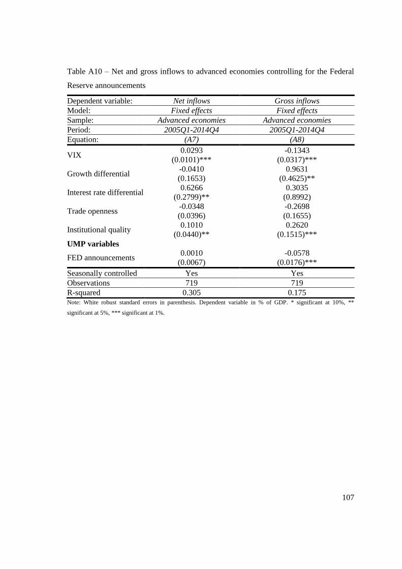
107
Table A10 – Net and gross inflows to advanced economies controlling for the Federal
Reserve announcements
Dependent variable: Net inflows Gross inflows
Model: Fixed effects Fixed effects
Sample: Advanced economies Advanced economies
Period: 2005Q1-2014Q4 2005Q1-2014Q4
Equation: (A7) (A8)
VIX 0.0293
(0.0101)***
-0.1343
(0.0317)***
Growth differential -0.0410
(0.1653)
0.9631
(0.4625)**
Interest rate differential 0.6266
(0.2799)**
0.3035
(0.8992)
Trade openness -0.0348
(0.0396)
-0.2698
(0.1655)
Institutional quality 0.1010
(0.0440)**
0.2620
(0.1515)***
UMP variables
FED announcements 0.0010
(0.0067)
-0.0578
(0.0176)***
Seasonally controlled Yes Yes
Observations 719 719
R-squared 0.305 0.175 Note: White robust standard errors in parenthesis. Dependent variable in % of GDP. * significant at 10%, **
significant at 5%, *** significant at 1%.

108
Table A11 – Net and gross inflows to all the economies controlling for the Federal
Reserve announcements
Dependent variable: Net inflows Gross inflows
Model: Fixed effects Fixed effects
Sample: All the economies All the economies Period: 2005Q1-2014Q4 2005Q1-2014Q4
Equation: (A9) (A10)
VIX 0.0052
(0.0062)
-0.0905
(0.0178)***
Growth differential -0.0007
(0.0763)
0.1014
(0.1824)
Interest rate differential -0.0646
(0.0890)
0.6074
(0.3325)*
Trade openness -0.0939
(0.0247)***
-0.2054
(0.0572)***
Institutional quality 0.1128
(0.0244)***
0.2474
(0.0636)***
UMP variables
FED announcements -0.0050
(0.0041)
-0.0488
(0.0097)***
Seasonally controlled Yes Yes
Observations 1605 1605
R-squared 0.299 0.161 Note: White robust standard errors in parenthesis. Dependent variable in % of GDP. * significant at 10%, **
significant at 5%, *** significant at 1%.
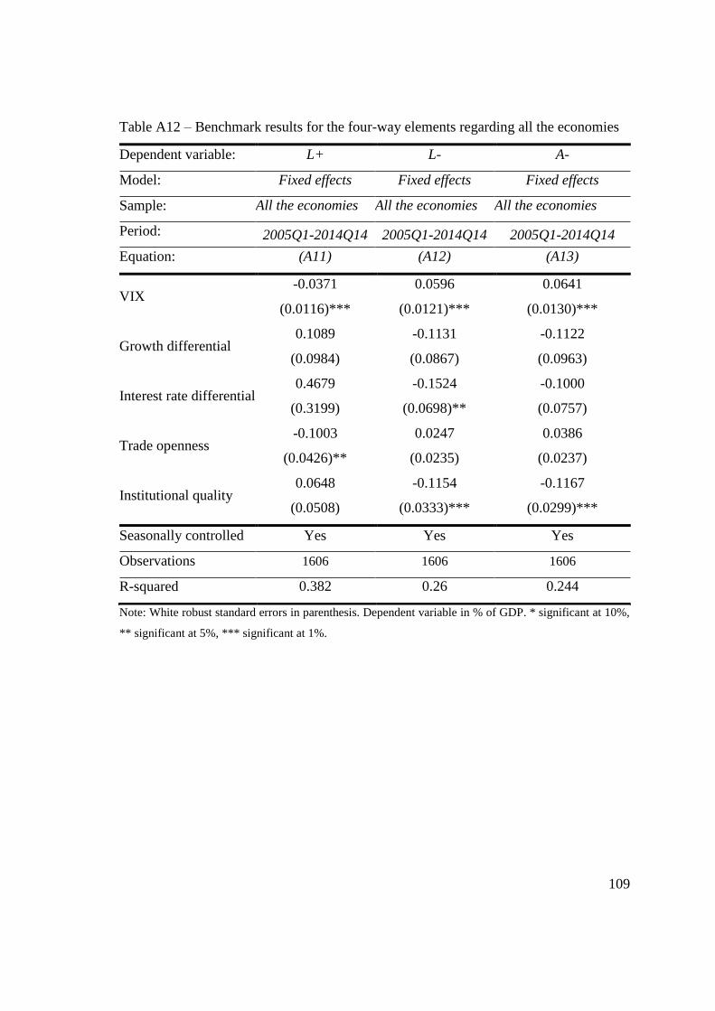
109
Table A12 – Benchmark results for the four-way elements regarding all the economies
Dependent variable: L+ L- A-
Model: Fixed effects Fixed effects Fixed effects
Sample: All the economies All the economies All the economies
Period: 2005Q1-2014Q14 2005Q1-2014Q14 2005Q1-2014Q14
Equation: (A11) (A12) (A13)
VIX -0.0371
(0.0116)***
0.0596
(0.0121)***
0.0641
(0.0130)***
Growth differential 0.1089
(0.0984)
-0.1131
(0.0867)
-0.1122
(0.0963)
Interest rate differential 0.4679
(0.3199)
-0.1524
(0.0698)**
-0.1000
(0.0757)
Trade openness -0.1003
(0.0426)**
0.0247
(0.0235)
0.0386
(0.0237)
Institutional quality 0.0648
(0.0508)
-0.1154
(0.0333)***
-0.1167
(0.0299)***
Seasonally controlled Yes Yes Yes
Observations 1606 1606 1606
R-squared 0.382 0.26 0.244
Note: White robust standard errors in parenthesis. Dependent variable in % of GDP. * significant at 10%,
** significant at 5%, *** significant at 1%.

110
Table A13 – UMP results for the four-way elements regarding all the economies
Dependent variable: L+ L- A-
Model: Fixed effects Fixed effects Fixed effects
Sample: All the economies All the economies All the economies
Period: 2005Q1-2014Q14 2005Q1-2014Q14 2005Q1-2014Q14
Equation: (A14) (A15) (A16)
VIX -0.0072
(0.0129)
0.0469
(0.0112)***
0.0534
(0.0118)***
Growth differential 0.0709
(0.1010)
-0.0648
(0.0946)
-0.0529
(0.1029)
Interest rate differential 0.4661
(0.3278)
-0.1700
(0.0826)*
-0.1410
(0.0872)
Trade openness -0.0744
(0.0459)
-0.0232
(0.0317)
-0.0004
(0.0305)
Institutional quality 0.1201
(0.0634)*
-0.1377
(0.0436)***
-0.1313
(0.0386)***
UMP variable:
G4 Central Banks
Balance Sheet
11.3806
(2.0262)***
-5.3644
(2.2300)**
-6.8285
(2.2664)***
Seasonally controlled Yes Yes Yes
Observations 1400 1400 1400
R-squared 0.385 0.28 0.276
Note: White robust standard errors in parenthesis. Dependent variable in % of GDP. * significant at 10%,
** significant at 5%, *** significant at 1%.

111
Table A14 – Benchmark results for the four-way elements regarding the advanced
economies
Dependent variable: L+ L- A-
Model: Fixed effects Fixed effects Fixed effects
Sample: Advanced
economies Advanced
economies Advanced
economies Period: 2005Q1-2014Q14 2005Q1-2014Q14 2005Q1-2014Q14
Equation: (A17) (A18) (A19)
VIX -0.0569
(0.0189)***
0.1016
(0.0244)***
0.1126
(0.0281)***
Growth differential 0.7306
(0.3474)**
-0.4024
(0.2803)
-0.4394
(0.2797)
Interest rate differential -0.0106
(0.5981)
-0.1501
(0.5386)
-0.2893
(0.5862)
Trade openness -0.3185
(0.1564)**
-0.0355
(0.0793)
-0.0306
(0.0705)
Institutional quality 0.0298
(0.1234)
-0.2605
(0.0842)***
-0.1156
('0.0774)
Seasonally controlled Yes Yes Yes
Observations 719 719 719
R-squared 0.307 0.252 0.246
Note: White robust standard errors in parenthesis. Dependent variable in % of GDP. * significant at 10%,
** significant at 5%, *** significant at 1%.

112
Table A15 – UMP results for the four-way elements regarding advanced economies
Dependent variable: L+ L- A-
Model: Fixed effects Fixed effects Fixed effects
Sample: Advanced
economies
Advanced
economies
Advanced
economies
Period: 2005Q1-2014Q14 2005Q1-2014Q14 2005Q1-2014Q14
Equation: (A20) (A21) (A22)
VIX -0.0091
(0.0225)
0.0696
(0.0214)***
0.0887
(0.0248)***
Growth differential 0.6093
(0.3740)
-0.2269
(0.3090)
-0.3235
(0.3047)
Interest rate differential -0.1316
(0.6346)
0.0751
(0.6798)
-0.0971
(0.7222)
Trade openness -0.3247
(0.1613)**
-0.1942
(0.1199)
-0.1691
(0.1086)
Institutional quality 0.0128
(0.1442)
-0.3143
(0.1072)***
-0.1364
(0.0987)
UMP variable:
G4 Central Banks
Balance Sheet
17.0362
(3.9098)***
-11.3504
(4.6417)**
-11.1261
(4.6713)**
Seasonally controlled Yes Yes Yes
Observations 619 619 619
R-squared 0.308 0.272 0.275
Note: White robust standard errors in parenthesis. Dependent variable in % of GDP. * significant at 10%,
** significant at 5%, *** significant at 1%.

113
Table A16 – Robustness check: relative expansion of G4 balance sheet regarding non-
advanced economies’ net and gross inflows
Dependent variable: Net inflows Gross inflows
Model: Fixed effects Fixed effects
Sample: Non-advanced economies Non-advanced economies
Period: 2005Q1-2014Q4 2005Q1-2014Q4
Equation: (A23) (A24)
VIX -0.0190
(0.0085)**
-0.0190
(0.0085)**
Growth differential 0.5877
(0.0989)***
0.9056
(0.1495)***
Interest rate differential -0.0211
(0.0762)
0.6659
(0.3964)*
Trade openness -0.1806
(0.0309)***
-0.1858
(0.0549)***
Institutional quality 0.0638
(0.0323)**
0.2377
(0.0717)***
UMP variables
Relative Expansion of
G4 Central Banks
Balance Sheet
0.2217
(0.0703)***
0.5261
(0.1323)***
Seasonally controlled Yes Yes
Observations 867 867
R-squared 0.295 0.265 Note: White robust standard errors in parenthesis. Dependent variable in % of GDP. * significant at 10%, **
significant at 5%, *** significant at 1%.

114
Table A17 – Robustness check: relative expansion of G4 balance sheet regarding non-
advanced economies’ four-way elements
Dependent variable: L+ L- A-
Model: Fixed effects Fixed effects Fixed effects
Sample: Non-advanced
economies Non-advanced
economies Non-advanced
economies Period: 2005Q1-2014Q14 2005Q1-2014Q14 2005Q1-2014Q14
Equation: (A25) (A26) (A27)
VIX -0.0041
(0.0121)
0.0226
('0.0063)***
0.0217
(0.0067)***
Growth differential 0.2595
(0.0863)***
-0.0497
(0.0535)
-0.2138
(0.0595)***
Interest rate differential 0.5718
(0.3354)*
-0.1012
(0.0631)
-0.0794
(0.0887)
Trade openness -0.0022
(0.0314)
0.0040
(0.0240)
0.0310
(0.0264)
Institutional quality 0.1454
(0.0541)***
-0.0186
(0.0186)
-0.0999
(0.0264)***
UMP variable:
Relative Expansion of
G4 Central Banks
Balance Sheet
0.2991
(0.0882)***
-0.0151
(0.0431)
-0.1364
(0.0516)***
Seasonally controlled Yes Yes Yes
Observations 746 746 746
R-squared 0.409 0.23 0.347
Note: White robust standard errors in parenthesis. Dependent variable in % of GDP. * significant at 10%,
** significant at 5%, *** significant at 1%.

115
Table A18 – Robustness check: relative expansion of G4 balance sheet regarding
advanced economies’ net and gross inflows
Dependent variable: Net inflows Gross inflows
Model: Fixed effects Fixed effects
Sample: Advanced economies Advanced economies
Period: 2005Q1-2014Q4 2005Q1-2014Q4
Equation: (A28) (A29)
VIX 0.0325
(0.0109)***
-0.0717
(0.0341)**
Growth differential -0.0041
(0.1828)
0.9438
(0.5048)*
Interest rate differential 0.3525
(0.3102)
-0.0579
(1.1119)
Trade openness -0.0800
(0.0546)
-0.1144
(0.2248)
Institutional quality 0.1070
(0.0542)**
0.3362
(0.1805)*
UMP variables
Relative Expansion of
G4 Central Banks
Balance Sheet
0.0433
(0.0861)
1.4304
(0.2813)***
Seasonally controlled Yes Yes
Observations 867 867
R-squared 0.276 0.166 Note: White robust standard errors in parenthesis. Dependent variable in % of GDP. * significant at 10%, **
significant at 5%, *** significant at 1%.

116
Table A19 – Robustness check: relative expansion of G4 balance sheet regarding
advanced economies’ four-way elements
Dependent variable: L+ L- A-
Model: Fixed effects Fixed effects Fixed effects
Sample: Advanced
economies
Advanced
economies
Advanced
economies
Period: 2005Q1-2014Q14 2005Q1-2014Q14 2005Q1-2014Q14
Equation: (A30) (A31) (A32)
VIX -0.0070
(0.0227)
0.0647
(0.0212)***
0.0856
(0.0246)***
Growth differential 0.7147
(0.3836)*
-0.2291
(0.3184)
-0.3390
(0.3121)
Interest rate differential -0.0474
(0.7005)
0.0104
(0.7357)
-0.1647
(0.7838)
Trade openness -0.3473
(0.1681)**
-0.2329
(0.1251)*
-0.1958
(0.1137)*
Institutional quality 0.0239
(0.1492)
-0.3123
(0.1146)***
-0.1322
(0.1052)
UMP variable:
Relative Expansion of
G4 Central Banks
Balance Sheet
0.8756
(0.1846)***
-0.5548
(0.2129)***
-0.5407
(0.2144)**
Seasonally controlled Yes Yes Yes
Observations 783 783 783
R-squared 0.322 0.277 0.28
Note: White robust standard errors in parenthesis. Dependent variable in % of GDP. * significant at 10%,
** significant at 5%, *** significant at 1%.

117
Table A20 – Robustness check: benchmark results not controlling for seasonal effects
regarding non-advanced economies’ net and gross inflows
Dependent variable: Net inflows Gross inflows
Model: Fixed effects Fixed effects
Sample: Non-advanced economies Non-advanced economies
Period: 2005Q1-2014Q4 2005Q1-2014Q4
Equation: (A33) (A34)
VIX -0.0258
(0.0077)***
-0.0601
(0.0160)***
Growth differential 0.6304
(0.0876)***
0.9167
(0.1267)***
Interest rate
differential
0.0065
(0.0668)
0.5726
(0.3982)
Trade openness -0.1585
(0.0272)***
-0.1914
(0.0459)***
Institutional quality 0.0735
(0.0304)**
0.1362
(0.0488)***
Seasonally controlled No No
Observations 867 867
R-squared 0.334 0.284 Note: White robust standard errors in parenthesis. Dependent variable in % of GDP. * significant at 10%, **
significant at 5%, *** significant at 1%.

118
Table A21 – Robustness check: benchmark results not controlling for seasonal effects
regarding advanced economies’ net and gross inflows
Dependent variable: Net inflows Gross inflows
Model: Fixed effects Fixed effects
Sample: Advanced economies Advanced economies
Period: 2005Q1-2014Q4 2005Q1-2014Q4
Equation: (A35) (A36)
VIX 0.0289
(0.0098)***
-0.1752
(0.0336)***
Growth differential -0.0398
(0.1684)
1.1920
(0.4697)**
Interest rate
differential
0.6420
(0.2776)**
0.3628
(0.9084)
Trade openness -0.0349
(0.0399)
-0.2725
(0.1786)
Institutional quality 0.0996
(0.0428)**
0.2754
(0.1505)***
Seasonally controlled No No
Observations 867 867
R-squared 0.304 0.121 Note: White robust standard errors in parenthesis. Dependent variable in % of GDP. * significant at 10%, **
significant at 5%, *** significant at 1%.

119
Table A22 – Robustness check: UMP results without controlling for seasonal effects
regarding non-advanced economies’ net inflows
Dependent variable: Net inflows Net inflows
Model: Fixed effects Fixed effects
Sample: Non-advanced economies Non-advanced economies
Period: 2005Q1-2014Q4 2005Q1-2014Q4
Equation: (A37) (A38)
VIX -0.0222
(0.0082)***
-0.0163
(0.0087)***
Growth differential 0.6202
(0.0958)***
0.5856
(0.0890)***
Interest rate differential -0.0008
(0.0714)
0.0084
(0.0667)
Trade openness -0.1806
(0.0302)***
-0.1555
(0.0269)***
Institutional quality 0.0647
(0.0316)**
0.0766
(0.0301)**
UMP variables:
G4 Central Banks Balance
Sheet
4.2601
(1.4783)***
UMP Announcements -0.0137
(0.0048)***
Seasonally controlled No No
Observations 764 867
R-squared 0.339 0.339
Note: White robust standard errors in parenthesis. Dependent variable in % of GDP. * significant at 10%,
** significant at 5%, *** significant at 1%.

120
Table A23 – Robustness check: UMP results without controlling for seasonal effects
regarding non-advanced economies’ gross inflows
Dependent variable: Gross inflows Gross inflows
Model: Fixed effects Fixed effects
Sample: Non-advanced economies Non-advanced economies
Period: 2005Q1-2014Q4 2005Q1-2014Q4
Equation: (A39) (A40)
VIX -0.0490
(0.0174)***
-0.0365
(0.0173)***
Growth differential 0.8739
(0.1384)***
0.8059
(0.1328)***
Interest rate differential 0.6182
(0.4005)
0.5772
(0.3875)
Trade openness -0.2096
(0.0518)***
-0.1839
(0.0456)***
Institutional quality 0.1911
(0.0616)***
0.1442
(0.0489)***
UMP variables:
G4 Central Banks Balance
Sheet
10.3220
(2.6632)***
UMP Announcements -0.0339
(0.0085)***
Seasonally controlled No No
Observations 764 867
R-squared 0.293 0.298
Note: White robust standard errors in parenthesis. Dependent variable in % of GDP. * significant at 10%,
** significant at 5%, *** significant at 1%.

121
Table A24 – Robustness check: UMP results not controlling for seasonal effects
regarding advanced economies’ net inflows
Dependent variable: Net inflows Net inflows
Model: Fixed effects Fixed effects
Sample: Advanced economies Advanced economies
Period: 2005Q1-2014Q4 2005Q1-2014Q4
Equation: (A41) (A42)
VIX 0.0313
(0.0106)***
0.0320
(0.0111)***
Growth differential -0.0136
(0.1777)
-0.0583
(0.1693)
Interest rate differential 0.3264
(0.2897)
0.6362
(0.2791)**
Trade openness -0.0722
(0.0537)
-0.0345
(0.0398)
Institutional quality 0.1050
(0.0516)**
0.0977
(0.0433)**
UMP variables:
G4 Central Banks Balance
Sheet
0.8241
(1.7949)
UMP Announcements -0.0041
(0.0062)
Seasonally controlled No No
Observations 619 719
R-squared 0.275 0.304
Note: White robust standard errors in parenthesis. Dependent variable in % of GDP. * significant at 10%,
** significant at 5%, *** significant at 1%.

122
Table A25 – Robustness check: UMP results not controlling for seasonal effects
regarding advanced economies’ gross inflows
Dependent variable: Gross inflows Gross inflows
Model: Fixed effects Fixed effects
Sample: Advanced economies Advanced economies
Period: 2005Q1-2014Q4 2005Q1-2014Q4
Equation: (A43) (A44)
VIX -0.0904
(0.0351)**
-0.0963
(0.0357)***
Growth differential 0.8802
(0.5031)*
0.7084
(0.4670)
Interest rate differential -0.0479
(0.9995)
0.2136
(0.8878)
Trade openness -0.1248
(0.2225)
-0.2602
(0.1759)
Institutional quality 0.3018
(0.1740)*
0.2264
(0.1506)
UMP variables:
G4 Central Banks Balance
Sheet
25.5426
(6.0352)***
UMP Announcements -0.1080
(0.0186)***
Seasonally controlled No No
Observations 619 719
R-squared 0.119 0.151
Note: White robust standard errors in parenthesis. Dependent variable in % of GDP. * significant at 10%,
** significant at 5%, *** significant at 1%.

123
Table A26 – Robustness check: benchmark model applied to non-advanced economies’
four-way elements not controlling for seasonal effects
Dependent variable: L+ L- A-
Model: Fixed effects Fixed effects Fixed effects
Sample: Non-advanced
economies
Non-advanced
economies Non-advanced
economies Period: 2005Q1-2014Q14 2005Q1-2014Q14 2005Q1-2014Q14
Equation: (A45) (A46) (A47)
VIX -0.0146
(0.0118)
0.0191
(0.0035)***
0.0226
(0.0043)***
Growth differential 0.2263
(0.0656)***
-0.0882
(0.0369)**
-0.2182
(0.0433)***
Interest rate differential 0.5280
(0.3558)
-0.0260
(0.0223)
-0.0079
(0.0413)
Trade openness -0.0128
(0.0276)
0.0068
(0.0120)
0.0288
(0.0172)*
Institutional quality 0.0588
(0.0329)*
-0.0007
(0.0089)
-0.0547
(0.0148)***
Seasonally controlled No No No
Observations 867 867 867
R-squared 0.408 0.235 0.295
Note: White robust standard errors in parenthesis. Dependent variable in % of GDP. * significant at 10%,
** significant at 5%, *** significant at 1%.
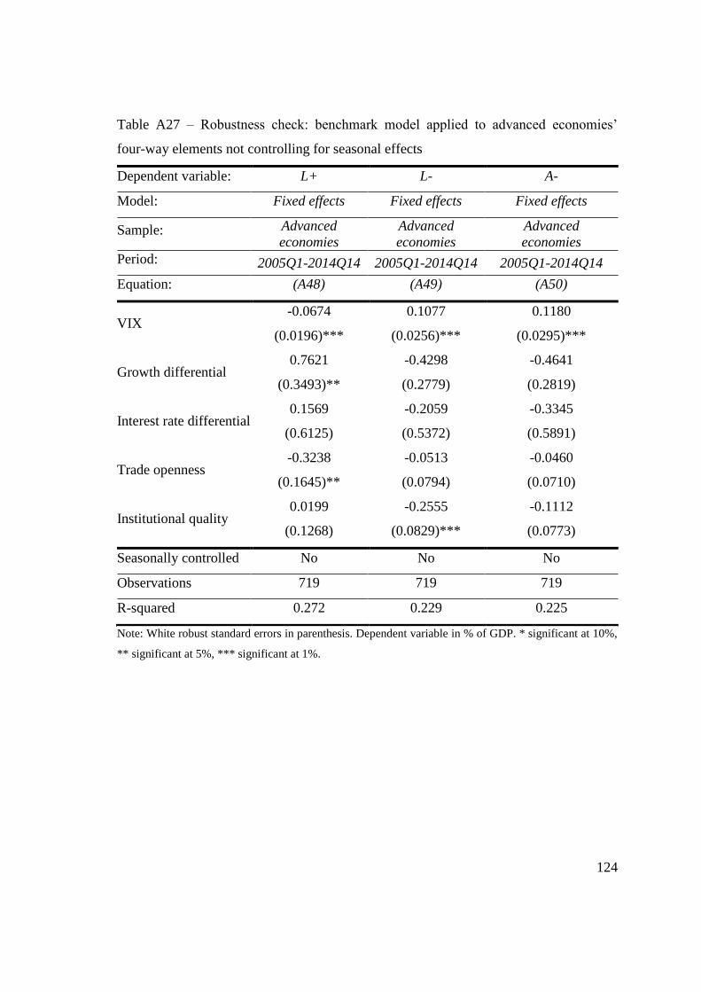
124
Table A27 – Robustness check: benchmark model applied to advanced economies’
four-way elements not controlling for seasonal effects
Dependent variable: L+ L- A-
Model: Fixed effects Fixed effects Fixed effects
Sample: Advanced
economies
Advanced
economies Advanced
economies Period: 2005Q1-2014Q14 2005Q1-2014Q14 2005Q1-2014Q14
Equation: (A48) (A49) (A50)
VIX -0.0674
(0.0196)***
0.1077
(0.0256)***
0.1180
(0.0295)***
Growth differential 0.7621
(0.3493)**
-0.4298
(0.2779)
-0.4641
(0.2819)
Interest rate differential 0.1569
(0.6125)
-0.2059
(0.5372)
-0.3345
(0.5891)
Trade openness -0.3238
(0.1645)**
-0.0513
(0.0794)
-0.0460
(0.0710)
Institutional quality 0.0199
(0.1268)
-0.2555
(0.0829)***
-0.1112
(0.0773)
Seasonally controlled No No No
Observations 719 719 719
R-squared 0.272 0.229 0.225
Note: White robust standard errors in parenthesis. Dependent variable in % of GDP. * significant at 10%,
** significant at 5%, *** significant at 1%.

125
Table A28 – Robustness check: UMP results regarding non-advanced economies’ four-
way elements not controlling for seasonal effects
Dependent variable: L+ L- A-
Model: Fixed effects Fixed effects Fixed effects
Sample: Non-advanced
economies Non-advanced
economies Non-advanced
economies Period: 2005Q1-2014Q14 2005Q1-2014Q14 2005Q1-2014Q14
Equation: (A51) (A52) (A53)
VIX -0.0078
(0.0126)
0.0182
(0.0037)***
0.0190
(0.0040)***
Growth differential 0.2017
(0.0744)***
-0.0838
(0.0365)**
-0.2040
(0.0425)***
Interest rate differential 0.5658
(0.3518)
-0.0339
(0.0244)
-0.0295
(0.0400)
Trade openness -0.0171
(0.0299)
0.0024
(0.0140)
0.0250
(0.0190)
Institutional quality 0.1323
(0.0469)***
0.0016
(0.0104)
-0.0593
(0.0168)***
UMP variable:
G4 Central Banks
Balance Sheet
5.5006
(1.7773)***
-1.2026
(0.6109)**
-3.4935
(0.8629)***
Seasonally controlled No No No
Observations 771 771 771
R-squared 0.437 0.252 0.347
Note: White robust standard errors in parenthesis. Dependent variable in % of GDP. * significant at 10%,
** significant at 5%, *** significant at 1%.

126
Table A29 – Robustness check: UMP results regarding advanced economies’ four-way
elements not controlling for seasonal effects
Dependent variable: L+ L- A-
Model: Fixed effects Fixed effects Fixed effects
Sample: Advanced
economies Advanced
economies Advanced
economies Period: 2005Q1-2014Q14 2005Q1-2014Q14 2005Q1-2014Q14
Equation: (A54) (A55) (A56)
VIX -0.0158
(0.0235)
0.0745
(0.0221)***
0.0928
(0.0259)***
Growth differential 0.6357
(0.3771)*
-0.2445
(0.3081)
-0.3381
(0.3071)
Interest rate differential 0.0076
(0.6292)
0.0555
(0.6733)
-0.1030
(0.7203)
Trade openness -0.3319
(0.1660)**
-0.2071
(0.1226)*
-0.1828
(0.1109)*
Institutional quality -0.0031
(0.1462)
-0.3049
(0.1056)***
-0.1287
(0.0979)
UMP variable:
G4 Central Banks
Balance Sheet
14.6128
(3.8049)***
-10.9299
(4.7191)***
-10.8928
(4.7248)**
Seasonally controlled No No No
Observations 619 619 619
R-squared 0.283 0.252 0.255
Note: White robust standard errors in parenthesis. Dependent variable in % of GDP. * significant at 10%,
** significant at 5%, *** significant at 1%.

127
Table A30 – Robustness check: estimation of the benchmark model regarding non-
advanced using random effects
Dependent variable: Net inflows Gross inflows
Model: Random effects Random effects
Sample: Non-advanced economies Non-advanced economies
Period: 2005Q1-2014Q4 2005Q1-2014Q4
Equation: (A57) (A58)
VIX -0.0211
(0.0080)***
-0.0548
(0.0164)***
Growth differential 0.5785
(0.0876)***
0.9039
(0.1345)***
Interest rate differential -0.0215
(0.0771)
0.4749
(0.3945)
Trade openness -0.0846
(0.0175)***
-0.0274
(0.0252)
Institutional quality 0.0573
(0.0129)***
0.0771
(0.0148)***
Seasonally controlled Yes Yes
Observations 867 867
R-squared 0.127 0.12 Note: White robust standard errors in parenthesis. Dependent variable in % of GDP. * significant at 10%, **
significant at 5%, *** significant at 1%.

128
Table A31 – Robustness check: estimation of the benchmark model regarding advanced
using random effects
Dependent variable: Net inflows Gross inflows
Model: Random effects Random effects
Sample: Advanced economies Advanced economies
Period: 2005Q1-2014Q4 2005Q1-2014Q4
Equation: (A59) (A60)
VIX 0.0260
(0.0101)**
-0.1557
(0.0293)***
Growth differential 0.0077
(0.1580)
0.9842
(0.4370)**
Interest rate differential 0.7225
(0.2873)**
-0.0226
(0.7604)
Trade openness -0.0459
(0.0225)**
0.0401
(0.0489)
Institutional quality -0.0181
(0.0182)
0.0241
(0.0289)
Seasonally controlled Yes Yes
Observations 719 719
R-squared 0.055 0.118 Note: White robust standard errors in parenthesis. Dependent variable in % of GDP. * significant at 10%, **
significant at 5%, *** significant at 1%.

129
Table A32 – Robustness check: estimation of the UMP model regarding non-advanced
economies’ net inflows using random effects
Dependent variable: Net inflows Net inflows
Model: Random effects Random effects
Sample: Non-advanced economies Non-advanced economies
Period: 2005Q1-2014Q4 2005Q1-2014Q4
Equation: (A61) (A62)
VIX -0.0141
(0.0086)
-0.0125
(0.0090)
Growth differential 0.5269
(0.0948)***
0.5276
(0.0884)***
Interest rate differential -0.0250
(0.0852)
-0.0129
(0.0737)
Trade openness -0.0827
(0.0172)***
-0.0820
(0.0172)***
Institutional quality 0.0526
(0.0134)***
0.0557
(0.0127)***
UMP variables:
G4 Central Banks Balance
Sheet
5.1682
(1.4951)***
UMP Announcements -0.0145
(0.0050)***
Seasonally controlled Yes Yes
Observations 764 867
R-squared 0.136 0.133
Note: White robust standard errors in parenthesis. Dependent variable in % of GDP. * significant at 10%,
** significant at 5%, *** significant at 1%.

130
Table A33 – Robustness check: estimation of the UMP model regarding non-advanced
economies’ gross inflows using random effects
Dependent variable: Gross inflows Gross inflows
Model: Random effects Random effects
Sample: Non-advanced economies Non-advanced economies
Period: 2005Q1-2014Q4 2005Q1-2014Q4
Equation: (A63) (A64)
VIX -0.0344
(0.0166)**
-0.0277
(0.0168)
Growth differential 0.7268
(0.1368)***
0.7548
(0.1377)***
Interest rate differential 0.4820
(0.4252)
0.5064
(0.3719)
Trade openness -0.0313
(0.0263)
-0.0303
(0.0251)
Institutional quality 0.0731
(0.0157)***
0.0768
(0.0149)***
UMP variables:
G4 Central Banks Balance
Sheet
11.7151
(2.7591)***
UMP Announcements -0.0465
(0.0101)***
Seasonally controlled Yes Yes
Observations 764 867
R-squared 0.133 0.143
Note: White robust standard errors in parenthesis. Dependent variable in % of GDP. * significant at 10%,
** significant at 5%, *** significant at 1%.

131
Table A34 – Robustness check: estimation of the UMP model regarding advanced
economies’ net inflows using random effects
Dependent variable: Net inflows Net inflows
Model: Random effects Random effects
Sample: Advanced economies Advanced economies
Period: 2005Q1-2014Q4 2005Q1-2014Q4
Equation: (A65) (A66)
VIX 0.0310
(0.0110)***
0.0304
(0.0112)***
Growth differential 0.0234
(0.1628)
-0.0188
(0.1613)
Interest rate differential 0.3488
(0.3039)
0.7151
(0.2876)**
Trade openness -0.0496
(0.0245)**
-0.0457
(0.0230)**
Institutional quality -0.0166
(0.0184)
-0.0172
(0.0188)
UMP variables:
G4 Central Banks Balance
Sheet
1.0073
(1.8572)
UMP Announcements -0.0063
(0.0067)
Seasonally controlled Yes Yes
Observations 619 719
R-squared 0.046 0.056
Note: White robust standard errors in parenthesis. Dependent variable in % of GDP. * significant at 10%,
** significant at 5%, *** significant at 1%.

132
Table A35 – Robustness check: estimation of the UMP model regarding advanced
economies’ gross inflows using random effects
Dependent variable: Gross inflows Gross inflows
Model: Random effects Random effects
Sample: Advanced economies Advanced economies
Period: 2005Q1-2014Q4 2005Q1-2014Q4
Equation: (A67) (A68)
VIX -0.0770
(0.0302)**
-0.1016
(0.0340)***
Growth differential 0.5475
(0.4378)
0.6910
(0.4424)
Interest rate differential 0.1158
(0.7895)
-0.0143
(0.7653)
Trade openness 0.0257
(0.0443)
0.0417
(0.0480)
Institutional quality 0.0206
(0.0267)
0.0228
(0.0292)
UMP variables:
G4 Central Banks Balance
Sheet
29.8745
(6.1222)***
UMP Announcements -0.0794
(0.0208)
Seasonally controlled Yes Yes
Observations 619 719
R-squared 0.118 0.133
Note: White robust standard errors in parenthesis. Dependent variable in % of GDP. * significant at 10%,
** significant at 5%, *** significant at 1%.

133
Table A36 – Robustness check: estimation of non-advanced economies’ four-way
elements using random effects
Dependent variable: L+ L- A-
Model: Random effects Random effects Random effects
Sample: Non-advanced
economies Non-advanced
economies Non-advanced
economies Period: 2005Q1-2014Q14 2005Q1-2014Q14 2005Q1-2014Q14
Equation: (A69) (A70) (A71)
VIX -0.0124
(0.0117)
0.0194
(0.0035)***
0.0232
(0.0047)***
Growth differential 0.2080
(0.0628)***
-0.0954
(0.0362)***
-0.2302
(0.0433)***
Interest rate differential 0.4659
(0.3662)
-0.0295
(0.0227)
-0.0114
(0.0333)
Trade openness 0.0311
(0.0176)*
0.0066
(0.0041)
0.0249
(0.0074)***
Institutional quality 0.0431
(0.0150)***
0.0074
(0.0029)**
-0.0006
(0.0038)
Seasonally controlled No No No
Observations 719 719 719
R-squared 0.129 0.389 0.418
Note: White robust standard errors in parenthesis. Dependent variable in % of GDP. * significant at 10%,
** significant at 5%, *** significant at 1%.

134
Table A37 – Robustness check: estimation of advanced economies’ four-way
components using random effects
Dependent variable: L+ L- A-
Model: Random effects Random effects Random effects
Sample: Advanced
economies Advanced
economies Advanced economies
Period: 2005Q1-2014Q14 2005Q1-2014Q14 2005Q1-2014Q14
Equation: (A72) (A73) (A74)
VIX -0.0465
(0.0181)**
0.1090
(0.0254)***
0.1166
(0.0285)***
Growth differential 0.6266
(0.3616)*
-0.6058
(0.2880)**
-0.4864
(0.2694)*
Interest rate differential -0.3482
(0.6456)
-0.1703
(0.4408)
-0.3209
(0.5193)
Trade openness 0.0599
(0.0638)
0.1271
(0.0376)***
0.0921
(0.0375)**
Institutional quality 0.0427
(0.0465)
-0.0159
(0.0215)
-0.0008
(0.0228)
Seasonally controlled Yes Yes Yes
Observations 719 719 719
R-squared 0.068 0.138 0.134
Note: White robust standard errors in parenthesis. Dependent variable in % of GDP. * significant at 10%,
** significant at 5%, *** significant at 1%.

135
Table A38 – Robustness check: estimation of the UMP model regarding the non-
advanced economies’ four-way elements using random effects
Dependent variable: L+ L- A-
Model: Random effects Random effects Random effects
Sample: Non-advanced
economies Non-advanced
economies Non-advanced
economies Period: 2005Q1-2014Q14 2005Q1-2014Q14 2005Q1-2014Q14
Equation: (A75) (A76) (A77)
VIX -0.0051
(0.0118)
0.0184
(0.0037)***
0.0200
(0.0047)***
Growth differential 0.1848
(0.0681)***
-0.0960
(0.0380)**
-0.2236
(0.0446)***
Interest rate differential 0.5220
(0.3655)
-0.0312
(0.0239)
-0.0255
(0.0328)
Trade openness 0.0307
(0.0184)*
0.0072
(0.0044)
0.0275
(0.0087)***
Institutional quality 0.0532
(0.0161)***
0.0083
(0.0030)***
-0.0004
(0.0045)
UMP variable:
G4 Central Banks
Balance Sheet
6.0302
(1.8359)***
-0.9928
(0.6387)
-3.0278
(0.7898)***
Seasonally controlled Yes Yes Yes
Observations 766 745 747
R-squared 0.113 0.159 0.199
Note: White robust standard errors in parenthesis. Dependent variable in % of GDP. * significant at 10%,
** significant at 5%, *** significant at 1%.

136
Table A39 – Robustness check: estimation of the UMP model regarding the advanced
economies’ four-way elements using random effects
Dependent variable: L+ L- A-
Model: Random effects Random effects Random effects
Sample: Advanced
economies Advanced
economies Advanced
economies Period: 2005Q1-2014Q14 2005Q1-2014Q14 2005Q1-2014Q14
Equation: (A78) (A79) (A80)
VIX 0.0159
(0.0199)
0.0945
(0.0243)***
0.1070
(0.0267)***
Growth differential 0.4085
(0.3772)
-0.5109
(0.3074)*
-0.4202
(0.2911)
Interest rate differential -0.4941
(0.7043)
-0.2599
(0.5282)
-0.4259
(0.6214)
Trade openness 0.0935
(0.0659)
0.1323
(0.0435)***
0.0967
(0.0431)**
Institutional quality 0.0289
(0.0476)
-0.0189
(0.0244)
-0.0018
(0.0257)
UMP variable:
G4 Central Banks
Balance Sheet
18.7745
(4.0871)***
-10.1148
(4.5716)**
-10.2462
(4.6345)**
Seasonally controlled Yes Yes Yes
Observations 619 619 619
R-squared 0.073 0.133 0.140
Note: White robust standard errors in parenthesis. Dependent variable in % of GDP. * significant at 10%,
** significant at 5%, *** significant at 1%.