Dynamic Risk Assessment of Process Facilities using Advanced Probabilistic Approaches

by

© Mohammad Zaid Kamil

A Thesis Submitted to the

School of Graduate Studies

in partial fulfilment of the requirements for the degree of

Master of Engineering

Faculty of Engineering and Applied Science

Memorial University of Newfoundland

May 2019

St. John’s Newfoundland and Labrador.

i

Abstract

A process accident can escalate into a chain of accidents, given the degree of congestion

and complex arrangement of process equipment and pipelines. To prevent a chain of

accidents, (called the domino effect), detailed assessments of risk and appropriate safety

measures are required. The present study investigates available techniques and develops

an integrated method to analyze evolving process accident scenarios, including the domino

effect. The work presented here comprises two main contributions: a) a predictive model

for process accident analysis using imprecise and incomplete information, and b) a

predictive model to assess the risk profile of domino effect occurrence. A brief description

of each is presented below.

In recent years the Bayesian network (BN) has been used to model accident causation and

its evolution. Though widely used, conventional BN suffers from two major uncertainties,

data and model uncertainties. The former deals with the used of evidence theory while the

latter uses canonical probabilistic models.

High interdependencies of chemical infrastructure makes it prone to the domino effect.

This demands an advanced approach to monitor and manage the risk posed by the domino

effect is much needed. Given the dynamic nature of the domino effect, the monitoring and

modelling methods need to be continuous time-dependent. A Generalized Stochastic Petri-

net (GSPN) framework was chosen to model the domino effect. It enables modelling of an

accident propagation pattern as the domino effect. It also enables probability analysis to

estimate risk profile, which is of vital importance to design effective safety measures.

ii

Acknowledgement

First and foremost, my sincere gratitude goes to my supervisors, Dr. Faisal Khan and Dr.

Salim Ahmed, for giving me the opportunity to research under their supervision and

providing constant encouragement throughout my program. They taught me how to

conduct successful research adhering to high research standards and always steered me in

the right direction. I am fortunate to have had Dr. Faisal Khan as an advisor who supported

me whenever I ran into a trouble spot. His patience, guidance and prompt feedback helped

me overcome the challenges and issues I faced during my studies. I am indebted to Dr.

Salim Ahmed, without whose engagement, the entire learning process during the research

work would not have been possible. His constructive feedback and review at various stages

of my research helped me to gear up my work in the right direction.

I would like to acknowledge the financial support provided by the Natural Science and

Engineering Council of Canada (NSERC) and Canada Research Chair (Tier I) Program in

Offshore Safety and Risk Engineering. I am grateful to Guozheng Song and Mohammed

Taleb-Berrouane for motivating me throughout my research, having discussions with me

to help me gain insights and providing their valuable comments. I would like to thank all

the members of C-RISE who supported and motivated me at every step of my work.

I want to acknowledge Dr. Ming Yang, Md. Alauddin and Shams Anwar for their

motivation and strength at difficult times. Last but not least, I am grateful for the constant

support, love and encouragement provided by my family, to whom I owe my success. I

dedicate my work to all of them.

iii

Table of Contents

ABSTRACT ............................................................................................................. I

ACKNOWLEDGEMENT ....................................................................................... II

TABLE OF CONTENTS .......................................................................................III

LIST OF TABLES ................................................................................................ VII

LIST OF FIGURES ............................................................................................... IX

LIST OF SYMBOLS, NOMENCLATURE AND ABBREVIATIONS ................. X

1. INTRODUCTION .............................................................................................1

1.1 Authorship Statement.......................................................................................... 1

1.2 Overview ............................................................................................................. 1

1.3 Dynamic Risk Analysis Evolution ...................................................................... 2

1.4 Motivation ........................................................................................................... 3

1.5 Application of BN in Dynamic risk assessment of process operations .............. 4

1.6 Application of Generalized Stochastic Petri-Nets in modelling domino effect

scenarios .......................................................................................................................... 6

1.7 Research objectives of the thesis ........................................................................ 7

1.8 Organization of the Thesis .................................................................................. 9

1.9 References ......................................................................................................... 11

iv

2 DYNAMIC RISK ANALYSIS USING INCOMPLETE AND IMPRECISE

INFORMATION ....................................................................................................17

Preface........................................................................................................................... 17

Abstract ......................................................................................................................... 17

2.1 Introduction ....................................................................................................... 18

2.2 Bayesian network .............................................................................................. 23

2.3 Preliminary ........................................................................................................ 24

2.3.1 Canonical probabilistic models ........................................................................ 24

2.3.2 Evidence theory ............................................................................................... 26

2.3.2.1 Yager combination rule................................................................................. 26

2.3.2.2 Definition of frame of discernment............................................................... 29

2.4 Proposed Framework ........................................................................................ 30

2.5 Application of Proposed methodology ............................................................. 33

2.5.1 Accident causal analysis .................................................................................. 34

2.5.2 Belief Structure ................................................................................................ 39

2.6 Probability calculation ...................................................................................... 40

2.7 Case study ......................................................................................................... 43

2.7.1 Accident description ........................................................................................ 43

2.7.2 Bayesian network analysis ............................................................................... 45

2.7.3 Probability updating ......................................................................................... 50

2.8 Conclusions ....................................................................................................... 53

2.9 Appendix ........................................................................................................... 54

v

2.10 References ......................................................................................................... 58

3 DYNAMIC RISK ANALYSIS OF DOMINO EFFECT USING GSPN .......63

Preface........................................................................................................................... 63

Abstract ......................................................................................................................... 63

3.1 Introduction ....................................................................................................... 64

3.2 PN model concepts ........................................................................................... 66

3.3 The Proposed DOMINO-GSPN Model ............................................................ 69

Step 1: Identification of accident-prone units ........................................................... 70

Step 2: Primary units’ specifications ........................................................................ 71

Step 3: Identification of accident scenarios .............................................................. 71

Step 4: Estimation of escalation vectors and comparison with threshold values ..... 71

Step 5: Probit values calculation ............................................................................... 72

Step 6: Initial marking of tokens ............................................................................... 73

Step 7: Identifying the transitions specification........................................................ 73

Step 8: Defining predicates and assertions ............................................................... 73

Step 9: Real-time risk/ failure profiles ...................................................................... 74

Step 10: Identification of secondary units ................................................................ 74

Step 11: Next level propagation of domino effect .................................................... 74

3.4 The Application of the DOMINO-GSPN Model .............................................. 75

3.4.1 Domino effect modelling using Petri-net .................................................. 75

3.5 Results and discussion ...................................................................................... 81

3.6 Conclusions ....................................................................................................... 87

vi

3.7 References ......................................................................................................... 89

4 SUMMARY, CONCLUSIONS AND RECOMMENDATIONS ...................96

4.1 Summary ........................................................................................................... 96

4.2 Conclusions ....................................................................................................... 97

4.3 Recommendations ............................................................................................. 98

vii

List of Tables

Table 2.1 CPTs of “Removal of excess liquid fails” using the Noisy-OR gate (based on

Expert judgement) ............................................................................................................. 36

Table 2.2 Conditional probability table of “High inlet flow in the tank” using the leaky

Noisy-AND gate (based on Expert judgement) ................................................................ 37

Table 2.3 Expert opinion on the probability of events...................................................... 38

Table 2.4 Belief structure .................................................................................................. 39

Table 2.5 Deterministic failure probabilities of each root cause and safety system (using

expert 1 opinion) ............................................................................................................... 41

Table 2.6 Probabilities of different consequences using evidence theory and a deterministic

approach ............................................................................................................................ 42

Table 2.7 Events along with their symbols used in accident modelling ........................... 47

Table 2.8 Results obtained from accident analysis using BN ........................................... 50

Table 2.9 ASP data recorded during plant operation ........................................................ 51

Table 2.10 Expert opinion on the probability of events.................................................... 54

Table 2.11 Belief structure obtained from Yager combination rule ................................. 55

Table 2.12 Prior probabilities of deterministic approach obtained by expert 1 ................ 56

Table 3.1 The specification of each transition used in DOMINO-GSPN model.............. 79

ix

List of Figures

Figure 1.1 Thesis organization .......................................................................................... 10

Figure 2.1 Proposed accident modelling framework using Bayesian network ................. 32

Figure 2.2 Tank equipped with process control system .................................................... 33

Figure 2.3 BN for “Liquid spill from the tank” ................................................................ 34

Figure 2.4 Multiple layers failure of level control and monitoring system (CSB, 2009) . 45

Figure 2.5 Bayesian network analysis for gasoline overflow ........................................... 46

Figure 2.6 Dynamic probability changes of the Gasoline release .................................... 52

Figure 2.7 Dynamic probability updating of consequence C7 .......................................... 53

Figure 3.1 The DOMINO-GSPN model for domino effect likelihood assessment .......... 70

Figure 3.2 Process plant layout, tank 1 where the fire occurs and neighboring tanks 2, 3

and 4 affected by escalation vector (i.e. heat radiation) ................................................... 75

Figure 3.3 GSPN model part of the domino effect propagation from the primary unit (Tank

1) to the secondary unit (Tank 2) ...................................................................................... 77

Figure 3.4 Distribution fitting on a probability vs time plot for transition T41 & T42 ....... 78

Figure 3.5 DOMINO-GSPN model for domino effect propagation pattern in a four tank

system ............................................................................................................................... 80

Figure 3.6 Failure profile of tank 2 and tank 3 by the domino effect ............................... 83

Figure 3.7 Failure profile of tank 4 by the domino effect of tank 1 & tank 2/3 ............... 84

x

List of symbols, Nomenclature and Abbreviations

BOP Blowout Preventer

MIMAH Methodology for Identification of Major Accident Hazards

MIRAS Methodology for Identification of Reference Accident Scenarios

QRA Quantitative Risk Assessment

PSA Probabilistic Safety Approach

BN Bayesian Network

GSPN Generalized Stochastic Petri Net

ASCE American Society of Civil Engineers

ASME American Society of Mechanical Engineers

DST Dempster Shafer Theory

CPT Conditional Probability Table

PRA Probabilistic Risk Assessment

BT Bow-Tie

FT Fault Tree

ET Event Tree

BPA Basic Probability Assessment

Bel Belief Measure

Pl Plausibility

FOD Frame of Discernment

PS Power Set

xi

CE Critical Event

HLA High Level Alarm

CAPECO Caribbean Petroleum Cooperation

CSB Chemical Safety Board

ASP Accident Sequence Precursor

LPG Liquefied Petroleum Gas

PN Peri Net

SPN Stochastic Petri Net

HAZOP Hazard and Operability study

FMEA Failure Modes and Effect Analysis

MAE Major Accidental Events

ttf time to failure

HR Heat Radiation

DRA Dynamic Risk Analysis

1

1. Introduction

1.1 Authorship Statement

Mohammad Zaid Kamil is the principal author of this thesis and also prepared the first

drafts of the two manuscripts included in Chapters 2 and 3. Professor Faisal Khan, co-

author of this thesis, provided the fundamental concepts, technical support and guidance

and verified all the concepts developed throughout the entire process. Dr. Salim Ahmed,

co-author of this thesis, provided guidance, technical advice and troubleshooting

assistance. In addition to the above, the co-authors contributed by reviewing, and revising

the two manuscripts and the thesis.

1.2 Overview

Process safety is a crucial part of all process operations that take place in the industry. It

aims to minimize the risk of a process hazard that may lead to the release of materials

and/or energy with the help of preventive and mitigative layers of safety (Health and Safety

Executive, 2015). However, despite the advancements of risk analysis techniques, they still

fail to foresee many undesired events in process facilities, for example, the recent

catastrophic accident at the Texas City refinery accident in 2005 (US Chemical Safety

Board, 2007) and the Deep-water Horizon oil spill in the Gulf of Mexico in 2010 (US

Chemical Safety and Hazard Investigation Board, 2016). The Texas City accident was

caused due to a lack of safety measures that allowed the risk to go above its acceptable

limits (US Chemical Safety Board, 2007). For the Deepwater Horizon accident, a blowout

preventer (BOP) failure was the root cause of the accident (US Chemical Safety and Hazard

2

Investigation Board, 2016). These accidents have significantly affected the industry

practices of process safety.

The most important step in safety analysis is accident scenario modeling. Various

approaches have been proposed for this purpose such as maximum credible accident

scenario by (Khan, 2001) that short-lists the potential scenarios based on the likelihood

and consequences of the undesired event, the Methodology for Identification of Major

Accident Hazards (MIMAH) and the Methodology for Identification of Reference Accident

Scenarios (MIRAS) proposed by Delvosalle (Delvosalle, Fievez, Pipart and Debray, 2006).

The MIRAS includes a safety system but the MIMAH does not consider it.

1.3 Dynamic Risk Analysis Evolution

Risk analysis aims to quantify the occurrence probability of an accident scenario and its

associated consequences (Crowl, D.A. and Louvar, 2013). In chemical/process industries,

risk analysis followed by a safety system implementation is important, due to the

involvement of hazardous substances. Several risk analysis methodologies have been used

to model accidents, which can be broadly divided into two main categories: a) Qualitative

approach and b) Quantitative approach. Both approaches identify hazards and estimate risk.

However, the former approach is often performed for a group of systems, used for

screening purposes and the estimated risk is relative in nature, whereas the latter is a

comprehensive approach, used to quantify the risk (probability of failure and consequence

assessment) and is often performed on specific system or equipment. The quantitative

approach can be either deterministic or probabilistic.

3

To perform Dynamic Risk Assessment (DRA), many attempts have been made to

dynamically adapt the model based on new observations from a process. The two principal

techniques used in DRA are the Bow-Tie (BT) and the Bayesian Network (BN). Both

methods have the ability to capture the accident scenario from causes to consequences.

However, the former suffers from the static nature of its constituents, i.e. the fault tree and

the event tree. Researchers have made attempts to overcome the limitation; e.g., FT has

been coupled with Bayesian theory to update the risk dynamically (Ching & Leu, 2009).

Similarly, ET has also been coupled with Bayesian theory to update the likelihood of safety

functions (Meel and Seider, 2006; Kalantarnia, Khan and Hawboldt, 2009; Rathnayaka,

Khan and Amyotte, 2011). Another attempt has been made to utilize the unique features of

BN by mapping BT on BN (Khakzad, Khan and Amyotte, 2013).

Moreover, BN has attracted much attention in the past five years due to its unique features,

such as capturing event dependency, incorporating common cause failure and dynamically

updating the risk by considering accident sequence precursor (ASP) data often gathered

during the process. However, it has a few disadvantages, such as a high computational load

which increases exponentially with the number of variables for constructing the conditional

probability table (CPT) and an inability to capture complex behaviour/dependency among

variables, deterministic and/or normally distributed failure probabilities. The current

research is an attempt to address the gaps and challenges in DRA.

1.4 Motivation

In the present study, the application of advanced probabilistic techniques such as BN and

PN are investigated and discussed in the context of dynamic risk assessment of process

4

operations. The following sections would provide a brief description of motivation as well

as these mentioned techniques application to bridge the gaps to perform effective DRA.

1.5 Application of BN in Dynamic risk assessment of process operations

BN is a graphical technique used to model accident scenarios in chemical industries. It can

incorporate causal relationships among variables using a Conditional Probability Table

(CPT). Another advantage of this method is that it models the complete accident scenario,

i.e., it has the ability to model causes as well as consequences in a single graphical diagram.

Using Bayes’ theorem, BN has the ability to perform reasoning and update the prior belief

when new information about the system becomes available (evidence). However,

sequential updating can also be performed using BN, as new data is gathered from the

process. The precursor data can be considered to adapt the probability of the system, which

is of great importance, particularly for rare event probability estimation.

In the past decade, BN has received a plethora of attention in the area of risk and safety

engineering. Moreover, BN models can produce results when subjected to model

uncertainty and/or data uncertainty. The former uncertainty can be caused due to imprecise

logic relationships used in the CPT to model the causal relationship among variables, while

the latter results from the crisp probability requirement of BN. Flexible logic gates are

required to build the CPT; they incorporate various interactions of variables. Traditional

logic gates such as OR & AND only depict the linear relationships among variables, which

is a naïve assumption in accident modeling. In risk analysis, the uncertainty cannot be

removed completely, due to the lack of system knowledge and variability in the system

response (Markowski, Mannan and Bigoszewska, 2009; Ferdous, Khan, Sadiq, Amyotte

5

and Veitch, 2013). In industrial systems, it is hard to acquire failure probabilities of process

components, due to the lack of understanding of failure mechanisms and design faults

(Yuhua and Datao, 2005). Obtaining failure data from process history is not possible for

all components. Therefore, subjective sources such as expert opinions become the only

source available to obtain the required information. The data obtained from various

subjective sources may have a high degree of inconsistency if all the experts do not reach

a consensus and the probabilistic approach (BN) cannot efficiently deal with the problem.

Various methods have been discussed in the literature; e.g. see Abrahamsson, (2002);

Wilcox and Ayyub, (2003); Thacker and Huyse, (2007); Ferdous, Khan, Sadiq, Amyotte

and Veitch (2009). Ferdous et al. (2009) used bow-tie analysis, where the Dempster-Shafer

Theory (DST), commonly known as evidence theory, is used to aggregate multi-expert

opinions, which reduces uncertainty significantly. In the present study, a modified

Dempster-Shafer (DS) combination rule known as the Yager combination rule has been

used, due to its numerical stability as compared to the DST (Sentz and Ferson, 2002).

The aim of this study is to utilize the advantages of BN in the risk assessment of process

operations and also to overcome its limitations. Incorporating methods to manage model

and data uncertainties in BN allows modeling an accident scenario more precisely, even

with incomplete and imprecise information. The incomplete information can be dealt with

using canonical models which are able to model various interactions among the causes and

the effects of an accident. Vague information available about the system from subjective

sources can be combined using the Yager combination rule. The study attempts to predict

6

the accident more precisely because it is preferable to avoid an accident rather than

minimize its consequences.

1.6 Application of Generalized Stochastic Petri-Nets in modelling domino effect

scenarios

Domino effects are in-frequent but can be very severe in consequences. To model domino

accidents is a challenging task (Khakzad, Khan, Amyotte and Cozzani, 2013). Since 1947,

the term domino effect has been documented in the literature (Kadri, Chatelet and

Lallement, 2013); however, it gained more attention after the LPG leakage in Mexico City

in 1984. Since then various attempts have been made in the past, based on different aspects

of the domino effect such as escalation probability (i.e., damage probability), use of

distance models (Bagster and Pitblado, 1991) and a combination of a probit model and

threshold limits (Khan and Abbasi, 1998; Cozzani et al., 2006). Moreover, other studies

used statistical surveys, which show accident sequences and estimate the frequency

(Darbra, Palacios and Casal, 2010; Vílchez, Sevilla, Montiel and Casal, 1995; Kourniotis

et al., 2000). Additionally, in the context of quantitative risk assessment (QRA) of domino

accident modelling and propagation, some work has been done (Khan and Abbasi, 1998a;

Cozzani, Gubinelli, Antonioni, Spadoni and Zanelli, 2005; Antonioni, Spadoni and

Cozzani, 2009; Abdolhamidzadeh et al., 2010; Reniers, Dullaert, Ale and Soudan, 2005;

Reniers and Dullaert, 2007; Khakzad, Reniers, Abbassi, & Khan, 2016;Khakzad et al.,

2013;Khakzad, 2015; Khakzad et al., 2013; Khakzad, Khan, Amyotte and Cozzani, 2014).

Previous attempts to model propagational patterns and likelihood assessments provide

discrete probabilities. However, those attempts have limitations, such as the inability to

7

model complex process behaviour in combined loading and time-dependent equipment

failure. In chapter 3 an attempt has been made to overcome limitations in modelling domino

effects. A model based on Generalized Stochastic Petri-Nets (GSPN) helps to overcome

the gap. The term Petri-net (PN) was first introduced in 1962 in the dissertation of Carl

Adam Petri (David and Alia, 2010). This probabilistic technique is receiving much

attention due to its flexibility to model concurrent, asynchronous, distributed, parallel non-

deterministic and/or stochastic systems (Murata, 1989).

The motivation is to utilize the potential probabilistic techniques which can model the

domino propagation pattern and assess its likelihood. The developed framework for

domino effect likelihood assessment by Cozzani et al., (2005) and Khakzad et al., (2013)

is considered in the present study to develop a DOMINO-GSPN model for modelling

accident scenarios, a model which is able to consider heat radiation from more than one

source and thereby render a time-dependent failure profile of the primary, secondary or

higher order domino level units.

1.7 Research objectives of the thesis

This thesis aims to bridge earlier identified knowledge gaps related to modelling dynamic

risk assessment and domino effect scenario modelling. The work is conducted to fulfill two

main research objectives:

• To address data uncertainty in BN which arises due to a lack of crisp data and model

uncertainty arising due to the use of linear relationships among variables

8

• To model propagation pattern and domino effect likelihood in a combined loading

and continuous time-dependent failure profile of equipment.

The first objective is to improve the BN model in order to predict the accident scenario

precisely by addressing the data and model uncertainties. The data uncertainty arises due

to the lack of available knowledge regarding failure probabilities of root causes and safety

barriers. It is not easy to record all the data of each component in a process plant. The other

uncertainty in BN is due to the use of traditional logic gates (OR & AND). These can only

model the linear relationship between the causes and effects. However, canonical

probabilistic models can overcome the arisen uncertainty by modelling various aspects of

the interaction of causes and effects. In previous attempts, the data uncertainty has been

addressed in Bow-tie analysis but not in BN. This study attempts to address it along with

the uncertainty due to logic gates.

The second objective is to model a series of accidents (cascading effect) known as the

domino effect. To model the domino effect is a challenging task because it requires more

computational time to model complex behaviour of process equipment. From the literature

review of the current chapter, it has been identified that there is a need for models which

can assess the domino effect likelihood and propagation patterns. The model should be able

to assess the likelihood in a combined load, i.e. heat loads from the different mechanisms

and provide a continuous time-dependent failure profile of the components. It can help to

monitor the process risk and also in applying the mitigation and control measures.

9

The aforementioned research objective is achieved by adopting advanced approaches to

the model accident and domino effect analysis.

1.8 Organization of the Thesis

The thesis is written in manuscript format. It comprises two manuscripts. The first

manuscript which is presented in chapter 2 has been submitted to the ASCE-ASME Journal

of Risk and Uncertainty in Engineering Systems, Part B: Mechanical Engineering. The

other manuscript presented in chapter 3 has been submitted to the Journal of Process Safety

and Environmental Protection. The organization of the thesis is also illustrated in Figure

1.1.

Chapter 2 is based on the first objective. It proposes a BN based model which is capable

of modelling an accident scenario when the information is incomplete and imprecise. It

includes a brief literature review of past techniques used in accident modeling along with

their deficiencies. The proposed model is first applied to a simple example of a tank

equipped with basic process control to show its efficacy. Further, a real-life case study is

also used to validate the approach and to provide a comparison with traditional BN.

10

Figure 1.1 Thesis organization

Chapter 3 is based on the second objective. It proposes a DOMINO-GSPN model that can

predict the domino likelihood of a combined loading and renders continuous time-

dependent failure of equipment. The failure profile can be used to determine the

vulnerability of a unit. This model has been used with heat radiation as an escalation vector;

additionally, its application can be extended to other escalation vectors such as

overpressure, impact of blast wave/missile etc. The proposed model has been applied to a

case study to show its efficacy. The results obtained from the analysis have been compared

with other probabilistic techniques to validate the model.

11

Chapter 4 comprises conclusions drawn from the study presented in chapters 2 and 3. It

also provides recommendations for future work.

1.9 References

Abdolhamidzadeh, B., Abbasi, T., Rashtchian, D., & Abbasi, S. A. (2010). A new method

for assessing domino effect in chemical process industry. Journal of Hazardous

Materials. https://doi.org/10.1016/j.jhazmat.2010.06.049

Abrahamsson, M. (2002). Uncertainty in quantitative risk analysis-characterisation and

methods of treatment. Lutvdg/Tvbb--1024--Se, 88. Retrieved from

http://lup.lub.lu.se/record/642153

Antonioni, G., Spadoni, G., & Cozzani, V. (2009). Application of domino effect

quantitative risk assessment to an extended industrial area. Journal of Loss Prevention

in the Process Industries. https://doi.org/10.1016/j.jlp.2009.02.012

Bagster, D. F., & Pitblado, R. M. (1991). Estimation of domino incident frequencies - an

approach. Process Safety and Environmental Protection: Transactions of the

Institution of Chemical Engineers, Part B.

Ching, J., & Leu, S. Sen. (2009). Bayesian updating of reliability of civil infrastructure

facilities based on condition-state data and fault-tree model. Reliability Engineering

and System Safety, 94(12), 1962–1974. https://doi.org/10.1016/j.ress.2009.07.002

Cozzani, V., Gubinelli, G., Antonioni, G., Spadoni, G., & Zanelli, S. (2005). The

assessment of risk caused by domino effect in quantitative area risk analysis. Journal

12

of Hazardous Materials. https://doi.org/10.1016/j.jhazmat.2005.07.003

Cozzani, V., Gubinelli, G., & Salzano, E. (2006). Escalation thresholds in the assessment

of domino accidental events. Journal of Hazardous Materials.

https://doi.org/10.1016/j.jhazmat.2005.08.012

Crowl, D.A. & Louvar, J. F. (2013). Chemical Process Safety: Fundamentals with

Applications (3rd ed.). NJ: Prentice Hall.

Darbra, R. M., Palacios, A., & Casal, J. (2010). Domino effect in chemical accidents: Main

features and accident sequences. Journal of Hazardous Materials, 183(1–3), 565–

573. https://doi.org/10.1016/j.jhazmat.2010.07.061

David, R., & Alia, H. (2005). Discrete, continuous, and hybrid petri nets. Discrete,

Continuous, and Hybrid Petri Nets. https://doi.org/10.1007/b138130

Delvosalle, C., Fievez, C., Pipart, A., & Debray, B. (2006). ARAMIS project: A

comprehensive methodology for the identification of reference accident scenarios in

process industries. Journal of Hazardous Materials.

Ferdous, R., Khan, F., Sadiq, R., Amyotte, P., & Veitch, B. (2009). Handling data

uncertainties in event tree analysis. Process Safety and Environmental Protection,

87(5), 283–292. https://doi.org/10.1016/j.psep.2009.07.003

Ferdous, R., Khan, F., Sadiq, R., Amyotte, P., & Veitch, B. (2013). Analyzing system

safety and risks under uncertainty using a bow-tie diagram: An innovative approach.

Process Safety and Environmental Protection, 91(1–2), 1–18.

13

https://doi.org/10.1016/j.psep.2011.08.010

Health and Safety Executive. (2015). (COMAH)The Control of Major Accident Hazards

Regulations 2015, 15(483), 1–132.

Kadri, F., Chatelet, E., & Lallement, P. (2013). The Assessment of Risk Caused by Fire

and Explosion in Chemical Process Industry: A Domino Effect-Based Study. Journal

of Risk Analysis and Crisis Response, 3(2), 66.

https://doi.org/10.2991/jrarc.2013.3.2.1

Kalantarnia, M., Khan, F., & Hawboldt, K. (2009). Dynamic risk assessment using failure

assessment and Bayesian theory. Journal of Loss Prevention in the Process Industries,

22(5), 600–606. https://doi.org/10.1016/j.jlp.2009.04.006

Khakzad, N. (2015). Application of dynamic Bayesian network to risk analysis of domino

effects in chemical infrastructures. Reliability Engineering & System Safety, 138,

263–272. https://doi.org/10.1016/j.ress.2015.02.007

Khakzad, N., Khan, F., & Amyotte, P. (2013). Dynamic safety analysis of process systems

by mapping bow-tie into Bayesian network. Process Safety and Environmental

Protection, 91(1–2), 46–53. https://doi.org/10.1016/j.psep.2012.01.005

Khakzad, N., Khan, F., Amyotte, P., & Cozzani, V. (2013). Domino Effect Analysis Using

Bayesian Networks. Risk Analysis, 33(2), 292–306. https://doi.org/10.1111/j.1539-

6924.2012.01854.x

Khakzad, N., Khan, F., Amyotte, P., & Cozzani, V. (2014). Risk Management of Domino

14

Effects Considering Dynamic Consequence Analysis. Risk Analysis, 34(6), 1128–

1138. https://doi.org/10.1111/risa.12158

Khakzad, N., Reniers, G., Abbassi, R., & Khan, F. (2016). Vulnerability analysis of process

plants subject to domino effects. Reliability Engineering and System Safety, 154, 127–

136. https://doi.org/10.1016/j.ress.2016.06.004

Khan, F. I., & Abbasi, S. A. (1998a). DOMIFFECT (DOMIno eFFECT): User-friendly

software for domino effect analysis. Environmental Modelling and Software.

https://doi.org/10.1016/S1364-8152(98)00018-8

Khan, F. I., & Abbasi, S. A. (1998b). Models for domino effect analysis in chemical

process industries. Process Safety Progress, 17(2), 107–123.

https://doi.org/10.1002/prs.680170207

Kourniotis, S. P., Kiranoudis, C. T., & Markatos, N. C. (2000). Statistical analysis of

domino chemical accidents. Journal of Hazardous Materials, 71(1–3), 239–252.

https://doi.org/10.1016/S0304-3894(99)00081-3

Markowski, A. S., Mannan, M. S., & Bigoszewska, A. (2009). Fuzzy logic for process

safety analysis. Journal of Loss Prevention in the Process Industries, 22(6), 695–702.

https://doi.org/10.1016/j.jlp.2008.11.011

Meel, A., & Seider, W. D. (2006). Plant-specific dynamic failure assessment using

Bayesian theory. Chemical Engineering Science, 61(21), 7036–7056.

https://doi.org/10.1016/j.ces.2006.07.007

15

Murata, T. (1989). Petri nets: Properties, analysis and applications. Proceedings of the

IEEE, 77(4), 541–580. https://doi.org/10.1109/5.24143

Rathnayaka, S., Khan, F., & Amyotte, P. (2011). SHIPP methodology: Predictive accident

modeling approach. Part II: Validation with case study. Process Safety and

Environmental Protection. https://doi.org/10.1016/j.psep.2011.01.002

Reniers, G. L. L., Dullaert, W., Ale, B. J. M., & Soudan, K. (2005). The use of current risk

analysis tools evaluated towards preventing external domino accidents. Journal of

Loss Prevention in the Process Industries. https://doi.org/10.1016/j.jlp.2005.03.001

Sentz, K., & Ferson, S. (2002). Combination of Evidence in Dempster- Shafer Theory.

Contract, (April), 96. https://doi.org/10.1.1.122.7929

Thacker, B. H., & Huyse, L. J. (2007). Probabilistic assessment on the basis of interval

data. In Structural Engineering and Mechanics (Vol. 25, pp. 331–345).

US Chemical Safety and Hazard Investigation Board. (2016). Investigation Report -

Executive Summary - Explosion and Fire at Macondo Well, 4, 24. Retrieved from

http://www.csb.gov/assets/1/19/20160412_Macondo_Full_Exec_Summary.pdf

US Chemical Safety Board. (2007). Investigation Report - Refinery Explosion and Fire BP

Texas City. Csb, 1–341. https://doi.org/REPORT No. 2005-04-I-TX

Vílchez, J. A., Sevilla, S., Montiel, H., & Casal, J. (1995). Historical analysis of accidents

in chemical plants and in the transportation of hazardous materials. Journal of Loss

Prevention in the Process Industries. https://doi.org/10.1016/0950-4230(95)00006-M

16

Wilcox, R. C., & Ayyub, B. M. (2003). Uncertainty Modeling of Data and Uncertainty

Propagation for Risk Studies. In the Proceedings of the Fourth International

Symposium on Uncertainty Modeling and Analysis, 0–7.

Yuhua, D., & Datao, Y. (2005). Estimation of failure probability of oil and gas transmission

pipelines by fuzzy fault tree analysis. Journal of Loss Prevention in the Process

Industries. https://doi.org/10.1016/j.jlp.2004.12.003

17

2 Dynamic Risk Analysis Using Incomplete and Imprecise

Information

Preface

A version of this manuscript has been submitted to ASCE-ASME Journal of Risk and

Uncertainty in Engineering Systems, Part B: Mechanical Engineering. I am the primary

author of this manuscript along with Co-authors Faisal Khan, Salim Ahmed and Guozheng

Song. I developed the proposed framework of the model and its application using a case

study along with the analysis of the result. I prepared the first draft of the proposed

framework and revised it based on the co-author's feedback. The co-author Faisal Khan

provided the research problem, help in developing the framework, revising and testing the

application of the model. The co-author Salim Ahmed support in giving constructive

feedback to improve the application of the model and also assisted in reviewing and

improving the presentation of the proposed framework in the manuscript. The co-author

Guozheng Song help to implement the feedback provided by other co-authors in revising

and finalizing the manuscript.

Abstract

Accident modelling is a vital step which helps in designing preventive measures to avoid

future accidents, and thus, to enhance process safety. Bayesian network is widely used in

accident modelling due to its capability to represent accident scenarios from their causes

to likely consequences. However, to assess likelihood of an accident using the BN, it

requires exact basic event probabilities which are often obtained from expert opinions.

18

Such subjective opinions are often inconsistent and sometimes conflicting and/or

incomplete. In this work, the evidence theory has been coupled with Bayesian network

(BN) to address inconsistency, conflict and incompleteness in the expert opinions. It

combines the acquired knowledge from various subjective sources, thereby rendering

accuracy in probability estimation. Another source of uncertainty in BN is model

uncertainty. To represent multiple interactions of a cause-effect relationship Noisy-OR and

leaky Noisy-AND gates are explored in the study. Conventional logic gates, i.e. OR/AND

gates can only provide a linear interaction of cause-effect relationship hence introduces

uncertainty in the assessment. The proposed methodology provides an impression how

dynamic risk assessment could be conducted when the sufficient information about a

process system is unavailable. To illustrate the execution of a proposed methodology a tank

equipped with a basic process control system has been used as an example. A real-life case

study has also been used to validate the proposed model and compare its results with those

using a deterministic approach.

Keywords: Bayesian network; Uncertainty; Canonical Probabilistic model; Evidence

theory

2.1 Introduction

Chemical process industries are prone to accidents and due to the handling of large amounts

of hazardous chemicals. Process facilities consist of distillation towers, heat exchangers,

separation units and various other equipment, depending on the process operation, along

with a cluster of pipelines. These have the potential to cause escalation, turning small

19

incidents into catastrophic events (Kalantarnia, Khan and Hawboldt, 2009). Such accidents

can involve fire and explosion which can further lead to a domino effect (chain of

accidents) resulting in severe losses, including fatalities, property damage and

environmental degradation (Khan and Abbasi, 1998). Process deviation is one of the main

causes of accidents in a process system, leading to a chain of events resulting in an accident.

These deviations are caused due to the malfunctioning or failure of equipment, human error

and process upset. Among the different methodologies for risk assessment such as

quantitative risk assessment (QRA) and probabilistic risk assessment (PRA), there is a

common step known as accident modelling. It is a theoretical framework used to analyze

the cause-consequence relationship of an accident. Khan (2001) used maximum credible

accident scenarios for realistic and reliable risk assessments, which help to analyze and

investigate past accidents and to prevent future accidents by taking into account safety

measures followed by risk assessment (Tan, Chen, Zhang, Fu and Li, 2014). Accident

modelling is an important analysis which can help to determine the root causes of an

accident, enhancing safety systems and developing preventive measures (Qureshi, 2008).

Al-shanini, Ahmad and Khan (2014) provided a detailed review of accident models in

chemical process industries along with the systematic classification of each model.

Among various available modelling techniques, Bow-tie (BT) and the Bayesian network

(BN) have gained attention in the past decade. BT consists of mainly two constituents,

namely, Fault tree (FT) and Event tree (ET). The former helps to develop the causal

relationship between causal factors and abnormal events (accidents), whereas the latter is

a sequential technique used to identify potential consequences of an abnormal event.

20

However, BT suffers limitations of both the FT and ET, which makes it less demanding

than BN for accident modelling (Khakzad, Khan and Amyotte, 2013). To address their

limitations, some researchers tried to couple Bayesian inference with BT (Badreddine and

Ben Amor, 2010). BN reduces the limitations of BT such as common cause failure, event

dependencies and multi-state variables which are encountered in chemical process

industries (Khakzad, Khan and Amyotte, 2013). Probability updating is another advantage

of BN, which is inherent, due to Bayes’ theorem. The model can be updated if new

information from the process plant is available which in turn helps to update the prior belief

about the root causes and safety barriers’ failure probabilities.

Methodologies have been proposed to map BT into the BN. Fault tree mapping into BN is

based on the work of Bobbio, Portinale, Minichino and Ciancamerla, (2001), and Marsh,

Bearfield and Marsh (2008) used event tree mapping for BN. Later, Khakzad, Khan and

Amyotte (2013), introduced BT mapping into the Bayesian network by combining fault

tree and event tree mapping methodologies. They applied BN to assess risk associated with

vapour ignition accidents, considering event dependencies and used ASP (accident

sequence precursor) data to dynamically update the probabilities for possible consequences

and root causes. Yuan, Khakzad, Khan and Amyotte, (2015) applied BN to assess the risk

of dust explosion considering root causes, dependencies and common cause failures.

Abimbola, Khan, Khakzad and Butt, (2015) used BN considering dependencies in the

pressure-drilling technique to update the belief for operational data. Recently, Adedigba,

Khan and Yang, (2016) developed the model of non-linear interaction of contributory

21

accident factors due to the flexibility of BN to accommodate relaxation assumptions in

conditional dependence.

A risk is a function of accident probability and consequences associated with it. The present

study focuses on improving prediction of accident probability because it is more viable to

prevent accident rather than minimizing its consequences. The main objective of this study

is to handle the uncertainty caused by imprecise logic relationships and incomplete (partial

ignorance) prior data in accident modelling. The model and data uncertainties can be

addressed using canonical probabilistic models and evidence theory. Traditionally, a linear

relationship between causal factors is assumed and represented using OR (AND) logic

gates. Flexible logic gates are needed to build the conditional dependencies that incorporate

the various interactions of a cause-effect relationship. Canonical probabilistic models are

used define the conditional dependence between the parent node and child node in BN. It

can also consider expert opinion (if data is unavailable) or available data, which includes

various interactions between child and parent nodes. In the current study, Noisy-OR and

leaky Noisy-AND logic gates have been taken into consideration in place of OR and AND

logic gates. The implementation of these logic gates is illustrated in detail using an example

in section 3.

While performing risk analysis, it is not possible to rule out uncertainty completely because

it arises due to lack of knowledge about the system and the physical variability of a system

response (Markowski, Mannan and Bigoszewska, 2009; Ferdous, Khan, Sadiq, Amyotte

and Veitch, (2013). The prior failure probabilities of basic events and safety barriers are

not often found in the literature. Therefore, one has to rely on subjective sources (e.g.,

22

experts’ opinions). The probabilities obtained from different experts suffer from the

limitations of inconsistency, limited knowledge about the system, lack of understanding of

failure mechanism and inability of the experts to reach a consensus. BN is not able to deal

with such concepts. Various methods have been discussed in the literature to handle

uncertainties arising from expert opinion and using it for risk analysis, including

Abrahamsson, (2002); Wilcox and Ayyub, (2003); Thacker and Huyse, (2007); Ferdous,

Khan, Sadiq, Amyotte and Veitch, 2009). Bayesian probability theory has a well-developed

decision-making theory which needs precise probability.

The key question this work is addressing, how opinions (subjective) can be aggregated

(in the probabilistic framework) to provide a consistent and robust prior and subsequent

updating using Bayesian theory. Probabilistic opinion pooling is one of the techniques to

find a consensus among a group of individuals. However, it is widely assumed that the

combined opinion should take the form of a single probability distribution in case of

probabilistic opinion pooling which is not an appropriate assumption when dealing with

imprecise probability. Since each opinion is subjected to imprecision, hence, Bayesian

probability theory may cause concern in dealing with imprecise probability. Stewart &

Quintana (2018) has re-emphasized this point in their recent work. The DS theory can

capture the imprecision in individual probability and also in multiple source probabilities

aggregation. Use of DS theory with Yager modification provides a reliable likelihood

estimate in an interval [Bel, Pl] with a median estimate as a bet. The objective of this

work is to capture the strength of Bayesian network and the DS theory, and thus, to

provide a reliable and robust means of probabilistic assessment.

23

The evidence theory (commonly known as Dempster-Shafer theory) has been used in BT

analysis and was found to significantly reduce uncertainty (Ferdous, Khan, Sadiq, Amyotte

and Veitch, 2013). Dempster-Shafer Theory (DST) is used to aggregate multi-expert

opinions to define prior belief about a system. The Yager combination rule is a

modification of the Dempster- Shafer combination rule which has been used in this study

due to its numerical stability in cases involving large conflicts among expert opinions

(Sentz and Ferson, 2002).

The remaining chapter is organized as follows. Section 2.2 gives a brief description of BN

and canonical probabilistic models along with DST. Section 2.5 illustrates the application

of the proposed model by modelling an accident using imprecise and incomplete prior

information. Section 2.7 shows the partial validation of the proposed model using a case

study based on a past accident. Finally, Section 2.8 provides the conclusion of the study.

2.2 Bayesian network

BN is a graphical model widely used in dynamic risk analysis based on uncertain and

probabilistic knowledge (Pearl, 1988;Neapolitan, 1990; Heckerman, Mamdani and

Wellman, 1995; Bobbio, Portinale, Minichino and Ciancamerla, 2001). Its nodes represent

a set of random variables, and arcs connecting the nodes represent the direct dependencies.

The quantitative relationship between nodes is represented by conditional probabilities

assigned in Conditional Probability Tables (CPTs) (Bobbio, Portinale, Minichino and

Ciancamerla, 2001; Khakzad, Khan and Amyotte 2013). The BN represents the joint

probability distribution P(A) of a random variable A= {A1, …., An}, based on the

conditional independence and chain rule. It can be incorporated into the BN structure as:

24

𝑃(𝐴) = ∏ 𝑃(𝐴𝑖|𝑝𝑎(𝐴𝑖))𝑛𝑖=1 (1)

where pa(Ai) is the parent of random variable Ai and P (A) is the joint probability

distribution of a set of random variables (Pearl, 1988; Nielsen and Jensen, 2009).

BN incorporates Bayes’ theorem, which provides a way to revise prior probabilities given

new or additional evidence. Bayesian statistics measures degree of belief by using prior

probabilities, updating it by evidence (likelihood) to obtain a posterior belief. The equation

used to obtain the posterior probability given evidence (E) is as follows:

𝑃(𝐴|𝐸) = 𝑃(𝐴,𝐸)𝑃(𝐸) = 𝑃(𝐴,𝐸)

∑ 𝑃(𝐴,𝐸)𝐴 (2)

2.3 Preliminary

2.3.1 Canonical probabilistic models

BN has been extensively used in accidental modelling of process facilities. However, one

of the challenges is to acquire the knowledge about the system to develop conditional

dependencies of child node to parent node. To develop a linear relationship of the former

on the latter, conventional logic gates (OR and AND gates) can easily be used. In practical

scenarios the conditional dependence is not always linear which introduces uncertainty in

the model and undermine the credibility of the process. To relax the assumption canonical

probabilistic models has been explored in modelling complex behavior in establishing

conditional dependencies. The canonical probabilistic model reduces the required number

of parameters to build the conditional distributions. There are various canonical

probabilistic models available such as Noisy-OR, leaky Noisy-OR, Noisy-AND and leaky

25

Noisy-AND logic gates (Diez and Druzdzel, 2007). These models can use expert opinion

to estimate the conditional probability of a child node on the parent node. Expert opinion

helps to reduce the uncertainty in the cause-effect relationship. Therefore, the current study

focuses on explaining the use of Noisy-OR and leaky Noisy-AND gates in a BN model,

which better reflects practical scenarios in accident modelling.

The Noisy-OR gate is used to describe various interactions between n number of causes

and their common effect Z. The term “Noisy” refers to the chance that causes fail to

produce the effect, due to the inhibitor preventing it (Diez and Druzdzel, 2007). Assume

that Ci is the causation probability of a child node produced by the parent node while qi is

the probability that inhibition is active, in other words, qi is the probability that the child

node is present but does not affect the parent node. In a Noisy-OR gate, only n parameters

are needed compared to 2n in the case of an unrestricted model (Heckerman and Breese,

1996). Comparing, OR gates and leaky Noisy-OR gates, Noisy-OR gates provide the

median condition among the mentioned logic gates. Therefore, it has been used in this

study. When there are multiple parents to a child node, its probability can be calculated

using following equation (Adedigba, Khan and Yang, 2016).

𝑃(𝑍/𝐴) = 1 − ∏ (1 − 𝐶𝑖) 𝑖∈𝐴 (3)

The leaky Noisy-AND gate is an extension of the standard Noisy-AND gate in which an

explicit inhibitor is added with a probability of qL that may prevent the effect Z when all

the conditions are fulfilled. Each condition necessary for Z to be true can be inhibited or

26

substituted. Let qi be the probability that ith inhibitor is active when condition Ai is satisfied.

Then, the causation probability, Ci =1-qi. Similarly, si is the probability that the ith

substitute replaces Ai when the condition is not fulfilled. The leaky-Noisy AND gate

requires 2n+1 parameter compared to the leaky Noisy-OR gate which only needs n+1

parameter, where qL is the leak probability which accounts for the factors which have not

taken into consideration. While in the AND logic condition, the leaky Noisy-AND

condition provides the median values. The formula for deriving the CPT of the leaky

Noisy-AND gate is represented by the following equation (Diez and Druzdzel, 2007).

𝑃(𝑍/𝐴) = (1 − 𝑞𝐿)[∏ 𝐶𝑖 ∏ 𝑠𝑖] 𝑗𝜖−𝐴𝑖𝜖+𝐴 (4)

2.3.2 Evidence theory

The BN requires the probability of basic events and failure of safety barriers as prior

information to conduct quantitative risk assessment (QRA). Usually, the occurrence

probabilities of events are rarely available as accurate data; therefore, expert opinions are

consulted to obtain prior information. Two types of uncertainties (i.e., aleatory and

epistemic uncertainties) need to be addressed while using expert opinions (Ayyub and Klir,

2006). Randomness in the data availability, as well as the behaviour of the system, are

reflected in the aleatory uncertainty. Vagueness and ambiguity are reflected in the

epistemic uncertainty, which mainly arises because of incompleteness and imprecision

(Ferdous, Khan, Sadiq, Amyotte and Veitch 2009; 2011; 2013). Probabilistic methods are

not effective to deal with imprecise and incomplete information without any incorporation

of technique which can deal with uncertainties especially uncertainty arising from lack of

27

data (Druschel, Ozbek and Pinder, 2006). To obtain promising results from the

probabilistic model the prior information obtained from subjective sources must be

aggregated.

Evidence theory was first proposed by Dempster (1968) and later extended by Shafer

(1976), and is commonly known as Dempster-Shafer theory (DST) (Sentz and Ferson,

2002). The DST consists of three basic parameters, namely, basic probability assessment

(BPA), belief measure (Bel), and plausibility measure. These pamaters are used to define

the belief structure (Cheng, 2000; Lefevre, Colot and Vannoorenberghe, 2002; Bae,

Grandhi and Canfield, 2004; Ferdous, Khan, Sadiq, Amyotte and Veitch, 2009; 2011;

2013). The belief structure consists of a continuous interval in the form of belief and

plausibility. The real probability lies in the belief structure. As the structure becomes

narrower, the probability becomes more precise.

In a probabilistic framework, the outcome of an event is in the form of true or false. In

evidence theory, frame of discernment (FOD) is nothing but defines the possible outcome

of an event {T, F} which lead to four possible subsets. To define the event occurrence

probability a basic probability assessment (BPA) or belief mass has to be defined. Expert

opinion is explicitly representing the degree of belief in determining the belief mass of each

subset. The combined evidence helps to decide the event probability implicitly. Suppose,

to define an event occurrence probability; the expert opinion would be in the form of 75%

true and 20% false. Mathematically, it would be (m{T} = 0.75, m{F} = 0.2 and m {T, F}

= 0.05)

28

The FOD |Ω| can be defined as a set of mutually exclusive elements that allows having 2|Ω|

subsets in a power set (PS), where |Ω| shows the cardinality of a FOD. If, |Ω| = {Y, N}, the

power set (PS) will include four subsets, namely, {{}, {Y}, {N} {Y, N}}, since the

cardinality is two. Moreover, the cardinality can be infinite.

The BPA represents the knowledge assigned to the proposition of the power set (PS). The

sum of all the assigned propositions within the power set (PS) is 1. The elements, i.e. 𝑏𝑖 ∈

𝑃𝑆 with 𝑚(𝑏𝑖) > 0, represent the evidence. The BPA can be characterized by equation (4)

(Ferdous et al., 2009, 2011, 2013).

𝑚(𝑏𝑖) → [0,1]; 𝑚(∅) = 0; ∑ 𝑚(𝑏𝑖) = 1𝑏𝑖∈𝑃𝑆 (4)

The belief (Bel) measure also refers to a lower bound for a set bi and can be defined as the

summation of all BPAs of the interest set bi. Mathematically, it can be defined as equation

(5).

𝐵𝑒𝑙(𝑏𝑖) = ∑ 𝑚(𝑏𝑘)𝑏𝑘⊆𝑏𝑖 (5)

The plausibility (Pl) measure, also referred to as an the upper bound for a set bi, can be

defined as the summation of all BPAs of the interest set bi that intersects with the sets bk.

Mathematically, it can be defined as equation (7).

𝑃𝑙(𝑏𝑖) = ∑ 𝑚(𝑏𝑘)𝑏𝑘∩𝑏𝑖 ≠∅ (6)

The Bet estimation:

29

The belief structure [Bel, Pl] shows a continuous interval in which real probability lies.

The Bet estimation provides a point estimation of a belief structure which can be calculated

by equation (8).

𝐵𝑒𝑡(𝑃𝑆) = ∑ 𝑚(𝑏𝑖)|𝑏𝑖|

𝑏𝑖∈𝑃𝑆 (7)

2.3.2.1 Yager combination rule

The Yager combination rule is a modification of the DS combination rule. If there is a large

conflict between expert opinions, the DS combination rule provides unstable results (Sentz

and Ferson, 2002), first pointed out by (Zadeh, 1984). Unlike the DS combination rule, the

Yager combination rule does not ignore conflicting evidence. Instead, it is assigned to be

a part of ignorance Ω. However, when there is less or no conflict, both the rules exhibit

similar results. In this study, the Yager combination rule has been considered. The Yager

combination rule uses equations (8-11) to combine the expert opinions.

{𝑚1 × 𝑚2}(𝑏𝑖) = ∑ 𝑚1(𝑏1)𝑚2(𝑏2)𝑏1∩𝑏2 =𝑏𝑖 , 𝑏𝑖 ≠ Ω (8)

{𝑚1 × 𝑚2}(𝑏𝑖) = ∑ 𝑚1(𝑏1)𝑚2(𝑏2)𝑏1∩𝑏2 =𝑏𝑖 + 𝐾 , 𝑏𝑖 = Ω (9)

{𝑚1 × 𝑚2}(𝑏𝑖) = 0, 𝑏𝑖 = ∅ (10)

where {𝑚1 × 𝑚2}(𝑏𝑖) reflects the combined knowledge regarding a particular event.

‘K’ represents the degree of conflict between expert opinions, which can be determined

by equation (12).

30

𝐾 = ∑ 𝑚1(𝑏1)𝑚2(𝑏2) 𝑏1∩𝑏2 =∅ (11)

2.3.2.2 Definition of frame of discernment

Two different FODs are defined for the two uncertain parameters (prior probabilities of

basic events and safety barrier failures). The operational state of a system is usually defined

in terms of yes (Y) or no (N) for the failure of basic components (Vesely, Goldberg,

Roberts, & Haasl, 1981). Therefore, FOD of basic events can be defined as Ω = {Y, N}.

The power set (PS) will include four subsets, namely, {{(null set)}, {Y}, {N} and {Y, N}}.

Similarly, the operational state of the safety barrier is defined in terms of success {S} or

failure {F}. Therefore, the FOD can be defined as Ω = {S, F}. The power set (PS) will

include four subsets, namely, {{(null set)}, {S}, {F} and {S, F}}.

2.4 Proposed Framework

A generic framework of the Bayesian network has been proposed in Figure 2.1. For the

model uncertainty, Noisy-OR and leaky Noisy-AND gates are considered in the present

study. These two canonical probabilistic methods provide a median condition for the

respective Boolean logic, i.e. OR and AND. To handle imprecise and incomplete data, an

evidence theory-based approach is considered, which allows aggregating the multi-expert

opinions, which in turn helps to reduce input data uncertainty.

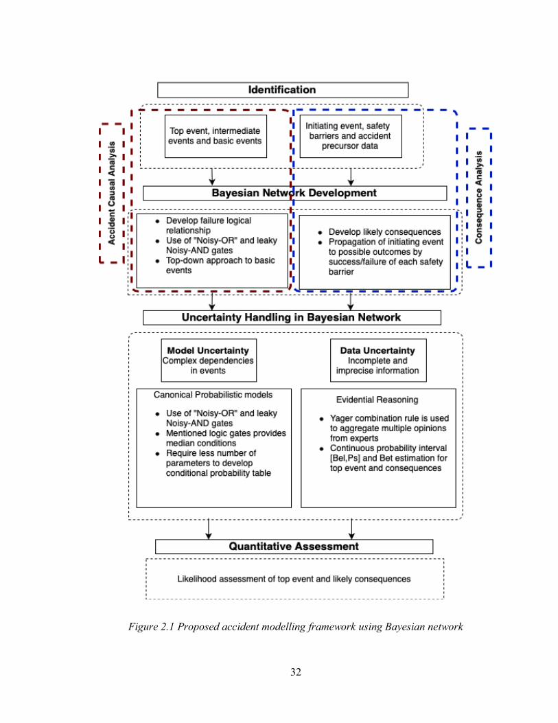
32

Figure 2.1 Proposed accident modelling framework using Bayesian network

33

2.5 Application of Proposed methodology

Figure 2.2 Tank equipped with process control system

The process considered in the present study is a tank which contains a hazardous chemical.

The potential hazard is the liquid spill from the tank through the high inlet flow and the

failure of the process control system. To ensure the safety of the system, it is equipped with

a feedback level controller which helps to maintain the desired tank level which is depicted

in Figure 2.2. The Level controller helps to ensure the desired inlet flow into the tank by

manipulating the A-valve. If it fails to operate, the increased tank level should be detected

by an independent High-level alarm (HLA) which will trigger the operator to open the

bypass valve to remove excess liquid from the tank and stop the incoming flow by closing

the manual valve. However, in the present study human error is not explicitly considered.

To demonstrate the process hazard in the case above, a Bayesian network has been made

in Figure 2.3. The liquid spill (CE) outcome is divided into two separate consequences,

namely, pool fire and loss of liquid.

34

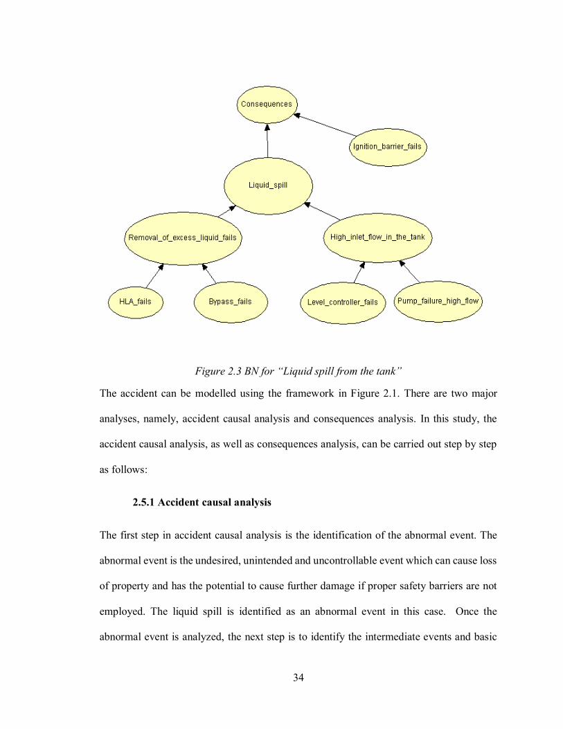
Figure 2.3 BN for “Liquid spill from the tank”

The accident can be modelled using the framework in Figure 2.1. There are two major

analyses, namely, accident causal analysis and consequences analysis. In this study, the

accident causal analysis, as well as consequences analysis, can be carried out step by step

as follows:

2.5.1 Accident causal analysis

The first step in accident causal analysis is the identification of the abnormal event. The

abnormal event is the undesired, unintended and uncontrollable event which can cause loss

of property and has the potential to cause further damage if proper safety barriers are not

employed. The liquid spill is identified as an abnormal event in this case. Once the

abnormal event is analyzed, the next step is to identify the intermediate events and basic

35

events responsible for causing the accident. In this case, two intermediate events are used,

namely, the high inlet flow in the tank due to level controller failure and pump failure (high

flow rate). Another event is the failure to remove excess liquid which is caused by due to

HLA failure and bypass valve failure.

In this problem, the identified root causes are Level controller failure, which is responsible

for maintaining the desired level in the tank and pumping failure, which causes a high

incoming flow. Moreover, the High-Level Alarm (HLA) fails to alert the operator to open

the bypass valve to remove the undesired liquid inside the tank.

2.5.2 Model Uncertainty reduction

The model uncertainty due to deterministic logic gates can be overcome by specifying the

conditional probabilities. Traditional logic gates may not allow construction of a refined

and detailed model because they are not able to reflect perfect knowledge about the system

behaviour (Bobbio, Portinale, Minichino and Ciancamerla, 2001). The conditional

dependence of the child node on the parent node is denoted using CPTs, which provides a

way to incorporate the canonical models to establish CPT’s. One can condition the variable

using Noisy gates on most of the possible behaviour of its parent node. This assumes that

the variable could be influenced by any single parent node independently of the other

parent node, which reduces the number of required parameters (Pearl, 1988).

The Noisy-OR and the leaky Noisy-AND gates are used in the present study, both the logic

gates provide the median condition for their respective logic. Diez and Druzdzel (2007)

provide details on the use of these canonical probabilistic models. In Figure 2.3, the node

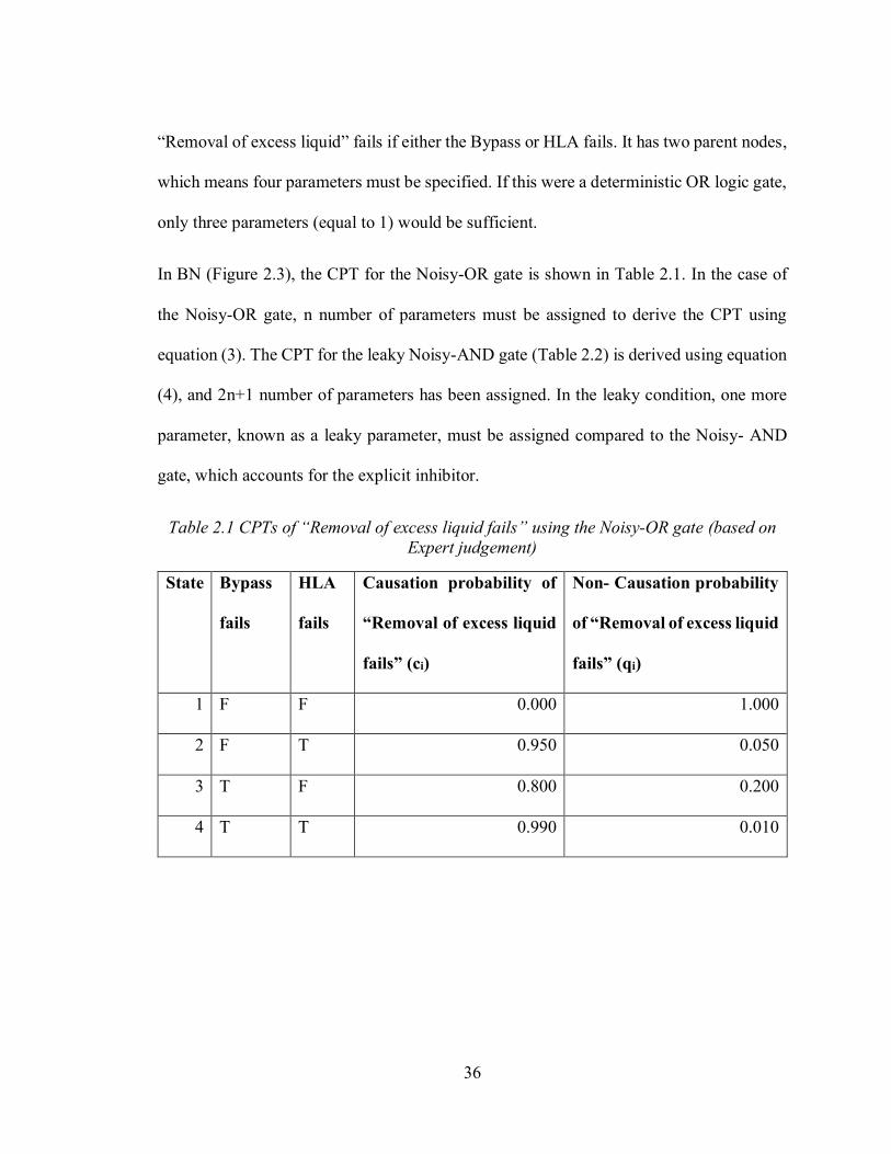
36

“Removal of excess liquid” fails if either the Bypass or HLA fails. It has two parent nodes,

which means four parameters must be specified. If this were a deterministic OR logic gate,

only three parameters (equal to 1) would be sufficient.

In BN (Figure 2.3), the CPT for the Noisy-OR gate is shown in Table 2.1. In the case of

the Noisy-OR gate, n number of parameters must be assigned to derive the CPT using

equation (3). The CPT for the leaky Noisy-AND gate (Table 2.2) is derived using equation

(4), and 2n+1 number of parameters has been assigned. In the leaky condition, one more

parameter, known as a leaky parameter, must be assigned compared to the Noisy- AND

gate, which accounts for the explicit inhibitor.

Table 2.1 CPTs of “Removal of excess liquid fails” using the Noisy-OR gate (based on Expert judgement)

State Bypass

fails

HLA

fails

Causation probability of

“Removal of excess liquid

fails” (ci)

Non- Causation probability

of “Removal of excess liquid

fails” (qi)

1 F F 0.000 1.000

2 F T 0.950 0.050

3 T F 0.800 0.200

4 T T 0.990 0.010

37

Table 2.2 Conditional probability table of “High inlet flow in the tank” using the leaky Noisy-AND gate (based on Expert judgement)

State Level

controller

fails

Pump

failure

Causation probability of

failure of “High inlet flow

in the tank” (ci)

Non- Causation

probability of “High

inlet flow in the tank”

(qi)

1 F F 0.001 0.999

2 F T 0.048 0.952

3 T F 0.018 0.982

4 T T 0.858 0.142

2.5.3 Consequence analysis

The initiating event is the abnormal event which has the potential to cause severe damage.

The liquid spill is taken to be the initiating event, which can cause more damage and losses

if the proper safety system is not employed. The liquid in the process system is a hazardous

chemical which if met with an unknown ignition source, can cause severe damage to the

process plant.

The initiating event can be propagated to an end point by considering the working and

failure of each safety barrier with the help of event tree analysis. If there is ignition, the

liquid spill can lead to the purely flammable event (i.e. pool fire); while in the case of no

ignition, a loss of liquid event is considered. It is worth noting that apart from the

38

consequences mentioned above (i.e. pool fire & near miss) another state, known as the safe

state, is generated, which accounts for the non-occurrence of the abnormal event. It is

developed by connecting the abnormal event (liquid spill) node to the consequence node.

2.5.4 Data Uncertainty reduction

The acquired input data is subject to vagueness and partial ignorance. To reduce the input

data uncertainty, the following steps are conducted according to section 2.3.2. In the

present study, an expert is one who has five to ten years’ experience in the area of Safety

and Risk Engineering and having a direct and indirect connection with process industry.

Two expert’s opinions have been taken, assuming each expert opinion is equally important.

Therefore, to consider both opinions evidence theory comes into play.

2.5.4.1 Basic probability assessment

Basic Probability Assessment (BPA), also known as belief mass, encompasses acquiring

expert opinion to define the likelihood of basic events and failure of the safety barriers.

Table 2.3 shows the BPAs assigned to each event, assuming that each source (expert

opinion) is independent.

Table 2.3 Expert opinion on the probability of events

Event Expert 1 (e1) Expert 2 (e2)

{T} {F} {T, F} {T} {F} {T, F}

Failure of HLA 0.200 0.700 0.100 0.150 0.750 0.100

Failure of Bypass 0.015 0.850 0.135 0.020 0.750 0.230

39

Failure of level controller 0.250 0.700 0.050 0.150 0.750 0.100

Failure of Pump (high flow) 0.050 0.850 0.100 0.100 0.800 0.100

Failure of ignition barrier 0.100 0.800 0.100 0.150 0.750 0.100

2.5.2 Belief Structure

The Yager combination rule allows for an aggregate multi-expert opinion from

independent sources. The Yager combination rule uses equations (8-11) to aggregate multi-

expert opinion. To derive belief and plausibility measures for the probability of basic

events, equations (5) and (6) are used, equation (7) is used to derive the point estimation

(i.e. Bet estimation). Table 2.4 shows the belief structure which consists of the belief,

plausibility and bet estimation of each root cause and safety system. Each term in belief

structure is explained as follows:

Bet (bet): In DST, the uncertainty is defined by a probability distribution defined on 2|Ω|

subset, if a decision has to be made it would be logical. Therefore, there must be a rule

which can develop a single probability distribution from the continuous probability

interval [Bel, Pl] when forced decisions have to be made. Hence, a bet is a pignistic

probability function (probability function in a decision context) that derives from the

belief function. The bet is often estimated using Generalised Insufficient Reason-

Principle. Most often it is considered as a median value between belief and plausibility

40

probability interval. Smets et al., (1991) provide a detailed explanation and the derivation

of bet estimation formula.

Table 2.4 Belief structure

Event State Yager combination rule

Bel Pl Bet

Failure of HLA {T} 0.065 0.330 0.198

{F} 0.670 0.935 0.803

Failure of Bypass valve {T} 0.006 0.066 0.036

{F} 0.934 0.994 0.964

Failure of Level controller {T} 0.070 0.368 0.219

{F} 0.633 0.930 0.781

Failure of Pump-high flow {T} 0.020 0.155 0.088

{F} 0.845 0.980 0.913

Failure of Ignition barrier {T} 0.040 0.245 0.143

{F} 0.755 0.960 0.858

2.6 Probability calculation

The deterministic approach is used to compare the result obtained from the proposed

approach. It relies on a single source for prior information which undermines the credibility

of accident modelling by illustrating a false impression of accident probability. In this

41

approach, a deterministic failure probability is assigned to each root cause and safety

barrier in the BN model rather than using evidence theory to aggregate the multi-expert

opinion to deal with input data uncertainty. The failure probabilities can be obtained by

available data for a specific process and expert opinion. The availability of crisp data for a

specific process is itself a difficult task and is one of the main sources of data uncertainty

in accident modelling. The failure probabilities are assumed to be same and are illustrated

in Table 2.1 by Expert 1(e1). Table 2.5 shows the deterministic failure probabilities of each

basic event and safety system.

Table 2.5 Deterministic failure probabilities of each root cause and safety system (using expert 1 opinion)

Event Failure probability

HLA fails 0.200

Bypass fails 0.015

Level controller fails 0.250

Pump failure-high flow 0.050

Ignition barrier fails 0.100

Table 2.6 shows the belief structure obtained by providing the belief, plausibility and bet

estimation for the basic events as well as a safety barrier. The obtained probability of a

Liquid spill (CE) and its consequences will be in terms of bel, pl and bet I respectively.

The combination rule consists of two bet estimations, namely, Bet I and Bet II, Bet I is an

estimate of a prior probability which is used directly in the BN model by providing the

42

basic events and safety barrier prior probabilities in terms of “Bet”, while Bet II is an

estimate for critical events and possible outcomes from BN with the help of belief and

plausibility obtained by BN for a liquid spill and its consequence node. For example, with

the Yager rule, Bet II for the liquid spill (CE) can be estimated as follows:

Since the cardinality of the event is two, therefore

Bel{T} = m{T} (12)

According to equation (7)

Pl {T}= m{T}+m {T, F} (13)

Substituting equations (12) & (13) into equation (7), the following equation is used to

estimate the Bet II.

𝐵𝑒𝑡 𝐼𝐼 (𝐶𝐸) = 𝐵𝑒𝑙(𝐶𝐸){𝑇}1 + {𝑃𝑙(𝐶𝐸){𝑇}−𝐵𝑙(𝐶𝐸){𝑇}}

2 (14)

Table 2.6 Probabilities of different consequences using evidence theory and a deterministic approach

Event Yager combination rule Deterministic approach

Bel Pl Bet I Bet II

Liquid spill 5.19E-03 3.54E-02 1.59E-02 2.03E-02 1.40E-02

Safe 9.95E-01 9.65E-01 9.84E-01 9.80E-01 9.86E-01

Pool fire 2.08E-04 8.66E-03 2.28E-03 4.44E-03 1.40E-03

Near miss 4.98E-03 2.67E-02 1.37E-02 1.58E-02 1.26E-02

43

In the evidence theory approach, the BPAs are assigned to define the prior probabilities of

root causes and the safety system. The incomplete and imprecise information obtained from

different sources is combined using the Yager combination rule, which provides a belief

structure in terms of belief (lower bound) and plausibility (upper bound). The Bet I show

the point estimation obtained by providing the bet obtained in Table 2.6 to all input events,

whereas Bet II shows the point estimation which can be calculated with the help of belief

and plausibility obtained from the BN model. The information about the system is based

on a subjective source, the risk estimation is subjected to imprecision if the failure

probabilities are not precise. Therefore, to overcome the issue it is desirable not to rely on

a single subjective source. As depicted in Table 2.6, the probabilities obtained using

evidence theory is continuous in nature which shows the real probability lies in the interval.

2.7 Case study

2.7.1 Accident description

To validate the proposed methodology, a gasoline release which led to a vapour cloud

ignition during offloading of gasoline at the Caribbean Petroleum Corporation (CAPECO)

facility in Bayamon, Puerto Rico on October 23, 2009 was selected. According to the report

submitted by the US. Chemical Safety Board (CSB, 2009), an aboveground storage tank

overflowed into a secondary containment dike. The gasoline converted to a fine suspension

in the air (aerosolized), forming a vapour cloud which was ignited when it met an unknown

ignition source after reaching the wastewater treatment (WWT) area, due to the opening of

a dike valve around Tank 409. This resulted in a multiple tank fire which continued for

almost 60 hours and later exploded. The accident resulted in the injury of 3 persons and

44

significant losses to the businesses up to 1.25 miles from the site, 300 neighbouring homes,

and considerable environmental degradation.

At the CAPECO refinery, tank level measurements occurred several times during filling

operations. The operator recorded the level of the tank hourly with the help of an automated

tank gauging system which included a float and a tape gauge mounted to the side of a tank.

In addition, an inspector had to check the tank level prior to starting and subsequent to the

end of filling operations by lowering the gauging tape into the tank. These multiple checks

helped them to determine the actual amount of gasoline in the tank.

According to the investigation report submitted by the Chemical Safety Board (CSB, 2009),

the only level control and the monitoring system, i.e. the automatic tank gauging system,

were out of service due to the use of an unreliable level transmitter and failure-prone float

and tape gauges system. Therefore, the level control and monitoring system failed to

provide an accurate tank level. The overfill time calculation is become the source of error,

during the gasoline unloading the variations in gasoline flow rate and pressure were not

identified and considered. Apart from these factors, another potential factor was the failure

of the internal floating roof due to fatigue, and other factors may have contributed to the

overfill.

There was no independent High-Level Alarm (HLA) and Automatic overfill protection

system. The CSB found that in addition to the lack of an independent overfill protection

system, multiple protection layers failed within the level control and monitoring system,

which further contributed to the overfill accident. According to CSB, James Reason’s

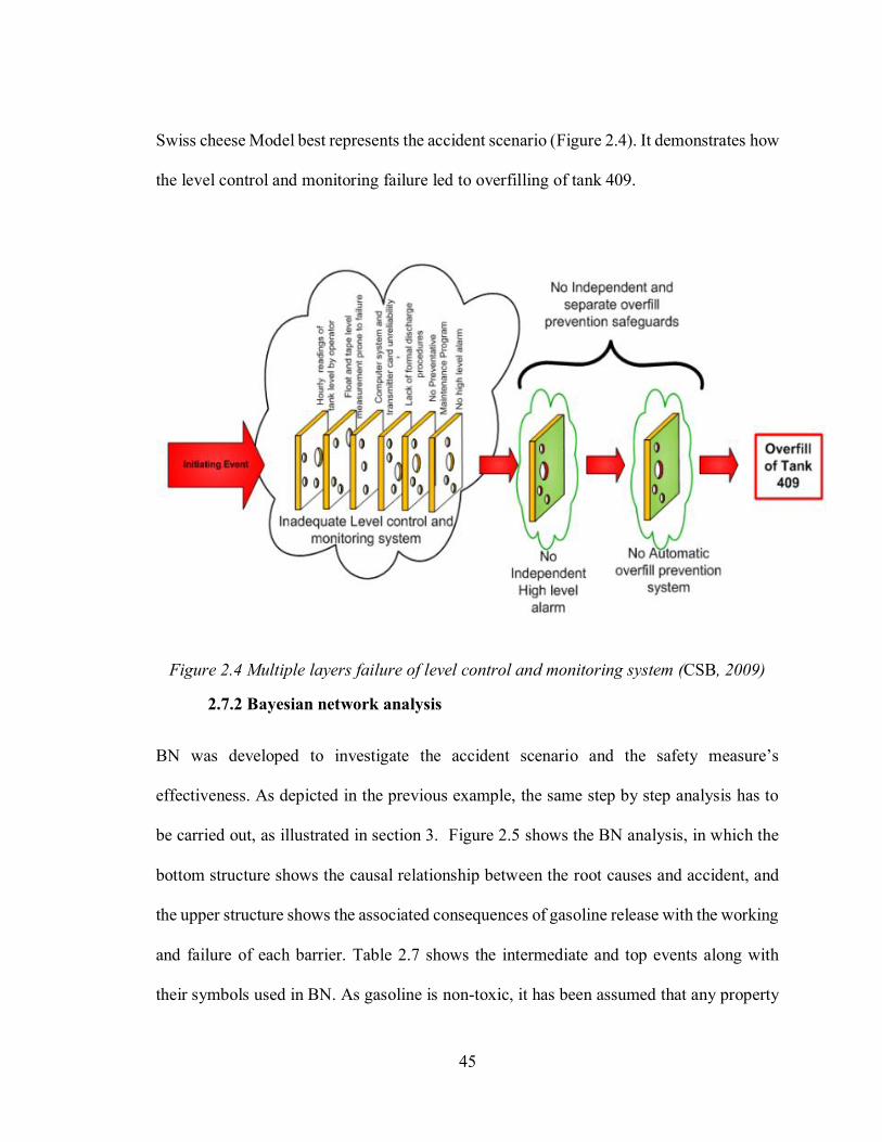
45

Swiss cheese Model best represents the accident scenario (Figure 2.4). It demonstrates how

the level control and monitoring failure led to overfilling of tank 409.

Figure 2.4 Multiple layers failure of level control and monitoring system (CSB, 2009)

2.7.2 Bayesian network analysis

BN was developed to investigate the accident scenario and the safety measure’s

effectiveness. As depicted in the previous example, the same step by step analysis has to

be carried out, as illustrated in section 3. Figure 2.5 shows the BN analysis, in which the

bottom structure shows the causal relationship between the root causes and accident, and

the upper structure shows the associated consequences of gasoline release with the working

and failure of each barrier. Table 2.7 shows the intermediate and top events along with

their symbols used in BN. As gasoline is non-toxic, it has been assumed that any property

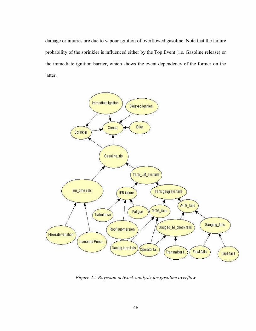
46

damage or injuries are due to vapour ignition of overflowed gasoline. Note that the failure

probability of the sprinkler is influenced either by the Top Event (i.e. Gasoline release) or

the immediate ignition barrier, which shows the event dependency of the former on the

latter.

Figure 2.5 Bayesian network analysis for gasoline overflow

47

Table 2.7 Events along with their symbols used in accident modelling

Events Symbols along with Boolean logic gates

Gauging system failure Gauging_fails (OR gate)

Gauged level checking failure Gauging_lvl check fails (AND gate)

Automatic-Tank Gauging system failure A-TG_fails (OR gate)

Manual-Tank Gauging system failure M-TG_fails (OR gate)

Internal Floating Roof failure IFR failure (OR gate)

Tank gauging system fails Tank gaug sys fails (AND gate)

Tank level measurement system fails Tank_LM_sys fails (OR gate)

Error in real time calculation in estimating

overfill time

Err_time calc

Gasoline release Gasoline_rls (AND gate)

Safe evacuation from the facility C1

Vapour cloud near tank 409 C2

Fire+ explosion, less damage in the facility C3

Pool fire C4

Gasoline Spill C5

Vapour cloud near the ground in the

neighbouring area of the facility

C6

48

Pool fire + explosion, moderate damage, fewer

fatalities or injuries

C7

Pool fire, moderate damage C8

Table 2.10 in the appendix depicts the BPAs assigned in modelling the CAPECO refinery

accident. Table 2.11 (appendix) shows the combined belief structure for the likelihood of

input data as shown in the previous example.

A deterministic failure probability is assigned to each root cause and safety barrier as

illustrated in the previous example. The failure probabilities are assumed to be the same

and are illustrated in Table 2.10 by Expert 1(e1). Table 2.12 (appendix) shows the

deterministic failure probabilities of each basic event and the safety system.

To implement the canonical probabilistic model in BN, expert opinion is considered. The

Noisy-OR and leaky Noisy-AND gates can accommodate various interactions between

child and parent nodes which traditional logic gates such as OR (AND) gates are unable to

do. It is worth noting that the Boolean logic gates (OR & AND gates) are replaced with

Noisy-OR and leaky Noisy-AND gates in BN to reflect the accident scenario better. These

two provide the median condition for their respective logic gates which, therefore, helps in

further reduction of uncertainty in accident modelling. The Noisy-OR and the leaky Noisy-

AND logic gates help to model every possible behaviour between the cause and its effect

to establish the practical scenario much more accurately compared with traditional OR and

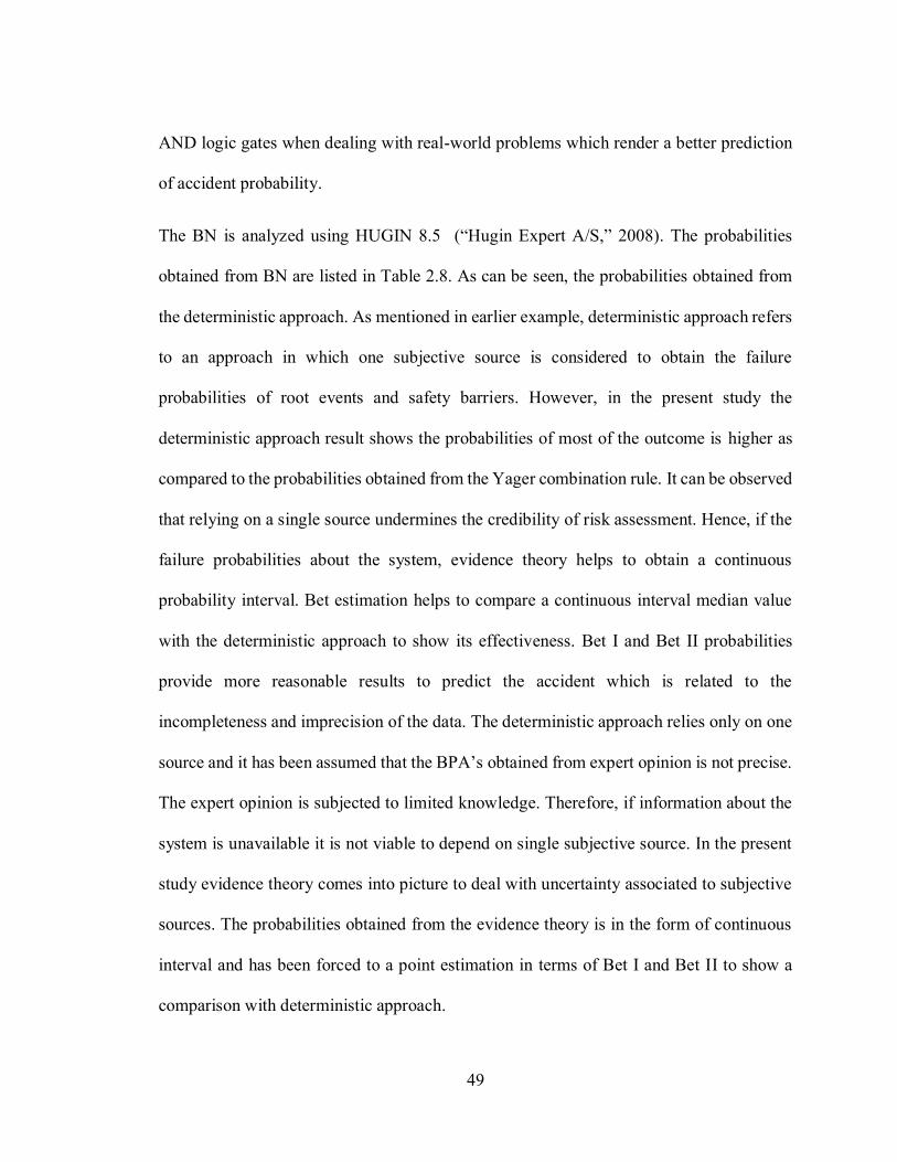
49

AND logic gates when dealing with real-world problems which render a better prediction

of accident probability.

The BN is analyzed using HUGIN 8.5 (“Hugin Expert A/S,” 2008). The probabilities

obtained from BN are listed in Table 2.8. As can be seen, the probabilities obtained from

the deterministic approach. As mentioned in earlier example, deterministic approach refers

to an approach in which one subjective source is considered to obtain the failure

probabilities of root events and safety barriers. However, in the present study the

deterministic approach result shows the probabilities of most of the outcome is higher as

compared to the probabilities obtained from the Yager combination rule. It can be observed

that relying on a single source undermines the credibility of risk assessment. Hence, if the

failure probabilities about the system, evidence theory helps to obtain a continuous

probability interval. Bet estimation helps to compare a continuous interval median value

with the deterministic approach to show its effectiveness. Bet I and Bet II probabilities

provide more reasonable results to predict the accident which is related to the

incompleteness and imprecision of the data. The deterministic approach relies only on one

source and it has been assumed that the BPA’s obtained from expert opinion is not precise.

The expert opinion is subjected to limited knowledge. Therefore, if information about the

system is unavailable it is not viable to depend on single subjective source. In the present

study evidence theory comes into picture to deal with uncertainty associated to subjective

sources. The probabilities obtained from the evidence theory is in the form of continuous

interval and has been forced to a point estimation in terms of Bet I and Bet II to show a

comparison with deterministic approach.

50

Table 2.8 Results obtained from accident analysis using BN

Event’s Yager combination rule Deterministic approach

Bel Pl Bet I Bet II

CE 8.97E-03 7.38E-02 2.79E-02 4.14E-02 1.08E-02

Safe 9.91E-01 9.26E-01 9.72E-01 9.59E-01 9.89E-01

C1 8.48E-03 4.88E-02 2.20E-02 2.86E-02 9.30E-03

C2 1.42E-04 3.99E-03 1.34E-03 2.06E-03 1.74E-04

C3 1.91E-05 3.68E-03 5.47E-04 1.85E-03 1.16E-04

C4 1.40E-04 4.50E-03 1.13E-03 2.32E-03 9.69E-05

C5 1.55E-02 1.03E-02 2.53E-03 1.29E-02 1.09E-03

C6 3.14E-06 8.40E-04 1.54E-04 4.21E-04 2.05E-05

C7 3.49E-07 7.75E-04 6.29E-05 3.88E-04 1.37E-05

C8 2.56E-06 9.50E-04 1.30E-04 4.76E-04 1.14E-05

2.7.3 Probability updating

Another advantage of BN is probability updating given new observations. Through

probability adapting, the conditional and marginal probability can be updated using

Accident Sequence Precursor (ASP) data. ASP is information accumulated over time,

which can be used to revise the probabilities of an accident. It can be in the form of a

number of observations of near misses, mishaps, and incidents or root events occurring

during operation of the facility.

51

The US Chemical Safety Board (CSB, 2009), found that multiple overfills and spills occur

during the operations. According to records, a total of 15 incidents occurred from 1992 to

1999 among them, 8 were overfills, and 7 were spills and three incidents after 2005 have

been reported, but the events are not clearly stated, it is assumed that these three incidents

are overfilling and spills from 2006 to 2008. These recorded observations (Table 2.9) are

considered in our BN model to predict the probability of Gasoline release and consequence

C7.

Table 2.9 ASP data recorded during plant operation

Consequences Year

1992

Year

1994

Year

1996

Year

1998

Year

2000

Year

2002

Year

2004

Year

2006

Year

2008

C1 2 2 2 2 - - - 2 -

C5 2 2 2 1 - - - - 1

0

0.1

0.2

0.3

0.4

0.5

0.6

0.7

1990 1992 1994 1996 1998 2000 2002 2004 2006 2008Occ

urre

nce

prob

abili

ty

Year

Gasoline_rls

Deterministic Bet I Bet II

52

Figure 2.6 Dynamic probability changes of the Gasoline release

The updated probability of “Gasoline release” and consequence C7 are obtained with the

help of backward inference that can be performed with the help of Bayes’ theorem. Figure

2.6 shows the dynamic probability of gasoline release. Deterministic plot shows the

posterior probability obtained from a deterministic approach, which relies on a single

source for prior information about the system. However, Bet I show the posterior

probabilities obtained when prior information is given in terms of Bet, whereas Bet II is

calculated from the belief and plausibility obtained from the network. The year 1990

denotes the prior probability of the event and the years 1992 to 2008 show the posterior

probabilities obtained from probability updating at the end of each year. It is worth noting

that the posterior probability obtained in the form of Bet I and Bet II are converging, which

provides a robust belief structure. On the other hand, the deterministic approach shows

slightly higher probability. This can be explained by the prior probabilities being given to

the root causes and safety barriers obtained from the knowledge of expert 1, which is on

the higher side compared to the probabilities obtained from the Yager combination rule,

which combines both the experts knowledge. Therefore, the deterministic approach

provides a false impression of risk analysis due to the vagueness of the data.

With the help of probability adapting, one can also predict the probability of those

consequences for which no information is given. Consequence C7 occurred 2009, resulting

in crucial property damage, environmental damage and injuries of persons. Figure 2.7

illustrates that during eighteen years of operation, the occurrence probability increases by

three orders of magnitude in the cases of Bet I and Bet II, whereas a deterministic approach

53

does not provide promising results due to the lack of certainty from relying on a single

source. This shows the safety measures of the plant were not adequate, which led to the

occurrence of C7 in 2009. This accident could have been prevented if proper safety

measures had been taken.

Figure 2.7 Dynamic probability updating of consequence C7

2.8 Conclusions

The current study proposed a BN-based probabilistic model to reduce uncertainty in

dynamic risk analysis. Evidence theory has been used to address the uncertainty arising

due to vagueness and partial ignorance of the acquired prior probabilities of basic events

and safety barriers. Another source of uncertainty (model uncertainty) is addressed by the

application of the proper logic gates (e.g., Noisy-OR and leaky Noisy-AND) which are

able to make the variables conditional on every possible behaviour of the parent node. The

effectiveness of the approach is validated through an application to the CAPECO refinery

0.00E+00

5.00E-04

1.00E-03

1.50E-03

2.00E-03

2.50E-03

1990 1992 1994 1996 1998 2000 2002 2004 2006 2008

Occ

urre

nce

prob

abili

ty

Year

Consequence (C7)

Deterministic Bet I Bet II

54

accident. The proposed method provides robust results by aggregating multi-expert

opinions for determining prior probabilities, compared to a deterministic approach.

Proposed methodology helps in improving the prediction of an accident probability which

helps in reducing catastrophic events like CAPECO refinery accident to happen in future.

2.9 Appendix

Table 2.10 Expert opinion on the probability of events

Event Expert 1 (e1) Expert 2 (e2)

{T} {F} {T, F} {T} {F} {T, F}

Failure of Tape 0.120 0.70 0.180 0.200 0.75 0.050

Failure of Float 0.220 0.68 0.100 0.100

0.88 0.020

Failure of Operator 0.100 0.80 0.100 0.001 0.95 0.049

Failure of Transmitter 0.200 0.75 0.050 0.050 0.80 0.190

Failure of Gauging tape 0.040 0.70 0.250 0.080 0.90 0.020

Fatigue 0.020 0.85 0.130 0.100 0.60 0.300

Turbulence 0.100 0.80 0.100 0.100 0.80 0.100

Roof submersion 0.100 0.70 0.200 0.200 0.75 0.050

Flow rate variation 0.020 0.85 0.130 0.100 0.60 0.300

Increased pressure 0.002 0.88 0.118 0.010 0.95 0.040

Containment dike 0.100 0.80 0.100 0.080 0.90 0.020

Water sprinkler 0.030 0.80 0.170 0.100 0.85 0.050

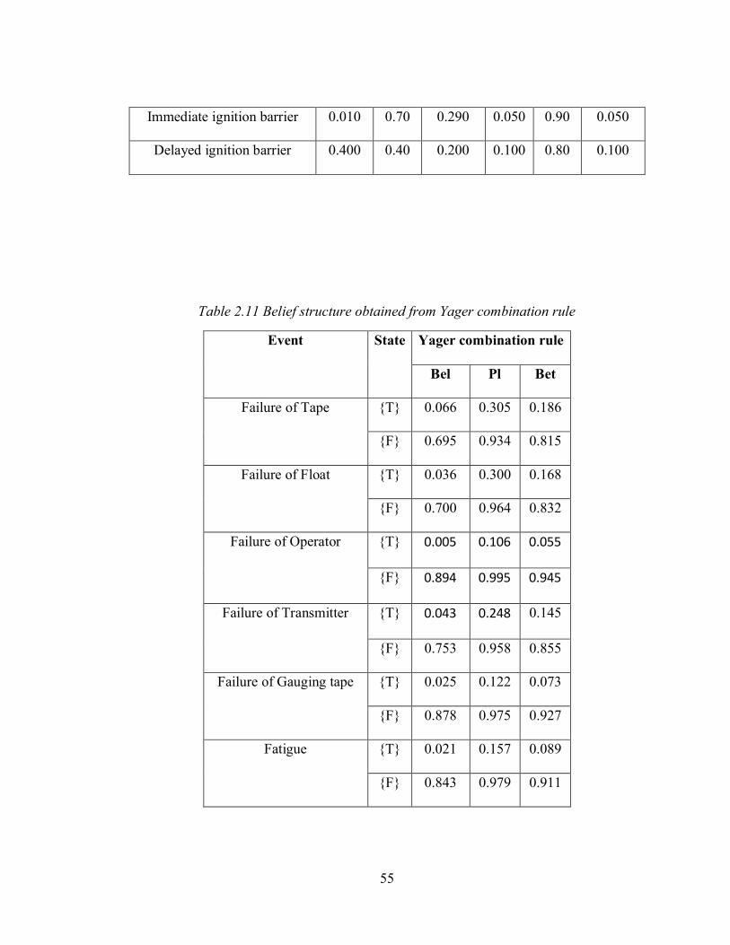
55

Immediate ignition barrier 0.010 0.70 0.290 0.050 0.90 0.050

Delayed ignition barrier 0.400 0.40 0.200 0.100 0.80 0.100

Table 2.11 Belief structure obtained from Yager combination rule

Event State Yager combination rule

Bel Pl Bet

Failure of Tape {T} 0.066 0.305 0.186

{F} 0.695 0.934 0.815

Failure of Float {T} 0.036 0.300 0.168

{F} 0.700 0.964 0.832

Failure of Operator {T} 0.005 0.106 0.055

{F} 0.894 0.995 0.945

Failure of Transmitter {T} 0.043 0.248 0.145

{F} 0.753 0.958 0.855

Failure of Gauging tape {T} 0.025 0.122 0.073

{F} 0.878 0.975 0.927

Fatigue {T} 0.021 0.157 0.089

{F} 0.843 0.979 0.911

56

Turbulence {T} 0.03 0.200 0.115

{F} 0.800 0.970 0.885

Roof submersion {T} 0.0655 0.290 0.178

{F} 0.710 0.935 0.823

Flow rate variation {T} 0.021 0.157 0.089

{F} 0.843 0.979 0.911

Increased pressure {T} 0.001 0.017 0.009

{F} 0.983 0.999 0.991

Containment dike {T} 0.018 0.174 0.096

{F} 0.826 0.982 0.904

Water sprinkler {T} 0.022 0.136 0.079

{F} 0.865 0.979 0.922

Immediate ignition barrier {T} 0.016 0.074 0.045

{F} 0.926 0.985 0.955

Delayed ignition barrier {T} 0.100 0.480 0.290

{F} 0.520 0.900 0.710

Table 2.12 Prior probabilities of deterministic approach obtained by expert 1

No. Event Prior probability

R1 Failure of Tape 0.120

R2 Failure of Float 0.220

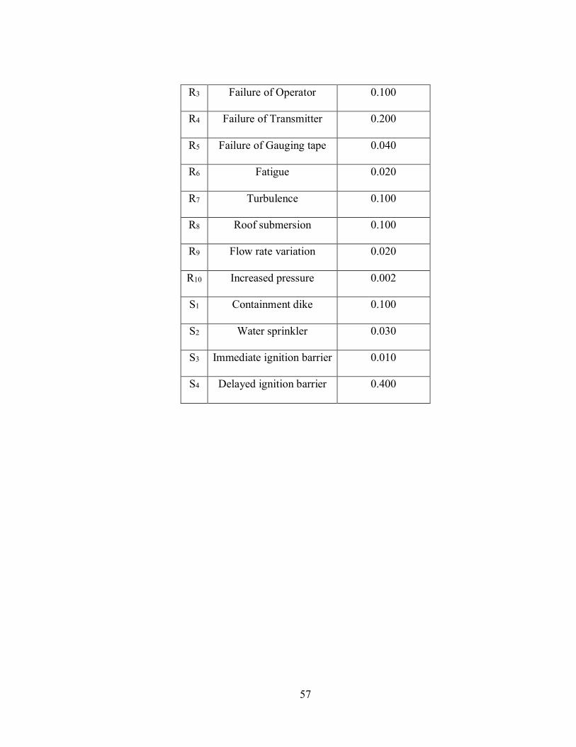
57

R3 Failure of Operator 0.100

R4 Failure of Transmitter 0.200

R5 Failure of Gauging tape 0.040

R6 Fatigue 0.020

R7 Turbulence 0.100

R8 Roof submersion 0.100

R9 Flow rate variation 0.020

R10 Increased pressure 0.002

S1 Containment dike 0.100

S2 Water sprinkler 0.030

S3 Immediate ignition barrier 0.010

S4 Delayed ignition barrier 0.400

58

2.10 References

Abimbola, M., Khan, F., Khakzad, N., & Butt, S. (2015). Safety And Risk Analysis Of Managed

Pressure Drilling Operation Using Bayesian Network. Safety Science, 76, 133–144.

https://doi.org/10.1016/j.ssci.2015.01.010

Abrahamsson, M. (2002). Uncertainty In Quantitative Risk Analysis-Characterisation And

Methods Of Treatment. Lutvdg/Tvbb--1024--Se, 88. Retrieved from

http://lup.lub.lu.se/record/642153

Adedigba, S. A., Khan, F., & Yang, M. (2016). Dynamic Safety Analysis Of Process Systems

Using Nonlinear And Non-Sequential Accident Model. Chemical Engineering Research and

Design, 111, 169–183. https://doi.org/10.1016/j.cherd.2016.04.013

Al-shanini, A., Ahmad, A., & Khan, F. (2014). Accident Modelling And Analysis In Process

Industries. Journal of Loss Prevention in the Process Industries.

https://doi.org/10.1016/j.jlp.2014.09.016

Ayyub, B. M., & Klir, G. J. (2006). Uncertainty Modeling And Analysis In Engineering And The

Sciences. Chapman and Hall/CRC. https://doi.org/10.1201/9781420011456

Badreddine, A., & Ben Amor, N. (2010). A Dynamic Barriers Implementation In Bayesian-Based

Bow Tie Diagrams For Risk Analysis. In 2010 ACS/IEEE International Conference on Computer

Systems and Applications, AICCSA 2010. https://doi.org/10.1109/AICCSA.2010.5587003

Bae, H.-R., Grandhi, R. V., & Canfield, R. A. (2004). An Approximation Approach For

Uncertainty Quantification Using Evidence Theory. Reliability Engineering & System Safety,

86(3), 215–225. https://doi.org/10.1016/j.ress.2004.01.011

59

Bobbio, A., Portinale, L., Minichino, M., & Ciancamerla, E. (2001). Improving The Analysis Of

Dependable Systems By Mapping Fault Trees Into Bayesian Networks. Reliability Engineering

and System Safety, 71(3), 249–260. https://doi.org/10.1016/S0951-8320(00)00077-6

Cheng, Y. (2000). Uncertainties In Fault Tree Analysis. Journal of Applied Science and

Engineering, 3(1), 23–29.

CSB. (2009). Carribbean Petroleum Tank Terminal Explosion And Multiple Tank, Bayamon,

Puerto Rico. Retrieved from

http://www.csb.gov/assets/1/19/CAPECO_Final_Report__10.21.2015.pdf

Diez, F. J., & Druzdzel, M. J. (2007). Canonical Probabilistic Models For Knowledge Engineering.

Information Sciences, 9, 1–59. https://doi.org/www.ia.uned.es/~fjdiez/papers/canonical.pdf

Druschel, B. R., Ozbek, M., & Pinder, G. F. (n.d.). Application Of Dempster-Shafer Theory To

Hydraulic Conductivity, 1–8.

Ferdous, R., Khan, F., Sadiq, R., Amyotte, P., & Veitch, B. (2009). Handling Data Uncertainties

In Event Tree Analysis. Process Safety and Environmental Protection, 87(5), 283–292.

https://doi.org/10.1016/j.psep.2009.07.003

Ferdous, R., Khan, F., Sadiq, R., Amyotte, P., & Veitch, B. (2011). Fault And Event Tree Analyses

For Process Systems Risk Analysis: Uncertainty Handling Formulations. Risk Analysis, 31(1), 86–

107. https://doi.org/10.1111/j.1539-6924.2010.01475.x

Ferdous, R., Khan, F., Sadiq, R., Amyotte, P., & Veitch, B. (2013). Analyzing System Safety And

Risks Under Uncertainty Using A Bow-Tie Diagram: An Innovative Approach. Process Safety

and Environmental Protection, 91(1–2), 1–18. https://doi.org/10.1016/j.psep.2011.08.010

60

Heckerman, D., & Breese, J. S. (1996). Causal Independence For Probability Assessment And

Inference Using Bayesian Networks. IEEE Transactions on Systems, Man, and Cybernetics Part

A:Systems and Humans., 26(6), 826–831. https://doi.org/10.1109/3468.541341

Heckerman, D., Mamdani, A., & Wellman, M. P. (1995). Real-World Applications Of Bayesian

Networks. Communications of the ACM, 38(3), 24–26. https://doi.org/10.1145/203330.203334

Hugin Expert A/S. (2008). Hugin researcher API, Denmark. Retrieved from www.hugin.com

Kalantarnia, M., Khan, F., & Hawboldt, K. (2009). Dynamic Risk Assessment Using Failure

Assessment And Bayesian Theory. Journal of Loss Prevention in the Process Industries, 22(5),

600–606. https://doi.org/10.1016/j.jlp.2009.04.006

Khakzad, N., Khan, F., & Amyotte, P. (2013). Dynamic Safety Analysis Of Process Systems By

Mapping Bow-Tie Into Bayesian Network. Process Safety and Environmental Protection, 91(1–

2), 46–53. https://doi.org/10.1016/j.psep.2012.01.005

Khan, F. I. (2001). Use Maximum-Credible Accident Scenarios For Realistic And Reliable Risk

Assessment. Chemical Engineering Progress, 97(11), 56–64.

Khan, F. I., & Abbasi, S. A. (1998). Models For Domino Effect Analysis In Chemical Process

Industries. Process Safety Progress, 17(2), 107–123. https://doi.org/10.1002/prs.680170207

Lefevre, E., Colot, O., & Vannoorenberghe, P. (2002). Belief Function Combination And Conflict

Management. Information Fusion, 3(2), 149–162. https://doi.org/10.1016/S1566-2535(02)00053-

2

Markowski, A. S., Mannan, M. S., & Bigoszewska, A. (2009). Fuzzy Logic For Process Safety

Analysis. Journal of Loss Prevention in the Process Industries, 22(6), 695–702.

61

https://doi.org/10.1016/j.jlp.2008.11.011

Marsh, D. W. R., Bearfield, G., & Marsh, W. (2008). Generalizing Event Trees Using Bayesian

Networks. Proceedings of the Institution of Mechanical Engineers, Part O: Journal of Risk and

Reliability, 222(2), 105–114. https://doi.org/10.1243/1748006XJRR131

Neapolitan, R. (1990). Probabilitsic Reasoning In Expert Systems. New York: Wiley.

Nielsen, T. D., & Jensen, F. V. (2009). Bayesian Network And Decision Graph. Springer Science

& Business Media. https://doi.org/10.1007/978-0-387-68282-2

Pearl, J. (1988). Probabilistic Reasoning In Intelligent Systems. Morgan Kauffmann San Mateo.

https://doi.org/10.2307/2026705

Qureshi, Z. H. (2008). A Review Of Accident Modelling Approaches For Complex Critical

Sociotechnical Systems. 12th Australian Workshop on Safety Related Programmable Systems

(SCS’07), Adelaide, 86, 47–59.

Rosqvist, T. (2003). On The Use Of Expert Judgement In The Qualification Of Risk Assessment.

VTT Publications.

Sentz, K., & Ferson, S. (2002). Combination Of Evidence In Dempster- Shafer Theory. Contract,

(April), 96. https://doi.org/10.1.1.122.7929

Smets, P., Hsia, Y. T., Saffiotti, A., Kennes, R., Xu, H., & Umkehrer, E. (1991). The Transferable

Belief Model. In Lecture Notes in Computer Science (including subseries Lecture Notes in

Artificial Intelligence and Lecture Notes in Bioinformatics). https://doi.org/10.1007/3-540-54659-

6_72

Stewart, R. T., & Quintana, I. O. (2018). Probabilistic Opinion Pooling With Imprecise

62

Probabilities. Journal of Philosophical Logic. https://doi.org/10.1007/s10992-016-9415-9

Tan, Q., Chen, G., Zhang, L., Fu, J., & Li, Z. (2014). Dynamic Accident Modeling For High-Sulfur

Natural Gas Gathering Station. Process Safety and Environmental Protection, 92(6), 565–576.

https://doi.org/10.1016/j.psep.2013.03.004

Thacker, B. H., & Huyse, L. J. (2007). Probabilistic Assessment On The Basis Of Interval Data.

In Structural Engineering and Mechanics (Vol. 25, pp. 331–345).

Vesely, W. E., Goldberg, F. F., Roberts, N. H., & Haasl, D. F. (1981). Fault Tree Handbook.

System and Reliability Research, Office of Nuclear Regulatory Research, U.S. Nuclear Regulatory

Commission. https://doi.org/NUREG–0492

Wilcox, R. C., & Ayyub, B. M. (2003). Uncertainty Modeling Of Data And Uncertainty

Propagation For Risk Studies. In the Proceedings of the Fourth International Symposium on

Uncertainty Modeling and Analysis, 0–7.

Yuan, Z., Khakzad, N., Khan, F., & Amyotte, P. (2015). Risk Analysis Of Dust Explosion

Scenarios Using Bayesian Networks. Risk Analysis, 35(2), 278–291.

https://doi.org/10.1111/risa.12283

Zadeh, L. A. (1984). Review Of A Mathematical Theory Of Evidence. AI Magazine, 5(3), 81.

https://doi.org/10.1609/aimag.v5i3.452

63

3 Dynamic Risk Analysis of Domino Effect Using GSPN

Preface

A version of this manuscript has been submitted to Journal of Process Safety and Environmental

Protection. I am the primary author of this manuscript along with Co-authors Faisal Khan, Salim

Ahmed and Mohammed Taleb-Berrouane. I developed the proposed model and its application

using a case study along with the analysis of the result. I prepared the first draft of the proposed

framework and revised it based on the co-author's feedback. The co-author Faisal Khan provided

foundational understating of the research problem, assisted in developing relevant model, provided

constructive feedback to improve the application of the model and also assisted in reviewing the

manuscript. The co-author Salim Ahmed helped in reviewing the proposed model, improving the

presentation of the proposed model application and finalizing the manuscript. The co-author

Mohammed Taleb-Berrouane help in developing the model and testing the application of the

model.

Abstract

The domino effect accidents in process industries poses a severe threat to human life and the

environment and has the potential to affect nearby facilities as well. Numerous techniques, such

as the Bayesian network, have been used for modelling the domino effect. However, these

techniques have inherent limitations. These include the ability to consider complex behaviour of

process equipment in combined loading and the time dependency of equipment failure. In the

current study, a Generalised Stochastic Petri-net model is developed to assess domino effect which

is referred as DOMINO-GSPN model. This model is proposed to model domino effect accident

likelihood and propagation pattern. The proposed model is capable of modelling time-dependent

64

failure behaviour of the process component in combined loading. The results of the model assist

in monitoring process risk. A case study is used to demonstrate the application and effectiveness

of the model. The results from the model are compared with the past study of a Bayesian network-

based domino effect model. This comparative analysis highlights the unique feature of the model

and its relevance as a domino effect risk assessment and management tool.

Keywords: Domino effect; Stochastic Petri nets; Risk analysis; Hazardous materials; Process

safety.

3.1 Introduction

Accidents occurring in chemical and process industries are often more worrisome than for any

other industry due to handling, storage, or processing of hazardous substances under potentially

dangerous operating conditions (Khakzad, 2015; Cozzani and Salzano, 2004). The word “domino”

is well described in the literature by Khan and Abbasi, (2001); it is derived from the domino

toppling game. Many dominos are arranged in a line adjacent to one another. If one falls, it hits

the next domino, triggering a series of collapsing dominoes. Simply, the domino effect can be

defined as one thing unleashing the next thing and so on. Authors use many definitions of domino

effects in the literature. Reniers (2010) and Abdolhamidzadeh, Abbasi, Rashtchian and Abbasi,

(2011) provided a list of those definitions, and most authors agreed that:

• A primary event (accident) is responsible for initiating the domino effect.

• Escalation vectors/physical effects (such as overpressure, heat flux, the impact of blast

wave/missile) are responsible for the propagation of a first accident to secondary or higher

order accidents based on the intensity of escalation vectors.

• The consequences of the domino effect are more severe in comparison to the primary

accident.

65

In a domino effect, a primary unit acts as an initiating event, which triggers the involvement of the

secondary unit by escalation vectors/ physical effects (Cozzani et al., 2006). The risk associated

with such an event is of utmost importance because the severity of such accidents increases

exponentially and the consequences of such an event is more severe in comparison to the primary

accident (Kourniotis, Kiranoudis and Markatos, 2000).

Significant research has been done on accident modelling of a single unit in past years, but limited

research has been carried out in the context of domino accident modelling, due to their high

complexity and low frequency (Khakzad, Khan, Amyotte and Cozzani, 2013). Since 1947, the

domino effect has been documented in literature (Kadri, Chatelet and Lallement, 2013), but it

gained more attention after the most severe LPG disaster in Mexico City in 1984. LPG leakage

occurred, which resulted in a vapour cloud explosion leading to several other explosions (Li,

Reniers, Cozzani and Khan, 2017). Another violent domino accident occurred in the BP Texas

City refinery in 2005, where a vapour cloud formed and ignite, followed by several explosions

(Khakzad, Khan, Amyotte, et al., 2013). Abdolhamidzadeh, Abbasi, Rashtchian and Abbasi (2010)

studied domino effect accidents occurring from 1917 to 2009. Two hundred and twenty-four

accidents have been reported, mostly occurring in process plants, followed by transportation

accidents. These accidents increased the demand for risk and safety analysis of the domino effect

in process facilities.

Early studies on the domino effect focused on determining escalation probability (i.e., damage

probability), using models based on distance (Bagster and Pitblado, 1991) and a combination of a

probit model along with threshold limits (Khan and Abbasi, 1998; Cozzani et al., 2006). However,

other studies used statistical surveys, which help in understanding accident sequences along with

frequency estimations (Darbra, Palacios and Casal, 2010; Vílchez, Sevilla, Montiel and Casal,

66

1995; Kourniotis et al., 2000). Additionally, some work has been done in quantitative risk

assessment (QRA) on domino accident modelling and propagation (Khan and Abbasi, 1998a;

Cozzani, Gubinelli, Antonioni, Spadoni and Zanelli, 2005; Antonioni, Spadoni and Cozzani, 2009;

Abdolhamidzadeh et al., 2010; Reniers, Dullaert, Ale and Soudan, 2005; Reniers and Dullaert,

2007).

A novel approach has been introduced in the article to model and assesses the domino effect

likelihood based on Petri-nets. The Petri-net is a mathematical modelling tool developed by Carl

Adam Petri in 1962. It is a promising tool to model concurrent, asynchronous, distributed, parallel

non-deterministic and/or stochastic systems (Murata, 1989). Petri-nets consist of two types of

elements, called places and transitions. Places represent states or conditions, whereas transitions

show the events. Arcs connecting places and transitions are either from places to transitions (input

arcs) or transitions to places (output arcs). In addition, the dynamic nature of the system is

demonstrated by the movement of tokens from one place to another. The position of a token

indicates the availability of resources at that particular place.

Section 3.2 of the thesis gives a brief description of GSPN, followed by proposed DOMINO-GSPN

model in section 3.3. Section 3.4 is devoted to domino accident modelling, using GSPN for

determining the propagation path and probability estimation. A hypothetical case study is used in

section 3.5 to show the efficacy of the proposed methodology. The conclusion obtained from the

study is presented in section 3.6.

3.2 PN model concepts

The Petri-net (PN) was first introduced in Carl Adam Petri’s dissertation in 1962 (David and Alia,

2010). It consists of places which are circular, transitions (rectangular bars), directed arcs

connecting input places to transitions and vice versa and tokens (black bullets). The places show

67

the state or condition of a system; the presence of a token shows the resource availability at that

place. The transition depicts the change in state from input to output place, and the PN can also

model the component dependency. Note that the token can only reside in places, not at transitions.

However, the direction of the flow of tokens is governed by the directed arcs. Each arc has a

multiplicity (weight), which depicts the token migration capacity of the arc. The transition firing

can only take place if the input place has at least an equal number of tokens as the arc multiplicity.

There are many extensions to PNs, such as timed, coloured Petri-nets that add properties which

cannot be modelled with the original PN. PNs are widely used in many fields, including process

industries (Angeli, De Leenheer and Sontag, 2007; Grunt and Briš, 2015; Wu, Chu, Chu and Zhou,

2010).

Murata, (1989), provided the definition of Petri-net as a quintuple:

𝑃𝑁 = (𝑃𝑖, 𝑇𝑗, 𝐼𝑀, 𝑂𝑀, 𝐼)

𝑃𝑖 = 𝑃𝑖=1, 𝑃𝑖=2, … , 𝑃𝑖=𝑘

𝑇𝑗 = 𝑇𝑗=1, 𝑇𝑗=2, … , 𝑇𝑗=𝑙

A Stochastic Petri-net (SPN) is defined as a sixtuple (Talebberrouane, Khan and Lounis, 2016):

𝑆𝑃𝑁 = (𝑃𝑥, 𝑇𝑦, 𝐼𝑀, 𝑂𝑀, 𝐼, 𝐹)

𝑃𝑥 = 𝑃𝑥=1, 𝑃𝑥=2, … , 𝑃𝑥=𝑘

𝑇𝑦 = 𝑇𝑦=1, 𝑇𝑦=2, … , 𝑇𝑦=𝑙

68

𝐼𝑀 = 𝑃𝑥 ∗ 𝑇𝑦 →(0,1) is an input matrix showing the input directed arcs from places to transitions.

𝑂𝑀 = 𝑃𝑥 ∗ 𝑇𝑦 →(0,1) is an output matrix showing the output directed arcs from transitions to

places.

𝐼: 𝑃𝑥 → 𝑁 is the initial marking of places for which the nth component shows the nth number of

black bullet (token) in the nth circle (place).

𝐹: 𝑇𝑦 → 𝐹𝑅+ is a firing rate or which the nth component represents the firing rate of nth transition.

In SPN if a transition is fired, the token wait until the firing delay (which helps to stop the token),

once the firing delay ends the migration of tokens take place from initial to final place, and the

number of tokens migrating depends upon the input and output functions (Zhou, DiCesare and

Guo, 1990). Note that the tokens always reside in places, not in transitions. Transitions are the

conditions which allow them to go from one place to another. Further, the multiplicity of directed

arcs must be at least equal to or more than the number of available tokens at the input place to fire

the transition. This defines the token delivery capacity of the arc either from place to transition or

vice versa.

Later, SPN was extended to incorporate the GSPN. All SPN features remain the same, with two

new features added, namely, immediate transition firing (without any time delay) and inhibitor

arcs (used to disable the transition when a token is present in input places). GSPN with predicates

and assertions have been used in the present study. The predicates or guards are mathematical

formulae used to allow the conditional transitions while assignments are mathematical variables

used to update the information if the firing occurs through the transition (such as true or false and

incrementation). Further, these variables’ behaviours can be used as a GSPN outcome, which can

be instantaneous, a time interval average or the firing frequency (Talebberrouane et al., 2016). In

69

PN each state is mapped based on Markov process. The firing of token (firing rate λ) corresponds

to a Markov state transition with probability λ. However, In SP what is stochastic is the firing rate

of token from the input place to the output place which is governed by probability distribution at

each transition with firing delays.

3.3 The Proposed DOMINO-GSPN Model

The safety system is a crucial part of industrial processes, which aims to avoid severe conditions

further developing into an abnormal situation. Failure of such a system can directly/indirectly

affect nearby equipment, causing unexpected process deviations, unexpected work stoppage and

threatening the environment. To assess the likelihood of such accidents, steps 1-11 describe the

DOMINO-GSPN model. Steps 1-5 are based on the work of Cozzani et al., (2005); and Khakzad

et al., (2013), whereas steps 6-9 are based on the development of GSPN to model the domino

effect. Each step briefly explains the formulation of the PN structure. Figure 3.1 illustrates the

development of DOMINO-GSPN to model domino effect accidents.

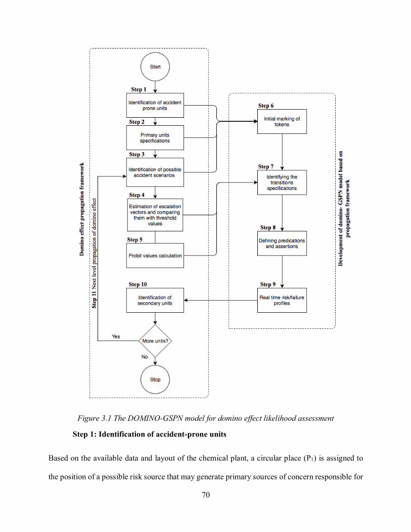
70

Figure 3.1 The DOMINO-GSPN model for domino effect likelihood assessment

Step 1: Identification of accident-prone units

Based on the available data and layout of the chemical plant, a circular place (P1) is assigned to

the position of a possible risk source that may generate primary sources of concern responsible for

71

the domino effect. The selected units either propagate a cascading effect or are likely to cause an

accident, that may include chemical reactors, distillation columns, or atmospheric/ pressurized

tanks (Khakzad et al., 2013).

Step 2: Primary units’ specifications

Using risk assessment approaches such as HAZOP (hazard and operability study) or FMEA

(failure modes and effect analysis), the event that is likely to trigger the cascading effect can be

determined. A large amount of hazardous inventory that is capable of producing credible escalation

vectors along with a high occurrence probability are important to consider when choosing primary

events (Khakzad et al., 2013). Cozzani et al. (2005) have identified two major causes to be

considered in this step: low-severity initiating event propagation and major accidental event’s

interactions. The former analysis should consider low severity events neglected in the safety

analysis of a plant, such as a minor pool fire or jet fire, which may lead to accident propagation,

whereas the latter analysis is used when there is a widespread damage from secondary or higher

order events, and only if those events are major accidents.

Step 3: Identification of accident scenarios

This step identifies the escalation vectors associated with each scenario. For instance, a mechanical

explosion escalation is triggered by a blast wave or fragment projection (Cozzani et al., 2005).

Therefore, it is essential to know all escalation vectors associated with a particular scenario.

Step 4: Estimation of escalation vectors and comparison with threshold values

Once the primary event is identified, each scenario escalation vector transmitted to nearby units

must be evaluated. Escalation vector’s quantification, such as explosion overpressure and heat

radiation calculations, can be found in Assael MJ (2010). Based on predefined threshold values

72

available in the literature for each scenario (Cozzani and Salzano, 2004; Mingguang and Juncheng,

2008), a comparison should be made with estimated escalation vectors to identify potential

secondary units. Once potential secondary units are identified (escalation vectors exceeding

threshold values), the unit is considered to be vulnerable. The failure profile helps to ensure the

vulnerability of a unit in a later step.

Step 5: Probit values calculation

Once the vulnerable units are identified, the probit values (Y) can be computed using equation (1)

from (Mannan, 2012). The calculated probit values are used to determine the distribution, which

can be used in the DOMINO-GSPN model to provide the failure profile of secondary units.

where D' is the thermal load, HR is the heat radiation (W/m2), and t is exposure time (sec). This

equation is developed for human injury but has been modified and used in the present study to

estimate the heat radiation effect from an external source. To account for heat absorption on the

outer surface of the tank, factor 9 has been introduced in the original equation as an assumption.

The introduced factor helps in estimating the thermal load on the outside tank’s surface. However,

if the original equation is used, it does not provide a satisfactory result because it has not been

developed for the atmospheric tank.

To estimate the probit value (Y) for the thermal load, equation (2) is used, where (a) and (b) are

the variables depending upon the type of escalation vector.

𝐷′ =𝑡 ∗ 𝐻𝑅

43

9 ∗ 10−4 (1)

73

Once the probit values are obtained, then it can be easily converted into the probability with the

help of equation (3) (Khakzad, Khan, Amyotte and Cozzani, 2014):

Step 6: Initial marking of tokens

Steps 1-3 help to determine the number of places which correspond to primary and higher order

events as well as escalation vectors, which aims to establish the DOMINO-GSPN model. Places

can represent each event/condition, while a transition represents a change of event/condition from

the prior state to the posterior state. Initial marking of tokens is based on prior states of equipment

and its failure conditions.

Step 7: Identifying the transitions specification

Each transition specification (distribution parameters, delay time and probability) will be different,

depending on the input and output places and these places shows the events/conditions associated

to the system. Steps 4-5 help in determining the specification of transition if a unit is found to be

vulnerable using the threshold criteria, the probit values vs time plot helps to identify the

parameters of distribution by distribution fitting. This step is explained in more detail when applied

using the case study.

Step 8: Defining predicates and assertions

The predicates or guards are the formulae that can be true or false. These are used for validating

the transitions, whereas assertions are variables that receive the predefined changes; their values

𝑌 = 𝑎 + 𝑏 ∗ 𝑙𝑛(𝐷′) (2)

𝑃 =1

√2𝜋∫ exp (−

𝐴2

2 ) 𝑑𝐴𝑌−5

−∞ (3)

74

may be altered as a firing consequence, such as incrementation, and become false or true,

depending on the condition. The behaviour of these variables can also be recorded as an outcome

of the GSPN model. For more details about the firing mechanism in GSPN with predicates and

assertions, the reader is referred to the work of Talebberrouane et al. (2016).

Step 9: Real-time risk/ failure profiles

Once the propagation pattern is developed, the simulation can be carried out and the output can be

estimated in terms of the failure profile for each level of the domino effects. This determines the

failure profile of secondary unit when the primary event has already occurred.

Step 10: Identification of secondary units

Once the secondary unit have been damaged, the potential hazard associated to it must be

identified. The hazard identification can be done either by identification of significant accident

hazards (MIMAH) (Khakzad et al., 2013) or the interactions of major accidental events (MAE)

(Cozzani et al., 2005). Along with these methodologies, one should also consider the type of

equipment, nature of the release, scale of damage and the surrounding ignition sources (Delvosalle,

Fievez, Pipart and Debray, 2006; Paltrinieri, Dechy, Salzano, Wardman and Cozzani, 2012).

Step 11: Next level propagation of domino effect

At this stage, the secondary units can alter other surrounding units and act as primary units. The

same process (i.e. steps 1-9) is repeated to identify potential tertiary units and other high order

units.

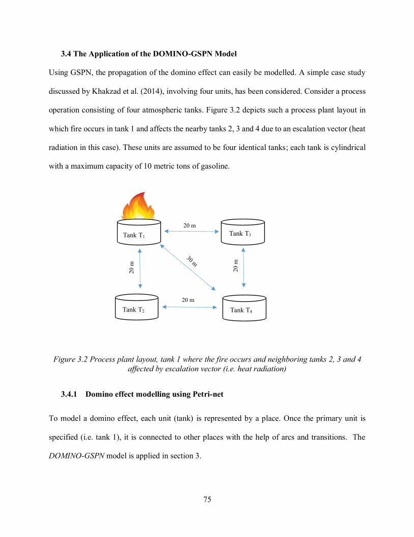
75

3.4 The Application of the DOMINO-GSPN Model

Using GSPN, the propagation of the domino effect can easily be modelled. A simple case study

discussed by Khakzad et al. (2014), involving four units, has been considered. Consider a process

operation consisting of four atmospheric tanks. Figure 3.2 depicts such a process plant layout in

which fire occurs in tank 1 and affects the nearby tanks 2, 3 and 4 due to an escalation vector (heat

radiation in this case). These units are assumed to be four identical tanks; each tank is cylindrical

with a maximum capacity of 10 metric tons of gasoline.

Figure 3.2 Process plant layout, tank 1 where the fire occurs and neighboring tanks 2, 3 and 4 affected by escalation vector (i.e. heat radiation)

3.4.1 Domino effect modelling using Petri-net

To model a domino effect, each unit (tank) is represented by a place. Once the primary unit is

specified (i.e. tank 1), it is connected to other places with the help of arcs and transitions. The

DOMINO-GSPN model is applied in section 3.

20 m Tank T1 Tank T3

20 m

20 m

20 m Tank T2 Tank T4

76

In this case study, tank 1 is considered to be a vulnerable unit. The accident first occurs in tank 1

and then propagates to other units, based on threshold criteria. The primary unit is responsible for

escalating a small accident into a series of accidents. In the case of an atmospheric storage tank,

the most probable accident scenario is a pool fire, which can escalate and affect the nearby units

due to heat radiation (Khakzad, Khan, Amyotte and Cozzani, 2014).To calculate the heat flux, a

detailed explanation and calculation procedure are available in the works of Assael MJ (2010).

The same procedure has been followed to calculate the heat radiation received by tank 2 and 3

when tank 1 is on fire, Q1 to 2 = 20.5 kW/m2. As can be seen, the heat received by both the tanks 2

and 3 are same and exceed the threshold heat intensity (i.e. QT = 15 kW/m2). Therefore, tank 1 can

potentially damage nearby units (tank 2 and 3), while Q1 to 4 = 11 kW/m2 is based on the distance

between tank 1 and 4, which is less than the threshold value. However, tank 1 being on fire along

with tank 2 or 3 leads to credible damage to tank 4. Figure 3.3 shows how propagation would take

place from the primary unit to the secondary unit. Firstly, tank 1 is in an operating state (i.e. token

presence in place P1), when leakage occurs (i.e. token presence in place P2) accompanied by an

ignition source (i.e. token presence in place P3); then tank 1 ignites. The heat radiation received by

the secondary unit due to the primary accident is modelled using three transitions, transition T2, T3

and T4, which is discussed in table 1. Further, higher-order sequential level propagation is

discussed later in this section.

77

Figure 3.3 GSPN model part of the domino effect propagation from the primary unit (Tank 1) to the secondary unit (Tank 2)

The probit values can be estimated using the probit equations mentioned in step 5. With the help

of the probit model, a probability vs time plot can be generated, as shown in Figure 3.4. In order

to use this information in the Petri-net model, distribution fitting has been done. The identified

distribution parameters are then entered as the respective transition specifications.

Initial marking of tokens is based on prior states of equipment and its failure conditions. In the

present case, tokens have been assigned to the operational state of each tank, leakage and ignition

source. Since leakage and an ignition source are combined, these conditions lead to a fire in the

primary unit (i.e. tank 1).

78

Figure 3.4 Distribution fitting on a probability vs time plot for transition T41 & T42

Each transition specification is provided in Table 3.1. The transition governs the movement of the

token from one place to another and dictates the dynamics of the model. The time to failure (ttf)

calculations of a processing unit requires a detailed estimation, including the primary accident’s

effect on the secondary unit and the amount of inventory (gasoline in the present case). An

empirical correlation has been introduced by Landucci, Gubinelli, Antonioni and Cozzani (2009)

based on the detailed simulation results. For the atmospheric cylindrical tank, ttf is a function in

terms of its volume, (V) in m3 and heat radiation (HR) in kW/m2 received from another source (i.e.

external fire). The following equation is used to estimate ttf (Cozzani et al., 2005). This criterion

is used to validate the results of the present study.

0

0.2

0.4

0.6

0.8

1

0 100 200 300 400 500 600 700 800 900 1000 1100 1200 1300

Pro

bab

ility

Exposure time (sec)

Probability Weibull distribution

𝑙𝑛(𝑡𝑡𝑓) = −1.128 𝑙𝑛(𝐻𝑅) − 2.667 ∗ 10−5𝑉 + 9.877

𝑌 = 12.54 − 1.847 ln(𝑡𝑡𝑓)

(4)

(5)

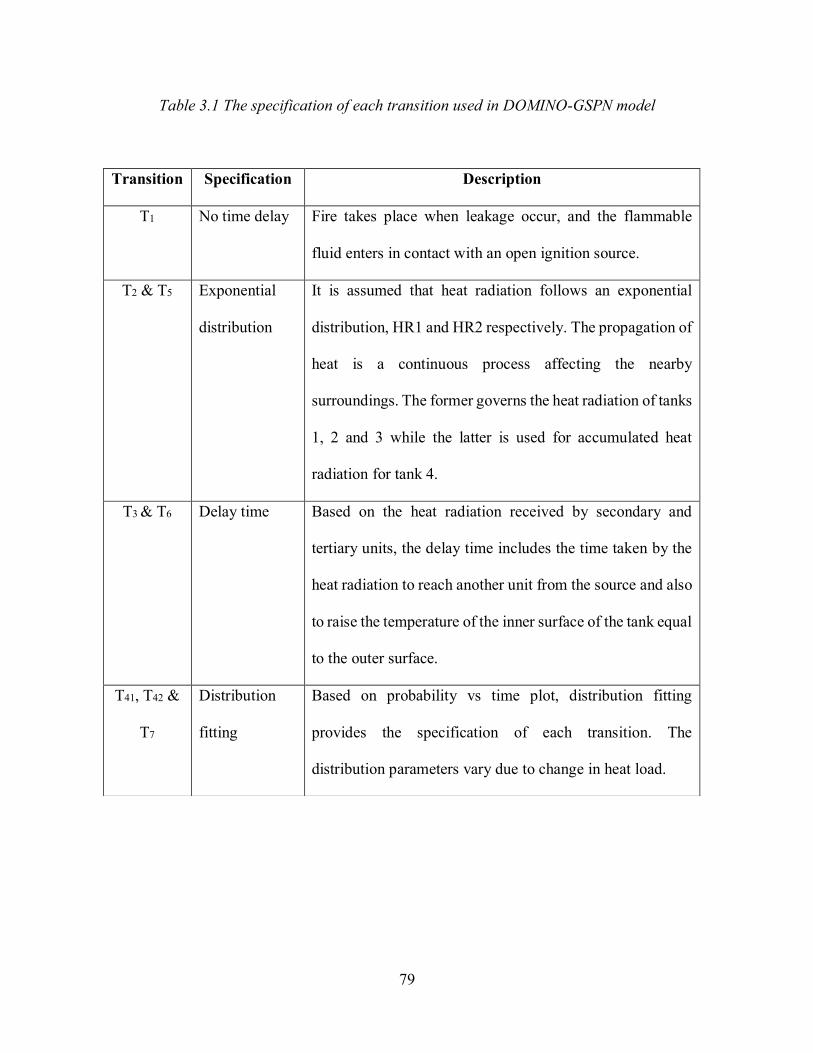
79

Table 3.1 The specification of each transition used in DOMINO-GSPN model

Transition Specification Description

T1 No time delay Fire takes place when leakage occur, and the flammable

fluid enters in contact with an open ignition source.

T2 & T5 Exponential

distribution

It is assumed that heat radiation follows an exponential

distribution, HR1 and HR2 respectively. The propagation of

heat is a continuous process affecting the nearby

surroundings. The former governs the heat radiation of tanks

1, 2 and 3 while the latter is used for accumulated heat

radiation for tank 4.

T3 & T6 Delay time Based on the heat radiation received by secondary and

tertiary units, the delay time includes the time taken by the

heat radiation to reach another unit from the source and also

to raise the temperature of the inner surface of the tank equal

to the outer surface.

T41, T42 &

T7

Distribution

fitting

Based on probability vs time plot, distribution fitting

provides the specification of each transition. The

distribution parameters vary due to change in heat load.

80

Figure 3.5 DOMINO-GSPN model for domino effect propagation pattern in a four tank system

81

3.5 Results and discussion

The propagation of fire in a four-tank system is shown in Figure 3.5 using the Domino-GSPN

model. For clarity, Figure 3.3 only shows the propagation from the primary to the secondary unit.

To model the domino effect, GRIF’s PN module (GRIF, 2016) has been used. Petri nets are still

in developing phase to become a user-friendly tool. There is a need for a model which can predict

the domino effect accident scenario. There are commercial tools available that assist in

developing Petri nets-based model. The GRIF is one such model used by industry.

The Monte Carlo simulation has been carried out from 0 to 30 mins with a step size of 1 minute.

Therefore, each transition has been defined concerning distributions or delay time, based on the

discussed calculation procedure and expert judgement.

The movement of the tokens decides the probability concerning the time at each observed place.

The failure profile for tanks 2 and 3 due to the domino effect is shown in Figure 3.6. Once the heat

radiation reaches the threshold criterion, the domino effect starts to propagate, which is shown by

transition T41 and T42 respectively. Note that from ttf criteria (equation 4), the credible damage

occurs after 11 minutes. As a result, the estimated ttf can be used to evaluate escalation probability

based on equation 5, which gives the probability of 5.42 E-06 for tank 2 given that tank 1 is on

fire. Although the earlier approach was quite capable of estimating the escalation probability, it

assumes time independence, which is not a valid assumption, particularly in a domino effect case

in which time is an important parameter to maintain the risk below acceptance criteria. However,

the proposed method shows a continuous time-dependent failure profile of nearby units, which is

the innovation of this work; a two-step approach is proposed for determining the secondary,

tertiary or higher order domino sequence. Moreover, as depicted in Figure 3.6, the probability of

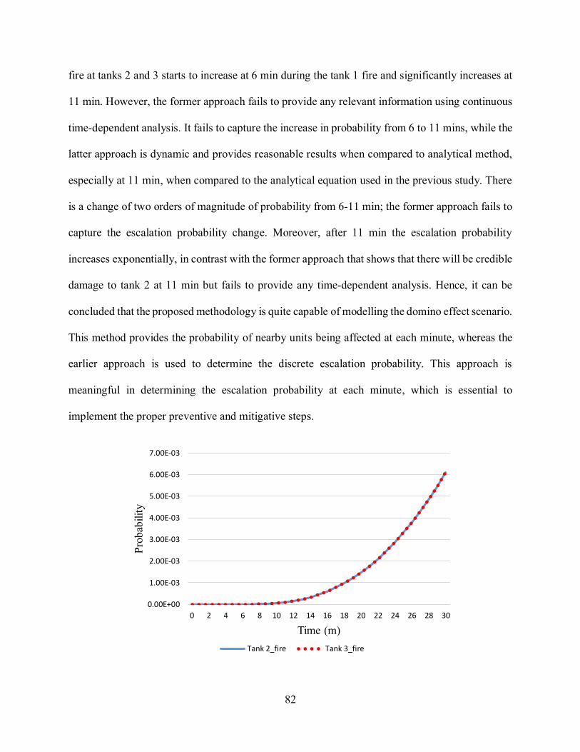
82

fire at tanks 2 and 3 starts to increase at 6 min during the tank 1 fire and significantly increases at

11 min. However, the former approach fails to provide any relevant information using continuous

time-dependent analysis. It fails to capture the increase in probability from 6 to 11 mins, while the

latter approach is dynamic and provides reasonable results when compared to analytical method,

especially at 11 min, when compared to the analytical equation used in the previous study. There

is a change of two orders of magnitude of probability from 6-11 min; the former approach fails to

capture the escalation probability change. Moreover, after 11 min the escalation probability

increases exponentially, in contrast with the former approach that shows that there will be credible

damage to tank 2 at 11 min but fails to provide any time-dependent analysis. Hence, it can be

concluded that the proposed methodology is quite capable of modelling the domino effect scenario.

This method provides the probability of nearby units being affected at each minute, whereas the

earlier approach is used to determine the discrete escalation probability. This approach is

meaningful in determining the escalation probability at each minute, which is essential to

implement the proper preventive and mitigative steps.

0.00E+00

1.00E-03

2.00E-03

3.00E-03

4.00E-03

5.00E-03

6.00E-03

7.00E-03

0 2 4 6 8 10 12 14 16 18 20 22 24 26 28 30

Prob

abili

ty

Time (m)Tank 2_fire Tank 3_fire

83

Figure 3.6 Failure profile of tank 2 and tank 3 by the domino effect

84

As discussed earlier, the distances of both the tanks 2 and 3 from the primary unit (i.e. tank

1) are the same. Hence, the failure profile is the same for both tanks. The results from the

study by Khakzad et al. (2014) provide a discrete value of probabilities of each tank while

comparing two approaches (worst case and dynamic approach) using a Bayesian network

approach, which is widely used in risk assessment and probabilistic modelling (Taleb-

Berrouane, Khan, Hawboldt, Eckert and Skovhus, 2018; Deyab, Taleb-berrouane, Khan

and Yang, 2018). However, the proposed Domino-GSPN approach provides a failure

profile of each level of domino effect, which is used to decide the potential secondary,

tertiary or higher order of domino effect. Further, it shows how the risk increases

exponentially with time. In the case of tank 2 and tank 3 being on fire, their probability is

the same at each time interval, showing that the most probable configuration of a domino

event is tank 1 to 2/3 to 4.

Figure 3.7 Failure profile of tank 4 by the domino effect of tank 1 & tank 2/3

0.00E+00

1.00E-05

2.00E-05

3.00E-05

4.00E-05

5.00E-05

0 5 10 15 20 25 30 35

Prob

abili

ty

Time (min)

85

Similarly, if we analyze the tertiary level of the domino effect, i.e., the tank 4 failure profile,

Figure 3.7 illustrates how its escalation probability evolves with time. Note that at 11

minutes (ttf), there will be credible damage to tank 2 and tank 3, causing the probability of

tank four being involved to increase from 0 to 2 E-08, which shows the dynamic nature of

the proposed model.

Further, based on the same ttf criterion, it takes 18 minutes for tank 4 to have likely damage,

given that tanks 1, 2 or 3 are on fire. As depicted in Figure 3.7, at 18 min the escalation

probability increases to 1.42 E-06 from 2 E-08. The two orders of magnitude change in the

probability of tank 4 is unacceptable and confirms the vulnerability of tank 4. However,

the analytical model only proposes the vulnerability of the equipment/process but fails to

illustrate the escalation probability evolving with time. The escalation probability increases

exponentially, and as a result, it increases by one order of magnitude from 18 to 30 min of

the time interval. However, the analytical equation provides a 1.53 E-04 escalation

probability at 18 min, which is a significantly higher probability for tank 4 to ignite.

Domino effect accidents are always considered to have a lower probability, and higher

consequences accidents and any overestimation provide a false impression of the estimated

risk.

This study demonstrates that the proposed approach provides a clear picture of domino

effect behaviour and generates time-dependent results, unlike previous studies. In the past,

the Bayesian network was only capable of modelling the conditional dependence between

the events in a domino scenario. However, the DOMINO-GSPN model can model the

domino propagation pattern which helps in determining the time dependence analysis.

86

Earlier approaches dealt with modelling the propagation pattern using mathematical

equations, which provided the probability which can then be directly used as a prior and

conditional probability, which can be used in techniques such as BN. To obtain crisp data

for the Bayesian network is a challenging task, especially for modelling complex accident

scenarios which include the domino effect. However, the proposed approach is capable of

modelling all scenarios and patterns of the domino effect in the probabilistic framework

and subsequently obtaining the risk profile of each level of the vulnerable unit. Therefore,

it introduces a robust approach to model such propagation by using an extended Petri-net

formalism. PN helps to model the propagation pattern by incorporating the firing rate

regarding continuous distributions and time delays, which helps to model complex

accidents simply, provided that the accident propagation pattern is known. This model also

provides the escalation probability of each level of the domino effect with time

dependency, which is essential to implement safety barriers for managing the risk.

Although it is a challenging task to model the accident caused by domino effect due to

complex interaction of components in process facilities. This article introduces a novel

approach to model the domino accident using the proposed DOMINO-GSPN model.

Further, if there is a need to model two or three consequences, namely, pool fire, jet fire

etc. The authors acknowledge the level of complexity that may arise when dealing with

combination of hazards. The concept presented here are able to capture the synergic

interactions and model as dependent network. The Petri net model is a combination of

many sub-networks or sub-models, each one is connected with the help of predicates and

87

assertions. Therefore, the traceability could be maintained while modelling the complex

sequence of domino accident.

The DOMINO-GSPN model enables a time-dependent analysis of domino scenarios. This

analysis would help to prepare better control and mitigation measures. The key advantage

of this model is that it provides a continuous time-dependent domino effect probability of

credible scenarios, which could be used for planning and design decision-making purposes.

The tools like PHAST and ALOHA are powerful in modelling gas dispersion, fuel

evaporation, and pool fire spreading. These tools are meant for consequence (impact)

analysis, they have limited ability to analyze domino effect occurrence likelihood and

most importantly these tools impact assessment is time independent. The present study

is unique as it attempts to demonstrate domino effect likelihood analysis as function of

duration of accident (pool fire) using advance probability analysis tool, Petri nets. The

proposed DOMINO-GSPN model is a generalized model that enable studying accident

escalation vector which lead to domino effect scenarios. The DOMINO-GSPN model can

be integrated with PHAST or ALOHA for detailed impact (consequence analysis) of

domino effect.

3.6 Conclusions

In process industries, a large amount of flammable material is stored and/or processed. A

small incident such as leakage in a processing unit can affect nearby units, resulting in a

cascading effect, known as the domino effect. Modelling the domino effect is a challenging

task. This work employs advanced probabilistic techniques to model domino effects; the

advantages of the proposed method are:

88

• A probabilistic analysis of the accident caused by domino effect provides a time-

dependent risk profile for each level of the domino effect.

• The domino effect propagation path is modelled as a time-dependent process.

• The complex interaction among units can be easily depicted using a Petri-net.

• The failure profile obtained is used to analyze the vulnerability of the unit instead

of using conventional threshold criteria to determine the next level of domino

propagation.

• Combined loading i.e., heat load through different mechanisms is considered.

This study focused on developing innovative domino effect propagation and likelihood

model, and also analyzing unit vulnerability based on the two-step criteria (threshold

criteria and risk profile). For the sake of clarity, a system consists of four atmospheric tanks

have been analyzed. The results obtained from that model are compared with another

probabilistic method which has been widely used in the field of safety and risk engineering.

In comparison to other techniques used to model the domino effect, this novel approach is

capable of assessing the failure likelihood as time-dependent. Discrete values can only

provide an evaluation of the system at a particular instant of time, whereas continuous time-

dependent results help to monitor risk, especially in complex systems where domino effect

accidents are quite common. Other aspects of the domino effect such as overpressure and

blast waves can also be modelled using the same approach. Past accidents due to the

domino effect can be easily modelled using the DOMINO-GSPN model, which helps to

prevent future accidents. Prevention of domino effect accidents results in saving the

environment, human life and property. This work can be improved by considering the

89

inventory of tanks as a probability distribution, all the calculations of heat radiation are

carried out using tank 1 inventory as a constant. Further, wind speed and direction can also

be considered to enhance the model further to capture complex, realistic situations.

3.7 References

Abdolhamidzadeh, B., Abbasi, T., Rashtchian, D., & Abbasi, S. A. (2010). A new method

for assessing the domino effect in the chemical process industry. Journal of Hazardous

Materials. https://doi.org/10.1016/j.jhazmat.2010.06.049

Abdolhamidzadeh, B., Abbasi, T., Rashtchian, D., & Abbasi, S. A. (2011). Domino effect

in process-industry accidents - An inventory of past events and the identification of some

90

patterns. Journal of Loss Prevention in the Process Industries.

https://doi.org/10.1016/j.jlp.2010.06.013

Angeli, D., De Leenheer, P., & Sontag, E. D. (2007). A Petri net approach to the study of

persistence in chemical reaction networks. Mathematical Biosciences.

https://doi.org/10.1016/j.mbs.2007.07.003

Antonioni, G., Spadoni, G., & Cozzani, V. (2009). Application of domino effect

quantitative risk assessment to an extended industrial area. Journal of Loss Prevention in

the Process Industries. https://doi.org/10.1016/j.jlp.2009.02.012

Assael MJ, K. K. (2010). Fires, Explosions, and Toxic Gas Dispersions. (N. C. Press, Ed.).

Taylor and Francis Group.

Bagster, D. F., & Pitblado, R. M. (1991). Estimation of domino incident frequencies - an

approach. Process Safety and Environmental Protection: Transactions of the Institution of

Chemical Engineers, Part B.

Cozzani, V., Gubinelli, G., Antonioni, G., Spadoni, G., & Zanelli, S. (2005). The

assessment of risk caused by the domino effect in quantitative area risk analysis. Journal

of Hazardous Materials. https://doi.org/10.1016/j.jhazmat.2005.07.003

Cozzani, V., Gubinelli, G., & Salzano, E. (2006). Escalation thresholds in the assessment

of accidental domino events. Journal of Hazardous Materials.

https://doi.org/10.1016/j.jhazmat.2005.08.012

Cozzani, V., & Salzano, E. (2004). The quantitative assessment of domino effects caused

91

by overpressure: Part I. Probit models. Journal of Hazardous Materials, 107(3), 67–80.

https://doi.org/10.1016/j.jhazmat.2003.09.013

Darbra, R. M., Palacios, A., & Casal, J. (2010). Domino effect in chemical accidents: Main

features and accident sequences. Journal of Hazardous Materials, 183(1–3), 565–573.

https://doi.org/10.1016/j.jhazmat.2010.07.061

David, R., & Alia, H. (2005). Discrete, continuous, and hybrid Petri nets. Discrete,

Continuous, and Hybrid Petri Nets. https://doi.org/10.1007/b138130

Delvosalle, C., Fievez, C., Pipart, A., & Debray, B. (2006). ARAMIS project: A

comprehensive methodology for the identification of reference accident scenarios in

process industries. Journal of Hazardous Materials.

https://doi.org/10.1016/j.jhazmat.2005.07.005

Deyab, S. M., Taleb-berrouane, M., Khan, F., & Yang, M. (2018). Failure analysis of the

offshore process component considering causation dependence. Process Safety and

Environmental Protection. https://doi.org/10.1016/j.psep.2017.10.010

GRIF-Workshop. (2016). SATODEV, TOTAL. Retrieved from http://grif-workshop.com

Grunt, O., & Briš, R. (2015). SPN as a tool for risk modelling of fires in process industries.

Journal of Loss Prevention in the Process Industries, 34, 72–81.

https://doi.org/10.1016/j.jlp.2015.01.024

Kadri, F., Chatelet, E., & Lallement, P. (2013). The Assessment of Risk Caused by Fire

and Explosion in Chemical Process Industry: A Domino Effect-Based Study. Journal of

92

Risk Analysis and Crisis Response, 3(2), 66. https://doi.org/10.2991/jrarc.2013.3.2.1

Khakzad, N. (2015). Application of dynamic Bayesian network to risk analysis of domino

effects in chemical infrastructures. Reliability Engineering & System Safety, 138, 263–272.

https://doi.org/10.1016/j.ress.2015.02.007

Khakzad, N., Khan, F., Amyotte, P., & Cozzani, V. (2013). Domino Effect Analysis Using

Bayesian Networks. Risk Analysis, 33(2), 292–306. https://doi.org/10.1111/j.1539-

6924.2012.01854.x

Khakzad, N., Khan, F., Amyotte, P., & Cozzani, V. (2014). Risk Management of Domino

Effects Considering Dynamic Consequence Analysis. Risk Analysis, 34(6), 1128–1138.

https://doi.org/10.1111/risa.12158

Khan, F. I., & Abbasi, S. A. (1998a). DOMIFFECT (DOMIno eFFECT): User-friendly

software for domino effect analysis. Environmental Modelling and Software.

https://doi.org/10.1016/S1364-8152(98)00018-8

Khan, F. I., & Abbasi, S. A. (1998b). Models for domino effect analysis in chemical

process industries. Process Safety Progress, 17(2), 107–123.

https://doi.org/10.1002/prs.680170207

Khan, F. I., & Abbasi, S. A. (2001). An assessment of the likelihood of occurrence, and

the damage potential of domino effect (chain of accidents) in a typical cluster of industries.

Journal of Loss Prevention in the Process Industries, 14(4), 283–306.

https://doi.org/10.1016/S0950-4230(00)00048-6

93

Kourniotis, S. P., Kiranoudis, C. T., & Markatos, N. C. (2000). Statistical analysis of

domino chemical accidents. Journal of Hazardous Materials, 71(1–3), 239–252.

https://doi.org/10.1016/S0304-3894(99)00081-3

Landucci, G., Gubinelli, G., Antonioni, G., & Cozzani, V. (2009). The assessment of the

damage probability of storage tanks in domino events triggered by fire. Accident Analysis

and Prevention, 41(6), 1206–1215. https://doi.org/10.1016/j.aap.2008.05.006

Li, J., Reniers, G., Cozzani, V., & Khan, F. (2017). A bibliometric analysis of peer-

reviewed publications on domino effects in the process industry. Journal of Loss

Prevention in the Process Industries. https://doi.org/10.1016/j.jlp.2016.06.003

Mannan, S. (2012). Lees’ Loss Prevention in the Process Industries: Hazard Identification,

Assessment And Control: Fourth Edition. Lees’ Loss Prevention in the Process Industries:

Hazard Identification, Assessment and Control: Fourth Edition.

https://doi.org/10.1016/C2009-0-24104-3

Mingguang, Z., & Juncheng, J. (2008). An improved probit method for assessment of

domino effect to chemical process equipment caused by overpressure. Journal of

Hazardous Materials, 158(2–3), 280–286. https://doi.org/10.1016/j.jhazmat.2008.01.076

Murata, T. (1989). Petri nets: Properties, analysis and applications. Proceedings of the

IEEE, 77(4), 541–580. https://doi.org/10.1109/5.24143

Paltrinieri, N., Dechy, N., Salzano, E., Wardman, M., & Cozzani, V. (2012). Lessons

Learned from Toulouse and Buncefield Disasters: From Risk Analysis Failures to the

94

Identification of Atypical Scenarios Through a Better Knowledge Management. Risk

Analysis. https://doi.org/10.1111/j.1539-6924.2011.01749.x

Reniers, G. (2010). An external domino effects investment approach to improving cross-

plant safety within chemical clusters. Journal of Hazardous Materials, 177(1–3), 167–174.

https://doi.org/10.1016/j.jhazmat.2009.12.013

Reniers, G. L. L., & Dullaert, W. (2007). DomPrevPlanning©: User-friendly software for

planning domino effects prevention. Safety Science.

https://doi.org/10.1016/j.ssci.2006.10.004

Reniers, G. L. L., Dullaert, W., Ale, B. J. M., & Soudan, K. (2005). The use of current risk

analysis tools evaluated toward preventing external domino accidents. Journal of Loss

Prevention in the Process Industries. https://doi.org/10.1016/j.jlp.2005.03.001

Taleb-Berrouane, M., Khan, F., Hawboldt, K., Eckert, R., & Skovhus, T. L. (2018). Model

for microbiologically influenced corrosion potential assessment for the oil and gas

industry. Corrosion Engineering, Science and Technology, 53(5), 378–392.

https://doi.org/10.1080/1478422X.2018.1483221

Talebberrouane, M., Khan, F., & Lounis, Z. (2016). Availability analysis of safety-critical

systems using advanced fault tree and stochastic Petri net formalisms. Journal of Loss

Prevention in the Process Industries, 44, 193–203.

https://doi.org/10.1016/j.jlp.2016.09.007

Vílchez, J. A., Sevilla, S., Montiel, H., & Casal, J. (1995). Historical analysis of accidents

95

in chemical plants and the transportation of hazardous materials. Journal of Loss

Prevention in the Process Industries. https://doi.org/10.1016/0950-4230(95)00006-M

Wu, N., Chu, F., Chu, C., & Zhou, M. (2010). Hybrid Petri net modelling and

schedulability analysis of high fusion point oil transportation under tank grouping strategy

for crude oil operations in the refinery. IEEE Transactions on Systems, Man and

Cybernetics Part C: Applications and Reviews.

https://doi.org/10.1109/TSMCC.2009.2032661

Zhou, M., DiCesare, F., & Guo, D. (1990). Modelling and performance analysis of a

resource-sharing manufacturing system using stochastic Petri nets. Proceedings 5th IEEE

International Symposium on Intelligent Control 1990.

https://doi.org/10.1109/ISIC.1990.128577

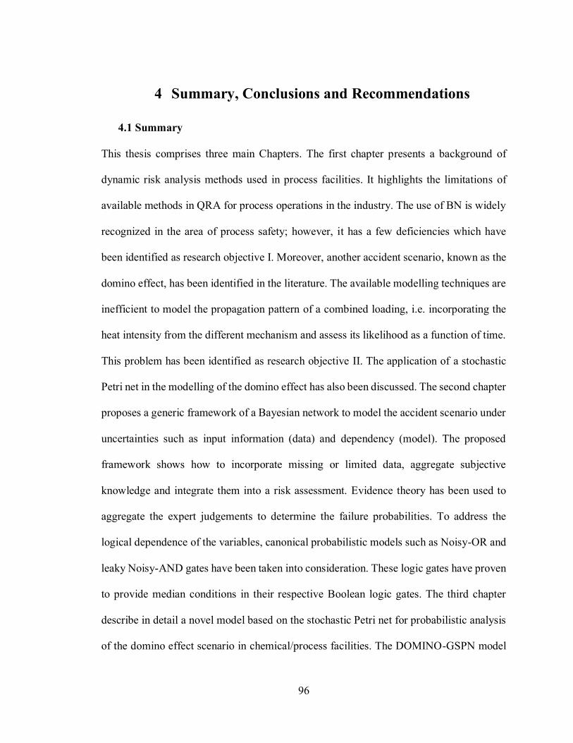
96

4 Summary, Conclusions and Recommendations

4.1 Summary

This thesis comprises three main Chapters. The first chapter presents a background of

dynamic risk analysis methods used in process facilities. It highlights the limitations of

available methods in QRA for process operations in the industry. The use of BN is widely

recognized in the area of process safety; however, it has a few deficiencies which have

been identified as research objective I. Moreover, another accident scenario, known as the

domino effect, has been identified in the literature. The available modelling techniques are

inefficient to model the propagation pattern of a combined loading, i.e. incorporating the

heat intensity from the different mechanism and assess its likelihood as a function of time.

This problem has been identified as research objective II. The application of a stochastic

Petri net in the modelling of the domino effect has also been discussed. The second chapter

proposes a generic framework of a Bayesian network to model the accident scenario under

uncertainties such as input information (data) and dependency (model). The proposed

framework shows how to incorporate missing or limited data, aggregate subjective

knowledge and integrate them into a risk assessment. Evidence theory has been used to

aggregate the expert judgements to determine the failure probabilities. To address the

logical dependence of the variables, canonical probabilistic models such as Noisy-OR and

leaky Noisy-AND gates have been taken into consideration. These logic gates have proven

to provide median conditions in their respective Boolean logic gates. The third chapter

describe in detail a novel model based on the stochastic Petri net for probabilistic analysis

of the domino effect scenario in chemical/process facilities. The DOMINO-GSPN model

97

can capture the propagation pattern of the domino scenarios in the form of Petri nets. The

graphical demonstration using the places, transitions, directed arcs and tokens helps to

visualize the patterns of domino effect scenarios. GSPN has the advantage of modelling

the complex interactions of process units with the help of transitions. The failure profile

obtained for secondary or higher order units represents the vulnerability of those units as a

function of time and is used to identify the next level. The most probable configuration of

the units can also be identified.

4.2 Conclusions

The present work illustrates the application of the advanced concept of the Bayesian

network and stochastic Petri net in the area of process safety and risk assessment. It is

focused on modelling complex process system and their behaviour by incorporating

advanced probability theory and algorithms. This work has developed two novel models

to i) analyze a single accident using limited imprecise data, and ii) analyze the chain of

process accidents. Both models are tested using available data and compared with

published literature. Their application has been verified using past accidents. The first

developed model has enhanced Bayesian network performance by the including new

logical relationships with the help of dynamic logic gates, along with incorporating expert

judgement in determining the failure probabilities of basic events and safety barriers. The

second model has enabled mathematical representation of the domino effect propagation

pattern and their likelihood estimate. This work is beneficial for academicians as it provides

novel methods and models; it is of equally high importance for industry practitioners, as it

98

enables better assessment of dynamic risk. Application of this work would help in

designing effective safety measures to prevent process accidents.

4.3 Recommendations

The present study can be further improved by considering structural uncertainty apart from

the model and data uncertainty. These uncertainties play an important role in rare event

scenarios which includes a domino effect analysis. Completeness and incorrectness of data

especially related to expert opinion is very important. This may be considered in future

studies.

Integrating incorrectness or incompleteness of the data in developing the BN model would

be a reasonable extension of the present work.

The modelling of the domino effect scenario presented in this study only considers heat

radiation as an escalation vector. However, the model can be extended to consider more

than one escalation vector such as overpressure caused by the explosion. Moreover, the

work can also be improved by considering the inventory of atmospheric tanks as a

probability distribution rather than as a constant value. Wind speed and direction can also

be considered to enhance the model to consider a more complex and realistic situation.

Data and model uncertainty can also be considered in modelling the domino effect. The

developed model may be integrated with a risk assessment framework.

The consequence analysis of the domino effect in economic terms will be an obvious

extension of the present work. The economic consequence assessment could be conducted

using loss function, which subsequently could be integrated with dynamic risk assessment.