PERSISTENCE IN LAW-OF-ONE-PRICE DEVIATIONS:EVIDENCE FROM MICRO-DATA

by

Mario J. Crucini and Mototsugu Shintani

Working Paper No. 06-W16

December 2002Revised July 2006

DEPARTMENT OF ECONOMICSVANDERBILT UNIVERSITY

NASHVILLE, TN 37235

www.vanderbilt.edu/econ

Persistence in Law-of-One-Price Deviations:Evidence from Micro-data

Mario J. Crucini and Mototsugu Shintani∗

Department of Economics, Vanderbilt University

June 24, 2006

AbstractWe study the dynamics of good-by-good real exchange rates using a

micro-panel of 270 goods prices drawn from major cities in 63 countriesand 258 goods prices drawn from 13 major U.S. cities. We find the half-life of deviations from the Law-of-One-Price for the average good is about1 year. The average half-life is very similar across the OECD, the LCDand within the U.S., suggesting little in the way of nominal exchange rateregime influences. The average non-traded good has a half-life of 1.9 yearscompared to 1.2 years for traded-goods, for the OECD, with modest differ-ences elsewhere. Aggregating the micro-data increases persistence in theOECD by 6 months to 1.5 years, well below levels obtained using aggregateCPI data. We attribute these differences to conceptual and methodologicalfactors and argue in favor of increased use of micro-price data in appliedtheory.

JEL Classification: E31, F31,D40.

Key words and phrases: Real exchange rates, Purchasing Power Parity, Lawof One Price, Dynamic panel.

∗Corresponding author: Mario J. Crucini, Department of Economics, Vanderbilt University,VU Station B #351819, 2301 Vanderbilt Place, Nashville, TN 37235-1819. Phone: (615)-322-7357, Fax: (615) 343-8495. The authors gratefully acknowledge the financial support of theNational Science Foundation (SES-0136979, SES-0524868) and the able research assistance pro-vided by Inkoo Lee financed by the grant. We are especially thankful for detailed and construc-tive comments provided by Charles Engel, Yanqin Fan, David Parsley, John Rogers, Andy Roseand Randy Verbrugge. We also thank numerous seminar and conference participants.

1. Introduction

Much of what is known about international relative price adjustment comes

from estimates of persistence of aggregate real exchange rates constructed from

consumer price indices. Typically these studies evaluate persistence in terms of

half-lives of deviations from purchasing power parity — the length of time it takes

for the real exchange rate to make it half of the distance back to its stationary

level following a shock. In his cogent review of the vast literature on the topic,

Rogoff (1996) places the consensus range for these half-lives at 3 to 5 years.1

High real exchange rate persistence is widely viewed as a litmus test of a macro-

economic theory. Consider models featuring sticky prices and imperfect competi-

tion, such as those pioneered by Obstfeld and Rogoff (1995) and Svennsson and

van Wijnbergen (1989). The consensus range is frequently cited as evidence that

this class of model is incapable of accounting for the time series properties of a key

variable their were designed to explain, namely, the aggregate real exchange rate

(see, for example, Chari, Kehoe and McGrattan (2002)).2 Generally, the volatility

and persistence of the aggregate real exchange rate is thought to pose an insur-

mountable empirical challenge to theoretical paradigms that presume the Law-of-

One-Price holds in an approximate sense. This has led to a resurgence of interest

in various forms of international market segmentation, including: transportation

and distribution costs, tariff and non-tariff barriers, imperfect competition, costly

1This range is further confirmed by studies following Rogoff’s survey. For example, Frankeland Rose (1996) utilize a panel of 150 countries and obtain strong evidence of mean-reversionof aggregate real exchange rates with a half-life of about four years. Murray and Papell (2005)conduct bias-corrections using similar data and arrive at a point estimate of 4.6 years with aconfidence interval of 2.7 to 5.3 years, which nicely embraces the consensus range.

2The model also has difficulty generating real exchange rate variability that matches thedata. This property, however, comes from an older puzzle relating to nominal exchange ratevariability and the inability of the monetary approach to explain this property of the data.

1

search and non-traded inputs into final consumption.

Each of these models is (or should be) about heterogeneity in Law-of-One-Price

deviations across goods. In models with trade costs or tariffs, the LOP deviations

are constant over time and different across goods and locations.3 In models with

non-traded inputs into final consumption, it is natural for the deviations to vary

over the business cycle and be common across goods within a category (i.e. traded

versus non-traded). Whether the deviations persist into the steady-state is usually

a maintained assumption, not a theoretical implication. Finally, the empirical

targets of sticky price models are large, but rapidly decaying deviations from the

Law-of-One-Price.

The goal of this paper is to bring empirical micro-foundations to the rapidly

evolving open economy macroeconomic literature that emphasizes market seg-

mentation in its various forms. We build upon Crucini, Telmer and Zachariadis

(2005) who had some success relating geographic price dispersion to the economic

characteristics of individual goods and services. Their study focused on major Eu-

ropean cities using a series of extensive cross-sections of micro-prices, but lacked

an explicit time series dimension. Here we study the domestic currency prices of

270 individual goods and services across 71 countries and 13 cities within the U.S.

over the period 1990 to 2000. Our focus is the time series dimension.

Our central finding relates to the persistence of the LOP deviation for the

median good. Estimating separate panel regressions for each good, pooling all

international locations, we find that the median good has a half-life of about 1

year. Aggregating the micro-data using consumption expenditure shares in an

attempt to emulate the construction of the CPI, the half-life rises by 6 months to

1.5 years (within the OECD).

3To be more precise, they may vary, but the variation is expected to be gradual over time(declining transportation costs) or abrupt (a significant trade agreement or a tariff war).

2

An immediate implication of this finding is that the criticism leveled at sticky-

price models seems largely unwarranted, since the persistence levels exhibited by

our micro-data are close to those produced by Chari, Kehoe and McGrattan’s

simulation experiments. A related implication is that the persistence of LOP

deviations that we estimate appear more in line with micro-evidence on the fre-

quency of price adjustment than does persistence estimated from the CPI-based

real exchange rate. A prominent recent study by Bils and Klenow (2004) uses data

from 1995-1997 on 350 individual good prices from the Bureau of Labor Statistics

and reports an average time between price changes of only 3.3 months.4

Some of the goods in our cross-section appear in existing studies, inviting

comparisons. Goldberg and Verboven (2005) estimate half-lives of relative price

deviations for automobiles in the range of 1.3 to 1.6 years; they focus on Europe.

Worldwide, we estimate half-lives of LOP deviations for automobiles ranging from

7 to 13 months. Cumby (1997) finds the half-life of international price deviations

in Big Mac hamburgers to be about 1 year. The LOP for ground beef has a

half-life of 11 months in our data.5

Moving from anecdotes to broader cross-sectional implications of our work, the

half-lives of LOP deviations increase from 1.1 years to 1.4 years as we move from

the average traded good to the average non-traded good, pooling all cities of the

world. This finding is robust across the OECD, LDC and U.S. city sub-samples.

We find less variation in half-lives across groups of locations than across types

of goods. The half-life of LOP deviations is 0.97 years for the median good in

4Also, Ahlin and Shintani (2006) use Mexican price data on 44 goods and report that theaverage monthly frequency of price changes was 28% in 1994 and as large as 50% in 1995.Blinder et al. (1998), on the other hand, use firm-level surveys and find that the median firmchanges its price once a year.

5Related studies in this vien are: wheat, butter and charcoal (Froot, Kim and Rogoff, 1995),the Economist Magazine (Ghosh and Wolf, 1994). More comprehensive coverage of goods isfound in Crownover, Pippenger and Steigerwald (1996), Isard (1977), Giovannini (1988), andRogers and Jenkins (1995).

3

the panel of U.S. cities, squarely between the values for the OECD cities (1.09)

and LDC cities (0.86). In our data, then, exchange rate regimes have quantita-

tively small and ambiguous implications for persistence. Exchange rate regimes,

do, however increase the time series variability of relative prices, consistent with

the work of Charles Engel (1993) and Engel and John Rogers (1996). A good

description of the time series behavior of relative prices that emerges is that price

deviations are moderately persistence and very volatile when a border is crossed

and moderately persistent and moderately volatile when a border is not crossed.

Thus far, we have said little about the size of the absolute price deviations

themselves, something absolute price data allow us to study. We consider two

views: one innocuous, the other stark. The first we call conditional price conver-

gence; it implies that, in the long-run, the differences in absolute prices across

locations converge to a nondegenerate distribution. The second convergence con-

cept is absolute price convergence; it implies that, in the long-run, the differences

in absolute prices across locations disappear, the price distribution is degenerate.

We find the null hypothesis of absolute price convergence is rejected for virtu-

ally all goods in the international data, but is not rejected for most of the goods

within the U.S. (results against absolute convergence are stronger across cities

within LDC than across cities within the OECD). Given the fact that absolute

LOP deviations are numerically smaller within the U.S. compared to internation-

ally and that the number of observations (i.e. location pairs) is also much smaller

for the U.S., our inability to reject the null of absolute price convergence in the

U.S. may reflect a combination of the smaller absolute deviations and greater sam-

pling variance. However, it seems safe to say that the long-run, cross-sectional

variance of prices at the level of the individual good is lower intranationally than

internationally, for virtually all goods.

These results may be summarized very succinctly as follows: the primary

4

feature of relative price behavior that distinguishes locations within countries from

what we observe internationally is not the persistence of the stochastic fluctuations

of relative prices around their long-run levels, but rather the magnitude of the

long-run deviations themselves and the voracity of the shocks that impinge upon

them.6

The remainder of the paper is organized as follows. Section 2 presents a simple

model of retail prices and introduces convergence concepts. Section 3 describes

the data. Section 4 examines the long-run stationary and convergence questions.

Section 5 contains the main results, dealing with persistence of LOP deviations.

We provide discussion of robustness in Section 6 and concluding remarks in Section

7.

2. Conceptual Framework

We organize our data using the framework Crucini, Telmer and Zachariadis

(2005) applied to study microeconomic price dispersion in a cross-section of Eu-

ropean capital cities. Retail firms combine traded and non-traded inputs and sell

the resulting composite good to consumers residing in the same location. In effect,

final consumption is completely home biased unless consumers bypass the local

retailer. The home bias of retailers, in contrast, varies with the proportion of their

marginal cost attributable to local inputs.

Formally, the cost function for the retail firm in location i, selling good m, is

6The intranational part of our analysis is most closely related to work by Parsley and Wei(1996) and Cecchetti, Mark and Sonora (2002). Parsley and Wei uses 51 retail prices across 48U.S. cities and find relatively rapid price convergence for traded goods. In contrast, Cecchetti,Mark and Sonora uses an almost century long panel of U.S. CPI data and find extremely slowadjustment. Our estimates are much more closer to the results of Parsley and Wei who also usemicro-data.

5

the solution to the following cost minimization problem solved at each date:

min{Nm

i ,Xmi }

Cmi = WiN

mi + Tm

i Xmi

s.t. Y mi ≡ (Nm

i )αm(Xm

i )(1−αm)

where Cmi is the cost of producing goodm in location i, Y m

i is the physical output

level, Nmi is the labor input, Xm

i is the traded intermediate input, Wi and Tmi are

the respective input prices, and 0 < αm < 1.7

We have adopted two assumptions. First, that factor mobility is sufficiently

high across sectors within a location thatWi is location-specific, not good-specific.

The wage would also lose location-specificity if labor was highly mobile across

locations. The second assumption is that retailers in all locations produce good

m using the same technology; αm is good-specific, not location-specific.

Under constant returns to scale and allowing for a markup over marginal cost,

Bmi ≥ 1, the per unit retail price of good m faced by a consumer in location i,

Pmi , is:

Pmi = Bm

i (Wi)αm (Tm

i )1−αm (2.1)

The bilateral real exchange rate for good m across city pair i and j (in logs) is

therefore:

qmij = lnPmi − lnPm

j = bmij + αmwij + (1− αm)τmij . (2.2)

Equation (2.2) says that prices will differ across locations due to differences

in markups, wages and traded input prices. Theoretical counterparts to these

wedges are imperfect competition, the Balassa-Samuelson hypothesis, transporta-

tion costs and tariffs, among others.

7Allowing for non-traded inputs beyond labor services (e.g., retail space, utilities, advertising,among others) and multiple traded inputs does not alter the key implications of the theory, wewould simply treat Nm

i and Xmi as composites of local and traded inputs.

6

2.1. Conditional and Absolute Price Convergence

Theory places stark restrictions on the right-hand-side of equation (2.2). It is

near universal to assume the deviations are constant in the long run, something

we provide evidence on in the section immediately following this one. Where

theories differ is in their assumptions about the sources and magnitudes of the long

run deviations. We contrast two prominent viewpoints. One we call conditional

convergence: the notion that relative prices converge to a fixed distribution as the

time period goes to infinity and all shocks are set to their unconditional mean

of zero. The other we call absolute convergence: the notion that the long run

distribution of relative prices is degenerate (i.e. the price of a good converges to

the same level across locations when expressed in a common currency).

Definition 1. Conditional price convergence. T−1PT

t=1 qmijt converges to a ran-

dom variable qmij in distribution as T →∞.

From the definition of convergence in distribution, conditional price conver-

gence is equivalent to the convergence of the cumulative distribution function

FmT (x) of T

−1PTt=1 q

mijt to Fm(x) of qmij as T → ∞, where qmij is determined by

the linear combination of the long-run levels of markups, wages and trade costs

across locations.

Definition 2. Absolute price convergence. T−1PT

t=1 qmijt converges to zero in

probability, for all i, as T →∞.

This definition formalizes the absolute version of the Law-of-One-Price in a

cross-section of locations. It is a special case of conditional price convergence. In

7

addition to requirement that FmT (x) of T

−1PTt=1 q

mijt converges to F

m(x) of qmij as

T → ∞, the distribution of qmij is now degenerate at zero: Fm(x) = 1 for x ≥ 0and 0 for x < 0 for all i.

The conditions necessary for absolute convergence are stringent. In the long

run we would need to observe: identical markups of price over marginal cost, equal

wages across location and a complete absence of trade costs and tariffs on traded

intermediate inputs.

In modeling deviations of relative prices from their long-run levels, we follow

much of the existing PPP literature and estimate a first-order autoregressive model

(here we use i to denote a bilateral pair):8

qmit − qmi = ρm(qmit−1 − qmi ) + vmit (2.3)

or equivalently,

qmit = ηmi + ρmqmit−1 + vmit . (2.4)

Assuming |ρm| < 1, qmi = ηi/(1 − ρm) defines the time-invariant individual city-

specific effect, assumed to have variance σ2η. It may be viewed as the steady state

level of qmit in the sense that it is the sample mean of qmit conditional on η

mi for large

t. Provided that σ2η > 0, the model is consistent with the conditional convergence

hypothesis. Evidently, it reduces to the model of absolute convergence for goods

satisfying the restriction ηmi = 0 for all i.

The error terms vmit are innovations to the transitory deviations of relative

prices from their long-run levels. We assume the vmit have mean zero conditional

on ηmi and lagged qmit ’s and variance σ2v.

Having laid out our conceptual framework, we now describe the data.

8Goldberg and Verboven (2005) also consider covergence toward the relative and absoluteversions of Law-of-One-Price by using specifications with and without allowing individual effects.

8

3. The Data

The source of our retail price data is the Economist Intelligence Unit’sWorld-

wide Cost of Living Survey.9 To our knowledge this is the most extensive ongoing

survey of international retail prices in the sense that it covers a significant fraction

of retail items that urban residents consume and spans cities in virtually every

country, including multiple cities within a select number of countries. Given our

time series focus, a significant advantage over other price surveys that have sim-

ilar coverage of goods and locations is its annual frequency and early starting

date, 1990. Most existing surveys are so infrequent as to render them useless for

addressing time series issues.

Turning to the details, the number of cities included in the survey is 122 and

these cities span 78 countries. The maximum number of goods and services priced

in any given year is 301. Our sample runs annually from 1990 to 2000.

We conduct our international analysis using one city from each country. We

chose the continental U.S. for our intranational analysis for the simple reason that

it contains by far the largest number of cities surveyed at 13. The next largest

number of cities surveyed equals 5 in Australia, China and Germany.

In our dynamic panel estimation we pool our data across locations and time

and run a separate regression for each good. Since the raw data contain a number

of missing observations and we want to work with balanced panels, we select goods

and locations in the following way. First, if the country underwent a currency

reformwe eliminate it from the sample.10 Second, for each good, cities that contain

9The target market for the data source is corporate human resource managers who use it tohelp determine compensation levels of their employees residing in different cities of the world.While the goods and services reflect this objective to some extent, the sample is extensive enoughto overlap significantly with what appears in a typical urban consumption basket.10The excluded countries are: Argentina, Brazil, Ecuador, Mexico, Peru, Poland, Russia, and

Uruguay.

9

missing observations are removed. In selecting the city to use when more than

one city is available our default choice is the city that comes first alphabetically.

When a price observation is not available for the first city in the alphabet, we

move on down the list alphabetically until we either find a price observation or

exhaust the available cities in that country.

After applying these rules, the number of cities utilized to estimate the per-

sistence of an individual good’s relative price ranges from 22 to 62, in the inter-

national panel, with the median number of cities used equal to 54. In the U.S.

panel, the number of cities utilized ranges from 10 to 13 and the median number

used (after rounding) is also 13, reflecting the fact that the U.S. panel contains

very few missing observations.

Table 1 presents the 82 cities, located in 63 countries, that survived our se-

lection criterion. We organize countries into four major groups. The first group

we call the ‘World’ since it comprises all international locations for which data is

available for a particular good spanning all 11 years. The second and third groups

are sub-groups of the World: the OECD and the remaining 40 countries we refer

to as the ‘LDC.’ (see Table 1 for a detailed listing). The fourth group of locations

are the 13 cities of the U.S., used for our intranational analysis.

The number of goods for which a particular city is used in the panel estimation

is noted in parentheses in Table 1. Descriptions of the individual goods and

services used in our analysis is provided in Table A1 of the Appendix. After

constructing our panel data we end up with 270 goods, however 58 goods are

priced in two different types of outlets. Thus, there are essentially 154 different

goods.

While we use bilateral relative prices in what follows, it is instructive to ex-

10

amine the sample distribution of:

qmkt = lnPmkt − n−1k

nkXk=1

lnPmkt (3.1)

which is the deviation of the price of good m in city k from its geometric average

price across all cities (there are nk locations that have price observations for good

k).

The international price data exhibits extraordinary geographic price disper-

sion. Pooling all the available international data, the standard deviation of qmktis 0.66 in 1990 and 0.60 in 2000. The dispersion in prices across U.S. cities is,

understandably, much lower, with a standard deviation of 0.28 in 1990 and 0.25 in

2000. What is important to note is that the implied geographic dispersion in all

of these settings exceeds what might be reasonably attributed to transportation

costs and tariffs. For example, Hummels (1999) finds that trade costs for U.S.

imports are typically less than 10%, well below the 25% or 60% needed to account

for retail price dispersion.

A number of theoretical perspectives predict price dispersion should be higher

for non-traded goods than traded goods. Figure 1 elucidates this property of the

micro-data, plotting the distribution of Law-of-One-Price deviations in 2000 for

traded and non-traded goods for international cities and U.S. cities. An unex-

pected feature is the lower dispersion of non-traded goods prices across U.S. cities

relative to the prices of traded goods internationally (their respective standard

deviations are 0.32 and 0.53). The retail model attributes this phenomenon to the

fact that traded goods have non-traded cost components and this generates higher

international price dispersion even among so-called traded goods.

While the comparisons of price distributions across groups of countries and

types of goods is instructive, it is impossible to infer how much of the observed

dispersion is due to long-run deviations from the LOP and how much is due

11

to transitory fluctuations away from those long-run deviations. To address this

question we turn to our time series model.

4. Long-run Properties

Beginning with the long-run properties of LOP deviations, we test for stationarity

and the type of long-run convergence. Our estimation is conducted at the level

of the relative price of an individual good across a city pair, pooling all locations

falling into the following four groups: i) all international cities, ii) cities located in

OECD countries, iii) cities located in less developed countries, and iv) U.S. cities.

Up to the issue of missing data, the OECD and the non-OECD countries (the

‘LDC’) together make up the group: all international cities (the ‘World’).

4.1. Testing for a unit root in Law-of-One-Price deviations

We begin with tests of the unit root null: ρm = 1 at the level of an individual

good, pooling N = n(n−1)/2 bilateral pairs, where n is the number of cities witha complete set of time series observations for the price of good m in the group of

locations under investigation.

Since we have a large cross-sectional dimension (i.e., bilateral pairs), but a

limited time series dimension (11 years), it is inappropriate to employ conventional

panel unit root tests that rely on large T asymptotics. Instead, we employ a unit

root test for short panels developed by Harris and Tzavalis (1999). The test

statistics are based on the least squares dummy variable (LSDV) estimator of ρmin (2.4) and converge to a standard normal distribution under the null hypothesis

of a unit root, as N grows to infinity with fixed T .

Table 2 summarizes the results of these tests. Using the international data

based on all the available cities in the world, we are able to reject the null hy-

pothesis of a unit root for virtually every good. The test with a constant is based

12

on the LSDV estimator. Here we reject the unit root hypothesis for 99% of the

270 goods at the 1% level. Interestingly, the two goods for which we are unable

to reject the unit root null are the both labor services: the average cost of labour

per hour and hourly wages paid to a baby-sitter.

If absolute price convergence, ηmi = 0 for all i in (2.4) is valid, applying this

restriction is likely to increase the power of the test. For this reason, we also

report the results of the test without a constant in Panel B of Table 2. These

tests are based on the simple least squares pooled estimator without including

dummy variables (i.e., imposing the restriction, ηmi = 0). We now reject the unit

root null for all goods at the 1% level of significance except for the cost of labour

per hour. The results are only slightly weaker in the context of the OECD and

LDC sub-groups, the proportions of goods for which the unit root null is rejected

remains above 97%.

The null hypothesis of a unit root is also rejected for most of the goods in the

U.S. panel (93% of 258 goods at 1% level in the test with a constant). The modest

reduction in the fraction of rejections that occurs as we move from international

to intranational data may simply reflect lower power of the test with a smaller

sample size in the U.S. panel (N = 78).

In summary, we find overwhelming support for the hypothesis that when a

disturbance alters the relative price of a good from its location-specific mean, the

deviations are temporary, not permanent. This conclusion holds both within and

across countries.

4.2. Absolute versus conditional price convergence

Having established that relative prices are level stationary, good-by-good, and

with absolute price data in hand, we are now in a position to consider the alter-

natives of absolute and conditional price convergence.

13

First, we review some econometric issues. It is necessary to model the long-run

and transitory deviations from the long-run in any attempt to assess the relative

merits of the absolute and conditional price convergence paradigms. Moreover,

the validity of the instruments will depend on which null hypothesis we consider.

The parameter of interest is ρm. To allow for conditional convergence, one may

employ the LSDV estimator using the dummy variable to capture ηmi . The LSDV

estimator, however, does not provide a consistent estimator when time dimension

T is small and fixed.11 For this reason, our benchmark estimator is Arellano and

Bond’s (1991) generalized method of moments (GMM) estimator. As a robustness

check, we will report LSDV estimates in a subsequent section.

The two-step GMM estimator of ρm is based upon the first difference trans-

formation of (2.4),

qmit − qmi,t−1 = ρm¡qmi,t−1 − qmi,t−2

¢+¡vmit − vmi,t−1

¢for t = 3, ..., T, (4.1)

with instruments selected from the following orthogonality conditions,

E£qmis¡vmit − vmi,t−1

¢¤= 0 for s = 1, ..., t− 2 and t = 3, ..., T. (4.2)

This choice of instruments, originally proposed by Holtz-Eakin, Newey, and Rosen

(1988) and Arellano and Bond (1991), is known to provide a consistent estimator

for fixed T and large N under fairly general assumptions.12

The GMM estimator for the dynamic panel model based on the moment con-

ditions (4.2) is valid under price convergence to any long-run level, whether it

is characterized by absolute or conditional price convergence. However, in the

case of absolute price convergence, the lack of individual effect, or ηmi = 0, in

11Our panel unit root test based on LSDV estimator works with fixed T since the test statisticsare corrected for asymptotic bias.12We also follow Arellano and Bond (1991) for the choice of a weighting matrix in the first-step

of the GMM estimation.

14

(2.4) provides T − 1 additional valid moment conditions E£qmit v

mi,t−1

¤= 0 for

t = 2, ..., T (see Holtz-Eakin, 1988, for more on this issue). We can thus employ

another GMM estimator that incorporates the new moment conditions in addi-

tion to those listed as equation (4.2) to estimate persistence under the null of

absolute convergence. The distance between the GMM objective functions using

these two alternative GMM estimates provides the inputs necessary to test the

absolute price convergence hypothesis (the details of this test are provided in the

Appendix).

The upper panel of Table 3 reports the GMM estimates under the null hypoth-

esis of absolute convergence, using the additional moment conditions that come

with that assumption. The lower panel reports the results of the test for absolute

price convergence.

Beginning with the persistence estimates under the restriction of no individual

effect (the upper panel of Table 3) we see estimates above 0.8, consistent with

half-lives in the range of 3.4 to 7.5 years using the medians. Note that all the

statistics reported in this table are averages or standard deviations of good-by-

good estimates of ρm.

While the medians of the half-lives of individual goods and services are in the

ballpark of the consensus estimates for PPP deviations of 3 to 5 years, our micro-

estimates are likely to be biased upward. The bias results from the fact that the

restriction that ηmi = 0 (absolute convergence) appears not to be valid. As the

lower panel of the table reports, we reject the absolute convergence hypothesis

resoundingly in the international context: for 99% of the goods we reject at the

1% level of significance. The rejection frequency falls off somewhat, to 77%, as we

move to the LDC group and even further to 19% and 4% as move to the OECD

and U.S. groups, respectively.

Even within the OECD group, however, the absolute convergence hypothesis

15

is rejected for about one half of the goods in the sample at the 10% level of

significance. While the evidence against the null is weaker in the U.S. case, this

finding may be partly the result of low power of the test since we have far fewer

U.S. city pairs than we have international city pairs. In any case, it seems fair to

say that the absolute convergence hypothesis is flagrantly violated in the global

economy and is finds some support within the U.S..

Since physical commodities and services are not traded in a frictionless envi-

ronment, rejection of absolute convergence is not too surprising. Based on these

findings, the remainder of our analysis allows for long-run deviations (i.e., our

benchmark model is conditional convergence).

5. Short-run Properties

We are interested in three issues related to the rate at which international

relative prices move back to their steady-state levels following a ‘shock.’ First,

we explore the persistence of the average good in each cross-section of locations.

Second, we consider potential explanations for differences in persistence across

goods. Third, we address the relationship between the time series properties of

LOP and PPP using our micro-data as an empirical laboratory.

5.1. Persistence of Law-of-One-Price Deviations

Table 4 presents summary statistics on LOP persistence. We see, first of all, that

the average persistence level is remarkably close to 0.5 in all four groupings. This

corresponds to a half-life of one year, a full 2 years shy of the lower bound of the 3

to 5 year consensus range for PPP. Relative prices adjust even quicker across the

LDC cities, where the half-life falls to 10 months. The latter finding is consistent

with the view that greater volatility of nominal exchange rates and more rapid

16

inflation gives rise to faster price adjustment in LDC countries.13

The median estimates are close to the means suggesting the distribution of

parameter estimates is not strongly skewed. The standard deviation of the esti-

mates across goods is high, for all groups of locations, ranging from 0.14 in the

LDC group to 0.19 for the OECD. This heterogeneity in persistence across goods

is obvious in Figure 2, which displays the entire distribution of estimates for each

group. Individual estimates based on all available world cities are presented in

Table A1 of the Appendix.

The first and third quartile of parameter estimates for all international pairs,

are 0.41 and 0.61, respectively. In half-lives these numbers translate to 0.8 years

and 1.4 years, respectively. Since our standard errors are typically below 0.03, one

cannot ascribe much of this heterogeneity to sampling error. Moreover, if sam-

pling error was to blame one would expect each distribution to resemble a normal

distribution. The tails of all the distributions are fatter than those of a normal

distribution. The distribution of OECD estimates looks bimodal, suggestive of a

mixture of distributions.

A second striking feature is that persistence differs much more across goods

than groups of locations.14 Consider the fact that the persistence of LOP devi-

ations for the median good in the U.S. panel lies exactly midway between the

median for the LDC and OECD estimates. The differences across the groups are

minor. From the perspective of the persistence of LOP deviations the nominal ex-

change rate regime appears to have little impact, contrary to what is often found

in the international finance literature.13This faster adjustment in LDCs was also observed in the cross country study of PPP by

Cheung and Lai (2000).14This suggests that small changes in the micro-samples underlying the CPI could have large

effects on estimates of aggregate persistence.

17

5.2. Compositional Bias

Having found substantial differences in persistence across goods we would like to

offer an explanation for it. We propose compositional bias, which arises from the

fact that each retail good is a composite of non-traded and traded intermediate

inputs.15 Since non-traded inputs are expected to experience larger and more

persistent deviations from the LOP than traded inputs, ‘compositional bias’ in

persistence of retail goods is expected to arise. The extent of the bias should

depend upon the cost-share parameter, αm.

Using OECD input-output tables, Crucini, Lee, Shintani and Telmer (2006)

estimate the cost-share of non-traded inputs into production. Placing each good in

the micro-sample into an input-output sector they find that most goods in the EIU

sample tend to fall into one of two categories, those with high non-traded inputs

shares (0.85) and those with low non-traded input shares, (0.18).16 Moreover,

when retail items are divided into the familiar dichotomous categories, traded

goods and non-traded services, the partition that results is very similar to the one

resulting from the alternative dichotomous partition of goods into high and low

non-traded input shares.

As a reflection of these empirical facts, in what follows we use label ‘non-traded

good’ to refer to a retail item that is not traded and has a non-traded input cost

share of αn = 0.85. We use the term ‘traded good’ to refer to a retail item that

is traded and has a non-traded input cost share of αt = 0.15. Note we have

adjusted the share for the traded good slightly so that the weights of traded and

non-traded inputs across the two types of goods are mirror images (this simplifies

the notation).

15Burstein et al (2003) develop a model of distribution costs to explain multi-stage exchangerate pass-through in the context of exchange rate stabilizations.16These numbers are taken from Crucini, Lee, Shintani and Telmer (2006).

18

For compositional bias to matter for persistence, it must be the case that

persistence differs across non-traded and traded components of cost. It seems

natural to assume that ρw > ρτ , where the subscripts denote non-traded (i.e.

wage) and intermediate traded inputs.

According to the retail model, the LOP deviation for a prototype retail good

is (suppressing the location indices):

qmt = αmwt + (1− αm)τmt ,

For a prototypical non-traded good, persistence is given by:

ρn = α2ρwσ2wσ2qn

+ (1− α)2ρτσ2τσ2qn

while for the prototypical traded good, it is :

ρt = (1− α)2ρwσ2wσ2qt

+ α2ρτσ2τσ2qt

where σ2qz is the variability of the LOP deviation for the retail good where z = n, t

denoting non-traded and traded goods, respectively. We are assuming simple first-

order autoregressive structures for the inputs here as well. Thus, as expected the

non-traded good has a large weight, α2 on the wage persistence, while the mirror

image is true for the traded good.17 As α→ 1, the persistence of LOP deviations

for the non-traded retail good will converge to the persistence of the wage cost.

The persistence of the traded good will equal that of an imported intermediate

good (since there is no longer any value added at the retail level).

Table 5 reports average persistence estimates for goods we classify as non-

traded and traded in our panel. The persistence of non-traded retail goods is

significantly higher than traded retail goods for the international city pairs, but

17If it were not for the denominators, the variances of the actual retail goods, these twoexpressions would be exact mirror images of one another.

19

only slightly so for the U.S. city pairs. The average OECD half-life approximately

doubles from 1.2 to 2 years as we move from traded to non-traded goods. Keep in

mind that these are averages across goods within each category and as Figures 3

and 4 show, there is also considerable variability within each group. Despite the

considerable overlap of the distributions, there is a pronounced rightward shift

in the distribution of persistence among the non-traded goods; it is particularly

pronounced for the OECD.

Using α = 0.85, and assuming the covariance of the innovations to traded

and non-traded costs is zero, and using the OECD mean estimates for traded and

non-traded retail price persistence of 0.49 and 0.63 as proxies for the persistence

of the underlying input persistence levels we predict bρn = 1.26bρt. The ratio of thepersistence of the non-traded and traded goods we started with was 0.63/0.49 =

1.28. The difference in persistence in moving from inputs prices to final goods

prices is thus less than 2% when evaluated at the unconditional group means.

We note that the range of persistence when we go from the prototypical traded

good to the prototypical non-traded good, 0.49 to 0.63, only slightly less than

the difference between the 25th and 75th percentile of persistence estimates in

the OECD distribution. Thus, compositional bias has the potential to explain a

substantial fraction of the cross-sectional heterogeneity in micro-persistence.

5.3. Aggregation Bias

In the context of persistence, aggregation bias refers to the fact that the persis-

tence of an aggregate series need not equal the mean of the persistence of the

individual series used to construct that aggregate. In other words, there is a

non-linear transformation in going from micro-persistence to macro-persistence.

Since we have the luxury of micro-data, our approach to evaluating aggregation

bias is direct. We aggregate our data and re-estimate the model. Comparisons

20

of the first-order autocorrelation at the micro-level and the macro-level is how we

summarize the impact of aggregation.

Individual goods are placed into consumption categories at the level of aggrega-

tion of the available consumption expenditure weights. Our OECD city aggregate

price levels are based on 174 prices for the same 23 OECD cities we have used to

this point. The aggregate city price levels for the LDC group uses 64 prices and

is computed for only 19 countries (Cote d’Ivoire, Egypt, Kenya, Morocco, Sene-

gal, Tunisia, Hong Kong, Indonesia, Pakistan, Philippines, Singapore, Sri Lanka,

Thailand, Chile, Panama, Venezuela, Bahrain, Hungary, and Israel).18 We use the

same set of goods to construct the aggregates across countries within each group

to ensure the baskets are comparable. We do this to avoid having aggregate per-

sistence confounding true price level inertia with compositional differences in the

CPI-basket across countries. Given the large differences in persistence found in

the micro-data this seems a worthwhile precaution. The substantial reduction in

goods in the LDC case is a reflection of this choice, whereas the significant drop

in locations is primarily dictated by the scope of the ICP. The aggregate price

indices for the 13 U.S. cities are based on 191 prices and were constructed using

city-level consumption expenditure weights provided to us by the Bureau of Labor

Statistics.19

Table 6 shows the results of GMM estimation applied after the micro-data has

been aggregated using each of three following weighting methods: (i) CPI-weights,

(ii) equal weights, (ii) good-specific weights. Good-specific weights are within-

group cross-country averages of country-specific expenditure weights, category-

by-category. Effectively this ensures a common basket, as does equal weighting,

18The 1990 weights for 78 expenditure categories are used for the OECD and the 1996 weightsfor 26 expenditure categories are used for the LDC.19The 1994 weights for 210 ELI (Entry Level Items) categories are used for the U.S. We thank

Randy Verbrugge at the BLS for providing us with these data.

21

but it keeps the weight on individual goods at the levels indicated by average

expenditure shares across locations for those goods. To assess various forms of

aggregation bias we also report the persistence of the median good. Note that this

median is slightly different than what is reported in early tables because we restrict

the average to be taken over goods that are actually used in our construction of

price levels.

In attempting to reconcile our median estimates at the level of goods with CPI-

based PPP measures, the construct that is conceptually similar to what national

statistical agencies do is contained in the row labelled CPI-weights. Comparing

the half-lives using CPI-weights to the median estimates, we see the OECD rises

from 1 year to 1.53 years, while the LDC half-lives are basically unchanged and

the U.S. half-lives fall. Results are also sensitive to the weighting method.

Imbs et al. (2005) provide a theoretical result that aggregation bias is positive

when the variance and persistence of the individual price series are positively

correlated across goods. We checked this correlation for our data set and found it

to be positive within the OECD and LDC groups, but small and negative within

the U.S. While their analytical result is specific to the estimation strategy they

pursue, it is at least consistent with the significant elevation of persistence in the

OECD setting.20

Imbs et al (2005) use sub-indices and the overall CPI across, mostly, European

Union countries. Obviously, the persistent of aggregate CPI-based real exchange

rates match up with the consensus estimates (though their estimation procedures

and sample periods differ somewhat from the existing literature). However, their

sub-indicies exhibit less persistence than the overall CPI, which they attribute to

20Evidence of aggregation bias in the LDC and US case is mixed. The small difference inthe parameter estimate for the LDC across the median and equal weighted version suggestsan absence of aggregation bias despite the positive signal of the Imbs et al correlation. Thesmall negative correlation in the US case suggests a lack of aggregation bias, despite an elevatedpersistence in going from the median good to the equally weighting prices in the micro-data.

22

aggregation bias.

While our aggregated OECD micro-data exhibits higher persistence than the

median persistence of the goods used in its construction, aggregate persistence

remains well below the consensus range. In this sense, our estimate of aggregation

bias is modest, as anticipated by the simulation procedures used by Chen and

Engel (2005). The question then becomes: What accounts for the difference

between our estimates of the aggregate real exchange rate (and its persistence)

and the one computed from price indices produced by the national statistical

agencies?

One obvious candidate explanation is that the sample of prices in our world-

wide survey is simply not representative of the overall consumption basket. An

alternative explanation is that we cannot emulate the procedures used by national

statistical agencies to construct the CPI, despite a valiant effort. On the first point,

the goods in the survey are, in fact, disproportionately goods relative to services

(traded goods out number non-traded goods 3 or 4 to one in our micro-data).

However, even if we stack the deck in favor of non-traded goods and aggregate only

non-traded goods, the highest half-life is 3.68 years (see Table 7) and only then

do we enter the consensus range of PPP estimates. Unfortunately, this number is

obtained by using common expenditure weights across the OECD, which are not

the weights used by each national statistical agency to construct their respective

CPIs. If we restrict ourselves to CPI-weighted aggregates of non-traded goods,

the longest half-life is 2.32 years (again the OECD), again below the consensus

range.

A more plausible explanation for the differences in our EIU-based real ex-

changes and those computed from official CPI data is simply that the two surveys

are pursuing different ends by different means. The goal of national statisti-

cal agencies is to measure the price of a basket of goods representative of what

23

consumers purchase locally. The contents of the baskets are allowed to change

gradually over time. The BLS and other statistical agencies also adjusts market

prices for changes in quality and other considerations. They often estimate and

treat entire consumption categories differently, such as the imputation of rental

costs. Thus, in many cases, market prices are not really the raw inputs into the

CPI construct. Yet market prices are what the Economist Intelligence Unit pro-

vide and the items are intended to be comparable across locations and stable over

time. The goal in terms of the location dimension is to price a standardized inter-

national basket. Such a procedure is counterproductive for a national statistical

agency intending to make the basket representative of local consumption patterns.

One look inside the contents of the food components of the CPIs of the United

States and Mexico makes this difference patently obvious.21

Where does this leave us? In terms of the persistence question, the evidence

presented here is consistent with frequent price adjustment documented by Bils

and Klenow (2004) as well as more frequent price changes for traded goods than

for services. At a conceptual level, comparing the prices of the same items across

locations and using a standardized international consumption basket is more in

the spirit of the LOP and PPP propositions. Here the EIU data and results seem

more intellectually satisfying.

6. Robustness

In this section we discuss the robustness of our estimates.21Related to this is what might be dubbed “structural shfits,” changes in the content or

structure of expenditure and prices that cause abrupt or gradual deviations from parity. Papell(2002) shows that trend breaks may be responsible for much of the persistence in the U.S. realexchange rate. Given our short time frame of analysis, it may be that we avoid this low frequencychanges and therefore arrive at a lower estimate of persistence.

24

6.1. An Alternative Estimator

Table 8 shows the results based on the LSDV estimator. Overall, the numbers

are very similar to the GMM estimates despite the presence of asymptotic bias

in the LSDV estimator. The notable exception is the LDC group where both the

average and median half-lives are now in excess of one year. However, like the

GMM result, the average adjustment speed in terms of the LDC half-life is still

faster than the OECD groups and the U.S. cities. We conclude that rapid price

adjustment with half-life of about a year is a robust result, given the insensitivity

of the estimates to the choice of an alternative estimator.

Table 9 presents the results for traded and non-traded goods. The results

are again, quite consistent with what we found using the GMM estimator. One

exception is that the traded and non-traded persistent levels now look more het-

erogeneous in the U.S. case. Thus, it could be that traded and non-traded price

dynamics are not as similar within countries as our GMM estimates had led us to

believe, but rather are more consistent with what we observe across international

cities, namely more persistence in non-traded goods relative prices than in traded

goods relative prices.

6.2. Small Sample Bias

For the LSDV estimator, the finite time series observation T is known to cause

downward bias, even ifN tends to infinity.22 Such an asymptotic bias of the LSDV

estimator bρ can be evaluated using the well-known formula for the dynamic panel22Correcting bias caused by finite T in the least-squares persistence estimates of real exchange

rates has been considered in studies by Andrews (1993), Murray and Papell (2002), and Choi,Mark and Sul (2005), among others.

25

derived by Nickell (1981),

p limN→∞

(bρ− ρ) =−(1 + ρ)

T − 1An

1− 2ρA(1−ρ)(T−1)

owhere A ≡ 1− 1

T

(1− ρT )

(1− ρ).

In contrast, there is no asymptotic bias in the GMM estimator we employ as long

as N tends to infinity. Of course, GMM may suffer from bias when N is finite.

Unfortunately, no closed form bias formula is available to make the adjustment. To

evaluate the effect of this finite sample bias we employed a Monte Carlo procedure.

We obtained key parameters, ρ, σ2η, and σ2v from our estimated dynamic panel

model and evaluated the extent of the bias with N set equal the values available

in our sample and repeatedly estimating the persistence parameters using the

artificially generated data. We found that finite sample bias had a very minor

impact on our results.23

6.3. Measurement Error

The fact that we are using micro data collected across quite distinct markets makes

the possibility of measurement error a concern in our estimation. The presence

of measurement error in qmit produces a correlation between instruments dated

t− 2 and the error in first difference, vmit − vmi,t−1, and thus the moment conditions

(4.2) become invalid (see Holtz-Eakin, Newey, and Rosen, 1988, for more on the

reasoning). In such a case, we may still use instruments dated t − 3 and earlier.To consider the issue of measurement error, we also used the measurement-error-

robust estimator based on this reduced number of moment conditions. We found

rapid convergence, very similar to the results we report in the text. For this

23An ealier version of our paper reported significant downward bias in the persistence esti-mates, but this was found to be due to a small programming error in the code for our MonteCarlo procedure.

26

reason, we conclude that measurement error is an implausible explanation for the

low persistence implied by our parameter estimates.

7. Conclusion

We have unearthed a number of novel findings relating to the size of absolute

price deviations, their persistence over time and how these features differ across

traded and non-traded goods or when a border is crossed. The richness of the

Economist Intelligence Unit data and other archives currently being developed

continue to improve our understanding of price dispersion and dynamics.

The analysis conducted in this paper has also uncovered large disparities in

the facts that arise using official CPI data and aggregated micro-data. Our hunch

is that some of this gap will turn out to rationalize the often stated concerns by

economists about the pitfalls of using the CPI index for international price com-

parisons. We have argued here and previously, in Crucini, Telmer and Zachariadis

(2005), that micro-data is necessary because the CPI averages away many sources

of cross-sectional variation implied by economic theory. The faster speed of rela-

tive price adjustment at the level of individual goods and aggregated micro-price

data compared to what the CPI-based real exchange rate suggests is yet another

major concern.

It is our hope that the micro-data used here and the facts developed with this

data will help to bring measurement closer to the existing theoretical frontier.

Much remains to be done.

Appendix: GMM-based test for absolute price convergence

In what follows, we drop the good index m since all of our estimation is good-

by-good pooling across all available city pairs i = 1, ..., N . The first-differenced

27

GMM estimator of AR coefficient ρ based on (T − 1)(T − 2)/2 total momentconditions can be written as

bρ = (X0ZcWNZ0X)−1X0ZcWNZ

0Y

where Z0 = (Z01,Z02, ...,Z

0N) is the (T − 1)(T − 2)/2×N(T − 2) matrix with

Zi =

⎡⎢⎢⎢⎣qi1 0 0 · · · 0 · · · 00 qi1 qi2 · · · 0 · · · 0...

......

......

0 0 0 · · · qi1 · · · qiT−2

⎤⎥⎥⎥⎦ ,Y0 = (∆q01,∆q

02, ...,∆q

0N) is the N(T − 2) vector with

∆qi = (∆qi3,∆qi4, ...,∆qi,T )0,

X0 = (∆q01,−1,∆q02,−1, ...,∆q

0N,−1) is the N(T − 2) vector with

∆qi,−1 = (∆qi2,∆qi3, ...,∆qi,T−1)0,

and cWN = S−1N is an optimal weighting matrix. Following Arellano and Bond

(1991), we employ

SN =

ÃN−1

NXi=1

Z0iHZi

!−1where

H =

⎡⎢⎢⎢⎢⎢⎣2 −1 0 · · · 0−1 2 0 · · · 00 −1 2 · · · 0...

......

...0 0 0 · · · 2

⎤⎥⎥⎥⎥⎥⎦for the first-step estimator. For the second-step estimation, we use

SN =

ÃN−1

NXi=1

Z0ibuibu0iZi

!−1

28

where bui are residual vectors from the first-step estimator.

For the GMM estimation without individual effects, T − 1 additional momentconditions are available since total of T (T − 1)/2 moment conditions are impliedby

E [qisvit] = 0 for s = 1, ..., t− 1 and t = 2, ..., T.

The GMM estimator without individual effects is given by

bρ∗ = (X∗0Z∗cW∗NZ

∗0X∗)−1X∗0Z∗cW∗NZ

∗0Y∗

where Z∗0 = (Z∗01 ,Z∗02 , ...,Z

∗0N) is the T (T − 1)/2×N(T − 2)+ (T − 1) matrix with

Z∗i =

⎡⎢⎢⎢⎣Zi 0 · · · 00 qi1 · · · 0...

......

0 0 · · · qiT−1

⎤⎥⎥⎥⎦ ,Y∗0 = (∆q∗01 ,∆q

∗02 , ...,∆q

∗0N) is the N(T − 2) + (T − 1) vector with∆q∗i = (∆q

0i, qi2, ..., qi,T )

0,

X∗0 = (∆q∗01,−1,∆q∗02,−1, ...,∆q

∗0N,−1) is the N(T − 2) + (T − 1) vector with

∆q∗i,−1 = (∆q0i,−1, qi1, ..., qi,T−1)

0,

and cW∗N = S

∗−1N is an optimal weighting matrix. Test statistic for the null hypoth-

esis of no individual effects can be constructed based on the test of the validity of

T − 1 additional restrictions (see Holtz-Eakin, 1988). Under the null hypothesis,L = J∗ − J

where J∗ is the GMM criterion function for bρ∗ and J is the GMM criterion functionfor bρwith weighting matrix obtained from the submatrix of S∗N , follows chi-squareddistribution with T − 1 degree of freedom as N → ∞. This test statistic can beused for testing the absolute price convergence in our context since it corresponds

to no individual effect.

29

References

[1] Ahlin, Christian, and Mototsugu Shintani, 2006, “Menu costs and Markov

inflation: A theoretical revision with new evidence,” Journal of Monetary

Economics, forthcoming.

[2] Andrews, Donald W. K., 1993, “Exactly median-unbiased estimation of first

order autoregressive/unit root models,” Econometrica 61(1), 139-165.

[3] Arellano, Manuel and Stephen Bond, 1991, “Some tests of specification for

panel data: Monte Carlo evidence and an application to employment equa-

tions,” Review of Economic Studies 58, 277-297.

[4] Bils, Mark and Peter J. Klenow, 2004, “Some evidence on the importance of

sticky prices,” Journal of Political Economy 112(5), 947-985.

[5] Blinder, Alan S., Elie R. D. Canetti, David E. Lebow and Jeremy B. Rudd,

1998, Asking about prices: a new approach to understanding price stickiness,

Russell Sage Foundation, New York.

[6] Burstein, Ariel T., Joao C. Neves, and Sergio Rebelo, 2003, “Distribution

costs and real exchange rate dynamics during exchange-rate-based stabiliza-

tions,” Journal of Monetary Economics 50(6), 1189-1401.

[7] Cecchetti, Stephen, Nelson Mark and Robert Sonora, 2002, “Price index con-

vergence among United States cities,” International Economic Review 43(4),

1081-1099.

[8] Chari, V.V., Patrick Kehoe and Ellen McGrattan, 2002, “Can Sticky Price

Models Generate Volatile and Persistent Real Exchange Rates?” Review of

Economic Studies 69(3), 533-.

30

[9] Chen, Shiu-Sheng and Charles Engel, 2005, “Does “aggregation bias” explain

the PPP puzzle?” Pacific Economic Review 10, 49-72.

[10] Cheung, Yin-Wong and Kon S. Lai, 2000, “On cross-country differences in

the persistence of real exchange rates,” Journal of International Economics

50, 375-397.

[11] Choi, Chi-Young, Nelson C. Mark and Donggyu Sul, 2004, “Unbiased esti-

mation of the half-life to PPP convergence in panel data,” Journal of Money,

Credit, and Banking, forthcoming.

[12] Crownover, Collin, John Pippenger and Douglas G. Steigerwald, 1996, “Test-

ing for absolute purchasing power parity,” Journal of International Money

and Finance 15, 783-796.

[13] Crucini, Mario J., Chris I. Telmer and Marios Zachariadis, 2005, “Under-

standing European real exchange rates,” American Economic Review 95(3),

724-738.

[14] Crucini, Mario J. Inkoo Lee, Mototsugu Shintani and Chris I. Telmer, 2006,

“Microeconomic sources of real exchange rates,” mimeo, Vanderbilt Univer-

sity.

[15] Cumby, Robert E., 1997, “Forecasting exchange rates and relative prices with

the hamburger standard: Is what you want what you get with McParity?”

mimeo, Georgetown University.

[16] Engel, Charles, 1993, “Real exchange rates and relative prices: An empirical

investigation,” Journal of Monetary Economics 32, 35-50.

[17] Engel, Charles and John H. Rogers, 1996, “How wide is the border?” Amer-

ican Economic Review 86, 1112-1125.

31

[18] Frankel, Jeffrey A. and AndrewK. Rose, 1996, “A panel project on purchasing

power parity: Mean reversion within and between countries,” Journal of

International Economics 40, 209-224.

[19] Froot, Kenneth A., Michael Kim and Kenneth Rogoff, 1995, “The law of one

price over 700 years,” NBER Working Paper No. 5132.

[20] Ghosh, Atish R. and Holger C. Wolf, 1994, “Pricing in international markets:

Lessons from the Economist,” NBER Working Paper No. 4806.

[21] Giovannini, Alberto, 1988, “Exchange rates and traded goods prices,” Jour-

nal of International Economics 24, 45-68.

[22] Goldberg, Pinelopi K. and Frank Verboven, 2005, “Market integration and

convergence to the Law of One Price: evidence from the European car mar-

ket,” Journal of International Economics 65(1), 49-73.

[23] Harris, Richard D.F. and Elias Tzavalis, 1999, “Inference for unit roots in

dynamic panels where the time dimension is fixed,” Journal of Econometrics,

91, 201-226.

[24] Holtz-Eakin, Douglas, 1988, “Testing for individual effects in autoregressive

models,” Journal of Econometrics 39, 297-307.

[25] Holtz-Eakin, Douglas, Whitney Newey and Harvey S. Rosen, 1988, “Estimat-

ing vector autoregressions with panel data,” Econometrica 56(6), 1371-1395.

[26] Hummel, David, 1999, “Have international transportation costs decline?”

mimeo, University of Chicago.

32

[27] Imbs, Jean, Haroon Mumtaz, Morten O. Ravn and Helene Rey, 2005, “PPP

strikes back: Aggregation and the real exchange rate,” Quarterly Journal of

Economics 120(1), 1-43.

[28] Isard, Peter, 1977, “How far can we push the Law of One Price,” American

Economic Review 67(3), 942-948.

[29] Murray, Christian J. and David H. Papell, 2002, “The purchasing power

parity persistence paradigm,” Journal of International Economics 56, 1-19.

[30] Murray, Christian J. and David H. Papell, 2005, “Do panels help solve the

purchasing power parity puzzle?” , Journal of Business and Economic Sta-

tistics 23, 410-415.

[31] Nickell, Stephen, 1981, “Biases in dynamic models with fixed effects,” Econo-

metrica 49, 1417-1426.

[32] Obtsfeld, Maurice and Kenneth Rogoff, 1995, “Exchange rate dynamics re-

duc,” Journal of Political Economy 103(3), 624-660.

[33] O’Connel, Paul, G. J., 1998, “The overvaluation of purchasing power parity,”

Journal of International Economics 44, 1-19.

[34] Parsley, David and Shang-Jin Wei, 1996, “Convergence to the law of one

price without trade barriers or currency fluctuations,” Quarterly Journal of

Economics 61, 1211-1236.

[35] Papell, David H., 2002, “The great appreciation, the great depreciation, and

the purchasing power parity hypothesis,” Journal of International Economics

57, 51-82.

33

[36] Rogers, John H. and Michael Jenkins, 1995, “Haircuts or hysteresis? Sources

of movements in real exchange rates,” Journal of International Economics

38, 339-360.

[37] Rogoff, Kenneth, 1996, “The purchasing power parity puzzle,” Journal of

Economic Literature 34(2), 647-668.

[38] Summer,s Robert and Heston, Alan, 1991, “The Penn World Table (Mark 5):

An expanded setof international comparisons, 1950-1988, Quarterly Journal

of Economics, 106(2), 327-368.

[39] Svennsson, Lars O. and Sweder van Wijnbergen, 1989, “Excess capacity,

monopolistic competition and international transmission of monetary distur-

bances,” Economic Journal 99, 785-805.

34

Table 1. LocationsAsia Tunis, Tunisia (186) † Central AmericaBahrain, Bahrain (230) † Harare, Zimbabwe (200) San Jose, Costa Rica (230)

Dhaka, Bangladesh (133) Europe Guatemala City, Guatemala (221)

Beijing, China (144) Vienna, Austria (263) * Panama City, Panama (242) †Hong Kong, Hong Kong (242) † Brussels, Belgium (263) * OceaniaNew Delhi, India (57) Prague, Czech (188) Adelaide, Australia (251) *

Mumbai, India (146) Copenhagen, Denmark (264) * Brisbane, Australia (12) *

Jakarta, Indonesia (183) † Helsinki, Finland (255) * Melbourne, Australia (2) *

Tehran, Iran (181) Lyon, France (261) * Perth, Australia (2) *

Tel Aviv, Israel (255) † Paris, France (7) * Sydney, Australia (2) *

Osaka Kobe, Japan (244) * Berlin, Germany (265) * Auckland, New Zealand (257) *

Tokyo, Japan (7) * Dusseldorf, Germany (5) * Wellington, New Zealand (5) *

Amman, Jordan (137) Athens, Greece (247) * North AmericaSeoul, Korea (167) Budapest, Hungary (255) † Calgary, Canada (250) *

Kuala Lumpur,Malaysia (244) Dublin, Ireland (248) * Montreal, Canada (15) *

Karachi, Pakistan (192) † Milan, Italy (263) * Toronto, Canada (3) *

Manila,Philippines (211) † Rome, Italy (5) * Atlanta, USA (249) *

Al Khobar, Saudi Arabia (203) Luxembourg, Luxembourg (260) * Boston, USA (11) *

Jeddah, Saudi Arabia (17) Amsterdam, Netherlands (260) * Chicago, USA (5) *

Singapore, Singapore (256) † Oslo, Norway (233) * Cleveland, USA (3) *

Colombo, Sri Lanka (212) † Lisbon, Portugal (267) * New York, USA (1) *

Taipei, Taiwan (215) Bucharest, Romania (1) United StatesBangkok, Thailand (257) † Barcelona, Spain (268) * Atlanta (248)

Abu Dhabi, UAE (238) Stockholm, Sweden (252) * Boston (257)

Dubai, UAE (11) Geneva, Switzerland (262) * Chicago (251)

Zurich, Switzerland (6) * Cleveland (249)

Africa Istanbul, Turkey (253) * Detroit (260)

Abidjan, Cote dIvoire (242) † London, UK (261) * Houston (250)

Cairo, Egypt (197) † Belgrade, Yugoslavia (105) Los Angeles (248)

Nairobi, Kenya (233) † Miami (253)

Tripoli, Libya (51) South America New York (234)

Casa Blanca, Morocco (199) † Santiago, Chile (257) † Pittsburgh (235)

Lagos, Nigeria (204) Bogota, Columbia (235) San Francisco (230)

Dakar, Senegal (197) † Asuncion, Paraguay (250) Seattle (252)

Johannesburg, South Africa (253) Caracas, Venezuela (238) † Washington DC (255)

Note: Number in parentheses are the number of goods in the analysis for which that city is used.

* indicates city belongs to OECD group.† indicates selected LDCs for CPI construction.35

Table 2. Panel Unit Root Tests for Individual Goods

World OECD LDC USPanel A: Rejection frequencies of test with constant

10% level 0.99 0.99 0.99 0.955% level 0.99 0.99 0.98 0.941% level 0.99 0.97 0.98 0.93

Panel B: Rejection frequencies of test without constant

10% level 1.00 0.99 0.99 0.975% level 1.00 0.99 0.98 0.971% level 1.00 0.98 0.97 0.95

Goods 270 270 270 258Observations 1431 253 465 78

Notes: Based on panel data with time-dimension T = 11 (1990-2000) and cross-

sectional dimension N (the number of city pairs) which may vary from good to

good. M is the total number of goods and unit root test statistics available for

each group of countries. The number shows the proportion of goods for which the

null hypothesis of unit root is rejected using the panel unit root test of Harris and

Tzavalis (1999). The test with constant is based on the LSDV estimator and test

without constant is based on the simple OLS estimator without dummy variables.

36

Table 3. Persistence of Law-of-One-Price Deviations

Under Absolute Convergence and Tests of Absolute Convergence

World OECD LDC US

Persistence (bρ)Mean 0.89 0.90 0.87 0.80Median 0.89 0.91 0.88 0.82Standard deviation 0.05 0.06 0.06 0.13

Half-lives (years)Mean 7.18 9.49 6.82 10.7Median 6.12 7.52 5.28 3.41Standard deviation 5.78 8.02 9.82 50.0

Rejections of absolute convergence10% level 1.00 0.48 0.87 0.045% level 1.00 0.38 0.83 0.041% level 0.99 0.19 0.77 0.04

Goods 270 270 270 258Observations 1431 253 465 78

Notes: In the upper two panels, the mean, median and standard deviation are

taken across the goods used in the estimation. Thus the mean bρ is the average ofthe persistence estimates across goods, with each estimate obtained by pooling all

locations in the group indicated by the column heading. The lower panel contains

the proportion of goods for which the null hypothesis of no individual effects is

rejected using the test based on the distance between GMM objective functions

evaluated at estimates under both conditional and absolute convergence. The

half-life is computed as hm = ln(0.5)/ ln ρm.

37

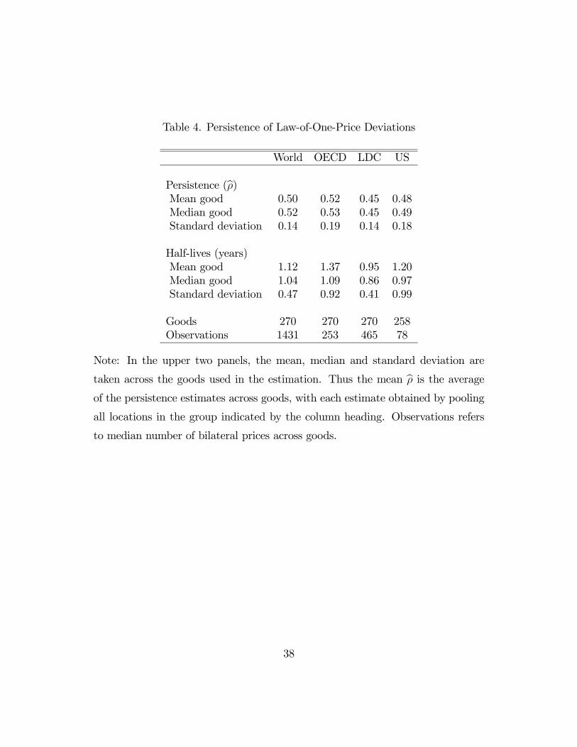
Table 4. Persistence of Law-of-One-Price Deviations

World OECD LDC US

Persistence (bρ)Mean good 0.50 0.52 0.45 0.48Median good 0.52 0.53 0.45 0.49Standard deviation 0.14 0.19 0.14 0.18

Half-lives (years)Mean good 1.12 1.37 0.95 1.20Median good 1.04 1.09 0.86 0.97Standard deviation 0.47 0.92 0.41 0.99

Goods 270 270 270 258Observations 1431 253 465 78

Note: In the upper two panels, the mean, median and standard deviation are

taken across the goods used in the estimation. Thus the mean bρ is the averageof the persistence estimates across goods, with each estimate obtained by pooling

all locations in the group indicated by the column heading. Observations refers

to median number of bilateral prices across goods.

38

Table 5. Persistence of Law-of-One-Price Deviations For Traded and

Non-Traded Goods

World OECD LDC USNon- Non- Non- Non-

Traded traded Traded traded Traded traded Traded traded

Persistence (bρ)Mean 0.49 0.57 0.49 0.63 0.44 0.50 0.48 0.51Median 0.50 0.57 0.50 0.66 0.43 0.50 0.48 0.52Standard deviation 0.13 0.13 0.18 0.17 0.13 0.13 0.17 0.21

Half lives (years)Mean 1.06 1.35 1.20 1.94 0.91 1.10 1.16 1.35Median 1.00 1.23 1.01 1.67 0.83 1.01 0.95 1.07Standard deviation 0.43 0.53 0.77 1.16 0.38 0.48 0.99 0.97

Goods 213 60 210 60 210 60 204 54Observations 1431 1485 253 253 465 545 78 78

Note: See notes to Table 4.

39

Table 6. Persistence of Purchasing Power Parity Deviations

OECD LDC US

Persistence (bρ)Median good 0.51 0.54 0.52

CPI-weights 0.64 0.51 0.45(0.02) (0.02) (0.03)

Equal weights 0.62 0.55 0.61(0.01) (0.01) (0.02)

Common weights 0.77 0.65 0.67(0.01) (0.01) (0.02)

Half-lives (years)Median good 1.01 1.14 1.05

CPI-weights 1.53 1.04 0.86(0.08) (0.05) (0.08)

Equal weights 1.46 1.18 1.39(0.05) (0.03) (0.12)

Common weights 2.71 1.58 1.72(0.17) (0.05) (0.14)

Goods 174 64 191Observations 253 171 78

Note: See notes to Table 4.

40

Table 7. Persistence of Purchasing Power Parity Deviations For Traded and

Non-Traded Aggregates

OECD LDC USNon- Non- Non-

Traded traded Traded traded Traded traded

Persistence (bρ)Median good 0.49 0.64 0.53 0.56 0.49 0.58

CPI-weights 0.68 0.74 0.61 0.68 0.28 0.64(0.01) (0.01) (0.01) (0.01) (0.03) (0.02)

Equal weights 0.60 0.77 0.49 0.61 0.62 0.49(0.01) (0.02) (0.01) (0.01) (0.02) (0.01)

Common weights 0.69 0.83 0.66 0.59 0.37 0.71(0.01) (0.01) (0.01) (0.01) (0.02) (0.01)

Half lives (years)Median good 0.96 1.57 1.08 1.21 0.96 1.27

CPI-weights 1.82 2.32 1.41 1.82 0.54 1.57(0.09) (0.11) (0.05) (0.07) (0.04) (0.09)

Equal weights 1.36 2.68 0.97 1.40 1.43 0.98(0.05) (0.20) (0.03) (0.04) (0.08) (0.04)

Common weights 1.86 3.68 1.69 1.29 0.70 1.99(0.08) (0.32) (0.07) (0.04) (0.04) (0.08)

Goods 139 35 44 20 160 31Observations 253 253 171 171 78 78

Note: See notes to Table 4.

41

Table 8. Persistence of Law-of-One-Price Deviations

Assuming Conditional Convergence (LSDV Estimates)

World OECD LDC USPersistence (bρ)Mean 0.52 0.53 0.51 0.53Median 0.53 0.54 0.52 0.54Standard deviation 0.10 0.13 0.12 0.17

Half-lives (years)Mean 1.05 1.26 1.03 1.34Median 1.07 1.12 1.04 1.12Standard deviation 0.92 0.92 0.98 0.91

Goods 270 270 270 236Observations 1431 253 465 78

Note: See notes to Table 4.

42

Table 9. Persistence of Law-of-One-Price Deviations For Traded and

Non-Traded Goods

(LSDV Estimates)

World OECD LDC UST NT T NT T NT T NT

Persistence (bρ)Mean 0.50 0.58 0.51 0.60 0.49 0.58 0.51 0.62Median 0.51 0.57 0.52 0.61 0.49 0.56 0.53 0.62Standard deviation 0.09 0.10 0.13 0.13 0.11 0.14 0.16 0.16

Half-livesMean 1.05 1.07 1.15 1.65 1.05 0.97 1.20 1.88Median 1.02 1.20 1.07 1.40 0.98 1.18 1.08 1.45Standard deviation 0.29 1.88 0.54 1.63 0.44 1.93 0.73 1.28

Goods 213 60 210 60 210 60 204 54Observations 1431 1485 253 253 465 545 78 78

Note: See notes to Table 4.

43

Figure 1. International and Intranational Price in 2000

0

0.2

0.4

0.6

0.8

1

1.2

1.4

1.6

1.8

2

-2 -1.5 -1 -0.5 0 0.5 1 1.5 2log price deviation from world (U.S.) mean

Traded goods (World)Non-traded goods (World)Traded goods (U.S.)Non-traded goods (U.S.)

Figure 2. Persistence of All Goods

0

0.5

1

1.5

2

2.5

3

3.5

0 0.1 0.2 0.3 0.4 0.5 0.6 0.7 0.8 0.9 1

ρ

WorldOECDLDCU.S.

Figure 3. Persistence of Traded and Non-traded Goods: World and U.S.

0

0.5

1

1.5

2

2.5

3

3.5

0 0.1 0.2 0.3 0.4 0.5 0.6 0.7 0.8 0.9 1

ρ

Traded goods (World)Non-traded goods (World)Traded goods (U.S.)Non-traded goods (U.S.)

Figure 4. Persistence of Traded and Non-traded Goods: OECD and LDCs

0

0.5

1

1.5

2

2.5

3

3.5

0 0.1 0.2 0.3 0.4 0.5 0.6 0.7 0.8 0.9 1

ρ

Traded goods (OECD)Non-traded goods (OECD)Traded goods (LDC)Non-traded goods (LDC)

48

Table A1. List of Individual Goods

Goods-name ρ Goods-name ρ [T] White bread (1 kg) * 0.67 [T] Fresh fish (1 kg) * 0.63[T] Butter (500 g) * 0.38 [T] Instant coffee (125 g) * 0.50[T] Margarine (500g) * 0.45 [T] Ground coffee (500 g) * 0.30[T] White rice (1 kg) * 0.52 [T] Tea bags (25 bags) * 0.48[T] Spaghetti (1 kg) * 0.47 [T] Cocoa (250 g) * 0.51[T] Flour, white (1 kg) * 0.52 [T] Drinking chocolate (500 g) * 0.52[T] Sugar, white (1 kg) * 0.42 [T] Coca-Cola (1 ℓ) * 0.41[T] Cheese, imported (500 g) * 0.53 [T] Tonic water (200 mℓ) * 0.31[T] Cornflakes (375 g) * 0.42 [T] Mineral water (1 ℓ) * 0.54[T] Milk, pasteurized (1 ℓ) * 0.54 [T] Orange juice (1 ℓ) * 0.50[T] Olive oil (1 ℓ) * 0.49 [T] Wine, superior quality (700 mℓ) * 0.56[T] Peanut or corn oil (1 ℓ) * 0.37 [T] Wine, fine quality (700 mℓ) * 0.66[T] Potatoes (2 kg) * 0.35 [T] Beer, local brand (1 ℓ) * 0.59[T] Onions (1 kg) * 0.37 [T] Beer, top quality (330 mℓ) * 0.59[T] Tomatoes (1 kg) * 0.12 [T] Scotch whisky, six years old (700 mℓ) * 0.35[T] Carrots (1 kg) * 0.38 [T] Gin, Gilbey's or equivalent (700 mℓ) * 0.60[T] Oranges (1 kg) * 0.45 [T] Vermouth, Martini & Rossi (1 ℓ) * 0.62[T] Apples (1 kg) * 0.46 [T] Cognac, French VSOP (700 mℓ) * 0.54[T] Lemons (1 kg) * 0.31 [T] Liqueur, Cointreau (700 mℓ) * 0.58[T] Bananas (1 kg) * 0.25 [T] Soap (100 g) * 0.46[T] Lettuce (one) * 0.29 [T] Laundry detergent (3 ℓ) * 0.42[T] Eggs (12) * 0.39 [T] Toilet tissue (two rolls) * 0.54[T] Peas, canned (250 g) * 0.39 [T] Dishwashing liquid (750 mℓ) * 0.60[T] Tomatoes, canned (250 g) * 0.30 [T] Insect-killer spray (330 g) * 0.51[T] Peaches, canned (500 g) * 0.27 [T] Light bulbs (two, 60 watts) * 0.39[T] Sliced pineapples, canned (500 g) * 0.51 [T] Batteries (two, size D/LR20) * 0.56[T] Beef: filet mignon (1 kg) * 0.52 [T] Frying pan (Teflon or good equivalent) * 0.45[T] Beef: steak, entrecote (1 kg) * 0.33 [T] Electric toaster (for two slices) * 0.32[T] Beef: stewing, shoulder (1 kg) * 0.41 [NT] Laundry (one shirt) * 0.44[T] Beef: roast (1 kg) * 0.54 [NT] Dry cleaning, man's suit * 0.52[T] Beef: ground or minced (1 kg) * 0.46 [NT] Dry cleaning, woman's dress * 0.44[T] Veal: chops (1 kg) * 0.45 [NT] Dry cleaning, trousers * 0.62[T] Veal: fillet (1 kg) * 0.35 [T] Aspirins (100 tablets) * 0.32[T] Veal: roast (1 kg) * 0.50 [T] Razor blades (five pieces) * 0.39[T] Lamb: leg (1 kg) * 0.47 [T] Toothpaste with fluoride (120 g) * 0.55[T] Lamb: chops (1 kg) * 0.47 [T] Facial tissues (box of 100) * 0.52[T] Lamb: Stewing (1 kg) * 0.45 [T] Hand lotion (125 mℓ) * 0.54[T] Pork: chops (1 kg) * 0.46 [T] Lipstick (deluxe type) * 0.40[T] Pork: loin (1 kg) * 0.49 [NT] Man's haircut (tips included) 0.50[T] Ham: whole (1 kg) * 0.57 [NT] Woman's cut & blow dry (tips included) 0.52[T] Bacon (1 kg) * 0.59 [T] Cigarettes, Marlboro (pack of 20) * 0.55[T] Chicken: frozen (1 kg) * 0.57 [T] Cigarettes, local brand (pack of 20) * 0.26[T] Chicken: fresh (1 kg) * 0.59 [T] Pipe tobacco (50 g) 0.51[T] Frozen fish fingers (1 kg) * 0.58 [NT] Telephone and line, monthly rental 0.73

49

Table A1. (continued)

Goods-name ρ Goods-name ρ [NT] Telephone, charge per local call (3 min) 0.59 [NT] Visit of four people to a nightclub 0.61[NT] Electricity, monthly bill 0.56 [NT] Four best seats at theatre or concert 0.54[NT] Gas, monthly bill 0.73 [NT] Four best seats at cinema 0.63[NT] Water, monthly bill 0.78 [T] Low priced car (900-1299 cc) * 0.33[NT] Heating oil (100 ℓ) 0.50 [T] Compact car (1300-1799 cc) * 0.42[T] Business suit, two piece, medium weight * 0.73 [T] Family car (1800-2499 cc) * 0.54[T] Business shirt, white * 0.65 [T] Deluxe car (2500 cc upwards) * 0.32[T] Men's shoes, business wear * 0.70 [NT] Yearly road tax or registration fee * 0.44[T] Mens raincoat, Burberry type * 0.63 [NT] Cost of a tune up (but no major repairs) * 0.73[T] Socks, wool mixture * 0.64 [NT] Annual premium for car insurance * 0.62[T] Dress, ready to wear, daytime * 0.64 [T] Regular unleaded petrol (1 ℓ) 0.41[T] Women's shoes, town * 0.65 [NT] Taxi: initial meter charge 0.22[T] Women's cardigan sweater * 0.68 [NT] Taxi rate per additional kilometre 0.48[T] Women's raincoat, Burberry type * 0.69 [NT] Taxi: airport to city centre 0.19[T] Tights, panty hose * 0.50 [NT] Furnished residential apartment: 1 bedroom * 0.74[T] Child's jeans * 0.58 [NT] Furnished residential apartment: 2 bedroom * 0.64[T] Child's shoes, dresswear * 0.54 [NT] Unfurnished residential apartment: 2 bedrooms * 0.64[T] Child's shoes, sportswear * 0.59 [NT] Unfurnished residential apartment: 3 bedrooms * 0.67[T] Girl's dress * 0.52 [NT] Unfurnished residential apartment: 4 bedrooms * 0.60[T] Boy's jacket, smart * 0.71 [NT] Furnished residential house: 3 bedrooms * 0.53[T] Boy's dress trousers * 0.63 [NT] Unfurnished residential house: 3 bedrooms * 0.49[NT] Hourly rate for domestic cleaning help 0.65 [NT] Unfurnished residential house: 4 bedrooms * 0.50[NT] Maid's monthly wages (full time) 0.25 [NT] Business trip, typical daily cost 0.64[NT] Babysitter's rate per hour 0.76 [NT] Hilton-type hotel, single room, 1 night 0.55[T] Compact disc album 0.55 [NT] Moderate hotel, single room, 1 night 0.60[T] Television, colour (66 cm) 0.43 [NT] One drink at bar of first class hotel 0.50[T] Kodak colour film (36 exposures) 0.41 [NT] Two-course meal for two people 0.56[NT] Cost of developing 36 colour pictures 0.67 [NT] Simple meal for one person 0.66[T] International foreign daily newspaper 0.21 [NT] Hire car, weekly rate for lowest classification 0.31[NT] Daily local newspaper 0.55 [NT] Hire car, weekly rate for moderate classification 0.46[T] International weekly news magazine (Time) 0.49 [NT] One good seat at cinema 0.63[T] Paperback novel (at bookstore) 0.65 [NT] Average cost of labor per hour 0.72[NT] Three course dinner for four people 0.61

Notes: Traded and non-traded goods are indicated by T and NT in brackets, respectively. * indicates the good with multiple price observations. GMM estimates of ρ are obtained using all the available countries. Estimates for goods with multiple price observations are averages.