by gregory koch - department of computer sciencegkoch/files/msc-thesis.pdf · abstract siamese...

Siamese Neural Networks for One-Shot Image Recognition

by

Gregory Koch

A thesis submitted in conformity with the requirementsfor the degree of Master of Science

Graduate Department of Computer ScienceUniversity of Toronto

c© Copyright 2015 by Gregory Koch

Abstract

Siamese Neural Networks for One-Shot Image Recognition

Gregory Koch

Master of Science

Graduate Department of Computer Science

University of Toronto

2015

The process of learning good features for machine learning applications can be very computationally

expensive and may prove difficult in cases where little data is available. A prototypical example of this

is the one-shot learning setting, in which we must correctly make predictions given only a single example

of each new class.

In this paper, we explore a method for learning siamese neural networks which employ a unique

structure to naturally rank similarity between inputs. Once a network has been tuned, we can then

capitalize on powerful discriminative features to generalize the predictive power of the network not just

to new data, but to entirely new classes from unknown distributions. Using a convolutional architecture,

we are able to achieve strong results which exceed those of other deep learning models with near state-

of-the-art performance on one-shot classification tasks.

ii

Contents

1 Introduction 1

1.1 Overview . . . . . . . . . . . . . . . . . . . . . . . . . . . . . . . . . . . . . . . . . . . . . . . . . 1

1.2 Related Work . . . . . . . . . . . . . . . . . . . . . . . . . . . . . . . . . . . . . . . . . . . . . . . 2

1.3 Approach . . . . . . . . . . . . . . . . . . . . . . . . . . . . . . . . . . . . . . . . . . . . . . . . . 4

2 The Omniglot Dataset 6

2.1 Overview . . . . . . . . . . . . . . . . . . . . . . . . . . . . . . . . . . . . . . . . . . . . . . . . . 6

2.2 One-Shot Learning Task . . . . . . . . . . . . . . . . . . . . . . . . . . . . . . . . . . . . . . . . . 6

3 Image Verification with Siamese Neural Nets 8

3.1 Overview . . . . . . . . . . . . . . . . . . . . . . . . . . . . . . . . . . . . . . . . . . . . . . . . . 8

3.2 Model Definition . . . . . . . . . . . . . . . . . . . . . . . . . . . . . . . . . . . . . . . . . . . . . 9

3.3 Learning . . . . . . . . . . . . . . . . . . . . . . . . . . . . . . . . . . . . . . . . . . . . . . . . . . 10

3.4 Experimental Results . . . . . . . . . . . . . . . . . . . . . . . . . . . . . . . . . . . . . . . . . . . 11

4 Learning Deep Convolutional Feature Hierarchies 13

4.1 Overview . . . . . . . . . . . . . . . . . . . . . . . . . . . . . . . . . . . . . . . . . . . . . . . . . 13

4.2 Model Definition . . . . . . . . . . . . . . . . . . . . . . . . . . . . . . . . . . . . . . . . . . . . . 14

4.3 Learning . . . . . . . . . . . . . . . . . . . . . . . . . . . . . . . . . . . . . . . . . . . . . . . . . . 14

4.4 Experimental Results . . . . . . . . . . . . . . . . . . . . . . . . . . . . . . . . . . . . . . . . . . . 15

5 Using Verification Networks for One-Shot Image Recognition 17

5.1 Overview . . . . . . . . . . . . . . . . . . . . . . . . . . . . . . . . . . . . . . . . . . . . . . . . . 17

5.2 One-Shot Learning Evaluation on Omniglot . . . . . . . . . . . . . . . . . . . . . . . . . . . . . . 17

5.3 Using Distortions During Evaluation . . . . . . . . . . . . . . . . . . . . . . . . . . . . . . . . . . 20

6 Conclusions 22

6.1 Summary . . . . . . . . . . . . . . . . . . . . . . . . . . . . . . . . . . . . . . . . . . . . . . . . . 22

6.2 Future Work . . . . . . . . . . . . . . . . . . . . . . . . . . . . . . . . . . . . . . . . . . . . . . . 22

Bibliography 24

A Data Generation 26

A.1 Generating One-Shot Tasks . . . . . . . . . . . . . . . . . . . . . . . . . . . . . . . . . . . . . . . 26

A.2 Generating Training Data for Verification . . . . . . . . . . . . . . . . . . . . . . . . . . . . . . . 26

A.3 GPU programming . . . . . . . . . . . . . . . . . . . . . . . . . . . . . . . . . . . . . . . . . . . . 27

A.4 Whetlab . . . . . . . . . . . . . . . . . . . . . . . . . . . . . . . . . . . . . . . . . . . . . . . . . . 27

iii

Chapter 1

Introduction

1.1 Overview

Humans exhibit a strong ability to acquire and recognize new patterns. In particular, we observe that

when presented with stimuli, people seem to be able to understand new concepts quickly and then rec-

ognize variations on these concepts in future percepts [14]. This principle applies more broadly than just

to generalizing to unseen images of a particular concept class. If shown an image of a specific species,

such as a tiger, a person is not only able to use that image to identify new images of tigers, but also

to make educated guesses about images of new species. For instance, we might be able to assert that

a lion is more similar to the tiger than some other mammal. This type of inference can therefore be

very useful but it is not necessarily an inherent property in our models, which may be closely fit to the

available classes without learning useful structure for other classes.

Machine learning has been successfully used to achieve state-of-the-art performance in a variety of

applications such as web search, spam detection, caption generation, and speech and image recognition.

However, these algorithms often break down when forced to make predictions about data for which

little supervised information is available. We desire to generalize to these unfamiliar categories without

necessitating extensive retraining which may be either expensive or impossible due to limited data or in

an online prediction setting, such as web retrieval.

One particularly interesting task is classification under the restriction that we may only observe a

single example of each possible class before making a prediction about a test instance. This is called

one-shot learning and it is the primary focus of our model presented in this work [7, 14]. This should be

distinguished from zero-shot learning, in which the model cannot look at any examples from the target

classes [20].

Children especially display a unique aptitude for one-shot learning. This manifests during the devel-

opment of motor and cognitive skills in early childhood. For example, young children acquire language at

a remarkable rate, learning new words every day without continual reenforcement. In addition, they can

generalize from simple linguistic constructs, developing sophisticated rules about new word categories

from very few or even no examples at all [27].

1

Chapter 1. Introduction 2

Figure 1.1: Learning discriminative features about tigers should help when classifying other felines thatare unfamiliar to the model.

The problem of one-shot learning can be directly addressed by developing domain-specific features

or inference procedures which possess highly discriminative properties for the target task. As a result,

systems which incorporate these methods tend to excel at similar instances but fail to offer robust

solutions that may be generally applied to other types of problems. In this paper, we present a novel

approach which limits assumptions on the structure of the inputs while automatically acquiring features

which enable the model to generalize successfully from few examples. We build upon the deep learning

framework, which uses many layers of non-linearities to capture invariances to transformation in the

input space, usually by leveraging a model with many parameters and then using a large amount of data

to prevent overfitting [2, 9]. These features are very powerful because we are able to learn them without

imposing strong priors, although the cost of the learning algorithm itself may be considerable.

1.2 Related Work

Overall, research into one-shot learning algorithms is fairly immature and has received limited attention

by the machine learning community. There are nevertheless a few key lines of work which precede this

paper.

Although a small handful of researchers addressed one-shot learning in the 1980’s and 1990’s, the

seminal work for using machine learning towards one-shot learning dates back to the early 2000’s [27]. In

[6] and [7], Li Fei-Fei et al. developed a variational Bayesian framework for one-shot image classification

using the premise that previously learned classes can be leveraged to help forecast future ones when very

few examples are available from a given class. This information can be successfully incorporated into

the prior, which is updated when examples from novel classes are observed, and then combined with the

likelihood to yield a new class posterior distribution. The authors specified a generative Constellation

model that has appearance and shape components and identifies distinctive regions of the feature space.


More recently, Lake et al. approached the problem of one-shot learning from the point of view of cog-

nitive science, addressing one-shot learning for character recognition with a method called Hierarchical

Bayesian Program Learning (HBPL) [16]. In a series of several papers, the authors modeled the process

of drawing characters generatively to decompose the image into small pieces [14, 15]. The goal of HBPL

is to determine a structural explanation for the observed pixels. Inference under HBPL is difficult since

the joint parameter space is very large, leading to an intractable integration problem. To circumvent

this, HBPL uses a set of high probability parses which are calculated by a heuristic algorithm. These

provide a point estimate of the posterior distribution, which can be combined with a MCMC approach

to evaluate any test images against the possible categories.

Traditional computer vision methods for one-shot learning usually fall into two fundamental cate-

gories: feature learning and metric learning [1, 12, 8, 28, 10]. For example, Wolf et al. chose to focus on

a metric learning approach using a standard bag of features representation to learn a similarity kernel

for image classification of insects [25]. Wan et al.’s work on gesture recognition problems went in the

other direction by developing a elaborate SIFT-based hierarchical feature extraction algorithm for which

the computed features are given to a nearest-neighbor classifier [24].

Some authors have considered other modalities. Lake et al. also have some very recent work which

uses a generative Hierarchical Hidden Markov model for speech primitives combined with a Bayesian

inference procedure to recognize individual words spoken by different speakers [13]. Maas and Kemp

have some of the only published work using Bayesian networks to predict attributes for Ellis Island pas-

senger data by modifying the conditional distributions at each node to be weighted by a soft indicator

λi [18]. This is the the so-called “concentration parameter” which measures whether the child is a near-

deterministic function of its parents. For certain observations, this allows some attributes to be identified

as crucial for inferring the latent variables of the graph. Wu and Dennis address one-shot learning in the

context of path planning algorithms for robotic actuation [26]. Actuation percepts determined during

the course of learning cannot necessarily be translated immediately to new tasks because environmental

constraints may have changed. The authors introduce a mapping from the learned action template to a

revised template by integrating the distance between these two feature spaces parameterized by the co-

ordinates of the Cartesian distortional space, implictly defining an energy function that can be minimized.

Work in transfer learning across object categories is also relevant for one-shot learning as shown by

Lin et al. [17]. While the authors do not explictly address one-shot learning, they instead focus on how

to “borrow” examples from other classes in the training set. This idea can be useful for data sets where

very few examples exist for some classes, providing a flexible and continuous means of incorporating

inter-class information into the model. The authors introduce a novel loss function which regularizes a

tunable weight vector corresponding to a soft measure of how much each category should borrow from

the current training exemplar.


Figure 1.2: Our general strategy. 1) Train a model to discriminate between a collection of same/differentpairs. 2) Generalize to evaluate new categories based on learned feature mappings for verification.

1.3 Approach

We restrict our attention to character recognition, although the general approach can be replicated

for almost any modality (Figure 1.2). For this domain, we employ large siamese convolutional neural

networks which a) are capable of learning generic image features useful for making predictions about

unknown class distributions even when very few examples from these new distributions are available; b)

are easily trained using standard optimization techniques on pairs sampled from the source data; and c)

provide a competitive approach that does not rely upon domain-specific knowledge by instead exploiting

deep learning techniques.

To develop a model for one-shot image classification, we aim to first learn a neural network that can

discriminate between the class-identity of image pairs, which is the standard verification task for image

recognition. That is, given any two images from the same alphabet (or potentially different alphabets,

although we do not consider this case), this network will predict whether those images depict the same

character.

We hypothesize that networks which do well at at verification should generalize to one-shot clas-

sification. The verification model learns to identify input pairs according to the probability that they

belong to the same class or different classes. This model can then be used to evaluate new images in a

pairwise manner against a lone test image. The pairing with the highest score according to the verifica-

tion network is then awarded the highest probability for the classification task. If the features learned

by the verification model are sufficient to confirm or deny the identity of characters drawn from one set

of alphabets, then they ought to be sufficient for other alphabets, provided that the model has exposed

to a variety of alphabets to encourage variance amongst the learned features.


By additionally choosing a good metric at final layer of the neural network and then imposing certain

constraints on the parameterization, we should be able to learn this sort of representation. Note taht we

do not propose to learn the metric, so our method concentrates solely on feature learning. In general, the

idea is to first learn good representations via a supervised metric-based approach with siamese neural

networks, then reuse that network’s features for one-shot learning without any retraining.

Chapter 2

The Omniglot Dataset

2.1 Overview

The Omniglot data set was collected by Brenden Lake and his collaborators at MIT via Amazon’s Me-

chanical Turk to produce a standard benchmark for learning from few examples in the handwritten

character recognition domain [14].1 Omniglot contains examples from 50 alphabets ranging from well-

established international languages like Latin and Korean to lesser known local dialects. It also includes

some fictitious character sets such as Aurek-Besh and Klingon (Figure 2.1).

The number of letters in each alphabet varies considerably, from about 15 to upwards of 40 charac-

ters. All characters across these alphabets are produced a single time by each of 20 drawers. The total

data set contains a small handful of samples for every possible class of letter; for this reason, the original

authors refer to it as a sort of “MNIST transpose”, where the number of classes far exceeds the number

of training instances [16].

Lake split the data into a 40 alphabet background set and a 10 alphabet evaluation set. We preserve

these two terms in order to distinguish from the normal training, validation, and test sets that can be

generated from the background set in order to tune models for verification. The background set is used

for developing a model by learning hyperparameters and feature mappings. Conversely, the evaluation

set is used only to measure the one-shot classification performance. Throughout this paper, our use of

the terms “background set” and “evaluation set” exactly correspond to those referenced in Lake’s work.

2.2 One-Shot Learning Task

To empirically evaluate one-shot learning performance, Lake developed a 20-way within-alphabet clas-

sification task in which an alphabet is first chosen from among those reserved for the evaluation set,

1The complete data set can be obtained from Brendan Lake by request ([email protected]). Each character inOmniglot is a 105x105 binary-valued image which was drawn by hand on an online canvas. All of the alphabets areavailable in the most recent version of the data set, in addition to the specific one-shot trials used in Lake’s original workand the stroke trajectories collected during the construction of the data set. The stroke trajectories were collected alongside the composite images, so it is possible to incorporate temporal and structural information into models trained onOmniglot.

6

Chapter 2. The Omniglot Dataset 7

Figure 2.1: The Omniglot dataset contains a variety of different images from alphabets across the world.

Figure 2.2: Example of a 20-way one-shot classification task using the Omniglot dataset. The lone testimage is shown above the grid of 20 images representing the possible unseen classes that we can choosefor the test image. These 20 images are our only known examples of each of those classes.

along with twenty characters taken uniformly at random (Figure 2.2). Two of the twenty drawers are

also selected from among the pool of evaluation drawers. These two drawers then produce a sample

of the twenty characters. Each one of the characters produced by the first drawer are denoted as test

images and individually compared against all twenty characters from the second drawer, with the goal

of predicting the class corresponding to the test image from among all of the second drawer’s characters.

This process is repeated twice for all alphabets, so that there are 40 one-shot learning trials for each

of the ten evaluation alphabets. This constitutes a total of 400 one-shot learning trials, from which the

standard classification accuracy is calculated. We specify more details for this generation procedure in

Appendix A.1.

We reproduced this procedure using an identical set of one-shot learning tasks as in [16]. We also

wrote code to generate new one-shot tasks from an arbitrary data set. This allows us to monitor one-shot

learning performance on our validation set while optimizing for the verification task.

Chapter 3

Image Verification with Siamese

Neural Nets

3.1 Overview

Siamese nets were first introduced in the early 1990s by Bromley and LeCun to solve signature verifica-

tion as an image matching problem [3]. A siamese neural network consists of twin networks which accept

distinct inputs but are joined by an energy function at the top. This function computes some metric

between the highest-level feature representation on each side (Figure 3.1). The parameters between the

twin networks are tied.

This strategy has two key properties:

• It ensures the consistency of its predictions. Weight tying guarantees that two extremely similar

images could not possibly be mapped by their respective networks to very different locations in

feature space because each network computes the same function.

• The network is symmetric: if we present two distinct images to the twin networks, the top con-

joining layer will compute the same metric as if we were to we present the same two images but

to the opposite twins.

In LeCun et al., the authors used a contrastive energy function which contained dual terms to de-

crease the energy of like pairs and increase the energy of unlike pairs [4]. However, in this paper we

use the weighted L1 distance between the twin feature vectors h1 and h2 combined with a sigmoid

activation, which maps onto the interval [0, 1]. Thus a cross-entropy objective is a natural choice for

training the network. Note that in LeCun et al., they directly learned the similarity metric, which was

implictly defined by the energy loss, whereas we fix the metric as specified above, following the approach

in Facebook’s DeepFace paper [23].

We now detail both the structure of the siamese nets and the specifics of the learning algorithm used

in our experiments.

8

Chapter 3. Image Verification with Siamese Neural Nets 9

x1,1

...x1,N1

x2,1

...x2,N1

h1,1

...h1,N2

h2,1

...h2,N2

d1

...dN2

p

w(1)1,1

w (1)1,N1

w(1)

3,1

w(1)3,N1

w(1)1,1

w (1)1,N1

w(1)

3,1

w(1)3,N1

w (2)3,1

w(2)

3,N2

Inputlayer

Hiddenlayer

Distancelayer

Outputlayer

Figure 3.1: A simple 2 hidden layer siamese network for binary classification with logistic prediction p.The structure of the network is replicated across the top and bottom sections to form twin networks,with shared weight matrices at each layer.

3.2 Model Definition

Our standard model is a siamese neural network with L fully-connected layers each with Nl units, where

h1,l represents the hidden vector in layer l for the first twin, and h2,l denotes the same for the second

twin. We use exclusively rectified linear (ReLU) units in the first L − 1 layers, so that for any layer

l ∈ {1, . . . , L− 1}:

h1,m = max(0,WTl−1,lh1,(l−1) + bl)

h2,m = max(0,WTl−1,lh2,(l−1) + bl)

where Wl−1,l is the Nl−1 ×Nl shared weight matrix connecting the Nl−1 units in layer l − 1 to the

Nl units in layer l, and bl is the shared bias vector for layer l.

After the (L − 1)th feed-forward layer, we compare the features computed by each twin via a fixed

distance function p = σ(∑

j αj |h(j)1,l −h

(j)2,l |), where σ is the sigmoidal activation function. This final layer

induces a metric on the learned feature space of the (L − 1)th hidden layer and scores the similarity

between the two feature vectors. The αj are additional parameters that are learned by the model

during training, weighting the importance of the component-wise distance. This defines a final Lth

fully-connected layer for the network which joins the two siamese twins. The full architecture is shown

for a small example in Figure 3.1 (above).


3.3 Learning

Loss function. Let M represent the minibatch size, where i indexes the ith minibatch. Now let

y(x(i)1 , x

(i)2 ) be a length-M vector which contains the labels for the minibatch, where we assume y(x

(i)1 , x

(i)2 ) =

1 whenever x1 and x2 are from the same character class and y(x(i)1 , x

(i)2 ) = 0 otherwise. We impose a

regularized cross-entropy objective on our binary classifier of the following form:

L(x(i)1 , x

(i)2 ) = y(x

(i)1 , x

(i)2 ) log p(x

(i)1 , x

(i)2 ) + (1− y(x

(i)1 , x

(i)2 )) log (1− p(x(i)1 , x

(i)2 )) + λT |w|2

Optimization. This objective is combined with standard backpropagation algorithm, where the

gradient is additive across the twin networks due to the tied weights. We fix a minibatch size of 128

with learning rate ηj , momentum µj , and L2 regularization weights λj defined layer-wise, so that our

update rule at epoch T is as follows:

w(T )kj (x

(i)1 , x

(i)2 ) = w

(T )kj + ∆w

(T )kj (x

(i)1 , x

(i)2 ) + 2λj |wkj |

∆w(T )kj (x

(i)1 , x

(i)2 ) = −ηj∇w(T )

kj + µj∆w(T−1)kj

where ∇wkj is the partial derivative with respect to the weight between the jth neuron in some layer

and the kth neuron in the successive layer.

Weight initialization. We drew network weights from a zero-mean normal distribution with a

standard deviation equal to1

fan-in, where we have defined the fan-in as the number of incoming weights

to each neuron in a particular layer of the network. Biases were drawn from a Gaussian with mean 0.5

and a fixed variance of 10−2.

Learning schedule. Although we allowed for a different learning rate for each layer, learning rates

were decayed uniformly across the network by 1 percent per epoch, so that η(T+1)j = 0.99η

(T−1)j . We

found that by annealing the learning rate, the network was able to converge to local minima more

easily without getting stuck in the error surface. We fixed momentum to start at 0.5 in every layer, in-

creasing linearly each epoch until reaching the value µj , the individual momentum term for the jth layer.

We trained each network for a maximum of 300 epochs, but monitored one-shot validation error on a

set of 320 one-shot learning tasks generated randomly from the alphabets and drawers in the validation

set. When the validation error did not decrease for 20 epochs, we stopped and used the parameters of

the model at the best epoch according to the one-shot validation error. If the validation error continued

to decrease for the entire learning schedule, we saved the final state of the model generated by this

procedure.


Figure 3.2: A sample of random affine distortions generated for a single character in the Omniglot dataset.

Affine distortions. In addition, we augmented the training set with small affine distortions (Fig-

ure 3.2). For each image pair x1, x2, we generate a pair of affine transformations T1, T2 to yield

x′1 = T1(x1), x′2 = T2(x2), where T1, T2 are determined stochastically by a multi-dimensional uni-

form distribution. So for an arbitrary transform T , we have T = (θ, ρx, ρy, sx, sy, tx, tx), with θ ∈[−10.0, 10.0], ρx, ρy ∈ [−0.3, 0.3], sx, sy ∈ [0.8, 1.2], and tx, ty ∈ [−2, 2]. Each of these components of the

transformation is included with probability 0.5.

3.4 Experimental Results

For our experiments, we used a three-layer architecture with two fully-connected layers, followed by an

L1 distance metric joining the siamese twins. Then we evaluated a linear combination of the component-

wise distances and mapped the activation to a category with a single sigmoid unit.

To train our verification network, we put together three different data set sizes with 30,000, 90,000,

and 150,000 training examples. We set aside sixty percent of the total data for training: 30 alphabets

out of 50 and 12 drawers out of 20. The Omniglot data set is not setup by default for verification

so we generated our own labeled examples. The essential process consisted of picking two character

classes and two drawers for an alphabet. We then combined these images to form a matching pair and

a non-matching pair. For more details, see Appendix A.2.

We fixed a uniform number of training examples per alphabet so that each alphabet receives equal

representation during optimization, although this is not guaranteed to the individual character classes

within each alphabet. By adding affine distortions, we also produced an additional copy of the data

set corresponding to the augmented version of each of these sizes. We added eight transforms for each

training example, so the corresponding data sets have 270,000, 810,000, and 1,350,000 effective examples.

To monitor performance during training, we used two strategies. First, we created a validation set for

verification with 10,000 example pairs taken from 10 alphabets and 4 additional drawers. We reserved

the last 10 alphabets and 4 drawers for testing, where we constrained these to be the same ones used


in Lake et al. [16]. This set test has 10,000 example pairs from the remaining 10 alphabets and 4 drawers.

Our other strategy leveraged the same alphabets and drawers to generate a set of 320 one-shot recog-

nition trials for the validation set which mimic the target task on the evaluation set. There was an

approximate correspondance between this one-shot validation metric and actual performance (Figure

5.1); we discuss one-shot performance in more detail in Chapter 5. This method of determining when

to stop was at least as effective as using the validation error for the verification task so we used it as our

primary termination criterion as described in the previous section.

In the table below (Table 3.1), we list the final verification results for each of the six possible training

sets, where the listed test accuracy is reported at the best validation checkpoint and threshold. These

six networks were selected by maximizing one-shot validation accuracy using Whetlab, a Bayesian hy-

perparameter optimization framework, although we omit the details of this procedure to Appendix A.4

[5].

Test

(2-layer)

Test

(3-layer)

Test

(4-layer)

30k training

no distortions 68.52 70.40 70.65

affine distortions x8 72.56 72.88 73.14

90k training



150k training



Table 3.1: Accuracy on Omniglot verification task (siamese neural net)

We found that 3-layer networks provided solid performance without overfitting; this was only achieved

with large data set sizes, heavy L2 regularization, and data augmentation. Fully-connected networks of

this type that were larger than 3 layers provided diminishing returns and did not learn noticeably better

features. However, our work was fairly limited in this category and we did not select the number of layers

or neuron configurations (e.g. - activation function) with our automatic hyperparameter selection, which

is a possible improvement for future runs. The best result among these networks was 80.84 percent with

a 512-2056-1 network.

Chapter 4

Learning Deep Convolutional

Feature Hierarchies

4.1 Overview

So far, we have restricted ourselves to a standard feedforward architecture using tied weights on each side

of the siamese network, but with all neurons attached indiscriminatively without any local connectivity.

Here, we describe a straightforward extension of the model presented in the previous section to include

convolutional layers. Convolutional neural networks have achieved top-level results in many large-scale

computer vision applications, particularly in image recognition tasks [2, 11, 21, 22]. Several factors make

convolutional networks especially appealing:

1. Local connectivity can greatly reduce the number of parameters in the model, which inherently

provides some form of built-in regularization, although convolutional layers are computationally

more expensive than standard nonlinearities.

2. For the image recognition tasks that we are primarily concerned with, convolutional networks

offer a particularly appealing interpretation since the convolution operation has a direct filtering

interpretation, where each feature map is convolved against input features to identify patterns as

groupings of pixels. Thus, the outputs of each convolutional layer correspond to important spatial

features in the original input space and offer some robustness to simple affine transformation.

3. Very fast, optimized libraries using modern GPU techniques are now available in order to build

large convolutional networks without an unacceptable amount of training time [19, 11, 21].

In the one-shot learning setting, we need to be able to handle hundreds or even thousands of new

classes without further training. If we do not choose to explictly include additional structure to the model,

it is essential that the features are very strong and are at least in part independent of any particular

class distributions in the training set. By first learning deep convolutional networks which perform

discrimination for the image verification task, we can acquire useful spatial features for classification and

translate these powerful hierarchies for one-shot learning. This is our approach in the next two chapters.

13

Chapter 4. Learning Deep Convolutional Feature Hierarchies 14

Figure 4.1: Best convolutional architecture selected for verification task. Siamese twin is not depicted,but joins immediately after the 4096 unit fully-connected layer where the L1 component-wise distancebetween vectors is computed.

4.2 Model Definition

We use a fairly conventional convolutional architecture which is replicated across each twin of the siamese

network. The model consists of a sequence of convolutional layers, each of which uses a single channel

with filters of varying size and a fixed stride of 1. The number of convolutional filters is specified as a

multiple of 16 to provide better performance in the GPU kernels. The network applies a ReLU activation

function to the output feature maps, optionally followed by max-pooling with a filter size and stride of

2. Thus the kth filter map in each layer takes the following form:

h(k)1,m = max-pool(max(0,W

(k)l−1,l ? h1,(l−1) + bl), 2)

h(k)2,m = max-pool(max(0,W

(k)l−1,l ? h2,(l−1) + bl), 2)

where Wl−1,l is the 3-dimensional tensor representing the feature maps for layer l and we have taken

? to be the valid convolutional operation corresponding to returning only those output units which were

the result of complete overlap between each convolutional filter and the input feature maps.

The units in the final convolutional layer are flattened into a single vector. This convolutional layer

is followed by a fully-connected layer, and then one more layer computing the induced distance metric

between each siamese twin, which is given to a single sigmoidal output unit. The details for the fully-

connected layer and distance metric are described in Chapter 3.

We depict one example above (Figure 4.1), which shows the largest version of our model that we

considered. This network also gave the best result for any network on the verification task.

4.3 Learning

Our learning procedure is identical to the one described in the previous section for training fully-

connected siamese networks with only a few minor modifications.

One of the primary differences for our convolutional networks is that we used a fixed weight ini-

tialization scheme regardless of the number of units in each layer of the network rather than using the

fan-in. We initialized all network weights in the convolutional layers from a normal distribution with


Figure 4.2: Examples of first-layer convolutional filters learned by the siamese network. Notice filtersadapt different roles: some look for very small point-wise features whereas others function like larger-scaleedge detectors.

zero-mean and a standard deviation of 10−2. Biases were also initialized from a normal distribution, but

with mean 0.5 and standard deviation 10−2. In the fully-connected layers, the biases were initialized

in the same way as the convolutional layers, but the weights were drawn from a much wider normal

distribution with zero-mean and standard deviation 2× 10−1.

For larger networks, we limited training to 200 epochs rather than 300 epochs since training time for

convolutional networks can be considerably longer.

4.4 Experimental Results

To fit our convolutional siamese networks, we used the same training, validation, and test splits that

were described in Chapter 3. Table 4.1 compares 6-layer convolutional networks for this task on that

data. Following our approach with regular siamese neural nets, we use Whetlab to select hyperparam-

eters for some key aspects of the model, such as learning rate, momentum, and the number and size of

the convolutional filters (Appendix A.4).

In Figure 4.2, we have extracted the first 32 filters from both of our top two performing networks

on the verification task, which were trained on the 90k and 150k data sets with affine distortions and

the architecture shown in Figure 4.1. While there is some co-adaptation between filters, it is easy to see

that some of the filters have assumed different roles with respect to the original input space.

We also created visualizations which map the training and test sets into the lower-dimensional feature

spaces in which we compute distances and make predictions with the network. The first histogram shows

how the siamese network learns to push apart the aggregate distance assigned to each training instance

depending on its label (Figure 4.3). The second histogram shows the distribution and magnitude of

predictions for all of the data points belonging to either class in the test set (Figure 4.4).


Figure 4.3: Left: Before training. Initially the distance is roughly in the middle depending on the weightinitialization of the convolutional network, but there is no clear pattern to the distances between thecomputed siamese twin feature vectors. Right: After training. (blue: y=1, same; red: y=0, different).Note that since this distance is weighted and activated by a sigmoid, the network is only indirectlymotivated to fully separate these distributions.

Figure 4.4: Left: Before training. Right: After training. Once optimized, the verification network notonly achieves high accuracy but exhibits a considerable degree of confidence in its predictions on thetest set (blue: y=1, same; red: y=0, different).

Test

(6-layer)

30k training

no distortions 90.61

affine distortions x8 91.90

90k training



150k training



Table 4.1: Accuracy on Omniglot verification task (siamese convolutional neural net)

Chapter 5

Using Verification Networks for

One-Shot Image Recognition

5.1 Overview

Once we have optimized a siamese network to master the verification task, we are ready to demonstrate

the discriminative potential of our learned features at one-shot learning. Recall that given a pair of

images, our siamese network outputs a prediction p ∈ [0, 1]. When making predictions for verification,

we thresholded this value by selecting an optimal cutoff point on the validation set so that it would

correspond to a binary label. However, we no longer need to concern ourselves with these semantics and

can just use the value as an unnormalized probability.

Suppose we are given a test image x, some column vector which we wish to classify into one of C

categories. We are also given some other images {xc}Cc=1, a set of column vectors representing examples

of each of those C categories. We can now query the network using x,xc as our input for a range of

c = 1, . . . , C.1 Then predict the class corresponding to the maximum similarity.

C∗ = argmaxcp(c)

Although the network has never seen any of the classes before, it will nevertheless be able to output

its confidence that each pair of images have been drawn from the same class distribution. If the features

learned for performing verification are sufficient for character recognition in general, then it should not

matter that we are testing on unknown classes.

5.2 One-Shot Learning Evaluation on Omniglot

Finally, we ran our models on the one-shot task for the evaluation set that was outlined in Chapter

2. It is prudent to gain some intuition for the one-shot task itself. To give a sense of the character of

our best model’s predictions, we have included two sample one-shot trials along with the top-5 predic-

1This can be processed efficiently by appending C copies of x into a single matrix X and stacking xTc in rows to form

another matrix XM so that we can perform just one feedforward pass with minibatch size C using input X,XC .

17

Chapter 5. Using Verification Networks for One-Shot Image Recognition 18

Figure 5.1: Examples of the model’s top-5 classification performance on 1-versus-20 one-shot classifica-tion tasks.

tions returned by the network (Figure 5.1). We include a graph depicting the optimization of one of

the convolutional networks on the 30k training set with affine transforms over 300 epochs (Figure 5.2).

Here, we see that one-shot validation accuracy is a good approximation to the desired one-shot evalu-

ation accuracy. In this example, we monitored both during a run of a convolutional network (6-layer,

30k training set with 8x global distortions), where only the one-shot validation accuracy was used for

training purposes.

We now present the final comparison of one-shot results (Table 5.3).2 We borrow the baseline results

from [16] for comparison to our two methods. We use the term ‘Regular’ to describe the standard 400

one-shot trial task on the evaluation set. ‘Distortions’ uses some k transforms to the test image and l

transforms to the 20 training images, which is described in more detail in the next section.

2HBPL - Hierarchical Bayesian Program Learning, Affine - models image variance as affine transformations, DBM -pre-trained Deep Boltzmann Machine with 3 layers of 1000 units each, HD - pre-trained Hierarchical Deep model, a hybridDBM/nonparametric Bayesian approach, SS - Simple Strokes, a simplified version of HBPL, 1-NN - 1-nearest-neighborwith cosine similarity metric.


Figure 5.2: One-shot validation and evaluation accuracy measured over the course of training a deepconvolutional siamese network on 30,000 training examples with 8x affine distortions on the inputs. Wealso include the training and validation curves for verification.

Our non-convolutional method fares no better than the majority of the other methods, but at 92

percent our convolutional method is stronger than any model except HBPL itself. which is only slightly

behind human error rates. We have excluded our result that used distortions at test time since this is a

more advanced testing procedure than those used by the other models. While HBPL performs slightly

better overall, our top-performing convolutional network did not include any extra prior knowledge about

characters or strokes such as generative information for drawing.

Regular Distortions

30k training

no distortions 41.0 47.8

affine distortions x8 50.3 54.0

90k training



150k training



Table 5.1: One-shot accuracy on evaluation set,

non-convolutional siamese nets (3-layer).

Regular Distortions

30k training



90k training



150k training



Table 5.2: One-shot accuracy on evaluation set,

convolutional siamese nets (6-layer).


Regular

Humans 95.5

HBPL 95.2

Affine 81.8

HD 65.2

DBM 62.0

SS 35.2

1-NN 21.7

Siamese Neural Net 58.3

Convolutional Siamese Net 92.0

Table 5.3: Comparing best one-shot accuracy from each type of network against baselines.

5.3 Using Distortions During Evaluation

Verification networks leverage several layers of learned features with a distance metric over the highest

level of those features. It is well-known that the prevalence of objects with similar properties generally

increases in proportion with the total number of classes [17]. Therefore, due to the differences in indi-

vidual drawers over large data sets, it is possible that a certain pair representing a similar but incorrect

character class could score highest under the learned model. This pair corresponds to a false positive

classification, which is an incorrect one-shot decision.

One strategy to reduce the variance in our one-shot predictions is to artificially generate more ex-

amples for ourselves at test time. We introduce an algorithm which applies some k affine transforms to

the test image, as well as l transforms to each available character from the various classes that we have

to choose from. For each of the k transforms, we start a new one-shot trial, then take the most frequent

prediction over all k+1 of these trials. Now for each of the l transforms, we add another 20l possibilities

to our pairwise evaluation so that the task becomes a 1-of-20(l+1) classification problem. This performs

two different types of model averaging. We did not have success with any further attempts to leverage

this strategy, such as using the mode of the top-5 rankings for a one-shot trial. This algorithm is outlined

with a simple example in Figure 5.3. For the purpose of illustration, we pose the original scenario as a

1-of-3 classification problem.

Our results indicate that this method provides a small boost to one-shot performance (Table 5.1/5.2),

although the algorithm takes longer to evaluate and therefore is less practical in real-time applications,

especially as k and l grow in size. We monitored one-shot accuracy on our validation split from the

background set to choose k, l, and the parameter vector governing each affine transformation. Typical

best values of k and l ranged from 3 to 7. The selected affine transforms were generally smaller than the

transforms that we used the augment the training set for learning verification networks.


Figure 5.3: Applying k = 3 affine distortions to the image that we wish to classify is a good way ofaveraging model predictions. Within each trial, we can do the same procedure for some l = 3 distortionsof the single examples from each class.

Chapter 6

Conclusions

6.1 Summary

We have presented a strategy for performing one-shot classification by first learning deep convolutional

siamese neural networks for verification. We outlined new results comparing the performance of our

networks to an existing state-of-the-art classifier developed for the Omniglot data set. Our networks

outperform all available baselines by a significant margin and come close to the best numbers achieved

by the previous authors. We have argued that the strong performance of these networks on this task

indicate not only that human-level accuracy is possible with our metric learning approach, but that this

approach should extend to one-shot learning tasks in other domains, especially for image classification.

6.2 Future Work

Although we have been able to come within a reasonable margin of humans and HBPL on the Omniglot

data set, we believe that closing this gap is more than possible by applying additional ideas from the

literature and expanding the scale of our convolutional networks. Most importantly, the largest neural

networks in this work consist of only five or six layers, only three or four of which are convolutional. This

is a similar depth to Krizhevsky et al.’s winning network for the ImageNet LSVRC-2010 competition,

but still constitutes a relatively shallow architecture compared to the convolutional networks ranging

up to 19 layers in Oxford’s VGGnet [11, 21]. The limitation on our work can mostly be attributed

to computational time, especially in the expensive hyperparameter tuning step, rather than any other

fundamental issue with increasing model capacity. Furthermore, we have not applied any sort of dropout

to regularize our networks, which we believe is a very promising source of future improvement, especially

as we continue to increase the size of the networks we train [22].

We are also interested in experimenting with a contrastive hinge loss to compare its performance with

our cross-entropy, where we would consider some function of the form max(0, α− dpos + dneg), where α

is a tunable hyperparameter, dpos is the distance between two images of the same class, and dneg is the

distance between two images of different classes. Unlike the smooth behavior of the cross-entropy loss,

this would instead encourage the network to focus only on adjusting its predictions if either the distance

between similar examples was large or the distance between different examples was small.

22

Chapter 6. Conclusions 23

Figure 6.1: Columns depict characters sampled from different drawers. Row 1: original images. Row 2:global affine transforms. Row 3: affine transforms on strokes. Row 4: global affine transforms layeredon top of stroke transforms. Notice how stroke distortions can add noise and affect the spatial relationsbetween individual strokes.

In this paper, we only considered training for the verification task by processing image pairs and their

distortions using a global affine transform. We have been experimenting with an extended algorithm

that exploits the data about the individual stroke trajectories to inform the final computed distortions

(Figure 6.1). By imposing local affine transformations on the strokes and overlaying them into a com-

posite image, we are hopeful that we can learn features which are better adapted to the variations that

are commonly seen in new examples.

One final area of particular importance is extending our approach to other data sets, since we believe

that our success on Omniglot can translate to other one-shot learning tasks. The next logical step is

to find new data which is either immediately amenable to one-shot learning, or from which we can

construct new one-shot experiments, and then train a similar version of our model. For example, due

to the use of convolutional features, we believe our approach is immediately applicable to any other

image recognition problem, such as one-shot facial recognition. We can also evaluate the ability of our

learned features to be useful across data sets and tasks, but within the same modality. For example, in

the character recognition domain, we could train a regular convolutional network on MNIST for a very

long time, then extract the features and fine-tune for the Omniglot verification task, or vice-versa, using

Omniglot features to pretrain for MNIST. This would provide a measure of the generalization capacity

of the features learned by our deep siamese networks.

Bibliography

[1] Aurelien Bellet, Amaury Habrard, and Marc Sebban. A survey on metric learning for feature vectors and

structured data. arXiv preprint arXiv:1306.6709, 2013.

[2] Yoshua Bengio. Learning deep architectures for ai. Foundations and Trends in Machine Learning, 2(1):1–127,

2009.

[3] Jane Bromley, James W Bentz, Leon Bottou, Isabelle Guyon, Yann LeCun, Cliff Moore, Eduard Sackinger,

and Roopak Shah. Signature verification using a siamese time delay neural network. International Journal

of Pattern Recognition and Artificial Intelligence, 7(04):669–688, 1993.

[4] Sumit Chopra, Raia Hadsell, and Yann LeCun. Learning a similarity metric discriminatively, with applica-

tion to face verification. In Computer Vision and Pattern Recognition, 2005. CVPR 2005. IEEE Computer

Society Conference on, volume 1, pages 539–546. IEEE, 2005.

[5] Katharina Eggensperger, Matthias Feurer, Frank Hutter, James Bergstra, Jasper Snoek, Holger Hoos, and

Kevin Leyton-Brown. Towards an empirical foundation for assessing bayesian optimization of hyperparam-

eters. In NIPS workshop on Bayesian Optimization in Theory and Practice, 2013.

[6] Li Fe-Fei, Robert Fergus, and Pietro Perona. A bayesian approach to unsupervised one-shot learning of

object categories. In Computer Vision, 2003. Proceedings. Ninth IEEE International Conference on, pages

1134–1141. IEEE, 2003.

[7] Li Fei-Fei, Robert Fergus, and Pietro Perona. One-shot learning of object categories. Pattern Analysis and

Machine Intelligence, IEEE Transactions on, 28(4):594–611, 2006.

[8] Matthieu Guillaumin, Jakob Verbeek, and Cordelia Schmid. Is that you? metric learning approaches for

face identification. In Computer Vision, 2009 IEEE 12th International Conference on, pages 498–505. IEEE,

2009.

[9] Geoffrey Hinton, Simon Osindero, and Yee-Whye Teh. A fast learning algorithm for deep belief nets. Neural

computation, 18(7):1527–1554, 2006.

[10] Erik Hjelmas and Boon Kee Low. Face detection: A survey. Computer vision and image understanding,

83(3):236–274, 2001.

[11] Alex Krizhevsky, Ilya Sutskever, and Geoffrey E Hinton. Imagenet classification with deep convolutional

neural networks. In Advances in neural information processing systems, pages 1097–1105, 2012.

[12] Brian Kulis. Metric learning: A survey. Foundations and Trends in Machine Learning, 5(4):287–364, 2012.

[13] Brenden M Lake, Chia-ying Lee, James R Glass, and Joshua B Tenenbaum. One-shot learning of generative

speech concepts. Cognitive Science Society, 2014.

[14] Brenden M Lake, Ruslan Salakhutdinov, Jason Gross, and Joshua B Tenenbaum. One shot learning of

simple visual concepts. In Proceedings of the 33rd Annual Conference of the Cognitive Science Society,

volume 172, 2011.

24

Bibliography 25

[15] Brenden M Lake, Ruslan Salakhutdinov, and Joshua B Tenenbaum. Concept learning as motor program

induction: A large-scale empirical study. In Proceedings of the 34th Annual Conference of the Cognitive

Science Society, pages 659–664, 2012.

[16] Brenden M Lake, Ruslan R Salakhutdinov, and Josh Tenenbaum. One-shot learning by inverting a compo-

sitional causal process. In Advances in neural information processing systems, pages 2526–2534, 2013.

[17] Joseph Jaewhan Lim. Transfer learning by borrowing examples for multiclass object detection. Master’s

thesis, Massachusetts Institute of Technology, 2012.

[18] Andrew Maas and Charles Kemp. One-shot learning with bayesian networks. Cognitive Science Society,

2009.

[19] Volodymyr Mnih. Cudamat: a cuda-based matrix class for python. 2009.

[20] Mark Palatucci, Dean Pomerleau, Geoffrey E Hinton, and Tom M Mitchell. Zero-shot learning with semantic

output codes. In Advances in neural information processing systems, pages 1410–1418, 2009.

[21] Karen Simonyan and Andrew Zisserman. Very deep convolutional networks for large-scale image recognition.

arXiv preprint arXiv:1409.1556, 2014.

[22] Nitish Srivastava. Improving neural networks with dropout. Master’s thesis, University of Toronto, 2013.

[23] Yaniv Taigman, Ming Yang, Marc’Aurelio Ranzato, and Lior Wolf. Deepface: Closing the gap to human-

level performance in face verification. In Computer Vision and Pattern Recognition (CVPR), 2014 IEEE

Conference on, pages 1701–1708. IEEE, 2014.

[24] Jun Wan, Qiuqi Ruan, Wei Li, and Shuang Deng. One-shot learning gesture recognition from rgb-d data

using bag of features. The Journal of Machine Learning Research, 14(1):2549–2582, 2013.

[25] Lior Wolf, Tal Hassner, and Yaniv Taigman. The one-shot similarity kernel. In Computer Vision, 2009

IEEE 12th International Conference on, pages 897–902. IEEE, 2009.

[26] Di Wu, Fan Zhu, and Ling Shao. One shot learning gesture recognition from rgbd images. In Computer

Vision and Pattern Recognition Workshops (CVPRW), 2012 IEEE Computer Society Conference on, pages

7–12. IEEE, 2012.

[27] Kenneth Yip and Gerald Jay Sussman. Sparse representations for fast, one-shot learning. 1997.

[28] Kin Choong Yow and Roberto Cipolla. Feature-based human face detection. Image and vision computing,

15(9):713–735, 1997.

Appendix A

Data Generation

A.1 Generating One-Shot Tasks

In this section, we provide the pseudocode for the general procedure of generating 20-way one-shot learning

tasks from an arbitrary data set. Assume that we have a collection of alphabets indexed by characters and

drawers which form this data set. Further assume that we can use any of the characters or drawers from an

alphabet without restriction. The following procedure sets up two fields in the dictionary trials: testImgs and

trainingImgs.

function generateOneshotTrials()

1 alph = randint(data.length, 1) // Draw an alphabet2 characters = randint(data[alph].length, 20) // Draw 20 distinct characters3 drawers = randint(20, 2) // Draw 2 distinct drawers4 // Now collect together 20 images for each drawer, defining 20 trials over this alphabet5 for i ∈ {0, 19} do6 trials[testImgs].append(data[alph][characters[i]][drawers[0]])7 trials[trainingImgs].append(data[alph][characters[i]][drawers[1]])

end8 return trials

Algorithm 1: One-shot task generation procedure

Once trials has been generated, iterate through each image in trials[testImgs] and compare against the

twenty images in trials[trainingImgs] to perform twenty one-shot trials. This can be repeated for as many

alphabets as desired. We recommend generating a .mat file with all of the one-shot trials specified, since this

both makes it easy to share a certain one-shot task with collaborators, as well as prevents extra computation

either during training or at test time.

A.2 Generating Training Data for Verification

We now provide pseudocode to generate a balanced training set of image pairs for verification with a uniform

number of examples from each alphabet. Assume that we have a collection of alphabets indexed by characters

and drawers which form this data set. The following procedure sets up an array data, where the first row contains

the first image of each pair and the second row has the second image.

26

Appendix A. Data Generation 27

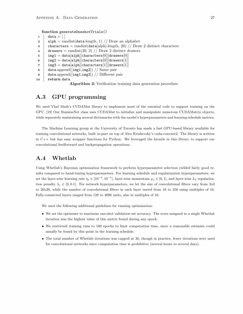
function generateOneshotTrials()

1 data = [ ]2 alph = randint(data.length, 1) // Draw an alphabet3 characters = randint(data[alph].length, 20) // Draw 2 distinct characters4 drawers = randint(20, 2) // Draw 2 distinct drawers5 img1 = data[alph][characters[0]][drawers[0]]6 img2 = data[alph][characters[0]][drawers[1]]7 img3 = data[alph][characters[1]][drawers[1]]8 data.append([img1,img2]) // Same pair9 data.append([img1,img3]) // Different pair

10 return dataAlgorithm 2: Verification training data generation procedure

A.3 GPU programming

We used Vlad Mnih’s CUDAMat library to implement most of the essential code to support training on the

GPU. [19] Our SiameseNet class uses CUDAMat to initialize and manipulate numerous CUDAMatrix objects,

while separately maintaining several dictionaries with the model’s hyperparameters and learning schedule metrics.

The Machine Learning group at the University of Toronto has made a fast GPU-based library available for

training convolutional networks, built in-part on top of Alex Krizhevsky’s cuda-convnet2. The library is written

in C++ but has easy wrapper functions for Python. We leveraged the kernels in this library to support our

convolutional feedforward and backpropagation operations.

A.4 Whetlab

Using Whetlab’s Bayesian optimization framework to perform hyperparameter selection yielded fairly good re-

sults compared to hand-tuning hyperparameters. For learning schedule and regularization hyperparameters, we

set the layer-wise learning rate ηj ∈ [10−4, 10−1], layer-wise momentum µj ∈ [0, 1], and layer-wise L2 regulariza-

tion penalty λj ∈ [0, 0.1]. For network hyperparameters, we let the size of convolutional filters vary from 3x3

to 20x20, while the number of convolutional filters in each layer varied from 16 to 256 using multiples of 16.

Fully-connected layers ranged from 128 to 4096 units, also in multiples of 16.

We used the following additional guidelines for running optimization:

• We set the optimizer to maximize one-shot validation set accuracy. The score assigned to a single Whetlab

iteration was the highest value of this metric found during any epoch.

• We restricted training runs to 100 epochs to limit computation time, since a reasonable estimate could

usually be found by this point in the learning schedule.

• The total number of Whetlab iterations was capped at 30, though in practice, fewer iterations were used

for convolutional networks since computation time is prohibitive (several hours to several days).

by gregory koch - department of computer sciencegkoch/files/msc-thesis.pdf · abstract siamese...

Documents