This PDF is a selection from an out-of-print volume from the National Bureauof Economic Research

Volume Title: Business Cycles: Theory, History, Indicators, and Forecasting

Volume Author/Editor: Victor Zarnowitz

Volume Publisher: University of Chicago Press

Volume ISBN: 0-226-97890-7

Volume URL: http://www.nber.org/books/zarn92-1

Conference Date: n/a

Publication Date: January 1992

Chapter Title: Major Macroeconomic Variables and Leading Indexes

Chapter Author: Victor Zarnowitz

Chapter URL: http://www.nber.org/chapters/c10383

Chapter pages in book: (p. 357 - 382)

12 Major Macroeconomic Variablesand Leading Indexes

12.1 Background and Objectives

How the economy moves over time depends on its structure, institutions,and policies, all of which are subject to large historical changes. It would besurprising if the character of the business cycle did not change in response tosuch far-reaching developments as the Great Contraction of the 1930s and thepost-Depression reforms, the expansion of government and private serviceindustries, the development of fiscal and other built-in stabilizers, and theincreased use and role of discretionary macroeconomic policies. It is consist­ent with our priors that the data for the United States and other developedmarket-oriented countries generally support the hypothesis that business con­tractions were less frequent, shorter, and milder after World War II than before(R. 1. Gordon 1986; see chapter 3).

Although business cycles have moderated, they retain a high degree of con­tinuity, which shows up most clearly in the comovements and timing se­quences among the main cyclical processes. 1 An important aspect of this con­tinuity is the role of the variables that tend to move ahead of aggregate outputand employment in the course of the business cycle. The composite index ofleading indicators combines the main series representing these variables. Sev­eral studies point to the existence of a relatively close and stable relationshipbetween prior changes in this index and changes in macroeconomic activity(Vaccara and Zamowitz 1977; Auerbach 1982; Zarnowitz and Moore 1982;Diebold and Rudebusch 1989). Yet, the currently popular, small reduced-form

This chapter is co-authored with PhillIp Braun and is reprinted from Analyzing Modern Busi­ness Cycles: Essays Honoring Geoffrey H. Moore, ed. P. A. Klein, chap. 11 (Armonk, NY:M. E. Sharpe, 1990).

1. For assessments and references concerning the U.S. record, see Moore 1983, chs. 10 and24; and Zarnowitz and Moore 1986.

357

358 Chapter Twelve

macro models make little or no use of the leading indicators. 2 We suspect thatthe reason is lack of familiarity. The role of the indicators is probably oftenmisperceived as being purely symptomatic. Heterogeneous combinations ofsuch series resist easy theoretical applications. On a deeper level, the notionthat the private market economy is inherently stable led to an emphasis on therole of the monetary and fiscal disturbances. Interest in the potential of stabi­lization policies had a similar effect in that it stimulated work on models dom­inated by factors considered to be amenable to government control.

This orientation is understandably appealing but can easily become one­sided and error-prone, both theoretically and statistically. For example, asimple vector autoregressive (VAR) model in log differences of real GNP,money, and government expenditures suggests the presence of strong laggedmonetary and fiscal effects on output. 3 However, it is easy to show that theserelationships are definitely misspecified. One way to demonstrate this is byadding changes in a leading index that excludes monetary and financial com­ponents so as not to overlap any of the other variables. In this expandedmodel, the dominant effects on output come from the past movements of theleading index, while the roles of the other variables (including the laggedvalues of output growth itself) are greatly reduced (see sec. 12.4). In general,omitting relevant variables in a VAR will cause the standard exogeneity tests,impulse responses, and variance decompositions to be biased, as shown inLiitkepohl1982 and Braun and Mittnik 1985.

The first objective of this chapter is to examine the lead-lag interactionswithin larger sets of important macroeconomic variables, including interestand inflation rates along with output, monetary, and fiscal variables, and anonduplicative leading index. The rationale for including this index is two­fold: (1) The changes in the leading index can be interpreted broadly as rep­resenting the early collective outcomes of investment and production (also,less directly, consumption) decisions. As such, they presumably reflect thedynamic forces that shape the basic processes within the private economy andaccount for the continuity of business cycles. Both aggregate demand andaggregate supply shifts are involved, but the demand effects may be strongerin the short run. (2) The addition of the leading index helps us overcome thebias due to the omitted variables. The index stands for a number of importantfactors that would otherwise be omitted. It would not be practical to includethe several individual series to represent these variables.

We work with equations that include up to six variables plus constant termsand time trends. They are estimated on quarterly series, each taken with fourlags, which means using up large numbers of degrees of freedom. Given thesize of the available data samples, it is not possible for such models to accom­modate more variables and still retain a chance to produce estimates of param-

2. Large econometric models incorporate some individual indicators but probably suboptimallyand not in a comprehensive and systematic way.

3. This recalls the old St. Louis Fed model with its reliance on Hpolicy variables" only.

359 Major Macroeconomic Variables and Leading Indexes

eters in which one could have some confidence. It is, of course, easy to thinkof additional, possibly important variables whose omission might cause someserious misspecifications. All VAR models face this dilemma, but the onlyway to avoid it is by assuming a full structural model, which could be stillmore deficient. We seek some partial remedies in alternative specificationsguided by economic theory and history as well as comparisons with relatedresults in the literature.

Although the format adopted is that of a VAR model, the implied system­wide dynamics (i.e., impulse response functions and variance decomposi­tions) are beyond the scope of this study. These statistics seek to describebehavior in reaction to innovations, require longer series of consistent datathan are actually available,4 and are probably often very imprecise even forsmaller systems (see Zellner 1985 and Runkle 1987 with discussion). In con­trast, there is sufficient information to estimate the individual equations well,even with more lagged terms. We find that much can be learned from attentionto the quality and implications of these estimates, which are logically prior toinferences on overall dynamics but carry no commitment to the particular in­terpretations of a VAR model.

The second and related objective is to extend the analysis to the periodsbetween the two world wars and earlier in another effort to study the conti­nuity and change in U. S. business cycles. To evaluate any persistent shifts orthe secular evolution in the patterns of macroeconomic fluctuation, it is ofcourse necessary to cover long stretches of varied historical experience. Esti­mates of the interrelations among the selected variables are calculated fromquarterly seasonally adjusted data for three periods: 1886-1914, 1919-40,and 1949-82. Generally, we look for the similarities and differences withinthe three periods that are suggested by this exercise.

Historical data are scanty and deficient, which inevitably creates some dif­ficult choices and problems. The next part of this chapter discusses this andlists the variables and series used. The following section discusses the appliedmethods and presents tests that determine what transformations must be usedon any of the series to validate our statistical procedures. Then the results areexamined, focusing on simple exogeneity and neutrality tests for a successionof models as well as on interperiod comparisons. The final section sums upour conclusions and views on the need for further work.

12.2 Data

12.2.1 The Selected Variables and Their Representations

Table 12.1 serves as a summary of the information on the data used in thisstudy. It defines the variables and identifies the time series by title, period,

4. With m = 6 variables and k = 4 lags, km 2 = 144. For the sample period 1949:2-1982:4 cov­ered by our postwar series, the number of degrees of freedom is 109.

Tab

le12

.1L

isto

fV

aria

bles

,S

ymbo

ls,

and

Sou

rces

ofD

ata

Num

ber

Var

iabl

eaP

erio

dsb

Form

eS

ymbo

ldS

ourc

ee

Not

eson

Der

ivat

ion!

(1)

(2)

(3)

(4)

(5)

(6)

(7)

Rea

lG

NP

(197

21,

2,3

aln

qB

&G

Ann

ual

data

from

F&

S19

82an

dK

uzne

tsdo

llar

s)19

61an

dC

omm

erce

NIP

A(1

981

ff.

sinc

e18

89),

inte

rpol

ated

quar

terl

yby

Cho

w-L

in(1

971)

met

hod

usin

gth

eP

erso

ns(1

931)

inde

xo

fin

dust

rial

prod

ucti

onan

dtr

ade

2Im

plic

itpr

ice

defl

ator

1,2,

3al

np

B&

G(n

omin

alG

NP

/rea

lG

NP

)x

100

3M

onet

ary

base

1,2,

3al

nb

B&

GB

ased

onda

tain

F&S

1970

and

1963

ath

roug

h19

14an

dR

.J.

Gor

don

and

Vei

tch

1986

for

1949

-82

4M

oney

supp

ly,

M1

2,3

aln

ml

B&

G1919~6:

R.

J.G

ordo

nan

dV

eitc

h19

86;

1947

-58:

old

Ml,

FR

B:

1958

-82:

new

Ml,

FR

B

5M

oney

supp

ly,

M2

1,2,

3al

nm

2B

&G

1886

-190

7:F&

S19

70;

1907

-14

and

1919

-80

;R

.J.

Gor

don

1982

a;19

80-8

2:F

RB

6C

omm

erci

alpa

per

1,3

Inle

vel

IB

&G

1886

-89:

inN

ewY

ork

Cit

y,fr

omM

acau

lay

rate

1938

;18

90-1

914,

1919

-80:

4-6

mon

thpr

ime,

from

R.

J.G

ordo

n19

82a;

1981

-82:

6m

onth

,fr

omF

RB

7C

omm

erci

alpa

per

2a

iB

&G

do.

rate

8 9 10 11 12 13

Fed

eral

expe

ndit

ures

Fed

eral

expe

ndit

ures

Fis

cal

inde

x

Dif

fusi

onin

dex,

75le

adin

gse

ries

Am

plit

ude-

adju

sted

(com

posi

te)

inde

x,si

xle

adin

gse

ries

Com

posi

tein

dex

of

lead

ing

indi

cato

rs

2 3 2 3

Inle

vel

~ln

Inle

vel

~ln

~ln

~ln

GX

gx G fdc

fd f

Fir

esto

ne

Fir

esto

neB

lanc

hard

Moo

re

Shi

skin

Com

mer

ce

Bas

edon

Dai

lyT

reas

ury

Stat

emen

tso

fthe

Uni

ted

Stat

es(s

eeF

ires

tone

1960

,ap

p.pp

.7

6-8

6,

and

data

,se

ason

ally

adju

sted

,pp

.97

-111

)do

.F

rom

Bla

ncha

rd19

85an

dB

lanc

hard

and

Wat

son

1986

,ap

p.2.

2;ba

sed

onda

tafo

rgo

vern

men

tsp

endi

ng,

debt

,an

dta

xes

Ana

lyze

din

Moo

re19

61,

vol.

1,ch

.7;

base

don

spec

ific

-cyc

leph

ases

;da

tafr

omM

oore

1961

,vo

l.2,

p.17

2A

naly

zed

inS

hisk

in19

61a,

pp.

43

-55

;D

ata

from

NB

ER

file

s

The

com

posi

tein

dex

of

12le

adin

gin

dica

tors

min

usth

ree

com

pone

nts:

M2

inco

nsta

ntdo

llar

s,ch

ange

inbu

sine

ssan

dco

nsum

ercr

edit

outs

tand

ing,

and

the

inde

xo

fst

ock

pric

es,

from

BC

D

aAll

vari

able

sar

eus

edas

quar

terl

yse

ries

.

bPer

iod

1:18

86-1

914;

peri

od2:

19

19

-40

;pe

riod

3:1

94

9-8

2.

c~ln:

firs

tdi

ffer

ence

inna

tura

llo

gari

thm

;~:

firs

tdi

ffer

ence

.

dSm

alll

ette

rsar

eus

edfo

rra

tes

of

chan

geo

rab

solu

tech

ange

s;ca

pita

lle

tter

sar

eus

edfo

rle

vels

of

the

seri

es.

eB&

G:

Bal

kean

dG

ordo

n19

86,

app.

B.

Fir

esto

ne:

Fir

esto

ne,

1960

,ap

p.ta

bles

,B

lanc

hard

:B

lanc

hard

and

Wat

son

1986

,ap

p.2.

2.M

oore

:M

oore

1961

.S

hisk

in:

Shi

skin

1961

a.C

omm

erce

:U

.S.

Dep

artm

ent

of

Com

mer

ce,

Bur

eau

of

Eco

nom

icA

naly

sis.

tF&

S:M

.F

ried

man

and

Sch

war

tz.

NIP

A:

nati

onal

inco

me

and

prod

uct

acco

unts

.F

RB

:F

eder

alR

eser

veB

ulle

tin.

NB

ER

:N

atio

nal

Bur

eau

of

Eco

nom

icR

esea

rch.

BC

D:

Bus

ines

sC

ondi

tion

sD

iges

t(U

.S.

Dep

artm

ent

of

Com

mer

ce).

362 Chapter Twelve

symbol, and source. Some notes on the derivation of the underlying data areincluded as well.

The table includes 11 different variables and 23 segments of the corre­sponding series, counting one per time period (cols. 2 and 3). No equationcontains more than six variables. Some variables have different representa­tions across the three periods covered because consistent data are not availablefor them. Further, unit root tests indicate that in some cases, levels of a seriesought to be used in one period and differences in another. (These tests and therequired transformations are discussed in sec. 12.3, which covers the statisti­cal framework.) As shown in column 4, natural logarithms are taken of allseries except the commercial paper rate. Federal expenditures in 1886-1914,the fiscal index in 1949-82, and the interest rate in both of these periods arelevel series; in all other cases first difference series are used.

Lowercase letters serve as symbols for variables cast in the form of firstdifferences; capital letters for those cast in levels (table 12.1, col. 5). Theseries relating to output (q), prices (p), the ~ltemative monetary aggregates(b, ml' m2), and interest (lor i) are staple ingredients of small reduced-form,or VAR, models. They appear in the table on lines 1-7. Of the additionalseries, three represent fiscal variables (8-10). For the postwar period, there isan index combining federal spending, debt, and taxes (G). For the interwarand prewar periods, there are two segments of the federal expenditures series(gx and GX, respectively).

Finally, there are three different indexes of leading indicators (11-13). Theonly such series presently available for 1886-1914 is a diffusion index basedon specific cycles in individual indicators (lde). The composite indexes for1919-40 and, particularly, for 1949-82 (ld and l, respectively) are muchmore satisfactory.

12.2.2 Data Sources and Problems

The "standard" historical estimates of GNP before World War II, basedmainly on the work of Kuznets, Kendrick, and Gallman, are annual at most.We use the new quarterly series for real GNP and the implicit price deflatorfrom Balke and Gordon (1986b). 5 These data are constructed from the stan­dard series by means of quarterly interpolators which include the Persons1931 index of industrial production and trade before 1930, the Federal Re­serve Board (FRB) industrial production index for 1930-40, constant terms,and linear time trends. The use of interpolations based on series with narrowercoverage than GNP is a source of unavoidable error if the unit period is to beshorter than a year. 6

5. New annual estimates of nominal GNP, the implicit price deflator (1982 = 100), and realGNP for 1869-1929 are presented in Balke and Gordon (1989). This study develops some addi­tional sources for direct measurement of nonmanufacturing output and the deflator. It concludesthat real GNP was on the average about as volatile as the traditional Kuznets-Kendrick seriesindicate, but that the GNP deflator was significantly less volatile.

6. The Persons index consists of a varying assortment of weighted and spliced series on bankclearings outside New York City, production of pig iron and electric power, construction contracts,

363 Major Macroeconomic Variables and Leading Indexes

The historical annual estimates of U. S. income and output leave much to bedesired, but it is difficult to improve on them because the required informationsimply does not exist. The series have been recently reevaluated, leading tonew estimates by Romer (1986 and 1987) and Balke and Gordon (1988).Romer's method imposes certain structural characteristics of the U. S. econ­omy in the post-World War II period on the pre-World War I data. This pro­duces results that contradict the evidence of postwar moderation of the busi­ness cycle by prejudging the issue (Lebergott 1986; Weir 1986; Balke andGordon 1988). It is mainly for this reason that we do not use Romer's data.The basic source of historical monetary statistics (monthly since May 1907,biennial earlier) is Friedman and Schwartz 1970. Here, too, interpolationsbased on related series are applied in early years. The data for money (likethose for income, output, and prices) improve over time but are never withoutserious problems. The interwar and postwar series are produced by the FRB.

Market interest rates are more easily and much better measured than themacroeconomic aggregates and indexes on our list. The commercial paperrate series (Macaulay 1938 and FRB) is of good quality, at least in a compar­ative sense.

The Blanchard fiscal index is designed to measure "the effect of fiscal pol­icy on aggregate demand at given interest rates" (Blanchard and Watson 1986,p. 149). This series moves countercyclically most of the time, hence presum­ably retains in large measure elements of built-in tax-and-transfer stabilizers.For the earlier periods, no comparable comprehensive index is available, andwe use the series on federal expenditures from Firestone ('1960).

From the Commerce Department's leading index for 1949-82, we excludereal money balances (M2 deflated by the consumer price index) and change inbusiness and consumer credit outstanding. This is done to avoid overlaps orconflicts with the monetary variables covered in our equations. The stockprice component (Standard & Poor's index of 500 common stocks) may bestrongly affected by monetary and fiscal developments, and adopting a con­servative bias, we remove it as well. This newly adjusted composite indexconsists of nine series representing primarily the early stages of fixed capitalinvestment, inventory investment, and marginal adjustments of employmentand production.?

The only composite index of leading indicators available in the literaturefor the interwar period covers six series: average workweek, new orders for

railroad car loadings and net ton-miles of freight, indexes of volume of manufacturing and min­ing, etc. The compilation is spotty and uneven, particularly before 1903. A few other historicalindexes of business activity are available but they have similar limitations (see chapter 7).

7. These indicators are average workweek, manufacturing; average weekly initial claims forunemployment insurance; vendor performance (Percentage of companies receiving slower deliv­eries); change in sensitive materials prices; manufacturers' orders in constant dollars, consumergoods and materials industries; contracts and orders for plant and equipment in constant dollars;index of net business formation; building permits for new private housing units; change in manu­facturing and trade inventories on hand and on order in constant dollars.

364 Chapter 1\velve

durable-goods manufacturers, nonfarm housing starts, commercial and indus­trial construction contracts, new business incorporations, and Standard &Poor's index of stock prices. The index is presented and discussed in Shiskin1961 a. Its method of construction is very similar to that presently used for theCommerce index. 8 The coverage of the Shiskin index, though narrower, alsoresembles that of the postwar index, particularly when the money and creditcomponents are deleted from the latter. The one major difference is that theinterwar index is based on changes in the component series over 5-monthspans, whereas the postwar index is based on month-to-month changes. 9

Unfortunately, no composite index of leading indicators exists for the pre­World War I period. To compute such an index from historical data wouldcertainly be worthwhile but also laborious; the project must be reserved forthe future. In the meantime, we report on some experimental work with theonly available series that summarizes the early cyclical behavior of a set ofindividual leading indicators. The set consists of 75 individual indicatorswhose turning points have usually led at business cycle peaks and troughs. Itcovers such diverse areas as business profits and failures, financial markettransactions and asset prices, bank clearings, loans and deposits, sensitivematerials prices, inventory investment, new orders for capital goods, con­struction contracts, and the average workweek. Moore (1961) presents a dif­fusion index showing the percentage of these series expanding in each monthfrom 1885 to 1940. The index is based on cyclical turns in each of its compo­nents: a series is simply counted as rising during each month of a specific­cycle expansion (and declining otherwise). Clearly, the type of smoothing im­plicit in this index construction is ill-suited for our purposes as it was designedfor a very different task of historical timing analysis. Nevertheless, for lack ofany other measure, we use this diffusion index by cumulating its deviationsfrom 50 and taking log differences of the results.

12.3 The Statistical Framework

12.3.1 Method of Estimation

Conflicting macromodels draw support not only from different theoreticalrationalizations of economic behavior but also, when implemented econo-

8. Percentage changes in each component series (computed so as to ensure symmetrical treat­ment of rises and declines) are standardized, that is, expressed as ratios to their own long-runmean, without regard to sign. The resulting changes are averaged across the series for each monthand then cumulated into an index. Simple averages are used by Shiskin, and weighted averagesby Commerce, but this makes little difference since the Commerce weights, based on performancescores of the selected indicators, are nearly equal. Also, the Commerce index has a trend adjustedto equal the trend in the index of coincident indicators (which is close to the trend in real GNP),whereas the Shiskin index has no such adjustment (Shiskin 1961a, pp. 43-47 and 123-25; U.S.Department of Commerce 1984, pp. 65-70).

9. Except for the inventory and price components, which are weighted 4-month moving aver­ages, trailing.

365 Major Macroeconomic Variables and Leading Indexes

metrically, from different empirical priors imposed on the data. Dissatisfac­tion with the "incredible identification" of existing large-scale simultaneousequation systems led to the recent popularity of vector autoregressions, whichtreat all variables as endogenous and shun unfounded a priori restrictions. Themethod has been used in attempts to discriminate among alternative explana­tions of money-income causality (Sims 1980a).

This chapter examines the interactions within a larger set of macroeco­nomic variables than that considered in the money-income causality studies.The particular statistics that interest us in this context are exogeneity and neu­trality tests for the selected macrovariables within the different time periods.

Define X~,t as a generic variable with s denoting the time series (q, p, b,. . .)and i denoting the time frame (prewar, interwar, postwar). For each series andtime frame, we estimate ordinary least squares regressions of the form (thesuperscript i is henceforth omitted for simplicity)

(1)R J

Xs,t = as + ~l + .L .L 'Yr.jxr,t-j + et ,r= I j= I

where R = 3, . . . up to 6 series and J = 4 quarterly lags. The neutrality test isa t-statistic which tests the null hypothesis

(2)J

Ho: .L 'Ys,j = 0j=1

against the alternative that the sum is not equal to O. The exogeneity test is anF-statistic which tests

(3)

against the alternative that not all 'Yare equal to o.

12.3.2 Unit Roots and Transformations

Since the work of Nelson and Plosser (1982), much interest has been paidto the existence of unit roots in macroeconomic time series. The magnitudesof the secular and cyclical components of these series receive primary atten­tion in the work of Cochrane (1988) and Campbell and Mankiw (1987). Sims,Stock, and Watson (1986) also consider the role unit roots play in hypothesistesting with VARs. They show that to interpret correctly exogeneity and neu­trality tests using standard asymptotic theory, it is necessary to transform thedata to zero-mean stationary series. Moreover, Stock and Watson (1987) shednew light on the long-debated problem of money-income causality by takingnonstationarities into account. Therefore, because of both an explicit interestin the results and also the necessity of having stationary series to employ stan­dard asymptotic theory, we calculate a set of unit root tests.

We test the null hypothesis

366 Chapter 1\velve

J

(4) xs.t = L Ps.jxs.t + etj=l

against the general alternative

(5)J

xs.t = J.1 s + tVst LPs.jxs.t + etj=l

with L Ps. i < 1 and, depending on the test, with and without tVs restricted tobe o. Rejection of the null hypothesis implies that the series does not containa unit root and is stationary either around its mean, when tV s is restricted to be0, or around a time trend, when tV s is not so restricted.

The unit root tests are presented in Tables 12.2, 12.3, and 12.4 for thepostwar, interwar, and prewar sample periods, respectively. Part A of eachtable includes the tests for a single unit root for each series, calculated usinglevels. Part B contains tests for a second unit root calculated using first differ­ences.

Because there is no uniformly most powerful test for unit roots, we use twodifferent sets of test statistics. To test the hypothesis that a series is stationaryaround its mean, we estimate the Dickey-Fuller T~ statistic and the Stock­Watson q'f statistic. These statistics restrict tV s in the alternative hypothesis(eq. [5]) to be O. To test the hypothesis that a series is stationary around alinear time trend, we estimate the Dickey-Fuller TT statistic and the Stock­Watson qTj statistic.

The Dickey-Fuller statistics are calculated by estimating via ordinary leastsquares (OLS) the following transformation of equation (5):

(6)J

xs.t = J.1s + tVl + <Ps.lxs.t + L <Ps.ixs.j+ 1- xs.t -);j=2

(7)

and calculating the adjusted t-statistic for <Ps.t as

A <Ps I - 1.00T ~ = SE(<p )s.l

with and without tV s restricted to be O. SE(<Ps.l) is the typically reported stan­dard error of <P s. The critical values for these statistics are tabulated in Fuller1976.

The Stock-Watson test statistics we use are based on the more generalStock-Watson qj(k, m) test for common trends in a vector of time-series vari­ables. The statistic is simply

(8) qj(k, m) = T[Re(~) - 1],

where ~ is the largest real (Re) root of the sample autocorrelation matrix andT is the number of observations. The qfk, m) statistic tests the hypothesis ofk versus m unit roots for an n-vector time series (m < k$;n). For the univar-

367 Major Macroeconomic Variables and Leading Indexes

Table 12.2 Univariate Tests for Unit Roots and Time Trends for the Postwar Sample:Quarterly Data, 1949:1-1982:4

Unit Root Test Statisticsb t-StatisticsC

Seriesa ff.l q'f fT q, Time Constant

A. Tests on Levelsd

Q -1.92 -0.61 -1.90 -7.82 2.17 2.04+

M( 4.21 1.39 0.53 0.44 0.71 - 3.23*M2 2.22 0.41 -1.56 -2.92 2.09+ -1.74°B 3.12 0.58 -1.45 -0.74 2.81* -2.64*G -2.90+ -15.56+ -4.76* -36.21** - 3.34** -2.81*L -1.54 -1.48 - 3.38° -17.83° 4.51** 1.72I -1.78 -7.00 - 3.73+ -24.96+ 3.17* 1.89°P 3.16 -0.13 0.68 -0.08 0.89 - 1.89°

B. Tests on Differencesdq -5.09* - 85.86** -5.41* - 88.41 ** - 1.72° 4.52**m, -2.67° -54.56** -4.21* - 89.71 ** 4.20** 3.51 **m2 -2.84° - 24.10** -4.07* -48.73** 3.21* 3.24*b - 3.29+ - 37.60** -4.73* - 65.18** 4.37** 3.08*g -6.28* -114.65** -6.24* -114.63** 0.50 -0.33e -7.26* -87.91** -7.39* - 88.68** -1.19 3.79**

-3.42+ -115.49** - 3.30° - 115.48** -0.06 0.64p - 3.30+ -39.14** -4.20* -67.00** 2.94* 3.05*

aOn the definitions of the variables, see table 12.1. Capital letters denote levels (in logs, except for I)Lowercase letters denote first differences (in logs, except for i).

bff.l denotes the Dickey-Fuller (1979) statistic computed using a regression with four lags. q'f is the Stock­Watson (1986) statistic, also from a regression with four lags. "T and q, are again, respectively, theDickey-Fuller and Stock-Watson statistics calculated using a time trend.

Ct-statistics for the time and constant coefficient estimated from a regression of the variable on four ownlags with time trend and without.

dSignificance level at the Yio of 1% level is denoted by ** (except for the Dickey-Fuller tests, for which0.001 significance levels are not tabulated); at the 1% level by *; 5% level by + ; and 10% level by 0.

iate tests used here, the null hypothesis (eq. [4]) is one unit root, k = 1,against the alternative (eq. [5]) of no unit root, m = O. The critical values forthe q'f and q; statistics are tabulated in Stock and Watson 1986.

We also test for the order of any deterministic components in these series.We regressed the level and first difference of each series against a constant,time, and four of its own lags. Likewise we tested for significant drift termsby replicating this estimation without a time trend. The last column reportsthe t-ratio on the constant term.

Looking at the results for the postwar sample (table 12.2), only the fiscalindex is stationary in levels around its mean as well as around a time trend.The leading index and the commercial paper rate are stationary in levelsaround a time trend only. All postwar series are stationary in first differences,with significant time trends occurring for all three money series and prices.

368 Chapter Twelve

Table 12.3 Univariate Tests for Unit Roots and Time Trends for the Interwar Sample:Quarterly Data, 1919:1-1940:1

Unit Root Test Statisticsb t-StatisticsC

Seriesaf~ q'f f

T qr Time Constant

A. Tests on Levelsd

Q -1.21 -8.74 -1.90 - 11.33 1.71° 1.60M( 0.29 1.05 -0.87 -3.15 2.17+ 0.05M2 -0.94 -2.55 -1.63 -5.71 1.78° 1.18B 3.06 3.14 0.48 -1.49 2.17+ - 2.28+GX 0.06 -1.36 -3.07* -13.65 3.33* 0.04LD -1.53 -4.99 -1.78 -7.04 -1.23 2.33+I -1.42 -4.26 - 3.38* -16.68 -2.93* 0.66p -3.38* -8.74 -3.11 -11.33 -1.26 3.28**

B. Tests on Differencesd

q - 3.33* - 35.18** - 3.22+ -35.64 0.59 0.96

m\ -2.67° - 21.32** -3.05 - 23.96** 1.80° 1.08m2 - 3.33* - 21.02** -2.58 -20.41** 0.89 0.89b -2.25 - 58.90** -4.30* -76.41 ** 3.76** 1.79°gx -5.85* -90.52** -6.72* -99.09** 2.20+ 0.90fd -4.80* -57.41** -4.77* - 54.29** 0.16 0.00

-5.43* -49.00** - 5.38* -48.95** 0.33 -1.21p -5.64* - 35.18** -6.10* - 35.65** -2.07 -1.26

aOn the definitions of the variables, see table 12. 1. Capital letters denote levels (in logs, except for l)Lowercase letters denote first differences (in logs, except for i).

hf~ denotes the Dickey-Fuller (1979) statistic computed using a regression with four lags. q'f is the Stock­Watson (1986) statistic, also from a regression with four lags. f

Tand Q.r are again, respectively, the

Dickey-Fuller and Stock-Watson statistics calculated using a time trend.

Ct-statistics for the time and constant coefficient estimated from a regression of the variable on four ownlags with time trend and without.

dSignificance level at the YIO of 1% level is denoted by ** (except for the Dickey-Fuller tests, for which0.001 significance levels are not tabulated); at the 1% level by *; 5% level by + ; and 10% level by 0.

We infer from this that it is necessary to take first differences of real GNP,money, and prices.

Although the tests indicate the leading index is stationary in levels arounda time trend, we decided to perform our subsequent analysis using first differ­ences. This is because the leading index has a built-in nonstationary compo­nent constructed from the trend of the coincident index (see U.S. Departmentof Commerce 1984, pp. 65-69). Because this nonstationary component isimplicitly related to the trend rate of growth of GNP and we take first differ­ences of GNP, we also take first differences of the leading index. Accordingto Sims, Stock, and Watson (1986), the presence of significant trends in theseries of money and price changes makes it necessary to include a time trendin our equations to permit us to use standard asymptotic theory to interpret theexogeneity and neutrality tests.

For the interwar period (table 12.3), the unit root tests are more difficult to

369 Major Macroeconomic Variables and Leading Indexes

Table 12.4 Univariate Tests for Unit Roots and Time Trends for the Prewar Sample:Quarterly Data, 1886:1-1914:4

Unit Root Test Statisticsb t-Statisticsc

Seriesa7~ qj 7

T qr Time Constant

A. Tests on LevelsdQ -0.93 -0.93 -2.24 -15.22 3.11 * 1.20M2 0.00 -0.45 -2.04 -6.50 1.85° 1.31B 0.17 -0.10 -1.94 -19.77 2.11 + 2.28+GX -1.17 -2.23 - 3.64* -43.42** 4.04** 1.52LDC - 2.84° -5.66 -4.24* - 21.90+ 2.66* 2.15+I -5.10* -49.94* -6.30* - 56.93** -2.68* 4.59**P 0.45 0.91 -1.35 -2.74 2.35+ -0.15

B. Tests on Differeneesdq -5.18* -70.48** -5.18* -70.77** -0.68 3.19*m2 -4.09* -161.64** - 8.04* - 39.39** 0.38 3.17*b -5.88* - 161.65** - 5.88* - 161.86** 0.60 3.87**gx -6.60* -150.58** -6.58* -150.58** -0.40 - 1.80°fde -7.45* - 68.23** -7.71* - 63.13** -1.40 2.02+

-6.98* -123.60** -6.95* -123.59** -0.18 0.09p -5.72* - 113.51 ** -6.15* -117.50** 2.11 + 1.30

aOn the definitions of the variables, see table 12.1. Capital letters denote levels (in logs, except for I)Lowercase letters denote first differences (in logs, except for i).

b7~ denotes the Dickey-Fuller (1979) statistic computed using a regression with four lags. qj is the Stock­Watson (1986) statistic, also from a regression with four lags. 7

Tand Qr are again, respectively, the

Dickey-Fuller and Stock-Watson statistics calculated using a time trend.

Ct-statistics for the time and constant coefficient estimated from a regression of the variable on four ownlags with time trend and without.

dSignificance level at the l!Jo of 1% level is denoted by ** (except for the Dickey-Fuller tests, for which0.001 significance levels are not tabulated); at the 1% level by *; 5% level by +; and 10% level by 0.

interpret because of the small sample size (87 observations). For levels (pt.A), the Dickey-Fuller tests indicate that the interest rate is stationary around atime trend and the price level is stationary around its mean. The Stock-Watsontests contradict these particular results, however, bringing into question thepower of these tests (see Dickey and Fuller 1979 for power calculations of,. 1-1). Looking at the tests on differences (pt. B), the tests indicate that all ofthe interwar series are stationary, except for the Dickey-Fuller tests for m] andm 2 around a trend and the monetary base around its mean. However, theseparticular tests again contradict the Stock-Watson tests. Because of these re­sults, we act conservatively and use first differences of all of the interwar se­ries. Moreover, following the arguments for the postwar sample, a time trendis also necessitated by the significant t-ratios for ml' b, and g on the trendcoefficients.

Finally, for the prewar sample (table 12.4) it is sufficient to take first differ­ences only of real GNP, the monetary base, M 2' and the implicit price deflator,whereas the series on government expenditures and the interest rate can be left

370 Chapter Twelve

in levels. Again, although the tests indicate the leading diffusion index is sta­tionary in levels around a trend, we instead use first differences of this seriesin our subsequent analysis. This is because the trend is artificially induced viathe accumulation of the original series. A time trend is also included becauseof the significant trend coefficient for inflation.

12.4 The Results

12.4.1 Factors Influencing Changes in Real GNP: A Stepwise Approach

1949-1982

Table 12.5 is based on regressions of real GNP growth on its own laggedvalues (qt-i' i = 1, ... ,4) and the lagged values of from two to five otherselected series, plus a constant term and time. Each variable has the formshown in table 12.1, col. 4, as indicated by the tests discussed previously. Thecalculations proceed by successively expanding the set of explanatory vari­ables, in four steps. First, only the lagged terms of q are used along with thecorresponding values of a fiscal and a monetary variable. The inflation groupis added next, and then the interest-rate group. The last step includes theleading-index terms as well.

This table and those that follow are standardized to show the F-statistics forconventional tests of exogeneity and, underneath these entries, the t-statisticsfor the neutrality tests, that is, for the sums of the regression coefficients ofthe same groups of lagged terms for each variable. The estimated individualcoefficients are too numerous to report and their behavior is difficult to de­scribe in the frequent cases where their successive values oscillate with mixedsigns. It seems advisable, however, to show at least the summary t-ratios ineach equation. When sufficiently large, these statistics suggest that the indi­vidual terms in each group are not all weak or not all transitory, that is, thatthey do not offset each other across the different lags.

In the 1949-82 equations with three variables only, the lagged q terms arealways significant at least at the 5% level; each of the monetary alternativesmakes a contribution (m 2 is particularly strong); and the fiscal index G is rel­atively weak, except when used along with the monetary base b (table 12.5,pt. A, eqs. [1]-[3]). Adding inflation (p) is of little help in explaining q, buton balance the coefficients of p are negative and some may matter (eqs. [4]­[6]). When the commercial paper rate (I) is entered, it acquires a dominantrole at the expense of the other (especially the monetary) variables (eqs. [7]­[9]).10 Finally, equations (10)-(12) show that of all the variables considered,

10. The addition of I reduces further the statistics for p. The simple correlation between I and pin 1949-82 is about 0.7. During the latter part of the postwar era, inflation spread and acceleratedand financial markets became increasingly sensitive to it. Since I depends on the real interest rate(R) and expected inflation (i.e., forecasts of p, probably based in part on Pt-)' our results suggestan independent role for R in codetermining q.

Tab

le12

.5R

ate

ofC

hang

ein

Rea

lG

NP

(q)

Reg

ress

edon

Its

Ow

nL

agge

dV

alue

san

dT

hose

ofO

ther

Sele

cted

Var

iabl

es:

Tes

tsof

Exo

gene

ityan

dSi

gnif

ican

ce,

Qua

rter

lyD

ata

for

Thr

eeP

erio

dsbe

twee

n18

86an

d19

82

Tes

tS

tati

stic

scfo

rL

agge

dE

quat

ion

Exp

lana

tory

qb,

ml'

mz

Gp

I,i

e,ed

,ed

ct

R zN

o.df

oV

aria

bles

b(1

)(2

)(3

)(4

)(5

)(6

)(7

)(8

)

A.

Sam

ple

Per

iod

1949

:2-1

982:

412

1q,

b,G

4.2*

3.4*

3.1

+0.

261.

6-0

.72.

7*1.

32

121

q,m

l'G

2.9+

3.1

+1.

60.

261.

11.

11.

60-0

.33

121

q,m

z'G

3.1

+5.

3**

1.3

0.30

0.8

2.7*

0.9

-1.5

411

7q,

b,G

,p3.

5*3.

2+2.

10

0.8

0.26

1.2

0.1

2.2+

-1.6

1.4

511

7g,

ml'

G,p

2.1

03.

5+1.

11.

30.

270.

61.

700.

9-1

.80

-0.3

611

7q,

mz'

G,p

2.3

05.

2**

1.0

0.9

0.30

0.8

2.4+

0.8

-0.8

-1.0

711

3q,

b,G

,p,

I2.

002.

4+0.

90.

34.

7**

0.34

0.4

-1.2

0.7

0.4

-3.2

*3.

0*8

113

q,m

l'G

,p,

I2.

30

2.00

0.7

0.4

4.0*

0.34

-0.7

2.3+

-0.8

-0.6

-3.

2**

0.5

911

3q,

mz'

G,

p,I

2.0

2.3

01.

00.

82.

8+0.

340.

21.

00.

70.

1-2

.4+

0.5

1010

9q,

b,G

,p,

I,e

1.3

1.3

1.7

0.7

3.7*

4.4*

0.41

-1.9

-0.1

-0.6

1.3

-3.

3**

3.7*

*1.

111

109

q,m

l'G

,p,

I,e

2.7+

2.40

2.5+

0.4

4.6*

6.0*

*0.

44-3

.1*

2.2*

-1.8

00.

9-

3.8*

*4.

7**

-0.5

(con

tinu

ed)

Tab

le12

.5C

onti

nued

Tes

tS

tati

stic

sCfo

rL

agge

dE

quat

ion

Exp

lana

tory

qh,

ml'

m2

Gp

I,i

f,fd

,fd

et

"8.2

No.

dfa

Var

iabl

esb

(1)

(2)

(3)

(4)

(5)

(6)

(7)

(8)

1210

9q,

m2

,G

,p

,I,

f1.

72.

10

2.4+

0.9

3.2+

5.3*

*0.

43-2

.30.

6-1

.01.

5-3

.1*

4.4*

*0.

2

B.

1920

:4-1

940:

413

67q,

h,gx

7.0*

*5.

2**

6.7*

*0.

443.

0*1.

4-1

.4-0

.714

67q,

ml'

gx2.

63.

9*5.

3***

0.40

0.7+

2.0+

-1.3

-0.5

1567

q,m

2,gx

4.6*

4.0*

5.2*

0.41

1.70

0.9

-1.5

0.4

1663

q,b,

gx,p

5.2*

*5.

3**

5.6*

*0.

90.

433.

0*1.

4-1

.5-0

.8-0

.417

63q,

ml'

gx,

P1.

15.

0*3.

9*1.

70.

430.

82.

7*-0

.8-2

.0+

-0.4

1863

q,m

2,

gx,

P2.

404.

6*3.

6*1.

20.

421.

61.

6-1

.0-1

.70

0.8

1959

q,h,

gx,

p,i

4.8*

4.4*

5.3*

*0.

80.

20.

412.

9*1.

5-1

.4-0

.6-0

.5-0

.520

59q,

ml'

gx,

p,i

0.8

4.2*

3.6*

1.8

0.3

0.40

0.6

2.7*

-0.8

-2.1

+0.

5-0

.521

59q,

m2

,gx

,p,

i2.

10

3.9*

3.6*

1.4

0.3

0.39

1.2

1.70

-1.0

-1.7

00.

30.

822

55q,

h,gx

,p

,i,

fd1.

44.

1*3.

0+1.

30.

23.

9*0.

50-0

.61.

3-1

.0-0

.1-0

.22.

6*-0

.7

2355

q,m

l'gx

,p,

i,fd

2.0

3.5*

1.9

1.9

0.2

3.5*

0.49

-1.4

2.4+

-0.7

-1.4

0.7

2.3+

-0.7

2455

q,m

2,

gx,

p,i,

fd1.

93.

7*1.

71.

20.

64.

0*0.

49-0

.81.

5-0

.5-1

.20.

42.

2+0.

4

C.

1886

:2-1

914:

425

101

q,b,

G,

x8.

9**

0.2

0.7

0.21

0.9

0.3

1.1

-1.2

2610

1q,

m2

,G

X3.

0+5.

3**

0.2

0.34

-0.5

2.2+

0.3

-0.6

2797

q,b,

GX

,P

7.2*

*0.

20.

81.

70.

231.

30.

41.

4-1

.7*

-1.4

2897

q,m

2,G

X,

p3.

0*5.

0**

0.2

1.6

0.36

-0.6

2.6*

0.3

-1.8

0-0

.429

93q,

b,G

X,

p,I

4.0*

0.3

0.3

1.7

3.3*

0.30

0.0

0.7

0.6

-1.7

0-2

.4+

-1.0

3093

q,m

2,G

X,

p,I

2.4+

3.0+

0.2

1.6

1.6

0.37

-0.8

2.2+

0.1

-1.7

0-1

.4-0

.431

89q,

b,G

X,

p,I,

fdc

4.0*

0.3

0.1

1.5

3.7*

0.7

0.29

-0.3

0.7

0.5

-1.4

-2.4

+-0

.7-1

.132

89q,

m2

,G

X,

p,I,

fdc

2.6+

3.5*

0.1

1.6

2.30

1.2

0.38

-1.1

2.20

-0.4

-1.5

-1.8

0-1

.2-0

.4

aDeg

rees

of

free

dom

.

bSe e

tabl

e12

.1fo

rde

fini

tion

so

fth

eva

riab

les

and

sour

ces

of

the

data

.

cThe

firs

tli

nefo

rea

cheq

uati

onli

sts

the

F-s

tati

stic

sfo

rgr

oups

of

lagg

edva

lues

of

each

vari

able

cove

red

(col

s.1-

6)an

dsq

uare

dco

rrel

atio

nco

effi

cien

tsad

just

edfo

rth

ede

gree

so

ffr

eedo

m(c

ol.

8).

The

seco

ndlin

elis

tsth

et-

stat

isti

csfo

rth

esu

ms

of

regr

essi

onco

effi

cien

tso

fth

esa

me

grou

ps(c

ols.

1-6)

and

for

the

tim

etr

end

(col

.7)

.S

igni

fica

nce

atth

eYt

oo

f1%

leve

lis

deno

ted

by**

;at

the

1%le

vel

by*;

atth

e5%

leve

lby

+;an

dat

the

10%

leve

lby

o.

374 Chapter 1\velve

the rate of change in the leading index exerts the statistically most significantinfluence on q. Five of the test statistics for l are significant at the 0.1 % level;one at the 1% level. The level of interest rates represented by I retains itsstrong net inverse effect on q. The direct contributions of m I' m2 , and G to thedetermination of real GNP growth are much fewer and weaker; those of bandp are altogether difficult to detect. II

Alternative calculations show that when l is added to the equations with themonetary and fiscal variables only, the effects of these variables on q are againdrastically reduced. Had we retained the money, credit, and stock price com­ponents in the leading index, the role of the index in these equations wouldhave been even stronger and that of the other regressors generally weaker. 12

In any event, the evidence indicates that the quarterly movements of the econ­omy's output in 1949-82 depended much more on recent changes in leadingindicators and interest rates than on recent changes in output itself, money, thefiscal factor, or inflation.

Conceivably, longer lags could produce different results, so we checked tosee what happens when eight instead of four lags are used. These tests suggestsome gains in power for the lagged q and G terms, but the leading index andthe interest rate still have consistently strong effects. However, we do not re­port these statistics because the restriction to lags of one-four quarters is dic­tated by the limitations of the available data. With eight lags, for example, thenumber of degrees of freedom is reduced from 109 to 81 for the six-variableequations.

1919-1940

In the equations for the interwar period, all variables appear in the form offirst differences. In the first subset (table 12.5, pt. B, eqs. [13]-[ 15]), q de­pends positively on its own lagged values and those of the monetary variablesand inversely on the recent values of federal expenditures gx. All the F­statistics are significant, most highly so. On the other hand, inflation contrib­utes but little to these regressions, as shown by the results for equations (16)­(18) (only two t-tests indicate significance and none of the F-tests). Further,no gains at all result from the inclusion of the change in the commercial paperrate (eqs. [19]-[21]).

11. These results are not inconsistent with b influencing q with longer lags via changes in m 1 orm2 or I, or with a negative effect of inflation uncertainty on output, which is found in some studiesthat work with higher moments or forecasts of inflation (see Makin 1982; Litterman and Weiss1985; chapter 17).

12. It should be noted that the index is robust in the sense of not being critically dePendent onany of its individual components or their weights. Thus, any large subset of these indicators canproduce a fair approximation to the total index under the adopted construction and standardizationprocedures. Some of the components are known to have good predictive records of their own(e.g., stock prices, as shown in Fischer and Merton 1984), but the leading index outPerforms anyof them on the average over time. The reductions in coverage and diversity detract from theforecasting potential of the index but, up to a point, only moderately. And, as in the present case,they may often be advisable for analytical purposes.

375 Major Macroeconomic Variables and Leading Indexes

In contrast, there is strong evidence in our estimates for 1919-40 that thelagged rates of change in the index of six leading indicators (id) had a largenet positive influence on q. Four of the corresponding test statistics are signif­icant at the 1% level and two at the 5% level (pt. B, col. 6). In equations (22)­(24), id shows the strongest effects, followed by the monetary variables; gx issignificant only in one case; and the tests for lagged q, p, and i terms are allnegative.

On the whole, the monetary series appear to playa somewhat stronger rolein the interwar than in the postwar equations, whereas the leading series ap­pear to playa somewhat weaker role. It should be recalled, however, that i isa more comprehensive index than id and is based on better data. Even for theseries that are more comparable across the two periods, the quality of thepostwar data is probably significantly higher. Further, the reliability ofthe results for 1919-40 suffers from the small-sample problem: the number ofobservations per parameter to be estimated here is little more than half thenumber available for 1949-82.

In light of these considerations, it seems important to note that the interwarresults resemble broadly the postwar results in most respects and look ratherreasonable, at least in the overall qualitative sense. The leading indexes arehighly effective in the regressions for both periods. The main difference be­tween the two sets of estimates is that the commercial paper rate contributesstrongly to the statistical explanation of q in 1949-82, but the change in thatrate does not help in the 1919-40 regressions (cf. col. 5 in pts. A and B oftable 12.5). We checked whether, interest levels (I) would have performedsignificantly better than interest changes (i) in the interwar equations, and theanswer is no.

1886-1914

For the pre-World War I period, the equations with three variables indicatestrong effects on q of its own lagged values and those of m2 , but no significantcontributions of either the monetary base or government expenditures (table12.5, pt. C, eqs. [25]-[26]). The inflation terms add only a weak negativeinfluence, as shown in the summary t-statistics for equations (27)-(28).

The recent values of the commercial paper rate have substantial inverse ef­fects on the current rate of change in real GNP, particularly in the equationswith the base and after the change in the diffusion index of leading indicators(ide) is added (eqs. [29]-[32]). The ide index itself appears to be ineffective.In light of the major importance of the leading indexes in the postwar andinterwar equations, this negative result is probably attributable mainly to theway ide is constructed. (Recall from a previous discussion that this index usesonly the historical information on specific-cycle turning points in a set of 75individual indicators.)

376 Chapter Twelve

12.4.2 Test Statistics for Six-Variable Equations

1949-1982

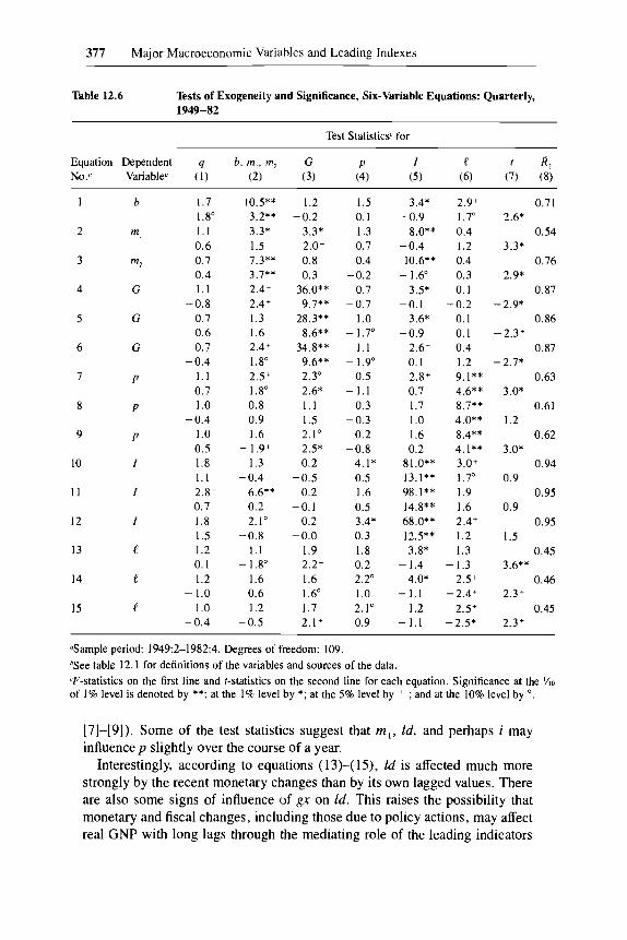
Each of the monetary variables (b, ml' m 2) depends strongly on its ownlagged values and those of the interest rate (I), as shown by the correspondingF-values in table 12.6, equations (1)-(3). The I terms have coefficients whosesigns vary, and their t-statistics are on balance small, though mostly negative.The fiscal index (G) appears to have a strong positive effect on m l' and thetime trends in column 7 are important. The effects of the other variables aresporadic and weak.

G is more strongly autoregressive yet. It also depends positively on bandm 2 and inversely on I, the change in the leading index l, and time (eqs. [4]­[6]).

Inflation (p) also depends mainly on its own lagged values, according toequations (7)-(9). A few relatively weak signs of influence appear for b, I,and G. The time trends are significant. These results are consistent with aview of the price level as a predetermined variable adjusting slowly with con­siderable inertia. Monetary influences on p involve much longer lags than areallowed here.

The interest rate depends most heavily on its own recent levels, as is im­mediately evident from equations (10)-(12). Still, some significant inputs intothe determination of I (which yields R2 as high as 0.95) are also made by otherfactors, notably m t and l.

As for l, it is not strongly influenced by either its own recent past or that ofthe other variables. The largest F-values here are associated with the interestrate in equations (13) and (14) and with inflation in equation (15).

The corresponding tests for real GNP (q) equations have already been dis­cussed in the previous section (relating to the estimates in the last six lines oftable 12.5, pt. A). It is interesting to note that very few significant F- or t­statistics are associated with the lagged q terms according to our tests (table12.6, col. 1).

1919-1940

Tests based on the interwar monetary regressions indicate high serial depen­dence for m l and m 2 but not b (table 12.7, eqs. [1]-[3]). The base is influ­enced strongly by recent changes in output (q), moderately by those in theleading index (ld). There are signs of some effects on m 2 of ld and p, but nomeasurable outside influences on mI'

Equations (4)-(6) for the rate of change in government expenditures (gx)

produce F-statistics that are generally low and significant only for the laggedvalues of the dependent variable. The same applies to equations (10)-(12) forthe change in the interest rate (i).

The rate of inflation (p) depends heavily on its own lagged values, too (eqs.

377 Major Macroeconomic Variables and Leading Indexes

Table 12.6 Tests of Exogeneity and Significance, Six-Variable Equations: Quarterly,1949-82

Test Statisticsc for

Equation Dependent q b t m p m2 G p I e R2

No.a Variableb (1) (2) (3) (4) (5) (6) (7) (8)

b 1.7 10.5** 1.2 1.5 3.4* 2.9+ 0.711.80 3.2** -0.2 0.1 -0.9 1.70 2.6*

2 m1 1.1 3.3* 3.3* 1.3 8.0** 0.4 0.540.6 1.5 2.0+ 0.7 -0.4 1.2 3.3*

3 m2 0.7 7.3** 0.8 0.4 10.6** 0.4 0.760.4 3.7** 0.3 -0.2 -1.60 0.3 2.9*

4 G 1.1 2.4+ 36.0** 0.7 3.5* 0.1 0.87-0.8 2.4+ 9.7** -0.7 -0.1 -0.2 -2.9*

5 G 0.7 1.3 28.3** 1.0 3.6* 0.1 0.86-0.6 1.6 8.6** -1.70 -0.9 0.1 -2.3+

6 G 0.7 2.4+ 34.8** 1.1 2.6+ 0.4 0.87-0.4 1.80 9.6** -1.90 0.1 1.2 -2.7*

7 p 1.1 2.5+ 2.30 0.5 2.8+ 9.1** 0.630.7 -1.80 2.6* -1.1 0.7 4.6** 3.0*

8 p 1.0 0.8 1.1 0.3 1.7 8.7** 0.61-0.4 0.9 1.5 -0.3 1.0 4.0** 1.2

9 p 1.0 1.6 2.1 0 0.2 1.6 8.4** 0.620.5 -1.9+ 2.5* -0.8 0.2 4.1** 3.0*

10 I 1.8 1.3 0.2 4.1* 81.0** 3.0+ 0.941.1 -0.4 -0.5 0.5 13.1** 1.70 0.9

11 I 2.8+ 6.6** 0.2 1.6 98.1** 1.9 0.950.7 0.2 -0.1 0.5 14.8** 1.6 0.9

12 I 1.8 2.1 0 0.2 3.4* 68.0** 2.4+ 0.951.5 -0.8 -0.0 0.3 12.5** 1.2 1.5

13 e 1.2 1.1 1.9 1.8 3.8* 1.3 0.450.1 -1.80 2.2+ 0.2 -1.4 -1.3 3.6**

14 e 1.2 1.6 1.6 2.20 4.0* 2.5+ 0.46-1.0 0.6 1.60 1.0 -1.1 -2.4+ 2.3+

15 e 1.0 1.2 1.7 2.1 0 1.2 2.5+ 0.45-0.4 -0.5 2.1 + 0.9 -1.1 -2.5* 2.3+

aSample period: 1949:2-1982:4. Degrees of freedom: 109.

bSee table 12.1 for definitions of the variables and sources of the data.

cF-statistics on the first line and t-statistics on the second line for each equation. Significance at the Ytoof 1% level is denoted by **; at the 1% level by *; at the 5% level by + ; and at the 10% level by o.

[7]-[9]). Some of the test statistics suggest that m I' ld, and perhaps i mayinfluence p slightly over the course of a year.

Interestingly, according to equations (13)-(15), ld is affected much morestrongly by the recent monetary changes than by its own lagged values. Thereare also some signs of influence of gx on ld. This raises the possibility thatmonetary and fiscal changes, including those due to policy actions, may affectreal GNP with long lags through the mediating role of the leading indicators

378 Chapter Twelve

Table 12.7 Tests of Exogeneity and Significance, Six-Variable Equations: Quarterly,1919-40

Test Statisticsc for

Equation Dependent q b, ml' mz g I p t RzNo.Q Variableb (I) (2) (3) (4) (5) (6) (7) (8)

b 3.5 0.1 1.4 2.6+ 0.7 0.7 0.402.8** -0.3 1.3 -1.70 -1.4 -0.7 3.7**

2 m\ 0.3 8.2** 1.4 0.9 0.1 1.3 0.55-0.1 3.3* -1.70 -0.3 -0.2 0.7 1.5

3 mz 0.6 4.6* 1.7 2.1 0 0.7 2.20 0.600.3 2.8* -2.4+ 0.7 -0.3 1.6 1.1

4 gx 1.9 1.1 2.7+ 1.4 1.5 0.8 0.36-1.8 -1.2 -2.0+ 1.4 0.4 1.5 2.1 +

5 gx 1.6 1.2 2.2+ 1.5 1.0 0.7 0.36-1.9 -0.4 -1.80 1.7 0.4 1.5 1.5

6 gx 1.3 1.2 3.3+ 1.2 0.9 0.9 0.36-1.5 -1.4 -2.3+ 1.5 0.3 1.9° 1.7

7 p 0.7 0.2 1.0 1.7 1.7 5.1 * 0.540.5 -0.2 1.4 1.4 -2.1 + 1.90 1.1

8 p 1.2 2.20 1.5 2.1 0 1.4 6.2** 0.600.2 -0.5 1.2 2.0+ -1.4 2.0+ 1.4

9 p 1.4 1.4 1.2 2.3+ 2.0 5.7** 0.580.7 -1.3 0.7 1.6 -1.6 2.2+ 1.6·

10 0.6 0.7 0.5 1.3 2.7+ 0.3 0.14-0.6 0.9 0.9 1.1 0.9 0.8 -0.7

11 0.5 0.1 0.4 1.0 2.7+ 0.3 0.10-0.1 0.1 1.0 0.7 0.7 0.6 -0.0

12 0.6 0.9 0.7 1.3 2.6+ 0.3 0.15-0.4 0.8 1.5 0.9 0.7 0.2 -0.1

13 ld 1.1 4.7* 2.20 3.0+ 0.8 1.4 0.39-1.1 2.4+ -1.4 2.2+ -0.6 -0.1 -1.4

14 ld 1.3 4.6* 1.5 2.00 0.5 1.8+ 0.39-1.80 3.0* -1.1 1.70 0.6 -1.7 -0.7

15 ld 1.3 7.4** 2.00 2.7+ 1.5 1.5 0.47-1.2 2.1 + -1.0 1.9° 0.5 1.6° 0.7

QSample period: 1920:4-1940:4. Degrees of freedom: 55.bSee table 12.1 for definitions of the variables and sources of the data.

cF-statistics on the first line and t-statistics on the second line for each equation. Significance at the YIOof 1% level is denoted by **; at the 1% level by *; at the 5% level by + ; and at the 10% level by o.

(ld). But note that this is suggested only by the estimates for the interwarperiod, not by those for the postwar era. 13

Comparing Tables 12.6 and 12.7 and drawing also on Table 12.5 (pts. Aand B, eqs. [10]-[12] and [22]-[24]), we observe that q depends strongly on

13. The difference could be related to the fact that the interwar index includes, while the post-war index excludes, the stock price series. Financial asset prices and returns are probably subjectto stronger monetary and fiscal influences than other leading indicators are.

379 Major Macroeconomic Variables and Leading Indexes

the leading indexes (I, Id) in both periods and on the monetary factors intheinterwar period. The autoregressive elements are weak in q, I, and Id andstrong (as a rule dominant) in the other variables according to the interwar aswell as the postwar estimates. The effects of q on the other factors are gener­ally weak or nonexistent.

1886-1914

The F-statistics for the own-lag terms are significant in all the pre-WorldWar I equations, highly so (at the 0.1 % level) for the monetary, fiscal, leading,and interest series, less so for q and p (see table 12.8 and table 12.5, pt. C,eqs. [30]-[32]). The leading index Ide for 1886-1914 is very strongly auto­correlated, in contrast to the indexes Id for 1919-40 and I for 1949-82. Thisreflects the construction of the prewar index, which assumes smooth cyclicalmovements in the index components (see section on data sources and prob­lems).

Prewar changes in the monetary base are poorly "explained," mainly byown lags and those of government expenditures (GX) and the commercial pa­per rate (I). The corresponding changes in the stock of money (m 2) are fittedmuch better by lagged values of m2 itself, I, and p. And as much as 94% ofthe variance of GX is explained statistically, mainly by lagged GX terms andthe time trend. (See table 12.8, eqs. [1]-[4]).

The estimates for inflation (p) are problematic. They suggest that p wasinfluenced positively by lagged money changes but also inversely by its ownlagged values and those of I and Ide. The R2 coefficients are of the order of0.2-0.3 (eqs. [5]-[6]).

The equations for the interest rate (eqs. [7]-[8]), besides being dominatedby autoregressive elements, indicate some short-term effects of q (with plussigns) and m 2 (minus). These results seem generally reasonable.

The leading diffusion index Ide (eqs. [9]-[10]) depends primarily on ownlags, with traces of positive effects of q and p and negative effects of I. In viewof the probable measurement errors involved (mainly in the ide series), theserviceability of these estimates is uncertain.

12.5 Conclusions and Further Steps

The following list of our principal findings begins with a point of particularimportance, which receives clear support from the better quality of the dataavailable for the postwar and interwar periods.

1. Output depends strongly on leading indexes in equations which also in­clude the monetary, fiscal, inflation, and interest variables (all taken in station­ary form, with four quarterly lags in each variable). Hence, models that omitthe principal leading indicators are probably seriously misspecified.

2. Short-term nominal interest rates had a strong inverse influence on out­put (specifically, the rate of change in real GNP) during the 1949-82 period.

380 Chapter Twelve

Table 12.8 Tests of Exogeneity and Significance, Six-Variable Equations: Quarterly,1886-1914

Test Statisticsc for

Equation Dependent q b, m2 GX p I fdc t R2

No.a Variableb (1) (2) (3) (4) (5) (6) (7) (8)

b 0.7 7.3** 2.00 0.3 2.8+ 0.9 0.141.4 -3.7** 1.70 0.1 2.8* 0.6 -1.1

2 m2 1.1 20.8** 0.5 1.7 2.8+ 4.2* 0.59-1.8 5.2** -0.2 -1.4 -2.0+ 0.6 -0.2

3 GX 0.9 0.4 10.8** 0.2 0.9 0.3 0.94-0.4 0.9 5.1 ** -0.4 -1.4 0.5 3.7**

4 GX 1.6 0.9 9.2** 0.3 0.4 0.1 0.94-1.0 1.1 4.6** 0.2 -0.9 0.4 3.7**

5 p 1.4 1.20 1.5 3.3* 3.7* 1.8 0.23-0.3 2.0+ -0.3 -2.7* -2.6+ -1.60 0.1

6 P 2.30 2.8+ 2.1 0 3.3* 2.7+ 2.5+ 0.28-1.80 3.2* -1.0 -3.1* 1.4 -2.3* 1.1

7 I 2.6+ 1.9 0.7 2.30 11.4** 1.5+ 0.492.8* -2.5* 0.1 1.2 4.6** 2.3+ -0.4

8 I 1.9 2.30 0.7 1.7 8.1** 0.8 0.512.3+ -1.2 -0.5 1.2 3.5** 1.3 0.1

9 fdc 1.8 0.3 1.9 55.6** 2.20 2.00 0.722.3+ 0.4 -0.5 6.6** -1.70 0.4 -0.2

10 fdc 1.3 0.3 1.9 56.3** 2.20 2.1 0 0.72-1.80 0.3 -0.5 6.7** -1.5 0.1 -0.1

aSample period: 1886:2-1914:4. Degrees of freedom: 89.bSee table 12.1 for definitions of the variables and sources of the data.

cF-statistics on the first line and t-statistics on the second line for each equation. Significance at the Yloof 1% level is denoted by **; at the 1% level by *; at the 5% level by + ; and at the 10% level by o.

When interest is included, the effects of the monetary and fiscal series arereduced (this resembles the results of some earlier studies; cf. Sims 1980a).When the leading index is also included, most of the monetary effects arefurther diminished.

3. In the interwar period, the role of money appears greater, and the fiscaland interest effects tend to wane. In the prewar (1886-1914) equations, outputis influenced mainly by its own lagged values and those of the money stockand the interest rate. The other factors, including a diffusion index based onspecific cycles in a large set of individual leading series, have no significanteffects. However, this probably reflects errors in the data, especially the weak­ness of the available leading index.

4. The monetary, fiscal, and interest variables depend more on their ownlagged values than on any of the other factors, and the same is true of infla­tion, except in 1886-1914. The opposite applies to the rates of change inoutput and (again, except in 1886-1914) the leading indexes. None of thevariables in question can be considered exogenous.

381 Major Macroeconomic Variables and Leading Indexes

5. The reported unit root tests are consistent with earlier findings that mostmacroeconomic time series are difference-stationary (see Nelson and Plosser1982 on annual interwar and postwar data, and Stock and Watson 1987 onmonthly postwar data). The major exceptions to this are the prewar and post­war fiscal and interest series.

Our work offers some suggestions for further research. The following stepsat least should be considered:

(a) Construct a satisfactory composite index of leading indicators for theperiods before World War II from the best available historical data.

(b) Compute variance decompositions and impulse response functions foralternative subsets of up to four variables represented by the quarterly seriesused in this paper.

(c) Do the same computations for larger sets of six variables by usingmonthly data. This would complement the results obtained here for individualequations in the same sets; further, it would permit comparisons with somerecent smaller VAR models estimated on monthly data. The main problemwith this approach is that no suitable monthly proxies for GNP may be found.

(d) Update the postwar series and check on predictions beyond the sampleperiod, for example, for 1983-88.

(e) Try to find out where the explanatory or predictive power of the leadingindex is coming from by testing important subindexes relating to investmentcommitments, profitability, etc.

(j) Compare the implications of this paper with those of the most recent andongoing studies of leading indicators (de Leeuw 1988, 1989; Stock and Wat­son 1988a, 1988b).