burden of proof - texas law · kaplow.present.boplaw6.711.wpd august 15, 2011 burden of proof louis...
TRANSCRIPT

Kaplow.Present.BOPlaw6.711.wpd August 15, 2011
Burden of Proof
Louis Kaplow
July 8, 2011
Abstract
The burden of proof is a central feature of all systems of adjudication, yet one that hasbeen subject to little normative analysis. This Article examines how strong evidence should haveto be in order to assign liability when the objective is to maximize social welfare. In basicsettings, there is a tradeoff between deterrence benefits and chilling costs, and the optimal proofrequirement is determined by factors that are almost entirely distinct from those underlying thepreponderance of the evidence rule and other traditional standards. As a consequence, thesefamiliar burden of proof rules have some surprising properties, as do alternative criteria that havebeen advanced. The Article also considers how setting the proof burden interacts with otherfeatures of legal system design, such as the determination of enforcement effort and the degree ofaccuracy of adjudication. It compares and contrasts a variety of legal environments and methodsof enforcement, explaining how the appropriate evidence requirements differ qualitatively acrosscontexts. Most of the questions raised and answers presented differ in kind — as well as in result— from those in prior literature.
NOTE TO WORKSHOP PARTICIPANTS: The workshop will focus on Parts I andII only – those plus the Introduction are entirely sufficient, although questions andcomments on the rest are certainly welcome as well.
Forthcoming, Yale Law Journal (2012)
© Louis Kaplow. All rights reserved.
Author: Finn M.W. Caspersen and Household International Professor of Law andEconomics, Harvard Law School, and Research Associate, National Bureau of EconomicResearch. I am grateful to Daniel Klerman, Steven Shavell, Matthew Stephenson, andparticipants in workshops at Harvard, UCLA, and USC for helpful discussions and comments;Michael Atamas, Sarah Beckerman, Noam Lerer, Daniel O’Brien, Stephen Pezzi, and ZacharyShapiro for research assistance; and Harvard Law School’s John M. Olin Center for Law,Economics, and Business for financial support.

Kaplow.Present.BOPlaw6.711.wpd August 15, 2011
- ii -
TABLE OF CONTENTS
INTRODUCTION
I. OPTIMAL EVIDENCE THRESHOLDA. Framework
1. Context2. Evidence Threshold
B. Analysis
II. CONVENTIONAL CONCEPTIONS COMPAREDA. Conventional Burden of ProofB. Comparison
1. Analysis2. Comment on Information Requirements
C. Elaboration1. Relationship Between Level of Evidence Threshold and Ex Post
Likelihood2. Alternative Ex Post Objectives
D. Comparison Revisited: Theory Versus Practice
III. INTERACTIONS BETWEEN THE BURDEN OF PROOF AND OTHER FEATURESOF THE LEGAL SYSTEMA. Enforcement EffortB. Sanctions
1. Level2. Nonmonetary Sanctions
C. Accuracy
IV. ALTERNATIVE METHODS OF ENFORCEMENTA. Monitoring and AuditingB. InvestigationC. Regulation of Future Conduct
1. Optimal Evidence Threshold2. Conventional Conceptions Compared3. Mixed Cases
D. Selection of Cases for Adjudication1. Public Enforcement2. Private Enforcement
CONCLUSION

Kaplow.Present.BOPlaw6.711.wpd August 15, 2011
I employ the term evidence threshold, a concept elaborated in Subsection I.A.2, to refer to the strength of the1
evidence required for liability. As will be noted in this Introduction and developed in Subsection II.C.1, conventionalburden of proof conceptions (regarding the persuasion burden; see infra note 4) have a subtle, complex, and sometimescounterintuitive relationship with the minimal strength of evidence that is required for liability. This is true even thoughthe two notions are ordinarily (implicitly) taken to be synonymous or at least related to each other in a simple, positivemanner.
On the probabilistic interpretation of the preponderance rule, see, for example, 2 MCCORMICK ON EVIDENCE2
484 (Kenneth S. Broun ed., 6th ed. 2006) (stating that “The most acceptable meaning to be given to the expression, proofby a preponderance, seems to be proof which leads the jury to find that the existence of the contested fact is moreprobable than its nonexistence.” and also citing the Model Code of Evidence in support), and David Kaye, NakedStatistical Evidence, 89 YALE L.J. 601, 603 (1980) (reviewing MICHAEL FINKELSTEIN, QUANTITATIVE METHODS IN LAW
(1978)) (“A majority of courts and almost all commentators have concluded that this standard [preponderance of theevidence] is satisfied by evidence that indicates to the trier of fact that the event that must be established is more likely tohave occurred than not.”).
Interestingly, many civil law jurisdictions purport to apply a much higher standard in noncriminal cases, one3
that on its face is closer to the criminal proof burden. See, e.g., Kevin M. Clermont & Emily Sherwin, A ComparativeView of Standards of Proof, 50 AM. J. COMP. L. 243 (2002). One might have expected this difference to spur substantialdebate, but it has not.
See, e.g., MCCORMICK ON EVIDENCE, supra note 2, §§ 336–338; 9 JOHN HENRY WIGMORE, EVIDENCE IN4
TRIALS AT COMMON LAW §§ 2486–93 (James H. Chadbourn rev., 1981). For the classic statement distinguishing theproduction burden from the persuasion burden (the stringency of the burden of proof), see James B. Thayer, The Burdenof Proof, 4 HARV. L. REV. 45 (1890), subsequently elaborated in JAMES BRADLEY THAYER, A PRELIMINARY TREATISE ON
EVIDENCE AT THE COMMON LAW 353–89 (1898). For discussions of terminology, see note 1; BLACK’S LAW DICTIONARY
190–91 (7th ed. 1999) (noting a modern trend to use the term “burden of proof” to refer only to the persuasion burden);THAYER, supra, at 384–89; and 21B CHARLES ALAN WRIGHT & KENNETH W. GRAHAM, JR., FEDERAL PRACTICE &PROCEDURE: FEDERAL RULES OF EVIDENCE § 5122 (2d ed 1987) (“McCormick’s oft-quoted ‘assertion that “presumption”is the slipperiest member of the family of legal terms, except for its first cousin, “burden of proof”’ still pops up 50 yearsafter it was first penned.”) (quoting CHARLES T. MCCORMICK, HANDBOOK OF THE LAW OF EVIDENCE 639 (1954)). Heretoo, many of the standard rationalizations have little content. See, e.g., Bruce L. Hay, Allocating the Burden of Proof, 72
- 11 -
INTRODUCTION
Systems of adjudication base outcomes on whether the strength of available evidencesatisfies a designated burden of proof. Similar modes of decisionmaking are employed in manyimportant nonlegal settings, such as when medical treatments are selected in light of test resultsand other diagnostics. The stringency of the proof burden determines how error is allocatedbetween mistakes of commission — improper assignment of liability — and mistakes ofomission — improper exoneration.
This Article explores how to set the evidence threshold in the manner that best advances1
social welfare. It seeks less to displace entrenched views than to fill a vacuum, for priorscholarship devotes surprisingly little attention to the rationale for how stringent proof burdensshould be. In the United States, civil litigation ordinarily is governed by a preponderance of theevidence rule, under which the plaintiff must establish that it is more likely than not that thedefendant is liable; in criminal trials, guilt must be established beyond a reasonable doubt. 2 3
Neither requirement is particularly controversial, and perhaps for this reason many treatises andtexts on the law of evidence and on civil and criminal procedure provide little or no explanationfor these rules. By contrast, somewhat greater attention has been devoted to the productionburden (how much evidence a party must present in order to avoid losing by default) and4

Kaplow.Present.BOPlaw6.711.wpd August 15, 2011
IND. L. J. 651, 656 (1997) (presenting criticism); Fleming James, Jr., Burdens of Proof, 47 VA. L. REV. 51, 58–63 (1961)(criticizing some standard arguments but offering more cogent reasons); cf. EDMUND MORRIS MORGAN, SOME PROBLEMS
OF PROOF UNDER THE ANGLO-AMERICAN SYSTEM OF LITIGATION 75–76 (1956) (criticizing parallel rationales forallocating the burden of persuasion). Some prior law and economics work, much of which emphasizes incentives topresent evidence and costs of adjudication, has examined the placement of the production burden. See, e.g., Hay, supra;Bruce L. Hay & Kathryn E. Spier, Burdens of Proof in Civil Litigation: An Economic Perspective, 26 J. LEGAL STUD.413 (1997); Joel Sobel, Disclosure of Evidence and Resolution of Disputes: Who Should Bear the Burden of Proof?, inGAME-THEORETIC MODELS OF BARGAINING 341 (Alvin E. Roth ed., 1985).
See infra note 32.5
See, e.g., In re Winship, 397 U.S. 358, 371 (1970) (Harlan, J., concurring) (“In a civil suit between two private6
parties for money damages, for example, we view it as no more serious in general for there to be an erroneous verdict inthe defendant's favor than for there to be an erroneous verdict in the plaintiff's favor.” (This statement is followed almostimmediately by a contrast with the criminal setting, quoted in note 9.)); Grogan v. Garner, 498 U.S. 279, 286 (1991)(“Because the preponderance-of-the-evidence standard results in a roughly equal allocation of the risk of error betweenlitigants, we presume that this standard is applicable in civil actions between private litigants unless ‘particularlyimportant individual interests or rights are at stake.’”) (quoting Herman & MacLean v. Huddleston, 459 U.S. 375, 389–90(1983)); MCCORMICK ON EVIDENCE, supra note 2, at 491 (stating, without further elaboration, that “Mistakes will bemade and in a civil case a mistaken judgment for the plaintiff is no worse than a mistaken judgment for the defendant.”(which claim is promptly contrasted with the criminal setting, as quoted in note 9)); RICHARD A. POSNER, ECONOMIC
ANALYSIS OF LAW 827 (8th ed. 2011) (“In the typical civil trial, there is no basis for supposing that Type I errors (falsepositives, such as convicting an innocent person, or, in the civil context, erroneously finding the defendant liable) onaverage impose higher costs than Type II errors (false negatives, such as an erroneous acquittal or the denial of ameritorious claim). So it is enough in the usual civil case to justify a verdict for the plaintiff that the probability that hisclaim is meritorious exceeds, however slightly, the probability that it is not.” (This statement is followed shortly by acontrast to the criminal setting, in which “Type I errors are more serious than Type II errors . . . .”)); V.C. Ball, TheMoment of Truth: Probability Theory and Standards of Proof, 14 VAND. L. REV. 807, 816–17 (1961) (“When we come tothe requirement of proof in civil actions, the case stands different. The problem then is whether there is a basis for givinga higher value to one of the two kinds of mistake, and applying a requirement which is intended to (1) increase the totalnumber of mistakes, and (2) change the proportion and number of one kind of mistake. The majority of courts seem tohave said there is not.”); Mike Redmayne, Standards of Proof in Civil Litigation, 62 MODERN L. REV. 167, 171 (1999)(“There are good reasons for making this assumption in the typical civil case. . . . There will usually be no reason forvaluing the defendant’s rights more than the plaintiff’s rights; consequently, there is no reason for preferring an error inone direction to one in the other.” (This view is contrasted with the criminal setting in his immediately precedingdiscussion.)).
See, e.g., Addington v. Texas, 441 U.S. 418, 423 (1979) (“At one end of the spectrum is the typical civil case7
involving a monetary dispute between private parties. Since society has a minimal concern with the outcome of suchprivate suits, plaintiff ’s burden of proof is a mere preponderance of the evidence.”); GENE R. SHREVE & PETER
RAVEN-HANSEN, UNDERSTANDING CIVIL PROCEDURE 409 (3d ed. 2002) (“The function of that level or standard of proofis to ‘instruct the fact-finder concerning the degree of confidence our society thinks he [or they] should have in thecorrectness of factual conclusions for a particular type of adjudication.’ In most civil cases society is only minimallyconcerned with outcome, and the level of certainty is usually expressed as a preponderance of the evidence . . . .”(quoting In re Winship, 397 U.S. at 370 (Harlan, J., concurring))).
- 22 -
tiebreaking (which party wins in a civil case when the factfinder believes there is a fifty percent5
chance that each side is correct) — subjects that are not the focus here.
When the question is broached directly, commonly proffered justifications are asunsatisfying as they are brief. In the civil context, the primary argument for the preponderancerule seems to be a lack of any apparent reason to do otherwise, a view often expressed by notingthe absence of the special features of the criminal context. Some authorities go so far as to6
express society’s negligible concern as to the outcome, which if pressed might lead one to7
wonder why civil litigation should exist at all (or why the authors bother to produce extensivetexts and treatises on how it should be conducted, while others write extensively on what

Kaplow.Present.BOPlaw6.711.wpd August 15, 2011
See, e.g., MICHAEL O. FINKELSTEIN, QUANTITATIVE METHODS IN LAW: STUDIES IN THE APPLICATION OF8
MATHEMATICAL PROBABILITY AND STATISTICS TO LEGAL PROBLEMS 66 (1978) (“A higher standard would cast adisproportionate burden on the proponents and would be arbitrary, because there would seem no rationale for selectingany particular decision probability above 0.50.” (emphasis added)).
See, e.g., In re Winship, 397 U.S. at 372 (Harlan, J., concurring) (“In a criminal case, on the other hand, we do9
not view the social disutility of convicting an innocent man as equivalent to the disutility of acquitting someone who isguilty.”); Addington v. Texas, 441 U.S. 418 at 423 (“In a criminal case, on the other hand, the interests of the defendantare of such magnitude that historically and without any explicit constitutional requirement they have been protected bystandards of proof designed to exclude as nearly as possible the likelihood of an erroneous judgment.”); 1 WAYNE R.LAFAVE, SUBSTANTIVE CRIMINAL LAW 77 (2d ed. 2003) (“It is a basic policy of Anglo-American criminal law that, inview of the serious consequences which follow conviction of crime, the prosecution has the burden of proving beyond areasonable doubt all the facts necessary to establish the defendant’s guilt.”); MCCORMICK ON EVIDENCE, supra note 2, at491 (“However, this is not the case in a criminal action. Society has judged that it is significantly worse for an innocentperson to be found guilty of a crime than for a guilty person to go free. The consequences . . . are usually more seriousthan the effects of an erroneous judgment in a civil case.”).
For elaboration, see note 53. For some critical views in this regard in the criminal context, including by Adam10
Smith and Pierre-Simon Laplace, see note 40. See also DAVID CRUMP ET AL., CRIMINAL LAW: CASES, STATUTES, AND
LAWYERING STRATEGIES 265–66 (2d ed. 2010) (raising but not answering questions about whether the standard ethicalbalance in the criminal setting is so clearly correct).
See infra Subsection II.C.1 and Section IV.B (on how the height of the evidence threshold affects the11
frequency of mistaken imposition of liability); Subsection III.B.2 (on how socially costly sanctions affect the optimalevidence threshold).
Cf. MORGAN, supra note 4, at 86 (“The truth is that in allocating the burden of persuasion and explaining to12
the jury their duties with reference to it, the courts have been performing their functions with a minimum of efficiencyand with what President Eliot of Harvard once described as a maximum of intellectual frugality. It is high time that theentire subject be critically reexamined.”).
As elaborated in Section IV.C, the analogy is fairly close regarding legal rules that regulate future conduct, but13
there are substantial differences when legal rules influence ex ante behavior. Despite the latter divergence, the exampleaptly illustrates some of the shortcomings of much existing understanding.
- 33 -
substantive rules should govern). It is hard to avoid the conclusion that the strong attraction ofthe 50% requirement is substantially attributable to its being a powerful focal point, some of itspower deriving from there being no other focal points — besides 0% and 100%, neither of whichhas any appeal.8
For criminal cases, the reasoning is more readily identified, mention often being made ofthe high stakes that make false convictions particularly problematic. Even here, elaboration is9
rare and the conclusions are not obvious: High stakes make erroneous acquittals moretroublesome as well; note that multiplying the consequences on both sides of a balance by acommon factor has no effect on which way the scale tips. Moreover, as will be elaborated in10
the body of this Article, stricter proof burdens can, in plausible settings, increase rather thandecrease the number of false convictions, and the presence of higher social costs of sanctionslikewise has ambiguous implications regarding whether the proof burden should be higher orlower. The point of these observations is not that existing evidence thresholds are too high or11
too low in either the civil or criminal settings but rather that current thinking — actually, fairlyold thinking that has been repeated but not much reconsidered — provides an insufficient basisfor addressing the question.12
To further motivate the inquiry, consider the application of conventional conceptionsabout the burden of proof in adjudication to the context of medical decisionmaking. Would we13

Kaplow.Present.BOPlaw6.711.wpd August 15, 2011
- 44 -
say that, since society per se — as distinct from the patient — has no special stake in mostmedical treatment decisions, the rule for whether to have surgery, receive chemotherapy, or besubject to some other procedure should be based on a fifty percent probability? Or that, if thestakes are high (say, a very serious medical condition), it is better to let ten diseased patients gountreated than to mistakenly undertake surgery on one who did not need it? Or — perhaps theopposite — that it is better to let ten nondiseased patients suffer side effects than to let onediseased individual go untreated? Such formulations are confused, indeed absurd. Surely insetting the treatment threshold we should weigh, along with the likelihood that the patient trulyhas the condition, the expected benefit of the treatment to those who need it (Would theyotherwise die? What are the side effects and other costs? Are there alternatives?) and theexpected cost to those who in fact do not. That is, we would balance the consequences of thepossible outcomes — treatment and abstention — for the truly sick and for those who onlyappear to be ill, factoring in the likelihoods of each.
Legal systems, like medical systems, are of great importance. Civil and criminal lawunderlie social order, playing an essential role in facilitating economic activity, ensuring publicsafety, and otherwise promoting social welfare. Accordingly, decision criteria for adjudication— the setting of proof burdens in various legal contexts — should rest on a stronger foundationthan age-old dictum. They should instead be grounded in explicit analysis that attends to theconsequences of legal outcomes: correct and mistaken imposition of liability as well as properand erroneous exoneration.
The pertinent effects are familiar in rough terms even though they have not systematicallyinformed discourse on how proof burdens ought to be set. For individuals who might in factcommit harmful acts, the prospect of liability produces deterrence whereas the possibility ofmistaken absolution dilutes it. Deterrence of wrongful conduct is central not only to controllingcrime but also to inducing individuals to perform contracts, comply with environmental andhealth regulations, avoid careless activity, and interact honestly in the marketplace. The controlof harmful behavior is, of course, the raison d’être for the legal system, and it is obviously crucialto consider how the system’s ability to achieve this objective is affected by how high the burdenof proof is set.
The strength of the burden of proof also determines the magnitude of the legal system’smajor negative consequence aside from direct operational costs: namely, erroneous assignmentsof liability. A nontrivial likelihood that those who commit benign acts might be found liable willtend to chill desirable behavior. Although chilling receives less explicit attention in generaltreatments of the legal system and in discussions of the burden of proof, it is nevertheless asignificant consideration in most areas of substantive law. Just as the anticipation of properassignment of liability encourages mutually beneficial contractual interaction, concerns formistakes may discourage it. Misapplication of antitrust law may chill aggressive competition oruseful collaboration; with securities law, costs of raising capital may be inefficiently elevated;with medical malpractice, doctors may avoid high-risk patients or treatments and otherwise

Kaplow.Present.BOPlaw6.711.wpd August 15, 2011
For empirical evidence suggesting the importance of these phenomena, see, for example, Thomas J. Walker et14
al., Legal Opportunism, Litigation Risk, and IPO Underpricing (July 2010) (unpublished manuscript), on IPO litigationrisk; David M. Studdert et al., Defensive Medicine Among High-Risk Specialist Physicians in a Volatile MalpracticeEnvironment, 293 JAMA 2609 (2005), on the avoidance of medical procedures and patients posing high litigation risks;and Daniel P. Kessler, William M. Sage & David J. Becker, Impact of Malpractice Reforms on the Supply of PhysicianServices, 293 JAMA 2618 (2005), on medical malpractice and physician supply.
Prior law and economics work on the burden of proof, or on errors, that focuses on ex ante behavior usually15
contemplates that individuals’ only behavioral decision is whether or not to commit a single harmful act — or,equivalently, whether or not to take precautions, where commission of the act is taken as given. See sources cited infranote 100. The results in such models are radically different from those derived here when there is a concern both fordeterrence and for the chilling of other, desirable behavior. For a formal demonstration of the contrast, see LouisKaplow, Optimal Proof Burdens, Deterrence, and the Chilling of Desirable Behavior, 101 AM. ECON. REV. PAPERS &PROC. 277 (2011) [hereinafter Kaplow, Proof Burdens], and for a more comprehensive formal analysis of subject, seeLouis Kaplow, On the Optimal Burden of Proof (Jan. 26, 2011) (unpublished manuscript) [hereinafter, Kaplow, OptimalBurden of Proof]. (There is a paper on errors that also considers the frequency with which individuals engage in anactivity, where there is also the question of actors’ level of care, but it does not analyze the burden of proof. See IvanP.L. Png, Optimal Subsidies and Damages in the Presence of Judicial Error, 6 INT’L REV. L. & ECON. 101 (1986).)
The analysis for raising the threshold is the same — with all the effects reversed — so the analysis is not16
repeated. Generally, if a slight reduction in the threshold has net negative welfare effects, then some increase would havepositive effects.
- 55 -
engage in defensive medicine.14
Part I of this Article investigates in a basic setting how optimally to set the evidencethreshold in light of deterrence and chilling effects. Slightly reducing the evidence threshold15
will increase the likelihood that individuals who contemplate the commission of both harmfuland benign acts would expect to be subject to sanctions. The extent of each effect depends on16
the nature of the evidence in a manner that is described. It also is necessary to determine howmany harmful and benign acts are deterred and chilled, respectively, on account of theseincreases in expected sanctions, which is shown to depend on how many individuals have privatebenefits for the two types of acts that approximately equal the corresponding expected sanctions. Finally, for given numbers deterred and chilled, the effects on social welfare need to bedetermined. In both cases, when acts are discouraged, individuals’ private benefits from theseacts are forgone; in the case of harmful acts, society is spared their negative consequences. Thecalculus for determining the optimal evidence threshold is, on reflection, conceptuallystraightforward and in accord with welfare-based intuitive reasoning. As a practical matter,however, the factors are many, their magnitudes undoubtedly vary greatly across contexts, andascertaining the pertinent quantities is likely to be difficult.
Part II juxtaposes this welfare-based analysis with conventional thinking about the burdenof proof. To begin, it offers a precise formulation for the preponderance rule in the presentsetting — and it is remarked that this expression requires only slight modification to characterizeother proof requirements, such as ones requiring a seventy-five percent or ninety-five percentlikelihood as a prerequisite for liability. Next is the comparison. The central finding is that thereis almost no overlap between the determinants of the preponderance rule (or other such rules,including proof beyond a reasonable doubt) and those for the optimal evidence threshold. Animmediate implication is that, depending on the context, the optimal rule could be much moredemanding or notably more lax than the preponderance rule (or even a requirement of proof

Kaplow.Present.BOPlaw6.711.wpd August 15, 2011
The latter is possible even on the high end: requiring proof beyond a reasonable doubt in practice does not17
require absolute certainty. See also sources cited infra note 76 (showing a wide range of probabilities associated with therequirement of proof beyond a reasonable doubt, most notably below 100%). If it was understood to require, forexample, a 95% likelihood, it may well be that in many cases this demand could readily be met, although insisting on a99% or perhaps a 99.99% likelihood would be prohibitive in most instances.
As explained in Part II, much of this difference has to do with the fact that the preponderance rule, and other18
rules based on the likelihood that the individual before the tribunal is one who committed the harmful act, embody an expost perspective that takes behavior as given (exogenous) and asks, in light of that behavior, what is the likelihood of oneversus another characterization. By contrast, a welfare-based, optimal threshold in these settings is determined by askinghow behavior (taken to be endogenous) will change as a function of a change in the evidence threshold. The other centraldifference, highlighted by the medical treatment example, is that welfare-based thresholds depend on the harms andbenefits of outcomes whereas likelihood-based formulations do not.
- 66 -
beyond a reasonable doubt). On reflection, this disjunction is not surprising since the many17
elements that determine the magnitudes of deterrence and chilling effects elucidated in thepreceding paragraph simply do not pertain to whether it is more likely than not (or some othertarget likelihood) that the individual before the tribunal committed a harmful act rather than abenign one — and conversely. Interestingly, even though the preponderance rule and other18
conventional ones have a seemingly simpler algebraic formulation, the information requirementsrequired to apply them in a given case — which are daunting — are similar to those needed todetermine the optimal rule. Of course, even if the preponderance rule and others were easier toemploy, they could hardly be commended on that account because their facility would be due totheir ignoring the welfare-relevant effects.
Part II continues by exploring other features of the preponderance rule (or otherqualitatively similar rules). One striking, unappreciated point is that imposing a higher evidencethreshold — requiring stronger evidence as a prerequisite for liability — could reduce thelikelihood that, when evidence is just at the (new, higher) threshold, the case at hand involvesone in which the individual in fact committed a harmful act. Accordingly, it is possible, startingfrom an evidence threshold that implements the preponderance rule, that substitution of a higher,more demanding threshold could have the property that cases with evidence barely above thatnew threshold fail the preponderance test. The reason is that raising the evidence thresholdreduces the chilling effect, so more benign acts are committed, more will tend to come beforetribunals, and therefore more close cases may involve benign rather than harmful acts despite thehigher threshold. This effect is one of many and hardly will dominate in all situations, but it isentirely plausible that it will in some. Closely related, demanding stronger proof could actuallyincrease the number of mistaken findings of liability.
In addition, Part II examines other proffered criteria for the burden of proof, such asseeking a high ratio of correct to incorrect impositions of liability, a minimum number ofmistaken findings of liability, or an equal likelihood of mistakes for those committing harmfulacts and benign ones. These and other, related desiderata are also shown to have virtually noconnection to the optimal evidence threshold. As well, they have anomalous implications oftheir own. For example, a system with perfect deterrence and rare mistakes will have a zero ratioof correct to mistaken findings of liability, whereas a system in which all engage in harmful actsand liability is random will have an infinite ratio of correct to mistaken findings of liability. Inaddition, bringing additional individuals who did not commit harmful acts into the system can

Kaplow.Present.BOPlaw6.711.wpd August 15, 2011
- 77 -
readily improve the ratio of correct to incorrect outcomes even if some of the additional casesresult in mistaken findings of liability. And attempts to equalize the likelihoods of mistakes ofthe two types could require an intentional increase in imposing liability on the wrong individualsif it is difficult to eliminate a fairly substantial rate of mistaken exoneration.
In sum, Part II indicates that conventional thinking about proof burdens is deeply flawed,both in terms of its own internal workings and regarding its (lack of) relationship to promotingsocial welfare. This Part concludes by inquiring whether conventional conceptions — in theiridealized form, as officially pronounced by courts and analyzed by commentators — are fullyreflected in current practice or perhaps instead are applied in ways that implicitly embody someconsequentialist elements of the sort developed in Part I. Relatedly, it offers some thoughtexperiments about alternative formulations of the burden of proof that entail more explicitattention to consequences of adjudication for individuals’ behavior.
The remainder of the Article returns to its core conceptual mission, the explication ofoptimal — welfare-promoting — policy, entertaining a wider range of factors and settings. PartIII addresses other features of the legal system. In an important sense, the proof burden canusefully be viewed as one of many of the enforcement instruments that a legal regime deploys tocontrol harmful conduct. Section A examines the interaction between setting the level ofenforcement effort, taking into account its costliness, and setting the evidence threshold. SectionB analyzes the level of sanctions. In addition, it considers how the social costs of sanctions,notably imprisonment, relate to how the evidence threshold should be set. It turns out that highersocial sanction costs do not unambiguously favor a higher evidence threshold: even though ahigher threshold reduces the rate of imposition of sanctions for the cases that come beforetribunals, the resulting reductions in deterrence and chilling increase the flow of cases intoadjudication, which has a countervailing effect on the frequency of use of costly sanctions. Likewise, if society has a greater concern for mistakenly imposing sanctions on the innocent, ahigher evidence threshold can sometimes be counterproductive because innocents will moreoften come before tribunals — even though the sanction probability per innocent individualbefore a tribunal is reduced. Finally, Section C analyzes the interaction between proof burdensand the accuracy of the legal system: roughly speaking, the latter determines the overall error ratewhereas the former dictates how to divide the errors between the two types. Different levels ofaccuracy may bear on the optimal evidence threshold, and vice versa.
Part IV introduces additional methods of enforcement. Until this point, the analysisfocuses (in a manner detailed in Section I.A) on a particular enforcement setting, one akin tomonitoring — such as the posting of police or security guards — or auditing, including the use ofinspections and spot-checks. Section A elaborates on these methods and their differences, withparticular attention to the administrative costs of enforcement. Section B explores the techniqueof investigation, which refers to waiting until harm is observed (such as when there is a murder,stolen automobile, or pollution discharge) and then attempting to identify the perpetrator. Thedeterminants of the optimal evidence threshold are different in important ways: there are morefactors and their interaction is somewhat more complicated. Furthermore, there is an evengreater contrast between this formulation and conventional ones — the preponderance rule andothers based on the likelihood that the individual before the tribunal is a wrongful actor. Another
Kaplow.Present.BOPlaw6.711.wpd August 15, 2011
This part comments briefly on the related question of parties’ incentives to develop evidence. Incentives to19
sue and to present evidence, and attendant costs, have been a focus of much prior law and economics writing on theburden of proof (often addressing the placement of the production burden), which literature is noted in this Section. Seealso sources cited supra note 4.
- 88 -
finding is that it is quite plausible that a higher evidence threshold might actually increase howoften sanctions are mistakenly imposed on innocent actors. The reason is that a higher thresholdreduces deterrence, so more harmful acts are committed, which triggers more investigations,which in turn are the genesis of potential erroneous findings of liability.
Part IV next considers an enforcement context that is qualitatively different from thoseanalyzed previously: the regulation of future conduct, such as through allowing zoning variances,granting licenses, authorizing drugs, or permitting mergers. Unlike with contract law, liabilityfor securities fraud, and most tort and criminal law, in these settings the central concern often isnot with prior conduct — which can be influenced (through deterrence and chilling) by theprospect of sanctions — but with future behavior. The decision at hand is whether to allow orprohibit some action, going forward. Here, the determination of the optimal evidence thresholddiffers quite substantially from that in the prior settings. Instead, it is akin to the sort of analysisused in making medical treatment decisions, as described at the outset of this Introduction. Thisformulation, in turn, is notably closer to the preponderance rule (and other such rules), althoughit still differs markedly by the explicit inclusion of the harms and benefits that may flow fromdifferent outcomes. For example, in deciding whether to approve a drug application, thegovernment agency will not simply ask, say, whether the drug is more than fifty percent likely tobe beneficial rather than harmful: it will also place great weight on the magnitudes of the benefitsand harms. Benefits may accrue to fewer than fifty percent of patients, but if the benefits aredramatic, the drug will be approved even in the presence of certain adverse side-effects, if theyare sufficiently mild. Interestingly, in this important context in which the optimal rule is leastqualitatively distinct from the preponderance rule, one does not ordinarily see the preponderancerule employed, presumably because the residual differences are obvious — and considerable.
Part IV concludes by examining briefly some aspects of how public and private modes ofenforcement determine the cases that enter the legal system. Emphasis is placed on the motives19
of public enforcers and private litigants, which unfortunately may diverge significantly fromadvancement of the social good. These incentives are of particular relevance here because ofpossible interactions with the burden of proof. For example, demanding stronger evidence maymake it harder for police and prosecutors to abuse their authority in pursuit of a regime’s politicalopponents. This effect is one of the familiar justifications for requiring proof beyond areasonable doubt in criminal cases, although as some have noted the rationale can have similarforce in civil settings in which the government is the enforcer.
This Article offers a preliminary, conceptual analysis of the optimal stringency of theburden of proof. Prior literature has devoted surprisingly little attention to this question. Conventional notions that focus on the likelihood that the individual before the tribunal hascommitted a harmful act turn out to be almost entirely unrelated to welfare-based analysis andalso to pose some unrecognized internal conundrums. The present analysis breaks new ground

Kaplow.Present.BOPlaw6.711.wpd August 15, 2011
For ease of exposition, it is supposed that there is only one possible level of harm and that each harmful act20
causes it with certainty. Allowing for variable or uncertain harm (in which case expected harm would replace the level ofharm) would not materially affect the analysis. Acts that cause different levels of expected harm may be viewed asdifferent types of acts that may, in principle, be subject to different rules (for example, different sanctions and differentevidence thresholds). An important and more subtle variation, not analyzed here, is the case where there is unobservablevariation in the level of harm that is correlated with the strength of the evidence likely to be generated; the main effect onthe analysis would be that the level of harm, for example, in the lower element of the left box in Figure 4 would refer tothe level of harm conditional on the evidence threshold under consideration.
If the marginal deterred harmful act is net socially desirable, it will be obvious that (in basic settings) the legal21
system is not designed optimally. Social welfare would be greater with, for example, lower sanctions, lower enforcementeffort, or a higher evidence threshold. Most of the tradeoffs elaborated throughout this Article would not arise.
A number of simplifying assumptions are implicit. First, individuals are assumed to act to maximize their self-22
interest. One could introduce other influences, such as an internal desire to abide by the law or the presence of socialsanctions, including reputational loss, without greatly affecting the analysis. (As a first cut in analyzing such a case, wecould reduce the valuation of the private benefit from acts subject to such costs accordingly; note that in some cases,particularly regarding harmful acts, this adjustment might convert an otherwise privately beneficial act into one involvinga net negative private benefit, in which case the act would not be committed even in the absence of legal sanctions.) Second, individuals are assumed to be risk neutral. Risk aversion also would not qualitatively affect much of the
- 99 -
across much of the territory — in terms of enforcement settings, legal system features, andpertinent factors — but it is hardly comprehensive or definitive along any of these dimensions. Moreover, in order to undertake the important constructive task of making sensiblerecommendations for system design, one would need context-specific empirical evidence that isnot readily available. Nevertheless, it is difficult to collect the requisite evidence or even tomake reasonable conjectures until one has identified what factors are relevant, why, and how. The inquiry must begin somewhere if it is to begin at all.
I. OPTIMAL EVIDENCE THRESHOLD
A. Framework
1. Context
Before discussing the nature of evidence and the evidence threshold that must be crossedfor liability to attach, our central interest, it is important to describe the context in whichadjudication is understood to arise. To begin, suppose that some individuals have opportunitiesto commit harmful acts, the prospect of which is the central justification for the legal system. Aharmful act is understood here to be one that generates some level of external harm — that is, toa third party — in addition to whatever benefit accrues to the individual who commits it. 20
Individuals’ benefits from such acts are assumed to vary. Although it is not ruled out that someindividuals’ benefits may exceed the harm caused, in which case the so-called harmful actswould be net socially desirable, attention will largely be confined to settings in which the level ofthe expected sanction is such that acts that are deterred involve a net social harm.21
In the absence of any legal restraint, it is assumed that individuals will act whenever theirprivate benefit from doing so is positive. With a legal system, they are assumed to act if and onlyif their private benefit exceeds the expected sanction. Accordingly, it is necessary to describe22

Kaplow.Present.BOPlaw6.711.wpd August 15, 2011
analysis; for brief further discussion, see note 142, and see also note 192 on the compensatory function of privatelitigation, which is set to the side here.
The main difference in this final scenario is that, when deterring a marginal harmful act, there is the chance23
that an individual would switch to a benign act instead of inaction, and since the benign act generates a benefit, the netsocial value of deterrence would be greater on this account. Likewise, when chilling a marginal benign act, someindividuals might switch to a harmful act, which would make the net social cost of chilling greater. Accordingly, thestakes regarding both behavioral effects would be raised, but much of the analysis, often concerning tradeoffs betweenthe two types of behavioral effects, would be qualitatively similar. (Another generalization, subject to similar analysis,would be to allow different choices to cause different, positive levels of harm — for example, the choice among a moreharmful act, a less harmful act, and inaction.)
- 1100 -
how the legal system generates sanctions.
Enforcement is taken to operate in two stages. First, some sort of scrutiny brings aportion of individuals into the legal system on account of the acts that they are observed tocommit. Second, for those brought into the system, adjudication assesses the evidence in orderto decide whether to exonerate or instead to assign liability and impose the applicable sanction —taken here to involve a monetary payment, which might be a fine paid to the state or damagespaid to a plaintiff (nonmonetary sanctions are considered in Subsection III.B.2 and outcomes thatinvolve the regulation of future conduct in Section IV.C). If it were known that every individualbrought into the legal system in the first stage indeed committed a harmful act, adjudicationwould be simple; accordingly, we now consider how individuals who have not committedharmful acts sometimes enter the system.
Another group of individuals is assumed to have opportunities to commit benign acts. Abenign act (like a harmful act) generates a benefit to the individual who commits it, but (unlike aharmful act) it does not generate any external harm. Individuals commit benign acts because ofthe benefits they receive, and since there is no external harm, these acts are net sociallybeneficial. (Note that the labels “harmful” and “benign” refer to the presence or absence ofexternal social harm, not to the act as a whole.) For ease of exposition, assume that the twogroups of individuals are distinct; that is, one only has opportunities to commit harmful acts andthe other only to commit benign acts. The analysis would be much the same if given individualssometimes had opportunities to commit one type of act and, at other times, opportunities tocommit the other. Also, the analysis would change somewhat but not drastically if individuals atthe same time could choose whether to engage in the harmful act, the benign act, or no act atall.23
It is assumed that the enforcement apparatus in the first stage brings some individualswho commit benign acts into the legal system. They too enter adjudication, so the adjudicator’stask will be the familiar one of trying to distinguish the two situations and, to the extent feasible,confine sanctions to those who committed harmful acts, without exonerating very many of thoseindividuals.
For both groups of individuals, the prospect of sanctions will influence decisions whetherto commit acts in the first instance. An individual with an opportunity to commit a harmful actwill be deterred from doing so when the private benefit of the act is less than the expected

Kaplow.Present.BOPlaw6.711.wpd August 15, 2011
The analysis here supposes that whether one or another harmful or benign act is swept into the system is24
independent of how many of the two types of acts occur or how others are scrutinized at this stage. (As we will see inSection IV.B, this assumption does not hold for enforcement by investigation, wherein scrutiny is triggered by theobservation of a harmful act). This assumption would not hold, for example, if enforcers’ incentives createdinterdependence, such as when a police officer or inspector feels pressure to generate a certain amount of fine revenue, inwhich case greater deterrence of harmful acts may induce enforcers to identify benign acts as harmful ones. Publicenforcers’ incentives are considered in Subsection IV.D.1.
To the extent that enforcement effort is being held constant, as is supposed, this assumption is not problematic25
for the pure case of monitoring at stage one (and with a cost-free stage two). More generally, however, as Section IV.Aexplores, enforcement costs are influenced by deterrence and chilling, which in turn are affected by the evidencethreshold, so a complete analysis cannot ignore these costs.
- 1111 -
sanction, which is the product of three factors: the likelihood that harmful acts will be identifiedin stage one, the likelihood that an individual in adjudication at stage two who committed aharmful act will be subject to sanctions, and the magnitude of the sanction. Likewise, anindividual with an opportunity to commit a benign act will be chilled from doing so when theprivate benefit of the act is less than the expected sanction, which also will be the product ofthree corresponding factors. Although deterrence and chilling are analytically the same, differentterms are employed to help keep the phenomena distinct because the social consequences differ:deterrence is desirable whereas chilling constitutes an undesirable side-effect of the legal system.
Although the three factors are conceptually the same for each type of act, the levels of thefirst two generally will differ. (The magnitude of the sanction does not because, at the time of itsapplication, the legal system will have failed to distinguish the two types of individuals.) Thesecond factor, involving evidence assessment and the assignment of liability, is considered indetail in the next Subsection. The first, concerning the likelihood that the two types of acts areidentified at the first stage of scrutiny, will depend on the method of enforcement. For Parts Ithrough III, attention will largely be confined to methods of enforcement that are akin tomonitoring (for example, officers posted along a highway or officers on the beat watching forcrime) or auditing (including random inspections, such as for environmental or fire codeviolations). Specifically, some fraction of each type of act is identified (typically, we wouldhope, a larger portion for the harmful type of act), and those fractions are determined by theintensity of enforcement effort (taken for now to be fixed). Such matters will be reexamined in24
some detail in Part IV, which considers alternative methods of enforcement and how theirdifferences are consequential for setting the evidence threshold. Also, for the present (untilSection III.A), the costs of enforcement will be set aside.25
As mentioned in the Introduction, the central problem arises because certain sorts ofbenign acts are sometimes confused with harmful ones. Therefore, it is useful to think of thebenign acts under consideration as limited to that type. For speeding, we might consider onlyindividuals who in fact are driving vehicles, and perhaps only those driving near the speed limitrather than substantially under it. For securities laws regulating disclosures at public offerings,we would consider as pertinent benign acts only other public offerings, specifically, onesaccompanied by valid disclosures but in circumstances where it might be hard to tell, readily and

Kaplow.Present.BOPlaw6.711.wpd August 15, 2011
If one defined the set of benign acts more broadly, little would change because the rates of identification at26
stage one and assessment of sanctions after adjudication would fall. Importantly, however, the expected sanction facingindividuals contemplating benign acts would vary in that case. Those contemplating acts that would rarely if ever beconfused with harmful ones would face an expected sanction essentially equal to zero, whereas those contemplating actsthat could plausibly be so confused would face a nontrivial expected sanction and hence may be chilled. Realistically,the likelihood of confusion (in those cases where such is conceivable) will vary across benign acts, and thus the intensityof chilling effects will differ as well.
How the evidence is generated will not be addressed, except in passing in Parts III and IV.27
There is a relationship between defining the strength of evidence and combining multiple pieces of evidence. 28
Formally — if one wishes to minimize the likelihood of one type of error while holding the rate of the other type of errorconstant —it is optimal to order evidence by the likelihood ratio: the ratio of the likelihood that such evidence would begenerated by a harmful act to the likelihood that such evidence would be generated by a benign act, where the likelihoodscorrespond to the height of the probability distributions in Figure 1. This concept has multidimensional analogues, and
- 1122 -
for sure, whether appropriate disclosures were made. These are the sorts of benign acts that26
might be brought into the legal system in stage one, and hence they are the ones that adjudicatorsmust distinguish at stage two, to which we now turn.
2. Evidence Threshold
To introduce evidence and the setting of an evidence threshold, consider a simple andreasonably familiar example in the medical context: the use of test results to determine whetherto treat a patient — perhaps administer a drug, perform surgery, or employ a more invasivefollow-up diagnostic procedure. The test is an imperfect signal, higher scores indicating a greaterlikelihood that the disease in question is present. That is, individuals who in fact have theailment produce a range of test results, but their scores cluster toward the high end, whereasindividuals who are disease-free also produce a range of results, but their scores cluster towardthe low end. The problem is to choose a cutoff or threshold, above which treatment will beapplied. A high cutoff will result in few false positives, which is to say that only a small portionof disease-free individuals will be mistakenly given the treatment; however, a high cutoff willalso result in many false negatives, so a nontrivial fraction of diseased individuals willmistakenly fail to receive treatment. In determining the optimal threshold, these error costs willbe traded off: if nontreatment of diseased individuals is serious and the treatment involves littlecost to disease-free individuals, a low cutoff will be optimal, but if nontreatment is onlymoderately problematic whereas treatment is very costly to disease-free individuals, a high cutoffwill be optimal. (It turns out that the optimal decision rule for this case is much like thatconsidered in Section IV.C, on the regulation of future conduct, yet quite unlike that appropriatein our present context. Nevertheless, the example is useful here because it does properly depictthe nature of evidence and of evidence thresholds, the present subject.)
Returning to our legal context, it is supposed that identification of an individual at thefirst stage in the law enforcement process will give rise to a body of evidence that the tribunalmust assess. In many instances, the evidence may be multidimensional and murky, unlike the27
simple medical test just described. Of course, actual medical decisionmaking typically involvesmany sorts of evidence, some of which are much less sharp than a blood test result. For presentpurposes, we will collapse all the evidence into a single indicator, x, of the overall strength of theevidence because our focus is on how strong a case should be required for liability. In accord28

Kaplow.Present.BOPlaw6.711.wpd August 15, 2011
the general principle is given by the Neymann-Pearson Lemma. See Jerzy Neyman & Egon Pearson, On the Problem ofthe Most Efficient Tests of Statistical Hypotheses, 231 PHIL. TRANSACTIONS OF THE ROYAL SOC’Y OF LONDON, SERIES A,CONTAINING PAPERS OF A MATHEMATICAL OR PHYSICAL CHARACTER 289 (1933); see also NEIL A. MACMILLAN & C.DOUGLAS CREELMAN, DETECTION THEORY: A USER’S GUIDE, ch. 6 (2d ed. 2005) (explaining the extension of signaldetection theory to multiple dimensions).
It is assumed that, ex ante, all acts of a given type generate the same probability distribution of evidence. 29
Allowing for heterogeneity in this regard (that is, for a given type of act) would complicate the analysis without alteringits qualitative features. Likewise, one could allow for the nature of the enforcement process — see infra Section III.Aand Part IV — to influence these distributions, conditional on cases appearing before a tribunal. See especially thediscussion at the end of Subsection IV.D.2.
This special case is typically used in presenting basic signal detection theory, which is the first formally30
developed system that closely corresponds to the construction used here. See generally MACMILLAN & CREELMAN, supranote 28; R. Duncan Luce, Detection and Recognition, in 1 HANDBOOK OF MATHEMATICAL PSYCHOLOGY 103 (R. DuncanLuce, Robert R. Bush & Eugene Galanter eds., 1963). This theory was originally developed for radar detection. See,e.g., J.I. Marcum, A Statistical Theory of Target Detection by Pulsed Radar (U.S. Air Force Project Rand, ResearchMemorandum 754, 1947).
Interestingly, Bentham, in the course of advocating that factfinders not merely count witnesses but instead31
consider the strength of the testimony, suggested that each witness be assigned a value on a scale from !10 to 10, where 0was a neutral point, negative values favored nonexistence of a fact, and positive values denoted existence. One wouldthen sum such values across witnesses and find a fact to exist if and only if the sum was positive. See 1 JEREMY
BENTHAM , RATIONALE OF JUDICIAL EVIDENCE, SPECIALLY APPLIED TO ENGLISH PRACTICE, ch. VI (Rothman & Co. 1995)(1827).
- 1133 -
with the medical diagnosis example, harmful and benign acts each generate a wide range ofpossible values of x, but values for harmful acts will tend to cluster at a higher level than do29
values for benign acts, as depicted in Figure 1.
Figure 1: Probability Distributions for Strength of Evidence
These curves are drawn roughly as normal distributions with different means and the samevariance merely for the sake of illustration. Also, no particular scale for x or zero point is30
indicated because, for present purposes, all that matters is the ordering, namely that higher valuesof x are taken to indicate stronger evidence.31
Given this depiction of evidence, the legal system must choose an evidence threshold,denoted here by x , which indicates the value of x above which liability will be assigned andT

Kaplow.Present.BOPlaw6.711.wpd August 15, 2011
Strictly speaking, with continuous probability distributions as in Figure 1, the probability that x will precisely32
equal any given x is zero, making ties quite unimportant. (Readers not familiar with this feature of probability theoryT
may ponder the likelihood that, say, it will be precisely twelve noon when one looks at one’s watch, as distinguished from11:59:59.999999999 or 12:00:00.000000001, and so forth.) It is familiar, by contrast, that the legal system — asreflected in legal commentary, lawyers’ arguments, and court opinions — attaches great weight to tiebreaking, whichsuggests that something else is going on. One phenomenon, not considered in this Article, involves production burdens. See supra note 4. Another is that factfinders psychologically may perceive a nontrivial range of close cases assufficiently difficult to decide to be viewed as ties. As a consequence, a more-likely-than-not requirement might, in manysettings, result in factfinders perceiving a tie (and thus awarding a victory to the defendant) when the probability is lessthan, say, 55%. It may be helpful to think of such settings as involving a de facto requirement of 55% rather than 50%.
For the most part, language of correct or mistaken liability or exoneration will be employed in lieu of referring33
to mistakes as false positives and false negatives or as type I and type II errors, respectively, because in my experienceindividuals (including sophisticated, trained analysts) occasionally confuse these terms and, even more often, musthesitate to make the appropriate translations.
These curves, like those in Figure 1, are hand drawn rather than generated mathematically; hence their shapes34
bear only an approximate correspondence to those that would be implied by a formal translation of Figure 1. For readersfamiliar with probability theory, each of the probabilities in Figure 2, for a given value of x , is given by one minus theT
value of the cumulative distribution function corresponding to the probability densities in Figure 1. (The cumulativedistribution function indicates the area to the left of x ; hence, one minus this value gives the area to the right.)T
- 1144 -
below which there is no liability. It is likewise conventional to suppose that ties go to thedefendant, so that, in cases in which x equals x , there is no liability.T 32
Now, for any given evidence threshold, x , we can use Figure 1 to determine theT
probability that (conditional on coming before the tribunal) an individual who has committed a
HARMFULharmful act will be found liable. This will be denoted P (x ). We can also determine theT
probability that one who has committed a benign act will (mistakenly) be found liable —
BENIGNP (x ). Suppose, for example, that x was set at the value of x in the middle of the figure,T T
HARMFULwhere the two curves happen to cross. In that case, P (x ) will be given by the portion ofT
the area under the Harmful Acts curve that lies to the right of this value of x (which looks to beT
roughly 95% of the area) because, for all such higher values of x, the individual would be foundliable (and correctly so). Similarly, for all lower values, the individual is (mistakenly)
HARMFULexonerated, and this probability, 1!P (x ), is given by the portion of the area under theT
BENIGNHarmful Acts curve that lies to the left of this value of x (about 5%). Likewise, P (x ) willT T
be given by the portion of the area under the Benign Acts curve that lies to the right of this valueof x (approximately 5% of the area) because, for all such higher values of x, the individualT
would be found liable (by mistake). Similarly, for all lower values, the individual is (correctly)
BENIGNexonerated, and this probability, 1!P (x ), is given by the portion of the area under theT
Benign Acts curve that lies to the left of this value of x (about 95%).T 33
BENIGNWe could instead set x higher, which would reduce P (x ), the likelihood inT T
adjudication of false assignments of liability for benign acts, but this change would also reduce
HARMFULP (x ), the likelihood of correct assignments of liability for harmful acts — which is to say,T
it would increase the frequency of mistaken exoneration. For lower values of x , the effectsT
BENIGN HARMFULwould be reversed. This relationship between x , on one hand, and P (x ) and P (x ),T T T
on the other hand, is depicted in Figure 2.34

Kaplow.Present.BOPlaw6.711.wpd August 15, 2011
Because there is no natural zero point on the horizontal axis, as previously mentioned, no vertical axis is35
drawn. However, it is supposed that the height of the two curves approaches one as we move sufficiently toward the leftof the horizontal axis and both heights approach zero toward the right.
This sort of curve, like Figure 1, is also used in presentations of signal detection theory; there, the analogue to36
the curve in Figure 3 is called the receiver operating characteristic (ROC) curve, although it is conventional to reverse theaxes, showing the false positive (called false alarm) rate on the horizontal axis and the true positive (called hit) rate on thevertical axis. See, e.g., R. DUNCAN LUCE, INDIVIDUAL CHOICE BEHAVIOR: A THEORETICAL ANALYSIS 60–61 (1959);MACMILLAN & CREELMAN, supra note 28, at 9–11.
- 1155 -
Figure 2: Probabilities of Liability as Function of Evidence Threshold xT
As the evidence threshold x required for application of the sanction is raised, both probabilitiesT
fall. Initially (for a very low x ), the probability of (mistakenly) sanctioning the benign act fallsT
quite rapidly relative to the fall in the probability of (correctly) sanctioning the harmful act, but asthe threshold becomes quite high, there is a sharper drop in the latter probability.35
The error tradeoff implicit in Figure 2 can be illustrated in another way. Suppose that thelegal system wishes to set the evidence threshold x in order to achieve some target rate ofT
liability for those before the tribunal who have committed harmful acts — that is, a target value
HARMFULof P (x ). We can then ask what is the resulting rate of mistaken imposition of sanctionsT
BENIGNon benign acts — that is, P (x ). If one traces this relationship for different target values ofT
HARMFULP (x ), the result would look something like that depicted in Figure 3.T 36

Kaplow.Present.BOPlaw6.711.wpd August 15, 2011
This would be so when the curves in Figure 1 are coincident (and likewise for Figure 2), which is to say that37
both types of acts are equally likely to result in any particular strength of evidence (value of x). In such a case, highervalues of x would not be stronger in any meaningful sense.
See supra note 34.38
- 1166 -
BENIGN HARMFULFigure 3: P (x ) as a Function of P (x )T T
(For convenience, a 45 degree dotted line is shown, which indicates what the relationship wouldbe if the evidence strength x had no discriminating power. ) Here, high values of the evidence37
threshold, x , would be toward the lower left of the figure, and low values toward the upper right:T
as stated in connection with Figure 2, high values correspond to low probabilities of liability, andlow values give rise to high probabilities of liability. To restate this point to avoid possibleconfusion: raising the evidence threshold, x , means that one moves from the upper right cornerT
toward the lower left corner — following the curve — and not the other way around.
HARMFULThis figure restates our tradeoff: the higher the value of P (x ), the likelihood thatT
adjudication will (correctly) assign liability when harmful acts are under consideration, the higher
BENIGNwill be the resulting value of P (x ), the likelihood that benign acts will (mistakenly) beT
HARMFULsubject to sanctions. Moreover, given the depicted relationship, raising P (x ) (i.e.,T
HARMFULlowering x ) when P (x ) is very low (x is very high) appears relatively advantageous inT T T
HARMFUL BENIGNthat P (x ) rises rapidly relative to the concomitant increase in P (x ). But whenT T
HARMFUL BENIGNP (x ) is already high (x is low), we see that P (x ) rises rapidly relative to theT T T
HARMFULconcomitant increase in P (x ).T
The shape of the curve, rising at first slowly and then more rapidly, is implied by theshapes of the curves in Figure 2, which in turn derive from the curves in Figure 1. In some38

Kaplow.Present.BOPlaw6.711.wpd August 15, 2011
See, e.g., Samuel Karlin & Herman Rubin, The Theory of Decision Procedures for Distributions with39
Monotone Likelihood Ratio, 27 ANNALS MATHEMATICAL STAT. 272 (1956); Paul R. Milgrom, Good News and BadNews: Representation Theorems and Applications, 12 BELL J. ECON. 380 (1981).
Justice Harlan, in his concurrence to the Supreme Court’s opinion in In re Winship, stated that “the choice of40
the standard for a particular variety of adjudication does . . . reflect a very fundamental assessment of the comparativesocial costs of erroneous factual determinations,” and that “the choice of the standard to be applied in a particular kind oflitigation should, in a rational world, reflect an assessment of the comparative social disutility of each.” 397 U.S. 358,370–71 (1970) (Harlan, J., concurring). He went on to claim that the U.S. legal system’s standards in the civil andcriminal context reflect such an assessment. For a defense of a focus on individuals’ welfare against alternatives thatsometimes are advocated, particularly by legal academics, see LOUIS KAPLOW & STEVEN SHAVELL, FAIRNESS VERSUS
WELFARE (2002) (especially chapter V on legal procedure and chapter VI on law enforcement). Nonwelfarist views areobviously influential in legal analysis, as indicated by many of the references cited in this book. Regarding proofburdens, see, for example, Redmayne, supra note 6, at 172 n.19 (finding the effects of proof burdens on harm-causingaccidents, safety costs, and prospective victim carelessness irrelevant to the author’s rights-based analysis).
Within a welfarist approach, there may also be concerns for distribution, which are not considered here. Notethat, in civil settings, there is often substantial symmetry (consider rules of contract law and procedures for contractualadjudication, for example). And in criminal settings, some of the tradeoffs involve similarly situated individuals. Forexample, Laplace urged that one should treat on a par the prospect of harm to innocent individuals due to falseconvictions and the prospect of harm to innocent individuals due to a lack of incapacitation and a failure of deterrence. He formulated the relevant question as follows:
Has the evidence for the offence with which the accused is charged the high degree of probability thatis necessary in order that citizens may have less to fear from the errors of the courts, if the accused isinnocent and convicted, than from his new attempts at crimes, and those of the unfortunate creatureswho would be encouraged by the example of his impunity, if he is guilty and acquitted?
PIERRE-SIMON LAPLACE, PHILOSOPHICAL ESSAY ON PROBABILITIES 77–78 (Andrew I. Dale trans., 1995) (5th ed. 1825);see ROBERT NOZICK, ANARCHY, STATE, AND UTOPIA 97 (1974) (offering as a central determinant of the proper standardof proof in criminal cases the following: “That system is most effective which minimizes the expected value of unearnedharm to me, either through my being unjustly punished or through my being a victim of a crime.”); Ronald J. Allen &Larry Laudan, Deadly Dilemmas, 41 TEX. TECH L. REV. 65 (2008) (advancing the view that mistaken exoneration is alsoa serious concern for innocent individuals and that it is a mistake to confine attention to error rates at trials); see alsoADAM SMITH, THE THEORY OF THE MORAL SENTIMENTS II.II.III.7 (D.D. Raphael & A.L. Macfie, eds., Oxford Univ.Press 1976) (6th ed. 1790) (“mercy to the guilty is cruelty to the innocent”).
- 1177 -
fields, this relationship is described as satisfying the monotone likelihood ratio property. This39
property captures the notion that stronger evidence is that which indicates a higher relativelikelihood that an act is of the harmful rather than benign type. As mentioned, insisting onstronger evidence corresponds to moving along the curve toward the lower left corner of the box. And, given this curvature, as the evidence threshold gets more demanding, starting from a laxpoint, the probability that sanctions are applied to benign acts before the tribunal falls rapidly fora given decline in the probability of sanctioning harmful acts. By contrast, when the threshold isalready fairly tough, the probability of sanctioning benign acts falls more slowly; after all, arather low proportion of benign acts would still be subject to sanctions when the evidencethreshold is already quite high.
B. Analysis
This Section analyzes how to determine the optimal evidence threshold in the settingpresented in Section A. Optimality here refers to the extent to which a policy — the level of theevidence threshold — maximizes the aggregate welfare of individuals in society. Put more40
concretely, the present objective is to maximize individuals’ benefits from the acts they commit

Kaplow.Present.BOPlaw6.711.wpd August 15, 2011
Recall from Subsection A.1 that administrative costs and sanction costs are set to the side here, to be taken up41
in Parts III and IV.
More precisely, to set expected sanctions so as to deter all acts that are net socially harmful but not others —42
which is referred to as first-best deterrence.
- 1188 -
minus the harms that their acts cause. In our setting there are two effects of adjustments to the41
evidence threshold: effects on the deterrence of harmful acts and on the chilling of benign acts. Ideally, we would like to maximize deterrence and minimize chilling, but in setting the42
evidence threshold, there is ordinarily a direct tradeoff, which will now be elaborated.
Suppose that the evidence threshold, x , is at some initial level and we contemplateT
lowering it slightly. Holding constant other features of the legal system — notably, enforcementeffort and sanctions, and also taking the quality of available evidence as given — what will be
HARMFULthe effects? As is apparent from Subsection A.2, a lower threshold will increase P (x ) andT
BENIGNP (x ), the likelihood of applying sanctions to individuals before the tribunal who committedT
harmful and benign acts, respectively. Returning to the analysis in Subsection A.1, theconsequence is to increase the expected sanctions for both types of acts. As a result, additionalharmful acts will be deterred and more benign acts will be chilled. Accordingly, we wish tocompare the aggregate deterrence benefit to the overall chilling cost; if the benefit is greater, thereduction is socially desirable, whereas if the cost is larger, the reduction is detrimental. Notethat, in the latter case, it would tend to be beneficial to raise the evidence threshold somewhat,since the effects will be reversed. At the optimal evidence threshold, x , these competing forcesT
will be in balance.
In order to undertake this comparison, we need to be able to quantify the two competingeffects, which involves identifying their components. This decomposition is depicted in Figure4.

Kaplow.Present.BOPlaw6.711.wpd August 15, 2011
- 1199 -
Figure 4: Effects of Reduction in Evidence Threshold
Let us begin by considering the left side of the figure. It indicates that the deterrencebenefit of a reduction in the evidence threshold will equal the increase in the expected sanctionfor harmful acts weighted by the concentration of marginal harmful acts, which product is thenmultiplied by the net gain per act that is deterred — itself the difference between the social harmof the act and its private benefit. Each of these elements needs elaboration.
The product of the first two terms gives the number of individuals who will be deterred asa consequence of a reduction in the evidence threshold. Beginning at the top, we wish to knowhow much reducing the evidence threshold increases the expected sanction for harmful acts. Recall from Subsection A.1 that this expected sanction is the product of the likelihood thatharmful acts are identified in stage one, the likelihood that an individual thus identified at stageone will be found liable in adjudication at stage two, and the magnitude of the sanction. Lowering the evidence threshold raises (only) the second component. But by how much?
This magnitude can be determined from either Figure 1 or Figure 2 in Subsection A.2. Using Figure 2, for a given initial level of the evidence threshold x , we can ask how muchT
HARMFULP (x ) rises as x is reduced a bit, which is to say, as we move slightly to the left. ThisT T
HARMFULincrement will be given by the (absolute value of the) slope of the P (x ) curve. ForT
example, if x is near the far left or far right of the figure, the increase would be small, but if xT T
began somewhat right of center, where the curve is steeper, the increase would be larger.
The same information can be gleaned instead from Figure 1. The magnitude of the
HARMFULincrease in P (x ) is given by the height of the probability distribution curve for the harmfulT
act (which, again, is low at the far left and far right of the figure but high when right of center). As one moves the cutoff, x , to the left, a small vertical slice of the area under the harmful actT

Kaplow.Present.BOPlaw6.711.wpd August 15, 2011
Formally, the height of each curve in Figure 1 is (the absolute value of) the derivative of the corresponding43
curve in Figure 2. See supra note 34.
Individuals whose acts would generate private benefits of precisely 100 were initially indifferent; after the44
reduction in the evidence threshold, those with private benefits of precisely 110 will be indifferent. Imagining thedistribution to be continuous, it is inconsequential how such individuals will behave. Cf. supra note 32 (describing how,with a continuum, any particular real number has zero probability). One might suppose, for example, that indifferentindividuals refrain from acting, or that they flip a coin.
To be clear, the distribution of private benefits from acts is an entirely distinct concept from the distribution of45
evidence generated by acts; there need not and in general would not be any relationship between the two.
- 2200 -
probability distribution that used to be to the left of x (meaning exoneration) will now be to theT
right of x (meaning that there is liability). The greater is that area — which is to say, the higherT
HARMFULis the curve — the larger is the increase in P (x ). (These alternative methods of assessingT
the change in the likelihood of liability are equivalent precisely because of the manner in whichFigure 2 was derived from Figure 1, as explained previously. )43
Given how much the probability of liability in adjudication rises, we can compute theincrease in the expected sanction simply by multiplying by the other two factors: the likelihoodof identification in stage one and the level of sanctions. Suppose that the expected sanction forthose contemplating harmful acts rises from 100 to 110. That is, suppose that the product of the
HARMFULthree factors was 100 initially and that P (x ) rises by 10%.T
We now need to determine how many individuals this increase in the expected sanctionwill deter. To answer this question, consider first which sorts of harmful acts will be deterred:they will be those that generate private benefits between 100 and 110, for those are the acts44
whose private benefit exceeded the expected sanction initially (when it was at 100) but is nowless than the expected sanction (110) when the evidence threshold is reduced. Acts with privatebenefits below 100 were already deterred, and those with benefits above 110 remain privatelybeneficial and hence continue to be undeterred.
The final step in computing how many individuals will be deterred by the reduction in theevidence threshold is to determine the concentration of marginal harmful acts, which is to say,how often private benefits from harmful acts fall in this range. The answer will depend on thecontext and on the level of the expected sanction at the outset. For example, it may be that mostharmful acts were already deterred, private benefits usually being quite low, far below 100. Inthat case, very few individuals may have private benefits between 100 and 110. Or it may be thatfew are deterred, but most have private benefits well in excess of 100, and thus also in excess of110, in which case nearly everyone will remain undeterred. If instead the initial expectedsanction is close to the level of many individuals’ private benefits — closer to the peak, or sweetspot, of the distribution of private benefits — then the number deterred will be substantial.45
For example, if many firms find the decision whether to (improperly) dump their wasteinto the nearby river to be a close call in light of the expected sanction, then reducing theevidence threshold would deter quite a few. By contrast, if most are already compliant or ifnearly everyone flouts the law because the expected sanction is negligible relative to the privatebenefits, then a modest reduction in the evidence threshold would have little deterrent effect.

Kaplow.Present.BOPlaw6.711.wpd August 15, 2011
Some acts, perhaps price fixing or certain forms of tax evasion (each undertaken to a particular degree), may46
generate very similar levels of benefits to different actors. This relationship will tend to hold when the private benefitconsists of profits and an act (of a given magnitude) is commonly associated with a particular profit level. In such cases,there may be little deterrence when the expected sanction is even moderately less than profits and nearly completedeterrence when the expected sanction is slightly higher than profits. Reducing the evidence threshold would thus bepotent when the expected sanction is close to the level of profits but not otherwise. More realistically, there will often begreater heterogeneity among actors due to different reputational or other costs to violations, varying perceptions of howthe legal system works, and differential actual likelihoods of being identified at stage one or found liable at stage two. The judgment-proof problem may also render a given sanction’s impact nonuniform.
For very small changes in the evidence threshold (for infinitesimal changes, when taking the derivative), the47
change in the expected sanction is small (approaching zero), and the range is extremely narrow (a point). For discretechanges, one would take the average of private benefits for acts that are deterred.
The assumption that the private benefits of individuals who commit harmful acts count as social benefits,48
providing some offset to the harm, may be controversial in some settings (notably, in the case of certain crimes; see, e.g.,KAPLOW & SHAVELL, supra note 40, at 320 n.54, 418–31); note that the analysis could be modified by excluding thiscomponent and proceeding otherwise as indicated. However, the view that private benefits are indeed benefits toindividuals and hence should be included does have appeal. And, in many specific contexts, inclusion is not regarded ascontroversial. For example, costs of performing contracts and employing more expensive technology to reduce pollutionare real social costs that are generally counted, and individuals’ benefits from many harmful acts — breaching contracts,polluting — are the avoidance of, or reduction in, such costs.
- 2211 -
Note, however, that if most are compliant at an expected sanction of 100, it may be that if theexpected sanction were initially only 10, many would be near the margin, so reducing theevidence threshold in that case would matter a great deal. Likewise, if most flout the law at anexpected sanction of 100, it might be that if the expected sanction were initially 500, perhapsmuch closer to the cost of proper disposal, then reducing the evidence threshold would determany.46
Having now determined how many individuals will be deterred and what this magnitudedepends on, it remains to assess the net social gain per deterred act. As Figure 4 indicates, thissocial gain is the difference between the social harm of the act and the private benefit itgenerates. The size of the social harm will obviously depend on the context; for littering, it willbe small, but for discharging highly toxic chemicals into the water supply, it will be large.
From the social harm per act, we need to subtract the act’s private benefit. Themagnitude of the private benefit of each forgone act is equal to the expected sanction that justsuffices to deter it. Taking the above example in which reducing the evidence threshold raisesthe expected sanction on harmful acts from 100 to 110, acts that are deterred each have privatebenefits of approximately (let us suppose) 105. So, if the social harm of the act in question was47
300, the net social gain per deterred act would be almost 200. Put concretely, if the privatebenefit of the harmful act is avoiding the higher production costs involved in compliance, thenthe net social gain from deterrence is not the full social harm avoided but only the differencebetween that level of harm and the cost that must be incurred to avoid it. Note further that the48
net social gain per deterred act depends very much on how high the expected sanction is initially. For example, if the expected sanction begins at 275 rather than 100, the forgone private benefitper deterred act when this sanction rises from, say, 275 to 285, is approximately 280, and the netsocial gain from deterring an act is only about 20 rather than nearly 200. In other words, themagnitude of the social gain from deterrence depends on whether underdeterrence is initially

Kaplow.Present.BOPlaw6.711.wpd August 15, 2011
As mentioned in Subsection A.1, analysis is largely confined to the case in which the social harm exceeds the49
expected sanction and thus the private benefit of marginal acts: that is, there is underdeterrence relative to the first best. Clearly, if harm is less than the private benefit of the act, then each act deterred involves a net social loss. (For clarity ofterminology, however, it is helpful to refer to such cases as involving deterrence — here, overdeterrence — reserving theterm chilling for the discouragement of benign acts, which here are acts that involve no external social harm.) As will beapparent when considering chilling costs in a moment, in this case the evidence threshold should definitely be raisedsince doing so would be desirable on both fronts.
- 2222 -
substantial or modest.49
In summary, the deterrence benefit from a reduction in the evidence threshold depends ona number of factors. They are the degree to which the probability of liability for a harmful act(conditional on stage-one scrutiny) rises, the concentration of marginal harmful acts, and themagnitude of underdeterrence — which itself is the difference between social harm and theprivate benefit of a marginal harmful act, the latter of which equals the expected sanction.
Against this deterrence benefit, we must weigh the chilling cost. The right side of Figure4 indicates that the chilling cost will equal the increase in the expected sanction for benign actsweighted by the concentration of marginal benign acts, which product is then multiplied by thenet cost per act that is chilled — itself equal to the private benefit of chilled acts. Each of theseelements needs elaboration, but the discussion will be brief since these components are nowfamiliar.
In this case, the product of the first two terms expresses how many benign acts will bechilled when the evidence threshold is reduced. The increase in the expected sanction for benignacts is determined, qualitatively, in the same manner as for harmful acts, the difference being that
BENIGNnow we are concerned with the magnitude of the increase in P (x ). As one slightly reducesT
x , we move a bit to the left in Figures 1 and 2. From Figure 2, the increase in the probability ofT
BENIGNa (mistaken) finding of liability is given by the (absolute value of the) slope of the P (x )T
curve; or, from Figure 1, this magnitude is indicated by the height of the probability distributioncurve for the benign act.
Using this rise in the probability of (mistaken) liability, we can determine the increase inthe expected sanction for benign acts. Suppose that it rises from 10 to 12. The number who arenewly chilled as a consequence will depend on how many individuals who contemplate benignacts have private benefits between 10 and 12. Acts with private benefits less than 10 werealready chilled and those with benefits above 12 remain privately advantageous and will continueto be unchilled. If there is a high concentration of private benefits in this intermediate region,many will be chilled, but if most have much lower benefits or far greater benefits, few additionalacts will be chilled.
The net cost per chilled act is straightforward: it is simply the act’s private benefitbecause the social loss consists of the forgone benefit from the act. These private benefits arealso social benefits, and there is no external harm that is avoided when individuals desist fromsuch acts. In the preceding example, the average benefit is, we may suppose, approximately 11. As with deterrence, this final component depends directly on the initial level of the expected

Kaplow.Present.BOPlaw6.711.wpd August 15, 2011
They are equal only at the point where the two probability distribution curves cross in Figure 1. To the right of50
H ARM FU L BEN IG Nthat point, P (x ) rises more as x is reduced, and to the left, P (x ) rises more.T T T
The text abstracts from some formalities. Notably, the posited equality is a necessary condition for what is51
referred to as an interior optimum — that is, an optimal x that is not extreme. Such an extreme would arise, for example,T
if social harm was negative (the external harm was actually a benefit), in which case no sanctions would be optimal and,given positive sanctions, an infinite evidence threshold would therefore be desirable. For a technical treatment, seeKaplow, Optimal Burden of Proof, supra note 15.
- 2233 -
sanction. If it was initially only 2 and would rise to 4, the net cost per chilled act would only be(roughly) 3, whereas if the initial expected sanction for benign acts was originally 60 and rose to62, the cost per chilled act would be about 61. Note that, in this latter pair of cases, the ratio ofthe chilling costs per act is about 20 to 1 even though the magnitude of the increase in theexpected sanction is the same. In other words, the chilling cost depends very strongly on themagnitude of the expected sanction for benign acts.
Multiplying these factors gives the overall chilling cost from a reduction in the evidencethreshold. With one exception (the external social harm from harmful acts), the components arequalitatively the same as when computing the deterrence benefit, although the magnitudes ofeach will differ, often greatly, and in different directions. For example, the magnitude of the
HARMFUL BENIGNincrease in expected sanctions depends on the increases in P (x ) and P (x ), which weT T
see from Figures 1 and 2 can differ substantially, and in either direction. (The magnitude of the50
increase also depends on the identification rates for the two types of acts in stage one — whichmay differ, often one supposes in the direction of a higher rate for harmful acts — and on thesanction, which is the same for the two acts.) The concentration of marginal acts also may differsignificantly and in either direction, for it depends on how concentrated are the private benefits atthe initial level of the expected sanction for the two types of acts, and these concentrations needhave no relationship to each other. (For example, benign acts could typically be highly privatelybeneficial compared to similar-looking harmful acts, or they might be much less so. Moreover,we measure this concentration at the initial levels of expected sanctions, which are generallygreater for the harmful acts.) In addition, the net gain from deterrence subtracts the value of theprivate benefit, whereas the chilling cost is given by the positive value of the private benefit. Furthermore, the magnitude of each depends on the expected sanctions for each, which differ. Finally, for the deterrence benefit, we also include the social harm avoided, which has noanalogue with regard to the chilling cost.
In all, we have focused on seven separate factors that together determine whether areduction in the evidence threshold from some initial level is desirable — and if it is undesirable,an increase in the threshold would be beneficial. The optimum will have the feature that thedeterrence benefit just equals the chilling cost — that is, there would be an equal sign betweenthe two boxes in Figure 4.51
In thinking about this tradeoff, it is useful to note that, as one reduces the evidencethreshold more and more, the magnitudes of the lower elements in Figure 4 are falling for thedeterrence benefit and rising for the chilling cost. As deterrence rises, the private benefit ofindividuals at the margin of committing harmful acts increases, which diminishes the net gainfrom deterrence; as explained above, this advantage is larger when underdeterrence is greater.

Kaplow.Present.BOPlaw6.711.wpd August 15, 2011
For example, even though the net gain per deterred act is falling as the evidence threshold is reduced, it is52
possible that the concentration of marginal harmful acts is rising, and at an even greater rate, in which case the deterrencebenefit in such a region would be rising. Furthermore, if we are in a range in which the deterrence benefit is rising, andat a faster rate than is the chilling cost, then one should continue reductions in the evidence threshold at least until this isno longer the case.
Note that greater harm favors a lower evidence threshold, but higher stakes more broadly have no immediate53
impact on the optimal threshold. To elaborate the latter point, suppose that, in moving from one context to another,external social harm and individuals’ private benefits from both types of acts (more precisely, the distributions of privatebenefits for each) rise by a factor of ten — and that the sanction is also ten times as high. In such a case, the marginalharmful act and the marginal beneficial act initially have private benefits that are ten times as great. Then only thebottom elements in Figure 4 will change, with each rising by a factor of ten. (For the deterrence benefit, if both the socialharm and the private benefit are multiplied by ten, the difference likewise rises by a factor of ten.) Multiplying both sidesby the same positive factor does not change the direction of inequality or the level of the evidence threshold at which thetwo sides would be in balance. The simple conclusion that greater harm, ceteris paribus, favors a lower threshold and thepoint that a proportional scaling of stakes and sanctions has no influence on the optimal threshold are contrary, forexample, to Lord Denning’s statement: “In criminal cases the charge must be proved beyond reasonable doubt, but theremay be degrees of proof within that standard. As . . . great judges have said, in proportion as the crime is enormous, soought the proof to be clear.” Bater v. Bater [1950] 2 All E.R. 458, 459 (Can. Que.) (internal quotations omitted); see alsoRONALD L. CARLSON ET AL., EVIDENCE: TEACHING MATERIALS FOR AN AGE OF SCIENCE AND STATUTES 922 (6th ed.2007) (“In principle, the court’s choice of a measure for the burden should reflect the stakes in the case; the moreimportant the stakes, the higher the burden should be.”). These points are also contrary to a common justification for therequirement of proof beyond a reasonable doubt in criminal cases. For example, in In re Winship, 397 U.S. 358, 363–64(1970), the Supreme Court’s rationale relies heavily on the high stakes for possibly innocent criminal defendants, butdoes not address why society’s stakes regarding mistaken exoneration are not similarly high. Likewise, the Court alsoargues that the public’s confidence in the legal system may be eroded by false convictions, see id. at 364, but does notmention that its confidence may also be undermined by frequent mistaken acquittals.
- 2244 -
Likewise, as chilling rises, the private benefit of individuals at the margin of committing benignacts similarly increases, which magnifies the chilling cost. Note that, when the risk of mistakenimposition of sanctions on benign acts is very low and thus the expected sanction on benign actsis quite small, the net cost per chilled act — equal to the private benefit, which, as explained,equals the expected sanction — will be negligible, favoring a low evidence threshold as long asthere is a nontrivial deterrence benefit. As a consequence of these factors, if, initially — say, at avery high evidence threshold — deterrence benefits exceed chilling costs, this inequality willtend to diminish and ultimately reverse as the evidence threshold is reduced. This point is not theentire story, however, because one must also attend to other factors; notably, the middle elementsin each of the boxes may be rising or falling, which complicates the story.52
In some cases, the optimal evidence threshold might be quite high. For example, if theact is not very harmful, there are many benign acts that look like the harmful act, and the legalsystem does not discriminate well between them, then chilling costs will exceed deterrencebenefits except possibly at very high evidence thresholds. On the other hand, if the act is quiteharmful, few benign acts are likely to be confused with the harmful type of act, and it isotherwise difficult to generate a high expected sanction (perhaps stage one only identifies a smallfraction of harmful acts), then deterrence benefits will exceed chilling costs until the evidencethreshold is reduced substantially.53
The formulation represented in Figure 4 is, unfortunately, complex. Much moreworrisome, it depends on a number of empirical facts that are likely to be quite difficult to

Kaplow.Present.BOPlaw6.711.wpd August 15, 2011
Note further that the elements have different natures. For the first element in each box, the variable that54
changes is the probability of liability, given that an individual is before the tribunal. For the two types of acts, thisdepends on the evidence that is produced — in particular, on how the relative degree of discrimination changes as theevidence threshold changes, as discussed in Subsection A.2. The second elements depend on something altogetherdifferent: how concentrated are individuals’ benefits from the two types of acts, evaluated at the prevailing level of theexpected sanction for each. For the third, the forgone private benefits are, as explained, equal to the expected sanction,which depends (also) on the stage-one identification rates for the two types of acts and on the sanction applied. And, forthe deterrence benefit, the third element also depends on the external social harm, also qualitatively distinct from each ofthe other factors.
For some discussion of how the legal system might already attend to these considerations or might be adjusted55
to do so to a greater extent, see Section II.D.
As will be elaborated in Parts III and IV, it is not complete in all dimensions, such as with regard to56
administrative costs and the possible social costs of sanctions, which factors have intentionally been set aside in this first-pass analysis that is designed to concentrate on the effects of the legal system in influencing individuals’ behavior.
In addition, as Subsection II.B.2 elaborates, the information requirements for determination of the optimal57
evidence threshold do not differ greatly from those for the determinants for the preponderance rule or other rules basedon ex post likelihoods.
To be clear, the present treatment considers conventional proof burdens in their idealized form, assuming for58
the sake of analysis that they are taken seriously — specifically that they are followed to the letter. Section D revisits thesubject, suggesting that actual practice may deviate in important respects.
- 2255 -
ascertain and that, as just suggested, vary by context. Nevertheless, it should be apparent from54
the foregoing exposition that each element really is central to the setting of an optimal evidencethreshold. That is, if one wishes to design the legal system in a manner that advances socialwelfare, it is hard to see how one could avoid attending to how much changes in the evidencethreshold affect the expected sanctions for harmful and benign acts, how many of each type of actare thereby deterred or chilled, and what is the social impact as a consequence of discouragingeach of the two types of acts. In addition, this exposition does, on reflection, appear to be55
reasonably complete in its domain in that it includes the two fundamental behavioral effects of56
changes in evidence thresholds and, with respect to each, considers the pertinent components. Insum, although the test for the optimal evidence threshold may initially seem formidable andforeign, it is on reflection quite intuitive, combining plausible elements in a natural manner.57
II. CONVENTIONAL CONCEPTIONS COMPARED
A. Conventional Burden of Proof
In elucidating conventional burden of proof notions and especially when comparing themto the analysis in Part I of optimal evidence thresholds, it is useful to adhere to the sameframework. Accordingly, as in Section I.A, we will continue to examine a setting in which someindividuals may commit harmful acts, others may commit benign acts, and a stage-one processresults in a given fraction of each type of committed act coming before a tribunal. In stage two,adjudication, the factfinder’s problem in any given case is, as before, to decide whether to holdthe person liable and apply the designated sanction or, instead, to exonerate the individual.
Under conventional burdens of proof, the factfinder is supposed to assess liability if thelikelihood that the individual committed the harmful act is sufficiently high. For concreteness,58

Kaplow.Present.BOPlaw6.711.wpd August 15, 2011
See supra note 2 (on the probabilistic interpretation of the preponderance rule).59
There is some controversy surrounding probabilistic interpretations of the burden of proof, particularly in the60
criminal context where, in the United States, it is required that proof be beyond a reasonable doubt. See infra note 76. This Article is not directed to the interpretive controversy, but it is worth noting that the concept of subjective probabilityand related demands of logical consistency indicate that decisionmakers should behave as if following some probabilisticrule. See LEONARD J. SAVAGE, THE FOUNDATIONS OF STATISTICS (1954). To see this, consider a set of cases that isidentical except for the probability that the individual before a tribunal committed a harmful act. Take a case in which
1that probability is p and suppose that, after reflection, the decisionmaker decides that it is appropriate for liability to be
1imposed. Then consistency demands the imposition of liability in all cases in which the probability exceeds p (for, afterall, it was stipulated that the class of cases differs only in the probability). In another case, the probability is at some
2lower level p , and the decisionmaker decides that it is appropriate to exonerate. Then consistency demands exoneration
2 1in all cases in which the probability is less than p . As one considers additional cases, with probabilities between p and
2p , further decisions will narrow the undecided range. Ultimately, there will, in principle, exist some probability p* abovewhich the decisionmaker would always find liability and below which it would always exonerate. (If not, then there mustexist at least one pair of cases with differing probabilities — and all else equal — such that the decisionmaker wouldexonerate in the case with the higher probability but find liability in the case with the lower probability, which does notmake sense.) For purposes of the present analysis, as just stated in the text, nothing turns on what the target probabilityp* is; all that is required is consistency.
For ease of exposition, the examples in this Section use discrete probability distributions even though the61
preceding figures use continuous ones.
- 2266 -
we will usually consider the preponderance of the evidence standard that is ordinarily employedin civil cases in the United States, under which liability is found if and only if it is more likelythan not that the case involves an individual who committed the harmful type of act rather thanthe benign type. At the end of this Section, it will be explained how the analysis is qualitatively59
the same for any requisite likelihood.60
To apply this burden of proof concept, it is necessary to determine the likelihood that anindividual before the tribunal committed the harmful type of act. (Note that this likelihood didnot need to be assessed in Part I for purposes of determining the optimal evidence threshold, acontrast discussed further in Sections B and C.) In any given case, there will be some set ofevidence, the strength of which we continue to denote by x. The pertinent likelihood in such acase will depend on two factors: the relative frequency that the acts coming before the tribunalare of the harmful type, and the relative probabilities that the two types of acts will generateevidence of strength x.
Begin by supposing (unrealistically in most instances) that there is an equal likelihoodthat harmful and benign types of acts come before the tribunal. In that event, in a given case withevidence x, it will be more likely than not that the act is of the harmful type when the harmful actis more likely to generate evidence x than is the benign type of act. To take a simplified example,suppose that there are 200 cases, 100 with harmful acts and 100 with benign acts. Furthermore,harmful acts generate evidence of x 10% of the time and benign acts generate such evidence only5% of the time. Then we would expect 10 cases (10% of 100) involving harmful acts to61
generate x and 5 cases (5% of 100) with benign acts to generate x. In sum, 10 in 15 cases (two-thirds, approximately 67%) that generate x will be ones with harmful acts. Therefore, in a casewith evidence of strength x, it is more likely than not that it is one with a harmful type of act. Bycontrast, if harmful acts generate evidence of some other, much lower level of x only 2% of thetime but benign acts generate that low level 8% of the time, then in only 2 in 10 (20%) of the

Kaplow.Present.BOPlaw6.711.wpd August 15, 2011
It is common to refer to the height of the curves in Figure 1 as indicating probabilities although, as discussed in62
note 32, the probability of evidence being exactly at some level x (with either type of act) is zero with a continuousdistribution. The height is also sometimes called the frequency or the density. What matters for the analysis, as emergesin the text, is the ratio of these heights, which remains a meaningful concept.
Indeed, the very fact that this likelihood ratio is higher for larger values of x is why it makes sense to refer to x63
as a (positive) indicator of the strength of the evidence.
The point that base rates are also relevant in Bayesian analysis (see the discussion in the text later in this64
Subsection) and can have dramatic effects is routinely emphasized in elementary discussions. See, e.g., Bayes’ Theorem,WIKIPEDIA, http://en.wikipedia.org/wiki/Bayes%27_theorem (last visited Jan. 5, 2011); False Positive Paradox,WIKIPEDIA, http://en.wikipedia.org/wiki/False_positive_paradox (last visited Jan. 5, 2011).
See, e.g., Andrew I. Gavil, Burden of Proof in U.S. Antitrust Law, in 1 ISSUES IN COMPETITION LAW AND65
POLICY 125, 134–36 (Wayne Dale Collins ed., 2008) (describing and criticizing the view). U.S. courts have imposedstrong burdens on predatory pricing claims that they justify in large part on the ground that most such cases flowing intothe legal system are likely to involve benign rather than harmful behavior. See, e.g., Brooke Grp. Ltd. v. Brown &Williamson Tobacco Corp., 509 U.S. 209, 227 (1993); Matsushita Elec. Indus. Co. v. Zenith Radio Corp., 475 U.S. 574,588–90 (1986). For further discussion, see Louis Kaplow & Carl Shapiro, Antitrust, in 2 HANDBOOK OF LAW AND
ECONOMICS 1073, 1196–97, 1199-1200 & n.192 (A. Mitchell Polinsky & Steven Shavell eds. 2007).
Regarding the latter, if police tended to stop only vehicles that exhibited extremely erratic behavior and arrest66
only those who badly failed field sobriety tests, then most coming before a tribunal would be individuals who hadengaged in drunk driving. Confused benign acts might be individuals who were temporarily dizzy for idiosyncraticreasons, were observed to swerve wildly, and, when pulled over, could not maintain their balance. A factfinder’sassessment of liability (in a criminal setting, by a higher standard of proof) would logically be based, in significant part,on how infrequent would be those acts that might be confused with extreme drunk driving in the first place.
- 2277 -
cases will a tribunal that observes this lower level of x have before it an act of the harmful type. Such a case fails to satisfy the requirement that it be more likely than not that the act is of theharmful type.
The probability of evidence at any level x, given the type of act, can be determined fromFigure 1 in Subsection I.A.2. Specifically, this probability is given by the height of the pertinentcurve. For high levels of x (to the right of center in the figure), harmful acts are more likely to62
generate the evidence, and for low levels of x (to the left of center in the figure), benign acts aremore likely to generate the evidence. The likelihoods are equal where the two curves cross. And, more broadly, the relative likelihood that the harmful act will generate evidence of strengthx is given by the ratio of the height of the probability distribution curve for harmful acts to theheight of the curve for benign acts, each measured at the x in question.63
The analysis to this point is incomplete, for it begins with the simplifying assumption thatthere is an equal likelihood that the two types of acts come before the tribunal in the first place. 64
In general, this will not be so. For example, if most harmful acts are deterred and there are alarge number of benign acts that may be confused with harmful ones, then the bulk of casescoming before the tribunal will be ones involving benign acts. (Some argue this to be the caseunder competition law with regard to predatory pricing allegations, where most suits are said tobe brought by less efficient competitors complaining about tough but actually legitimatecompetitive behavior. ) By contrast, if deterrence is weak and there are very few benign acts65
that might readily be confused with harmful acts (or if most that might be so confused are chilledin any event), then most acts before the tribunal will be harmful ones. (Perhaps this was the casewith drunk driving when penalties were low and enforcement was lax. ) These differences66
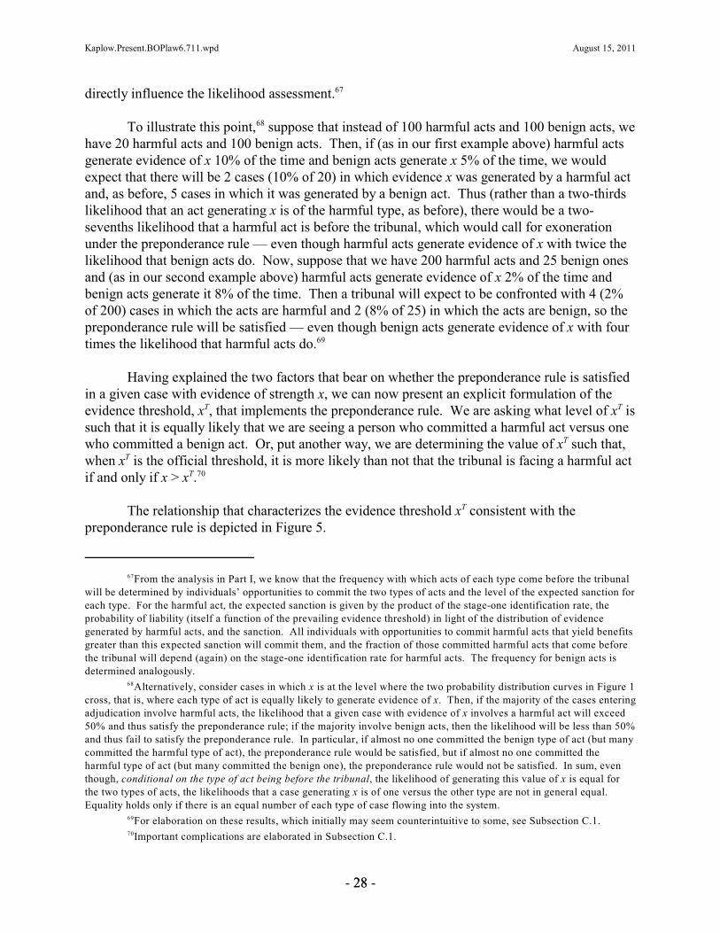
Kaplow.Present.BOPlaw6.711.wpd August 15, 2011
From the analysis in Part I, we know that the frequency with which acts of each type come before the tribunal67
will be determined by individuals’ opportunities to commit the two types of acts and the level of the expected sanction foreach type. For the harmful act, the expected sanction is given by the product of the stage-one identification rate, theprobability of liability (itself a function of the prevailing evidence threshold) in light of the distribution of evidencegenerated by harmful acts, and the sanction. All individuals with opportunities to commit harmful acts that yield benefitsgreater than this expected sanction will commit them, and the fraction of those committed harmful acts that come beforethe tribunal will depend (again) on the stage-one identification rate for harmful acts. The frequency for benign acts isdetermined analogously.
Alternatively, consider cases in which x is at the level where the two probability distribution curves in Figure 168
cross, that is, where each type of act is equally likely to generate evidence of x. Then, if the majority of the cases enteringadjudication involve harmful acts, the likelihood that a given case with evidence of x involves a harmful act will exceed50% and thus satisfy the preponderance rule; if the majority involve benign acts, then the likelihood will be less than 50%and thus fail to satisfy the preponderance rule. In particular, if almost no one committed the benign type of act (but manycommitted the harmful type of act), the preponderance rule would be satisfied, but if almost no one committed theharmful type of act (but many committed the benign one), the preponderance rule would not be satisfied. In sum, eventhough, conditional on the type of act being before the tribunal, the likelihood of generating this value of x is equal forthe two types of acts, the likelihoods that a case generating x is of one versus the other type are not in general equal. Equality holds only if there is an equal number of each type of case flowing into the system.
For elaboration on these results, which initially may seem counterintuitive to some, see Subsection C.1.69
Important complications are elaborated in Subsection C.1.70
- 2288 -
directly influence the likelihood assessment.67
To illustrate this point, suppose that instead of 100 harmful acts and 100 benign acts, we68
have 20 harmful acts and 100 benign acts. Then, if (as in our first example above) harmful actsgenerate evidence of x 10% of the time and benign acts generate x 5% of the time, we wouldexpect that there will be 2 cases (10% of 20) in which evidence x was generated by a harmful actand, as before, 5 cases in which it was generated by a benign act. Thus (rather than a two-thirdslikelihood that an act generating x is of the harmful type, as before), there would be a two-sevenths likelihood that a harmful act is before the tribunal, which would call for exonerationunder the preponderance rule — even though harmful acts generate evidence of x with twice thelikelihood that benign acts do. Now, suppose that we have 200 harmful acts and 25 benign onesand (as in our second example above) harmful acts generate evidence of x 2% of the time andbenign acts generate it 8% of the time. Then a tribunal will expect to be confronted with 4 (2%of 200) cases in which the acts are harmful and 2 (8% of 25) in which the acts are benign, so thepreponderance rule will be satisfied — even though benign acts generate evidence of x with fourtimes the likelihood that harmful acts do.69
Having explained the two factors that bear on whether the preponderance rule is satisfiedin a given case with evidence of strength x, we can now present an explicit formulation of theevidence threshold, x , that implements the preponderance rule. We are asking what level of x isT T
such that it is equally likely that we are seeing a person who committed a harmful act versus onewho committed a benign act. Or, put another way, we are determining the value of x such that,T
when x is the official threshold, it is more likely than not that the tribunal is facing a harmful actT
if and only if x > x .T 70
The relationship that characterizes the evidence threshold x consistent with theT
preponderance rule is depicted in Figure 5.

Kaplow.Present.BOPlaw6.711.wpd August 15, 2011
- 2299 -
Figure 5: Evidence Threshold for Preponderance Rule
The product in the box on the left side indicates how often harmful acts before the tribunal willbe associated with evidence at the threshold x , and the product in the right box indicates howT
often this is so for benign acts. If the product in the left box exceeds that in the right box, thenthe acts are more likely to be harmful; in this case, it seems that the x that satisfies theT
preponderance rule must be lower. If the product on the left is less than that on the right, then theacts are more likely to be benign; in this case, it seems that the requisite x must be higher. TheT
evidence threshold that satisfies the preponderance rule is that where these two likelihoods areequal; that is, when the evidence strength is precisely at such an x , it is just as likely that the caseT
at hand involves a harmful act as a benign one.
The two elements in each box correspond to the two factors identified and illustratedpreviously. The frequencies that harmful and benign acts come before the tribunal are the rates atwhich each type of case flows into the system of adjudication. The probabilities of evidence atthe threshold, given the type of act, are the heights of the probability distribution curves in Figure1. The preceding numerical examples illustrate the manner in which these factors interact todetermine each likelihood and thus whether the preponderance rule is satisfied.
Note that if the two frequencies (the top elements in each box) were equal, then thepreponderance rule threshold would be one for which the probabilities of evidence of thatstrength were equal for the two types of acts (which is the level of x where the two probabilitydistribution curves in Figure 1 cross, at the center of the axis). If the frequency of harmful acts isrelatively greater than that for benign acts, then the evidence threshold under the preponderancerule will be such that the probability of evidence at the threshold when a benign act wascommitted is correspondingly higher than that for a harmful act (i.e., the value of x would beT
lower, to the left of center in Figure 1). The reason is that — for the products in the two boxes tobe equal — if the first factor is higher in the left box, then the second factor must be lower (andin the same proportion). Similarly, if the frequency of harmful acts is relatively less, then theevidence threshold under the preponderance rule will be such that the probability of evidence atthat level for the harmful act is relatively greater (i.e., the value of x would be higher, to the rightT
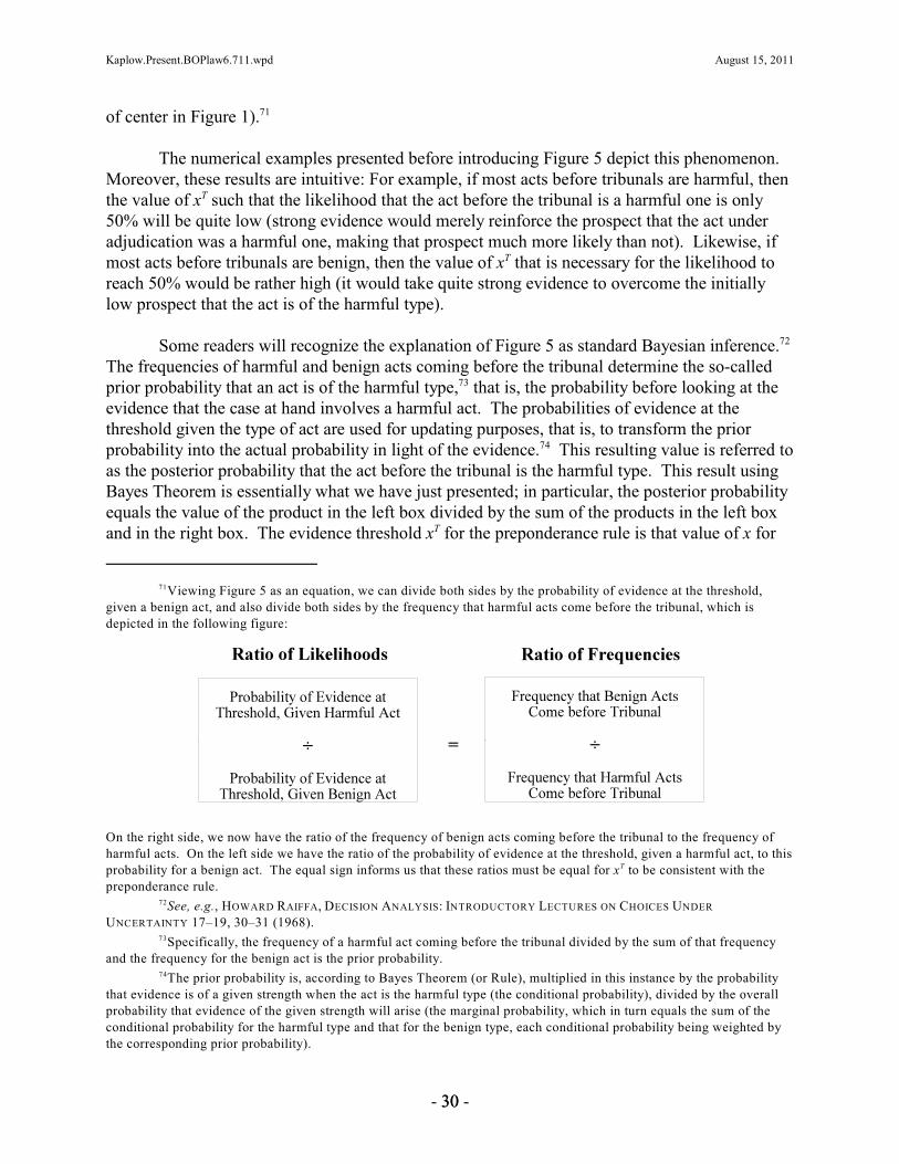
Kaplow.Present.BOPlaw6.711.wpd August 15, 2011
Viewing Figure 5 as an equation, we can divide both sides by the probability of evidence at the threshold,71
given a benign act, and also divide both sides by the frequency that harmful acts come before the tribunal, which isdepicted in the following figure:
On the right side, we now have the ratio of the frequency of benign acts coming before the tribunal to the frequency ofharmful acts. On the left side we have the ratio of the probability of evidence at the threshold, given a harmful act, to thisprobability for a benign act. The equal sign informs us that these ratios must be equal for x to be consistent with theT
preponderance rule.
See, e.g., HOWARD RAIFFA, DECISION ANALYSIS: INTRODUCTORY LECTURES ON CHOICES UNDER72
UNCERTAINTY 17–19, 30–31 (1968).
Specifically, the frequency of a harmful act coming before the tribunal divided by the sum of that frequency73
and the frequency for the benign act is the prior probability.
The prior probability is, according to Bayes Theorem (or Rule), multiplied in this instance by the probability74
that evidence is of a given strength when the act is the harmful type (the conditional probability), divided by the overallprobability that evidence of the given strength will arise (the marginal probability, which in turn equals the sum of theconditional probability for the harmful type and that for the benign type, each conditional probability being weighted bythe corresponding prior probability).
- 3300 -
of center in Figure 1).71
The numerical examples presented before introducing Figure 5 depict this phenomenon. Moreover, these results are intuitive: For example, if most acts before tribunals are harmful, thenthe value of x such that the likelihood that the act before the tribunal is a harmful one is onlyT
50% will be quite low (strong evidence would merely reinforce the prospect that the act underadjudication was a harmful one, making that prospect much more likely than not). Likewise, ifmost acts before tribunals are benign, then the value of x that is necessary for the likelihood toT
reach 50% would be rather high (it would take quite strong evidence to overcome the initiallylow prospect that the act is of the harmful type).
Some readers will recognize the explanation of Figure 5 as standard Bayesian inference. 72
The frequencies of harmful and benign acts coming before the tribunal determine the so-calledprior probability that an act is of the harmful type, that is, the probability before looking at the73
evidence that the case at hand involves a harmful act. The probabilities of evidence at thethreshold given the type of act are used for updating purposes, that is, to transform the priorprobability into the actual probability in light of the evidence. This resulting value is referred to74
as the posterior probability that the act before the tribunal is the harmful type. This result usingBayes Theorem is essentially what we have just presented; in particular, the posterior probabilityequals the value of the product in the left box divided by the sum of the products in the left boxand in the right box. The evidence threshold x for the preponderance rule is that value of x forT

Kaplow.Present.BOPlaw6.711.wpd August 15, 2011
See, e.g., SYDNEY A. BECKMAN, SUSAN CRUMP & FRED GALVES, EVIDENCE: A CONTEMPORARY APPROACH75
697 (2009); C.M.A. McCauliff, Burdens of Proof: Degrees of Belief, Quanta of Evidence, or ConstitutionalGuarantees?, 35 VAND. L. REV. 1293, 1328 tbl.5, 1332 tbl.8 (1982) (presenting results from a survey of federal judgesindicating that the standard was associated with a probability of 75% by just over a third, with either 70% or 80% bynearly a third more, and with 74.99% on average).
Some embrace probabilistic interpretations of all proof standards. See, e.g., MCCORMICK ON EVIDENCE, supra76
note 2, at 490–91 (stating, when commenting on the requirement of proof beyond a reasonable doubt, “As we have seenwith reference to civil cases, a lawsuit is essentially a search for probabilities. A margin of error must be anticipated inany such search.”). However, many commentators resist the idea of assigning any probability to the requirement of proofbeyond a reasonable doubt, and there is considerable variation in what probabilities are thought to be associated with thisproof standard when figures are assigned. See, e.g., RICHARD O. LEMPERT, SAMUEL R. GROSS & JAMES S. LIEBMAN, AMODERN APPROACH TO EVIDENCE: TEXT, PROBLEMS, TRANSCRIPTS AND CASES 1244 n.13 (3d ed. 2000) (discussingstudies suggesting that most jurors place the requirement in the 85% to 90% range); MARC L. MILLER & RONALD F.WRIGHT, CRIMINAL PROCEDURES: CASES, STATUTES, AND EXECUTIVE MATERIALS 1319 (3d ed. 2007) (“Most state andfederal courts discourage or prohibit trial judges from efforts to quantify the reasonable doubt standard.”); id. (noting onestudy suggesting that jurors view beyond a reasonable doubt to mean about 86% certainty and another indicating a widerange from 50% to 100%); Hal R. Arkes & Barbara A. Mellers, Do Juries Meet Our Expectations?, 26 LAW & HUM.BEHAV. 625, 630–31 (2002) (citing surveys of judges, where mean and median numerical responses were at or near 90%,with 90, 95, and 100% being the most frequent specific responses); Erik Lillquist, Recasting Reasonable Doubt: DecisionTheory and the Virtues of Variability, 36 U.C. DAVIS L. REV. 85 (2002) (arguing that the reasonable doubt standard inaction requires less certainty than we generally assume, and that jurors should and do use the standard flexibly);McCauliff, supra note 75, at 1325 tbl.2, 1332 tbl.8 (presenting results of a survey of federal judges showing that about athird associated beyond a reasonable doubt with 90%; most others offering 80%, 85%, 95%, or 100%; and a meanresponse of 90.28%); Charles R. Nesson, Reasonable Doubt and Permissive Inferences: The Value of Complexity, 92HARV. L. REV. 1187, 1196–97 (1979) (claiming that ambiguity in the meaning of the reasonable doubt requirementusefully serves the legal system’s need to make verdicts externally acceptable to the public at large); Lawrence M. Solan,Refocusing the Burden of Proof in Criminal Cases: Some Doubt About Reasonable Doubt, 78 TEX. L. REV. 105 (1999);see also infra Section D (questioning the relevance of quantification of conventional proof requirements in a vacuum). Regarding the theoretical question whether the beyond a reasonable doubt requirement (or any other not-explicitly-quantitative standard) can be reduced to a probability, see note 60.
The formula that determines the factor by which to multiply on the right side equals the target percentage77
divided by the quantity: one minus the target percentage.
- 3311 -
which this fraction (posterior probability) is 0.5 or 50%.
Before proceeding, it is important to recognize that essentially the same analysis and aslightly modified version of Figure 5 can be used to determine the evidence threshold consistentwith any desired minimum likelihood that the act before the tribunal is of the harmful type. Toillustrate, suppose that one wanted to require a likelihood of at least 75% rather than 50% (whichelevated likelihood might roughly be associated by some with the “clear and convincing” proofstandard ). Then one could simply multiply the product in the right box by 3. To see why, note75
that our target likelihood that the act under scrutiny is a harmful one is 75%, which implies thatthe likelihood that it is benign is 25%. To achieve this relationship, we need the value in the leftbox to be 3 times higher than the value in the right box (75% = 3 × 25%). If we multiply thevalue on the right side by 3 and then determine for what evidence threshold x there is equality,T
we will have our answer. If we instead wanted a 95% likelihood that the act is of the harmfultype (which some might loosely associate with the beyond a reasonable doubt requirement ), we76
would need the left side to be 19 times the value of the right side (95% = 19 × 5%), so we wouldmultiply by 19 on the right. And so forth.77
Observe that multiplying the right side by a constant does change the value of the

Kaplow.Present.BOPlaw6.711.wpd August 15, 2011
- 3322 -
evidence threshold x but does not change the analysis by which it is determined. We still haveT
the two factors in each box in Figure 5, and these two factors are evaluated as just described. Thus, although different strengths of the burden of proof are implemented by different evidencethresholds, the relevant elements and basic concepts are entirely the same — except forincorporating the multiplicative factor, which for the preponderance rule was implicitly taken toequal 1 (50% = 1 × 50%) and thus could be omitted from the figure. Accordingly, in most of thediscussion to follow, the text will continue to speak, for concreteness, in terms of thepreponderance rule. We can, however, interpret these references for most purposes as ashorthand for preponderance-like rules, which is to say rules of the class that the determinants ofthe evidence threshold are essentially the same as those under the preponderance rule — whichincludes all rules that deem it necessary and sufficient that the likelihood that the act is of theharmful type exceed some given likelihood (be it 50%, 75%, 95%, or any other value).
B. Comparison
This Section compares the determinants of the evidence threshold for the preponderancerule (and, as just noted, for any rule formulated in terms of the likelihood that the act before thetribunal is of the harmful type) with those of the optimal evidence threshold, which is to say thatwhich maximizes social welfare. This being a conceptual analysis, the focus is qualitative, onhow and why the relevant factors differ.
1. Analysis
To facilitate a side-by-side comparison, it is helpful to reproduce Figure 4, slightly alteredby placing an equals sign between the boxes to denote the optimal threshold.

Kaplow.Present.BOPlaw6.711.wpd August 15, 2011
- 3333 -
Figure 6: Effects of Reduction in Evidence Thresholdat the Optimal Threshold
On their face, Figures 5 and 6 have no elements in common. Figure 6 for the optimal evidencethreshold has seven elements: three of them — the increase in the expected sanction,concentration of acts, and private benefit — applicable to each type of act; and social harm,relevant for only the harmful act. Figure 5 has four elements: two — the frequency of acts andprobability of evidence at the threshold — applicable to each type of act. The overlap is nil. (Ifwe modified the right side of Figure 5 to include a constant multiplier to reflect a likelihood-stylerule not pegged at 50% — for example, a factor of 3 for a 75% rule — we would be introducingyet another difference.)
On further analysis, it turns out that there are some underlying commonalities, althoughnot nearly enough to alter the conclusion that the differences are overwhelming. Specifically, thetop elements in Figure 6 for the optimal evidence threshold — the increases in expectedsanctions — are determined in part (recall from Section I.B) by the extent to which theprobability of finding liability, given that an individual is before the tribunal, rises as theevidence threshold is reduced. That change in probability for the two types of acts is, in turn,indicated by the height of the corresponding probability curves in Figure 1. (To review, as theevidence threshold x is reduced slightly, some of the area under the probability curves that usedT
to be to the left of x will now be to the right of x , and the heights of the probability curvesT T
indicates how great these changes will be.) In Figure 5 for the evidence threshold under thepreponderance rule, the bottom elements in the boxes are the probabilities of evidence at thethreshold for the two types of acts. Those probabilities are also given by the heights of the curvesin Figure 1. Accordingly, one component of the top elements in the boxes in Figure 6 is equal to

Kaplow.Present.BOPlaw6.711.wpd August 15, 2011
Interestingly, although these values are the same, they arise for different reasons. In Figure 6 for the optimal78
threshold, the origin pertains to the changes in deterrence and chilling as the threshold is reduced, whereas in Figure 5 forthe preponderance rule, it pertains to the likelihood that evidence would be observed.
Such is hardly surprising since there is a single underlying scenario used to determine all of the values in both79
figures. Specifically, the upper elements in the boxes in Figure 5, the frequencies with which each type of act comesbefore the tribunal, depend on the level of the expected sanction for each type of act, which level (as previouslyexplained) also equals the private benefit of the marginal deterred or chilled individual. That private benefit is relevant inFigure 6 but not in any direct way in Figure 5. Additionally, one of the components in the first element in the boxes inFigure 6 (the increase in expected sanctions) is the fraction of each type of act that is identified in stage one, and thisfraction is also a component of the first element in the boxes in Figure 5 (the frequency that acts come before thetribunal). For related discussion, see Subsection 2.
- 3344 -
the corresponding values of the bottom elements in the boxes in Figure 5. No other direct78
linkages exist, although there are some further indirect connections, as noted in the margin.79
To appreciate how great is the difference between these two approaches to setting anevidence threshold — choosing a target likelihood versus aiming to maximize social welfare —it is useful to examine briefly each of the many differences between these two figures. The topelements in the boxes in Figure 6 are the increases in expected sanctions for harmful and forbenign acts. If the concern is welfare, these factors are crucial because they indicate how muchdeterrence and chilling rise when the evidence threshold is reduced. They are not directlyreflected in Figure 5 for the preponderance rule because that rule is not concerned at all with theeffects of the evidence threshold on behavior; concomitantly, it is concerned with properties at agiven level of the threshold and not at all with how anything changes as the threshold is changed. This difference in perspective is fundamental and explains some of the other contrasts as well.
The middle elements in the boxes in Figure 6 are the concentrations of marginal harmfuland benign acts. As explained in Section I.B, this information indicates whether the increases inexpected sanctions for both harmful and benign acts translate into large or small numbers ofindividuals being deterred and chilled, respectively. Again, these factors are obviously central inassessing the welfare consequences of different evidence thresholds, but they have nothing to dowith the likelihood, at some given evidence strength x, that the act before the tribunal is of theharmful rather than the benign type.
For the final row of Figure 6, we have individuals’ private benefits of acts that areforgone when such acts are deterred or chilled, and the social harm that is avoided when harmfulacts are deterred. These are the social welfare impacts of the changes in behavior just described. They are of obvious social consequence but again are entirely irrelevant to whether evidence ofsome strength x indicates that the likelihood of an act before the tribunal is above or below 50%(or any other stipulated magnitude).
Relatedly, the elements in Figure 5 for the preponderance rule do not appear directly inFigure 6, and the reason is that they do not directly relate to the welfare effects of differentevidence thresholds. The top elements in the boxes in Figure 5 are the frequencies with whichacts of the two types come before the tribunal. Although of central relevance in computing thelikelihoods, as explained in Section A, they have no direct welfare relevance in setting the

Kaplow.Present.BOPlaw6.711.wpd August 15, 2011
- 3355 -
optimal evidence threshold. This may be surprising because the frequencies of harmful andbenign acts seem highly pertinent. However, as mentioned just above, what matters in decidingwhether the evidence threshold is too high, too low, or just right (optimal) is how much thenumber of harmful and benign acts changes as the threshold is changed, not on how many actsthere are. (As will be discussed in Parts III and IV, however, in other settings and for otherreasons, these overall frequencies of harmful and benign acts will matter in determining theoptimal evidence threshold.) Last, as already discussed, the bottom elements in the boxes inFigure 5 — the probabilities of evidence at the threshold for the two types of acts — are the otherkey determinants of the likelihood, which is the matter of interest under the preponderance rule(and other likelihood-based rules) but is not relevant per se for determining the optimal evidencethreshold (although it is a component of the change in expected sanctions for the two types ofacts).
The large — one might say radical — difference between the two formulations has anumber of implications. First, as a conceptual matter, it reinforces the notion that we do not justhave some subtle or technical distinctions but rather two entirely different outlooks on what theburden of proof is all about. Figure 6, for the optimal evidence threshold, was derived by askingwhat would be the effects of changing the threshold on social welfare, and then analyzing howthe relevant effects, the deterrence benefit and the chilling cost, are determined. By contrast,Figure 5, for the preponderance rule, was derived by asking under what circumstances would thelikelihood that the case before the tribunal involves a harmful act be 50% (or some otherstipulated probability).
Second, as a pragmatic matter, if one is actually concerned with welfare, taking alikelihood-based approach such as that under the preponderance rule does not serve as a proxyfor identifying a welfare-maximizing evidence threshold, not even approximately so. A goodproxy ordinarily is determined by most of the same elements as the true objective and in a similarfashion — or, relatedly, there needs to be a substantial correlation between the proxy and theobjective. The foregoing comparison makes it plain that, instead, the two calculuses are almostentirely distinct. For example, it would be a pure coincidence if the evidence threshold for thepreponderance rule was equal to or even close to the optimal level. After all, factors that couldmake the optimal evidence threshold very high or quite low have no impact at all on the evidencethreshold that implements the preponderance rule, and vice versa.
An immediate corollary of this practical point is that the optimal evidence threshold couldbe associated with any ex post probability whatsoever. This claim is true in light of threeconsiderations: First, the optimal evidence threshold is determined by the combination of a largenumber of factors, as depicted in Figure 6, that each could take on a wide range of values. Second, the ex post probability (which, recall from the discussion of the Bayesian posteriorprobability at the end of Section A, is the value of the product in the left box in Figure 5 dividedby the sum of the products in the two boxes in Figure 5) is also determined by many factors thateach could take on a wide range of values. Third, the determinants of the first and of the secondare largely unrelated, making it entirely plausible that the first could be high and the second low,the first low and the second high, and so forth.

Kaplow.Present.BOPlaw6.711.wpd August 15, 2011
This setting is closer to that examined in Section IV.C, where it will be explained that, even though the80
qualitative difference between the formulation for the optimal evidence threshold and that for the preponderance rule isfar less, it is still true that the optimal threshold could take on any value and be associated with any ex post likelihood.
The reader may wonder whether even this would suffice, for at a low threshold there may still be relatively81
few benign acts (there were not many to begin with, and the reduction in the threshold will chill even more). Thisconcern turns out to be warranted, as discussed further in Subsection C.1.
Echoing the preceding footnote, it is not obvious that one would ever achieve the balance of likelihoods82
required by the preponderance rule.
- 3366 -
To be more specific, consider the first point, regarding the optimal evidence threshold. All else equal, if harm is extremely high and few beneficial acts would be chilled, the optimalevidence threshold would be very low. However, if harm was negligible and many beneficialacts would be chilled, the optimal evidence threshold would be very high — one could imaginecases in which the optimum would be little different from de facto legal immunity. Theseperhaps jarring illustrations should not, however, be seen as particularly counterintuitive. Evenin the analytically simpler medical diagnosis example mentioned in the Introduction and inSubsection I.A.2, it is familiar that the optimal treatment threshold may be extremely low orquite high depending on the risks and benefits of the treatment. For example, an immunization80
may be advantageous to an individual with less than a one in a thousand chance of contracting adisease in light of the magnitude of harm averted and the small cost; by contrast, a dangerousexperimental treatment may be undesirable even for an individual with a ninety percent chance ofdying without it if the prospective benefit is sufficiently small and there is a serious risk that itwould cause death in the remaining ten percent of cases. On reflection, we should instead betroubled by the notion that it may make sense, even as an approximation, to employ a singlethreshold or to demand a particular likelihood (like 50%) to make important decisions in a widerange of contexts in which the consequences vary dramatically.
Now consider the second point concerning the evidence threshold implied, say, by thepreponderance rule. One might suppose that it is at some intermediate, moderate level (perhapsnear where the probability distribution curves in Figure 1 cross). However, as explained inSection A, this is not the case due to the importance of the upper elements in the boxes in Figure5 pertaining to the frequencies with which harmful and benign acts come before the tribunal. Suppose, for example, that many of the harmful type of act are committed but there are fewbenign acts that might be confused with it. In that case, a moderate evidence threshold would beassociated with a very high likelihood that a given act before the tribunal was of the harmfultype. To implement the preponderance rule may then require an extremely low evidencethreshold. Now imagine instead that there are many benign acts and few harmful ones. Then,81
in order to raise the ex post likelihood from a very low level to 50%, it may be necessary to setthe evidence threshold at an extremely high level.82
In sum, optimal evidence thresholds may be very high or quite low. Likewise for theevidence thresholds required to implement the preponderance rule — or any other rule thattargets an ex post likelihood that the individual before the tribunal committed the harmful type ofact. And, as previously elaborated, there is little relationship between the factors determining theevidence threshold under these two contrasting conceptions of the problem, so indeed anyrelationship is possible. If one is concerned with social welfare, this finding should be disturbing

Kaplow.Present.BOPlaw6.711.wpd August 15, 2011
As discussed in Section D, it is hardly clear that the legal system in fact operates in this manner.83
The optimal level of generality of burden-of-proof rules is beyond the scope of the present investigation. It84
should be apparent, however, that both optimal evidence thresholds and the evidence threshold for the preponderance rule(or other rules of that type) will vary greatly by context, even at fairly refined levels. For example, even within contractdisputes, different claims in different settings may vary substantially with regard to all of the key factors. For furtherdiscussion, see note 123.
- 3377 -
if the legal system in fact operates under the preponderance rule or some other likelihood-basedformulation, for such a regime would sometimes insist on very high thresholds when the optimalthreshold was not merely lower but very low, and it would sometimes employ quite lowthresholds when the optimal threshold was extremely high.83
2. Comment on Information Requirements
An obvious practical challenge posed by the formulation for the optimal evidencethreshold developed in Part I and revisited in the preceding Subsection concerns the highinformation requirements for its application, whether to a broad class of cases, a narrower cluster,or a given case. This concern is a serious one given the number of elements in Figures 4 and 684
as well as the difficulty of ascertaining many of them, such as the likelihoods that harmful andbenign acts each give rise to evidence of a particular strength and the concentration ofindividuals’ private benefits from acts of the two types. This Subsection extends the comparisonbetween an optimal evidence threshold and that implied by the preponderance rule (or otherssimilarly grounded in ex post likelihoods) to consider differential information requirements.
Before examining the details, it should be emphasized at the outset that possibledifferences in information requirements have little to do with the merits of one or another way ofsetting the burden of proof. The optimal evidence threshold is that which maximizes socialwelfare. If welfare is the objective, it would make no sense to substitute some other formulationbecause it happened to be easier to employ when that alternative has essentially no relationship towhat matters. (Easiest of all would be to flip a coin, but its ease offers little to commend it.) Asemphasized in Subsection 1, a preponderance rule does not depend at all on most of what iswelfare relevant and instead depends on much that is not. That is, conventional formulations arenot even plausible proxies for welfare.
In comparing the information requirements under the two approaches, it may initiallyappear that the preponderance rule is less demanding since it depends on fewer components. However, this impression is misleading; in fact, the underlying information requirements arequite similar. To see this point, consider the pertinent factors.
Using Figure 6 for the optimal evidence threshold, begin with the top and middleelements, the increases in expected sanctions due to a reduction in the evidence threshold and theconcentrations of marginal acts. Recall from Section I.B that the reason these elements appear isthat their product determines the number of acts deterred (for the left box) and the number of actschilled (for the right box) when the threshold is changed. These products, therefore, indicate thechanges in the frequencies that harmful and benign acts are committed. Multiplying these by the
Kaplow.Present.BOPlaw6.711.wpd August 15, 2011
If one was already employing some evidence threshold x and, moreover, it so happened that the threshold was85 T
one that satisfied the preponderance rule (or some other ex post likelihood target), one might be able to verify this bylooking at the existing frequencies for the two types of acts coming before the tribunal (if these could be directlyobserved) and the distributions of evidence associated with each type of act. However, if not already at such a point(whether by chance or by prior calculation), one would need to know the sorts of information described in the text todetermine how to set the threshold so as to meet the target likelihood. Moreover, in light of the problems identified inSubsection C.1, it may not be easy to iterate to an evidence threshold producing the requisite ex post likelihood, in partbecause it would not be obvious in which direction to move the threshold if not already at the desired target.
Although the text explains the underlying connections between the information requirements for each86
approach, they are rather subtle, and one may not be entirely convinced by such an informal exposition. For a formaltreatment, see Kaplow, Optimal Burden of Proof, supra note 15. As explained there, the frequency distributions requiredfor determining the ex post likelihood are the cumulative distribution functions for the benefits from the two types of acts,whereas the concentrations required for determining the optimal evidence thresholds are the corresponding densityfunctions. (Since the density functions are simply the derivatives of the distribution functions and the latter are theintegrals of the former, knowledge of one is equivalent to knowledge of the other.) Moreover, one needs to know whereto evaluate each of these functions for a given evidence threshold, and those points are given by the benefits of themarginal individual of each type, which in turns constitutes the information on private benefits in the lower elements ofFigure 6.
In a narrowly retributive system, in which the magnitude of the punishment is supposed to equal the gravity of87
the crime (or some given proportion thereof), this would necessarily be true. More broadly, when sanctions are set in anysense with welfare in mind, this information will be important (or at least indirectly so, in determining enforcement effortand thus the expected sanction; see infra Part III).
- 3388 -
likelihood that acts are identified at stage one (itself a component of the expected sanctions)yields the change in the frequencies with which harmful and benign acts come before thetribunal. But it is apparent from Figure 5 that the levels of these frequencies are a central input todetermining the evidence threshold for the preponderance rule and other likelihood-based rules. 85
The other element for the preponderance rule, the probabilities of evidence at the threshold, are,as explained in Subsection 1, components of the increases in expected sanctions, the topelements in Figure 6.
Next, consider the private benefits of the two types of acts, in the bottom elements inFigure 6. These do not appear directly in Figure 5, but the underlying determinants are employedindirectly. Recall that these benefits refer to those for marginal acts, and these in turn (asexplained in Section I.B) will equal the expected sanctions for the respective types of acts. (Individuals just on the brink of being deterred or chilled are those whose private benefits fromtheir act just equal the pertinent expected sanction.) And these expected sanctions determinehow many harmful acts are deterred and benign acts are chilled, with the undeterred andunchilled acts being the frequency with which each type of act is committed, a component of thetop elements in Figure 5 (which factor is multiplied by the stage-one identification rates).
At this point, we can see that all the information needed to determine the optimalevidence threshold — except for the magnitude of social harm — is likewise necessary forapplication of the preponderance rule or similar likelihood-based rules. Reflection on the86
foregoing suggests that the converse is true as well. Hence, the only fundamental informationaldifference between the two contrasting formulations for the evidence threshold concerns thedegree of social harm from harmful acts. But presumably the legal system has pertinentinformation on this element (or what it considers to be a workable estimate) since this is a centraldeterminant of the magnitude of the sanction. For civil liability, ordinary compensatory87

Kaplow.Present.BOPlaw6.711.wpd August 15, 2011
To implement a preponderance (or similar type of) rule, one method would be for the system designers to88
determine (in various classes of cases) the appropriate evidence threshold and then communicate this threshold tofactfinders, just as one might imagine being done if the optimal evidence threshold was employed. See infra note 130. Ifinstead the matter is left to factfinders in individual cases, application of the preponderance rule would be much morecomplicated, as the analysis in Subsection C.1 indicates. Additional factors influencing the selection of cases in stageone, some explored in Section IV.D, make the analysis even more challenging — see especially note 210.
- 3399 -
damages equal harm, which consequently must be measured.
For the most part, then, the great gulf between the formulation for the optimal evidencethreshold and that for the threshold that implements the preponderance rule (or other likelihood-based rules) does not involve what information is required. Instead, the difference is in how thatinformation is utilized. Informational requirements are a significant challenge underconventional conceptions and under welfare maximization. Regarding the former, the subtle,demanding informational basis for application of the preponderance rule seems not to have beenfully appreciated. In any event, even if the preponderance rule and others like it were simpler to88
apply, this facility would hardly constitute a sound argument in their favor.
C. Elaboration
Section B raises serious questions about the normative basis for the preponderance of theevidence rule and for other conventional burden of proof standards that determine liability basedon a target ex post likelihood. As explained, the main factors relevant to social welfare arelargely irrelevant under all such rules. Not only do conventional formulations answer a questionthat turns out to have almost nothing to do with what matters for society, but they also haveadditional features that are, on reflection, quite surprising, as elaborated in Subsection 1. Subsection 2 examines alternative objectives advanced in some of the literature and explains howsimilar problems as well as additional difficulties arise.
1. Relationship Between Level of Evidence Threshold and Ex Post Likelihood
The last topic in Subsection B.1 concerns how any relationship between the optimalevidence threshold and the ex post likelihood could prevail. Another basic question concerns thefunctional relationship between the evidence threshold (optimal or not) and the ex post likelihoodthat the individual before the tribunal committed a harmful act. It is generally supposed andseems intuitively correct that, say, raising the evidence threshold will increase this likelihoodsince a higher threshold demands stronger evidence in order to assign liability. This presumedrelationship, however, need not hold: it is entirely possible, and also plausible, that a higherthreshold will sometimes result in a lower ex post likelihood rather than a higher one for casesthat just meet the new, heightened threshold. In other words, insisting on stronger evidence mayhave the result that, in cases just meeting the stricter threshold, a greater fraction involvesindividuals who committed benign acts and are thus being sanctioned by mistake. Moreover, thisfact and the analysis that underlies it have additional, unappreciated consequences.
This counterintuitive result can be understood by reexamining Figure 5, reproduced here
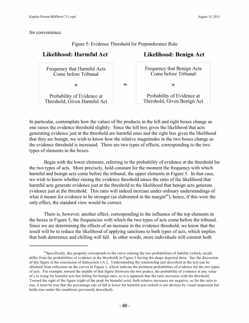
Kaplow.Present.BOPlaw6.711.wpd August 15, 2011
Specifically, this property corresponds to the curve relating the two probabilities of liability (which, recall,89
differ from the probabilities of evidence at the threshold) in Figure 3 having the shape depicted there. See the discussionof this figure at the conclusion of Subsection I.A.2. Understanding the relationship just described in the text can beobtained from reflection on the curves in Figure 1, which indicate the pertinent probabilities of evidence for the two typesof acts. For example, toward the middle of that figure (between the two peaks), the probability of evidence at any valueof x is rising for harmful acts but falling for benign ones, so it is apparent that the ratio increases with the threshold. Toward the right of the figure (right of the peak for harmful acts), both relative increases are negative, so for the ratio torise, it must be true that the percentage rate of fall is lower for harmful acts (which is not obvious by visual inspection butholds true under the conditions previously described).
- 4400 -
for convenience.
Figure 5: Evidence Threshold for Preponderance Rule
In particular, contemplate how the values of the products in the left and right boxes change asone raises the evidence threshold slightly. Since the left box gives the likelihood that actsgenerating evidence just at the threshold are harmful ones and the right box gives the likelihoodthat they are benign, we wish to know how the relative magnitudes in the two boxes change asthe evidence threshold is increased. There are two types of effects, corresponding to the twotypes of elements in the boxes.
Begin with the lower elements, referring to the probability of evidence at the threshold forthe two types of acts. More precisely, hold constant for the moment the frequency with whichharmful and benign acts come before the tribunal, the upper elements in Figure 5. In that case,we wish to know whether raising the evidence threshold raises the ratio of the likelihood thatharmful acts generate evidence just at the threshold to the likelihood that benign acts generateevidence just at the threshold. This ratio will indeed increase under ordinary understandings ofwhat it means for evidence to be stronger (as elaborated in the margin ); hence, if this were the89
only effect, the standard view would be correct.
There is, however, another effect, corresponding to the influence of the top elements inthe boxes in Figure 5, the frequencies with which the two types of acts come before the tribunal. Since we are determining the effects of an increase in the evidence threshold, we know that theresult will be to reduce the likelihood of applying sanctions to both types of acts, which impliesthat both deterrence and chilling will fall. In other words, more individuals will commit both

Kaplow.Present.BOPlaw6.711.wpd August 15, 2011
Note that, although an argument was given about the nature of stronger evidence implying that the former90
effect is in the normally supposed direction, there was no particular basis for assuming anything about the magnitude ofthis effect, specifically, relative to the behavioral effect. It can be shown that the ex post evidentiary effect depends onthe comparison of the slopes of the two curves in Figure 1, each relative to their height, at the evidence threshold x inT
question, but the behavioral effect does not. By contrast, the latter depends on a number of factors that have no influenceon the former.
- 4411 -
harmful acts and benign acts, so more of both types of acts will come before the tribunal. Theformer effect further increases the likelihood that acts before the tribunal with evidence just at the(new, heightened) threshold are harmful ones, but the latter effect reduces this likelihood. Therefore, if the heightened evidence threshold reduces the chilling of benign acts relativelymore than it reduces the deterrence of harmful acts, the shift in the flow of cases will be such thata higher fraction of cases entering the system will involve benign acts. Holding constant therates of finding liability for each type of act (the lower elements in the boxes in Figure 5), thisphenomenon would increase the likelihood that individuals found liable would be ones thatcommitted benign acts rather than harmful ones.
Although there is certainly no guarantee that this relationship regarding the upperelements will hold, it is entirely plausible. That is, nothing in the setup of the problem rules itout or makes it somehow unlikely. Note further that this property actually tends to make raisingthe evidence threshold attractive. After all, it indicates that the increase does less to underminedeterrence than to alleviate the chilling of benign acts. Accordingly, it makes sense tocontemplate seriously cases in which this effect is in the direction of raising the fraction ofbenign acts coming before the tribunal, even though this possibility is not the only one.
Let us now combine these two effects, corresponding to the two types of elements inFigure 5. The more familiar one, corresponding to the lower elements, raises the relativelikelihood that an act generating evidence just at the (new, heightened) threshold is of theharmful type, but the other effect, corresponding to the upper elements, may well (but need not)lower this likelihood. If this latter effect is in the opposing direction and happens to have agreater magnitude than the former effect, then indeed the combined result of a heightenedthreshold would be to reduce (not increase) the ex post likelihood that an individual withevidence just meeting the higher threshold would be one who committed a harmful act. Putanother way, findings of liability in cases that just pass the higher threshold may involve a higher(not lower) fraction in which sanctions are imposed by mistake.
This outcome is not a mere theoretical possibility but rather is entirely conceivable, itbeing an empirical matter how often and under what circumstances it will arise. To illustrate90
this situation, suppose that there is a relatively large set of opportunities to commit benign acts,but most are just barely chilled under the current regime. In that setting, an increase in theevidence threshold may, through the reduced chilling effect, cause a relatively large increase inthe flow of benign acts into adjudication, causing a notable rise in the relative rate of mistakenimposition of sanctions despite the fact that such is less likely on a per-case basis.
The foregoing analysis demonstrates that a higher evidence threshold may be associated

Kaplow.Present.BOPlaw6.711.wpd August 15, 2011
Consider the following depiction:91
In this figure, if the dotted line indicating the target ex post likelihood were, say, at 50%, then there would be three levelsof x at which the rule would be satisfied. As drawn, this would also be true at targets of 49% or 51%, but not, sayT
(interpreting the figure roughly), at 35% or 65%. Also, as drawn, for sufficiently low or high targets, say 10% or 90%,there is no value of x that works, which supports the next point in the text. Similarly, for the target of 50%, all levels ofT
x would have been insufficient if the curve happened to be much lower (everywhere below the dotted line), and all levelsT
would have been excessive if the curve had been much higher (everywhere above the dotted line).
- 4422 -
with a lower de facto burden of proof if the proof burden is understood as a minimum ex postlikelihood that cases with evidence just at the threshold involve individuals who actually are oneswho committed harmful acts. Conversely, a system designer hoping to raise the burden of proof,thus defined, may in some instances need to lower the minimum required level of evidence, asparadoxical as that may seem. These consequences, two sides of the same coin, are not onlypossible but do not require far-fetched assumptions in order to occur.
This possibility has additional implications. Notably, it may be that a given target ex postlikelihood — such as the 50% threshold of the preponderance rule — would be associated withmultiple, distinct evidence thresholds. To see this, begin with the standard supposition that, asone raises the evidence threshold, the ex post likelihood rises. In that case, when the evidencethreshold is very low, we might suppose that the resulting ex post likelihood is well below 50%. As the threshold is increased more and more, the ex post likelihood will continue to rise andeventually cross 50%. Once it does, it rises ever further as the threshold is increasedadditionally. Hence, there will be a unique evidence threshold at which the ex post likelihoodequals 50%.
Now introduce the just-established possibility that the ex post likelihood falls with theevidence threshold in some circumstances. Then, after the likelihood passes 50% in theforegoing illustration, it may be that the likelihood at some point begins to fall; and, with furtherincreases in the threshold, it may fall even more, perhaps again crossing 50%, this time movingin the downward direction. In that case, there would be two different evidence thresholds that areeach associated with a 50% ex post likelihood. Moreover, if after further increases in thethreshold, the ex post likelihood once again started to rise, it could now cross 50% a third time;and so forth. In all, there could be one, two, three, or any number of evidence thresholds that91
yield a 50% probability — or a 75% probability, a 95% probability, or any other.

Kaplow.Present.BOPlaw6.711.wpd August 15, 2011
The difficulties raised in the text need to be understood as equilibrium phenomena. When there are multiple92
thresholds that meet a target likelihood, it is the case that, given the choice of one of those thresholds, it is true thatindividuals who anticipate that choice will behave ex ante such that, when factfinders indeed apply that threshold, thestated ex post likelihood will result for cases with evidence just at that threshold. Had one of the other thresholds beenchosen and anticipated by individuals ex ante, then different behavior would have resulted, producing a different flow ofcases into the system, and with that different mix, it would again be true that, for cases just at the alternative threshold,the target likelihood would be produced. Put another way, the ex post likelihoods associated with a given x in the figureT
in note 91 are determined under the assumption that, when individuals decide whether to commit the two types of acts,they are supposing that the threshold that will be applied in adjudication is indeed x .T
In the figure in note 91, evidence thresholds between the middle and right intersections are associated with ex93
post likelihoods below the target level, yet thresholds between the left and middle intersections are associated with expost likelihoods above the target.
See the figure and accompanying discussion in note 91.94
Observe that these complications have no analogue with regard to the optimal evidence threshold. The95
analysis thereof, summarized in Figures 4 and 6, indicates which threshold is best with regard to effects on welfare. Once such a threshold is chosen, that threshold can itself constitute the applicable rule. Note further that, given an
- 4433 -
This possibility is obviously disturbing for a system designer trying to implement, say, thepreponderance rule. It can also be problematic for a factfinder because it might be difficult to actfaithfully on the command to find liability if and only if the preponderance rule — or any otherrule that is based on the ex post likelihood — is satisfied in cases in which the strength of theevidence lies above the lowest threshold that works but below the highest such threshold. 92
Relatedly, in such situations the evidence threshold could be at a level higher than one of thosethat just hits the target likelihood and yet, when evidence is at that threshold, it would not besufficient to meet the target ex post likelihood; and evidence just at a weaker threshold may bestronger than necessary to meet the target likelihood.93
A less subtle but related point is that there is no guarantee that there exists any strength ofevidence such that evidence of that strength is associated with the target ex post likelihood. Taking again, for concreteness, the preponderance rule, it is possible that all levels of evidence,no matter how strong, would be below the threshold. And it is also possible that all levels ofevidence, no matter how weak, would be above the threshold. These scenarios are likewise94
attributable to the top elements in the boxes in Figure 5. For example, if pertinent opportunitiesoverwhelmingly involve benign acts, then even fairly strong evidence may be more likely to havearisen as a consequence of one of the many benign acts that ends up before the tribunal than oneof the very few harmful ones. Employing an ever higher threshold would increase the flow ofharmful acts coming before the tribunal, as explained above, but it would also raise the numberof benign acts. In the reverse case (nearly all opportunities involve harmful acts), even weakevidence may almost always be attributable to a harmful act since nearly all acts that make it tothe tribunal are harmful ones. Reducing the evidence threshold ever further will, to be sure,augment deterrence, but it will also increase chilling, and there is no guarantee that the ratio ofharmful acts coming into the system will not continue to be high enough to offset the weaknessof the evidence.
Combining these points, we find that there may be no evidence threshold associated witha target ex post likelihood (either because all thresholds are too high or all are too low), or onethreshold (as ordinarily assumed), or multiple thresholds. Which situation will hold depends on95
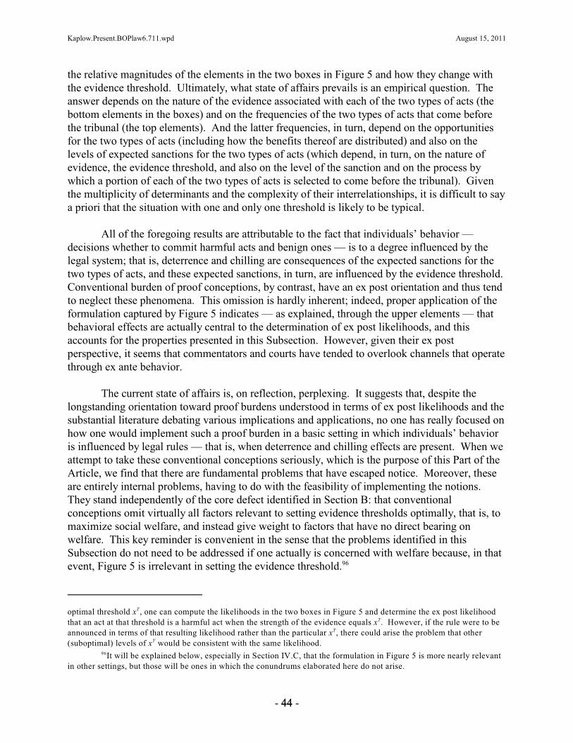
Kaplow.Present.BOPlaw6.711.wpd August 15, 2011
optimal threshold x , one can compute the likelihoods in the two boxes in Figure 5 and determine the ex post likelihoodT
that an act at that threshold is a harmful act when the strength of the evidence equals x . However, if the rule were to beT
announced in terms of that resulting likelihood rather than the particular x , there could arise the problem that otherT
(suboptimal) levels of x would be consistent with the same likelihood.T
It will be explained below, especially in Section IV.C, that the formulation in Figure 5 is more nearly relevant96
in other settings, but those will be ones in which the conundrums elaborated here do not arise.
- 4444 -
the relative magnitudes of the elements in the two boxes in Figure 5 and how they change withthe evidence threshold. Ultimately, what state of affairs prevails is an empirical question. Theanswer depends on the nature of the evidence associated with each of the two types of acts (thebottom elements in the boxes) and on the frequencies of the two types of acts that come beforethe tribunal (the top elements). And the latter frequencies, in turn, depend on the opportunitiesfor the two types of acts (including how the benefits thereof are distributed) and also on thelevels of expected sanctions for the two types of acts (which depend, in turn, on the nature ofevidence, the evidence threshold, and also on the level of the sanction and on the process bywhich a portion of each of the two types of acts is selected to come before the tribunal). Giventhe multiplicity of determinants and the complexity of their interrelationships, it is difficult to saya priori that the situation with one and only one threshold is likely to be typical.
All of the foregoing results are attributable to the fact that individuals’ behavior —decisions whether to commit harmful acts and benign ones — is to a degree influenced by thelegal system; that is, deterrence and chilling are consequences of the expected sanctions for thetwo types of acts, and these expected sanctions, in turn, are influenced by the evidence threshold. Conventional burden of proof conceptions, by contrast, have an ex post orientation and thus tendto neglect these phenomena. This omission is hardly inherent; indeed, proper application of theformulation captured by Figure 5 indicates — as explained, through the upper elements — thatbehavioral effects are actually central to the determination of ex post likelihoods, and thisaccounts for the properties presented in this Subsection. However, given their ex postperspective, it seems that commentators and courts have tended to overlook channels that operatethrough ex ante behavior.
The current state of affairs is, on reflection, perplexing. It suggests that, despite thelongstanding orientation toward proof burdens understood in terms of ex post likelihoods and thesubstantial literature debating various implications and applications, no one has really focused onhow one would implement such a proof burden in a basic setting in which individuals’ behavioris influenced by legal rules — that is, when deterrence and chilling effects are present. When weattempt to take these conventional conceptions seriously, which is the purpose of this Part of theArticle, we find that there are fundamental problems that have escaped notice. Moreover, theseare entirely internal problems, having to do with the feasibility of implementing the notions. They stand independently of the core defect identified in Section B: that conventionalconceptions omit virtually all factors relevant to setting evidence thresholds optimally, that is, tomaximize social welfare, and instead give weight to factors that have no direct bearing onwelfare. This key reminder is convenient in the sense that the problems identified in thisSubsection do not need to be addressed if one actually is concerned with welfare because, in thatevent, Figure 5 is irrelevant in setting the evidence threshold.96

Kaplow.Present.BOPlaw6.711.wpd August 15, 2011
See generally Richard Lempert, The New Evidence Scholarship: Analyzing the Process of Proof, 66 B.U. L.97
REV. 439 (1986) (commenting on the debate about the role of Bayesian modes of inference in factfinding); DanielShaviro, Statistical Probability Evidence and the Appearance of Justice, 103 HARV. L. REV. 530 (1989) (criticizingskepticism about Bayesian reasoning); Laurence H. Tribe, Trial by Mathematics: Precision and Ritual in the LegalProcess, 84 HARV. L. REV. 1329 (1971) (criticizing the use of probability and statistics in trials, including reliance onBayesian inference). Regarding the belief of some academics that factfinders cannot be expected to give consideration toBayesian priors, consider Lord Hoffman’s contrary statement in Secretary of State for the Home Department v. Rehman,[2001] UKHL 47, [2003] 1 A.C. (H.L.) 153 [55] (appeal taken from Special Immigration Appeals Commission):
But . . . some things are inherently more likely than others. It would need more cogent evidence tosatisfy one that the creature seen walking in Regent’s Park was more likely than not to have been alioness than to be satisfied to the same standard of probability that it was an Alsatian [Germanshepherd]. On this basis, cogent evidence is generally required to satisfy a civil tribunal that a personhas been fraudulent or behaved in some other reprehensible manner. But the question is alwayswhether the tribunal thinks it more probable than not.
There is an interesting distinction being made in such discussions, for the fact of the individual appearing98
before the tribunal, standing accused of the offense charged — or of the civil wrong alleged by the plaintiff — is itselfnot taken to be part of the set of evidence the factfinder should consider. Furthermore, although some object to Bayesianreasoning with regard to the fact of an individual being before the tribunal, fewer would object in principle to itsapplication to assessing the evidence, which seems unavoidable. For example, if it is alleged that a wealthy individual,not in financial trouble, executed an elaborate plot (planning, accomplices, secret compartments in the getaway vehicle)to steal one dollar, a factfinder would find the story incredible and would demand unusually strong proof, whereas if anindividual who has been fired and faced financial hardship stood accused of taking cash from the register on the way outthe door, a higher a priori plausibility would be assumed. These Bayesian priors would not, in general, be based on otherevidence, such as expert testimony on the background frequencies of these distinct acts, but rather on factfinders’ generalunderstandings of human nature and other features of the social system. In addition, it can be hard to separate priorsabout evidence from priors about who appears before the tribunal. For example, if a case is quite far-fetched, should theprior nevertheless be implicitly set at 50%, so that evidence slightly more likely to arise when the individual is in fact onewho committed a harmful act is sufficient for liability? Or, instead, should the factfinder draw negative inferences fromthe lack of evidence or weakness of evidence that fails to counteract the initial implausibility of the scenario alleged togive rise to liability? (In this instance, application of an ex post likelihood standard, including the frequencies thattogether constitute the Bayesian prior, may serve implicitly as a production burden. The requirement of proof beyond areasonable doubt can be understood in part in this fashion, placing a high production burden on the prosecution, one thatallows a defendant to prevail without offering any evidence whatsoever if the prosecution’s case is not sufficientlystrong.)
- 4455 -
A further observation may be made about the relationship between the present analysisand some of the current literature: it might seem fortuitous that the formulation in Figure 5, withits troublesome upper elements, can properly be jettisoned since the relevance of thosefrequencies under traditional burden of proof notions has proved controversial. A number ofcommentators seem bothered by the idea that the outcome in a legal case may depend on theseBayesian priors, which, as explained in Section A, refer to the relative likelihood that theindividual before the tribunal committed a harmful act, with that likelihood (frequency) assessedbefore examining the evidence presented. The claim is that factfinders should decide cases97
based on the evidence and solely on the evidence, being uninfluenced by any thoughts about thechances that the case they hear will involve an individual who in fact committed a harmful actrather than one who committed a benign act.98
Note initially that this objection is more an assertion than an argument, for it presumesthat ignoring priors is desirable, which some simply take to be self-evident. Against this, onemight consider an opposite view that may seem more compelling. If, for example, we lived in asociety where it was known that authorities often attempted to prosecute innocent individuals,

Kaplow.Present.BOPlaw6.711.wpd August 15, 2011
As explained in the comparison in Section B, factors that determine the flows of cases are components of99
determinants of deterrence and chilling effects, which are relevant to welfare.
In some of the economics literature on burdens of proof, a decision rule that omits priors (or, equivalently,100
takes them to be equal) is sometimes referred to as a preponderance of the evidence rule. See Dominique Demougin &Claude Fluet, Preponderance of Evidence, 50 EUR. ECON. REV. 963 (2006); Dominique Demougin & Claude Fluet, Rulesof Proof, Courts, and Incentives, 39 RAND J. ECON. 20 (2008) [hereinafter Demougin & Fluet, Rules of Proof]; HenrikLando, When is the Preponderance of the Evidence Standard Optimal?, 27 GENEVA PAPERS ON RISK & INS. – ISSUES &PRAC. 602 (2002). This decision rule, which equates the values of the lower elements in Figure 5, turns out to be optimal
- 4466 -
perhaps factfinders should be more reluctant to convict. In the civil context, if it was understoodthat frivolous suits were quite frequent in a given domain, again caution might seem in order. Bycontrast, if cases of some type are ones that prosecutors might be most reluctant to bring absenthigh confidence and are known to be difficult to prove, one might suppose that a decisionmakershould be somewhat more forgiving. Of course, all of these statements should be qualified (and,in a sense, discarded) because determination of the optimal evidence threshold does not in thepresent setting depend on the frequencies that harmful and benign acts come before the tribunal. 99
Moreover, application of a given evidence threshold x requires determining whether or not theT
strength of evidence x lies above x , which does not require ascertaining the Bayesian prior.T
Some have suggested in particular that Bayesian priors be ignored in applying burdens ofproof — whether the preponderance rule, the requirement of proof beyond a reasonable doubt, orother standards. In one sense, the suggestion is obscure: how can one insist simultaneously onapplying a formula and on ignoring some of its elements? It is as if one was asked to choose therectangle with the greater area, but in so doing to ignore the length of the rectangles underconsideration. What seems to be meant, and is sometimes stated explicitly, is that factfindersshould decide as if the ignored components were equal. For the rectangles, choosing the onewith the greater area is converted into choosing the one with the greater width, even ifexamination of the lengths would reveal that it has less area. For the burden of proof, thistransformation involves deciding based solely on the probability of the evidence for each type ofact, disregarding the frequencies. Therefore, one might find liability even when, if frequencieswere considered, the individual’s act being of the harmful type was most improbable — whichwould arise when nearly all acts in the system were benign. And one would exonerate evenwhen the frequencies implied that the case at hand almost certainly involved a harmful act —which would arise when few benign acts entered the system. A further implication is thatliability would be assessed in cases where the likelihood that there was indeed a harmful act wasfar lower than in other cases where individuals were exonerated.
Two features of this approach may be noted. First, it really is no longer apt to refer to theburden of proof as a preponderance rule, a requirement of proof beyond a reasonable doubt, orany other formulation that suggests that the criterion involves ex post likelihoods. After all, itdoes not. Different language, including different jury instructions, and different rationales wouldbe required since the transformed rules are qualitatively different from the corresponding originalones. Second, since the ex post formulations captured in Figure 5 have little relationship to theformulation for an optimal evidence threshold, depicted in Figures 4 and 6, one might simplyreturn to the point that this debate should be viewed as moot, at least if the concern is with thepromotion of social welfare. In any event, this issue will be revisited in Section D, which100

Kaplow.Present.BOPlaw6.711.wpd August 15, 2011
in a very special case, one in which there are no chilling effects and the only adverse consequence of mistaken liability isto reduce deterrence of harmful acts (due to the fact that abstention has become less attractive). See Kaplow, ProofBurdens, supra note 15. Similar models are also used in Louis Kaplow, The Value of Accuracy in Adjudication: AnEconomic Analysis, 23 J. LEGAL STUD. 307, 345–62 (1994); Louis Kaplow & Steven Shavell, Accuracy in theDetermination of Liability, 37 J.L. & ECON. 1 (1994); and A. Mitchell Polinsky & Steven Shavell, The Theory of PublicEnforcement of Law, in 1 HANDBOOK OF LAW AND ECONOMICS 403, 427–29 (A. Mitchell Polinsky & Steven Shavelleds., 2007).
See, e.g., Brian Forst, Toward an Understanding of the Effect of Changes in Standards of Proof on Errors of101
Justice, 41 JURIMETRICS J. 489 (2001); D.H. Kaye, The Error of Equal Error Rates, 1 L. PROBABILITY & RISK 3 (2002);Ronald J. Allen, The Error of Expected Loss Minimization, 2 L. PROBABILITY & RISK 1 (2003) (reply to Kaye); D.H.Kaye, Two Theories of the Civil Burden of Persuasion, 2 L. PROBABILITY & RISK 9 (2003) (response to Allen). It isfamiliar in economic analysis of the law, and more widely, that looking at outcomes of the trial or appellate process canbe misleading due to selection effects. For example, if most valid cases settle or result in plea bargains, then cases goingto trial will be an unrepresentative sample of all cases entering the system. By contrast, the present analysis demonstratesthe folly of looking at ex post results in a setting in which there are no such selection effects; hence, the analysis reveals adeeper problem with the ex post perspective. See generally KAPLOW & SHAVELL, supra note 40, at 327–28, 372–73(discussing limitations imposed by the ex post character of most fairness-based analysis of law enforcement).
For prior discussion of many such criteria, with an emphasis on their divergence from the dictates of102
probabilistic standards of proof, see Michael L. DeKay, The Difference Between Blackstone-Like Error Ratios andProbabilistic Standards of Proof, 21 L. & SOC. INQUIRY 95 (1996). DeKay further argues that we should care abouteffects on utility rather than arbitrary probability ratios, although he implicitly takes behavior to be exogenous and thusprovides arguments more pertinent to settings akin to that analyzed in Section IV.C on the regulation of future conduct.
To see that the analysis is virtually identical, let C denote correct findings of liability, I incorrect findings, and103
R = C/I. Simple algebraic manipulation confirms that C/(C+I) = R/(1+R); I/C = 1/R; and I/(C+I) = 1/(1+R). Therefore,the determinants of R are also the determinants of each of these other ratios, and the first of these three alternatives isalways rising in R while the second and third are always falling in R, so properties of R can readily be translated intothose of any of the other three ratios (and conversely).
- 4477 -
raises the question of the extent to which, in practice, factfinders actually follow officialformulations of proof burdens.
2. Alternative Ex Post Objectives
In setting a burden of proof or more broadly in judging the success of a system ofadjudication in terms of error rates, commentators advance or implicitly employ a number ofobjectives that, like the preponderance rule and related formulations, take an ex post view of theoutputs of the legal system. These alternative criteria are deficient for similar reasons: their101
determinants have little relationship to the factors pertinent to the advancement of social welfare,and the formulas can have rather bizarre implications regarding what counts as an effective legalsystem — the latter being an implication of the former. This Subsection considers a number ofsuch objectives, and it will be apparent that others based on similar considerations would fare nobetter.102
First, consider judging a system based on the ratio of correct to incorrect assignments ofliability — true to false convictions in the criminal context. (Examination of other ratios, likethat of correct to total assignments of liability, or of incorrect to correct or total assignments ofliability, would lead to essentially the same conclusions. ) This fraction is depicted in Figure 7:103

Kaplow.Present.BOPlaw6.711.wpd August 15, 2011
- 4488 -
Figure 7: Ratio of Correct to Incorrect Findings of Liability
The upper elements in the two boxes are, of course, the same as the upper elements in thetwo boxes in Figure 5 for the preponderance rule. Once again we have factors that differ from(do not appear in) the formulation for the optimal evidence threshold, Figures 4 and 6.
The lower elements in Figure 7 importantly differ from those in Figure 5, as indicated bythe italics: here, we are considering the probability that evidence is above rather than at thethreshold. The reason is that, for this ratio of correct to mistaken findings of liability, we areinterested in knowing the total number of each type of finding — rather than, with thepreponderance rule, knowing the characteristics of cases just at the threshold. To determine, say,the number of correct findings, we need to know how many cases actually involving harmful actscome before the tribunal — the upper element in the left box in Figure 7 — and what portion ofthose cases result in a finding of liability. The latter will be all those cases with evidencestronger than the minimum requirement, that is, above the threshold. The analysis for benignacts is the same.
To see this difference in another way, consider Figure 1 and take, for example, a very lowthreshold (toward the left of the figure). In that instance, the probability of evidence being just atthe threshold is low for both types of acts, but the probability of evidence being above thethreshold (the area to the right) is high for both. For a threshold in the middle of the figure, sayat the crossing point of the two probability distributions, the likelihood at the threshold is thesame for both types of acts, but the probability of evidence above the threshold (the area to theright) is still very large for harmful acts but is fairly small for benign acts. The probability ofevidence above the threshold is simply the probability of liability for a given threshold, which isdepicted in Figure 2. Thus, one way to see the difference between relative probabilities of beingat versus above the thresholds is to compare Figures 1 and 2.
The probabilities of liability for harmful and benign acts, the lower elements in the boxesin Figure 7, also do not appear in Figures 4 and 6 for the optimal evidence threshold — whereaswith the preponderance rule, Figure 5, the lower elements are a component of the top elements inFigures 4 and 6, as explained in Section B. Accordingly, taking this ratio of correct to incorrectfindings of liability as a criterion for system quality is even more removed from the formulationof the optimal evidence threshold than was the preponderance rule. We now have no elements in

Kaplow.Present.BOPlaw6.711.wpd August 15, 2011
Similar analysis would be applicable under the criterion that the number of the two types of error — false104
exonerations and mistaken findings of liability — should be equated. See, e.g., FINKELSTEIN, supra note 8, at 65–69(suggesting that equalizing errors between the parties in civil cases is an independent goal, which must be balancedagainst the competing, strong policy of reducing the total number of errors). That formulation can be represented bymaking two alterations in Figure 7: substitute an equals sign for the divided by sign, and, for the lower element in the leftbox (only), substitute “below” for “above.” The latter implies that the product in the left box becomes the number ofcases involving harmful acts that result in exoneration (rather than liability), and the criterion calls for this number to beequated to the number already represented in the right box. This formulation, like the ratios in the text, has no elementsin common with that for the optimal evidence threshold.
Consider also a criterion requiring an equal chance of error for cases coming before the tribunal. This criterionwould be the same as that just considered, except ignoring the upper elements in the boxes (the frequencies that the twotypes of acts come before the tribunal). Again, there is no overlap with determinants of the optimal evidence threshold.
An implication is that, if the legal system were to insist that this ratio exceed some minimum, it may be105
infeasible to maintain a well-functioning system, a point reinforced by the next example. See also Ezra Friedman &Abraham L. Wickelgren, Bayesian Juries and the Limits to Deterrence, 22 J. L. ECON. & ORG. 70 (2006) (presenting amodel in which insistence on a minimum ex post probability that defendants are truly guilty puts a floor on the level ofcrime).
This scenario departs in one respect from the framework presented in Subsection I.A.1 because individuals106
are choosing between the two types of acts, but, as suggested there, this difference is inconsequential for many purposes,including the present one.
Actually, the ratio, which involves dividing by zero, is undefined. But we could modify the example ever so107
slightly be assuming that there is a tiny probability that one person puts money in the meter. As this probabilityapproaches zero, the expected value of the ratio approaches infinity.
- 4499 -
common.104
The lesson is that, if we care about social welfare, this sort of ratio tells us nothing aboutwhether a system is functioning well. To illustrate this point, consider first a case of anextremely well functioning legal system, one that deters virtually all harmful acts and chillsalmost none of a huge number of benign acts. In that case, even if adjudication is reasonablyaccurate, we know that the value in the left box has to be close to zero (since the upper element isnear zero and the lower element cannot exceed one). And the value in the right box may well benotably above zero (the upper element is taken to be quite large, so even if the second element isquite small, say, only a few percent of cases with benign acts result in liability, the product willbe nontrivial, that is, not close to zero). Accordingly, the ratio of correct to incorrect findings ofliability will be near zero, which initial intuition would have interpreted as a terrible score.105
Next, consider a different scenario: Individuals decide whether or not to put money in106
parking meters, and their only motivation for doing so is to avoid having to pay tickets for meterviolations. The police give tickets entirely randomly to a portion of cars parked at meters (that is,without regard to whether money was put in the meters). Adjudication involves a coin flip, withhalf of these tickets being upheld. In this scenario, no one would put money in a parking meter. Hence, everyone would in fact be truly liable. Therefore, the value in the left box in Figure 7would be large and that in the right box would be zero. The resulting ratio is infinite — surely107
a perfect score according to the criterion of the ratio of correct to incorrect assignments ofliability.
Combining these examples, we can see that horrible systems can yield a perfect score andwonderful systems a terrible score, confirming that this sort of ratio is a nonsensical way to

Kaplow.Present.BOPlaw6.711.wpd August 15, 2011
No attempt is made to be exhaustive. To consider another such objective, suppose that the criterion is to108
minimize the fraction of mistakes in those cases that come before the tribunal. Again, the formulation for this criterionhas no connection with that for an optimal evidence threshold. And, as a consequence, there can be anomalies. Forexample, deterrence will reduce the flow of harmful cases into the system, which reduces both the numerator anddenominator of this fraction, and if the fraction of harmful acts resulting in liability is high, the ratio could worsen as aconsequence. Analogously, greater chilling might, though need not, make the system look better. Note also that floodingthe system with extremely weak cases involving almost entirely benign acts (say, the police engage in a random sweep ofunlikely suspects) — nearly all of which result in ultimate exoneration — would improve this ratio, suggesting that thesystem is performing better. Contrariwise, dropping all but a tiny number of cases, leaving only sure winners (or a tinynumber that are sure losers) might result in an excellent ratio but virtually eliminate deterrence.
If instead the criterion was to minimize the total number of mistakes, combining the two types — and if,109
moreover, one took behavior as given – then the preponderance rule would be indicated, a justification commonly notedin the literature. See, e.g., FINKELSTEIN, supra note 8, at 66–67; Ball, supra note 6, at 822–23; James Brook, InevitableErrors: The Preponderance of the Evidence Standard in Civil Litigation, 18 TULSA L.J. 79, 86 (1982); Neil Orloff & JeryStedinger, A Framework for Evaluating the Preponderance-of-the-Evidence Standard, 131 U. PA. L. REV. 1159, 1161–63(1983); Redmayne, supra note 6, at 169–70. Note that if one cared about the total number of mistakes in fact, and notconditional on behavior, which varies with the burden of proof, it is unlikely that the preponderance rule would minimizemistakes. Many of the comments in the text on the criterion of minimizing the number of mistaken findings of liabilitywould be applicable to this more inclusive criterion.
It is interesting to reflect on why so many who view the legal system, especially for criminal cases, fixate on110
mistaken convictions of the innocent, as reflected in discussions of the so-called Blackstone ratio. See, e.g., DeKay,supra note 102 (criticizing the focus); Alexander Volokh, n Guilty Men, 146 U. PA. L. REV. 173 (1997) (describing anddocumenting the practice). Laplace and others cited and quoted in note 40, by contrast, advance the more compellingview (although still incomplete in light of this Article’s analysis) that society should minimize unjust harm suffered byinnocents, which would focus on the sum of the false conviction rate and the victimization rate. See also Larry Laudan,The Rules of Trial, Political Morality and the Costs of Error: Or, Is Proof Beyond a Reasonable Doubt Doing MoreHarm than Good?, in 1 OXFORD STUDIES IN THE PHILOSOPHY OF LAW, ch. 7 (Leslie Green & Brian Leiter eds.,forthcoming 2011) (presenting data indicating that the likelihood of being a victim of a serious crime, such as rape ormurder, is orders of magnitude higher than the likelihood of being falsely convicted for such a crime). A hypothesis isthat standard views in part reflect framing effects: in considering the standard of proof, one focuses on a criminal trialand on the defendant who is before the tribunal, not on the statistics about the expected number of additional crimes onaccount of the deterrence reduction that results from a higher evidence threshold. This perspective helps to explain whyprosecutors try to focus the factfinder’s attention on the victim. (As a further explanation, particularly for analysts of thelegal system, a strong focus on victims seems to be avoided because it is associated with a retributive urge that manyscholars believe to be inappropriate. See generally KAPLOW & SHAVELL, supra note 40, at 352–71.)
Moreover, this strong aversion toward mistaken findings of liability seems far weaker or even absent in the civilcontext, where in the United States a preponderance of the evidence suffices. In such cases, the victim is before the court— as the plaintiff — so either outcome, if mistaken, harms an innocent individual who is directly before the factfinderand inevitably on the mind of an analyst.
- 5500 -
assess the performance of a system of adjudication, despite the initial appeal of the criterion. Buton reflection, such odd implications should have been anticipated since the criterion has norelationship to the formulation for the optimal evidence threshold: that which is aimed atmaximizing social welfare.
Some additional ex post objectives will now be considered more briefly. Another108
criterion would be to minimize the number of mistaken findings of liability. That number is109
the value in the right box in Figure 7, and we have already seen that its components haveessentially no overlap with the determinants of an optimal (welfare-maximizing) evidencethreshold. Also, the two examples just given illustrate how problematic this criterion can be. 110
In the first example with the well-functioning system, the number may be fairly high (because thenumber of unchilled benign acts is huge), and in the second example of the entirely capricious

Kaplow.Present.BOPlaw6.711.wpd August 15, 2011
Similar conclusions follow if the objective (in whole or in part) is to minimize the number of mistaken111
exonerations. For example, under the approach in Thomas J. Miceli, Optimal Criminal Procedure: Fairness andDeterrence, 11 INT’L REV. L. & ECON. 3 (1991), it would improve fairness in this sense if a large number of probablyguilty individuals were allowed to go free without trial rather than bringing them into adjudication, knowing that in alllikelihood some of them would be mistakenly set free. Focusing on outcomes in adjudication rather than viewing alloutcomes can be quite misleading, as discussed in KAPLOW & SHAVELL, supra note 40, ch. 6.
As explained previously, it can also rise relatively more than does the number of harmful acts resulting in112
sanctions, so the ratio discussed just above could fall rather than rise as the evidence threshold is increased.
By contrast, note 104 considers the criterion that the number of the two types of mistakes — rather than the ex113
ante likelihood for those committing the two types of acts — should be equal.
- 5511 -
legal system, that number is zero. More broadly, one could guarantee a zero (perfect) score byelimination of the legal system, or come very close to it by screening out — say, through theexercise of prosecutorial discretion or application of an extreme summary judgment hurdle — allbut a tiny number of cases, leaving only ones in which the evidence is overwhelming (or onlyones with extremely weak evidence).111
In addition, for reasons given in Subsection 1, it is not even true that the number ofmistaken findings of liability necessarily falls as the evidence threshold is increased. Recall thatraising the threshold reduces the chilling of benign acts, so more of them are committed; hence,more benign acts come before the tribunal. Since this effect can be larger than that from the fallin the probability of liability for a given benign act due to the higher threshold, the number ofbenign acts subject to sanctions can rise. Put another way, a criterion of minimizing the112
number of mistaken findings of liability is advanced by chilling effects and undermined by theirreduction: that is, from this perspective, the more the legal system discourages benign behavior,the better (all else equal).
Finally, consider a criterion under which the likelihood of mistakes is supposed to beequal for those committing the two types of acts. For harmful acts, mistakes occur when113
individuals are not identified at stage one and also when, although identified at stage one, theyare exonerated in adjudication. Put another way, mistakes occur except when such individualsare both identified and found liable. For benign acts, mistakes require the conjunction ofidentification at stage one and mistaken assessment of liability at stage two. Insisting that thesetwo likelihoods be equated again involves a formulation whose elements are entirely distinctfrom those that determine the optimal evidence threshold.
Note further that this criterion may be impossible to meet: If less than half of harmful actsare brought into the legal system at stage one, the error rate for harmful acts as a wholenecessarily exceeds 50%. Now, assuming that the rate that benign acts are identified in stage oneis no higher than that for harmful acts, we could not achieve equality (which requires exceeding a50% error rate) even if all individuals who commit benign acts and reach adjudication are foundliable. Note that a higher rate of mistaken imposition of liability helps us move closer to thisequality criterion, although it still falls short. What is in fact needed is rounding up additionalindividuals who committed benign acts so that more can be subject to adjudication and foundliable. The superficial appeal of this equality criterion rapidly dissolves upon examination; it toocan be perverse.

Kaplow.Present.BOPlaw6.711.wpd August 15, 2011
Conventionally, in discussing these issues in the United States, courts and commentators have in mind juries114
as factfinders, but similar analysis is applicable to judges, agencies, or other decisionmakers. On empirical questions,answers may differ substantially, although it is not obvious how great such differences would be or just how they wouldbe manifested.
As one important indication that the preponderance rule is not applied literally, consider the discussion of115
tiebreaking in note 32. It is explained that actual, precise ties formally have a zero probability. Therefore, aggressivedisputes about who wins in the event of a tie suggest that the party bearing the burden under a preponderance rule in factis understood to have to prove a substantially higher likelihood than fifty percent, or in any case a notably differentlikelihood than would be the case if the legal command broke the tie the other way. Another consideration is that theanalysis of Subsection C.1 shows that it is possible that multiple evidence thresholds exist or that no possible evidencethreshold satisfies the preponderance rule or any other particular likelihood-based rule, in which case there is no clearmeaning to taking such a rule literally.
Furthermore, as noted in Subsection C.1, some have expressed an aversion to taking into account Bayesianpriors (corresponding to the upper elements in Figure 5) on the ground that factfinders should consider only the evidencebefore them or in any case do not have the relevant information or the understanding to employ Bayesian analysis, whichmay also imply that they do not adhere to likelihood-based instructions. But it was already explained that these points arenot obviously correct: individuals do to an extent think in these ways in other settings, and it seems unlikely that theywould ignore, for example, whether a characterization of events proffered by a party was a priori quite unlikely or bizarreversus entirely ordinary human behavior. See supra note 97. Additionally, information limitations are also significantregarding the evidence itself (the lower elements in Figure 5, which assume knowledge of the two probabilitydistributions in Figure 1), so it is hardly clear that factfinders would gravitate toward a modified likelihood-basedassessment confined to these other components. See also supra note 98 (raising the difficulty of distinguishing betweenpriors about acts before the tribunal and priors used for inference about evidence in the case at hand).
Furthermore, in many settings — such as in raising children (and in deciding how to respond to possible116
misbehavior in particular) and dealing with coworkers — individuals appreciate that many decisions and actions affectothers’ subsequent behavior by influencing expectations about how they will be treated. Accounting for the lesson thatwill be taught or the message that will be sent is a basic ingredient of common sense. As mentioned below in the text,however, it is an empirical question how much factfinders in various settings attend to consequences in general and
- 5522 -
D. Comparison Revisited: Theory Versus Practice
The foregoing analysis takes conventional conceptions of the burden of proof on theirface. Canonical statements, discussions, and rationalizations by commentators focus on theminimal requisite ex post likelihood that the individual before the tribunal committed theharmful act. This Section considers two questions motivated by the preceding analysis in thisPart. First, to what extent do factfinders actually adhere to such commands rather than implicitlyputting at least some weight on the likely consequences of their determinations, perhaps alongthe lines of the welfare-based analysis in Part I? Second, how could the burden of proof be114
reformulated to attend more explicitly to welfare considerations? Both inquiries are brief andspeculative, involving important empirical matters about which little is known. The analysishere should be understood as posing thought experiments rather than offering suggestions forreform.
Beginning with the first inquiry, a number of types of deviation between idealizedunderstandings of conventional proof burdens and actual practice seem possible. Most broadly,factfinders may not understand instructions very well, they may not take them very literally inany case, or they might consciously choose to disregard them. More relevant for present115
purposes, it seems implausible that factfinders would routinely pay no attention whatsoever toconsiderations of consequences; after all, individuals typically do attend to consequences whenmaking decisions in everyday life.116

Kaplow.Present.BOPlaw6.711.wpd August 15, 2011
effects on ex ante behavior in particular and how that attention might depend on the instructions they are given (or otheraspects of the adjudication environment).
Or, in a tort case, factfinders may worry that failure to assess liability might encourage dangerous behavior117
whereas improperly assigning liability could discourage legitimate activity or inappropriately drive up its costs.
This state of affairs exists despite counsel being precluded from explicitly advocating nullification — i.e., that118
the factfinder ignore legal instructions. See, e.g., United States v. Dougherty, 473 F.2d 1113, 1130–37 (D.C. Cir. 1972)(tracing the origins of the current approach to United States v. Battiste, 24 F. Cas. 1042 (C.C.D. Mass. 1835) (No.14545), and Sparf v. United States, 156 U.S. 51 (1895)).
Explicit appeals to consequences by prosecutors in criminal cases are consistently condemned by appellate119
courts, although they are sometimes deemed harmless error. See, e.g., United States v. Roberts, 986 F.2d 1026, 1031–32(6th Cir. 1993) (deeming harmless error, partly in light of jury instruction to decide case solely on the evidence and notthe lawyers’ statements, prosecutor’s call on jurors to put a stop to dope dealers carrying guns); United States v. Barlin,686 F.2d 81, 93 (2d Cir. 1982) (failing to find reversible error in prosecutor’s statement that jurors had a duty to dosomething about drug trafficking in their community); United States v. Barker, 553 F.2d 1013, 1025 (6th Cir. 1977)(reversing conviction for many reasons, including a prosecutor’s statement to the jury that acquittal in a bank robberycase would be tantamount to opening all the banks to make their money freely available to robbers); Brown v. UnitedStates, 370 F.2d 242, 246 (D.C. Cir. 1966) (reversing conviction on multiple grounds, including the prosecutor’sstatement that failure to convict would lead to martial law, during a period of race riots).
See sources cited supra note 76. Similarly, the occasionally used requirement of clear and convincing120
evidence specifically asks the factfinder to form a conviction about the matter.
- 5533 -
Consider the civil context. In adjudicating a contract dispute, factfinders may wellappreciate that a general failure to find a contract breach when one in fact occurred mightencourage opportunism and chill individuals from entering into sensible contracts in the firstplace. Likewise, they plausibly would understand that a practice of finding breach when therewas none would discourage useful contracts and induce those in contracts to behave inexcessively cautious ways. Moreover, there are various ways that advocates might encourage117
such thinking, such as through subtle suggestion during opening and closing arguments, throughcross-examination, or by the manner in which witnesses are prepared to answer questions at trial. Note that such appeals, upon reflection, should be understood as attempts to persuade jurors notto follow the command to find liability if and only if evidence meets, say, the more-likely-than-not standard — keeping in mind that, as explained in Subsection B.1, such consequentialistthinking is inapposite to assessing this likelihood.118
We might suppose that a similar situation prevails in the criminal context, where therequirement is proof beyond a reasonable doubt. Indeed, the use of the term “reasonable” can beunderstood as an invitation to engage in such consequentialist deliberation. In criminal cases,prosecutors may find subtle ways to advocate for conviction in part on the ground that it isimportant to send a message to prospective criminals, and they otherwise attempt to bring tomind concerns for victimization that would result from too strict a demand for proof. 119
Likewise, defense attorneys may attempt to generate fears in factfinders’ minds about how theytoo might be falsely accused, and so forth.
This idea is related to some commentators’ resistance to probabilistic interpretations ofproof burdens on the ground that they instead call upon a factfinder to formulate a belief aboutthe matter in question. In practice, individuals’ beliefs are associated with requisite120
probabilities that depend on the circumstances. Consider, for example, the likelihoods impliedby the following sorts of statements: “I believe that 1+1=2.” “I believe it will not rain on our

Kaplow.Present.BOPlaw6.711.wpd August 15, 2011
Consider, for example, the range of answers reported by the sources cited in note 76 to the probability121
associated with a requirement of proof beyond a reasonable doubt. Of particular interest, Solan, supra note 76,catalogues a wide range of probabilities and conviction likelihoods associated with different forms of the “beyond areasonable doubt” jury instruction in varying settings, some real and some hypothetical.
Rigorously applying the formulations in Figure 4 or 6 would be daunting, but this does not rule out the122
possibility of an intuitive consideration of the likely weight of the competing factors — just as the challenge of properlyapplying the preponderance rule’s actual formulation in Figure 5 (which, as explained in Subsection B.2, has informationrequirements similar to those of the welfare-based test) does not lead us to conclude that factfinders could not possibly doanything remotely like it.
- 5544 -
picnic tomorrow.” “I believe I should get a flu shot.” “I believe that murder is evil.” Obviously,these statements do not all correspond to a more-likely-than-not standard. Nor do they all implythat the statement is true beyond a reasonable doubt (although some do). Rather, they convey alevel of confidence that is ordinarily deemed appropriate to the context. Furthermore, some ofthese statements, particularly those directed toward decisions (going on a picnic, gettingimmunized), undoubtedly reflect consequentialist analysis, at least implicitly. For example, onemight think that a flu shot has only a ten percent probability of being useful but, in light of itslow cost and potentially large benefit, believe that it is almost certainly a good idea; in this case,the confidence in the belief (that I should get a flu shot) is high although the estimatedprobability that the shot will truly help is fairly low. The converse — a high probability ofbenefit, but a low level of belief, because costs are high and benefits low — is also possible.
The question of what probability factfinders actually associate with, say, thepreponderance of the evidence rule — and how that minimum required probability varies bycontext — is an empirical one. Furthermore, it is one about which little is known. Answers tosurveys on the meaning of “more likely than not” may convey little, for the suggestion here isthat its meaning in practice can depend very much on the circumstances. Therefore, thereprobably is no one answer, maybe not even approximately, and an answer given in a vacuum121
may not provide a reliable basis for prediction of actual factfinders’ behavior. Substantialinvestigation is required to better understand the operational significance of existing proofrequirements and, moreover, the extent to which they might implicitly depend on the sort ofwelfare-based reasoning presented in Part I.
The second inquiry concerns the possibility of bringing welfare consequences moreexplicitly into burden of proof rules. As mentioned, this discussion should be understoodprimarily as posing thought experiments given its brevity and the paucity of empirical evidenceon both optimal evidence thresholds and on the just-addressed question of how factfinders wouldactually respond to one or another formulation.
To begin, one could imagine a rule that spoke fairly directly in terms of consequences. Inthe contract breach illustration, a factfinder might be asked to come to a reasonable conclusion inlight of the risks, on one hand, that failing to find a breach of contract due to an overly stringentdemand for proof might encourage opportunism and discourage contracting and, on the otherhand, that finding breach based on flimsy evidence might itself chill contracting and also induceexcessive caution in contractual performance. Many variants, more or less case-specific, might122

Kaplow.Present.BOPlaw6.711.wpd August 15, 2011
A basic question about proof burdens concerns the level of generality with which they should be expressed. 123
In the United States, a single requirement is applied in most civil cases and another, more stringent requirement, incriminal cases. But there are exceptions, such as the occasional use of a rule requiring clear and convincing evidence incivil settings and of burden-shifting or redefinition of elements in the criminal context. But greater variation can beimagined. As Section IV.C suggests, administrative agencies in many realms probably already employ context-sensitivecost-benefit analyses, and even traditional rules for standard court cases could vary much more than at present. Moreover, it should be kept in mind that even a single requirement, like preponderance of the evidence, depends on manycontext-specific factors; indeed, as Subsection B.2 explains, its information requirements are actually similar to those of acase-by-case assessment of welfare effects. Additionally, the text earlier in the present Section suggests that theapparently one-size-fits-all conventional rules may already be applied by factfinders in a manner that depends importantlyon the circumstances of particular cases much as would a case-specific welfare-based standard that was explicitly open-ended.
One might also be concerned about how different proof standards would influence the legitimacy of the124
system of adjudication as perceived externally. Specifically, likelihood-based criteria might, at first glance, seem moreappealing because they are directed at the truth of the matter. Nevertheless, because citizens attend to consequences ofimportant decisions in their own lives and expect their government to do likewise, they might be surprised and upsetrather than comforted to learn that judgments in adjudication were based exclusively on ex post likelihoods, withfactfinders being forbidden from attending to whether their decisions might support productive interactions or insteadwreak havoc on society. Recall the medical decisionmaking illustration from the Introduction, where it seems difficult toimagine that a likelihood-based method that ignored consequences could arise or would command any respect, whetherfrom medical professionals or the lay public. On the general question of how system legitimacy fits into a welfare-basedapproach, see KAPLOW & SHAVELL, supra note 40, at 286–87, 407–08, and Kaplow, supra note 100, at 395–96.
This premise is, as stated, a supposition, and one that may well be incorrect. See, e.g., McCauliff, supra note125
75, at 1324–33 (showing survey responses of federal judges that display highly varying probability estimates associatedwith various conventional proof burden formulations); Solan, supra note 76 (discussing the wide range of probabilitiesassociated with the “beyond a reasonable doubt” standard when formulated in different ways and employed in differentsettings).
See, e.g., McCauliff, supra note 75, at 1332 tbl.8 (presenting the mean percentages associated with nine126
verbal formulations in a survey of federal judges, with the range spanning roughly from 30% to 90%; although it must bekept in mind that these answers were in a vacuum and showed substantial variation for most formulations).
The statement in the text is intentionally rough in many respects. For example, the best choice would not127
necessarily be that which had an average de facto threshold closest to the optimal threshold because errors in bothdirections are not generally of equal weight and the magnitude of error costs in a given direction are nonlinear.
- 5555 -
be imagined. Whether such an approach constitutes good policy — fairly broadly or perhaps123
just in certain settings — would depend on how factfinders would actually behave and on howthe welfare consequences that result compare to those under other formulations, including theconventional ones.124
This comparative assessment suggests an alternative approach. Suppose, for example,that commands like the conventional ones could be shown to produce more predictable factfinderbehavior. In that event, one might choose proof burdens as follows: First, employ the sort of125
analysis in Part I to determine (estimate) the optimal evidence threshold in a given context. Second, ask what de facto evidence threshold would likely (perhaps on average) be employed bythe pertinent type of factfinder under various verbal formulations of the proof requirement. 126
Third, pick that formulation which produces a de facto threshold that, crudely, is closest to whatis optimal.127
For example, in some cases, a preponderance rule might be the best (albeit imperfect)choice, not because it is the right rule in principle and not because factfinders necessarily apply it

Kaplow.Present.BOPlaw6.711.wpd August 15, 2011
Indeed, its desirability may be due in significant part to their failure to do so, if the deviations tend to correlate128
positively with likely welfare consequences.
As this discussion suggests, it would be natural to include in the initial set of alternatives the familiar rules129
and perhaps some others. In performing empirical work, it does seem appealing to assess as well more explicit, welfare-based formulations like that suggested previously (in the contracts illustration) and to experiment with variations. Afterall, it is not unreasonable to contemplate that an instruction that is explicitly in terms of the relevant considerations mightperform better than instructions that are explicitly in terms of factors that we know (from Section B) to exclude allrelevant determinants and substitute ones that are irrelevant to what really matters. The present claim is not that thispoint is true, but merely that it has sufficient prima facie plausibility to be taken seriously in subsequent investigations. Relatedly, there may be other tests that turn out to be best that are neither explicit, fairly direct welfare assessments norconventional standards that are wholly divorced from consequences.
One possibility is to explore ways of formulating an instruction explicitly in terms of the evidence threshold130
itself. If analysis determined, say, that x was the optimal evidence threshold in some setting, a factfinder might beT
instructed to assess liability if and only if the strength of the evidence x exceeds x . This method has the virtue that theT
factfinder is not asked to perform either the welfare-based calculations of Figure 4 or 6 or to undertake the Bayesiananalysis of Figure 5, both of which involve heavy informational demands. There are, unfortunately, two significantlimitations to such an approach. First, in most settings there is no natural metric or language for evidence strength, thatis, the magnitude of x. If the only or primary evidence is the reading on some meter (perhaps a vehicle’s speed registeredby radar or an individual’s blood-alcohol level measured by a blood test), this method might be workable and may well bebest. But in the broad range of cases with many types of evidence that have varying strength (not usually indicated bysome instrument) and whose force depends on complex interactions, it is not clear how this approach could beimplemented. (On the theory of evidence strength, see note 28.) Second, as explained in the text, even if it could be, itremains an empirical question how factfinders would behave under such a command. Nevertheless, given the underlyingbenefits of this tactic, it seems worth further exploration in formulating possible commands to subject to empiricaltesting.
- 5566 -
literally, but rather because, given how factfinders would actually behave under it, they would128
tend to come fairly close to the optimum in most cases — that is, closer than under alternativeformulations. In another setting, perhaps adjudicators would be too lax, on average, under suchan instruction, so employing a clear and convincing requirement or proof beyond a reasonabledoubt would do better. Sometimes even those choices might be too weak, so a new, tougherphrasing may be superior, perhaps a demand for almost absolute certainty. Likewise, thepreponderance rule, as it would typically be employed, might be too demanding in certain typesof cases; there, perhaps a weaker command, like that there exist a reasonable basis for theplaintiff’s case, may perform better. In each context, the instruction would not be chosen basedon whether it was correct in some intrinsic or Platonic sense — after all, unless it is couched interms of the explicit welfare-based analysis of Part I, we know that it is not — but rather becauseits predicted consequences result in greater welfare than do those of the alternatives.129
Whether the use of an explicit, welfare-based formulation, choosing differentformulations by context, or something quite different would prove to be best is an empirical130
and practical question about which little more than conjecture is possible at this juncture. Thepurpose of this analysis, which merely scratches the surface, is to sharpen the point that we needto give much more explicit attention to this basic question of system design. Perhaps we arelucky in that factfinders currently apply conventional burden of proof formulations — which, iftaken literally, are fundamentally misconceived — in a manner that attends significantly towelfare-relevant consequences, and it may even be the case that society cannot do much better. One reason might be that instructions about the burden of proof have little effect in any event,and factfinders instead use their common sense, which perhaps is the most that can be expected

Kaplow.Present.BOPlaw6.711.wpd August 15, 2011
Moreover, it would be unfortunate if we were indeed reasonably lucky at present, yet the legal system131
undertook (successful) efforts to push factfinders to adhere more faithfully to the traditional instructions once it wasrecognized that existing formulations are not closely followed.
Likewise, when enforcement is by investigation — a subject examined in Section IV.B — additional cases132
can be pursued or they may be investigated more intensively, which entails additional resource costs and results in moreindividuals being identified in stage one (taking behavior as given).
- 5577 -
of them. But it is hard to know whether this is true — or, instead, that we now fare quite poorly— unless the relevant questions are asked and attempts are made to determine the answers.131
III. INTERACTIONS BETWEEN THE BURDEN OF PROOF AND OTHERFEATURES OF THE LEGAL SYSTEM
This Part and Part IV return to the normative question of how to design the legal systemto maximize social welfare. Part I analyzed determination of the optimal evidence thresholdtaking other features of the legal system as given, and it also set to the side direct costs ofenforcement and of the application of sanctions. Here, we will take resource costs into accountand consider interactions among the system’s components, viewing the evidence threshold as oneof a number of instruments in a system that aims to control harmful behavior. Proof burdens arenot often examined from this perspective, but the analysis of Part I makes clear that one of theprimary effects of the evidence threshold is on the commission of harmful acts. To be sure, italso influences the chilling of benign acts — that is its other behavioral effect — but so too doother enforcement instruments: Greater enforcement effort, which brings a larger proportion ofharmful acts into the legal system, also tends to sweep in additional benign acts. Highersanctions, unfortunately, apply as well to those mistakenly subject to them. And changes in theaccuracy of adjudication generally influence both the likelihood of correctly sanctioning harmfulacts and the frequency of mistakenly penalizing benign acts.
Because most of the phenomena examined here have not received significant previousattention and because the number of considerations is large, the analysis will in many respects bepreliminary. Furthermore, for ease of exposition, only two moving parts will be considered at atime: in each instance, the evidence threshold and one of the other system components —enforcement effort, sanctions, and accuracy — in Sections A, B, and C, respectively.
A. Enforcement Effort
As introduced in Subsection I.A.1, government enforcement, in the first stage, brings intothe legal system a portion of individuals who commit the harmful type of act and also a portionwho commit the benign type, all of whom then face adjudication in stage two. It was supposedthat acts might be identified by the posting of monitors or auditing, the intensity or rates of whichwere taken as given — and, for simplicity, the direct costs of which were set to the side. Ofcourse, these enforcement techniques can be applied with different levels of effort, which in turngenerate different levels of direct costs: posting more monitors or conducting more audits entailshigher expenditures.132

Kaplow.Present.BOPlaw6.711.wpd August 15, 2011
See, e.g., Polinsky & Shavell, supra note 100 (surveying the literature).133
Likewise, if we wished, say, to raise deterrence somewhat, we could inquire into the extent to which this134
should be accomplished by increasing enforcement effort versus reducing the evidence threshold.
A qualitatively different sort of increase in enforcement effort would arise if, say, the number of monitors or135
audits were held constant but the quality of such were enhanced — for example, using higher-precision radar in thedetection of speeding or employing better-trained auditors. Such expenditures enhance accuracy, the subject of SectionC.
If both fractions were increased by a different amount, say 8%, the analysis would be the same. Note that, as136
before, nothing is said about the relationship between these two fractions. For example, it might be that, initially,monitors detect 40% of harmful acts and 10% of benign ones; in that case, a 10% rise in the number of monitors would,
- 5588 -
One can ask, following a substantial literature on the economics of law enforcement,133
how the optimal level of enforcement is determined, but now in a context in which there are twotypes of errors in adjudication. Moreover, it is interesting to inquire into the merits of adjustingenforcement effort versus recalibrating the stringency of the proof requirement in achieving agiven level of deterrence. After all, these two instruments are substitutes: for example, one couldraise the evidence threshold (which reduces deterrence) and raise enforcement effort (whichraises deterrence) in a manner that keeps deterrence constant. Such an exercise will generally134
change both overall enforcement expenditures and the extent to which benign acts are chilled,potentially raising a different sort of tradeoff from the one examined previously: that betweendeterrence benefits and chilling costs.
To avoid introducing too many new elements simultaneously, in this Section the onlyenforcement costs considered will be those of, say, posting a number of monitors. (Section IV.Awill discuss the additional expenditures required to process more cases.) Regarding theseenforcement costs, the higher effort required to bring more cases into the system raises legalsystem expenditures, but there is no offsetting savings from raising the evidence threshold. Putanother way, in achieving a target level of deterrence, using additional enforcement effort entailsdirect resource costs whereas employing a lower evidence threshold does not. Hence, on thisaccount, a reduced evidence threshold is superior.
If, however, one were to reduce the evidence threshold and enforcement effort so as tokeep deterrence constant, it is not generally the case that chilling costs would remain constant. Instead, chilling costs would tend to rise. Indeed, note that, if they did not, the system could notbe at an optimum, for reducing the evidence threshold and enforcement effort — keepingdeterrence constant — would be unambiguously desirable. Hence, in a well designed system, itmust be that this combination of adjustments increases the chilling of benign acts, creating atradeoff with the reduction in enforcement expenditures. It remains to explain why this occurs.
To begin, reducing enforcement, taken by itself, will reduce chilling, whereas reducingthe evidence threshold raises chilling. Therefore, the suggestion is that the latter effect exceedsthe former. To examine this relationship, begin with enforcement effort. In this regard, supposethat, roughly speaking, changing the monitoring intensity changes the rates of identifying harmfuland benign acts in stage one by the same proportion. For example, if monitors were increased135
by 10%, the fraction of both harmful and benign acts brought into the legal system would rise by10%.136

Kaplow.Present.BOPlaw6.711.wpd August 15, 2011
using the 10% multiplier from the text, increase these rates to 44% and 11% respectively. Of course, it need not be thatthese rates move in fixed proportions. Specifically, one might suppose that, in prioritizing the placement of monitors, onewould first target locations where, ceteris paribus, the relative frequency of harmful acts was highest. In that event, themarginal influence from additional monitors might be relatively less favorable — in targeting harmful rather than benignacts — than the average influence. For random audits, however, these relative proportions might be constant, althoughaudits or inspections in many settings are not entirely random but instead target individuals based on observableindicators of different underlying likelihoods of harmful versus benign acts.
- 5599 -
The argument that a lower evidence threshold fares worse than this can be explained bothintuitively and diagramatically. The intuition compares the targeting precision of the twoenforcement instruments. As just stated, greater enforcement effort is taken to increaseproportionally the flow of cases of each type into the system of adjudication. At a given evidencethreshold, the targeting precision on this new flow of cases is the same as that on the preexistingcases. A lower evidence threshold, by contrast, assigns liability rather than no liability formarginal cases, those where the evidence less strongly indicates that the acts in question wereindeed harmful — in particular, less strongly than for those cases previously in the system forwhich liability was assigned, for all those has levels of x above the preexisting x , whereas theT
newly added liability findings all have an x somewhat below that x . Hence, for a commonT
increase in the number of correct findings of liability, an evidence threshold reduction involves agreater increase in the number of mistaken findings of liability than results from raisingenforcement effort. This differential is the reason that chilling effects rise when substituting alower evidence threshold for greater enforcement effort in achieving a given degree ofdeterrence.
For a graphical exposition that permits a more precise statement, we can use Figure 3from Subsection I.A.2, which is reproduced here with slight modification as Figure 8.
BENIGN HARMFULFigure 8: P (x ) as a Function of P (x )T T
for Enforcement Effort / Evidence Threshold Comparison
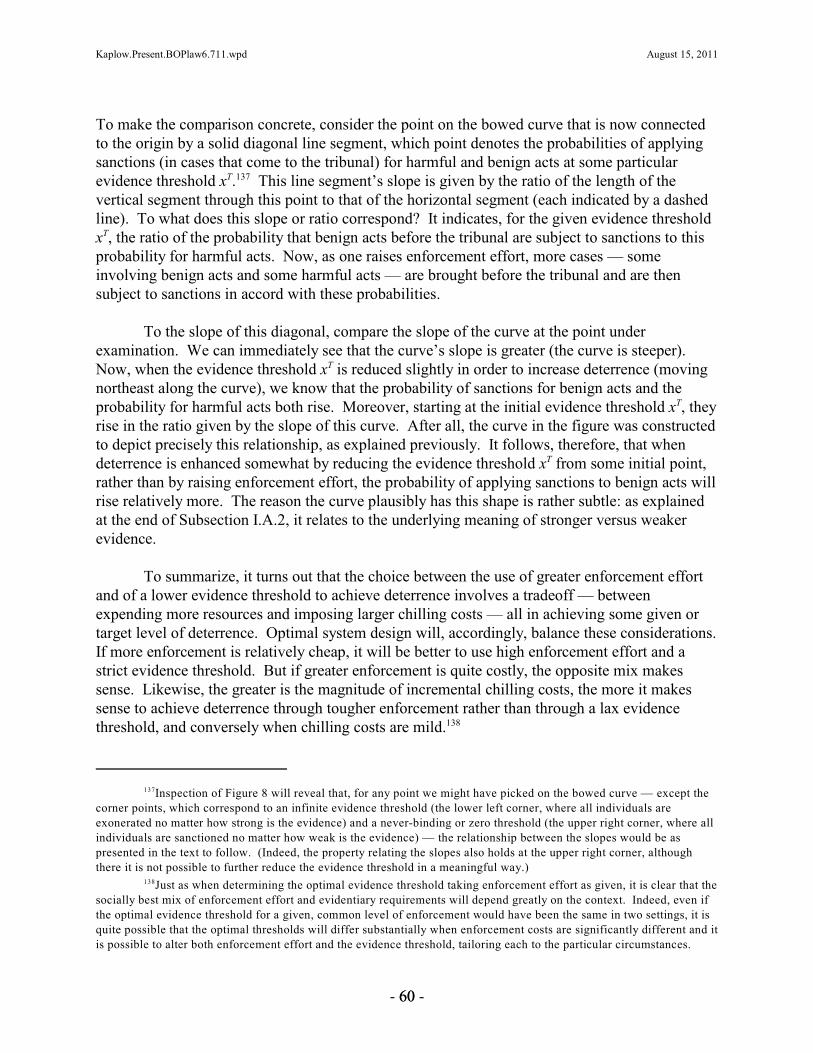
Kaplow.Present.BOPlaw6.711.wpd August 15, 2011
Inspection of Figure 8 will reveal that, for any point we might have picked on the bowed curve — except the137
corner points, which correspond to an infinite evidence threshold (the lower left corner, where all individuals areexonerated no matter how strong is the evidence) and a never-binding or zero threshold (the upper right corner, where allindividuals are sanctioned no matter how weak is the evidence) — the relationship between the slopes would be aspresented in the text to follow. (Indeed, the property relating the slopes also holds at the upper right corner, althoughthere it is not possible to further reduce the evidence threshold in a meaningful way.)
Just as when determining the optimal evidence threshold taking enforcement effort as given, it is clear that the138
socially best mix of enforcement effort and evidentiary requirements will depend greatly on the context. Indeed, even ifthe optimal evidence threshold for a given, common level of enforcement would have been the same in two settings, it isquite possible that the optimal thresholds will differ substantially when enforcement costs are significantly different and itis possible to alter both enforcement effort and the evidence threshold, tailoring each to the particular circumstances.
- 6600 -
To make the comparison concrete, consider the point on the bowed curve that is now connectedto the origin by a solid diagonal line segment, which point denotes the probabilities of applyingsanctions (in cases that come to the tribunal) for harmful and benign acts at some particularevidence threshold x . This line segment’s slope is given by the ratio of the length of theT 137
vertical segment through this point to that of the horizontal segment (each indicated by a dashedline). To what does this slope or ratio correspond? It indicates, for the given evidence thresholdx , the ratio of the probability that benign acts before the tribunal are subject to sanctions to thisT
probability for harmful acts. Now, as one raises enforcement effort, more cases — someinvolving benign acts and some harmful acts — are brought before the tribunal and are thensubject to sanctions in accord with these probabilities.
To the slope of this diagonal, compare the slope of the curve at the point underexamination. We can immediately see that the curve’s slope is greater (the curve is steeper). Now, when the evidence threshold x is reduced slightly in order to increase deterrence (movingT
northeast along the curve), we know that the probability of sanctions for benign acts and theprobability for harmful acts both rise. Moreover, starting at the initial evidence threshold x , theyT
rise in the ratio given by the slope of this curve. After all, the curve in the figure was constructedto depict precisely this relationship, as explained previously. It follows, therefore, that whendeterrence is enhanced somewhat by reducing the evidence threshold x from some initial point,T
rather than by raising enforcement effort, the probability of applying sanctions to benign acts willrise relatively more. The reason the curve plausibly has this shape is rather subtle: as explainedat the end of Subsection I.A.2, it relates to the underlying meaning of stronger versus weakerevidence.
To summarize, it turns out that the choice between the use of greater enforcement effortand of a lower evidence threshold to achieve deterrence involves a tradeoff — betweenexpending more resources and imposing larger chilling costs — all in achieving some given ortarget level of deterrence. Optimal system design will, accordingly, balance these considerations. If more enforcement is relatively cheap, it will be better to use high enforcement effort and astrict evidence threshold. But if greater enforcement is quite costly, the opposite mix makessense. Likewise, the greater is the magnitude of incremental chilling costs, the more it makessense to achieve deterrence through tougher enforcement rather than through a lax evidencethreshold, and conversely when chilling costs are mild.138

Kaplow.Present.BOPlaw6.711.wpd August 15, 2011
See Gary S. Becker, Crime and Punishment: An Economic Approach, 76 J. POL. ECON. 169, 183–84 (1968).139
See, e.g., Polinsky & Shavell, supra note 100, at 414 n.19, 415–16, 431–34.140
For prior analysis of this point, which implicitly takes the burden of proof to be fixed, see Kaplow, supra note141
100, at 349–50, and Kaplow & Shavell, supra note 100, at 5–6.
- 6611 -
This set of prescriptions is, on reflection, in accord with intuition — that is, if theobjective in designing the legal system as a whole is to maximize social welfare — even thoughthis seemingly obvious and natural tradeoff depends on factors that are more elusive than onemight have suspected. The main purpose of the analysis in this Section is to highlight a designchoice that is not often considered explicitly. Part I analyzes determination of the optimalevidence threshold when other features of the legal system, like enforcement effort, are taken asgiven. But the evidence threshold is a component of the broader system, so it makes sense whenconsidering how, in principle, it should be set to also have on the table the question of how otherenforcement instruments should be calibrated.
B. Sanctions
1. Level
Before turning to the interaction between setting an optimal evidence threshold anddetermining the appropriate level of sanctions, it is useful to begin with some remarks on theoptimal determination of enforcement effort and sanctions, which has been a significant topic inthe economics of law enforcement literature, although usually in settings in which errors are notpart of the analysis. Specifically, there is an argument associated with Gary Becker that, for anygiven, nonmaximal level of sanctions, it tends to be optimal to raise sanctions and reduceenforcement effort. If this is done so as to keep deterrence constant, one saves enforcement139
resources while, in simple settings, having no other effects. The literature then explores variousreasons why this prescription may not hold.140
In this regard, it is natural to inquire whether the presence of errors upsets this basicargument. As a first cut — and taking the evidence threshold as fixed — the answer isnegative. Regarding mistaken exoneration of individuals who in fact committed harmful acts,141
it is true that, as a consequence of errors, a lower portion are sanctioned. But if, say, enforcementeffort is reduced so as to cut in half the flow of individuals into the legal system, and the sanctionis simultaneously doubled, the expected sanction on individuals contemplating harmful actsremains the same. The presence of errors — say, adjudication mistakenly exonerates 20% ofindividuals who actually committed harmful acts — means that the ex ante probability ofsanctions is 20% lower in both instances, but a 20% reduction in two numbers keeps theirrelative proportion unchanged.
The analysis is the same regarding the mistaken imposition of sanctions on individualswho committed benign acts, which error rate we might imagine for concreteness to be 10%. This10% reduction in the ex ante probability of sanctions again applies in both the higher and lowerenforcement effort scenarios. Given the hypothesized reduction in enforcement effort, whichhalves the number of individuals who are subject to adjudication, the ex ante likelihood that

Kaplow.Present.BOPlaw6.711.wpd August 15, 2011
Many complications can be imagined. Consider some involving costly sanctions, the subject of Subsection 2. 142
One possibility is that sanctions involve social costs of imposition that are proportional to the sanctions imposed. In thatcase, there would be no direct effect of sanction costs: after all, although sanctions are twice as high, they are imposedhalf as often; hence, the total imposition of sanctions is constant. Another possibility is that sanction costs are nonlinear,as arises with risk aversion in the case of monetary penalties. See, e.g., Michael K. Block & Joseph Gregory Sidak, TheCost of Antitrust Deterrence: Why Not Hang a Price Fixer Now and Then?, 68 GEO. L.J. 1131, 1135–38 (1980)(discussing risk aversion and error); A. Mitchell Polinsky & Steven Shavell, The Optimal Tradeoff Between theProbability and Magnitude of Fines, 69 AM. ECON. REV. 880 (1979). The most direct implication is that, to maintain agiven level of deterrence when the probability of sanctions is cut in half, the sanction need not double but can be raisedby a lesser amount. Risk-bearing costs are greater, which may make the policy revision welfare reducing overall. Notethat, in any case, there is a parallel between the increase in risk-bearing costs imposed on both sets of individuals, in thatboth face the same higher sanction. The amount by which the sanction must increase does not depend on the presence oferror per se, but rather (since deterrence is being held constant) only on individuals’ degree of risk aversion, whichdictates how much monetary sanctions must increase to double the disutility of sanctions. The main difference is that,with errors, sanctions are imposed more frequently at any given level of deterrence because they also fall on someindividuals who commit benign acts, so sanction costs become relatively more important. For prior analyses of howsanction costs influence optimal enforcement effort and sanction levels — in settings that do not examine errors — see,for example, Louis Kaplow, A Note on the Optimal Use of Nonmonetary Sanctions, 42 J. PUB. ECON. 245 (1990); LouisKaplow, The Optimal Probability and Magnitude of Fines for Acts that Definitely Are Undesirable, 12 INT’L REV. L. &ECON. 3 (1992); Polinsky & Shavell, supra; A. Mitchell Polinsky & Steven Shavell, The Optimal Use of Fines andImprisonment, 24 J. PUB. ECON. 89 (1984).
Taking the evidence threshold — in addition to enforcement effort — to be an adjustable enforcement143
instrument thus offers an additional type of argument paralleling Becker’s in favor of higher sanctions. Moreover,because it operates differently, it can apply in contexts in which Becker’s original argument does not hold, and vice versa. See Kaplow, Optimal Burden of Proof, supra note 15.
- 6622 -
individuals who contemplate benign acts would thereby be sanctioned is cut in half. And, whenthey are sanctioned, they face double the sanction. As a consequence, their expected sanction islikewise the same. More broadly, it is not immediately obvious that making bigger mistakes lessoften is worse than making smaller mistakes more often; and in the basic setting underexamination, these proportions are the same, so the costs of mistakes in terms of reductions insocial welfare are the same. In sum, both deterrence and chilling effects are unaffected by thispolicy experiment, but enforcement resources are saved. (This core argument may or may not beaffected when additional complications are introduced. )142
Consider next our prime concern, the interaction between setting the evidence thresholdand the level of sanctions. Here, the analysis has some features in common with Section A’sanalysis of enforcement effort, but there is also a notable difference. Recall that raisingenforcement effort and raising the evidence threshold simultaneously, in a manner that holdsdeterrence constant, entails additional expenditures but reduces chilling costs. If one insteadraises the level of sanctions and the evidence threshold, holding deterrence constant, there is nolonger any increase in enforcement expenditures but there still is a reduction in chilling costs. Tounderstand this result more fully, note first that raising sanctions and raising enforcement effortare taken to hit both groups — individuals who committed harmful acts and those who engagedin benign ones — in the same proportion. As a consequence, this experiment of raising sanctionsand the evidence threshold in a manner that keeps deterrence constant manages to holdexpenditures on stage-one enforcement constant (since enforcement is unchanged, unlike before)but also to reduce expected sanctions on those who commit benign acts (because in this respect itacts just like the increase in enforcement), making the overall welfare impact positive.143

Kaplow.Present.BOPlaw6.711.wpd August 15, 2011
Another consideration is suggested by Kaplow, supra note 100, at 351–52, and Kaplow & Shavell, supra note144
100, at 5–6, who observe that if one raises sanctions and reduces enforcement effort so as to keep deterrence constant,there are fewer cases in adjudication and hence greater accuracy (the subject of Section C) can be achieved with lowerexpenditures, providing another channel by which error costs may be reduced.
Some discussion of sanction costs was offered in addressing errors and the level of sanctions in the preceding145
Subsection, in note 142. Note that even with monetary sanctions and risk neutrality, there is a further implicit assumptionthat collecting sanctions is costless. If instead such costs were, say, proportional to the sanction, then the analysis of thisSubsection would apply directly. If collection costs were fixed, independent of the magnitude of the sanction, theanalysis would differ, having some features in common with audit costs, examined in Section IV.A (the difference beingthat audit costs are, in the simplest case, proportional to the number of acts whereas this sort of sanction costs would alsoweight the relevant numbers by the rate at which sanctions are ultimately imposed).
See, e.g., POSNER, supra note 6, at 828 (arguing that the cost of imprisonment favors erring on the side of146
acquittals, thereby providing a rationale for the criminal law’s requirement of proof beyond a reasonable doubt).
For prior analysis of the issue in a simpler model without chilling effects, in which the analysis is somewhat147
different, see Kaplow, supra note 100, at 359–62.
- 6633 -
The result that consideration of errors — and in particular, errors involving the mistakenimposition of sanctions on individuals who committed benign acts — generates an argument infavor of high sanctions may seem surprising. But, first, we already saw that, in a simple anddirect sense, such mistakes do not in fact favor lower sanctions because, if one wishes tomaintain deterrence, the shortfall must be made up with greater enforcement effort, whichincreases the overall rate of mistakes. Second, an advantage of higher sanctions is that theyallow us to reduce the legal system’s pressure on harmful acts in other ways, one of which is byenabling a stricter evidence threshold. And this tougher proof requirement, in turn, means lowerexpected sanctions for benign acts, even taking into account the contrary but weaker effectthereon due to the higher sanctions.144
This observation illustrates the broader theme of this Part of the Article: that optimallegal system design must not only consider each component in isolation but also needs to takeinto account interactions among them. Before concluding the present discussion of the level ofsanctions, note that this Subsection does not purport to suggest that optimal sanctions aremaximal; it only shows that the influence of error and consideration of how the evidencethreshold might be set do not provide a simple, strong basis for employing low sanctions. Explanations will need to be found elsewhere, either in more subtle and complex considerationsinvolving error and proof burdens or in other factors entirely.
2. Nonmonetary Sanctions
Until now, sanctions themselves have been taken to be socially costless, as is the casewhen monetary sanctions (fines or damages) are imposed on risk-neutral individuals — wheredefendants’ payments are offset by receipts by the state or private plaintiffs. Consider instead145
nonmonetary sanctions, such as imprisonment, that are costly in themselves: neither the loss ofliberty nor the costs of operating prisons are mere transfers. When sanctions are socially costly,it tends to be optimal to reduce their imposition, which may seem to favor a higher evidencethreshold. While the initial hypothesis is correct, this conclusion need not follow because the146
evidence threshold affects behavior.147

Kaplow.Present.BOPlaw6.711.wpd August 15, 2011
It is not obvious that this is so, and one can imagine various reasons that cut in different directions. To be148
sure, the psychological cost of imprisonment may be greater for those who are there by mistake. On the other hand, thecriminogenic effect of imprisonment may be larger for those who did commit harmful acts. Yet another factor is thatthere may be incapacitation benefits regarding those who commit harmful acts but no such effects (or reduced ones) forthose who did not. Such benefits reduce the net social cost of imprisonment and, if sufficiently strong, can make the netcost negative, that is, a net benefit, with regard to individuals who committed harmful acts.
- 6644 -
To begin the analysis, if behavior is taken as given, a higher evidence threshold reducesboth the rate of (correct) imposition of sanctions on individuals who committed harmful acts andthe rate of (incorrect) imposition of sanctions on individuals who committed benign acts. Moreover, both reductions are, in themselves, advantageous on account of the reduction in socialsanction costs. But this consideration is only part of the story.
As is familiar by now, a higher evidence threshold also affects behavior. Specifically, byreducing the expected frequency with which sanctions are imposed on both types of actors, agreater number of individuals will commit harmful acts and benign acts. Both effects increasethe number of individuals who enter adjudication, and hence both increase the frequency ofimposition of sanctions and, thereby, the magnitude of social sanction costs.
A priori, either effect could be greater: the increased flow of cases could raise the totalimposition of sanctions by less than the decreased likelihood of sanctions in a given case reducesthe total, or vice versa. It seems plausible to suppose that in some situations the former will bedominant and in others the latter. Hence, introducing social costs of sanctions, such as those thatarise with nonmonetary sanctions, will sometimes favor a higher evidence threshold and in otherinstances a lower one. Likewise, factors indicating that social sanctions costs are greater thanmight previously have been contemplated will, in general, have an ambiguous effect on theoptimal height of the evidence threshold.
Note, moreover, that similar logic applies with regard to possible asymmetries in sanctioncosts. For example, suppose that the direct social cost of imposing each unit of a sanction — thatis, behavioral effects aside — is greater with regard to individuals who committed benign actsand bear the sanction by mistake than with regard to those who committed harmful acts andproperly bear the sanction. Again, we have a tradeoff: a higher evidence threshold reduces the148
likelihood of imposition of the more costly sanction on any given individual who committed abenign act and is before the tribunal, but the resulting reduction in the expected sanction forbenign acts implies that fewer of them are chilled, so a greater number of such individuals comebefore tribunals and thus may bear sanctions by mistake. Either effect could be larger. In otherwords, it does not follow that a higher social cost associated per se with the mistaken impositionof sanctions on innocent individuals favors a higher evidence threshold. The opposite is alsoplausible, and which situation prevails in any given setting is an empirical question.
It is worth reflecting briefly on why it is ordinarily imagined that a heightened evidencethreshold is favored by a greater social cost being associated with the mistaken imposition ofsanctions on individuals who have not committed harmful acts. It seems likely that thissupposition is generated by an ex post view of the legal system, which takes as given who comesbefore the tribunal, a perspective closely related to those underlying conventional conceptions of

Kaplow.Present.BOPlaw6.711.wpd August 15, 2011
Interestingly, there is also a tension within this behavioral channel: ordinarily, we suppose that the chilling of149
benign acts is undesirable, but here chilling also reduces the imposition of socially costly sanctions. Now, from the exante perspective of individuals who contemplate committing benign acts, they are better off if the expected sanction (interms of the expected overall utility cost) is reduced. Moreover, if this leads them to commit a benign act that otherwisewould have been chilled, it is necessarily the case that, prospectively, they are better off. It is possible, however, that thenet effect, focusing solely on this shift, is socially undesirable as a consequence of externalities, the most obvious ofwhich in the present context is that individuals do not directly bear the costs of operating prisons. (Society as a wholedoes, but a particular individual contemplating an act only bears, through taxes, a negligible fraction of the expectedincrease in the cost of operating prisons that flows from committing the act in question.)
By analogy, consider an x-ray or other form of imaging used for medical diagnosis. The quality of150
information can be improved through a higher-resolution scan or by employing a more highly skilled interpreter (whichitself may be achieved, de facto, in many ways, including better training, more time, and the use of second opinions).
For example, when Section A explored raising enforcement effort, it was supposed that this was151
accomplished by posting more monitors or auditing more actors. But one could instead consider improving the quality ofmonitoring, auditing, inspection, investigation, and so forth, in which case the analysis of the present Section would beapplicable.
More precisely, what matters is how these error rates change with the evidence threshold.152
This inquiry also prompts a comparison of prior literature on the subjects by commentators. When153
researching an extensive treatment on accuracy in adjudication, Kaplow, supra note 100, I similarly discovered that mostlegal analysis did not really attempt to examine the consequences of different levels of accuracy for how well the legalsystem functioned. That is, there was also essentially a vacuum with regard to the rationales that underlie the relevanttradeoff, there between accuracy and system cost.
See id. at 357–59.154
- 6655 -
the burden of proof that were the subject of Part II. In considering the question, onlookerspresumably contemplate an actual case, one in which there is uncertainty about the truth withregard to the individual before the tribunal. In considering what decision is best, a greater costassociated with the mistaken imposition of sanctions naturally favors a tougher proof burden. We can now see that this perspective overlooks the ex ante effect on behavior that works in theopposite direction and can result in a net increase in the mistaken imposition of sanctions.149
C. Accuracy
Throughout this investigation, the quality of the evidence is taken as given, so the onlysystem design question regarding evidence is how strong it must be in order to assign liability. However, myriad features of the legal system influence its accuracy, regarding both the actualinformation that is generated and also the care with which it is assessed (another feature ofquality, really). Many rules of legal procedure, including laws regulating evidence and150
governing appeals, affect accuracy, as do policies affecting the ability, available time, andincentives of investigators and lawyers. Since the accuracy of the legal system determines the151
error rates associated with a given proof requirement, and these error rates are key determinantsof the optimal evidence threshold, it is appropriate to inquire into the relationship between152
accuracy and the burden of proof.153
As a preliminary matter, it is important to distinguish the two concepts, which aresometimes confused because many changes in system design simultaneously influence both, evenif not formally. Consider the effects of providing additional investigative resources to indigent154
criminal defendants. Suppose that the result is to improve the overall quality of information

Kaplow.Present.BOPlaw6.711.wpd August 15, 2011
There are different ways to understand whether the implicit change in the proof burden should be understood155
as merely de facto or also de jure. For a given evidence threshold x , one might view a general enhancement ofT
presentations by the defense as reducing the distribution of evidence strengths x for both types of actors (shifting bothcurves in Figure 1 to the left), in which case the de facto proof burden would be higher (met less often) even though thede jure burden is the same. Alternatively, one could say that the de jure burden has changed because the meaning ofevidence strength and thus of a given x has shifted. Nothing in the present analysis depends on this difference inT
interpretations.
On the selection of evidence in adjudication, see, for example, Louis Kaplow & Steven Shavell, Legal Advice156
About Information to Present in Litigation: Its Effects and Social Desirability, 102 HARV. L. REV. 565 (1989).
Note that if, instead of stating the evidentiary requirement in terms of an evidence threshold x , one employs a157 T
conventional burden of proof notion of the sort examined in Part II — a formulation based on ex post likelihoods — thena Bayesian factfinder would implicitly adjust the evidence threshold x in order to keep constant the requisite likelihood,T
and there would in that sense be no implicit shift in the proof burden. To see this, the additional investigative resourcesmight be seen as shifting both curves in Figure 1 to the left. For any level of x, there will accordingly be associated adifferent probability than before. Hence, when examining the lower elements of the boxes in Figure 5, it would generallybe true that different values would be assigned for any contemplated x . For concreteness, consider the case in which theT
shapes of the two curves in Figure 1 remain the same and they shift left by precisely the same amount. Then, whatever xT
previously worked in Figure 5, it will now be true that a new x that is lower by precisely the amount of that leftward shiftT
will work (since it will be associated with the same level for both probabilities as prevailed — and worked — initially).
- 6666 -
available to the tribunal; better information may be associated with greater accuracy. However,in this instance there may also be a de facto strengthening of the burden of proof: even if therequisite minimum strength of evidence for conviction is literally unchanged, investigators155
working for defendants will be selective both in where they focus their efforts and in what subsetof their findings are presented to the tribunal. As a consequence, it will on average be more156
difficult to establish guilt — for individuals who committed benign acts and also for those whocommitted harmful acts.157
This entanglement of accuracy and the proof burden can helpfully be separated. Specifically, one can combine a proposed intervention that affects both — such as in ourexample — with a simultaneous adjustment to the formal evidence threshold that restores theprior de facto proof burden. This clarifies the difference between the two phenomena, which isuseful conceptually. It also has pragmatic appeal. For example, if the intervention is desirableon accuracy grounds — perhaps important information that may exonerate innocent defendants isoften overlooked — but not on proof burden grounds — perhaps the previous balance was justright — then it would be sensible to implement the change but adjust the evidence threshold soas to hold the de facto proof burden constant. On the other hand, if little informationimprovement results, so that the reform is not cost-justified on accuracy grounds, but it wasmotivated by a desire to raise an excessively lenient proof burden, it would be preferable toaccomplish the latter directly and forgo the initial reform.
Having distinguished the concepts of accuracy and proof burden, consider next how thedegree of accuracy affects the optimal evidence threshold. Suppose, for example, that the systemis redesigned in some fashion so as to increase accuracy at the existing evidence threshold, whichis to say that there is a reduction in both error rates: the likelihood of mistakenly exoneratingthose before tribunals who committed harmful acts and the likelihood of mistakenly sanctioning

Kaplow.Present.BOPlaw6.711.wpd August 15, 2011
One way to define greater accuracy is to consider a regime such that the curve in Figure 3 is everywhere158
(except at the corner points) closer to the lower right corner of the box. This depiction immediately suggests a furthercomplication: one can imagine reforms that would raise accuracy for some thresholds (perhaps low ones, correspondingto the right side of the figure) but reduce it for others (perhaps high ones, corresponding to the left side of the figure). Inthat case, the new curve would be lower on the right side and higher (closer to the 45 degree line) on the left."
One could align proof burdens by initially imposing in the new regime the same ex post likelihood that the159
individual before the tribunal committed a harmful act as prevailed in the old, and then asking how optimally it should beadjusted. However, that calibration is just one possible choice, and the analysis in Subsection II.C.1 suggests that it couldhave strange properties since it depends on behavior, which in turn is influenced by the degree of accuracy and theevidence threshold that is chosen.
- 6677 -
those who committed benign acts. Is the optimal evidence threshold in this new regime higher158
or lower?
It turns out that there is no simple or unambiguous answer to this question. First, it isdifficult to give it sharp meaning — that is, it is hard to compare the stringency of evidencethresholds across regimes with different levels of accuracy. To illustrate some of the problems,suppose that in the more accurate regime we begin with an evidence threshold that involves thesame rate of mistakenly sanctioning individuals before the tribunal who committed benign acts— which, since accuracy is higher, entails that the rate of mistaken exoneration is lower. In thatcase, it may be optimal to raise the evidence threshold somewhat. But if we begin in the newregime at a threshold that involves the same rate of mistaken exoneration as before — whichentails a lower rate of mistaken sanctioning — it may be optimal to lower the thresholdsomewhat. Supposing that both are true, it may seem natural to consider points in between, butdepending on the starting point chosen, it may be optimal to raise the evidence threshold, lowerit, or keep it as is. To draw an analogy, suppose that for medical diagnosis we switch to a new,more accurate test meter, whose accuracy is generated by utilizing a different type of test. Theresimply may be no natural, inherent relationship between the scales of the new meter and the oldone, so there is no clear basis for saying what cutoff reading should be viewed as correspondingto what was used before.159
Second, putting this definitional question to the side, as a matter of substance there aremultiple and conflicting effects. Consider a starting point in the new regime such that the rate ofboth types of errors is lower. A reduced rate of mistaken exonerations means that the expectedsanction facing those contemplating harmful acts is higher, which improves deterrence. Asexplained in Section I.B, when deterrence is higher, the marginal benefit of further deterrence islower, so on this account the optimal evidence threshold would rise. On the other hand, a lowerrate of mistaken sanctions reduces the expected sanction facing those contemplating benign acts,which reduces chilling. Section I.B further explained that, when chilling is lower, the marginalcost of further chilling is reduced, so on this account the optimal evidence threshold would fall.
Examination of Figure 4 or 6, indicating the determinants of the optimal evidencethreshold, reveals other possible differences, the preceding argument having addressed only thebottom elements in the two boxes. The middle elements, the concentrations of marginal harmfuland benign acts, could each be higher or lower, depending on the distributions of individuals’private benefits for the two types of acts. And even the top elements could differ, depending on

Kaplow.Present.BOPlaw6.711.wpd August 15, 2011
As explained in note 158, greater accuracy can be depicted as the curve in Figure 3 being bowed further160
toward the lower right. Depending on where one starts on the new curve, the curve’s slope — which indicates the ratiodescribed in the text — could be higher or lower than (or the same as) the slope on the original curve at the originalevidence threshold.
Kaplow, supra note 100, and Kaplow & Shavell, supra note 100, address accuracy in the determination of161
liability, but in a setting that does not include chilling effects, so the analysis is quite different.
- 6688 -
what starting point for the evidence threshold is chosen in the new regime and on what is theratio between the rates of change in the probabilities of sanctions for harmful and benign actsunder the new regime versus the old.160
In sum, raising accuracy has many effects on the determinants of the optimal evidencethreshold; some point in opposite directions while others have ambiguous implications. Accordingly, little can be said about how changing the degree of accuracy affects the optimalthreshold. A corollary is that it is difficult to say how evidence thresholds should vary acrosslegal systems with differing degrees of accuracy.
A final question of interest is how the analysis in the present investigation illuminates theimportant but rarely addressed question of how one can determine the value of accuracy in a legalsystem — that is, how many additional resources it makes sense to expend in order to achievesome degree of improvement in accuracy. Regarding this inquiry, a fairly direct method of161
valuation is provided. Consult again Figure 4 or 6: the left box indicates the deterrence benefit ofa reduction in the evidence threshold and the right box the chilling cost. With somereinterpretation, these same boxes indicate the effects of an increase in accuracy.
To see this point, suppose that we reduce the two types of error by some amounts buthold everything else in the system constant. There will be an increase in deterrence benefits anda reduction in chilling costs (not an increase, as when relaxing the evidence threshold). Toquantify the former, we can start with the top element in the left box. Using our analysis fromSection I.B, it is straightforward to determine the increase in the expected sanction for harmfulacts: we again have an increase in the probability of being subject to sanctions when before thetribunal, and all else is constant, so the expected sanction for harmful acts rises in proportion tothe rise in this probability on account of the increase in accuracy. The other elements in the leftbox are the same, so the deterrence benefit is calculated as before.
For the chilling benefit, we look to the right box and repeat the exercise. The greateraccuracy implies a fall in the expected sanction for benign acts, proportional to the drop in theprobability of benign acts being sanctioned when before the tribunal. The other elements in theright box are the same, so we can calculate the chilling benefit.
Taken together, we have a deterrence benefit and a chilling benefit. The sum of thesegains is the value of the increase in accuracy, and this total can be compared to the resource costof the improvement to accuracy to determine whether that expenditure is desirable — that is,whether it raises social welfare. Although, as with the determination of the optimal evidencethreshold itself, these calculations will be difficult because the information on the determinants is

Kaplow.Present.BOPlaw6.711.wpd August 15, 2011
Moreover, as discussed in Subsection II.B.2, challenges in applying the correct mode of assessment do not162
justify substituting alternative, easier criteria unless they are reasonably good proxies for what really matters.
- 6699 -
hard to come by (see Subsection II.B.2), the correct conceptual formulation is evident.162
V. ALTERNATIVE METHODS OF ENFORCEMENT
Until now, little attention was given to the particular method of enforcement or to howdifferent methods may have different implications regarding how the evidence threshold shouldbe set. For ease of exposition, it has been assumed that enforcement sweeps in certain fractionsof acts of each type and that greater effort raises those proportions. This analysis most closelycorresponds to what Section A calls monitoring. This context was chosen because it is lesscomplex than some of the others and because its core features are present under other techniqueswhen ex ante behavior is central. In this Part, alternatives are considered. Section A discussesauditing alongside monitoring, showing their similarities with regard to effects on behavior —deterrence and chilling effects — but differences with regard to enforcement costs. Section Bexamines investigation, which is qualitatively distinctive on both dimensions. Section Cexplores a highly dissimilar enforcement setting, the regulation of future conduct (for example,licensing), wherein legal rulings dictate what parties are permitted to do going forward ratherthan being chiefly concerned with affixing sanctions in light of past behavior. Finally, Section Dconsiders how the evidence threshold may influence prosecutors’ and plaintiffs’ behavior and, asa consequence, what cases come before the tribunal in the first instance, even taking individuals’acts as given.
It is worth observing at the outset that varying enforcement techniques are sometimesused interchangeably or in a complementary fashion even when addressing a single problem. Forexample, with some environmental regulation, there may be audits through spot checks andinvestigations when contamination is detected, as well as regulations that dictate specific futureconduct; likewise, harmful activities may be subject to both public and private enforcement. Bycontrast, in other settings, a single mode may be primary. For example, with arson, enforcementis mainly through investigation that is undertaken by public authorities.
A. Monitoring and Auditing
This Section begins with monitoring, the focus until now, and then analyzes auditing. Asmentioned, the two modes of enforcement are similar with regard to behavior but differ in termsof enforcement costs.
Monitoring may, for example, be implemented by posting police officers, such as along ahighway for the purpose of detecting speeding or through the use of patrols on the lookout for avariety of violations. There are private analogues as well. Stores may employ security guards todetect shoplifting, large property owners may post monitors for trespassing, and intellectualproperty owners may task some employees to keep a lookout for infringement. Monitors arepresumed here to detect some fraction of individuals who commit harmful acts and also a

Kaplow.Present.BOPlaw6.711.wpd August 15, 2011
- 7700 -
fraction (perhaps much lower) of individuals who actually commit benign acts, and these are theacts that enter adjudication. As a simplification and rough approximation for some settings, it isimagined that, although posting more monitors to raise the detection rate (for harmful acts and, asa byproduct, for benign acts) is more expensive, as analyzed in Section III.A, the cost depends onthe number of monitors and not on how many apparent violations they observe. For example, asecurity guard will spend most of the time just watching, and occasionally will detect what seemsto be a perpetrator, but the cost of employing the guard will be essentially independent ofwhether one shoplifter or five are identified per week.
Compare and contrast auditing. This technique is perhaps most familiar from its use inenforcing income tax laws, but it is also deployed much more widely. Random inspections areused to check for violations of health laws, fire regulations, environmental edicts, andoccupational safety measures. Private parties engage in similar practices, such as when theyexamine some inputs from suppliers to check for defects. The essential character is that a givenproportion of all activity is examined, and it costs more (perhaps proportionally more) toexamine a higher proportion. When an audit or spot-check is conducted, some fraction each ofharmful and benign acts (presumably, a greater percentage of the former) will be detected asinvolving apparent violations. These are the acts that will enter adjudication.
Regarding effects on behavior, monitoring and auditing are quite similar. A givenintensity of enforcement is associated with the identification of some portion of each of the twotypes of acts, and raising enforcement effort increases these portions. Of course, the particularfractions will depend on the setting, and in some cases we might expect one or the othertechnique to have a higher targeting precision or to be more expensive for a given hit rate. Whenit comes to setting the evidence threshold, therefore, the numbers for each element in the boxesin Figures 4 or 6 may well differ, so different thresholds may be optimal with regard tobehavioral effects on social welfare. But, qualitatively, the analysis is the same.
However, behavioral effects on welfare are not all that is relevant; enforcement costsmust also be taken into account. In Part I, these costs were ignored. For monitoring, thatomission was inconsequential because enforcement effort and thus the cost of monitoring wasconstant — in particular, it was unaffected by the evidence threshold. However, even as anapproximation, this constancy of enforcement costs does not extend to auditing.
Here’s the difference: As noted, with monitoring, the cost is taken to be the same whetherone or five apparent violations is observed by the posted agent. But, with auditing, even holdingthe audit rate constant, say, at 10%, costs depend on individuals’ levels of activity. For example,if more restaurants operate (whether properly or not), more health inspections need to beconducted — although the percentage audited remains the same. If more manufacturing isundertaken, there need to be more safety inspections. And so forth.
The implication is that, for auditing, the evidence threshold directly affects audit costs. Specifically, when the evidence threshold is reduced somewhat — our thought experiment fromPart I — we know that there is more deterrence and more chilling. Both involve reductions inactivity: harmful and benign acts fall. Because there are fewer acts, fewer audits need to be

Kaplow.Present.BOPlaw6.711.wpd August 15, 2011
It is true that the frequencies of the two types of acts and the audit rate are relevant under the preponderance163
rule (they are components of the upper elements in the boxes in Figure 5) and in the calculation of total audit costs. However, these factors are used in an entirely different manner. For the preponderance rule, the two frequencies(multiplied by the common audit rate and also multiplied by different hit rates) are on opposite sides of an equation,whereas for audit costs these frequencies (multiplied by the audit rate and also by the cost per audit) are added together.
If one considers that many disputes settle (plea bargaining in the criminal context), these costs are lower than164
otherwise, but they are still positive and, in many settings, significant.
- 7711 -
conducted at our fixed audit rate, so audit costs are lower. Hence, a lower evidence threshold ismore desirable than one would have concluded considering solely the direct social welfareconsequences associated with behavior.
Reflecting on the foregoing, we can see that deterrence is more valuable with auditingthan with monitoring, because in addition to avoiding the external harm caused by harmful actswe also reduce expected audit costs. Moreover, chilling is less undesirable as well; that is, whatwas previously a pure cost — losing the benefits of benign acts — is now less of a social costbecause of the partial offset from saving audit expenses. It is even possible that chilling could bebeneficial. This seemingly unexpected conclusion is not, however, that surprising on reflection. Consider, for example, an activity that can be highly dangerous when not conducted properly,which as a consequence makes it optimal to employ a high audit rate; in some settings, the rate isessentially 100% for this reason. It would be socially advantageous for such activities not to beconducted if they are at a very small scale, even if the operator would in fact behave in a benignmanner, for the expense of performing the necessary audits could exceed any benefit from theactivity. In fact, for some dangerous activities, fees must be paid to cover inspection costs, andpresumably such fees discourage operations on so small a scale that the fees cannot be recovered.
Paralleling the discussion in Section II.B, we can compare the determinants of the optimalevidence threshold when enforcement is by auditing with the determinants of the preponderanceof the evidence rule and other rules based on the ex post likelihood that the individual before thetribunal committed a harmful act. Again, the contrast is striking. Regarding the direct effects ofbehavior on welfare, we have all the differences we had before. And now we have additionaldivergences because the enforcement cost effects just described are also omitted from thepreponderance rule and others like it, reinforcing the idea that conventional conceptions of the163
burden of proof are not even proxies for the social welfare effects of changing the evidencethreshold.
Finally, note that this discussion of audit costs and the preceding discussion of monitoringcosts oversimplify by omitting processing costs that follow initial targeting. In both instances,once individuals are identified — correctly or not — in stage one, they enter into the legalsystem, ultimately resulting in adjudication, and this second stage is itself costly. Therefore,164
both modes of enforcement entail yet another cost, one that depends on enforcement intensity,the number of the two types of acts that are committed, and the hit rates for each of the two typesof acts. Because one component is, again, the number of acts committed, there is a furtherbenefit to deterrence and to chilling (perhaps a partial offset to the chilling cost) as a consequence

Kaplow.Present.BOPlaw6.711.wpd August 15, 2011
This factor is yet another difference between the determinants of the optimal evidence threshold — that which165
maximizes social welfare — and of the preponderance rule and others like it. As explained in note 163, we again havesome overlap in components, but for assessing welfare the quantities associated with harmful acts and benign ones areadded rather than balanced against each other, as they are under the preponderance rule.
Often in civil settings and sometimes with crime, uncertainty may exist not with regard to who caused harm166
but rather about whether there was improper behavior. For example, it may be clear to a buyer that goods were notdelivered but require further investigation to determine whether the seller was at fault and thus in breach of contract. And with some crimes, one may be excused from causing injury, for example, on account of self defense. As willbecome clear, the analysis of these situations would not differ as significantly from the cases with monitoring or auditingbecause one who causes harm even when acting properly may thereby trigger scrutiny.
- 7722 -
of reducing the evidence threshold.165
B. Investigation
Enforcement by investigation differs substantially from enforcement by monitoring orauditing and in ways that have important implications for the determination of the optimalevidence threshold. Investigation refers here to enforcement triggered by the observation of aharmful act, which event instigates follow-up activity designed to ascertain responsibility. Suchan investigation with some probability identifies the individual who committed the harmful act,and with another probability (hopefully, a much lower one) it identifies an individual whoactually committed a benign act. With most instances of murder or automobile theft, forexample, it may be readily apparent that a harmful act has occurred but require investigativeresources to identify the perpetrator. There are civil analogues, most obviously regarding manytorts, where again the fact of injury may be clear.
When enforcement is by investigation, there is an important difference in the manner inwhich harmful acts versus benign acts may give rise to an individual actor ending up inadjudication. One contemplating a harmful act anticipates that the act will result in aninvestigation (with near certainty or probabilistically, depending on the setting), which might inturn identify the actor and lead to adjudication. By contrast, in many settings the commission ofa benign act will not trigger an investigation. So why, then, would individuals who commit166
such benign acts nevertheless face adjudication in some instances? This possibility arises in thepresent context because of actions that may lead an individual to be confused with an actualperpetrator. Driving a van at night in the vicinity of a high-burglary neighborhood might leadone to be mistakenly apprehended for a break-in. Purchasing used electronics from an individualon the street may lead to suspicion of complicity. Being a relative or acquaintance of someonewith enemies, especially if one is known to be among those enemies, may lead one to be accusedif the person is harmed by someone else. In the civil context, the manufacture of products thatare quite safe but are used in conjunction with others that are not could result in products liabilityallegations. These are the sorts of actions that might be chilled by the prospect of mistakenidentification, followed by a finding of liability.
This contrast between the present setting and that considered with monitoring or auditinghas an immediate and important implication: anything that contributes to the deterrence ofharmful acts will, as a direct consequence, reduce the expected sanction for benign acts and thus

Kaplow.Present.BOPlaw6.711.wpd August 15, 2011
If, say, a police force has a fixed budget for investigations, this reduction in the number of investigations167
might not occur. However, over time, if there are fewer crimes to investigate, one would expect budgets to fall. Moreover, even in the short run, if there are fewer crimes, one response is likely to involve more intensive investigationof remaining cases (rather than a greater number of investigations), which depth may on average improve the accuracy ofthe results, a subject explored in Section III.C.
- 7733 -
chilling costs. The reason is that harmful acts are what triggers the investigations that sometimesmisfire and lead to sanctions being imposed on individuals who commit benign acts. When thereare fewer harmful acts, fewer investigations are triggered, and — for a given misfire rate —167
fewer instances of mistaken imposition of sanctions will result. This is not the only impact ofpolicies that raise deterrence, but it is one effect. Note also that the reduction in investigationswill save enforcement resources, another benefit of deterrence.
Consider the determinants of the optimal evidence threshold when enforcement has thesefeatures. Figures 4 and 6 depict the components of deterrence benefits and chilling costs whenenforcement is by monitoring or auditing. When enforcement is by investigation, there are anumber of differences. Starting with deterrence benefits, the lower element in the left box in thefigures would have two supplements, corresponding to the two additional effects just explained:each act deterred, in addition to avoiding the external social harm of the act itself and forgoingthe private benefit from the act, now also reduces chilling costs and enforcement costs, both as aconsequence of there being fewer investigations. These factors favor a lower evidence threshold,all else equal. Furthermore, on the right side, the increase in the expected sanction for benignacts — the upper element in the right box — is computed on a different base because benign actsare investigated only when harmful acts are committed. The impact of this difference is hard toassess; one might assume that in many instances there would be far fewer opportunities formistaken identification to occur, but that will depend on the nature of the benign acts in questionand the targeting precision of investigators versus monitors or auditors.
Although this analysis suggests that lower evidence thresholds seem optimal whenenforcement is by investigation, the results are not really very comparable across enforcementmethods. Each occurs in entirely different situations, in which different sorts of benign actsmight be confused for harmful ones, and with different relative likelihoods. And the method ofidentification differs as well, as may the nature of evidence generated. All that can be concludedwith confidence is that the determinants differ in important ways across methods.
Next, examine the difference between the determinants of the optimal evidence thresholdand of the preponderance rule (and others like it) when enforcement is by investigation. The twoadded deterrence benefits have no analogue in the determinants of rules based on ex postlikelihoods since, as explored at length in Part II, they do not in any direct way depend ondeterrence effects. Recall the observation that the optimal evidence threshold depends on howbehavior changes as a consequence of adjusting the threshold, whereas the preponderance ruledepends on the aggregate level of harmful and benign acts at a given threshold, since theseaggregates influence the flow of acts into adjudication. In the present setting, the determinants of

Kaplow.Present.BOPlaw6.711.wpd August 15, 2011
The difference is that the frequency of harmful acts — a key component of the upper element in the left box168
in Figure 5 — no longer enters into the formulation because it influences both sides of the equation in the same way andthus cancels. The reason is that, as explained in the text, commission of each harmful act triggers an investigation,perhaps with some probability; then, conditional on an investigation, there is some likelihood that the individualcommitting the harmful act is identified and some other likelihood that an individual who committed a benign act isidentified. Fewer harmful acts proportionally reduces the flow of both groups into adjudication.
See Richard A. Posner, An Economic Approach to Legal Procedure and Judicial Administration, 2 J. LEGAL169
STUD. 399, 413 (1973); see also KAPLOW & SHAVELL, supra note 40, at 336–38 (observing how high sanctions maysimilarly benefit the innocent through greater deterrence). Note that innocent individuals would also in such a scenariofare worse ex ante, which means that chilling could rise despite the higher evidence threshold. This result contrasts withthat under monitoring (or auditing) examined previously, because there the only way more individuals who commitbenign acts might end up being sanctioned despite a tougher proof requirement is on account of reduced chilling, which isthe source of the increased number of benign acts entering adjudication. Furthermore, observe that, taking the criminalsetting, there would be two senses in which innocent individuals may be worse off with a higher evidence threshold: theyboth suffer more as crime victims due to reduced deterrence (the familiar point), and they also may more often bemistakenly subject to both trial and conviction, for the reason just given in the text.
- 7744 -
the preponderance rule differ somewhat from what they were before, but not in ways that168
influence the conclusion that they are fundamentally distinct from those for the optimal evidencethreshold. Once again, the preponderance rule and others based on the ex post likelihood that theindividual before the tribunal committed a harmful act are not even serious proxies for some ofthe determinants of the effects on social welfare and thus in no way suggest what evidencethreshold is optimal.
Finally, it is worth elaborating on the deterrence benefit of a lower evidence thresholdwith regard to those who commit benign acts. It was already noted in Section II.C that raising theevidence threshold could actually increase the frequency of the mistaken imposition of sanctions. When enforcement is by investigation, this possibility also arises, and indeed it seems moreplausible. Raising the evidence threshold, to be sure, makes it less likely that a given individualwho both commits a benign act and ends up before a tribunal will be sanctioned. However, itmay also notably increase the number of such individuals who come before the tribunal preciselybecause the higher threshold reduces deterrence and thus triggers more investigations. Accordingly, individuals committing benign acts may fare worse under a higher evidencethreshold. This effect is hardly certain, and it is difficult to say how likely it may be, but it169
appears to be entirely plausible, not merely conceivable. Once again, we see how misleading canbe an ex post perspective that concentrates on an individual imagined to be before a tribunal andignores how the evidence threshold influences behavior and thus who comes before tribunals inthe first instance.
C. Regulation of Future Conduct
This Section shifts from the focus in the rest of the Article to a fundamentally differentmeans of legal regulation: that which dictates future conduct. Until now, the analysis hasconcentrated on how the evidence threshold, by influencing expected sanctions for harmful andfor benign acts, influences ex ante behavior. The central welfare effects of the evidencethreshold have involved the social benefits and costs of these behavioral consequences:deterrence and chilling. The primary significance of the imposition of sanctions was taken to be

Kaplow.Present.BOPlaw6.711.wpd August 15, 2011
Some licensing is more akin to registration, in many cases to alert authorities about who must be subject to170
inspection or to document the payment of a required fee.
Some of these examples may be less different than meets the eye. Notably, a party bound by an injunction —171
or, more often, one who might be threatened with suit for an injunction — may settle with the plaintiff, making a paymentin return for future freedom of action. The overall effect is more akin to a suit for damages, the prospect of whichinfluences behavior as before.
This distinction also proved central — for similar reasons — in my prior work on accuracy in adjudication. 172
See Kaplow, supra note 100, at 369–81. As in that case, the present framework looks more akin to traditional cost-benefit analysis. See id. at 380. Standard cost-benefit analysis would look more like a comparison of the bottomelements in Figure 9, below, supposing certainty. In cost-benefit analysis, uncertainty is often analyzed using decisiontrees that, when collapsed into an algebraic expression, would resemble the complete formulation in Figure 9.
As emphasized at a number of points, however, all such rules depend on the flow of cases into adjudication,173
which in turn depends on ex ante effects. Hence, it is less true that the rules themselves ignore ex ante behavior than thatthe analysts who find them appealing tend to adopt an ex post outlook.
- 7755 -
these ex ante behavioral effects. Secondarily, but sometimes importantly, it was recognized thatsanctions are themselves costly, in which case it is socially desirable, ceteris paribus, to minimizetheir imposition.
The central purpose of some aspects of the legal system is, by contrast, to regulate futureconduct. Many forms of licensing — of drivers, certain professionals (doctors, lawyers), andfacilities (restaurants, nuclear power plants) — are designed to permit or prohibit future activitybased on whether it is likely to be socially beneficial or detrimental. Zoning regulations170
control what structures may be built or how they may be used (residential versus commercial orindustrial). Competition regimes may require large mergers to be approved in advance, whichauthorization is withheld if anticompetitive effects are expected to be significant. Andinjunctions limit parties’ future activities.171
Because the central effects of the regulation of future conduct differ (in the pure case,entirely) from those examined thus far, Subsection 1 presents a fresh analysis of how the optimalevidence threshold should be determined in this setting. It turns out that the problem is172
analytically simpler than those considered previously; in fact, the framework is essentially thesame as that applicable to medical decisionmaking and hence is familiar.
Subsection 2 compares the determinants of the optimal evidence threshold for this modeof enforcement with the preponderance of the evidence rule and others based on the ex postlikelihood that the individual before the tribunal is of the harmful type. On one hand, the twoformulations are much more similar than was true in any of the prior cases — where there wasalmost no resemblance whatsoever. This greater commonality is, on reflection, to be expectedbecause, as emphasized in Part II, conventional conceptions seem to arise from an ex postperspective that takes as given the cases that come before the tribunal, and this stance is173
appropriate when the legal policy question concerns what future conduct should be permittedrather than what rule for imposing sanctions best influences ex ante behavior in anticipationthereof. On the other hand, in the present context there are still central determinants of theoptimal evidence threshold that are omitted from the formulation of the preponderance rule andothers of its kind. Moreover, it will be apparent that this divergence means that the optimalthreshold will often differ markedly from the preponderance rule (or any other rule of that type),

Kaplow.Present.BOPlaw6.711.wpd August 15, 2011
The latter was briefly discussed in note 148 with regard to how differential costs of sanctions on harmful and174
benign acts influence the analysis of the optimal evidence threshold.
That Subsection does not focus on another sort of mixing, noted previously, between different modes of175
enforcement. For example, there may be both environmental licensing of facilities and also subsequent enforcement toensure compliance, including monitoring, auditing (inspections), and investigation (such as when contaminants arediscovered in groundwater).
This description contains a number of simplifications, including that harmful acts generate a given degree of176
harm, that benign acts generate no harm, and (as will become clear) that the tribunal does not know individuals’ privatebenefits. None of these assumptions greatly affect the core ideas, in large part because one can think of differences thetribunal can observe as constituting different classes of cases, each subject to its own evidence threshold (and, forexample, harm can be understood as the average harm in a class of cases in which the tribunal cannot distinguish thelevel of harm). Another important assumption is that the magnitudes of different types of individuals’ private benefitsand of the social harm are independent of the strength of the evidence that the tribunal observes, on which see note 183.
Furthermore, it is supposed that individuals’ private benefits are positive, so they wish to apply for permission. Individuals’ whose expected private benefits are negative would not act in any case and thus are irrelevant for presentpurposes. If there was an application cost — whether a fee or a preparation and appearance cost — then only individualswith private benefits sufficiently high (not merely above the total application cost, since the private benefit must bediscounted to take into account the probability that the application will be denied) would apply and come before tribunals. In that case, the average benefit levels noted below would need to take this truncation into account; moreover, reducingthe evidence threshold would also deter some applications (for both harmful and benign acts) and also influence the totalapplication (administrative) costs incurred, which considerations would also be relevant under a complete analysis but,for simplicity, are omitted here.
In the present analysis, the default is immaterial, and it may as well be taken to be prohibition, with ties (on177
which, see note 32) resulting in prohibition. For some acts, like initial permission to drive, this is the typical legal default,whereas with others, such as the right to go about one’s life rather than be civilly committed, the default is permission.
- 7766 -
and that the differences can involve an optimal evidence threshold that is much higher or farlower.
Subsections 1 and 2 examine a simple, pure form of adjudication aimed to regulate futureconduct. In many actual settings, however, such adjudication has a mixed nature, ofteninfluencing ex ante behavior as well. One important instance is imprisonment, which hasdeterrent (and chilling) effects as well as an incapacitation effect via the direct regulation(limitation) of imprisoned individuals’ future activities. Likewise, license revocations are174
often both penalties for past misbehavior and limitations on future activity. Accordingly,Subsection 3 briefly analyzes how evidence thresholds should be determined in mixed cases, thatis, those in which adjudication has important ex ante effects as well as a significant influence onfuture conduct.175
1. Optimal Evidence Threshold
For ease of exposition and of comparability with the analysis in Parts I and II, supposethat there are two types of actors, those whose future acts are of the harmful type and thosewhose future acts are benign — which, again, means that the former involve some level ofexternal social harm and the latter do not. Also as before, individuals in each group vary in theprivate benefits that their acts would generate.176
The tribunal must decide whether to permit the future conduct or to prohibit it. If the177
individual is given permission, the act — harmful or benign as the case may be — will be

Kaplow.Present.BOPlaw6.711.wpd August 15, 2011
In essence, there is an implicit assumption of perfect and costless enforcement of the prohibition. In many178
contexts, this depiction is not a plausible approximation, and one would have to consider as well enforcement by the sortsof means considered previously, which would offer a sort of mixed case discussed in note 191.
Some who address these sorts of problems assign nonzero costs or benefits to the prohibition outcomes for the179
two types of acts. Cf. Arkes & Mellers, supra note 76, at 627–30 (assigning values to all four outcomes but presentinganalysis that depends on only the two differences; note that their analysis is inapposite in the typical setting theycontemplate, due to the endogeneity of behavior). However, for many purposes, all that matters for each type of act is thedifference between the outcome with permission and prohibition, and the benefits and harm described in the text can betaken to be these differences. After all, any notion of gain or loss is relative to some benchmark, and here it is convenientto take as the benchmark (zero point) the consequences when each type of act is not undertaken.
- 7777 -
committed, generating the private benefits and social harm (if applicable), as just described. Ifprohibited, no act will be committed, and both private benefits and social harm are taken to be178
zero.179
To determine what evidence threshold is optimal in this setting, we can again (as whenintroducing Figure 4 in Section I.B) inquire into the effects of a slight reduction in the thresholdfrom any given level. The relevant analysis for this case is depicted in Figure 9.
Figure 9: Effects of Reduction in Evidence Threshold: Future Conduct
The benefit of a lower threshold is that additional acts that would turn out to be harmful areprohibited, and the cost is that additional benign acts, which generate private benefits at no socialcost, are forgone. If the former exceeds the latter, a lower threshold is socially beneficial; if theformer is smaller, a higher threshold would be beneficial; and the optimal evidence threshold ischaracterized by the incremental benefit and cost of any marginal adjustment being in balance.

Kaplow.Present.BOPlaw6.711.wpd August 15, 2011
Abstractly, the same curves and the same analysis as before are appropriate. Practically, the shapes of the180
curves could, of course, be entirely different because here we are considering a different kind of factfinding: aprospective determination of which sorts of individuals would cause harm if permitted to act, rather than a retrospectiveanalysis of whether acts already committed are harmful rather than benign.
For convenience, the relevant probability is referred to as that at the threshold, when in fact we are181
considering two thresholds, the new one slightly below the original one. As “slight” becomes very slight (strictlyspeaking, with a derivative, infinitesimal), any difference in probability levels in the pertinent regions vanishes.
This difference explains why the left box is labeled a prohibition benefit rather than a deterrence benefit, and182
the right box a prohibition cost rather than a chilling cost.
If the level of harm or of private benefits was correlated with evidence strength, then the social harm and183
average private benefit would each be conditional on the strength of the evidence at the threshold in question.
- 7788 -
Observe that the elements in Figure 9 appear, roughly speaking, to be a combination ofthose from Figure 4 for the optimal evidence threshold in our base case focusing on ex antebehavior (the lower elements being particularly similar) and from Figure 5 for the preponderancerule in that case (particularly regarding the upper and middle elements). To see the similaritiesand differences more precisely, we should consider each component in turn. (Explicitcomparison to Figure 5 is deferred to Subsection 2.)
The prohibition benefit — the left box — depicts the product of the number of harmfulacts that would be prohibited by a lower threshold and the social gain per prohibited harmful act. The former has two elements. First, we wish to know how many individuals would seekpermission to commit acts that would be harmful, that is, the population of such acts. Second, ofthose acts, the portion newly prohibited as a consequence of the threshold reduction will be givenby the change in the probability that harmful acts are prohibited. This change was the keycomponent of the top element in Figure 4 as well, and is given by the magnitude of the slope of
HARMFULthe P (x ) curve in Figure 2 (which indicates the rate of change in that probability as theT
threshold x is changed) — or, equivalently, by the height of the probability distribution curve forT
the harmful act in Figure 1. Reducing the threshold means that cases with evidence strength180
extremely close to the thresholds (just below the old one but just above the new one) will beprohibited rather than permitted. Multiplying this factor by the relevant population of harmful181
acts indicates the number of acts newly prohibited.
The number of harmful acts prohibited must then be multiplied by the average net socialgain per prohibited act. Much like in Figure 4, this net gain is the social harm avoided minus theprivate benefit forgone. There is, however, a difference regarding the latter. When harmreduction was accomplished by deterrence — the effect presented in Figure 4 — the forgoneprivate benefit is that of the marginal individual just deterred (and hence is equal, as explained inSection I.B, to the prevailing expected sanction for harmful acts). Here, it is not the case thatsome individuals are deterred, with them deciding who that will be. Instead, among allindividuals with harmful acts, the tribunal, as a consequence of a lower evidence threshold, willprohibit essentially a random subset: those whose cases happen to be associated with evidencejust at the threshold. Accordingly, the forgone private benefit will be the average private182
benefit for such acts, which are taken to be equally likely to be associated with evidence at anyparticular level — the evidence likelihoods, as throughout this Article, being influenced solely bywhether the act is of the harmful or benign type.183

Kaplow.Present.BOPlaw6.711.wpd August 15, 2011
BEN IG NOne could also determine this x from Figure 2, it being the point where the slope of the P (x ) curve is184 T T
H ARM FU Ltwice that of the P (x ) curve. And it can be determined implicitly from Figure 3, as the point where the slope ofT
BEN IG N H ARM FU Lthe bowed curve for P (x ) as a function of P (x ) equals two. Note further that the given shape of the curve,T T
which is discussed in Subsection I.A.2, implies that this point will be unique.
- 7799 -
The determination of the prohibition cost is qualitatively the same. We multiply thepopulation size for benign acts by the corresponding probability of evidence at the threshold todetermine the number of benign acts that will be prohibited as a consequence of the reducedthreshold. This number is multiplied by the average social cost per prohibited benign act, whichin turn equals the average private benefit of such acts — again, the average being pertinent ratherthan the marginal benefit that was relevant when considering chilling costs.
Return now to the characterization of the optimal evidence threshold. There is animportant respect in which the analysis here, corresponding to Figure 9, is more straightforwardthan that needed for Figure 4 because, previously, where behavior was endogenous, many of ourcomponents were moving targets. Here, the population fractions — the upper elements in theboxes in Figure 9 — are constant. Likewise, the values in the lower elements are also taken to beconstant. Accordingly, the first and third elements in each box can be multiplied. To determinethe optimal evidence threshold, we need to choose the level of x such that the middle elementsT
will offset the others. For example, if the product of the first and third elements in the left box,for the prohibition benefit, is twice the product of the corresponding elements in the right box,for the prohibition cost, then at the optimal threshold, the probability from the middle element ofthe right box will necessarily be double that for the middle element of the left box. We canreturn to Figure 1 and determine the optimal x as that which has this property; it would be an xT T
somewhat to the left of center in the figure.184
The formulation for this case involving the regulation of future conduct is also in accordwith intuition. Consider each of the three elements in the boxes: If the population of harmful actsis larger than that of benign acts, a lower evidence threshold is socially advantageous becauselowering the threshold prohibits more harmful acts than benign ones, all else being equal. At thecurrent level of the evidence threshold, the greater the probability of evidence being at (verynear) the threshold for harmful acts than for benign ones — that is, the more strongly evidence atthe current threshold signals that the act before the tribunal is harmful rather than benign — thebetter it is to lower the threshold. Finally, the greater the net social gain per prohibited harmfulact (which depends both on the external social harm and the private benefit from such an act)relative to the cost per prohibited benign act, the more desirable is a lower evidence threshold. And the overall optimal threshold reflects a simple product of these three considerations.
2. Conventional Conceptions Compared
For concreteness, let us compare the determination of the optimal evidence threshold withthat for the evidence threshold which satisfies the preponderance of the evidence rule. Just as inSection II.A, we could readily extend the analysis to any ex post likelihood (such as 75%, whichsome loosely associate with a clear and convincing requirement) by incorporating amultiplicative factor (in this example, a factor of 3 on the right side).
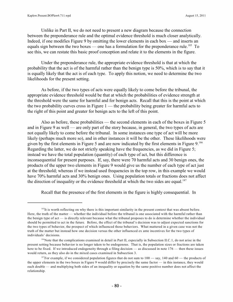
Kaplow.Present.BOPlaw6.711.wpd August 15, 2011
It is worth reflecting on why there is this important similarity in the present context that was absent before. 185
Here, the truth of the matter — whether the individual before the tribunal is one associated with the harmful rather thanthe benign type of act — is directly relevant because what the tribunal proposes to do is determine whether the individualshould be permitted to act in the future. Before, the effect of the tribunal’s decision was to adjust expected sanctions forthe two types of behavior, the prospect of which influenced those behaviors. What mattered in a given case was not thetruth of the matter but instead how one decision versus the other influenced ex ante incentives for the two types ofindividuals’ decisions.
Note that the complications examined in detail in Part II, especially in Subsection II.C.1, do not arise in the186
present setting because behavior is no longer taken to be endogenous. That is, the population sizes or fractions are takenhere to be fixed. If we introduced endogeneity through a filing decision — as discussed in note 176 — then these issueswould return, as they also do in the mixed cases examined in Subsection 3.
For example, if we considered population figures that do not sum to 100 — say, 140 and 60 — the products of187
the upper elements in the two boxes in Figure 9 would differ by precisely the same factor — in this instance, they wouldeach double — and multiplying both sides of an inequality or equation by the same positive number does not affect therelationship.
- 8800 -
Unlike in Part II, we do not need to present a new diagram because the connectionbetween the preponderance rule and the optimal evidence threshold is much closer analytically. Indeed, if one modifies Figure 9 by omitting the lower elements in each box — and inserts anequals sign between the two boxes — one has a formulation for the preponderance rule. To185
see this, we can restate this basic proof conception and relate it to the elements in the figure.
Under the preponderance rule, the appropriate evidence threshold is that at which theprobability that the act is of the harmful rather than the benign type is 50%, which is to say that itis equally likely that the act is of each type. To apply this notion, we need to determine the twolikelihoods for the present setting.
As before, if the two types of acts were equally likely to come before the tribunal, theappropriate evidence threshold would be that at which the probabilities of evidence strength atthe threshold were the same for harmful and for benign acts. Recall that this is the point at whichthe two probability curves cross in Figure 1 — the probability being greater for harmful acts tothe right of this point and greater for benign acts to the left of this point.
Also as before, these probabilities — the second elements in each of the boxes in Figure 5and in Figure 9 as well — are only part of the story because, in general, the two types of acts arenot equally likely to come before the tribunal. In some instances one type of act will be morelikely (perhaps much more so), and in other instances it will be the other. These likelihoods weregiven by the first elements in Figure 5 and are now indicated by the first elements in Figure 9. 186
Regarding the latter, we do not strictly speaking have the frequencies, as we did in Figure 5;instead we have the total population (quantity) of each type of act, but this difference isinconsequential for present purposes. If, say, there were 70 harmful acts and 30 benign ones, theproducts of the upper two elements in Figure 9 would give us the number of each type of act justat the threshold; whereas if we instead used frequencies in the top row, in this example we wouldhave 70% harmful acts and 30% benign ones. Using population totals or fractions does not affectthe direction of inequality or the evidence threshold at which the two sides are equal.187
Recall that the presence of the first elements in the figure is highly consequential. In

Kaplow.Present.BOPlaw6.711.wpd August 15, 2011
As discussed at the end of Subsection II.C.1, the use of Bayesian priors — which here correspond to the188
population fractions (themselves proportional to the upper elements in the boxes in Figure 9) — is controversial. There itwas noted that the controversy may be avoided because such priors are immaterial in determining the optimal (welfare-maximizing) threshold in that setting. Here, however, these priors, as just explained, are highly consequential: they couldtip the optimal evidence threshold in either direction, and substantially so. Hence, it would be socially detrimental ifqueasiness about the use of Bayesian priors influenced the determination of decision rules for the regulation of futureconduct. The problem is equivalent to that in the medical decisionmaking context, noted just below in the text, where itwould be unimaginable in interpreting tests and other diagnostic evidence to ignore base rates (which, as here, can varyradically across contexts) in prescribing treatment.
Suppose that one both adopts an ex post perspective that takes behavior as given — which this Section189
indicates is more nearly appropriate regarding the regulation of future conduct — and then further stipulates that errorcosts are equal — essentially an ad hoc notion that, from some unstated normative perspective, all errors are of equalimportance, a view that is widely endorsed by courts and commentators alike in the civil setting (see sources quotedsupra note 6). Under these assumptions, the social objective reduces to the minimization of the total number of errors,which, as is familiar (when one implicitly takes the flow of cases into adjudication as given), implies the optimality of thepreponderance rule. See supra note 109; see also John Kaplan, Decision Theory and the Factfinding Process, 20 STAN.L. REV. 1065, 1071–72 (1968) (noting that a preponderance standard supposes that the two types of errors have equalcost); Posner, supra note 169, at 408 (same).
- 8811 -
some instances, most possible acts will be harmful, in which case a very low evidence thresholdwould implement the preponderance rule, whereas in others most will be benign, in which case avery high threshold would be indicated.188
At this point, we can see that there is one qualitative difference between the formulationfor the optimal evidence threshold and that for the preponderance rule: the former had anadditional pair of elements, the lower ones in Figure 9, that are omitted from the latter. Thisdivergence mirrors one of the key distinctions considered in Subsection II.B.1, and it again canbe extremely important.
To appreciate the significance, begin with the evidence threshold that implements thepreponderance rule: it by definition is one for which the product of the first two elements in theleft box in Figure 9 equals the corresponding product for the right box. Now we can examinewhether and how the third elements may differ. Even supposing that the private benefits for thetwo types of acts are the same (which in general they need not be), we note that they enter thetwo sides with opposite signs. That is, the average private benefit of a harmful act reduces thebenefit side of the calculus but increases the cost side of the calculus. This opposition is hardlysurprising since individuals’ private benefits are social costs of prohibition for both types of acts. Moreover, the left, benefit side has the external social harm, which is avoided by the prohibitionof harmful acts, and the right, cost side has no corresponding component. Hence, thedeterminants of the two sides are entirely different.
Only by coincidence could we expect the third elements to be equal. They could differ189
in either direction, and the differences could be small or large. It follows that the ex postlikelihood at the optimal threshold could be anything: it would be very high when acts posedlittle harm relative to private benefits, and it would be very low when acts posed great harm. Toillustrate, the degree to which one administering a driving test should be convinced that theapplicant would generally be safe should be quite different for an ordinary driver’s license thanfor a license to operate vehicles carrying hazardous substances.

Kaplow.Present.BOPlaw6.711.wpd August 15, 2011
See, e.g., eBay Inc. v. MercExchange, L.L.C., 547 U. S. 388, 391 (2006) (“[A] plaintiff seeking a permanent190
injunction must satisfy a four-factor test before a court may grant such relief. A plaintiff must demonstrate: (1) that it hassuffered an irreparable injury; (2) that remedies available at law, such as monetary damages, are inadequate tocompensate for that injury; (3) that, considering the balance of hardships between the plaintiff and defendant, a remedy inequity is warranted; and (4) that the public interest would not be disserved by a permanent injunction.”). Regardingpreliminary injunctions, where the concern for error is at the fore, it is standard to take into account the costs to the twoparties of different outcomes as well as the probabilities that one or another result on the merits is correct. See POSNER,supra note 6, at 760–61; John Leubsdorf, The Standard for Preliminary Injunctions, 91 HARV. L. REV. 525 (1978).
Another type of mixed case arises when a prohibition is not self-executing. Then one is, from that point191
forward, back to the situation examined in the rest of this Article. Indeed, that analysis assumed that all harmful actswere prohibited to begin with, and the problem is that individuals nevertheless commit harmful acts when private benefitsexceed the expected sanction. The existence of prior proceedings may still matter. One possibility is that the prior
- 8822 -
Moreover, this point is regarded as obvious in other settings, like medicaldecisionmaking. If a medical procedure is very expensive and highly risky, it is sensible toemploy it only when tests indicate that the patient is almost certain to be a type who wouldbenefit (some cancer treatments). But if a procedure is inexpensive and poses almost no risk ofserious side-effects, it might be used, perhaps prophylactically, even on patients who only have asmall likelihood of any benefit (some vitamins).
To summarize, the difference between the preponderance rule (or others like it) and theformulation for the optimal evidence threshold is, qualitatively, quite less in the present settingthan in those centrally concerned with ex ante behavior. Instead of an almost completedisconnect, we have a substantial overlap of relevant factors. Nevertheless, the preponderancerule omits considerations of harm and benefit, which are of critical importance if one isconcerned with the consequences of adjudication for social welfare.
Interestingly, in many settings in which decisions are made about the permission orprohibition of future conduct — which often is not done through conventional adjudication —we see implicit or explicit use of cost-benefit analysis that is much like the analysis in Subsection1 for the optimal evidence threshold rather than deployment of a preponderance of the evidencerule (or others like it). Many licensing and zoning decisions are made by regulatory bodies thatundertake an inclusive analysis that attends to social harm and private benefits. New doctors andnew drugs must pass certification tests, and the minimum threshold is not set based on a purelikelihood calculus, one presumes. Even for injunctions determined by courts, factors includeconsiderations of harm and benefit, not just likelihoods. It is notable that when the likelihood190
test is less distant from a sensible formulation, the legal system tends to move even closer to anexplicit welfare-based analysis, whereas when it is not even close, the legal system tends to stickwith ex post likelihood rules.
3. Mixed Cases
The analysis to this point of the regulation of future conduct examines a simple, purescenario in which individuals — certain numbers of whom are associated with harmful and withbenign acts — seek permission to perform future acts and the legal system either grants or deniespermission, which determines which acts are committed. This Subsection considers mixedcases in which the prospect of prohibitions influences ex ante behavior as well. Examples191 192

Kaplow.Present.BOPlaw6.711.wpd August 15, 2011
determination may be viewed as decisive with regard to aspects of liability, so the only question may be whether or not aperson acted. For example, the offense of driving without a license may require proof that the person denied a licensewas driving, but there is no further determination needed regarding whether the act is regarded to be harmful. (For someregulations, violations would be sufficiently obvious that the rules may be regarded as self-enforcing. For example, autility cannot very well secretly operate an unlicensed nuclear power plant. Nor is a major pharmaceutical companylikely to sell a drug prohibited by the regulators, although obviously the sale of some prohibited drugs is widespread andenforcement is very costly.) In other settings, there may be little difference. If what is illegal is not operating a plant butdischarging a substance (where permission might sometimes be granted), one will need to determine whether harmfulsubstances were discharged, by whom, and so forth.
Cf. Kaplow, supra note 100, at 379–81 (examining how mixed cases affect the analysis of accuracy in192
adjudication). Similar analysis, with some of the effects reversed, is applicable to determination of eligibility for futurerewards, which could include intellectual property rights (the granting of a patent — which, note, also constitutes aconditional prohibition on others’ behavior) or transfer payments (for example, disability benefits determinations). Thelatter case also brings to mind the compensatory function of some private litigation: that is, lawsuit outcomes may matternot only on account of the provision of ex ante incentives but also because compensation may be independently beneficial(or detrimental) on account of parties’ risk aversion. Although the present Section focuses on future conduct, theanalytical structure really refers to any consequence that follows directly from the outcome of adjudication, by contrast toeffects due to the anticipation of adjudication outcomes. Cf. id. at 369–78 (addressing the value of accuracy indetermining future entitlements); id. at 383–86 (discussing the accuracy of compensation); Louis Kaplow, OptimalInsurance Contracts When Establishing the Amount of Loss Is Costly, 19 GENEVA PAPERS ON RISK & INS. THEORY 139(1994) (analyzing the value of accuracy in providing compensation through insurance).
An important analogous example involves merger approval. Not only is the application process nontrivially193
costly, but since there is a serious prospect of denial for some mergers, the ex ante incentives to find possible mergerpartners, negotiate deals, arrange financing, and so forth will be reduced, for both harmful and benign mergers, in degreesthat depend on the subsequent standard for approval.
This phenomenon includes but is not limited to the ex ante behavior required to file the application itself — a194
subject discussed briefly in note 176. Since the analysis is conceptually quite similar, no sharp distinction need be drawn.
- 8833 -
already given were imprisonment — the prospect of which deters (and chills) acts and theimposition of which governs future conduct for a time — and license revocation, such as fordrunk driving — the prospect of which deters (and chills) certain driving behavior and theimposition of which prevents future driving by the individual. Clearly, many, although notnearly all, denials of permission influence ex ante behavior of various sorts, including myriadtypes of investment: putting together a development project, which requires permission from azoning board to go forward; studying to become a doctor, which requires obtaining a medical193
license; or research and development in the pharmaceutical industry, which requires drugapproval.194
The optimal evidence threshold in these mixed cases will reflect a weighted average ofthe two prior calculuses. In conducting the balance of benefits and costs, we can sum the resultsin the left boxes in Figures 4 and 9 and the results in the right boxes, and then compare the twosums. Because the sanction has both sets of effects, both of the benefits (deterrence and thesocial gains from the prohibition of future harmful acts) and both of the costs (chilling and thesocial costs from the prohibition of future benign acts) are pertinent. And clearly, depending onwhich sorts of effects are largest, the optimal threshold may more nearly resemble one from theformer pure case or from the latter one.
D. Selection of Cases for Adjudication
Return to the core setting in which adjudication examines past acts to determine whether

Kaplow.Present.BOPlaw6.711.wpd August 15, 2011
As mentioned at some points below, the evidence threshold also influences parties’ incentives to generate195
evidence.
Prior discussions of how proof burdens may affect prosecutors’ and defendants’ efforts in litigation include196
Thomas J. Miceli, Optimal Prosecution of Defendants Whose Guilt Is Uncertain, 6 J. L. ECON. & ORG. 189 (1990);Daniel L. Rubinfeld & David E.M. Sappington, Efficient Awards and Standards of Proof in Judicial Proceedings, 18RAND J. ECON. 308 (1987); and Okan Yilankaya, A Model of Evidence Production and Optimal Standard of Proof andPenalty in Criminal Trials, 35 CAN. J. ECON. 385 (2002). See also Tracy Lewis & Michael Poitevin, Disclosure ofInformation in Regulatory Proceedings, 13 J. L. ECON. & ORG. 50 (1997) (analyzing applicants’ incentives to presentevidence in regulatory proceedings of the sort analyzed in Section C); Derek Pyne, Can Making It Harder to ConvictCriminals Ever Reduce Crime?, EUR. J. L. & ECON. 191 (2004) (examining a model in which police are rewarded forconvictions, regardless of their accuracy, and finding that a higher proof burden may increase their efforts to identify thetruly guilty and thereby increase deterrence); Matthew C. Stephenson, Evidentiary Standards and InformationAcquisition in Public Law, 10 AM. L. & ECON. REV. 351 (2008) (studying the effect of reviewing courts’ evidentiarydemands on agencies’ incentives to acquire information).
- 8844 -
sanctions should be imposed. Most of the analysis of this Article takes as given that someportion of harmful acts and of benign acts will come before tribunals. The exception is SectionIII.A, which examines how optimally to choose the level of enforcement effort in conjunctionwith setting an evidence threshold. However, with both public and private enforcement, theprocess by which cases are identified and brought forward is not mechanical but rather dependson the behavior of government enforcers and private litigants. Even more relevant for presentpurposes, the manner in which cases are selected for adjudication may bear on the optimalevidence threshold, in part because the evidence threshold itself may influence the flow of casesinto adjudication. This complex relationship raises myriad issues, only a handful of which are195
touched upon here.
1. Public Enforcement
Most of the discussion has implicitly or explicitly contemplated public enforcers, such aswhen the government decides how to deploy a police force; conduct tax audits or environmental,health, and safety inspections; and prosecute cases. However, even for a given budget and set ofrules guiding government officials in these tasks, one must take into account the incentives theyface. Agents’ rewards may be variously affected — perhaps directly but often more subtly onaccount of norms, promotion and retention criteria, and elections — by many factors, including:the number or portion of investigations or audits that generate prosecutions, the quantity orpercentage of successful prosecutions, the quantity of fines or other sanctions imposed, the rateof crime or other infractions and changes therein over time, complaints about abuse, andembarrassment about exposed error. Some of these are influenced by the proof burden to whichcases will be subject, and some may in any event be relevant to how it should be set. Thesephenomena are likely to be important because such incentives determine both the cases that arepursued and the evidence that is developed.196
Suppose, for example, that the evidence threshold is raised for a set of violations. If oneassumes that enforcers are most heavily influenced by the fraction of cases that ultimately areprosecuted successfully, they might pursue fewer cases, putting more effort into those thatremain. The consequence might be that the increase in the evidence threshold would reducedeterrence by even more than if such a response was ignored since prospective violators care not

Kaplow.Present.BOPlaw6.711.wpd August 15, 2011
In discussions of government prosecutions, criminal and civil, it is often remarked that the government’s197
resources vastly exceed those of private parties. The comparison, however, is quite misleading because, in general, thegovernment needs to spread its resources across many priorities, only a small fraction of which involves police andprosecution, and those resources in turn must cover all manner of violations by the entire population. In many settings —notably some white collar crime — the government is often significantly outspent by private parties. The importantcaveat, which the text emphasizes, is that the government has great discretion over how it allocates resources acrosscases. It can choose to concentrate them on particular individuals or firms — or threaten to do so, perhaps to great effect. See POSNER, supra note 6, at 828–29 (explaining that prosecutors can threaten to expend sizable resources at trial inorder to induce favorable plea bargaining outcomes).
Relatedly, a high burden on the prosecution makes it more difficult for the government to impose large198
defense costs on its targets because they can succeed in many instances with more modest effort.
Another class of abuse concerns prosecutions motivated by the personal gain of the prosecutor. One seeking199
promotion, reelection, higher office, or fame might pursue high-profile defendants who may well not be politicalopponents or even politically associated.
Another rationale is that criminal cases may involve the deprivation of liberty, although the analysis in200
Subsection III.B.2 shows how higher social sanction costs actually have ambiguous implications for the optimal evidencethreshold.
- 8855 -
about the likelihood of being sanctioned conditional on their case being pushed forward butrather on the overall likelihood of sanctions. Furthermore, if the cases dropped are weaker onesand some additional ones are winnowed out when more intensive effort reveals exoneratingevidence, the ex ante likelihood of mistaken imposition of sanctions may also fall by even morethan without this reaction by enforcers. Note also that a more complete analysis needs to accountfor defendants’ and their lawyers’ incentives. With a higher burden on the enforcer, the defensemight expend less effort since it is easier to prevail — which could partly offset theaforementioned effects — but sometimes the defense might strive harder since some nearlyhopeless cases may have become more winnable. It is important to keep in mind in this instanceand others that enforcers’ behavior can to a degree be controlled, such as in setting agencybudgets and adjusting actors’ financial and other rewards.
Other effects are possible with different incentives. One set of considerations isparticularly important, especially in cases that involve political opponents of a regime or otherindividuals the government would improperly like to attack through the legal system. In suchsituations, a high evidence threshold may be especially valuable in light of the government’sability to concentrate significant resources on such cases and possibly attempt to fabricate197
evidence. Moreover, the resulting chilling effects (stifling of political opposition) if such198
prosecutions are too easy could have a particularly high social cost. For these reasons, a very199
tough threshold may be optimal. The problem is that it is hard to know which cases should be sotreated, and having to treat all cases (or large sets of them) this way can itself be quitetroublesome. The difficulty is especially great because another priority of many governments,including those from whom abuse may most be feared, is combating corruption, which requiressuccessful prosecution of behaviors in settings that may be observationally similar to those with ahigh potential for improper enforcement activity.
This argument for a particularly high evidence threshold may help to explain therequirement of proof beyond a reasonable doubt in U.S. criminal cases as well as itsconstitutional status, along with other procedural protections distinctive to the criminal sphere,200

Kaplow.Present.BOPlaw6.711.wpd August 15, 2011
Observe further that if this set of protections is largely effective — that is, in deterring government abuse,201
although possibly at the expense of higher ordinary crime — examination of trial outcomes in equilibrium may give theimpression that the proof standard is too high, illustrating the analysis in Section II.C that indicates how an ex post viewfocused on outcomes is highly misleading regarding whether the evidence threshold is set optimally.
See sources quoted supra note 6. Note further that the Supreme Court’s analysis of proof standards in civil202
cases employs the balancing test of Mathews v. Eldridge, 424 U.S. 319 (1976). See, e.g., Santosky v. Kramer, 455 U.S.745, 754 (1982); see also Kaplow, supra note 100, at 373–78 (suggesting respects in which this cost-benefit test isconfused). With regard to the termination of parental rights on grounds of neglect and the use of involuntary civilcommitment — where the stakes involve liberty — the Supreme Court has applied this test to require proof by clear andconvincing evidence (but not proof beyond a reasonable doubt). See Santosky v. Kramer; Addington v. Texas, 441 U.S.418 (1979). But see supra note 53 (criticizing the assumption that higher stakes generally favor a more stringentevidence threshold).
Prior economic analysis of the burden of proof and parties’ incentives to expend resources on lawsuits and on203
the presentation of evidence includes Antonio E. Bernardo, Eric Talley & Ivo Welch, A Theory of Legal Presumptions,16 J. L. ECON. & ORG. 1 (2000); Demougin & Fluet, Rules of Proof, supra note 100; Hay & Spier, supra note 4; andChris William Sanchirico, A Primary-Activity Approach to Proof Burdens, 37 J. LEGAL STUD. 273 (2008). See also A.Mitchell Polinsky & Steven Shavell, Legal Error, Litigation, and the Incentive to Obey the Law, 5 J. L. ECON. & ORG. 99(1989) (examining the effects of errors on the incentive to sue and discussing how fines and subsidies could be employedto alter this incentive).
The calculus is more subtle on account of strategic factors related to asymmetric information and the204
sequencing of parties’ expenditures (which may make some negative expected value suits viable), risk aversion, and otherconsiderations. See generally Kathryn E. Spier, Litigation, in 1 HANDBOOK OF LAW AND ECONOMICS 259, 305–07 (A.Mitchell Polinsky & Steven Shavell eds. 2007) (surveying pertinent literature). These details are not central for presentpurposes. Relatedly, the present discussion also abstracts from settlement.
The text oversimplifies in a manner that depends on the nature of prospective plaintiffs’ information. To205
begin, note that the suggestion is that a higher evidence threshold discourages suit in a particular case, taking as givenwhat a prospective plaintiff knows ex ante (a subject further discussed at the end of this Subsection). Note that, eventhough suit conditional on, say, a harmful act, may be less likely, the deterrence reduction could raise the total number ofsuits and thus legal expenditures. Moreover, as deterrence falls, it is possible that individuals who suffer harm and areuncertain (perhaps before discovery) whether their injury was due to improper behavior might be more likely to suebecause they will realize that true liability is more likely. In equilibrium, suits cannot be more likely per harmful act, for
- 8866 -
many of which seem motivated by concerns for abuse of power rather than cost-benefitcalculations for routine policy-making by benevolent officials. Bolstering this view is the201
commonplace advancement of a preponderance rule for civil cases on the ground that the specialconcerns in the criminal context are absent, so society has no particular reason to tilt the legalsystem in favor of one outcome versus the other. Note, however, that all manner of abuse can202
arise whenever the government (rather than a private plaintiff) is the prosecuting party, whicharguably calls for a higher evidence threshold regardless of whether the legal action involves acriminal proceeding. Moreover, when targeted defendants are corporations (or otherorganizations) and the main penalties are fines or possible reputational costs, civil proceedingsmay be quite a good substitute in advancing the objectives of overly zealous governmentofficials.
2. Private Enforcement203
In civil cases with private plaintiffs, the primary determinant of suit will be whether aprospective plaintiff’s expected recovery exceeds its expected litigation costs. Furthermore,204
plaintiffs’ expected recoveries depend on the evidence threshold. In particular, higher thresholdsdiscourage suit, which reduces deterrence and chilling, whereas lower thresholds encourage205

Kaplow.Present.BOPlaw6.711.wpd August 15, 2011
in that case deterrence would be greater, which would nullify (reverse) the factor encouraging suit, leaving only the directeffect of a higher evidence threshold in deterring suit. See Bernardo, Talley & Welch, supra note 203 (analyzing a modelof the negligence rule in which this inference phenomenon is operative).
These effects do tend to favor an intermediate proof standard, for an extremely low one would encourage all206
manner of suits with little merit (mostly involving benign acts) and an extremely high one would discourage even mostmeritorious suits (mostly involving harmful acts). However — despite the Goldilocks Principle, see GoldilocksPrinciple, WIKIPEDIA, http://en.wikipedia.org/wiki/Goldilocks_Principle (last visited Feb. 4, 2011) — knowing that theoptimal evidence threshold requires more than nothing and less than infinity hardly suggests that a 50% rule, or anythingclose to it, is optimal. In this regard, as mentioned in the Introduction, the attraction of the 50% rule probably has muchto do with its power as a focal point and the lack of alternative focal points, other than 0% and 100%, which areobviously ruled out.
See, e.g., Louis Kaplow, Shifting Plaintiffs’ Fees Versus Increasing Damage Awards, 24 RAND J. ECON. 625207
(1993); Spier, supra note 204 (surveying literature on many of these instruments and others).
Consider, for example, the Private Securities Litigation Reform Act of 1995, Pub. L. No. 104-67, 109 Stat.208
737 (codified as amended in scattered sections of Title 15 of the U.S. Code).
- 8877 -
suit and thereby heighten deterrence and chilling.206
As a consequence, recognition that the selection of civil disputes for adjudication dependson the evidence threshold tends to augment the behavioral effects of adjusting the evidencethreshold. Hence, in determining what threshold is optimal, such as in the setting examined inPart I, one would need to adjust (raise) the impacts on expected sanctions (the upper elements inFigure 4). Note that it is a priori ambiguous which way this consideration cuts since both thedeterrence benefit and the chilling cost of a lower threshold are increased. The direction of thenet effect would depend on whether cases at the margin of profitability for prospective plaintiffswere more likely to be valid or not.
In Section III.A, it was supposed, by contrast, that the level of enforcement effort couldbe chosen by the state, along with the evidence threshold; that is, they could be optimizedtogether. The current remarks, and similar ones in Subsection 1, suggest that effort levels are toa significant degree endogenous — that is, responsive to how the evidence threshold is set. However, in both instances, this story is incomplete. For public enforcement, it remains true thatbudgets and other policy instruments significantly influence enforcement effort. Moreover, someof the incentives are themselves publically determined: for example, compensation andpromotion criteria can be chosen with effects on enforcement effort in mind.
Similar logic extends to private enforcement, although some of the mechanisms aredifferent. For a given evidence threshold, one can encourage or discourage suits through theoffering of subsidies or setting of fees, adjusting rules for damages (including through the use ofmultipliers and decoupling), fee shifting, and other tools. Therefore, one still needs to take207
into account how setting the evidence threshold affects incentives for suit, but there remainssubstantial room to adjust enforcement effort separately. Indeed, especially with the privateenforcement of public law, fee shifting (sometimes one-way) and damages rules (includingstatutory minimums) are selectively deployed to influence suit. Also, various procedural rules,such as standards governing dismissals and class actions, may be customized.208
Another consideration, mentioned with regard to public prosecutors, is that private

Kaplow.Present.BOPlaw6.711.wpd August 15, 2011
The latter conclusion requires the additional assumption that the factfinder always follows instructions; if not,209
one could suppose further for the purposes of the hypothetical illustration that such deviations can also be predictedperfectly.
This statement ignores the possibility of settlement, which parties would find advantageous. More broadly,210
the analysis assumes that the legal rule is formulated as an evidence threshold rather than as an ex post likelihood. Asexplained in Subsection II.C.1, the relationship between the two notions is complex due to the endogeneity of behavior. The present discussion adds a further complication to that story, for factfinders, in assessing the frequencies with whichharmful and benign acts come before tribunals — the upper elements in Figure 5 — would now also have to take intoaccount parties’ incentives to drop and settle cases. In the scenario in the text, for example, factfinders would know thatany case that reached them was one meriting a finding of liability, so they would always do so. But if parties anticipatedthis, even those with weak cases would not drop them or settle. The result would be an equilibrium in which a greatervariety of cases came before tribunals. Application of the preponderance rule (or others like it) would accordingly beeven more difficult than previously suggested.
- 8888 -
litigants’ incentives to develop evidence — through investigation, analysis, and trial preparation— are influenced by the evidence threshold. For example, a higher evidence threshold, inaddition to discouraging some suits, may encourage plaintiffs to spend more on those that they dobring. In such cases, defendants may spend less, because it is easier to win, or more, becausepreviously unpromising cases now present serious prospects for success. These efforts have afurther influence on the deterrence and chilling effects of the legal system and also constituteresource costs in themselves, all of which bears on what evidence threshold is optimal.
Regarding both private and public enforcement, it has also been implicitly assumed thatthe quality of evidence, however generated, does not become apparent until adjudication itself. At that point, liability is assessed if and only if the strength of the evidence exceeds the statedthreshold. Consider, by contrast, the opposite extreme: where parties know before trial exactlyhow strong the factfinder will perceive the evidence to be and accordingly can predict theoutcome perfectly. Then, as long as adjudication involves any cost, public and private209
enforcers would drop all cases where the evidence strength x failed to exceed the threshold x . T
As a consequence, all adjudicated cases would find in favor of the prosecutor or plaintiff. Note210
that, in this simplified scenario, none of the outcomes would be different; instead, for everydefendant victory we would substitute a dropped case.
If, however, one attempted to assess the effectiveness of the legal system based on theoutcome of adjudicated cases — a precarious endeavor even without regard to the current point,as developed in Subsection II.C.2 — one’s view would be skewed even further. There would beno mistaken exonerations since all cases with that prospect would be dropped, and there wouldbe no correct exonerations for the same reason, so one hundred percent of individuals whoactually committed benign acts but are nevertheless subject to adjudication would be mistakenlysubject to sanctions. The system would appear much worse on this dimension when in fact itwould be no different; it would merely be saving the resource costs of adjudication in cases thatwould not assign liability.
Realistically, the truth is somewhere in between what has implicitly been assumedthroughout and this extreme hypothetical alternative. That is, parties will to some degree knowhow a factfinder is likely to assess the evidence in a given case, but there will remain significantuncertainty — due, for example, to incomplete discovery, unpredictable variations in how

Kaplow.Present.BOPlaw6.711.wpd August 15, 2011
- 8899 -
evidence will be presented (for example, how witnesses will hold up under cross-examination),and variations in factfinder perceptions. Presumably, in close cases — those in which x is closeto x — prediction will be difficult, but in cases that are not at all close, parties will be nearlyT
certain of the outcome. These differences will, no doubt, significantly affect which cases arepursued and which are settled (including through the use of plea bargaining). And theseconsiderations are also relevant to how the evidence threshold should be set since settlementsinfluence both expected sanctions — for harmful and for benign acts — and the administrativecosts of adjudication.
CONCLUSION
The burden of proof is a central feature of adjudication. Nevertheless, the normativequestion of how high it should be set has received remarkably little attention, particularly in thecivil context. This Article begins to fill the vacuum, offering a preliminary conceptual analysisof the subject. It addresses the question of how strong evidence should be in order to assessliability when the objective is the maximization of social welfare.
The initial focus is on a basic law enforcement setting in which some fraction of harmfulacts as well as a portion of benign ones will be brought into adjudication. Demanding strongerevidence as a prerequisite to imposing sanctions will dilute deterrence, to some extentundermining the core mission of the legal system: controlling harmful conduct. There is,however, a concomitant benefit: reducing the expected sanctions on benign acts, which decreasesthe chilling of desirable activity. This tradeoff of deterrence and chilling determines how theoptimal evidence threshold should be set. The analysis reveals that it depends on the extent towhich raising the evidence threshold reduces the expected sanction for both harmful and benignacts, the number of additional harmful and benign acts committed as a consequence of suchreductions, the magnitude of the benefit produced by each type of act that is no longerdiscouraged, and the harm caused by the additional harmful acts committed. On reflection, all ofthe pertinent considerations identified and their interaction in determining an optimal evidencethreshold seem natural if the goal is indeed to advance social welfare. Unfortunately, therelevant magnitudes are likely to vary greatly by context and will often be difficult to measure, sothe practical problem of determining optimal proof burdens is daunting.
This approach is contrasted with conventional conceptions of the burden of proof. Analysis focuses on the preponderance of the evidence rule, which assigns liability when it ismore likely than not that the defendant committed the harmful act. It is noted, however, that thisrule is qualitatively similar to others that may impose a more stringent requirement — such asdemanding clear and convincing evidence or proof beyond a reasonable doubt — because underall such formulations the matter addressed is the likelihood that the individual before the tribunalcommitted the harmful act.
When one compares the determinants of the evidence threshold under these traditionalrules to the determinants of the optimal evidence threshold, it becomes apparent that there isvirtually no overlap. Accordingly, neither the preponderance rule nor other likelihood-based

Kaplow.Present.BOPlaw6.711.wpd August 15, 2011
- 9900 -
rules are even plausible proxies for the evidence threshold that maximizes social welfare. Theoptimal threshold in a particular context could be far more stringent or much more lax than thatimplied by any given likelihood-based rule. The core reason for the divergence is thatconventional formulations inquire as to the nature of the case before the tribunal, whereas settingan optimal evidence threshold depends on how changes in the level of the threshold willinfluence individuals’ ex ante behavior and, moreover, on the welfare consequences of sucheffects.
The preponderance rule and related formulations also present a number of internalproblems. Some are attributable to the fact that the evidence threshold influences behavior,which in turn affects the mix of cases before the tribunal, which itself is a determinant of thelikelihood that the factfinder is supposed to assess. This phenomenon renders application oftraditional criteria far more complicated than seems to be appreciated by courts or commentators. It also gives rise to counterintuitive possibilities. Notably, one might have supposed that raisingthe evidence threshold makes it more likely that cases just at the new, elevated threshold involveharmful rather than benign acts because they involve stronger evidence. But this is only part ofthe story. A heightened threshold also reduces deterrence and the chilling of benign acts, and thelatter effect means that more individuals who in fact committed benign acts will come beforetribunals. If this effect is sufficiently large — and it is entirely plausible that sometimes it will be— then the net effect of demanding stronger evidence will be to reduce the likelihood that casesjust at the new, elevated threshold involve a harmful act rather than a benign one. It is furtherdemonstrated that this feature makes it possible that multiple evidence thresholds will satisfy,say, the preponderance rule, and it is also possible that none will. Likewise, demanding strongerevidence can increase the likelihood that innocent individuals are subject to sanctions. Otherconundrums are also identified, including that an extremely well functioning legal system mayhave most of its findings of liability be erroneous and a purely random legal system can have aperfect score (all findings of liability being correct).
In sum, conventional burden of proof formulations are deeply problematic in ways thathave gone unnoticed, and these defects are in addition to the central one already noted: that theirdeterminants have almost nothing in common with those that indicate what evidence requirementmaximizes social welfare. These conclusions motivate some inquiry into whether conventionalproof burdens, in their canonical, idealized form, completely determine factfinders’ actualbehavior or whether, in practice, adjudicators are influenced to some nontrivial degree byattention to the consequences of their decisions. Also, some highly preliminary remarks areoffered on alternative formulations of the burden of proof that are more attentive to socialwelfare.
The remainder of the Article returns to the central question of what evidence threshold isoptimal and introduces a range of further considerations. One set pertains to other features of thelegal system. First, this portion explores how to set the evidence threshold optimally when it isalso possible to adjust the level of enforcement effort: a reduced threshold and heightenedenforcement are substitute means of achieving a given increment to deterrence. A reducedthreshold has the advantage of avoiding the additional expense involved with strongerenforcement but the disadvantage of faring relatively worse with regard to chilling effects. The

Kaplow.Present.BOPlaw6.711.wpd August 15, 2011
- 9911 -
relationship between the optimal evidence threshold and the level of sanctions is also addressed,and some similar interactions are identified. Attention is also devoted to how the direct costs ofsanctions, such as with imprisonment, influence the optimal threshold. One might have thoughta heightened threshold preferable because this would reduce the imposition of costly sanctions,but again this effect is only half of the story. The higher threshold, by reducing both deterrenceand chilling, increases the number of cases that flow into the system, which tends to increase therate of imposition of costly sanctions. Similar analysis applies to costs that might be associatedper se with sanctioning the innocent: a higher evidence threshold makes that outcome less likelyin a given case but tends to increase the number of cases involving innocents, so the net impactcould be in either direction. This Part of the Article also examines the interplay between theaccuracy of the legal system and how optimally to set the evidence threshold.
Finally, the Article considers similarities and differences across alternative enforcementenvironments. Monitoring (such as by the posting of police officers and use of patrols or privatesecurity guards) has effects on behavior that are similar to those of auditing (including variousforms of inspection used to enforce myriad regulations), but the two methods differ inenforcement costs. Specifically, both deterrence and chilling, by reducing the level of activity,reduce the number of audits that need to be performed, even for a given audit rate. Enforcementby investigation, such as when a harmful act has clearly been committed (murder, auto theft) andofficials attempt to identify the perpetrator, is notably different. The key point is that deterrenceis more valuable: when fewer harmful acts are committed, fewer investigations are triggered,which both saves enforcement costs and also reduces the number of instances in which benignbehavior may mistakenly be caught in the dragnet. An implication of the latter is that it seemsentirely conceivable that demanding stronger evidence will increase the frequency with whichinnocent individuals are mistakenly sanctioned. Here the channel is that a tougher evidencethreshold dilutes deterrence, which provokes more investigations and thereby creates moreopportunities for mistakes to occur. This effect need not dominate the reduction due to thereduced likelihood that any given individual before a tribunal will be sanctioned, but it could.
A much different mode of enforcement involves the regulation of future conduct, such aswhen authorities decide whether to grant a zoning variance, license an individual or a facility,approve a drug, or allow a merger. In these settings, the determination of the optimal evidencethreshold is more like traditional cost-benefit analysis, and it is perhaps most familiar from howone might decide whether to administer medical treatment following a diagnostic test. Unlike inthe rest of the Article, the relevant factors differ much less from the determinants of thepreponderance rule. Nevertheless, the differences that remain — namely, that the preponderancerule and other likelihood-based rules do not depend on harm and benefit — are of greatconsequence, making the traditional conceptions very poor proxies for guiding system design. Again, optimal evidence thresholds could be much stricter or notably weaker than any of theseconventional rules dictates. Interestingly, in many of these contexts, legal systems often seem toproceed more in accord with what is socially optimal, eschewing customary burden of proofformulations.
The incentives of enforcers — both public prosecutors, police, and agencies and alsoprivate plaintiffs — may affect the analysis as well. Such individuals and entities often seek to

Kaplow.Present.BOPlaw6.711.wpd August 15, 2011
- 9922 -
advance their own interests rather than the social good. This fact may be relevant in setting theevidence threshold both because it influences the mix of cases that will come before tribunals(which mix affects what is optimal) and because the height of the threshold may have feedbackeffects that influence, for better or worse, which cases are pursued.
This Article constitutes a conceptual investigation of the burden of proof, specificallyanalyzing how to set the evidence threshold so as to maximize social welfare. Although thecentral question is normative, much of the analysis is positive, concerning the effects of changingthe evidence threshold in a variety of settings. Formulations are offered for the optimalthreshold, indicating what factors are relevant and how they are to be combined. Sharp contrastsare drawn between the present analysis and conventional thinking about the burden of proof.
The investigation is, nevertheless, preliminary. It turns out that many of the identifiedeffects, conclusions, and contrasts have received little prior attention, and a number arecounterintuitive, in some cases rendering traditional understandings incoherent — in addition toindicating their great divergence from the advancement of social welfare. Introducing additionalsystem features — enforcement effort, the magnitude of sanctions, and the degree of accuracy —and alternative enforcement contexts indicates numerous ways in which the results wouldchange. A first cut at so complex and multifaceted a problem is inevitably incomplete, and otherfactors and settings remain to be examined. Perhaps most worrisome, many of the keydeterminants of the optimal evidence threshold seem quite difficult to quantify in any particularsituation, which is all the more troubling given the extent to which they probably vary with thecircumstances.
In the end, however, the only way forward is to fill in the many remaining blanks in theanalysis, refine our thinking, and do our best to estimate pertinent empirical parameters. If wewish the legal system to better serve its function of controlling harmful activity while also takinginto account costs due to the mistaken imposition of sanctions — that is, to maximize socialwelfare — there is no real alternative. Conventional conceptions of the burden of proof do notconstitute even weak proxies for welfare since they depend almost entirely on factors differentfrom those that determine the optimal evidence threshold. Moreover, they are vastly morecomplex to apply than is appreciated and raise a number of conundrums that cannot be avoided,that is, except by refocusing our inquiry in a welfare-maximizing direction. In short, analysis ofthe burden of proof needs to start from scratch, and it is hoped that the present investigation willhelp instigate that effort.