bulk plan performance and tuning guide
TRANSCRIPT

Bulk Plan Performance and Tuning Guide


i
Table of Contents Bulk Plan Performance and Tuning ................................................................................. 1
Overview ...................................................................................................................... 1
Bulk Plan Performance and Tuning .......................................................................... 1
Data Setup ................................................................................................................... 2
Bulk Plan Data Setup ............................................................................................... 2
Locations and Location Attributes in Bulk Planning.................................................. 2
Equipment Groups and Equipment Types in Bulk Planning ..................................... 3
Fleet and Bulk Planning ........................................................................................... 4
Transport Modes and Service Providers in Bulk Planning ....................................... 5
Rate Offerings and Rate Records in Bulk Planning.................................................. 6
Rate Service and Bulk Plan ..................................................................................... 6
Carrier Capacities and Commitments in Bulk Planning ............................................ 7
Location Capacities and Bulk Planning .................................................................... 8
Itineraries and Bulk Plan .......................................................................................... 9
Itinerary Legs and Bulk Planning............................................................................ 10
Bulk Plan Processes and Routing ............................................................................. 13
Bulk Plan Processes .............................................................................................. 13
Bulk Plan Cost Based Routing ............................................................................... 14
Bulk Plan Network Routing .................................................................................... 17
Network Routing and Carrier Capacity ................................................................... 21
Solution Quality Tuning .............................................................................................. 24
Bulk Plan Solution Quality Tuning .......................................................................... 24
Bulk Plan Tuning Order Bundling Logic ................................................................. 24
Bulk Plan Tuning Direct Shipment Building ............................................................ 28
Bulk Plan Tuning Container Optimization Logic ..................................................... 31
Bulk Plan Tuning Continuous Moves Logic ............................................................ 40
Bulk Plan Multi-stop Shipment Logic ...................................................................... 46
Shipment Groups in Bulk Planning ............................................................................ 70
Shipment Groups in Bulk Planning ......................................................................... 70
Shipment Group Rule Details in Bulk Planning ...................................................... 72
Performance Tuning .................................................................................................. 74
Bulk Plan Performance Tuning .............................................................................. 74
Understanding the Bulk Plan Run .......................................................................... 74
Table of Contents
ii
Bulk Plan Multi-threading ....................................................................................... 77
Multi-threading Logic in OTM ................................................................................. 85
Bulk Plan Partitioning ............................................................................................. 87
Diagnostics ................................................................................................................ 89
Bulk Plan Diagnostics ............................................................................................ 89
Graphical Diagnostics ............................................................................................ 90
Bulk Plan Logs ....................................................................................................... 94
Container Optimization ........................................................................................... 97
Bulk Plan Caches ................................................................................................... 99

1
Bulk Plan Performance and Tuning
Overview
If you have any questions or comments about this topic or the online help, please contact us.
bulk_plan_manager/bulk_plan_performance_and_tuning.htm
Bulk Plan Performance and Tuning
Related Topics
The main objective of bulk plan is to recommend an efficient way to transport a group of orders from their sources to destinations by optimally consolidating the orders into one or more shipments. Bulk plan makes several key recommendations for the orders such as, the right choice of orders to combine to form a shipment, the right sequence of pickups and deliveries, the right sized equipment and the mode and carrier for transporting the shipment. The bulk plan also determines the cost of the shipments and the schedules for pickup and delivery at each stop. In many instances, these orders also have a choice of flowing through a network of cross-docks, ports, rail terminals, and so on. In such cases, the optimal decision also includes the order’s route through the network. Several business considerations are taken into account in forming the shipments. Among the important ones are the carrier rate information, location calendars, pickup and delivery windows on the orders, size and dimensions of ship units on the orders, driver’s hours of service restrictions, and available equipment.
By orders we mean either order releases or order movements unless specified.
See the following for more details
Data Setup describes the objects involved during bulk planing.
Bulk Plan Processes and Routing Methods describes the bulk plan process and routing methods at a high level and the pieces that comprise the bulk plan process. This section provides a high level look at the processes and routing methods used for bulk plan. The details about the algorithms and how to best tune bulk plan are described under solution quality tuning.
Solution Quality Tuning describes the algorithms that can be used to tune the solution quality of the bulk plan functionality.
Shipment Groups in Bulk Planning describes how shipment groups are built in the bulk plan post process step, how shipment group rules that have been defined determine the circumstances in which shipments are assembled into shipment groups during planning and related parameters.
Performance Tuning looks at reasons why some bulk plans run slowly, while other bulk plans, even with larger data sets run fast. Many performance problems though can be resolved through careful data modeling, algorithm tuning and multi-thread property settings.

Bulk Plan Performance and Tuning
2
Diagnostics -provides tips for diagnosing issues during bulk planning. This also includes Ask Oracle - Container Optimization and Object and Method Instrumentation.
Related Topics
Bulk Plan
Bulk Plan Performance and Tuning PDF
Data Setup
If you have any questions or comments about this topic or the online help, please contact us.
bulk_plan_manager/data_setup/bulk_plan_data_setup.htm
Bulk Plan Data Setup
Related Topics
A successful run of bulk plan depends on proper setup of data – both static and transactional. This topic provides links to the key entities and their descriptions and roles in the bulk plan process.
Locations and Location Attributes in Bulk Planning
Equipment Groups/Equipment Types in Bulk Planning
Fleet and Bulk Planning
Transportation Modes and Service Providers in Bulk Planning
Rate Offerings and Rate Records in Bulk Planning
Rate Service and Bulk Planning
Carrier Capacities and Commitments in Bulk Planning
Location Capacities and Bulk Planning
Itineraries and Bulk Planning
Itinerary Legs and Bulk Planning
Related Topics
Bulk Plan Performance and Tuning Overview
Bulk Plan Performance and Tuning PDF
If you have any questions or comments about this topic or the online help, please contact us.
bulk_plan_manager/data_setup/locations_and_bulk_planning.htm
Locations and Location Attributes in Bulk Planning
Related Topics
The key attributes of locations that affect the bulk plan process are: Location Calendars, Address Components, Latitudes & Longitudes, Location Roles, Location Activity Times and Special Services.

Bulk Plan Performance and Tuning Guide
3
Location Calendars specify the times when a location is open for pickup and delivery. Depending on the type of rate service, different types of calendar activities are used. For shipments involving SIMULATION rate service type, the hours associated with the calendar activity of LOAD are used to determine if a particular order can be loaded/picked up at a location. Similarly, hours associated with the calendar activity of RECEIVE are used to determine the open times when an order can be delivered at a location. However, for DAY DURATION rate service type, PICKUP and RECEIVE calendar activities are used.
Address fields, along with the location ID, on the location are used to match the location or a pair of locations to lanes for rating and resourcing purposes.
Latitudes and Longitudes on the locations are used to estimate the distances between locations. Estimating distances using latitudes/longitudes is faster than looking up the distances from the database or invoking an external distance engine.
Location Role defines the type of location.
Note: Define only one location role per location. Planning only uses the first role it sees on the location and having multiple roles could confuse the engine.
Activity times are defined on the location for the location role. These times specify the fixed and variable times for loading and unloading based on the type of the commodity. Activity times can also be defined for special services.
Special Services are services that are required for a shipment to occur. For example, special services could include delivery of a specific order to a construction site, or a mandatory item inspection. Special services can be applied to locations, items, order releases and order movements. OTM can only use rates that include a specific special service if that specific special service is on the location, item, or order.
On the location, you can specify compatible equipment groups and service providers. For example, a particular location cannot handle any equipment larger than 48 FT and hence is incompatible with 50 FT and 53 FT equipment.
Related Topics
Bulk Plan Performance and Tuning Overview
Bulk Plan Data Setup
Bulk Plan Performance and Tuning PDF
If you have any questions or comments about this topic or the online help, please contact us.
bulk_plan_manager/data_setup/equipment_groups_and_types_in_bulk_planning.htm
Equipment Groups and Equipment Types in Bulk Planning
Related Topics

Bulk Plan Performance and Tuning
4
Equipment groups define the size and shape of the equipment. The capacity of the equipment is defined in terms of Effective Weight, Effective Volume, Equipment Reference Units (ERUs) and equipment dimensions, Compartments, Length, Width and Height. The equipment dimensions are important for placing the items inside the equipment using the 3D load configuration engine.
An equipment group can have different types of equipment. For example, a 48FT equipment group might have an equipment type of rollup or swing door trailer. However, the weight, volume, ERUs, and dimensions of these equipment types are assumed to be the same as that of the equipment group. Although OTM supports many-to-many associations of equipment groups to equipment types, it is strongly recommended that each equipment type is associated with only one equipment group. However, an equipment group can be associated with several equipment types.
Equipment group profiles categorize equipment groups which have a common attribute. Equipment Group Profiles can be defined on:
Itinerary Legs (Itinerary Legs can also define multiple equipment group profiles through Multi-Modal Equipment Sets)
Order Release Constraints and Order Movement Constraints
Locations
Rate Offerings
Rate Records
Related Topics
Bulk Plan Performance and Tuning Overview
Bulk Plan Data Setup
Bulk Plan Performance and Tuning PDF
If you have any questions or comments about this topic or the online help, please contact us.
bulk_plan_manager/data_setup/fleet_and_bulk_planning.htm
Fleet and Bulk Planning
Related Topics
When running a bulk plan, you can use fleet criteria to generate shipments. This is known as Fleet Aware Bulk Planning. Fleet Aware Bulk Planning will only be performed when the FLEET AWARE BULK PLAN parameter is set to true. Network routing path creations, creation of order movements and the shipment building processes will not be influenced by the availability of fleet resource such as resource schedules. After direct and multistop shipments are created, the knowledge of resource schedules will be considered to determine which shipments need to be strung together to form optimal work assignments. In a bulk plan, OTM will first create work assignments and then continuous moves. Only shipments that are not part of a work assignment are considered for continuous moves.

Bulk Plan Performance and Tuning Guide
5
Note: Multiple simultaneous bulk plans should not be run when using fleet aware bulk plan.
Running multiple simultaneous bulk plans can result in loading the same resource schedule instance into multiple bulk plans and generating work assignments for a resource schedule instance that exceeds the resource schedule instance's resource count.
Work assignment creation happens if the Fleet Aware Bulk Planning parameter is set to True, regardless of the value set for CM AUTO CREATE. Here are some rules followed in the work assignment formation:
Shipments built on 2 different legs with 2 different leg consolidation groups can be combined only if they have same resource scheduler logic scenario set on them.
Shipments built on two different groups with the same leg consolidation group can be combined.
Shipments built on legs that do not have leg consolidation groups cannot be combined with shipments on another leg. They can only be combined with shipments in the same leg.
Related Topics
Bulk Plan Performance and Tuning Overview
Bulk Plan Data Setup
Work Assignment
Resource Schedule
Resource Schedule Profile
Resource Schedule Instance
Logic Configuration - Resource Scheduler
Bulk Plan Performance and Tuning PDF
If you have any questions or comments about this topic or the online help, please contact us.
bulk_plan_manager/data_setup/transport_modes_and_servprovs_in_bulk_planning.htm
Transport Modes and Service Providers in Bulk Planning
Related Topics
OTM allows you to use the public transportation modes such as TL, LTL, RAIL, PARCEL, EXPRESS, etc. or define your own transport modes. While OTM’s bulk plan does not associate any logic to the modes, these modes can be used as constraints on rate offerings, rate service, resources, networks and orders. OTM also includes information about service providers and their rates. A service provider can be a carrier, a freight forwarder, a third party logistic provider and so on.
Related Topics

Bulk Plan Performance and Tuning
6
Bulk Plan Performance and Tuning Overview
Bulk Plan Data Setup
Bulk Plan Performance and Tuning PDF
If you have any questions or comments about this topic or the online help, please contact us.
bulk_plan_manager/data_setup/rate_offerings_and_records_in_bulk_planning.htm
Rate Offerings and Rate Records in Bulk Planning
Related Topics
Bulk plan takes several constraints from rate offerings. Rate offerings contain the contract level data specific to a service provider. Rate offerings are defined for a service provider and a mode. Rate offerings are also defined for a set of equipment groups. A rate service is associated with a rate offering and it defines how the times on the shipments are calculated.
In OTM, a lane connects two different geographies or regions. Rate records store detailed rate information at the individual lane level. A rate offering can contain several rate records defined for various lanes. There are several constraints that can be applied at the rate record level as well. These constraints are:
Minimum and Maximum Number of Stops
Maximum Number of Pickup Stops
Maximum Number of Delivery Stops
Maximum Circuity Distance
Maximum Circuity Distance Percent
Performance Tip: Rating is the last step performed during the shipment creation in bulk plan. There are several time consuming steps such as sequencing that are performed prior to rating. If you know that a particular lane does not support more than 3 stops no matter what, place the max stops constraints at a high level such as on the itinerary or itinerary leg so that some computational time can be saved.
Related Topics
Bulk Plan Performance and Tuning Overview
Bulk Plan Data Setup
Bulk Plan Performance and Tuning PDF
If you have any questions or comments about this topic or the online help, please contact us.
bulk_plan_manager/data_setup/rate_service_and_bulk_plan.htm
Rate Service and Bulk Plan
Related Topics
Rate Service determines how to calculate the transit times between shipment stops. OTM supports several different types of rate services – Air Schedule, Day Duration,

Bulk Plan Performance and Tuning Guide
7
External Drive, External Transit Days, Ground Service, Lookup, Simulation, Time Definite Service and Voyage Schedule. See Rate Service Details for more information. The figure below shows different scheduling engines in OTM that use different types of rate services.
By Day Schedules: Day Duration, Distance Duration, External Transit Time, Time Definite
Fixed Schedulers: Air Schedule, Voyage Schedule, Ground Schedule
Simulation Schedulers: Drive Simulation, External Rate Service, Lookup Rate Service
Related Topics
Bulk Plan Performance and Tuning Overview
Bulk Plan Data Setup
Bulk Plan Performance and Tuning PDF
If you have any questions or comments about this topic or the online help, please contact us.
bulk_plan_manager/data_setup/carrier_capacities_and_commitments_in_bulk_planning.htm
Carrier Capacities and Commitments in Bulk Planning
Related Topics

Bulk Plan Performance and Tuning
8
Carrier Capacities define the number of equipment resources a carrier has on a given lane or capacity limit group during a specific time period. The capacities can be defined as a recurring capacity or as a daily capacity. Once the capacities are defined, OTM ensures the capacity limits are honored.
A carrier commitment represents a contract between the shipper and a carrier. The shipper promises to give the carrier a certain number of shipments per time period (such as per week or per month) in return for a negotiated rate. You can model commitments either by count or as a percentage of total volume.
A bulk plan running service provider assignment optimization will only take into account that bulk plan even if another bulk plan is also running service provider assignment optimization at the same time. However, the parallel bulk plans will not over-scribe carrier capacity.
Related Topics
Bulk Plan Performance and Tuning Overview
Bulk Plan Data Setup
Network Routing and Carrier Capacity
Bulk Plan Performance and Tuning PDF
If you have any questions or comments about this topic or the online help, please contact us.
bulk_plan_manager/data_setup/location_capacities_and_bulk_planning.htm
Location Capacities and Bulk Planning
Examples | Related Topics
Location capacity allows you to define different types of constraints at any location. These constraints limit the amount of work you can do for a specific activity during a time frame or a time bucket. For example, a store receiving truck loads of goods may have limited space in their yard to receive more than a few loads at the same time. Even in situations where there is enough yard space, some locations might have a shortage of skilled resources to unload the freight. OTM’s optimization engines recognize these constraints and shifts the start time of the shipments in order to honor these constraints.
You can define several time buckets with different durations (or bucket widths), and provide target capacities and maximum capacities. The capacities can be defined on shipment count, total weight of freight handled at the stop or total volume of freight handled at the stop. You can also specify how the capacity is consumed at the stop through the capacity allocation rule.
A bulk plan running location capacity optimization will only take into account that bulk plan even if another bulk plan is also running location capacity optimization at the same time.
Examples

Bulk Plan Performance and Tuning Guide
9
For example, you can define a capacity of 1 shipment per 24 hours by entering the following: an activity ID of 'Pickup', a calendar ID of 24 hours, a capacity type of 'Shipment', a time bucket duration of 1, and maximum and target quantities of 1.
As another example, you can create a location capacity calendar that defines a target capacity of 5000 lbs of freight per hour with a maximum of 5500 lbs of freight. The target represents a desired level for balancing the workload at the location. In addition to these hourly targets, there are certain overrides defined for certain hours of the day where the maximum capacities are higher. You would define this by entering the following: an activity ID of Receive, a capacity type of 'Weight', a maximum weight of 5500 lbs, and a target weight of 5000 lbs.
It is important to remember that location capacities will disturb the times on the shipment stops and hence could potentially override the decisions made by the carrier capacity logic, at times even violating certain carrier capacities. When this happens, the violated shipments will be unassigned during the final commit of the shipments to the database. Therefore, it is strongly suggested that carrier capacity and location capacity logic not be used together in the same bulk plan run.
Related Topics
Bulk Plan Performance and Tuning Overview
Bulk Plan Data Setup
Bulk Plan Performance and Tuning PDF
If you have any questions or comments about this topic or the online help, please contact us.
bulk_plan_manager/data_setup/itineraries_and_bulk_plan.htm
Itineraries and Bulk Plan
Status | Source Region / Destination Region | Pool-crossdock itinerary | Itinerary
Constraints | Related Topics
An itinerary consists of one or more legs. Proper setup of itineraries is extremely important in shaping the single-leg and multi-leg shipments. Itineraries provide a template for the movement of order releases through the transportation network. Itineraries are comprised of one or more legs that form the guideline for routing the order releases. Several constraints can be specified on the itinerary to define the nature of shipments built using the itinerary.
Status
An itinerary can be Active, Inactive or Manual. Active itineraries are used during bulk plan and OTM actions. An inactive itinerary does not get considered during any planning process: neither during bulk plan or during a planning action. However, setting an itinerary to Manual will prevent the bulk plan from using the itinerary, but the itinerary will be used when performing planning actions.
Source Region / Destination Region

Bulk Plan Performance and Tuning
10
An itinerary has a source region and a destination region, which are used to match order bundles to the itineraries. An order bundle can match to more than one itinerary. Matching to multiple itineraries is typically used to compare the planning of orders on multiple itineraries and then to choose the best one.
Pool-crossdock Itinerary
The itineraries that have the Pool-crossdock Itinerary check box set are called pool-crossdock itineraries or consolidation itineraries. Here are a few things to know about pool-crossdock itineraries:
The pool-crossdock itineraries can have only one leg.
The orders matching to pool-crossdock itineraries can be planned on to multi-stop shipments. Note that OTM plans multi-stop shipments on non-pool-crossdock itineraries as well. However, OTM builds multi-stop shipments on the first and last legs of the itinerary only. Multi-stop shipments are not built on middle legs of the itinerary.
OTM bulk plan prefers pool-crossdock itineraries over non-pool-crossdock itineraries. If an order release cannot be planned on a pool-crossdock itinerary, then OTM will consider non-pool-crossdock itineraries. If more than one pool-crossdock itinerary is available for an order bundle, then the itinerary selection rule, which is based on either the total weight of orders matched to the itinerary or number of order releases matched to the itinerary, is used to choose the itinerary. This rule is set using the parameter CHOOSE ITINERARY BY NUM OF ORDERS. If the parameter is set to true, OTM uses the number of orders matching to the itinerary as a criteria for selecting the itinerary.
Itinerary Constraints
There are several constraints that can be defined on the itinerary for controlling how shipments are built. The constraints are defined in the Details section of the Parameters tab on the Itinerary.
Note: These constraints will not be used for an itinerary which includes a network on one of its legs.
Related Topics
Bulk Plan Performance and Tuning Overview
Bulk Plan Data Setup
Bulk Plan Performance and Tuning PDF
If you have any questions or comments about this topic or the online help, please contact us.
bulk_plan_manager/data_setup/itinerary_legs_and_bulk_planning.htm
Itinerary Legs and Bulk Planning
Tuning Options | Related Topics

Bulk Plan Performance and Tuning Guide
11
Some of the most important constraints that the bulk plan or any planning action honors are held on the itinerary leg. Listed below are just some of the constraints that are relevant to the bulk plan.
Rate Offering ID
Rate Record ID
Leg Classification
Mode Profile
Service Provider Profile
Rate Service Profile
Equipment Group Profile and Multi-modal Equipment Sets
Network ID
Tuning Options
In addition to constraints, itinerary legs also hold the following options.
Auto Consolidation Type
The Auto consolidation type option specifies how the order releases and order movements get consolidated into equipment. This option is used in the shipment building process. The values for Auto Consolidation Type are as follows: NO AUTO CONSOLIDATE, MULTISTOP INTO ONE EQUIP, CONSOL INTO ONE EQUIP, and CONSOL INTO ONE SHIP MULTIEQUIP.
This option only applies when the ORDER ROUTING METHOD parameter is set to Cost-based Order Routing.
Equipment Assignment Type
The equipment assignment type option has the following values: Optimize Equipment, Re-use Equipment and No Equipment. This option determines if the equipment is stuffed at a consolidation location and then de-stuffed at a deconsolidation location. Between the stuffing and de-stuffing locations, the contents of the equipment are not changed and the containers are moved as a whole.
This option only applies when the ORDER ROUTING METHOD parameter is set to Cost-based Order Routing.
Equipment Group Profile Versus Multi-modal Equipment Set
Note: Multi-modal equipment group sets were developed to handle the cost based selection of the right equipment group across various modes. With the enhanced container optimization logic (added in OTM 6.3), cost based optimization became an integral part of container optimization. This change made the multi-modal equipment

Bulk Plan Performance and Tuning
12
group sets redundant. Multi-modal equipment group sets were kept for backward compatibility for existing implementations.
An equipment group profile contains a set of equipment that can be used during the shipment building process. The shipment building process will take the common equipment from the Equipment Group Profile on the following sources:
itinerary leg
order releases on the order bundle
locations
rate offering and rate records
Multi-modal equipment groups serve the purpose of defining an equipment group profile for each mode. The shipment building logic and the multi-stop logic chooses the equipment group that best fits from each of the equipment group profiles in the set and chooses the best one based on the cost. Even though the purpose of this logic was to compare between modes, nothing prevents you from defining any combination of equipment in these multi-modal equipment group sets.
ROUTING NETWORKS AND ITINERARIES
This option only applies when the ORDER ROUTING METHOD parameter is set to Network Routing.
Network Routing provides the following:
An additional way of modeling transportation networks in an easier and more flexible manner.
Logic for intelligently routing order releases through transportation networks.
This logic accounts for order volumes and synergies of flow when making routing decisions.
This logic can be used for both order release planning and order movement planning.
Note: Pre-6.3 order routing logic is still available, so that scenarios set up prior to version 6.3 will still work in OTM 6.3.
Network Routing solves problems about how to route order releases through transportation networks where one or more shipments in sequence are needed to transport the order release from its source to its destination. Order releases may need to be routed through cross-docks and pools or other intermediate locations (or "through-points"), and in many transportation scenarios, there is a choice about which cross-docks or pools or through-points to use.
Network Routing is useful when the following is true:

Bulk Plan Performance and Tuning Guide
13
When sending an order release from its source to its destination, multiple shipments are potentially needed and where some shipments deliver into intermediate locations such as cross-docks, etc. For example, the order release must first ship into a Denver cross-dock, before being put on another truck to ship to its destination.
A given order release has a choice of different intermediate points. For example, there are three different cross-docks that might be used for this order release, or perhaps two through-points in succession, such as an order release routed through a cross-dock and then a deconsolidation pool.
This routing choice of intermediate points is determined at the time of planning, rather than being fixed ahead of time.
Network routing is especially relevant when the routing choice depends in part upon the order release volumes and where they are coming from and going to. For example, there are already some orders being sent through the Indianapolis cross-dock, so it is cheaper to fill up those trucks with orders that otherwise might more cheaply be routed through the Louisville cross-dock.
Related Topics
Bulk Plan Performance and Tuning Overview
Bulk Plan Data Setup
Bulk Plan Performance and Tuning PDF
Bulk Plan Processes and Routing
If you have any questions or comments about this topic or the online help, please contact us.
bulk_plan_manager/bulk_plan_algorithm/bulk_plan_algorithm.htm
Bulk Plan Processes
Routing | Consolidation | Related Topics
The bulk plan process builds shipments out of order releases/order movements and it involves two major steps:
routing
shipment consolidation.
Let's review at a high level the routing and shipment consolidation.
Routing
The first major step in the bulk planning order releases is routing. There are two types of routing methods: cost-based and network. To specify the routing logic used by Oracle Transportation Management, set the parameter ORDER ROUTING METHOD to either Cost-based Routing or Network Routing.
Cost Based Routing
Network Routing

Bulk Plan Performance and Tuning
14
Consolidation
The second major step in the process is shipment building and consolidation. The shipment building and consolidation for both the cost based and network based routing methods involves the following major decisions:
Splitting decisions – how should the order release be split in order to fit on the available pieces of equipment. Inside bulk plan, the splitting decision is handled by the Container Optimization Logic.
Routing decisions – how should the order release be routed using an itinerary and a choice of pools and cross-docks or available networks.
Consolidation decisions – how should the order releases be consolidated in order to achieve the lowest transportation cost.
Sequencing Decisions
Carrier Decisions
Equipment Decisions
There are several tuning parameters that control the decisions listed above which are described in Tuning Order Bundling Logic for the cost based routing and in Tuning Direct Shipment Building for the network based routing.
Related Topics
Bulk Plan Performance and Tuning Overview
Bulk Plan Solution Quality Tuning
Bulk Plan Performance and Tuning PDF
If you have any questions or comments about this topic or the online help, please contact us.
bulk_plan_manager/bulk_plan_algorithm/cost_based_routing.htm
Bulk Plan Cost Based Routing
Order Bundling | Itinerary Matching | Limitations | Related Topics
To turn on cost-based routing, set the parameter ORDER ROUTING METHOD to Cost-based Routing.
Each order release bundle is evaluated against all applicable itineraries and the route based on the cheapest itinerary is determined. For a pool-crossdock itinerary, multi-stop consolidation is checked. If it is not a pool-crossdock itinerary, multi-leg consolidation is checked. Once the route is established, the different leg components of the bundles are built into shipments and then consolidated with other order bundles. The figure below shows the logic flow at a high level.

Bulk Plan Performance and Tuning Guide
15
Order Bundling
The first step in the process is to bundle the order releases/order movements. Order bundling combines orders that have the same source, same destination, overlapping time windows, and several other matching criteria. Order bundling is described in greater detail in Bulk Plan Tuning Order Bundling Logic.
Itinerary Matching
Once the order releases/order movements are bundled, they are matched against itineraries. An order bundle can match to more than one itinerary. Once the order bundles are matched to itineraries, the itineraries are ranked and the order bundles matched to each itinerary are processed in the order of ranking. The itineraries are ranked according to the following criteria:
Multi-stop or consolidation itineraries are considered before multi-leg itineraries. A single-leg itinerary with the consolidation option turned off is considered to be a multi-leg itinerary.
The number of orders or total weight of orders matched. For each itinerary, if the parameter CHOOSE ITINERARY BY NUM OF ORDERS is set to TRUE, the total number of order releases that matched is used to rank the itineraries. If the parameter is set to FALSE then the total weight of orders is used in ranking the itineraries.
Multi-stop Consolidation
For pool-crossdock itineraries, the bulk plan logic selects all the order bundles that match to the pool-crossdock itinerary and have not yet been planned. Direct shipments are built first for each order bundle. These order bundles are then built into shipments going through pools, cross-docks and/or multi-stops.

Bulk Plan Performance and Tuning
16
The following parameters control the building of shipments through pools and cross-docks. These parameters are used mainly for fine tuning the routing decisions through a network of pools and cross-docks that are setup on itinerary and itinerary legs.
PREFER XDOCK SHIPMENTS THAN DIRECT SHIPMENTS: Use this parameter to possibly route orders through cross-docks rather than direct.
OPTIMIZE POOL BY NUM OF ORDERS
BUILD DIRECT SHIPMENT OPTION FOR BULK PLAN
PLAN THRU POOL BEFORE XDOCK
PERFORM POOL SWAPPING
MIN INBOUND UNLOAD TIME AT XDOCK
MULTISTOP FAVOR SAME DOWNSTREAM SHIPMENT (logic configuration parameter for MULTISTOP)
MULTISTOP POOL LINEHAUL SHIPMENT WITH DIRECT
MULTISTOP POOL LINEHAUL WITH DIRECT ALL AT ONCE
MULTISTOP XDOCK INBOUND SHIPMENT WITH DIRECT
MULTISTOP XDOCK INBOUND AFTER OUTBOUND COMPLETE
SEGMENT MULTISTOP SHIPMENTS BY POOLS
PERFORM COST BASED POOL/ XDOCK SELECTION: The cost based pool and cross-dock selection algorithm performs a cost based optimization of pools and cross-docks using a logistics guide. Note use the network routing instead of this option.
USE DYNAMIC POOL SELECTION: If the USE DYNAMIC POOL SELECTION parameter is set to true, the dynamic pooling algorithm is used with the following parameters available for further tuning of the dynamic pooling algorithm.
DYNPOL DIRECT ENCOURAGEMENT FACTOR
DYNPOL DIRECT PRORATING FACTOR
DYNPOL DISTANCE MODE
DYNPOL MAX CAPACITY VOLUME
DYNPOL MAX CAPACITY WEIGHT
DYNPOL MAX POOL CAPACITY VOLUME
DYNPOL MAX POOL CAPACITY WEIGHT
DYNPOL MULTISTOP LINEHAULS TO POOL
DYNPOL PERFORM MULTIPOOL OPTIMIZATION

Bulk Plan Performance and Tuning Guide
17
DYNPOL POOL PRORATING FACTOR
DYNPOL SKIP MULTISTOPS DIRECT STEP
There are several tuning parameters that control how the multi-stop shipments are formed. They are described in Bulk Plan Tuning Multi-stop Shipment Logic in greater detail.
Multi-leg Consolidation
Multi-leg consolidation involves:
Building direct shipments for all orders bundles matched on various itineraries
Consolidating shipments on different legs of the itinerary
Building multi-stop shipments on the first and last legs of the itineraries
Limitations
While cost based routing allows you to model several routing scenarios, there are certain limitations of using this approach. The limitations are:
On each itinerary, you can specify only one cross-dock. This means that in the networks that contain more than one cross-dock, you must model multiple cross-docks using separate itineraries. However, modeling this way has the limitation that the cost comparison across cross-docks cannot be made.
You can specify several consolidation pools and deconsolidation pools on an itinerary leg. However, an order release cannot be routed through more than one consolidation pool, deconsolidation pool. The order releases can be routed through a cross-dock and then to one of the available deconsolidation pools. However, they cannot be routed to a consolidation pool followed by a cross-dock or deconsolidation pool.
The dynamic pooling algorithm works only with deconsolidation pools. It cannot be used with consolidation pools.
Related Topics
Bulk Plan Performance and Tuning Overview
Bulk Plan Solution Quality Tuning
Work Assignment
Bulk Plan Performance and Tuning PDF
If you have any questions or comments about this topic or the online help, please contact us.
bulk_plan_manager/bulk_plan_algorithm/network_based_routing.htm
Bulk Plan Network Routing
Parameters | Representative Location | Limitations | Related Topics

Bulk Plan Performance and Tuning
18
The network routing logic optimizes the routes for the order releases by considering all the order releases and network leg options simultaneously. In order to use network routing, order planning must use a parameter set with the parameter ORDER ROUTING METHOD set to Network Routing. The parameter NETWORK ROUTING CONFIG ID points to the network routing logic configuration, which specifies a number of different network routing logic parameters.
The figure below shows the logic flow at a high level.
Let's look at the network routing steps in the above flow chart which are different from those in cost based routing.
First, each order release is matched to all the active itineraries for which it qualifies. These itineraries represent the possible ways that the order releases can travel from source to destination.
The set of itineraries (that have now been matched to the input order releases) is converted to a single network (representing all the itineraries) with different possible leg options on the legs.
The network routing engine takes in this network and the order releases as inputs and creates order movements using the network routing algorithm. In this step, for each order release, a path is determined that will route the order release from its source to its destination and order movements will be created for this path. The order movements may be itinerary-leg-level (ordinary) order
Bulk Plan Performance and Tuning Guide
19
movements and/or network routable (parent) and network-leg-level (child) order movements if the order is routed through a routing network.
Once these order movements are available, these can be planned into shipments using logic similar to the logic that the order movement bulk plan process uses.
NETWORK ROUTING LOGIC CONFIGURATION PARAMETERS
PATH FINDER ALGORITHM PARAMETER
The parameter PATH FINDER ALGORITHM specifies the algorithm to find routes for the orders through the routing network. The “Enumeration” algorithm finds all possible routes for an order from its source to its destination. Though considering all possible routes can improve the routing solution quality, this improvement comes are the expense of additional run time. Therefore the Enumeration algorithm is recommended for only small networks.
The “Shortest Path” and “Iterative Shortest Path” algorithms run faster, and they can be used for larger networks. In the Iterative Shortest Path algorithm, the maximum number of routes to be generated can be limited through the logic parameter MAX NUM SHORTEST PATHS.
EXTEND LEG BY LEG OPTION PARAMETER
While finding routes for an order, if the logic parameter EXTEND LEG BY LEG OPTION is set to true, OTM will create separate routes through various possible leg options (e.g. with different transport modes, equipment, rates etc.) along a network leg.
If this parameter is set to false, OTM will save time by creating a route only through the cheapest cost leg option along a leg. This option is recommended for avoiding excessive run-time within the route finding logic in case of networks with a very large number of leg options.
PERFORM DYNAMIC CLUSTER LOGIC PARAMETER
Network Routing logic makes certain cost and consolidation related approximations to make routing decisions in a time-effective manner. However, for more effective routing, Network Routing can use the Dynamic Clustering logic which simulates direct and multi-stop consolidations on all applicable first legs (if the parameter PERFORM DYNAMIC CLUSTER LOGIC FOR SOURCE REGIONS is true) and last legs (if the parameter PERFORM DYNAMIC CLUSTER LOGIC FOR DEST REGIONS is true) of the orders to determine realistic costs and consolidation opportunities at the source and destination locations of the orders. Dynamic Clustering logic typically causes higher run times in network routing.
ROUTING SOLUTION METHOD PARAMETER

Bulk Plan Performance and Tuning
20
Some bulk plan scenarios using network routing may have straightforward routing decisions. In that case, the logic parameter ROUTING SOLUTION METHOD can help save time by disabling the logic associated with route optimization. When this parameter is set to “Simple Solve With Rating”, OTM rates the network, but does not perform route optimization. This option is useful for networks where there is only one route possible for every order.
When this parameter is set to “Simple Solve With No Rating”, OTM neither rates the network, nor performs route optimization. This option is useful when the planning scenario (e.g. single leg itinerary with no network set up) does not necessitate going through most of the Network Routing logic.
ORDER REMNANT ROUTING PARAMETER
PERFORM ORDER REMNANT ROUTING: Though network routing logic does not generally split an order along different routes, the order remnant routing feature can be used in certain planning scenarios to split orders along different routes to save cost.
DESIRED EQUIPMENT UTILIZATION PERCENTAGE: Specifies the desired minimum equipment utilization for full containers in order remnant routing. If the equipment utilization is equal or more than this value in at least one metric (for example, weight, volume, or ERU), the packed equipment is considered as fully utilized.
See Order Remnant Routing.
Use of Representative Location
In Network Routing, the representative location of a region is used as a stand-in for the true source/destination locations in that region. While creating the network, the leg options on the source/destination legs are created considering only the representative location of the source/destination regions so that the network creation logic does not need to rate with every source/destination location in the regions.
However, the representative location based approximations can sometimes lead to sub-optimal routing decisions when there are source/destination legs that do not allow multistop consolidation. Relevant scenarios include LTL and Parcel legs, Ocean/Air/Rail legs, and TL legs with no multistop consolidation. Though the Dynamic Clustering logic is typically used to avoid issues related to representative location based approximations, it is a time intensive step, and it also applies to all source/destination legs. In this case, as an alternative to using the Dynamic Clustering logic, you can check the "Ignore Representative Location" field on the relevant source/destination leg.
Limitations
The following are not handled in this path of the bulk plan:
Trailer Builds
Route Execution

Bulk Plan Performance and Tuning Guide
21
Related Topics
Bulk Plan Performance and Tuning Overview
Bulk Plan Data Setup
Bulk Plan Solution Quality Tuning
Bulk Plan Performance Tuning
glog.cache Properties
Network Routing and Carrier Capacity
Bulk Plan Performance and Tuning PDF
If you have any questions or comments about this topic or the online help, please contact us.
bulk_plan_manager/bulk_plan_algorithm/network_routing_and_carrier_capacity.htm
Network Routing and Carrier Capacity
Properties | Related Topics
You can enable network routing optimizer to take capacity usage availability into consideration to make a more accurate routing decision.
Configuring Carrier Capacity
The following fields are required to set up capacity limits:
Capacity Group (typically Rate Offering)
Equipment Type (a one-to-one with equipment group is recommended)
Time Period (e.g., Daily, Day-of-Week, Weekly, Monthly, etc)
Lane OR Capacity Limit Group
Note that this is the only set up for network routing logic to understand carrier capacity at the routing decision step. The concept of carrier capacity limit group is a group of capacity limit records. It represents the carrier capacity constraints that should apply to a leg or a group of legs, instead of having to define carrier capacity by lane.
The leg consolidation group has an optional capacity limit group. The leg consolidation group represents a group of legs, and some constraints that are shared across those legs. In this case, all the legs in the leg consolidation group will use the carrier capacity defined in the capacity limit group.
This is illustrated in the following somewhat more complicated example:

Bulk Plan Performance and Tuning
22
Handle Carrier Capacity in Network Routing
The main challenge to expand network routing framework is to constrain the optimization problem to a manageable size. Thus, OTM provides two approaches:
1. Default Behavior: The property glog.optimization.networkrouting.useMultipleIterationSolve is set to true: This property controls whether to use multiple pass approach to solve the network routing with carrier capacity. Solve the problem multiple times and gradually expand the problem. The workflow can be seen in the following flow: OTM will make routing decisions without capacity constraints. Then expand selected routes. Then make routing decisions with capacity constraints. If necessary expand selected routes again until network is fully expanded or no new routes get selected.

Bulk Plan Performance and Tuning Guide
23
By performing this multi-iteration algorithm, OTM can effectively control the size of the problem. However, the down-side is that the whole process is difficult to analyze.
2. Alternate behavior: The glog.optimization.networkrouting.useMultipleIterationSolve is set to false: OTM will expand all the feasible routes. The advantage of this approach is that it is easier to analyze. However, it could expand all the unnecessary routes and hence make the problem more difficult to solve than necessary.
Network Routing & Carrier Capacity Properties
The following glog.optimization properties impact network routing and carrier capacity.
glog.optimization.networkrouting.maximalExpansionDaysForLegOption
glog.optimization.networkrouting.maximalExpansionDaysForOrderRoute
glog.optimization.networkrouting.maximalNumOfIterations
glog.optimization.networkrouting.useMultipleIterationSolve
Related Topics
Bulk Plan Performance and Tuning Overview
Bulk Plan Data Setup
Bulk Plan Solution Quality Tuning
Bulk Plan Performance Tuning

Bulk Plan Performance and Tuning
24
glog.cache Properties
Bulk Plan Performance and Tuning PDF
Solution Quality Tuning
If you have any questions or comments about this topic or the online help, please contact us.
bulk_plan_manager/bulk_plan_solution_quality_tuning.htm
Bulk Plan Solution Quality Tuning
Related Topics
You can tune the Oracle Transportation Management bulk plan functionality based on the following sections of logic that run when you run a bulk plan to build shipments:
Order bundling logic controls how order releases or order movements are placed into order bundles.
Direct shipment building controls the building of direct shipments for an order release bundle through a multi-leg network or building a single stop shipment (one pickup and one drop off) for an order release or order movement bundle.
Container optimization logic controls the optimal equipment combination for packing a set of ship units and the placement of ship units into pieces of equipment and their compartments, etc.
Multi-stop shipment logic controls the building of multi-stop shipments.
Continuous moves logic controls the building of continuous move tours.
Related Topics
Bulk Plan Performance and Tuning Overview
Bulk Plan Performance and Tuning PDF
If you have any questions or comments about this topic or the online help, please contact us.
bulk_plan_manager/bulk_plan_tuning_order_bundling_logic.htm
Bulk Plan Tuning Order Bundling Logic
Source and Destination Location | Time Window Overlap | Date Emphasis | To
Bundle or Not | Optimize the Size of Order Bundles | Order Constraint of Ship
With Group | Order Priority | Routing Sequence | Related Topics
In Oracle Transportation Management, order bundles are internal structures that hold several order releases or order movements together. A bundle is a separate unit inside the bulk plan where the orders always stay together during the bulk plan run. There are only two places inside bulk plan where an order bundle can get split – container optimization logic and the LTL (less-than-truckload) split logic. Though this order bundle structure is internal, it is important to understand the criteria for bundling. Also, if two orders do not get bundled together in the bundling stage, they could still be consolidated into the same shipment at a later stage of bulk plan.

Bulk Plan Performance and Tuning Guide
25
When split configurations are defined on the pallets, OTM works as follows. Since the preference is to avoid splitting the pallet, OTM first places as many full pallets as possible and when no more full pallets can fit, the remaining pallets are attempted to be placed based on their split configurations. Consider a scenario where there are 10 pallets sorted according to priority. If the first 9 full pallets can be placed successfully but there is no space for the 10th full pallet, OTM looks at its (10th pallet) split configuration and if defined, splits the pallet accordingly and places the partials, if possible, into the spaces available.
However, in the above scenario, if there is no split configuration defined on the 10th pallet (lowest priority pallet), OTM cannot place it in this container and will be placed in the next container. Moreover, if split configuration were defined on another pallet (say 5th pallet), OTM does not go back and split the 5th one as it has already been placed as a full pallet. In other words, the priority of the pallet is given the highest importance in placement and if the leftovers have split configurations defined, they will be split and packed for better utilization.
The property glog.business.consolidation.bulkplan.orderSortByDateType specifies which date is used to sort the orders in order bundling.
Note: Unless specified, this pertains to both order releases and order movements.
Let's review the following criteria for bundling orders:
Source and Destination Location
All the orders in the order bundle will have the same source and destination location. The source and destination location on the order release can be changed by setting the Plan From Location ID and Plan To Location ID. If plan from location and/or plan to location IDs are set on the order releases, all the orders in the bundle must have the same plan from location ID and plan to location ID. See also Plan From/To Location.
Time Window Overlap
In order for two orders to be bundled together, they must have overlapping pickup and delivery time windows. The resulting bundle will contain the overlapping time window. The bundle overlapping time window can be relaxed by using the parameter MAX BUNDLE OVERLAP TOLERANCE. The MAX BUNDLE OVERLAP TOLERANCE extends the overlapping time window of the order bundle by the tolerance amount on both pickup and delivery windows.
The parameter "MIN BUNDLING TIME WINDOW FOR PLANNING" impacts order release and order movement bundling. If this is set, order movements can bundle if the resulting bundle pickup and delivery early/late time windows are each at least as long as specified duration. Also, order releases or order movements with identical pickup and delivery windows can bundle together even if these windows are shorter than the specified duration.
Date Emphasis
Bulk Plan Performance and Tuning
26
The Date Emphasis field on the order releases influences the order bundle’s time windows and influences the ability for order releases to be in the same bundle.
To Bundle or Not to Bundle?
A frequently asked question is whether to bundle the orders. The answer is not straightforward and it depends on various factors. The advantage of creating a large bundle out of many small orders is to give the container optimization algorithm an opportunity to right-size the bundles based on equipment availability and costs. On the other hand, if the order bundle is not large enough for container optimization to split, but during multi-stop logic it needs to be split in order to form fully utilized pieces of equipment, then having each order on a separate bundle is more useful.
If the parameters MAX WEIGHT PER BUNDLE and/or MAX VOLUME PER BUNDLE are set, then the combined weight/volume of the order bundles must not exceed these parameter values; however, a single order release bundle can exceed these parameter values. Thus setting the maximum weight or volume per bundle to 0 will not bundle two orders together, but will still create a bundle for individual order releases.
Note: Setting the MAX WEIGHT PER BUNDLE or MAX VOLUME PER BUNDLE to 0 ensures that the orders do not get bundled.
In addition, you should also disable the same origin/destination (OD) pairing logic in multi-stop. The same OD pairing logic will essentially do the same thing as bundling and defeats the purpose of disabling bundling.
Note: In order to have multi-stop logic perform the consolidation of orders as individual order bundles, set the multi-stop logic configuration parameter MULTISTOP DISABLE SAME OD PAIRING to TRUE.
Optimize the Size of Bundles
The parameter PERFORM ORDER BUNDLE SPLITTING USING CONTAINER OPT can be used to create bundles that are optimized based on the available equipment. This parameter will take one large order bundle and break it into optimized bundles using the various algorithms available in container optimization. If this parameter is set to true, on the Performance tab of the Bulk Plan details page, you see a line for Split Order Bundles under Planning Milestone ID.
Order Constraint of Ship with Group
Bundling logic will only bundle orders together if the Ship With Group values are the same. See the order release constraints help topic for more details about the Ship With Group field.
The bulk plan logic in Oracle Transportation Management treats the ship with group values on the orders as a soft constraint. The logic will attempt to keep the orders with the same ship with group together. However, orders with the same ship with group value can go on different shipments for various reasons. One such case is when the

Bulk Plan Performance and Tuning Guide
27
total weight of volume of the orders exceeds the capacity of the equipment. Likewise, orders with different ship with group values can be on the same shipment.
In order to have multi-stop logic favor orders that have the same ship with group, set the multi-stop logic configuration parameter MULTISTOP FAVOR SAME SHIP WITH GROUP to TRUE.
When the parameter MULTISTOP FAVOR SAME SHIP WITH GROUP is set to true, the multi-stop logic configuration parameter MULTISTOP SAME SHIP WITH GROUP EMPHASIS can be set to control how much the bulk plan logic favors those shipment combinations that have multiple orders containing the same ship with group value. The parameter MULTISTOP SAME SHIP WITH GROUP EMPHASIS is a currency value that is added to the cost associated with the uncombined shipments, so that the combined shipment appears to have a very large cost savings when it is combining orders having the same ship with group value. By default, this parameter is very large (1,000,000) so consolidation within the same ship with group value is strongly encouraged.
Also see the property “glog.business.consolidation.bulkplan.favorSameSWGConsolidation”.
Order Priority
A priority can be assigned to order releases and order movements. Orders with high priorities are given preferences over orders with lower priorities when there is a short supply of resources. Valid values are 1-999, the higher the number, the higher the priority. You can define its use as well as the upper limit of the low priority and medium priority by using parameters UPPER LIMIT FOR LOW PRIORITY RANGE and UPPER LIMIT FOR MEDIUM PRIORITY RANGE.
During the order bundling process, the orders with similar priorities are bundled together. All the other bundling criteria such as same source and destination location and overlapping time windows still have to be met. You can optionally ignore consideration of order priorities in bundling through the parameter USE PRIORITY IN BUNDLING. The order priorities can be completely ignored everywhere inside bulk plan by setting the parameter PRIORITY IN USE to false.
To have priority honored in ship unit building, you need to turn on the following two parameters: "PRIORITY_IN_USE" and "USE_PRIORITY_IN_CONOPT_SORTING"..
Routing Sequence
Through routing sequences, you can control the sequence of the stops based on order release or location. Orders that have a lower pickup routing sequence will get picked up earlier than orders that have a higher routing sequence. Routing sequences also can be specified at the location level. See the section Generating Stop Sequences in the Bulk Plan Tuning Multistop Shipment Logic help topic for a detailed description of routing sequences.

Bulk Plan Performance and Tuning
28
Order bundling logic will bundle orders that have similar routing sequences – both pickup routing sequence and delivery routing sequence. Use of routing sequences can be disabled by turning off the multi-stop logic configuration parameter MULTISTOP USE ROUTING SEQUENCE CONSTRAINTS.
Some Relevant Properties
The following properties are relevant to order bundling:
glog.business.consolidation.bulkplan.orderSortByDateType: specifies which date is used to sort the orders in order bundling.
Related Topics
Bulk Plan Performance and Tuning Overview
Bulk Plan Tuning Container Optimization Logic
Bulk Plan Tuning Continuous Moves Logic
Bulk Plan Tuning Direct Shipment Building
Bulk Plan Tuning Multi-stop Shipment Logic
Bulk Plan Performance and Tuning PDF
If you have any questions or comments about this topic or the online help, please contact us.
bulk_plan_manager/bulk_plan_tuning_direct_shipment_building.htm
Bulk Plan Tuning Direct Shipment Building
Direct Shipment Building of Order Releases to Multi-leg Shipments | Direct
Shipment Building of Order Movements | Related Topics
Direct shipment building involves building direct shipments for an order release bundle through a multi-leg network or building a single stop shipment (one pickup and one drop off) for an order release or order movement bundle.
Direct Shipment Building of Order Releases to Multi-leg Shipments
The direct shipment building of order releases to multi-leg shipments through a multi-leg network is done only for the cost based routing method.
In this form of direct shipment building, different routing paths through an itinerary are explored. In each routing path, various leg options of packing and transporting the order are explored for each leg. An example of a leg option can be one 40 ft equipment using carrier A. The bulk plan logic takes into account all of the leg options along with the associated costs and comes up with an optimal routing path for the order bundle. Identifying and evaluating the transportation options on the leg involves effectively packing the ship units of the order release into one or more pieces of equipment. The choice of right equipment and the placement of ship units into the correct pieces of equipment are critical in reducing the number of containers needed. The container optimization algorithm determines the number and size of the pieces of equipment used. Due to the extensive tuning capabilities available inside container optimization,

Bulk Plan Performance and Tuning Guide
29
tuning container optimization is covered in a separate topic, Bulk Plan Tuning Container Optimization Logic.
Depending on how the itineraries and its associated legs are defined, an itinerary might offer several paths for the order releases to take. Even for a small number of legs in the itinerary, the number of such paths could become very large. To limit the number of paths evaluated, you can set the parameter MAX NUM OF ITINERARY LOCATION COMBINATIONS. While setting this parameter to a smaller number reduces the run time, it negatively impacts the solution quality as it arbitrarily eliminates several paths from consideration, some of which could be good routing paths. Instead, it is recommended you model the itineraries so that the itineraries do not have too many paths. There can be excessive itinerary option creation in bulk plan for non-network routing logic. For order release bulk plans with Cost-Based Routing, multi-leg itineraries, and many rate options for each order (or especially when using itineraries with Multi-model Equipment Group Profile Sets), OTM can run out of memory due to the many combinations of rates, equipment, and legs. Each of these combinations is an "itinerary option". The property glog.business.shipment.legOptionOptimizer.maxNumItineraryOptions can guard against this. The default is 100000. For any order bundle, the bulk plan will not create more than this number of itinerary options. If this number of itinerary options is reached, the bulk plan will proceed normally, but it is possible that it will not find a least-cost solution. Note that even with this property, we do not recommend using Multi-modal Equipment Group Profile Sets on itinerary legs.
When an order bundle gets created, the bundle will contain overlapping time windows of all the associated order releases. This is true with order movement bundles as well. For example, if an order release has a delivery time window of 9:00 AM Monday, April 8, 2013 to 5:00 PM Friday, April 12, 2013, and gets bundled with another order release that has a delivery time window of 9:00 AM Friday, April 12, 2013 to 5:00 PM Friday, April 19, 2013, the bundle will have a time window of 9:00 AM Friday, April 12, 2013 to 5:00 PM Friday, April 12, 2013.
Time Window Order Release 1 Order Release 2 Order Release 3
Time Window Start
Mon, April 8, 2013 09:00
Fri, April 12, 2013 09:00
Fri, April 12, 2013 09:00
Time Window End
Fri, April 12, 2013 17:00
Fri, April 19, 2013 17:00
Fri, April 12, 2013 17:00
If this order bundle gets split into two during container optimization, each split containing one order release, the splits will still have the overlapping time windows and not the time windows reflected by the order releases in the split. This is important to understand as the shipments built for the first split with the first order release will start on Friday even though the order is available on Monday. More importantly, both orders might get
Bulk Plan Performance and Tuning
30
planned on very expensive transportation modes as they have very restricted time windows. This is one reason why you might consider turning off bundling.
When the order bundle gets split during container optimization, you can choose to use the same rate record for all the splits or explore different rate records for each split. This choice is controlled by the parameter, ALLOW DIFFERENT RATE RECORDS FOR SPLIT ORDERS. Use caution when using this parameter as it has the potential to increase run time as each of the order splits will be rated against all the matching rate records. The parameter, MAX NUMBER OF RATE RECORDS FOR SPLIT ORDER, limits the number of rate records that are used in evaluating the split orders. Similarly, the parameter ALLOW DIFFERENT RATE SERVICES FOR SPLIT ORDERS allows different rate services for different splits. One split of an order release can use TL-SIM (Simulation rate service type) rate service while another split can use Day Duration.
If it is known up front that all the splits will have the same cost, you can use the parameter SAME COST PER CARRIER FOR SPLIT ORDER to reduce the computational effort in rating each and every split.
MULTILEG SERVICE TIME CALC STEP
During the shipment building process involving multi-legs, each leg option is driven several times with different start times in order to find the correct start time. The parameter MULTILEG SERVICE TIME CALC STEP specifies the interval between drive runs. For example, if the value of the parameter is 1 hour, then the shipment will be driven with start times that are separated by 1 hour. Each leg of the multi-leg itinerary will have several shipment options with different start times and they get linked optimally through a shortest path algorithm that optimizes the cost and the time between the shipments. Small values such as 15 minutes or 1 hour tend to increase the number of calls to the drive engine, potentially increasing the overall run time. Larger values on the other hand might miss opportunities to combine shipments.
MULTILEG START TIME SEARCH SPACE
The parameter MULTILEG START TIME SEARCH SPACE specifies the total time for the search. This, in conjunction with the previous parameter, determines the total number of calls to the drive engine. For example, if the MULTILEG SERVICE TIME CALC STEP is 1 hour and the MULTILEG START TIME SEARCH SPACE is 7 days, then the total number of drive call with each leg option is 7 * 24 hours in a day, or 168 calls.
Direct Shipment Building of Order Movements
The direct shipment building of order movements during bulk plan happens in one of the following ways:
1. When you select a group of order movements and run bulk plan.
2. When a group of order releases are planned using the parameter ORDER ROUTING METHOD set to Network Routing.

Bulk Plan Performance and Tuning Guide
31
Related Topics
Bulk Plan Performance and Tuning Overview
Bulk Plan Tuning Order Bundling Logic
Bulk Plan Tuning Multi-stop Shipment Logic
Bulk Plan Tuning Continuous Moves Logic
Bulk Plan Tuning Container Optimization Logic
Bulk Plan Performance and Tuning PDF
If you have any questions or comments about this topic or the online help, please contact us.
bulk_plan_manager/bulk_plan_tuning_cont_opt_logic.htm
Bulk Plan Tuning Container Optimization Logic
Container Optimization Algorithms | Heuristics Algorithms - Non 3D Based |
Heuristics Algorithms - 3D Based | Column Generation Algorithms | Multi-
Container MIP| Multicontainer Heuristic | Group Packing | Related Topics
Container optimization is used to:
Determine the optimal equipment combination for packing a set of ship units. This optimally can either be based on cost or equipment usage;
Determine the placement of ship units into pieces of equipment and their compartments. This is achieved through 3D load configuration;
Test whether a group of items can fit into a container;
Make splitting decisions for order bundles;
Make bundle size decisions.
Oracle Transportation Management provides several algorithms for packing items into containers – ranging from simple packing algorithms for speed to more robust mixed integer programming (MIP) based approaches such as the single container MIP and the column generation algorithm. The packing algorithm also includes placing rectangular and cylindrical shared objects into the equipment through various 3D load configuration algorithms. The figure below shows all the algorithms that Oracle Transportation Management supports for packing.
You can select a container optimization logic configuration through the parameter CONTAINER OPT CONFIG ID. You can also have the option of providing multiple container optimization configuration IDs through the parameter, LOGIC CONFIG SET ID. If set, Oracle Transportation Management performs container optimization using each logic configuration parameter in the set, and chooses the one that is most optimal.
This figure shows the packing algorithms; Quick Packing, Single Container MIP, Enumerative, 3D Load Packing and Pattern Based Packing, as well as the other algorithms Column Generation, Multi-container Heuristic and Multi-container MIP that can all be used with container optimization.

Bulk Plan Performance and Tuning
32
Container Optimization Algorithms
Container optimization algorithms primarily deal with two different types of problems.
Determine the optimal set of equipment needed to pack all the items.
For a given equipment, pack as tightly as possible – or as many items as possible. This is done using one of the packing algorithms – quick packing, single container MIP, enumerative algorithm, 3D load packing (greedy and tree-search), and pattern based packing algorithm).
Both problems, optimal choice of equipment and tight packing of each equipment, are related to each other, as tight packing typically leads to the smallest number of containers needed to pack. The determination of the optimal set of equipment is done by one of the following algorithms:
Non 3D load configuration based heuristics
3D load configuration based heuristics
Column generation (using one or more packers used for tightly packing the container)
Multi-container MIP
Heuristics Algorithms – Non 3D Based
Heuristics algorithms are used to quickly determine the right set of equipment to pack all the items. The following algorithms are considered heuristic algorithms that are not 3D based. This means that the items are placed into the container and are checked only against weight, volume, and ERUs. These algorithms do not check if they can be feasibly placed using box or cylinder geometry.
Quick packing algorithm – set the parameter USE QUICK PACKING ALGORITHM
Single container MIP – set the parameter USE SINGLE CONTAINER MIP
Enumerative algorithm – set the parameter USE ENUMERATIVE ALGORITHM

Bulk Plan Performance and Tuning Guide
33
More than one algorithm from this group can be selected in the same logic configuration. If more than one algorithm is set to true, Oracle Transportation Management will run all the selected algorithms and choose the best solution.
The three non-3D based packing algorithms are described below. The input to the packing algorithms are one container (with or without compartments) and a set of ship units with counts.
Quick Packing Algorithm
This is the simplest packing algorithm. For a given resource or container, this quick packing algorithm will pack the sorted list of items one at a time until the resource is full. It first packs items without splitting. Once no more items can be packed, it then considers splitting the items for packing.
In order to use quick packing only, the USE QUICK PACKING ALGORITHM parameter is the only algorithm that needs to be turned on. If the number of items to pack is less than the size of the container, it is the best algorithm to use as it is the fastest.
Note: In order to use the 3D load configuration algorithm, set the parameter LOAD CONFIG ENGINE TYPE to No Load Config. In addition, one or more of these container optimization logic configuration parameters must be set – USE 3D BASED LOAD CONFIGURATION, USE PATTERN BASED LOAD CONFIGURATION, and USE TREE SEARCH LOAD CONFIGURATION.
Single Container MIP Algorithm
The single container MIP algorithm uses the mixed integer programming (MIP) algorithm to optimally pack the best set of items into the container. The algorithm checks the constraints of weight, volume, and equipment reference units to create a solution.
However, there are constraints that cannot be handled in the single container MIP. Constraints involving compatibility among the packed items, such as mixing rule, commodity to commodity compatibility, etc., are only checked after the solve. Once the MIP completes, these constraints are checked to ensure that the items can be packed on to the container. This post check might cause the solution to be sub-optimal.
Enumerative Algorithm
The enumerative algorithm, like the single container MIP, produces tightly packed containers. Since it is based on a technique known as dynamic programming, it has a tendency to enumerate all possible combinations – and hence could be computationally expensive.
Unlike the single container MIP, this algorithm does check for all the constraints during the main solve and not afterward. In situations where the placement of a shipment unit

Bulk Plan Performance and Tuning
34
into a container depends on other ship units already placed, this is a superior algorithm to single container MIP.
Heuristics Algorithms – 3D Based
To handle a richer set of problems, you can use the 3D load configuration algorithms available via the container optimization logic configuration parameters. In order to use the updated algorithm, the parameter LOAD CONFIG ENGINE TYPE must be set to No Load Config. In addition, one or more of the 3D load configuration engines must be selected in the container optimization logic configuration.
You still have access to the older legacy 3D load configuration algorithm via parameters. To use the legacy 3D load configuration algorithm, select one of the legacy algorithms in the parameter LOAD CONFIG ENGINE TYPE. The legacy algorithms are Pattern Based, Pattern Based Optimize, and Volume Estimation.
The following algorithms are considered as heuristic algorithms for placing regular shaped objects such as boxes, pallets or cylindrical objects. These algorithms determine the coordinates of where the items are placed in the container. In addition to checking for constraints pertaining to 3D placement, these algorithms also check for weight, volume, and ERU constraints.
3D Based Load Configuration
3D based load configuration is designed to pack a number of different sizes of 3 dimensional (3D) objects into containers with known dimensions subject to many different constraints such as orientations and stacking compatibilities. Set the USE 3D BASED LOAD CONFIGURATION logic configuration parameter. Note that, in order to guarantee 3D scoring mechanism always returns a solution with a better solution quality, OTM also spends one iteration to pack equipment with a non-scoring packing algorithm.
3D SCORING MECHANISM: The 3D scoring mechanism can be used to find better or equal packing options when using the 3D load configuration algorithm. Performance will be impacted based on the 3D Scoring Number of Iterations parameter and the number of items to be packed. Performance will be slower as either or both values get higher.
Solution quality improvement: The 3D based load configuration algorithm finds the first feasible item-orientation-space combination and uses the placement combination in the container. With the scoring mechanism on, all item-orientation combinations are evaluated in a fixed space and each placement is scored to estimate the best combination based on the criteria.
Related Parameters and Properties: There are Logic Configuration - Container Optimization parameters that let you define your preferences. These are in the CONTAINER OPTIMIZATION 3D SCORING section.

Bulk Plan Performance and Tuning Guide
35
CONSIDER SCORING LOGIC IN 3D PLACEMENT Used to turn on/off the 3D scoring mechanism so must be set to true to use this functionality. The following parameters are not considered when this parameter is true:
EMPTY SPACE SORT CRITERIA
EVALUATION DEPTH
ITEM SORT CRITERIA
LOAD PLACEMENT ITERATION CRITERIA
3D SCORING NUMBER OF ITERATIONS: This parameter limits the number of times the 3D scoring mechanism will run.
3D SCORING MAXIMUM ITERATIONS WITHOUT IMPROVEMENT: This parameter limits how many iterations the 3D scoring mechanism will try without seeing improvement.
Max and Min parameters: The following parameters work together to determine the priority, or weighting, of the criteria for placement. There is a minimum and maximum for each. By setting lower and higher values for these parameters, you can indicate the importance of that criteria. If you do not want a criterion considered, set the minimum and maximum values to zero. If you only want one criterion used, set all others to zero and set a non-zero value for that one. If you want two criteria used, such as both box size loading height criteria and box space dimension match criteria, set non-zero values for those parameters - the more important one, with higher values. The remaining parameters can be set to '0' for both the maximum and minimum. Note that weight does not refer to the actual weight but weighting or priority of the criteria.
MAX/MIN WEIGHT FOR BOX SIZE LOADING HEIGHT CRITERIA: This criterion tries to pack items with larger volumes closer to the floor. The rationale here is to allow smaller items to be stacked on larger items.
MAX/MIN WEIGHT FOR BOX SPACE DIMENSION MATCH CRITERIA: This criterion measures how well an item fits into the space being evaluated.
MAX/MIN WEIGHT FOR COLUMN BUILDING CRITERIA: OTM looks at the number of units with the same dimensions that can be stacked into a column. If many identical items of a particular item type can be placed as a row, column, or stack, thus utilizing the space more efficiently and reducing the fragmentation, then it follows that it must be a good placement.
MAX/MIN WEIGHT FOR LOAD BEARING CRITERIA: This criterion impacts placement of high load bearing weight items in the stacking layers and puts low weight bearing items in the top most layer.

Bulk Plan Performance and Tuning
36
MAX/MIN WEIGHT FOR SPACE DEFRAGMENTATION CRITERIA: This criterion impacts placement that reduces the number of fragmented spaces. The default is 100.
MAX/MIN WEIGHT FOR UNUSABLE SPACE CRITERIA: When placing an item, new spaces are generated. If no item can fit into the new spaces generated, the space is considered as wasted space. Placement which generates minimum wasted space is preferred.
glog.optimization.packingparameters.randomizationSeed: This property is used when using 3D scoring mechanism. It is used to initialize the random number generator. Changing this value can change the resulting shipments from bulkplan.
glog.optimization.packingparameters.scoringInMultistop: This property needs to be enabled (in addition to the parameter) to use the 3D scoring mechanism inside the Multistop logic.
Priorities: In order to handle priorities in 3D scoring, a multi-pass approach is used. In the first pass, the items are treated equally – as though they are all of the same priority and OTM tries to do packing with a simplified (one iteration) scoring algorithm. The first pass is to get an estimate of the volume of items packed in the partially filled last container. Once this is done, if the solution generates more than one equipment, the total volume of the last equipment (typically partially filled) is used to take out all of the low priority items that add up to this volume. Internally, two priorities are created – high and low, high being the items that could potentially fill all the full equipment and low are those low priority items that will fill the last container. The number of items with low priorities are increased until the maximum priority of items in the last container is not greater than the minimum priority of items in other containers. Note that it is possible that another container has some small fragment space which is not large enough for big high priority items, but large enough for small low priority items. In this case, OTM will fill those fragment spaces with low priority items to maximize utilization.
glog.optimization.packingparameters.enforcePropertyGroup: This property determines how scoring logic will place higher priority and lower priority releases.
USE LAST CONTAINER PRIORITY HEURISTIC: This Logic Configuration Container Optimization parameter controls packing when scoring and priority are both enabled.
Pattern Based Load Configuration
Pattern based load configuration is used for packing objects based on a specific loading pattern such as lengthwise, pinwheel, and standing nested. Set the USE PATTERN BASED LOAD CONFIGURATION logic configuration parameter.
Tree Search Load Configuration

Bulk Plan Performance and Tuning Guide
37
Tree search load configuration has the potential of producing higher quality load placements than 3D based load configuration or pattern based load configuration algorithms by exploring many more placement combinations. The increased solution quality does come at the expense of increased run time. Set the USE TREE SEARCH LOAD CONFIGURATION logic configuration parameter.
As with non-3D based heuristic algorithms, more than one algorithm from this group can be selected and the one with the best result will be used.
Note: If you select algorithms from both 3D based and non-3D based groups, Oracle Transportation Management will use the 3D based algorithms and ignore the non-3D based algorithms. The reason is that Oracle Transportation Management cannot compare the results of the 3D and non-3D, as the non-3D based algorithms will produce more tightly packed loads, but may be infeasible from a 3D perspective.
Column Generation Algorithms
The column generation algorithms, whether intended for packing, multi-stop or any other purpose, contain two major parts – solution generators (or column generators) and the optimizer to select the best combination of solutions (or columns). The optimizer in Oracle Transportation Management is a third party mixed integer programming solver – FICO’s XPressMP.
To generate solution combinations, the column generation algorithm in container optimization uses one or more seed heuristic packing algorithms. You can turn on column generation algorithm by setting the parameter USE COLUMN GENERATION ALGORITHM to true. Along with this parameter, you can choose one or more algorithms from the non-3D based heuristics set or the 3D based heuristic set. The number of column generation iterations can be controlled via the parameter CONOPT COLUMN GENERATION NUMBER OF ITERATIONS. The iterations specify the number of times the seed algorithms are invoked in order to generate the solutions. To explain this a bit further, consider the following settings:
parameter USE COLUMN GENERATION ALGORITHM set to true
parameter USE SINGLE CONTAINER MIP set to true
parameter CONOPT COLUMN GENERATION NUMBER OF ITERATIONS set to 5
Since the column generation algorithm is set to true, OTM will use the seed algorithm, single container MIP, to generate the solutions. The single container MIP algorithm will be invoked at most 5 times. Each time the single container MIP is invoked, it will update “value” to improve the column generation solution.
Note: With the above settings, the single container MIP algorithm is used as a seed algorithm for column generation by using USE SINGLE CONTAINER MIP set to true. However, other algorithms (e.g. quick packing, enumerative) can be used for this purpose.

Bulk Plan Performance and Tuning
38
Multi-Container MIP
The multi-container MIP algorithm uses mixed integer programming to select the right set of equipment (and the compartments therein) to pack a given collection of ship units. The multi-container MIP is limited in functionality as it cannot 3D load configuration, order priorities and various item-to-resource and item-to-item incompatibilities. Note that, since the Multi-container MIP formulation uses a lot of binary and integer variables, and its size can increase dramatically with the increase of number of orders and equipment in the bulk plan. Therefore, we do not recommend this algorithm for very large bulk plans.
Multicontainer Heuristic
Most of the container optimization algorithms in OTM are very efficient in packing the items tightly to achieve high equipment utilization. However, they sometimes make "greedy" decisions while trying to obtain a solution quickly and fall short of the optimal solution. The Multicontainer Heuristic algorithm is designed to avoid such greedy decisions as much as possible. This algorithm is suitable for planning cases where multiple equipment choices are available, and it is particularly very effective when the objective is to minimize the cost of the equipment combination.
This algorithm runs primarily in two iterative steps. In the first step, the algorithm solves a mixed integer programming model to determine the combination of resources required to pack all the items. In the second step, the algorithm tries to pack the items based on the solution from Step 1, and sends feedback information back to step 1 to improve the solution, if necessary.
To use this algorithm, set the logic configuration - container optimization parameter "USE MULTICONTAINER HEURISTIC ALGORITHM" to true. Further, this algorithm will use 3D based load configuration to pack items when the container optimization parameter "USE 3D IN MULTICONTAINER HEURISTIC" is true.
Group Packing
To achieve high equipment utilization, Container Optimization logic can mix items from different orders and ship unit lines in the 3D placement of items in an equipment. Therefore the group of items from an order or from a ship unit may not always be collated and placed together in the equipment. However, at times it may be desirable to collate items in such groups and place every group of items in a contiguous manner. In this situation, the Container Optimization logic configuration parameter ITEM GROUPING CRITERIA can be used to pack items in groups using one of the following grouping criteria:
1. Group by Order: All ship unit items in an order will be put in one group.
2. Group by Ship Unit: All ship unit items with the same dimensions (across all orders and the ship unit lines) will be put into one group.
3. Group by Order and Ship Unit: All ship unit items of a ship unit line in an order will be put in one group.

Bulk Plan Performance and Tuning Guide
39
Group packing mainly achieves the following objectives:
maintain continuity in the 3D placement of group items in an equipment
help reduce splitting of item groups.
For example, when the ITEM GROUPING CRITERIA parameter is set to “1. Group by Order", all the items in every order are packed in continuum. In this case, while packing items of an order, if the equipment capacity is exhausted before the order is fully packed, the next equipment will be packed starting with the same order. This not only achieves continuity in the packing of same order items, but it also helps reduce splitting of the orders.
The group packing approach can be used with all packing algorithms in OTM except Multicontainer MIP and Column Generation packing algorithms. In every algorithm, item groups are first sorted based on the container optimization metric and then packed one after the other starting with the largest group.
When order priority is used in container optimization (i.e. USE PRIORITY IN CONOPT SORTING = true), group packing satisfies both the priority and grouping criteria. To understand this, consider the following orders with priority:
Order 1: Weight = 100 LB, Priority = 3
Order 2: Weight = 200 LB, Priority = 2
Order 3: Weight = 300 LB, Priority = 2
Order 4: Weight = 400 LB, Priority = 1
In this example, container optimization logic will pack the above orders in the following manner in different priority/grouping situations.
1. USE PRIORITY IN CONOPT SORTING = false, ITEM GROUPING CRITERIA = None
Orders will be packed in the following sequence: Order 4, Order 3, Order 2, Order 1. Since group packing is not used, items of each order may not be packed in a contiguous manner.
2. USE PRIORITY IN CONOPT SORTING = false, ITEM GROUPING CRITERIA = Group by Order
Orders will be packed in the following sequence: Order 4, Order 3, Order 2, Order 1. Since items are grouped by order, items of each order will be contiguously packed.
3. USE PRIORITY IN CONOPT SORTING = true, ITEM GROUPING CRITERIA = None
Orders will be packed in the following sequence: Order 1, Order 3, Order 2, Order 4. Note that, even though priority enforces continuity in the packing of same-priority items,

Bulk Plan Performance and Tuning
40
items from different orders with the same priority can still get mixed up. So, in this case, items of Order 2 or Order 3 may not be contiguously packed.
4. USE PRIORITY IN CONOPT SORTING = true, ITEM GROUPING CRITERIA = Group by Order
Orders will be packed in the following sequence: Order 1, Order 3, Order 2, Order 4. In this case, not only are priority expectations honored in packing, items of every order will also be contiguously packed.
When a 3D Load Configuration based packing algorithm is used, the Container Optimization logic configuration parameter USE SIMILARITY SORTING IN GROUP PACKING can be set to true to keep item groups containing similar sized ship unit items close to each other in group packing sequence. This improves the consistency in item placement and also helps increase equipment utilization.
Additionally, in 3D Load Configuration, the Container Optimization parameter REMOVE FRAGMENT SPACE IN GROUP PACKING can be set to true to eliminate the possibility of using the constricted space atop one packed group of items. Though this improves the arrangement of the group load placement, it can lead to reduced equipment utilization.
Related Topics
Bulk Plan Performance and Tuning Overview
Bulk Plan Tuning Order Bundling Logic
Bulk Plan Tuning Direct Shipment Building
Bulk Plan Tuning Multi-stop Shipment Logic
Bulk Plan Tuning Continuous Moves Logic
Bulk Plan Performance and Tuning PDF
If you have any questions or comments about this topic or the online help, please contact us.
bulk_plan_manager/bulk_plan_tuning_continuous_moves_logic.htm
Bulk Plan Tuning Continuous Moves Logic
Continuous Move Tour-builder Algorithms | Savings Algorithms | Complete
Enumeration Algorithm | Sequencing Algorithms | Tour Pairing | Related Topics
A continuous moves tour is a sequence of shipments that are strung together to be tendered to one carrier. Continuous move shipments are typically close together geographically and time wise. Bulk plan will automatically create continuous move tours if the parameter CM AUTO CREATE is set to true.
The continuous moves logic provides different parameter and algorithm choices via various logic parameters in the logic configuration type of CONTINUOUS MOVES. In order to tune the continuous moves logic for solution quality or performance, it is

Bulk Plan Performance and Tuning Guide
41
important to understand the related algorithms and their internal workings at a high level.
Continuous Move Tour-builder Algorithms
Similar to the multi-stop logic, Oracle Transportation Management offers several major algorithms for building continuous move tours:
Savings Algorithms (sequential savings and concurrent savings),
Column Generation Algorithm
Complete Enumeration Algorithm
Greedy Heuristic (legacy continuous moves logic)
The input to these algorithms is a set of shipments from the bulk plan.
Note: The continuous moves logic configuration parameter CM CONSOLIDATION ALGORITHM TYPE should be set to "2. Greedy Heuristic" if the legacy continuous moves logic is to be used.
Savings Algorithms
In the continuous moves logic, the savings algorithm is used (similar to multi-stop shipments) to create consolidations of continuous move tours by iteratively pairing tours and selecting the tour pair that has the best savings. In this case, the savings in combining every pair of tours is calculated as:
savings = total cost of individual tours – cost of combined tour
Once the savings matrix is created, the pair of tours with the best positive savings is combined and the new savings matrix with the combined tour and the rest of the tours is

Bulk Plan Performance and Tuning
42
created. This step continues until there are no combinations that results in positive savings.
The savings calculations can be based on distance or actual cost of the tours. This can be selected by the continuous moves logic configuration parameter CM SAVINGS CALCULATION TYPE. Setting this parameter to Distance based Savings performs distance-based savings calculations. This eliminates the need for detailed cost calculations, reducing the run time of the logic. The other option Cost based Savings causes the logic to run longer, but it computes more accurate savings.
For the continuous moves logic, the savings algorithm is currently available in two types: Sequential Savings and Concurrent Savings.
Concurrent Savings (Recommended Option)
The concurrent savings algorithm works by consolidating the tour pairs in the order of the savings. In this case, several tours are being formed simultaneously at any stage of the algorithm. This algorithm can be used by setting the continuous moves logic configuration parameter CM CONSOLIDATION ALGORITHM TYPE to Concurrent Savings.
Sequential Savings
In sequential savings, the focus is to complete formation of one complete continuous move tour before starting a new tour. This version of the savings algorithm can be used by setting the continuous moves logic configuration parameter CM CONSOLIDATION ALGORITHM TYPE to Sequential Savings.
Complete Enumeration Algorithm
The complete enumeration algorithm can be used for the consolidation of continuous move tours by setting the continuous moves logic configuration parameter CM CONSOLIDATION ALGORITHM TYPE to Complete Enumeration. This algorithm enumerates all possible tour combinations and selects the best set of combinations using a mixed integer programming solver.
Since the complete enumeration algorithm evaluates all possible combinations, it can effectively handle only a limited number of shipments (which is equal to the initial number of tours). The maximum number of shipments that can be considered for complete enumeration can be set using the continuous moves logic configuration parameter CM ENUMERATION MERGE MAX SHIPMENTS.
Note: If the actual number of shipments is more than this parameter value, the concurrent savings algorithm will be used instead of complete enumeration. It is recommended that you set this to CM ENUMERATION MERGE MAX SHIPMENTS to 30.
Column Generation Algorithm

Bulk Plan Performance and Tuning Guide
43
The column generation algorithm can be used for the consolidation of continuous move tours by setting CM CONSOLIDATION ALGORITHM TYPE to Column Generation.
Similar to complete enumeration, the column generation algorithm looks at several tour combinations and selects the best set of combinations. However, column generation considers a much smaller subset of tour combinations and it can be used for larger number of shipments than complete enumeration. The column generation algorithm employs the concurrent savings algorithm for generating the additional columns or solutions. The number of column generation iterations can be controlled by the continuous moves logic configuration parameter CM COLGEN NUMBER OF ITERATIONS. This specifies the number of times the savings algorithm will be invoked in order to generate the solutions. Setting this parameter to 1 consumes almost the same amount of run time as the savings algorithm; however the solution quality is expected to be better.
Sequencing Algorithms
Once a consolidated tour is created by any of the above continuous moves algorithms, the shipments on it must be sequenced so that the total distance (or total cost) is minimized. The sequencing algorithm choices available for the continuous moves logic are:
Insertion
2-Opt
3-Opt
Complete Enumeration
The following figure presents a comparison of these algorithms.
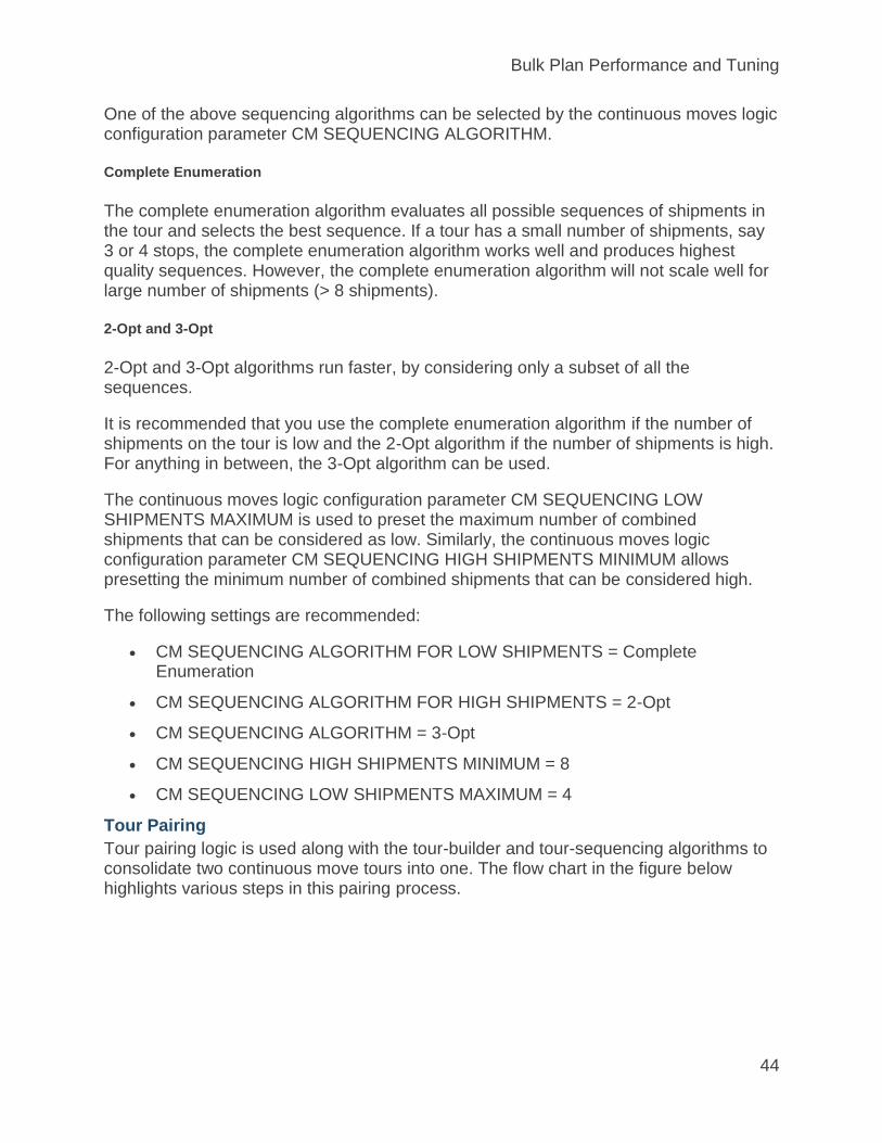
Bulk Plan Performance and Tuning
44
One of the above sequencing algorithms can be selected by the continuous moves logic configuration parameter CM SEQUENCING ALGORITHM.
Complete Enumeration
The complete enumeration algorithm evaluates all possible sequences of shipments in the tour and selects the best sequence. If a tour has a small number of shipments, say 3 or 4 stops, the complete enumeration algorithm works well and produces highest quality sequences. However, the complete enumeration algorithm will not scale well for large number of shipments (> 8 shipments).
2-Opt and 3-Opt
2-Opt and 3-Opt algorithms run faster, by considering only a subset of all the sequences.
It is recommended that you use the complete enumeration algorithm if the number of shipments on the tour is low and the 2-Opt algorithm if the number of shipments is high. For anything in between, the 3-Opt algorithm can be used.
The continuous moves logic configuration parameter CM SEQUENCING LOW SHIPMENTS MAXIMUM is used to preset the maximum number of combined shipments that can be considered as low. Similarly, the continuous moves logic configuration parameter CM SEQUENCING HIGH SHIPMENTS MINIMUM allows presetting the minimum number of combined shipments that can be considered high.
The following settings are recommended:
CM SEQUENCING ALGORITHM FOR LOW SHIPMENTS = Complete Enumeration
CM SEQUENCING ALGORITHM FOR HIGH SHIPMENTS = 2-Opt
CM SEQUENCING ALGORITHM = 3-Opt
CM SEQUENCING HIGH SHIPMENTS MINIMUM = 8
CM SEQUENCING LOW SHIPMENTS MAXIMUM = 4
Tour Pairing
Tour pairing logic is used along with the tour-builder and tour-sequencing algorithms to consolidate two continuous move tours into one. The flow chart in the figure below highlights various steps in this pairing process.

Bulk Plan Performance and Tuning Guide
45
The steps in the tour pairing process areas follows. First, combine the tours in a paired tour. Then using the sequencing algorithms, generate shipment sequences. Next the best cost sequence is selected by evaluating equipment, cost and drive feasibility and the continuous move tour is created. These steps are similar to those in the shipment pairing process in the multistep logic.
Various continuous move logic configuration parameters are available to improve performance during the tour pairing process.
Setting the Rate Distance Engine
The continuous moves logic configuration parameter CM RATE DISTANCE ID selects the rate distance engine used to calculate distances during tour paring process. Similar to the multistep logic, it is recommended that you use Estimate. This setting only influences the distances used in the continuous moves logic. The actual rating and the final shipments are still based on the true distances as specified on the rate.

Bulk Plan Performance and Tuning
46
Important Parameters
Additionally, following continuous moves logic configuration parameters are important and can be used to tune performance and solution quality in the continuous moves logic. A low value for these parameters will improve run time at the expense of tour build quality. The recommended values for these continuous moves logic configuration parameter are:
CM MAX DISTANCE BETWEEN SHIPMENTS = 200 MI
CM MAX DURATION BETWEEN SHIPMENTS = 5H
CM MAX DURATION OF TOUR = 2 D
CM MAX SHIPMENTS IN CONTINUOUS MOVE TOUR = 4
Related Topics
Bulk Plan Performance and Tuning Overview
Bulk Plan Performance and Tuning PDF
Bulk Plan Multi-stop Shipment Logic If you have any questions or comments about this topic or the online help, please contact us.
bulk_plan_manager/bulk_plan_tuning_multistop_ship_logic.htm
Bulk Plan Tuning Multi-stop Shipment Logic
Shipment Pairing | Constructing Paired Shipments | Distance-Based Parameters |
Time-Based Parameters | Generating Stop Sequences | Multi-segment
Sequencing | Topping Off | Related Topics
Oracle Transportation Management provides several algorithms for multi-stop shipment creation. In order to tune multi-stop shipment creation for solution quality or performance, it is important to understand various multi-stop algorithms in Oracle Transportation Management and their internal workings at a high level.

Bulk Plan Performance and Tuning Guide
47
Oracle Transportation Management offers these major algorithms for building multi-stop shipments:
Clustering Merge Algorithm
Conopt Merge Algorithm
Savings Algorithm
Column Generation Algorithm
Complete Enumeration Algorithm
The input to these algorithms is a set of direct shipments. The goal of the multi-stop logic is to consolidate these shipments into multi-stop shipments.
Shipment Pairing
For all of the multi-stop shipment algorithms, a shipment pairing logic is used to consolidate two shipments into one. The shipment pairing is used both for evaluating the savings, as well as, committing a particular pair and combining the shipments in the pair. The flow chart below highlights various steps in the pairing process: The shipments are paired to construct a paired shipment. Then stop sequences are generated using algorithms. Next the best cost sequence is selected after evaluating equipment, cost and drive feasibility to create a paired shipment.

Bulk Plan Performance and Tuning
48
Constructing Paired Shipment
This step takes two shipments and constructs a paired shipment. Stops from the individual shipments are added to the paired shipment. Stops having the same location are merged together into one. There are times when two stops at the same location must be kept separate. For example, when you drop off and pickup at the same location, you may wish to have two separate stops, one for drop off and one for pickup.
Prior to pairing the two shipments, there are several constraints that are checked to ensure that the two shipments can be paired together:
Can the combined shipment’s weight and volume fit the equipment’s weight and volume capacities?
Are the orders that are being placed into the equipment compatible with each other?
In addition to the constraints, there are also several quick checks to eliminate certain less than optimal combinations in order to reduce the overall run time. The distance-based and time-based tuning parameters described below help in reducing the number of shipment pairs to evaluate.
Distance-Based Parameters

Bulk Plan Performance and Tuning Guide
49
There are several multi-stop logic configuration parameters that can be used to limit the number of shipment pair computations that the algorithm performs. By eliminating the number of shipment pairs to evaluate, the run times can be drastically reduced. While mainly used for improving performance, these parameters also help solution quality by clustering the stops close to each other. For example, setting the MULTISTOP MAX RADIUS FOR DELIVERIES to 50 miles will cluster all the delivery stops to within a 50 mile radius of the farthest delivery point.
MULTISTOP MAX DISTANCE BETWEEN DELIVERIES = 50
MULTISTOP MAX DISTANCE BETWEEN PICKUPS = 50
MULTISTOP MAX RADIUS FOR DELIVERIES = 50
MULTISTOP MAX RADIUS FOR PICKUPS = 50
MULTISTOP MAX RADIUS PERCENTAGE FOR DELIVERIES = 25
MULTISTOP MAX RADIUS PERCENTAGE FOR PICKUPS = 25
The MULTISTOP MAX RADIUS PERCENTAGE FOR PICKUPS and MULTISTOP MAX RADIUS PERCENTAGE FOR DELIVERIES parameters work well for situations when you have long stem miles and several pickups or deliveries clustered together. For example, consider a pickup at a distribution center and traveling over 500 miles and delivering to 3 or 4 locations. Setting the MULTISTOP MAX RADIUS PERCENTAGE FOR DELIVERIES to 10% in this case, ensures that all the deliveries are within 50 miles of each other.
Note: These parameters also exist on itineraries. However, since the multi-stop logic in certain points in the algorithm does not have access to an itinerary, the parameters defined on the multi-stop logic configuration are used. If the itinerary is available, the parameters from the itinerary are used instead. As a result, it is recommended that you set these parameters on the itinerary, as well as, on the multi-stop logic configuration.
The parameter IGNORE PROXIMITY CHECKS FOR RETURN TO SOURCE allows the distance or time from the source location to the service area to be longer than any specified limit. When this parameter is set to true, while departing or returning to the shipment source location, OTM will not perform checks for maximum distance or time between pickups or deliveries.
The parameter MULTISTOP MAX DISTANCE BETWEEN STOPS specifies the maximum distance limit between certain pair of consecutive stops in a multi-stop shipment. This parameter will work only if IGNORE PROXIMITY CHECKS FOR RETURN TO SOURCE is set to true.
The parameter MULTISTOP MAX DISTANCE BETWEEN CO-LOCATED STOPS specifies the maximum distance within which two locations can be considered co-located. The default is 0, so the co-located multistop logic is not used in this case.

Bulk Plan Performance and Tuning
50
Time-Based Parameters
The time-based multi-stop logic configuration parameters also help reduce the computations by looking at the times on the shipments. In addition, the parameters will cluster the orders together that are close to each other in time.
MULTISTOP MAX TIME BETWEEN DELIVERIES = 60 Minutes
MULTISTOP MAX TIME BETWEEN PICKUPS = 60 Minutes
Generating Stop Sequences
Once the consolidated shipment is formed, the stops must be sequenced so that the total distance (or total cost) is minimized. Oracle Transportation Management provides several multi-stop sequencing algorithms for you to choose from. The available sequencing algorithms are:
2-Opt
3-Opt
Insertion
Enumeration
MIP
Time Window MIP
2-Opt and 3-Opt
The 2-opt and 3-opt algorithms run fast by considering only a subset of all the sequences. With these algorithms, it is possible that some good stop sequences are not generated.
Insertion
Insertion retains the original stop sequences of the first and second shipment.
Enumeration

Bulk Plan Performance and Tuning Guide
51
If a shipment has a small number of stops, say 3 or 4 stops, then the enumeration algorithm works well and produces highest quality sequences. However, the enumeration algorithm does not scale well for shipments with a large number of stops (greater than 8 stops).
MIP
In the MIP Sequencer algorithm, OTM solves a mixed integer programming (MIP) formulation of the stop-sequencing problem (which is essentially a travelling salesman problem). This algorithm provides high quality sequences (as good as Complete Enumeration), and it also runs much faster than the Enumeration algorithm for a high number of stops.
Time Window MIP
In the time window MIP algorithm, OTM takes time constraints into consideration (location calendar, order pick-up & delivery date). This algorithm can provide the optimal solution, but also can be time consuming for high number of stops.
Oracle Transportation Management provides the ability to choose different algorithms based on the number of shipments. The following multi-stop logic configuration parameters control the sequencing algorithms with default values. With the default settings, the 2-Opt algorithm will be used for shipments with 8 or more stops and the Enumeration algorithm for shipments with 4 or fewer stops. For anything in between, the 3-Opt algorithm will be used.
MULTISTOP SEQUENCING HIGH STOPS MINIMUM = 8
MULTISTOP SEQUENCING LOW STOPS MAXIMUM = 4
MULTISTOP SEQUENCING ALGORITHM = 3-Opt
MULTISTOP SEQUENCING ALGORITHM FOR HIGH STOPS = 2-Opt
MULTISTOP SEQUENCING ALGORITHM FOR LOW STOPS = Enumeration
Other Sequencing Related Parameters
There also several other sequencing related multi-stop logic configuration parameters that control how the shipment sequences are formed.
MULTISTOP QUICK HOS CHECK IN SEQUENCING: This multi-stop logic configuration parameter provides the option of doing quick HOS check while generating multistop sequences. Generated sequences can be infeasible due to various time-constraining factors such as HOS Rules. OTM can improve performance and solution quality by throwing out time-infeasible sequences during the sequence generation step itself by running a quick time-feasibility check on HOS. This parameter is helpful if there is a maximum duration for the shipment.

Bulk Plan Performance and Tuning
52
MULTISTOP SEQUENCE COST FOR DISTANCE: This multi-stop logic configuration parameter specifies the distance based cost to be considered during sequence generation.
MULTISTOP SEQUENCE COST FOR TIME: This multi-stop logic configuration parameter specifies the time based cost to be considered during sequence generation.
Following are a few examples using the two cost parameters above in multistop sequencing:
1. Consider only distance: MULTISTOP SEQUENCE COST FOR DISTANCE = 1.0, MULTISTOP SEQUENCE COST FOR TIME = 0.0
2. Consider only time: MULTISTOP SEQUENCE COST FOR DISTANCE = 0.0, MULTISTOP SEQUENCE COST FOR TIME = 1.0
3. Consider distance and time costs (e.g. distance cost = 5 per unit distance and time cost = 100 per hour): MULTISTOP SEQUENCE COST FOR DISTANCE = 5.0, MULTISTOP SEQUENCE COST FOR TIME = 100.0
MULTISTOP SEQUENCING ALLOW PICKUP REVISIT and MULTISTOP SEQUENCING ALLOW DROPOFF REVISIT: These multi-stop logic configuration parameters allow a pickup or drop off location to be revisited more than once. This is very useful in situations where a particular distribution center (DC) has more than one truckload worth of orders and these orders are shipped by having the driver perform multiple trips on the same shipment.
MULTISTOP START OR END AT DEPOT REWARD: This multi-stop logic configuration parameter encourages shipments to start (or end) at a pickup (or drop off) location that is also a depot. In the figure below, the DC is marked as both pickup and delivery depot.
When a shipment is formed by consolidating orders A and B, the logic does not take into account depot locations. So, the following two sequences are evaluated and the second one will be selected as it covers less distance.

Bulk Plan Performance and Tuning Guide
53
DC – A – B – DC
B – DC – A
Later, the logic adds the depot locations to the selected sequence and the second sequence now looks like this: Depot (DC) – B – DC – A – Depot (DC), which incurs the two extra empty moves. By encouraging the depot pickups and drop offs as the first and/or last locations, the first option is selected as it contains the first stop and last stop at the depot location.
MULTISTOP USE RETURN MILES IN SEQUENCING: This multi-stop logic configuration parameter considers the return miles to the first stop when finding the least distance sequence. This is useful if you know that the driver will return to the start location.
MULTISTOP USE UNMERGED STOPS IN SEQUENCING LOGIC
The multi-stop logic will always combine two stops if they are at the same location. In some instances, it may be useful to keep the stops separate, as in multi-segment shipments or when dealing with situations requiring revisits to the same stop. Even though the sequencing logic keeps the stops separate, the stops get merged together into one if two stops of the same type (pickup or delivery) and at the same location are next to each other in the final sequence. Keeping the stops separate is controlled via the multi-stop logic configuration parameter MULTISTOP USE UNMERGED STOPS IN SEQUENCING LOGIC.
Last in First out (LIFO)
LIFO means that the last order loaded into the equipment must be the first one to be removed from the equipment. LIFO influences the stop sequences in that it eliminates the non-LIFO sequences being considered for evaluation. The multi-stop logic configuration parameter MULTISTOP USES LIFO PICKUP DROPFF is used to control this behavior. With LIFO on, you can still get shipments with multiple pickup and multiple drop off stops.
Multistop Sequencing in Multi-segment Shipments
A multi-segment shipment is a multistop shipment where the equipment is emptied at least once before the final delivery. Each segment in a multi-segment shipment is a continuous part in the journey of the shipment where the equipment is non-empty.
The following figure shows a 2-segment shipment that picks up 3 orders at a distribution center (DC) and delivers these orders at different drop-off locations. Then the shipment equipment remains empty until it picks up the first of the 2 backhaul orders to be delivered back to the DC.
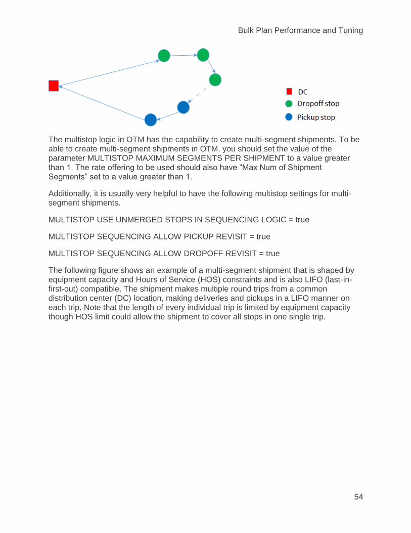
Bulk Plan Performance and Tuning
54
The multistop logic in OTM has the capability to create multi-segment shipments. To be able to create multi-segment shipments in OTM, you should set the value of the parameter MULTISTOP MAXIMUM SEGMENTS PER SHIPMENT to a value greater than 1. The rate offering to be used should also have “Max Num of Shipment Segments” set to a value greater than 1.
Additionally, it is usually very helpful to have the following multistop settings for multi-segment shipments.
MULTISTOP USE UNMERGED STOPS IN SEQUENCING LOGIC = true
MULTISTOP SEQUENCING ALLOW PICKUP REVISIT = true
MULTISTOP SEQUENCING ALLOW DROPOFF REVISIT = true
The following figure shows an example of a multi-segment shipment that is shaped by equipment capacity and Hours of Service (HOS) constraints and is also LIFO (last-in-first-out) compatible. The shipment makes multiple round trips from a common distribution center (DC) location, making deliveries and pickups in a LIFO manner on each trip. Note that the length of every individual trip is limited by equipment capacity though HOS limit could allow the shipment to cover all stops in one single trip.

Bulk Plan Performance and Tuning Guide
55
In shipment planning scenarios like this, it is typically very challenging to create multi-segment shipments involving a high number of stops and segments (for example more than 15 stops is high). That is because, in the multi-segment case, it is not easy to find feasible stop sequences satisfying various constraints such as equipment capacity, Hours of Service (HOS), LIFO stop sequencing etc. In this case, using the following options can be helpful.
Quick Checks in Sequencing
Multistop logic provides the options for performing various quick checks in sequencing so that sequences failing in these checks can be identified and rejected during sequence generation. Some of these important quick checks can be turned on through the following parameters.
CHECK EQUIPMENT CAPACITY IN SEQUENCING
CHECK ITEM COMPATIBILITY IN SEQUENCING
CHECK LIFO IN SEQUENCING
MULTISTOP QUICK HOS CHECK IN SEQUENCING
Note that these additional checks aim to improve multistop shipment quality, but that improvement may come at the expense of additional run time in the multistop logic.
DC Based Multi-segment Sequencing

Bulk Plan Performance and Tuning
56
This DC based multi-segment sequencing logic is suitable for planning scenarios such as the above example. This logic can be turned on by setting the parameter INSERT DC STOPS AFTER SEQUENCE GENERATION to true.
This logic only works for the case where there is only one source DC and one destination DC (both the source and destination DCs can also be the same location). The logic internally identifies a location pair as source DC and destination DC only if all the orders either start from the source DC or end with the destination DC.
This logic tries to reduce workload for sequencing logic by identifying and eliminating the frequently occurring DC stops in the beginning and later inserting them appropriately into the generated stop sequences. Further, while inserting the DC stops back into a stop sequence, feasibility quick checks can be performed if specified.
Topping off Multi-stop Shipments
OTM can use top-off orders to fill under-utilized shipments. Top-off orders are not consolidated with core orders (i.e. orders that are not top-off) while building direct shipments. However towards the end of multi-stop processing, in the multi-stop top-off pass, top-off shipments (i.e. shipments containing only top-off orders) are brought in for consolidation with the consolidated core shipments.
The multi-stop logic configuration parameter USE CONOPT MERGE IN TOP-OFF PASS provides an option to use the Conopt Merge algorithm for shipment consolidation in the top-off pass. Note that the main objective in the top-off pass is to move contents of the top-off shipments to the consolidated core shipments to utilize their equipment as much as possible. You have the option of using the Conopt Merge algorithm in this step (which does a better job than the Savings based algorithms) to achieve high equipment utilization. See current limitations of Conopt Merge algorithm.
The multi-stop logic configuration parameter IGNORE CAPACITY OVERRIDES IN TOP-OFF PASS provides an option to ignore capacity overrides on the itinerary legs during shipment consolidation in the top-off pass. It makes sense to use this option only when the enforced capacity overrides are required, only until the top-off stop which should also be the last pick-up stop.
Top-off Scenario Example 1
Consider the planning scenario on a 2-leg itinerary as shown in the figure below. There are 4 core orders of 20,000 LB each, with 4 different source locations in a city region and a common destination at a port of discharge (POD). Only one type of equipment is available with a load capacity of 50,000 LB.

Bulk Plan Performance and Tuning Guide
57
In this situation, multi-stop shipments will arrive at the port of loading (POL) location and continue on the ocean leg with under utilized equipment (10,000 LB capacity still available). To avoid this waste of equipment capacity, first leg shipments with unused capacity are brought to a top-off location (T in the above figure) where a top-off order of 20,000 is available for pick-up. In this case, as shown in the following figure, planning with the setting “USE CONOPT MERGE IN TOP-OFF PASS = true” will result in the 2 fully-utilized shipments on the first leg.
Top-off Scenario Example 2
The planning scenario in this example is shown in the following figure and is similar to Example 1. The main difference in this case is that a street legal load limit of 40,000 LB is imposed in the city region. This is defined as an equipment capacity override on the first leg. However, the full equipment capacity of 50,000 LB is allowed between the top-off location T and POL as T is strategically located very close to POL.

Bulk Plan Performance and Tuning
58
Suppose there are 2 "core” orders of 60,000 LB each, with 2 different source locations in the city region and a common destination at a port of discharge (POD). In this situation, multi-stop shipments will arrive at the POL location and continue on the ocean leg with underutilized equipments (with at least 10,000 LB capacity still available). To avoid this waste of equipment capacity, a top-off order of 30,000 LB is available for pick-up at T. In this case, as shown in the following figure, planning with the setting “USE CONOPT MERGE IN TOP-OFF PASS = true” and “IGNORE CAPACITY OVERRIDES IN TOP-OFF PASS = true” will result in 3 fully-utilized shipments on the first leg.
Related Topics
Bulk Plan Multi-stop Shipment Complete Enumeration Algorithm
Bulk Plan Multi-stop Shipment Column Generation Algorithm
Bulk Plan Multi-stop Conopt Merge Algorithm
Bulk Plan Multi-stop Shipment Common Scenarios
Tuning Time Window Effect in Multistop Sequencing
Bulk Plan Performance and Tuning Overview
Bulk Plan Solution Quality Tuning
Bulk Plan Performance and Tuning Guide
59
Bulk Plan Performance and Tuning PDF
If you have any questions or comments about this topic or the online help, please contact us.
bulk_plan_manager/solution_quality_tuning/bulk_plan_multi-stop_shipment_saving_algorithms.htm
Bulk Plan Multi-stop Shipment Saving Algorithms
Savings Algorithm | Important Multi-stop Parameters | Types of Savings
Algorithms | Related Topics
Savings Algorithm
The savings algorithm works by creating a savings matrix for every pair of shipments that are feasible to combine. The savings is defined as follows:
savings = cost of shipments before consolidation – cost of shipment after consolidation
Once the savings matrix is created, the pair with the best positive savings is combined and the new savings with the combined shipment with the rest of the shipments is evaluated. This continues until there is no combination that results in positive savings.
You can influence the savings value through multi-stop logic configuration parameters and influence the shape and consolidation of the shipments. For example, you can make the shipments with the same SHIP WITH GROUP attract each other even at the expense of traveling extra distance or incurring extra cost. Similarly, order priorities can be used to inflate or deflate the savings value.
There are two steps in the savings algorithm:
Step One
The first step is the savings calculation for all pairs of shipments. The savings calculation can be very time consuming. This step can be multi-threaded speeding up the savings calculations. See the help topic on bulk plan multi-threading for information on how to set up multi-threading.
Step Two
The second step involves choosing the best savings pair and combining the shipments in the pair. Once the new shipment is formed, the old shipments are removed from the savings matrix and savings are calculated for pairing up the newly created shipment with the rest of the shipments in the matrix.
Important Multi-stop Parameters

Bulk Plan Performance and Tuning
60
There are several parameters that influence the performance and quality of multi-stop shipment creation. While there are several such parameters, a few of the very important and often used are listed here:
Multi-stop Cost Savings Check Type
The savings calculations can be sped up by looking at only the distances during the savings calculation. This can be done by turning on the multi-stop logic configuration parameter MULTISTOP COST SAVINGS CHECK TYPE to “1. Perform cost savings check after each iteration.” This setting performs distance based savings calculations thus eliminating the need for detailed rating. However, a cost based check is still made whenever two shipments are combined together.
When the parameter MULTISTOP COST SAVINGS CHECK TYPE is set to “4. Calculate cost for all paired shipments,” the savings calculations are based on actual costs rather than distances. This causes logic to run longer, but will compute more accurate savings.
There are other options, “2. Perform cost savings check at the end of process” and “3. Do not perform cost savings check.” Do not use option 3 at all as it is very important to perform cost savings check. Option 2, performs cost savings check at the very end, but this has a bad side effect. If the cost savings check fails for combining the shipments, then the shipments do not get merged, and they will go unconsolidated. The recommendation is to use option 1 when the costs are proportional to distances or run time is a concern. Otherwise, the recommendation is to use option 4, where cost savings are calculated for each pair of shipments.
Following parameter and property settings in OTM provide options to influence multi-stop savings calculations based on the priorities of shipment contents.
Parameter USE PRIORITY IN COST SAVINGS (add link to this parameter)
Property glog.business.consolidation.multistop.prioritysavingsalgorithm
Property glog.business.consolidation.multistop.priorityagressiveness
Multi-stop Rate Distance ID
It is recommended that you use MULTISTOP RATE DISTANCE ID set to Estimate. Using Estimate, the logic uses latitudes and longitudes of locations and estimates the distances. This gives close enough distances to perform the necessary optimization quickly. Using Lookup has the additional overhead of querying the distances from a lookup table, but will give more accurate distances for computations. Using an external distance engine will slow down the process considerably and should be avoided unless that level of accuracy is needed. Remember that this setting only influences the distances used during the multi-stop logic. The actual rating and the final shipment are still based on the true distances as specified on the rate.
Types of Savings Algorithms

Bulk Plan Performance and Tuning Guide
61
Savings algorithms come in the following types:
Sequential Savings
Concurrent Savings
Look Ahead Savings
Iterative Savings
Sequential Savings
MULTISTOP CONSOLIDATION ALGORITHM = Sequential Savings
In sequential savings, the focus is to complete the formation of one multi-stop shipment before starting a new multi-stop shipment. This is useful when you need to form shipments with higher utilization. In sequential savings, the shipments are consolidated as follows.
Shipment12 = shipment1 + shipment2
Shipment123 = Shipment12 + Shipment3
Shipment1234 = Shipment123 + Shipment4
The savings are still used to select the next shipment to consolidate.
The parameter MULTISTOP SEQUENTIAL SAVINGS SORT METHOD allows you to choose which method to use in determining the first shipment from which to build a multi-stop shipment using the Sequential Savings merge algorithm.
The parameter RS PAIRWISE CONSOLIDATION provides the option of adding shipment pairs to the work assignment string, instead of individual shipments.
Concurrent Savings (Recommended Option)
MULTISTOP CONSOLIDATION ALGORITHM = Concurrent Savings
The concurrent savings algorithm works by consolidating the best savings pairs in the order of the savings. At any stage of the multi-stop logic using concurrent savings, there could be several multi-stop shipments that are partially formed. This approach tends to pair up shipments that have big savings. Here is a sample of how the concurrent savings logic might consolidate:
Shipment12 = Shipment1 +Shipment 2
Shipment35 = Shipment3 + Shipment5
Shipment124 = Shipment12 + Shipment4
Once two shipments are consolidated, they cannot be separated. In the example above, the logic will not create Shipment1234 by separating shipments 3 and 5 and then combining 3 with Shipment124.

Bulk Plan Performance and Tuning
62
Look Ahead Savings
MULTISTOP CONSOLIDATION ALGORITHM = Look Ahead
There are times when combining two shipments might be more attractive than other pairs. However, Oracle Transportation Management might not combine these shipments. The concurrent savings algorithm described above suffers from the possibility of combining two shipments too early. The look ahead savings algorithm ranks the shipments based on the difference of the savings of the first best pair and second best pair. The shipment that has the greatest difference in savings will be selected and its best pair will be chosen for combining.
Iterative Savings
MULTISTOP CONSOLIDATION ALGORITHM = Iterative Savings
In this algorithm, OTM increases the search space to look for an optimal route. It follows an approach similar to concurrent savings to form routes at each iteration. This is an iterative algorithm. In each iteration, multistop shipments are generated and considered as a potential candidate for the final result. Finally, the set-covering problem is solved to pick the cheapest solution so that all order releases/order movements are fulfilled.
Parameters:
MULTISTOP CONSOLIDATION ALGORITHM TYPE = Iterative Savings
MULTISTOP COLGEN SAVINGS ALGORITHM TYPE = '0-Concurrent' (only value supported with Iterative Savings)
MULTISTOP COLGEN NUMBER OF ITERATIONS = 5
MULTISTOP SAVINGS COST TOLERANCE PERCENTAGE = 15
Note: Increasing number of iterations increases run-time almost proportionally in most of the cases but also guarantees a better or same quality solution.
Related Topics
Bulk Plan Performance and Tuning Overview
Bulk Plan Solution Quality Tuning
Bulk Plan Tuning Order Bundling Logic
Bulk Plan Tuning Direct Shipment Building
Bulk Plan Tuning Container Optimization Logic
Bulk Plan Tuning Continuous Moves Logic
Bulk Plan Performance and Tuning PDF
If you have any questions or comments about this topic or the online help, please contact us.
bulk_plan_manager/multi-stop_shipment_complete_enumeration_alg.htm

Bulk Plan Performance and Tuning Guide
63
Bulk Plan Multi-stop Shipment Complete Enumeration Algorithm
Related Topics
The complete enumeration algorithm enumerates all consolidation combinations and selects the best set of consolidations to cover all the order releases/order movements. To turn on complete enumeration, set the multi-stop logic configuration parameter MULTISTOP CONSOLIDATION ALGORITHM to Complete Enumeration.
To illustrate how this works, let's use five order release going from a distribution center (DC) to locations A, B, C, D and E. The complete enumeration logic will enumerate all feasible combinations of order releases (with their best sequences) and determine the total cost. In the table below, different shipment possibilities are represented by columns. For example, column ABC represents the shipment that has order releases A, B, and C. The enumeration algorithm will enumerate all the combinations that are feasible. The optimization engine takes in all the shipment combinations and selects the set of shipments that covers all the order releases with the lowest total cost. In the example below, shipments AE and BCD provide the lowest total cost (171 + 214 = 385).
Since this enumerates all the possible combinations, this algorithm can only handle a small set of order bundles – around 100 order bundles. The number of order bundles per shipment should also be small. There are two parameters that control the run time.
MULTISTOP ENUMERATION MERGE MAX SHIPMENTS = 30. If the algorithm encounters more than this number of shipments, then it will revert to the concurrent savings algorithm.
MULTISTOP ENUMERATION MERGE MAX MERGES PER SHIP = 3. The enumeration algorithm will not consider shipments that contain more than this number of order bundles.
For this algorithm type, if the property glog.optimization.mip.setcovering.writeToFile is set to true, the set covering MIP problem will be written to the OTM logging directory as "SetCover.lp".
Related Topics

Bulk Plan Performance and Tuning
64
Bulk Plan Performance and Tuning Overview
Bulk Plan Solution Quality Tuning
Bulk Plan Tuning Order Bundling Logic
Bulk Plan Tuning Direct Shipment Building
Bulk Plan Tuning Container Optimization Logic
Bulk Plan Tuning Continuous Moves Logic
Bulk Plan Performance and Tuning PDF
If you have any questions or comments about this topic or the online help, please contact us.
bulk_plan_manager/multi-stop_shipment_column_generation_alg.htm
Bulk Plan Multi-stop Shipment Column Generation Algorithm
Related Topics
The column generation algorithm is selected by setting the multi-stop logic configuration parameter, MULTISTOP CONSOLIDATION ALGORITHM TYPE, to Column Generation.
The column generation algorithm is similar to complete enumeration in that it looks at several shipment consolidation combinations and selects the best set of shipments to cover all the order releases/order movements. However, the column generation algorithm, unlike complete enumeration, generates a much smaller subset of shipment combinations and can scale to larger problem sizes. The column generation algorithm employs either a concurrent, sequential, or look-ahead savings algorithm for generating the additional columns (or shipments). The underlying savings algorithm can be called multiple times to generate several different consolidation options. Each savings algorithm call takes the same amount of time as the original savings algorithm. The following combination of parameter settings is typical with column generation algorithm. Setting the iterations to 1, consumes the same amount of run time as the savings algorithm, with the advantage of getting similar or better solution quality as with the savings algorithm. Note that this is only true when cost savings is used instead of distance savings (i.e. when MULTISTOP COST SAVING CHECK TYPE is set to "4 - Calculate cost for all paired shipments" or MULTISTOP PERFORM THOROUGH SEQUENCE CHECKS is set to true).
MULTISTOP CONSOLIDATION ALGORITHM TYPE = Column Generation
MULTISTOP COLGEN SAVINGS ALGORITHM TYPE = Concurrent
MULTISTOP COLGEN NUMBER OF ITERATIONS = 5
For this algorithm type, if the property glog.optimization.mip.setcovering.writeToFile is set to true, the set covering MIP problem will be written to the OTM logging directory as "SetCover.lp".
Related Topics
Bulk Plan Performance and Tuning Overview

Bulk Plan Performance and Tuning Guide
65
Bulk Plan Solution Quality Tuning
Bulk Plan Tuning Order Bundling Logic
Bulk Plan Tuning Direct Shipment Building
Bulk Plan Tuning Container Optimization Logic
Bulk Plan Tuning Continuous Moves Logic
Bulk Plan Performance and Tuning PDF
If you have any questions or comments about this topic or the online help, please contact us.
bulk_plan_manager/bulk_plan_multi-stop_shipment_conopt_algorithm.htm
Bulk Plan Multi-stop Shipment Conopt Merge Algorithm
Examples | Multistop Logic Parameter Settings | Related Topics
The 'Conopt merge' algorithm is selected by setting the multi-stop logic configuration parameter, MULTISTOP CONSOLIDATION ALGORITHM TYPE, to 'Conopt Merge'.
The Conopt Merge algorithm allows you to merge shipments if the total size (in terms of weight, volume and ERU) of two shipments exceeds the full-equipment capacity. This algorithm allows splitting of the shipments during the shipment consolidation steps in order to produce full-capacity shipments, thereby saving costs. Note that other existing multistop algorithms (e.g., Savings algorithm) primarily try to minimize the total distance of the consolidated shipments. However, in Conopt Merge, the main objective is to maximize the capacity utilization in consolidated shipments.
Though Conopt Merge algorithm has the capability to split and redistribute contents of input shipments, it takes care not to split the input shipments excessively. To be able to do that, OTM tries to keep items from an input shipment together as much as possible at the following levels (in order of increasing importance): stops, order, ship unit. It does not split ship units further by count. The Count Splittable check box on the order release ship unit triggers this, not the Bulk Splittable check box (also on the order release ship unit).
When Conopt Merge algorithm is used, we recommend setting the logic parameter MULTISTOP DISABLE SAME OD PAIRING to true.
If you want to use Conopt merge for multi-leg planning, you must use network routing.
Note: In Conopt Merge algorithm, the container optimization logic is used in OTM to repack tightly the ship units from all the direct shipments that are broken down at the beginning. It is important to note that, in this step, the container optimization logic does not check most multistop parameter settings, nor the rating and drive constraints. So the consolidated items may actually fail to combine in the end when all constraints are checked. This can impact the solution quality in the Conopt Merge algorithm when the planning scenario is very constrained (which could be due to location calenders, HOS rules etc.)
The following is NOT currently supported with the Conopt Merge algorithm:

Bulk Plan Performance and Tuning
66
3D load configuration
Carrier capacities
Equipment capacity overrides
Optimizing cost of the equipment set
Examples
Scenario 1 - One source and two destinations
This scenario has two shipments with 60 ship units each from source A to destinations B and C which are close to each other in the same geographical region. If the equipment capacity is 100 ship units, these two shipments would not be combined as a multistop shipment.
However, you may want to create a full capacity multistop shipment (i.e. with 100 ship units) to locations B and C, and another shipment with 20 ship units to location C alone (maybe you can hold the second shipment for another day when it can be combined with other shipments).
Scenario 2 - Single source and multiple destinations
Consider 5 direct shipments from source A to destinations B, C, D, E, and F which are close to each other in the same geographical region. Suppose each of these shipments has 60 ship units (each weighing 1,000 LB) on an equipment with weight capacity 100,000 LB. Without this algorithm, OTM cannot split shipments inside multistop, so these shipments would not be consolidated into multistop shipments. However, this algorithm will allow splitting of these shipments, which will lead to three multistop shipments, thereby saving costs.

Bulk Plan Performance and Tuning Guide
67
Scenario 3 - Multiple sources and single destination
Now, consider the reverse of the above; 5 direct shipments from source locations B, C, D, E, and F (which are again close to each other in the same geographical region) to one single destination location A. Each of these shipments has 60 ship units on an equipment of ship unit capacity 100.
Scenario 4 - One source and multiple destinations, different quantities
Consider again a scenario with a single source and multiple destinations. Now suppose the direct shipments from A to B, D and F have 60 ship units each, and the direct shipments from A to C and E have 20 ship units each. Again assume that shipments use only an equipment with a ship unit capacity of 100. In this case, Conopt Merge as well as any existing multistop algorithm (e.g., Savings algorithm) will consolidate the 5 direct shipments to 3 shipments. However, note that Conopt Merge will create more tightly packed multistop shipments, which will come at the expense of additional travel distance for the shipments.

Bulk Plan Performance and Tuning
68
Multistop Logic Parameter Settings (for Conopt Merge Algorithm)
Note that the following multistop logic configuration parameters are not used by the Conopt Merge algorithm.
MULTISTOP COLGEN NUMBER OF ITERATIONS
MULTISTOP COLGEN SAVINGS ALGORITHM TYPE
MULTISTOP CONSOLIDATION ALLOW MULTITHREADING
MULTISTOP ENUMERATION MERGE MAX MERGES PER SHIP
MULTISTOP ENUMERATION MERGE MAX SHIPMENTS
All other multistop logic parameters are used in the Conopt Merge algorithm. In particular, Conopt Merge considers the following parameters at all stages:
MULTISTOP MAX DISTANCE BETWEEN DELIVERIES
MULTISTOP MAX DISTANCE BETWEEN PICKUPS
MULTISTOP MAX RADIUS FOR DELIVERIES
MULTISTOP MAX RADIUS FOR PICKUPS
MULTISTOP MAX TIME BETWEEN DELIVERIES
MULTISTOP MAX TIME BETWEEN PICKUPS
MAXIMUM PICKUP STOPS ALLOWED
MAXIMUM DELIVERY STOPS ALLOWED
MAXIMUM STOPS ALLOWED

Bulk Plan Performance and Tuning Guide
69
We recommend that you use your settings for only the above parameters and use default settings for the remaining logic parameters.
When Conopt Merge algorithm is used, we recommend setting the logic parameter MULTISTOP DISABLE SAME OD PAIRING to true.
Container Optimization Settings
The user settings in the container optimization logic configuration will not be used by this multistop split logic while repacking contents of the shipments tightly. OTM will use some default container optimization parameter settings for that purpose, but you have a choice on the settings for the following logic parameters (in the Multistop logic configuration parameters under 'MULTISTOP PACKING').
MULTISTOP PACKING ALGORITHM
MULTISTOP PACKING METRIC
MULTISTOP PACKING OBJECTIVE
Logs and Diagnostics
The following System Log IDs, "Multistop" and "MultistopDetails" help to analyze program flow and detect failures that occur inside the code for this algorithm.
Related Topics
Bulk Plan Performance and Tuning Overview
Bulk Plan Solution Quality Tuning
Bulk Plan Tuning Order Bundling Logic
Bulk Plan Tuning Direct Shipment Building
Bulk Plan Tuning Container Optimization Logic
Bulk Plan Tuning Continuous Moves Logic
Bulk Plan Tuning Multi-stop Shipment Logic
Bulk Plan Performance and Tuning PDF
If you have any questions or comments about this topic or the online help, please contact us.
bulk_plan_manager/multi-stop_shipment_common_scenarios.htm
Bulk Plan Multi-stop Shipment Common Scenarios
Related Topics
Multi-stop Parameter Recommendations for Common Scenarios
Here are some common scenarios and the associated parameters. It is not necessary that these parameters must be used as detailed below. Each implementation is different and might require different parameter settings.

Bulk Plan Performance and Tuning
70
Simple Multi-stop Shipment (1 pickup multi-drop, multi-pick 1 drop off)
MULTISTOP USES LIFO PICKUP DROPOFF = true
Multiple Pickups and Dropoffs (LIFO)
MULTISTOP USES LIFO PICKUP DROPOFF = true
Multiple Pickups and Dropoffs (non-LIFO)
MULTISTOP USES LIFO PICKUP DROPOFF = false
Multi-Segment Shipments
MULTISTOP MAXIMUM SEGMENTS PER SHIPMENT set so greater than 1
Related Topics
Bulk Plan Performance and Tuning Overview
Bulk Plan Solution Quality Tuning
Bulk Plan Tuning Order Bundling Logic
Bulk Plan Tuning Direct Shipment Building
Bulk Plan Tuning Container Optimization Logic
Bulk Plan Tuning Continuous Moves Logic
Bulk Plan Performance and Tuning PDF
Shipment Groups in Bulk Planning
If you have any questions or comments about this topic or the online help, please contact us.
bulk_plan_manager/shipment_groups_in_bulk_planning.htm
Shipment Groups in Bulk Planning
Process Management and Actions | Related Topics
A shipment group is a set of shipments that are carried together in a single move for one or more legs of a journey. For example, shipments that are placed together in a single vessel can be represented as a shipment group. Shipment groups are built in the bulk plan post process step.
The parameter 'CREATE SHIPMENT GROUPS DURING SHIPMENT BUILDING' indicates whether the shipment building process should create shipment groups. By default the shipment group build logic is turned OFF.

Bulk Plan Performance and Tuning Guide
71
Shipment group rules in bulk planning determine the circumstances in which shipments are assembled into shipment groups during the planning process. You can configure the parameters on this page and the Detail tab to control how and when shipment groups are created.
Shipment Group Process Management and Actions
Create Shipment Group Process
Shipment groups can also be created using the Create Shipment Group Process.
Shipment Group Actions
Additionally, you can create shipment groups manually using the action 'Create Shipment Group'.
You can add/remove shipments from a shipment group manually using the following actions:
Add Shipments to Group

Bulk Plan Performance and Tuning
72
Add Partial Shipments to Group
Remove Shipments from Group
Remove Partial Shipments from Group
Related Topics
Bulk Plan Performance and Tuning Overview
Shipment Group Rules in Bulk Planning
Bulk Plan Performance and Tuning PDF
If you have any questions or comments about this topic or the online help, please contact us.
bulk_plan_manager/shipment_group_rules_in_bulk_planning.htm
Shipment Group Rule Details in Bulk Planning
Related Topics
Shipment Group Rules determine the circumstances in which shipments are assembled into shipment groups during the planning process. You can configure the parameters on this page and the Detail tab to control how and when shipment groups are created.
When shipment groups are created as part of planning, the flex fields defined on the shipment group rule are automatically copied to created shipment groups. This is controlled by the parameter 'COPY SHIPMENT GROUP RULE FLEX FIELDS AUTOMATICALLY'. By default this parameter is turned OFF.
There are a few fields, such as Geographical Definition ID, Lane ID, Mode Profile, Itinerary Profile ID, that allow you to define rules for a specific requirement. The Effective Date and Expiration Date fields enable you to make the rule 'active' only for a particular time period.
There are broadly two types of rules:
Full Shipment Group Rules: when enabled, create shipment groups that point to the entire shipments.
Partial Shipment Group Rules: point to part of the shipment, usually corresponding to a particular order release or line.
Full Shipment Group Rules:
Full shipment group rules include Match Service Provider (boolean), Match Service Schedule (boolean), Match Port of Loading (Boolean), Match Port of Discharge (Boolean), Match Reference Qualifier (String), Match Involved Party Qualifier (String). Let’s take one rule – Match Service Provider. The shipments that satisfy the basic rules (Lane ID, Mode Profile etc) are grouped according to the service providers. No two shipments with different service providers can be in the same group. For Match Reference Qualifier, for example, the value for all the shipments for this reference number must match. If this field is null, then the match rule is not in effect. The reference table is SHIPMENT_REFNUM_QUAL.

Bulk Plan Performance and Tuning Guide
73
Multiple full shipment group rules can be enabled at once. If two or more full shipment group rules are enabled, the shipments are grouped together only when all the values match.
For example, if Match Service Provider and Match Port of Loading are enabled, even if the service provider for two shipments match, they cannot have the same shipment group if the port of loading is different. The full shipment group rules (individual or in combination) always create Full Shipment groups, meaning, one shipment has only one shipment group.
Partial Shipment Group Rules:
In addition to the full shipment group rules, there are several partial rules such as Same Equipment (Boolean), Same Order Source (Boolean), Same Order Destination (Boolean), Match Order Release Reference Qual (String), Match Order Release Line Reference Qual (String), and Match Order Release Involved Party (String). Here, only a part of the shipment (identified by the order release or order release line). If the Same Order Source rule is enabled, only the order releases packed with the same source are grouped together. It can work in two ways:
1. Two direct shipments that can otherwise have the same shipment group, will have different shipment groups because they have different order source locations.
2. A multi-stop shipment (say, combining two order releases from different sources but same destination) will have two shipment groups, one for each order release.
Except for the Match Order Release Line Reference Qual, all other partial groups are divided by order release. This one rule groups the shipments based on order release lines.
You can have two or more partial group rules. Similar to full shipment group rules, when two or more partial shipment group rules are enabled, the groups are created to make sure all rules are adhered to. For example, if both Same Order Source and Same Order Destination are on, none of the groups can have order releases with different source or destination locations.
Partial Rules and Full Rules Enabled at the Same Time
Both partial and full shipment group rules can be enabled at the same time. When at least one partial rule is enabled, OTM will always create partial shipment groups (that is, the shipment group is order release specific). For example, let’s say Match Service Provider (full rule) and Match Order Destination (partial rule) are enabled. If you have two direct shipments that have the same destination but have different carriers, two partial shipment groups are created, one for one shipment with its order, and another for the second shipment with its order, even though there is only one order per shipment.
Related Topics
Bulk Plan Performance and Tuning Overview
Shipment Groups in Bulk Planning

Bulk Plan Performance and Tuning
74
Bulk Plan Performance and Tuning PDF
Performance Tuning
If you have any questions or comments about this topic or the online help, please contact us.
bulk_plan_manager/performance_tuning//bulk_plan_performance_tuning.htm
Bulk Plan Performance Tuning
Related Topics
There are several reasons why some bulk plans run slowly, while other bulk plans, even with larger data sets run fast. For example, high run time may be warranted due to the nature of the underlying problem and the complexity of the network. Many performance problems though can be resolved through careful data modeling, algorithm tuning and multi-thread property settings.
One of the most important contributors to long run time is the amount of logs that are turned on. It is recommended that logs be used during the test phase, and turned off during production runs. Remember to turn off logs from all the domains, as the logs from other domains will influence the run time even though no logs are printed.
Understanding the Bulk Plan Run provides an overview of the bulk plan process as well as key areas to check for performance.
Bulk Plan Multi-threading is one way to take advantage of multiple CPUs when running bulk plans. You can run several bulk plans simultaneously by setting up multiple batch threads or by bulk plan partitioning.
Multi-threading Logic explains how multi-threading works.
Bulk Plan Partitioning is a way to enhance the overall performance of the bulk plan run.
Bulk Plan Caches help reduce database access and computation times significantly and improve bulk plan performance.
Related Topics
Bulk Plan Performance and Tuning Overview
Bulk Plan Logs
Bulk Plan Performance and Tuning PDF
If you have any questions or comments about this topic or the online help, please contact us.
bulk_plan_manager/performance_tuning/understanding_the_bulk_plan_run.htm
Understanding the Bulk Plan Run
Key Process Steps | Related Topics
The performance tab of the bulk plan manager provides useful information regarding performance. Performance metrics are gathered if the number of orders is greater than the value set in the parameter MINIMUM ORDERS FOR MILESTONE COLLECTION.

Bulk Plan Performance and Tuning Guide
75
This parameter is set to 50 by default. To generate the information in the performance tab for smaller bulk plans, you should set this parameter to 1.
The following processes in bulk plan have been identified as taking the most time. The next few sections provide typical processes and tips on how to improve performance. Remember that bulk plan run times are dependent on various factors and the problem may be very complex and require the time taken to produce quality solutions.
Key Process Steps
Bundle Orders
Order bundling is typically the first step during a bulk plan run and often includes querying order releases. If you encounter slowness during order bundling, a likely suspect is slow queries. There may be opportunities for tuning the database for faster queries. Order bundling is not multi-threaded and hence the multi-thread settings will not help order bundling performance.
Find Itineraries
The run time during the find itinerary step can be improved by specifying a particular itinerary on the order releases and reducing the need for evaluating different itineraries. The find itineraries step is not multi-threaded.
Direct Shipment Building
Following are some reasons for long direct shipment building run times and tips for improving performance.
Complex Itineraries
If there are itineraries that have several legs and each leg has several routing options, carrier options and equipment options, the number of combinations to evaluate will be huge. Reducing the number of available options for routing orders can result in huge performance gains.
Number of Itineraries
Having too many itineraries to consider may negatively impact performance. Reduce the number of itineraries for each order by specifying an itinerary GID on the order releases.
Setup Multi-threading in Planning Build
The shipment building process is multi-threaded. Setting up the right number of threads to take advantage of the processes on the server will improve the overall performance of direct shipment building. See the topic Bulk Plan Multi-threading for further information on how to setup multi-thread properties.

Bulk Plan Performance and Tuning
76
True Container Optimization for Performance
The shipment building process invokes container optimization for packing ship units into containers. Ensure that there is only one container optimization algorithm, one metric, and one objective chosen so that only one container optimization run is performed for each call. Choosing Multi-Container MIP, Column Generation, or Enumerative packing could result in significant computational time. Use Quick Packing instead.
Multi-Stop Shipments
If the performance issue is during multi-stop shipment building, there are several things that can be done to improve the performance including changing some settings for multi-stop logic configuration parameters.
Setup Distance and Time Parameters
Using maximum distance and time between pickup and drop-off stops could significantly improve the run time. The following multi-stop logic configuration parameters will help in reducing the overall run times (performance is better for smaller values of these parameters).
MULTISTOP MAX DISTANCE BETWEEN DELIVERIES
MULTISTOP MAX DISTANCE BETWEEN PICKUPS
MULTISTOP MAX RADIUS FOR DELIVERIES
MULTISTOP MAX RADIUS FOR PICKUPS
MULTISTOP MAX RADIUS PERCENTAGE FOR DELIVERIES
MULTISTOP MAX RADIUS PERCENTAGE FOR PICKUPS
MULTISTOP MAX TIME BETWEEN DELIVERIES
MULTISTOP MAX TIME BETWEEN PICKUPS
Avoid Using Computationally Expensive Multi-Stop Options
Setting the logic configuration parameter MULTISTOP COST SAVINGS CHECK TYPE to "4. Calculate cost for all paired shipments," significantly increases the run time as costing and driving are done for every pair of shipment savings calculations. Instead of using this option, try options 1 or 2, which calculate the costs at the end of the iteration or at the end of the process.
When building multi-stop shipments, and selecting the value for the Multistop Consolidation Algorithm Type parameter, avoid using expensive algorithms such as "Complete Enumeration" which cannot scale well to large order sets. Instead, use "Column Generation" if solution quality is important.
Bulk Plan Performance and Tuning Guide
77
For the generation of stop sequences, avoid using the Complete Enumeration algorithm: 2-Opt or 3-Opt algorithms generally produce great sequences.
Avoid setting MULTISTOP PERFORM THOROUGH SEQUENCE CHECK to "TRUE".
Use "Estimate" for MULTISTOP RATE DISTANCE ID. Using an external rate distance will perform expensive calls to an external engine and thus slow down the multi-stop process.
Set Up Leg Consolidation Groups
Setting up many leg consolidation groups will create multiple small multi-stop runs rather than one huge run. For example, running 10 multi-stops with 100 order releases each executes a lot faster than running one large multi-stop with 1000 order releases.
Related Topics
Bulk Plan Performance and Tuning Overview
Bulk Plan Performance Tuning
Bulk Plan Tuning Direct Shipment Building
Bulk Plan Tuning Multi-stop Shipment Logic
Bulk Plan Performance and Tuning PDF
If you have any questions or comments about this topic or the online help, please contact us.
bulk_plan_manager/performance_tuning/bulk_plan_multi-threading.htm
Bulk Plan Multi-threading
Running Multiple Bulk Plans Simultaneously | Threads Inside Bulk Plans |
Definition of Terms | Multi-thread Properties Associated to Each Task Type |
Related Topics
OTM provides two key ways to take advantage of multiple CPUs when running bulk plans. You can run several bulk-plans simultaneously by setting up multiple batch threads or by bulk plan partitioning. Bulk plan partitioning is a way to partition the order releases or order movements through pre-defined saved queries, and then run each partition in its own thread. In order to understand and effectively use multi-threading, it is important to understand how OTM’s multi-threading logic works.
In addition to bulk plan partitioning, you can configure OTM to multi-thread several time consuming areas within the bulk plan logic. The following areas in bulk-plan support multi-threading:
Shipment Building of Order Releases and Order Movements
Multi-stop
Committing Shipments

Bulk Plan Performance and Tuning
78
Driver and Equipment Assignment Actions
Continuous Moves
Running Multiple Bulk Plans Simultaneously
Setting Up Properties for Multi-threading
The threading for bulk plan is set up via thread group settings. The thread group name for the bulk plan is "batch" and the number of threads for this group is set as follows: glog.workflow.queueThreads.batch=2.
By default, the batch thread group is assigned 2 threads. Depending on the number of processors and the load on the system, you can increase this to more than 2. The group thread counts should be set before starting the server.
You can also change the batch threads through the Event Queues page. However, the recommended approach is to set the group thread counts before starting the server. If the threads are changed through the Event Queues page, the changes will be lost once the server is brought down. The Event Queues page can be accessed via Configuration and Administration > Technical Support > Diagnostics and Tools > Event Management > Event Queues. You must be logged into OTM has DBA.ADMIN to access the Event Queues page.
Once on the screen, click on Show Threads button at the bottom to see all the threads. To increase the number of threads, click on Threads. To kill a thread (if it hangs up), click on the thread to terminate. Remember that killing a thread will not terminate any existing bulk plans. No future bulk plans will be scheduled to run on that thread though.
Running Bulk Plans
Once the threads are set up, you can run multiple bulk plans simultaneously. If there are more bulk plans than the number of threads, then the bulk plans will be queued up and will start executing as soon as the threads get freed up.
Threads Inside Bulk Plans
While the entire set of bulk plans can be run in parallel, you can also set up threads for processing key functions inside a bulk plan in parallel. These functions are described in the table below. Similar to the bulk plan process thread group called "batch", the areas within the bulk plans are assigned many functional thread groups. These areas are also called task groups. The table below describes the default thread count settings for these task groups. These properties can be found in glog.task properties file and can be overridden in glog.properties file.

Bulk Plan Performance and Tuning Guide
79
Functional Area (Task Type) Description Default Thread Group
Build Shipments
(BuildShipments)
For every order bundle on a single leg, OTM plans them onto a shipment using the shipment building logic. Several bundles can be simultaneously built into shipments.
planningBuild
Build Shipment Graphs
(BuildShipmentGraphs)
This is the logic for building the shipments on various legs of an itinerary.
planningBuild
Build Shipment Graph Collections
(BuildShipmentGraphCollections)
This logic is used for building several shipment graphs for an order bundle based on order releases.
planningBuild
Build Shipment Graphs for Order Movements
(BuildShipmentGraphsForOrderMovements)
The shipment building logic for building shipments for a bundle of order movements.
planningBuild
Commit Shipment Graphs This logic commits
planningCommit

Bulk Plan Performance and Tuning
80
(CommitShipmentGraphs) shipments to the database at the end of order release bulk plan.
Commit Shipment Graphs for Order Movements
(CommitShipmentGraphsForOrderMovements)
This logic commits shipments to the database at the end of order movement bulk plan.
planningCommit
Compute Transit Time
(ComputeTransitTime)
Compute transit time happens as part of Route Orders process of bulk plan that uses Network Routing
planningBuild
Delete Shipment Graph
(DeleteShipmentGraph)
During unassign stage in bulk plan order releases, if the shipments are to be deleted instead of to be updated, the deleting process can be configured in multi-thread
planningCommit
Fleet Assignment
(FleetAssignment)
Driver and Equipment assignment actions.
planningBuild

Bulk Plan Performance and Tuning Guide
81
NR Network Rater
(NRNetworkRater)
This logic computes rating information for itinerary and network legs inside the Network Routing logic.
planningBuild
SNRO Build Shipment for Order Movements
(SNROBuildShipmentForOrderMovements)
This logic computes shipment information during the Show Network Routing Options - Ocean action.
planningBuild
Savings Algorithm
(SavingsAlgorithm)
Inside the multi-stop algorithm, pairs of shipments are evaluated for combining, determining the potential savings. These tasks can be run in parallel to achieve potential savings.
planningBuild
Shortest Path
(ShortestPath)
The shortest path logic inside Dispatch Plan Optimization (DPO) algorithm.
planningOptimization

Bulk Plan Performance and Tuning
82
Although several task groups inside the bulk plan use the same thread group, you can override the default and create your own thread group. For example, you can create a thread group for Fleet Assignment for the driver and equipment assignment actions, so that these actions do not contend with for the same threads that shipment building logic uses.
Definition of Terms
In order to understand how multi-threading works and how to set up the threads and their properties, it is important to know certain terms.
Tasks and Task Types
A task is an atomic unit of work. A task runs on a single thread. It cannot be distributed across threads. Examples of tasks in OTM are building a shipment for one order release bundle, building a shipment for one order movement bundle, evaluating the savings of combining two shipments, committing a shipment graph, etc. Each task is characterized by its Task Type – such as BuildShipment, CommitShipments, etc.
Task Batch and Batch Size
A task batch is a collection of similar tasks that are processed sequentially on a single thread. For example, a task batch can be comprised of one hundred order bundles (similar tasks). Each of these hundred order bundles are processed one at a time sequentially on a single thread to build shipments. The number of tasks within a task batch represents the batch size of the task batch.
Thread Group
A thread group is a collection of threads. In the table above, planningBuild is a thread group. A thread group contains a certain number of threads available for that group. All the tasks in a task batch are processed by a thread within a thread group sequentially. The task batches assigned to different threads in a thread group are run in parallel. Each thread group is allocated a certain number of threads as follows:
glog.workflow.queueThreads.PlanningBuild=16
Please note that setting the multi-valued thread group setting glog.workflow.topicGroup=<queue>,<threadCount> has been deprecated. It has been replaced with glog.workflow.queueThreads.<queue>=<threadCount>.
In order to change the topic group assignment of PlanningBuild to 10, you can override the property in the CUSTOM property set as follows:
glog.workflow.queueThreads.PlanningBuild=10
Example
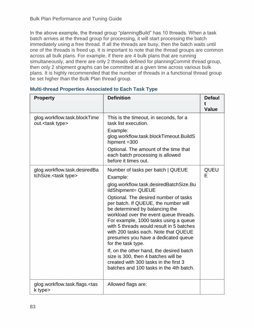
Bulk Plan Performance and Tuning Guide
83
In the above example, the thread group “planningBuild” has 10 threads. When a task batch arrives at the thread group for processing, it will start processing the batch immediately using a free thread. If all the threads are busy, then the batch waits until one of the threads is freed up. It is important to note that the thread groups are common across all bulk plans. For example, if there are 4 bulk plans that are running simultaneously, and there are only 2 threads defined for planningCommit thread group, then only 2 shipment graphs can be committed at a given time across various bulk plans. It is highly recommended that the number of threads in a functional thread group be set higher than the Bulk Plan thread group.
Multi-thread Properties Associated to Each Task Type
Property Definition Default Value
glog.workflow.task.blockTimeout.<task type>
This is the timeout, in seconds, for a task list execution.
Example: glog.workflow.task.blockTimeout.BuildShipment =300
Optional. The amount of the time that each batch processing is allowed before it times out.
glog.workflow.task.desiredBatchSize.<task type>
Number of tasks per batch | QUEUE
Example:
glog.workflow.task.desiredBatchSize.BuildShipment= QUEUE
Optional. The desired number of tasks per batch. If QUEUE, the number will be determined by balancing the workload over the event queue threads. For example, 1000 tasks using a queue with 5 threads would result in 5 batches with 200 tasks each. Note that QUEUE presumes you have a dedicated queue for the task type.
If, on the other hand, the desired batch size is 300, then 4 batches will be created with 300 tasks in the first 3 batches and 100 tasks in the 4th batch.
QUEUE
glog.workflow.task.flags.<task type>
Allowed flags are:

Bulk Plan Performance and Tuning
84
WAIT_ON_LIFETIME. If set, the TaskList.execute method blocks on all activity related to the batches, including agents and notification. Otherwise, the method blocks only on the execution of the tasks.
ABORT_ON_TIMEOUT. If set, any timeout in the TaskList.execute method removes any related batches from the event queues. Active batches are not interrupted. This flag results in indeterministic behavior and should only be used to reduce unnecessary work on the application server.
LOG_BATCHES
glog.workflow.task.group.<task type>
The task type equals the event queue.
Example:
glog.workflow.task.group.BuildShipment=planningBuild
glog.workflow.task.group.CommitShipment=planningCommit
glog.workflow.task.group.Rating
The thread group assigned to the task type.
Configuring the “rating” queue with multiple threads will allocate same number of threads for evaluating multiple rate geos instead of single thread processing all rate geos.
Required – no defaults associated
glog.workflow.task.minimumBatchSize.<task type>
Minimum number of tasks per batch.
Example: glog.workflow.task.minimumBatchSize.BuildShipment = 1
Optional. Batches can have overhead due to shared resources and workflow processing. This property allows you to assign a minimum number of tasks in any batch. If the total # of tasks is less than the minimum, OTM creates a single batch to process the tasks.
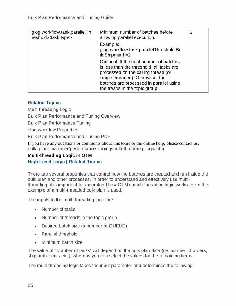
Bulk Plan Performance and Tuning Guide
85
glog.workflow.task.parallelThreshold.<task type>
Minimum number of batches before allowing parallel execution.
Example: glog.workflow.task.parallelThreshold.BuildShipment =2
Optional. If the total number of batches is less than the threshold, all tasks are processed on the calling thread (or single threaded). Otherwise, the batches are processed in parallel using the treads in the topic group.
2
Related Topics
Multi-threading Logic
Bulk Plan Performance and Tuning Overview
Bulk Plan Performance Tuning
glog.workflow Properties
Bulk Plan Performance and Tuning PDF
If you have any questions or comments about this topic or the online help, please contact us.
bulk_plan_manager/performance_tuning/multi-threading_logic.htm
Multi-threading Logic in OTM
High Level Logic | Related Topics
There are several properties that control how the batches are created and run inside the bulk plan and other processes. In order to understand and effectively use multi-threading, it is important to understand how OTM’s multi-threading logic works. Here the example of a multi-threaded bulk plan is used.
The inputs to the multi-threading logic are:
Number of tasks
Number of threads in the topic group
Desired batch size (a number or QUEUE)
Parallel threshold
Minimum batch size
The value of "Number of tasks" will depend on the bulk plan data (i.e. number of orders, ship unit counts etc.), whereas you can select the values for the remaining items.
The multi-threading logic takes the input parameter and determines the following:

Bulk Plan Performance and Tuning
86
Whether the tasks should run in the caller thread. If yes, the tasks will be run single-threaded, otherwise batches of tasks will be created and run in parallel threads.
Number of batches to use
Tasks in each batch (Most batches have the same number of tasks, with the last one possibly having fewer tasks.)
Whether or not to run the tasks in the caller
High Level Logic
In order to describe the high level logic, we will use the following sample inputs:
Number of tasks: 10000
Average runtime per task: 1 time unit
Number of threads: 20
Desired batch size: QUEUE
Parallel Threshold: 2
Minimum Batch Size: 800
Step 1: Determine the number of batches
Typically, the number of batches is the same as the number of threads. However, given a minimum batch size, there might not be enough tasks to use up all of these threads. Based on the number of tasks and the minimum batch size, the number of batches is computed as Number of tasks / Minimum Batch Size (10000 / 800 = 12). Thus the total number of batches is 12, even though there are 20 threads.
Step 2: Determine the batch size
If the desired batch size is QUEUE, the batch size is determined by dividing the number of tasks by the number of threads in the topic group. If the batch size is greater than the minimum batch size, then the batch size is set to the minimum.
In the example above, the batch size is determined by dividing the number of tasks by the number of threads (10000 / 20 = 500). However, since the minimum batch size is set at 800, and the computed number of batches is 12, the revised batch size is 10000 / 12 = 833.
Step 3: Determine if the batches should be run in caller thread
If the number of batches determined in step 1 is smaller than the parallel threshold value, then all the tasks will be run in the caller thread. Otherwise, the batches will be queued up to be run on multiple threads in parallel.
Bulk Plan Performance and Tuning Guide
87
In this example, the number of batches (12) is greater than the parallel threshold (2) so the batches will be queued up to run on 12 threads.
General Comments
While multi-threading helps process tasks in parallel, it is not normal to get 100% parallelism. If there are 10 tasks, each taking 1 time unit, and they are run in parallel using 10 threads, it is not typical to see the run time of 1 unit. It is almost always higher. This is due to unavoidable thread contentions that require synchronized blocks or sequential processing.
Moreover, the tasks themselves are not always uniform in that their processing times are different from each other. Hence, even though the batches have the same number of tasks, their loads may be quite different.
Given that a topic group containing a certain number of threads can be shared across multiple bulk plan runs, the individual computations on the number of batches and batch size is still based on the total number of threads even though some of the threads may be busy processing tasks for other bulk plans. Hence, this might result in longer wait times for the threads to be freed up.
Related Topics
Bulk Plan Multi-threading
Bulk Plan Performance and Tuning Overview
Bulk Plan Performance Tuning
Bulk Plan Performance and Tuning PDF
glog.thread Property
Rate Maintenance Multi-threading
If you have any questions or comments about this topic or the online help, please contact us.
bulk_plan_manager/performance_tuning/bulk_plan_partitioning.htm
Bulk Plan Partitioning
Bulk Plan Partition Setup | Partitions | Partition Profiles | Assigning Partitions |
Running Partitioned Bulk Plans | Related Topics
Bulk plan partitioning enhances the overall performance of the bulk plan run. By partitioning, or grouping, the order releases/order movements into many sets, OTM runs smaller bulk plans on each partition and hence runs faster, even if these smaller bulk plans are run sequentially one after the other. A further boost in performance can be achieved by running several partitioned bulk plans simultaneously in different threads. The multi-threading of the individual portioned bulk plans are automatic and no further configuration is needed.
While it is tempting to consider using the bulk plan partition as a way to keep orders from consolidating, that is not the intent of bulk plan partitioning and is strongly
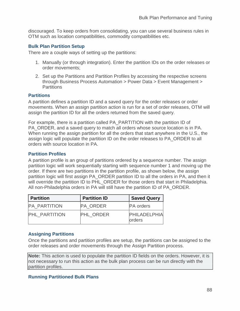
Bulk Plan Performance and Tuning
88
discouraged. To keep orders from consolidating, you can use several business rules in OTM such as location compatibilities, commodity compatibilities etc.
Bulk Plan Partition Setup
There are a couple ways of setting up the partitions:
1. Manually (or through integration). Enter the partition IDs on the order releases or order movements;
2. Set up the Partitions and Partition Profiles by accessing the respective screens through Business Process Automation > Power Data > Event Management > Partitions
Partitions
A partition defines a partition ID and a saved query for the order releases or order movements. When an assign partition action is run for a set of order releases, OTM will assign the partition ID for all the orders returned from the saved query.
For example, there is a partition called PA_PARTITION with the partition ID of PA_ORDER, and a saved query to match all orders whose source location is in PA. When running the assign partition for all the orders that start anywhere in the U.S., the assign logic will populate the partition ID on the order releases to PA_ORDER to all orders with source location in PA.
Partition Profiles
A partition profile is an group of partitions ordered by a sequence number. The assign partition logic will work sequentially starting with sequence number 1 and moving up the order. If there are two partitions in the partition profile, as shown below, the assign partition logic will first assign PA_ORDER partition ID to all the orders in PA, and then it will override the partition ID to PHL_ORDER for those orders that start in Philadelphia. All non-Philadelphia orders in PA will still have the partition ID of PA_ORDER.
Partition Partition ID Saved Query
PA_PARTITION PA_ORDER PA orders
PHL_PARTITION PHL_ORDER PHILADELPHIA orders
Assigning Partitions
Once the partitions and partition profiles are setup, the partitions can be assigned to the order releases and order movements through the Assign Partition process.
Note: This action is used to populate the partition ID fields on the orders. However, it is not necessary to run this action as the bulk plan process can be run directly with the partition profiles.
Running Partitioned Bulk Plans

Bulk Plan Performance and Tuning Guide
89
The partitioned bulk plans can only be run through process manager. It works for both order release bulk plans (for both buy and sell) and order movement bulk plans. When a bulk plan is run outside the process manager, all partitions are ignored unless the parameter PARTITION PROFILE ID is defined.
Setting up Order Movement Bulk Plan Process
For the bulk plan order movements process, in the "Based on Order Movements" field, specify a saved query for the collection of the order movements to consider. If the partition profile is selected, then the assign profile logic will be applied to the considered order movements.
As described before, the order movements can be pre-populated with the partition IDs. If you want to bulk plan with the pre-populated partition IDs, you should select the Use Partition check box. The order movements with null partition IDs will be grouped and run together.
Setting up Order Release Bulk Plan Process
To setup and run the bulk plan order releases process, the field "Based on Order Releases" provides the saved query for the set of order releases to consider for planning. The partition assignment is done on this set of order releases. The Use Partition check box is used to take the partitions on the order releases for the partitioned bulk plan. The orders releases with null partitions will be processed together in one bulk plan run.
Related Topics
Bulk Plan Performance and Tuning Overview
Bulk Plan Performance Tuning
Bulk Plan Performance and Tuning PDF
Diagnostics
If you have any questions or comments about this topic or the online help, please contact us.
bulk_plan_manager/diagnostics/bulk_plan_diagnostics.htm
Bulk Plan Diagnostics
Related Topics
OTM provides several means for diagnosing a bulk plan run. OTM Logs are the most widely used and offer the ability to research both solution quality and performance issues. In addition to logging, OTM has Planning Diagnostics that provide useful information regarding the decisions made during various steps in the bulk plan. You can also use graphical diagnostics.
Diagnostics
Logs: Logs are a great tool to research a problem in bulk plan. It is important to get the right amount of logs – too much logging will make it extremely difficult to

Bulk Plan Performance and Tuning
90
navigate to the exact issue and too little logging information may not be enough. For details, see Bulk Plan Logs.
Planning Diagnostics: Planning diagnostics provide a systematic view of the logic and the decisions that OTM makes during the bulk plan process. Diagnostics are meant to provide the reasons as to why a certain step failed. For example, if an order failed to plan due to a service time violation, the diagnostics can provide this information. This is very valuable as you can quickly understand what caused the failure and correct the problem.
Ask Oracle - Container Optimization: This is a way to test container optimization and load configuration via XML files.
Bulk Plan Caches: OTM caches various data and computed results to improve bulk plan performance. However you may not get good performance if frequently used caches have insufficient capacity.
Related Topics
Bulk Plan Performance and Tuning Overview
Bulk Plan Performance and Tuning PDF
If you have any questions or comments about this topic or the online help, please contact us.
bulk_plan_manager/diagnostics/about_graphical_diagnostics.htm
Graphical Diagnostics
Related Topics
There are numerous reasons why an order can fail to plan. This page shows a graphical user interface to help you understand why a particular order fails to plan as well as helping you visualize the planning process in OTM. Graphical diagnostics allows you to drill down through multiple levels of details. The diagnostics are color coded - gray for success and red for failure. There are several different views: Block View, Sunburst and Text View (this is the same as the previous diagnostics).
This page is accessed via bulk plan. Once the bulk plan has finished running, you can access the new Graphical Diagnostics page by clicking the Graphical Diagnostics button.
Note: For Diagnostics to be enabled two checks must be in place. The property glog.otmdiag.log must be On (it is On (true) by default). Also, either the Diagnostic user preference or the Tracking Diagnostic option on the Settings and Actions page must be On.
In addition to the graphical diagnostics, OTM also has Planning Diagnostics that provide useful information regarding the decisions made during various steps in the bulk plan as well as bulk plan logs which offer the ability to research both solution quality and performance issues.
Tree Node Description

Bulk Plan Performance and Tuning Guide
91
A tree structure, or tree diagram, is a way of representing the hierarchical nature of a structure in a graphical form. It is named a "tree structure" because the classic representation resembles a tree, even though the chart is generally upside down compared to an actual tree, with the "root" at the top and the "leaves" at the bottom. The tree structure is represented by the Sunburst and Block View user interface. A tree node is one process within the whole tree structure (like one of the leaves in the tree). In diagnostics, each tree node represents a process inside OTM. It is opened by clicking on a node. It summarizes the key information about the corresponding planning process. Some of the tree nodes in this tree are:
Bulk Plan (root node).
Un-assign Orders.
Create Bundles.
Identify Valid Itineraries.
Build Direct Shipments.
Commit Shipments etc.
A tree node usually contains the process name which shows which process the tree node is corresponding to as well as the following fields:
Status: indicates the status of the corresponding process: Successful, Failure, Information, Warning, and Exception.
Duration: displays how much time it takes to go through the corresponding process in the back-end logic.
Failure Reasons: highlights the reason why the process is failing in the corresponding process.
Entities: reveals what database entities are being used or evaluated by the corresponding process.
Remarks: exhibits some key information that you should notice for the corresponding process.
Additional Information: provides non-database entities information of the corresponding process.
The graphical user interface has the following major components:
Central view component displays the entire tree structure that corresponds to the planning process. This shows in the main panel. There are hyperlinks to all the database entities displayed on the page (except “Filter” panel). By clicking on these hyperlinks, you can access the entity in a new window directly. See below for details.
Failure summary component is to the right of the main panel. It populates after a filter is applied, if there was a failure in a process in which selected entities were involved. See below for details.
Bulk Plan Performance and Tuning
92
Statistics component is a horizontal bar across the top of the page that shows how many orders successfully planned and how many failed to plan.
Download Panel is a pop-up that appears when you click Download Files (if there are files to download). Here you can make multiple choices about the files that you want to download such as container optimization and network routing XMLs. Then click Download to download a zip file which contains all the files you selected.
Filter Diagnostics Panel is a pop-up that appears when Filter is clicked. See below for details.
Note that the panels are re-sizable.
Central View Component
The central view component displays the entire tree structure that corresponds to the planning process. The view modes are: Block View, Sunburst and Text View.
Block View
The Block View displays the bulk plan process and its children and grandchildren in nodes (or points at which subsidiary parts originate or center) as a set of nested rectangles. Each branch of the tree is given a rectangle, which is then tiled with smaller rectangles representing sub-branches. For each node, you can directly see its name and status (by color).
In order to further navigate each node or process, move your mouse to the corresponding node, then basic information will pop out as hover text. Then click on the node. You can see the complete information in the pop up window. You can also drag the pop up window anywhere.
Drilling is used to navigate through a hierarchy and display more detailed information. Drilling is most useful when the drill action results in the display of more detailed data. Double click on a node to set that node as the root of the Block View. You can also use the breadcrumbs to navigate back up the hierarchy.
Isolation is used to magnify one node to display more detailed information. Isolation is most useful when the node has a lot of children. Click on the Isolation icon in the top right corner and you will be in Isolation mode. Restore the normal mode by clicking on the Restore icon in the top right.
Sunburst
The Sunburst view displays the bulk plan process and its children and grandchildren in nodes (or points at which subsidiary parts originate or center) as a set of circles. The central circle is the root node of the sunburst. The first layer of those fan shapes are the children of the root node. The second layer of fan nodes are the children of the corresponding nodes (where they are grown from) of the first layer, and they are the grandchildren of the root-node. After expanding, there can be more than two layers, but

Bulk Plan Performance and Tuning Guide
93
the parent and children relations persist. The parent and children relation can also be interpreted in the following way: the more centralized node is more senior, given a node, all the outer layer nodes that grow from it are its children. For each node, you can directly observe its name and status (by color). In addition, given a root node, its first child is located on the right of the 12 o'clock direction, and the following children are spread out clock-wisely.
In order to further navigate each node, you can move your mouse to the corresponding node, then basic information will pop out as hover text. Click on the node and you can see the complete information in the pop out window. You can also drag the pop out window anywhere.
If you want to display more detailed information, expand the tree by clicking the Expand icon. Likewise, if you want to hide the unnecessary information, click the Collapse icon.
Sunburst Drilling
Drilling is used to navigate through a hierarchy and display more detailed information. It is most useful when the drill action results in the display of more detailed data.
Double click on a node to set that node as the root of the sunburst.
Use the breadcrumbs to navigate back up the hierarchy.
Text View
The Text View is a tree table that works the same as the original diagnostics without the "expand all" functionality. See Diagnostic Log Viewer.
Filter Panel & Failure Summary
Once you click Filter, the Filter panel opens and you see a list of entity types. Expand any of the entity types and you can see a list of entities. All the entities showing in the filter panel are somehow involved in the planning process (thus printed to the diagnostics log file). The Filter panel has Ok and Reset buttons. The Ok button applies the filter. Note that by moving the mouse to the Ok button, all the entities that you have checked will be displayed in the hover. The Reset button restores all the components to the initial state. Note that the check boxes will not be saved unless you click the Ok button.
For example, click Filter and select an entity, such as an itinerary. Click Ok to apply the filter. You could notice the following:
The central view has changed. It is no longer the tree that corresponds to the whole planning process, but a sub-tree that corresponds to the processes that are relevant to the entities that you filtered. For instance, if you filtered on order releases, the tree basically tells the life cycle of the filtered order release inside OTM planning.
You could see some content appear in the failure summary table.

Bulk Plan Performance and Tuning
94
There is some node showing in the Failure Tree.
The Failure Summary table consists of three columns:
Failure Nodes: lists processes that contribute to the failure of the whole planning process.
Summary: provides some high-level description to indicate why the status of the corresponding process is 'Failure'.
Entity: lists all the entities that get involved in the corresponding process.
The failure tree displays the failure node that you choose. Initially, OTM will display the first failure node in the failure node list. You can do some further investigation by expanding and navigating the failure tree.
Note that the Failure Summary is populated only if there was a failure in a process in which selected entities were involved. A Failure in one of the processes also need not necessarily mean that my Bulk Plan will fail. For example: An order release can be rated with multiple rate records and it might fail in rating for all but one. The order can still be planned successfully.
Related Topics
Bulk Plan Performance and Tuning Overview
Bulk Plan Performance and Tuning PDF
If you have any questions or comments about this topic or the online help, please contact us.
bulk_plan_manager/diagnostics/bulk_plan_logs.htm
Bulk Plan Logs
Related Topics
OTM Logs are the most widely used and offer the ability to research both solution quality and performance issues. Here are some general guidelines:
Always turn on BulkPlanMilestone. Optionally you can also turn on BulkplanMilestoneDetails, although in most cases this is not necessary.
It is highly recommended that you create a separate log file for BulkplanMilestone so that it does not get cluttered with other logs. Moreover, if you have a lot of detailed logs turned on, some of the milestone lines may get lost as OTM recycles the log files. By having the milestones in a separate log, this will not be an issue.
Limit the number of detailed logs. The guideline is to quickly zero in on a specific problem area and then turn on the detailed logs pertaining to that area. For example, if you know that the problem is with multi-stop logic, it does not make sense to turn on RateEngine or RateEngineDetails unless you think there is some problem in rating along with multi-stop. The table below lists the log IDs to use for different areas in planning.

Bulk Plan Performance and Tuning Guide
95
Table of Planning Logs
Logic Log ID Log ID for Detailed Logs
Notes
General Bulk Plan
BulkPlanning, BulkPlanningMilestone
BulkPlanningMilestoneDetails
BulkplanMilestone is something you should consider keeping on. It creates only a few lines of logs, but they are very useful in understanding the flow of the logic.
Order Releasing
OrderPacking, OrderReleasing, OrderPacker
OrderPackerDetails
Bundling Planning, OrderBundling OrderBundlingDetails
Order Priorities
OrderPriorities
Equipment Assignment
AssignEquipment
Container Optimization Algorithm
Conopt, PackingSolver PackingSolverDetails PackingSolverData for generating XML file.
3D Load Config
PackingSolver, LoadConfig
PackingSolverDetails, LoadConfigDetails
Shipment Builder
Planning PlanningDetails Planning logs provide useful information during the bulk plan. It is not specific to any one area of bulk plan, but provides enough details for
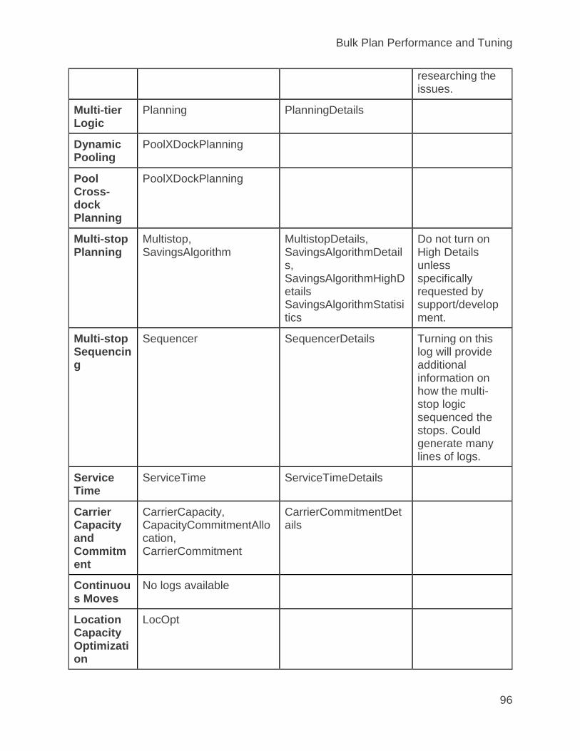
Bulk Plan Performance and Tuning
96
researching the issues.
Multi-tier Logic
Planning PlanningDetails
Dynamic Pooling
PoolXDockPlanning
Pool Cross-dock Planning
PoolXDockPlanning
Multi-stop Planning
Multistop, SavingsAlgorithm
MultistopDetails, SavingsAlgorithmDetails, SavingsAlgorithmHighDetails SavingsAlgorithmStatisitics
Do not turn on High Details unless specifically requested by support/development.
Multi-stop Sequencing
Sequencer SequencerDetails Turning on this log will provide additional information on how the multi-stop logic sequenced the stops. Could generate many lines of logs.
Service Time
ServiceTime ServiceTimeDetails
Carrier Capacity and Commitment
CarrierCapacity, CapacityCommitmentAllocation, CarrierCommitment
CarrierCommitmentDetails
Continuous Moves
No logs available
Location Capacity Optimization
LocOpt

Bulk Plan Performance and Tuning Guide
97
Cooperative Routing
Coroute, CorouteRouting, CorouteSolver
Route Execution
RouteExecution
Cooperative Routing Aggregation
CorouteAggregation
Fleet Assignment
FleetAssignment FleetAssignmentDetails
Fleet Optimization
FleetString FleetStringDetails
Procurement (Sourcing)
ProcOpt
Dash
(FICO Xpress-Optimizer) Optimization
OptMip OptMipDetails, DashDetails
Solution Improvement
PlanningImprovement
Related Topics
Bulk Plan Performance and Tuning Overview
Bulk Plan Diagnostics
Bulk Plan Performance and Tuning PDF
If you have any questions or comments about this topic or the online help, please contact us.
askglog/container_optimization.htm
Container Optimization
Ask Oracle | Double Sorting | Container Optimization using XML File | Related
Topics

Bulk Plan Performance and Tuning
98
This page is accessed via:
Ask Oracle > Container Optimization
Operational Planning > Ask Oracle > Container Optimization
The Container Optimization query helps you determine the optimal equipment group for bulk and packaged shipments based upon weight and volume. The same logic is used as in bulk planning.
There are logic configuration container optimization parameters that determine how Oracle Transportation Management optimizes containers.
Ask Oracle About Container Optimization
1. Select Bulk. OR Select Packaged.
2. Select a Parameter Set ID or accept the default to get the related container optimization configuration and the load configuration related parameters.
3. From the drop-down list, choose an Equipment Group Profile.
4. Select the Ignore Equipment Cost check box. If selected, you can enter equipment cost in the input details screen.
5. Select the Ignore Equipment Availability check box. If selected, you can enter equipment availability in the input details screen.
6. Click Next. The corresponding details page opens for Bulk or Packaged details.
Double Sorting
It is possible to perform container optimization using a 2-way approach. Such an approach enables you to first sort by raw priority (instead of priority range) and then by one of the dimensions used for 3D load building.
In order to trigger this type of sorting, the PRIORITY IN USE and USE PRIORITY IN CONOPT SORTING must both be set to True. When this condition exists, the container optimization logic will first sort by priority and then by what is specified by the ITEM SORT CRITERIA parameter.
Container Optimization using XML File
This provides a convenient way to test container optimization and load configuration through XML files to help with bulk plan diagnostics. By turning on diagnostics and a log, you can capture an XML file that can be used to simulate the container optimization run without having to go through a replication process. You can upload XML files (.xml). The <?xml> header line preferred but nor required.
Capturing XML Files

Bulk Plan Performance and Tuning Guide
99
1. Turn on Tracking Diagnostics. An easy way to do this is via the Settings and Actions page in the top right of any OTM page.
2. Turn on PackingSolverDataLog.
3. Run bulk plan.
4. In the bulk plan results page, click the Diagnostics button. In the Container Optimization section, there will be a link to an XML which you can download by clicking the link.
Running XML Files
The XML file captured from the Capturing XML Files step above, can be used to run through Ask Oracle.
1. Click on the 'container optimization using xml file' link.
2. Enter the XML file.
3. Click Optimize.
Related Topics
Logic Configuration-Container Optimization
Bulk Plan Performance and Tuning PDF
If you have any questions or comments about this topic or the online help, please contact us.
bulk_plan_manager/diagnostics/bulk_plan_caches.htm
Bulk Plan Caches
Related Topics
OTM stores in memory, or caches, various data and computed results that are used frequently in a bulk plan. The cached information helps reduce database access and computation times significantly and improve bulk plan performance.
Important statistics on cache usages can be accessed on the Diagnostics and Tools servlet “glog.webserver.cache.CacheDiagServlet”. This servlet provides cache statistics such as size, capacity, timeout, hit ratio, swap ratio, gets, and puts.
The following cache attributes are specific to an LRU (least recently used) type cache, and these can be set through a cache property.
Capacity: This specifies the size limit of an LRU cache.
Timeout: This specifies the time limit in seconds after which an item could be removed from an LRU cache.
The following are important performance measures of a cache.
Size: Number of elements currently in the cache.

Bulk Plan Performance and Tuning
100
Gets: Total number of items requested from the cache.
Puts: Total number of items put into the cache.
Hit Ratio: Ratio of cache Hits to cache Gets.
Swap Ratio: Ratio of cache Swaps to cache Gets.
A Hit occurs if a requested item is already in the cache. A Hit Ratio of 1.0 is ideal. If the cache is full (i.e. size = capacity), and hit ratio is not very high (less than 0.95), this means that current cache capacity is not sufficient. In this case, bulk plan runtime performance can be further improved by increasing the capacity of these caches. The following properties are available to provide cache performance related warnings during a bulk plan.
glog.bulkplan.warning.minimumGetsForWarning
glog.bulkplan.warning.minimumHitRatio
glog.bulkplan.warning.turnOnCacheChecking
When the "glog.bulkplan.warning.turnOnCacheChecking" property is on, OTM will warn about caches with low hit ratio in the Bulk Plan Performance tab, but only for certain caches: TItemCache, TLocation, TRateOfferingCache, TRateGeoCache, TPackagedItemCache, TSpecialServiceCache, TEquipmentGroupCache.
Related Topics
Bulk Plan Performance and Tuning Overview
Bulk Plan Diagnostics
Bulk Plan Performance and Tuning PDF