, 20130236, published 15 May 201310 2013 J. R. Soc. Interface Christopher T. Richards and Christofer J. Clemente power swimmingBuilt for rowing: frog muscle is tuned to limb morphology to  

Supplementary data

l http://rsif.royalsocietypublishing.org/content/suppl/2013/05/10/rsif.2013.0236.DC1.htm

"Data Supplement"

Referenceshttp://rsif.royalsocietypublishing.org/content/10/84/20130236.full.html#ref-list-1

This article cites 40 articles, 21 of which can be accessed free

Subject collections (75 articles)biomimetics   �

 Articles on similar topics can be found in the following collections

Email alerting service hereright-hand corner of the article or click Receive free email alerts when new articles cite this article - sign up in the box at the top

http://rsif.royalsocietypublishing.org/subscriptions go to: J. R. Soc. InterfaceTo subscribe to

on May 15, 2013rsif.royalsocietypublishing.orgDownloaded from

on May 15, 2013rsif.royalsocietypublishing.orgDownloaded from

rsif.royalsocietypublishing.org

ResearchCite this article: Richards CT, Clemente CJ.

2013 Built for rowing: frog muscle is tuned to

limb morphology to power swimming. J R Soc

Interface 10: 20130236.

http://dx.doi.org/10.1098/rsif.2013.0236

Received: 13 March 2013

Accepted: 25 April 2013

Subject Areas:biomechanics, biomimetics

Keywords:muscle, power, rowing, swimming,

frogs, robotics

Author for correspondence:Christopher T. Richards

e-mail: richards@fas.harvard.edu

Electronic supplementary material is available

at http://dx.doi.org/10.1098/rsif.2013.0236 or

via http://rsif.royalsocietypublishing.org.

& 2013 The Author(s) Published by the Royal Society. All rights reserved.

Built for rowing: frog muscle is tuned tolimb morphology to power swimming

Christopher T. Richards and Christofer J. Clemente

The Rowland Institute at Harvard, Harvard University, 100 Edwin H. Land Boulevard,Cambridge, MA 02142, USA

Rowing is demanding, in part, because drag on the oars increases as the

square of their speed. Hence, as muscles shorten faster, their force capacity

falls, whereas drag rises. How do frogs resolve this dilemma to swim

rapidly? We predicted that shortening velocity cannot exceed a terminal

velocity where muscle and fluid torques balance. This terminal velocity,

which is below Vmax, depends on gear ratio (GR ¼ outlever/inlever) and

webbed foot area. Perhaps such properties of swimmers are ‘tuned’,

enabling shortening speeds of approximately 0.3Vmax for maximal power.

Predictions were tested using a ‘musculo-robotic’ Xenopus laevis foot

driven either by a living in vitro or computational in silico plantaris longus

muscle. Experiments verified predictions. Our principle finding is that GR

ranges from 11.5 to 20 near the predicted optimum for rowing (GR � 11).

However, gearing influences muscle power more strongly than foot area.

No single morphology is optimal for producing muscle power. Rather,

the ‘optimal’ GR decreases with foot size, implying that rowing ability

need not compromise jumping (and vice versa). Thus, despite our neglect

of additional forces (e.g. added mass), our model predicts pairings of phys-

iological and morphological properties to confer effective rowing. Beyond

frogs, the model may apply across a range of size and complexity from

aquatic insects to human-powered rowing.

1. IntroductionThe study of spectacular frog jumps [1,2] has enriched our understanding of

muscles [3] as well as muscle–tendon joint mechanics [4]. Less celebrated is

their impressive swimming ability [5–7] which has revealed important mech-

anisms of fluid propulsion [8–10], making frogs ideal models to probe the

limits of muscle-powered swimming.

From frog muscle studies, the principles of muscle contraction are well

understood. As active muscle shortens, the available force rises then falls

depending on overlap between thick and thin filaments as the muscle’s operat-

ing length changes [11]. In addition, muscle force capacity decays to zero as

contraction speed approaches maximum shortening velocity, Vmax [12]. Along

with time-dependent properties (such as rates of force rise and decay), these

force–length and force–velocity (F–V) properties define the ceiling of force

and power which muscle cannot exceed. Yet, independent from the familiar F–V

property, fluid dynamics dictate that drag force is approximately proportional to

approximately velocity2. Hence, Daniel et al. [13] observed a dilemma: as muscle

shortening velocity increases, force capacity falls owing to the F–V limitation

while drag force rises steeply. Given this conflict between muscle versus fluid

properties, how can a muscle move a limb rapidly for swimming?

We illustrate Daniel’s dilemma with a hypothetical muscle moving a flat

plate in water (figure 1). In this simple case where we neglect both added

mass effects [13] and changes in fluid force orientation, drag is proportional

to muscle shortening velocity (Vm)2. Thus, F–V and drag curves can be super-

imposed. As the muscle contracts, the plate accelerates until drag balances the

limiting force of the F–V curve where the curves intersect (point ‘X’). Vm

cannot exceed X because drag force at faster speeds would exceed available

muscle force, constraining the muscle to operate leftward of X. Furthermore,

muscle F–V

curve

fluid

drag

-velo

city

curv

e

0.2 0.4 0.6 0.8 1.0

0.2

0.6

0.4

0.8

1.0

muscle shortening velocity (fraction of Vmax)

forc

e (f

ract

ion

of F

max

)

Vmaxmorph

x

Figure 1. Daniel’s dilemma [13]: the muscle force – velocity (F – V) curve(black) opposes the rising drag force (grey). A muscle moving a flat platethrough water predicts that the intersection point (Vmaxmorph

) limits short-ening velocity because faster speeds incur drag forces above the F – V curve.Theoretically, muscle must operate both below the F – V curve and above thedrag curve (hatched region) since the muscle must generate at least enoughforce to overcome drag. The current study predicts that decreasing plate areadecreases drag, shifting Vmaxmorph

rightward (dashed). Decreasing musclecross-sectional area (lowering maximum force) shifts Vmaxmorph

leftward(dashed-dotted).

rsif.royalsocietypublishing.orgJR

SocInterface10:20130236

2

on May 15, 2013rsif.royalsocietypublishing.orgDownloaded from

both muscle properties (physiological cross-sectional area

‘PCSA’ and Vmax) as well as plate morphology influence

the location of point X. For example, decreasing the plate

area lowers the drag force at any given velocity, thus shifting

X rightward (dashed line, figure 1). Reciprocally, decreasing

PCSA lowers maximum muscle force, shifting X leftward

(dashed-dotted line, figure 1). Hence, we name X the ‘mor-

phological Vmax ðVmaxmorphÞ’ because both the morphology

of the muscle and of the plate determine the maximum Vm,

regardless of the physiological Vmax.

In light of Vmaxmorph, we attempt to resolve Daniel’s

dilemma. Because muscle power (force � velocity) peaks at

approximately 1/3Vmax we expect Vmaxmorph� 0:3Vmax for

rapid swimming. We consider Xenopus laevis, an obligatorily

aquatic frog which catches prey and avoids predators [14]

using webbed foot rowing. The plantaris longus (PL) in

X. laevis attaches to a lever rotating a joint at a distance r(inlever; figure 2) to generate propulsive drag at an outlever

distance, R. The resulting joint rotation causes tangential vel-

ocity (velocity tangent to the foot’s arc rotating about the

ankle joint) creating propulsive fluid reaction force which is

a function of gear ratio (‘GR’ ¼ R/r). Since drag is pro-

portional tangential velocity2 (¼R2 . joint angular velocity2),

drag owing to muscle shortening rises with GR. Knowing

that drag is a major component of the fluid force acting on

X. laevis feet [15], we can analytically demonstrate that

Vmaxmorphdecreases with GR because increasing GR raises

the muscle force required to move a given load [16,17]. More-

over, foot area increases drag, therefore, will decrease

Vmaxmorph. Therefore, since muscle power peaks at approxi-

mately 1/3Vmax [3], increases in foot area (or GR) will

either increase or decrease muscle power, depending on

whether Vmaxmorphlies above or below 1/3Vmax, respectively.

Thus, we predict that X. laevis hindlimb morphology (GR

and area) is ‘tuned’ to the muscle intrinsic properties to maxi-

mize muscle power output. Using the PL from X. laevis, we

derived analytical predictions that were then verified using

a ‘musculo-robotic’ frog foot [18].

2. Material and methods2.1. The analytical modelBased upon recent models [19,20], we assumed that muscle F–V

properties dominate muscle function in frog swimming. For a

rigid, flat, fin rotating at 908 angle-of-incidence, we expressed

hydrodynamic thrust in terms of inertia, muscle contractile prop-

erties, gearing and fin size. Equations were modified from earlier

work [20]. Inertial torque on the foot is the difference of muscle

torque and drag torque,

I � €u ¼ Fmuscle � r� Fdrag � R; ð2:1Þ

where I is the system moment of inertia (see below), and u is the

anterior–posterior foot angle with respect to the body midline

(i.e. 08 points to the forward direction of swimming). The inlever

is r and the outlever is R (figure 2). Note that because the orien-

tation of the Fdrag vector can change through time, R can also be

time-varying (see §4). Drag torque is

R � 12� CD � Afin � r �

du

dtRþ nbackward þ nCOM

� �2

; ð2:2Þ

where CD is the foot drag coefficient (¼2 for this study; [15]),

Afin is the fin surface area, r is water density. R . du/dt is the tan-

gential rotational velocity vector normal to the foot surface.

Translational velocity terms represent the backward push of

the legs relative to the body (vbackward) and the forward motion

of the centre of mass (vCOM) [8]. Note, the fluid force vector is

normal to the foot with pure rotational motion, however when

translational motion is substantial, the vector deviates from

normal (see §4). For an initial kick of X. laveis from rest, transla-

tional terms nearly cancel [15], leaving drag only a function of

tangential rotational velocity2. Thus, in our simple analytical

model, we neglect translational velocity (see §4). For our

rotational model, the inertial torque is the sum of the foot’s

moment of inertia (Ifoot) and the added mass torque, each

calculated about the centre of foot rotation,

I ¼ Ifoot þM66 � €u; ð2:3Þ

where Mij is the 6 � 6 added mass coefficient matrix describing jforce components caused by i velocity components which vary

depending on orientation and shape of the foot. M66 is the

purely rotational added mass coefficient. Translational terms intro-

duce substantially more complex equations which have been

previously described [15]. For our simple analytical model, we

exclude added mass (see below).

For the PL muscle, we considered a simplified Hill-type

muscle model,

Fmuscle ¼ ActðtÞ � FVðtÞ � FLðtÞ; ð2:4Þ

where Act(t) is the time-varying activation of the muscle (repre-

senting both the active state as well as the maximum isometric

force) and FV(t) and FL(t) (see equation (2.10)) are time-varying

gain functions signifying the contributions of F–V and F–L

effects. As we aim to model peak muscle performance, we

assume FL ¼ 1 and Act ¼maximum, assuming that a muscle

should reach maximum activation at Lo, the plateau of the F–L

curve. This is a valid assumption for frogs given their ability

to begin muscle contractions at long lengths (starting length .

Lo) such that they reach Lo at peak activation ([21,22]; i.e. FL¼ 1

at maximum activation). If starting length were to vary

significantly, our exclusion of F–L properties would be invalid

(see §4). Thus, we estimate the muscle force limit

� maximum Act � FV ¼ 20 � PCSA � FV; ð2:5Þ

with peak isometric stress ¼ 20 N cm– 2 and PCSA ¼ 0.3 cm2

[23], giving a maximum force of 6 N at peak activation. The

r

R

foot centroid ankle joint centre of

rotation

knee

Xenopus laevis tracing

generalized rowing animal

jointoar blade or fin

muscle

r R

ankle and foot detail

q q

plantaris longus (PL)

hipknee

ankle

(a) (c)

(d )(i) (ii)

(b)

Figure 2. Anatomy of a hypothetical animal rower (a) showing a pair of rowing appendages that rotate about an angle (u) driven by muscles contracting against aninlever (r). Propulsive drag arises at the end of the outlever (R). A tracing of Xenopus laevis (b) shows the PL muscle as the main motor for swimming. A sketch ofthe lower limb (c) shows how r and R are defined with respect to the ankle joint. Schematic diagrams (d ) of a notonectid insect (i) and a frog (ii) illustrate how theoars rotate with respect to the water as the body moves forward.

rsif.royalsocietypublishing.orgJR

SocInterface10:20130236

3

on May 15, 2013rsif.royalsocietypublishing.orgDownloaded from

F–V curve was fitted from the following equation [18]:

FVðtÞ ¼ 2:61� VmðtÞ � 2:61=vmax

VmðtÞ þ 2:61; VðtÞ � 0; ð2:6Þ

where average Vmax � 8 [22]. Since drag forces dominate in

X. laevis swimming [15], we assumed peak fluid force occurs

when drag is maximum (i.e. at peak rotational velocity and

rotational acceleration ¼ 0). Thus, at peak fluid force, we ignore

added mass effects (although they are included in the physical

model experiments below). Finally, for small angular changes

du

dt� Vm

r: ð2:7Þ

Substituting GR ¼ R/r into equation (2.2) given the torque

balance at 0 acceleration equation (2.1), we obtain

Fmuscle ¼ 20 � PCSA2:61� VmðtÞ � 2:61=vmax

VmðtÞ þ 2:61

� �; at Vm ¼ Vmaxmorph

ð2:8Þ

and

Fdrag ¼ GR � 12CDAfinr � ðGR � lrestVmÞ2; at Vm ¼ Vmaxmorph

ð2:9Þ

where PCSA is in cm2 and Vm is in terms of muscle lengths s21

(ML s21) and lrest is the resting muscle length. Vmaxmorphis found

either by setting equation (2.8) ¼ equation (2.9) or by plotting

the curves and finding the intersection point. Note that our sim-

plified model assumes that maximum activation occurs nearly

simultaneous with the peak of the FL curve (see §4).

2.2. Musculo-robotic experimentsPredictions from the analytical model were tested with a

bio-robotic setup (see the electronic supplementary material,

figure S1) that was recently described [18]. Briefly, circular

rigid plexiglass feet were mounted to a rotating servo motor rest-

ing above an aquarium. Three foot areas were chosen (areas ¼ 2,

5 and 10 cm2) corresponding to 0.4�, 1� and 2� natural

X. laevis foot area. The motor was controlled either by a living

muscle isolated in vitro (in vitro-robotic method) or by a compu-

tational model simulating the behaviour of a Hill-type muscle

(in silico-robotic method). For in vitro-robotic experiments, PL

muscle was removed from the animal and mounted to a 305C-

LR servo ergometer (Aurora Scientific, Inc., Aurora, Ontario,

Canada) as described previously [23]. The muscle was stimulated

supramaximally with a 80 ms train of 1 ms pulses at 250 Hz

using parallel stainless steel plate electrodes. Using a ‘real-time’

platform (cRio9074 FPGA controller, National Instruments,

Austin, TX, USA), force recoded from the muscle was multiplied

by a virtual inlever, r, and applied as a torque command signal to

the robotic foot. Following a 0.1 ms feedback delay, displacement

of the robotic foot was then relayed back to the ergometer

enabling the muscle to shorten as if actuating the robotic fin

directly. For in silico-robotic experiments, the computational

model was fed an activation waveform output (see below)

from a USB-6289 A/D module (National Instruments). In the

real-time controller, position data from the motor were moni-

tored and input into F–V and F–L equations to compute force

at the next 0.1 ms time step. Force was converted to torque via

r in software. For both in vitro or in silico experiments, R was

assumed to be the constant distance between the motor centre

of rotation and the foot centroid, and GR could be controlled

by changing r in software. Although F–L properties were

excluded from the simple analytical model, experimental trials

included both F–L and F–V curves. Consequently, the robotic

foot behaves as an ankle joint actuated by a simplified Hill-

type model (equation (2.4)) with F–V properties (described

above) and the following F–L equation [22,24]:

FLðtÞ ¼ e�jððL=LoÞb�1Þ=sja ; ð2:10Þ

where L/Lo¼ instantaneous length/optimal length, b ¼ 22.53,

s ¼ 20.59 and a ¼ 1.41. Activation dynamics were simulated by

inputting a train of spikes (identical to the stimulation used for invitro-robotic experiments) into a three-stage activation equation [25]

d

dtai ¼

1

tiai�1 �

ai

ti½bi þ ð1� biÞai�1�

� �ð2:11Þ

Table 1. Summary of simplifying assumptions made in the analytical versus experimental approaches used.

property included analytical modelmusculo-robotic experiments(in silico-robotic and in vitro-robotic)

muscle activation dynamics absent present

muscle force – length effects absent present

muscle force – velocity effects present present

fluid added mass effects absent present

fluid drag effects present present

rsif.royalsocietypublishing.orgJR

SocInterface10:20130236

4

on May 15, 2013rsif.royalsocietypublishing.orgDownloaded from

t1;2;3 ¼ {19:75; 0:44; 23:62}; b1;2;3 ¼ {0:92; 0:08; 0:96};

where i is the activation stage (i from 1 to 3), ai21 is the activation

waveform from the previous stage, a0 is the input waveform of

spikes and a3 is the output muscle active state, Act, used to simulate

muscle force (equation (2.4)). Values of t and b were obtained using

a genetic algorithm [26] in LABVIEW 2011 (National Instruments) to

match both twitch and tetanic force profiles from isometric contrac-

tions of the X. laevis PL. To minimize confounding FL effects, for

each in silico-robotic trial, muscle starting length was adjusted

between 1.0 and 1.26 to enable peak activation to coincide with

peak force [22]. Given the simplifying assumptions of our above

analytical model (table 1), in silico-robotic and in vitro-robotic exper-

iments were used for verification.

Hydrodynamic force was measured from strain gauges

mounted to a custom-built sensor attached at the base of the

robotic foot (see [18] for details). The force signal was amplified

using a model 2120 amplifier (Vishay Intertechnology, Inc.,

Malvern, PA, USA). All signals were recorded using a

National Instruments A/D board (USB-6289).

2.3. Estimating in vivo gear ratiosEstimates for GRs were from small adult male X. laevis frogs

(28.59+4.34 g mean+ s.d. body mass; N ¼ 5). The PL inlever,

r, value of 0.14 cm was obtained from the tendon travel tech-

nique [27]. To calculate R, the foot centroid was located from

digital tracings of photographs of the feet (ImageJ, U.S. National

Institutes of Health, Bethesda, MD, USA). R was estimated at

‘mid-stroke’ (foot angle ¼ 908 to flow). Using joint kinematics

data [15], a line was drawn normal to the foot originating at

the centroid. R was calculated as the perpendicular distance

between the drawn line and the ankle joint at mid-stroke.

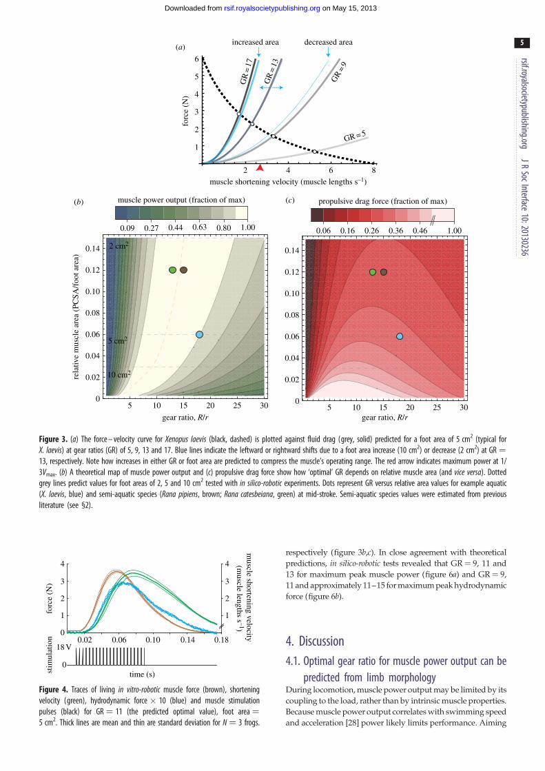
3. Results3.1. Morphological Vmaxmorph

predictions from the modelcompared with in vivo data

For a 5 cm2 foot (similar to the size of a X. laevis foot), the

model predicted drag force curves of increasing steepness

as GR varied from 5 to 17 (figure 3a). Vmaxmorphdecreased

from 5.2–3.3 to 2.3–1.7 muscle lengths s21 (ML s21). Simi-

larly, increasing foot area from 2 to 10 cm2 (at GR ¼ 13)

caused Vmaxmorphto decrease from 3.1 to 1.8 ML s21. Increasing

either GR or area also caused power to increase then decrease

as Vmaxmorphshifted towards then away from 1/3Vmax. For any

given relative muscle area (muscle PCSA/foot area), both

muscle power and hydrodynamic force rise and fall about

an ‘optimal’ GR value. This optimal GR was predicted to

shift rightward as relative muscle area increases (figure 3b,c).

From this theoretical performance map, the GR of the X.laevis PL (relative area ¼ 0.3 cm2/5 cm2¼ 0.06) was predicted

to be approximately 11. Near this predicted maximum

muscle power and fluid force, estimates of in vivo GR

ranged from 11.5 to 20, measured at different points of the

foot stroke and GR � 18 at mid-stroke.

3.2. Musculo-robotic measurements ofmorphological Vmax

Following electrical stimulation, in vitro muscle force devel-

oped in response to hydrodynamic force (figure 4). Since

experiments to determine the F–V curve could not be per-

formed on the same muscle preparations as in vitro-robotictrials, Vmaxmorph

could not be found precisely. However, the

data clearly show muscle force and velocity increasing until

reaching a maximum velocity near the predicted range of

Vmaxmorph(figure 5a). As GR increased from 5 to 11 to 17,

the operating range of the muscle also shifted leftward, as

predicted by the superimposed drag curves from the

model. To more precisely test predictions of Vmaxmorph, in

silico-robotic experiments were performed. Similar to in vitro-robotic trials, both force and velocity increased rapidly until

near the point of maximum activation, at which time

muscle force reached the limit imposed by the F–V curve

(figure 5b). Plots of force versus velocity intercepted with

the F–V curve near the predicted values of Vmaxmorph. Reflect-

ing in vitro-robotic experiments, increasing GR compressed the

muscle velocity range (i.e. approx. 0–5 MLs versus approx.

0–1.8 for GR ¼ 5 versus 17). Although the analytical model

predicted muscle force and velocity values to only occur

above the drag force curve, both in vitro and in silico data

fell below the drag curves during the relaxation phase of

the muscle. This underestimate could be due to (i) slight devi-

ations of the fluid reaction force vector causing lower outlever

values than estimated by our model (see §4) or (ii) backward-

directed force caused by added mass effects which counteract

fluid drag late in the swimming stroke [15]. Consequently,

Vmaxmorphslightly underestimated actual peak Vm values.

3.3. Bio-robotic measurements of muscle power andhydrodynamic force

Relative peak muscle power (peak trial power relative to the

maximum value observed) and hydrodynamic force were

tested over a range of GR and foot sizes. For foot sizes of 2, 5

and 10 cm2, the analytical model predicted maximum power

and hydrodynamic force to occur at GR¼ 9, 11.4 and 15,

0.160.06 0.26 0.36 0.46 1.00

5 10 15 20 25 300

0.02

0.04

0.06

0.08

0.10

0.12

0.14

propulsive drag force (fraction of max)

gear ratio, R/r

(c)

0.270.09 0.44 0.63 0.80 1.00

rela

tive

mus

cle

area

(PC

SA/f

oot a

rea)

5 10 15 20 25 300

0.02

0.04

0.06

0.08

0.10

0.12

0.14

gear ratio, R/r

muscle power output (fraction of max)(b)

10 cm2

5 cm2

2 cm2

muscle shortening velocity (muscle lengths s–1)fo

rce

(N)

2 4 6 8

1

2

3

4

5

6

GR = 5

GR

= 9

GR

= 1

3

GR

= 1

7

(a)increased area decreased area

Figure 3. (a) The force – velocity curve for Xenopus laevis (black, dashed) is plotted against fluid drag (grey, solid) predicted for a foot area of 5 cm2 (typical forX. laevis) at gear ratios (GR) of 5, 9, 13 and 17. Blue lines indicate the leftward or rightward shifts due to a foot area increase (10 cm2) or decrease (2 cm2) at GR ¼13, respectively. Note how increases in either GR or foot area are predicted to compress the muscle’s operating range. The red arrow indicates maximum power at 1/3Vmax. (b) A theoretical map of muscle power output and (c) propulsive drag force show how ‘optimal’ GR depends on relative muscle area (and vice versa). Dottedgrey lines predict values for foot areas of 2, 5 and 10 cm2 tested with in silico-robotic experiments. Dots represent GR versus relative area values for example aquatic(X. laevis, blue) and semi-aquatic species (Rana pipiens, brown; Rana catesbeiana, green) at mid-stroke. Semi-aquatic species values were estimated from previousliterature (see §2).

muscle shortening velocity

(muscle lengths s –1)

forc

e (N

)

0

0

18 V

1

2

3

4

1

2

3

4

fluid force x10

forcevelocity

stim

ulat

ion

time (s)

0.02 0.06 0.10 0.14 0.18

Figure 4. Traces of living in vitro-robotic muscle force (brown), shorteningvelocity (green), hydrodynamic force � 10 (blue) and muscle stimulationpulses (black) for GR ¼ 11 (the predicted optimal value), foot area ¼5 cm2. Thick lines are mean and thin are standard deviation for N ¼ 3 frogs.

rsif.royalsocietypublishing.orgJR

SocInterface10:20130236

5

on May 15, 2013rsif.royalsocietypublishing.orgDownloaded from

respectively (figure 3b,c). In close agreement with theoretical

predictions, in silico-robotic tests revealed that GR¼ 9, 11 and

13 for maximum peak muscle power (figure 6a) and GR¼ 9,

11 and approximately 11–15 for maximum peak hydrodynamic

force (figure 6b).

4. Discussion4.1. Optimal gear ratio for muscle power output can be

predicted from limb morphologyDuring locomotion, muscle power output may be limited by its

coupling to the load, rather than by intrinsic muscle properties.

Because muscle power output correlates with swimming speed

and acceleration [28] power likely limits performance. Aiming

forc

e, F

/Fm

ax

GR = 9GR = 13GR = 17

0 1 2 3 4 5 6 7 8

0.2

0.4

0.6

0.8

1.0re

lativ

e fo

rce,

F/F

max

GR = 5

GR = 5GR = 9GR = 13GR = 17

GR = 5GR = 11

GR = 11

GR = 17

GR = 17

(b)

(a)

GR = 5

0.17

0.33

0.50

0.67

0.83

1.00

muscle shortening velocity (muscle lengths s–1)0 1 2 3 4 5 6 7 8

Figure 5. Force versus velocity plots for (a) in vitro-robotic and (b) in silico-robotic experiments. Grey curves are F – V curves. Dotted grey lines are 95%confidence bands representing uncertainty of matching in vitro-robotic datawith F – V curves from separate experiments. Drag curves (blue, dotted) pre-dict the diminishing operating range of the muscle as GR increases. Bold linesare mean and thin are standard deviation (N ¼ 3 frogs or N ¼ 3 replicatesfor in vitro-robotic or in silico-robotic trials, respectively). For in silico trials,thick lines represent data prior to peak muscle activation.

1

2

3

4

5

6

7

8

kick number10 20 30 40 50

peak

sho

rten

ing

velo

city

(M

L s

–1)

morphological Vmax (GR = 11)

physiological Vmax(c)

gear ratio, R/r

(b)

5 10 15 20 25

peak

hyd

rody

nam

ic f

orce

(N

)

0.12

0.08

0.16

0.20

gear ratio, R/r

(a)

5 10 15 20 25

peak

mus

cle

pow

er (

W)

0.085

0.075

0.095

0.105

0.1152 cm2

5 cm2

10 cm2

Figure 6. (a) Peak muscle power and (b) peak hydrodynamic force for GR ¼5, 7, 9, 11, 13, 15, 17, 21 and 23 tested using circular foot sizes of 2 (blue), 5(green) and 10 cm2 (red). Arrows show analytically predicted locations ofmaxima (along dotted grey lines of contour plots; figure 3b,c). Dots aremean values and shaded areas are + standard deviation for N ¼ 3 repli-cates. Muscle starting length was adjusted so that peak force coincidedwith peak activation (see §2). (c) Peak in vivo PL muscle shortening velocityduring X. laevis swimming [28].

rsif.royalsocietypublishing.orgJR

SocInterface10:20130236

6

on May 15, 2013rsif.royalsocietypublishing.orgDownloaded from

to explore conditions under which power is ‘optimized’ (i.e.

shortening velocity � 1/3Vmax), we developed a predictive

model that was tested using recent musculo-robotic tools. As

predicted, results from both the analytical model and exper-

imental trials suggest that aquatic frog physiological and

limb morphological properties may be tuned for swimming.

Findings also suggest that there need not be a trade-off between

swimming and jumping ability.

Our analytical model, despite its simplicity, accurately

predicted how changes in external morphology (e.g. foot

area) and in internal morphology (e.g. joint gear ratio, ‘GR’)

limit muscle power. Simple analysis reveals that drag force

experienced by the muscle is proportional to Afin� GR3

(equation (2.9)). Thus, we expected slower contraction

speeds (lower Vmaxmorph) owing to increases in either GR or

foot area, as demonstrated by our experimental data (figure 5).

In addition, as expected, increases in GR caused peak

muscle power to rise and fall as Vmaxmorphapproached then

regressed from 1/3Vmax. More broadly, current findings

suggest that for high Reynolds number rowing, the limits to

muscle power and hydrodynamic force can be predicted as

a simple function of muscle area relative to foot area (relative

area ¼ PCSA/foot area) and GR. Consequently, our analyti-

cal model reveals two general strategies for maximizing

muscle power against a fluid load: (i) high gear with large

relative muscle area (e.g. large muscle, small fin) or (ii) low

gear with small relative muscle area (e.g. small muscle,

large fin). Specifically, larger feet (smaller relative muscle

area) require lower GR to maintain a given power output

against a fluid load, whereas small feet (large relative

muscle area) would not be sufficiently loaded if the GR

were too low. Xenopus laevis frogs, for example, have larger

fin areas and smaller PL PCSA than Rana pipiens or Ranacatesbeiana of similar body mass (relative area ¼ 0.06 versus

0.12; (this study, [4,21,29–31]). From these interspecific mor-

phological differences, our model predicts X. laevis to operate

at slightly lower gears (GR ¼ 11) than ranid frogs (GR ¼ 14).

Consistent with model predictions, GR measurements of

X. laevis ranged from 11 to 20 (depending on limb kinematics)

and estimated GR values from previous literature [4,21,

29–31] for R. pipiens and R. catesbeiana were GR � 15 and

13, respectively (figure 3b). However, because GR varies

rsif.royalsocietypublishing.orgJR

SocInterface10:20130236

7

on May 15, 2013rsif.royalsocietypublishing.orgDownloaded from

in vivo (see below), these species are all likely to operate over

a similar gearing range.

4.2. Estimated morphological Vmax predicts maximumin vivo shortening velocity in Xenopus laevis

In addition to exploring how limb morphology might be tuned

for rowing, our current findings have important implications

on our understanding of in vivo muscle data. In traditio-

nal approaches to dynamic muscle function, one might use

in vitro work loops [32,33] to address whether in vivo muscle

operates at or near its intrinsic power limits. For example,

some muscles may produce less power in vivo compared

with their intrinsic potential measured in vitro [34]. However,

muscle physiological approaches do not explain why muscle

power output may be submaximal in vivo. Our current model

predicts that if muscle contractile properties are not matched

to the surrounding fluid via appropriate limb morphology, a

muscle will operate below its power limits. Knowing that

X. laevis operates at a minimum GR of approximately 11, short-

ening velocity should not exceed the Vmaxmorphof approximately

2.7 ML s21. Data from experiments performed previously [28]

show that in vivo PL shortening velocity remains below the pre-

dicted limit of approximately 2.7 ML s21 (figure 6c). The match

between Vmaxmorphpredictions and in vivo data suggests three

points: (i) the PL is velocity-limited during swimming, (ii) the

maximum contractile velocities observed in vivo approach

0.3Vmax which is optimal for power generation, and

(iii) in vitro work loop experiments performed above the

Vmaxmorphwould produce results that are not physiologically

possible for the muscle in vivo.

4.3. Jumping frogs may also possess morphologicaltuning for rowing at no expense to jumpingperformance

Armed with an understanding of how fluid loading may limit

in vivo muscle function, we describe how the current model

can be applied to address questions of comparative functional

morphology. We illustrate the applications of the model by an

analogy to human-powered rowing. Hypothetically, the rower

represents a muscle which must operate within intrinsic speed

and strength limits. The oar blade and oar lock represent the

webbed foot and limb joint, respectively, whose gearing is

determined by the inboard and outboard oar lengths (i.e. ‘rig-

ging’). Finally, the rules and regulations of the rowing sport

represent functional constraints which may, for example, con-

strain the size of the oar blade. Knowing the strength and

speed capacities of the rower, one should be able to predict

the appropriate rigging to match the capabilities of a particular

rower to optimize muscular power output.

Given the relationship between rowing ability, limb mor-

phology and muscle properties, our model could be used to

address morphological trade-offs between swimming and

other locomotor tasks. Frog jumping ability [1,2] correlates

to modifications of the skeleton [35], potentially in conflict

with swimming. However, morphology of ranids ( jumper–

swimmers; [36]) and swimming performance of ranids versus

pipids (swimmers; [37]) reveal no evidence that jumping

diminishes swimming capacity. How can the musculoskeletal

system excel both at swimming and jumping? The map of

muscle power versus GR and relative area (figure 3b) suggests

that there exist multiple combinations of foot size and GR which

maximize muscle power. This broad ‘solution space’ perhaps

could accommodate specializations for jumping while main-

taining swimming ability (or vice versa). For instance, the

recoil of elastic tendons to amplify muscle–tendon power

output for jumping [4] requires appropriate tuning of GR to

body mass [38], suggesting that jumping requirements may

constrain GR. In such cases, changes in foot area could compen-

sate (i.e. moving vertically along the power map). Alternatively,

foot area may be constrained due to shorter feet. Large forces

during jumping [4,10] may limit foot length in order to

minimize joint torques. Indeed, the feet of hylid frogs, the cham-

pion jumpers, are short despite their elongated total hindlimb

length relative to fully aquatic species [35]. In this case, adjust-

ments of GR can move the limb horizontally along the power

map to optimize power when faced with a foot area constraint.

Thus, we speculate that due to the many pairings of GR and

foot area that confer power output during swimming, there

need not be a swimming–jumping trade-off—a ‘specialized’

jumper may still be morphologically tuned to optimize power

during rowing. Further modelling would be necessary to

address the consequences of morphological constraints on

swimming versus jumping.

4.4. Variation in Vmax probably influences the ‘optimal’limb morphology for rowing

In addition to the morphological predictors of muscle per-

formance, physiological properties such as Vmax influence

the relationship between limb morphology and power

output. Specifically, increasing or decreasing Vmax causes a

leftward or rightward shift of the entire power map, respect-

ively. For ectothermic animals such as anurans, large

fluctuations in environmental temperature (either seasonally

or with climate change [39]) would influence Vmax, affecting

where muscles operate on the FV curve. Vmax in X. laevisincreases with temperature (Vmax � 0.004 � temperature2þ0.11 � temperature þ 2.5 ML s21; [40]). Given that X. laevisswim to catch active prey and escape predators [14], climate

fluctuations might influence their ecological success. Yet,

the invasive population of X. laevis of the Santa Clara River

(CA, USA) thrive year-round [14], despite average daily

temperature fluctuations from approximately 7 to 248C [41].

At the higher temperature extreme, the PL muscle functions

slightly rightward of the predicted optimum (figure 3b).

However during winter, Vmax may drop to approximately

3.7 ML s21, causing a rightward shift in peak GR from 11.4

to 18. Consequently, the PL produces approximately 90 per

cent of its maximum power during warm months and

approximately 100 per cent of its potential power (given

the depressed Vmax) during colder months. Thus, although

colder temperatures depress absolute muscle power, the right-

ward shift of the power map might enable muscles to use their

full power potential at that given temperature by maintaining

the muscle’s ability to operate at approximately 1/3Vmax.

Alternatively, if X. laevis limbs were to operate leftward the

predicted peak power (GR , 11), falling temperatures would

further reduce performance. For example, if X. laevis operated

at GR ¼ 9, it would produce approximately 98 per cent of its

maximum power at 228C, but only approximately 70 per cent

at 78C. In addition to low temperature effects, power would

likely also be depressed at higher temperatures (despite greater

Vmax) owing to a rightward shift away from the optimum GR

rsif.royalsocietypublishing.orgJR

SocInterface10:20130236

8

on May 15, 2013rsif.royalsocietypublishing.orgDownloaded from

measured at laboratory temperature (228C). Perhaps the right-

shift of the power map could explain the depressed swimming

performance of Xenopus at high temperatures [39]. One should

note however, that beyond our simple model, animals might

also respond to temperature changes by modifying stroke kin-

ematics or the dynamic shape of their feet. Regardless, such

influences of temperature imply that limb morphology of

birds and mammals might be more tightly tuned, given that

their Vmax would remain constant at their physiologically regu-

lated temperature.

Using published Vmax data, one also can make broad taxo-

nomic comparisons among high Reynold’s number rowers. For

example, notonectid insects swim using a slow muscle (Vmax

approx. 1 ML s21; [20]) compared with frogs (Vmax� 9). Conse-

quently for notonectids, we see a very high GR (approx. 40)

given both the rightward-shifted Vmaxmorphand their small

rowing appendage. By contrast, aquatic bird and mammal

muscles operate at higher physiological temperatures, causing

Vmax to be higher [42], perhaps requiring relatively lower GR

values. This requires further investigation.

4.5. Simplifying assumptions of the current model areappropriate for certain cases of aquatic locomotion,but not for others

Our model is simple, thus has physiological and morphologi-

cal limitations which must be addressed. The most evident

morphological simplification is the neglect of leg joints prox-

imal to the ankle. We justify this simplification for X. laeviswhere ankle rotation produces most of the thrust. However,

ranids rely considerably less on their ankle joint (producing

approx. 50% of total thrust; [37]). Nevertheless, even in ranids,

both ankle rotation and ankle stabilization (to maintain the

foot’s position as the proximal joints push backward) require

great amounts of power produced at the ankle, justifying our

model’s focus on distal rather than proximal joints. Regardless

of the model’s simplicity, identical principles of Vmaxmorph

tuning would apply to more complex future models. In terms

of the physiological simplifications, the interactions among

F–V and F–L effects are potentially confounding given that

large length changes reduce the optimal V/Vmax for producing

power [43]. However, recent work demonstrates that muscle

contractions beginning at longer starting lengths (stretched

slightly beyond optimal length) enable the muscle to reach the

plateau of the F–L curve at the time of maximum muscle acti-

vation [22]. Thus, at the time point of peak activation and

muscle power, F–L effects would not influence maximum

muscle power for the current model. Indeed, our in silico-roboticexperiments, which do include F–L effects, match well with our

simple model predictions (figure 6).

Secondly, experiments were performed in still water

without translational motion of the foot. In a simple rower

(figure 2d), oar blades would have an aft-directed rotational

and translational component as they rotate about their base.

Therefore, in a tethered animal, the oar would ‘slip’ backward.

However if untethered, the body moves forward with respect

to the water, whereas the blade moves backward with respect to

the body. As a result, an oar’s backwards translation is can-

celled by forward swimming such that the motion of the oar

base is nearly fixed in the global reference frame, as evident

in swimming insects [20], aquatic frogs [8,15] and in human-

powered rowing [44]. In these cases, we capture important

aspects of muscle–fluid dynamics in the absence of modelling

forward body motion. In cases where rowing appendages are

thrust backwards (e.g. ranid frogs [10]), our model is less accu-

rate. In either forward or backward translation cases, our

simple model would overestimate outlever (R) length as the

fluid reaction force vector deviates from normal to the foot sur-

face [8]. Consequently for large foot sizes which cause large

fluid forces and faster swimming speeds, our simple model

would overestimate GR. For our current results, such an over-

estimation would shift our estimates of in vivo GR rightward

(away from the predicted optimum for ranids and towards

the optimum for X. laevis; figure 3b). Thus, in cases of fast for-

ward swimming (e.g. the second or third kick when the foot

rotates as the body is already in motion) or in rapid backward

translation (common in ranids), one must quantify transla-

tional and rotational velocity components to account for the

deflection of the fluid reaction force vector [8]. In addition,

the current simple analytical model is not appropriate for

acceleration-based swimming. In cases when limb accelera-

tions are extreme and fluid dynamic loads are dominated by

the acceleration reaction (e.g. very small frogs [8] or suction

feeding fish [45]), our model does not apply because the coup-

ling between shortening velocity and fluid drag would be

relatively unimportant. Finally, we address time-varying gear-

ing. Although inlever (r) does not vary over the in vivo range of

frog ankle joint motion [27,30,31], the outlever (R) may vary

due to (i) the angle of the fluid reaction force vector changing

with respect to the foot orientation [8] or (ii) as the foot’s pos-

ition relative to the ankle changes throughout a stroke. To

address this, R can be estimated at various points in the foot

stroke (see §2).

4.6. SummaryWe present an approach which may be used to predict

muscle performance during swimming using morphological

(GR, foot area) and physiological (Vmax, Fmax) constants.

We found that X. laevis hindlimbs possess morphology that

is appropriate given muscle intrinsic properties and PCSA.

Such ‘tuning’ of morphological and physiological properties

probably enable the muscle to shorten near 1/3Vmax to

approach maximal power during swimming.

More generally, the current study addresses dilemmas

that arise when limb morphology is considered without

regard to underlying muscle properties (and vice versa).

Based on fin area alone, one might falsely conclude that

ranid frogs produce lower power outputs in fluid than

aquatic frogs which possess larger feet. However, based on

the larger PCSA of ranids compared with X. laevis, one

might reach the opposite conclusion. We resolve such dilem-

mas with a model that predicts functional relationships

among morphological and physiological properties. Perhaps

our simple approach can be used to suggest pathways by

which natural selection influences performance through the

modification of either muscle or limb properties.

Firstly, we thank Andrew Carroll for discussions prior to the onset ofthis work that stimulated our interest in the coupling of fluid dragand muscle force–velocity effects. We thank Henry Astley for helpfuladvice regarding force–velocity experiments. We thank Tom Robertsfor his suggestion to investigate temperature effects of Vmax. Inaddition, we are thankful for informative discussions with JimDreher, Coleen Fuerst and Linda Stern regarding the mechanics ofhuman rowing. This work was supported by the Rowland Jr. Fellowsprogramme at the Rowland Institute at Harvard.

9

on May 15, 2013rsif.royalsocietypublishing.orgDownloaded from

References

rsif.royalsocietypublishing.orgJR

SocInterface10:20130236

1. Rand SA. 1952 Jumping ability of certain anurans,with notes on endurance. Copeia 1952, 15 – 20.(doi:10.2307/1437615)

2. Zug GR. 1978 Anuran locomotion—structure andfunction, 2: jumping performance of semiaquatic,terrestrial and arboreal frogs. Smithsonian contrib.Zool. 276, 1 – 30. (doi:10.5479/si.00810282.276)

3. Lutz GJ, Rome LC. 1994 Built for jumping: thedesign of the frog muscular system. Science 263,370 – 372. (doi:10.1126/science.8278808)

4. Roberts TJ, Marsh RL. 2003 Probing the limits tomuscle-powered accelerations: lessons from jumpingbullfrogs. J. Exp. Biol. 206, 2567 – 2580. (doi:10.1242/jeb.00452)

5. Howard WE. 1950 Birds as bullfrog food. Copeia1950, 152. (doi:10.2307/1438964)

6. Altevogt R, Holtmann H, Kaschek N. 1986 Highfrequency cinematography studies on locomotion andpreying in Indian skitter frogs Rana cyanophlyctis.J. Bombay Nat. Hist. Soc. 83, 102 – 111.

7. Nauwelaerts S, Scholliers J, Aerts P. 2004 Afunctional analysis of how frogs jump out of water.Biol. J. Linn. Soc. 83, 413 – 420. (doi:10.1111/j.1095-8312.2004.00403.x)

8. Gal JM, Blake RW. 1988 Biomechanics of frogswimming. I. Estimation of the propulsive forcegenerated by Hymenochirus boettgeri. J. Exp. Biol.138, 399 – 411.

9. Johansson LC, Lauder GV. 2004 Hydrodynamics ofsurface swimming in leopard frogs (Rana pipiens).J. Exp. Biol. 207, 3945 – 3958. (doi:10.1242/jeb.01258)

10. Nauwelaerts S, Stamhuis EJ, Aerts P. 2005Propulsive force calculations in swimming frogs I.A momentum-impulse approach. J. Exp. Biol. 208,1435 – 1443. (doi:10.1242/jeb.01509)

11. Gordon AM, Huxley AF, Julian FJ. 1966 The variationin isometric tension with sarcomere length invertebrate muscle fibres. J. Physiol. 184, 170 – 192.

12. Hill AV. 1938 The heat of shortening and thedynamic constants of muscle. Proc. R. Soc. Lond. B126, 136 – 195. (doi:10.1098/rspb.1938.0050)

13. Daniel T, Jordan C, Grunbaum D. 1992Hydromechanics of swimming. Adv. Comp.Environ. Physiol. 11, 17 – 49. (doi:10.1007/978-3-642-76693-0_2)

14. Lafferty KD, Page CJ. 1997 Predation on theendangered tidewater goby, Eucyclogobiusnewberryi, by the introduced African clawedfrog, Xenopus laevis, with notes on the frog’sparasites. Copeia 1997, 589 – 592. (doi:10.2307/1447564)

15. Richards CT. 2008 The kinematic determinants ofanuran swimming performance: an inverse andforward dynamics approach. J. Exp. Biol. 211,3181 – 3194. (doi:10.1242/jeb.019844)

16. Lieber RL. 1992 Skeletal muscle structure and function.Baltimore, MD: Lippincott Williams & Wilkins.

17. Biewener A. 2003 Animal locomotion. Oxford, UK:Oxford University Press.

18. Richards CT, Clemente CJ. 2012 A bio-robotic platformfor integrating internal and external mechanics duringmuscle-powered swimming. Bioinspir. Biomim. 7,016010. (doi:10.1088/1748-3182/7/1/016010)

19. Aerts P, Nauwelaerts S. 2009 Environmentallyinduced mechanical feedback in locomotion: frogperformance as a model. J. Theor. Biol. 261,372 – 378. (doi:10.1016/j.jtbi.2009.07.042)

20. Daniel TL. 1995 Invertebrate swimming: integratinginternal and external mechanics. Symp. Soc. Exp.Biol. 49, 61 – 89.

21. Azizi E, Roberts TJ. 2010 Muscle performance duringfrog jumping: influence of elasticity on muscleoperating lenghts. Proc. R. Soc. B 277, 1523 – 1530.(doi:10.1098/rspb.2009.2051)

22. Clemente CJ, Richards C. 2012 Determining theinfluence of muscle operating length on muscleperformance during frog swimming using a bio-robotic model. Bioinspir. Biomim. 7, 036018.(doi:10.1088/1748-3182/7/3/036018)

23. Richards CT. 2011 Building a robotic link betweenmuscle dynamics and hydrodynamics. J. Exp. Biol.214, 2381 – 2389. (doi:10.1242/jeb.056671)

24. Otten E. 1987 A myocybernetic model of the jawsystem of the rat. J. Neurosci. Methods 21,287 – 302. (doi:10.1016/0165-0270(87)90123-3)

25. Lee SSM, de Boef Miara M, Arnold AS, Biewener AA,Wakeling JM. 2011 EMG analysis tuned fordetermining the timing and level of activation indifferent motor units. J. Electromyogr. Kinesiol. 4,557 – 565. (doi:10.1016/j.jelekin.2011.04.003)

26. Moore JH. 1995 Artificial intelligence programmingwith LabVIEW: genetic algorithms forinstrumentation control and optimization. Comput.Methods Programs Biomed. 47, 73 – 79. (doi:10.1016/0169-2607(95)01630-C)

27. Clemente CJ, Richards CT. Submitted. Musclefunction and hydrodynamics limit power and speedin swimming frogs.

28. Richards CT, Biewener AA. 2007 Modulation ofin vivo muscle power output during swimming inthe African clawed frog (Xenopus laevis). J. Exp. Biol.210, 3147 – 3159. (doi:10.1242/jeb.005207)

29. Kargo WK, Rome LC. 2002 Functional morphologyof proximal hindlimb muscles in the frog Ranapipiens. J. Exp. Biol. 205, 1987 – 2004.

30. Lieber RL, Brown CG. 1992 Sarcomere length –joint angle relationships of seven frog hindlimbmuscles. Acta Anat. 145, 289 – 295. (doi:10.1159/000147380)

31. Astley HC, Roberts TJ. 2011 Evidence for a vertebratecatapult: elastic energy storage in the plantaris

tendon during frog jumping. Biol. Lett. 8, 386 – 389.(doi:10.1098/rsbl.2011.0982)

32. Josephson R. 1985 The mechanical power outputfrom striated muscle during cyclic contraction.J. Exp. Biol. 114, 493 – 512.

33. Altringham JD, Johnston IA. 1990 Scaling effects onmuscle function: power output of isolated fishmuscle fibers performing oscillatory work. J. Exp.Biol. 151, 453 – 467.

34. Tu MS, Daniel TL. 2004 Submaximal power outputfrom the dorsolongitudinal flight muscles of thehawkmoth Manduca sexta. J. Exp. Biol. 207,4651 – 4662. (doi:10.1242/jeb.01321)

35. Emerson SB. 1982 Frog postcranial morphology:identification of a functional complex. Copeia 1982,603 – 613. (doi:10.2307/1444660)

36. Nauwelaerts S, Ramsay J, Aerts P. 2007Morphological correlates of aquatic and terrestriallocomotion in a semi-aquatic frog, Rana esculenta:no evidence for a design conflict. J. Anat. 210,304 – 317. (doi:10.1111/j.1469-7580.2007.00691.x)

37. Richards CT. 2010 Kinematics and hydrodynamicsanalysis of swimming anurans reveals striking inter-specific differences in the mechanism for producingthrust. J. Exp. Biol. 213, 621 – 634. (doi:10.1242/jeb.032631)

38. Galantis A, Woledge RC. 2003 The theoretical limits tothe power output of a muscle– tendon complex withinertial and gravitational loads. Proc. R. Soc. Lond. B270, 1493. (doi:10.1098/rspb.2003.2403)

39. Herrel A, Bonneaud C. 2012 Trade-offs betweenburst performance and maximal exertion capacity ina wild amphibian, Xenopus tropicalis. J. Exp. Biol.215, 3106 – 3111. (doi:10.1242/jeb.072090)

40. Marsh R. 1994 Jumping ability of anuranamphibians. Adv. Vet. Sci. Comp. Med. 38, 51 – 111.

41. Western Regional Climate Center. 2012 Westernregional climate center. Reno, NV, USA. See http://www.wrcc.dri.edu/.

42. Nelson FE, Gabaldon AM, Roberts TJ. 2004 Force –velocity properties of two avian hindlimb muscles.Comp. Biochem. Physiol. A Mol. Integr. Physiol. 137,711 – 721. (doi:10.1016/j.cbpb.2004.02.004)

43. Askew GN, Marsh RL. 1998 Optimal shorteningvelocity (V/Vmax) of skeletal muscle during cyclicalcontractions: length – force effects and velocity-dependent activation and deactivation. J. Exp. Biol.201, 1527 – 1540.

44. Macrossan MN. 2008 The direction of the waterforce on a rowing blade and its effect on efficiency.Mechanical Engineering report 3. The University ofQueensland, St Lucia QLD, Australia.

45. Van Wassenbergh S, Strother JA, Flammang BE, Ferry-Graham LA, Aerts P. 2008 Extremely fast prey capture inpipefish is powered by elastic recoil. J. R. Soc. Interface5, 285 – 296. (doi:10.1098/rsif.2007.1124)