Introduction to Bayesian VARs

Tony Yates, lecture to MSc Time Series, Bristol, Spring 2014

Objectives and plan

• Objective:  enable you to estimate large dimension VARs using Bayesian shrinkage.

• Two kinds:  where priors are chosen to be natural conjugates, giving us convenient expressions for the posterior from which we can sample.

• And where they are not, and we are forced to use (eg) Gibbs Sampling

Plan

• Preliminaries about density functions.• Deriving Bayes’ theorem, and computing the posterior over parameters or over models.

• Controversies between Bayesian and frequentiststatisticians.

• Bayesian AR(1) using conjugate priors.• Pointless but illustrative Gibbs sampling for a bivariate normal.

• Gibbs Sampling for an AR(1) with non‐conjugate priors

The Bayesian posterior for an AR(1)

yt yt−1 et,e N0,2

,

p ∣ y py∣ppy

posterior

Likelihood of the data

Prior over parameters

Marginal data density, or predictive density

The likelihood through classical and Bayesian spectacles

• For a frequentist, or a classical econometrician, likelihood is something to be maximised.

• ..In knowledge that as data sample increases this maximum (thetahat) would approach the ONE TRUE THETA.

• For a Bayesian, this is a distribution function, expressing the data’s perspective on the probability mass on all possible thetas, with stance that there is NO SINGLE TRUE THETA.

Back track on some preliminaries

f

fd 1

∑i1

N

f i 1

Density function takes some parameter value, maps to a number we interpret as a probability

Since they are probabilities, their sum=1, so when we integrate it wrt theta, across all thetas we must get 1

Or, if the different possibilities for theta are countable, ie discrete, then the probabilities must sum to 1.

Joint, conditional, marginal densities

f1 ,2

fd 1 f1 ,2d1d2

f1 ∣ 2

f1 ∣ 2d1 1

2 dimensional, joint distribution function, which also has to be proper, ie integrate to 1

A conditional density for theta1 given theta2 known, which also has to integrtate to 1 when we do so wrt theta1

A density that gives us the probability of different theta1s, computed by integrating the joint for theta1,theta2, wrt theta2p1 f1 ,2d2

Getting to Bayes’ theorem from defnof a conditional probability

pA ∣ B pB∩ApB

Prob of A given B Prob of A and B occurring

pB ∣ A pB ∩ ApA

pB ∩ A pA ∩ B

pB ∣ ApA pB ∩ A

pA ∣ B pB ∣ ApApB

Reverse the labels, write down condprob again.Sub p(b) and p(a) into first definition.You are done.Remember A will be our model parameter theta, B will be our vector or matrix of data

The Bayesian posterior for an AR(1)

yt yt−1 et,e N0,2

,

p ∣ y py∣ppy

posterior

Likelihood of the data

Prior over parameters

Marginal data density, or predictive density

Without going deep into philosophy of statistics...

• Bayesian view:  there are many models, over which one forms a prior probability distribution, and uses the data to form a posterior

• Classical, or frequentist view:  there is one model, and one tries to make inference about it, namely, deducing the probability that the model is true or false

Interpretation of p:  divergences between the Bayesian and frequentist

view• Bayesian view:  p(A) measures strength of subjective ‘belief in’.  Movement from prior to posterior=‘in light of evidence, my belief has changed from p1 to p2’

• Frequentist or classical view:  above meaningless, since things either are or not true. 

Applicability of Bayes’ Theorem• Bayesian:  anywhere.• Frequentist:  only applies to situations where it is 

meaningful to think of an actual or hypothetical repeated sequence in which A occurs sometimes [with given frequency] or B

• Bayesian:  allows us to make concrete statements about whether the moon is made of cheese or not.  No hypothetical sequence of events in which it is or it isn’t.

• But gives math content to common expressions like ‘the moon is very unlikely to be made of cheese’.  Or This by Neil Armstrong:  ‘I used to think it was highly unlikely to be made of cheese.  Then I stood on it, and I became almost certain it wasn’t.’

What is the marginal data density, the denominator in the Bayesian posterior 

for an AR(1)

yt yt−1 et,e N0,2

,

p ∣ y py∣ppy

posterior

Likelihood of the data

Prior over parameters

Marginal data density, or predictive density

‘Marginal data density/likelihood’, or ‘predictive density’

‘The integral of the joint density of the data and parameters with respect to the parameters’.

This gives us a number.  It’s just a normalising constant that tells us what we need to get the numerator in BT to integrate to 1.

Not needed if all we want to do is find the mode, or the median, or report some interval of the posterior, since these quantities are not altered by dividing every possible value for that numerator by a constant.

But useful to know what it is, and one has to calculate it sometimes.

And calculating it can actually be very tricky.

py py1 ,y2 . . .yT py ∣ pd

Marginal likelihood/ctd…

• Usually have to approximate it.• Empirical Bayesian papers will sometimes use marginal likelihood in the same way that frequentists use the likelihood:  as a measure of fit.

Hierarchical priors over models

M1 : yt yt−1 et,e N0,2

1 ,

M2 : yt a1yt−1 a2yt−2 ht0.5et

lnht ht−1 ut,u N0,u

2 a,h,u

Either the world is AR(1), 

…or it’s AR(2) with stochastic volatility.

pM

p1 ∣ M1

p2 ∣ M2

We have our prior over models..

.. and our prior over parameters, given a particular model M is true

Why ‘hierarchical’?

• Priors formed over models…• Contain within them priors over parameters, conditional on a model.

Computing the posterior over models

pM ∣ y py ∣ MpMpy

,

py py ∣ MpMdM ∑i1

2

py ∣ MipMi

This is just a trivial relabelling of what you have seen for events A and B, where the models M are the two events.

Second line is the marginal data density again.  Notes this time the integral is just a sum over two events.

This is just an example.  There could be infinitely many models of course.  In fact there are.

But to make progress you would probably begin with a small number.

Posterior odds and Bayes Factors

pM1∣ypM2∣y

py∣M1

py∣M2

pM1

pM2

Posterior oddsBayes Factor

Prior Odds

Predictive densities/marginal likelihoods for each model, ie integrating out the parameters theta.

Before I look at the evidence, what do I think the odds are that model 1 is true compared to model 2?  How are these odds altered by the evidence?

Pragmatic motivation for estimating Bayesian VARs

• Large dimension to avoid omitted variables• Curse of dimensionality:  parameters increase with n^2.  Quickly become ill‐determined.

• Forecasting performance poor.• Possibility of data driving you to misleading local maximum of the likelihood.

• Prior ‘shrinkage’ [shrinkage of probability mass around some mode, for example] alleviates these difficulties.

Pragmatic motivation/ctd

• Bayesian computational machinery allows us to learn about estimating using ML some complicated models.

• This machinery includes something we will learn about, Gibbs sampling, a variant of a larger family of ‘Markov Chain Monte Carlo’ methods you might meet if you continue with your studies.

• If you don’t like the Bayesian aspect, you can, with care, make your priors ‘uninformative’

NB on Bayesian VARs

• Everything we will do can be combined with our techniques for identification of VARs (SVARS).

• Eg:  we can perform sign restriction identification for every realisation in a posterior distribution for our reduced form VAR coefficients.  Or recursive ID.  Or long run ID.  Or max‐share ID.

• For example:  see my paper ‘Risk news shocks and the business cycle’.

Milestones in Bayesian time series macroeconometrics.

• Sims (1988) Using priors to resolve difficulties about stationarity or otherwise of macro time series, given low power of tests.

• Ingram and Whiteman (1994). Priors from RBC models in time series models.

• Doan, Litterman and Sims (1984):  conjugate priors in Bayesian VARs.

• Del Negro and Schorfheide’s DSGE‐VAR.

Knowledge journey in Estimation of Bayesian VARs [and other things]

• First step:  posterior for VAR parameters when we assume the vcov matrix is known.

• Second step:  allow vcov itself to have a distribution.  Notion of conjugacy in priors for this that guarantee known distribution for posterior that we can draw from.

• Third step:  Gibbs sampling when conjugacy is not possible or desirable.

• Final step for later life, not here:  Metropolis‐Hastings, when you can’t factor to leave distributions from which you can draw.

• Another step for the afterlife:  particle filtering.  When one cannot even evaluate the likelihood for a candidate parameter value.

Derivation of moments of normal posterior for a Bayesian VAR:  

KK(1997)

yt ∑i1

p

yt−iAi x tC ut

y is a row vector;  KK allow for exogenous variables too, which our course generally ignores on Sims’ grounds.

y t∗ y t−1

∗ A x tD ut∗

y t∗ y1 ,yt−1 , . . .yt−p

A

A1 I 0 . . . 0

A2 0 I . . 0

. . . . . . . . . . . . . .

Ap 0 0 . . . I

This step writes the VAR(p) as a VAR(1).  Now the original y is a row, the coefficient appears afterwards.  Note complication of the exogenous variables too.

Rewriting and manipulating the ‘VAR’

yt ztΓ ut

Γ C′,A1′ ,A2

′ . . .Ap′

Different rewriting of the original VAR(p).  Now collect all RHS variables together.  Allows us to forget about complication of exogvariables.

Y ZΓ U Above defined for every t;  below stacks equations for every t.

yi Zi ui

Picks out the ith equation of the above.

Minnessota prior

• Treat vcov matrix as known [unappealing].  And diagonal [equally so.]

• Shrinkage:  priors on lags other than own zero.• Prior variances tighter as lag length gets longer.

• Has the effect of reducing the chance of oscillatory IRFs.  Eg effect of shock in an AR(1) dies out monotonically.

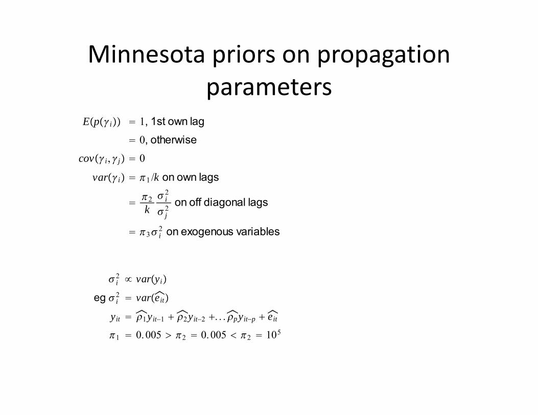
Minnesota priors on propagation parameters

Epi 1, 1st own lag 0, otherwise

covi,j 0

vari 1 /k on own lags

2k i2

j2 on off diagonal lags

3 i2 on exogenous variables

i2 varyi

eg i2 vareit

yit 1yit−1 2yit−2 . . .pyit−p eit

1 0.005 2 0.005 2 105

From normal priors to normal posteriors for ‘VAR’ coefficients

i Ni,i

i |y Ni,i

i i−1 ii

−1ZZ−1 ,

i ii−1i ii

−1Z ′yi

If the prior is a normal, defined by some mean and variance.

Then the posterior is normal.

And its mean is a weighted sum of the means of the prior and the ‘data’.

Where the weights are proportional to the prior variance.   [lower prior variance=more weight on prior mean]

And its variance is also a weighted sum of the prior and the ‘data’ variance.

Relaxing Minnesota prior conditions

• We assumed vcov of errors known and diagonal.

• Can relax both.• If we relax ‘known’, we are in a world where the vcov resid matrix itself has a distribution!

• Prior distributions for the vcov matrix chosen with care to preserve eg normality of posteriors.  Such distributions known as ‘conjugates’.

Markov chain monte carlo methods

• What if we don’t have natural conjugates?• After all, they do have some disadvantages.• Now can’t sample from our desired distribution.• We can evaluate the probability of a draw.  But we can’t characterise the density analytically.

• Instead, use results from Gibbs, Metropolis, Hastings to sample from proposal densities, which, in the limit, will generate samples from our target density.

Gibbs sampling when we don’t need to do it

Suppose we have a bivariate normal.  We have analytical expressions for the moments of this distribution, and can sample from it readily using MATLAB or similar.

However, we can use it to illustrate Gibbs Sampling.

So pretend that we can’t draw from this distribution directly, but wish nonetheless to draw from some other distribution that we can draw from, and, with some magic, get a sample from the distribution we can’t (or, in this case, are pretending we can’t)

1 ,2 N0,0,, 1

1

Gibbs sampling using two conditionally univariate normals

Theta1 conditional on theta2 is a univariatenormal with known mean and variance.And vice versa.We can draw from these conditionals.

1.Choose arbitary 20

2.Draw 10 from 1 ∣ 2

0

3.Draw 21 from 2 ∣ 1

0

4.Repeat

This is a cyclical Gibbs Sampling algorithmStart from any point, and we will end up with a collection of draws from the joint bivariate normal.

1 ∣ 2 N2 , 1 − 2

2 ∣ 1 N1 , 1 − 2

Output of Gibbs Samping algorithm

11 12

21 22

. . . .

n1 n2

We will get a very large matrix with two columns.

Each row is a draw from the joint distribution of theta1 and theta2.

As n gets very large, this matrix can be treated as the joint distribution.

E1 |2 1/n∑i1

n

i1

For example, we compute the expectation of theta1 given theta2 by taking the average of the first column.

p1 |2

∑i

n

I1,i1

n

Conditional interval probusing an indicator variable and the first column.

Doan, Litterman and Sims

• First well known Bayesian VAR model.• Minnesota Priors.• Prior is that coefficients off the diagonal are zero.  Tighter for longer and longer lags.

• Improves forecasting because it tames the otherwise diffuse distributions on VAR parameters.

• Also ‘stabilises’ the VAR too.

Pinter, Theodoridis and Yates

• Came across this in the discussion of the max share method for identifying news shocks.

• Well, they begin by estimating a Bayesian VAR with 3 lags in 10 variables.

• Using Minnesota‐like Priors, an update of this devised by Banburra et al (2010).

Cogley, de Paoli, Nikolov, Matthes, Yates

• Optimal Bayesian monetary policy.• Policy maximise expected posterior loss, given probability on many models.

• Models include DSGE models, and a semi‐structural Cowles‐Commission model by Svensson and Rudebusch.

Cogley, Morozov and Sargent:  Bayesian fan charts for UK inflation

• Estimate Bayesian time‐varying parameter VAR for inflation in the UK.

• Observe that policymakers have their own judgementally arrived at but incompletely specified priors, eg specify a mean and a variance.

• Seek to find the ‘twist’ to the estimated posterior that satisfies policymakers’ moment conditions while doing minimal damage to the posterior.

• ...Or creating minimal ‘entropy’ wrt posterior

What does Cogley Morozov and Sargent give us?

• Policymakers can impose their views, but still make use of the VAR.

• We can use the entropy that is the minimum entropy as a measure of the disagreement between policymakers and the model.

• Technique actually borrowed from Robertson, Tallman and Whiteman.

Useful references and resources

• Doan, Litterman and Sims• Cogley, Morozov and Sargent:  Bayesian fan charts for UK inflation

• Lancaster ‘In introduction to modern Bayesian Econometrics

• Kadiyalla and Karlsson, 1997, JAE• Sims and Zha (1996) ‘Bayesian Methods for dynamic multivariate models’

• Garry Koop’s textbook and teaching webpages

More sources

• DeJong Textbook, eg Ch 9• Gelman et al ‘Bayesian data analysis’• Roberts and Casella ‘Monte carlo statistical methods’

• Sims and Zha ‘Bayesian methods for dynamic multivariate models’

• A Bayesian is one who, vaguely expecting a horse and catching a glimpse of a donkey, strongly concludes he has seen a mule’ (Senn)