budgeting and quantifying data - cornell university · – select the first range/cell then use...

Slide

Budgeting and Quantifying DataClerk’s Institute 2016

Slide

What is a Worksheet?

• A way to collect and organize information into columns and rows– Each column is lettered

– Each row is numbered

• Information is entered into the cells

• Every cell has a unique reference or address, for example, A10, ZM799

9/20/2016 Christina Homrighouse, [email protected] 2

Slide

Why Use Excel?

• A worksheet is big

• Perform calculations, create and recalculate scenarios quickly and accurately– Change data

– Manipulate data

– Reorganize information

• To create charts from worksheet data


Slide

“thick cross” = selecting cells

“down arrow” = selecting column(s)

“right arrow” = selecting row(s)

“thin cross” = AutoFill, copy

“double headed arrow” = resizing

“ four headed arrow” = move, drag and drop

Cursor Shapes

If the cursor is this shape

+

Christina Homrighouse, [email protected] 49/20/2016

This will happen when you click and drag

Slide

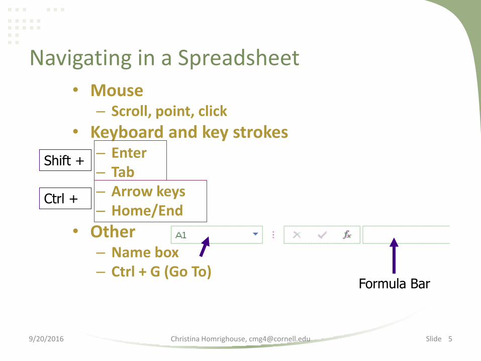
• Mouse– Scroll, point, click

• Keyboard and key strokes– Enter– Tab– Arrow keys– Home/End

• Other– Name box– Ctrl + G (Go To)

Formula Bar

Navigating in a Spreadsheet

Shift +

Ctrl +


Slide

Selecting Cells

• Cell Range = single cell or contiguous cells (forms a square or a rectangle)– Click and drag (thick cross)– Shift+Arrow keys or Shift+Click– Control+Shift+Arrow keys or End– Name box

• Type range (A1:D10), press enter• Colon (:) means “through”

• Entire row or column– Click on column or row heading– Ctrl or Shift + Space Bar

• Non-contiguous– Use the Ctrl key– Select the first range/cell THEN use Ctrl to select

the next range(s) – don’t start with the Ctrl key down

• Entire spreadsheet or data set– Select All button– Ctrl + A (sometimes twice)

9/20/2016 Christina Homrighouse, [email protected]

Ctrl = “jump”Shift = select

Slide

Entering Data

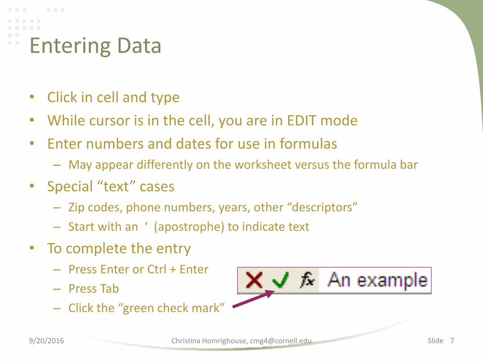
• Click in cell and type

• While cursor is in the cell, you are in EDIT mode

• Enter numbers and dates for use in formulas– May appear differently on the worksheet versus the formula bar

• Special “text” cases– Zip codes, phone numbers, years, other “descriptors”

– Start with an ‘ (apostrophe) to indicate text

• To complete the entry– Press Enter or Ctrl + Enter

– Press Tab

– Click the “green check mark”


Slide

Editing Data

• To overwrite ALL data in a SINGLE cell, select cell and begin to type

• To use EDIT mode, activate the cell for editing first

– Click on the cell and press F2

– Double click on cell

– Click on cell then click in formula bar

• In EDIT mode use the backspace and arrow keys to move around within the cell’s contents

• To delete contents of a cell or cell range, press the DELETE key (NOT backspace)

• To cancel/undo

– Press ESC if still in edit mode

– Ctrl + Z if no longer in edit mode (already pressed enter)


Slide

Entering Formulas

• Create formulas to perform calculations

• Process – Click in the cell where the result should appear

– Begin the formula with an = then

• Create the remainder of the formula using numbers, dates, cell references and operators (+, -, /, *, &)

• Can use the percent symbol (%) for percentages

– IMPORTANT: upon completion, press Enter, Ctrl + Enter or the in the formula bar

• Use the keyboard, mouse or both to create the formula (be careful – don’t be a happy clicker!), and remember: ESC is your friend


Slide

More on Entering Formulas

• Standard rules of precedence followed (PEMDAS)– Examples

• =5+2*3 Result = 11• =(5+2)*3 Result = 21• =((c5+g7)*60%)+2500

– But don’t use parenthesis unnecessarily: =A1+B1, not =(A1+B1)• Use cell references when

– The formula structure will be the same, but it will be used with different cells (A1 + B1 uses the same structure as A2 + B2)

– When you want to change data in a cell(s) that the formula refers to in order to see the effects of that change on the result (“what if” scenarios)

– Any instance when raw numbers/original values may change• Double check your results!

– Verify data entry accuracy– Test with sample data (be careful)– F2 or double click in cell with result to verify structure

• Edit a cell with a formula the same way you edit a cell with text(F2, double click or use formula bar)

Sweet keystroke: Ctrl + ~ will toggle between show results and show formula


Slide

Inserting and Deleting Rows, Columns and Cells• Rows are inserted above the active cell,

columns are inserted to the left of the active cell

• Not really “inserting” or “deleting”…• Home Ribbon|Cells Group• Alt + IR (insert row) or Alt + IC (insert column)• Right click

– Column letter or row number– Cell or cell range

• When deleting a cell(s), Excel will want to know what to do with the surrounding cells

• RECHECK FORMULAS!!


Slide

Formatting Rows and Columns


• Column width and row height – ########

– Double click column or row border

– Drag column or row border

– Home Ribbon|CellsGroup|Format Button

– Effects columns to the left and rows above

• For multiple columns, rows or whole spreadsheet, select first

Slide

General Formatting Guidelines

• Type in data first, do formatting last• Deleting the contents of a cell does not remove the formatting from

the cell• Once formatting is placed on a cell, the formatting will continue to be

used until it is changed or removed using– Home Ribbon|Editing Group|Clear– Home Ribbon|Cells Group|Format– Other formatting buttons in Home Ribbon

• When a cell is copiedor cut, the formattinggoes with it, to changeuse– Paste Options– AutoFill Options– Other formatting buttons

in Home Ribbon


Slide

Formatting in the Home Ribbon

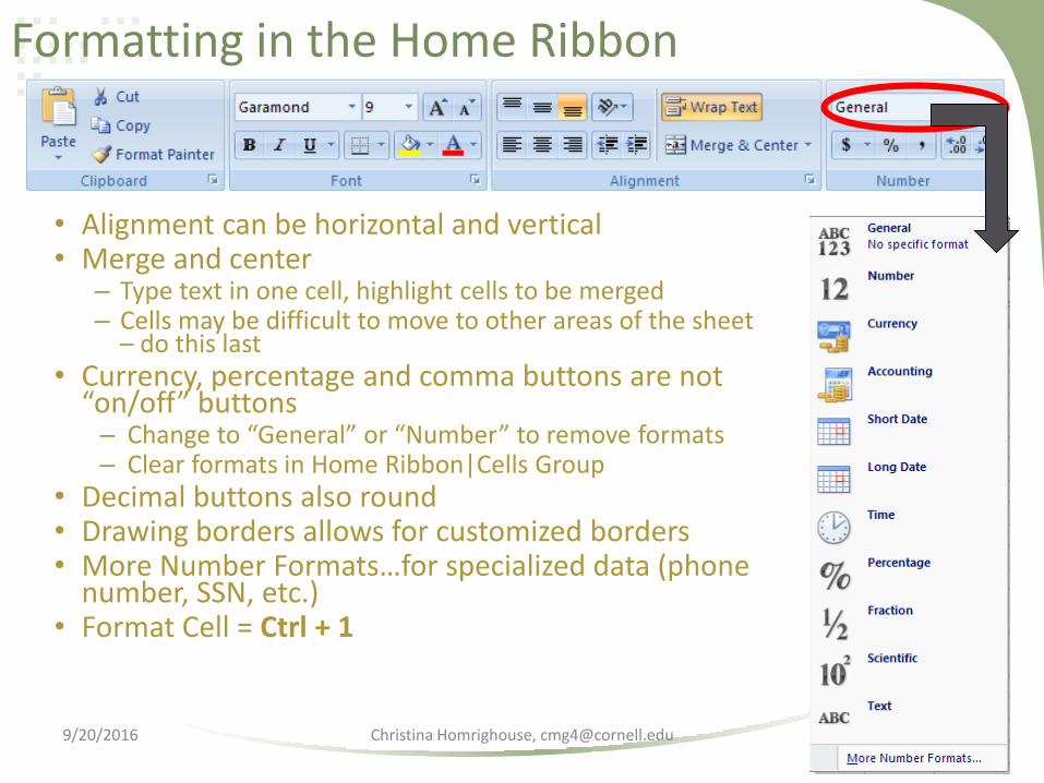
• Alignment can be horizontal and vertical• Merge and center

– Type text in one cell, highlight cells to be merged– Cells may be difficult to move to other areas of the sheet

– do this last• Currency, percentage and comma buttons are not

“on/off” buttons– Change to “General” or “Number” to remove formats– Clear formats in Home Ribbon|Cells Group

• Decimal buttons also round• Drawing borders allows for customized borders• More Number Formats…for specialized data (phone

number, SSN, etc.)• Format Cell = Ctrl + 1

Christina Homrighouse, [email protected]/20/2016

Slide

Printing

• Ctrl + P goes to Print Preview where most print options can be changed

– Common commands already available

– Use Page Setup for more customized settings

• Margins: centering

• Header/Footer: add common information such as date and page numbers and customize

• Sheet: set print titles and print area (MUST use Page Layout Ribbon for these), grid lines and column and row markers

• Page Layout Ribbon also has print options…but need to go to Print Preview to see the results of any changes

• To specify a range

– Page Layout|Page Setup Group|Print Area Button

– Settings in Print Preview


Slide

Freezing Panes

• View Ribbon|Window Group|Freeze Panes

• Freeze Panes– Used to freeze rows and columns simultaneously

– Freezes rows above and columns to the left of the active cell

– If active cell is A1, window is frozen in the middle

• Regardless of position in the worksheet– Freeze Top Row

freezes top row only

– Freeze First Column freezes first column only

9/20/2016 Christina Homrighouse, [email protected] Slide 16

Slide

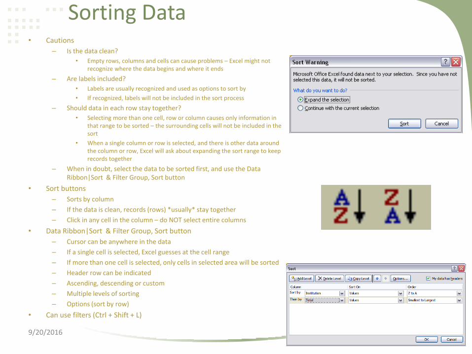
Sorting Data• Cautions

– Is the data clean?

• Empty rows, columns and cells can cause problems – Excel might not recognize where the data begins and where it ends

– Are labels included?

• Labels are usually recognized and used as options to sort by

• If recognized, labels will not be included in the sort process

– Should data in each row stay together?

• Selecting more than one cell, row or column causes only information in that range to be sorted – the surrounding cells will not be included in the sort

• When a single column or row is selected, and there is other data around the column or row, Excel will ask about expanding the sort range to keep records together

– When in doubt, select the data to be sorted first, and use the Data Ribbon|Sort & Filter Group, Sort button

• Sort buttons

– Sorts by column

– If the data is clean, records (rows) *usually* stay together

– Click in any cell in the column – do NOT select entire columns

• Data Ribbon|Sort & Filter Group, Sort button

– Cursor can be anywhere in the data

– If a single cell is selected, Excel guesses at the cell range

– If more than one cell is selected, only cells in selected area will be sorted

– Header row can be indicated

– Ascending, descending or custom

– Multiple levels of sorting

– Options (sort by row)

• Can use filters (Ctrl + Shift + L)

9/20/2016 Slide 17

SlideSlide 18

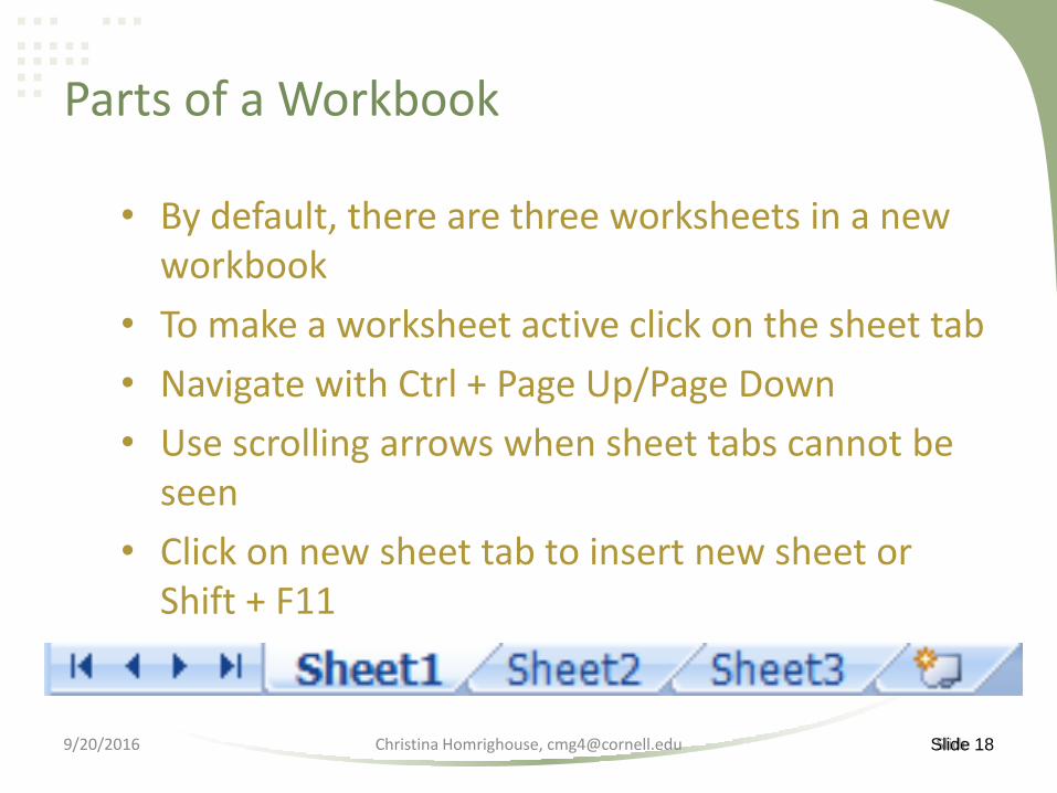
• By default, there are three worksheets in a new workbook

• To make a worksheet active click on the sheet tab

• Navigate with Ctrl + Page Up/Page Down

• Use scrolling arrows when sheet tabs cannot be seen

• Click on new sheet tab to insert new sheet or Shift + F11

Parts of a Workbook


SlideSlide 19

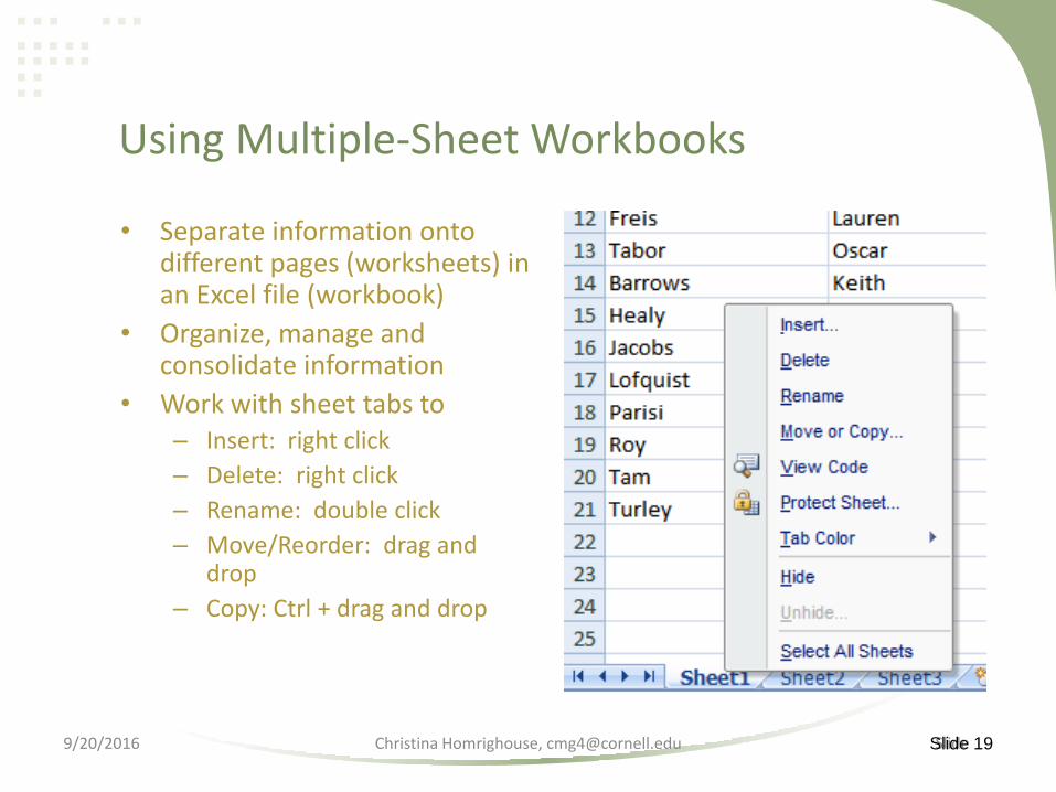
Using Multiple-Sheet Workbooks

• Separate information onto different pages (worksheets) in an Excel file (workbook)

• Organize, manage and consolidate information

• Work with sheet tabs to– Insert: right click

– Delete: right click

– Rename: double click

– Move/Reorder: drag and drop

– Copy: Ctrl + drag and drop


SlideSlide 20

What is a Function?

• A function is a substitute for entering lengthy or complicated formulas

• Excel’s function categories include

DatabaseDate & TimeFinancial

Math & TrigStatisticalText

InformationLogical Lookup & Reference


Slide

The Sum Function

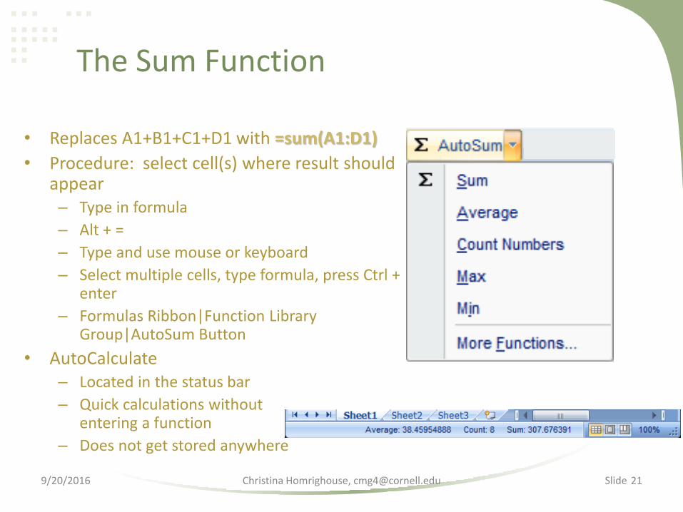
• Replaces A1+B1+C1+D1 with =sum(A1:D1)

• Procedure: select cell(s) where result should appear– Type in formula

– Alt + =

– Type and use mouse or keyboard

– Select multiple cells, type formula, press Ctrl + enter

– Formulas Ribbon|Function Library Group|AutoSum Button

• AutoCalculate– Located in the status bar

– Quick calculations without entering a function

– Does not get stored anywhere

Christina Homrighouse, [email protected]/20/2016 21

Slide

Function Basics

• = function name followed by the argument(s) in parenthesis

• Parenthesis always required; some functions have no arguments

• Arguments are separated by a comma

• Use quotes when specifying text, including spaces

• When nesting use the same number of left and right parenthesis

• Read it like a word problem

• Date and time functions may require reformatting

=SUM(A1:D1)


Slide

Entering a Function

• Methods– Insert Function button– Formulas Ribbon|Function

Library Group|AutoSum Button– More Functions…from AutoSum

button– Type = and first letter, list pops

up

• Provides list of functions• The Function Arguments dialog

box– Activated by clicking on the

Insert Function button– “Fill in the blanks” – Bold text means required– Result is shown

Formula Bar Insert Function Button

Slide 239/20/2016

Slide

VLOOKUP

• Returns a value from one data set (D1/table array) to another data set (D2) based on a value that exists in both data sets

• lookup_value– The value that exists in both data sets, select it from D2

• table_array– The first column MUST contain the lookup value– Do not need to select all data in D1 only the range which includes the lookup value and the value you

want returned– Best practice: sort in ascending order by the lookup value column (required if working with numeric

values) and name the range

• col_index_num– The column in the table array which contains the data you wish to display in D2– Column LETTERS are irrelevant, the first column, containing the lookup value is always column 1 – start

counting from there– It does not matter where the table is located n the worksheet

• range_lookup– Optional argument; best practice: always use it– TRUE: approximate match, used primarily for numeric ranges– FALSE: exact match, used primarily for text


• Copies contents (formula, text, numbers) in any direction

• If cell references are used, they change, or “adjust” when copied across or down (unless absolute)

• Allows you to quickly enter a series or sequence of data that follows a pattern

• Drag the fill handle of the cell or range• Paste options button

– Depending on type of data, options will be different

– Fill Without Formatting uses formatting of destination cell

AutoFill Feature

Fill Handle

Series

Active Cell

+

Slide

Relative Cell Addresses

• A cell reference that changes in a formula, relative to the direction in which it is copied– If a formula is copied left or right, COLUMN references change (row

references do not)

– If a formula is copied up or down, ROW references change (column references do not)

• Default when mouse or keyboard is used to enter references in formulas


Slide

Copying Formulas Using Relative Addresses

Becomes this

when

copied down

Becomes this

when

copied across

=(b6+c8)*d10

=(c5+d7)*e9=(b5+c7)*d9

COLUMNS

Change

ROWS

Change


Slide

Absolute and Mixed Cell Addresses

• A cell reference in a formula that does not change when the formula is copied or cut

• In the reference, the column and/or row is preceded by a dollar sign– Type the $ sign or

– Select the reference(s) and press the F4 key

• The $ “locks” the column and/or row and it cannot change when copied

• Reference will change when– Rows or columns are inserted

– Data in a referring cell is moved

• Why use absolute references?– For CLARITY and EFFICIENCY

• Creating formulas that continually reference the same cell(s), such as a “constant”

• It is easier to understand and update a calculation when the values used can be seen and referenced on the worksheet

– Because results will be INCORRECT if mixed or absolute references are not used


Slide

Copying Formulas Using Absolute or Mixed Addresses

=($b$5+$c7)*d$9 =($b$5+$c7)*e$9

=($b$5+$c8)*d$9

Only COLUMNS change

when copied across, so:

• Rows 5, 7 and 9 would never

change when copied across

• Columns B and C are

locked/absolute, and will not

change

• Column D becomes column E

because it is not

locked/absolute

Only ROWS change

when copied down, so:

• Columns B, C and D would never

change when copied down

• Rows 5 and 9 are locked/absolute,

and will not change

• Row 7 becomes row 8 because it is

not locked/absolute


Slide

Types of Cell References

• Relative: A1– Columns change when copied across (becomes B1)

– Rows change when copied down (becomes A2)

• Absolute: $A$1– Neither columns OR rows change when copied across or down

(remains $A$1)

• Mixed: A$1 (only row is locked)– Column changes when copied across (becomes B$1)

– Row does not change when copied down (becomes A$1)

• Mixed: $A1 (only column is locked)– Column does not change when copied across (becomes $A1)

– Row changes when copied down (becomes $A2)


Slide

Using Business Graphics

• Most people are visual learners– Graphics clarify

– Graphics are easier to interpret (or at least they should be!)

• Graphics are produced in a variety of formats to suit specific needs


Line Charts: Plots trends or show changes over

a period of time

Bar or Column Charts: Compare one

data element with another data element

Pie Charts: Used to show the

proportions of individual components

compared to the total

Scatter Plot Charts: Shows how one or more

data elements relate to another data element


Slide

Principles of Business Graphics

• Simplicity: Only use graphics that help to clarify your point

• Unity/Relational: Graphics must clearly relate to the data

• Emphasis: Use emphasis sparingly to draw attention to certain elements or trends

• Balance: Ensure balance within the chart and in relation to the page


Slide

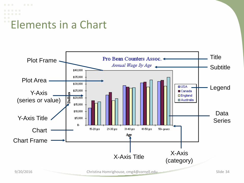
Elements in a Chart

Plot Area

Plot Frame

Y-Axis Title

Chart

Chart Frame

Y-Axis

(series or value)

X-Axis TitleX-Axis

(category)

Data

Series

Legend

Title

Subtitle


Slide

Chart Fundamentals

• Y-axis: “series or value”

– Quantifies whatever you are plotting

– Examples – dollars, percentage, number of units, cost

– Whatever is entered as values is plotted as the series points and is used to establish the range used on the Y-axis

• X-axis: “category or label”

– Describes what is being plotted

– Examples – date, location, product, name

– Two categories result in one being used on the X-axis and one being used in the legend


Slide

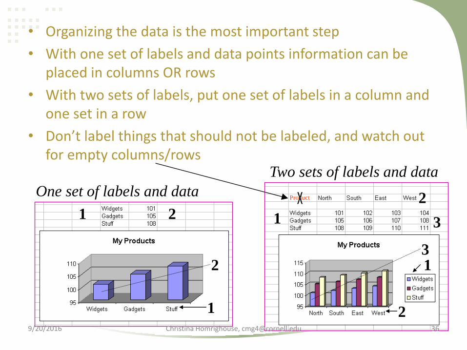
• Organizing the data is the most important step

• With one set of labels and data points information can be placed in columns OR rows

• With two sets of labels, put one set of labels in a column and one set in a row

• Don’t label things that should not be labeled, and watch out for empty columns/rows

One set of labels and data

Two sets of labels and data

1 2 1

2

3

ProductX

1

2 1

2

3


Slide

Column In columns or rows, like:

Bar

Line Lorem Ipsum

Area 1 2

Surface 3 4

Radar Or:

Lorem 1 3

Ipsum 2 4

Pie In one column or row of data and one

column or row of data labels, like:

Doughnut

(with one series) A 1

B 2

C 3

Or:

A B C

1 2 3

Pie In multiple columns or rows of data and

one column or row of data labels, like:

Doughnut

(with more than one series) A 1 2

B 3 4

C 5 6

Or:

A B C

1 2 3

4 5 6

XY (scatter) In columns, placing x values in the

first column and corresponding y

values and/or bubble size values in

adjacent columns, like:

Bubble

X Y Bubble size

1 2 3

4 5 6

Stock In columns or rows in the following

order, using names or dates as labels:

high values, low values, and closing

values

Like:

Date High Low Close

1/1/2002 46.125 42 44.063Or:

Date 1/1/2002

High 46.125

Low 42

Close 44.063


Slide

Creating a Chart

• Charts can be created as a separate sheet in a workbook

• Charts can be embedded on an existing worksheet, which gets layered, similar to a graphic image

• Select the data range to be charted, including labels

• If the range in non-contiguous, use the Ctrl key

• Insert Ribbon|Charts Group


Slide

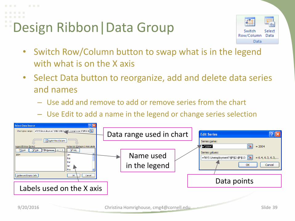
Design Ribbon|Data Group

• Switch Row/Column button to swap what is in the legend with what is on the X axis

• Select Data button to reorganize, add and delete data series and names– Use add and remove to add or remove series from the chart

– Use Edit to add a name in the legend or change series selection

Name used in the legend

Data pointsLabels used on the X axis

Data range used in chart


Slide

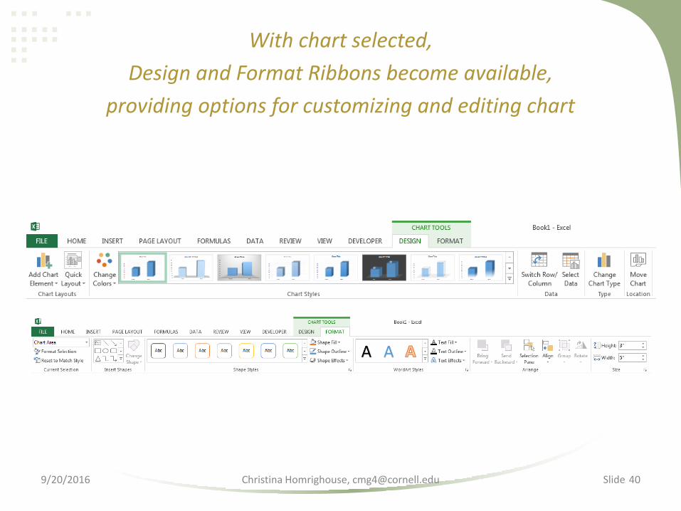
With chart selected,

Design and Format Ribbons become available,

providing options for customizing and editing chart


Slide

Formatting shortcut buttons become are on the chart and expand to provide further formatting options

Chart Elements

Chart Styles

Chart Filters


Slide

Printing a Chart

• A Chart Sheet– Design|Location Group|Move Chart Button to place in separate sheet

– Select the chart sheet to print

• An Embedded Chart– If nothing is selected, all data and the chart will print

– To print only the chart, select the chart


Slide

What is a Pivot Table?

A way to organize, filter andsummarize large amounts ofdata without effecting orrearranging the original data


Slide

The Terminology

• Source list: where the data comes from– Excel file

– External database

– Another pivot table

– Crosstab table in Excel

• Field: a category of data (usually organized in columns in the original worksheet), which contains a limited number of unique entries– Row or Column Field: describes layout of table

– Page Field: filters overall table

– Data Field: the data you wish to summarize (salary, age, sales); must be numeric

• Item: an element in a field (a cell)


Slide

Column Field

Row Field

Page Field

Data Field (Average Salary)

Fields =

• Page: Education Level

• Column: M/F (gender)

• Row: Source of Employment


Slide

Creating a Pivot Table

• Have at least one set of data that has a limited number of types of entries

• Label each field

• Place the cursor somewhere in the data set

• Insert|PivotTable and PivotChart Report

• Select data source


Layout Classic Layout

• Enables direct drag and drop onto the table

• Pivot Table Button|Options|Display Tab –Classic Pivot Table

• Can also drag to field area

Use field area to drag and drop fields

Format by selecting field once it is placed here

Modify with Options and Design Ribbons

Slide

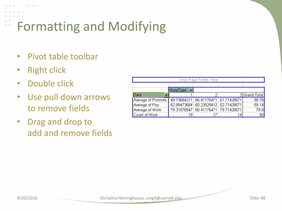
Formatting and Modifying

• Pivot table toolbar

• Right click

• Double click

• Use pull down arrowsto remove fields

• Drag and drop to add and remove fields


budgeting and quantifying data - cornell university · – select the first range/cell then use...

Documents