Bubbles for Fama*

Robin Greenwood, Andrei Shleifer, and Yang You

Harvard University

Revised, February 2017

Abstract

We evaluate Eugene Fama’s claim that stock prices do not exhibit price bubbles. Based on US industry returns 1926-2014 and international sector returns 1985-2014, we present four findings: (1) Fama is correct in that a sharp price increase of an industry portfolio does not, on average, predict unusually low returns going forward; (2) such sharp price increases predict a substantially heightened probability of a crash; (3) attributes of the price run-up, including volatility, turnover, issuance, and the price path of the run-up can all help forecast an eventual crash and future returns; and (4) some of these characteristics can help investors earn superior returns by timing the bubble. Results hold similarly in US and international samples.

* We thank Randy Cohen, Josh Coval, Harry DeAngelo, Eugene Fama, Niels Gormsen, Sam Hanson, Owen Lamont, Juhani Linnainmaa, Yueran Ma, Lubos Pastor, Jeremy Stein, Adi Sunderam, Tuomo Vuolteenaho, and seminar participants at the University of Chicago, the University of Southern California, and the Federal Reserve Bank of Boston for their helpful suggestions. We are especially grateful to Niels Gormsen for extensive advice on Compustat Xpressfeed and independent replication of the results.

2

“For bubbles, I want a systematic way of identifying them. It’s a simple proposition. You have to be able to predict that there is some end to it. All the tests people have done trying to do that don’t work. Statistically, people have not come up with ways of identifying bubbles.”

-- Eugene F. Fama, June 20161

I. Introduction

The eminent financial economist Eugene F. Fama does not believe that security prices

exhibit price “bubbles,” which he defines in his Nobel Lecture as an “irrational strong price

increase that implies a predictable strong decline” Fama 2014, p. 1475). He calls the term

“treacherous.” Fama’s argument, in essence, is that if one looks at stocks or portfolios that have

gone up a lot in price, then going forward, returns on average are not unusually low. Fama’s

conclusion runs contrary to a long literature studying bubbles historically (e.g., Mackay 1841,

Galbraith 1955, Kindleberger 1978, Shiller 2000), as well as many modern theoretical, empirical,

and experimental investigations. But is it correct?

In this paper, we seek to address this question. In particular, we look at all episodes since

1928 in which stock prices of a US industry have increased over 100% in terms of both raw and

net of market returns over the previous two years. We identify 40 such episodes in US data. We

examine the characteristics of these portfolios as well as their performance going forward, just as

Fama recommends. We then repeat the exercise for international sector portfolios between 1987

and 2013 to see if the US findings obtain out of sample.

We present four main findings. First, Fama is mostly right in that a sharp price increase

of an industry portfolio does not, on average, predict unusually low returns going forward.

Average returns following a price run-up approximately match those of the broader market in the

following two years, and are unremarkable in raw terms as well. The historical accounts are

typically based on burst bubbles, and do not take into consideration the fact that many industries

that have gone up in price a lot just keep going up. The famed technology bubble of the late

1990s is one that has actually burst. In contrast, health sector stocks rose by over 100% between

1 Chicago Booth Review, June 30, 2016. Available at http://review.chicagobooth.edu/economics/2016/video/are-markets-efficient

3

April 1976 and April 1978, and continued going up by more than 65% per year on average in the

next three years, not experiencing a significant drawdown until 1981.

Second, although sharp price increases do not predict unusually low future returns, they

do predict a heightened probability of a crash. If we define a crash as a 40% drawdown

occurring within a two-year period—a definition that captures many famous price run-ups and

their crashes—then going from 50% industry net of market return in the previous two years to

100%, the probability of a crash rises from 20% to 53%. If we focus on episodes with a 150%

industry net of market return, the probability of a crash rises to 80%. We show that this increase

in the likelihood of a crash goes beyond what one would expect based solely on the past

volatility of returns, and far exceeds the unconditional probability of an industry crashing. The

predictability of a future crash from past industry returns suggests that Fama’s conclusion should

be interpreted carefully, as it implicitly draws a distinction between future returns and the

likelihood of a crash.

The reasons for the difference in results between returns and crash probabilities are two-

fold. First, as already noted, some industries just keep going up, and do not crash at all.

Second, as importantly, bubble peaks are notoriously hard to tell, and prices often keep going up,

at least for a while, before they crash, leading to good net returns for an investor who stays all

the way through. As Fama (2014, p. 1476) points out, Robert Shiller “called” the US stock price

bubble in December 1996, and prices proceeded to double after that. At its low, in 2003, US

stock price index was higher than when Shiller first called the bubble. In our data, we find that

even of the 21 episodes in which a crash does occur ex post, on average prices peak 6 months

after we first identify the industry as a potential bubble candidate. The average return between

the first identification of the price run-up and the peak price is 30%, confirming the adage that it

is difficult to bet against the bubble, even if one can call it correctly ex ante.

This leads to a third lens through which we evaluate Fama’s conclusions. Curiously for

the inventor of three forms of market efficiency, Fama only looks at the weak form in his

assessment of “bubbles”. Of course, investors looking at industries with large price increases

have a good deal of other information at their disposal, such as turnover, issuance, patterns of

volatility, and fundamentals. This raises the obvious semi-strong form market efficiency

4

question: in conjunction with an observation of a rapid price increase, can any of this information

be helpful for predicting crashes or future returns?

To answer this question, we again distinguish between forecasting crashes and

forecasting future returns. We examine characteristics of industry portfolio growth episodes,

most of which have been discussed to some extent in earlier work. These include: volatility (in

levels and changes), turnover (in levels and changes), age of firms in the industry, the return on

new companies versus old companies, stock issuance, the book-to-market ratio, sales growth,

and the market price-earnings ratio. We also propose a new variable, “acceleration”, based on the

abruptness of the price run-up.

Our third finding is that many of these characteristics vary systematically between

episodes in which prices keep rising, and those in which they ultimately crash. In particular, run-

ups that end in a crash are more likely to have increases in volatility, stock issuance, especially

acceleration, associated increases in the market P/E, and disproportionate price rises among

newer firms. We find no ability of fundamentals (as proxied by sales growth) to help distinguish

between episodes.

We then investigate whether these characteristics can help a savvy investor earn superior

returns by timing the bubble. In other words, with all the difficulties of calling the top, can one

still identify characteristics of portfolios that will earn low returns, on average? Our fourth

conclusion is that, indeed, some characteristics of sharp price rise episodes do help predict future

returns. Looking at the same characteristics as before, we find that, in line with Fama’s broad

thrust, some of these attributes are not predictive of future returns. In particular, share turnover

tends to be high in the price run-ups that crash, but also in the price run-ups that do not. Sales

growth, which presumably measures fundamentals, does not help identify which episodes will

crash (although it has some forecasting power in international sample). At the same time several

variables do help predict which bubbles both crash and earn low returns. Increases in volatility,

issuance, the relative performance of new versus old firms, and acceleration tend to be predictive

characteristics. It is still the case that we cannot call the peak of the bubble, and some of the

portfolios we examine keep going up. Nonetheless, investment strategies that condition on high

past returns in combination with these characteristics exceed the returns to a passive buy-and-

hold all industries strategy by 10 percentage points or more on a two-year or longer basis.

5

A significant concern with our analysis is statistical power. Large price run-ups, by

nature, are rare—we identify only 40 of them in all of US stock market history since 1928.2 With

the benefit of hindsight, we can surely point to some common elements in these events, with

potentially dubious predictive value going forward. We have two responses to this concern. First,

we examine international industry data between 1986 and 2013 as an out-of-sample test. We

confirm that in the international data as well, price run-ups do not forecast average returns, but

they are associated with a substantially elevated probability of a crash. More importantly, several

of the features of price run-ups that predict crashes in the US – high volatility and share issuance

– also have predictive value in the international data. Second, in the spirit of Bonferroni (1936)

and Dunn (1959), we conduct statistical tests to adjust for the “multiple comparison problem”,

which holds that some of the characteristics predicting returns we uncover do so by chance

because we are studying many at the same time. We address this problem by controlling for the

false discovery rate, which is the percentage of characteristics that are expected to be Type-I

errors. Even with these adjustments, and despite the limited number of observations, at least five

characteristics emerge as predictive of future returns.

To sum up, our evidence suggests that Fama is correct in his claim that a mere price

increase does not predict low returns in the future. But even from this perspective, he is not

correct that there is no predictability, since sharp price increases do predict a heightened

likelihood of a crash. More importantly, returns are in fact predictable, since there are other

attributes of well-performing portfolios that in fact help distinguish portfolios that earn low and

high returns going forward. Based on this information, there are times when one can call a

bubble with some confidence.

Our broad conclusion is one that historians – particularly Kindleberger -- have reached

already. There is much more to a bubble than a mere security price increase. There is

innovation, displacement of existing firms, creation of new ones, and more generally a

“paradigm shift” as entrepreneurs and investors rush toward a new Eldorado. Our contribution is

to show that this shift is to some extent measurable in financial data. And because one can

2 For this reason, bubbles are not a particularly fertile field for testing market efficiency. Market efficiency is much more effectively tested by looking at the violations of the law of one price (e.g., Lee, Shleifer, and Thaler 1991 for closed end funds, Froot and Dabora 1999 for dual listing stocks, or Lamont and Thaler 2003 for spinoffs).

6

measure it, one can also identify – imperfectly but well enough to predict returns – asset price

bubbles in advance.

Our paper is related to several lines of research in finance. First, a large literature

uses characteristics to forecast industry returns, especially industry momentum, although we

differ from most of these papers by focusing on episodes subsequent to a large price run-up.3

More recently, Daniel, Klos, and Rottke (2016) show that some high momentum stocks

subsequently experience violent crashes. Second, there have been many empirical studies of

individual bubbles, and especially the most recent .com episode of the late 1990s.4 Our paper

helps ask whether some of the findings from these studies (such as patterns of high issuance and

trading volume) generalize. A few papers have also suggested that some apparent bubble

episodes can be reconciled with rational asset pricing, either because of cash flow forecasts or

changes in discount rates (Garber 1990; Pastor and Stambaugh 2006, 2009). Others have

suggested that high prices during bubble episodes might be driven by a combination of risk

premia and learning (Pastor and Veronesi 2006, 2009). Third, some research has tried to forecast

market crashes using characteristics such as past skewness, returns, or trading volume (Chen,

Hong, and Stein 2001). Fourth, Goetzmann (2015) studies rapid price increases of national stock

markets and their subsequent returns, but not characteristics of these markets beyond the price

run-up. Finally, our paper connects to a vast theoretical literature on bubbles, including De Long

et al (1990), Abreu and Brunnermeier (2003), Scheinkman and Xiong (2003), and Barberis,

Greenwood, Jin, and Shleifer (2016). To be sure, there is a lot of research in finance on so-called

rational bubbles (e.g., Blanchard and Watson 1982, Tirole 1985) but recent evidence has not

been kind to these theories (Giglio, Maggiori, and Stroebel 2016).

II. Average Returns after Price Run-ups

We start by identifying in US industry data all episodes in which an industry experienced

value-weighted returns of 100% or more in the past two years, in both raw and net of market

3 See Grinblatt and Moskowitz (1999), Asness, Porter and Stevens (2000), Hou and Robinson (2006), Hong, Torous, and Valkanov (2007), Greenwood and Hanson (2012), among others.

4 Ofek and Richardson (2003), Brunnermeier and Nagel (2004), Pastor and Veronesi (2006), Griffin, Harris, Shu, and Topaloglu (2011),

7

terms, as well as 50% or more raw return over the past five years. We require high returns at

both a 2- and 5-year horizon to avoid picking up recoveries from periods of poor performance.

Our database includes returns from January 1926 to March 2014. This allows us to identify every

price run-up episode between January 1928 and March 2012, because we require a two-year

return to identify price run-ups and a two-year price path afterward to classify collapses and

evaluate the performance of trading strategies.

Our choice of 100% returns is meant to conform to Fama and others’ notion that a

bubble, if it exists, begins with a large price run-up. A return threshold of 100% is able to pick up

most episodes that historians have suggested were bubbles ex-post, such as utility stocks in 1929,

and .com stocks in the late 1990s. We require both high raw and high net-of-market performance

so as to avoid classifying as a potential bubble an industry with modest or flat performance

during a time when the market performed poorly. Below we discuss how our conclusions depend

on the return threshold we choose.

Our unit of analysis is an industry, identified according to the Fama and French (1997)

49-industry classification scheme (although the precise industry identification scheme is not

important for our results)5. We use the first 48 of their industries, excluding the residual industry

“other”, and restrict attention to industries with 10 or more firms, to ensure that the price run-up

is experienced by multiple firms. Following standard procedure, returns are measured monthly

and based on all stocks with share codes of 10 or 11 in the CRSP database. Stocks are matched to

industries each month using the most recent SIC code on Compustat, or CRSP if not available.6

Returns are value-weighted across stocks.

5 One subtle complication is that bubbles often tend to be associated with relatively new industries, such as utilities in the 1920s or .com stocks in the 1990s. No single ex ante industry definition is likely to perfectly match to the theme of any particular bubble. For example, Fama and French’s 49 industries of “software”, “hardware”, “chips”, and “electrical equipment” all include firms that were ostensibly part of the Technology bubble. We have experimented with different definitions of industries, notably 2-digit SIC code and broader Fama-French industry aggregates, as well as GICS-industry definitions popular among investment professionals.

6 We do not match exactly the industry returns reported by Ken French on his website, because our industries include recently listed firms, which have historically been an important part of stock market bubbles. Fama and French compute industry returns from July of year t until June of year t+1 based on industry affiliation in June of year t. The unconditional correlation between their reported monthly value-weighted industry returns and ours is 97.6%.

8

We study industries for three reasons. First, most historical accounts of bubbles have a

strong industry component. White’s (1990, 2007) descriptions of the 1929 stock market boom

and subsequent bust, for example, emphasize utilities and telecommunications stocks. The stock

market boom of the late 1990s was concentrated in .com stocks (Ofek and Richardson 2003).

Second, analyzing industries gives us more statistical power than analyzing the entire stock

market, although many of the price run-ups we identify occurred during periods of good market

performance. Third, we can compare potential bubble industries to other stocks trading at the

same time. This matters because many of the industry features that we study, such as trading

volume, vary substantially over time.

Price run-ups of 100% or more are quite rare: we observe only 40 since 1928. This is not

surprising, given that the average price run-up represents a 5.5 standard deviation event7. These

40 price run-ups tend to be concentrated during particular periods, a reflection of the relatively

fine industry classifications we are using. Because the Fama-French 49 industry definitions are

quite narrow, our methodology sometimes separately identifies industries that are part of a

broader sectoral bubble. For example, our procedure separately identifies four Fama-French

industries with price run-ups in the late 1990s: Computer Software, Computer Hardware.

Electronic Equipment and Measure & Control Equipment, but all four were components of the

broader .com bubble. Ex post, it might seem reasonable to categorize the industry run-ups into a

few number of episodes, each of which encompassed a particular time and theme, such as the

1929 stock market boom which included Automobiles, Chemicals, Electrical Equipment, and

Utilities. Such ex post consolidation limits our ability to use the data for predictive purposes.

Nevertheless, we recognize that price run-up episodes are not all independent, and adjust

statistical inference by reporting standard errors and t-statistics clustered by calendar year

throughout.8 For the international data, we cluster standard errors by country-calendar year.

7 Across all episodes, we compute the ratio between returns from t-24 to t and the square root of 24 times the standard deviation of monthly returns between t-36 and t-24. The average value of this ratio is 5.5.

8 In the Appendix, we also show t-statistics based on standard errors clustered by episode, where “episode” is defined ex post for all run-ups during a two-year time period.

9

As noted, our definition of a price run-up is based on the industry value-weighted return.

This does not mean that the price run-up is limited only to the large firms in the industry. Across

the price run-ups that we study, an average of 61% of firms in the industry experience price

increases of 100% or more during the run-up period.

We separate the 40 episodes into 21 that crash in the subsequent two years, and 19 that do

not. We define a crash as a 40 percent or more drawdown in absolute terms beginning at any

point after we have first identified the price increase. This successfully identifies a number of

episodes that historians have described ex post as having been stock price bubbles, and a few

more episodes that are not as well known. Automobiles, Chemicals, and Electrical Equipment

were all part of the bubble economy of the late 1920s (White 1990, 2006, 2007). Software,

Hardware, and Electrical equipment all denote industries affected by the .com bubble of the late

1990s and early 2000s (Ofek and Richardson 2003). Coal reflects the commodity price run-up

during 2006 and 2007, followed by its dramatic collapse in 2008. All of these are cleanly

identified as sharing a rapid price run-up and subsequent collapse.9

The cutoff of two years for analyzing subsequent performance is meant to set a high bar

for calling the bubble. This relatively short window prevents us from, for example, calling an

industry a potential bubble in 1996 and claiming vindication when it crashes in 2000. This

conservative approach exposes us to Type II errors –concluding that an episode is not a bubble,

even if, for example, an industry with a price run-up in year t experiences returns of -20% per

year in each year from t+1 through t+4. In fact, because our threshold for a crash is quite high,

some of the industries we classify as not having crashed nevertheless experience mediocre

subsequent returns. For example, airlines experience a large price run-up prior to 1980 and

slightly negative returns in the 24 months thereafter, but this performance is not sufficiently poor

to be classified as a crash.

9 There are many other ways to identify a crash, which all produce similar classifications of our price run-ups into “crashed” and “non crashed.” For example, Mishkin and White suggest looking at 20% market declines over horizons of one day, one week, one month, three months, and one year.

10

Although our criteria of a 40% drawdown does not require the crash to be sudden, in

most cases it is: in 17 of the 21 episodes in which there is a crash, the industry experiences a

single-month return of -20% or worse during the drawdown period.

Figure 1 summarizes the average returns for the 40 price run-ups. The figure confirms

Fama’s central claim: a sharp price increase of an industry portfolio does not, on average, predict

unusually low returns going forward. On average, industries that experienced a price run-up

continue to go up by 7% over the next year (5% net of market), and 0% over the next two years

(0% net of market). Neither raw nor market adjusted returns are statistically distinguishable from

zero.

Figure 1 also shows average market returns during and after the industry price run-up.

Although industry run-ups tend to coincide with broad market rallies, an industry run-up is

associated with poor average subsequent market returns: across all episodes the value-weighted

market earns only 2% in the first year post-run-up, and 0% over two years. After netting out the

risk-free return, market excess returns are -2% in the first year, and -10% over two years. The

market performs particularly poorly during the episodes that we record as experiencing industry

crashes: the average two year raw market return in these 21 cases is -42%, the average two year

excess market return is -29%. Overall, the substantial correlation between large industry crashes

and market underperformance supports our approach of studying industry portfolios.

Table 1 summarizes returns for each episode, grouping episodes by whether there was an

ultimate crash or not. For the 21 industries that do crash, average returns are -5% (-3% net of

market) in the next year and -42% in the next two years (-29% net of market). The two-year

returns are more impressively negative than the one-year returns because the crash does not

necessarily come right away. This can be seen in Figure 1, which shows that the crash begins an

average of five months after we call a potential bubble. Overall, if we study only the cases in

which a crash does occur, the average return experienced between the initial price run-up and the

subsequent peak price is 30% (and is as much as 107% in the case of precious metal stocks in the

late 1970s). This confirms the adage that it is difficult to bet against the bubble, even if one has

correctly identified it as such ex ante.

11

The second panel in Table 1 shows the list of the 19 industries that experienced a price

run-up but no major crash in the subsequent two years. These industries continue to go up by an

average of 21% in the subsequent year (13% net of market), and 46% in the next two years (31%

net of market).

International Industries

As an out-of-sample test, we repeat our analysis using a sample of all international firms

with complete volume and returns in the Compustat Xpressfeed database. The international data

is not a fully independent test, since many of the price run-ups are common across countries. For

example, many countries experienced rapid price run-ups in materials and commodities related

stocks in 2007 and early 2008. However, even in episodes that are shared across industries in

different countries, the timing of the price boom and bust varies substantially.

We use all non-US stocks with complete volume and returns in the Compustat

Xpressfeed database. Stocks are matched to sectors based on their GICS-code. The GICS-sector

is a broader definition of industry than that of Fama and French (there are 11 sectors vs. 49

Fama-French industries) but this helps ensure that for smaller stock markets such as Sweden, an

industry includes a sufficient number of firms to be meaningful. As in the US, we restrict our

attention to industries with 10 firms or more. Returns are measured in US dollars (the return in

US dollar is 99.9% correlated with the return computed in local currency) terms and are value-

weighted within sectors. For these portfolios, the “market” benchmark is the local market value-

weighted return, measured in dollars, and the risk-free rate is the dollar return on US Treasury

bills. 10 The data begins in October 1985, but 88% of the observations are in 1996 or later.

Overall, the starting point is 85,226 sector-months of returns, compared to 50,451 industry-

months in our US analysis.

Following an otherwise identical methodology, we identify 107 price run-ups in 31

countries between October 1987 and December 2012, summarized in Table 2. Of these price run-

ups, 53 crash and 54 do not. Average returns to the crashed and non-crashed samples are 10 We use dollar returns rather than local currency returns to avoid picking up potential bubbles during high inflation periods in some countries. Stocks are classified by country of their headquarters. We only use securities that are traded on exchanges in their home country, i.e., we exclude ADRs and equivalents.

12

surprisingly close to those of the US sample despite different industry definitions and sample

years. Figure 2 shows that Fama’s central claim holds up in the international data as well: a sharp

price increase of an industry portfolio does not, on average, predict unusually low returns going

forward. Across all price run-ups, these sectors experience an average return of 1% (2% net of

market) in the next year, and 7% (0% net of market) in the next two years. In short, our

conclusion about average returns drawn from US industries also holds in the international data.

Because there are too many international episodes to list them individually, Table 2

summarizes price run-up episodes by country. As before, we start with the episodes in which

there was a subsequent crash. For these episodes, average one-year returns following the price

run-up are -23% (-5% net of market); average two-year returns are -38% (-13% net of market).

These industries experience an average maximal drawdown of -65% in the two-year period

following the price run-up. As with the US sample, the drawdown is more severe than average

return because the price run-up is not a sufficient statistic to perfectly identify the peak. Consider

the .com bubble, which is identified at different times in Germany, the United Kingdom, Japan,

France, Hong Kong, Singapore, Norway, and Switzerland. In Germany, we first observe a large

price run-up in March 1998, a full 23 months before the bubble peaks in February 2000. In

Singapore, Norway, and Switzerland, our price run-up screen of 100% correctly identifies the

peak. On average, the period between the initial price run-up and the price peak is 4.1 months,

with a 38% subsequent return until the price peak, similar to that in the US sample.

Turning to the international episodes in which there is no crash in the two years post-

price-run-up, average one-year returns are 24% (10% net of market); average two-year returns

are 51% (13% net of market), and these industries experience an average maximal drawdown of

only 22 percent. The best performing industries include IT in India, which experienced a first

price run-up of 100% between June 1997 and June 1996, and subsequent returns of 436% until

the price peak, in part because the entire stock market boomed; and Consumer related stocks in

Austria, which continue to rise by another 307% (172% net of market) in the two-year period

following the initial price run-up.

Sensitivity to Degree of Price Run-up

13

How sensitive is our conclusion about average returns to the 100% past return cutoff? In

Table 3, we list raw, excess (of the risk free rate) and net-of-market returns for the 12- and 24-

month period subsequent to the price run-up; average post-run-up returns for both US industries

and international sectors are based on different return thresholds. As in Table 1 and Table 2, for a

given return threshold, we require both value-weighted raw and net of market industry returns to

excess this threshold in a two-year period. In the appendix, we provide summary statistics for

different ways of identifying price run-ups (such as based on raw returns alone, or based on price

run-ups of three standard deviations or greater), with similar results.

For return cutoffs under 100%, our conclusion remains that Fama is correct about average

returns. Average net-of-market returns in the 24 months following the price run-up average less

than 4%, whether our cutoff for a price run-up is 50%, 75% or 100%. But if we increase the

cutoff to 125% or 150%, these returns drop below -13% in US sample. In the 15 incidents of a

150% price run-up in US data, average raw returns over the subsequent 12 and 24 months were -

10% and -13%; average net of market returns were -9% and -10%, and average excess returns

were -17% and -28%, both one year performance statistically significant at the 10% level. The

general pattern is that subsequent returns fall as the ex-ante threshold rises.

Panel B in Table 3 shows that we obtain similar findings when we study international

sectors. Using a 150% return threshold, we identify 51 price run-ups, with subsequent returns of

-15% in 12 months and -17% in 24 months, and excess returns of -18% and -23%, with both

statistically below zero at the 10% significance level.

In short, our earlier conclusion that Fama is correct about average returns must be

substantially tempered, because in the two years following very high past returns, excess returns

subsequent to the price run-up are negative.

III. Probability of a Crash Following a Price Run-up

While average returns following a 100% price run-up are roughly zero, Table 1 shows

that slightly more than half of the industries experience a crash in the subsequent two years, with

a similar proportion crashing among international sectors. A crash probability of one half is

14

substantially higher than the unconditional probability of a crash in our data. Averaging across

all industry-months between 1928 and 2013, the unconditional probability of a crash in any two-

year period is 14%, and 11% after 1970, the midpoint in the sample. The unconditional

probability of a crash among international sectors is higher, at 24%.

In this section, we show that the probability of a crash is strongly associated with high

past returns. In fact, for very high past returns (such as 150% in a two-year period), a crash is

nearly certain, although its timing is not.

Figure 3 shows simple kernel density plots of the probability of a crash conditional on

past returns. The underlying sample contains all industry months in which past returns were

positive and the industry in question had at least ten firms. Panel C and D repeat the analysis

using international sector returns, with nearly identical results.

Panel A shows the probability of a crash as a function of the industry return net of

market; Panel B shows the probability as a function of the past raw return. As before, a crash

event takes on a value of 1 if the industry experiences a 40% or greater drawdown at any point in

the next 24 months. Panel A shows that the probability of such a crash is approximately 20% at

past net of market returns of 50% or less, but then rises rapidly to 35% at past net of market

returns of 100%, and increases further at higher return thresholds.

In addition to average returns that we discussed earlier, Table 3 also summarizes the

crash probability as a function of past industry return. As in Tables 1 and 2, for a given return

threshold, we require both value-weighted raw and net of market industry returns to exceed the

return threshold in a two year period.11 At a past return threshold of 50%, only 20% of episodes

crash in US industries and 36% in international country-sectors, only slightly above the

unconditional crash probabilities. However, the probability of a crash increases substantially

with past returns, from 20% to 53% in US industries, and from 36% to 50% in international

sectors. As we increase the threshold further to 150%, we identify fewer price run-ups of this

magnitude, but a higher percentage of them crash. Of the 15 episodes in which there was a 150% 11 Because we require both net of market returns and raw returns to exceed the threshold, the crash probabilities do not exactly match those shown in the kernel density plots in Figure 3, but the overall pattern of crash probability substantially increasing as a function of past returns is evident in both the figure and the table.

15

price run-up observed in US data, 80% crashed in the subsequent two years. Among international

sectors, 67% of the 51 episodes with 150% price run-ups subsequently experienced a crash. Our

findings of elevated crash probabilities following price run-ups are similar to those in

Goetzmann (2015), who studies returns following one-year 100% price increases in national

stock markets. He too finds an elevated probability of a crash, but the magnitudes are modest.12

Our finding that crash probability is related to the size of the price run-up may be in part

a reflection of high industry volatility: highly volatile industries are surely more likely to

experience both booms with very high returns and crashes with very low returns, even if a boom

is not predictive of a crash. Close inspection of Figure 3 suggests this is not a concern: there is

almost no difference in crash probability between episodes with a 0% and a 50% price run-up,

but enormous differences between a 50% and 100% price run-up. We can alternately estimate

regressions of the form

,%][ 11 itititit ucXRbaCrash ++>⋅+= −− s (1)

where Crash takes a value of 1 if the industry experiences a 40% drawdown at any point

between month t and month t+24. [Rit-1>X%] denotes a dummy variable that takes a value of 1 if

the industry’s return (or net-of-market return) is greater than a threshold X, and σ denotes

volatility of returns prior to the price run-up. We estimate (1) using the same data as was used for

the kernel plots in Figure 3, and where σ is estimated using one year of monthly industry returns

ending just before the run-up period.13 These regressions are similar to Chen, Hong, and Stein

(2001) who estimate panel regressions to forecast negative skewness at the individual stock

level. We estimate equation (1) with and without the volatility term on the right-hand-side.

Whether our past return threshold X is 50%, 75%, 100%, 125% or 150%, we find that controlling

for lagged volatility slightly attenuates the coefficient on past returns, but the effect is modest.

12 Apart from the differences in sample, our results are different from Goetzmann’s because we distinguish between a crash and low returns. Our definition of a crash is a 40% drawdown at any point in the subsequent two years. If such a drawdown occurs after continued price run-up, total returns post price run-up may be modest (even positive) despite the presence of a crash. 13 We have experimented with different forms of the volatility control with little effect.

16

For example, for a return threshold of 100%, controlling for volatility reduces the coefficient on

past return from 0.712 to 0.621. The results for all return thresholds is presented in the Appendix.

The data thus show that crashes are much more predictable than returns: what explains

this? First, as shown in Table 1 and 2, some industries just keep going up, and do not crash at all.

Second, for the episodes with a crash, prices often keep going up, at least for a while before the

crash occurs. This leads to modest returns for an investor who holds the full way through. Figure

4 shows this result more formally across all 21 of our crash episodes. Here we plot “event-time”

returns for the 21 episodes in which there was an eventual crash. In each episode, event-time of

zero denotes the end of the month in which we first notice a large price run-up. Then, for each

price run-up, we mark with a square the month with the peak cumulative return prior to the start

of the crash. As can be seen, there is considerable heterogeneity between episodes in how long it

takes before the crash starts. Not surprisingly, average returns are much lower for the episodes in

which the crash comes sooner. For example, for the nine episodes in which the crash begins

within three months, average one-year raw returns are -41%, while for the remaining episodes,

average one-year raw returns are 22% --- vastly different experiences for an investor betting

against the bubble! At a two-year horizon, the question of when the crash begins is less

important: for the 9 episodes in which the crash begins within 3 months, average two-year

returns are -49%, compared to -37% for the remaining episodes.

The evidence that larger industry stock prices increases are associated with sharply higher

probabilities of a crash is not, by itself, dispositive on the question of market efficiency. After

all, it is possible that investors update their valuations of new industries in response to positive

news until and unless they learn something that disappoints them. Still, the crash evidence casts

doubt on at least some leading models of bubbles. First, in the models of rational bubbles, the

probability of a crash is usually taken to be constant. Unlike in the data, it does not increase with

past returns. Second, in the rational model of “bubbles” of Pastor and Veronesi (2009), the stock

price decline comes when an industry becomes a large part of the economy, and its cash flows

become systematic, leading to high discount rates. Since discount rates are likely to change

smoothly, this model does not naturally explain abrupt crashes that we see in the data.

Moreover, changes in discount rates can perhaps explain the magnitude of a crash but not its

probability that we find in the data. In contrast, behavioral models such as Barberis et al. (2016),

17

in which larger run-ups are associated with larger deviations of prices from fundamental values,

naturally explain the evidence on the higher probability of a crash.

IV. Characteristics of Price Run Ups and Crashes

Investors looking at industries with large price increases have a good deal of information

at their disposal beyond price, such as turnover, issuance, patterns of volatility, and

fundamentals. In this section, we draw on narrative accounts of bubbles from Mackay (1852),

Kindleberger (1978) and others, as well as studies of the .com bubbles of the late 1990s, to

systematically construct non-price features of the price run-ups identified in the last section. Our

first objective is to establish whether any of these characteristics differ systematically between

price run-ups that subsequently crash, and price run-ups that do not. In Section V, we ask

whether these additional characteristics also help forecast future average returns, meaning

whether an investor can use the information to time a potential bubble.

We consider characteristics of six types, all but one motivated by prior accounts of

bubbles, and partially driven by data availability (since we require the characteristics to be

available as far back 1926 in the US data). Our first measures are related to trading volume and

volatility, which some studies find to be elevated during recent bubbles (Hong and Stein 2007).

Second, bubbles may arise from new industries and paradigm shifts (Kindleberger 1978; Garber

1989, 1990; Pastor and Veronesi 2006; Greenwood and Nagel 2009). We construct a variable

“age tilt”, defined below, which measures the extent to which the price run-up is concentrated

among younger firms. Third, some authors have suggested that during periods of extreme

mispricing, firms issue additional equity, both to take advantage of such mispricing and to fund

investment opportunities (Ritter 1995; Baker and Wurgler 2000; Pontiff and Woodgate 2008).

Fourth, a vast empirical literature shows that scaled price variables (such as P/E or book-to-

market ratios) help forecast average return in the cross-section of equities (Fama and French

1992, 1993). Fama and French provide book equity value for firms between 1926 and the 1960s

(when they become available more broadly on Compustat), allowing us to compute book-to-

market ratios for most industries in our sample. We also include a measure of market

valuations, the Shiller cyclically adjusted price-earnings ratio (CAPE). Fifth, we measure

fundamentals using sales growth across the industry, beginning in 1951 when the data becomes

available from Compustat. Last, we create a new variable to capture the acceleration of the price

18

path. Here we have in mind that the past 24-month return only coarsely captures the path of

prices. A return of 100% over 3 months may be more likely to end in a crash than one accrued

more steadily over a two-year period.

Measuring bubble features systematically is a data challenge. We must respect secular

changes in the data, such as vast increases in trading volume between 1925 and today, or large

time-series variation in idiosyncratic volatility (Campbell, Lettau, Malkiel, Xu 2001), while at

the same time comparing episodes that occur at different times. For example, our construction of

characteristics must allow us to compare the run-up in utility stocks in 1929 with that of .com

stocks in the late 1990s. These concerns loom particularly large for volatility, turnover, and age.

We have experimented with two ways to deal with this challenge. The first is to compute

the percentage change of that characteristic (say, volatility or turnover) compared to its average

value in the year prior to when the price run-up began. The second approach is to use a purely

cross-sectional measure of each characteristic by comparing the industry to other industries at the

same time. The former emphasizes time-series changes in industry attributes, while the latter

emphasizes contemporaneous differences between industries. Both can be heavily impacted by

the listings of new firms if the new firms differ in their characteristics from existing firms in the

industry. In practice, both ways of measuring industry characteristics lead us to similar

conclusions. For example, as documented by Hong and Stein (2007), .com stocks experienced an

increase in trading volume between 1997 and 1999, but also had high trading volume compared

to other industries in 1999. Below we present results based on cross-sectional comparisons, but

the Appendix presents results for time-series adjusted comparisons.

We define the following characteristics:

Volatility: Each month, we compute volatility of daily returns of each stock in the

industry. Let X denote the percentile rank of volatility in the full cross-section of firms. Industry

volatility is the value-weighted mean of X for that industry. For example, following the 100%

price run-up over a two-year period in March 1928, the volatility rank of Automobiles was 0.63,

meaning that 63% of firms had lower volatility than the average firm in the Automobile industry

at that time.

19

Turnover: Turnover is shares traded divided by shares outstanding. For Nasdaq stocks,

due to the well-known double counting, we divide turnover by two (Anderson and Dyl 2007). To

compute industry turnover, we percentile rank monthly turnover for every stock in CRSP, and

then compute the value-weighted turnover rank for each industry. For example, turnover of the

software industry in March 1999 was 0.86, meaning that value-weighted turnover of the industry

was higher than 86% of all listed stocks.

Age: Firm age is measured as the number of years since the firm first appeared on

Compustat or on CRSP, whichever of these came first. To compute industry “age”, we percentile

rank age for every stock in CRSP, and then compute the value-weighted rank for each industry.

Age “tilt”: Because industry definitions are imperfect, this variable is meant to capture

whether the price run-up occurred disproportionately among the younger firms in the industry.

Age tilt is the difference between the equal-weighted industry return and the age-weighted

industry return.

Issuance: Percentage of firms in the industry that issued equity in the past year. A firm is

said to have issued equity if its split-adjusted share count increased by five percent or more.

Issuance was elevated in many, but not all, price run-ups. In March 1999 in the Software

industry, Issuance was 48%, meaning that 48% of the firms in the industry had either gone public

or issued at least 5% new stock in the most recent year.

Book-to-market ratio: We use book-to-market ratio mainly because we can compute it for

all stocks going back to the 1920s, relying on Ken French’s book equity data for firms between

1925 and 1965.

Sales growth: For firms with at least two years of revenue data ending in in the month of

the price run-up or before, we calculate the one-year sales growth based on the most recent two

observations, and then compute the value-weighted rank for each industry. By construction, this

this omits information on newly listed firms for which we do not have two years of data.

CAPE: The cyclically-adjusted market price-earnings ratio in the month in which the

price run-up is identified, available on Robert Shiller’s website. International CAPE series are

available through Global Financial Data, covering 30 countries in our sample.

20

Acceleration: This measures the convexity of the price path. We define it as the

difference between the two year return and the return for the first year of that two year period Rt-

24→t - Rt-24→t-12. This measures how much of the price appreciation has occurred most recently.

Because our measures for volatility, age, turnover and sales growth are based on

percentile ranks, by construction the equal-weighted mean of each characteristic is 0.50 at all

points in time. The remaining variables, have a construction which is more time invariant, and so

we use these variables in their natural units.

Figure 5 plots these characteristics for the 40 industry price run-ups that we identify in

US data. For each characteristic, the left panel plots means for the industries that crash and

compares them to the industries that do not. All plots are done in “event time” where event time

of zero corresponds to the end of the month in which we first noticed a 100% price run-up. The

most stunning patterns in the data occur for the attributes of volatility, age tilt, issuance, the

book-to-market ratio, and the market-level CAPE ratio. For example, Panel A shows that that

volatility and turnover tends to be elevated during the price run-ups that subsequently crash,

compared to price run-ups that do not crash. Panel H shows that, consistent with our earlier

observations, crash episodes are associated with large increases in the market adjusted P/E.

Table 4 summarizes features of price run-ups and crashes. For each characteristic, in

columns (1) and (2), as a benchmark we show the mean and standard deviation of that

characteristic across all industry-months. In the next two columns, we summarize the

characteristic for all price run-ups, and then separately show means for the price run-ups that

crashed, and those that did not. Finally, in the last two columns, we show the difference in

characteristics between price run-ups with and without a crash, and the t-statistics on this

difference. As before, standard errors account for the clustering of events in calendar time.

Significant values in the last column suggest that, conditional on a price run-up, these

characteristics may help forecast a potential crash. The top four lines of the table summarize

average pre- and post-run-up returns for these subsamples, mirroring our results from Table 1.

We start with volatility. Table 4 shows that in general, price run-ups are associated with

highly volatile firms. Industry volatility for price run-ups is 0.50, compared with 0.33 for the full

sample mean. The table shows that the average level of volatility is approximately the same

21

among the price run-ups that crash and the price run-ups that do not. However, we see significant

differences when we study one-year changes in volatility. On average, industries that crash have

experience rapid increases in volatility relative to other industries in the year prior (1-year Δ =

0.09), while industries that do not subsequently crash experience no such increase (1-year Δ = -

0.03), with the difference of 0.11 significant at the 5% level.

Proceeding in this way down column (9) in Table 4, we can read the difference between

the characteristics of price run-ups that crash, and those that keep going. Changes in volatility,

age tilt, issuance, the market CAPE, and acceleration differ between price run-ups that crash and

price run-ups that keep going at the 5% level. Firm age and the industry book-to-market ratio

also appear predictive, although the results are only significant at the 10% level. In short, price

run-ups experiencing increases in volatility, involving younger firms, higher returns among the

younger firms, and accelerating faster and in periods of overall good stock market performance,

are all more likely to crash.

Surprisingly given the attention paid to trading volume in the most recent .com bubble,

turnover does not seem to be a characteristic that meaningfully distinguishes the price run-ups

that ultimately crash. On average, turnover is extremely elevated among the 40 run-ups (an

average of 0.68, compared to an unconditional average of 0.55). but it is equally elevated in the

run-ups that keep going as it is among the episodes in which the price run-up ultimately crashes.

Table 4 also shows that sales growth, our proxy for fundamentals, is of little use to distinguish

between price run-ups that crash and those that continue, because all of the episodes that we

study have high sales growth.

The bottom lines of Table 4 present F-statistics on the joint hypothesis that there is no

difference between the characteristics of crashes and non-crashes, for all of the characteristics we

have considered, from volatility to acceleration. In conducting this test, we account for the fact

that regressors are correlated across episodes using a seemingly unrelated regressions (SUR)

methodology. The F-statistic of 4.91 means that we can reject this joint hypothesis with a high

level of confidence. In other words, while many of the characteristics we have studied – such as

turnover – do not have much predictive power for crashes, overall we can easily reject the

hypothesis that crashes and non-crashes are identical ex ante.

22

Table 5 repeats this analysis for the 107 price run-ups among international sector

portfolios. Across all the characteristics we consider, the results in Panel B are broadly

consistent, and in some cases statistically somewhat stronger, than our findings in the US, mainly

driven by the larger number of observations. For example, the one-year change in volatility is

higher among the price run-ups that crash and the price run-ups that do not (a difference of

0.060, t-statistic of 1.68). But unlike in the US, the level of volatility of the industry also appears

to be a strong signal that the price run-up will crash: the difference between run-ups with a crash

and run-ups without is 15.4 percentile points, with a t-statistic of 5.58.

Much like in the US data, we find that price run-ups experiencing increases in volatility,

involving younger firms, higher returns among the younger firms, higher issuance, lower book to

market ratios, high market P/E, and faster acceleration, are all more likely to crash. However,

issuance is a statistically weaker feature of price run-ups that crash internationally than in the

US. And, as with our results for the US, turnover is elevated during price run-ups, but does not

help distinguish between the price run-ups that do and do not crash. The F-statistic of 5.29 on the

joint test across all characteristics confirms that, much like in the US data, we can easily reject

the hypothesis that crashes and non-crashes have identical characteristics ex ante.

V. Betting on Bubbles Crashing

The fact that volatility, age, turnover, issuance and price acceleration are associated with

price run-ups that crash does not automatically mean that they can help an investor time the

bubble. In this section, we move from static correlates of a price run-up to the returns

experienced by an investor who seeks to avoid the crash.

We begin by presenting simple forecasting regressions of future returns on characteristics

of the price run-up. These regressions have the form:

iittit uCharbaR +⋅+=+→ 24 , (2)

for each price run-up episode i. The dependent variable R denotes either the 24-month raw return

to the industry, the 24-month excess (net of risk-free) return, or the 24-month net-of-market

return. Charit denotes a characteristic of the price run-up episode – such as the change in

23

volatility or issuance – measured using data through the end of month t. We use the same set of

characteristics as in Table 4 and Table 5.

Table 6 presents these results. Panel A presents regressions using the 40 US run-up

episodes. The change in volatility, Age Tilt, issuance, book-to-market ratio, CAPE, and

Acceleration significantly predict both raw returns and excess returns. Only the change in

volatility and Age Tilt successfully predict net-of-market returns, suggesting that the concept of

an industry bubble is closely intertwined with that of overall market valuation, an observation we

return to later. The bottom line of Table 6 presents the F-statistic on the joint test that all

coefficients predicting returns are zero, a hypothesis we can reject with a high degree of

confidence, even for net-of-market returns in the last three columns.

Panel B of Table 6 shows that our forecasting results using US data hold similarly, if not

stronger, in the international data. Volatility, firm age, age tilt, issuance, the book-to-market

ratio, sales growth, CAPE, and Acceleration all predict excess and raw returns. Most of these

characteristics also predict net of market returns as well. In contrast with the results using the US

sample, turnover and sales growth are more helpful for predicting returns – price run-ups

experiencing either high turnover or high sales growth are more likely to experience low

subsequent returns.

Assessing Statistical Significance

We have assessed the statistical significance of our findings using conventional t-

statistics clustered by calendar year. For example, for each characteristic such as turnover or age,

the t-statistics in Table 6 test a null hypothesis of no predictability. We have also presented the

joint F-test based on all of the trading strategies shown in each column of the table. These tests

reject the null hypothesis that none of the characteristics have any predictive value for crashes

(Table 4 and Table 5) or returns (Table 6).

A separate concern is the potential for data snooping. The “multiple comparison

problem” described by Bonferroni (1936) and Dunn (1959) suggests that some of the

characteristics we uncover as being predictive may arise by chance because we are studying

many at the same time. For example, at a 5% significance level, 5% of the characteristics that we

study would be significant merely by chance. This problem is mitigated by the fact that we have

24

shown results for all variables that we have examined, including those that turn out not to be

especially predictive (such as turnover). Data snooping is also limited by our long historical

sample, limiting how many variables we can study. Nevertheless, we must be cautious in over

attributing statistical significance to any individual characteristic.

To address the multiple comparison problem, we first apply the Bonferroni adjustment to

each of our individual findings. Let H1, ….Hk be the family of t-tests in Table 4 and p1…pk be

their corresponding p-values. The Bonferroni inequality states that individual hypotheses must be

significant at the α/k level, where α is a pre-determined significance level and k (k=11 here) is the

number of characteristics we study. With eleven characteristics and a desired significance level

of 5%, this means requiring a p-value of 0.45%, or a t-statistic of approximately 3.01. With a

desired significance level of 10%, this means requiring a t-statistic of 2.75.

Only a few of the characteristics we have studied here clear the Bonferroni adjustment.

With only 40 observations in the US sample, only Acceleration can pass the 10% level test after

Bonferroni adjustment. In the international sample, having more run-up observations increases

the power of our tests: volatility, acceleration, CAPE and Book to Market ratio are significant at

the 10% level.

The Bonferroni adjustment controls for the probability of making a single Type I error

across all the variables we test, setting a very high bar for statistical significance – perhaps

explaining why it is so seldom used in empirical work. For our purposes, the Bonferroni

adjustment is useful for accepting or rejecting the null hypothesis of zero predictability for each

characteristic individually. For example, a p-value of 0.9% for each characteristic implies that

there is only a 10% probability of incorrectly rejecting a single null hypothesis across all 11 t-

tests that we run, a very high bar indeed. Applying the Bonferroni criteria, we are far more

likely to make a Type-II error.

An alternative approach is to control for the fraction of rejections that are expected to be

Type-I errors or “false discoveries” in the sense that they incorrectly reject the null hypothesis of

zero predictability. In essence, such an approach ensures that of all the rejections we make, only

a very limited number, say 10%, can be expected to be Type I errors. For a researcher interested

in the question of whether returns can be predicted at all, or whether there are any characteristics

25

that forecast the end of a bubble, but is less concerned with the statistical significance of any

individual characteristic, this is a more appropriate approach.

We control for the false discovery rate using the Benjamini-Hochberg (1995) procedure.

The essence of this procedure is to impose a tolerance for false discovery across all of the

characteristics we study and to ask, given this tolerance, how many characteristics can we admit

as being predictive? To implement it, we rank all 11 characteristic variables from lowest to

highest by their p-value, and compare the p-value to the adjusted p-value, given by (α×rank)/11.

This stepwise procedure starts with the variable with the highest p-value. If the p-value is higher

than the adjusted p-value, the variable is taken to be insignificant. As soon as a variable is

reached for which the p-value is lower than the adjusted p-value, the procedure concludes that

this variable and all variables with lower p-values are significant. For the lowest p-value

characteristic, this is the same as the Bonferroni-adjustment. We apply the false discovery tests

to all of the characteristic-related findings shown previously in Tables 4, 5, and 6.

Panel A of Table 7 shows the false discovery tests that correspond to our prior results in

Table 4 and Table 5, in which we compared characteristics between price run-ups that did and

did not crash. With a 10% false discovery rate, three characteristics – Acceleration, Age Tilt, and

the change in Volatility – are admitted as jointly predictive. In the international data, six

characteristics – Volatility, Acceleration, CAPE, the book-to-market ratio, Age Tilt, and Firm

Age – are admitted as jointly predictive. For comparison, the table also shows in boldface the

characteristics that pass the stricter Bonferroni test.

Panel B of Table 7 shows the false discovery tests applied to our regressions from Table

6. We use characteristics at the time of price run-up to predict future 24-month returns. With a

false discovery rate of 10%, five characteristics (the change in volatility, age tilt, issuance, book-

to-market, and CAPE) predict raw returns, and four characteristics (change in volatility, age tilt,

issuance, CAPE) predict excess returns in US data. In the international data, seven characteristics

(volatility, age, issuance, book-to-market, sales growth, CAPE, and Acceleration) predict raw

returns, and eight characteristics (volatility, age, age tilt, issuance, book-to-market, sales growth,

CAPE, and Acceleration) predict excess returns.

26

From Forecasting Regressions to Trading Strategies

The fact that many characteristics predict returns following a price run-up directly

implies that an investor with this information could form a trading strategy based on these

characteristics. Here we present the results of this trading strategy directly.

Designing a trading strategy reveals a distinction between identifying a bubble that

crashes – as we did in Table 4 and Table 5 – and actually earning a positive abnormal return

from timing it. First, even if a bubble is called correctly ex ante, an investor may experience

losses as prices continue to rise prior to the crash, particularly at short horizons. Second, in an

effort to avoid losses from a potential crashing bubble, the investor may pass up the equity

premium for too long, undermining whatever excess returns we may earn during the crash itself.

Third, there is tremendous variation in ex post returns, even among the run-ups that crash (from -

29% excess returns at a 2-year horizon in Real Estate stocks in 1969 and 1970, to the -77%

excess return experienced by Steel stocks in 2001 and 2002.).

Our baseline strategy, from which all other strategies are evaluated, is to simply hold the

industry following the initial price run-up. From this starting point, we develop trading signals

that instruct an investor to exit this holding by conditioning on the price run-up, or the price run-

up in conjunction with other characteristics. We consider two ways to use such a sell signal. In

the first, we move capital from the industry into the value-weighted market portfolio. In the

second, once a signal has identified a bubble, we move all of the capital into the risk-free asset.

Switching to the risk-free asset, rather than the market, is likely to produce better returns only if

the bubbles we identify correctly crash during periods of poor market performance.

Table 8 summarizes the returns to simple strategies that, conditional on a price run-up

having occurred, monitor characteristics of the industry such as volatility, turnover, or issuance,

and decide whether or not to sell right away based on that data. This approach corresponds

exactly to our previous weak-form tests of returns after a run-up, except we use additional data.

To avoid data snooping, all strategies: (1) are based on average characteristic values identified in

Table 4 and Table 5; (2) only consider one characteristic at a time; and (3) never buy back the

industry once the industry meets the “sell” signal.

27

The table shows that holding all industries with a price run-up leads to compounded total

returns of 7% at a one-year horizon, 0% at a two-year horizon, and 5% at a four-year horizon,

reflecting exactly ex post performance reported in Table 1 and Table 3. A strategy of simply

conditioning on a price run-up of 100% (and thus “selling” all price run-ups) slightly

underperforms the passive benchmark by roughly 5% at a one-year horizon. This is because

conditioning on the price increase alone identifies 40 price run-ups, 53% of which turn out to

crash, and 47% of which are false positives. As we showed earlier, even when we correctly

identify a price run-up that will crash, on average the industry continues to perform well for

another 6 months.

At horizons of 2- and 4-years, conditioning on the price run-up alone slightly outperforms

the passive benchmark if the proceeds are invested into the market when the bubble is identified.

The strategy outperforms more significantly (by 10% at a two-year horizon) if the proceeds are

invested in the risk-free asset. The statistical significance is quite limited, however, indicating

that an investor bears significant uncertainty of the future return. We should bear in mind that

these tests are based on only 40 observations.

We now turn to strategies that in addition to the price run-up, condition on volatility,

turnover, and other characteristics examined in Table 4. In Table 4 and Table 5 we showed that

price run-ups that crash have higher volatility during the run-up, compared to price run-ups that

do not. We can incorporate volatility into the trading strategy by checking whether, at the

moment of the price run-up, the volatility is greater than the mean among crashed price run-ups

shown in Table 4. Doing so identifies 20 bubble candidates, 60% of which eventually crash, and

40% of which continue to go up.14

Table 8 shows the returns to an investor who follows strategies of this sort. By

conditioning on volatility and switching to the risk-free asset when a bubble is identified, the

14 Our choice of threshold for calling the bubble in effect balances type 1 and type 2 error. In general, by setting a very high threshold, we have increasing confidence that the strategy calls the bubble correctly. On the other hand, by setting a very high threshold we also avoid making a call on a larger set of episodes. We use the mean reported in column (5) of Table 4 (and Table 5 for International Sectors) to avoid concerns of data mining. Because we condition on the sample mean, this introduces some look-ahead bias into our portfolio results. But any strategy we consider here is subject to this critique, because for each characteristic we must choose a threshold at which to sell.

28

investor earns 7% at a 1-year horizon, 8% at a 2-year horizon, and 17% at a 4-year horizon.

Compared to the passive strategy, this represents outperformance of 0%, 8%, and 12%

respectively, with the alphas statistically significant at horizons of 4 years.

Proceeding in this way for the other characteristics (i.e., selling the industry when it

reaches a threshold value based on Table 4), Table 8 shows that an investor can condition on

characteristics to earn positive abnormal returns relative to the passive strategy. Column (13)-(15)

of the table show 1-year, 2-year and 4-year alphas from the “switch into risk-free when bubble

identified” strategies. Strategies based on volatility, company age and acceleration produce

excess performance of 10% or more over two years.

At a two-year horizon, conditioning on a price increase and characteristics generates

outperformance magnitudes that are comparable to those from conditioning on prices alone.

However, in nearly all cases, conditioning on characteristics produces returns with lower

standard deviations (and thus greater statistical significance) than conditioning just on prices.

This is because characteristics can help an investor avoid the most devastating crashes, but at the

cost of also exiting the market in a few cases where there were large subsequent price increases.

As Panel A of Table 8 shows, trading strategies that move capital into the risk-free asset

when a bubble is identified tend to perform better than the strategies that move capital into the

value-weighted market. This can be seen by comparing column (4) and column (7) at a one-year

horizon, column (5) and column (8) at a two-year horizon, and column (6) and column (9) at a

four-year horizon. For example, at a two-year horizon, an investor who conditions on age and

moves capital into the risk-free earns two-year raw returns of 11% (t-statistic of 2.04), compared

to an investor who moves capital into the market, who earns raw returns of only 4% (t-statistic of

1.23).

Panel B of Table 8 shows the corresponding results for international sectors.

Conditioning on a price run-up alone, an investor who switches to the risk-free when the bubble

is identified earns returns of 3%, 5%, and 9% at horizons of 1, 2, and 4 years. These represent

alphas of 3%, -1%, and -30%. Conditioning on characteristics, and particularly volatility,

issuance, age, and acceleration (and less so for turnover or age tilt) improves performance,

particularly at horizons of 1, and 2 years. Compared to the results in Panel A, the outperformance

29

achieved by conditioning on characteristics is smaller in magnitude, but the overall pattern of

results is largely the same.

We draw three conclusions from this analysis. First, the ability to time a bubble depends

on the horizon. At a horizon of one-year, it is virtually impossible to generate outperformance,

reflecting our earlier observation that even if a bubble is called correctly, we tend to miss the

peak by an average of five months. However, at a horizon of two years or more, conditioning on

the price run-up together with volatility, issuance, and age, age tilt, book-to-market, and

acceleration generates statistically significant outperformance, even with our small sample of

bubble events. Crucially, there is significant variation in the ability of characteristics to help

generate performance. Turnover, for example, despite being elevated during many prominent

historical bubbles, appears to be of little use in timing the bubble.

Second, outperformance tends to be larger, in terms of both economic and statistical

significance, for trading strategies in which we switch out of the industry with a price run-up,

and into the risk-free asset, compared to the strategies that put the proceeds into the broader

stock market. This is because industry price run-ups tend to occur during broader market rallies.

When an industry bubble is called correctly, it is best to avoid the stock market altogether. We

have investigated this issue further (see Internet Appendix) using time-series regressions that

forecast the market excess return. Consistent with our findings here, the presence of one or more

industry bubbles negatively predicts future market returns at a two year horizon. These findings

are consistent with Hong, Touros, and Valkanov (2007) who show that some industries lead the

overall stock market.

Third, as a practical matter, trading strategies that condition on characteristics trade off

false positives and false negatives. Conditioning on high issuance, for example, identifies 13

“bubbles” ex ante, 9 of which actually crash—an excellent hit rate – but also fails to call the

remaining 13 bubbles that do crash.

VI. Conclusions

In this paper we addressed Fama’s challenge of whether stock market bubbles can be

identified ex ante. We used industry-level data for both the US and internationally, and asked

30

whether we can predict what happens after a 100% industry return. We presented four findings.

First, Fama is largely correct that returns going forward are largely unpredictable from the mere

fact that an industry has gone up 100%. Some of the industries with such run-ups crash, but

others keep going up at least for some time. Second, although average returns are hard to predict,

the probability of a substantial crash after a 100% return is much higher than it is on average, and

in fact rises monotonically as past returns increase. Third, industries with run-ups that

subsequently crash exhibit some attributes that are significantly different from those that do not.

They have higher volatility, stock issuance, especially rapid price increases, and disproportionate

price rises among newer firms. Fourth, using these attributes does help to earn abnormal returns

through avoidance of some of the crashes.

In analyzing this evidence we have followed particularly simple methodologies. We have

not tried to search the data to find ex post optimal screens or combinations of variables to predict

returns. We have only used variables that the literature has already talked about and we used

them one at a time. We have not sought to identify dynamic strategies of optimal exit from the

industry, but focused on simply exiting after a run-up. Most importantly, we started from

industries with a very large price increase of 100% above market, which has limited our sample

to 40 episodes in US data and 107 in international data. All of this can be perhaps changed to use

more sophisticated algorithms, and some of these algorithms could increase the reliability and

size of abnormal returns. On the other hand, looking for more complex trading strategies would

raise concerns about the lookback bias and data mining that we have tried to avoid.

We should also stress that this paper deals with predicting expected returns and crashes,

and not with how to make money to take advantage of predictability. The evidence makes it

abundantly clear, and we stressed throughout, that bubble peaks are extremely hard to call and

therefore betting against bubbles – especially by selling short – is risky, and especially so for a

leveraged investor. An arbitrageur would need to have extremely deep pockets and investors

with high tolerance for volatility to make such bets.

To put these points somewhat differently, Fama has set a bar for identifying bubbles. He

said that one needs to find evidence that crashes and returns can be predicted. We should note

that this is a relatively high bar. If assets are overvalued relative to fundamentals but adjust to

31

efficient valuations slowly over time and with some volatility, Fama would not call it a bubble.

Nonetheless, we believe that the evidence clears Fama’s bar. Several variables predict both

crashes and returns at high levels of statistical significance even once we correct for the standard

version of the multiple comparison problem. We have few observations, and the patterns are

very different across episodes, but we can still detect an end to bubbles.

Of course, the bar can be raised in many ways. Perhaps the future will not be like the

past, and the characteristics that helped us identify which price run-ups crash will be different for

the next bubble. Perhaps what really matters is arbitrage profits, not predictability. Perhaps

portfolios that have gone up sharply in price and exhibit characteristics that entail poor

subsequent performance are not “real bubbles”. And perhaps even the flat average returns we

have documented following price run-ups will be judged to be inconsistent with the logic of

conventional asset pricing, in which periods of high risk reward investors with higher returns.

We leave the clearing of these higher bars to future work.

32

References

Abreu, Dilip, and Markus K. Brunnermeier, 2003, “Bubbles and Crashes,” Econometrica 71, 173-204.

Allen, Frederick Lewis, 1931, Only Yesterday: An Informal History of the 1920’s. Harper and Brothers: New York, NY.

Anderson, Anne M., and Edward A. Dyl, 2007, “Trading Volume: NASDAQ and NYSE,” Financial Analysts Journal 63.

Asness, Clifford S., R. Burt Porter and Ross L. Stevens, 2000, “Predicting Stock Returns Using Industry-Relative Firm Characteristics,” unpublished working paper.

Bagehot, Walter, 1873, Lombard Street: A Description of the Money Market, Wiley: New York, NY.

Barberis, Nicholas, Robin Greenwood, Lawrence Jin, and Andrei Shleifer, 2016, “Extrapolation and Bubbles,” working paper.

Blanchard, Olivier J., and Mark W. Watson, 1982, “Bubbles, Rational Expectations, and Financial Markets,” Crisis in the Economic and Financial Structure, ed. By P. Wachtel, 295-315. Lexington, Lexington, MA.

Hochberg, Yosi and Yoav Benjamini, 1990, “More powerful procedures for multiple significance testing,”. Statistics in Medicine 9, 811–818.

Bonferroni, Carlo Emilio, 1936, Teoria statistica delle classi e calcolo delle probabilità, Pubblicazioni del R Istituto Superiore di Scienze Economiche e Commerciali di Firenze 1936

Brunnermeier, Markus K., and Stefan Nagel, 2004, “Hedge Funds and the Technology Bubble,” Journal of Finance 59, 2013-2040.

Campbell, John Y., Martin Lettau, Burton G. Malkiel, and Yexiao Xu, 2001, “Have Individual Stocks Become More Volatile? An Empirical Exploration of Idiosyncratic Risk,” Journal of Finance 56, 1-43.

Chen, Joseph, Harrison Hong, and Jeremy C. Stein, 2001, “Forecasting Crashes: Trading Volume, Past Returns, and Conditional Skewness in Stock Prices,” Journal of Financial Economics 61, 345-381.

Daniel, Kent, Alexander Klos and Simon Rottke, 2016, “Betting Against Winners,” Working paper.

DeLong, J. Bradford, Andrei Shleifer, Lawrence H. Summers, and Robert J. Waldmann, 1990, “Positive Feedback Investment Strategies and Destabilizing Rational Speculation,” Journal of Finance 45, 379-395.

33

Dunn, Olive Jean, 1959, “Estimation of the Medians for Dependent Variables,” Annals of Mathematical Statistics 30, 192–197.

Fama, Eugene F., 1965, “The Behavior of Stock-Market Prices,” Journal of Business 38, 34-105.

Fama, Eugene F, and Kenneth R. French, 1992, “The Cross-Section of Expected Stock Returns,” Journal of Finance 47, 427-465.

Fama, Eugene F, and Kenneth R. French, 1997, “Industry Costs of Equity,” Journal of Financial Economics 43, 153-193.

Fama, Eugene F., 2014, “Two Pillars of Asset Pricing,” American Economic Review 104, 1467-1485.

Froot, Kenneth A, and Emil Dabora, 1999, “How are stock prices affected the location of trade?” Journal of Financial Economics 53, 189-216.

Galbraith, John Kenneth, 1954, The Great Crash 1929, Houghton Mifflin: New York, NY.

Garber, Peter M., 1989, “Tulipmania,” Journal of Political Economy 97, 535-560.

Garber, Peter, 1990, “Famous First Bubbles,” Journal of Economic Perspectives 4, 35-54.

Giglio, Stefano, Matteo Maggiori and Johannes Stroebel, 2016, “No-Bubble Condition: Model-Free Tests in Housing Markets,” Econometrica 84(3), 1047-1091.

Goetzmann, William, 2015, “Bubble Investing: Learning from History,” NBER working paper 21693.

Greenwood, Robin, and Stefan Nagel, 2009 “Inexperienced Investors and Bubbles,” Journal of Financial Economics 93, 239-258.

Griffin, John, Jeffrey Harris, Tao Shu, and Selim Topaloglu, 2011, “Who Drove and Burst the Tech Bubble?” Journal of Finance 66, 1251-1290.

Grinblatt, Mark, and Tobias J. Moskowitz, 1999, “Do Industries Explain Momentum?” Journal of Finance 54, 1249-1290.

Hong, Harrison, Walter Touros, and Rossen Valkanov, 2007, “Do Industries Lead Stock Markets?” Journal of Financial Economics 83, 367-396.

Hou, Kewei, and David T. Robinson, 2006, “Industry Concentration and Average Stock Returns,” Journal of Finance 61, 1927-1956.

Kindleberger, Charles P., 1978, Manias, Panics, and Crashes: A History of Financial Crises, Palgrave MacMillan: London, UK.

Lamont, Owen A and Richard Thaler, 2003, “Can the Market Add and Subtract? Mispricing in Tech Stock Carveouts,” Journal of Political Economy 111, 227-268.

Lee, Charles M. C., Andrei Shleifer and Richard Thaler, 1991, Investor Sentiment and the Closed-End Fund Puzzle, Journal of Finance 46, 75-109.

34

Loughran, Tim, and Jay Ritter, 1995, “The New Issues Puzzle,” Journal of Finance 50, 23-51.

Mackay, Charles, 1841, Extraordinary Popular Delusions and the Madness of Crowds, Richard Bentley, London UK.

Mishkin, Frederic S. and Eugene N. White, 2003, “U.S. Stock Market Crashes and Their Aftermath: Implications for Monetary Policy,” in William C. Hunter, George G. Kaufman and Michael Pomerleano, Asset Price Bubbles: The Implications for Monetary, Regulatory, and International Policies, MIT Press: Cambridge, MA, pp. 53-79.

Ofek, Eli, and Matthew Richardson, 2003, “DotCom Mania: The Rise and Fall of Internet Stock Prices,” Journal of Finance 58, 1113-1138.

Pastor, Lubos, and Pietro Veronesi, 2005, “Rational IPO Waves,” Journal of Finance 60, 1713-1757.

Pastor, Lubos, and Pietro Veronesi, 2006, “Was there a NASDAQ bubble in the late 1990s?” Journal of Financial Economics 81, 61-100.

Pastor, Lubos, and Pietro Veronesi, 2009, “Technological Revolutions and Stock Prices,” American Economic Review 99, 1713-1757.

Scheinkman, Jose, and Wei Xiong, 2003, “Overconfidence and Speculative Bubbles,” Journal of Political Economy 111, 1183–1219.

Shiller, Robert, 2000, Irrational Exuberance. Princeton University Press: Princeton, NJ.

Soric, B, 1989, “Statistical ‘discoveries’ and effect size estimation,” Journal of American Statistical Association 84, 608-60.

Tirole, Jean, 1985, “Asset Bubbles and Overlapping Generations.” Econometrica, 53 (6), 1499-1528.

White, Eugene, 1990, “The Stock Market Boom and Crash of 1929 Revisited,” Journal of Economic Perspectives 4, 67-83.

White, Eugene, 2006, “Bubbles and Busts: the 1990s in the Mirror of the 1920” eds. Gianni Toniolo and Paul Rhode, The Global Economy in the 1990s: A Long-run perspective Cambridge University Press: Cambridge, UK, pp. 193-217.

White, Eugene, 2007, “Bubbles and Busts: The Great Bull Markets of the 1920s and 1990s,” Financial History 89, 12-15, 27.

Wigmore, Barrie A., 1985, The Crash and Its Aftermath: A History of Securities Markets in the United States, 1923-1933. Greenwood Press: Westport, CT.

Figure 1. Returns following 100% Price Run-ups The figure plots cumulative returns to all US industries that experienced a large price run-up between month t-24 and t. The sample includes all industries between 1928 and 2012 and is based on Fama and French (1997) 49-industry classifications. We identify 40 episodes in which an industry experiences both a raw and net-of-market return of 100% in a two-year period, and a raw return of 50% or more in a five-year period. 21 of these 40 episodes experienced a subsequent crash, and 19 episodes did not. A crash is defined as a 40% drawdown from any point in the two years after the initial price run-up. In the figure’s horizontal axis, 0 denotes the period in which an industry first experiences a 100% return as described by our screens.

Non-Crashes

Average

Crashes

Market

Figure 2. Returns following 100% Price Run-ups: International Data The figure plots cumulative returns to all country-sectors that experienced a large price run-up between month t-24 and t. The sample includes all GICS sectors in 38 countries between 1987 and 2012 and is based on two-digit GICS sector classifications. We identify 107 episodes in which an industry experiences a raw and net-of-market return of 100% in a two-year period, and a raw return of 50% or more in a five-year period. 54 episodes experienced a subsequent crash, and 53 episodes did not. A crash is defined as a 40% drawdown from any point in the two years after the initial price run-up. In the figure’s horizontal axis, 0 denotes the period in which an industry first experiences a 100% return as described by our screens.

Non-Crashes

Average

Crashes

Market

Figure 3. The Role of Past Returns in Predicting Crashes The figure estimates the probability of crash as a function of past two-year raw and net-of-market returns in both US industries and international country-sectors. Panel A and B are based on a monthly Fama-French 48 US industry panel data 1926-2014 with no less than 10 firms and positive past 24-month raw or net-of-market return. Panel C and Panel D are based on monthly country-sector panel data 1985-2014 with no less than 10 firms and positive past raw or net-of-market return. Crash for any month is defined as a 40% drawdown from any point in the subsequent two years. The shaded area represents the 95% confidence interval.

Panel A: US Industries Predictor Variable: 2-year Raw Past Return

Panel B: US Industries Predictor Variable: 2-year net-of-market Return

Panel C: International Sectors

Predictor Variable: 2-year Raw Past Return

Panel D: International Sectors

Predictor Variable: 2-year net-of-market Return

Figure 4. Bubble Peaks Following the Run-up The figure shows cumulative returns for the 21 episodes for which there was a subsequent crash following price run-up. Event time of 0 denotes the month when price run-up is first identified. The vertical axis denotes a cumulative return index. All price run-ups have been normalized to have a total return index of 1 at this time. We separate the episodes into four figures for visibility.

Panel A: Crashes in 1927-1937

Panel B: Crashes in 1937-1972

Panel C: Crashes in 1972-1999

Panel D: Crashes in 1999-2012

Figure 5. Features of Price Run-ups The figure shows the characteristics for price run-ups, separated by those that crash (solid line) and those that do not (dashed). The figures in the left-column show event-time plots of these characteristics, which include volatility, turnover, age, age tilt, issuance, the book-to-market ratio, sales growth, and the market cyclically adjusted P/E from Shiller. Construction of the characteristics and their aggregation to the industry level is described in the text. To illustrate the timing of characteristics relative to the crash, the right column shows these same characteristics for the crash episodes only. They are plotted in “peak time”, where period 0 denotes the month-end just before the start of the crash.

Panel A: Volatility

Total Return Index

Volatility

Non-crash Episodes

Crash Episodes

Panel B: Turnover

Panel C: Company Age

Total Return Index

Total Return Index

Turnover

Company Age

Non-crash Episodes

Non-crash Episodes

Crash Episodes

Crash Episodes

Panel D: Age Tilt

Panel E: Issuer Pecentage

Total Return Index

% Issuers

Total Return Index

Age Tilt

Non-crash Episodes

Non-crash Episodes

Crash Episodes

Crash Episodes

Panel F: Book-to-Market Ratio

Panel G: Sales Growth

Total Return Index

BM Ratio Non-crash Episodes

Crash Episodes

Total Return Index Sales Growth

Non-crash Episodes

Crash Episodes

Panel H: Market CAPE Ratio

Total Return Index

CAPE

Non-crash Episodes

Crash Episodes

Table 1. Returns after Industry Price Run-ups, US industries 1926-2012 We list all price run-ups of Fama-French 49 industries, defined as any incident with (1) 100% raw and value-weighted return over the past two years (2) 100% net-of-market returns over the past two years, and (3) 100% raw return over the past five years. A crash is defined as a 40% drawdown from any point in the two years after the initial price run-up. We document subsequent performance for all price run-ups, including raw/net-of-risk-free/net-of-market return, maximal price drawdown within 24 months, number of months to price peak (for crashes only) and raw return to price peak (for crashes only).

Panel A. Run-ups that Subsequently Experienced a Crash (21 Episodes)

Industry Name Number

of Firms

Price Run-up

first observed:

Subsequent Performance & Maximal Drawdown over next 2-years

12mo Raw

Return (%)

24mo Raw

Return (%)

12mo net-of-

RF Return

(%)

24mo net-of-

RF Return

(%)

12mo net-of-market Return

(%)

24mo net-of-market Return

(%)

24mo Maximal Drawdo

wn

Months to Price

Peak

Return to Peak

Automobiles and Trucks 42 1928/03 29% -22% 25% -30% -6% -58% -53% 11 30% Chemicals 13 1929/01 -5% -47% -9% -54% 4% -15% -67% 7 54% Electrical Equipment 18 1929/01 -11% -41% -16% -48% -3% -8% -55% 7 31% Utilities 23 1929/07 -24% -45% -28% -51% 0% 4% -53% 2 11% Machinery 37 1936/05 32% -34% 32% -34% 15% -3% -55% 14 41% Steel Works 61 1937/02 -44% -35% -44% -36% -9% -11% -63% 1 6% Tobacco Products 13 1961/11 -42% -42% -45% -48% -32% -52% -44% 0 0% Real Estate 24 1968/05 76% -16% 70% -29% 68% 1% -52% 12 76% Personal Services 12 1968/05 -21% -63% -27% -76% -29% -46% -69% 5 20% Entertainment 24 1972/05 -25% -54% -30% -67% -24% -39% -60% 7 11% Restaurants &Hotels 40 1972/06 -39% -53% -44% -67% -39% -39% -55% 6 4% Precious Metals 14 1979/12 65% 9% 54% -19% 33% -17% -48% 9 108% Petro and Natural Gas 272 1980/10 -13% -25% -28% -53% -13% -43% -49% 1 24% Construction 51 1980/10 -40% -40% -55% -68% -41% -57% -64% 1 11% Computer Hardware 190 1999/03 103% -32% 99% -43% 85% -25% -68% 17 113% Computer Software 551 1999/03 54% -36% 49% -47% 36% -29% -60% 11 59% Electronic Equipment 347 1999/12 -37% -56% -43% -66% -28% -37% -75% 3 31% Steel Works 77 2000/08 -53% -70% -58% -77% -29% -33% -66% 0 0% Meas. & Control Equipment 127 2000/02 -46% -65% -51% -72% -21% -27% -61% 0 0% Steel Works 48 2007/05 7% -59% 4% -63% 14% -22% -75% 12 7% Coal 13 2008/06 -72% -64% -73% -65% -46% -49% -74% 0 0%

Crash Mean 95 N/A -5% -42% -10% -53% -3% -29% -60% 6.0 30%

All Run-up Mean 68 NA 7% 0% 3% -10% 5% 0% -41% N/A N/A

[Table 1 Continued]

Panel B. Run-ups without a Crash in the next 2 years (19 Episodes)

Industry Name Number of Firms

Price Run-up first

observed:

Subsequent Performance & Maximal Drawdown over next 2-years

12mo Raw

Return (%)

24mo Raw

Return (%)

12mo net-of-

RF Return

(%)

24mo net-of-

RF Return

(%)

12mo net-of-market Return

(%)

24mo net-of-market Return

(%)

24mo Maximal

Drawdown

Aircraft 12 1939/10 -11% -8% -11% -8% -2% 8% -27% Textile 21 1946/05 -35% -4% -36% -5% -13% 1% -32% Aircraft 21 1954/12 27% 50% 26% 46% -4% 11% -17% Pharma. Products 17 1958/11 35% 31% 32% 25% 20% 18% -14% Aircraft 31 1965/11 3% 48% -2% 39% 13% 37% -26% Industrial Mining 31 1966/01 3% 32% -2% 23% 7% 26% -28% Meas. & Control Equipment 28 1967/04 6% 14% 2% 4% -1% -3% -21% Construction 19 1967/06 43% 21% 38% 11% 29% 7% -26% Entertainment 27 1967/06 56% 40% 51% 30% 42% 26% -17% Restaurants &Hotels 23 1967/11 45% 34% 41% 23% 32% 19% -29% Aircraft 33 1976/09 62% 56% 57% 44% 44% 50% -19% Healthcare 36 1978/04 4% 70% -1% 58% 8% 63% -12% Computer Software 14 1978/08 23% 128% 15% 106% 16% 100% -25% Healthcare 35 1980/04 15% 124% 5% 102% 3% 92% -28% Computer Software 205 1992/10 16% 42% 13% 36% 1% 23% -8% Textile 49 1992/10 16% -3% 13% -10% 2% -23% -21% Recreation 44 1992/10 29% 22% 26% 15% 14% 3% -14% Construction 51 2003/10 21% 68% 20% 64% 11% 49% -13% Industrial Mining 14 2005/02 41% 110% 37% 101% 32% 88% -12%

Non-crash Mean 38 N/A 21% 46% 17% 37% 13% 31% -20%

All Run-up Mean 68 NA 7% 0% 3% -10% 5% 0% -41%

Table 2. Returns after Industry Price Run-ups, International Country Sectors 1987-2012 We list all price run-ups of international sectors, defined as any incident with (1) 100% raw and value-weighted return over the past two years (2) 100% net of market returns over the past two years, and (3) 100% raw return over the past five years. International data covers 38 countries with more than 8 years of data available in Compustat. We identify 107 country-sector price run-ups in 31 countries.

Panel A. Run-ups that Subsequently Experienced a Crash (53 Episodes)

Country Number

of Episodes

Country-means: Subsequent Performance & Maximal Drawdown over next 2-years across all episodes

Average Number of Firms

12mo Raw

Return (%)

24mo Raw

Return (%)

12mo net-of-

RF Return

(%)

24mo net-of-

RF Return

(%)

12mo net-of-market Return

(%)

24mo net-of-market Return

(%)

24mo Maximal

Drawdown

Average Months to Price

Peak

Average Return to

Peak

Australia 1 27 -53% -79% -59% -89% -40% -71% -84% 4 19% Austria 1 17 46% 5% 42% -4% -2% -95% -56% 12 46% Belgium 1 13 -46% -53% -46% -53% -37% -73% -63% 5 21% Brazil 7 33 -19% -53% -23% -59% 10% 4% -71% 8 42% Canada 2 638 -27% -36% -29% -40% -10% -20% -48% 2 7% China 5 175 -34% -31% -37% -34% -2% -4% -62% 2 14% France 2 51 -41% -55% -45% -61% -12% -25% -69% 4 5% Germany 1 15 -14% 81% -19% 71% -15% 45% -48% 23 107% Greece 3 26 -3% -48% -8% -58% 17% 3% -80% 4 141% Hong Kong 4 37 5% -33% 1% -38% -11% -15% -65% 4 48% India 3 101 43% -18% 38% -26% 58% 10% -68% 5 155% Italy 2 38 -47% -61% -53% -71% -26% -22% -59% 0 0% Japan 1 350 -30% -60% -36% -70% -8% -15% -73% 3 27% Korea 3 89 -44% -36% -45% -38% -8% -13% -59% 1 4% Malaysia 2 75 -37% -37% -43% -47% -12% -15% -62% 2 30% Norway 1 16 -37% -11% -37% -11% -38% -22% -52% 6 25% Portugal 1 15 -79% -90% -85% -100% -51% -42% -88% 0 0% Singapore 2 30 -66% -15% -68% -17% -20% -3% -69% 3 2% Sri Lanka 3 45 12% -26% 12% -26% -21% -19% -47% 6 23% Sweden 1 39 -33% -68% -39% -78% -10% -27% -85% 2 47% Switzerland 2 14 -41% -51% -45% -56% -25% -42% -63% 1 9% Thailand 2 35 -47% -42% -53% -52% 0% 2% -57% 1 16% Taiwan 2 52 -34% -11% -38% -18% 4% 17% -46% 4 4% UK 1 137 -34% -73% -40% -83% -21% -50% -87% 3 52%

Crash Mean 2.3 85 -23% -38% -27% -44% -5% -13% -65% 4.1 38%

All Run-up Mean 2.3 74 1% 7% -2% 2% 2% 0% -43% N/A N/A

[Table 2 Continued] Panel B. Run-ups without a Crash in the next 2 years (54 Episodes)

Country Number of Episodes

Country-means: Subsequent Performance & Maximal Drawdown over next 2-years across all episodes Average

Number of Firms

12mo Raw Return (%)

24mo Raw Return (%)

12mo net of Risk-Free (%)

24mo net of Risk-Free (%)

12mo net of Market

Return (%)

24mo net of Market

Return (%)

24mo Maximal

Drawdown Australia 1 108 27% 71% 22% 62% 6% 4% -11% Austria 1 15 97% 156% 96% 153% 23% -1% -6% Belgium 2 11 -21% -24% -23% -29% -2% -21% -35% Brazil 2 31 26% 108% 23% 101% 41% 87% -25% Canada 1 30 13% 48% 11% 46% 20% 32% -4% China 2 228 -8% -24% -8% -24% -3% -3% -36% Denmark 2 18 10% 23% 6% 17% 0% -26% -22% Finland 5 26 30% 66% 29% 62% 28% 43% -15% France 1 19 14% 68% 8% 58% 2% 14% -12% Greece 1 20 71% 22% 67% 12% 21% -1% -40% Hong Kong 2 232 -14% -12% -14% -12% -3% -11% -30% India 5 119 20% 69% 19% 65% 3% 5% -26% Korea 2 177 24% 77% 19% 67% 3% 12% -31% Malaysia 2 64 15% -29% 12% -35% -10% -21% -11% Mexico 1 12 -7% 21% -7% 21% -2% 4% -26% Netherlands 1 40 33% 53% 30% 45% 13% 11% -14% New Zealand 1 10 40% 39% 35% 32% 40% 22% -10% Singapore 6 38 2% 20% 1% 18% -1% -9% -21% South Africa 2 62 46% 95% 45% 92% 15% -4% -17% Spain 1 12 -19% -18% -24% -28% -14% -16% -38% Switzerland 2 24 19% 42% 18% 40% 11% 11% -20% Thailand 9 37 64% 105% 63% 103% 19% 43% -20% UK 2 85 5% 9% 3% 4% 3% -3% -31%

Non-crash Mean 2.4 63 24% 51% 23% 46% 10% 13% -22%

All Run-up Mean 2.3 74 1% 7% -2% 2% 2% 0% -43%

Table 3. Price Run-ups & Crashes We experiment with different price run-up thresholds (50%, 75%, 100%, 125%, 150%), classify the identified episodes and document their subsequent performance. We define a price run-up as occurring when an industry or sector experiences a raw and net of market return of X% in a two-year period, and a raw return of 50% or more in a five-year period. A crash is defined as a 40% drawdown from any point in the two years after the initial price run-up. For each specific pick-up threshold, we report the probability of a subsequent crash, drawdown and subsequent average returns. Our data in Panel A is US industries 1926-2012. In Panel B we show results for international sectors 1987-2012. t-statistics are shown in brackets. Standard errors are clustered by calendar year in Panel A and by sector-calendar year in Panel B.

Subsequent Average Returns Probability of a Subsequent Crash & Drawdown Raw Return Net of Risk-Free Returns Net of Market Returns

Pick-up Threshold

12-month Raw

Return (%)

24-month Raw

Return (%)

12-month Net of

Risk-Free Return (%)

24-month Net of

Risk-Free Return (%)

12-month Net of Market

Return (%)

24-month Net of Market

Return (%)

Number of Run-ups

Identified

Number of Crashes % Crashes

Drawdown of Crashes

(%)

Average Drawdown

(%)

Panel A: US Industries 1926-2012 50% 12% 21% 7% 11% 2% 3% 168 34 20% -53% -27% [3.07] [3.61] [1.79] [1.89] [0.83] [0.63] [-28.40] [-13.03]

75% 10% 11% 5% 0% 3% 1% 77 28 36% -54% -34% [2.14] [1.51] [1.10] [0.04] [0.95] [0.32] [-32.87] [-11.02]

100% 7% 0% 3% -10% 5% 0% 40 21 53% -60% -41% [0.95] [-0.04] [0.53] [-0.89] [0.90] [-0.03] [-31.08] [-8.27]

125% -5% -17% -11% -30% -6% -14% 21 16 76% -60% -51% [-0.62] [-0.98] [-1.32] [-1.72] [-1.02] [-1.04] [-17.64] [-9.91]

150% -10% -13% -17% -28% -9% -10% 15 12 80% -62% -54% [-1.22] [-0.52] [-2.23] [-1.22] [-1.45] [-0.57] [-17.39] [-10.48]

Panel B: International Sectors 1987-2012

50% 11% 20% 9% 15% 5% 5% 237 85 36% -62% -36% [3.31] [3.21] [2.58] [2.45] [2.67] [1.70] [-25.16] [-12.44]

75% 6% 13% 4% 9% 4% 4% 153 64 42% -62% -39% [1.46] [2.04] [0.90] [1.34] [1.55] [1.21] [-25.20] [-13.81]

100% 1% 7% -2% 2% 2% 0% 107 53 50% -65% -43% [0.15] [0.78] [-0.31] [0.20] [0.82] [-0.00] [-22.95] [-12.02]

125% -3% -1% -6% -6% -1% -6% 74 39 53% -68% -47% [-0.56] [-0.13] [-0.99] [-0.64] [-0.44] [-1.33] [-23.39] [-11.12]

150% -15% -17% -18% -23% -6% -14% 51 34 67% -70% -54% [-2.13] [-1.49] [-2.55] [-1.94] [-1.48] [-2.27] [-23.31] [-10.60]

Table 4. Features of Price Run-ups and Crashes: US Industries The table summarizes features of price run-ups of US industries in the first-identified month, all industry-month average of the features and the difference between the run-ups with subsequent crash and run-ups without. A crash is defined as a 40% drawdown from any point in the two years after the initial price run-up. The features include: (1) Value-weighted volatility and its 1-year change (2) Value-weighted percentile ranked turnover and its 1-year change (3) Value-weighted percentile ranked firm age (4) Age tilt: equal-weight 1-year gross return minus age-weighted 1-year gross return. (5) Percentage of issuers and its 1-year change. An issuer is defined as a company that issued 5% or more shares or IPO within one year (6) Value-weighted book to market ratio (7) Value-weighted percentile ranked sales growth (8) Market CAPE (9) Acceleration: 2-year gross return minus first half 1-year gross return. t-statistics are based on standard errors clustered by calendar year. Seemly unrelated regression (SUR) tests the joint significance of all bubble features. We report the joint F-statistic and its corresponding p-value.

All industry-years Run-ups Run-ups with Crash Run-ups with no Crash Crash minus no Crash

Mean SD Mean SD Mean SD Mean SD Difference [t] Past 2-year Return 0.272 (0.42) 1.574 (0.33) 1.722 (0.34) 1.411 (0.22) 0.311 [2.76] Excess Past 2-year Return 0.023 (0.32) 1.123 (0.15) 1.138 (0.17) 1.108 (0.13) 0.030 [0.61] Turnover and Volatility: Volatility (VW) 0.328 (0.14) 0.498 (0.12) 0.508 (0.12) 0.487 (0.12) 0.021 [0.44]

Volatility (VW)- 1yr-Δ -0.002 (0.10) 0.039 (0.14) 0.093 (0.16) -0.028 (0.07) 0.113 [2.38] Turnover (VW) 0.545 (0.19) 0.684 (0.16) 0.667 (0.17) 0.703 (0.14) -0.036 [-0.62]

Turnover (VW)- 1yr-Δ 0.002 (0.09) 0.032 (0.10) 0.029 (0.10) 0.034 (0.10) -0.005 [-0.14] Age: Firm Age (VW) 0.740 (0.17) 0.652 (0.21) 0.724 (0.21) 0.574 (0.17) 0.150 [2.15] Age tilt -0.002 (0.06) 0.017 (0.12) 0.053 (0.14) -0.022 (0.08) 0.075 [2.44] Issuance: % Issuers 0.245 (0.18) 0.285 (0.17) 0.343 (0.18) 0.221 (0.14) 0.122 [1.94] Fundamentals vs. Price:

Book to Market (VW) 0.603 (0.65) 0.367 (0.21) 0.291 (0.19) 0.439 (0.20) -0.148 [-1.76] Sales Growth 0.197 (0.41) 0.257 (0.15) 0.289 (0.18) 0.229 (0.12) 0.061 [1.00] CAPE 18.272 (7.56) 22.438 (9.34) 25.454 (11.32) 19.104 (4.90) 6.350 [1.61]

Acceleration: Acceleration N/A N/A 1.074 (0.34) 1.228 (0.26) 0.905 (0.33) 0.323 [2.78]

Joint F-stat [4.91] p-value (Prob>F) 0.000

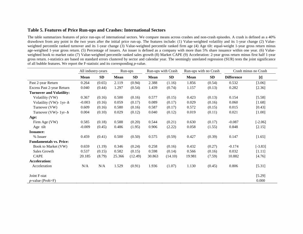
Table 5. Features of Price Run-ups and Crashes: International Sectors The table summarizes features of price run-ups of international sectors. We compare means across crashes and non-crash episodes. A crash is defined as a 40% drawdown from any point in the two years after the initial price run-up. The features include: (1) Value-weighted volatility and its 1-year change (2) Value-weighted percentile ranked turnover and its 1-year change (3) Value-weighted percentile ranked firm age (4) Age tilt: equal-weight 1-year gross return minus age-weighted 1-year gross return. (5) Percentage of issuers. An issuer is defined as a company with more than 5% share issuance within one year. (6) Value-weighted book to market ratio (7) Value-weighted percentile ranked sales growth (8) Market CAPE (9) Acceleration: 2-year gross return minus first half 1-year gross return. t-statistics are based on standard errors clustered by sector and calendar year. The seemingly unrelated regression (SUR) tests the joint significance of all bubble features. We report the F-statistic and its corresponding p-value.

All industry-years Run-ups Run-ups with Crash Run-ups with no Crash Crash minus no Crash

Mean SD Mean SD Mean SD Mean SD Difference [t] Past 2-year Return 0.264 (0.65) 2.119 (0.94) 2.388 (1.16) 1.856 (0.54) 0.532 [3.06] Excess Past 2-year Return 0.040 (0.44) 1.297 (0.54) 1.439 (0.74) 1.157 (0.13) 0.282 [2.36] Turnover and Volatility: Volatility (VW) 0.367 (0.16) 0.500 (0.16) 0.577 (0.15) 0.423 (0.13) 0.154 [5.58] Volatility (VW)- 1yr-Δ -0.003 (0.16) 0.059 (0.17) 0.089 (0.17) 0.029 (0.16) 0.060 [1.68] Turnover (VW) 0.609 (0.16) 0.580 (0.16) 0.587 (0.17) 0.572 (0.15) 0.015 [0.43] Turnover (VW)- 1yr-Δ 0.004 (0.10) 0.029 (0.12) 0.040 (0.12) 0.019 (0.11) 0.021 [1.00] Age: Firm Age (VW) 0.585 (0.18) 0.588 (0.20) 0.544 (0.21) 0.630 (0.17) -0.087 [-2.06] Age tilt -0.009 (0.45) 0.486 (1.95) 0.906 (2.22) 0.058 (1.55) 0.848 [2.15] Issuance: % Issuer 0.459 (0.41) 0.500 (0.50) 0.575 (0.59) 0.427 (0.39) 0.147 [1.65] Fundamentals vs. Price: Book to Market (VW) 0.659 (1.19) 0.346 (0.24) 0.258 (0.16) 0.432 (0.27) -0.174 [-3.83] Sales Growth 0.537 (0.15) 0.582 (0.15) 0.598 (0.14) 0.566 (0.16) 0.032 [1.11] CAPE 20.185 (8.79) 25.366 (12.49) 30.863 (14.10) 19.981 (7.59) 10.882 [4.76] Acceleration: Acceleration N/A N/A 1.529 (0.91) 1.936 (1.07) 1.130 (0.45) 0.806 [5.31]

Joint F-stat [5.29] p-value (Prob>F) 0.000

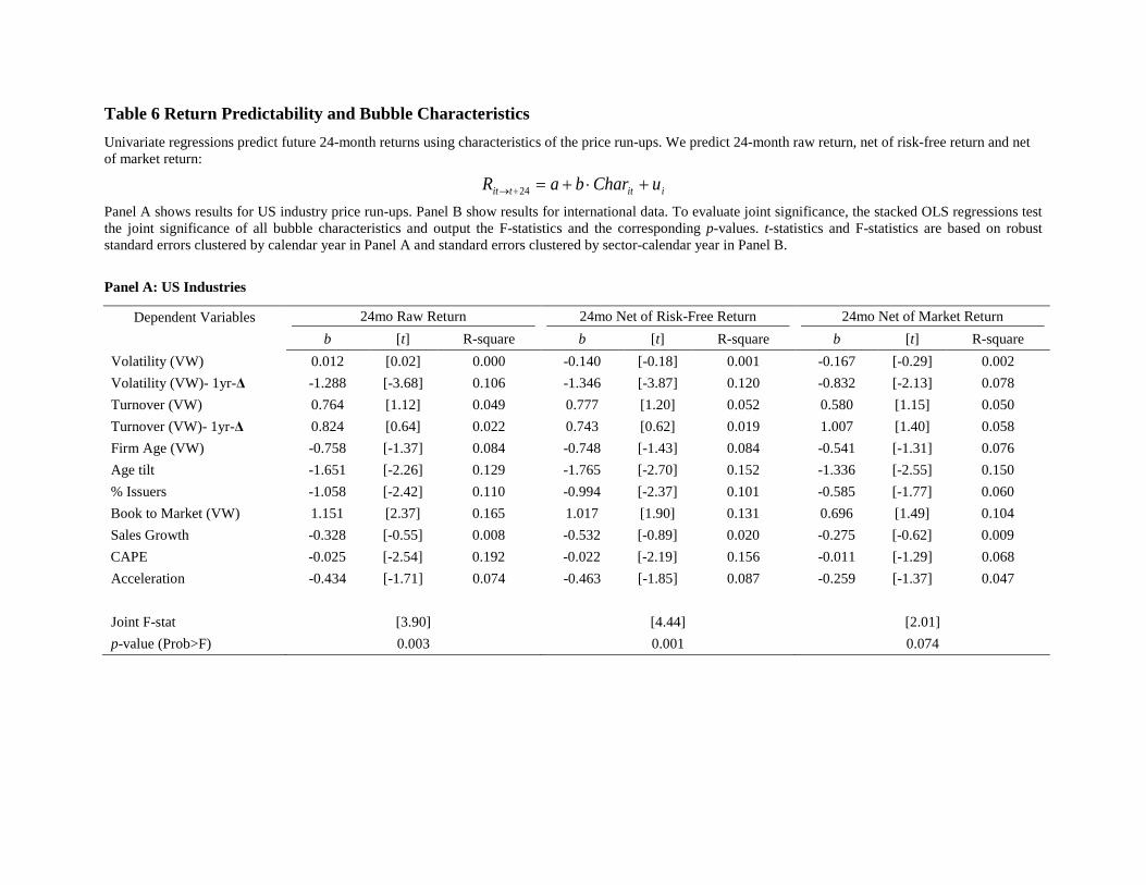
Table 6 Return Predictability and Bubble Characteristics Univariate regressions predict future 24-month returns using characteristics of the price run-ups. We predict 24-month raw return, net of risk-free return and net of market return:

iittit uCharbaR +⋅+=+→ 24

Panel A shows results for US industry price run-ups. Panel B show results for international data. To evaluate joint significance, the stacked OLS regressions test the joint significance of all bubble characteristics and output the F-statistics and the corresponding p-values. t-statistics and F-statistics are based on robust standard errors clustered by calendar year in Panel A and standard errors clustered by sector-calendar year in Panel B. Panel A: US Industries

Dependent Variables 24mo Raw Return 24mo Net of Risk-Free Return 24mo Net of Market Return

b [t] R-square b [t] R-square b [t] R-square Volatility (VW) 0.012 [0.02] 0.000 -0.140 [-0.18] 0.001 -0.167 [-0.29] 0.002 Volatility (VW)- 1yr-Δ -1.288 [-3.68] 0.106 -1.346 [-3.87] 0.120 -0.832 [-2.13] 0.078 Turnover (VW) 0.764 [1.12] 0.049 0.777 [1.20] 0.052 0.580 [1.15] 0.050 Turnover (VW)- 1yr-Δ 0.824 [0.64] 0.022 0.743 [0.62] 0.019 1.007 [1.40] 0.058 Firm Age (VW) -0.758 [-1.37] 0.084 -0.748 [-1.43] 0.084 -0.541 [-1.31] 0.076 Age tilt -1.651 [-2.26] 0.129 -1.765 [-2.70] 0.152 -1.336 [-2.55] 0.150 % Issuers -1.058 [-2.42] 0.110 -0.994 [-2.37] 0.101 -0.585 [-1.77] 0.060 Book to Market (VW) 1.151 [2.37] 0.165 1.017 [1.90] 0.131 0.696 [1.49] 0.104 Sales Growth -0.328 [-0.55] 0.008 -0.532 [-0.89] 0.020 -0.275 [-0.62] 0.009 CAPE -0.025 [-2.54] 0.192 -0.022 [-2.19] 0.156 -0.011 [-1.29] 0.068 Acceleration -0.434 [-1.71] 0.074 -0.463 [-1.85] 0.087 -0.259 [-1.37] 0.047

Joint F-stat [3.90] [4.44] [2.01] p-value (Prob>F) 0.003 0.001 0.074

[Table 6 Continued]

Panel B: International Sectors

Dependent Variables 24mo Raw Return 24mo Net of Risk-Free Return 24mo Net of Market Return

b [t] R-square b [t] R-square b [t] R-square Volatility (VW) -1.677 [-5.36] 0.146 -1.722 [-5.43] 0.152 -0.746 [-3.98] 0.085 Volatility (VW)- 1yr-Δ -0.615 [-1.38] 0.022 -0.610 [-1.33] 0.022 -0.757 [-3.20] 0.100 Turnover (VW) -0.651 [-1.58] 0.023 -0.698 [-1.67] 0.026 -0.547 [-2.23] 0.048 Turnover (VW)- 1yr-Δ 0.112 [0.08] 0.000 0.079 [0.02] 0.000 -0.055 [-0.15] 0.000 Firm Age (VW) 0.994 [2.46] 0.080 1.026 [2.50] 0.084 0.525 [2.13] 0.061 Age tilt -0.055 [-1.72] 0.024 -0.059 [-1.84] 0.028 -0.035 [-1.46] 0.028 % Issuers -0.261 [-2.81] 0.035 -0.261 [-2.76] 0.035 -0.135 [-2.31] 0.028 Book to Market (VW) 1.176 [3.071 0.163 1.220 [3.16] 0.173 0.311 [1.31] 0.034 Sales Growth -0.019 [-2.77] 0.008 -0.020 [-2.88] 0.009 -0.005 [-1.90] 0.002 CAPE -0.026 [-4.92] 0.206 -0.027 [-5.041 0.219 -0.007 [-2.38] 0.052 Acceleration -0.201 [-4.65] 0.068 -0.210 [-3.19] 0.073 -0.068 [-2.67] 0.023

Joint F-stat [6.52] [7.34] [2.25] p-value (Prob>F) 0.000 0.000 0.023

Table 7 False Discovery Tests The table tests the joint significance of the bubble features in Table 4, Table 5 and Table 6 allowing for a maximal false discovery rate of 10%. In the spirit of Bonferroni correction (Dunn, 1959), we adopt the maximal false discovery rate procedure from Soric (1989) and Benjamini and Hochberg (1995) to compute the probability of false discovery. We rank all variables by their p-values. In Panel A, Column 1 tabulates bubble features sorted ascending in order by p-values. Column 2 and 3 present the t-statistics and corresponding p-values for the last column in Table 4 and 5. Column 4 displays the p-value thresholds for 10% and column 5 reports whether the bubble features can pass the false discovery test. Panel A shows the results of false discovery tests for Table 4 and 5. In Panel B and Panel C, we report the joint false discovery tests for all regressions in Table 6. “True” in Column “10% Significance” column represents that the bubble characteristic jointly passes the false discovery test at 10% significance. Numbers in bold represent the bubble characteristic individually passes the Bonferroni test at 10% significance.

Panel A: Tests for Table 4 & 5

US Industries [t] p-value 10% Threshold 10% Significance Acceleration [2.78] 0.008 0.009 TRUE Age Tilt [2.44] 0.019 0.018 TRUE Volatility (VW)- 1yr-Δ [2.38] 0.022 0.027 TRUE Firm Age (VW) [2.15] 0.038 0.036 FALSE % Issuers [1.94] 0.060 0.045 FALSE Book to Market (VW) [-1.76] 0.086 0.055 FALSE CAPE [1.61] 0.115 0.064 FALSE Sale Growth [1.00] 0.323 0.073 FALSE Turnover (VW) [-0.62] 0.539 0.082 FALSE Volatility (VW) [0.44] 0.662 0.091 FALSE Turnover (VW) - 1yr-Δ [-0.14] 0.889 0.100 FALSE

International Sectors

[t] p-value 10% Threshold 10% Significance Volatility (VW) [5.58] 0.000 0.009 TRUE Acceleration [5.31] 0.000 0.018 TRUE CAPE [4.76] 0.000 0.027 TRUE Book to Market Ratio (VW) [-3.83] 0.000 0.036 TRUE Age Tilt [2.15] 0.034 0.045 TRUE Firm Age (VW) [-2.06] 0.042 0.055 TRUE % Issuers [1.65] 0.102 0.064 FALSE Volatility (VW) - 1yr-Δ [1.62] 0.108 0.073 FALSE Sale Growth [1.11] 0.270 0.082 FALSE Turnover (VW) - 1yr-Δ [1.10] 0.274 0.091 FALSE Turnover (VW) [0.43] 0.668 0.100 FALSE

[Table 7 Continued]

Panel B: Tests for Table 6 US industries

Dependent Variables 24mo Raw Return 24mo Net of Risk-Free Return 24mo Net of Market Return

[t] p-value 10% Significance [t] p-value 10% Significance [t] p-value 10% Significance Volatility (VW) [0.02] 0.984 FALSE [-0.18] 0.858 FALSE [-0.29] 0.773 FALSE Volatility (VW)- 1yr-Δ [-3.68] 0.001 TRUE [-3.87] 0.000 TRUE [-2.13] 0.040 FALSE Turnover (VW) [1.12] 0.270 FALSE [1.20] 0.237 FALSE [1.15] 0.257 FALSE Turnover (VW)- 1yr-Δ [0.64] 0.526 FALSE [0.62] 0.539 FALSE [1.40] 0.169 FALSE Firm Age (VW) [-1.37] 0.179 FALSE [-1.43] 0.161 FALSE [-1.31] 0.198 FALSE Age tilt [-2.26] 0.029 TRUE [-2.70] 0.010 TRUE [-2.55] 0.015 FALSE % Issuers [-2.42] 0.020 TRUE [-2.37] 0.023 TRUE [-1.77] 0.085 FALSE Book to Market (VW) [2.37] 0.023 TRUE [1.90] 0.065 FALSE [1.49] 0.144 FALSE Sales Growth [-0.55] 0.585 FALSE [-0.89] 0.379 FALSE [-0.62] 0.539 FALSE CAPE [-2.54] 0.015 TRUE [-2.19] 0.035 TRUE [-1.29] 0.205 FALSE Acceleration [-1.71] 0.095 FALSE [-1.85] 0.072 FALSE [-1.37] 0.179 FALSE

Panel C: Tests for Table 6 International Sectors

Dependent Variables 24mo Raw Return 24mo Net of Risk-Free Return 24mo Net of Market Return

[t] p-value 10% Significance [t] p-value 10% Significance [t] p-value 10% Significance Volatility (VW) [-5.24] 0.000 TRUE [-5.19] 0.000 TRUE [-3.17] 0.002 TRUE Volatility (VW)- 1yr-Δ [-1.49] 0.139 FALSE [-1.44] 0.153 FALSE [-2.83] 0.006 TRUE Turnover (VW) [-1.35] 0.180 FALSE [-1.40] 0.164 FALSE [-1.87] 0.064 FALSE Turnover (VW)- 1yr-Δ [0.18] 0.857 FALSE [0.13] 0.897 FALSE [-0.13] 0.897 FALSE Firm Age (VW) [3.84] 0.000 TRUE [3.85] 0.000 TRUE [3.34] 0.001 TRUE Age tilt [-1.77] 0.080 FALSE [-1.90] 0.060 TRUE [-1.38] 0.170 FALSE % Issuers [-2.50] 0.014 TRUE [-2.40] 0.018 TRUE [-2.01] 0.047 TRUE Book to Market (VW) [2.14] 0.035 TRUE [2.23] 0.028 TRUE [0.99] 0.324 FALSE Sales Growth [-2.91] 0.004 TRUE [-2.99] 0.003 TRUE [-2.23] 0.028 TRUE CAPE [-4.08] 0.000 TRUE [-4.21] 0.000 TRUE [-2.13] 0.035 TRUE Acceleration [-3.09] 0.003 TRUE [-3.19] 0.002 TRUE [-1.66] 0.100 FALSE

Table 8 Betting Against Bubbles Using Bubble Features The table reports the performance of trading strategies based on the features identified in Tables 4 and 5. “Hold” strategy denotes the benchmark for portfolio evaluation in which we hold the industry following a price run-up. Alternatively, the investor may choose to exit the industry and hold another asset, either the value-weighted market return or the risk-free rate. The “sell” signal for each strategy is to exit the industry if the feature reported in column (1) is greater (or smaller for special cases) than the corresponding mean of among crashed price run-ups in Tables 4 and 5. Column 2 reports the number of price run-ups identified as potential bubbles by the strategy. Column 3 reports the percentage of the identified run-ups followed by a subsequent crash. Column 4-9 report the raw returns of the strategy at the end of 1-, 2- and 4-year. Column 10-15 report the net of benchmark returns and the corresponding t-statistics in parenthesis. All numbers in bold are the returns of strategies beating the benchmark at 90% significance level. In Panel A, we specifically set “sell” signal as “smaller than mean” for book-to-market ratio in the spirit of Table 4. t-statistics are based on clustered standard errors by calendar year. In Panel B, we set “sell” signal as “smaller than mean” for book-to-market ratio and firm age in the spirit of Table 5. t-statistics in Panel B are based on standard errors clustered by sector and calendar year. The seemingly unrelated regressions (SUR) test the joint significance of net of benchmark returns in all trading strategies and output the F-stat and the corresponding p-values in the bottom two rows of both panels.

Panel A: US Industries

Strategy

# Price Run-ups Identified as potential bubbles

% Identified run-ups with a subsequent crash

Raw Returns Net of Benchmark Returns Switch to Market when “Bubble”

Identified

Switch to Risk-free when “Bubble”

Identified

Switch to Market when “Bubble”

Identified

Switch to Risk-free when “Bubble”

Identified

1-yr ret

2-yr ret

4-yr ret

1-yr ret

2-yr ret

4-yr ret

1-yr ret

2-yr ret

4-yr ret

1-yr ret

2-yr ret

4-yr ret

(1) (2) (3) (4) (5) (6) (7) (8) (9) (10) (11) (12) (13) (14) (15)

Hold = Benchmark 0 0 7% 0% 5% 7% 0% 5% 0% 0% 0% 0% 0% 0% Exit based on Price Run-up Only 40 (All) 53% 3% 0% 16% 5% 10% 20% -5% 0% 11% -3% 10% 15%

[-0.90] [0.04] [0.98] [-0.35] [0.89] [1.13] Price Run-up +

Volatility 20 60% 6% 2% 13% 7% 8% 17% -2% 3% 8% 0% 8% 12%

[-0.51] [0.53] [1.22] [-0.02] [1.21] [1.68] Volatility 1yr-Δ 11 91% 10% 5% 10% 11% 10% 17% 3% 5% 5% 4% 10% 12%

[1.48] [1.43] [1.16] [1.42] [1.88] [1.67] Turnover 19 47% 4% -4% 6% 4% -2% 5% -3% -4% 1% -3% -2% 0%

[-0.75] [-0.58] [0.07] [-0.54] [-0.23] [-0.01] Turnover 1yr-Δ 18 56% 7% -1% 8% 11% 6% 14% 0% -1% 3% 4% 6% 9%

[-0.11] [-0.15] [0.32] [0.84] [0.77] [0.84] Age 15 80% 8% 4% 12% 12% 11% 20% 1% 5% 8% 4% 12% 16%

Strategy

# Price Run-ups Identified as potential bubbles

% Identified run-ups with a subsequent crash

Raw Returns Net of Benchmark Returns Switch to Market when “Bubble”

Identified

Switch to Risk-free when “Bubble”

Identified

Switch to Market when “Bubble”

Identified

Switch to Risk-free when “Bubble”

Identified

1-yr ret

2-yr ret

4-yr ret

1-yr ret

2-yr ret

4-yr ret

1-yr ret

2-yr ret

4-yr ret

1-yr ret

2-yr ret

4-yr ret

(1) (2) (3) (4) (5) (6) (7) (8) (9) (10) (11) (12) (13) (14) (15)

[0.49] [1.23] [1.57] [1.21] [2.04] [2.10] Age Tilt 10 70% 6% 2% 11% 7% 7% 15% -1% 3% 6% 0% 7% 10%

[-0.53] [0.87] [1.92] [-0.05] [1.52] [2.27] %Issuer 13 69% 7% 0% 5% 7% 0% 5% 1% 4% 9% 3% 10% 13%

[0.72] [1.17] [2.34] [1.04] [1.64] [1.61] Book-to-Market 9 67% 7% 1% 6% 7% 4% 8% -1% 1% 1% 0% 4% 4% [-0.28] [0.26] [0.19] [-0.09] [0.77] [0.47] Sales Growth 20 52% 2% -1% 7% 0% 2% 4% -6% -1% 3% -7% 2% -1% [-1.45] [-0.14] [0.26] [-1.39] [0.25] [-0.08] CAPE 11 82% 5% 1% 9% 7% 8% 19% -3% 1% 4% 0% 9% 15% [-0.91] [0.36] [1.40] [-0.02] [1.27] [1.87] Acceleration 17 76% 8% 4% 14% 9% 11% 22% 0% 5% 9% 2% 12% 17%

[0.16] [1.15] [1.52] [0.47] [1.84] [2.06]

Joint F-stat

[2.15] [2.20] [1.78] [2.12] [1.94] [1.81]

p-value (Prob>F)

0.017 0.014 0.056 0.018 0.033 0.050

[Table 8 Continued]

Panel B: International Sectors

Strategy

# Price Run-ups Identified as potential bubbles

% Identified run-ups with a subsequent crash

Raw Returns Net of Benchmark Returns Switch to Market when “Bubble”

Identified

Switch to Risk-free when “Bubble”

Identified

Switch to Market when “Bubble”

Identified

Switch to Risk-free when “Bubble”

Identified 1-yr ret

2-yr ret

4-yr ret

1-yr ret

2-yr ret

4-yr ret

1-yr ret

2-yr ret

4-yr ret

1-yr ret

2-yr ret

4-yr ret

(1) (2) (3) (4) (5) (6) (7) (8) (9) (10) (11) (12) (13) (14) (15)

Hold = Benchmark 0 0 0% 6% 39% 0% 6% 39% 0% 0% 0% 0% 0% 0%

Exit based on Price Run-up Only 107 (All) 50% -2% 6% 30% 3% 5% 9% -2% 0% -9% 3% -1% -30%

[-0.72] [-0.01] [-0.80] [0.52] [-0.12] [-1.66] Price Run-up +

Volatility 31 84% 3% 11% 38% 10% 18% 39% 2% 4% -2% 9% 12% 0%

[1.45] [2.15] [-0.26] [2.47] [2.58] [-0.03] Volatility 1yr-Δ 42 62% 4% 13% 40% 5% 12% 26% 3% 6% -2% 5% 6% -13%

[1.71] [2.33] [-0.34] [1.55] [1.23] [-1.03] Turnover 53 49% 2% 11% 45% 5% 10% 36% 1% 5% 7% 5% 4% -1%

[0.58] [1.61] [0.92] [1.38] [0.62] [-0.07] Turnover 1yr-Δ 45 51% 1% 9% 39% 3% 9% 38% 0% 1% -3% 2% 0% -4%

[-0.09] [0.36] [-0.43] [0.44] [0.08] [-0.42] Age 46 61% -2% 2% 31% -1% -3% 13% 1% 5% 1% 5% 7% -3%

[0.61] [2.09] [0.18] [1.53] [1.43] [-0.25] Age Tilt 30 60% -1% 8% 36% 2% 9% 32% -2% 1% -3% 0% 1% -9%

[-0.89] [0.60] [-0.54] [0.08] [0.25] [-0.84] %Issuer 31 61% 3% 10% 44% 7% 13% 43% 2% 3% 5% 6% 5% 3%

[1.44] [1.21] [1.53] [2.53] [1.30] [0.78] Book-to-Market 46 65% 3% 12% 40% 6% 14% 35% -2% -1% 5% 4% 9% 12%

[-0.76] [-0.21] [1.20] [0.89] [1.65] [2.10] Sales Growth 48 60% 0% 6% 36% 4% 6% 29% -1% -1% -5% 4% 1% -9%

[-0.31] [-0.19] [-0.64] [0.93] [0.14] [-0.78] CAPE 21 76% 4% 10% 45% 8% 16% 50% 3% 3% 4% 8% 8% 8%

[2.17] [1.94] [1.86] [3.09] [2.51] [2.57] Acceleration 22 82% 0% 9% 37% 3% 14% 35% -1% 2% -3% 2% 6% -6%

[-0.54] [1.42] [-0.48] [0.81] [1.89] [-0.53]

Strategy

# Price Run-ups Identified as potential bubbles

% Identified run-ups with a subsequent crash

Raw Returns Net of Benchmark Returns Switch to Market when “Bubble”

Identified

Switch to Risk-free when “Bubble”

Identified

Switch to Market when “Bubble”

Identified

Switch to Risk-free when “Bubble”

Identified 1-yr ret

2-yr ret

4-yr ret

1-yr ret

2-yr ret

4-yr ret

1-yr ret

2-yr ret

4-yr ret

1-yr ret

2-yr ret

4-yr ret

(1) (2) (3) (4) (5) (6) (7) (8) (9) (10) (11) (12) (13) (14) (15)

Joint F-stat

[2.36] [2.47] [1.59] [2.68] [2.29] [2.10] p-value (Prob>F)

0.007 0.005 0.095 0.002 0.009 0.018