DETECTION & DIAGNOSIS OF RUSTDISEASE IN WHEAT LEAVES: AN

INTEGRATED DIGITAL IMAGE PROCESSINGAPPROACH

Prepared By

Diptesh MajumdarSamit BhattacharyaGobinda Agarwalla

Md. Wasim

Under the Guidance of

Dr. Aruna ChakrabortyAssistant professor

Department of Computer Science & EngineeringSt. Thomas’ College Of Engineering & Technology

Dr. Dipak Kumar KoleAssistant professor

Department of Computer Science & EngineeringSt. Thomas’ College Of Engineering & Technology

Project Report

Submitted for the degree of Bachelor of Technology in Computer Science &Engineering

St. Thomas’ College of Engineering & Technology

Affiliated to

West Bengal University Of Technology, West Bengal

St. Thomas’ College of Engineering & Technology

Certification

St. Thomas’ College of Engineering &

Technology

This is to certify that the work in preparing the project entitled “Detection& Diagnosis of Rust Disease in Wheat Leaves: An Image Processing

Approach”, has been carried out by Diptesh Majumdar, SamitBhattacharya, Gobinda Agarwalla and Md. Wasim under our guidanceduring the session 2012-13 for the degree of Bachelor of Technology in

Computer Science & Engineering.

. . . . . . . . . . . . . . . . . . . . . . . . . . .(Dr. Aruna Chakraborty)

SupervisorDepartment of Computer Science &

EngineeringSt. Thomas’ College of Engineering

& Technology

. . . . . . . . . . . . . . . . . . . . . . . . . . .(Dr. Dipak Kumar Kole)

SupervisorDepartment of Computer Science &

EngineeringSt. Thomas’ College of Engineering

& Technology

. . . . . . . . . . . . . . . . . . . . . . . . . . .(Mrs. Subarna Bhattacharjee)

(Ph.D.)Head of the Department

Computer Science & EngineeringSt. Thomas’ College of Engineering

& Technology

i

Preface

The project, work summarized in this report, deals with the development ofan integrated Image Processing System that will be used for detection anddiagnosis of rust disease in wheat leaf. The system has been successfullybuilt using Matlab and the application has been subsequently loaded on aserver machine which will enable end users to utilize the system even if hismachine does not have Matlab installed in it. This intranet module allowsusers to submit a wheat leaf image and the server can return informationabout the presence of rust disease in the leaf. We have also built a GraphicalUser Interface through which a researcher can choose which features of leafimage to use for the experiment, with which images will he train the classi-fier etc. Thus he can manipulate the system variables and observe changesin output or use the system for other applications. The GUI also includescommon image processing applications and this will prove extremely helpfulfor researchers.

. . . . . . . . . . . . . . . . . . . . . . . . . . . . . . . . . . . . . . . . . . . . .Diptesh Majumdar Samit Bhattacharya

. . . . . . . . . . . . . . . . . . . . . . . . . . . . . . . . . . . .Gobinda Agarwalla Md. Wasim

Acknowledgements

This project and documentation would never have been more educative andefficient without the constant help and guidance of our project guides Dr.Aruna Chakraborty and Dr. Dipak Kumar Kole. We would like tothank them for giving us the right guidance and encouraging us to completethe project within time. We also express our deepest and sincere gratitudeto all our teachers for their kind comments and advice on our project. Wewould also like to express our heartiest gratitude to Prof. Swapna Sen(Principal), Prof. Gautam Banerjea (Registrar), Prof. Subarna Bhat-tacharjee (Head of the Department of Computer Science & Engineering)and other faculties for their encouragement and kind suggestions. We wouldlike to specially thank Mr. Amit Dutta for his co-operation throughoutthe duration of the project. We would also like to thank St. Thomas’Library for their constant support.Our sincere thanks also goes to Mr. Arya Ghosh who is responsible forcollection of more than 300 wheat leaf images from a wheat farm at FieldCrop Research Station, Department of Agriculture, Govt of West Bengal,Burdwan. Then the leaves where classified according to the severity of in-fection in the leaves by two experienced doctors, Dr. Amitava Ghosh(Ex. Economic Botanist IX, West Bengal) and Dr. P. K. Maity (ChiefAgronomist & Ex-Officio Joint Director of Agriculture, West Bengal). Thisproject would never have been possible without the benchmark of wheat leafdisease, provided by them.Last but not the least, we would like to thank Prof. Dwijesh Dutta Ma-jumder, Professor Emeritus in Electronics and Communication SciencesUnit, Indian Statistical Institute, for his continuous support and enthusi-asm for our project.

Contents

1 Introduction 21.1 Problem Statement . . . . . . . . . . . . . . . . . . . . . . . . 21.2 Problem Definition . . . . . . . . . . . . . . . . . . . . . . . . 21.3 Objective . . . . . . . . . . . . . . . . . . . . . . . . . . . . . 21.4 Tools & Platforms . . . . . . . . . . . . . . . . . . . . . . . . 3

1.4.1 Developer side tools and platform . . . . . . . . . . . 31.4.2 Minimum Requirement for User . . . . . . . . . . . . . 5

1.5 Brief Discussion on Problem . . . . . . . . . . . . . . . . . . . 5

2 Concepts and Problem Analysis 72.1 Concepts . . . . . . . . . . . . . . . . . . . . . . . . . . . . . 7

2.1.1 Recognition of Wheat Leaf Diseases & Gradations . . 72.1.2 Image Processing . . . . . . . . . . . . . . . . . . . . . 82.1.3 Neural Network . . . . . . . . . . . . . . . . . . . . . . 212.1.4 Clustering Methods . . . . . . . . . . . . . . . . . . . 302.1.5 Web Technology . . . . . . . . . . . . . . . . . . . . . 312.1.6 Client Server Architecture . . . . . . . . . . . . . . . . 362.1.7 XML . . . . . . . . . . . . . . . . . . . . . . . . . . . . 37

2.2 Literature Survey . . . . . . . . . . . . . . . . . . . . . . . . . 382.2.1 Introduction . . . . . . . . . . . . . . . . . . . . . . . 382.2.2 General Architecture of the System . . . . . . . . . . . 382.2.3 Image Acquisition Phase . . . . . . . . . . . . . . . . . 402.2.4 Image Enhancement Techniques . . . . . . . . . . . . 402.2.5 Noise Reduction Techniques . . . . . . . . . . . . . . . 422.2.6 Image Segmentation Phase . . . . . . . . . . . . . . . 422.2.7 Feature Extraction Phase . . . . . . . . . . . . . . . . 442.2.8 The Classifiers . . . . . . . . . . . . . . . . . . . . . . 47

2.3 Brief Overview of the System . . . . . . . . . . . . . . . . . . 48

iv

3 Design & Methodology 503.1 Offline Phase . . . . . . . . . . . . . . . . . . . . . . . . . . . 50

3.1.1 Image Acquisition Phase . . . . . . . . . . . . . . . . . 503.1.2 Image Enhancement Phase . . . . . . . . . . . . . . . 503.1.3 Image Segmentation Phase . . . . . . . . . . . . . . . 513.1.4 Feature Extraction Phase . . . . . . . . . . . . . . . . 523.1.5 The Classifier . . . . . . . . . . . . . . . . . . . . . . . 58

3.2 Online Phase . . . . . . . . . . . . . . . . . . . . . . . . . . . 603.2.1 Creation of XML file . . . . . . . . . . . . . . . . . . . 603.2.2 Creation of a Home Page for User . . . . . . . . . . . 603.2.3 Uploading of Image by User . . . . . . . . . . . . . . . 623.2.4 Storing & Processing of Uploaded Image File in the

Server . . . . . . . . . . . . . . . . . . . . . . . . . . . 623.2.5 Sending Response to the Client . . . . . . . . . . . . . 63

3.3 Graphical User Interfaces . . . . . . . . . . . . . . . . . . . . 653.3.1 Image Processing Applications . . . . . . . . . . . . . 653.3.2 Feature Extraction . . . . . . . . . . . . . . . . . . . . 713.3.3 Training & Testing of Neural Network . . . . . . . . . 72

4 Sample Codes 764.1 Back Propagation Main Function . . . . . . . . . . . . . . . . 764.2 Storing & Processing of input image at Server . . . . . . . . . 85

5 Experimental Results 935.1 Neural Network . . . . . . . . . . . . . . . . . . . . . . . . . . 93

6 Conclusion & Future Scope 94

v

List of Figures

1.1 The structure of the project . . . . . . . . . . . . . . . . . . . 6

2.1 Recognition of Wheat Leaf Diseases Gradations . . . . . . . 82.2 Neighbourhood Concept in Spatial Domain . . . . . . . . . . 92.3 Histogram Processing . . . . . . . . . . . . . . . . . . . . . . 102.4 Histogram Equalization . . . . . . . . . . . . . . . . . . . . . 112.5 Smoothing Filters . . . . . . . . . . . . . . . . . . . . . . . . . 122.6 Smooth Filtering . . . . . . . . . . . . . . . . . . . . . . . . . 132.7 Median Filtering . . . . . . . . . . . . . . . . . . . . . . . . . 142.8 Mask for Segmentation . . . . . . . . . . . . . . . . . . . . . . 152.9 Basic Global Thresholding . . . . . . . . . . . . . . . . . . . . 162.10 Optimum global Thresholding using Otsu’s Method . . . . . 172.11 Structuring Elements - Hits & Fits . . . . . . . . . . . . . . . 182.12 Erosion . . . . . . . . . . . . . . . . . . . . . . . . . . . . . . 192.13 Properties of Erosion . . . . . . . . . . . . . . . . . . . . . . . 192.14 Dilation . . . . . . . . . . . . . . . . . . . . . . . . . . . . . . 202.15 Properties of Dilation . . . . . . . . . . . . . . . . . . . . . . 202.16 Neural Network . . . . . . . . . . . . . . . . . . . . . . . . . . 222.17 Simple Neuron & Transfer Function . . . . . . . . . . . . . . 222.18 Neuron with Vector Input . . . . . . . . . . . . . . . . . . . . 232.19 A Layer of Neurons . . . . . . . . . . . . . . . . . . . . . . . . 242.20 Multiple Layer of Neurons . . . . . . . . . . . . . . . . . . . . 252.21 Attributes of neurons and weight adjustments by the back-

propagation learning algorithm . . . . . . . . . . . . . . . . . 282.22 The Error Generation at Neuron p lying in layer j . . . . . . 292.23 Architecture of the General System for Detection and Recog-

nition of Disease in Plant Leaf . . . . . . . . . . . . . . . . . 392.24 Overall structure of the system . . . . . . . . . . . . . . . . . 49

vi

3.1 Result of application of HSI transformation of color imageand its normalized histogram . . . . . . . . . . . . . . . . . . 51

3.2 Results of application of Fuzzy C-means Clustering on Imagesof Diseased Wheat Leaves . . . . . . . . . . . . . . . . . . . . 53

3.3 Result of feature extraction on 2 diseased and 1 normal wheatleaf images . . . . . . . . . . . . . . . . . . . . . . . . . . . . 56

3.4 Result of feature extraction on diseased wheat leaf images . . 593.5 Output of XML Creation Program . . . . . . . . . . . . . . . 613.6 XML File immediately after creation . . . . . . . . . . . . . . 613.7 User Home Page . . . . . . . . . . . . . . . . . . . . . . . . . 623.8 Page Where User can Upload an Image . . . . . . . . . . . . 623.9 Message after Successful Uploading of Image . . . . . . . . . 633.10 Information of Uploaded Images Stored in XML file . . . . . 643.11 MS Access Database If used for Storage of File Properties . . 643.12 Response Sent from the Client to the Server . . . . . . . . . . 653.13 Image Processing Applications GUI . . . . . . . . . . . . . . . 663.14 Image Negative . . . . . . . . . . . . . . . . . . . . . . . . . . 673.15 Smooth Filtering . . . . . . . . . . . . . . . . . . . . . . . . . 673.16 Histogram Processing . . . . . . . . . . . . . . . . . . . . . . 683.17 Edge Detection through Sobel Operator . . . . . . . . . . . . 683.18 Basic Global Thresholding . . . . . . . . . . . . . . . . . . . . 693.19 Watershed Segmentation . . . . . . . . . . . . . . . . . . . . . 693.20 Erosion . . . . . . . . . . . . . . . . . . . . . . . . . . . . . . 703.21 Dilation . . . . . . . . . . . . . . . . . . . . . . . . . . . . . . 703.22 Boundary Extraction . . . . . . . . . . . . . . . . . . . . . . . 703.23 Feature Extraction GUI . . . . . . . . . . . . . . . . . . . . . 713.24 Feature Extraction GUI after data is written to the MS Excel

worksheet . . . . . . . . . . . . . . . . . . . . . . . . . . . . . 713.25 MS Excel worksheet containing the feature data . . . . . . . . 723.26 Training & Testing GUI . . . . . . . . . . . . . . . . . . . . . 733.27 Training & Testing GUI:Training . . . . . . . . . . . . . . . . 733.28 Training & Testing GUI:Testing . . . . . . . . . . . . . . . . . 743.29 Training & Testing GUI after data is written to the MS Excel

worksheet . . . . . . . . . . . . . . . . . . . . . . . . . . . . . 743.30 MS Excel worksheet containing the testing result . . . . . . . 75

4.1 Flow Chart Demonstrating Back Propagation Main Function 86

1

Chapter 1

Introduction

1.1 Problem Statement

A Web-Based Integrated System to Detect and Diagnose Rust Disease inWheat Leaf using Image Processing & Soft Computing Techniques

1.2 Problem Definition

Wheat leaves need to be scouted routinely for early detection and recogni-tion of rust diseases. This facilitates timely management decisions. In thisproject, an integrated image processing and analysis system has been devel-oped to automate the inspection of these leaves and detection of any diseasepresent in them. Disease features of wheat leaves have been extracted anddisease detection, recognition of its type and identification algorithm hasbeen developed based on artificial neural network (ANN). Through the useof ANN and more specifically multilayer perceptrons, detection of the pres-ence of disease in wheat leaves have been successful in 97% of the cases, afteranalysis of more than 300 test images of wheat leaves. Also, identificationof type of disease, if present, in wheat leaf has been successful in 85% of thecases.

1.3 Objective

Wheat Leaf (Triticum Aestivum) has been a part of the human diet forthousands of years. Recent research has found the young shoots of wheatleaf to be rich in many essential vitamins, minerals, enzymes and antioxi-dants. Wheat Leaf rust, Puccinia recondite, usually does not cause spec-

2

tacular damage, but on a world-wide basis it probably causes more damagethan the other wheat rusts. It occurs wherever wheat is grown, and it isthe commonest, most widely distributed of all cereal rusts. Although theparasites have no doubt occurred on wheat through the course of its devel-opment, it is probably more damaging now that large areas tend to be sownto single, genetically homogeneous cultivars or to closely related cultivars.In India, average losses of 3% have been estimated, although higher lossesoccur in certain areas if the cultivars are susceptible to leaf rust. The de-tection of presence of a disease in a wheat leaf may cause some confusiondue to similarities between a diseased and a normal leaf, but only an expertcan identify it. The adequate recognition of their presence, i.e. correct di-agnosis, is the first step in fighting against the disease and the recognitionof the type of disease the leaf is infected with. In this work, an integratedimage processing system has been proposed aiming at the identification ofthe wheat leaf spots. The development of such an intelligent system is jus-tified by its economical relevance and by hard effort necessary to perform acorrect detection. This includes the knowledge and experience accumulatedby the human experts. Other important aspects are the speed, safety, andreliability of the response of the system.

1.4 Tools & Platforms

1.4.1 Developer side tools and platform

The main tools used for developing the system are:

• Matlab: MATLAB (matrix laboratory) is a numerical computing en-vironment and fourth-generation programming language. Developedby MathWorks, MATLAB allows matrix manipulations, plotting offunctions and data, implementation of algorithms, creation of user in-terfaces, and interfacing with programs written in other languages,including C, C++, Java, and Fortran.The most frequently used functions employed in our system takes thehelp of Image Processing Toolbox. Image Processing Toolbox pro-vides a comprehensive set of reference-standard algorithms, functions,and apps for image processing, analysis, visualization, and algorithmdevelopment. You can perform image enhancement, image deblur-ring, feature detection, noise reduction, image segmentation, geomet-ric transformations, and image registration. Many toolbox functionsare multithreaded to take advantage of multicore and multiprocessor

3

computers.Image Processing Toolbox supports a diverse set of image types, in-cluding high dynamic range, gigapixel resolution, embedded ICC pro-file, and tomographic. Visualization functions let you explore an im-age, examine a region of pixels, adjust the contrast, create contours orhistograms, and manipulate regions of interest (ROIs). With toolboxalgorithms you can restore degraded images, detect and measure fea-tures, analyze shapes and textures, and adjust color balance.The Matlab Code has been compiler using Matlab Compiler. MAT-LAB Compiler lets you share your MATLAB application as an exe-cutable or a shared library. Executables and libraries created withMATLAB Compiler use a runtime engine called the MATLAB Com-piler Runtime (MCR). The MCR is provided with MATLAB Compilerfor distribution with your application and can be deployed royalty-free.

• JSP: Java Server Pages (JSP) is a technology that helps softwaredevelopers create dynamically generated web pages based on HTML,XML, or other document types. Released in 1999 by Sun Microsys-tems, JSP is similar to PHP, but it uses the Java programming lan-guage. To deploy and run Java Server Pages, a compatible web serverwith a servlet container, such as Apache Tomcat or Jetty, is required.Architecturally, JSP may be viewed as a high-level abstraction of Javaservlets. JSPs are translated into servlets at runtime; each JSP’sservlet is cached and re-used until the original JSP is modified.

• HTML:Short for Hyper Text Markup Language, the authoring lan-guage used to create documents on the World Wide Web. HTML issimilar to SGML, although it is not a strict subset. HTML definesthe structure and layout of a Web document by using a variety oftags and attributes. The correct structure for an HTML documentstarts with < HTML > < HEAD > (enter here what documentis about) < /HEAD > < BODY > and ends with < /BODY >< /HTML >. All the information you’d like to include in your Webpage fits in between the < BODY > and < /BODY > tags. Thereare hundreds of other tags used to format and layout the informationin a Web page. Tags are also used to specify hypertext links. Theseallow Web developers to direct users to other Web pages with only aclick of the mouse on either an image or word.

4

1.4.2 Minimum Requirement for User

The greatest advantage of the Developed System is that the user does notrequire anything other than a contemporary Windows Operating System.A Web Browser comes along with the installation of the Operating System.User need to access a Web Server designed for this application. He willupload a wheat leaf image, submit the image file to the server and theserver will generate a response to the client regarding the presence of diseasein the Wheat Leaf. Hence the system can be utilised irrespective of theconfiguration of the system on Client Side. Only three concerns are therethat the user need to take care of.

1. Windows OS (32/64 bit) must be installed in the Client Machine

2. The input image must contain only a whole or a portion of a wheatleaf and nothing else, i.e. the system might not work properly if, say,the background of the image, behind the leaf, contains a house, sky,person etc. The camera must be focused such that it captures theimage of the leaf only.

3. Users must note that the system will not work for detection of diseasein leaves of plants other than wheat. The system will be built keepingin mind only the conditions of a diseased and undiseased leaf of wheat.

1.5 Brief Discussion on Problem

Various threats to production of wheat are in the increase today. Indiais a agriculture based country where agriculturist are keen to increase theproduction of wheat. This project provides a novel approach to detect leafrust, the most dangerous disease of wheat plants. So the identification ofthe disease at the earliest is very important.The experts in charge of this identification and detection of disease aretherefore employing various manual and visual means. They would visuallyestimate the intensity of the disease and put forth remedies that could varyfrom expert to expert.This integrated image processing based approach would assist the expertsin more accurate decision making. This system would enhance better pro-ductivity and thus in turn yield economic growth of a country.Our proposed system comprises of five distinct stages. At the onset weconsider image acquisition, the second phase constitutes of Image Enhance-ment followed by Segmentation, Feature Extraction and finally in the fifth

5

phase we have the classifier using Artificial Neural Network. Our researchindicates that the systems works efficiently and achieves accurate diagnosisin 85% of the cases. The entire structure of the project may be pictoriallyrepresented by the following figure:

Figure 1.1: The structure of the project

6

Chapter 2

Concepts and ProblemAnalysis

2.1 Concepts

2.1.1 Recognition of Wheat Leaf Diseases & Gradations

A wheat leaf can be infected with the following four diseases:

• Powdery Mildew: Elliptical patches of white fungal growth appearon both leaf surfaces.

• Septoria Leaf Spot: Yellow flecks first appear on the lower leaves.Later, yellow to red-brown or gray-brown spots or blotches may de-velop on all above-ground parts of wheat.

• Tan spot or Yellow Leaf : Oval-shaped tan spots up to 12 mm inlength appear on the leaves.

• Snow Molds: Leaves may be partly or entirely dried and appearbrown or bleached. When the crowns are attacked, the plants areusually killed. When the crowns are unharmed, new leaves emergeamong the damaged leaves and the wheat plants often recover.

All four diseases mentioned above can be considered to be wheat leafrusts with various degrees of infections. A study by Pathologists Marsalisand Goldberg [31] reveals that Wheat Leaf rust disease symptoms beginas small, circular to oval yellow spots on infected tissues of the upper leafsurface. As the disease progresses, the spots develop into orange coloredpustules which may be surrounded by a yellow halo.

7

Figure 2.1: Relative resistances of wheat to leaf rust: R=resistant, MR=moderately resistant, MS= moderately susceptible, and S= susceptible.Source: Rust Scoring Guide, Research Institute for Plant Protection, Wa-geningen, Netherlands

Accordingly, our proposed system is able to identify a wheat leaf asdiseased or not, and if found to be diseased, it can determine the severity ofthe infection by labeling it as R, MR, MS or S.

2.1.2 Image Processing

Image Enhancement Techniques in the Spatial Domain

The term spatial domain [15] refers to the aggregate of pixels composingan image. Spatial domain methods are procedures that operate directly onthese pixels. Spatial domain processes will be denoted by the expression

g(x, y) = T [f(x, y)]

where f(x, y) is the input image, g(x, y) is the processed image, and T is anoperator on f, defined over some neighborhood of (x, y). In addition, T canoperate on a set of input images, such as performing the pixel-by-pixel sumof K images for noise reduction.

8

The principal approach in defining a neighborhood about a point (x, y)is to use a square or rectangular sub image area centered at (x, y), as in thefigure below

Figure 2.2: Neighbourhood Concept in Spatial Domain

The center of the sub image is moved from pixel to pixel starting, say,at the top left corner. The operator T is applied at each location (x, y) toyield the output, g, at that location. The process utilizes only the pixels inthe area of the image spanned by the neighborhood.Although other neighborhood shapes, such as approximations to a circle,sometimes are used, square and rectangular arrays are by far the most pre-dominant because of their ease of implementation.

1. Histogram ProcessingThe histogram of a digital image [15] with gray levels in the range[0, L− 1] is a discrete function h (rk) = nk, where rk is the kth graylevel and nk is the number of pixels in the image having gray level rk.It is common practice to normalize a histogram by dividing each of itsvalues by the total number of pixels in the image, denoted by n. Thus,a normalized histogram is given by

p(rk) =nkn

for k=0...L-1. Loosely speaking, p(rk) gives an estimate of the proba-bility of occurrence of gray level rk. Note that the sum of all compo-nents of a normalized histogram is equal to 1.

9

Histograms are the basis for numerous spatial domain processing tech-niques. Histogram manipulation can be used effectively for image en-hancement, as shown in this section. In addition to providing usefulimage statistics, we shall see in subsequent chapters that the informa-tion inherent in histograms also is quite useful in other image process-ing applications, such as image compression and segmentation. His-tograms are simple to calculate in software and also lend themselvesto economic hardware implementations, thus making them a populartool for real-time image processing.

Figure 2.3: Histogram Processing

We note in the dark image that the components of the histogram areconcentrated on the low (dark) side of the gray scale. Similarly, thecomponents of the histogram of the bright image are biased towardthe high side of the gray scale. An image with low contrast has a his-togram that will be narrow and will be centered toward the middle ofthe gray scale. For a monochrome image this implies a dull, washed-out gray look. Finally, we see that the components of the histogramin the high-contrast image cover a broad range of the gray scale and,further, that the distribution of pixels is not too far from uniform, withvery few vertical lines being much higher than the others. Intuitively,it is reasonable to conclude that an image whose pixels tend to occupythe entire range of possible gray levels and, in addition, tend to be dis-tributed uniformly, will have an appearance of high contrast and willexhibit a large variety of gray tones. The net effect will be an imagethat shows a great deal of gray-level detail and has high dynamic range.

10

2. Histogram EqualizationThe idea is to change the histogram to one which is uniform; that isthat every bar on the histogram is of the same height, or in other wordsthat each grey level in the image occurs with the same frequency [15].In practice this is generally not possible, although as we shall see theresult of histogram equalization provides very good results.Suppose our image has L different gray levels 0, 1, 2 L-1, and thatgray level I occurs ni times in the image. Suppose also that the totalnumber of pixels in the image is n so that n0+n1+n2+· · ·+nL−1 = n.To transform the gray levels to obtain a better contrasted image, wechange gray level i to(

n0 + n1 + · · ·+ nin

)(L− 1)

and this number is rounded to the nearest integer.

Figure 2.4: Histogram Equalization

3. Smoothing Spatial FilterThe output (response) of a smoothing, linear spatial filter is simplythe average of the pixels contained in the neighborhood of the filtermask [15]. These filters sometimes are called averaging filters.The idea behind smoothing filters is straightforward. By replacing thevalue of every pixel in an image by the average of the gray levels in the

11

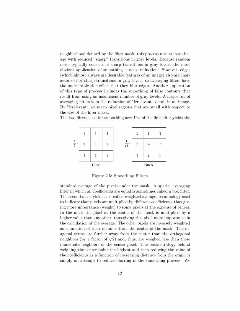
neighborhood defined by the filter mask, this process results in an im-age with reduced ”sharp” transitions in gray levels. Because randomnoise typically consists of sharp transitions in gray levels, the mostobvious application of smoothing is noise reduction. However, edges(which almost always are desirable features of an image) also are char-acterized by sharp transitions in gray levels, so averaging filters havethe undesirable side effect that they blur edges. Another applicationof this type of process includes the smoothing of false contours thatresult from using an insufficient number of gray levels. A major use ofaveraging filters is in the reduction of ”irrelevant” detail in an image.By ”irrelevant” we mean pixel regions that are small with respect tothe size of the filter mask.The two filters used for smoothing are: Use of the first filter yields the

Figure 2.5: Smoothing Filters

standard average of the pixels under the mask. A spatial averagingfilter in which all coefficients are equal is sometimes called a box filter.The second mask yields a so-called weighted average, terminology usedto indicate that pixels are multiplied by different coefficients, thus giv-ing more importance (weight) to some pixels at the expense of others.In the mask the pixel at the center of the mask is multiplied by ahigher value than any other, thus giving this pixel more importance inthe calculation of the average. The other pixels are inversely weightedas a function of their distance from the center of the mask. The di-agonal terms are further away from the center than the orthogonalneighbors (by a factor of

√2) and, thus, are weighed less than these

immediate neighbors of the center pixel. The basic strategy behindweighing the center point the highest and then reducing the value ofthe coefficients as a function of increasing distance from the origin issimply an attempt to reduce blurring in the smoothing process. We

12

could have picked other weights to accomplish the same general ob-jective. However, the sum of all the coefficients in the mask is equalto 16, an attractive feature for computer implementation because ithas an integer power of 2. In practice, it is difficult in general to seedifferences between images smoothed by using either of the masks, orsimilar arrangements, because the area these masks span at any onelocation in an image is so small.

Figure 2.6: Smooth Filtering

4. Order-Statistics Filter (Median Filter)

Order-statistics filters [15] are nonlinear spatial filters whose responseis based on ordering (ranking) the pixels contained in the image areaencompassed by the filter, and then replacing the value of the centerpixel with the value determined by the ranking result. The best-knownexample in this category is the median filter, which, as its name im-plies, replaces the value of a pixel by the median of the gray levelsin the neighborhood of that pixel (the original value of the pixel isincluded in the computation of the median). Median filters are quitepopular because, for certain types of random noise, they provide excel-lent noise-reduction capabilities, with considerably less blurring than

13

linear smoothing filters of similar size. Median filters are particularlyeffective in the presence of impulse noise, also called salt-and-peppernoise [15] because of its appearance as white and black dots superim-posed on an image. The median, j, of a set of values is such that halfthe values in the set are less than or equal to j, and half are greaterthan or equal to j. In order to perform median filtering at a pointin an image, we first sort the values of the pixel in question and itsneighbors, determine their median, and assign this value to that pixel.

Figure 2.7: Median Filtering

Image Segmentation

Segmentation subdivides an image into its constituent regions or objects.The level to which the subdivision is carried depends on the problem beingsolved. That is, segmentation should stop when the objects of interest in anapplication have been isolated.

Segmentation algorithms for monochrome images generally are based onone of two basic properties of image intensity values: discontinuity and sim-ilarity. In the first category, the approach is to partition an image based

14

on abrupt changes in intensity, such as edges. The principal approaches inthe second category are based on partitioning an image into regions that aresimilar according to a set of predefined criteria.In this section, we will be presenting some image segmentation techniqueswe have implemented, which may have to be incorporated in later stagesduring the course of this project.First of all, we present several techniques for detecting the three basic typesof gray-level discontinuities in a digital image: points, lines and edges. Themost common way to look for discontinuities is to run a mask through theimage. For the 3 X 3 mask shown in the figure below, this procedure involvescomputing the sum of the products of the coefficients with the gray levelscontained in the region encompassed by the mask.

Figure 2.8: Mask for Segmentation

The response, R, of the mask at any point in the image is given by

R = w1z1 + w2z2 + · · ·+ w9z9 =

9∑i=1

wizi

whereziis the intensity of the pixel associated with mask coefficientwi. Asbefore, the response of the mask is defined at its center.

1. Thresholding

(a) Basic Global Thresholding

When the intensity distribution of objects and background pix-els are sufficiently distinct, it is possible to use a single (global)threshold applicable over the entire image. In most applications,there is usually enough variability between images that, even if

15

global Thresholding is a suitable approach, an algorithm capableof estimating automatically the threshold value for each image isrequired.

The following iterative algorithm can be used for this purpose:

• Select an initial estimate for the global threshold, T. Here,we have assumed T=130.

• Segment the image using T in the following equation:

g(x, y) =

{1 if f(x, y) > T0 if f(x, y) ≤ T

This will produce two groups of pixels: G1 consisting of allpixels with intensity values > T and G2 consisting of pixelswith values <= T .

• Compute the average (mean) intensity values m1 and m2 forthe pixels in G1 and G2, respectively.

• Compute a new threshold value: T=1/2(m1+m2)

• Repeat steps 2 through 4 until the difference between val-ues of T in successive iterations is smaller than a predefinedparameter T0. Here it is assumed to be 20.

Figure 2.9: Basic Global Thresholding

16

(b) Otsu’s Method

This method [35] minimizes the between-class variance, a well-known measure used in statistical discriminant analysis. Thebasic idea is that well-thresholded classes should be distinct withrespect to the intensity values of their pixels and, conversely, thata threshold giving the best separation between classes in termsof their intensity values would be the best (optimum) threshold.In addition to its optimality, Otsu’s method has the importantproperty that it is based entirely on computations performed onthe histogram of the image, an easily obtainable 1-D array.

Figure 2.10: Optimum global Thresholding using Otsu’s Method

Morphological Operations

Morphological image processing (or morphology) describes a range of imageprocessing techniques that deal with the shape (or morphology) of featuresin an image. Once segmentation is complete, morphological operations canbe used to remove imperfections in the segmented image and provide infor-mation on the form and structure of the image. Morphological operationsare typically applied to remove imperfections introduced during segmenta-tion, and so typically operate on bi-level images. A structuring element is

17

Figure 2.11: Structuring Elements - Hits & Fits

a small image - used as a moving window - whose support delineates pixelneighborhoods in the image plane. The structuring element is moved across

every pixel in the original image to give a pixel in a new processed image.The value of this new pixel depends on the operation performed. There aretwo basic morphological operations: Erosion and Dilation.

1. Erosion

The structuring element s is positioned with its origin at (x, y) andthe new pixel value is determined using the rule:

g(x, y) =

{1 if s fits f0 otherwise

18

Figure 2.12: Erosion

Figure 2.13: Properties of Erosion

2. Dilation

The structuring element s is positioned with its origin at (x, y) andthe new pixel value is determined using the rule:

g(x, y) =

{1 if s hits f0 otherwise

19

Figure 2.14: Dilation

Figure 2.15: Properties of Dilation

20

2.1.3 Neural Network

Introduction

Neural networks are composed of simple elements operating in parallel.These elements are inspired by biological nervous systems. As in nature,the network function is determined largely by the connections between ele-ments. We can train a neural network to perform a particular function byadjusting the values of the connections (weights) between elements.

An artificial neural net is an electrical analogue of a biological neuralnet. The cell body in an artificial neural net is modeled by a linear acti-vation function. The activation function, in general, attempts to enhancethe signal contribution received through different dendrons. The action isassumed to be signal conduction through resistive devices. The synapse inthe artificial neural net is modeled by a non-linear inhibiting function, forlimiting the amplitude of the signal processed at cell body.

Commonly neural networks are adjusted, or trained, so that a particu-lar input leads to a specific target output. Such a situation is shown below.There, the network is adjusted, based on a comparison of the output and thetarget, until the network output matches the target. Typically many suchinput/target pairs are used, in this supervised learning, to train a network.

Batch training of a network proceeds by making weight and bias changesbased on an entire set (batch) of input vectors. Incremental training changesthe weights and biases of a network as needed after presentation of eachindividual input vector. Incremental training is sometimes referred to as“on line” or“adaptive” training.

Neuron Model

1. Simple Neuron A neuron with a single scalar input and no bias appearson the left below.

The scalar input p is transmitted through a connection that multipliesits strength by the scalar weight w, to form the product wp, again ascalar. Here the weighted input wp is the only argument of the trans-fer function f, which produces the scalar output a. The neuron onthe right has a scalar bias, b. You may view the bias as simply beingadded to the product wp as shown by the summing junction or as

21

Figure 2.16: Neural Network

shifting the function f to the left by an amount b. The bias is muchlike a weight, except that it has a constant input of 1.

The transfer function net input n, again a scalar, is the sum of theweighted input wp and the bias b. This sum is the argument of thetransfer function f. Here f is a transfer function, typically a step func-tion or a sigmoid function, which takes the argument n and producesthe output a.

Figure 2.17: Simple Neuron & Transfer Function

22

Note that w and b are both adjustable scalar parameters of the neu-ron. The central idea of neural networks is that such parameters canbe adjusted so that the network exhibits some desired or interestingbehavior. Thus, we can train the network to do a particular job byadjusting the weight or bias parameters, or perhaps the network itselfwill adjust these parameters to achieve some desired end.

2. Transfer Function

The activation function used in our problem is the bipolar sigmoidfunction.

f(x) =2

1 + e−cx− 1 =

1− e−cx

1 + e−cx

where c is the steepness parameter and the sigmoid function range is-1 to +1. The derivative of this function can be

f ′(x) =c

2[1 + f(x)][1− f(x)]

3. Neuron with Vector Input

A neuron with a single R-element input vector is shown below. Herethe individual element inputsp1, p2, . . . pR are multiplied by weightsw1,1, w1,2, . . . w1,R and the weighted values are fed to the summingjunction. Their sum is simply Wp, the dot product of the (single row)matrix W and the vector p.

Figure 2.18: Neuron with Vector Input

The neuron has a bias b, which is summed with the weighted inputsto form the net input n. This sum, n, is the argument of the transfer

23

function f.n = w1,1p1 + w1,2p2 + . . .+ w1,RpR + b

4. Network Architectures Two or more of the neurons shown earlier canbe combined in a layer [2], and a particular network could contain oneor more such layers. First consider a single layer of neurons.

(a) A Layer of Neurons

A one-layer network with R input elements and S neurons follows.In this network, each element of the input vector p is connected

Figure 2.19: A Layer of Neurons

to each neuron input through the weight matrix W. The ith neu-ron has a summer that gathers its weighted inputs and bias toform its own scalar output n(i). The various n(i) taken togetherform an S-element net input vector n. Finally, the neuron layeroutputs form a column vector a. We show the expression for a atthe bottom of the figure.

24

Note that it is common for the number of inputs to a layer to bedifferent from the number of neurons (i.e., R S). A layer is notconstrained to have the number of its inputs equal to the numberof its neurons.

(b) Multiple Layer of Neurons

A network can have several layers [2]. Each layer has a weightmatrix W, a bias vector b, and an output vector a. To distinguishbetween the weight matrices, output vectors, etc., for each ofthese layers in our figures, we append the number of the layer asa superscript to the variable of interest. You can see the use ofthis layer notation in the three-layer network shown below, andin the equations at the bottom of the figure.

Figure 2.20: Multiple Layer of Neurons

The network shown above has R1 inputs, S1 neurons in the firstlayer, S2 neurons in the second layer, etc. It is common for dif-ferent layers to have different numbers of neurons. A constantinput 1 is fed to the biases for each neuron.

Note that the outputs of each intermediate layer are the inputsto the following layer. Thus layer 2 can be analyzed as a one-

25

layer network with S1 inputs, S2 neurons, and an S2xS1 weightmatrix W2. The input to layer 2 is a1; the output is a2. Nowthat we have identified all the vectors and matrices of layer 2, wecan treat it as a single-layer network on its own. This approachcan be taken with any layer of the network. The layers of amultilayer network play different roles. A layer that producesthe network output is called an output layer. All other layersare called hidden layers. The three-layer network shown earlierhas one output layer (layer 3) and two hidden layers (layer 1 andlayer 2). Some authors refer to the inputs as a fourth layer. Wewill not use that designation.

Back Propagation Neural Network

The back-propagation training [2] requires a neural net of feed-forward topol-ogy. Since it is a supervised training algorithm, both the input and the targetpatterns are given. For a given input pattern, the output vector is estimatedthrough a forward pass on the network. After the forward pass is over, theerror vector at the output layer is estimated by taking the component-wisedifference of the target pattern and the generated output vector. A functionof errors of the output layered nodes is then propagated back through thenetwork to each layer for adjustment of weights in that layer. The weightadaptation policy in back-propagation algorithm is derived following theprinciple of steepest descent approach of finding minima of a multi-valuedfunction.

Properly trained back-propagation networks tend to give reasonable an-swers when presented with inputs that they have never seen. Typically, anew input leads to an output similar to the correct output for input vectorsused in training that are similar to the new input being presented. This gen-eralization property makes it possible to train a network on a representativeset of input/target pairs and get good results without training the networkon all possible input/output pairs.

The most significant issue of a back-propagation algorithm is the propa-gation of error through non-linear inhibiting function in backward direction.Before this was invented, training with a multi-layered feed-forward neuralnetwork was just beyond imagination. In this section, the process of propa-gation of error from one layer to its previous layer will be discussed shortly.Further, how these propagated errors are used for weight adaptation will

26

also be presented schematically. Let us consider the figure shown below.Typical neurons employed in back-propagation learning contain two mod-

ules (vide Fig.2.21.(a)). The circle containing∑wixi denotes a weighted

sum of the inputs xi for i= 1 to n. The rectangular box in Fig.2.21.(a)represents the sigmoid type non-linearity. It may be added here that thesigmoid has been chosen here because of the continuity of the function overa wide range. The continuity of the nonlinear function is required in back-propagation, as we have to differentiate the function to realize the steepestdescent criteria of learning. Fig.2.21.(b) is a symbolic representation of theneurons used in Fig.4.1.(c ).

In Fig.2.21.(c), two layers of neurons have been shown. The left side layeris the penultimate (k -1)-th layer, whereas the single neuron in the next k-th layer represents one of the output layered neurons. We denote the toptwo neurons at the (k-1)-th and k-th layer by neuron p and q respectively.The connecting weight between them is denoted by wp,q,k. For computingwp,q,k(n+ 1), from its value at iteration n, we use the formula presented inthe following expressions:

∆wp,q,k = ηδq,kOutp,j

wp,q,k(n+ 1) = wp,q,k(n) + ∆wp,q,k

where wp,q,k(n)=the weight from neuron p to neuron q,at nth step,where qlies in the layer k and neuron p in the(k − 1)th layer counted from the inputlayer;δp,k=the error generated in neuron q,lying in layer k;Outp,j=output ofneuron p,positioned at layer j.

We already mentioned that a function of error is propagated from thenodes in the output layer to other layers for the adjustment of weight. Thisfunctional form of the back-propagated error is presented in expression:

δp,j = Outp,j(1−Outp,j)(∑q

δq,kwp,q,k)

where q = q1, q2, q3 in the following figure. It is seen from expressionabove that the contribution of the errors of each node at the output layer istaken into account in an exhaustively connected neural net.

For training a network by this algorithm, one has to execute the follow-ing 4 steps in order for all patterns one by one.

For each input-output pattern do begin

27

Figure 2.21: Attributes of neurons and weight adjustments by the back-propagation learning algorithm

28

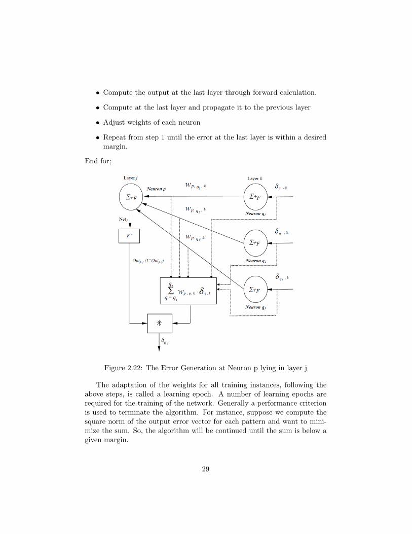
• Compute the output at the last layer through forward calculation.

• Compute at the last layer and propagate it to the previous layer

• Adjust weights of each neuron

• Repeat from step 1 until the error at the last layer is within a desiredmargin.

End for;

Figure 2.22: The Error Generation at Neuron p lying in layer j

The adaptation of the weights for all training instances, following theabove steps, is called a learning epoch. A number of learning epochs arerequired for the training of the network. Generally a performance criterionis used to terminate the algorithm. For instance, suppose we compute thesquare norm of the output error vector for each pattern and want to mini-mize the sum. So, the algorithm will be continued until the sum is below agiven margin.

29

The error of a given output node, which is used for propagation to theprevious layer, is designated by , which is given by the following expression:

δ = F ′ ∗ (t arg et−Out) = Out(1−Out)(t arg et−Out)

2.1.4 Clustering Methods

Fuzzy C-Means Clustering Algorithm

Segmentation of an image of defected leaf involves distribution of the pixelintensity values of an image into clusters, such that the defected portionsor rust-spots in the leaf falls in one such cluster, and the rest of the leaf(which is supposed to be normal) contributes to other clusters. Apparently,the process is simple, but confusion creeps in when we deal with the pixelsthat belong to the boundary of the rust-spots, whether to consider them asa part of the rust and hence draft it into the corresponding cluster, or weconsider it to be a part of the normal portion and hence, accommodate itin some other cluster. The concept of Fuzzy sets [30, 29] allows us to dealwith the ambiguity mentioned above. Suppose there are n elements in a set,and we need to distribute these n elements into c clusters. Each of thesen elements will have c degree of membership values which will correspondto c clusters. Among these c values, the element will be considered to be apart of that cluster which will have the highest membership value for thatelement.

In our case, the set consists of all the pixel-intensity values of the image.We have applied Fuzzy c-means Clustering Algorithm [14, 23, 37, 13, 7, 25,16, 54, 26, 27, 24] which iteratively minimizes the objective function:

Jm =N∑i=1

C∑j=1

uijm ‖ xi − cj‖2

Where m is any real number greater than 1, uij is the degree of membershipof xi in the cluster j, xi is the ith of d-dimensional measured data, cj isthe d-dimension center of the cluster, and ‖ ∗ ‖ is any norm expressing thesimilarity between any measured data and the center.

30

K-Means Clustering Algorithm

K-means [1, 5, 32] is one of the simplest unsupervised learning algorithmsthat solve the well known clustering problem. The procedure follows a simpleand easy way to cluster a given data set through a certain number of clusterswhich is given a priori. The main idea is to define k centroids, one foreach cluster. These centroids should be placed carefully because differentlocations cause different results. So, the better choice is to place them asfar away from each other as possible.

The steps are as follows:

1. For K-number of clusters define K number of centroids as far awayfrom each other as possible.

2. For each object of the data set, the object is placed in the groupbelonging to the centroid to which it is closest.

3. Recalculation of centroids is done by the formula:∑Xk(i, j)

Nk

where Xk(i, j)=objects belonging to kth cluster and Nk=number ofelements in kth cluster

4. Steps 2 and 3 are repeated until the centroids do not change any furtherand thus finds the appropriate centroids for k number of clusters.

2.1.5 Web Technology

HTML

HTML is a language for describing web pages.

• HTML stands for Hyper Text Markup Language

• HTML is a markup language

• A markup language is a set of markup tags

• The tags describe document content

• HTML documents contain HTML tags and plain text

• HTML documents are also called web pages

31

HTML markup tags are usually called HTML tags.

• HTML tags are keywords (tag names) surrounded by angle brackets

• HTML tags normally come in pairs

• The first tag in a pair is the start tag, the second tag is the end tag

• The end tag is written like the start tag, with a forward slash beforethe tag name

• Start and end tags are also called opening tags and closing tags.

JSP

JSP simply puts Java inside HTML pages. You can take any existing HTMLpage and change its extension to ”.jsp” instead of ”.html”. A JSP life cyclecan be defined as the entire process from its creation till the destructionwhich is similar to a servlet life cycle with an additional step which is re-quired to compile a JSP into servlet. The following are the paths followedby a JSP.

1. Compilation

2. Initialization

3. Execution

4. Cleanup

JSP directives provide directions and instructions to the container, tellingit how to handle certain aspects of JSP processing. A JSP directive affectsthe overall structure of the servlet class. It usually has the following form:

<\%@ directive attribute="value" \%>

Directives can have a number of attributes which you can list down as key-value pairs and separated by commas. The blanks between the @ symboland the directive name, and between the last attribute and the closing %¿,are optional.There are four types of tag in jsp scripting elements.

• JSP Declaration tag

• JSP scriptlet tag

32

• JSP Expression tag

• Comment tag

JSP Implicit Objects are the Java objects that the JSP Container makesavailable to developers in each page and developer can call them directlywithout being explicitly declared. JSP Implicit Objects are also called pre-defined variables.

JDBC-ODBC (Database connectivity)

Creating JDBC Application: There are six steps involved in building aJDBC application.

1. Import the packages: This requires that to include the packages con-taining the JDBC classes needed for database programming.//STEP 1. Import required packages

import java.sql.*;

2. Register the JDBC driver: This requires that to initialize a driverso that one can open a communication channel with the database.Following is the code snippet to achieve this://STEP 2: Register JDBC driver

Class.forName("com.mysql.jdbc.Driver");

3. Open and establish a connection: First, we need to establish a con-nection with the data source we want to use. A data source can bea DBMS, a legacy file system, or some other source of data with acorresponding JDBC driver. Typically, a JDBC application connectsto a target data source using one of two classes:

• DriverManager: This fully implemented class connects an appli-cation to a data source, which is specified by a database URL.When this class first attempts to establish a connection, it au-tomatically loads any JDBC 4.0 drivers found within the classpath.

• DataSource: This interface is preferred over DriverManager be-cause it allows details about the underlying data source to be

33

transparent to the application. Note: The samples in this tuto-rial use the DriverManager class instead of the DataSource classbecause it is easier to use and the samples do not require thefeatures of the DataSource class.

• Using the DriverManager Class

• Specifying Database Connection URLs

This requires using the DriverManager.getConnection() method to cre-ate a Connection object, which represents a physical connection withthe database as follows://STEP 3: Open a connection // Database credentials

static final String USER = "username";

static final String PASS = "password";

System.out.println("Connecting to database...");

conn = DriverManager.getConnection(DB\_URL,USER,PASS);

DataSource objects can provide connection pooling and distributedtransactions. This functionality is essential for enterprise databasecomputing. In particular, it is integral to Enterprise JavaBeans (EJB)technology.

4. Execute a query: This requires using an object of type Statement orPreparedStatement for building and submitting an SQL statement tothe database as follows://STEP 4: Execute a query

System.out.println("Creating statement...");

stmt = conn.createStatement();

String sql;

sql = "SELECT id, first, last, age FROM Employees";

ResultSet rs = stmt.executeQuery(sql);

If there is an SQL UPDATE, INSERT or DELETE statement required,then following code snippet would be required://STEP 4: Execute a query

System.out.println("Creating statement...");

stmt = conn.createStatement();

34

String sql;

sql = "DELETE FROM Employees";

ResultSet rs = stmt.executeUpdate(sql);\

5. Extract data from result set:This step is required in case you are fetch-ing data from the database.//STEP 5: Extract data from result set

while(rs.next()){

//Retrieve by column name

int id = rs.getInt("id");

int age = rs.getInt("age");

String first = rs.getString("first");

String last = rs.getString("last");

//Display values

System.out.print("ID: " + id);

System.out.print(", Age: " + age);

System.out.print(", First: " + first);

System.out.println(", Last: " + last);

}

6. Clean up the environment: One should explicitly close all databaseresources versus relying on the JVM’s garbage collection as follows://STEP 6: Clean-up environment

rs.close();

stmt.close();

conn.close();

JSP FILE UPLOADING

A JSP can be used with an HTML form tag to allow users to upload filesto the server. An uploaded file could be a text file or binary or image file orany document.The following HTM code below creates an uploader form. Following are theimportant points to be noted down:

35

• The form method attribute should be set to POST method and GETmethod can not be used.

• The form enctype attribute should be set to multipart/form-data.

• The form action attribute should be set to a JSP file which wouldhandle file uploading at backend server. Following example is usinguploadFile.jsp program file to upload file.

• To upload a single file you should use a single ¡input .../¿ tag withattribute type=”file”. To allow multiple files uploading, include morethan one input tags with different values for the name attribute. Thebrowser associates a Browse button with each of them.

<html>

<head>

<title>File Uploading Form</title>

</head>

<body>

<h3>File Upload:</h3>

Select a file to upload: <br //>

<form action="UploadServlet" method="post"

enctype="multipart/form-data">

<input type="file" name="file" size="50" />

<br />\\

<input type="submit" value="Upload File" />

</form>

</body>

</html>

This will display following result which would allow to select a file from localPC and when user would click at ”Upload File”, form would be submittedalong with the selected file.

2.1.6 Client Server Architecture

Client/server describes the relationship between two computer programs inwhich one program, the client, makes a service request from another pro-gram, the server, which fulfills the request. Although the client/server ideacan be used by programs within a single computer, it is a more important

36

idea in a network. In a network, the client/server model provides a con-venient way to interconnect programs that are distributed efficiently acrossdifferent locations. Computer transactions using the client/server model arevery common.

2.1.7 XML

• XML stands for Extensible Markup Language

• XML is a markup language much like HTML

• XML was designed to carry data, not to display data

• XML was designed to carry data, not to display data

• XML tags are not predefined. You must define your own tags

• XML is designed to be self-descriptive

• XML is a W3C Recommendation

The Difference Between XML and HTML are:

• XML was designed to transport and store data, with focus on whatdata is, while HTML was designed to display data, with focus on howdata looks

• HTML is about displaying information, while XML is about carryinginformation.

• All XML Elements Must Have a Closing Tag. In HTML, some ele-ments do not have to have a closing tag

• XML Tags are Case Sensitive

• XML Elements Must be Properly Nested. In HTML, you might seeimproperly nested elements

• XML documents must contain one element that is the parent of allother elements. This element is called the root element.

An XML element is everything from (including) the element’s starttag to (including) the element’s end tag. An element can contain:

• other elements

37

• text

• attributes

• or a mix of all of the above

A ”well-formatted” XML file must apply to the following conditions:

• A XML document always starts with a prolog (see below for an expla-nation of what a prolog is)

• Every opening tag has a closing tag.

• All tags are completely nested.

A XML file is called valid, if it is well-formatted and if it is contains alink to a XML schema and is valid according to the schema.

2.2 Literature Survey

2.2.1 Introduction

Agriculture has always been the mainstay in economy of most of the de-veloping countries, especially the ones located in South-Asia. The amountof crops that are damaged every year, due to adverse climatic conditions orinvasion of pathogens, can never be neglected. Hence, it is important for thefarmers to detect the growth of disease in plant at an early stage, and takenecessary steps in order to prevent it from spreading to others parts of thefield. It is difficult for the farmers to keep an eye on each and every plant inthe cultivation area to detect manifestation of any infection. Many an imageprocessing approaches has been developed in recent years to serve the pur-pose of a watch-dog, i.e. detecting the growth of a disease at an early stage,determining the type of the disease the leaf is infected with and suggestingnecessary actions. This section will go through most of the research workthat has been done in the field of Image Processing and Artificial NeuralNetwork for the purpose of detection and diagnosis of disease in a plant leaffrom its image.

2.2.2 General Architecture of the System

Researches in Image Processing and Analysis for Detection of Plant Diseaseshave grown immensely over the past decade. Various methods have been

38

Figure 2.23: Architecture of the General System for Detection and Recog-nition of Disease in Plant Leaf

devised that are used to study plant diseases or traits using Image Process-ing. The methods studied are aimed at increasing throughput & reducingsubjectiveness arising from human experts in detecting the plant diseases.As shown in Fig. 2.23, the general system for detection and recognition ofdisease in plant leaf consists of three main components: Image analyzer,Feature extraction and classifier.The processing that is done by using these components is divided into twophases. The first processing phase is the offline phase or Training Phase. Inthis phase, a set of input images of leaves, diseased and normal, were pro-cessed by image analyzer and certain features were extracted. Then thesefeatures were given as input to the classifier, and along with it, the informa-tion whether the image is that of a diseased or a normal leaf. The classifierthen learns the relation among the features extracted and the possible con-clusion about the presence of the disease. Thus the system is trained.The second processing phase is the online phase, in which the features ofa specified image is extracted by image analyzer and then tested by theclassifier whether the leaf is diseased or not, according to the informationprovided to it in the learning phase i.e. offline phase.

This section explores each of the stages involved and presents all the

39

methods that have been incorporated in each of the stages in all researchworks done till date on detection and recognition of plant leaf disease. Someof the plant leaf diseases we aim to detect, diagnose and identify in thissection are shown in Table 1.

2.2.3 Image Acquisition Phase

The Leaf images are collected using digital camera [1] and stored in RGBformat [9] for further processing. Canon IXY55 model was used by Powbun-thorn et. al [22] for collection of Cassava leaves. The focal length was setto 8 mm along with the maintenance of bird’s eye view at 50 cm. In case ofRice Leaves [43], Phadikar et. al used Nikon COOLPIX P4 digital camerain macro mode. On the other hand, Yao et. al. [41] used a CCD color cam-era (Nikon D80, zoom lens 18-200mm, F3.5-5.6, 10.2 Mega pixels) for thepurpose of capturing rice leaf images. The photos of Groundnut leaves [34]were taken by keeping them in the black box in order to avoid the variancein the light intensities each time the photos were taken. Moreover, the inter-ference of external light source can be avoided as in [52]. The RGB colourimages of paddy leaf [44] were captured using a Nokia 3G Mobile Phone,with pixel resolution 240 x 320. The digitized images were about 255KBsize each. Pomegranate leaf images were captured using Nikon Coolpix L20digital camera having 10 megapixels of resolution and 3.6x optical zoom,maintaining an equal distance of 16 cm to the object [28]. In case of Sugar-cane, the infected leaf was placed flat on a white background; Light sourceswere placed at 45 degree on each side of the leaf so as to eliminate any re-flection and to get even light everywhere, thus a better view and brightness.The leaf was zoomed on so as to ensure that the picture taken contains onlythe leaf and white background [40].

2.2.4 Image Enhancement Techniques

Image enhancement is a sub-field of image processing and consists of tech-niques to improve the appearance of an image, to highlight important fea-tures of an image, and to make this image more suitable for use in a partic-ular application (e.g. make features easier to see by modifying the colors orintensities).The acquired leaf images are typically resized according to the requirements.For example, Cassava Leaf images were resized to 640X480 pixels [22], PaddyLeaf images were cropped to get dimensions of 109X310 pixels [45] and Rice

40

Table 2.1: Leaf Diseases whose detection and recognition have been dis-cussed till datePlant Leaf Diseases of Leaf Considerd

Apple Apple mosaic, Apple rust and Apple alternaria leaf spot [19]

Cassava Brown leaf spot [49, 22]

Citrus Citrus Canker [49, 22]

Cotton• Bacterial disease: e.g. Bacterial Blight, Crown Gall,

Lint Degradation.

• Fungal diseases: e.g. Anthracnose, Leaf Spot.

• Viral disease: e.g. Leaf Curl, Leaf Crumple, Leaf Roll.

• Diseases Due To insects: e.g. White flies, Leafinsects.[17]

• Red Spots, Leaf Crumpel

GroundNut iron, zinc and magnesium deficiencies [34]

Maize gray spot & common rust disease

Paddy Blast Disease (BD), Brown-Spot Disease (BSD), and NarrowBrown-Spot Disease (NBSD) [44]

Rice

• Rice blast caused by the fungus Pricularia Grisea, Leafbrown spot caused by the fungus Bypolaris Oryza [43,36, 50]

• RBLB, RSB and RB [41]

Sugarcane Fungi-caused brown spot disease [40]

Tomato Early Blight, Late Blight Septoria Leaf Spot [39]

General Early scorch, Cottony mold, ashen mold, late scorch, tinywhiteness [1]

41

Leaf images were reduced to 800X600 pixels [41].Another popularly technique is transformation of the images from RGB toHSI color space, as is done in case of Cassava [22], Maize, Beans, Banana [4],Citrus [60] and Grape [3] leaves. Phadikar et. al. [43] obtained the grey-level image from the RGB colored image of Rice leaf using the followingequation:

MG = 2× (G− (0.75×R− 0.25×B))

Bashish et. al. [1] suggests applying device-independent color space trans-formation, which converts the color values in the leaf image to the colorspace specified in the color transformation structure. The color transforma-tion structure specifies various parameters of the transformation.In case of Grape [3] and Cotton [17] Leaves, H & B components from HSI&LAB color space are used to reduce effect of illumination and distinguishbetween disease & non-diseased leaf color efficiently.

2.2.5 Noise Reduction Techniques

The techniques generally used to remove unnecessary noise from the acquiredleaf images, are:

1. Erosion and dilation, used on Cassava leaf images

2. Mean filter or smoothing filter [15], used on Tobacco [5], Paddy[45] and Rice leaf [43] images.

3. Median filter of color image with 3*3 rectangle filter window, alsoon Rice Leaf images

4. Anisotropic-diffusion technique used on Cotton and Grape Leafimages.

5. Gaussian Filter, used on Pomegranate leaves [32].

2.2.6 Image Segmentation Phase

Image segmentation is the first step in image analysis and pattern recogni-tion. It is a critical and essential step and is one of the most difficult tasks inimage processing, as it determines the quality of the final result of analysis.Segmentation subdivides an image into its constituent regions or objects.The level to which the subdivision is carried depends on the problem beingsolved. That is, segmentation should stop when the objects of interest in an

42

application have been isolated.Segmentation algorithms for monochrome images generally are based on oneof two basic properties of image intensity values: discontinuity and similar-ity. In the first category, the approach is to partition an image based onabrupt changes in intensity, such as edges. The principal approaches in thesecond category are based on partitioning an image into regions that aresimilar according to a set of predefined criteria.Segmentation techniques that are generally applied are:

1. Optimum Global Thresholding using Otsu’s Method- Thismethod [35] minimizes the between-class variance, a well-known mea-sure used in statistical discriminant analysis. The basic idea is thatwell-thresholded classes should be distinct with respect to the intensityvalues of their pixels and, conversely, that a threshold giving the bestseparation between classes in terms of their intensity values would bethe best (optimum) threshold. In addition to its optimality, Otsu’smethod has the important property that it is based entirely on com-putations performed on the histogram of the image, an easily obtain-able 1-D array. Images of leaves of Cassava, Tobacco and Paddy usedOtsu’s Method for thresholding. Phadikar et. al.used Otsu’s Methodon Hue plane instead of applying the same on Intensity plane of RiceLeaf image represented in HSI model. On the other hand Yao et. alemployed a different approach for segmentation of image of Rice Leaf.The images were first transformed from a red, green, blue (RGB) colorrepresentation to y1 and y2 representation using the following equa-tion: {

y1 = 2g − r − by2 = 2r − g − b

Then in y1 and y2 representation, Otsu’s Method was applied to seg-ment disease spots from rice leaf and two threshold values t1 and t2were automatically generated.

2. Other Thresholding Methods: Rajan et. al. used local entropythreshold method of Eliza and Chang [12] for segmentation for seg-mentation of Paddy Leaves, and compared the results with that, ac-quired using Otsu’s Method. Simple threshold and Triangle thresh-olding methods were used on Sugarcane Leaf images to segment theleaf area and lesion region area respectively.

3. K-Means Clustering: K-means is one of the simplest unsupervisedlearning algorithms that solve the well known clustering problem. The

43

procedure follows a simple and easy way to cluster a given data setthrough a certain number of clusters which is given a priori. The mainidea is to define k centroids, one for each cluster. These centroidsshould be placed carefully because different location causes differentresult. So, the better choice is to place them as further away fromeach other as possible. K-Means Clustering Algorithm was used forsegmentation of images of Tobacco and Pomegranate leaves. Bashishet. al. used K-means clustering to partition the leaf image into fourclusters in which one or more clusters contain the disease in case whenthe leaf is infected by more than one disease. K-means used squaredEuclidean distances.

4. Artificial Neural Network: The colour pixels are clustered by theunsupervised SOFM network to obtained group of colour in the image.The back propagation neural network is then applied to extract leafcolour from diseased part of image. This approach has been appliedfor segmentation of images of Cotton and Grape Leaves.

2.2.7 Feature Extraction Phase

The purpose of the feature extraction [21] is to reduce the image data bymeasuring certain features or properties of each segmented regions such as:color, shape, or texture. The most popular features used to describe animage of plant leaf, are:

1. Percentage of Leaf Area Infected (PI): Image Segmentation byany of the methods mentioned above, characterize some pixels in theimage as that of the diseased portion of the leaf, while the others liein the undiseased portion. Thus we can calculate values of Area ofdiseased portion (AD) and the total area of the leaf (AL). Then, wecalculate percentage of area infected, using the following equation:

PI = (AD

AL)× 100

This value of PI has been used as one of the features of Cassava ,Pomegranate and Sugarcane leaf images.

2. Color Moments: : In order to extract the features based on color[18], we have used the 3 color moments. Firstly, we separated eachcolor image into 3 planes- H plane, S plane and I plane. Then we

44

found out 3 color moments- Moment 1 or Mean, Moment 2 or StandardDeviation and Moment 3 or Skewness, for each plane [57]. Hence eachimage consists of 9 color moments, 3 moments for each color channel.These 9 color moments form a part of the feature vector for an image.This feature has been used for characterizing Tomato , Maize, Appleand Cotton leaf images.

3. Texture-Based Features: In case of feature extraction based ontexture of the image, we used gray level co-occurrence matrix [28, 42].The co-occurrence matrix C(i,j) counts the number of co-occurrenceof pixels with gray-levels i and j respectively, at a given distance d.The matrix [59] is given by:

C(i, j) = cord

((x1, y1), (x2, y2)) ∈ XY ∗XYf(x1, y1) = i, f(x2, y2) = j(x2, y2) = (x1, y1) + (d cos θ, d sin θ)0 < i, j < N

Where d is the distance defined in polar coordinates (d,θ ) with discretelength and orientation. θ takes values 0, 45, 90, 135, 180, 225, 270and 315. Cord represents the number of elements present in the set.The texture features that have been obtained from the co-occurrencematrix of the gray-level image [55] are:

(a) Inertia:Also known as Variance and contrast, Inertia measuresthe local variations in the matrix.

Inertia =∑i

∑j

(i− j)2c(i, j)

(b) Correlation:It measures the sum of joint probabilities of occur-rence of every possible gray-level pair.

Correlation =∑i

∑j

(i− µi)(j − µj)c(i, j)σiσj

where

µi =∑i

i∑j

c(i, j)

µj =∑j

j∑i

c(i, j)

45

σi =∑i

(i− µi)2∑j

c(i, j)

σj =∑i

(j − µj)2∑j

c(i, j)

(c) Energy:Also known as uniformity or the angular second moment,It provides the sum of squared elements in the matrix.

Energy =∑i

∑j

(c(i, j))2

(d) Homogeneity:It measures the closeness of the distribution of theelements in the matrix to their diagonal elements respectively.

Homogeneity =∑i,j

c(i, j)

1 + |i− j|

Texture based features are essential for description of Maize , Apple ,Beans, Banana, Guava, Lemon, Mango and Rice Leaves.

4. Features obtained by Color Co-occurrence Method or CCMmethod:It is a method, in which both the color and texture of animage are taken into account, to arrive at unique features, which rep-resent that image. Bashish et. al used these features to describe plantleaf images. The color co-occurrence texture analysis method was de-veloped through the use of Spatial Gray-level Dependence Matrices orin short SGDM’s.

5. Shape based Features: The area (A) and perimeter (P) of diseasespots were calculated from the binary image of disease spot. Theminimum enclosing rectangle (MER) of a disease spot were obtained bythe method of rotating image with same angle [6]. The long axis lengthand short axis length of MER represented the length (l) and width(w) of a disease spot. The shape features including rectangularity,compactness, elongation and roundness were calculated using area,perimeter, MER of disease spot in Rice Leaf images. Lesion shape andlesion colour feature of disease spot has also been used in detection ofdisease in Paddy Leaves.

6. Other Features:Zhang et al proposed Two-level features to describecitrus canker lesions: at the first level, global features are extracted for

46

detecting canker lesion area from the image background; these globalfeatures are mean, standard deviation, variance and correlation coef-ficient in RGB color space and HIS color space; FFT texture features,and edges. At the second level a kind of combined local features areconstructed to identify canker lesion from other confusable citrus dis-eases lesions. Local Binary Pattern based on Hue was used for thispurpose. Gulhane et al used Eigen feature regularization and extrac-tion Algorithm [20] for feature extraction from cotton leaf images. InRice Leaf Radial distribution of the hue from the center towards theboundary of the diseased spot has been considered as feature to distin-guish the spots since the color of the spots vary from center towardsthe boundary.An improved AdaBoost algorithm or KPCA based feature selection areadopted on the large feature set to select the most significant featuresto produce the classifier.

2.2.8 The Classifiers

A classifier is a system which classifies input images of leaves according tothe degree of presence of a disease in a leaf, and this classification is basedon the features we evaluated in the previous step. The classifier that havebeen used for the purpose of proper detection and recognition of disease inleaves, are:

1. Percentage Infection (PI): The range of PI values will be dividedinto regions for each of the possible outcomes. Eg: In case of Cas-sava Leaves , the range of PI values is divided into two regions- onecorresponding to the leaves having Brown Leaf Spots and the otheris for the ones not having Brown Leaf Spots. Thus, the value of PIevaluated will determine the type of disease the leaf is infected with.The same principle is used for detection of disease in Sugarcane Leaves.Fuzzy Logic (FL) is used for the purpose of disease grading in PomegranateLeaves. A Fuzzy Inference System (FIS) is developed for disease grad-ing by referring to the disease scoring scale. For the FIS for diseasegrading, input variable is Percent Infection (PI) and output variableis Grade. Triangular membership functions are used to define thevariables and six fuzzy rules are set to grade the disease.

2. Support Vector Machine (SVM): This classifier [47, 38, 61, 33, 48]is used for classifying leaves of Apple and Rice. Multiclass SVMs aredeployed for grape leaf disease classification. In case of classification

47

of Apple leaves, genetic algorithm is used to determine the parametersof SVM [58, 53].

3. Back-Propagation Neural Network: This type of Artificial NeuralNetwork is excellent for performing classification task. The developerof the Artificial Neural Network has to decide which configuration ofthe Artificial Neural Network is appropriate for a good out-of-sampleprediction. The configuration of the Artificial Neural Network needs tobe determined accurately to give an optimal classification result. Thisconfiguration includes the number of layers, the number of neurons ineach layer, and the minimal number of training samples. This configu-ration is also called the topology of the Artificial Neural Network. It isknown that too many neurons in any layer degrade the effectiveness ofthe model, leads to the undesirable consequences, long training times,and local minima. Large number of connection weights in the ArtificialNeural Network model may cause over-fitting and loss of the gener-alization capacity. On the other hand, choosing less than requirednumber of neurons may not capture the full range and dynamicity ofthe data. Many heuristic rules were suggested for finding the optimalnumber of neurons in the hidden layer, and several techniques are nowavailable. Most of them employ trial-and-error methods, in which thetraining starts with a small number of neurons, and additional neuronsare gradually added until some performance goal is satisfied. Unfortu-nately there is no theoretical consideration for determining the opticalnetwork topology for the specified problem. Bashish et al used thisclassifier for plant leaf disease recognition.

4. Others: Production rule method with forward chaining is used as aclassifier for diseases in Paddy Leaf. Zhang et al proposed a hierarchi-cal citrus canker detection algorithm for detection of canker disease incitrus.

2.3 Brief Overview of the System

As shown in Fig. 1, the system consists of three main components: Imageanalyzer, Feature extraction and classifier.The processing that is done by using these components is divided into twophases. The first processing phase is the offline phase or Training Phase.In this phase, a set of input images of wheat leaves (diseased and normal)were processed by image analyzer and certain features were extracted. Then

48

these features were given as input to the classifier, and along with it, theinformation whether the image is that of a diseased (R, MR, MS or S) or anormal wheat leaf. The classifier then learns the relation among the featuresextracted and the possible conclusion about the presence of the rust disease.Thus the system is trained.The second processing phase is the online phase, in which the features ofa specified image is extracted by image analyzer and then tested by theclassifier whether the leaf is diseased or not, according to the informationprovided to it in the learning phase (offline phase).

Figure 2.24: Overall structure of the system

49

Chapter 3

Design & Methodology

3.1 Offline Phase

3.1.1 Image Acquisition Phase

The images are captured by using a high resolution 3-CCD color camera with3.3 million-pixel sensitivity, 3X optical zoom lens, auto focus illuminatorlight, and focal length 8-24 mm. The camera was placed at about 60mmfrom the top of the wheat leaves. The image from the camera is digitizedinto a 24-bit image with resolution 720 X 540 pixels.

3.1.2 Image Enhancement Phase

Image enhancement is a subfield of image processing and consists of tech-niques to improve the appearance of an image, to highlight important fea-tures of an image, and to make this image more suitable for use in a par-ticular application (eg: make certain features easier to see by modifying thecolors or intensities).The abnormalities of the diseased leaves are revealed by the appearance ofthe rust-spots. From the inspection of the infected leaves it was found thatthe diseased parts have higher intensity values than other normal tissues. Toextract the abnormal tissues, we transform the defected image into HSI colorspace [46, 8, 56, 51, 10], and then perform certain segmentation techniques,as will be depicted shortly.

50

Figure 3.1: Result of application of HSI transformation of color image andits normalized histogram

3.1.3 Image Segmentation Phase

Image segmentation is the first step in image analysis and pattern recogni-tion. It is a critical and essential step and is one of the most difficult tasks inimage processing, as it determines the quality of the final result of analysis.Segmentation subdivides an image into its constituent regions or objects.The level to which the subdivision is carried depends on the problem beingsolved. That is, segmentation should stop when the objects of interest in anapplication have been isolated.Segmentation of an image of defected leaf involves distribution of the pixelintensity values of an image into clusters, such that the defected portionsor rust-spots in the leaf falls in one such cluster, and the rest of the leaf(which is supposed to be normal) contributes to other clusters. Apparently,the process is simple, but confusion creeps in when we deal with the pixelsthat belong to the boundary of the rust-spots, whether to consider them asa part of the rust and hence draft it into the corresponding cluster, or weconsider it to be a part of the normal portion and hence, accommodate itin some other cluster. The concept of Fuzzy sets allows us to deal with theambiguity mentioned above. Suppose there are n elements in a set, and weneed to distribute these n elements into c clusters. Each of these n elementswill have c degree of membership values which will correspond to c clusters.

51

Among these c values, the element will be considered to be a part of thatcluster which will have the highest membership value for that element.In our case, the set consists of all the pixel-intensity values of the image.We have applied Fuzzy c-means Clustering Algorithm which iteratively min-imizes the objective function:

Jm =N∑i=1

C∑j=1

uijm||xi − cj ||2

Where m is any real number greater than 1, uij is the degree of membershipof xi in the cluster j, xi is the ith of d-dimensional measured data, cj isthe d-dimension center of the cluster, and || ∗ || is any norm expressing thesimilarity between any measured data and the center.Here, the value of m is taken as 2, and by trial and error method, we haveachieved best results when the number of clusters is 4. When this algorithmterminates, we obtain a clustered image where each pixel has taken the valueof one of the four generated cluster centers.Generally the intensity values of the pixels belonging to the diseased part ofa leaf have greater intensity compared to the normal ones. Hence, the rust-spots are assumed to be accommodated in the cluster having the highestintensity value. We give all the pixels in that cluster the maximum availableintensity value and we give the minimum to the rest. The binary repre-sentation thus obtained will later be used in the Feature Extraction Phase[30, 29, 11] for calculating the number of occurrences of zeros as well as thenumber of connected components present in the image. The results of Fuzzyc-means Algorithm, applied on some original images are shown in Fig. 4.

3.1.4 Feature Extraction Phase

The fifth phase is the feature extraction phase. The purpose of the featureextraction is to reduce the image data by measuring certain features orproperties of each segmented regions such as: color, shape, or texture.The features that we have used are:

1. Entropy: Entropy is the minimum amount of data that is sufficientto describe an image without losing information.If an image is considered to be the output of an imaginary zero-memory”intensity source”, we can use the histogram of the observed image toestimate the symbol probabilities of the source. Then the intensity

52

Figure 3.2: Results of application of Fuzzy C-means Clustering on Imagesof Diseased Wheat Leaves

source’s entropy is given by the following Equation.

H = −L−1∑k=0

pr(rk) log pr(rk)

Where L is the number of intensity values. A discrete random variablerk in the interval [0..L-1] is used to represent the intensities of an M *N image and that each rk occurs with probability pk(rk ).Base of the Logarithm is taken as 2. Hence, the average informationper intensity output of the imaginary intensity source in bits. It is notpossible to code the intensity values of the imaginary source (and the

53

sample image) with fewer than H bits/pixel.

2. Median:All the pixel intensity values of an image is taken in a 1-dimensional array, and then they are sorted in ascending order. Themiddle element of the sorted array is the median of the image.

3. Mode:The mode of an image refers to that pixel intensity value of theimage which occurs the maximum number of times in that image. Itis also the pixel intensity value for which the histogram of the imageattains the maximum height.

4. Variance:Let (x, y) be the coordinates of a pixel in an image, and letSxy denote a neighborhood (subimage) of specified size, centered at(x, y). Therefore, the mean value of the pixels in Sxy can be computedusing the expression given in the following equation.

mSxy=

∑(s,t)∈Sxy

rs,tp(rs,t)

where rs, t is the gray level at coordinates (s,t) in the neighborhood,and p(rs,t ) is the neighborhood normalized histogram component cor-responding to that value of gray level. Similarly, the gray-level varianceof the pixels in region Sxy is given by Eq. 4.

The local mean is a measure of average gray level in neighborhoodSxy, and the variance (or standard deviation) is a measure of contrastin that neighborhood.

5. Standard Deviation: Standard Deviation is obtained by taking thesquare root of the measure of variance determined while consideringthe earlier pattern.

6. Number of zeros in the binary image: The color image or thegray-level image that has been taken as input is converted into binaryimage after application of segmentation using Fuzzy C-means algo-rithm, as we discussed in the previous section. Then we count thenumber of zeros present in this binary image.

54

7. Number of peaks in the histogram: A peak in a histogram isdefined as those values which are greater than their nearest two neigh-bors. We obtain such peaks from the histogram of the gray-scale imageand then we count the number of such peaks for that image.

8. Number of connected components in the binary image: Let Srepresent a subset of pixels in an image. Two pixels p and q are saidto be connected in S if there exists a path between them consistingentirely of pixels in S. For any pixel p in S, the set of pixels that areconnected to it in S is called a connected component of S. If it only hasone connected component, then set S is called a connected set. Wehave considered 8-connected neighbors while determining the pathsbetween pixels.

9. Green density of an image: Here we have considered only the G-plane of the RGB image and found out how many pixel intensity valueson this G-plane is above a certain threshold ( say, 150). That numberis then divided by the total number of pixel intensity values to get thegreen-density of the image.Table 3.3 represents the results of Feature Extraction on images of twodiseased leaves and one normal leaf.

10. Color Moments: In order to extract the features based on color, wehave used the 3 color moments. Firstly, we separated each color imageinto 3 planes- H plane, S plane and I plane. Then we found out 3color moments- Moment 1 or Mean, Moment 2 or Standard Deviationand Moment 3 or Skewness, for each plane. Hence each image consistsof 9 color moments, 3 moments for each color channel. These 9 colormoments form a part of the feature vector for an image.

55

Figure 3.3: Result of feature extraction on 2 diseased and 1 normal wheatleaf images

56

11. Texture-Based Features: In case of feature extraction based ontexture of the image, we used gray level co-occurrence matrix. The co-occurrence matrix C(i,j) counts the number of co-occurrence of pixelswith gray-levels i and j respectively, at a given distance d. The matrixis given by:

C(i, j) = cord

((x1, y1), (x2, y2)) ∈ XY ∗XYf(x1, y1) = i, f(x2, y2) = j(x2, y2) = (x1, y1) + (d cos θ, d sin θ)0 < i, j < N

Where d is the distance defined in polar coordinates (d,θ ) with dis-crete length and orientation. θ takes values 0, 45, 90, 135, 180, 225, 270and 315. Cord {} represents the number of elements present in the set.

The texture features that have been obtained from the co-occurrencematrix of the gray-level image, are:

(a) Inertia:Also known as Variance and contrast, Inertia measuresthe local variations in the matrix.

Inertia =∑i

∑j

(i− j)2c(i, j)

(b) Correlation:It measures the sum of joint probabilities of occur-rence of every possible gray-level pair.

Correlation =∑i

∑j

(i− µi)(j − µj)c(i, j)σiσj

where

µi =∑i

i∑j

c(i, j)

µj =∑j

j∑i

c(i, j)

σi =∑i

(i− µi)2∑j

c(i, j)

σj =∑i

(j − µj)2∑j

c(i, j)

57

(c) Energy:Also known as uniformity or the angular second moment,It provides the sum of squared elements in the matrix.

Energy =∑i

∑j

(c(i, j))2

(d) Homogeneity:It measures the closeness of the distribution of theelements in the matrix to their diagonal elements respectively.

Homogeneity =∑i,j

c(i, j)

1 + |i− j|

Table 3.4 demonstrates the use of the color and texture features thatwe have discussed. It can be seen that the combination of these fea-tures can separate the 4 categories of diseased wheat leaves- R, MR,MS, S.After the successful completion of the Feature Extraction phase, we

have obtained the values of the features, which will be input to a clas-sifier. For this purpose, we have used a multi-layered feed-forwardback-propagation Network. The classifier is discussed in detail in thenext section.

3.1.5 The Classifier

Before the on-line processing is done, the system needs to be manuallytrained using a set of training samples. An artificial Neural Network wasused to perform our classification task. There are many types of ArtificialNeural Networks. The most widely used is Back Propagation Artificial Neu-ral Network.This type of Artificial Neural Network is excellent for performing classifi-cation task. The developer of the Artificial Neural Network has to decidewhich configuration of the Artificial Neural Network is appropriate for agood out-of-sample prediction. The configuration of the Artificial NeuralNetwork needs to be determined accurately to give an optimal classifica-tion result. This configuration includes the number of layers, the number ofneurons in each layer, and the minimal number of training samples. Thisconfiguration is also called the topology of the Artificial Neural Network. Itis known that too many neurons in any layer degrade the effectiveness of themodel, leads to the undesirable consequences, long training times, and localminima. Large number of connection weights in the Artificial Neural Net-work model may cause over-fitting and loss of the generalization capacity.

58

Figure 3.4: Result of feature extraction on diseased wheat leaf images

59

On the other hand, choosing less than required number of neurons may notcapture the full range and dynamicity of the data. Many heuristic rules weresuggested for finding the optimal number of neurons in the hidden layer, andseveral techniques are now available. Most of them employ trial-and-errormethods, in which the training starts with a small number of neurons, andadditional neurons are gradually added until some performance goal is sat-isfied. Unfortunately there is no theoretical consideration for determiningthe optical network topology for the specified problem.By trial-and-error method, we kept four neurons in the hidden layer of thenetwork.

3.2 Online Phase

3.2.1 Creation of XML file

A JSP page ”Initial.jsp” is coded. If we run this page , it will create anempty XML file showing the client ”File saved”. The root element will be< info >. For every user a < data > element will be appended to the rootelement. Every < data > element will have the following sub-elements:

• < c id >: Unique id given to every uploaded image

• < f name >: Name of the uploaded image file

• < c date >: The exact date and time of uploading the image

• < result >: Result produced after processing the image

• < timeP >: The processing time of the image

• < c ip >: The IP address of the client uploaded the particular image

3.2.2 Creation of a Home Page for User

A JSP file ”Index.jsp” is created for the purpose of giving a choice to theuser: whether he wants to upload a new image or want to get informationabout an already uploaded image. If he chooses to upload a new image,”Index.jsp” page will lead him to the page ”page.jsp”. if he gives choiceto get result of an already uploaded image it will lead him to the page”getId.jsp”.

60

Figure 3.5: Output of XML Creation Program

Figure 3.6: XML File immediately after creation

61

Figure 3.7: User Home Page

3.2.3 Uploading of Image by User

A JSP page ”page.jsp” has been designed for this purpose. This page willgive the client the option to browse an image machine. There is a submitbutton ”Send File ”. If the client click here it will pass the image as argumentto the page ”uploadandstore.jsp”.

Figure 3.8: Page Where User can Upload an Image

3.2.4 Storing & Processing of Uploaded Image File in theServer

”Uploadandstore.jsp” page is prepared to handle the following series of ac-tivities:

62

1. Rename and Upload the file which it received from the page ”page.jsp”.

2. Show the type of file uploaded.

3. Generate a unique ID to every uploaded image and display it.

4. Process the image and save the following

• File name

• Unique ID

• Date and time of uploading the image

• Generated Result

• Time taken to process the image

• IP address of the client from where the file is received

5. Display the following:

• Name of the uploaded file

• IP address of the client from where the file is received.

• The time and date of uploading the image

Figure 3.9: Message after Successful Uploading of Image

3.2.5 Sending Response to the Client

”GetResult.jsp” is a page which displays the Following Information to theUser:

63

Figure 3.10: Information of Uploaded Images Stored in XML file

Figure 3.11: MS Access Database If used for Storage of File Properties

64

• The Input Image

• The Unique ID

• Result Generated by the Server

• Processing Time

• RAM, Processor and OS Information of the Server

Figure 3.12: Response Sent from the Client to the Server

3.3 Graphical User Interfaces

During the course of this project,two softwares were built which were imple-mented through some GUIs.The following sections gives a rough idea aboutthe GUIs.

3.3.1 Image Processing Applications

This GUI is built to perform all kinds Image Processing techniques ongrayscale images in the Spatial Domain.The software name is Photo MagicV1.0.

The software allows the user to execute different Image Processing tech-niques on grayscale images.The areas of Image Processing that it deals withare-

• Image Enhancement

• Image Segmentation

• Morphological Operations

65

It allows the user to browse the image to be processed as well as save itafter processing is completed. Here’s a snapshot of how the main GUI lookslike-

Figure 3.13: Image Processing Applications GUI:Photo Magic V 1.0

1. Image Enhancement

• Image Negative

• Power-Law Transfromations

66

• Histogram Processing

• Histogram Equalization

• Smooth Filtering(Mean Filtering)

• Median Filtering

• Unsharp Masking

• High Boost Filtering

Figure 3.14: Image Negative

Figure 3.15: Smooth Filtering

67

Figure 3.16: Histogram Processing

2. Image Segmentation

• Point Detection

• Line Detection

• Edge Detection using Robert,Prewitt & Sobel Operators

• Region Growing

• Thresholding

• Watershed Segmentation

Figure 3.17: Edge Detection through Sobel Operator

68

Figure 3.18: Basic Global Thresholding

Figure 3.19: Watershed Segmentation

3. Morphological Operations

• Erosion

• Dilation

• Opening

• Closing

• Boundary Extraction

69

Figure 3.20: Erosion

Figure 3.21: Dilation

Figure 3.22: Boundary Extraction

70

3.3.2 Feature Extraction

This GUI is built to extract the values of various features of an image(generallyimage of wheat leaf).The GUI allows the user to browse the image,select thefeatures whose values are to be calculated by means of checkboxes and pro-vides the output through a MS Excel worksheet.

Here are some snapshots of the Feature Extraction GUI-

Figure 3.23: Feature Extraction GUI

Figure 3.24: Feature Extraction GUI after data is written to the MS Excelworksheet

71

Figure 3.25: MS Excel worksheet containing the feature data

3.3.3 Training & Testing of Neural Network

This GUI is built to train an artificial neural network inorder to detect anddiagnose rust disease in wheat leaves.It consists of two parts-Training andTesting.

The Training part trains the network based on some feature values ofalready detected(i.e whether diseased or undiseased) wheat leaves and storethe entire data into a cell array.

The Testing part deals with the detection and diagnosis(if detected) ofa wheat leaf which has not been tested previously. Here are some snapshotsof the Feature Extraction GUI-

72

Figure 3.26: Training & Testing GUI

Figure 3.27: Training & Testing GUI:Training

73

Figure 3.28: Training & Testing GUI:Testing

Figure 3.29: Training & Testing GUI after data is written to the MS Excelworksheet

74

Figure 3.30: MS Excel worksheet containing the testing result

75

Chapter 4

Sample Codes

4.1 Back Propagation Main Function

The steps followed by the Main Function are:

1. Search the patterns from the input images using Pattern Recognizerand add it to the input vector of the Back-Propagation Network.

2. Set the desired output= +1 if the input images is that of a diseasedwheat leaf from S Category, set it to -1 if the wheat Leaf is Undiseasedand belongs to R Category. The values for the rest of the Categoriesare determined dynamically as any value between 1 and -1. The desiredoutput are then added to the Output Vector of the Back-PropagationNetwork.

3. Train the Back-Propagation Network.

4. Testing Phase- Give input images and let the network evaluate whetherthe Input image is that of a diseased leaf or not.

5. Evaluate the percentage of correct result that is produced by the Back-Propagation Network.

Source Code: backPropMain.m file

clc

% %IMAGE RESIZING

% rows=20;

76

% cols=200;

NoOfPatterns=13;

% L is a vector of integers specifying the number of nodes at each Layer,

% i.e for all i, L(i)=number of nodes at Layer i. There must be at least

% 3 layers and the input layer L(1) must equal the dimension of each vector

% in input. Likewise L(end) must be equal to the dimension of each vector

% in Desired output

L=[NoOfPatterns 6 1];

% n is the training rate for network learning [0.1 - 0.9]

n=0.3;

%Satmse is the Satisfactory Mean squared error at which to terminate

%computation

Satmse=0.0004;

% d=0.2;

% MS=0;

% MR=-0.2;

% FMR=-0.4;

% R=-1;

d=input(’Range of S= 1 to ’);

string=sprintf(’Range of MS= %0.2f to ’,d);

MS=input(string);

string=sprintf(’Range of MR= %0.2f to ’,MS);

MR=input(string);

string=sprintf(’Range of FMR= %0.2f to ’,MR);

FMR=input(string);

string=sprintf(’Range of R= %0.2f to -1 ’,FMR);

disp(string);

% X is the Input - the training samples, a P-by-N matrix, where each

% Input[p] is a training vector

X=zeros(1,NoOfPatterns);

%X=[30 40 60; 255 1 100];

%b= Feature vector added to Input training vector

b=zeros(1,NoOfPatterns);

%D is the desired outputs, a P-by-M matrix where each Desired[p] is the

77

%desired output for the corresponding input Input[p]

D=[1];

%D=[1; -1];

choice=1;

%disp(’LEARNING BEGINS..’);

fileID=fopen(’Test Results 20.2.2013 without extraction Try 5.txt’,’w’);

fprintf(fileID,’Images considered for Training:\n’);

fclose(fileID);

while choice==1

img=input(’enter the name of the image file: ’,’s’);

imgrgb=imread(img);

imggray=rgb2gray(imgrgb);

% imggray=imresize(imggray,[rows cols]);

%converting the 2d image matrix into 1d array

% imgtrans=imggray’;

% b=imgtrans(:)’;

% b=double(b);

b=double(FeatureExtractionColorTexture(imgrgb));

fileID=fopen(’Test Results 20.2.2013 without extraction Try 5.txt’,’a’);

fprintf(fileID,’%s\n’,img);

% maximum=max(max(b));

% b=b/maximum;

%append to training vector

X=[X;b];

disease=input(’image is diseased[(S=1),(MS=0.2),(MR=0)] or

undiseased[(MR=-0.2),(R=-1)]: ’);

D=[D;disease];

choice=input(’Do you want to train the network with more test-images?

78

yes(1) or no(0): ’);

end

fclose(fileID);

%DELETE 1ST ROWS FROM INPUT-TRAINING VECTOR X & DESIRED OUTPUT VECTOR D

X(1,:)=[];

D(1,:)=[];

disp(’LEARNING IS GOING ON...PLEASE WAIT’);

X=double(X);

Network = backprop(L,n,Satmse,X,D);

disp(’LEARNING IS COMPLETE’);

% Network.epochs

% input(’ ’)

disp(’automatic testing of all files in current directory is going on...’);

% disp(’WRONG RESULTS’);

choice=1;

CorrectOutput=0;

Tested=0;

fileID=fopen(’Test Results 20.2.2013 without extraction Try 5.txt’,’a’);

fprintf(fileID,’\n\n’);

fclose(fileID);

for i=1:50

fileID=fopen(’Test Results 20.2.2013 without extraction Try 5.txt’,’a’);

Tested=Tested+1;

img=sprintf(’d%d.png’,i);

imgrgb=imread(img);

imggray=rgb2gray(imgrgb);

tes=sprintf(’Testing d%d.png’,i);

79

disp(tes);

X=double(FeatureExtractionColorTexture(imgrgb));

Out = backproptest(Network,X);

if Out.Output>=d

fprintf(fileID,’d%d.png Diseased S\n’,i);

CorrectOutput=CorrectOutput+1;

elseif (Out.Output<d && Out.Output>MS)

fprintf(fileID,’d%d.png Diseased MS\n’,i);

elseif (Out.Output<MS && Out.Output>=MR)

fprintf(fileID,’d%d.png Diseased MR\n’,i);

elseif (Out.Output<MR && Out.Output>=FMR)

fprintf(fileID,’d%d.png Undiseased MR\n’,i);

else

fprintf(fileID,’d%d.png Undiseased R\n’,i);

end

fclose(fileID);

end

for i=1:57

fileID=fopen(’Test Results 20.2.2013 without extraction Try 5.txt’,’a’);

Tested=Tested+1;

img=sprintf(’FMR%d.jpg’,i);

tes=sprintf(’Testing FMR%d.jpg’,i);

disp(tes);

imgrgb=imread(img);

imggray=rgb2gray(imgrgb);

X=double(FeatureExtractionColorTexture(imgrgb));

80

Out = backproptest(Network,X);

if Out.Output>=d

fprintf(fileID,’FMR%d.jpg Diseased S\n’,i);

elseif (Out.Output<d && Out.Output>=MS)

fprintf(fileID,’FMR%d.jpg Diseased MS\n’,i);

elseif (Out.Output<MS && Out.Output>=MR)

fprintf(fileID,’FMR%d.jpg Diseased MR\n’,i);

elseif (Out.Output<MR && Out.Output>=FMR)

fprintf(fileID,’FMR%d.jpg Undiseased MR\n’,i);

CorrectOutput=CorrectOutput+1;

else

fprintf(fileID,’FMR%d.jpg Undiseased R\n’,i);

end

fclose(fileID);

end

for i=1:5

fileID=fopen(’Test Results 20.2.2013 without extraction Try 5.txt’,’a’);

Tested=Tested+1;

img=sprintf(’MR%d.png’,i);

tes=sprintf(’Testing MR%d.png’,i);

disp(tes);

imgrgb=imread(img);

imggray=rgb2gray(imgrgb);

X=double(FeatureExtractionColorTexture(imgrgb));

Out = backproptest(Network,X);

81

if Out.Output>=d

fprintf(fileID,’MR%d.png Diseased S\n’,i);

elseif (Out.Output<d && Out.Output>=MS)

fprintf(fileID,’MR%d.png Diseased MS\n’,i);

elseif (Out.Output<MS && Out.Output>=MR)

fprintf(fileID,’MR%d.png Diseased MR\n’,i);

CorrectOutput=CorrectOutput+1;

elseif (Out.Output<MR && Out.Output>=FMR)

fprintf(fileID,’MR%d.png Undiseased MR\n’,i);

else

fprintf(fileID,’MR%d.png Undiseased R\n’,i);

end

fclose(fileID);

end

for i=1:4

fileID=fopen(’Test Results 20.2.2013 without extraction Try 5.txt’,’a’);

Tested=Tested+1;

img=sprintf(’MS%d.png’,i);

tes=sprintf(’Testing MS%d.png’,i);

disp(tes);

imgrgb=imread(img);

imggray=rgb2gray(imgrgb);

X=double(FeatureExtractionColorTexture(imgrgb));

Out = backproptest(Network,X);

if Out.Output>=d

fprintf(fileID,’MS%d.png Diseased S\n’,i);

82

elseif (Out.Output<d && Out.Output>=MS)

fprintf(fileID,’MS%d.png Diseased MS\n’,i);

CorrectOutput=CorrectOutput+1;

elseif (Out.Output<MS && Out.Output>=MR)

fprintf(fileID,’MS%d.png Diseased MR\n’,i);

elseif (Out.Output<MR && Out.Output>=FMR)

fprintf(fileID,’MS%d.png Undiseased MR\n’,i);

else

fprintf(fileID,’MS%d.png Undiseased R\n’,i);

end

fclose(fileID);

end

for i=1:149

fileID=fopen(’Test Results 20.2.2013 without extraction Try 5.txt’,’a’);

Tested=Tested+1;

img=sprintf(’%dMod.png’,i);

tes=sprintf(’Testing R%d.jpg’,i);

disp(tes);

imgrgb=imread(img);

imggray=rgb2gray(imgrgb);

X=double(FeatureExtractionColorTexture(imgrgb));

Out = backproptest(Network,X);

if Out.Output>=d

fprintf(fileID,’R%d.jpg Diseased S\n’,i);

elseif (Out.Output<d && Out.Output>=MS)

fprintf(fileID,’R%d.jpg Diseased MS\n’,i);

elseif (Out.Output<MS && Out.Output>=MR)

83

fprintf(fileID,’R%d.jpg Diseased MR\n’,i);

elseif (Out.Output<MR && Out.Output>=FMR)

fprintf(fileID,’R%d.jpg Undiseased MR\n’,i);

else

fprintf(fileID,’R%d.jpg Undiseased R\n’,i);

CorrectOutput=CorrectOutput+1;

end

fclose(fileID);

end

p=int8((CorrectOutput/Tested)*100);

str=sprintf(’Out of %d images tested, number of correct results are %d.

Percentage=%d’,Tested,CorrectOutput,p);

disp(str)

Output produced on the Command Window of Matlab is:

Range of S= 1 to 0.2

Range of MS= 0.20 to 0

Range of MR= 0.00 to -0.2

Range of FMR= -0.20 to -0.8

Range of R= -0.80 to -1

enter the name of the image file: d1.png

image is diseased[(S=1),(MS=0.2),(MR=0)] or undiseased[(MR=-0.2),(R=-1)]: 1

Do you want to train the network with more test-images? yes(1) or no(0): 1

enter the name of the image file: R1.jpg

image is diseased[(S=1),(MS=0.2),(MR=0)] or undiseased[(MR=-0.2),(R=-1)]: -1

Do you want to train the network with more test-images? yes(1) or no(0): 0

LEARNING IS GOING ON...PLEASE WAIT

LEARNING IS COMPLETE

automatic testing of all files in current directory is going on...

Testing d1.png

Testing d2.png

Testing d3.png

Testing d4.png

84

Testing d5.png

Testing d6.png

Testing d7.png

Testing d8.png

Testing d9.png

Testing d10.png

Testing d11.png

Testing d12.png

Testing d13.png

Testing d14.png

Testing d15.png

Testing d16.png

Testing d17.png

Testing d18.png

Content of the Output File Test Results.txt is:

d1.png Diseased S

d2.png Diseased S

d3.png Diseased S

d4.png Diseased S

d5.png Diseased MS

d6.png Diseased S

d7.png Diseased S

d8.png Diseased S

d9.png Diseased S

d10.png Diseased S

d11.png Diseased S

d12.png Diseased S

d13.png Diseased S

d14.png Diseased S

d15.png Diseased S

d16.png Diseased S

The following Flow-Chart represents the stages of the Back-PropagationMain Function:

4.2 Storing & Processing of input image at Server

The following is the code of the JSP page ”Uploadandstore.jsp” discussedin Detailed Design.

85

Figure 4.1: Flow Chart Demonstrating Back Propagation Main Function

86

<%@ page import="java.io.*" %>

<%@ page import="java.util.Date, java.text.SimpleDateFormat" %>

<%@ page import="java.awt.image.BufferedImage"%>

<%@ page import="java.io.File"%>

<%@ page import="java.io.IOException"%>

<%@ page import="javax.imageio.ImageIO"%>

<%@ page import="java.util.Calendar" %>

<%@ page import="java.io.File"%>

<%@ page import="javax.xml.parsers.DocumentBuilder"%>

<%@ page import="javax.xml.parsers.DocumentBuilderFactory"%>

<%@ page import="javax.xml.parsers.ParserConfigurationException"%>

<%@ page import="javax.xml.transform.Transformer"%>

<%@ page import="javax.xml.transform.TransformerException"%>

<%@ page import="javax.xml.transform.TransformerFactory"%>

<%@ page import="javax.xml.transform.dom.DOMSource"%>

<%@ page import="javax.xml.transform.stream.StreamResult"%>

<%@ page import="org.w3c.dom.Attr"%>

<%@ page import="org.w3c.dom.Document"%>

<%@ page import="org.w3c.dom.Element"%>

<%@ page import="org.w3c.dom.NodeList"%>

<%@ page import="org.w3c.dom.Node"%>

<% java.util.Locale locale = request.getLocale(); %>

<html>

<BODY bgcolor="#999999">

<%

String saveFile="";

String contentType = request.getContentType();

if ((contentType != null) && (contentType.indexOf("multipart/form-data") >= 0)) {

DataInputStream in = new DataInputStream(request.getInputStream());

int formDataLength = request.getContentLength();

byte dataBytes[] = new byte[formDataLength];

int byteRead = 0;

int totalBytesRead = 0;

while (totalBytesRead < formDataLength)

{

87

byteRead = in.read(dataBytes, totalBytesRead,formDataLength);

totalBytesRead += byteRead;

}

String file = new String(dataBytes);

saveFile = file.substring(file.indexOf("filename=\"") + 10);

saveFile = saveFile.substring(0, saveFile.indexOf("\n"));

saveFile = saveFile.substring(saveFile.lastIndexOf("\\") + 1,saveFile.indexOf("\""));

int lastIndex = contentType.lastIndexOf("=");

String boundary = contentType.substring(lastIndex + 1,contentType.length());

int pos;

pos = file.indexOf("filename=\"");

pos = file.indexOf("\n", pos) + 1;

pos = file.indexOf("\n", pos) + 1;

pos = file.indexOf("\n", pos) + 1;

int boundaryLocation = file.indexOf(boundary, pos) - 4;

int startPos = ((file.substring(0, pos)).getBytes()).length;

int endPos = ((file.substring(0, boundaryLocation)).getBytes()).length;

Date d = new Date();

String dateString = getFormattedDate (d);

String ch=new String();

int j=0;

int l=dateString.length();

for(int i=0;i<l;i++)

{

char c=dateString.charAt(i);

if(c>=’0’ && c<=’9’)

{

ch+=c;

}

}

String b=saveFile;

int str_length=b.length();

int str_index=b.indexOf(".");

String ext=b.substring(str_index,str_length);

88

String res="";

saveFile="webapps/root/images/"+ch+ext;

File f = new File(saveFile);

FileOutputStream fileOut = new FileOutputStream(f);

fileOut.write(dataBytes, startPos, (endPos - startPos));

fileOut.flush();

fileOut.close();

long MILLIS_PER_DAY = 24 * 60 * 60 * 1000;

long p_time=0;

long timePortion1=0;

long timePortion2=0;

if(ext.equals(".jpg") || ext.equals(".png") || ext.equals(".bmp"))

{

Date now1 = Calendar.getInstance().getTime();

timePortion1 = now1.getTime() % MILLIS_PER_DAY;

File f_read = new File(saveFile);

BufferedImage image = ImageIO.read(f_read);

int height = image.getHeight();

int width = image.getWidth();

res="Height is: "+height+" and width is: "+width;

Date now2 = Calendar.getInstance().getTime();

timePortion2 = now2.getTime() % MILLIS_PER_DAY;

p_time=(timePortion2-timePortion1);

}

else

res="This is not an image file! Cannot be processed!!! Sorry..";

String p_time_s = ""+p_time;

String ip=request.getRemoteAddr();

try {

89

File fXmlFile = new File("webapps/root/database.xml");

DocumentBuilderFactory docFactory = DocumentBuilderFactory.newInstance();

DocumentBuilder docBuilder = docFactory.newDocumentBuilder();

Document doc = docBuilder.parse(fXmlFile);

Element rootElement = doc.getDocumentElement();

Element data = doc.createElement("data");

rootElement.appendChild(data);

Element c_id = doc.createElement("c_id");

c_id.appendChild(doc.createTextNode(ch));

data.appendChild(c_id);

Element f_name = doc.createElement("f_name");

f_name.appendChild(doc.createTextNode(b));

data.appendChild(f_name);

Element c_date = doc.createElement("c_date");

c_date.appendChild(doc.createTextNode(dateString));

data.appendChild(c_date);

Element result = doc.createElement("result");

result.appendChild(doc.createTextNode(res));

data.appendChild(result);

Element timeP = doc.createElement("timeP");

timeP.appendChild(doc.createTextNode(p_time_s));

data.appendChild(timeP);

Element c_ip = doc.createElement("c_ip");

c_ip.appendChild(doc.createTextNode(ip));

data.appendChild(c_ip);

TransformerFactory transformerFactory = TransformerFactory.newInstance();

Transformer transformer = transformerFactory.newTransformer();

DOMSource source = new DOMSource(doc);

StreamResult result1 = new StreamResult(new File("webapps/root/database.xml"));

90

transformer.transform(source, result1);

}

catch (ParserConfigurationException pce)

{

pce.printStackTrace();

}

catch (TransformerException tfe)

{

tfe.printStackTrace();

}

out.println("\n");

%>

<font size="6" color="#111199">You have successfully uploaded the<i>

<%

if(b.endsWith(".jpg"))

out.println("Image file!!");

else if(b.endsWith(".pdf"))

out.println("Pdf file");

else if((b.endsWith(".doc"))||(b.endsWith(".docx")))

out.println("Word file!!");

else if(b.endsWith(".txt"))

out.println("Text file!!");

else

out.println("Unknown type file!!");

%>

</i></font><br><br>

<font size="5" color="#111111">Your id is:<font color="red"><b><%=ch%></b></font>

<br><br>

Selected file is :<%= b %><br>

from the client :<%= ip %><br>

on :<%= dateString %>

<br><br>

91

<form action="getResult.jsp" method="post">

<input name="h_td" type="hidden" value="<%= ch %>">

<input type="submit" value="Result">

</form>

<%

}

%>

<%!

String getFormattedDate(Date d)

{

SimpleDateFormat simpleDate = new SimpleDateFormat("dd/MM/yy hh:mm:ss");

return simpleDate.format(d);

}

%>

</body>

</html>

92

Chapter 5

Experimental Results

5.1 Neural Network

We trained the network using ten input images:

• Two images of Disease-free Wheat Leaf

• Two images of Diseased Leaf belonging to MR class

• Four images of Diseased Leaf belonging to S class

• One image of Diseased Leaf belonging to R class

• One image of Diseased Leaf belonging to MS class

After the training phase is completed and all the weights in the network isestablished, we gave 342 images as input to the network one after the other(the process has been automated such that it takes as input, all the imagespresent in the current directory) and found out that for 290 of those 342images we get accurate estimate, thus yielding 84.8% success rate.

Table 5.1: Summary of Results of ClassifierDisease Type Diseased Undiseased

TotalDisease Rating S MS MR MR R

Number of Test Images 60 32 30 114 106 342

Number of correct diagnosis by Classifier 57 25 24 85 99 290

Number of incorrect Diagnosis by Classifier 3 7 6 29 7 52

Percentage of correct diagnosis 95 78.1 80 74.6 93.4 84.8%

93

Chapter 6

Conclusion & Future Scope

In this project, we have developed an integrated image processing and anal-ysis system which is capable of identifying rust disease in wheat leaves. Thesystem has been successfully loaded on a server and can respond to clientrequest. This approach may also be effective in case of plant leaves otherthan Wheat. The features needed for description of the leaves must be cho-sen carefully.As a proposal for future work, we envisage modifying this system such thatit will be effortlessly reachable to the farmers, the possible end users to thissystem. We can develop a system with contract from government, whichcan be used in Block-Development Offices and Panchayats.One such solution to the problem of reaching this system to the targetedend-users is simulating the application on Android Platform. The AndroidApplication will be loaded on the mobiles of the users. This approach hastwo drawbacks. If there is any change in information, about infections inwheat leaves in real world, after the application has already been loadedto the respective mobiles, we cannot modify any module of the system toaccommodate the aforesaid change in the real world information. Moreover,today, a mobile phone supporting Android Operating System is quite ex-pensive and hence it may not be easily affordable to the farmer.Being located at the server, this system overcomes the first drawback men-tioned above. If there is a change in the information of Disease Category ofWheat Leaves, the change may be reflected by altering the required lines ofcode and recompiling the program. The user need not have to worry aboutthem.The other platforms on which the system can be built, and the possible ar-chitecture of the system is a matter of further research and implementation.

94

Bibliography

[1] Bashish D. A., Braik M., and Bani-Ahmad S. Grape leaf disease de-tection from color imagery using hybrid intelligent system. In IEEE,2010.

[2] Konar A. Artificial Intelligence and Soft Computing. CRC Press, firstedition, 1999.

[3] Meunkaewjinda A., Kumsawat P., Attakitmongcol K., and Srikaew A.Grape leaf disease detection from color imagery using hybrid intelligentsystem. In IEEE, 2008.

[4] Varthini S. Ananthi S. Detection and classification of plant leaf diseases.International Journal of Research in Engineering Applied Sciences,2(2):ISSN: 2249–3905, February 2012.

[5] Deshmukh P. R. Badnake M. R. Infected leaf analysis and comparisonby otsu threshold and k-means clustering. International Journal ofAdvanced Research in Computer Science and Software Engineering, 2,March 2012.

[6] G. Bradski and A. Kaehler. Learning opencv: computer vision with theopencv library. In California: OReilly Media, pages 238– 250, 2008.

[7] Bezdek J. C. Pattern recognition with fuzzy objective function algo-rithms. In Plenum Press, New York, NY, 1981.

[8] T. Carron and P. Lambert. Color edge detector using jointly hue, sat-uration and intensity. In IEEE international conference on Image Pro-cessing, pages 977–082, Austin, USA, 1994.

[9] M. M. Chang, M. I. Sezan, and A. M. Tekalp. Adaptive bayesian seg-mentation of color images. volume 3, pages 404–414, 1994.

95

[10] H. D. Cheng, X. H. Jiang, Y. Sun, and Jing Li Wang. Color imagesegmentation: Advances prospects. In Pattern Recognition, volume 34,pages 2259–2281, 2001.

[11] Majumder D. D. Fuzzy mathematical approach in pattern recognitionand image processing. In Proc. 1st int. Fuzzy Syst. Assoc. Cong. Palma-De-Mallorc, s, Spain, July 1985.

[12] Eliza Yingzi Du and Chein-I Chang. An unsupervised approach tocolour video thresholding. Ieee proc.international conference on multi-media and expo icme033:iii-337-40, 2009.

[13] Dunn and J. C. Well-separated clusters and the optimal fuzzy parti-tions. Journal of Cybernetics, pages 4:95–104, 1974.

[14] Bezdek J.C.and R. Ehrlich and W. Full. Fcm: the fuzzy c-mean cluster-ing algorithm. In Computer and Geoscience, 10, pages 191–203, 1984.

[15] R.C. Gonzalez and R.E. Woods. Digital Image Processing. Pearson,USA, 3rd edition, isbn: 0-13-234563-3 edition, 2010.

[16] Dubuission B. Gu. T. Similarity of classes and fuzzy clustering. InFuzzy Sets and Systems, pages 34:213–221, 1990.

[17] Gurjar A. A. Gulhane V. A. Detection of diseases on cotton leavesand its possible diagnosis. International Journal of Image Processing(IJIP), 5, 2011.

[18] Zhi-Chun Huang, Patrick P. K. Chan, Wing. W. Y. Ng, and Daniel S.Yeung. Content based image retrieval using color moment and gabortexture feature. In Proceedings of 9th international conference on ma-chine learning and cybernetics, pages 719–724, Qingdao, July 2010.

[19] Tian J., HU Q., MA X., and HAN M. An improved kpca/ga-svmclassification model for plant leaf disease recognition. Journal of Com-putational Information Systems 8: 18 (2012) 7737-7745, 2012.

[20] Xudong Jiang, Bappaditya Mandal, and Alex Kot. Eigenfeature reg-ularization and extraction in face recognition. IEEE Transaction onPattern analysis and Machine intelligence, 30(3), March 2008.

[21] Young He Jiazhi Pan. Recognition of plants by leaves digital image andneural network. IEEE proceedings on 2008 International Conference onComputer Science and Software Engineering, 2008.

96

[22] Powbunthorn K., Abudullakasim W., and Unartngam J. Assessmentof the severity of brown leaf spot disease in cassava using image analy-sis. In The International conference of the Thai Society of AgriculturalEngineering 2012, Chiangmai, Thailand, August 4-5 2012.

[23] Dzung L.and Chenyang X.and Jerry L. A survey of current methodsin medical image segmentation. In Technical Report JHU/ECE, pages99–01, The John Hopkins University, 2001.

[24] El-Helly M., Onsi H., Rafea A., and El-Gammal S. Segmentation tech-nique for detecting leaf spots in cucumber crop using fuzzy clusteringalgorithm. In 11th international conference on AI (ICAIA), 2003.

[25] Rouben. M. Fuzzy clustering algorithms and their clustering validity.European Journal of Operational Research, 10, pages 10:294–301, 1982.

[26] Y. B. M. V. M. Halkidi. Cluster validity methods: Part i. In SIGMODRecord, September 2002.

[27] Y. B. M. V. M. Halkidi. Cluster validity methods: Part ii. In SIGMODRecord, September 2002.

[28] Chanda B. Majumder D. D. Digital image processing and analysis.Prentince Hall of India Private Limited, September 2007.

[29] Majumder S. Majumder D. D. fuzzy set in pattern recognition andimage analysis, in advances in inform. sc. and tech. (ed. d. dutta ma-jumder). In Statistical Publishing Society, ISI), pages 50–69, ISI, Cal-cutta, 1982.

[30] Pal S. K. Majumder D. D. Concepts of fuzzy sets and its application inpattern recognition problems. In Proc. Nat. Conf. of CSI, Hyderabad,India, January 1976.

[31] Goldberg N. P Marsalis M. A. Leaf, stem and stripe rust diseases ofwheat. March 2011.

[32] Sannaki S. N., Rajpurohit V. S., Nargund V. B., Kumar A., and Yal-lur P. S. Leaf disease grading by machine vision and fuzzy logic. Int.J. Comp. Tech. Appl, 2(5):1709–1716 ISSN:2229–609.

[33] C. Nello and J. S. Taylor. In: An Introduction to Support Vector Ma-chines and Other Kernel-based Learning. Cambridge University Press,2000.

97

[34] Bharambe C. J. Nisale S. S. Detection and analysis of deficiencies ingroundnut plant using geometric moments. World Academy of Science,Engineering and Technology 58, 2011.

[35] N. Otsu. A threshold selection method from gray-level histogram. IEEETrans. Syst., Man and Cybern, 9(1):62–66, Jan 1979.

[36] S. H. OU. In: Rice Diseases. Kew Surrey. PhD thesis, CommonwealthMycological Institute, England, 1972.

[37] S. K. Pal. Image segmentation using fuzzy correlation. In Informationsciences, 62, pages 223–250, 1992.

[38] J. L. Pang, C. L. Zhang, W. Pan, and et al. Automated identificationof tomatoes with diseases using artificial neural network trained withgenetic algorithms. Transactions of the Chinese Society of AgriculturalEngineering, 20 (3):113 – 116, 2004.

[39] Kumar R. Patil J. K. Color feature extraction of tomato leaf diseases.International Journal of Engineering Trends and Technology, 2, March2011.

[40] Bodhe S. K. Patil S. B. Leaf disease severity measurement using im-age processing. International Journal of Engineering and Technology,3(5):297–301, 2011.

[41] Yao Q., Guan Z., Zhou Y., Tang J., Hu Y., and Yang B. Application ofsupport vector machine for detecting rice diseases using shape and colortexture features. International conference on engineering computations,2009.

[42] K. Shanmugam R.M. Haralick and I. Dinstein. Textual features forimage classification. IEEE Trans. Syst. Man Cybern., 3(6):610621, Nov1973.

[43] Phadikar S., Sil J., and Das A. K. Classification of rice leaf diseasesbased on morphological changes. International Journal of Informationand Electronics Engineering, 2(3), May 2012.

[44] Rajan A. S. Image processing techniques for diagnosing paddy disease.In Proceedings of the World Congress on Engineering 2012 Vol II WCE2012, London, U.K, July 4 - 6 2012.

98

[45] Rajan A. S. Image processing techniques for diagnosing paddy disease.In Proceedings of the World Congress on Engineering 2012 Vol II WCE2012, London, U.K, July 4 - 6 2012.

[46] C. L. Jacobs T. L. Hunstberger and R. L. Cannon. Iterative fuzzy imagesegmentation. Pattern Recognition, 18(2):131–138, 1985.

[47] Y. W. Tian, T. L. Li, C. H. Li, and et al. Method for recognition ofgrape disease based on support vector machine. Transactions of theCSAE, 23(6):175 – 180, 2007.

[48] V Vapnik. The nature of statistical learning theory. In Springer Verlag,New York, 1995.

[49] Msikita W., B. James, E. Nnodu, J. Legg, K. Wydra, and F. Ogbe.Disease control in cassava farms. International Institute of TropicalAgriculture, Nigeria, 2000.

[50] R. K. Webster. In: Rice Blast Disease Identification Guide. Davis,Dept. of Plant Pathology, University of California, 2000.

[51] W.S.Kim and R.H. Park. Color image palette construction based onthe hsi color system for minimizing the reconstruction error. In IEEEInternational Conference on Image Processing, C, pages 1041–1044,1996.

[52] Kim W.Y. A practical pattern recognition system for translation, scaleand rotation invariance. In Intl. Conf. on Computer Vision and PatternRecgn, pages 391–396, 1994.

[53] L. M. Cao X. P. Wang. Genetic algorithms: theory, applications andsoftware. In Xi’an: Xi’an Jiaotong University Press, pages 28 – 51,2000.

[54] G. Beni X.L.Xie. A validity measure for fuzzy clustering. IEEETrans.On Pattern Analysis and Machine Intelligence, 13(8):841–847,1991.

[55] K. Xu and Y. Li. An image search approach based on local main colorfeature and texture feature. volume 20(2), pages 77 – 79, 2005.

[56] A. C. She Y.Rui and T. S. Huang. Automated region segmentationusing attraction-based grouping in spatial-color-texture space. In In-ternational Conference on Image Processing, A, pages 53–56., 1994.

99

[57] Hui Yu, Mingjing Li, Hong-Jiang Zhang, and Jufu Feng. Color texturemoments for content-based image retrieval. International Conferenceon Image Processing, 2003.

[58] Jian Zhang, Jiliu Zhou, Kun He, and Mei Gong. An improved quantumgenetic algorithm for image segmentation. Journal of ComputationalInformation Systems, 7(11):3979 – 3985, 2011.

[59] Xinhong Zhang and Fan Zhang. Congress on image and signal process-ing. IEEE computer society, pages 773–776, 2008.

[60] Meng Q. Zhang M. Citrus canker detection based on leaf images anal-ysis. In IEEE, 2010.

[61] C. L. Zhao, C. X. Zheng, M. Zhao, and et al. Automatic classificationof driving mental fatigue with eeg by wavelet packet energy and kpca-svm. International Journal of Innovative Computing, Information andControl, 7(3):1157 – 1168, May 2011.

100