Federal Reserve Bank of New YorkStaff Reports

Broker-Dealer Risk Appetite and Commodity Returns

Erkko Etula

Staff Report no. 406November 2009

Revised September 2010

This paper presents preliminary findings and is being distributed to economistsand other interested readers solely to stimulate discussion and elicit comments.The views expressed in the paper are those of the author and are not necessarilyreflective of views at the Federal Reserve Bank of New York or the FederalReserve System. Any errors or omissions are the responsibility of the author.

Broker-Dealer Risk Appetite and Commodity ReturnsErkko EtulaFederal Reserve Bank of New York Staff Reports, no. 406November 2009; revised September 2010JEL classification: G10, G12, G13, G24

Abstract

This paper shows that the risk-bearing capacity of U.S. securities brokers and dealers is astrong determinant of risk premia in commodity derivatives markets. Commodityderivatives are the principal instrument used by producers and purchasers of commoditiesto hedge against commodity price risk. Broker-dealers play an important role in thishedging process because commodity derivatives are traded primarily over the counter. Icapture the limits of arbitrage in this market in a simple asset pricing model whereproducers and purchasers of commodities share risk with broker-dealers who are subjectto funding constraints. In equilibrium, the price of aggregate commodity risk decreases inthe relative leverage of the broker-dealer sector. Empirical evidence from fourteencommodity markets lends substantial support to the model’s predictions. Fluctuations inrisk-bearing capacity have particularly strong forecasting power for energy returns, bothin sample and out of sample.

Key words: asset pricing, financial intermediaries, commodity prices, futures markets,risk appetite

Etula: Federal Reserve Bank of New York (e-mail: erkko.etula@ny.frb.org). The views expressedin this paper are those of the author and do not necessarily reflect the position of the FederalReserve Bank of New York or the Federal Reserve System.

1. Introduction

I present evidence that the risk-bearing capacity of U.S. securities brokers and

dealers is a strong determinant of risk premia in commodity derivatives. These

markets are important for producers and purchasers of commodities because they

provide an easy way to share the price risk of physical commodity holdings with

�nancial investors. Since the majority of commodity derivatives are bilateral over-

the-counter (OTC) contracts between a client and a �nancial intermediary, broker-

dealers play a key role in this hedging process. I capture the limits of arbitrage

(Shleifer and Vishny, 1997) in this market by deriving a simple asset pricing model

where producers and consumers of commodities share risk with broker-dealers

who are subject to funding constraints. In equilibrium, the price of aggregate

commodity risk decreases in the relative leverage of the broker-dealer sector. I

�nd substantial empirical support for the model�s predictions using data from

14 commodity markets. Fluctuations in risk-bearing capacity have particularly

strong forecasting power for energy returns, both in-sample and out-of-sample.

Broker-dealers are leveraged �nancial institutions, such as investment banks,

who �buy and sell securities for a fee, hold an inventory of securities for resale,

or do both.�1 They are distinguished from other investor classes by their active,

pro-cyclical management of leverage: Adrian and Shin (2008a) document that

expansions in broker-dealer assets are accompanied by increases in leverage as

broker-dealers take advantage of greater balance sheet capacity. Conversely, con-

tractions in broker-dealer assets are accompanied by decreases in leverage as risk

constraints tighten. Consequently, to an outside observer, it would appear that

the risk-bearing capacity, or e¤ective risk aversion, of broker-dealers varies over

time. The literature on limits of arbitrage and its applications to segmented mar-

kets suggests that the pricing implications of time-varying e¤ective risk aversion

1Guide to the Flow of Funds Accounts, Board of Governors of the Federal Reserve (2000)

1

are largest when broker-dealers are predominantly on one side of the market.2

Following these insights, this paper argues that the e¤ective risk aversion of

broker-dealers determines risk premia in commodity derivatives because broker-

dealers are, to a large extent, the marginal investor on the speculative side of

the market. In this way, the paper presents a departure from the vast literature

on hedging pressure e¤ects that focuses on the producer and purchaser side of

the market.3 The importance of broker-dealers stems from the high degree of

intermediation required to funnel �nancial investor capital into commodities. Un-

like stocks, bonds and other securities, the trading of many physical commodities

involves signi�cant transportation and storage costs as well as possible informa-

tional asymmetries (such as quality concerns), which discourage �nancial investors

from engaging in physical commodity transactions in the marketplace. This is

why the risk associated with physical commodity positions is often termed �non-

marketable�(Mayers, 1972). To bypass these market imperfections, commodity

price risk can be securitized and traded via derivatives that reference physical

commodities. A brief overview of this market is provided below.

1.1. Market for Commodity Derivatives

There are two broad categories of commodity derivatives: exchange-traded deriv-

atives and OTC derivatives. Exchange-traded derivatives include futures and op-

tions traded in exchanges such as the New York Mercantile Exchange and Chicago

Mercantile Exchange. While in principle any investor can buy or sell these secu-

rities, the large notional sizes of futures contracts and the perceived riskiness of

commodities have traditionally discouraged retail and institutional investors alike.

Only recently have investable commodity indexes and exchange traded funds made

2Gromb and Vayanos (2010) provide an excellent survey of the theoretical literature on limitsof arbitrage. An example of a situation where �nancial intermediaries are predominantly on oneside of the market is provided by Froot (1999) who studies the pricing of catastrophe insurance.

3A review of this literature is provided below.

2

the asset class more accessible to a broader class of investors.4 Despite this de-

velopment, the exchange-traded market still represents less than 10% of the total

market for commodity derivatives.5

Unlike standardized contracts traded in exchanges, OTC derivatives (such as

forwards, swaps, and options) are tailored to suit the needs of individual investors.

In OTC transactions clients bargain directly with broker-dealers who are the mar-

ket makers in these derivatives. Upon reaching an agreement, the broker-dealer

may hold the commodity risk on its trading book until it receives an o¤setting

OTC position, or it may hedge its net exposure using an exchange-traded deriva-

tive or another OTC contract. In addition to the price risk associated with pure

market making, most commodity traders take on commodity risk by choosing to

leave parts of their books unhedged or by holding entirely speculative positions.

Some larger broker-dealers even speculate by holding outright positions in physical

commodities.6

The overwhelming size of the OTC market relative to the exchange-traded

market highlights the importance of broker-dealer capital for the functioning of

commodity derivatives markets. As such, the premium that hedgers are required

to pay for insurance against commodity price risk is likely to be a¤ected by the

e¤ective risk aversion of broker-dealers.7 To the extent that hedgers� demand

4Tang and Xiong (2010) examine the �nancialization process of commodities precipitated bythe rapid growth of index investment to the commodities markets since the early 2000s.

5At the peak of the June 2008 commodity boom, the Commodity Futures Trading Commis-sion (2008) estimated the total notional value of all commodity futures and options outstandingin U.S. exchanges to be $946 billion, which is approximately 85% of all exchange-traded com-modity derivatives outstanding worldwide (Bank for International Settlements, 2008). At thesame time, the Bank for International Settlements estimated the total notional value of all OTCcommodity derivatives outstanding worldwide to be $13.2 trillion.

6However, relative to the total notional value of the commodity derivatives market, broker-dealers�outright positions in physical commodities (such as tankers of crude oil in the Gulf ofMexico) are small.

7Grossman and Miller (1988) emphasize that hedgers also have a strong preference for im-mediacy in hedging transactions. This further increases their vulnerability to shifts in broker-dealers�e¤ective risk aversion.

3

for insurance is independent of broker-dealers�risk constraints, the e¤ective risk

aversion of broker-dealers can be expected to impact the equilibrium returns on

commodity derivatives. Absence of arbitrage across derivatives markets implies

that the risk premia of OTC transactions are also incorporated in the returns on

exchange-traded derivatives.8

1.2. Theoretical and Empirical Strategy

I motivate the link between broker-dealer risk-bearing capacity and commodity

risk premia by deriving a simple asset pricing model where risk-constrained broker-

dealers provide insurance to households who wish to hedge their positions in phys-

ical commodities. Broker-dealer leverage is limited by a value-at-risk (VaR) con-

straint, which caps the probability of insolvency.9 In equilibrium, the required

return on a security depends on its comovement with the market portfolio, but

also on its residual comovement with the aggregate portfolio of physical commodi-

ties. I refer to the latter as the aggregate non-marketable portfolio. Thus, there is

an additional systematic risk factor� the return on the aggregate non-marketable

portfolio� which determines security returns in addition to the market risk factor.

The premium per unit of non-marketable risk is pinned down by the economy�s

e¤ective risk aversion. I show that the e¤ective risk aversion varies over time

with the tightness of broker-dealers�risk constraints and it can be expressed as a

function of aggregate balance sheet components of broker-dealers and households.

This innovation allows me to test the empirical predictions of the model using

aggregate balance sheet data from the Federal Reserve�s Flow of Funds Accounts.

The model predicts that, controlling for market risk, the measure of e¤ective

risk aversion forecasts returns on securities that co-move with the aggregate non-

8Indeed, due to poor availability of reliable data on OTC forwards, the empirical section usesdata on futures contracts.

9Adrian and Shin (2008c) provide a micro foundation for this constraint from a moral hazardproblem between borrowers and lenders.

4

marketable portfolio. Since the market risk adjusted returns of di¤erent securities

load di¤erently on the non-marketable risk factor, the model also delivers a cross-

sectional prediction for the magnitude and direction of the forecasting relationship.

The empirical section of the paper investigates these predictions for 14 commodity

futures, two investable commodity indexes, and other securities.

1.3. Related Literature

This paper builds on two broad strands of literature: the literature on �nancial

market frictions and asset prices as well as the extensive literature on the deter-

minants of expected commodity returns.

The idea that the risk-bearing capacity of arbitrageurs is limited and has con-

sequences for asset prices originates in the work on limits of arbitrage pioneered

by Shleifer and Vishny (1997). Gromb and Vayanos (2002) and Brunnermeier and

Pedersen (2009) are among the �rst to relate arbitrageurs�inability to exploit price

di¤erences to endogenous balance sheet constraints. The speci�c funding con-

straints analyzed in this paper build on the work of Adrian and Shin (2008a,b,c)

who demonstrate that the active management of �nancial intermediary balance

sheets generates procyclical leverage, which has consequences for asset prices. My

�nding that the risk-bearing capacity of broker-dealers determines risk premia in

commodity markets is most similar in spirit to the �nding of Adrian, Etula and

Shin (2009) that �uctuations in short-term U.S. dollar funding liquidity determine

risk premia in foreign exchange markets, and to the �nding of Adrian and Shin

(2008a) that �uctuations in short-term funding liquidity forecast changes in the

VIX risk premium.

The literature on the determinants of expected commodity returns can be

roughly divided into two groups. The �rst group uses the CAPM to argue that

the expected return on commodity holdings is compensation for systematic risk.

Early studies include Black (1976) and Breeden (1980) who explain the variation

5

in futures prices by systematic risk that stems from changes in economic state

variables. Tests of these models �nd scant evidence in the data, as shown by

Jagannathan (1985) and a number of other studies. More recently, Bessembinder

and Chan (1992) �nd that the same variables that forecast market returns �

e.g., dividend yield, interest rate, and yield spread � also forecast commodity

returns. This suggests that time-varying risk premia in commodities could be

driven by macro-economic forces that determine asset allocation. Gorton and

Rouwenhorst (2006) argue that commodity futures, as an asset class, provide a

risk-return pro�le that is comparable to that of equities.

The second group of studies argues that the expected return of holding com-

modities is driven largely by commodity-speci�c factors. Most relevant for the

present paper are the studies that �nd additional forecastability of commodity

futures returns using the net positions of hedgers in the futures market, which is

known as hedging pressure. The idea of hedging pressure dates back to Keynes

(1930) whose theory of normal backwardation argues that producers short fu-

tures to hedge their initially long positions in the underlying physical commod-

ity. Gorton, Hayashi and Rouwenhorst (2007) provide a comprehensive review

of the literature and show that while the direction of net hedging is consistent

with Keynes�hedging pressure hypothesis, commodity-speci�c hedging pressures

do not have signi�cant forecasting ability for futures returns. Models that allow

both systematic and commodity-speci�c predictors of futures prices include Stoll

(1979) and Hirschleifer (1988, 1989). Empirical evidence for the combined role of

commodity-speci�c hedging pressure and systematic risk include Carter, Rausser

and Schmidt (1992), Bessembinder (1992), and de Roon, Nijman and Veld (2000).

Hong and Yogo (2009) show that the aggregate futures basis explains as much of

the variation in expected returns as systematic predictors.

The empirical section of this paper contributes to the �rst group of commodity

studies by demonstrating that, for a set of commodities, a substantial portion of

6

the time-variation in expected returns can be attributed to time-variation in the

risk-bearing capacity of U.S. broker-dealers. The paper�s argument for why broker-

dealers�capacity to bear risk matters for expected commodity returns builds on

the second group of studies: broker-dealers have an important role in providing

insurance to producers and purchasers of commodities who wish to hedge their

physical positions. Anson (2002) and Erb and Harvey (2006) suggest that futures

strategies that engage in such insurance provision have earned positive excess

returns. The results in this paper are also nicely consistent with the recent �nding

of Acharya, Lochstoer and Ramadorai (2009) that the risk appetite of oil and

gas producers, as proxied by their default risk, forecasts future returns on these

commodities. The authors build on my results to show that both broker-dealer

risk-bearing capacity and producer default risk forecast commodity returns.

My theoretical motivation combines insights from the commodity pricing mod-

els of Mayers (1972), Stoll (1979), Hirschleifer (1988, 1989) and de Roon, Nijman

and Veld (2000), and the asset pricing model of Danielsson, Shin and Zigrand

(2008). In the latter model, the risk appetite of arbitrageurs shifts endogenously

with balance sheet constraints that �uctuate with market outcomes, generating

endogenous risk. The balance sheet constraints are imposed by a contracting set-

ting of Adrian and Shin (2008c), which yields a value-at-risk rule. In addition

to the literature on limits of arbitrage, the model has similarities with the large

behavioral �nance literature on noise trader risk (e.g. DeLong, Shleifer, Summers

and Waldmann, 1990; Barberis, Shleifer and Vishny, 1998; Hong and Stein, 1999)

, and market making (e.g. Grossman and Miller, 1988; Kyle, 1985). It is also con-

sistent with Du¢ e and Strulovici�s (2009) model of limited capital mobility where

higher costs of intermediation increase return volatility and prolong temporary risk

premia. Overall, the distinguishing feature of the current theoretical framework

is its ability to generate time-varying e¤ective risk aversion without restrictive

assumptions on the behavior of passive traders. By focusing on the actions of

7

risk-constrained �nancial institutions, the model is also distinctly di¤erent from

the consumption-based models that generate time-varying risk aversion through,

for instance, habit formation (Campbell and Cochrane, 1999; Chan and Kogan,

2002).

The outline of the paper is as follows. As a motivation to my empirical in-

vestigation, section 2 develops a simple theoretical model, which introduces risk-

constrained broker-dealers in an equilibrium pricing model for commodities. Sec-

tion 3 tests the predictions of the model in the data and conducts robustness

checks. Section 4 digs deeper into energy commodities and o¤ers a discussion of

the 2008 run-up in energy prices. Section 5 concludes.

2. Theoretical Motivation

As discussed above, there is an extensive literature that relates commodity risk

premia to two components: systematic marketable risk and commodity-speci�c

hedging pressure. The latter arises from risks that agents cannot, or do not want

to, trade because of market frictions such as transaction costs or informational

asymmetries. Following this literature, consider an economy with marketable

assets A, forwards contracts F , and non-marketable assets N . The returns on

marketable assets and non-marketable assets are denoted by the vectors rA;t+1

and rN;t+1, respectively, where the ith element is given by Pi;t+1=Pi;t � 1.10 Withslight abuse of notation, the percentage price changes of zero-investment forwards

are denoted by rF;t+1 with the ith element given by F it+1=Fit � 1. The forwards

contracts may reference both marketable and non-marketable assets. The risk-free

rate is rD:

Let there be two types of agents in the economy: funding constrained broker-

dealers and risk averse households. Each agent j is endowed with �nancial wealth

ejt . The agents allocate their �nancial wealth across marketable assets with port-

10Throughout the paper, vectors are printed in boldface type.

8

folio weights !jA;t that satisfy the budget constraint !j0A;t� + !

jD;t = 1, where � is

a vector of ones and !jD;t denotes risk-free borrowing or lending. The agents may

also take zero-investment positions in forwards contracts where !jF;t denotes the

notional value of these positions as a fraction of the agent�s �nancial wealth. In

addition, each agent may have holdings of non-marketable assets, where these po-

sitions qjt are also expressed as a fraction of �nancial wealth. Using this notation,

the return on agent j0s overall portfolio is given by:

rjt+1 = rD + !j0A;t (rA;t+1 � rD�) + !

j0F;trF;t+1 + q

j0t rN;t+1:

2.1. Funding Constrained Broker-Dealers

Suppose broker-dealers (bd) are risk neutral but subject to risk constraints, which

ensure that each dealer�s equity�ebdt�is su¢ ciently large to cover their Value

at Risk (V aRt).11 I assume that broker-dealers trade only marketable securi-

ties. That is, they tend to shy away from direct purchases and sales of physical

commodities because of aforementioned costs associated with such transactions.

Thus, the return on broker-dealer equity, in excess of the risk-free rate, derives

from positions in marketable assets and forwards:

rbdt+1 � rD = !bd0A;t (rA;t+1 � rD�) + !bd0F;trF;t+1:

Each broker-dealer chooses its portfolio to maximize expected excess return

on equity subject to the VaR constraint:

max!bdA;t;!

bdF;t

Et�rbdt+1 � rD

�s:t: V aRt � ebdt :

By risk neutrality, the risk constraint binds with equality, limiting the lever-

age of the dealer�s portfolio. If V aRt is some multiple � of equity volatility

11Danielsson, Shin and Zigrand (2009) study a similar optimization problem in another con-text.

9

ebdt

qV art

�rbdt+1

�, the Lagrangian is:

Lt = Et�rbdt+1 � rD

�� �t

�qV art

�rbdt+1

�� 1

�

�: (2.1)

To simplify notation, stack rt+1 =�rA;t+1 � rD�rF;t+1

�, !bdt =

�!bdA;t!bdF;t

�, and use

the binding VaR constraint to obtain the �rst order condition:

!bdt =1

��t[V art (rt+1)]

�1Et (rt+1) : (2.2)

Note that equation (2:2) is identical to the standard mean-variance portfo-

lio choice but with the risk-aversion parameter replaced by ��t, where �t is the

Lagrange multiplier associated with the risk constraint. In other words, broker-

dealers are risk-neutral but behave as if they were risk-averse. As the risk con-

straint binds harder, the shadow price �t increases, and leverage must be reduced.

The scaled Lagrange multiplier ��t measures the e¤ective risk aversion of broker-

dealers. Plugging (2:2) in the binding VaR constraint, one obtains:

�t =

qEt (rt+1)

0 [V art (rt+1)]�1Et (rt+1):

That is, the Lagrange multiplier associated with the risk constraint is proportional

to the generalized Sharpe ratio for the set of risky securities traded in the market

as a whole.

2.2. Risk Averse Households

Suppose the rest of the investors are risk averse households (hh). They trade o¤

mean against variance in the portfolio return, which depends on the returns on

marketable assets, forwards, and non-marketable assets:

rhht+1 � rD = !hh0A;t (rA;t+1 � rD�) + !hh0F;trF;t+1 + qhh0t rN;t+1:

10

Households choose positions in marketable securities to solve:

max!hhA;t;!

hhF;t

Et�rhht+1 � rD

�� 2V art

�rhht+1

�:

De�ning !hht =

�!hhA;t!hhF;t

�, one obtains the optimal portfolio choice:

!hht =1

[V art (rt+1)]

�1 �Et (rt+1)� Covt (rt+1; rN;t+1)qhht � : (2.3)

2.3. Market Clearing and Equilibrium Returns

Since forwards contracts and risk-free debt are in zero net supply, and since non-

marketable assets are by de�nition excluded from the market portfolio, the equi-

librium market portfolio consists of marketable assets only:

!Mt =

0@ ehhtebdt +e

hht!hhA;t +

ebdtebdt +e

hht!bdA;t

ehhtebdt +e

hht!hhF;t +

ebdtebdt +e

hht!bdF;t

1A =

�!MA;t0�

�; (2.4)

which implies that return on the market portfolio, in excess of the risk-free rate,

is given by rM;t+1 = !M 0t rt+1.

12

Before solving for the equilibrium returns, let us introduce some notation.

Since the vector of aggregate non-marketable positions in the economy consists

only of households�non-marketable holdings, de�ne:

qMt =ehht

ebdt + ehht

qhht ; (2.5)

and let the return on the economy�s aggregate Non-Marketable portfolio be de-

noted by rNM;t+1 = r0N;t+1qMt . Finally, de�ne the economy�s e¤ective risk aversion

�Mt from:1

�Mt=

ehhtebdt + e

hht

1

+

ebdtebdt + e

hht

1

��t: (2.6)

12Alternatively, rM;t+1 = !M 0A;t (rA;t+1 � rD�). Hence, !M 0

t � = 1.

11

If the market portfolio is e¢ cient in the sense that it satis�es the two investor

groups��rst order conditions (2:2) and (2:3), the expected asset and forwards

returns satisfy:

Proposition 1 (Equilibrium Returns). The risk premia of marketable assets

(A) and forwards contracts (F ) depend on their comovement with the aggregate

portfolio of marketable assets and their comovement with the aggregate portfolio

of non-marketable assets:

Et (rA;t+1)� rD� = �A;tEt (rM;t+1) + �A;t�Mt ; (2.7)

Et (rF;t+1) = �F;tEt (rM;t+1) + �F;t�Mt ; (2.8)

where �i;t = Covt (ri;t+1; rM;t+1) =V art (rM;t+1) denotes the security�s beta with

the market portfolio and �i;t = Covt�ri;t+1 � �i;trM;t+1; rNM;t+1

�denotes the co-

variance of the security�s risk-adjusted return with the aggregate non-marketable

portfolio. The risk premium per a unit of � is the expected return on the port-

folio of marketable assets, Et (rM;t+1). The risk premium per a unit of � is the

economy�s e¤ective risk aversion, �Mt .

Proof. See Appendix A.

Importantly, the compensation for systematic non-marketable risk varies across

securities, as summarised in the following corollary:

Corollary 1 (Cross-Sectional Implication). The risk premium of security

i increases in e¤ective risk aversion if its risk-adjusted return covaries positively

with the portfolio of non-marketable assets, �i > 0. Conversely, the risk premium

of security i decreases in e¤ective risk aversion if its risk-adjusted return covaries

negatively with the portfolio of non-marketable assets, �i < 0.

Strictly speaking (2:7)-(2:8) price only securities� marketable assets and for-

wards. However, it is possible that e¢ cient inventory management (basis ar-

bitrage) by holders of physical commodities keeps the excess returns on some

12

cash commodities close to the returns on the corresponding nearby forwards con-

tracts.13 Hence, the equilibrium pricing predictions of the model may carry over

to some spot returns.

2.4. Empirical Implementation

Proposition 1 states that security risk premia are determined by two systematic

risk components: one that stems from aggregate marketable risk and another that

stems from aggregate non-marketable risk. One can investigate this empirical

prediction by estimating (2:7)-(2:8) for individual securities returns. Replacing

the expectations by realizations, assuming constant conditional second moments,

and adding a constant yields:

ri;t+1 = �i + �irM;t+1 + �i�Mt + �i;t+1; (2.9)

where ri;t+1 denotes either the excess return on an asset or the percentage price

change of a zero-investment forwards contract. Note, however, that due to poor

availability of OTC forwards data, the empirical section will use prices of exchange-

traded futures and futures indexes instead. By absence of arbitrage, futures re-

turns can be expected to re�ect the risk premia of OTC contracts.

The next step is to derive an expression for �Mt , the economy�s e¤ective risk

aversion, in terms of observable state variables. Appendix B uses the above the-

oretical framework to show that:

Proposition 2 (E¤ective Risk Aversion). In equilibrium, the economy�s ef-

fective risk aversion �Mt has the representation:

�Mt =

�1 +

ebdtehht

�1� levbdt

levMt +Ht

��; (2.10)

where levbdt denotes the leverage (assets / equity) of broker-dealers, levMt denotes

the leverage of the market, and Ht captures the aggregate net short open interest

of agents with physical commodity exposures.13See, for instance, Acharya, Lochstoer and Ramadorai (2009).

13

Proof. See Appendix B

Note that Ht, the net short open interest of hedgers aggregated over all com-

modities, is loosely related to the notion of hedging pressure, which is commonly

de�ned as the net short open interest of hedgers divided by the total open inter-

est of hedgers. Since the focus of this paper is the broker-dealer sector, not the

hedging decisions of producers and consumers of commodities, my main empiri-

cal analysis assumes that Ht is constant over time.14 For completeness, hedging

pressure is included as a control in my empirical analysis.

Proposition 2 states that the time-variation in e¤ective risk aversion can be

explained by the product of two terms: the �rst term is the fraction of broker-

dealer equity relative to household equity; the second term is the fraction of

broker-dealer �nancial leverage relative to the �nancial leverage of the market

plus a constant. In the absence of broker-dealers�ebdt = 0

�, the e¤ective risk

aversion is constant and given by � that is, the model reduces to the standard

CAPM. Normalizing the constants = 1 and H = 0, equation (2:10) motivates

the following empirical proxy for e¤ective risk aversion:

�̂M

t = 1 +Broker-Dealer Equityt

Household Equityt

�1� Broker-Dealer Leveraget

Market Leveraget

�: (2.11)

2.4.1. Time-Series

Substituting (2:11)�s representation of e¤ective risk aversion into (2:9), one obtains

the time-series regression:

ri;t+1 = �i + �irM;t+1 + �i�̂M

t + �i;t+1; (2.12)

This is the main regression speci�cation to be estimated in Section 3.2.

14Studies of hedging pressure and related e¤ects include Carter, Rausser and Schmitz (1983),Bessembinder (1993), de Roon, Nijman and Veld (2000), and Acharya, Lochstoer and Ramadorai(2009).

14

A few words of caution. First, since the aggregate balance sheet variables

that describe the evolution of e¤ective risk aversion �̂M

t are endogenous � they

shift in response to some (unobserved) underlying shocks in the economy � the

regression speci�cation (2:12) cannot be used to make claims about causality.

Rather, my asset pricing tests focus on investigating an empirical link between

future commodity returns and this representation of e¤ective risk aversion.

Second, another potential caveat of �̂M

t is the implicit assumption that one can

always infer broker-dealers�risk-bearing capacity from their level of leverage. In

reality, however, this assumption may not hold. For instance, it is conceivable that

there are frictions in the market that do not allow broker-dealers to adjust leverage

instantaneously in response to changes in risk constraints. One such potential

friction is market illiquidity, which limits the broker-dealer�s ability to rapidly

buy and sell large quantities of securities in the marketplace. In the presence

of such frictions, tighter risk constraints may coincide with high but decreasing

leverage (rather than low leverage) as broker-dealers gradually decrease the size of

their balance sheets. Conversely, more permissive funding conditions may coincide

with low but increasing leverage (rather than high leverage) as broker-dealers look

for ways to put their increased balance sheet capacity to work.

Thus, it is possible that one cannot accurately infer the level of e¤ective risk

aversion from the levels of balance sheet variables. Even so, one might be able to

capture changes in e¤ective risk aversion, or at least the direction of these changes,

from observable balance sheet dynamics. To investigate this possibility, Section

3.2 also implements the following speci�cation:

ri;t+1 = �i + �irMt+1 + �i��̂

M

t + �i;t+1; (2.13)

where ��̂M

t = �̂M

t � �̂M

t�1 is the �rst di¤erence in (2:11). The use of lagged changes

instead of levels in (2:13)�s predictive regression also sidesteps a number of well-

known econometric issues associated with persistent regressors (e.g. Stambaugh,

1999).

15

2.4.2. Cross-Section

In order to investigate the cross-sectional implication of the model (Corollary 1),

I compute the model-predicted loadings on �Mt for individual commodity futures

and indexes by:

�Modeli = Cov (ri;t+1 � �irM;t+1; rNM;t+1) ; (2.14)

where �i is the OLS estimate of security i�s market beta, rM;t+1 is the market

excess return, and rNM;t+1 is the return on the GSCI Spot index, which weights

commodities by their respective production quantities.15 I then compare these

model-predicted loadings �Modeli to the OLS estimates of �i obtained from (2:12) :

The results are analyzed in Section 3.3.

3. Empirical Results

The previous section provided a simple theoretical justi�cation for the link be-

tween the tightness of broker-dealer risk constraints and the economy�s e¤ective

risk aversion, �Mt . The analysis also demonstrated how to construct an empirical

proxy for �Mt using data on the aggregate balance sheet components of broker-

dealers and households. In this section, I follow these instructions to investigate

the extent to which the predictions of the theory hold in the data. The baseline

regressions cover the time period Q3/1990-Q4/2007, the beginning of which was

selected based on data availability. The time period Q1/2008-Q3/2009, which

includes the 2008 run-up and crash in energy prices as well as the dramatic con-

traction in broker-dealer balance sheets, is studied separately at the end of the

section.15Recall that the weights of the non-marketable portfolio rNM;t+1 are given by the vector of

aggregate non-marketable positions qMt in the economy.

16

3.1. Data

The empirical analysis focuses on the futures and spot returns of four energy

commodities (crude oil, heating oil, gasoline and natural gas), four metals (copper,

silver, platinum, gold), and six agricultural commodities (sugar, cotton, corn,

soybeans, cocoa, and wheat). The individual commodities were selected based on

their respective world production quantities and the liquidity of futures contracts.

I also use data on two investable commodity futures indexes (S&P Goldman Sachs

Commodity Index and Dow Jones-UBS Commodity Index). The price data on

individual commodities and commodity indexes are obtained from Bloomberg

and Datastream. Excess spot returns are generated by subtracting the 3-Month

Treasury Bill rate from the total quarterly returns. Since positions in futures

contracts are �pure bets� in the sense that they require no investment outlays,

excess futures returns are given simply by percentage price changes. To ensure

liquidity, I compute quarterly returns from rolling front-month contracts.16

The balance sheet data are obtained from the Federal Reserve�s Flow of Funds

database, which reports quarterly aggregate values of �nancial assets and liabilities

for U.S. securities broker-dealers and households. These data and the precise

instructions in (2:11) allow me to construct an empirical measure of e¤ective risk

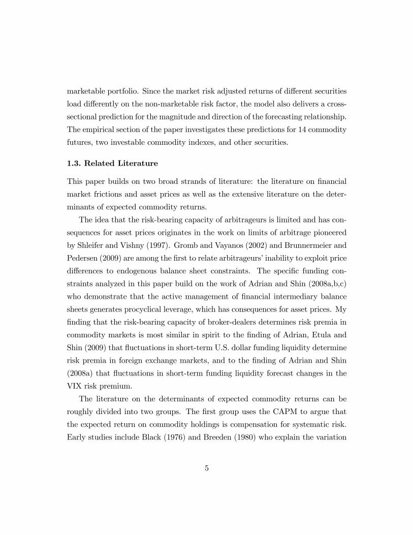
aversion.17 I remove a secular downward trend by orthogonalizing the variable

relative to a linear time trend. A plot of the resulting series is displayed in Figure

3.1. Note the sharp increases in e¤ective risk aversion following the U.S. bond

market blow-up and the Latin American crisis of 1994-95, the LTCM crisis of

16The one-month excess return at the end of month t is given by

Ft;TFt�1;T

� 1;

where Ft�1;T is the futures price at the end of month t � 1 on the nearest contract whoseexpiration date T is after the end of month t, and Ft;T is the price of the same contract at theend of month t. The quarterly return is the product of three monthly returns.17Financial leverage is de�ned as (total �nancial assets) / (total �nancial assets - total �nancial

liabilities).

17

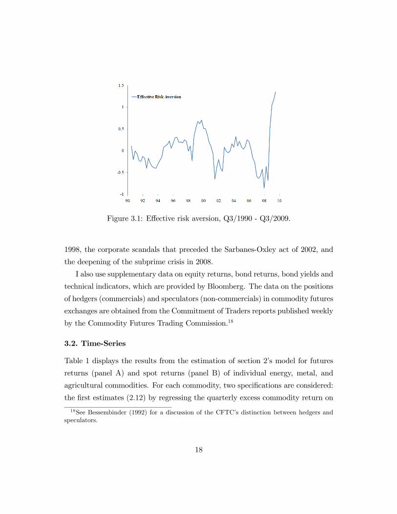
Figure 3.1: E¤ective risk aversion, Q3/1990 - Q3/2009.

1998, the corporate scandals that preceded the Sarbanes-Oxley act of 2002, and

the deepening of the subprime crisis in 2008.

I also use supplementary data on equity returns, bond returns, bond yields and

technical indicators, which are provided by Bloomberg. The data on the positions

of hedgers (commercials) and speculators (non-commercials) in commodity futures

exchanges are obtained from the Commitment of Traders reports published weekly

by the Commodity Futures Trading Commission.18

3.2. Time-Series

Table 1 displays the results from the estimation of section 2�s model for futures

returns (panel A) and spot returns (panel B) of individual energy, metal, and

agricultural commodities. For each commodity, two speci�cations are considered:

the �rst estimates (2:12) by regressing the quarterly excess commodity return on

18See Bessembinder (1992) for a discussion of the CFTC�s distinction between hedgers andspeculators.

18

the S&P 500 excess return and lagged e¤ective risk aversion; the second estimates

(2:13) by regressing the quarterly excess return on the S&P 500 excess return and

lagged change in e¤ective risk aversion. Note that all independent variables have

been standardized to zero mean and unit variance to facilitate the interpretation

of regression results.

Beginning with the �rst speci�cation, the results in panel A show that e¤ective

risk aversion is a statistically signi�cant predictor of expected futures returns for

crude oil, its derivatives heating oil and unleaded gasoline, natural gas, soybeans,

cocoa, and wheat. The coe¢ cients of e¤ective risk aversion also reveal an inter-

esting sign pattern: they are positive for energy commodities but negative for

most agricultural commodities. For instance, if the level of e¤ective risk aversion

is one standard deviation above average, investors require 4 percentage points

higher returns on their long positions in crude oil futures but 5 percentage points

lower returns on their long positions in wheat futures over the following quarter.

This cross-sectional �nding is consistent with the theoretical model and will be

discussed in detail in the next subsection.

The results from the second speci�cation are very similar. The only qualitative

di¤erence is that the change in e¤ective risk aversion seems to beat the level

as a predictor of returns on energy commodities while the level seems to beat

the change as a predictor of returns on agricultural commodities. For instance,

if the increase in e¤ective risk aversion is one standard deviation greater than

the average quarterly change, investors require as much as 8 percentage points

higher returns on long crude oil futures positions but only about 3 percent lower

returns on long wheat positions over the following quarter. The �nding that the

change in risk appetite also forecasts excess returns lends support to the conjecture

that there may be frictions in the marketplace that prevent broker-dealers from

adjusting leverage instantaneously in response to changes in risk constraints; thus,

the change in this balance sheet based measure of e¤ective risk aversion may be

19

a better proxy for higher-frequency �uctuations in risk constraints.

While my asset pricing theory does not directly apply to prices of physical

commodities, e¢ cient inventory management may generate comovement between

the expected spot and futures return for some commodities, as discussed above.

Panel B investigates this possibility by conducting the above set of regressions for

excess spot returns. The table shows that the level of e¤ective risk aversion is not

a statistically signi�cant predictor of excess returns for most spot commodities.

The change in e¤ective risk aversion o¤ers more explanatory power but overall

the results for spot returns are substantially weaker than the results for futures

returns.19

Finally, Table 1C estimates (2:12) and (2:13) index returns. The �rst columns

consider the S&P Goldman Sachs Commodity Index (GSCI) and the Dow Jones-

UBS Commodity Index (DJCI), which are tradable futures indexes with di¤erent

underlying compositions. The GSCI is weighted by world production values and

is thereby biased toward energy commodities.20 In light of Table 1A�s results, it

is then not surprising that higher e¤ective risk aversion forecasts higher returns

on the GSCI. The construction methodology of the DJCI, on the other hand,

relies also on other characteristics, such as the liquidity of futures contracts, and

is thereby substantially more diversi�ed across di¤erent classes of commodities.21

The results show that only the change in e¤ective risk aversion is a statistically

signi�cant predictor of DJCI returns. As a check, the last columns of the table

estimate the model for the Dow Jones Corporate Bond index. The results show

that my measures of e¤ective risk aversion have no predictive power for excess

bond returns.19An additional set of regressions for the futures basis (futures price relative to the spot price)

as the dependent variable shows that my measure of e¤ective risk aversion is not related to thebasis. These supplementary results can be obtained from the author.20Over the sample period, energy commodities have constituted approximately 50-60% of the

GSCI portfolio in dollar terms.21See http://www.djindexes.com/ubs/.

20

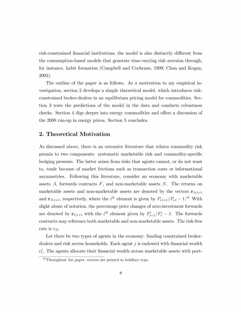
Figure 3.2: Commodity futures and futures indexes: Estimated vs. model-predicted coe¢ cients of e¤ective risk aversion for energy (squares), metal (circles)and agricultural (triangles) commodities, plus three indexes (diamonds).

3.3. Cross-Section

The time-series results in Table 1 uncovered an interesting cross-sectional pattern:

an increase in e¤ective risk aversion forecasts higher returns on energy futures but

lower returns on most agricultural futures. In this subsection, I will investigate

how this pattern squares with the cross-sectional prediction of the model (Corol-

lary 1). First, I follow the instructions in (2:14) to construct model-predicted co-

e¢ cients �Modeli for individual commodity futures. I then plot the OLS-estimated

coe¢ cients from Tables 1A and 1C against the model-predicted coe¢ cients. The

resulting scatter plot, displayed in Figure 3.2, shows that the empirical coe¢ cient

estimates line up well with the model-predicted coe¢ cients.

Figure 3.2 can be interpreted as an asset-pricing explanation for the diverse im-

pact of e¤ective risk aversion on risk premia across commodities. As predicted by

the model, time-variation in e¤ective risk aversion has the greatest impact on secu-

21

rities whose risk-adjusted returns covary the most (positively or negatively) with

the aggregate non-marketable portfolio, which constitutes an additional source of

systematic risk. Intuitively, some securities are riskier than what is predicted by

their loading on the market risk factor since they comove positively with the ag-

gregate non-marketable portfolio. Investors demand higher risk premia for holding

these securities and the risk premia grow as e¤ective risk aversion increases. Con-

versely, other securities may be hedges against aggregate non-marketable risk and

command a lower risk premium than what would be predicted by their loading on

the market risk factor. When e¤ective risk aversion increases, the hedging value

of these securities increase and their risk premia compress.

One can of course go beyond Figure 3.2�s graphical illustration by computing

the average compensation investors require for exposure to non-marketable risk.

Using the time-series coe¢ cient estimates from Tables 1A and 1C, a straight-

forward application of the Fama-MacBeth (1973) two-step approach delivers a

cross-sectional price of risk per a unit of � of 0:47% per quarter, which is statis-

tically signi�cant at 10% level. The cross-sectional price of risk per a unit of �

(market risk) is statistically insigni�cant �0:15% per quarter. The cross-sectionalpricing error (�alpha�) is rather large at 0:93% per quarter but statistically in-

signi�cant, which suggests that the two-factor model does a decent job explaining

the average returns in this cross-section. These results lend additional support

to the view that aggregate non-marketable risk is priced in the cross-section of

commodity futures.

3.4. Robustness

The estimation results in Tables 1A and 1C demonstrated that e¤ective risk aver-

sion is a statistically and economically signi�cant predictor of many commodity

futures returns, controlling for market risk. In this subsection, I investigate the

extent to which the predictive information contained in my measure of e¤ective

22

risk aversion is new to the literature. Speci�cally, I compare the forecasting ability

of e¤ective risk aversion to the forecasting ability of other variables that previous

literature has identi�ed as signi�cant predictors of commodity returns. In the

interest of space, I focus the analysis on two commodity futures, crude oil and

wheat, which represent the two extremes in terms of the direction of the predictive

relationship.

The results are displayed in the panels of Table 2. Panel A regresses the crude

oil futures return on lagged e¤ective risk aversion, lagged change in e¤ective risk

aversion and a set of lagged controls. Panel B conducts the same regressions for

wheat futures. Column (i) shows that e¤ective risk aversion alone explains ap-

proximately 18% of the returns on crude oil futures over the next quarter; and

approximately 12% of the returns on wheat futures. Column (ii) includes an au-

toregressive term and columns (iii)-(viii) add a number of lagged control variables

from the literature:22 The common predictors include the VIX volatility index,

interest rate, yield spread, dividend yield, and in�ation rate. The commodity

speci�c predictors include the futures basis and hedging pressure.23 For wheat,

the coe¢ cient of e¤ective risk aversion is signi�cant across all speci�cations and

its magnitude increases from �4:6 to �7:2 as one adds the full set of controls. Forcrude oil, the level of e¤ective risk aversion seems to be dominated by the change

in risk aversion, which is highly signi�cant across all speci�cations. The magni-

tude of the coe¢ cient is also robust to the addition of controls; it stays above 8:2

in all speci�cations. These results suggest that the information contained in the

measure of e¤ective risk aversion is quite di¤erent from the information content

of existing predictors.24

22See, for instance, Bessembinder and Chan (1992) and Hong and Yogo (2009).23Hedging pressure is de�ned as the net short open interest of commercial futures traders

divided by the total open interest of commercial futures traders.24The results are also robust to the inclusion of: seasonal dummies, inventory �gures, investor

sentiment (Baker and Wurgler, 2007), earnings growth, cay (Lettau and Ludvigson, 2001), anda number of other controls from the literature on equity premium prediction (Goyal and Welch,

23

The results also demonstrate that few controls help predict commodity returns

beyond the measure of e¤ective risk aversion: For crude oil, only lagged hedging

pressure is statistically signi�cant; and for wheat, only lagged VIX and lagged

hedging pressure are signi�cant. One might suspect that multicollinearity causes

part of the observed insigni�cance of control variables. However, comparing the

adjusted R2 across di¤erent speci�cations suggests that only the statistically sig-

ni�cant controls contribute materially to the power of the regressions.25

3.5. Focus on Energy

In order to dig deeper in the link between e¤ective risk aversion and risk premia,

this subsection narrows the scope of investigation by focusing on energy returns.

I �rst investigate the emergence of return forecastability. I then study the robust-

ness of the forecasting relationship out-of-sample. Finally, I examine the extent to

which my measure of e¤ective risk aversion can explain the large �uctuations of

energy prices in 2008-2009. While the primary focus is on crude oil, the qualitative

results hold also for heating oil, gasoline, and the GSCI.

3.5.1. Emergence of Return Forecastability

I use rolling regressions to investigate the predictive power of e¤ective risk aversion

over time. Since the trading of crude oil futures began only in 1983, I can extend

the sample by using the excess return on spot crude oil as a dependent variable

instead. Building on the result of Tables 1A-B that the change in e¤ective risk

aversion predicts both futures and spot returns, I use the lagged change in e¤ective

risk aversion as the explanatory variable. Figure 3.3 plots theR2 from the resulting

2008). These additional results can be obtained from the author.25As an additional test, one can investigate the robustness of the above predictive relationships

at di¤erent forecast horizons. Regressions for returns 2� 8 quarters ahead show that both thestatistical signi�cance and the economic magnitude of the relationships remain stable over longerhorizons. These results lend additional support to the strength and robustness of the dynamicconnection between e¤ective risk aversion and commodity returns.

24

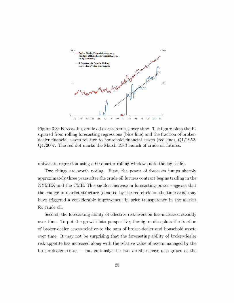
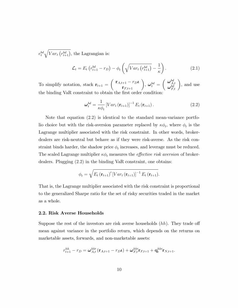
Figure 3.3: Forecasting crude oil excess returns over time. The �gure plots the R-squared from rolling forecasting regressions (blue line) and the fraction of broker-dealer �nancial assets relative to household �nancial assets (red line), Q1/1952-Q4/2007. The red dot marks the March 1983 launch of crude oil futures.

univariate regression using a 60-quarter rolling window (note the log scale).

Two things are worth noting. First, the power of forecasts jumps sharply

approximately three years after the crude oil futures contract begins trading in the

NYMEX and the CME. This sudden increase in forecasting power suggests that

the change in market structure (denoted by the red circle on the time axis) may

have triggered a considerable improvement in price transparency in the market

for crude oil.

Second, the forecasting ability of e¤ective risk aversion has increased steadily

over time. To put the growth into perspective, the �gure also plots the fraction

of broker-dealer assets relative to the sum of broker-dealer and household assets

over time. It may not be surprising that the forecasting ability of broker-dealer

risk appetite has increased along with the relative value of assets managed by the

broker-dealer sector � but curiously, the two variables have also grown at the

25

same rate as indicated by the parallel trend lines. These �ndings lend support to

with the view that the link between broker-dealer risk constraints and commodity

risk premia strengthens as the economic size of the broker-dealer sector increases.

3.5.2. Out-of-Sample Forecasts

As is well known, the high in-sample forecasting power of a regressor does not

guarantee robust out-of sample performance, which is more sensitive to mis-

speci�cation problems. To investigate the extent to which my measure of e¤ective

risk aversion survives this tougher test, the following tests the forecastability of

energy returns out of sample. In order to avoid look-ahead bias in constructing

the regressor, I proxy e¤ective risk aversion by the quarterly changes in (2:11),

without detrending the level. I use recursive regressions with the out-of-sample

portion starting in the third quarter of 1995.

Table 3 compares the predictive power of e¤ective risk aversion to three bench-

marks (restricted models) that are standard in the literature of out-of-sample fore-

casting:26 (1) random walk, (2) random walk with drift, and (3) �rst-order autore-

gression. These benchmarks are nested in the �unrestricted�speci�cations, which

allows one to evaluate their performance using the Clark andWest (2006) adjusted

di¤erence in mean squared errors, MSEr � (MSEu � adj:). The Clark-West testaccounts for the small-sample forecast bias (adj:), which works in favor of the

simpler restricted models and is present in the unadjusted Diebold-Mariano/West

(DMW) tests. As Rogo¤ and Stavrakeva (2009) show, a signi�cant Clark-West

adjusted statistic implies that there exists an optimal combination between the

unrestricted model and the restricted model, which will produce a combined fore-

cast that outperforms the restricted model in terms of mean squared forecast

error; i.e., the forecast will have a DMW statistic that is signi�cantly greater than

zero.26See for instance Chen, Rogo¤ and Rossi (2009) who study the forecastability of commodity

returns by the exchange rates of commodity currencies.

26

The results in Table 3 show that the models with e¤ective risk aversion out-

perform all three benchmarks at 1% signi�cance level. The strength of these

out-of-sample results lends additional support to the robustness of the forecasting

relationship over time.

3.5.3. E¤ective Risk Aversion and the Energy Boom of 2008

My baseline analysis deliberately excludes the recent time period 2008-2009, which

features large �uctuations in both broker-dealer leverage and energy prices. To put

this period of high volatility in a historical perspective, Figure 3.4 plots quarterly

crude oil excess returns over the past two decades. The �gure also plots the

change in e¤ective risk aversion, lagged by one quarter. The time-series of crude

oil returns demonstrates that the sequence of strong positive returns fromQ1/2007

to Q2/2008 has few rivals in the recent history. Similarly, the dramatic decline

in the price of crude oil in the second half of 2008 from $140 per barrel to less

than $40 per barrel exceeds previous price drops by a factor of two. The rate of

recovery in the �rst half of 2009 is also record-breaking within the sample.

Inspection of the two time-series con�rms the regression result that the change

in e¤ective risk aversion has a strong track record in predicting quarterly crude

oil returns. But note that this variable does not explain the sharp rise and fall in

the oil price during the commodity rally of mid-2008. While there is no reason to

expect that excess returns to crude oil futures and lagged changes in e¤ective risk

aversion would be perfectly correlated at each point in time, this �nding seems

curiously at odds with the popular belief that the 2008 bubble in the price of

crude oil was driven by speculators. Note, however, that the current measure

of e¤ective risk aversion merely re�ects the capacity of broker-dealers to bear

risk; hence, it may have been unre�ective of broader appetite for commodity risk

over the period. For instance, in spring 2008 hedge funds were actively involved

in a "long oil/short �nancials" trade, which unraveled in July 2008 as the SEC

27

Figure 3.4: Crude oil excess returns and lagged changes in e¤ective risk aversion

announced a ban on naked short sales. Some have also argued that increasing

demand for long commodity futures positions by non-traditional investor classes

such as index and pension funds were driving a bubble in energy prices that burst

in the summer of 2008.27 The validity of such claims cannot be addressed by the

current analysis.

4. Conclusion

This paper presents evidence that the risk-bearing capacity of U.S. security broker-

dealers is an important determinant of risk premia in the market for commodity

derivatives. I motivate my empirical analysis by a simple asset pricing model

where time-variation in broker-dealer risk constraints generates time-variation in

the price of non-marketable risk, which stems from systematic �uctuations in

27These commentators include George Soros who argued on April 17, 2008, that there is �ageneralized commodity bubble due to commodities having become an asset class that institutionsuse to an increasing extent.�Masters and White (2008) estimate that over the period from 2003to mid-2008 investments in commodity indexes increased from $13 billion to $317 billion.

28

the aggregate value of physical commodities. In equilibrium, the price of non-

marketable risk can be expressed as a function of aggregate balance sheet com-

ponents of broker-dealers and households. This makes it easy to investigate the

asset pricing implications of the model in the data.

My empirical results lend strong support to the theory�s predictions, both in

the time-series and in the cross-section of commodity futures. Fluctuations in

broker-dealer risk-bearing capacity have particularly strong forecasting power for

energy returns, both in-sample and out-of-sample. The �nding that risk con-

straints of broker-dealers are hardwired to risk premia in commodity derivatives

can also be interpreted in the context of the current debate on OTC market reg-

ulation. Speci�cally, the paper shows how restrictions on broker-dealer trading

activities can be expected to increase the costs of hedging for producers and con-

sumers of commodities. This result is central to understanding why restrictions

on speculation by market makers may adversely impact the functioning of many

derivatives markets.

In sum, the contributions of this paper may be regarded as �rst steps toward

quantifying the asset pricing implications of limits of arbitrage in the broker-

dealer sector. Similar investigations in other derivatives markets and asset classes

constitute a fruitful area for future research.

29

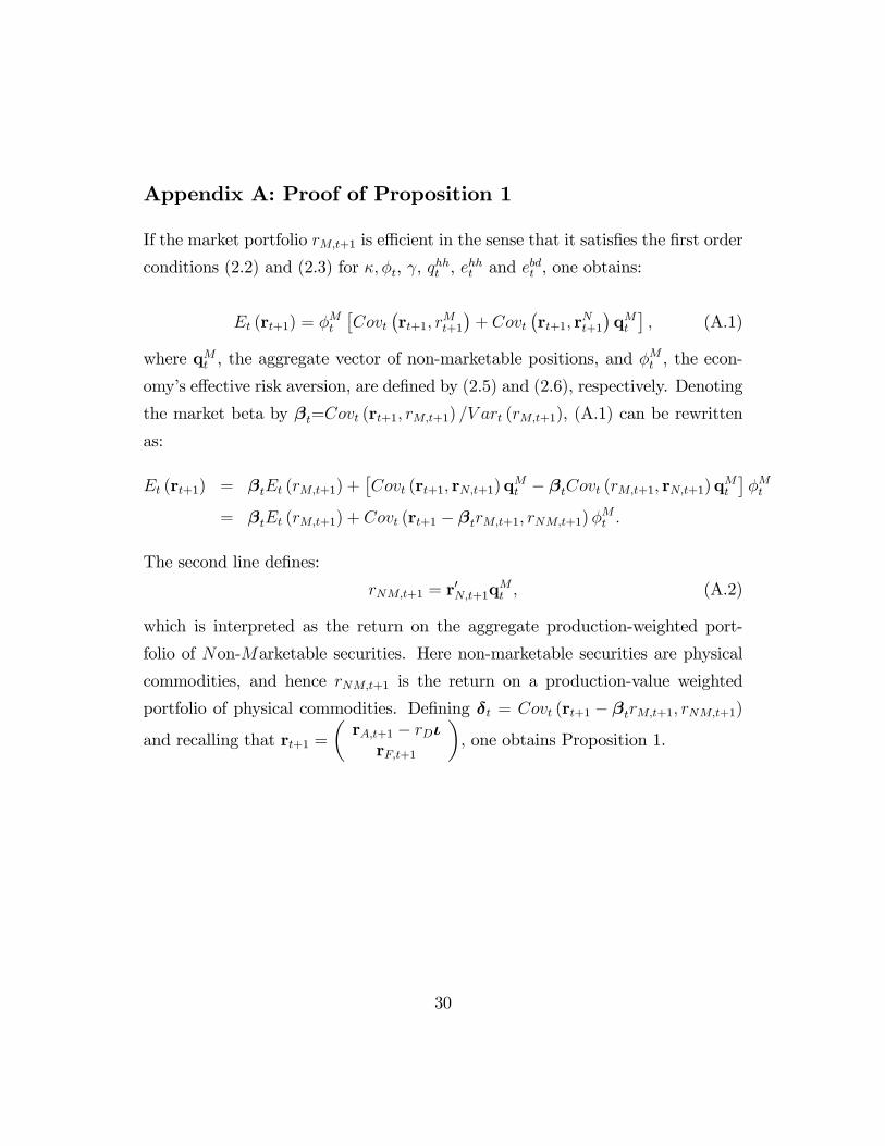
Appendix A: Proof of Proposition 1

If the market portfolio rM;t+1 is e¢ cient in the sense that it satis�es the �rst order

conditions (2.2) and (2.3) for �; �t, , qhht , e

hht and ebdt , one obtains:

Et (rt+1) = �Mt

�Covt

�rt+1; r

Mt+1

�+ Covt

�rt+1; r

Nt+1

�qMt�; (A.1)

where qMt , the aggregate vector of non-marketable positions, and �Mt , the econ-

omy�s e¤ective risk aversion, are de�ned by (2.5) and (2.6), respectively. Denoting

the market beta by �t=Covt (rt+1; rM;t+1) =V art (rM;t+1), (A.1) can be rewritten

as:

Et (rt+1) = �tEt (rM;t+1) +�Covt (rt+1; rN;t+1)q

Mt � �tCovt (rM;t+1; rN;t+1)qMt

��Mt

= �tEt (rM;t+1) + Covt (rt+1 � �trM;t+1; rNM;t+1)�Mt :

The second line de�nes:

rNM;t+1 = r0N;t+1q

Mt ; (A.2)

which is interpreted as the return on the aggregate production-weighted port-

folio of Non-Marketable securities. Here non-marketable securities are physical

commodities, and hence rNM;t+1 is the return on a production-value weighted

portfolio of physical commodities. De�ning �t = Covt (rt+1 � �trM;t+1; rNM;t+1)

and recalling that rt+1 =�rA;t+1 � rD�rF;t+1

�, one obtains Proposition 1.

30

Appendix B: Proof of Proposition 2

In order to derive an expression for �Mt in terms of observable state variables,

start by rewriting (2.6) as

�Mt =

�1 +

ebdtehht

�1� �Mt

��t

��; (B.3)

and work with the variable �Mt��t. Speci�cally, plug (A.1) in the broker-dealer�s �rst

order condition (2.2) to obtain:

!bdt =�Mt��t

[V art (rt+1)]�1 �Covt (rt+1; rM;t+1) + Covt (rt+1; rN;t+1)qMt � :

Using the de�nition of the market portfolio and de�ning ht � [V art (rt+1)]�1

Covt (rt+1; rN;t+1)qMt , the above simpli�es to:

!bdt =�Mt��t

�!Mt + ht

�; (B.4)

where vector ht captures the net short open interest of households. To see this,

note that households collectively wish to short hit�ebdt + e

hht

�dollars worth of se-

curity i to hedge the price risk that stems from their aggregate holdings of non-

marketable assets.28 Equation (B.4) states that broker-dealers ful�ll a fraction �Mt��t

of this open interest. Note that hit is loosely related to the notion of hedging pres-

sure, which is commonly de�ned as the net short open interest of hedgers divided

by the total open interest of hedgers. Summing (B.4) over individual securities

positions, one obtains:�Mt��t

=

Pi !

bdi;tP

i !Mi;t +

Pi hi;t

: (B.5)

By balance sheet identity, the value of risky securities holdings of investor j

must equal the value of equity plus the value of debt:

ejtXi

!ji;t = ejt + debt

jt ;

28Since the net supply of hedging positions is zero, these positions are not part of the marketportfolio.

31

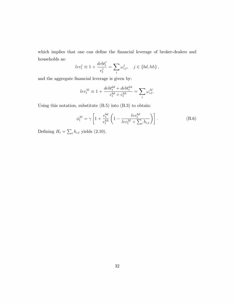
which implies that one can de�ne the �nancial leverage of broker-dealers and

households as:

levjt � 1 +debtjt

ejt=Xi

!ji;t; j 2 fbd; hhg ;

and the aggregate �nancial leverage is given by:

levMt � 1 + debtbdt + debt

hht

ebdt + ehht

=Xi

!Mi;t :

Using this notation, substitute (B.5) into (B.3) to obtain:

�Mt =

�1 +

ebdtehht

�1� levbdt

levMt +P

i hi;t

��: (B.6)

De�ning Ht =P

i hi;t yields (2.10).

32

Acknowledgements

This paper was published as Chapter 1 of my 2009 Ph.D. dissertation at Harvard

University. I am grateful to my advisers Jeremy Stein, John Campbell, Ken Ro-

go¤, and Andrei Shleifer, and to Tobias Adrian, Viral Acharya, Yakov Amihud,

Alvaro Cartea, Richard Crump, Darrell Du¢ e, Emmanuel Farhi, Xavier Gabaix,

Gary Gorton, Robin Greenwood, Ravi Jagannathan, Owen Lamont, Lasse Ped-

ersen, Christopher Polk, Ernst Schaumburg, Hyun Song Shin, Erik Sta¤ord, and

Motohiro Yogo for their comments and advice. I also thank seminar participants

at Harvard University, New York University Stern School of Business, University

Carlos III, and the Federal Reserve Bank of New York. Ariel Zucker provided

outstanding research assistance. All errors are my own.

33

References

[1] Acharya, V.V., Lochstoer, L. and T. Ramadorai. 2009. �Does Hedging A¤ect

Commodity Prices? The Role of Producer Default Risk.�Working Paper.

[2] Adrian, T. and H.S. Shin. 2008a. �Liquidity and Leverage.� Journal of Fi-

nancial Intermediation, forthcoming.

[3] Adrian, T. and H.S. Shin. 2008b. �Financial Intermediaries, Financial Stabil-

ity, and Monetary Policy.�Jackson Hole Economic Symposium Proceedings,

Federal Reserve Bank of Kansas City.

[4] Adrian, T. and H.S. Shin. 2008c. �Financial Intermediary Leverage and

Value-at-Risk.�Federal Reserve Bank of New York Sta¤ Report no. 338.

[5] Adrian, T. and E. Moench. 2008. �Pricing the Term Structure with Linear

Regressions.�Federal Reserve Bank of New York Sta¤ Report no. 340.

[6] Adrian, T., Etula, E. and H. Shin. 2008. �Risk Appetite and Exchange

Rates.�Federal Reserve Bank of New York Sta¤ Report no. 361.

[7] Anson, M.J. 2002. �Handbook of Alternative Assets.�Wiley Finance.

[8] Barberis, N., A. Shleifer and R. Vishny. 1998. �A Model of Investor Senti-

ment.�Journal of Financial Economics 69:307�343.

[9] Baker, M. and J. Wurgler. �Investor Sentiment in the Stock Market.�Journal

of Economic Perspectives 21:129�151.

[10] Bessembinder, H. 1992. �Systematic Risk, Hedging Pressure, and Risk Pre-

miums in Futures Markets.�Review of Financial Studies 5:637�667.

[11] Bessembinder, H. and K. Chan. 1992. �Time-Varying Risk Premia and

Forecastable Returns in Futures Markets.� Journal of Financial Economics

32:169�193.

34

[12] Bank for International Settlements. 2009. BIS Quarterly Review. December.

[13] Black, F., 1976. �The Pricing of Commodity Contracts.�Journal of Financial

Economics 3:167�179.

[14] Board of Governors of the Federal Reserve. 2000. Guide to the Flow of Funds

Accounts. Volume 2.

[15] Breeden, D.T. 1980. �Consumption Risk in Futures Markets.� Journal of

Finance 35:503�520.

[16] Brunnermeier, M. and L. Pedersen. 2009. �Market Liquidity and Funding

Liquidity.�Review of Financial Studies 22:2201�2238.

[17] Campbell, J.Y. and J.H. Cochrane. 1999. �By Force of Habit: A

Consumption-Based Explanation of Aggregate Stock Market Behavior.�

Journal of Political Economy 107:205�251.

[18] Campbell, J.Y., Grossman S.J. and J. Wang. 1993. �Trading Volume and

Serial Correlation in Stock Returns.�The Quarterly Journal of Economics

108:905�939.

[19] Campbell, J.Y. and A.S. Kyle. 1993. �Smart Money, Noise Trading and Stock

Price Behaviour.�The Review of Economics Studies 60:1�34.

[20] Carter, C.A., Rausser, G.C. and A. Schmitz. 1983. �E¢ cient Asset Portfolios

and the Theory of Normal Backwardation.�Journal of Financial Economics

91:319�331.

[21] Chan, Y.L. and L. Kogan. 2002. �Catching Up with the Joneses: Heteroge-

neous Preferences and the Dynamics of Asset Prices.� Journal of Political

Economy 110:1255�1285.

35

[22] Chen, Y., K. Rogo¤, and B. Rossi. 2008. �Can Exchange Rates Forecast

Commodity Prices?�Quarterly Journal of Economics, forthcoming.

[23] Clark, T.E. and K.D. West. 2006. �Using Out-of-Sample Mean Squared Pre-

diction Errors to Test the Martingale Hypothesis.�Journal of Econometrics

135:155�186.

[24] Clark, T.E. and K.D. West. 2007. �Approximately Normal Tests for Equal

Predictive Accuracy in Nested Models.� Journal of Econometrics 138:291�

311.

[25] Danielsson, J., Shin, H.S and J. Zigrand. 2008. �Endogenous Risk and Risk

Appetite.�working paper, London School of Economics and Princeton Uni-

versity.

[26] DeLong, J.B., Shleifer, A., Summers, L.H. and R. Waldmann. 1990. �Noise

Trader Risk in Financial Markets.�Journal of Political Economy 98:703�738.

[27] Du¢ e, D. 2009. �How Should We Regulate Derivatives Markets?�Brie�ng

Paper Number 5, The Pew Financial Reform Project.

[28] Erb, C.B., and C.R. Harvey. 2006. �The Strategic and Tactical Value of

Commodity Futures.�Financial Analysts Journal 62:69�97.

[29] Fama, E. and J. MacBeth. 1973. �Risk, Return, and Equilibrium: Empirical

Tests.�Journal of Political Economy 81:607�636.

[30] Gorton, G. and K.G. Rouwenhorst. 2006. �Facts and Fantasies about Com-

modity Futures.�Financial Analysts Journal 62:47�68.

[31] Gorton, G., Hayashi, F. and K.G. Rouwenhorst. 2007. �The Fundamentals

of Commodity Futures Returns.�Yale ICF Working Paper No. 07-08.

36

[32] Goyal, A. and I. Welch. 2008. �A Comprehensive Look at the Empirical

Performance of Equity Premium Prediction.� Review of Financial Studies

21:1455�1508.

[33] Gromb, D. and D. Vayanos. 2002. �Equilibrium and Welfare in Markets

with Financially Constrained Arbitrageurs.�Journal of Financial Economics

66:361�407.

[34] Gromb, D. and D. Vayanos. 2010. �Limits of Arbitrage: The State of the

Theory.�Working Paper.

[35] Grossman, S.J. and M.H. Miller. 1988. �Liquidity and Market Structure.�

Journal of Finance 43:617�633.

[36] Hicks, J. 1939. Value and Capital. Oxford University Press. Cambridge, UK.

[37] Hirschleifer, D. 1988. �Residual Risk, Trading Costs, and Commodity Risk

Premia.�Review of Financial Studies 1:173�193.

[38] Hirschleifer, D. 1989. �Determinants of Hedging and Risk Premia in Com-

modity Futures Markets.� Journal of Financial and Quantitative Analysis

24:313�331.

[39] Hodrick, R.J. and S. Srivastava. 1984. �An Investigation of Risk and Return

in Forward Foreign Exchange.�Journal of International Money and Finance

3:5�29.

[40] Hong, H. and J. Stein. 1999. �A Uni�ed Theory of Underreaction, Momentum

Trading and Overreaction in Asset Markets.�Journal of Financial Economics

54:2143�2184.

[41] Hong, H. and M. Yogo. 2009. �Digging into Commodities.�Working Paper.

37

[42] Jagannathan, R. 1985. �An Investigation of Commodity Futures Prices Using

the Consumption-Based Intertemporal Capital Asset Pricing Model.�Journal

of Finance 40:175�191.

[43] Keynes, J.M. 1930. A Treatise on Money, Vol II. Macmillan. London.

[44] Kyle, A.S. 1985. �Continuous Auctions and Insider Trading.�Econometrica

53:1315�1336.

[45] Lettau, Martin, and Ludvigson, Sydney, 2001, Resurrecting the (C)CAPM:

A cross-sectional test when risk premia are time-varying, Journal of Political

Economy 109, 1238-1287.

[46] Masters, M.W., A.K. White. 2008. �The 2008 Commodities Bubble: As-

sessing the Damage to the United States and its Citizens.�Working Paper,

Masters Capital Management.

[47] Mayers, D. 1972. �Nonmarketable Assets and Capital Market Equilibrium

under Uncertainty.� In M. Jensen (Ed.), Studies in the Theory of Capital

Markets. Praeger. New York.

[48] Rogo¤, K. and V. Stavrakeva. 2009. �The Continuing Puzzle of Short Horizon

Exchange Rate Forecasting.�NBER Working Paper No. 14656.

[49] de Roon, F.A., Nijman, T.E. and Veld, C. 2000. �Hedging Pressure E¤ects

in Fufures Markets.�Journal of Finance 55:1437�1456.

[50] Shleifer, A. and R. Vishny. 1997. �The Limits of Arbitrage.�Journal of Fi-

nance 52:35�55.

[51] Stambaugh, R., 1999. �Predictive Regressions.� Journal of Financial Eco-

nomics 54:375-421.

38

[52] Stoll, H. 1979. �Commodity Futures and Spot Price Determination and Hedg-

ing in Capital Market Equilibrium.�Journal of Financial and Quantitative

Analysis 14:873�894.

[53] Tang, K. and W. Xiong. 2010. �Index Investing and the Financialization of

Commodities.�Working Paper.

39

Table 1A: Commodity FuturesThe table displays the results from the estimation of (2.12) and (2.13) for returns on commodity futures. The

dependent variable is the per-quarter percentage price change of the futures contract. Independent variables

are the lagged e¤ective risk aversion, the lagged change in e¤ective risk aversion, and the excess return on the

S&P 500. All independent variables have zero mean and unit variance. The table reports point estimates with

heteroskedasticity-robust t-statistics in parentheses (omitted for S&P 500 and the constant); *** p < 0.01, ** p

< 0.05, * p < 0.1. The sample period is Q3/1990 - Q4/2007.

Independent Variables

E¤ective Risk Aversion � E¤ective Risk Aversion S&P 500

Excess Futures Return (Lag 1) (Lag 1) Excess Return Constant Adj-R2

Crude Oil 4.398** (2.530) -8.130** 4.971** 17.5%

7.985*** (4.638) -6.548* 5.162** 27.7%

Heating Oil 5.607*** (2.609) -7.464** 4.990** 16.7%

5.851*** (3.321) -6.276* 5.177** 17.1%

Gasoline 5.209*** (2.819) -8.233* 5.426** 15.9%

6.826*** (3.623) -6.864 5.617** 19.6%

Natural Gas 4.891* (1.783) -2.559 1.406 0.7%

5.027 (1.594) -1.538 1.568 0.8%

Copper 1.501 (1.094) 0.291 2.663* -1.6%

2.827* (1.879) 0.850 2.729* 1.5%

Silver -0.295 (-0.272) -0.161 0.994 -2.9%

2.284* (1.850) 0.272 1.018 1.6%

Platinum 0.300 (0.277) 1.313 2.041** -0.1%

0.830 (0.744) 1.475 2.058** 0.8%

Gold -1.164 (-1.429) -1.377** 0.398 6.4%

0.474 (0.748) -1.301** 0.382 3.2%

Sugar 0.518 (0.306) -1.669 0.836 -2.0%

0.499 (0.210) -1.567 0.853 -2.0%

Cotton -1.572 (-1.304) 1.468 -1.404 0.5%

1.857 (1.500) 1.804 -1.411 1.2%

Corn -1.254 (-0.850) 1.133 -1.443 -1.2%

0.458 (0.343) 1.205 -1.461 -2.1%

Soybeans -2.228* (-1.682) 0.160 1.031 1.5%

-0.415 (-0.310) 0.054 0.982 -2.8%

Cocoa -3.322*** (-2.697) -3.333* -0.511 13.4%

-3.317** (-2.248) -4.008** -0.620 13.2%

Wheat -5.072** (-2.493) 0.702 -0.468 11.8%

-2.812** (-2.204) 0.102 -0.604 1.6%

40

Table 1B: Spot CommoditiesThe table displays the results from the estimation of (2.12) and (2.13) for returns on spot commodities. The

dependent variable is the per-quarter spot return, in excess of the risk-free rate. Independent variables are

the lagged e¤ective risk aversion, the lagged change in e¤ective risk aversion, and the excess return on the

S&P 500. All independent variables have zero mean and unit variance. The table reports point estimates with

heteroskedasticity-robust t-statistics in parentheses (omitted for S&P 500 and the constant); *** p < 0.01, ** p

< 0.05, * p < 0.1. The sample period is Q3/1990 - Q4/2007.

Independent Variables

E¤ective Risk Aversion � E¤ective Risk Aversion S&P 500

Excess Spot Return (Lag 1) (Lag 1) Excess Return Constant Adj-R2

Crude Oil 2.665 (1.530) -8.588** 3.113 15.6%

7.122*** (3.495) -7.193* 3.259 25.2%

Heating Oil 3.202* (1.846) -8.450** 3.417 14.0%

6.199*** (2.600) -7.225* 3.561 19.6%

Gasoline 2.715 (1.394) -7.086*** 2.993 9.9%

7.564*** (3.013) -5.605** 3.145 20.6%

Natural Gas 2.918 (0.698) 3.158 5.887 -1.4%

-1.099 (-0.301) 2.984 5.930 -2.0%

Copper 0.933 (0.716) 0.210 0.939 -2.4%

2.588* (1.905) 0.716 0.992 1.4%

Silver -0.532 (-0.512) -0.196 1.116 -2.7%

1.993* (1.693) 0.179 1.132 0.7%

Platinum 0.068 (0.070) 1.378 0.979 0.1%

1.342 (1.364) 1.636 0.998 3.0%

Gold -1.264 (-1.525) -1.500** 0.320 7.5%

0.410 (0.647) -1.437** 0.301 3.7%

Sugar 0.474 (0.317) -0.832 -0.052 -2.5%

1.008 (0.465) -0.634 -0.029 -2.1%

Cotton -2.184 (-1.440) 0.688 -0.472 1.3%

0.646 (0.559) 0.785 -0.506 -2.3%

Corn -2.267 (-1.340) 1.459 0.803 0.3%

-1.119 (-0.729) 1.218 0.744 -1.5%

Soybeans -2.953* (-1.912) 0.819 0.811 2.7%

-0.984 (-0.659) 0.595 0.740 -2.0%

Cocoa -2.801*** (-2.629) -3.078** 0.371 12.7%

-3.208*** (-2.667) -3.726** 0.274 14.7%

Wheat -5.171** (-2.144) 2.079 1.579 9.5%

-4.427*** (-3.045) 1.169 1.420 6.4%

41

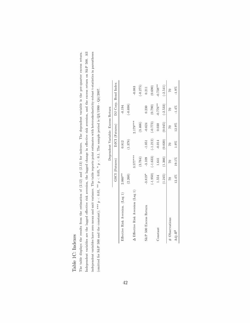
Table1C:Indexes

Thetabledisplaystheresultsfrom

theestimationof(2.12)and(2.13)forindexes.Thedependentvariableistheper-quarterexcessreturn.

Independentvariablesarethelaggede¤ectiveriskaversion,thelaggedchangeine¤ectiveriskaversion,andtheexcessreturnon

S&P500.All

independentvariableshavezeromeanandunitvariance.Thetablereportspointestimateswithheteroskedasticity-robustt-statisticsinparentheses

(omittedforS&P500andtheconstant);***p<0.01,**p<0.05,*p<0.1.ThesampleperiodisQ3/1990-Q4/2007.

DependentVariable:ExcessReturn

GSCI(Futures)

DJCI(Futures)

DJCorp.BondIndex

E¤ectiveRiskAversion.(Lag1)

2.060**

0.812

-0.194

(2.260)

(1.378)

(-0.698)

�E¤ectiveRiskAversion(Lag1)

3.577***

2.179***

-0.083

(3.764)

(3.466)

(-0.275)

S&P500ExcessReturn

-3.819*

-3.109

-1.051

-0.624

0.230

0.211

(-1.950)

(-1.633)

(-1.212)

(-0.773)

(0.790)

(0.690)

Constant

1.554

1.641

-0.014

0.030

-0.776**

-0.738**

(1.245)

(1.366)

(0.020)

(0.045)

(-2.533)

(-2.541)

#Observations

7070

7070

7070

Adj-R2

12.4%

19.1%

1.9%

12.9%

-1.4%

-1.9%

42

Table2A:RobustnessChecks(CrudeOil)

Thedependentvariableistheper-quarterpercentagepricechangeofcrudeoilfutures.Forecastingvariablesarethelaggedlevelandthelagged

changeine¤ectiveriskaversion.Controlvariables(eachlaggedbyonequarter)are:theVIX

impliedvolatilityoftheS&P500,the3-monthU.S.

treasurybillrate,theyieldspread(di¤erencebetweenMoody�sAaacorporateyieldandthetreasuryrate),theS&P500dividendyield,theU.S.

in�ation,thebasis(futurepriceoverspotprice),andthehedgingpressure(netshortopeninterestofhedgersrelativetothetotalopeninterestof

hedgers,asreportedby

theCFTC).Alagofthedependentvariableisincludedin(ii)-(viii).Allindependentvariableshavezeromeanandunit

variance.Thetablereportspointestimateswithheteroskedasticity-robustt-statisticsinparentheses;***p<0.01,**p<0.05,*p<0.1.The

sampleperiodisQ3/1990-Q4/2007.

CrudeOilFuturesExcessReturn

(i)

(ii)

(iii)

(iv)

(v)

(vi)

(vii)

(viii)

E¤ectiveRiskAversion.(Lag1)

1.267

2.239

2.289

1.841

2.408

0.662

0.615

0.342

(0.686)

(1.057)

(1.057)

(0.752)

(0.925)

(0.271)

(0.247)

(0.130)

�E¤ectiveRiskAversion(Lag1)

8.822***

8.466***

8.312***

8.576***

8.210***

8.655***

8.501***

8.500***

(4.288)

(4.149)

(4.163)

(3.548)

(3.524)

(4.207)

(4.137)

(3.493)

DependentVariable(Lag1)

-0.180

-0.174

-0.171

-0.182

-0.158

-0.146

-0.260*

(-1.373)

(-1.357)

(-1.370)

(-1.343)

(-1.136)

(-1.097)

(-1.672)

VIX

(Lag1)

-0.955

-0.860

-1.048

-2.262

-2.163

-0.577

(-0.556)

(-0.502)

(-0.607)

(-1.151)

(-1.070)

(-0.218)

InterestRate(Lag1)

1.077

2.165

5.782

6.008

5.238

(0.248)

(0.397)

(1.360)

(1.377)

(1.201)

YieldSpread(Lag1)

1.803

4.676

4.679

3.405

(0.601)

(1.609)

(1.589)

(1.120)

DividendYield(Lag1)

-4.027

-3.652

-1.960

(-1.161)

(-0.982)

(-0.451)

In�ation(Lag1)

-1.358

-1.821

(-0.743)

(-0.936)

Basis(Lag1)

1.174

(0.718)

HedgingPressure(Lag1)

5.571**

(2.238)

Constant

5.174**

5.953**

5.916**

5.906**

5.917**

5.809**

5.764**

6.344**

(2.299)

(2.307)

(2.287)

(2.302)

(2.290)

(2.196)

(2.188)

(2.321)

#Observations

7070

7070

7070

7070

Adj-R2

18.0%

20.0%

19.0%

18.0%

17.0%

17.2%

16.2%

20.6%

43

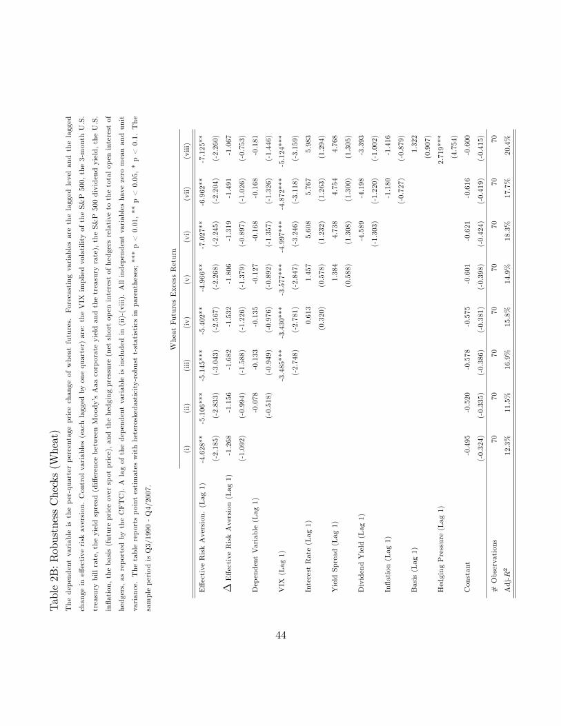
Table2B:RobustnessChecks(Wheat)

Thedependentvariableistheper-quarterpercentagepricechangeofwheatfutures.Forecastingvariablesarethelagged

levelandthelagged

changeine¤ectiveriskaversion.Controlvariables(eachlaggedbyonequarter)are:theVIX

impliedvolatilityoftheS&P500,the3-monthU.S.

treasurybillrate,theyieldspread(di¤erencebetweenMoody�sAaacorporateyieldandthetreasuryrate),theS&P500dividendyield,theU.S.

in�ation,thebasis(futurepriceoverspotprice),andthehedgingpressure(netshortopeninterestofhedgersrelativetothetotalopeninterestof

hedgers,asreportedby

theCFTC).Alagofthedependentvariableisincludedin(ii)-(viii).Allindependentvariableshavezeromeanandunit

variance.Thetablereportspointestimateswithheteroskedasticity-robustt-statisticsinparentheses;***p<0.01,**p<0.05,*p<0.1.The

sampleperiodisQ3/1990-Q4/2007.

WheatFuturesExcessReturn

(i)

(ii)

(iii)

(iv)

(v)

(vi)

(vii)

(viii)

E¤ectiveRiskAversion.(Lag1)

-4.628**

-5.106***

-5.145***

-5.402**

-4.966**

-7.027**

-6.962**

-7.125**

(-2.185)

(-2.833)

(-3.043)

(-2.567)

(-2.268)

(-2.245)

(-2.204)

(-2.260)

�E¤ectiveRiskAversion(Lag1)

-1.268

-1.156

-1.682

-1.532

-1.806

-1.319

-1.491

-1.067

(-1.092)

(-0.994)

(-1.588)

(-1.226)

(-1.379)

(-0.897)

(-1.026)

(-0.753)

DependentVariable(Lag1)

-0.078

-0.133

-0.135

-0.127

-0.168

-0.168

-0.181

(-0.518)

(-0.949)

(-0.976)

(-0.892)

(-1.357)

(-1.326)

(-1.446)

VIX

(Lag1)

-3.485***

-3.430***

-3.577***

-4.997***

-4.872***

-5.124***

(-2.748)

(-2.781)

(-2.847)

(-3.246)

(-3.118)

(-3.159)

InterestRate(Lag1)

0.613

1.457

5.608

5.767

5.983

(0.320)

(0.578)

(1.232)

(1.263)

(1.294)

YieldSpread(Lag1)

1.384

4.738

4.754

4.768

(0.588)

(1.308)

(1.300)

(1.305)

DividendYield(Lag1)

-4.589

-4.198

-3.393

(-1.303)

(-1.220)

(-1.002)

In�ation(Lag1)

-1.180

-1.416

(-0.727)

(-0.879)

Basis(Lag1)

1.322

(0.907)

HedgingPressure(Lag1)

2.719***

(4.754)

Constant

-0.495

-0.520

-0.578

-0.575

-0.601

-0.621

-0.616

-0.600

(-0.324)

(-0.335)

(-0.386)

(-0.381)

(-0.398)

(-0.424)

(-0.419)

(-0.415)

#Observations

7070

7070

7070

7070

Adj-R2

12.3%

11.5%

16.9%

15.8%

14.9%

18.3%

17.7%

20.4%

44

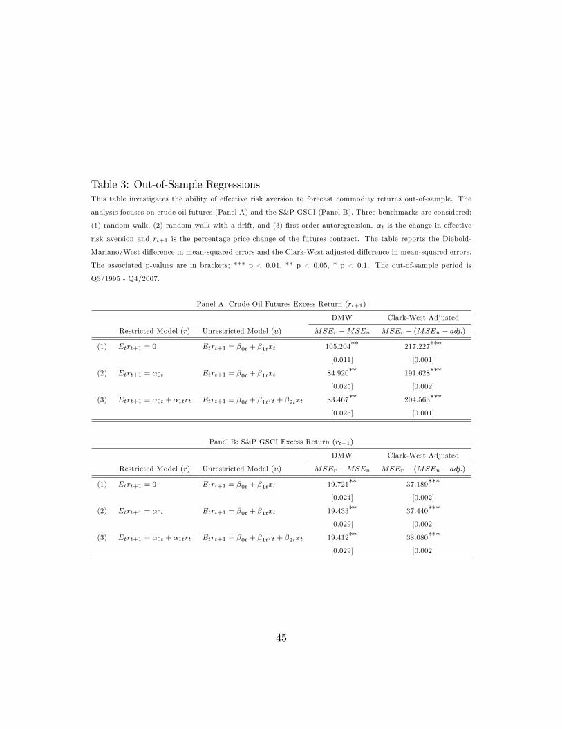
Table 3: Out-of-Sample RegressionsThis table investigates the ability of e¤ective risk aversion to forecast commodity returns out-of-sample. The

analysis focuses on crude oil futures (Panel A) and the S&P GSCI (Panel B). Three benchmarks are considered:

(1) random walk, (2) random walk with a drift, and (3) �rst-order autoregression. xt is the change in e¤ective

risk aversion and rt+1 is the percentage price change of the futures contract. The table reports the Diebold-

Mariano/West di¤erence in mean-squared errors and the Clark-West adjusted di¤erence in mean-squared errors.

The associated p-values are in brackets; *** p < 0.01, ** p < 0.05, * p < 0.1. The out-of-sample period is

Q3/1995 - Q4/2007.

Panel A: Crude Oil Futures Excess Return (rt+1)

DMW Clark-West Adjusted

Restricted Model (r) Unrestricted Model (u) MSEr �MSEu MSEr � (MSEu � adj:)

(1) Etrt+1 = 0 Etrt+1 = �0t + �1txt 105.204�� 217.227���

[0.011] [0.001]

(2) Etrt+1 = �0t Etrt+1 = �0t + �1txt 84.920�� 191.628���

[0.025] [0.002]

(3) Etrt+1 = �0t + �1trt Etrt+1 = �0t + �1trt + �2txt 83.467�� 204.563���

[0.025] [0.001]

Panel B: S&P GSCI Excess Return (rt+1)

DMW Clark-West Adjusted

Restricted Model (r) Unrestricted Model (u) MSEr �MSEu MSEr � (MSEu � adj:)

(1) Etrt+1 = 0 Etrt+1 = �0t + �1txt 19.721�� 37.189���

[0.024] [0.002]

(2) Etrt+1 = �0t Etrt+1 = �0t + �1txt 19.433�� 37.440���

[0.029] [0.002]

(3) Etrt+1 = �0t + �1trt Etrt+1 = �0t + �1trt + �2txt 19.412�� 38.080���

[0.029] [0.002]

45