broadening frequency range of a ferromagnetic axion
TRANSCRIPT

Broadening Frequency Range of a Ferromagnetic Axion Haloscope withStrongly Coupled Cavity-Magnon Polaritons
Graeme Flower,1, a) Jeremy Bourhill,1 Maxim Goryachev,1 and Michael E. Tobar1, b)
ARC Centre of Excellence for Engineered Quantum Systems, Department of Physics, University of Western Australia,35 Stirling Highway, Crawley WA 6009, Australia
(Dated: 10 October 2021)
With the axion being a prime candidate for dark matter, there has been some recent interest in direct detectionthrough a so called ‘Ferromagnetic haloscope.’ Such devices exploit the coupling between axions and electronsin the form of collective spin excitations of magnetic materials with the readout through a microwave cavity.Here, we present a new, general, theoretical treatment of such experiments in a Hamiltonian formulation forstrongly coupled magnons and photons, which hybridise as cavity-magnon polaritons. Such strongly coupledsystems have an extended measurable dispersive regime. Thus, we extend the analysis and operation ofsuch experiments into the dispersive regime, which allows any ferromagnetic haloscope to achieve improvedbandwidth with respect to the axion mass parameter space. This experiment was implemented in a cryogenicsetup, and initial search results are presented setting laboratory limits on the axion-electron coupling strengthof gaee > 3.7×10⁻⁹ in the range 33.79 µeV< ma < 33.94 µeV with 95% confidence. The potential bandwidthof the Ferromagnetic haloscope was calculated to be in two bands, the first of about 1 GHz around 8.24 GHz(or 4.1 µeV mass range around 34.1 µeV) and the second of about 1.6 GHz around 10 GHz (6.6 µeV mass rangearound 41.4 µeV). Frequency tuning may also be easily achieved via an external magnetic field which changesthe ferromagnetic resonant frequency with respect to the cavity frequency. The requirements necessary forfuture improvements to reach the DFSZ axion model band are discussed in the paper.
INTRODUCTION
Dark matter continues to be one of the major un-solved problems in physics. Evidence of its existenceis abundant but its identity remains a mystery. Manyphysicists believe it consists of particles that comefrom extensions to the current Standard Model (SM).The axion is one such particle that comes from an SMextension originally proposed to solve a problem inQuantum Chromodynamics known as the strong chargeparity problem1. It has since been shown to make anexcellent candidate for dark matter, potentially able toaccount for all of dark matter2,3. A key parameter inaxion theory is the Pecci-Quinn symmetry breaking scale(fa) which determines the mass and coupling strengthsto ordinary matter. The most known model parameterbands are KSVZ (Kim-Shifman-Vainshtein-Zakharov)4,5
and DFSZ (Dine-Fischler-Srednicki-Zhitnitsky)6,7. De-spite existence of several theoretical proposals8,9, thisparameter is unknown with limited bounds on it. Assuch there is a vast portion of the parameter spaceof axion mass and couplings to search making thefirst observation of axion or axion like particles verychallenging10.
The most successful implementation of axion directdetection experiments11 are, so called, axion halo-scopes, such as the Axion Dark Matter eXperiment(ADMX)12,13, HAYSTAC14, CULTASK15, ORGAN16,
a)Electronic mail: [email protected])Electronic mail: [email protected]
ACTION17 and multi-cell cavity approaches18,19. Theseexperiments focus on photon coupling to galactic axionhalo probing the hypothesis that axions constitute thebulk of dark matter in the Milky Way as opposed tohelioscopes20,21 focusing on axion and Axion Like Parti-cles sourced from the Sun. Mentioned above haloscopesexploit the inverse Primakoff effect22 and strong DCmagnetic fields as virtual photons to detect axions atRF and microwave frequencies putting limits on axion-photon coupling parameter gaγγ . The same coupling isinvestigated using a slightly modified approach based ondielectric materials in experiments such as MADMAX23.On the other hand, ferromagnetic haloscopes, consideredin this work, probe axion coupling to electron spin,coupling parameter gaee. Such experiments probe theinteraction between axions in the dark matter halo andcollective spin excitations in ferromagnetic materials,quantized version of which is widely known as a magnon.This resultant signal is then readout through couplingthe magnetic mode to a photon mode by placing themagnetic sample inside a microwave cavity. Similar inspirit to ferromagnetic haloscope, searches with nuclearspins, such as CASPER24, constitute another class ofgalactic haloscope targeting another coupling parametergaNN .
There has been some recent interest in this scheme withthe QUaerere AXion (QUAX) experiment25–27. Cur-rently, though, the QUAX experiment is largely staticin frequency due to it operating in the, so called, fullyhybridised regime, and so has limited capability in scan-ning axion mass, a critical feature for an axion halo-scope. In the recent development of this setup25, twomethods to make the experiment frequency tunable are
arX
iv:1
811.
0934
8v3
[ph
ysic
s.in
s-de
t] 2
9 M
ar 2
019
2
proposed. The first approach is to tune both the cav-ity and magnon mode equally to move the hybrid fre-quencies. This approach, while achievable in principle,adds significant complexity to the experiment. The sec-ond tuning method for a ferromagnetic haloscope is todetune the magnetic resonance from the cavity reso-nance. Though, this is practical and could be easily im-plemented, no method to determine how the experimentsensitivity changes in such a regime is provided. In thepresent work, we cover this lack of knowledge about thismethod by considering a new approach to determiningthe dynamics of such the cavity-magnon system.
I. DETECTION PRINCIPLES
A. Axion Electron Interaction
To understand working principles of magnetic axionhaloscopes, one needs to consider interaction between ax-ions and an individual electron. The starting point hereis the following Lagrangian for the DSVZ axion coupledto fermionic field:
L = ψ(x)(i~γµ∂µ−mc)ψ(x)−igaeea(x)ψ(x)γ5ψ(x), (1)
where ψ(x) is the spinor field of the fermion, m is itsmass, a(x) is the axion field, γµ are the Dirac matricesand gaee is the axion to electron coupling strength. Basedon this Lagrangian and ignoring the, so called, parityviolating term one can derive a Hamiltonian operator foran electron in the non-relativistic limit:
H = − ~2
2me∇2 − gaee~2
2meσ · ∇a, (2)
where e is the electron charge, σ is the Pauli matricesvector. This Hamiltonian can be compared to the onefor an electron in a magnetic field B:
H = − ~2
2me∇2 − e~2
meσ ·B. (3)
The similarity between Hamiltonians (2) and (3) allowsto introduce the pseudo-magnetic field1,25,28–30:
Baee =gaee2e∇a. (4)
Thus, the axion effects on electrons could be regardedas an effect of an anomalous oscillating magnetic field.Parameters of these oscillations as well as its directionare considered later in Section II. Thus far only the DFSZaxion has been considered. This is due to the suppressionof the KSVZ axion to ordinary quark and lepton couplingat the tree level31,32. The coupling constant, gaee, for theDFSZ axion, however, is given by:
gaee =me
3facos2(β), (5)
where cot(β) is the ratio of two Higgs vacuum expecta-tion values of this model6,33. For the following work, itis assumed cos(β) = 1.
B. Ferromagnetic Haloscopes
In order to maximise the axion induced signal in arealistic detector, it is important to shift from a singlespin system to a system with a very high spin number.This number of spins is maximised in ferromagneticcrystals, particularly Yttrium Iron Garnet (YIG), thathave been proposed as the core sensing element in pre-vious proposals25,26,28. In addition to this, high qualityYIG is characterised by relatively narrow linewidthsthat makes it a popular choice for research in thefield of hybrid quantum system for future quantuminformation processing34–39. Also, it has been proposedto use a microwave cavity to read out axion inducedmagnetisation. An excited ferromagnetic sample in freespace will dissipate energy by dipole radiation. Placingit in a microwave cavity, therefore, has the additionalbenefit of mitigating this dissipation by collecting theradiation in the cavity. Thus, the haloscope based onaxion-electron coupling appears as the hybrid modecavity-ferromagnetic quasi particle (or cavity-magnonpolariton) widely considered for applications in quantuminformation processing40,41.
To model the dynamics of a ferromagnet, it is commonto use the Bloch equations to determine the induced mag-netization from the pseudo-magnetic field. In the con-text of the QUAX proposal25,26, the solutions to theseequations were modified in conjunction with the cavityequations of motion in the fully hybridised regime as-suming the magneto-static and cavity mode form coupledharmonic oscillators. Analysis of this system, however,needs to be extended to the dispersive regime. To modelthe system in a single framework, this work considers aHamiltonian approach. The Hamiltonian of the total de-tector system consists of its cavity and magnon parts, Hc
and Hm respectively, as well magnon-cavity and axion-magnon interaction parts, Hint and Haee respectively (forunits where ~ = 1):
H = Hc +Hm +Hint +Haee
H = ωcc†c+ ωmb
†b+ gcm(c† + c)(b† + b) +Haee,(6)
where c† (c) is a creation (annihilation) operator forphoton, b† (b) is a magnon creation (annihilation) opera-tor, ωc is the cavity frequency, ωm is magnon frequency,and gcm is the cavity-magnon coupling rate. Theseexpressions can been found from first principles42,43. Itcan also be noted that the magnon Hamiltonian assumesthe demagnetizing and magneto-crystalline anisotropicfield do not introduce non-linearities into the dynamics.These assumptions are satisfied using a spherical sampleand small input fields respectively43. The magnon reso-nance frequency is set by the external magnetic field B0
via the Zeeman effect ωm = γ(B0 +Bani), where γ is thegyromagnetic ratio and Bani is the linear contribution ofthe magneto-crystalline anisotropy, typically determinedexperimentally.

3
To determine the magnon-axion interaction term in theHamiltonian, it is straightforward to write the interactionin terms of its Zeeman energy:
Haee = −∫Vm
M ·BaeedV, (7)
where M is the sample magnetization vector, Vm is itsvolume. Given the uniform precession magneto-static(Kittel) mode, which has constant magnetisation over thesample volume, the expression can be easily integrated:
Haee =− γS ·Baee, (8)
where S = MVm
γ is a macrospin operator. For this oper-
ator, raising and lowing spin operators are introduced asS± = Sx± iSy, where for the following, the z direction ischosen to align with the external DC magnetic field. Us-ing this set of spin operators, the spin-axion interactionHamiltonian is expanded as:
Haee =− γBaee[ sin(φ)
2(S+e−iθ + S−eiθ) + Sz cos(φ)
],
(9)
where θ and φ are the spherical coordinate azimuthal andpolar angles of the pseudo-magnetic field vector respec-tively. Finally, the Primakoff-Holstein transformationsare used to write the interaction it in terms of magnonoperators introduced above44:
S+ = (√
2S − b†b)b,
S− = b†(√
2S − b†b),Sz = S − b†b,
(10)
where S is the total spin number of the macrospinoperator. This number is determined by S = µ
gµBNs,
where µ is the magnetic moment of the magnetic sample,µB is the Bohr magneton, g is the g-factor (g = 2)and Ns is the number of spins in the sample (given byNs = nsVm with ns as spin density and Vm as volume).For YIG, used in previous proposals as well as this work,it is estimated that µ
µB= 5.045 and the spin density
ns = 2.2 × 1028m−3. From these values the total spinnumber for a 2mm diameter YIG sphere used in thiswork may be estimated as S = 2.3× 10²⁰.
For low excitation numbers (〈b†b〉 2S), themacrospin operators may be approximated by S+ ≈√
2Sb and S− ≈√
2Sb† giving the final expression forthe axion-magnon coupling term:
Haee = −γBaee[√S
2sin(φ)(be−iθ + b†eiθ)+
b†b cos(φ)],
(11)
where constant terms are ignored. It can be notedthe axion-magnon interaction Hamiltonian (11) includestwo sets of terms: components relating to the pseudo-magnetic field perpendicular to the external magneticfield and producing magnon excitations, and terms cou-pled to the parallel component producing a modulation ofthe magnon frequency. For an axion producing magnonsin the GHz frequency range, it is shown in the follow-ing discussion that the latter frequency modulation termcan be ignored under a Rotating Wave Approximation(RWA), but could be used to search for low mass axionsusing frequency metrology techniques46,47. Thus, onlythe former term producing excess of power in the magnonspectrum can be used for the current experiment.
C. Detector Dynamics
In order to capture the dynamics of the total exper-iment, one needs to include dissipation. This is doneby deriving the Heisenberg-Langevin equations of mo-tion for open systems. In this case internal dissipation inthe cavity and magnon modes are modelled as couplingto internal thermal baths as well as the cavity couplingto an external bath through a probe/port. The generalform of these equations is given by48:
df
dt= −i[f,H] +
∑n
((κn2g† + i
√κna
in†n
)[f, g]−
[f, g†](κn
2g + i
√κna
inn
)),
(12)
where f and g are arbitrary system operators, ainn and
κn is the input field and dissipation rate due to couplingof some a field to the nth thermal bath respectively. Forderivation of axion induced output power, all noise termsare ignored, and it is assumed that the magnon modedoes not couple to the external excitation port.
The resulting equations of motion for annihilation op-erators are then converted to the rotating frame (c →ce−iωat, b → be−iωat, where ωa is the axion signal fre-quency) and a RWA is made. This procedure gives theequations of motion as follows in the lab frame:
dc
dt= −i
(ωc − i
κc2
)c− igcmb, (13)
db
dt= −i
(ωm − i
κm2
)b− igcmc+ i
√S
2γBaee sin(φ)eiθ,
(14)
where κc = κintc + κext
c and κm = κintm are the dissipa-
tion rates of the cavity and magnon respectively. Thesequantities include internal and external (from the cavityprobe) dissipation where applicable.
The derived equations of motion (13) can be easilysolved for the cavity field in terms of the driving pseudo-
4
magnetic field giving:
c(ωa) =igcm
√S8 γBaee sin(φ)eiθ
κcκm∆c∆m − g2cm
, (15)
where ∆n = ωa−ωn
κn+ i
2 . This result can be convertedto the output fields using the boundary conditions frominput-output theory cout + cin =
√κextc c, as well as the
output power from Pout = ~ωa〈c∗out(t)cout(t)〉:
Pout(ωa) =~ωaκext
c g2cm
S8 γ
2B2aee sin2(φ)
|κcκm∆c∆m − g2cm|2
. (16)
Note should be taken that the only geometrical de-pendence left in the output power is sin2(φ), which ismaximum when the pseudo-magnetic field from axioninteraction is perpendicular to the DC magnetic field.This dependence is discussed in Section II.
To determine the axion induced power on resonance,the resonant frequency of the coupled normal modes canbe used, where a simplification has been made under theassumption of a strongly coupled system (gcm κc, κm):
ω± =ωc + ωm
2±√(Ωcm
2
)2
+ g2cm, (17)
where Ωcm = ωm − ωc. These expression give the onresonance (ωa = ω±) power expressions:
P± =~ωaκext
cS2 γ
2B2aee sin2(φ)
κ2cκ
2m
4g2cm+(
Ωcm
2gcm(κm − κc)±
√(Ωcm
2gcm
)2
+ 1(κc + κm))2.
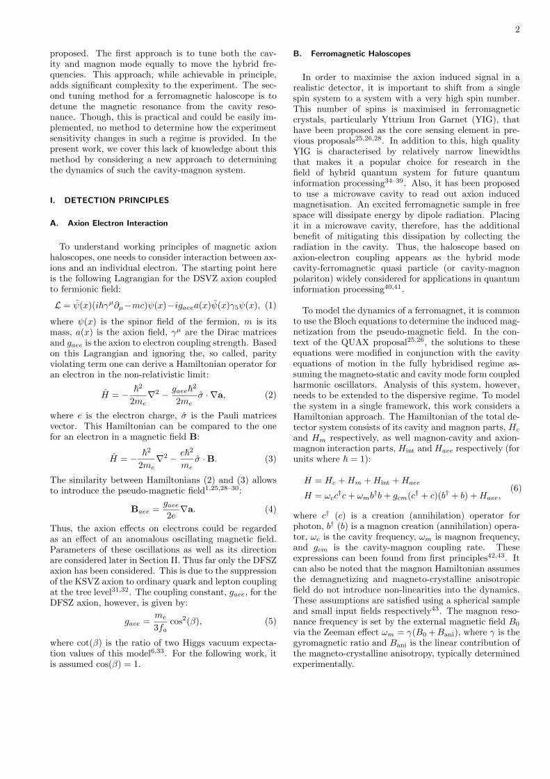
(18)It can be noted that this form of the power on reso-nance is a function of the detuning over coupling rate.Thus, the range of frequencies where this experimentis sensitive is proportional to the coupling rate gcm.Importantly, this formula allows the determination ofthe sensitivity of this experiment in the dispersive regimewhen ωc 6= ωm. To demonstrate the response of the sys-tem in the dispersive regime a set of output powers arecalculated for a 2mm diameter YIG sphere for variousrelationships between linewidths of subsystems. Givenlinewidths κ1 = (2π)10MHz and κ2 = (2π)50MHz, threecases are considered: (1) for κc > κm, κc = κ1 andκm = κ2, (2) for κc = κm = κ1, (3) for κc < κm, κc = κ2
and κm = κ1. In all cases κextc = κc/2. The result for
gcm = (2π)745MHz, ωa = (2π)8.2GHz (correspondingto |Baee| = 3.4 × 10⁻²³T) and sin(φ) = 1 is depictedin Fig. 1. As the magnon excitation is readout throughthe cavity mode, this might imply that the outputsignal will be strongest in the full hybridisation regime.However, Fig. 1 shows that this is not the case ingeneral. Particularly, when κc 6= κm, the maximumsignal strength is obtained in the dispersive regime. Thisopens up new ways to optimise such an experiment,often by operating in the dispersive regime.
(A)
(B)
FIG. 1: Detector output power as a function of scaleddetuning Ωcm
gcmfor an YIG sphere for various linewidths:
(A) from the higher frequency normal mode (P+), (B)from the lower frequency normal mode (P−).
II. AXION WIND
With the detector dynamics determined in terms ofthe driving pseudo-magnetic field, it is now necessary todetermine its components in the laboratory frame. Assuch a classical axion field can be substituted (a stepwhich will be justified later). This is given by:
a(r, t) = a0 sin(ωat−
mava·r~
), (19)
where a0 =√
2ρac
~ma
is the magnitude of the axion field,
ρa ≈ 0.45GeV/cm3 is the local dark matter density49,and va is the velocity of the axion wind.
Baee =gaee2e
ma|va|~
a0 sin(ωat−
ma|va|x~
)x, (20)
where x is the direction of the axion wind. In the presentwork, the velocity in the galactic frame of the axion windis treated as a Maxwell distribution with mean velocity
5
of zero and velocity dispersion of σv = 270km/s. Thus,in the laboratory frame it has the velocity of the galacticframe of approximately 220km/s in the direction of theconstellation Cygnus50. It should be noted that this ex-periment being a directional detector of the axion darkmatter field makes it also sensitive to the so called ‘darkmatter hurricane’ or S1 stream which provides an addi-tional source of axions as well as different velocity distri-bution compared with those in the dark matter halo51.In this work, however, we only consider the axion windfrom the earth’s movement through the dark matter halowhich gives the following parameters25:
|Baee| = 3.4× 10⁻²³( ma
34µeV
)T, (21)
ωa2π
= 8.2( ma
34µeV
)GHz, (22)
gaee = 1.0× 10⁻¹⁵( ma
34µeV
), (23)
λ∇a = 0.74λa = 0.75h
mava= 8.8
(34µeV
ma
)m. (24)
Note the de-Broglie wavelength of galactic axions ismuch larger than the scale of a haloscope experiment forthe frequencies considered. This justifies the treatmentof the axion field a(r, t) as a classical field.
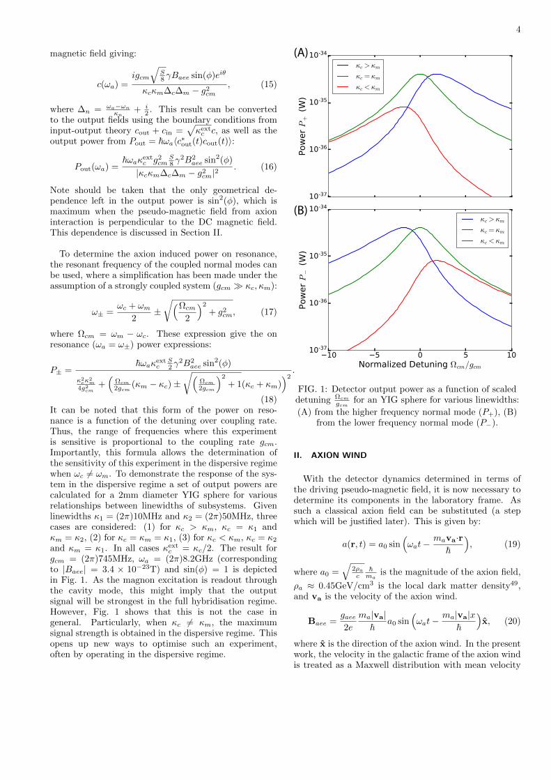
The next step is to determine the direction of the ax-ion wind with the laboratory frame in Perth, WesternAustralia. For this, the velocity due to the Sun’s orbitaround the galactic centre as well as the velocity dueto the Earth’s orbit around the Sun can be taken intoaccount. Appropriate coordinate transforms52 give thevelocity of the axion wind in the laboratory frame. Inthese calculations, only the components which are per-pendicular to the external DC magnetic field orientedlocally upwards (from the centre of the Earth), are im-portant to the operation of the haloscope. The mag-nitude of the perpendicular components of the velocity
Baee,⊥ =√B2aee,x +B2
aee,y is shown in Fig. 2 for the 27th
of August 2018 (local time) in Perth where it is scaled toits absolute value. It can be seen that there is an 8 hourperiod per day which a ferromagnetic haloscope wouldbe sensitive and a 2 hour period where our signal shoulddisappear.
III. EXPERIMENTAL DESIGN
From the expression of output power, Eq. (18), itfollows that in order to maximise the detector sensitivityit is required to maximise the number of spins (i.e. spindensity and volume) as well as cavity and magnon modeQuality factors. For a scanning tunable experiment,it is also important to widen the range of sensitivefrequencies that can be done by improving the couplingrate between cavity and magnon modes. This has beenachieved using two post re-entrant cavities allowing to
0 5 10 15 20Time of Day (Hours)
0.3
0.4
0.5
0.6
0.7
0.8
0.9
1.0
Baee,/|Baee|
FIG. 2: The daily modulation of the pseudo-magneticfield perpendicular to the direction of an external fieldat the University of Western Australia on the 27th of
August 2018.
reach the strong coupling regime34. As a system ofessentially two coupled quasi-lumped resonators, suchcavities exhibit two modes: the bright and the darkmodes. In the former mode, the magnetic field aroundeach post as well as the electric fields in the gaps are inphase. This phase relation concentrates the magneticenergy in between the posts. So, by placing the magneticsample in that space, one achieves large magnetic fillingfactors and thus a large coupling between the photonand magnon mode.
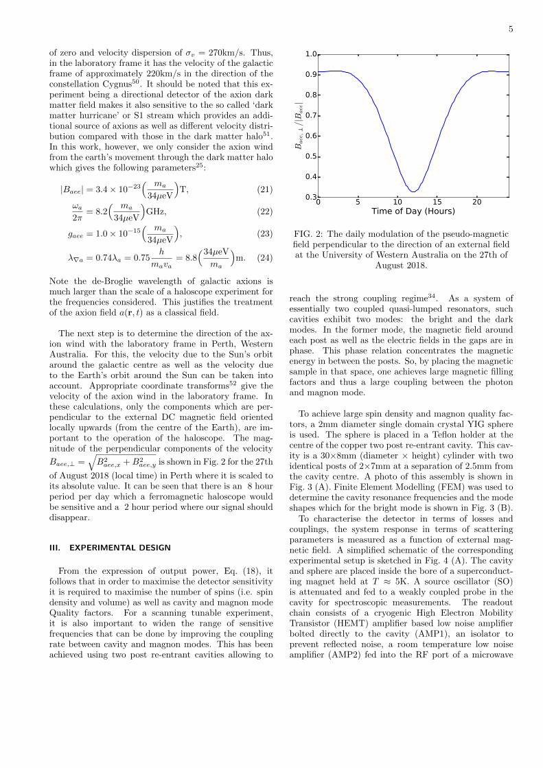
To achieve large spin density and magnon quality fac-tors, a 2mm diameter single domain crystal YIG sphereis used. The sphere is placed in a Teflon holder at thecentre of the copper two post re-entrant cavity. This cav-ity is a 30×8mm (diameter × height) cylinder with twoidentical posts of 2×7mm at a separation of 2.5mm fromthe cavity centre. A photo of this assembly is shown inFig. 3 (A). Finite Element Modelling (FEM) was used todetermine the cavity resonance frequencies and the modeshapes which for the bright mode is shown in Fig. 3 (B).
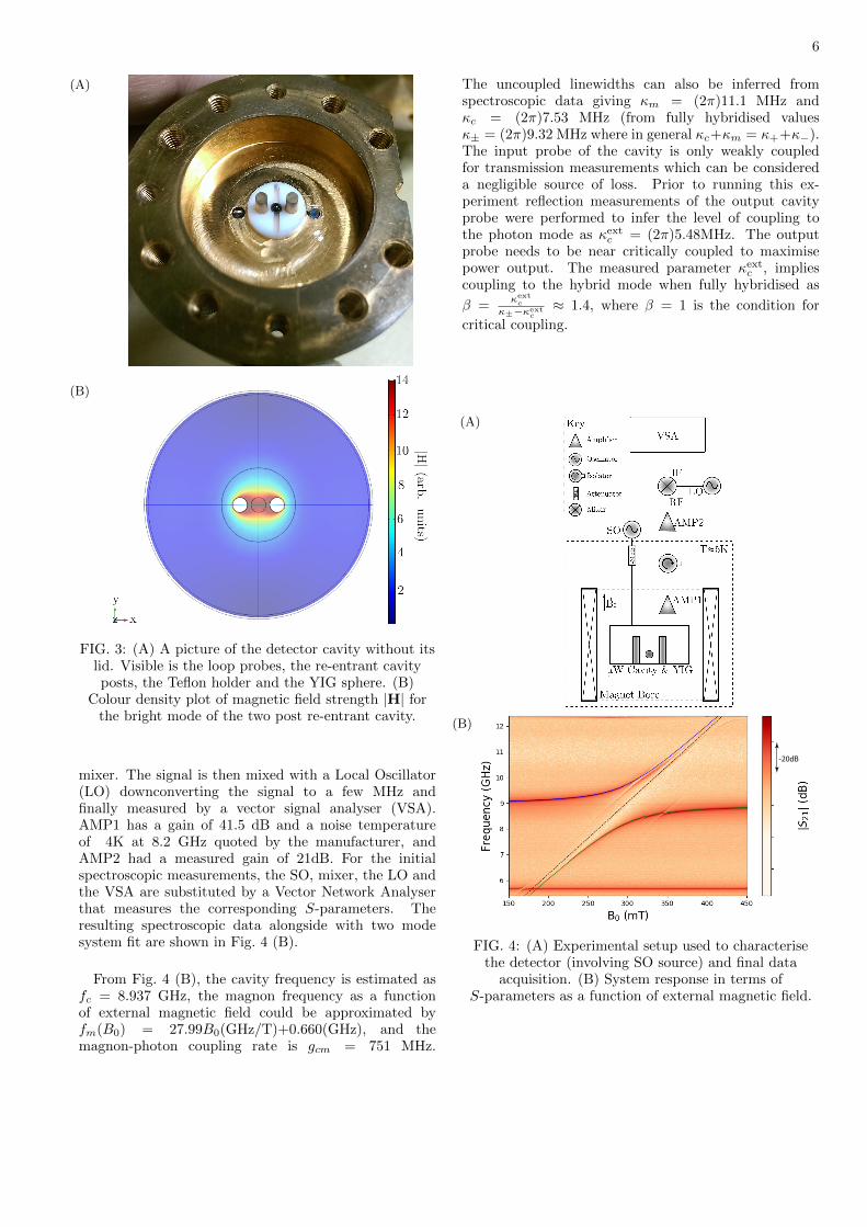
To characterise the detector in terms of losses andcouplings, the system response in terms of scatteringparameters is measured as a function of external mag-netic field. A simplified schematic of the correspondingexperimental setup is sketched in Fig. 4 (A). The cavityand sphere are placed inside the bore of a superconduct-ing magnet held at T ≈ 5K. A source oscillator (SO)is attenuated and fed to a weakly coupled probe in thecavity for spectroscopic measurements. The readoutchain consists of a cryogenic High Electron MobilityTransistor (HEMT) amplifier based low noise amplifierbolted directly to the cavity (AMP1), an isolator toprevent reflected noise, a room temperature low noiseamplifier (AMP2) fed into the RF port of a microwave
6
(A)
(B)
FIG. 3: (A) A picture of the detector cavity without itslid. Visible is the loop probes, the re-entrant cavityposts, the Teflon holder and the YIG sphere. (B)
Colour density plot of magnetic field strength |H| forthe bright mode of the two post re-entrant cavity.
mixer. The signal is then mixed with a Local Oscillator(LO) downconverting the signal to a few MHz andfinally measured by a vector signal analyser (VSA).AMP1 has a gain of 41.5 dB and a noise temperatureof 4K at 8.2 GHz quoted by the manufacturer, andAMP2 had a measured gain of 21dB. For the initialspectroscopic measurements, the SO, mixer, the LO andthe VSA are substituted by a Vector Network Analyserthat measures the corresponding S-parameters. Theresulting spectroscopic data alongside with two modesystem fit are shown in Fig. 4 (B).
From Fig. 4 (B), the cavity frequency is estimated asfc = 8.937 GHz, the magnon frequency as a functionof external magnetic field could be approximated byfm(B0) = 27.99B0(GHz/T)+0.660(GHz), and themagnon-photon coupling rate is gcm = 751 MHz.
The uncoupled linewidths can also be inferred fromspectroscopic data giving κm = (2π)11.1 MHz andκc = (2π)7.53 MHz (from fully hybridised valuesκ± = (2π)9.32 MHz where in general κc+κm = κ++κ−).The input probe of the cavity is only weakly coupledfor transmission measurements which can be considereda negligible source of loss. Prior to running this ex-periment reflection measurements of the output cavityprobe were performed to infer the level of coupling tothe photon mode as κext
c = (2π)5.48MHz. The outputprobe needs to be near critically coupled to maximisepower output. The measured parameter κext
c , impliescoupling to the hybrid mode when fully hybridised as
β =κextc
κ±−κextc≈ 1.4, where β = 1 is the condition for
critical coupling.
(A)
(B)
-20dB
FIG. 4: (A) Experimental setup used to characterisethe detector (involving SO source) and final data
acquisition. (B) System response in terms ofS-parameters as a function of external magnetic field.

7
IV. RESULTS
The axion signal is expected to appear as excess ofpower over background noise in a power spectra. Itis therefore necessary to discriminate against artificialpeaks that could appear due to various spurious signals.For this reason, two sets of data for each frequencyrange are taken each day. The first is over an 8hrperiod where the velocity is ∼ 90% perpendicular to theexternal magnetic field (corresponding to ∼ 81% of themaximum power) and then a second set of data is takenover the 2 hours period when the velocity is only ∼ 35%perpendicular to the external field (corresponding to∼ 12% of the maximum power). The second datasetallows any persistent spurious signals to be identifiedand eliminated.
The exclusion data was taken over a range of frequen-cies for a period of 6 days in August 2018. Each day ofmeasurements consists of 320,000 individual power spec-tra measured over a sensitive period of time (∼ 8hrs in-tegration time) and 80,000 power spectra collected overthe minimally sensitive period (∼ 2hrs integration time).The frequency of the hybrid resonance was tuned usingthe external magnetic field allowing to scan for ∼ 36MHzaround 8.2GHz. In this case only the lower hybrid modewas used to attempt to measure an axion signal and thea limited 36MHz tuning range used considered due toavailability of equipment. The full potential range ofthis haloscope can be calculated from equations 17 and 18giving a full width at half maximum (FWHM) of 1.6GHzaround 10GHz for the upper hybrid mode and a FWHMof 1.0GHz around 8.2GHz for the lower hybrid mode.Throughout the experiment the cavity and first ampli-fier were kept at a temperature of ∼ 5K. The sum of thecavity physical temperature and the noise temperatureof the first stage amplifier can be used to estimate theexpected noise temperature of the system as ∼ 9K at8.2GHz. Analysis of the spectra was done using a sim-ilar method to E. Daw53. For each set of data, definedby the DC magnetic field B0 used to set a central fre-quency of the lower hybrid mode, f−, a span of ∼ 6MHz(reduced from the ∼ 9MHz hybrid linewidth due to spu-rious system noise) of data around the central frequencywas analysed. In each case, the power spectral density,with bin width ∆f = 3.125kHz (chosen to be similar tothe axion signal width 4.1kHz), was scaled by the ampli-fier gains and a polynomial fit was made. The residualswere then analysed to confirm the validity of the fit. Nextthe lowest possible cut is made in the sensitive data suchthat any bins above this chosen power value also existabove the same cut in the insensitive data. This allowsthe identification of bad bins, as any bins above the cut inboth the sensitive and insensitive data are irrelevant spu-rious signals and thus can be removed from the analysis.The remaining Gaussian noise can be analysed to deter-mine standard deviation (σ) and effective noise temper-ature of the system, making use of the Dicke radiometer
B0 (mT) f− (GHz) σ (10−23W) Teff (K) Cut (σ) Pexl (σ)298 8.2086 4.89 11.0 6.2 15.8297.5 8.2018 4.73 10.4 4.2 10.3297 8.1950 5.81 12.8 5.0 13.2296.5 8.1879 5.50 12.1 5.7 14.9296.1 8.1820 5.74 12.6 5.0 12.9295.6 8.1754 5.78 12.7 5.2 13.6
TABLE I: Measured standard deviations of residuals(scaled by amplifier gains), cuts made and excluded
power for each set of data.
equation54:
σ = kBTeff
√∆f
t, (25)
where kB is the Boltzmann constant, Teff is the effectivesystem noise temperature, and t is the integration time.A potential axion signal would appear as a residual binwith an excess of power over the mean, with the cutmade earlier defining the largest distinguishable signalamongst the noise. Gaussian statistics are then usedto determine the excluded signal power (Pexl) to a 95%confidence based on the cut made53. These results areshown in Table I. From Table I, it can be seen that theeffective temperature determined from the measurednoise is comparable to the estimate based on the physicaltemperature and first stage amplifier, thus the measuredresults are consistent with expectations. The largermeasured effective noise temperature is due to the smallcontribution of noise due to cables and second stageamplifier.
To determine excluded couplings and magnetic fieldsthe following relations were used:
Pexl
P−=g2aee,exl
g2aee
, (26)
where gaee,exl is the excluded axion to electron couplingstrength. Here the excluded power is also scaled by aLorentzian line-shape and multiplied by 0.81 to accountfor the reduction in sensitivity due to the proportion ofaxion wind perpendicular to the external magnetic fieldat that time of day. This relation allows to put limitson the axion-electron coupling strength gaee as shownin Fig. 5 where also several predictions are made in theform of the dashed lines (see Section V for detailed dis-cussions).
V. DISCUSSION AND PERSPECTIVES
It can be seen in Fig. 5 that the results of this analysisare still orders of magnitude from current astronomicallimits on axion electron coupling and expected DFSZmodel predictions. They do, however, demonstrate

8
FIG. 5: The DFZS axion model band and exclusion plotfor axion-electron coupling strength gaee as a function
of axion mass: limits due to white dwarf cooling55,56 arein light blue, this work limits are in dark blue, dashed
lines show several predictions for the future work.
how such ferromagnetic haloscopes, in a single cavityconfiguration, can search over a larger range than theirlinewidth by tuning their hybrid frequencies. Thislarger range isn’t strictly experimental improvementsbut rather from improved capabilities of the experimentdue to more general theoretical analysis. Additionally,whilst this detector isn’t sensitive enough to detectDFSZ axions, it does have the capability to detectaxion-like particles (ALPs) which don’t have a fixedrelation between axion mass and axion-normal mattercoupling strengths.
While this initial result demonstrates the experimentsusability, further improvements, particularly in samplevolume and line-widths, are needed to improve theoverall sensitivity. Single domain ferrimagnetic sphereswith a diameter of 5mm are easily available and in-ferred magnon linewidths of around 2.4MHz at centralfrequency 14GHz can be seen for a Ga:YIG sample inthe QUAX experiment25. Additionally, their approachto increasing the effective volume of the magnetic ma-terial in the cavity by including multiple spheres couldalso be utilised. Such improvements would boost theoutput power from an axion signal. The correspondingimprovement is shown in Fig. 5 by the dark blue dashedline assuming a larger 5mm diameter sphere, improvedlinewidths of κm = (2π)2.4MHz and a measurementtime of one day with existing amplifiers. Alternatively,one may consider materials with higher spin density suchas Lithium Ferrite where the same order of magneticlosses together with absence of spurious modes havebeen observed57.
The sensitivity would also be improved by reducingthe detector background noise, for example, by imple-mentation of quantum limited parametric amplifiersbased on Josephson junctions. Successful operation of
such amplifiers, viable in the considered frequency range,has been demonstrated for axion-photon haloscopes14.The result of these improvements changing sensitivity ofthe detector is shown in Fig. 5 with the purple dashedline.
In order to improve the limits even further, one needsto build a viable detection scheme based on a singlephoton or magnon counter, ideally using a QuantumNon-Demolition (QND) measurement to surpass thestandard quantum limit. Such devices would then onlybe limited by shot noise due to a non-zero temperatureof the cavity. Single photon counters in the context onaxion haloscopes and are discussed by Lamoreaux, etal.58, showing superconducting qubits in cavities to bea promising avenue for a QND single photon counter59.A single magnon counter could similarly be constructedby coupling a qubit to a magnon mode which wasrecently achieved to resolve numbers state60,61. This isone experimental advantage of ferromagnetic haloscopesover traditional photon haloscopes as the DC magneticfield need not extend over the entire cavity, thus afocused magnetic field on the ferrimagnetic samplewould allow the presence of superconducting devices inthe cavity to aid measurement. Non-QND, single photoncounters have also been shown to be another promisingavenue for axion haloscopes62,63. The result of a QNDmeasurement based experiment is predicted in Fig. 5with both reasonable and optimistic improvements inthe signal-to-noise ratio. The red dashed line is theresult of the above assuming a perfect efficiency QNDmeasurement is achieved requiring a maximum physicaltemperature of 12.5mK to ensure a 95% confidence ofno dark counts of the detector over the measurementtime. The final black dashed line in Fig. 5 is a predictionof an extremely optimistic QND measurement schemeassuming the signal power can be further boosted witha volume of the magnetic sample of Vm = 0.13 L and animproved linewidth of κm = (2π)200 kHz. These esti-mations are done following the procedure by Lamoreauxet al.58, where it is noted that in this case the limitingfactor is the minimum detectable power required tocount at least three photons over the measurement time.
CONCLUSIONS
A new theoretical perspective on ferromagnetic halo-scopes was presented which demonstrated methods ofimproving the operation of a ferromagnetic haloscope.Particularly easy frequency tunability to search the ax-ion mass parameter space is achievable by operating inthe dispersive regime. It also highlighted the importanceof a large cavity-magnon coupling strength to producea large bandwidth and provided new methods to opti-mise experimental design and operation. The device wasimplemented and set limits on axion-electron coupling of

9
gaee > 3.7×10⁻⁹ in the range 33.79µeV< ma < 33.94µeVwith 95% confidence. Limitations of this experiment, inthe form of electronic noise and small sample volume arediscussed, and improvements are suggested in the formof quantum or shot noise limited measurement. Thesepredictions highlight the need for shot noise limited mea-surement in the form of single photon or magnon coun-ters, as well as the requirement to dramatically improvesignal power.
ACKNOWLEDGEMENTS
This work was supported by the Australian ResearchCouncil grant number DP190100071 and CE170100009as well as the Australian Government’s Research Train-ing Program.
REFERENCES
1R. D. Peccei and H. R. Quinn, Phys. Rev. Lett. 38, 1440 (1977).2J. Ipser and P. Sikivie, Phys. Rev. Lett. 50, 925 (1983).3J. Jaeckel and A. Ringwald, Annual Review of Nuclear and Par-ticle Science, Annual Review of Nuclear and Particle Science 60,405 (2010).
4J. E. Kim, Phys. Rev. Lett. 43, 103 (1979).5M. A. Shifman, A. I. Vainshtein, and V. I. Zakharov, NuclearPhysics B 166, 493 (1980).
6M. Dine, W. Fischler, and M. Srednicki, Physics Letters B 104,199 (1981).
7A. R. Zhitnitskij, Yadernaya Fizika, Yadernaya Fizika 31, 497(1980).
8G. Ballesteros, J. Redondo, A. Ringwald, and C. Tamarit, Phys-ical Review Letters 118, 071802 (2017).
9J. D. Clarke and R. R. Volkas, Phys. Rev. D 93, 035001 (2016).10I. G. Irastorza and J. Redondo, Progress in Particle and Nuclear
Physics 102, 89 (2018).11P. W. Graham, I. G. Irastorza, S. K. Lamoreaux, A. Lindner,
and K. A. van Bibber, Annual Review of Nuclear and ParticleScience, Annual Review of Nuclear and Particle Science 65, 485(2015).
12S. J. Asztalos, G. Carosi, C. Hagmann, D. Kinion, K. van Bib-ber, M. Hotz, L. J. Rosenberg, G. Rybka, J. Hoskins, J. Hwang,P. Sikivie, D. B. Tanner, R. Bradley, and J. Clarke, Phys. Rev.Lett. 104, 041301 (2010).
13A. Collaboration, N. Du, N. Force, R. Khatiwada, E. Lentz,R. Ottens, L. J. Rosenberg, G. Rybka, G. Carosi, N. Woollett,D. Bowring, A. S. Chou, A. Sonnenschein, W. Wester, C. Boutan,N. S. Oblath, R. Bradley, E. J. Daw, A. V. Dixit, J. Clarke, S. R.O’Kelley, N. Crisosto, J. R. Gleason, S. Jois, P. Sikivie, I. Stern,N. S. Sullivan, D. B. Tanner, and G. C. Hilton, Physical ReviewLetters 120, 151301 (2018).
14B. M. Brubaker, L. Zhong, Y. V. Gurevich, S. B. Cahn, S. K.Lamoreaux, M. Simanovskaia, J. R. Root, S. M. Lewis, S. Al Ke-nany, K. M. Backes, I. Urdinaran, N. M. Rapidis, T. M. Shokair,K. A. van Bibber, D. A. Palken, M. Malnou, W. F. Kindel, M. A.Anil, K. W. Lehnert, and G. Carosi, Phys. Rev. Lett. 118,061302 (2017).
15S. Youn, International Journal of Modern Physics: ConferenceSeries 43, 1660193 (2016).
16B. T. McAllister, G. Flower, E. N. Ivanov, M. Goryachev,J. Bourhill, and M. E. Tobar, Physics of the Dark Universe18, 67 (2017).
17J. Choi, H. Themann, M. J. Lee, B. R. Ko, and Y. K. Se-mertzidis, Phys. Rev. D 96, 061102 (2017).
18J. Jeong, S. Youn, S. Ahn, J. E. Kim, and Y. K. Semertzidis,Physics Letters B 777, 412 (2018).
19J. Jeong, S. Youn, S. Ahn, C. Kang, and Y. K. Semertzidis,Astroparticle Physics 97, 33 (2018).
20E. F. Ribas, E. Armengaud, F. T. Avignone, M. Betz, P. Brax,P. Brun, G. Cantatore, J. M. Carmona, G. P. Carosi, F. Caspers,S. Caspi, S. A. Cetin, D. Chelouche, F. E. Christensen, A. Dael,T. Dafni, M. Davenport, A. V. Derbin, K. Desch, A. Di-ago, B. Dobrich, I. Dratchnev, A. Dudarev, C. Eleftheriadis,G. Fanourakis, J. Galan, J. A. Garcıa, J. G. Garza, T. Geralis,B. Gimeno, I. Giomataris, S. Gninenko, H. Gomez, D. Gonzalez-Diaz, E. Guendelman, C. J. Hailey, T. Hiramatsu, D. H. H.Hoffmann, D. Horns, F. J. Iguaz, I. G. Irastorza, J. Isern,K. Imai, J. Jaeckel, A. C. Jakobsen, K. Jakovcic, J. Kaminski,M. Kawasaki, M. Karuza, M. Krcmar, K. Kousouris, C. Krieger,B. Lakic, O. Limousin, A. Lindner, A. Liolios, G. Luzon, S. Mat-suki, V. N. Muratova, C. Nones, I. Ortega, T. Papaevangelou,M. J. Pivovaroff, G. Raffelt, J. Redondo, A. Ringwald, S. Russen-schuck, J. Ruz, K. Saikawa, I. Savvidis, T. Sekiguchi, Y. K.Semertzidis, I. Shilon, P. Sikivie, H. Silva, H. H. J. ten Kate,A. Tomas, S. Troitsky, T. Vafeiadis, K. van Bibber, P. Vedrine,J. A. Villar, J. K. Vogel, L. Walckiers, A. Weltman, W. Wester,S. C. Yildiz, and K. Zioutas, Journal of Physics: ConferenceSeries 650, 012009 (2015).
21T. Dafni, M. Arik, E. Armengaud, S. Aune, F. T. Avignone,K. Barth, A. Belov, M. Betz, H. Brauninger, P. Brax, N. Brei-jnholt, P. Brun, G. Cantatore, J. M. Carmona, G. P. Carosi,F. Caspers, S. Caspi, S. A. Cetin, D. Chelouche, F. E. Chris-tensen, J. I. Collar, A. Dael, M. Davenport, A. V. Derbin,K. Desch, A. Diago, B. Dobrich, I. Dratchnev, A. Dudarev,C. Eleftheriadis, G. Fanourakis, E. Ferrer-Ribas, P. Friedrich,J. Galan, J. A. Garcıa, A. Gardikiotis, J. G. Garza, E. N.Gazis, E. Georgiopoulou, T. Geralis, B. Gimeno, I. Giomataris,S. Gninenko, H. Gomez, D. Gonzalez-Dıaz, E. Gruber, E. Guen-delman, T. Guthorl, C. J. Hailey, R. Hartmann, S. Hauf,F. Haug, M. D. Hasinoff, T. Hiramatsu, D. H. H. Hoffmann,D. Horns, F. J. Iguaz, I. G. Irastorza, J. Isern, K. Imai,J. Jacoby, J. Jaeckel, A. C. Jakobsen, K. Jakovcic, J. Kamin-ski, M. Kawasaki, M. Karuza, K. Konigsmann, R. Kotthaus,M. Krcmar, K. Kousouris, C. Krieger, M. Kuster, B. Lakic,J. M. Laurent, O. Limousin, A. Lindner, A. Liolios, A. Ljubicic,G. Luzon, S. Matsuki, V. N. Muratova, S. Neff, T. Niinikoski,C. Nones, I. Ortega, T. Papaevangelou, M. J. Pivovaroff, G. Raf-felt, J. Redondo, H. Riege, A. Ringwald, A. Rodrıguez, M. Rosu,S. Russenschuck, J. Ruz, K. Saikawa, I. Savvidis, T. Sekiguchi,Y. K. Semertzidis, I. Shilon, P. Sikivie, H. Silva, S. K. Solanki,L. Stewart, H. H. J. ten Kate, A. Tomas, S. Troitsky, T. Vafeiadis,K. van Bibber, P. Vedrine, J. A. Villar, J. K. Vogel, L. Walckiers,A. Weltman, W. Wester, S. C. Yildiz, and K. Zioutas, 37th Inter-national Conference on High Energy Physics (ICHEP), Nuclearand Particle Physics Proceedings 273-275, 244 (2016).
22P. Sikivie, Physical Review letters 61, 1415 (1983).23M. W. Group, A. Caldwell, G. Dvali, B. Majorovits, A. Millar,
G. Raffelt, J. Redondo, O. Reimann, F. Simon, and F. Steffen,Physical Review Letters 118, 091801 (2017).
24A. Garcon, D. Aybas, J. W. Blanchard, G. Centers, N. L.Figueroa, P. W. Graham, D. F. J. Kimball, S. Rajendran, M. G.Sendra, A. O. Sushkov, L. Trahms, T. Wang, A. Wickenbrock,T. Wu, and D. Budker, Quantum Science and Technology 3,014008 (2018).
25N. Crescini, D. Alesini, C. Braggio, G. Carugno,D. Di Gioacchino, C. S. Gallo, U. Gambardella, C. Gatti,G. Iannone, G. Lamanna, C. Ligi, A. Lombardi, A. Ortolan,S. Pagano, R. Pengo, G. Ruoso, C. C. Speake, and L. Taffarello,The European Physical Journal C 78, 703 (2018).
26R. Barbieri, C. Braggio, G. Carugno, C. Gallo, A. Lombardi,A. Ortolan, R. Pengo, G. Ruoso, and C. Speake, Physics of theDark Universe 15, 135 (2017).

10
27G. Ruoso, A. Lombardi, A. Ortolan, R. Pengo, C. Braggio,G. Carugno, C. S. Gallo, and C. C. Speake, Journal of Physics:Conference Series 718, 042051 (2016).
28R. Barbieri, M. Cerdonio, G. Fiorentini, and S. Vitale, PhysicsLetters B 226, 357 (1989).
29A. Kakhizde and I. Kolokolov, Sov. Phys. JETP , 598 (1991).30P. Vorob’ev, A. Kakhizde, and I. Kolokolov, Phys. Atom. Nuclei
, 959 (1995).31J. E. Kim, Phys. Rev. Lett. 43, 103 (1979).32M. Shifman, A. Vainshtein, and V. Zakharov, Nuclear Physics
B 166, 493 (1980).33A. R. Zhitnitsky, Sov. J. Nucl. Phys. 31, 260 (1980), [Yad.
Fiz.31,497(1980)].34M. Goryachev, W. G. Farr, D. L. Creedon, Y. Fan, M. Kostylev,
and M. E. Tobar, Phys. Rev. Applied 2, 054002 (2014).35Y. Tabuchi, S. Ishino, T. Ishikawa, R. Yamazaki, K. Usami, and
Y. Nakamura, Physical Review Letters 113, 083603 (2014).36P. Andrich, C. F. de las Casas, X. Liu, H. L. Bretscher, J. R.
Berman, F. J. Heremans, P. F. Nealey, and D. D. Awschalom,npj Quantum Information 3, 28 (2017).
37Y. Tabuchi, S. Ishino, A. Noguchi, T. Ishikawa, R. Yamazaki,K. Usami, and Y. Nakamura, Science 349, 405 (2015).
38X. Zhang, C.-L. Zou, L. Jiang, and H. X. Tang, Physical ReviewLetters 113, 156401 (2014).
39D. Lachance-Quirion, Y. Tabuchi, S. Ishino, A. Noguchi,T. Ishikawa, R. Yamazaki, and Y. Nakamura, Science Advances3 (2017).
40A. V. Chumak, A. A. Serga, and B. Hillebrands, Nature Com-munications 5, 4700 (2014), article.
41A. V. Chumak, V. I. Vasyuchka, A. A. Serga, and B. Hillebrands,Nature Physics 11, 453 (2015), review Article.
42M. Harder, L. Bai, C. Match, J. Sirker, and C. Hu, Science ChinaPhysics, Mechanics & Astronomy 59, 117511 (2016).
43Y.-P. Wang, G.-Q. Zhang, D. Zhang, X.-Q. Luo, W. Xiong, S.-P.Wang, T.-F. Li, C.-M. Hu, and J. Q. You, Phys. Rev. B 94,224410 (2016).
44T. Holstein and H. Primakoff, Phys. Rev. 58, 1098 (1940).45S. J. Blundell, Magnetism in Condensed Matter (Oxford Univer-
sity Press, 2001) p. 98.46M. Goryachev, B. Mcallister, and M. E. Tobar, arXivarXiv:1806.07141 [physics.ins-det] (2018).
47M. Goryachev, B. Mcallister, and M. E. Tobar, arXivarXiv:1809.07723 [hep-ex] (2018).
48D. F. Walls and G. Milburn, Quantum Optics (Springer, 1994)Chap. 7, pp. 121–136.
49S. Sivertsson, H. Silverwood, J. I. Read, G. Bertone, and P. Ste-ger, Monthly Notices of the Royal Astronomical Society 478,1677 (2018).
50M. S. Turner, Phys. Rev. D 42, 3572 (1990).51C. A. J. O’Hare, C. McCabe, N. W. Evans, G. Myeong, and
V. Belokurov, Phys. Rev. D 98, 103006 (2018).52J. Meeus, Astronomical Algorithms (Willmann-Bell Inc., Rich-
mond, VA, 1991) Chap. 12.53E. Daw, Search for Halo Axions, Ph.D. thesis, Physics (1998).54R. H. Dicke, Review of Scientific Instruments 17, 268 (1946),
https://doi.org/10.1063/1.1770483.55A. H. Corsico, O. G. Benvenuto, L. G. Althaus, J. Isern, and
E. Garcia-Berro, New Astronomy 6, 197 (2001).56J. Isern and E. Garcıa-Berro, Nuclear Physics B - Proceedings
Supplements 114, 107 (2003), proceedings of the XXXth Inter-national Meeting of Fundamentals Physics.
57M. Goryachev, S. Watt, J. Bourhill, M. Kostylev, and M. E.Tobar, Physical Review B 97, 155129 (2018).
58S. K. Lamoreaux, K. A. van Bibber, K. W. Lehnert, andG. Carosi, Phys. Rev. D 88, 035020 (2013).
59A. Dixit, A. Chou, and D. Schuster, Springer Proc. Phys. 211,97 (2018).
60Y. Tabuchi, S. Ishino, A. Noguchi, T. Ishikawa, R. Yamazaki,K. Usami, and Y. Nakamura, Comptes Rendus Physique 17,729 (2016), quantum microwaves / Micro-ondes quantiques.
61D. Lachance-Quirion, Y. Tabuchi, S. Ishino, A. Noguchi,T. Ishikawa, R. Yamazaki, and Y. Nakamura, Sci-ence Advances 3 (2017), 10.1126/sciadv.1603150,http://advances.sciencemag.org/content/3/7/e1603150.full.pdf.
62L. S. Kuzmin, A. S. Sobolev, C. Gatti, D. Di Gioacchino,N. Crescini, A. Gordeeva, and E. Il’ichev, IEEE Transactionson Applied Superconductivity 28, 1 (2018).
63L. S. K. D. V. Anghel, arXiv arXiv:1811.05326 [hep-ph](2018).