British Social Attitudes 2016

User guide

UK Data Archive Study Number 8252 - British Social Attitudes Survey, 2016

At NatCen Social Research we believe that social research has the power to make life better. By really understanding the complexity of people’s lives and what they think about the issues that affect them, we give the public a powerful and influential role in shaping decisions and services that can make a difference to everyone. And as an independent, not for profit organisation we’re able to put all our time and energy into delivering social research that works for society.

NatCen Social Research 35 Northampton Square London EC1V 0AX T 020 7250 1866 www.natcen.ac.uk

A Company Limited by Guarantee Registered in England No.4392418. A Charity registered in England and Wales (1091768) and Scotland (SC038454)

NatCen Social Research | British Social Attitudes data user guide 2016 2

Contents. 1 British Social Attitudes ................................................... 4

2 Accessing the data ......................................................... 5

3 What topics do the datasets cover? ............................... 6

4 The sample..................................................................... 7Selection of sectors.............................................................................................................. 7

Selection of addresses ......................................................................................................... 7 Selection of individuals ........................................................................................................ 8

5 Fieldwork ....................................................................... 9Advance mailings ............................................................................................................ 10

6 Weighting the data .......................................................11

7 Analysing the data ....................................................... 16Derived variables ............................................................................................................ 16

Multi-code variables .......................................................................................................... 22

Further information ............................................................ 23

Tables and Figures Table 1 Response rate1 on British Social Attitudes, 2016 ..............................................................9

Table 2. The final non-response model ...................................................................................... 12

Table 3 Weighted and unweighted sample distribution, by GOR, age and sex .......................... 14

Table 4 Range of weights ............................................................................................................ 15

Table 5 Demographic variables ................................................................................................... 16

Table 6 Coding of region ............................................................................................................. 17

Page 3 of 23

1 British Social Attitudes

The British Social Attitudes survey has been running since 1983. During that time we have surveyed over 90,000 members of the public, each year asking around 3,000 people up to 300 questions about their attitudes on a variety of topics ranging from welfare to genomic science. (The survey was not run in 1988 and 1992 when we ran the British Election Study series, which included relevant attitudinal questions.)

The British Social Attitudes surveys inform the development of public policy and are an important barometer of public attitudes used by opinion leaders and social commentators. The topics we cover in each survey are determined by the interests of our funders, some questions have been asked every year, others every couple of years, and others less frequently. Repeating some questions over time means that we are able to provide a unique insight into how social attitudes have changed during the last three decades.

Each year we publish a report, freely available online, using the data we have collected to present a compelling picture of Britain’s social, moral and political attitudes. Our latest report, based on data collected in 2015 is our 33nd Report: www.bsa.natcen.ac.uk.

Page 4 of 23

2 Accessing the data Users from non-commercial organisations can download the data directly from the UK Data Service: http://discover.ukdataservice.ac.uk/series/?sn=200006. Access to the data requires Athens registration. You can download the data as SPSS or STATA files, or as a TAB file. Data is archived around twelve months after the completion of fieldwork (giving time for analysis and reporting).

Commercial organisations must notify the National Centre for Social Research by email (BSA@natcen.ac.uk) stating their intended use and seeking permission for download. Permission to download may incur a charge. UKDS will be monitoring usage and providing NatCen with usage reports.

Page 5 of 23

3 What topics do the datasets cover? The questionnaire normally has two parts – the face to face interview and the self-completion. The self-completion follows on from some of the topics touched on in the interview and contains questions which may be particularly sensitive, are a battery of questions which are easy to answer, or have historically always been asked via this mode. Self-completion variables appear towards the end of the dataset.

In 2016 the survey covered the following:

Topic Funder Political party identification NatCen Social Research European Union & political issues NatCen Social Research Newspaper readership NatCen Social Research Social security and welfare Department for Work and Pensions (DWP) Health The King’s Fund Housing National Housing Federation (NHF) Education Department for Education (DfE) Transport Department for Transport (DfT) Trust in Statistics UK Statistics Authority General issues Joseph Rowntree Foundation (JRF) Income Joseph Rowntree Foundation (JRF) Transgender General Equalities Office (GEO) Trade unions Trades Union Congress (TUC) Employment and pensions Department for Work and Pensions (DWP) Moral issues NatCen Social Research Role of government (as part of the International Social Survey Programme)

Economic and Social Research Council

A wide range of background and classificatory questions are also always included.

A number of the same questions are asked most years, enabling us to track change over time.

To see which questions have been asked in which years, check BritSocAt (www.britsocat.com) where you will find a searchable database of questions asked over the survey’s history, or contact a member of the British Social Attitudes team.

Page 6 of 23

4 The sample

In 2016 the sample for the British Social Attitudes survey was split into three equally-sized portions (each portion still being nationally representative in its own right). Each portion was asked a different version of the questionnaire (version A, B or C). Depending on the number of versions in which it was included, each ‘module’ of questions was thus asked either of the full sample (2,942 respondents) or of a random third, or two thirds of the sample.

The British Social Attitudes survey is designed to yield a representative sample of adults aged 18 or over. Since 1993, the sampling frame for the survey has been the Postcode Address File (PAF), a list of addresses (or postal delivery points) compiled by the Post Office. For practical reasons, the sample is confined to those living in private households. People living in institutions (though not in private households at such institutions) are excluded, as are households whose addresses were not on the PAF.

The sampling method involved a multi-stage design, with three separate stages of selection.

1. Selection of sectorsAt the first stage postcode sectors were selected systematically from a list of all postal sectors in Great Britain. Before selection, any sectors with fewer than 500 addresses were identified and grouped together with an adjacent sector; in Scotland all sectors north of the Caledonian Canal were excluded (because of the prohibitive costs of interviewing there). Sectors were then stratified on the basis of:

• 37 sub-regions;• population density, (population in private households/area of the postal sector

in hectares), with variable banding used in order to create three equal-sizedstrata per sub-region; and

• ranking by percentage of homes that were owner-occupied.

This resulted in the selection of 271 postcode sectors, with probability proportional to the number of addresses in each sector.

2. Selection of addressesTwenty-six addresses were selected in each of the 271 sectors or groups of sectors. The issued sample was therefore 271 x 26 = 7,046 addresses, selected by starting from a random point on the list of addresses for each sector, and choosing each address at a fixed interval. The fixed interval was calculated for each sector in order to generate the correct number of addresses.

The Multiple-Occupancy Indicator (MOI) available through PAF was used when selecting addresses in Scotland. The MOI shows the number of accommodation spaces sharing one address. Thus, if the MOI indicated more than one accommodation space at a given address, the chances of the given address being selected from the list of addresses would increase so that it matched the total number of accommodation spaces. The MOI is largely irrelevant in England and Wales, as separate dwelling units (DUs) generally appear as separate entries on PAF. In Scotland, tenements with many flats tend to appear as one entry on PAF. However,

Page 7 of 23

even in Scotland, the vast majority (98.9%) of MOIs in the sample had a value of one. The remainder had MOIs greater than one. The MOI affects the selection probability of the address, so it was necessary to incorporate an adjustment for this into the weighting procedures (described below).

3. Selection of individualsInterviewers called at each address selected from PAF and listed all those eligible for inclusion in the British Social Attitudes sample – that is, all persons currently aged 18 or over and resident at the selected address. The interviewer then selected one respondent using a computer-generated random selection procedure (KISH grid). Where there were two or more DUs at the selected address, interviewers first had to select one DU using the same random procedure. They then followed the same procedure to select a person for interview within the selected DU.

Page 8 of 23

5 FieldworkThe vast majority of interviewing was carried out between July and October 2016, with a very small number of interviews taking place in November 2016.

Fieldwork was conducted by interviewers drawn from NatCen Social Research’s regular panel and conducted using face-to-face computer-assisted interviewing. Interviewers either attended a half-day briefing conference to familiarise them with the selection procedures and questionnaires or carried out a self-briefing at home before starting fieldwork.

The mean interview length was 66 minutes for version A of the questionnaire, 67 minutes for version B, and 68 minutes for version C.[4] Interviewers achieved an overall response rate of between 45.9 and 46.4%. Details are shown in Table 1.

Table 1 Response rate1 on British Social Attitudes, 2016

Number Lower limit of response (%)

Upper limit of response (%)

Addresses issued 7046

Out of scope 638 % %

Upper limit of eligible cases 6408 100.0

Uncertain eligibility 71 1.1

Lower limit of eligible cases 6337 100.0

Interview achieved 2942 45.9 46.4

Interview not achieved 3395 53.0 53.6

Refused2 2508 39.1 39.6

Non-contacted3 469 7.3 7.4

Other non-response 418 6.5 6.6

1 Response is calculated as a range from a lower limit where all unknown eligibility cases (for example, address inaccessible, or unknown whether address is residential) are assumed to be eligible and therefore included in the unproductive outcomes, to an upper limit where all these cases are assumed to be ineligible and therefore excluded from the response calculation

2 ‘Refused’ comprises refusals before selection of an individual at the address, refusals to the office, refusal by the selected person, ‘proxy’ refusals (on behalf of the selected respondent) and broken appointments after which the selected person could not be recontacted

3 ‘Non-contacted’ comprises households where no one was contacted and those where the selected person could not be contacted

4 ‘Interview times recorded as less than 20 minutes were excluded, as these timings were likely to be errors.

As in earlier rounds of the series, the respondent was asked to fill in a self-completion questionnaire which, whenever possible, was collected by the interviewer. Otherwise, the respondent was asked to post it to NatCen Social Research. If necessary, up to three postal reminders were sent to obtain the self-completion supplement.

A total of 542 respondents (18% of those interviewed) did not return their self-completion questionnaire in 2016. As in previous rounds, we judged that it was not

Page 9 of 23

necessary to apply additional weights to correct for non-response to the self-completion questionnaire.

We spoke to 2525 people in England, 252 people in Scotland and 165 people in Wales.

5. Advance mailingsSampled addresses were sent an advance letter informing the residents that an interviewer would be calling at the address. The letter also described the purpose of the survey.

Page 10 of 23

6 Weighting the dataAll datasets for surveys based on samples from the Postcode Address File must be weighted to take account of differing selection probabilities and non-response. Households are selected with equal probability, but only one person in each household is interviewed for British Social Attitudes. People in small households therefore have a higher probability of selection than people in large households and the weighting corrects for this. In addition, where information is available about both responding and non-responding addresses, this can be used in the weighting to reduce non-response bias. Information about non-responding addresses is available from two sources: census information about the area of the address and interviewer observation. Calibration weighting is designed to adjust the sample to the regional sex and age profiles of the population.

Please note that the data must be weighted in all analysis. The file is not pre-weighted. Before running any analysis, please weight the data using the NatCen computed weight which can be found in all datasets and is named wtfactor.

Selection weights Selection weights are required because not all the units covered in the survey had the same probability of selection. The weighting reflects the relative selection probabilities of the individual at the three main stages of selection: address, DU and individual. First, because addresses in Scotland were selected using the MOI, weights were needed to compensate for the greater probability of an address with an MOI of more than one being selected, compared with an address with an MOI of one (this stage was omitted for the English and Welsh data). Secondly, data were weighted to compensate for the fact that a DU at an address that contained a large number of DUs was less likely to be selected for inclusion in the survey than a DU at an address that contained fewer DUs (we used this procedure because in most cases where the MOI is greater than one, the two stages will cancel each other out, resulting in more efficient weights.) Thirdly, data were weighted to compensate for the lower selection probabilities of adults living in large households, compared with those in small households.

At each stage the selection weights were trimmed to avoid a small number of very high or very low weights in the sample; such weights would inflate standard errors, reducing the precision of the survey estimates and causing the weighted sample to be less efficient. A maximum of 1% of the selection weights were trimmed at each stage.

7. Non-response modelIt is known that certain subgroups in the population are more likely to respond to surveys than others. These groups can end up over represented in the sample, which can bias the survey estimates. Where information is available about non-responding households, the response behaviour of the sample members can be modelled and the results used to generate a non-response weight. This non-response weight is intended to reduce bias in the sample resulting from differential response to the survey.

Page 11 of 23

The data was modelled using logistic regression, with the dependent variable indicating whether or not the selected individual responded to the survey. Ineligible households1 were not included in the non-response modelling. A number of area-level and interviewer observation variables were used to model response. Not all the variables examined were retained for the final model: variables not strongly related to a household’s propensity to respond were dropped from the model.

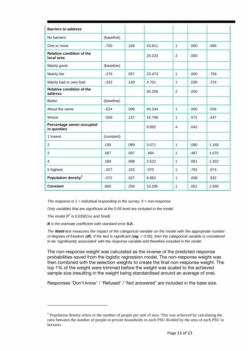
The variables found to be related to response, once controlled for the rest of the predictors in the model, were: region, type of dwelling, whether there were entry barriers to the selected address, the relative condition of the immediate local area, the relative condition of the address, the percentage of owner occupied properties in quintiles and population density. The model shows that response increases if there are no barriers to entry (for instance, if there are no locked gates around the address and no entry phone) and if the general condition of the address is better than other addresses in the area, rather than being about the same or worse. Response is also higher for flats than detached houses. Response increases if the relative condition of the immediate surrounding area is mainly good, and decreases as population density increases. Response is also generally higher for addresses in the North East of England. The full model is given in Table 2.

Table 2. The final non-response model

Variable B S.E. Wald Df Sig. Odds

Region 55.955 11 .000

Inner London (baseline)

North East .733 .191 14.683 1 .000 2.082

North West .173 .158 1.200 1 .273 1.189

Yorkshire and The Humber .043 .169 .064 1 .801 1.044

East Midlands .006 .177 .001 1 .972 1.006

West Midlands -.106 .168 .399 1 .528 .899

East of England -.052 .166 .100 1 .752 .949

Outer London -.222 .167 1.768 1 .184 .801

South East .149 .161 .864 1 .353 1.161

South West .328 .170 3.722 1 .054 1.388

Wales .095 .187 .258 1 .612 1.100

Scotland .012 .166 .005 1 .944 1.012

Type of dwelling 9.301 3 .026

Detached House (baseline)

Semi-detached house -.063 .075 .714 1 .398 .939

Terraced house (including end of terrace)

.058 .082 .496 1 .481 1.059

Flat or maisonette and other .248 .113 4.800 1 .028 1.281

1 This includes households not containing any adults aged 18 or over, vacant dwelling units, derelict dwelling units, non-resident addresses and other deadwood.

Page 12 of 23

Barriers to address

No barriers (baseline)

One or more -.700 .106 43.811 1 .000 .496

Relative condition of the local area 24.223 2 .000

Mainly good (baseline)

Mainly fair -.276 .057 23.473 1 .000 .759

Mainly bad or very bad -.323 .149 4.701 1 .030 .724

Relative condition of the address 40.256 2 .000

Better (baseline)

About the same -.624 .098 40.244 1 .000 .536

Worse -.559 .137 16.708 1 .572 .437

Percentage owner-occupied in quintiles 9.892 4 .042

1 lowest (constant)

2 .155 .089 3.071 1 .080 1.168

3 .067 .097 .484 1 .487 1.070

4 .184 .098 3.522 1 .061 1.202

5 highest -.027 .102 .070 1 .791 .974

Population density2 -.072 .027 6.962 1 .008 .932

Constant .660 .206 10.295 1 .001 1.935

The response is 1 = individual responding to the survey, 0 = non-response

Only variables that are significant at the 0.05 level are included in the model

The model R2 is 0.039(Cox and Snell)

B is the estimate coefficient with standard error S.E.

The Wald-test measures the impact of the categorical variable on the model with the appropriate number of degrees of freedom (df). If the test is significant (sig. < 0.05), then the categorical variable is considered to be ‘significantly associated’ with the response variable and therefore included in the model

The non-response weight was calculated as the inverse of the predicted response probabilities saved from the logistic regression model. The non-response weight was then combined with the selection weights to create the final non-response weight. The top 1% of the weight were trimmed before the weight was scaled to the achieved sample size (resulting in the weight being standardised around an average of one).

Responses ‘Don’t know’ / ‘Refused’ / ‘Not answered’ are included in the base size.

2 Population density refers to the number of people per unit of area. This was achieved by calculating the ratio between the number of people in private households in each PSU divided by the area of each PSU in hectares.

Page 13 of 23

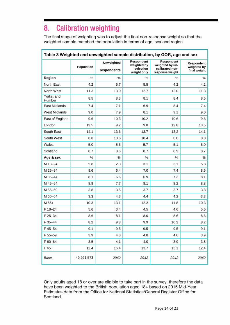
8. Calibration weightingThe final stage of weighting was to adjust the final non-response weight so that the weighted sample matched the population in terms of age, sex and region.

Table 3 Weighted and unweighted sample distribution, by GOR, age and sex

Population Unweighted Respondent

weighted by selection

weight only

Respondent weighted by un-calibrated non-

response weight

Respondent weighted by final weight respondents

Region % % % % %

North East 4.2 5.7 5.5 4.2 4.2

North West 11.3 13.0 12.7 12.0 11.3 Yorks. and Humber 8.5 8.3 8.1 8.4 8.5

East Midlands 7.4 7.1 6.9 8.4 7.4

West Midlands 9.0 7.9 8.1 9.1 9.0

East of England 9.6 10.3 10.2 10.6 9.6

London 13.5 9.2 9.8 12.8 13.5

South East 14.1 13.6 13,7 13,2 14.1

South West 8.8 10.6 10.4 8.8 8.8

Wales 5.0 5.6 5.7 5.1 5.0

Scotland 8.7 8.6 8.7 8.9 8.7

Age & sex % % % % %

M 18–24 5.8 2.3 3.1 3.1 5.8

M 25–34 8.6 6.4 7.0 7.4 8.6

M 35–44 8.1 6.6 6.9 7.3 8.1

M 45–54 8.8 7.7 8.1 8.2 8.8

M 55–59 3.8 3.5 3.7 3.7 3.8

M 60–64 3.3 4.3 4.4 4.2 3.3

M 65+ 10.3 13.1 12.2 11.8 10.3

F 18–24 5.6 3.4 4.5 4.6 5.6

F 25–34 8.6 8.1 8.0 8.6 8.6

F 35–44 8.2 9.8 9.9 10.2 8.2

F 45–54 9.1 9.5 9.5 9.5 9.1

F 55–59 3.9 4.8 4.8 4.6 3.9

F 60–64 3.5 4.1 4.0 3.9 3.5

F 65+ 12.4 16.4 13.7 13.1 12.4

Base 49,921,573 2942 2942 2942 2942

Only adults aged 18 or over are eligible to take part in the survey, therefore the data have been weighted to the British population aged 18+ based on 2015 Mid-Year Estimates data from the Office for National Statistics/General Register Office for Scotland.

Page 14 of 23

The survey data were weighted to the marginal age/sex and region distributions using calibration weighting. As a result, the weighted data should exactly match the population across these three dimensions. This is shown in Table 3.

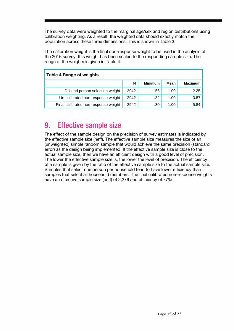
The calibration weight is the final non-response weight to be used in the analysis of the 2016 survey; this weight has been scaled to the responding sample size. The range of the weights is given in Table 4.

Table 4 Range of weights

N Minimum Mean Maximum

DU and person selection weight 2942 .56 1.00 2.25

Un-calibrated non-response weight 2942 .32 1.00 3.87

Final calibrated non-response weight 2942 .30 1.00 5.84

9. Effective sample sizeThe effect of the sample design on the precision of survey estimates is indicated by the effective sample size (neff). The effective sample size measures the size of an (unweighted) simple random sample that would achieve the same precision (standard error) as the design being implemented. If the effective sample size is close to the actual sample size, then we have an efficient design with a good level of precision. The lower the effective sample size is, the lower the level of precision. The efficiency of a sample is given by the ratio of the effective sample size to the actual sample size. Samples that select one person per household tend to have lower efficiency than samples that select all household members. The final calibrated non-response weights have an effective sample size (neff) of 2,276 and efficiency of 77%.

Page 15 of 23

7 Analysing the dataBritish Social Attitudes provides a compelling account of the public’s economic, political, moral and social attitudes over a 34 year period. It can be used to provide an annual snapshot of the public’s attitudes through an analysis of a single dataset or to create a narrative of the public’s attitudes over a period of time by analysing several datasets.

A number of questions have been repeated over a number of years. Unless the question wording has been changed, the original variable name is retained.

Please note that the data must be weighted in all analysis. The file is not pre-weighted. Before running any analysis, please weight the data using the NatCen computed weight which can be found in all datasets and is named Wtfactor.

Unlike some other surveys, on British Social Attitudes, responses of ‘Don’t know’ / ‘Refused’ or ‘Not answered’ are considered to be valid responses, and should be included in the base for analysis.

There are a number of identification variables that users may find useful in analyses. These are listed below. In addition there are a number of potentially useful derived variables that are outlined in the following section.

Table 5 Demographic variables

RSex Respondent’s sex

RAgeCat Respondent’s age group

RaceOri3 Respondent’s ethnicity

ReligSum Respondent’s religion

RClassGp Respondent’s occupational class

HEdQual Respondent’s highest educational qualification

HHType Household type

MarStat Respondent’s marital status

11. Derived variablesThe following derived variables are included in the datasets as standard.

Age The dataset contains 5 variables that split respondents into different age categories: [RAgeCat], [RAgeCat2], [RAgeCat3], [RAgeCat4] and [RAgeCat5].

Page 16 of 23

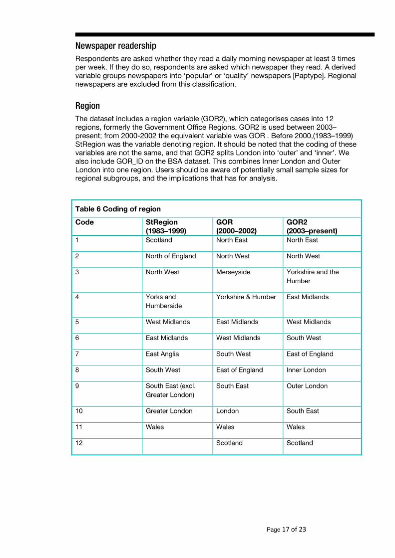
Newspaper readership Respondents are asked whether they read a daily morning newspaper at least 3 times per week. If they do so, respondents are asked which newspaper they read. A derived variable groups newspapers into ‘popular’ or ‘quality’ newspapers [Paptype]. Regional newspapers are excluded from this classification.

Region The dataset includes a region variable (GOR2), which categorises cases into 12 regions, formerly the Government Office Regions. GOR2 is used between 2003–present; from 2000-2002 the equivalent variable was GOR . Before 2000,(1983–1999) StRegion was the variable denoting region. It should be noted that the coding of these variables are not the same, and that GOR2 splits London into ‘outer’ and ‘inner’. We also include GOR_ID on the BSA dataset. This combines Inner London and Outer London into one region. Users should be aware of potentially small sample sizes for regional subgroups, and the implications that has for analysis.

Table 6 Coding of region

Code StRegion (1983–1999)

GOR (2000–2002)

GOR2 (2003–present)

1 Scotland North East North East

2 North of England North West North West

3 North West Merseyside Yorkshire and the Humber

4 Yorks and Humberside

Yorkshire & Humber East Midlands

5 West Midlands East Midlands West Midlands

6 East Midlands West Midlands South West

7 East Anglia South West East of England

8 South West East of England Inner London

9 South East (excl. Greater London)

South East Outer London

10 Greater London London South East

11 Wales Wales Wales

12 Scotland Scotland

Page 17 of 23

Standard Occupational Classification Respondents are classified according to their own occupation, not that of the ‘head of household’. Each respondent was asked about their current or last job, so that all respondents except those who had never worked were coded. Additionally, all job details were collected for all spouses and partners in work.

Since the 2011 survey we have coded occupation to the new Standard Occupational Classification 2010 (SOC 2010). The main socio-economic grouping based on SOC 2010 is the National Statistics Socio-Economic Classification (NS-SEC). However, to maintain time series, some analysis has continued to use the older schemes based on SOC 90 – Registrar General’s Social Class and Socio-Economic Group – though these are now derived from SOC 2000 (which is derived from SOC 2010).

National Statistics Socio-Economic Classification The combination of SOC 2010 and employment status for current or last job generates the following NS-SEC analytic classes. The name of this variable is [RClass]: RClass is correct as per the seven categories below.

• Employers in large organisations, higher managerial and professional• Lower professional and managerial; higher technical and supervisory• Intermediate occupations• Small employers and own account workers• Lower supervisory and technical occupations• Semi-routine occupations• Routine occupations

For some analyses, it may be more appropriate to classify respondents according to their current socio-economic status, which takes into account only their present economic position. Respondents not currently in paid work can be allocated to one of the following categories: “not classifiable”, “retired”, “looking after the home”, “unemployed” or “others not in paid occupations” using the data recorded at REconsum.

Registrar General’s Social Class As with NS-SEC, each respondent’s social class is based on his or her current or last occupation. The combination of SOC 90 with employment status for current or last job generates the following six social classes. The variable is called [RNSocCL]:

I Professional etc. occupations II Managerial and technical occupations ‘Non-manual’ III (Non-manual) Skilled occupations III (Manual) Skilled occupations IV Partly skilled occupations ‘Manual’ V Unskilled occupations

Socio-Economic Group As with NS-SEC, each respondent’s Socio-Economic Group (SEG) is based on his or her current or last occupation.

SEG aims to bring together people with jobs of similar social and economic status, and is derived from a combination of employment status and occupation. The full SEG

Page 18 of 23

classification identifies 18 categories, but these are usually condensed into six groups. The variable name is [RNSEGGrp]:

• Professionals, employers and managers• Intermediate non-manual workers• Junior non-manual workers

• Skilled manual workers• Semi-skilled manual workers• Unskilled manual workers

Note on analysing changing attitudes by social class over time When analysing how the attitudes of different social classes have changed over time, you need to construct a variable that gives a comparable measure of social class across the lifetime of the survey (during which class has been measured using a range of different variables). There is no perfect solution, but our strong preference is to use Goldthorpe-Heath (5 category version) class – RGHClass – before the 2000 SOC became a standard feature of the survey in 2000, and NS-SEC analytic class – RNSEG – thereafter. At the 5 class level these two schemes are conceptually based on moreor less the same principles. (You can only do this going back to 1987.)

For BSA 2001 and later years use: RNSEGD (derived as below) RECODE RNSEG (1, 2, 4, 5, 6, 7, 8 = 1) (9 = 2) (3, 15, 16, 17 = 3) (11, 12 = 4) (10, 13,14, 18 = 5) (else = sysmis) into RNSEGD. Execute. Variable labels RNSEGD "RNSEG compressed". Value labels RNSEGD 1 "Salariat (Higher & Lower)" 2 "Clerical (Junior non-manual)" 3 "Petty Bourgeois" 4 "Foremen/Technicians" 5 "Working class" 99 "Don't know".

For BSA 2000 and earlier years use: RGHClass (1983 Heath Goldthorpe scale) RECODE RGHClass (1 thru 2 = 1) (3 thru 4 = 2) (5 thru 7 = 3) (8 = 4) (9 thru 11 = 5) (else = sysmis) into RGHClassD. Execute. Variable labels RGHClassD "RGHClass compressed". Value labels RGHClassD 1 "Professional / managerial" 2 "Routine" 3 "Small petty bourgeoisie / farmers" 4 "Manual" 5 "Other manual" 99 "Don't know".

Industry All respondents whose occupation could be coded were allocated a Standard Industrial Classification 2007 (SIC 07). Two-digit class codes are used. As with social class, SIC may be generated on the basis of the respondent’s current occupation only, or on his or her most recently classifiable occupation. The variable is called [RSIC07Gp].

Page 19 of 23

Party identification Respondents can be classified as identifying with a particular political party on one of three counts: if they consider themselves supporters of that party, closer to it than to others, or more likely to support it in the event of a general election. The three groups are generally described respectively as partisans, sympathisers and residual identifiers. In combination, the three groups are referred to as ‘identifiers’. Responses are derived from the following questions: [SupParty] Generally speaking, do you think of yourself as a supporter of any one political party? [Yes/No]

[If “No”/“Don’t know”] [ClosePty] Do you think of yourself as a little closer to one political party than to the others? [Yes/No]

[If “Yes” at either question or “No”/“Don’t know” at 2nd question] [PartyFW]3 Which one?/If there were a general election tomorrow, which political party do you think you would be most likely to support?

[Conservative; Labour; Liberal Democrat; Scottish National Party; Plaid Cymru; Green Party; UK Independence Party (UKIP); British National Party (BNP)/National Front; Trade Union and Socialist Coalition (TUSC); RESPECT/Other socialist party; Other party; Other answer; None; Refused to say]

Note: [PartyFW] is called [PartyIDN] in the dataset. From this we derive the variables [PartyId1] (14 categories), [PartyId2] (7 categories) and [PartyId3] (8 categories).

Note: 2014 PartyId3 was added with additional code for UKIP.

Note: 1983–1987 the Green Party did not have its own code.

Note: 1983–1987 Liberal Party, Social Democratic Party, and Liberal Alliance are separate codes and often combined for analysis purposes.

Income The BSA dataset includes a standard measure of household income [HHIncome]. The bandings used are designed to be representative of those that exist in Britain and are taken from the Family Resources Survey (see http://research.dwp.gov.uk/asd/frs). Two derived variables give income deciles/quartiles: [HHIncD] and [HHIncQ]. Deciles and quartiles are calculated based on household incomes in Britain as a whole.

In 2016 BSA included some more detailed questions on respondent individual and household income. The dataset includes a derived variable using these data [eq_inc_quintiles] which is the net equivalised household income after housing costs in quintiles. More detailed income data can be made available to researchers on request.

3 Called [PartyIDN] on SPSS file.

Page 20 of 23

We did not include our standard question on earnings [REarn] in 2016, nor the derived variables associated with that ([RearnD] and [REarnQ].

Attitude scales Since 1986, the British Social Attitudes surveys have included two attitude scales which aim to measure where respondents stand on certain underlying value dimensions: left–right and libertarian–authoritarian. Since 1987 (except in 1990), a similar scale on ‘welfarism’ has also been included. Some of the items in the welfarism scale were changed in 2000–2001. The current version of the scale is shown below. A useful way of summarising the information from a number of questions of this sort is to construct an additive index (Spector, 1992; DeVellis, 2003). This approach rests on the assumption that there is an underlying – ‘latent’ –attitudinal dimension which characterises the answers to all the questions within each scale. If so, scores on the index are likely to be a more reliable indication of the underlying attitude than the answers to any one question.

Each of these scales consists of a number of statements to which the respondent is invited to “agree strongly”, “agree”, “neither agree nor disagree”, “disagree” or “disagree strongly”. The items are:

Left–right scale Government should redistribute income from the better off to those who are less well off. [Redistrb]

Big business benefits owners at the expense of workers. [BigBusnN]

Ordinary working people do not get their fair share of the nation’s wealth. [Wealth]

There is one law for the rich and one for the poor. [RichLaw]

Management will always try to get the better of employees if it gets the chance. [Indust4]

Libertarian–authoritarian scale Young people today don’t have enough respect for traditional British values. [TradVals]

People who break the law should be given stiffer sentences. [StifSent]

For some crimes, the death penalty is the most appropriate sentence. [DeathApp]

Schools should teach children to obey authority. [Obey]

The law should always be obeyed, even if a particular law is wrong. [WrongLaw]

Censorship of films and magazines is necessary to uphold moral standards. [Censor]

Welfarism scale

Page 21 of 23

The welfare state encourages people to stop helping each other. [WelfHelp]

The government should spend more money on welfare benefits for the poor, even if it leads to higher taxes. [MoreWelf]

Around here, most unemployed people could find a job if they really wanted one. [UnempJob]

Many people who get social security don’t really deserve any help. [SocHelp]

Most people on the dole are fiddling in one way or another. [DoleFidl]

If welfare benefits weren’t so generous, people would learn to stand on their own two feet. [WelfFeet]

Cutting welfare benefits would damage too many people’s lives. [DamLives]

The creation of the welfare state is one of Britain’s proudest achievements. [ProudWlf]

The indices for the three scales are formed by scoring the leftmost, most libertarian or most pro-welfare position, as 1 and the rightmost, most authoritarian or most anti-welfarist position, as 5. The “neither agree nor disagree” option is scored as 3. The scores to all the questions in each scale are added and then divided by the number of items in the scale, giving indices ranging from 1 (leftmost, most libertarian, most pro-welfare) to 5 (rightmost, most authoritarian, most anti-welfare).

The scores on the three indices have been placed on the dataset.

The scales were tested for reliability (as measured by Cronbach’s alpha) using the BSA 2015 data. The Cronbach’s alpha (unstandardised items) for the scales in 2015 were 0.83 for the left–right scale, 0.82 for the welfarism scale and 0.76 for the libertarian authoritarian scale. This level of reliability can be considered ‘good’ for the left–right and welfare scales and ‘respectable’ for the libertarian authoritarian scale. (DeVellis, 2003: 95–96)

Multi-code variables Where a respondent was given the opportunity to give more than one response at a question, we have created binary variables for each response option available. These binary variables record the number of respondents who chose that response option. If a respondent answered “don’t know” or refused to answer a multi-code question, the don’t know or refusal response has been included at each of the binary variables.

Page 22 of 23

Further informationFor further information on anything contained in this booklet please contact: bsa@natcen.ac.uk

Page 23 of 23