breakdown studies of helium and nitrogen in partial …
TRANSCRIPT

BREAKDOWN STUDIES OF HELIUM AND NITROGEN IN PARTIAL VACUUM
SUBJECT TO NON-UNIFORM, UNIPOLAR FIELDS IN THE 20-220 KHZ RANGE
Except where reference is made to the work of others, the work described in this dissertation is my own or was done in collaboration with my advisory committee. This
dissertation does not include proprietary or classified information.
____________________________ Kalyan Koppisetty
Certificate of Approval:
_________________________________ _____________________________________ Charles A. Gross Hulya Kirkici, Chair Professor Associate Professor Electrical and Computer Engineering Electrical and Computer Engineering _______________________________ __________________________________ Thaddeus A. Roppel George T. Flowers Associate Professor Interim Dean Electrical and Computer Engineering Graduate School
BREAKDOWN STUDIES OF HELIUM AND NITROGEN IN PARTIAL VACUUM
SUBJECT TO NON-UNIFORM, UNIPOLAR FIELDS IN THE 20-220 KHZ RANGE
Kalyan Koppisetty
A Dissertation
Submitted to
the Graduate Faculty of
Auburn University
in Partial Fulfillment of the
Requirements for the
Degree of
Doctor of Philosophy
Auburn, Alabama
August 09, 2008
iii
BREAKDOWN STUDIES OF HELIUM AND NITROGEN IN PARTIAL VACUUM
SUBJECT TO NON-UNIFORM, UNIPOLAR FIELDS IN THE 20-220 KHZ RANGE
Kalyan Koppisetty
Permission is granted to Auburn University to make copies of this dissertation at its discretion, upon the request of individuals or institutions and at
their expense. The author reserves all publication rights.
____________________________
Signature of Author
____________________________
Date of Graduation
iv
VITA
Kalyan Koppisetty, son of Ganeswara Rao and Rajani Kumari Koppisetti, was
born on August 24, 1978 in Hyderabad, Andhra Pradesh, India. He joined Indian
Institute of Technology (I.I.T.), Madras (also called Chennai), India, in 1996 for his
Bachelors in Technology and worked as a Computer Programmer / Systems
Administrator in CoralGrid and Photon InfoTech Pvt. Ltd, Chennai, while in school. He
then worked for Cybernet Software Systems, Inc., India, before entering the Graduate
School at Auburn University in August 2001. After receiving his M.S. in Electrical and
Computer Engineering from Auburn University, he has been working on high frequency
gaseous breakdown under non-uniform fields in partial vacuum conditions.
v
DISSERTATION ABSTRACT
BREAKDOWN STUDIES OF HELIUM AND NITROGEN IN PARTIAL VACUUM
SUBJECT TO NON-UNIFORM, UNIPOLAR FIELDS IN THE 20-220 KHZ RANGE
Kalyan Koppisetty
Doctor of Philosophy, 9 August 2008 (M.S. Auburn University, Auburn, AL, Aug, 2004)
139 Typed Pages
Directed by Hulya Kirkici
Partial discharges and corona are considered as unwanted processes in electrical
power systems since they are constant source of power loss and electrical noise (EMI).
These effects can further develop into a major problem at the component level, causing
solid insulation deterioration and component failure leading to possible bulk electrical
breakdown.
The problems are well documented for traditional ground-based (i.e. utility)
electrical power systems, and there exists a considerable knowledge base on the subject.
However, this knowledge base does not readily extend to on-board electrical power
systems in aerospace vehicles because such systems are required to operate at very low
atmospheric pressure (i.e. in partial vacuum) and frequencies in the tens of kHz range.

vi
Also, much of what is known for aerospace systems is limited to standard 28 V dc
systems, whereas the next generation of aerospace systems is expected to operate at
higher voltages. Thus, there is an incentive to conduct basic research into corona,
partial discharge and gaseous breakdown in gases at partial vacuum conditions,
voltages, and frequencies, and for geometries corresponding to the environment
encountered in current and future aerospace power systems.
This work presents studies on the breakdown characteristics of helium, nitrogen
and zero air under unipolar sinusoidal and pulsed voltages at frequencies varying from
20 kHz to 220 kHz in partial vacuum, for a point-to-point and point-to-plane electrode
configurations. These voltages are compared to the dc data obtained under similar
conditions. Also, breakdown voltage versus pressure curves similar to Pashcen plots
are presented. Breakdown voltages of these gases as a function of signal frequency are
also presented.

vii
ACKNOWLEDGEMENTS
I would like to thank my advisor, Dr. Hulya Kirkici for her patience and
guidance during the course of this project. This work would have been impossible with
out her support and encouragement. I would like to thank Dr. Schweickart from
AFRL/WPAFB, Ohio for fundingξ this project and also helping me over the years with
technical discussions. I would like to thank Dr. Gross and Dr. Roppel for serving as the
committee members and Dr. Bozack from Physics Department for promptly reviewing
my dissertation as the outside reader. The Electrical and Computer Engineering
Department staff has made my work lot easier with their prompt support in many
regards. I really appreciate the help and effort by Linda Barresi and Joe Haggerty with
all the workshop tasks and my late Friday afternoon sessions. Thanks are also due to all
the members of our group for helping me around the lab and making the place fun to
work: Shaomao Li, Mark Lipham, Chrsitopher Leach and Haitao Zhao. I would also
like to thank my previous lab mates for making this journey even more memorable:
Aditya Goel, Chris Seymore, Mert Serkan and Esin Sozer. Though they may never
understand what I was up to in the lab, support from my parents has been enormous in
this undertaking, I am truly grateful for that. Last and most importantly, I should give
credit to my wife Keerthi for her support and tolerance especially over those long days.
ξ Work supported in part by Universal Technology Corp., under contract to the Air Force Research Laboratory, Propulsion Directorate, contract number F33615-02-D-2299/DO-0024
viii
Style manual or journal used Graduate School: Guide to preparation and
submission of theses and dissertations
Computer software used Microsoft Office 2003

ix
TABLE OF CONTENTS
LIST OF TABLES.......................................................................................................... XI
LIST OF FIGURES ....................................................................................................... XII
RESEARCH OBJECTIVE ...............................................................................................1
CHAPTER I. INTRODUCTION & BACKGROUND ....................................................3
1.1 Power requirements in space ............................................................................3
1.2 Need for High Voltage in Space and the Role of High Frequency ..................4
1.3 Spacecraft Environment Effects and Design Considerations ...........................5
1.4 High Frequency ................................................................................................7
1.5 Work in Literature ............................................................................................8
1.6 Gaseous breakdown below RF .......................................................................10
1.7 Breakdown at RF and UHF ............................................................................13
1.8 Solid and Liquid insulation breakdown..........................................................15
1.9 Need for further investigation.........................................................................18
CHAPTER II. HIGH VOLTAGE BREAKDOWN IN PARTIAL VACUUM..............21
2.1 Air as Insulator ...............................................................................................21
2.2 Corona and Townsend Discharges .................................................................22
2.3 Development of a Gas Discharge ...................................................................23
2.4 Townsend breakdown criterion ......................................................................27
2.5 Low pressure DC glow discharge...................................................................29
2.6 Current-Voltage Characteristics of normal glow discharge ...........................30
2.7 Regions of the normal glow discharge ...........................................................32
2.8 Non-Uniform Electrode configuration ...........................................................35
2.9 Paschen’s Law ................................................................................................35
2.10 Deviations from Paschen’s Law .....................................................................38
CHAPTER III. HIGH FREQUENCY BREAKDOWN.................................................40
3.1 Background.....................................................................................................40

x
3.2 Role of Alternating Field ................................................................................42
3.3 Role of Gas Density........................................................................................44
3.4 Effect of Frequency on Breakdown Phenomenon ..........................................48
3.5 Pulsed/Unipolar Electric Fields ......................................................................51
CHAPTER IV. OPTICAL EMISSION SPECTRA OF DISCHARGES .......................53
4.1 Atomic Spectra ...............................................................................................53
4.2 Molecular Spectra ...........................................................................................60
CHAPTER V. EXPERIMENTAL SETUP AND PROCEDURE..................................63
5.1 Experimental Setup.........................................................................................63
5.2 Experimental Procedure..................................................................................66
CHAPTER VI. RESULTS AND DISCUSSION ...........................................................68
6.1 DC Breakdown Experiments ..........................................................................68
6.1.1 Point-to-point Configuration .............................................................69
6.1.2 Point-to-plane Configuration .............................................................71
6.2 Unipolar 20 kHz Sinusoid Breakdown Experiments......................................73
6.2.1 Point-to-point Configuration .............................................................74
6.2.2 Point-to-plane Configuration .............................................................76
6.3 Unipolar Pulsed Breakdown Experiments......................................................79
6.3.1 Breakdown Voltage versus Gas Pressure ..........................................81
6.3.2 Breakdown Voltage – Signal Frequency ...........................................83
6.4 Effect of Duty Cycle on Breakdown Voltage.................................................90
6.5 Optical Spectroscopy ......................................................................................94
CHAPTER VII. IMAGE ANALYSIS TOOL FOR OPTICAL EMISSION CHARACTERIZATION OF PARTIAL VACUUM BREAKDOWN........................103
7.1 Introduction...................................................................................................103
7.2 Experimental Setup.......................................................................................105
7.3 Image Analysis .............................................................................................106
7.4 Results...........................................................................................................110
7.5 Conclusions...................................................................................................114
CONCLUSIONS AND FUTURE WORK...................................................................116
BIBLIOGRAPHY.........................................................................................................118

xi
LIST OF TABLES
Table 1. Table summarizing the work in the literature presented in this report. ........12 Table 2. Breakdown Voltages at the Critical Pressure-Spacing Dimension for
Pure Gases at dc and 400 Hz.................................................................................37
Table 3. Emission wavelengths of a Helium discharge [42], typically seen in
the visible spectrum and the corresponding intensity values and the calculated energies........................................................................................58
Table 4. Duty cycle and the corresponding THigh / TLow at various frequencies. ........91 Table 5. The dominant wavelengths in the nitrogen spectrum and the
corresponding electron transitions. .............................................................101 Table 6. The dominant wavelengths in the helium spectrum and the
corresponding electron transitions. .............................................................102

xii
LIST OF FIGURES
Figure 1. Breakdown at high frequency voltage in air for point-plane electrodes - inhomogeneous field at 50 Hz and 75 kHz for both the polarities [2] .........11
Figure 2. Breakdown at high frequency voltage in air for homogenous field of plane-plane configuration at various frequencies [2] ...................................11
Figure 3. Variation of RF breakdown voltage with pressure illustrating the pressure transition region from gas discharge to multipactor [2] .................15
Figure 4. Corona inception and extinction voltages for polypropylene using needle-plane electrodes in air. ......................................................................16
Figure 5. Dielectric constant and dissipation factor of polypropylene under low voltage stress.................................................................................................16
Figure 6. Frequency dependence of the real (ε'r) and imaginary (ε''r) parts of the dielectric constant in various polarization mechanisms. ..............................17
Figure 7. Widely used electrode geometries for breakdown/corona testing. ...............23
Figure 8. Regions of dark discharge regime [27].........................................................25
Figure 9. I-V characteristics of a glow discharge for flat copper electrodes (10 cm2), .............................................................................................................26
Figure 10. Voltage and current density as a function of the total current drawn by dc discharge ..................................................................................................30
Figure 11. Variation of various parameters observed in a typical glow discharge. .......31
Figure 12. Paschen curves for helium and nitrogen for dc fields, reproduced from literature data [29, 30]...................................................................................36
Figure 13. Breakdown voltage of several gases as a function of pd at room temperature [9]..............................................................................................38
Figure 14. Variation of RF breakdown voltage with pressure illustrating the pressure transition region from gas discharge to multipactor [12]. ..............41
Figure 15. Motion of an electron in high frequency field (a) at very low pressure (collision frequency << signal frequency) and (b) at medium and high pressures (collision frequency > signal frequency) [33]...............................45

xiii
Figure 16. Multipactor effect in hydrogen at 10-4 torr (Ag-Cu electrodes, gap = 3cm) [33] ......................................................................................................46
Figure 17. Variation of relative breakdown voltage with applied field frequency for a uniform 1 cm electrode gap at atmospheric conditions. [28].....................49
Figure 18. Typical applied voltage waveforms at 50 kHz for different duty cycles. The ‘On’ and ‘Off’ times vary from 2 µs to 18 µs at this frequency............52
Figure 19. Energy level diagram of a hypothetical doubly ionized atom with Z = 3. ...56
Figure 20. Typical spectrum recorded using a chart recorder for a Cu-He calibration lamp [39].......................................................................................................57
Figure 21. Atomic energy levels for neutral Helium [40].............................................59
Figure 22. Absolute intensities of various lines of the Helium spectrum over a pressure range (2 to 40 Torr) [41].................................................................60
Figure 23. Potential energy plot as a function of the internuclear distance for a simple diatomic molecule [39]. ....................................................................61
Figure 24. (a) Incident electromagnetic wave exerting torque on an electric dipole and (b) portion of the potential diagram for a stable electronic state of a diatomic molecule [39]. ................................................................................62
Figure 25. Vacuum Chamber .........................................................................................64
Figure 26. Electrode geometries used in current studies................................................64
Figure 27. Power supply schematics (a) Unipolar sinusoid, (b) Unipolar square pulse..............................................................................................................66
Figure 28. Schematic of the experimental setup with the diagnostics (point-to-plane electrode under unipolar sinusoidal applied voltage. ...................................66
Figure 29. Electrode geometries: (a) point-to-point electrode (b) point-to-point electrode and (c) point-to-plane electrode (Plane electrode always grounded) (All point electrodes have a tip radius = 0.5 mm).......................68
Figure 30. Voltage (top), current (middle) and optical emission (bottom) waveforms of a breakdown event point-to-plane electrode geometry for dc applied voltage. ........................................................................................69
Figure 31. Breakdown voltage of nitrogen under dc fields for point-to-point electrode configuration. ................................................................................70
Figure 32. Breakdown voltage of helium under dc fields for point-to-point electrode configuration.................................................................................................70
Figure 33. The dc breakdown voltage plots for helium and nitrogen for point-to-point configuration........................................................................................71
Figure 34. Paschen curves for helium and nitrogen - reproduced from literature data [29, 30]..........................................................................................................71

xiv
Figure 35. The dc breakdown voltage plots for nitrogen for point-to-plane configuration, d = 0.5 cm..............................................................................72
Figure 36. The dc breakdown voltage plots for zero air for point-to-plane configuration, d = 0.5 cm..............................................................................72
Figure 37. The dc breakdown voltage plots for helium for point-to-plane configuration, d = 1.0 cm..............................................................................72
Figure 38. Sample frames captured during the breakdown event for dc fields in helium at 1.6 Torr. Captured at 30 fps, each consecutive frame is about 33 ms apart....................................................................................................73
Figure 39. Electrode geometries: (a) point-to-point electrode (b) point-to-point electrode and (c) point-to-plane electrode (Plane electrode always grounded) (All point electrodes have a tip radius = 0.5 mm).......................73
Figure 40. Representative breakdown voltage waveform for point-to-point configuration in helium at 1.4 Torr for 20 kHz unipolar applied field.........74
Figure 41. Optical image of the glow discharge during a breakdown event at 20 kHz at 1.4 Torr, point-to-point electrode. (Anode on top, images captured at 30 fps). .......................................................................................74
Figure 42. Breakdown voltage versus pressure for point-to-point electrode configuration with 1-cm gap distance in helium for 20 kHz unipolar applied voltage..............................................................................................75
Figure 43. Optical emission duration during a breakdown event as a function of pressure for unipolar 20 kHz helium ac breakdown experiments (point-to-point electrode).........................................................................................75
Figure 44. Voltage (top), current (middle) and optical emission (bottom) waveforms of a breakdown event at 1.8 Torr helium for point-to-plane electrode geometry at unipolar 20 kHz applied voltage. ..............................76
Figure 45. Breakdown voltage versus pressure for point-to-plane electrode configuration with 1-cm gap distance in Helium for unipolar 20 kHz sinusoid applied voltages. .............................................................................76
Figure 46. Optical images of the glow discharge during a breakdown event at unipolar 20 kHz sinusoid at 1.6 Torr, point-to-plane electrode. (Images captured at 30 fps). .......................................................................................77
Figure 47. Transient current peak as a function of pressure for point-to-plane electrode geometry at 20 kHz .......................................................................78
Figure 48. A typical applied voltage pulse at 20 kHz 0.2 Torr nitrogen showing the pulse shape just at the breakdown. The bottom plot shows the light emission recorded by the PMT. ....................................................................78

xv
Figure 49. Breakdown voltage as a function of pressure for point-to-plane electrode configuration with 0.5-cm gap distance for 20 kHz unipolar sinusoid signal for nitrogen.........................................................................................78
Figure 50. Breakdown voltage as a function of pressure for point-to-plane electrode configuration with 0.5-cm gap distance for 20 kHz unipolar sinusoid signal for zero air. .........................................................................................79
Figure 51. Electrode geometries: (a) point-to-point electrode and (b) point-to-plane electrode (Plane electrode always grounded) (All point electrodes have a tip radius = 0.5 mm)......................................................................................80
Figure 52. Typical Breakdown voltage (middle), current from the Pearson coil (top) and the light emission waveforms (bottom) at 0.4 Torr for a 100 kHz applied field in nitrogen. The first arrow indicates the breakdown initiation and the second indicates the formation of fully developed breakdown.....................................................................................................81
Figure 53. Breakdown voltage as a function of pressure at dc, 50 kHz and 150 kHz signals for helium, point-to-point configuration...........................................82
Figure 54. Breakdown voltages as a function of pressure at dc, 50 kHz, 100 kHz, 150 kHz, and 200 kHz in nitrogen, point-to-point configuration. The doted line (top) is dc data and the dashed line (bottom) is the average of the high frequency breakdown data. .............................................................83
Figure 55. Breakdown voltage as a function of pressure at 50 kHz, 100 kHz, 150 kHz and 200 kHz signals for helium, point-to-plane configuration. ............83
Figure 56. Breakdown voltage as a function of pressure at dc, 50 kHz and 150 kHz signals for nitrogen, point-to-plane configuration. .......................................83
Figure 57. Breakdown voltage as a function of the applied signal frequency for helium at 1.2 Torr and 2.0 Torr, point-to-point configuration. The voltage variation seems to be a double-exponential function of the signal frequency. A possible curve fit of the form
)0003.0exp(254)0454.0exp(219)( fffV ∗−∗+∗−∗= is shown (V(f) in Volts and f in kHz)........................................................................................84
Figure 58. Nitrogen breakdown voltage as a function of frequency at 0.4, 1.2 and 2.4 Torr pressures, point-to-point configuration. (V is in Volts and f in kHz). .............................................................................................................85
Figure 59. Breakdown voltage as a function of signal frequency for unipolar pulsed square wave, for nitrogen for point-to-plane configuration. V(0.4) and V(1.2) correspond to the breakdown voltage at gas pressures of 0.4 and 1.2 Torr respectively. ....................................................................................85
Figure 60. Breakdown voltage as a function of signal frequency for unipolar pulsed square wave, for zero air for point-to-plane configuration. V(0.4) and

xvi
V(1.2) correspond to the breakdown voltage at gas pressures of 0.4 and 1.2 Torr respectively. ....................................................................................85
Figure 61. Breakdown voltage as a function of pressure for point-to-plane electrode configuration with 0.5-cm gap distance for 20 kHz unipolar pulsed square signal in nitrogen. ..............................................................................88
Figure 62. Breakdown voltage as a function of pressure for point-to-plane electrode configuration with 0.5-cm gap distance for 20 kHz unipolar pulsed square signal in zero air. ...............................................................................89
Figure 63. Voltage waveform acquired at the breakdown for 1 Torr and 50 kHz frequency with 20 % duty cycle. Arrow indicates the breakdown initiation time................................................................................................92
Figure 64. Typical voltage waveforms at 50 kHz and different (10, 30, 50, 70, and 90%) duty cycles...........................................................................................93
Figure 65. Breakdown voltage versus duty cycle at 1.2 Torr (a) 100 kHz and (b) 150 kHz for helium under point-to-point configuration ...............................93
Figure 66. Nitrogen spectrum at 1.2 Torr for 100 kHz unipolar pulsed field and 10 ms integration time. (Point-to-point electrode configuration) ......................96
Figure 67. Helium spectrum at 1.2 Torr for 100 kHz unipolar pulsed field and 10 ms integration time. (Point-to-point electrode configuration) ......................97
Figure 68. Variation of intensity with time for the two most dominant wavelengths in Figure 66, corresponding to the (0, 0) and (0, 1) lines in the first negative system of nitrogen. .........................................................................97
Figure 69. Variation of intensity with time for the two most dominant wavelengths in helium discharge in Figure 67. .................................................................99
Figure 70. Spectrum of the dc nitrogen discharge for point-to-plane setup at 0.8 Torr. ..............................................................................................................99
Figure 71. The potential energy diagrams for nitrogen first negative and second positive systems ..........................................................................................100
Figure 72. Comparison of discharge spectra of nitrogen and zero air at 0.4 Torr and 20 kHz pulsed applied field. (The intensities are shifted to better display the peaks) ....................................................................................................100
Figure 73. Spectrum of 100 kHz unipolar pulsed helium discharge for point-to-point setup at 1.2 Torr.................................................................................101
Figure 74. The energy diagram for helium systems.....................................................102
Figure 75. The breakdown voltage as a function of pressure of Helium for point-to-point geometry under 20 kHz ac applied voltage [51] ...............................107

xvii
Figure 76. Selected frames of the frame-by-frame images of a typical unipolar breakdown event for Helium at 20 kHz applied voltage. (Bottom electrode is cathode and top is anode) ........................................................107
Figure 77. A generic spectral response of a CCD array...............................................107
Figure 78. (a) Applied voltage signal, VAnode-Cathode (Cathode is always ground) (b) Typical image of the breakdown process showing the anode and the cathode boundaries (drawn) (c) The five regions selected for image analysis. ......................................................................................................108
Figure 79. (a) The ‘R’ value variation with time for the five regions used in image analysis. (b) Variation of R/G/B values at ‘Cathode2’ region as a function of time (Helium at 20 kHz and 1.4 Torr) .....................................110
Figure 80. Optical emission duration of the afterglow plasma after breakdown is initiated as a function of pressure [51]. ......................................................110
Figure 81. R/G/B values at different locations at t = 0.4 s (left) and t = 1s (right) respectively at gas pressure of 0.350 Torr. The center of the electrode gap is located at 0 cm, anode tip is located at 0.5 cm, and the cathode tip at negative 0.5 cm. ......................................................................................111
Figure 82. R/G/B values at different locations at t = 0.4 s (left) and t = 1s (right) respectively at gas pressure of 1.4 Torr. The center of the electrode gap is located at 0 cm, anode tip is located at 0.5 cm, and the cathode tip at negative 0.5 cm. ..........................................................................................112
Figure 83. Variation of R/G/B with pressure at the ‘Anode’ and the ‘Cathode’ regions shown in Figure 75 at t = 0.4s after breakdown initiation. ............113
Figure 84. Variation of R/G/B with pressure at the ‘Anode’ and the ‘Cathode’ regions shown in Figure 75 at t = 1.0 s after breakdown initiation. ...........113

1
RESEARCH OBJECTIVE
The most common high voltage signals observed in the high frequency range (in
kHz range) in power systems are due to the switching circuits in commercial
applications like inverters and dc-dc converters. Most of these waveforms are either
half/full wave rectified or square pulse trains. In case of a half-wave rectifier circuit,
depending on the amplitude and the frequency of the signal, the filtered output can have
rise times as high as 2 ms for 50 Hz signal and as low as less than 0.4 µs for a 250 kHz
sinusoidal signal. Similarly, a typical square pulse at 50 Hz and 50 % duty cycle has a
‘flat top’ (constant field) for 10 ms, which is fairly long for most of the physical
processes involving electrons. But for a 250 kHz signal, the same 50% duty cycle
would have a ‘flat top’ duration of 2 µs, which is comparable to the duration of the
electron motion in a gas (depending on the gas pressure). The duration for which the
voltage signal stays ‘high’ can be even smaller (fraction of a µs) if the particular
application uses duty cycles less than 50%. Hence, the study of the effect of pulsed
signals with various frequencies and duty cycles on the gaseous breakdown can be of
importance to power systems operating at partial vacuum conditions.
The primary objective of this work is to study the electrical breakdown
characteristics of gases commonly encountered in high altitude applications (Helium,
Nitrogen, and Air) under non-uniform electrode geometries (point-to-point and point-to-

2
plane) and high frequency applied fields (20 kHz to 220 kHz) over a sub-atmospheric
pressure range of 0.1 to 10.0 Torr. The optical emission characteristics of the
breakdown/discharge phenomenon are studied by observing the simple light emission
by a Photo Multiplier Tube (PMT) and a 30 fps video camera; the spectroscopic data
are also collected and analyzed.
This work can broadly be summarized as a study under the following conditions:
Frequency Range 20 kHz to 220 kHz
Electrode Geometry Point-point and Point-plane
Voltage Waveform DC, Unipolar sinusoid at 20 kHz and
unipolar pulsed square wave
Gaseous Medium Helium, Nitrogen (Scientific Grade),
Zero Air (N2, 20-22% of O2, and < 3 ppm H2O)
Diagnostics:
Electrical Voltage and current at the breakdown initiation
Optical Light emission (visible), Spectroscopic data (190
to 640 nm)

3
CHAPTER I
INTRODUCTION & BACKGROUND
1.1 POWER REQUIREMENTS IN SPACE
Knowledge of electrical insulation and partial or corona discharge behavior is
essential if reliable high voltage systems are to be designed for any electrical
applications. Historically, most of the power systems on space vehicles have been
operating at the nominal 28 V dc. This voltage level was inherited from the aircraft
industry. For spacecraft design considerations, these low voltages produce negligible
plasma interactions in Low Earth Orbit (LEO). Over the past few decades, the interest
in the use of high voltage-high frequency in compact economical packages in the
electrical power systems has grown significantly due to the current technological
advances. In particular, the demand for such a technology is extremely high in the
aerospace industry due to economic reasons. Very dense and light weight packaging is
used in the modern spacecraft electronics industry to make the equipment fit within a
restricted volume and economize fuel. This demand can also be seen in other aspects of
defense and communication technologies in addition to space exploration. Power
requirements for some of these missions range from 100 kW to 1 MW.

4
1.2 NEED FOR HIGH VOLTAGE IN SPACE AND THE ROLE OF HIGH FREQUENCY
The higher power requirement can be met by either higher voltage or higher
current power supply systems. Due to the operation hazards and heating losses of high
current systems, higher voltage sources are conventionally preferred over systems with
higher current sources. In space applications, high voltage means voltages just a few
hundreds of volts of distribution or bus power level. The distributed nature of the
power bus makes it difficult to shield from the detrimental effects of the space
environment for a system operating in this environment. A large solar array is an
example of one such component. Apart from the spacecraft applications, there are
numerous specialized systems such as accelerators, electron microscopes and vacuum
switch gear which employ vacuum insulation (or low pressure environment) in
terrestrial applications.
Some sub-systems of spacecraft may use high frequency (in the tens of kHz)
voltages, for switched mode power conversion. Apart from these, commercial dc-dc
voltage converters typically operate with intermediate frequencies in the range of 20
kHz to 100 kHz. The MHz range is already used in waveguides and particle accelerator
systems and is expected to be in use in more common equipment in the near future.
Considering the general trend for miniaturization, it should be understood that
equipment will be facing higher stresses not only because of the applied voltages but
also because of the higher operating frequencies. Partial discharges and corona are
detrimental to any power system as they are constant sources of power loss and
electrical noise (EMI). Furthermore, they can be a major problem at the component
level, causing solid insulation deterioration and eventual breakdown. Consequently,

5
high electrical field stresses, which enhance partial discharge activity, are often present
around these power systems. Such phenomena within power system components are
considered unacceptable where long lifetime and equipment reliability are of foremost
concern [1, 2]. In general, power systems operating in vacuum or space environment
are more susceptible to partial discharges, corona, or volume discharges due to the
partial vacuum conditions.
The corona or partial discharge initiation voltage in general, is a function of
several design and environmental parameters. The most important factors to be noted
are the operation pressure, the electrode gap/geometry, and the frequency and voltage
level of the applied signal within a power system [2]. Studies reveal that high
frequency operation of a power system could be a contributing factor in lowering the
breakdown voltage of insulation [3]. The availability of these power systems operating
at partial vacuum conditions makes it important to consider the effects of the operating
frequencies (in addition to the voltage signal characteristics in general) on corona,
partial discharge and gaseous breakdown in space applications.
Currently, there are several initiatives within the government agencies (such as
NASA and Air Force), planning to use 270-volt distribution power (the International
Space Station already utilizes 120 V dc sub-systems) [4]. Some sub-systems also use
high frequency (in the tens of kHz) voltages, for switched mode power conversion.
1.3 SPACECRAFT ENVIRONMENT EFFECTS AND DESIGN CONSIDERATIONS
The space environment is not pure vacuum, but a low-pressure, weakly ionized
gas, due to cosmic radiation, and randomly occurring solar activities. Electrical and

6
electronic equipment used in space applications are exposed to a wide range of pressure
and temperature changes during the normal course of operation. There have been
numerous instances of spacecraft anomalies which have been attributed to
breakdown/discharge phenomenon associated with environmental effects [5]. The
ability to design a spacecraft to survive in the local environment is the key to long life
and cost effective performance. The spacecraft as a whole uses materials which range
from gases to solids, including plastics and metallic materials. Local pressure is the
most important of all the environmental factors which can influence the electrical
behavior of a spacecraft, and is highly influenced by the spacecraft and the materials
used in its construction. As an example, at altitudes over 150 kilometers, the pressure is
3x10⁻⁶ to 4 x10⁻⁶ Torr, which is of the order used in a controlled terrestrial vacuum
insulation system. But, the presence of the spacecraft itself modifies the local pressure
in a largely unpredictable way, sometimes by a few orders of magnitude. Extensive
studies have been conducted on the gases and particulates near space shuttles over the
years. Data from various early STS (Space Transportation System – The official name
for the US space shuttle program) flights are presented and interpreted in work by
Green, et.al, [6] with regard to the gaseous envelope surrounding the shuttle, the particle
population in the orbit, and the optical interference from the local sources. The neutral
species measured in the spacecraft bay area were: H2O, He, NO, Ar, Freon, O2, CO2,
N2/CO and other heavy molecules identifiable with cleaning agents. The principle
contaminants however were water and Helium.
There are several circumstances for which an electrical breakdown can occur in
a high altitude vehicle. The vehicle’s wiring harness contains numerous cables with

7
varied configurations. Breakdown can occur in these wiring bundles and their
connectors due to differential pressure as a result of outgassing. Exposed cable traces
connecting the power supply to the body of the satellite are also subjected to breakdown
between conductors at different potentials and between the conductor bundles and space
plasma [7].
From studies by Katz [8] and others, it is evident that at orbital altitudes of about
200 – 500 km, there is a higher possibility of discharge/breakdown between exposed
conductors at voltages below 300 V. This is consistent with the results of Hastings et
al. [9] both from space and laboratory experiments. At altitudes over 20,000 km (MEO
– Medium Earth Orbit) however, the data suggest that the threshold for breakdown is
usually several kilovolts. The data from earlier studies and from our laboratory work
[3] clearly suggest that an effective limit for the maximum dc voltage between bare
conductors is less than 1000 volts for most of the equipment in aerospace and high
altitude applications. For larger structures such as the ISS (International Space Station),
the capacitance of the structure can result in substantial energy storage. Studies
conducted on the arcing rate for high voltage solar arrays show that the arcing begins at
a threshold of just 200 volts for orbits typical of Space Station Freedom [10].
1.4 HIGH FREQUENCY
Most terrestrial high voltage equipment is usually exposed to frequencies
generally at 50/60 Hz. Therefore, most of the literature data available for a long time
has been focused essentially on voltages at this frequency at atmospheric conditions. At
present, high frequency working voltages with frequencies over 100 Hz are being used

8
in low voltage equipment also, like the 400 Hz solid state power supply in most
domestic airplanes. Some sub-systems may also use high frequency (in the 10s of kHz)
voltages, for switched mode power conversion.
The availability of these power systems operating at partial vacuum conditions
in case of aerospace applications makes it important to consider the effects of the
operating frequencies on corona, partial discharge and gaseous breakdown in high
altitude and space applications [11].
1.5 WORK IN LITERATURE
During the first reported spacecraft high frequency electronic failure [11, 12], it
was assumed that the breakdown phenomenon that occurred at pressures between 1 Torr
and vacuum were due to high frequency effects. This led to the studies on voltage
breakdown dependence on high frequency and partial vacuum. By understanding the
failure mechanisms of these dielectrics, especially under long-term exposure to high
electric fields and high frequency, we can develop techniques to reliably predict the
behavior of materials.
It is well known that the breakdown in the electrode gaps usually occurs in the
sub-microsecond time scale. With respect to this time scale an ac voltage of power
frequency effectively has constant amplitude. For a 60 Hz sine wave, the amplitude
remains within 99% of its peak value for around 1 ms. Therefore in effect, during the
whole breakdown development, the peak value of voltage is effective, which normally
results in identical dc and ac (peak) breakdown voltages [13]. However, if the
frequency is increased, the effective field peak duration is shortened and the ions will

9
have insufficient time to cross the electrode gap, then, because of the charge
accumulation and field distortion between the cycles, the breakdown voltage can drop
below the dc breakdown level. At much higher frequencies a reduction of voltage from
its peak value and even polarity reversal need to be considered during breakdown.
In sinusoidal electric fields, the positive and negative ions generated at the
voltage maximum, normally have enough time to travel to the electrodes during the
remaining part of that sine half-wave. However, if the gaps are large or if the applied
frequency is high enough, it may so happen that the polarity is reversed before the ions
are extracted from the gap. This will result in a distortion of the electrostatic field and
will reduce the breakdown voltage. In the time interval between the peak and the zero
crossing of the sine wave, which is about 5 ms at a 50/60 Hz signal, those ions can
travel up to 300 cm [13] under atmospheric conditions. Therefore, at power frequencies
this problem will only be relevant in very large gaps, which is well established in high
voltage engineering. However, if the frequency is increased to kHz range, this
phenomenon will also be prominent for small gaps. The actual reduction in the electric
field depends on the electrostatic field distribution within a gap. In homogenous field
gaps the reduction is rather low. Studies conducted by A. W. Bright [14] in nitrogen
revealed that for small gaps the reduction may only be 10%. But for frequencies over
1MHz it becomes evident for gaps less than 0.5 mm [15]. Similar studies on inceptions
voltages were also conducted by R. Y. Amer [16] in mixtures of SF6-N2 and the results
were found to follow a similar pattern.
The experimental data in the literature indicate that the dielectric strength at
atmospheric pressure of certain gases decreases drastically at frequencies over 100 kHz
10
for homogeneous fields (plane-to-plane geometry). Also, compared to the breakdown
voltage at 50 Hz, about 50% decrease is observed in inhomogeneous applied fields
(point-to-plane electrode geometry) [13] at a signal frequency of 75 kHz. In a similar
work, Mason et. al. reported that the breakdown voltage in air decreases with increasing
signal frequency – noticeably at 300 kHz for gaps larger than 2 mm, and about 20 %
drop at MHz range for a gap of 5 mm [17]. Multipactor breakdown may occur at MHz
frequency ranges at vacuum conditions in waveguide and antenna structures, due to the
resonant effect which is different than the mechanisms at kHz breakdown events and is
well explained in the literature [18, 19].
1.6 GASEOUS BREAKDOWN BELOW RF
Early high frequency studies in air by Reukema (1929) [31] have shown that for
gaps up to 2.5 cm between spheres of 6.25 cm diameter there is no appreciable change
in breakdown voltage for frequencies up to 20 kHz. From 20 kHz to 60 kHz, there is a
progressive lowering of the breakdown voltage for a given gap. However, for higher
frequencies, up to a maximum of 425 kHz, the breakdown voltage almost stayed
constant at about 15% below its value at 60 Hz.
The earliest comprehensive work done on high frequency breakdown in air
seems to be by Lassen [15] in 1931. The studies involved breakdown in air for
inhomogeneous fields from frequencies of 50 Hz and 75 kHz and for homogenous gaps
from 50 Hz and 25 MHz. These earlier studies from 1930-1950s are summarized in
Pfieffer’s work [13] in early 1990s and are presented in Figures 1 and 2. It is evident

11
that the breakdown voltage has no simple dependence on the signal frequency, and the
behavior gets more complicated under the inhomogeneous field gaps.
Figure 1. Breakdown at high frequency voltage in air for point-plane electrodes - inhomogeneous field at 50 Hz and 75 kHz for both the polarities [2]
Figure 2. Breakdown at high frequency voltage in air for homogenous field of plane-plane configuration at various frequencies [2]
Similar results in atmospheric conditions were also reported by other early
investigators (Misere, Luft) [31], who extended these measurements to other
frequencies and electrode geometries. These investigations involved voltages up to 150
kV and frequencies up to 1 MHz. The results showed that the lowering of breakdown
voltage at the higher frequencies is appreciably greater only for non-uniform electric
fields compared to uniform or nearly uniform fields (Misere 1932). Later work by Luft
(1937) showed a similar pattern, but includes a 46% lowering at 370 kHz for a 3 cm
point-plane setup and a 70% lowering for a 25 cm gap, as compared to 50 Hz signals.
Most of these studies also confirmed that below a certain critical electrode gap (for
spheres or plates) the breakdown voltage is independent of the frequency, with this
critical gap decreasing with increasing frequency.

12
Hale (1948) later conducted experiments on xenon and argon at 5 to 50 MHz for
gas pressures around 20 to 50 milli Torr to propose a theory to explain the mechanism
of breakdown [31]. It was suggested that breakdown occurs when electrical field and
the frequency are such that an electron acquires the ionizing energy at the end of one
mean free path. Calculations made using this theory helped in determining the
minimum breakdown voltage in hydrogen and the gas pressure at which this minimum
occurs. These results were comparable to those obtained by Thomson (1937) for
minimum breakdown voltages at higher frequencies of about 100 MHz, but
considerable differences in the corresponding gas pressures were found [31]. It is
debated that the theoretical expressions used by Thomson were over simplified as the
mean free path used was derived from the kinetic theory without considering the effect
of sinusoidal field.
Table 1. Table summarizing the work in the literature presented in this report.
Years Author Frequency Operating Gas Field Type Electrode Geometry
Pressure Range
1929 Reukema Upto 425 kHz Air gaps upto 2.5 cm
1931 Lassen 50 & 75 kHz, 1 & 25 MHz
Inhomogeneous gaps under 0.5 mm
1932 Misere upto 1 MHz Uniform & Nonuniform
1937 Luft upto 370 kHz point-plane gaps 3 cm to 25 cm
1937 Thomson wide range (MHz) wide range
1943 Ganger around 100 kHz compressed gases sphere-to-plate
1948 Hale 5 to 50 MHz Xe and Ar 20 – 50 mTorr
1950 A. W. Bright Nitrogen
1965 to 1970
E. R. Bunker Space environment
vacuum to 1 Torr
1991 W. Pfeiffer 75 kHz, 100 kHz Point-to-plane
1992 J. H. Mason around 300 kHz range
2-5 mm gaps
1992 R. Y. Amer SF6-N2 Mixtures

13
1.7 BREAKDOWN AT RF AND UHF
Most of the High Frequency breakdown studies were basically done for radar
and antenna systems and therefore dealt with radio frequencies in air. As such, the data
available for frequencies below 1 MHz for mediums other than air is limited.
Following the early work in 1920s and 1930s, Gill and Von Engel (1948) investigated
the electric field strengths required to initiate high-frequency discharges in gases at low
pressures. The measurements in gases at milli Torr range and for wavelengths between
4 and 80 meters (signal frequency of 3.75 MHz to 75 MHz) showed that the starting
fields are independent of the gas and only slightly dependent on the pressure. It was
also observed in their later studies between 0.2 to 350 Torr that the nature of the gas
became an important criterion. Most of these studies involved associating the fields to
the electron drift velocity and the length of the vacuum tubes used in these experiments.
Hatch and Williams (1958) studied the breakdown scenarios where secondary
electron emission from the electrodes in parallel-plate high-vacuum experiment
controlled the breakdown processes. Multipaction at the container surfaces at
frequencies of 70 MHz and 140 MHz were observed. Later work by Brown (1966) for
low frequency breakdown experiments using discharge vessels with dimensions smaller
than the wavelength revealed that the uniform field conditions rigorously apply. At
very high frequencies, the limit to the discharge vessel was observed to half
wavelength. Haydon and Plumb (1975) studied the high frequency and ultra high
frequency breakdown in air in the transition region between the low frequency and the
ultra high frequency conditions, ie., where the amplitude of the oscillation becomes
comparable to the spark length. Their work at 9.6 MHz and 2.85 GHz clearly shows

14
that the breakdown at a given value of E/p tends to be at a lower pd for 9.6 MHz, while
for 2.85 GHz, it takes place at a much lower E/p for the same pd value. The credit for
most of the theory of UHF breakdown goes however to the work by MacDonald (1967)
[36].
Due to increasing communications problems associated with satellite vehicles,
the microwave electrical breakdown of air has become a subject of interest.
Consequently, many investigators have contributed to this aspect. Most of this data can
be summarized from MacDonald’s work [36], essentially for uniform electric field
conditions ranging from 200 MHz to 10 GHz for continuous waves and from 1 - 24
GHz for pulsed conditions. For inhomogeneous gaps, the influence of the frequency on
the breakdown voltages is much more significant. This can be seen in rather large
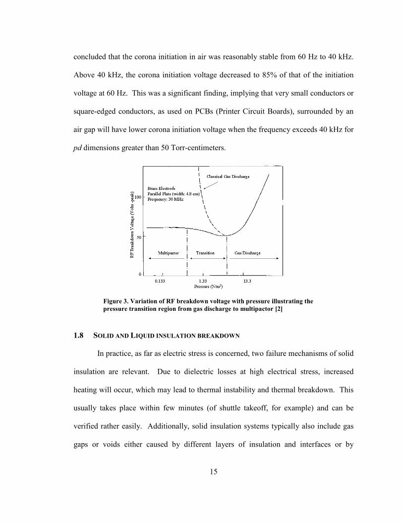
electrode gaps. Figure 3 shows transitions from classical discharge as seen in Paschen
curve to multipactor phenomenon in RF range at lower pressures. The dotted line in
Figure 3 shows the expected behavior of the breakdown voltage from the classical dc
gas discharge (breakdown voltage); the horizontal line branching off in the transition
region is the speculated behavior due to the influence of the high frequency applied
fields. The multipactor (RF) and the classical dc gas discharge mechanisms (low
frequency ~400 Hz) are well studied and documented in the literature, the behavior in
the transition region, however, is not entirely understood as the breakdown mechanism
in this region is neither multipactor nor classical discharge [2].
Studies were conducted by Dunbar et, al., [2, 20] involving various parameters
like the corona initiation voltages and extinction voltages at frequencies from 20 kHz to
over 60 kHz at pressures of 10 Torr to 50 Torr. The results of these experiments
15
concluded that the corona initiation in air was reasonably stable from 60 Hz to 40 kHz.
Above 40 kHz, the corona initiation voltage decreased to 85% of that of the initiation
voltage at 60 Hz. This was a significant finding, implying that very small conductors or
square-edged conductors, as used on PCBs (Printer Circuit Boards), surrounded by an
air gap will have lower corona initiation voltage when the frequency exceeds 40 kHz for
pd dimensions greater than 50 Torr-centimeters.
Figure 3. Variation of RF breakdown voltage with pressure illustrating the pressure transition region from gas discharge to multipactor [2]
1.8 SOLID AND LIQUID INSULATION BREAKDOWN
In practice, as far as electric stress is concerned, two failure mechanisms of solid
insulation are relevant. Due to dielectric losses at high electrical stress, increased
heating will occur, which may lead to thermal instability and thermal breakdown. This
usually takes place within few minutes (of shuttle takeoff, for example) and can be
verified rather easily. Additionally, solid insulation systems typically also include gas
gaps or voids either caused by different layers of insulation and interfaces or by
16
improper manufacturing of materials. In these voids, partial discharges are very likely
to occur at much lower field than is typical for the solid insulating bulk materials. Both,
the measurements of the phenomenon and the failure analysis are much more
complicated in this case. For solid insulation in general, the frequency of the voltage
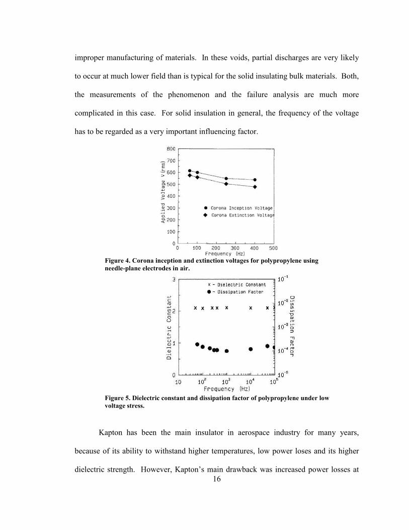
has to be regarded as a very important influencing factor.
Figure 4. Corona inception and extinction voltages for polypropylene using needle-plane electrodes in air.
Figure 5. Dielectric constant and dissipation factor of polypropylene under low voltage stress.
Kapton has been the main insulator in aerospace industry for many years,
because of its ability to withstand higher temperatures, low power loses and its higher
dielectric strength. However, Kapton’s main drawback was increased power losses at

17
higher temperatures. One of the first attempts to study the benefits of polypropylene
over Kapton for airborne applications (with frequencies under 400 Hz) was conducted
by Khachen and Laghari [21]. According to their studies, there is a slight decrease in
the breakdown voltage of polypropylene as the frequency is increased from 60 Hz to
400 Hz; reduction of material life was also observed. It was concluded from the
preliminary studies that polypropylene could be suitable for low stress, high frequency
airborne applications. However, there was a noticeable decrease in the dielectric
strength with increase in frequency of the applied voltage up to 30 kHz [22]. Also, the
lifetime decreases drastically at these high frequencies, which is probably caused
because of the heat build-up in the insulating film caused by the accelerated partial
discharge activity and by increased dielectric losses. The variation of the dielectric
constant and the dissipation factors of polypropylene at various frequencies under this
study are presented in Figures 4 and 5.
Figure 6. Frequency dependence of the real (εεεε'r) and imaginary (εεεε''r) parts of the dielectric constant in various polarization mechanisms.
Figure 6 shows the frequency dependence of the real and imaginary parts of the
dielectric constant in the presence of interfacial, orientational, ionic and electronic

18
polarization mechanisms. From the observations, it can be speculated that the space
charge behavior plays an important role in the process of PD generation, extension and
transition to a BD (Breakdown), mostly at lower frequencies. This implies that the
space charge consideration is quite important for successful breakdown prediction at
frequencies up to and just over power frequencies. At frequencies over 50/60 Hz and
up to 1 MHz the variation in dielectric constant is negligible. However, at much higher
frequencies, the role of interfacial space charge is replaced by the orientational, dipolar
or ionic polarization mechanisms. Moreover, these results also suggest that the applied
power frequency dependence of PD especially under positive polarity should be taken
into consideration at higher frequency.
Elanseralathan et al conducted studies for development of capacitors operating
at high frequency voltages for various space-based applications on PTFE,
polypropylene, and paper with thickness of 10 to 12.5 micrometers, at frequencies from
50 Hz to 90 kHz and found a 25% to 50% decrease in breakdown voltage for these
materials compared to dc breakdown [22]. Similar behavior of decreasing electrical
breakdown strength with increasing frequency was also observed earlier in oil [17].
1.9 NEED FOR FURTHER INVESTIGATION
In spite of all the studies, there is still not a complete fundamental understanding
of partial discharge or corona initiation in partial vacuum, because each study is either
application or design specific and differs from each other. In addition, existing data
cannot be extrapolated for miniature systems with smaller electrode gaps operating at
very low pressures [17, 23]. Although there have been studies on the high frequency

19
breakdown of gases at atmospheric pressures, there are either no data or very limited
data available in the literature for kHz frequency ac breakdown in partial vacuum for
inhomogeneous field gaps at frequencies under 1 MHz.
A study [1] was very recently initiated to determine the limitations of electrical
insulation systems and design guides. These shortcomings, if not properly accounted
for, may result in breakdowns leading to unpredicted premature electrical failures.
Even though gas breakdown studies have been conducted over a wide range of
parameters, the specific conditions have been defined by the needs of the commercial
equipment design. As such, the requirements for an advanced power system in
aerospace environment have therefore been much more stringent. It is noted that in the
study of gaseous environments, volume breakdown caused by dc voltages is well
documented. However, there is very limited data for various environments on
conditions involving other applied waveforms. Also, breakdown caused by short pulsed
waveforms under special conditions at pressures of 1 atmosphere and below, for
frequencies under 1 MHz has not been studied in depth.
At low frequencies, electron energy relaxation processes are sufficiently rapid
for the electron mean energy to ‘follow’ the applied field. In this situation, the
breakdown is expected to occur when the applied field attains its peak value, which in
fact is mostly observed in practice. At higher frequencies, however, the time constant
for electron energy relaxation can be long compared to the field period and the electron
mean energy can assume a constant value corresponding to the rms value of the field.
The data from spectral analysis can help determine the energy levels of the
prominent species (various ions) involved in the breakdown processes. By finding the
20
active species and their energy levels in the discharge, we can determine various details
of breakdown events such as, the mechanisms involved during the discharge processes,
determine whether the dominant processes are because of the initial electrons (possible
at low pressure/small gap) or due to the secondary electrons/ions, know if there is
enough time within a given voltage/signal cycle for the electrons to gain enough energy
to cause ionizing collisions (ie., determine the critical frequency for a given gap/signal
at which we have the most ionizing collisions), and the role of space charge at these
frequencies.

21
CHAPTER II
HIGH VOLTAGE BREAKDOWN IN PARTIAL VACUUM
This chapter deals with the basic phenomenon of gaseous breakdown in partial
vacuum conditions. A general overview of the dc breakdown mechanism is provided
followed by the structure of a typical low pressure discharge and related processes.
This is followed by the Paschen’s law and its limitations.
2.1 AIR AS INSULATOR
For a long time air has been the insulating media most commonly used in
electrical installations. Among its greatest assets, in addition to its abundance, is its self
restoring capability after breakdown. Furthermore, liquids and solids often contain gas
voids that are likely to break down. Therefore, the subject of electrical breakdown of
gases in general (as gaseous insulating media or as gas voids in liquid and solid media)
is indispensable for designers and operators of electrical equipment. A general theory
of breakdown phenomenon is presented in this chapter with focus on dc breakdown
phenomenon.
Two typical gas breakdown mechanisms have been known – ‘Townsend
mechanism’ and ‘Streamer mechanism.’ For several decades there has been
controversy as to which of these mechanisms governed spark breakdown. It is now
widely accepted that both mechanisms operate, each under its own most favorable
22
conditions. The electron avalanche process usually observed is basic for both
breakdown mechanisms. Because of its relevance to the current study, the focus here is
primarily on the Townsend mechanism.
2.2 CORONA AND TOWNSEND DISCHARGES
The Townsend electron avalanche forms the building block of all the dc and ac
coronas and most of the other gas discharges. Under the influence of an electric field,
electrons released in a gas will drift along the field lines and in the process produce
more electron-ion pairs (α) and undergo attachments (η). To make this amplification
self excited, there is a secondary ionization process, replacing each electron which
leaves its starting point with a new one, to get a self-sustained discharge. In a positive
corona, each electron reaching the ionization boundary must cause so many positive
ions, photons, and metastables that at least one of them succeeds in providing a new
electron at the ionization boundary, for the discharge to sustain. Further explanation of
this condition is provided in the following sections.
The pioneering work of Townsend [24, 25] in the beginning of the last century
made gas discharges a science and gave coronas their first useful formula. This work
was later continued in detail by Loeb [26]. From an electrical engineering view point,
coronas and partial discharges are unwanted phenomenon and are warnings of imminent
electrical/system breakdowns. Corona is a self-sustained electrical discharge where a
Laplacian (geometrical) electric field confines the ionization processes to regions close
to high-field electrodes or insulators. Thus, a corona discharge consists of:

23
1. Active electrodes or surfaces surrounded by ionization regions where free
charges are produced,
2. Low-field drift regions where charged particles drift and react,
3. Low-field passive electrodes, mainly acting as charge collectors.
When describing corona, ac, dc and hf usually refer to the supply voltage and
unipolar or bipolar refer to whether one or both the electrodes are active. Some of the
common test configurations for breakdown/corona studies are illustrated in Figure 7.
Figure 7. Widely used electrode geometries for breakdown/corona testing.
Ionization regions exist in all gas discharges. The characteristic of coronas is
really the drift region, which acts mostly as large impedance in series with the
ionization regions and gives coronas their intrinsic stability. The complete corona has a
large positive differential resistance due to its drift region impedance, even when most
of the current is conducted by the bipolar streamers.
2.3 DEVELOPMENT OF A GAS DISCHARGE
Any sample of gas under normal room conditions contains a number of ions and
electrons. At earth’s surface, atmosphere contains an average of 1000 positive and
negative ions per cc because of the UV and cosmic radiations. The rate of ionization to

24
maintain this is about 2-10/cc.sec. When two metal plates (electrodes) are setup at a
close distance, they both emit electrons due to these radiations, and this emission rate
can be greatly increased by external applied field conditions. In the absence of an
electric field, these electrodes form equilibrium where the rate of ionization balances
the rate of recombination. If a very small voltage is now applied to the electrodes
resulting in field strength of 1V/cm or less, then the current flows by the movement of
these already existing electrons and ions. As long as this current is small enough (10-10
to 10-9 A), the equilibrium is not disturbed and the current is proportional only to the
speed at which the ions and electrons can move between the electrodes. This is called
as the ‘Background ionization’ as shown in Figure 8. As the electron and ion mobilities
are nearly constant under these conditions, the current density j is proportional to the
field strength E. The gas therefore acts just like an ohmic conductor whose
conductivity depends upon the rate of ion and electron production, recombination rate
and mobilities. As E and j gradually increase, the equilibrium is disturbed by the ions
and electrons reaching the electrodes and getting neutralized. This increases the
effective recombination coefficient and therefore reduces the total charged particles
present in the gas. As a result, the rate of increase of current with voltage decreases,
marked as the saturation region in Figure 8.
25
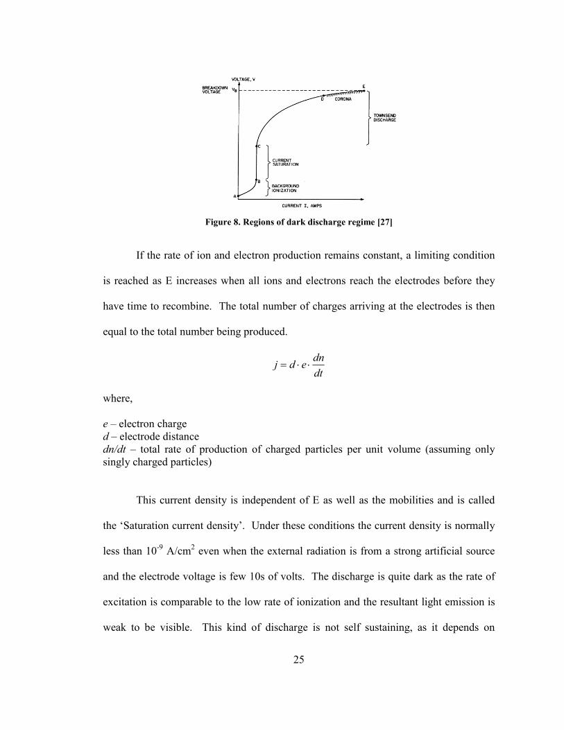
Figure 8. Regions of dark discharge regime [27]
If the rate of ion and electron production remains constant, a limiting condition
is reached as E increases when all ions and electrons reach the electrodes before they
have time to recombine. The total number of charges arriving at the electrodes is then
equal to the total number being produced.
dt
dnedj ⋅⋅=
where,
e – electron charge d – electrode distance dn/dt – total rate of production of charged particles per unit volume (assuming only singly charged particles)
This current density is independent of E as well as the mobilities and is called
the ‘Saturation current density’. Under these conditions the current density is normally
less than 10-9 A/cm2 even when the external radiation is from a strong artificial source
and the electrode voltage is few 10s of volts. The discharge is quite dark as the rate of
excitation is comparable to the low rate of ionization and the resultant light emission is
weak to be visible. This kind of discharge is not self sustaining, as it depends on

26
external radiation, it is the principle cause of leakage from charged bodies and is the
starting point of many other forms or discharge. This region of the I-V characteristics is
called as the ‘Dark discharge’ as the active species involved do not have enough energy
to cause any visible emissions. These discharges can be easily produced independent of
the external effects like radiation by using only heated cathode to provide electrons.
After saturation is reached, the voltage between the electrodes is further
increased; we get to a stage where the current further increases. This current increase
depends primarily on the gas pressure. Now, consider the low pressure case of few torr,
where the mean free path is still small compared to the electrode gap. With increasing
applied voltage the current rises at a higher rate until a Breakdown Voltage (Vb) is
reached at point ‘E’ in the I-V characteristics curve as shown in Figure 9. Vb depends
on the gas conditions and the electrode spacing/material/form and is usually in the order
of several hundred volts. Beyond Vb, the current is usually in the micro amp range for
small electrode systems (in this case for example). The section between the saturation
region and the breakdown point is represented by the so called ‘Townsend discharge’.
Figure 9. I-V characteristics of a glow discharge for flat copper electrodes (10 cm2),

27
2.4 TOWNSEND BREAKDOWN CRITERION
For simplicity, consider a parallel-plane electrode setup with the electrode
dimensions large compared to the electrode gap and where a constant external source of
radiation (ambient light, sun light, etc) is allowed to fall on the cathode to produce the
initial electrons. As the applied field E increases, the electrons leaving the cathode
accelerate more and more between consecutive collisions till eventually they gain
enough energy between collisions to ionize a neutral atom. Some electrons thus ionize
neutral atoms in their course of motion from cathode to the anode, leading to positive
ions and additional electrons. These additional electrons may themselves make ionizing
collisions on their path. This leads to an increase in the current compared to the
saturation value as the number of electrons reaching the anode is now more than the
number leaving the cathode. This current is further increased because of the positive
ions moving towards the cathode. In order to explain this increase, a Townsend’s first
ionization coefficient α was introduced. It is defined as the number of ionizing
collisions made on the average by an electron as it travels 1 cm in the direction of the
electric field. The ionization coefficient is related to the total cross section or the
probability for ionization by electron collision. Let dn be the increase (from an initial n)
in number of electrons over a distance of dx in one second crossing a plane parallel to
the electrodes. We then have
xenndxndn αα ⋅==>⋅⋅= 0
where n0 is the number of electrons leaving the cathode surface each second. For an
electrode spacing of d, assuming no electron loss due to diffusion, the current in the gap
would be

28
dd eieeni αα ⋅=⋅⋅= 00
where i0 is the electron current at the cathode and is dependent only on the
external radiation causing the photoelectric emission, and is called the primary current.
The electrons constituting i0 are called the primary electrons. The difference (i – i0) is
the positive ion current resulting from all the ionizing collisions made by the electrons
in the gas. The ratio i/i0 is frequently called the multiplication factor or the electron
multiplication. It should be noted however that the current density is not used in these
calculations as diffusion causes the current density to decrease towards the anode.
A statement of gas conditions strictly involves both the pressure and the
temperature separately. Density alone is not sufficient as temperature affects the
possibility of ionization at a collision and also the energies of the species involved.
However, in ionizations by electrons, only the electron energy is relevant and this is
determined primarily by the electric field strength. The transfer of kinetic energy to the
gas atoms here is so small that the gas kinetic temperature is practically unrelated to
electron energies. Hence, for a given E, only the gas density can effect α. Also,
temperature can be assumed constant in these conditions as the heating is quite
negligible. Pressure can therefore be treated as the variable, rather than the gas density.
So, in effect the variation of α with only p and E is required. In principle, α can be
calculated in terms of p and E if the exact behavior of the electrons and the variation of
the collision cross section for ionization are known. The secondary ionizing agents –
positive ions, excited atoms, photons, metastables, etc. are represented quantitatively by
the secondary ionization coefficient (γ); it is the average number of secondary electrons
produced at the cathode for each ionizing collision in the gap. Like α, γ is also a

29
function of E/p but is usually much smaller in magnitude. Under these conditions, it
can be easily shown that the steady state current I will be given by:
)1(10
−−=
d
d
e
eII α
α
γ
In the absence of the Townsend’s secondary mechanism, where γ = 0, the above
equation simplifies to:
deII α0=
The complete current equation above describes the growth of the average
current in the gap before the breakdown occurs. At low field strengths, in the region
‘C-D’ of Figure 8, deII α0= . As the voltage increases, current also increases, limited
only by the source impedance, this condition is called the ‘Breakdown’ or the so called
“Townsend criterion” and requires:
0)1(1 =−− deαγ
2.5 LOW PRESSURE DC GLOW DISCHARGE
The glow discharge owes its name to the fact that the plasma is usually
luminous. This is because of the electron energy and density being high enough to
result in generation of visible light due to collisions. Most of the industrial applications
such as the classical electrical discharge tube in florescent lights, parallel-plate plasma
reactors, magnetron discharges for thin film depositions, and electron-bombardment
plasma sources use the glow discharge regime.
30
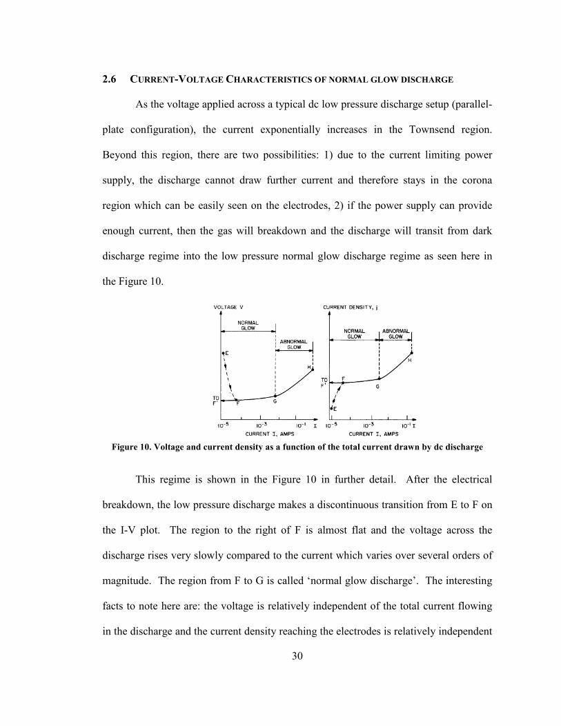
2.6 CURRENT-VOLTAGE CHARACTERISTICS OF NORMAL GLOW DISCHARGE
As the voltage applied across a typical dc low pressure discharge setup (parallel-
plate configuration), the current exponentially increases in the Townsend region.
Beyond this region, there are two possibilities: 1) due to the current limiting power
supply, the discharge cannot draw further current and therefore stays in the corona
region which can be easily seen on the electrodes, 2) if the power supply can provide
enough current, then the gas will breakdown and the discharge will transit from dark
discharge regime into the low pressure normal glow discharge regime as seen here in
the Figure 10.
Figure 10. Voltage and current density as a function of the total current drawn by dc discharge
This regime is shown in the Figure 10 in further detail. After the electrical
breakdown, the low pressure discharge makes a discontinuous transition from E to F on
the I-V plot. The region to the right of F is almost flat and the voltage across the
discharge rises very slowly compared to the current which varies over several orders of
magnitude. The region from F to G is called ‘normal glow discharge’. The interesting
facts to note here are: the voltage is relatively independent of the total current flowing
in the discharge and the current density reaching the electrodes is relatively independent

31
of the total current. In the normal glow discharge regime, the plasma is in contact with
only a small part of the cathode surface at low currents. As the current increase, the
plasma covers more area of the cathode surface until we reach ‘G’, the boundary of the
abnormal glow, by when the plasma covers the entire cathode surface delivering the
required current but holding up constant current density (Current density plot in Figure
10). In the abnormal glow regime of G to H, the voltage increases, significantly
increasing the total current. At H, the electrodes get sufficiently hot and the cathode
starts thermionic electron emission. If the power supply can deliver further current,
then the glow-to-arc transition can be observed, where the I-V gradient turns negative
and a current increase is observed.
Discharge layout
Glow Intensity
Potential
Longitudinal field
Electron & ion current densities
Charge densities
Space Charge
Figure 11. Variation of various parameters observed in a typical glow discharge.

32
2.7 REGIONS OF THE NORMAL GLOW DISCHARGE
Typical plasmas formed in DC low pressure glow discharges can be ideally
shown as in Figure 11. These regions were first observed by Michael Faraday in 1830’s
and later by other investigators of low pressure discharge tubes. These regions appear
over a wide range of operating conditions and are very characteristic of the normal glow
discharge. Listed here are the various regions of the normal glow discharge.
1. Cathode: This is the electrically conductive metal whose secondary electron
emission coefficient plays a significant role in the discharge formation.
Typically, the cathode is desired to operate under normal temperatures and does
not rely on the thermionic electron emission to sustain discharge. The
secondary electron emission plays a significant role in supporting the Townsend
theory. To increase the electron emission, sometimes other configurations like
hollow cathode are also used.
2. Aston dark space: This is the space immediately beyond the cathode surface
and is thin and dark with strong electric field and a negative space charge due to
the slow electrons accelerating from the cathode surface. This region is dark as
the electrons coming off the cathode are of low energy/density to result in any
visible excitations.
3. Cathode glow: This region has a relatively high ion number density and
depending on the gas can be often seen reddish or orange in air due to emissions
by excited atoms sputtered off the cathode surface or due to positive ions
moving towards the cathode. The length of this region depends on the pressure

33
and type of gas. It is not unusual to see the cathode glow very close to the
cathode surface completely masking the Aston dark space.
4. Cathode dark space: Also called as the Crookes/Hittorf dark space has a
moderate electric field, a positive space charge and relatively high ion density.
5. Cathode region: This is where most of the applied voltage drop is observed.
This voltage drop is called the ‘cathode fall’. In this region, the electrons are
accelerated to high enough energies to result in ionizing collisions and
avalanches in the negative glow and beyond. Under low pressure operation, the
axial length of this region adjusts itself to establish a minimum pd for the gas.
In the normal glow discharge, the current density flowing to the cathode remains
almost constant even as the total current varies. This is due to varying contact
area of the discharge plasma with the cathode surface.
6. Negative glow: This is the brightest region of the entire discharge. This region
has relatively low electric field and is long compared to the cathode glow and
brighter on the cathode side. Almost all the current in this region is carried by
the electrons (typical electron number density of 1016/m3). Electrons accelerated
from the cathode region produce intense excitation and ionization in the
negative glow region resulting in its brightness. These electrons then slow down
and lack any excitation energy leading to the next dark region.
7. Faraday dark space: the electron energy in this region is very low as a result of
high activity in the negative glow region. In this region, the recombination and
radial diffusion result in decreased electron density. The space charge is very
low and so is the axial electric field.

34
8. Positive column: This region is a long, quasi-neutral uniform glow with small
electric field, typically about 1V/cm. The electric field is just enough to
maintain the required ionization towards the cathode end of this region. The
electron density is typically 1015 to 1016 /m3 here with the electron kinetic
energy of 1 to 2 eV. This region when formed in air would be pinkish to blue.
The peculiar property of this region is that as the length of the discharge tube is
increased, under a given pressure, the positive column lengthens while the
cathode region stays intact.
9. Anode dark space: This is the anode sheath between the anode and the anode
glow with negative space charge due to the electrons traveling from the positive
column to the anode, and has a higher electric field than the positive column.
The electrons are pulled out of the positive column by the anode.
10. Anode glow: This is the bright region at the anode end of the positive column,
brighter than the positive column but can not always be observed. This region
marks the beginning of the anode sheath.
11. Striations: These are traveling waves or stationary perturbations in the electron
number density which occur in partially ionized gases. In the usual form
moving striations are propagating luminous bands which appear in the positive
column and can be easily observed. Most of the homogeneous partially ionized
gases have moving striations.
A general observation in studying the normal glow discharge regions is that
most of the power dissipation is in the cathode region where the field is highest. Thus,
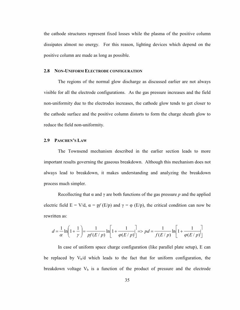
35
the cathode structures represent fixed losses while the plasma of the positive column
dissipates almost no energy. For this reason, lighting devices which depend on the
positive column are made as long as possible.
2.8 NON-UNIFORM ELECTRODE CONFIGURATION
The regions of the normal glow discharge as discussed earlier are not always
visible for all the electrode configurations. As the gas pressure increases and the field
non-uniformity due to the electrodes increases, the cathode glow tends to get closer to
the cathode surface and the positive column distorts to form the charge sheath glow to
reduce the field non-uniformity.
2.9 PASCHEN’S LAW
The Townsend mechanism described in the earlier section leads to more
important results governing the gaseous breakdown. Although this mechanism does not
always lead to breakdown, it makes understanding and analyzing the breakdown
process much simpler.
Recollecting that α and γ are both functions of the gas pressure p and the applied
electric field E = V/d, α = pf (E/p) and γ = φ (E/p), the critical condition can now be
rewritten as:
+==>
+=
+=
)/(
11ln
)/(
1
)/(
11ln
)/(
111ln
1
pEpEfpd
pEpEpfd
ϕϕγα
In case of uniform space charge configuration (like parallel plate setup), E can
be replaced by Vb/d which leads to the fact that for uniform configuration, the
breakdown voltage Vb is a function of the product of pressure and the electrode

36
separation for a given gas and electrode material. Thus, regardless of the forms of the
functions f and φ, Vb depends just on the pd product. This fact was first experimentally
observed by Rue and Muller [28] in 1880 and later studied further by Paschen. It
should be noted that the gas density N rather than the pressure p should be used in these
equations to account for the effect of temperature at constant pressure on the mean free
path. The above equations can be rearranged to get the final form for the breakdown
voltage as:
)1
1ln(ln
γ+
=Apd
BpdVb
It should be noted that the form of Vb leads to a minimum for a certain pd value:
)1
1ln(718.2
)( min γ+=
Apd and )
11ln(718.2(min) γ+=
A
BVb
Figure 12. Paschen curves for helium and nitrogen for dc fields, reproduced from literature data [29, 30]

37
For voltages smaller than Vb, it is impossible to cause a uniform gap to reach the
breakdown no matter how the spacing and gas pressure are adjusted. Empirical work
by many others on uniform-field gaps at atmospheric conditions, shows the behavior as:
Vb = (2440d + 61√d) kV, where d is the gap distance in meters
Figure 12 shows typical Paschen plots for helium and nitrogen from literature
data. As mentioned, these curves have a breakdown minimum corresponding to a pd
minimum and the voltage curve increases on either side of this point. Because of
various power requirements in aircrafts and high altitude vehicles, the switching circuits
typically operate at 400 Hz. The Paschen like plots at this frequency are preferred
instead of the conventional dc breakdown data; one such plot for various gases is shown
in Figure 13 with the corresponding breakdown voltages in Table 2. At frequencies
much higher than 400 Hz, the Paschen like behavior is still observed even for non-
uniform geometries, and is the main focus of this study.
Table 2. Breakdown Voltages at the Critical Pressure-Spacing Dimension for Pure Gases at dc and 400 Hz
Gas DC AC Air 327 230 Helium 189 132 Hydrogen 292 205 Nitrogen 265 187

38
Figure 13. Breakdown voltage of several gases as a function of pd at room temperature [9]
Although these derivations assume a very simple breakdown phenomenon, all
the empirical inferences from the Paschen law have been experimentally verified
including the numerical values.
2.10 DEVIATIONS FROM PASCHEN’S LAW
The behavior of gases under low pressures and uniform and non-uniform fields
and in particular the breakdown characteristics are covered in detail in work by Craggs
and Meek [31]. Under low pressures (<< milli Torr), the gaseous breakdown
mechanism is dominated mostly by the electrodes, and is called the ‘Vacuum
Breakdown’ and is not affected much by the gases involved. Under these and many
other conditions (high pd, field non-uniformity, etc), deviations from the Paschen law
and the derived expressions have been observed. At very large values of pd, the so
called ‘Streamer mechanism’ becomes responsible for the breakdown and the
Townsend mechanism ceases to be active. Also, the law is not applicable in many gas

39
mixtures (especially Penning mixtures) where the role of metastables is dominant.
Another important observation is that γ, which has been assumed a constant in
derivation of the equations is actually a function of both E/p and p which usually leads
to the deviations from the law. The law however has been found to hold good both in
theory and experimental results for many non-uniform configurations [32] (Further
details/observations in the results chapter).

40
CHAPTER III
HIGH FREQUENCY BREAKDOWN
3.1 BACKGROUND
Historically, power systems on US space vehicles have been operating at 28 V
dc inherited from the aircraft industry. At such low voltages, the plasma interactions in
low earth orbits are negligible and therefore, have not been a concern in spacecraft
design. Due to recent advances, some of the high power systems for aerospace and
space applications (parts of ISS) are being operated at voltages much higher than the
traditional voltage levels. To reduce the cable mass and the induced magnetic fields
due to higher currents, the new systems are designed with higher system voltages and
low currents. As an example, parts of ISS already use 110 V dc and there are currently
several initiatives within the government agencies (such as NASA and Air Force),
planning to use 270 volt distribution power [2]. Some sub-systems also use high
frequency (in the 10s of kHz) voltages, for switched mode power conversion.
With increasing voltage levels, gaseous breakdown at and around power systems
could be a concern. On the other hand, most of the literature data on high voltage
breakdown has been developed primarily for domestic utility power system related
applications working at 50/60 Hz. Furthermore, the only data for high frequency fields
has been for equipment operating at MHz frequencies (and higher), such as antennas
and waveguides. In summary, the majority of information traditionally has been either

41
at low frequency and atmospheric conditions or at very high frequency at atmospheric
or vacuum conditions.
Early in the space program, it was discovered that the use of very low frequency
partial discharge criteria leads to failures when applied to high-frequency, high-density
packaging, especially when non-sinusoidal frequencies greater than 20 kHz were
introduced due to weight and volume restrictions in spacecrafts [11, 12]. Later studies
revealed that for electrode spacing larger than 0.04 cm, the high frequency breakdown
voltage is much less than the low frequency breakdown for pd > 50 torr-cm. For
smaller spacing (<0.04 cm) and same pd conditions, however, the breakdown voltage
remained almost constant from 50 Hz to 20 MHz [2].
Figure 14. Variation of RF breakdown voltage with pressure illustrating the pressure transition region from gas discharge to multipactor [12].
During the first reported high frequency electrical failure in spacecrafts, it was
assumed that the breakdown phenomenon that occurred below 1 torr was due to the
high frequency effects [2]. This lead to the breakdown voltage studies at higher
frequencies. From the limited data collected earlier [2], Figure 14 shows the expected
behavior of the voltage at 30 MHz. From this figure it clear that at pressures higher

42
than ~ 40 milli Torr, Paschen like behavior is noticed. However, below this pressure,
instead of following the Paschen curve (dotted line in Figure 14) the breakdown pattern
follows a completely different ‘Multipactor’ mechanism where the resonant effects are
dominant.
Typical setups for high frequency discharge studies normally include, (a) simple
two electrode systems (various geometries) with a fixed electrode gap, (b) discharges
induced by high current passing through a solenoid surrounding the gas, and (c)
waveguides or metal cavities. Due to the charge movement in gas discharges, the
alternating fields are usually associated with induced magnetic fields. For larger
wavelengths (thus smaller frequencies) they become more localized at certain locations
of the setup and therefore, for frequencies less than 1 MHz, the magnetic field can be
neglected in a setup of type (a) and the electric field can be neglected for setup of type
(b). Thus, for the current study, as the applied frequency is always under 1 MHz, the
effect of magnetic field is entirely neglected.
3.2 ROLE OF ALTERNATING FIELD
The gas discharges can usually be associated with a time constant which defines
the duration of the transition states. If the voltage applied across the electrode gap is
time varying, and if this variation is comparable to the time constant of the gas
discharge, there could be noticeable differences is the discharge phenomenon. The
sequence of phenomenon observed during the voltage decreasing period may not be
exactly opposite to those observed in the increasing period of the applied voltage. Thus,
the voltage at the extinction of the discharge is less than that at the beginning. As long
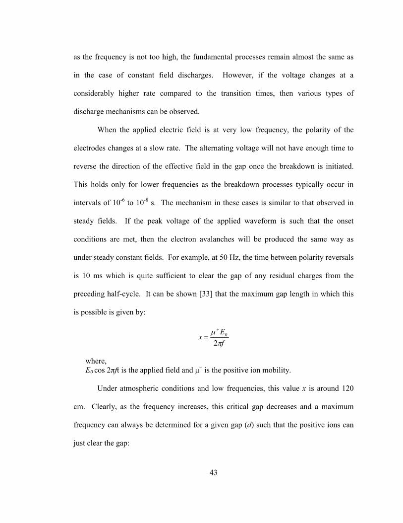
43
as the frequency is not too high, the fundamental processes remain almost the same as
in the case of constant field discharges. However, if the voltage changes at a
considerably higher rate compared to the transition times, then various types of
discharge mechanisms can be observed.
When the applied electric field is at very low frequency, the polarity of the
electrodes changes at a slow rate. The alternating voltage will not have enough time to
reverse the direction of the effective field in the gap once the breakdown is initiated.
This holds only for lower frequencies as the breakdown processes typically occur in
intervals of 10-6 to 10-8 s. The mechanism in these cases is similar to that observed in
steady fields. If the peak voltage of the applied waveform is such that the onset
conditions are met, then the electron avalanches will be produced the same way as
under steady constant fields. For example, at 50 Hz, the time between polarity reversals
is 10 ms which is quite sufficient to clear the gap of any residual charges from the
preceding half-cycle. It can be shown [33] that the maximum gap length in which this
is possible is given by:
f
Ex
πµ2
0+
=
where, E0 cos 2πft is the applied field and µ
+ is the positive ion mobility.
Under atmospheric conditions and low frequencies, this value x is around 120
cm. Clearly, as the frequency increases, this critical gap decreases and a maximum
frequency can always be determined for a given gap (d) such that the positive ions can
just clear the gap:

44
d
Ef
πµ2
0max
+
=
On the other hand, for a fixed frequency, dmax would be:
f
Ed
πµ2
0max
+
=
For gaps larger than dmax, the positive ions will not reach the cathode before
voltage and field reversal. It should be noted that fmax is inversely proportional to the
electrode gap and directly proportional to the field intensity and the positive ion
mobility. For frequencies beyond fmax, field distortion due to the positive space charge
may result in modified breakdown mechanism.
3.3 ROLE OF GAS DENSITY
The motion of an electron in a gas is highly influenced by its collisions with the
surrounding gas molecules. If the applied electric field is continuous, in steady state,
the electrons will have a constant drift velocity which depends only on the field and the
electron mobility. If the same is to be assumed for higher gas density, then since the
velocity is in phase with the acting force, the electrons absorb energy and the gas acts as
resistive metal. This energy gained from the field is subsequently lost to the ambient
gas, heating it.
On the other hand, in a low density gas, the frequency of collisions may be too
high to be neglected but not high enough to affect the drift velocity. Under these
conditions, it can be assumed that the action of collisions is equivalent to a frictional
force proportional to the mean velocity. In this regime, the gas acts similar to a
dielectric medium with a constant power factor; and in the steady state, the electrons

45
give up the absorbed energy to the molecules of the ambient gas. In both the above
cases, interactions between the charged species are usually neglected since the densities
are, in general, very small.
In general, an electron leaving the vicinity of a cathode undergoes collisions
with other species in the gas resulting in energy transfers and eventually either reaches
the opposite electrode or the chamber wall or is absorbed in the gas. A sketch of typical
motion of an electron under alternating fields at low pressures is shown in Figure 15a.
As the gas pressure is increased considerably, this is considerably affected and the
electrons travel lesser distances before consecutive collisions and the typical path looks
similar to Figure 15b. It should be noted here that even though the gas pressure is the
critical parameter, the basic mechanisms are dominated by the relationship between the
applied field frequency and the electron collisions frequency.
(a) (b)
Figure 15. Motion of an electron in high frequency field (a) at very low pressure (collision frequency << signal frequency) and (b) at medium and high pressures (collision frequency > signal frequency) [33]
Very low pressure normally refers to p < 10 milli Torr, and under these
conditions, the electron-wall collisions outnumber the electron-molecule collisions.
The breakdown voltage is in the order of 100 V and it depends essentially on the
nature/setup of the electrodes than on the gas pressure. There is a cutoff frequency

46
fcritical which defines the discharge at low pressure and electrode gaps, and is empirically
given as:
fcritical ≈ 0.7 MHz / d (mm)
This equation defines the signal frequency below which a discharge cannot be
initiated. The plot in Figure 16 shows typical behavior for hydrogen at 0.1 milli Torr.
As seen from Figure 16, there are two values for breakdown voltage
corresponding to each frequency. Outside the interval defined by these voltages, it is
impossible to initiate a breakdown or maintain a discharge. At these frequencies, a
phenomenon called the ‘multipactor’ effect based on electron resonance is observed and
most of the breakdown events occurring at radio frequencies in antennas and
waveguides are attributed to this phenomenon.
Figure 16. Multipactor effect in hydrogen at 10-4 torr (Ag-Cu electrodes, gap = 3cm) [33]
The theory of secondary electron resonance is based on the idea that an
avalanche of electrons can only develop if the time for electrons to travel the electrode
gap (in a direction parallel to the electric field) is approximately half the time period of

47
the applied signal, such that the possible secondary electrons in turn leave with the
phase necessary for them to be accelerated by the field. There is a resonance between
the field and the motion of the electrons. Also, this can occur when the field imparts
energy to the electrons such that when they strike the electrodes or the walls, each
electron extracts at least one secondary electron.
At higher gas pressures (> 10 milli Torr), however, there are two possible
scenarios depending on whether the peak amplitude (x) of the electron oscillation is
smaller or larger than the dimensions of the gas enclosure (d). It can be shown that the
oscillation amplitude is proportional to 1/ω2 and so, for higher applied frequencies, the
latter case is valid.
For x > d, the electron cloud is displaced due to the effect of the electric field
and strikes the walls twice each period and the walls therefore play a major role in the
breakdown process. For x < d, the ionization is localized in the gas while charge is lost
mostly due to diffusion towards the walls (attachment and recombination are negligible
in general).
Breakdown takes place at a critical field such that each electron produces, on an
average, at least one ion pair in the course of its oscillatory motion before disappearing
due to diffusion. Thus, when the dimensions of the gas container (chamber) and the
electrode gap increase, the life time of an electron in the gas increases and it has higher
chances of ionizing the gas before disappearing. The breakdown voltage is reduced,
leading to the Paschen minimum, depending on the gas pressure. It can be seen that the
energy absorbed by an electron reaches a maximum when the collision frequency is

48
same as the signal frequency. It can be verified that this value of the collision
frequency actually corresponds well with the pd minimum observed in Paschen curves.
3.4 EFFECT OF FREQUENCY ON BREAKDOWN PHENOMENON
Normally, the phenomenon in a gas discharge at high frequency can be
classified depending on the characteristics lengths involved [34]. These lengths are:
volume size (d), electron free path (l), and the oscillation amplitude of free electrons (a)
or drift electrons (A). Depending on which of the frequencies is higher: field frequency
or electron collision frequency, ‘a’ or ‘A’ is chosen. If the gas pressure is low enough
that l >> d, then an electron experiences no collisions with atoms in the gas. In typical
conditions, d ~ 1cm and upper boundary for such low pressure (l ~ d) in most gases is ~
10-2 Torr.
When an electric field is applied across an electrode gap, the charged particles
are accelerated. Because of the difference in mass, the electrons are accelerated more
than the ions and also the energy transferred to these electrons is so much more that for
the most part the heavier ions can be assumed stationary. Typically, electrons are
always present in a gas and depending on the field direction; they are always
accelerated in certain direction. In case of alternating fields, the electrons experience
opposite forces at the end of each half-cycle and oscillate within the gas if the container
is large enough. This distinguishes high frequency breakdown from dc or low
frequency discharges. When the frequencies are low (few kHz), the reversal of field
direction does not occur before the electron reaches either the chamber walls or the
electrodes (assuming gaps < few cm).

49
Figure 17. Variation of relative breakdown voltage with applied field frequency for a uniform 1 cm electrode gap at atmospheric conditions. [28]
At higher frequencies, in the absence of any gas atoms (assuming only electrons
existed), the electrons would oscillate out of phase with the field and there would be no
energy transfer. In the presence of the gas, the electron-atom collisions occur and the
electrons are accelerated by the field after each collision, sometimes losing energy and
sometimes gaining energy but on the average, a net energy transfer occurs from the
field to the electrons. This gained energy is also lost to the gas atoms via collisions. In
case the applied field is large enough, the electrons can accumulate enough energy to
exceed the excitation energy of the atom, leading to excitation of the atom. Thus, in
addition to elastic collisions, electrons also loose energy through inelastic collisions. As
only a fraction of the electrons with energies more than the excitation energy actually
excite the atoms, some will have enough kinetic energy to ionize the atoms on
collisions. This leads to each electron producing an additional electron. This results in
electron production. On the other hand, electrons are also lost due to diffusion to the
walls and recombination with positive ions or by attachment to neutral species. The
production and loss rates are complicated functions of the type of gas, gas density,

50
electric field magnitude, frequency, electrode geometry, etc. Figure 17 shows the
predicted frequency dependence of the breakdown voltage for a uniform 1 cm field gap
at atmospheric conditions. Two important aspects of electron motion are generally
observed in the r.f. region [35]. Under conditions typical to these experiments, with
gaps of 5-20 mm and pressures of 10 to 760 Torr, the electrons oscillate in phase with
the applied electric field; with amplitude of 2-3 mm. This amplitude is clearly smaller
than the discharge gap width, so an electron will typically oscillate in the gap for several
cycles, thus having an ionization path length longer than the electrode gap before it is
lost to either of the electrodes. At lower frequencies, an electron will travel through the
gap only once, so the parameter pd is a measure of the number of collisions suffered by
an electron before it is lost to an electrode by drift motion, while at microwave
frequencies, the oscillation amplitude is so small in comparison to the electrode gap that
the drift loses to the electrodes are negligible. The electron loss because of diffusion or
attachment therefore, needs consideration [36]. As frequency increases, the number of
collisions suffered by an electron before it is lost to the walls increases and the electric
field strength at breakdown is lowered. Perhaps of greater significance is the fact that
for a particular value of electric field strength at breakdown, the values of pd at which
the breakdown occurs differ quite significantly from dc to r.f. cases.
At low frequencies, electron energy relaxation processes are sufficiently rapid
for the electron mean energy to ‘follow’ the applied field. In this situation, the
breakdown is expected to occur when the applied field attains its peak value, this is
observed in practice. At microwave frequencies, however, the time constant for

51
electron energy relaxation is long compared to the field of the period and the electron
mean energy assumes a constant value corresponding to the rms value of the field.
Plots of the applied voltage, the r.f. current and the photon intensity can be used
to understand these processes. Studies in [35] show that the photon output peaks at
twice the applied frequency and falls almost to zero at the voltage zero points,
indicating that the electron mean energy responds rapidly to the changing electric field.
While the electron mean energy is clearly changing rapidly with applied field, as
expected, it is not obvious that the breakdown event will consequently occur at the field
peak. The formative time of the ionization process responsible for the electrical
breakdown must be considered in relation to the period of the applied voltage before
this question can be resolved in this transition region. This raises the question about
temporal characteristics of the secondary processes as well as the influence of the
excitation energy transfer in these events.
3.5 PULSED/UNIPOLAR ELECTRIC FIELDS
Due to higher switching frequencies in some of the commercial applications in
high altitude systems, the breakdown characteristics of pulsed or unipolar applied fields
under partial vacuum conditions are of increasing interest. Unlike alternating fields,
where the electrons/ions experience opposing forces during consecutive half cycles,
unipolar fields typically force the motion in one direction for half cycle and exert no net
force in the other half cycle. Depending on the signal frequency and the duty cycle,
these ‘on’ and ‘off’ times as shown in Figure 18 can significantly affect the breakdown

52
characteristics of the gas. The breakdown voltages for ac and unipolar fields have been
observed to be typically less than the corresponding dc fields, as reported in [37].
10 %
20 %
30 %
40 %
50 %
Figure 18. Typical applied voltage waveforms at 50 kHz for different duty cycles. The ‘On’ and ‘Off’ times vary from 2 µµµµs to 18 µµµµs at this frequency.

53
CHAPTER IV
OPTICAL EMISSION SPECTRA OF DISCHARGES
4.1 ATOMIC SPECTRA
Assuming a simple Bohr’s atomic model to account for the basic processes, an
atom typically consists of electrons orbiting around a nucleus. These electrons are
however restricted only to certain energy levels. The electrons can therefore move from
one energy level to another energy level as long as they are limited to these discrete
‘acceptable orbitals’. The energy differences between these orbital levels correspond to
the wavelengths of light emitted or absorbed by the atoms. This has been the basis for
one of the oldest methods for elemental analysis, called ‘Atomic Spectroscopy.’
Because every element has a specific line spectrum, the presence of an elemental line
directly implies the presence of that element in the sample being studied. Also, the
same principle is used to analyze and understand various energy transitions within a
particular element. Traditional emission spectroscopy was done with flames/arcs for
analyzing samples of liquids and solids. Glow discharges replaced them as potential
radiation sources. A simple electrode setup in a gas chamber when excited with enough
applied voltage/field can result in a glow discharge, giving out the spectral lines of the
gases present in the chamber.
54
For understanding the atomic spectra, the plasma is produced by an electric
discharge and the charged particles are moved under the influence of the electric field
across the chamber. When considerable field is applied across the electrodes, free
ions/electrons are formed in the gas and measurable current.
These processes result in the partial ionization of the gas and plasma formation.
As a result of the collision between all kinds of particles in the gas phase, energy
exchange takes place. It should be noted that there are different types of collisions here:
inelastic collisions, charge transfer, and recombination
In an equilibrium state, the number of particles leaving an energy state equals
the number of particles excited to this state and to characterize the equilibrium, all the
process causing these excitations and de-excitations must be known. They are:
• Collisions with neutrals where atoms are excited (first kind)
• Collisions where excited atom returns to lower energy level without emitting
radiation (second kind)
• Excitation by collisions with electrons
• De-excitation of excited atoms through collisions with electrons
• Excitation of atoms by absorption of radiation
• De-excitation of atoms by spontaneous or stimulated emission of radiation
Typically, in a dc glow discharge in air, the excitation is mainly due to collisions
of the first kind with neutral particles. However, at lower pressures and in inert gases,
collisions with electrons play a more important role and the absorption and emissions of
radiation can no longer be neglected. The excited levels are normally not energetically

55
favorable and usually lead to decays by emission of radiation and also by collisions with
other particles. When allowed to decay by emission of radiation, the active species
lifetime is usually short (< 10-8 s), however, when this is not allowed, the so called
metastable levels are formed which can loose their energy only by collisions. In
discharges at low pressures, as the chances of collision are low, the metastable lifetimes
are long (up to seconds), this gives rise to the afterglow phenomenon [38].
Over the years, when determining the wavelengths for atomic lines emitted by
different elements, some empirical rules were established. Balmer found that for
hydrogen, the wavelengths could be given by:
)]4/([ 22 −= nnkλ ,
which when written using wavenumbers transforms to
)/1(/1 22
21 nnRv −==′ λ
where v′ is the wavenumber (cm-1) R is the Rydberg’s constant (109.677 cm-1) n2 is a series number (> n1)
Rydberg later adapted this equation to other elements by adding another term for
the charge of the nucleus Z:
)/1(/1 22
21
2 nnRZv −==′ λ
Clearly, this equation shows that the energy levels are related to the atomic structure
itself and there can be as many spectral lines as there are possible differences of terms.

56
As mentioned earlier, various intermediate species formed during the discharge
processes have different lifetimes. This finite lifetime of an excited species results in
‘widening’ the spectral lines. There are several possible mechanisms:
• Doppler or temperature broadening of lines results from the fact that the
emitting species have a velocity component in the direction of observation.
• Lorentz or pressure broadening results from the interaction between emitting
atoms and atoms from other elements.
• Resonance broadening results from the interaction between emitting and non-
emitting atoms of the same element.
• Stark broadening results from interaction with the electrical fields.
For demonstration, Figure 19 shows the energy level diagram of the hypothetical
situation of a doubly ionized atom with Z = 3 (Lithium). A transition, for example,
from level n = 2 to n = 1, would result in a photon of energy = 91.8 eV (since, 122.4 -
30.6 eV)
Figure 19. Energy level diagram of a hypothetical doubly ionized atom with Z = 3.

57
These emissions are normally plotted as intensities as function of the
wavelength, which is typically the output of a spectrometer. One such spectrum
recorded by a chart recorder for Cu-He calibration lamp is shown in Figure 20. The
physical widths of spectral lines in most radiation sources (as in Figure 20) are 1 to 20
pico-meters but can be much larger when observed in spectrometers [38]
Figure 20. Typical spectrum recorded using a chart recorder for a Cu-He calibration lamp [39].
The negative glow of a glow discharge is analytically the most important region
of the discharge as the number densities of all the active species (atoms/ions/electrons)
are high in this region. In noble gases, the metastables formed here under low pressures
have long lifetimes and can excite other atoms through collisions. This is usually
reflected in the peak intensities at various wavelengths in the spectrum for these energy
levels. Table 3 lists the commonly observed wavelengths and their energy levels in
helium discharge spectra.
Typical spectral line plots from the literature [40] as shown in Figure 21 help
determine the actual electron transitions at these wavelengths. From Figure 21, one can
observe that, for example, an emission of 5875.6 A corresponds to the transition 2(2, 1,

58
0) → 3(3, 2, 1) (or 23P – 33D) in Helium triplet. Also, depending on the gas pressure,
the probabilities corresponding to each electron transition vary, usually resulting in
lower intensity at those wavelengths as the gas pressure is increased. Earlier work
conducted by C. Hodges and W. C. Michels [41] is presented in Figure 22 for one such
variation over a pressure range of 2 to 40 Torr in Helium.
Table 3. Emission wavelengths of a Helium discharge [42], typically seen in the visible spectrum and the corresponding intensity values and the calculated energies.
Wavelength (Å) Intensity Energy (eV)
3964.73 20 3.14
4009.27 1 3.10
4026.19 50 3.09
4026.36 5 3.09
4120.82 12 3.02
4120.99 2 3.02
4143.76 3 3.00
4387.93 10 2.83
4437.55 3 2.80
4471.48 200 2.78
4471.68 25 2.78
4685.4 6 2.65
4685.7 30 2.65
Wavelength (Å) Intensity Energy (eV)
4713.15 30 2.64
4713.38 4 2.64
4921.93 20 2.53
5015.68 100 2.48
5047.74 10 2.46
5411.52 5 2.30
5875.62 500 2.12
5875.97 100 2.12
6560.1 8 1.89
6678.15 100 1.86
6867.48 3 1.81
7065.19 200 1.76
7065.71 30 1.76

59
Figure 21. Atomic energy levels for neutral Helium [40]

60
Figure 22. Absolute intensities of various lines of the Helium spectrum over a pressure range (2 to 40 Torr) [41]
4.2 MOLECULAR SPECTRA
Unlike atomic spectra, the most commonly observed molecular spectra involve
three transitions: electronic, vibrational, and rotational. For a simple diatomic molecule
like nitrogen, the electronic states can be represented by potential energy plot as
function of the internuclear distance as shown in Figure 23. The electron transitions in
this figure are usually almost vertical as they occur so rapidly that the internuclear
distance can not change much in the process. The vibrational transitions occur between

61
different vibrational levels of the same electronic state. Rotational transitions occur
mostly between the rotational levels of the same vibrational state, there are however
cases where this is not always true (seen mostly in light molecules).
Depending on the electric dipole moment of a molecule, an incident
electromagnetic wave can excite the rotational levels of the molecule. This is due to the
torque exerted on the molecule by the incident field (Figure 24a). The plot in Figure
24b shows the portion of a potential diagram for a stable electronic state of a diatomic
molecule. Each of these electronic states has several vibrational states associated with it
and therefore, the vibrational spectra can be observed. The rotational transitions
associated with the ground vibrational state are the most commonly observed
transitions. One should note here that a molecule in a particular vibrational mode can
also be in one of several rotational states. These rotational states have a degeneracy of
(2J+1). As a photon resulting from any transition must have angular momentum and
this angular momentum must be conserved, molecules in a particular vibrational and
rotational state may transition to another rotational state only if the change in J is ±1.
Figure 23. Potential energy plot as a function of the internuclear distance for a simple diatomic molecule [39].
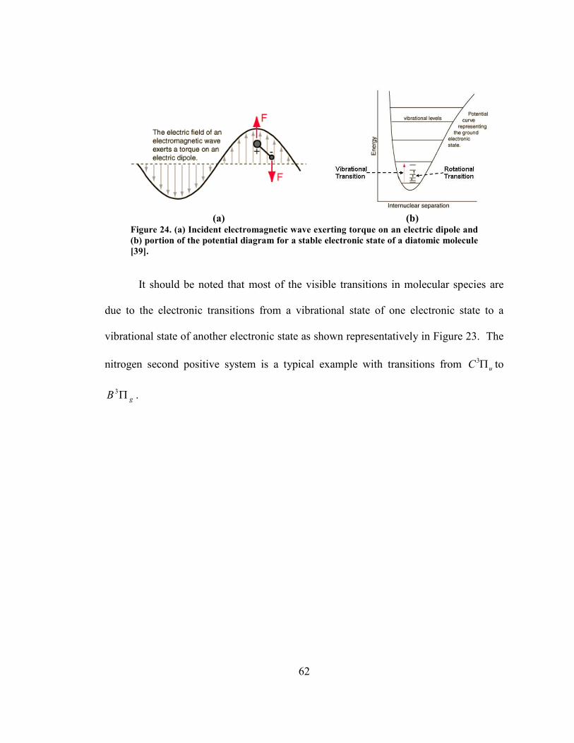
62
(a) (b)
Figure 24. (a) Incident electromagnetic wave exerting torque on an electric dipole and (b) portion of the potential diagram for a stable electronic state of a diatomic molecule [39].
It should be noted that most of the visible transitions in molecular species are
due to the electronic transitions from a vibrational state of one electronic state to a
vibrational state of another electronic state as shown representatively in Figure 23. The
nitrogen second positive system is a typical example with transitions from uC Π3 to
gB Π3 .

63
CHAPTER V
EXPERIMENTAL SETUP AND PROCEDURE
5.1 EXPERIMENTAL SETUP
To accomplish the tasks mentioned above, experiments were conducted using
different setups. The vacuum chambers used in these experiments are equipped with
various ports to accommodate gas inlet/outlet, optical windows for recording
PMT/Spectroscopy data and high voltage feed-throughs for electrical connections. The
voltage is monitored using a Tektronix p6015 high voltage probe. The current on the
cathode/ground connection is monitored using a Pearson coil. The data acquisition
system is configured to trigger off the light emission during the breakdown initiation.
This emission is monitored by a Hamamatsu Photo Multiplier Tube and the
corresponding current is converted to voltage using a Keithley 485 pico-ammeter and
then fed to a digital oscilloscope. A Tektronix TDS 2024 digital oscilloscope is used to
capture the voltage, current and the PMT data simultaneously.
The discharge current in these systems is mostly circuit/instrumentation
dependent and hence cannot be a very reliable trigger parameter. Also, to avoid
triggering off the small initial current, the initiation of the light emission recorded by
the PMT is used as the triggering mechanism for the diagnostic equipment instead of
the discharge current as done traditionally. Optical data is collected by means of video

64
camera (at 30 fps) for optical images, the PMT data for the time evolution of the light
emission from the breakdown events and optical spectrometer for emission spectra.
The videos are later converted into frame-by-frame still images to analyze the spatial
evolution of the discharge (Complete details in Chapter 6). The discharge spectrum is
acquired using an Ocean Optics HR2000+ Spectrometer (Range: 190 nm to 640 nm) and
Spectrasuite® software. Experiments are also conducted with dc source to obtain dc
breakdown data for comparison with the ac-high frequency data.
Figure 25. Vacuum Chamber Two electrode geometries are used all through the experiments; they are point-
to-point and point-to-plane as shown in Figure 26. The point-to-point setup consists of
two point electrodes made of stainless steel with a tip radius of 0.5 mm and placed 1 cm
apart. The point-plane setup consists of similar point electrode and a 4.8 cm diameter
copper disc placed 1 cm apart. For the point-to-plane configuration, the plane electrode
is always used as the ground/cathode and the point electrode always as the anode.
Figure 26. Electrode geometries used in current studies

65
The studies are conducted under three different applied voltages and to obtain
these voltages, the following configurations are used:
DC: A CVC SDC-100 High voltage dc power supply is used for dc breakdown
studies. The power supply has an internal current limiting mechanism and hence no
additional current limiting resistors were used in the external circuit.
Unipolar Sinusoidal waveform: A BK Precision-4040 20 MHz function
generator is used to produce a sinusoid of fixed frequency. This signal is fed to a
California Instruments 251 ac power supply which amplifies it to a maximum of 160 V
RMS. This signal is then connected to an in-house made step-up coil with a turns ratio
of 1:2.5 and the amplified output is then connected in series with a high voltage dc
power supply. Under normal conditions, the ac and the dc supplies are simultaneously
increased and the voltage applied across the electrodes is monitored to make sure that it
is a dc shifted unipolar sinusoid (with no net negative voltage).
Unipolar Square/Pulsed waveform: A BK Precision-4040 20 MHz function
generator is used to produce a dc shifted (unipolar) square pulse train of fixed duty
cycle. This pulse train and the adjustable output of a CVC SDC-100 high voltage dc
power supply are fed to a DEI PVX-4150 pulse generator. The output of this pulse
generator is an amplified square pulse train with rise and fall times within 20 ns and
with a maximum output voltage of ±1500 V.
The typical configuration of a complete setup comprises of the vacuum chamber
with all the desired ports, a power supply configured specifically for each experiment,
all the diagnostic equipment for measuring the breakdown voltage/current/light

66
emission/Spectrum and the data acquisition system to digitally store all this information.
One such setup is shown in the Figure 28.
(a) (b)
Figure 27. Power supply schematics (a) Unipolar sinusoid, (b) Unipolar square pulse
Figure 28. Schematic of the experimental setup with the diagnostics (point-to-plane electrode under unipolar sinusoidal applied voltage.
5.2 EXPERIMENTAL PROCEDURE
Experimental studies are conducted under the conditions listed above for helium
and nitrogen separately. For each configuration (electrode/applied signal/pressure) the
vacuum chamber is first thoroughly pumped down to under 100 milli Torr and then
brought to the desired pressure with the fill gas. The applied signal is gradually
increased at a rate of about 100 V/s until a breakdown is initiated. This is true for both

67
dc and unipolar pulsed/square applied fields. For unipolar sinusoidal fields, the ac
amplitude and the dc offset are simultaneously increased so as to make sure that the net
field is never negative. At the breakdown, voltage, current and light emission
waveforms of the events are collected. Once the required data is collected, the chamber
is flushed with the appropriate gas and the experiment is continued. For each condition,
at least three data points are collected and averaged. As the circuit is current limited, it
does not allow the breakdown to grow into an arc with complete voltage collapse, but
allows the development of a glow discharge across the electrodes for just a few
milliseconds after the initiation. The primary focus of this study is on the breakdown
voltage and not on the corona discharge inception voltage. Hence, only the breakdown
voltage is recorded. The discharge current in these systems is mostly
circuit/instrumentation dependent and hence is not analyzed as an experimental
parameter.
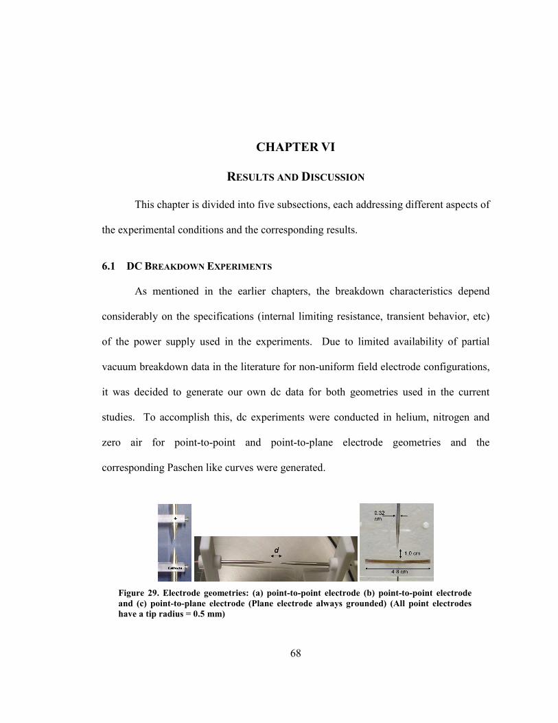
68
CHAPTER VI
RESULTS AND DISCUSSION
This chapter is divided into five subsections, each addressing different aspects of
the experimental conditions and the corresponding results.
6.1 DC BREAKDOWN EXPERIMENTS As mentioned in the earlier chapters, the breakdown characteristics depend
considerably on the specifications (internal limiting resistance, transient behavior, etc)
of the power supply used in the experiments. Due to limited availability of partial
vacuum breakdown data in the literature for non-uniform field electrode configurations,
it was decided to generate our own dc data for both geometries used in the current
studies. To accomplish this, dc experiments were conducted in helium, nitrogen and
zero air for point-to-point and point-to-plane electrode geometries and the
corresponding Paschen like curves were generated.
Figure 29. Electrode geometries: (a) point-to-point electrode (b) point-to-point electrode and (c) point-to-plane electrode (Plane electrode always grounded) (All point electrodes have a tip radius = 0.5 mm)

69
The experimental setup for these studies is detailed in Chapter 5. The electrode
configurations used through out these studies are given in Figure 29. For helium, the
electrode gap is fixed at 1 cm and for nitrogen and zero air it is 0.5 cm.
6.1.1 POINT-TO-POINT CONFIGURATION
A dc voltage is applied across the electrodes in Figure 29a and is gradually
increased until a breakdown event is registered. The initiation is captured by a PMT
due to the light emission from the discharge. Representative voltage, current and light
emission waveforms captured at the breakdown are shown in Figure 30. Similar plots
were collected over the entire pressure range of interest. For each of these waveforms,
the voltage at the breakdown is calculated from the plots and a Paschen like, pressure
versus breakdown voltage plot is generated. Figure 31 shows such plot for the point-to-
point configuration for nitrogen. Similar experiments were also conducted in helium
and the corresponding plot is shown in Figure 32.
Figure 30. Voltage (top), current (middle) and optical emission (bottom) waveforms of a breakdown event point-to-plane electrode geometry for dc applied voltage.
For comparison with the literature data, these two breakdown plots are
superimposed to form Figure 33. The corresponding data for parallel plane setup from

70
the literature is plotted in Figure 34. There is considerable similarity in these plots in
terms of the relative positions of the voltage minimums for helium and nitrogen. The
actual voltages however can not be directly compared due to the reasons mentioned
earlier.
Figure 31. Breakdown voltage of nitrogen under dc fields for point-to-point electrode configuration.
Figure 32. Breakdown voltage of helium under dc fields for point-to-point electrode configuration.
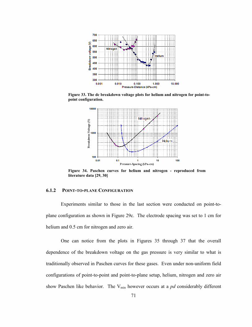
71
Figure 33. The dc breakdown voltage plots for helium and nitrogen for point-to-point configuration.
Figure 34. Paschen curves for helium and nitrogen - reproduced from literature data [29, 30]
6.1.2 POINT-TO-PLANE CONFIGURATION
Experiments similar to those in the last section were conducted on point-to-
plane configuration as shown in Figure 29c. The electrode spacing was set to 1 cm for
helium and 0.5 cm for nitrogen and zero air.
One can notice from the plots in Figures 35 through 37 that the overall
dependence of the breakdown voltage on the gas pressure is very similar to what is
traditionally observed in Paschen curves for these gases. Even under non-uniform field
configurations of point-to-point and point-to-plane setup, helium, nitrogen and zero air
show Paschen like behavior. The Vmin however occurs at a pd considerably different
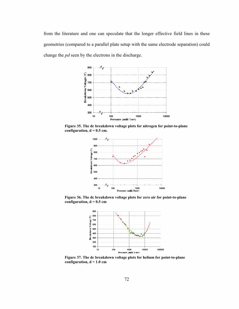
72
from the literature and one can speculate that the longer effective field lines in these
geometries (compared to a parallel plate setup with the same electrode separation) could
change the pd seen by the electrons in the discharge.
Figure 35. The dc breakdown voltage plots for nitrogen for point-to-plane configuration, d = 0.5 cm.
Figure 36. The dc breakdown voltage plots for zero air for point-to-plane configuration, d = 0.5 cm
Figure 37. The dc breakdown voltage plots for helium for point-to-plane configuration, d = 1.0 cm

73
Figure 38. Sample frames captured during the breakdown event for dc fields in helium at 1.6 Torr. Captured at 30 fps, each consecutive frame is about 33 ms apart.
The optical images collected during these breakdown events were later used for
further analysis as explained in detail in the next chapter. Figure 38 shows one such
sequence of images captured for point-to-point configuration.
6.2 UNIPOLAR 20 KHZ SINUSOID BREAKDOWN EXPERIMENTS This section deals with the breakdown characteristics of point-to-point and
point-to-plane configurations under helium, nitrogen and zero air subject to a dc offset
unipolar sinusoid (with no negative value). This voltage is generated using the system
described in Chapter 5 by connecting a high voltage dc supply in series with the
amplified output of an ac source. The complete experimental setup for these studies is
mentioned in detail in earlier chapter. The electrode configurations used in these
studies are given in Figure 39.
Figure 39. Electrode geometries: (a) point-to-point electrode (b) point-to-point electrode and (c) point-to-plane electrode (Plane electrode always grounded) (All point electrodes have a tip radius = 0.5 mm)
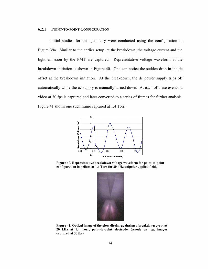
74
6.2.1 POINT-TO-POINT CONFIGURATION
Initial studies for this geometry were conducted using the configuration in
Figure 39a. Similar to the earlier setup, at the breakdown, the voltage current and the
light emission by the PMT are captured. Representative voltage waveform at the
breakdown initiation is shown in Figure 40. One can notice the sudden drop in the dc
offset at the breakdown initiation. At the breakdown, the dc power supply trips off
automatically while the ac supply is manually turned down. At each of these events, a
video at 30 fps is captured and later converted to a series of frames for further analysis.
Figure 41 shows one such frame captured at 1.4 Torr.
Figure 40. Representative breakdown voltage waveform for point-to-point configuration in helium at 1.4 Torr for 20 kHz unipolar applied field.
Figure 41. Optical image of the glow discharge during a breakdown event at 20 kHz at 1.4 Torr, point-to-point electrode. (Anode on top, images captured at 30 fps).
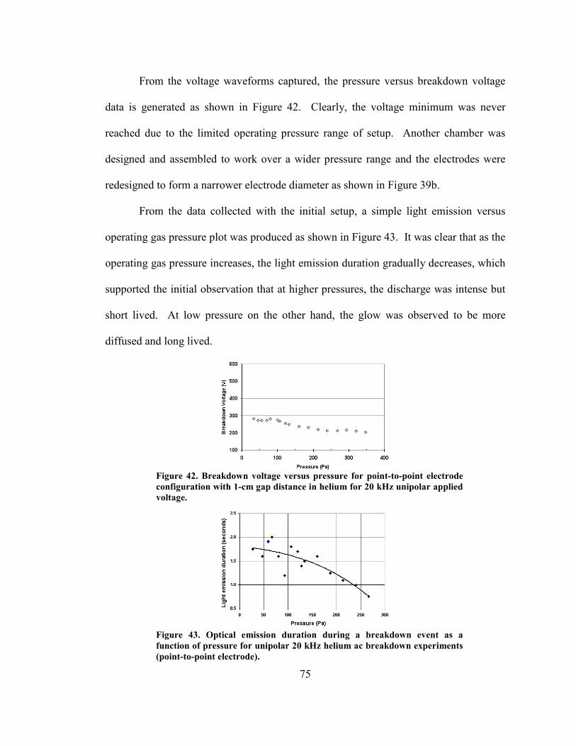
75
From the voltage waveforms captured, the pressure versus breakdown voltage
data is generated as shown in Figure 42. Clearly, the voltage minimum was never
reached due to the limited operating pressure range of setup. Another chamber was
designed and assembled to work over a wider pressure range and the electrodes were
redesigned to form a narrower electrode diameter as shown in Figure 39b.
From the data collected with the initial setup, a simple light emission versus
operating gas pressure plot was produced as shown in Figure 43. It was clear that as the
operating gas pressure increases, the light emission duration gradually decreases, which
supported the initial observation that at higher pressures, the discharge was intense but
short lived. At low pressure on the other hand, the glow was observed to be more
diffused and long lived.
Figure 42. Breakdown voltage versus pressure for point-to-point electrode configuration with 1-cm gap distance in helium for 20 kHz unipolar applied voltage.
Figure 43. Optical emission duration during a breakdown event as a function of pressure for unipolar 20 kHz helium ac breakdown experiments (point-to-point electrode).

76
6.2.2 POINT-TO-PLANE CONFIGURATION
Similar to the point-to-point configuration, the point-to-plane configuration
studies involved acquiring the voltage, current and the light emission data at the
breakdown. A representative plot is shown in Figure 44. For initial studies, the
experiments were conducted from 0.10 to 3.00 Torr. The breakdown voltage variation
with gas pressure for helium is shown in Figure 45.
Figure 44. Voltage (top), current (middle) and optical emission (bottom) waveforms of a breakdown event at 1.8 Torr helium for point-to-plane electrode geometry at unipolar 20 kHz applied voltage.
Figure 45. Breakdown voltage versus pressure for point-to-plane electrode configuration with 1-cm gap distance in Helium for unipolar 20 kHz sinusoid applied voltages.
Similar to the earlier cases, the frame by frame images were generated at each
breakdown event for further analysis. Figure 46 shows one such frame collected at 1.6

77
Torr in helium. The operating pressure range was not enough to conclusively determine
the voltage minimum and the corresponding pd minimum. However, the data collected
from the initial setup proved useful in determining the current variation with operating
pressure. Figure 47 shows the variation of the peak current registered at the breakdown
as a function of the operating gas pressure. One may notice a gradual increase in the
peak current as the operating pressure increases beyond 0.7 to 1.0 Torr.
The experiments were then conducted in a new chamber capable of wider
operating pressure range to conclusively determine the voltage minimum and the
corresponding pd for nitrogen and zero air. Figure 48 shows a typical voltage
waveform at the breakdown and the light emission registered by the PMT. From these
plots, the breakdown voltage at each pressure was determined. Figures 49 and 50
respectively show the breakdown voltage versus operating pressure for nitrogen and
zero air for point-to-plane configuration.
Figure 46. Optical images of the glow discharge during a breakdown event at unipolar 20 kHz sinusoid at 1.6 Torr, point-to-plane electrode. (Images captured at 30 fps).

78
Figure 47. Transient current peak as a function of pressure for point-to-plane electrode geometry at 20 kHz
Figure 48. A typical applied voltage pulse at 20 kHz 0.2 Torr nitrogen showing the pulse shape just at the breakdown. The bottom plot shows the light emission recorded by the PMT.
Figure 49. Breakdown voltage as a function of pressure for point-to-plane electrode configuration with 0.5-cm gap distance for 20 kHz unipolar sinusoid signal for nitrogen.
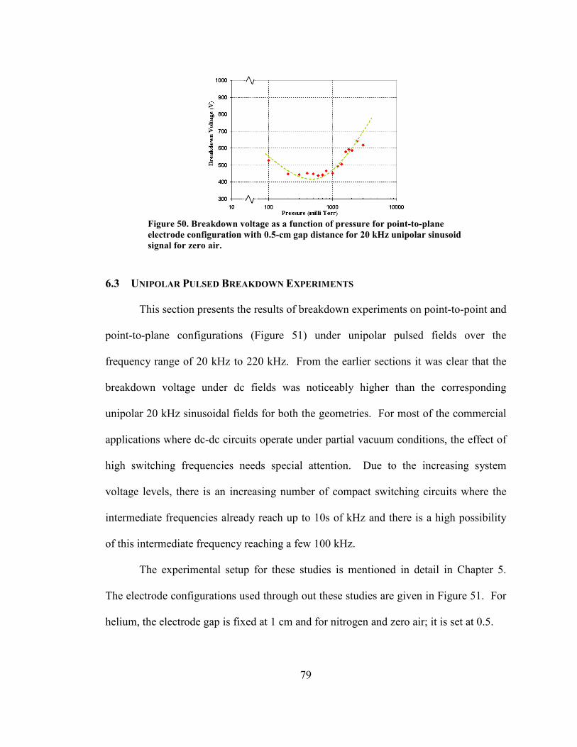
79
Figure 50. Breakdown voltage as a function of pressure for point-to-plane electrode configuration with 0.5-cm gap distance for 20 kHz unipolar sinusoid signal for zero air.
6.3 UNIPOLAR PULSED BREAKDOWN EXPERIMENTS This section presents the results of breakdown experiments on point-to-point and
point-to-plane configurations (Figure 51) under unipolar pulsed fields over the
frequency range of 20 kHz to 220 kHz. From the earlier sections it was clear that the
breakdown voltage under dc fields was noticeably higher than the corresponding
unipolar 20 kHz sinusoidal fields for both the geometries. For most of the commercial
applications where dc-dc circuits operate under partial vacuum conditions, the effect of
high switching frequencies needs special attention. Due to the increasing system
voltage levels, there is an increasing number of compact switching circuits where the
intermediate frequencies already reach up to 10s of kHz and there is a high possibility
of this intermediate frequency reaching a few 100 kHz.
The experimental setup for these studies is mentioned in detail in Chapter 5.
The electrode configurations used through out these studies are given in Figure 51. For
helium, the electrode gap is fixed at 1 cm and for nitrogen and zero air; it is set at 0.5.
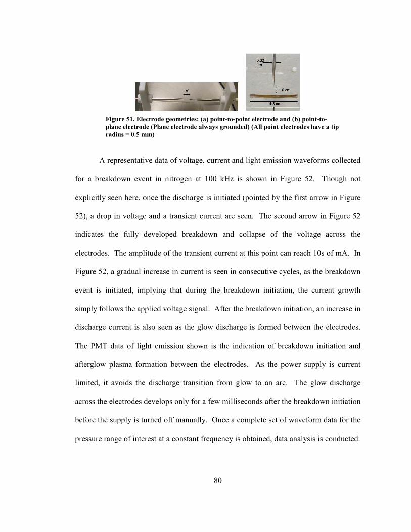
80
Figure 51. Electrode geometries: (a) point-to-point electrode and (b) point-to-plane electrode (Plane electrode always grounded) (All point electrodes have a tip radius = 0.5 mm)
A representative data of voltage, current and light emission waveforms collected
for a breakdown event in nitrogen at 100 kHz is shown in Figure 52. Though not
explicitly seen here, once the discharge is initiated (pointed by the first arrow in Figure
52), a drop in voltage and a transient current are seen. The second arrow in Figure 52
indicates the fully developed breakdown and collapse of the voltage across the
electrodes. The amplitude of the transient current at this point can reach 10s of mA. In
Figure 52, a gradual increase in current is seen in consecutive cycles, as the breakdown
event is initiated, implying that during the breakdown initiation, the current growth
simply follows the applied voltage signal. After the breakdown initiation, an increase in
discharge current is also seen as the glow discharge is formed between the electrodes.
The PMT data of light emission shown is the indication of breakdown initiation and
afterglow plasma formation between the electrodes. As the power supply is current
limited, it avoids the discharge transition from glow to an arc. The glow discharge
across the electrodes develops only for a few milliseconds after the breakdown initiation
before the supply is turned off manually. Once a complete set of waveform data for the
pressure range of interest at a constant frequency is obtained, data analysis is conducted.

81
Figure 52. Typical Breakdown voltage (middle), current from the Pearson coil (top) and the light emission waveforms (bottom) at 0.4 Torr for a 100 kHz applied field in nitrogen. The first arrow indicates the breakdown initiation and the second indicates the formation of fully developed breakdown.
From the voltage waveforms, the breakdown voltages as a function of gas
pressure for a fixed signal frequency are obtained. Same procedure is repeated for other
frequencies. It should be noted that the focus here is primarily on the “breakdown
voltage” which is the worst case scenario and not on the corona discharge inception
voltage. Hence, only the breakdown voltage is recorded without much significance
given to the corona inception voltage.
6.3.1 BREAKDOWN VOLTAGE VERSUS GAS PRESSURE
The breakdown data is collected over the pressure range of 0.2 to 10.0 Torr for
both helium and nitrogen gases for signal frequencies ranging from 50 to 200 kHz using
point-to-point and point-to-plane configurations. For clarity, these four plots are shown
individually in Figures 53 through 56. In addition to the high frequency square-wave

82
breakdown curves, dc breakdown data is also presented in these figures for comparison.
Since the classical Paschen curves in the literature are typically for parallel plate
electrode configuration and either dc or 400 Hz, a direct comparison of our breakdown
data is not easily possible. Furthermore, there are no extensive high frequency
electrical breakdown data in kHz range in the literature for similar electrode
configuration under partial vacuum conditions.
It should be noted that the electrode configuration in the literature that closely
resembles our setup was obtained primarily for atmospheric pressures and for power
distribution related systems, whereas the data here is for partial vacuum conditions.
Therefore, no attempt is made here to directly compare this data with the data available
in the literature. The plots in figures above show similar behavior to the earlier results
from unipolar 20 kHz sinusoidal fields and the other predictions present in [2], showing
that the breakdown voltages at higher frequencies are lower than the dc breakdown
voltages and these plots are similar to the Paschen curves [29].
Figure 53. Breakdown voltage as a function of pressure at dc, 50 kHz and 150 kHz signals for helium, point-to-point configuration.

83
Figure 54. Breakdown voltages as a function of pressure at dc, 50 kHz, 100 kHz, 150 kHz, and 200 kHz in nitrogen, point-to-point configuration. The doted line (top) is dc data and the dashed line (bottom) is the average of the high frequency breakdown data.
Figure 55. Breakdown voltage as a function of pressure at 50 kHz, 100 kHz, 150 kHz and 200 kHz signals for helium, point-to-plane configuration.
Figure 56. Breakdown voltage as a function of pressure at dc, 50 kHz and 150 kHz signals for nitrogen, point-to-plane configuration.
6.3.2 BREAKDOWN VOLTAGE – SIGNAL FREQUENCY
Although the frequency effect on breakdown is seen in Figures 53 through 56,
the breakdown voltage behavior as a function of signal frequency is not apparent. To

84
investigate this effect, experiments were conducted at constant pressures while varying
the signal frequency from 20 to 220 kHz. This data is presented in Figures 57 for
helium and in Figure 58 for nitrogen for point-to-point configuration. The constant
pressures of 1.2 Torr and 2.0 Torr used in these events are chosen at the points close to
the Paschen like minimum observed in Figure 53 for helium. For nitrogen, the chosen
pressures are 0.4 Torr - representing points close to the voltage minimum, 1.2 Torr for
comparison with helium data, and 2.4 Torr where the difference between the breakdown
voltages at different frequencies is the lowest in Figure 54. Similar data was also
collected for nitrogen and zero air for point-to-plane configuration and is presented in
Figures 59 and 60.
Figure 57. Breakdown voltage as a function of the applied signal frequency for helium at 1.2 Torr and 2.0 Torr, point-to-point configuration. The voltage variation seems to be a double-exponential function of the signal frequency. A possible curve fit of the form
)0003.0exp(254)0454.0exp(219)( fffV ∗−∗+∗−∗= is shown (V(f) in Volts and f in
kHz).

85
Figure 58. Nitrogen breakdown voltage as a function of frequency at 0.4, 1.2 and 2.4 Torr pressures, point-to-point configuration. (V is in Volts and f in kHz).
Figure 59. Breakdown voltage as a function of signal frequency for unipolar pulsed square wave, for nitrogen for point-to-plane configuration. V(0.4) and V(1.2) correspond to the breakdown voltage at gas pressures of 0.4 and 1.2 Torr respectively.
Figure 60. Breakdown voltage as a function of signal frequency for unipolar pulsed square wave, for zero air for point-to-plane configuration. V(0.4) and V(1.2) correspond to the breakdown voltage at gas pressures of 0.4 and 1.2 Torr respectively.

86
In case of helium in Figure 57, a consistent drop in breakdown voltage with
applied signal frequency is observed. This reduction in breakdown voltage exhibits a
double-exponential dependence on the signal frequency. One could speculate that this
trend will probably continue further down the frequency scale into early MHz/GHz
range till the electron resonance effects start dominating. Once this high frequency
effects at MHz/GHz ranges start dominating the breakdown processes, the well known
multipactor phenomenon is observed and the breakdown voltage will start rising [19].
Clearly, the lowering of the breakdown voltage in the current study can not be attributed
to the electron resonance effects [31]. Under the pressure, temperature and field
strength conditions of our set up, the electron resonance frequency is in the range of
MHz/GHz, which is at least an order of magnitude higher than the applied signal
frequency (100 kHz range).
In Pfeiffer’s earlier work on high frequency breakdown [13] (75 kHz and MHz
ranges, in atmospheric pressure), it was proposed that the ions (positive and negative)
do not have sufficient time between the other half-cycles of the field to be extracted
from the gap, and this, resulting in field distortion, is given as a possible explanation for
the lowering of breakdown voltage from the dc values. Although there are similarities,
in our study, instead of having a field reversal (“negative” voltage for the other half-
cycle), we have an “off” state (no applied field for that half-cycle). One should expect
the charged species (ions and electrons) to drift during this “off” state, but still carry
some of the energy gained during the previous “on” state of the field. This basically
could lead to an increased number of collision sites for the next pulse of the applied
voltage. Compared to dc fields, one can therefore expect additional charges in the gap

87
through increased collisions with the background gas. This might be a possible reason
for lower breakdown voltage amplitudes under unipolar pulsed signals compared to the
dc case. However, for conclusive explanations, further studies are needed. Also, one
should note that there are fundamental differences between [13] and the current study;
one is true ac in atmospheric pressure, while ours is unipolar in partial vacuum.
Therefore, the differences in breakdown mechanisms between the two are to be
expected.
Based on the data presented above in helium for breakdown voltage versus
signal frequency, a curve fitting resulted in a function of the form
)exp()exp()( fdcfbafV ∗∗+∗∗= , where f is in kHz and V is in Volts. There could
also be other functions fit to this data. In case of nitrogen, as seen in Figure 58, the
breakdown voltage variation with the signal frequency compared to helium is not as
prominent. We do however, notice that the voltage decreases as the signal frequency is
increased, but at a lot slower rate compared to helium. To show this decrease, Figure
58 also shows linear fits of the form bfafV +∗=)( , where f is in kHz and V is in
Volts for the data collected in the frequency range studied here, and a negative gradient
(‘a’ in the above equation) can be seen for all the pressures studied. It is essential to
note that the curve fit equations shown in Figures 57 and 58, result in the dc breakdown
voltages (by substituting f = 0) very close to what is presented in Figures 53 and 54
respectively. These differences between the linear and the double-exponential behavior
of breakdown voltages as a function of frequency have not been studied. However, one
can suspect this to be due to the differences in species, i.e. atomic state versus diatomic
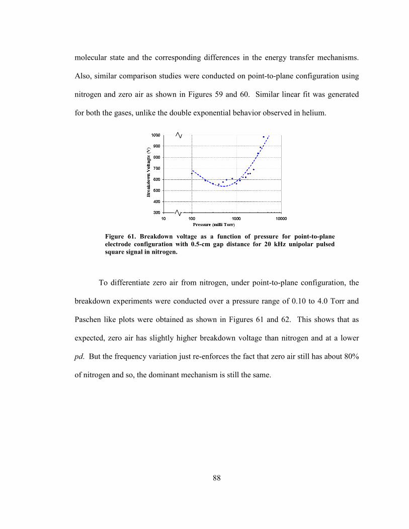
88
molecular state and the corresponding differences in the energy transfer mechanisms.
Also, similar comparison studies were conducted on point-to-plane configuration using
nitrogen and zero air as shown in Figures 59 and 60. Similar linear fit was generated
for both the gases, unlike the double exponential behavior observed in helium.
Figure 61. Breakdown voltage as a function of pressure for point-to-plane electrode configuration with 0.5-cm gap distance for 20 kHz unipolar pulsed square signal in nitrogen.
To differentiate zero air from nitrogen, under point-to-plane configuration, the
breakdown experiments were conducted over a pressure range of 0.10 to 4.0 Torr and
Paschen like plots were obtained as shown in Figures 61 and 62. This shows that as
expected, zero air has slightly higher breakdown voltage than nitrogen and at a lower
pd. But the frequency variation just re-enforces the fact that zero air still has about 80%
of nitrogen and so, the dominant mechanism is still the same.

89
Figure 62. Breakdown voltage as a function of pressure for point-to-plane electrode configuration with 0.5-cm gap distance for 20 kHz unipolar pulsed square signal in zero air.
In conclusion, it is observed that the unipolar high frequency breakdown voltage
of helium, nitrogen and zero air in partial vacuum, for point-to-point and point-to-plane
field configurations has a behavior similar to a typical Paschen curve. Comparing the
dc data obtained for same electrode configuration and experimental conditions to the
kHz data, it is observed that the high frequency breakdown voltages are relatively lower
than the dc breakdown voltages. Also, with increasing signal frequency there is a
consistent decrease in the breakdown voltage for all three gases in the kHz range
studied here. However, the rate of decrease in the breakdown voltage for nitrogen/zero
air is not as drastic as it is seen in the case of helium. Helium seems to have a double-
exponential dependence on the applied frequency whereas nitrogen/zero air seem to
have a linear dependence. Extrapolating the “curve-fit” equations presented here to
zero frequency yields data close to the dc breakdown data observed in our experiments.
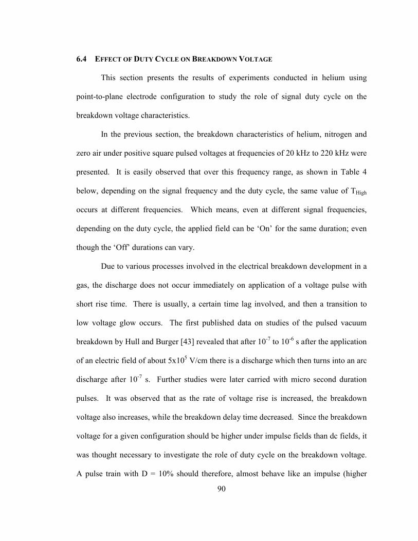
90
6.4 EFFECT OF DUTY CYCLE ON BREAKDOWN VOLTAGE
This section presents the results of experiments conducted in helium using
point-to-plane electrode configuration to study the role of signal duty cycle on the
breakdown voltage characteristics.
In the previous section, the breakdown characteristics of helium, nitrogen and
zero air under positive square pulsed voltages at frequencies of 20 kHz to 220 kHz were
presented. It is easily observed that over this frequency range, as shown in Table 4
below, depending on the signal frequency and the duty cycle, the same value of THigh
occurs at different frequencies. Which means, even at different signal frequencies,
depending on the duty cycle, the applied field can be ‘On’ for the same duration; even
though the ‘Off’ durations can vary.
Due to various processes involved in the electrical breakdown development in a
gas, the discharge does not occur immediately on application of a voltage pulse with
short rise time. There is usually, a certain time lag involved, and then a transition to
low voltage glow occurs. The first published data on studies of the pulsed vacuum
breakdown by Hull and Burger [43] revealed that after 10-7 to 10-6 s after the application
of an electric field of about 5x10⁵ V/cm there is a discharge which then turns into an arc
discharge after 10-7 s. Further studies were later carried with micro second duration
pulses. It was observed that as the rate of voltage rise is increased, the breakdown
voltage also increases, while the breakdown delay time decreased. Since the breakdown
voltage for a given configuration should be higher under impulse fields than dc fields, it
was thought necessary to investigate the role of duty cycle on the breakdown voltage.
A pulse train with D = 10% should therefore, almost behave like an impulse (higher

91
breakdown voltage than dc) while the one with D = 90% should have breakdown
voltage closer to the dc level, as long as the rise times are unaltered. From the earlier
work, it was found that discharges occur mostly on the impulse front. From the data
here, it is clear that for a given rise time and frequency, the breakdown voltage depends
on the duty cycle. For a given frequency, smaller duty cycle provides more time for the
charges to diffuse, thereby reducing the residual field in the gap and hence increasing
the inception voltage.
Table 4. Duty cycle and the corresponding THigh / TLow at various frequencies.
D% / freq 50 kHz 100 kHz 150 kHz 200 kHz
10 % 2.00 / 18.00 1.00 / 9.00 0.67 / 6.00 0.50 / 4.50
20 % 4.00 / 16.00 2.00 / 8.00 1.33 / 5.33 1.00 / 4.00
30 % 6.00 / 14.00 3.00 / 7.00 2.00 / 4.67 1.50 / 3.50
40 % 8.00 / 12.00 4.00 / 6.00 2.67 / 4.00 2.00 / 3.00
50 % 10.0 / 10.0 5.00 / 5.00 3.33 / 3.33 2.50 / 2.50
60 % 12.00 / 8.00 6.00 / 4.00 4.00 / 2.67 3.00 / 2.00
70 % 14.00 / 6.00 7.00 / 3.00 4.67 / 2.00 3.50 / 1.50
80 % 16.00 / 4.00 8.00 / 2.00 5.33 / 1.33 4.00 / 1.00
90 % 18.00 / 2.00 9.00 / 1.00 6.00 / 0.67 4.50 / 0.50
It is important to note that the study of the development of vacuum breakdown
under short rise time pulses can only be qualitative, as the processes contributing to the
initiation most likely depend on the rate of rise of the applied voltage. It has been
shown in the literature that the transient processes in 1 mm gaps can stay up to 100 ms
[43], therefore, it is preferable to use voltage pulses with rise times in 10-9 s range. The
configuration used for this study consisted of a point-to-point electrode setup placed 1

92
cm apart in partial pressure helium and the pulsed voltages are produced using a
commercial pulse generator with rise and fall times under 25 ns. To understand the
effect of the duty cycle on the breakdown voltage, a signal with fixed frequency and
duty cycle ranging from 10% to 90% was applied. Figure 63 shows typical voltage and
light emission waveforms captured at the breakdown for a 50 kHz pulse at 20 % duty
cycle. From Table 4 and Figure 64, the TOn or THigh for this pulse train is same as the
corresponding TOn for 100 kHz 40 % duty cycle, 150 kHz 60 % duty cycle and 200 kHz
80 % duty cycle signals.
Figure 63. Voltage waveform acquired at the breakdown for 1 Torr and 50 kHz frequency with 20 % duty cycle. Arrow indicates the breakdown initiation time.
The variation of breakdown voltage with applied signal duty cycle for the case
of 100 kHz and 150 kHz signals is shown in Figure 65. As discussed earlier, the
breakdown voltage decreases as the duty cycle increases from 10 % and after 30-40% it
gradually increases. Due to the limited number of data points here, we can not
conclusively estimate the minimum to occur at a certain duty cycle. However, the data
here for both frequencies confirm the initial speculation on the role of the signal duty
cycle.

93
It should be noted here that the breakdown voltages are low compared to
literature data. This could be due to the low gas pressure and comparatively low
resistance of the circuitry. In dc breakdown studies, the system resistance is usually
high, but to obtain the rapidly rising short pulses, it is necessary to keep the system
resistance low, pushing the operating currents higher; this considerably changes the
behavior of the power supply and hence the breakdown characteristics being studied.
Figure 64. Typical voltage waveforms at 50 kHz and different (10, 30, 50, 70, and 90%) duty cycles.
(a) (b)
Figure 65. Breakdown voltage versus duty cycle at 1.2 Torr (a) 100 kHz and (b) 150 kHz for helium under point-to-point configuration

94
One possible reason for this behavior is that, during the part of the cycle with no
field (referred here as ‘the relaxation time’ or the ‘Off’ time), the electrons/ions formed
during the earlier part of the cycle diffuse to larger areas and help form the seed
electrons/ions for collision processes in the following part of the cycle. Unlike dc
fields, where the motion is dominated by drift, one can speculate that in unipolar fields,
the motion is dominated by drift during TOn and diffusion during TOff, resulting in
increased collisions for the successive cycles.
Further studies are required over a wider frequency range to understand the
breakdown variation with duty cycle and to determine if the lowest voltage occurs at a
certain duty cycle % or for a certain value of THigh depending on the gas being
investigated.
6.5 OPTICAL SPECTROSCOPY
When investigating the breakdown properties of gaseous media, understanding
the characters of the discharge such as the space-charge distribution, the energy of the
carriers, and the electrical field in the discharge region would prove very useful. A
spectroscopic study of the discharge is one way of obtaining such information. Physical
data on the elementary excitation processes is not exhaustive and in particular not
always very accurate. But this information helps in analyzing spectroscopic results to
obtain information on the mechanisms of a gas discharge. As the normal discharges are
mostly repeatable, and typically develop through discrete phases, it is necessary in the
future to develop a time-resolved study of the spectrum for each breakdown event. This

95
is beyond the scope of this work and only the spectral data at discrete times are
discussed here.
For the current studies, the gaseous breakdown is observed by (a) a photo
multiplier tube which integrates the light over the whole spectrum (depending on the
spectral window of the PMT) and by (b) a spectrometer looking into the discharge. The
discharge under these conditions is expected to develop in stages, each of which is
usually associated with a small transient pulse on the PMT output. The amplitude of
these light pulses varies considerably with consecutive shots but is typical of the
electrode geometry. These pulses, if observed, could explain the difference between the
first leader corona and the rest of the follower lines in the glow discharge. To analyze
the corona spectra, the lines have been identified by the wavelengths corresponding to
the known systems in the literature from wavelength tables. In addition, the measured
intensity ratios of these bands should approximately correspond to the excitation and
transition probabilities in the literature.
Once the breakdown voltage behavior is documented, the glow discharge
spectra are analyzed. The HR-2000+ spectrometer from Ocean Optics is used for this
purpose. This device is capable of monitoring the spectra from 190 nm to 640 nm. The
spectra collected contain the intensity variation of wavelengths over time by gating the
CCDs. This data results in 3-D plots of light emission (i.e. Intensity versus wavelength
and time). A snapshot of this data over the entire wavelength range (after a finite delay
after the breakdown initiation) is usually analyzed for the known transitions. One such
spectrum for nitrogen breakdown under 100 kHz unipolar pulsed fields is shown in
96
Figure 66; the integration time for this data was set at 10 ms. Figure 67 shows similar
plot for helium under the same experimental conditions.
Figure 66. Nitrogen spectrum at 1.2 Torr for 100 kHz unipolar pulsed field and 10 ms integration time. (Point-to-point electrode configuration)
To understand the time variation of the intensities, for each of the two most
dominant lines in Figure 66 and 67, a plot of intensity versus time was generated from
the original data collected by the spectrometer. This data is shown in Figure 68 and 69
for nitrogen and helium respectively. Both these plots show periods of complete
inactivity at the chosen wavelengths. To determine whether this was truly the case or
due to the limitation of the diagnostic equipment, a He-Ne laser was shone on the
electrode setup during the breakdown event and the discharge spectrum was collected.
The third additional line in Figure 68 shows this He-Ne line and is unaltered during the
entire time. This clearly indicated that the glow in fact fluctuates. Similar behavior was
also seen in case of helium as seen in Figure 69.

97
Figure 67. Helium spectrum at 1.2 Torr for 100 kHz unipolar pulsed field and 10 ms integration time. (Point-to-point electrode configuration)
Figure 68. Variation of intensity with time for the two most dominant wavelengths in Figure 66, corresponding to the (0, 0) and (0, 1) lines in the first negative system of nitrogen.
Similar studies were also conducted on point-to-plane configuration. One such
spectrum for a dc breakdown event in nitrogen is given in Figure 70. This data is
obtained by gating the CCD to 2 ms integration time. The most dominant wavelength
in this plot corresponds to a (0, 0) transition of first negative system in nitrogen at 391.4
nm. A similar pattern was observed at other pressures also. The most intense lines

98
from this figure and the corresponding electron transitions and intensities are listed in
Table 5. Figure 71 shows the potential energy diagram of nitrogen molecule relevant to
the first negative and the second positive systems. Notice that the energy levels
corresponding to the transitions observed here are within 3 to 4 eV. To compare the
electron transitions in nitrogen discharge and the discharge in zero air, a similar spectra
snapshot was taken at 0.4 Torr and 20 kHz pulsed applied field as shown in Figure 72.
To better analyze the spectral lines, the points in Figure 72 are shifted and a narrower
spectral window is plotted. Unlike what was initially expected, there were no oxygen
lines in this range. Further analysis revealed that the wavelength range used in this
study is too narrow to detect the most common lines in oxygen spectra which are
usually either in the IR or UV ranges. However, during the experiments, a noticeably
bright red/pink glow was observed in zero air discharge which we suspect would be in
the higher wavelengths (IR), corresponding to the oxygen molecular lines. In nitrogen
experiments, these lines correspond to the radiation of nitrogen molecules, both neutral
(second positive) and ionized (first negative system). However, there was no significant
contribution from the atomic nitrogen. The lines of the ‘First negative system’ usually
correspond to the transitions seen in the cathode glow of the discharge and those of the
‘Second positive system’ are normally observed in the positive column of the discharge.
In the near-UV region, the main spectral component is the strong radiation of the
nitrogen (second positive/first negative) system.

99
Figure 69. Variation of intensity with time for the two most dominant wavelengths in helium discharge in Figure 67.
Figure 70. Spectrum of the dc nitrogen discharge for point-to-plane setup at 0.8 Torr.
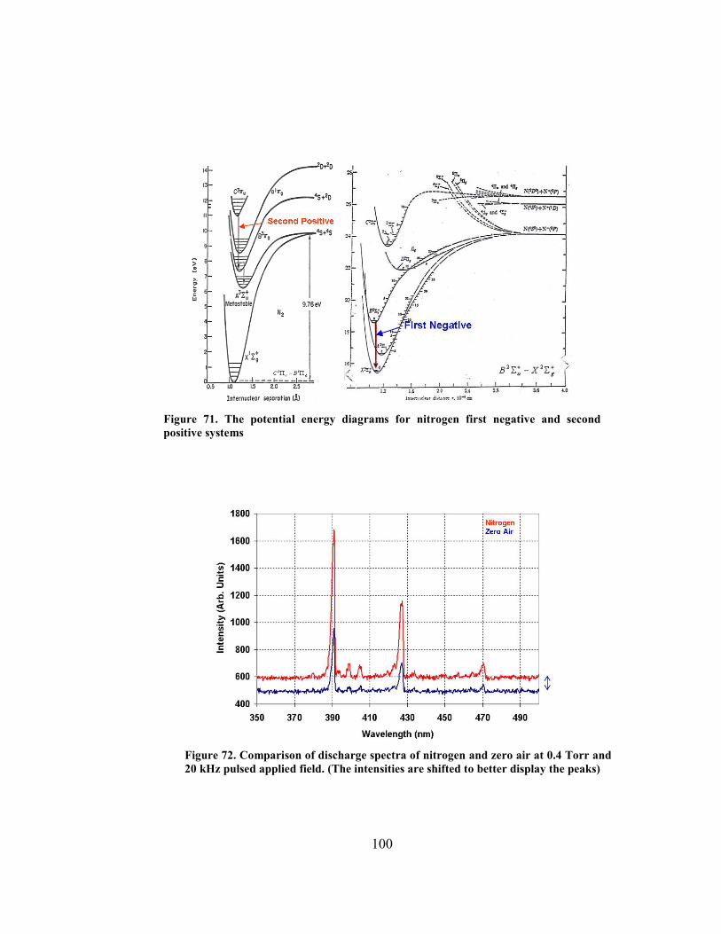
100
Figure 71. The potential energy diagrams for nitrogen first negative and second positive systems
Figure 72. Comparison of discharge spectra of nitrogen and zero air at 0.4 Torr and 20 kHz pulsed applied field. (The intensities are shifted to better display the peaks)
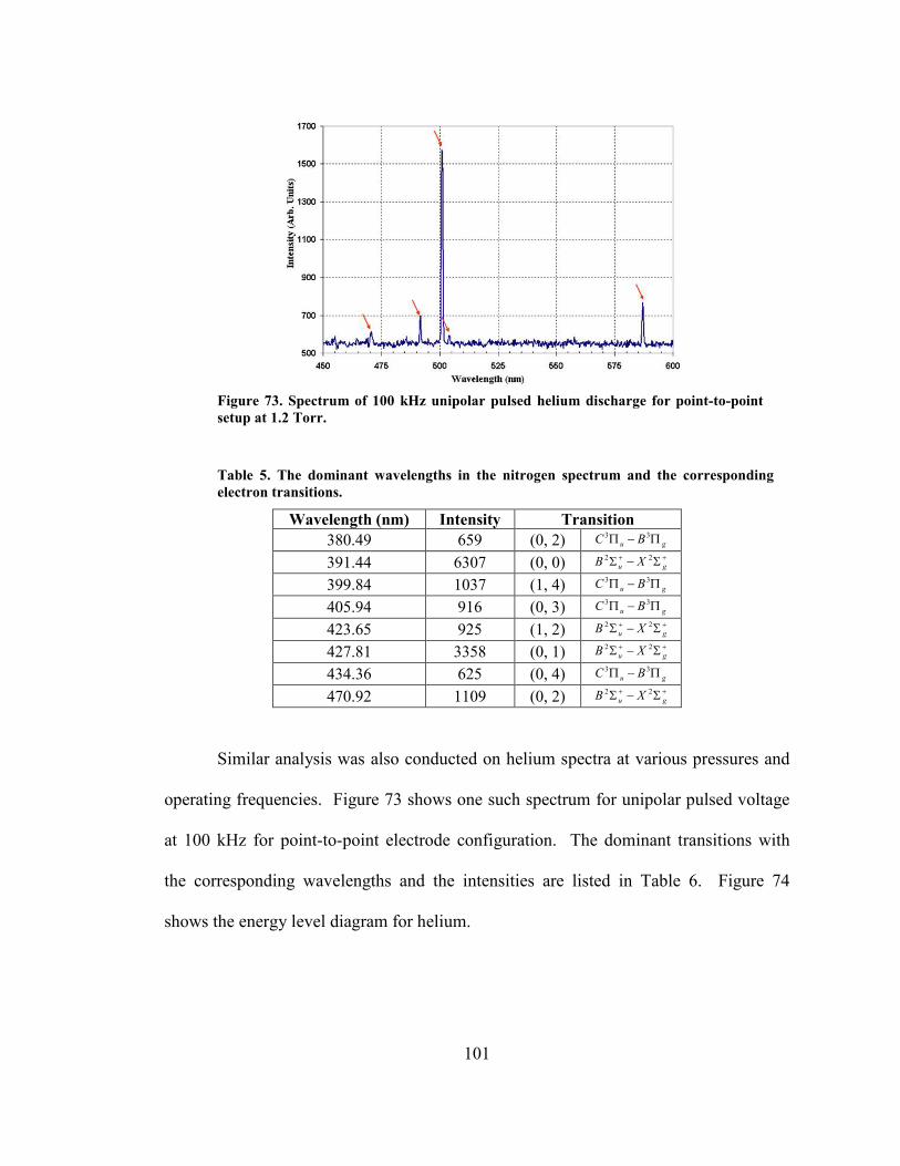
101
Figure 73. Spectrum of 100 kHz unipolar pulsed helium discharge for point-to-point setup at 1.2 Torr.
Table 5. The dominant wavelengths in the nitrogen spectrum and the corresponding electron transitions.
Wavelength (nm) Intensity Transition 380.49 659 (0, 2) gu BC Π−Π 33
391.44 6307 (0, 0) ++ Σ−Σ gu XB 22
399.84 1037 (1, 4) gu BC Π−Π 33
405.94 916 (0, 3) gu BC Π−Π 33
423.65 925 (1, 2) ++ Σ−Σ gu XB 22
427.81 3358 (0, 1) ++ Σ−Σ gu XB 22
434.36 625 (0, 4) gu BC Π−Π 33
470.92 1109 (0, 2) ++ Σ−Σ gu XB 22
Similar analysis was also conducted on helium spectra at various pressures and
operating frequencies. Figure 73 shows one such spectrum for unipolar pulsed voltage
at 100 kHz for point-to-point electrode configuration. The dominant transitions with
the corresponding wavelengths and the intensities are listed in Table 6. Figure 74
shows the energy level diagram for helium.

102
Figure 74. The energy diagram for helium systems
Table 6. The dominant wavelengths in the helium spectrum and the corresponding electron transitions.
Wavelength (nm) Intensity Transition 587.56 768 1s2p — 1s3d 504.77 590 1s2p — 1s4s 501.56 1573 1s2s — 1s3p 492.19 700 1s2p — 1s4d 471.31 614 1s2p — 1s4s
Unlike what was expected, no direct relation between the emission spectra and
the applied signal frequency or operating pressure was found in the range studied (190
nm to 640 nm). Further investigation over a wider spectrum is needed to thoroughly
determine the dependence of the intensities/transition probabilities on the gas pressure
and the operating signal frequencies.

103
CHAPTER VII
IMAGE ANALYSIS TOOL FOR OPTICAL EMISSION CHARACTERIZATION OF
PARTIAL VACUUM BREAKDOWN 7.1 INTRODUCTION
During the early course of this work, it was realized that the videos recorded
using a regular 30 fps camera can be used to understand some basic processes in the
breakdown events. For this purpose, a simple image analysis tool/procedure was
developed as a means to analyze the R/G/B variation of the discharge over time at
various locations of the discharge. In this chapter, an image analysis technique and its
results for optical emission characterization of a breakdown initiation are presented.
The example set for demonstration is breakdown events under a 20 kHz unipolar-
sinusoidal applied field for a point-to-point electrode geometry at partial vacuum in
helium. The voltage and current waveforms along with the light emission data are
collected. The results of the image analysis technique used to obtain the R/G/B
emission characteristics of the breakdown events as a function of time, location, and
pressure are presented.
In general, breakdown events are studied from the electrical view point by
analyzing the voltage and current signals at breakdown. Optical and spectroscopic
imaging techniques are powerful tools in these cases and other technical areas such as
turbulent flows, combustion systems, turbulent plasmas, hypersonics and biomedical
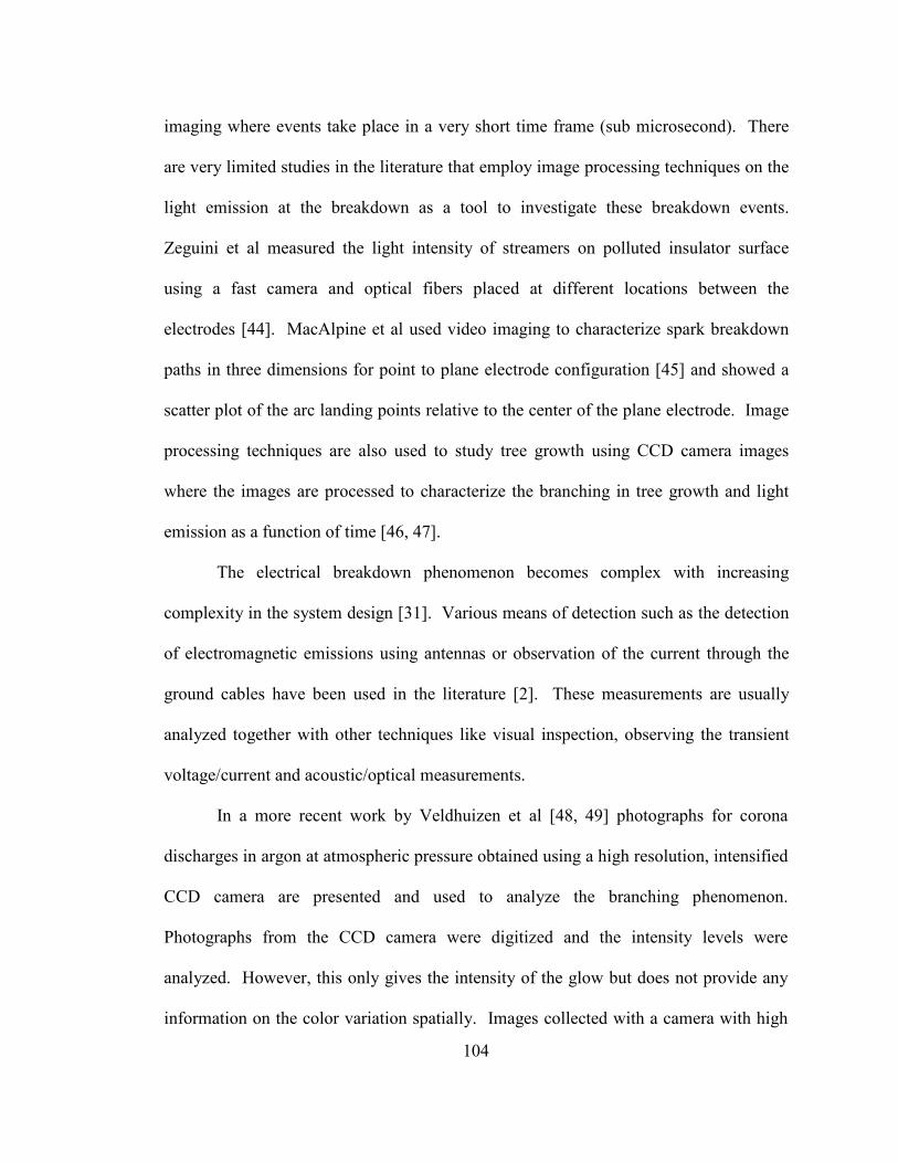
104
imaging where events take place in a very short time frame (sub microsecond). There
are very limited studies in the literature that employ image processing techniques on the
light emission at the breakdown as a tool to investigate these breakdown events.
Zeguini et al measured the light intensity of streamers on polluted insulator surface
using a fast camera and optical fibers placed at different locations between the
electrodes [44]. MacAlpine et al used video imaging to characterize spark breakdown
paths in three dimensions for point to plane electrode configuration [45] and showed a
scatter plot of the arc landing points relative to the center of the plane electrode. Image
processing techniques are also used to study tree growth using CCD camera images
where the images are processed to characterize the branching in tree growth and light
emission as a function of time [46, 47].
The electrical breakdown phenomenon becomes complex with increasing
complexity in the system design [31]. Various means of detection such as the detection
of electromagnetic emissions using antennas or observation of the current through the
ground cables have been used in the literature [2]. These measurements are usually
analyzed together with other techniques like visual inspection, observing the transient
voltage/current and acoustic/optical measurements.
In a more recent work by Veldhuizen et al [48, 49] photographs for corona
discharges in argon at atmospheric pressure obtained using a high resolution, intensified
CCD camera are presented and used to analyze the branching phenomenon.
Photographs from the CCD camera were digitized and the intensity levels were
analyzed. However, this only gives the intensity of the glow but does not provide any
information on the color variation spatially. Images collected with a camera with high

105
spatial resolution and sub-nano second optical gate times (not high frame rates camera)
have been used [48] to calculate the streamer propagation velocities over the entire
region of the electrode gap.
Our experience with optical diagnostic methods in high voltage and electrical
insulation research shows that the main challenge is obtaining time resolved data of the
optical emission. If spatially resolved data is required, the challenges are increased
partially due to geometry of the test article and relative positions of the occurring
events. The emission sites usually change rapidly in time, making a time-sequential
approach to spectral imaging very complex. In our work, the images obtained by a
standard video camera at 30 fps are analyzed to characterize the progress of the
breakdown and light emission in time and as a function of pressure at predetermined
locations. The scope of this paper is to establish a procedure to understand the
breakdown events in time and space and verify this method by applying it to an event
for which the characteristics are known. This can help in qualitatively understanding
plasma generation process without the use of expensive methods. A simple case of a
non-uniform field, point-to-point electrode configuration [50] at frequencies
comparable to the switching frequencies encountered in commercial applications is used
in this paper to demonstrate the developed analysis technique [51].
7.2 EXPERIMENTAL SETUP
The experimental setup is similar to what is descried in the last chapter for point-
to-point electrode configuration and 20 kHz unipolar sinusoidal fields. Additionally, a
standard 30 fps digital video camera is used to capture the images of the discharge for

106
further analysis. The chamber pressure is maintained constant throughout a particular
set of breakdown events. The breakdown experiments are conducted over a pressure
range of 27 Pa to 347 Pa (0.2 to 2.6 Torr). The dc-shifted sinusoid voltage at 20 kHz is
applied to the electrodes, until a breakdown event is observed. Once the breakdown
initiation is captured, the power supply is turned-off and the voltage, current, light
emission and the video/images are stored for each pressure. The visual observation of
the breakdown events is also conducted to verify the path of the breakdown across the
electrode-gap.
7.3 IMAGE ANALYSIS
Once a breakdown is observed, the voltage and current data are recorded for
each pressure and used to obtain the breakdown voltage versus pressure data. The
breakdown voltages are plotted as a function of pressure as shown in Figure 75 [51].
Each data point in this figure represents a breakdown event that is recorded as a short
video of the optical emission from the plasma produced at the breakdown. Once the
breakdown is initiated, a relatively long optical emission spanning up to 2 seconds is
observed. Optical data collected by means of the video camera are converted into
frame-by-frame still images for further analysis. Figure 76 shows the frame-images of
one such breakdown event for 1.6 Torr. The time difference between each consecutive
frame is approximately 33 ms, corresponding to a 30 fps video. A CCD camera works
based on the eye’s response to light. A generic spectral response of a CCD array is
shown in Figure 77. Based on the type of the camera, a filtering design, such as Bayer
filter (RGB) or RGBE, is used to discriminate the red (R), blue (B) and green (G) colors

107
of the image and the final image formed almost resembles the colors of the actual
object.
Figure 75. The breakdown voltage as a function of pressure of Helium for point-to-point geometry under 20 kHz ac applied voltage [51]
Frame #06
Frame #11
Frame #48
Frame #50
Figure 76. Selected frames of the frame-by-frame images of a typical unipolar breakdown event for Helium at 20 kHz applied voltage. (Bottom electrode is cathode and top is anode)
Figure 77. A generic spectral response of a CCD array.

108
Among these breakdown events, fourteen data sets are chosen to represent
fourteen different pressures in the range of 0.2 to 2.0. As seen in Figure 76, the most
prominent colors in all the frames are blue and red. The blue and red colors correspond
to the extremes of the visible spectrum with the energy levels in the UV and IR ranges.
As the main objective of this work is to understand and characterize the optical
emission and the breakdown evolution in time, five areas in the electrode region are
selected as shown in Figure 78c, representing different areas of the glow quantitatively.
These regions are identified as:
Anode : A 20x20-pixel area at the tip of the anode.
Anode2 : A 20x20-pixel area just beyond the anode-area.
Middle : A 30x30-pixel area between the tips of the anode and cathode.
Cathode : A 20x20-pixel area at the tip of the cathode.
Cathode2 : A 20x20-pixel area just beyond the cathode-area.
(These dimensions in pixels are chosen depending on the dimension of the original
images.)
(a) (b) (c)
Figure 78. (a) Applied voltage signal, VAnode-Cathode (Cathode is always ground) (b) Typical image of the breakdown process showing the anode and the cathode boundaries (drawn) (c) The five regions selected for image analysis.
Regions labeled ‘Anode’ and ‘Cathode’ represent the tips of the electrodes,
where the field intensity/non-uniformity is expected to be at its maximum. Regions
labeled ‘Anode2’ and ‘Cathode2’ represent the areas just after the electrode tips, away

109
from the points of maximum field stress. The region labeled ‘Middle’ is chosen to
represent the activity in the glow discharge region of the electrode gap. As we are
interested in analyzing the glow initiation rather than the arc formation, the region
marked ‘Middle’ is chosen to be off the central axis to collect as much light emission as
possible. By looking at various images it was decided to select a 30x30-pixel area
instead of 20x20 area for the ‘Middle’ region.
Most of the technical software packages are capable of extracting the R/G/B
values from a still picture and MATLAB has a built in routine for this task. A
MATLAB routine is written to average the individual red (R), green (G), and blue (B)
values over each of these five regions as given by the following equation Each image
frame is loaded into MATLAB workspace as a matrix containing different values (from
0 to 255) for each of R/G/B colors. Using this routine a data set of R/G/B values as a
function of time for these five areas at each pressure is created. The color values as read
from the image files range from 0 to 255; however, these values for all the processed
data seem to stay under 200. The background level for each color in the absence of the
glow is about 30 and is consistent. Figure 79a shows a representative curve for
variation of ‘R’ at 1.4 Torr. Figure 79b shows the R/G/B variation as a function of time
for the ‘Cathode2’ area at 1.4 Torr. Similar curves, not shown here, for ‘G’ and ‘B’ and
rest of the regions are also plotted for different pressures.
Average Intensity (for R/G/B) = area)in that pixels ofnumber (Total
area)given theof pixeleach for valuesR/G/B'' individual theall of (Sum

110
(a) (b)
Figure 79. (a) The ‘R’ value variation with time for the five regions used in image analysis. (b) Variation of R/G/B values at ‘Cathode2’ region as a function of time (Helium at 20 kHz and 1.4 Torr)
Figure 80. Optical emission duration of the afterglow plasma after breakdown is initiated as a function of pressure [51].
7.4 RESULTS
Using this R/G/B data from the initial plots, the duration of light emission after
breakdown initiation as a function of pressure is determined and shown in Figure 80. It
is observed that the duration of light emission is relatively long at low pressures
compared to that at high pressure as initially observed in [50]. It is known from the
literature that typical afterglow at a few torr pressure is normally in the millisecond
regime [52]. One should notice that the light emission duration in Figure 74 is not the
duration of an “after glow” as observed in the literature, but the life of the light emission

111
from the breakdown initiation until after the applied voltage across the electrodes is
removed. The power supply in these experiments is set to trip-off immediately (after a
fixed finite delay) after a breakdown event is registered. However, this delay was not
measured as one of the experimental parameters. Although the time scale in Figure 80
is in seconds, it should be noted that even by compensating the delay induced by the
power supply, the shape of the curve and the duration dependence on the pressure will
not be altered. On the other hand, data similar to Figure 80 can be also recorded by
simultaneously measuring the light emission waveform and the applied voltage across
the gap as a function of time. In the current experiments, the primary focus is on
measuring the voltage at the breakdown initiation (which is in microsecond range) and
the diagnostics are set accordingly. Therefore, the voltage/light emission waveforms
over a longer duration (ms) are neither recorded nor presented.
Figure 81. R/G/B values at different locations at t = 0.4 s (left) and t = 1s (right) respectively at gas pressure of 0.350 Torr. The center of the electrode gap is located at 0 cm, anode tip is located at 0.5 cm, and the cathode tip at negative 0.5 cm.
The data collected from the images are also used to observe the R/G/B variation
in any of the mentioned five regions at a given time of the breakdown events. For
example, the color variation at a given pressure as a function of location (spatial
variation at constant pressure and time), can be obtained from the initial data.

112
Representative plots for this are shown in Figures 81 and 8 at t = 0.4 s and t = 1 s after
the breakdown initiation for pressures of 0.35 Torr and 1.4 Torr respectively.
Figure 82. R/G/B values at different locations at t = 0.4 s (left) and t = 1s (right) respectively at gas pressure of 1.4 Torr. The center of the electrode gap is located at 0 cm, anode tip is located at 0.5 cm, and the cathode tip at negative 0.5 cm.
From the R/G/B plots in Figures 81 and 82 we observe that intensity of the R
component is higher at the cathode region and gradually decreases as we move towards
the middle and then gradually increases towards the anode region. Similar pattern is
observed for blue and green colors. Although green is not significant to make any
spectral characterization, blue and red colors are. Comparing Figures 81 and 82, it is
observed that at low pressure (0.35 milli Torr), R and B values are comparable at the
cathode region while latter is relatively dominant at anode region. At high pressure
however, R is relatively dominant at cathode (different than low pressure case) while B
is still dominant at the anode. Even though it is not a spectroscopic study, this
observation shows that at high pressure (1.4 Torr in this study), the high energy
collision processes resulting in optical emission in UV range are dominant at anode and
low energy processes resulting in near-IR emission are dominant in the cathode area. In
general, the cathode region is the brightest, indicating as expected, that it is the area
with most active interactions.

113
Figure 83. Variation of R/G/B with pressure at the ‘Anode’ and the ‘Cathode’ regions shown in Figure 75 at t = 0.4s after breakdown initiation.
Figure 84. Variation of R/G/B with pressure at the ‘Anode’ and the ‘Cathode’ regions shown in Figure 75 at t = 1.0 s after breakdown initiation.
Also, the R/G/B variations as a function of pressure for each of the five regions
at any desired time are determined from the initially calculated values. Figures 83 and
84 show respectively, the representative plots of R/G/B variation as a function of
pressure at t = 0.4 s and t = 1 s after the breakdown initiation. It is observed from these
figures that R is relatively dominant in the cathode region while blue B is dominant in
the anode region. This supports the fact that the electrons emitted from the cathode
resulting in a collision have just sufficient energy to generate low energy photons in the
IR range (R). Whereas, those electrons which do not suffer collisions and are able to
propagate to anode gain energy in the plasma, and thus, have higher energies to

114
generate photons closer to the UV range (B). A very similar study conducted by
Tochikubo et al, [53] presents the optical emission characteristics of a pulsed corona
discharge in nitrogen and other nitrogen radicals. However, their work involved time
resolved spectra to identify various excitation processes and does not address the spatial
variation of these processes. It is clear that in addition to being a simple diagnostic tool,
our technique can be complementary to time resolved spectroscopic studies in these
works.
7.5 CONCLUSIONS
A simple image analysis technique is presented to determine the characteristics
of a breakdown initiation. From the calculated R/G/B brightness values of each frame
we can determine the duration of each breakdown event. It is clear that this work is not
a spectroscopic analysis of the light emission but can be easily implemented where
spectroscopic analysis is not feasible. The R/G/B data as a function of pressure and
spatial location can be used to study and understand possible processes occurring during
the discharge events. Though this technique is demonstrated here for the videos
captured using a regular 30 fps camera, it can be far more effectively used in
understanding and visually analyzing the breakdown phenomenon when used with the
videos captured using a higher frame rate camera. Only five regions of the breakdown
images are presented here for demonstration, however, this technique can also be used
to analyze various regions of the electrode gap, the electrode surfaces, etc. by choosing
the desired regions and dimensions of the captured images. This study intends to be a
foundation for a sequential optical spectroscopy analysis of breakdown events in
115
conjunction with the images captured by a high-frame rate camera to correlate time and
space resolved data. Therefore, this seemingly simple image analysis technique can be
used in conjunction with the conventional diagnostics equipment to characterize
discharges and breakdown phenomenon in various high-voltage and pulsed-power
applications.

116
CONCLUSIONS AND FUTURE WORK
In this work, an attempt was made to understand the breakdown characteristics
of helium, nitrogen and zero air in partial vacuum conditions under non-uniform,
unipolar applied fields. Within the pressure range and the signal frequencies
investigated, it was confirmed that for 0.5 and 1.0 cm gaps in point-to-point and point-
to-plane geometries, under the above mentioned fields, a Paschen like behavior is
clearly observed. This was only speculated in the literature but to our knowledge, it
was not experimentally verified under these conditions. Also, the breakdown voltage is
considerably lower than the corresponding dc breakdown voltage at the same electrode
gap. For a given signal frequency, the unipolar shifted sinusoid has the lowest
breakdown voltage (RMS) (compared to dc and unipolar pulsed fields) for both the
geometries and all the gases studied while the dc breakdown voltage was the highest.
Furthermore, an increase in the signal frequency clearly showed a decreased breakdown
voltage. However, the rate at which the breakdown voltage decreases with the signal
frequency varies drastically from helium to nitrogen or zero air. Helium shows a
double exponential relationship while nitrogen and dry air show a more linear fall with
increasing signal frequency. As expected, zero air shows properties very similar to
nitrogen.

117
In addition to the effect of signal frequency, preliminary studies have also been
conducted to determine the role of duty cycle on the breakdown voltage. It was
observed that at low duty cycles, the breakdown voltage is similar to the impulse
breakdown while at higher duty cycles, the breakdown is closer to the dc level. Further
studies are required to conclusively determine the exact relation between the duty cycle,
the signal frequency and the breakdown voltage at a given operating pressure.
To further understand the changes in behavior in helium and nitrogen, some
spectroscopic studies have been conducted. This was done to understand the temporal
evolution of electron transitions/processes in the glow discharges of these two gases.
Due to limited temporal and spectral resolution of the equipment, only the dominant
transitions could be studied. Further investigation into developing a high speed
diagnostic system can certainly improve the understanding of these processes in the low
pressure range.
Also, a simple image analysis tool was developed to analyze the videos captured
during the breakdown initiation. This tool can be used on videos captured at higher
frame rates to understand the spatial and temporal evolution of the glow discharge.
This can prove useful in situations where the use of a spectrometer is not practical. This
technique, when used in combination with a high speed video camera, spectrometer and
a data acquisition system (for voltage and current) can help better understand the
breakdown behavior of any gaseous environment.

118
BIBLIOGRAPHY
[1] D. L. Schweickart, J. C. Horwath, H. Krompholz, L. C. Walko, "The relevancy of environmental parameter space for electrical insulation design in aerospace vehicles," IEEE Power Modulator Symposium and High-Voltage Workshop, pp. 30-33, 2004.
[2] D. K. Hill, W. G. Dunbar, H. Kirkici, D. L. Schweickart, G. Barry Hillard,
"Spacecraft High Voltage Design Guide (in preparation), NASA-AFRL Design Guide.
[3] H. Kirkici, K. Koppisetty, "Gaseous breakdown at high frequencies under partial
vacuum," IEEE Conference on Electrical Insulation and Dielectric Phenomena, pp. 451-454, 2003.
[4] L. B. Gordon, "Engineering high voltage in the space vacuum," ISDEIV
Proceedings on Discharges and Electrical Insulation in Vacuum, vol.2, pp.663-667, 1996.
[5] R. V. Latham, High voltage vacuum insulation: Basic concepts and technological
practice, Academic Press, 1995. [6] B. D. Green, G. Caledonia, D. Wilkerson, "The Shuttle Environment: Gases,
Particulates, and Glow," Journal of Spacecraft and Rockets, Vol. 22, pp.500-511, 1985.
[7] W. Dunbar, "Design Guide: Designing and Building High Voltage Power
Supplies," Interim Report, 20 Jul. 1987 - 19 Jul. 1988 Auburn Univ., AL. Space Power Inst.
[8] Katz, I.; Jongeward, G.A.; Mandell, M.J.; Maffei, K.C.; Cooper, J.R., "Preventing
ion bombardment caused breakdown in high voltage space power systems and applications to Space Power Experiments Aboard Rockets (SPEAR)," Proceedings of Energy Conversion Engineering Conference, vol. 1, pp.447-451, 1989.

119
[9] E. Hastings, G. Weyl, Guy, D. Kaufman, "Threshold voltage for arcing on negatively biased solar arrays," Journal of Spacecraft and Rockets, vol. 27, pp. 539-544, 1990
[10] M. Cho, D. E. Hastings, "Dielectric charging processes and arcing rates of high
voltage solararrays," Journal of Spacecraft and Rockets, vol. 28, pp. 698-706, 1991.
[11] E. R. Bunker Jr., "Proceedings of the Second Workshop on Voltage Breakdown in
Electronic Equipment at Low Air Pressure (Preventing voltage breakdowns in electronic equipment operating in aerospace environments)," Jet propulsion laboratory, pp. 33-447, 1970.
[12] E. R. Bunker Jr., "Proceedings of Workshop on Voltage Breakdown in Electronic
Equipment at Low Air Pressures," Jet propulsion laboratory, vol. TR-33-280, 1965.
[13] W. Pfeiffer, "High-frequency voltage stress of insulation. Methods of testing,"
IEEE Transactions on Electrical Insulation, vol. 26, pp. 239-246, 1991. [14] A. W. Bright, British Elect. Allied Ind. Research Association Report, 1950. [15] H. Lassen, "Frequency Dependence of the Breakdown Voltage in Air," Archiv
fuer Elektrotechnik, vol. 25, pp. 322-332, 1931. [16] R. Y. Amer, "Calculation of inception voltages in SF6-N2 mixtures," Conference
on Dielectric Materials, Measurements and Applications, pp. 190-192, 1992. [17] J. H. Mason, "Effects of frequency on the electric strength of polymers,"
Transactions on Electrical Insulation, vol. 27, pp. 1213-1216, 1992. [18] D. Raboso, "Multipactor effect on board spacecrafts: present situation, future
research activities and testing capabilities at the European Space Agency", Vacuum Electronics Conference, pp.2, 2000.
[19] W. Richard, "Multipacting Discharges between Coaxial Electrodes," Journal of
Applied Physics, vol. 39, pp. 1528-1533, 1968. [20] W. G. Dunbar, D. L. Schweickart, J. C. Horwath, and L. C. Walko, "High
frequency breakdown characteristics of various electrode geometries in air," IEEE Pulsed Power Conference, pp. 221-224, 1998.
[21] W. Khachen and J. R. Laghari, "Polypropylene for high voltage high frequency
airborne applications," IEEE Conference on Electrical Insulation and Dielectric Phenomena, pp. 80-83, 1990.
120
[22] W. Khachen, J. R. Laghari, and W. J. Sarjeant, "Dielectric breakdown of polypropylene under high frequency fields," IEEE Conference on Electrical Insulation and Dielectric Phenomena, pp. 185-188, 1992.
[23] K. Elanseralathan, M. J. Thomas, and G. R. Nagabhushana, "Breakdown of solid
insulating materials under high frequency high voltage stress," Conference on Properties and Applications of Dielectric Materials, pp. 999-1001 vol.2., 2000.
[24] J. S. Townsend, Electricity in Gases, Oxford University Press, London, 1914. [25] J. S. Townsend, "The potentials required to maintain currents between coaxial
cylinders," Phil Magazine, vol. 28, pp. 83-90, 1914. [26] L. B. Loeb, “Electrical coronas,” University of California press, Berkeley 1965. [27] J. R. Roth, Industrial plasma engineering, Institute of Physics Pub., 1995. [28] E. Nasser, Fundamentals of gaseous ionization and plasma electronics:
Fundamentals of gaseous ionization and plasma electronics, Wiley, 1971. [29] G. Dakin, "Paschen Curve for Helium,” Electra, vol. 52, pp. 82-86, 1977. [30] E. Hussain, R. S. Nema, "Electric stress at breakdown in uniform field for air,
nitrogen and sulfur hexaflouride,” Ed. L. G. Christophorou and M. O. Pace, International Symposium on Gaseous Dielectrics, pp. 168-173, 1984.
[31] J. M. Meek and J. D. Craggs, “Electrical breakdown of gases,” Wiley, 1978. [32] A. M. Howatson, “An introduction to gas discharges,” 2 Editions, Pergamon
press, 1976. [33] R. Papoular, Electrical phenomena in gases, Elsevier Publishing, 1965. [34] I. U. P. Raizer, Gas discharge physics, Springer-Verlag, 1991. [35] S. C. Haydon, I. C. Plumb, "The electrical breakdown of air at radio frequencies in
the H. F. band," Conference on Phenomena in Ionized Gases, Part I: Contributed papers, edited by J. G. A. Hölscher and D. C. Schram, p.89, 1975.
[36] A. D. MacDonald, “Microwave Breakdown in Gases,” John Wiley & Sons, Inc.,
New York, 1967. [37] H. Kirkici. K. Koppisetty, "Breakdown Characteristics of Helium and Nitrogen at
kHz Frequency Range in Partial Vacuum for Point-to-Point Electrode,"

121
Transaction on Dielectrics and Electric Insulation, vol. 15, no. 3, pp.749-755, 2008.
[38] R. Marcus, J. Broekart, Glow Discharge Plasmas in Analytical Spectroscopy,
Wiley, 2003. [39] La Palma Technical Notes: http://www.ing.iac.es/Astronomy/observing/manuals/man_tn.html [40] Frederick M. Phelps, III, “Wavelengths by element,” Vol. II, MIT Press, 1982. [41] Hodges, Clarence and Michels, "Intensity measurements in the Helium spectrum,"
Physical review, vol. 32, pp. 913-917, 1928. [42] S. Bashkin Jr, Atomic energy levels and grotrian diagrams III Vol. I, Elsevier,
1975. [43] G. Mesyats, Pulsed Electrical Discharge in Vacuum, Springer Verlag, 1989. [44] B. Zegnini, D. Mahi, C. Huraux, and A. Chaker, "Electrical and optical analysis of
the electric discharge, energized by AC voltage, on polluted insulating surface," International Symposium on Electrical Insulating Materials, pp. 316-319, 2001.
[45] J. M. K. MacAlpine and H. T. Yim, "An investigation of spark breakdown paths
in air using an image processing technique," Conference on Electrical Insulation and Dielectric Phenomena, pp. 122-125, 1995.
[46] J. M. Bryden, I. J. Kemp, A. Nesbitt, J. V. Champion, S. J. Dodd, and Z.
Richardson, "Correlations among light emission and partial discharge measurements made during electrical tree growth," Conference on Dielectric Materials, Measurements and Applications, No. 473, pp. 513-518, 2000.
[47] D. B. Watson and M. I. Barber, "Image-processing technique for investigating
dielectric breakdown trees," Proceedings of Science, Measurement and Technology, vol. 139, pp. 79-83, 1992.
[48] E. M. Veldhuizen, P. C. M. Kemps, and W. R. Rutgers, "Streamer branching in a
short gap: the influence of the power supply," Transactions on Plasma Science, vol. 30, pp. 162-163, 2002.
[49] E. M. Veldhuizen, A. H. F. M. Baede, D. Hayashi, W. R. Rutgers, "Fast imaging
of streamer propagation," APP Spring Meeting, Bad Honnef, Germany, pp. 231-234, 2001.

122
[50] H. Kirkici, K. Koppisetty, D. L. Schweickart "Partial Vacuum Breakdown Characteristics of Helium at 20 kHz for Inhomogeneous Field Gap," Transaction on Dielectrics and Electric Insulation, vol. 14. no. 3, pp.553-559, 2007.
[51] K. Koppisetty, H. Kirkici, M. Serkan, and D. L. Schweickart, "Optical emission
characteristics of helium breakdown at partial vacuum for point to point geometry," Conference on Electrical Insulation and Dielectric Phenomena, pp. 47-50, 2005.
[52] L. C. Pitchford, K. N. Taylor, and C. B. Collins, "Excited state chemistry of the
low-pressure helium afterglow. I. Reactions involving metastable species, 23S and 2s3Σ+
u," Journal of Physics B: Atomic and Molecular Physics, pp.142-155, 1975. [53] F. Tochikubo and T. H. Teich, "Optical emission from a pulsed corona discharge
and its associated reactions," Japanese Journal of applied physics, vol. 39, pp. 1343-1350, 2000.