BRDF approximation and estimation for Augmented Reality

Patrick Kuhtreiber∗

Institute of Computer Graphics and AlgorithmsVienna University of Technology, Austria

Figure 1: [Lafortune et al. 1997]

Abstract

In Augmented Reality applications it is important to have a gooddescription of the surfaces of real objects if a consistent shadingbetween real and virtual object is required. This thesis emphasizeson this topic as the thesis is a part of the RESHADE1 project whoseaim is to deliver a scene of virtual and real objects mixed togetherwhere difference is not noticable for the viewer. That means thatvirtual objects also influence the appearance of the real objects.If such a description of a surface is not available it has to be esti-mated or approximated during runtime.In my bachelor thesis I will present certain methods that deal withreal-time bi-directional reflectance distribution function (BRDF)approximation in augmented reality. Of course the most impor-tant thing is that the applications I present all work in real-time andcompute good (and real) looking results.There are different methods on how to achieve this goal. Most ofthe methods I am going to present work via image based lightingand require a 3D polygonal mesh representation of the object whoseBRDF shall be approximated. Some methods estimate the BRDFparameters via error values and provide results at each iteration.

Keywords: Real-time BRDF approximation, Augmented Reality

∗e-mail: patrick.kuehtreiber@chello.at1http://www.cg.tuwien.ac.at/research/projects/RESHADE/

1 Structure of this thesis

After a brief introduction about augmented reality, BRDF andBRDF approximation I will describe the papers listed in Section2 in detail, give a summary about the parts that concern BRDFapproximation or estimation and I will conclude each method de-scription with a short paragraph where I will point out some prob-lems with the algorithm and their performance and usability in aug-mented reality. The summaries of the papers are chronologicallyarranged beginning with a paper from Yu et al. from 1997 and con-cluding with a paper from Ritschel and Grosch from 2008.In each section I will give a summary of the presented paper witha short discussion about performance and problems which mightoccur. After the summary of the papers I will compare all the pre-sented papers. The main focus here will be performance, as this isthe most important part of the approximation, but photorealism (ifprovided) is also important.At the end I will compare the presented methods in matter of per-formance and photorealism and give a general conclusion over thetopic.

2 Introduction

Several papers deal with the problem of real-time BRDF approxi-mation. BRDFs are functions with lots of parameters that describehow a certain surface reflects incoming light. If a BRDF forcertain objects is not known it has to be approximated as closely as

possible. In Augmented Reality applications it would be desireableto do it during runtime to allow maximal scene dynamic.We need a good representation of the reflection behaviours of thesurfaces and, what makes it even more difficult, we need them inreal-time.The most of the presented methods are rather similar, as all useimage based lighting. Still there are differences in performance andphotorealism which I will try to point out at the end of the sectionand again in the section at the end of this thesis.

The papers presented in this thesis are:

• Inverse global illumination: Recovering reflectance models ofreal scenes from photographs, [Yu et al. 1999]

• Image-Based Rendering of Diffuse, Specular and Glossy Sur-faces from a Single Image, [Boivin and Gagalowicz 2001]

• Photorealistic rendering for augmented reality using environ-ment illumination, [Agusanto et al. 2003]

• Recovery of material under complex illumination conditions,[Wu et al. 2004]

• A Framework for Automatically Recovering Object Shape,Reflectance and Light Sources from Calibrated Images,[Mercier et al. 2007]

• Recovering surface reflectance and multiple light locationsand intensities from image data, [Xu and Wallace 2008]

• On-line estimation of diffuse materials, [Ritschel and Grosch2008]

2.1 A survey to Augmented Reality

Basically Augmented Reality is an alteration of Virtual Reality. InAugmented Reality virtual three dimensional objects are being in-tegrated into a real scene, so the user can still see and move in theworld around him. According to Azuma Augmented Reality sys-tems must meet the following charactaristics: [Azuma 1997]

1. Combines real and virtual

2. Interactive in real-time

3. Registered in 3D

What is important here is that all virtual objects must be interactive3D objects. So simple blending of 2D objects does not count asAugmented Reality. Augmented Reality applications are found inmedicine, entertainment and visualisation amongst others.

Figure 2: A video see through HMD. Picture fromhttp://www.vrlogic.com/

How is this being achieved?

There are two different approaches to Augmented Reality namelyoptical and video. The optical approach is realized with asee-through HMD (Head-Mounted Displays). As the name says,the user sees the real world through this device but also virtualobjects can be added to the users sight by reflecting these virtualimages onto the combiners. While in the 90s those devices werebig and not really handy, there are nowadays HMD which havethe size of normal glasses. They can be adapted to smartphoneswhich could process complex AR applications in future asthere are already some rudimentary applications like World WideSignpost2 which lets you annotate buildings at different viewpoints.

The other possibility is to use video-see-through HMD (seeFigure 2). The real world gets recorded by a camera, merged withvirtual objects and then is shown on an HMD-device [Azuma1997]. This method is nowadays used in many smartphone andtablet PC applications like games or architecture programs.

2.2 BRDF approximation

Bidirectional Reflectance Distribution Functions describe how in-coming light gets reflected by a particular material and has firstbeen described by Nicodemus et al. [Nicodemus et al. 1977]. Itshould at least combine both the diffuse and the specular part (i.e.highlights) of the reflection. The BRDF shown here is a 6 dimen-sional (location, four angles and wavelength) function, but it can bemore- or less-dimensional:

fr =Lr(ωr)

Li(ωi)cosθidωi, (1)

where L(ωr) marks the flux of reflected light at direction ωr, L(ωi)is the flux of incoming light at direction ωi and θi is the angle be-tween the surface normal at a point i and the light incident on thatpoint. An image of the BRDF and those parameters can be seen inFigure 3.

Figure 3: Geometry of incoming and reflected light. The z-axismarks the surface normal [Nicodemus et al. 1977].

2http://studierstube.icg.tu-graz.ac.at/handheld ar/wwsignpost.php

Reflected radiance is defined by

Lr(θr,φr) =∫ 2π

0

∫π/2

0Li(θi,φi) fr(θi,φi;θr,φr)cosθi sinθidθidφi.

(2)

where fr is the BRDF (the rest of the parameters will be explainedlater in Section 9 at Equation 39 which is basically the same equa-tion with a different parametrization) defined by two incident andtwo reflected angles. fr is bi-directional because the incident andreflected directions can be reversed and the function will return thesame result [Ward 1992].If the BRDF is not known it has to be approximated or interpo-lated respectively. In most of these cases we use the algorithmspresented by Phong [Phong 1975] or Ward [Ward 1992]. Wewill later see that there exist some BRDF-approximations for Aug-mented Reality which deliver parameters for these BRDF mod-els. For a better approximation of the BRDF Lafortune [Lafor-tune et al. 1997] made an important contribution in presenting theGeneralized Cosine Lobe Model, where reflectance properties atdifferent camera angles were rendered properly with just linear ba-sis functions. Their method works very well on broad and glossyreflectance lobes.Basically the BRDF is the most important part of the RenderingEquation (see Equation 2). Sometimes the BRDF alone is calledRendering Equation.

2.2.1 Lambert’s Law

A Lambertian reflector is a surface which can be thinked of aspurely diffuse. The reflected radiant light energy from any pointon the surface is calculated with Lambert’s cosine law which statesthat the amount of radiant energy coming from any small surfacearea dA in a direction φN relative to the surface normal is porpor-tional to cosφn. The intensity is the same for all viewing directionswhich can be described as

αcosφN

dAcosφN= constant (3)

where α is the viewing angle [Hearn and Baker 2004]. This con-stant parameter is usually spoken of as kd which denotes the diffusereflectance parameter.

2.2.2 Phong’s reflectance model

One of the most efficient and frequently used BRDF models wasintroduced by Phong [Phong 1975]. He defines shading as a func-tion which yields the intensity value of each point on the surface ofan object from the characteristics of the light source, the object (thematerial properties) and the position of the observer (important forspecular highlights) [Phong 1975].The specular part of the reflected light at point p can be computedas

Ip = ks cosnφ (4)

where φ is the viewing angle relative to the specular reflection di-rection ωr, ks is the specular reflectance parameter, and n is thespecular exponent where the value for n is direct proportional to thespecular reflectance of the surface [Phong 1975] [Hearn and Baker2004].

The interesting part of his work is of course the specular reflectance.To simplify this model, cosφ from the original fomula can be re-placed with V ·ωr, where ωr = (2N ·ωi)N −ωi, N is the surfacenormal of this point, V is the viewing vector and ωi is the directionof the incoming light [Hearn and Baker 2004].This simplification works under the assumptions that the lightsource and the observer are located at infinity [Phong 1975]. Thatleaves us with

Sspecular = ks(V ·ωr)n. (5)

So for the Phong shading model you only need three parameters:the diffuse reflectance kd , the specular reflectance ks and the shini-ness n.

2.2.3 Ward’s reflectance model

Here more parameters are needed as this model is more physicallyplausible.

Figure 4: A gonioreflectometer with movable lightsource. Pictureby [Ward 1992]

To find the correct BRDF Ward proposed to use a goniorefelctome-ter (see Figure 4) to get all the parameters needed and then use themfor the isotropic gaussian model

fr,iso(θi,φi;θr,φr) =ρd

π+

ρs√cosθi cosθr

exp[− tan2 δ/α2]4πα2 . (6)

where ρd is the diffuse, ρs is the specular reflectance and α is thestandard deviation of the surface slope. 1

4πα2 is the normalizationfactor which replaces the geometric attenuation factors which areusually difficult to integrate [Ward 1992].Ward states that this model is superior to the model presented byPhong (Section 2.2.2) as it is more physical plausible and the nor-malization factor guarantees energy balance. The alteration of theisotropic gaussian model to the anisotropic case is realtively simple.The anisotropic gaussian model is

fr(θi,φi;θr,φr) = ρdπ

+ρs√

cosθi cosθr

exp[− tan2 δ (cos2 φ/α2x +sin2

φ/α2y )]

4παxαy

(7)

where φ is the azimuth angle of the half vector projected into thesurface plane, αx is the standard deviation of the surface slop in the~x direction and αy is the same for the~y direction. [Ward 1992].The papers I will present that try to approximate the parameters forWard’s reflectance model try to find all the missing parameters forthis gaussian anisotropic model.

2.3 Finding Illumination from an image

Some of the following papers determine the scene illuminationfrom a high dynamic range (HDR) image. This method of imagebased rendering was developed by Debevec [Debevec 1998] and[Debevec and Malik 1997].Before these contributions light sources had to be determined man-ually or the user at least had to refine a lot of the resulting data. Withthe method of the image based model an HDR fisheye picture of thescene is taken and all light sources of this scene can be determined.To achieve this, they split the scene into three components:

1. Distant scene

2. Local scene

3. Virtual objects in the scene

The distant scene illuminates the objects but all light reflected tothe distance will be ignored. The local scene are all the polygonsand meshes that interact with the object. So here the intereflectionsbetween the objects and the scene should be taken into account.Ideally all these three components are well modeled and positionedand a global illumination algorithm renders the whole scene.

3 Inverse Global Illumination: RecoveringReflectance Models of Real Scenes fromPhotographs

An approach at image based rendering has been made by Yu et al.[Yu et al. 1999]. Although their paper has not much to do withaugmented reality (and nothing with real-time) it still presents aninteresting algorithm on how to gain reflectance properties froma real scene and use them afterwards as paremeters for a virtualscene, which of course can be adapted to augmented reality asthey write in their introduction. They don’t say that their approachworks at real-time, however this paper is from 1999 and it is a goodguess that it will work interactively today. Little disadvantagesare that their algorithm limits itself to low parameter reflectancemodels, it presumes the diffuse part of the reflectance to vary arbi-trarily over any surface and furthermore it presumes the specularpart to be constant. Nevertheless I will discuss their contribution inthis section as their sampling of diffuse and specular reflectance israther interesting for approximating BRDFs in augmented realityapplications.

Basically their algorithm creates a 3D geometric representa-tion of the scene using a sparse set of photographs. From this rathersmall set it is impossible to gain all the needed information on theBRDFs, that’s why they made the aforementioned limitations.The inputs for their algorithm are the geometric model of the scene,a set of radiance maps taken from the photographs under knownillumination and partitioning of the scene into areas with similarreflectance properties for the non-diffuse parts. They address theproblem of gaining the illumination parameters as inverse globalillumination and the recovering of the diffuse reflectance inverseradiosity [Yu et al. 1999].

Before addressing the problem of general surfaces they makea number of calculations for special cases. At first they make theassumption that all surfaces are purely diffuse reflectant.The inverse radiosity equation is easy to calculate. For ”normal”radiosity they have the well known equation as

Bi = Ei +ρi ∑j

B jFi j, (8)

where Bi is the resulting radiosity, Ei is the emission of the lightcoming from that patch i, ρi is the diffuse albedo and Fi j is the formfactor between the patches i and j [Sillion and Puech 1994].From the photographs which are also taken from the lightsourceswe can get the radiance Bi via HDR-techniques contributed by De-bevec [Debevec and Malik 1997]. Since they assumed the surfacesto be perfectly diffuse, Ei is also known. The formfactors can beretrieved from the known geometry, so that leaves us with

ρi =Bi−Ei

∑j

B jFi j(9)

to get to the diffuse albedo in this special case.

Another special case helps them to calculate the BRDF. Thespecial case here is that they assume to have a surface withuniform BRDF which is illuminated by a point light which is againphotographed with a camera. As input they get the radiance Lifrom the photograph of every point Pi in direction of the camerawhich lets them calculate Ii, the irradiance incident at that point.They use Ward’s [Ward 1992] BRDF model for this case, as itonly needs two parameters the diffuse term ρd

πand the specular

term ρsK(α,θ), where ρd and ρs are the diffuse und specularreflectence properties of the surface and K(α,θ) is a function,where α is the surface roughness vector (for the specular highlight)and θ is a vector of the azimuths and elevation of the incident andviewing directions (see Section 2.2.3).So for each surface they now get

Li =(

ρd

π+ρsK(α,θi)

)Ii. (10)

As mentioned before, Li and Ii can be measured or calculated re-spectively from the photographs. θ is also known, so they justneed to estimate the reflectance parameters and the roughness vec-tor, which can be done through nonlinear optimization according toYu et al. [Yu et al. 1999].Now I will discuss the general case of finding BRDFs in the contri-bution from Yu et al. We now have surfaces which can be diffuseand/or specular. To get the BRDF of such a point Pi viewed fromcamera Cv, we first need to get the irradiance. We already havethis equation for the special perfectly diffuse case. Generally Equa-tion 10 is

LCvPi = ECvPi +ρd ∑j

LPiA j FPiA j +ρs ∑j

LPiA j KCvPiA j . (11)

Again everything except for α and the reflectance terms ρs and ρdare known. To get these parameters they need a photograph of everysurface under specular lighting conditions, to record the radiancecoming from that patch.

The specular component of a surface is different to the directionfrom the viewpoint of the camera and from the direction of anothersurface (see Figure 5). This difference is denoted as ∆S. Tocalculate these specular differences the BRDF of A j has to beknown, which is not the case. So ∆S needs to be estimated which

Figure 5: Specular highlight from Pi as viewed from the camera andanother patch A j. Picture from [Yu et al. 1999]

happens in an iterative framework also presented by the authors.The initial value for this iterative process sets ∆S = 0, so that theL-values (the radiance) from Figure 5 are equal.

As now all the patches’ radiances are recorded we have asimilar optimization problem as we had above. This process canbe made easier if the surfaces get subdivided into a hierarchy ofpatches and link the sample points. So we get the radiance from apatch to a sample point LPiA j and an associated ∆S.Each sample point gathers radiance from not only one patch butfrom all the surfaces surrounding it. To obtain all the highlights theauthors present the following algorithm

1. For each camera position C

2. For each polygon T

3. For each light source O

4. Obtain the intersection P between plane of T and line CO′ (O′and O are symmetric about T);

5. Check if P falls inside polygon T;

6. Check if there is any occlusion between P and O;

7. Check if there is any occlusion between C and any point in alocal neighborhood of P;

A highlight area is detected if P passed all the above tests.Now to complete the inverse global illumination process they firstfind a BRDF for all surfaces independently. After having done thisthey use the found information on the radiance parameters L andthe specular differences ∆S to refine the found BRDFs. They dothis a couple of times until the final solution is found.

A rather huge challenge is to estimate the ∆S. Yu et al. didthis with Monte Carlo raytracing with only one bounce. Thebounce of a patch A j is random but weighted by the functionK(α,θ) which denotes the direction of the specular light. So mostof the bounces will fall into the cones Q in Figure 6, which arecentered around the mirror directions. Now ∆S can be calculated as

∆S = ρsA j (LQPiA j−LQCK A j

) (12)

according to Yu et al. [Yu et al. 1999].

The next part is to model a function, called albedo map, on eachsurface. Yu et al. present the diffuse albedo for a point x on asurface as

ρd(x) =πD(x)I(x)

, (13)

where D(x) is the diffuse radiance map and I(x) is the irradiancemap.D(x) gets computed by substracting the specular part from thewhole radiance L(x), which we obtained from the photographs. I(x)can be calculated from the direct illumination using the form fac-tors. To minimize errors that can occur due to wrongly estimatedhigh specular components they eliminate the highest observed spec-ular part at different viewing angles.

Figure 6: Ray tracing through the patches to find specular reflec-tions. Picture from [Yu et al. 1999]

3.1 Problems and Performance

The running time of their algorithm was about six hours on a 300MHz PC using 40 HDR images. Whereas I don’t think that’s possi-ble to do in real-time now, it still shows an interesting approach toget BRDF parameters for a known lighting model.Also there occured errors in the estimation of the BRDF which af-fected the diffuse part of the illumination the most.Another disadvantage is, that a 3D geometric representation of thescene is needed as input parameter.

Figure 7: Result after the first iteration. All specular componentsare zero.

Figure 8: Result after all iterations. Both pictures from [Yu et al.1999]

4 Image-Based Rendering of Diffuse,Specular and Glossy Surfaces from aSingle Image

This approach, developed by Boivin and Gagalowicz, addressesthe problem in an iterative way [Boivin and Gagalowicz 2001].Every iteration step adds another level of detail to the renderedscene until the result - rendered with Ward’s BRDF reflectancemodel [Ward 1992] - looks well enough.The input for this algorithm are a simple photograph and a 3Dgeometric model of the scene. Note that no HDR picture is needed.The 3D geometrical model is built from the single photographwhich they achieved with Alias Wavefront’s Maya modeler andwhich took them six hours. The 3D geometrical model of the sceneincludes camera position and lightsources which are not exact butapproximated. Another idea is to add the lightsources manually tothe model. For the Ward reflectance model (which was also used inthe paper I presented in Section 3) five parameters are needed: thediffuse reflectance ρd , the specular reflectance ρs, the anisotropydirection ~x and the anisotropic roughness parameters αx and αy[Boivin and Gagalowicz 2001].

As stated before the algorithm works iteratively and each it-eration step is refined several times. Each subsequent state refinesthe previous one based on an error picture between the (offscreen)rendered picture and the original photograph. The algorithmruns through a couple of assumptions where the next step is onlycomputed if the error value from the previous picture is over acertain threshold. The assumptions are that the surface is

1. perfect diffuse

2. perfect specular

3. non-perfect specular

4. diffuse and non-perfect specular

5. isotropic (rough)

6. anisotropic (rough)

7. textured

Only if the assumption before is proven wrong with the errorpicture the next assumption is being taken and a new picture getsrendered and compared afterwards.

4.1 Perfect diffuse

The error ε is computed as the ratio between the average of theradiances from an object (more exactly its a group of objects) in thereal picture and in the synthetic one.

ε j =Bo j

Bn j

=T−1(Po j )T−1(Pn j )

(14)

where Bo j and Po j are the averages of the radiances and the pixelsof an object j in the real image and the index n marks the averagesof the same object j in the synthetic image. T () is a γ correctioncamera transfer function.The diffuse reflectance ρd can be corrected iteratively now withhelp of this error value. For each rerendering iteration k:

ρdik+1 = ρdik × εi

ρdik+1 = ρdik ×∑

nij=1 f (ε j)·(ε j×m j)ni

∑j=1

f (ε j) ·m j︸ ︷︷ ︸6=0

(15)

where

f (ε j) =

0, if ε j ≥ (1+λ ) ·md1, else

and is used to eliminate problems caused by smaller objects whichare more affected by noise. εi and ε j are the total error values be-tween the original and the synthetic image for group i and objectj, ni is the number of objects for group i, md is the median of theerros, λ is the authorized dispersion criteria and finally m j is thenumber of pixels covered by the projection of object j [Boivin andGagalowicz 2001].The steady refinement of ρd can be seen in Figure 9.

Figure 9: In the top row are from left to right the refined imagesbased on the error pictures below. Picture from [Boivin and Gaga-lowicz 2001].

If the perfectly diffuse assumption failes (i.e. the error is too high)the second assumption is tried (perfectly specular = all objects aremirrors). This is easy to accomplish as you simply have to set thediffuse reflectance ρd = 0 and the specular reflectance ρs = 1 andreplace all the ρd in Equation 15 with ρs.

4.2 Diffuse and specular

If there are still objects that have a high error value, it is now consid-ered to be diffuse and specular (but no roughness is so far assumed)although those surfaces do not appear so often. To get good ap-proximations to these surface reflectances the error value has to beminimized.

(T−1(Isynth)−T−1(Io))2 =nbg

∑i=1

(ρd ·Bd +ρs ·Bs−T−1(Io))2

where nbg is the number of pixels covered by the group projection.Now the minimization

(ρdρs

)=(

∑nbg BdT−1(Io)∑nbg BsT−1(Io)

)(∑nbg B2

d ∑nbg BdBs

∑nbg BdBs ∑nbg B2s

)−1

has a solution for each wavelength R,G,B [Boivin and Gagalowicz2001].

4.3 Isotropic surfaces

Now the surfaces are assumed to have a certain roughness factorα . This roughness factor is considered in Ward’s BRDF Model[Ward 1992]. Now ρd , ρs and α have to be minimized. Boivin andGagalowicz did this with the downhill simplex method [Nelderand Mead 1965]. As the accuracy does not have to be that high(10−2 for ρd and ρs and 10−4 for α respectively) the parameterscan be found within two minutes [Boivin and Gagalowicz 2001].

4.4 Anisotropic surfaces

Now all five parameters of Ward’s BRDF model have to be takeninto account: The diffuse and specular reflectances ρd and ρs, theanisotropy direction~x and the roughness factors αx and αy. As theyalready computed the rather independant ρd and ρs, they do nothave to calculate them anew.Minimization of the remaining three parameters does not work andonly makes the error bigger as no global minimum can be found bythe downhill simplex method used in the isotropic case. So they de-termined~x from the original picture. Their algorithm to that worksas follows:

1. Assume that the anisotropic surface is a perfect mirror

2. Estimate difference between the original image and the syn-thetic one

3. In this difference picture find the part of the mirror where thespecular reflection is ”extended”.

4. Compute an index buffer for this mirror of all objects visiblefrom it

5. Find a reference surface which covers the largest area of themirror while being closest to it in a manner that the ratioArea(reflected surface)/d(S, p) is maximized

6. Sample the anisotropy direction creating a number of vectors,where each one determines a direction to traverse the errorimage and compute the average of the standard error deriva-tions computed in the error image, around the normal to theanisotropic surface

7. Select the direction for which the average error becomessmallest

8. This direction equals~x

where d(S, p) is the Euclidian distance between the center of grav-ity of the selected surface and the center of gravity of the mirror[Boivin and Gagalowicz 2001].Now that their algorithm computed the anisotropy direction the re-maining two parameters can be determined via the previously men-tioned downhill simplex method.

4.5 Textured surfaces

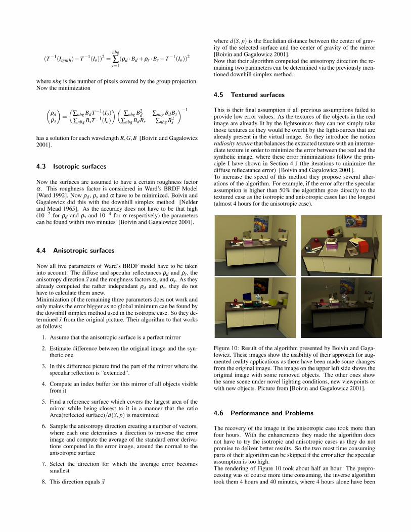
This is their final assumption if all previous assumptions failed toprovide low error values. As the textures of the objects in the realimage are already lit by the lightsources they can not simply takethose textures as they would be overlit by the lightsources that arealready present in the virtual image. So they introduce the notionradiosity texture that balances the extracted texture with an interme-diate texture in order to minimize the error between the real and thesynthetic image, where these error minimizations follow the prin-ciple I have shown in Section 4.1 (the iterations to minimize thediffuse reflecatance error) [Boivin and Gagalowicz 2001].To increase the speed of this method they propose several alter-ations of the algorithm. For example, if the error after the specularassumption is higher than 50% the algorithm goes directly to thetextured case as the isotropic and anisotropic cases last the longest(almost 4 hours for the anisotropic case).

Figure 10: Result of the algorithm presented by Boivin and Gaga-lowicz. These images show the usability of their approach for aug-mented reality applications as there have been made some changesfrom the original image. The image on the upper left side shows theoriginal image with some removed objects. The other ones showthe same scene under novel lighting conditions, new viewpoints orwith new objects. Picture from [Boivin and Gagalowicz 2001].

4.6 Performance and Problems

The recovery of the image in the anisotropic case took more thanfour hours. With the enhancments they made the algorithm doesnot have to try the isotropic and anisotropic cases as they do notpromise to deliver better results. So the two most time consumingparts of their algorithm can be skipped if the error after the specularassumption is too high.The rendering of Figure 10 took about half an hour. The prepro-cessing was of course more time consuming, the inverse algorithmtook them 4 hours and 40 minutes, where 4 hours alone have been

spent to recover the anisotropy parameters for the aluminium sur-face [Boivin and Gagalowicz 2001].

5 Photorealistic rendering for augmentedreality using environment illumination

Agusanto et al. used an image based lighting approach [Agusantoet al. 2003], [Debevec and Malik 1997]. They acquire the sceneradiance with HDR photography and process the data afterwards intheir rendering framework and render the pictures with the Phongillumination model [Phong 1975].Image based lighting means that radiance maps taken from areal (HDR) picture are used to get the scene illumination. Thoseradiance maps can be used to correctly illuminate virtual objectsrendered into the scene.Other than Ritschel and Grosch who used two HDR cameras, Agu-santo et al. used photography and a light probe. The light probeis a calibrated reflectance sphere (a mirror ball) made of chrome.A big advantage is the low cost of the utilities. The ball is placedin the scene where the virtual objects will be positioned later andpictures (with varying position, shuttertimes and exposure values,see Figure 11) are taken. They made low dynamic range picturesand assambled them with HDRShop [HDRShop ] developed byDebevec et al. into one single HDR picture.Of course the lighting conditions of the AR application needs tobe the same it was during the recording of the scene with the lightprobe. Plus the camera should ideally be aligned to the viewer’spoint of view.As they also obtain the interreflections between all objects inthe scene, these radiance maps can be used as environmentillumination maps in hardware based rendering which is employedfor AR.

Figure 11: The lightprobes photographed at different shutter times.Picture from [Agustanto et al. 2008]

5.1 Creating illumination maps

To keep flexibility within their approach the environment maps arederived from the radiance maps. Otherwise they would have to usea sphere with different surfaces and materials for different objects.Instead these different types of spheres (diffuse, specular, glossy...)are simulated in a virtual environment which is basically just a boxtextured with the previously obtained illumination map and thedemanded type of sphere in the middle of it (in a very small ratio

from 1:50 to 1:500).The viewing vector needs to be directed at the center of thesphere. The surrounding box serves as area light source for theglobal illumination algorithm (ray tracing) to obtain the syntheticillumination map.

5.2 Environment map prefiltering

To obtain the diffuse and the specular illuminations the environ-ment maps run through a prefiltering process. This process is thesolving of the rendering equation (Equation 2). Agusanto et al.used an approach presented by Kautz et al. [Kautz et al. 2000].A prefiltered environment map captures all the reflected radianceto a certain direction.

Lglossy(x;~v,~n,~t) =∫

Ω

fr(~ω(~v,~n,~t), ~ω(~l,~n,~t))Li(x;~l) <~n,~l > d~l,

(16)

where ~v is the viewing direction and ~l is the light direction,~n,~t,~n×~t is the local coordinate frame of the reflective surface,~ω(~v,~n,~t) represents the viewing direction and ~ω(~l,~n,~t) the lightdirection relative to that frame. The pre-filtered environment mapnow stores the radiance of light reflected towards the viewingdirection ~v which is computed by weighting the incoming lightLi (which is basically the unfiltered environment map) from alldirection~l with the BRDF fr [Kautz et al. 2000].

5.2.1 Diffuse Environment Maps

Miller proposed to use only purely diffuse BRDF to prefilter envi-ronment maps [Miller and Hoffman 1984]. So from Equation 16they get

Ldi f f use(x;~v,~n,~t) =∫

Ω

kdLi(x;~l) <~n,~l > d~l. (17)

Now all dependencies except for the normal vector are dropped andthe resulting two dimensional environment map is:

Ldi f f use(x;~n) = kd

∫Ω

Li(x;~l) <~n,~l > d~l. (18)

and stores all diffuse illumination at point x [Kautz et al. 2000].

Agusanto et al. used several prefiltering techniques. Apart fromthe diffuse map they also applied the Phong environment map sincethey used the Phong illumination model for their rendering.

5.2.2 Phong Environment Map

The environment map for Phong’s BRDF model can be expressedas:

Lphong(x;~v,~n,~t) =∫

Ωks

<~rv(~n),~l>N

<~n~l>Li(x;~l) <~n,~l > d~l

= ks∫

Ω<~rv(~n),~l >N Li(x;~l)d~l.

(19)

For the usage without prefiltering (as is supported in OpenGL) theindexing can be done just with the reflection vector~rv:

Lphong(x;~rv) = ks

∫Ω

<~rv,~l >N Li(x;~l)d~l. (20)

For the complete illumination model which Agusanto et al. used,they follow a method from Miller [Miller and Hoffman 1984] andHeidrich [Heidrich and Seidel 1999] and use a weighted sum ofa diffuse and a Phong environment map with a Fresnel term thatvaries the ratio between the diffuse reflection and the lobe of thespecular reflection so that a wider variety of materials can be ren-dered [Kautz et al. 2000]. The final environment map is:

Lo(~rv,~n) = Fd(<~rv,~n >)Ldi f f use +Fp(<~rv,~n >)Lphong (21)

5.3 Rendering

Rendering is done within a multi pass rendering framework to ren-der different effects like antialiasing, stencil buffer and so on. Theframework presents itself as follows:

for a number of image samples doJitter the cameraEnable stenceling / blending operationfor a number of passes do

Add effects to the polygon modelend forRender the polygon modelDo stencil / blending testPerform accumulation buffer operation

end for

Some operations - like sampling of images - are only needed ifphotorealism is required as they reduce the speed remarkably.The number of images being sampled can be reduced to one ifphotorealism is not that important.As this framework enables stencil buffer (e.g. for shadow maps)we don’t need global illumination to obtain shadows.

Now their implementation (with OpenGL commands) of thismultipass framework is presented. The most important commandsof their implementation are:

1. Enable blending

2. Transform the object

3. Enable 2D texture mapping

4. Set blending functions (GL ONE, GL ZERO)

5. Render the virtual object

6. Enable environment mapping

7. Set environment mapping to GL DECAL mode

8. Generate the sphere mapping texture coordinates

9. Set blending function(GL DST COLOR, GL ONE MINUS SRC ALPHA)

10. Render the virtual object

and do this for all virtual objects.

The reason behind the multiple passes is to add one photorealisticeffect after the other in each pass. In the second pass for example,the previously obtained illumination map is used to illuminate thevirtual object. With the use of the derived environment map theydon’t need to specify light sources for the rendering process. Forshadowing the lightsources are being approximated by the alsopreviously taken light probe image.

The algorithm has been tested using ARToolKit [Shared-Space-ARToolKit. ] and 3D polygon models (The programminglanguage was C with OpenGL).

5.4 Performance and Problems

All models that have been rendered with this algorithm could bedrawn at almost real-time (> 17 fps). As this is a seven year oldpaper (using just a 400 MHz machine) this surely will be muchfaster today.

The main problem is that a lot of computations have to bedone before the actual rendering is done. The biggest advantage ofthis approach is the high photorealism it provides (see Figure 12)

Figure 12: Diffuse and glossy models rendered at 17 fps. Picturefrom [Agusanto et al. 2008]

6 Recovery of material under complex illu-mination conditions

Wu et al. presented a method on how to recover the BRDF forRADIANCE’s low parameter reflectance model, which also usesWard’s model, for a real homogenous object under complex light-ing conditions from a HDR photograph of the object and one of theenvironment to find the lightsources [Wu et al. 2004].Important is that the object is lit in a way that enough specular high-lights are seen, so that only one HDR image is sufficient. The il-lumination field is computed via environment maps taken from dif-ferent viewpoints.Again their aim is to recover fr (here ρ) - the BRDF - from Equa-tion 2, where all other variables are known. The parameters they

need for their modified RADIANCE reflectance model are specu-lar, diffuse and directional diffuse refleactance and transmission.The BRDF model they used can be expressed as

fr = max(0,~q ·~np)[

ρd

π+ρs

]+max(0,−~q ·~np)

[τd

π+ τs

](22)

whereρd = pC(1−a4)

ρs = rsfs(~q)√

(~q·~np)(−~v·~np)

τd = a6(1− rs)(1−a7)pC

τs = a6a7(1− rs)gs(~q)√

(−~q·~np)(−~v·~np)

rs =

a4 plastica1a4,a2a4,a3a4 metal

where ~q is the direction from the surface point to a light sourcesample, ~v is the direction of an eye ray, ~np is the surface normalat the point p, C is the surface colour, p is the material patternand ai(i = 1, . . . ,7) are parameters. The ρ-parameters define thereflection, the τ-parameters the transmission coefficients [Wu et al.2004].The two functions fs(~q) and gs(~q) have the form

fs(~q) =

e[(~h·~np)2−‖~h‖2 ]/(~h·~np)2/α

4πα, isotropic

14π√

αxαyexp

[(~h·~x)2

αx+ (~h·~y)2

αy

(~h·~np)2

], anisotropic

(23)

and as they only consider opaque materials for the anisotropic case,for the isotropic case

gs(~q) =e(2~q·~t−2)/β

πβ, (24)

whereαx = α = a2

5 + ω

4π

αy = a26 + ω

4π

β = a25−

ω

π

~t = ~v‖~v‖

and~h is the bisection vector between the incident light ray and theeye ray [Wu et al. 2004].

After the acquisition of the illumination maps they now pro-ceed to recover the wanted materials for the object which is lit byknown lighting that is represented as an illumination field. Similarto the approach described in Section 4 the recovery of the materialparameters is done via the minimization of a difference valuebetween the real (Ir) and a synthetic rendered (Io) image of theobject. The difference in the mean of least squares is

χ2 = ‖Io− Ir‖2 = ∑i ‖pOi− pri‖2 == ∑i[(roi− rri)2 +(goi−gri)2 +(boi−bri)2]

(25)

where r, g and b mark the colour values of a certain point p. This isa nonlinear optimization problem that Wu et al. solved with simu-lated annealing algorithm. The algorithm works with a set of initialparameter values to optimize them and to reduce χ2 step by stepuntil a global minimum is found. These calculated parameters arethen used to render the object with ray tracing. A result of theirwork can be seen in Figures 13 and 14.

Figure 13: a), b) and c) show the real objects, d), e), and f) therendered ones after the last optimization step. Picture by [Wu et al.2004]

Figure 14: Left: Virtual objects rendered into a real (augmentedreality) scene. Right: Virtual objects rendered into a virtual scene.Picture by [Wu et al. 2004]

6.1 Performance and problems

The recovery of the materials took them about 2 to 3 hours on a DellDimension 4100 with a 667 MHz CPU and with 128 MB of work-ing memory [Wu et al. 2004]. The method is similar to the methodby Boivin and Gagalowicz [Boivin and Gagalowicz 2001] and isnot remarkably faster. On the other hand they do not need a 3Dgeometrical model of the scene which makes the precomputationscheaper. The illumination calculations (extraction of lightsourcesfor the illumination map to light the virtual objects) they presented

were also rather interesting and take some computation cost butthey are not topic of this thesis.As they also noted they can not reconstruct all materials especiallynot high frequent materials as they would require additional light-sources in the real scene.

7 A Framework for Automatically Recover-ing Object Shape, Reflectance and LightSources from Calibrated Images

Mercier et al. [Mercier et al. 2007] present a method for recoveringobject shapes, reflectance properties (for the modified Phong model[Lewis 1994]) and the position of light sources from a set of images.In my thesis only the surface and reflectance recovery is going tobe discussed. The modified Phong model is expressed as

Lr =Lskd

πr2 cosθ +(n+2)Lsks

2πr2 cosθ cosnφ (26)

where Lr is the radiance reflected, Ls is the radiance emitted by alight source S arriving at P, r is the distance between S and P, θ isthe angle between the surface normal and the direction of the lightsource, φ is the angle between the mirror reflection direction and theactual reflection direction and again ks and kd are the specular anddiffuse parameters and n is the specular exponent.

For each of the images in the image-set the position and orientationof the camera have to be known (see Figure 15).

Figure 15: Camera setup with fixed light sources. [Mercier et al.2007]

They made different images for different purposes. In Figure 15you see that they made an overexposed image for segmentation ofthe surfaces and a second image for reflectance and for the estima-tion of the lightsources.

Their first step is to acquire the object shape from these imagesusing a shape to silhouette approach. With the help of imagepixels they used the marching cubes algorithm for providingthe polygonal surface and the surface normals (that need to beestimated for each voxel) that are later needed to estimate theBRDF parameters.After they have acquired the polygonal mesh of the object theynow proceed to the estimation of the light source directions whichcan be found using specular highlights seen on images. They alsonote that diffuse or specular self-interreflections sometimes disturbthe BRDF estimation [Mercier et al. 2007].

Figure 16: a) The overexposed image, b) normal image, [Mercieret al. 2007]

During the estimation of the lightsources they also presentan identification algorithm to provide the BRDF coefficients againusing an error function Ea.They split the estimation of lightsources into two classes. The firstone applies to diffuse the second to the glossy surfaces. To find thetype of surface a variation coefficient V class is computed from theradiance samples:

V class =

√√√√∑NbVi=1 ∑

NbLii=1

(Li, j−Lmoy

iLmoy

i

)∑

NbVi=1 NbLi

(27)

where NbV represents the number of voxels in the class, Vi is the ithvoxel, Li, j is the jth radiance sample of Vi, and Lmoy

i is the averageradiance of Vi; NbLi corresponds to the number of radiance samplesin the voxel Vi [Mercier et al. 2007]. Now for a perfectly diffusesurface Equation 27 equals zero. V class increases directly propor-tional to the specular aspect of the surface i.e. that it is higher theglossier a surface is. Some examples for V class:

• V class < 0.15⇒ perfectly diffuse

• V class > 0.30⇒ glossy

• 0.15 ≤ V class ≤ 0.30⇒ no decision possible. For this classMercier et al. apply algorithms for both diffuse and glossysurfaces.

For both surface types a point light and a directional light source areestimated according to the error function Ea [Mercier et al. 2007]:

NbV

∑i=1

NbLi

∑j=1

[(Lskπr2 cosθi +

(n+2)Lsks

2πr2 cosθi cosnφi, j

)−Li, j

]2

(28)

where Li, j corresponds to the radiance sample j of the voxel Vi.The reflectance paramters Lskd , Lsks and n are not known and needto be estimated. Mercier et al. applied an identification algorithmwith the help of a gradient descent method in order to minimizeEa and hereby find the BRDF parameters. The parameters are cho-sen this way that Ea becomes as low as possible and the type ofsurface is known. This is applied for each class and to refine theBRDF parameters a final identification algorithm is applied againusing the error Ea. To reduce noise and grazing angles, Mercier etal. used only radiance samples corresponding to a small incidenceangle lower than 45 degrees (see Figure 17).

Figure 17: Estimated BRDF together with actual radiance samples[Mercier et al. 2007]

7.1 Performance and Problems

They used a Dual Intel Xeon 2.4 GHz processor with 1 GB of work-ing memory. The BRDF estimation of the clown Figure (see Fig-ure 18) took 6 minutes and 30 seconds precomputation time.

Figure 18: Result of the algorithm with sharp specular highlights[Mercier et al. 2007]

The approach by Mercier et al. has also certain limitations. Forexample is it hard to acquire the surface proberties if the objectposseses a variety of textures. Also diffuse interreflections are ig-nored hence certain artifacts can affect the shading [Mercier et al.2007].

8 Recovering surface reflectance and mul-tiple light locations and intensities fromimage data

Xu and Wallace presented a method to recover reflectence prop-erties from multiple objects using a 3D image. Their approachprovides the diffuse and constant specular reflectance parametersfrom object images [Xu and Wallace 2008]. They also recover thelight source parameters.

To get the surface geometry they used an active 3D scannerand a stereo pair of CCD cameras. They split their approach intotwo steps. The first step is to get the light source parameters and thespecular reflection for the Phong-Blinn reflection model with thesimplified formula for the specular irradiance which also considersthe light intensity (see Equation 5 for the original formula)

Ispec = ksL(P)(H ·N)n (29)

where L(P) is the light intensity at point P, N is the normal at thatpoint, n is the specular exponent and H is the halfway vector whichcalculates as

H =l +V|l +V |

,

where l is the normalized vector pointing to the lightsource and Vis the viewing vector [Xu and Wallace 2008], [Hearn and Baker2004].

8.1 Obtaining the specular reflectance

Remember that they used two cameras. They assume that bothcameras have the same radiometric constant α0 and give the im-age brightness (diffuse and specular reflectance) as

I(p) =α0kdL0

|l−P|3[(l−P) ·N]+

α0ksL0

|l−P|2(H ·N)n (30)

which gives two equations one for each camera where only thehalfway vector H differs.

I(p1) = α0kd L0

|l−P|3 [(l−P) ·N]+ α0ksL0|l−P|2 (H1 ·N)n

I(p2) = α0kd L0|l−P|3 [(l−P) ·N]+ α0ksL0

|l−P|2 (H2 ·N)n (31)

Now for convenience Ss = α0ksL0 and the difference from bothcamera images is

∆I(P) =Ss

|l−P|2[(H1 ·N)n− (H2 ·N)n]. (32)

The part for the diffuse reflectance disappeared as the diffuse re-flectance is the same for each viewpoint and only the specular re-flectance differs. Now Xu and Wallace compute the difference εrbetween the meassured and the predicted values

εr(Pi) = ∆Im(Pi)−∆I(Pi)= ∆Im(Pi)− Ss

|l−Pi|2 [(Hi1 ·Ni)c− (Hi2 ·Ni)n] (33)

where i = 1, . . . ,n, n indicates the number of successfully measuredbrightness values in the paired images [Xu and Wallace 2008].Now this error gets again minimized. The unkown variables arethe X ,Y,Z values of l, the specular coefficient Ss and the specularexponent c. The minimization function is called f.

flr =n

∑i=1

[∆Im(Pi)−

m

∑j=1

(Ss j

|l j−Pi|2[(Hi j1 ·Ni)c− (Hi j2 ·Ni)c]

)]2

.

(34)

To solve this minimization Xu and Wallace used a gradient de-scent least-square optimization procedure on f using the Levenberg-Marquardt method. To compute the initial values for Ss j (the j pa-rameter is for multiple lightsources) the following steps have to bemade. First a linear system is obtained by approximating the mea-sured image brightness difference ∆Im using the predicted values∆I.

1

|l−P1|2 [(H11 ·N1)c− (H12 ·N1)n]...

1|l−Pn|2 [(Hn1 ·Nn)c− (Hn2 ·Nn)n]

[Ss] =

∆Im(P1)...

∆Im(Pn)

(35)

This equation has the form BlrSs = ∆Im. The least-squares solutionfor this linear system is determined from [Xu and Wallace 2008]

Ss = (BTlrBlr)−1BT

lr∆Im. (36)

8.2 Obtaining the diffuse reflectance

Following the method to gain the specular reflectance Xu and Wal-lace now use Equation 30 to estimate the diffuse parameter.

δ1(Pi)Im(pi1) = δ0(Pi)δ1(Pi)

[SdiSs|l−Pi|3 [(l−Pi) ·Ni]+ Ss

|l−Pi|2 (Hi1 ·Ni)n]

δ2(Pi)Im(pi2) = δ0(Pi)δ2(Pi)[

SdiSs|l−Pi|3 [(l−Pi) ·Ni]+ Ss

|l−Pi|2 (Hi2 ·Ni)n]

(37)

By adding those two equations Sdi,(i = 1, . . . ,n′) are estimated by

Sdi = [δ1(Pi)Im(pi1)+δ2(Pi)Im(pi2)]δ0(Pi)(δi(P−I)+δ2(Pi))Ss[(l−Pi)·Ni]

−

δ0(Pi)Ss|l−Pi|[δ1(Pi)(Hi1·Ni)n+δ2(Pi)(Hi2·Ni)n]δ0(Pi)(δi(P−I)+δ2(Pi))Ss[(l−Pi)·Ni]

(38)

where n′ is the number of successfully measured brightness values,the δx(Pi) denote visibiltiy of the point Pi to the light (δ0), the first(δ1) and the second image (δ2) [Xu and Wallace 2008].

Figure 19: a) and b) are the two stereo images of the camel cup,c) is the rendered image with the estimated parameters from a newviewpoint [Xu and Wallace 2008]

8.3 Performance and Problems

A result of Xu and Wallace’s work can be seen in Figure 19.The difference between the estimated specular parameters and the

ground truth was (at 1% additive noise) 4.76% for Ss and 1.1% forc. This image had only one point light source. The error goes up asthe number of lightsources increases.

9 Online Estimation of Diffuse Materials

Ritschel and Grosch presented a way to get diffuse parts of BRDFsat runtime from digital photographs [Ritschel and Grosch 2008].They do not really work in real-time environments but expect theirapproach to also work in real-time. The only difference really is theparametrization of the model (which has to be done automaticallyat real-time). They used two HDR video cameras to get the diffusematerials. The equation for the outgoing radiance on a photographat a surface point is

L0 =∫2π

fr(ωi,ω0)Li(ωi)cos(θi)dωi (39)

where fr is the BRDF of the surface, Li is the incoming radiancefrom direction ωi and cos(θi) is the cosine of the angle betweenincoming direction and surface normal.

If we follow the calculations of Debevec [Debevec 1998] the initialvalues for L0 are being approximated as perfectly diffuse ( fr = 1).So after putting fr in front of the integral and dividing by the in-coming radiance L (and inverting the whole equation afterwards)we get fr for each part of the image as a result of the fraction

fr =L∫

2π

Li(ωi)cos(θi)dωi. (40)

The previously mentioned HDR cameras are positioned as follows.One is observing the object whose BRDF shall be approximatedand the second is filming the light source (see Figure 20). Thislight-camera is at a fixed position and records the whole environ-ment illumination with a fisheye lens. The object-camera shouldbe moved as close to the object as possible so we get the sameillumination on the virtual object as on the camera.

The object camera should take pictures from different viewingangles and capture the illumination of the objects it observes.The rotation of the objects needs to be known. Also a marker isplaced besides the object to track camera position and orientation.This happens via optical tracking with ARToolkit [Shared-Space-ARToolKit. ]. They used a couple of markes with known positionto increase the precision of the process.But first the synthetic object is required to be in a polygonalmesh representation. As said before, Ritschel and Grosch didthis offline (manually), but this can be done using an automaticparametrization as presented by Levy [Levy et al. 2002].

The images captured with this camera run through a coupleof processes discussed in the following. The software side of theirprocedure is divided into two steps: Inverse Texturing (storing thecamera images to a texture) and Inverse Lighting (processing thesetextures to one final reflectance texture).As their approach only works for diffuse lighting, they propose tofactorize the software steps into orthogonal components to get thespecular part as well.

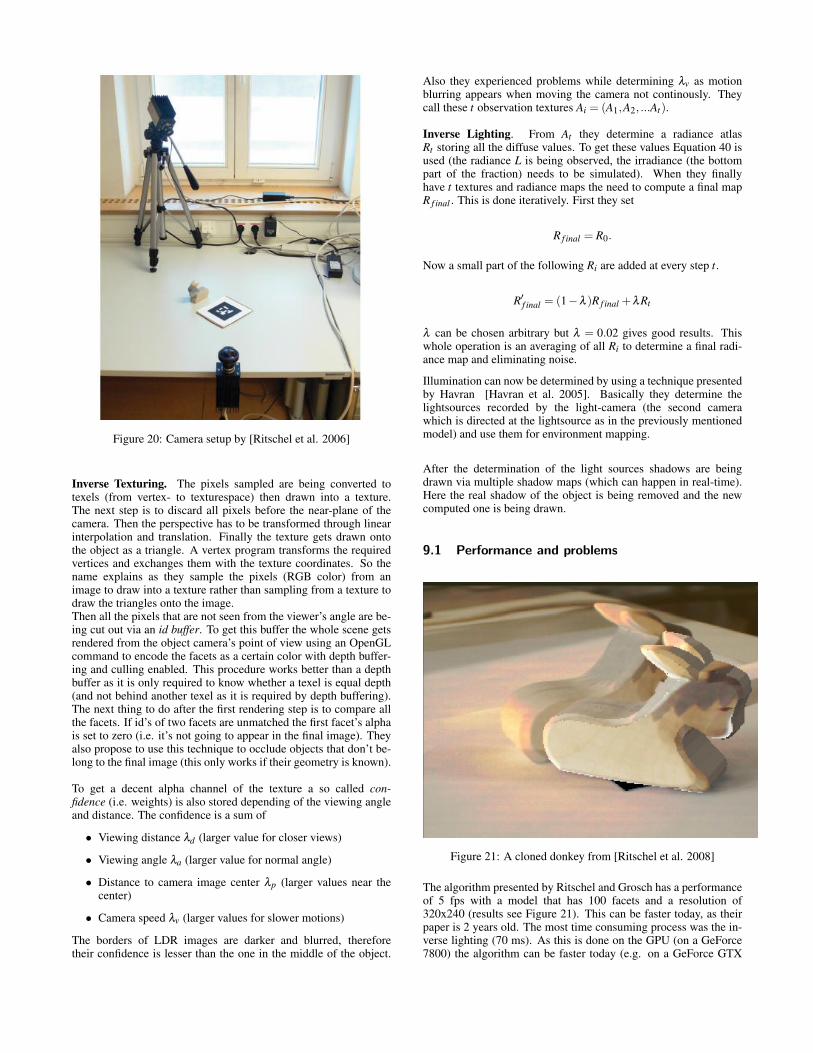
Figure 20: Camera setup by [Ritschel et al. 2006]

Inverse Texturing. The pixels sampled are being converted totexels (from vertex- to texturespace) then drawn into a texture.The next step is to discard all pixels before the near-plane of thecamera. Then the perspective has to be transformed through linearinterpolation and translation. Finally the texture gets drawn ontothe object as a triangle. A vertex program transforms the requiredvertices and exchanges them with the texture coordinates. So thename explains as they sample the pixels (RGB color) from animage to draw into a texture rather than sampling from a texture todraw the triangles onto the image.Then all the pixels that are not seen from the viewer’s angle are be-ing cut out via an id buffer. To get this buffer the whole scene getsrendered from the object camera’s point of view using an OpenGLcommand to encode the facets as a certain color with depth buffer-ing and culling enabled. This procedure works better than a depthbuffer as it is only required to know whether a texel is equal depth(and not behind another texel as it is required by depth buffering).The next thing to do after the first rendering step is to compare allthe facets. If id’s of two facets are unmatched the first facet’s alphais set to zero (i.e. it’s not going to appear in the final image). Theyalso propose to use this technique to occlude objects that don’t be-long to the final image (this only works if their geometry is known).

To get a decent alpha channel of the texture a so called con-fidence (i.e. weights) is also stored depending of the viewing angleand distance. The confidence is a sum of

• Viewing distance λd (larger value for closer views)

• Viewing angle λa (larger value for normal angle)

• Distance to camera image center λp (larger values near thecenter)

• Camera speed λv (larger values for slower motions)

The borders of LDR images are darker and blurred, thereforetheir confidence is lesser than the one in the middle of the object.

Also they experienced problems while determining λv as motionblurring appears when moving the camera not continously. Theycall these t observation textures Ai = (A1,A2, ...At).

Inverse Lighting. From At they determine a radiance atlasRt storing all the diffuse values. To get these values Equation 40 isused (the radiance L is being observed, the irradiance (the bottompart of the fraction) needs to be simulated). When they finallyhave t textures and radiance maps the need to compute a final mapR f inal . This is done iteratively. First they set

R f inal = R0.

Now a small part of the following Ri are added at every step t.

R′f inal = (1−λ )R f inal +λRt

λ can be chosen arbitrary but λ = 0.02 gives good results. Thiswhole operation is an averaging of all Ri to determine a final radi-ance map and eliminating noise.

Illumination can now be determined by using a technique presentedby Havran [Havran et al. 2005]. Basically they determine thelightsources recorded by the light-camera (the second camerawhich is directed at the lightsource as in the previously mentionedmodel) and use them for environment mapping.

After the determination of the light sources shadows are beingdrawn via multiple shadow maps (which can happen in real-time).Here the real shadow of the object is being removed and the newcomputed one is being drawn.

9.1 Performance and problems

Figure 21: A cloned donkey from [Ritschel et al. 2008]

The algorithm presented by Ritschel and Grosch has a performanceof 5 fps with a model that has 100 facets and a resolution of320x240 (results see Figure 21). This can be faster today, as theirpaper is 2 years old. The most time consuming process was the in-verse lighting (70 ms). As this is done on the GPU (on a GeForce7800) the algorithm can be faster today (e.g. on a GeForce GTX

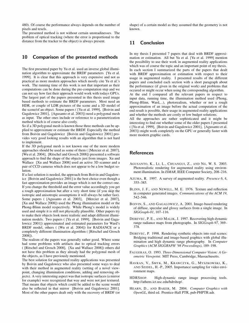
480). Of course the performance always depends on the number ofpixels and texels.The presented method is not without certain unsteadinesses. Theproblem of optical tracking (where the error is proportional to thedistance from the tracker to the object) is always present.

10 Comparison of the presented methods

The first presented paper by Yu et al. used an inverse global illumi-nation algorithm to approximate the BRDF parameters [Yu et al.1999]. It is clear that this approach is very expensive and not aspractical as more modern approaches which mostly cite Yu et al.’swork. The running time of this work is not that important as theircomputations can be done during the pre-computation step and wecan not say how fast their approach would work with todays GPUs.The largest part of the papers presented in this thesis used imagebased methods to estimate the BRDF parameters. Most need anHDR, or couple of LDR pictures of the scene and a 3D model ofthe scene/of an object. Some papers ( [Yu et al. 1999], [Boivin andGagalowicz 2001], [Agusanto et al. 2003]) need a polygonal meshas input. The other ones include or reference to a parametrizationmethod which is of course also costly.So if a 3D polygonal mesh is known those three methods can be ap-plied to approximate or estimate the BRDF. Especially the methodfrom Boivin and Gagalowicz [Boivin and Gagalowicz 2001] pro-vides very good looking results with an algorithm that is not hardto implement.If the 3D polygonal mesh is not known one of the more modernapproaches should be used as some of them ( [Mercier et al. 2007],[Wu et al. 2004], [Ritschel and Grosch 2008]) presented a softwareapproach to find the shape of the objects just from images. Xu andWallace [Xu and Wallace 2008] used an active 3D scanner and apair of CCD cameras which does not appear to be a low budget so-lution.If a fast solution is needed, the approach from Boivin and Gagalow-icz [Boivin and Gagalowicz 2001] is the best choice even though afast approximation provides an image which is not the correct one.If you change the threshold and the error value accordingly you geta rough approximation but after a very short time (if you skip theisotropic and anisotropic assumptions it will always be rather fast).Some papers ( [Agusanto et al. 2003], [Mercier et al. 2007],[Xu and Wallace 2008]) used the Phong illumination model or thePhong-Blinn model respectively. While Phong’s model is widelyused and simple it is still not physically plausible. Other papers tryto make their objects look more realistic and adapt different illumi-nation models. Two papers ( [Yu et al. 1999], [Boivin and Gaga-lowicz 2001]) approximated and estimated parameters for Ward’sBRDF model, others ( [Wu et al. 2004]) for RADIANCE or acompletely different illumination algorithm ( [Ritschel and Grosch2008]).The realism of the papers was generally rather good. Where somehad some problems with artifacts due to optical tracking errors( [Ritschel and Grosch 2008], [Xu and Wallace 2008]) others didnot have this problem as they already had the polygonal mesh ofthe objects, as I have previously mentioned.The best solution for augmented reality applications was presentedby Boivin and Gagalowicz who also presented some ways to dealwith their method in augmented reality (setting of a novel view-point, changing illumination conditions, adding and removing ob-jects). A very interesting aspect was that isotropic surfaces (a mirrorfor example) were recognized that way and were not just textured.That means that objects which could be added to the scene wouldalso be reflected in that mirror [Boivin and Gagalowicz 2001].Most of the other papers dealt only with the recovery of BRDF (or

shape) of a certain model as they assumed that the geometry is notknown.

11 Conclusion

In my thesis I presented 7 papers that deal with BRDF approxi-mation or estimation. All but Yu et al. [Yu et al. 1999] mentionthe possibility to use their work in augmented reality applicationswhich was of course the topic and an important point of my thesis.In each section I summarized the parts of the papers that dealtwith BRDF approximation or estimation with respect to theirusage in augmented reality. I presented results of the differentpapers and concluded each section with a short paragraph aboutthe performance (if given in the original work) and problems thatoccured or might occur when using the corresponding algorithm.At the end I compared all the relevant papers in respect toinput data, running time, the illumination method used (Phong,Phong-Blinn, Ward,...), photorealism, whether or not a roughapproximation of an image before the actual computation of theend result is possible, their usage in augmented reality applicationsand whether the methods are costly or low budget solutions.All the approaches are rather sophisticated and it might beinteresting to find out whether some of the older papers I presented( [Yu et al. 1999], [Boivin and Gagalowicz 2001], [Agusanto et al.2003]) might work completely on the GPU or generally faster withmore modern graphic cards.

References

AGUSANTO, K., LI, L., CHUANGUI, Z., AND NG, W. S. 2003.Photorealistic rendering for augmented reality using environ-ment illumination. In ISMAR, IEEE Computer Society, 208–216.

AZUMA, R. 1997. A survey of augmented reality. Presence 6, 4,355–385.

BLINN, J. F., AND NEWELL, M. E. 1976. Texture and reflectionin computer generated images. Communications of the ACM 19,542–546.

BOIVIN, S., AND GAGALOWICZ, A. 2001. Image-based renderingof diffuse, specular and glossy surfaces from a single image. InSIGGraph-01, 107–116.

DEBEVEC, P. E., AND MALIK, J. 1997. Recovering high dynamicrange radiance maps from photographs. In SIGGraph-97, 369–378.

DEBEVEC, P. 1998. Rendering synthetic objects into real scenes:Bridging traditional and image-based graphics with global illu-mination and high dynamic range photography. In ComputerGraphics (ACM SIGGRAPH ’98 Proceedings), 189–198.

FAUGERAS, O. 1993. Three-Dimensional Computer Vision: A Ge-ometric Viewpoint. MIT Press, Cambridge, Massachusetts.

HAVRAN, V., SMYK, M., KRAWCZYK, G., MYSZKOWSKI, K.,AND SEIDEL, H.-P., 2005. Importance sampling for video envi-ronment maps.

HDRSHOP. High-dynamic range image processing tools.http://athens.ict.usc.edu/hdrshop/.

HEARN, D., AND BAKER, M. 2004. Computer Graphics withOpenGL, third ed. Prentice-Hall PTR, pub-PHPTR:adr.

HEIDRICH, W., AND SEIDEL, H.-P. 1999. Realistic, hardware-accelerated shading and lighting. In SIGGRAPH, 171–178.

KAUTZ, J., AND MCCOOL, M. D. 1999. Interactive renderingwith arbitrary BRDFs using separable approximations. In Ren-dering Techniques ’99, Springer Wien, 247–260.

KAUTZ, J., PAU VZQUEZ, P., HEIDRICH, W., PETER SEIDEL, H.,AND UDG, A., 2000. A unified approach to prefiltered environ-ment maps, Sept. 14.

LAFORTUNE, E. P. F., FOO, S.-C., TORRANCE, K. E., ANDGREENBERG, D. P. 1997. Non-linear approximation of re-flectance functions. In SIGGRAPH 97 Conference Proceedings,Addison Wesley, T. Whitted, Ed., Annual Conference Series,ACM SIGGRAPH, 117–126.

LEVY, B., PETITJEAN, S., RAY, N., AND MAILLOT, J. 2002.Least squares conformal maps for automatic texture atlas gener-ation. ACM Transactions on Graphics 21, 3 (July), 362–371.

LEWIS, R. R. 1994. Making shaders more physically plausible.Computer Graphics Forum 13, 2 (Jan.), 109–120.

MARK, W. R., GLANVILLE, R. S., AKELEY, K., AND KILGARD,M. J. 2003. Cg: a system for programming graphics hardwarein a C-like language. In Proceedings of ACM SIGGRAPH 2003,J. Hodgins and J. C. Hart, Eds., vol. 22(3) of ACM Transactionson Graphics, 896–907.

MERCIER, B., MENEVEAUX, D., AND FOURNIER, A. 2007.A framework for automatically recovering object shape, re-flectance and light sources from calibrated images. InternationalJournal of Computer Vision 73, 1 (June), 77–93.

MILLER, G. S., AND HOFFMAN, C. R. 1984. Illumination andreflection maps: Simulated objects in simulated and real envi-ronments. In SIGGRAPH ’84 Advanced Computer Graphics An-imation course notes. jul.

NELDER, J. A., AND MEAD, R. 1965. A simplex method forfunction minimization. Computer Journal 7, 308–313.

NICODEMUS, F. E., RICHMOND, J. C., HSIA, J. J., GINSBERG,I. W., AND LIMPERIS, T. 1977. Geometric considerations andnomenclature for reflectance. Monograph 161, National Bureauof Standards (US), Oct.

PHONG, B. T. 1975. Illumination for computer generated pictures.Communications of the ACM 18, 6, 311–317.

RITSCHEL, T., AND GROSCH, T., 2008. On-line estimation ofdiffuse materials, Apr. 01.

SHARED-SPACE-ARTOOLKIT. www.hitl.washington.edu/projects/sharedspace.

SILLION, F., AND PUECH, C. 1994. Radiosity and Global Illumi-nation. Morgan Kaufmann, San Francisco. excellent coverageof radiosity and global illumination algorithms.

WARD, G. J. 1992. Measuring and modeling anisotropic reflection.In Computer Graphics (SIGGRAPH ’92 Proceedings), E. E. Cat-mull, Ed., vol. 26, 265–272.

WU, E., SUN, Q., AND LIU, X. 2004. Recovery of material undercomplex illumination conditions. In GRAPHITE, ACM, Y. T.Lee, S. N. Spencer, A. Chalmers, and S. H. Soon, Eds., 39–45.

XU, S., AND WALLACE, A. M. 2008. Recovering surface re-flectance and multiple light locations and intensities from imagedata. Pattern Recognition Letters 29, 11 (Aug.), 1639–1647.

YU, Y., DEBEVEC, P. E., MALIK, J., AND HAWKINS, T. 1999.Inverse global illumination: Recovering reflectance models ofreal scenes from photographs. In SIGGraph-99, 215–224.