brazil trade
TRANSCRIPT
7242019 Brazil Trade
httpslidepdfcomreaderfullbrazil-trade 149
NBER WORKING PAPER SERIES
TRADE AND INEQUALITY
FROM THEORY TO ESTIMATION
Elhanan Helpman
Oleg Itskhoki
Marc-Andreas Muendler
Stephen J Redding
Working Paper 17991
httpwwwnberorgpapersw17991
NATIONAL BUREAU OF ECONOMIC RESEARCH
1050 Massachusetts Avenue
Cambridge MA 02138
April 2012
We thank the National Science Foundation for financial support We also thank SECEXMEDIC and
Ricardo Markwald at FUNCEX Rio de Janeiro for sharing firm trade data We are very grateful to
Sam Bazzi Lorenzo Casaburi Itzik Fadlon Adam Guren Eduardo Morales and Jesse Schreger for excellent research assistance We thank Mark Aguiar Carlos Henrique Corseuil Kerem Cosar Angus
Deaton Thibault Fally Cecilia Fieler Leo Feler Gita Gopinath Gene Grossman Bo Honore Guido
Imbens Larry Katz Francis Kramarz Rasmus Lentz Marc Melitz Naercio Menezes-Filho Eduardo
Morales Ulrich Muller Andriy Norets Richard Rogerson Esteban Rossi-Hansberg Andres Santos
Mine Senses Chris Sims John Van Reenen Jon Vogel Yoto Yotov and seminar participants at theIAE Workshop at UAB Columbia FGV Rio de Janeiro Harvard Humboldt Berlin IAS IGC Trade
Programme Meeting at Columbia JHU-SAIS Notre Dame Princeton Toronto the Philadelphia Fed
Trade Workshop UC San Diego Wisconsin and WTO for helpful comments and suggestions The
usual disclaimer applies The views expressed herein are those of the authors and do not necessarily
reflect the views of the National Bureau of Economic Research
NBER working papers are circulated for discussion and comment purposes They have not been peer-
reviewed or been subject to the review by the NBER Board of Directors that accompanies official
NBER publications
copy 2012 by Elhanan Helpman Oleg Itskhoki Marc-Andreas Muendler and Stephen J Redding All
rights reserved Short sections of text not to exceed two paragraphs may be quoted without explicit
permission provided that full credit including copy notice is given to the source
7242019 Brazil Trade
httpslidepdfcomreaderfullbrazil-trade 249
Trade and Inequality From Theory to Estimation
Elhanan Helpman Oleg Itskhoki Marc-Andreas Muendler and Stephen J Redding
NBER Working Paper No 17991
April 2012
JEL No E24F12F16
ABSTRACT
While neoclassical theory emphasizes the impact of trade on wage inequality between occupations
and sectors more recent theories of firm heterogeneity point to the impact of trade on wage dispersion
within occupations and sectors Using linked employer-employee data for Brazil we show that much
of overall wage inequality arises within sector-occupations and for workers with similar observable
characteristics this within component is driven by wage dispersion between firms and wage dispersion
be tw een firm s is re la ted to firm em ploy men t s ize an d trade pa rt icipat ion We then ex tend the he teroge no us -f irm
model of trade and inequality from Helpman Itskhoki and Redding (2010) and structurally estimate
it with Brazilian data We show that the estimated model fits the data well both in terms of key moments
as well as in terms of the overall distributions of wages and employment and find that international
trade is important for this fit In the estimated model reductions in trade costs have a sizeable effect
on wage inequality
Elhanan Helpman
Department of Economics
Harvard University
1875 Cambridge Street
Cambridge MA 02138
and NBER ehelpmanharvardedu
Oleg Itskhoki
Department of Economics
Princeton University
Fisher Hall 306
Princeton NJ 08544-1021
and NBER
itskhokiprincetonedu
Marc-Andreas Muendler
Department of Economics 0508
University of California San Diego
9500 Gilman Drive
La Jolla CA 92093-0508
and NBER muendlerucsdedu
Stephen J Redding
Department of Economics
and Woodrow Wilson School
Princeton University
Fisher Hall
Princeton NJ 08544
and NBER
reddingsprincetonedu
7242019 Brazil Trade
httpslidepdfcomreaderfullbrazil-trade 349
1 Introduction
The field of international trade has undergone a transformation in the last decade as attention
has shifted to heterogeneous firms as drivers of foreign trade Until recently however research on
the labor market effects of international trade has been heavily influenced by the Heckscher-Ohlin
and Specific Factors models which provide predictions about relative wages across skill groups
occupations and sectors In contrast to the predictions of these theories empirical studies find
increased wage inequality in both developed and developing countries growing residual wage
dispersion among workers with similar observed characteristics and increased wage dispersion
across plants and firms within sectors In a large part due to this disconnect previous studies
have concluded that the contribution of international trade to growing wage inequality is modest
at best (see for example the survey by Goldberg and Pavcnik 2007)
This paper argues that these apparently discordant empirical findings are in fact consistent
with a trade-based explanation for wage inequality but one rooted in recent models of firm
heterogeneity rather than neoclassical trade theories For this purpose we develop a theory-
based structural model and a methodology for estimating it and illustrate with Brazilian datahow to use this model to quantify the contribution of trade to wage inequality
To motivate our structural model we first report reduced-form evidence on the level and
growth of wage inequality in Brazil First much of overall wage inequality occurs within sectors
and occupations rather than between sectors and occupations Second a large share of this
wage inequality within sectors and occupations is driven by wage inequality between rather
than within firms Third both of these findings are robust to controlling for observed worker
characteristics suggesting that this wage inequality between firms within sector-occupations is
residual wage inequality These features of the data motivate our theoretical modelrsquos focus on
wage inequality between firms for workers with similar observed characteristicsTo quantify the overall contribution of firm-based variation in wages to wage inequality we
first estimate the firm component of wages by including a firm-occupation-year fixed effect in
a Mincer regression of log worker wages on controls for observed worker characteristics This
firm effect includes both wage premia for workers with identical characteristics and unobserved
differences in workforce composition across firms Our analysis focuses on this wage component
because recent theories of firm heterogeneity emphasize both sources of wage differences across
firms We estimate the firm wage component separately for each sector-occupation-year because
our theoretical model implies that differences in wages across firms can change over time and
these changes can be more important in some sectors and occupations than others
In the data the firm component of wages is systematically related to trade participation
exporters are on average larger and pay higher wages than non-exporters However this relation-
ship is far from perfect as there is substantial overlap in the employment and wage distributions
of these two groups of firms so that some non-exporting firms are larger and pay higher wages
than some exporting firms Nonetheless an exporter wage premium after controlling for firm
size is a robust feature of the data This feature holds both in the cross-section of firms and for
1
7242019 Brazil Trade
httpslidepdfcomreaderfullbrazil-trade 449
a given firm over time as it switches in and out of exporting
To account for these features of the data we extend the theoretical framework of Helpman
Itskhoki and Redding (2010) to include two additional sources of heterogeneity across firms
besides productivity the cost of screening workers and the size of the fixed cost of exporting
Heterogeneous screening costs allow for variation in wages across firms after controlling for
their employment size and export status while idiosyncratic exporting costs allow some smalllow-wage firms to profitably export and some large high-wage firms to serve only the domestic
market Nevertheless in this model exporters are on average larger and pay higher wages than
non-exporters both due to selection into exporting and due to the additional revenue from
foreign market access Using Brazilian data on firm wages employment and export status we
estimate the parameters of the model with maximum likelihood We show that the parameterized
model provides a good fit to the data both for a wide set of moments as well as for the overall
employment and wage distributions across firms
We further show that our explicit modelling of firm export status contributes in an important
way to the overall fit of the model In particular a nested version of the model without the link
between export participation and firm size and wages fares substantially worse in explaining
the cross-sectional employment and wage distributions This allows us to conclude that trade
participation is indeed an important determinant of the overall wage distribution and in par-
ticular of various measures of wage inequality We then use the estimated model to undertake
a counterfactual exercise that illustrates the effects of trade on wage inequality
Our paper is related to a number of strands of the existing literature As mentioned above
several empirical studies have suggested that the Heckscher-Ohlin and Specific Factors modelsmdash
as conventionally interpretedmdashprovide at best an incomplete explanation for observed wage
inequality First changes in the relative returns to observed measures of skills (eg education
and experience) and changes in sectoral wage premia account for a limited share of changein overall wage inequality leaving a substantial role for residual wage inequality1 Second
the Stolper-Samuelson theorem predicts a rise in the relative skilled wage in skill-abundant
countries and a fall in the relative skilled wage in unskilled-abundant countries in response to
trade liberalization Yet wage inequality rises following trade liberalization in both developed
and developing countries (eg Goldberg and Pavcnik 2007)2 Third much of the change in
the relative demand for skilled and unskilled workers in developed countries has occurred within
sectors and occupations rather than across sectors and occupations (eg Katz and Murphy 1992
and Berman Bound and Griliches 1994) Fourth while wage dispersion between plants and
firms is an empirically-important source of wage inequality (eg Davis and Haltiwanger 19911For developed country evidence see for example Autor Katz and Kearney (2008) Juhn Murphy and Pierce
(1993) and Lemieux (2006) For developing country evidence see for example Attanasio Goldberg and Pavcnik(2004) Ferreira Leite and Wai-Poi (2010) Goldberg and Pavcnik (2005) Gonzaga Menezes-Filho and Terra(2006) and Menezes-Filho Muendler and Ramey (2008)
2Increasing wage inequality in both developed and developing countries can be explained by re-interpreting theStolper-Samuelson Theorem as applying within sectors as when production stages are offshored (see for exampleFeenstra and Hanson (1996) Feenstra and Hanson (1999) and Trefler and Zhu (2005))
2
7242019 Brazil Trade
httpslidepdfcomreaderfullbrazil-trade 549
and Faggio Salvanes and Van Reenen 2010) neoclassical trade theory is not able to elucidate
it Each of these features of the data can be explained within the class of new trade models
based on firm heterogeneity
Models of firm heterogeneity suggest two sets of reasons for wage variation across firms
One line of research assumes competitive labor markets so that all workers with the same
characteristics are paid the same wage but wages vary across firms as a result of differencesin workforce composition (see for example Yeaple 2005 Verhoogen 2008 Bustos 2011 Burstein
and Vogel 2003 and Monte 2011) Another line of research introduces labor market frictions
so that workers with the same characteristics can be paid different wages by different firms
For example search and matching frictions and the resulting bargaining over the surplus from
production can induce wages to vary across firms (see for example Davidson Matusz and
Shevchenko 2008 Cosar Guner and Tybout 2011 Helpman Itskhoki and Redding 2010)3
Efficiency or fair wages are another potential source of wage variation where the wage that
induces worker effort or is perceived to be fair varies with revenue across firms (see for example
Egger and Kreickemeier 2009 Amiti and Davis 2011 and Davis and Harrigan 2011)
Following Bernard and Jensen (1995 1997) empirical research using plant and firm data has
provided evidence of substantial differences in wages and employment between exporters and
non-exporters More recent research has used linked employer-employee datasets to examine the
determinants of the exporter wage premium including Schank Schnabel and Wagner (2007)
Munch and Skaksen (2008) Frıas Kaplan and Verhoogen (2009) Davidson Heyman Matusz
Sjoholm and Zhu (2011) Krishna Poole and Senses (2011) and Baumgarten (2011) These
empirical studies typically find evidence of both unobserved differences in workforce composition
and wage premia for workers with identical characteristics with the relative importance of these
two forces varying across studies By focusing on the overall firm wage component including
both these sources of wage differences across firms we are not required to make the assumptionof conditional random matching of workers to firms commonly invoked in this literature and
can allow for the assortative matching of workers across firms Furthermore while these studies
typically estimate a time-invariant wage fixed effect for each firm a key feature of our approach
is that the firm component of wages can change over time with firm trade participation
In contrast to the above empirical literature which is focused on estimating the exporter
wage premium our objective is to develop a theory-based methodology for estimating a struc-
tural model of international trade with heterogeneous firms in which employment and wages
are jointly determined with export status and to show how this model can be used to quantify
the contribution to wage inequality of firm-based variation in wages Using a structural modelwe estimate the extent of heterogeneity in productivity screening and fixed export costs across
firms and isolate their impact through employment and wages on wage inequality Our paper
is therefore related to two recent papers structurally estimating models of heterogeneous firms
and trade Eaton Kortum and Kramarz (2010) on patterns of trade across firms and destina-
3Search and matching frictions may also influence income inequality through unemployment as in Davidsonand Matusz (2010) Felbermayr Prat and Schmerer (2011) and Helpman and Itskhoki (2010)
3
7242019 Brazil Trade
httpslidepdfcomreaderfullbrazil-trade 649
tions and Irarrazabal Moxnes and Opromolla (2011) on multinational activity across firms and
destinations4
The remainder of the paper is structured as follows In Section 2 we introduce our data
and some background information In Section 3 we report reduced-form evidence on wage in-
equality in Brazil Motivated by these findings Section 4 sets up and estimates a structural
heterogeneous-firm model of trade and inequality using the Brazilian data Section 5 concludesA supplementary web appendix contains detailed derivations description of the data and ad-
ditional results5
2 Data and Background
Our main dataset is a linked employer-employee dataset for Brazil from 1986-1998 which we
briefly describe here and provide further details in the web appendix The source for these ad-
ministrative data is the Relac˜ ao Anual de Informac˜ oes Sociais (Rais) database of the Brazilian
Ministry of Labor which requires by law that all formally-registered firms report information
each year on each worker employed by the firm The data contain a unique identifier for each
worker which remains with the worker throughout his or her work history as well as the tax
identifier of the workerrsquos employer
We focus on the formal manufacturing sector because manufacturing goods are typically
tradable and there is substantial heterogeneity across sectors occupations and firms within
manufacturing Therefore this sector provides a suitable testing ground for traditional and
heterogeneous firm theories of international trade Manufacturing is also an important source
of employment in Brazil accounting in 1990 and 1998 for around 23 and 19 percent of total
employment (formal plus informal) respectively Of this manufacturing employment Goldberg
and Pavcnik (2003) estimate that the formal sector accounts for around 84 percent of the totalOur annual earnings measure is a workerrsquos mean monthly wage averaging the workerrsquos wage
payments over the course of a workerrsquos employment spell during a calendar year6 For every
worker with employment during a calendar year we keep the workerrsquos last recorded job spell
and if there are multiple spells spanning into the final month of the year the highest-paid job
spell (randomly dropping ties) Therefore our definition of firm employment is the count of
employees whose employment spell at the firm is their final (highest-paid) job of the year
We undertake our analysis at the firm rather than the plant level because recent theories
of firm heterogeneity and trade are concerned with firms and wage and exporting decisions are
arguably firm based For our baseline sample we focus on firms with five or more employees4Eaton Kortum and Kramarz together with Raul Sampognaro have been working contemporaneously on
extending their structural model to account for wage variation across firms Egger Egger and Kreickemeier(2011) provide evidence on the wage inequality predictions of a model of firm heterogeneity and fair wages
5Access at httpwwwprincetonedu~itskhokipapersTradeInequalityEvidence_appendixpdf6Wages are reported as multiples of the minimum wage which implies that inflation that raises the wages of all
workers by the same proportion leaves this measure of relative wages unchanged Empirically we find a smoothleft tail of the wage distribution in manufacturing which suggests that the minimum wage is not strongly bindingin manufacturing during our sample period Rais does not report hours or overtime
4
7242019 Brazil Trade
httpslidepdfcomreaderfullbrazil-trade 749
Table 1 Occupation Employment Shares and Relative Mean Log Wages 1990
Employment Relative meanCBO Occupation share (percent) log wage
1 Professional and Managerial 78 1082 Skilled White Collar 111 0403 Unskilled White Collar 84 013
4 Skilled Blue Collar 574 minus0155 Unskilled Blue Collar 152 minus035
Note Share in total formal manufacturing-sector employment log wage minus average log wage in formal man-ufacturing sector
since we analyze wage variation within and across firms and the behavior of firms with a handful
of employees may be heavily influenced by idiosyncratic factors But we also show that we find a
similar pattern of results using the universe of firms As discussed further in the web appendix
our baseline sample includes around 7 million workers and around 100000 firms in each year
Each worker is classified in each year by her or his occupation In our baseline empirical
analysis we use five standard occupational categories (1) Professional and Managerial (2)
Skilled White Collar (3) Unskilled White Collar (4) Skilled Blue Collar (5) Unskilled Blue
Collar The employment shares of each occupation and the mean log wage in each occupation
relative to the overall manufacturing mean log wage are reported in Table 1 Skilled Blue Collar
workers account for almost 60 percent of employment while Professional and Managerial workers
account for the smallest share of employment Over our sample period the employment share of
Unskilled Blue Collar (Unskilled White Collar) workers falls (rises) from 16 to 10 percent (from
8 to 15 percent) while the employment shares of the other occupations remain relatively stable
In robustness checks we also make use of the more disaggregated Classificac˜ ao Brasileira de
Ocupac˜ oes (CBO) definition of occupations which breaks down manufacturing into around 350
occupations as listed in the web supplement
Each firm is classified in each year by its main sector according to a classification compiled by
the Instituto Brasileiro de Geografia e Estatistica (IBGE) which disaggregates manufacturing
into twelve sectors roughly corresponding to two-digit International Standard Industrial Classifi-
cation (ISIC) sectors Sectoral employment shares and the mean log wage in each sector relative
to the overall manufacturing mean log wage are reported in Table 2 Apparel and Textiles and
Food Beverages and Alcohol are the largest sectors (each about 16 percent of employment) and
have relatively low wages (along with Wood Products and Footwear) Two other large sectors
are Metallic Products and Chemicals and Pharmaceuticals which have relatively high wages(along with Transport Equipment) Most other sectors are of roughly the same size and each
accounts for about 6 percent of employment The employment shares of sectors are relatively
constant over our sample period with the exception of Food Beverages and Alcohol (which in-
creases from around 16 to 23 percent) and Electrical and Telecommunications Equipment (which
decreases from roughly 6 to 4 percent) From 1994 onwards firms are classified according to
5
7242019 Brazil Trade
httpslidepdfcomreaderfullbrazil-trade 849
Table 2 Sectoral Employment Shares and Relative Mean Log Wages 1990
Emplmnt Relative Exportershare mean share (percent)
IBGE Sector (percent) log wage Firms Emplmnt
2 Non-metallic Minerals 55 minus012 23 3233 Metallic Products 98 027 61 499
4 Mach Equip and Instruments 66 038 123 5415 Electrical amp Telecomm Equip 60 037 118 5636 Transport Equip 63 061 112 7067 Wood amp Furniture 65 minus048 32 2358 Paper amp Printing 54 014 25 3069 Rubber Tobacco Leather etc 70 minus004 86 508
10 Chem amp Pharm Products 99 040 112 50611 Apparel amp Textiles 157 minus032 25 34812 Footwear 44 minus044 122 65713 Food Bev amp Alcohol 169 minus030 39 380
Note Share in total formal manufacturing-sector employment log wage minus average log wage in formal man-
ufacturing sector share of firms that export employment share of exporters
the more finely-detailed National Classification of Economic Activities (CNAE) which breaks
down manufacturing into over 250 industries as listed in the web supplement In robustness
checks we use this more detailed classification when it is available
From Tables 1ndash2 there is substantial variation in average wages across both occupations and
sectors For example Skilled White Collar workers are paid on average 55 and 75 log points
over respectively Skilled and Unskilled Blue Collar workers which correspond to wage premia of
roughly 70 and 110 percent respectively Similarly machinery and equipment sectors 4ndash6 pay an
average wage premium of around 50 percent compared to the typical manufacturing wage whilefurniture and footwear sectors (7 and 12) pay on average less than two thirds of the typical
manufacturing wage Occupations and sectors are therefore consequential for wages leaving
open the possibility that reallocations across sectors and occupations could be important for
understanding the evolution of overall wage inequality We provide evidence on the extent to
which this is the case below
Rais also reports information on worker educational attainment which we group into the fol-
lowing four categories (i) Less than High School (ii) High School (iii) Some College (iv) College
Degree Over our sample period the employment shares of the two highest educational cate-
gories are relatively constant over time while the share of workers with (without) high-school
education rises (declines) by around 10 percentage points In addition to these data on educa-
tional attainment rais also reports information on age and gender for each worker Finally we
also construct a measure of potential labor market experience for each worker equal to his or
her age less the typical age for completing his or her education level
We combine the linked employer-employee data from rais with trade transactions data
from Secretaria de Comercio Exterior (secex) that are available from 1986-1998 These trade
6
7242019 Brazil Trade
httpslidepdfcomreaderfullbrazil-trade 949
transactions data report for each export and import customs shipment the tax identifier of the
firm the product exported and the destination country served We merge the trade transactions
and linked employer-employee data using the tax identifier of the firm
Our sample period includes changes in both trade and labor market policies in Brazil Tariffs
are lowered in 1988 and further reduced between 1990 and 1993 whereas non-tariff barriers are
dropped by presidential decree in January 1990 Following this trade liberalization the shareof exporting firms nearly doubles between 1990 and 1993 and their employment share increases
by around 10 percentage points7 In contrast following Brazilrsquos real exchange rate appreciation
of the mid-1990s both the share of firms that export and the employment share of exporters
decline by around the same magnitude In 1988 there was also a reform of the labor market8
Finally the late 1980s and early 1990s also witnessed some industrial policy initiatives which
were mostly applied on an industry-wide basis9
The main focus of our analysis is quantifying the contribution of the firm wage component
to the cross-sectional dispersion in worker wages Accordingly our structural model is a model
of cross-sectional differences in wages between firms within sectors As shown in the third and
fourth columns of Table 2 there are substantial differences in the share of firms that export and
the employment share of exporters across sectors which we exploit in our empirical analysis
To ensure that the estimates of our structural model are not driven by the changes in trade
and labor market polices discussed above we estimate the model separately for each year from
1986-1998 which includes years both before and after the reforms Additionally we report some
results that make use of the time-series variation in the data In our structural estimation we
examine the fit of the model over time to see whether changes in the measures of trade openness
in the model can capture changes in wage inequality in the data In our reduced form estimation
we report results for both the level and growth of wage inequality over time
3 Reduced-form Evidence
In this section we use a non-structural approach that imposes relatively few restrictions on the
data to provide evidence on the determinants of wage inequality We use a sequence of variance
decompositions to quantify the importance of different components to the level and growth of
Brazilian wage inequality
Specifically in each year we decompose overall wage inequality (T ) into a within (W ) and a
between component (B) as follows
T t = W t + Bt (1)
with
7For an in-depth discussion of trade liberalization in Brazil see for example Kume Piani and Souza (2003)8The main elements of this labor market reform include a reduction of the maximum working hours per week
from 48 to 44 an increase in the minimum overtime premium from 20 percent to 50 percent and a reduction inthe maximum number of hours in a continuous shift from 8 to 6 hours among other institutional changes
9Some tax exemptions differentially benefit small firms while foreign-exchange restrictions and special importregimes tend to favor select large-scale firms until 1990
7
7242019 Brazil Trade
httpslidepdfcomreaderfullbrazil-trade 1049
T t = 1N t
sumℓ
sumiisinℓ (wit minus wt)
2
W t = 1N t
sumℓ
sumiisinℓ (wit minus wℓt)
2
Bt = 1N t
sumℓN ℓt (wℓt minus wt)
2
where workers are indexed by i and time by t ℓ denotes sector occupation or sector-occupation
cells depending on the specification N t and N ℓt denote the overall number of workers and the
number of workers within cell ℓ wit wℓt and wt are the log worker wage the average log wage
within cell ℓ and the overall average log wage We undertake this decomposition using the
log wage because this ensures that the results of the decomposition are not sensitive to the
choice of units for wages and it also facilitates the inclusion of controls for observable worker
characteristics below
Taking differences relative to a base year the proportional growth in overall wage inequality
can be expressed as the following weighted average of the proportional growth of the within and
between components of wage inequality
∆T = ∆W + ∆B or ∆T T = W T ∆W W + BT ∆BB (2)
where ∆ is the difference operator and the weights are the initial-period shares of the within
and between components in overall wage inequality In our exercises below we focus on changes
relative to a base year so that for example ∆W = W t minus W 0 for year t and base year 0
In Section 31 we decompose overall wage inequality into within and between components
using sector occupation and sector-occupation cells In Section 32 we control for observable
worker characteristics and apply the within-between decomposition to residual wage inequal-
ity In Section 33 we further decompose wage inequality within sector-occupations into wage
dispersion between and within firms In Section 34 we examine the relationship between firmwages employment and export status
31 Within versus between sectors and occupations
We start by decomposing overall wage inequality into within and between components using the
decomposition (1) for sector occupation and sector-occupation cells In Panel A of Table 3 we
report the contribution of each within component to the level (in 1990 using (1)) and growth
(from 1986-1995 using (2)) of overall wage inequality Although the contribution of the within
component inevitably falls as one considers more and more disaggregated categories it accounts
for 80 83 and 67 percent of the level of overall wage inequality for occupations sectors andsector-occupations respectively (first column) Therefore the wage variation within these types
of categories is larger than the wage variation between them upon which much existing empirical
research has focused From 1986-1995 the variance of log wages increases by 174 percent
(corresponding to a 83 percent increase in the standard deviation of log wages) Almost none
of this increase is accounted for by rising wage inequality between occupations (first row second
column) While inequality between sectors increases substantially over this period (by more
8
7242019 Brazil Trade
httpslidepdfcomreaderfullbrazil-trade 1149
Table 3 Contribution of the Within Component to Log Wage Inequality
Level (percent) Change (percent)A Main Period 1990 1986ndash95
Within occupation 80 92Within sector 83 73Within sector-occupation 67 67
Within detailed-occupation 58 60Within sectorndashdetailed-occupation 52 54
B Late Period 1994 1994ndash98
Within sector-occupation 68 125Within detailed-sectorndashdetailed-occupation 47 140
Note Decomposition of the level and growth of wage inequality 12 sectors and 5 occupations as in Tables 1and 2 Detailed occupations are based on the CBO classification which assigns manufacturing workers into 348occupations Detailed sectors are based on the CNAE classification which disaggregates manufacturing into 283industries (starting in 1994) Each cell in the table reports the contribution of the within component to total logwage inequality In the first column the contribution of the within component (W ) to total wage inequality (T ) iscalculated as 100 middotWT based on equation (1) In the second column the contribution of the within component to
the growth in total wage inequality is calculated according to (2) as 100middot(WT )(∆WW )(∆T T ) = 100middot∆W∆T The unreported between component is 100 percent minus the reported within component The change in thebetween component can be negative so the within component can exceed 100 percent Given our large numberof observations on individual workers all the changes in variance shown in Table 3 are statistically significant atconventional critical values More generally the equality of the wage distributions in 1986 and 1995 is rejected atconventional critical values using a nonparametric Kolmogorov-Smirnov test
than 20 percent) the between-sector component accounts for only around 17 percent of the
level of wage inequality in the base year which results in a modest contribution of the between-
sector component to the growth of wage inequality (second row second column) Finally using
sector-occupation cells the within components of wage inequality increase slightly faster than
the between component over this period Since the within component accounts for around twothirds of the level of wage inequality in the base year it also accounts for around two thirds of
the growth of wage inequality (third row second column)10
In Figure 1 we display changes in overall wage inequality and its components using sectors
(Panel A) occupations (Panel B) and sector-occupations (Panel C) For each variable we sub-
tract the 1986 value of the variable to generate an index that takes the value zero in 1986 which
allows us to quantify the contribution of the within and between components to the change in
overall wage inequality after 1986 Whether we use sectors occupations or sector-occupations
we find that the within component of wage inequality closely mirrors the time-series evolution
of overall wage inequality and accounts for most of its growth over our sample period For eachwithin component we observe the same inverted U-shaped pattern as for overall wage inequality
10For example the quantitative decomposition of inequality (2) into between and within sector-occupationscomponents over this period is as follows
∆T T = WT middot ∆WW + B T middot ∆BB174 = 067 middot 177 + 033 middot 168
9
7242019 Brazil Trade
httpslidepdfcomreaderfullbrazil-trade 1249
0
0 2
0 4
0 6
0 8
1
1 2
V a r i a n c e l o g w a g e
1986 1990 1994 1998Year
Total Within sector
Between sector
Panel A Sectors
0
0 2
0 4
0 6
0 8
1
1 2
V a r i a n c e l o g w a g e
1986 1990 1994 1998Year
Total Within occupation
Between occupation
Panel B Occupations
0
0 2
0
4
0 6
0 8
1
1 2
V
a r i a n c e l o g w a g e
1986 1990 1994 1998Year
Total Within sectorminusoccupation
Between sectorminusoccupation
Panel C Sectorminusoccupations
Figure 1 Changes in Log Wage Inequality and its Components
Note Decomposition of overall log wage inequality into within and b etween components based on (2) 1986 isused as the base year that is each series expressed as difference from its 1986 value
This finding is also robust to the use of alternative base years to 1986
We summarize these findings as follows
Fact 1 The within sector-occupation component of wage inequality accounts for over two thirds
of both the level and growth of wage inequality in Brazil between 1986 and 1995
While our baseline results use the IBGE classification of twelve manufacturing sectors and
five occupations the importance of the within component is robust to the use of alternative
more detailed definitions of sectors and occupations In Panel A of Table 3 we report results
using detailed occupation cells based on more than 300 occupations in the CBO classification(fourth row) and using sectorndashdetailed-occupation cells defined using IBGE sectors and CBO
occupations (fifth row) As a further robustness check Panel B of Table 3 reports results using
the more finely-detailed CNAE sector classification which is available from 1994 onwards and
breaks down manufacturing into more than 250 disaggregated industries Since this classification
is available for a more limited time period we show results for the level (1994) and growth
(between 1994 and 1998) of overall wage inequality To provide a point of comparison the
10
7242019 Brazil Trade
httpslidepdfcomreaderfullbrazil-trade 1349
first row of Panel B reports results for this later period using our twelve IBGE sectors and five
occupations (compare with row three of Panel A for the earlier time period) In the second row
of Panel B we report results using detailed-sectorndashdetailed-occupation cells based on more than
300 CNAE sectors and more than 250 CBO occupations While some occupations do not exist
in some sectors there are still around 40000 sector-occupation cells in this specification yet we
continue to find that the within component accounts for around 50 percent of the level and allthe growth of wage inequality11
Our results are consistent with prior findings in the labor economics literature Davis and
Haltiwanger (1991) show that between-plant wage dispersion within sectors accounts for a sub-
stantial amount of the level and growth of wage inequality in US manufacturing from 1975ndash86 12
Katz and Murphy (1992) find that shifts in demand within sector-occupation cells are more im-
portant than those across sector-occupation cells in explaining changes in US relative wages for
different types of workers from 1963ndash87 Our findings show the importance of wage inequality
within sector-occupations in accounting for the level and growth of wage inequality in Brazil
Neoclassical theories of international trade emphasize wage inequality between different types
of workers (Heckscher-Ohlin model) or sectors (Specific Factors model) Our findings suggest
that this focus on the between component abstracts from an important potential channel through
which trade can affect wage inequality Of course our results do not rule out the possibility
that Heckscher-Ohlin and Specific-Factors forces play a role in the wage distribution As shown
in Feenstra and Hanson (1996) Feenstra and Hanson (1999) and Trefler and Zhu (2005) the
Stolper-Samuelson Theorem can be re-interpreted as applying at a more disaggregated level
within sectors and occupations such as production stages But these neoclassical theories em-
phasize dissimilarities across sectors and occupations and if their mechanisms are the dominant
influences on the growth of wage inequality we would expect to observe a substantial between-
component for grossly-different occupations and sectors (eg Managers versus Unskilled Blue-collar workers and Textiles versus Chemicals and Pharmaceuticals) Yet the within component
dominates the growth in wage inequality in the final column of Table 3 and this dominance
remains even when we consider around 40000 disaggregated sector-occupations Therefore
while the forces highlighted by neoclassical trade theory may be active there appear to be other
important mechanisms that are also at work
32 Worker observables and residual wage inequality
We now examine whether the contribution of the within-sector-occupation component of wage
inequality is robust to controlling for observed worker characteristics To control for worker
11In fact the between and the within components of inequality move in the opposite direction in this periodwith the movement in the within component dominating the movement in the between component
12See also Barth Bryson Davis and Freeman (2011) for other evidence using US plant-level data and FaggioSalvanes and Van Reenen (2010) for results using UK firm-level data
11
7242019 Brazil Trade
httpslidepdfcomreaderfullbrazil-trade 1449
Table 4 Worker Observables and Residual Log Wage Inequality
Level (percent) Change (percent)1990 1986ndash95
Residual wage inequality 57 48
mdash within sector-occupation 88 91
Note Decomposition of the level and growth of overall log wage inequality into the contributions of workerobservables and residual (within-group) wage inequality according to (4) based on a Mincer regression of logwages on observed worker characteristics (3) The unreported contribution of worker observables to overall wageinequality equals 100 percent minus the reported residual wage inequality component in the first row The secondrow reports the within sector-occupation component of the residual wage inequality applying decompositions (1)and (2) to the residuals ν it from the Mincer regression (3) using the 12 sectors and 5 occupations reported inTables 1 and 2
observables we estimate the following OLS Mincer regression for log worker wages
wit = z primeitϑt + ν it (3)
where i still denotes workers zit is a vector of observable worker characteristics ϑt is a vector
of returns to worker observables and ν it is a residual
We control for worker observables nonparametrically by including indicator variables for the
following categories education (high school some college and college degree where less than
high school is the excluded category) age (where 10ndash14 15ndash17 18ndash24 25ndash29 30ndash39 40ndash49
50ndash64 65+ are the included categories) experience quintiles (where the first quintile is the
excluded category) and gender (where male is the excluded category) We estimate the Mincer
regression for each year separately allowing the coefficients on worker observables (ϑt) to change
over time to capture changes in the rate of return to these characteristics
The empirical specification (3) serves as a conditioning exercise which allows us to decom-pose the variation in log wages into the component correlated with worker observables and the
orthogonal residual component
T t = var (wit) = var
zprimeitϑt
+ var (ν it) (4)
where the hat denotes the estimated value from regression (3) We refer to var (ν it) as residual
or within-group wage inequality This measure of residual wage inequality can further be de-
composed into its within and between components using sector occupation or sector-occupation
cells by applying (1) and (2) above to the estimated residuals ν it
Table 4 reports the results of the variance decomposition (4) We find that the worker observ-
ables and residual components make roughly equal contributions towards both the level (1990)
and growth (1986ndash1995) of overall wage inequality (first row) We next decompose the level and
growth of residual wage inequality into its within and between sector-occupation components
We find that the within sector-occupation component dominates explaining around 90 percent
12
7242019 Brazil Trade
httpslidepdfcomreaderfullbrazil-trade 1549
0
0 2
0 4
0 6
0 8
1
1 2
I n d e x
( 1 9 8 6 = 0 )
1986 1990 1994 1998Year
Total Observables
Residual
Panel A Observables and Residual Inequality
0
0 2
0 4
0 6
0 8
1
1 2
I n d e x
( 1 9 8 6 = 0 )
1986 1990 1994 1998Year
Residual Within SectorminusOccupation
Between SectorminusOccupation
Panel B Residual Inequality
Figure 2 Changes in Observable and Residual Log Wage Inequality
Note Left panel Decomposition of overall log wage inequality into the contributions of the worker observablesand residual components based on (4) Right panel Decomposition of residual log wage inequality into withinand between components based on (2) applied to the residual ν it from the Mincer regression (3) 1986 is used asthe base year
of both level and growth of the residual wage inequality (second row)13 Comparing the results
in Tables 4 and 3 we find that the within sector-occupation component is more important for
residual wage inequality than for overall wage inequality which is consistent with the fact that
much of the variation in worker observables is between sector-occupation cells
Figure 2 further illustrates these findings by plotting the changes in the components of wage
inequality over time taking 1986 as the base year The left panel plots the change in overall
wage inequality as well as its worker-observable and residual components according to (4)
While both components of overall wage inequality initially increase from 1986 onwards overall
wage inequality inherits its inverted U-shaped pattern from residual wage inequality which risesuntil 1994 and declines thereafter The right panel uses (2) to decompose changes in residual
wage inequality into its within and between sector-occupation components again relative to the
base year of 1986 The time-series evolution of residual wage inequality is entirely dominated by
the evolution of the within sector-occupation component while the between component remains
relatively stable over time14 As is clear from the two panels of the figure our conclusions are
not sensitive to the choice of the base year and if anything the role of the residual inequality
becomes more pronounced as we move forward the base year
Note that residual wage inequality is measured relative to the worker characteristics included
in the regression (3) In principle there can be other unmeasured worker characteristics that
matter for wages and that are observed by the firm but are uncorrelated with the worker char-
acteristics available in our data To the extent that this is the case the contribution of worker
13Repeating the robustness tests in Table 3 we find a similar dominance of the within component usingalternative definitions of sectors and occupations For example we find that over 80 percent of both level andgrowth of residual wage inequality is within detailed-sector-detailed-occupations
14Since the within component dominates using sector-occupation cells it follows that it also dominates usingsector and occupation cells separately and hence for brevity we do not report these results
13
7242019 Brazil Trade
httpslidepdfcomreaderfullbrazil-trade 1649
characteristics could be larger than estimated here On the other hand the decomposition (4)
projects all variation in wages that is correlated with the included worker characteristics on
worker observables Therefore if the firm component of wages is correlated with these worker
characteristics some of its contribution to wage variation can be attributed to worker observ-
ables In the next subsection we use a different decomposition in which we explicitly control
for firm fixed effects and find a smaller contribution from worker observables towards overallwage inequality Keeping these caveats in mind we state
Fact 2 Residual wage inequality is at least as important as worker observables in explaining the
overall level and growth of wage inequality in Brazil from 1986-1995 Around 90 percent of both
the level and growth of residual wage inequality is within-sector-occupation
Our estimates of the role played by worker observables are in line with the existing empirical
literature which finds that observed worker characteristics typically account for around one
third of the cross-section variation in worker wages as discussed in Mortensen (2003) Our
finding that worker observables contribute towards the rise in overall wage inequality followingBrazilian trade liberalization is corroborated by other studies that have found an increase in
the estimated returns to schooling during our sample period such as Attanasio Goldberg and
Pavcnik (2004) and Menezes-Filho Muendler and Ramey (2008)15 Our finding that residual
wage inequality shapes the time-series evolution of overall wage inequality is consistent with
the results of recent studies using US data as in Autor Katz and Kearney (2008) Juhn
Murphy and Pierce (1993) and Lemieux (2006) The enhanced dominance of the within-
sector-occupation component after controlling for worker observables implies that the majority
of residual wage inequality is a within sector-occupation phenomenon
One potential source of wage inequality within sector-occupations for workers with the same
observed characteristics is regional variation in wages16 To show that our results for wage
inequality within sector-occupations are not driven by regional effects we have replicated the
results in Tables 3 and 4 controlling for region In Table 5 we first report results for the state
of Sao Paulo which accounts for around 45 percent of formal manufacturing employment in our
sample (compare the first and second rows) We next report results using sector-occupation-
region cells instead of sector-occupation cells where we define regions in terms of either 26 states
(third row) or 133 meso regions (fourth row) These specifications abstract from any variation
in wages across workers within sector-occupations that occurs between regions Nonetheless in
each specification we continue to find that a sizeable fraction of wage inequality is a within phe-
nomenon This is particularly notable for residual wage inequality where the within component
still accounts for over two thirds of the level and around half of the growth of residual inequality
even for the detailed meso-regions
15From the estimated coefficients on worker observables in the Mincer log wage equation (3) for each year wefind an increase in the rate of return to both education and experience over time as reported in the web appendix
16For empirical evidence of wage variation across Brazilian states see for example Fally Paillacar and Terra(2010) and Kovak (2011)
14
7242019 Brazil Trade
httpslidepdfcomreaderfullbrazil-trade 1749
Table 5 Regional Robustness
overall inequality residual inequality
Level Change Level Change1990 1986ndash95 1990 1986ndash95
Within sector-occupation 67 67 88 91
Within sector-occupation Sao Paulo 66 49 91 71Within sector-occupation-state 57 38 73 57Within sector-occupation-meso 53 30 69 49
Note All entries are in percent The first line duplicates the baseline results from Table 3 (overall inequality)and 4 (residual inequality) The second line reports the same decomposition for the state of Sao Paulo The lasttwo lines report the within component using sector-occupation-region cells where regions are first 26 states andsecond 133 meso regions
Another potential concern is that our findings for wage inequality could be influenced by
changes in workforce composition Residual wage inequality is typically higher for older more
experienced and more educated workers Therefore changes in the composition of the work-
force according to age experience and education can influence the magnitude of residual wage
inequality and its contribution to overall wage inequality To address this concern we follow
Lemieux (2006) in using the fact that our controls for worker observables take the form of in-
dicator variables for cells (eg age 25-29 college degree etc) which implies that all residual
inequality is within cells As a result the variance of the residuals in the Mincer regression (3)
can be expressed as
var (ν it) =sumℓ sℓt var (ν it|zℓt) (5)
where ℓ now indexes the cells for observable worker characteristics (education times age times experience
times sex) zℓt are common observables for all workers in cell ℓ and sℓt is the share of workers in
cell ℓ at time t
To examine the role of changes in workforce composition we use (5) to construct a coun-
terfactual measure of residual wage inequality (var (ν it)) in which workforce composition across
cells sℓt is held constant at its beginning of the sample values As reported in the web ap-
pendix we find that counterfactual residual wage inequality displays the same time-series pattern
as actual residual wage inequality and if anything exhibits greater variation over time Our
findings for residual wage inequality are therefore not driven by changes in observable workforce
composition
33 Between versus within-firm wage inequality
Having established the importance of wage inequality within sector-occupations we now further
decompose this source of wage inequality into within-firm and between-firm components We
undertake this decomposition using both the average firm wage and the estimated firm effect
from a Mincer regression for worker wages that controls for observable worker characteristics
In both cases we consider each sector-occupation-year cell in turn and decompose wage
15
7242019 Brazil Trade
httpslidepdfcomreaderfullbrazil-trade 1849
Table 6 Decomposition of Log Wage Inequality within Sector-Occupations
unconditional worker observablesaverage wage w jℓt firm fixed effect ψ jℓt
Level Change Level Change1990 1986ndash1995 1990 1986ndash1995
Between-firm wage inequality 55 115 38 86
Within-firm wage inequality 45 minus15 34 minus11Worker observables 17 2Covar observablesndashfirm effects 11 24
Note All entries are in percent Decomposition of the level and growth of wage inequality within sector-occupations (employment-weighted average of the results for each sector-occupation) The decomposition inthe first two columns is based on the average firm-occupation-year log wage wjℓt and does not control for workerobservables The decomposition in the last two columns is based on (7) using the firm-occupation-year fixedeffects ψjℓt from the Mincer regression (6) Figures may not sum exactly to 100 percent due to rounding
inequality across workers in that cell into within and between-firm components In our first de-
composition we use the unconditional average log wage paid by each firm to its workers in that
sector-occupation-year cell (w jℓt) to construct the within and between-firm components by anal-
ogy to (1) where cells now correspond to individual firms We summarize the aggregate results
from this decomposition as the employment-weighted average across sector-occupation cells in
each year and report the results in the first two columns of Table 617 While between-firm and
within-firm wage inequality make roughly equal contributions to the level of wage inequality
within sector-occupations (first column) we find that changes in wage inequality within sector-
occupations are almost entirely dominated by wage inequality between firms (second column)
While for brevity Table 6 focuses on the years 1990 and 1986ndash1995 and uses our baseline spec-
ification of sectors and occupations we find similar results using other years and definitions of
sectors and occupations And while for brevity we concentrate on aggregate results this samepattern is pervasive across sectors and occupations
To show that the role of between-firm wage dispersion within sectors and occupations is
robust to controlling for observed worker characteristics we estimate the following fixed effects
Mincer regression for log worker wages separately for each sector-occupation-year
wit = z primeitϑℓt + ψ jℓt + ν it (6)
where i again indexes workers j indexes firms ℓ indexes sector-occupation cells ψ jℓt is a firm-
occupation-year fixed effect and ν it is the residual18
17This average firm wage is equivalent to a fixed effect estimate from wit = wjℓt + ν it which is a restrictedversion of our specification (6) with worker observables The decompositions in Table 6 are based on var(wit) =var1048616
wjℓt
1048617+var(ν it) Again we work with log wages (wit) so that the results of the decomposition are not sensitive
to the choice of units for wages and to facilitate the inclusion of controls for observable worker characteristicsbelow
18Firms are assigned to a single main sector and we estimate the Mincer regression (6) separately for eachsector-occupation-year so that the fixed effects ψjℓt vary by firm-occupation-year We abuse notation slightly byadopting ν it as a residual in both (3) and (6)
16
7242019 Brazil Trade
httpslidepdfcomreaderfullbrazil-trade 1949
We use the estimated firm-occupation-year fixed effects ψ jℓt as our baseline measure of
the firm component of wages in the structural estimation of our model below This baseline
measure controls for worker observables (zprimeitϑℓt) where we allow the effects of these observables
to vary across sector-occupations ℓ and time t Our baseline specification also allows the firm-
occupation-year fixed effects to be correlated with worker observables as will be the case for
example if there is assortative matching on worker observables across firms
19
The firm-occupation-year fixed effects capture both firm wage premia for workers with iden-
tical characteristics and unobserved differences in workforce composition across firms (including
average match effects) The theoretical literature on heterogeneous firms and labor markets
considers both these sources of wage differences across firms and our objective is to quan-
tify the overall contribution of the firm component to wage inequality rather than sorting out
further its different components Since we focus on the overall firm component we are not re-
quired to assume conditional random matching of workers to firms as often invoked using linked
employer-employee datasets and can allow for assortative matching of workers and firms20
Our second decomposition splits overall wage inequality into the following four terms
var (wit) = var
zprimeitϑℓt
+ var
ψ jℓt
+ 2 cov
zprimeitϑℓt ψ jℓt
+ var
ν it
(7)
These four terms are (1) worker observables (2) the between-firm component (firm-occupation
year fixed effects) (3) the covariance between worker observables and the firm component (4) the
within-firm component (residual) which by construction is orthogonal to the other terms
We undertake this decomposition separately for each sector-occupation-year In the final
two columns of Table 6 we summarize the aggregate results from this decomposition as the
employment-weighted average of the results for each sector-occupation-year cell In the third
column we find that the between-firm (firm effects) and within-firm (residual) componentsaccount for roughly equal amounts of the level of wage inequality within sector-occupations
(38 and 34 percent respectively) Of the other two components worker observables account
for around one sixth and the covariance between worker observables and the firm component
of wages accounts for the remaining one tenth In contrast in the fourth column changes in
between-firm wage dispersion account for the lionrsquos share (86 percent) of the growth in wage
inequality within sector-occupations The next largest contribution (around one quarter) comes
from an increased covariance between worker observables and the firm component of wages
19In Table 6 we treat the average firm wage (wjℓt) and the firm-occupation-year fixed effect (ψjℓt) as data Inthe model developed below we make the theoretical assumption that the firm observes these wage components
and that the model is about these wage components which can be therefore taken as data in its estimation Incontrast without this theoretical assumption wjℓt and ψjℓt should be interpreted as estimates in which case thevariance of these estimates equals their true variance plus the variance of a sampling error that depends on theaverage number of workers employed by a firm Since this average is around twenty workers in our data theresulting correction for the variance of the sampling error is small as discussed further in the web appendix
20For a subsample of firms in RAIS that are covered by a separate annual survey data on total firm revenue areavailable that can be used to construct revenue-based productivity For this subsample of firms Menezes-FilhoMuendler and Ramey (2008) show that the estimated firm effect from a similar Mincer regression is closely relatedto revenue-based productivity consistent with findings using linked employer-employee data for other countries
17
7242019 Brazil Trade
httpslidepdfcomreaderfullbrazil-trade 2049
minus
0 2
0
0 2
0 4
0 6
0 8
I n d e x
( 1 9
8 6 = 0 )
1986 1990 1994 1998
Year
Total Worker Obs Covariance
BetweenminusFirm WithinminusFirm
Figure 3 Changes in Log Wage Inequality within Sector-Occupations and its Components
Note Decomposition of log wage inequality within sector-occupations (employment-weighted) based on (7)changes relative to the base year of 1986
which is consistent with increased assortative matching on worker observables across firms
Changes in the residual within-firm wage dispersion make a small negative contribution Notably
now that we focus on wage inequality within sector-occupations and control for firm effects
changes in the variance of worker observables account for a negligible share of the growth of wage inequality within sector-occupations in sharp contrast to our findings in Section 3221
Figure 3 further illustrates these findings by plotting the change in wage inequality within
sector-occupations and its components in (7) relative to the base year of 1986 We con-
firm that between-firm wage dispersion dominates the evolution of wage inequality within
sector-occupations and drives the inverted U-shaped pattern in wage inequality within sector-
occupations (which in turn drives the inverted U-shaped pattern in overall wage inequality)
This is the component of wage inequality that we aim to capture in our structural model of
Section 4
21This reduced contribution from worker observables is explained by two differences from the specification in
Section 32 First the Mincer regression (6) is estimated separately for each sector-occupation-year insteadof po oling observations across sectors and occupations within each year Since much of the variation in workerobservables occurs across sectors and occupations (sorting across sectors and occupations) this generates a smallercontribution from worker observables Second the Mincer regression (6) includes firm-occupation-year fixedeffects which can be correlated with worker observables (sorting across firms) Once we allow for this correlationwe again find a smaller contribution from worker observables Empirically these two differences are of roughlyequal importance in explaining the reduction in the contribution from worker observables When we re-estimatethe Mincer regression (6) for each sector-occupation-year excluding the firm-occupation-year fixed effects we finda contribution from worker observables halfway in between the results in this section and Section 32
18
7242019 Brazil Trade
httpslidepdfcomreaderfullbrazil-trade 2149
We summarize the findings above as follows
Fact 3 Between-firm and within-firm dispersion make roughly equal contributions to the level
of wage inequality within sector-occupations but the growth of wage inequality within sector-
occupations is largely accounted for by between-firm wage dispersion
These findings are also consistent with existing results in the labor economics literature For
example Lazear and Shaw (2009) summarize evidence from linked employer-employee data for
several OECD countries and conclude that the firm fixed effect explains a large and growing share
of the wage distribution This importance of between rather than within firm variation points
towards theories of heterogeneity between firms as the relevant framework for understanding
both the overall wage distribution and the wage distribution across workers with similar observed
characteristics
34 Size and exporter wage premia
Having established the importance of wage variation between firms within sector-occupations
for overall wage inequality we now examine the relationship between firm wages employment
and export status We first construct a measure of firm wages in each year by aggregating our
firm-occupation-year wage measures from the previous subsection to the firm-year level using
employment weights We next estimate the following cross-section regression of firm wages on
employment and export status for each year
ω jt = λoℓt + λsth jt + λxt ιt + ν jt for ω jt isin w jt ψ jt (8)
where we again index firms by j ℓ now denotes sectors h jt is log firm employment ι jt isin 0 1
is a dummy for whether a firm exports and ν jt is the residual The dependent variable is
the firm-year average log wage w jt or the firm-year effect ψ jt constructed from the Mincer
regression (6) by aggregating the firm-occupation-year fixed effects using employment weights
We estimate a sector-time fixed effect λoℓt a time-varying employment size wage premium λst
and a time-varying firm export premium λxt
Columns one and three of Table 7 report these estimated size and exporter wage premia for
1990 using the firm average log wage and the firm wage component from the Mincer regression
respectively Consistent with a large empirical literature in labor economics (eg Oi and Idson
1999) and international trade (eg Bernard and Jensen 1995 1997) we find positive and statis-
tically significant premia for employment size and export status In the third column using the
firm wage component from the Mincer regression (ψ jt) we find a size premium of λs = 012 and
an exporter premium of λx = 00922 We emphasize that the exporter wage premium in this
reduced-form specification cannot be given a causal interpretation because omitted unobserved
22Augmenting regression (8) with firm employment growth has little effect on either the estimated size andexporter wage premia or on the regression fit
19
7242019 Brazil Trade
httpslidepdfcomreaderfullbrazil-trade 2249
Table 7 Size and Exporter Wage Premia
unconditional worker observablesaverage wage w jt firm fixed effect ψ jt
Cross-Section Panel Cross-Section Panel1990 1986ndash1998 1990 1986ndash1998
Firm Employment Size 0126lowastlowastlowast minus0003lowast 0118lowastlowastlowast 0048lowastlowastlowast
(0008) (0002) (0006) (0001)
Firm Export Status 0202lowastlowastlowast 0216lowastlowastlowast 0088lowastlowastlowast 0012lowastlowastlowast
(0046) (0004) (0027) (0002)
Sector Fixed Effects yes no yes noFirm Fixed Effects no yes no yesWithin R-squared 0164 0007 0146 0013Observations 93 392 1 229 133 93 392 1 229 133
Note The first two columns use average firm-occupation-year wages without conditioning on worker observableswhile the last two columns use the firm-occupation-year fixed effects from the Mincer regression (6) in both casesfirm-occupation variables are aggregated to the firm level by using firm-occupation employment weights Columnsone and three report parameter estimates from the cross-section specification (8) Columns two and four report
estimated coefficients from the panel data specification (9) which controls for firm fixed effects lowast
and lowastlowastlowast
denotestatistical significance at the 10 and 1 percent levels respectively Standard errors in columns one and three areheteroscedasticity robust standard errors in columns two and four are heteroscedasticity robust and adjusted forclustering at the firm level
variables (eg firm productivity imperfectly correlated with employment) could induce firms to
both pay high wages and export That is the reduced-form exporter wage premium (λx) cap-
tures both the non-random selection of high-wage firms into exporting (beyond that captured
by firm size) and the impact of exporting on the wage paid by a given firm In our structural
model below we separate out these two components of the exporter wage premium by explicitly
modeling a firmrsquos endogenous decision of whether or not to export
Before developing the structural model we consider a panel data reduced-form specifica-
tion that partially alleviates concerns about unobserved firm heterogeneity by including time-
invariant firm fixed effects
ω jt = λo j + λot + λsh jt + λxιt + ν jt for ω jt isin w jt ψ jt (9)
where λo j is a firm fixed effect λot is a year fixed effect and the other variables are defined as in
the cross-section specification (8) In this panel data specification the exporter wage premium
(λx) is identified solely from firms that switch in and out of exporting
Columns two and four of Table 7 report the results from this specification using the firmaverage log wage and the firm wage component from the Mincer regression respectively In both
columns we find an employment size wage premium that is much smaller in magnitude and
becomes negative (though close to zero) in column two This pattern of results is consistent
with the idea that the employment-size wage premium in the cross-section specifications in
columns one and three is largely driven by selection on time-invariant firm characteristics that
20
7242019 Brazil Trade
httpslidepdfcomreaderfullbrazil-trade 2349
result in both higher firm employment and higher firm wages23 Similarly in column four using
the firm-occupation-year fixed effects we find a much smaller exporter wage premium which is
in line with the selection of high-wage firms into exporting In contrast in column two using
the firm average log wage we continue to find an exporter wage premium of a similar size to our
cross-section specification above This contrast between the two columns suggests that some of
the increase in a firmrsquos average log wage in column two when it enters export markets is due toa change in the composition of its workforce in terms of observable worker characteristics that
is controlled for in column four24
Finally although the employment size and exporter wage premia are statistically significant
in both specifications the correlations between firm wages employment and export status are far
from perfect In the cross-section regression the within R-squared after netting out the sector
fixed effects is around 015 while in the panel data regression the within R-squared after netting
out the firm fixed effects is an order of magnitude smaller In the structural model developed
below we explicitly model these imperfect correlations between firm wages employment size
and export status We summarize our empirical findings in this section as
Fact 4 Larger firms on average pay higher wages controlling for size exporters on average pay
higher wages than non-exporters Firms switching into exporting increase their wage even after
controlling for the associated increase in firm size Nonetheless controlling for size and export
status residual wage inequality across firms is substantial
Taken together the findings of this section have established a number of key stylized facts
about wage inequality in Brazil We have shown that within-sector-occupation inequality ac-
counts for much of overall wage inequality in Brazil Most of this within-sector-occupation
inequality is residual wage inequality Furthermore between-firm variation in wages accounts
for 86 percent of wage inequality within sector-occupations even after controlling for worker
observables Finally there are statistically significant employment size and exporter wage pre-
mia but the correlations between firm wages employment size and export status are imperfect
These findings are encouraging for recent theories of wage inequality based on firm heterogene-
ity In the next section we structurally estimate such a model to provide further evidence on
its ability to account quantitatively for the patterns observed in the data
4 Structural Estimation
Guided by the empirical findings in the previous section we now develop an extension of Help-
man Itskhoki and Redding (2010 HIR henceforth) In the HIR model wages vary between
23Indeed in models of wage bargaining variation in employment around the desired size of the firm results ina negative correlation between employment and wages which can explain the smaller or even negative size wagepremium estimated off time-series variation
24Regressing log firm employment on export status in an analogous panel data specification we find that entryinto export markets is also associated with a statistically significant increase in firm size by around 25 percent
21
7242019 Brazil Trade
httpslidepdfcomreaderfullbrazil-trade 2449
firms within sector-occupations and are correlated with firm employment size and export sta-
tus25 Our non-structural evidence suggests that these are essential ingredients for a model to
capture the empirical patterns of inequality and its relationship with trade openness In what
follows we first describe and generalize the HIR model we then develop a method for structurally
estimating this enhanced model and lastly we apply the model to the Brazilian data
41 Theoretical framework
We begin by briefly describing the theoretical framework of HIR emphasizing the modifications
we make in order to take the model to the data Motivated by our empirical findings above the
model focuses on between-firm variation in wages for workers with the same observed charac-
teristics Therefore workers are ex ante identical and all workers employed by a firm are paid
the same wage We augment HIR with two additional sources of heterogeneity to capture the
overlap in the employment and wage distributions across exporters and non-exporters as well
as the substantial dispersion in firm wages after controlling for firm employment size and export
status Although we make strong assumptions about the economic relationships between firmrevenue employment and wages and about the statistical distributions for the three sources of
heterogeneity we show that our parsimoniously parameterized model fits the data well
The economy consists of many sectors some or all of which manufacture differentiated prod-
ucts The modelrsquos predictions for wages and employment across firms within each differentiated
sector hold regardless of general equilibrium effects Therefore we focus on variation across
firms and workers within one such differentiated sector Our goal is to explain the observed
cross-section dispersion in wages and employment across firms and we develop a static model to
characterize such cross-section dispersion
Within the sector there is a large number of monopolistically competitive firms each supply-
ing a distinct horizontally-differentiated variety Demand functions for varieties emanate from
constant elasticity of substitution (CES) preferences As a result a firmrsquos revenue in market m
(domestic or foreign) can be expressed in terms of its output supplied to this market (Y m) and
a demand shifter (Am)
Rm = AmY mβ m isin d x
where d denotes the domestic market and x the export market The demand shifter Am depends
on aggregate sectoral expenditure and the sectoral price index in market m Since every firm is
small relative to the sector the firm takes this demand shifter as given The parameter β isin (0 1)
controls the elasticity of substitution between varieties25We focus our structural analysis on firm exporting rather than firm importing While the mechanism linking
trade and wage inequality in our theoretical model is driven by firm export-market participation as in Melitz(2003) the model can also be extended to capture firm selection into importing as in Amiti and Davis (2011) Tothe extent that firm importing increases productivity and raises revenue per worker it results in a similar importer
wage premium and our methodology could be applied to this other dimension of firm selection In practice firmexporting and importing are strongly positively correlated in the cross section and hence in our estimation wecapture most of the overall effect of firm trade participation
22
7242019 Brazil Trade
httpslidepdfcomreaderfullbrazil-trade 2549
In order to export a firm has to incur a fixed cost eεF x where ε is firm-specific and F x
is common to all firms in the sector In addition there are iceberg-type variable trade costs
τ gt 1 units of a variety have to be exported for one unit to arrive in the foreign market
An exporting firm allocates its output between the domestic and export market to maximize
revenue As a result the firmrsquos revenue (R = Rd + Rx) can be expressed as a function of its
output (Y = Y d + Y x) the demand shifter in the domestic market and a market access variable(Υx)
R = [1 + ι (Υx minus 1)]1minusβ AdY β (10)
where the market access variable is
Υx = 1 + τ minusβ1minusβ
1048616AxAd
1048617 11minusβ
and ι is an indicator variable equal to one when the firm exports and equal to zero otherwise
The revenue of a non-exporter is R = AdY β while the revenue of an exporter is R = Υ1minusβx AdY β
The firm revenue premium from exporting is decreasing in the variable trade cost parameterand increasing in the foreign demand shifter relative to the domestic demand shifter
We assume that firm output (Y ) depends on firm productivity (θ) the measure of workers
hired by the firm (H ) and the average ability of these workers (a)
Y = eθH γ a 0 lt γ lt 1 (11)
HIR show that this production function can be derived from human capital complementarities
(eg production takes place in teams and the productivity of a worker depends on the average
productivity of her team) or from a model of a managerial time constraint (eg a manager
with a fixed amount of time who needs to allocate some time to every worker as in Rosen
1982) Importantly the production technology (11) exhibits complementarity between the firmrsquos
productivity and average worker ability
Firms and workers are matched in a labor market that exhibits search and matching frictions
of the Diamond-Mortensen-Pissarides type A firm bears a search cost bN in order to randomly
match with N workers The hiring cost b is endogenously determined by the tightness of the
labor market and is taken as given by each firm in the sector26
Upon matching with a firm a worker draws a match-specific ability a from a Pareto distri-
bution G (a) = 1 minus (amina)k for a ge amin gt 0 and k gt 1 This distribution is identical and
independent across workers and matches Although a firm cannot observe the match-specificabilities of its N workers it can invest resources in screening in order to obtain a signal of these
abilities By choosing an ability threshold ac a firm can identify workers with abilities below
ac but it cannot identify the precise ability of every worker Screening costs increase with the
ability threshold and equal eminusηC
acδ
δ where η is firm specific while δ and C are common to
26In our econometric model labor market tightness is absorbed in the constants of the estimation equationsFor this reason we do not elaborate these details below The interested reader can find them in HIR
23
7242019 Brazil Trade
httpslidepdfcomreaderfullbrazil-trade 2649
all firms The incentive to screen workers results from the complementarity of firm productivity
and worker abilities in the production function (11) We also assume δ gt k which ensures
a positive size-wage premium (ie the empirically-observed positive relationship between firm
wages and employment)
Note that all workers are ex ante identical but their ex post outcomes depend on their
match-specific ability and the productivity of the firm they are matched with This modelingassumption is consistent with our empirical focus on the firm component of wages for workers
with similar observable characteristics In HIR we extend the framework to explicitly account
for observable worker heterogeneity and different occupations but here we do not attempt to
explain this additional dimension of wage variation and keep the analysis focused on residual
wage dispersion within occupations
The timing of decisions is as follows Each firm in a given sector has a draw (θηε)
which represents its idiosyncratic components of productivity screening costs and fixed export
costs Given this triplet the firm chooses whether to serve only the domestic market or to also
export where each firm in the sector serves the domestic market27 All firms in the sector post
vacancies Based on these vacancies firms are matched with workers After the matching every
firm chooses its screening threshold and hires the workers with match-specific abilities above
this threshold Therefore a firm that has been matched with N workers and has chosen the
ability cutoff ac hires
H = N
1 minus G(ac)
= N (aminac)k (12)
workers whose expected ability is
a = E
1048699a|a ge ac
1048701=
k
k minus 1 ac (13)
by the properties of the Pareto distribution Neither the firm nor its hired workers have infor-
mation on the match-specific abilities of individual workers beyond the fact that they are above
the cutoff ac
After the firm has paid all the costsmdashexporting matching and screeningmdashit engages in
multilateral bargaining with its H workers over wages as in Stole and Zwiebel (1996) HIR
show that the outcome of this bargaining game is a wage rate
W = βγ
1 + βγ
R
H
so that the wage bill is a fixed fraction of firm revenue Workers who have not been matchedwith firms or whose match-specific abilities have fallen below their firmrsquos threshold become
unemployed and are not observed in our data28
27All firms serving the domestic market can be rationalized by a fixed number of potential firms as in Chaney(2008) and no fixed costs of domestic production In our empirical implementation we condition on firm entryinto production and analyze a firmrsquos decision to serve the export market and its choice of employment and wagesTherefore we do not model the firmrsquos entry decision here
28Therefore sectoral employment is determined by firm labor demand given the hiring cost b We do not
24
7242019 Brazil Trade
httpslidepdfcomreaderfullbrazil-trade 2749
Anticipating this bargaining outcome a firm maximizes its profits by choosing the number
of workers to match with (N ) the screening threshold (ac) and whether to export
Π = maxNacιisin01
983163 1
1 + βγ R(N ac ι) minus bN minus
C eminusη
δ
acδminus ιF xe
ε
983165
where the revenue function R (N ac ι) is derived from (10)ndash(13) HIR show that the solutionto this problem yields (see (S16) in the online supplement to HIR and the web appendix)
R = κr
1 + ι (Υx minus 1) 1minusβ
Γ
983080eθ983081β
Γ983080
eη983081β(1minusγk)
δΓ (14)
H = κh
1 + ι (Υx minus 1) (1minusβ)(1minuskδ)
Γ
983080eθ983081β(1minuskδ)
Γ983080
eη983081β(1minusγk)(1minuskδ)
δΓ minus k
δ (15)
W = κw
1 + ι (Υx minus 1) k(1minusβ)
δΓ
983080eθ983081βk
δΓ983080
eη983081 k
δ
9830801+β(1minusγk)
δΓ
983081
(16)
where Γ equiv 1 minus βγ minus β (1 minus γk)δ gt 0 is a derived parameter and the κsrsquos (s = r h w) are
combinations of variables and parameters that are common to all firms in the sector Giventhese solutions a firm chooses to export in addition to serving the domestic market if the
additional profits from exporting are positive
κπ
1048616Υ
1minusβΓx minus 1
1048617983080eθ983081β
Γ983080
eη983081β(1minusγk)
δΓge F xeε (17)
where κπ is constant across firms This condition derives from the fact that operational profits
are a constant fraction Γ(1 + β ) of revenues (14) When this inequality fails the firm serves
only the domestic market A firm is more likely to export the higher are its production and
screening productivity draws θ and η and the lower is its fixed export cost productivity draw εWhen condition (17) holds ι = 1 otherwise ι = 0
Equations (15)ndash(17) describe firm employment wages and export participation This model
features two sources of firm heterogeneity that do not exist in HIR heterogeneity in fixed export
costs and heterogeneity in screening costs Without heterogeneous export-market entry costs
a firmrsquos revenue and wage bill would perfectly predict its export status This prediction is
inconsistent with the data in which there is considerable overlap in the wage and employment
distributions between non-exporters and exporters Without heterogeneous screening costs
employment and wages are perfectly correlated across firms whereas in the data this correlation
is imperfect Incorporating these two additional sources of heterogeneity enables the model to
match the empirical cross-sectional distribution of firm employment wages and export status
Our theoretical model predicts that firms with higher productivity θ hire more workers are
more likely to export and pay higher wages29 However while firms with higher productivity
explicitly model a workerrsquos decision whether to search for employment in the sector here In HIR we embed thesector in general equilibrium and show that workers are indifferent between the sectors in which to search foremployment
29In this model with Stole-Zwiebel bargaining equilibrium wages are equalized with the firmrsquos outside option
25
7242019 Brazil Trade
httpslidepdfcomreaderfullbrazil-trade 2849
in screening η also pay higher wages and are more likely to export they may hire more or fewer
workers The reason for this ambiguity stems from two opposing effects on hiring On the one
hand lower screening costs raise overall profitability thereby raising the incentive to expand
and hire more workers On the other hand lower screening costs make selectivity in hiring more
attractive thereby lowering employment On net lower screening costs may increase or reduce
employmentLower fixed export costs make exporting more profitable and induce more firms to export
In the model an exporter has higher employment and wages than a non-exporter with the
same productivity An exporter employs more workers because it has access to a larger market
which justifies a larger scale of operation The higher wage results from the greater labor
market selectivity (tougher screening for hiring) of exporters implied by the complementarity
between a larger scale of operation and higher average worker ability Since exporters screen
more intensively and have workforces of higher average ability their workforces are more costly
to replace which improves the workersrsquo stance in the wage bargaining Consequently exporters
pay higher wages This export wage premium is important for matching the model to the data
The heterogeneity in fixed export costs implies that the productivity draws in production
and screening only imperfectly determine a firmrsquos export status As a result some small and
low-wage firms find it profitable to export while some large and high-wage firms prefer to serve
only the domestic market Yet on average exporters are larger and pay higher wages than
non-exporters as observed in the data As we show below firm-specific heterogeneity in the
triplet (θηε) is crucial for the empirical success of the model
42 Econometric model
Having described the theoretical structure of the model we now adapt it for empirical estimation
Our econometric model consists of two equations for employment and wages and a selection
equation for export status Taking logarithms of (15)ndash(17) we obtain a linear selection model
h = αh + microhι + β (1 minus kδ )
Γ θ +
10486161 minus
k
δ
1048617983131β (1 minus γk)
δ Γ minus
kδ
1 minus kδ
983133η
w = αw + microwι + βk
δ Γ θ +
k
δ
10486161 +
β (1 minus γk)
δ Γ
1048617η
ι = I
983163β
Γ θ +
β (1 minus γk)
δ Γ η minus ε ge σf
983165
to replace a worker As a result firms that are more selective in the labor market end up paying higher wagesDue to complementarity in production more productive firms choose to be both larger and more selective andhence pay higher wages Through this mechanism exporters are larger and pay higher wages than non-exporters
26
7242019 Brazil Trade
httpslidepdfcomreaderfullbrazil-trade 2949
where h and w are the natural logarithms of employment and wages respectively Imiddot denotes
an indicator function
microh = (1 minus kδ )logΥ1minusβΓx
microw = kδ
1 minus kδ microh
f = 1
σ
983080minusαπ + log F x minus log
852059Υ(1minusβ)Γx minus 1
852061983081
and αs = log κs for s = hwπ Lastly we use σ to denote the standard deviation of the
composite firm-specific shock in the selection equation above (see the web appendix for the
explicit expression) which we use below as a constant of normalization To complete the model
we impose a distributional assumption on the firm-specific shocks (θηε) which we assume are
drawn from a joint normal distribution with an arbitrary covariance matrix we normalize the
means of the shocks to zero which is without loss of generality because of the presence of the
constants denoted by αs
In order to estimate the model we make a substitution of variables and rewrite the system
as an exactly-identified reduced form
h = αh + microhι + u
w = αw + microwι + ζu + v
ι = Iz ge f
uvz
primesim N
0
σ2u 0 ρuσu
0 σ2v ρvσv
ρuσu ρvσv 1
(18)
where
u = 1
1 + χ 1048616β
Γ θ + 1048616
β (1 minus γk)
δ Γ minus χ1048617 η1048617
v = χ
η minus Eη|u
= χ
η minus πu
z = 1
σ
1048616β
Γ θ +
β (1 minus γk)
δ Γ η minus ε
1048617=
1
σ
(1 + ζ )u + v minus ε
and
χ = kδ
1 minus kδ gt 0 and ζ = χ(1 + π)
with π denoting the projection coefficient of η on u The details of this derivation are provided
in the web appendix which also relates the parameters of the distributions of the reduced-form
shocks (σu σv ρu ρv) to the covariance matrix of the structural shocks (θηε) In general notall of the modelrsquos structural parameters can be recovered from the reduced-form (18) the web ap-
pendix discusses additional assumptions resulting in identification Furthermore the estimated
reduced-form parameters are sufficient to undertake model-based counterfactuals quantifying
the contribution of trade openness to wage inequality as we do below
The only additional parameter restriction on the econometric model (18) implied by the
27
7242019 Brazil Trade
httpslidepdfcomreaderfullbrazil-trade 3049
theory is positive employment and wage premia in exporting firms30
microh microw gt 0 (19)
Note that the two premia are linked by the following relationship microw = χmicroh This however does
not impose an additional constraint on the model since χ is not identified separately
We now discuss two special cases of the model with additional parameter restrictions First
we note that in general the selection correlations (ρu ρv) can be positive or negative depending
on the covariance matrix of the structural shocks It is sufficient to require however that
the productivity shocks (θ η) are not too strongly positively correlated with the exporting cost
shock ε for these correlations to be non-negative In particular if we assume that ε is orthogonal
to (θ η) the two selection correlations must be positive and in addition constrained by the
following relationship31ρuρv
= (1 + ζ )σuσv
(20)
There is no strong a priori economic reason why the productivity and screening shocks (θ η)
should be uncorrelated with the exporting cost shock ε and hence we do not impose (20) as a
default parameter restriction
The second special case assumes that the productivity shocks θ and η are orthogonal and
the screening cost shock η does not affect firm employment size The latter is the case under the
following parameter restriction χ = β (1 minus γk)(δ Γ) which implies that the two effects of the
screening cost shocks on employment discussed in Section 41 exactly offset each other Under
these assumptions we have π = 0 and ζ = χ which implies that the reduced-form shocks u and
v are proportional to the structural shocks θ and η respectively The reduced-form parameter
restriction implied by these assumptions is simply
microw = ζ microh (21)
which we can test in the data While there is again no a priori economic reason to impose these
assumptions this constrained specification is appealing because the reduced-form model in this
case can be estimated directly without transforming the shocks and hence the reduced-form
shocks have a structural interpretation
Our model features two channels of interrelationship between export participation and the
employment and wage distributions across firmsmdashthe export selection correlations (ρu ρv) and
the employment and wage exporter premia (microh microw) The first channelmdashthe selection effect mdash jointly determines the export status employment sizes and wage rates of firms through the
30The model imposes the parameter inequalities Υx gt 1 0 lt kδ lt 1 0 lt γk lt 1 and Γ gt 0 which implies
microh microw gt 0 Also note that microh + microw = logΥ(1minusβ)Γx which allows us to isolate the variation in f induced by
changes in market access Υ(1minusβ)Γx
31This restriction derived in the web appendix arises because under this orthogonality assumption wagebills revenues and operating profits are perfectly correlated in the cross-section of firms As a result the jointcorrelation structure between employment wages and export status is constrained by (20)
28
7242019 Brazil Trade
httpslidepdfcomreaderfullbrazil-trade 3149
underlying productivity distribution where more productive firms are larger pay higher wages
and are more likely to export The second channelmdashthe market access effect mdashensures that
exporting firms are larger and pay higher wages even after controlling for productivity32 We
test below whether either or both effects are important in the data In particular we evaluate
the hypothesis of no relationship between trade and the employment and wage distributions
across firms by estimating the model under the parameter restriction
microh = microw = ρu = ρv = 0 (22)
Likelihood function Our econometric model (18) takes a form similar to a Tobit Type 5
model in Amemiya (1985) or a switching regression model with endogenous switching in Maddala
(1983) This model admits a closed-form likelihood function which we now describe
A unit of observation in the model is a firm j and each observation is a triplet of firm log
employment log wages and binary export status x j = (h j w j ι j)prime We denote the data by X =
x j j and we use it to estimate the parameter vector Θ = (αh αw ζ σu σv ρu ρv microh microw f )prime
We denote the likelihood of the data X given the parameter vector Θ by
L
Θ|X
=prod j Px j |Θ (23)
In the web appendix we show that
P x j|Θ = 1
σuφ(u j)
1
σvφ(v j)
1048667Φ
852008f minus ρuu j minus ρvv jradic
1 minus ρ2u minus ρ2v
85200910486691minusιj 10486671 minus Φ
852008f minus ρuu j minus ρvv jradic
1 minus ρ2u minus ρ2v
8520091048669ιj
where φ(middot) and Φ(middot) are respectively the density and cumulative distribution functions of a
standard normal and
u j =
h j minus αh minus microhι j
σu
v j =
(w j minus αw minus microwι j) minus ζ (h j minus αh minus microhι j)
σv
This simple expression for the density of the data x j is intuitive the first two terms reflect the
likelihood of the continuous distribution of shocks which result in the observed employment and
wages while the last two terms are a standard Probit likelihood for binary export status given
the employment and wages of the firm
We estimate the parameters of the model by maximizing the likelihood function (23) subject
to the structural constraint (19) Additionally we evaluate the maximized likelihood of an
unconstrained model as well as the maximum likelihood under the various parameter restrictions
discussed above The model is identified through functional form and distributional assumptions
32In the literature following Melitz (2003) and in particular in HIR the two effects are typically not separatedbecause firm productivity p erfectly predicts export status Our framework emphasizes the distinction betweenthe two effects as a result of idiosyncratic differences in exporting costs across firms
29
7242019 Brazil Trade
httpslidepdfcomreaderfullbrazil-trade 3249
As a check on our functional form assumptions we show that the estimated model provides a
good fit of the empirical cross-section distributions of employment and wages
While the maximum likelihood estimation uses efficiently all possible moments of the data
the first and second moments of the joint distribution of employment wages and export status
provide intuition for the identification of the modelrsquos parameters33 The parameters αw αh σu
σv and f can be identified from the first and second moments of employment and wages as well asthe fraction of exporting firms ζ is pinned down by the wage-employment covariance The key
parameters of interestmdashmicrow microh ρu and ρvmdashare identified from the first and second moments of
employment and wages conditional on export status with their separate identification coming
from the modelrsquos functional form assumptions including the discrete increase in wages and
employment upon entry into export markets
We focus on cross-section dispersion in wages employment and export status across firms
and hence estimate the modelrsquos parameters using data on a cross-section of firms To ensure
that our results are not driven by changes in policies or other aspects of the market environment
over time we estimate the parameters of the model separately for each year in our sample and
examine the extent to which the parameters change over time We allow all parameters to
vary over time in an unrestricted manner since all the parameters are functions of endogenous
aggregate variables which in the data are likely to change over time For example exporter
premia (microh microw) depend on variable trade costs (τ ) and relative export market demand (AxAd)
which change over time
As discussed in the Introduction there exist other models of competitive and frictional labor
marketsmdashincluding competitive assignment search-and-matching fair-wage and efficiency-wage
modelsmdashwhich can generate a firm-size wage premium and exporter premia for wages and em-
ployment Obtaining the empirically relevant correlations between shocks to employment and
wages on the one hand and shocks to export participation on the other hand is not simplehowever For example if in our theoretical model we were to replace the shock to screening with
a shock to the bargaining power of a firm relative to its workers the resulting correlations would
not be consistent with the data34 In other words not every model that predicts variation of
wages size and export status across firms in a sector is capable of explaining the data While we
do not know whether there exist other models that lead to an econometric specification similar
to (18) we conjecture that models of this type exist and that (18) may be a good approximation
to some models even if it does not represent an exact specification Indeed (18) is a general
33The web appendix provides closed-form expressions for these moments as functions of the parameter vector Θ
It also lays out the details of an alternative GMM estimation procedure based on these moments The GMMresults provide an additional check on the modelrsquos functional form assumptions Efficient GMM yields estimatesquantitatively very similar to our maximum likelihood (ML) estimates and for brevity we do not report themTable 8 reports the values of the GMM objective for different specifications of interest and Table 9 displays thefit of the moments used in the GMM estimation
34In this alternative specification a high-wage firm is other things equal the one with low bargaining powerrelative to its workers which in turn reduces the firmrsquos profitability and makes it less likely to export In otherwords controlling for employment exporters should be relatively low-wage firms reflecting their high bargainingpower and hence high profitability
30
7242019 Brazil Trade
httpslidepdfcomreaderfullbrazil-trade 3349
log linear model of firm employment wages and selection into exporting which can be further
augmented to allow for reduced-form variation in σu σv and ζ with export status A theoretical
underpinning of the econometric model is desirable however because it helps to form priors
and identify the parameters of interest as well as conduct internally-consistent counterfactual
exercises using the estimated reduced-form model The next section illustrates both of these
points
43 Maximum Likelihood results
We estimate the econometric model (18) using data on firm export status employment and
wages Since the theory focuses on the firm-specific wages of workers with similar ex-ante
characteristics we use the firm-occupation-year fixed effects ψ jℓt from the Mincer regression (6)
in Section 33 for wages Noting that the equation for selection into exporting is defined at the
firm level we also aggregate the firm-occupation-year fixed effects to the firm-year level ( ψ jt)
using the firmrsquos employment in each occupation as weights as in Section 3435 For employment
and export status we use the actual dataIn the first two columns of Table 8 we summarize the results of the maximum likelihood
estimation We report results for 1990 but the pattern of results is robust across years The web
appendix reports all the results for 1994 for comparison We consider five specificationsmdashthe
unconstrained specification three structurally constrained specifications corresponding to the
parameter restrictions (19) (20) and (21) respectively and one counterfactual specification in
which we shut down the effects of trade altogether by imposing (22) For each specification we
report the log of the likelihood function and for the four constrained specifications we report the
likelihood ratio test statistic (LR) that assesses the validity of the constraints36 Given our large
sample of about 100000 firms per year we reject every conceivable constraint on the parameters
of the econometric model For example the LR test statistic for the structural specification (ii)
subject to the theoretical requirement (19) equals 628 while the 1 percent critical value for a
χ2(1)-test is 66
Since a constraint can be statistically rejected and yet have little impact on the economic fit
of the model the final column of Table 8 reports the square root of the Generalized Method of
Moments (GMM) objective based on the first and second moments of wages employment and
export status37 This GMM objective can be interpreted as the distance from a perfect fit in
35As discussed in footnote 19 we assume that the firm controls the average wage conditional on observedworker characteristics (ψjt) which we therefore treat as data in our estimation of the model The web appendix
described the estimation procedure under the alternative assumption that this wage component is measured witherror Further as a robustness check we estimate the model using the firm average log worker wage wjt insteadand find qualitatively similar results as discussed in the web appendix
36The LR test equals twice the difference between the log likelihood of the unconstrained and constrainedmodels and has an asymptotic χ2(r) distribution when r parameter restrictions are imposed We also consideredalternative information criteria such as BIC and they suggest similar conclusions
37As discussed in footnote 33 and the web appendix the modelrsquos parameters can be also estimated with GMMusing 11 first and second moments to identify the ten parameters of the model Here we use the ML parameterestimates to evaluate these eleven moments which include the fraction of exporters the mean employment andwage conditional on exporting and non-exporting and the variance-covariance matrix of employment and wages
31
7242019 Brazil Trade
httpslidepdfcomreaderfullbrazil-trade 3449
Table 8 Maximum Likelihood of Unconstrained and Restricted Models 1990
Specification logL LR Sqrt GMM Obj
(i) Unconstrained minus393496 mdash 0013
(ii) microh microw gt 0 minus393810 628 0021
(iii) microw = ζ microh minus394413 1834 0034
(iv) Orthogonal structural shocks minus394452 1911 0035
(v) No trade effects minus495436 203879 0370microh = microw = ρu = ρv = 0
Note Unconstrained model (i) maximizes the likelihood function imposing no constraints on the parametersStructural specification (ii) imposes the inequality constraint (19) implied by the theoretical model Specification(iii) imposes constraint (21) while inequality (19) turns out to be non-binding Specification (iv) imposes theorthogonality constraint (20) while both inequality (19) and ρu ρv gt 0 turn out to be non-binding The no-trade-effects specification (v) sets both selection correlations (ρu and ρv) and exporter premia (microh and microw) tozero implying that firm employment and wages are independent of export status Column one reports the valueof the log-likelihood function Column two reports the LR statistic equal to twice the difference between the loglikelihood of unconstrained and constrained models Column three reports the square root of the GMM objectivewhich is the square of 11 first and second moments of firm employment wages and export status weighted bythe diagonal of the efficient GMM weighting matrix as discussed in the text and web appendix
terms of the standard deviations of the moments so that 002 corresponds to a discrepancy in the
moment fit of 2 of the momentrsquos standard deviation in the sample Under exact identification
the value of this GMM objective is equal to zero and it is in general positive under over-
identification The restricted specifications impose an extra degree of over-identification (10
parameters minus one restriction compared to the 11 moments) As reported in the table the
loss in the GMM objective in moving from the unconstrained specification (i) to the constrained
specifications (ii)-(iv) is around the same magnitude as the initial loss in the GMM objective in
the unconstrained specification (i) Therefore according to the GMM objective the fit of thestructurally constrained specifications is nearly as good as the fit of the unconstrained model
We further explore the fit of the model below by looking at the individual moments of the data
as well as the overall employment and wage distributions
In contrast the likelihood ratio test statistic for the no trade specification ( microh = microw =
ρu = ρv = 0) in (v) is two orders of magnitude larger than for the structurally constrained
also conditional on exporting and non-exporting We normalize the deviation of the theoretical moments fromtheir data counterparts by the standard deviation of the respective moment in the data The square root of theGMM objective is therefore a Euclidian distance in the space of normalized moments
Sqrt GMM Obj = S991761
s=1
9830801
N sumj ms1048616xj |ˆΘR1048617983081
2
var1048616
ms(xj |ΘU )1048617
12
where var1048616ms(xj |ΘU )1048617 = 1N 991761j
ms1048616xj|ΘU 10486172
where s indexes the moments (the number of moments in our case is S = 11) ms(x|Θ) is the value of themoment-s function for data vector x given parameter vector Θ var(middot) is the sample variance estimator for amean-zero variable ΘU is the unconstrained ML parameter estimate and ΘR is the (constrained) parametervector of interest For example for moment s = 1 (fraction of exporters) we have m1(xj |Θ) = ιj minus Eι|Θwhere Eι|Θ = EIz ge f |Θ = 1 minus Φ(f ) Note that Ems(xj|Θ)|Θ = 0 for all s under the correct modelspecification
32
7242019 Brazil Trade
httpslidepdfcomreaderfullbrazil-trade 3549
specifications In terms of the GMM objective the fit of the no-trade specification (v) is an order
of magnitude worse than the unconstrained specification (i) or the constrained specifications
(ii)-(iv) We therefore conclude that firm trade participationmdashthrough the combination of the
selection effects (ρu ρv) and the market access effects (microh microw)mdashis important for explaining the
observed distributions of wages and employment Some other constraints on the parameters are
equally strongly rejected For example the data strongly rejects the constraint of no marketaccess effect microh = microw = 0 or no exporter wage premium microw = ρv = 038 The data also strongly
rejects the hypothesis that the observed variation in wages is due to pure measurement error
This hypothesis is tested by imposing (21) implied by the HIR model without screening shocks
and additionally imposing ρv = 0 since measurement error in wages should not correlate with
export status
Comparing specifications (i)-(iv) the estimated wage-equation parameters (microw ρv) differ
substantially across specifications microw varies from minus02 to 08 while ρv changes from 05 to
minus05 as we report in the web appendix Recall that microw is the structural exporter wage pre-
mium while the correlation parameter ρv measures the strength of the selection of high-wage
firms into exporting The joint effect results in the reduced-form exporter wage premium which
can be fitted with either a high microw or a high ρv explaining the negative relationship between the
two across specifications In contrast the estimated employment-equation parameters (microh ρu)
exhibit limited variation with the data favoring both positive market access and positive se-
lection effects (microh varies from 21 to 25 while ρu changes from 01 to 00) Additionally the
remaining parameters (αh αw ζ σu σv f ) correspond closely to the first and second moments
of employment and wages and the fraction of exporters and hardly change across specifica-
tions Given this pattern of parameter variation across specifications we proceed to visualize
the shape of the log likelihood in the (microw ρv)-spacemdashthe two parameters that change the most
across specificationsFigure 4 displays the contour plot of the log likelihood function in the space of the two
parameters (microw ρv) Specifically we fix the values of (microw ρv) on a grid and for each combination
on the grid maximize the log likelihood with respect to the other eight parameters of the model
In line with our findings above the estimates of these other eight parameters vary little across
the alternative values of (microw ρv) on the grid As illustrated in the figure for 1990 a generic
feature of our estimates is the presence of a global maximum which in 1990 has a negative microw
and a positive ρv and a local maximum which in 1990 has a positive microw and a negative ρv39
Apart from these global and local maxima there is a whole ridge in (microw ρv) spacemdasha downward
slopping yellow curve in the figuremdashthat yields high levels of likelihood and model fit Given38Interestingly the constraint of no selection effect ρu = ρv = 0 is not strongly rejected and in terms of fit is
similar to the structural specification (iv) Also note that the model without screening shocks (σv = 0) or withoutexporting cost shocks (ρ2u + ρ2v = 1) have a likelihood of zero (log-likelihood of minusinfin) since in the former case wagesmust perfectly correlate with employment while in the latter case export status must be perfectly predictable bya linear combination of employment and wages In the data both these correlations are far from perfect
39The global maximum remains in the negative microw region in 1990-93 and 1995-98 while it shifts to the negativeρv region in 1986-89 and 1994 In the web appendix we also present the results for 1994
33
7242019 Brazil Trade
httpslidepdfcomreaderfullbrazil-trade 3649
minus 3 9 8
minus 3 9 8
minus 3 9 8
minus 3 9 8
minus 3 9 8
minus 3 9 8
minus 3
9 7
minus 3 9 7
minus 3 9 7
minus 3 9 7
minus 3 9 7
minus 3 9 7
minus 3 9 6
minus 3 9 6
minus 3 9 6
minus 3 9 6
minus 3 9 6
minus 3 9 6
minus 3 9 6
minus 3 9 6
minus 3 9
minus 3 9 5
minus 3 9 5
minus 3 9 5
minus 3 9 5
minus 3 9 5
minus 3 9 5
minus 3 9 5
minus 3 9 4
minus 3 9 4
microw
ρ v
minus05 minus025 0 025 05 075 1minus075
minus05
minus025
0
025
05
075
microw = ζ microhminus3944
microw ge 0
minus3938
Global Max
minus3935
Orthog shocks
minus3945
Local Max
minus3939
Figure 4 Contour plot of the log likelihood 1990
Note Log likelihood normalized by 10000 as a function of (microw ρv) with the remaining eight parameters opti-mized given (microw ρv) The values of the log likelihood 500 log points below the peak are censored (blue area inthe figure) The downward sloping yellow curve (dashed and solid) depicts the high likelihood ridge for a givenvalue of microw the curve displays the value of ρv that maximizes the log likelihood function The solid segment of
the curve represents the economically meaningful range of parameters in the first quadrant (while only microw gt 0 isrequired by the theory ρv gt 0 is also favored in view of previous empirical evidence on the importance of selectioninto exporting) The five yellow squares indicate the location of the estimates under the specifications (i)-(iv)considered in Table 8 and the text as well as a local maximum the reported numbers correspond to the value of the log likelihood function normalized by 10000
our large number of observations the global maximum is statistically distinguishable from other
points along the ridge Nevertheless as shown in Table 8 the economic fit of the model is good
at any point on the ridge and close to the fit at the global maximum In particular the model
can successfully account for the reduced-form exporter wage premium observed in the data with
a strong selection effect (ρv ≫ 0 and microw asymp 0) a strong market access effect (microw ≫ 0 and ρv asymp 0)
or both positive selection and positive market access effect (microw ρv gt 0)40
When we only impose constraint (19) corresponding to positive market access effects (spec-
40The reason why the data favors either a large negative ρv or a large positive ρv which by consequenceresults either in large positive microw or moderately negative microw has to do with the fact that our theoretical modelis parsimonious and sparsely parameterized As becomes clear from Tables 9ndash10 and Figure 6 the conditionalvariance of wages for exporters is lower than for non-exporters and the only way the model can accommodatethis difference is by blowing up the (absolute value of) selection correlation of high-wage firms into exportingLower absolute values of ρv result in a poorer fit of this moment but in fact better fit of most other moments
34
7242019 Brazil Trade
httpslidepdfcomreaderfullbrazil-trade 3749
ification (ii)) we estimate microw close to zero Alternatively when we impose (20) emanating
from the assumption of orthogonal structural shocks (specification (iv)) we estimate ρv close
to zero41 Finally when we impose (21) implying no effects of screening shocks on employment
(specification (iii)) we estimate both microw gt 0 and ρv gt 0 The points corresponding to these
three alternative structural restrictions are shown in Figure 4 along with the unconstrained
global and local maxima Each of these five points lies along the ridge of high likelihood in theparameter space (microw ρv) and provides almost as good a fit to the data as the unconstrained
model as reported in Table 8 and further shown below
Any departures from this one-dimensional line of values of (microw ρv) in the 10-dimensional
parameter space lead to a steep decline in the likelihood function In other words the data
strongly identifies a compact segment in the parameter space but beyond this does not sharply
discriminate between different points along this segment The reason is that the market access
(microw) and selection (ρv) components of the exporter wage premium are only separately identified
in our model through the functional form assumptions and specifically the discontinuous effect
of foreign market access on wages in contrast to the smooth selection effect While the discrete
increase in employment (microh) as firms enter export markets and expand to meet export demand is
large the discrete increase in wages (microw) as firms enter export markets is substantially smaller
which makes it harder to separately identify the market access and selection effects for wages
Hence in what follows we use economic reasoning to select a point along the segment shown in
Figure 4
Our theoretical model imposes the restriction that microw microh gt 0 Additionally a number of
empirical studies find that future exporters are larger and pay higher wages than other non-
exporters even before they enter export markets (see for example Bernard and Jensen 1997
1999) which suggests selection into export markets (ρu ρh gt 0) Therefore we adopt the
structural restriction (21) microw = ζ microh or specification (iii) as our preferred specification whichgenerates both positive market access effects (microw microh gt 0) and positive selection effects (ρu ρv gt
0) Under this restriction the reduced-form model has an attractive structural interpretation in
which wages and employment depend on two orthogonal structural shocksmdashone to productivity
(θ) that enters both the employment and wage equations and another to screening (η) that
enters only the wage equation where both can be correlated with the shock in the export
selection equation (z) Finally this constrained specification also generates a similar level of fit
as the unconstrained specification as shown in Tables 8 9 and 10 below
Before analyzing further the fit of the model Figure 5 presents the ML parameter estimates
for our preferred specification (iii) for each year during our sample period 1986ndash98 We esti-mate the model using the cross-section data on firms for each year separately without imposing
restrictions on the evolution of the parameters over time The figure also shows the 98 percent
confidence intervals (two standard-deviation bands) using a robust (sandwich) covariance ma-
trix which are tight around the estimated parameter values given our large sample size The
41This is a robust outcome of constraint (20) The reason is somewhat mechanical arising from the fact thatthe data favors estimates that satisfy 0 lt ρu lt ρv and σu gt σv which is inconsistent with (20) unless ρu ρv asymp 0
35
7242019 Brazil Trade
httpslidepdfcomreaderfullbrazil-trade 3849
86 88 90 92 94 96 98006
008
01
012
ζ
86 88 90 92 94 96 9813
14
15
16
f
86 88 90 92 94 96 981
11
12
σu
86 88 90 92 94 96 98035
04
045
σv
86 88 90 92 94 96 980
002
004
ρu
86 88 90 92 94 96 98005
01
015
02
025
ρv
86 88 90 92 94 96 9818
2
22
24
26
microh
86 88 90 92 94 96 9801
02
microw
86 88 90 92 94 96 9826
27
28
29
αh and αw
minus04
minus035
minus03
minus025
Figure 5 Maximum Likelihood Parameter Estimates Across Years
Note ML estimates from the structural specification (iii) under constraint (20) based on separate cross sectionsof firm employment firm wages and export status for each year and two standard-error bands based on MLasymptotic sandwich covariance matrix
estimated parameters evolve smoothly over time consistent with the idea that our model cap-
tures systematic cross-section dispersion in wages and employment The parameter estimatesfeature substantial employment and wage export premia (microh and microw) as well as positive selec-
tion correlations (ρu and ρv) In other words our constrained specification suggests that both
selection and market access effects are present in the data42 The estimated dispersion of u
(σu) falls over time which is driven by the decline in the dispersion of firm employment ob-
served in the data The estimated dispersion of v (σv) follows an inverted U-shape pattern over
time which reflects the inverted U-shape pattern in the dispersion of firm wages observed in the
data Finally the estimated export threshold parameter f follows a U-shape which captures
the inverted U-shape in the observed share of exporters over time
Fit of the model In Tables 9 and 10 we provide further evidence on the modelrsquos fit in the
cross-section for 1990 We find a similar pattern for other years and report results for 1994 in the
web appendix In each table the first column reports cross-section moments in the data while
42Note however that the estimated selection correlations are small with ρu fluctuating around 002 and ρvranging between 01 and 02 The overall strength of the selection effect can be measured by
radic ρ2u + ρ2v and it
fluctuates around 017 over the years
36
7242019 Brazil Trade
httpslidepdfcomreaderfullbrazil-trade 3949
Table 9 Model Fit for Firm-level Moments 1990
Data ModelUnconstrained StructuralA Full Sample
Mean Employment 297 297 297
Mean Wages minus0340 minus0341 minus0341
St Dev Employment 127 127 127St Dev Wages 0424 0424 0423
Covar Emplmnt and Wages 0352 0354 0352
Fraction of Exporters 55 55 55
B Non-exporters
Mean Employment 283 283 283
Mean Wages minus0359 minus0360 minus0360
St Dev Employment 112 114 114
St Dev Wages 0419 0419 0416
Covar Emplmnt and Wages 0306 0309 0304
C ExportersMean Employment 528 529 529
Mean Wages minus0010 minus0010 minus0006
St Dev Employment 152 114 114
St Dev Wages 0366 0373 0417
Covar Emplmnt and Wages 0322 0289 0304
Note Moments of the log wage and log employment distributions across firms in 1990 The log wage measure inthe data is the firm-occupation-year fixed effect estimated from (6) aggregated to the firm-year level using occu-pation employment weights Model moments are calculated in the same way in an artificial cross-section of firmsgenerated from ML estimated model (18) under the unconstrained specification (i) and structural specifications(iii) respectively
the next two columns report model-predicted moments from the unconstrained specification and
our preferred structural specification (iii) respectively To calculate the moments in the model
we simulate the data based on (18) given the estimated parameter vector Θ
Table 9 presents firm-level moments first and second moments for employment and wagesmdash
for the full sample and conditional on exporting and non-exportingmdashas well as the fraction of
exporting firms These are the moments used in calculating the GMM ob jective in Table 843
Additionally Table 10 presents the worker-level moments of the wage distribution Since we
focus on the firm component of wages abstracting from wage variation within firms the distri-
bution of wages across workers in our analysis is the firm-employment-weighted distribution of wages across firms That is wage observations for a large firm in terms of employment receive
a proportionately larger weight in the worker-wage distribution Panel A of Table 10 reports
the mean and variance of worker wages for the full sample as well as for workers employed by
43Note that the full sample moments for employment and wages in Table 9 are linear combinations of the 10moments for exporters and non-exporters and the fraction of exporters and hence we exclude them in calculatingthe GMM objective
37
7242019 Brazil Trade
httpslidepdfcomreaderfullbrazil-trade 4049
Table 10 Model Fit for Worker-level Moments 1990
Data ModelUnconstrained StructuralA First and Second Moments
Mean Log Wage 0000 minus0085 minus0072
Non-exporters minus0122 minus0213 minus0215
Exporters 0152 0109 0140St Dev Log Wages 0404 0429 0450
Non-exporters 0407 0415 0416
Exporters 0345 0374 0414
Emplmnt Share of Exporters 446 400 403
B Wage Inequality Measures
Gini 0215 0236 0250
9010 277 300 318
9050 154 170 179
5010 180 176 178
C Size and Exporter Wage Premia
Size premium 0111 0112 0111
Exporter premium 0077 0075 0082
Note Moments are calculated across workers in 1990 the wage measures are the firm-occupation-year fixed effectsestimated from (6) aggregated to the firm-year level using occupation employment weights and weighted by thenumber of workers employed by the firm The firm-occupation-year fixed effects are normalized so that in everyyear their mean is zero across workers within each sector-occupation cell for this reason the mean worker wageequals zero Simulated moments for log wages and log employment generated using ML estimates for 1990 fromthe unconstrained specification (i) and structural specification (iii) 9010 denotes the 90-10 wage percentile ratio(the ratio of the exponents of the log wage percentiles) and similarly for 9050 and 5010 Size and exporterpremia are coefficient estimates from an OLS regression of log firm wages on log firm employment and a dummy for
export status without including sector fixed effects which explains the small difference in the exporter premiumfrom the results reported in Section 34
exporters and non-exporters this panel also reports the share of workers employed by exporters
Panel B then reports additional measures of wage inequality namely the Gini coefficient and
the 9010 9050 and 5010 percentile ratios Finally Panel C reports the coefficients from the
size-exporter wage premium regression parallel to (8) in Section 34
Judging by the moments in Tables 9 and 10 the model provides a close fit to the data Both
firm and worker moments generated by the structural model closely match the moments in the
data and this match is not noticeably worse than the moments generated by the unconstrained
model As discussed in footnote 40 the one moment that the unconstrained model fits better is
the standard deviation of wages across exporting firms and across workers employed in exporting
firms The structural model provides a tight fit to all moments across the full sample of firms
and across non-exporters it does slightly worse on the dispersion of employment and wages
across exporters The fit of the model is good but less than perfect for the worker-level moments
in Table 10 Of particular interest is the fact that the model fits not only the first and second
38
7242019 Brazil Trade
httpslidepdfcomreaderfullbrazil-trade 4149
moments of firm employment and wage distributions but also nonlinear transformations of the
worker wage distribution such as the 9010 9050 and 5010 wage percentile ratios and the
Gini coefficient In fact the model generates a Lorenz curve that closely fits the Lorenz curve
in the data Finally the structural model matches the size and exporter wage premia estimated
in the data We conclude that our parsimonious theoretical model provides a very reasonable
fit to a rich set of empirical moments of employment and wage distributions across firms andworkers Furthermore the constrained structural specification is almost indistinguishable in
terms of economic fit from the unconstrained model that has a superior statistical fit
Figures 6ndash7 provide further evidence of the quality of the cross-sectional fit of the structural
model They display kernel density estimates of the distributions of employment and wages
across firms and the distribution of wages across workers in our data and in artificial data
generated from the estimated structural model We provide the comparison for 1990 and report
the results for 1994 in the web appendix results for other years are again similar
Figure 6 displays kernel densities for the firm distributions while Figure 7 displays kernel
densities for the worker distributions which again weight firm wages by firm employment The
left two panels of Figure 6 report results for firm employment while the right two panels report
results for firm wages The upper panels report results for all firms while the lower panels
report separate estimates for exporters and non-exporters Our log-normal assumption for the
distribution of shocks allows us to nearly perfectly fit the distribution of wages across the full
sample of firms The fit of the distribution of employment across the full sample of firms is
good but imperfect because the distribution in the data is skewed and has a fatter tail than the
distribution in the model
A striking feature of the data is the substantial overlap between the employment and wage
distributions of exporters and non-exporters although the distributions of both employment
and wages are shifted to the right for exporters relative to non-exporters Our theoretical modelwith firm heterogeneity in export costs can accommodate the overlap in the empirical wage
and employment distributions (lower panel of Figure 6) However as discussed in footnote 40
the model is sparsely parameterized and cannot fit the different dispersion of employment and
wages for exporters versus non-exporters In the data employment is more dispersed among
the exporters while wages are more dispersed among non-exporters Given our theoretical
assumption that σu and σv are common for both exporters and non-exporters the structural
model cannot fully capture these two features of the data
In Figure 7 the model fits well the distribution of wages across all workers as well as across
workers employed by exporting firms and non-exporting firms However the model slightlyoverstates the variance of wages among exporters Overall Figures 6ndash7 confirm our earlier
results for selected moments of the worker and firm distributions and further illustrate that the
model provides a good fit to the empirical cross-sectional distributions
Taken together the results in Tables 9ndash10 and Figures 6ndash7 support our structural model
Despite the modelrsquos sparsity and its strong functional form assumptions we find that it approx-
imates the data well The model captures both the higher average employment and wages of
39
7242019 Brazil Trade
httpslidepdfcomreaderfullbrazil-trade 4249
minus2 0 2 4 6 8 100
025
05
Log Employment
minus2 minus1 0 1
0
05
1
Log Firm Wages
minus2 0 2 4 6 8 100
025
05
Exporters vs Non-Exporters
minus2 minus1 0 1
0
05
1
Exporters vs Non-Exporters
Data (non-exp) Data (exporters) M odel (non-exp) M odel (exporters)
DataModel
Figure 6 Model Fit for the Distribution of Log Firm Employment and Log Firm Wages 1990
Note Kernel densities of the employment and wage distributions across firms (using normal kernels with optimalbandwidth) Simulated data generated from the estimated model under structural specification (iii)
minus2 minus1 0 1 20
05
1
Log Worker Wages
minus2 minus1 0 1 20
05
1
Exporters vs Non-Exporters
Data
Model
Figure 7 Model Fit for the Distribution of Log Worker Wages 1990
Note Kernel densities of the wage distribution across workers in which firm wages are weighted by firm employ-ment (using normal kernels with optimal bandwidth) Simulated data generated from the estimated model understructural specification (iii)
40
7242019 Brazil Trade
httpslidepdfcomreaderfullbrazil-trade 4349
86 88 90 92 94 96 980
001
002
003
004
005
006
007
V a r i a n c e l o g w o r k e r w a g e s
Data
Structural Model
Figure 8 Model Fit of Log Wage Inequality over Time
Note Change in the variance of log worker wages relative to 1986 where the worker wage distribution weightsfirm wages by firm employment The data curve corresponds to the between-firm component in Figure 3 Themodel curve is based on simulated data generated separately for each year using the respective ML estimates of the parameters under the structural specification (iii) as reported in Figure 5
exporters relative to non-exporters and the substantial overlap in the distributions of employ-
ment and wages between these two groups of firms
Figure 8 reports one final measure of fit by displaying the true and predicted evolution of log
wage inequality over time Specifically we simulate the model in every year between 1986 and
1998 using the parameters estimated year-by-year from our preferred structural specification (iii)
as reported in Figure 5 Figure 8 then reports the change over time in the variance of log worker
wages relative to 1986 both in the data and in the model-simulated cross sections Althoughthe model slightly overstates the variance of log worker wages (Table 10) this discrepancy is
relatively stable over time and as a result the model tracks closely the evolution of wage
inequality In particular the model captures the hump shape in log wage inequality over our
sample period 1986-1998
Counterfactual exercise In closing this section we discuss the results from a model-based
counterfactual exercise that illustrates the effects of trade on wage inequality in the estimated
structural model Specifically we consider the effect of a reduction in variable trade costs τ
on export participation and the cross-sectional distributions of employment and wages with a
focus on the variance of log worker wages
Recall from Section 41 that the market access variable is related to variable trade costs
according to
Υx = 1 + τ minusβ1minusβ
1048616AxAd
1048617 11minusβ
41
7242019 Brazil Trade
httpslidepdfcomreaderfullbrazil-trade 4449
and the exporter employment and wage premia are given respectively by
microh = 1
1 + χ log Υ
1minusβΓx and microw =
χ
1 + χ log Υ
1minusβΓx
Another parameter affected by variable trade costs is the reduced-form threshold for export
participation
f = 1σ
983080minusαπ + log F x minus log
852059Υ(1minusβ)Γx minus 1
852061983081
The remaining seven estimation parameters are not directly affected by variable trade costs and
hence we hold them constant in our counterfactual exercise Specifically we take the estimated
parameters Θ under our preferred structural specification (iii) for 1990 and then vary (microh microw f )
in a way consistent with variation in Υx as summarized in the equations above44 We change
Υx from the value of 1 corresponding to autarky to a very large value for which nearly all
workers are employed by exporting firms Then for every given counterfactual parameter vector
ΘC corresponding to a particular value of Υx we simulate the model and calculate various
moments of the firm and worker distributionsFigure 9 displays the resulting variance of log worker wages as a function of the market
access measure microh + microw = log Υ(1minusβ)Γx Wage inequality displays a hump-shape in response to
a reduction in variable trade costs consistent with the theoretical prediction in HIR Therefore
once the economy is open to trade further trade liberalization can either raise or reduce wage
inequality depending on the initial level of trade openness As variable trade costs decline
from autarky employment reallocates from non-exporters to exporters along both the extensive
margin of export market entry and the intensive margin of an expansion of employment at
exporters and the fraction of workers employed by exporters changes from zero to one This
in turn first increases and later decreases wage inequality with the peak attained when the
majority of workers are employed at exporting firms
In Figure 9 the dashed lines represents the estimated market access measure (microh + microw =
logΥ(1minusβ)Γx ) in 1986 and 1990 while the red square represents the within-sample point in 1990
which is the benchmark for our counterfactual exercise The change in variable trade costs which
would move the market access measure from its 1986 to its 1990 levels leads to an increase in
inequality that corresponds to a quarter of the inequality increase in Brazil between these years
Furthermore the change in inequality shown in Figure 9 as the economy goes from autarky to
the peak of trade-induced inequality is quite substantial corresponding to three quarters of the
increase in inequality in Brazil between 1986 and 1995
In the web appendix we report a number of robustness checks to show how sensitive the44The only complication arises due to the fact that σ in the expression for f is not identified as discussed in the
web appendix Under the assumption that (u v) are orthogonal to ε we have σ2 =983131
(1 + ζ )2σ2u + σ2
v
9831331048616
ρ2u + ρ2v1048617
which we use in our benchmark calculation displayed in Figure 9 This overstates the true value of σ if (u v)are positively correlated with ε which in turn would understate the effect of Υx on f As a sensitivity check inthe web appendix we consider a smaller value of σ and find very similar results to those displayed in Figure 9This is because in our estimated model variation in f and the fraction of exporting firms is quantitatively not thedominant channel through which variable trade costs affect inequality
42
7242019 Brazil Trade
httpslidepdfcomreaderfullbrazil-trade 4549
0 1 2 3 4 5 6 7 8017
018
019
02
021
022
logΥ(1minusβ)Γx
V a r i a n c e l o g w o r k e r w a g e s
1986
Estimate
1990
Figure 9 Counterfactual Reduction in Variable Trade Costs and Log Wage InequalityNote Counterfactual variation in the variance of log worker wages in response to a reduction in variable tradecosts τ from its autarky level to the limit of trade openness when almost all workers are employed by exportingfirms The distribution of wages across workers weights firm wages by firm employment The variance of log workerwages is plotted against the market access measure microh + microw = log Υ(1minusβ)Γ
x where Υx increases as τ decreasesDashed lines correspond to the estimated values of microh + microw in 1986 and 1990 under structural specification (iii)The red square indicates the prediction of the model given the baseline 1990 estimated parameter vector
quantitative predictions of the model are to variations in its parameters While the quantitative
results are robust to many variations in the parameters they are sensitive to the relative strength
of the market access and selection effects the response of inequality is largest when microw is large
and smallest when microw is close to zero although the qualitative inverted U-shape is preserved as
long as microw gt 0
To summarize this counterfactual exercise illustrates that in our estimated structural model
variation in variable trade costs can have sizeable effects on wage inequality This is true both
for large changes from autarky to intermediate degrees of openness as well as for local changes
in variable trade costs around the estimated value in our sample
It is important to note that this counterfactual exercise is likely to provide a lower bound on
the potential size of trade effects on inequality This is because in the model we have allowed
for only one extensive marginmdasha given firm either exports or does not In contrast in the data
firms can choose to export to a number of destinations and access to each additional destinationresults in incremental employment and wage premia A reduction in variable trade costs is likely
to trigger effects along multiple extensive margins and raise market access premia for a variety
of destinations which would amplify the inequality effects of greater trade openness We leave
to future research the generalization of the present model to multiple exporting destinations and
the quantification of the resulting trade effects on wage inequality
43
7242019 Brazil Trade
httpslidepdfcomreaderfullbrazil-trade 4649
5 Conclusion
Recent theories of firm heterogeneity and trade emphasize variation in wages with firm produc-
tivity and trade participation as sources of wage inequality Guided by these theories we use
linked employer-employee data for Brazil to examine the empirical relevance of these sources of
wage inequality
In contrast to neoclassical trade theory which stresses wage inequality between sectors and
occupations we find that around two thirds of overall wage inequality occurs within sector-
occupations Residual wage inequality is as important as worker observables in explaining overall
wage inequality and occurs predominantly within sector-occupations Consistent with recent
theories of firm heterogeneity and trade between-firm differences in wages account for much
of the observed wage inequality within sector-occupations and are particularly influential for
residual wage inequality These between-firm differences in wages are strongly but imperfectly
related to firm employment and trade participation
Motivated by these findings we estimate a structural econometric model of firm export sta-
tus employment and wages which is derived from an augmented version of Helpman Itskhokiand Redding (2010) This augmented model incorporates three sources of firm heterogeneity in
productivity fixed exporting costs and worker screening each of which is central to matching
the data We show that the estimated model is empirically successful in accounting for the ob-
served distributions of wages and employment for parameter values consistent with theoretical
restrictions We find that firm trade participationmdashthrough a combination of market access and
firm selection effectsmdashis important for the modelrsquos explanatory power We show that counter-
factual changes in variable trade costs can have sizeable effects on wage inequality through this
mechanism of wage dispersion between firms
Trade expands the set of opportunities available to firms and workers which is the sourceof welfare gains from trade But only some firms find it profitable to take advantage of these
opportunities which is the mechanism behind tradersquos effect on wage inequality that we empha-
size When only a few firms export further trade liberalization increases wage inequality but
once the fraction of firms exporting becomes sufficiently large wage inequality reaches a peak
and starts to fall back
44
7242019 Brazil Trade
httpslidepdfcomreaderfullbrazil-trade 4749
References
Amemiya T (1985) Advanced Econometrics Harvard University Press Cambridge Mass
Amiti M and D R Davis (2011) ldquoTrade Firms and Wages Theory and Evidencerdquo Review of
Economic Studies forthcoming
Attanasio O P K Goldberg and N Pavcnik (2004) ldquoTrade Reforms and Wage Inequality in
Colombiardquo Journal of Development Economics 74(2) 331ndash366Autor D H L F Katz and M S Kearney (2008) ldquoTrends in US Wage Inequality Revising
the Revisionistsrdquo Review of Economics and Statistics 90(2) 300ndash323
Barth E A Bryson J C Davis and R Freeman (2011) ldquoThe Contribution of Dispersion
across Plants to the Increase in US Earnings Dispersionrdquo unpublished manuscript presented at the
EEA-ESEM meetings 2011
Baumgarten D (2011) ldquoExporters and the Rise in Wage Inequality Evidence from German Linked
Employer-Employee Datardquo RWI unpublished manuscript
Berman E J Bound and Z Griliches (1994) ldquoChanges in the Demand for Skilled Labor within
US Manufacturing Evidence from the Annual Survey of Manufacturesrdquo Quarterly Journal of Eco-
nomics 109(2) 367ndash97Bernard A B and J B Jensen (1995) ldquoExporters Jobs and Wages in US Manufacturing
1976-1987rdquo Brookings Papers on Economic Activity Microeconomics 1995(1) 67ndash112
(1997) ldquoExporters Skill Upgrading and the Wage Gaprdquo Journal of International Economics
42(1-2) 3ndash31
(1999) ldquoExceptional Exporter Performance Cause Effect or Bothrdquo Journal of International
Economics 47(1) 1ndash25
Burstein A and J Vogel (2003) ldquoGlobalization Technology and the Skill Premium A Quanti-
tative Analysisrdquo NBER Working Paper 16459
Bustos P (2011) ldquoTrade Liberalization Exports and Technology Upgrading Evidence on the Impact
of Mercosur on Argentinian Firmsrdquo American Economic Review 101(1) 30440Chaney T (2008) ldquoDistorted Gravity The Intensive and Extensive Margins of International Traderdquo
American Economic Review 98(4) 1707ndash21
Cosar A K N Guner and J Tybout (2011) ldquoFirm Dynamics Job Turnover and Wage Distri-
butions in an Open Economyrdquo IMDEA Working Paper 201106
Davidson C F Heyman S Matusz F Sjoholm and S C Zhu (2011) ldquoGlobalization and
Imperfect Labor Market Sortingrdquo Research Institute of Industrial Economics Working Paper 856
Stockholm
Davidson C and S J Matusz (2010) International Trade with Equilibrium Unemployment Prince-
ton University Press Princeton NJ
Davidson C S J Matusz and A Shevchenko (2008) ldquoGlobalization and Firm Level Adjustmentwith Imperfect Labor Marketsrdquo Journal of International Economics 75(2) 295ndash309
Davis D R and J Harrigan (2011) ldquoGood Jobs Bad Jobs and Trade Liberalizationrdquo Journal of
International Economics 84(1) 26ndash36
Davis S J and J C Haltiwanger (1991) ldquoWage Dispersion Between and Within US Manufac-
turing Plants 1963-86rdquo Brookings Papers on Economic Activity Microeconomics 1991(1) 115ndash80
Eaton J S Kortum and F Kramarz (2010) ldquoAn Anatomy of International Trade Evidence
45
7242019 Brazil Trade
httpslidepdfcomreaderfullbrazil-trade 4849
from French Firmsrdquo University of Chicago unpublished manuscript
Egger H P Egger and U Kreickemeier (2011) ldquoTrade Wages and Profitsrdquo University of
Tubingen unpublished manuscript
Egger H and U Kreickemeier (2009) ldquoFirm Heterogeneity and the Labor Market Effects of Trade
Liberalizationrdquo International Economic Review 50(1) 187ndash216
Faggio G K G Salvanes and J Van Reenen (2010) ldquoThe Evolution of Inequality in Produc-
tivity and Wages Panel Data Evidencerdquo Industrial and Corporate Change 19(6) 1919ndash1951
Fally T R Paillacar and C Terra (2010) ldquoEconomic Geography and Wages in Brazil Evidence
from Micro-Datardquo Journal of Development Economics 91(1) 155ndash168
Feenstra R C and G H Hanson (1996) ldquoForeign Investment Outsourcing and Relative Wagesrdquo
in The Political Economy of Trade Policy Papers in Honor of Jagdish Baghwati ed by R C Feenstra
G M Grossman and D A Irwin chap 6 pp 89ndash128 MIT Press Cambridge Mass
(1999) ldquoThe Impact of Outsourcing and High-Technology Capital on Wages Estimates for the
United States 1979-1990rdquo Quarterly Journal of Economics 114(3) 907ndash40
Felbermayr G J Prat and H-J Schmerer (2011) ldquoGlobalization and Labor Market Outcomes
Wage Bargaining Search Frictions and Firm Heterogeneityrdquo Journal of Economic Theory 146(1) 39ndash
73
Ferreira F H G P G Leite and M Wai-Poi (2010) ldquoTrade Liberalization Employment Flows
and Wage Inequality in Brazilrdquo in The Poor under Globalization in Asia Latin America and Africa
ed by M Nissanke and E Thorbecke UNU-Wider Studies in Development Economics chap 8 pp
199ndash254 Oxford University Press Oxford
Frıas J A D S Kaplan and E A Verhoogen (2009) ldquoExports and Wage Premia Evidence
from Mexican Employer-Employee Datardquo Columbia University unpublished manuscript
Goldberg P K and N Pavcnik (2003) ldquoThe Response of the Informal Sector to Trade Liberal-
izationrdquo Journal of Development Economics 72(2) 463ndash96
(2005) ldquoTrade Wages and the Political Economy of Trade Protection Evidence from the
Colombian Trade Reformsrdquo Journal of International Economics 66(1) 75ndash105
(2007) ldquoDistributional Effects of Globalization in Developing Countriesrdquo Journal of Economic
Literature 45(1) 39ndash82
Gonzaga G N A Menezes-Filho and M C Terra (2006) ldquoTrade Liberalization and the
Evolution of Skill Earnings Differentials in Brazilrdquo Journal of International Economics 68(2) 345ndash67
Helpman E and O Itskhoki (2010) ldquoLabour Market Rigidities Trade and Unemploymentrdquo Review
of Economic Studies 77(3) 11001137
Helpman E O Itskhoki and S Redding (2010) ldquoInequality and Unemployment in a Global
Economyrdquo Econometrica 78(4) 1239ndash1283
Irarrazabal A A Moxnes and L D Opromolla (2011) ldquoThe Margins of Multinational Pro-
duction and the Role of Intra-firm Traderdquo Dartmouth College unpublished manuscript
Juhn C K M Murphy and B Pierce (1993) ldquoWage Inequality and the Rise in Returns to Skillrdquo
Journal of Political Economy 101(3) 410ndash442
Katz L F and K M Murphy (1992) ldquoChanges in Relative Wages 1963-1987 Supply and Demand
Factorsrdquo Quarterly Journal of Economics 107(1) 35ndash78
Kovak B K (2011) ldquoLocal Labor Market Effects of Trade Policy Evidence from Brazilian Liberal-
46
7242019 Brazil Trade
httpslidepdfcomreaderfullbrazil-trade 4949
izationrdquo Carnegie Mellon University unpublished manuscript
Krishna P J P Poole and M Z Senses (2011) ldquoTrade Liberalization Firm Heterogneity
and Wages New Evidence from Matched Employer-Employee Datardquo World Bank Policy Research
Working Paper 5711
Kume H G Piani and C F B d Souza (2003) ldquoA Polıtica Brasileira de Importacao no Perıodo
1987-98 Descricao e Avaliacaordquo in A abertura comercial brasileira nos anos 1990 Impactos sobre
emprego e salacute arios ed by C H Corseuil and H Kume chap 1 pp 9ndash37 MTE and IPEA Rio de
Janeiro
Lazear E P and K L Shaw (2009) ldquoWage Structure Raises and Mobility An Introduction to
International Comparisons of the Structure of Wages Within and Across Firmsrdquo in The Structure of
Wages An International Comparison ed by E P Lazear and K L Shaw chap 1 University of
Chicago Press Chicago
Lemieux T (2006) ldquoIncreasing Residual Wage Inequality Composition Effects Noisy Data or Rising
Demand for Skillrdquo American Economic Review 96(3) 461ndash498
Maddala G S (1983) Limited-dependent and qualitative variables in econometrics vol 3 of Econo-
metric Society Monographs Cambridge University Press Cambridge UK
Melitz M J (2003) ldquoThe Impact of Trade on Intra-Industry Reallocations and Aggregate Industry
Productivityrdquo Econometrica 71(6) 1695ndash1725
Menezes-Filho N A M-A Muendler and G Ramey (2008) ldquoThe Structure of Worker Com-
pensation in Brazil with a Comparison to France and the United Statesrdquo Review of Economics and
Statistics 90(2) 324ndash346
Monte F (2011) ldquoSkill Bias Trade and Wage Dispersionrdquo Journal of International Economics 83(2)
202ndash218
Mortensen D T (2003) Wage dispersion Why are similar workers paid differently Zeuthen lecture
book series MIT Press Cambridge Mass
Munch J R and J R Skaksen (2008) ldquoHuman Capital and Wages in Exporting Firmsrdquo Journal
of International Economics 75(2) 363ndash372
Oi W Y and T L Idson (1999) ldquoFirm Size and Wagesrdquo in Handbook of labor economics ed by
O Ashenfelter and D Card vol 3B pp 2165ndash2214 Elsevier Science North-Holland Amsterdam
New York and Oxford
Rosen S (1982) ldquoAuthority Control and the Distribution of Earningsrdquo Bell Journal of Economics
13(2) 311ndash323
Schank T C Schnabel and J Wagner (2007) ldquoDo Exporters Really Pay Higher Wages First
Evidence from German Linked Employer-Employee Datardquo Journal of International Economics 72(1)
52ndash74
Stole L A and J Zwiebel (1996) ldquoIntra-firm Bargaining under Non-binding Contractsrdquo Review
of Economic Studies 63(3) 375ndash410
Trefler D and S C Zhu (2005) ldquoTrade and Inequality in Developing Countries A General
Equilibrium Analysisrdquo Journal of International Economics 65(1) 21ndash48
Verhoogen E A (2008) ldquoTrade Quality Upgrading and Wage Inequality in the Mexican Manufac-
turing Sector rdquo Quarterly Journal of Economics 123(2) 489 530

7242019 Brazil Trade
httpslidepdfcomreaderfullbrazil-trade 749
Table 1 Occupation Employment Shares and Relative Mean Log Wages 1990
Employment Relative meanCBO Occupation share (percent) log wage
1 Professional and Managerial 78 1082 Skilled White Collar 111 0403 Unskilled White Collar 84 013
4 Skilled Blue Collar 574 minus0155 Unskilled Blue Collar 152 minus035
Note Share in total formal manufacturing-sector employment log wage minus average log wage in formal man-ufacturing sector
since we analyze wage variation within and across firms and the behavior of firms with a handful
of employees may be heavily influenced by idiosyncratic factors But we also show that we find a
similar pattern of results using the universe of firms As discussed further in the web appendix
our baseline sample includes around 7 million workers and around 100000 firms in each year
Each worker is classified in each year by her or his occupation In our baseline empirical
analysis we use five standard occupational categories (1) Professional and Managerial (2)
Skilled White Collar (3) Unskilled White Collar (4) Skilled Blue Collar (5) Unskilled Blue
Collar The employment shares of each occupation and the mean log wage in each occupation
relative to the overall manufacturing mean log wage are reported in Table 1 Skilled Blue Collar
workers account for almost 60 percent of employment while Professional and Managerial workers
account for the smallest share of employment Over our sample period the employment share of
Unskilled Blue Collar (Unskilled White Collar) workers falls (rises) from 16 to 10 percent (from
8 to 15 percent) while the employment shares of the other occupations remain relatively stable
In robustness checks we also make use of the more disaggregated Classificac˜ ao Brasileira de
Ocupac˜ oes (CBO) definition of occupations which breaks down manufacturing into around 350
occupations as listed in the web supplement
Each firm is classified in each year by its main sector according to a classification compiled by
the Instituto Brasileiro de Geografia e Estatistica (IBGE) which disaggregates manufacturing
into twelve sectors roughly corresponding to two-digit International Standard Industrial Classifi-
cation (ISIC) sectors Sectoral employment shares and the mean log wage in each sector relative
to the overall manufacturing mean log wage are reported in Table 2 Apparel and Textiles and
Food Beverages and Alcohol are the largest sectors (each about 16 percent of employment) and
have relatively low wages (along with Wood Products and Footwear) Two other large sectors
are Metallic Products and Chemicals and Pharmaceuticals which have relatively high wages(along with Transport Equipment) Most other sectors are of roughly the same size and each
accounts for about 6 percent of employment The employment shares of sectors are relatively
constant over our sample period with the exception of Food Beverages and Alcohol (which in-
creases from around 16 to 23 percent) and Electrical and Telecommunications Equipment (which
decreases from roughly 6 to 4 percent) From 1994 onwards firms are classified according to
5
7242019 Brazil Trade
httpslidepdfcomreaderfullbrazil-trade 849
Table 2 Sectoral Employment Shares and Relative Mean Log Wages 1990
Emplmnt Relative Exportershare mean share (percent)
IBGE Sector (percent) log wage Firms Emplmnt
2 Non-metallic Minerals 55 minus012 23 3233 Metallic Products 98 027 61 499
4 Mach Equip and Instruments 66 038 123 5415 Electrical amp Telecomm Equip 60 037 118 5636 Transport Equip 63 061 112 7067 Wood amp Furniture 65 minus048 32 2358 Paper amp Printing 54 014 25 3069 Rubber Tobacco Leather etc 70 minus004 86 508
10 Chem amp Pharm Products 99 040 112 50611 Apparel amp Textiles 157 minus032 25 34812 Footwear 44 minus044 122 65713 Food Bev amp Alcohol 169 minus030 39 380
Note Share in total formal manufacturing-sector employment log wage minus average log wage in formal man-
ufacturing sector share of firms that export employment share of exporters
the more finely-detailed National Classification of Economic Activities (CNAE) which breaks
down manufacturing into over 250 industries as listed in the web supplement In robustness
checks we use this more detailed classification when it is available
From Tables 1ndash2 there is substantial variation in average wages across both occupations and
sectors For example Skilled White Collar workers are paid on average 55 and 75 log points
over respectively Skilled and Unskilled Blue Collar workers which correspond to wage premia of
roughly 70 and 110 percent respectively Similarly machinery and equipment sectors 4ndash6 pay an
average wage premium of around 50 percent compared to the typical manufacturing wage whilefurniture and footwear sectors (7 and 12) pay on average less than two thirds of the typical
manufacturing wage Occupations and sectors are therefore consequential for wages leaving
open the possibility that reallocations across sectors and occupations could be important for
understanding the evolution of overall wage inequality We provide evidence on the extent to
which this is the case below
Rais also reports information on worker educational attainment which we group into the fol-
lowing four categories (i) Less than High School (ii) High School (iii) Some College (iv) College
Degree Over our sample period the employment shares of the two highest educational cate-
gories are relatively constant over time while the share of workers with (without) high-school
education rises (declines) by around 10 percentage points In addition to these data on educa-
tional attainment rais also reports information on age and gender for each worker Finally we
also construct a measure of potential labor market experience for each worker equal to his or
her age less the typical age for completing his or her education level
We combine the linked employer-employee data from rais with trade transactions data
from Secretaria de Comercio Exterior (secex) that are available from 1986-1998 These trade
6
7242019 Brazil Trade
httpslidepdfcomreaderfullbrazil-trade 949
transactions data report for each export and import customs shipment the tax identifier of the
firm the product exported and the destination country served We merge the trade transactions
and linked employer-employee data using the tax identifier of the firm
Our sample period includes changes in both trade and labor market policies in Brazil Tariffs
are lowered in 1988 and further reduced between 1990 and 1993 whereas non-tariff barriers are
dropped by presidential decree in January 1990 Following this trade liberalization the shareof exporting firms nearly doubles between 1990 and 1993 and their employment share increases
by around 10 percentage points7 In contrast following Brazilrsquos real exchange rate appreciation
of the mid-1990s both the share of firms that export and the employment share of exporters
decline by around the same magnitude In 1988 there was also a reform of the labor market8
Finally the late 1980s and early 1990s also witnessed some industrial policy initiatives which
were mostly applied on an industry-wide basis9
The main focus of our analysis is quantifying the contribution of the firm wage component
to the cross-sectional dispersion in worker wages Accordingly our structural model is a model
of cross-sectional differences in wages between firms within sectors As shown in the third and
fourth columns of Table 2 there are substantial differences in the share of firms that export and
the employment share of exporters across sectors which we exploit in our empirical analysis
To ensure that the estimates of our structural model are not driven by the changes in trade
and labor market polices discussed above we estimate the model separately for each year from
1986-1998 which includes years both before and after the reforms Additionally we report some
results that make use of the time-series variation in the data In our structural estimation we
examine the fit of the model over time to see whether changes in the measures of trade openness
in the model can capture changes in wage inequality in the data In our reduced form estimation
we report results for both the level and growth of wage inequality over time
3 Reduced-form Evidence
In this section we use a non-structural approach that imposes relatively few restrictions on the
data to provide evidence on the determinants of wage inequality We use a sequence of variance
decompositions to quantify the importance of different components to the level and growth of
Brazilian wage inequality
Specifically in each year we decompose overall wage inequality (T ) into a within (W ) and a
between component (B) as follows
T t = W t + Bt (1)
with
7For an in-depth discussion of trade liberalization in Brazil see for example Kume Piani and Souza (2003)8The main elements of this labor market reform include a reduction of the maximum working hours per week
from 48 to 44 an increase in the minimum overtime premium from 20 percent to 50 percent and a reduction inthe maximum number of hours in a continuous shift from 8 to 6 hours among other institutional changes
9Some tax exemptions differentially benefit small firms while foreign-exchange restrictions and special importregimes tend to favor select large-scale firms until 1990
7
7242019 Brazil Trade
httpslidepdfcomreaderfullbrazil-trade 1049
T t = 1N t
sumℓ
sumiisinℓ (wit minus wt)
2
W t = 1N t
sumℓ
sumiisinℓ (wit minus wℓt)
2
Bt = 1N t
sumℓN ℓt (wℓt minus wt)
2
where workers are indexed by i and time by t ℓ denotes sector occupation or sector-occupation
cells depending on the specification N t and N ℓt denote the overall number of workers and the
number of workers within cell ℓ wit wℓt and wt are the log worker wage the average log wage
within cell ℓ and the overall average log wage We undertake this decomposition using the
log wage because this ensures that the results of the decomposition are not sensitive to the
choice of units for wages and it also facilitates the inclusion of controls for observable worker
characteristics below
Taking differences relative to a base year the proportional growth in overall wage inequality
can be expressed as the following weighted average of the proportional growth of the within and
between components of wage inequality
∆T = ∆W + ∆B or ∆T T = W T ∆W W + BT ∆BB (2)
where ∆ is the difference operator and the weights are the initial-period shares of the within
and between components in overall wage inequality In our exercises below we focus on changes
relative to a base year so that for example ∆W = W t minus W 0 for year t and base year 0
In Section 31 we decompose overall wage inequality into within and between components
using sector occupation and sector-occupation cells In Section 32 we control for observable
worker characteristics and apply the within-between decomposition to residual wage inequal-
ity In Section 33 we further decompose wage inequality within sector-occupations into wage
dispersion between and within firms In Section 34 we examine the relationship between firmwages employment and export status
31 Within versus between sectors and occupations
We start by decomposing overall wage inequality into within and between components using the
decomposition (1) for sector occupation and sector-occupation cells In Panel A of Table 3 we
report the contribution of each within component to the level (in 1990 using (1)) and growth
(from 1986-1995 using (2)) of overall wage inequality Although the contribution of the within
component inevitably falls as one considers more and more disaggregated categories it accounts
for 80 83 and 67 percent of the level of overall wage inequality for occupations sectors andsector-occupations respectively (first column) Therefore the wage variation within these types
of categories is larger than the wage variation between them upon which much existing empirical
research has focused From 1986-1995 the variance of log wages increases by 174 percent
(corresponding to a 83 percent increase in the standard deviation of log wages) Almost none
of this increase is accounted for by rising wage inequality between occupations (first row second
column) While inequality between sectors increases substantially over this period (by more
8
7242019 Brazil Trade
httpslidepdfcomreaderfullbrazil-trade 1149
Table 3 Contribution of the Within Component to Log Wage Inequality
Level (percent) Change (percent)A Main Period 1990 1986ndash95
Within occupation 80 92Within sector 83 73Within sector-occupation 67 67
Within detailed-occupation 58 60Within sectorndashdetailed-occupation 52 54
B Late Period 1994 1994ndash98
Within sector-occupation 68 125Within detailed-sectorndashdetailed-occupation 47 140
Note Decomposition of the level and growth of wage inequality 12 sectors and 5 occupations as in Tables 1and 2 Detailed occupations are based on the CBO classification which assigns manufacturing workers into 348occupations Detailed sectors are based on the CNAE classification which disaggregates manufacturing into 283industries (starting in 1994) Each cell in the table reports the contribution of the within component to total logwage inequality In the first column the contribution of the within component (W ) to total wage inequality (T ) iscalculated as 100 middotWT based on equation (1) In the second column the contribution of the within component to
the growth in total wage inequality is calculated according to (2) as 100middot(WT )(∆WW )(∆T T ) = 100middot∆W∆T The unreported between component is 100 percent minus the reported within component The change in thebetween component can be negative so the within component can exceed 100 percent Given our large numberof observations on individual workers all the changes in variance shown in Table 3 are statistically significant atconventional critical values More generally the equality of the wage distributions in 1986 and 1995 is rejected atconventional critical values using a nonparametric Kolmogorov-Smirnov test
than 20 percent) the between-sector component accounts for only around 17 percent of the
level of wage inequality in the base year which results in a modest contribution of the between-
sector component to the growth of wage inequality (second row second column) Finally using
sector-occupation cells the within components of wage inequality increase slightly faster than
the between component over this period Since the within component accounts for around twothirds of the level of wage inequality in the base year it also accounts for around two thirds of
the growth of wage inequality (third row second column)10
In Figure 1 we display changes in overall wage inequality and its components using sectors
(Panel A) occupations (Panel B) and sector-occupations (Panel C) For each variable we sub-
tract the 1986 value of the variable to generate an index that takes the value zero in 1986 which
allows us to quantify the contribution of the within and between components to the change in
overall wage inequality after 1986 Whether we use sectors occupations or sector-occupations
we find that the within component of wage inequality closely mirrors the time-series evolution
of overall wage inequality and accounts for most of its growth over our sample period For eachwithin component we observe the same inverted U-shaped pattern as for overall wage inequality
10For example the quantitative decomposition of inequality (2) into between and within sector-occupationscomponents over this period is as follows
∆T T = WT middot ∆WW + B T middot ∆BB174 = 067 middot 177 + 033 middot 168
9
7242019 Brazil Trade
httpslidepdfcomreaderfullbrazil-trade 1249
0
0 2
0 4
0 6
0 8
1
1 2
V a r i a n c e l o g w a g e
1986 1990 1994 1998Year
Total Within sector
Between sector
Panel A Sectors
0
0 2
0 4
0 6
0 8
1
1 2
V a r i a n c e l o g w a g e
1986 1990 1994 1998Year
Total Within occupation
Between occupation
Panel B Occupations
0
0 2
0
4
0 6
0 8
1
1 2
V
a r i a n c e l o g w a g e
1986 1990 1994 1998Year
Total Within sectorminusoccupation
Between sectorminusoccupation
Panel C Sectorminusoccupations
Figure 1 Changes in Log Wage Inequality and its Components
Note Decomposition of overall log wage inequality into within and b etween components based on (2) 1986 isused as the base year that is each series expressed as difference from its 1986 value
This finding is also robust to the use of alternative base years to 1986
We summarize these findings as follows
Fact 1 The within sector-occupation component of wage inequality accounts for over two thirds
of both the level and growth of wage inequality in Brazil between 1986 and 1995
While our baseline results use the IBGE classification of twelve manufacturing sectors and
five occupations the importance of the within component is robust to the use of alternative
more detailed definitions of sectors and occupations In Panel A of Table 3 we report results
using detailed occupation cells based on more than 300 occupations in the CBO classification(fourth row) and using sectorndashdetailed-occupation cells defined using IBGE sectors and CBO
occupations (fifth row) As a further robustness check Panel B of Table 3 reports results using
the more finely-detailed CNAE sector classification which is available from 1994 onwards and
breaks down manufacturing into more than 250 disaggregated industries Since this classification
is available for a more limited time period we show results for the level (1994) and growth
(between 1994 and 1998) of overall wage inequality To provide a point of comparison the
10
7242019 Brazil Trade
httpslidepdfcomreaderfullbrazil-trade 1349
first row of Panel B reports results for this later period using our twelve IBGE sectors and five
occupations (compare with row three of Panel A for the earlier time period) In the second row
of Panel B we report results using detailed-sectorndashdetailed-occupation cells based on more than
300 CNAE sectors and more than 250 CBO occupations While some occupations do not exist
in some sectors there are still around 40000 sector-occupation cells in this specification yet we
continue to find that the within component accounts for around 50 percent of the level and allthe growth of wage inequality11
Our results are consistent with prior findings in the labor economics literature Davis and
Haltiwanger (1991) show that between-plant wage dispersion within sectors accounts for a sub-
stantial amount of the level and growth of wage inequality in US manufacturing from 1975ndash86 12
Katz and Murphy (1992) find that shifts in demand within sector-occupation cells are more im-
portant than those across sector-occupation cells in explaining changes in US relative wages for
different types of workers from 1963ndash87 Our findings show the importance of wage inequality
within sector-occupations in accounting for the level and growth of wage inequality in Brazil
Neoclassical theories of international trade emphasize wage inequality between different types
of workers (Heckscher-Ohlin model) or sectors (Specific Factors model) Our findings suggest
that this focus on the between component abstracts from an important potential channel through
which trade can affect wage inequality Of course our results do not rule out the possibility
that Heckscher-Ohlin and Specific-Factors forces play a role in the wage distribution As shown
in Feenstra and Hanson (1996) Feenstra and Hanson (1999) and Trefler and Zhu (2005) the
Stolper-Samuelson Theorem can be re-interpreted as applying at a more disaggregated level
within sectors and occupations such as production stages But these neoclassical theories em-
phasize dissimilarities across sectors and occupations and if their mechanisms are the dominant
influences on the growth of wage inequality we would expect to observe a substantial between-
component for grossly-different occupations and sectors (eg Managers versus Unskilled Blue-collar workers and Textiles versus Chemicals and Pharmaceuticals) Yet the within component
dominates the growth in wage inequality in the final column of Table 3 and this dominance
remains even when we consider around 40000 disaggregated sector-occupations Therefore
while the forces highlighted by neoclassical trade theory may be active there appear to be other
important mechanisms that are also at work
32 Worker observables and residual wage inequality
We now examine whether the contribution of the within-sector-occupation component of wage
inequality is robust to controlling for observed worker characteristics To control for worker
11In fact the between and the within components of inequality move in the opposite direction in this periodwith the movement in the within component dominating the movement in the between component
12See also Barth Bryson Davis and Freeman (2011) for other evidence using US plant-level data and FaggioSalvanes and Van Reenen (2010) for results using UK firm-level data
11
7242019 Brazil Trade
httpslidepdfcomreaderfullbrazil-trade 1449
Table 4 Worker Observables and Residual Log Wage Inequality
Level (percent) Change (percent)1990 1986ndash95
Residual wage inequality 57 48
mdash within sector-occupation 88 91
Note Decomposition of the level and growth of overall log wage inequality into the contributions of workerobservables and residual (within-group) wage inequality according to (4) based on a Mincer regression of logwages on observed worker characteristics (3) The unreported contribution of worker observables to overall wageinequality equals 100 percent minus the reported residual wage inequality component in the first row The secondrow reports the within sector-occupation component of the residual wage inequality applying decompositions (1)and (2) to the residuals ν it from the Mincer regression (3) using the 12 sectors and 5 occupations reported inTables 1 and 2
observables we estimate the following OLS Mincer regression for log worker wages
wit = z primeitϑt + ν it (3)
where i still denotes workers zit is a vector of observable worker characteristics ϑt is a vector
of returns to worker observables and ν it is a residual
We control for worker observables nonparametrically by including indicator variables for the
following categories education (high school some college and college degree where less than
high school is the excluded category) age (where 10ndash14 15ndash17 18ndash24 25ndash29 30ndash39 40ndash49
50ndash64 65+ are the included categories) experience quintiles (where the first quintile is the
excluded category) and gender (where male is the excluded category) We estimate the Mincer
regression for each year separately allowing the coefficients on worker observables (ϑt) to change
over time to capture changes in the rate of return to these characteristics
The empirical specification (3) serves as a conditioning exercise which allows us to decom-pose the variation in log wages into the component correlated with worker observables and the
orthogonal residual component
T t = var (wit) = var
zprimeitϑt
+ var (ν it) (4)
where the hat denotes the estimated value from regression (3) We refer to var (ν it) as residual
or within-group wage inequality This measure of residual wage inequality can further be de-
composed into its within and between components using sector occupation or sector-occupation
cells by applying (1) and (2) above to the estimated residuals ν it
Table 4 reports the results of the variance decomposition (4) We find that the worker observ-
ables and residual components make roughly equal contributions towards both the level (1990)
and growth (1986ndash1995) of overall wage inequality (first row) We next decompose the level and
growth of residual wage inequality into its within and between sector-occupation components
We find that the within sector-occupation component dominates explaining around 90 percent
12
7242019 Brazil Trade
httpslidepdfcomreaderfullbrazil-trade 1549
0
0 2
0 4
0 6
0 8
1
1 2
I n d e x
( 1 9 8 6 = 0 )
1986 1990 1994 1998Year
Total Observables
Residual
Panel A Observables and Residual Inequality
0
0 2
0 4
0 6
0 8
1
1 2
I n d e x
( 1 9 8 6 = 0 )
1986 1990 1994 1998Year
Residual Within SectorminusOccupation
Between SectorminusOccupation
Panel B Residual Inequality
Figure 2 Changes in Observable and Residual Log Wage Inequality
Note Left panel Decomposition of overall log wage inequality into the contributions of the worker observablesand residual components based on (4) Right panel Decomposition of residual log wage inequality into withinand between components based on (2) applied to the residual ν it from the Mincer regression (3) 1986 is used asthe base year
of both level and growth of the residual wage inequality (second row)13 Comparing the results
in Tables 4 and 3 we find that the within sector-occupation component is more important for
residual wage inequality than for overall wage inequality which is consistent with the fact that
much of the variation in worker observables is between sector-occupation cells
Figure 2 further illustrates these findings by plotting the changes in the components of wage
inequality over time taking 1986 as the base year The left panel plots the change in overall
wage inequality as well as its worker-observable and residual components according to (4)
While both components of overall wage inequality initially increase from 1986 onwards overall
wage inequality inherits its inverted U-shaped pattern from residual wage inequality which risesuntil 1994 and declines thereafter The right panel uses (2) to decompose changes in residual
wage inequality into its within and between sector-occupation components again relative to the
base year of 1986 The time-series evolution of residual wage inequality is entirely dominated by
the evolution of the within sector-occupation component while the between component remains
relatively stable over time14 As is clear from the two panels of the figure our conclusions are
not sensitive to the choice of the base year and if anything the role of the residual inequality
becomes more pronounced as we move forward the base year
Note that residual wage inequality is measured relative to the worker characteristics included
in the regression (3) In principle there can be other unmeasured worker characteristics that
matter for wages and that are observed by the firm but are uncorrelated with the worker char-
acteristics available in our data To the extent that this is the case the contribution of worker
13Repeating the robustness tests in Table 3 we find a similar dominance of the within component usingalternative definitions of sectors and occupations For example we find that over 80 percent of both level andgrowth of residual wage inequality is within detailed-sector-detailed-occupations
14Since the within component dominates using sector-occupation cells it follows that it also dominates usingsector and occupation cells separately and hence for brevity we do not report these results
13
7242019 Brazil Trade
httpslidepdfcomreaderfullbrazil-trade 1649
characteristics could be larger than estimated here On the other hand the decomposition (4)
projects all variation in wages that is correlated with the included worker characteristics on
worker observables Therefore if the firm component of wages is correlated with these worker
characteristics some of its contribution to wage variation can be attributed to worker observ-
ables In the next subsection we use a different decomposition in which we explicitly control
for firm fixed effects and find a smaller contribution from worker observables towards overallwage inequality Keeping these caveats in mind we state
Fact 2 Residual wage inequality is at least as important as worker observables in explaining the
overall level and growth of wage inequality in Brazil from 1986-1995 Around 90 percent of both
the level and growth of residual wage inequality is within-sector-occupation
Our estimates of the role played by worker observables are in line with the existing empirical
literature which finds that observed worker characteristics typically account for around one
third of the cross-section variation in worker wages as discussed in Mortensen (2003) Our
finding that worker observables contribute towards the rise in overall wage inequality followingBrazilian trade liberalization is corroborated by other studies that have found an increase in
the estimated returns to schooling during our sample period such as Attanasio Goldberg and
Pavcnik (2004) and Menezes-Filho Muendler and Ramey (2008)15 Our finding that residual
wage inequality shapes the time-series evolution of overall wage inequality is consistent with
the results of recent studies using US data as in Autor Katz and Kearney (2008) Juhn
Murphy and Pierce (1993) and Lemieux (2006) The enhanced dominance of the within-
sector-occupation component after controlling for worker observables implies that the majority
of residual wage inequality is a within sector-occupation phenomenon
One potential source of wage inequality within sector-occupations for workers with the same
observed characteristics is regional variation in wages16 To show that our results for wage
inequality within sector-occupations are not driven by regional effects we have replicated the
results in Tables 3 and 4 controlling for region In Table 5 we first report results for the state
of Sao Paulo which accounts for around 45 percent of formal manufacturing employment in our
sample (compare the first and second rows) We next report results using sector-occupation-
region cells instead of sector-occupation cells where we define regions in terms of either 26 states
(third row) or 133 meso regions (fourth row) These specifications abstract from any variation
in wages across workers within sector-occupations that occurs between regions Nonetheless in
each specification we continue to find that a sizeable fraction of wage inequality is a within phe-
nomenon This is particularly notable for residual wage inequality where the within component
still accounts for over two thirds of the level and around half of the growth of residual inequality
even for the detailed meso-regions
15From the estimated coefficients on worker observables in the Mincer log wage equation (3) for each year wefind an increase in the rate of return to both education and experience over time as reported in the web appendix
16For empirical evidence of wage variation across Brazilian states see for example Fally Paillacar and Terra(2010) and Kovak (2011)
14
7242019 Brazil Trade
httpslidepdfcomreaderfullbrazil-trade 1749
Table 5 Regional Robustness
overall inequality residual inequality
Level Change Level Change1990 1986ndash95 1990 1986ndash95
Within sector-occupation 67 67 88 91
Within sector-occupation Sao Paulo 66 49 91 71Within sector-occupation-state 57 38 73 57Within sector-occupation-meso 53 30 69 49
Note All entries are in percent The first line duplicates the baseline results from Table 3 (overall inequality)and 4 (residual inequality) The second line reports the same decomposition for the state of Sao Paulo The lasttwo lines report the within component using sector-occupation-region cells where regions are first 26 states andsecond 133 meso regions
Another potential concern is that our findings for wage inequality could be influenced by
changes in workforce composition Residual wage inequality is typically higher for older more
experienced and more educated workers Therefore changes in the composition of the work-
force according to age experience and education can influence the magnitude of residual wage
inequality and its contribution to overall wage inequality To address this concern we follow
Lemieux (2006) in using the fact that our controls for worker observables take the form of in-
dicator variables for cells (eg age 25-29 college degree etc) which implies that all residual
inequality is within cells As a result the variance of the residuals in the Mincer regression (3)
can be expressed as
var (ν it) =sumℓ sℓt var (ν it|zℓt) (5)
where ℓ now indexes the cells for observable worker characteristics (education times age times experience
times sex) zℓt are common observables for all workers in cell ℓ and sℓt is the share of workers in
cell ℓ at time t
To examine the role of changes in workforce composition we use (5) to construct a coun-
terfactual measure of residual wage inequality (var (ν it)) in which workforce composition across
cells sℓt is held constant at its beginning of the sample values As reported in the web ap-
pendix we find that counterfactual residual wage inequality displays the same time-series pattern
as actual residual wage inequality and if anything exhibits greater variation over time Our
findings for residual wage inequality are therefore not driven by changes in observable workforce
composition
33 Between versus within-firm wage inequality
Having established the importance of wage inequality within sector-occupations we now further
decompose this source of wage inequality into within-firm and between-firm components We
undertake this decomposition using both the average firm wage and the estimated firm effect
from a Mincer regression for worker wages that controls for observable worker characteristics
In both cases we consider each sector-occupation-year cell in turn and decompose wage
15
7242019 Brazil Trade
httpslidepdfcomreaderfullbrazil-trade 1849
Table 6 Decomposition of Log Wage Inequality within Sector-Occupations
unconditional worker observablesaverage wage w jℓt firm fixed effect ψ jℓt
Level Change Level Change1990 1986ndash1995 1990 1986ndash1995
Between-firm wage inequality 55 115 38 86
Within-firm wage inequality 45 minus15 34 minus11Worker observables 17 2Covar observablesndashfirm effects 11 24
Note All entries are in percent Decomposition of the level and growth of wage inequality within sector-occupations (employment-weighted average of the results for each sector-occupation) The decomposition inthe first two columns is based on the average firm-occupation-year log wage wjℓt and does not control for workerobservables The decomposition in the last two columns is based on (7) using the firm-occupation-year fixedeffects ψjℓt from the Mincer regression (6) Figures may not sum exactly to 100 percent due to rounding
inequality across workers in that cell into within and between-firm components In our first de-
composition we use the unconditional average log wage paid by each firm to its workers in that
sector-occupation-year cell (w jℓt) to construct the within and between-firm components by anal-
ogy to (1) where cells now correspond to individual firms We summarize the aggregate results
from this decomposition as the employment-weighted average across sector-occupation cells in
each year and report the results in the first two columns of Table 617 While between-firm and
within-firm wage inequality make roughly equal contributions to the level of wage inequality
within sector-occupations (first column) we find that changes in wage inequality within sector-
occupations are almost entirely dominated by wage inequality between firms (second column)
While for brevity Table 6 focuses on the years 1990 and 1986ndash1995 and uses our baseline spec-
ification of sectors and occupations we find similar results using other years and definitions of
sectors and occupations And while for brevity we concentrate on aggregate results this samepattern is pervasive across sectors and occupations
To show that the role of between-firm wage dispersion within sectors and occupations is
robust to controlling for observed worker characteristics we estimate the following fixed effects
Mincer regression for log worker wages separately for each sector-occupation-year
wit = z primeitϑℓt + ψ jℓt + ν it (6)
where i again indexes workers j indexes firms ℓ indexes sector-occupation cells ψ jℓt is a firm-
occupation-year fixed effect and ν it is the residual18
17This average firm wage is equivalent to a fixed effect estimate from wit = wjℓt + ν it which is a restrictedversion of our specification (6) with worker observables The decompositions in Table 6 are based on var(wit) =var1048616
wjℓt
1048617+var(ν it) Again we work with log wages (wit) so that the results of the decomposition are not sensitive
to the choice of units for wages and to facilitate the inclusion of controls for observable worker characteristicsbelow
18Firms are assigned to a single main sector and we estimate the Mincer regression (6) separately for eachsector-occupation-year so that the fixed effects ψjℓt vary by firm-occupation-year We abuse notation slightly byadopting ν it as a residual in both (3) and (6)
16
7242019 Brazil Trade
httpslidepdfcomreaderfullbrazil-trade 1949
We use the estimated firm-occupation-year fixed effects ψ jℓt as our baseline measure of
the firm component of wages in the structural estimation of our model below This baseline
measure controls for worker observables (zprimeitϑℓt) where we allow the effects of these observables
to vary across sector-occupations ℓ and time t Our baseline specification also allows the firm-
occupation-year fixed effects to be correlated with worker observables as will be the case for
example if there is assortative matching on worker observables across firms
19
The firm-occupation-year fixed effects capture both firm wage premia for workers with iden-
tical characteristics and unobserved differences in workforce composition across firms (including
average match effects) The theoretical literature on heterogeneous firms and labor markets
considers both these sources of wage differences across firms and our objective is to quan-
tify the overall contribution of the firm component to wage inequality rather than sorting out
further its different components Since we focus on the overall firm component we are not re-
quired to assume conditional random matching of workers to firms as often invoked using linked
employer-employee datasets and can allow for assortative matching of workers and firms20
Our second decomposition splits overall wage inequality into the following four terms
var (wit) = var
zprimeitϑℓt
+ var
ψ jℓt
+ 2 cov
zprimeitϑℓt ψ jℓt
+ var
ν it
(7)
These four terms are (1) worker observables (2) the between-firm component (firm-occupation
year fixed effects) (3) the covariance between worker observables and the firm component (4) the
within-firm component (residual) which by construction is orthogonal to the other terms
We undertake this decomposition separately for each sector-occupation-year In the final
two columns of Table 6 we summarize the aggregate results from this decomposition as the
employment-weighted average of the results for each sector-occupation-year cell In the third
column we find that the between-firm (firm effects) and within-firm (residual) componentsaccount for roughly equal amounts of the level of wage inequality within sector-occupations
(38 and 34 percent respectively) Of the other two components worker observables account
for around one sixth and the covariance between worker observables and the firm component
of wages accounts for the remaining one tenth In contrast in the fourth column changes in
between-firm wage dispersion account for the lionrsquos share (86 percent) of the growth in wage
inequality within sector-occupations The next largest contribution (around one quarter) comes
from an increased covariance between worker observables and the firm component of wages
19In Table 6 we treat the average firm wage (wjℓt) and the firm-occupation-year fixed effect (ψjℓt) as data Inthe model developed below we make the theoretical assumption that the firm observes these wage components
and that the model is about these wage components which can be therefore taken as data in its estimation Incontrast without this theoretical assumption wjℓt and ψjℓt should be interpreted as estimates in which case thevariance of these estimates equals their true variance plus the variance of a sampling error that depends on theaverage number of workers employed by a firm Since this average is around twenty workers in our data theresulting correction for the variance of the sampling error is small as discussed further in the web appendix
20For a subsample of firms in RAIS that are covered by a separate annual survey data on total firm revenue areavailable that can be used to construct revenue-based productivity For this subsample of firms Menezes-FilhoMuendler and Ramey (2008) show that the estimated firm effect from a similar Mincer regression is closely relatedto revenue-based productivity consistent with findings using linked employer-employee data for other countries
17
7242019 Brazil Trade
httpslidepdfcomreaderfullbrazil-trade 2049
minus
0 2
0
0 2
0 4
0 6
0 8
I n d e x
( 1 9
8 6 = 0 )
1986 1990 1994 1998
Year
Total Worker Obs Covariance
BetweenminusFirm WithinminusFirm
Figure 3 Changes in Log Wage Inequality within Sector-Occupations and its Components
Note Decomposition of log wage inequality within sector-occupations (employment-weighted) based on (7)changes relative to the base year of 1986
which is consistent with increased assortative matching on worker observables across firms
Changes in the residual within-firm wage dispersion make a small negative contribution Notably
now that we focus on wage inequality within sector-occupations and control for firm effects
changes in the variance of worker observables account for a negligible share of the growth of wage inequality within sector-occupations in sharp contrast to our findings in Section 3221
Figure 3 further illustrates these findings by plotting the change in wage inequality within
sector-occupations and its components in (7) relative to the base year of 1986 We con-
firm that between-firm wage dispersion dominates the evolution of wage inequality within
sector-occupations and drives the inverted U-shaped pattern in wage inequality within sector-
occupations (which in turn drives the inverted U-shaped pattern in overall wage inequality)
This is the component of wage inequality that we aim to capture in our structural model of
Section 4
21This reduced contribution from worker observables is explained by two differences from the specification in
Section 32 First the Mincer regression (6) is estimated separately for each sector-occupation-year insteadof po oling observations across sectors and occupations within each year Since much of the variation in workerobservables occurs across sectors and occupations (sorting across sectors and occupations) this generates a smallercontribution from worker observables Second the Mincer regression (6) includes firm-occupation-year fixedeffects which can be correlated with worker observables (sorting across firms) Once we allow for this correlationwe again find a smaller contribution from worker observables Empirically these two differences are of roughlyequal importance in explaining the reduction in the contribution from worker observables When we re-estimatethe Mincer regression (6) for each sector-occupation-year excluding the firm-occupation-year fixed effects we finda contribution from worker observables halfway in between the results in this section and Section 32
18
7242019 Brazil Trade
httpslidepdfcomreaderfullbrazil-trade 2149
We summarize the findings above as follows
Fact 3 Between-firm and within-firm dispersion make roughly equal contributions to the level
of wage inequality within sector-occupations but the growth of wage inequality within sector-
occupations is largely accounted for by between-firm wage dispersion
These findings are also consistent with existing results in the labor economics literature For
example Lazear and Shaw (2009) summarize evidence from linked employer-employee data for
several OECD countries and conclude that the firm fixed effect explains a large and growing share
of the wage distribution This importance of between rather than within firm variation points
towards theories of heterogeneity between firms as the relevant framework for understanding
both the overall wage distribution and the wage distribution across workers with similar observed
characteristics
34 Size and exporter wage premia
Having established the importance of wage variation between firms within sector-occupations
for overall wage inequality we now examine the relationship between firm wages employment
and export status We first construct a measure of firm wages in each year by aggregating our
firm-occupation-year wage measures from the previous subsection to the firm-year level using
employment weights We next estimate the following cross-section regression of firm wages on
employment and export status for each year
ω jt = λoℓt + λsth jt + λxt ιt + ν jt for ω jt isin w jt ψ jt (8)
where we again index firms by j ℓ now denotes sectors h jt is log firm employment ι jt isin 0 1
is a dummy for whether a firm exports and ν jt is the residual The dependent variable is
the firm-year average log wage w jt or the firm-year effect ψ jt constructed from the Mincer
regression (6) by aggregating the firm-occupation-year fixed effects using employment weights
We estimate a sector-time fixed effect λoℓt a time-varying employment size wage premium λst
and a time-varying firm export premium λxt
Columns one and three of Table 7 report these estimated size and exporter wage premia for
1990 using the firm average log wage and the firm wage component from the Mincer regression
respectively Consistent with a large empirical literature in labor economics (eg Oi and Idson
1999) and international trade (eg Bernard and Jensen 1995 1997) we find positive and statis-
tically significant premia for employment size and export status In the third column using the
firm wage component from the Mincer regression (ψ jt) we find a size premium of λs = 012 and
an exporter premium of λx = 00922 We emphasize that the exporter wage premium in this
reduced-form specification cannot be given a causal interpretation because omitted unobserved
22Augmenting regression (8) with firm employment growth has little effect on either the estimated size andexporter wage premia or on the regression fit
19
7242019 Brazil Trade
httpslidepdfcomreaderfullbrazil-trade 2249
Table 7 Size and Exporter Wage Premia
unconditional worker observablesaverage wage w jt firm fixed effect ψ jt
Cross-Section Panel Cross-Section Panel1990 1986ndash1998 1990 1986ndash1998
Firm Employment Size 0126lowastlowastlowast minus0003lowast 0118lowastlowastlowast 0048lowastlowastlowast
(0008) (0002) (0006) (0001)
Firm Export Status 0202lowastlowastlowast 0216lowastlowastlowast 0088lowastlowastlowast 0012lowastlowastlowast
(0046) (0004) (0027) (0002)
Sector Fixed Effects yes no yes noFirm Fixed Effects no yes no yesWithin R-squared 0164 0007 0146 0013Observations 93 392 1 229 133 93 392 1 229 133
Note The first two columns use average firm-occupation-year wages without conditioning on worker observableswhile the last two columns use the firm-occupation-year fixed effects from the Mincer regression (6) in both casesfirm-occupation variables are aggregated to the firm level by using firm-occupation employment weights Columnsone and three report parameter estimates from the cross-section specification (8) Columns two and four report
estimated coefficients from the panel data specification (9) which controls for firm fixed effects lowast
and lowastlowastlowast
denotestatistical significance at the 10 and 1 percent levels respectively Standard errors in columns one and three areheteroscedasticity robust standard errors in columns two and four are heteroscedasticity robust and adjusted forclustering at the firm level
variables (eg firm productivity imperfectly correlated with employment) could induce firms to
both pay high wages and export That is the reduced-form exporter wage premium (λx) cap-
tures both the non-random selection of high-wage firms into exporting (beyond that captured
by firm size) and the impact of exporting on the wage paid by a given firm In our structural
model below we separate out these two components of the exporter wage premium by explicitly
modeling a firmrsquos endogenous decision of whether or not to export
Before developing the structural model we consider a panel data reduced-form specifica-
tion that partially alleviates concerns about unobserved firm heterogeneity by including time-
invariant firm fixed effects
ω jt = λo j + λot + λsh jt + λxιt + ν jt for ω jt isin w jt ψ jt (9)
where λo j is a firm fixed effect λot is a year fixed effect and the other variables are defined as in
the cross-section specification (8) In this panel data specification the exporter wage premium
(λx) is identified solely from firms that switch in and out of exporting
Columns two and four of Table 7 report the results from this specification using the firmaverage log wage and the firm wage component from the Mincer regression respectively In both
columns we find an employment size wage premium that is much smaller in magnitude and
becomes negative (though close to zero) in column two This pattern of results is consistent
with the idea that the employment-size wage premium in the cross-section specifications in
columns one and three is largely driven by selection on time-invariant firm characteristics that
20
7242019 Brazil Trade
httpslidepdfcomreaderfullbrazil-trade 2349
result in both higher firm employment and higher firm wages23 Similarly in column four using
the firm-occupation-year fixed effects we find a much smaller exporter wage premium which is
in line with the selection of high-wage firms into exporting In contrast in column two using
the firm average log wage we continue to find an exporter wage premium of a similar size to our
cross-section specification above This contrast between the two columns suggests that some of
the increase in a firmrsquos average log wage in column two when it enters export markets is due toa change in the composition of its workforce in terms of observable worker characteristics that
is controlled for in column four24
Finally although the employment size and exporter wage premia are statistically significant
in both specifications the correlations between firm wages employment and export status are far
from perfect In the cross-section regression the within R-squared after netting out the sector
fixed effects is around 015 while in the panel data regression the within R-squared after netting
out the firm fixed effects is an order of magnitude smaller In the structural model developed
below we explicitly model these imperfect correlations between firm wages employment size
and export status We summarize our empirical findings in this section as
Fact 4 Larger firms on average pay higher wages controlling for size exporters on average pay
higher wages than non-exporters Firms switching into exporting increase their wage even after
controlling for the associated increase in firm size Nonetheless controlling for size and export
status residual wage inequality across firms is substantial
Taken together the findings of this section have established a number of key stylized facts
about wage inequality in Brazil We have shown that within-sector-occupation inequality ac-
counts for much of overall wage inequality in Brazil Most of this within-sector-occupation
inequality is residual wage inequality Furthermore between-firm variation in wages accounts
for 86 percent of wage inequality within sector-occupations even after controlling for worker
observables Finally there are statistically significant employment size and exporter wage pre-
mia but the correlations between firm wages employment size and export status are imperfect
These findings are encouraging for recent theories of wage inequality based on firm heterogene-
ity In the next section we structurally estimate such a model to provide further evidence on
its ability to account quantitatively for the patterns observed in the data
4 Structural Estimation
Guided by the empirical findings in the previous section we now develop an extension of Help-
man Itskhoki and Redding (2010 HIR henceforth) In the HIR model wages vary between
23Indeed in models of wage bargaining variation in employment around the desired size of the firm results ina negative correlation between employment and wages which can explain the smaller or even negative size wagepremium estimated off time-series variation
24Regressing log firm employment on export status in an analogous panel data specification we find that entryinto export markets is also associated with a statistically significant increase in firm size by around 25 percent
21
7242019 Brazil Trade
httpslidepdfcomreaderfullbrazil-trade 2449
firms within sector-occupations and are correlated with firm employment size and export sta-
tus25 Our non-structural evidence suggests that these are essential ingredients for a model to
capture the empirical patterns of inequality and its relationship with trade openness In what
follows we first describe and generalize the HIR model we then develop a method for structurally
estimating this enhanced model and lastly we apply the model to the Brazilian data
41 Theoretical framework
We begin by briefly describing the theoretical framework of HIR emphasizing the modifications
we make in order to take the model to the data Motivated by our empirical findings above the
model focuses on between-firm variation in wages for workers with the same observed charac-
teristics Therefore workers are ex ante identical and all workers employed by a firm are paid
the same wage We augment HIR with two additional sources of heterogeneity to capture the
overlap in the employment and wage distributions across exporters and non-exporters as well
as the substantial dispersion in firm wages after controlling for firm employment size and export
status Although we make strong assumptions about the economic relationships between firmrevenue employment and wages and about the statistical distributions for the three sources of
heterogeneity we show that our parsimoniously parameterized model fits the data well
The economy consists of many sectors some or all of which manufacture differentiated prod-
ucts The modelrsquos predictions for wages and employment across firms within each differentiated
sector hold regardless of general equilibrium effects Therefore we focus on variation across
firms and workers within one such differentiated sector Our goal is to explain the observed
cross-section dispersion in wages and employment across firms and we develop a static model to
characterize such cross-section dispersion
Within the sector there is a large number of monopolistically competitive firms each supply-
ing a distinct horizontally-differentiated variety Demand functions for varieties emanate from
constant elasticity of substitution (CES) preferences As a result a firmrsquos revenue in market m
(domestic or foreign) can be expressed in terms of its output supplied to this market (Y m) and
a demand shifter (Am)
Rm = AmY mβ m isin d x
where d denotes the domestic market and x the export market The demand shifter Am depends
on aggregate sectoral expenditure and the sectoral price index in market m Since every firm is
small relative to the sector the firm takes this demand shifter as given The parameter β isin (0 1)
controls the elasticity of substitution between varieties25We focus our structural analysis on firm exporting rather than firm importing While the mechanism linking
trade and wage inequality in our theoretical model is driven by firm export-market participation as in Melitz(2003) the model can also be extended to capture firm selection into importing as in Amiti and Davis (2011) Tothe extent that firm importing increases productivity and raises revenue per worker it results in a similar importer
wage premium and our methodology could be applied to this other dimension of firm selection In practice firmexporting and importing are strongly positively correlated in the cross section and hence in our estimation wecapture most of the overall effect of firm trade participation
22
7242019 Brazil Trade
httpslidepdfcomreaderfullbrazil-trade 2549
In order to export a firm has to incur a fixed cost eεF x where ε is firm-specific and F x
is common to all firms in the sector In addition there are iceberg-type variable trade costs
τ gt 1 units of a variety have to be exported for one unit to arrive in the foreign market
An exporting firm allocates its output between the domestic and export market to maximize
revenue As a result the firmrsquos revenue (R = Rd + Rx) can be expressed as a function of its
output (Y = Y d + Y x) the demand shifter in the domestic market and a market access variable(Υx)
R = [1 + ι (Υx minus 1)]1minusβ AdY β (10)
where the market access variable is
Υx = 1 + τ minusβ1minusβ
1048616AxAd
1048617 11minusβ
and ι is an indicator variable equal to one when the firm exports and equal to zero otherwise
The revenue of a non-exporter is R = AdY β while the revenue of an exporter is R = Υ1minusβx AdY β
The firm revenue premium from exporting is decreasing in the variable trade cost parameterand increasing in the foreign demand shifter relative to the domestic demand shifter
We assume that firm output (Y ) depends on firm productivity (θ) the measure of workers
hired by the firm (H ) and the average ability of these workers (a)
Y = eθH γ a 0 lt γ lt 1 (11)
HIR show that this production function can be derived from human capital complementarities
(eg production takes place in teams and the productivity of a worker depends on the average
productivity of her team) or from a model of a managerial time constraint (eg a manager
with a fixed amount of time who needs to allocate some time to every worker as in Rosen
1982) Importantly the production technology (11) exhibits complementarity between the firmrsquos
productivity and average worker ability
Firms and workers are matched in a labor market that exhibits search and matching frictions
of the Diamond-Mortensen-Pissarides type A firm bears a search cost bN in order to randomly
match with N workers The hiring cost b is endogenously determined by the tightness of the
labor market and is taken as given by each firm in the sector26
Upon matching with a firm a worker draws a match-specific ability a from a Pareto distri-
bution G (a) = 1 minus (amina)k for a ge amin gt 0 and k gt 1 This distribution is identical and
independent across workers and matches Although a firm cannot observe the match-specificabilities of its N workers it can invest resources in screening in order to obtain a signal of these
abilities By choosing an ability threshold ac a firm can identify workers with abilities below
ac but it cannot identify the precise ability of every worker Screening costs increase with the
ability threshold and equal eminusηC
acδ
δ where η is firm specific while δ and C are common to
26In our econometric model labor market tightness is absorbed in the constants of the estimation equationsFor this reason we do not elaborate these details below The interested reader can find them in HIR
23
7242019 Brazil Trade
httpslidepdfcomreaderfullbrazil-trade 2649
all firms The incentive to screen workers results from the complementarity of firm productivity
and worker abilities in the production function (11) We also assume δ gt k which ensures
a positive size-wage premium (ie the empirically-observed positive relationship between firm
wages and employment)
Note that all workers are ex ante identical but their ex post outcomes depend on their
match-specific ability and the productivity of the firm they are matched with This modelingassumption is consistent with our empirical focus on the firm component of wages for workers
with similar observable characteristics In HIR we extend the framework to explicitly account
for observable worker heterogeneity and different occupations but here we do not attempt to
explain this additional dimension of wage variation and keep the analysis focused on residual
wage dispersion within occupations
The timing of decisions is as follows Each firm in a given sector has a draw (θηε)
which represents its idiosyncratic components of productivity screening costs and fixed export
costs Given this triplet the firm chooses whether to serve only the domestic market or to also
export where each firm in the sector serves the domestic market27 All firms in the sector post
vacancies Based on these vacancies firms are matched with workers After the matching every
firm chooses its screening threshold and hires the workers with match-specific abilities above
this threshold Therefore a firm that has been matched with N workers and has chosen the
ability cutoff ac hires
H = N
1 minus G(ac)
= N (aminac)k (12)
workers whose expected ability is
a = E
1048699a|a ge ac
1048701=
k
k minus 1 ac (13)
by the properties of the Pareto distribution Neither the firm nor its hired workers have infor-
mation on the match-specific abilities of individual workers beyond the fact that they are above
the cutoff ac
After the firm has paid all the costsmdashexporting matching and screeningmdashit engages in
multilateral bargaining with its H workers over wages as in Stole and Zwiebel (1996) HIR
show that the outcome of this bargaining game is a wage rate
W = βγ
1 + βγ
R
H
so that the wage bill is a fixed fraction of firm revenue Workers who have not been matchedwith firms or whose match-specific abilities have fallen below their firmrsquos threshold become
unemployed and are not observed in our data28
27All firms serving the domestic market can be rationalized by a fixed number of potential firms as in Chaney(2008) and no fixed costs of domestic production In our empirical implementation we condition on firm entryinto production and analyze a firmrsquos decision to serve the export market and its choice of employment and wagesTherefore we do not model the firmrsquos entry decision here
28Therefore sectoral employment is determined by firm labor demand given the hiring cost b We do not
24
7242019 Brazil Trade
httpslidepdfcomreaderfullbrazil-trade 2749
Anticipating this bargaining outcome a firm maximizes its profits by choosing the number
of workers to match with (N ) the screening threshold (ac) and whether to export
Π = maxNacιisin01
983163 1
1 + βγ R(N ac ι) minus bN minus
C eminusη
δ
acδminus ιF xe
ε
983165
where the revenue function R (N ac ι) is derived from (10)ndash(13) HIR show that the solutionto this problem yields (see (S16) in the online supplement to HIR and the web appendix)
R = κr
1 + ι (Υx minus 1) 1minusβ
Γ
983080eθ983081β
Γ983080
eη983081β(1minusγk)
δΓ (14)
H = κh
1 + ι (Υx minus 1) (1minusβ)(1minuskδ)
Γ
983080eθ983081β(1minuskδ)
Γ983080
eη983081β(1minusγk)(1minuskδ)
δΓ minus k
δ (15)
W = κw
1 + ι (Υx minus 1) k(1minusβ)
δΓ
983080eθ983081βk
δΓ983080
eη983081 k
δ
9830801+β(1minusγk)
δΓ
983081
(16)
where Γ equiv 1 minus βγ minus β (1 minus γk)δ gt 0 is a derived parameter and the κsrsquos (s = r h w) are
combinations of variables and parameters that are common to all firms in the sector Giventhese solutions a firm chooses to export in addition to serving the domestic market if the
additional profits from exporting are positive
κπ
1048616Υ
1minusβΓx minus 1
1048617983080eθ983081β
Γ983080
eη983081β(1minusγk)
δΓge F xeε (17)
where κπ is constant across firms This condition derives from the fact that operational profits
are a constant fraction Γ(1 + β ) of revenues (14) When this inequality fails the firm serves
only the domestic market A firm is more likely to export the higher are its production and
screening productivity draws θ and η and the lower is its fixed export cost productivity draw εWhen condition (17) holds ι = 1 otherwise ι = 0
Equations (15)ndash(17) describe firm employment wages and export participation This model
features two sources of firm heterogeneity that do not exist in HIR heterogeneity in fixed export
costs and heterogeneity in screening costs Without heterogeneous export-market entry costs
a firmrsquos revenue and wage bill would perfectly predict its export status This prediction is
inconsistent with the data in which there is considerable overlap in the wage and employment
distributions between non-exporters and exporters Without heterogeneous screening costs
employment and wages are perfectly correlated across firms whereas in the data this correlation
is imperfect Incorporating these two additional sources of heterogeneity enables the model to
match the empirical cross-sectional distribution of firm employment wages and export status
Our theoretical model predicts that firms with higher productivity θ hire more workers are
more likely to export and pay higher wages29 However while firms with higher productivity
explicitly model a workerrsquos decision whether to search for employment in the sector here In HIR we embed thesector in general equilibrium and show that workers are indifferent between the sectors in which to search foremployment
29In this model with Stole-Zwiebel bargaining equilibrium wages are equalized with the firmrsquos outside option
25
7242019 Brazil Trade
httpslidepdfcomreaderfullbrazil-trade 2849
in screening η also pay higher wages and are more likely to export they may hire more or fewer
workers The reason for this ambiguity stems from two opposing effects on hiring On the one
hand lower screening costs raise overall profitability thereby raising the incentive to expand
and hire more workers On the other hand lower screening costs make selectivity in hiring more
attractive thereby lowering employment On net lower screening costs may increase or reduce
employmentLower fixed export costs make exporting more profitable and induce more firms to export
In the model an exporter has higher employment and wages than a non-exporter with the
same productivity An exporter employs more workers because it has access to a larger market
which justifies a larger scale of operation The higher wage results from the greater labor
market selectivity (tougher screening for hiring) of exporters implied by the complementarity
between a larger scale of operation and higher average worker ability Since exporters screen
more intensively and have workforces of higher average ability their workforces are more costly
to replace which improves the workersrsquo stance in the wage bargaining Consequently exporters
pay higher wages This export wage premium is important for matching the model to the data
The heterogeneity in fixed export costs implies that the productivity draws in production
and screening only imperfectly determine a firmrsquos export status As a result some small and
low-wage firms find it profitable to export while some large and high-wage firms prefer to serve
only the domestic market Yet on average exporters are larger and pay higher wages than
non-exporters as observed in the data As we show below firm-specific heterogeneity in the
triplet (θηε) is crucial for the empirical success of the model
42 Econometric model
Having described the theoretical structure of the model we now adapt it for empirical estimation
Our econometric model consists of two equations for employment and wages and a selection
equation for export status Taking logarithms of (15)ndash(17) we obtain a linear selection model
h = αh + microhι + β (1 minus kδ )
Γ θ +
10486161 minus
k
δ
1048617983131β (1 minus γk)
δ Γ minus
kδ
1 minus kδ
983133η
w = αw + microwι + βk
δ Γ θ +
k
δ
10486161 +
β (1 minus γk)
δ Γ
1048617η
ι = I
983163β
Γ θ +
β (1 minus γk)
δ Γ η minus ε ge σf
983165
to replace a worker As a result firms that are more selective in the labor market end up paying higher wagesDue to complementarity in production more productive firms choose to be both larger and more selective andhence pay higher wages Through this mechanism exporters are larger and pay higher wages than non-exporters
26
7242019 Brazil Trade
httpslidepdfcomreaderfullbrazil-trade 2949
where h and w are the natural logarithms of employment and wages respectively Imiddot denotes
an indicator function
microh = (1 minus kδ )logΥ1minusβΓx
microw = kδ
1 minus kδ microh
f = 1
σ
983080minusαπ + log F x minus log
852059Υ(1minusβ)Γx minus 1
852061983081
and αs = log κs for s = hwπ Lastly we use σ to denote the standard deviation of the
composite firm-specific shock in the selection equation above (see the web appendix for the
explicit expression) which we use below as a constant of normalization To complete the model
we impose a distributional assumption on the firm-specific shocks (θηε) which we assume are
drawn from a joint normal distribution with an arbitrary covariance matrix we normalize the
means of the shocks to zero which is without loss of generality because of the presence of the
constants denoted by αs
In order to estimate the model we make a substitution of variables and rewrite the system
as an exactly-identified reduced form
h = αh + microhι + u
w = αw + microwι + ζu + v
ι = Iz ge f
uvz
primesim N
0
σ2u 0 ρuσu
0 σ2v ρvσv
ρuσu ρvσv 1
(18)
where
u = 1
1 + χ 1048616β
Γ θ + 1048616
β (1 minus γk)
δ Γ minus χ1048617 η1048617
v = χ
η minus Eη|u
= χ
η minus πu
z = 1
σ
1048616β
Γ θ +
β (1 minus γk)
δ Γ η minus ε
1048617=
1
σ
(1 + ζ )u + v minus ε
and
χ = kδ
1 minus kδ gt 0 and ζ = χ(1 + π)
with π denoting the projection coefficient of η on u The details of this derivation are provided
in the web appendix which also relates the parameters of the distributions of the reduced-form
shocks (σu σv ρu ρv) to the covariance matrix of the structural shocks (θηε) In general notall of the modelrsquos structural parameters can be recovered from the reduced-form (18) the web ap-
pendix discusses additional assumptions resulting in identification Furthermore the estimated
reduced-form parameters are sufficient to undertake model-based counterfactuals quantifying
the contribution of trade openness to wage inequality as we do below
The only additional parameter restriction on the econometric model (18) implied by the
27
7242019 Brazil Trade
httpslidepdfcomreaderfullbrazil-trade 3049
theory is positive employment and wage premia in exporting firms30
microh microw gt 0 (19)
Note that the two premia are linked by the following relationship microw = χmicroh This however does
not impose an additional constraint on the model since χ is not identified separately
We now discuss two special cases of the model with additional parameter restrictions First
we note that in general the selection correlations (ρu ρv) can be positive or negative depending
on the covariance matrix of the structural shocks It is sufficient to require however that
the productivity shocks (θ η) are not too strongly positively correlated with the exporting cost
shock ε for these correlations to be non-negative In particular if we assume that ε is orthogonal
to (θ η) the two selection correlations must be positive and in addition constrained by the
following relationship31ρuρv
= (1 + ζ )σuσv
(20)
There is no strong a priori economic reason why the productivity and screening shocks (θ η)
should be uncorrelated with the exporting cost shock ε and hence we do not impose (20) as a
default parameter restriction
The second special case assumes that the productivity shocks θ and η are orthogonal and
the screening cost shock η does not affect firm employment size The latter is the case under the
following parameter restriction χ = β (1 minus γk)(δ Γ) which implies that the two effects of the
screening cost shocks on employment discussed in Section 41 exactly offset each other Under
these assumptions we have π = 0 and ζ = χ which implies that the reduced-form shocks u and
v are proportional to the structural shocks θ and η respectively The reduced-form parameter
restriction implied by these assumptions is simply
microw = ζ microh (21)
which we can test in the data While there is again no a priori economic reason to impose these
assumptions this constrained specification is appealing because the reduced-form model in this
case can be estimated directly without transforming the shocks and hence the reduced-form
shocks have a structural interpretation
Our model features two channels of interrelationship between export participation and the
employment and wage distributions across firmsmdashthe export selection correlations (ρu ρv) and
the employment and wage exporter premia (microh microw) The first channelmdashthe selection effect mdash jointly determines the export status employment sizes and wage rates of firms through the
30The model imposes the parameter inequalities Υx gt 1 0 lt kδ lt 1 0 lt γk lt 1 and Γ gt 0 which implies
microh microw gt 0 Also note that microh + microw = logΥ(1minusβ)Γx which allows us to isolate the variation in f induced by
changes in market access Υ(1minusβ)Γx
31This restriction derived in the web appendix arises because under this orthogonality assumption wagebills revenues and operating profits are perfectly correlated in the cross-section of firms As a result the jointcorrelation structure between employment wages and export status is constrained by (20)
28
7242019 Brazil Trade
httpslidepdfcomreaderfullbrazil-trade 3149
underlying productivity distribution where more productive firms are larger pay higher wages
and are more likely to export The second channelmdashthe market access effect mdashensures that
exporting firms are larger and pay higher wages even after controlling for productivity32 We
test below whether either or both effects are important in the data In particular we evaluate
the hypothesis of no relationship between trade and the employment and wage distributions
across firms by estimating the model under the parameter restriction
microh = microw = ρu = ρv = 0 (22)
Likelihood function Our econometric model (18) takes a form similar to a Tobit Type 5
model in Amemiya (1985) or a switching regression model with endogenous switching in Maddala
(1983) This model admits a closed-form likelihood function which we now describe
A unit of observation in the model is a firm j and each observation is a triplet of firm log
employment log wages and binary export status x j = (h j w j ι j)prime We denote the data by X =
x j j and we use it to estimate the parameter vector Θ = (αh αw ζ σu σv ρu ρv microh microw f )prime
We denote the likelihood of the data X given the parameter vector Θ by
L
Θ|X
=prod j Px j |Θ (23)
In the web appendix we show that
P x j|Θ = 1
σuφ(u j)
1
σvφ(v j)
1048667Φ
852008f minus ρuu j minus ρvv jradic
1 minus ρ2u minus ρ2v
85200910486691minusιj 10486671 minus Φ
852008f minus ρuu j minus ρvv jradic
1 minus ρ2u minus ρ2v
8520091048669ιj
where φ(middot) and Φ(middot) are respectively the density and cumulative distribution functions of a
standard normal and
u j =
h j minus αh minus microhι j
σu
v j =
(w j minus αw minus microwι j) minus ζ (h j minus αh minus microhι j)
σv
This simple expression for the density of the data x j is intuitive the first two terms reflect the
likelihood of the continuous distribution of shocks which result in the observed employment and
wages while the last two terms are a standard Probit likelihood for binary export status given
the employment and wages of the firm
We estimate the parameters of the model by maximizing the likelihood function (23) subject
to the structural constraint (19) Additionally we evaluate the maximized likelihood of an
unconstrained model as well as the maximum likelihood under the various parameter restrictions
discussed above The model is identified through functional form and distributional assumptions
32In the literature following Melitz (2003) and in particular in HIR the two effects are typically not separatedbecause firm productivity p erfectly predicts export status Our framework emphasizes the distinction betweenthe two effects as a result of idiosyncratic differences in exporting costs across firms
29
7242019 Brazil Trade
httpslidepdfcomreaderfullbrazil-trade 3249
As a check on our functional form assumptions we show that the estimated model provides a
good fit of the empirical cross-section distributions of employment and wages
While the maximum likelihood estimation uses efficiently all possible moments of the data
the first and second moments of the joint distribution of employment wages and export status
provide intuition for the identification of the modelrsquos parameters33 The parameters αw αh σu
σv and f can be identified from the first and second moments of employment and wages as well asthe fraction of exporting firms ζ is pinned down by the wage-employment covariance The key
parameters of interestmdashmicrow microh ρu and ρvmdashare identified from the first and second moments of
employment and wages conditional on export status with their separate identification coming
from the modelrsquos functional form assumptions including the discrete increase in wages and
employment upon entry into export markets
We focus on cross-section dispersion in wages employment and export status across firms
and hence estimate the modelrsquos parameters using data on a cross-section of firms To ensure
that our results are not driven by changes in policies or other aspects of the market environment
over time we estimate the parameters of the model separately for each year in our sample and
examine the extent to which the parameters change over time We allow all parameters to
vary over time in an unrestricted manner since all the parameters are functions of endogenous
aggregate variables which in the data are likely to change over time For example exporter
premia (microh microw) depend on variable trade costs (τ ) and relative export market demand (AxAd)
which change over time
As discussed in the Introduction there exist other models of competitive and frictional labor
marketsmdashincluding competitive assignment search-and-matching fair-wage and efficiency-wage
modelsmdashwhich can generate a firm-size wage premium and exporter premia for wages and em-
ployment Obtaining the empirically relevant correlations between shocks to employment and
wages on the one hand and shocks to export participation on the other hand is not simplehowever For example if in our theoretical model we were to replace the shock to screening with
a shock to the bargaining power of a firm relative to its workers the resulting correlations would
not be consistent with the data34 In other words not every model that predicts variation of
wages size and export status across firms in a sector is capable of explaining the data While we
do not know whether there exist other models that lead to an econometric specification similar
to (18) we conjecture that models of this type exist and that (18) may be a good approximation
to some models even if it does not represent an exact specification Indeed (18) is a general
33The web appendix provides closed-form expressions for these moments as functions of the parameter vector Θ
It also lays out the details of an alternative GMM estimation procedure based on these moments The GMMresults provide an additional check on the modelrsquos functional form assumptions Efficient GMM yields estimatesquantitatively very similar to our maximum likelihood (ML) estimates and for brevity we do not report themTable 8 reports the values of the GMM objective for different specifications of interest and Table 9 displays thefit of the moments used in the GMM estimation
34In this alternative specification a high-wage firm is other things equal the one with low bargaining powerrelative to its workers which in turn reduces the firmrsquos profitability and makes it less likely to export In otherwords controlling for employment exporters should be relatively low-wage firms reflecting their high bargainingpower and hence high profitability
30
7242019 Brazil Trade
httpslidepdfcomreaderfullbrazil-trade 3349
log linear model of firm employment wages and selection into exporting which can be further
augmented to allow for reduced-form variation in σu σv and ζ with export status A theoretical
underpinning of the econometric model is desirable however because it helps to form priors
and identify the parameters of interest as well as conduct internally-consistent counterfactual
exercises using the estimated reduced-form model The next section illustrates both of these
points
43 Maximum Likelihood results
We estimate the econometric model (18) using data on firm export status employment and
wages Since the theory focuses on the firm-specific wages of workers with similar ex-ante
characteristics we use the firm-occupation-year fixed effects ψ jℓt from the Mincer regression (6)
in Section 33 for wages Noting that the equation for selection into exporting is defined at the
firm level we also aggregate the firm-occupation-year fixed effects to the firm-year level ( ψ jt)
using the firmrsquos employment in each occupation as weights as in Section 3435 For employment
and export status we use the actual dataIn the first two columns of Table 8 we summarize the results of the maximum likelihood
estimation We report results for 1990 but the pattern of results is robust across years The web
appendix reports all the results for 1994 for comparison We consider five specificationsmdashthe
unconstrained specification three structurally constrained specifications corresponding to the
parameter restrictions (19) (20) and (21) respectively and one counterfactual specification in
which we shut down the effects of trade altogether by imposing (22) For each specification we
report the log of the likelihood function and for the four constrained specifications we report the
likelihood ratio test statistic (LR) that assesses the validity of the constraints36 Given our large
sample of about 100000 firms per year we reject every conceivable constraint on the parameters
of the econometric model For example the LR test statistic for the structural specification (ii)
subject to the theoretical requirement (19) equals 628 while the 1 percent critical value for a
χ2(1)-test is 66
Since a constraint can be statistically rejected and yet have little impact on the economic fit
of the model the final column of Table 8 reports the square root of the Generalized Method of
Moments (GMM) objective based on the first and second moments of wages employment and
export status37 This GMM objective can be interpreted as the distance from a perfect fit in
35As discussed in footnote 19 we assume that the firm controls the average wage conditional on observedworker characteristics (ψjt) which we therefore treat as data in our estimation of the model The web appendix
described the estimation procedure under the alternative assumption that this wage component is measured witherror Further as a robustness check we estimate the model using the firm average log worker wage wjt insteadand find qualitatively similar results as discussed in the web appendix
36The LR test equals twice the difference between the log likelihood of the unconstrained and constrainedmodels and has an asymptotic χ2(r) distribution when r parameter restrictions are imposed We also consideredalternative information criteria such as BIC and they suggest similar conclusions
37As discussed in footnote 33 and the web appendix the modelrsquos parameters can be also estimated with GMMusing 11 first and second moments to identify the ten parameters of the model Here we use the ML parameterestimates to evaluate these eleven moments which include the fraction of exporters the mean employment andwage conditional on exporting and non-exporting and the variance-covariance matrix of employment and wages
31
7242019 Brazil Trade
httpslidepdfcomreaderfullbrazil-trade 3449
Table 8 Maximum Likelihood of Unconstrained and Restricted Models 1990
Specification logL LR Sqrt GMM Obj
(i) Unconstrained minus393496 mdash 0013
(ii) microh microw gt 0 minus393810 628 0021
(iii) microw = ζ microh minus394413 1834 0034
(iv) Orthogonal structural shocks minus394452 1911 0035
(v) No trade effects minus495436 203879 0370microh = microw = ρu = ρv = 0
Note Unconstrained model (i) maximizes the likelihood function imposing no constraints on the parametersStructural specification (ii) imposes the inequality constraint (19) implied by the theoretical model Specification(iii) imposes constraint (21) while inequality (19) turns out to be non-binding Specification (iv) imposes theorthogonality constraint (20) while both inequality (19) and ρu ρv gt 0 turn out to be non-binding The no-trade-effects specification (v) sets both selection correlations (ρu and ρv) and exporter premia (microh and microw) tozero implying that firm employment and wages are independent of export status Column one reports the valueof the log-likelihood function Column two reports the LR statistic equal to twice the difference between the loglikelihood of unconstrained and constrained models Column three reports the square root of the GMM objectivewhich is the square of 11 first and second moments of firm employment wages and export status weighted bythe diagonal of the efficient GMM weighting matrix as discussed in the text and web appendix
terms of the standard deviations of the moments so that 002 corresponds to a discrepancy in the
moment fit of 2 of the momentrsquos standard deviation in the sample Under exact identification
the value of this GMM objective is equal to zero and it is in general positive under over-
identification The restricted specifications impose an extra degree of over-identification (10
parameters minus one restriction compared to the 11 moments) As reported in the table the
loss in the GMM objective in moving from the unconstrained specification (i) to the constrained
specifications (ii)-(iv) is around the same magnitude as the initial loss in the GMM objective in
the unconstrained specification (i) Therefore according to the GMM objective the fit of thestructurally constrained specifications is nearly as good as the fit of the unconstrained model
We further explore the fit of the model below by looking at the individual moments of the data
as well as the overall employment and wage distributions
In contrast the likelihood ratio test statistic for the no trade specification ( microh = microw =
ρu = ρv = 0) in (v) is two orders of magnitude larger than for the structurally constrained
also conditional on exporting and non-exporting We normalize the deviation of the theoretical moments fromtheir data counterparts by the standard deviation of the respective moment in the data The square root of theGMM objective is therefore a Euclidian distance in the space of normalized moments
Sqrt GMM Obj = S991761
s=1
9830801
N sumj ms1048616xj |ˆΘR1048617983081
2
var1048616
ms(xj |ΘU )1048617
12
where var1048616ms(xj |ΘU )1048617 = 1N 991761j
ms1048616xj|ΘU 10486172
where s indexes the moments (the number of moments in our case is S = 11) ms(x|Θ) is the value of themoment-s function for data vector x given parameter vector Θ var(middot) is the sample variance estimator for amean-zero variable ΘU is the unconstrained ML parameter estimate and ΘR is the (constrained) parametervector of interest For example for moment s = 1 (fraction of exporters) we have m1(xj |Θ) = ιj minus Eι|Θwhere Eι|Θ = EIz ge f |Θ = 1 minus Φ(f ) Note that Ems(xj|Θ)|Θ = 0 for all s under the correct modelspecification
32
7242019 Brazil Trade
httpslidepdfcomreaderfullbrazil-trade 3549
specifications In terms of the GMM objective the fit of the no-trade specification (v) is an order
of magnitude worse than the unconstrained specification (i) or the constrained specifications
(ii)-(iv) We therefore conclude that firm trade participationmdashthrough the combination of the
selection effects (ρu ρv) and the market access effects (microh microw)mdashis important for explaining the
observed distributions of wages and employment Some other constraints on the parameters are
equally strongly rejected For example the data strongly rejects the constraint of no marketaccess effect microh = microw = 0 or no exporter wage premium microw = ρv = 038 The data also strongly
rejects the hypothesis that the observed variation in wages is due to pure measurement error
This hypothesis is tested by imposing (21) implied by the HIR model without screening shocks
and additionally imposing ρv = 0 since measurement error in wages should not correlate with
export status
Comparing specifications (i)-(iv) the estimated wage-equation parameters (microw ρv) differ
substantially across specifications microw varies from minus02 to 08 while ρv changes from 05 to
minus05 as we report in the web appendix Recall that microw is the structural exporter wage pre-
mium while the correlation parameter ρv measures the strength of the selection of high-wage
firms into exporting The joint effect results in the reduced-form exporter wage premium which
can be fitted with either a high microw or a high ρv explaining the negative relationship between the
two across specifications In contrast the estimated employment-equation parameters (microh ρu)
exhibit limited variation with the data favoring both positive market access and positive se-
lection effects (microh varies from 21 to 25 while ρu changes from 01 to 00) Additionally the
remaining parameters (αh αw ζ σu σv f ) correspond closely to the first and second moments
of employment and wages and the fraction of exporters and hardly change across specifica-
tions Given this pattern of parameter variation across specifications we proceed to visualize
the shape of the log likelihood in the (microw ρv)-spacemdashthe two parameters that change the most
across specificationsFigure 4 displays the contour plot of the log likelihood function in the space of the two
parameters (microw ρv) Specifically we fix the values of (microw ρv) on a grid and for each combination
on the grid maximize the log likelihood with respect to the other eight parameters of the model
In line with our findings above the estimates of these other eight parameters vary little across
the alternative values of (microw ρv) on the grid As illustrated in the figure for 1990 a generic
feature of our estimates is the presence of a global maximum which in 1990 has a negative microw
and a positive ρv and a local maximum which in 1990 has a positive microw and a negative ρv39
Apart from these global and local maxima there is a whole ridge in (microw ρv) spacemdasha downward
slopping yellow curve in the figuremdashthat yields high levels of likelihood and model fit Given38Interestingly the constraint of no selection effect ρu = ρv = 0 is not strongly rejected and in terms of fit is
similar to the structural specification (iv) Also note that the model without screening shocks (σv = 0) or withoutexporting cost shocks (ρ2u + ρ2v = 1) have a likelihood of zero (log-likelihood of minusinfin) since in the former case wagesmust perfectly correlate with employment while in the latter case export status must be perfectly predictable bya linear combination of employment and wages In the data both these correlations are far from perfect
39The global maximum remains in the negative microw region in 1990-93 and 1995-98 while it shifts to the negativeρv region in 1986-89 and 1994 In the web appendix we also present the results for 1994
33
7242019 Brazil Trade
httpslidepdfcomreaderfullbrazil-trade 3649
minus 3 9 8
minus 3 9 8
minus 3 9 8
minus 3 9 8
minus 3 9 8
minus 3 9 8
minus 3
9 7
minus 3 9 7
minus 3 9 7
minus 3 9 7
minus 3 9 7
minus 3 9 7
minus 3 9 6
minus 3 9 6
minus 3 9 6
minus 3 9 6
minus 3 9 6
minus 3 9 6
minus 3 9 6
minus 3 9 6
minus 3 9
minus 3 9 5
minus 3 9 5
minus 3 9 5
minus 3 9 5
minus 3 9 5
minus 3 9 5
minus 3 9 5
minus 3 9 4
minus 3 9 4
microw
ρ v
minus05 minus025 0 025 05 075 1minus075
minus05
minus025
0
025
05
075
microw = ζ microhminus3944
microw ge 0
minus3938
Global Max
minus3935
Orthog shocks
minus3945
Local Max
minus3939
Figure 4 Contour plot of the log likelihood 1990
Note Log likelihood normalized by 10000 as a function of (microw ρv) with the remaining eight parameters opti-mized given (microw ρv) The values of the log likelihood 500 log points below the peak are censored (blue area inthe figure) The downward sloping yellow curve (dashed and solid) depicts the high likelihood ridge for a givenvalue of microw the curve displays the value of ρv that maximizes the log likelihood function The solid segment of
the curve represents the economically meaningful range of parameters in the first quadrant (while only microw gt 0 isrequired by the theory ρv gt 0 is also favored in view of previous empirical evidence on the importance of selectioninto exporting) The five yellow squares indicate the location of the estimates under the specifications (i)-(iv)considered in Table 8 and the text as well as a local maximum the reported numbers correspond to the value of the log likelihood function normalized by 10000
our large number of observations the global maximum is statistically distinguishable from other
points along the ridge Nevertheless as shown in Table 8 the economic fit of the model is good
at any point on the ridge and close to the fit at the global maximum In particular the model
can successfully account for the reduced-form exporter wage premium observed in the data with
a strong selection effect (ρv ≫ 0 and microw asymp 0) a strong market access effect (microw ≫ 0 and ρv asymp 0)
or both positive selection and positive market access effect (microw ρv gt 0)40
When we only impose constraint (19) corresponding to positive market access effects (spec-
40The reason why the data favors either a large negative ρv or a large positive ρv which by consequenceresults either in large positive microw or moderately negative microw has to do with the fact that our theoretical modelis parsimonious and sparsely parameterized As becomes clear from Tables 9ndash10 and Figure 6 the conditionalvariance of wages for exporters is lower than for non-exporters and the only way the model can accommodatethis difference is by blowing up the (absolute value of) selection correlation of high-wage firms into exportingLower absolute values of ρv result in a poorer fit of this moment but in fact better fit of most other moments
34
7242019 Brazil Trade
httpslidepdfcomreaderfullbrazil-trade 3749
ification (ii)) we estimate microw close to zero Alternatively when we impose (20) emanating
from the assumption of orthogonal structural shocks (specification (iv)) we estimate ρv close
to zero41 Finally when we impose (21) implying no effects of screening shocks on employment
(specification (iii)) we estimate both microw gt 0 and ρv gt 0 The points corresponding to these
three alternative structural restrictions are shown in Figure 4 along with the unconstrained
global and local maxima Each of these five points lies along the ridge of high likelihood in theparameter space (microw ρv) and provides almost as good a fit to the data as the unconstrained
model as reported in Table 8 and further shown below
Any departures from this one-dimensional line of values of (microw ρv) in the 10-dimensional
parameter space lead to a steep decline in the likelihood function In other words the data
strongly identifies a compact segment in the parameter space but beyond this does not sharply
discriminate between different points along this segment The reason is that the market access
(microw) and selection (ρv) components of the exporter wage premium are only separately identified
in our model through the functional form assumptions and specifically the discontinuous effect
of foreign market access on wages in contrast to the smooth selection effect While the discrete
increase in employment (microh) as firms enter export markets and expand to meet export demand is
large the discrete increase in wages (microw) as firms enter export markets is substantially smaller
which makes it harder to separately identify the market access and selection effects for wages
Hence in what follows we use economic reasoning to select a point along the segment shown in
Figure 4
Our theoretical model imposes the restriction that microw microh gt 0 Additionally a number of
empirical studies find that future exporters are larger and pay higher wages than other non-
exporters even before they enter export markets (see for example Bernard and Jensen 1997
1999) which suggests selection into export markets (ρu ρh gt 0) Therefore we adopt the
structural restriction (21) microw = ζ microh or specification (iii) as our preferred specification whichgenerates both positive market access effects (microw microh gt 0) and positive selection effects (ρu ρv gt
0) Under this restriction the reduced-form model has an attractive structural interpretation in
which wages and employment depend on two orthogonal structural shocksmdashone to productivity
(θ) that enters both the employment and wage equations and another to screening (η) that
enters only the wage equation where both can be correlated with the shock in the export
selection equation (z) Finally this constrained specification also generates a similar level of fit
as the unconstrained specification as shown in Tables 8 9 and 10 below
Before analyzing further the fit of the model Figure 5 presents the ML parameter estimates
for our preferred specification (iii) for each year during our sample period 1986ndash98 We esti-mate the model using the cross-section data on firms for each year separately without imposing
restrictions on the evolution of the parameters over time The figure also shows the 98 percent
confidence intervals (two standard-deviation bands) using a robust (sandwich) covariance ma-
trix which are tight around the estimated parameter values given our large sample size The
41This is a robust outcome of constraint (20) The reason is somewhat mechanical arising from the fact thatthe data favors estimates that satisfy 0 lt ρu lt ρv and σu gt σv which is inconsistent with (20) unless ρu ρv asymp 0
35
7242019 Brazil Trade
httpslidepdfcomreaderfullbrazil-trade 3849
86 88 90 92 94 96 98006
008
01
012
ζ
86 88 90 92 94 96 9813
14
15
16
f
86 88 90 92 94 96 981
11
12
σu
86 88 90 92 94 96 98035
04
045
σv
86 88 90 92 94 96 980
002
004
ρu
86 88 90 92 94 96 98005
01
015
02
025
ρv
86 88 90 92 94 96 9818
2
22
24
26
microh
86 88 90 92 94 96 9801
02
microw
86 88 90 92 94 96 9826
27
28
29
αh and αw
minus04
minus035
minus03
minus025
Figure 5 Maximum Likelihood Parameter Estimates Across Years
Note ML estimates from the structural specification (iii) under constraint (20) based on separate cross sectionsof firm employment firm wages and export status for each year and two standard-error bands based on MLasymptotic sandwich covariance matrix
estimated parameters evolve smoothly over time consistent with the idea that our model cap-
tures systematic cross-section dispersion in wages and employment The parameter estimatesfeature substantial employment and wage export premia (microh and microw) as well as positive selec-
tion correlations (ρu and ρv) In other words our constrained specification suggests that both
selection and market access effects are present in the data42 The estimated dispersion of u
(σu) falls over time which is driven by the decline in the dispersion of firm employment ob-
served in the data The estimated dispersion of v (σv) follows an inverted U-shape pattern over
time which reflects the inverted U-shape pattern in the dispersion of firm wages observed in the
data Finally the estimated export threshold parameter f follows a U-shape which captures
the inverted U-shape in the observed share of exporters over time
Fit of the model In Tables 9 and 10 we provide further evidence on the modelrsquos fit in the
cross-section for 1990 We find a similar pattern for other years and report results for 1994 in the
web appendix In each table the first column reports cross-section moments in the data while
42Note however that the estimated selection correlations are small with ρu fluctuating around 002 and ρvranging between 01 and 02 The overall strength of the selection effect can be measured by
radic ρ2u + ρ2v and it
fluctuates around 017 over the years
36
7242019 Brazil Trade
httpslidepdfcomreaderfullbrazil-trade 3949
Table 9 Model Fit for Firm-level Moments 1990
Data ModelUnconstrained StructuralA Full Sample
Mean Employment 297 297 297
Mean Wages minus0340 minus0341 minus0341
St Dev Employment 127 127 127St Dev Wages 0424 0424 0423
Covar Emplmnt and Wages 0352 0354 0352
Fraction of Exporters 55 55 55
B Non-exporters
Mean Employment 283 283 283
Mean Wages minus0359 minus0360 minus0360
St Dev Employment 112 114 114
St Dev Wages 0419 0419 0416
Covar Emplmnt and Wages 0306 0309 0304
C ExportersMean Employment 528 529 529
Mean Wages minus0010 minus0010 minus0006
St Dev Employment 152 114 114
St Dev Wages 0366 0373 0417
Covar Emplmnt and Wages 0322 0289 0304
Note Moments of the log wage and log employment distributions across firms in 1990 The log wage measure inthe data is the firm-occupation-year fixed effect estimated from (6) aggregated to the firm-year level using occu-pation employment weights Model moments are calculated in the same way in an artificial cross-section of firmsgenerated from ML estimated model (18) under the unconstrained specification (i) and structural specifications(iii) respectively
the next two columns report model-predicted moments from the unconstrained specification and
our preferred structural specification (iii) respectively To calculate the moments in the model
we simulate the data based on (18) given the estimated parameter vector Θ
Table 9 presents firm-level moments first and second moments for employment and wagesmdash
for the full sample and conditional on exporting and non-exportingmdashas well as the fraction of
exporting firms These are the moments used in calculating the GMM ob jective in Table 843
Additionally Table 10 presents the worker-level moments of the wage distribution Since we
focus on the firm component of wages abstracting from wage variation within firms the distri-
bution of wages across workers in our analysis is the firm-employment-weighted distribution of wages across firms That is wage observations for a large firm in terms of employment receive
a proportionately larger weight in the worker-wage distribution Panel A of Table 10 reports
the mean and variance of worker wages for the full sample as well as for workers employed by
43Note that the full sample moments for employment and wages in Table 9 are linear combinations of the 10moments for exporters and non-exporters and the fraction of exporters and hence we exclude them in calculatingthe GMM objective
37
7242019 Brazil Trade
httpslidepdfcomreaderfullbrazil-trade 4049
Table 10 Model Fit for Worker-level Moments 1990
Data ModelUnconstrained StructuralA First and Second Moments
Mean Log Wage 0000 minus0085 minus0072
Non-exporters minus0122 minus0213 minus0215
Exporters 0152 0109 0140St Dev Log Wages 0404 0429 0450
Non-exporters 0407 0415 0416
Exporters 0345 0374 0414
Emplmnt Share of Exporters 446 400 403
B Wage Inequality Measures
Gini 0215 0236 0250
9010 277 300 318
9050 154 170 179
5010 180 176 178
C Size and Exporter Wage Premia
Size premium 0111 0112 0111
Exporter premium 0077 0075 0082
Note Moments are calculated across workers in 1990 the wage measures are the firm-occupation-year fixed effectsestimated from (6) aggregated to the firm-year level using occupation employment weights and weighted by thenumber of workers employed by the firm The firm-occupation-year fixed effects are normalized so that in everyyear their mean is zero across workers within each sector-occupation cell for this reason the mean worker wageequals zero Simulated moments for log wages and log employment generated using ML estimates for 1990 fromthe unconstrained specification (i) and structural specification (iii) 9010 denotes the 90-10 wage percentile ratio(the ratio of the exponents of the log wage percentiles) and similarly for 9050 and 5010 Size and exporterpremia are coefficient estimates from an OLS regression of log firm wages on log firm employment and a dummy for
export status without including sector fixed effects which explains the small difference in the exporter premiumfrom the results reported in Section 34
exporters and non-exporters this panel also reports the share of workers employed by exporters
Panel B then reports additional measures of wage inequality namely the Gini coefficient and
the 9010 9050 and 5010 percentile ratios Finally Panel C reports the coefficients from the
size-exporter wage premium regression parallel to (8) in Section 34
Judging by the moments in Tables 9 and 10 the model provides a close fit to the data Both
firm and worker moments generated by the structural model closely match the moments in the
data and this match is not noticeably worse than the moments generated by the unconstrained
model As discussed in footnote 40 the one moment that the unconstrained model fits better is
the standard deviation of wages across exporting firms and across workers employed in exporting
firms The structural model provides a tight fit to all moments across the full sample of firms
and across non-exporters it does slightly worse on the dispersion of employment and wages
across exporters The fit of the model is good but less than perfect for the worker-level moments
in Table 10 Of particular interest is the fact that the model fits not only the first and second
38
7242019 Brazil Trade
httpslidepdfcomreaderfullbrazil-trade 4149
moments of firm employment and wage distributions but also nonlinear transformations of the
worker wage distribution such as the 9010 9050 and 5010 wage percentile ratios and the
Gini coefficient In fact the model generates a Lorenz curve that closely fits the Lorenz curve
in the data Finally the structural model matches the size and exporter wage premia estimated
in the data We conclude that our parsimonious theoretical model provides a very reasonable
fit to a rich set of empirical moments of employment and wage distributions across firms andworkers Furthermore the constrained structural specification is almost indistinguishable in
terms of economic fit from the unconstrained model that has a superior statistical fit
Figures 6ndash7 provide further evidence of the quality of the cross-sectional fit of the structural
model They display kernel density estimates of the distributions of employment and wages
across firms and the distribution of wages across workers in our data and in artificial data
generated from the estimated structural model We provide the comparison for 1990 and report
the results for 1994 in the web appendix results for other years are again similar
Figure 6 displays kernel densities for the firm distributions while Figure 7 displays kernel
densities for the worker distributions which again weight firm wages by firm employment The
left two panels of Figure 6 report results for firm employment while the right two panels report
results for firm wages The upper panels report results for all firms while the lower panels
report separate estimates for exporters and non-exporters Our log-normal assumption for the
distribution of shocks allows us to nearly perfectly fit the distribution of wages across the full
sample of firms The fit of the distribution of employment across the full sample of firms is
good but imperfect because the distribution in the data is skewed and has a fatter tail than the
distribution in the model
A striking feature of the data is the substantial overlap between the employment and wage
distributions of exporters and non-exporters although the distributions of both employment
and wages are shifted to the right for exporters relative to non-exporters Our theoretical modelwith firm heterogeneity in export costs can accommodate the overlap in the empirical wage
and employment distributions (lower panel of Figure 6) However as discussed in footnote 40
the model is sparsely parameterized and cannot fit the different dispersion of employment and
wages for exporters versus non-exporters In the data employment is more dispersed among
the exporters while wages are more dispersed among non-exporters Given our theoretical
assumption that σu and σv are common for both exporters and non-exporters the structural
model cannot fully capture these two features of the data
In Figure 7 the model fits well the distribution of wages across all workers as well as across
workers employed by exporting firms and non-exporting firms However the model slightlyoverstates the variance of wages among exporters Overall Figures 6ndash7 confirm our earlier
results for selected moments of the worker and firm distributions and further illustrate that the
model provides a good fit to the empirical cross-sectional distributions
Taken together the results in Tables 9ndash10 and Figures 6ndash7 support our structural model
Despite the modelrsquos sparsity and its strong functional form assumptions we find that it approx-
imates the data well The model captures both the higher average employment and wages of
39
7242019 Brazil Trade
httpslidepdfcomreaderfullbrazil-trade 4249
minus2 0 2 4 6 8 100
025
05
Log Employment
minus2 minus1 0 1
0
05
1
Log Firm Wages
minus2 0 2 4 6 8 100
025
05
Exporters vs Non-Exporters
minus2 minus1 0 1
0
05
1
Exporters vs Non-Exporters
Data (non-exp) Data (exporters) M odel (non-exp) M odel (exporters)
DataModel
Figure 6 Model Fit for the Distribution of Log Firm Employment and Log Firm Wages 1990
Note Kernel densities of the employment and wage distributions across firms (using normal kernels with optimalbandwidth) Simulated data generated from the estimated model under structural specification (iii)
minus2 minus1 0 1 20
05
1
Log Worker Wages
minus2 minus1 0 1 20
05
1
Exporters vs Non-Exporters
Data
Model
Figure 7 Model Fit for the Distribution of Log Worker Wages 1990
Note Kernel densities of the wage distribution across workers in which firm wages are weighted by firm employ-ment (using normal kernels with optimal bandwidth) Simulated data generated from the estimated model understructural specification (iii)
40
7242019 Brazil Trade
httpslidepdfcomreaderfullbrazil-trade 4349
86 88 90 92 94 96 980
001
002
003
004
005
006
007
V a r i a n c e l o g w o r k e r w a g e s
Data
Structural Model
Figure 8 Model Fit of Log Wage Inequality over Time
Note Change in the variance of log worker wages relative to 1986 where the worker wage distribution weightsfirm wages by firm employment The data curve corresponds to the between-firm component in Figure 3 Themodel curve is based on simulated data generated separately for each year using the respective ML estimates of the parameters under the structural specification (iii) as reported in Figure 5
exporters relative to non-exporters and the substantial overlap in the distributions of employ-
ment and wages between these two groups of firms
Figure 8 reports one final measure of fit by displaying the true and predicted evolution of log
wage inequality over time Specifically we simulate the model in every year between 1986 and
1998 using the parameters estimated year-by-year from our preferred structural specification (iii)
as reported in Figure 5 Figure 8 then reports the change over time in the variance of log worker
wages relative to 1986 both in the data and in the model-simulated cross sections Althoughthe model slightly overstates the variance of log worker wages (Table 10) this discrepancy is
relatively stable over time and as a result the model tracks closely the evolution of wage
inequality In particular the model captures the hump shape in log wage inequality over our
sample period 1986-1998
Counterfactual exercise In closing this section we discuss the results from a model-based
counterfactual exercise that illustrates the effects of trade on wage inequality in the estimated
structural model Specifically we consider the effect of a reduction in variable trade costs τ
on export participation and the cross-sectional distributions of employment and wages with a
focus on the variance of log worker wages
Recall from Section 41 that the market access variable is related to variable trade costs
according to
Υx = 1 + τ minusβ1minusβ
1048616AxAd
1048617 11minusβ
41
7242019 Brazil Trade
httpslidepdfcomreaderfullbrazil-trade 4449
and the exporter employment and wage premia are given respectively by
microh = 1
1 + χ log Υ
1minusβΓx and microw =
χ
1 + χ log Υ
1minusβΓx
Another parameter affected by variable trade costs is the reduced-form threshold for export
participation
f = 1σ
983080minusαπ + log F x minus log
852059Υ(1minusβ)Γx minus 1
852061983081
The remaining seven estimation parameters are not directly affected by variable trade costs and
hence we hold them constant in our counterfactual exercise Specifically we take the estimated
parameters Θ under our preferred structural specification (iii) for 1990 and then vary (microh microw f )
in a way consistent with variation in Υx as summarized in the equations above44 We change
Υx from the value of 1 corresponding to autarky to a very large value for which nearly all
workers are employed by exporting firms Then for every given counterfactual parameter vector
ΘC corresponding to a particular value of Υx we simulate the model and calculate various
moments of the firm and worker distributionsFigure 9 displays the resulting variance of log worker wages as a function of the market
access measure microh + microw = log Υ(1minusβ)Γx Wage inequality displays a hump-shape in response to
a reduction in variable trade costs consistent with the theoretical prediction in HIR Therefore
once the economy is open to trade further trade liberalization can either raise or reduce wage
inequality depending on the initial level of trade openness As variable trade costs decline
from autarky employment reallocates from non-exporters to exporters along both the extensive
margin of export market entry and the intensive margin of an expansion of employment at
exporters and the fraction of workers employed by exporters changes from zero to one This
in turn first increases and later decreases wage inequality with the peak attained when the
majority of workers are employed at exporting firms
In Figure 9 the dashed lines represents the estimated market access measure (microh + microw =
logΥ(1minusβ)Γx ) in 1986 and 1990 while the red square represents the within-sample point in 1990
which is the benchmark for our counterfactual exercise The change in variable trade costs which
would move the market access measure from its 1986 to its 1990 levels leads to an increase in
inequality that corresponds to a quarter of the inequality increase in Brazil between these years
Furthermore the change in inequality shown in Figure 9 as the economy goes from autarky to
the peak of trade-induced inequality is quite substantial corresponding to three quarters of the
increase in inequality in Brazil between 1986 and 1995
In the web appendix we report a number of robustness checks to show how sensitive the44The only complication arises due to the fact that σ in the expression for f is not identified as discussed in the
web appendix Under the assumption that (u v) are orthogonal to ε we have σ2 =983131
(1 + ζ )2σ2u + σ2
v
9831331048616
ρ2u + ρ2v1048617
which we use in our benchmark calculation displayed in Figure 9 This overstates the true value of σ if (u v)are positively correlated with ε which in turn would understate the effect of Υx on f As a sensitivity check inthe web appendix we consider a smaller value of σ and find very similar results to those displayed in Figure 9This is because in our estimated model variation in f and the fraction of exporting firms is quantitatively not thedominant channel through which variable trade costs affect inequality
42
7242019 Brazil Trade
httpslidepdfcomreaderfullbrazil-trade 4549
0 1 2 3 4 5 6 7 8017
018
019
02
021
022
logΥ(1minusβ)Γx
V a r i a n c e l o g w o r k e r w a g e s
1986
Estimate
1990
Figure 9 Counterfactual Reduction in Variable Trade Costs and Log Wage InequalityNote Counterfactual variation in the variance of log worker wages in response to a reduction in variable tradecosts τ from its autarky level to the limit of trade openness when almost all workers are employed by exportingfirms The distribution of wages across workers weights firm wages by firm employment The variance of log workerwages is plotted against the market access measure microh + microw = log Υ(1minusβ)Γ
x where Υx increases as τ decreasesDashed lines correspond to the estimated values of microh + microw in 1986 and 1990 under structural specification (iii)The red square indicates the prediction of the model given the baseline 1990 estimated parameter vector
quantitative predictions of the model are to variations in its parameters While the quantitative
results are robust to many variations in the parameters they are sensitive to the relative strength
of the market access and selection effects the response of inequality is largest when microw is large
and smallest when microw is close to zero although the qualitative inverted U-shape is preserved as
long as microw gt 0
To summarize this counterfactual exercise illustrates that in our estimated structural model
variation in variable trade costs can have sizeable effects on wage inequality This is true both
for large changes from autarky to intermediate degrees of openness as well as for local changes
in variable trade costs around the estimated value in our sample
It is important to note that this counterfactual exercise is likely to provide a lower bound on
the potential size of trade effects on inequality This is because in the model we have allowed
for only one extensive marginmdasha given firm either exports or does not In contrast in the data
firms can choose to export to a number of destinations and access to each additional destinationresults in incremental employment and wage premia A reduction in variable trade costs is likely
to trigger effects along multiple extensive margins and raise market access premia for a variety
of destinations which would amplify the inequality effects of greater trade openness We leave
to future research the generalization of the present model to multiple exporting destinations and
the quantification of the resulting trade effects on wage inequality
43
7242019 Brazil Trade
httpslidepdfcomreaderfullbrazil-trade 4649
5 Conclusion
Recent theories of firm heterogeneity and trade emphasize variation in wages with firm produc-
tivity and trade participation as sources of wage inequality Guided by these theories we use
linked employer-employee data for Brazil to examine the empirical relevance of these sources of
wage inequality
In contrast to neoclassical trade theory which stresses wage inequality between sectors and
occupations we find that around two thirds of overall wage inequality occurs within sector-
occupations Residual wage inequality is as important as worker observables in explaining overall
wage inequality and occurs predominantly within sector-occupations Consistent with recent
theories of firm heterogeneity and trade between-firm differences in wages account for much
of the observed wage inequality within sector-occupations and are particularly influential for
residual wage inequality These between-firm differences in wages are strongly but imperfectly
related to firm employment and trade participation
Motivated by these findings we estimate a structural econometric model of firm export sta-
tus employment and wages which is derived from an augmented version of Helpman Itskhokiand Redding (2010) This augmented model incorporates three sources of firm heterogeneity in
productivity fixed exporting costs and worker screening each of which is central to matching
the data We show that the estimated model is empirically successful in accounting for the ob-
served distributions of wages and employment for parameter values consistent with theoretical
restrictions We find that firm trade participationmdashthrough a combination of market access and
firm selection effectsmdashis important for the modelrsquos explanatory power We show that counter-
factual changes in variable trade costs can have sizeable effects on wage inequality through this
mechanism of wage dispersion between firms
Trade expands the set of opportunities available to firms and workers which is the sourceof welfare gains from trade But only some firms find it profitable to take advantage of these
opportunities which is the mechanism behind tradersquos effect on wage inequality that we empha-
size When only a few firms export further trade liberalization increases wage inequality but
once the fraction of firms exporting becomes sufficiently large wage inequality reaches a peak
and starts to fall back
44
7242019 Brazil Trade
httpslidepdfcomreaderfullbrazil-trade 4749
References
Amemiya T (1985) Advanced Econometrics Harvard University Press Cambridge Mass
Amiti M and D R Davis (2011) ldquoTrade Firms and Wages Theory and Evidencerdquo Review of
Economic Studies forthcoming
Attanasio O P K Goldberg and N Pavcnik (2004) ldquoTrade Reforms and Wage Inequality in
Colombiardquo Journal of Development Economics 74(2) 331ndash366Autor D H L F Katz and M S Kearney (2008) ldquoTrends in US Wage Inequality Revising
the Revisionistsrdquo Review of Economics and Statistics 90(2) 300ndash323
Barth E A Bryson J C Davis and R Freeman (2011) ldquoThe Contribution of Dispersion
across Plants to the Increase in US Earnings Dispersionrdquo unpublished manuscript presented at the
EEA-ESEM meetings 2011
Baumgarten D (2011) ldquoExporters and the Rise in Wage Inequality Evidence from German Linked
Employer-Employee Datardquo RWI unpublished manuscript
Berman E J Bound and Z Griliches (1994) ldquoChanges in the Demand for Skilled Labor within
US Manufacturing Evidence from the Annual Survey of Manufacturesrdquo Quarterly Journal of Eco-
nomics 109(2) 367ndash97Bernard A B and J B Jensen (1995) ldquoExporters Jobs and Wages in US Manufacturing
1976-1987rdquo Brookings Papers on Economic Activity Microeconomics 1995(1) 67ndash112
(1997) ldquoExporters Skill Upgrading and the Wage Gaprdquo Journal of International Economics
42(1-2) 3ndash31
(1999) ldquoExceptional Exporter Performance Cause Effect or Bothrdquo Journal of International
Economics 47(1) 1ndash25
Burstein A and J Vogel (2003) ldquoGlobalization Technology and the Skill Premium A Quanti-
tative Analysisrdquo NBER Working Paper 16459
Bustos P (2011) ldquoTrade Liberalization Exports and Technology Upgrading Evidence on the Impact
of Mercosur on Argentinian Firmsrdquo American Economic Review 101(1) 30440Chaney T (2008) ldquoDistorted Gravity The Intensive and Extensive Margins of International Traderdquo
American Economic Review 98(4) 1707ndash21
Cosar A K N Guner and J Tybout (2011) ldquoFirm Dynamics Job Turnover and Wage Distri-
butions in an Open Economyrdquo IMDEA Working Paper 201106
Davidson C F Heyman S Matusz F Sjoholm and S C Zhu (2011) ldquoGlobalization and
Imperfect Labor Market Sortingrdquo Research Institute of Industrial Economics Working Paper 856
Stockholm
Davidson C and S J Matusz (2010) International Trade with Equilibrium Unemployment Prince-
ton University Press Princeton NJ
Davidson C S J Matusz and A Shevchenko (2008) ldquoGlobalization and Firm Level Adjustmentwith Imperfect Labor Marketsrdquo Journal of International Economics 75(2) 295ndash309
Davis D R and J Harrigan (2011) ldquoGood Jobs Bad Jobs and Trade Liberalizationrdquo Journal of
International Economics 84(1) 26ndash36
Davis S J and J C Haltiwanger (1991) ldquoWage Dispersion Between and Within US Manufac-
turing Plants 1963-86rdquo Brookings Papers on Economic Activity Microeconomics 1991(1) 115ndash80
Eaton J S Kortum and F Kramarz (2010) ldquoAn Anatomy of International Trade Evidence
45
7242019 Brazil Trade
httpslidepdfcomreaderfullbrazil-trade 4849
from French Firmsrdquo University of Chicago unpublished manuscript
Egger H P Egger and U Kreickemeier (2011) ldquoTrade Wages and Profitsrdquo University of
Tubingen unpublished manuscript
Egger H and U Kreickemeier (2009) ldquoFirm Heterogeneity and the Labor Market Effects of Trade
Liberalizationrdquo International Economic Review 50(1) 187ndash216
Faggio G K G Salvanes and J Van Reenen (2010) ldquoThe Evolution of Inequality in Produc-
tivity and Wages Panel Data Evidencerdquo Industrial and Corporate Change 19(6) 1919ndash1951
Fally T R Paillacar and C Terra (2010) ldquoEconomic Geography and Wages in Brazil Evidence
from Micro-Datardquo Journal of Development Economics 91(1) 155ndash168
Feenstra R C and G H Hanson (1996) ldquoForeign Investment Outsourcing and Relative Wagesrdquo
in The Political Economy of Trade Policy Papers in Honor of Jagdish Baghwati ed by R C Feenstra
G M Grossman and D A Irwin chap 6 pp 89ndash128 MIT Press Cambridge Mass
(1999) ldquoThe Impact of Outsourcing and High-Technology Capital on Wages Estimates for the
United States 1979-1990rdquo Quarterly Journal of Economics 114(3) 907ndash40
Felbermayr G J Prat and H-J Schmerer (2011) ldquoGlobalization and Labor Market Outcomes
Wage Bargaining Search Frictions and Firm Heterogeneityrdquo Journal of Economic Theory 146(1) 39ndash
73
Ferreira F H G P G Leite and M Wai-Poi (2010) ldquoTrade Liberalization Employment Flows
and Wage Inequality in Brazilrdquo in The Poor under Globalization in Asia Latin America and Africa
ed by M Nissanke and E Thorbecke UNU-Wider Studies in Development Economics chap 8 pp
199ndash254 Oxford University Press Oxford
Frıas J A D S Kaplan and E A Verhoogen (2009) ldquoExports and Wage Premia Evidence
from Mexican Employer-Employee Datardquo Columbia University unpublished manuscript
Goldberg P K and N Pavcnik (2003) ldquoThe Response of the Informal Sector to Trade Liberal-
izationrdquo Journal of Development Economics 72(2) 463ndash96
(2005) ldquoTrade Wages and the Political Economy of Trade Protection Evidence from the
Colombian Trade Reformsrdquo Journal of International Economics 66(1) 75ndash105
(2007) ldquoDistributional Effects of Globalization in Developing Countriesrdquo Journal of Economic
Literature 45(1) 39ndash82
Gonzaga G N A Menezes-Filho and M C Terra (2006) ldquoTrade Liberalization and the
Evolution of Skill Earnings Differentials in Brazilrdquo Journal of International Economics 68(2) 345ndash67
Helpman E and O Itskhoki (2010) ldquoLabour Market Rigidities Trade and Unemploymentrdquo Review
of Economic Studies 77(3) 11001137
Helpman E O Itskhoki and S Redding (2010) ldquoInequality and Unemployment in a Global
Economyrdquo Econometrica 78(4) 1239ndash1283
Irarrazabal A A Moxnes and L D Opromolla (2011) ldquoThe Margins of Multinational Pro-
duction and the Role of Intra-firm Traderdquo Dartmouth College unpublished manuscript
Juhn C K M Murphy and B Pierce (1993) ldquoWage Inequality and the Rise in Returns to Skillrdquo
Journal of Political Economy 101(3) 410ndash442
Katz L F and K M Murphy (1992) ldquoChanges in Relative Wages 1963-1987 Supply and Demand
Factorsrdquo Quarterly Journal of Economics 107(1) 35ndash78
Kovak B K (2011) ldquoLocal Labor Market Effects of Trade Policy Evidence from Brazilian Liberal-
46
7242019 Brazil Trade
httpslidepdfcomreaderfullbrazil-trade 4949
izationrdquo Carnegie Mellon University unpublished manuscript
Krishna P J P Poole and M Z Senses (2011) ldquoTrade Liberalization Firm Heterogneity
and Wages New Evidence from Matched Employer-Employee Datardquo World Bank Policy Research
Working Paper 5711
Kume H G Piani and C F B d Souza (2003) ldquoA Polıtica Brasileira de Importacao no Perıodo
1987-98 Descricao e Avaliacaordquo in A abertura comercial brasileira nos anos 1990 Impactos sobre
emprego e salacute arios ed by C H Corseuil and H Kume chap 1 pp 9ndash37 MTE and IPEA Rio de
Janeiro
Lazear E P and K L Shaw (2009) ldquoWage Structure Raises and Mobility An Introduction to
International Comparisons of the Structure of Wages Within and Across Firmsrdquo in The Structure of
Wages An International Comparison ed by E P Lazear and K L Shaw chap 1 University of
Chicago Press Chicago
Lemieux T (2006) ldquoIncreasing Residual Wage Inequality Composition Effects Noisy Data or Rising
Demand for Skillrdquo American Economic Review 96(3) 461ndash498
Maddala G S (1983) Limited-dependent and qualitative variables in econometrics vol 3 of Econo-
metric Society Monographs Cambridge University Press Cambridge UK
Melitz M J (2003) ldquoThe Impact of Trade on Intra-Industry Reallocations and Aggregate Industry
Productivityrdquo Econometrica 71(6) 1695ndash1725
Menezes-Filho N A M-A Muendler and G Ramey (2008) ldquoThe Structure of Worker Com-
pensation in Brazil with a Comparison to France and the United Statesrdquo Review of Economics and
Statistics 90(2) 324ndash346
Monte F (2011) ldquoSkill Bias Trade and Wage Dispersionrdquo Journal of International Economics 83(2)
202ndash218
Mortensen D T (2003) Wage dispersion Why are similar workers paid differently Zeuthen lecture
book series MIT Press Cambridge Mass
Munch J R and J R Skaksen (2008) ldquoHuman Capital and Wages in Exporting Firmsrdquo Journal
of International Economics 75(2) 363ndash372
Oi W Y and T L Idson (1999) ldquoFirm Size and Wagesrdquo in Handbook of labor economics ed by
O Ashenfelter and D Card vol 3B pp 2165ndash2214 Elsevier Science North-Holland Amsterdam
New York and Oxford
Rosen S (1982) ldquoAuthority Control and the Distribution of Earningsrdquo Bell Journal of Economics
13(2) 311ndash323
Schank T C Schnabel and J Wagner (2007) ldquoDo Exporters Really Pay Higher Wages First
Evidence from German Linked Employer-Employee Datardquo Journal of International Economics 72(1)
52ndash74
Stole L A and J Zwiebel (1996) ldquoIntra-firm Bargaining under Non-binding Contractsrdquo Review
of Economic Studies 63(3) 375ndash410
Trefler D and S C Zhu (2005) ldquoTrade and Inequality in Developing Countries A General
Equilibrium Analysisrdquo Journal of International Economics 65(1) 21ndash48
Verhoogen E A (2008) ldquoTrade Quality Upgrading and Wage Inequality in the Mexican Manufac-
turing Sector rdquo Quarterly Journal of Economics 123(2) 489 530
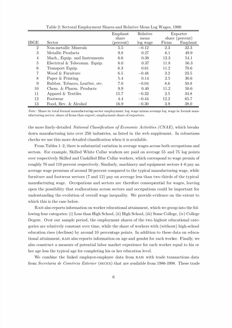
7242019 Brazil Trade
httpslidepdfcomreaderfullbrazil-trade 849
Table 2 Sectoral Employment Shares and Relative Mean Log Wages 1990
Emplmnt Relative Exportershare mean share (percent)
IBGE Sector (percent) log wage Firms Emplmnt
2 Non-metallic Minerals 55 minus012 23 3233 Metallic Products 98 027 61 499
4 Mach Equip and Instruments 66 038 123 5415 Electrical amp Telecomm Equip 60 037 118 5636 Transport Equip 63 061 112 7067 Wood amp Furniture 65 minus048 32 2358 Paper amp Printing 54 014 25 3069 Rubber Tobacco Leather etc 70 minus004 86 508
10 Chem amp Pharm Products 99 040 112 50611 Apparel amp Textiles 157 minus032 25 34812 Footwear 44 minus044 122 65713 Food Bev amp Alcohol 169 minus030 39 380
Note Share in total formal manufacturing-sector employment log wage minus average log wage in formal man-
ufacturing sector share of firms that export employment share of exporters
the more finely-detailed National Classification of Economic Activities (CNAE) which breaks
down manufacturing into over 250 industries as listed in the web supplement In robustness
checks we use this more detailed classification when it is available
From Tables 1ndash2 there is substantial variation in average wages across both occupations and
sectors For example Skilled White Collar workers are paid on average 55 and 75 log points
over respectively Skilled and Unskilled Blue Collar workers which correspond to wage premia of
roughly 70 and 110 percent respectively Similarly machinery and equipment sectors 4ndash6 pay an
average wage premium of around 50 percent compared to the typical manufacturing wage whilefurniture and footwear sectors (7 and 12) pay on average less than two thirds of the typical
manufacturing wage Occupations and sectors are therefore consequential for wages leaving
open the possibility that reallocations across sectors and occupations could be important for
understanding the evolution of overall wage inequality We provide evidence on the extent to
which this is the case below
Rais also reports information on worker educational attainment which we group into the fol-
lowing four categories (i) Less than High School (ii) High School (iii) Some College (iv) College
Degree Over our sample period the employment shares of the two highest educational cate-
gories are relatively constant over time while the share of workers with (without) high-school
education rises (declines) by around 10 percentage points In addition to these data on educa-
tional attainment rais also reports information on age and gender for each worker Finally we
also construct a measure of potential labor market experience for each worker equal to his or
her age less the typical age for completing his or her education level
We combine the linked employer-employee data from rais with trade transactions data
from Secretaria de Comercio Exterior (secex) that are available from 1986-1998 These trade
6
7242019 Brazil Trade
httpslidepdfcomreaderfullbrazil-trade 949
transactions data report for each export and import customs shipment the tax identifier of the
firm the product exported and the destination country served We merge the trade transactions
and linked employer-employee data using the tax identifier of the firm
Our sample period includes changes in both trade and labor market policies in Brazil Tariffs
are lowered in 1988 and further reduced between 1990 and 1993 whereas non-tariff barriers are
dropped by presidential decree in January 1990 Following this trade liberalization the shareof exporting firms nearly doubles between 1990 and 1993 and their employment share increases
by around 10 percentage points7 In contrast following Brazilrsquos real exchange rate appreciation
of the mid-1990s both the share of firms that export and the employment share of exporters
decline by around the same magnitude In 1988 there was also a reform of the labor market8
Finally the late 1980s and early 1990s also witnessed some industrial policy initiatives which
were mostly applied on an industry-wide basis9
The main focus of our analysis is quantifying the contribution of the firm wage component
to the cross-sectional dispersion in worker wages Accordingly our structural model is a model
of cross-sectional differences in wages between firms within sectors As shown in the third and
fourth columns of Table 2 there are substantial differences in the share of firms that export and
the employment share of exporters across sectors which we exploit in our empirical analysis
To ensure that the estimates of our structural model are not driven by the changes in trade
and labor market polices discussed above we estimate the model separately for each year from
1986-1998 which includes years both before and after the reforms Additionally we report some
results that make use of the time-series variation in the data In our structural estimation we
examine the fit of the model over time to see whether changes in the measures of trade openness
in the model can capture changes in wage inequality in the data In our reduced form estimation
we report results for both the level and growth of wage inequality over time
3 Reduced-form Evidence
In this section we use a non-structural approach that imposes relatively few restrictions on the
data to provide evidence on the determinants of wage inequality We use a sequence of variance
decompositions to quantify the importance of different components to the level and growth of
Brazilian wage inequality
Specifically in each year we decompose overall wage inequality (T ) into a within (W ) and a
between component (B) as follows
T t = W t + Bt (1)
with
7For an in-depth discussion of trade liberalization in Brazil see for example Kume Piani and Souza (2003)8The main elements of this labor market reform include a reduction of the maximum working hours per week
from 48 to 44 an increase in the minimum overtime premium from 20 percent to 50 percent and a reduction inthe maximum number of hours in a continuous shift from 8 to 6 hours among other institutional changes
9Some tax exemptions differentially benefit small firms while foreign-exchange restrictions and special importregimes tend to favor select large-scale firms until 1990
7
7242019 Brazil Trade
httpslidepdfcomreaderfullbrazil-trade 1049
T t = 1N t
sumℓ
sumiisinℓ (wit minus wt)
2
W t = 1N t
sumℓ
sumiisinℓ (wit minus wℓt)
2
Bt = 1N t
sumℓN ℓt (wℓt minus wt)
2
where workers are indexed by i and time by t ℓ denotes sector occupation or sector-occupation
cells depending on the specification N t and N ℓt denote the overall number of workers and the
number of workers within cell ℓ wit wℓt and wt are the log worker wage the average log wage
within cell ℓ and the overall average log wage We undertake this decomposition using the
log wage because this ensures that the results of the decomposition are not sensitive to the
choice of units for wages and it also facilitates the inclusion of controls for observable worker
characteristics below
Taking differences relative to a base year the proportional growth in overall wage inequality
can be expressed as the following weighted average of the proportional growth of the within and
between components of wage inequality
∆T = ∆W + ∆B or ∆T T = W T ∆W W + BT ∆BB (2)
where ∆ is the difference operator and the weights are the initial-period shares of the within
and between components in overall wage inequality In our exercises below we focus on changes
relative to a base year so that for example ∆W = W t minus W 0 for year t and base year 0
In Section 31 we decompose overall wage inequality into within and between components
using sector occupation and sector-occupation cells In Section 32 we control for observable
worker characteristics and apply the within-between decomposition to residual wage inequal-
ity In Section 33 we further decompose wage inequality within sector-occupations into wage
dispersion between and within firms In Section 34 we examine the relationship between firmwages employment and export status
31 Within versus between sectors and occupations
We start by decomposing overall wage inequality into within and between components using the
decomposition (1) for sector occupation and sector-occupation cells In Panel A of Table 3 we
report the contribution of each within component to the level (in 1990 using (1)) and growth
(from 1986-1995 using (2)) of overall wage inequality Although the contribution of the within
component inevitably falls as one considers more and more disaggregated categories it accounts
for 80 83 and 67 percent of the level of overall wage inequality for occupations sectors andsector-occupations respectively (first column) Therefore the wage variation within these types
of categories is larger than the wage variation between them upon which much existing empirical
research has focused From 1986-1995 the variance of log wages increases by 174 percent
(corresponding to a 83 percent increase in the standard deviation of log wages) Almost none
of this increase is accounted for by rising wage inequality between occupations (first row second
column) While inequality between sectors increases substantially over this period (by more
8
7242019 Brazil Trade
httpslidepdfcomreaderfullbrazil-trade 1149
Table 3 Contribution of the Within Component to Log Wage Inequality
Level (percent) Change (percent)A Main Period 1990 1986ndash95
Within occupation 80 92Within sector 83 73Within sector-occupation 67 67
Within detailed-occupation 58 60Within sectorndashdetailed-occupation 52 54
B Late Period 1994 1994ndash98
Within sector-occupation 68 125Within detailed-sectorndashdetailed-occupation 47 140
Note Decomposition of the level and growth of wage inequality 12 sectors and 5 occupations as in Tables 1and 2 Detailed occupations are based on the CBO classification which assigns manufacturing workers into 348occupations Detailed sectors are based on the CNAE classification which disaggregates manufacturing into 283industries (starting in 1994) Each cell in the table reports the contribution of the within component to total logwage inequality In the first column the contribution of the within component (W ) to total wage inequality (T ) iscalculated as 100 middotWT based on equation (1) In the second column the contribution of the within component to
the growth in total wage inequality is calculated according to (2) as 100middot(WT )(∆WW )(∆T T ) = 100middot∆W∆T The unreported between component is 100 percent minus the reported within component The change in thebetween component can be negative so the within component can exceed 100 percent Given our large numberof observations on individual workers all the changes in variance shown in Table 3 are statistically significant atconventional critical values More generally the equality of the wage distributions in 1986 and 1995 is rejected atconventional critical values using a nonparametric Kolmogorov-Smirnov test
than 20 percent) the between-sector component accounts for only around 17 percent of the
level of wage inequality in the base year which results in a modest contribution of the between-
sector component to the growth of wage inequality (second row second column) Finally using
sector-occupation cells the within components of wage inequality increase slightly faster than
the between component over this period Since the within component accounts for around twothirds of the level of wage inequality in the base year it also accounts for around two thirds of
the growth of wage inequality (third row second column)10
In Figure 1 we display changes in overall wage inequality and its components using sectors
(Panel A) occupations (Panel B) and sector-occupations (Panel C) For each variable we sub-
tract the 1986 value of the variable to generate an index that takes the value zero in 1986 which
allows us to quantify the contribution of the within and between components to the change in
overall wage inequality after 1986 Whether we use sectors occupations or sector-occupations
we find that the within component of wage inequality closely mirrors the time-series evolution
of overall wage inequality and accounts for most of its growth over our sample period For eachwithin component we observe the same inverted U-shaped pattern as for overall wage inequality
10For example the quantitative decomposition of inequality (2) into between and within sector-occupationscomponents over this period is as follows
∆T T = WT middot ∆WW + B T middot ∆BB174 = 067 middot 177 + 033 middot 168
9
7242019 Brazil Trade
httpslidepdfcomreaderfullbrazil-trade 1249
0
0 2
0 4
0 6
0 8
1
1 2
V a r i a n c e l o g w a g e
1986 1990 1994 1998Year
Total Within sector
Between sector
Panel A Sectors
0
0 2
0 4
0 6
0 8
1
1 2
V a r i a n c e l o g w a g e
1986 1990 1994 1998Year
Total Within occupation
Between occupation
Panel B Occupations
0
0 2
0
4
0 6
0 8
1
1 2
V
a r i a n c e l o g w a g e
1986 1990 1994 1998Year
Total Within sectorminusoccupation
Between sectorminusoccupation
Panel C Sectorminusoccupations
Figure 1 Changes in Log Wage Inequality and its Components
Note Decomposition of overall log wage inequality into within and b etween components based on (2) 1986 isused as the base year that is each series expressed as difference from its 1986 value
This finding is also robust to the use of alternative base years to 1986
We summarize these findings as follows
Fact 1 The within sector-occupation component of wage inequality accounts for over two thirds
of both the level and growth of wage inequality in Brazil between 1986 and 1995
While our baseline results use the IBGE classification of twelve manufacturing sectors and
five occupations the importance of the within component is robust to the use of alternative
more detailed definitions of sectors and occupations In Panel A of Table 3 we report results
using detailed occupation cells based on more than 300 occupations in the CBO classification(fourth row) and using sectorndashdetailed-occupation cells defined using IBGE sectors and CBO
occupations (fifth row) As a further robustness check Panel B of Table 3 reports results using
the more finely-detailed CNAE sector classification which is available from 1994 onwards and
breaks down manufacturing into more than 250 disaggregated industries Since this classification
is available for a more limited time period we show results for the level (1994) and growth
(between 1994 and 1998) of overall wage inequality To provide a point of comparison the
10
7242019 Brazil Trade
httpslidepdfcomreaderfullbrazil-trade 1349
first row of Panel B reports results for this later period using our twelve IBGE sectors and five
occupations (compare with row three of Panel A for the earlier time period) In the second row
of Panel B we report results using detailed-sectorndashdetailed-occupation cells based on more than
300 CNAE sectors and more than 250 CBO occupations While some occupations do not exist
in some sectors there are still around 40000 sector-occupation cells in this specification yet we
continue to find that the within component accounts for around 50 percent of the level and allthe growth of wage inequality11
Our results are consistent with prior findings in the labor economics literature Davis and
Haltiwanger (1991) show that between-plant wage dispersion within sectors accounts for a sub-
stantial amount of the level and growth of wage inequality in US manufacturing from 1975ndash86 12
Katz and Murphy (1992) find that shifts in demand within sector-occupation cells are more im-
portant than those across sector-occupation cells in explaining changes in US relative wages for
different types of workers from 1963ndash87 Our findings show the importance of wage inequality
within sector-occupations in accounting for the level and growth of wage inequality in Brazil
Neoclassical theories of international trade emphasize wage inequality between different types
of workers (Heckscher-Ohlin model) or sectors (Specific Factors model) Our findings suggest
that this focus on the between component abstracts from an important potential channel through
which trade can affect wage inequality Of course our results do not rule out the possibility
that Heckscher-Ohlin and Specific-Factors forces play a role in the wage distribution As shown
in Feenstra and Hanson (1996) Feenstra and Hanson (1999) and Trefler and Zhu (2005) the
Stolper-Samuelson Theorem can be re-interpreted as applying at a more disaggregated level
within sectors and occupations such as production stages But these neoclassical theories em-
phasize dissimilarities across sectors and occupations and if their mechanisms are the dominant
influences on the growth of wage inequality we would expect to observe a substantial between-
component for grossly-different occupations and sectors (eg Managers versus Unskilled Blue-collar workers and Textiles versus Chemicals and Pharmaceuticals) Yet the within component
dominates the growth in wage inequality in the final column of Table 3 and this dominance
remains even when we consider around 40000 disaggregated sector-occupations Therefore
while the forces highlighted by neoclassical trade theory may be active there appear to be other
important mechanisms that are also at work
32 Worker observables and residual wage inequality
We now examine whether the contribution of the within-sector-occupation component of wage
inequality is robust to controlling for observed worker characteristics To control for worker
11In fact the between and the within components of inequality move in the opposite direction in this periodwith the movement in the within component dominating the movement in the between component
12See also Barth Bryson Davis and Freeman (2011) for other evidence using US plant-level data and FaggioSalvanes and Van Reenen (2010) for results using UK firm-level data
11
7242019 Brazil Trade
httpslidepdfcomreaderfullbrazil-trade 1449
Table 4 Worker Observables and Residual Log Wage Inequality
Level (percent) Change (percent)1990 1986ndash95
Residual wage inequality 57 48
mdash within sector-occupation 88 91
Note Decomposition of the level and growth of overall log wage inequality into the contributions of workerobservables and residual (within-group) wage inequality according to (4) based on a Mincer regression of logwages on observed worker characteristics (3) The unreported contribution of worker observables to overall wageinequality equals 100 percent minus the reported residual wage inequality component in the first row The secondrow reports the within sector-occupation component of the residual wage inequality applying decompositions (1)and (2) to the residuals ν it from the Mincer regression (3) using the 12 sectors and 5 occupations reported inTables 1 and 2
observables we estimate the following OLS Mincer regression for log worker wages
wit = z primeitϑt + ν it (3)
where i still denotes workers zit is a vector of observable worker characteristics ϑt is a vector
of returns to worker observables and ν it is a residual
We control for worker observables nonparametrically by including indicator variables for the
following categories education (high school some college and college degree where less than
high school is the excluded category) age (where 10ndash14 15ndash17 18ndash24 25ndash29 30ndash39 40ndash49
50ndash64 65+ are the included categories) experience quintiles (where the first quintile is the
excluded category) and gender (where male is the excluded category) We estimate the Mincer
regression for each year separately allowing the coefficients on worker observables (ϑt) to change
over time to capture changes in the rate of return to these characteristics
The empirical specification (3) serves as a conditioning exercise which allows us to decom-pose the variation in log wages into the component correlated with worker observables and the
orthogonal residual component
T t = var (wit) = var
zprimeitϑt
+ var (ν it) (4)
where the hat denotes the estimated value from regression (3) We refer to var (ν it) as residual
or within-group wage inequality This measure of residual wage inequality can further be de-
composed into its within and between components using sector occupation or sector-occupation
cells by applying (1) and (2) above to the estimated residuals ν it
Table 4 reports the results of the variance decomposition (4) We find that the worker observ-
ables and residual components make roughly equal contributions towards both the level (1990)
and growth (1986ndash1995) of overall wage inequality (first row) We next decompose the level and
growth of residual wage inequality into its within and between sector-occupation components
We find that the within sector-occupation component dominates explaining around 90 percent
12
7242019 Brazil Trade
httpslidepdfcomreaderfullbrazil-trade 1549
0
0 2
0 4
0 6
0 8
1
1 2
I n d e x
( 1 9 8 6 = 0 )
1986 1990 1994 1998Year
Total Observables
Residual
Panel A Observables and Residual Inequality
0
0 2
0 4
0 6
0 8
1
1 2
I n d e x
( 1 9 8 6 = 0 )
1986 1990 1994 1998Year
Residual Within SectorminusOccupation
Between SectorminusOccupation
Panel B Residual Inequality
Figure 2 Changes in Observable and Residual Log Wage Inequality
Note Left panel Decomposition of overall log wage inequality into the contributions of the worker observablesand residual components based on (4) Right panel Decomposition of residual log wage inequality into withinand between components based on (2) applied to the residual ν it from the Mincer regression (3) 1986 is used asthe base year
of both level and growth of the residual wage inequality (second row)13 Comparing the results
in Tables 4 and 3 we find that the within sector-occupation component is more important for
residual wage inequality than for overall wage inequality which is consistent with the fact that
much of the variation in worker observables is between sector-occupation cells
Figure 2 further illustrates these findings by plotting the changes in the components of wage
inequality over time taking 1986 as the base year The left panel plots the change in overall
wage inequality as well as its worker-observable and residual components according to (4)
While both components of overall wage inequality initially increase from 1986 onwards overall
wage inequality inherits its inverted U-shaped pattern from residual wage inequality which risesuntil 1994 and declines thereafter The right panel uses (2) to decompose changes in residual
wage inequality into its within and between sector-occupation components again relative to the
base year of 1986 The time-series evolution of residual wage inequality is entirely dominated by
the evolution of the within sector-occupation component while the between component remains
relatively stable over time14 As is clear from the two panels of the figure our conclusions are
not sensitive to the choice of the base year and if anything the role of the residual inequality
becomes more pronounced as we move forward the base year
Note that residual wage inequality is measured relative to the worker characteristics included
in the regression (3) In principle there can be other unmeasured worker characteristics that
matter for wages and that are observed by the firm but are uncorrelated with the worker char-
acteristics available in our data To the extent that this is the case the contribution of worker
13Repeating the robustness tests in Table 3 we find a similar dominance of the within component usingalternative definitions of sectors and occupations For example we find that over 80 percent of both level andgrowth of residual wage inequality is within detailed-sector-detailed-occupations
14Since the within component dominates using sector-occupation cells it follows that it also dominates usingsector and occupation cells separately and hence for brevity we do not report these results
13
7242019 Brazil Trade
httpslidepdfcomreaderfullbrazil-trade 1649
characteristics could be larger than estimated here On the other hand the decomposition (4)
projects all variation in wages that is correlated with the included worker characteristics on
worker observables Therefore if the firm component of wages is correlated with these worker
characteristics some of its contribution to wage variation can be attributed to worker observ-
ables In the next subsection we use a different decomposition in which we explicitly control
for firm fixed effects and find a smaller contribution from worker observables towards overallwage inequality Keeping these caveats in mind we state
Fact 2 Residual wage inequality is at least as important as worker observables in explaining the
overall level and growth of wage inequality in Brazil from 1986-1995 Around 90 percent of both
the level and growth of residual wage inequality is within-sector-occupation
Our estimates of the role played by worker observables are in line with the existing empirical
literature which finds that observed worker characteristics typically account for around one
third of the cross-section variation in worker wages as discussed in Mortensen (2003) Our
finding that worker observables contribute towards the rise in overall wage inequality followingBrazilian trade liberalization is corroborated by other studies that have found an increase in
the estimated returns to schooling during our sample period such as Attanasio Goldberg and
Pavcnik (2004) and Menezes-Filho Muendler and Ramey (2008)15 Our finding that residual
wage inequality shapes the time-series evolution of overall wage inequality is consistent with
the results of recent studies using US data as in Autor Katz and Kearney (2008) Juhn
Murphy and Pierce (1993) and Lemieux (2006) The enhanced dominance of the within-
sector-occupation component after controlling for worker observables implies that the majority
of residual wage inequality is a within sector-occupation phenomenon
One potential source of wage inequality within sector-occupations for workers with the same
observed characteristics is regional variation in wages16 To show that our results for wage
inequality within sector-occupations are not driven by regional effects we have replicated the
results in Tables 3 and 4 controlling for region In Table 5 we first report results for the state
of Sao Paulo which accounts for around 45 percent of formal manufacturing employment in our
sample (compare the first and second rows) We next report results using sector-occupation-
region cells instead of sector-occupation cells where we define regions in terms of either 26 states
(third row) or 133 meso regions (fourth row) These specifications abstract from any variation
in wages across workers within sector-occupations that occurs between regions Nonetheless in
each specification we continue to find that a sizeable fraction of wage inequality is a within phe-
nomenon This is particularly notable for residual wage inequality where the within component
still accounts for over two thirds of the level and around half of the growth of residual inequality
even for the detailed meso-regions
15From the estimated coefficients on worker observables in the Mincer log wage equation (3) for each year wefind an increase in the rate of return to both education and experience over time as reported in the web appendix
16For empirical evidence of wage variation across Brazilian states see for example Fally Paillacar and Terra(2010) and Kovak (2011)
14
7242019 Brazil Trade
httpslidepdfcomreaderfullbrazil-trade 1749
Table 5 Regional Robustness
overall inequality residual inequality
Level Change Level Change1990 1986ndash95 1990 1986ndash95
Within sector-occupation 67 67 88 91
Within sector-occupation Sao Paulo 66 49 91 71Within sector-occupation-state 57 38 73 57Within sector-occupation-meso 53 30 69 49
Note All entries are in percent The first line duplicates the baseline results from Table 3 (overall inequality)and 4 (residual inequality) The second line reports the same decomposition for the state of Sao Paulo The lasttwo lines report the within component using sector-occupation-region cells where regions are first 26 states andsecond 133 meso regions
Another potential concern is that our findings for wage inequality could be influenced by
changes in workforce composition Residual wage inequality is typically higher for older more
experienced and more educated workers Therefore changes in the composition of the work-
force according to age experience and education can influence the magnitude of residual wage
inequality and its contribution to overall wage inequality To address this concern we follow
Lemieux (2006) in using the fact that our controls for worker observables take the form of in-
dicator variables for cells (eg age 25-29 college degree etc) which implies that all residual
inequality is within cells As a result the variance of the residuals in the Mincer regression (3)
can be expressed as
var (ν it) =sumℓ sℓt var (ν it|zℓt) (5)
where ℓ now indexes the cells for observable worker characteristics (education times age times experience
times sex) zℓt are common observables for all workers in cell ℓ and sℓt is the share of workers in
cell ℓ at time t
To examine the role of changes in workforce composition we use (5) to construct a coun-
terfactual measure of residual wage inequality (var (ν it)) in which workforce composition across
cells sℓt is held constant at its beginning of the sample values As reported in the web ap-
pendix we find that counterfactual residual wage inequality displays the same time-series pattern
as actual residual wage inequality and if anything exhibits greater variation over time Our
findings for residual wage inequality are therefore not driven by changes in observable workforce
composition
33 Between versus within-firm wage inequality
Having established the importance of wage inequality within sector-occupations we now further
decompose this source of wage inequality into within-firm and between-firm components We
undertake this decomposition using both the average firm wage and the estimated firm effect
from a Mincer regression for worker wages that controls for observable worker characteristics
In both cases we consider each sector-occupation-year cell in turn and decompose wage
15
7242019 Brazil Trade
httpslidepdfcomreaderfullbrazil-trade 1849
Table 6 Decomposition of Log Wage Inequality within Sector-Occupations
unconditional worker observablesaverage wage w jℓt firm fixed effect ψ jℓt
Level Change Level Change1990 1986ndash1995 1990 1986ndash1995
Between-firm wage inequality 55 115 38 86
Within-firm wage inequality 45 minus15 34 minus11Worker observables 17 2Covar observablesndashfirm effects 11 24
Note All entries are in percent Decomposition of the level and growth of wage inequality within sector-occupations (employment-weighted average of the results for each sector-occupation) The decomposition inthe first two columns is based on the average firm-occupation-year log wage wjℓt and does not control for workerobservables The decomposition in the last two columns is based on (7) using the firm-occupation-year fixedeffects ψjℓt from the Mincer regression (6) Figures may not sum exactly to 100 percent due to rounding
inequality across workers in that cell into within and between-firm components In our first de-
composition we use the unconditional average log wage paid by each firm to its workers in that
sector-occupation-year cell (w jℓt) to construct the within and between-firm components by anal-
ogy to (1) where cells now correspond to individual firms We summarize the aggregate results
from this decomposition as the employment-weighted average across sector-occupation cells in
each year and report the results in the first two columns of Table 617 While between-firm and
within-firm wage inequality make roughly equal contributions to the level of wage inequality
within sector-occupations (first column) we find that changes in wage inequality within sector-
occupations are almost entirely dominated by wage inequality between firms (second column)
While for brevity Table 6 focuses on the years 1990 and 1986ndash1995 and uses our baseline spec-
ification of sectors and occupations we find similar results using other years and definitions of
sectors and occupations And while for brevity we concentrate on aggregate results this samepattern is pervasive across sectors and occupations
To show that the role of between-firm wage dispersion within sectors and occupations is
robust to controlling for observed worker characteristics we estimate the following fixed effects
Mincer regression for log worker wages separately for each sector-occupation-year
wit = z primeitϑℓt + ψ jℓt + ν it (6)
where i again indexes workers j indexes firms ℓ indexes sector-occupation cells ψ jℓt is a firm-
occupation-year fixed effect and ν it is the residual18
17This average firm wage is equivalent to a fixed effect estimate from wit = wjℓt + ν it which is a restrictedversion of our specification (6) with worker observables The decompositions in Table 6 are based on var(wit) =var1048616
wjℓt
1048617+var(ν it) Again we work with log wages (wit) so that the results of the decomposition are not sensitive
to the choice of units for wages and to facilitate the inclusion of controls for observable worker characteristicsbelow
18Firms are assigned to a single main sector and we estimate the Mincer regression (6) separately for eachsector-occupation-year so that the fixed effects ψjℓt vary by firm-occupation-year We abuse notation slightly byadopting ν it as a residual in both (3) and (6)
16
7242019 Brazil Trade
httpslidepdfcomreaderfullbrazil-trade 1949
We use the estimated firm-occupation-year fixed effects ψ jℓt as our baseline measure of
the firm component of wages in the structural estimation of our model below This baseline
measure controls for worker observables (zprimeitϑℓt) where we allow the effects of these observables
to vary across sector-occupations ℓ and time t Our baseline specification also allows the firm-
occupation-year fixed effects to be correlated with worker observables as will be the case for
example if there is assortative matching on worker observables across firms
19
The firm-occupation-year fixed effects capture both firm wage premia for workers with iden-
tical characteristics and unobserved differences in workforce composition across firms (including
average match effects) The theoretical literature on heterogeneous firms and labor markets
considers both these sources of wage differences across firms and our objective is to quan-
tify the overall contribution of the firm component to wage inequality rather than sorting out
further its different components Since we focus on the overall firm component we are not re-
quired to assume conditional random matching of workers to firms as often invoked using linked
employer-employee datasets and can allow for assortative matching of workers and firms20
Our second decomposition splits overall wage inequality into the following four terms
var (wit) = var
zprimeitϑℓt
+ var
ψ jℓt
+ 2 cov
zprimeitϑℓt ψ jℓt
+ var
ν it
(7)
These four terms are (1) worker observables (2) the between-firm component (firm-occupation
year fixed effects) (3) the covariance between worker observables and the firm component (4) the
within-firm component (residual) which by construction is orthogonal to the other terms
We undertake this decomposition separately for each sector-occupation-year In the final
two columns of Table 6 we summarize the aggregate results from this decomposition as the
employment-weighted average of the results for each sector-occupation-year cell In the third
column we find that the between-firm (firm effects) and within-firm (residual) componentsaccount for roughly equal amounts of the level of wage inequality within sector-occupations
(38 and 34 percent respectively) Of the other two components worker observables account
for around one sixth and the covariance between worker observables and the firm component
of wages accounts for the remaining one tenth In contrast in the fourth column changes in
between-firm wage dispersion account for the lionrsquos share (86 percent) of the growth in wage
inequality within sector-occupations The next largest contribution (around one quarter) comes
from an increased covariance between worker observables and the firm component of wages
19In Table 6 we treat the average firm wage (wjℓt) and the firm-occupation-year fixed effect (ψjℓt) as data Inthe model developed below we make the theoretical assumption that the firm observes these wage components
and that the model is about these wage components which can be therefore taken as data in its estimation Incontrast without this theoretical assumption wjℓt and ψjℓt should be interpreted as estimates in which case thevariance of these estimates equals their true variance plus the variance of a sampling error that depends on theaverage number of workers employed by a firm Since this average is around twenty workers in our data theresulting correction for the variance of the sampling error is small as discussed further in the web appendix
20For a subsample of firms in RAIS that are covered by a separate annual survey data on total firm revenue areavailable that can be used to construct revenue-based productivity For this subsample of firms Menezes-FilhoMuendler and Ramey (2008) show that the estimated firm effect from a similar Mincer regression is closely relatedto revenue-based productivity consistent with findings using linked employer-employee data for other countries
17
7242019 Brazil Trade
httpslidepdfcomreaderfullbrazil-trade 2049
minus
0 2
0
0 2
0 4
0 6
0 8
I n d e x
( 1 9
8 6 = 0 )
1986 1990 1994 1998
Year
Total Worker Obs Covariance
BetweenminusFirm WithinminusFirm
Figure 3 Changes in Log Wage Inequality within Sector-Occupations and its Components
Note Decomposition of log wage inequality within sector-occupations (employment-weighted) based on (7)changes relative to the base year of 1986
which is consistent with increased assortative matching on worker observables across firms
Changes in the residual within-firm wage dispersion make a small negative contribution Notably
now that we focus on wage inequality within sector-occupations and control for firm effects
changes in the variance of worker observables account for a negligible share of the growth of wage inequality within sector-occupations in sharp contrast to our findings in Section 3221
Figure 3 further illustrates these findings by plotting the change in wage inequality within
sector-occupations and its components in (7) relative to the base year of 1986 We con-
firm that between-firm wage dispersion dominates the evolution of wage inequality within
sector-occupations and drives the inverted U-shaped pattern in wage inequality within sector-
occupations (which in turn drives the inverted U-shaped pattern in overall wage inequality)
This is the component of wage inequality that we aim to capture in our structural model of
Section 4
21This reduced contribution from worker observables is explained by two differences from the specification in
Section 32 First the Mincer regression (6) is estimated separately for each sector-occupation-year insteadof po oling observations across sectors and occupations within each year Since much of the variation in workerobservables occurs across sectors and occupations (sorting across sectors and occupations) this generates a smallercontribution from worker observables Second the Mincer regression (6) includes firm-occupation-year fixedeffects which can be correlated with worker observables (sorting across firms) Once we allow for this correlationwe again find a smaller contribution from worker observables Empirically these two differences are of roughlyequal importance in explaining the reduction in the contribution from worker observables When we re-estimatethe Mincer regression (6) for each sector-occupation-year excluding the firm-occupation-year fixed effects we finda contribution from worker observables halfway in between the results in this section and Section 32
18
7242019 Brazil Trade
httpslidepdfcomreaderfullbrazil-trade 2149
We summarize the findings above as follows
Fact 3 Between-firm and within-firm dispersion make roughly equal contributions to the level
of wage inequality within sector-occupations but the growth of wage inequality within sector-
occupations is largely accounted for by between-firm wage dispersion
These findings are also consistent with existing results in the labor economics literature For
example Lazear and Shaw (2009) summarize evidence from linked employer-employee data for
several OECD countries and conclude that the firm fixed effect explains a large and growing share
of the wage distribution This importance of between rather than within firm variation points
towards theories of heterogeneity between firms as the relevant framework for understanding
both the overall wage distribution and the wage distribution across workers with similar observed
characteristics
34 Size and exporter wage premia
Having established the importance of wage variation between firms within sector-occupations
for overall wage inequality we now examine the relationship between firm wages employment
and export status We first construct a measure of firm wages in each year by aggregating our
firm-occupation-year wage measures from the previous subsection to the firm-year level using
employment weights We next estimate the following cross-section regression of firm wages on
employment and export status for each year
ω jt = λoℓt + λsth jt + λxt ιt + ν jt for ω jt isin w jt ψ jt (8)
where we again index firms by j ℓ now denotes sectors h jt is log firm employment ι jt isin 0 1
is a dummy for whether a firm exports and ν jt is the residual The dependent variable is
the firm-year average log wage w jt or the firm-year effect ψ jt constructed from the Mincer
regression (6) by aggregating the firm-occupation-year fixed effects using employment weights
We estimate a sector-time fixed effect λoℓt a time-varying employment size wage premium λst
and a time-varying firm export premium λxt
Columns one and three of Table 7 report these estimated size and exporter wage premia for
1990 using the firm average log wage and the firm wage component from the Mincer regression
respectively Consistent with a large empirical literature in labor economics (eg Oi and Idson
1999) and international trade (eg Bernard and Jensen 1995 1997) we find positive and statis-
tically significant premia for employment size and export status In the third column using the
firm wage component from the Mincer regression (ψ jt) we find a size premium of λs = 012 and
an exporter premium of λx = 00922 We emphasize that the exporter wage premium in this
reduced-form specification cannot be given a causal interpretation because omitted unobserved
22Augmenting regression (8) with firm employment growth has little effect on either the estimated size andexporter wage premia or on the regression fit
19
7242019 Brazil Trade
httpslidepdfcomreaderfullbrazil-trade 2249
Table 7 Size and Exporter Wage Premia
unconditional worker observablesaverage wage w jt firm fixed effect ψ jt
Cross-Section Panel Cross-Section Panel1990 1986ndash1998 1990 1986ndash1998
Firm Employment Size 0126lowastlowastlowast minus0003lowast 0118lowastlowastlowast 0048lowastlowastlowast
(0008) (0002) (0006) (0001)
Firm Export Status 0202lowastlowastlowast 0216lowastlowastlowast 0088lowastlowastlowast 0012lowastlowastlowast
(0046) (0004) (0027) (0002)
Sector Fixed Effects yes no yes noFirm Fixed Effects no yes no yesWithin R-squared 0164 0007 0146 0013Observations 93 392 1 229 133 93 392 1 229 133
Note The first two columns use average firm-occupation-year wages without conditioning on worker observableswhile the last two columns use the firm-occupation-year fixed effects from the Mincer regression (6) in both casesfirm-occupation variables are aggregated to the firm level by using firm-occupation employment weights Columnsone and three report parameter estimates from the cross-section specification (8) Columns two and four report
estimated coefficients from the panel data specification (9) which controls for firm fixed effects lowast
and lowastlowastlowast
denotestatistical significance at the 10 and 1 percent levels respectively Standard errors in columns one and three areheteroscedasticity robust standard errors in columns two and four are heteroscedasticity robust and adjusted forclustering at the firm level
variables (eg firm productivity imperfectly correlated with employment) could induce firms to
both pay high wages and export That is the reduced-form exporter wage premium (λx) cap-
tures both the non-random selection of high-wage firms into exporting (beyond that captured
by firm size) and the impact of exporting on the wage paid by a given firm In our structural
model below we separate out these two components of the exporter wage premium by explicitly
modeling a firmrsquos endogenous decision of whether or not to export
Before developing the structural model we consider a panel data reduced-form specifica-
tion that partially alleviates concerns about unobserved firm heterogeneity by including time-
invariant firm fixed effects
ω jt = λo j + λot + λsh jt + λxιt + ν jt for ω jt isin w jt ψ jt (9)
where λo j is a firm fixed effect λot is a year fixed effect and the other variables are defined as in
the cross-section specification (8) In this panel data specification the exporter wage premium
(λx) is identified solely from firms that switch in and out of exporting
Columns two and four of Table 7 report the results from this specification using the firmaverage log wage and the firm wage component from the Mincer regression respectively In both
columns we find an employment size wage premium that is much smaller in magnitude and
becomes negative (though close to zero) in column two This pattern of results is consistent
with the idea that the employment-size wage premium in the cross-section specifications in
columns one and three is largely driven by selection on time-invariant firm characteristics that
20
7242019 Brazil Trade
httpslidepdfcomreaderfullbrazil-trade 2349
result in both higher firm employment and higher firm wages23 Similarly in column four using
the firm-occupation-year fixed effects we find a much smaller exporter wage premium which is
in line with the selection of high-wage firms into exporting In contrast in column two using
the firm average log wage we continue to find an exporter wage premium of a similar size to our
cross-section specification above This contrast between the two columns suggests that some of
the increase in a firmrsquos average log wage in column two when it enters export markets is due toa change in the composition of its workforce in terms of observable worker characteristics that
is controlled for in column four24
Finally although the employment size and exporter wage premia are statistically significant
in both specifications the correlations between firm wages employment and export status are far
from perfect In the cross-section regression the within R-squared after netting out the sector
fixed effects is around 015 while in the panel data regression the within R-squared after netting
out the firm fixed effects is an order of magnitude smaller In the structural model developed
below we explicitly model these imperfect correlations between firm wages employment size
and export status We summarize our empirical findings in this section as
Fact 4 Larger firms on average pay higher wages controlling for size exporters on average pay
higher wages than non-exporters Firms switching into exporting increase their wage even after
controlling for the associated increase in firm size Nonetheless controlling for size and export
status residual wage inequality across firms is substantial
Taken together the findings of this section have established a number of key stylized facts
about wage inequality in Brazil We have shown that within-sector-occupation inequality ac-
counts for much of overall wage inequality in Brazil Most of this within-sector-occupation
inequality is residual wage inequality Furthermore between-firm variation in wages accounts
for 86 percent of wage inequality within sector-occupations even after controlling for worker
observables Finally there are statistically significant employment size and exporter wage pre-
mia but the correlations between firm wages employment size and export status are imperfect
These findings are encouraging for recent theories of wage inequality based on firm heterogene-
ity In the next section we structurally estimate such a model to provide further evidence on
its ability to account quantitatively for the patterns observed in the data
4 Structural Estimation
Guided by the empirical findings in the previous section we now develop an extension of Help-
man Itskhoki and Redding (2010 HIR henceforth) In the HIR model wages vary between
23Indeed in models of wage bargaining variation in employment around the desired size of the firm results ina negative correlation between employment and wages which can explain the smaller or even negative size wagepremium estimated off time-series variation
24Regressing log firm employment on export status in an analogous panel data specification we find that entryinto export markets is also associated with a statistically significant increase in firm size by around 25 percent
21
7242019 Brazil Trade
httpslidepdfcomreaderfullbrazil-trade 2449
firms within sector-occupations and are correlated with firm employment size and export sta-
tus25 Our non-structural evidence suggests that these are essential ingredients for a model to
capture the empirical patterns of inequality and its relationship with trade openness In what
follows we first describe and generalize the HIR model we then develop a method for structurally
estimating this enhanced model and lastly we apply the model to the Brazilian data
41 Theoretical framework
We begin by briefly describing the theoretical framework of HIR emphasizing the modifications
we make in order to take the model to the data Motivated by our empirical findings above the
model focuses on between-firm variation in wages for workers with the same observed charac-
teristics Therefore workers are ex ante identical and all workers employed by a firm are paid
the same wage We augment HIR with two additional sources of heterogeneity to capture the
overlap in the employment and wage distributions across exporters and non-exporters as well
as the substantial dispersion in firm wages after controlling for firm employment size and export
status Although we make strong assumptions about the economic relationships between firmrevenue employment and wages and about the statistical distributions for the three sources of
heterogeneity we show that our parsimoniously parameterized model fits the data well
The economy consists of many sectors some or all of which manufacture differentiated prod-
ucts The modelrsquos predictions for wages and employment across firms within each differentiated
sector hold regardless of general equilibrium effects Therefore we focus on variation across
firms and workers within one such differentiated sector Our goal is to explain the observed
cross-section dispersion in wages and employment across firms and we develop a static model to
characterize such cross-section dispersion
Within the sector there is a large number of monopolistically competitive firms each supply-
ing a distinct horizontally-differentiated variety Demand functions for varieties emanate from
constant elasticity of substitution (CES) preferences As a result a firmrsquos revenue in market m
(domestic or foreign) can be expressed in terms of its output supplied to this market (Y m) and
a demand shifter (Am)
Rm = AmY mβ m isin d x
where d denotes the domestic market and x the export market The demand shifter Am depends
on aggregate sectoral expenditure and the sectoral price index in market m Since every firm is
small relative to the sector the firm takes this demand shifter as given The parameter β isin (0 1)
controls the elasticity of substitution between varieties25We focus our structural analysis on firm exporting rather than firm importing While the mechanism linking
trade and wage inequality in our theoretical model is driven by firm export-market participation as in Melitz(2003) the model can also be extended to capture firm selection into importing as in Amiti and Davis (2011) Tothe extent that firm importing increases productivity and raises revenue per worker it results in a similar importer
wage premium and our methodology could be applied to this other dimension of firm selection In practice firmexporting and importing are strongly positively correlated in the cross section and hence in our estimation wecapture most of the overall effect of firm trade participation
22
7242019 Brazil Trade
httpslidepdfcomreaderfullbrazil-trade 2549
In order to export a firm has to incur a fixed cost eεF x where ε is firm-specific and F x
is common to all firms in the sector In addition there are iceberg-type variable trade costs
τ gt 1 units of a variety have to be exported for one unit to arrive in the foreign market
An exporting firm allocates its output between the domestic and export market to maximize
revenue As a result the firmrsquos revenue (R = Rd + Rx) can be expressed as a function of its
output (Y = Y d + Y x) the demand shifter in the domestic market and a market access variable(Υx)
R = [1 + ι (Υx minus 1)]1minusβ AdY β (10)
where the market access variable is
Υx = 1 + τ minusβ1minusβ
1048616AxAd
1048617 11minusβ
and ι is an indicator variable equal to one when the firm exports and equal to zero otherwise
The revenue of a non-exporter is R = AdY β while the revenue of an exporter is R = Υ1minusβx AdY β
The firm revenue premium from exporting is decreasing in the variable trade cost parameterand increasing in the foreign demand shifter relative to the domestic demand shifter
We assume that firm output (Y ) depends on firm productivity (θ) the measure of workers
hired by the firm (H ) and the average ability of these workers (a)
Y = eθH γ a 0 lt γ lt 1 (11)
HIR show that this production function can be derived from human capital complementarities
(eg production takes place in teams and the productivity of a worker depends on the average
productivity of her team) or from a model of a managerial time constraint (eg a manager
with a fixed amount of time who needs to allocate some time to every worker as in Rosen
1982) Importantly the production technology (11) exhibits complementarity between the firmrsquos
productivity and average worker ability
Firms and workers are matched in a labor market that exhibits search and matching frictions
of the Diamond-Mortensen-Pissarides type A firm bears a search cost bN in order to randomly
match with N workers The hiring cost b is endogenously determined by the tightness of the
labor market and is taken as given by each firm in the sector26
Upon matching with a firm a worker draws a match-specific ability a from a Pareto distri-
bution G (a) = 1 minus (amina)k for a ge amin gt 0 and k gt 1 This distribution is identical and
independent across workers and matches Although a firm cannot observe the match-specificabilities of its N workers it can invest resources in screening in order to obtain a signal of these
abilities By choosing an ability threshold ac a firm can identify workers with abilities below
ac but it cannot identify the precise ability of every worker Screening costs increase with the
ability threshold and equal eminusηC
acδ
δ where η is firm specific while δ and C are common to
26In our econometric model labor market tightness is absorbed in the constants of the estimation equationsFor this reason we do not elaborate these details below The interested reader can find them in HIR
23
7242019 Brazil Trade
httpslidepdfcomreaderfullbrazil-trade 2649
all firms The incentive to screen workers results from the complementarity of firm productivity
and worker abilities in the production function (11) We also assume δ gt k which ensures
a positive size-wage premium (ie the empirically-observed positive relationship between firm
wages and employment)
Note that all workers are ex ante identical but their ex post outcomes depend on their
match-specific ability and the productivity of the firm they are matched with This modelingassumption is consistent with our empirical focus on the firm component of wages for workers
with similar observable characteristics In HIR we extend the framework to explicitly account
for observable worker heterogeneity and different occupations but here we do not attempt to
explain this additional dimension of wage variation and keep the analysis focused on residual
wage dispersion within occupations
The timing of decisions is as follows Each firm in a given sector has a draw (θηε)
which represents its idiosyncratic components of productivity screening costs and fixed export
costs Given this triplet the firm chooses whether to serve only the domestic market or to also
export where each firm in the sector serves the domestic market27 All firms in the sector post
vacancies Based on these vacancies firms are matched with workers After the matching every
firm chooses its screening threshold and hires the workers with match-specific abilities above
this threshold Therefore a firm that has been matched with N workers and has chosen the
ability cutoff ac hires
H = N
1 minus G(ac)
= N (aminac)k (12)
workers whose expected ability is
a = E
1048699a|a ge ac
1048701=
k
k minus 1 ac (13)
by the properties of the Pareto distribution Neither the firm nor its hired workers have infor-
mation on the match-specific abilities of individual workers beyond the fact that they are above
the cutoff ac
After the firm has paid all the costsmdashexporting matching and screeningmdashit engages in
multilateral bargaining with its H workers over wages as in Stole and Zwiebel (1996) HIR
show that the outcome of this bargaining game is a wage rate
W = βγ
1 + βγ
R
H
so that the wage bill is a fixed fraction of firm revenue Workers who have not been matchedwith firms or whose match-specific abilities have fallen below their firmrsquos threshold become
unemployed and are not observed in our data28
27All firms serving the domestic market can be rationalized by a fixed number of potential firms as in Chaney(2008) and no fixed costs of domestic production In our empirical implementation we condition on firm entryinto production and analyze a firmrsquos decision to serve the export market and its choice of employment and wagesTherefore we do not model the firmrsquos entry decision here
28Therefore sectoral employment is determined by firm labor demand given the hiring cost b We do not
24
7242019 Brazil Trade
httpslidepdfcomreaderfullbrazil-trade 2749
Anticipating this bargaining outcome a firm maximizes its profits by choosing the number
of workers to match with (N ) the screening threshold (ac) and whether to export
Π = maxNacιisin01
983163 1
1 + βγ R(N ac ι) minus bN minus
C eminusη
δ
acδminus ιF xe
ε
983165
where the revenue function R (N ac ι) is derived from (10)ndash(13) HIR show that the solutionto this problem yields (see (S16) in the online supplement to HIR and the web appendix)
R = κr
1 + ι (Υx minus 1) 1minusβ
Γ
983080eθ983081β
Γ983080
eη983081β(1minusγk)
δΓ (14)
H = κh
1 + ι (Υx minus 1) (1minusβ)(1minuskδ)
Γ
983080eθ983081β(1minuskδ)
Γ983080
eη983081β(1minusγk)(1minuskδ)
δΓ minus k
δ (15)
W = κw
1 + ι (Υx minus 1) k(1minusβ)
δΓ
983080eθ983081βk
δΓ983080
eη983081 k
δ
9830801+β(1minusγk)
δΓ
983081
(16)
where Γ equiv 1 minus βγ minus β (1 minus γk)δ gt 0 is a derived parameter and the κsrsquos (s = r h w) are
combinations of variables and parameters that are common to all firms in the sector Giventhese solutions a firm chooses to export in addition to serving the domestic market if the
additional profits from exporting are positive
κπ
1048616Υ
1minusβΓx minus 1
1048617983080eθ983081β
Γ983080
eη983081β(1minusγk)
δΓge F xeε (17)
where κπ is constant across firms This condition derives from the fact that operational profits
are a constant fraction Γ(1 + β ) of revenues (14) When this inequality fails the firm serves
only the domestic market A firm is more likely to export the higher are its production and
screening productivity draws θ and η and the lower is its fixed export cost productivity draw εWhen condition (17) holds ι = 1 otherwise ι = 0
Equations (15)ndash(17) describe firm employment wages and export participation This model
features two sources of firm heterogeneity that do not exist in HIR heterogeneity in fixed export
costs and heterogeneity in screening costs Without heterogeneous export-market entry costs
a firmrsquos revenue and wage bill would perfectly predict its export status This prediction is
inconsistent with the data in which there is considerable overlap in the wage and employment
distributions between non-exporters and exporters Without heterogeneous screening costs
employment and wages are perfectly correlated across firms whereas in the data this correlation
is imperfect Incorporating these two additional sources of heterogeneity enables the model to
match the empirical cross-sectional distribution of firm employment wages and export status
Our theoretical model predicts that firms with higher productivity θ hire more workers are
more likely to export and pay higher wages29 However while firms with higher productivity
explicitly model a workerrsquos decision whether to search for employment in the sector here In HIR we embed thesector in general equilibrium and show that workers are indifferent between the sectors in which to search foremployment
29In this model with Stole-Zwiebel bargaining equilibrium wages are equalized with the firmrsquos outside option
25
7242019 Brazil Trade
httpslidepdfcomreaderfullbrazil-trade 2849
in screening η also pay higher wages and are more likely to export they may hire more or fewer
workers The reason for this ambiguity stems from two opposing effects on hiring On the one
hand lower screening costs raise overall profitability thereby raising the incentive to expand
and hire more workers On the other hand lower screening costs make selectivity in hiring more
attractive thereby lowering employment On net lower screening costs may increase or reduce
employmentLower fixed export costs make exporting more profitable and induce more firms to export
In the model an exporter has higher employment and wages than a non-exporter with the
same productivity An exporter employs more workers because it has access to a larger market
which justifies a larger scale of operation The higher wage results from the greater labor
market selectivity (tougher screening for hiring) of exporters implied by the complementarity
between a larger scale of operation and higher average worker ability Since exporters screen
more intensively and have workforces of higher average ability their workforces are more costly
to replace which improves the workersrsquo stance in the wage bargaining Consequently exporters
pay higher wages This export wage premium is important for matching the model to the data
The heterogeneity in fixed export costs implies that the productivity draws in production
and screening only imperfectly determine a firmrsquos export status As a result some small and
low-wage firms find it profitable to export while some large and high-wage firms prefer to serve
only the domestic market Yet on average exporters are larger and pay higher wages than
non-exporters as observed in the data As we show below firm-specific heterogeneity in the
triplet (θηε) is crucial for the empirical success of the model
42 Econometric model
Having described the theoretical structure of the model we now adapt it for empirical estimation
Our econometric model consists of two equations for employment and wages and a selection
equation for export status Taking logarithms of (15)ndash(17) we obtain a linear selection model
h = αh + microhι + β (1 minus kδ )
Γ θ +
10486161 minus
k
δ
1048617983131β (1 minus γk)
δ Γ minus
kδ
1 minus kδ
983133η
w = αw + microwι + βk
δ Γ θ +
k
δ
10486161 +
β (1 minus γk)
δ Γ
1048617η
ι = I
983163β
Γ θ +
β (1 minus γk)
δ Γ η minus ε ge σf
983165
to replace a worker As a result firms that are more selective in the labor market end up paying higher wagesDue to complementarity in production more productive firms choose to be both larger and more selective andhence pay higher wages Through this mechanism exporters are larger and pay higher wages than non-exporters
26
7242019 Brazil Trade
httpslidepdfcomreaderfullbrazil-trade 2949
where h and w are the natural logarithms of employment and wages respectively Imiddot denotes
an indicator function
microh = (1 minus kδ )logΥ1minusβΓx
microw = kδ
1 minus kδ microh
f = 1
σ
983080minusαπ + log F x minus log
852059Υ(1minusβ)Γx minus 1
852061983081
and αs = log κs for s = hwπ Lastly we use σ to denote the standard deviation of the
composite firm-specific shock in the selection equation above (see the web appendix for the
explicit expression) which we use below as a constant of normalization To complete the model
we impose a distributional assumption on the firm-specific shocks (θηε) which we assume are
drawn from a joint normal distribution with an arbitrary covariance matrix we normalize the
means of the shocks to zero which is without loss of generality because of the presence of the
constants denoted by αs
In order to estimate the model we make a substitution of variables and rewrite the system
as an exactly-identified reduced form
h = αh + microhι + u
w = αw + microwι + ζu + v
ι = Iz ge f
uvz
primesim N
0
σ2u 0 ρuσu
0 σ2v ρvσv
ρuσu ρvσv 1
(18)
where
u = 1
1 + χ 1048616β
Γ θ + 1048616
β (1 minus γk)
δ Γ minus χ1048617 η1048617
v = χ
η minus Eη|u
= χ
η minus πu
z = 1
σ
1048616β
Γ θ +
β (1 minus γk)
δ Γ η minus ε
1048617=
1
σ
(1 + ζ )u + v minus ε
and
χ = kδ
1 minus kδ gt 0 and ζ = χ(1 + π)
with π denoting the projection coefficient of η on u The details of this derivation are provided
in the web appendix which also relates the parameters of the distributions of the reduced-form
shocks (σu σv ρu ρv) to the covariance matrix of the structural shocks (θηε) In general notall of the modelrsquos structural parameters can be recovered from the reduced-form (18) the web ap-
pendix discusses additional assumptions resulting in identification Furthermore the estimated
reduced-form parameters are sufficient to undertake model-based counterfactuals quantifying
the contribution of trade openness to wage inequality as we do below
The only additional parameter restriction on the econometric model (18) implied by the
27
7242019 Brazil Trade
httpslidepdfcomreaderfullbrazil-trade 3049
theory is positive employment and wage premia in exporting firms30
microh microw gt 0 (19)
Note that the two premia are linked by the following relationship microw = χmicroh This however does
not impose an additional constraint on the model since χ is not identified separately
We now discuss two special cases of the model with additional parameter restrictions First
we note that in general the selection correlations (ρu ρv) can be positive or negative depending
on the covariance matrix of the structural shocks It is sufficient to require however that
the productivity shocks (θ η) are not too strongly positively correlated with the exporting cost
shock ε for these correlations to be non-negative In particular if we assume that ε is orthogonal
to (θ η) the two selection correlations must be positive and in addition constrained by the
following relationship31ρuρv
= (1 + ζ )σuσv
(20)
There is no strong a priori economic reason why the productivity and screening shocks (θ η)
should be uncorrelated with the exporting cost shock ε and hence we do not impose (20) as a
default parameter restriction
The second special case assumes that the productivity shocks θ and η are orthogonal and
the screening cost shock η does not affect firm employment size The latter is the case under the
following parameter restriction χ = β (1 minus γk)(δ Γ) which implies that the two effects of the
screening cost shocks on employment discussed in Section 41 exactly offset each other Under
these assumptions we have π = 0 and ζ = χ which implies that the reduced-form shocks u and
v are proportional to the structural shocks θ and η respectively The reduced-form parameter
restriction implied by these assumptions is simply
microw = ζ microh (21)
which we can test in the data While there is again no a priori economic reason to impose these
assumptions this constrained specification is appealing because the reduced-form model in this
case can be estimated directly without transforming the shocks and hence the reduced-form
shocks have a structural interpretation
Our model features two channels of interrelationship between export participation and the
employment and wage distributions across firmsmdashthe export selection correlations (ρu ρv) and
the employment and wage exporter premia (microh microw) The first channelmdashthe selection effect mdash jointly determines the export status employment sizes and wage rates of firms through the
30The model imposes the parameter inequalities Υx gt 1 0 lt kδ lt 1 0 lt γk lt 1 and Γ gt 0 which implies
microh microw gt 0 Also note that microh + microw = logΥ(1minusβ)Γx which allows us to isolate the variation in f induced by
changes in market access Υ(1minusβ)Γx
31This restriction derived in the web appendix arises because under this orthogonality assumption wagebills revenues and operating profits are perfectly correlated in the cross-section of firms As a result the jointcorrelation structure between employment wages and export status is constrained by (20)
28
7242019 Brazil Trade
httpslidepdfcomreaderfullbrazil-trade 3149
underlying productivity distribution where more productive firms are larger pay higher wages
and are more likely to export The second channelmdashthe market access effect mdashensures that
exporting firms are larger and pay higher wages even after controlling for productivity32 We
test below whether either or both effects are important in the data In particular we evaluate
the hypothesis of no relationship between trade and the employment and wage distributions
across firms by estimating the model under the parameter restriction
microh = microw = ρu = ρv = 0 (22)
Likelihood function Our econometric model (18) takes a form similar to a Tobit Type 5
model in Amemiya (1985) or a switching regression model with endogenous switching in Maddala
(1983) This model admits a closed-form likelihood function which we now describe
A unit of observation in the model is a firm j and each observation is a triplet of firm log
employment log wages and binary export status x j = (h j w j ι j)prime We denote the data by X =
x j j and we use it to estimate the parameter vector Θ = (αh αw ζ σu σv ρu ρv microh microw f )prime
We denote the likelihood of the data X given the parameter vector Θ by
L
Θ|X
=prod j Px j |Θ (23)
In the web appendix we show that
P x j|Θ = 1
σuφ(u j)
1
σvφ(v j)
1048667Φ
852008f minus ρuu j minus ρvv jradic
1 minus ρ2u minus ρ2v
85200910486691minusιj 10486671 minus Φ
852008f minus ρuu j minus ρvv jradic
1 minus ρ2u minus ρ2v
8520091048669ιj
where φ(middot) and Φ(middot) are respectively the density and cumulative distribution functions of a
standard normal and
u j =
h j minus αh minus microhι j
σu
v j =
(w j minus αw minus microwι j) minus ζ (h j minus αh minus microhι j)
σv
This simple expression for the density of the data x j is intuitive the first two terms reflect the
likelihood of the continuous distribution of shocks which result in the observed employment and
wages while the last two terms are a standard Probit likelihood for binary export status given
the employment and wages of the firm
We estimate the parameters of the model by maximizing the likelihood function (23) subject
to the structural constraint (19) Additionally we evaluate the maximized likelihood of an
unconstrained model as well as the maximum likelihood under the various parameter restrictions
discussed above The model is identified through functional form and distributional assumptions
32In the literature following Melitz (2003) and in particular in HIR the two effects are typically not separatedbecause firm productivity p erfectly predicts export status Our framework emphasizes the distinction betweenthe two effects as a result of idiosyncratic differences in exporting costs across firms
29
7242019 Brazil Trade
httpslidepdfcomreaderfullbrazil-trade 3249
As a check on our functional form assumptions we show that the estimated model provides a
good fit of the empirical cross-section distributions of employment and wages
While the maximum likelihood estimation uses efficiently all possible moments of the data
the first and second moments of the joint distribution of employment wages and export status
provide intuition for the identification of the modelrsquos parameters33 The parameters αw αh σu
σv and f can be identified from the first and second moments of employment and wages as well asthe fraction of exporting firms ζ is pinned down by the wage-employment covariance The key
parameters of interestmdashmicrow microh ρu and ρvmdashare identified from the first and second moments of
employment and wages conditional on export status with their separate identification coming
from the modelrsquos functional form assumptions including the discrete increase in wages and
employment upon entry into export markets
We focus on cross-section dispersion in wages employment and export status across firms
and hence estimate the modelrsquos parameters using data on a cross-section of firms To ensure
that our results are not driven by changes in policies or other aspects of the market environment
over time we estimate the parameters of the model separately for each year in our sample and
examine the extent to which the parameters change over time We allow all parameters to
vary over time in an unrestricted manner since all the parameters are functions of endogenous
aggregate variables which in the data are likely to change over time For example exporter
premia (microh microw) depend on variable trade costs (τ ) and relative export market demand (AxAd)
which change over time
As discussed in the Introduction there exist other models of competitive and frictional labor
marketsmdashincluding competitive assignment search-and-matching fair-wage and efficiency-wage
modelsmdashwhich can generate a firm-size wage premium and exporter premia for wages and em-
ployment Obtaining the empirically relevant correlations between shocks to employment and
wages on the one hand and shocks to export participation on the other hand is not simplehowever For example if in our theoretical model we were to replace the shock to screening with
a shock to the bargaining power of a firm relative to its workers the resulting correlations would
not be consistent with the data34 In other words not every model that predicts variation of
wages size and export status across firms in a sector is capable of explaining the data While we
do not know whether there exist other models that lead to an econometric specification similar
to (18) we conjecture that models of this type exist and that (18) may be a good approximation
to some models even if it does not represent an exact specification Indeed (18) is a general
33The web appendix provides closed-form expressions for these moments as functions of the parameter vector Θ
It also lays out the details of an alternative GMM estimation procedure based on these moments The GMMresults provide an additional check on the modelrsquos functional form assumptions Efficient GMM yields estimatesquantitatively very similar to our maximum likelihood (ML) estimates and for brevity we do not report themTable 8 reports the values of the GMM objective for different specifications of interest and Table 9 displays thefit of the moments used in the GMM estimation
34In this alternative specification a high-wage firm is other things equal the one with low bargaining powerrelative to its workers which in turn reduces the firmrsquos profitability and makes it less likely to export In otherwords controlling for employment exporters should be relatively low-wage firms reflecting their high bargainingpower and hence high profitability
30
7242019 Brazil Trade
httpslidepdfcomreaderfullbrazil-trade 3349
log linear model of firm employment wages and selection into exporting which can be further
augmented to allow for reduced-form variation in σu σv and ζ with export status A theoretical
underpinning of the econometric model is desirable however because it helps to form priors
and identify the parameters of interest as well as conduct internally-consistent counterfactual
exercises using the estimated reduced-form model The next section illustrates both of these
points
43 Maximum Likelihood results
We estimate the econometric model (18) using data on firm export status employment and
wages Since the theory focuses on the firm-specific wages of workers with similar ex-ante
characteristics we use the firm-occupation-year fixed effects ψ jℓt from the Mincer regression (6)
in Section 33 for wages Noting that the equation for selection into exporting is defined at the
firm level we also aggregate the firm-occupation-year fixed effects to the firm-year level ( ψ jt)
using the firmrsquos employment in each occupation as weights as in Section 3435 For employment
and export status we use the actual dataIn the first two columns of Table 8 we summarize the results of the maximum likelihood
estimation We report results for 1990 but the pattern of results is robust across years The web
appendix reports all the results for 1994 for comparison We consider five specificationsmdashthe
unconstrained specification three structurally constrained specifications corresponding to the
parameter restrictions (19) (20) and (21) respectively and one counterfactual specification in
which we shut down the effects of trade altogether by imposing (22) For each specification we
report the log of the likelihood function and for the four constrained specifications we report the
likelihood ratio test statistic (LR) that assesses the validity of the constraints36 Given our large
sample of about 100000 firms per year we reject every conceivable constraint on the parameters
of the econometric model For example the LR test statistic for the structural specification (ii)
subject to the theoretical requirement (19) equals 628 while the 1 percent critical value for a
χ2(1)-test is 66
Since a constraint can be statistically rejected and yet have little impact on the economic fit
of the model the final column of Table 8 reports the square root of the Generalized Method of
Moments (GMM) objective based on the first and second moments of wages employment and
export status37 This GMM objective can be interpreted as the distance from a perfect fit in
35As discussed in footnote 19 we assume that the firm controls the average wage conditional on observedworker characteristics (ψjt) which we therefore treat as data in our estimation of the model The web appendix
described the estimation procedure under the alternative assumption that this wage component is measured witherror Further as a robustness check we estimate the model using the firm average log worker wage wjt insteadand find qualitatively similar results as discussed in the web appendix
36The LR test equals twice the difference between the log likelihood of the unconstrained and constrainedmodels and has an asymptotic χ2(r) distribution when r parameter restrictions are imposed We also consideredalternative information criteria such as BIC and they suggest similar conclusions
37As discussed in footnote 33 and the web appendix the modelrsquos parameters can be also estimated with GMMusing 11 first and second moments to identify the ten parameters of the model Here we use the ML parameterestimates to evaluate these eleven moments which include the fraction of exporters the mean employment andwage conditional on exporting and non-exporting and the variance-covariance matrix of employment and wages
31
7242019 Brazil Trade
httpslidepdfcomreaderfullbrazil-trade 3449
Table 8 Maximum Likelihood of Unconstrained and Restricted Models 1990
Specification logL LR Sqrt GMM Obj
(i) Unconstrained minus393496 mdash 0013
(ii) microh microw gt 0 minus393810 628 0021
(iii) microw = ζ microh minus394413 1834 0034
(iv) Orthogonal structural shocks minus394452 1911 0035
(v) No trade effects minus495436 203879 0370microh = microw = ρu = ρv = 0
Note Unconstrained model (i) maximizes the likelihood function imposing no constraints on the parametersStructural specification (ii) imposes the inequality constraint (19) implied by the theoretical model Specification(iii) imposes constraint (21) while inequality (19) turns out to be non-binding Specification (iv) imposes theorthogonality constraint (20) while both inequality (19) and ρu ρv gt 0 turn out to be non-binding The no-trade-effects specification (v) sets both selection correlations (ρu and ρv) and exporter premia (microh and microw) tozero implying that firm employment and wages are independent of export status Column one reports the valueof the log-likelihood function Column two reports the LR statistic equal to twice the difference between the loglikelihood of unconstrained and constrained models Column three reports the square root of the GMM objectivewhich is the square of 11 first and second moments of firm employment wages and export status weighted bythe diagonal of the efficient GMM weighting matrix as discussed in the text and web appendix
terms of the standard deviations of the moments so that 002 corresponds to a discrepancy in the
moment fit of 2 of the momentrsquos standard deviation in the sample Under exact identification
the value of this GMM objective is equal to zero and it is in general positive under over-
identification The restricted specifications impose an extra degree of over-identification (10
parameters minus one restriction compared to the 11 moments) As reported in the table the
loss in the GMM objective in moving from the unconstrained specification (i) to the constrained
specifications (ii)-(iv) is around the same magnitude as the initial loss in the GMM objective in
the unconstrained specification (i) Therefore according to the GMM objective the fit of thestructurally constrained specifications is nearly as good as the fit of the unconstrained model
We further explore the fit of the model below by looking at the individual moments of the data
as well as the overall employment and wage distributions
In contrast the likelihood ratio test statistic for the no trade specification ( microh = microw =
ρu = ρv = 0) in (v) is two orders of magnitude larger than for the structurally constrained
also conditional on exporting and non-exporting We normalize the deviation of the theoretical moments fromtheir data counterparts by the standard deviation of the respective moment in the data The square root of theGMM objective is therefore a Euclidian distance in the space of normalized moments
Sqrt GMM Obj = S991761
s=1
9830801
N sumj ms1048616xj |ˆΘR1048617983081
2
var1048616
ms(xj |ΘU )1048617
12
where var1048616ms(xj |ΘU )1048617 = 1N 991761j
ms1048616xj|ΘU 10486172
where s indexes the moments (the number of moments in our case is S = 11) ms(x|Θ) is the value of themoment-s function for data vector x given parameter vector Θ var(middot) is the sample variance estimator for amean-zero variable ΘU is the unconstrained ML parameter estimate and ΘR is the (constrained) parametervector of interest For example for moment s = 1 (fraction of exporters) we have m1(xj |Θ) = ιj minus Eι|Θwhere Eι|Θ = EIz ge f |Θ = 1 minus Φ(f ) Note that Ems(xj|Θ)|Θ = 0 for all s under the correct modelspecification
32
7242019 Brazil Trade
httpslidepdfcomreaderfullbrazil-trade 3549
specifications In terms of the GMM objective the fit of the no-trade specification (v) is an order
of magnitude worse than the unconstrained specification (i) or the constrained specifications
(ii)-(iv) We therefore conclude that firm trade participationmdashthrough the combination of the
selection effects (ρu ρv) and the market access effects (microh microw)mdashis important for explaining the
observed distributions of wages and employment Some other constraints on the parameters are
equally strongly rejected For example the data strongly rejects the constraint of no marketaccess effect microh = microw = 0 or no exporter wage premium microw = ρv = 038 The data also strongly
rejects the hypothesis that the observed variation in wages is due to pure measurement error
This hypothesis is tested by imposing (21) implied by the HIR model without screening shocks
and additionally imposing ρv = 0 since measurement error in wages should not correlate with
export status
Comparing specifications (i)-(iv) the estimated wage-equation parameters (microw ρv) differ
substantially across specifications microw varies from minus02 to 08 while ρv changes from 05 to
minus05 as we report in the web appendix Recall that microw is the structural exporter wage pre-
mium while the correlation parameter ρv measures the strength of the selection of high-wage
firms into exporting The joint effect results in the reduced-form exporter wage premium which
can be fitted with either a high microw or a high ρv explaining the negative relationship between the
two across specifications In contrast the estimated employment-equation parameters (microh ρu)
exhibit limited variation with the data favoring both positive market access and positive se-
lection effects (microh varies from 21 to 25 while ρu changes from 01 to 00) Additionally the
remaining parameters (αh αw ζ σu σv f ) correspond closely to the first and second moments
of employment and wages and the fraction of exporters and hardly change across specifica-
tions Given this pattern of parameter variation across specifications we proceed to visualize
the shape of the log likelihood in the (microw ρv)-spacemdashthe two parameters that change the most
across specificationsFigure 4 displays the contour plot of the log likelihood function in the space of the two
parameters (microw ρv) Specifically we fix the values of (microw ρv) on a grid and for each combination
on the grid maximize the log likelihood with respect to the other eight parameters of the model
In line with our findings above the estimates of these other eight parameters vary little across
the alternative values of (microw ρv) on the grid As illustrated in the figure for 1990 a generic
feature of our estimates is the presence of a global maximum which in 1990 has a negative microw
and a positive ρv and a local maximum which in 1990 has a positive microw and a negative ρv39
Apart from these global and local maxima there is a whole ridge in (microw ρv) spacemdasha downward
slopping yellow curve in the figuremdashthat yields high levels of likelihood and model fit Given38Interestingly the constraint of no selection effect ρu = ρv = 0 is not strongly rejected and in terms of fit is
similar to the structural specification (iv) Also note that the model without screening shocks (σv = 0) or withoutexporting cost shocks (ρ2u + ρ2v = 1) have a likelihood of zero (log-likelihood of minusinfin) since in the former case wagesmust perfectly correlate with employment while in the latter case export status must be perfectly predictable bya linear combination of employment and wages In the data both these correlations are far from perfect
39The global maximum remains in the negative microw region in 1990-93 and 1995-98 while it shifts to the negativeρv region in 1986-89 and 1994 In the web appendix we also present the results for 1994
33
7242019 Brazil Trade
httpslidepdfcomreaderfullbrazil-trade 3649
minus 3 9 8
minus 3 9 8
minus 3 9 8
minus 3 9 8
minus 3 9 8
minus 3 9 8
minus 3
9 7
minus 3 9 7
minus 3 9 7
minus 3 9 7
minus 3 9 7
minus 3 9 7
minus 3 9 6
minus 3 9 6
minus 3 9 6
minus 3 9 6
minus 3 9 6
minus 3 9 6
minus 3 9 6
minus 3 9 6
minus 3 9
minus 3 9 5
minus 3 9 5
minus 3 9 5
minus 3 9 5
minus 3 9 5
minus 3 9 5
minus 3 9 5
minus 3 9 4
minus 3 9 4
microw
ρ v
minus05 minus025 0 025 05 075 1minus075
minus05
minus025
0
025
05
075
microw = ζ microhminus3944
microw ge 0
minus3938
Global Max
minus3935
Orthog shocks
minus3945
Local Max
minus3939
Figure 4 Contour plot of the log likelihood 1990
Note Log likelihood normalized by 10000 as a function of (microw ρv) with the remaining eight parameters opti-mized given (microw ρv) The values of the log likelihood 500 log points below the peak are censored (blue area inthe figure) The downward sloping yellow curve (dashed and solid) depicts the high likelihood ridge for a givenvalue of microw the curve displays the value of ρv that maximizes the log likelihood function The solid segment of
the curve represents the economically meaningful range of parameters in the first quadrant (while only microw gt 0 isrequired by the theory ρv gt 0 is also favored in view of previous empirical evidence on the importance of selectioninto exporting) The five yellow squares indicate the location of the estimates under the specifications (i)-(iv)considered in Table 8 and the text as well as a local maximum the reported numbers correspond to the value of the log likelihood function normalized by 10000
our large number of observations the global maximum is statistically distinguishable from other
points along the ridge Nevertheless as shown in Table 8 the economic fit of the model is good
at any point on the ridge and close to the fit at the global maximum In particular the model
can successfully account for the reduced-form exporter wage premium observed in the data with
a strong selection effect (ρv ≫ 0 and microw asymp 0) a strong market access effect (microw ≫ 0 and ρv asymp 0)
or both positive selection and positive market access effect (microw ρv gt 0)40
When we only impose constraint (19) corresponding to positive market access effects (spec-
40The reason why the data favors either a large negative ρv or a large positive ρv which by consequenceresults either in large positive microw or moderately negative microw has to do with the fact that our theoretical modelis parsimonious and sparsely parameterized As becomes clear from Tables 9ndash10 and Figure 6 the conditionalvariance of wages for exporters is lower than for non-exporters and the only way the model can accommodatethis difference is by blowing up the (absolute value of) selection correlation of high-wage firms into exportingLower absolute values of ρv result in a poorer fit of this moment but in fact better fit of most other moments
34
7242019 Brazil Trade
httpslidepdfcomreaderfullbrazil-trade 3749
ification (ii)) we estimate microw close to zero Alternatively when we impose (20) emanating
from the assumption of orthogonal structural shocks (specification (iv)) we estimate ρv close
to zero41 Finally when we impose (21) implying no effects of screening shocks on employment
(specification (iii)) we estimate both microw gt 0 and ρv gt 0 The points corresponding to these
three alternative structural restrictions are shown in Figure 4 along with the unconstrained
global and local maxima Each of these five points lies along the ridge of high likelihood in theparameter space (microw ρv) and provides almost as good a fit to the data as the unconstrained
model as reported in Table 8 and further shown below
Any departures from this one-dimensional line of values of (microw ρv) in the 10-dimensional
parameter space lead to a steep decline in the likelihood function In other words the data
strongly identifies a compact segment in the parameter space but beyond this does not sharply
discriminate between different points along this segment The reason is that the market access
(microw) and selection (ρv) components of the exporter wage premium are only separately identified
in our model through the functional form assumptions and specifically the discontinuous effect
of foreign market access on wages in contrast to the smooth selection effect While the discrete
increase in employment (microh) as firms enter export markets and expand to meet export demand is
large the discrete increase in wages (microw) as firms enter export markets is substantially smaller
which makes it harder to separately identify the market access and selection effects for wages
Hence in what follows we use economic reasoning to select a point along the segment shown in
Figure 4
Our theoretical model imposes the restriction that microw microh gt 0 Additionally a number of
empirical studies find that future exporters are larger and pay higher wages than other non-
exporters even before they enter export markets (see for example Bernard and Jensen 1997
1999) which suggests selection into export markets (ρu ρh gt 0) Therefore we adopt the
structural restriction (21) microw = ζ microh or specification (iii) as our preferred specification whichgenerates both positive market access effects (microw microh gt 0) and positive selection effects (ρu ρv gt
0) Under this restriction the reduced-form model has an attractive structural interpretation in
which wages and employment depend on two orthogonal structural shocksmdashone to productivity
(θ) that enters both the employment and wage equations and another to screening (η) that
enters only the wage equation where both can be correlated with the shock in the export
selection equation (z) Finally this constrained specification also generates a similar level of fit
as the unconstrained specification as shown in Tables 8 9 and 10 below
Before analyzing further the fit of the model Figure 5 presents the ML parameter estimates
for our preferred specification (iii) for each year during our sample period 1986ndash98 We esti-mate the model using the cross-section data on firms for each year separately without imposing
restrictions on the evolution of the parameters over time The figure also shows the 98 percent
confidence intervals (two standard-deviation bands) using a robust (sandwich) covariance ma-
trix which are tight around the estimated parameter values given our large sample size The
41This is a robust outcome of constraint (20) The reason is somewhat mechanical arising from the fact thatthe data favors estimates that satisfy 0 lt ρu lt ρv and σu gt σv which is inconsistent with (20) unless ρu ρv asymp 0
35
7242019 Brazil Trade
httpslidepdfcomreaderfullbrazil-trade 3849
86 88 90 92 94 96 98006
008
01
012
ζ
86 88 90 92 94 96 9813
14
15
16
f
86 88 90 92 94 96 981
11
12
σu
86 88 90 92 94 96 98035
04
045
σv
86 88 90 92 94 96 980
002
004
ρu
86 88 90 92 94 96 98005
01
015
02
025
ρv
86 88 90 92 94 96 9818
2
22
24
26
microh
86 88 90 92 94 96 9801
02
microw
86 88 90 92 94 96 9826
27
28
29
αh and αw
minus04
minus035
minus03
minus025
Figure 5 Maximum Likelihood Parameter Estimates Across Years
Note ML estimates from the structural specification (iii) under constraint (20) based on separate cross sectionsof firm employment firm wages and export status for each year and two standard-error bands based on MLasymptotic sandwich covariance matrix
estimated parameters evolve smoothly over time consistent with the idea that our model cap-
tures systematic cross-section dispersion in wages and employment The parameter estimatesfeature substantial employment and wage export premia (microh and microw) as well as positive selec-
tion correlations (ρu and ρv) In other words our constrained specification suggests that both
selection and market access effects are present in the data42 The estimated dispersion of u
(σu) falls over time which is driven by the decline in the dispersion of firm employment ob-
served in the data The estimated dispersion of v (σv) follows an inverted U-shape pattern over
time which reflects the inverted U-shape pattern in the dispersion of firm wages observed in the
data Finally the estimated export threshold parameter f follows a U-shape which captures
the inverted U-shape in the observed share of exporters over time
Fit of the model In Tables 9 and 10 we provide further evidence on the modelrsquos fit in the
cross-section for 1990 We find a similar pattern for other years and report results for 1994 in the
web appendix In each table the first column reports cross-section moments in the data while
42Note however that the estimated selection correlations are small with ρu fluctuating around 002 and ρvranging between 01 and 02 The overall strength of the selection effect can be measured by
radic ρ2u + ρ2v and it
fluctuates around 017 over the years
36
7242019 Brazil Trade
httpslidepdfcomreaderfullbrazil-trade 3949
Table 9 Model Fit for Firm-level Moments 1990
Data ModelUnconstrained StructuralA Full Sample
Mean Employment 297 297 297
Mean Wages minus0340 minus0341 minus0341
St Dev Employment 127 127 127St Dev Wages 0424 0424 0423
Covar Emplmnt and Wages 0352 0354 0352
Fraction of Exporters 55 55 55
B Non-exporters
Mean Employment 283 283 283
Mean Wages minus0359 minus0360 minus0360
St Dev Employment 112 114 114
St Dev Wages 0419 0419 0416
Covar Emplmnt and Wages 0306 0309 0304
C ExportersMean Employment 528 529 529
Mean Wages minus0010 minus0010 minus0006
St Dev Employment 152 114 114
St Dev Wages 0366 0373 0417
Covar Emplmnt and Wages 0322 0289 0304
Note Moments of the log wage and log employment distributions across firms in 1990 The log wage measure inthe data is the firm-occupation-year fixed effect estimated from (6) aggregated to the firm-year level using occu-pation employment weights Model moments are calculated in the same way in an artificial cross-section of firmsgenerated from ML estimated model (18) under the unconstrained specification (i) and structural specifications(iii) respectively
the next two columns report model-predicted moments from the unconstrained specification and
our preferred structural specification (iii) respectively To calculate the moments in the model
we simulate the data based on (18) given the estimated parameter vector Θ
Table 9 presents firm-level moments first and second moments for employment and wagesmdash
for the full sample and conditional on exporting and non-exportingmdashas well as the fraction of
exporting firms These are the moments used in calculating the GMM ob jective in Table 843
Additionally Table 10 presents the worker-level moments of the wage distribution Since we
focus on the firm component of wages abstracting from wage variation within firms the distri-
bution of wages across workers in our analysis is the firm-employment-weighted distribution of wages across firms That is wage observations for a large firm in terms of employment receive
a proportionately larger weight in the worker-wage distribution Panel A of Table 10 reports
the mean and variance of worker wages for the full sample as well as for workers employed by
43Note that the full sample moments for employment and wages in Table 9 are linear combinations of the 10moments for exporters and non-exporters and the fraction of exporters and hence we exclude them in calculatingthe GMM objective
37
7242019 Brazil Trade
httpslidepdfcomreaderfullbrazil-trade 4049
Table 10 Model Fit for Worker-level Moments 1990
Data ModelUnconstrained StructuralA First and Second Moments
Mean Log Wage 0000 minus0085 minus0072
Non-exporters minus0122 minus0213 minus0215
Exporters 0152 0109 0140St Dev Log Wages 0404 0429 0450
Non-exporters 0407 0415 0416
Exporters 0345 0374 0414
Emplmnt Share of Exporters 446 400 403
B Wage Inequality Measures
Gini 0215 0236 0250
9010 277 300 318
9050 154 170 179
5010 180 176 178
C Size and Exporter Wage Premia
Size premium 0111 0112 0111
Exporter premium 0077 0075 0082
Note Moments are calculated across workers in 1990 the wage measures are the firm-occupation-year fixed effectsestimated from (6) aggregated to the firm-year level using occupation employment weights and weighted by thenumber of workers employed by the firm The firm-occupation-year fixed effects are normalized so that in everyyear their mean is zero across workers within each sector-occupation cell for this reason the mean worker wageequals zero Simulated moments for log wages and log employment generated using ML estimates for 1990 fromthe unconstrained specification (i) and structural specification (iii) 9010 denotes the 90-10 wage percentile ratio(the ratio of the exponents of the log wage percentiles) and similarly for 9050 and 5010 Size and exporterpremia are coefficient estimates from an OLS regression of log firm wages on log firm employment and a dummy for
export status without including sector fixed effects which explains the small difference in the exporter premiumfrom the results reported in Section 34
exporters and non-exporters this panel also reports the share of workers employed by exporters
Panel B then reports additional measures of wage inequality namely the Gini coefficient and
the 9010 9050 and 5010 percentile ratios Finally Panel C reports the coefficients from the
size-exporter wage premium regression parallel to (8) in Section 34
Judging by the moments in Tables 9 and 10 the model provides a close fit to the data Both
firm and worker moments generated by the structural model closely match the moments in the
data and this match is not noticeably worse than the moments generated by the unconstrained
model As discussed in footnote 40 the one moment that the unconstrained model fits better is
the standard deviation of wages across exporting firms and across workers employed in exporting
firms The structural model provides a tight fit to all moments across the full sample of firms
and across non-exporters it does slightly worse on the dispersion of employment and wages
across exporters The fit of the model is good but less than perfect for the worker-level moments
in Table 10 Of particular interest is the fact that the model fits not only the first and second
38
7242019 Brazil Trade
httpslidepdfcomreaderfullbrazil-trade 4149
moments of firm employment and wage distributions but also nonlinear transformations of the
worker wage distribution such as the 9010 9050 and 5010 wage percentile ratios and the
Gini coefficient In fact the model generates a Lorenz curve that closely fits the Lorenz curve
in the data Finally the structural model matches the size and exporter wage premia estimated
in the data We conclude that our parsimonious theoretical model provides a very reasonable
fit to a rich set of empirical moments of employment and wage distributions across firms andworkers Furthermore the constrained structural specification is almost indistinguishable in
terms of economic fit from the unconstrained model that has a superior statistical fit
Figures 6ndash7 provide further evidence of the quality of the cross-sectional fit of the structural
model They display kernel density estimates of the distributions of employment and wages
across firms and the distribution of wages across workers in our data and in artificial data
generated from the estimated structural model We provide the comparison for 1990 and report
the results for 1994 in the web appendix results for other years are again similar
Figure 6 displays kernel densities for the firm distributions while Figure 7 displays kernel
densities for the worker distributions which again weight firm wages by firm employment The
left two panels of Figure 6 report results for firm employment while the right two panels report
results for firm wages The upper panels report results for all firms while the lower panels
report separate estimates for exporters and non-exporters Our log-normal assumption for the
distribution of shocks allows us to nearly perfectly fit the distribution of wages across the full
sample of firms The fit of the distribution of employment across the full sample of firms is
good but imperfect because the distribution in the data is skewed and has a fatter tail than the
distribution in the model
A striking feature of the data is the substantial overlap between the employment and wage
distributions of exporters and non-exporters although the distributions of both employment
and wages are shifted to the right for exporters relative to non-exporters Our theoretical modelwith firm heterogeneity in export costs can accommodate the overlap in the empirical wage
and employment distributions (lower panel of Figure 6) However as discussed in footnote 40
the model is sparsely parameterized and cannot fit the different dispersion of employment and
wages for exporters versus non-exporters In the data employment is more dispersed among
the exporters while wages are more dispersed among non-exporters Given our theoretical
assumption that σu and σv are common for both exporters and non-exporters the structural
model cannot fully capture these two features of the data
In Figure 7 the model fits well the distribution of wages across all workers as well as across
workers employed by exporting firms and non-exporting firms However the model slightlyoverstates the variance of wages among exporters Overall Figures 6ndash7 confirm our earlier
results for selected moments of the worker and firm distributions and further illustrate that the
model provides a good fit to the empirical cross-sectional distributions
Taken together the results in Tables 9ndash10 and Figures 6ndash7 support our structural model
Despite the modelrsquos sparsity and its strong functional form assumptions we find that it approx-
imates the data well The model captures both the higher average employment and wages of
39
7242019 Brazil Trade
httpslidepdfcomreaderfullbrazil-trade 4249
minus2 0 2 4 6 8 100
025
05
Log Employment
minus2 minus1 0 1
0
05
1
Log Firm Wages
minus2 0 2 4 6 8 100
025
05
Exporters vs Non-Exporters
minus2 minus1 0 1
0
05
1
Exporters vs Non-Exporters
Data (non-exp) Data (exporters) M odel (non-exp) M odel (exporters)
DataModel
Figure 6 Model Fit for the Distribution of Log Firm Employment and Log Firm Wages 1990
Note Kernel densities of the employment and wage distributions across firms (using normal kernels with optimalbandwidth) Simulated data generated from the estimated model under structural specification (iii)
minus2 minus1 0 1 20
05
1
Log Worker Wages
minus2 minus1 0 1 20
05
1
Exporters vs Non-Exporters
Data
Model
Figure 7 Model Fit for the Distribution of Log Worker Wages 1990
Note Kernel densities of the wage distribution across workers in which firm wages are weighted by firm employ-ment (using normal kernels with optimal bandwidth) Simulated data generated from the estimated model understructural specification (iii)
40
7242019 Brazil Trade
httpslidepdfcomreaderfullbrazil-trade 4349
86 88 90 92 94 96 980
001
002
003
004
005
006
007
V a r i a n c e l o g w o r k e r w a g e s
Data
Structural Model
Figure 8 Model Fit of Log Wage Inequality over Time
Note Change in the variance of log worker wages relative to 1986 where the worker wage distribution weightsfirm wages by firm employment The data curve corresponds to the between-firm component in Figure 3 Themodel curve is based on simulated data generated separately for each year using the respective ML estimates of the parameters under the structural specification (iii) as reported in Figure 5
exporters relative to non-exporters and the substantial overlap in the distributions of employ-
ment and wages between these two groups of firms
Figure 8 reports one final measure of fit by displaying the true and predicted evolution of log
wage inequality over time Specifically we simulate the model in every year between 1986 and
1998 using the parameters estimated year-by-year from our preferred structural specification (iii)
as reported in Figure 5 Figure 8 then reports the change over time in the variance of log worker
wages relative to 1986 both in the data and in the model-simulated cross sections Althoughthe model slightly overstates the variance of log worker wages (Table 10) this discrepancy is
relatively stable over time and as a result the model tracks closely the evolution of wage
inequality In particular the model captures the hump shape in log wage inequality over our
sample period 1986-1998
Counterfactual exercise In closing this section we discuss the results from a model-based
counterfactual exercise that illustrates the effects of trade on wage inequality in the estimated
structural model Specifically we consider the effect of a reduction in variable trade costs τ
on export participation and the cross-sectional distributions of employment and wages with a
focus on the variance of log worker wages
Recall from Section 41 that the market access variable is related to variable trade costs
according to
Υx = 1 + τ minusβ1minusβ
1048616AxAd
1048617 11minusβ
41
7242019 Brazil Trade
httpslidepdfcomreaderfullbrazil-trade 4449
and the exporter employment and wage premia are given respectively by
microh = 1
1 + χ log Υ
1minusβΓx and microw =
χ
1 + χ log Υ
1minusβΓx
Another parameter affected by variable trade costs is the reduced-form threshold for export
participation
f = 1σ
983080minusαπ + log F x minus log
852059Υ(1minusβ)Γx minus 1
852061983081
The remaining seven estimation parameters are not directly affected by variable trade costs and
hence we hold them constant in our counterfactual exercise Specifically we take the estimated
parameters Θ under our preferred structural specification (iii) for 1990 and then vary (microh microw f )
in a way consistent with variation in Υx as summarized in the equations above44 We change
Υx from the value of 1 corresponding to autarky to a very large value for which nearly all
workers are employed by exporting firms Then for every given counterfactual parameter vector
ΘC corresponding to a particular value of Υx we simulate the model and calculate various
moments of the firm and worker distributionsFigure 9 displays the resulting variance of log worker wages as a function of the market
access measure microh + microw = log Υ(1minusβ)Γx Wage inequality displays a hump-shape in response to
a reduction in variable trade costs consistent with the theoretical prediction in HIR Therefore
once the economy is open to trade further trade liberalization can either raise or reduce wage
inequality depending on the initial level of trade openness As variable trade costs decline
from autarky employment reallocates from non-exporters to exporters along both the extensive
margin of export market entry and the intensive margin of an expansion of employment at
exporters and the fraction of workers employed by exporters changes from zero to one This
in turn first increases and later decreases wage inequality with the peak attained when the
majority of workers are employed at exporting firms
In Figure 9 the dashed lines represents the estimated market access measure (microh + microw =
logΥ(1minusβ)Γx ) in 1986 and 1990 while the red square represents the within-sample point in 1990
which is the benchmark for our counterfactual exercise The change in variable trade costs which
would move the market access measure from its 1986 to its 1990 levels leads to an increase in
inequality that corresponds to a quarter of the inequality increase in Brazil between these years
Furthermore the change in inequality shown in Figure 9 as the economy goes from autarky to
the peak of trade-induced inequality is quite substantial corresponding to three quarters of the
increase in inequality in Brazil between 1986 and 1995
In the web appendix we report a number of robustness checks to show how sensitive the44The only complication arises due to the fact that σ in the expression for f is not identified as discussed in the
web appendix Under the assumption that (u v) are orthogonal to ε we have σ2 =983131
(1 + ζ )2σ2u + σ2
v
9831331048616
ρ2u + ρ2v1048617
which we use in our benchmark calculation displayed in Figure 9 This overstates the true value of σ if (u v)are positively correlated with ε which in turn would understate the effect of Υx on f As a sensitivity check inthe web appendix we consider a smaller value of σ and find very similar results to those displayed in Figure 9This is because in our estimated model variation in f and the fraction of exporting firms is quantitatively not thedominant channel through which variable trade costs affect inequality
42
7242019 Brazil Trade
httpslidepdfcomreaderfullbrazil-trade 4549
0 1 2 3 4 5 6 7 8017
018
019
02
021
022
logΥ(1minusβ)Γx
V a r i a n c e l o g w o r k e r w a g e s
1986
Estimate
1990
Figure 9 Counterfactual Reduction in Variable Trade Costs and Log Wage InequalityNote Counterfactual variation in the variance of log worker wages in response to a reduction in variable tradecosts τ from its autarky level to the limit of trade openness when almost all workers are employed by exportingfirms The distribution of wages across workers weights firm wages by firm employment The variance of log workerwages is plotted against the market access measure microh + microw = log Υ(1minusβ)Γ
x where Υx increases as τ decreasesDashed lines correspond to the estimated values of microh + microw in 1986 and 1990 under structural specification (iii)The red square indicates the prediction of the model given the baseline 1990 estimated parameter vector
quantitative predictions of the model are to variations in its parameters While the quantitative
results are robust to many variations in the parameters they are sensitive to the relative strength
of the market access and selection effects the response of inequality is largest when microw is large
and smallest when microw is close to zero although the qualitative inverted U-shape is preserved as
long as microw gt 0
To summarize this counterfactual exercise illustrates that in our estimated structural model
variation in variable trade costs can have sizeable effects on wage inequality This is true both
for large changes from autarky to intermediate degrees of openness as well as for local changes
in variable trade costs around the estimated value in our sample
It is important to note that this counterfactual exercise is likely to provide a lower bound on
the potential size of trade effects on inequality This is because in the model we have allowed
for only one extensive marginmdasha given firm either exports or does not In contrast in the data
firms can choose to export to a number of destinations and access to each additional destinationresults in incremental employment and wage premia A reduction in variable trade costs is likely
to trigger effects along multiple extensive margins and raise market access premia for a variety
of destinations which would amplify the inequality effects of greater trade openness We leave
to future research the generalization of the present model to multiple exporting destinations and
the quantification of the resulting trade effects on wage inequality
43
7242019 Brazil Trade
httpslidepdfcomreaderfullbrazil-trade 4649
5 Conclusion
Recent theories of firm heterogeneity and trade emphasize variation in wages with firm produc-
tivity and trade participation as sources of wage inequality Guided by these theories we use
linked employer-employee data for Brazil to examine the empirical relevance of these sources of
wage inequality
In contrast to neoclassical trade theory which stresses wage inequality between sectors and
occupations we find that around two thirds of overall wage inequality occurs within sector-
occupations Residual wage inequality is as important as worker observables in explaining overall
wage inequality and occurs predominantly within sector-occupations Consistent with recent
theories of firm heterogeneity and trade between-firm differences in wages account for much
of the observed wage inequality within sector-occupations and are particularly influential for
residual wage inequality These between-firm differences in wages are strongly but imperfectly
related to firm employment and trade participation
Motivated by these findings we estimate a structural econometric model of firm export sta-
tus employment and wages which is derived from an augmented version of Helpman Itskhokiand Redding (2010) This augmented model incorporates three sources of firm heterogeneity in
productivity fixed exporting costs and worker screening each of which is central to matching
the data We show that the estimated model is empirically successful in accounting for the ob-
served distributions of wages and employment for parameter values consistent with theoretical
restrictions We find that firm trade participationmdashthrough a combination of market access and
firm selection effectsmdashis important for the modelrsquos explanatory power We show that counter-
factual changes in variable trade costs can have sizeable effects on wage inequality through this
mechanism of wage dispersion between firms
Trade expands the set of opportunities available to firms and workers which is the sourceof welfare gains from trade But only some firms find it profitable to take advantage of these
opportunities which is the mechanism behind tradersquos effect on wage inequality that we empha-
size When only a few firms export further trade liberalization increases wage inequality but
once the fraction of firms exporting becomes sufficiently large wage inequality reaches a peak
and starts to fall back
44
7242019 Brazil Trade
httpslidepdfcomreaderfullbrazil-trade 4749
References
Amemiya T (1985) Advanced Econometrics Harvard University Press Cambridge Mass
Amiti M and D R Davis (2011) ldquoTrade Firms and Wages Theory and Evidencerdquo Review of
Economic Studies forthcoming
Attanasio O P K Goldberg and N Pavcnik (2004) ldquoTrade Reforms and Wage Inequality in
Colombiardquo Journal of Development Economics 74(2) 331ndash366Autor D H L F Katz and M S Kearney (2008) ldquoTrends in US Wage Inequality Revising
the Revisionistsrdquo Review of Economics and Statistics 90(2) 300ndash323
Barth E A Bryson J C Davis and R Freeman (2011) ldquoThe Contribution of Dispersion
across Plants to the Increase in US Earnings Dispersionrdquo unpublished manuscript presented at the
EEA-ESEM meetings 2011
Baumgarten D (2011) ldquoExporters and the Rise in Wage Inequality Evidence from German Linked
Employer-Employee Datardquo RWI unpublished manuscript
Berman E J Bound and Z Griliches (1994) ldquoChanges in the Demand for Skilled Labor within
US Manufacturing Evidence from the Annual Survey of Manufacturesrdquo Quarterly Journal of Eco-
nomics 109(2) 367ndash97Bernard A B and J B Jensen (1995) ldquoExporters Jobs and Wages in US Manufacturing
1976-1987rdquo Brookings Papers on Economic Activity Microeconomics 1995(1) 67ndash112
(1997) ldquoExporters Skill Upgrading and the Wage Gaprdquo Journal of International Economics
42(1-2) 3ndash31
(1999) ldquoExceptional Exporter Performance Cause Effect or Bothrdquo Journal of International
Economics 47(1) 1ndash25
Burstein A and J Vogel (2003) ldquoGlobalization Technology and the Skill Premium A Quanti-
tative Analysisrdquo NBER Working Paper 16459
Bustos P (2011) ldquoTrade Liberalization Exports and Technology Upgrading Evidence on the Impact
of Mercosur on Argentinian Firmsrdquo American Economic Review 101(1) 30440Chaney T (2008) ldquoDistorted Gravity The Intensive and Extensive Margins of International Traderdquo
American Economic Review 98(4) 1707ndash21
Cosar A K N Guner and J Tybout (2011) ldquoFirm Dynamics Job Turnover and Wage Distri-
butions in an Open Economyrdquo IMDEA Working Paper 201106
Davidson C F Heyman S Matusz F Sjoholm and S C Zhu (2011) ldquoGlobalization and
Imperfect Labor Market Sortingrdquo Research Institute of Industrial Economics Working Paper 856
Stockholm
Davidson C and S J Matusz (2010) International Trade with Equilibrium Unemployment Prince-
ton University Press Princeton NJ
Davidson C S J Matusz and A Shevchenko (2008) ldquoGlobalization and Firm Level Adjustmentwith Imperfect Labor Marketsrdquo Journal of International Economics 75(2) 295ndash309
Davis D R and J Harrigan (2011) ldquoGood Jobs Bad Jobs and Trade Liberalizationrdquo Journal of
International Economics 84(1) 26ndash36
Davis S J and J C Haltiwanger (1991) ldquoWage Dispersion Between and Within US Manufac-
turing Plants 1963-86rdquo Brookings Papers on Economic Activity Microeconomics 1991(1) 115ndash80
Eaton J S Kortum and F Kramarz (2010) ldquoAn Anatomy of International Trade Evidence
45
7242019 Brazil Trade
httpslidepdfcomreaderfullbrazil-trade 4849
from French Firmsrdquo University of Chicago unpublished manuscript
Egger H P Egger and U Kreickemeier (2011) ldquoTrade Wages and Profitsrdquo University of
Tubingen unpublished manuscript
Egger H and U Kreickemeier (2009) ldquoFirm Heterogeneity and the Labor Market Effects of Trade
Liberalizationrdquo International Economic Review 50(1) 187ndash216
Faggio G K G Salvanes and J Van Reenen (2010) ldquoThe Evolution of Inequality in Produc-
tivity and Wages Panel Data Evidencerdquo Industrial and Corporate Change 19(6) 1919ndash1951
Fally T R Paillacar and C Terra (2010) ldquoEconomic Geography and Wages in Brazil Evidence
from Micro-Datardquo Journal of Development Economics 91(1) 155ndash168
Feenstra R C and G H Hanson (1996) ldquoForeign Investment Outsourcing and Relative Wagesrdquo
in The Political Economy of Trade Policy Papers in Honor of Jagdish Baghwati ed by R C Feenstra
G M Grossman and D A Irwin chap 6 pp 89ndash128 MIT Press Cambridge Mass
(1999) ldquoThe Impact of Outsourcing and High-Technology Capital on Wages Estimates for the
United States 1979-1990rdquo Quarterly Journal of Economics 114(3) 907ndash40
Felbermayr G J Prat and H-J Schmerer (2011) ldquoGlobalization and Labor Market Outcomes
Wage Bargaining Search Frictions and Firm Heterogeneityrdquo Journal of Economic Theory 146(1) 39ndash
73
Ferreira F H G P G Leite and M Wai-Poi (2010) ldquoTrade Liberalization Employment Flows
and Wage Inequality in Brazilrdquo in The Poor under Globalization in Asia Latin America and Africa
ed by M Nissanke and E Thorbecke UNU-Wider Studies in Development Economics chap 8 pp
199ndash254 Oxford University Press Oxford
Frıas J A D S Kaplan and E A Verhoogen (2009) ldquoExports and Wage Premia Evidence
from Mexican Employer-Employee Datardquo Columbia University unpublished manuscript
Goldberg P K and N Pavcnik (2003) ldquoThe Response of the Informal Sector to Trade Liberal-
izationrdquo Journal of Development Economics 72(2) 463ndash96
(2005) ldquoTrade Wages and the Political Economy of Trade Protection Evidence from the
Colombian Trade Reformsrdquo Journal of International Economics 66(1) 75ndash105
(2007) ldquoDistributional Effects of Globalization in Developing Countriesrdquo Journal of Economic
Literature 45(1) 39ndash82
Gonzaga G N A Menezes-Filho and M C Terra (2006) ldquoTrade Liberalization and the
Evolution of Skill Earnings Differentials in Brazilrdquo Journal of International Economics 68(2) 345ndash67
Helpman E and O Itskhoki (2010) ldquoLabour Market Rigidities Trade and Unemploymentrdquo Review
of Economic Studies 77(3) 11001137
Helpman E O Itskhoki and S Redding (2010) ldquoInequality and Unemployment in a Global
Economyrdquo Econometrica 78(4) 1239ndash1283
Irarrazabal A A Moxnes and L D Opromolla (2011) ldquoThe Margins of Multinational Pro-
duction and the Role of Intra-firm Traderdquo Dartmouth College unpublished manuscript
Juhn C K M Murphy and B Pierce (1993) ldquoWage Inequality and the Rise in Returns to Skillrdquo
Journal of Political Economy 101(3) 410ndash442
Katz L F and K M Murphy (1992) ldquoChanges in Relative Wages 1963-1987 Supply and Demand
Factorsrdquo Quarterly Journal of Economics 107(1) 35ndash78
Kovak B K (2011) ldquoLocal Labor Market Effects of Trade Policy Evidence from Brazilian Liberal-
46
7242019 Brazil Trade
httpslidepdfcomreaderfullbrazil-trade 4949
izationrdquo Carnegie Mellon University unpublished manuscript
Krishna P J P Poole and M Z Senses (2011) ldquoTrade Liberalization Firm Heterogneity
and Wages New Evidence from Matched Employer-Employee Datardquo World Bank Policy Research
Working Paper 5711
Kume H G Piani and C F B d Souza (2003) ldquoA Polıtica Brasileira de Importacao no Perıodo
1987-98 Descricao e Avaliacaordquo in A abertura comercial brasileira nos anos 1990 Impactos sobre
emprego e salacute arios ed by C H Corseuil and H Kume chap 1 pp 9ndash37 MTE and IPEA Rio de
Janeiro
Lazear E P and K L Shaw (2009) ldquoWage Structure Raises and Mobility An Introduction to
International Comparisons of the Structure of Wages Within and Across Firmsrdquo in The Structure of
Wages An International Comparison ed by E P Lazear and K L Shaw chap 1 University of
Chicago Press Chicago
Lemieux T (2006) ldquoIncreasing Residual Wage Inequality Composition Effects Noisy Data or Rising
Demand for Skillrdquo American Economic Review 96(3) 461ndash498
Maddala G S (1983) Limited-dependent and qualitative variables in econometrics vol 3 of Econo-
metric Society Monographs Cambridge University Press Cambridge UK
Melitz M J (2003) ldquoThe Impact of Trade on Intra-Industry Reallocations and Aggregate Industry
Productivityrdquo Econometrica 71(6) 1695ndash1725
Menezes-Filho N A M-A Muendler and G Ramey (2008) ldquoThe Structure of Worker Com-
pensation in Brazil with a Comparison to France and the United Statesrdquo Review of Economics and
Statistics 90(2) 324ndash346
Monte F (2011) ldquoSkill Bias Trade and Wage Dispersionrdquo Journal of International Economics 83(2)
202ndash218
Mortensen D T (2003) Wage dispersion Why are similar workers paid differently Zeuthen lecture
book series MIT Press Cambridge Mass
Munch J R and J R Skaksen (2008) ldquoHuman Capital and Wages in Exporting Firmsrdquo Journal
of International Economics 75(2) 363ndash372
Oi W Y and T L Idson (1999) ldquoFirm Size and Wagesrdquo in Handbook of labor economics ed by
O Ashenfelter and D Card vol 3B pp 2165ndash2214 Elsevier Science North-Holland Amsterdam
New York and Oxford
Rosen S (1982) ldquoAuthority Control and the Distribution of Earningsrdquo Bell Journal of Economics
13(2) 311ndash323
Schank T C Schnabel and J Wagner (2007) ldquoDo Exporters Really Pay Higher Wages First
Evidence from German Linked Employer-Employee Datardquo Journal of International Economics 72(1)
52ndash74
Stole L A and J Zwiebel (1996) ldquoIntra-firm Bargaining under Non-binding Contractsrdquo Review
of Economic Studies 63(3) 375ndash410
Trefler D and S C Zhu (2005) ldquoTrade and Inequality in Developing Countries A General
Equilibrium Analysisrdquo Journal of International Economics 65(1) 21ndash48
Verhoogen E A (2008) ldquoTrade Quality Upgrading and Wage Inequality in the Mexican Manufac-
turing Sector rdquo Quarterly Journal of Economics 123(2) 489 530
7242019 Brazil Trade
httpslidepdfcomreaderfullbrazil-trade 949
transactions data report for each export and import customs shipment the tax identifier of the
firm the product exported and the destination country served We merge the trade transactions
and linked employer-employee data using the tax identifier of the firm
Our sample period includes changes in both trade and labor market policies in Brazil Tariffs
are lowered in 1988 and further reduced between 1990 and 1993 whereas non-tariff barriers are
dropped by presidential decree in January 1990 Following this trade liberalization the shareof exporting firms nearly doubles between 1990 and 1993 and their employment share increases
by around 10 percentage points7 In contrast following Brazilrsquos real exchange rate appreciation
of the mid-1990s both the share of firms that export and the employment share of exporters
decline by around the same magnitude In 1988 there was also a reform of the labor market8
Finally the late 1980s and early 1990s also witnessed some industrial policy initiatives which
were mostly applied on an industry-wide basis9
The main focus of our analysis is quantifying the contribution of the firm wage component
to the cross-sectional dispersion in worker wages Accordingly our structural model is a model
of cross-sectional differences in wages between firms within sectors As shown in the third and
fourth columns of Table 2 there are substantial differences in the share of firms that export and
the employment share of exporters across sectors which we exploit in our empirical analysis
To ensure that the estimates of our structural model are not driven by the changes in trade
and labor market polices discussed above we estimate the model separately for each year from
1986-1998 which includes years both before and after the reforms Additionally we report some
results that make use of the time-series variation in the data In our structural estimation we
examine the fit of the model over time to see whether changes in the measures of trade openness
in the model can capture changes in wage inequality in the data In our reduced form estimation
we report results for both the level and growth of wage inequality over time
3 Reduced-form Evidence
In this section we use a non-structural approach that imposes relatively few restrictions on the
data to provide evidence on the determinants of wage inequality We use a sequence of variance
decompositions to quantify the importance of different components to the level and growth of
Brazilian wage inequality
Specifically in each year we decompose overall wage inequality (T ) into a within (W ) and a
between component (B) as follows
T t = W t + Bt (1)
with
7For an in-depth discussion of trade liberalization in Brazil see for example Kume Piani and Souza (2003)8The main elements of this labor market reform include a reduction of the maximum working hours per week
from 48 to 44 an increase in the minimum overtime premium from 20 percent to 50 percent and a reduction inthe maximum number of hours in a continuous shift from 8 to 6 hours among other institutional changes
9Some tax exemptions differentially benefit small firms while foreign-exchange restrictions and special importregimes tend to favor select large-scale firms until 1990
7
7242019 Brazil Trade
httpslidepdfcomreaderfullbrazil-trade 1049
T t = 1N t
sumℓ
sumiisinℓ (wit minus wt)
2
W t = 1N t
sumℓ
sumiisinℓ (wit minus wℓt)
2
Bt = 1N t
sumℓN ℓt (wℓt minus wt)
2
where workers are indexed by i and time by t ℓ denotes sector occupation or sector-occupation
cells depending on the specification N t and N ℓt denote the overall number of workers and the
number of workers within cell ℓ wit wℓt and wt are the log worker wage the average log wage
within cell ℓ and the overall average log wage We undertake this decomposition using the
log wage because this ensures that the results of the decomposition are not sensitive to the
choice of units for wages and it also facilitates the inclusion of controls for observable worker
characteristics below
Taking differences relative to a base year the proportional growth in overall wage inequality
can be expressed as the following weighted average of the proportional growth of the within and
between components of wage inequality
∆T = ∆W + ∆B or ∆T T = W T ∆W W + BT ∆BB (2)
where ∆ is the difference operator and the weights are the initial-period shares of the within
and between components in overall wage inequality In our exercises below we focus on changes
relative to a base year so that for example ∆W = W t minus W 0 for year t and base year 0
In Section 31 we decompose overall wage inequality into within and between components
using sector occupation and sector-occupation cells In Section 32 we control for observable
worker characteristics and apply the within-between decomposition to residual wage inequal-
ity In Section 33 we further decompose wage inequality within sector-occupations into wage
dispersion between and within firms In Section 34 we examine the relationship between firmwages employment and export status
31 Within versus between sectors and occupations
We start by decomposing overall wage inequality into within and between components using the
decomposition (1) for sector occupation and sector-occupation cells In Panel A of Table 3 we
report the contribution of each within component to the level (in 1990 using (1)) and growth
(from 1986-1995 using (2)) of overall wage inequality Although the contribution of the within
component inevitably falls as one considers more and more disaggregated categories it accounts
for 80 83 and 67 percent of the level of overall wage inequality for occupations sectors andsector-occupations respectively (first column) Therefore the wage variation within these types
of categories is larger than the wage variation between them upon which much existing empirical
research has focused From 1986-1995 the variance of log wages increases by 174 percent
(corresponding to a 83 percent increase in the standard deviation of log wages) Almost none
of this increase is accounted for by rising wage inequality between occupations (first row second
column) While inequality between sectors increases substantially over this period (by more
8
7242019 Brazil Trade
httpslidepdfcomreaderfullbrazil-trade 1149
Table 3 Contribution of the Within Component to Log Wage Inequality
Level (percent) Change (percent)A Main Period 1990 1986ndash95
Within occupation 80 92Within sector 83 73Within sector-occupation 67 67
Within detailed-occupation 58 60Within sectorndashdetailed-occupation 52 54
B Late Period 1994 1994ndash98
Within sector-occupation 68 125Within detailed-sectorndashdetailed-occupation 47 140
Note Decomposition of the level and growth of wage inequality 12 sectors and 5 occupations as in Tables 1and 2 Detailed occupations are based on the CBO classification which assigns manufacturing workers into 348occupations Detailed sectors are based on the CNAE classification which disaggregates manufacturing into 283industries (starting in 1994) Each cell in the table reports the contribution of the within component to total logwage inequality In the first column the contribution of the within component (W ) to total wage inequality (T ) iscalculated as 100 middotWT based on equation (1) In the second column the contribution of the within component to
the growth in total wage inequality is calculated according to (2) as 100middot(WT )(∆WW )(∆T T ) = 100middot∆W∆T The unreported between component is 100 percent minus the reported within component The change in thebetween component can be negative so the within component can exceed 100 percent Given our large numberof observations on individual workers all the changes in variance shown in Table 3 are statistically significant atconventional critical values More generally the equality of the wage distributions in 1986 and 1995 is rejected atconventional critical values using a nonparametric Kolmogorov-Smirnov test
than 20 percent) the between-sector component accounts for only around 17 percent of the
level of wage inequality in the base year which results in a modest contribution of the between-
sector component to the growth of wage inequality (second row second column) Finally using
sector-occupation cells the within components of wage inequality increase slightly faster than
the between component over this period Since the within component accounts for around twothirds of the level of wage inequality in the base year it also accounts for around two thirds of
the growth of wage inequality (third row second column)10
In Figure 1 we display changes in overall wage inequality and its components using sectors
(Panel A) occupations (Panel B) and sector-occupations (Panel C) For each variable we sub-
tract the 1986 value of the variable to generate an index that takes the value zero in 1986 which
allows us to quantify the contribution of the within and between components to the change in
overall wage inequality after 1986 Whether we use sectors occupations or sector-occupations
we find that the within component of wage inequality closely mirrors the time-series evolution
of overall wage inequality and accounts for most of its growth over our sample period For eachwithin component we observe the same inverted U-shaped pattern as for overall wage inequality
10For example the quantitative decomposition of inequality (2) into between and within sector-occupationscomponents over this period is as follows
∆T T = WT middot ∆WW + B T middot ∆BB174 = 067 middot 177 + 033 middot 168
9
7242019 Brazil Trade
httpslidepdfcomreaderfullbrazil-trade 1249
0
0 2
0 4
0 6
0 8
1
1 2
V a r i a n c e l o g w a g e
1986 1990 1994 1998Year
Total Within sector
Between sector
Panel A Sectors
0
0 2
0 4
0 6
0 8
1
1 2
V a r i a n c e l o g w a g e
1986 1990 1994 1998Year
Total Within occupation
Between occupation
Panel B Occupations
0
0 2
0
4
0 6
0 8
1
1 2
V
a r i a n c e l o g w a g e
1986 1990 1994 1998Year
Total Within sectorminusoccupation
Between sectorminusoccupation
Panel C Sectorminusoccupations
Figure 1 Changes in Log Wage Inequality and its Components
Note Decomposition of overall log wage inequality into within and b etween components based on (2) 1986 isused as the base year that is each series expressed as difference from its 1986 value
This finding is also robust to the use of alternative base years to 1986
We summarize these findings as follows
Fact 1 The within sector-occupation component of wage inequality accounts for over two thirds
of both the level and growth of wage inequality in Brazil between 1986 and 1995
While our baseline results use the IBGE classification of twelve manufacturing sectors and
five occupations the importance of the within component is robust to the use of alternative
more detailed definitions of sectors and occupations In Panel A of Table 3 we report results
using detailed occupation cells based on more than 300 occupations in the CBO classification(fourth row) and using sectorndashdetailed-occupation cells defined using IBGE sectors and CBO
occupations (fifth row) As a further robustness check Panel B of Table 3 reports results using
the more finely-detailed CNAE sector classification which is available from 1994 onwards and
breaks down manufacturing into more than 250 disaggregated industries Since this classification
is available for a more limited time period we show results for the level (1994) and growth
(between 1994 and 1998) of overall wage inequality To provide a point of comparison the
10
7242019 Brazil Trade
httpslidepdfcomreaderfullbrazil-trade 1349
first row of Panel B reports results for this later period using our twelve IBGE sectors and five
occupations (compare with row three of Panel A for the earlier time period) In the second row
of Panel B we report results using detailed-sectorndashdetailed-occupation cells based on more than
300 CNAE sectors and more than 250 CBO occupations While some occupations do not exist
in some sectors there are still around 40000 sector-occupation cells in this specification yet we
continue to find that the within component accounts for around 50 percent of the level and allthe growth of wage inequality11
Our results are consistent with prior findings in the labor economics literature Davis and
Haltiwanger (1991) show that between-plant wage dispersion within sectors accounts for a sub-
stantial amount of the level and growth of wage inequality in US manufacturing from 1975ndash86 12
Katz and Murphy (1992) find that shifts in demand within sector-occupation cells are more im-
portant than those across sector-occupation cells in explaining changes in US relative wages for
different types of workers from 1963ndash87 Our findings show the importance of wage inequality
within sector-occupations in accounting for the level and growth of wage inequality in Brazil
Neoclassical theories of international trade emphasize wage inequality between different types
of workers (Heckscher-Ohlin model) or sectors (Specific Factors model) Our findings suggest
that this focus on the between component abstracts from an important potential channel through
which trade can affect wage inequality Of course our results do not rule out the possibility
that Heckscher-Ohlin and Specific-Factors forces play a role in the wage distribution As shown
in Feenstra and Hanson (1996) Feenstra and Hanson (1999) and Trefler and Zhu (2005) the
Stolper-Samuelson Theorem can be re-interpreted as applying at a more disaggregated level
within sectors and occupations such as production stages But these neoclassical theories em-
phasize dissimilarities across sectors and occupations and if their mechanisms are the dominant
influences on the growth of wage inequality we would expect to observe a substantial between-
component for grossly-different occupations and sectors (eg Managers versus Unskilled Blue-collar workers and Textiles versus Chemicals and Pharmaceuticals) Yet the within component
dominates the growth in wage inequality in the final column of Table 3 and this dominance
remains even when we consider around 40000 disaggregated sector-occupations Therefore
while the forces highlighted by neoclassical trade theory may be active there appear to be other
important mechanisms that are also at work
32 Worker observables and residual wage inequality
We now examine whether the contribution of the within-sector-occupation component of wage
inequality is robust to controlling for observed worker characteristics To control for worker
11In fact the between and the within components of inequality move in the opposite direction in this periodwith the movement in the within component dominating the movement in the between component
12See also Barth Bryson Davis and Freeman (2011) for other evidence using US plant-level data and FaggioSalvanes and Van Reenen (2010) for results using UK firm-level data
11
7242019 Brazil Trade
httpslidepdfcomreaderfullbrazil-trade 1449
Table 4 Worker Observables and Residual Log Wage Inequality
Level (percent) Change (percent)1990 1986ndash95
Residual wage inequality 57 48
mdash within sector-occupation 88 91
Note Decomposition of the level and growth of overall log wage inequality into the contributions of workerobservables and residual (within-group) wage inequality according to (4) based on a Mincer regression of logwages on observed worker characteristics (3) The unreported contribution of worker observables to overall wageinequality equals 100 percent minus the reported residual wage inequality component in the first row The secondrow reports the within sector-occupation component of the residual wage inequality applying decompositions (1)and (2) to the residuals ν it from the Mincer regression (3) using the 12 sectors and 5 occupations reported inTables 1 and 2
observables we estimate the following OLS Mincer regression for log worker wages
wit = z primeitϑt + ν it (3)
where i still denotes workers zit is a vector of observable worker characteristics ϑt is a vector
of returns to worker observables and ν it is a residual
We control for worker observables nonparametrically by including indicator variables for the
following categories education (high school some college and college degree where less than
high school is the excluded category) age (where 10ndash14 15ndash17 18ndash24 25ndash29 30ndash39 40ndash49
50ndash64 65+ are the included categories) experience quintiles (where the first quintile is the
excluded category) and gender (where male is the excluded category) We estimate the Mincer
regression for each year separately allowing the coefficients on worker observables (ϑt) to change
over time to capture changes in the rate of return to these characteristics
The empirical specification (3) serves as a conditioning exercise which allows us to decom-pose the variation in log wages into the component correlated with worker observables and the
orthogonal residual component
T t = var (wit) = var
zprimeitϑt
+ var (ν it) (4)
where the hat denotes the estimated value from regression (3) We refer to var (ν it) as residual
or within-group wage inequality This measure of residual wage inequality can further be de-
composed into its within and between components using sector occupation or sector-occupation
cells by applying (1) and (2) above to the estimated residuals ν it
Table 4 reports the results of the variance decomposition (4) We find that the worker observ-
ables and residual components make roughly equal contributions towards both the level (1990)
and growth (1986ndash1995) of overall wage inequality (first row) We next decompose the level and
growth of residual wage inequality into its within and between sector-occupation components
We find that the within sector-occupation component dominates explaining around 90 percent
12
7242019 Brazil Trade
httpslidepdfcomreaderfullbrazil-trade 1549
0
0 2
0 4
0 6
0 8
1
1 2
I n d e x
( 1 9 8 6 = 0 )
1986 1990 1994 1998Year
Total Observables
Residual
Panel A Observables and Residual Inequality
0
0 2
0 4
0 6
0 8
1
1 2
I n d e x
( 1 9 8 6 = 0 )
1986 1990 1994 1998Year
Residual Within SectorminusOccupation
Between SectorminusOccupation
Panel B Residual Inequality
Figure 2 Changes in Observable and Residual Log Wage Inequality
Note Left panel Decomposition of overall log wage inequality into the contributions of the worker observablesand residual components based on (4) Right panel Decomposition of residual log wage inequality into withinand between components based on (2) applied to the residual ν it from the Mincer regression (3) 1986 is used asthe base year
of both level and growth of the residual wage inequality (second row)13 Comparing the results
in Tables 4 and 3 we find that the within sector-occupation component is more important for
residual wage inequality than for overall wage inequality which is consistent with the fact that
much of the variation in worker observables is between sector-occupation cells
Figure 2 further illustrates these findings by plotting the changes in the components of wage
inequality over time taking 1986 as the base year The left panel plots the change in overall
wage inequality as well as its worker-observable and residual components according to (4)
While both components of overall wage inequality initially increase from 1986 onwards overall
wage inequality inherits its inverted U-shaped pattern from residual wage inequality which risesuntil 1994 and declines thereafter The right panel uses (2) to decompose changes in residual
wage inequality into its within and between sector-occupation components again relative to the
base year of 1986 The time-series evolution of residual wage inequality is entirely dominated by
the evolution of the within sector-occupation component while the between component remains
relatively stable over time14 As is clear from the two panels of the figure our conclusions are
not sensitive to the choice of the base year and if anything the role of the residual inequality
becomes more pronounced as we move forward the base year
Note that residual wage inequality is measured relative to the worker characteristics included
in the regression (3) In principle there can be other unmeasured worker characteristics that
matter for wages and that are observed by the firm but are uncorrelated with the worker char-
acteristics available in our data To the extent that this is the case the contribution of worker
13Repeating the robustness tests in Table 3 we find a similar dominance of the within component usingalternative definitions of sectors and occupations For example we find that over 80 percent of both level andgrowth of residual wage inequality is within detailed-sector-detailed-occupations
14Since the within component dominates using sector-occupation cells it follows that it also dominates usingsector and occupation cells separately and hence for brevity we do not report these results
13
7242019 Brazil Trade
httpslidepdfcomreaderfullbrazil-trade 1649
characteristics could be larger than estimated here On the other hand the decomposition (4)
projects all variation in wages that is correlated with the included worker characteristics on
worker observables Therefore if the firm component of wages is correlated with these worker
characteristics some of its contribution to wage variation can be attributed to worker observ-
ables In the next subsection we use a different decomposition in which we explicitly control
for firm fixed effects and find a smaller contribution from worker observables towards overallwage inequality Keeping these caveats in mind we state
Fact 2 Residual wage inequality is at least as important as worker observables in explaining the
overall level and growth of wage inequality in Brazil from 1986-1995 Around 90 percent of both
the level and growth of residual wage inequality is within-sector-occupation
Our estimates of the role played by worker observables are in line with the existing empirical
literature which finds that observed worker characteristics typically account for around one
third of the cross-section variation in worker wages as discussed in Mortensen (2003) Our
finding that worker observables contribute towards the rise in overall wage inequality followingBrazilian trade liberalization is corroborated by other studies that have found an increase in
the estimated returns to schooling during our sample period such as Attanasio Goldberg and
Pavcnik (2004) and Menezes-Filho Muendler and Ramey (2008)15 Our finding that residual
wage inequality shapes the time-series evolution of overall wage inequality is consistent with
the results of recent studies using US data as in Autor Katz and Kearney (2008) Juhn
Murphy and Pierce (1993) and Lemieux (2006) The enhanced dominance of the within-
sector-occupation component after controlling for worker observables implies that the majority
of residual wage inequality is a within sector-occupation phenomenon
One potential source of wage inequality within sector-occupations for workers with the same
observed characteristics is regional variation in wages16 To show that our results for wage
inequality within sector-occupations are not driven by regional effects we have replicated the
results in Tables 3 and 4 controlling for region In Table 5 we first report results for the state
of Sao Paulo which accounts for around 45 percent of formal manufacturing employment in our
sample (compare the first and second rows) We next report results using sector-occupation-
region cells instead of sector-occupation cells where we define regions in terms of either 26 states
(third row) or 133 meso regions (fourth row) These specifications abstract from any variation
in wages across workers within sector-occupations that occurs between regions Nonetheless in
each specification we continue to find that a sizeable fraction of wage inequality is a within phe-
nomenon This is particularly notable for residual wage inequality where the within component
still accounts for over two thirds of the level and around half of the growth of residual inequality
even for the detailed meso-regions
15From the estimated coefficients on worker observables in the Mincer log wage equation (3) for each year wefind an increase in the rate of return to both education and experience over time as reported in the web appendix
16For empirical evidence of wage variation across Brazilian states see for example Fally Paillacar and Terra(2010) and Kovak (2011)
14
7242019 Brazil Trade
httpslidepdfcomreaderfullbrazil-trade 1749
Table 5 Regional Robustness
overall inequality residual inequality
Level Change Level Change1990 1986ndash95 1990 1986ndash95
Within sector-occupation 67 67 88 91
Within sector-occupation Sao Paulo 66 49 91 71Within sector-occupation-state 57 38 73 57Within sector-occupation-meso 53 30 69 49
Note All entries are in percent The first line duplicates the baseline results from Table 3 (overall inequality)and 4 (residual inequality) The second line reports the same decomposition for the state of Sao Paulo The lasttwo lines report the within component using sector-occupation-region cells where regions are first 26 states andsecond 133 meso regions
Another potential concern is that our findings for wage inequality could be influenced by
changes in workforce composition Residual wage inequality is typically higher for older more
experienced and more educated workers Therefore changes in the composition of the work-
force according to age experience and education can influence the magnitude of residual wage
inequality and its contribution to overall wage inequality To address this concern we follow
Lemieux (2006) in using the fact that our controls for worker observables take the form of in-
dicator variables for cells (eg age 25-29 college degree etc) which implies that all residual
inequality is within cells As a result the variance of the residuals in the Mincer regression (3)
can be expressed as
var (ν it) =sumℓ sℓt var (ν it|zℓt) (5)
where ℓ now indexes the cells for observable worker characteristics (education times age times experience
times sex) zℓt are common observables for all workers in cell ℓ and sℓt is the share of workers in
cell ℓ at time t
To examine the role of changes in workforce composition we use (5) to construct a coun-
terfactual measure of residual wage inequality (var (ν it)) in which workforce composition across
cells sℓt is held constant at its beginning of the sample values As reported in the web ap-
pendix we find that counterfactual residual wage inequality displays the same time-series pattern
as actual residual wage inequality and if anything exhibits greater variation over time Our
findings for residual wage inequality are therefore not driven by changes in observable workforce
composition
33 Between versus within-firm wage inequality
Having established the importance of wage inequality within sector-occupations we now further
decompose this source of wage inequality into within-firm and between-firm components We
undertake this decomposition using both the average firm wage and the estimated firm effect
from a Mincer regression for worker wages that controls for observable worker characteristics
In both cases we consider each sector-occupation-year cell in turn and decompose wage
15
7242019 Brazil Trade
httpslidepdfcomreaderfullbrazil-trade 1849
Table 6 Decomposition of Log Wage Inequality within Sector-Occupations
unconditional worker observablesaverage wage w jℓt firm fixed effect ψ jℓt
Level Change Level Change1990 1986ndash1995 1990 1986ndash1995
Between-firm wage inequality 55 115 38 86
Within-firm wage inequality 45 minus15 34 minus11Worker observables 17 2Covar observablesndashfirm effects 11 24
Note All entries are in percent Decomposition of the level and growth of wage inequality within sector-occupations (employment-weighted average of the results for each sector-occupation) The decomposition inthe first two columns is based on the average firm-occupation-year log wage wjℓt and does not control for workerobservables The decomposition in the last two columns is based on (7) using the firm-occupation-year fixedeffects ψjℓt from the Mincer regression (6) Figures may not sum exactly to 100 percent due to rounding
inequality across workers in that cell into within and between-firm components In our first de-
composition we use the unconditional average log wage paid by each firm to its workers in that
sector-occupation-year cell (w jℓt) to construct the within and between-firm components by anal-
ogy to (1) where cells now correspond to individual firms We summarize the aggregate results
from this decomposition as the employment-weighted average across sector-occupation cells in
each year and report the results in the first two columns of Table 617 While between-firm and
within-firm wage inequality make roughly equal contributions to the level of wage inequality
within sector-occupations (first column) we find that changes in wage inequality within sector-
occupations are almost entirely dominated by wage inequality between firms (second column)
While for brevity Table 6 focuses on the years 1990 and 1986ndash1995 and uses our baseline spec-
ification of sectors and occupations we find similar results using other years and definitions of
sectors and occupations And while for brevity we concentrate on aggregate results this samepattern is pervasive across sectors and occupations
To show that the role of between-firm wage dispersion within sectors and occupations is
robust to controlling for observed worker characteristics we estimate the following fixed effects
Mincer regression for log worker wages separately for each sector-occupation-year
wit = z primeitϑℓt + ψ jℓt + ν it (6)
where i again indexes workers j indexes firms ℓ indexes sector-occupation cells ψ jℓt is a firm-
occupation-year fixed effect and ν it is the residual18
17This average firm wage is equivalent to a fixed effect estimate from wit = wjℓt + ν it which is a restrictedversion of our specification (6) with worker observables The decompositions in Table 6 are based on var(wit) =var1048616
wjℓt
1048617+var(ν it) Again we work with log wages (wit) so that the results of the decomposition are not sensitive
to the choice of units for wages and to facilitate the inclusion of controls for observable worker characteristicsbelow
18Firms are assigned to a single main sector and we estimate the Mincer regression (6) separately for eachsector-occupation-year so that the fixed effects ψjℓt vary by firm-occupation-year We abuse notation slightly byadopting ν it as a residual in both (3) and (6)
16
7242019 Brazil Trade
httpslidepdfcomreaderfullbrazil-trade 1949
We use the estimated firm-occupation-year fixed effects ψ jℓt as our baseline measure of
the firm component of wages in the structural estimation of our model below This baseline
measure controls for worker observables (zprimeitϑℓt) where we allow the effects of these observables
to vary across sector-occupations ℓ and time t Our baseline specification also allows the firm-
occupation-year fixed effects to be correlated with worker observables as will be the case for
example if there is assortative matching on worker observables across firms
19
The firm-occupation-year fixed effects capture both firm wage premia for workers with iden-
tical characteristics and unobserved differences in workforce composition across firms (including
average match effects) The theoretical literature on heterogeneous firms and labor markets
considers both these sources of wage differences across firms and our objective is to quan-
tify the overall contribution of the firm component to wage inequality rather than sorting out
further its different components Since we focus on the overall firm component we are not re-
quired to assume conditional random matching of workers to firms as often invoked using linked
employer-employee datasets and can allow for assortative matching of workers and firms20
Our second decomposition splits overall wage inequality into the following four terms
var (wit) = var
zprimeitϑℓt
+ var
ψ jℓt
+ 2 cov
zprimeitϑℓt ψ jℓt
+ var
ν it
(7)
These four terms are (1) worker observables (2) the between-firm component (firm-occupation
year fixed effects) (3) the covariance between worker observables and the firm component (4) the
within-firm component (residual) which by construction is orthogonal to the other terms
We undertake this decomposition separately for each sector-occupation-year In the final
two columns of Table 6 we summarize the aggregate results from this decomposition as the
employment-weighted average of the results for each sector-occupation-year cell In the third
column we find that the between-firm (firm effects) and within-firm (residual) componentsaccount for roughly equal amounts of the level of wage inequality within sector-occupations
(38 and 34 percent respectively) Of the other two components worker observables account
for around one sixth and the covariance between worker observables and the firm component
of wages accounts for the remaining one tenth In contrast in the fourth column changes in
between-firm wage dispersion account for the lionrsquos share (86 percent) of the growth in wage
inequality within sector-occupations The next largest contribution (around one quarter) comes
from an increased covariance between worker observables and the firm component of wages
19In Table 6 we treat the average firm wage (wjℓt) and the firm-occupation-year fixed effect (ψjℓt) as data Inthe model developed below we make the theoretical assumption that the firm observes these wage components
and that the model is about these wage components which can be therefore taken as data in its estimation Incontrast without this theoretical assumption wjℓt and ψjℓt should be interpreted as estimates in which case thevariance of these estimates equals their true variance plus the variance of a sampling error that depends on theaverage number of workers employed by a firm Since this average is around twenty workers in our data theresulting correction for the variance of the sampling error is small as discussed further in the web appendix
20For a subsample of firms in RAIS that are covered by a separate annual survey data on total firm revenue areavailable that can be used to construct revenue-based productivity For this subsample of firms Menezes-FilhoMuendler and Ramey (2008) show that the estimated firm effect from a similar Mincer regression is closely relatedto revenue-based productivity consistent with findings using linked employer-employee data for other countries
17
7242019 Brazil Trade
httpslidepdfcomreaderfullbrazil-trade 2049
minus
0 2
0
0 2
0 4
0 6
0 8
I n d e x
( 1 9
8 6 = 0 )
1986 1990 1994 1998
Year
Total Worker Obs Covariance
BetweenminusFirm WithinminusFirm
Figure 3 Changes in Log Wage Inequality within Sector-Occupations and its Components
Note Decomposition of log wage inequality within sector-occupations (employment-weighted) based on (7)changes relative to the base year of 1986
which is consistent with increased assortative matching on worker observables across firms
Changes in the residual within-firm wage dispersion make a small negative contribution Notably
now that we focus on wage inequality within sector-occupations and control for firm effects
changes in the variance of worker observables account for a negligible share of the growth of wage inequality within sector-occupations in sharp contrast to our findings in Section 3221
Figure 3 further illustrates these findings by plotting the change in wage inequality within
sector-occupations and its components in (7) relative to the base year of 1986 We con-
firm that between-firm wage dispersion dominates the evolution of wage inequality within
sector-occupations and drives the inverted U-shaped pattern in wage inequality within sector-
occupations (which in turn drives the inverted U-shaped pattern in overall wage inequality)
This is the component of wage inequality that we aim to capture in our structural model of
Section 4
21This reduced contribution from worker observables is explained by two differences from the specification in
Section 32 First the Mincer regression (6) is estimated separately for each sector-occupation-year insteadof po oling observations across sectors and occupations within each year Since much of the variation in workerobservables occurs across sectors and occupations (sorting across sectors and occupations) this generates a smallercontribution from worker observables Second the Mincer regression (6) includes firm-occupation-year fixedeffects which can be correlated with worker observables (sorting across firms) Once we allow for this correlationwe again find a smaller contribution from worker observables Empirically these two differences are of roughlyequal importance in explaining the reduction in the contribution from worker observables When we re-estimatethe Mincer regression (6) for each sector-occupation-year excluding the firm-occupation-year fixed effects we finda contribution from worker observables halfway in between the results in this section and Section 32
18
7242019 Brazil Trade
httpslidepdfcomreaderfullbrazil-trade 2149
We summarize the findings above as follows
Fact 3 Between-firm and within-firm dispersion make roughly equal contributions to the level
of wage inequality within sector-occupations but the growth of wage inequality within sector-
occupations is largely accounted for by between-firm wage dispersion
These findings are also consistent with existing results in the labor economics literature For
example Lazear and Shaw (2009) summarize evidence from linked employer-employee data for
several OECD countries and conclude that the firm fixed effect explains a large and growing share
of the wage distribution This importance of between rather than within firm variation points
towards theories of heterogeneity between firms as the relevant framework for understanding
both the overall wage distribution and the wage distribution across workers with similar observed
characteristics
34 Size and exporter wage premia
Having established the importance of wage variation between firms within sector-occupations
for overall wage inequality we now examine the relationship between firm wages employment
and export status We first construct a measure of firm wages in each year by aggregating our
firm-occupation-year wage measures from the previous subsection to the firm-year level using
employment weights We next estimate the following cross-section regression of firm wages on
employment and export status for each year
ω jt = λoℓt + λsth jt + λxt ιt + ν jt for ω jt isin w jt ψ jt (8)
where we again index firms by j ℓ now denotes sectors h jt is log firm employment ι jt isin 0 1
is a dummy for whether a firm exports and ν jt is the residual The dependent variable is
the firm-year average log wage w jt or the firm-year effect ψ jt constructed from the Mincer
regression (6) by aggregating the firm-occupation-year fixed effects using employment weights
We estimate a sector-time fixed effect λoℓt a time-varying employment size wage premium λst
and a time-varying firm export premium λxt
Columns one and three of Table 7 report these estimated size and exporter wage premia for
1990 using the firm average log wage and the firm wage component from the Mincer regression
respectively Consistent with a large empirical literature in labor economics (eg Oi and Idson
1999) and international trade (eg Bernard and Jensen 1995 1997) we find positive and statis-
tically significant premia for employment size and export status In the third column using the
firm wage component from the Mincer regression (ψ jt) we find a size premium of λs = 012 and
an exporter premium of λx = 00922 We emphasize that the exporter wage premium in this
reduced-form specification cannot be given a causal interpretation because omitted unobserved
22Augmenting regression (8) with firm employment growth has little effect on either the estimated size andexporter wage premia or on the regression fit
19
7242019 Brazil Trade
httpslidepdfcomreaderfullbrazil-trade 2249
Table 7 Size and Exporter Wage Premia
unconditional worker observablesaverage wage w jt firm fixed effect ψ jt
Cross-Section Panel Cross-Section Panel1990 1986ndash1998 1990 1986ndash1998
Firm Employment Size 0126lowastlowastlowast minus0003lowast 0118lowastlowastlowast 0048lowastlowastlowast
(0008) (0002) (0006) (0001)
Firm Export Status 0202lowastlowastlowast 0216lowastlowastlowast 0088lowastlowastlowast 0012lowastlowastlowast
(0046) (0004) (0027) (0002)
Sector Fixed Effects yes no yes noFirm Fixed Effects no yes no yesWithin R-squared 0164 0007 0146 0013Observations 93 392 1 229 133 93 392 1 229 133
Note The first two columns use average firm-occupation-year wages without conditioning on worker observableswhile the last two columns use the firm-occupation-year fixed effects from the Mincer regression (6) in both casesfirm-occupation variables are aggregated to the firm level by using firm-occupation employment weights Columnsone and three report parameter estimates from the cross-section specification (8) Columns two and four report
estimated coefficients from the panel data specification (9) which controls for firm fixed effects lowast
and lowastlowastlowast
denotestatistical significance at the 10 and 1 percent levels respectively Standard errors in columns one and three areheteroscedasticity robust standard errors in columns two and four are heteroscedasticity robust and adjusted forclustering at the firm level
variables (eg firm productivity imperfectly correlated with employment) could induce firms to
both pay high wages and export That is the reduced-form exporter wage premium (λx) cap-
tures both the non-random selection of high-wage firms into exporting (beyond that captured
by firm size) and the impact of exporting on the wage paid by a given firm In our structural
model below we separate out these two components of the exporter wage premium by explicitly
modeling a firmrsquos endogenous decision of whether or not to export
Before developing the structural model we consider a panel data reduced-form specifica-
tion that partially alleviates concerns about unobserved firm heterogeneity by including time-
invariant firm fixed effects
ω jt = λo j + λot + λsh jt + λxιt + ν jt for ω jt isin w jt ψ jt (9)
where λo j is a firm fixed effect λot is a year fixed effect and the other variables are defined as in
the cross-section specification (8) In this panel data specification the exporter wage premium
(λx) is identified solely from firms that switch in and out of exporting
Columns two and four of Table 7 report the results from this specification using the firmaverage log wage and the firm wage component from the Mincer regression respectively In both
columns we find an employment size wage premium that is much smaller in magnitude and
becomes negative (though close to zero) in column two This pattern of results is consistent
with the idea that the employment-size wage premium in the cross-section specifications in
columns one and three is largely driven by selection on time-invariant firm characteristics that
20
7242019 Brazil Trade
httpslidepdfcomreaderfullbrazil-trade 2349
result in both higher firm employment and higher firm wages23 Similarly in column four using
the firm-occupation-year fixed effects we find a much smaller exporter wage premium which is
in line with the selection of high-wage firms into exporting In contrast in column two using
the firm average log wage we continue to find an exporter wage premium of a similar size to our
cross-section specification above This contrast between the two columns suggests that some of
the increase in a firmrsquos average log wage in column two when it enters export markets is due toa change in the composition of its workforce in terms of observable worker characteristics that
is controlled for in column four24
Finally although the employment size and exporter wage premia are statistically significant
in both specifications the correlations between firm wages employment and export status are far
from perfect In the cross-section regression the within R-squared after netting out the sector
fixed effects is around 015 while in the panel data regression the within R-squared after netting
out the firm fixed effects is an order of magnitude smaller In the structural model developed
below we explicitly model these imperfect correlations between firm wages employment size
and export status We summarize our empirical findings in this section as
Fact 4 Larger firms on average pay higher wages controlling for size exporters on average pay
higher wages than non-exporters Firms switching into exporting increase their wage even after
controlling for the associated increase in firm size Nonetheless controlling for size and export
status residual wage inequality across firms is substantial
Taken together the findings of this section have established a number of key stylized facts
about wage inequality in Brazil We have shown that within-sector-occupation inequality ac-
counts for much of overall wage inequality in Brazil Most of this within-sector-occupation
inequality is residual wage inequality Furthermore between-firm variation in wages accounts
for 86 percent of wage inequality within sector-occupations even after controlling for worker
observables Finally there are statistically significant employment size and exporter wage pre-
mia but the correlations between firm wages employment size and export status are imperfect
These findings are encouraging for recent theories of wage inequality based on firm heterogene-
ity In the next section we structurally estimate such a model to provide further evidence on
its ability to account quantitatively for the patterns observed in the data
4 Structural Estimation
Guided by the empirical findings in the previous section we now develop an extension of Help-
man Itskhoki and Redding (2010 HIR henceforth) In the HIR model wages vary between
23Indeed in models of wage bargaining variation in employment around the desired size of the firm results ina negative correlation between employment and wages which can explain the smaller or even negative size wagepremium estimated off time-series variation
24Regressing log firm employment on export status in an analogous panel data specification we find that entryinto export markets is also associated with a statistically significant increase in firm size by around 25 percent
21
7242019 Brazil Trade
httpslidepdfcomreaderfullbrazil-trade 2449
firms within sector-occupations and are correlated with firm employment size and export sta-
tus25 Our non-structural evidence suggests that these are essential ingredients for a model to
capture the empirical patterns of inequality and its relationship with trade openness In what
follows we first describe and generalize the HIR model we then develop a method for structurally
estimating this enhanced model and lastly we apply the model to the Brazilian data
41 Theoretical framework
We begin by briefly describing the theoretical framework of HIR emphasizing the modifications
we make in order to take the model to the data Motivated by our empirical findings above the
model focuses on between-firm variation in wages for workers with the same observed charac-
teristics Therefore workers are ex ante identical and all workers employed by a firm are paid
the same wage We augment HIR with two additional sources of heterogeneity to capture the
overlap in the employment and wage distributions across exporters and non-exporters as well
as the substantial dispersion in firm wages after controlling for firm employment size and export
status Although we make strong assumptions about the economic relationships between firmrevenue employment and wages and about the statistical distributions for the three sources of
heterogeneity we show that our parsimoniously parameterized model fits the data well
The economy consists of many sectors some or all of which manufacture differentiated prod-
ucts The modelrsquos predictions for wages and employment across firms within each differentiated
sector hold regardless of general equilibrium effects Therefore we focus on variation across
firms and workers within one such differentiated sector Our goal is to explain the observed
cross-section dispersion in wages and employment across firms and we develop a static model to
characterize such cross-section dispersion
Within the sector there is a large number of monopolistically competitive firms each supply-
ing a distinct horizontally-differentiated variety Demand functions for varieties emanate from
constant elasticity of substitution (CES) preferences As a result a firmrsquos revenue in market m
(domestic or foreign) can be expressed in terms of its output supplied to this market (Y m) and
a demand shifter (Am)
Rm = AmY mβ m isin d x
where d denotes the domestic market and x the export market The demand shifter Am depends
on aggregate sectoral expenditure and the sectoral price index in market m Since every firm is
small relative to the sector the firm takes this demand shifter as given The parameter β isin (0 1)
controls the elasticity of substitution between varieties25We focus our structural analysis on firm exporting rather than firm importing While the mechanism linking
trade and wage inequality in our theoretical model is driven by firm export-market participation as in Melitz(2003) the model can also be extended to capture firm selection into importing as in Amiti and Davis (2011) Tothe extent that firm importing increases productivity and raises revenue per worker it results in a similar importer
wage premium and our methodology could be applied to this other dimension of firm selection In practice firmexporting and importing are strongly positively correlated in the cross section and hence in our estimation wecapture most of the overall effect of firm trade participation
22
7242019 Brazil Trade
httpslidepdfcomreaderfullbrazil-trade 2549
In order to export a firm has to incur a fixed cost eεF x where ε is firm-specific and F x
is common to all firms in the sector In addition there are iceberg-type variable trade costs
τ gt 1 units of a variety have to be exported for one unit to arrive in the foreign market
An exporting firm allocates its output between the domestic and export market to maximize
revenue As a result the firmrsquos revenue (R = Rd + Rx) can be expressed as a function of its
output (Y = Y d + Y x) the demand shifter in the domestic market and a market access variable(Υx)
R = [1 + ι (Υx minus 1)]1minusβ AdY β (10)
where the market access variable is
Υx = 1 + τ minusβ1minusβ
1048616AxAd
1048617 11minusβ
and ι is an indicator variable equal to one when the firm exports and equal to zero otherwise
The revenue of a non-exporter is R = AdY β while the revenue of an exporter is R = Υ1minusβx AdY β
The firm revenue premium from exporting is decreasing in the variable trade cost parameterand increasing in the foreign demand shifter relative to the domestic demand shifter
We assume that firm output (Y ) depends on firm productivity (θ) the measure of workers
hired by the firm (H ) and the average ability of these workers (a)
Y = eθH γ a 0 lt γ lt 1 (11)
HIR show that this production function can be derived from human capital complementarities
(eg production takes place in teams and the productivity of a worker depends on the average
productivity of her team) or from a model of a managerial time constraint (eg a manager
with a fixed amount of time who needs to allocate some time to every worker as in Rosen
1982) Importantly the production technology (11) exhibits complementarity between the firmrsquos
productivity and average worker ability
Firms and workers are matched in a labor market that exhibits search and matching frictions
of the Diamond-Mortensen-Pissarides type A firm bears a search cost bN in order to randomly
match with N workers The hiring cost b is endogenously determined by the tightness of the
labor market and is taken as given by each firm in the sector26
Upon matching with a firm a worker draws a match-specific ability a from a Pareto distri-
bution G (a) = 1 minus (amina)k for a ge amin gt 0 and k gt 1 This distribution is identical and
independent across workers and matches Although a firm cannot observe the match-specificabilities of its N workers it can invest resources in screening in order to obtain a signal of these
abilities By choosing an ability threshold ac a firm can identify workers with abilities below
ac but it cannot identify the precise ability of every worker Screening costs increase with the
ability threshold and equal eminusηC
acδ
δ where η is firm specific while δ and C are common to
26In our econometric model labor market tightness is absorbed in the constants of the estimation equationsFor this reason we do not elaborate these details below The interested reader can find them in HIR
23
7242019 Brazil Trade
httpslidepdfcomreaderfullbrazil-trade 2649
all firms The incentive to screen workers results from the complementarity of firm productivity
and worker abilities in the production function (11) We also assume δ gt k which ensures
a positive size-wage premium (ie the empirically-observed positive relationship between firm
wages and employment)
Note that all workers are ex ante identical but their ex post outcomes depend on their
match-specific ability and the productivity of the firm they are matched with This modelingassumption is consistent with our empirical focus on the firm component of wages for workers
with similar observable characteristics In HIR we extend the framework to explicitly account
for observable worker heterogeneity and different occupations but here we do not attempt to
explain this additional dimension of wage variation and keep the analysis focused on residual
wage dispersion within occupations
The timing of decisions is as follows Each firm in a given sector has a draw (θηε)
which represents its idiosyncratic components of productivity screening costs and fixed export
costs Given this triplet the firm chooses whether to serve only the domestic market or to also
export where each firm in the sector serves the domestic market27 All firms in the sector post
vacancies Based on these vacancies firms are matched with workers After the matching every
firm chooses its screening threshold and hires the workers with match-specific abilities above
this threshold Therefore a firm that has been matched with N workers and has chosen the
ability cutoff ac hires
H = N
1 minus G(ac)
= N (aminac)k (12)
workers whose expected ability is
a = E
1048699a|a ge ac
1048701=
k
k minus 1 ac (13)
by the properties of the Pareto distribution Neither the firm nor its hired workers have infor-
mation on the match-specific abilities of individual workers beyond the fact that they are above
the cutoff ac
After the firm has paid all the costsmdashexporting matching and screeningmdashit engages in
multilateral bargaining with its H workers over wages as in Stole and Zwiebel (1996) HIR
show that the outcome of this bargaining game is a wage rate
W = βγ
1 + βγ
R
H
so that the wage bill is a fixed fraction of firm revenue Workers who have not been matchedwith firms or whose match-specific abilities have fallen below their firmrsquos threshold become
unemployed and are not observed in our data28
27All firms serving the domestic market can be rationalized by a fixed number of potential firms as in Chaney(2008) and no fixed costs of domestic production In our empirical implementation we condition on firm entryinto production and analyze a firmrsquos decision to serve the export market and its choice of employment and wagesTherefore we do not model the firmrsquos entry decision here
28Therefore sectoral employment is determined by firm labor demand given the hiring cost b We do not
24
7242019 Brazil Trade
httpslidepdfcomreaderfullbrazil-trade 2749
Anticipating this bargaining outcome a firm maximizes its profits by choosing the number
of workers to match with (N ) the screening threshold (ac) and whether to export
Π = maxNacιisin01
983163 1
1 + βγ R(N ac ι) minus bN minus
C eminusη
δ
acδminus ιF xe
ε
983165
where the revenue function R (N ac ι) is derived from (10)ndash(13) HIR show that the solutionto this problem yields (see (S16) in the online supplement to HIR and the web appendix)
R = κr
1 + ι (Υx minus 1) 1minusβ
Γ
983080eθ983081β
Γ983080
eη983081β(1minusγk)
δΓ (14)
H = κh
1 + ι (Υx minus 1) (1minusβ)(1minuskδ)
Γ
983080eθ983081β(1minuskδ)
Γ983080
eη983081β(1minusγk)(1minuskδ)
δΓ minus k
δ (15)
W = κw
1 + ι (Υx minus 1) k(1minusβ)
δΓ
983080eθ983081βk
δΓ983080
eη983081 k
δ
9830801+β(1minusγk)
δΓ
983081
(16)
where Γ equiv 1 minus βγ minus β (1 minus γk)δ gt 0 is a derived parameter and the κsrsquos (s = r h w) are
combinations of variables and parameters that are common to all firms in the sector Giventhese solutions a firm chooses to export in addition to serving the domestic market if the
additional profits from exporting are positive
κπ
1048616Υ
1minusβΓx minus 1
1048617983080eθ983081β
Γ983080
eη983081β(1minusγk)
δΓge F xeε (17)
where κπ is constant across firms This condition derives from the fact that operational profits
are a constant fraction Γ(1 + β ) of revenues (14) When this inequality fails the firm serves
only the domestic market A firm is more likely to export the higher are its production and
screening productivity draws θ and η and the lower is its fixed export cost productivity draw εWhen condition (17) holds ι = 1 otherwise ι = 0
Equations (15)ndash(17) describe firm employment wages and export participation This model
features two sources of firm heterogeneity that do not exist in HIR heterogeneity in fixed export
costs and heterogeneity in screening costs Without heterogeneous export-market entry costs
a firmrsquos revenue and wage bill would perfectly predict its export status This prediction is
inconsistent with the data in which there is considerable overlap in the wage and employment
distributions between non-exporters and exporters Without heterogeneous screening costs
employment and wages are perfectly correlated across firms whereas in the data this correlation
is imperfect Incorporating these two additional sources of heterogeneity enables the model to
match the empirical cross-sectional distribution of firm employment wages and export status
Our theoretical model predicts that firms with higher productivity θ hire more workers are
more likely to export and pay higher wages29 However while firms with higher productivity
explicitly model a workerrsquos decision whether to search for employment in the sector here In HIR we embed thesector in general equilibrium and show that workers are indifferent between the sectors in which to search foremployment
29In this model with Stole-Zwiebel bargaining equilibrium wages are equalized with the firmrsquos outside option
25
7242019 Brazil Trade
httpslidepdfcomreaderfullbrazil-trade 2849
in screening η also pay higher wages and are more likely to export they may hire more or fewer
workers The reason for this ambiguity stems from two opposing effects on hiring On the one
hand lower screening costs raise overall profitability thereby raising the incentive to expand
and hire more workers On the other hand lower screening costs make selectivity in hiring more
attractive thereby lowering employment On net lower screening costs may increase or reduce
employmentLower fixed export costs make exporting more profitable and induce more firms to export
In the model an exporter has higher employment and wages than a non-exporter with the
same productivity An exporter employs more workers because it has access to a larger market
which justifies a larger scale of operation The higher wage results from the greater labor
market selectivity (tougher screening for hiring) of exporters implied by the complementarity
between a larger scale of operation and higher average worker ability Since exporters screen
more intensively and have workforces of higher average ability their workforces are more costly
to replace which improves the workersrsquo stance in the wage bargaining Consequently exporters
pay higher wages This export wage premium is important for matching the model to the data
The heterogeneity in fixed export costs implies that the productivity draws in production
and screening only imperfectly determine a firmrsquos export status As a result some small and
low-wage firms find it profitable to export while some large and high-wage firms prefer to serve
only the domestic market Yet on average exporters are larger and pay higher wages than
non-exporters as observed in the data As we show below firm-specific heterogeneity in the
triplet (θηε) is crucial for the empirical success of the model
42 Econometric model
Having described the theoretical structure of the model we now adapt it for empirical estimation
Our econometric model consists of two equations for employment and wages and a selection
equation for export status Taking logarithms of (15)ndash(17) we obtain a linear selection model
h = αh + microhι + β (1 minus kδ )
Γ θ +
10486161 minus
k
δ
1048617983131β (1 minus γk)
δ Γ minus
kδ
1 minus kδ
983133η
w = αw + microwι + βk
δ Γ θ +
k
δ
10486161 +
β (1 minus γk)
δ Γ
1048617η
ι = I
983163β
Γ θ +
β (1 minus γk)
δ Γ η minus ε ge σf
983165
to replace a worker As a result firms that are more selective in the labor market end up paying higher wagesDue to complementarity in production more productive firms choose to be both larger and more selective andhence pay higher wages Through this mechanism exporters are larger and pay higher wages than non-exporters
26
7242019 Brazil Trade
httpslidepdfcomreaderfullbrazil-trade 2949
where h and w are the natural logarithms of employment and wages respectively Imiddot denotes
an indicator function
microh = (1 minus kδ )logΥ1minusβΓx
microw = kδ
1 minus kδ microh
f = 1
σ
983080minusαπ + log F x minus log
852059Υ(1minusβ)Γx minus 1
852061983081
and αs = log κs for s = hwπ Lastly we use σ to denote the standard deviation of the
composite firm-specific shock in the selection equation above (see the web appendix for the
explicit expression) which we use below as a constant of normalization To complete the model
we impose a distributional assumption on the firm-specific shocks (θηε) which we assume are
drawn from a joint normal distribution with an arbitrary covariance matrix we normalize the
means of the shocks to zero which is without loss of generality because of the presence of the
constants denoted by αs
In order to estimate the model we make a substitution of variables and rewrite the system
as an exactly-identified reduced form
h = αh + microhι + u
w = αw + microwι + ζu + v
ι = Iz ge f
uvz
primesim N
0
σ2u 0 ρuσu
0 σ2v ρvσv
ρuσu ρvσv 1
(18)
where
u = 1
1 + χ 1048616β
Γ θ + 1048616
β (1 minus γk)
δ Γ minus χ1048617 η1048617
v = χ
η minus Eη|u
= χ
η minus πu
z = 1
σ
1048616β
Γ θ +
β (1 minus γk)
δ Γ η minus ε
1048617=
1
σ
(1 + ζ )u + v minus ε
and
χ = kδ
1 minus kδ gt 0 and ζ = χ(1 + π)
with π denoting the projection coefficient of η on u The details of this derivation are provided
in the web appendix which also relates the parameters of the distributions of the reduced-form
shocks (σu σv ρu ρv) to the covariance matrix of the structural shocks (θηε) In general notall of the modelrsquos structural parameters can be recovered from the reduced-form (18) the web ap-
pendix discusses additional assumptions resulting in identification Furthermore the estimated
reduced-form parameters are sufficient to undertake model-based counterfactuals quantifying
the contribution of trade openness to wage inequality as we do below
The only additional parameter restriction on the econometric model (18) implied by the
27
7242019 Brazil Trade
httpslidepdfcomreaderfullbrazil-trade 3049
theory is positive employment and wage premia in exporting firms30
microh microw gt 0 (19)
Note that the two premia are linked by the following relationship microw = χmicroh This however does
not impose an additional constraint on the model since χ is not identified separately
We now discuss two special cases of the model with additional parameter restrictions First
we note that in general the selection correlations (ρu ρv) can be positive or negative depending
on the covariance matrix of the structural shocks It is sufficient to require however that
the productivity shocks (θ η) are not too strongly positively correlated with the exporting cost
shock ε for these correlations to be non-negative In particular if we assume that ε is orthogonal
to (θ η) the two selection correlations must be positive and in addition constrained by the
following relationship31ρuρv
= (1 + ζ )σuσv
(20)
There is no strong a priori economic reason why the productivity and screening shocks (θ η)
should be uncorrelated with the exporting cost shock ε and hence we do not impose (20) as a
default parameter restriction
The second special case assumes that the productivity shocks θ and η are orthogonal and
the screening cost shock η does not affect firm employment size The latter is the case under the
following parameter restriction χ = β (1 minus γk)(δ Γ) which implies that the two effects of the
screening cost shocks on employment discussed in Section 41 exactly offset each other Under
these assumptions we have π = 0 and ζ = χ which implies that the reduced-form shocks u and
v are proportional to the structural shocks θ and η respectively The reduced-form parameter
restriction implied by these assumptions is simply
microw = ζ microh (21)
which we can test in the data While there is again no a priori economic reason to impose these
assumptions this constrained specification is appealing because the reduced-form model in this
case can be estimated directly without transforming the shocks and hence the reduced-form
shocks have a structural interpretation
Our model features two channels of interrelationship between export participation and the
employment and wage distributions across firmsmdashthe export selection correlations (ρu ρv) and
the employment and wage exporter premia (microh microw) The first channelmdashthe selection effect mdash jointly determines the export status employment sizes and wage rates of firms through the
30The model imposes the parameter inequalities Υx gt 1 0 lt kδ lt 1 0 lt γk lt 1 and Γ gt 0 which implies
microh microw gt 0 Also note that microh + microw = logΥ(1minusβ)Γx which allows us to isolate the variation in f induced by
changes in market access Υ(1minusβ)Γx
31This restriction derived in the web appendix arises because under this orthogonality assumption wagebills revenues and operating profits are perfectly correlated in the cross-section of firms As a result the jointcorrelation structure between employment wages and export status is constrained by (20)
28
7242019 Brazil Trade
httpslidepdfcomreaderfullbrazil-trade 3149
underlying productivity distribution where more productive firms are larger pay higher wages
and are more likely to export The second channelmdashthe market access effect mdashensures that
exporting firms are larger and pay higher wages even after controlling for productivity32 We
test below whether either or both effects are important in the data In particular we evaluate
the hypothesis of no relationship between trade and the employment and wage distributions
across firms by estimating the model under the parameter restriction
microh = microw = ρu = ρv = 0 (22)
Likelihood function Our econometric model (18) takes a form similar to a Tobit Type 5
model in Amemiya (1985) or a switching regression model with endogenous switching in Maddala
(1983) This model admits a closed-form likelihood function which we now describe
A unit of observation in the model is a firm j and each observation is a triplet of firm log
employment log wages and binary export status x j = (h j w j ι j)prime We denote the data by X =
x j j and we use it to estimate the parameter vector Θ = (αh αw ζ σu σv ρu ρv microh microw f )prime
We denote the likelihood of the data X given the parameter vector Θ by
L
Θ|X
=prod j Px j |Θ (23)
In the web appendix we show that
P x j|Θ = 1
σuφ(u j)
1
σvφ(v j)
1048667Φ
852008f minus ρuu j minus ρvv jradic
1 minus ρ2u minus ρ2v
85200910486691minusιj 10486671 minus Φ
852008f minus ρuu j minus ρvv jradic
1 minus ρ2u minus ρ2v
8520091048669ιj
where φ(middot) and Φ(middot) are respectively the density and cumulative distribution functions of a
standard normal and
u j =
h j minus αh minus microhι j
σu
v j =
(w j minus αw minus microwι j) minus ζ (h j minus αh minus microhι j)
σv
This simple expression for the density of the data x j is intuitive the first two terms reflect the
likelihood of the continuous distribution of shocks which result in the observed employment and
wages while the last two terms are a standard Probit likelihood for binary export status given
the employment and wages of the firm
We estimate the parameters of the model by maximizing the likelihood function (23) subject
to the structural constraint (19) Additionally we evaluate the maximized likelihood of an
unconstrained model as well as the maximum likelihood under the various parameter restrictions
discussed above The model is identified through functional form and distributional assumptions
32In the literature following Melitz (2003) and in particular in HIR the two effects are typically not separatedbecause firm productivity p erfectly predicts export status Our framework emphasizes the distinction betweenthe two effects as a result of idiosyncratic differences in exporting costs across firms
29
7242019 Brazil Trade
httpslidepdfcomreaderfullbrazil-trade 3249
As a check on our functional form assumptions we show that the estimated model provides a
good fit of the empirical cross-section distributions of employment and wages
While the maximum likelihood estimation uses efficiently all possible moments of the data
the first and second moments of the joint distribution of employment wages and export status
provide intuition for the identification of the modelrsquos parameters33 The parameters αw αh σu
σv and f can be identified from the first and second moments of employment and wages as well asthe fraction of exporting firms ζ is pinned down by the wage-employment covariance The key
parameters of interestmdashmicrow microh ρu and ρvmdashare identified from the first and second moments of
employment and wages conditional on export status with their separate identification coming
from the modelrsquos functional form assumptions including the discrete increase in wages and
employment upon entry into export markets
We focus on cross-section dispersion in wages employment and export status across firms
and hence estimate the modelrsquos parameters using data on a cross-section of firms To ensure
that our results are not driven by changes in policies or other aspects of the market environment
over time we estimate the parameters of the model separately for each year in our sample and
examine the extent to which the parameters change over time We allow all parameters to
vary over time in an unrestricted manner since all the parameters are functions of endogenous
aggregate variables which in the data are likely to change over time For example exporter
premia (microh microw) depend on variable trade costs (τ ) and relative export market demand (AxAd)
which change over time
As discussed in the Introduction there exist other models of competitive and frictional labor
marketsmdashincluding competitive assignment search-and-matching fair-wage and efficiency-wage
modelsmdashwhich can generate a firm-size wage premium and exporter premia for wages and em-
ployment Obtaining the empirically relevant correlations between shocks to employment and
wages on the one hand and shocks to export participation on the other hand is not simplehowever For example if in our theoretical model we were to replace the shock to screening with
a shock to the bargaining power of a firm relative to its workers the resulting correlations would
not be consistent with the data34 In other words not every model that predicts variation of
wages size and export status across firms in a sector is capable of explaining the data While we
do not know whether there exist other models that lead to an econometric specification similar
to (18) we conjecture that models of this type exist and that (18) may be a good approximation
to some models even if it does not represent an exact specification Indeed (18) is a general
33The web appendix provides closed-form expressions for these moments as functions of the parameter vector Θ
It also lays out the details of an alternative GMM estimation procedure based on these moments The GMMresults provide an additional check on the modelrsquos functional form assumptions Efficient GMM yields estimatesquantitatively very similar to our maximum likelihood (ML) estimates and for brevity we do not report themTable 8 reports the values of the GMM objective for different specifications of interest and Table 9 displays thefit of the moments used in the GMM estimation
34In this alternative specification a high-wage firm is other things equal the one with low bargaining powerrelative to its workers which in turn reduces the firmrsquos profitability and makes it less likely to export In otherwords controlling for employment exporters should be relatively low-wage firms reflecting their high bargainingpower and hence high profitability
30
7242019 Brazil Trade
httpslidepdfcomreaderfullbrazil-trade 3349
log linear model of firm employment wages and selection into exporting which can be further
augmented to allow for reduced-form variation in σu σv and ζ with export status A theoretical
underpinning of the econometric model is desirable however because it helps to form priors
and identify the parameters of interest as well as conduct internally-consistent counterfactual
exercises using the estimated reduced-form model The next section illustrates both of these
points
43 Maximum Likelihood results
We estimate the econometric model (18) using data on firm export status employment and
wages Since the theory focuses on the firm-specific wages of workers with similar ex-ante
characteristics we use the firm-occupation-year fixed effects ψ jℓt from the Mincer regression (6)
in Section 33 for wages Noting that the equation for selection into exporting is defined at the
firm level we also aggregate the firm-occupation-year fixed effects to the firm-year level ( ψ jt)
using the firmrsquos employment in each occupation as weights as in Section 3435 For employment
and export status we use the actual dataIn the first two columns of Table 8 we summarize the results of the maximum likelihood
estimation We report results for 1990 but the pattern of results is robust across years The web
appendix reports all the results for 1994 for comparison We consider five specificationsmdashthe
unconstrained specification three structurally constrained specifications corresponding to the
parameter restrictions (19) (20) and (21) respectively and one counterfactual specification in
which we shut down the effects of trade altogether by imposing (22) For each specification we
report the log of the likelihood function and for the four constrained specifications we report the
likelihood ratio test statistic (LR) that assesses the validity of the constraints36 Given our large
sample of about 100000 firms per year we reject every conceivable constraint on the parameters
of the econometric model For example the LR test statistic for the structural specification (ii)
subject to the theoretical requirement (19) equals 628 while the 1 percent critical value for a
χ2(1)-test is 66
Since a constraint can be statistically rejected and yet have little impact on the economic fit
of the model the final column of Table 8 reports the square root of the Generalized Method of
Moments (GMM) objective based on the first and second moments of wages employment and
export status37 This GMM objective can be interpreted as the distance from a perfect fit in
35As discussed in footnote 19 we assume that the firm controls the average wage conditional on observedworker characteristics (ψjt) which we therefore treat as data in our estimation of the model The web appendix
described the estimation procedure under the alternative assumption that this wage component is measured witherror Further as a robustness check we estimate the model using the firm average log worker wage wjt insteadand find qualitatively similar results as discussed in the web appendix
36The LR test equals twice the difference between the log likelihood of the unconstrained and constrainedmodels and has an asymptotic χ2(r) distribution when r parameter restrictions are imposed We also consideredalternative information criteria such as BIC and they suggest similar conclusions
37As discussed in footnote 33 and the web appendix the modelrsquos parameters can be also estimated with GMMusing 11 first and second moments to identify the ten parameters of the model Here we use the ML parameterestimates to evaluate these eleven moments which include the fraction of exporters the mean employment andwage conditional on exporting and non-exporting and the variance-covariance matrix of employment and wages
31
7242019 Brazil Trade
httpslidepdfcomreaderfullbrazil-trade 3449
Table 8 Maximum Likelihood of Unconstrained and Restricted Models 1990
Specification logL LR Sqrt GMM Obj
(i) Unconstrained minus393496 mdash 0013
(ii) microh microw gt 0 minus393810 628 0021
(iii) microw = ζ microh minus394413 1834 0034
(iv) Orthogonal structural shocks minus394452 1911 0035
(v) No trade effects minus495436 203879 0370microh = microw = ρu = ρv = 0
Note Unconstrained model (i) maximizes the likelihood function imposing no constraints on the parametersStructural specification (ii) imposes the inequality constraint (19) implied by the theoretical model Specification(iii) imposes constraint (21) while inequality (19) turns out to be non-binding Specification (iv) imposes theorthogonality constraint (20) while both inequality (19) and ρu ρv gt 0 turn out to be non-binding The no-trade-effects specification (v) sets both selection correlations (ρu and ρv) and exporter premia (microh and microw) tozero implying that firm employment and wages are independent of export status Column one reports the valueof the log-likelihood function Column two reports the LR statistic equal to twice the difference between the loglikelihood of unconstrained and constrained models Column three reports the square root of the GMM objectivewhich is the square of 11 first and second moments of firm employment wages and export status weighted bythe diagonal of the efficient GMM weighting matrix as discussed in the text and web appendix
terms of the standard deviations of the moments so that 002 corresponds to a discrepancy in the
moment fit of 2 of the momentrsquos standard deviation in the sample Under exact identification
the value of this GMM objective is equal to zero and it is in general positive under over-
identification The restricted specifications impose an extra degree of over-identification (10
parameters minus one restriction compared to the 11 moments) As reported in the table the
loss in the GMM objective in moving from the unconstrained specification (i) to the constrained
specifications (ii)-(iv) is around the same magnitude as the initial loss in the GMM objective in
the unconstrained specification (i) Therefore according to the GMM objective the fit of thestructurally constrained specifications is nearly as good as the fit of the unconstrained model
We further explore the fit of the model below by looking at the individual moments of the data
as well as the overall employment and wage distributions
In contrast the likelihood ratio test statistic for the no trade specification ( microh = microw =
ρu = ρv = 0) in (v) is two orders of magnitude larger than for the structurally constrained
also conditional on exporting and non-exporting We normalize the deviation of the theoretical moments fromtheir data counterparts by the standard deviation of the respective moment in the data The square root of theGMM objective is therefore a Euclidian distance in the space of normalized moments
Sqrt GMM Obj = S991761
s=1
9830801
N sumj ms1048616xj |ˆΘR1048617983081
2
var1048616
ms(xj |ΘU )1048617
12
where var1048616ms(xj |ΘU )1048617 = 1N 991761j
ms1048616xj|ΘU 10486172
where s indexes the moments (the number of moments in our case is S = 11) ms(x|Θ) is the value of themoment-s function for data vector x given parameter vector Θ var(middot) is the sample variance estimator for amean-zero variable ΘU is the unconstrained ML parameter estimate and ΘR is the (constrained) parametervector of interest For example for moment s = 1 (fraction of exporters) we have m1(xj |Θ) = ιj minus Eι|Θwhere Eι|Θ = EIz ge f |Θ = 1 minus Φ(f ) Note that Ems(xj|Θ)|Θ = 0 for all s under the correct modelspecification
32
7242019 Brazil Trade
httpslidepdfcomreaderfullbrazil-trade 3549
specifications In terms of the GMM objective the fit of the no-trade specification (v) is an order
of magnitude worse than the unconstrained specification (i) or the constrained specifications
(ii)-(iv) We therefore conclude that firm trade participationmdashthrough the combination of the
selection effects (ρu ρv) and the market access effects (microh microw)mdashis important for explaining the
observed distributions of wages and employment Some other constraints on the parameters are
equally strongly rejected For example the data strongly rejects the constraint of no marketaccess effect microh = microw = 0 or no exporter wage premium microw = ρv = 038 The data also strongly
rejects the hypothesis that the observed variation in wages is due to pure measurement error
This hypothesis is tested by imposing (21) implied by the HIR model without screening shocks
and additionally imposing ρv = 0 since measurement error in wages should not correlate with
export status
Comparing specifications (i)-(iv) the estimated wage-equation parameters (microw ρv) differ
substantially across specifications microw varies from minus02 to 08 while ρv changes from 05 to
minus05 as we report in the web appendix Recall that microw is the structural exporter wage pre-
mium while the correlation parameter ρv measures the strength of the selection of high-wage
firms into exporting The joint effect results in the reduced-form exporter wage premium which
can be fitted with either a high microw or a high ρv explaining the negative relationship between the
two across specifications In contrast the estimated employment-equation parameters (microh ρu)
exhibit limited variation with the data favoring both positive market access and positive se-
lection effects (microh varies from 21 to 25 while ρu changes from 01 to 00) Additionally the
remaining parameters (αh αw ζ σu σv f ) correspond closely to the first and second moments
of employment and wages and the fraction of exporters and hardly change across specifica-
tions Given this pattern of parameter variation across specifications we proceed to visualize
the shape of the log likelihood in the (microw ρv)-spacemdashthe two parameters that change the most
across specificationsFigure 4 displays the contour plot of the log likelihood function in the space of the two
parameters (microw ρv) Specifically we fix the values of (microw ρv) on a grid and for each combination
on the grid maximize the log likelihood with respect to the other eight parameters of the model
In line with our findings above the estimates of these other eight parameters vary little across
the alternative values of (microw ρv) on the grid As illustrated in the figure for 1990 a generic
feature of our estimates is the presence of a global maximum which in 1990 has a negative microw
and a positive ρv and a local maximum which in 1990 has a positive microw and a negative ρv39
Apart from these global and local maxima there is a whole ridge in (microw ρv) spacemdasha downward
slopping yellow curve in the figuremdashthat yields high levels of likelihood and model fit Given38Interestingly the constraint of no selection effect ρu = ρv = 0 is not strongly rejected and in terms of fit is
similar to the structural specification (iv) Also note that the model without screening shocks (σv = 0) or withoutexporting cost shocks (ρ2u + ρ2v = 1) have a likelihood of zero (log-likelihood of minusinfin) since in the former case wagesmust perfectly correlate with employment while in the latter case export status must be perfectly predictable bya linear combination of employment and wages In the data both these correlations are far from perfect
39The global maximum remains in the negative microw region in 1990-93 and 1995-98 while it shifts to the negativeρv region in 1986-89 and 1994 In the web appendix we also present the results for 1994
33
7242019 Brazil Trade
httpslidepdfcomreaderfullbrazil-trade 3649
minus 3 9 8
minus 3 9 8
minus 3 9 8
minus 3 9 8
minus 3 9 8
minus 3 9 8
minus 3
9 7
minus 3 9 7
minus 3 9 7
minus 3 9 7
minus 3 9 7
minus 3 9 7
minus 3 9 6
minus 3 9 6
minus 3 9 6
minus 3 9 6
minus 3 9 6
minus 3 9 6
minus 3 9 6
minus 3 9 6
minus 3 9
minus 3 9 5
minus 3 9 5
minus 3 9 5
minus 3 9 5
minus 3 9 5
minus 3 9 5
minus 3 9 5
minus 3 9 4
minus 3 9 4
microw
ρ v
minus05 minus025 0 025 05 075 1minus075
minus05
minus025
0
025
05
075
microw = ζ microhminus3944
microw ge 0
minus3938
Global Max
minus3935
Orthog shocks
minus3945
Local Max
minus3939
Figure 4 Contour plot of the log likelihood 1990
Note Log likelihood normalized by 10000 as a function of (microw ρv) with the remaining eight parameters opti-mized given (microw ρv) The values of the log likelihood 500 log points below the peak are censored (blue area inthe figure) The downward sloping yellow curve (dashed and solid) depicts the high likelihood ridge for a givenvalue of microw the curve displays the value of ρv that maximizes the log likelihood function The solid segment of
the curve represents the economically meaningful range of parameters in the first quadrant (while only microw gt 0 isrequired by the theory ρv gt 0 is also favored in view of previous empirical evidence on the importance of selectioninto exporting) The five yellow squares indicate the location of the estimates under the specifications (i)-(iv)considered in Table 8 and the text as well as a local maximum the reported numbers correspond to the value of the log likelihood function normalized by 10000
our large number of observations the global maximum is statistically distinguishable from other
points along the ridge Nevertheless as shown in Table 8 the economic fit of the model is good
at any point on the ridge and close to the fit at the global maximum In particular the model
can successfully account for the reduced-form exporter wage premium observed in the data with
a strong selection effect (ρv ≫ 0 and microw asymp 0) a strong market access effect (microw ≫ 0 and ρv asymp 0)
or both positive selection and positive market access effect (microw ρv gt 0)40
When we only impose constraint (19) corresponding to positive market access effects (spec-
40The reason why the data favors either a large negative ρv or a large positive ρv which by consequenceresults either in large positive microw or moderately negative microw has to do with the fact that our theoretical modelis parsimonious and sparsely parameterized As becomes clear from Tables 9ndash10 and Figure 6 the conditionalvariance of wages for exporters is lower than for non-exporters and the only way the model can accommodatethis difference is by blowing up the (absolute value of) selection correlation of high-wage firms into exportingLower absolute values of ρv result in a poorer fit of this moment but in fact better fit of most other moments
34
7242019 Brazil Trade
httpslidepdfcomreaderfullbrazil-trade 3749
ification (ii)) we estimate microw close to zero Alternatively when we impose (20) emanating
from the assumption of orthogonal structural shocks (specification (iv)) we estimate ρv close
to zero41 Finally when we impose (21) implying no effects of screening shocks on employment
(specification (iii)) we estimate both microw gt 0 and ρv gt 0 The points corresponding to these
three alternative structural restrictions are shown in Figure 4 along with the unconstrained
global and local maxima Each of these five points lies along the ridge of high likelihood in theparameter space (microw ρv) and provides almost as good a fit to the data as the unconstrained
model as reported in Table 8 and further shown below
Any departures from this one-dimensional line of values of (microw ρv) in the 10-dimensional
parameter space lead to a steep decline in the likelihood function In other words the data
strongly identifies a compact segment in the parameter space but beyond this does not sharply
discriminate between different points along this segment The reason is that the market access
(microw) and selection (ρv) components of the exporter wage premium are only separately identified
in our model through the functional form assumptions and specifically the discontinuous effect
of foreign market access on wages in contrast to the smooth selection effect While the discrete
increase in employment (microh) as firms enter export markets and expand to meet export demand is
large the discrete increase in wages (microw) as firms enter export markets is substantially smaller
which makes it harder to separately identify the market access and selection effects for wages
Hence in what follows we use economic reasoning to select a point along the segment shown in
Figure 4
Our theoretical model imposes the restriction that microw microh gt 0 Additionally a number of
empirical studies find that future exporters are larger and pay higher wages than other non-
exporters even before they enter export markets (see for example Bernard and Jensen 1997
1999) which suggests selection into export markets (ρu ρh gt 0) Therefore we adopt the
structural restriction (21) microw = ζ microh or specification (iii) as our preferred specification whichgenerates both positive market access effects (microw microh gt 0) and positive selection effects (ρu ρv gt
0) Under this restriction the reduced-form model has an attractive structural interpretation in
which wages and employment depend on two orthogonal structural shocksmdashone to productivity
(θ) that enters both the employment and wage equations and another to screening (η) that
enters only the wage equation where both can be correlated with the shock in the export
selection equation (z) Finally this constrained specification also generates a similar level of fit
as the unconstrained specification as shown in Tables 8 9 and 10 below
Before analyzing further the fit of the model Figure 5 presents the ML parameter estimates
for our preferred specification (iii) for each year during our sample period 1986ndash98 We esti-mate the model using the cross-section data on firms for each year separately without imposing
restrictions on the evolution of the parameters over time The figure also shows the 98 percent
confidence intervals (two standard-deviation bands) using a robust (sandwich) covariance ma-
trix which are tight around the estimated parameter values given our large sample size The
41This is a robust outcome of constraint (20) The reason is somewhat mechanical arising from the fact thatthe data favors estimates that satisfy 0 lt ρu lt ρv and σu gt σv which is inconsistent with (20) unless ρu ρv asymp 0
35
7242019 Brazil Trade
httpslidepdfcomreaderfullbrazil-trade 3849
86 88 90 92 94 96 98006
008
01
012
ζ
86 88 90 92 94 96 9813
14
15
16
f
86 88 90 92 94 96 981
11
12
σu
86 88 90 92 94 96 98035
04
045
σv
86 88 90 92 94 96 980
002
004
ρu
86 88 90 92 94 96 98005
01
015
02
025
ρv
86 88 90 92 94 96 9818
2
22
24
26
microh
86 88 90 92 94 96 9801
02
microw
86 88 90 92 94 96 9826
27
28
29
αh and αw
minus04
minus035
minus03
minus025
Figure 5 Maximum Likelihood Parameter Estimates Across Years
Note ML estimates from the structural specification (iii) under constraint (20) based on separate cross sectionsof firm employment firm wages and export status for each year and two standard-error bands based on MLasymptotic sandwich covariance matrix
estimated parameters evolve smoothly over time consistent with the idea that our model cap-
tures systematic cross-section dispersion in wages and employment The parameter estimatesfeature substantial employment and wage export premia (microh and microw) as well as positive selec-
tion correlations (ρu and ρv) In other words our constrained specification suggests that both
selection and market access effects are present in the data42 The estimated dispersion of u
(σu) falls over time which is driven by the decline in the dispersion of firm employment ob-
served in the data The estimated dispersion of v (σv) follows an inverted U-shape pattern over
time which reflects the inverted U-shape pattern in the dispersion of firm wages observed in the
data Finally the estimated export threshold parameter f follows a U-shape which captures
the inverted U-shape in the observed share of exporters over time
Fit of the model In Tables 9 and 10 we provide further evidence on the modelrsquos fit in the
cross-section for 1990 We find a similar pattern for other years and report results for 1994 in the
web appendix In each table the first column reports cross-section moments in the data while
42Note however that the estimated selection correlations are small with ρu fluctuating around 002 and ρvranging between 01 and 02 The overall strength of the selection effect can be measured by
radic ρ2u + ρ2v and it
fluctuates around 017 over the years
36
7242019 Brazil Trade
httpslidepdfcomreaderfullbrazil-trade 3949
Table 9 Model Fit for Firm-level Moments 1990
Data ModelUnconstrained StructuralA Full Sample
Mean Employment 297 297 297
Mean Wages minus0340 minus0341 minus0341
St Dev Employment 127 127 127St Dev Wages 0424 0424 0423
Covar Emplmnt and Wages 0352 0354 0352
Fraction of Exporters 55 55 55
B Non-exporters
Mean Employment 283 283 283
Mean Wages minus0359 minus0360 minus0360
St Dev Employment 112 114 114
St Dev Wages 0419 0419 0416
Covar Emplmnt and Wages 0306 0309 0304
C ExportersMean Employment 528 529 529
Mean Wages minus0010 minus0010 minus0006
St Dev Employment 152 114 114
St Dev Wages 0366 0373 0417
Covar Emplmnt and Wages 0322 0289 0304
Note Moments of the log wage and log employment distributions across firms in 1990 The log wage measure inthe data is the firm-occupation-year fixed effect estimated from (6) aggregated to the firm-year level using occu-pation employment weights Model moments are calculated in the same way in an artificial cross-section of firmsgenerated from ML estimated model (18) under the unconstrained specification (i) and structural specifications(iii) respectively
the next two columns report model-predicted moments from the unconstrained specification and
our preferred structural specification (iii) respectively To calculate the moments in the model
we simulate the data based on (18) given the estimated parameter vector Θ
Table 9 presents firm-level moments first and second moments for employment and wagesmdash
for the full sample and conditional on exporting and non-exportingmdashas well as the fraction of
exporting firms These are the moments used in calculating the GMM ob jective in Table 843
Additionally Table 10 presents the worker-level moments of the wage distribution Since we
focus on the firm component of wages abstracting from wage variation within firms the distri-
bution of wages across workers in our analysis is the firm-employment-weighted distribution of wages across firms That is wage observations for a large firm in terms of employment receive
a proportionately larger weight in the worker-wage distribution Panel A of Table 10 reports
the mean and variance of worker wages for the full sample as well as for workers employed by
43Note that the full sample moments for employment and wages in Table 9 are linear combinations of the 10moments for exporters and non-exporters and the fraction of exporters and hence we exclude them in calculatingthe GMM objective
37
7242019 Brazil Trade
httpslidepdfcomreaderfullbrazil-trade 4049
Table 10 Model Fit for Worker-level Moments 1990
Data ModelUnconstrained StructuralA First and Second Moments
Mean Log Wage 0000 minus0085 minus0072
Non-exporters minus0122 minus0213 minus0215
Exporters 0152 0109 0140St Dev Log Wages 0404 0429 0450
Non-exporters 0407 0415 0416
Exporters 0345 0374 0414
Emplmnt Share of Exporters 446 400 403
B Wage Inequality Measures
Gini 0215 0236 0250
9010 277 300 318
9050 154 170 179
5010 180 176 178
C Size and Exporter Wage Premia
Size premium 0111 0112 0111
Exporter premium 0077 0075 0082
Note Moments are calculated across workers in 1990 the wage measures are the firm-occupation-year fixed effectsestimated from (6) aggregated to the firm-year level using occupation employment weights and weighted by thenumber of workers employed by the firm The firm-occupation-year fixed effects are normalized so that in everyyear their mean is zero across workers within each sector-occupation cell for this reason the mean worker wageequals zero Simulated moments for log wages and log employment generated using ML estimates for 1990 fromthe unconstrained specification (i) and structural specification (iii) 9010 denotes the 90-10 wage percentile ratio(the ratio of the exponents of the log wage percentiles) and similarly for 9050 and 5010 Size and exporterpremia are coefficient estimates from an OLS regression of log firm wages on log firm employment and a dummy for
export status without including sector fixed effects which explains the small difference in the exporter premiumfrom the results reported in Section 34
exporters and non-exporters this panel also reports the share of workers employed by exporters
Panel B then reports additional measures of wage inequality namely the Gini coefficient and
the 9010 9050 and 5010 percentile ratios Finally Panel C reports the coefficients from the
size-exporter wage premium regression parallel to (8) in Section 34
Judging by the moments in Tables 9 and 10 the model provides a close fit to the data Both
firm and worker moments generated by the structural model closely match the moments in the
data and this match is not noticeably worse than the moments generated by the unconstrained
model As discussed in footnote 40 the one moment that the unconstrained model fits better is
the standard deviation of wages across exporting firms and across workers employed in exporting
firms The structural model provides a tight fit to all moments across the full sample of firms
and across non-exporters it does slightly worse on the dispersion of employment and wages
across exporters The fit of the model is good but less than perfect for the worker-level moments
in Table 10 Of particular interest is the fact that the model fits not only the first and second
38
7242019 Brazil Trade
httpslidepdfcomreaderfullbrazil-trade 4149
moments of firm employment and wage distributions but also nonlinear transformations of the
worker wage distribution such as the 9010 9050 and 5010 wage percentile ratios and the
Gini coefficient In fact the model generates a Lorenz curve that closely fits the Lorenz curve
in the data Finally the structural model matches the size and exporter wage premia estimated
in the data We conclude that our parsimonious theoretical model provides a very reasonable
fit to a rich set of empirical moments of employment and wage distributions across firms andworkers Furthermore the constrained structural specification is almost indistinguishable in
terms of economic fit from the unconstrained model that has a superior statistical fit
Figures 6ndash7 provide further evidence of the quality of the cross-sectional fit of the structural
model They display kernel density estimates of the distributions of employment and wages
across firms and the distribution of wages across workers in our data and in artificial data
generated from the estimated structural model We provide the comparison for 1990 and report
the results for 1994 in the web appendix results for other years are again similar
Figure 6 displays kernel densities for the firm distributions while Figure 7 displays kernel
densities for the worker distributions which again weight firm wages by firm employment The
left two panels of Figure 6 report results for firm employment while the right two panels report
results for firm wages The upper panels report results for all firms while the lower panels
report separate estimates for exporters and non-exporters Our log-normal assumption for the
distribution of shocks allows us to nearly perfectly fit the distribution of wages across the full
sample of firms The fit of the distribution of employment across the full sample of firms is
good but imperfect because the distribution in the data is skewed and has a fatter tail than the
distribution in the model
A striking feature of the data is the substantial overlap between the employment and wage
distributions of exporters and non-exporters although the distributions of both employment
and wages are shifted to the right for exporters relative to non-exporters Our theoretical modelwith firm heterogeneity in export costs can accommodate the overlap in the empirical wage
and employment distributions (lower panel of Figure 6) However as discussed in footnote 40
the model is sparsely parameterized and cannot fit the different dispersion of employment and
wages for exporters versus non-exporters In the data employment is more dispersed among
the exporters while wages are more dispersed among non-exporters Given our theoretical
assumption that σu and σv are common for both exporters and non-exporters the structural
model cannot fully capture these two features of the data
In Figure 7 the model fits well the distribution of wages across all workers as well as across
workers employed by exporting firms and non-exporting firms However the model slightlyoverstates the variance of wages among exporters Overall Figures 6ndash7 confirm our earlier
results for selected moments of the worker and firm distributions and further illustrate that the
model provides a good fit to the empirical cross-sectional distributions
Taken together the results in Tables 9ndash10 and Figures 6ndash7 support our structural model
Despite the modelrsquos sparsity and its strong functional form assumptions we find that it approx-
imates the data well The model captures both the higher average employment and wages of
39
7242019 Brazil Trade
httpslidepdfcomreaderfullbrazil-trade 4249
minus2 0 2 4 6 8 100
025
05
Log Employment
minus2 minus1 0 1
0
05
1
Log Firm Wages
minus2 0 2 4 6 8 100
025
05
Exporters vs Non-Exporters
minus2 minus1 0 1
0
05
1
Exporters vs Non-Exporters
Data (non-exp) Data (exporters) M odel (non-exp) M odel (exporters)
DataModel
Figure 6 Model Fit for the Distribution of Log Firm Employment and Log Firm Wages 1990
Note Kernel densities of the employment and wage distributions across firms (using normal kernels with optimalbandwidth) Simulated data generated from the estimated model under structural specification (iii)
minus2 minus1 0 1 20
05
1
Log Worker Wages
minus2 minus1 0 1 20
05
1
Exporters vs Non-Exporters
Data
Model
Figure 7 Model Fit for the Distribution of Log Worker Wages 1990
Note Kernel densities of the wage distribution across workers in which firm wages are weighted by firm employ-ment (using normal kernels with optimal bandwidth) Simulated data generated from the estimated model understructural specification (iii)
40
7242019 Brazil Trade
httpslidepdfcomreaderfullbrazil-trade 4349
86 88 90 92 94 96 980
001
002
003
004
005
006
007
V a r i a n c e l o g w o r k e r w a g e s
Data
Structural Model
Figure 8 Model Fit of Log Wage Inequality over Time
Note Change in the variance of log worker wages relative to 1986 where the worker wage distribution weightsfirm wages by firm employment The data curve corresponds to the between-firm component in Figure 3 Themodel curve is based on simulated data generated separately for each year using the respective ML estimates of the parameters under the structural specification (iii) as reported in Figure 5
exporters relative to non-exporters and the substantial overlap in the distributions of employ-
ment and wages between these two groups of firms
Figure 8 reports one final measure of fit by displaying the true and predicted evolution of log
wage inequality over time Specifically we simulate the model in every year between 1986 and
1998 using the parameters estimated year-by-year from our preferred structural specification (iii)
as reported in Figure 5 Figure 8 then reports the change over time in the variance of log worker
wages relative to 1986 both in the data and in the model-simulated cross sections Althoughthe model slightly overstates the variance of log worker wages (Table 10) this discrepancy is
relatively stable over time and as a result the model tracks closely the evolution of wage
inequality In particular the model captures the hump shape in log wage inequality over our
sample period 1986-1998
Counterfactual exercise In closing this section we discuss the results from a model-based
counterfactual exercise that illustrates the effects of trade on wage inequality in the estimated
structural model Specifically we consider the effect of a reduction in variable trade costs τ
on export participation and the cross-sectional distributions of employment and wages with a
focus on the variance of log worker wages
Recall from Section 41 that the market access variable is related to variable trade costs
according to
Υx = 1 + τ minusβ1minusβ
1048616AxAd
1048617 11minusβ
41
7242019 Brazil Trade
httpslidepdfcomreaderfullbrazil-trade 4449
and the exporter employment and wage premia are given respectively by
microh = 1
1 + χ log Υ
1minusβΓx and microw =
χ
1 + χ log Υ
1minusβΓx
Another parameter affected by variable trade costs is the reduced-form threshold for export
participation
f = 1σ
983080minusαπ + log F x minus log
852059Υ(1minusβ)Γx minus 1
852061983081
The remaining seven estimation parameters are not directly affected by variable trade costs and
hence we hold them constant in our counterfactual exercise Specifically we take the estimated
parameters Θ under our preferred structural specification (iii) for 1990 and then vary (microh microw f )
in a way consistent with variation in Υx as summarized in the equations above44 We change
Υx from the value of 1 corresponding to autarky to a very large value for which nearly all
workers are employed by exporting firms Then for every given counterfactual parameter vector
ΘC corresponding to a particular value of Υx we simulate the model and calculate various
moments of the firm and worker distributionsFigure 9 displays the resulting variance of log worker wages as a function of the market
access measure microh + microw = log Υ(1minusβ)Γx Wage inequality displays a hump-shape in response to
a reduction in variable trade costs consistent with the theoretical prediction in HIR Therefore
once the economy is open to trade further trade liberalization can either raise or reduce wage
inequality depending on the initial level of trade openness As variable trade costs decline
from autarky employment reallocates from non-exporters to exporters along both the extensive
margin of export market entry and the intensive margin of an expansion of employment at
exporters and the fraction of workers employed by exporters changes from zero to one This
in turn first increases and later decreases wage inequality with the peak attained when the
majority of workers are employed at exporting firms
In Figure 9 the dashed lines represents the estimated market access measure (microh + microw =
logΥ(1minusβ)Γx ) in 1986 and 1990 while the red square represents the within-sample point in 1990
which is the benchmark for our counterfactual exercise The change in variable trade costs which
would move the market access measure from its 1986 to its 1990 levels leads to an increase in
inequality that corresponds to a quarter of the inequality increase in Brazil between these years
Furthermore the change in inequality shown in Figure 9 as the economy goes from autarky to
the peak of trade-induced inequality is quite substantial corresponding to three quarters of the
increase in inequality in Brazil between 1986 and 1995
In the web appendix we report a number of robustness checks to show how sensitive the44The only complication arises due to the fact that σ in the expression for f is not identified as discussed in the
web appendix Under the assumption that (u v) are orthogonal to ε we have σ2 =983131
(1 + ζ )2σ2u + σ2
v
9831331048616
ρ2u + ρ2v1048617
which we use in our benchmark calculation displayed in Figure 9 This overstates the true value of σ if (u v)are positively correlated with ε which in turn would understate the effect of Υx on f As a sensitivity check inthe web appendix we consider a smaller value of σ and find very similar results to those displayed in Figure 9This is because in our estimated model variation in f and the fraction of exporting firms is quantitatively not thedominant channel through which variable trade costs affect inequality
42
7242019 Brazil Trade
httpslidepdfcomreaderfullbrazil-trade 4549
0 1 2 3 4 5 6 7 8017
018
019
02
021
022
logΥ(1minusβ)Γx
V a r i a n c e l o g w o r k e r w a g e s
1986
Estimate
1990
Figure 9 Counterfactual Reduction in Variable Trade Costs and Log Wage InequalityNote Counterfactual variation in the variance of log worker wages in response to a reduction in variable tradecosts τ from its autarky level to the limit of trade openness when almost all workers are employed by exportingfirms The distribution of wages across workers weights firm wages by firm employment The variance of log workerwages is plotted against the market access measure microh + microw = log Υ(1minusβ)Γ
x where Υx increases as τ decreasesDashed lines correspond to the estimated values of microh + microw in 1986 and 1990 under structural specification (iii)The red square indicates the prediction of the model given the baseline 1990 estimated parameter vector
quantitative predictions of the model are to variations in its parameters While the quantitative
results are robust to many variations in the parameters they are sensitive to the relative strength
of the market access and selection effects the response of inequality is largest when microw is large
and smallest when microw is close to zero although the qualitative inverted U-shape is preserved as
long as microw gt 0
To summarize this counterfactual exercise illustrates that in our estimated structural model
variation in variable trade costs can have sizeable effects on wage inequality This is true both
for large changes from autarky to intermediate degrees of openness as well as for local changes
in variable trade costs around the estimated value in our sample
It is important to note that this counterfactual exercise is likely to provide a lower bound on
the potential size of trade effects on inequality This is because in the model we have allowed
for only one extensive marginmdasha given firm either exports or does not In contrast in the data
firms can choose to export to a number of destinations and access to each additional destinationresults in incremental employment and wage premia A reduction in variable trade costs is likely
to trigger effects along multiple extensive margins and raise market access premia for a variety
of destinations which would amplify the inequality effects of greater trade openness We leave
to future research the generalization of the present model to multiple exporting destinations and
the quantification of the resulting trade effects on wage inequality
43
7242019 Brazil Trade
httpslidepdfcomreaderfullbrazil-trade 4649
5 Conclusion
Recent theories of firm heterogeneity and trade emphasize variation in wages with firm produc-
tivity and trade participation as sources of wage inequality Guided by these theories we use
linked employer-employee data for Brazil to examine the empirical relevance of these sources of
wage inequality
In contrast to neoclassical trade theory which stresses wage inequality between sectors and
occupations we find that around two thirds of overall wage inequality occurs within sector-
occupations Residual wage inequality is as important as worker observables in explaining overall
wage inequality and occurs predominantly within sector-occupations Consistent with recent
theories of firm heterogeneity and trade between-firm differences in wages account for much
of the observed wage inequality within sector-occupations and are particularly influential for
residual wage inequality These between-firm differences in wages are strongly but imperfectly
related to firm employment and trade participation
Motivated by these findings we estimate a structural econometric model of firm export sta-
tus employment and wages which is derived from an augmented version of Helpman Itskhokiand Redding (2010) This augmented model incorporates three sources of firm heterogeneity in
productivity fixed exporting costs and worker screening each of which is central to matching
the data We show that the estimated model is empirically successful in accounting for the ob-
served distributions of wages and employment for parameter values consistent with theoretical
restrictions We find that firm trade participationmdashthrough a combination of market access and
firm selection effectsmdashis important for the modelrsquos explanatory power We show that counter-
factual changes in variable trade costs can have sizeable effects on wage inequality through this
mechanism of wage dispersion between firms
Trade expands the set of opportunities available to firms and workers which is the sourceof welfare gains from trade But only some firms find it profitable to take advantage of these
opportunities which is the mechanism behind tradersquos effect on wage inequality that we empha-
size When only a few firms export further trade liberalization increases wage inequality but
once the fraction of firms exporting becomes sufficiently large wage inequality reaches a peak
and starts to fall back
44
7242019 Brazil Trade
httpslidepdfcomreaderfullbrazil-trade 4749
References
Amemiya T (1985) Advanced Econometrics Harvard University Press Cambridge Mass
Amiti M and D R Davis (2011) ldquoTrade Firms and Wages Theory and Evidencerdquo Review of
Economic Studies forthcoming
Attanasio O P K Goldberg and N Pavcnik (2004) ldquoTrade Reforms and Wage Inequality in
Colombiardquo Journal of Development Economics 74(2) 331ndash366Autor D H L F Katz and M S Kearney (2008) ldquoTrends in US Wage Inequality Revising
the Revisionistsrdquo Review of Economics and Statistics 90(2) 300ndash323
Barth E A Bryson J C Davis and R Freeman (2011) ldquoThe Contribution of Dispersion
across Plants to the Increase in US Earnings Dispersionrdquo unpublished manuscript presented at the
EEA-ESEM meetings 2011
Baumgarten D (2011) ldquoExporters and the Rise in Wage Inequality Evidence from German Linked
Employer-Employee Datardquo RWI unpublished manuscript
Berman E J Bound and Z Griliches (1994) ldquoChanges in the Demand for Skilled Labor within
US Manufacturing Evidence from the Annual Survey of Manufacturesrdquo Quarterly Journal of Eco-
nomics 109(2) 367ndash97Bernard A B and J B Jensen (1995) ldquoExporters Jobs and Wages in US Manufacturing
1976-1987rdquo Brookings Papers on Economic Activity Microeconomics 1995(1) 67ndash112
(1997) ldquoExporters Skill Upgrading and the Wage Gaprdquo Journal of International Economics
42(1-2) 3ndash31
(1999) ldquoExceptional Exporter Performance Cause Effect or Bothrdquo Journal of International
Economics 47(1) 1ndash25
Burstein A and J Vogel (2003) ldquoGlobalization Technology and the Skill Premium A Quanti-
tative Analysisrdquo NBER Working Paper 16459
Bustos P (2011) ldquoTrade Liberalization Exports and Technology Upgrading Evidence on the Impact
of Mercosur on Argentinian Firmsrdquo American Economic Review 101(1) 30440Chaney T (2008) ldquoDistorted Gravity The Intensive and Extensive Margins of International Traderdquo
American Economic Review 98(4) 1707ndash21
Cosar A K N Guner and J Tybout (2011) ldquoFirm Dynamics Job Turnover and Wage Distri-
butions in an Open Economyrdquo IMDEA Working Paper 201106
Davidson C F Heyman S Matusz F Sjoholm and S C Zhu (2011) ldquoGlobalization and
Imperfect Labor Market Sortingrdquo Research Institute of Industrial Economics Working Paper 856
Stockholm
Davidson C and S J Matusz (2010) International Trade with Equilibrium Unemployment Prince-
ton University Press Princeton NJ
Davidson C S J Matusz and A Shevchenko (2008) ldquoGlobalization and Firm Level Adjustmentwith Imperfect Labor Marketsrdquo Journal of International Economics 75(2) 295ndash309
Davis D R and J Harrigan (2011) ldquoGood Jobs Bad Jobs and Trade Liberalizationrdquo Journal of
International Economics 84(1) 26ndash36
Davis S J and J C Haltiwanger (1991) ldquoWage Dispersion Between and Within US Manufac-
turing Plants 1963-86rdquo Brookings Papers on Economic Activity Microeconomics 1991(1) 115ndash80
Eaton J S Kortum and F Kramarz (2010) ldquoAn Anatomy of International Trade Evidence
45
7242019 Brazil Trade
httpslidepdfcomreaderfullbrazil-trade 4849
from French Firmsrdquo University of Chicago unpublished manuscript
Egger H P Egger and U Kreickemeier (2011) ldquoTrade Wages and Profitsrdquo University of
Tubingen unpublished manuscript
Egger H and U Kreickemeier (2009) ldquoFirm Heterogeneity and the Labor Market Effects of Trade
Liberalizationrdquo International Economic Review 50(1) 187ndash216
Faggio G K G Salvanes and J Van Reenen (2010) ldquoThe Evolution of Inequality in Produc-
tivity and Wages Panel Data Evidencerdquo Industrial and Corporate Change 19(6) 1919ndash1951
Fally T R Paillacar and C Terra (2010) ldquoEconomic Geography and Wages in Brazil Evidence
from Micro-Datardquo Journal of Development Economics 91(1) 155ndash168
Feenstra R C and G H Hanson (1996) ldquoForeign Investment Outsourcing and Relative Wagesrdquo
in The Political Economy of Trade Policy Papers in Honor of Jagdish Baghwati ed by R C Feenstra
G M Grossman and D A Irwin chap 6 pp 89ndash128 MIT Press Cambridge Mass
(1999) ldquoThe Impact of Outsourcing and High-Technology Capital on Wages Estimates for the
United States 1979-1990rdquo Quarterly Journal of Economics 114(3) 907ndash40
Felbermayr G J Prat and H-J Schmerer (2011) ldquoGlobalization and Labor Market Outcomes
Wage Bargaining Search Frictions and Firm Heterogeneityrdquo Journal of Economic Theory 146(1) 39ndash
73
Ferreira F H G P G Leite and M Wai-Poi (2010) ldquoTrade Liberalization Employment Flows
and Wage Inequality in Brazilrdquo in The Poor under Globalization in Asia Latin America and Africa
ed by M Nissanke and E Thorbecke UNU-Wider Studies in Development Economics chap 8 pp
199ndash254 Oxford University Press Oxford
Frıas J A D S Kaplan and E A Verhoogen (2009) ldquoExports and Wage Premia Evidence
from Mexican Employer-Employee Datardquo Columbia University unpublished manuscript
Goldberg P K and N Pavcnik (2003) ldquoThe Response of the Informal Sector to Trade Liberal-
izationrdquo Journal of Development Economics 72(2) 463ndash96
(2005) ldquoTrade Wages and the Political Economy of Trade Protection Evidence from the
Colombian Trade Reformsrdquo Journal of International Economics 66(1) 75ndash105
(2007) ldquoDistributional Effects of Globalization in Developing Countriesrdquo Journal of Economic
Literature 45(1) 39ndash82
Gonzaga G N A Menezes-Filho and M C Terra (2006) ldquoTrade Liberalization and the
Evolution of Skill Earnings Differentials in Brazilrdquo Journal of International Economics 68(2) 345ndash67
Helpman E and O Itskhoki (2010) ldquoLabour Market Rigidities Trade and Unemploymentrdquo Review
of Economic Studies 77(3) 11001137
Helpman E O Itskhoki and S Redding (2010) ldquoInequality and Unemployment in a Global
Economyrdquo Econometrica 78(4) 1239ndash1283
Irarrazabal A A Moxnes and L D Opromolla (2011) ldquoThe Margins of Multinational Pro-
duction and the Role of Intra-firm Traderdquo Dartmouth College unpublished manuscript
Juhn C K M Murphy and B Pierce (1993) ldquoWage Inequality and the Rise in Returns to Skillrdquo
Journal of Political Economy 101(3) 410ndash442
Katz L F and K M Murphy (1992) ldquoChanges in Relative Wages 1963-1987 Supply and Demand
Factorsrdquo Quarterly Journal of Economics 107(1) 35ndash78
Kovak B K (2011) ldquoLocal Labor Market Effects of Trade Policy Evidence from Brazilian Liberal-
46
7242019 Brazil Trade
httpslidepdfcomreaderfullbrazil-trade 4949
izationrdquo Carnegie Mellon University unpublished manuscript
Krishna P J P Poole and M Z Senses (2011) ldquoTrade Liberalization Firm Heterogneity
and Wages New Evidence from Matched Employer-Employee Datardquo World Bank Policy Research
Working Paper 5711
Kume H G Piani and C F B d Souza (2003) ldquoA Polıtica Brasileira de Importacao no Perıodo
1987-98 Descricao e Avaliacaordquo in A abertura comercial brasileira nos anos 1990 Impactos sobre
emprego e salacute arios ed by C H Corseuil and H Kume chap 1 pp 9ndash37 MTE and IPEA Rio de
Janeiro
Lazear E P and K L Shaw (2009) ldquoWage Structure Raises and Mobility An Introduction to
International Comparisons of the Structure of Wages Within and Across Firmsrdquo in The Structure of
Wages An International Comparison ed by E P Lazear and K L Shaw chap 1 University of
Chicago Press Chicago
Lemieux T (2006) ldquoIncreasing Residual Wage Inequality Composition Effects Noisy Data or Rising
Demand for Skillrdquo American Economic Review 96(3) 461ndash498
Maddala G S (1983) Limited-dependent and qualitative variables in econometrics vol 3 of Econo-
metric Society Monographs Cambridge University Press Cambridge UK
Melitz M J (2003) ldquoThe Impact of Trade on Intra-Industry Reallocations and Aggregate Industry
Productivityrdquo Econometrica 71(6) 1695ndash1725
Menezes-Filho N A M-A Muendler and G Ramey (2008) ldquoThe Structure of Worker Com-
pensation in Brazil with a Comparison to France and the United Statesrdquo Review of Economics and
Statistics 90(2) 324ndash346
Monte F (2011) ldquoSkill Bias Trade and Wage Dispersionrdquo Journal of International Economics 83(2)
202ndash218
Mortensen D T (2003) Wage dispersion Why are similar workers paid differently Zeuthen lecture
book series MIT Press Cambridge Mass
Munch J R and J R Skaksen (2008) ldquoHuman Capital and Wages in Exporting Firmsrdquo Journal
of International Economics 75(2) 363ndash372
Oi W Y and T L Idson (1999) ldquoFirm Size and Wagesrdquo in Handbook of labor economics ed by
O Ashenfelter and D Card vol 3B pp 2165ndash2214 Elsevier Science North-Holland Amsterdam
New York and Oxford
Rosen S (1982) ldquoAuthority Control and the Distribution of Earningsrdquo Bell Journal of Economics
13(2) 311ndash323
Schank T C Schnabel and J Wagner (2007) ldquoDo Exporters Really Pay Higher Wages First
Evidence from German Linked Employer-Employee Datardquo Journal of International Economics 72(1)
52ndash74
Stole L A and J Zwiebel (1996) ldquoIntra-firm Bargaining under Non-binding Contractsrdquo Review
of Economic Studies 63(3) 375ndash410
Trefler D and S C Zhu (2005) ldquoTrade and Inequality in Developing Countries A General
Equilibrium Analysisrdquo Journal of International Economics 65(1) 21ndash48
Verhoogen E A (2008) ldquoTrade Quality Upgrading and Wage Inequality in the Mexican Manufac-
turing Sector rdquo Quarterly Journal of Economics 123(2) 489 530

7242019 Brazil Trade
httpslidepdfcomreaderfullbrazil-trade 1149
Table 3 Contribution of the Within Component to Log Wage Inequality
Level (percent) Change (percent)A Main Period 1990 1986ndash95
Within occupation 80 92Within sector 83 73Within sector-occupation 67 67
Within detailed-occupation 58 60Within sectorndashdetailed-occupation 52 54
B Late Period 1994 1994ndash98
Within sector-occupation 68 125Within detailed-sectorndashdetailed-occupation 47 140
Note Decomposition of the level and growth of wage inequality 12 sectors and 5 occupations as in Tables 1and 2 Detailed occupations are based on the CBO classification which assigns manufacturing workers into 348occupations Detailed sectors are based on the CNAE classification which disaggregates manufacturing into 283industries (starting in 1994) Each cell in the table reports the contribution of the within component to total logwage inequality In the first column the contribution of the within component (W ) to total wage inequality (T ) iscalculated as 100 middotWT based on equation (1) In the second column the contribution of the within component to
the growth in total wage inequality is calculated according to (2) as 100middot(WT )(∆WW )(∆T T ) = 100middot∆W∆T The unreported between component is 100 percent minus the reported within component The change in thebetween component can be negative so the within component can exceed 100 percent Given our large numberof observations on individual workers all the changes in variance shown in Table 3 are statistically significant atconventional critical values More generally the equality of the wage distributions in 1986 and 1995 is rejected atconventional critical values using a nonparametric Kolmogorov-Smirnov test
than 20 percent) the between-sector component accounts for only around 17 percent of the
level of wage inequality in the base year which results in a modest contribution of the between-
sector component to the growth of wage inequality (second row second column) Finally using
sector-occupation cells the within components of wage inequality increase slightly faster than
the between component over this period Since the within component accounts for around twothirds of the level of wage inequality in the base year it also accounts for around two thirds of
the growth of wage inequality (third row second column)10
In Figure 1 we display changes in overall wage inequality and its components using sectors
(Panel A) occupations (Panel B) and sector-occupations (Panel C) For each variable we sub-
tract the 1986 value of the variable to generate an index that takes the value zero in 1986 which
allows us to quantify the contribution of the within and between components to the change in
overall wage inequality after 1986 Whether we use sectors occupations or sector-occupations
we find that the within component of wage inequality closely mirrors the time-series evolution
of overall wage inequality and accounts for most of its growth over our sample period For eachwithin component we observe the same inverted U-shaped pattern as for overall wage inequality
10For example the quantitative decomposition of inequality (2) into between and within sector-occupationscomponents over this period is as follows
∆T T = WT middot ∆WW + B T middot ∆BB174 = 067 middot 177 + 033 middot 168
9
7242019 Brazil Trade
httpslidepdfcomreaderfullbrazil-trade 1249
0
0 2
0 4
0 6
0 8
1
1 2
V a r i a n c e l o g w a g e
1986 1990 1994 1998Year
Total Within sector
Between sector
Panel A Sectors
0
0 2
0 4
0 6
0 8
1
1 2
V a r i a n c e l o g w a g e
1986 1990 1994 1998Year
Total Within occupation
Between occupation
Panel B Occupations
0
0 2
0
4
0 6
0 8
1
1 2
V
a r i a n c e l o g w a g e
1986 1990 1994 1998Year
Total Within sectorminusoccupation
Between sectorminusoccupation
Panel C Sectorminusoccupations
Figure 1 Changes in Log Wage Inequality and its Components
Note Decomposition of overall log wage inequality into within and b etween components based on (2) 1986 isused as the base year that is each series expressed as difference from its 1986 value
This finding is also robust to the use of alternative base years to 1986
We summarize these findings as follows
Fact 1 The within sector-occupation component of wage inequality accounts for over two thirds
of both the level and growth of wage inequality in Brazil between 1986 and 1995
While our baseline results use the IBGE classification of twelve manufacturing sectors and
five occupations the importance of the within component is robust to the use of alternative
more detailed definitions of sectors and occupations In Panel A of Table 3 we report results
using detailed occupation cells based on more than 300 occupations in the CBO classification(fourth row) and using sectorndashdetailed-occupation cells defined using IBGE sectors and CBO
occupations (fifth row) As a further robustness check Panel B of Table 3 reports results using
the more finely-detailed CNAE sector classification which is available from 1994 onwards and
breaks down manufacturing into more than 250 disaggregated industries Since this classification
is available for a more limited time period we show results for the level (1994) and growth
(between 1994 and 1998) of overall wage inequality To provide a point of comparison the
10
7242019 Brazil Trade
httpslidepdfcomreaderfullbrazil-trade 1349
first row of Panel B reports results for this later period using our twelve IBGE sectors and five
occupations (compare with row three of Panel A for the earlier time period) In the second row
of Panel B we report results using detailed-sectorndashdetailed-occupation cells based on more than
300 CNAE sectors and more than 250 CBO occupations While some occupations do not exist
in some sectors there are still around 40000 sector-occupation cells in this specification yet we
continue to find that the within component accounts for around 50 percent of the level and allthe growth of wage inequality11
Our results are consistent with prior findings in the labor economics literature Davis and
Haltiwanger (1991) show that between-plant wage dispersion within sectors accounts for a sub-
stantial amount of the level and growth of wage inequality in US manufacturing from 1975ndash86 12
Katz and Murphy (1992) find that shifts in demand within sector-occupation cells are more im-
portant than those across sector-occupation cells in explaining changes in US relative wages for
different types of workers from 1963ndash87 Our findings show the importance of wage inequality
within sector-occupations in accounting for the level and growth of wage inequality in Brazil
Neoclassical theories of international trade emphasize wage inequality between different types
of workers (Heckscher-Ohlin model) or sectors (Specific Factors model) Our findings suggest
that this focus on the between component abstracts from an important potential channel through
which trade can affect wage inequality Of course our results do not rule out the possibility
that Heckscher-Ohlin and Specific-Factors forces play a role in the wage distribution As shown
in Feenstra and Hanson (1996) Feenstra and Hanson (1999) and Trefler and Zhu (2005) the
Stolper-Samuelson Theorem can be re-interpreted as applying at a more disaggregated level
within sectors and occupations such as production stages But these neoclassical theories em-
phasize dissimilarities across sectors and occupations and if their mechanisms are the dominant
influences on the growth of wage inequality we would expect to observe a substantial between-
component for grossly-different occupations and sectors (eg Managers versus Unskilled Blue-collar workers and Textiles versus Chemicals and Pharmaceuticals) Yet the within component
dominates the growth in wage inequality in the final column of Table 3 and this dominance
remains even when we consider around 40000 disaggregated sector-occupations Therefore
while the forces highlighted by neoclassical trade theory may be active there appear to be other
important mechanisms that are also at work
32 Worker observables and residual wage inequality
We now examine whether the contribution of the within-sector-occupation component of wage
inequality is robust to controlling for observed worker characteristics To control for worker
11In fact the between and the within components of inequality move in the opposite direction in this periodwith the movement in the within component dominating the movement in the between component
12See also Barth Bryson Davis and Freeman (2011) for other evidence using US plant-level data and FaggioSalvanes and Van Reenen (2010) for results using UK firm-level data
11
7242019 Brazil Trade
httpslidepdfcomreaderfullbrazil-trade 1449
Table 4 Worker Observables and Residual Log Wage Inequality
Level (percent) Change (percent)1990 1986ndash95
Residual wage inequality 57 48
mdash within sector-occupation 88 91
Note Decomposition of the level and growth of overall log wage inequality into the contributions of workerobservables and residual (within-group) wage inequality according to (4) based on a Mincer regression of logwages on observed worker characteristics (3) The unreported contribution of worker observables to overall wageinequality equals 100 percent minus the reported residual wage inequality component in the first row The secondrow reports the within sector-occupation component of the residual wage inequality applying decompositions (1)and (2) to the residuals ν it from the Mincer regression (3) using the 12 sectors and 5 occupations reported inTables 1 and 2
observables we estimate the following OLS Mincer regression for log worker wages
wit = z primeitϑt + ν it (3)
where i still denotes workers zit is a vector of observable worker characteristics ϑt is a vector
of returns to worker observables and ν it is a residual
We control for worker observables nonparametrically by including indicator variables for the
following categories education (high school some college and college degree where less than
high school is the excluded category) age (where 10ndash14 15ndash17 18ndash24 25ndash29 30ndash39 40ndash49
50ndash64 65+ are the included categories) experience quintiles (where the first quintile is the
excluded category) and gender (where male is the excluded category) We estimate the Mincer
regression for each year separately allowing the coefficients on worker observables (ϑt) to change
over time to capture changes in the rate of return to these characteristics
The empirical specification (3) serves as a conditioning exercise which allows us to decom-pose the variation in log wages into the component correlated with worker observables and the
orthogonal residual component
T t = var (wit) = var
zprimeitϑt
+ var (ν it) (4)
where the hat denotes the estimated value from regression (3) We refer to var (ν it) as residual
or within-group wage inequality This measure of residual wage inequality can further be de-
composed into its within and between components using sector occupation or sector-occupation
cells by applying (1) and (2) above to the estimated residuals ν it
Table 4 reports the results of the variance decomposition (4) We find that the worker observ-
ables and residual components make roughly equal contributions towards both the level (1990)
and growth (1986ndash1995) of overall wage inequality (first row) We next decompose the level and
growth of residual wage inequality into its within and between sector-occupation components
We find that the within sector-occupation component dominates explaining around 90 percent
12
7242019 Brazil Trade
httpslidepdfcomreaderfullbrazil-trade 1549
0
0 2
0 4
0 6
0 8
1
1 2
I n d e x
( 1 9 8 6 = 0 )
1986 1990 1994 1998Year
Total Observables
Residual
Panel A Observables and Residual Inequality
0
0 2
0 4
0 6
0 8
1
1 2
I n d e x
( 1 9 8 6 = 0 )
1986 1990 1994 1998Year
Residual Within SectorminusOccupation
Between SectorminusOccupation
Panel B Residual Inequality
Figure 2 Changes in Observable and Residual Log Wage Inequality
Note Left panel Decomposition of overall log wage inequality into the contributions of the worker observablesand residual components based on (4) Right panel Decomposition of residual log wage inequality into withinand between components based on (2) applied to the residual ν it from the Mincer regression (3) 1986 is used asthe base year
of both level and growth of the residual wage inequality (second row)13 Comparing the results
in Tables 4 and 3 we find that the within sector-occupation component is more important for
residual wage inequality than for overall wage inequality which is consistent with the fact that
much of the variation in worker observables is between sector-occupation cells
Figure 2 further illustrates these findings by plotting the changes in the components of wage
inequality over time taking 1986 as the base year The left panel plots the change in overall
wage inequality as well as its worker-observable and residual components according to (4)
While both components of overall wage inequality initially increase from 1986 onwards overall
wage inequality inherits its inverted U-shaped pattern from residual wage inequality which risesuntil 1994 and declines thereafter The right panel uses (2) to decompose changes in residual
wage inequality into its within and between sector-occupation components again relative to the
base year of 1986 The time-series evolution of residual wage inequality is entirely dominated by
the evolution of the within sector-occupation component while the between component remains
relatively stable over time14 As is clear from the two panels of the figure our conclusions are
not sensitive to the choice of the base year and if anything the role of the residual inequality
becomes more pronounced as we move forward the base year
Note that residual wage inequality is measured relative to the worker characteristics included
in the regression (3) In principle there can be other unmeasured worker characteristics that
matter for wages and that are observed by the firm but are uncorrelated with the worker char-
acteristics available in our data To the extent that this is the case the contribution of worker
13Repeating the robustness tests in Table 3 we find a similar dominance of the within component usingalternative definitions of sectors and occupations For example we find that over 80 percent of both level andgrowth of residual wage inequality is within detailed-sector-detailed-occupations
14Since the within component dominates using sector-occupation cells it follows that it also dominates usingsector and occupation cells separately and hence for brevity we do not report these results
13
7242019 Brazil Trade
httpslidepdfcomreaderfullbrazil-trade 1649
characteristics could be larger than estimated here On the other hand the decomposition (4)
projects all variation in wages that is correlated with the included worker characteristics on
worker observables Therefore if the firm component of wages is correlated with these worker
characteristics some of its contribution to wage variation can be attributed to worker observ-
ables In the next subsection we use a different decomposition in which we explicitly control
for firm fixed effects and find a smaller contribution from worker observables towards overallwage inequality Keeping these caveats in mind we state
Fact 2 Residual wage inequality is at least as important as worker observables in explaining the
overall level and growth of wage inequality in Brazil from 1986-1995 Around 90 percent of both
the level and growth of residual wage inequality is within-sector-occupation
Our estimates of the role played by worker observables are in line with the existing empirical
literature which finds that observed worker characteristics typically account for around one
third of the cross-section variation in worker wages as discussed in Mortensen (2003) Our
finding that worker observables contribute towards the rise in overall wage inequality followingBrazilian trade liberalization is corroborated by other studies that have found an increase in
the estimated returns to schooling during our sample period such as Attanasio Goldberg and
Pavcnik (2004) and Menezes-Filho Muendler and Ramey (2008)15 Our finding that residual
wage inequality shapes the time-series evolution of overall wage inequality is consistent with
the results of recent studies using US data as in Autor Katz and Kearney (2008) Juhn
Murphy and Pierce (1993) and Lemieux (2006) The enhanced dominance of the within-
sector-occupation component after controlling for worker observables implies that the majority
of residual wage inequality is a within sector-occupation phenomenon
One potential source of wage inequality within sector-occupations for workers with the same
observed characteristics is regional variation in wages16 To show that our results for wage
inequality within sector-occupations are not driven by regional effects we have replicated the
results in Tables 3 and 4 controlling for region In Table 5 we first report results for the state
of Sao Paulo which accounts for around 45 percent of formal manufacturing employment in our
sample (compare the first and second rows) We next report results using sector-occupation-
region cells instead of sector-occupation cells where we define regions in terms of either 26 states
(third row) or 133 meso regions (fourth row) These specifications abstract from any variation
in wages across workers within sector-occupations that occurs between regions Nonetheless in
each specification we continue to find that a sizeable fraction of wage inequality is a within phe-
nomenon This is particularly notable for residual wage inequality where the within component
still accounts for over two thirds of the level and around half of the growth of residual inequality
even for the detailed meso-regions
15From the estimated coefficients on worker observables in the Mincer log wage equation (3) for each year wefind an increase in the rate of return to both education and experience over time as reported in the web appendix
16For empirical evidence of wage variation across Brazilian states see for example Fally Paillacar and Terra(2010) and Kovak (2011)
14
7242019 Brazil Trade
httpslidepdfcomreaderfullbrazil-trade 1749
Table 5 Regional Robustness
overall inequality residual inequality
Level Change Level Change1990 1986ndash95 1990 1986ndash95
Within sector-occupation 67 67 88 91
Within sector-occupation Sao Paulo 66 49 91 71Within sector-occupation-state 57 38 73 57Within sector-occupation-meso 53 30 69 49
Note All entries are in percent The first line duplicates the baseline results from Table 3 (overall inequality)and 4 (residual inequality) The second line reports the same decomposition for the state of Sao Paulo The lasttwo lines report the within component using sector-occupation-region cells where regions are first 26 states andsecond 133 meso regions
Another potential concern is that our findings for wage inequality could be influenced by
changes in workforce composition Residual wage inequality is typically higher for older more
experienced and more educated workers Therefore changes in the composition of the work-
force according to age experience and education can influence the magnitude of residual wage
inequality and its contribution to overall wage inequality To address this concern we follow
Lemieux (2006) in using the fact that our controls for worker observables take the form of in-
dicator variables for cells (eg age 25-29 college degree etc) which implies that all residual
inequality is within cells As a result the variance of the residuals in the Mincer regression (3)
can be expressed as
var (ν it) =sumℓ sℓt var (ν it|zℓt) (5)
where ℓ now indexes the cells for observable worker characteristics (education times age times experience
times sex) zℓt are common observables for all workers in cell ℓ and sℓt is the share of workers in
cell ℓ at time t
To examine the role of changes in workforce composition we use (5) to construct a coun-
terfactual measure of residual wage inequality (var (ν it)) in which workforce composition across
cells sℓt is held constant at its beginning of the sample values As reported in the web ap-
pendix we find that counterfactual residual wage inequality displays the same time-series pattern
as actual residual wage inequality and if anything exhibits greater variation over time Our
findings for residual wage inequality are therefore not driven by changes in observable workforce
composition
33 Between versus within-firm wage inequality
Having established the importance of wage inequality within sector-occupations we now further
decompose this source of wage inequality into within-firm and between-firm components We
undertake this decomposition using both the average firm wage and the estimated firm effect
from a Mincer regression for worker wages that controls for observable worker characteristics
In both cases we consider each sector-occupation-year cell in turn and decompose wage
15
7242019 Brazil Trade
httpslidepdfcomreaderfullbrazil-trade 1849
Table 6 Decomposition of Log Wage Inequality within Sector-Occupations
unconditional worker observablesaverage wage w jℓt firm fixed effect ψ jℓt
Level Change Level Change1990 1986ndash1995 1990 1986ndash1995
Between-firm wage inequality 55 115 38 86
Within-firm wage inequality 45 minus15 34 minus11Worker observables 17 2Covar observablesndashfirm effects 11 24
Note All entries are in percent Decomposition of the level and growth of wage inequality within sector-occupations (employment-weighted average of the results for each sector-occupation) The decomposition inthe first two columns is based on the average firm-occupation-year log wage wjℓt and does not control for workerobservables The decomposition in the last two columns is based on (7) using the firm-occupation-year fixedeffects ψjℓt from the Mincer regression (6) Figures may not sum exactly to 100 percent due to rounding
inequality across workers in that cell into within and between-firm components In our first de-
composition we use the unconditional average log wage paid by each firm to its workers in that
sector-occupation-year cell (w jℓt) to construct the within and between-firm components by anal-
ogy to (1) where cells now correspond to individual firms We summarize the aggregate results
from this decomposition as the employment-weighted average across sector-occupation cells in
each year and report the results in the first two columns of Table 617 While between-firm and
within-firm wage inequality make roughly equal contributions to the level of wage inequality
within sector-occupations (first column) we find that changes in wage inequality within sector-
occupations are almost entirely dominated by wage inequality between firms (second column)
While for brevity Table 6 focuses on the years 1990 and 1986ndash1995 and uses our baseline spec-
ification of sectors and occupations we find similar results using other years and definitions of
sectors and occupations And while for brevity we concentrate on aggregate results this samepattern is pervasive across sectors and occupations
To show that the role of between-firm wage dispersion within sectors and occupations is
robust to controlling for observed worker characteristics we estimate the following fixed effects
Mincer regression for log worker wages separately for each sector-occupation-year
wit = z primeitϑℓt + ψ jℓt + ν it (6)
where i again indexes workers j indexes firms ℓ indexes sector-occupation cells ψ jℓt is a firm-
occupation-year fixed effect and ν it is the residual18
17This average firm wage is equivalent to a fixed effect estimate from wit = wjℓt + ν it which is a restrictedversion of our specification (6) with worker observables The decompositions in Table 6 are based on var(wit) =var1048616
wjℓt
1048617+var(ν it) Again we work with log wages (wit) so that the results of the decomposition are not sensitive
to the choice of units for wages and to facilitate the inclusion of controls for observable worker characteristicsbelow
18Firms are assigned to a single main sector and we estimate the Mincer regression (6) separately for eachsector-occupation-year so that the fixed effects ψjℓt vary by firm-occupation-year We abuse notation slightly byadopting ν it as a residual in both (3) and (6)
16
7242019 Brazil Trade
httpslidepdfcomreaderfullbrazil-trade 1949
We use the estimated firm-occupation-year fixed effects ψ jℓt as our baseline measure of
the firm component of wages in the structural estimation of our model below This baseline
measure controls for worker observables (zprimeitϑℓt) where we allow the effects of these observables
to vary across sector-occupations ℓ and time t Our baseline specification also allows the firm-
occupation-year fixed effects to be correlated with worker observables as will be the case for
example if there is assortative matching on worker observables across firms
19
The firm-occupation-year fixed effects capture both firm wage premia for workers with iden-
tical characteristics and unobserved differences in workforce composition across firms (including
average match effects) The theoretical literature on heterogeneous firms and labor markets
considers both these sources of wage differences across firms and our objective is to quan-
tify the overall contribution of the firm component to wage inequality rather than sorting out
further its different components Since we focus on the overall firm component we are not re-
quired to assume conditional random matching of workers to firms as often invoked using linked
employer-employee datasets and can allow for assortative matching of workers and firms20
Our second decomposition splits overall wage inequality into the following four terms
var (wit) = var
zprimeitϑℓt
+ var
ψ jℓt
+ 2 cov
zprimeitϑℓt ψ jℓt
+ var
ν it
(7)
These four terms are (1) worker observables (2) the between-firm component (firm-occupation
year fixed effects) (3) the covariance between worker observables and the firm component (4) the
within-firm component (residual) which by construction is orthogonal to the other terms
We undertake this decomposition separately for each sector-occupation-year In the final
two columns of Table 6 we summarize the aggregate results from this decomposition as the
employment-weighted average of the results for each sector-occupation-year cell In the third
column we find that the between-firm (firm effects) and within-firm (residual) componentsaccount for roughly equal amounts of the level of wage inequality within sector-occupations
(38 and 34 percent respectively) Of the other two components worker observables account
for around one sixth and the covariance between worker observables and the firm component
of wages accounts for the remaining one tenth In contrast in the fourth column changes in
between-firm wage dispersion account for the lionrsquos share (86 percent) of the growth in wage
inequality within sector-occupations The next largest contribution (around one quarter) comes
from an increased covariance between worker observables and the firm component of wages
19In Table 6 we treat the average firm wage (wjℓt) and the firm-occupation-year fixed effect (ψjℓt) as data Inthe model developed below we make the theoretical assumption that the firm observes these wage components
and that the model is about these wage components which can be therefore taken as data in its estimation Incontrast without this theoretical assumption wjℓt and ψjℓt should be interpreted as estimates in which case thevariance of these estimates equals their true variance plus the variance of a sampling error that depends on theaverage number of workers employed by a firm Since this average is around twenty workers in our data theresulting correction for the variance of the sampling error is small as discussed further in the web appendix
20For a subsample of firms in RAIS that are covered by a separate annual survey data on total firm revenue areavailable that can be used to construct revenue-based productivity For this subsample of firms Menezes-FilhoMuendler and Ramey (2008) show that the estimated firm effect from a similar Mincer regression is closely relatedto revenue-based productivity consistent with findings using linked employer-employee data for other countries
17
7242019 Brazil Trade
httpslidepdfcomreaderfullbrazil-trade 2049
minus
0 2
0
0 2
0 4
0 6
0 8
I n d e x
( 1 9
8 6 = 0 )
1986 1990 1994 1998
Year
Total Worker Obs Covariance
BetweenminusFirm WithinminusFirm
Figure 3 Changes in Log Wage Inequality within Sector-Occupations and its Components
Note Decomposition of log wage inequality within sector-occupations (employment-weighted) based on (7)changes relative to the base year of 1986
which is consistent with increased assortative matching on worker observables across firms
Changes in the residual within-firm wage dispersion make a small negative contribution Notably
now that we focus on wage inequality within sector-occupations and control for firm effects
changes in the variance of worker observables account for a negligible share of the growth of wage inequality within sector-occupations in sharp contrast to our findings in Section 3221
Figure 3 further illustrates these findings by plotting the change in wage inequality within
sector-occupations and its components in (7) relative to the base year of 1986 We con-
firm that between-firm wage dispersion dominates the evolution of wage inequality within
sector-occupations and drives the inverted U-shaped pattern in wage inequality within sector-
occupations (which in turn drives the inverted U-shaped pattern in overall wage inequality)
This is the component of wage inequality that we aim to capture in our structural model of
Section 4
21This reduced contribution from worker observables is explained by two differences from the specification in
Section 32 First the Mincer regression (6) is estimated separately for each sector-occupation-year insteadof po oling observations across sectors and occupations within each year Since much of the variation in workerobservables occurs across sectors and occupations (sorting across sectors and occupations) this generates a smallercontribution from worker observables Second the Mincer regression (6) includes firm-occupation-year fixedeffects which can be correlated with worker observables (sorting across firms) Once we allow for this correlationwe again find a smaller contribution from worker observables Empirically these two differences are of roughlyequal importance in explaining the reduction in the contribution from worker observables When we re-estimatethe Mincer regression (6) for each sector-occupation-year excluding the firm-occupation-year fixed effects we finda contribution from worker observables halfway in between the results in this section and Section 32
18
7242019 Brazil Trade
httpslidepdfcomreaderfullbrazil-trade 2149
We summarize the findings above as follows
Fact 3 Between-firm and within-firm dispersion make roughly equal contributions to the level
of wage inequality within sector-occupations but the growth of wage inequality within sector-
occupations is largely accounted for by between-firm wage dispersion
These findings are also consistent with existing results in the labor economics literature For
example Lazear and Shaw (2009) summarize evidence from linked employer-employee data for
several OECD countries and conclude that the firm fixed effect explains a large and growing share
of the wage distribution This importance of between rather than within firm variation points
towards theories of heterogeneity between firms as the relevant framework for understanding
both the overall wage distribution and the wage distribution across workers with similar observed
characteristics
34 Size and exporter wage premia
Having established the importance of wage variation between firms within sector-occupations
for overall wage inequality we now examine the relationship between firm wages employment
and export status We first construct a measure of firm wages in each year by aggregating our
firm-occupation-year wage measures from the previous subsection to the firm-year level using
employment weights We next estimate the following cross-section regression of firm wages on
employment and export status for each year
ω jt = λoℓt + λsth jt + λxt ιt + ν jt for ω jt isin w jt ψ jt (8)
where we again index firms by j ℓ now denotes sectors h jt is log firm employment ι jt isin 0 1
is a dummy for whether a firm exports and ν jt is the residual The dependent variable is
the firm-year average log wage w jt or the firm-year effect ψ jt constructed from the Mincer
regression (6) by aggregating the firm-occupation-year fixed effects using employment weights
We estimate a sector-time fixed effect λoℓt a time-varying employment size wage premium λst
and a time-varying firm export premium λxt
Columns one and three of Table 7 report these estimated size and exporter wage premia for
1990 using the firm average log wage and the firm wage component from the Mincer regression
respectively Consistent with a large empirical literature in labor economics (eg Oi and Idson
1999) and international trade (eg Bernard and Jensen 1995 1997) we find positive and statis-
tically significant premia for employment size and export status In the third column using the
firm wage component from the Mincer regression (ψ jt) we find a size premium of λs = 012 and
an exporter premium of λx = 00922 We emphasize that the exporter wage premium in this
reduced-form specification cannot be given a causal interpretation because omitted unobserved
22Augmenting regression (8) with firm employment growth has little effect on either the estimated size andexporter wage premia or on the regression fit
19
7242019 Brazil Trade
httpslidepdfcomreaderfullbrazil-trade 2249
Table 7 Size and Exporter Wage Premia
unconditional worker observablesaverage wage w jt firm fixed effect ψ jt
Cross-Section Panel Cross-Section Panel1990 1986ndash1998 1990 1986ndash1998
Firm Employment Size 0126lowastlowastlowast minus0003lowast 0118lowastlowastlowast 0048lowastlowastlowast
(0008) (0002) (0006) (0001)
Firm Export Status 0202lowastlowastlowast 0216lowastlowastlowast 0088lowastlowastlowast 0012lowastlowastlowast
(0046) (0004) (0027) (0002)
Sector Fixed Effects yes no yes noFirm Fixed Effects no yes no yesWithin R-squared 0164 0007 0146 0013Observations 93 392 1 229 133 93 392 1 229 133
Note The first two columns use average firm-occupation-year wages without conditioning on worker observableswhile the last two columns use the firm-occupation-year fixed effects from the Mincer regression (6) in both casesfirm-occupation variables are aggregated to the firm level by using firm-occupation employment weights Columnsone and three report parameter estimates from the cross-section specification (8) Columns two and four report
estimated coefficients from the panel data specification (9) which controls for firm fixed effects lowast
and lowastlowastlowast
denotestatistical significance at the 10 and 1 percent levels respectively Standard errors in columns one and three areheteroscedasticity robust standard errors in columns two and four are heteroscedasticity robust and adjusted forclustering at the firm level
variables (eg firm productivity imperfectly correlated with employment) could induce firms to
both pay high wages and export That is the reduced-form exporter wage premium (λx) cap-
tures both the non-random selection of high-wage firms into exporting (beyond that captured
by firm size) and the impact of exporting on the wage paid by a given firm In our structural
model below we separate out these two components of the exporter wage premium by explicitly
modeling a firmrsquos endogenous decision of whether or not to export
Before developing the structural model we consider a panel data reduced-form specifica-
tion that partially alleviates concerns about unobserved firm heterogeneity by including time-
invariant firm fixed effects
ω jt = λo j + λot + λsh jt + λxιt + ν jt for ω jt isin w jt ψ jt (9)
where λo j is a firm fixed effect λot is a year fixed effect and the other variables are defined as in
the cross-section specification (8) In this panel data specification the exporter wage premium
(λx) is identified solely from firms that switch in and out of exporting
Columns two and four of Table 7 report the results from this specification using the firmaverage log wage and the firm wage component from the Mincer regression respectively In both
columns we find an employment size wage premium that is much smaller in magnitude and
becomes negative (though close to zero) in column two This pattern of results is consistent
with the idea that the employment-size wage premium in the cross-section specifications in
columns one and three is largely driven by selection on time-invariant firm characteristics that
20
7242019 Brazil Trade
httpslidepdfcomreaderfullbrazil-trade 2349
result in both higher firm employment and higher firm wages23 Similarly in column four using
the firm-occupation-year fixed effects we find a much smaller exporter wage premium which is
in line with the selection of high-wage firms into exporting In contrast in column two using
the firm average log wage we continue to find an exporter wage premium of a similar size to our
cross-section specification above This contrast between the two columns suggests that some of
the increase in a firmrsquos average log wage in column two when it enters export markets is due toa change in the composition of its workforce in terms of observable worker characteristics that
is controlled for in column four24
Finally although the employment size and exporter wage premia are statistically significant
in both specifications the correlations between firm wages employment and export status are far
from perfect In the cross-section regression the within R-squared after netting out the sector
fixed effects is around 015 while in the panel data regression the within R-squared after netting
out the firm fixed effects is an order of magnitude smaller In the structural model developed
below we explicitly model these imperfect correlations between firm wages employment size
and export status We summarize our empirical findings in this section as
Fact 4 Larger firms on average pay higher wages controlling for size exporters on average pay
higher wages than non-exporters Firms switching into exporting increase their wage even after
controlling for the associated increase in firm size Nonetheless controlling for size and export
status residual wage inequality across firms is substantial
Taken together the findings of this section have established a number of key stylized facts
about wage inequality in Brazil We have shown that within-sector-occupation inequality ac-
counts for much of overall wage inequality in Brazil Most of this within-sector-occupation
inequality is residual wage inequality Furthermore between-firm variation in wages accounts
for 86 percent of wage inequality within sector-occupations even after controlling for worker
observables Finally there are statistically significant employment size and exporter wage pre-
mia but the correlations between firm wages employment size and export status are imperfect
These findings are encouraging for recent theories of wage inequality based on firm heterogene-
ity In the next section we structurally estimate such a model to provide further evidence on
its ability to account quantitatively for the patterns observed in the data
4 Structural Estimation
Guided by the empirical findings in the previous section we now develop an extension of Help-
man Itskhoki and Redding (2010 HIR henceforth) In the HIR model wages vary between
23Indeed in models of wage bargaining variation in employment around the desired size of the firm results ina negative correlation between employment and wages which can explain the smaller or even negative size wagepremium estimated off time-series variation
24Regressing log firm employment on export status in an analogous panel data specification we find that entryinto export markets is also associated with a statistically significant increase in firm size by around 25 percent
21
7242019 Brazil Trade
httpslidepdfcomreaderfullbrazil-trade 2449
firms within sector-occupations and are correlated with firm employment size and export sta-
tus25 Our non-structural evidence suggests that these are essential ingredients for a model to
capture the empirical patterns of inequality and its relationship with trade openness In what
follows we first describe and generalize the HIR model we then develop a method for structurally
estimating this enhanced model and lastly we apply the model to the Brazilian data
41 Theoretical framework
We begin by briefly describing the theoretical framework of HIR emphasizing the modifications
we make in order to take the model to the data Motivated by our empirical findings above the
model focuses on between-firm variation in wages for workers with the same observed charac-
teristics Therefore workers are ex ante identical and all workers employed by a firm are paid
the same wage We augment HIR with two additional sources of heterogeneity to capture the
overlap in the employment and wage distributions across exporters and non-exporters as well
as the substantial dispersion in firm wages after controlling for firm employment size and export
status Although we make strong assumptions about the economic relationships between firmrevenue employment and wages and about the statistical distributions for the three sources of
heterogeneity we show that our parsimoniously parameterized model fits the data well
The economy consists of many sectors some or all of which manufacture differentiated prod-
ucts The modelrsquos predictions for wages and employment across firms within each differentiated
sector hold regardless of general equilibrium effects Therefore we focus on variation across
firms and workers within one such differentiated sector Our goal is to explain the observed
cross-section dispersion in wages and employment across firms and we develop a static model to
characterize such cross-section dispersion
Within the sector there is a large number of monopolistically competitive firms each supply-
ing a distinct horizontally-differentiated variety Demand functions for varieties emanate from
constant elasticity of substitution (CES) preferences As a result a firmrsquos revenue in market m
(domestic or foreign) can be expressed in terms of its output supplied to this market (Y m) and
a demand shifter (Am)
Rm = AmY mβ m isin d x
where d denotes the domestic market and x the export market The demand shifter Am depends
on aggregate sectoral expenditure and the sectoral price index in market m Since every firm is
small relative to the sector the firm takes this demand shifter as given The parameter β isin (0 1)
controls the elasticity of substitution between varieties25We focus our structural analysis on firm exporting rather than firm importing While the mechanism linking
trade and wage inequality in our theoretical model is driven by firm export-market participation as in Melitz(2003) the model can also be extended to capture firm selection into importing as in Amiti and Davis (2011) Tothe extent that firm importing increases productivity and raises revenue per worker it results in a similar importer
wage premium and our methodology could be applied to this other dimension of firm selection In practice firmexporting and importing are strongly positively correlated in the cross section and hence in our estimation wecapture most of the overall effect of firm trade participation
22
7242019 Brazil Trade
httpslidepdfcomreaderfullbrazil-trade 2549
In order to export a firm has to incur a fixed cost eεF x where ε is firm-specific and F x
is common to all firms in the sector In addition there are iceberg-type variable trade costs
τ gt 1 units of a variety have to be exported for one unit to arrive in the foreign market
An exporting firm allocates its output between the domestic and export market to maximize
revenue As a result the firmrsquos revenue (R = Rd + Rx) can be expressed as a function of its
output (Y = Y d + Y x) the demand shifter in the domestic market and a market access variable(Υx)
R = [1 + ι (Υx minus 1)]1minusβ AdY β (10)
where the market access variable is
Υx = 1 + τ minusβ1minusβ
1048616AxAd
1048617 11minusβ
and ι is an indicator variable equal to one when the firm exports and equal to zero otherwise
The revenue of a non-exporter is R = AdY β while the revenue of an exporter is R = Υ1minusβx AdY β
The firm revenue premium from exporting is decreasing in the variable trade cost parameterand increasing in the foreign demand shifter relative to the domestic demand shifter
We assume that firm output (Y ) depends on firm productivity (θ) the measure of workers
hired by the firm (H ) and the average ability of these workers (a)
Y = eθH γ a 0 lt γ lt 1 (11)
HIR show that this production function can be derived from human capital complementarities
(eg production takes place in teams and the productivity of a worker depends on the average
productivity of her team) or from a model of a managerial time constraint (eg a manager
with a fixed amount of time who needs to allocate some time to every worker as in Rosen
1982) Importantly the production technology (11) exhibits complementarity between the firmrsquos
productivity and average worker ability
Firms and workers are matched in a labor market that exhibits search and matching frictions
of the Diamond-Mortensen-Pissarides type A firm bears a search cost bN in order to randomly
match with N workers The hiring cost b is endogenously determined by the tightness of the
labor market and is taken as given by each firm in the sector26
Upon matching with a firm a worker draws a match-specific ability a from a Pareto distri-
bution G (a) = 1 minus (amina)k for a ge amin gt 0 and k gt 1 This distribution is identical and
independent across workers and matches Although a firm cannot observe the match-specificabilities of its N workers it can invest resources in screening in order to obtain a signal of these
abilities By choosing an ability threshold ac a firm can identify workers with abilities below
ac but it cannot identify the precise ability of every worker Screening costs increase with the
ability threshold and equal eminusηC
acδ
δ where η is firm specific while δ and C are common to
26In our econometric model labor market tightness is absorbed in the constants of the estimation equationsFor this reason we do not elaborate these details below The interested reader can find them in HIR
23
7242019 Brazil Trade
httpslidepdfcomreaderfullbrazil-trade 2649
all firms The incentive to screen workers results from the complementarity of firm productivity
and worker abilities in the production function (11) We also assume δ gt k which ensures
a positive size-wage premium (ie the empirically-observed positive relationship between firm
wages and employment)
Note that all workers are ex ante identical but their ex post outcomes depend on their
match-specific ability and the productivity of the firm they are matched with This modelingassumption is consistent with our empirical focus on the firm component of wages for workers
with similar observable characteristics In HIR we extend the framework to explicitly account
for observable worker heterogeneity and different occupations but here we do not attempt to
explain this additional dimension of wage variation and keep the analysis focused on residual
wage dispersion within occupations
The timing of decisions is as follows Each firm in a given sector has a draw (θηε)
which represents its idiosyncratic components of productivity screening costs and fixed export
costs Given this triplet the firm chooses whether to serve only the domestic market or to also
export where each firm in the sector serves the domestic market27 All firms in the sector post
vacancies Based on these vacancies firms are matched with workers After the matching every
firm chooses its screening threshold and hires the workers with match-specific abilities above
this threshold Therefore a firm that has been matched with N workers and has chosen the
ability cutoff ac hires
H = N
1 minus G(ac)
= N (aminac)k (12)
workers whose expected ability is
a = E
1048699a|a ge ac
1048701=
k
k minus 1 ac (13)
by the properties of the Pareto distribution Neither the firm nor its hired workers have infor-
mation on the match-specific abilities of individual workers beyond the fact that they are above
the cutoff ac
After the firm has paid all the costsmdashexporting matching and screeningmdashit engages in
multilateral bargaining with its H workers over wages as in Stole and Zwiebel (1996) HIR
show that the outcome of this bargaining game is a wage rate
W = βγ
1 + βγ
R
H
so that the wage bill is a fixed fraction of firm revenue Workers who have not been matchedwith firms or whose match-specific abilities have fallen below their firmrsquos threshold become
unemployed and are not observed in our data28
27All firms serving the domestic market can be rationalized by a fixed number of potential firms as in Chaney(2008) and no fixed costs of domestic production In our empirical implementation we condition on firm entryinto production and analyze a firmrsquos decision to serve the export market and its choice of employment and wagesTherefore we do not model the firmrsquos entry decision here
28Therefore sectoral employment is determined by firm labor demand given the hiring cost b We do not
24
7242019 Brazil Trade
httpslidepdfcomreaderfullbrazil-trade 2749
Anticipating this bargaining outcome a firm maximizes its profits by choosing the number
of workers to match with (N ) the screening threshold (ac) and whether to export
Π = maxNacιisin01
983163 1
1 + βγ R(N ac ι) minus bN minus
C eminusη
δ
acδminus ιF xe
ε
983165
where the revenue function R (N ac ι) is derived from (10)ndash(13) HIR show that the solutionto this problem yields (see (S16) in the online supplement to HIR and the web appendix)
R = κr
1 + ι (Υx minus 1) 1minusβ
Γ
983080eθ983081β
Γ983080
eη983081β(1minusγk)
δΓ (14)
H = κh
1 + ι (Υx minus 1) (1minusβ)(1minuskδ)
Γ
983080eθ983081β(1minuskδ)
Γ983080
eη983081β(1minusγk)(1minuskδ)
δΓ minus k
δ (15)
W = κw
1 + ι (Υx minus 1) k(1minusβ)
δΓ
983080eθ983081βk
δΓ983080
eη983081 k
δ
9830801+β(1minusγk)
δΓ
983081
(16)
where Γ equiv 1 minus βγ minus β (1 minus γk)δ gt 0 is a derived parameter and the κsrsquos (s = r h w) are
combinations of variables and parameters that are common to all firms in the sector Giventhese solutions a firm chooses to export in addition to serving the domestic market if the
additional profits from exporting are positive
κπ
1048616Υ
1minusβΓx minus 1
1048617983080eθ983081β
Γ983080
eη983081β(1minusγk)
δΓge F xeε (17)
where κπ is constant across firms This condition derives from the fact that operational profits
are a constant fraction Γ(1 + β ) of revenues (14) When this inequality fails the firm serves
only the domestic market A firm is more likely to export the higher are its production and
screening productivity draws θ and η and the lower is its fixed export cost productivity draw εWhen condition (17) holds ι = 1 otherwise ι = 0
Equations (15)ndash(17) describe firm employment wages and export participation This model
features two sources of firm heterogeneity that do not exist in HIR heterogeneity in fixed export
costs and heterogeneity in screening costs Without heterogeneous export-market entry costs
a firmrsquos revenue and wage bill would perfectly predict its export status This prediction is
inconsistent with the data in which there is considerable overlap in the wage and employment
distributions between non-exporters and exporters Without heterogeneous screening costs
employment and wages are perfectly correlated across firms whereas in the data this correlation
is imperfect Incorporating these two additional sources of heterogeneity enables the model to
match the empirical cross-sectional distribution of firm employment wages and export status
Our theoretical model predicts that firms with higher productivity θ hire more workers are
more likely to export and pay higher wages29 However while firms with higher productivity
explicitly model a workerrsquos decision whether to search for employment in the sector here In HIR we embed thesector in general equilibrium and show that workers are indifferent between the sectors in which to search foremployment
29In this model with Stole-Zwiebel bargaining equilibrium wages are equalized with the firmrsquos outside option
25
7242019 Brazil Trade
httpslidepdfcomreaderfullbrazil-trade 2849
in screening η also pay higher wages and are more likely to export they may hire more or fewer
workers The reason for this ambiguity stems from two opposing effects on hiring On the one
hand lower screening costs raise overall profitability thereby raising the incentive to expand
and hire more workers On the other hand lower screening costs make selectivity in hiring more
attractive thereby lowering employment On net lower screening costs may increase or reduce
employmentLower fixed export costs make exporting more profitable and induce more firms to export
In the model an exporter has higher employment and wages than a non-exporter with the
same productivity An exporter employs more workers because it has access to a larger market
which justifies a larger scale of operation The higher wage results from the greater labor
market selectivity (tougher screening for hiring) of exporters implied by the complementarity
between a larger scale of operation and higher average worker ability Since exporters screen
more intensively and have workforces of higher average ability their workforces are more costly
to replace which improves the workersrsquo stance in the wage bargaining Consequently exporters
pay higher wages This export wage premium is important for matching the model to the data
The heterogeneity in fixed export costs implies that the productivity draws in production
and screening only imperfectly determine a firmrsquos export status As a result some small and
low-wage firms find it profitable to export while some large and high-wage firms prefer to serve
only the domestic market Yet on average exporters are larger and pay higher wages than
non-exporters as observed in the data As we show below firm-specific heterogeneity in the
triplet (θηε) is crucial for the empirical success of the model
42 Econometric model
Having described the theoretical structure of the model we now adapt it for empirical estimation
Our econometric model consists of two equations for employment and wages and a selection
equation for export status Taking logarithms of (15)ndash(17) we obtain a linear selection model
h = αh + microhι + β (1 minus kδ )
Γ θ +
10486161 minus
k
δ
1048617983131β (1 minus γk)
δ Γ minus
kδ
1 minus kδ
983133η
w = αw + microwι + βk
δ Γ θ +
k
δ
10486161 +
β (1 minus γk)
δ Γ
1048617η
ι = I
983163β
Γ θ +
β (1 minus γk)
δ Γ η minus ε ge σf
983165
to replace a worker As a result firms that are more selective in the labor market end up paying higher wagesDue to complementarity in production more productive firms choose to be both larger and more selective andhence pay higher wages Through this mechanism exporters are larger and pay higher wages than non-exporters
26
7242019 Brazil Trade
httpslidepdfcomreaderfullbrazil-trade 2949
where h and w are the natural logarithms of employment and wages respectively Imiddot denotes
an indicator function
microh = (1 minus kδ )logΥ1minusβΓx
microw = kδ
1 minus kδ microh
f = 1
σ
983080minusαπ + log F x minus log
852059Υ(1minusβ)Γx minus 1
852061983081
and αs = log κs for s = hwπ Lastly we use σ to denote the standard deviation of the
composite firm-specific shock in the selection equation above (see the web appendix for the
explicit expression) which we use below as a constant of normalization To complete the model
we impose a distributional assumption on the firm-specific shocks (θηε) which we assume are
drawn from a joint normal distribution with an arbitrary covariance matrix we normalize the
means of the shocks to zero which is without loss of generality because of the presence of the
constants denoted by αs
In order to estimate the model we make a substitution of variables and rewrite the system
as an exactly-identified reduced form
h = αh + microhι + u
w = αw + microwι + ζu + v
ι = Iz ge f
uvz
primesim N
0
σ2u 0 ρuσu
0 σ2v ρvσv
ρuσu ρvσv 1
(18)
where
u = 1
1 + χ 1048616β
Γ θ + 1048616
β (1 minus γk)
δ Γ minus χ1048617 η1048617
v = χ
η minus Eη|u
= χ
η minus πu
z = 1
σ
1048616β
Γ θ +
β (1 minus γk)
δ Γ η minus ε
1048617=
1
σ
(1 + ζ )u + v minus ε
and
χ = kδ
1 minus kδ gt 0 and ζ = χ(1 + π)
with π denoting the projection coefficient of η on u The details of this derivation are provided
in the web appendix which also relates the parameters of the distributions of the reduced-form
shocks (σu σv ρu ρv) to the covariance matrix of the structural shocks (θηε) In general notall of the modelrsquos structural parameters can be recovered from the reduced-form (18) the web ap-
pendix discusses additional assumptions resulting in identification Furthermore the estimated
reduced-form parameters are sufficient to undertake model-based counterfactuals quantifying
the contribution of trade openness to wage inequality as we do below
The only additional parameter restriction on the econometric model (18) implied by the
27
7242019 Brazil Trade
httpslidepdfcomreaderfullbrazil-trade 3049
theory is positive employment and wage premia in exporting firms30
microh microw gt 0 (19)
Note that the two premia are linked by the following relationship microw = χmicroh This however does
not impose an additional constraint on the model since χ is not identified separately
We now discuss two special cases of the model with additional parameter restrictions First
we note that in general the selection correlations (ρu ρv) can be positive or negative depending
on the covariance matrix of the structural shocks It is sufficient to require however that
the productivity shocks (θ η) are not too strongly positively correlated with the exporting cost
shock ε for these correlations to be non-negative In particular if we assume that ε is orthogonal
to (θ η) the two selection correlations must be positive and in addition constrained by the
following relationship31ρuρv
= (1 + ζ )σuσv
(20)
There is no strong a priori economic reason why the productivity and screening shocks (θ η)
should be uncorrelated with the exporting cost shock ε and hence we do not impose (20) as a
default parameter restriction
The second special case assumes that the productivity shocks θ and η are orthogonal and
the screening cost shock η does not affect firm employment size The latter is the case under the
following parameter restriction χ = β (1 minus γk)(δ Γ) which implies that the two effects of the
screening cost shocks on employment discussed in Section 41 exactly offset each other Under
these assumptions we have π = 0 and ζ = χ which implies that the reduced-form shocks u and
v are proportional to the structural shocks θ and η respectively The reduced-form parameter
restriction implied by these assumptions is simply
microw = ζ microh (21)
which we can test in the data While there is again no a priori economic reason to impose these
assumptions this constrained specification is appealing because the reduced-form model in this
case can be estimated directly without transforming the shocks and hence the reduced-form
shocks have a structural interpretation
Our model features two channels of interrelationship between export participation and the
employment and wage distributions across firmsmdashthe export selection correlations (ρu ρv) and
the employment and wage exporter premia (microh microw) The first channelmdashthe selection effect mdash jointly determines the export status employment sizes and wage rates of firms through the
30The model imposes the parameter inequalities Υx gt 1 0 lt kδ lt 1 0 lt γk lt 1 and Γ gt 0 which implies
microh microw gt 0 Also note that microh + microw = logΥ(1minusβ)Γx which allows us to isolate the variation in f induced by
changes in market access Υ(1minusβ)Γx
31This restriction derived in the web appendix arises because under this orthogonality assumption wagebills revenues and operating profits are perfectly correlated in the cross-section of firms As a result the jointcorrelation structure between employment wages and export status is constrained by (20)
28
7242019 Brazil Trade
httpslidepdfcomreaderfullbrazil-trade 3149
underlying productivity distribution where more productive firms are larger pay higher wages
and are more likely to export The second channelmdashthe market access effect mdashensures that
exporting firms are larger and pay higher wages even after controlling for productivity32 We
test below whether either or both effects are important in the data In particular we evaluate
the hypothesis of no relationship between trade and the employment and wage distributions
across firms by estimating the model under the parameter restriction
microh = microw = ρu = ρv = 0 (22)
Likelihood function Our econometric model (18) takes a form similar to a Tobit Type 5
model in Amemiya (1985) or a switching regression model with endogenous switching in Maddala
(1983) This model admits a closed-form likelihood function which we now describe
A unit of observation in the model is a firm j and each observation is a triplet of firm log
employment log wages and binary export status x j = (h j w j ι j)prime We denote the data by X =
x j j and we use it to estimate the parameter vector Θ = (αh αw ζ σu σv ρu ρv microh microw f )prime
We denote the likelihood of the data X given the parameter vector Θ by
L
Θ|X
=prod j Px j |Θ (23)
In the web appendix we show that
P x j|Θ = 1
σuφ(u j)
1
σvφ(v j)
1048667Φ
852008f minus ρuu j minus ρvv jradic
1 minus ρ2u minus ρ2v
85200910486691minusιj 10486671 minus Φ
852008f minus ρuu j minus ρvv jradic
1 minus ρ2u minus ρ2v
8520091048669ιj
where φ(middot) and Φ(middot) are respectively the density and cumulative distribution functions of a
standard normal and
u j =
h j minus αh minus microhι j
σu
v j =
(w j minus αw minus microwι j) minus ζ (h j minus αh minus microhι j)
σv
This simple expression for the density of the data x j is intuitive the first two terms reflect the
likelihood of the continuous distribution of shocks which result in the observed employment and
wages while the last two terms are a standard Probit likelihood for binary export status given
the employment and wages of the firm
We estimate the parameters of the model by maximizing the likelihood function (23) subject
to the structural constraint (19) Additionally we evaluate the maximized likelihood of an
unconstrained model as well as the maximum likelihood under the various parameter restrictions
discussed above The model is identified through functional form and distributional assumptions
32In the literature following Melitz (2003) and in particular in HIR the two effects are typically not separatedbecause firm productivity p erfectly predicts export status Our framework emphasizes the distinction betweenthe two effects as a result of idiosyncratic differences in exporting costs across firms
29
7242019 Brazil Trade
httpslidepdfcomreaderfullbrazil-trade 3249
As a check on our functional form assumptions we show that the estimated model provides a
good fit of the empirical cross-section distributions of employment and wages
While the maximum likelihood estimation uses efficiently all possible moments of the data
the first and second moments of the joint distribution of employment wages and export status
provide intuition for the identification of the modelrsquos parameters33 The parameters αw αh σu
σv and f can be identified from the first and second moments of employment and wages as well asthe fraction of exporting firms ζ is pinned down by the wage-employment covariance The key
parameters of interestmdashmicrow microh ρu and ρvmdashare identified from the first and second moments of
employment and wages conditional on export status with their separate identification coming
from the modelrsquos functional form assumptions including the discrete increase in wages and
employment upon entry into export markets
We focus on cross-section dispersion in wages employment and export status across firms
and hence estimate the modelrsquos parameters using data on a cross-section of firms To ensure
that our results are not driven by changes in policies or other aspects of the market environment
over time we estimate the parameters of the model separately for each year in our sample and
examine the extent to which the parameters change over time We allow all parameters to
vary over time in an unrestricted manner since all the parameters are functions of endogenous
aggregate variables which in the data are likely to change over time For example exporter
premia (microh microw) depend on variable trade costs (τ ) and relative export market demand (AxAd)
which change over time
As discussed in the Introduction there exist other models of competitive and frictional labor
marketsmdashincluding competitive assignment search-and-matching fair-wage and efficiency-wage
modelsmdashwhich can generate a firm-size wage premium and exporter premia for wages and em-
ployment Obtaining the empirically relevant correlations between shocks to employment and
wages on the one hand and shocks to export participation on the other hand is not simplehowever For example if in our theoretical model we were to replace the shock to screening with
a shock to the bargaining power of a firm relative to its workers the resulting correlations would
not be consistent with the data34 In other words not every model that predicts variation of
wages size and export status across firms in a sector is capable of explaining the data While we
do not know whether there exist other models that lead to an econometric specification similar
to (18) we conjecture that models of this type exist and that (18) may be a good approximation
to some models even if it does not represent an exact specification Indeed (18) is a general
33The web appendix provides closed-form expressions for these moments as functions of the parameter vector Θ
It also lays out the details of an alternative GMM estimation procedure based on these moments The GMMresults provide an additional check on the modelrsquos functional form assumptions Efficient GMM yields estimatesquantitatively very similar to our maximum likelihood (ML) estimates and for brevity we do not report themTable 8 reports the values of the GMM objective for different specifications of interest and Table 9 displays thefit of the moments used in the GMM estimation
34In this alternative specification a high-wage firm is other things equal the one with low bargaining powerrelative to its workers which in turn reduces the firmrsquos profitability and makes it less likely to export In otherwords controlling for employment exporters should be relatively low-wage firms reflecting their high bargainingpower and hence high profitability
30
7242019 Brazil Trade
httpslidepdfcomreaderfullbrazil-trade 3349
log linear model of firm employment wages and selection into exporting which can be further
augmented to allow for reduced-form variation in σu σv and ζ with export status A theoretical
underpinning of the econometric model is desirable however because it helps to form priors
and identify the parameters of interest as well as conduct internally-consistent counterfactual
exercises using the estimated reduced-form model The next section illustrates both of these
points
43 Maximum Likelihood results
We estimate the econometric model (18) using data on firm export status employment and
wages Since the theory focuses on the firm-specific wages of workers with similar ex-ante
characteristics we use the firm-occupation-year fixed effects ψ jℓt from the Mincer regression (6)
in Section 33 for wages Noting that the equation for selection into exporting is defined at the
firm level we also aggregate the firm-occupation-year fixed effects to the firm-year level ( ψ jt)
using the firmrsquos employment in each occupation as weights as in Section 3435 For employment
and export status we use the actual dataIn the first two columns of Table 8 we summarize the results of the maximum likelihood
estimation We report results for 1990 but the pattern of results is robust across years The web
appendix reports all the results for 1994 for comparison We consider five specificationsmdashthe
unconstrained specification three structurally constrained specifications corresponding to the
parameter restrictions (19) (20) and (21) respectively and one counterfactual specification in
which we shut down the effects of trade altogether by imposing (22) For each specification we
report the log of the likelihood function and for the four constrained specifications we report the
likelihood ratio test statistic (LR) that assesses the validity of the constraints36 Given our large
sample of about 100000 firms per year we reject every conceivable constraint on the parameters
of the econometric model For example the LR test statistic for the structural specification (ii)
subject to the theoretical requirement (19) equals 628 while the 1 percent critical value for a
χ2(1)-test is 66
Since a constraint can be statistically rejected and yet have little impact on the economic fit
of the model the final column of Table 8 reports the square root of the Generalized Method of
Moments (GMM) objective based on the first and second moments of wages employment and
export status37 This GMM objective can be interpreted as the distance from a perfect fit in
35As discussed in footnote 19 we assume that the firm controls the average wage conditional on observedworker characteristics (ψjt) which we therefore treat as data in our estimation of the model The web appendix
described the estimation procedure under the alternative assumption that this wage component is measured witherror Further as a robustness check we estimate the model using the firm average log worker wage wjt insteadand find qualitatively similar results as discussed in the web appendix
36The LR test equals twice the difference between the log likelihood of the unconstrained and constrainedmodels and has an asymptotic χ2(r) distribution when r parameter restrictions are imposed We also consideredalternative information criteria such as BIC and they suggest similar conclusions
37As discussed in footnote 33 and the web appendix the modelrsquos parameters can be also estimated with GMMusing 11 first and second moments to identify the ten parameters of the model Here we use the ML parameterestimates to evaluate these eleven moments which include the fraction of exporters the mean employment andwage conditional on exporting and non-exporting and the variance-covariance matrix of employment and wages
31
7242019 Brazil Trade
httpslidepdfcomreaderfullbrazil-trade 3449
Table 8 Maximum Likelihood of Unconstrained and Restricted Models 1990
Specification logL LR Sqrt GMM Obj
(i) Unconstrained minus393496 mdash 0013
(ii) microh microw gt 0 minus393810 628 0021
(iii) microw = ζ microh minus394413 1834 0034
(iv) Orthogonal structural shocks minus394452 1911 0035
(v) No trade effects minus495436 203879 0370microh = microw = ρu = ρv = 0
Note Unconstrained model (i) maximizes the likelihood function imposing no constraints on the parametersStructural specification (ii) imposes the inequality constraint (19) implied by the theoretical model Specification(iii) imposes constraint (21) while inequality (19) turns out to be non-binding Specification (iv) imposes theorthogonality constraint (20) while both inequality (19) and ρu ρv gt 0 turn out to be non-binding The no-trade-effects specification (v) sets both selection correlations (ρu and ρv) and exporter premia (microh and microw) tozero implying that firm employment and wages are independent of export status Column one reports the valueof the log-likelihood function Column two reports the LR statistic equal to twice the difference between the loglikelihood of unconstrained and constrained models Column three reports the square root of the GMM objectivewhich is the square of 11 first and second moments of firm employment wages and export status weighted bythe diagonal of the efficient GMM weighting matrix as discussed in the text and web appendix
terms of the standard deviations of the moments so that 002 corresponds to a discrepancy in the
moment fit of 2 of the momentrsquos standard deviation in the sample Under exact identification
the value of this GMM objective is equal to zero and it is in general positive under over-
identification The restricted specifications impose an extra degree of over-identification (10
parameters minus one restriction compared to the 11 moments) As reported in the table the
loss in the GMM objective in moving from the unconstrained specification (i) to the constrained
specifications (ii)-(iv) is around the same magnitude as the initial loss in the GMM objective in
the unconstrained specification (i) Therefore according to the GMM objective the fit of thestructurally constrained specifications is nearly as good as the fit of the unconstrained model
We further explore the fit of the model below by looking at the individual moments of the data
as well as the overall employment and wage distributions
In contrast the likelihood ratio test statistic for the no trade specification ( microh = microw =
ρu = ρv = 0) in (v) is two orders of magnitude larger than for the structurally constrained
also conditional on exporting and non-exporting We normalize the deviation of the theoretical moments fromtheir data counterparts by the standard deviation of the respective moment in the data The square root of theGMM objective is therefore a Euclidian distance in the space of normalized moments
Sqrt GMM Obj = S991761
s=1
9830801
N sumj ms1048616xj |ˆΘR1048617983081
2
var1048616
ms(xj |ΘU )1048617
12
where var1048616ms(xj |ΘU )1048617 = 1N 991761j
ms1048616xj|ΘU 10486172
where s indexes the moments (the number of moments in our case is S = 11) ms(x|Θ) is the value of themoment-s function for data vector x given parameter vector Θ var(middot) is the sample variance estimator for amean-zero variable ΘU is the unconstrained ML parameter estimate and ΘR is the (constrained) parametervector of interest For example for moment s = 1 (fraction of exporters) we have m1(xj |Θ) = ιj minus Eι|Θwhere Eι|Θ = EIz ge f |Θ = 1 minus Φ(f ) Note that Ems(xj|Θ)|Θ = 0 for all s under the correct modelspecification
32
7242019 Brazil Trade
httpslidepdfcomreaderfullbrazil-trade 3549
specifications In terms of the GMM objective the fit of the no-trade specification (v) is an order
of magnitude worse than the unconstrained specification (i) or the constrained specifications
(ii)-(iv) We therefore conclude that firm trade participationmdashthrough the combination of the
selection effects (ρu ρv) and the market access effects (microh microw)mdashis important for explaining the
observed distributions of wages and employment Some other constraints on the parameters are
equally strongly rejected For example the data strongly rejects the constraint of no marketaccess effect microh = microw = 0 or no exporter wage premium microw = ρv = 038 The data also strongly
rejects the hypothesis that the observed variation in wages is due to pure measurement error
This hypothesis is tested by imposing (21) implied by the HIR model without screening shocks
and additionally imposing ρv = 0 since measurement error in wages should not correlate with
export status
Comparing specifications (i)-(iv) the estimated wage-equation parameters (microw ρv) differ
substantially across specifications microw varies from minus02 to 08 while ρv changes from 05 to
minus05 as we report in the web appendix Recall that microw is the structural exporter wage pre-
mium while the correlation parameter ρv measures the strength of the selection of high-wage
firms into exporting The joint effect results in the reduced-form exporter wage premium which
can be fitted with either a high microw or a high ρv explaining the negative relationship between the
two across specifications In contrast the estimated employment-equation parameters (microh ρu)
exhibit limited variation with the data favoring both positive market access and positive se-
lection effects (microh varies from 21 to 25 while ρu changes from 01 to 00) Additionally the
remaining parameters (αh αw ζ σu σv f ) correspond closely to the first and second moments
of employment and wages and the fraction of exporters and hardly change across specifica-
tions Given this pattern of parameter variation across specifications we proceed to visualize
the shape of the log likelihood in the (microw ρv)-spacemdashthe two parameters that change the most
across specificationsFigure 4 displays the contour plot of the log likelihood function in the space of the two
parameters (microw ρv) Specifically we fix the values of (microw ρv) on a grid and for each combination
on the grid maximize the log likelihood with respect to the other eight parameters of the model
In line with our findings above the estimates of these other eight parameters vary little across
the alternative values of (microw ρv) on the grid As illustrated in the figure for 1990 a generic
feature of our estimates is the presence of a global maximum which in 1990 has a negative microw
and a positive ρv and a local maximum which in 1990 has a positive microw and a negative ρv39
Apart from these global and local maxima there is a whole ridge in (microw ρv) spacemdasha downward
slopping yellow curve in the figuremdashthat yields high levels of likelihood and model fit Given38Interestingly the constraint of no selection effect ρu = ρv = 0 is not strongly rejected and in terms of fit is
similar to the structural specification (iv) Also note that the model without screening shocks (σv = 0) or withoutexporting cost shocks (ρ2u + ρ2v = 1) have a likelihood of zero (log-likelihood of minusinfin) since in the former case wagesmust perfectly correlate with employment while in the latter case export status must be perfectly predictable bya linear combination of employment and wages In the data both these correlations are far from perfect
39The global maximum remains in the negative microw region in 1990-93 and 1995-98 while it shifts to the negativeρv region in 1986-89 and 1994 In the web appendix we also present the results for 1994
33
7242019 Brazil Trade
httpslidepdfcomreaderfullbrazil-trade 3649
minus 3 9 8
minus 3 9 8
minus 3 9 8
minus 3 9 8
minus 3 9 8
minus 3 9 8
minus 3
9 7
minus 3 9 7
minus 3 9 7
minus 3 9 7
minus 3 9 7
minus 3 9 7
minus 3 9 6
minus 3 9 6
minus 3 9 6
minus 3 9 6
minus 3 9 6
minus 3 9 6
minus 3 9 6
minus 3 9 6
minus 3 9
minus 3 9 5
minus 3 9 5
minus 3 9 5
minus 3 9 5
minus 3 9 5
minus 3 9 5
minus 3 9 5
minus 3 9 4
minus 3 9 4
microw
ρ v
minus05 minus025 0 025 05 075 1minus075
minus05
minus025
0
025
05
075
microw = ζ microhminus3944
microw ge 0
minus3938
Global Max
minus3935
Orthog shocks
minus3945
Local Max
minus3939
Figure 4 Contour plot of the log likelihood 1990
Note Log likelihood normalized by 10000 as a function of (microw ρv) with the remaining eight parameters opti-mized given (microw ρv) The values of the log likelihood 500 log points below the peak are censored (blue area inthe figure) The downward sloping yellow curve (dashed and solid) depicts the high likelihood ridge for a givenvalue of microw the curve displays the value of ρv that maximizes the log likelihood function The solid segment of
the curve represents the economically meaningful range of parameters in the first quadrant (while only microw gt 0 isrequired by the theory ρv gt 0 is also favored in view of previous empirical evidence on the importance of selectioninto exporting) The five yellow squares indicate the location of the estimates under the specifications (i)-(iv)considered in Table 8 and the text as well as a local maximum the reported numbers correspond to the value of the log likelihood function normalized by 10000
our large number of observations the global maximum is statistically distinguishable from other
points along the ridge Nevertheless as shown in Table 8 the economic fit of the model is good
at any point on the ridge and close to the fit at the global maximum In particular the model
can successfully account for the reduced-form exporter wage premium observed in the data with
a strong selection effect (ρv ≫ 0 and microw asymp 0) a strong market access effect (microw ≫ 0 and ρv asymp 0)
or both positive selection and positive market access effect (microw ρv gt 0)40
When we only impose constraint (19) corresponding to positive market access effects (spec-
40The reason why the data favors either a large negative ρv or a large positive ρv which by consequenceresults either in large positive microw or moderately negative microw has to do with the fact that our theoretical modelis parsimonious and sparsely parameterized As becomes clear from Tables 9ndash10 and Figure 6 the conditionalvariance of wages for exporters is lower than for non-exporters and the only way the model can accommodatethis difference is by blowing up the (absolute value of) selection correlation of high-wage firms into exportingLower absolute values of ρv result in a poorer fit of this moment but in fact better fit of most other moments
34
7242019 Brazil Trade
httpslidepdfcomreaderfullbrazil-trade 3749
ification (ii)) we estimate microw close to zero Alternatively when we impose (20) emanating
from the assumption of orthogonal structural shocks (specification (iv)) we estimate ρv close
to zero41 Finally when we impose (21) implying no effects of screening shocks on employment
(specification (iii)) we estimate both microw gt 0 and ρv gt 0 The points corresponding to these
three alternative structural restrictions are shown in Figure 4 along with the unconstrained
global and local maxima Each of these five points lies along the ridge of high likelihood in theparameter space (microw ρv) and provides almost as good a fit to the data as the unconstrained
model as reported in Table 8 and further shown below
Any departures from this one-dimensional line of values of (microw ρv) in the 10-dimensional
parameter space lead to a steep decline in the likelihood function In other words the data
strongly identifies a compact segment in the parameter space but beyond this does not sharply
discriminate between different points along this segment The reason is that the market access
(microw) and selection (ρv) components of the exporter wage premium are only separately identified
in our model through the functional form assumptions and specifically the discontinuous effect
of foreign market access on wages in contrast to the smooth selection effect While the discrete
increase in employment (microh) as firms enter export markets and expand to meet export demand is
large the discrete increase in wages (microw) as firms enter export markets is substantially smaller
which makes it harder to separately identify the market access and selection effects for wages
Hence in what follows we use economic reasoning to select a point along the segment shown in
Figure 4
Our theoretical model imposes the restriction that microw microh gt 0 Additionally a number of
empirical studies find that future exporters are larger and pay higher wages than other non-
exporters even before they enter export markets (see for example Bernard and Jensen 1997
1999) which suggests selection into export markets (ρu ρh gt 0) Therefore we adopt the
structural restriction (21) microw = ζ microh or specification (iii) as our preferred specification whichgenerates both positive market access effects (microw microh gt 0) and positive selection effects (ρu ρv gt
0) Under this restriction the reduced-form model has an attractive structural interpretation in
which wages and employment depend on two orthogonal structural shocksmdashone to productivity
(θ) that enters both the employment and wage equations and another to screening (η) that
enters only the wage equation where both can be correlated with the shock in the export
selection equation (z) Finally this constrained specification also generates a similar level of fit
as the unconstrained specification as shown in Tables 8 9 and 10 below
Before analyzing further the fit of the model Figure 5 presents the ML parameter estimates
for our preferred specification (iii) for each year during our sample period 1986ndash98 We esti-mate the model using the cross-section data on firms for each year separately without imposing
restrictions on the evolution of the parameters over time The figure also shows the 98 percent
confidence intervals (two standard-deviation bands) using a robust (sandwich) covariance ma-
trix which are tight around the estimated parameter values given our large sample size The
41This is a robust outcome of constraint (20) The reason is somewhat mechanical arising from the fact thatthe data favors estimates that satisfy 0 lt ρu lt ρv and σu gt σv which is inconsistent with (20) unless ρu ρv asymp 0
35
7242019 Brazil Trade
httpslidepdfcomreaderfullbrazil-trade 3849
86 88 90 92 94 96 98006
008
01
012
ζ
86 88 90 92 94 96 9813
14
15
16
f
86 88 90 92 94 96 981
11
12
σu
86 88 90 92 94 96 98035
04
045
σv
86 88 90 92 94 96 980
002
004
ρu
86 88 90 92 94 96 98005
01
015
02
025
ρv
86 88 90 92 94 96 9818
2
22
24
26
microh
86 88 90 92 94 96 9801
02
microw
86 88 90 92 94 96 9826
27
28
29
αh and αw
minus04
minus035
minus03
minus025
Figure 5 Maximum Likelihood Parameter Estimates Across Years
Note ML estimates from the structural specification (iii) under constraint (20) based on separate cross sectionsof firm employment firm wages and export status for each year and two standard-error bands based on MLasymptotic sandwich covariance matrix
estimated parameters evolve smoothly over time consistent with the idea that our model cap-
tures systematic cross-section dispersion in wages and employment The parameter estimatesfeature substantial employment and wage export premia (microh and microw) as well as positive selec-
tion correlations (ρu and ρv) In other words our constrained specification suggests that both
selection and market access effects are present in the data42 The estimated dispersion of u
(σu) falls over time which is driven by the decline in the dispersion of firm employment ob-
served in the data The estimated dispersion of v (σv) follows an inverted U-shape pattern over
time which reflects the inverted U-shape pattern in the dispersion of firm wages observed in the
data Finally the estimated export threshold parameter f follows a U-shape which captures
the inverted U-shape in the observed share of exporters over time
Fit of the model In Tables 9 and 10 we provide further evidence on the modelrsquos fit in the
cross-section for 1990 We find a similar pattern for other years and report results for 1994 in the
web appendix In each table the first column reports cross-section moments in the data while
42Note however that the estimated selection correlations are small with ρu fluctuating around 002 and ρvranging between 01 and 02 The overall strength of the selection effect can be measured by
radic ρ2u + ρ2v and it
fluctuates around 017 over the years
36
7242019 Brazil Trade
httpslidepdfcomreaderfullbrazil-trade 3949
Table 9 Model Fit for Firm-level Moments 1990
Data ModelUnconstrained StructuralA Full Sample
Mean Employment 297 297 297
Mean Wages minus0340 minus0341 minus0341
St Dev Employment 127 127 127St Dev Wages 0424 0424 0423
Covar Emplmnt and Wages 0352 0354 0352
Fraction of Exporters 55 55 55
B Non-exporters
Mean Employment 283 283 283
Mean Wages minus0359 minus0360 minus0360
St Dev Employment 112 114 114
St Dev Wages 0419 0419 0416
Covar Emplmnt and Wages 0306 0309 0304
C ExportersMean Employment 528 529 529
Mean Wages minus0010 minus0010 minus0006
St Dev Employment 152 114 114
St Dev Wages 0366 0373 0417
Covar Emplmnt and Wages 0322 0289 0304
Note Moments of the log wage and log employment distributions across firms in 1990 The log wage measure inthe data is the firm-occupation-year fixed effect estimated from (6) aggregated to the firm-year level using occu-pation employment weights Model moments are calculated in the same way in an artificial cross-section of firmsgenerated from ML estimated model (18) under the unconstrained specification (i) and structural specifications(iii) respectively
the next two columns report model-predicted moments from the unconstrained specification and
our preferred structural specification (iii) respectively To calculate the moments in the model
we simulate the data based on (18) given the estimated parameter vector Θ
Table 9 presents firm-level moments first and second moments for employment and wagesmdash
for the full sample and conditional on exporting and non-exportingmdashas well as the fraction of
exporting firms These are the moments used in calculating the GMM ob jective in Table 843
Additionally Table 10 presents the worker-level moments of the wage distribution Since we
focus on the firm component of wages abstracting from wage variation within firms the distri-
bution of wages across workers in our analysis is the firm-employment-weighted distribution of wages across firms That is wage observations for a large firm in terms of employment receive
a proportionately larger weight in the worker-wage distribution Panel A of Table 10 reports
the mean and variance of worker wages for the full sample as well as for workers employed by
43Note that the full sample moments for employment and wages in Table 9 are linear combinations of the 10moments for exporters and non-exporters and the fraction of exporters and hence we exclude them in calculatingthe GMM objective
37
7242019 Brazil Trade
httpslidepdfcomreaderfullbrazil-trade 4049
Table 10 Model Fit for Worker-level Moments 1990
Data ModelUnconstrained StructuralA First and Second Moments
Mean Log Wage 0000 minus0085 minus0072
Non-exporters minus0122 minus0213 minus0215
Exporters 0152 0109 0140St Dev Log Wages 0404 0429 0450
Non-exporters 0407 0415 0416
Exporters 0345 0374 0414
Emplmnt Share of Exporters 446 400 403
B Wage Inequality Measures
Gini 0215 0236 0250
9010 277 300 318
9050 154 170 179
5010 180 176 178
C Size and Exporter Wage Premia
Size premium 0111 0112 0111
Exporter premium 0077 0075 0082
Note Moments are calculated across workers in 1990 the wage measures are the firm-occupation-year fixed effectsestimated from (6) aggregated to the firm-year level using occupation employment weights and weighted by thenumber of workers employed by the firm The firm-occupation-year fixed effects are normalized so that in everyyear their mean is zero across workers within each sector-occupation cell for this reason the mean worker wageequals zero Simulated moments for log wages and log employment generated using ML estimates for 1990 fromthe unconstrained specification (i) and structural specification (iii) 9010 denotes the 90-10 wage percentile ratio(the ratio of the exponents of the log wage percentiles) and similarly for 9050 and 5010 Size and exporterpremia are coefficient estimates from an OLS regression of log firm wages on log firm employment and a dummy for
export status without including sector fixed effects which explains the small difference in the exporter premiumfrom the results reported in Section 34
exporters and non-exporters this panel also reports the share of workers employed by exporters
Panel B then reports additional measures of wage inequality namely the Gini coefficient and
the 9010 9050 and 5010 percentile ratios Finally Panel C reports the coefficients from the
size-exporter wage premium regression parallel to (8) in Section 34
Judging by the moments in Tables 9 and 10 the model provides a close fit to the data Both
firm and worker moments generated by the structural model closely match the moments in the
data and this match is not noticeably worse than the moments generated by the unconstrained
model As discussed in footnote 40 the one moment that the unconstrained model fits better is
the standard deviation of wages across exporting firms and across workers employed in exporting
firms The structural model provides a tight fit to all moments across the full sample of firms
and across non-exporters it does slightly worse on the dispersion of employment and wages
across exporters The fit of the model is good but less than perfect for the worker-level moments
in Table 10 Of particular interest is the fact that the model fits not only the first and second
38
7242019 Brazil Trade
httpslidepdfcomreaderfullbrazil-trade 4149
moments of firm employment and wage distributions but also nonlinear transformations of the
worker wage distribution such as the 9010 9050 and 5010 wage percentile ratios and the
Gini coefficient In fact the model generates a Lorenz curve that closely fits the Lorenz curve
in the data Finally the structural model matches the size and exporter wage premia estimated
in the data We conclude that our parsimonious theoretical model provides a very reasonable
fit to a rich set of empirical moments of employment and wage distributions across firms andworkers Furthermore the constrained structural specification is almost indistinguishable in
terms of economic fit from the unconstrained model that has a superior statistical fit
Figures 6ndash7 provide further evidence of the quality of the cross-sectional fit of the structural
model They display kernel density estimates of the distributions of employment and wages
across firms and the distribution of wages across workers in our data and in artificial data
generated from the estimated structural model We provide the comparison for 1990 and report
the results for 1994 in the web appendix results for other years are again similar
Figure 6 displays kernel densities for the firm distributions while Figure 7 displays kernel
densities for the worker distributions which again weight firm wages by firm employment The
left two panels of Figure 6 report results for firm employment while the right two panels report
results for firm wages The upper panels report results for all firms while the lower panels
report separate estimates for exporters and non-exporters Our log-normal assumption for the
distribution of shocks allows us to nearly perfectly fit the distribution of wages across the full
sample of firms The fit of the distribution of employment across the full sample of firms is
good but imperfect because the distribution in the data is skewed and has a fatter tail than the
distribution in the model
A striking feature of the data is the substantial overlap between the employment and wage
distributions of exporters and non-exporters although the distributions of both employment
and wages are shifted to the right for exporters relative to non-exporters Our theoretical modelwith firm heterogeneity in export costs can accommodate the overlap in the empirical wage
and employment distributions (lower panel of Figure 6) However as discussed in footnote 40
the model is sparsely parameterized and cannot fit the different dispersion of employment and
wages for exporters versus non-exporters In the data employment is more dispersed among
the exporters while wages are more dispersed among non-exporters Given our theoretical
assumption that σu and σv are common for both exporters and non-exporters the structural
model cannot fully capture these two features of the data
In Figure 7 the model fits well the distribution of wages across all workers as well as across
workers employed by exporting firms and non-exporting firms However the model slightlyoverstates the variance of wages among exporters Overall Figures 6ndash7 confirm our earlier
results for selected moments of the worker and firm distributions and further illustrate that the
model provides a good fit to the empirical cross-sectional distributions
Taken together the results in Tables 9ndash10 and Figures 6ndash7 support our structural model
Despite the modelrsquos sparsity and its strong functional form assumptions we find that it approx-
imates the data well The model captures both the higher average employment and wages of
39
7242019 Brazil Trade
httpslidepdfcomreaderfullbrazil-trade 4249
minus2 0 2 4 6 8 100
025
05
Log Employment
minus2 minus1 0 1
0
05
1
Log Firm Wages
minus2 0 2 4 6 8 100
025
05
Exporters vs Non-Exporters
minus2 minus1 0 1
0
05
1
Exporters vs Non-Exporters
Data (non-exp) Data (exporters) M odel (non-exp) M odel (exporters)
DataModel
Figure 6 Model Fit for the Distribution of Log Firm Employment and Log Firm Wages 1990
Note Kernel densities of the employment and wage distributions across firms (using normal kernels with optimalbandwidth) Simulated data generated from the estimated model under structural specification (iii)
minus2 minus1 0 1 20
05
1
Log Worker Wages
minus2 minus1 0 1 20
05
1
Exporters vs Non-Exporters
Data
Model
Figure 7 Model Fit for the Distribution of Log Worker Wages 1990
Note Kernel densities of the wage distribution across workers in which firm wages are weighted by firm employ-ment (using normal kernels with optimal bandwidth) Simulated data generated from the estimated model understructural specification (iii)
40
7242019 Brazil Trade
httpslidepdfcomreaderfullbrazil-trade 4349
86 88 90 92 94 96 980
001
002
003
004
005
006
007
V a r i a n c e l o g w o r k e r w a g e s
Data
Structural Model
Figure 8 Model Fit of Log Wage Inequality over Time
Note Change in the variance of log worker wages relative to 1986 where the worker wage distribution weightsfirm wages by firm employment The data curve corresponds to the between-firm component in Figure 3 Themodel curve is based on simulated data generated separately for each year using the respective ML estimates of the parameters under the structural specification (iii) as reported in Figure 5
exporters relative to non-exporters and the substantial overlap in the distributions of employ-
ment and wages between these two groups of firms
Figure 8 reports one final measure of fit by displaying the true and predicted evolution of log
wage inequality over time Specifically we simulate the model in every year between 1986 and
1998 using the parameters estimated year-by-year from our preferred structural specification (iii)
as reported in Figure 5 Figure 8 then reports the change over time in the variance of log worker
wages relative to 1986 both in the data and in the model-simulated cross sections Althoughthe model slightly overstates the variance of log worker wages (Table 10) this discrepancy is
relatively stable over time and as a result the model tracks closely the evolution of wage
inequality In particular the model captures the hump shape in log wage inequality over our
sample period 1986-1998
Counterfactual exercise In closing this section we discuss the results from a model-based
counterfactual exercise that illustrates the effects of trade on wage inequality in the estimated
structural model Specifically we consider the effect of a reduction in variable trade costs τ
on export participation and the cross-sectional distributions of employment and wages with a
focus on the variance of log worker wages
Recall from Section 41 that the market access variable is related to variable trade costs
according to
Υx = 1 + τ minusβ1minusβ
1048616AxAd
1048617 11minusβ
41
7242019 Brazil Trade
httpslidepdfcomreaderfullbrazil-trade 4449
and the exporter employment and wage premia are given respectively by
microh = 1
1 + χ log Υ
1minusβΓx and microw =
χ
1 + χ log Υ
1minusβΓx
Another parameter affected by variable trade costs is the reduced-form threshold for export
participation
f = 1σ
983080minusαπ + log F x minus log
852059Υ(1minusβ)Γx minus 1
852061983081
The remaining seven estimation parameters are not directly affected by variable trade costs and
hence we hold them constant in our counterfactual exercise Specifically we take the estimated
parameters Θ under our preferred structural specification (iii) for 1990 and then vary (microh microw f )
in a way consistent with variation in Υx as summarized in the equations above44 We change
Υx from the value of 1 corresponding to autarky to a very large value for which nearly all
workers are employed by exporting firms Then for every given counterfactual parameter vector
ΘC corresponding to a particular value of Υx we simulate the model and calculate various
moments of the firm and worker distributionsFigure 9 displays the resulting variance of log worker wages as a function of the market
access measure microh + microw = log Υ(1minusβ)Γx Wage inequality displays a hump-shape in response to
a reduction in variable trade costs consistent with the theoretical prediction in HIR Therefore
once the economy is open to trade further trade liberalization can either raise or reduce wage
inequality depending on the initial level of trade openness As variable trade costs decline
from autarky employment reallocates from non-exporters to exporters along both the extensive
margin of export market entry and the intensive margin of an expansion of employment at
exporters and the fraction of workers employed by exporters changes from zero to one This
in turn first increases and later decreases wage inequality with the peak attained when the
majority of workers are employed at exporting firms
In Figure 9 the dashed lines represents the estimated market access measure (microh + microw =
logΥ(1minusβ)Γx ) in 1986 and 1990 while the red square represents the within-sample point in 1990
which is the benchmark for our counterfactual exercise The change in variable trade costs which
would move the market access measure from its 1986 to its 1990 levels leads to an increase in
inequality that corresponds to a quarter of the inequality increase in Brazil between these years
Furthermore the change in inequality shown in Figure 9 as the economy goes from autarky to
the peak of trade-induced inequality is quite substantial corresponding to three quarters of the
increase in inequality in Brazil between 1986 and 1995
In the web appendix we report a number of robustness checks to show how sensitive the44The only complication arises due to the fact that σ in the expression for f is not identified as discussed in the
web appendix Under the assumption that (u v) are orthogonal to ε we have σ2 =983131
(1 + ζ )2σ2u + σ2
v
9831331048616
ρ2u + ρ2v1048617
which we use in our benchmark calculation displayed in Figure 9 This overstates the true value of σ if (u v)are positively correlated with ε which in turn would understate the effect of Υx on f As a sensitivity check inthe web appendix we consider a smaller value of σ and find very similar results to those displayed in Figure 9This is because in our estimated model variation in f and the fraction of exporting firms is quantitatively not thedominant channel through which variable trade costs affect inequality
42
7242019 Brazil Trade
httpslidepdfcomreaderfullbrazil-trade 4549
0 1 2 3 4 5 6 7 8017
018
019
02
021
022
logΥ(1minusβ)Γx
V a r i a n c e l o g w o r k e r w a g e s
1986
Estimate
1990
Figure 9 Counterfactual Reduction in Variable Trade Costs and Log Wage InequalityNote Counterfactual variation in the variance of log worker wages in response to a reduction in variable tradecosts τ from its autarky level to the limit of trade openness when almost all workers are employed by exportingfirms The distribution of wages across workers weights firm wages by firm employment The variance of log workerwages is plotted against the market access measure microh + microw = log Υ(1minusβ)Γ
x where Υx increases as τ decreasesDashed lines correspond to the estimated values of microh + microw in 1986 and 1990 under structural specification (iii)The red square indicates the prediction of the model given the baseline 1990 estimated parameter vector
quantitative predictions of the model are to variations in its parameters While the quantitative
results are robust to many variations in the parameters they are sensitive to the relative strength
of the market access and selection effects the response of inequality is largest when microw is large
and smallest when microw is close to zero although the qualitative inverted U-shape is preserved as
long as microw gt 0
To summarize this counterfactual exercise illustrates that in our estimated structural model
variation in variable trade costs can have sizeable effects on wage inequality This is true both
for large changes from autarky to intermediate degrees of openness as well as for local changes
in variable trade costs around the estimated value in our sample
It is important to note that this counterfactual exercise is likely to provide a lower bound on
the potential size of trade effects on inequality This is because in the model we have allowed
for only one extensive marginmdasha given firm either exports or does not In contrast in the data
firms can choose to export to a number of destinations and access to each additional destinationresults in incremental employment and wage premia A reduction in variable trade costs is likely
to trigger effects along multiple extensive margins and raise market access premia for a variety
of destinations which would amplify the inequality effects of greater trade openness We leave
to future research the generalization of the present model to multiple exporting destinations and
the quantification of the resulting trade effects on wage inequality
43
7242019 Brazil Trade
httpslidepdfcomreaderfullbrazil-trade 4649
5 Conclusion
Recent theories of firm heterogeneity and trade emphasize variation in wages with firm produc-
tivity and trade participation as sources of wage inequality Guided by these theories we use
linked employer-employee data for Brazil to examine the empirical relevance of these sources of
wage inequality
In contrast to neoclassical trade theory which stresses wage inequality between sectors and
occupations we find that around two thirds of overall wage inequality occurs within sector-
occupations Residual wage inequality is as important as worker observables in explaining overall
wage inequality and occurs predominantly within sector-occupations Consistent with recent
theories of firm heterogeneity and trade between-firm differences in wages account for much
of the observed wage inequality within sector-occupations and are particularly influential for
residual wage inequality These between-firm differences in wages are strongly but imperfectly
related to firm employment and trade participation
Motivated by these findings we estimate a structural econometric model of firm export sta-
tus employment and wages which is derived from an augmented version of Helpman Itskhokiand Redding (2010) This augmented model incorporates three sources of firm heterogeneity in
productivity fixed exporting costs and worker screening each of which is central to matching
the data We show that the estimated model is empirically successful in accounting for the ob-
served distributions of wages and employment for parameter values consistent with theoretical
restrictions We find that firm trade participationmdashthrough a combination of market access and
firm selection effectsmdashis important for the modelrsquos explanatory power We show that counter-
factual changes in variable trade costs can have sizeable effects on wage inequality through this
mechanism of wage dispersion between firms
Trade expands the set of opportunities available to firms and workers which is the sourceof welfare gains from trade But only some firms find it profitable to take advantage of these
opportunities which is the mechanism behind tradersquos effect on wage inequality that we empha-
size When only a few firms export further trade liberalization increases wage inequality but
once the fraction of firms exporting becomes sufficiently large wage inequality reaches a peak
and starts to fall back
44
7242019 Brazil Trade
httpslidepdfcomreaderfullbrazil-trade 4749
References
Amemiya T (1985) Advanced Econometrics Harvard University Press Cambridge Mass
Amiti M and D R Davis (2011) ldquoTrade Firms and Wages Theory and Evidencerdquo Review of
Economic Studies forthcoming
Attanasio O P K Goldberg and N Pavcnik (2004) ldquoTrade Reforms and Wage Inequality in
Colombiardquo Journal of Development Economics 74(2) 331ndash366Autor D H L F Katz and M S Kearney (2008) ldquoTrends in US Wage Inequality Revising
the Revisionistsrdquo Review of Economics and Statistics 90(2) 300ndash323
Barth E A Bryson J C Davis and R Freeman (2011) ldquoThe Contribution of Dispersion
across Plants to the Increase in US Earnings Dispersionrdquo unpublished manuscript presented at the
EEA-ESEM meetings 2011
Baumgarten D (2011) ldquoExporters and the Rise in Wage Inequality Evidence from German Linked
Employer-Employee Datardquo RWI unpublished manuscript
Berman E J Bound and Z Griliches (1994) ldquoChanges in the Demand for Skilled Labor within
US Manufacturing Evidence from the Annual Survey of Manufacturesrdquo Quarterly Journal of Eco-
nomics 109(2) 367ndash97Bernard A B and J B Jensen (1995) ldquoExporters Jobs and Wages in US Manufacturing
1976-1987rdquo Brookings Papers on Economic Activity Microeconomics 1995(1) 67ndash112
(1997) ldquoExporters Skill Upgrading and the Wage Gaprdquo Journal of International Economics
42(1-2) 3ndash31
(1999) ldquoExceptional Exporter Performance Cause Effect or Bothrdquo Journal of International
Economics 47(1) 1ndash25
Burstein A and J Vogel (2003) ldquoGlobalization Technology and the Skill Premium A Quanti-
tative Analysisrdquo NBER Working Paper 16459
Bustos P (2011) ldquoTrade Liberalization Exports and Technology Upgrading Evidence on the Impact
of Mercosur on Argentinian Firmsrdquo American Economic Review 101(1) 30440Chaney T (2008) ldquoDistorted Gravity The Intensive and Extensive Margins of International Traderdquo
American Economic Review 98(4) 1707ndash21
Cosar A K N Guner and J Tybout (2011) ldquoFirm Dynamics Job Turnover and Wage Distri-
butions in an Open Economyrdquo IMDEA Working Paper 201106
Davidson C F Heyman S Matusz F Sjoholm and S C Zhu (2011) ldquoGlobalization and
Imperfect Labor Market Sortingrdquo Research Institute of Industrial Economics Working Paper 856
Stockholm
Davidson C and S J Matusz (2010) International Trade with Equilibrium Unemployment Prince-
ton University Press Princeton NJ
Davidson C S J Matusz and A Shevchenko (2008) ldquoGlobalization and Firm Level Adjustmentwith Imperfect Labor Marketsrdquo Journal of International Economics 75(2) 295ndash309
Davis D R and J Harrigan (2011) ldquoGood Jobs Bad Jobs and Trade Liberalizationrdquo Journal of
International Economics 84(1) 26ndash36
Davis S J and J C Haltiwanger (1991) ldquoWage Dispersion Between and Within US Manufac-
turing Plants 1963-86rdquo Brookings Papers on Economic Activity Microeconomics 1991(1) 115ndash80
Eaton J S Kortum and F Kramarz (2010) ldquoAn Anatomy of International Trade Evidence
45
7242019 Brazil Trade
httpslidepdfcomreaderfullbrazil-trade 4849
from French Firmsrdquo University of Chicago unpublished manuscript
Egger H P Egger and U Kreickemeier (2011) ldquoTrade Wages and Profitsrdquo University of
Tubingen unpublished manuscript
Egger H and U Kreickemeier (2009) ldquoFirm Heterogeneity and the Labor Market Effects of Trade
Liberalizationrdquo International Economic Review 50(1) 187ndash216
Faggio G K G Salvanes and J Van Reenen (2010) ldquoThe Evolution of Inequality in Produc-
tivity and Wages Panel Data Evidencerdquo Industrial and Corporate Change 19(6) 1919ndash1951
Fally T R Paillacar and C Terra (2010) ldquoEconomic Geography and Wages in Brazil Evidence
from Micro-Datardquo Journal of Development Economics 91(1) 155ndash168
Feenstra R C and G H Hanson (1996) ldquoForeign Investment Outsourcing and Relative Wagesrdquo
in The Political Economy of Trade Policy Papers in Honor of Jagdish Baghwati ed by R C Feenstra
G M Grossman and D A Irwin chap 6 pp 89ndash128 MIT Press Cambridge Mass
(1999) ldquoThe Impact of Outsourcing and High-Technology Capital on Wages Estimates for the
United States 1979-1990rdquo Quarterly Journal of Economics 114(3) 907ndash40
Felbermayr G J Prat and H-J Schmerer (2011) ldquoGlobalization and Labor Market Outcomes
Wage Bargaining Search Frictions and Firm Heterogeneityrdquo Journal of Economic Theory 146(1) 39ndash
73
Ferreira F H G P G Leite and M Wai-Poi (2010) ldquoTrade Liberalization Employment Flows
and Wage Inequality in Brazilrdquo in The Poor under Globalization in Asia Latin America and Africa
ed by M Nissanke and E Thorbecke UNU-Wider Studies in Development Economics chap 8 pp
199ndash254 Oxford University Press Oxford
Frıas J A D S Kaplan and E A Verhoogen (2009) ldquoExports and Wage Premia Evidence
from Mexican Employer-Employee Datardquo Columbia University unpublished manuscript
Goldberg P K and N Pavcnik (2003) ldquoThe Response of the Informal Sector to Trade Liberal-
izationrdquo Journal of Development Economics 72(2) 463ndash96
(2005) ldquoTrade Wages and the Political Economy of Trade Protection Evidence from the
Colombian Trade Reformsrdquo Journal of International Economics 66(1) 75ndash105
(2007) ldquoDistributional Effects of Globalization in Developing Countriesrdquo Journal of Economic
Literature 45(1) 39ndash82
Gonzaga G N A Menezes-Filho and M C Terra (2006) ldquoTrade Liberalization and the
Evolution of Skill Earnings Differentials in Brazilrdquo Journal of International Economics 68(2) 345ndash67
Helpman E and O Itskhoki (2010) ldquoLabour Market Rigidities Trade and Unemploymentrdquo Review
of Economic Studies 77(3) 11001137
Helpman E O Itskhoki and S Redding (2010) ldquoInequality and Unemployment in a Global
Economyrdquo Econometrica 78(4) 1239ndash1283
Irarrazabal A A Moxnes and L D Opromolla (2011) ldquoThe Margins of Multinational Pro-
duction and the Role of Intra-firm Traderdquo Dartmouth College unpublished manuscript
Juhn C K M Murphy and B Pierce (1993) ldquoWage Inequality and the Rise in Returns to Skillrdquo
Journal of Political Economy 101(3) 410ndash442
Katz L F and K M Murphy (1992) ldquoChanges in Relative Wages 1963-1987 Supply and Demand
Factorsrdquo Quarterly Journal of Economics 107(1) 35ndash78
Kovak B K (2011) ldquoLocal Labor Market Effects of Trade Policy Evidence from Brazilian Liberal-
46
7242019 Brazil Trade
httpslidepdfcomreaderfullbrazil-trade 4949
izationrdquo Carnegie Mellon University unpublished manuscript
Krishna P J P Poole and M Z Senses (2011) ldquoTrade Liberalization Firm Heterogneity
and Wages New Evidence from Matched Employer-Employee Datardquo World Bank Policy Research
Working Paper 5711
Kume H G Piani and C F B d Souza (2003) ldquoA Polıtica Brasileira de Importacao no Perıodo
1987-98 Descricao e Avaliacaordquo in A abertura comercial brasileira nos anos 1990 Impactos sobre
emprego e salacute arios ed by C H Corseuil and H Kume chap 1 pp 9ndash37 MTE and IPEA Rio de
Janeiro
Lazear E P and K L Shaw (2009) ldquoWage Structure Raises and Mobility An Introduction to
International Comparisons of the Structure of Wages Within and Across Firmsrdquo in The Structure of
Wages An International Comparison ed by E P Lazear and K L Shaw chap 1 University of
Chicago Press Chicago
Lemieux T (2006) ldquoIncreasing Residual Wage Inequality Composition Effects Noisy Data or Rising
Demand for Skillrdquo American Economic Review 96(3) 461ndash498
Maddala G S (1983) Limited-dependent and qualitative variables in econometrics vol 3 of Econo-
metric Society Monographs Cambridge University Press Cambridge UK
Melitz M J (2003) ldquoThe Impact of Trade on Intra-Industry Reallocations and Aggregate Industry
Productivityrdquo Econometrica 71(6) 1695ndash1725
Menezes-Filho N A M-A Muendler and G Ramey (2008) ldquoThe Structure of Worker Com-
pensation in Brazil with a Comparison to France and the United Statesrdquo Review of Economics and
Statistics 90(2) 324ndash346
Monte F (2011) ldquoSkill Bias Trade and Wage Dispersionrdquo Journal of International Economics 83(2)
202ndash218
Mortensen D T (2003) Wage dispersion Why are similar workers paid differently Zeuthen lecture
book series MIT Press Cambridge Mass
Munch J R and J R Skaksen (2008) ldquoHuman Capital and Wages in Exporting Firmsrdquo Journal
of International Economics 75(2) 363ndash372
Oi W Y and T L Idson (1999) ldquoFirm Size and Wagesrdquo in Handbook of labor economics ed by
O Ashenfelter and D Card vol 3B pp 2165ndash2214 Elsevier Science North-Holland Amsterdam
New York and Oxford
Rosen S (1982) ldquoAuthority Control and the Distribution of Earningsrdquo Bell Journal of Economics
13(2) 311ndash323
Schank T C Schnabel and J Wagner (2007) ldquoDo Exporters Really Pay Higher Wages First
Evidence from German Linked Employer-Employee Datardquo Journal of International Economics 72(1)
52ndash74
Stole L A and J Zwiebel (1996) ldquoIntra-firm Bargaining under Non-binding Contractsrdquo Review
of Economic Studies 63(3) 375ndash410
Trefler D and S C Zhu (2005) ldquoTrade and Inequality in Developing Countries A General
Equilibrium Analysisrdquo Journal of International Economics 65(1) 21ndash48
Verhoogen E A (2008) ldquoTrade Quality Upgrading and Wage Inequality in the Mexican Manufac-
turing Sector rdquo Quarterly Journal of Economics 123(2) 489 530
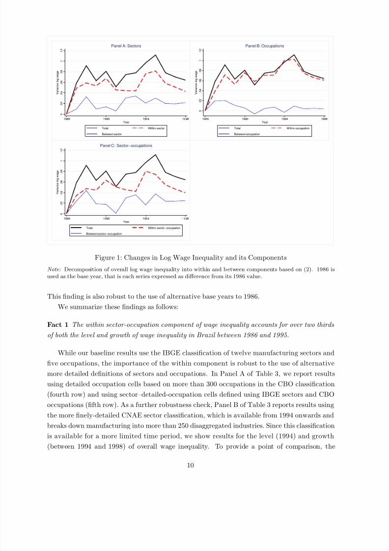
7242019 Brazil Trade
httpslidepdfcomreaderfullbrazil-trade 1649
characteristics could be larger than estimated here On the other hand the decomposition (4)
projects all variation in wages that is correlated with the included worker characteristics on
worker observables Therefore if the firm component of wages is correlated with these worker
characteristics some of its contribution to wage variation can be attributed to worker observ-
ables In the next subsection we use a different decomposition in which we explicitly control
for firm fixed effects and find a smaller contribution from worker observables towards overallwage inequality Keeping these caveats in mind we state
Fact 2 Residual wage inequality is at least as important as worker observables in explaining the
overall level and growth of wage inequality in Brazil from 1986-1995 Around 90 percent of both
the level and growth of residual wage inequality is within-sector-occupation
Our estimates of the role played by worker observables are in line with the existing empirical
literature which finds that observed worker characteristics typically account for around one
third of the cross-section variation in worker wages as discussed in Mortensen (2003) Our
finding that worker observables contribute towards the rise in overall wage inequality followingBrazilian trade liberalization is corroborated by other studies that have found an increase in
the estimated returns to schooling during our sample period such as Attanasio Goldberg and
Pavcnik (2004) and Menezes-Filho Muendler and Ramey (2008)15 Our finding that residual
wage inequality shapes the time-series evolution of overall wage inequality is consistent with
the results of recent studies using US data as in Autor Katz and Kearney (2008) Juhn
Murphy and Pierce (1993) and Lemieux (2006) The enhanced dominance of the within-
sector-occupation component after controlling for worker observables implies that the majority
of residual wage inequality is a within sector-occupation phenomenon
One potential source of wage inequality within sector-occupations for workers with the same
observed characteristics is regional variation in wages16 To show that our results for wage
inequality within sector-occupations are not driven by regional effects we have replicated the
results in Tables 3 and 4 controlling for region In Table 5 we first report results for the state
of Sao Paulo which accounts for around 45 percent of formal manufacturing employment in our
sample (compare the first and second rows) We next report results using sector-occupation-
region cells instead of sector-occupation cells where we define regions in terms of either 26 states
(third row) or 133 meso regions (fourth row) These specifications abstract from any variation
in wages across workers within sector-occupations that occurs between regions Nonetheless in
each specification we continue to find that a sizeable fraction of wage inequality is a within phe-
nomenon This is particularly notable for residual wage inequality where the within component
still accounts for over two thirds of the level and around half of the growth of residual inequality
even for the detailed meso-regions
15From the estimated coefficients on worker observables in the Mincer log wage equation (3) for each year wefind an increase in the rate of return to both education and experience over time as reported in the web appendix
16For empirical evidence of wage variation across Brazilian states see for example Fally Paillacar and Terra(2010) and Kovak (2011)
14
7242019 Brazil Trade
httpslidepdfcomreaderfullbrazil-trade 1749
Table 5 Regional Robustness
overall inequality residual inequality
Level Change Level Change1990 1986ndash95 1990 1986ndash95
Within sector-occupation 67 67 88 91
Within sector-occupation Sao Paulo 66 49 91 71Within sector-occupation-state 57 38 73 57Within sector-occupation-meso 53 30 69 49
Note All entries are in percent The first line duplicates the baseline results from Table 3 (overall inequality)and 4 (residual inequality) The second line reports the same decomposition for the state of Sao Paulo The lasttwo lines report the within component using sector-occupation-region cells where regions are first 26 states andsecond 133 meso regions
Another potential concern is that our findings for wage inequality could be influenced by
changes in workforce composition Residual wage inequality is typically higher for older more
experienced and more educated workers Therefore changes in the composition of the work-
force according to age experience and education can influence the magnitude of residual wage
inequality and its contribution to overall wage inequality To address this concern we follow
Lemieux (2006) in using the fact that our controls for worker observables take the form of in-
dicator variables for cells (eg age 25-29 college degree etc) which implies that all residual
inequality is within cells As a result the variance of the residuals in the Mincer regression (3)
can be expressed as
var (ν it) =sumℓ sℓt var (ν it|zℓt) (5)
where ℓ now indexes the cells for observable worker characteristics (education times age times experience
times sex) zℓt are common observables for all workers in cell ℓ and sℓt is the share of workers in
cell ℓ at time t
To examine the role of changes in workforce composition we use (5) to construct a coun-
terfactual measure of residual wage inequality (var (ν it)) in which workforce composition across
cells sℓt is held constant at its beginning of the sample values As reported in the web ap-
pendix we find that counterfactual residual wage inequality displays the same time-series pattern
as actual residual wage inequality and if anything exhibits greater variation over time Our
findings for residual wage inequality are therefore not driven by changes in observable workforce
composition
33 Between versus within-firm wage inequality
Having established the importance of wage inequality within sector-occupations we now further
decompose this source of wage inequality into within-firm and between-firm components We
undertake this decomposition using both the average firm wage and the estimated firm effect
from a Mincer regression for worker wages that controls for observable worker characteristics
In both cases we consider each sector-occupation-year cell in turn and decompose wage
15
7242019 Brazil Trade
httpslidepdfcomreaderfullbrazil-trade 1849
Table 6 Decomposition of Log Wage Inequality within Sector-Occupations
unconditional worker observablesaverage wage w jℓt firm fixed effect ψ jℓt
Level Change Level Change1990 1986ndash1995 1990 1986ndash1995
Between-firm wage inequality 55 115 38 86
Within-firm wage inequality 45 minus15 34 minus11Worker observables 17 2Covar observablesndashfirm effects 11 24
Note All entries are in percent Decomposition of the level and growth of wage inequality within sector-occupations (employment-weighted average of the results for each sector-occupation) The decomposition inthe first two columns is based on the average firm-occupation-year log wage wjℓt and does not control for workerobservables The decomposition in the last two columns is based on (7) using the firm-occupation-year fixedeffects ψjℓt from the Mincer regression (6) Figures may not sum exactly to 100 percent due to rounding
inequality across workers in that cell into within and between-firm components In our first de-
composition we use the unconditional average log wage paid by each firm to its workers in that
sector-occupation-year cell (w jℓt) to construct the within and between-firm components by anal-
ogy to (1) where cells now correspond to individual firms We summarize the aggregate results
from this decomposition as the employment-weighted average across sector-occupation cells in
each year and report the results in the first two columns of Table 617 While between-firm and
within-firm wage inequality make roughly equal contributions to the level of wage inequality
within sector-occupations (first column) we find that changes in wage inequality within sector-
occupations are almost entirely dominated by wage inequality between firms (second column)
While for brevity Table 6 focuses on the years 1990 and 1986ndash1995 and uses our baseline spec-
ification of sectors and occupations we find similar results using other years and definitions of
sectors and occupations And while for brevity we concentrate on aggregate results this samepattern is pervasive across sectors and occupations
To show that the role of between-firm wage dispersion within sectors and occupations is
robust to controlling for observed worker characteristics we estimate the following fixed effects
Mincer regression for log worker wages separately for each sector-occupation-year
wit = z primeitϑℓt + ψ jℓt + ν it (6)
where i again indexes workers j indexes firms ℓ indexes sector-occupation cells ψ jℓt is a firm-
occupation-year fixed effect and ν it is the residual18
17This average firm wage is equivalent to a fixed effect estimate from wit = wjℓt + ν it which is a restrictedversion of our specification (6) with worker observables The decompositions in Table 6 are based on var(wit) =var1048616
wjℓt
1048617+var(ν it) Again we work with log wages (wit) so that the results of the decomposition are not sensitive
to the choice of units for wages and to facilitate the inclusion of controls for observable worker characteristicsbelow
18Firms are assigned to a single main sector and we estimate the Mincer regression (6) separately for eachsector-occupation-year so that the fixed effects ψjℓt vary by firm-occupation-year We abuse notation slightly byadopting ν it as a residual in both (3) and (6)
16
7242019 Brazil Trade
httpslidepdfcomreaderfullbrazil-trade 1949
We use the estimated firm-occupation-year fixed effects ψ jℓt as our baseline measure of
the firm component of wages in the structural estimation of our model below This baseline
measure controls for worker observables (zprimeitϑℓt) where we allow the effects of these observables
to vary across sector-occupations ℓ and time t Our baseline specification also allows the firm-
occupation-year fixed effects to be correlated with worker observables as will be the case for
example if there is assortative matching on worker observables across firms
19
The firm-occupation-year fixed effects capture both firm wage premia for workers with iden-
tical characteristics and unobserved differences in workforce composition across firms (including
average match effects) The theoretical literature on heterogeneous firms and labor markets
considers both these sources of wage differences across firms and our objective is to quan-
tify the overall contribution of the firm component to wage inequality rather than sorting out
further its different components Since we focus on the overall firm component we are not re-
quired to assume conditional random matching of workers to firms as often invoked using linked
employer-employee datasets and can allow for assortative matching of workers and firms20
Our second decomposition splits overall wage inequality into the following four terms
var (wit) = var
zprimeitϑℓt
+ var
ψ jℓt
+ 2 cov
zprimeitϑℓt ψ jℓt
+ var
ν it
(7)
These four terms are (1) worker observables (2) the between-firm component (firm-occupation
year fixed effects) (3) the covariance between worker observables and the firm component (4) the
within-firm component (residual) which by construction is orthogonal to the other terms
We undertake this decomposition separately for each sector-occupation-year In the final
two columns of Table 6 we summarize the aggregate results from this decomposition as the
employment-weighted average of the results for each sector-occupation-year cell In the third
column we find that the between-firm (firm effects) and within-firm (residual) componentsaccount for roughly equal amounts of the level of wage inequality within sector-occupations
(38 and 34 percent respectively) Of the other two components worker observables account
for around one sixth and the covariance between worker observables and the firm component
of wages accounts for the remaining one tenth In contrast in the fourth column changes in
between-firm wage dispersion account for the lionrsquos share (86 percent) of the growth in wage
inequality within sector-occupations The next largest contribution (around one quarter) comes
from an increased covariance between worker observables and the firm component of wages
19In Table 6 we treat the average firm wage (wjℓt) and the firm-occupation-year fixed effect (ψjℓt) as data Inthe model developed below we make the theoretical assumption that the firm observes these wage components
and that the model is about these wage components which can be therefore taken as data in its estimation Incontrast without this theoretical assumption wjℓt and ψjℓt should be interpreted as estimates in which case thevariance of these estimates equals their true variance plus the variance of a sampling error that depends on theaverage number of workers employed by a firm Since this average is around twenty workers in our data theresulting correction for the variance of the sampling error is small as discussed further in the web appendix
20For a subsample of firms in RAIS that are covered by a separate annual survey data on total firm revenue areavailable that can be used to construct revenue-based productivity For this subsample of firms Menezes-FilhoMuendler and Ramey (2008) show that the estimated firm effect from a similar Mincer regression is closely relatedto revenue-based productivity consistent with findings using linked employer-employee data for other countries
17
7242019 Brazil Trade
httpslidepdfcomreaderfullbrazil-trade 2049
minus
0 2
0
0 2
0 4
0 6
0 8
I n d e x
( 1 9
8 6 = 0 )
1986 1990 1994 1998
Year
Total Worker Obs Covariance
BetweenminusFirm WithinminusFirm
Figure 3 Changes in Log Wage Inequality within Sector-Occupations and its Components
Note Decomposition of log wage inequality within sector-occupations (employment-weighted) based on (7)changes relative to the base year of 1986
which is consistent with increased assortative matching on worker observables across firms
Changes in the residual within-firm wage dispersion make a small negative contribution Notably
now that we focus on wage inequality within sector-occupations and control for firm effects
changes in the variance of worker observables account for a negligible share of the growth of wage inequality within sector-occupations in sharp contrast to our findings in Section 3221
Figure 3 further illustrates these findings by plotting the change in wage inequality within
sector-occupations and its components in (7) relative to the base year of 1986 We con-
firm that between-firm wage dispersion dominates the evolution of wage inequality within
sector-occupations and drives the inverted U-shaped pattern in wage inequality within sector-
occupations (which in turn drives the inverted U-shaped pattern in overall wage inequality)
This is the component of wage inequality that we aim to capture in our structural model of
Section 4
21This reduced contribution from worker observables is explained by two differences from the specification in
Section 32 First the Mincer regression (6) is estimated separately for each sector-occupation-year insteadof po oling observations across sectors and occupations within each year Since much of the variation in workerobservables occurs across sectors and occupations (sorting across sectors and occupations) this generates a smallercontribution from worker observables Second the Mincer regression (6) includes firm-occupation-year fixedeffects which can be correlated with worker observables (sorting across firms) Once we allow for this correlationwe again find a smaller contribution from worker observables Empirically these two differences are of roughlyequal importance in explaining the reduction in the contribution from worker observables When we re-estimatethe Mincer regression (6) for each sector-occupation-year excluding the firm-occupation-year fixed effects we finda contribution from worker observables halfway in between the results in this section and Section 32
18
7242019 Brazil Trade
httpslidepdfcomreaderfullbrazil-trade 2149
We summarize the findings above as follows
Fact 3 Between-firm and within-firm dispersion make roughly equal contributions to the level
of wage inequality within sector-occupations but the growth of wage inequality within sector-
occupations is largely accounted for by between-firm wage dispersion
These findings are also consistent with existing results in the labor economics literature For
example Lazear and Shaw (2009) summarize evidence from linked employer-employee data for
several OECD countries and conclude that the firm fixed effect explains a large and growing share
of the wage distribution This importance of between rather than within firm variation points
towards theories of heterogeneity between firms as the relevant framework for understanding
both the overall wage distribution and the wage distribution across workers with similar observed
characteristics
34 Size and exporter wage premia
Having established the importance of wage variation between firms within sector-occupations
for overall wage inequality we now examine the relationship between firm wages employment
and export status We first construct a measure of firm wages in each year by aggregating our
firm-occupation-year wage measures from the previous subsection to the firm-year level using
employment weights We next estimate the following cross-section regression of firm wages on
employment and export status for each year
ω jt = λoℓt + λsth jt + λxt ιt + ν jt for ω jt isin w jt ψ jt (8)
where we again index firms by j ℓ now denotes sectors h jt is log firm employment ι jt isin 0 1
is a dummy for whether a firm exports and ν jt is the residual The dependent variable is
the firm-year average log wage w jt or the firm-year effect ψ jt constructed from the Mincer
regression (6) by aggregating the firm-occupation-year fixed effects using employment weights
We estimate a sector-time fixed effect λoℓt a time-varying employment size wage premium λst
and a time-varying firm export premium λxt
Columns one and three of Table 7 report these estimated size and exporter wage premia for
1990 using the firm average log wage and the firm wage component from the Mincer regression
respectively Consistent with a large empirical literature in labor economics (eg Oi and Idson
1999) and international trade (eg Bernard and Jensen 1995 1997) we find positive and statis-
tically significant premia for employment size and export status In the third column using the
firm wage component from the Mincer regression (ψ jt) we find a size premium of λs = 012 and
an exporter premium of λx = 00922 We emphasize that the exporter wage premium in this
reduced-form specification cannot be given a causal interpretation because omitted unobserved
22Augmenting regression (8) with firm employment growth has little effect on either the estimated size andexporter wage premia or on the regression fit
19
7242019 Brazil Trade
httpslidepdfcomreaderfullbrazil-trade 2249
Table 7 Size and Exporter Wage Premia
unconditional worker observablesaverage wage w jt firm fixed effect ψ jt
Cross-Section Panel Cross-Section Panel1990 1986ndash1998 1990 1986ndash1998
Firm Employment Size 0126lowastlowastlowast minus0003lowast 0118lowastlowastlowast 0048lowastlowastlowast
(0008) (0002) (0006) (0001)
Firm Export Status 0202lowastlowastlowast 0216lowastlowastlowast 0088lowastlowastlowast 0012lowastlowastlowast
(0046) (0004) (0027) (0002)
Sector Fixed Effects yes no yes noFirm Fixed Effects no yes no yesWithin R-squared 0164 0007 0146 0013Observations 93 392 1 229 133 93 392 1 229 133
Note The first two columns use average firm-occupation-year wages without conditioning on worker observableswhile the last two columns use the firm-occupation-year fixed effects from the Mincer regression (6) in both casesfirm-occupation variables are aggregated to the firm level by using firm-occupation employment weights Columnsone and three report parameter estimates from the cross-section specification (8) Columns two and four report
estimated coefficients from the panel data specification (9) which controls for firm fixed effects lowast
and lowastlowastlowast
denotestatistical significance at the 10 and 1 percent levels respectively Standard errors in columns one and three areheteroscedasticity robust standard errors in columns two and four are heteroscedasticity robust and adjusted forclustering at the firm level
variables (eg firm productivity imperfectly correlated with employment) could induce firms to
both pay high wages and export That is the reduced-form exporter wage premium (λx) cap-
tures both the non-random selection of high-wage firms into exporting (beyond that captured
by firm size) and the impact of exporting on the wage paid by a given firm In our structural
model below we separate out these two components of the exporter wage premium by explicitly
modeling a firmrsquos endogenous decision of whether or not to export
Before developing the structural model we consider a panel data reduced-form specifica-
tion that partially alleviates concerns about unobserved firm heterogeneity by including time-
invariant firm fixed effects
ω jt = λo j + λot + λsh jt + λxιt + ν jt for ω jt isin w jt ψ jt (9)
where λo j is a firm fixed effect λot is a year fixed effect and the other variables are defined as in
the cross-section specification (8) In this panel data specification the exporter wage premium
(λx) is identified solely from firms that switch in and out of exporting
Columns two and four of Table 7 report the results from this specification using the firmaverage log wage and the firm wage component from the Mincer regression respectively In both
columns we find an employment size wage premium that is much smaller in magnitude and
becomes negative (though close to zero) in column two This pattern of results is consistent
with the idea that the employment-size wage premium in the cross-section specifications in
columns one and three is largely driven by selection on time-invariant firm characteristics that
20
7242019 Brazil Trade
httpslidepdfcomreaderfullbrazil-trade 2349
result in both higher firm employment and higher firm wages23 Similarly in column four using
the firm-occupation-year fixed effects we find a much smaller exporter wage premium which is
in line with the selection of high-wage firms into exporting In contrast in column two using
the firm average log wage we continue to find an exporter wage premium of a similar size to our
cross-section specification above This contrast between the two columns suggests that some of
the increase in a firmrsquos average log wage in column two when it enters export markets is due toa change in the composition of its workforce in terms of observable worker characteristics that
is controlled for in column four24
Finally although the employment size and exporter wage premia are statistically significant
in both specifications the correlations between firm wages employment and export status are far
from perfect In the cross-section regression the within R-squared after netting out the sector
fixed effects is around 015 while in the panel data regression the within R-squared after netting
out the firm fixed effects is an order of magnitude smaller In the structural model developed
below we explicitly model these imperfect correlations between firm wages employment size
and export status We summarize our empirical findings in this section as
Fact 4 Larger firms on average pay higher wages controlling for size exporters on average pay
higher wages than non-exporters Firms switching into exporting increase their wage even after
controlling for the associated increase in firm size Nonetheless controlling for size and export
status residual wage inequality across firms is substantial
Taken together the findings of this section have established a number of key stylized facts
about wage inequality in Brazil We have shown that within-sector-occupation inequality ac-
counts for much of overall wage inequality in Brazil Most of this within-sector-occupation
inequality is residual wage inequality Furthermore between-firm variation in wages accounts
for 86 percent of wage inequality within sector-occupations even after controlling for worker
observables Finally there are statistically significant employment size and exporter wage pre-
mia but the correlations between firm wages employment size and export status are imperfect
These findings are encouraging for recent theories of wage inequality based on firm heterogene-
ity In the next section we structurally estimate such a model to provide further evidence on
its ability to account quantitatively for the patterns observed in the data
4 Structural Estimation
Guided by the empirical findings in the previous section we now develop an extension of Help-
man Itskhoki and Redding (2010 HIR henceforth) In the HIR model wages vary between
23Indeed in models of wage bargaining variation in employment around the desired size of the firm results ina negative correlation between employment and wages which can explain the smaller or even negative size wagepremium estimated off time-series variation
24Regressing log firm employment on export status in an analogous panel data specification we find that entryinto export markets is also associated with a statistically significant increase in firm size by around 25 percent
21
7242019 Brazil Trade
httpslidepdfcomreaderfullbrazil-trade 2449
firms within sector-occupations and are correlated with firm employment size and export sta-
tus25 Our non-structural evidence suggests that these are essential ingredients for a model to
capture the empirical patterns of inequality and its relationship with trade openness In what
follows we first describe and generalize the HIR model we then develop a method for structurally
estimating this enhanced model and lastly we apply the model to the Brazilian data
41 Theoretical framework
We begin by briefly describing the theoretical framework of HIR emphasizing the modifications
we make in order to take the model to the data Motivated by our empirical findings above the
model focuses on between-firm variation in wages for workers with the same observed charac-
teristics Therefore workers are ex ante identical and all workers employed by a firm are paid
the same wage We augment HIR with two additional sources of heterogeneity to capture the
overlap in the employment and wage distributions across exporters and non-exporters as well
as the substantial dispersion in firm wages after controlling for firm employment size and export
status Although we make strong assumptions about the economic relationships between firmrevenue employment and wages and about the statistical distributions for the three sources of
heterogeneity we show that our parsimoniously parameterized model fits the data well
The economy consists of many sectors some or all of which manufacture differentiated prod-
ucts The modelrsquos predictions for wages and employment across firms within each differentiated
sector hold regardless of general equilibrium effects Therefore we focus on variation across
firms and workers within one such differentiated sector Our goal is to explain the observed
cross-section dispersion in wages and employment across firms and we develop a static model to
characterize such cross-section dispersion
Within the sector there is a large number of monopolistically competitive firms each supply-
ing a distinct horizontally-differentiated variety Demand functions for varieties emanate from
constant elasticity of substitution (CES) preferences As a result a firmrsquos revenue in market m
(domestic or foreign) can be expressed in terms of its output supplied to this market (Y m) and
a demand shifter (Am)
Rm = AmY mβ m isin d x
where d denotes the domestic market and x the export market The demand shifter Am depends
on aggregate sectoral expenditure and the sectoral price index in market m Since every firm is
small relative to the sector the firm takes this demand shifter as given The parameter β isin (0 1)
controls the elasticity of substitution between varieties25We focus our structural analysis on firm exporting rather than firm importing While the mechanism linking
trade and wage inequality in our theoretical model is driven by firm export-market participation as in Melitz(2003) the model can also be extended to capture firm selection into importing as in Amiti and Davis (2011) Tothe extent that firm importing increases productivity and raises revenue per worker it results in a similar importer
wage premium and our methodology could be applied to this other dimension of firm selection In practice firmexporting and importing are strongly positively correlated in the cross section and hence in our estimation wecapture most of the overall effect of firm trade participation
22
7242019 Brazil Trade
httpslidepdfcomreaderfullbrazil-trade 2549
In order to export a firm has to incur a fixed cost eεF x where ε is firm-specific and F x
is common to all firms in the sector In addition there are iceberg-type variable trade costs
τ gt 1 units of a variety have to be exported for one unit to arrive in the foreign market
An exporting firm allocates its output between the domestic and export market to maximize
revenue As a result the firmrsquos revenue (R = Rd + Rx) can be expressed as a function of its
output (Y = Y d + Y x) the demand shifter in the domestic market and a market access variable(Υx)
R = [1 + ι (Υx minus 1)]1minusβ AdY β (10)
where the market access variable is
Υx = 1 + τ minusβ1minusβ
1048616AxAd
1048617 11minusβ
and ι is an indicator variable equal to one when the firm exports and equal to zero otherwise
The revenue of a non-exporter is R = AdY β while the revenue of an exporter is R = Υ1minusβx AdY β
The firm revenue premium from exporting is decreasing in the variable trade cost parameterand increasing in the foreign demand shifter relative to the domestic demand shifter
We assume that firm output (Y ) depends on firm productivity (θ) the measure of workers
hired by the firm (H ) and the average ability of these workers (a)
Y = eθH γ a 0 lt γ lt 1 (11)
HIR show that this production function can be derived from human capital complementarities
(eg production takes place in teams and the productivity of a worker depends on the average
productivity of her team) or from a model of a managerial time constraint (eg a manager
with a fixed amount of time who needs to allocate some time to every worker as in Rosen
1982) Importantly the production technology (11) exhibits complementarity between the firmrsquos
productivity and average worker ability
Firms and workers are matched in a labor market that exhibits search and matching frictions
of the Diamond-Mortensen-Pissarides type A firm bears a search cost bN in order to randomly
match with N workers The hiring cost b is endogenously determined by the tightness of the
labor market and is taken as given by each firm in the sector26
Upon matching with a firm a worker draws a match-specific ability a from a Pareto distri-
bution G (a) = 1 minus (amina)k for a ge amin gt 0 and k gt 1 This distribution is identical and
independent across workers and matches Although a firm cannot observe the match-specificabilities of its N workers it can invest resources in screening in order to obtain a signal of these
abilities By choosing an ability threshold ac a firm can identify workers with abilities below
ac but it cannot identify the precise ability of every worker Screening costs increase with the
ability threshold and equal eminusηC
acδ
δ where η is firm specific while δ and C are common to
26In our econometric model labor market tightness is absorbed in the constants of the estimation equationsFor this reason we do not elaborate these details below The interested reader can find them in HIR
23
7242019 Brazil Trade
httpslidepdfcomreaderfullbrazil-trade 2649
all firms The incentive to screen workers results from the complementarity of firm productivity
and worker abilities in the production function (11) We also assume δ gt k which ensures
a positive size-wage premium (ie the empirically-observed positive relationship between firm
wages and employment)
Note that all workers are ex ante identical but their ex post outcomes depend on their
match-specific ability and the productivity of the firm they are matched with This modelingassumption is consistent with our empirical focus on the firm component of wages for workers
with similar observable characteristics In HIR we extend the framework to explicitly account
for observable worker heterogeneity and different occupations but here we do not attempt to
explain this additional dimension of wage variation and keep the analysis focused on residual
wage dispersion within occupations
The timing of decisions is as follows Each firm in a given sector has a draw (θηε)
which represents its idiosyncratic components of productivity screening costs and fixed export
costs Given this triplet the firm chooses whether to serve only the domestic market or to also
export where each firm in the sector serves the domestic market27 All firms in the sector post
vacancies Based on these vacancies firms are matched with workers After the matching every
firm chooses its screening threshold and hires the workers with match-specific abilities above
this threshold Therefore a firm that has been matched with N workers and has chosen the
ability cutoff ac hires
H = N
1 minus G(ac)
= N (aminac)k (12)
workers whose expected ability is
a = E
1048699a|a ge ac
1048701=
k
k minus 1 ac (13)
by the properties of the Pareto distribution Neither the firm nor its hired workers have infor-
mation on the match-specific abilities of individual workers beyond the fact that they are above
the cutoff ac
After the firm has paid all the costsmdashexporting matching and screeningmdashit engages in
multilateral bargaining with its H workers over wages as in Stole and Zwiebel (1996) HIR
show that the outcome of this bargaining game is a wage rate
W = βγ
1 + βγ
R
H
so that the wage bill is a fixed fraction of firm revenue Workers who have not been matchedwith firms or whose match-specific abilities have fallen below their firmrsquos threshold become
unemployed and are not observed in our data28
27All firms serving the domestic market can be rationalized by a fixed number of potential firms as in Chaney(2008) and no fixed costs of domestic production In our empirical implementation we condition on firm entryinto production and analyze a firmrsquos decision to serve the export market and its choice of employment and wagesTherefore we do not model the firmrsquos entry decision here
28Therefore sectoral employment is determined by firm labor demand given the hiring cost b We do not
24
7242019 Brazil Trade
httpslidepdfcomreaderfullbrazil-trade 2749
Anticipating this bargaining outcome a firm maximizes its profits by choosing the number
of workers to match with (N ) the screening threshold (ac) and whether to export
Π = maxNacιisin01
983163 1
1 + βγ R(N ac ι) minus bN minus
C eminusη
δ
acδminus ιF xe
ε
983165
where the revenue function R (N ac ι) is derived from (10)ndash(13) HIR show that the solutionto this problem yields (see (S16) in the online supplement to HIR and the web appendix)
R = κr
1 + ι (Υx minus 1) 1minusβ
Γ
983080eθ983081β
Γ983080
eη983081β(1minusγk)
δΓ (14)
H = κh
1 + ι (Υx minus 1) (1minusβ)(1minuskδ)
Γ
983080eθ983081β(1minuskδ)
Γ983080
eη983081β(1minusγk)(1minuskδ)
δΓ minus k
δ (15)
W = κw
1 + ι (Υx minus 1) k(1minusβ)
δΓ
983080eθ983081βk
δΓ983080
eη983081 k
δ
9830801+β(1minusγk)
δΓ
983081
(16)
where Γ equiv 1 minus βγ minus β (1 minus γk)δ gt 0 is a derived parameter and the κsrsquos (s = r h w) are
combinations of variables and parameters that are common to all firms in the sector Giventhese solutions a firm chooses to export in addition to serving the domestic market if the
additional profits from exporting are positive
κπ
1048616Υ
1minusβΓx minus 1
1048617983080eθ983081β
Γ983080
eη983081β(1minusγk)
δΓge F xeε (17)
where κπ is constant across firms This condition derives from the fact that operational profits
are a constant fraction Γ(1 + β ) of revenues (14) When this inequality fails the firm serves
only the domestic market A firm is more likely to export the higher are its production and
screening productivity draws θ and η and the lower is its fixed export cost productivity draw εWhen condition (17) holds ι = 1 otherwise ι = 0
Equations (15)ndash(17) describe firm employment wages and export participation This model
features two sources of firm heterogeneity that do not exist in HIR heterogeneity in fixed export
costs and heterogeneity in screening costs Without heterogeneous export-market entry costs
a firmrsquos revenue and wage bill would perfectly predict its export status This prediction is
inconsistent with the data in which there is considerable overlap in the wage and employment
distributions between non-exporters and exporters Without heterogeneous screening costs
employment and wages are perfectly correlated across firms whereas in the data this correlation
is imperfect Incorporating these two additional sources of heterogeneity enables the model to
match the empirical cross-sectional distribution of firm employment wages and export status
Our theoretical model predicts that firms with higher productivity θ hire more workers are
more likely to export and pay higher wages29 However while firms with higher productivity
explicitly model a workerrsquos decision whether to search for employment in the sector here In HIR we embed thesector in general equilibrium and show that workers are indifferent between the sectors in which to search foremployment
29In this model with Stole-Zwiebel bargaining equilibrium wages are equalized with the firmrsquos outside option
25
7242019 Brazil Trade
httpslidepdfcomreaderfullbrazil-trade 2849
in screening η also pay higher wages and are more likely to export they may hire more or fewer
workers The reason for this ambiguity stems from two opposing effects on hiring On the one
hand lower screening costs raise overall profitability thereby raising the incentive to expand
and hire more workers On the other hand lower screening costs make selectivity in hiring more
attractive thereby lowering employment On net lower screening costs may increase or reduce
employmentLower fixed export costs make exporting more profitable and induce more firms to export
In the model an exporter has higher employment and wages than a non-exporter with the
same productivity An exporter employs more workers because it has access to a larger market
which justifies a larger scale of operation The higher wage results from the greater labor
market selectivity (tougher screening for hiring) of exporters implied by the complementarity
between a larger scale of operation and higher average worker ability Since exporters screen
more intensively and have workforces of higher average ability their workforces are more costly
to replace which improves the workersrsquo stance in the wage bargaining Consequently exporters
pay higher wages This export wage premium is important for matching the model to the data
The heterogeneity in fixed export costs implies that the productivity draws in production
and screening only imperfectly determine a firmrsquos export status As a result some small and
low-wage firms find it profitable to export while some large and high-wage firms prefer to serve
only the domestic market Yet on average exporters are larger and pay higher wages than
non-exporters as observed in the data As we show below firm-specific heterogeneity in the
triplet (θηε) is crucial for the empirical success of the model
42 Econometric model
Having described the theoretical structure of the model we now adapt it for empirical estimation
Our econometric model consists of two equations for employment and wages and a selection
equation for export status Taking logarithms of (15)ndash(17) we obtain a linear selection model
h = αh + microhι + β (1 minus kδ )
Γ θ +
10486161 minus
k
δ
1048617983131β (1 minus γk)
δ Γ minus
kδ
1 minus kδ
983133η
w = αw + microwι + βk
δ Γ θ +
k
δ
10486161 +
β (1 minus γk)
δ Γ
1048617η
ι = I
983163β
Γ θ +
β (1 minus γk)
δ Γ η minus ε ge σf
983165
to replace a worker As a result firms that are more selective in the labor market end up paying higher wagesDue to complementarity in production more productive firms choose to be both larger and more selective andhence pay higher wages Through this mechanism exporters are larger and pay higher wages than non-exporters
26
7242019 Brazil Trade
httpslidepdfcomreaderfullbrazil-trade 2949
where h and w are the natural logarithms of employment and wages respectively Imiddot denotes
an indicator function
microh = (1 minus kδ )logΥ1minusβΓx
microw = kδ
1 minus kδ microh
f = 1
σ
983080minusαπ + log F x minus log
852059Υ(1minusβ)Γx minus 1
852061983081
and αs = log κs for s = hwπ Lastly we use σ to denote the standard deviation of the
composite firm-specific shock in the selection equation above (see the web appendix for the
explicit expression) which we use below as a constant of normalization To complete the model
we impose a distributional assumption on the firm-specific shocks (θηε) which we assume are
drawn from a joint normal distribution with an arbitrary covariance matrix we normalize the
means of the shocks to zero which is without loss of generality because of the presence of the
constants denoted by αs
In order to estimate the model we make a substitution of variables and rewrite the system
as an exactly-identified reduced form
h = αh + microhι + u
w = αw + microwι + ζu + v
ι = Iz ge f
uvz
primesim N
0
σ2u 0 ρuσu
0 σ2v ρvσv
ρuσu ρvσv 1
(18)
where
u = 1
1 + χ 1048616β
Γ θ + 1048616
β (1 minus γk)
δ Γ minus χ1048617 η1048617
v = χ
η minus Eη|u
= χ
η minus πu
z = 1
σ
1048616β
Γ θ +
β (1 minus γk)
δ Γ η minus ε
1048617=
1
σ
(1 + ζ )u + v minus ε
and
χ = kδ
1 minus kδ gt 0 and ζ = χ(1 + π)
with π denoting the projection coefficient of η on u The details of this derivation are provided
in the web appendix which also relates the parameters of the distributions of the reduced-form
shocks (σu σv ρu ρv) to the covariance matrix of the structural shocks (θηε) In general notall of the modelrsquos structural parameters can be recovered from the reduced-form (18) the web ap-
pendix discusses additional assumptions resulting in identification Furthermore the estimated
reduced-form parameters are sufficient to undertake model-based counterfactuals quantifying
the contribution of trade openness to wage inequality as we do below
The only additional parameter restriction on the econometric model (18) implied by the
27
7242019 Brazil Trade
httpslidepdfcomreaderfullbrazil-trade 3049
theory is positive employment and wage premia in exporting firms30
microh microw gt 0 (19)
Note that the two premia are linked by the following relationship microw = χmicroh This however does
not impose an additional constraint on the model since χ is not identified separately
We now discuss two special cases of the model with additional parameter restrictions First
we note that in general the selection correlations (ρu ρv) can be positive or negative depending
on the covariance matrix of the structural shocks It is sufficient to require however that
the productivity shocks (θ η) are not too strongly positively correlated with the exporting cost
shock ε for these correlations to be non-negative In particular if we assume that ε is orthogonal
to (θ η) the two selection correlations must be positive and in addition constrained by the
following relationship31ρuρv
= (1 + ζ )σuσv
(20)
There is no strong a priori economic reason why the productivity and screening shocks (θ η)
should be uncorrelated with the exporting cost shock ε and hence we do not impose (20) as a
default parameter restriction
The second special case assumes that the productivity shocks θ and η are orthogonal and
the screening cost shock η does not affect firm employment size The latter is the case under the
following parameter restriction χ = β (1 minus γk)(δ Γ) which implies that the two effects of the
screening cost shocks on employment discussed in Section 41 exactly offset each other Under
these assumptions we have π = 0 and ζ = χ which implies that the reduced-form shocks u and
v are proportional to the structural shocks θ and η respectively The reduced-form parameter
restriction implied by these assumptions is simply
microw = ζ microh (21)
which we can test in the data While there is again no a priori economic reason to impose these
assumptions this constrained specification is appealing because the reduced-form model in this
case can be estimated directly without transforming the shocks and hence the reduced-form
shocks have a structural interpretation
Our model features two channels of interrelationship between export participation and the
employment and wage distributions across firmsmdashthe export selection correlations (ρu ρv) and
the employment and wage exporter premia (microh microw) The first channelmdashthe selection effect mdash jointly determines the export status employment sizes and wage rates of firms through the
30The model imposes the parameter inequalities Υx gt 1 0 lt kδ lt 1 0 lt γk lt 1 and Γ gt 0 which implies
microh microw gt 0 Also note that microh + microw = logΥ(1minusβ)Γx which allows us to isolate the variation in f induced by
changes in market access Υ(1minusβ)Γx
31This restriction derived in the web appendix arises because under this orthogonality assumption wagebills revenues and operating profits are perfectly correlated in the cross-section of firms As a result the jointcorrelation structure between employment wages and export status is constrained by (20)
28
7242019 Brazil Trade
httpslidepdfcomreaderfullbrazil-trade 3149
underlying productivity distribution where more productive firms are larger pay higher wages
and are more likely to export The second channelmdashthe market access effect mdashensures that
exporting firms are larger and pay higher wages even after controlling for productivity32 We
test below whether either or both effects are important in the data In particular we evaluate
the hypothesis of no relationship between trade and the employment and wage distributions
across firms by estimating the model under the parameter restriction
microh = microw = ρu = ρv = 0 (22)
Likelihood function Our econometric model (18) takes a form similar to a Tobit Type 5
model in Amemiya (1985) or a switching regression model with endogenous switching in Maddala
(1983) This model admits a closed-form likelihood function which we now describe
A unit of observation in the model is a firm j and each observation is a triplet of firm log
employment log wages and binary export status x j = (h j w j ι j)prime We denote the data by X =
x j j and we use it to estimate the parameter vector Θ = (αh αw ζ σu σv ρu ρv microh microw f )prime
We denote the likelihood of the data X given the parameter vector Θ by
L
Θ|X
=prod j Px j |Θ (23)
In the web appendix we show that
P x j|Θ = 1
σuφ(u j)
1
σvφ(v j)
1048667Φ
852008f minus ρuu j minus ρvv jradic
1 minus ρ2u minus ρ2v
85200910486691minusιj 10486671 minus Φ
852008f minus ρuu j minus ρvv jradic
1 minus ρ2u minus ρ2v
8520091048669ιj
where φ(middot) and Φ(middot) are respectively the density and cumulative distribution functions of a
standard normal and
u j =
h j minus αh minus microhι j
σu
v j =
(w j minus αw minus microwι j) minus ζ (h j minus αh minus microhι j)
σv
This simple expression for the density of the data x j is intuitive the first two terms reflect the
likelihood of the continuous distribution of shocks which result in the observed employment and
wages while the last two terms are a standard Probit likelihood for binary export status given
the employment and wages of the firm
We estimate the parameters of the model by maximizing the likelihood function (23) subject
to the structural constraint (19) Additionally we evaluate the maximized likelihood of an
unconstrained model as well as the maximum likelihood under the various parameter restrictions
discussed above The model is identified through functional form and distributional assumptions
32In the literature following Melitz (2003) and in particular in HIR the two effects are typically not separatedbecause firm productivity p erfectly predicts export status Our framework emphasizes the distinction betweenthe two effects as a result of idiosyncratic differences in exporting costs across firms
29
7242019 Brazil Trade
httpslidepdfcomreaderfullbrazil-trade 3249
As a check on our functional form assumptions we show that the estimated model provides a
good fit of the empirical cross-section distributions of employment and wages
While the maximum likelihood estimation uses efficiently all possible moments of the data
the first and second moments of the joint distribution of employment wages and export status
provide intuition for the identification of the modelrsquos parameters33 The parameters αw αh σu
σv and f can be identified from the first and second moments of employment and wages as well asthe fraction of exporting firms ζ is pinned down by the wage-employment covariance The key
parameters of interestmdashmicrow microh ρu and ρvmdashare identified from the first and second moments of
employment and wages conditional on export status with their separate identification coming
from the modelrsquos functional form assumptions including the discrete increase in wages and
employment upon entry into export markets
We focus on cross-section dispersion in wages employment and export status across firms
and hence estimate the modelrsquos parameters using data on a cross-section of firms To ensure
that our results are not driven by changes in policies or other aspects of the market environment
over time we estimate the parameters of the model separately for each year in our sample and
examine the extent to which the parameters change over time We allow all parameters to
vary over time in an unrestricted manner since all the parameters are functions of endogenous
aggregate variables which in the data are likely to change over time For example exporter
premia (microh microw) depend on variable trade costs (τ ) and relative export market demand (AxAd)
which change over time
As discussed in the Introduction there exist other models of competitive and frictional labor
marketsmdashincluding competitive assignment search-and-matching fair-wage and efficiency-wage
modelsmdashwhich can generate a firm-size wage premium and exporter premia for wages and em-
ployment Obtaining the empirically relevant correlations between shocks to employment and
wages on the one hand and shocks to export participation on the other hand is not simplehowever For example if in our theoretical model we were to replace the shock to screening with
a shock to the bargaining power of a firm relative to its workers the resulting correlations would
not be consistent with the data34 In other words not every model that predicts variation of
wages size and export status across firms in a sector is capable of explaining the data While we
do not know whether there exist other models that lead to an econometric specification similar
to (18) we conjecture that models of this type exist and that (18) may be a good approximation
to some models even if it does not represent an exact specification Indeed (18) is a general
33The web appendix provides closed-form expressions for these moments as functions of the parameter vector Θ
It also lays out the details of an alternative GMM estimation procedure based on these moments The GMMresults provide an additional check on the modelrsquos functional form assumptions Efficient GMM yields estimatesquantitatively very similar to our maximum likelihood (ML) estimates and for brevity we do not report themTable 8 reports the values of the GMM objective for different specifications of interest and Table 9 displays thefit of the moments used in the GMM estimation
34In this alternative specification a high-wage firm is other things equal the one with low bargaining powerrelative to its workers which in turn reduces the firmrsquos profitability and makes it less likely to export In otherwords controlling for employment exporters should be relatively low-wage firms reflecting their high bargainingpower and hence high profitability
30
7242019 Brazil Trade
httpslidepdfcomreaderfullbrazil-trade 3349
log linear model of firm employment wages and selection into exporting which can be further
augmented to allow for reduced-form variation in σu σv and ζ with export status A theoretical
underpinning of the econometric model is desirable however because it helps to form priors
and identify the parameters of interest as well as conduct internally-consistent counterfactual
exercises using the estimated reduced-form model The next section illustrates both of these
points
43 Maximum Likelihood results
We estimate the econometric model (18) using data on firm export status employment and
wages Since the theory focuses on the firm-specific wages of workers with similar ex-ante
characteristics we use the firm-occupation-year fixed effects ψ jℓt from the Mincer regression (6)
in Section 33 for wages Noting that the equation for selection into exporting is defined at the
firm level we also aggregate the firm-occupation-year fixed effects to the firm-year level ( ψ jt)
using the firmrsquos employment in each occupation as weights as in Section 3435 For employment
and export status we use the actual dataIn the first two columns of Table 8 we summarize the results of the maximum likelihood
estimation We report results for 1990 but the pattern of results is robust across years The web
appendix reports all the results for 1994 for comparison We consider five specificationsmdashthe
unconstrained specification three structurally constrained specifications corresponding to the
parameter restrictions (19) (20) and (21) respectively and one counterfactual specification in
which we shut down the effects of trade altogether by imposing (22) For each specification we
report the log of the likelihood function and for the four constrained specifications we report the
likelihood ratio test statistic (LR) that assesses the validity of the constraints36 Given our large
sample of about 100000 firms per year we reject every conceivable constraint on the parameters
of the econometric model For example the LR test statistic for the structural specification (ii)
subject to the theoretical requirement (19) equals 628 while the 1 percent critical value for a
χ2(1)-test is 66
Since a constraint can be statistically rejected and yet have little impact on the economic fit
of the model the final column of Table 8 reports the square root of the Generalized Method of
Moments (GMM) objective based on the first and second moments of wages employment and
export status37 This GMM objective can be interpreted as the distance from a perfect fit in
35As discussed in footnote 19 we assume that the firm controls the average wage conditional on observedworker characteristics (ψjt) which we therefore treat as data in our estimation of the model The web appendix
described the estimation procedure under the alternative assumption that this wage component is measured witherror Further as a robustness check we estimate the model using the firm average log worker wage wjt insteadand find qualitatively similar results as discussed in the web appendix
36The LR test equals twice the difference between the log likelihood of the unconstrained and constrainedmodels and has an asymptotic χ2(r) distribution when r parameter restrictions are imposed We also consideredalternative information criteria such as BIC and they suggest similar conclusions
37As discussed in footnote 33 and the web appendix the modelrsquos parameters can be also estimated with GMMusing 11 first and second moments to identify the ten parameters of the model Here we use the ML parameterestimates to evaluate these eleven moments which include the fraction of exporters the mean employment andwage conditional on exporting and non-exporting and the variance-covariance matrix of employment and wages
31
7242019 Brazil Trade
httpslidepdfcomreaderfullbrazil-trade 3449
Table 8 Maximum Likelihood of Unconstrained and Restricted Models 1990
Specification logL LR Sqrt GMM Obj
(i) Unconstrained minus393496 mdash 0013
(ii) microh microw gt 0 minus393810 628 0021
(iii) microw = ζ microh minus394413 1834 0034
(iv) Orthogonal structural shocks minus394452 1911 0035
(v) No trade effects minus495436 203879 0370microh = microw = ρu = ρv = 0
Note Unconstrained model (i) maximizes the likelihood function imposing no constraints on the parametersStructural specification (ii) imposes the inequality constraint (19) implied by the theoretical model Specification(iii) imposes constraint (21) while inequality (19) turns out to be non-binding Specification (iv) imposes theorthogonality constraint (20) while both inequality (19) and ρu ρv gt 0 turn out to be non-binding The no-trade-effects specification (v) sets both selection correlations (ρu and ρv) and exporter premia (microh and microw) tozero implying that firm employment and wages are independent of export status Column one reports the valueof the log-likelihood function Column two reports the LR statistic equal to twice the difference between the loglikelihood of unconstrained and constrained models Column three reports the square root of the GMM objectivewhich is the square of 11 first and second moments of firm employment wages and export status weighted bythe diagonal of the efficient GMM weighting matrix as discussed in the text and web appendix
terms of the standard deviations of the moments so that 002 corresponds to a discrepancy in the
moment fit of 2 of the momentrsquos standard deviation in the sample Under exact identification
the value of this GMM objective is equal to zero and it is in general positive under over-
identification The restricted specifications impose an extra degree of over-identification (10
parameters minus one restriction compared to the 11 moments) As reported in the table the
loss in the GMM objective in moving from the unconstrained specification (i) to the constrained
specifications (ii)-(iv) is around the same magnitude as the initial loss in the GMM objective in
the unconstrained specification (i) Therefore according to the GMM objective the fit of thestructurally constrained specifications is nearly as good as the fit of the unconstrained model
We further explore the fit of the model below by looking at the individual moments of the data
as well as the overall employment and wage distributions
In contrast the likelihood ratio test statistic for the no trade specification ( microh = microw =
ρu = ρv = 0) in (v) is two orders of magnitude larger than for the structurally constrained
also conditional on exporting and non-exporting We normalize the deviation of the theoretical moments fromtheir data counterparts by the standard deviation of the respective moment in the data The square root of theGMM objective is therefore a Euclidian distance in the space of normalized moments
Sqrt GMM Obj = S991761
s=1
9830801
N sumj ms1048616xj |ˆΘR1048617983081
2
var1048616
ms(xj |ΘU )1048617
12
where var1048616ms(xj |ΘU )1048617 = 1N 991761j
ms1048616xj|ΘU 10486172
where s indexes the moments (the number of moments in our case is S = 11) ms(x|Θ) is the value of themoment-s function for data vector x given parameter vector Θ var(middot) is the sample variance estimator for amean-zero variable ΘU is the unconstrained ML parameter estimate and ΘR is the (constrained) parametervector of interest For example for moment s = 1 (fraction of exporters) we have m1(xj |Θ) = ιj minus Eι|Θwhere Eι|Θ = EIz ge f |Θ = 1 minus Φ(f ) Note that Ems(xj|Θ)|Θ = 0 for all s under the correct modelspecification
32
7242019 Brazil Trade
httpslidepdfcomreaderfullbrazil-trade 3549
specifications In terms of the GMM objective the fit of the no-trade specification (v) is an order
of magnitude worse than the unconstrained specification (i) or the constrained specifications
(ii)-(iv) We therefore conclude that firm trade participationmdashthrough the combination of the
selection effects (ρu ρv) and the market access effects (microh microw)mdashis important for explaining the
observed distributions of wages and employment Some other constraints on the parameters are
equally strongly rejected For example the data strongly rejects the constraint of no marketaccess effect microh = microw = 0 or no exporter wage premium microw = ρv = 038 The data also strongly
rejects the hypothesis that the observed variation in wages is due to pure measurement error
This hypothesis is tested by imposing (21) implied by the HIR model without screening shocks
and additionally imposing ρv = 0 since measurement error in wages should not correlate with
export status
Comparing specifications (i)-(iv) the estimated wage-equation parameters (microw ρv) differ
substantially across specifications microw varies from minus02 to 08 while ρv changes from 05 to
minus05 as we report in the web appendix Recall that microw is the structural exporter wage pre-
mium while the correlation parameter ρv measures the strength of the selection of high-wage
firms into exporting The joint effect results in the reduced-form exporter wage premium which
can be fitted with either a high microw or a high ρv explaining the negative relationship between the
two across specifications In contrast the estimated employment-equation parameters (microh ρu)
exhibit limited variation with the data favoring both positive market access and positive se-
lection effects (microh varies from 21 to 25 while ρu changes from 01 to 00) Additionally the
remaining parameters (αh αw ζ σu σv f ) correspond closely to the first and second moments
of employment and wages and the fraction of exporters and hardly change across specifica-
tions Given this pattern of parameter variation across specifications we proceed to visualize
the shape of the log likelihood in the (microw ρv)-spacemdashthe two parameters that change the most
across specificationsFigure 4 displays the contour plot of the log likelihood function in the space of the two
parameters (microw ρv) Specifically we fix the values of (microw ρv) on a grid and for each combination
on the grid maximize the log likelihood with respect to the other eight parameters of the model
In line with our findings above the estimates of these other eight parameters vary little across
the alternative values of (microw ρv) on the grid As illustrated in the figure for 1990 a generic
feature of our estimates is the presence of a global maximum which in 1990 has a negative microw
and a positive ρv and a local maximum which in 1990 has a positive microw and a negative ρv39
Apart from these global and local maxima there is a whole ridge in (microw ρv) spacemdasha downward
slopping yellow curve in the figuremdashthat yields high levels of likelihood and model fit Given38Interestingly the constraint of no selection effect ρu = ρv = 0 is not strongly rejected and in terms of fit is
similar to the structural specification (iv) Also note that the model without screening shocks (σv = 0) or withoutexporting cost shocks (ρ2u + ρ2v = 1) have a likelihood of zero (log-likelihood of minusinfin) since in the former case wagesmust perfectly correlate with employment while in the latter case export status must be perfectly predictable bya linear combination of employment and wages In the data both these correlations are far from perfect
39The global maximum remains in the negative microw region in 1990-93 and 1995-98 while it shifts to the negativeρv region in 1986-89 and 1994 In the web appendix we also present the results for 1994
33
7242019 Brazil Trade
httpslidepdfcomreaderfullbrazil-trade 3649
minus 3 9 8
minus 3 9 8
minus 3 9 8
minus 3 9 8
minus 3 9 8
minus 3 9 8
minus 3
9 7
minus 3 9 7
minus 3 9 7
minus 3 9 7
minus 3 9 7
minus 3 9 7
minus 3 9 6
minus 3 9 6
minus 3 9 6
minus 3 9 6
minus 3 9 6
minus 3 9 6
minus 3 9 6
minus 3 9 6
minus 3 9
minus 3 9 5
minus 3 9 5
minus 3 9 5
minus 3 9 5
minus 3 9 5
minus 3 9 5
minus 3 9 5
minus 3 9 4
minus 3 9 4
microw
ρ v
minus05 minus025 0 025 05 075 1minus075
minus05
minus025
0
025
05
075
microw = ζ microhminus3944
microw ge 0
minus3938
Global Max
minus3935
Orthog shocks
minus3945
Local Max
minus3939
Figure 4 Contour plot of the log likelihood 1990
Note Log likelihood normalized by 10000 as a function of (microw ρv) with the remaining eight parameters opti-mized given (microw ρv) The values of the log likelihood 500 log points below the peak are censored (blue area inthe figure) The downward sloping yellow curve (dashed and solid) depicts the high likelihood ridge for a givenvalue of microw the curve displays the value of ρv that maximizes the log likelihood function The solid segment of
the curve represents the economically meaningful range of parameters in the first quadrant (while only microw gt 0 isrequired by the theory ρv gt 0 is also favored in view of previous empirical evidence on the importance of selectioninto exporting) The five yellow squares indicate the location of the estimates under the specifications (i)-(iv)considered in Table 8 and the text as well as a local maximum the reported numbers correspond to the value of the log likelihood function normalized by 10000
our large number of observations the global maximum is statistically distinguishable from other
points along the ridge Nevertheless as shown in Table 8 the economic fit of the model is good
at any point on the ridge and close to the fit at the global maximum In particular the model
can successfully account for the reduced-form exporter wage premium observed in the data with
a strong selection effect (ρv ≫ 0 and microw asymp 0) a strong market access effect (microw ≫ 0 and ρv asymp 0)
or both positive selection and positive market access effect (microw ρv gt 0)40
When we only impose constraint (19) corresponding to positive market access effects (spec-
40The reason why the data favors either a large negative ρv or a large positive ρv which by consequenceresults either in large positive microw or moderately negative microw has to do with the fact that our theoretical modelis parsimonious and sparsely parameterized As becomes clear from Tables 9ndash10 and Figure 6 the conditionalvariance of wages for exporters is lower than for non-exporters and the only way the model can accommodatethis difference is by blowing up the (absolute value of) selection correlation of high-wage firms into exportingLower absolute values of ρv result in a poorer fit of this moment but in fact better fit of most other moments
34
7242019 Brazil Trade
httpslidepdfcomreaderfullbrazil-trade 3749
ification (ii)) we estimate microw close to zero Alternatively when we impose (20) emanating
from the assumption of orthogonal structural shocks (specification (iv)) we estimate ρv close
to zero41 Finally when we impose (21) implying no effects of screening shocks on employment
(specification (iii)) we estimate both microw gt 0 and ρv gt 0 The points corresponding to these
three alternative structural restrictions are shown in Figure 4 along with the unconstrained
global and local maxima Each of these five points lies along the ridge of high likelihood in theparameter space (microw ρv) and provides almost as good a fit to the data as the unconstrained
model as reported in Table 8 and further shown below
Any departures from this one-dimensional line of values of (microw ρv) in the 10-dimensional
parameter space lead to a steep decline in the likelihood function In other words the data
strongly identifies a compact segment in the parameter space but beyond this does not sharply
discriminate between different points along this segment The reason is that the market access
(microw) and selection (ρv) components of the exporter wage premium are only separately identified
in our model through the functional form assumptions and specifically the discontinuous effect
of foreign market access on wages in contrast to the smooth selection effect While the discrete
increase in employment (microh) as firms enter export markets and expand to meet export demand is
large the discrete increase in wages (microw) as firms enter export markets is substantially smaller
which makes it harder to separately identify the market access and selection effects for wages
Hence in what follows we use economic reasoning to select a point along the segment shown in
Figure 4
Our theoretical model imposes the restriction that microw microh gt 0 Additionally a number of
empirical studies find that future exporters are larger and pay higher wages than other non-
exporters even before they enter export markets (see for example Bernard and Jensen 1997
1999) which suggests selection into export markets (ρu ρh gt 0) Therefore we adopt the
structural restriction (21) microw = ζ microh or specification (iii) as our preferred specification whichgenerates both positive market access effects (microw microh gt 0) and positive selection effects (ρu ρv gt
0) Under this restriction the reduced-form model has an attractive structural interpretation in
which wages and employment depend on two orthogonal structural shocksmdashone to productivity
(θ) that enters both the employment and wage equations and another to screening (η) that
enters only the wage equation where both can be correlated with the shock in the export
selection equation (z) Finally this constrained specification also generates a similar level of fit
as the unconstrained specification as shown in Tables 8 9 and 10 below
Before analyzing further the fit of the model Figure 5 presents the ML parameter estimates
for our preferred specification (iii) for each year during our sample period 1986ndash98 We esti-mate the model using the cross-section data on firms for each year separately without imposing
restrictions on the evolution of the parameters over time The figure also shows the 98 percent
confidence intervals (two standard-deviation bands) using a robust (sandwich) covariance ma-
trix which are tight around the estimated parameter values given our large sample size The
41This is a robust outcome of constraint (20) The reason is somewhat mechanical arising from the fact thatthe data favors estimates that satisfy 0 lt ρu lt ρv and σu gt σv which is inconsistent with (20) unless ρu ρv asymp 0
35
7242019 Brazil Trade
httpslidepdfcomreaderfullbrazil-trade 3849
86 88 90 92 94 96 98006
008
01
012
ζ
86 88 90 92 94 96 9813
14
15
16
f
86 88 90 92 94 96 981
11
12
σu
86 88 90 92 94 96 98035
04
045
σv
86 88 90 92 94 96 980
002
004
ρu
86 88 90 92 94 96 98005
01
015
02
025
ρv
86 88 90 92 94 96 9818
2
22
24
26
microh
86 88 90 92 94 96 9801
02
microw
86 88 90 92 94 96 9826
27
28
29
αh and αw
minus04
minus035
minus03
minus025
Figure 5 Maximum Likelihood Parameter Estimates Across Years
Note ML estimates from the structural specification (iii) under constraint (20) based on separate cross sectionsof firm employment firm wages and export status for each year and two standard-error bands based on MLasymptotic sandwich covariance matrix
estimated parameters evolve smoothly over time consistent with the idea that our model cap-
tures systematic cross-section dispersion in wages and employment The parameter estimatesfeature substantial employment and wage export premia (microh and microw) as well as positive selec-
tion correlations (ρu and ρv) In other words our constrained specification suggests that both
selection and market access effects are present in the data42 The estimated dispersion of u
(σu) falls over time which is driven by the decline in the dispersion of firm employment ob-
served in the data The estimated dispersion of v (σv) follows an inverted U-shape pattern over
time which reflects the inverted U-shape pattern in the dispersion of firm wages observed in the
data Finally the estimated export threshold parameter f follows a U-shape which captures
the inverted U-shape in the observed share of exporters over time
Fit of the model In Tables 9 and 10 we provide further evidence on the modelrsquos fit in the
cross-section for 1990 We find a similar pattern for other years and report results for 1994 in the
web appendix In each table the first column reports cross-section moments in the data while
42Note however that the estimated selection correlations are small with ρu fluctuating around 002 and ρvranging between 01 and 02 The overall strength of the selection effect can be measured by
radic ρ2u + ρ2v and it
fluctuates around 017 over the years
36
7242019 Brazil Trade
httpslidepdfcomreaderfullbrazil-trade 3949
Table 9 Model Fit for Firm-level Moments 1990
Data ModelUnconstrained StructuralA Full Sample
Mean Employment 297 297 297
Mean Wages minus0340 minus0341 minus0341
St Dev Employment 127 127 127St Dev Wages 0424 0424 0423
Covar Emplmnt and Wages 0352 0354 0352
Fraction of Exporters 55 55 55
B Non-exporters
Mean Employment 283 283 283
Mean Wages minus0359 minus0360 minus0360
St Dev Employment 112 114 114
St Dev Wages 0419 0419 0416
Covar Emplmnt and Wages 0306 0309 0304
C ExportersMean Employment 528 529 529
Mean Wages minus0010 minus0010 minus0006
St Dev Employment 152 114 114
St Dev Wages 0366 0373 0417
Covar Emplmnt and Wages 0322 0289 0304
Note Moments of the log wage and log employment distributions across firms in 1990 The log wage measure inthe data is the firm-occupation-year fixed effect estimated from (6) aggregated to the firm-year level using occu-pation employment weights Model moments are calculated in the same way in an artificial cross-section of firmsgenerated from ML estimated model (18) under the unconstrained specification (i) and structural specifications(iii) respectively
the next two columns report model-predicted moments from the unconstrained specification and
our preferred structural specification (iii) respectively To calculate the moments in the model
we simulate the data based on (18) given the estimated parameter vector Θ
Table 9 presents firm-level moments first and second moments for employment and wagesmdash
for the full sample and conditional on exporting and non-exportingmdashas well as the fraction of
exporting firms These are the moments used in calculating the GMM ob jective in Table 843
Additionally Table 10 presents the worker-level moments of the wage distribution Since we
focus on the firm component of wages abstracting from wage variation within firms the distri-
bution of wages across workers in our analysis is the firm-employment-weighted distribution of wages across firms That is wage observations for a large firm in terms of employment receive
a proportionately larger weight in the worker-wage distribution Panel A of Table 10 reports
the mean and variance of worker wages for the full sample as well as for workers employed by
43Note that the full sample moments for employment and wages in Table 9 are linear combinations of the 10moments for exporters and non-exporters and the fraction of exporters and hence we exclude them in calculatingthe GMM objective
37
7242019 Brazil Trade
httpslidepdfcomreaderfullbrazil-trade 4049
Table 10 Model Fit for Worker-level Moments 1990
Data ModelUnconstrained StructuralA First and Second Moments
Mean Log Wage 0000 minus0085 minus0072
Non-exporters minus0122 minus0213 minus0215
Exporters 0152 0109 0140St Dev Log Wages 0404 0429 0450
Non-exporters 0407 0415 0416
Exporters 0345 0374 0414
Emplmnt Share of Exporters 446 400 403
B Wage Inequality Measures
Gini 0215 0236 0250
9010 277 300 318
9050 154 170 179
5010 180 176 178
C Size and Exporter Wage Premia
Size premium 0111 0112 0111
Exporter premium 0077 0075 0082
Note Moments are calculated across workers in 1990 the wage measures are the firm-occupation-year fixed effectsestimated from (6) aggregated to the firm-year level using occupation employment weights and weighted by thenumber of workers employed by the firm The firm-occupation-year fixed effects are normalized so that in everyyear their mean is zero across workers within each sector-occupation cell for this reason the mean worker wageequals zero Simulated moments for log wages and log employment generated using ML estimates for 1990 fromthe unconstrained specification (i) and structural specification (iii) 9010 denotes the 90-10 wage percentile ratio(the ratio of the exponents of the log wage percentiles) and similarly for 9050 and 5010 Size and exporterpremia are coefficient estimates from an OLS regression of log firm wages on log firm employment and a dummy for
export status without including sector fixed effects which explains the small difference in the exporter premiumfrom the results reported in Section 34
exporters and non-exporters this panel also reports the share of workers employed by exporters
Panel B then reports additional measures of wage inequality namely the Gini coefficient and
the 9010 9050 and 5010 percentile ratios Finally Panel C reports the coefficients from the
size-exporter wage premium regression parallel to (8) in Section 34
Judging by the moments in Tables 9 and 10 the model provides a close fit to the data Both
firm and worker moments generated by the structural model closely match the moments in the
data and this match is not noticeably worse than the moments generated by the unconstrained
model As discussed in footnote 40 the one moment that the unconstrained model fits better is
the standard deviation of wages across exporting firms and across workers employed in exporting
firms The structural model provides a tight fit to all moments across the full sample of firms
and across non-exporters it does slightly worse on the dispersion of employment and wages
across exporters The fit of the model is good but less than perfect for the worker-level moments
in Table 10 Of particular interest is the fact that the model fits not only the first and second
38
7242019 Brazil Trade
httpslidepdfcomreaderfullbrazil-trade 4149
moments of firm employment and wage distributions but also nonlinear transformations of the
worker wage distribution such as the 9010 9050 and 5010 wage percentile ratios and the
Gini coefficient In fact the model generates a Lorenz curve that closely fits the Lorenz curve
in the data Finally the structural model matches the size and exporter wage premia estimated
in the data We conclude that our parsimonious theoretical model provides a very reasonable
fit to a rich set of empirical moments of employment and wage distributions across firms andworkers Furthermore the constrained structural specification is almost indistinguishable in
terms of economic fit from the unconstrained model that has a superior statistical fit
Figures 6ndash7 provide further evidence of the quality of the cross-sectional fit of the structural
model They display kernel density estimates of the distributions of employment and wages
across firms and the distribution of wages across workers in our data and in artificial data
generated from the estimated structural model We provide the comparison for 1990 and report
the results for 1994 in the web appendix results for other years are again similar
Figure 6 displays kernel densities for the firm distributions while Figure 7 displays kernel
densities for the worker distributions which again weight firm wages by firm employment The
left two panels of Figure 6 report results for firm employment while the right two panels report
results for firm wages The upper panels report results for all firms while the lower panels
report separate estimates for exporters and non-exporters Our log-normal assumption for the
distribution of shocks allows us to nearly perfectly fit the distribution of wages across the full
sample of firms The fit of the distribution of employment across the full sample of firms is
good but imperfect because the distribution in the data is skewed and has a fatter tail than the
distribution in the model
A striking feature of the data is the substantial overlap between the employment and wage
distributions of exporters and non-exporters although the distributions of both employment
and wages are shifted to the right for exporters relative to non-exporters Our theoretical modelwith firm heterogeneity in export costs can accommodate the overlap in the empirical wage
and employment distributions (lower panel of Figure 6) However as discussed in footnote 40
the model is sparsely parameterized and cannot fit the different dispersion of employment and
wages for exporters versus non-exporters In the data employment is more dispersed among
the exporters while wages are more dispersed among non-exporters Given our theoretical
assumption that σu and σv are common for both exporters and non-exporters the structural
model cannot fully capture these two features of the data
In Figure 7 the model fits well the distribution of wages across all workers as well as across
workers employed by exporting firms and non-exporting firms However the model slightlyoverstates the variance of wages among exporters Overall Figures 6ndash7 confirm our earlier
results for selected moments of the worker and firm distributions and further illustrate that the
model provides a good fit to the empirical cross-sectional distributions
Taken together the results in Tables 9ndash10 and Figures 6ndash7 support our structural model
Despite the modelrsquos sparsity and its strong functional form assumptions we find that it approx-
imates the data well The model captures both the higher average employment and wages of
39
7242019 Brazil Trade
httpslidepdfcomreaderfullbrazil-trade 4249
minus2 0 2 4 6 8 100
025
05
Log Employment
minus2 minus1 0 1
0
05
1
Log Firm Wages
minus2 0 2 4 6 8 100
025
05
Exporters vs Non-Exporters
minus2 minus1 0 1
0
05
1
Exporters vs Non-Exporters
Data (non-exp) Data (exporters) M odel (non-exp) M odel (exporters)
DataModel
Figure 6 Model Fit for the Distribution of Log Firm Employment and Log Firm Wages 1990
Note Kernel densities of the employment and wage distributions across firms (using normal kernels with optimalbandwidth) Simulated data generated from the estimated model under structural specification (iii)
minus2 minus1 0 1 20
05
1
Log Worker Wages
minus2 minus1 0 1 20
05
1
Exporters vs Non-Exporters
Data
Model
Figure 7 Model Fit for the Distribution of Log Worker Wages 1990
Note Kernel densities of the wage distribution across workers in which firm wages are weighted by firm employ-ment (using normal kernels with optimal bandwidth) Simulated data generated from the estimated model understructural specification (iii)
40
7242019 Brazil Trade
httpslidepdfcomreaderfullbrazil-trade 4349
86 88 90 92 94 96 980
001
002
003
004
005
006
007
V a r i a n c e l o g w o r k e r w a g e s
Data
Structural Model
Figure 8 Model Fit of Log Wage Inequality over Time
Note Change in the variance of log worker wages relative to 1986 where the worker wage distribution weightsfirm wages by firm employment The data curve corresponds to the between-firm component in Figure 3 Themodel curve is based on simulated data generated separately for each year using the respective ML estimates of the parameters under the structural specification (iii) as reported in Figure 5
exporters relative to non-exporters and the substantial overlap in the distributions of employ-
ment and wages between these two groups of firms
Figure 8 reports one final measure of fit by displaying the true and predicted evolution of log
wage inequality over time Specifically we simulate the model in every year between 1986 and
1998 using the parameters estimated year-by-year from our preferred structural specification (iii)
as reported in Figure 5 Figure 8 then reports the change over time in the variance of log worker
wages relative to 1986 both in the data and in the model-simulated cross sections Althoughthe model slightly overstates the variance of log worker wages (Table 10) this discrepancy is
relatively stable over time and as a result the model tracks closely the evolution of wage
inequality In particular the model captures the hump shape in log wage inequality over our
sample period 1986-1998
Counterfactual exercise In closing this section we discuss the results from a model-based
counterfactual exercise that illustrates the effects of trade on wage inequality in the estimated
structural model Specifically we consider the effect of a reduction in variable trade costs τ
on export participation and the cross-sectional distributions of employment and wages with a
focus on the variance of log worker wages
Recall from Section 41 that the market access variable is related to variable trade costs
according to
Υx = 1 + τ minusβ1minusβ
1048616AxAd
1048617 11minusβ
41
7242019 Brazil Trade
httpslidepdfcomreaderfullbrazil-trade 4449
and the exporter employment and wage premia are given respectively by
microh = 1
1 + χ log Υ
1minusβΓx and microw =
χ
1 + χ log Υ
1minusβΓx
Another parameter affected by variable trade costs is the reduced-form threshold for export
participation
f = 1σ
983080minusαπ + log F x minus log
852059Υ(1minusβ)Γx minus 1
852061983081
The remaining seven estimation parameters are not directly affected by variable trade costs and
hence we hold them constant in our counterfactual exercise Specifically we take the estimated
parameters Θ under our preferred structural specification (iii) for 1990 and then vary (microh microw f )
in a way consistent with variation in Υx as summarized in the equations above44 We change
Υx from the value of 1 corresponding to autarky to a very large value for which nearly all
workers are employed by exporting firms Then for every given counterfactual parameter vector
ΘC corresponding to a particular value of Υx we simulate the model and calculate various
moments of the firm and worker distributionsFigure 9 displays the resulting variance of log worker wages as a function of the market
access measure microh + microw = log Υ(1minusβ)Γx Wage inequality displays a hump-shape in response to
a reduction in variable trade costs consistent with the theoretical prediction in HIR Therefore
once the economy is open to trade further trade liberalization can either raise or reduce wage
inequality depending on the initial level of trade openness As variable trade costs decline
from autarky employment reallocates from non-exporters to exporters along both the extensive
margin of export market entry and the intensive margin of an expansion of employment at
exporters and the fraction of workers employed by exporters changes from zero to one This
in turn first increases and later decreases wage inequality with the peak attained when the
majority of workers are employed at exporting firms
In Figure 9 the dashed lines represents the estimated market access measure (microh + microw =
logΥ(1minusβ)Γx ) in 1986 and 1990 while the red square represents the within-sample point in 1990
which is the benchmark for our counterfactual exercise The change in variable trade costs which
would move the market access measure from its 1986 to its 1990 levels leads to an increase in
inequality that corresponds to a quarter of the inequality increase in Brazil between these years
Furthermore the change in inequality shown in Figure 9 as the economy goes from autarky to
the peak of trade-induced inequality is quite substantial corresponding to three quarters of the
increase in inequality in Brazil between 1986 and 1995
In the web appendix we report a number of robustness checks to show how sensitive the44The only complication arises due to the fact that σ in the expression for f is not identified as discussed in the
web appendix Under the assumption that (u v) are orthogonal to ε we have σ2 =983131
(1 + ζ )2σ2u + σ2
v
9831331048616
ρ2u + ρ2v1048617
which we use in our benchmark calculation displayed in Figure 9 This overstates the true value of σ if (u v)are positively correlated with ε which in turn would understate the effect of Υx on f As a sensitivity check inthe web appendix we consider a smaller value of σ and find very similar results to those displayed in Figure 9This is because in our estimated model variation in f and the fraction of exporting firms is quantitatively not thedominant channel through which variable trade costs affect inequality
42
7242019 Brazil Trade
httpslidepdfcomreaderfullbrazil-trade 4549
0 1 2 3 4 5 6 7 8017
018
019
02
021
022
logΥ(1minusβ)Γx
V a r i a n c e l o g w o r k e r w a g e s
1986
Estimate
1990
Figure 9 Counterfactual Reduction in Variable Trade Costs and Log Wage InequalityNote Counterfactual variation in the variance of log worker wages in response to a reduction in variable tradecosts τ from its autarky level to the limit of trade openness when almost all workers are employed by exportingfirms The distribution of wages across workers weights firm wages by firm employment The variance of log workerwages is plotted against the market access measure microh + microw = log Υ(1minusβ)Γ
x where Υx increases as τ decreasesDashed lines correspond to the estimated values of microh + microw in 1986 and 1990 under structural specification (iii)The red square indicates the prediction of the model given the baseline 1990 estimated parameter vector
quantitative predictions of the model are to variations in its parameters While the quantitative
results are robust to many variations in the parameters they are sensitive to the relative strength
of the market access and selection effects the response of inequality is largest when microw is large
and smallest when microw is close to zero although the qualitative inverted U-shape is preserved as
long as microw gt 0
To summarize this counterfactual exercise illustrates that in our estimated structural model
variation in variable trade costs can have sizeable effects on wage inequality This is true both
for large changes from autarky to intermediate degrees of openness as well as for local changes
in variable trade costs around the estimated value in our sample
It is important to note that this counterfactual exercise is likely to provide a lower bound on
the potential size of trade effects on inequality This is because in the model we have allowed
for only one extensive marginmdasha given firm either exports or does not In contrast in the data
firms can choose to export to a number of destinations and access to each additional destinationresults in incremental employment and wage premia A reduction in variable trade costs is likely
to trigger effects along multiple extensive margins and raise market access premia for a variety
of destinations which would amplify the inequality effects of greater trade openness We leave
to future research the generalization of the present model to multiple exporting destinations and
the quantification of the resulting trade effects on wage inequality
43
7242019 Brazil Trade
httpslidepdfcomreaderfullbrazil-trade 4649
5 Conclusion
Recent theories of firm heterogeneity and trade emphasize variation in wages with firm produc-
tivity and trade participation as sources of wage inequality Guided by these theories we use
linked employer-employee data for Brazil to examine the empirical relevance of these sources of
wage inequality
In contrast to neoclassical trade theory which stresses wage inequality between sectors and
occupations we find that around two thirds of overall wage inequality occurs within sector-
occupations Residual wage inequality is as important as worker observables in explaining overall
wage inequality and occurs predominantly within sector-occupations Consistent with recent
theories of firm heterogeneity and trade between-firm differences in wages account for much
of the observed wage inequality within sector-occupations and are particularly influential for
residual wage inequality These between-firm differences in wages are strongly but imperfectly
related to firm employment and trade participation
Motivated by these findings we estimate a structural econometric model of firm export sta-
tus employment and wages which is derived from an augmented version of Helpman Itskhokiand Redding (2010) This augmented model incorporates three sources of firm heterogeneity in
productivity fixed exporting costs and worker screening each of which is central to matching
the data We show that the estimated model is empirically successful in accounting for the ob-
served distributions of wages and employment for parameter values consistent with theoretical
restrictions We find that firm trade participationmdashthrough a combination of market access and
firm selection effectsmdashis important for the modelrsquos explanatory power We show that counter-
factual changes in variable trade costs can have sizeable effects on wage inequality through this
mechanism of wage dispersion between firms
Trade expands the set of opportunities available to firms and workers which is the sourceof welfare gains from trade But only some firms find it profitable to take advantage of these
opportunities which is the mechanism behind tradersquos effect on wage inequality that we empha-
size When only a few firms export further trade liberalization increases wage inequality but
once the fraction of firms exporting becomes sufficiently large wage inequality reaches a peak
and starts to fall back
44
7242019 Brazil Trade
httpslidepdfcomreaderfullbrazil-trade 4749
References
Amemiya T (1985) Advanced Econometrics Harvard University Press Cambridge Mass
Amiti M and D R Davis (2011) ldquoTrade Firms and Wages Theory and Evidencerdquo Review of
Economic Studies forthcoming
Attanasio O P K Goldberg and N Pavcnik (2004) ldquoTrade Reforms and Wage Inequality in
Colombiardquo Journal of Development Economics 74(2) 331ndash366Autor D H L F Katz and M S Kearney (2008) ldquoTrends in US Wage Inequality Revising
the Revisionistsrdquo Review of Economics and Statistics 90(2) 300ndash323
Barth E A Bryson J C Davis and R Freeman (2011) ldquoThe Contribution of Dispersion
across Plants to the Increase in US Earnings Dispersionrdquo unpublished manuscript presented at the
EEA-ESEM meetings 2011
Baumgarten D (2011) ldquoExporters and the Rise in Wage Inequality Evidence from German Linked
Employer-Employee Datardquo RWI unpublished manuscript
Berman E J Bound and Z Griliches (1994) ldquoChanges in the Demand for Skilled Labor within
US Manufacturing Evidence from the Annual Survey of Manufacturesrdquo Quarterly Journal of Eco-
nomics 109(2) 367ndash97Bernard A B and J B Jensen (1995) ldquoExporters Jobs and Wages in US Manufacturing
1976-1987rdquo Brookings Papers on Economic Activity Microeconomics 1995(1) 67ndash112
(1997) ldquoExporters Skill Upgrading and the Wage Gaprdquo Journal of International Economics
42(1-2) 3ndash31
(1999) ldquoExceptional Exporter Performance Cause Effect or Bothrdquo Journal of International
Economics 47(1) 1ndash25
Burstein A and J Vogel (2003) ldquoGlobalization Technology and the Skill Premium A Quanti-
tative Analysisrdquo NBER Working Paper 16459
Bustos P (2011) ldquoTrade Liberalization Exports and Technology Upgrading Evidence on the Impact
of Mercosur on Argentinian Firmsrdquo American Economic Review 101(1) 30440Chaney T (2008) ldquoDistorted Gravity The Intensive and Extensive Margins of International Traderdquo
American Economic Review 98(4) 1707ndash21
Cosar A K N Guner and J Tybout (2011) ldquoFirm Dynamics Job Turnover and Wage Distri-
butions in an Open Economyrdquo IMDEA Working Paper 201106
Davidson C F Heyman S Matusz F Sjoholm and S C Zhu (2011) ldquoGlobalization and
Imperfect Labor Market Sortingrdquo Research Institute of Industrial Economics Working Paper 856
Stockholm
Davidson C and S J Matusz (2010) International Trade with Equilibrium Unemployment Prince-
ton University Press Princeton NJ
Davidson C S J Matusz and A Shevchenko (2008) ldquoGlobalization and Firm Level Adjustmentwith Imperfect Labor Marketsrdquo Journal of International Economics 75(2) 295ndash309
Davis D R and J Harrigan (2011) ldquoGood Jobs Bad Jobs and Trade Liberalizationrdquo Journal of
International Economics 84(1) 26ndash36
Davis S J and J C Haltiwanger (1991) ldquoWage Dispersion Between and Within US Manufac-
turing Plants 1963-86rdquo Brookings Papers on Economic Activity Microeconomics 1991(1) 115ndash80
Eaton J S Kortum and F Kramarz (2010) ldquoAn Anatomy of International Trade Evidence
45
7242019 Brazil Trade
httpslidepdfcomreaderfullbrazil-trade 4849
from French Firmsrdquo University of Chicago unpublished manuscript
Egger H P Egger and U Kreickemeier (2011) ldquoTrade Wages and Profitsrdquo University of
Tubingen unpublished manuscript
Egger H and U Kreickemeier (2009) ldquoFirm Heterogeneity and the Labor Market Effects of Trade
Liberalizationrdquo International Economic Review 50(1) 187ndash216
Faggio G K G Salvanes and J Van Reenen (2010) ldquoThe Evolution of Inequality in Produc-
tivity and Wages Panel Data Evidencerdquo Industrial and Corporate Change 19(6) 1919ndash1951
Fally T R Paillacar and C Terra (2010) ldquoEconomic Geography and Wages in Brazil Evidence
from Micro-Datardquo Journal of Development Economics 91(1) 155ndash168
Feenstra R C and G H Hanson (1996) ldquoForeign Investment Outsourcing and Relative Wagesrdquo
in The Political Economy of Trade Policy Papers in Honor of Jagdish Baghwati ed by R C Feenstra
G M Grossman and D A Irwin chap 6 pp 89ndash128 MIT Press Cambridge Mass
(1999) ldquoThe Impact of Outsourcing and High-Technology Capital on Wages Estimates for the
United States 1979-1990rdquo Quarterly Journal of Economics 114(3) 907ndash40
Felbermayr G J Prat and H-J Schmerer (2011) ldquoGlobalization and Labor Market Outcomes
Wage Bargaining Search Frictions and Firm Heterogeneityrdquo Journal of Economic Theory 146(1) 39ndash
73
Ferreira F H G P G Leite and M Wai-Poi (2010) ldquoTrade Liberalization Employment Flows
and Wage Inequality in Brazilrdquo in The Poor under Globalization in Asia Latin America and Africa
ed by M Nissanke and E Thorbecke UNU-Wider Studies in Development Economics chap 8 pp
199ndash254 Oxford University Press Oxford
Frıas J A D S Kaplan and E A Verhoogen (2009) ldquoExports and Wage Premia Evidence
from Mexican Employer-Employee Datardquo Columbia University unpublished manuscript
Goldberg P K and N Pavcnik (2003) ldquoThe Response of the Informal Sector to Trade Liberal-
izationrdquo Journal of Development Economics 72(2) 463ndash96
(2005) ldquoTrade Wages and the Political Economy of Trade Protection Evidence from the
Colombian Trade Reformsrdquo Journal of International Economics 66(1) 75ndash105
(2007) ldquoDistributional Effects of Globalization in Developing Countriesrdquo Journal of Economic
Literature 45(1) 39ndash82
Gonzaga G N A Menezes-Filho and M C Terra (2006) ldquoTrade Liberalization and the
Evolution of Skill Earnings Differentials in Brazilrdquo Journal of International Economics 68(2) 345ndash67
Helpman E and O Itskhoki (2010) ldquoLabour Market Rigidities Trade and Unemploymentrdquo Review
of Economic Studies 77(3) 11001137
Helpman E O Itskhoki and S Redding (2010) ldquoInequality and Unemployment in a Global
Economyrdquo Econometrica 78(4) 1239ndash1283
Irarrazabal A A Moxnes and L D Opromolla (2011) ldquoThe Margins of Multinational Pro-
duction and the Role of Intra-firm Traderdquo Dartmouth College unpublished manuscript
Juhn C K M Murphy and B Pierce (1993) ldquoWage Inequality and the Rise in Returns to Skillrdquo
Journal of Political Economy 101(3) 410ndash442
Katz L F and K M Murphy (1992) ldquoChanges in Relative Wages 1963-1987 Supply and Demand
Factorsrdquo Quarterly Journal of Economics 107(1) 35ndash78
Kovak B K (2011) ldquoLocal Labor Market Effects of Trade Policy Evidence from Brazilian Liberal-
46
7242019 Brazil Trade
httpslidepdfcomreaderfullbrazil-trade 4949
izationrdquo Carnegie Mellon University unpublished manuscript
Krishna P J P Poole and M Z Senses (2011) ldquoTrade Liberalization Firm Heterogneity
and Wages New Evidence from Matched Employer-Employee Datardquo World Bank Policy Research
Working Paper 5711
Kume H G Piani and C F B d Souza (2003) ldquoA Polıtica Brasileira de Importacao no Perıodo
1987-98 Descricao e Avaliacaordquo in A abertura comercial brasileira nos anos 1990 Impactos sobre
emprego e salacute arios ed by C H Corseuil and H Kume chap 1 pp 9ndash37 MTE and IPEA Rio de
Janeiro
Lazear E P and K L Shaw (2009) ldquoWage Structure Raises and Mobility An Introduction to
International Comparisons of the Structure of Wages Within and Across Firmsrdquo in The Structure of
Wages An International Comparison ed by E P Lazear and K L Shaw chap 1 University of
Chicago Press Chicago
Lemieux T (2006) ldquoIncreasing Residual Wage Inequality Composition Effects Noisy Data or Rising
Demand for Skillrdquo American Economic Review 96(3) 461ndash498
Maddala G S (1983) Limited-dependent and qualitative variables in econometrics vol 3 of Econo-
metric Society Monographs Cambridge University Press Cambridge UK
Melitz M J (2003) ldquoThe Impact of Trade on Intra-Industry Reallocations and Aggregate Industry
Productivityrdquo Econometrica 71(6) 1695ndash1725
Menezes-Filho N A M-A Muendler and G Ramey (2008) ldquoThe Structure of Worker Com-
pensation in Brazil with a Comparison to France and the United Statesrdquo Review of Economics and
Statistics 90(2) 324ndash346
Monte F (2011) ldquoSkill Bias Trade and Wage Dispersionrdquo Journal of International Economics 83(2)
202ndash218
Mortensen D T (2003) Wage dispersion Why are similar workers paid differently Zeuthen lecture
book series MIT Press Cambridge Mass
Munch J R and J R Skaksen (2008) ldquoHuman Capital and Wages in Exporting Firmsrdquo Journal
of International Economics 75(2) 363ndash372
Oi W Y and T L Idson (1999) ldquoFirm Size and Wagesrdquo in Handbook of labor economics ed by
O Ashenfelter and D Card vol 3B pp 2165ndash2214 Elsevier Science North-Holland Amsterdam
New York and Oxford
Rosen S (1982) ldquoAuthority Control and the Distribution of Earningsrdquo Bell Journal of Economics
13(2) 311ndash323
Schank T C Schnabel and J Wagner (2007) ldquoDo Exporters Really Pay Higher Wages First
Evidence from German Linked Employer-Employee Datardquo Journal of International Economics 72(1)
52ndash74
Stole L A and J Zwiebel (1996) ldquoIntra-firm Bargaining under Non-binding Contractsrdquo Review
of Economic Studies 63(3) 375ndash410
Trefler D and S C Zhu (2005) ldquoTrade and Inequality in Developing Countries A General
Equilibrium Analysisrdquo Journal of International Economics 65(1) 21ndash48
Verhoogen E A (2008) ldquoTrade Quality Upgrading and Wage Inequality in the Mexican Manufac-
turing Sector rdquo Quarterly Journal of Economics 123(2) 489 530
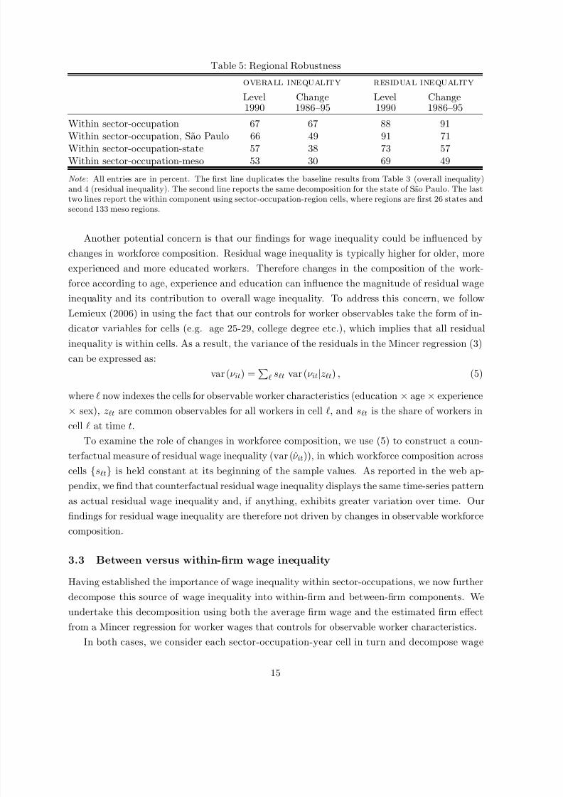
7242019 Brazil Trade
httpslidepdfcomreaderfullbrazil-trade 3649
minus 3 9 8
minus 3 9 8
minus 3 9 8
minus 3 9 8
minus 3 9 8
minus 3 9 8
minus 3
9 7
minus 3 9 7
minus 3 9 7
minus 3 9 7
minus 3 9 7
minus 3 9 7
minus 3 9 6
minus 3 9 6
minus 3 9 6
minus 3 9 6
minus 3 9 6
minus 3 9 6
minus 3 9 6
minus 3 9 6
minus 3 9
minus 3 9 5
minus 3 9 5
minus 3 9 5
minus 3 9 5
minus 3 9 5
minus 3 9 5
minus 3 9 5
minus 3 9 4
minus 3 9 4
microw
ρ v
minus05 minus025 0 025 05 075 1minus075
minus05
minus025
0
025
05
075
microw = ζ microhminus3944
microw ge 0
minus3938
Global Max
minus3935
Orthog shocks
minus3945
Local Max
minus3939
Figure 4 Contour plot of the log likelihood 1990
Note Log likelihood normalized by 10000 as a function of (microw ρv) with the remaining eight parameters opti-mized given (microw ρv) The values of the log likelihood 500 log points below the peak are censored (blue area inthe figure) The downward sloping yellow curve (dashed and solid) depicts the high likelihood ridge for a givenvalue of microw the curve displays the value of ρv that maximizes the log likelihood function The solid segment of
the curve represents the economically meaningful range of parameters in the first quadrant (while only microw gt 0 isrequired by the theory ρv gt 0 is also favored in view of previous empirical evidence on the importance of selectioninto exporting) The five yellow squares indicate the location of the estimates under the specifications (i)-(iv)considered in Table 8 and the text as well as a local maximum the reported numbers correspond to the value of the log likelihood function normalized by 10000
our large number of observations the global maximum is statistically distinguishable from other
points along the ridge Nevertheless as shown in Table 8 the economic fit of the model is good
at any point on the ridge and close to the fit at the global maximum In particular the model
can successfully account for the reduced-form exporter wage premium observed in the data with
a strong selection effect (ρv ≫ 0 and microw asymp 0) a strong market access effect (microw ≫ 0 and ρv asymp 0)
or both positive selection and positive market access effect (microw ρv gt 0)40
When we only impose constraint (19) corresponding to positive market access effects (spec-
40The reason why the data favors either a large negative ρv or a large positive ρv which by consequenceresults either in large positive microw or moderately negative microw has to do with the fact that our theoretical modelis parsimonious and sparsely parameterized As becomes clear from Tables 9ndash10 and Figure 6 the conditionalvariance of wages for exporters is lower than for non-exporters and the only way the model can accommodatethis difference is by blowing up the (absolute value of) selection correlation of high-wage firms into exportingLower absolute values of ρv result in a poorer fit of this moment but in fact better fit of most other moments
34
7242019 Brazil Trade
httpslidepdfcomreaderfullbrazil-trade 3749
ification (ii)) we estimate microw close to zero Alternatively when we impose (20) emanating
from the assumption of orthogonal structural shocks (specification (iv)) we estimate ρv close
to zero41 Finally when we impose (21) implying no effects of screening shocks on employment
(specification (iii)) we estimate both microw gt 0 and ρv gt 0 The points corresponding to these
three alternative structural restrictions are shown in Figure 4 along with the unconstrained
global and local maxima Each of these five points lies along the ridge of high likelihood in theparameter space (microw ρv) and provides almost as good a fit to the data as the unconstrained
model as reported in Table 8 and further shown below
Any departures from this one-dimensional line of values of (microw ρv) in the 10-dimensional
parameter space lead to a steep decline in the likelihood function In other words the data
strongly identifies a compact segment in the parameter space but beyond this does not sharply
discriminate between different points along this segment The reason is that the market access
(microw) and selection (ρv) components of the exporter wage premium are only separately identified
in our model through the functional form assumptions and specifically the discontinuous effect
of foreign market access on wages in contrast to the smooth selection effect While the discrete
increase in employment (microh) as firms enter export markets and expand to meet export demand is
large the discrete increase in wages (microw) as firms enter export markets is substantially smaller
which makes it harder to separately identify the market access and selection effects for wages
Hence in what follows we use economic reasoning to select a point along the segment shown in
Figure 4
Our theoretical model imposes the restriction that microw microh gt 0 Additionally a number of
empirical studies find that future exporters are larger and pay higher wages than other non-
exporters even before they enter export markets (see for example Bernard and Jensen 1997
1999) which suggests selection into export markets (ρu ρh gt 0) Therefore we adopt the
structural restriction (21) microw = ζ microh or specification (iii) as our preferred specification whichgenerates both positive market access effects (microw microh gt 0) and positive selection effects (ρu ρv gt
0) Under this restriction the reduced-form model has an attractive structural interpretation in
which wages and employment depend on two orthogonal structural shocksmdashone to productivity
(θ) that enters both the employment and wage equations and another to screening (η) that
enters only the wage equation where both can be correlated with the shock in the export
selection equation (z) Finally this constrained specification also generates a similar level of fit
as the unconstrained specification as shown in Tables 8 9 and 10 below
Before analyzing further the fit of the model Figure 5 presents the ML parameter estimates
for our preferred specification (iii) for each year during our sample period 1986ndash98 We esti-mate the model using the cross-section data on firms for each year separately without imposing
restrictions on the evolution of the parameters over time The figure also shows the 98 percent
confidence intervals (two standard-deviation bands) using a robust (sandwich) covariance ma-
trix which are tight around the estimated parameter values given our large sample size The
41This is a robust outcome of constraint (20) The reason is somewhat mechanical arising from the fact thatthe data favors estimates that satisfy 0 lt ρu lt ρv and σu gt σv which is inconsistent with (20) unless ρu ρv asymp 0
35
7242019 Brazil Trade
httpslidepdfcomreaderfullbrazil-trade 3849
86 88 90 92 94 96 98006
008
01
012
ζ
86 88 90 92 94 96 9813
14
15
16
f
86 88 90 92 94 96 981
11
12
σu
86 88 90 92 94 96 98035
04
045
σv
86 88 90 92 94 96 980
002
004
ρu
86 88 90 92 94 96 98005
01
015
02
025
ρv
86 88 90 92 94 96 9818
2
22
24
26
microh
86 88 90 92 94 96 9801
02
microw
86 88 90 92 94 96 9826
27
28
29
αh and αw
minus04
minus035
minus03
minus025
Figure 5 Maximum Likelihood Parameter Estimates Across Years
Note ML estimates from the structural specification (iii) under constraint (20) based on separate cross sectionsof firm employment firm wages and export status for each year and two standard-error bands based on MLasymptotic sandwich covariance matrix
estimated parameters evolve smoothly over time consistent with the idea that our model cap-
tures systematic cross-section dispersion in wages and employment The parameter estimatesfeature substantial employment and wage export premia (microh and microw) as well as positive selec-
tion correlations (ρu and ρv) In other words our constrained specification suggests that both
selection and market access effects are present in the data42 The estimated dispersion of u
(σu) falls over time which is driven by the decline in the dispersion of firm employment ob-
served in the data The estimated dispersion of v (σv) follows an inverted U-shape pattern over
time which reflects the inverted U-shape pattern in the dispersion of firm wages observed in the
data Finally the estimated export threshold parameter f follows a U-shape which captures
the inverted U-shape in the observed share of exporters over time
Fit of the model In Tables 9 and 10 we provide further evidence on the modelrsquos fit in the
cross-section for 1990 We find a similar pattern for other years and report results for 1994 in the
web appendix In each table the first column reports cross-section moments in the data while
42Note however that the estimated selection correlations are small with ρu fluctuating around 002 and ρvranging between 01 and 02 The overall strength of the selection effect can be measured by
radic ρ2u + ρ2v and it
fluctuates around 017 over the years
36
7242019 Brazil Trade
httpslidepdfcomreaderfullbrazil-trade 3949
Table 9 Model Fit for Firm-level Moments 1990
Data ModelUnconstrained StructuralA Full Sample
Mean Employment 297 297 297
Mean Wages minus0340 minus0341 minus0341
St Dev Employment 127 127 127St Dev Wages 0424 0424 0423
Covar Emplmnt and Wages 0352 0354 0352
Fraction of Exporters 55 55 55
B Non-exporters
Mean Employment 283 283 283
Mean Wages minus0359 minus0360 minus0360
St Dev Employment 112 114 114
St Dev Wages 0419 0419 0416
Covar Emplmnt and Wages 0306 0309 0304
C ExportersMean Employment 528 529 529
Mean Wages minus0010 minus0010 minus0006
St Dev Employment 152 114 114
St Dev Wages 0366 0373 0417
Covar Emplmnt and Wages 0322 0289 0304
Note Moments of the log wage and log employment distributions across firms in 1990 The log wage measure inthe data is the firm-occupation-year fixed effect estimated from (6) aggregated to the firm-year level using occu-pation employment weights Model moments are calculated in the same way in an artificial cross-section of firmsgenerated from ML estimated model (18) under the unconstrained specification (i) and structural specifications(iii) respectively
the next two columns report model-predicted moments from the unconstrained specification and
our preferred structural specification (iii) respectively To calculate the moments in the model
we simulate the data based on (18) given the estimated parameter vector Θ
Table 9 presents firm-level moments first and second moments for employment and wagesmdash
for the full sample and conditional on exporting and non-exportingmdashas well as the fraction of
exporting firms These are the moments used in calculating the GMM ob jective in Table 843
Additionally Table 10 presents the worker-level moments of the wage distribution Since we
focus on the firm component of wages abstracting from wage variation within firms the distri-
bution of wages across workers in our analysis is the firm-employment-weighted distribution of wages across firms That is wage observations for a large firm in terms of employment receive
a proportionately larger weight in the worker-wage distribution Panel A of Table 10 reports
the mean and variance of worker wages for the full sample as well as for workers employed by
43Note that the full sample moments for employment and wages in Table 9 are linear combinations of the 10moments for exporters and non-exporters and the fraction of exporters and hence we exclude them in calculatingthe GMM objective
37
7242019 Brazil Trade
httpslidepdfcomreaderfullbrazil-trade 4049
Table 10 Model Fit for Worker-level Moments 1990
Data ModelUnconstrained StructuralA First and Second Moments
Mean Log Wage 0000 minus0085 minus0072
Non-exporters minus0122 minus0213 minus0215
Exporters 0152 0109 0140St Dev Log Wages 0404 0429 0450
Non-exporters 0407 0415 0416
Exporters 0345 0374 0414
Emplmnt Share of Exporters 446 400 403
B Wage Inequality Measures
Gini 0215 0236 0250
9010 277 300 318
9050 154 170 179
5010 180 176 178
C Size and Exporter Wage Premia
Size premium 0111 0112 0111
Exporter premium 0077 0075 0082
Note Moments are calculated across workers in 1990 the wage measures are the firm-occupation-year fixed effectsestimated from (6) aggregated to the firm-year level using occupation employment weights and weighted by thenumber of workers employed by the firm The firm-occupation-year fixed effects are normalized so that in everyyear their mean is zero across workers within each sector-occupation cell for this reason the mean worker wageequals zero Simulated moments for log wages and log employment generated using ML estimates for 1990 fromthe unconstrained specification (i) and structural specification (iii) 9010 denotes the 90-10 wage percentile ratio(the ratio of the exponents of the log wage percentiles) and similarly for 9050 and 5010 Size and exporterpremia are coefficient estimates from an OLS regression of log firm wages on log firm employment and a dummy for
export status without including sector fixed effects which explains the small difference in the exporter premiumfrom the results reported in Section 34
exporters and non-exporters this panel also reports the share of workers employed by exporters
Panel B then reports additional measures of wage inequality namely the Gini coefficient and
the 9010 9050 and 5010 percentile ratios Finally Panel C reports the coefficients from the
size-exporter wage premium regression parallel to (8) in Section 34
Judging by the moments in Tables 9 and 10 the model provides a close fit to the data Both
firm and worker moments generated by the structural model closely match the moments in the
data and this match is not noticeably worse than the moments generated by the unconstrained
model As discussed in footnote 40 the one moment that the unconstrained model fits better is
the standard deviation of wages across exporting firms and across workers employed in exporting
firms The structural model provides a tight fit to all moments across the full sample of firms
and across non-exporters it does slightly worse on the dispersion of employment and wages
across exporters The fit of the model is good but less than perfect for the worker-level moments
in Table 10 Of particular interest is the fact that the model fits not only the first and second
38
7242019 Brazil Trade
httpslidepdfcomreaderfullbrazil-trade 4149
moments of firm employment and wage distributions but also nonlinear transformations of the
worker wage distribution such as the 9010 9050 and 5010 wage percentile ratios and the
Gini coefficient In fact the model generates a Lorenz curve that closely fits the Lorenz curve
in the data Finally the structural model matches the size and exporter wage premia estimated
in the data We conclude that our parsimonious theoretical model provides a very reasonable
fit to a rich set of empirical moments of employment and wage distributions across firms andworkers Furthermore the constrained structural specification is almost indistinguishable in
terms of economic fit from the unconstrained model that has a superior statistical fit
Figures 6ndash7 provide further evidence of the quality of the cross-sectional fit of the structural
model They display kernel density estimates of the distributions of employment and wages
across firms and the distribution of wages across workers in our data and in artificial data
generated from the estimated structural model We provide the comparison for 1990 and report
the results for 1994 in the web appendix results for other years are again similar
Figure 6 displays kernel densities for the firm distributions while Figure 7 displays kernel
densities for the worker distributions which again weight firm wages by firm employment The
left two panels of Figure 6 report results for firm employment while the right two panels report
results for firm wages The upper panels report results for all firms while the lower panels
report separate estimates for exporters and non-exporters Our log-normal assumption for the
distribution of shocks allows us to nearly perfectly fit the distribution of wages across the full
sample of firms The fit of the distribution of employment across the full sample of firms is
good but imperfect because the distribution in the data is skewed and has a fatter tail than the
distribution in the model
A striking feature of the data is the substantial overlap between the employment and wage
distributions of exporters and non-exporters although the distributions of both employment
and wages are shifted to the right for exporters relative to non-exporters Our theoretical modelwith firm heterogeneity in export costs can accommodate the overlap in the empirical wage
and employment distributions (lower panel of Figure 6) However as discussed in footnote 40
the model is sparsely parameterized and cannot fit the different dispersion of employment and
wages for exporters versus non-exporters In the data employment is more dispersed among
the exporters while wages are more dispersed among non-exporters Given our theoretical
assumption that σu and σv are common for both exporters and non-exporters the structural
model cannot fully capture these two features of the data
In Figure 7 the model fits well the distribution of wages across all workers as well as across
workers employed by exporting firms and non-exporting firms However the model slightlyoverstates the variance of wages among exporters Overall Figures 6ndash7 confirm our earlier
results for selected moments of the worker and firm distributions and further illustrate that the
model provides a good fit to the empirical cross-sectional distributions
Taken together the results in Tables 9ndash10 and Figures 6ndash7 support our structural model
Despite the modelrsquos sparsity and its strong functional form assumptions we find that it approx-
imates the data well The model captures both the higher average employment and wages of
39
7242019 Brazil Trade
httpslidepdfcomreaderfullbrazil-trade 4249
minus2 0 2 4 6 8 100
025
05
Log Employment
minus2 minus1 0 1
0
05
1
Log Firm Wages
minus2 0 2 4 6 8 100
025
05
Exporters vs Non-Exporters
minus2 minus1 0 1
0
05
1
Exporters vs Non-Exporters
Data (non-exp) Data (exporters) M odel (non-exp) M odel (exporters)
DataModel
Figure 6 Model Fit for the Distribution of Log Firm Employment and Log Firm Wages 1990
Note Kernel densities of the employment and wage distributions across firms (using normal kernels with optimalbandwidth) Simulated data generated from the estimated model under structural specification (iii)
minus2 minus1 0 1 20
05
1
Log Worker Wages
minus2 minus1 0 1 20
05
1
Exporters vs Non-Exporters
Data
Model
Figure 7 Model Fit for the Distribution of Log Worker Wages 1990
Note Kernel densities of the wage distribution across workers in which firm wages are weighted by firm employ-ment (using normal kernels with optimal bandwidth) Simulated data generated from the estimated model understructural specification (iii)
40
7242019 Brazil Trade
httpslidepdfcomreaderfullbrazil-trade 4349
86 88 90 92 94 96 980
001
002
003
004
005
006
007
V a r i a n c e l o g w o r k e r w a g e s
Data
Structural Model
Figure 8 Model Fit of Log Wage Inequality over Time
Note Change in the variance of log worker wages relative to 1986 where the worker wage distribution weightsfirm wages by firm employment The data curve corresponds to the between-firm component in Figure 3 Themodel curve is based on simulated data generated separately for each year using the respective ML estimates of the parameters under the structural specification (iii) as reported in Figure 5
exporters relative to non-exporters and the substantial overlap in the distributions of employ-
ment and wages between these two groups of firms
Figure 8 reports one final measure of fit by displaying the true and predicted evolution of log
wage inequality over time Specifically we simulate the model in every year between 1986 and
1998 using the parameters estimated year-by-year from our preferred structural specification (iii)
as reported in Figure 5 Figure 8 then reports the change over time in the variance of log worker
wages relative to 1986 both in the data and in the model-simulated cross sections Althoughthe model slightly overstates the variance of log worker wages (Table 10) this discrepancy is
relatively stable over time and as a result the model tracks closely the evolution of wage
inequality In particular the model captures the hump shape in log wage inequality over our
sample period 1986-1998
Counterfactual exercise In closing this section we discuss the results from a model-based
counterfactual exercise that illustrates the effects of trade on wage inequality in the estimated
structural model Specifically we consider the effect of a reduction in variable trade costs τ
on export participation and the cross-sectional distributions of employment and wages with a
focus on the variance of log worker wages
Recall from Section 41 that the market access variable is related to variable trade costs
according to
Υx = 1 + τ minusβ1minusβ
1048616AxAd
1048617 11minusβ
41
7242019 Brazil Trade
httpslidepdfcomreaderfullbrazil-trade 4449
and the exporter employment and wage premia are given respectively by
microh = 1
1 + χ log Υ
1minusβΓx and microw =
χ
1 + χ log Υ
1minusβΓx
Another parameter affected by variable trade costs is the reduced-form threshold for export
participation
f = 1σ
983080minusαπ + log F x minus log
852059Υ(1minusβ)Γx minus 1
852061983081
The remaining seven estimation parameters are not directly affected by variable trade costs and
hence we hold them constant in our counterfactual exercise Specifically we take the estimated
parameters Θ under our preferred structural specification (iii) for 1990 and then vary (microh microw f )
in a way consistent with variation in Υx as summarized in the equations above44 We change
Υx from the value of 1 corresponding to autarky to a very large value for which nearly all
workers are employed by exporting firms Then for every given counterfactual parameter vector
ΘC corresponding to a particular value of Υx we simulate the model and calculate various
moments of the firm and worker distributionsFigure 9 displays the resulting variance of log worker wages as a function of the market
access measure microh + microw = log Υ(1minusβ)Γx Wage inequality displays a hump-shape in response to
a reduction in variable trade costs consistent with the theoretical prediction in HIR Therefore
once the economy is open to trade further trade liberalization can either raise or reduce wage
inequality depending on the initial level of trade openness As variable trade costs decline
from autarky employment reallocates from non-exporters to exporters along both the extensive
margin of export market entry and the intensive margin of an expansion of employment at
exporters and the fraction of workers employed by exporters changes from zero to one This
in turn first increases and later decreases wage inequality with the peak attained when the
majority of workers are employed at exporting firms
In Figure 9 the dashed lines represents the estimated market access measure (microh + microw =
logΥ(1minusβ)Γx ) in 1986 and 1990 while the red square represents the within-sample point in 1990
which is the benchmark for our counterfactual exercise The change in variable trade costs which
would move the market access measure from its 1986 to its 1990 levels leads to an increase in
inequality that corresponds to a quarter of the inequality increase in Brazil between these years
Furthermore the change in inequality shown in Figure 9 as the economy goes from autarky to
the peak of trade-induced inequality is quite substantial corresponding to three quarters of the
increase in inequality in Brazil between 1986 and 1995
In the web appendix we report a number of robustness checks to show how sensitive the44The only complication arises due to the fact that σ in the expression for f is not identified as discussed in the
web appendix Under the assumption that (u v) are orthogonal to ε we have σ2 =983131
(1 + ζ )2σ2u + σ2
v
9831331048616
ρ2u + ρ2v1048617
which we use in our benchmark calculation displayed in Figure 9 This overstates the true value of σ if (u v)are positively correlated with ε which in turn would understate the effect of Υx on f As a sensitivity check inthe web appendix we consider a smaller value of σ and find very similar results to those displayed in Figure 9This is because in our estimated model variation in f and the fraction of exporting firms is quantitatively not thedominant channel through which variable trade costs affect inequality
42
7242019 Brazil Trade
httpslidepdfcomreaderfullbrazil-trade 4549
0 1 2 3 4 5 6 7 8017
018
019
02
021
022
logΥ(1minusβ)Γx
V a r i a n c e l o g w o r k e r w a g e s
1986
Estimate
1990
Figure 9 Counterfactual Reduction in Variable Trade Costs and Log Wage InequalityNote Counterfactual variation in the variance of log worker wages in response to a reduction in variable tradecosts τ from its autarky level to the limit of trade openness when almost all workers are employed by exportingfirms The distribution of wages across workers weights firm wages by firm employment The variance of log workerwages is plotted against the market access measure microh + microw = log Υ(1minusβ)Γ
x where Υx increases as τ decreasesDashed lines correspond to the estimated values of microh + microw in 1986 and 1990 under structural specification (iii)The red square indicates the prediction of the model given the baseline 1990 estimated parameter vector
quantitative predictions of the model are to variations in its parameters While the quantitative
results are robust to many variations in the parameters they are sensitive to the relative strength
of the market access and selection effects the response of inequality is largest when microw is large
and smallest when microw is close to zero although the qualitative inverted U-shape is preserved as
long as microw gt 0
To summarize this counterfactual exercise illustrates that in our estimated structural model
variation in variable trade costs can have sizeable effects on wage inequality This is true both
for large changes from autarky to intermediate degrees of openness as well as for local changes
in variable trade costs around the estimated value in our sample
It is important to note that this counterfactual exercise is likely to provide a lower bound on
the potential size of trade effects on inequality This is because in the model we have allowed
for only one extensive marginmdasha given firm either exports or does not In contrast in the data
firms can choose to export to a number of destinations and access to each additional destinationresults in incremental employment and wage premia A reduction in variable trade costs is likely
to trigger effects along multiple extensive margins and raise market access premia for a variety
of destinations which would amplify the inequality effects of greater trade openness We leave
to future research the generalization of the present model to multiple exporting destinations and
the quantification of the resulting trade effects on wage inequality
43
7242019 Brazil Trade
httpslidepdfcomreaderfullbrazil-trade 4649
5 Conclusion
Recent theories of firm heterogeneity and trade emphasize variation in wages with firm produc-
tivity and trade participation as sources of wage inequality Guided by these theories we use
linked employer-employee data for Brazil to examine the empirical relevance of these sources of
wage inequality
In contrast to neoclassical trade theory which stresses wage inequality between sectors and
occupations we find that around two thirds of overall wage inequality occurs within sector-
occupations Residual wage inequality is as important as worker observables in explaining overall
wage inequality and occurs predominantly within sector-occupations Consistent with recent
theories of firm heterogeneity and trade between-firm differences in wages account for much
of the observed wage inequality within sector-occupations and are particularly influential for
residual wage inequality These between-firm differences in wages are strongly but imperfectly
related to firm employment and trade participation
Motivated by these findings we estimate a structural econometric model of firm export sta-
tus employment and wages which is derived from an augmented version of Helpman Itskhokiand Redding (2010) This augmented model incorporates three sources of firm heterogeneity in
productivity fixed exporting costs and worker screening each of which is central to matching
the data We show that the estimated model is empirically successful in accounting for the ob-
served distributions of wages and employment for parameter values consistent with theoretical
restrictions We find that firm trade participationmdashthrough a combination of market access and
firm selection effectsmdashis important for the modelrsquos explanatory power We show that counter-
factual changes in variable trade costs can have sizeable effects on wage inequality through this
mechanism of wage dispersion between firms
Trade expands the set of opportunities available to firms and workers which is the sourceof welfare gains from trade But only some firms find it profitable to take advantage of these
opportunities which is the mechanism behind tradersquos effect on wage inequality that we empha-
size When only a few firms export further trade liberalization increases wage inequality but
once the fraction of firms exporting becomes sufficiently large wage inequality reaches a peak
and starts to fall back
44
7242019 Brazil Trade
httpslidepdfcomreaderfullbrazil-trade 4749
References
Amemiya T (1985) Advanced Econometrics Harvard University Press Cambridge Mass
Amiti M and D R Davis (2011) ldquoTrade Firms and Wages Theory and Evidencerdquo Review of
Economic Studies forthcoming
Attanasio O P K Goldberg and N Pavcnik (2004) ldquoTrade Reforms and Wage Inequality in
Colombiardquo Journal of Development Economics 74(2) 331ndash366Autor D H L F Katz and M S Kearney (2008) ldquoTrends in US Wage Inequality Revising
the Revisionistsrdquo Review of Economics and Statistics 90(2) 300ndash323
Barth E A Bryson J C Davis and R Freeman (2011) ldquoThe Contribution of Dispersion
across Plants to the Increase in US Earnings Dispersionrdquo unpublished manuscript presented at the
EEA-ESEM meetings 2011
Baumgarten D (2011) ldquoExporters and the Rise in Wage Inequality Evidence from German Linked
Employer-Employee Datardquo RWI unpublished manuscript
Berman E J Bound and Z Griliches (1994) ldquoChanges in the Demand for Skilled Labor within
US Manufacturing Evidence from the Annual Survey of Manufacturesrdquo Quarterly Journal of Eco-
nomics 109(2) 367ndash97Bernard A B and J B Jensen (1995) ldquoExporters Jobs and Wages in US Manufacturing
1976-1987rdquo Brookings Papers on Economic Activity Microeconomics 1995(1) 67ndash112
(1997) ldquoExporters Skill Upgrading and the Wage Gaprdquo Journal of International Economics
42(1-2) 3ndash31
(1999) ldquoExceptional Exporter Performance Cause Effect or Bothrdquo Journal of International
Economics 47(1) 1ndash25
Burstein A and J Vogel (2003) ldquoGlobalization Technology and the Skill Premium A Quanti-
tative Analysisrdquo NBER Working Paper 16459
Bustos P (2011) ldquoTrade Liberalization Exports and Technology Upgrading Evidence on the Impact
of Mercosur on Argentinian Firmsrdquo American Economic Review 101(1) 30440Chaney T (2008) ldquoDistorted Gravity The Intensive and Extensive Margins of International Traderdquo
American Economic Review 98(4) 1707ndash21
Cosar A K N Guner and J Tybout (2011) ldquoFirm Dynamics Job Turnover and Wage Distri-
butions in an Open Economyrdquo IMDEA Working Paper 201106
Davidson C F Heyman S Matusz F Sjoholm and S C Zhu (2011) ldquoGlobalization and
Imperfect Labor Market Sortingrdquo Research Institute of Industrial Economics Working Paper 856
Stockholm
Davidson C and S J Matusz (2010) International Trade with Equilibrium Unemployment Prince-
ton University Press Princeton NJ
Davidson C S J Matusz and A Shevchenko (2008) ldquoGlobalization and Firm Level Adjustmentwith Imperfect Labor Marketsrdquo Journal of International Economics 75(2) 295ndash309
Davis D R and J Harrigan (2011) ldquoGood Jobs Bad Jobs and Trade Liberalizationrdquo Journal of
International Economics 84(1) 26ndash36
Davis S J and J C Haltiwanger (1991) ldquoWage Dispersion Between and Within US Manufac-
turing Plants 1963-86rdquo Brookings Papers on Economic Activity Microeconomics 1991(1) 115ndash80
Eaton J S Kortum and F Kramarz (2010) ldquoAn Anatomy of International Trade Evidence
45
7242019 Brazil Trade
httpslidepdfcomreaderfullbrazil-trade 4849
from French Firmsrdquo University of Chicago unpublished manuscript
Egger H P Egger and U Kreickemeier (2011) ldquoTrade Wages and Profitsrdquo University of
Tubingen unpublished manuscript
Egger H and U Kreickemeier (2009) ldquoFirm Heterogeneity and the Labor Market Effects of Trade
Liberalizationrdquo International Economic Review 50(1) 187ndash216
Faggio G K G Salvanes and J Van Reenen (2010) ldquoThe Evolution of Inequality in Produc-
tivity and Wages Panel Data Evidencerdquo Industrial and Corporate Change 19(6) 1919ndash1951
Fally T R Paillacar and C Terra (2010) ldquoEconomic Geography and Wages in Brazil Evidence
from Micro-Datardquo Journal of Development Economics 91(1) 155ndash168
Feenstra R C and G H Hanson (1996) ldquoForeign Investment Outsourcing and Relative Wagesrdquo
in The Political Economy of Trade Policy Papers in Honor of Jagdish Baghwati ed by R C Feenstra
G M Grossman and D A Irwin chap 6 pp 89ndash128 MIT Press Cambridge Mass
(1999) ldquoThe Impact of Outsourcing and High-Technology Capital on Wages Estimates for the
United States 1979-1990rdquo Quarterly Journal of Economics 114(3) 907ndash40
Felbermayr G J Prat and H-J Schmerer (2011) ldquoGlobalization and Labor Market Outcomes
Wage Bargaining Search Frictions and Firm Heterogeneityrdquo Journal of Economic Theory 146(1) 39ndash
73
Ferreira F H G P G Leite and M Wai-Poi (2010) ldquoTrade Liberalization Employment Flows
and Wage Inequality in Brazilrdquo in The Poor under Globalization in Asia Latin America and Africa
ed by M Nissanke and E Thorbecke UNU-Wider Studies in Development Economics chap 8 pp
199ndash254 Oxford University Press Oxford
Frıas J A D S Kaplan and E A Verhoogen (2009) ldquoExports and Wage Premia Evidence
from Mexican Employer-Employee Datardquo Columbia University unpublished manuscript
Goldberg P K and N Pavcnik (2003) ldquoThe Response of the Informal Sector to Trade Liberal-
izationrdquo Journal of Development Economics 72(2) 463ndash96
(2005) ldquoTrade Wages and the Political Economy of Trade Protection Evidence from the
Colombian Trade Reformsrdquo Journal of International Economics 66(1) 75ndash105
(2007) ldquoDistributional Effects of Globalization in Developing Countriesrdquo Journal of Economic
Literature 45(1) 39ndash82
Gonzaga G N A Menezes-Filho and M C Terra (2006) ldquoTrade Liberalization and the
Evolution of Skill Earnings Differentials in Brazilrdquo Journal of International Economics 68(2) 345ndash67
Helpman E and O Itskhoki (2010) ldquoLabour Market Rigidities Trade and Unemploymentrdquo Review
of Economic Studies 77(3) 11001137
Helpman E O Itskhoki and S Redding (2010) ldquoInequality and Unemployment in a Global
Economyrdquo Econometrica 78(4) 1239ndash1283
Irarrazabal A A Moxnes and L D Opromolla (2011) ldquoThe Margins of Multinational Pro-
duction and the Role of Intra-firm Traderdquo Dartmouth College unpublished manuscript
Juhn C K M Murphy and B Pierce (1993) ldquoWage Inequality and the Rise in Returns to Skillrdquo
Journal of Political Economy 101(3) 410ndash442
Katz L F and K M Murphy (1992) ldquoChanges in Relative Wages 1963-1987 Supply and Demand
Factorsrdquo Quarterly Journal of Economics 107(1) 35ndash78
Kovak B K (2011) ldquoLocal Labor Market Effects of Trade Policy Evidence from Brazilian Liberal-
46
7242019 Brazil Trade
httpslidepdfcomreaderfullbrazil-trade 4949
izationrdquo Carnegie Mellon University unpublished manuscript
Krishna P J P Poole and M Z Senses (2011) ldquoTrade Liberalization Firm Heterogneity
and Wages New Evidence from Matched Employer-Employee Datardquo World Bank Policy Research
Working Paper 5711
Kume H G Piani and C F B d Souza (2003) ldquoA Polıtica Brasileira de Importacao no Perıodo
1987-98 Descricao e Avaliacaordquo in A abertura comercial brasileira nos anos 1990 Impactos sobre
emprego e salacute arios ed by C H Corseuil and H Kume chap 1 pp 9ndash37 MTE and IPEA Rio de
Janeiro
Lazear E P and K L Shaw (2009) ldquoWage Structure Raises and Mobility An Introduction to
International Comparisons of the Structure of Wages Within and Across Firmsrdquo in The Structure of
Wages An International Comparison ed by E P Lazear and K L Shaw chap 1 University of
Chicago Press Chicago
Lemieux T (2006) ldquoIncreasing Residual Wage Inequality Composition Effects Noisy Data or Rising
Demand for Skillrdquo American Economic Review 96(3) 461ndash498
Maddala G S (1983) Limited-dependent and qualitative variables in econometrics vol 3 of Econo-
metric Society Monographs Cambridge University Press Cambridge UK
Melitz M J (2003) ldquoThe Impact of Trade on Intra-Industry Reallocations and Aggregate Industry
Productivityrdquo Econometrica 71(6) 1695ndash1725
Menezes-Filho N A M-A Muendler and G Ramey (2008) ldquoThe Structure of Worker Com-
pensation in Brazil with a Comparison to France and the United Statesrdquo Review of Economics and
Statistics 90(2) 324ndash346
Monte F (2011) ldquoSkill Bias Trade and Wage Dispersionrdquo Journal of International Economics 83(2)
202ndash218
Mortensen D T (2003) Wage dispersion Why are similar workers paid differently Zeuthen lecture
book series MIT Press Cambridge Mass
Munch J R and J R Skaksen (2008) ldquoHuman Capital and Wages in Exporting Firmsrdquo Journal
of International Economics 75(2) 363ndash372
Oi W Y and T L Idson (1999) ldquoFirm Size and Wagesrdquo in Handbook of labor economics ed by
O Ashenfelter and D Card vol 3B pp 2165ndash2214 Elsevier Science North-Holland Amsterdam
New York and Oxford
Rosen S (1982) ldquoAuthority Control and the Distribution of Earningsrdquo Bell Journal of Economics
13(2) 311ndash323
Schank T C Schnabel and J Wagner (2007) ldquoDo Exporters Really Pay Higher Wages First
Evidence from German Linked Employer-Employee Datardquo Journal of International Economics 72(1)
52ndash74
Stole L A and J Zwiebel (1996) ldquoIntra-firm Bargaining under Non-binding Contractsrdquo Review
of Economic Studies 63(3) 375ndash410
Trefler D and S C Zhu (2005) ldquoTrade and Inequality in Developing Countries A General
Equilibrium Analysisrdquo Journal of International Economics 65(1) 21ndash48
Verhoogen E A (2008) ldquoTrade Quality Upgrading and Wage Inequality in the Mexican Manufac-
turing Sector rdquo Quarterly Journal of Economics 123(2) 489 530
7242019 Brazil Trade
httpslidepdfcomreaderfullbrazil-trade 3749
ification (ii)) we estimate microw close to zero Alternatively when we impose (20) emanating
from the assumption of orthogonal structural shocks (specification (iv)) we estimate ρv close
to zero41 Finally when we impose (21) implying no effects of screening shocks on employment
(specification (iii)) we estimate both microw gt 0 and ρv gt 0 The points corresponding to these
three alternative structural restrictions are shown in Figure 4 along with the unconstrained
global and local maxima Each of these five points lies along the ridge of high likelihood in theparameter space (microw ρv) and provides almost as good a fit to the data as the unconstrained
model as reported in Table 8 and further shown below
Any departures from this one-dimensional line of values of (microw ρv) in the 10-dimensional
parameter space lead to a steep decline in the likelihood function In other words the data
strongly identifies a compact segment in the parameter space but beyond this does not sharply
discriminate between different points along this segment The reason is that the market access
(microw) and selection (ρv) components of the exporter wage premium are only separately identified
in our model through the functional form assumptions and specifically the discontinuous effect
of foreign market access on wages in contrast to the smooth selection effect While the discrete
increase in employment (microh) as firms enter export markets and expand to meet export demand is
large the discrete increase in wages (microw) as firms enter export markets is substantially smaller
which makes it harder to separately identify the market access and selection effects for wages
Hence in what follows we use economic reasoning to select a point along the segment shown in
Figure 4
Our theoretical model imposes the restriction that microw microh gt 0 Additionally a number of
empirical studies find that future exporters are larger and pay higher wages than other non-
exporters even before they enter export markets (see for example Bernard and Jensen 1997
1999) which suggests selection into export markets (ρu ρh gt 0) Therefore we adopt the
structural restriction (21) microw = ζ microh or specification (iii) as our preferred specification whichgenerates both positive market access effects (microw microh gt 0) and positive selection effects (ρu ρv gt
0) Under this restriction the reduced-form model has an attractive structural interpretation in
which wages and employment depend on two orthogonal structural shocksmdashone to productivity
(θ) that enters both the employment and wage equations and another to screening (η) that
enters only the wage equation where both can be correlated with the shock in the export
selection equation (z) Finally this constrained specification also generates a similar level of fit
as the unconstrained specification as shown in Tables 8 9 and 10 below
Before analyzing further the fit of the model Figure 5 presents the ML parameter estimates
for our preferred specification (iii) for each year during our sample period 1986ndash98 We esti-mate the model using the cross-section data on firms for each year separately without imposing
restrictions on the evolution of the parameters over time The figure also shows the 98 percent
confidence intervals (two standard-deviation bands) using a robust (sandwich) covariance ma-
trix which are tight around the estimated parameter values given our large sample size The
41This is a robust outcome of constraint (20) The reason is somewhat mechanical arising from the fact thatthe data favors estimates that satisfy 0 lt ρu lt ρv and σu gt σv which is inconsistent with (20) unless ρu ρv asymp 0
35
7242019 Brazil Trade
httpslidepdfcomreaderfullbrazil-trade 3849
86 88 90 92 94 96 98006
008
01
012
ζ
86 88 90 92 94 96 9813
14
15
16
f
86 88 90 92 94 96 981
11
12
σu
86 88 90 92 94 96 98035
04
045
σv
86 88 90 92 94 96 980
002
004
ρu
86 88 90 92 94 96 98005
01
015
02
025
ρv
86 88 90 92 94 96 9818
2
22
24
26
microh
86 88 90 92 94 96 9801
02
microw
86 88 90 92 94 96 9826
27
28
29
αh and αw
minus04
minus035
minus03
minus025
Figure 5 Maximum Likelihood Parameter Estimates Across Years
Note ML estimates from the structural specification (iii) under constraint (20) based on separate cross sectionsof firm employment firm wages and export status for each year and two standard-error bands based on MLasymptotic sandwich covariance matrix
estimated parameters evolve smoothly over time consistent with the idea that our model cap-
tures systematic cross-section dispersion in wages and employment The parameter estimatesfeature substantial employment and wage export premia (microh and microw) as well as positive selec-
tion correlations (ρu and ρv) In other words our constrained specification suggests that both
selection and market access effects are present in the data42 The estimated dispersion of u
(σu) falls over time which is driven by the decline in the dispersion of firm employment ob-
served in the data The estimated dispersion of v (σv) follows an inverted U-shape pattern over
time which reflects the inverted U-shape pattern in the dispersion of firm wages observed in the
data Finally the estimated export threshold parameter f follows a U-shape which captures
the inverted U-shape in the observed share of exporters over time
Fit of the model In Tables 9 and 10 we provide further evidence on the modelrsquos fit in the
cross-section for 1990 We find a similar pattern for other years and report results for 1994 in the
web appendix In each table the first column reports cross-section moments in the data while
42Note however that the estimated selection correlations are small with ρu fluctuating around 002 and ρvranging between 01 and 02 The overall strength of the selection effect can be measured by
radic ρ2u + ρ2v and it
fluctuates around 017 over the years
36
7242019 Brazil Trade
httpslidepdfcomreaderfullbrazil-trade 3949
Table 9 Model Fit for Firm-level Moments 1990
Data ModelUnconstrained StructuralA Full Sample
Mean Employment 297 297 297
Mean Wages minus0340 minus0341 minus0341
St Dev Employment 127 127 127St Dev Wages 0424 0424 0423
Covar Emplmnt and Wages 0352 0354 0352
Fraction of Exporters 55 55 55
B Non-exporters
Mean Employment 283 283 283
Mean Wages minus0359 minus0360 minus0360
St Dev Employment 112 114 114
St Dev Wages 0419 0419 0416
Covar Emplmnt and Wages 0306 0309 0304
C ExportersMean Employment 528 529 529
Mean Wages minus0010 minus0010 minus0006
St Dev Employment 152 114 114
St Dev Wages 0366 0373 0417
Covar Emplmnt and Wages 0322 0289 0304
Note Moments of the log wage and log employment distributions across firms in 1990 The log wage measure inthe data is the firm-occupation-year fixed effect estimated from (6) aggregated to the firm-year level using occu-pation employment weights Model moments are calculated in the same way in an artificial cross-section of firmsgenerated from ML estimated model (18) under the unconstrained specification (i) and structural specifications(iii) respectively
the next two columns report model-predicted moments from the unconstrained specification and
our preferred structural specification (iii) respectively To calculate the moments in the model
we simulate the data based on (18) given the estimated parameter vector Θ
Table 9 presents firm-level moments first and second moments for employment and wagesmdash
for the full sample and conditional on exporting and non-exportingmdashas well as the fraction of
exporting firms These are the moments used in calculating the GMM ob jective in Table 843
Additionally Table 10 presents the worker-level moments of the wage distribution Since we
focus on the firm component of wages abstracting from wage variation within firms the distri-
bution of wages across workers in our analysis is the firm-employment-weighted distribution of wages across firms That is wage observations for a large firm in terms of employment receive
a proportionately larger weight in the worker-wage distribution Panel A of Table 10 reports
the mean and variance of worker wages for the full sample as well as for workers employed by
43Note that the full sample moments for employment and wages in Table 9 are linear combinations of the 10moments for exporters and non-exporters and the fraction of exporters and hence we exclude them in calculatingthe GMM objective
37
7242019 Brazil Trade
httpslidepdfcomreaderfullbrazil-trade 4049
Table 10 Model Fit for Worker-level Moments 1990
Data ModelUnconstrained StructuralA First and Second Moments
Mean Log Wage 0000 minus0085 minus0072
Non-exporters minus0122 minus0213 minus0215
Exporters 0152 0109 0140St Dev Log Wages 0404 0429 0450
Non-exporters 0407 0415 0416
Exporters 0345 0374 0414
Emplmnt Share of Exporters 446 400 403
B Wage Inequality Measures
Gini 0215 0236 0250
9010 277 300 318
9050 154 170 179
5010 180 176 178
C Size and Exporter Wage Premia
Size premium 0111 0112 0111
Exporter premium 0077 0075 0082
Note Moments are calculated across workers in 1990 the wage measures are the firm-occupation-year fixed effectsestimated from (6) aggregated to the firm-year level using occupation employment weights and weighted by thenumber of workers employed by the firm The firm-occupation-year fixed effects are normalized so that in everyyear their mean is zero across workers within each sector-occupation cell for this reason the mean worker wageequals zero Simulated moments for log wages and log employment generated using ML estimates for 1990 fromthe unconstrained specification (i) and structural specification (iii) 9010 denotes the 90-10 wage percentile ratio(the ratio of the exponents of the log wage percentiles) and similarly for 9050 and 5010 Size and exporterpremia are coefficient estimates from an OLS regression of log firm wages on log firm employment and a dummy for
export status without including sector fixed effects which explains the small difference in the exporter premiumfrom the results reported in Section 34
exporters and non-exporters this panel also reports the share of workers employed by exporters
Panel B then reports additional measures of wage inequality namely the Gini coefficient and
the 9010 9050 and 5010 percentile ratios Finally Panel C reports the coefficients from the
size-exporter wage premium regression parallel to (8) in Section 34
Judging by the moments in Tables 9 and 10 the model provides a close fit to the data Both
firm and worker moments generated by the structural model closely match the moments in the
data and this match is not noticeably worse than the moments generated by the unconstrained
model As discussed in footnote 40 the one moment that the unconstrained model fits better is
the standard deviation of wages across exporting firms and across workers employed in exporting
firms The structural model provides a tight fit to all moments across the full sample of firms
and across non-exporters it does slightly worse on the dispersion of employment and wages
across exporters The fit of the model is good but less than perfect for the worker-level moments
in Table 10 Of particular interest is the fact that the model fits not only the first and second
38
7242019 Brazil Trade
httpslidepdfcomreaderfullbrazil-trade 4149
moments of firm employment and wage distributions but also nonlinear transformations of the
worker wage distribution such as the 9010 9050 and 5010 wage percentile ratios and the
Gini coefficient In fact the model generates a Lorenz curve that closely fits the Lorenz curve
in the data Finally the structural model matches the size and exporter wage premia estimated
in the data We conclude that our parsimonious theoretical model provides a very reasonable
fit to a rich set of empirical moments of employment and wage distributions across firms andworkers Furthermore the constrained structural specification is almost indistinguishable in
terms of economic fit from the unconstrained model that has a superior statistical fit
Figures 6ndash7 provide further evidence of the quality of the cross-sectional fit of the structural
model They display kernel density estimates of the distributions of employment and wages
across firms and the distribution of wages across workers in our data and in artificial data
generated from the estimated structural model We provide the comparison for 1990 and report
the results for 1994 in the web appendix results for other years are again similar
Figure 6 displays kernel densities for the firm distributions while Figure 7 displays kernel
densities for the worker distributions which again weight firm wages by firm employment The
left two panels of Figure 6 report results for firm employment while the right two panels report
results for firm wages The upper panels report results for all firms while the lower panels
report separate estimates for exporters and non-exporters Our log-normal assumption for the
distribution of shocks allows us to nearly perfectly fit the distribution of wages across the full
sample of firms The fit of the distribution of employment across the full sample of firms is
good but imperfect because the distribution in the data is skewed and has a fatter tail than the
distribution in the model
A striking feature of the data is the substantial overlap between the employment and wage
distributions of exporters and non-exporters although the distributions of both employment
and wages are shifted to the right for exporters relative to non-exporters Our theoretical modelwith firm heterogeneity in export costs can accommodate the overlap in the empirical wage
and employment distributions (lower panel of Figure 6) However as discussed in footnote 40
the model is sparsely parameterized and cannot fit the different dispersion of employment and
wages for exporters versus non-exporters In the data employment is more dispersed among
the exporters while wages are more dispersed among non-exporters Given our theoretical
assumption that σu and σv are common for both exporters and non-exporters the structural
model cannot fully capture these two features of the data
In Figure 7 the model fits well the distribution of wages across all workers as well as across
workers employed by exporting firms and non-exporting firms However the model slightlyoverstates the variance of wages among exporters Overall Figures 6ndash7 confirm our earlier
results for selected moments of the worker and firm distributions and further illustrate that the
model provides a good fit to the empirical cross-sectional distributions
Taken together the results in Tables 9ndash10 and Figures 6ndash7 support our structural model
Despite the modelrsquos sparsity and its strong functional form assumptions we find that it approx-
imates the data well The model captures both the higher average employment and wages of
39
7242019 Brazil Trade
httpslidepdfcomreaderfullbrazil-trade 4249
minus2 0 2 4 6 8 100
025
05
Log Employment
minus2 minus1 0 1
0
05
1
Log Firm Wages
minus2 0 2 4 6 8 100
025
05
Exporters vs Non-Exporters
minus2 minus1 0 1
0
05
1
Exporters vs Non-Exporters
Data (non-exp) Data (exporters) M odel (non-exp) M odel (exporters)
DataModel
Figure 6 Model Fit for the Distribution of Log Firm Employment and Log Firm Wages 1990
Note Kernel densities of the employment and wage distributions across firms (using normal kernels with optimalbandwidth) Simulated data generated from the estimated model under structural specification (iii)
minus2 minus1 0 1 20
05
1
Log Worker Wages
minus2 minus1 0 1 20
05
1
Exporters vs Non-Exporters
Data
Model
Figure 7 Model Fit for the Distribution of Log Worker Wages 1990
Note Kernel densities of the wage distribution across workers in which firm wages are weighted by firm employ-ment (using normal kernels with optimal bandwidth) Simulated data generated from the estimated model understructural specification (iii)
40
7242019 Brazil Trade
httpslidepdfcomreaderfullbrazil-trade 4349
86 88 90 92 94 96 980
001
002
003
004
005
006
007
V a r i a n c e l o g w o r k e r w a g e s
Data
Structural Model
Figure 8 Model Fit of Log Wage Inequality over Time
Note Change in the variance of log worker wages relative to 1986 where the worker wage distribution weightsfirm wages by firm employment The data curve corresponds to the between-firm component in Figure 3 Themodel curve is based on simulated data generated separately for each year using the respective ML estimates of the parameters under the structural specification (iii) as reported in Figure 5
exporters relative to non-exporters and the substantial overlap in the distributions of employ-
ment and wages between these two groups of firms
Figure 8 reports one final measure of fit by displaying the true and predicted evolution of log
wage inequality over time Specifically we simulate the model in every year between 1986 and
1998 using the parameters estimated year-by-year from our preferred structural specification (iii)
as reported in Figure 5 Figure 8 then reports the change over time in the variance of log worker
wages relative to 1986 both in the data and in the model-simulated cross sections Althoughthe model slightly overstates the variance of log worker wages (Table 10) this discrepancy is
relatively stable over time and as a result the model tracks closely the evolution of wage
inequality In particular the model captures the hump shape in log wage inequality over our
sample period 1986-1998
Counterfactual exercise In closing this section we discuss the results from a model-based
counterfactual exercise that illustrates the effects of trade on wage inequality in the estimated
structural model Specifically we consider the effect of a reduction in variable trade costs τ
on export participation and the cross-sectional distributions of employment and wages with a
focus on the variance of log worker wages
Recall from Section 41 that the market access variable is related to variable trade costs
according to
Υx = 1 + τ minusβ1minusβ
1048616AxAd
1048617 11minusβ
41
7242019 Brazil Trade
httpslidepdfcomreaderfullbrazil-trade 4449
and the exporter employment and wage premia are given respectively by
microh = 1
1 + χ log Υ
1minusβΓx and microw =
χ
1 + χ log Υ
1minusβΓx
Another parameter affected by variable trade costs is the reduced-form threshold for export
participation
f = 1σ
983080minusαπ + log F x minus log
852059Υ(1minusβ)Γx minus 1
852061983081
The remaining seven estimation parameters are not directly affected by variable trade costs and
hence we hold them constant in our counterfactual exercise Specifically we take the estimated
parameters Θ under our preferred structural specification (iii) for 1990 and then vary (microh microw f )
in a way consistent with variation in Υx as summarized in the equations above44 We change
Υx from the value of 1 corresponding to autarky to a very large value for which nearly all
workers are employed by exporting firms Then for every given counterfactual parameter vector
ΘC corresponding to a particular value of Υx we simulate the model and calculate various
moments of the firm and worker distributionsFigure 9 displays the resulting variance of log worker wages as a function of the market
access measure microh + microw = log Υ(1minusβ)Γx Wage inequality displays a hump-shape in response to
a reduction in variable trade costs consistent with the theoretical prediction in HIR Therefore
once the economy is open to trade further trade liberalization can either raise or reduce wage
inequality depending on the initial level of trade openness As variable trade costs decline
from autarky employment reallocates from non-exporters to exporters along both the extensive
margin of export market entry and the intensive margin of an expansion of employment at
exporters and the fraction of workers employed by exporters changes from zero to one This
in turn first increases and later decreases wage inequality with the peak attained when the
majority of workers are employed at exporting firms
In Figure 9 the dashed lines represents the estimated market access measure (microh + microw =
logΥ(1minusβ)Γx ) in 1986 and 1990 while the red square represents the within-sample point in 1990
which is the benchmark for our counterfactual exercise The change in variable trade costs which
would move the market access measure from its 1986 to its 1990 levels leads to an increase in
inequality that corresponds to a quarter of the inequality increase in Brazil between these years
Furthermore the change in inequality shown in Figure 9 as the economy goes from autarky to
the peak of trade-induced inequality is quite substantial corresponding to three quarters of the
increase in inequality in Brazil between 1986 and 1995
In the web appendix we report a number of robustness checks to show how sensitive the44The only complication arises due to the fact that σ in the expression for f is not identified as discussed in the
web appendix Under the assumption that (u v) are orthogonal to ε we have σ2 =983131
(1 + ζ )2σ2u + σ2
v
9831331048616
ρ2u + ρ2v1048617
which we use in our benchmark calculation displayed in Figure 9 This overstates the true value of σ if (u v)are positively correlated with ε which in turn would understate the effect of Υx on f As a sensitivity check inthe web appendix we consider a smaller value of σ and find very similar results to those displayed in Figure 9This is because in our estimated model variation in f and the fraction of exporting firms is quantitatively not thedominant channel through which variable trade costs affect inequality
42
7242019 Brazil Trade
httpslidepdfcomreaderfullbrazil-trade 4549
0 1 2 3 4 5 6 7 8017
018
019
02
021
022
logΥ(1minusβ)Γx
V a r i a n c e l o g w o r k e r w a g e s
1986
Estimate
1990
Figure 9 Counterfactual Reduction in Variable Trade Costs and Log Wage InequalityNote Counterfactual variation in the variance of log worker wages in response to a reduction in variable tradecosts τ from its autarky level to the limit of trade openness when almost all workers are employed by exportingfirms The distribution of wages across workers weights firm wages by firm employment The variance of log workerwages is plotted against the market access measure microh + microw = log Υ(1minusβ)Γ
x where Υx increases as τ decreasesDashed lines correspond to the estimated values of microh + microw in 1986 and 1990 under structural specification (iii)The red square indicates the prediction of the model given the baseline 1990 estimated parameter vector
quantitative predictions of the model are to variations in its parameters While the quantitative
results are robust to many variations in the parameters they are sensitive to the relative strength
of the market access and selection effects the response of inequality is largest when microw is large
and smallest when microw is close to zero although the qualitative inverted U-shape is preserved as
long as microw gt 0
To summarize this counterfactual exercise illustrates that in our estimated structural model
variation in variable trade costs can have sizeable effects on wage inequality This is true both
for large changes from autarky to intermediate degrees of openness as well as for local changes
in variable trade costs around the estimated value in our sample
It is important to note that this counterfactual exercise is likely to provide a lower bound on
the potential size of trade effects on inequality This is because in the model we have allowed
for only one extensive marginmdasha given firm either exports or does not In contrast in the data
firms can choose to export to a number of destinations and access to each additional destinationresults in incremental employment and wage premia A reduction in variable trade costs is likely
to trigger effects along multiple extensive margins and raise market access premia for a variety
of destinations which would amplify the inequality effects of greater trade openness We leave
to future research the generalization of the present model to multiple exporting destinations and
the quantification of the resulting trade effects on wage inequality
43
7242019 Brazil Trade
httpslidepdfcomreaderfullbrazil-trade 4649
5 Conclusion
Recent theories of firm heterogeneity and trade emphasize variation in wages with firm produc-
tivity and trade participation as sources of wage inequality Guided by these theories we use
linked employer-employee data for Brazil to examine the empirical relevance of these sources of
wage inequality
In contrast to neoclassical trade theory which stresses wage inequality between sectors and
occupations we find that around two thirds of overall wage inequality occurs within sector-
occupations Residual wage inequality is as important as worker observables in explaining overall
wage inequality and occurs predominantly within sector-occupations Consistent with recent
theories of firm heterogeneity and trade between-firm differences in wages account for much
of the observed wage inequality within sector-occupations and are particularly influential for
residual wage inequality These between-firm differences in wages are strongly but imperfectly
related to firm employment and trade participation
Motivated by these findings we estimate a structural econometric model of firm export sta-
tus employment and wages which is derived from an augmented version of Helpman Itskhokiand Redding (2010) This augmented model incorporates three sources of firm heterogeneity in
productivity fixed exporting costs and worker screening each of which is central to matching
the data We show that the estimated model is empirically successful in accounting for the ob-
served distributions of wages and employment for parameter values consistent with theoretical
restrictions We find that firm trade participationmdashthrough a combination of market access and
firm selection effectsmdashis important for the modelrsquos explanatory power We show that counter-
factual changes in variable trade costs can have sizeable effects on wage inequality through this
mechanism of wage dispersion between firms
Trade expands the set of opportunities available to firms and workers which is the sourceof welfare gains from trade But only some firms find it profitable to take advantage of these
opportunities which is the mechanism behind tradersquos effect on wage inequality that we empha-
size When only a few firms export further trade liberalization increases wage inequality but
once the fraction of firms exporting becomes sufficiently large wage inequality reaches a peak
and starts to fall back
44
7242019 Brazil Trade
httpslidepdfcomreaderfullbrazil-trade 4749
References
Amemiya T (1985) Advanced Econometrics Harvard University Press Cambridge Mass
Amiti M and D R Davis (2011) ldquoTrade Firms and Wages Theory and Evidencerdquo Review of
Economic Studies forthcoming
Attanasio O P K Goldberg and N Pavcnik (2004) ldquoTrade Reforms and Wage Inequality in
Colombiardquo Journal of Development Economics 74(2) 331ndash366Autor D H L F Katz and M S Kearney (2008) ldquoTrends in US Wage Inequality Revising
the Revisionistsrdquo Review of Economics and Statistics 90(2) 300ndash323
Barth E A Bryson J C Davis and R Freeman (2011) ldquoThe Contribution of Dispersion
across Plants to the Increase in US Earnings Dispersionrdquo unpublished manuscript presented at the
EEA-ESEM meetings 2011
Baumgarten D (2011) ldquoExporters and the Rise in Wage Inequality Evidence from German Linked
Employer-Employee Datardquo RWI unpublished manuscript
Berman E J Bound and Z Griliches (1994) ldquoChanges in the Demand for Skilled Labor within
US Manufacturing Evidence from the Annual Survey of Manufacturesrdquo Quarterly Journal of Eco-
nomics 109(2) 367ndash97Bernard A B and J B Jensen (1995) ldquoExporters Jobs and Wages in US Manufacturing
1976-1987rdquo Brookings Papers on Economic Activity Microeconomics 1995(1) 67ndash112
(1997) ldquoExporters Skill Upgrading and the Wage Gaprdquo Journal of International Economics
42(1-2) 3ndash31
(1999) ldquoExceptional Exporter Performance Cause Effect or Bothrdquo Journal of International
Economics 47(1) 1ndash25
Burstein A and J Vogel (2003) ldquoGlobalization Technology and the Skill Premium A Quanti-
tative Analysisrdquo NBER Working Paper 16459
Bustos P (2011) ldquoTrade Liberalization Exports and Technology Upgrading Evidence on the Impact
of Mercosur on Argentinian Firmsrdquo American Economic Review 101(1) 30440Chaney T (2008) ldquoDistorted Gravity The Intensive and Extensive Margins of International Traderdquo
American Economic Review 98(4) 1707ndash21
Cosar A K N Guner and J Tybout (2011) ldquoFirm Dynamics Job Turnover and Wage Distri-
butions in an Open Economyrdquo IMDEA Working Paper 201106
Davidson C F Heyman S Matusz F Sjoholm and S C Zhu (2011) ldquoGlobalization and
Imperfect Labor Market Sortingrdquo Research Institute of Industrial Economics Working Paper 856
Stockholm
Davidson C and S J Matusz (2010) International Trade with Equilibrium Unemployment Prince-
ton University Press Princeton NJ
Davidson C S J Matusz and A Shevchenko (2008) ldquoGlobalization and Firm Level Adjustmentwith Imperfect Labor Marketsrdquo Journal of International Economics 75(2) 295ndash309
Davis D R and J Harrigan (2011) ldquoGood Jobs Bad Jobs and Trade Liberalizationrdquo Journal of
International Economics 84(1) 26ndash36
Davis S J and J C Haltiwanger (1991) ldquoWage Dispersion Between and Within US Manufac-
turing Plants 1963-86rdquo Brookings Papers on Economic Activity Microeconomics 1991(1) 115ndash80
Eaton J S Kortum and F Kramarz (2010) ldquoAn Anatomy of International Trade Evidence
45
7242019 Brazil Trade
httpslidepdfcomreaderfullbrazil-trade 4849
from French Firmsrdquo University of Chicago unpublished manuscript
Egger H P Egger and U Kreickemeier (2011) ldquoTrade Wages and Profitsrdquo University of
Tubingen unpublished manuscript
Egger H and U Kreickemeier (2009) ldquoFirm Heterogeneity and the Labor Market Effects of Trade
Liberalizationrdquo International Economic Review 50(1) 187ndash216
Faggio G K G Salvanes and J Van Reenen (2010) ldquoThe Evolution of Inequality in Produc-
tivity and Wages Panel Data Evidencerdquo Industrial and Corporate Change 19(6) 1919ndash1951
Fally T R Paillacar and C Terra (2010) ldquoEconomic Geography and Wages in Brazil Evidence
from Micro-Datardquo Journal of Development Economics 91(1) 155ndash168
Feenstra R C and G H Hanson (1996) ldquoForeign Investment Outsourcing and Relative Wagesrdquo
in The Political Economy of Trade Policy Papers in Honor of Jagdish Baghwati ed by R C Feenstra
G M Grossman and D A Irwin chap 6 pp 89ndash128 MIT Press Cambridge Mass
(1999) ldquoThe Impact of Outsourcing and High-Technology Capital on Wages Estimates for the
United States 1979-1990rdquo Quarterly Journal of Economics 114(3) 907ndash40
Felbermayr G J Prat and H-J Schmerer (2011) ldquoGlobalization and Labor Market Outcomes
Wage Bargaining Search Frictions and Firm Heterogeneityrdquo Journal of Economic Theory 146(1) 39ndash
73
Ferreira F H G P G Leite and M Wai-Poi (2010) ldquoTrade Liberalization Employment Flows
and Wage Inequality in Brazilrdquo in The Poor under Globalization in Asia Latin America and Africa
ed by M Nissanke and E Thorbecke UNU-Wider Studies in Development Economics chap 8 pp
199ndash254 Oxford University Press Oxford
Frıas J A D S Kaplan and E A Verhoogen (2009) ldquoExports and Wage Premia Evidence
from Mexican Employer-Employee Datardquo Columbia University unpublished manuscript
Goldberg P K and N Pavcnik (2003) ldquoThe Response of the Informal Sector to Trade Liberal-
izationrdquo Journal of Development Economics 72(2) 463ndash96
(2005) ldquoTrade Wages and the Political Economy of Trade Protection Evidence from the
Colombian Trade Reformsrdquo Journal of International Economics 66(1) 75ndash105
(2007) ldquoDistributional Effects of Globalization in Developing Countriesrdquo Journal of Economic
Literature 45(1) 39ndash82
Gonzaga G N A Menezes-Filho and M C Terra (2006) ldquoTrade Liberalization and the
Evolution of Skill Earnings Differentials in Brazilrdquo Journal of International Economics 68(2) 345ndash67
Helpman E and O Itskhoki (2010) ldquoLabour Market Rigidities Trade and Unemploymentrdquo Review
of Economic Studies 77(3) 11001137
Helpman E O Itskhoki and S Redding (2010) ldquoInequality and Unemployment in a Global
Economyrdquo Econometrica 78(4) 1239ndash1283
Irarrazabal A A Moxnes and L D Opromolla (2011) ldquoThe Margins of Multinational Pro-
duction and the Role of Intra-firm Traderdquo Dartmouth College unpublished manuscript
Juhn C K M Murphy and B Pierce (1993) ldquoWage Inequality and the Rise in Returns to Skillrdquo
Journal of Political Economy 101(3) 410ndash442
Katz L F and K M Murphy (1992) ldquoChanges in Relative Wages 1963-1987 Supply and Demand
Factorsrdquo Quarterly Journal of Economics 107(1) 35ndash78
Kovak B K (2011) ldquoLocal Labor Market Effects of Trade Policy Evidence from Brazilian Liberal-
46
7242019 Brazil Trade
httpslidepdfcomreaderfullbrazil-trade 4949
izationrdquo Carnegie Mellon University unpublished manuscript
Krishna P J P Poole and M Z Senses (2011) ldquoTrade Liberalization Firm Heterogneity
and Wages New Evidence from Matched Employer-Employee Datardquo World Bank Policy Research
Working Paper 5711
Kume H G Piani and C F B d Souza (2003) ldquoA Polıtica Brasileira de Importacao no Perıodo
1987-98 Descricao e Avaliacaordquo in A abertura comercial brasileira nos anos 1990 Impactos sobre
emprego e salacute arios ed by C H Corseuil and H Kume chap 1 pp 9ndash37 MTE and IPEA Rio de
Janeiro
Lazear E P and K L Shaw (2009) ldquoWage Structure Raises and Mobility An Introduction to
International Comparisons of the Structure of Wages Within and Across Firmsrdquo in The Structure of
Wages An International Comparison ed by E P Lazear and K L Shaw chap 1 University of
Chicago Press Chicago
Lemieux T (2006) ldquoIncreasing Residual Wage Inequality Composition Effects Noisy Data or Rising
Demand for Skillrdquo American Economic Review 96(3) 461ndash498
Maddala G S (1983) Limited-dependent and qualitative variables in econometrics vol 3 of Econo-
metric Society Monographs Cambridge University Press Cambridge UK
Melitz M J (2003) ldquoThe Impact of Trade on Intra-Industry Reallocations and Aggregate Industry
Productivityrdquo Econometrica 71(6) 1695ndash1725
Menezes-Filho N A M-A Muendler and G Ramey (2008) ldquoThe Structure of Worker Com-
pensation in Brazil with a Comparison to France and the United Statesrdquo Review of Economics and
Statistics 90(2) 324ndash346
Monte F (2011) ldquoSkill Bias Trade and Wage Dispersionrdquo Journal of International Economics 83(2)
202ndash218
Mortensen D T (2003) Wage dispersion Why are similar workers paid differently Zeuthen lecture
book series MIT Press Cambridge Mass
Munch J R and J R Skaksen (2008) ldquoHuman Capital and Wages in Exporting Firmsrdquo Journal
of International Economics 75(2) 363ndash372
Oi W Y and T L Idson (1999) ldquoFirm Size and Wagesrdquo in Handbook of labor economics ed by
O Ashenfelter and D Card vol 3B pp 2165ndash2214 Elsevier Science North-Holland Amsterdam
New York and Oxford
Rosen S (1982) ldquoAuthority Control and the Distribution of Earningsrdquo Bell Journal of Economics
13(2) 311ndash323
Schank T C Schnabel and J Wagner (2007) ldquoDo Exporters Really Pay Higher Wages First
Evidence from German Linked Employer-Employee Datardquo Journal of International Economics 72(1)
52ndash74
Stole L A and J Zwiebel (1996) ldquoIntra-firm Bargaining under Non-binding Contractsrdquo Review
of Economic Studies 63(3) 375ndash410
Trefler D and S C Zhu (2005) ldquoTrade and Inequality in Developing Countries A General
Equilibrium Analysisrdquo Journal of International Economics 65(1) 21ndash48
Verhoogen E A (2008) ldquoTrade Quality Upgrading and Wage Inequality in the Mexican Manufac-
turing Sector rdquo Quarterly Journal of Economics 123(2) 489 530

7242019 Brazil Trade
httpslidepdfcomreaderfullbrazil-trade 4249
minus2 0 2 4 6 8 100
025
05
Log Employment
minus2 minus1 0 1
0
05
1
Log Firm Wages
minus2 0 2 4 6 8 100
025
05
Exporters vs Non-Exporters
minus2 minus1 0 1
0
05
1
Exporters vs Non-Exporters
Data (non-exp) Data (exporters) M odel (non-exp) M odel (exporters)
DataModel
Figure 6 Model Fit for the Distribution of Log Firm Employment and Log Firm Wages 1990
Note Kernel densities of the employment and wage distributions across firms (using normal kernels with optimalbandwidth) Simulated data generated from the estimated model under structural specification (iii)
minus2 minus1 0 1 20
05
1
Log Worker Wages
minus2 minus1 0 1 20
05
1
Exporters vs Non-Exporters
Data
Model
Figure 7 Model Fit for the Distribution of Log Worker Wages 1990
Note Kernel densities of the wage distribution across workers in which firm wages are weighted by firm employ-ment (using normal kernels with optimal bandwidth) Simulated data generated from the estimated model understructural specification (iii)
40
7242019 Brazil Trade
httpslidepdfcomreaderfullbrazil-trade 4349
86 88 90 92 94 96 980
001
002
003
004
005
006
007
V a r i a n c e l o g w o r k e r w a g e s
Data
Structural Model
Figure 8 Model Fit of Log Wage Inequality over Time
Note Change in the variance of log worker wages relative to 1986 where the worker wage distribution weightsfirm wages by firm employment The data curve corresponds to the between-firm component in Figure 3 Themodel curve is based on simulated data generated separately for each year using the respective ML estimates of the parameters under the structural specification (iii) as reported in Figure 5
exporters relative to non-exporters and the substantial overlap in the distributions of employ-
ment and wages between these two groups of firms
Figure 8 reports one final measure of fit by displaying the true and predicted evolution of log
wage inequality over time Specifically we simulate the model in every year between 1986 and
1998 using the parameters estimated year-by-year from our preferred structural specification (iii)
as reported in Figure 5 Figure 8 then reports the change over time in the variance of log worker
wages relative to 1986 both in the data and in the model-simulated cross sections Althoughthe model slightly overstates the variance of log worker wages (Table 10) this discrepancy is
relatively stable over time and as a result the model tracks closely the evolution of wage
inequality In particular the model captures the hump shape in log wage inequality over our
sample period 1986-1998
Counterfactual exercise In closing this section we discuss the results from a model-based
counterfactual exercise that illustrates the effects of trade on wage inequality in the estimated
structural model Specifically we consider the effect of a reduction in variable trade costs τ
on export participation and the cross-sectional distributions of employment and wages with a
focus on the variance of log worker wages
Recall from Section 41 that the market access variable is related to variable trade costs
according to
Υx = 1 + τ minusβ1minusβ
1048616AxAd
1048617 11minusβ
41
7242019 Brazil Trade
httpslidepdfcomreaderfullbrazil-trade 4449
and the exporter employment and wage premia are given respectively by
microh = 1
1 + χ log Υ
1minusβΓx and microw =
χ
1 + χ log Υ
1minusβΓx
Another parameter affected by variable trade costs is the reduced-form threshold for export
participation
f = 1σ
983080minusαπ + log F x minus log
852059Υ(1minusβ)Γx minus 1
852061983081
The remaining seven estimation parameters are not directly affected by variable trade costs and
hence we hold them constant in our counterfactual exercise Specifically we take the estimated
parameters Θ under our preferred structural specification (iii) for 1990 and then vary (microh microw f )
in a way consistent with variation in Υx as summarized in the equations above44 We change
Υx from the value of 1 corresponding to autarky to a very large value for which nearly all
workers are employed by exporting firms Then for every given counterfactual parameter vector
ΘC corresponding to a particular value of Υx we simulate the model and calculate various
moments of the firm and worker distributionsFigure 9 displays the resulting variance of log worker wages as a function of the market
access measure microh + microw = log Υ(1minusβ)Γx Wage inequality displays a hump-shape in response to
a reduction in variable trade costs consistent with the theoretical prediction in HIR Therefore
once the economy is open to trade further trade liberalization can either raise or reduce wage
inequality depending on the initial level of trade openness As variable trade costs decline
from autarky employment reallocates from non-exporters to exporters along both the extensive
margin of export market entry and the intensive margin of an expansion of employment at
exporters and the fraction of workers employed by exporters changes from zero to one This
in turn first increases and later decreases wage inequality with the peak attained when the
majority of workers are employed at exporting firms
In Figure 9 the dashed lines represents the estimated market access measure (microh + microw =
logΥ(1minusβ)Γx ) in 1986 and 1990 while the red square represents the within-sample point in 1990
which is the benchmark for our counterfactual exercise The change in variable trade costs which
would move the market access measure from its 1986 to its 1990 levels leads to an increase in
inequality that corresponds to a quarter of the inequality increase in Brazil between these years
Furthermore the change in inequality shown in Figure 9 as the economy goes from autarky to
the peak of trade-induced inequality is quite substantial corresponding to three quarters of the
increase in inequality in Brazil between 1986 and 1995
In the web appendix we report a number of robustness checks to show how sensitive the44The only complication arises due to the fact that σ in the expression for f is not identified as discussed in the
web appendix Under the assumption that (u v) are orthogonal to ε we have σ2 =983131
(1 + ζ )2σ2u + σ2
v
9831331048616
ρ2u + ρ2v1048617
which we use in our benchmark calculation displayed in Figure 9 This overstates the true value of σ if (u v)are positively correlated with ε which in turn would understate the effect of Υx on f As a sensitivity check inthe web appendix we consider a smaller value of σ and find very similar results to those displayed in Figure 9This is because in our estimated model variation in f and the fraction of exporting firms is quantitatively not thedominant channel through which variable trade costs affect inequality
42
7242019 Brazil Trade
httpslidepdfcomreaderfullbrazil-trade 4549
0 1 2 3 4 5 6 7 8017
018
019
02
021
022
logΥ(1minusβ)Γx
V a r i a n c e l o g w o r k e r w a g e s
1986
Estimate
1990
Figure 9 Counterfactual Reduction in Variable Trade Costs and Log Wage InequalityNote Counterfactual variation in the variance of log worker wages in response to a reduction in variable tradecosts τ from its autarky level to the limit of trade openness when almost all workers are employed by exportingfirms The distribution of wages across workers weights firm wages by firm employment The variance of log workerwages is plotted against the market access measure microh + microw = log Υ(1minusβ)Γ
x where Υx increases as τ decreasesDashed lines correspond to the estimated values of microh + microw in 1986 and 1990 under structural specification (iii)The red square indicates the prediction of the model given the baseline 1990 estimated parameter vector
quantitative predictions of the model are to variations in its parameters While the quantitative
results are robust to many variations in the parameters they are sensitive to the relative strength
of the market access and selection effects the response of inequality is largest when microw is large
and smallest when microw is close to zero although the qualitative inverted U-shape is preserved as
long as microw gt 0
To summarize this counterfactual exercise illustrates that in our estimated structural model
variation in variable trade costs can have sizeable effects on wage inequality This is true both
for large changes from autarky to intermediate degrees of openness as well as for local changes
in variable trade costs around the estimated value in our sample
It is important to note that this counterfactual exercise is likely to provide a lower bound on
the potential size of trade effects on inequality This is because in the model we have allowed
for only one extensive marginmdasha given firm either exports or does not In contrast in the data
firms can choose to export to a number of destinations and access to each additional destinationresults in incremental employment and wage premia A reduction in variable trade costs is likely
to trigger effects along multiple extensive margins and raise market access premia for a variety
of destinations which would amplify the inequality effects of greater trade openness We leave
to future research the generalization of the present model to multiple exporting destinations and
the quantification of the resulting trade effects on wage inequality
43
7242019 Brazil Trade
httpslidepdfcomreaderfullbrazil-trade 4649
5 Conclusion
Recent theories of firm heterogeneity and trade emphasize variation in wages with firm produc-
tivity and trade participation as sources of wage inequality Guided by these theories we use
linked employer-employee data for Brazil to examine the empirical relevance of these sources of
wage inequality
In contrast to neoclassical trade theory which stresses wage inequality between sectors and
occupations we find that around two thirds of overall wage inequality occurs within sector-
occupations Residual wage inequality is as important as worker observables in explaining overall
wage inequality and occurs predominantly within sector-occupations Consistent with recent
theories of firm heterogeneity and trade between-firm differences in wages account for much
of the observed wage inequality within sector-occupations and are particularly influential for
residual wage inequality These between-firm differences in wages are strongly but imperfectly
related to firm employment and trade participation
Motivated by these findings we estimate a structural econometric model of firm export sta-
tus employment and wages which is derived from an augmented version of Helpman Itskhokiand Redding (2010) This augmented model incorporates three sources of firm heterogeneity in
productivity fixed exporting costs and worker screening each of which is central to matching
the data We show that the estimated model is empirically successful in accounting for the ob-
served distributions of wages and employment for parameter values consistent with theoretical
restrictions We find that firm trade participationmdashthrough a combination of market access and
firm selection effectsmdashis important for the modelrsquos explanatory power We show that counter-
factual changes in variable trade costs can have sizeable effects on wage inequality through this
mechanism of wage dispersion between firms
Trade expands the set of opportunities available to firms and workers which is the sourceof welfare gains from trade But only some firms find it profitable to take advantage of these
opportunities which is the mechanism behind tradersquos effect on wage inequality that we empha-
size When only a few firms export further trade liberalization increases wage inequality but
once the fraction of firms exporting becomes sufficiently large wage inequality reaches a peak
and starts to fall back
44
7242019 Brazil Trade
httpslidepdfcomreaderfullbrazil-trade 4749
References
Amemiya T (1985) Advanced Econometrics Harvard University Press Cambridge Mass
Amiti M and D R Davis (2011) ldquoTrade Firms and Wages Theory and Evidencerdquo Review of
Economic Studies forthcoming
Attanasio O P K Goldberg and N Pavcnik (2004) ldquoTrade Reforms and Wage Inequality in
Colombiardquo Journal of Development Economics 74(2) 331ndash366Autor D H L F Katz and M S Kearney (2008) ldquoTrends in US Wage Inequality Revising
the Revisionistsrdquo Review of Economics and Statistics 90(2) 300ndash323
Barth E A Bryson J C Davis and R Freeman (2011) ldquoThe Contribution of Dispersion
across Plants to the Increase in US Earnings Dispersionrdquo unpublished manuscript presented at the
EEA-ESEM meetings 2011
Baumgarten D (2011) ldquoExporters and the Rise in Wage Inequality Evidence from German Linked
Employer-Employee Datardquo RWI unpublished manuscript
Berman E J Bound and Z Griliches (1994) ldquoChanges in the Demand for Skilled Labor within
US Manufacturing Evidence from the Annual Survey of Manufacturesrdquo Quarterly Journal of Eco-
nomics 109(2) 367ndash97Bernard A B and J B Jensen (1995) ldquoExporters Jobs and Wages in US Manufacturing
1976-1987rdquo Brookings Papers on Economic Activity Microeconomics 1995(1) 67ndash112
(1997) ldquoExporters Skill Upgrading and the Wage Gaprdquo Journal of International Economics
42(1-2) 3ndash31
(1999) ldquoExceptional Exporter Performance Cause Effect or Bothrdquo Journal of International
Economics 47(1) 1ndash25
Burstein A and J Vogel (2003) ldquoGlobalization Technology and the Skill Premium A Quanti-
tative Analysisrdquo NBER Working Paper 16459
Bustos P (2011) ldquoTrade Liberalization Exports and Technology Upgrading Evidence on the Impact
of Mercosur on Argentinian Firmsrdquo American Economic Review 101(1) 30440Chaney T (2008) ldquoDistorted Gravity The Intensive and Extensive Margins of International Traderdquo
American Economic Review 98(4) 1707ndash21
Cosar A K N Guner and J Tybout (2011) ldquoFirm Dynamics Job Turnover and Wage Distri-
butions in an Open Economyrdquo IMDEA Working Paper 201106
Davidson C F Heyman S Matusz F Sjoholm and S C Zhu (2011) ldquoGlobalization and
Imperfect Labor Market Sortingrdquo Research Institute of Industrial Economics Working Paper 856
Stockholm
Davidson C and S J Matusz (2010) International Trade with Equilibrium Unemployment Prince-
ton University Press Princeton NJ
Davidson C S J Matusz and A Shevchenko (2008) ldquoGlobalization and Firm Level Adjustmentwith Imperfect Labor Marketsrdquo Journal of International Economics 75(2) 295ndash309
Davis D R and J Harrigan (2011) ldquoGood Jobs Bad Jobs and Trade Liberalizationrdquo Journal of
International Economics 84(1) 26ndash36
Davis S J and J C Haltiwanger (1991) ldquoWage Dispersion Between and Within US Manufac-
turing Plants 1963-86rdquo Brookings Papers on Economic Activity Microeconomics 1991(1) 115ndash80
Eaton J S Kortum and F Kramarz (2010) ldquoAn Anatomy of International Trade Evidence
45
7242019 Brazil Trade
httpslidepdfcomreaderfullbrazil-trade 4849
from French Firmsrdquo University of Chicago unpublished manuscript
Egger H P Egger and U Kreickemeier (2011) ldquoTrade Wages and Profitsrdquo University of
Tubingen unpublished manuscript
Egger H and U Kreickemeier (2009) ldquoFirm Heterogeneity and the Labor Market Effects of Trade
Liberalizationrdquo International Economic Review 50(1) 187ndash216
Faggio G K G Salvanes and J Van Reenen (2010) ldquoThe Evolution of Inequality in Produc-
tivity and Wages Panel Data Evidencerdquo Industrial and Corporate Change 19(6) 1919ndash1951
Fally T R Paillacar and C Terra (2010) ldquoEconomic Geography and Wages in Brazil Evidence
from Micro-Datardquo Journal of Development Economics 91(1) 155ndash168
Feenstra R C and G H Hanson (1996) ldquoForeign Investment Outsourcing and Relative Wagesrdquo
in The Political Economy of Trade Policy Papers in Honor of Jagdish Baghwati ed by R C Feenstra
G M Grossman and D A Irwin chap 6 pp 89ndash128 MIT Press Cambridge Mass
(1999) ldquoThe Impact of Outsourcing and High-Technology Capital on Wages Estimates for the
United States 1979-1990rdquo Quarterly Journal of Economics 114(3) 907ndash40
Felbermayr G J Prat and H-J Schmerer (2011) ldquoGlobalization and Labor Market Outcomes
Wage Bargaining Search Frictions and Firm Heterogeneityrdquo Journal of Economic Theory 146(1) 39ndash
73
Ferreira F H G P G Leite and M Wai-Poi (2010) ldquoTrade Liberalization Employment Flows
and Wage Inequality in Brazilrdquo in The Poor under Globalization in Asia Latin America and Africa
ed by M Nissanke and E Thorbecke UNU-Wider Studies in Development Economics chap 8 pp
199ndash254 Oxford University Press Oxford
Frıas J A D S Kaplan and E A Verhoogen (2009) ldquoExports and Wage Premia Evidence
from Mexican Employer-Employee Datardquo Columbia University unpublished manuscript
Goldberg P K and N Pavcnik (2003) ldquoThe Response of the Informal Sector to Trade Liberal-
izationrdquo Journal of Development Economics 72(2) 463ndash96
(2005) ldquoTrade Wages and the Political Economy of Trade Protection Evidence from the
Colombian Trade Reformsrdquo Journal of International Economics 66(1) 75ndash105
(2007) ldquoDistributional Effects of Globalization in Developing Countriesrdquo Journal of Economic
Literature 45(1) 39ndash82
Gonzaga G N A Menezes-Filho and M C Terra (2006) ldquoTrade Liberalization and the
Evolution of Skill Earnings Differentials in Brazilrdquo Journal of International Economics 68(2) 345ndash67
Helpman E and O Itskhoki (2010) ldquoLabour Market Rigidities Trade and Unemploymentrdquo Review
of Economic Studies 77(3) 11001137
Helpman E O Itskhoki and S Redding (2010) ldquoInequality and Unemployment in a Global
Economyrdquo Econometrica 78(4) 1239ndash1283
Irarrazabal A A Moxnes and L D Opromolla (2011) ldquoThe Margins of Multinational Pro-
duction and the Role of Intra-firm Traderdquo Dartmouth College unpublished manuscript
Juhn C K M Murphy and B Pierce (1993) ldquoWage Inequality and the Rise in Returns to Skillrdquo
Journal of Political Economy 101(3) 410ndash442
Katz L F and K M Murphy (1992) ldquoChanges in Relative Wages 1963-1987 Supply and Demand
Factorsrdquo Quarterly Journal of Economics 107(1) 35ndash78
Kovak B K (2011) ldquoLocal Labor Market Effects of Trade Policy Evidence from Brazilian Liberal-
46
7242019 Brazil Trade
httpslidepdfcomreaderfullbrazil-trade 4949
izationrdquo Carnegie Mellon University unpublished manuscript
Krishna P J P Poole and M Z Senses (2011) ldquoTrade Liberalization Firm Heterogneity
and Wages New Evidence from Matched Employer-Employee Datardquo World Bank Policy Research
Working Paper 5711
Kume H G Piani and C F B d Souza (2003) ldquoA Polıtica Brasileira de Importacao no Perıodo
1987-98 Descricao e Avaliacaordquo in A abertura comercial brasileira nos anos 1990 Impactos sobre
emprego e salacute arios ed by C H Corseuil and H Kume chap 1 pp 9ndash37 MTE and IPEA Rio de
Janeiro
Lazear E P and K L Shaw (2009) ldquoWage Structure Raises and Mobility An Introduction to
International Comparisons of the Structure of Wages Within and Across Firmsrdquo in The Structure of
Wages An International Comparison ed by E P Lazear and K L Shaw chap 1 University of
Chicago Press Chicago
Lemieux T (2006) ldquoIncreasing Residual Wage Inequality Composition Effects Noisy Data or Rising
Demand for Skillrdquo American Economic Review 96(3) 461ndash498
Maddala G S (1983) Limited-dependent and qualitative variables in econometrics vol 3 of Econo-
metric Society Monographs Cambridge University Press Cambridge UK
Melitz M J (2003) ldquoThe Impact of Trade on Intra-Industry Reallocations and Aggregate Industry
Productivityrdquo Econometrica 71(6) 1695ndash1725
Menezes-Filho N A M-A Muendler and G Ramey (2008) ldquoThe Structure of Worker Com-
pensation in Brazil with a Comparison to France and the United Statesrdquo Review of Economics and
Statistics 90(2) 324ndash346
Monte F (2011) ldquoSkill Bias Trade and Wage Dispersionrdquo Journal of International Economics 83(2)
202ndash218
Mortensen D T (2003) Wage dispersion Why are similar workers paid differently Zeuthen lecture
book series MIT Press Cambridge Mass
Munch J R and J R Skaksen (2008) ldquoHuman Capital and Wages in Exporting Firmsrdquo Journal
of International Economics 75(2) 363ndash372
Oi W Y and T L Idson (1999) ldquoFirm Size and Wagesrdquo in Handbook of labor economics ed by
O Ashenfelter and D Card vol 3B pp 2165ndash2214 Elsevier Science North-Holland Amsterdam
New York and Oxford
Rosen S (1982) ldquoAuthority Control and the Distribution of Earningsrdquo Bell Journal of Economics
13(2) 311ndash323
Schank T C Schnabel and J Wagner (2007) ldquoDo Exporters Really Pay Higher Wages First
Evidence from German Linked Employer-Employee Datardquo Journal of International Economics 72(1)
52ndash74
Stole L A and J Zwiebel (1996) ldquoIntra-firm Bargaining under Non-binding Contractsrdquo Review
of Economic Studies 63(3) 375ndash410
Trefler D and S C Zhu (2005) ldquoTrade and Inequality in Developing Countries A General
Equilibrium Analysisrdquo Journal of International Economics 65(1) 21ndash48
Verhoogen E A (2008) ldquoTrade Quality Upgrading and Wage Inequality in the Mexican Manufac-
turing Sector rdquo Quarterly Journal of Economics 123(2) 489 530
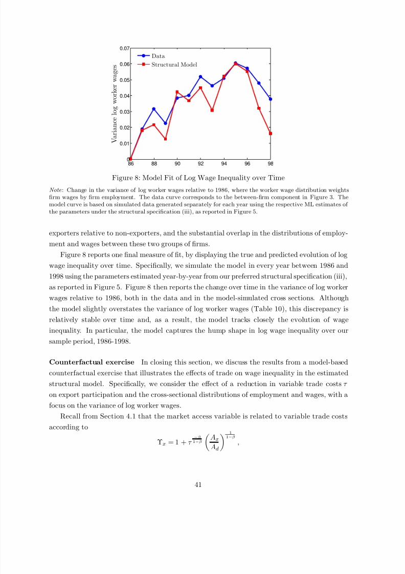
7242019 Brazil Trade
httpslidepdfcomreaderfullbrazil-trade 4649
5 Conclusion
Recent theories of firm heterogeneity and trade emphasize variation in wages with firm produc-
tivity and trade participation as sources of wage inequality Guided by these theories we use
linked employer-employee data for Brazil to examine the empirical relevance of these sources of
wage inequality
In contrast to neoclassical trade theory which stresses wage inequality between sectors and
occupations we find that around two thirds of overall wage inequality occurs within sector-
occupations Residual wage inequality is as important as worker observables in explaining overall
wage inequality and occurs predominantly within sector-occupations Consistent with recent
theories of firm heterogeneity and trade between-firm differences in wages account for much
of the observed wage inequality within sector-occupations and are particularly influential for
residual wage inequality These between-firm differences in wages are strongly but imperfectly
related to firm employment and trade participation
Motivated by these findings we estimate a structural econometric model of firm export sta-
tus employment and wages which is derived from an augmented version of Helpman Itskhokiand Redding (2010) This augmented model incorporates three sources of firm heterogeneity in
productivity fixed exporting costs and worker screening each of which is central to matching
the data We show that the estimated model is empirically successful in accounting for the ob-
served distributions of wages and employment for parameter values consistent with theoretical
restrictions We find that firm trade participationmdashthrough a combination of market access and
firm selection effectsmdashis important for the modelrsquos explanatory power We show that counter-
factual changes in variable trade costs can have sizeable effects on wage inequality through this
mechanism of wage dispersion between firms
Trade expands the set of opportunities available to firms and workers which is the sourceof welfare gains from trade But only some firms find it profitable to take advantage of these
opportunities which is the mechanism behind tradersquos effect on wage inequality that we empha-
size When only a few firms export further trade liberalization increases wage inequality but
once the fraction of firms exporting becomes sufficiently large wage inequality reaches a peak
and starts to fall back
44
7242019 Brazil Trade
httpslidepdfcomreaderfullbrazil-trade 4749
References
Amemiya T (1985) Advanced Econometrics Harvard University Press Cambridge Mass
Amiti M and D R Davis (2011) ldquoTrade Firms and Wages Theory and Evidencerdquo Review of
Economic Studies forthcoming
Attanasio O P K Goldberg and N Pavcnik (2004) ldquoTrade Reforms and Wage Inequality in
Colombiardquo Journal of Development Economics 74(2) 331ndash366Autor D H L F Katz and M S Kearney (2008) ldquoTrends in US Wage Inequality Revising
the Revisionistsrdquo Review of Economics and Statistics 90(2) 300ndash323
Barth E A Bryson J C Davis and R Freeman (2011) ldquoThe Contribution of Dispersion
across Plants to the Increase in US Earnings Dispersionrdquo unpublished manuscript presented at the
EEA-ESEM meetings 2011
Baumgarten D (2011) ldquoExporters and the Rise in Wage Inequality Evidence from German Linked
Employer-Employee Datardquo RWI unpublished manuscript
Berman E J Bound and Z Griliches (1994) ldquoChanges in the Demand for Skilled Labor within
US Manufacturing Evidence from the Annual Survey of Manufacturesrdquo Quarterly Journal of Eco-
nomics 109(2) 367ndash97Bernard A B and J B Jensen (1995) ldquoExporters Jobs and Wages in US Manufacturing
1976-1987rdquo Brookings Papers on Economic Activity Microeconomics 1995(1) 67ndash112
(1997) ldquoExporters Skill Upgrading and the Wage Gaprdquo Journal of International Economics
42(1-2) 3ndash31
(1999) ldquoExceptional Exporter Performance Cause Effect or Bothrdquo Journal of International
Economics 47(1) 1ndash25
Burstein A and J Vogel (2003) ldquoGlobalization Technology and the Skill Premium A Quanti-
tative Analysisrdquo NBER Working Paper 16459
Bustos P (2011) ldquoTrade Liberalization Exports and Technology Upgrading Evidence on the Impact
of Mercosur on Argentinian Firmsrdquo American Economic Review 101(1) 30440Chaney T (2008) ldquoDistorted Gravity The Intensive and Extensive Margins of International Traderdquo
American Economic Review 98(4) 1707ndash21
Cosar A K N Guner and J Tybout (2011) ldquoFirm Dynamics Job Turnover and Wage Distri-
butions in an Open Economyrdquo IMDEA Working Paper 201106
Davidson C F Heyman S Matusz F Sjoholm and S C Zhu (2011) ldquoGlobalization and
Imperfect Labor Market Sortingrdquo Research Institute of Industrial Economics Working Paper 856
Stockholm
Davidson C and S J Matusz (2010) International Trade with Equilibrium Unemployment Prince-
ton University Press Princeton NJ
Davidson C S J Matusz and A Shevchenko (2008) ldquoGlobalization and Firm Level Adjustmentwith Imperfect Labor Marketsrdquo Journal of International Economics 75(2) 295ndash309
Davis D R and J Harrigan (2011) ldquoGood Jobs Bad Jobs and Trade Liberalizationrdquo Journal of
International Economics 84(1) 26ndash36
Davis S J and J C Haltiwanger (1991) ldquoWage Dispersion Between and Within US Manufac-
turing Plants 1963-86rdquo Brookings Papers on Economic Activity Microeconomics 1991(1) 115ndash80
Eaton J S Kortum and F Kramarz (2010) ldquoAn Anatomy of International Trade Evidence
45
7242019 Brazil Trade
httpslidepdfcomreaderfullbrazil-trade 4849
from French Firmsrdquo University of Chicago unpublished manuscript
Egger H P Egger and U Kreickemeier (2011) ldquoTrade Wages and Profitsrdquo University of
Tubingen unpublished manuscript
Egger H and U Kreickemeier (2009) ldquoFirm Heterogeneity and the Labor Market Effects of Trade
Liberalizationrdquo International Economic Review 50(1) 187ndash216
Faggio G K G Salvanes and J Van Reenen (2010) ldquoThe Evolution of Inequality in Produc-
tivity and Wages Panel Data Evidencerdquo Industrial and Corporate Change 19(6) 1919ndash1951
Fally T R Paillacar and C Terra (2010) ldquoEconomic Geography and Wages in Brazil Evidence
from Micro-Datardquo Journal of Development Economics 91(1) 155ndash168
Feenstra R C and G H Hanson (1996) ldquoForeign Investment Outsourcing and Relative Wagesrdquo
in The Political Economy of Trade Policy Papers in Honor of Jagdish Baghwati ed by R C Feenstra
G M Grossman and D A Irwin chap 6 pp 89ndash128 MIT Press Cambridge Mass
(1999) ldquoThe Impact of Outsourcing and High-Technology Capital on Wages Estimates for the
United States 1979-1990rdquo Quarterly Journal of Economics 114(3) 907ndash40
Felbermayr G J Prat and H-J Schmerer (2011) ldquoGlobalization and Labor Market Outcomes
Wage Bargaining Search Frictions and Firm Heterogeneityrdquo Journal of Economic Theory 146(1) 39ndash
73
Ferreira F H G P G Leite and M Wai-Poi (2010) ldquoTrade Liberalization Employment Flows
and Wage Inequality in Brazilrdquo in The Poor under Globalization in Asia Latin America and Africa
ed by M Nissanke and E Thorbecke UNU-Wider Studies in Development Economics chap 8 pp
199ndash254 Oxford University Press Oxford
Frıas J A D S Kaplan and E A Verhoogen (2009) ldquoExports and Wage Premia Evidence
from Mexican Employer-Employee Datardquo Columbia University unpublished manuscript
Goldberg P K and N Pavcnik (2003) ldquoThe Response of the Informal Sector to Trade Liberal-
izationrdquo Journal of Development Economics 72(2) 463ndash96
(2005) ldquoTrade Wages and the Political Economy of Trade Protection Evidence from the
Colombian Trade Reformsrdquo Journal of International Economics 66(1) 75ndash105
(2007) ldquoDistributional Effects of Globalization in Developing Countriesrdquo Journal of Economic
Literature 45(1) 39ndash82
Gonzaga G N A Menezes-Filho and M C Terra (2006) ldquoTrade Liberalization and the
Evolution of Skill Earnings Differentials in Brazilrdquo Journal of International Economics 68(2) 345ndash67
Helpman E and O Itskhoki (2010) ldquoLabour Market Rigidities Trade and Unemploymentrdquo Review
of Economic Studies 77(3) 11001137
Helpman E O Itskhoki and S Redding (2010) ldquoInequality and Unemployment in a Global
Economyrdquo Econometrica 78(4) 1239ndash1283
Irarrazabal A A Moxnes and L D Opromolla (2011) ldquoThe Margins of Multinational Pro-
duction and the Role of Intra-firm Traderdquo Dartmouth College unpublished manuscript
Juhn C K M Murphy and B Pierce (1993) ldquoWage Inequality and the Rise in Returns to Skillrdquo
Journal of Political Economy 101(3) 410ndash442
Katz L F and K M Murphy (1992) ldquoChanges in Relative Wages 1963-1987 Supply and Demand
Factorsrdquo Quarterly Journal of Economics 107(1) 35ndash78
Kovak B K (2011) ldquoLocal Labor Market Effects of Trade Policy Evidence from Brazilian Liberal-
46
7242019 Brazil Trade
httpslidepdfcomreaderfullbrazil-trade 4949
izationrdquo Carnegie Mellon University unpublished manuscript
Krishna P J P Poole and M Z Senses (2011) ldquoTrade Liberalization Firm Heterogneity
and Wages New Evidence from Matched Employer-Employee Datardquo World Bank Policy Research
Working Paper 5711
Kume H G Piani and C F B d Souza (2003) ldquoA Polıtica Brasileira de Importacao no Perıodo
1987-98 Descricao e Avaliacaordquo in A abertura comercial brasileira nos anos 1990 Impactos sobre
emprego e salacute arios ed by C H Corseuil and H Kume chap 1 pp 9ndash37 MTE and IPEA Rio de
Janeiro
Lazear E P and K L Shaw (2009) ldquoWage Structure Raises and Mobility An Introduction to
International Comparisons of the Structure of Wages Within and Across Firmsrdquo in The Structure of
Wages An International Comparison ed by E P Lazear and K L Shaw chap 1 University of
Chicago Press Chicago
Lemieux T (2006) ldquoIncreasing Residual Wage Inequality Composition Effects Noisy Data or Rising
Demand for Skillrdquo American Economic Review 96(3) 461ndash498
Maddala G S (1983) Limited-dependent and qualitative variables in econometrics vol 3 of Econo-
metric Society Monographs Cambridge University Press Cambridge UK
Melitz M J (2003) ldquoThe Impact of Trade on Intra-Industry Reallocations and Aggregate Industry
Productivityrdquo Econometrica 71(6) 1695ndash1725
Menezes-Filho N A M-A Muendler and G Ramey (2008) ldquoThe Structure of Worker Com-
pensation in Brazil with a Comparison to France and the United Statesrdquo Review of Economics and
Statistics 90(2) 324ndash346
Monte F (2011) ldquoSkill Bias Trade and Wage Dispersionrdquo Journal of International Economics 83(2)
202ndash218
Mortensen D T (2003) Wage dispersion Why are similar workers paid differently Zeuthen lecture
book series MIT Press Cambridge Mass
Munch J R and J R Skaksen (2008) ldquoHuman Capital and Wages in Exporting Firmsrdquo Journal
of International Economics 75(2) 363ndash372
Oi W Y and T L Idson (1999) ldquoFirm Size and Wagesrdquo in Handbook of labor economics ed by
O Ashenfelter and D Card vol 3B pp 2165ndash2214 Elsevier Science North-Holland Amsterdam
New York and Oxford
Rosen S (1982) ldquoAuthority Control and the Distribution of Earningsrdquo Bell Journal of Economics
13(2) 311ndash323
Schank T C Schnabel and J Wagner (2007) ldquoDo Exporters Really Pay Higher Wages First
Evidence from German Linked Employer-Employee Datardquo Journal of International Economics 72(1)
52ndash74
Stole L A and J Zwiebel (1996) ldquoIntra-firm Bargaining under Non-binding Contractsrdquo Review
of Economic Studies 63(3) 375ndash410
Trefler D and S C Zhu (2005) ldquoTrade and Inequality in Developing Countries A General
Equilibrium Analysisrdquo Journal of International Economics 65(1) 21ndash48
Verhoogen E A (2008) ldquoTrade Quality Upgrading and Wage Inequality in the Mexican Manufac-
turing Sector rdquo Quarterly Journal of Economics 123(2) 489 530
7242019 Brazil Trade
httpslidepdfcomreaderfullbrazil-trade 4749
References
Amemiya T (1985) Advanced Econometrics Harvard University Press Cambridge Mass
Amiti M and D R Davis (2011) ldquoTrade Firms and Wages Theory and Evidencerdquo Review of
Economic Studies forthcoming
Attanasio O P K Goldberg and N Pavcnik (2004) ldquoTrade Reforms and Wage Inequality in
Colombiardquo Journal of Development Economics 74(2) 331ndash366Autor D H L F Katz and M S Kearney (2008) ldquoTrends in US Wage Inequality Revising
the Revisionistsrdquo Review of Economics and Statistics 90(2) 300ndash323
Barth E A Bryson J C Davis and R Freeman (2011) ldquoThe Contribution of Dispersion
across Plants to the Increase in US Earnings Dispersionrdquo unpublished manuscript presented at the
EEA-ESEM meetings 2011
Baumgarten D (2011) ldquoExporters and the Rise in Wage Inequality Evidence from German Linked
Employer-Employee Datardquo RWI unpublished manuscript
Berman E J Bound and Z Griliches (1994) ldquoChanges in the Demand for Skilled Labor within
US Manufacturing Evidence from the Annual Survey of Manufacturesrdquo Quarterly Journal of Eco-
nomics 109(2) 367ndash97Bernard A B and J B Jensen (1995) ldquoExporters Jobs and Wages in US Manufacturing
1976-1987rdquo Brookings Papers on Economic Activity Microeconomics 1995(1) 67ndash112
(1997) ldquoExporters Skill Upgrading and the Wage Gaprdquo Journal of International Economics
42(1-2) 3ndash31
(1999) ldquoExceptional Exporter Performance Cause Effect or Bothrdquo Journal of International
Economics 47(1) 1ndash25
Burstein A and J Vogel (2003) ldquoGlobalization Technology and the Skill Premium A Quanti-
tative Analysisrdquo NBER Working Paper 16459
Bustos P (2011) ldquoTrade Liberalization Exports and Technology Upgrading Evidence on the Impact
of Mercosur on Argentinian Firmsrdquo American Economic Review 101(1) 30440Chaney T (2008) ldquoDistorted Gravity The Intensive and Extensive Margins of International Traderdquo
American Economic Review 98(4) 1707ndash21
Cosar A K N Guner and J Tybout (2011) ldquoFirm Dynamics Job Turnover and Wage Distri-
butions in an Open Economyrdquo IMDEA Working Paper 201106
Davidson C F Heyman S Matusz F Sjoholm and S C Zhu (2011) ldquoGlobalization and
Imperfect Labor Market Sortingrdquo Research Institute of Industrial Economics Working Paper 856
Stockholm
Davidson C and S J Matusz (2010) International Trade with Equilibrium Unemployment Prince-
ton University Press Princeton NJ
Davidson C S J Matusz and A Shevchenko (2008) ldquoGlobalization and Firm Level Adjustmentwith Imperfect Labor Marketsrdquo Journal of International Economics 75(2) 295ndash309
Davis D R and J Harrigan (2011) ldquoGood Jobs Bad Jobs and Trade Liberalizationrdquo Journal of
International Economics 84(1) 26ndash36
Davis S J and J C Haltiwanger (1991) ldquoWage Dispersion Between and Within US Manufac-
turing Plants 1963-86rdquo Brookings Papers on Economic Activity Microeconomics 1991(1) 115ndash80
Eaton J S Kortum and F Kramarz (2010) ldquoAn Anatomy of International Trade Evidence
45
7242019 Brazil Trade
httpslidepdfcomreaderfullbrazil-trade 4849
from French Firmsrdquo University of Chicago unpublished manuscript
Egger H P Egger and U Kreickemeier (2011) ldquoTrade Wages and Profitsrdquo University of
Tubingen unpublished manuscript
Egger H and U Kreickemeier (2009) ldquoFirm Heterogeneity and the Labor Market Effects of Trade
Liberalizationrdquo International Economic Review 50(1) 187ndash216
Faggio G K G Salvanes and J Van Reenen (2010) ldquoThe Evolution of Inequality in Produc-
tivity and Wages Panel Data Evidencerdquo Industrial and Corporate Change 19(6) 1919ndash1951
Fally T R Paillacar and C Terra (2010) ldquoEconomic Geography and Wages in Brazil Evidence
from Micro-Datardquo Journal of Development Economics 91(1) 155ndash168
Feenstra R C and G H Hanson (1996) ldquoForeign Investment Outsourcing and Relative Wagesrdquo
in The Political Economy of Trade Policy Papers in Honor of Jagdish Baghwati ed by R C Feenstra
G M Grossman and D A Irwin chap 6 pp 89ndash128 MIT Press Cambridge Mass
(1999) ldquoThe Impact of Outsourcing and High-Technology Capital on Wages Estimates for the
United States 1979-1990rdquo Quarterly Journal of Economics 114(3) 907ndash40
Felbermayr G J Prat and H-J Schmerer (2011) ldquoGlobalization and Labor Market Outcomes
Wage Bargaining Search Frictions and Firm Heterogeneityrdquo Journal of Economic Theory 146(1) 39ndash
73
Ferreira F H G P G Leite and M Wai-Poi (2010) ldquoTrade Liberalization Employment Flows
and Wage Inequality in Brazilrdquo in The Poor under Globalization in Asia Latin America and Africa
ed by M Nissanke and E Thorbecke UNU-Wider Studies in Development Economics chap 8 pp
199ndash254 Oxford University Press Oxford
Frıas J A D S Kaplan and E A Verhoogen (2009) ldquoExports and Wage Premia Evidence
from Mexican Employer-Employee Datardquo Columbia University unpublished manuscript
Goldberg P K and N Pavcnik (2003) ldquoThe Response of the Informal Sector to Trade Liberal-
izationrdquo Journal of Development Economics 72(2) 463ndash96
(2005) ldquoTrade Wages and the Political Economy of Trade Protection Evidence from the
Colombian Trade Reformsrdquo Journal of International Economics 66(1) 75ndash105
(2007) ldquoDistributional Effects of Globalization in Developing Countriesrdquo Journal of Economic
Literature 45(1) 39ndash82
Gonzaga G N A Menezes-Filho and M C Terra (2006) ldquoTrade Liberalization and the
Evolution of Skill Earnings Differentials in Brazilrdquo Journal of International Economics 68(2) 345ndash67
Helpman E and O Itskhoki (2010) ldquoLabour Market Rigidities Trade and Unemploymentrdquo Review
of Economic Studies 77(3) 11001137
Helpman E O Itskhoki and S Redding (2010) ldquoInequality and Unemployment in a Global
Economyrdquo Econometrica 78(4) 1239ndash1283
Irarrazabal A A Moxnes and L D Opromolla (2011) ldquoThe Margins of Multinational Pro-
duction and the Role of Intra-firm Traderdquo Dartmouth College unpublished manuscript
Juhn C K M Murphy and B Pierce (1993) ldquoWage Inequality and the Rise in Returns to Skillrdquo
Journal of Political Economy 101(3) 410ndash442
Katz L F and K M Murphy (1992) ldquoChanges in Relative Wages 1963-1987 Supply and Demand
Factorsrdquo Quarterly Journal of Economics 107(1) 35ndash78
Kovak B K (2011) ldquoLocal Labor Market Effects of Trade Policy Evidence from Brazilian Liberal-
46
7242019 Brazil Trade
httpslidepdfcomreaderfullbrazil-trade 4949
izationrdquo Carnegie Mellon University unpublished manuscript
Krishna P J P Poole and M Z Senses (2011) ldquoTrade Liberalization Firm Heterogneity
and Wages New Evidence from Matched Employer-Employee Datardquo World Bank Policy Research
Working Paper 5711
Kume H G Piani and C F B d Souza (2003) ldquoA Polıtica Brasileira de Importacao no Perıodo
1987-98 Descricao e Avaliacaordquo in A abertura comercial brasileira nos anos 1990 Impactos sobre
emprego e salacute arios ed by C H Corseuil and H Kume chap 1 pp 9ndash37 MTE and IPEA Rio de
Janeiro
Lazear E P and K L Shaw (2009) ldquoWage Structure Raises and Mobility An Introduction to
International Comparisons of the Structure of Wages Within and Across Firmsrdquo in The Structure of
Wages An International Comparison ed by E P Lazear and K L Shaw chap 1 University of
Chicago Press Chicago
Lemieux T (2006) ldquoIncreasing Residual Wage Inequality Composition Effects Noisy Data or Rising
Demand for Skillrdquo American Economic Review 96(3) 461ndash498
Maddala G S (1983) Limited-dependent and qualitative variables in econometrics vol 3 of Econo-
metric Society Monographs Cambridge University Press Cambridge UK
Melitz M J (2003) ldquoThe Impact of Trade on Intra-Industry Reallocations and Aggregate Industry
Productivityrdquo Econometrica 71(6) 1695ndash1725
Menezes-Filho N A M-A Muendler and G Ramey (2008) ldquoThe Structure of Worker Com-
pensation in Brazil with a Comparison to France and the United Statesrdquo Review of Economics and
Statistics 90(2) 324ndash346
Monte F (2011) ldquoSkill Bias Trade and Wage Dispersionrdquo Journal of International Economics 83(2)
202ndash218
Mortensen D T (2003) Wage dispersion Why are similar workers paid differently Zeuthen lecture
book series MIT Press Cambridge Mass
Munch J R and J R Skaksen (2008) ldquoHuman Capital and Wages in Exporting Firmsrdquo Journal
of International Economics 75(2) 363ndash372
Oi W Y and T L Idson (1999) ldquoFirm Size and Wagesrdquo in Handbook of labor economics ed by
O Ashenfelter and D Card vol 3B pp 2165ndash2214 Elsevier Science North-Holland Amsterdam
New York and Oxford
Rosen S (1982) ldquoAuthority Control and the Distribution of Earningsrdquo Bell Journal of Economics
13(2) 311ndash323
Schank T C Schnabel and J Wagner (2007) ldquoDo Exporters Really Pay Higher Wages First
Evidence from German Linked Employer-Employee Datardquo Journal of International Economics 72(1)
52ndash74
Stole L A and J Zwiebel (1996) ldquoIntra-firm Bargaining under Non-binding Contractsrdquo Review
of Economic Studies 63(3) 375ndash410
Trefler D and S C Zhu (2005) ldquoTrade and Inequality in Developing Countries A General
Equilibrium Analysisrdquo Journal of International Economics 65(1) 21ndash48
Verhoogen E A (2008) ldquoTrade Quality Upgrading and Wage Inequality in the Mexican Manufac-
turing Sector rdquo Quarterly Journal of Economics 123(2) 489 530

7242019 Brazil Trade
httpslidepdfcomreaderfullbrazil-trade 4949
izationrdquo Carnegie Mellon University unpublished manuscript
Krishna P J P Poole and M Z Senses (2011) ldquoTrade Liberalization Firm Heterogneity
and Wages New Evidence from Matched Employer-Employee Datardquo World Bank Policy Research
Working Paper 5711
Kume H G Piani and C F B d Souza (2003) ldquoA Polıtica Brasileira de Importacao no Perıodo
1987-98 Descricao e Avaliacaordquo in A abertura comercial brasileira nos anos 1990 Impactos sobre
emprego e salacute arios ed by C H Corseuil and H Kume chap 1 pp 9ndash37 MTE and IPEA Rio de
Janeiro
Lazear E P and K L Shaw (2009) ldquoWage Structure Raises and Mobility An Introduction to
International Comparisons of the Structure of Wages Within and Across Firmsrdquo in The Structure of
Wages An International Comparison ed by E P Lazear and K L Shaw chap 1 University of
Chicago Press Chicago
Lemieux T (2006) ldquoIncreasing Residual Wage Inequality Composition Effects Noisy Data or Rising
Demand for Skillrdquo American Economic Review 96(3) 461ndash498
Maddala G S (1983) Limited-dependent and qualitative variables in econometrics vol 3 of Econo-
metric Society Monographs Cambridge University Press Cambridge UK
Melitz M J (2003) ldquoThe Impact of Trade on Intra-Industry Reallocations and Aggregate Industry
Productivityrdquo Econometrica 71(6) 1695ndash1725
Menezes-Filho N A M-A Muendler and G Ramey (2008) ldquoThe Structure of Worker Com-
pensation in Brazil with a Comparison to France and the United Statesrdquo Review of Economics and
Statistics 90(2) 324ndash346
Monte F (2011) ldquoSkill Bias Trade and Wage Dispersionrdquo Journal of International Economics 83(2)
202ndash218
Mortensen D T (2003) Wage dispersion Why are similar workers paid differently Zeuthen lecture
book series MIT Press Cambridge Mass
Munch J R and J R Skaksen (2008) ldquoHuman Capital and Wages in Exporting Firmsrdquo Journal
of International Economics 75(2) 363ndash372
Oi W Y and T L Idson (1999) ldquoFirm Size and Wagesrdquo in Handbook of labor economics ed by
O Ashenfelter and D Card vol 3B pp 2165ndash2214 Elsevier Science North-Holland Amsterdam
New York and Oxford
Rosen S (1982) ldquoAuthority Control and the Distribution of Earningsrdquo Bell Journal of Economics
13(2) 311ndash323
Schank T C Schnabel and J Wagner (2007) ldquoDo Exporters Really Pay Higher Wages First
Evidence from German Linked Employer-Employee Datardquo Journal of International Economics 72(1)
52ndash74
Stole L A and J Zwiebel (1996) ldquoIntra-firm Bargaining under Non-binding Contractsrdquo Review
of Economic Studies 63(3) 375ndash410
Trefler D and S C Zhu (2005) ldquoTrade and Inequality in Developing Countries A General
Equilibrium Analysisrdquo Journal of International Economics 65(1) 21ndash48
Verhoogen E A (2008) ldquoTrade Quality Upgrading and Wage Inequality in the Mexican Manufac-
turing Sector rdquo Quarterly Journal of Economics 123(2) 489 530