BRANCHED COVERS OF CONTACT MANIFOLDS

A ThesisPresented to

The Academic Faculty

by

Meredith Casey

In Partial Fulfillmentof the Requirements for the Degree

Doctor of Philosophy in theSchool of Mathematics

Georgia Institute of TechnologyDecember 2013

Copyright c� 2013 by Meredith Casey

BRANCHED COVERS OF CONTACT MANIFOLDS

Approved by:

Professor John Etnyre, AdvisorSchool of MathematicsGeorgia Institute of Technology

Professor Igor BelegradekSchool of MathematicsGeorgia Institute of Technology

Professor Dan MarglitSchool of MathematicsGeorgia Institute of Technology

Professor Thang LeSchool of MathematicsGeorgia Institute of Technology

Professor William KazezDepartment of MathematicsThe University of Georgia

Date Approved: October 10, 2013

to my husband

iii

ACKNOWLEDGEMENTS

First I would like to thank my adviser John Etnyre for all his help and support

throughout writing this thesis and during my entire time at Georgia Tech. I would

also like to thank Will Kazez and Dan Margalit for their feedback and for many helpful

conversations. I am also greatful to my fellow graduate students Bulent Tosun, Amey

Kaloti, Alan Diaz, Jamie Conway, Rebecca Winarski, and Chris Pryby for their help

and friendship.

I want to thank the faculty and sta↵ of the math department at Georgia Tech

for such wonderful support over the years. In particular I am sincerely grateful to

Klara Grodzinsky for her help and encouragement, and to Genola Turner, Sharon

McDowell, Annette Annette Rohrs, Inetta Worthy, Christy Dalton, Justin Filoseta,

Matt Hanes, and Lew Lefton for their support, assistance and patience.

Finally I am eternally grateful to my family and friends for all their encouagement

over the years. Thank you especially to my parents and grandparents for believing

in me when times were tough and listening to me ramble on about math when things

were going well. And to my husband Shaughn - I would never have finished this

without you. Your help and support mean the world to me.

iv

List of Figures

1 The standard contact structure on R3 (Picture by Patrick Massot) . . 7

2 Symmetric Contact Structure on R3 (Picture by Patrick Massot) . . . 7

3 Overtwisted Contact Structure on R3 . . . . . . . . . . . . . . . . . . 8

4 Segments not allowed in projections of transverse knots. . . . . . . . 12

5 Transverse Stabilization . . . . . . . . . . . . . . . . . . . . . . . . . 14

6 A 3-Braid . . . . . . . . . . . . . . . . . . . . . . . . . . . . . . . . . 15

7 Braid Stablilzation . . . . . . . . . . . . . . . . . . . . . . . . . . . . 16

8 In both pictures the shaded region is to the right of A. . . . . . . . . 23

9 In the figure above B is to the left of A. . . . . . . . . . . . . . . . . 23

10 Finding the prongs for a boundary component for a pseudo-Anosov

map on a surface . . . . . . . . . . . . . . . . . . . . . . . . . . . . . 26

11 Cyclic Branched Cover over Disk . . . . . . . . . . . . . . . . . . . . 31

12 Branched Cover of 2-sphere by genus 2 surface. . . . . . . . . . . . . 31

13 A Branched Covering Example . . . . . . . . . . . . . . . . . . . . . 34

14 Example of a Construction . . . . . . . . . . . . . . . . . . . . . . . . 35

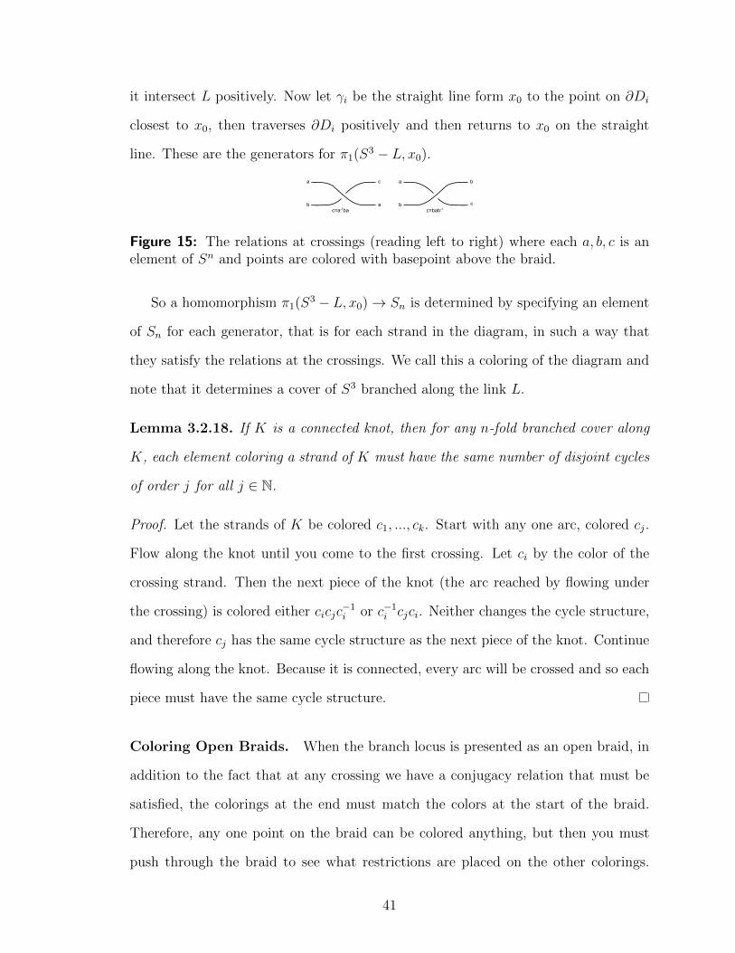
15 The relations at crossings (reading left to right) where each a, b, c is an

element of Sn and points are colored with basepoint above the braid. 41

16 An admissible transformation. . . . . . . . . . . . . . . . . . . . . . . 42

v

17 Open Book Decomposition . . . . . . . . . . . . . . . . . . . . . . . . 45

18 Finding the Branching Word . . . . . . . . . . . . . . . . . . . . . . . 51

19 Finding the Branching Word . . . . . . . . . . . . . . . . . . . . . . . 52

20 The Reduced Branching Word . . . . . . . . . . . . . . . . . . . . . . 52

21 The Reduced Branching Word . . . . . . . . . . . . . . . . . . . . . . 52

22 K’ inside the stabilized knot K . . . . . . . . . . . . . . . . . . . . . . 53

23 �(�) . . . . . . . . . . . . . . . . . . . . . . . . . . . . . . . . . . . . 54

24 The section of g�(�) containing the ith and hth sheets . . . . . . . . . . 55

25 Image of � under � . . . . . . . . . . . . . . . . . . . . . . . . . . . . 57

26 Coloring the Figure-Eight . . . . . . . . . . . . . . . . . . . . . . . . 59

27 The preimages of particular arcs after isotoping to be minimally inter-

secting. . . . . . . . . . . . . . . . . . . . . . . . . . . . . . . . . . . . 62

28 Images of curves under �. . . . . . . . . . . . . . . . . . . . . . . . . 62

29 Images under �0. . . . . . . . . . . . . . . . . . . . . . . . . . . . . . 63

30 Destabilized Open Book. . . . . . . . . . . . . . . . . . . . . . . . . . 63

vi

Contents

DEDICATION . . . . . . . . . . . . . . . . . . . . . . . . . . . . . . . . . . iii

ACKNOWLEDGEMENTS . . . . . . . . . . . . . . . . . . . . . . . . . . iv

LIST OF TABLES . . . . . . . . . . . . . . . . . . . . . . . . . . . . . . . ix

LIST OF FIGURES . . . . . . . . . . . . . . . . . . . . . . . . . . . . . . x

I INTRODUCTION . . . . . . . . . . . . . . . . . . . . . . . . . . . . . 1

II CONTACT GEOMETRY BACKGROUND . . . . . . . . . . . . . 6

2.1 Contact Structures . . . . . . . . . . . . . . . . . . . . . . . . . . . . 6

2.1.1 Basic Definitions and Examples . . . . . . . . . . . . . . . . 6

2.1.2 Tight and Overtwisted Contact Structures . . . . . . . . . . 10

2.2 Links, Knots, and Braids in Contact Structures . . . . . . . . . . . . 11

2.2.1 Transverse Knots . . . . . . . . . . . . . . . . . . . . . . . . 12

2.2.2 Braids . . . . . . . . . . . . . . . . . . . . . . . . . . . . . . 14

2.3 Open Book Decompositions of Contact Manifolds . . . . . . . . . . . 17

2.3.1 Open Book Decompositions . . . . . . . . . . . . . . . . . . . 17

2.3.2 Pseudo-Anosov Homeomorphisms . . . . . . . . . . . . . . . 21

2.3.3 Right-veering . . . . . . . . . . . . . . . . . . . . . . . . . . . 22

2.3.4 Fractional Dehn Twist Coe�cients . . . . . . . . . . . . . . . 25

III TOPOLOGICAL BRANCHED COVERS . . . . . . . . . . . . . . 28

3.1 Ordinary Covering Spaces . . . . . . . . . . . . . . . . . . . . . . . . 28

3.1.1 The Monodromy . . . . . . . . . . . . . . . . . . . . . . . . . 29

3.2 Branched Coverings of Manifolds . . . . . . . . . . . . . . . . . . . . 30

3.2.1 Surfaces . . . . . . . . . . . . . . . . . . . . . . . . . . . . . 30

3.2.2 3-Manifolds . . . . . . . . . . . . . . . . . . . . . . . . . . . 38

3.3 Branched Covers of Contact Structures . . . . . . . . . . . . . . . . 43

3.3.1 Generalizing Topological Results . . . . . . . . . . . . . . . . 43

3.4 Covers of Open Book Decompositions . . . . . . . . . . . . . . . . . 44

vii

IV BRANCHED COVERS OVER TRANSVERSE KNOTS . . . . . 47

4.1 Branching Over a Contact Manifold . . . . . . . . . . . . . . . . . . 47

4.2 Covers over (S3, ⇠std) . . . . . . . . . . . . . . . . . . . . . . . . . . 49

4.3 Contact Universal Knots . . . . . . . . . . . . . . . . . . . . . . . . 57

4.3.1 The Figure-Eight Knot . . . . . . . . . . . . . . . . . . . . . 57

4.3.2 The Whitehead Link . . . . . . . . . . . . . . . . . . . . . . 60

REFERENCES . . . . . . . . . . . . . . . . . . . . . . . . . . . . . . . . . . 64

viii

List of Tables

ix

List of Figures

x

Chapter I

INTRODUCTION

This thesis focuses on questions in low-dimemsional topology, contact geometry, and

knot theory. We want to understand contact structures via branched covering maps.

Contact structures originally arose from areas of physics, but recently they have been

seen to have mathematical beauty in their own right and are now being studied by

low-dimensional topologists. Topologists are interested in the characteristics, con-

struction, and classification of contact structures. In particular, given known topo-

logical constructions and results, one could ask what generalizations can be made to

the case of contact manifolds. One such construction is branched covers. In the past

50 years, topologists have proven many amazing results about branched covers and

3-manifolds, and recently much attention has been given to the interaction of these

covers with contact structures. Our goal is to better understand branched covers of

3-manifolds and contact manifolds.

A map p : M ! N is called a branched covering if there exists a co-dimension 2

subcomplex L such that p�1(L) is a co-dimension 2 subcomplex and p|M�p�1(L) is a

covering. We will study here manifolds of dimension 2 or 3. Essentially, a branched

covering is a map between manifolds such that away from a set of codimension 2

(called the branch locus) p is a honest covering.

Recall a contact structure ⇠ on an oriented 3-manifold M is a non-integrable plane

field in the tangent bundle of M . Branching over knots transverse to the contact

structure (i.e. transversal knots) we can pull back the contact structure downstairs

to obtain contact structures on the upstairs manifold. Bennequin proved that any

link transverse to the standard contact structure in S3 is transversally isotopic to a

1

closed braid so often we will think of a transversal link in terms of its braid word [3].

For covers of simply connected spaces, a convenient technique for describing a

branched covering map is that of coloring the branch locus, which is defined in Chap-

ter 3. Essentially, a coloring is an assignment to the branch locus of an element of

the symmetric group which determines (and is determined by) the covering map. In

Chapter 3 we use colorings to prove results on the construction of branched coverings

for surfaces and three-manifolds.

The real substance to the subject of branched covers of contact manifolds came in

2002 when Giroux proved the following fundamental theorem: Every contact manifold

is a 3-fold simple cover over S3 branching along some transverse link. The following

theorem, proven in Chapter 3, is a strengthening of Giroux’s result to a connected

branch locus.

Theorem 1.0.1. Given a contact manifold (M, ⇠), there exists a 3-fold simple cover

p : (M, ⇠) ! (S3, ⇠std) whose branch locus is a knot.

A link L in (S3 is called universal if every 3-manifold can be seen as the branched

cover over L. Known universal links include the figure-eight knot, Borromean rings,

andWhitehead link, see [18]. We call a transversal link L in (S3, ⇠std) contact universal

if every contact manifold is a branched cover over L. As any such transversal link

would also have to be topologically universal, one would want to look at tranversal

links that are topologically universal and study lifts of ⇠std branching along that link.

Theorem 1.0.2. Any transversal link that destabilizes is not contact universal.

Thus for any link which is topologically universal, we must choose a transversal

presentation which does not destablize to test for contact universality. This is par-

ticularly helpful for the figure-eight knot because Etnyre and Honda showed that the

only transversal figure-eight knot which does not destablize is the one described by

2

the braid word �1��12 �1�

�12 . We want to determine if every contact manifold can be

obtained by branching over this knot.

Harvey, Kawamuro, and Plamenevskaya showed that for any transverse braid

L ⇢ (S3, ⇠std) with braid word !, if for some i, ! contains ��1i and not �i then

every cyclic cover branching along L is an overtwisted manifold. The figure-eight

knot, Borromean rings, and Whitehead link all meet this conditions and therefore

any cyclic cover branching along any one of these figure-eight knots is overtwisted.

We can strengthen their result slightly to the following theorem, which will yield the

result that any fully ramified cover branching alone the figure-eight knot, Borromean

rings, or Whitehead link will be overtwisted.

Proposition 1.0.3. If K is transverse knot in (S3, ⇠std) whose braid word contains a

��1i and no �i for some i then any fully ramified cover branching over K is overtwisted.

If one of these topologically universal knots is going to be contact universal then a

minimal condition would be that tight contact structures can be obtained by branch-

ing along the knot. We focus first on the figure-eight knot. One method for determin-

ing if a contact structure is overtwisted is the theory of right-veering curves. In 2007

Honda, Kazez, and Matic defined a property of a di↵eomorphism called right-veering,

which indicates whether curves are taken to the right or to the left under the map. If

a monodromy for an open book decomposition of a contact manifold takes any curve

to the left, then the contact structure is overtwisted. (Open book decompositions

of manifolds are discussed in more detail in the next section, but for now imagine

any cover of a braid downstairs determines a map, called the monodromy, upstairs.)

Using this principle and some nice properties of the figure-eight knot we are able to

prove the next theorem.

Theorem 1.0.4. Every cover of (S3, ⇠std) branching over the figure-eight knot is

overtwisted.

3

So the figure-eight knot cannot be a contact universal knot as it cannot yield any

tight contact structure.

This result is special to the figure-eight knot, and not a property of knots and

links whose braid word contains a ��1i and no �i for some i, as we see with our next

result.

Theorem 1.0.5. Let L in (S3, ⇠std) be the transverse Whitehead link with braid word

�1��12 �1�

�22 . There exist covers branching over L that are tight.

To pin down concrete results about the behavior of branched covers of 3-manifolds,

much more needs to be understood about their construction. To do so we will ut-

lize open book decompositions, which are defined below. It is known that every

3-manifold has an open book decomposition. Furthermore, due to the celebrated

Giroux correspondence, the study of contact structures up to isomorphism is equiv-

alent to studying open book decompositions up to stabilization. Thus, open books

are important because they have immediate applications not only to low-dimensional

topology but at the same time to contact geometry.

Given a link K in S3 (with the standard contact structure if interested in contact

manifolds) we want to construct open book decompositions for manifolds obtained by

branching along K. Start with the open book decomposition (D2, id) of S3. We can

consider K as a link braided transversally through the pages. We want to constuct

an open book decoposition for the covering manifold. In the case that the cover is

cyclic, [17] give an algorithm for doing so, but no algorithm exists for the general

case.

Given a general 3-manifold M and open book (⌃,�), covers could be constructed

by either branching along a link transverse to the pages or by branching along the

binding. Though cyclic covers branched along the binding of the open book decom-

position are reasonbly well understood, but almost no work has been done in the

non-cyclic case. If branching along a transversal knot, it would be helpful to have a

4

method to compute these properties for the covering manifold given the information

about the manifold downstairs.

One property of particular interest is overtwistedness. If a contact manifold is

overtwisted, any non-branched cover would also be overtwisted. Is the same true of

branched covers of overtwisted manifolds? Or, if not always true, would it be true

for some class of manifolds? The answer is no.

Theorem 1.0.6. Given any contact manifold (M, ⇠) with ⇠ overtwisted, there exists a

trasversal knot K 2 (M, ⇠) and integer N such that any n-fold cyclic cover branching

along K (n > N) is tight.

This thesis is organized as follows: Chapter 2 presents basic definitions and the-

orems in contact geometry. Chapter 3 gives an introduction to branched coverings,

including detailed constructions, fundamental theorems, and some new work in topo-

logical branched covers. Chapter 4 is devoted to proving our main results.

5

Chapter II

CONTACT GEOMETRY BACKGROUND

Contact structures have been used in many areas of physics and mathematics in the

past twenty years. Some important results whose proofs involve contact structures in-

clude proving the Property P Conjecture [21] (which had been outstanding 30 years),

giving a surgery characterization of the unknot [25], figure-eight, and trefoil [26], and

proving that Heegaard floer homology detects fibered knots [23]. Knots and links in

contact structures are also very important, and useful for understanding much about

the behavior of the structure and for constructing contact manifolds via surgery and,

as we will see in the next chapter, branched covers. One way we study branched cov-

ers of manifolds is via open book decompositions. In this chapter we will introduce

all of these ideas more carefully and give many examples.

2.1 Contact Structures

This section introduces contact structures and important associated terminology. Af-

ter giving the basic definitions and examples, we will discuss what is known of their

classification.

2.1.1 Basic Definitions and Examples

An oriented 2-plane field ⇠ on a 3-manifold M is called a contact structure if there

exists a 1-form ↵ 2 ⌦1(M) such that ↵ ^ d↵ > 0. Such a ⇠ is totally non-integrable,

and thus there is no embedded surface in M which is tangent to ⇠ on any open

neighborhood. A 3-manifold equipped with a contact structure ⇠ is called a contact

manifold.

It will be helpful to establish a few examples we can reference throughout the

6

paper.

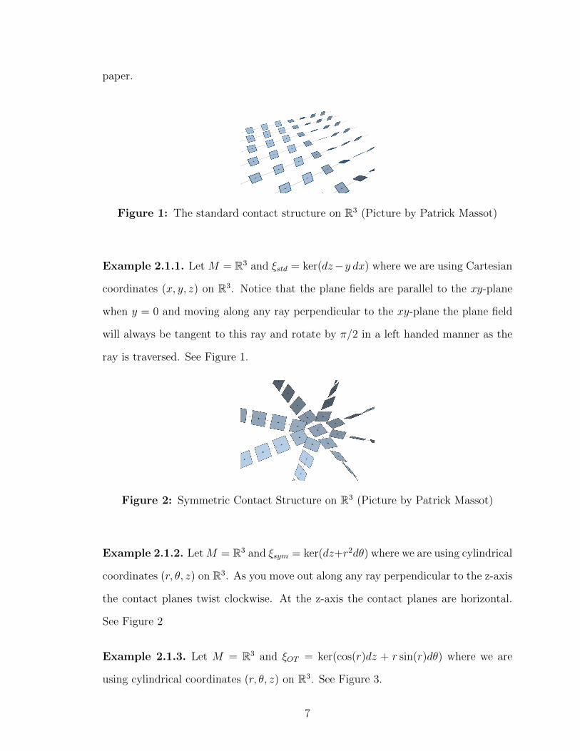
Figure 1: The standard contact structure on R3 (Picture by Patrick Massot)

Example 2.1.1. Let M = R3 and ⇠std = ker(dz�y dx) where we are using Cartesian

coordinates (x, y, z) on R3. Notice that the plane fields are parallel to the xy-plane

when y = 0 and moving along any ray perpendicular to the xy-plane the plane field

will always be tangent to this ray and rotate by ⇡/2 in a left handed manner as the

ray is traversed. See Figure 1.

Figure 2: Symmetric Contact Structure on R3 (Picture by Patrick Massot)

Example 2.1.2. LetM = R3 and ⇠sym = ker(dz+r2d✓) where we are using cylindrical

coordinates (r, ✓, z) on R3. As you move out along any ray perpendicular to the z-axis

the contact planes twist clockwise. At the z-axis the contact planes are horizontal.

See Figure 2

Example 2.1.3. Let M = R3 and ⇠OT = ker(cos(r)dz + r sin(r)d✓) where we are

using cylindrical coordinates (r, ✓, z) on R3. See Figure 3.

7

Figure 3: Overtwisted Contact Structure on R3

Topologists are interested in classification of objects. For example, consider closed

orientable surfaces. Every such surface is homeomorphic to a sphere with n holes (i.e.

of genus n), and two closed orientable surfaces are homeomorphic if and only if they

have the same number of holes. Computationally, two surfaces are homeomorphic if

and only if they have the same Euler Characteristic. So we have a classification of

closed, orientable surfaces up to homeomorphism and an invariant to determine when

two are the same.

Another important set of objects, mentioned above, for which we have a classifi-

cation is 2-plane fields on closed, oriented 3-manifolds. The theorem is stated below,

but first we should give some explanation of the notation. First, � is a 2-dimensional

invariant of ⇠ and gives a map �⇠ from the group of spin structures on M to a group

G in H1(M ;Z). This invariant refines the Euler class because 2�(⇠, s) = e(⇠) where

e(⇠) denotes the Euler class. And ✓(⇠) is a rational number which is a 3-dimensional

invariant of ⇠. For more details on these invariants and a proof of the theorem see

[15].

Theorem 2.1.4. Let ⇠1 and ⇠2 be two 2-plane fields on a closed rational homology

3-sphere. If e(⇠0) is a torsion class then ⇠1 and ⇠2 are homotopic if and only if, for

some choice of spin structure s, �(⇠1, s) = �(⇠2, s) and ✓(⇠1) = ✓(⇠2).

Remark 2.1.5. There is a similar theorem for general 3-manifolds but the associated

invariants are more complicated.

8

Therefore we have a complete classification of plane fields up to homotopy via

invariants that can tell them apart.

With classification being such an important question, it is natural that after defin-

ing contact structures, we would immediately ask for a classification. But first we

must determine what we want it to mean for two contact structures to be the same.

The two most commonly used definitions are that they are isotopic through contact

structures, and (though less strong) that they are contactomorphic. Two contact man-

ifold (M1, ⇠1) and (M2, ⇠2) are said to be contactomorphic if there is a di↵eomorphism

f : M1 ! M2 with Tf(⇠1) = ⇠2, where Tf : TM1 ! TM2 denotes the di↵erential of

f . Unless otherwise specified, we will always be working up to contactomorphism in

this paper.

Theorem 2.1.6. [16] (Gray’s Theorem) Let M be an oriented (2n+ 1)-dimensional

manifold and ⇠t , t 2 [0, 1] a family of contact structures on M that agree o↵ of some

compact subset of M . Then there is a family of di↵eomorphisms ft : M ! M such

that (ft)⇤⇠t = ⇠0.

Notice that Gray’s theorem tells us that on a compact manifold M , two isotopic

contact structures are also contactomorphic: Let ⇠, ⇠0be isotopic contact structures

on a compact manifold M and ⇠t t 2 [0, 1], the isotopy between them. Gray’s theorem

gives a di↵eomorphism ft such that (ft)⇤⇠t = ⇠0 = ⇠. Thus (f1)⇤⇠0= (f1)⇤⇠1 = ⇠ and

we see ⇠ and ⇠0are contactomorphic.

While it does not seem reasonable to completely classify contact structures at this

point, we would like to find invariants to determine when two contact structures are

di↵erent. Recall from above that contact structures on closed orientable 3-manifolds

are plane fields. Therefore, the invariants of plane fields discussed above give invari-

ants of contact structures and hence can be used to tell when two contact structures

are not the same. If the invariants � and ✓ of two contact structures are the same

9

then we can only conclude that they are homotopic as plane fields but not necessar-

ily through contact structures. Thus the contact structure might or might not be

contatomorphic.

We will discuss this through the examples mentioned above. We can find a di↵eo-

morphism of R3 taking ⇠std to ⇠sym which makes them contactomorphic. So in some

sense they are the same contact structure, but sometimes one is easier to work with

than the other. However, they are not contactomorphic to the structure labled OT

(see [3] for proof).

Theorem 2.1.7. [3] (Bennequin) The contact structure ⇠std is not contactomorphic

to ⇠OT .

Local Model. One important fact to note before we move on is the local model for

contact structure. First we state Darboux’s theorem in contact geometry.

Theorem 2.1.8. [6] (Darboux) Suppose ⇠i is a contact structure on the manifold

Mi, i = 0, 1, of the same dimension. Given any points p0 and p1 in M0 and M1,

respectively, there are neighborhoods Ni of pi in Mi and a contactomorphism from

(N0, ⇠0|N0) to (N1, ⇠1|N1). Moreover, if ↵i is a contact form for ⇠i near pi then the

contactomorphism can be chosen to pull ↵1 back to ↵0.

This says that any point in any contact 3-manifold has a neighborhood that can

be identified with the standard contact structure on an open ball in R3. For this

reason, when we are only interested in local behavior, we will often focus on the case

of (R3, ⇠std).

2.1.2 Tight and Overtwisted Contact Structures

In Example 2.1.3, look at the following disk:

D = {(r.✓, z)|z = 0, r ⇡}.

10

The disk D is tangent to ⇠OT along the boundary. Any contact structure is called

overtwisted if such an embedded disk exists, and tight otherwise.

Clearly every contact structure is either tight or overtwisted be definition. The

usefulless of dividing contact structures into these two classes is not immediately clear,

but we will show why this is a helpful definition to have. Recall that we are interested

in classification of contact structures, and we have an invariant which can determine

if two contact structures are homotopic through plane fields, but none (yet) that

can determine if they are contactomorphic or isotopic through contact structures. In

1989 Eliashberg showed that every homotopy class of an oriented 2-plane field contains

exactly one overtwisted contact structure and the classification of overtwisted contact

structures on a given closed 3-manifold coincides with the homotopy classification of

tangent 2-plane fields [7]. Therefore, for overtwisted contact structures, we have a

classification and our invarients for 2-plane fields are complete invarients in this class

as well. We then need to address tight contact structures.

Notice also that this means that every closed, oriented 3-manifold admits an

overtwisted contact structure. Naturally, we might think that every 3-manifold also

has a tight contact strucutre. Etnyre and Honda showed that there exists three

manifolds that admit no tight contact structure [10]. So in addition to asking for

a classification and invariants, we also would simply like to know which 3-manifolds

even admit tight contact structures.

2.2 Links, Knots, and Braids in Contact Structures

Knot theory has applications all over mathematics: geometric group theory, algebra,

mathematical physics, and many branches of topology. We will be using some of the

applications in this paper so we must discuss some of the fundamentals of knots and

links in contact manifolds. We will assume that the reader has a basic knowledge of

knots and braids in topological manifolds, and for details see [27].

11

2.2.1 Transverse Knots

There are two types of knots that are studied in contact manifolds: Legendrian and

transverse. We will focus on and overview transverse knots, but see [9] for a discussion

of Legendrian knots and more details on transverse knots. A transverse knot in a

contact manifold (M, ⇠) is an oriented, embedded S1 whose tangent vector at every

point is transverse to ⇠. Two transverse knots are transverse isotopic if there is an

isotopy taking one to the other while staying transverse.

In this section we will assume our knots and links are in (R3, ⇠std). Transverse

knots are pictured using front projections ⇧ : R3 ! R3 with (x, y, z) 7! (x, z). One

can show that the front projection of a transveral knot is an immersed curve and

any immursed curve in R2 is the front projection of a transverse knot if it satisfies

two constraints: no vertical tangencies pointing down, and no double points from

a positive crossing with both strands pointing down. Both of these are pictured in

Figure 4.

Figure 4: Segments not allowed in projections of transverse knots.

Classical Invariants. Given two transverse knots, we want to be able to tell if they

are transversely isotopic. Thus, we would like an invariant we can compute that will

determine when two transverse knots are not the same (and hopefully, also determine

when they are the same.) Given a transverse knot T , we still have the most basic

invariant - the topological knot type (T ). Clearly two transverse knots with di↵erent

knot types cannot be transverally isotopic. This is a very weak invariant as it cannot

distinguish di↵erent transverse knots of the same knot type. So we would like to find

12

such an invariant. For notation, denote the set of all transverse knots that realize a

fixed topological knot type K by T (K).

The main invariant for transverse knots is the self-linking number. To define the

self-linking number of T we assume it is homologically trivial. Thus there is a surface

⌃ such that @⌃ = T . The contact planes form a trivial two dimensional bundle

as any orientable two plane bundle is trivial over a surface with boundary, meaning

⇠|⌃ is trivial and thus there exists a non-zero vector field V over ⌃ in ⇠. Define a

new knot T 0 by pushing o↵ from T slightly in the direction of V . Now we have two

transverse knots, and we compute their linking number l(T, T 0) and this is precisely

the self-linkng number of T , denoted sl(T ). Notice that if V were to be a non-zero

vector field in ⇠ \ T⌃ along T that we could extend over all of ⌃ then we could push

T to form T 0 totally “above” T and thus sl(T ) would be 0. An alternate way to view

the self linking number is to start with a vector field that points out of ⌃. Then the

self-linking number is the obstruction to extending V over ⌃ to a non-zero vector

field in ⇠. If ⇧(T ) is the front projection of T , then the sl(T ) is the writhe of ⇧(T ),

(see [9]). There is a formula to compute the self-linking number of T given a braid

presentaton as well, which we will see in Section 2.2.2.

Notice that this gives an invariant of transverse knots; i.e. if two transverse knots

are transversally isotopic then they must have the same self-linking number. To see

this, notice if two transverse knots T0 and T1 are transversally isotopic then there

exists an isotopy �t : M ! M such that (�t)⇤⇠ = ⇠ and �t(T0) = Tt. Now we can

use �t to isotop ⌃ and V (the surface and non-zero vector field used to compute the

self-linking number for T0) and use their images to compute the self-linking number

for T1. At all points along the isotopy, we can compute the self-linking number of

the Tt. But this is an integer that must change continuously as t varies between 0

and 1, and thus cannot change. Therefore, T0 and T1 must have the same self-linking

13

number. However, two transverse knots in the same knot type with the same self-

linking number need not be transversely isotopic. For examples, see [8]. A knot type

whose transverse knots are classified by their self-linking number is called transversely

simple.

Stabilizations. Given a transverse knot T , a stabilization of T will produce a trans-

verse knot in the same knot type which is not transversely isotopic to T . Drawn as

front projections, the move is pictured below. Stabilizing a transverse knot reduces

the self-linking number by two.

Figure 5: Transverse Stabilization

2.2.2 Braids

For the majority of this paper we will look at links and knots as braids. Recall a closed

braid is a knot or link in R3 that can be parametrized by a map f : S1 ! R3 where

s 7! (r(s), ✓(s), z(s)) for which r(s) is not zero and ✓0(s) > 0. In the 1920s Alexander

showed that every link in R3 is isotopic to a closed braid by giving an algorithm to

braid any link. As we will see, braids are especially useful for constructing three-

manifolds.

An open n-strand braid is a picture of n horizontal strands, oriented from left

to right and labeled from bottom to top, with positive and negative crossings. A

closed braid is associated to an open braid by identifying the beginning and end of

the strands. A open braid is obtained from a closed braid (thought of as braided

about the z-axis) by isotoping the braid so that all crossings appear below the x-axis

and cutting the braid along its intersection with the half-plane y > 0, x = 0. An

example is pictured in Figure 6.

14

Figure 6: A 3-Braid

We denote the simple n-strand braid with one positive crossing between the ith

and (i+1)st strands by �i, and similarly ��1i if the crossing is negative. A braid can be

pictured by concatenation of the braids �±i , and thus we call the �i the the generators.

This list of generators that form the braid is called the braid word of the braid. Any

braid word uniquely defines the braid, one knot or braid may have many di↵erent

braid words. For example, in Figure 6, the braid word would be �2��11 �2�1�

�12 .

The set of all braids on n stands form a group, called the braid group, and is

denoted Bn [4]. The generators of the group are �i, i = 1, ..., n � 1, and the group

operation is conncatonation [4].

A fixed topological knotK can have many di↵erent associated braids. Alexander’s

theorem does not give a unique braid representation. Markov’s Theorem, stated

below, gives us a relationship between di↵erent braid representations of the same

knot.

Theorem 2.2.1. [22] (Markov’s Theorem) Let X,X 0 be closed braid reperesentatives

of the same oriented link type K in oriented 3-space. Then there exists a sequence of

closed braid representatives of K:

X = X1 ! X2 ! · · · ! Xr = X 0

taking such that each Xi+1 is obtained from Xi by either (i) braid isotopy, or (ii) a

single stabilization or destabilization.

By braid isotopy, we mean simply an isotopy of a closed braid, through closed

braids, in the complement of the braid axis. A braid stabilization is shown for open

15

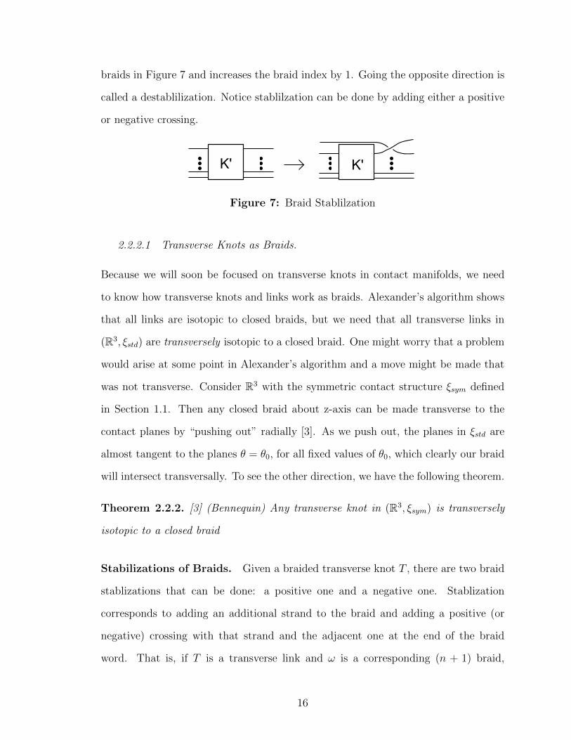
braids in Figure 7 and increases the braid index by 1. Going the opposite direction is

called a destablilization. Notice stablilzation can be done by adding either a positive

or negative crossing.

Figure 7: Braid Stablilzation

2.2.2.1 Transverse Knots as Braids.

Because we will soon be focused on transverse knots in contact manifolds, we need

to know how transverse knots and links work as braids. Alexander’s algorithm shows

that all links are isotopic to closed braids, but we need that all transverse links in

(R3, ⇠std) are transversely isotopic to a closed braid. One might worry that a problem

would arise at some point in Alexander’s algorithm and a move might be made that

was not transverse. Consider R3 with the symmetric contact structure ⇠sym defined

in Section 1.1. Then any closed braid about z-axis can be made transverse to the

contact planes by “pushing out” radially [3]. As we push out, the planes in ⇠std are

almost tangent to the planes ✓ = ✓0, for all fixed values of ✓0, which clearly our braid

will intersect transversally. To see the other direction, we have the following theorem.

Theorem 2.2.2. [3] (Bennequin) Any transverse knot in (R3, ⇠sym) is transversely

isotopic to a closed braid

Stabilizations of Braids. Given a braided transverse knot T , there are two braid

stablizations that can be done: a positive one and a negative one. Stablization

corresponds to adding an additional strand to the braid and adding a positive (or

negative) crossing with that strand and the adjacent one at the end of the braid

word. That is, if T is a transverse link and ! is a corresponding (n + 1) braid,

16

then !�n would be a positive stabilization and !��1n would be the braid word of a

negative stabilization. Positive braid stablizations do not change the transverse link,

but negative stablilzations correspond to doing a transverse stablilzation [9].

Self-Linking Numbers of Braids. We can also give a formula for the self-linking

number sl(L) in terms of a braid representation for L. Given a link L, braid L around

the z axis in R3 with the symmetric contact structure. We then have

sl(L) = a(L)� n(L)

where n(L) is the number of strands in the braid representing L and a(L) is the

algebraic length (sum of exponents on the generators) of the braid [3].

Given two braid words for two transverse knots, how can we tell if they represent

the same transverse knot?

Theorem 2.2.3. (Orevkov and Shevchishin 2003, [24]). Two braids represent the

same transverse knot if and only if they are related by positive stabilization and braid

isotopy.

2.3 Open Book Decompositions of Contact Manifolds

2.3.1 Open Book Decompositions

There are a few di↵erent ways to construct and visualize 3-manifolds. In this paper

we will use open book decompositions. Though they are a great way to visualize

3-manifolds topologically, the real power in open book decompositions comes with

the Giroux correspondence. The Giroux correspondence states that given a closed

oreinted 3-manifold M there is a 1-1 correspondence between open book decomposi-

tions up to positive stablilzation and oriented contact structures on M up to isotopy

[14]. We will also see their usefulness in terms of branched covers in the next chapter.

But before we can get to all of the applications we must go through the definitions

and theory.

17

Definition 2.3.1. An open book decomposition is a pair (B, ⇡) where

1. B is an oriented link in M called the binding of the open book and

2. ⇡ : (M �B) ! S1 is a fibration of the complement of B such that ⇡�1(✓) is the

interior of a compact surface ⌃✓ ⇢ M and @⌃✓ = B

The surface ⌃ = ⌃✓ is called the page.

For almost all of this paper, we will use abstact open book decompositions, which

are defined below. An abstract open book only determines a manifold up to di↵eo-

morphism. For everything we will do in this paper, di↵eomorphism is strong enough,

and this way of thinking of open books is more useful for our purposes.

Definition 2.3.2. An (abstract) open book is a pair (⌃,�) where

1. ⌃ is an oriented compact surface with boundary and

2. � : ⌃! ⌃ is a di↵eomorphism such that � is the identity in a neighborhood of

@⌃. The map � is called the monodromy.

Given an abstract open book we can construct a 3-manifold M� by

M� = ⌃� [

0

@a

|@⌃|

S1 ⇥D2

1

A

Above, |@⌃| is the number of boundary components of ⌃. The mapping torus of �

is ⌃� and [ means that the di↵eomorphism is used to identify the boundaries of

the two manifolds. (Recall we construct a mapping torus by taking ⌃⇥ [0, 1] modded

out by the equivalence relation ⇠ where ⇠ identifies (�(x), 0) with (x, 1)). For each

boundary component b of ⌃, : @(S1 ⇥ D2) ! b ⇥ S1 ⇢ ⌃� is the unique (up to

isotopy) di↵eomorphism that takes S1 ⇥ {p} to b (where p 2 @D2) and {q}⇥ @D2 to

{q0}⇥ [0, 1]/⇠ where q0 2 @⌃.

18

Let (⌃,�) be an open book decomposition for a manifold M . For notation, let

⌃t = ⌃⇥ {t} in ⌃⇥ [0, 1]. The following lemma gives the relationship between open

book decompositions and abstract open book decompositions. Note, two abstract

open books (⌃1,�1) and (⌃2,�2) are called equivalent if there is a di↵eomrophism

h : ⌃1 ! ⌃2 such that h � �2 = �1 � h.

Lemma 2.3.3. [11]

• An open book decomposition (B, ⇡) of M gives an abstract open book (⌃⇡,�⇡)

such that (M�⇡ , B�⇡) is di↵eomorphic to (M,B).

• An abstract open book determines M� and an open book (B�, ⇡) up to di↵eo-

morphism.

• Equivalent open books give di↵eomorphic 3-manifolds.

Example 2.3.4. One example we will use often throughout this paper is the open

book decomposition (D2, id) for S3. There are many other open books for S3 but we

will use this one the most.

Example 2.3.5. Let ⌃ be the annulus, and � be a right-handed Dehn twist around

the core curve. Then (⌃,�k) = L(k, k � 1).

Stablilzations of Open Books. It is clear that any abstract open book decom-

position determines a 3-manifold. Alexander showed that the other direction holds

as well: Every closed oriented 3-manifold has an open book decomposition. But 3-

manifolds do not have unique open books; even S3 has many di↵erent associated open

books. Given one open book, we might want to get another open book for the same

manifold, or tell when two open books determine the same manifold.

Definition 2.3.6. A positive (negative) stabilization of an abstract open book (⌃,�)

is the open book (⌃0,�0)

19

1. with page ⌃0 = ⌃[1-handle and

2. monodromy �0 = � � ⌧c where ⌧c is a right- (left-) handed Dehn twist along a

curve c in ⌃0 that intersects the co-core of the 1-handle exactly one time.

Positive or negative stablization of an open book does not change the 3-manifold.

Open Books for Contact Manifolds.

Definition 2.3.7. A contact structure ⇠ on M is supported by an open book decom-

position if ⇠ can be isotoped through contact structures so that there is a contact

1-form ↵ for ⇠ such that

1. d↵ is a positive area form on each page ⌃t of the open book and

2. ↵ > 0 on the binding.

The next two theorems show that every open book decomposition supports a

contact structure and every oriented contact manifold is supported by an open book

decomposition. Finally, we state the celebrated Giroux correspondence which gives

the 1-1 relationship between these two structures.

Theorem 2.3.8. [29] (Thurston-Winkelnkemper) Every open book decomposition

(⌃,�) supports a contact structure ⇠� on M�

Theorem 2.3.9. [14] (Giroux) Every oriented contact structure on a closed oriented

3-manifold is supported by an open book decomposition.

Theorem 2.3.10. [14] (Giroux) Let M be a closed oriented 3-manifold. Then there

is a one-to-one correspondence between the set of oriented contact structures on M up

to isotopy and the set of open book decompositions of M up to positive stabilization.

Example 2.3.11. Consdier the open book we have been using for S3: (D2, id). This

open book supports the tight contact structure and thus is an open book for (S3, ⇠std).

It does not support the overtwisted contact structure.

20

Knots in Open Books. Given a link K inside a 3-manifold M , there are three

natural ways K might appear in an open book decomposition for M : as the binding

(the boundary of the page ⌃), braided transversely through the pages so that K

intersects each ⌃ the same number of times, or sitting on a page. This paper will

primarily deal with the second case, occasionally the first, but we will not use the

third here.

2.3.2 Pseudo-Anosov Homeomorphisms

Given an open book decomposition (⌃,�) recall that the monodromy � is a homeo-

morphism of the surface ⌃. Recall a homeomorphism of a closed surface ⌃ is called

pseudo-Anosov if there exists a transverse pair of measured foliations on ⌃, F s (sta-

ble) and F u (unstable), and a real number � > 1 such that the foliations are preserved

by f and their transverse measures are multiplied by 1�and �. See [6] for more details

on pseudo-Anosov homeomorphisms.

We recall Thurston’s classification of surface automorphisms.

Theorem 2.3.12. Let ⌃ be an oriented hyperbolic surface with geodesic boundary,

and let h 2 Aut(⌃, @⌃). Then h is freely isotopic to either

1. a pseudo-Anosov homeomorphism �

2. a periodic homeomorphism �

3. a reducible homeomorphism � that fixes setwise a collection of simple closed

geodesic curves.

In any mapping class there is one such representative � and it is called the

Thurston representative of h.

21

2.3.3 Right-veering

Honda, Kazez, and Matic introduced the notion of right-veering di↵eomorphisms in

2005 [19]. Given a homeomorphism of a surface �, whether it is left-veering, right-

veering, or neither can give insight into whether the open book (⌃,�) gives a tight

or overtwisted contact structure. To get some intuition, it might help to look at a

special case first.

Let S be a compact surface with a nonempty boundary. Choose any oriented

properly embedded arc ↵ : [0, 1] ! S with ↵(0),↵(1) 2 @S such that ↵ divides S into

two regions. Call the region where the boundary orientation induced from the region

coincides with the orientation on ↵ the region to the left of ↵ and the other to the

right.

Let � : [0, 1] ! S be another properly embedded arc with ↵(0) = �(0) 2 @S. We

say that � is to the right of ↵ if, after isotoping � so that it intersects ↵ minimally,

there is some c 2 [0, 1] such that for all 0 < t < c, either �(t) lies in the region to the

right of ↵(t) or �(t) = ↵(t).

Example 2.3.13. Consider the two pictures in Figure 8, each of which has oriented

arcs A and B. The shaded region is to the right of A. On the left, the curve B lies

in the region to the left of A and therefore we say B is to the left of A. On the right,

the curve B lies in the region to the left of A and in the region to the right of A. But

there is a connected subarc of B, containing the initial point, which lied entirely in

the region to the left of A, and therefore we say B is to the left of A. Notice if we

oriented the curves in the opposite directions, the shaded regions would be to the left

of A and therefore curve B would be to the right of A in the picture on the left, but

B would be to the left of A in the other. When the curves share only one endpoint,

orientation is implied to be out of the common endpoint, but when both endpoints

are shared it is very important to specify orientation.

22

A

B

AB

Figure 8: In both pictures the shaded region is to the right of A.

The case above is useful for developing intuition, but it will not happen in general

that ↵ divides our surface into two disconnected regions. For example, imagine an

annulus with ↵ running between the two boundary componets. So we need a more

general notion of when one curve is “to the left” or “to the right” of another.

Once again we start with a curve ↵ whose endpoints lie on the boundary of S.

We want to define what it means for another curve � to be to the left or right of ↵.

Let ↵ and � be two non-isotopic curves whose starting points coincide and lie on the

boundary of S. If after isotoping the curves to be minimally intersecting, the ordered

pair of tangent vectors {�̇(0), ↵̇(0)} define a positive orientation on S then we say �

is to the right of ↵. If they define a negtive orientation, we say � is to the left of ↵.

Figure 9: In the figure above B is to the left of A.

Definition 2.3.14. Let h : S ! S be a di↵eomorphism that restricts to the identity

on @S. We say that h is right-veering if for every oriented arc � : [0, 1] ! S with

�(0), �(1) 2 @S, h(�) is to the right of � or isotopic to �. If every h(�) is always to

the left of � then we say h is left-veering.

Equivalently, we could define h to be right (left) veering if for every arc � :

[0, 1] ! S with �(0), �(1) 2 @S, h(�) is to the right (left) of � at each endpoint.

23

This definition has the advantage of not having to worry about the orientation of

the arcs. Sometimes we will only be concerned with the behavior at a particular

boundary component. Let C be a boundary component of ⌃. If for every oriented

arc � : [0, 1] ! S with �(0) 2 C, h(�) is to the right (left) of �, then we say h is right

(left)-veering with respect to C.

Example 2.3.15. Let f be a map from the annulus to itself given by a positive Dehn

twist around the core curve. Then any arc would be mapped back to itself or to the

right. Therefore f is right-veering.

The notion of right-veering and left-veering homeomorphisms is by definition a

term describing automorphisms of surfaces. As one might imagine, they were devel-

oped for application to open book decomposition, which are presentations of (contact)

manifolds involving automorphisms of surfaces. So the first question that should be

asked is if there is a relationship between the right or left-veering properties of the

monodromy map and the corresponding contact structure.

Theorem 2.3.16. (Honda-Kazez-Matic) [19] A contact structure (M, ⇠) is tight if

and only if all of its open book decompositions have right-veering monodromy.

Notice that an immediate corollary of this theorem is that if even one open book

decomposition that supports a contact manifold has a monodromy that is not right-

veering then the contact structure is overtwisted. Moreover, because a right-veering

monodromy must move every arc to the right, we need only find one arc on the page

of one open book whose image under the monodromy is to the left.

Perhaps we also need only look at one open book decomposition to determine

that a contact structure is tight. One might hope that stabiliation preserves the left-

veering or right-veering property, and thus that if one monodromy is right-veering all

are right-veering. However, this is far from the case.

24

Theorem 2.3.17. [5] (Colin, Honda) Let S be a compact oriented surface with

nonempty boundary and h be a di↵eomorphism of S which is the identity on @S.

Then there exists a sequence of positive stabilizations of (S, h) to (S 0, h0) , where @S 0

is connected and h0 is right-veering and freely homotopic to a pseudo-Anosov homeo-

morphism.

Applying this theorem to open book decompositions, it says that for any contact

manifold we can always find a supporting open book that has a connecting binding and

a right-veering pseudo-Anosov monodromy. Thus, finding a supporting open book

with left-veering monodromy is su�cient to say the contact manifold is overtwisted,

but finding a right-veering monodromy is not su�cient to say the structure is tight.

2.3.4 Fractional Dehn Twist Coe�cients

We would like introduce the notion of Fractional Dehn Twist Coe�cients, as defined

in [19]. Let ⌃ be a surface with geodesic boundary, and � : ⌃! ⌃ a pseudo-Anosov

homeomorphism equipped with stable and unstable laminations. Let C be a boundary

component of ⌃. Then around C is a semi-open annulus A whose metric completion

has geodesic boundary consisting of n infinite geodesics �1, ...�n. Number the �i so

that i increases modulo n in the direction consistant with the orientation of C. Let Pi

be a semi-infinite geodesic which begins on C, is perpendicular to C, and runs parallel

(as it heads away from the boundary) to to �i and �i+1 (mod n). Label points (called

prongs) x1, ...xn so that xi = Pi \ C. (See Figure 10.) The di↵eomorphism � rotates

the prongs and that there is an integer k such that � maps xi 7! xi+k for all i.

Let h be a di↵eomorphism and � as above its pseudo-Anosov represntative. Let

H : ⌃ ⇥ [0, 1] ! ⌃ be an isotopy from h to �. Define � : C ⇥ [0, 1] ! C ⇥ [0, 1] by

sending (x, t) 7! (H(x, t), t). Then the arc �(xi ⇥ [0, 1]) connects (xi, 0) and (xi+k, 1)

where k is from above. Define the fractional Dehn twist coe�cient (FDTC) of C to

be c ⌘ knmodulo 1, the number of times �(xi ⇥ [0, 1] circles around C ⇥ [0, 1] (in the

25

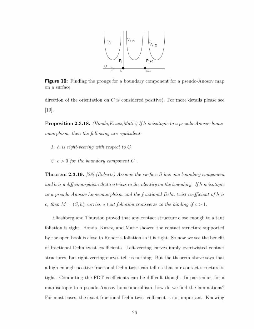
Figure 10: Finding the prongs for a boundary component for a pseudo-Anosov mapon a surface

direction of the orientation on C is considered positive). For more details please see

[19].

Proposition 2.3.18. (Honda,Kazez,Matic) If h is isotopic to a pseudo-Anosov home-

omorphism, then the following are equivalent:

1. h is right-veering with respect to C.

2. c > 0 for the boundary component C .

Theorem 2.3.19. [28] (Roberts) Assume the surface S has one boundary component

and h is a di↵eomorphism that restricts to the identity on the boundary. If h is isotopic

to a pseudo-Anosov homeomorphism and the fractional Dehn twist coe�cient of h is

c, then M = (S, h) carries a taut foliation transverse to the binding if c > 1.

Eliashberg and Thurston proved that any contact structure close enough to a taut

foliation is tight. Honda, Kazez, and Matic showed the contact structure supported

by the open book is close to Robert’s foliation so it is tight. So now we see the benefit

of fractional Dehn twist coe�cients. Left-veering curves imply overtwisted contact

structures, but right-veering curves tell us nothing. But the theorem above says that

a high enough positive fractional Dehn twist can tell us that our contact structure is

tight. Computing the FDT coe�cients can be di�cult though. In particular, for a

map isotopic to a pseudo-Anosov homeomorphism, how do we find the laminations?

For most cases, the exact fractional Dehn twist co�cient is not important. Knowing

26

a lower bound, such as c > 1 is all we need to say the structure is tight. To that end,

Roberts and Kazez gave a method for bounding a fractional Dehn twist coe�cient.

Let h be a pseudo-Anosov homeomorphism on a surface S. Let ↵ be an oriented,

properly embedded arc which begins on a boundary component C. Isotop the ↵ and

h(↵), relative to their boundaries, to intersect minimally. Define ih(↵) to be a signed

count of the number points, x, in the interiors of ↵ and h(↵) with the property that

the union of the initial segments of these arcs, up to x, is contained in an annular

neighborhood of C. More details can be found in [20].

Theorem 2.3.20. [20] Suppose h is right-veering at C. Then either

1. c(h) /2 Z and ih(↵) = bc(h)c or

2. c(h) 2 Z and ih(↵) 2 {c(h)� 1, c(h)}.

27

Chapter III

TOPOLOGICAL BRANCHED COVERS

Our overarching goal is to understand 3-manifolds using branched covers. We will see

that any 3-manifold can be seen as a cover branching over some knot in S3. First we

need to understand the basics. We will start with the 2-manifold case, then use those

results to develop the 3-manifold case. Finally, we will introduce a beautiful and

useful theory called coloring the branch locus. This method will be fundamental in

our main proofs. After presenting the basics, we will discuss some of the history and

important results in the field, as well as prove results about constuction of branched

covers and improvements on 3-manifold constructions.

3.1 Ordinary Covering Spaces

Recall a map p : M ! N is called a covering if there exists an open cover {U↵} of N

such that for each ↵, p�1(U↵) is a disjoint union of open sets in M , each of which is

mapped homeomorphically onto U↵ by p. It will be helpful to review some facts from

algebraic topology about covering spaces. First, we recall an important classification

theorem for covering spaces.

Theorem 3.1.1. [12] Let X be a CW-complex. The isomorphism classes of connected

coverings of X preserving base points are in 1� 1 correspondence with the subgroups

of ⇡1(X, x0).

This relationship is of course that for any covering space p : ( eX, ex0) ! (X, x0),

the corresponding subgroup H of ⇡1(X, x0) is p⇤(⇡1( eX, ex0)) [12].

28

3.1.1 The Monodromy

Given a connected n-fold covering space p : eX ! X we get a homomorphism

m : ⇡1(X, x0) ! Sn

(where Sn is the symmetric group of n letters) as follows: let x1, . . . , xn be any fixed

numbering of the points in p�1(x0). Given any loop � : S1 ! X based at x0 let e�i

be the lift of � to a path beginning at xi. The other end point of the path will be

a point xk. We define ��(i) = k. Clearly �� is an element of Sn and one can easily

check that it is independent of the homotopy class of � as a based loop. Thus we can

define m([�]) = �� where [�] is the element of ⇡1(X, x0) that � defines. Notice that

if we labeled the points in another order then we would get another homomorphism

that was conjugate to the one above.

So to every connected n-fold covering space we get a conjugacy class of represen-

tation called the monodromy of the covering space. Notice that if the covering space

is not connected we still get a monodromy representation.

Lemma 3.1.2. [12] If p : eX ! X is an n-fold covering space then eX is connected

if and only if the image of the monodromy acts transitively on {1, . . . , n}. More

precisely the number of components of eX is precisely the number of equivalence classes

of {1, . . . , n} under the action of the image of the monodromy.

Given a connected manifold X and a homomorphism m : ⇡1(X, x0) ! Sn, choose

one representative i1, ..., in from each equivalence class of {1, ..., n} under the action

of ⇡1(X, x0). Let Hj = {g 2 ⇡1(X, x0) : m(g)(ij) = ij} and eXj the covering space

corresponding to Hj. If eX = [nj=1

eXj then eX ! X is a covering space of X for some

labeling of the points p�1(x0) one may check that the monodromy of p is m.

So to every monodromy representation of ⇡1(X, x0) into Sn we get an n-fold cov-

ering space and it will be connected if and only if the image of the monodromy acts

transitively on 1, . . . , n.

29

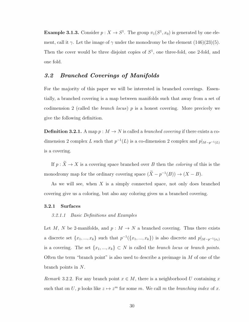
Example 3.1.3. Consider p : X ! S1. The group ⇡1(S1, x0) is generated by one ele-

ment, call it �. Let the image of � under the monodromy be the element (146)(23)(5).

Then the cover would be three disjoint copies of S1, one three-fold, one 2-fold, and

one fold.

3.2 Branched Coverings of Manifolds

For the majority of this paper we will be interested in branched coverings. Essen-

tially, a branched covering is a map between manifolds such that away from a set of

codimension 2 (called the branch locus) p is a honest covering. More precicely we

give the following definition.

Definition 3.2.1. A map p : M ! N is called a branched covering if there exists a co-

dimension 2 complex L such that p�1(L) is a co-dimension 2 complex and p|M�p�1(L)

is a covering.

If p : eX ! X is a covering space branched over B then the coloring of this is the

monodromy map for the ordinary covering space ( eX � p�1(B)) ! (X � B).

As we will see, when X is a simply connected space, not only does branched

covering give us a coloring, but also any coloring gives us a branched covering.

3.2.1 Surfaces

3.2.1.1 Basic Definitions and Examples

Let M , N be 2-manifolds, and p : M ! N a branched covering. Thus there exists

a discrete set {x1, ..., xk} such that p�1({x1, ..., xk}) is also discrete and p|M�p�1(xi)

is a covering. The set {x1, ..., xk} ⇢ N is called the branch locus or branch points.

Often the term “branch point” is also used to describe a preimage in M of one of the

branch points in N .

Remark 3.2.2. For any branch point x 2 M , there is a neighborhood U containing x

such that on U , p looks like z 7! zm for some m. We call m the branching index of x.

30

Figure 11: Cyclic Branched Cover over Disk

Example 3.2.3. Let p : D2 ! D2 by z 7! z3, as shown in Figure 11. Notice that

every point other than the origin has exactly three preimages, like the point z in

the figure. But the origin has one preimage, the origin. Therefore, this is a 3-fold

branched covering with branch locus the origin.

Figure 12: Branched Cover of 2-sphere by genus 2 surface.

Example 3.2.4. Let p : ⌃g ! ⌃g/� = S2 where � : ⌃g ! ⌃g is hyperelliptic

involution. Figure 12 shows the case for g=2. Notice there would always be 2g + 2

branch points.

Riemann-Hurwitz Formula. Recall that if ⌃g,d is a surface with genus g and d

boundary components, then the Euler characteristic of ⌃g,d is given by the formula

�(⌃) = 2� 2g � d

The Euler characteristic is a tool for idenifying a surface. Recall that any surface is

determined up to homeomorphism by the Euker characteristic and number of bound-

ary components. For an n-fold covering map p : M ! N , we have the relationship

�(M) = n�(N). The Riemann-Hurwitz formula generlizes this to the case of branch

covers.

31

Theorem 3.2.5. [27] (Riemann-Hurwitz Formula) Suppose p : M2 ! N2 is an n-fold

branched covering of compact 2-manifolds, y1, ..., yj are the preimages of the branch

points, and d1, ..., dj the corresponding branching indices. Then

�(M) = n�(N)�jX

i=1

(di � 1)

It is a standard result of complex analysis that any compact orientable surface

M can be seen as some branched cover over the disk (if M has boundary) or the

sphere (if M is closed). Restrictions can be placed on either the fold of the cover or

the number of branched points without changing the result. In particular, for every

closed surface (so M a sphere with g holes) Example 3.2.4 shows there exists a 2-fold

cyclic branched covering of M over the sphere with 2g+2 branched points. It is also

known that there exists a branched covering of M over the sphere with exactly three

branched points.

3.2.1.2 Colorings of Branch Sets in Surfaces

Lemma 3.2.6. Given any surface ⌃ and finite set of points B, any ordinary finite

fold covering space of ⌃� B extends to a covering space of ⌃ branched over B.

Proof. Let ⌃ be a surface, B a finite set of points on ⌃, and X = ⌃/B. Let eX be a

covering space of X. Then we have a covering map p : eX ! X. We want to extend p

to a branched cover p0 : e⌃! ⌃. Intuitively, e⌃ is constructed by filling in the “holes”

of eX and near those holes, p0 looks like z 7! zm for some m.

Let b 2 B. We have a disk Db containing b such that the annulus Ab = Db � b is

contained in the image of p. Because p is a covering, the inverse image under p of Ab

must be disjoint annuli. Let A be one of those annuli. For any fixed radius r, we can

isotop p on the circle of radius r inside A to be the map (r, ✓) 7! (r, n✓) for some n.

Then on a subannuli of A we can isotop further to (r, ✓) 7! (rn, n✓) = zn. This map

clearly can be extended to the disk.

32

It is clear then how to color the branch locus for any branched covering over a

surface. In general, specifying a coloring of the branch locus of a surface will not deter-

mine a unique branched covering space. If the surface downstairs is simply connected

then any combinatorial data coloring the branch locus will uniquely determine the

covering manifold. Because the surface is simply connected, we can label any point

independent of the colorings of the other points in the branch locus: the coloring of

each branch point is determined by the preimage of based loops in the fundamental

group, and for a simply connected surface, there are no relations between those loops.

In particular if the base is D2 then we have the following simple description.

The branched set B is a collection of points B = {x1, . . . , xk}. We know the

fundamental group of D2 � B is

⇡1(D2 � B, x0) = ⇤kZ,

where x0 is any base point and ⇤kZ means the free product of Z with itself k times,

that is ⇤kZ is the free group on k generators. Thus one may specify a monodromy

and hence a cover of D2 � B by choosing k arbitrary elements of Sn.

To make this more explicit we set some notation that will be used throughout the

rest of the paper.

Remark 3.2.7. Assume that D2 is the unit disk in R2. Let x1, . . . , xn be points on

the y-axis contained in D2 so that their indices increase as one moves up the y-axis.

Let x0 be the point (�1, 0). We can now pick explicit generators of ⇡1(D2�B, x0) as

follows. Let si be a circle of radius ✏ about xi where ✏ is chosen so that all the si are

disjoint. Now let �i be the loop that starts at x0 goes along the straight line towards

xi until it hits si, then traverses si counterclockwise and finally returns to x0 along

the straight line. Notice that �1, . . . , �n generate ⇡1(D2�B, x0). Thus the generators

of ⇡1(D2 � B, x0) are in one to one correspondence with the branched locus B.

So one can specify a “coloring” ofD2�B by labeling the points in B with elements

33

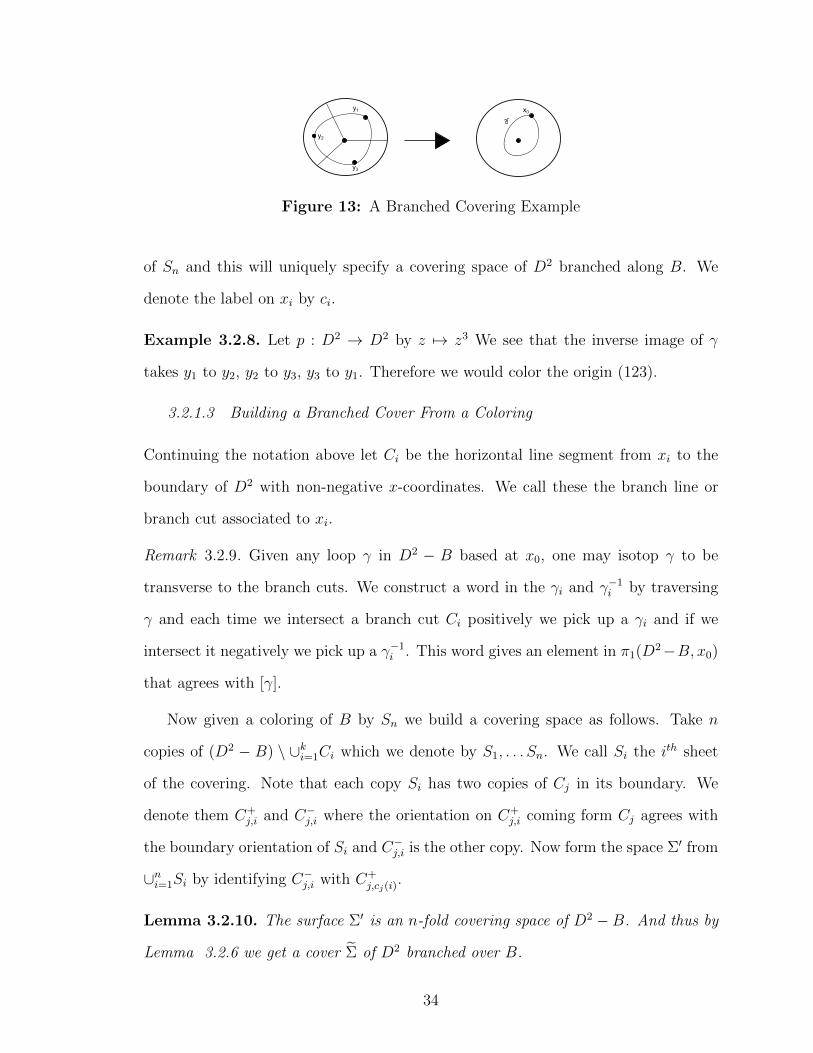
Figure 13: A Branched Covering Example

of Sn and this will uniquely specify a covering space of D2 branched along B. We

denote the label on xi by ci.

Example 3.2.8. Let p : D2 ! D2 by z 7! z3 We see that the inverse image of �

takes y1 to y2, y2 to y3, y3 to y1. Therefore we would color the origin (123).

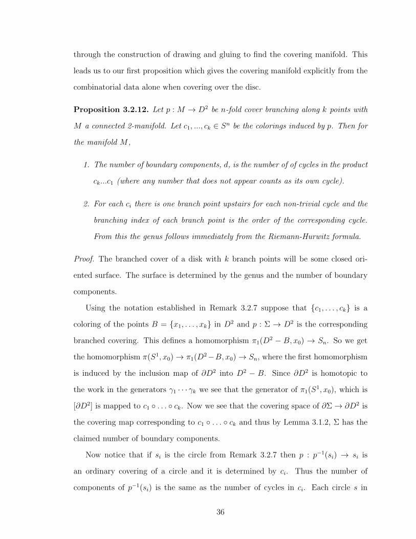
3.2.1.3 Building a Branched Cover From a Coloring

Continuing the notation above let Ci be the horizontal line segment from xi to the

boundary of D2 with non-negative x-coordinates. We call these the branch line or

branch cut associated to xi.

Remark 3.2.9. Given any loop � in D2 � B based at x0, one may isotop � to be

transverse to the branch cuts. We construct a word in the �i and ��1i by traversing

� and each time we intersect a branch cut Ci positively we pick up a �i and if we

intersect it negatively we pick up a ��1i . This word gives an element in ⇡1(D2�B, x0)

that agrees with [�].

Now given a coloring of B by Sn we build a covering space as follows. Take n

copies of (D2 � B) \ [ki=1Ci which we denote by S1, . . . Sn. We call Si the ith sheet

of the covering. Note that each copy Si has two copies of Cj in its boundary. We

denote them C+j,i and C�

j,i where the orientation on C+j,i coming form Cj agrees with

the boundary orientation of Si and C�j,i is the other copy. Now form the space ⌃0 from

[ni=1Si by identifying C�

j,i with C+j,cj(i)

.

Lemma 3.2.10. The surface ⌃0 is an n-fold covering space of D2 �B. And thus by

Lemma 3.2.6 we get a cover e⌃ of D2 branched over B.

34

Figure 14: Example of a Construction

Proof. Let {U↵} be an open cover of D2 � B such that for every ↵, U↵ intersects

at most one Cj and for any Cj which does intersect U↵, U↵ \ Cj is a connected set.

(This condition is not necessary but will make our work simpler.) For any ↵, if U↵ is

disjoint from each Cj, then by construction each preimage p�1(U↵) is clearly mapped

homeomorphically onto U↵. If U↵ intersects some Cj, then Cj divides U↵ into two

pieces, call them U+↵ and U�

↵ where U+↵ is above Cj. (Recall that Cj is a horizontal

line segment with positive x coordinate so the notion of above means towards the

positive y direction.) Then each preimage of U↵ contains is cut in two pieces by the

preimages of Cj. We form ⌃0 by identifying C�j,i with C+

j,cj(i). Notice that this will

identify a preimage of U+↵ with a preimage of U�

↵ on each sheet above. Clearly then

this set, which we will call p�1(U↵)j,c(j) is identified homeomorphically with U↵.

Example 3.2.11. Suppose our disc downstairs had 2 branched points, one colored

(12) and the other colored (243). This describes a 4-fold cover, so first we take 4 copies

of the disc downstairs. Then we make branched cuts going out from each branched

point to the boundary of the disc. The combinatorial data shows how to glue the cuts

together. The Figure 3.2.1.3 shows the construction and we see the resulting surface

is a disc.

It is easy to see that more complicated coverings will get more complex to construct

very fast. Even for a simple coloring of points on a disc, it seems necessary to go

35

through the construction of drawing and gluing to find the covering manifold. This

leads us to our first proposition which gives the covering manifold explicitly from the

combinatorial data alone when covering over the disc.

Proposition 3.2.12. Let p : M ! D2 be n-fold cover branching along k points with

M a connected 2-manifold. Let c1, ..., ck 2 Sn be the colorings induced by p. Then for

the manifold M ,

1. The number of boundary components, d, is the number of of cycles in the product

ck...c1 (where any number that does not appear counts as its own cycle).

2. For each ci there is one branch point upstairs for each non-trivial cycle and the

branching index of each branch point is the order of the corresponding cycle.

From this the genus follows immediately from the Riemann-Hurwitz formula.

Proof. The branched cover of a disk with k branch points will be some closed ori-

ented surface. The surface is determined by the genus and the number of boundary

components.

Using the notation established in Remark 3.2.7 suppose that {c1, . . . , ck} is a

coloring of the points B = {x1, . . . , xk} in D2 and p : ⌃ ! D2 is the corresponding

branched covering. This defines a homomorphism ⇡1(D2 � B, x0) ! Sn. So we get

the homomorphism ⇡(S1, x0) ! ⇡1(D2�B, x0) ! Sn, where the first homomorphism

is induced by the inclusion map of @D2 into D2 � B. Since @D2 is homotopic to

the work in the generators �1 · · · �k we see that the generator of ⇡1(S1, x0), which is

[@D2] is mapped to c1 � . . . � ck. Now we see that the covering space of @⌃! @D2 is

the covering map corresponding to c1 � . . . � ck and thus by Lemma 3.1.2, ⌃ has the

claimed number of boundary components.

Now notice that if si is the circle from Remark 3.2.7 then p : p�1(si) ! si is

an ordinary covering of a circle and it is determined by ci. Thus the number of

components of p�1(si) is the same as the number of cycles in ci. Each circle s in

36

p�1(si) surounds exactly one branched point and the ramification index is the degree

of the cover s ! si.

Example 3.2.13. Let N = D2 with three branch points each colored (1234). Thus

we are representing a 4-fold cyclic cover p : M ! N with three branch points and

we want to find the covering manifold M . To calculate the number of boundary

components of M we compute (1234)(1234)(1234) = (1432) and see there is one

cycle so one boundary component. Now we compute the genus by first computing

the Euler characteristic. According to the theorem, the number of inverse images of

branch points is 3 because there are 3 non-trivial cycles, one for each branch point,

and each has branching index 4.

�(M) = n�(N)� 3(d� 1) = 4(1)� 3(3) = 4� 9 = �5

Now, �(M) = 2 � 2g � d so �5 = 2 � 2g � 1 and therefore the genus is 3. So M

is a surface with genus 3 and 1 boundary component. The cut and paste method

discussed above involving branch cuts will confirm this the cover is this surface.

Example 3.2.14. Let N = D2 with two branch points, colored (145)(23), and

(15)(43)(2). Thus we are representing a 5-fold cover p : M ! N with two branch

points and we want to find M . To calculate the number of boundary components of

M we compute (12)(43)(145)(23) = (13)(245) and see there are two disjoint cycles so

two boundary components. Now we compute the genus by first computing the Eu-

ler characteristic. Notice there are three inverse images with index two, one inverse

image with index three, and one with index 1.

�(M) = n�(N)� (3(2� 1) + 1(3� 1) + 1(1� 1)) = 5(1)� 3(1)� 2 = 0

Now, �(M) = 2 � 2g � d so 0 = 2 � 2g � 2 and therefore the genus is 0. So M is a

surface with genus 0 and 2 boundary components - an annulus. Again the cut and

37

paste method discussed above involving branch cuts will confirm this the cover is this

surface.

Corollary 3.2.15. If p above is a cyclic covering of D2 branched over k points,

then the number of boundary components is d = gcd(n, k) and the genus is g =

12 (k(n� 1) + (2� n� d)).

Proof. First we give the formula for the boundary. We showed above that the number

of boundary components is the number of cycles in the product ck...c1. For an n-fold

cover, each c1 = (12...n). If there are k branch points, then (ck...c1)(j) = (k + j)

mod(n). The order of the cycle containing j in the product ck...c1 is the number of

iterations before j comes back to itself; i.e. ck...c1(j) = (k+j) mod(n). Then j comes

back to itself after ngcd(n,k) iterations, meaning each cycle has length n

dand thus the

number of total cycles is exactly gcd(n, k).

And finally the formula for g:

�(M) = n�(N)�X

yi

(ri � 1)

�(M) = n⇥ 1� k ⇥ (n� 1) = n� kn+ k

And the genus then is given by the formula 2� 2g � d = n� kn� k. Solving for g,

g =1

2(k(n� 1) + 2� n� d))

3.2.2 3-Manifolds

Before we discuss the generalization of 2-manifold results to 3-manifolds, we will

present some basic definitions and constructions.

3.2.2.1 Basic Definitions

Let M , N be 3-manifolds and p : M ! N a branched covering. That is, there exists

a one-dimensional complex L such that p�1(L) is a one-dimensional complex and

38

p|M�p�1(L) is a covering.

Branched covers of surfaces have been well-understood for some time. Low-

dimensional topologists sought to determine if branched coverings could be as power-

ful a tool for studying 3-manifolds as they are for surfaces. The first progress on this

question was given by Alexander in the 1920s when he showed that every compact,

closed, oriented 3-manifold is some branched cover branching along a 1-complex in

S3 [2]. This result shows that branched covers are not simply a method for construct-

ing some 3-manifolds, but a tool for constructing every three-manifold. Yet this is

simply an existence result; the degree of the cover could be arbitrarily large and the

complex could be unusably complicated. One would like to know if, as with surfaces,

restrictions can be placed on the branch locus or the cover and still construct every

3-manifold. This questions was answered in 1980.

Theorem 3.2.16. (Hilden-Montesinos) Let M be a compact oriented 3-manifold.

Then there exists a 3-fold branched covering p : M ! S3 branching along a knot.

In Section 3.2 we saw that all surfaces can be constructed by either looking only at

covers with three branched points or looking only at 2-fold cyclic covers. Hilden and

Montessinos showed we can look only at all 3-fold covers to obtain all 3-manifolds.

Could we also look only at covers over one fixed branch locus, or over a finite set

of knots and still construct all closed oriented 3-manifolds, mirroring the result for

surfaces?

Universal Links. Not only can we restrict to a finite subset of links, but in fact

we can restrict to just one link. A link K is called universal if every 3-manifold can

be obtained as a branched cover branching along K. Thurston showed the existance

of universal links, [30] and since then many explicit universal links and knots have

been found, including the figure-eight knot, Borromean rings, Whitehead link, and

946 [18, 30]. Thus, to study closed oriented 3-manifolds, we can restrict either to

39

studying covers over one particular knot, or restrict to 3-fold simple covers and vary

the knots.

Though many results have been found involving the existance of branched cov-

erings with certain properties, the actual constructions are often di�cult. The next

two section will present some of the known methods for visualizing and constructing

branched covers, with particular emphasis on the case for three-manifolds. In addi-

tion, we will prove some results about their construction for both the case of surfaces

and 3-manifolds.

3.2.2.2 Coloring 3-manifolds

Lemma 3.2.17. Given any 3-manifold M link L in M , any ordinary finite fold

covering space of M � L extends to a covering space of M branched over L.

Near any point on L, we can intersect with a disk transverse to L and reduce this

problem to the same argument made in Lemma 3.2.6.

In general branched covers are complicated, but if the base is S3 then we have the

following simple description.

Any link in S3 can be assumed to miss a fix point in S3 and thus we can think

of links in S3 as the same a links in R3. Now for a link L in R3 we can project it

to the xy-plane (and after isotopy we can assume this projection is generic) to get a

diagram for L. A diagram is an immersed curve in R2 with only transverse double

points and at each double points over and under crossing information is recorded.

Recall the Wirtinger presentation: to each strand in the diagram we have a gen-

erator and to each crossing we have a relation. Recall that the generator for each

strand is really the meridian to the strand. That is take a base point x0 with very

positive z-coordinate and orient the knot L. Then you get the curve �i associated

to the ith strand as follows. Let Di be a small disk that is transverse the the ith

strand, intersects it once and does not intersect the other strands. Orient Di so that

40

it intersect L positively. Now let �i be the straight line form x0 to the point on @Di

closest to x0, then traverses @Di positively and then returns to x0 on the straight

line. These are the generators for ⇡1(S3 � L, x0).

Figure 15: The relations at crossings (reading left to right) where each a, b, c is anelement of Sn and points are colored with basepoint above the braid.

So a homomorphism ⇡1(S3 � L, x0) ! Sn is determined by specifying an element

of Sn for each generator, that is for each strand in the diagram, in such a way that

they satisfy the relations at the crossings. We call this a coloring of the diagram and

note that it determines a cover of S3 branched along the link L.

Lemma 3.2.18. If K is a connected knot, then for any n-fold branched cover along

K, each element coloring a strand of K must have the same number of disjoint cycles

of order j for all j 2 N.

Proof. Let the strands of K be colored c1, ..., ck. Start with any one arc, colored cj.

Flow along the knot until you come to the first crossing. Let ci by the color of the

crossing strand. Then the next piece of the knot (the arc reached by flowing under

the crossing) is colored either cicjc�1i or c�1

i cjci. Neither changes the cycle structure,

and therefore cj has the same cycle structure as the next piece of the knot. Continue

flowing along the knot. Because it is connected, every arc will be crossed and so each

piece must have the same cycle structure.

Coloring Open Braids. When the branch locus is presented as an open braid, in

addition to the fact that at any crossing we have a conjugacy relation that must be

satisfied, the colorings at the end must match the colors at the start of the braid.

Therefore, any one point on the braid can be colored anything, but then you must

push through the braid to see what restrictions are placed on the other colorings.

41

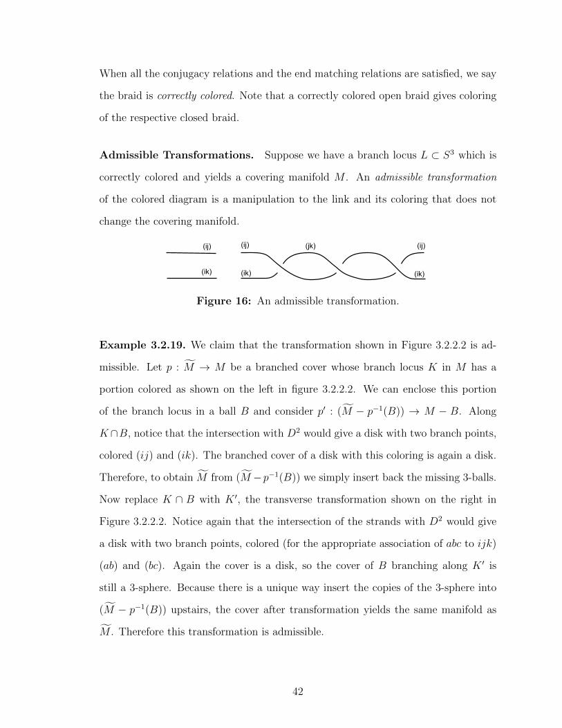
When all the conjugacy relations and the end matching relations are satisfied, we say

the braid is correctly colored. Note that a correctly colored open braid gives coloring

of the respective closed braid.

Admissible Transformations. Suppose we have a branch locus L ⇢ S3 which is

correctly colored and yields a covering manifold M . An admissible transformation

of the colored diagram is a manipulation to the link and its coloring that does not

change the covering manifold.

Figure 16: An admissible transformation.

Example 3.2.19. We claim that the transformation shown in Figure 3.2.2.2 is ad-

missible. Let p : fM ! M be a branched cover whose branch locus K in M has a

portion colored as shown on the left in figure 3.2.2.2. We can enclose this portion

of the branch locus in a ball B and consider p0 : (fM � p�1(B)) ! M � B. Along

K\B, notice that the intersection with D2 would give a disk with two branch points,

colored (ij) and (ik). The branched cover of a disk with this coloring is again a disk.

Therefore, to obtain fM from (fM �p�1(B)) we simply insert back the missing 3-balls.

Now replace K \ B with K 0, the transverse transformation shown on the right in

Figure 3.2.2.2. Notice again that the intersection of the strands with D2 would give

a disk with two branch points, colored (for the appropriate association of abc to ijk)

(ab) and (bc). Again the cover is a disk, so the cover of B branching along K 0 is

still a 3-sphere. Because there is a unique way insert the copies of the 3-sphere into

(fM � p�1(B)) upstairs, the cover after transformation yields the same manifold as

fM . Therefore this transformation is admissible.

42

3.3 Branched Covers of Contact Structures

How do we take branched covers of contact manifolds? In other words, given a

transverse link L in (M, ⇠) and branched covering p : fM ! M branching along L,

how would we define e⇠?

Construct fM as normal. Let eL = p�1(L). Then p : (fM � eL) ! M � L is a true

cover, and thus ⇠ = p⇤(⇠) on (fM � eL). Then extend to a plane field on all of fM and

perturb to make contact [13].

3.3.1 Generalizing Topological Results

Topologically, we know from the previous section that we can see any three manifold

as the branched cover over S3 and that we can restrict to looking only at 3-fold

covers or looking only at covers over a fixed knot. We want to try to generalize these

results to the contact manifolds. Can every contact manifold be seen as a cover over

(S3, ⇠std)? If so, what restrictions can be placed on the fold of the cover or the branch

locus without changing the answer? Giroux gave the following answer [14].

Theorem 3.3.1. (Giroux) Every contact manifold can be seens as a 3-fold simple

cover over some transverse link in (S3, ⇠std).

Thus every contact manifold is a branched cover over (S3, ⇠std), and (as with the

result of Hilden and Montesinos) we can restrict to looking at 3-fold covers. This is

not yet a full generalization, as it seems we may need to allow for multiple-component

links. We would like to have the same result as in the topological world and restrict

to covers over knots. Our next theorem does this.

Theorem 3.3.2. Given a contact manifold (M, ⇠), there exists a 3-fold simple cover

p : (M, ⇠) ! (S3, ⇠std) whose branch locus is a knot.

Proof. Let L be the branch locus for a cover coming from Theorem 3.3.1, presesnted

as a braid. Color the braid according to p. Take a D2 ⇥ I containing a section of

43

L with no crossings. For each adjacent pair of strands, if they do not belong to the

same connected component of the link, perform the admissible transformation shown

in Figure 3.2.2.2. Note that because Theorem 3.3.1 gives us a simple, 3-fold cover,

each strand will either be colored (12), (23), or (13).

This move connects the two previously separate components, does not change the

fact that the cover is 3-fold or simple, and does not change the manifold upstairs. All

that remains is to check that it does not change the contact structure. Notice that

the cover of any D2 ⇥ t is also a disk, so the cover of D2 ⇥ I is still a ball. This ball,

in the cover, is away from the binding and thus the contact structure on it is tight.

There is a unique tight contact structure on a ball so the contact structure remains

unchained under this transformation.

Contact Universal Links. Giroux’s theorem guarantees that any contact 3-manifold

can be obtained via some 3-fold simple branched cover, and the strengthening guar-

antees the branch locus can be a knot. As with topological 3-manifold, we would like

to also be able to obtain any contact 3-manifold by branching over some fixed knot

or link.

Definition 3.3.3. A transverse knot K is called contact universal if every contact

manifold (M, ⇠) can be realized as some cover p : M ! S3 with branch locus K.

3.4 Covers of Open Book Decompositions

Given an open book decomposition (⌃,�) for a manifold M and a knot inside K we

want to see how to take covers over M branching along K in terms of the open book.

We can consider the case where the knot is transverse to the pages, or is the binding.

Specifically, we want to look at two cases: cyclic covers branched over the binding

and general covers over S3 where K is braided through the pages.

Start with covers over S3. Let (D2, id) be the open book decomposition of S3.

44

Recall the notation ⌃t = ⌃ ⇥ {t} in ⌃ ⇥ [0, 1]. (Each ⌃t is a D2.) Let K be a knot

braided transversely through the sheets. Each ⌃0 intersects K at k distinct points.

Let Lt = K \ ⌃t. On ⌃0, label the points of L0 as x1, ...xk so that doing a half twist

�i would correspond to interchanding points xi and xi+1.

In any open book decomposition, the monodromy tells how to glue ⌃0 to ⌃1. Let

� be the composition of half-Dehn twists that trace out K. Because any map of the

disk is isotopic to the identity, the open book (D2,�) will also give S3. It can be

helpful for intuition to define a continuous family of maps �t to trace out the knot

as follows: �0 = id, �1 = �, �t : ⌃0 ! ⌃t so that �t(L0) = Lt. We will think of � as

the monodromy downstairs. Notice, that though � is isotopic to the identity on D2,

on D2 � L it is not.

Figure 17: Open Book Decomposition

Next let p : M ! S3 give a covering of S3. Color the knot as determined by the

map. Then each point of L0 inherits a corresponding color, as shown in figure 3.4. To

construct the cover, we need to make our branch cuts along ⌃0. To keep notation and

orientation consistant, we will make the branch cuts so that traversing the boundary

in the positive direction crosses the branch cuts in the order c1, ..., ck.

Notice now that we commutative diagram as seen below. It is important to note

that this composition is continuous; in particular that given a curve � downstairs and

a lift e� upstairs, p(e�(e�)) = �(�). By definition of the lift, for a curve � upstairs,

p(e�(�)) = �(p(�)).

45

e⌃e����! e⌃

??yp

??yp

⌃����! ⌃

Now we know how to calculate the page e⌃ of the open book for M - use the

same construction as for surfaces. However, the monodromy is significantly more

di�cult to calculate. In the case for cyclic covers, we can compute the monodromy,

though not in terms of the essential curves upstairs. In [17] is given a formula for the

monodromy of cylic covers in terms of specific curves they describe upstairs. No such

formula exists for a general cover.

Branching Over the Binding Now suppose K is the binding and we want to do

an n-fold cyclic cover. This case is actually very simple. If p is a branched cover over

(⌃,�) with branch locus K then any cyclic cover branched over the binding would be

(⌃,�n).

Lifting Open Books of Contact Manifolds Finally we want to consider using

open book decompositions to look at contact manifolds as covers over (S3, ⇠std). The

open book decomposition (D2, id) supports the contact structure. We take covers as

discussed previously, and the open book constructed determines a supported contact

structure on the covering manifold, as stated more formally below.

Theorem 3.4.1. Let K be a knot braided transversely through the pages of the open

book decomposition (D2, id), which supports (S3, ⇠std). Let (M, ⇠) be the covering con-

tact manifold obtained by branching over K. The open book constructed as described

above supports the contact manifold (M, ⇠).

46

Chapter IV

BRANCHED COVERS OVER TRANSVERSE KNOTS

Our goal is to understand the properties of covering contact structures from the

contact manifold downstairs and the combinatorial data of the branch locus. More

specifically, given a specific map (via combinatorial data) we want to know what is the

covering contact manifold or be able to determine properties of the covering contact

structure. Given a specific contact manifold, we would like to understand all possible

covers of that manifold over a fixed branch locus.

We will examine both of these problems, starting with what is already known.

The second problem will lay the groundwork for a very interesting area of study -

finding a contact unversal knot.

4.1 Branching Over a Contact Manifold

Given a contact manifold what can we say about the cover? We certainly know that

branched covers of tight manifolds need not stay tight. For example, the 2-fold cyclic

branched cover in S3 with the standard contact structure branched over the figure-

eight knot is overtwisted [17]. But once a structure is overtwisted, do all its branched

covers stay overtwisted? If not, how rare is it for a cover or an overtwisted manifold

to be tight?

Theorem 4.1.1. Given any 3-manifold M with any overtwisted contact structure,

there exists some transverse knot inside M such that some cyclic cover branching

over M is tight.

This is a somewhat surprising result, given the strong contrast to what happens for

true covering maps; all non-branched covers of overtwisted manifolds stay overwisted.

47

Proof. Let (M, ⇠) be any contact manifold. Let (⌃, f) be an open book for ⇠.

Recall Theorem 2.3.17 says we can positively stabilize (⌃, f) to get (⌃0, f

0) with

connectd boundary and f 0 a right-veering pseudo-Anosov di↵eomorphism. For sim-

plicity in notation, (⌃, f) will now refer to the stabilized open book. Our new open

book has connected binding B and monodromy f which is right-veering and freely

isotopic to a pseudo-Anosov homeomorphism.

Let c be the fractional Dehn twist of f on @⌃. Because f is right-veering, Propo-

sition 2.3.18 tells us that c > 0. Let � : (fM, e⇠) ! (M, ⇠) be the n-fold cyclic map

branching over B.

Lemma 4.1.2. (fM, e⇠) has open book (⌃, fn), and fn is isotopic to pseudo-Anosov

homeomorphism.

Proof. That (⌃, fn) is an open book for the covering manifold is immediate: The

covering manifold is constructed by cutting M along ⌃, taking n copies, and glueing

them together. Thus clearly the page upstairs is still ⌃, and the monodromy is fn.

We still need to show that fn is also isotopic to a pseudo-Anosov homeomorphism.

Let be the pseudo-Anosov homeomorphism isotopic to f . Then we have an

isotopy � : ⌃ ⇥ [0, 1] ! ⌃ such that �(x, 0) = f(x) and �(x, 1) = (x). We

need an isotopy e� : ⌃ ⇥ [0, 1] ! ⌃ from fn to n. We first define a series of

functions gk as follows. First let g2(x, t) = �(�(x, t), t). Then, for any k 2 N, k > 2

gk(x, t) = �(gk�1(x, t), t). Then define e� = gn(x, t). Notice that for n = 2, e�(x, 0)

= �(�(x, 0), 0) = �(f(x), 0)=f 2(x) and e�(x, 1) = �(�(x, 1), 1) = �( (x), 1)= 2(x),

similarly for larger n. Continuity of this isotopy is immediate from the continuity of

�. Therefore fn is isotopic to pseudo-Anosov homeomorphism n

Downstairs, we have one connected boundary component with a fixed number of

prongs x0, ...xk�1 given by and fractional Dehn twist coe�cient c ⌘ mk(mod 1), as

described in Section 2.3.4. Because the branching locus is the boundary and we are

48

taking a cyclic cover, we have still one boundary component upstairs with the same

number of prongs x0, ...xk�1 for n. And moves x1 to xm+1, therefore n would

take x1 to xn·c (mod c). Therefore the fractional Dehn twist n is n · c. Because we

know c > 0, for large enough n, n ·c > 1. By Theorem 2.3.19 this means large enough

n will yield a tight contact structure upsairs.

4.2 Covers over (S3, ⇠std)

Given a link L in (S3, ⇠std), what possible contact structures can be seen as covers

branching over L? Given a particular coloring, what can we say about its cover?

The goal of this section is to be able to give conditions on a knot or conditions

on its lift that will guarantee the covering manifold is tight or overtwisted. We will

do this by finding arcs who move to the left or to the right under the monodromy

upstairs and showing that the monodromy must be left or right veering.

As before we take our standard open book decomposition for (S3, ⇠std): (D2, id).

Let K be a transverse knot or link braided through the pages. On ⌃0, let � denote

an arc that begins and ends on the boundary of the disk and encloses exactly one

branch point, say xi, and its branch cut. (When it is important which branch point

is enclosed, we will use the notation �i.) Orient � so that xi is in the region to the

right of � as described in Section 2.3.3.

Let p be a branched covering with base (S3, ⇠std), branch locus K, and covering

manifold (M, ⇠). The lift e� of any � will have n components if p is a n-fold cover.

Let e�i denote be the piece of e� that has its endpoints on the ith sheet upstairs.

Notice that determining if �(�) is to the left or to the right of � on D2 � L0 is

simply a matter of looking at the image of � under the half twists that correspond

to the braid word. (Of course, on D2 they will be isotopic to each other.) However,

determining if e�(e�) is to the left or to the right of e� on e⌃ is a significantly more

complex probem because the exact ramifications of the branch points can result in

49

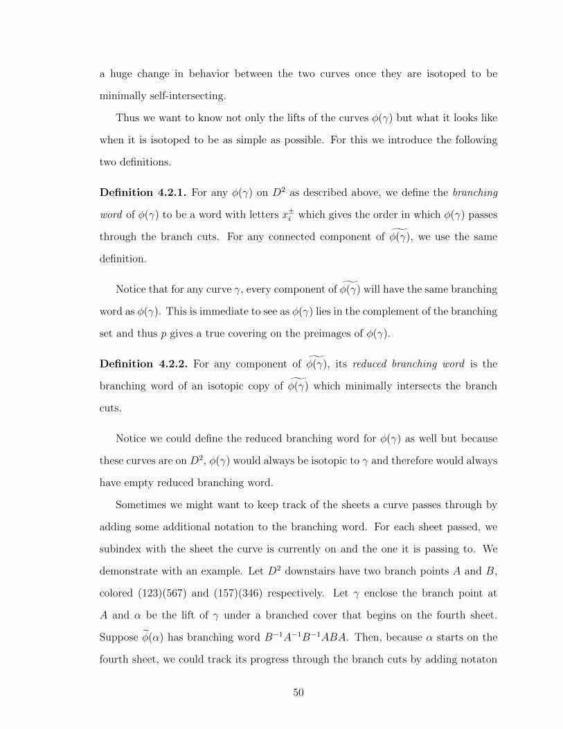
a huge change in behavior between the two curves once they are isotoped to be

minimally self-intersecting.

Thus we want to know not only the lifts of the curves �(�) but what it looks like

when it is isotoped to be as simple as possible. For this we introduce the following

two definitions.

Definition 4.2.1. For any �(�) on D2 as described above, we define the branching

word of �(�) to be a word with letters x±i which gives the order in which �(�) passes

through the branch cuts. For any connected component of g�(�), we use the same

definition.

Notice that for any curve �, every component of g�(�) will have the same branching

word as �(�). This is immediate to see as �(�) lies in the complement of the branching

set and thus p gives a true covering on the preimages of �(�).

Definition 4.2.2. For any component of g�(�), its reduced branching word is the

branching word of an isotopic copy of g�(�) which minimally intersects the branch

cuts.

Notice we could define the reduced branching word for �(�) as well but because

these curves are on D2, �(�) would always be isotopic to � and therefore would always

have empty reduced branching word.

Sometimes we might want to keep track of the sheets a curve passes through by

adding some additional notation to the branching word. For each sheet passed, we

subindex with the sheet the curve is currently on and the one it is passing to. We

demonstrate with an example. Let D2 downstairs have two branch points A and B,

colored (123)(567) and (157)(346) respectively. Let � enclose the branch point at

A and ↵ be the lift of � under a branched cover that begins on the fourth sheet.

Suppose e�(↵) has branching word B�1A�1B�1ABA. Then, because ↵ starts on the

fourth sheet, we could track its progress through the branch cuts by adding notaton

50

for the sheets as follows: B�143 A

�132 B

�122 A23B34A44. We call this the detailed branching

word.

Now with this notation we can obtain the reduced branching word for e�(↵) in two

steps. First, remove any letters where no branching occurs. In our example above we

would be left with B�143 A

�132 A23B34. Next, remove any adjacent letters that cancel each

other out, keeping in mind that for transpositions any letter is its own inverse. Here

we would be left with B�143 B34, and then the empty word. Therefore, without drawing

it out, we know that e�(↵) is isotopic to ↵. To give one more example, if for the same

colorings we had chosen ↵ to be the component that began on the third sheet, then

the branching word would be B�136 A

�165 B

�151 A12B22A23 so the reduced branching word

would be B�136 A

�165 B

�151 A12A23.

When it becomes important to clearly distinguish between the branched point and

the coloring of the branched point, we will use the following convention for notation.

Capital letters will signify the specific points, and lower case letters will signify the

colorings of those points as determined by the branched covering.

Before we use these definitions to prove any results, we will first see many examples

of the branchng word and reduced branching word.

Figure 18: Finding the Branching Word

Example 4.2.3. The branching word of the curve seen in Figure 18 would be (reading

left to right) BA�1C�1A.

Example 4.2.4. The branching word of � and of and each component of e� as seen

in Figure 19 would both be ABAB�1A�1B�1.

51

Figure 19: Finding the Branching Word

Figure 20: The Reduced Branching Word

Example 4.2.5. The reduced branching word of any component of e� from Figures 19

and 20 would both be the empty word.

Figure 21: The Reduced Branching Word

Example 4.2.6. The branching word of � in Figure 21 is BC�1B�1C�1ACBA�1.

The reduced branching word is BC�1A�1.

Before we get to our main proofs we need a lemma.

Lemma 4.2.7. Let (D2,�) be the open book for (S3, ⇠std), K a transverse link braided

through the pages and � the map induced by the braid word of K. The page D2

intersects K at k distinct points. Let x1, ..., xk be the branch points, colored by c1...ck.

Let p be a branched covering map over (S3, ⇠std) with branch locus K and � on D2

52

be a curve that encloses exactly one branch point xi and is disjoint from the branch

cuts so that xi lies in the region to the right of �. If for some component ↵ of e�, the

reduced branching word of e�(e↵ does not start with xi then e� is left-veering.

Proof. Let ↵ be a component of e� such that the reduced branching word of e�(e↵ does

not start with xi. Because � encloses xi downstairs, ↵ will locally (restricting to

the sheet on which it starts) enclose one preimage of xi. Isotop e�(↵) to minimally

intersect the branch cuts. Because ↵ has reduced branching word that does not begin

with xi, we know that after isotoping to intersect the branch cuts minimally, e�(↵)

crosses a branch cut other than xi first. Let t 2 [0, 1] be such that e�(↵(t)) is the point

where e�(↵) first crosses the branch cut. Then the subarc of e�(↵) connecting e�(↵(0))

to e�(↵(t)) can be isotoped to never cross ↵. This subarc would thus lie in the region

to the left of ↵, and therefore e�(↵) is to the left of ↵. Therefore e� is left-veering.

Theorem 4.2.8. Given any transverse knot that destabilizes, every cover branching

over that knot will be overtwisted.

Proof. Let p : (M, ⇠) ! (S3, ⇠std) be a branched covering, and S3 presented as the

open book (D2, id) with all the same notation as above. Let K be a stablization

of another transverse knot K 0, braided through the pages. Assume K 0 is a j-braid

whose braid work � is written in terms of �1, ..., �j�1. Then K is a j +1-braid whose

braid word is ���1j . (See Figure 22).

Figure 22: K’ inside the stabilized knot K

Color K as determined by the branched covering. Let A,B represet the strands

that would be twisted by �j, with B the strand that is also included in K 0. We will

53

use a and b to denote the respective colorings. Because the braid for K must match

up at each end, but there is only one crossing between thee strands, we see that a = b.

(See Figure 22).

Let � on D2 be an arc with endpoints on the boundary that encloses the branch

cut of A and passes through no other branch cuts. Because � encloses only A, and

no twist in � (the braid word for K 0) involves the j + 1 strand, �(�) involves only

one twist: it will start at the same points as � but enclose B after curving to the left

(see Figure 23.

Figure 23: �(�)

Choose any i such that B branches on the ith sheet. Let ↵ be the component of

e� which is contained on the ith sheet. We claim that e�(↵) is to the left of ↵, and

thus e� is left-veering. Recall from Chapter 2 that e�(↵) is isotopic to the component

of g�(�) which begins and ends on the ith sheet. By Lemma 4.2.7, we know that if the

reduced branching word of e�(↵) does not begin with xi then e� is left-veering.

Lift �(�). We chose i so that it is not fixed by B, and therefore the coloring of B

is an element of Sn which sending some number, call it h, to i . Then on the ith sheet,

e�(↵i) moves through the branch cut at B to the hth sheet (because � hits the branch

cut at B in a negative direction), and then hits the branch cut at A in a positive

direction. But we proved b = a, meaning A also sends h to i, and therefore e�(↵i)

then returns to the ith sheet, as shown in Figure 24.

The curve e�(↵i) passes first through the branch cut at B. And because it never

passes back through that same cut before it returns to the boundary on the ith sheet,

54

Figure 24: The section of g�(�) containing the ith and hth sheets

we know it cannot be isotoped away from the branch cut at B and thus has branching

word B�1A, which clearly cannot reduced [lemma to cite here]. Therefore, by Lemma

4.2.7, e� is left-veering. From Chapter 2 we know that (e⌃, e�) gives the open book

decomposition supporting (M, ⇠) and therefore (M, ⇠) is overtwisted.

Notice the main ideas of the proof that covers of stabilized knots are overtwisted

boiled down to two main points: First, that we had a ��1j to move arcs to the left and

no �j to move them back; and second that there was a curve that passed to a new

sheet at every branch cut, preventing the e�(↵i) to be pulled away from the branch cut

it crosses in the region to the left. Our next result is a generalization of this method.

Proposition 4.2.9. If K is transverse knot in (S3, ⇠std) whose braid word contains a

��1i and no �i for some i then any fully ramified cover branching over K is overtwisted.

Remark 4.2.10. This was proven in the cyclic case by [17].

Proof. Letting all notation be the same as before, we see we need to show exactly

the things mentioned above: that for some curve � which encloses some point A on

a page of the open book downstairs there is a component ↵i of its lift so that e�(↵i)

is to the left of ↵i.

Let K be a transverse knot in (S3, ⇠std) whose braid word contains a ��1i and no

�i for some i. Without loss, assume that the braid word starts with ��1i (cut the

55

braid accordingly). Choose � to be an oriented arc on the D2 page downstairs that

encloses xi+1 (from here on called A) so that A lies in the region to the right of �.

Claim. The curve �(�) is to the left of � on D2 � L0.

Proof. We can conjugate the braid word (cut at the appropriate position) so that the

first twist applied to � is ��1i . Notice ��1

i (�) is to the left of � on D2�L0. Any �±k for

k > i or k < i� 1 would not move ��1i (�). The only twist which could a↵ect ��1

i (�)

are �±i and �±

i�1. By assumption, no �+1i occurs in the braid word. Twists ��1

i and

�±i�1 would keep ��1

i (�) to the left of �. Continuing down the braid word, any �±i (�)

for k > i would still have no e↵ect on the initial behavior of the curve, and any �±k

for k < i � 1 or �i�1 would keep the image of � to the left of �. Therefore �(�) will

end up to the left of � on D2 � L0.

So downstairs we know that �(�) is to the left of � (on D2 � L0). Thus, for any

lift e� the initial tangent vector of e�(e�) at the initial point will be to the left of e�.

This means that whatever the branching word is for e�(e�), it will not begin with A.

Because p is a fully ramified branched cover, e�(e�) will branch at each sheet and thus

will have the same reduced branching word as branching word. Therefore the reduced

branching word will not begin with A, and thus by Lemma 4.2.7 e� is not right-veering

and so the covering contact structure is overtwisted.

Corollary 4.2.11. If K a transverse link in (S3, ⇠std) which is the figure-eight knot

with braid word �1��12 �1�

�12 , the Borromean rings with braid word �1�

�12 �1�

�12 �1�

�12 ,

or the Whitehead with braid word �1��12 �1�

�22 then and branched cover branching over

K which is fully ramified yields an overtwisted contact structure upstairs.

56

4.3 Contact Universal Knots

4.3.1 The Figure-Eight Knot

Because we have a classification of transverse knots with knot type the figure-eight

knot and know the only one that does not destabilize is that with maximal self-linking

number (�3), notice an immediate corollary of Theorem 4.2.8 is that a figure-eight

knot with any other self-linking number cannot be contact universal. So what about

the figure-eight knot with sl = �3 - could it be contact universal?

Theorem 4.3.1. Every cover of S3 branching over the figure-eight knot is overtwisted.

Proof. The figure-eight (with sl=-3) is a 3-braid so L0 is a set of three points x1 =

C, x2 = B, x3 = A. As in the previous section, let � be a curve that encloses

the branch cut at A. The monodromy � will take � and perform the half twists

�1��12 �1�

�12 . Figure 25 shows � and �(�).

Figure 25: Image of � under �

We need to show that there is a component ↵i of e� such that e�(↵i) is to the left of

↵i. Recall, from Lemma 4.2.7 we know it su�ces to show that that e�(↵i) has reduced

branching word that does not begin with A. Notice that the branching word for any

component ↵i is B�1AC�1A�1BA. Let a, b, c be the elements of Sn that color the

respective branch points A,B,C.

Lemma 4.3.2. If for some i, b�1(i) 6= i and c(a(b�1))(i) 6= a(b(i)) then the reduced

branching word for e�(↵i) does not begin with A or A�1.

57

Proof. The branching word for any component ↵i is B�1AC�1A�1BA. Suppose for

some i, e�(↵i) branches the first time is crosses the branch cut at B (i.e. b�1(i) 6= i)

and when it crosses the branch cut at C (i.e. c(a(b�1))(i) 6= a(b(i))). Say B takes j

to i. Then the detailed branching word for e�(↵i) would be B�1ji AikC

�1kl A

�1lmBmxAxj.

Where j is distinct from i and k is distinct from l. To remove the first term, B�1ji , it

would have to be canceled out by a Bij. But between the B�1ji and the only B+ term

is the C�1kl , which will not be removed in the first step because k is distinct from l and

cannot be cancelled out later because of the absense of the C+ term. Therefore at no

point in the reduction algorithm will B�1ji be adjacent to Bmx, and thus they cannot

cancel. This means the reduced branching word must begin with the B�1ji term.

Notice that by Lemma 4.2.7, if such a component as specified in the above lemma

did exist, then the covering contact structure would be overtwisted.

Lemma 4.3.3. Given any coloring of the figure-eight knot, there exists i, such that

b�1(i) 6= i and c(a(b�1))(i) 6= a(b(i)).

Proof. Suppose no such i existed. For each component e�(↵i), the branching word is

B�1AC�1A�1BA. Choose any i such that the coloring of B includes branching at i.

Then we assume that for any such e�(↵i), no branching occurs as it passes through the

branch cut at C, leaving us with a detailed branching word of B�1ji AikC

�1kk A

�1kmBmlAlj.

Then the resulting reduced branching word, after step 1 removed the C term, would

be B�1ji AikA

�1kmBmlAlj. Immediately we see that m = i because A takes i to k and

A�1 takes k to m. The partially reduced branching word can then be written as

B�1ji AikA

�1ki BilAlj. This allows us to cancel the A and A�1: B�1

ji BilAlj. Applyig the

same logic again we see that l = j, modifying the word to B�1ji BijAjj. Now we can

remove the A term and cancel the B and B�1 terms, giving us an empty reduced

branching word.

We just showed that if B sends i to j, but no branching occurs when e�(↵i) passes

58

through the branch cut at C, then the coloring of A does not include branching at j.

Therefore, no number present in the coloring of B is present in the coloring of A.

Figure 26: Coloring the Figure-Eight

Figure 26 shows the braid of the figure-eight, cut at ⌃0 = ⌃1. Let D be the only

arc of the braid that is alienated from ⌃0 and ⌃1 by crossings. Because the coloring

is correct, we immediately get the following relationships:

D = A�1BA

C = DAD�1

A = C�1BC

If A and B have no numbers in common then the first relationship above tell us

that D=B. Therefore D and A have no numbers in common, which means the second

relationship tells us that C = A. Then C and B have no numbers in common, so the

third relationship tells us that A = B, which is a contradiction.

Therefore, no coloring of the figure-eight has A and B without numbers in com-

mon, which brings us to a contradiction. Therefore our assumption, that there is no

component of e�(e�) which does not branch both the first time it crosses B and when

it crosses at C must be false.

So finally, we know there exists i such that b�1(i) 6= i and c(a(b�1))(i) 6= a(b(i)),

and therefore by Lemma 4.3.2 there exists a component of e� whose image has reduced

branching word that does not begin with A, and therefore by Lemma 4.2.7 e� is left

veering therefore any cover branching over the figure-eight is overtwisted.

59

4.3.2 The Whitehead Link

One might hope that any transverse braid whose braid word contains ��1i and no �i

for some i would have every cover overtwisted, as was the case with the figure-eight

and with destabilized links. This would help to rule out the Whitehead link as a

contact universal link. Yet this is not the case. Below is one counterexamples.

Theorem 4.3.4. Let L in (S3, ⇠std) be the transverse Whitehead link with braid word

�1��12 �1�

�22 . There exist covers branching over L that are tight.

Proof. Let K be the transverse Whitehead link with braid word �1��12 �1�

�22 in

(S3, ⇠std) with open book (D2,�). Let A,B,C denote the branch points on D2⇥ {0},

reading top to bottom (i.e. A,B would be twisted by �2, B,C would be twisted by

�1). Let p : (M, ⇠) ! (S3, ⇠std) a 9-fold branched covering branching over K given

by colorings a, b, c = (123), (145267389), and (123) respectively. Then by Propo-

sition 3.2.12 we know that the covering manifold will be a genus 1 surface with 3

boundary components.

Let � be an arc that begins and ends on the boundary of D2, enclosing the point

A such that A lies in the region to the right of �. Let � do the same for the point C.

�(�) has branching word B�1A�1BAC�1A�1B�1ABA. The curve �(�) has branching

word CA�1BAC�1A�1B�1A�1BACA�1B�1A.

Each of the curves �, �, �(�), and �(�) has nine preimages. Denote the preimages

of these curves with a subscript noting which sheet in the preimage the curve begins

and ends on. For examplle, g�(�)2 would be the preimage of �(�) which begins on

the sheet labeled with a 2. We want to focus on particular preimages of g�(�) and

g�(�), namely the preimages surrounding the ramfied preimages of A and C. The

branch point A downstairs has only one preimage which is ramified, where sheets 1,

2, and 3 connect, likewise for C. For these desired preimages (i = 1, 2, 3), the detailed

branching words are below.

60

g�(�)1: B�11,9A

�19,9B9,1A1,2C

�12,1A

�11,3B

�13,7A7,7B7,3A3,1

g�(�)2: B�12,5A

�15,5B5,2A2,3C

�13,2A

�12,1B

�11,9A9,9B9,1A1,2

g�(�)3: B�13,7A

�17,7B7,3A3,1C

�11,3A

�13,2B

�12,5A5,5B5,2A2,3

g�(�)1: C12A�12,1B14A4,4C

�14,4A

�14,4B

�14,1A

�11,3B3,8A8,8C8,8A

�18,8B

�18,3A3,1

g�(�)2: C2,3A�13,2B26A6,6C

�16,6A

�16,6B

�16,2A

�12,1B1,4A4,4C4,4A

�14,4B

�14,1A12

g�(�)3: C3,1A�11,3B38A8,8C

�18,8A

�18,8B

�18,3A

�13,2B2,6A6,6C6,6A

�16,6B

�16,2A2,3

Using the algebraic method described in the previous section, we achieve the

reduced branching words given below.

g�(�)1: A1,2C�12,1

g�(�)2: A2,3C�13,2

g�(�)3: A3,1C�11,3

g�(�)1: C12A�121

g�(�)2: C23A�132

g�(�)3: C31A�113

Therefore the preimages g�(�)i and g�(�)i can be isotoped to the curves show in

Figure 27. The curves �i and g�(�)i are shown, paired by color. (We should also

note that all of the algebraic work above can be confirmed using the cut and paste

method combined with brute force isotoping of curves, but we will not include those

calculations here.)

Claim. The open book constructed above destabilizes to (T, id) where T is the punc-

tured torus.

Recall that a positive stabilization of an abstract open book (⌃,�) is the open

book with page ⌃0 = ⌃[1-handle and monodromy �0 = � � ⌧c where ⌧c is a right-

handed Dehn twist along a curve c in ⌃0 that intersects the co-core of the 1-handle

61

Figure 27: The preimages of particular arcs after isotoping to be minimally inter-secting.

exactly one time. We want to show that our open book is a positive stabilization of

(T, id) by destabilizing our open book along particular curves.

Choose c to be the bolded blue curve shown in the image on the left in Figure 28.

Define � := D�1c � e� (D denotes a positive Dehn twist). The picture on the right in

Figure 28 shows �(e�i) and �(e�i) for the preimages from Figure 27 under � as well

as the original e�i and e�i for reference.

Figure 28: Images of curves under �.

Notice that � fixes the green curve. Therefore we can cut along it to destabilize

our surface. On the new surface choose d to be the bolded blue curve pictured in

Figure 29. Let �0 = D�1d ��. As before the images of our curves under �0 are below.

We see that the red curve is fixed, so we cut our surface along it to destabilize.

The two core curves are both fixed under �0, giving us a monodromy isotopic to

the identity. We then have shown that we can destabilize ⌃ to the punctured torus

with identity monodromy.

62

Figure 29: Images under �0.

Figure 30: Destabilized Open Book.

From [11] we know this open book yields the manifold (S1 ⇥ S2)#(S1 ⇥ S2) and

from [14] and [1] we know that when supported with this open book it is Stein fillable

and thus tight.

Therefore, we have constructed a cover over the transverse Whitehead link with

braid word �1��12 �1�

�22 which is tight.

This tells us that the Whitehead link has the potential to be contact universal,

but whether or not it is remains an open question.

63

REFERENCES

[1] Akbulut and Ozbagci, “Lefschetz fibrations on compact stein surfaces,” Ge-ometry and Topology, vol. 5, pp. 319–334, 2001.

[2] Alexander, J. W., “A lemma on systems of knotted curves,” Proc. Nat. Acad.Sci, 1923.

[3] Bennequin, D., “Entrelacements et equations de pfa↵,” Asterisque, 1983.

[4] Birman, J. S. and Brendle, T. E., Braids: A Survey. 2004.

[5] Colin, V. and Honda, K., “Stabilizing the monodromy of an open book de-composition,” TBD, 2007.

[6] Darboux, G., “Sur le problme de pfa↵,” Bull. Sci. Math., 1882.

[7] Eliashberg, “Classification of overtwisted contact structures on 3-manifolds,”Invent. Math., 1989.

[8] Etnyre, J. and Honda, K., “Cabling and transverse simplicity,” Ann. ofMath., p. 13051333, 2005.

[9] Etnyre, J. B., “Legendrian and transversal knots,” Handbook of Knot Theory,2005.

[10] Etnyre, J. B. and Honda, K., “On the non-existance of tight contact struc-tures,” Annals of Math., 2001.

[11] Etyre, J. B., “Lectures on open book decompositions and contact structures,”jgr, vol. 5, no. E2, pp. 103–105, 2006.

[12] Fenn, R., Techniques of Geometric Topology. Cambridge University Press, 1983.

[13] Geiges, “Contact geometry,” arXiv:math/0307242, 2004.

[14] Giroux, E., “Geometrie de contact: de la dimension trois vers les dimensionssuperieures,” Proceedings of the International Congress of Mathematicians, 2002.

[15] Gomph, E. E., “Handlebody construction of stein surfaces,” The Annals ofMathematics, pp. 619–693, 1998.

[16] Gray, J., “Some global properties of contact structures,” Ann. Math, pp. 421–450, 1959.

[17] Harvey, S.,Kawamuro, K., and Plamenevskaya, O., “On transverse knotsand branched covers,” Int. Math. Res. Not, Dec. 10 2009.

64

[18] Hilden, Lozano, and Montesinos, “Universal knots,” Bull. Ameri. Math.Soc. (N.S.), 1983.

[19] Honda, K., Kazez, W., and Matic, G., “Right-veering di↵eomorphisms ofcompact surfaces with boundary i,” Invent. Math., 2007.

[20] Kazez, W. and Roberts, R., “Fractional dehn twists in knot theory andcontact topology,” arXiv:1201.5290, 2012.

[21] Kronheimer and Mrowka, “Witten’s conjecture and property p,” Geometryand Topology, vol. 8, p. 295310, 2004.

[22] Markov, A., “Uber die freie aquivqlenz geschlossener zopfe,” Recueil Math.,1935.

[23] Ni, Y., “Heegaard floer homology and fibred 3-manifolds,” American Journal ofMathematics, vol. 131, pp. 1047–1063, 2009.

[24] Orevkov, S. and Shevchishin, V., “Markov theorem for transverse links,” J.Knot Theory Ramifications 12, p. 905913, Dec. 10 2003.

[25] Peter Ozsvath, Z. S., “Holomorphic disks and link invariants,”arXiv:math/0512286, 2005.

[26] Peter Ozsvath, Z. S., “The dehn surgery characterization of the trefoil andthe figure-eight knot,” arXiv:math/0604079, 2006.

[27] Prasolov, V. V. and Sossinsky, A. B., Knots, Links, Braids, and 3-Manifolds. American Mathematical Society, 1997.

[28] Roberts, R., “Taut foliations in punctured surface bundles, i,” Proc. LondonMath. Soc., p. 747768, 2001.

[29] Thurston and Winkelnkemper, “On the existence of contact forms,” Proc.Amer. Math. Soc., pp. 441–454, 1975.

[30] Thurston, W., “Universal links (preprint),” 1982.

65