bounds on the gain of network coding and broadcasting in wireless
TRANSCRIPT
University of Massachusetts - AmherstScholarWorks@UMass AmherstComputer Science Department Faculty PublicationSeries Computer Science
2007
Bounds on the Gain of Network Coding andBroadcasting in Wireless NetworksJunning LiuUniversity of Massachusetts Amherst
Follow this and additional works at: http://scholarworks.umass.edu/cs_faculty_pubsPart of the Computer Sciences Commons
This Article is brought to you for free and open access by the Computer Science at ScholarWorks@UMass Amherst. It has been accepted for inclusionin Computer Science Department Faculty Publication Series by an authorized administrator of ScholarWorks@UMass Amherst. For more information,please contact [email protected].
Liu, Junning, "Bounds on the Gain of Network Coding and Broadcasting in Wireless Networks" (2007). Computer Science DepartmentFaculty Publication Series. Paper 146.http://scholarworks.umass.edu/cs_faculty_pubs/146

1
Bounds on the Gain of Network Coding andBroadcasting in Wireless Networks
Junning Liu�, Dennis Goeckel
�and Don Towsley
��Dept. of Computer Science, University of Massachusetts, Amherst, MA
Email: � liujn,towsley � @cs.umass.edu�Dept. of Electrical and Computer Engineering, University of Massachusetts, Amherst, MA
Email: [email protected]
Abstract
Gupta and Kumar established that the per node throughput of ad hoc networks with multi-pair unicast trafficscales with an increasing number of nodes � as �������� �������� ��������� , thus indicating that network performancedoes not scale well. However, Gupta and Kumar did not consider the possibility of network coding and broadcastingin their model, and recent work has suggested that such techniques have the potential to greatly improve networkthroughput.
Here, for multiple unicast flows in a random topology under the protocol communication model of Gupta andKumar [1], we show that for arbitrary network coding and broadcasting in a ��� random topology that the throughputscales as ������� ��������"!#�$�� where � is the total number of nodes and !#��� is the transmission radius. When!#��� is set to ensure connectivity, �����%�& ������ � �'���(�)� , which is of the same order as the lower bound for thethroughput without network coding and broadcasting; in other words, network coding and broadcasting at mostprovides a constant factor improvement in the throughput. This result is also extended to other dimensional randomdeployment topologies, where it is shown that �����*�� ��+���,� for the �-� topology, �����*�� �� ./� 021 3547680 for 9(�networks and �;:<���>=? �� @A� 01 354 ACBED 0 in F#� , combined with the lower bounds of non-coding throughput, we show
coding&broadcasting provide no order difference improvement.Of course, in practice the constant factor of improvement is important; thus, to more precisely characterize
the benefit of network coding for multi-pair communication in wireless networks, we derive tight bounds for thethroughput benefit ratio - the ratio of optimal network coding scheme throughput to the optimal non-coding flowscheme throughput. We show that the improvement factor is .+GH.�G2HJI5K for �-� random networks, where LNM�O is a
parameter of the wireless medium that characterizes the intensity of the interference. We obtain this by giving tightbounds (both upper and lower) on the throughput of the coding and flow schemes. For ��� networks, we obtain anupper bound for the throughput benefit ratio as P��$�*=Q��R HTS � U .�G2HH for large � , where R HTS �?VXW,Y7Z��#[ � L K>\ �(L^] .This is obtained by finding a tighter upper bound for the coding scheme throughput and a tighter lower bound forthe flow scheme throughput.
We then consider the more general physical communication model as in Gupta and Kumar [1]. We show thatthe coding scheme throughput under the physical model is upper bounded by �� .0 for the �_� random network
and by ��`.a 0 for the ��� case. We also show the flow scheme throughput for the �-� case can achieve the same
order throughput as the coding scheme. Combined with previous work on a ��� lower bound [2], we conclude thatthe throughput benefit ratio under the physical model is also bounded by a constant. Thus we have shown for boththe protocol and physical model, the coding benefit on throughput is a constant factor.
Finally, we evaluate the potential coding gain from another important perspective - total energy efficiency - andshow that the factor by which the total energy is decreased is upper bounded by 9 .

2
I. INTRODUCTION
Multi-hop wireless networks have been intensively studied in recent years for both commercial and governmentapplications. Such networks, static or mobile, have the potential to serve as either a self-contained network thatprovides communication without the presence of an established infrastructure, or as a ubiquitous bridge betweenend users and the high speed wired infrastructure. Two representative applications are wireless sensor networks andwireless mesh networks. Multi-hop wireless sensor networks can be deployed randomly in geographic regions tocollect large volume of environment data and provide distributed query services. Wireless mesh networks can bepotentially deployed in the streets of big cities, campuses, conference centers, combat fields, etc. Hence, issues ofthe connectivity and capacity of such networks are of interest.
Even though these self-contained wireless mesh networks alone may not be enough to sustain all of the communi-cation among users, they probably will be mandatory for supporting the last several hops to the end users, and thusserve as a glue between the end users at any corner and the wired infrastructure. For either case, one major concernwith such wireless networks is scalability. Under a traditional communication model without network coding,Gupta&Kumar [1] shows that the per node throughput of such random networks scales as b�ced>fhgjihc kl mTnporqsm fwhere d is the total number of nodes in the network and each node needs to send to a randomly chosen destinationwith a rate of b�ctd>f . This result shows that as the total number of nodes increases, the many to many throughputdecreases polynomially. However, recent work by Ahlswede, Cai, Li and Yeoung [3] introduces the concept ofnetwork coding (NC), and there has been tremendous interest in applying network coding in both wired [4] andwireless networks [5] [6] [7]. For the wired case, the benefit of network coding in terms of throughput and capacityis often limited. Specifically, for networks with bidirectional links that can be modelled as an arbitrary undirectedgraph, [4] shows that the throughput improvement is upper bounded by a factor of u for the single multicast case,and upper bounded by one (no benefit) for the single unicast or broadcast case, and it is conjectured that there isno throughput benefit for the multi-pair unicast case; this is called the Li&Li conjecture, which is still open withno counter-examples found yet.
For wireless networks, network coding, combined with wireless broadcasting, can potentially improve the per-formance on throughput [6] [7], energy efficiency and congestion control [5] [6]. In addition, recent work by Kattiet al. [8] demonstrates the potential throughput benefit of applying network coding to wireless networks throughconstructive examples and experiments. Since network coding was not taken into consideration in Gupta&Kumar’soriginal work [1] and the related works that followed, an interesting question raised after [8] is how much throughputbenefit can it provide to such networks. Answering this question will help us to better understand not only thebenefit and limitations of network coding on the capacity of wireless networks and networks in general, but also thedegree of scalability of random wireless networks, thus providing design guidelines for the coverage ratio betweenwireless mesh net and the infrastructure wired net in hybrid networks.
The idea of [8] is to broadcast combined information (coded) of intersecting flows, and then each flow’s nexthop relaying node is able to decode its relaying flow’s traffic based on all of the broadcasts that it has received aswell as on local information (source data generated locally). In this way a node can potentially deliver to multipleneighboring nodes multiple data flows with a single broadcast transmission. An example of this is shown inFig. 1. Without network coding and broadcasting, four transmissions are required; however, when the opportunisticalgorithm of [8] is applied, with the middle node broadcasting the XOR of v and w , only three transmissions arerequired to move packets v and w forward two hops.
Thus, intuitively it appears that there could be a throughput benefit ratio proportional to the expected number of

3
neighbors, ihcexzy#{|d>f in the case of uniformly random deployed networks. However, here we demonstrate that sucha large improvement is not possible; in fact, only a constant improvement in throughput can be achieved. Sincebandwidth is a scarce resource in wireless networks, and also because we may not use the ad-hoc mesh networkalone to support the end to end traffic, the significance of the constant factor matters. So we further provide boundson the scalar throughput benefit ratio and extend the results to more realistic communication models.
aa
bb
a⊕⊕⊕⊕b a⊕⊕⊕⊕b
a b
b a
Without coding/broadcasting 4 transmissions
With coding/broadcasting 3 transmissions
Fig. 1. An example demonstrating the benefit of Katti etc. [8]’s opportunistic coding scheme
More formally, we first derive a tighter upper bound on the throughput of schemes aided by network coding andbroadcasting. We obtain this by analyzing the information rate across a sparsity cut of the network. By exploitingthe geometric constraints on the receivers’ locations, we derive a fairly tight upper bound on the maximum numberof simultaneous transmissions across any sparsity cut. This, combined with an information compression coding rateconstraint, yields the throughput upper bound for the coding scheme. Next, we derive a tighter lower bound forthe non-coding scheme throughput in a semi-constructive way by showing that there exist flow schemes within aconstructive framework that can achieve the lower bound throughput rate. With these two bounds together, we showthat in the u�} case, the constant factor improvement that network coding can provide for multi-pair concurrentunicast throughput is bounded as ~|ced>f`��u����>�(� ��kC� �� for large d , where ��� � is a parameter of the wireless
medium that characterizes the intensity of the interference and �(�>��g����E�)�(u;� � ���%�&u#��� . For the �,} case, weobtain a tight benefit ratio as kC� �kC� �%� � , i.e., we show that kC� �kC� �%� � throughput improvement is the maximum achievable.
The reason that we can get this tighter result for the �,} case is because of the lower geometric complexity in �,}than in the higher dimensional cases.
The protocol communication model of [1] is a nice abstraction of the wireless communication channel. A moregeneral and realistic refined model is the physical communication model [1]. To make our results more persuasive,we also analyze the throughput benefit of network coding under the physical model. We show that the codingscheme throughput is upper bounded by ihc km f for the �,} case and by ihc kl m f for the u�} case. We also show
a same order lower bound for the �,} flow scheme throughput. Combining this and [2]’s previous result on theu�} throughput lower bound, we demonstrate that the throughput benefit ratio of coding schemes is also at most aconstant under the physical model.
At first, our results might seem counter-intuitive, since, with network coding and broadcasting, each node cansend information to all neighbors with one transmission as demonstrated in [8]. However, essentially each node stillneeds to receive information one transmission at a time. In other words, whereas there is simultaneous transmission,there is no simultaneous receptions. Since the information flow rate across any node also needs to be conserved,the incoming information rate will be a bottleneck for the throughput improvement.
Another concern with multi-hop wireless networks is energy consumption. For either static or mobile nodes inthe network, the power is mostly supported by a self-carried battery which has limited energy. This is especiallytrue for low cost cheap sensors. [9] studies the problem of minimizing the total energy cost of collecting correlateddata at a single sink and proves that a special joint coding/routing scheme can achieve the minimum cost. In this

4
work, we evaluate the energy efficiency for multiple source-sink pair unicast traffic. We assume the data (messages)from different sources are independent of each other. Without network coding, the minimum cost scheme is tostraightforwardly send each source to its sink independently along a shortest path (in terms of energy cost) route.We focus on the further coding gain based on the minimum cost flow scheme. For both the coding scheme andflow scheme, we ignore the delay and throughput aspects and merely ask the question of how much energy couldbe further saved by exploiting network coding and broadcasting. [10] gives coding gain bounds for the limited casewhere overhearing is not used for coding, we conisder the more general case where coding is based on a node’scurrent possessed info. including all the overhearings and show that this energy benefit is at most a factor of � .Main Contributions Our main contributions are summarized as follows:� We show that, contrary to the common intuition, for multi-pair unicast traffic in wireless multi-hop networks,
the benefit of network coding and broadcasting on the concurrent throughput rate is upper bounded by aconstant factor for both the protocol model and the physical model. This is true for random deployed networksin �,} , u�} , ��} and in general �;} Euclidean space.� We further bound the constant factor as ~�ced>f'�&u����>�E� ��kC� �� for u�} networks and kC� �kC� �%� � for the �,} case.� We first characterize the throughput order of the coding scheme on such networks and also derive tight boundsfor the constants. We also develop tighter lower bounds for the non-coding scheme on such networks.� We show that the coding gain for energy efficiency is bounded by a constant factor of � for the COPE [10]type of point to point codings.
II. MODEL FORMULATION
For both static and mobile ad-hoc networks, we consider the network model of Gupta&Kumar [1], where d nodesare randomly located, i.e., independently and uniformly distributed, in a region of fixed area. The reason that thismodel is often justified is two-fold: first, in reality, deploying a large volume of static nodes is costly, and randomdeployment is the most economic option; second, even if the nodes are mobile, the mobility pattern is often eitherdynamically random or not available for use, or, even if the knowledge is present, the cost to use the mobilityinformation may not be worth its benefit(e.g. imagine mobile users in the streets of NYC); in addition, often thespeed of the node movement is much far below the wireless signal transmitting speed, and thus the mobile casecan be treated as a static random network for the lifetime of a packet.
Gupta&Kumar [1] studies two types of regions: a disk and the surface of a sphere, both with an area of onemeter squared. More generally, we do not limit the shape of the region or its dimension. However, for simplicityof presentation, we derive our results based on a unit square in two dimensions ( u�} ), a unit line segment in onedimension ( �,} ), and a unit cube in three dimensions ( ��} ).
There are d source-destination pairs in the network. Each node � in the network is a data source that needs toroute its data through multi-hop wireless communications to a destination node that is independently and uniformlyrandomly chosen. The same protocol and physical communication models as in Gupta&Kumar [1] are employed.
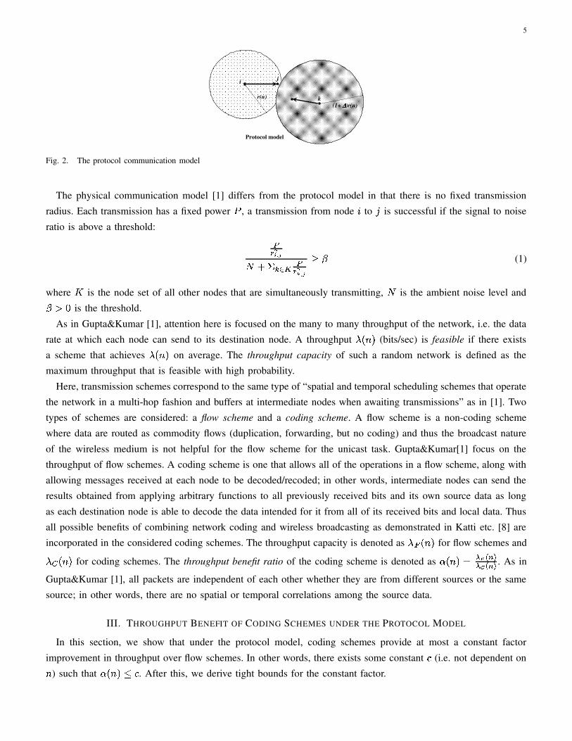
For the protocol model, as shown in Fig. 2, a transmission from node � to � is successful iff the distance betweenthem satisfies ¡�¢�£�¡�¤¥ s�&¦sced>f and any other simultaneously transmitting node � satisfies ¡�§)£�¡�¤¥ s¨©cr�;���ªf�¦sced>f .Here, ¡«¢ is node � ’s location, ¦;ced>f is the transmission radius and �¬�� ensures a safety zone that limits theinterference; in particular, � is a constant that depends on the properties of the wireless medium. In addition,there is a finite bandwidth limit of ® bits/sec for each transmission. In order to ensure connectivity, the fixed
transmission radius for the protocol model needs to be at least ¦sced>f>g©ihc l nporq;ml m f [1].
5
r(n)
i j
k(1+ ∆∆∆∆)r(n)
Protocol model
Fig. 2. The protocol communication model
The physical communication model [1] differs from the protocol model in that there is no fixed transmissionradius. Each transmission has a fixed power ¯ , a transmission from node � to � is successful if the signal to noiseratio is above a threshold: °
±C²³�´ µ¶ �&·¸§�¹�º°± ²AC´ µ ¨¼» (1)
where ½ is the node set of all other nodes that are simultaneously transmitting, ¶ is the ambient noise level and»¾�&� is the threshold.As in Gupta&Kumar [1], attention here is focused on the many to many throughput of the network, i.e. the data
rate at which each node can send to its destination node. A throughput b�ced>f (bits/sec) is feasible if there existsa scheme that achieves b�ced>f on average. The throughput capacity of such a random network is defined as themaximum throughput that is feasible with high probability.
Here, transmission schemes correspond to the same type of “spatial and temporal scheduling schemes that operatethe network in a multi-hop fashion and buffers at intermediate nodes when awaiting transmissions” as in [1]. Twotypes of schemes are considered: a flow scheme and a coding scheme. A flow scheme is a non-coding schemewhere data are routed as commodity flows (duplication, forwarding, but no coding) and thus the broadcast natureof the wireless medium is not helpful for the flow scheme for the unicast task. Gupta&Kumar[1] focus on thethroughput of flow schemes. A coding scheme is one that allows all of the operations in a flow scheme, along withallowing messages received at each node to be decoded/recoded; in other words, intermediate nodes can send theresults obtained from applying arbitrary functions to all previously received bits and its own source data as longas each destination node is able to decode the data intended for it from all of its received bits and local data. Thusall possible benefits of combining network coding and wireless broadcasting as demonstrated in Katti etc. [8] areincorporated in the considered coding schemes. The throughput capacity is denoted as b�¿�ced>f for flow schemes and
b�À'ced>f for coding schemes. The throughput benefit ratio of the coding scheme is denoted as ~�ced>f%gjÁ�Â2à m#ÄÁ�Å2à m#Ä . As in
Gupta&Kumar [1], all packets are independent of each other whether they are from different sources or the samesource; in other words, there are no spatial or temporal correlations among the source data.
III. THROUGHPUT BENEFIT OF CODING SCHEMES UNDER THE PROTOCOL MODEL
In this section, we show that under the protocol model, coding schemes provide at most a constant factorimprovement in throughput over flow schemes. In other words, there exists some constant � (i.e. not dependent ond ) such that ~�ced>f��&� . After this, we derive tight bounds for the constant factor.

6
A. Sparsity Cut for a Random Network
Before we present the throughput improvement results, we redefine sparsity cut for a random network.In general, a cut Æ is defined as a partition of the nodes in a graph, the cut capacity is the sum of the links’
bandwidths crossing the cut, and the sparsity cut is a cut where the cut capacity divided by the traffic demand is theminimum over all cuts. Since the network studied here is a random network embedded in an Euclidean space andtransmissions are between neighboring nodes, attention can be focused on a narrow class of cuts that are inducedby a line segment (or a plane in the ��} case) that cuts the region into two regions. The cut length Ç�È is defined asthe length of the cut line segment. The cut lines that we consider have zero width measuring such that no nodeslie on it. Denote the two subregions divided by the cut as Æ k and Æ � . A sparsity cut for a random network isdefined as a cut induced by the line segment with the minimum length that separates the region into two equalarea subregions. For the square deployment region illustrated in Fig. 3, the line segment É�Ê induces a sparsity cutÆÌË)Í . Since nodes are uniformly randomly deployed in a random network, such a sparsity cut captures the trafficbottleneck of these random networks on average. The cut capacity is defined as ceÎ È De´ 6 �ÏÎ È 6 ´ D f where Î È De´ 6 equalsthe transmission bandwidth ® times the maximum possible number of simultaneous transmissions (broadcast ornon-broadcast) across the cut from Æ k to Æ � 1; and Î�È 6 ´ D equals the same quantity from Æ � to Æ k . This cut capacityconstrains the information rate that the nodes from one side of the cut as a whole can deliver to the nodes at theother side as a whole. The number of sources in Æ k whose destinations are in Æ � is denoted as d�Ð De´ 6 .B. Throughput Order of Coding Scheme
The cut capacity is bounded by deriving an upper bound on the maximum number of simultaneous transmissionsacross the cut. It is easy to see that all of the direct receivers of transmissions across a cut Æ in one direction
lie in the shaded rectangle region with area Ç ÈÒÑ ¦sced>f as shown in Fig. 3. In [1], disks of radius � ± à m#Ä� centeredat each receiver are disjoint2. However, [1] does not exploit broadcast transmissions while a coding scheme does.As shown in Fig. 4, with the consideration of broadcast and network coding, observe that such disks centered atreceivers of the same sender (broadcast transmission) could overlap, disks centered at receivers of different sendersare still disjoint. In other words, we have the following Observation:
Observation 1: The union of disks (with radius± à m#Ä� ) centered at the receivers of one transmission should be
disjoint from the union of disks centered at the receivers of another transmission.1) u�} case::
Lemma 1: The capacity of a cut Æ for a u�} region has an upper bound of Ó�Ô"Õ Ð,Ö± à m�Ä where ����g×���E�^�Øk5ÙÚ � 6 � l Û� �Proof: The cut capacity is bounded by deriving an upper bound on the maximum number of simultaneous
transmissions across the cut. It is easy to see that all of the direct receivers of all transmissions across a cut Æ inone direction lie in the shaded rectangle region with area Ç È�Ñ ¦sced>f as shown in Fig. 3. When �ÝÜÞu , Observation
1 means each transmission across the cut consumes at least an area of k� �%c � ± à m#Ä� f � of the shaded region in Fig.3,with the minimum achieved when receiver lies in the corner of the shaded region. Thus, the maximum number of
simultaneous transmissions across the cut is upper bounded by the area of the shaded region divided by k� �%c � ± à m�Ä� f � ,which is k5ÙrÕ ÐÚ � 6 ± à m#Ä .
1The maximum number of bits of information per second that can be transmitted across the cut from one side ( ß)à ) to the other ( ßsá )2Otherwise some sender is within âtã)ä�å¸æèç�âzésæ of some other sender’s receiver.

7
1Γ
A
B
r(n)
2Γ
Fig. 3. Cut Capacity in 2D
Allowed…
…Not Allowed
……
2)(nr∆
Fig. 4. Interference of coding schemes in 2D
)(23 nr⋅∆≥
Ar(n)
)(nr∆
B
When ∆∆∆∆ ≥≥≥≥ 2222
Fig. 5. ê_ë Cut capacity: åíìªê case
When �ݨÞu , as shown in Fig. 5, any two receivers of two different transmissions require al Û� ��¦;ced>f difference
in their coordinates along the cut line. Thus, there can be at most Õ Ðl Û � ± à m�Ä � � �î�`�l Û Õ Ð� ± à m#Ä simultaneous transmissions
across the cut.

8
Since each transmission is able to send ® bits/sec, combining the two cases above, the cut capacity is upper
bounded by Î È De´ 6 �ïÓ�ÔsÕ Ð�Ö± à m�Ä and Î È 6 ´ D �ïÓ�Ô"Õ Ð,Ö± à m�Ä , where �,�&gð���E���Øk5ÙÚ � 6 � l Û� � .Corollary 1: The sparsity cut capacity of a u�} random network has an upper bound of Ó Ô Ö± à m�Ä .
Proof: Regardless of the shape of the unit area region, there exists a sparsity cut for each orientation of thecut line. If we rotate the cut line, there has to be at least one sparsity cut with cut length Ç È �Ý� . Hence, fromLemma 1, we derive the corollary.
Next an upper bound for the throughput of coding schemes in a u�} random network is derived.Theorem 1: The throughput of coding schemes in a u�} random network is upper bounded by ihc Öm ± à m�Ä fñgihc Öl m�nporqsm f
Proof: Assume the coding throughput of the d node random network is bÌÀ�ced>f . Then, by its definition, with highprobability (w.h.p.) there exists some coding scheme that, for some ò Üôó , during each time interval õ�ce�ö£Ò�Efeò��Ï�eòø÷(in seconds), every node can send ò^bTÀ'ced>f bits of information to its corresponding destination node. For a sparsitycut ÆÌË)Í in the middle, by a Chernoff bound [11] argument we have that w.h.p. there are ihced>f pairs of source-destination nodes that need to cross Æ Ë)Í in one direction, i.e., d Ð De´ 6 g d Ð 6 ´ D g�ihced>f w.h.p.. Now we view all ofthe nodes lying on the right side of É�Ê as a super node, and treat all of the distinct messages it receives fromthe left side of ÉùÊ within the time interval õ�ce�>£Þ�Efeòù�Ï�tòø÷ as a single ‘meta’ message ú . We denote the numberof bits of ú as Ê`û . According to the definition of our coding scheme, this meta message ú can be arbitrarilycoded but with only one coding constraint: by Shannon’s data compression theorem [12], in order for the right sidedestination nodes to decode the original data from the left side sources which are independent of each other, úhas to satisfy ÊXûü¨�òùdTÐ Dt´ 6 b)À'ced>f or Ê`ûü¨�ò^ihced>f8b)À'ced>f w.h.p..
At the same time, our work above has provided a capacity constraint that upper bounds Êhû . A broadcasttransmission across the cut to multiple receivers delivers identical information to the receivers; however, by thedefinition of ú , the identical messages will only be counted once in ú for one of the receivers. Also by thedefinition of cut capacity and Corollary 1, we get Ê û � Ó Ô Ö± Ã m#Ä ò . Combined with the coding constraint above,
we derive b À ced>f¸� Ó Ô Öý à m#Ä ± à m#Ä w.h.p.. Since ¦sced>f is at least ihc l n orq;ml m f to ensure connectivity [1], and throughput is
defined as a high probability quantity, we have b�À�ced>f|� Ó�Ô Öý à l mTnporq;m�Ä .Theorem 2: The u�} throughput benefit ratio is upper bounded by a constant:
~|ced>f%g©ihcr�EfProof: Gupta&Kumar [1] already establishes a lower bound for the throughput of flow schemes, b ¿ ced>fh¨
ihc Ó D Öà kC� � Ä 6 l mTnporq;m f where � k �Þ� is a constant. Combined with Theorem 1, we get ~|ced>f*gþÁ Å Ã m�ÄÁ  à m�Ä �ÿihcr�Ef . Meanwhile,
since coding scheme is a superset of flow scheme, ~|ced>f'¨©� , thus ~�ced>f*g©i«cr�Ef .This constant throughput benefit ratio is true for a random network deployed in any arbitrarily shaped region.
First, the upper bound for the throughput of the coding scheme still holds. Second, the constructive lower bound ofGupta&Kumar [1] can in fact be extended to arbitrarily shaped regions, even though the asymmetry may cause theconstructive scheme in [1] to have a skewed load distribution for some cut. Since the region is of fixed area, thethroughput loss due to the asymmetric shape will be a fixed constant factor as d increases. Thus, we have shownthat network coding combined with wireless broadcast provides no order-different improvement on the throughputof a random network deployed in any arbitrarily shaped u�} region.

9
2) 1D case: The �,} case is easier to deal with than the u�} case. Traffic either goes left or right along oneline. However, �,} differs from u�} in that the transmission radius does not affect the order of throughput. Thus,we are able to give a constructive lower bound for the �,} throughput that does not have a xzy#{'d factor as in theu�} and ��} cases.
First we make the following straightforward observation.Observation 2: Under the protocol, for any cut in the �,} line, there can be at most one transmission across the
cut (including both directions) at any given point in time.Lemma 2: The throughput of the coding scheme on a �,} random network is upper bounded by
b�À'ced>f|� u#®dProof: We prove this by showing that for any given constant �`�ð� that is arbitrarily small, b�À'ced>f�� � Öà k ��� Ä�m
for large d .Consider the sparsity cut �� that cuts the line segment in the middle. Using a Chernoff bound [11], it is easy to
show that the number of sources that need to send data across Æ � from left to right is larger than cr�|£���f m � w.h.p.,and that the same is true for the number of sources crossing the cut from right to left.
Applying the same technique as in Theorem 1 and by Observation 2, we have bÌÀ'ced>f8uscr�`£���f m � �N® , whichyields the desired result.
To our knowledge, there is no constructive lower bound for the throughput of a �,} random network yet. In thispaper, we first construct a lower bound for a �,} random network and show that its throughput capacity is on theorder of ihc Ö m f .
Lemma 3: The throughput of flow schemes on a �,} random network is lower bounded by
b ¿ ced>f�¨ ��� 6 ®dwhere ��� 6 gð� � � k� � � � � ��� ��� �ök� � .
Proof: We prove this by showing that for any given constant �^�ð� that is arbitrarily small, b ¿ ced>f�¨ Ó Ô 6 Öà kC� � Ä�mfor large d .
We choose a transmission radius ¦sced>fÒg ��� nporqsmm , divide the line deployed region into bins each of length± à m�Ä� g � � nporqsmm and all togetherm� � nporqsm bins. Then by the same union bound argument as in [13], w.h.p. every bin
contains at least one node. Furthermore, a node in one bin can reach any node in an adjacent bin directly.Routing consists of hopping from one bin to the next bin in direction of the destination unless the destination
is in the same bin as the source. Any node in the next bin can be a relay but for the last bin the algorithm willchoose the destination node itself.
Next we show that there exists a spatial&temporal scheduling scheme that on average allows each bin a chance totransmit ® bits to each of its two neighboring bins every ���E��� 6 seconds. This is done by mapping the bin-hoppingtransmissions to a new graph. For each bin we construct two virtual vertices in a new graph, one for transmissionsfrom this bin going to the right, one for transmissions going left. We connect any two vertices in the new graphwith an edge if the transmissions that they represent could potentially interfere with each other when occurringsimultaneously. When �ÝÜ©� , each vertex in the new graph will have a degree of at most ��� . By the graph coloringtheorem [14], ���>�í� colors are enough to color the vertices s.t. no two interfering vertices (transmissions) have the

10
same color. This gives a schedule of length ��� where each bin gets a chance to transmit to both directions. When� ¨ � , we count the potential interfering bin transmissions and it is not hard to see that the vertex degree is atmost ���tu#���¸�©�,� , so there is a schedule of length ���tu#���ø�×�#� . Combining these two cases, we have on averagethat every ���E��� 6 seconds each bin will get a chance to transmit one second ( ® bits) for both directions.
There are altogether ½ g m� � nporqsm bins. Denote the sum of the number of source and destination nodes in each
bin as w k � w � �������Ì� w º . Then, using the Chernoff bound and the union bound of probability, we have w�¢*Ü � � nporqsmm forall ��g������������Ͻ simultaneously w.h.p.. Also, using the Chernoff bound and union bound, for any cut, the numberof sources that need to send traffic across the cut is upper bounded by cr�ø� ��f m � for each of the two directions,
where ���&� is an arbitrarily small constant. Thus a throughput of b�ced>f*g Ö� � Ó Ô 6 Ã$à kC� � Ä"! # �%$'&)( *'+ !! Ä is achievable w.h.p.,
because there exists a schedule that can deliver b�ced>f cr�ù�,��f m � bits/sec across any cut w.h.p.. This throughput is
just bÌced>f�g Ó Ô 6 ÖÃ$à kC� � Äzm � 6 &'&�( *'+ !! Ä g Ó Ô 6 Öà kC� � � 6 &-&)( *-+ !! 6 Ä�m . Since � �.� n orq;mm 6 / � as d / ó , it can be absorbed into the � term,
yielding the lemma.Theorem 3: The �,} throughput improvement of the coding scheme over the flow scheme is at most a constant
factor; more specifically:
~�ced>f�� u��� 6where � � 6 gð� � � k� � � � � ��� ��� � k� � .
Proof: This follows directly from Lemmas 2 and 3.From Theorem 3, we see that, as in u�} , coding schemes provide no order different throughput improvement
as in �,} . One thing to notice is that in �,} there is no x�y#{�d factor in the throughput. The reason that such canbe achieved is because in �,} the transmission radius has no order difference effect on the throughput. Intuitively,in u�} , as we increase the transmission radius ¦sced>f , the number of hops and the relaying traffic for each nodedrops linearly, while the spatial multiplexing drops quadratically, and thus the joint effect on throughput will bedecreasing linearly on ¦sced>f . However, for �,} , as we increase ¦sced>f , the spatial multiplexing also drops linearly;thus, there is no order difference effect on throughput no matter what ¦sced>f we choose, and the xzy#{|d factor can beeliminated.
In [2], percolation theory is employed to construct a lower bound of the throughput in u�} that removes thexzy#{�d factor. Essentially, this is achieved by using smaller ¦sced>f for the majority of the transmissions. For �,} , thepercolation result does not hold, but our result shows that the percolation technique is not required to remove thexzy#{�d factor.
3) 3D case: The ��} case is similar to the u�} situation. Applying the same technique as in u�} , similar resultsfollows as below.
Theorem 4: The throughput of the coding scheme on a ��} random network is upper bounded by b�À'ced>fª�ihc Ö/l mTnporq 6 m f . More specifically, bTÀ'ced>f�� Ó Ô / Öm ± à m�Ä 6 where ��� / gð� � ��k10 �Ú � / � �.� Ùl Û Ú � 6 � .
Proof: The proof uses the same technique as in the u�} and �,} cases. One difference is now that, when
�ÝÜÞu , each transmission occupies at least a volume of � Û �%c � ± à m�Ä� fÛ k2 , i.e. one eighth of a sphere of radius � ± à m#Ä� ;
when � ¨ðu , each transmission will occupy at least one fourth of a circle with radiusl Û � ± à m#Ä� on the cut plane.
Another difference is that ensuring connectivity in ��} requires that ¦sced>f|g�ihc /3 nporqsmm f . The rest of the argument

11
is the same.Theorem 5: The ��} throughput benefit ratio is upper bounded by a constant:
~|ced>f%g©ihcr�EfProof: Gupta&Kumar have already shown a constructive lower bound for the throughput of flow schemes in
[15], b ¿ ced>f|¨ôihc ÖÃ mTnporq 6 m#Ä D/ f . Combined with Theorem 4, we get ~|ced>f%g©ihcr�Ef .
In general, we can show that for a random network in an abstract �;} ( ���©� ) Euclidean space, the coding schemeprovides no order different benefit on throughput. More specifically, the coding throughput is upper bounded byb�À'ced>f��ÿi«c ÖA� mTnporq ACBED mÌf , and there exists a flow scheme achieving the same order throughput.
C. Bounds on the throughput benefit ratio ~Now we bound the constant as tight as we can. The technique we used is similar to those we used in Subsection
III-B, but now we want to derive tighter bounds for the coding scheme and the flow scheme. We do this for the�,} and u�} case.1) 1D throughput improvement: The �,} situation is different from u�} or ��} . Traffic either goes left or right
along one line. Also in �,} the transmission radius does not affect order of the throughput. For �,} , we derivea tight bound, which is an upper bound as well as a lower bound, for the coding scheme throughput and a tightbound for the flow scheme throughput, thus a tight bound for the throughput benefit ratio ~|ced>f . The reason that weare able to do this is because the simpler geometry of �,} node deployment and we can choose larger transmissionradius in �,} without sacrificing throughput.
From Theorem 3, we already know an upper bound of at least 4 for ~ . This is actually a quite loose bound. Toget a tighter bound, we first present two tighter upper bounds for the flow scheme and coding scheme, then showthat there exist corresponding schemes achieve these two bounds asymptotically w.h.p., thus make them also lowerbounds.
Theorem 6: The throughput of the flow scheme on a �,} random network is upper bounded by
b ¿ ced>f�� u#®cr���¼�ªf�d �Proof: We prove this by showing that for any given constant ���¼� that is arbitrarily small, bÌ¿'ced>f�� � Öà k ��� Äzm kkC� �
for large d .We use the same method as in Lemma 2. Additionally now we show for large d , the usage rate of capacity of
a sparsity cut is at most kkC� � for almost all the traffic crossing the cut in any flow scheme.As argued in Lemma 2, w.h.p. there are at least cr��£5��f m � sources need to cross the sparsity cut from left to right,
and the same for the other way around. Of all these sources, w.h.p. cr��£��,f m � £Øihcexzy#{'d>f of them are from sourcesthat are more than ���#¦;ced>f away from the cut. We evaluate the cut capacity usage for traffic from these sources.
We first look at the case when � Ü � . As shown in Fig. 6, the top transmission 6 k /87 k is a transmissionacross the sparsity cut and the traffic is originally from sources ���#¦sced>f away from the cut. Since the sender 6 k isa relaying node, there has to be some supporting transmission 6 � / 6 k to satisfy the flow conservation constraint.Due to the wireless interference, the spatial gap between 6 � / 6 k and another transmission to its right is at least�«¦sced>f . Since there are at most ihcexzy#{'d>f sources within ���#¦sced>f from the cut w.h.p., the transmission to pair up with

12
)(nr∆≥
Cut≤ r(n)
∆
≤ 1
… … …
S1 R1
S2 R3
R3R4
S1
Silent slotGap across the cut
Fig. 6. Tighter Bound of ãrë flow scheme
6 � / 6 k will be a transmission of traffic from sources ���#¦sced>f away from the cut as well w.h.p.. More specifically,for b ¿ ced>f cr�ø£9��f m � £¾b ¿ ced>f5i«cexzy#{�d>f of bits per second cross the sparsity cut, the pair up transmission sent to 7 Ûalso need to be supported by other transmission (to be forwarded in this case). And this pattern continues, we willsee that there is a drifting spatial gap of size at least �«¦sced>f between transmissions(see Fig. 6). In the end, this gapwill hit the cut and there will be a zero bits crossing period (silent period) for the cut, and the length of the silentperiod equals the time slot length for 6 k /:7 k .
From Fig. 6, we can easily see that there will be one silent slot for the cut at most every �Ìk� �'�×� slots. When
k� is not an integer, we can actually approach its value arbitrarily close using arbitrarily large periodic patterns.So we have shown that averagely for b ¿ ced>f cr�¸£;��f m � £Øb ¿ ced>f5ihcexzy#{'d>f bits traffic that cross the sparsity cut every
second, the time needed is at least < k g Á�Â"à m�Ä Ã k ��� Ä ! 6 � Á�Â2à m#Ä ý à nporq"m#ÄÖ D'= ÔD->ED'= Ô seconds. The rest of the traffic that needs to
cross the cut is the b ¿ ced>f5ihcexzy#{�d>f part, and it needs at least b ¿ ced>f5ihcexzy#{'d>f1��® seconds. On average, the two partstraffic has to cross the cut in one second, so < k �9< � �©� , then we get b ¿ ced>f'� � Öà k ��� Äzm � 6 ÔD-> Ô ý à n orq"m#Ä kkC� � w.h.p.. The
ihcexzy#{�d>f component will get absorbed in �Ïd , thus we have b ¿ ced>fù� � Öà k ��� Ä�m kkC� � for arbitrarily small � �©� , thus
b ¿ � � Öà kC� � Ä�m .For the � ¨ � case, the proof is almost the same. The only difference is now the gap is bigger and we are
drifting the transmissions to fill the gap. The cut usage will be bounded as one transmission across it at least every� k �×� slots, or equivalently at most one transmission can across it every � k �ð� slots. Again, this means a usable
bandwidth of ÖkC� � across the sparsity cut.Theorem 7: The throughput of the coding scheme on a �,} random network is upper bounded by
b)À�ced>f|� u#®cr��� � � f�dwhere �ø�&� is an arbitrary small constant.
Proof: We prove this by showing that for any given constant ���&� that is arbitrarily small, b À ced>f|� � Öà k ��� Ä�m kkC� Ô 6for large d .
The proof differs from Theorem 6 in only one regard. For the coding scheme, one transmission could deliverinformation to both directions. Thus as we can see in Fig. 7, the gap drifting pace is decreased, and so is thefrequency of the silent slot. Now we have one gap cross the cut at most every �¸�&u k� when � Üï� . Arguing in
the same way as in Theorem 6 we derive b À ced>fù� � Öà k ��� Äzm kkC� Ô 6 . Similarly we can derive the same bound for the
case of �ݨ©� .

13
)(nr∆≥
Cut≤ r(n)
∆
≤ 12
Silent slotGap across the cut
S1 R1
R3
R3R4
S1
Fig. 7. Tighter Bound of ãrë coding scheme
Another subtle issue for the coding scheme is the flow conservation argument. Since the source data areindependent and by the throughput of the coding scheme we mean the throughput of the optimal coding scheme,there should be no redundancy in messages of the coding scheme. At the same time, any source information 6 kdelivers to 7 k that is not originally from 6 k has to be received by 6 k beforehand, and since information are allmaximally compressed, the receiving will consume an equal amount of time slots as the transmission of 6 k /?7 k .The difference from the flow scheme is that now the pairing is rather between the time fraction of receiving andsending of a node than between transmissions. The actual receiving of the information forwarded could be morethan one transmissions from different senders, but the time fraction is still the same so the argument still holds.
Next we will show w.h.p. there exist schemes that can achieve a throughput arbitrarily close to the above twobounds and thus the ratio of the above two bounds is a tight bound for the throughput benefit ratio.
Theorem 8: The throughput of the flow scheme on a �,} random network is lower bounded by
b ¿ ced>f�¨ u#®cr���¼�ªf�d �Proof: We prove this by showing that for any given constant ���¼� that is arbitrarily small, b ¿ ced>f�¨ � Öà kC� � Äzm kkC� �
for large d . We use the same binning technique as in Lemma 3 with the same bin size of � � nporqsmm but a larger
¦;ced>f>g@4�� n orq 6 mm .Since w.h.p. there are at least one node in each bin, we randomly choose a node in each bin as a representative
relaying node, which we refer as bin relaying node.The flow scheme that we construct has two phases, the scheduling phase and the routing phase. Every second
will be split for the two phases. The first phase’s goal (scheduling) is to deliver the traffic generated by all thenodes within this second to their corresponding bin relaying nodes using one hop transmissions, we denote thetime assigned to this phase as < k . The second phase (routing) is to relay traffic mostly among bin relaying nodes,denote the time assigned as < � . The only exception in the second phase is when the destination is in the same binas the scheduled bin relaying node, we will route to the destination node directly in this case.
We design the routing phase to pack the transmissions in a pattern as shown in Fig. 6 but a bin approximatingversion. What we want ideally is each transmission travels a distance of ¦sced>f and there is a gap of exactly �«¦sced>fbetween two adjacent transmissions. Here we tolerate a small disturbing of twice the bin size, �7� nporq;mm . Thus in our
routing each transmission travels a distance in the interval of ce¦sced>fÌ£;�7� nporq"mm �Ϧsced>frf , each gap is in the interval of
c+�«¦sced>fÏ� �«¦sced>f)�A�7� nporq"mm f .

14
By Lemma 3, there are at most i«cexzy#{�d>f source nodes in each bin w.h.p.. Also for the scheduling phase, eachtransmission has a degree of confliction with other bins as ihcexzy#{'d>f due to the increasing of ¦;ced>f . Thus by thevertex coloring argument as in Lemma 3, we know there is a scheduling scheme that can achieve the scheduling
phase’s goal in time < k gÁ�à m#Ä ý à nporq 6 m#ÄÖ .For the routing phase, also by Lemma 3, we know w.h.p. there are at most bÌced>f cr��� �,f m � bits/second of data
that needs to cross any cut. By the bin approximation of the scheduling as in Fig. 6, the cut capacity usage is
at least BkC�CB g k � 6( *-+ !kC� � where D g ± Ã m#Ä �FEHG !�I6 ( *'+ !� ± Ã m#Ä � EHG !JI6 ( *'+ ! . Thus w.h.p. this scheme can support any throughput that satisfies
< � ® k � 6( *'+ !kC� � ¨Þb�ced>f cr���K�,f�d ��u . Applying < � g��ø£L< k yields bÌced>f|� � Ö Ã k � 6( *-+ ! Äm à kC� � Ä Ã kC� � Ä � � ý à nporq 6 m#Ä Ã k � 6( *'+ ! Ä .Again, the ihcexzy#{ � d>f component gets absorbed in the � d term. Thus we get for large d any throughput ofbÌced>f*g � Öà kC� � Äzm kkC� � is achievable w.h.p. where ���&� is an arbitrary small constant.
Theorem 9: The throughput of the flow scheme on a �,} random network is
b ¿ ced>f*g u#®cr���¼�ªf�d �Proof: This follows directly from Theorem 6 and 8.
Theorem 10: The throughput of the coding scheme on a �,} random network is lower bounded by
b�À'ced>f|¨ u#®cr��� � � f�d �Proof: We prove this by showing that for any given constant ���&� that is arbitrarily small, b�À�ced>f|¨ � Öà kC� � Ä�m kkC� Ô 6
for large d .Use the same technique as in Theorem 8. Schedule the flows as Fig. 7. Simply choose ‘XOR’ as the coding
operation. Each transmission will then broadcast to two receivers on both sides a ‘XOR’ result of the two flowsrelayed at the sender going to opposite directions.
Theorem 11: The throughput of the coding scheme on a �,} random network is
b�À'ced>f>g u#®cr��� � � f�d �Proof: This follows directly from Theorem 7 and 10.
Theorem 12: The throughput benefit ratio on a �,} random network is ~�ced>f*g kC� �kC� Ô 6 .
Proof: This is a straightforward conclusion from Theorem 9 and 11.2) 2D throughput improvement: The u�} case is harder to derive a tight bound for ~ . The reason is two fold:
we do not have the �,} flexibility of choosing arbitrary large transmission radius without sacrificing throughput;packing non-conflict transmissions is more complex in the u�} case than �,} . We will first give a tighter upperbound for the capacity of the sparsity cut and thus the coding scheme throughput bÌÀ�ced>f , then we construct a tighterlower bound for the flow scheme throughput b ¿ ced>f .
We first define a two way cut capacity which differs from the previous cut capacity in that it evaluates themaximum possible bits that can cross the cut concurrently, regardless of in which of the two directions. Note thatan upper bound for the two way cut capacity is automatically an upper bound for the one way cut capacity. Infact, being able to bound the maximum packing of two-way instead of one-way transmissions across the cut makes

15
all the upper bounds we derived for the throughput a factor of u tighter. Before we describe the upper bound, wederive some basic properties for a transmission across a cut.
Lemma 4: For any two transmissions across a cut, 6 k /?7 k and 6 � /:7 � 3, the line segments 6 k 7 k and 6 � 7 �have no intersection point and 7 k 7 � can not be vertical to the cut line.
Proof: The first property is actually universally true for any two transmissions, not necessarily only fortransmissions across a cut.
X
R1R2
S1 S2
R1
S1S2
R2
R1
S1
S2
R2
Cut line
no intersecting transmissions
no receivers in a line vertical to the cut
line
Y
A
h
h
Not allowed
Fig. 8. Geometric properties of transmissions across a cut
As shown in Fig. 8, connect 7 k 7 � , draw the perpendicular bisector M of 7 k 7 � . By the protocol communicationmodel, we know N6 k 7 k �� N6 k 7 � and N6 � 7 � �� N6 � 7 k . Thus 6 k and 7 k lie on one side of M and 6 � and 7 �lie on the opposite side. So there can never be an intersecting point between 6 k 7 k and 6 � 7 � . The middle case inFig. 8 can not occur.
Also if 7 k 7 � is vertical to the cut line, as we see in Fig. 8, M is parallel to the cut line. Then one of thetransmissions could never cross the cut, contradicted with the assumption. Thus this is impossible for any twotransmissions across a cut.
Next, we construct a coordinate system for a cut ÉùÊ . Let É be the origin, the line of ÉùÊ be the ¡ axis, anda line vertical to É�Ê be the O axis (see Fig. 9). We denote a node 7 ’s ¡ coordinates by 7 cQPJf . Order all of thesimultaneous transmissions across the cut by their intersecting points with the ¡ axis (the cut line), from small¡ coordinates to big ones. Label the sender-receiver pair of the ordered transmissions as 6 k / 7 k , 6 � /87 � ,����� , 6 � / 7 � , where R is the total number of scheduled simultaneous transmissions across the cut. Denote¡�§^gð� �E���S6T§;cQP�fÏ� 7 §scQP�fr� for �`�ÿ����R and ¡ � g×� .
Lemma 5: ¡�§�£Ø¡�§ � k ¨Þ�«¦sced>f for all u��Þ����R .Proof: W.l.o.g., consider the first two consecutive transmissions in the ordered list 6 k /T7 k and 6 � /T7 � .
By Lemma 4, we know 7 � cQPJf�� 7 k cQP�f ; otherwise the ordering should be switched.Senario � : We first consider scenario � as shown in Fig. 9 that the senders are on one side of the cut and
receivers on the other side. Within this, Fig. 9 shows the case for 6 k cQP�fø� 7 k cQPJf . There are two possibilities for7 � cQUf : either 7 � cQUf�� 7 k cQU2f or 7 � cQUf�� 7 k cQU2f .When 7 � cQU2f�� 7 k cQU2f , from the facts that N6 k 7 � 2¨©cr���Þ�ªf�¦sced>f , N6 k 7 k "�&¦sced>f , 6 k cQP�f�� 7 k cQPJf and 6 k cQUf�Ü7 k cQUf we can easily get 7 � cQPJf�£ 7 k cQP�f��Þ��¦;ced>f thus ¡ � £Ø¡ k �Þ�«¦sced>f .When 7 � cQUf�� 7 k cQUf as shown in Fig. 9, we look at the triangle 7 k 7 � 6 � . By the protocol model, 7 k 6 � T¨cr�s�ª�ªf�¦sced>f , 7 � 6 � ;�Þ¦;ced>f . From 7 � draw 7 ��VXW 7 k 6 � and intersect 7 k 6 � at V , then 7 k V s¨ 7 k 6 � �£ñ 7 � 6 � ;¨�«¦sced>f . Note that V has to be between 7 k and 6 � because Y&Ü[Z��]\ (because 7 k 6 � Ì� 7 � 6 � ). Then from 7 k
3Note that each transmission could have multiple receivers, we just pick any one of them.

16
X
R1
S1 S2
)()1( nr∆+≥
≤ r(n)
R2
θθθθ
Cut lineE
F
φφφφ
Y
A
Fig. 9. Tighter bound for packing transmissions across a cut: Scenario ãdraw a line 7 kJ^ parallel to the ¡ axis, from 7 � draw 7 � ^ vertical to 7 k�^ and intersect with it at ^ . Easy to see 7 k�^ 7g 7 � cQP�fö£ 7 k cQPJf . Since 6 � cQU2f'Ü 7 k cQUf , _�Ü`Y . Thus we get 7 k�^ "� 7 k V , then 7 � cQPJfö£ 7 k cQP�f��Þ��¦;ced>fand ¡ � £?¡ k �Þ�«¦sced>f .
Combining these two cases, we have shown ¡ � £í¡ k ���«¦sced>f for the situation when 6 k cQPJf�� 7 k cQPJf . Then,apply two transformations, both separately and simultaneously: mirror mapping the two transmissions by the cutline; reverse the sender receiver role of the two transmissions. We automatically show ¡ � £?¡ k �©�«¦sced>f for allsituations of two senders at one side and two receivers at the other side.
Senario u : The other scenario is when senders are on different sides. There are two cases for this scenario aswell.
Case a): When we have 6 � cQU2f«� 7 k cQUf as shown in Fig. 10, using the same triangle technique we can get 7 k�^ s� 7 k V s�Þ��¦;ced>f thus ¡ � £?¡ k �Þ�«¦sced>f .
X
R1
S1
S2
)()1( nr∆+≥
≤ r(n)
R2
θθθθCut line
E
F
φφφφ
Fig. 10. Tighter bound for packing transmissions across a cut: Scenario ê case a
Case b): Fig. 11 shows the other case when 6 � cQUfø� 7 k cQUf . As it shows that now we have 6 � cQP�f*£ 7 k cQP�fø¨� �«�<�¼u#�«¦sced>f|�Þ�«¦sced>f .Also by the axis symmetry of the cut line and sender-receiver symmetry we show ¡ � £í¡ k � �«¦sced>f for this
scenario. Combining these two scenarios, and noting that 6 k 7 k and 6 � 7 � can be an adjacent pair of transmissionsanywhere in the ordered list 6J§ 7 § , �`�ÿ���`R , the Lemma is proved.
Lemma 6: The two way capacity of a cut Æ for a u�} region has an upper bound of ® cüÕ Ð� ± à m#Ä �ð�EfProof: Applying Lemma 5 to the fact that a k"b § b � ct¡�§^£Ø¡�§ � k f|�&Ç È yields this.
Theorem 13: The throughput of the coding scheme on a u�} square random network is upper bounded by
b)À�ced>f'� u#®d c ��«¦sced>f �ð�Ef��

17
X
R1
S1
S2
)()1( nr∆+≥
≤ r(n)
R2
Cut line G
( ) )(22 nr∆+∆≥
Fig. 11. Tighter bound for packing transmissions across a cut: Scenario ê case b)
Proof: The proof is almost the same as Theorem 1, except that now we use the tighter bound for cut capacityin Lemma 6, and We prove this by showing that for any given constant ��� � that is arbitrarily small, b À ced>fù�� Öm à k ��� Ä c¬k� ± à m�Ä �ð�Ef for large d .
Theorem 14: The throughput of the flow scheme on a u�} square random network is lower bounded by
b ¿ ced>f�¨ ®���>��� �%cr���¼��f�d�¦;ced>fwhere ���>�ùgð���E�)�(u;� � �«�<�¼u#�ª�
Proof: We prove this by showing that for any given constant �ÿ� � that is arbitrarily small, b ¿ ced>fí¨ÖÓ�Ô # l Ú Ã kC� � Ä Ã kC� � Ä�m ± à m�Ä for large d .For the case of � Ü � , we choose a larger ¦dctced>f for the actual transmission radius according to the given ¦sced>f
which already ensures connectivity as ¦ c ced>fXg l Úl � 6 � � � ¦sced>f . Then divide the square region into grid cells with
each cell as a square of size � ��¦;ced>f Ñh� ��¦;ced>f . Then ¦sced>f is a valid transmission radius, by the same union boundargument as in [13], w.h.p. each square cell contains at least one node.
Define a ¡ axis as one direction of the square edge, O as the other dimension. We construct a scheme that is anatural extension of the �,} scheme in Theorem 8. Set the transmission radius to ¦ c ced>f , route along cells that liesin a line parallel to either the ¡ axis or O axis. The scheduling and routing within one line is the same as the �,}case. To deal with the interference between lines, assign half of the time routing along lines in ¡ , half along O ;also schedule the transmissions along the ¡ lines or O lines as every other line works simultaneously while theother half of lines keep silent. Each source routes its data along ¡ axis first until it reaches a cell that is in thesame O line as the destination cell, then it starts to route along the O line.
By Chernoff bound and union bound, the load among lines is asymptotically balanced(equally loaded), morespecifically, w.h.p. the ratios of the load between lines is arbitrarily close to � for large d . Thus based on Theorem8 we can evaluate the cut capacity usage level and derive the a lower bound as b ¿ ced>f�¨ Ö� l Ú Ã kC� � Ä Ã kC� � Äzm ± à m�Ä for
large d .For the case of �Ý�©� , we choose ¦ c ced>f*g©� ��¦sced>f and now schedule one line to transmit every � �«�<�¼u#� lines
instead of every two lines. Thus for this case a throughput of Öl � 6 � � � l Ú Ã kC� � Ä Ã kC� � Äzm ± Ã m#Ä is achievable. Combining
these two cases we prove the theorem.Theorem 15: The throughput improvement of the flow scheme on a u�} square random network is upper bounded

18
by
~|ced>f'�Þu������ � � cr���¼�ªf�for large d , where ���>�ùgð� �E���(u;� � �«�|��u#���
Proof: From Theorem 13 and Theorem 14 we get this result.
IV. PHYSICAL MODEL
In this section we extend our constant benefit ratio results for the protocol model to the physical model.Denote the coding scheme throughput and flow scheme throughput under the physical model as b�e À ced>f and bfe ¿ ced>fcorrespondingly.
A. �,} case:
Observation 3: Under the physical model, for any cut in the �,} line, there can be at most one transmissionacross the cut (including both directions) at any given point in time.
Theorem 16: The coding scheme throughput of the �,} random network under the physical model is upperbounded as:
b e À ced>f|�ÿi[g ® dFhProof: As shown in [1], (1) implies that
¦�§ji ¤ ¨©cr���&�ªf�¦,¢ i ¤ (2)
for all �lk ½ , � gô» D² £ � . Since »¾�©� , we always have � �&� . Also Observation 3 still holds, thus, our previousresult for the �,} throughput upper bound holds.
Theorem 17: For any wireless medium with mQ�©� , the flow scheme throughput of the �,} random network underthe physical model is lower bounded as:
bfe ¿ ced>f�¨ÿi g ® dFhProof: Normally wireless mediums satisfy m �þ� , then ·on¢qp k k¢ ² converges to some constant � . The binning
technique that we used for the protocol model also works for the physical model, and we just need to schedulethe bin transmissions so as to guarantee the signal to noise ratio. This can be done by the following: first use
the previous protocol model schedule for a mapped protocol model from the physical model with �üg » D² £ð� ,and then make this schedule a constant factor - � D² - sparser. This guarantees the SNR with a constant factor lowerthroughput but achieves the same order throughput as the upper bound.
Theorem 18: The throughput benefit ratio of coding schemes for the �,} random network under the physicalmodel is a constant factor. ~�ced>f*g©ihcr�Ef and b e ¿ ced>f>g×b e À ced>f*g©ihc+®K�Ed>f
Proof: This follows from Theorems 16 and 17.4
4Implicitly, we also use the fact that r�s t�âzésæ�ìur�s v�âzé;æ because any flow scheme is also a coding scheme in the trivial sense.

19
B. u�} case:
Before we derive the u�} throughput bounds under the physical model, we show some geometric properties thatthe transmissions across a cut under the physical model need to satisfy.
Under the physical model, Lemma 4 is only partially true: receivers could lie in a line vertical to the cut line.However, the no crossing property for any two transmissions is still valid, and two senders of transmissions acrossthe cut in one direction cannot be in a line vertical to the cut line for the physical model. We have the followinglemma, which is actually also true under the protocol model.
Lemma 7: Under both the physical and the protocol model, for any two transmissions across a cut, 6 k /w7 kand 6 � /:7 � 5, the line segments 6 k 7 k and 6 � 7 � have no intersection point and 6 k 6 � can not be vertical to thecut line.
Proof: The proof is similar to the proof of Lemma 4. Now we connect 6 k 6 � , draw the perpendicular bisectorM of 6 k 6 � . For any communication model, protocol or physical, N6 k 7 k ;Ü N6 � 7 k �( N6 � 7 � sÜ N6 k 7 � is always true.Thus 6 k and 7 k lie on one side of M and 6 � and 7 � lie on the opposite side. So there can never be an intersectingpoint between 6 k 7 k and 6 � 7 � 6. Also if 6 k 6 � is vertical to the cut line, M is parallel to the cut line. Then one ofthe transmissions could never cross the cut, because if both cross the cut line, one of them has to cross M as wellwhich is impossible from above. Thus this is impossible for any two transmissions across a cut.
Theorem 19: The coding throughput of a u�} random network under the physical model is upper bounded by
b e À ced>f|�ÿi[g ®� d hfor large d .
Proof: We show that the maximum number of simultaneous transmissions across a sparsity cut in one directionunder the physical model is upper bounded by ihcC� d�f , and then use the same argument as in Theorem 13 to derivethe upper bound.
Under the physical model, nodes could transmit with any hop distance ¦ so long as the signal to noise ratio issatisfied.
We order all the transmissions across the cut in one direction in the same way as in Lemma 5. Now, sendersare on one side since we focus on the one way capacity (crossing the cut in one direction). By Lemma 7, we canargue in a similar way as Lemma 6 and apply (2), we have 6�¤¥cQP�f)£L6"¤ � k cQPJf�¨Þ�¼� � ��¦ ¤#�Ϧ ¤ � k � for �hgðu;����������Rwhere R is the total number of transmissions across the cut in that direction and ¦�¤�g N6"¤ 7 ¤¥ . The sparsity cutline has unit length; thus, we have
· �¤�p � � �q ��¦ ¤7�Ϧ ¤ � k � � �� � (3)
Consider a band region of size �l m Ñ É�Êñ with the cut line in the center; by the Chernoff bound, we know that
w.h.p. there are less than or equal to � � d nodes in this band region; thus, there are at most � � d transmissionswith a radius less than kl m across the cut. Then there are at least R�£xZ � d transmissions crossing the cut such that
any one of them has 62¤Jy 7 ¤"y satisfying � �q ��¦_¤Jye�Ϧ ¤Jy � k �Ϧ ¤Jy �Jk ��¨ kl m . Then, by (3), we have
cQRÝ£9Z � d>f �� d � ��{z Rj�ÿihc � d�f��5Note that each transmission could have multiple receivers, we just pick any one of them.6Thus this is in general true for any two transmissions, not necessarily two across a cut.

20
Thus we obtain an order upper bound for the sparsity cut capacity, and then derive an upper bound for the codingthroughput in the same way as we did for the protocol model in Theorem 13.
Theorem 20: Franceschetti et al. [2] The flow throughput of a u�} physical random network is lower boundedby
b e ¿ ced>f|¨ÿi[g ®� d hfor large d .
Theorem 21: The throughput benefit ratio of a u�} physical random network is a constant, and b e ¿ ced>f%g×b e À ced>f>gihc+®K� � d�f��Proof: This follows from Theorem 19 and Theorem 20.
In summary, we have extended the constant throughput improvement of coding schemes over flow scheme tophysical communication models.
V. BOUNDS ON GAINS IN ENERGY CONSUMPTION
In this section, we evaluate the coding benefit from a different perspective, and ask the question of how muchthe coding gain is in terms of the total energy consumption. We assume the COPE [10] type of coding is applied.More precisely, in this section we consider the type of coding where the coded bits that each node sends out canand will be decoded before recoding at the next hop, i.e., a node will not send out some information from othernodes that it can not decode, refer to this type of coding as point to point coding. We assume packets are decodedat the receiver side based on all its possessed information which includes all the overhearing information.
We define the coding gain as the ratio of minimum total energy cost of the flow scheme to that of the codingscheme. Since nodes are uniformly randomly distributed, the expected per hop distance is uniformly the same acrossthe deployed region. We assume transmissions use the same power then the total energy cost is the total numberof transmissions multiplied by a constant depending on the transmission power but is the same for both codingand flow scheme, so the coding gain equals the ratio of the total number of transmissions of the flow scheme tothe coding scheme7. In [10], the coding gain is bounded for the case of no opportunistic listening is allowed, wenow derive bounds for the general case when opportunistic listening is allowed, which is the major benefit that theopportunistic coding relies on.
Before presenting the result, we denote the average one hop transmission distance as ¦�ctced>f , which is less thanthe overhearing range ¦;ced>f . Thus, ¦dc ced>f is the employed one hop range while ¦sced>f characterizes the real capablerange of the signal transmitting power. In other words, even though nodes may choose a smaller distance for onehop, they could potentially use a stronger transmission power, i.e. larger ¦sced>f than ¦�ctced>f , to increase opportunitiesfor overhearing. We define the degree of a coded packet as the number of original source packets it combines(coded into one packet)8, this coded packet aids the decoding of the original packets at their corresponding nexthop receivers.9
Lemma 8: The coding gain is lower bounded by u .Proof: A coding gain of u is achievable even without overhearing. [10] shows that when traffic is going in
opposite directions along a path, the number of transmissions can be cut in half. Here we argue that w.h.p. there7This is the definition of coding gain in [10].8This is defined in the context of point to point coding, the non-coding packet has a degree of ã .9Receivers may not decode only based on this coded packet but can rely on all history data.

21
exists a scheme that reduces the number of transmissions by half. First, the optimal flow scheme uses shortest pathrouting (in terms of energy cost); second, because the nodes are uniformly random distributed, by the Chernoffbound the traffic load ratio will be asymptotically one between the two opposite directions of any path. Thus wecan reduce the total number of transmissions of the whole network by one-half.
For upper bounds, we first analyze the case when ¦sced>f>gð¦ c ced>f .Lemma 9: The coding gain is upper bounded by u when ¦sced>f>gð¦|c ced>f .
Proof: For any transmission of the coding scheme from 6 to 7 of degree }ª�Þu , by the definition of point topoint coding, the information sources combined in this packet all come from points that lie on a circle of radius¦jctced>f centered at 6 . Since ¦;ced>f<gצ]ctced>f , the original flow is uniformly distributed, and packets are still followingthe shortest path route of the flow scheme; on average, 7 can overhear at most ~ Û packets of information of thesources coded in 6 /87 . Since the unicast sources are mutually independent, in order to decode this degree }packet at 7 , it has to receive at least � ~Û packets sent from 6 . Thus, to deliver the original } packets outgoing from6 , it has to send at least � ~Û packets, leading to a coding gain of at most �]��� for }î��u . Thus, the }ñgïu codinggain of 2 is the upper bound.
Next, we study the case when the overhearing range is larger than the actual one hop distance. We show thatthe overhearing gain can not compensate much of the loss due to higher transmission power. We also assume anode can decode everything it overhears, since we expect in practice that if a node can decode in this randomenvironment, it must be that the distributed random coding is designed to guarantee that the expected number ofoverheard bits exceeds or equals the expected entropy of overheard sources.
Lemma 10: The coding gain is upper bounded by � for ¦sced>f|�&¦ c ced>f , and u when ¦sced>f�� ¦ c ced>f .Proof: Let the total number of sources that is overheard (in any coded format) by a node Ê be P . We draw
a circle of radius ¦sced>f centered at Ê . Denote the average intersection length between the circle and the path forany of the P sources as �Ç . Then by point to point coding, on average, each of the P sources is involved in �ÇH�E¦ c ced>ftransmissions overheard by Ê . Then the total number of original flow transmissions that are overheard by Ê isP��ÇH�E¦Sc ced>f . Let the average degree of the coding scheme’s transmissions be �} , since one of the P sources is from Êitself, in order for Ê to decode all of the P sources, we needP��ÇH�E¦ c ced>f�} ¨`P £&�]�Let �ÇXg���¦sced>f . This means �}ÿ��� � ± à m�ÄÃ�� � k Ä ± y à m#Ä . Since �} is also the expected ratio of the number of original flow
transmissions to the number of coding transmissions, with consideration of the energy efficiency loss because ofusing small ¦ c ced>f to go ¦;ced>f1�E¦ c ced>f multiple hops when the nodes can actually make one hop with the same power,
the overall coding gain for all the transmissions overheard by Ê is upper bounded by± y à m#ı à m#Ä �}Ò��� �� � k � u �� � k . 10
Thus, when P¼¨ï� , the coding gain is upper bounded by � ; since we also have �}Ø��P � � at the same time, so
when P �ðu , the coding gain is upper bounded by± y à m�ı à m#Ä �}ñ��P«�ð� �ô� as well. When ¦sced>f�� ¦ c ced>f , Px� � , then
the coding gain is bounded by ��Üðu . Since this is true for any node picked in the network and this is a uniformsampling for the flow transmissions, we know on average the coding gain for the whole network is upper boundedby � .
10The latter inequality is because ����ê since each source traverses the network along a shortest path.

22
Theorem 22: The coding gain in terms of total energy cost in a random network in �;} Euclidean space ( � g��� u;� �;������� ) is upper bounded by � .Proof: This follows from Lemma 10 and 22.
In fact, If the u�} deployed region is a sphere surface, then �ªg����E� , the coding gain then has an tighter upperbound as ���E�ª�×� . If we do not assume the sphere surface or other torus type surface, then we have to deal withthe boundary effect. Even in this case, � can be tighter bounded by � � , thus a tighter bound for coding gain as� �`��� . Certainly, for any situation, including other dimensional spaces, � Ü u is always right, and thus � is ageneral bound of coding gain for any dimension and any type of regions.
VI. DISCUSSIONS
Our work, combined with the previous work of [4] on the throughput benefit of network coding for wiredundirected networks, seems to be not positive about network coding’s utility for improving network capacity, whilewe believe this does not damage network coding’s overall benefit to improve the performance of informationnetworks in general. In the future, to improve the performance of any information networks, we still should checkif network coding will help. From previous successful/unsuccessful examples of network coding and our work, webelieve that what we learned is not that network coding is not helpful but rather better guidance on where networkcoding’s true advantage lies. In fact, we think the key benefit of network coding lies in its ability to blur theinformation’s identities. So where there is a need for information blurring, network coding can have much utility.For example, communication in lossy, unstable, dynamic environments (e.g. Delay/Disruption Tolerant Networks(DTN)), distributed storage/recoveries in disaster, fault-tolerant situations (e.g. growth codes [16]) etc. For thesescenarios, network coding’s ability to blur the information identities can help to balance out the risks and redistributethem uniformly across all packets, which could benefit the delay, reliability and robustness of the system. Also,the benefit factor is often in the order of ihcex�y#{�d>f because of the coupon collector effect. If we think about thecapacity benefit of network coding on directed graphs, the benefit also essentially comes from its ability to blurthe information identity. For our case of bidirectional wireless networks modelled as using lossless communicationchannels without a random unreliable factor, even though network coding is able to blur the information identities,the overall information content cannot be compressed with network coding and the capacity gain for this case isthus limited.
The techniques that we used to bound the throughput benefit ratio, is to match the order of the upper boundof coding throughput with a lower bound of the flow scheme throughput. We derive the upper bound for codingthroughput by analyzing the information flow across the sparsity cut of the network, bounding the maximum numberof transmissions from the receiving constraint and bounding the throughput by the coding constraint.
The well known Li&Li conjecture [4] on the benefit of network coding for undirected pint to point link networks(no broadcasting) is related to our problem, it conjectures that network coding provides no throughput benefit forsuch networks. There has been no counter examples found yet, people tend to believe it is true and there has beensome approach trying to prove it [17] but until today we only know it can be reduced to a long-standing open questionin Input/Output (I/O) complexity [18]. Also inspired by the coding scheme proposed in Katti etc.’s paper [8], weconjecture that the only possible network coding scheme that could improve the throughput for wireless networksis to do point-by-point coding, packets are decoded at the receiver side based on all the overhearing. Proving thismay involved solving the hardcore of Li&Li’s conjecture, but assuming this is true, it is possible that we can gettighter constant upper bound for the throughput benefit ratio based on point-by-point coding.

23
VII. CONCLUSION AND FUTURE WORK
We study the benefit of network coding & broadcasting on the many to many throughput of wireless networksunder the framework proposed by Gupta and Kumar [1]. We show that the benefit is upper bounded by a constantboth for the protocol model and the physical model. Further, we develop tight bounds for these constants. We alsoshow that the energy saving factor in such unicast random networks is upper bounded by u .
The tighter constant bound that we find for the throughput benefit ratio ~�ced>f of the u�} random network is stillloose, and we suspect that the constant factor is even smaller; specifically, we conjecture it is u , and proving it evenpartially may involve solving the well known Li&Li conjecture [4], which is still open. Thus, part of the futurework is to develop tighter constant bounds for the coding throughput and flow throughput. The future work alsoincludes studying possibilities of improving the throughput with other forms of coordination among the wirelessnodes and studying the impact of network coding on delay and buffer size.
ACKNOWLEDGMENTS
This research is continuing through participation in the International Technology Alliance sponsored by the U.S.Army Research Laboratory and the U.K. Ministry of Defence under Agreement Number W911NF-06-3-0001. Thiswork is also performed under a subcontract to BAE Systems for the Defense Advanced Research Project Agencyand the Space and Naval Warfare Systems Center, San Diego, under Contract no. N66001-06-C-2020. Part of thework is also supported by the National Science Foundation under ECS-0300130, CCF-0430892 and NSF equipmentgrant NSF EIA-0080119. Any opinions, findings, and conclusions or recommendations expressed in this materialare those of the authors and do not necessarily reflect the views or policies of the funding agencies.
REFERENCES
[1] P. Gupta and P. R. Kumar, “The capacity of wireless networks,” IEEE Transactions On Information Theory, vol. 46, pp. 388–404, Mar.2000.
[2] M. Franceschetti, O. Dousse, D. Tse, and P. Thiran, “On the throughput capacity of random wireless networks,” IEEE Transactions onInformation Theory, under review, 2006.
[3] R. Ahlswede, N. Cai, S. Li, and R. Yeung, “Network information flow,” IEEE Transactions on Information Theory, vol. 46, pp. 1204–1216, July 2000.
[4] Z. Li and B. Li, “Network coding in undirected networks,” in CISS, 2004.[5] S. Deb, M. Effros, T. Ho, D. R. Karger, R. Koetter, D. S. Lun, M. Medard, and N. Ratnakar, “Network coding for wireless applications:
A brief tutorial,” in IWWAN, 2005.[6] D. S. Lun, M. Medard, and R. Koetter, “Efficient operation of wireless packet networks using network coding,” in IWCT, 2005.[7] D. S. Lun, M. Medard, and R. Koetter, “Network coding for efficient wireless unicast,” in IEEE International Zurich Seminar on
Communications, 2006.[8] S. Katti, D. Katabi, W. Hu, and R. Hariharan, “The importance of being opportunistic: Practical network coding for wireless
environments,” in Allerton, 2005.[9] J. Liu, M. Adler, D. Towsley, and C. Zhang, “On optimal communication cost for gathering correlated data through wireless sensor
networks,” in MobiCom, 2006.[10] S. Katti, H. Rahul, W. Hu, D. Katabi, M. Medard, and J. Crowcroft, “Xors in the air: Practical wireless network coding,” in SIGCOMM,
2006.[11] R. Motwani and P. Raghavan, Randomized algorithms. Cambridge University Press, 1995.[12] T. Cover and J. Thomas, Elements of Information Theory. Wiley Series in Telecommunications, New York, NY, USA: John Wiley &
Sons, 1991.[13] P. Kumar, “A correction to the proof of a lemma in “the capacity of wireless networks”,” IEEE Transactions on Information Theory,
vol. 49, p. 3117, November 2003.[14] J. Bondy and U. Murthy, Graph Theory With Applications. Elsevier, 1976.

24
[15] P. Gupta and P. Kumar, “Internets in the sky: The capacity of three dimensional wireless networks,” 2001.[16] A. Kamra, J. Feldman, V. Misra, and D. Rubenstein, “Growth codes: Maximizing sensor network data persistence,” in SIGCOMM,
2006.[17] N. Harvey, R. Kleinberg, and A. Lehman, “On the capacity of information networks,” in Special Issue On Network Coding, 2006.[18] M. Adler, N. Harvey, K. Jain, R. Kleinberg, and A. Lehman, “On the capacity of information networks,” in SODA, 2006.