BOUNDS, AND ROBUST HEDGING OF THE AMERICAN OPTION

Anthony Neuberger(University of Warwick)

University of Warwick, 11/12 July 2008

2

Objective

• What is the value of American as opposed to European-style rights?– when are they particularly valuable?

– the essence of being American is the right to chose the timing of the exercise decision

– value depends on what information you will get– most past work in the area assumes that asset price process is

Markov – so only useful information is current stock price– very restrictive; eg future option prices likely to contain additional

information

3

Problem Formulated

• Assume we have a complete set of European options (all strikes, maturities)– frictionless markets, known interest rates, no

dividends on asset

• What is the upper bound on the price of the American option?– under what process is that bound achieved?

4

Supplementary Questions

• What is the trading strategy that enforces the bounds?– does it provide a useful hedging strategy?– when does it make money?– can it be refined without losing robustness?

• How do robust hedging strategies compare with conventional dynamic hedging strategies?

5

Outline of Seminar

• Two upper bounds for American put• The generalised European portfolio• Rational bounds• Numeric examples

– how wide are the bounds?– what do the bounding portfolios look like?– what do the bounding processes look like?

• Tightening the bounds– imposing a floor on implied volatility– comparison with dynamic hedging

• ConclusionsWill speak only about the American put option, but

argument works for any American option

6

Upper Bounds on Amcan Option

• Work with discounted prices

• American option is function A(S,t)

– if exercised at t, receive A(St,t)

• Portfolio of European options V(S,t)

– pays V(St,t)- V(St,t+dt) over interval (t, t+dt)

– pays over [0,T]

0

,T tV S tdt

t

7

Proposition

• If V is convex in S, decreasing in t, with V(.,T)=0 and V A, then V dominates A

Proof:

Strategy is to do nothing until exercise (at time t*), then delta hedge. Terminal cash is:

*

*0 *

* *

2

* 2*

* *

, , ,, *

, , ,, * since 0

,, * since 0

, * , * since (., ) 0

0.

t Tt t tt t

T t t tt t

T tt t

t t

V S t V S t V S tdt A S t dt dS

t t S

V S t V S t V S tA S t dt dS

t S t

V S tA S t dV

SA S t V S t V T

8

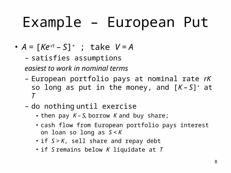
Example – European Put

• A = [Ke-rt – S]+ ; take V = A– satisfies assumptions

easiest to work in nominal terms – European portfolio pays at nominal rate rK so long as

put in the money, and [K – S]+ at T– do nothing until exercise

• then pay K – S, borrow K and buy share;

• cash flow from European portfolio pays interest on loan so long as S < K

• if S > K, sell share and repay debt• if S remains below K liquidate at T

9

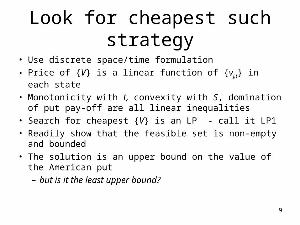
Look for cheapest such strategy

• Use discrete space/time formulation

• Price of {V} is a linear function of {vj,t} in each state

• Monotonicity with t, convexity with S, domination of put pay-off are all linear inequalities

• Search for cheapest {V} is an LP - call it LP1• Readily show that the feasible set is non-empty and

bounded• The solution is an upper bound on the value of the

American put– but is it the least upper bound?

10

The dual problem

• Consider a regime switching model:– two regimes I = 1 (initial state) and 2

• no switching from 1 to 0

– consider processes where (It , St) is Markov

– specify transition matrix P• make sure EP[Max{0, St – x} ¦S0] = CE(t, x) for all nodes (t, x)

• also EP [St+1¦St, It] = St at all nodes

• Value American option assuming it is exercised when regime switches v(P) = EP[(Kt – St)dIt]

– v is a feasible price for the American

11

LP2

• Find feasible process P to maximise v(P)– can also be formulated as an LP– call it LP2

• Main result: LP1 and LP2 are primal/dual, so solution to LP1 is not only an upper bound but the upper bound

12

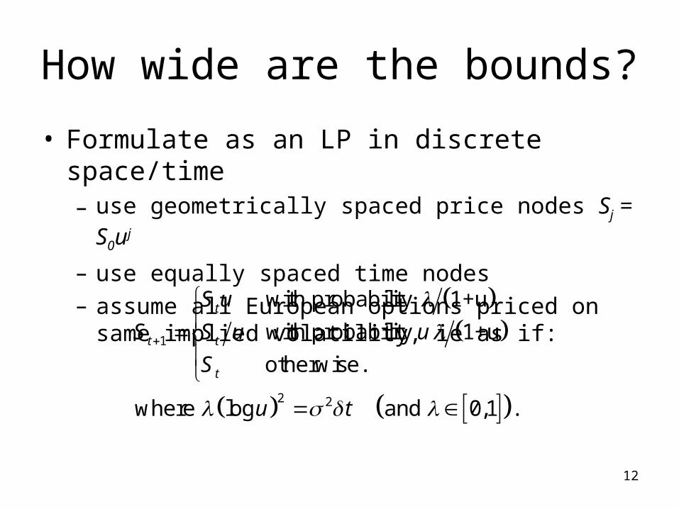
How wide are the bounds?

• Formulate as an LP in discrete space/time– use geometrically spaced price nodes Sj = S0uj

– use equally spaced time nodes– assume all European options priced on same implied

volatility, ie as if:

1

2 2

with probability 1+u

with probability 1+u

otherwise.

where log and 0,1 .

t

t t

t

S u

S S u u

S

u t

13

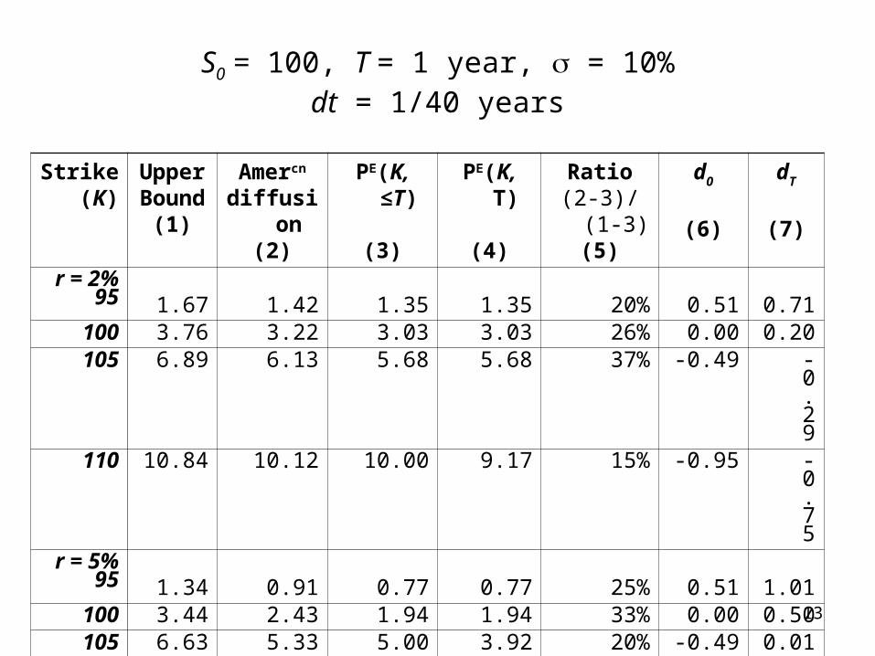
S0 = 100, T = 1 year, = 10%dt = 1/40 years

Strike(K)

UpperBound(1)

Amercn

diffusion(2)

PE(K, ≤T)

(3)

PE(K, T)

(4)

Ratio(2-3)/(1-3)

(5)

d0

(6)

dT

(7)r = 2%

95 1.67 1.42 1.35 1.35 20% 0.51 0.71100 3.76 3.22 3.03 3.03 26% 0.00 0.20105 6.89 6.13 5.68 5.68 37% -0.49 -0.29110 10.84 10.12 10.00 9.17 15% -0.95 -0.75

r = 5%95 1.34 0.91 0.77 0.77 25% 0.51 1.01

100 3.44 2.43 1.94 1.94 33% 0.00 0.50105 6.63 5.33 5.00 3.92 20% -0.49 0.01110 10.68 10.00 10.00 6.82 0% -0.95 -0.45

r = 10%95 0.83 0.44 0.26 0.26 31% 0.51 1.51

100 2.90 1.61 1.01 0.79 32% 0.00 1.00105 6.25 5.00 5.00 1.90 0% -0.49 0.51110 10.46 10.00 10.00 3.76 0% -0.95 0.05

14

Bound is very high…(same data as in table)

0

2

4

6

8

10

12

95 100 105 110 95 100 105 110 95 100 105 110

Strike

r = 2% r = 10%r = 5%

1 yr Eu

1 yr Eu

Am

Bound

15

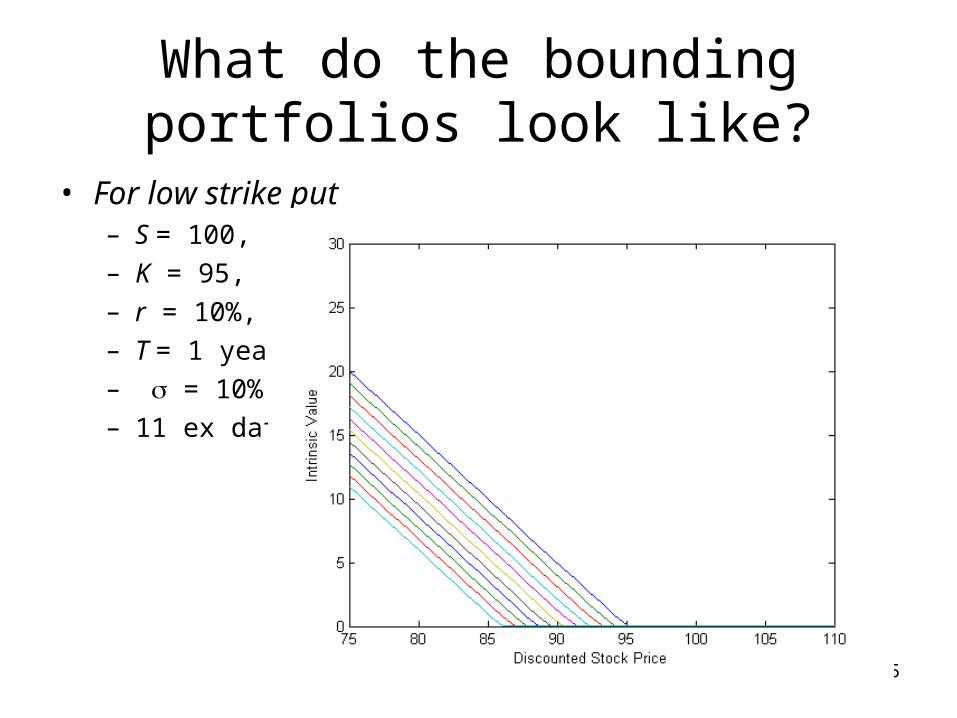
What do the bounding portfolios look like?

• For low strike put– S = 100,– K = 95,– r = 10%,– T = 1 year,– = 10%,– 11 ex dates

16

What do the bounding portfolios look like?

• For high strike put– S = 100,– K = 105,– r = 10%,– T = 1 year,– = 10%,– 11 ex dates

17

Nature of the hedging strategy that enforces rational bounds

1. Write the American option at time 02. Buy the dominating European portfolio3. Do nothing until option is exercised4. Then delta hedge European portfolio to release

intrinsic value

but step 4 is not necessary – if European options are traded can liquidate portfolio provided they trade at least at intrinsic value

– then you have a static hedging strategy

How well does it work?

18

The Horse Race

• Take a “true” returns generating model– all options are priced according to the true model– American option is exercised optimally– one bank writes an American option at fair value,

buys the European option and liquidates at exercise/expiry

– other bank does same but hedges dynamically using incorrect model

• Race outcome depends on– how incorrect the model of the dynamic trader– how much weight we put on extreme losses

19

The Race• Assume the world is Heston:

– dynamic trader uses underlying and the European option with same strike and maturity to hedge

– assumes the world is Black-Scholes, but uses the European option price to impute the current volatility

– constructs a portfolio that is delta-gamma neutral– rebalances every period– implement on a lattice (exact tri x tri – nomial process) with 100,000

simulations

• Note that since all transactions occur at fair prices and since we assume no risk premia, all strategies are mean zero

; ; . .s v s vt t t t t t t t t tdS S v dz dv v dt v dz E dz dz dt

20

The Result

Parameters• 1 year maturity• rms volatility 10%• coefficient of variation of

variance = 1• mean reversion rate = 2/yr• correlation = 0

Sensitivities• DG hedge improves if vol of vol

declines and mean reversion rate increases

• Results not very sensitive to initial vol or to correlation

StrikeDelta-

gammaRational bounds

r=2%95 0.09 0.36

(0.34) (0.28)100 0.18 0.54

(0.47) (0.59)105 0.30 0.63

(0.67) (0.87)r=10%

95 0.36 0.79(1.29) (0.38)

100 0.78 1.04(1.79) (1.25)

105 0.00 0.00(0.00) (0.00)

Hedge Error Std dev and 99%'ile

21

Tightening the bounds

• Allowing for option to trade on intrinsic is pessimistic

• Implied volatility is volatile, but does not go to zero

• Suppose we put a floor on implied volatility …S&P VIX (Volatility Index) (CBOE)

0

10

20

30

40

1993 1995 1997 1999 2001 2003 2005 2007

22

A volatility floor

• Consider an “instantaneous volatility contract” (IVC)– buy it at time t– pays $1 if price next period is different from price

today– price of contract is implied jump probability

• Assume a permanent floor on the price of IVC– implies a minimum level of implied volatility for all

options– means trader can sell IVCs against her portfolio– easy to incorporate this constraint in LP

23

The outcome with a floor

Strike Delta-gamma(K ) hedge 0% 5% 8% 10%

r=2%95 0.09 0.36 0.20 0.13 0.11

(0.34) (0.28) (0.14) (0.24) (0.35)100 0.18 0.54 0.33 0.20 0.19

(0.47) (0.59) (0.38) (0.40) (0.43)105 0.30 0.63 0.41 0.25 0.25

(0.67) (0.87) (0.66) (0.45) (0.47)r=10%

95 0.36 0.79 0.55 0.30 0.21(1.29) (0.38) (0.25) (0.30) (0.73)

100 0.78 1.04 0.94 0.50 0.40(1.79) (1.25) (0.91) (0.77) (1.19)

105 0.00 0.00 0.00 0.00 0.00(0.00) (0.00) (0.00) (0.00) (0.00)

Hedge Error - Standard deviation and 99%'ileRobust hedge with floor on imp vol of

24

Conclusions from Horse race

• Rational bounds hedge generally has larger standard error, but lower VAR than delta-gamma hedge

• Floor on implied volatility greatly reduces standard error and VAR, and retains substantial robustness

• Conclusions depend on how far true process departs from assumed model

• Robust hedges are not only robust but involve no intermediate trading

25

Conclusions• Demonstrated how to find rational bounds on the value of an

American option, and also robust hedges

• For reasonable parameters, possible value of being American several times the value assuming a Markov diffusion

• Have characterized the processes that lead to extreme high values – great uncertainty over future volatility

• Rational bounds allow for possibility of implausibly low volatilities – can tighten bounds and get better robust hedging strategies through restrictions on implied volatility– appear to have considerable advantages over conventional dynamic

strategies when true process unknown

• General approach can be applied to other hedging problems