boundary recognition in sensor networks by topology methods yue wang, jie gao dept. of computer...
TRANSCRIPT

Boundary Recognition in Sensor Networks by Topology Methods
Yue Wang, Jie GaoDept. of Computer Science Stony Brook University Sto
ny Brook, NY
Joseph S.B. MitchellDept. of Applied Math. And Statistics Stony
Brook UniversityStony Brook, NY
MobiCom ‘06

Outline
Introduction Topological Boundary Recognition Simulations Conclusions

Introduction WSNs are tightly coupled with the geometri
c environment in which they are deployed
WSN applications such as environment monitoring and data collection require sufficient coverage over the region interest
Global topology of a WSN plays an important role such as point-to-point routing and data gathering mechanism

Introduction This paper focus on the discovering the
global geometry of the sensor field including both inner and outer boundaries
Understanding the global geometry and topology of the sensor field is important for networking operation
The goal of this paper is to find the boundary nodes by using only connectivity information
Contributions Developing a practical distributed
algorithm for boundary detection using only the communication graph
Do not need assume any location, angular or distance information
The propose algorithm doesn’t require follow the unit disc graph model

Contributions The boundary detection algorithm is
motivated by an observation that holes in a sensor field create irregularities in hop count distance

Topology Boundary Recognition
Assumption Sensors are random scattered in a
geometric region
Nearby nodes communicate with each other directly

Topology Boundary Recognition
Goal Discovering the nodes on the boundary of the se
nor field
Using only local connectivity information
Proposing a distributed algorithm that identifies boundary cycles for the sensor field

Topology Boundary Recognition
Basic idea Exploit special structure of the shortest path
tree to detect the existence of holes
Inner holes of the sensor field “disrupt” the natural flow of the shortest path tree
Shortest paths diverge prior to a hole and then meet after the hole

Topology Boundary Recognition
Flood the network from an arbitrary node, r.
Each node records the minimum hop count to r.
Generally prefer to select r as a node on the outer boundary of the sensor field

Topology Boundary Recognition
Determine the nodes that form the cut, where the shortest paths of distinct homotopy type meet after passing around holes.
The nodes of a branch of the cut have their least common ancestor (LCA) relatively far away and their paths to the LCA well separated

Topology Boundary Recognition

Topology Boundary Recognition
Determine a shortest cycle, R, enclosing the composite hole; R serves as a coarse inner boundary

Topology Boundary Recognition
Flood the network from the cycle R. Each node in the network records its minimum hop count to R.

Topology Boundary Recognition
Detect “extremal nodes” whose hop counts to R are locally maximal

Topology Boundary Recognition
Refine the coarse inner boundary R to provide tight inner and outer boundaries. These boundaries are in fact cycles of shortest paths connecting adjacent extremal nodes.
Topology Boundary Recognition
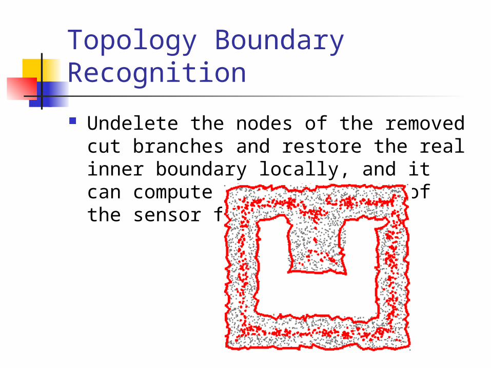
Undelete the nodes of the removed cut branches and restore the real inner boundary locally, and it can compute the medial axis of the sensor field

Topology Boundary Recognition
Build a shortest path tree Find cuts in the shortest path tree Detect a coarse inner boundary Find extremal nodes Find the outer boundary and refine the coarse inne
r boundary Restore the inner boundary The medial axis of the sensor field
Build a shortest path tree
Flood the network from an arbitrary root node r
Each sensor node p sets a timer with a random remaining time
When the timer of p reaches 0 then flood and build a shortest tree T(p)
The tree with a timer of minimum value starts first and suppresses the other trees

Build a shortest path tree When the frontier of T(p) encounters a node
q, there are two cases If q does not belong to any other tree, then q is i
ncluded in the tree T(p) and q will broadcast the packet
If q already included in another tree T(p‘), then the start time of T(p) and T(p’) are compared

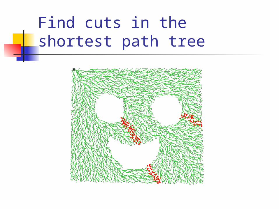
Find cuts in the shortest path tree
Definition of a cut pair (p,q)
The (hop) distance between p or q and y = LCA(p,q) is above a threshold δ1
The maximum (hop) distance between a node on the path in T from p to y and the path in T from q to y is above a threshold δ2
Find cuts in the shortest path tree

Detect a coarse inner boundary
The cut pair p and q will find the shortest paths between them that do not go through any cut node Using any shortest path algorithm to find this pa
th We can use the two shortest paths from q and q
to LCA(p,q)

Detect a coarse inner boundary

Find extremal nodes An extremal node is a node whose minimu
m hop count to nodes in R is locally maximal

Find the outer boundary and refine the coarse inner boundary

Restore the inner boundary
The final step is to recover the inner holes in the sensor field and find their boundaries
For each cut, we find a cut pair (p,q) such that the inclusion of edge pq in the refined inner boundary R

The medial axis of the sensor field
The medial axis is defined as the set of nodes with at least two closest boundary nodes
Medial axis can be used to generate virtual coordinates for efficient greedy routing

Simulations Effect of node distribution and density
Random distribution of sensors
Low density, sparse graphs
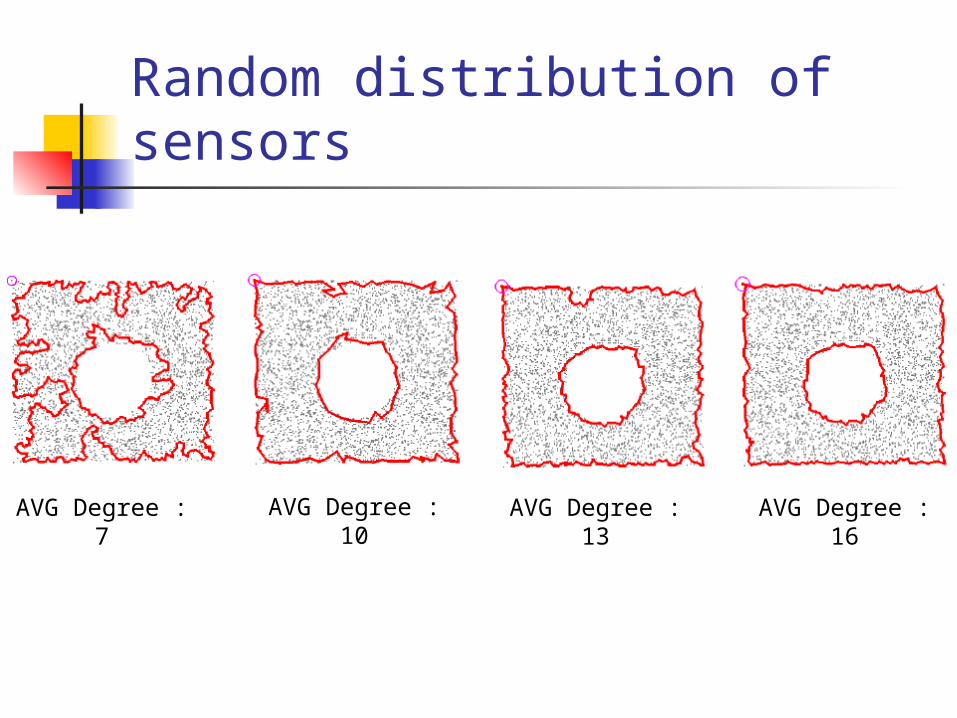
Random distribution of sensors
AVG Degree : 7
AVG Degree : 10
AVG Degree : 13
AVG Degree : 16

Random distribution of sensors
Based on original
neighbors
Using 2-hop neighbors as fake 1-hop neighbors
Using 3-hop neighbors as fake 1-hop neighbors

Low density, sparse graphs
3443 nodes AVG degree
35
2628 nodes AVG degree
25
1742 nodes AVG degree
16
842 nodes AVG degree 7

Conclusions This paper proposes an algorithm to
discover both inner and outer boundary nodes
The proposed mechanism only needs the connected graph to apply to the algorithm
The simulations show that the proposed algorithm is efficient to discover the boundaries

Thank You!!