boundary layer, upper ocean, and ice observations in the greenland sea marginal ice...

JOURNAL OF GEOPHYSICAL RESEARCH, VOL. 92, NO. C7, PAGES 6987-7011, JUNE 30, 1987

Boundary Layer, Upper Ocean, and Ice Observations in the Greenland Sea Marginal Ice Zone

J^•ms H. Mornsos

Polar Science Center, Applied Physics Laboratory, College of Ocean and Fishery Sciences, University of Washington, Seattle

MILES G. McP•

McPhee Research Company, Yakima, Washington

GARY A.

Department of Atmospheric Sciences, University of Washington, Seattle

During the 1984 Marginal Ice Zone Experiment, a coordinated ocean boundary layer and mixed layer experiment was carried out in concert with a complete heat and mass balance study in the summer marginal ice zone (MIZ) of the Greenland Sea. The measurements were made at two drifting ice stations and included observations of ocean boundary layer turbulence, profiles of water temperature, salinity, and velocity, ice ablation, ice concentration, solar radiation, and spectral albedos. Ocean conditions were found to be extremely variable. The ice and water velocities were heavily influenced by tidal and inertial motions with amplitudes from 6 to 12 cm s -1. In the course of the drift, a 30-km eddy was crossed wherein ice and water velocities exceeded 15 cm s -1. The northern extension of the East Greenland Polar Front was encountered, and a northward flow of Atlantic Water into the Arctic basin was observed below the eastern edge of the front, but the drift station never moved quite far enough west to be caught in lhe southward transport of Arctic Surface Water. Heat from the ocean was a major factor in ice melt, and when the ice was over Atlantic Water it was the dominant factor. The events that had the greatest impact on the ice were two "outbreaks" during which off-ice winds blew the ice across warm ice edge ocean fronts. Once south of these fronts and over surface water as warm as 1 øC, the ice bottom melted at rates up to 100 kg m -2 d -•. The rapid changes in stratification associated with the outbreaks had a dramatic impact on the drag and heat transfer coefficients. The drag coefficient (relative to the square of the relative water velocity at 30 m) ranged from 0.002 to 0.02 and averaged 0.006. The heat transfer coefficient (relative to the friction velocity u. and the mixed layer temperature elevation above freezing) ranged from 0.0025 to 0.009 and averaged 0.0038. In agreement with the idea that stratification inhibits turbulent exchange, the heat transfer coefficient decreased when stratification increased. In fact, the observed melt rates can be simulated well if molecular heat and salt transfer through a thin, near-surface, laminar boundary layer are accounted for, as well as transfer through the turbulent outer boundary layer. Also in agreement with turbulent boundary layer theory, the drag coefficient decreased when stratification increased slightly above neutral. However, for the large increases in surface stratification, the drag coefficient increased. This was due to the generation of internal gravity waves by ice bottom roughness. Because the surface exchange coefficients are so sensitive to surface stratification, which is in turn highly variable in the MIZ, accurate simu, lations of ice motion and ice melt will require realistic estimates of stratification and a good understanding of the relation between the ice-ocean interactions and upper ocean conditions.

1. INTRODUCTION

The upper ocean processes and ice mass changes that control the vertical transfer of momentum, heat, and salt between the ice and water are of fundamental importance in controlling ice extent and motion in the marginal ice zone (MiZ). When the wind blows across ice, the ice moves over the water; how fast it moves and in what direction are determined largely by the physics of the boundary layer under the ice. When the ice is blown over warm water, the underside melts; how fast it melts depends on the rate of heat exchange in the ocean boundary layer. At the same time, the transfer of heat, salt, and momentum modifies the upper ocean and changes the physics of subsequent ice and ocean interaction. When the upper surface of the ice is melted by radiative and sensible heat input, the resultant mass flux also has an impact on upper ocean conditions. The ice and upper

Copyright 1987 by the American Geophysical Union.

Paper number 7C0230. 0148-0227/87/007C-0230505.00

ocean thus represent a strongly coupled system whose quantita- tive description relies on a detailed understanding of these heat, salt, and momentum transfer processes.

Previous work on under-ice boundary layer and mixed layer processes has mainly concentrated on the central Arctic basin, where it has been possible to take advantage of the stable platform offered by the ice and the relatively uniform ocean conditions to obtain measurements that would have been impossible in the open ocean. Some of the earliest and best studies of the marine planetary boundary layers have been carried out in ice- covered waters. One of the first measurements of a full Elmtan

spiral was made by Hunkins [1966] in the Arctic Ocean. Hun- k/ns [1975] also obtained water surface stress estimates using the momentum integral technique with data gathered beneath pack ice. McPhee and Smith [1976] succeeded in making the first measurements of both mean velocity and Reynolds stress throughout a planetary boundary layer under the pack ice of the Beaufort Sea and found agreement with second-order closure models. McPhee [1980] used a long time series of wind stress, ice motion, and current measurements to obtain an estimate of

6987

6988 MORI$ONET AL.: GREENLAND SEA MARGINAL ICE ZONE OBSERVATIONS

the ocean drag coefficient for sea ice in summer, I Cw•l = 5.5 x 10 -•.

The behavior of the mixed layer under pack ice is closely coupled to surface forcings related to changes in the ice cover. Short-term fluctuations in mixed layer depth can be attributed to Ekman pumping [McPhee, 1975] and mesoscale gradients in buoyancy flux associated with brine rejection in refreezing leads [Morison, 1980]. The seasonal fluctuations in mixed layer depth and salt content are due to the effect of seasonal changes in buoyancy flux on boundary layer turbulence; the seasonal fluctuations in average surface stress are negligible [Morison and Smith, 1981; Lemke ar.d Manley, 1984]. While conditions in the upper ocean in the central Arctic are fairly homogeneous horizontally, at least compared with those in the MIZ, nonuniformi- ties in the ice cover (leads, ridges) play a major role in determin- ing regional heat exchange with the atmosphere, overall ice production and buoyancy fluxes, and mechanical coupling between the ice and water. Winter salinization of the upper ocean is largely due to salt input from refreezing leads, and most of the vertical heat exchange between the ice and the mixed layer is derived from solar energy transmitted to the ocean through leads and areas of thin ice [Morison and Smith, 1981; Maykut, 1982].

While studies in the central Arctic have revealed fundamental

principles regarding the coupling of the ice cover, upper ocean, and atmosphere, applying these principles to conditions in the MIZ is difficult. Studies in the MIZ are complicated not only by large spatial and temporal gradients but also by the practical problems of making measurements in such a variable environment. For example, field data from the Greenland Sea MIZ [Buckley et al., 1979; Johannessen et al., 1983] show it to be an area of extreme upper ocean variability with numerous fronts, upwelling or downwelling features, and eddies. Moreover, the MIZ is a region with a great deal of variation in ice parameters; the concentration varies from 100% in the interior to 0% at the

edge, with large fluctuations occurring over distances of a few kilometers in both the across edge and along edge directions. Also, because of the effect of incoming surface waves, average floe sizes in the MIZ range from a few meters at the edge to thousands of meters 100 km to 200 km into the interior [Wad- hams, 1973].

The marked variability of ice concentration and floe size can cause variability in the magnitude of the ice-water drag and the partition between form drag and skin drag. When the ice concentration is reduced, the exposed edges of floes are important sources of form drag; for small floes, the edge form drag may dominate bottom friction. For example, consider ice floes with a bottom drag coefficient of 5 x 10 -a. If the drag coefficient for the bluff edges of the floes is taken as 1, as is suggested by the data of Hoerner [1965], form drag on the ends will be more important than bottom friction for floes with a horizontal scale smaller than about 100 times the draft. Thus the drag may be greater in areas where floes are smaller than 200-300 m than where floes are larger.

The variations in ocean stratification caused by fronts and eddies can also have a profound effect on upper ocean transfer processes. McPhee [1983] shows the effect of stratification on ocean boundary layer processes to be extremely important when ice melts rapidly upon encountering warm water. However, few details are known regarding melt rates or oceanic heat fluxes near the ice edge.

In addition to heat flux from warm water, absorption of shortwave radiation in leads causes lateral melting on floe edges, setting up a positive feedback process that decreases ice concert-

tration. In dynamically active areas, some of the energy absorbed in the upper few meters of the leads will be advected beneath the surrounding ice where it will ultimately be lost to the ice through bottom melting. The amount of solar heating in the mixed layer thus depends on both ice concentration and ice movement and therefore may also be quite variable.

The conditions in the marginal ice zone that make the study of surface fluxes and oceanographic conditions scientifically interesting also make it a logistically difficult area in which to operate. Detailed boundary layer measurements at the 1972 Arc- tic Ice Dynamics Joint Experiment (AIDJEX) camp [McPhee and Smith, 1976] involved several under-ice towers (extending to depths as great as 50 m) prefabricated computer and diving huts, a team of divers and technicians, and a complete conductivity-temperature-depth (CTD) system. In the MIZ the small ice floes, variable ice concentration, and high potential for floe breakup make mounting such a large operation from the ice difficult and hazardous. Operating directly from a ship is scientifically undesirable because a ship disturbs the boundary layer and mixed layer around it. Rapid temporal variations in the MIZ also require more rapid sampling of ocean conditions than is required in the central Arctic.

In spite of all these difficulties a number of measurements of melt rates, water stress, and drag coefficients have been made in the marginal ice zone, particularly in the Bering Sea. Josberger and Meldrum [1985] measured ice bottom ablation rates as high as 67 cm d -• very near the Bering Sea ice edge. Johannessen [1970] measured the drag coefficient under small (10 to 15 m) ice floes in the Gulf of Saint Lawrence using the profile technique and obtained values of 9-17 x 10 -• at 2 m. Pease et al. [1983] measured the 1.1-m water drag coefficient under 10- to 20-m floes in the Bering Sea MIZ and obtained values from 18-22 x 10 -a. These are larger than the values McPhee and Smith [1976] obtained for shallow depth drag coefficients under a relatively smooth floe in the central pack ice. However, McPhee [1979] also obtained a 1-m drag coefficient of 20 x 10 -a for average pack ice conditions by adjusting the AIDJEX model geostrophic drag coefficient (5.5 x 10 -a) for height. Reynolds et al. [1985] obtained a relatively low 2-m drag coefficient of 7.8 x 10 -a (13.5 x 10 -a at l-m) under a smooth Bering Sea ice floe and found that the ice moved at about 4% of the 3-m wind

speed. Unfortunately, when the ice undersurface is rough, and form

drag is dominant, measurement of drag at a single shallow depth, or measurements of drag coefficients relative to a shallow depth, may be of limited applicability. Stress and velocity profile measurements [McPhee and Smith, 1976] indicate that even under relatively smooth pack ice, turbulent stress estimates made from near-surface measurements are typically half the total stress estimated by other techniques because the form drag only appears as turbulence far from the boundary. Conversely, coefficients for total drag relative to the velocity at shallow depths may be artificially high because of the velocity reduction caused by form drag elements at shallow depths. In the marginal ice zone, stress measurements must be made at several depths, and drag coefficients must be referenced to depths in the outer- most parts of the boundary layer. In this way the integrated effects of form drag and skin friction can be accounted for. Also, because boundary layer behavior depends on floe size, concentration, existing stratification, and surface buoyancy flux, measurements of boundary layer stress or drag coefficients are not useful unless these other environmental parameters are also known. In spite of this, until now there have existed no simul-

MORISON ET AL.: GREENLAND SEA MARGINAL ICE ZONE OBSERVATIONS 6989

81.OøN

0 o 2 o 4 o 6 ø 8OE

80.4 ø

80.8 ø

80.6 o-

80.2 ø

80.0 ø

...... DAY 169 15 km --- DAY 186

Fig. 1. Drift tracks of the Polar Queen during MIZEX '84 (heavy solid lines). The pluses indicate positions of 0000 UT the day indicated. The thin solid lines with crossbars indicate helicopter flight tracks to the edge [Hall, 1984]. Ice edge positions on days 169 and 186 are also shown (R. A. Shuchman et al., unpublished manuscript, 1987).

taneous measurements of turbulent momentum transfer, surface heat and buoyancy fluxes, and mixed layer behavior at a common site in the MIZ.

During the Marginal Ice Zone Experiment (MIZEX) our objective was to carry out a comprehensive ocean boundary layer and mixed layer experiment in concert with a heat and mass balance study of the ice cover in the summer MIZ of the Greenland Sea. We wished to address a number of questions including these: What are the effects of eddies, fronts, and other upper ocean features on the vertical transport of heat, mass, and momentum through the boundary layer? Does the presence of strong horizontal gradients in the ocean preclude the use of existing boundary layer and mixed layer models? What is the effect of variable stratification on drag and mass transfer? What are the principal factors and processes controlling the interactions of shortwave radiation with the ice and upper ocean? What is the relative importance of the ocean and atmosphere in the melt cycle of the summer MIZ?

To overcome the practical difficulties in making sophisticated upper ocean and ice measurements in the MIZ, all the experimental equipment was designed to be as light and portable as possible. The measurements were to be made from ice floes to which a small icebreaker would be tied while drifting with the ice. The ship was to provide transportation and logistic support, and only scientific activities were to be carried out on the ice. In June 1983, a successful 1-week pilot study was carried out at the drift site of the MV Polarbjorn near 80ø20'N, 7øE as part of MIZEX '83. During MIZEX '84 the main study, lasting nearly 40 days, was carried out at the drift site of the MV Polar Queen.

This paper discusses the results of the main study in 1984. In a related paper, McPhee et al. [this issue], derailed measurements of boundary layer and mix6d layer parameters during a storm and the crossing of an ocean front are described and compared with the behavior predicted by theory. The problems associated with applying boundary layer theory to a region of rapid ice melt and large horizontal gradients are addressed. In this paper a broader but less detailed view is taken. The aim is to describe the general character of ice and upper ocean vertical exchange processes and how they vary over a range of conditions.

In the following sections a broad overview of ice and upper ocean conditions encountered during the experiment is presented. The magnitude and importance of inertial motions, tides, eddies, and large-scale currents are evaluated and discussed in the context of ice-ocean interactions. Vertical fluxes of

heat and momentum at the underside of the ice are calculated

and used to construct time histories of drag and heat transfer coefficients. Variations in these coefficients are shown to reveal

much about the structure of the boundary layer adjacent to the ice and about processes (buoyancy feedback, internal wave generation) that impact vertical fluxes.

2. EXPERIMENTAL PROGRAM

During MIZEX '84, all three components of the measurement program (ocean boundary layer studies, mixed layer and upper ocean studies, and heat and mass balance studies) were carried out from ice floes adjacent to the MV Polar Queen during two drift periods. The first drift was from June 8 (day 160) to June 16 (day 168). During this time the Polar Queen drifted from 80ø55'N, 6ø30'E to 80ø24'N, 5ø45'E (see Figure 1). The ship was tied to a 200 x 300 m ice floe (floe 1), which was an aggregate of several first-year floes fused together. The site was abandoned when it drifted near the ice edge and broke up as a result of rapid thinning and melting. The second drift started June 18 (day 170) and ended July 18 (day 200) and went from 80ø51'N, 4ø18'E to 80ø12'N, 5øE. During the second drift the ship was tied to a 400 x 800 m floe (floe 2) composed primarily of thicker multiyear ice.

The experiment was broken into three measurement programs: the boundary layer program, the mixed layer and upper ocean program, and the surface heat and mass balance program. The objective of the boundary layer program was to provide direct measurements of the turbulent transfer of momentum, heat, and salt as well as measurements of mean parameters close to the underside of the ice. This was accomplished by mounting clusters of three small, ducted rotor current meters [McPhee and Smith, 1976] and fast-response Sea-Bird temperature and conductivity sensors on stainless steel masts suspended from the ice. Sensor packages were deployed 1 m, 2 m, 4 m, 7 m, and 15 m from the bottom of the ice at a relatively smooth site on the floe about 150 m from the nearest edge. At floe 2 an additional sensor package was suspended 2 m below the bottom of the ice at a site approximately 100 m from the main mast. Because the ice was 2 m thick the sensor depths were 3 m, 4 m, 6 m, 9 m, and 17 m. Except for short maintenance and orientation adjustment periods, three components of velocity, along with temperature and conductivity, were measured six times per second at the six levels during all periods of the experiment when ice velocity relative to the water was above 5 cm sq. Turbulent velocity measurements were processed by separating the time series into 15-rain blocks, calculating the mean vector and covariance matrix for each cluster over each time block, and then rotating the mean vector and covariance (Reynolds stress) tensor into an east-north-vertical reference frame in which the mean vertical

velocity component vanishes. Because the time scale of the eddies that contribute most to the turbulent energy is typically 1 to 5 rain, a number of these 15-rain samples must be smoothed or block-averaged to arrive at stable turbulence statistics. The end product is the mean horizontal velocity and the Reynolds stress tensor, which includes the turbulent kinetic energy (sum of the diagonal elements) and the horizontal traction at each level (< u'w'>i+<v'w'>j where i and j are unit vectors). Similar techniques were used for processing the fast-response

6990 MORISON •r AL.: GP•maLAND SEA MARGINAL Ic• ZoN• OBSERVATIONS

temperature data to obtain mean temperature and the vertical heat flux (w'T'), at each level. In principle, the salinity flux can be derived from the conductivity measurements in a similar fashion, but the longer time constant for the conductivity meters requires more sophisticated algorithms, which have not been tested thoroughly enough for inclusion here. A discussion of measurement accuracies is given by McPhee et al. [this issue].

The objective of the mixed layer and upper ocean measurements was to obtain a continuous record of ocean temperature, salinity, density, and velocity profiles to 300 m. The data were gathered with a profiling current meter-CTD system called the Arctic Profiling System (APS). The instrument is identical in principle to an earlier version described by Morison [1978, 1980]. The present unit consists of a Sea-Bird CTD plus a triplet of small, ducted rotor velocity sensors measuring three orthogo- nal components of velocity relative to the instrument. A flux gate slaved, directional gyro and two accelerometers are used to determine the orientation of the instrument in order to rotate the

measured velocities into an earth-centered coordinate system. The APS sensor data are transmitted up a single conductor, steel armored cable at a sample rate of 12 Hz and recorded directly on analog cassette tapes for redundancy and examination of fine- scale structure. The data are also averaged over 1 s by the Sea- Bird deck unit and recorded on 5.25-inch floppy disks with an Apple microcomputer.

During MIZEX '84, the APS was cycled to depths of up to 250 m using a winch mounted in a 3 x 1.5 m boat/sled called the Northern Light (the smallest of the MIZEX research vessels). The Northern Light employed a small diesel engine to power the winch hydraulics and provide electrical power for the instrumen- tation. The winch raised and lowered the APS at a speed of 0.7 m s -• and was equipped with a simple automatic control system which allowed continuous cycling of the instrument with a minimum of operator attention. Casts were made at least once every 3 hours. In addition, nine sequences of continuous cycling were carried out for periods of 12 hours or more. These were usually done during periods of rapid ice motion. During these continuous runs, the profile interval was from 10 to 15 rain depending on depth range. A total of 1083 casts were made.

In analyzing the APS data, the first step is to transform data from the nine APS sensors into raw depth profiles of temperature, salinity, density (o,), and water velocity. These profiles are then smoothed and bin-averaged. Salinity spiking problems, due to the long flushing time of the conductivity cell, were elim- inated in 1984 by the addition of a Sea-Bird conductivity cell pump to flush the cell mechanically. As a result it was necessary to smooth the CTD data over only 2 m. Unfortunately, the presence of the pump disturbed the flow around the APS and caused it to spin as it descended. This resulted in slight harmonic oscillations in measured current direction which were filtered out of

the velocity data by smoothing over 20 m. A discussion of the APS accuracy is given by McPhee et al. [this issue].

The surface heat and mass balance program was designed to obtain data on temporal changes in energy fluxes and ice ablation at the boundaries of selected floes within the MIZ. Ice

thickness and bottom ablation were measured using electric thickness gauges installed through 6.4-cm boreholes. A total of 32 gauges were deployed in floe 1, with another 26 in floe 2. Several sites were set up around the perimeter of each floe to look for evidence of heat exchange between leads and the underlying ocean, while other sites were set up beneath unreformed ice in the vicinity of the oceanographic arrays and across a small pressure ridge keel. Surface melting was monitored at an array

of ablation stakes, as well as at all thickness gauge sites. Read- ings were taken daily at about 0800 UT, so that ablation rates are usually shown centered on 2000 UT. Sequential wall profiles and lateral ablation were measured at several locations on the

edge of floe 2. The lateral melt data are a measure of the rate of horizontal heat transport in the leads and yield information on how solar energy is distributed and transported within the ice- ocean system. Periodic surveys of snow depth and melt pond coverage were also made throughout the experiment.

Incoming shortwave and longwave radiation were measured at the surface of both floes using Kipp & Zonen and Eppley radiometers. Data were sampled every 10 rain throughout the experiment. Also, the spectral composition (400-2500 rim) of the incident shortwave was measured under a variety of cloud conditions. Total and spectral albedos of the major surface types were also measured periodically. Areally averaged albedos were obtained in three wavelength bands (500, 650, and 1000nm) during helicopter transects to the ice edge and were used to obtain estimates of ice concentration and pond coverage. Because shortwave radiation is a major source of energy for the decay cycle, special attention was given to properties and processes that affect its distribution within the ice-ocean system. Of particular concern was the input of solar energy to the upper 2 to 3 m of the ocean between the ice floes and its subsequent interaction with the ice cover and mixed layer. To determine changes in the heat content of the upper ocean between floes, horizontal and vertical CTD profiles were taken in leads around the floe every 1 to 2 days. Observations of lead width and mor- phology were made several times a day at each of the edge ablation sites. Vertical profiles of light intensity were measured to a depth of 15 m below the ice at 3- to 4-day intervals. Tempera- ture profiles in the ice were monitored daily from an array of six thermistors frozen into the ice with a spacing of 0.3 m. Knowing the conductive heat flux in the ice, it is possible to infer the oceanic heat flux to the ice from the observed bottom ablation for

comparison with direct measurements of turbulent heat flux in the mixed layer.

3. OBSERVATIONS

3.1. Location and Basic Ice Conditions

Figure 1 shows the trajectories of the two Polar Queen drift sites. The positions are satellite navigation points smoothed using the complex demodulation technique of McPhee [1986]. The positions of the ice edge, as determined by R. A. Shuchman et al. (unpublished manuscript, 1987) for day 170 (June 18, 1984) and day 186 (July 4, 1984), am also shown. These two positions roughly represent the extreme positions of the edge observed during the period. After day 186 (July 4), much of the edge was obscured by fog. (Note that time is often given as day of the year 1984, including the day fraction; for example, June 1, 1984, at 1200 UT equals day 153.5.) The distance and heading to the edge are shown for a number of the ship positions. These are based on the ice reconnaissance data of Hall [1984] and the ice edge data of R. A. Shuchman et al. (unpublished manuscript, 1987). During both drifts the ice usually moved toward the southwest except during the last 8 days, when drift was to the northeast. During the first drift the ship was initially positioned 40 lcm from the edge, but as the drift proceeded south it moved closer to the boundary between the consolidated edge and scat- tered ice floes. At the end of the first drift, floe 1 moved into the area of low concentration and broke up. During the second drift,

MORISONET At,.: GREENLAND SEA MARGINAL ICE ZONE OBSERVATIONS 6991

o

I-,.-

z

z o

On-Ice Winds I H

25 June 1984 O I , I , I , I , I , I , I ,' /

0 5 •.0 •.5 ;::>0 •5 30 35

L Off-Ice Winds _.J

01 , I , I I I I I , I , / 0 •0 RO 30 40 50 60

DISTANCE (Km)

Fig. 2. Photometrically determined ice concentrations between the drifting ship Polar Queen and the ice edge during MIZEX '84. The values were derived from spectral albedo data taken during helicopter transects to the edge. The figure illustrates how atmospheric forcing affects the character of the ice cover in the MIZ.

floe 2 always remained 41 km + 11 km from the edge, at least until day 191, in spite of variations of up to 45 km in ice edge position.

The ice reconnaissance flights [Hall, 1984] and spectral albedo assessments of ice concentration [Maykut and Perovich, 1985] indicate that the MIZ usually contained three regions: an inner zone of larger first-year and multiyear floes, a transition zone of uniformly broken smaller floes, and a complex region of brash and tiny floes near the extreme edge. Multiyear floes in the inner region where the Polar Queen was located were typically a few hundred meters across'and 2-5 m thick. First-year floes were much smaller, tending to be broken up between the heavier floes.

The transition zone (5-15 km wide) was characterized by fairly uniform floes whose average size decreased as the edge was approached, evidence that wave propagation from the open water was a dominant factor in the development of this zone. Ice concentration was frequently high (70-90%), showing only a slight tendency to decrease with floe size. Leads between the floes were generally free of brash, allowing substantial amounts of solar energy to enter the upper ocean there. In the outer part of the transition zone the effects of local wave action and

warmer surface water on lateral erosion were clearly evident, with as much as 10-20% of the floe area being made up of underwater shelves. Floes at the extreme edge were much smaller, and their spatial distribution was highly variable. On some days the edge was quite distinct, being composed of a narrow region of nearly 100% concentration, while on others it was very diffuse and contained bands, streamers, fingers, or detached patches of small floes.

The size and characteristics of these zones appear to be strongly influenced by wind direction. Figure 2 shows pho-

to me tric al ly determined ice concentrations as a function of distance between the ship and the ice edge during two different wind regimes. The upper part of the figure shows variations on day 177, following a period of strong on-ice winds. The ice cover in the first 20 km was made up of rounded floes with a rich size distribution. At about 22 km there was an abrupt transition to angular, more uniformly sized floes. The reason for such an abrupt change is not entirely clear, but it may signal a change in average ice thickness. Over the next 10 km the floes became less angular and decreased in size from about 200 m across the long axis to less than 100 m. At the extreme edge was a compact, 2- to 3-kin-wide band of brash and small floes, most less than 40 m in diameter. The lower part of the figure shows variations on day 191, a period of strong off-ice winds. The average concentration was dramatically lower (58% versus 82%) and the distance between the Polar Queen and the extreme edge was nearly twice as large. The edge itself was indistinct, with bands and fingers of ice extending over a distance of 5-10 km. Between 10 and 25 km the ice was very loose, containing several narrow bands of small (100-m diameter) floes and open water. Wave- broken outer floes began at about 35 km, again decreasing in size toward the edge. Although many of the differences between days 177 and 191 can be attributed to the wind field, the situation on day 191 was complicated by advection of the ice into Atlantic water which resulted in very rapid decay and increased divergence. These effects will be discussed in more detail in subsequent sections.

Surprisingly, multiyear ice was found to be far more abundant than first-year ice in the summer MIZ [Tucker et al., this issue]. This may in part reflect limited local ice production during the winter and the first-year/multiyear ratio of the ice advected into the region; however, dynamic and thermodynamic processes also combine to produce selective removal of first-year ice during the summer. The most effective of these processes is associated with the breakup of younger and weaker floes between heavier floes. By greatly increasing the surface area of ice in contact with the water, this increases the overall rate at which heat can be transferred from the water to the ice cover. During much of MIZEX '84, leads near the Polar Queen were filled with brash which appeared to be derived from first-year ice rather than from mechanical erosion at the edges of multiyear floes. As a result, most of the solar radiation entering the leads went to the melting of brash (i.e., first-year ice) instead of the thicker ice. Only after encountering warmer Atlantic Water did the brash finally vanish and significant lateral melting on multiyear floes occur.

3.2. Time Histories of Ocean and Ice Conditions

Figure 3 shows wind and ice velocity vectors for both drifts. The velocity vectors are given at 12-hour intervals. The wind data were measured at the Polar Queen and adjusted to 10 m [Lindsay, 1985]. The ice velocity is from a fit to the satellite navigation data by McPhee [1986]. With the chosen scales, ice velocity vectors that are 2% of the wind speed appear to have the same magnitude as the wind vector. Generally, winds were rather weak and variable in direction. The two major wind events occurred late in the second drift, the first during a storm with northerly winds centered on day 189 and the second during a period of persistent southerly winds at the end of the experiment.

Oceanographic conditions in the marginal ice zone are quite variable, and many of the results will be shown in contour form. However, it is instructive first to examine data from a typical

6992 MOrnSON Lrr AL.: GI••AND SEA MAYORAL ICE ZON• OBSERVATIONS

.... ••-' t .i d m $-I

'• 1 ce 5.13 cms -• I

I I I I I I I I I i i i i i i I I i i i I I I i i i I L I I I I I I I I I I I I I

160 164 168 17• 176 180 184 188 19• 196 •00

DAY OF 1984

Fig. 3. Wind and ice velocity v,sctors at the Polar Queen. The winds are 6-hour averages of measured wind at 10 m, centered at the time shown. The ice velocity is the 24-hour mean ice velocity phasor; diurnal and semidiurnal/inertial motions have been removed.

individual profile. Figure 4a, showing results of a single APS cast made at 1346 UT on day 178, illustrates some features common to most of the profiles. The water column was capped by a mixed layer approximately 20 m deep with a salinity of 33.4%,. The mixed layer temperature was near the freezing point, about -1.7øC. Below the mixed layer, conditions corresponded to those for Atlantic Water, with temperatures above 2øC and salin- ities approaching 35ø/•,. In the course of the experiment, mixed

layer depths ranged from 3 m (stratification to the bottom of the ice) to 25 m. Also, although this profile shows the thermocline to be at the same depth as the pycnocline, sometimes the thermocline was below the pycnocline.

Figure 4b shows the Brunt V•/ish]•/frequency N, computed from the CTD data

N2 = g dpw p. TEMPERATURE (øC)

-I I

SALINITY (ø/oo) 33 34

SIGMA T

26.5 27.0 27.5

4O

60

80

I00

120

140

160

180

200

3 5

35 36

28.0

Temperature Salinity Sigma T

BRUNT-VAISALA FREQUENCY (cph) v (north) u (east) 0 ̧ 2 4 6 8 I0 12 14 -20 -I0 0 -20 -I0 0

4O

6O

! I

160•- 2OO

Fig. 4a Fig. 4b

Fig. 4. Oceanographic profiles from an APS cast made at floe 2 at 1346 LIT on day 178. (a) Temperature, salinity, and or. (b) Brunt-Viiish][ frequency and water velocities north and east relative to the ice.

MORISON ET AL: GREENLAND SEA M,•OINAL IC'• ZOl'• OBSERVATIONS 6993

o

2o

40

60

8o

IOO

12o

140

161

0

2O

4O

• 6o

uJ 80

ioo

12o

165 166

b) 140

161 162 163 168

o

20

40

60

80

I00

120

140

161

i

164 165 166 167

27.8

162 163 164 165 166 167 168 169

DAY OF 1984

Fig. 5. Contours of oceanographic parameters measured with the APS during the drift at floe 1. (a) Contours of temperature in degrees Celsius. (b) Contours of salinity per mil. (c) Contours of or.

where Pw is water density, g is the acceleration of gravity, and z is depth. Also shown in the figure is the horizontal velocity relative to the ice. N was high at the pycnocline, decreased rapidly below the seasonal pycnocline, and was less than 1.5 cph below 100 m. This level of stratification is generally lower than that in most temperate oceans or in the western Arctic. For these particular velocity profiles, speeds in the mixed layer were about 15 cm s -a, the shear being concentrated near the surface. In view of the lack of stratification above about 14 m, this must have been due to wind-forced (or ice-forced) ice motion relative to the water. Below 14 m, an additional shear in excess of 10 cm s -4 occurred which was probably density driven.

The variable nature of oceanographic conditions in the marginal ice zone is evident in depth/time contours of temperature, salinity, and o, shown in Figures 5-7 and the temporal changes in ice melt rates, ice concentration, and solar input to the upper ocean shown in Figure 8. Conditions during the first drift, a

period characteristic of a situation in which ice is forced out over warm water and melts, are shown in Figure 5. This drift occurred close to the edge (Figure 1), and during a period of fairly light winds (Figure 3). Temperature gradients extended all the way to the surface, as did the salinity and o, gradients. There was virtually no mixed layer. Temperatures in the top 5 m ranged from- 1.0øC near the beginning of the period to +0.5øC at the end, while near-surface salinity remained near 33.75%0. Thus the water was 0.8ø-1.3øC above the freezing point, resulting in rapid melting on the underside of the ice (Figure 8).

During the second drift, winds were light until day 175 (Fig- ure 3) and, aside from a slight cooling and freshening of the mixed layer, the upper ocean changed little during this period (Figure 6). In contrast to the first drift, the top 20 m was not strongly stratified and was near the freezing point. As a result, bottom ablation rates were low (Figure 8).

On day 175.5 the wind blew initially from the north at over

6994 MORISON Err AL.: G••AND SEA MAROINAL Ic• ZONE OBSERVATIONS

o

2O

40

60

80

IOO

12o

14o

o

20

40

IOO

120

140

0

20

40

60

80

I00

120

140

a)

b)

c)

169 170 171 172 173 174 175 176 177 178 179 180 181 182 183 184 DAY OF 1984

Fig. 6. Contours of oceanographic parameters measured with the APS during the first half of the drift at floe 2: (a) temperature, (b) salinity, and (c) or.

10 m s -] and then abruptly shifted to southerly and dropped to about 6 m s -]. The event appears to have been too short (and perhaps from the wrong direction) to have produced major changes in the ocean conditions. There was a small peak in ice surface ablation which may have been related to a slight air temperature rise.

Starting on day 179.5, northerly winds of nearly 10 m s -] blew and drove the ice southwestward (Figure 3). Associated with this event were a decrease in ice concentration in the vicinity of floe 2 and a slight increase in bottom ablation (Figure 8). The mixed layer also warmed slightly and became freshet. The observed melting accounts for only about a 0.07•,, freshening of the mixed layer while the actual freshening was 0.5•, so most of the change must have been due to advection of the ice into a region of warmer, less saline water. It is interesting to note that the increase in the amount of shortwave energy entering the ocean through leads because of the drop in ice concentration is sufficient to account for half the increase in bottom ablation

(Figure 8). This is so for a relatively small decrease in concentration.

Winds were calm and ice drift was slow to the northwest

between days 181 and 184. Ocean conditions remained fairly constant except for a slight cooling in the upper 20 m and a slight increase in salinity at 110 m on day 183 (Figures 1, 3, 6a, and 6b).

On day 184, northerly winds again increased to 10 m s -] and blew the ice southwestward. Late on day 185 the wind reversed to southwesterly and blew the ice eastward until day 188 (Fig- ures 1 and 3). Associated with this westward excursion of the

ice were marked changes in ocean conditions. Figures 7a, 7b, and 7c show a drop in the isotherms, isohalines, and isopycnals of up to 60 m between day 184.5 and day 185.8. With the subsequent eastward motion of the ice, the isohalines and isopycnals below 40 m returned to their previous depths and the isotherms returned partway to their original depths by day 187.5. Above 40 m the salinity, density, and stratification were greater after the event than before. These observations and the cooling of the near-surface waters after day 184 are consistent with the notion that the ice passed over the eastern edge of the East Greenland Polar Front and then moved back eastward partially out of the front. After the event, the thermocline remained as much as 30 m below the pycnocline until day 190.5. The vertical structure is like that in the Arctic basin where a layer of cold, salty Arctic Surface Water lies between relatively fresh, cold mixed layer water above and warm, salty Atlantic Water below. The effect of this structure on the vertical oceanic heat flux is profound: erosion of the pycnocline does not result in a vertical heat flux from the Atlantic Water because the water just below the mixed layer is cold. In this case, the melt rate remained low until day 190 because of the presence of Arctic Surface Water

MORISONET AL.: GREENLAND SEA MAROn•AL ICE ZONE OBSERVATIONS 6995

2O

4O

IO0

120

140

26.6

• 27/•••

,2ø I 185 186 187 188 189 190 191 192 195 194 195 196 197 198

DAY OF 1984

Fig. 7. Contours of oceanographic parameters measured with the APS during the second half of the drift at floe 2: (a) temperature, (b) salinity, and (c) •3,.

200

too

8o

i- ,• w

z 8 40 0 --0

m --

o 160

- •( . Surface abJation -- ) I) ß ß Ice concentration ß --- Short wave radiation

- entering ocean per • I• unit of ice area

- /",, i !",

i ", , i ",, ß --*' ,' ', )-• I','-"o / \ ' •. ,. , ./øxø/"•

165 170 175 •80 lB5 190 195

DAY OF 1984

200

Fig. 8. Surface ablation, bottom ablation, ice concentration, and shortwave radiation available for bottom ablation as measured at floes 1 and 2. Surface and bottom ablation are averages of measurements made with arrays of gauges. Ice concentration was observed from the bridge of the Polar Queen once per day. The radiation available for bottom ablation was determined from measurements of total shortwave radiation and ice concentration. It is the radiation energy entering the upper ocean through open water and expressed as an equivalent ice melt.

6996 MORISONET AL.: GREENLAND SEA MAROtNAL ICE ZONE OBSERVATIONS

below the mixed layer. It is noteworthy that on day 180 a helicopter reconnaissance flight parallel to the ice edge from the Polar •ueen to the FS Polar Stern to the west disclosed a rapid decrease in ice concentration, from 90% to 50%, westward of 0 ø longitude. This boundary in ice concentration is a persistent feature in Naval Polar Oceanographic Center ice charts. Its proximity to the East Greenland Polar Front may indicate it is caused by divergence in ice drift. The divergence probably occurs because the ambient wind drift causes the ice to move

into the region of strong southward flowing surface currents. Figure 3 shows that a small storm with northerly winds began

on day 188.5. It lasted until day 192 and drove the ice rapidly south (Figure 1). During the first half of the storm, significant changes occurred in the upper ocean. As represented by the ot = 27.0 isopycnal (Figure 7c), the surface layer deepened 10 m in less than 24 hours, and the salinity of the mixed layer increased, a classic case of stress-induced mixed layer deepening. During the second half of the storm, beginning on about day 190.5, the isopycnals began to move up in spite of continued rapid ice drift. On day 190.75 the near-surface isotherms rapidly shoaled, and ice bottom ablation began to increase rapidly. Floe 2 at this time was within about 3 km of where the ice edge was observed on day 188. After day 191, floe 2 was southeast of the ice edge positions for all days prior to day 186. Thus the front that was crossed late on day 190 was one that had been established by the presence of a relatively constant ice edge position for at least 20 days prior to day 191.

Day 191 marks a turning point in the behavior of the ice and ocean in the vicinity of floe 2. Figure 3 shows that on day 191.5 the wind backed enough toward the east to impart an eastward component to the ice motion. By day 192 the ice motion was fully eastward. After this, conditions were remarkably different from those during the previous 22 days. After traversing the previously observed ice edge position, floe 2 moved into regions of progressively warmer surface water where the ice concentration decreased dramatically and the bottom ablation rates increased by an order of magnitude. As a result, twice as much ice melted in the last 10 days as in the previous 20 days of the second drift. Unfortunately, one outcome of the excursion of the ice into warm water was the production of fog, which made it impossible to get an accurate measurement of ice edge position. As will be shown, the physics controlling momentum transfer and the behavior of the upper ocean were also markedly different after day 191.

4. CHARACTERIZATION OF ICE AND

UPPER OCEAN CONDITIONS

4.1. Water Velocities, High Frequency Motions, Fronts, and Eddies

The water velocity structure in the Greenland Sea marginal ice zone is complicated by the presence of eddies, ice edge jets, and frontal currents [Johannessen et al., 1983]. Observations with the APS and current meter masts during MIZEX '84 show very strong diurnal and semidiurnal motions in addition to the vigorous effects of fronts and eddies.

Figure 9 shows the ice velocities measured at floe 2. They are dominated by semidiurnal and diurnal motions. The semidiurnal component is more important over most of the record, with an amplitude of about 10 cm s -t. The diurnal component is especially apparent between days 182 and 190. Such strong semidiurnal and diurnal motions were not entirely unexpected; similar

observations had been made previously nearby. Because the inertial frequency in the MIZEX area is in the semidiurnal tide band, any semidiurnal tidal motion can readily excite resonant inertial-frequency velocity oscillations. The work of Hunkins [1986] indicates that the slope of the Yermak Plateau, which is 40 n. mi. (74 kin) east of the MIZEX '84 site, is an area of strong diurnal and semidiurnal velocities induced by the interaction of topography and tidal motions. Observations during MIZEX '83 [Morison and D'Asaro, 1984] indicate the presence of strong, near-inertial, internal waves, forced by interaction of the tide with bottom topography, near the Yermak Plateau.

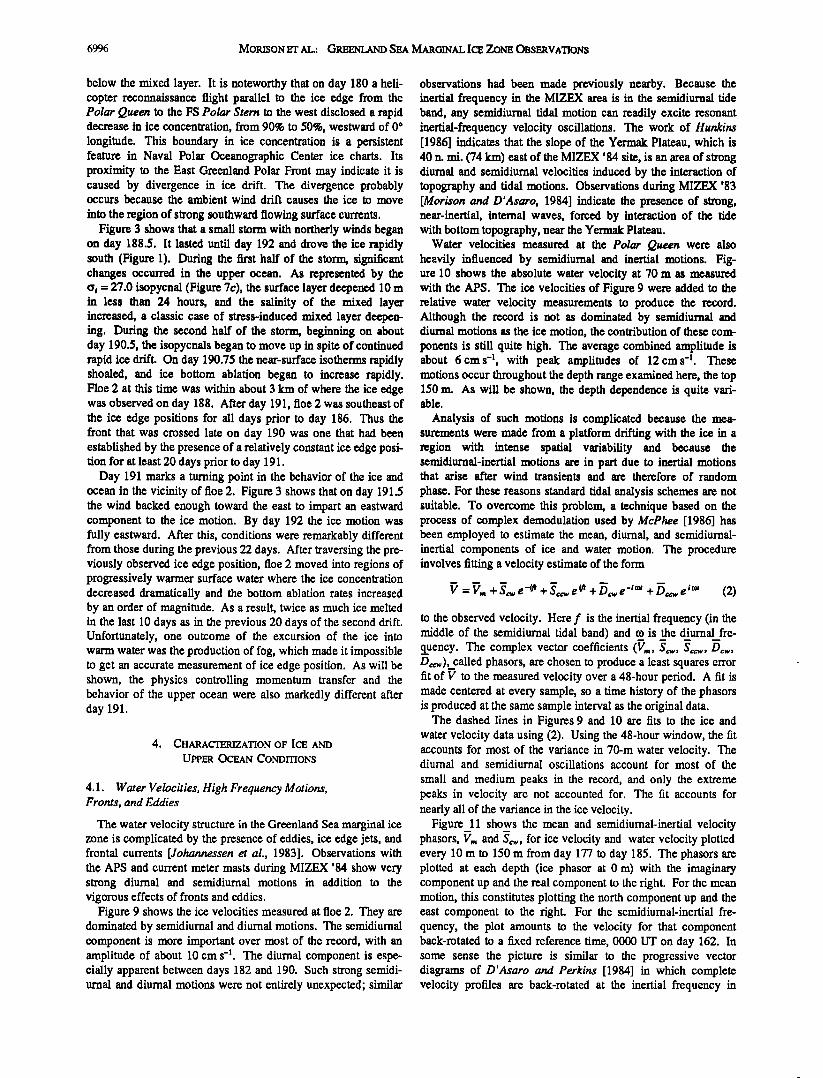
Water velocities measured at the Polar Queen were also heavily influenced by semidiurnal and inertial motions. Fig- ure 10 shows the absolute water velocity at 70 m as measured with the APS. The ice velocities of Figure 9 were added to the relative water velocity measurements to produce the record. Although the record is not as dominated by semidiurnal and diurnal motions as the ice motion, the contribution of these components is still quite high. The average combined amplitude is about 6cms -•, with peak amplitudes of 12cms -•. These motions occur throughout the depth range examined here, the top 150 m. As will be shown, the depth dependence is quite variable.

Analysis of such motions is complicated because the measurements were made from a platform drifting with the ice in a region with intense spatial variability and because the semidiurnal-inertial motions are in part due to inertial motions that arise after wind transients and are therefore of random

phase. For these reasons standard tidal analysis schemes are not suitable. To overcome this problem, a technique based on the process of complex demodulation used by McPhee [1986] has been employed to estimate the mean, diurnal, and semidiurnal- inertial components of ice and water motion. The procedure involves fitting a velocity estimate of the form

V = V,• + S,•e -il• + Sc•e •I• + D,•e -• + D•.•e • (2)

to the observed velocity. Here f is the inertial frequency (in the middle of the semidiurnal tidal band) and to is the diurnal fre- q_uency. The complex vector coefficients (V,,,, S•, Stew, Dew, D½•),_.called phasors, are chosen to produce a least squares error fit of V to the measured velocity over a 48-hour period. A fit is made centered at every sample, so a time history of the phasors is produced at the same sample interval as the original data.

The dashed lines in Figures 9 and 10 are fits to the ice and water velocity data using (2). Using the 48-hour window, the fit accounts for most of the variance in 70-m water velocity. The diurnal and semidiurnal oscillations account for most of the

small and medium peaks in the record, and only the extreme peaks in velocity are not accounted for. The fit accounts for nearly all of the variance in the ice velocity.

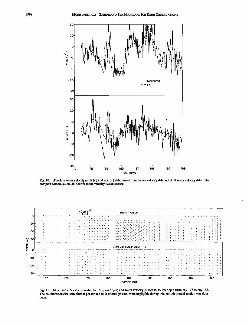
Figure 11 shows the mean and semidiurnal-inertial velocity phasors, V,,, and So•, for ice velocity and water velocity plotted every 10 m to 150 m from day 177 to day 185. The phasors are plotted at each depth (ice phasor at 0 m) with the imaginary component up and the real component to the right. For the mean motion, this constitutes plotting the north component up and the east component to the right. For the semidiurnal-inertial frequency, the plot amounts to the velocity for that component back-rotated to a fixed reference time, 0000 UT on day 162. In some sense the picture is similar to the progressive vector diagrams of D'Asaro and Perkins [1984] in which complete velocity profiles are back-rotated at the inertial frequency in

MORISONL• AL.: GREENLAND SEA Mnt•OINnL IC• ZON• OBSERVATIONS 6997

30

2O

IO

0

-IO

-20

-:50

$0

2O

IO

E 0

-I0

-20

Measured

Fit

I -3O 170 74 178 182 186 190 194 198

TIME (days)

Fig. 9. Ice velocity north (v) and east (u) determined from salellite navigation fixes for the Polar Queen while at floe 2. The complex demodulation, 48-hour fit to the velocity is also shown.

order to expose any dominant inertial motion. However, the technique used here explicitly separates the inertial frequency component from the other components so inertial frequency motions can be identified even in the presence of other strong signals.

The period shown in Figure 11 is a classic case of wind-driven inertial motion. The counterclockwise semidiurnal-inertial com-

ponent Sc,.• and both diurnal_components, D• and Dc,.•, are small relative to V= and S,.•. S• is substantial and, at least for days 180 through 183, is quite steady in orientation and magnitude. The dominance of the clockwise component suggests this is a case of inertial motion. In fact, McPhee [this issue] shows that the trajectory of the ice can be predicted during this period by assuming that the motion is inertial.

The development of the motion with time and the change in current direction with depth suggest that the inertial motions were wind induced. The motion began in the ice (0 m) and the mixed layer (15 m and 20 m) on day 179 when the wind (Fig- ure 3) shifted rapidly from southerly to northerly and the ice velocity made a rapid but short-lived shift to the southwest. The inertial motion then spread through the top 150 m throughout day 180 and into day 181. From day 180 to the middle of day 181, the inertial phasor turned slightly to the fight with depth through the pycnocline, indicating upward inertial frequency phase propagation and downward energy propagation. This

result is consistent with the results of Leaman [1976] and D'Asaro and Perkins [1984] who found that near-inertial internal wave motions in the mid-Atlantic were excited at the surface

and could be detected by examining the sense of velocity rotation with depth. Thus the explanation for the inertial motion is clear. When the wind shifted from southerly to northerly, the ice was blown south and diverged slightly (Figure 8). This freed the ice to move and excited inertial motions in the ice, which spread rapidly through the mixed layer to 20 m. On day 180 the ice was advected into a region where the stratification extended to the surface (Figure 6). After this time the energy propagated downward to at least 150 m.

Figure 12 shows a very different regime, dominated by mean motion and diurnal fides where inertial motion does not appear to have been a major factor. The mean motion on days 188 to 190 was characterized by rapid ice motion (up to 26 cm s -1) produced by strong winds. Days 192 to 194 were characterized by nearly barotropic mean motions with magnitudes up to 16 cm s -• (Figure 12). Throughout the period from day 188 to 194, the two semidiurnal-inertial components were weak and variable, while the diurnal components were also variable but ranged in value up to 12 cm s -•. The diurnal motions were fairly constant with depth except on days 192 and 193 and at the end of day 194. The ice phasor was usually not the same as the water phasor in the semidiurnal band. During most of this time the

6998 MORISONET AL.: GREENLAND SEA MAROtNAL ICE ZONE OBSERVATIONS

30

20

E 0

-I0

-20

-30

30

20

I0

E 0

-I0

-20

-30 171 175 179 183 187 191 195 199

TIME (days)

Fig. 10. Absolute water velocity north (v) and east (u) determined from the ice velocity data and APS water velocity data. The complex demodulation, 48-hour fit to the velocity is also shown.

5O

I00

•' 150 T I--

W

,

,

,

MEAN PHASOR

.;,_•__., ...... ._ ........ , ...... ., .... •_ .• ,....• .., •, .•--•- • • • • • • -•--•--•

• • • • / / / 2 i i i i i i / • ....... • / /

SEMI-DIURNAL PHASOR (+)

177 178 179 180 181 182

DAY OF 1984

....... , , / , , , / z , / i / , , /

........ / ! , . / i ,, i / i ! , . .

........ , , , , i • / , i , , ,

............. / • , , / • , ,

.............. i • , , ,

......

.......................

183 184 185

Fig. 11. Mean and clockwise semidiurnal ice (0-m depth) and water velocity phasor to 150 m depth from day 177 to day 185. The counterclockwise semidiurnal phasor and both diurnal phasors were negligible during this period; inertial motion was dominant.

MORISONET AL.: GREENLAND SEA MAROtNAL ICE ZONE OBSERVATIONS 6999

• 50

,,'

150

40 cm s '1 • MEAN PHASOR i ,

, • , _ ,

............................................ , ........... , .............. , ............................................ • .......................

SEMI-DIURNAL PHASOR (+) o ................................................ ; .................................................

. , • ......... , , , . . ; ............. i .......

......... , ....

.... , .. , .... ß . .• ...... ß •. : :::: : .... ' ................. i .......

........ • , , ....

:::: :::: ; .......... • .... :: ....... : ....... ......... : : : ....... , ..... . 'i. ::::: : ........ , ....... , ...... • ...... ,, ....... ........ • . . . , , • ...... { ...... ,, .......

• ..... • ...... i ...... : ....... ............ i .......

....... ,• ...................... • ...................... , ........................ , ................................................................... ,

,, ; , ; ,, } SEMI-DIURNAL PHASOR (-)

.............. ß ........ • ....................... • ................... • .................. r ....................... ß ......... • .......... , ................ . ......

5O

I00

150 ,

188 189 190

: ; " : :

:: ..... . . .

ß ,

191

DAY OF 1984

Fig. 12a

40 cm

0 I------I DIURNAL PHASOR (+) .......... -,---+ -4- .............. . ..... -,- ........ -,- ............... .• ..... t .... *--" "-"* ,*--•---t ...... *--,- ........ •- -.--•--t--.---• ....... t--,---+ ........ .__..__.._

.... ": : I • : : ' • ,, ; ' : • "" "" "" •'- -- :" "" 5o :ii" .... " '-i :::::'i::::::

ß , i . . • • .... , ........ ß ,, -' ': .... z:l ...... ': .............. ß i ' ' ' • ...... 'I, ..............

:::; .............................. ß ß ' • i ", ..... , • • - - . • . ? .......

_ . ,

• •5o ' ' - - •: .... • ............................... , , ,

a. ! DIURNAL PHASOR (-) ILl ,

r• 0 .......... - ........ • ....... •---- .......... -t- ....... -• ..... v--• .... 1- ............... *---t ..... •---•--•---• .... *--+ ..... •--•---*--*--*- ........ -•-4--• --•-4--•---•--

5o .... ,• '' ;::: ' '; .... • ............ ', .... '• '' i .... • :-:::.: ............. • .... ,q • • , .... • • • ,, ................. L .... , • I

.... •. • t : ..................... • t

.... • • , ; - - . j ...... ,, ........... • • I / .... ,• • • .................. i i I /

•5o .... • ;; , I ' , , • : ............. • ' • ' , .......... • • I /

, ,,

188 189 190 191 192 193 194 DAY OF 1984

Fig. 12b

Fig. 12. Ice (0-m depth) and water velocity phasors to 150-m depth from day 188 to day 194. (a) Mean and semidiurnal phasors. (b) Diurnal phasors.

mixed layer was less than 15 m deep (Figure 7c). The diurnal component of velocity measured with the APS is in agreement motions, therefore, may have been a combination of a forced with geostrophic shear calculations based on the density data. internal tide with a barotropic motion. The baroclinic motion The mean northward velocity component of absolute current may be interpreted as that of a two-layer system, the ice and measured on day 185.5 and the geostrophic velocity shear calcu- shallow mixed layer constituting the surface layer. Only the lated on the basis of the density profiles on day 184.75 and day existence of a forced baroclinic mode could explain the observed 185.75 are shown in Figure 13. The observed mean shear is temporal and spatial variability in the phasors; the horizontal about 10cms -• between 30 m and 110m, and the geostrophic scale of barotropic modes is too great to show such extreme vari- shear is about 15 cm s -•. The mean shear is lower in part ability. because it is a 48-hour, smoothed estimate. The general shape of

Floe 2 drifted into the easternmost part of the East Greenland the two profiles is the same and is in agreement with the general Polar Front starting on day 184. The shear in the northward consensus on the East Greenland Current; that is, the surface

7000 MORISONET AL.: GREENLAND SEA MARGINAL IC• ZO• OBSERVATIONS

20

40

60

a. 8O

IO0

120

140

u (cms '1) -30 -20 -I0 0 I0 20 50

i i I i i i i

_

',,! Geostrophic I APS - _

_

_

I I I I i Ii• i I Fig. 13. Northward component of water velocity at the eastern edge of the East Greenland Polar Front, 80 ø 38'N, 1 ø 25'E. The solid line is the absolute current from the APS data and ice navigation data for day 185.5. The dashed line is the geostrophic shear calculated on the basis of the day 184.7:5 and day 18:5.75 density profiles.

water is moving south relative to water at depth. The interesting aspect of the observed water velocity is that it is northward at all depths. Even when floe 2 was farthest into the frontal region, the southward ice drift component was very low. Thus the geo- strophie shear and relative velocity measurements indicate northward transport.

The location of the front may explain the northward transport. Floe 2 was actually east of the center of Fram Strait when the measurements were made in the front. This was far enough east to encounter the westernmost edge of the northern extension of the West Spitzbergen Current. At this northern extension of both the East Greenland Polar Front and the West Spitzbergen Current, the two features are apparently not separated by a gyre of recirculating Atlantic Water; southward moving Arctic Water simply overlies northward flowing Atlantic Water. The northward flow at depth was thus the baroclinic inflow of Atlantic Water to the Arctic Ocean. Floe 2 was nearly at a null point with regard to surface current, between the barotropic surface components of the north flowing Atlantic Water and south flowing Arctic Water. Such a place, between strong opposing currents, is a likely location for the generation of eddies. Indeed, R. A. Shuchman et al. (unpublished manuscript, 1987) indicate that Argos buoys to the southwest of the ship drifted rapidly southward during days 184 to 188, and from this they conclude that the Polar Queen was caught on the eastern edge of a large cyclonic eddy. Presumably, this eddy would have been a product of the meander in the East Greenland Current described by Manley et al. [1987] as being centered at 80.7øN, 1.0øE from day 177 to day 182. In any event, it seems that the ship did not go quite far enough west to be caught up in the southward surface component of the East Greenland Current. The very sharp drop in ice concentration observed at 0 ø longitude (12 km west of floe 2's westernmost position) during the aerial reconnaissance flight on day 182 suggests that this was the location of the surface manifestation of the East Greenland Current. Also, from day 184 to 188 a cyclesonde buoy, originally located 7 km to the west of floe 2, drifted rapidly south relative to floe 2. It was finally recovered 60 km southwest of the ship. Apparently floe 2

came within a few kilometers of being swept southwest with the East Greenland Current.

The eddy that floe 2 crossed between days 192 and 194 produced an interesting pattern in the velocity field. Vector profiles of mean absolute velocity for this period (Figure 12) illustrate the vertical structure in the eddy. On day 192.0, when the wind first blew the ice eastward, the absolute water velocity in the mixed layer was to the northeast, veering slightly to east- northeastward with depth. As the ice continued to move eastward on days 192 and 193, the water velocities turned eastward and finally southeastward. Despite northward winds, the ice motion veered from eastward to east-southeastward. The ice

motion was thus a combination of the surface eddy motion and a superimposed northeastward wind drift.

The mean absolute currents for days 192 to 194 shown in Fig- ure 12 are constant with depth except for attenuation in the mixed layer and a slight maximum at 90 m. The profiles give the appearance of an eddy that was originally active from the surface to over 150 m and then had the energy removed from the surface layer by turbulent dissipation at the surface. The 90-m mean current data can be used to produce a picture illustrating the eddy geometry. Figure 14 shows the mean 90-m velocity vectors plotted versus position. The dashed lines perpendicular to the vectors intersect at what would be the eddy's center if the eddy were exactly round and did not move. These assumptions are not perfect, but the cloud of intersection points does suggest an average eddy center at about 79ø51'N and 1ø57'E. Also shown in the figure is an approximate outline of the edge posi- ton on day 188 taken from the SAR image of Shuchman et al. [1987]. On day 193 the center of the eddy was roughly 17 km south of floe 2 and about 17 km south of its position on day 188.

This eddy is different in its sense of rotation from most of the eddies encountered in the Greenland Sea MIZ. Eddies described

by Johannessen et al. [1983] and Wadhams and Squire [1983] are all cyclonic. The velocity pattern of Figure 14 and the SAR image indicate this eddy was anticyclonic. The observations of Johannessen et al. [1983] suggest eddies of this size (10-kin to 30-kin diameter) are quite common at the ice edge. It is argued that, because these small eddies scale with the Rossby deforma- tion radius (5 km at floe 2) and appear at the ice edge in the presence of strong horizontal shear, they are due to barotropic instability. Because the prevailing currents and jets at the ice edge are southwestward, eddies caused by barotropic instability that appear at the ice edge tend to be cyclonic. However, an anticyclonic eddy might be generated by an anomalous northeastward moving jet (unlikely in this case, given the observed winds and ice motion) or might be generated, under the ice, on the northwest side of a southwestward jet. In the latter case the anticyclonic eddy would appear when the ice edge moved north or the eddy moved south (as this eddy appears to have done). Thus it seems plausible that the eddy observed from day 192 to 193 was generated by barotropic instability on the northwest side of a southwestward ice edge jet, dissipated some near-surface energy while under the ice, and then moved south relative to the edge. The water temperature in the eastern half of the eddy (days 183 to 195.5 in Figure 7) is slightly lower than the surrounding water, reinforcing the notion that the eddy originated under the ice.

4.2. Surface Heat and Mass Balance

Both the atmosphere and ocean supply energy needed to drive the melt cycle in the MIZ. The primary source of energy from the atmosphere is incident shortwave radiation (F,), and the pro-

MORISONET AL.: GREENLAND SEA MARGINAL ICE ZONE OBSERVATIONS 7001

80o20'N

80 ø 10'N

80øN

79ø50'N

10 km I I

2OE 3OE

i

• 192 75 193 0 r•/"'• 193 75 J --i • 192 7'- 5 • =ø'u/•. r•-//'•?•."" _.• DIF•'•'•E 192.5 •" • / / • = ICE

.,,,,•1,,. _• ', •, • •- .• ./ ' .

I ', , •/ x • •.q •t /

•1 ,7 'v' I•,'• • I

Fig. 14. The 90-m absolute water velocity (mean phasor) plotted at floe 2 positions from day 192 to day 194. The dashed lines are drawn perpendicular to the vectors and, in an idealized situation, would intersect at the center of an eddy that was observed in the area on day 188. Also shown is the outline of the ice edge eddy taken from the day 188 SAR image of Shuchman et al. [•9871.

perties of the ice that affect its absorption and distribution must be considered as important variables. Maximum values of F, during MIZEX '84 were typically 400--450 W m -2 under clear skies and 250-300 W m -2 when cloudy. Daily averages ranged from 104 to 305 W m -z, the mean for the entire drift being about 200 W m -2. Totals for both June and July were about 30% greater in the northern Greenland Sea than climatological averages given for the central Arctic [Marshunova, 1961]. Observa- tions at the drifting ship in 1984 indicated that turbulent heat input to the surface was very small (P. Guest, personal communication, 1985), but this may not have been the case in the outer MIZ, where ponds and patches of bare ice were clearly visible in the helicopter photographs in late June. The proximity of warm water and evidence of more rapid surface melting suggest that the turbulent fluxes may be significant near the extreme edge.

Despite the larger F,, observations during both MIZEX '83 and MIZEX '84 indicate that the melt progression in the Green- land Sea MIZ lags that of the central Arctic by several weeks. This is primarily related to heavier snow cover in the MIZ. Sur- veys carried out in the vicinity of the Polar Queen in late June 1984 revealed average snow depths as much as 50% greater than the maximum depths found in areas of perennial ice. The snow on multiyear floes was frequently 3 to 4 times as deep as that on nearby first-year floes, indicating that much of the snowfall occurred early in the freezing season. Similar results were also

found during MIZEX '83. With the exception of the extreme ice edge and the outer part of the transition zone, extensive snow remained until nearly mid-July and was, in fact, present throughout the drift at several surface ablation sites. Snow coverage at the end of the drift was estimated to be about 20%; superimposed ice produced by the melting and refreezing of snow accounting for about 25% of the remaining area. Evidence from MIZEX '83 suggests that snow is even more persistent to the west of the MIZEX area. Observations taken in late July 1983 during a transect of the FS Polar Stern to the Greenland coast indicated the ice in the Greenland drift stream still supported a substantial snow cover (T.C. Grenfell, personal communication, 1983). At this point the data are insufficient to determine whether greater snowfall or lower energy input at the surface was primarily responsible for the longitudinal gradient in snow depth.

The significance of the late snow melt is twofold. First, the higher albedo of the snow means that considerably less shortwave radiation is absorbed by the system than would be the case with a bare ice cover; second, much of the energy that is absorbed during June and July, the period of maximum F,, is utilized in melting the snow rather than the underlying ice. Heat contained in the ocean must therefore be the principal agent responsible for thinning the ice during this period, although not necessarily later in the summer. In fact, once the ice became

7002 MORISONET AL.: GREENLAND SEA MARGINAL IC• ZON• OBSERVATIONS

2 .• 15

:.•

•.5

•1.0_ .0 0

• 5

x 0 • 1GO IG5 170 175 180 185 lgO lg5 200

O

-10

-1•

180 185 170 175 180 185 lgO lg5 200- o

DAY OF

Fig. 15. Surface flux and mixed layer parameters measured daring MIZEX '84. (a) Friction velocity u. and ice melt rate. (b) Average mixed layer salinity and temperature. (c) Mixed layer depth, defined as the shallowest depth where the Brunt- V//is/il//frequency exceeded 4 cph.

mostly snow-free, after day 193, average surface ablation rates were as large or larger than any observed at the underside of the ice prior to its entry into Atlantic Water (Figure 8). Ablation rates for the entire drift averaged about 20 kg rn -2 d -• at the bottom and 8.5 kg m -2 d -• at the surface; corresponding values before day 190 were 9 and 6.5 kg m -2 d -• (Figure 8). Bottom ablation during both periods was much greater than that observed in areas of perennial ice. Internal ice temperature profiles measured in floe 2 showed the ice to be nearly isother- mal near the bottom, so that mass losses at the bottom were a direct measure of heat input from the water to the ice.

Lateral ablation, which appears to be a major factor in the summer decay cycle of perennial ice, was fairly small near the drifting ship prior to day 191 because most of the solar energy entering the leads went to the preferential melting of the broken-up first-year ice. Upon entering the Atlantic Water, however, brash in the leads quickly vanished, and between day 191 and 193 about 80 cm of lateral ablation took place, slightly more than the total observed during the preceding 3 weeks. During the next several days, lateral ablation was very rapid, the total thermal and mechanical erosion reaching as much as 10 m at some sites. It is interesting to note that bottom ablation was greater near the edge of the floe than beneath the interior when leads were filled with brash, but this pattern reversed once the leads became open. The probable reason for this behavior is that some stable water from the leads was being advected beneath

surrounding floes, a factor which is of importance in modeling the regional interaction of shortwave radiation with the ice and upper ocean [Maykut and Perovich, this issue]. During the first half of the summer, then, it appears that lateral ablation on multiyear floes is significant only during the final decay of the ice cover in the outer MIZ. Although it is of potential importance throughout the MIZ in late July and August, its role then remains dependent on ice concentration and the degree to which leads are occupied by first-year brash.

4.3. Momentum and Heat Transfer

The results of measurements of momentum and heat transfer

during MIZEX '84 are well illustrated with time histories of total ice-ocean stress, turbulent stress in the upper ocean, mixed layer properties, and ice melt. Time histories of the heat and mass exchange coefficients give a convenient summary view of boundary layer behavior. A subset of MIZEX '84 upper ocean data is considered in great detail by McPhee et al. [this issue]. The boundary layer response to the storm from day 188 to 192 is examined, and the turbulence and mixed layer measurements are compared with a model for a specific set of circumstances. The aim here is to show the variability of the exchange coefficients as they relate to changes in oceanographic conditions throughout MIZEX '84.

Time histories of ice-ocean stress, ice melt rate, and mixed

MORISONET AL.: GREENLAND SEA MARGINAL IC• ZON• OBSERVATIONS 7003

2.0

1.5

0.5

+ 1; 1/2

,,, .... , .... , .... 160 165 170 175 188 185 190 195 200

4.0

30

õ20

I o

2.0

0.0 // 0.0

160 165 170 175 180 185 190 195 200

DAY OF 1984

4.0

, Slope: 0.69

3,0 B

I I Ol /

Slope: 2.03 00/

0 -

/oO [ i [ 0.0

0.5 1.0 1.5 2.0 0.0 0.5 1.0 1.5 2.0

u,(cm s '1) u,(cm s '1)

Fig. 16. Friction velocity u, plotted with Reynolds stress I; v• and the square root of twice the turbulent kinetic energy q. (a) Plot of u, and x • versus time for the duration of MIZEX '84. (b) 2u, and q versus time for the duration of MIZEX '84. (c) Scatter plot of I; vi versus u, and the linear fit, I; vi = 0.69u, (dashed line). (d) Scatter plot of q versus u, and the linear fit, q = 2.03u, (dashed line).

layer depth, temperature, and salinity are plotted together in Fig- ure 15. The ice-ocean stress is presented in terms of the friction velocity u,, where

% = p• u, u'-, (3)

and ¾w is the total stress exerted by the ice on the water, u. is the magnitude of •., and p,• is the water density. The overbars denote complex vectors with real parts positive east and imaginary parts positive north. Total stress Y, is calculated from the wind stress corrected for Coriolis force acting on the ice using a Rossby similarity expression in the steady, free-drift, force balance [McPhee, 1982, this issue],

x% - C,0•,0 I•,01 - i P--Lihf• (4) P•

V=-- n -A-/B (5)

The Coriolis term involves the relative ice velocity V computed with the Rossby similarity expression (5), where f is the Coriolis parameter, h is the ice thickness, Pi iS the ice density, and •c is von K•m•n's constant. A and B are the similarity parameters and are numerically equal to 2.0 [McPhee, 1982].

Except when stress levels are low, the main effect of the Coriolis term is to rotate the horizontal stress vector. Wind stress is cal-

culated as the quadratic term involving the measured wind, adjusted to the 10-m level Ul0 and the 10-m drag coefficient C l0 (C10=0.0023) determined by K. Davidson and P. Guest (personal communication, 1985).

The mixed layer parameters shown in Figure 15 are taken from the APS data. Except for the melt rate (interpolated between 24-hour ice thickness differences), the time series represents 6-hour averages of the measured variables. Several of the key episodes discussed previously show clearly in Figure 15. The excursion into the East Greenland Polar Front on day 186 appears as a momentary deepening and salinization of the mixed layer. The storm-induced deepening and freshening of the mixed layer on days 188 and 189 and the subsequent frontal crossing and entry into the high melt regime on day 190 are also apparent.

The friction velocity u. of Figure 15 is representative of the total ice-water stress including components due to turbulent skin friction and form drag. The MIZEX '84 measurements of the ratio of total stress to other turbulence parameters are consistent with the ratios found in other boundary layer studies. For example, Figure 16a shows u, plotted versus time along with x vi

7004 MORISONET AL.: GP.E•U. AND SEA MARGINAL IC• ZON• OBSERVATIONS

1/2

P0 a) ----- u, < Cd > = 0.079 16

u30 rel :•• .+"[[-.7 • ,- 15 -iF H- .-h 1• •

ß

.L,,,X,,,,,,,,V,,,,, . 160 165 170 175 180 185 190 195 200

0.0 0

160 165 170 175 180 185 190 195 200

18

12 o o o

x

o

DAY OF 1984

Fig. 17. Boundary layer I•, rameters and exchange coefficients versus time for the duration of MIZEX '84. (a) The square root of the drag coefficient, Ca •, plotted as pluses along with the friction velocity u. and the 30-m relative current U 3ore. (b) The heat transfer coefficient Ck plotted as pluses along with the heat transfer temperature scale 0. (see equations (11) and (12) in text) and the elevation bTat of the mixed layer temperature above the freezing point.

where

•= [<u' w' > •' + < v' w'>z] '• (6)

and where <u' w'> and <v' w'> are horizontal Reynolds stress components in the east and north directions. Figure 16b shows 2u. plotted versus time along with the square root of twice the turbulent kinetic energy,

q = [<ua> + <va> + <w'2>] v• (7)

Scatter diagrams of x '• and q versus u. are shown in Figures 16c and 16d; x '• and q were averaged for sensor clusters at 2 m (two clusters), 4 m, and 7 m below the ice. The average Reynolds stress is about half u. 2, and q 2 is about 4 times u-2. For an idealized horizontally homogeneous boundary layer, x v• equals u. near the surface and decreases monotonically with depth. The under-ice boundary layer is usually too rough to conform with this idealization; owing to the effects of form drag on the larger roughness elements, the Reynolds stress levels near the ice surface are about half the total stress [McPhee and Smith, 1976]. In fact, turbulent stress often increases with depth near the surface [McPhee et al., this issue]. According to data from several sources compiled by Mellor and Yamada [1982], the ratio of (q/u.)•' in flows where production balances dissipation is 6.50. Data from Klebanoff [Hinze 1975, p. 642] show the average ratio through the boundary layer to be about 4.

The constitutive relationship between total drag and the relative velocity between the ice and water is illustrated by Figure 17a in which the magnitude of the 30-m water velocity relative to the ice (U3o), the friction velocity u., and C,? (the ratio of u. to U ao) are plotted. The ratio is equal to the square root of the magnitude of the geostrophic drag coefficient in the quadratic drag law

= u2 = ca U (s)

An equivalent and convenient formula for the drag law yields the stress as a product of u-, which expresses the level of turbulence, and the free-stream velocity U zo:

x-2-• = C• u. U ao (9)

A complementary expression can be used for heat flux

H (P•o C•,)-' = O. u- = C•, u. ATat (lO)

In (10) the heat flux H is also equated with the turbulence parameter u. and the free-stream parameter ATat. ATat is the difference between the mixed layer temperature Tat and the freezing point T/ at the mixed layer salinity Sat. C•, is the specific heat of water.

Referencing the drag law to the free-stream velocity is desir- able to avoid the unpredictable local effects of form drag on velocity at shallow depth. The 30-m reference depth has been chosen for the free-stream velocity in (9) because it is the shallowest depth at which no boundary layer turning was observed. The magnitude of the V= phasor is used to represent relative velocity, so tidal and inertial motion are removed. In order to match the 48-hour complex demodulation window, the time series of u. was smoothed over 48 hours. Because the drag coefficient is a ratio, it is unduly affected by extraneous factors (e.g., density driven currents or internal ice stress gradients) when either u. or U ao is small, so it was calculated only when u, exceeded 0.4 cm s -• and U ao exceeded 5 cm s -•.

The heat flux, characterized by the heat transfer temperature scale 0. and the mixed layer temperature elevation ATat are

MORISONET AL: GREENLAND SEA MARGINAL ICE ZONE OBSERVATIONS 7005

2.8 15

1 5 0

õ10 ,•

85

00

168 165 170 175 188 185 191t 195 288

DAY OF 1984

Fig. 18. Observed ice rr•lt, friction velocity u,, and the theoretical ice rr•lt from the mod•l of McPhee et al. [this issue], all plotted versus time.

plotted versus time in Figure 17b. From (10) it follows that 0. is

H

O. = PaCt u. (11) The time history of H has been derived from ice bottom melt rate data. Measurements of ice temperature gradients during MIZEX '84 show that conduction of heat in the lower part of the ice was negligible [Maykut and Perovich, 1985]. Thus melting was due to heat flux from the mixed layer and

p•Ld O, = • (12)

where L is an effective- (corrected for brine volume) latent heat of fusion, Pi is the ice density, and d is the melt rate. The time series of melt rate and mixed layer temperature elevation were smoothed over 48 hours. Also shown in Figure 17b is the ratio of 9. to ATe, which equals the heat transfer coefficient Ca of (10). As in the calculation of C,• •, Ca was computed only for u. greater than 0.4 cm s -•.

The average value of C• for the whole experiment was 0.079. This value corresponds to a Cd of 0.0062, close to the value of 0.0055 found for the AIDJEX camps in the central Arc- tic by McPhee [ 1979]. In retrospect, this may not be surprising because the AIDJEX coefficients were derived from data gathered during the summer when, on average, conditions may not have been too different from those around floe 2. Equations (9) and (10) and Figure 17a deal only with stress and velocity magnitudes and the magnitude of the drag coefficient. In fact, the average turning angle between the stress and relative velocity was 28% a value nearly equal to the value of 23 • found for the AIDJEX data by McPhee [ 1979].

The average heat transfer coefficient Ca is 0.0038. The formulation of (9) and (10) suggests there should be some correspondence between C• and Ca. If Reynold's analogy holds (i.e., if turbulence in the boundary layer transports heat and momentum at roughly equal rates) and ff the temperature at the top of the turbulent boundary layer is at the freezing point, then Ca should roughly equal C•. In fact, the average Ca is 20 times smaller than C•. As was shown by McPhee et al. [this issue], this implies that most of the temperature gradient actually occurs across a thin, laminar sublayer near the bottom of the ice. Fig- ure 18 shows ice melt as predicted with the model of McPhee et al. [this issue] which incorporates the effects of the laminar sublayer on heat transport. The correspondence with the observed melt rate is quite good for most of the record.

The most remarkable aspect of drag and heat transfer coefficients is their variability. Prior to day 187, u. was rela-

tively low, and some of the variability in Ca and Ca may have been due to the effects of floe-to-floe interaction forces or small

errors in u. or U 3o. During this period, some of the variation in C•, may also have been due to measurement errors superimposed on relatively small values of heat flux. However, the variations in the coefficients generally seem to fall into two groups depending on the surface stratification.

During periods of weak surface stratification, Ca and Ca tend to rise and fall together. This was the case from day 170 to day 180 (Figures 6c, 17a, and 17b) and from day 184.5 to late on day 191 (Figures 6c, 17a, and 17b). The situation is illustrated in the most definitive way during the small storm from day 188 to 192 described in detail by McPhee et al. [this issue]. From day 189 to the middle of day 192, C,• h decreased steadily. McPhee et al. [this issue] identify three stages in upper ocean response to the storm. As is shown in Figure 15c, during the first day the mixed layer, which had little heat content, deepened steadily under the influence of surface stress. Then at about 189.5, the floe drifted over a salinity-controlled density front, and the mixed layer shoaled slightly (Figures 15b and 15c) despite high turbulence levels. Starting on day 190 and continu- ing until late on day 191, the floe crossed a second front, this time with an abrupt rise in upper ocean temperature, and a corresponding increase in bottom melt rate (Figure 15b). The decrease in drag between days 190 and 191.5 indicates the importance of surface buoyancy flux on boundary layer dynamics. The heat transfer coefficient behaves similarly, thus demon- strating the buoyancy feedback mechanism identified by McPhee [1983]' as ice melts rapidly, the influx of relatively fresh water stabilizes the boundary layer, decreasing the efficiency with which turbulence transports momentum and heat through the boundary layer. Because heat and momentum are both transported by turbulence in regions of weak upper ocean stratification, a form of Reynolds analogy does hold; decreases (increases) in turbulence decrease (increase) both Ca and Cal.

During periods of stronger upper ocean stratification, Cd and Ca varied in opposition; when Cd increased, Ca decreased, and vice versa. While floe 1 was in a region of surface stratification from day 163 to 166, the drop in Cd Was associated with a rise in Ca (Figures 5c, 17a, and 17b). When the ice moved into a region of surface stratification on day 180, Cd increased and Ca decreased (Figures 6c, 17a, and 17b). At the same time, strong inertial motions began at the surface and propagated downward (Figure 11), indicating that downward momentum transfer was occurring. The most significant example of the effects of surface stratification begins to appear beginning late on day 191, when floe 2 moved out into warm water. The drag coefficient rose to a

7006 MORtSONET AL.: GREENLAND SEA MARGINAL IC• ZO• OBSERVATIONS

I I I I I I I I I I

2.B

ß

-2. B 4 m

• m

I I I I I I I I I I

B lB 2B ':lB 4B ;B F;B 7B rmB qB

2.B

E Ore. Ore 2 m

ß

-2.Ore 4 m

• m

b)

I I I I I I I I I I

2.B

• B.B • 2 m

-•.Om 4 m

I I I I I I I I I I

TIME (min.)

Fig. 19. Vertical velocity fluctuations w' measured with current meter clusters at 2 m, 4 m, and 7 m below the ice, or at 4-m, 6-m, and 9-m depth. The friction velocity u. was equal to about 1.0 for all three cases. (a) Measurements starting at day 188.465. The horizontal velocity at 7 m below the ice was 13.8 cm s -]. (b) Measurements starting at davy 191.711. The horizontal velocity at 7 m below the ice was 12.7 cm s-'. (c) Measurements starting at day 197.896. The horizontal velocity at 7 m below the ice was 12.4 cm s -].

maximum of Ca • = 0.14 (Ca = 0.0196), while the heat transfer coefficient decreased to a minimum of Ch = 0.0025. The values of u., U •o, and heat flux during this period were high, so the results are unambiguous. The increase in drag coefficient during this period is especially surprising because stratification inhibits turbulent momentum transfer. In fact, Figure 16a shows that the Reynolds stress was quite low relative to u. from days 193 to 200, and the decrease in heat transfer coefficient suggests that stratification did inhibit turbulent heat transport.

Apparently, in regions of strong, near surface stratification a process was operating that preferentially transferred momentum over heat and did not involve turbulence. One such process is the generation of internal waves by the motion of a rough ice surface over a stratified surface layer. Turbulent heat flux occurs by direct fluid overturn. Momentum flux, on the other hand, responds according to the pressure terms in the equations of motion, so considerable energy may be radiated away from the interface as internal gravity waves ff a density gradient exists

near the surface. After day 193 the top 10 m was stratified. Figure 15c shows that the mixed layer depth was usually near 5 m. Thus ocean conditions were ideal for ice bottom roughness to generate internal waves. Furthermore, a decrease in ice concentration after day 193 made the floe edges more effective as potential roughness elements and generators of internal waves.

High-frequency velocity, temperature, and salinity perturbations give strong indications of near-surface internal wave activity. Figure 19 shows the vertical velocity w' measured with current meter clusters at 4-m, 6-m, and 9-m depths during three periods when u. was equal to about 1 cm s -•. Figures 19a and 19b are from days 188.5 and 191.7, respectively, the beginning and end of the storm. The velocity patterns are typical of turbulent boundary layer conditions. The motion is vigorous, but the patterns are not coherent with depth. Figure 19c from day 197.9, when the drag coefficient was high, shows coherent oscillations in w' with periods from 5 rain to 14 rain and an average period of 8.6 min. The peak-to-peak amplitude of these motions is 2 cm s -• at 9-m depth (7 m below the ice) and 1 cm s -• at 4-m depth. There also appears to be a first-harmonic oscillation over the 90-rain record which is coherent between the levels and has a

2 cm s -• peak-to-peak amplitude at 9 m. Figure 20 shows measurements of temperature and salinity

perturbations for the same period shown in Figure 19c. The vertical displacement scales on the right of Figures 20a and 20b are constructed on the basis of the average temperature and salinity gradients (0.33 ø m -• and 0.2 %, m -•) estimated from Figures 7a and 7b. The salinity perturbations lag the temperature perturbations by about 1 rain, presumably because of the flushing time of the conductivity cells. The temperature fluctuations usually lag the velocity fluctuations by 90ø; that is, temperature increases while the water moves upward. This supports the notion that the fluctuations are due to internal waves.

i I I I I I I I I I

-01.2 m 1.0

• 0

a) -1.0

I I I I I I I I I I

B lB 2B 3B 4B 5B EB ?B BB 9B

B. 2

o•. B.B .....

F-

-B. 2

7 m 0 E

-1 .o I I

B lB 2B 3B 4B SB BB ?B BB 9B

TIME (min.)

Fig. 20. (a) Salinity and (b) temperature perturbations measured at sensor clusters 2 m, 4 m, and 7 m below the ice starting at day 197.896. The equivalent displacement scales are derived by dividing the salinity and temperature scales by the vertical gradients in the variables.

MOlUSON ET AL.: GREENLAND SEA MARGINAL IC• ZON• OBSERVATIONS 7007

The motions observed from the ice are Doppler shifted by the motion of the ice relative to the water, but it is possible to estimate a horizontal wave number and true frequency if both the displacement and velocity data are used and it is assumed the motions are due to an interfacial wave with

cos • (13)

W = mE sin • (14)

where • is the vertical displacement, W is the vertical velocity, •o is the frequency, and E is the displacement amplitude. Then for a measured rms displacement • and velocity W

W•m•

The amplitude of the displacement fluctuations averages about 0.30 m, and the amplitude of the velocity fluctuations averages about 1.0 cm s -•. Thus o• is 3.33 x 10 '-2 s -•, or 19.1 cph, nearly equal to the local Brunt-V•/isi/l•/frequency.

For an interfacial wave with wave number k, density difference across the interface Ap (1.35 kg m-g), and interface depth D (D = 9 m is chosen as the center of the density jump), the dispersion relation is

m2: $kap (16) (1 + coth kD )p,•

For an •o of 19.1 cph, this formula suggests the waves have a horizontal wavelength of 40 m, a phase speed of 20 cm s -•, and a group velocity of 11 cm s -•.

Using these parameters and the formula for the Doppler- shifted frequency •Oob measured from the ice moving parallel to the waves at Vi (12.4 cm

mo: Im-

(oob is found to be 0.011 s -•, or 6.5 cph. This corresponds to a period of 7.5 rain, which is reasonably close to the average observed period of 8.6 min. If the waves were assumed to be traveling in any direction but that of the ice, the calculated which is a little too high, would be even higher. Thus the observed waves must be moving parallel to the ice.

There are several points regarding the velocities of the observed waves that are worth noting. The phase velocity of the observed waves, 19 cms -•, is greater than the ice velocity, whereas the group velocity, 11 cm s -•, is slightly less than the ice velocity. The wavelength is neither shortwave, kD >> 1, nor longwave, kD << 1; rather, kD is of the order of 1. The longwave phase speed C•on•,,,• is 34.5 cm s -•, so the internal Froude number, Vi / C •o,,m•, is 0.36.

Now that the observed waves have been characterized, the remaining questions are, were they generated by ice motion, and could wave generation cause the observed increase in drag? A number of authors have suggested that the effects of internal wave generation by ice motion can be important. Two types of forcing are generally considered. An example of the first is discussed by Muench et al. [1983], who present evidence that internal waves forced by stress divergence between ice floes and open water may give rise to a feedback mechanism that results in the creation of ice edge bands. Morison [1980, 1986] also exam- ines internal wave forcing by surface stress curl and divergence and by surface pressure and buoyancy flux. For horizontal length scales under 5 kin, he concludes that stress curl and divergence

are much less effective than pressure gradients or buoyancy flux at forcing waves.

A great deal of interest has been expressed in the second type of forcing, generation of internal waves by ice bottom roughness, and the resulting drag on the ice. Because the observed wave motions were of small scale and because the drag increased after the surface stratification became high, this mode of generation appears most pertinent here. Rigby [1974, 1976] deals with the generation of internal wakes by pressure ridge keels. Because he deals strictly with motions with phase speeds matched to the ice velocity, it is difficult to relate his results to the observed waves. The laboratory results of Muench and Hachmeister [1984] are more pertinent. By towing a model two-dimensional pressure ridge keel (or double keel) in a stratified tank, they were able to observe the generation of internal wakes and determine the increase in drag as a function of internal Froude number. For both single and double keels the drag caused by internal generation was a maximum at a critical ice speed of about haft the longwave interfacial wave speed.

The tow tank tests indicate that a generated wake need not be completely stationary in phase relative to the ice. It was found that in steady state the moving keel generated a stationary wake that persisted one to six wave cycles domstream and then degenerated into wave motions that were not stationary. This implies that, while there may be a local disturbance around any one keel, the aggregate effect of wave generation by many roughness elements is to produce multiple waves that are not stationary in phase relative to the ice. In a similar vein, Elanan [1906] obtained results similar to those of Muench and Hachmeister [1984] by towing a three-dimensional model of the Fram in a stratified tank to determine the effects of "dead water."

The tests revealed that maximum drag occurred at a critical tow speed about haft the shallow-water internal wave speed, just as in the Muench and Hachmeister [1984] study. Furthermore, at the maximum drag point, the waves behind the vessel had a phase speed greater than the tow speed. Thus the results of both laboratory studies indicate waves should appear with group velocities less than the ice velocity and a phase velocity greater than the ice velocity. This is indeed the situation with the observed waves during the period shown in Figure 19c. The ice speed was 36% of the long internal wave speed. Admittedly, the observed group velocity is only very slightly less than the ice velocity, but this might be explained in two ways. First (switch- ing now between thinking in terms of interfacial waves and thinking in terms of waves in a continuously stratified medium), the observed waves have the highest frequency possible, nearly equal to the local Brunt-V•/is•tl•/frequency, and hence the lowest possible group velocity as interfacial waves. Second, waves with a group velocity near the ice velocity will have energy continuously added to them, cannot propagate energy downward because of their high frequency, and will tend to increase in energy with time.

The tests of Muench and Hachmeister [1984] can also be applied to estimating the magnitude of wave-induced drag during MIZEX '84. They found that at the critical tow speed the added drag due to wave generation was equal to twice the total drag measured at the same speed in an unstratified tank. Because of the small horizontal extent of their model, the drag in the unstratified tank was probably mostly form drag. Therefore it may be more precise (conservative) to say the wave drag was double the form drag. For tow speeds equal to 0.36 times the longwave speed, the wave drag was equal to the form drag.

Relating the wave drag of a two-dimensional single or double

7008 MORISONET AL.: G•]mLAND SEA MAgOINAL IC• ZONE OBSERVATIONS

keel model to a situation involving the real three-dimensional roughness is not straightforward. Some comfort can be taken from the fact that the three-dimensional tests of Ekman [1906] produced results substantially similar to those from the two- dimensional tests. The main problem is that Muench and Hachmeister [ 1984] present only one ratio r of keel draft to the mixed layer depth, r = 0.187. As was discussed by Topham et al. [1986], the minimum set of nondimensional parameters required to describe the wave generation process is the internal Froude number and r. However, the mixed layer depth was so shallow on day 197 that conservative extrapolation of the laboratory results to the field situation suggests internal wave generation as a plausible cause of the observed drag increase. The mixed layer depth on day 197 was 9 m., so that an r of 0.187 corresponds to a ridge draft of 1.7 m. Floe 2 itself averaged 2 m in draft, and on day 197 there was adequate separation of the ice floes for each to act as a separate drag element. Furthermore, divers observed numerous roughness elements on the bottom of the ice, ranging from 0.5-m bumps at 15-m spacing to a large pressure ridge with a draft over 6 m (D.K. Perovich, personal communication, 1986). Basically, the ice floes around floe 2 were rougher and projected deeper into the mixed layer than did those in the model of Muench and Hachmeister [1984]. Thus their wave drag augmentation results should be considered a minimum for the MIZEX '84 case. Estimating the wave- induced drag at tloe 2 to be equal to the form drag without waves and recalling that the form drag and skin friction contributions are about equal, we would expect a 50% increase in drag when wave generation occurs. This would result in a drag coefficient of 9.0 x 10 -3 (C,? = 0.095), whereas the observed value is 11.0 x 10 -3. It also should be mentioned that, because there is a sharp maximum in drag at a particular velocity, the ice may act like a vessel trying to plane: the wind can blow harder and harder, but until the maximum force is exceeded, the ice speed will change very litfie and the drag coefficient will simply increase. This looks exactly like what was happening from day 193 to day 200 in Figure 17a.

5. CONCLUSIONS

Several new facets of upper ocean and ice behavior in the MIZ were revealed by this study. The upper ocean environment in the Greenland Sea MIZ is quite energetic in ways that had not been anticipated. The strength of the diurnal and semidiurnal- inertial velocities are quite substantial in the Greenland Sea MIZ, in some cases comparable to eddy and frontal velocities. Much of the inertial motion is excited by surface forcing, whereas all of the diurnal and some of the semidiurnal-inertial motion appear to be tidally forced. Both baroclinic and barotropic modes occur. The inertial motions are important because they transfer momentum through the mixed layer and cause shear at the pycnocline. They also transfer wind energy into the internal wave field [D'Asaro and Perkins, 1984]. The tidal motions interact with topographic features to produce internal waves and various trapped oscillations [Hunkins, 1986; Manley et al., 1987]. Researchers must be aware of these oscillatory motions in order to interpret velocity data correctly; absolute velocity measurements made at a single point and single time are really no better then relative velocity measurements unless the oscillatory barotropic velocity is known. Also, oscillatory motions with shear can cause nonisotropic refraction of sound waves wherever

the sound speed gradient is small [Sanford, 1974]. The sound velocity profiles from MIZEX '84 are quite variable in the upper 200 m, but it is common to find a velocity maximum at a depth where stratification is high enough to permit significant oscillatory shear. Thus oscillatory motions can cause changes in sound propagation.

The MIZEX '84 heat and mass balance results indicate that, even in summer, oceanic heat tlux is a major factor in the decay pattern of ice in the Greenland Sea MIZ. In general, surface melt rates in the MIZ were comparable to those observed in the central Arctic during the early summer, but bottom melt rates were at least an order of magnitude larger. For example, average bottom melting during the second drift was 20 kg m-: d -1, the rate increasing from about 9 kg m -2 d -• before day 190 to 42 kg m -2 d -• after day 190 when the ice drifted into warm (2ø-3øC) surface water. Surface melting amounted to 5 kg m -2 d -• before day 190 and 15 kg m -2 d -• thereafter. The increase in surface melting was due in part to a 1ø-2øC rise in air temperature and in part to disappearance of the snow cover and a consequent decrease in surface albedo.

The above figures refer only to melting observed on the horizontal boundaries of the floe and do not take into account lateral

melting on floe edges, the melting of young ice in the leads, or the component of bottom melting indirectly due to radiative heating. In order to estimate the relative importance of the ocean and atmosphere in the mass balance of the ice, the amount of solar energy absorbed in leads must be accounted for, and the heat fluxes must be calculated on the basis of total ice and open water area. On the average, sensible heat flux from the atmosphere was negligible (P. Guest, personal communication, 1985) and will be ignored. Ice concentration averaged about 92% before day 190 and about 73% afterward (Figure 8), which according to the shortwave data reported by Maykaa and Pero- rich [1985] means that the area integrated input of solar energy with the ocean averaged 18 W m -2 and 36 Wm-: during the two periods. Roughly half this energy was absorbed above the draft of the ice and went to the lateral melting of ice in leads, while the other half penetrated below the ice, where it ultimately con- tributed to the observed bottom melting. Taking shortwave energy into account suggests that the atmosphere provided 34 W m -2 for melting during the first period and 76 Wm-: during the second, compared with 21 Wm-: and 92 W m -2 provided by the ocean. Thus energy input from the ocean produced about 38% of the melting before day 190 and about 55% of the subsequent melting. The impact of the ocean on ice melting was actually greater than these percentages may suggest. The higher percentages of ocean flux after day 190 refer to much larger total fluxes. Also, floe 2 was at least 40 km from the edge when the front was crossed, and ice upstream must have encountered even greater ocean heat fluxes and cooled the upper ocean ahead of floe 2. Observations made at the extreme ice edge as it crossed into warm Atlantic Water [Josberger, 1984] yielded melt rates as high as 0.5 m d -• (1600 W m-2). Finally, calculations like those above but for data from the end of the experiment indicate that the percentage of ocean heat flux increased to a final value of 63%.

A heat budget of the mixed layer beneath the ice reveals the sources of ocean heat flux. In the mixed layer, horizontal advection of heat must have balanced (1)the temporal change in mixed layer heat content, (2) the heat exchanged with the atmosphere by radiation, (3) the heat lost to bottom melting, and

MORISONET AL.: GREENLAND SEA MARGINAL ICE ZONE OBSERVATIONS 7009

(4) the heat entrained from below the mixed layer. Before day 190, the average rate of change in heat content was -6 W m -a (Figures 15 and 17), while shortwave input beneath the ice averaged 9 W m -a. Because of low surface stresses, heat entrainment at the base of the mixed layer was essentially negligible except during the storm from day 188.5 to day 189.5, when the heat input was about 115 W m -a (Figures 7 and 15). Averaged over the whole period, this amounts to about 6 W m -a. The heat required for bottom melting, taking ice concentration into account, was 30 W m -a. This means that the advective flux in the mixed layer must have averaged 9 W m -a. Clearly, the period was one of relatively low energy exchange, with about 30% of the bottom melting coming indirectly from shortwave radiation and with roughly equal contributions to the energy balance being made by each of the three truly oceanic heat sources.

After day 190, the average rate of change of heat content was 34 W m -z, and the rate of shortwave input was 18 W m -a. Ice melting required 110 W m -z, so that the net heat input due to entrainment and advection must have been 126 W m -a. The

mixed layer was so thin (averaging only 3 m deeper than the bottom of the ice) and stratified that the distinction between mixed layer advection and entrainment is vague. It may therefore be more appropriate to think of the upper 20 m of the ocean as a warm stratified layer with a turbulent boundary layer at the top where heat is both advected in horizontally and mixed vertically. Advected heat clearly dominated the heat balance at the underside of the ice and was responsible for nearly 90% of the observed bottom melting.

If the ocean heat flux from Atlantic Water can be a major factor in ice melt in the summer, in the winter it may be the only factor. The position of the Atlantic front would then provide a strong constraint on ice growth. The situation may be similar to that observed by Hendricks et al. [1985] and Muench and Schumacher [1985] in the springtime Bering Sea MIZ, where upper ocean currents provide nearly all the heat necessary to melt southward moving ice. The seasonal fluctuations in ice extent may be due to the way ocean heat flux is balanced against seasonal fluctuations in interior pack ice conditions and in the surface heat flux. During the winter, when the ice is thick prior to entering the MIZ and some ice is formed at the surface, the ice can move a great. distance into warm water before being melted by oceanic heat flux. In the summer, when the ice has already been decimated before entering the MIZ and when surface melting is also occurring, the ice can go only a short distance across the warm ocean front before disappearing.

This simple picture is complicated by the fact that the ice may move across the warm surface front in episodic outbreaks when the wind blows in an off-ice direction. Certainly, during MIZEX '84, the outbreak of day 191 completely dominated the heat and mass balance histories and the behavior of the heat and

momentum transfer coefficients, completely overshadowing the effects of passing through an eddy or entering the East Green- land frontal region. The magnitude, frequency, and duration of these outbreaks must have a pronounced effect on average melt rates and ice extent for two reasons. First, the outbreaks occur over large segments of the edge because they are associated with the general wind pattern. Second, unlike shifts in ocean currents due to eddies and meanders which can cause perturbations in ice edge position, wind-driven outbreaks result in relative motion between the ice and the surface water. Therefore the ice can be

advected across fronts and into warm water over large areas, so

that the potential for melting ice is enormous compared with the effects of small-scale perturbations in ocean currents, which simply carry localized segments of ice on top of cold "under-ice" water.

The MIZEX '84 measurements of exchange coefficients suggest it may be most challenging to estimate melt rates and ice velocities precisely when the ice is over warm water and stratification extends to the surface. The measurements of drag coefficient yielded an average value, 0.006, not much different from typical summer, central pack ice conditions. However, the deviations of the drag and heat transfer coefficients are substantial and are related to stratification in the MIZ. The tur-

bulence measurements reinforce the well-known concept that positive buoyancy flux downward or increased stratification reduces turbulent momentum transfer. This is particularly obvious from the measurements during the latter half of the storm on days 188 to 191; as melt rate increased the drag coefficient decreased in good agreement with boundary layer theory [McPhee et al., this issue]. The complications arise when stratification at the surface becomes great enough that internal waves are generated by ice motion. Although the effects of wave motion seemed to occur to some extent whenever surface

stratification existed, the effects really became obvious starting on day 193, when the mixed layer depth, defined as the shallowest depth where N exceeded 4 cph, reached 5 m. This depth is less than the depth of the maximum observed draft of floe 2. In estimating internal wave parameters, an upper layer depth of 9 m has been used because this was the depth of maximum stratification and the Brunt-V•iis•l•i frequency at this depth was typically 20 cph. In contrast, the mixed layer depth at floe 1 was usually less than 5 m, but the magnitude of the stratification at floe 1 was one-fifth that at floe 2 after day 191 (Figures 5 and 7c), too low to cause a really large increase in drag. However, correlated increases in C,• and decreases in Ca suggest there were periods of internal wave drag at floe 1.

The importance of the sensitivity of momentum transfer to stratification is profound, especially for those modeling ice motion in the MIZ. To predict drag, one must know both the effective depth and strength of the stratification. Without a detailed picture of the stratification, it will be impossible to predict whether drag will be less than average because of suppression of turbulence or greater than average because of wave generation. Even with a detailed knowledge of the stratification, it will be difficult to predict the exact effects of wave drag until more research is done on the subject. More laboratory experiments should be conducted, preferably with models of distributed random roughness elements, and over a range of r and Froude numbers. Theoretical models, validated by laboratory studies, should be used to extrapolate the results over a broader range of conditions. Until more information is available, these data suggest a crude rule of thumb: if the mixed layer depth is less than or nearly equal to the maximum draft of an ice floe, the drag will approach twice the form drag as the ice speed approaches half the shallow water internal wave speed.

The heat transfer coefficient is easier to predict because internal wave generation has no effect on heat transfer. Thus a model based purely on boundary layer theory can be used to account for the effects of stratification. The maximum measured melt rate

near the ship was 100 kg m -a d -• or about 10 cm d -1, for a mixed layer temperature about 3 ø above the freezing point and an ice velocity of 10 cm s -•. This value is much smaller than the values

7010 MORISONET At,.: GREENLAND SEA MARO•AL ICE ZONE OBSERVATIONS

predicted by the models of Josberger [1983] and Mellor et al. [1986]. The model of McPhee et al. [this issue], which accounts for boundary layer stratification and the effect of the thermoha- line laminar sublayer, is able to simulate the observed heat flux quite well. In general, the heat transfer coefficient is about one- twentieth the square root of the drag coefficient, but departures from this ratio under varying stratification conditions are substantial; therefore if suitable boundary layer data are available, the detailed heat transfer model of McPhee et al. [this issue] should be applied in studies of ice melt in the MIZ.

Acknowledgments. We wish to thank the following people: Roger Andersen for his efforts both in the execution of MIZEX '83 and MIZEX

'84 and in the analysis of the data, Allen Hielscher who built the North- ern Light, Arne Hanson who collected the heat and mass balance data, and Don Perovich who analyzed much of the heat and mass balance data. This research was supported by the Office of Naval Research under con- tracts N00014-84-C-0111, N00014-78-C-0135, and N00014-84-C-0028.

REFERENCES

BuckIcy, J. R., T. Gammelsrod, J. A. Johannessen, O. M. Johannessen, and L. P. Roed, Upwelling: Oceanic structure at the edge of the Arctic ice pack in winter, Science, 203(4376), 165-167, 1979.

D'Asaro, E., and H. Perkins, A near-inertial internal wave spectrum for the Sargasso Sea in late summer, J. Phys. Oceanogr., 14(3), 489-505, 1984.

Ekman, V. M., On dead water, Sci. Results, Norw. North Polar Expedi- tion 1893-1896, 5(15), 152 pp., 1906.

Hall, R. T., MIZEX 84 Polar Queen helicopter photography, Rep. APL- [3V 10-84, 28 pp., Appl. Phys. Lab., Univ. of Wash., Seattle, 1984.

Hendricks, P. J., R. D. Muench, and G. R. Stegen, A heat balance for the Bering Sea ice edge, J. Phys. Oceanogr., 15, 1747-1758, 1985.

Hinze, J. O., Turbulence, 790 pp., McGraw Hill, New York, 1975. Hoerner, S., Fluid-Dynamic Drag, Practical Information on Aero-

dynamic Drag and Hydrodynamic Resistance, p. 11-6, 1toemer, Mid- land Park, N.J., 1965.

Hunkins, K. L., Ekman drift currents in the Arctic Ocean, Deep Sea Res., 13(4), 607-620, 1966.

Hunkins, K. L., The oceanic boundary layer and stress beneath a drifting ice floe, J. Geophys. Res., 80(24), 3425-3433, 1975.

Hunkins, K. L., Anomalous diurnal tidal currents on the Yermak Plateau, J. Mar. Res., 44, 51-69, 1986.

Johannessen, O. M., Note on some vertical current profiles below ice floes in the Gulf of St. Lawrence and near the North Pole, J. Geophys. Res., 75(15), 2857-2863, 1970.

Johannessen, O. M., J. A. Johannessen, J. H. Morison, B. A. Farrelly, and E. A. S. Svendsen, Oceanographic conditions in the marginal ice zone north of Svalbard in early fall 1979 with an emphasis on mesoscale processes, J. Geophys. Res., 88(C5), 2755-2769, 1983.

Josberger, E.G., Sea ice melting in the marginal ice zone, J. Geophys. Res., 88(C5), 2841-2844, 1983.

Josberger, E.G., Extreme ice edge ablation studies, MIZEX Bull. 5, CRREL Spec. Rep. 84-28, pp. 74-75, U.S. Army Cold Reg. Res. and Eng. Lab., Hanover, N.H., 1984.

Josberger, E.G., and D. Meldrum, Bottom ablation measurements and heat transfer coefficients from MIZEX-West, MIZEX Bull. 6, CRREL Spec. Rep. 85-6, pp. 68-72, U.S. Army Cold Reg. Res. and Eng. Lab., Hanover, N.H., 1985.

Leaman, K. D., Observations on the vertical polarization and energy flux of near-inertial waves, J. Phys. Oceanogr., 6, 894--908, 1976.

Lemke, P., and T. O. Manley, The seasonal variation of the mixed layer and the pycnocline under polar sea ice, J. Geophys. Res., 89(C4), 6494-6504, 1984.

Lindsay, R. W., MIZEX '84 integrated surface meteorological data set and meteorological atlas, 2nd ed., report, 130 pp., Polar Sci. Center, Univ. of Wash., Seattle, 1985.

ManIcy, T. O., J. Z. Villanueva, J. C. Gascard, P. F. Jeannin, K. L. Hun- kins, and J. Van Leer, The mesoscale beneath the ice-covered region of Fram Strait: Unique and consistent views from different perspec- tives, Science, in press, 1987.

Marshunova, M. S., Principal characteristics of the radiation balance of the underlying surface and of the atmosphere in the Arctic (in Rus- sian), Tr. Arkt. Antarkt. Nauchno-lssled. Inst., 229, 1961. (English

translation, Rep. RM-5003-PR, pp. 51-131, Rand Corp., Santa Mon- ica, CA, 1966).

Maykut, G. A., Large-scale heat exchange and ice production in the central Arctic, J. Geophys. Res., 87(C9), 7971-7984, 1982.

Maykut, G. A., and D. K. Perovich, MIZEX 84 heat and mass balance data, Rep. APL-IOV 12-85, 73 pp., Appl. Phys. Lab., Univ. of Wash., Seattle, 1985.

Maykut, G. A., and D. K. Perovich, The role of shortwave radiation in the summer decay of a sea ice cover, J. Geophys. Res., this issue.

McPhee, M. G., The effect of ice motion on the mixed layer under the Arctic ice pack, AIDJEX Bull. 30, pp. 1-28, Univ. of Wash., Seattle, 1975.

McPhee, M. G., The effect of the oceanic boundary layer on the mean drift of pack ice: Application of a simple model, J. Phys. Oceanogr., 9, 388-400, 1979.

McPhee, M. G., An analysis of pack ice drift in summer, in Sea Ice Processes and Models, edited by R. S. Pritchard, pp. 62-75, Univer- sity of Washington Press, Seattle, 1980.

MoPbee, M. G., Sea ice drag laws and simple boundary layer concepts, including applications to rapid melting, CRREL Rep. 82-4, 17 pp., U. S. Army Cold Reg. Res. and Eng. Lab., Hanover, N.H., 1982.

McPhee, M. G., Turbulent heat and momentum transfer in the oceanic boundary layer under melting pack ice, J. Geophys. Res., 88(C5), 2827-2835, 1983.

McPhee, M. G., Analysis and prediction of short-term ice drift, in Proceedings of the 5th International Offshore Mechanics and Arctic Engineering Symposium, Tokyo, April 13-18, 1986, pp. 385-393, ASME, New York, 1986.

McPhee, M. G., A time-dependent model for turbulent transfer in a stratified oceanic boundary layer, J. Geophys. Res., this issue.

McPhee, M. G., and J. D. Smith, Measurements of the turbulent boundary layer under pack ice, J. Phys. Oceanogr., 6, 696-711, 1976.

McPhee, M. G., G. A. Maykut, and J. H. Morison, Dynamics and thermodynamics of the ice/upper ocean system of the marginal ice zone of the Greenland Sea, J. Geophys. Res., this issue.

Melior, G. M., and T. Yamada, Development of a turbulence closure for geophysical fluid problems, Rev. Geophys.,20, 851-875, 1982.

Melior, G. M., M. G. McPhee, and M. Steele, Ice-sea water turbulent boundary layer interaction with melting or freezing, J. Phys. Oceanogr., 16, 1829-1846, 1986.

Morison, J. H., The Arctic profiling system, in Proceedings of the Work- ing Conference on Current Measurement, pp. 313-317, University of Delaware, Newark, 1978.

Morison, J. H., Forced internal waves in the Arctic Ocean, Ph.D. thesis, 287 pp., Dep. of Geophys., Univ. of Wash., Seattle, 1980.

Morison, J. H., Internal waves in the Arctic: A review, in Geophysics of Sea Ice, edited by N. Untersteiner, pp. 1163-1183, Plenum, New York, 1986.

Morison, J. H., and E. A. D'Asaro, Near-inertial currents at MIZEX 83 (abstract), Eos Trans. AGU, 65(45), 935, 1984.

Morison, J. H., and J. D. Smith, Seasonal variations in the upper Arctic Ocean as observed at T-3, Geophys. Res. Lett., 8(7), 753-756, 1981.

Muench, R. D., and L. E. Hathmeister, Internal wave forces on ice keels in the marginal ice zone: Some preliminary laboratory results, MIZF. X Bull. 3, CRREL Spec. Rep. 84-7, pp. 83-90, U.S. Army Cold Reg. Res. and Eng. Lab., Hanover, N.H., 1984.

Muench, R. D., and J. D. Schumacher, On the Bering Sea ice edge front, J. Geophys. Res., 90(C2), 3185-3197, 1985.

Muench, R. D., P. It. LeBlond, and L. E. tIachmeister, On some possible interactions between internal waves and sea ice in the marginal ice zone, J. Geophys. Res., 88(C5), 2819-2826, 1983.

Pease, C. H., S. A. Salo, and J. E. Overland, Drag measurements for first-year sea ice over a shallow sea, J. Geophys. Res., 88(C5), 2853-2862, 1983.

Reynolds, M., C. H. Pease, and J. E. Overland, Ice drift and regional meteorology in the southern Bering Sea: Results from MIZEX West, J. Geophys. Res., 90(C6), 11,967-11,981, 1985.

Rigby, F. A., Theoretical calculations of internal wave drag on sea ice, AIDJEX Buff., 26, pp. 129-140, Univ. of Wash., Seattle, 1974.

Rigby, F. A., Pressure ridge generated internal wave wakes at the base of the mixed layer in the Arctic Ocean, Master's thesis, Geophys. Pro- gram, Univ. of Wash., Seattle, 1976.

Sanford, T. B., Observations of strong current shears in the deep ocean and some implications on sound rays, J. Acoust. Soc. Am., 56(4), 1118-1121, 1974.

Shuchman, R. A., B. A. Bums, O. M. Johannessen, E.G. Josberger, W.

MORISONET AL.: GREENLAND SEA MAROINAL ICE ZONE OBSERVATIONS 7011

J. Campbell, T. Manley, and N. Lannelongue, Remote sensing of the Fram Strait marginal ice zone, Science, in press, 1987.

Topham, D. R., H. D. Pite, P. Johnston, and D. L. Richards, Field observations of flow patterns generated by an ice keel in stratified flow, in Proceedings of the Canadian East Coast Workshop on Sea Ice, Janu- ary 7-9, 1986, compiled by G. Symonds and I. K. Peterson, pp. 328-349, Can. Tech. Rep. Hydrogr. Ocean Sci. No. 73, 674 pp., Min- ister of Supply and Services Canada, Ottawa, Ontario, 1986.

Tucker, W. B., III., A. J. Gow, and W. F. Weeks, Physical properties cf summer sea ice in the Fram Strait, J. Geophys. Res., this issue.

Wadhams, P., Attenuation of swell by sea ice, J. Geophys. Res., 78(18), 3552-3563, 1973.

Wadhams, P., and V. A. Squire, An ice-water vortex at the edge of the East Greenland Cuttent, J. Geophys. Res., 88(C5), 2770-2780, 1983.

G. A. Maylout, Department of Atmospheric Sciences, University of Washington, Seattle, WA 98195.

M. G. McPhee, McPhee Research Company, Yakima, WA 98908. J. H. Morison, Polar Science Center, Applied Physics Laboratory,

University of Washington, Seattle, WA 98195.

(Received November 14, 1986; accepted February 6, 1987.)

boundary layer, upper ocean, and ice observations in the greenland sea marginal ice...

Documents