boudhoum-thesis-2013

An Undergraduate Honors College Thesis

in the

College of Engineering University of Arkansas

Fayetteville, AR

by

1 | P a g e

Abstract

This project consists of developing a Location Allocation model that focuses on

determining the locations of relief supply Points of Distribution (PODs) after a natural disaster

and how to assign demand points to them. According to FEMA, PODs are “centralized locations

where the public picks up life sustaining commodities following a disaster or emergency” [1].

After each disaster, decisions have to be made to ensure a good delivery of resources in a timely

manner. The road infrastructure may be damaged due to the disaster. Some roads might become

inoperable, and some bridges are expected to fail. The model studied in this research makes

decisions about the locations of PODs after knowing the real-time information about the road

infrastructure and magnitude of demand at the beginning of each period of the planning horizon.

A case study developed based on the New Madrid Seismic Zone (NMSZ) is used to

demonstrate the usefulness of our model. Our study area is limited to the nineteen counties in

Arkansas that are most likely to be affected by the New Madrid earthquake. Many lives can be

saved if a good logistics plan exists. A good humanitarian logistics plan can reduce the suffering

of the affected population and the cost associated with providing supplies. This project extends

previous work completed as part of the Department of Transportation Mack Blackwell

Transportation Center Project 3028, “Models for Disaster Relief Shelter Location and Supply

Routing” [2]. We examine 96 potential disaster scenarios by alternating problem parameters. We

are considering four road networks instances, three budgets, four demand patterns, and two POD

capacities. An offline model is used in order to compare the online model results.

2 | P a g e

Table of Contents

1. Background/ Motivating Case Study ..........................................................................................5

2. Literature Review ........................................................................................................................6

3. Problem statement and formulation .............................................................................................8

4. Case Study Development ............................................................................................................9

4.1 Planning Horizon ..............................................................................................................9

4.2 Points of Distribution ......................................................................................................10

4.3 Demand Points ................................................................................................................10

4.4 Demand Magnitude .........................................................................................................11

4.5 Road Network .................................................................................................................12

4.6 Budget ............................................................................................................................13

5. Results Discussion .....................................................................................................................13

5.1 Offline Results ................................................................................................................17

5.1.1 Expected demand pattern ......................................................................................17

5.1.1.1 Medium capacity PODs .............................................................................18

5.1.1.2 High capacity PODs ...................................................................................19

5.1.2 Constant Demand Pattern .....................................................................................20

5.1.2.1 Medium capacity PODs .............................................................................20


5.1.3 Increasing demand .................................................................................................21

5.1.3.1 Medium capacity PODs ............................................................................21

5.1.3.2 High capacity PODs ..................................................................................22

5.1.4 Decreasing Demand ...............................................................................................22

5.1.4.1 Medium capacity PODs ............................................................................22


5.1.5 General Patterns .....................................................................................................23

5.2 Online Approach Results ................................................................................................25

6. Conclusion/Future Work ...........................................................................................................28

References ......................................................................................................................................31

Appendix A: Models ......................................................................................................................33

Appendix B: Results ......................................................................................................................36

3 | P a g e

List of Tables

Table 1: Characteristics of the online vs. offline models.............................................................. 13

Table 2 : Number of connected demand points per day ............................................................... 14

Table 3: Connected demand per day for each instance ................................................................. 16

Table 4 : Gap to optimality ........................................................................................................... 17

Table 5: PODs opening pattern for online approach solutions ..................................................... 26

Table 6 : Comparison of demand serviced online vs. offline ....................................................... 28

Table 7: Model elements ............................................................................................................... 33

Table 8 : Demand fulfilled offline Results for expected demand pattern using medium capacity

PODs ............................................................................................................................................. 36

Table 9 : PODs opening pattern for expected demand using medium capacity PODs................. 36

Table 10 : Demand points serviced offline results for expected demand pattern using medium

capacity PODs ............................................................................................................................... 37

Table 11 : Demand fulfilled offline Results for expected demand pattern using high capacity

PODs ............................................................................................................................................. 37

Table 12 : PODs opening pattern for expected demand using high capacity PODs..................... 38

Table 13 : Demand points serviced offline results for expected demand pattern using high

capacity PODs ............................................................................................................................... 38

Table 14 : Demand fulfilled offline Results for constant demand pattern using medium capacity

PODs ............................................................................................................................................. 39

Table 15 : PODs opening pattern for constant demand using medium capacity PODs ............... 39

Table 16 : Demand points serviced offline results for constant demand pattern using medium

capacity PODs ............................................................................................................................... 40

Table 17 : Demand fulfilled offline Results for constant demand pattern using high capacity

PODs ............................................................................................................................................. 40

Table 18 : PODs opening pattern for constant demand using high capacity PODs ..................... 41

Table 19 : Demand points serviced offline results for constant demand pattern using high

capacity PODs ............................................................................................................................... 41

Table 20 : Demand fulfilled offline Results for increasing demand pattern using medium

capacity PODs ............................................................................................................................... 42

Table 21 : PODs opening pattern for increasing demand using medium capacity PODs ............ 42

Table 22 : Demand points serviced offline results for increasing demand pattern using medium

capacity PODs ............................................................................................................................... 43

Table 23 : Demand fulfilled offline Results for increasing demand pattern using high capacity

PODs ............................................................................................................................................. 43

Table 24 : PODs opening pattern for increasing demand using high capacity PODs .................. 44

Table 25 : Demand points serviced offline results for increasing demand pattern using high

capacity PODs ............................................................................................................................... 44

Table 26 : Demand fulfilled offline Results for decreasing demand pattern using medium

capacity PODs ............................................................................................................................... 45

4 | P a g e

Table 27 : PODs opening pattern for decreasing demand using medium capacity PODs ............ 45

Table 28: Demand points serviced offline results for decreasing demand pattern using medium

capacity PODs ............................................................................................................................... 46

Table 29 : Demand fulfilled offline Results for decreasing demand pattern using high capacity

PODs ............................................................................................................................................. 46

Table 30 : PODs opening pattern for decreasing demand using high capacity PODs .................. 47

Table 31 : Demand points serviced offline results for decreasing demand pattern using high

capacity PODs ............................................................................................................................... 47

Table 32 : Percent demand per county for expected demand pattern ........................................... 48

Table 33 : Percent demand per county for the increasing demand pattern ................................... 49

Table 34 : Percent demand per county for the decreasing demand pattern .................................. 50

Table 35: Percent demand per county for the constant demand pattern ....................................... 51

List of Figures

Figure 1: Effect of failed bridges on shortest paths between a demand point and POD .............. 12

Figure 2: Total demand associated with demand patterns per day ............................................... 15

Figure 3: Demand served using medium and high capacity PODs .............................................. 23

Figure 4: Demand served with the different demand patterns ...................................................... 24

Figure 5: demand served using online approach vs. offline approach with medium capacity PODs

....................................................................................................................................................... 26

Figure 6: demand served using online approach vs. offline approach with high capacity PODs . 27

5 | P a g e

1. Background/ Motivating Case Study

In 1811-1812, The New Madrid Seismic Zone experienced a series of magnitude eight

earthquakes. If such a scenario occurred today, the damage would be devastating. Logistical

decisions, about where to locate the Points of Distribution (PODs) and which demand points to

assign to them, have to be made.

In case of a 7.7 magnitude earthquake in the New Madrid Seismic Zone, eight states are

expected to be affected: Alabama, Arkansas, Indiana, Kentucky, Mississippi, Missouri, Ohio,

and Tennessee. Over 3,600 bridges are expected to be damaged. By day three, over 7.2 million

people will be in need of support, with over 2,000,000 population seeking shelter. More than

1,280 water trucks, 705 Meals Ready to Eat (MREs) trucks, and 1,533 ice trucks are needed to

support the affected population. In Arkansas alone, 169 truckloads of water and 93 truckloads of

meals are expected to be needed [3].

It is impossible to predict an earthquake’s magnitude and time of occurrence, and the

location and magnitude of demand. These factors make planning complicated and almost

impossible. The model created in this research makes decisions about where to locate PODs and

which demand points to assign to them. This type of model is known as a location/allocation

model. Two types of models have been created. The online approach model relies on real time

information in order to make decisions, which means that the information associated with the

road network, demand location and magnitude are revealed in an ongoing fashion after the

earthquake occurs. The offline model is used for comparison with the results of the online

approach model. The offline model assumes that all information is known in advance. At the

time of the disaster, offline solutions are not an option, since it is impossible to know all

information at time zero. The offline solutions serve as a reference to how good the solutions

6 | P a g e

could be if all information were available as soon as the disaster occurred. The availability of

information is the main difference between the online and offline approaches, so, for our case

study, even a good online solution will serve less demand than the offline solution. The model

consists of determining the POD locations to open and when to open them in order to maximize

population access to supplies, taking into consideration the budget constraint and road

limitations.

A good logistics plan will help maximize the population served while minimizing social

costs such as travel time for the affected population. However, due to the infrastructure

constraints, it may be that not all the population can be served.

2. Literature Review

Previous research has studied the problem of locating Points of Distribution following a

disaster. However, the existing literature focuses mostly on the pre-disaster phase. Disaster

operations can be divided in two main stages: pre-disaster and post disaster. The pre-disaster

stage consists of the mitigation and preparedness phases. While the mitigation phase consists of

preventing the disaster or reducing its impact, the preparedness phase consists of making

response plans. The post disaster consists of response and recovery phases. The response phase

starts immediately after the disaster and consists of activities that reduce the impact of the

disaster on the affected population. The mitigation phase focuses on the long term activities that

will lead to restoring the impacted region [4].

The previous research efforts differ from each other based on the objective considered and

the information that is not assumed to be known with certainty. Some studies use non-traditional

objective functions to capture the costs associated with opening PODs. A study by Yushimoto et

al. (2012) aims to determine where to locate Distribution Centers (DCs) in order to maximize the

7 | P a g e

coverage of the affected regions while minimizing a function of urgency that depends on

distance [5]. It is assumed that travel time and demand is known with certainty. On the other

hand, Balcik and Beamon (2008) developed a model that is only concerned with maximizing the

service to the affected population [9]. The model solves the problem of determining the location

and number of PODs to open, and the amount of supplies to assign to each one. Campbell and

Jones (2011) used a cost model in order to determine where to preposition supplies and the

quantity that should be stored [6]. The model consists of choosing the best point of distribution

location from a finite number of choices based on combinations of distance and the uncertainty

associated with failure. Pre-positioning supplies close to the expected disaster location will

reduce the distance, thus the cost associated with transportation; however, it will increase the

probability of failure [6]. Rawls and Turnquist (2010) developed a stochastic model that aims to

determine where to preposition supplies and the quantity of supplies given that there is

uncertainty associated with demand locations, demand magnitude, and transportation network

status. The objective function is to minimize the total cost associated with the decision. The total

cost is a function of resource purchase costs, opening facility cost, and transportation costs [7].

Jaller and Holguin-Veras (2011) developed a model that estimates the needed number of points

of distribution and their capacity in case of a disaster. The model aims to reduce the total cost.

The total cost was modeled as a function of monetary cost and social cost. The monetary cost is

represented by the fixed costs associated with opening a facility, while the social cost is

represented by the waiting time of individuals, and traveling time [8].

De la Torre et al.’s (2012) research presents a comprehensive summary of different

researches concerning disaster relief routing. They describe the objective of each model and its

unique characteristics [12]. Since our problem is more a location/allocation problem, this

8 | P a g e

research is not discussed in detail in this paper. The problem we are solving is different from

those we have reviewed because it focuses more in the post disaster phase rather than the pre-

disaster phase. The model determines which PODs to operate and thus how many to operate,

given that the demand and the infrastructure is revealed on an online fashion taking in

consideration budgetary, capacity, and other logistical constraints.

3. Problem statement and formulation

After the occurrence of a disaster, demand for commodities such as food and water arises

from a set of demand points I with known locations and magnitudes. On the other hand, a set of

possible PODs J locations is known with their associated capacities. At the beginning of each

period t of the planning horizon with length T, a cost hijt is associated with moving from the

demand points to the POD locations. The cost represents the shortest distance between demand

point i and POD location j. Due to the road infrastructure damage, not all of the demand points i

and PODs j are connected. Moreover, the shortest path at period t might be different than the pre-

disaster shortest path. The main objective for this problem is to maximize the total demand

served during the entire planning horizon. A secondary objective is introduced that aims to

reduce the total distance traveled between the demand points and the PODs without affecting the

POD location decisions. A total budget B is available to open and operate the PODs. There is a

one-time cost Cf associated with opening the POD for the first time, and a variable cost Co

associated with operating the POD each period. The decisions to be made are as follows:

Which PODs to open?

What demand points to assign to each open POD?

What portion Aijt of demand associated with the assigned demand points to serve?

However, some logistical constraints have to be met:

9 | P a g e

If POD j is open at period t, it must stay open for the remaining time periods.

A demand point i can only be assigned to a single POD j.

A demand point i can only be assigned to a POD j within the maximum allowable

distance D (25 miles for the purpose of our problem).

If a portion of demand Aijt is served at period t, at least the same portion of demand has to

be served at period t+1.

If a demand point i is served by POD j at period t, it must be served by the same POD j

for the remaining of the planning horizon.

The mathematical models used are provided in Appendix A. They were directly retrieved from

[2].

4. Case Study Development

In order to be able to realistically create a scenario similar to a potential NMSZ earthquake,

it was necessary to determine a planning horizon, possible candidate locations for PODs, and

demand points [2]. ArcGIS was used to determine the road network and the connectivity

between the PODs and demand points.

4.1 Planning Horizon

The PODs typically operate only for a few days after a disaster. Their operation lifetime is

between three to seven days, as demand begins to decrease after the seventh day [13]. This is

likely due to the impacted populations relocating to unaffected areas and becoming more self-

sustaining. For the purpose of this project, the planning horizon is seven days [2]. The beginning

of each day is considered the beginning of planning period t (1, 2, 3…7).

10 | P a g e

4.2 Points of Distribution

After the occurrence of a disaster, the sustaining commodities are moved to large

centralized locations that resisted the earthquake. Schools are considered good candidates for

PODs as they are generally large and in the center of population. A list of schools in the

impacted area is gathered from the EducationBug website [14]. According to the POD guide

published by FEMA, there are three types of PODs:

Type I (Small capacity) POD: can service up to 5000 people per day.

Type II (Medium Capacity) POD: can service up to 10000 people per day.

Type III (High capacity) POD: can service up to 20000 people per day [1].

We chose to consider medium capacity and high capacity PODs due to the demographics of the

impacted counties. It was assumed that the fixed cost associated with opening the two types of

PODs is the same; however, the variable cost associated with operating the facility is twice as

much for the high capacity PODs. For the purpose of our case study, we assumed that it takes

one unit cost to open medium and high capacity PODs for the first time, while it takes one unit of

cost to operate medium capacity and two units of cost to operate high capacity PODs for every

day of the planning horizon.

4.3 Demand Points

The NMSZ earthquake is expected to affect nineteen counties, leaving almost 480,000

without water and/or power, and 150,000 shelter seeking population by day three after the

earthquake [3].

The origination point of demand was obtained by dividing each county into subdivisions

based on a census report [15]. Since a demand point with a demand magnitude greater than

10,000 cannot be fully served by a single medium capacity POD, four of the subdivisions that

11 | P a g e

had more than 10,000 population demand at a certain day were divided into n sub-regions such

that each region have a maximum of 10,000 demand magnitude while keeping n at its minimum.

We obtained a total of 343 possible demand points.

4.4 Demand Magnitude

In the previous research by Milburn et al. [2], the NMSZ Catastrophic Event Planning

report was used to provide estimates of the percentage of the expected shelter seeking population

in each of the affected counties on day one and three. The affected population percentage for

days five through seven was developed based on the demand pattern of hurricane Katrina [16].

However, for the purpose of this thesis, we conduct sensitivity analysis on this parameter by

using four demand patterns. We used a decreasing, increasing, constant, and expected demand

pattern [2]. The decreasing demand pattern assumes that demand starts high during the first two

days and then starts decreasing for the rest of the planning horizon. The increasing demand

pattern assumes that demand starts low and then starts increasing until it reaches its maximum on

day six and seven. With a constant demand pattern, the demand magnitude of each demand point

is assumed to be constant throughout the planning horizon. The total demand associated with

each of the demand patterns throughout the planning horizon is the same for the four demand

patterns. While one of the four demand patterns represents an expected pattern, the other three

(constant, increasing, decreasing) represent extreme cases of demand patterns. Tables

32,33,34,35 on appendix C summarize the percent demand by county for each day for the four

different demand patterns. For the four different instances, the total demand over the planning

horizon is the same so that we can compare the results.

12 | P a g e

4.5 Road Network

ArcGIS, a software from ESRI, is used to model the underlying road network. “StreetMap

North America – Detailed Streets” is used as the road network in the study region. The

inoperable transportation infrastructure after an earthquake is modeled as barriers in ArcGIS.

The probability of having a bridge fail from the NSMZ report is used to determine a list of

bridges failing during each day of the planning period. Having a road barrier affects the shortest

distance between the demand points and the PODs. Figure 1 describes how barriers affect the

shortest path between PODs and demand points [2].

Figure 1: Effect of failed bridges on shortest paths between a demand point and POD

Before the occurrence of the earthquake, the shortest road between the demand point and POD is

the middle road. At time period one (t=1), the middle road and top road become inoperable,

making the bottom path the shortest operable road between POD and demand point with a cost of

25. In time period two (t=2), the top road is operable again, which makes it the shortest path with

a cost of 20 [2]. For more details about the case study development refer to [2]. Four road

instances were developed. The only difference between the four instances is the barriers

disrupting the network, which changes the shortest distances and the connectivity between the

demand points and PODs.

13 | P a g e

4.6 Budget

We decided to use three different levels of budget 368 (high budget), 184 (medium

budget), and 92 (low budget). A high budget is considered as the best case scenario. With a high

budget, it is possible to open and operate 46 PODs from day one. Theoretically, opening 46

PODs should be enough to satisfy all the demand throughout the planning horizon. A medium

budget is enough to open enough PODs for the first time at day five, in which demand reaches its

maximum using an expected demand pattern, and services the whole demand during the

remaining planning horizon. A low budget was used in order to determine the decisions made

with extremely low budgets.

5. Results Discussion

The differences between the online and offline models can be seen in Table 1.

Table 1: Characteristics of the online vs. offline models

Characteristics Online model Offline model

Distance between Demand point

i and POD j at time t

Known at the beginning of period t Known at time zero

Demand magnitude Known at the beginning of period t Known at time zero

POD candidates Known at time zero Known at time zero

Since all the information of the offline problem is known in advance, it will lead to a better

solution than the online approach. The online model has to make a decision to open a POD or not

without knowing the future demand magnitude and road network. It is hard to decide to either

open a POD at time t and serve the demand and commit to serve it in future periods, versus

waiting until a future period and saving the one-time and variable costs until that future period .

This section focuses on the discussion of the results of the 96 offline instances solved using

CPLEX1, and the online solution solved using the algorithm described in Appendix A. Our

analysis considers the effect of varying:

1All experiments were performed using CPLEX 12 on a DELL computer with an Intel® Core™ i7 CPU 2.93 GHz processor and 8 GB of RAM

14 | P a g e

Budget: three different budgets

Demand Pattern: expected, increasing, decreasing, constant

Types of PODs: medium capacity and high capacity

Road networks: four different road network instances

We accounted for 343 possible demand points, and 127 candidate locations for PODs. The

cost associated with opening a POD for both medium capacity and high capacity is one, while

the cost associated with operating a medium capacity and high capacity POD is one and two

respectively. The four road networks are different; however, they have the same magnitude of

inoperable roads due to the random selection of the barriers.

In each road network instance, there were some demand points that were not connected to

any of the demand points either throughout the whole planning horizon or just for certain

periods. For the purpose of this project, we consider a demand point not connected if it is not

connected or not within the minimum allowable distance D to a POD (25 miles). Table 2

summarizes the number of connected demand points for each of the instances per day:

Table 2 : Number of connected demand points per day

Day 1,2 Day 3,4 Day 5,6,7

Instance 1 325 328 328

Instance 2 328 333 333

Instance 3 329 329 331

Instance 4 324 327 328

The total demand over the planning horizon is the same; however, since we are using 4

different demand patterns, the demand for each day is different. Figure 2 illustrates the four

different demand patterns:

15 | P a g e

Figure 2: Total demand associated with demand patterns per day

Taking into consideration the isolated demand points, the possible demand to meet will be

less than the total demand in Figure 2. Since we are using four different instances and four

demand patterns, this will result in sixteen different possible scenarios of the magnitude of

demand to meet. Table 3 summarizes the results.

0

50

100

150

200

250

300

350

400

0 1 2 3 4 5 6 7

De

man

d in

Th

ou

san

ds

Day

Demand Patterns

Increasing

Decreasing

Excpected

Constant

16 | P a g e

Table 3: Connected demand per day for each instance Demand

Pattern

Day 1 Day 2 Day 3 Day 4 Day 5 Day 6 Day 7 Total

Inst

ance

1

Increasing

32,176

32,176

84,307

135,807

135,745

327,467

327,467

1,075,206

Decreasing

321,459

321,459

135,807

135,807

84,269

32,774

32,774

1,075,169

Expected

32,176

32,176

135,807

135,807

327,467

327,467

84,269

1,071,342

Constant

150,840

150,840

153,996

153,996

153,890

153,890

153,890

1,114,503

Inst

ance

2

Increasing

34,140

34,140

87,729

140,655

140,655

338,592

338,592

1,114,503

Decreasing

332,390

332,390

140,655

140,655

87,729

34,784

34,784

1,103,387

Expected

34,140

34,140

140,655

140,655

338,592

338,592

87,729

1,114,503

Constant

156,470

156,470

159,406

159,406

159,406

159,406

159,406

1,109,970

Inst

ance

3

Increasing

32,408

32,408

82,689

132,952

133,271

322,662

322,662

1,059,052

Decreasing

321,861

321,861

132,952

132,952

82,883

32,475

32,475

1,057,459

Expected

32,408

32,408

132,952

132,952

322,662

322,662

82,883

1,058,927

Constant

151,161

151,161

151,161

151,161

151,529

151,529

151,529

1,059,231

Inst

ance

4

Increasing

32,963

32,963

83,650

134,134

135,435

327,969

327,969

1,075,083

Decreasing

323,183

323,183

134,134

134,134

84,527

33,598

33,598

1,066,357

Expected

32,963

32,963

134,134

134,134

327,969

327,969

84,529

1,074,661

Constant

151,812

151,812

152,801

152,801

154,219

154,219

154,219

1,071,883

As it can be deduced from Table 3, changing the demand patterns affects the total

connected demand that can be served. In general a decreasing pattern will have less connected

demand as more demand points are isolated during the first few days when demand is high. The

expected and increasing demand patterns have the highest connected demand as during day five

and six when demand reaches its maximum, the number of connected demand points reaches its

maximum as well. For example using road network instance one, the total connected demand

using an increasing and expected demand patterns is around 1,075,000, while it is only 1,064,000

using a decreasing pattern.

17 | P a g e

5.1 Offline Results

In the offline approach, the decision maker knows all the information concerning the

demand and road networks before making any decision. A commercial solver, CPLEX, was used

to find a solution. However, due to the magnitude of the problem, most of the instances were not

solved to optimality. Table 4 summarizes the average gap to optimality for a combination of

POD capacity, demand pattern, and budget available:

Table 4 : Gap to optimality

Pod Capacity Demand High budget Medium Budget Low

Budget

Constant 0.31% 0.44% 1.38%

Decreasing 0.00% 0.10% 2.34%

Medium Increasing 0.01% 7.81% 8.97%

Expected 1.09% 8.43% 8.64%

Constant 0.09% 0.42% 0.42%

Decreasing 0.42% 1.19% 0.70%

High Increasing 0.40% 3.87% 6.55%

Expected 0.36% 3.14% 3.91%

The solution of models using a high budget was closer to optimality. We are going to break

the discussion of results into eight different sections based on the demand pattern and the PODs

type.

5.1.1 Expected demand pattern

The instances used medium capacity PODs (10,000 capacity), with three different type of

budget. The expected demand pattern starts with a low demand in day one and two, starts

increasing in day three and four, reaches its maximum during day five and six, and starts

decreasing during day seven.

18 | P a g e

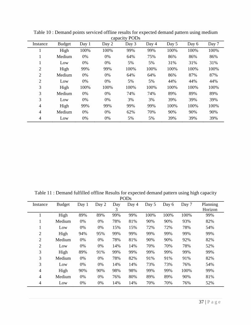
5.1.1.1 Medium capacity PODs

Table 8 on appendix B gives a detailed look at the percent of demand served for each day

and for the whole horizon. When using a high budget, the offline solution approach is able to

serve all the demand in the four instances. The relatively high budget allows to open as many

PODs as needed to serve the whole demand. The percent demand satisfied in Table 8 on

appendix B is based on the demand associated with the connected PODs. When decreasing the

budget to half, medium budget, an average of 86% of demand is served during the whole

planning horizon. No demand is served during day one and day two, which constitutes only 6%

of the total demand. The maximum demand served is reached on day five with an average of

94%. The difference between the demand served with high and medium budgets is only 14%,

with a 6% not met during day one and two. When decreasing the budget to 92, there is a

tendency to not serve any demand during day one and two as well, and serve only an average of

7.5% of demand during day three and four. On average, only 50% of the demand is served

throughout the planning horizon. The percentage of demand served is greater than the percentage

of demand points served which suggests that the offline approach serves the demand points that

are associated with high demand.

Table 11 on appendix B summarizes the pattern of opening PODs. When using a high

budget, all PODs are opened for the first time during day one, as the budget is enough to run

them for the rest of the planning horizon. However, when using a medium and low budget, there

is a tendency to wait until later days in the planning horizon to open the PODs. For the medium

budget instances, most of the PODs are open for the first time during day three as demand starts

to increase. For the low budget instances, the offline approach waits until day five when demand

19 | P a g e

reaches its maximum. For both budgets, the maximum number of facilities open is reached on

day five when demand reaches its maximum.

5.1.1.2 High capacity PODs

As described before, high capacity PODs have a capacity of 20,000. In our case we

assumed that the cost associated with operating a high capacity PODs is twice as much as a

medium capacity PODs. Due to the operating cost, fewer facilities will be operating throughout

the planning horizon. The results obtained using high capacity PODs are close to the results

using medium capacity PODs. On average, there is a two to three percent difference between the

population served throughout the planning horizon using medium capacity and high capacity

PODs. When using a high budget, the majority of demand associated with day one and two is

satisfied, while using the other budget does not serve any demand during the first days. The

number of demand served reaches its maximum during day five. Unlike when using the medium

capacity PODs, not all PODs are open during the first day when using a high budget, due to the

cost of operating them throughout the rest of the planning horizon. Two instances reach the

maximum number of open PODs during the third day, while two others reach it during the fifth

day. With a medium budget, similar to using medium capacity PODs, there is a tendency to wait

until day three to open most of the PODs for the first time, and then the number of PODs open

reaches its maximum on day five. In the instances with low budget, the solution approach tends

to open a small number of PODs during day three, and then open most of the PODs during day

five. The number of demand points serviced is slightly lower when using a high capacity PODs

in comparison with medium capacity PODs. Tables 12, 13, and 14 summarize the results

discussed.

20 | P a g e

5.1.2 Constant Demand Pattern

The constant demand pattern assumes that demand will be constant throughout the whole

planning horizon.


Using a high budget with constant demand over the planning horizon, almost the whole

connected demand is satisfied across the whole planning horizon for the four instances. Using a

medium budget results in meeting an average of 97.5% of the total demand, even though the

number of facilities open is twice as much for the high budget. This can be explained by the

secondary objective of minimizing the travel distance, and the fact that some demand points

account for a small percentages of the demand. While the high budget services almost 100% of

demand points, the medium budget only services 91% of the demand points, which means that

9% of the demand points accounts for only 2% of the demand. Using a low budget will lead to

meeting 72% of the demand and 48% of the demand points. With a constant demand, the offline

approach solutions tend to open the maximum number of possible PODs during day one, and if

budget allow open extra facilities at later days. With a constant demand, the approach is able to

serve more demand in comparison with the expected demand. Tables 15, 16, and 17 in appendix

B summarize the results.


When using high capacity PODs, less demand is being served in comparison with using

medium capacity PODs. When using a high budget, the difference between the demands served

using the two types of PODs is only 1%. The difference is much bigger between a medium and

low budget. A decrease of 13% and 16% on the population served using medium and low budget

respectively is noted between the two types of PODs. However, the solution approach keeps the

21 | P a g e

same tendency concerning opening PODs as it opens the maximum possible number of PODs

during day one, and depending on the remaining budget, it opens extra PODs later. The number

of served demand points is fewer when using high capacity PODs in contrast with medium

capacity. The percent of demand points served is significantly less than the percent demand

served which means that the solution approach tends to service demand points with high demand

associated with it first. Tables 18, 19, and 20 in appendix B summarize the results.

5.1.3 Increasing demand

The increasing demand pattern is close to the expected demand pattern except that demand

on day seven of the expected pattern is now demand for day three and the rest of demand is

shifted one day up.


As the other demand patterns, a high budget will result in meeting 100% of the demand and

servicing 100% of the demand points by opening the maximum number of PODs since day one.

When a medium budget is used, on average 87% of the connected demand is met. On day six, we

reach the maximum demand met. The magnitude of day six and seven demand of the increasing

demand pattern is equivalent on the magnitude of day five and six demand of the expected

demand pattern. Most PODs are open for the first time during day four when demand starts

increasing. The number of facilities open reaches its maximum on day six. The demand points

percent served is less than the percent demand met. Using low budget results in opening most of

the PODs for the first time during day six when demand reaches its maximum. No demand is

served during the first three days, as the total demand associated with the three first days, only

accounts for 14% of the total demand. In day four and five, few PODs are open to serve a small

portion of the demand. Tables 21, 22, and 23 in appendix B summarize the results.

22 | P a g e


Unlike all the other demand patterns when using a high budget with high capacity PODs,

not all the PODs are open for the first time during the first day. The number of PODs open

reaches its maximum during day six. However, the offline solution approach is still able to meet

99% of the demand throughout the whole planning horizon. With a medium budget, most of the

PODs open for the first time during day three, and the number of open PODs reach its maximum

during day six when demand is at its maximum. The percent of demand served using high

capacity PODs is slightly less than when using a medium capacity PODs. With a low budget, the

average demand served is 56%. Most PODs start opening for the first time during day six. No

demand is served during the first three days. In all cases, the percent of served demand points is

less than the percent demand served. Tables 24, 25, and 26 in appendix B summarize the results.

5.1.4 Decreasing Demand

With the decreasing demand pattern, it is assumed that demand is high during the first two

days and starts decreasing throughout the rest of the planning horizon to reach its minimum

during day six and seven.


With all three types of budgets, all PODs are open during the first day when demand is at

its maximum, and if the budget allows it, one more POD is open later (low budget). As expected,

the solution tries to maximize the demand met during the first two days as it accounts for 60% of

the total demand. With a low budget, during the first two days, servicing 8% of demand points

leads to meet 34% of demand during these days. The total percent demand met when demand is

decreasing is slightly less than the other patterns. Tables 27, 28, and 29 in appendix B summarize

the results.

23 | P a g e


Like medium capacity PODs solutions, all the PODs are open during the first day as

demand is at its maximum. An extra POD is open at a later period if budget allows it. High

capacity PODs leads to a less percent demand served than medium capacity PODs. Tables 30,

31, and 32 in appendix B summarize the results.

5.1.5 General Patterns

Even though the solutions were different in each of the 96 instances, some general patterns

were observed:

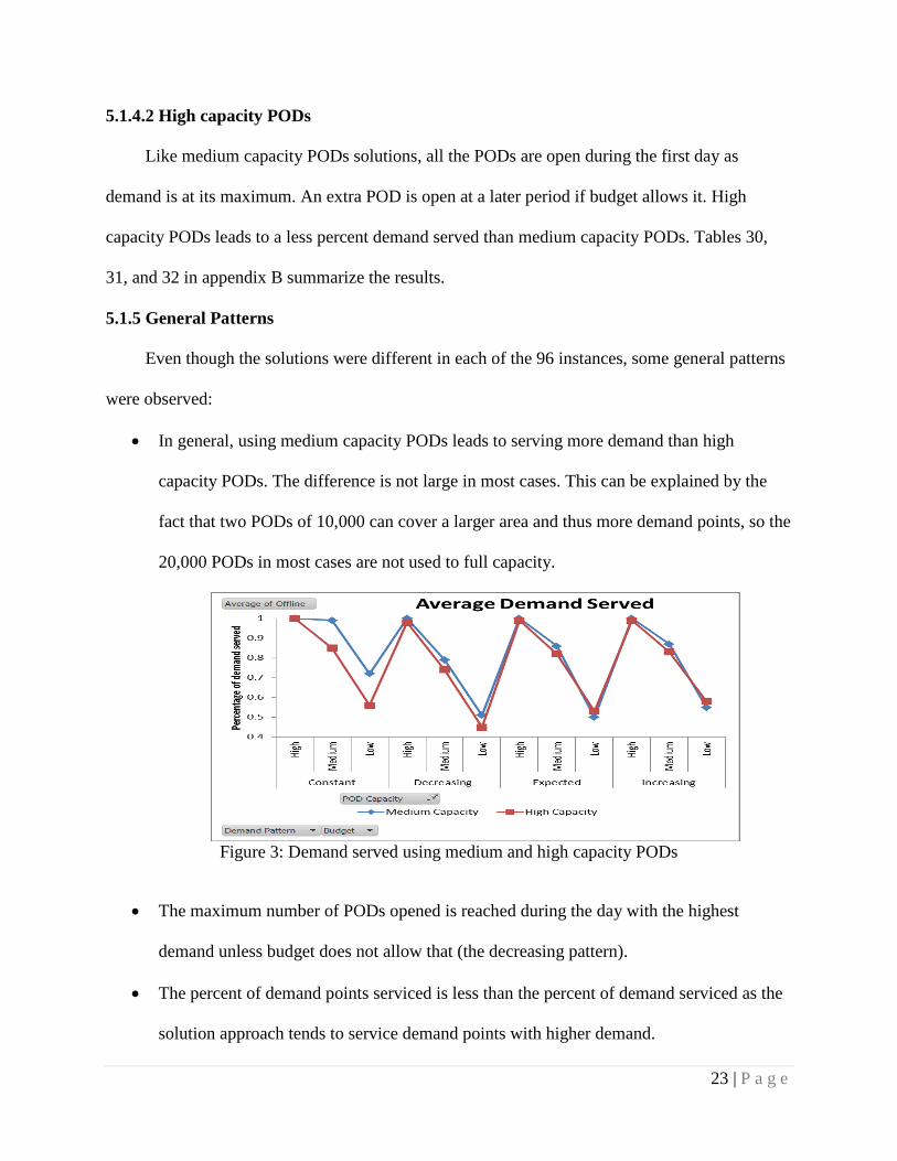
In general, using medium capacity PODs leads to serving more demand than high

capacity PODs. The difference is not large in most cases. This can be explained by the

fact that two PODs of 10,000 can cover a larger area and thus more demand points, so the

20,000 PODs in most cases are not used to full capacity.

Figure 3: Demand served using medium and high capacity PODs

The maximum number of PODs opened is reached during the day with the highest

demand unless budget does not allow that (the decreasing pattern).

The percent of demand points serviced is less than the percent of demand serviced as the

solution approach tends to service demand points with higher demand.

24 | P a g e

When the demand is constant, the demand serviced reaches its maximum, slightly greater

than the increasing and expected demand pattern.

When the demand pattern is decreasing; less demand is serviced in comparison with the

other demand patterns. Less demand points are open throughout the whole planning

horizon as all of them are open during day 1 and the cost associated with operating them

for the rest of the planning horizon is high.

Figure 4: Demand served with the different demand patterns

The offline approach decision of either opening a POD or not is not necessarily driven by

the total demand surrounding a POD. For each instance, the total demand that is possible to serve

by each POD location was calculated. This demand is calculated based on the demand that each

POD can serve within the 25-mile allowable distance. The possible demand for each day is the

minimum of demand within the allowable distance and the POD capacity. Not all PODs

associated with high demand were opened. Some PODs were ranked 117 based on the amount of

demand surrounding the POD and still got opened seven out of twelve times using medium

capacity POD with instance one. The decision made by CPLEX is far more comprehensive. The

fact that each demand point can be serviced by multiple PODs makes ranking the PODs in a

25 | P a g e

traditional way not significant. Once a POD services a demand point that can be serviced by a

second POD, the possible demand that can be serviced with the second POD decreases.

5.2 Online Approach Results

The online model makes decisions on a day by day basis without knowing future period

information. In this section, we are comparing how the choices made in the online approach

solutions differ from those of the offline solutions. The majority of the PODs are open during

day one for all instances, while in the offline solution the pattern at which PODs open depends

on the demand pattern. The online approach does not get the benefit of knowing demand in the

upcoming days which leads to opening the PODs as early as possible; therefore, if demand is

increasing, the approach does not get the benefit of fulfilling a lot of demand, as it is restricted by

the decisions of opening PODs at earlier days. In some instances, the decision of opening a POD

is late as well. For example using a high budget with medium capacity PODs, the POD opened

during day two could have been opened during day one without violating the budget constraint.

From Table 5, we observe that the budget is not used to its fullest in all cases. With the medium

capacity PODs, if the last POD was opened one day earlier, the solution would have been

feasible. However, since the information concerning future demand is not known in advance, the

solution approach decided that it is beneficial to save the budget for a later period. On the other

hand, with the high capacity PODs, the unused budget (one or two units of budget) could not

have been used due to the decisions made on day one. The operating cost of high capacity PODs

is two units of budget at each period of the planning horizon.

26 | P a g e

Table 5: PODs opening pattern for online approach solutions

Budget POD

Capacity

Day 1 Day 2 Day 3 Day 4 Day 5 Day 6 Day 7 Cost

High Medium 45 1 0 0 0 0 0 367

High High 24 0 0 0 1 0 0 367

Medium Medium 22 1 0 0 0 0 0 183

Medium High 12 0 0 0 0 0 1 183

Low Medium 11 0 0 0 0 1 0 91

Low High 6 0 0 0 0 0 0 90

There is an average difference of 17% between the demand met using online and offline

approach. However, the gap is around 22% when using a medium budget, and 13% when using a

high budget. The gap is much smaller when the demand pattern is decreasing as the online

approach solutions and offline solutions are following the same pattern of opening PODs. In an

offline solution with a decreasing pattern, the PODs are open during the first days in order to

fulfill the high demand during day one and two. The gap is much greater (21% average) when

the demand is increasing, as opening PODs earlier leads to not meeting the high demand during

later periods.

Figure 5: Demand served using online approach vs. offline approach with medium capacity

PODs

27 | P a g e

Figure 6: Demand served using online approach vs. offline approach with high capacity PODs

Interestingly, when demand is decreasing, using high capacity PODs and with a low

budget, both the online and offline solutions are opening six PODs; but the percent of demand

served is different. Moreover, only considering day one, the offline model solution still does

much better than the online approach. The online approach strategy is based on ranking the

demand points in an increasing order and then assigning them to the demand points in that order,

while the offline model does not consider the order of the magnitude of demand at each demand

point. Milburn et al. (2013) state that “the probability of opening a desired POD is determined by

the ratio of the cost to open and operate the POD for the remainder of the horizon versus the

distance from the demand location consideration to its desired POD” [2].

It seems that the online approach sacrifices servicing higher demand to service demand

points with higher demand magnitude. The online solution serves less demand points than the

offline solution. The online approach solution has the tendency to open the same demand points

during the four instances while in the offline solution, the PODs opened are different from

instance to instance. In the offline solutions, 120 PODs were opened at least once in comparison

with 85 using the online approach. Only two of the non-opened PODs using the offline approach

28 | P a g e

were not opened using the online approach. More interestingly, the fifth most opened POD using

the online approach was never opened using an offline approach.

Table 6 : Comparison of demand serviced online vs. offline

Demand Pattern Budget POD Capacity Online Offline

Expected High Medium 95% 100%

Expected High High 76% 99%

Expected Medium Medium 67% 86%

Expected Medium High 48% 82%

Expected Low Medium 41% 50%

Expected Low High 31% 53%

Constant High Medium 99% 100%

Constant High High 83% 100%

Constant Medium Medium 82% 99%

Constant Medium High 54% 85%

Constant Low Medium 50% 72%

Constant Low High 35% 56%

Decreasing High Medium 94% 100%

Decreasing High High 81% 98%

Decreasing Medium Medium 73% 79%

Decreasing Medium High 55% 74%

Decreasing Low Medium 44% 51%

Decreasing Low High 32% 45%

Increasing High Medium 92% 100%

Increasing High High 76% 99%

Increasing Medium Medium 67% 87%

Increasing Medium High 49% 83%

Increasing Low Medium 41% 55%

Increasing Low High 30% 58%

6. Conclusion/Future Work

Having a good response plan after a major earthquake is extremely complicated due to the

high uncertainty associated with the road network, demand locations and magnitude. An online

disaster relief model making decisions about where to locate points of distribution based on real

time information was developed. The model mimics the decisions that a decision maker has to

make after an earthquake given limited information. A mixed integer program was created to

29 | P a g e

consider what an optimal solution with perfect information would be, and to be able to judge the

quality of the online solution. The “Models for disaster relief shelter location and supply routing”

suggested conducting analysis on the impact of the budget level and PODs operating cost on the

solution of both approaches. The analysis was conducted in addition to studying the impact of

having different demand patterns and different POD capacities.

The offline solution, or the perfect information solution, changes the pattern of opening

PODs depending on the demand pattern. It seems that it is better to open PODs as early as

possible when the demand is decreasing or constant, while it is better to wait for later periods for

the expected and decreasing demand patterns. In general, the budget had an effect on the number

of facilities open, but not the pattern at which PODs are open. With a high budget, the solution

tends to open the maximum possible number of facilities during day one, which leads to a high

coverage of nearly 100%. However with the two limiting budgets medium and low, the solution

follows the same pattern of opening the PODs. In general, using medium capacity PODs

(Capacity 10,000) leads to satisfying more demand than using high capacity PODs (Capacity

20,000). Varying the barriers did not have an impact on the pattern of opening the facilities;

however, it affected which facilities to open for both the online and offline solution.

The online approach solution was less vulnerable to changing the parameters. In all

instances, the model solution opened the maximum possible number of PODs during the first day

of the planning horizon. Maximizing the demand served during day one by opening the

maximum number of PODs during day one is attractive from an online perspective as no future

information is known. However, the decision leads to not satisfying higher demand during future

periods in case of an expected or increasing demand pattern. On average, the online solution

served 17% less demand than the offline solution.

30 | P a g e

In some cases, the online and offline model solutions opened the same number of facilities

during day one, however the demand served during day one was much higher in favor of the

offline solution. Future work might be done to reconsider the POD opening strategy used on the

online approach which is based on ranking the demand points based on the magnitude of demand

associated with them. Another approach that might lead to better results is to rank the PODs

based on the demand that might be served, and once one of the PODs is open and a set of

demand points I1 are assigned to it, dynamically recalculate the demand associated with the

remaining PODs after taking off the demand associated with set of demand points I1, and repeat

the same action until the number of PODs that needs to be opened are already operating. More

constraints might be added to opening PODs during day one, such as the demand associated with

it.

31 | P a g e

References

1. Federal Emergency Management Agency. 2008. IS-26 guide to Points of Distribution.

Available from http://training.fema.gov/EMIWeb/IS/is26.asp.

2. Milburn, A.B., Rainwater, C.E., Boudhoum, O,Young , S. 2013. Models for disaster

relief shelter location and supply routing.Mack Blackwell National Rural Transportation

Center. Available from http://trid.trb.org/view.aspx?id=1246217

3. Elnashai AS, Cleveland LJ, Jefferson T and Harrald J. 2009. Impact of New Madrid

SeismicZone earthquakes on the central USA volume I. MAE Center Report No. 09-03.

Available from http://mae.cee.illinois.edu/publications/2009/09-03.htm.

4. Celik M, Ergun O, Johnson B, Keskinocak P, Lorca A, Pekgun P and Swann J. 2012.

Humanitarian logistics. InTutorials in Operations Research: New Directions in

Informatics,Optimization, Logistics, and Production. Hanover, MD: Institute for

Operations Research and the Management Sciences.

5. Yushimito W, Jaller M and Ukkusuri S. 2012. A Voronoi-Based heuristic algorithm for

locating distribution centers in Disasters. Networks and Spatial Economics 10(3), p. 1-19.

6. Campbell AM and Jones PC. 2011. Prepositioning supplies in preparation for disasters.

European Journal of Operational Research 209, p. 156-165.

7. Rawls CG and Turnquist MA. 2010. Pre-positioning of emergency supplies for disaster

response. Transportation Research Part B: Methodological 44(4), p. 521-534.

8. Jaller M and Holguín-Veras J. 2011. Locating points of distribution with social costs

considerations. Submitted to the 90th Transportation Research Board Annual Meeting.

9. Balcik B and Beamon BM. 2008. Facility location in humanitarian relief. International

Journal of Logistics: Research and Applications 11(2), p. 101-121.

10. Perez N, Holguín-Veras J, Mitchell JE and Sharkey TC. 2010. Integrated vehicle routing

problem with explicit consideration of social costs in humanitarian logistics. Submitted.

11. Balcik B, Beamon BM and Smilowitz K. 2008. Last mile distribution in humanitarian

relief. Journal of Intelligent Transportation Systems 12(2), p. 51-63.

12. De la Torre LE, Dolinskaya IS and Smilowitz KR. 2012. Disaster relief routing:

integrating research and practice. Socio-Economic Planning Sciences 46(1), p. 88-97.

13. Hagan, C. 2010. County Points of Distribution (PODs) Course. Florida Department of

Emergency Management. Available from http://www.floridadisater.org.

14. Educationbug. 2012. Public schools by county. Available from

http://arkansas.educationbug.org/public-schools/

http://training.fema.gov/EMIWeb/IS/is26.asp

http://trid.trb.org/view.aspx?id=1246217

http://mae.cee.illinois.edu/publications/2009/09-03.htm

http://arkansas.educationbug.org/public-schools/

32 | P a g e

15. U.S. Census Bureau. 2003. Arkansas: 2000 population and housing unit counts.

Retrieved from http://www.census.gov/prod/cen2000/phc-3-5.pdf.

16. Holguín-Veras, J. and Jaller, M. 2012. ”Immediate Resource Requirements after

Hurricane Katrina.” Nat. Hazards Rev., 13(2), 117–131.

http://www.census.gov/prod/cen2000/phc-3-5.pdf

33 | P a g e

Appendix A: Models

The offline Model

Table 7: Model elements

Item Type Description

Xijt binary variable equals 1 if demand point i is assigned to POD j in

planning period t and 0 otherwise

Aijt continuous variable

with range [0,1]

percentage of demand of point i satisfied by POD j in

period t

Zjt binary decision

variable

equals 1 if POD opened at potential POD location j in

period t and 0 otherwise

Yjt binary decision

variable

equals 1 if POD j operates in period t and 0 otherwise

dit input parameter demand of point i in period t

hijt input parameter length of shortest path from i to j in Gt

CF input parameter fixed cost to open a POD

co input parameter cost per period to operate a POD

B input parameter total budget for opening and operating PODs

Q input parameter POD capacity

D input parameter maximum allowable distance between a demand

point and its assigned POD location

M input parameter sufficiently large constant

“The objective is to maximize the total demand served during the planning horizon. A

secondary objective is to minimize the distance between demand points and their assigned POD

locations using the available road network in each period. Constraints (1) are used to ensure each

demand point is served by at most one POD. Constraints (2)-(4) control the opening and

operating of PODs. Constraints (2) ensure that an opened POD will continue to operate until the

end of the planning horizon. Constraints (3) ensure that unopened PODs cannot be operated, and

constraints (4) ensure that each POD location can be opened at most once. Constraints (5) are

used to enforce that once a portion of demand from a demand point has been assigned to a POD,

the same POD will continue to satisfy at least that quantity of demand from the point for the

remainder of the planning horizon. Constraints (6) ensure that demand cannot be assigned to

34 | P a g e

PODs in periods they are not operating. Constraint (7) ensures the total budget for opening and

operating PODs is not exceeded, and constraints (8) ensure the capacities of operating PODs are

not exceeded. Constraints (9) enforce the maximum allowable distance between a demand point

and its assigned POD location using the accessible road network in each period.”

Maximize ∑ ∑ ∑

[1] ∑ ,

[2] ∑ ,

[3] ∑ ,

[4] ∑

[5]

[6]

[7] ∑ ∑

[8] ∑

[9]

The online solution approach

The detailed description of our online algorithm is presented as follows.

Notation:

Let Dt be the set of available demand points in period t

Let b be the remaining budget available in each period

Let be the amount of remaining capacity at POD p in period t

Let Fi be the set of PODs located within 25 miles of demand location i

35 | P a g e

Let Apt be the demand points assigned to POD p in period t

Let Mp be the set of minimum levels in which we must satisfy those demand points assigned to

POD p

Let mk be the minimum level at with demand point k can be satisfied

Online Algorithm:

Step 0 (Initialization): Apt = Ø, Spt = Ø for all and . Sort Dt in non-increasing order

hit for all . Set

Step 1 (Satisfy established demand): If , STOP, else initialize for all and

. If , continue to Step 2. Else, for all , first update ,

∑

and then continue to Step 2.

Step 2 (Consider new demand): Set { } and to be the first demand point in

. If and return to Step 1. Else, if let = argmin

. If

and continue to Step 2a. If and set and

repeat Step 2. If , continue to Step 2b.

Step 2a (Assign new demand to open facility): Assign to by updating

Set { }. Update the remaining capacity of the POD to be

Return to Step 2.

Step 2b (Consider opening desired POD): If ∑ set and return

to Step 2. Else, generate r = U(0,1). If r > ∑

, set and return to Step 2.

Otherwise, Set { }, ∑ and

. Return to Step 2.” [2]

36 | P a g e

Appendix B: Results

Table 8 : Demand fulfilled offline Results for expected demand pattern using medium capacity

PODs

Instance Budget Day 1 Day 2 Day 3 Day 4 Day 5 Day 6 Day 7 Planning

Horizon

1 High 100% 100% 100% 100% 100% 100% 100% 100%

1 Medium 0% 0% 84% 89% 94% 94% 99% 87%

1 Low 0% 0% 7% 7% 67% 67% 92% 50%

2 High 100% 100% 100% 100% 100% 100% 100% 100%

2 Medium 0% 0% 81% 81% 94% 94% 97% 85%

2 Low 0% 0% 7% 7% 65% 65% 92% 49%

3 High 100% 100% 100% 100% 100% 100% 100% 100%

3 Medium 0% 0% 85% 85% 94% 94% 97% 86%

3 Low 0% 0% 8% 8% 68% 68% 90% 51%

4 High 100% 100% 100% 100% 100% 100% 100% 100%

4 Medium 0% 0% 79% 83% 94% 94% 96% 85%

4 Low 0% 0% 8% 8% 67% 67% 87% 50%

Table 9 : PODs opening pattern for expected demand using medium capacity PODs

Instance Budget Day 1 Day 2 Day 3 Day 4 Day 5 Day 6 Day 7

1 High 46 0 0 0 0 0 0

1 Medium 0 0 27 2 3 0 0

1 Low 0 0 2 0 20 0 0

2 High 46 0 0 0 0 0 0

2 Medium 0 0 26 0 7 0 0

2 Low 0 0 2 0 20 0 0

3 High 46 0 0 0 0 0 0

3 Medium 0 0 28 0 4 0 0

3 Low 0 0 2 0 20 0 0

4 High 46 0 0 0 0 0 0

4 Medium 0 0 25 6 0 0 0

4 Low 0 0 2 0 20 0 0

37 | P a g e

Table 10 : Demand points serviced offline results for expected demand pattern using medium

capacity PODs


1 High 100% 100% 99% 99% 100% 100% 100%

1 Medium 0% 0% 64% 75% 86% 86% 86%

1 Low 0% 0% 5% 5% 31% 31% 31%

2 High 99% 99% 100% 100% 100% 100% 100%

2 Medium 0% 0% 64% 64% 86% 87% 87%

2 Low 0% 0% 5% 5% 44% 44% 44%

3 High 100% 100% 100% 100% 100% 100% 100%

3 Medium 0% 0% 74% 74% 89% 89% 89%

3 Low 0% 0% 3% 3% 39% 39% 39%

4 High 99% 99% 99% 99% 100% 100% 100%

4 Medium 0% 0% 62% 70% 90% 90% 90%

4 Low 0% 0% 5% 5% 39% 39% 39%

Table 11 : Demand fulfilled offline Results for expected demand pattern using high capacity

PODs

Instance Budget Day 1 Day 2 Day

3

Day 4 Day 5 Day 6 Day 7 Planning

Horizon

1 High 89% 89% 99% 99% 100% 100% 100% 99%

1 Medium 0% 0% 78% 81% 90% 90% 93% 82%

1 Low 0% 0% 15% 15% 72% 72% 78% 54%

2 High 94% 95% 99% 99% 99% 99% 99% 99%

2 Medium 0% 0% 78% 81% 90% 90% 92% 82%

2 Low 0% 0% 14% 14% 70% 70% 78% 52%

3 High 89% 91% 99% 99% 99% 99% 99% 99%

3 Medium 0% 0% 78% 82% 91% 91% 91% 82%

3 Low 0% 0% 14% 14% 73% 73% 76% 54%

4 High 90% 90% 98% 98% 99% 99% 100% 99%

4 Medium 0% 0% 76% 80% 89% 89% 90% 81%

4 Low 0% 0% 14% 14% 70% 70% 76% 52%

38 | P a g e

Table 12 : PODs opening pattern for expected demand using high capacity PODs


1 High 17 0 9 0 2 0 0

1 Medium 0 0 14 1 3 0 0

1 Low 0 0 2 0 10 0 0

2 High 20 1 5 0 0 0 0

2 Medium 0 0 14 1 3 0 0

2 Low 0 0 2 0 10 0 0

3 High 18 1 7 0 1 0 0

3 Medium 0 0 14 1 3 0 0

3 Low 0 0 2 0 10 0 0

4 High 18 0 7 0 3 0 0

4 Medium 0 0 14 1 3 0 0

4 Low 0 0 2 0 10 0 0

Table 13 : Demand points serviced offline results for expected demand pattern using high

capacity PODs


1 High 58% 58% 94% 94% 97% 97% 97%

1 Medium 0% 0% 67% 71% 79% 79% 79%

1 Low 0% 0% 4% 4% 55% 55% 55%

2 High 72% 80% 96% 96% 96% 96% 96%

2 Medium 0% 0% 61% 66% 75% 75% 75%

2 Low 0% 0% 5% 5% 46% 46% 46%

3 High 60% 63% 93% 93% 97% 97% 97%

3 Medium 0% 0% 63% 68% 82% 82% 82%

3 Low 0% 0% 4% 4% 47% 47% 47%

4 High 61% 61% 94% 94% 97% 97% 97%

4 Medium 0% 0% 50% 58% 77% 77% 77%

4 Low 0% 0% 4% 4% 52% 52% 52%

39 | P a g e

Table 14 : Demand fulfilled offline Results for constant demand pattern using medium capacity

PODs


Horizon

1 High 100% 100% 100% 100% 100% 100% 100% 100%

1 Medium 98% 98% 97% 97% 98% 98% 98% 98%

1 Low 65% 65% 74% 74% 74% 74% 74% 71%

2 High 100% 100% 100% 100% 100% 100% 100% 100%

2 Medium 98% 98% 98% 98% 98% 98% 98% 98%

2 Low 72% 72% 72% 72% 77% 77% 77% 74%

3 High 100% 100% 100% 100% 100% 100% 100% 100%

3 Medium 97% 97% 97% 97% 97% 97% 97% 97%

3 Low 71% 71% 71% 71% 74% 74% 81% 73%

4 High 100% 100% 100% 100% 100% 100% 100% 100%

4 Medium 97% 97% 97% 97% 98% 98% 98% 97%

4 Low 68% 68% 68% 68% 72% 72% 72% 70%

Table 15 : PODs opening pattern for constant demand using medium capacity PODs


1 High 46 0 0 0 0 0 0

1 Medium 23 0 0 0 0 0 0

1 Low 10 0 2 0 0 0 0

2 High 46 0 0 0 0 0 0

2 Medium 23 0 0 0 0 0 0

2 Low 11 0 0 0 1 0 0

3 High 46 0 0 0 0 0 0

3 Medium 23 0 0 0 0 0 0

3 Low 11 0 0 0 1 0 0

4 High 46 0 0 0 0 0 0

4 Medium 23 0 0 0 0 0 0

4 Low 11 0 0 0 1 0 0

40 | P a g e

Table 16 : Demand points serviced offline results for constant demand pattern using medium

capacity PODs


1 High 100% 100% 100% 100% 100% 100% 100%

1 Medium 91% 91% 91% 91% 91% 91% 91%

1 Low 42% 42% 52% 52% 52% 52% 52%

2 High 100% 100% 100% 100% 100% 100% 100%

2 Medium 90% 90% 91% 91% 91% 91% 91%

2 Low 38% 38% 38% 38% 42% 42% 42%

3 High 100% 100% 100% 100% 100% 100% 100%

3 Medium 88% 88% 88% 88% 90% 90% 90%

3 Low 49% 49% 49% 49% 54% 54% 54%

4 High 100% 100% 99% 99% 100% 100% 100%

4 Medium 93% 93% 92% 92% 93% 93% 93%

4 Low 43% 43% 43% 43% 45% 45% 45%

Table 17 : Demand fulfilled offline Results for constant demand pattern using high capacity

PODs


Horizon

1 High 99% 99% 99% 99% 99% 99% 99% 99%

1 Medium 80% 80% 84% 84% 85% 85% 88% 84%

1 Low 51% 51% 59% 59% 60% 66% 7% 50%

2 High 99% 99% 99% 99% 99% 99% 99% 99%

2 Medium 86% 86% 88% 88% 89% 89% 91% 88%

2 Low 52% 52% 54% 61% 68% 68% 68% 60%

3 High 99% 99% 99% 99% 99% 99% 99% 99%

3 Medium 82% 82% 82% 82% 83% 83% 86% 83%

3 Low 55% 55% 55% 55% 56% 56% 56% 55%

4 High 99% 99% 99% 99% 99% 99% 99% 99%

4 Medium 84% 84% 84% 84% 84% 84% 86% 85%

4 Low 60% 60% 59% 59% 59% 59% 59% 59%

41 | P a g e

Table 18 : PODs opening pattern for constant demand using high capacity PODs


1 High 24 0 0 0 1 0 0

1 Medium 12 0 0 0 0 0 1

1 Low 5 0 1 0 0 1 0

2 High 24 0 0 0 1 0 0

2 Medium 12 0 0 0 0 0 1

2 Low 5 0 0 1 1 0 0

3 High 24 0 0 0 1 0 0

3 Medium 12 0 0 0 0 0 1

3 Low 6 0 0 0 0 0 0

4 High 24 0 0 0 1 0 0

4 Medium 12 0 0 0 0 0 1

4 Low 6 0 0 0 0 0 0

Table 19 : Demand points serviced offline results for constant demand pattern using high

capacity PODs


1 High 95% 95% 95% 95% 96% 96% 96%

1 Medium 69% 69% 70% 70% 71% 71% 71%

1 Low 37% 37% 42% 42% 42% 45% 45%

2 High 95% 95% 96% 96% 96% 96% 96%

2 Medium 68% 68% 68% 68% 69% 69% 69%

2 Low 37% 37% 37% 41% 43% 43% 43%

3 High 95% 95% 95% 95% 97% 97% 97%

3 Medium 67% 67% 68% 68% 69% 69% 69%

3 Low 40% 40% 40% 40% 41% 41% 41%

4 High 94% 94% 94% 94% 95% 95% 95%

4 Medium 71% 71% 71% 71% 71% 71% 71%

4 Low 43% 43% 43% 43% 44% 44% 44%

42 | P a g e

Table 20 : Demand fulfilled offline Results for increasing demand pattern using medium

capacity PODs


Horizon

1 High 100% 100% 100% 100% 100% 100% 100% 100%

1 Medium 0% 0% 68% 92% 92% 97% 97% 87%

1 Low 0% 0% 0% 8% 11% 88% 88% 56%

2 High 100% 100% 100% 100% 100% 100% 100% 100%

2 Medium 0% 0% 67% 85% 90% 97% 97% 87%

2 Low 0% 0% 0% 4% 4% 87% 88% 54%

3 High 100% 100% 100% 100% 100% 100% 100% 100%

3 Medium 0% 0% 62% 93% 93% 96% 96% 87%

3 Low 0% 0% 0% 15% 15% 86% 86% 56%

4 High 100% 100% 100% 100% 100% 100% 100% 100%

4 Medium 0% 0% 66% 86% 90% 96% 96% 86%

4 Low 0% 0% 0% 7% 11% 87% 87% 55%

Table 21 : PODs opening pattern for increasing demand using medium capacity PODs


1 High 46 0 0 0 0 0 0

1 Medium 0 0 20 11 0 3 0

1 Low 0 0 0 2 1 26 0

2 High 46 0 0 0 0 0 0

2 Medium 0 0 20 8 3 4 0

2 Low 0 0 0 1 0 29 0

3 High 46 0 0 0 0 0 0

3 Medium 0 0 18 14 0 2 0

3 Low 0 0 0 4 0 24 0

4 High 46 0 0 0 0 0 0

4 Medium 0 0 19 10 2 4 0

4 Low 0 0 0 2 1 26 0

43 | P a g e

Table 22 : Demand points serviced offline results for increasing demand pattern using medium

capacity PODs


1 High 100% 100% 100% 100% 100% 100% 100%

1 Medium 0% 0% 41% 77% 77% 91% 91%

1 Low 0% 0% 0% 5% 6% 69% 69%

2 High 99% 99% 100% 100% 100% 100% 100%

2 Medium 0% 0% 41% 70% 81% 92% 92%

2 Low 0% 0% 0% 2% 2% 63% 63%

3 High 100% 100% 100% 100% 100% 100% 100%

3 Medium 0% 0% 39% 82% 82% 91% 91%

3 Low 0% 0% 0% 6% 6% 69% 69%

4 High 100% 100% 99% 99% 100% 100% 100%

4 Medium 0% 0% 35% 71% 78% 95% 95%

4 Low 0% 0% 0% 4% 5% 74% 74%

Table 23 : Demand fulfilled offline Results for increasing demand pattern using high capacity

PODs


Horizon

1 High 91% 92% 98% 99% 99% 100% 100% 99%

1 Medium 0% 0% 64% 81% 88% 94% 94% 84%

1 Low 0% 0% 0% 28% 48% 80% 80% 58%

2 High 93% 93% 99% 99% 99% 100% 100% 99%

2 Medium 0% 0% 58% 83% 87% 94% 94% 83%

2 Low 0% 0% 0% 35% 40% 80% 80% 58%

3 High 90% 92% 98% 99% 99% 100% 100% 99%

3 Medium 0% 0% 59% 84% 89% 94% 94% 84%

3 Low 0% 0% 0% 28% 48% 81% 81% 59%

4 High 92% 93% 98% 98% 99% 100% 100% 99%

4 Medium 0% 0% 59% 83% 86% 93% 93% 82%

4 Low 0% 0% 0% 33% 40% 79% 79% 57%

44 | P a g e

Table 24 : PODs opening pattern for increasing demand using high capacity PODs


1 High 18 1 6 1 0 2 0

1 Medium 0 0 10 5 2 3 0

1 Low 0 0 0 4 3 7 0

2 High 19 0 6 0 1 2 0

2 Medium 0 0 9 7 1 3 0

2 Low 0 0 0 5 1 8 0

3 High 18 1 6 1 0 2 0

3 Medium 0 0 9 7 1 3 0

3 Low 0 0 0 4 3 7 0

4 High 19 1 5 0 0 3 0

4 Medium 0 0 9 7 1 3 0

4 Low 0 0 0 5 1 8 0

Table 25 : Demand points serviced offline results for increasing demand pattern using high

capacity PODs


1 High 60% 65% 93% 94% 95% 97% 97%

1 Medium 0% 0% 36% 66% 75% 84% 84%

1 Low 0% 0% 0% 10% 22% 65% 65%

2 High 66% 66% 95% 95% 96% 98% 98%

2 Medium 0% 0% 28% 66% 72% 83% 83%

2 Low 0% 0% 0% 14% 16% 58% 58%

3 High 69% 69% 92% 94% 96% 98% 98%

3 Medium 0% 0% 34% 74% 82% 86% 86%

3 Low 0% 0% 0% 11% 25% 69% 69%

4 High 66% 67% 94% 94% 95% 98% 98%

4 Medium 0% 0% 29% 65% 73% 83% 83%

4 Low 0% 0% 0% 12% 16% 59% 59%

45 | P a g e

Table 26 : Demand fulfilled offline Results for decreasing demand pattern using medium

capacity PODs


Horizon

1 High 100% 100% 100% 100% 100% 100% 100% 100%

1 Medium 69% 69% 96% 96% 96% 96% 96% 80%

1 Low 34% 34% 74% 74% 82% 86% 86% 51%

2 High 100% 100% 100% 100% 100% 100% 100% 100%

2 Medium 67% 67% 96% 96% 97% 97% 97% 79%

2 Low 33% 33% 74% 74% 80% 82% 82% 50%

3 High 100% 100% 100% 100% 100% 100% 100% 100%

3 Medium 68% 68% 96% 96% 96% 96% 96% 79%

3 Low 34% 34% 75% 75% 79% 80% 80% 51%

4 High 100% 100% 100% 100% 100% 100% 100% 100%

4 Medium 69% 69% 94% 94% 94% 94% 94% 78%

4 Low 34% 34% 73% 73% 79% 81% 81% 50%

Table 27 : PODs opening pattern for decreasing demand using medium capacity PODs


1 High 46 0 0 0 0 0 0

1 Medium 23 0 0 0 0 0 0

1 Low 11 0 0 0 1 0 0

2 High 46 0 0 0 0 0 0

2 Medium 23 0 0 0 0 0 0

2 Low 11 0 0 0 1 0 0

3 High 46 0 0 0 0 0 0

3 Medium 23 0 0 0 0 0 0

3 Low 11 0 0 0 1 0 0

4 High 46 0 0 0 0 0 0

4 Medium 23 0 0 0 0 0 0

4 Low 11 0 0 0 1 0 0

46 | P a g e

Table 28: Demand points serviced offline results for decreasing demand pattern using medium

capacity PODs


1 High 100% 100% 100% 100% 100% 100% 100%

1 Medium 41% 41% 88% 88% 89% 89% 89%

1 Low 8% 8% 51% 51% 60% 60% 60%

2 High 100% 100% 100% 100% 100% 100% 100%

2 Medium 49% 49% 89% 89% 90% 90% 90%

2 Low 7% 7% 48% 48% 56% 56% 56%

3 High 100% 100% 100% 100% 100% 100% 100%

3 Medium 49% 49% 91% 91% 91% 91% 91%

3 Low 9% 9% 59% 59% 64% 64% 64%

4 High 100% 100% 99% 99% 100% 100% 100%

4 Medium 46% 46% 88% 88% 88% 88% 88%

4 Low 7% 7% 60% 60% 64% 64% 64%

Table 29 : Demand fulfilled offline Results for decreasing demand pattern using high capacity

PODs


Horizon

1 High 98% 98% 98% 98% 99% 99% 100% 98%

1 Medium 69% 69% 80% 80% 80% 80% 84% 74%

1 Low 37% 37% 57% 57% 59% 61% 61% 45%

2 High 98% 98% 98% 98% 99% 99% 99% 98%

2 Medium 70% 70% 78% 78% 78% 78% 83% 73%

2 Low 36% 36% 57% 57% 58% 64% 64% 45%

3 High 97% 97% 99% 99% 99% 99% 99% 98%

3 Medium 71% 71% 80% 80% 80% 78% 83% 74%

3 Low 37% 37% 55% 55% 55% 54% 54% 44%

4 High 98% 98% 97% 97% 99% 99% 99% 98%

4 Medium 71% 71% 76% 76% 76% 76% 81% 73%

4 Low 37% 37% 58% 58% 59% 65% 65% 46%

47 | P a g e

Table 30 : PODs opening pattern for decreasing demand using high capacity PODs


1 High 24 0 0 0 1 0 0

1 Medium 12 0 0 0 0 0 1

1 Low 6 0 0 0 0 0 0

2 High 24 0 0 0 1 0 0

2 Medium 12 0 0 0 0 0 1

2 Low 6 0 0 0 0 0 0

3 High 24 0 0 0 1 0 0

3 Medium 12 0 0 0 0 0 1

3 Low 6 0 0 0 0 0 0

4 High 24 0 0 0 1 0 0

4 Medium 12 0 0 0 0 0 1

4 Low 6 0 0 0 0 0 0

Table 31 : Demand points serviced offline results for decreasing demand pattern using high

capacity PODs


1 High 92% 92% 92% 92% 93% 93% 93%

1 Medium 52% 52% 69% 69% 70% 70% 70%

1 Low 10% 10% 37% 37% 38% 38% 38%

2 High 93% 93% 94% 94% 95% 95% 95%

2 Medium 44% 44% 61% 61% 61% 61% 61%

2 Low 11% 11% 27% 27% 27% 27% 27%

3 High 90% 90% 93% 93% 96% 96% 96%

3 Medium 40% 40% 67% 67% 69% 69% 69%

3 Low 11% 11% 41% 41% 42% 42% 42%

4 High 94% 94% 93% 93% 95% 95% 95%

4 Medium 51% 51% 61% 61% 62% 62% 62%

4 Low 12% 12% 33% 33% 34% 34% 34%

48 | P a g e

Appendix C: Data

Table 32 : Percent demand per county for expected demand pattern

Demand Percentage

County Day 1 Day 2 Day 3 Day 4 Day 5 Day 6 Day 7

Arkansas 3.60% 3.60% 20.60% 20.60% 60.30% 60.30% 12.10%

Clay 6.10% 6.10% 30.73% 30.73% 65.36% 65.36% 18.42%

Craighead 7.65% 7.65% 27.88% 27.88% 63.94% 63.94% 17.76%

Crittenden 10.23% 10.23% 31.57% 31.57% 65.78% 65.78% 20.90%

Cross 7.47% 7.47% 31.12% 31.12% 65.56% 65.56% 19.29%

Greene 6.86% 6.86% 27.29% 27.29% 63.64% 63.64% 17.07%

Independence 3.41% 3.41% 16.25% 16.25% 58.13% 58.13% 9.83%

Jackson 6.25% 6.25% 30.14% 30.14% 65.07% 65.07% 18.20%

Lawrence 4.12% 4.12% 25.12% 25.12% 62.56% 62.56% 14.62%

Lee 7.37% 7.37% 37.02% 37.02% 68.51% 68.51% 22.19%

Mississippi 12.15% 12.15% 31.97% 31.97% 65.99% 65.99% 22.06%

Monroe 4.34% 4.34% 25.04% 25.04% 62.52% 62.52% 14.69%

Phillips 4.69% 4.69% 24.92% 24.92% 62.46% 62.46% 14.80%

Poinsett 10.70% 10.70% 30.70% 30.70% 65.35% 65.35% 20.70%

Prairie 3.65% 3.65% 20.41% 20.41% 60.21% 60.21% 12.03%

Randolph 1.60% 1.60% 20.93% 20.93% 60.47% 60.47% 11.27%

St. Francis 6.82% 6.82% 35.69% 35.69% 67.84% 67.84% 21.25%

White 1.36% 1.36% 14.39% 14.39% 57.20% 57.20% 7.88%

Woodruff 7.28% 7.28% 33.67% 33.67% 66.83% 66.83% 20.47%

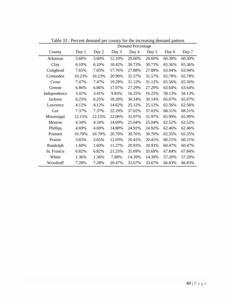
49 | P a g e

Table 33 : Percent demand per county for the increasing demand pattern

Demand Percentage


Arkansas 3.60% 3.60% 12.10% 20.60% 20.60% 60.30% 60.30%

Clay 6.10% 6.10% 18.42% 30.73% 30.73% 65.36% 65.36%

Craighead 7.65% 7.65% 17.76% 27.88% 27.88% 63.94% 63.94%

Crittenden 10.23% 10.23% 20.90% 31.57% 31.57% 65.78% 65.78%

Cross 7.47% 7.47% 19.29% 31.12% 31.12% 65.56% 65.56%

Greene 6.86% 6.86% 17.07% 27.29% 27.29% 63.64% 63.64%

Independence 3.41% 3.41% 9.83% 16.25% 16.25% 58.13% 58.13%

Jackson 6.25% 6.25% 18.20% 30.14% 30.14% 65.07% 65.07%

Lawrence 4.12% 4.12% 14.62% 25.12% 25.12% 62.56% 62.56%

Lee 7.37% 7.37% 22.19% 37.02% 37.02% 68.51% 68.51%

Mississippi 12.15% 12.15% 22.06% 31.97% 31.97% 65.99% 65.99%

Monroe 4.34% 4.34% 14.69% 25.04% 25.04% 62.52% 62.52%

Phillips 4.69% 4.69% 14.80% 24.92% 24.92% 62.46% 62.46%

Poinsett 10.70% 10.70% 20.70% 30.70% 30.70% 65.35% 65.35%

Prairie 3.65% 3.65% 12.03% 20.41% 20.41% 60.21% 60.21%

Randolph 1.60% 1.60% 11.27% 20.93% 20.93% 60.47% 60.47%

St. Francis 6.82% 6.82% 21.25% 35.69% 35.69% 67.84% 67.84%

White 1.36% 1.36% 7.88% 14.39% 14.39% 57.20% 57.20%

Woodruff 7.28% 7.28% 20.47% 33.67% 33.67% 66.83% 66.83%

50 | P a g e

Table 34 : Percent demand per county for the decreasing demand pattern

Demand Percentage


Arkansas 60.30% 60.30% 20.60% 20.60% 12.10% 3.60% 3.60%

Clay 65.36% 65.36% 30.73% 30.73% 18.42% 6.10% 6.10%

Craighead 63.94% 63.94% 27.88% 27.88% 17.76% 7.65% 7.65%

Crittenden 65.78% 65.78% 31.57% 31.57% 20.90% 10.23% 10.23%

Cross 65.56% 65.56% 31.12% 31.12% 19.29% 7.47% 7.47%

Greene 63.64% 63.64% 27.29% 27.29% 17.07% 6.86% 6.86%

Independence 58.13% 58.13% 16.25% 16.25% 9.83% 3.41% 3.41%

Jackson 65.07% 65.07% 30.14% 30.14% 18.20% 6.25% 6.25%

Lawrence 62.56% 62.56% 25.12% 25.12% 14.62% 4.12% 4.12%

Lee 68.51% 68.51% 37.02% 37.02% 22.19% 7.37% 7.37%

Mississippi 65.99% 65.99% 31.97% 31.97% 22.06% 12.15% 12.15%

Monroe 62.52% 62.52% 25.04% 25.04% 14.69% 4.34% 4.34%

Phillips 62.46% 62.46% 24.92% 24.92% 14.80% 4.69% 4.69%

Poinsett 65.35% 65.35% 30.70% 30.70% 20.70% 10.70% 10.70%

Prairie 60.21% 60.21% 20.41% 20.41% 12.03% 3.65% 3.65%

Randolph 60.47% 60.47% 20.93% 20.93% 11.27% 1.60% 1.60%

St. Francis 67.84% 67.84% 35.69% 35.69% 21.25% 6.82% 6.82%

White 57.20% 57.20% 14.39% 14.39% 7.88% 1.36% 1.36%

Woodruff 66.83% 66.83% 33.67% 33.67% 20.47% 7.28% 7.28%

51 | P a g e

Table 35: Percent demand per county for the constant demand pattern

State Demand Percentage

Arkansas 25.87%

Clay 31.83%

Craighead 30.96%

Crittenden 33.72%

Cross 32.51%

Greene 30.38%

Independence 23.63%

Jackson 31.59%

Lawrence 28.32%

Lee 35.43%

Mississippi 34.61%

Monroe 28.36%

Phillips 28.42%

Poinsett 33.46%

Prairie 25.80%

Randolph 25.32%

St. Francis 34.56%

White 21.97%

Woodruff 33.72%

boudhoum-thesis-2013

Documents

demand points

disaster relief models

natural disaster

location of points

magnitude of demand

demand magnitude

locations of pods

potential disaster scenarios