Bootstrapping a Heteroscedastic Regression Model with Application to 3D

Rigid Motion Evaluation

Bogdan Matei Peter Meer

Electrical and Computer Engineering Department

Rutgers University

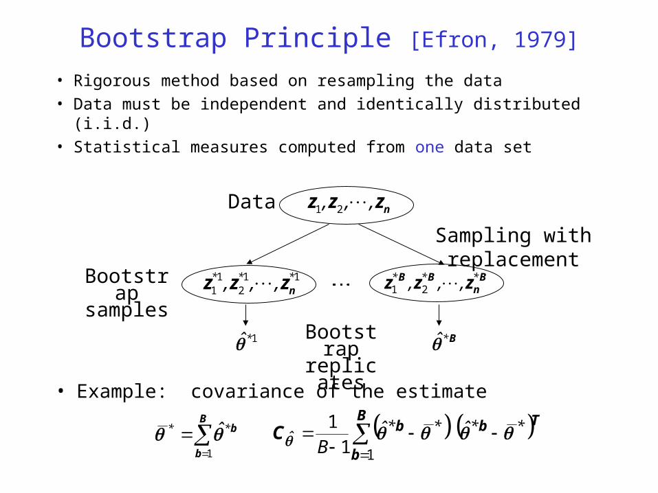
• Rigorous method based on resampling the data

• Data must be independent and identically distributed (i.i.d.)

• Statistical measures computed from one data set

Bootstrap Principle [Efron, 1979]

nzzz ,,, 21

Bn

BB zzz *** ,,, 21

Data

Bootstrap samples

Sampling with replacement

112

11

*** ,,, nzzz

1* B*

TbB

b

bC ****ˆ ˆˆ

B

11

1

B

b

b

1

**

Bootstrap replicates

• Example: covariance of the estimate

B = 50

TRUEESTIMATE

X

Y

B = 200

TRUEESTIMATE

X

Y

Bootstrap for Regression

0Tioz

iiio zzz

iz

ioz

iz

iz

iz

• Resample from residuals

• Obtain bootstrap samples as

nzzz ˆ,,ˆ,ˆ 21

** ˆˆ iii zzz

• Model

• Measurements

I20 σ,GI iz

– pseudoinverse of the bootstrapped covariance matrix

– the percentile of the distribution

Building Confidence Regions

• Relation to error propagation– does not imply linearization

– provides more accurate coverage

– trades computation time for analytical derivations

11ˆˆ

ˆCDT

• The ellipsoid

1contains the true estimate with probability

ˆˆˆˆ *

ˆ** C

T

1 1

C

Heteroscedasticity

• Point dependent errors

• Appears in many 3D vision problems

– due to linearization

– multi-stage tasks

ii Cz 20 σ,GI

021322110 ioioioio yyθyθyθθ 220 Iσ,GIyi

iiii yyyy 21211z

22

2112

1

22

0

100

010

0000

ioioioio

io

io

yyyy

y

yσiC

e.g. estimating the 3D rigid motion of a stereo head

• Total least squares (TLS) algorithm assumes i.i.d. data. Under heteroscedasticity yields biased solutions.

• Non-linear methods, like Levenberg-Marquard – may converge to local minima

– are computationally intensive

• Proposed methods– renormalization [Kanatani, 1996]

– HEIV algorithm [Leedan & Meer, ICCV’ 98; Matei & Meer, CVPR’ 99]

Heteroscedastic Regression

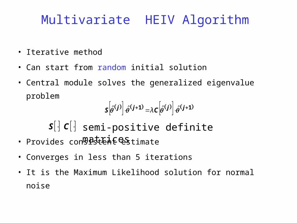
• Iterative method

• Can start from random initial solution

• Central module solves the generalized eigenvalue problem

• Provides consistent estimate

• Converges in less than 5 iterations

• It is the Maximum Likelihood solution for normal noise

Multivariate HEIV Algorithm

CS semi-positive definite matrices

11 jjjj CS ˆˆλˆˆ

Multivariate HEIV Algorithm

• The true values satisfy the linear constraint

mpio RRZ ,,0 Tm

ioioio zzZ 1

• The true values are corrupted by heteroscedastic noise

ki

kio

ki zzz

kli

li

ki

ki CzzzE ,, cov0

Multivariate HEIV Algorithm

• Start with an initial solution

jkli

Tjkli C ˆˆˆ

n

iii

T

ij ZZZZS

1

1 ~ˆ~

jiii

n

ipii

Tpi

j ZZICIC ˆ~ˆ,ˆ

1

1

0

• Compute

• Find the scatter

n

iii

n

ii ZZ

1

11

1

1 ˆˆ~

• Update the solution as the smallest eigenvalue of

11 jjjj CS ˆˆˆˆ

Error Analysis for Heteroscedastic Problems

• To analyze any algorithm applied to heteroscedastic data the bootstrap samples must be based on the HEIV residuals

pmn

ˆˆˆσˆˆσ

__

ˆ

SCSC

T22

• First order approximation of the HEIV estimate covariance

Bootstrap for Heteroscedastic Regression

• The measurements are not i.i.d.

• Need a consistent estimator for the residuals

• Use a whiten-color cycle to generate bootstrap samples

• Outliers must be eliminated with robust preprocessing

Datanzzz ,,, 21

Data correction

nzzz ˆ,,ˆ,ˆ 21

Residuals

Whitening

Sampling with replacement

Coloring

B. samples*** ,,, nzzz 21

B. replicates

izC ˆ

iC

3D Rigid Motion of a Stereo Head

• 3D points recovered from stereo have heteroscedastic noise [Blostein et al., 1987]

• In quaternion representation the rigid motion constraint is

tRuv ioio

0qMo

0uvuvuv

uv0uvuv

uvuv0uv

xoxoyoyozozo

xoxozozoyoyo

yoyozozoxoxo

oM

012

103

230

qqq

qqq

qqq

QQt

• True values are related

• Rigid motion estimation of a stereo head is a multivariate heteroscedastic regression problem

tR

iou iov

• The corrected measurements are

0

tIP

u

vP

u

v

i

i

i

i ˆ

ˆ

ˆ

2211

2211

PPR

PRPP Tˆ

ˆ

• The covariance of the residuals

• The covariance matrices of the 3D points , are obtained through bootstrap

Error Analysis of 3D Rigid Motion

Ti

T

iiPIvCRuCRPIvC 1111

ˆˆˆ

Tii

T

iPIuCRvCRPIuC 2222

ˆˆˆ

iuC

ivC

11

22

1111

RCRCIP

RCRCIP

ii

ii

vT

u

Tuv

ˆˆ

ˆˆ

Evaluation of 3D Rigid Motion Methods

• Methods

– quaternion [Horn et al., 1988] and SVD [Arun et al., 1987] algorithms give identical results. Both are TLS type (biased).

– HEIV algorithm

• B = 200 bootstrap replicates were used for the covariances (confidence regions) of the motion parameters

• Angle-axis representation for the rotation matrix

• Using error propagation is very difficult [Pennec & Thirion, 1997]

• Bootstrap compared with Monte Carlo analysis– Monte Carlo uses the true data and the true noise distribution

– bootstrap uses only the available measurements

Synthetic Data

bootstrap: ‘o’ HEIV ‘x’ quaternion/SVD

bootstrap ‘ ’ HEIV ‘+’ quaternion/SVD

Translation error tCt ˆtr RCr ˆtrRotation error

Real Data

• Four images, planar texture sequence (CIL-CMU)– ground truth about the relative position of the frames available

Frame 1

• Points were matched using Z. Zhang’s program

• 3D data recovered by triangulation [Hartley, 1997]

Frame 4

Real Data

Translation estimate quaternion/SVD

Translation estimate HEIV

• Bootstrap confidence regions with 0.95 probability of coverage

Real Data

Rotation estimate quaternion/SVD

Rotation estimate HEIV

• Bootstrap confidence regions with 0.95 probability of coverage

Conclusions

• The HEIV algorithm is a general tool for 3D vision

• Bootstrap can supplement the execution of a vision task with statistical information which

– captures the actual operating conditions

– reduces the dependence on simplifying assumptions

• Confidence regions in the input domain can provide uncertainty information about the true locations of features