Boosting and Semi-supervised

Learning

Machine Learning II: Advanced Topics CSE 8803ML, Spring 2012

Le Song

String Kernels

Compare two sequences for similarity

Exact matching kernel

Counting all matching substrings

Flexible weighting scheme

Does not work well for noisy case

Successful applications in bio-informatics

Linear time algorithm using suffix trees 2

K( , )=0.7 ACAAGAT GCCATTG TCCCCCG GCCTCCT GCTGCTG

GCATGAC GCCATTG ACCTGCT GGTCCTA

Exact matching string kernels

Bag of Characters

Count single characters, set 𝑤𝑠 = 0 for 𝑠 > 1

Bag of Words

s is bounded by whitespace

Limited range correlations

Set 𝑤𝑠 = 0 for all 𝑠 > 𝑛 given a fixed 𝑛

K-spectrum kernel

Account for matching substrings of length 𝑘, set 𝑤𝑠 = 0 for all 𝑠 ≠ 𝑘

3

Suffix trees

Definitions: compact tree built from all the suffixes of a string.

Eg. suffix tree of ababc denoted by S(ababc)

Node Label = unique path from the root

Suffix links are used to speed up parsing of strings: if we are at node 𝑎𝑥 then suffix links help us to jump to node 𝑥

Represent all the substrings of a given string

Can be constructed in linear time and stored in linear space

Each leaf corresponds to a unique suffix

Leaves on the subtree give number of occurrence 4

Graph Kernels

Each data point itself is a graph, and kernel is a similarity measure between graphs

5

Use graph isomorphism test design kernel

Similarity score be high for identical graphs, low for very different graphs

Efficient computation

The resulting similarity measure has to be positive semidefinite

Graph isomorphism test tries to test whether two graphs are identical (eg. Weisfeiler-Lehman algorithm)

Modify a graph isomorphism test to design kernels

6

Weisfeiler-Lehman algorithm

Use multiset labels to capture neighborhood structure in a graph

If two graphs are the same, then the multiset labels should be the same as well

7

Weisfeiler-Lehman algorithm II

Relabel graph and construct new multiset label

Check whether the new labels are the same

8

Weisfeiler-Lehman algorithm II

If the new multilabel sets are not the same, stop the algorithm and declare the two graphs are not the same

Effectively it is unrolling the graph into trees rooted at each node and use multilabels to identify these trees

9

Design kernel from isomorphism test

10

Graph kernel example

Feature vectors are produced in each iteration, and they are concatenated into a long feature vector

Feature vectors counts the occurrences of unique labels

11

Graph kernel example II

Relabel the graph, and obtain new feature vector

When the maximum iteration is reached, just do inner product of the feature feature vector to obtain the kernel value

12

Combining classifiers

Ensemble learning: a machine learning paradigm where multiple learners are used to solve the problem

The generalization ability of the ensemble is usually significantly better than that of an individual learner

Boosting is one of the most important families of ensemble methods

13

Problem

… ... … ...

Problem

Learner Learner Learner Learner

Previously: Ensemble:

Combining classifiers

Average results from several different models

Bagging

Stacking (meta-learning)

Boosting

Why?

Better classification performance than individual classifiers

More resilience to noise

Concerns

Take more time to obtain the final model

Overfitting

14

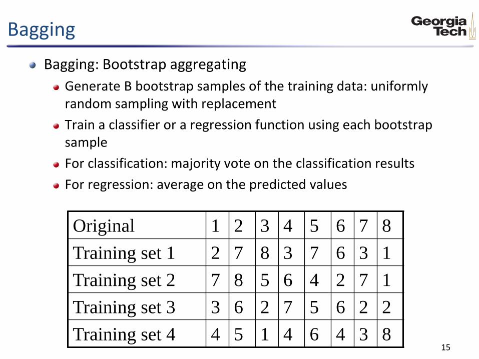
Bagging

Bagging: Bootstrap aggregating

Generate B bootstrap samples of the training data: uniformly random sampling with replacement

Train a classifier or a regression function using each bootstrap sample

For classification: majority vote on the classification results

For regression: average on the predicted values

15

Original 1 2 3 4 5 6 7 8

Training set 1 2 7 8 3 7 6 3 1

Training set 2 7 8 5 6 4 2 7 1

Training set 3 3 6 2 7 5 6 2 2

Training set 4 4 5 1 4 6 4 3 8

Stacking classifiers

16

Level-0 models are based on different learning models and use original data (level-0 data)

Level-1 models are based on results of level-0 models (level-1 data are outputs of level-0 models) -- also called “generalizer”

If you have lots of models, you can stacking into deeper hierarchies

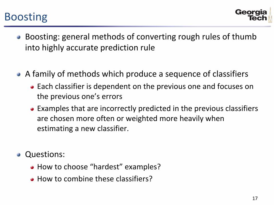
Boosting

Boosting: general methods of converting rough rules of thumb into highly accurate prediction rule

A family of methods which produce a sequence of classifiers

Each classifier is dependent on the previous one and focuses on the previous one’s errors

Examples that are incorrectly predicted in the previous classifiers are chosen more often or weighted more heavily when estimating a new classifier.

Questions:

How to choose “hardest” examples?

How to combine these classifiers?

17

AdaBoost

18

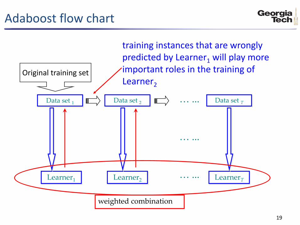
Adaboost flow chart

19

Data set 1

Learner1

Data set 2

Learner2 LearnerT

Data set T

… ...

… ...

… ...

training instances that are wrongly predicted by Learner1 will play more important roles in the training of Learner2

weighted combination

Original training set

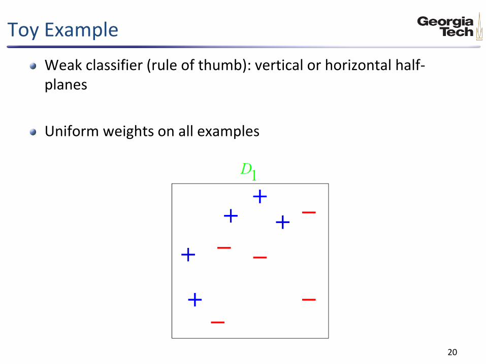
Toy Example

Weak classifier (rule of thumb): vertical or horizontal half-planes

Uniform weights on all examples

20

Boosting round 1

Choose a rule of thumb (weak classifier)

Some data points obtain higher weights because they are classified incorrectly

21

Boosting round 2

Choose a new rule of thumb

Reweight again. For incorrectly classified examples, weight increased

22

Boosting round 3

Repeat the same process

Now we have 3 classifiers

23

Boosting aggregate classifier

Final classifier is weighted combination of weak classifiers

24

Thus, if each base classifier is slightly better than random so

that for some , then the training error drops

exponentially fast in T since the above bound is at most

Theoretical properties

Y. Freund and R. Schapire [JCSS97] have proved that the training error of AdaBoost is bounded by:

25

where

How will train/test error behave?

Expect: training error to continue to drop (or reach zero)

First guess: test error to increase when the continued classifier becomes too complex

Overfitting: hard to know when to stop training

26

Actual experimental observation

Test error does not increase, even after 1000 rounds

Test error continues to drop even after training error is zeros!

27

Theoretical properties (con’t)

Y. Freund and R. Schapire [JCSS97] have tried to bound the generalization error as:

It suggests Adaboost will overfit if T is large. However, empirical studies show that Adaboost often does not overfit. Classification error only measure whether classification right or wrong, also need to consider confidence of classifier

Margin-based bound: for any 𝜃 > 0 with high probability

28

Where 𝑚 is the number of samples and d is the VC-dimension of the weak learner Pr [𝑓 𝑥 ≠ 𝑦] ≤ 𝑂

𝑇𝑑

𝑚

Pr [𝑚𝑎𝑟𝑔𝑖𝑛𝑓 𝑥, 𝑦 ≤ 𝜃] ≤ 𝑂𝑑

𝑚𝜃2

Applications of boosting

AdaBoost and its variants have been applied to diverse domains with great success. Here I only show one example

P. Viola & M. Jones [CVPR’01] combined AdaBoost with a cascade process for face detection

They regarded rectangular features as weak classifiers

29

Applications of boosting

By using AdaBoost to weight the weak classifiers, they got two very intuitive features for face detection

Finally, a very strong face detector: On a 466MHz SUN machine,

a 384288 image requires only 0.067 seconds! (in average, only 8 features needed to be evaluated per image)

30

Boosting for face detection

31

Semi-supervised learning

Supervised Learning = learning from labeled data. Dominant paradigm in Machine Learning.

E.g, say you want to train an email classifier to distinguish spam from important messages

32

Semi-supervised learning

Supervised Learning = learning from labeled data. Dominant paradigm in Machine Learning.

E.g, say you want to train an email classifier to distinguish spam from important messages

Take sample S of data, labeled according to whether they were/weren’t spam.

33

recognize speech

steer a car

classify documents

classify proteins

recognizing faces, objects in images

...

Basic paradigm has many successes

34

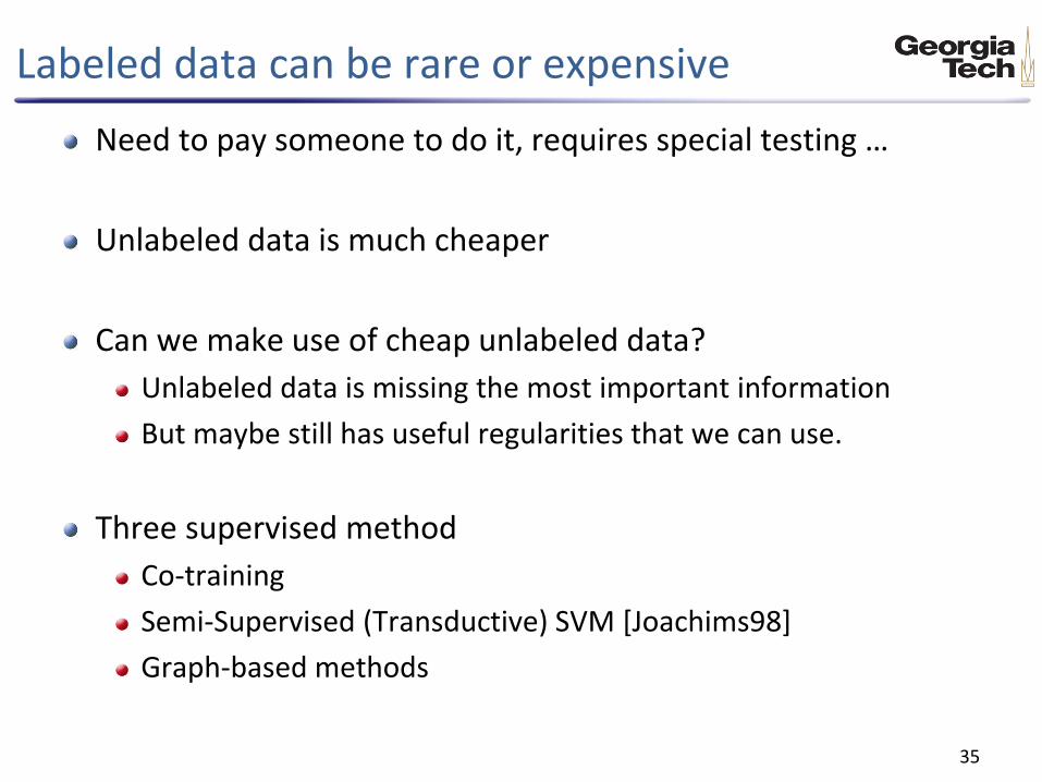
Labeled data can be rare or expensive

Need to pay someone to do it, requires special testing …

Unlabeled data is much cheaper

Can we make use of cheap unlabeled data?

Unlabeled data is missing the most important information

But maybe still has useful regularities that we can use.

Three supervised method

Co-training

Semi-Supervised (Transductive) SVM [Joachims98]

Graph-based methods

35

Co-training

36

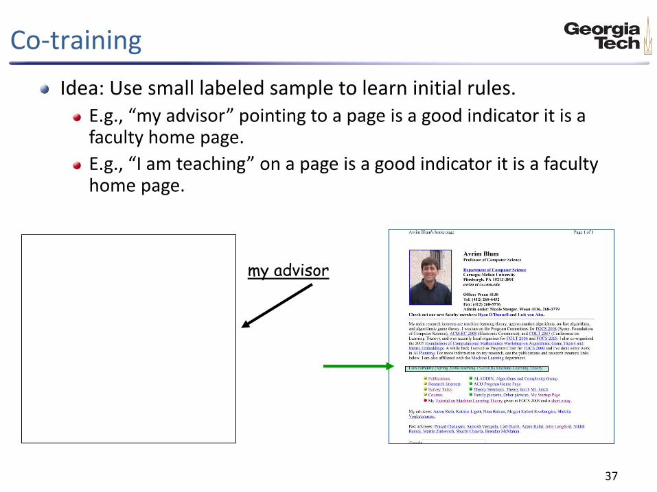
Many problems have two different sources of info you can use to determine label.

E.g., classifying webpages: can use words on page or words on links pointing to the page.

My Advisor Prof. Avrim Blum My Advisor Prof. Avrim Blum

x2- Text info x1- Link info x - Link info & Text info

Co-training

37

Idea: Use small labeled sample to learn initial rules. E.g., “my advisor” pointing to a page is a good indicator it is a faculty home page.

E.g., “I am teaching” on a page is a good indicator it is a faculty home page.

my advisor

Co-training

38

Then look for unlabeled examples where one rule is confident and the other is not. Have it label the example for the other.

Training 2 classifiers, one on each type of info. Using each to help train the other.

hx1,x2i

hx1,x2i

hx1,x2i

hx1,x2i

hx1,x2i

hx1,x2i

Co-training

39

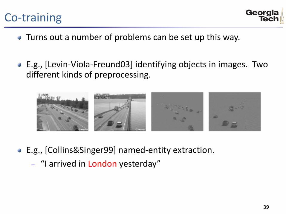
Turns out a number of problems can be set up this way.

E.g., [Levin-Viola-Freund03] identifying objects in images. Two different kinds of preprocessing.

E.g., [Collins&Singer99] named-entity extraction.

– “I arrived in London yesterday”

Co-training

40

Setting is each example x = (x1,x2), where x1, x2 are two “views” of the data.

Have separate algorithms running on each view. Use each to help train the other.

Basic hope is that two views are consistent. Using agreement as proxy for labeled data.

hx1,x2i

hx1,x2i

hx1,x2i

hx1,x2i

hx1,x2i

hx1,x2i

Toy example: intervals

As a simple example, suppose x1, x2 ∈ 𝑅. Target function is some interval [a,b].

+

+

+

+ +

a1 b1

a2

b2

41

Webpage classification 12 labeled examples, 1000 unlabeled

(sample run)

42

Images classification

Visual detectors with different kinds of processing

• [Levin-Viola-Freund ‘03]: • Images with 50 labeled

cars. 22,000 unlabeled images.

• Factor 2-3+ improvement.

43

Semi-Supervised SVM (S3VM)

Suppose we believe decision boundary goes through low density regions of the space/large margin.

Aim for classfiers with large margin wrt labeled and unlabeled data. (L+U)

+

+

_

_

Labeled data only

+

+

_

_

+

+

_

_

S3VM

SVM

44

Unfortunately, optimization problem is now NP-hard. Algorithm instead does local optimization.

Start with large margin over labeled data. Induces labels on U.

Then try flipping labels in greedy fashion.

Or, branch-and-bound, other methods (Chapelle etal06)

Quite successful on text data.

Semi-Supervised SVM (S3VM)

+

+ _

_

+

+ _

_

+

+ _

_

45

Graph-based methods

Suppose that very similar examples probably have the same label

If you have a lot of labeled data, this suggests a Nearest-Neighbor type of algorithm

If you have a lot of unlabeled data, perhaps can use them as “stepping stones”

E.g., handwritten digits [Zhu07]:

46

Graph-based methods

Idea: construct a graph with edges between very similar examples.

Unlabeled data can help “glue” the objects of the same class together.

47

Graph-based methods

Idea: construct a graph with edges between very similar examples.

Unlabeled data can help “glue” the objects of the same class together.

48

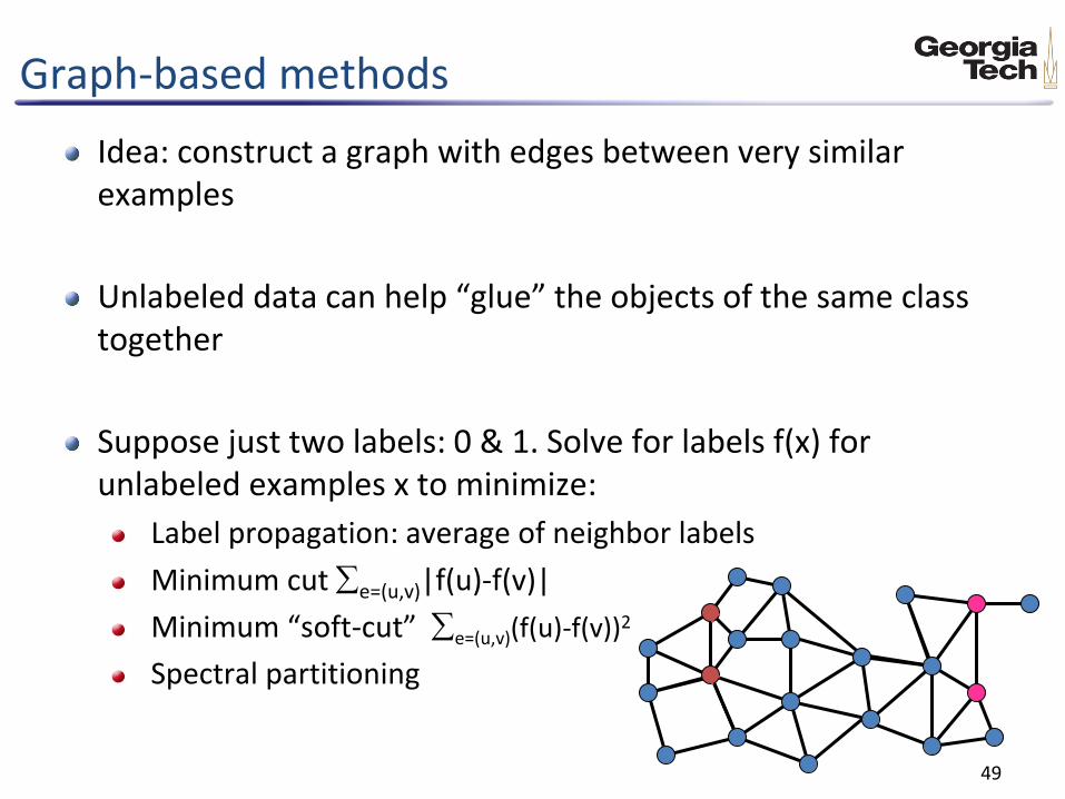
Graph-based methods

Idea: construct a graph with edges between very similar examples

Unlabeled data can help “glue” the objects of the same class together

Suppose just two labels: 0 & 1. Solve for labels f(x) for unlabeled examples x to minimize:

Label propagation: average of neighbor labels

Minimum cut e=(u,v)|f(u)-f(v)|

Minimum “soft-cut” e=(u,v)(f(u)-f(v))2

Spectral partitioning -

- +

+

49