Boomer Manual

!! David Bourne

v3.4 - Feb 2016 Copyright © David Bourne 2016

Boomer Manual

!! David Bourne

v3.4 - Feb 2016 Copyright © David Bourne 2016

Boomer 6 .........................................................................................

1. Background 7 ..............................................................................

2. Fitting Algorithms 8 ....................................................................Gauss-Newton 8 ......................................................................................................

Damping Gauss-Newton 8 ......................................................................................

Modified Marquardt 8 .............................................................................................

Simplex 8 .................................................................................................................

Simplex -> Damping Gauss-Newton 8 ...................................................................

Grid Search 9 ..........................................................................................................

One Parameter Optimization 9 ...............................................................................

3. Numerical Integration Algorithms 10 .........................................Classical Fourth Order Runge-Kutta 10 ..................................................................

Runge-Kutta-Gill 10 ................................................................................................

Fehlberg RKF45 10 .................................................................................................

Adams Predictor-Corrector 10 ................................................................................

Gear with PEDERV subroutine 10 .........................................................................

Gear without PEDERV subroutine 10 ....................................................................

4. Instructions for Boomer 12 .........................................................Starting Boomer 12 .................................................................................................

Data Entry 12 ..........................................................................................................

B. Method of Analysis 13 ........................................................................................

D. Model definition - Boomer 18 ............................................................................

E. Specifying Parameter Values and Limits 29 ........................................................

F. Example Models - Boomer 31 .............................................................................

H. Numerical Integration Method 32 .....................................................................

I. Numerical Integration - Error Terms 34 .............................................................

J. Fitting Algorithm 34 .............................................................................................

K. Fitting Criteria 35 ...............................................................................................

L. Data Set Title 35 .................................................................................................

M. Individual Data Value Entry 35 .........................................................................

N. Weighting Scheme 36 .........................................................................................

O. Entry of Initial Parameter Estimates 37 .............................................................

P. Simulation with Error Input 38 ...........................................................................

Q. AUC, AUMC, and MRT 39 ..............................................................................

R. Additional Output including Saving Data, Graphs, Extra Files and Sensitivity Ouput 39 ................................................................................................

S. Notes 44 ...............................................................................................................

5. Output Information 46 ...............................................................

6. Boomer Tutorial 49 .....................................................................A. Normal Fitting - Two Compartment I.V. Bolus Model 49 .................................

B. Bayesian Analysis - I.V. Infusion with kel function of Creatinine Clearance....52

C. Working with Batch (.BAT) files - Simulation 53 ................................................

D. Simultaneous Fit to IV and Oral Data - IRWLS 55 ...........................................

E. Simulation with Error and Monte-Carlo Simulations 57 ...................................

F. Grid Search Method 58 .......................................................................................

Online Tutorials 60 ..................................................................................................

7. Error Messages 62 .......................................................................A. FORTRAN error messages 62 ...........................................................................

B. RKF45 error messages 62 ...................................................................................

F. DIFSUB error messages 63 .................................................................................

8. Appendices 64 .............................................................................

9. Acknowledgments 65 ..................................................................

10. Applications 66.........................................................................

Boomer Non-linear Regression Program for the Analysis of

Pharmacokinetic and Pharmacodynamic Data David W.A. Bourne, OU College of Pharmacy, 1110 N. Stonewall Ave., Oklahoma City, OK

72117 U.S.A.

Copyright © 1986-2011 David W.A. Bourne

� A Boomer

June 2011 - Version 3.3.7

References

Bourne, D.W.A. 1986 MULTI-FORTE, a microcomputer program for modeling and simulation of pharmacokinetic data. Computer Methods and Programs in Biomedicine 23, 277-281

Bourne, D.W.A. 1989 BOOMER, a simulation and modeling program for pharmacokinetic and pharmacodynamic data analysis. Computer Methods and Programs in Biomedicine 29, 191-195

1. Background MULTI-FORTE started as a direct FORTRAN 77 translation of the MULTI program

written in BASIC by Yamaoka et.al (1981).

MULTI was written for a microcomputer in BASIC and allowed for the nonlinear least squares analysis of integrated equations. Four fitting algorithms were included in this original program. Later versions of MULTI incorporated Bayesian fitting and numerical integration of differential equations as separate programs (Yamaoka, 1983, 1985).

MULTI-FORTE includes normal fitting, Bayesian estimation, or simulation only with integrated or differential equation models in the one program. Also, the selection of weighting schemes and methods for numerical integration have been expanded. With MULTI-FORTE the pharmacokinetic model is written in FORTRAN 77, compiled and linked with the rest of the program.

BOOMER was developed with the same fitting and numerical integration routines found in MULTI-FORTE. However, with BOOMER the model is described using model parameters (based on the approach used by SAAM, Berman and Weiss, 1967, Berman et al., 1962) and thus the user doesn’t need to have a FORTRAN compiler.

References

Berman, M. and Shahn, E. and Weiss, M.F. 1962 The Routine Fitting of Kinetic Data to Models: A Mathematical Formalism for Digital Computers, Biophysical J.,

Berman, M. and Weiss, M.F. 1967 SAAM Manual., U. S. Public Health Service Publication No. 1703. U. S. Government Printing Office, Washington, D. C.

Yamaoka, K., Tanigawara, Y., Nakagawa, T., and Uno, T. 1981 A Pharmacokinetic Analysis Program (MULTI) for Microcomputer. J. Pharmacobio-Dyn., 4, 879-885

Yamaoka, K. and Nakagawa, T. 1983 A Nonlinear Least Squares Program Based on Differential Equations, MULTI(RUNGE), for microcomputers. J. Pharmacobio-Dyn., 6, 595-606

Yamaoka, K., Nakagawa, T., Tanaka, H., Yasuhara, M., Okumura, K. and Hori, R. 1985 A nonlinear multiple regression program, MULTI2(BAYES), based on Bayesian algorithm for microcomputers. J. Pharmacobio-Dyn., 8, 246-256

2. Fitting Algorithms 1

GAUSS-NEWTON This is a method based on expanding the model equation(s) of interest in a Taylor series

(Hartley, 1961).

DAMPING GAUSS-NEWTON The correction term applied to the 'old' parameter values is reduced by a factor of two if the

'new' parameter values result in a worse value for WSS. This is allowed up to 25 times during each iteration, although rounding error may become significant above 15 reductions.

MODIFIED MARQUARDT The Marquardt method is intermediate between the Taylor series (Gauss-Newton) method

and the method of steepest descent (gradient method). In the method of steepest descent the new parameter values are calculated in the direction of the negative slope of the WSS with respect to each of the parameters. Marquardt has suggested that the direction of change in parameters calculated by these two methods is not always in the same direction. Marquardt's method attempts to find a best compromise (Marquardt, 1963). The method used in MULTI and MULTI-FORTE was that further modified by Flecher (Flecher, 1971).

SIMPLEX The simplex method of Nelder and Mead is the fourth option. This method involves the

progression of a moving simplex across the WSS surface. Typically the worst point of the simplex is projected across the center (centroid) of the simplex to a better value. There are a series of simple rules to move the simplex to the WSS minimum. It is a relatively robust (but slower) method (Nelder and Mead, 1965). Other than the initial parameter estimates provided by the use the other points on the simplex are generated randomly.

SIMPLEX -> DAMPING GAUSS-NEWTON 2

The Simplex method is quite robust and can be used with less accurate initial parameter estimates. However, it is not possible to estimate parameter value variances by this method. Thus it may be useful to automatically proceed from the final Simplex values to the input stage of another method. Presently that other method is the Damping Gauss-Newton. This option is especially attractive when used with the multi-run approach described later. Each run starts with a different simplex with only the initial parameter estimate point fixed. The others are randomly generated. Thus, each run is started from a different place in the WSS surface. This increase the possibility of converging on the global minimum.

See Appendix A for more details1

Preferred, first choice method2

GRID SEARCH By specifying upper and lower parameter limits as well as the number of grids, it is possible to

calculate the weighted sum of squares at each grid intersection. The results of this analysis can be output to disk for incorporation into a 3-D graphing program such as DeltaGraph®

(Macintosh graphing program).

ONE PARAMETER OPTIMIZATION

References

Flecher, R. 1971 A Modified Marquardt Subroutine for Non-Linear Least Squares. Tech. Report AERE R6799, U.K. Atomic Energy Authority Research Establishment, Harwell, UK

Hartley, H.O. 1961 The modified Gauss-Newton method for the fitting of non-linear regression functions by least squares, Technometrics, 3(2), 269-280

Marquardt, D.W. 1963 An Algorithm for Least-Squares Estimation of NonLinear Parameters. J.Soc. Indust. Appl. Math., 11(2), 431-441

Nelder, J.A. and Mead, R. 1965. A simplex method for function minimization. Computer J., 7, 308-313

3. Numerical Integration

Algorithms 3

CLASSICAL FOURTH ORDER RUNGE-KUTTA This method is an implementation of the fourth order Runge-Kutta method. A relative error

term is used to adjust the step-size. Error control is achieved by simply halving the step size until the change in calculated values is smaller than the error requested (Kutta, 1901).

RUNGE-KUTTA-GILL This is the numerical integration method used in MULTI(RUNGE) by Yamaoka et.al. (1983)

It has also been modified to give automatic step-size control. Again, error control is achieved by halving the step size until the desired accuracy is achieved. In MULTI(RUNGE) the step size was adjusted manually (Gill, 1951).

FEHLBERG RKF45 4

This is a further modification of the Runge-Kutta fourth order method which uses a fifth order calculation to determine the appropriate step size given values for the required relative and absolute error. This is the subroutine written by Watts and Shampine and published as Subroutine RKF45 in the book by Forsythe and Moler (Forsythe and Moler 1967; Fehlberg, 1969; Watt and Shampine, 1977 and Shampine and Watt, 1977). This method is very efficient and appears to be the method of choice for non-stiff systems of differential equations.

ADAMS PREDICTOR-CORRECTOR This is one of the options of the subroutine written by Gear. This method is also for non-stiff

systems of differential equations. Step-size and order are automatically controlled to achieve a user defined absolute error (Gear 1969; Gear 1971a and Gear 1971b).

GEAR WITH PEDERV SUBROUTINE This is the most efficient option for use with stiff equations. The subroutines DECOMP and

SOLVE were modified from those presented in the text by Forsythe and Moler (Forsythe and Moler, 1967).

GEAR WITHOUT PEDERV SUBROUTINE

See Appendix B for more details3

Preferred, first choice method4

The partial derivatives are calculated by numerical differencing thus a user supplied PEDERV subroutine is not required.

References

Fehlberg, E. 1969 Low-order classical Runge-Kutta formulas with stepsize control and their application to some heat transfer problems. NASA Technical Report, NASA TR R-315

Forsythe, G.E. and Moler, C. 1967 Computer Solutions of Algebraic Systems. Prentice-Hall, Englewood Cliffs, NJ 68-69

Gear, C.W. 1969 DIFSUB for solution of ordinary differential equations. Algorithm 407. Collected Algorithms from CACM

Gear, C.W. 1971a Numerical Initial Value Problems in Ordinary Differential Equations. Prentice-Hall, Englewood Cliffs, NJ 158-166

Gear, C.W. 1971b The automatic integration of ordinary differential equations. Comm. A.C.M., 14(3), 176-179

Gill, S. 1951 A process for the step-by-step integration of differential equations in an automatic digital computing machine. Proc. Cambridge Philos. Soc., 47, 96-108

Kutta, W. 1901 Beitrag zur naherungsweisen Integration totaler Differentialgleichunge. Zeit. Math. Physik, 46, 435-453

Shampine, L.F. and Watts, H.A. 1977 The art of writing a Runge-Kutta code, Part 1. in Mathematical Software III, ed. Rice, J.R. Academic Press, New York, NY

Watt, H.A. and Shampine, L.F. 1977 Subroutine RKF45 in Computer Methods for Mathematical Computations, Forsythe, G.E., Malcolm, M.A. and Moler, C.B. Prentice-Hall, Englewood, NJ 133-147

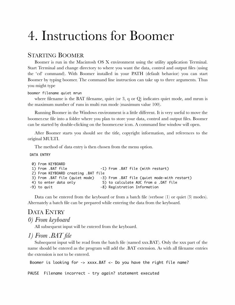
4. Instructions for Boomer STARTING BOOMER

Boomer is run in the Macintosh OS X environment using the utility application Terminal. Start Terminal and change directory to where you want the data, control and output files (using the ‘cd’ command). With Boomer installed in your PATH (default behavior) you can start Boomer by typing boomer. The command line instruction can take up to three arguments. Thus you might type boomer filename quiet mrun

where filename is the BAT filename, quiet (or 3, q or Q) indicates quiet mode, and mrun is the maximum number of runs in multi run mode (maximum value 100).

Running Boomer in the Windows environment is a little different. It is very useful to move the boomer.exe file into a folder where you plan to store your data, control and output files. Boomer can be started by double-clicking on the boomer.exe icon. A command line window will open.

After Boomer starts you should see the title, copyright information, and references to the original MULTI.

The method of data entry is then chosen from the menu option.

DATA ENTRY

0) From KEYBOARD 1) From .BAT file -1) From .BAT file (with restart) 2) From KEYBOARD creating .BAT file 3) From .BAT file (quiet mode) -3) From .BAT file (quiet mode-with restart) 4) to enter data only 5) to calculate AUC from a .DAT file -9) to quit -8) Registration Information

Data can be entered from the keyboard or from a batch file (verbose (1) or quiet (3) modes). Alternately a batch file can be prepared while entering the data from the keyboard.

DATA ENTRY 0) From keyboard

All subsequent input will be entered from the keyboard.

1) From .BAT file Subsequent input will be read from the batch file (named xxx.BAT). Only the xxx part of the

name should be entered as the program will add the .BAT extension. As with all filename entries the extension is not to be entered.

Boomer is looking for -> xxxx.BAT <- Do you have the right file name?

PAUSE Filename incorrect - try again? statement executed

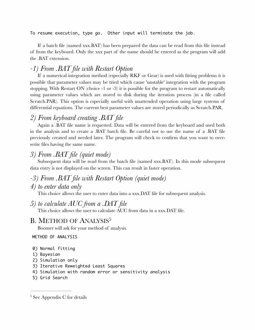
To resume execution, type go. Other input will terminate the job.

If a batch file (named xxx.BAT) has been prepared the data can be read from this file instead of from the keyboard. Only the xxx part of the name should be entered as the program will add the .BAT extension.

-1) From .BAT file with Restart Option If a numerical integration method (especially RKF or Gear) is used with fitting problems it is

possible that parameter values may be tried which cause 'unstable' integration with the program stopping. With Restart ON (choice -1 or -3) it is possible for the program to restart automatically using parameter values which are stored to disk during the iteration process (in a file called Scratch.PAR). This option is especially useful with unattended operation using large systems of differential equations. The current best parameter values are stored periodically as Scratch.PAR.

2) From keyboard creating .BAT file Again a .BAT file name is requested. Data will be entered from the keyboard and used both

in the analysis and to create a .BAT batch file. Be careful not to use the name of a .BAT file previously created and needed later. The program will check to confirm that you want to over-write files having the same name.

3) From .BAT file (quiet mode) Subsequent data will be read from the batch file (named xxx.BAT). In this mode subsequent

data entry is not displayed on the screen. This can result in faster operation.

-3) From .BAT file with Restart Option (quiet mode) 4) to enter data only

This choice allows the user to enter data into a xxx.DAT file for subsequent analysis.

5) to calculate AUC from a .DAT file This choice allows the user to calculate AUC from data in a xxx.DAT file.

B. METHOD OF ANALYSIS 5

Boomer will ask for your method of analysis.

METHOD OF ANALYSIS

0) Normal fitting 1) Bayesian 2) Simulation only 3) Iterative Reweighted Least Squares 4) Simulation with random error or sensitivity analysis 5) Grid Search

See Appendix C for details5

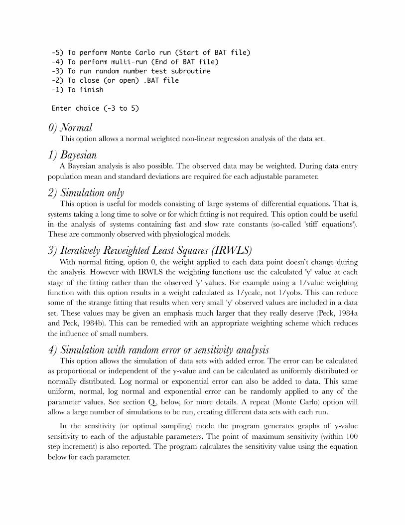
-5) To perform Monte Carlo run (Start of BAT file) -4) To perform multi-run (End of BAT file) -3) To run random number test subroutine -2) To close (or open) .BAT file -1) To finish

Enter choice (-3 to 5)

0) Normal This option allows a normal weighted non-linear regression analysis of the data set.

1) Bayesian A Bayesian analysis is also possible. The observed data may be weighted. During data entry

population mean and standard deviations are required for each adjustable parameter.

2) Simulation only This option is useful for models consisting of large systems of differential equations. That is,

systems taking a long time to solve or for which fitting is not required. This option could be useful in the analysis of systems containing fast and slow rate constants (so-called 'stiff equations'). These are commonly observed with physiological models.

3) Iteratively Reweighted Least Squares (IRWLS) With normal fitting, option 0, the weight applied to each data point doesn’t change during

the analysis. However with IRWLS the weighting functions use the calculated 'y' value at each stage of the fitting rather than the observed 'y' values. For example using a 1/value weighting function with this option results in a weight calculated as 1/ycalc, not 1/yobs. This can reduce some of the strange fitting that results when very small 'y' observed values are included in a data set. These values may be given an emphasis much larger that they really deserve (Peck, 1984a and Peck, 1984b). This can be remedied with an appropriate weighting scheme which reduces the influence of small numbers.

4) Simulation with random error or sensitivity analysis This option allows the simulation of data sets with added error. The error can be calculated

as proportional or independent of the y-value and can be calculated as uniformly distributed or normally distributed. Log normal or exponential error can also be added to data. This same uniform, normal, log normal and exponential error can be randomly applied to any of the parameter values. See section Q, below, for more details. A repeat (Monte Carlo) option will allow a large number of simulations to be run, creating different data sets with each run.

In the sensitivity (or optimal sampling) mode the program generates graphs of y-value sensitivity to each of the adjustable parameters. The point of maximum sensitivity (within 100 step increment) is also reported. The program calculates the sensitivity value using the equation below for each parameter.

"

The time when this value is maximum could be used as an optimal sampling time.

5) Grid search method This option allows a systematic search of a specified parameter space. The space is defined by

specifying upper and lower limits and the number of steps in the grid. Output can be in the normal form or as disk files of parameter values and weighted sum of squares values for input into a graphing program for 3-D surface plotting.

-5) Monte Carlo run This is similar to the multi run option below with one significant difference. If data files are

input or output they will be created with unique (incremental) names. They can be useful in the generation of many multiple data sets that might be useful as a clinical trial simulation. A Monte Carlo run .BAT file can also be created from a 'ordinary' .BAT file by adding the number of runs (>10) as the second line in the .BAT file.

Monte Carlo run Option

It is possible to run repeated analyzes of 10 to 99999 data sets (memory and time permitting). This could be be useful in a Monte Carlo type analysis. I have found this useful for generating homework data sets. It could also be used to simulate data sets for other purposes such as clinical trial simulations. An additional output data file (extension .NDT) is generated with the same name as the 'normal' output (.OUT) file but in format suitable for use with NONMEM (Beal, S.L. and Sheiner, L.B. 1989 NONMEM Users Guide -- Part I Users Basic Guide, NONMEM Project Group, UCSF, San Francisco, CA). Another output file (extension .csv) is generated in a format suitable for Pmetrics (Neely MN, van Guilder MG, Yamada WM, Schumitzky A, Jelliffe RW. Accurate Detection of Outliers and Subpopulations With Pmetrics, a Nonparametric and Parametric Pharmacometric Modeling and Simulation Package for R. Therapeutic Drug Monitoring. 2012; 34(4): 467-476).

These runs can be set-up during the creation of the .BAT file as above or by creating a single run batch files as normal with -2 at the end. Open the .BAT file in a text editor and insert above the first data line the number of repeats required (must be greater than 10). Boomer Batch File 4 wls,bayes,sim,irwls,sim+error,gridTop of the .BAT file before editing andBoomer Batch File25 4 wls,bayes,sim,irwls,sim+error,grid

after editing to simulate 25 data sets.

Save the file and select batch file run. When simulating data sets use the simulate with error option to make different data sets on each run. When saving the calculated data set (the first time through when creating the batch file) use any reasonable, short file name (e.g. test: A maximum of 4 characters are used with the DOS version). In repeat mode the program will create file names with a numbered extension. For example test0001.DAT, test0002.DAT, test0003.DAT ... in sequence. When reading the data sets in using the repeat option the same naming convention is used. That is specify 'test' and the program will expect to read files test0001.DAT, test0002.DAT, test0003.DAT etc. [There are four columns in the number field to accommodate file names from test0001.DAT to test9999.DAT].

The auxiliary program cDAT can read these multiple DAT files and combine them into a tab delimited summary file suitable for importing into a spreadsheet program. The cDAT program is installed by the Mac OS X boomer installation package in /usr/bin and provided in the DOS zip folder. The program can be invoked by typing cDAT and then providing the DAT file name and the number of files. It can also be invoked as one line command.

cDAT test nnn

where 'test' is the first part of the DAT file name (can be entered as test0001 or the complete name test0001.DAT) and 'nnn' is the number of DAT files.

The auxiliary program eOUT can extract specified lines from .OUT files (especially useful for Monte Carlo or Multi runs), optionally converting spaces to tabs. The output file is suitable for importing into a spreadsheet program. The eOUT program is installed by the Mac OS X boomer installation package in /usr/bin and provided in the DOS zip folder. The program can be invoked by typing eOUT and then providing the OUT file name and other parameters. It can also be invoked as one command.

eOUT test.OUT key nskip nline tflag

where test.out is the .OUT file name (test should also work), key is the string to seach (enclose with '' if it contains spaces), nskip is the number of lines to skip after key is found, nline is the number of lines to export and tflag is 0 or 1 (if equal to 1 converts run of spaces to one tab). It is useful to examine the .OUT file before running eOUT to determine the best values of the parameters, especially key, nskip and nline. This could be useful in extracting the final fit parameter values from a multi-run .OUT file.

The auxilliary program eBEST can extract the best run from a multi-run .OUT file. The eBEST program is installed by the Mac OS X boomer installation package in /usr/bin and provided in the DOS zip folder. The program can be invoked by typing eBEST and then providing the OUT file name. It can also be invoked as one command.

eBEST test.OUT

where test.out is the .OUT file name. The program then asks Enter percent from Best WWW

Enter a percent (x) and the program displays the number of runs with a WSS within x% of the best. The best run is placed in a file BEST.OUT which is opened by BBEdit (Macintosh if installed) or NotePad (Windows) for review and saving. eBest also provides the file eBestP.OUT containing the WSS and parameter values for each run.

-4) Multi run This option allows either repeated runs of the BAT file or chaining to another BAT file. It will

not be selected initially but only at the end of the first run. Repeatedly running a BAT file is useful when fitting data using the Simplex method as each run starts with a randomly generated simplex. A multi run .BAT file can be created from a 'ordinary' .BAT file by changing the -1 or -2 on the last line to -4 and entering the .BAT file name on the following line. This could be used to chain a number of control files for multiple subjects.

-3) Random Number Test The Macintosh toolbox routine, random, is used to generate random numbers for the simplex

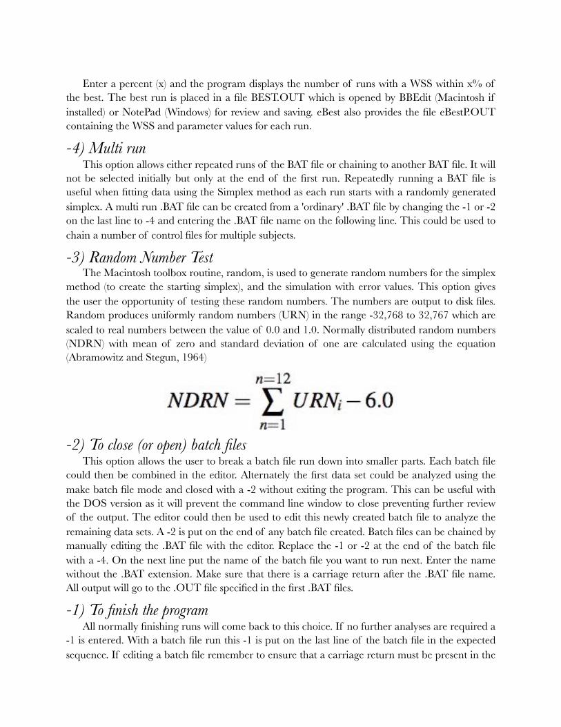
method (to create the starting simplex), and the simulation with error values. This option gives the user the opportunity of testing these random numbers. The numbers are output to disk files. Random produces uniformly random numbers (URN) in the range -32,768 to 32,767 which are scaled to real numbers between the value of 0.0 and 1.0. Normally distributed random numbers (NDRN) with mean of zero and standard deviation of one are calculated using the equation (Abramowitz and Stegun, 1964)

�-2) To close (or open) batch files

This option allows the user to break a batch file run down into smaller parts. Each batch file could then be combined in the editor. Alternately the first data set could be analyzed using the make batch file mode and closed with a -2 without exiting the program. This can be useful with the DOS version as it will prevent the command line window to close preventing further review of the output. The editor could then be used to edit this newly created batch file to analyze the remaining data sets. A -2 is put on the end of any batch file created. Batch files can be chained by manually editing the .BAT file with the editor. Replace the -1 or -2 at the end of the batch file with a -4. On the next line put the name of the batch file you want to run next. Enter the name without the .BAT extension. Make sure that there is a carriage return after the .BAT file name. All output will go to the .OUT file specified in the first .BAT files.

-1) To finish the program All normally finishing runs will come back to this choice. If no further analyses are required a

-1 is entered. With a batch file run this -1 is put on the last line of the batch file in the expected sequence. If editing a batch file remember to ensure that a carriage return must be present in the

batch file after the -1 for it to be correctly interpreted. Actually all batch, data, or model files must end with a carriage return to be interpreted correctly.

C. Output options

Where do you want the output?

0) Terminal screen 1) Disk file

Enter choice (0-1)

0) Terminal screen All output is directed to the computer terminal screen. This is useful for a quick check of the

input data or for rapid analysis which doesn't need to be kept.

1) Disk file Again a disk file name is requested after selecting this option. The final results and requested

plots can be directed to an .OUT file output file for later printing or enhancement. The output is saved as a text type file which could be read into a word processor for editing or other visual enhancement. The disk receiving a large output file will need to have enough space.

D. MODEL DEFINITION - BOOMER One limitation of the original implementation of MultiForte was that the user had to have

and know how to use the Fortran compiler in order to study different pharmacokinetic models. This is still an option with the original version of MultiForte. Boomer, a version of Multi-Forte described in this section, allows the user to describe a model in terms of time interrupts (e.g. dose times or lag times), dose, first order rate constants, zero order rate constants, constants, Michaelis-Menten kinetics elimination rate systems (Portmann, 1970; Michaelis and Menten, 1913), multipliers (i.e. inverse apparent volumes of distribution), sums of exponentials, Hill equation components (Rubinow, 1975; Hill, 1910), second order rate constants, or simple physiological models (Duddy et al. 1984). This building of a model is similar to the approach taken with the mainframe simulation and modeling program, SAAM (Berman and Weiss, 1967). MODEL Definition and Parameter Entry * Allowed Parameter Types *

-5) read model -3) display choices -2) display parameters

0) Time interrupt 1) Dose/initial amount 2) First order rate 3) Zero order 4-5) Vm and Km of Michaelis-Menten 6) Added constant 7) Kappa-Reciprocal volume 8-10) C = a * EXP(-b * (X-c)) 11-13) Emax (Hill) Eq with Ec(50%) & S term 14) Second order rate 15-17) Physiological Model Parameters (Q, V, and R) 18) Apparent volume of distribution 19) Dummy parameter for double dependence 20-22) C = a * SIN(2 * pi * (X - c)/b)

Special Functions for First-order Rate Constants 23-24) k = a * X + b 25-27) k = a * EXP(-b * (X - c)) 28-30) k = a * SIN(2 * pi * (X - c)/b) 31,32-33) dAt/dt = - k * V * Cf (Saturable Protein Binding) 34-36) k * (1 - Imax * C/(IC(50%) + C)) Inhibition 0 or 1st order 37-39) k * (1 + Smax * C/(SC(50%) + C)) Stimulation 0 or 1st order 40) Uniform [-1 to 1] and 41) Normal [-3 to 3] Probability 42) Switch parameter 43) Clone component 44-47) Four parameter logistic model 48-51) Four parameter Weibull model

Enter type# for parameter 1 (-5 to 51)

With this approach the model is constructed step-by-step during the data entry process. Once a useful model is chosen it may be more convenient to use the batch mode, by first preparing a batch file, editing, and running the program using the edited batch file (see Data entry section 1 and 2). The types of parameters available are shown in the screen dump above.

-5) Read model from .mdl file The model, described with adjustable or fixed constants, can be defined using a .mdl file. If a

file has been previously defined it could be read at this point of the data entry.

-4) Write model from .mdl file (available after the model is defined) The model, described with adjustable or fixed constants, can be defined using a .mdl file.

Once the model has been defined a .mdl file can be written for later use.

0) Time interrupt These are times during a simulation at which you may wish to make a change. For example,

give a second or subsequent dose, start or stop an infusion, or incorporate a lag time into the calculation. The information requested for this parameter is simply a name and a value. It is necessary to specify any interrupt time before it can be used (e.g. to turn off an infusion). Also, when you request a list of time interrupt values they will be numbered excluding other parameter types. It is easier to specify all the parameters that don't change first then the time interrupt values, and finally the doses or other parameters that depend on a time. As with any of the parameter types these time interrupt values may be fixed, adjustable, or dependent.

1) Dose/initial amount This would typically be the dose or it could be an initial concentration. Given as a dose it

would generally be fixed, however, as an initial concentration it may be more appropriate to 'best-fit' this value. Name, value, and component to receive the dose should be specified. F-dependence is possible with this type of parameter. Specifying a positive (or negative) component for F-dependence multiplies the above value by the amount in the specified component and adds or subtracts this amount from the To component. For example, this might be useful if you are removing a sample and replacing it with an equal volume of fresh solvent. For 1 mL removed and replaced from 100 mL use 0.01 (1%) as the value.

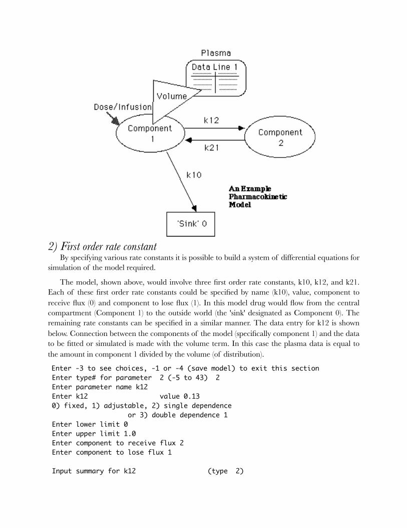
�2) First order rate constant

By specifying various rate constants it is possible to build a system of differential equations for simulation of the model required.

The model, shown above, would involve three first order rate constants, k10, k12, and k21. Each of these first order rate constants could be specified by name (k10), value, component to receive flux (0) and component to lose flux (1). In this model drug would flow from the central compartment (Component 1) to the outside world (the 'sink' designated as Component 0). The remaining rate constants can be specified in a similar manner. The data entry for k12 is shown below. Connection between the components of the model (specifically component 1) and the data to be fitted or simulated is made with the volume term. In this case the plasma data is equal to the amount in component 1 divided by the volume (of distribution).

Enter -3 to see choices, -1 or -4 (save model) to exit this section Enter type# for parameter 2 (-5 to 43) 2 Enter parameter name k12 Enter k12 value 0.13 0) fixed, 1) adjustable, 2) single dependence or 3) double dependence 1 Enter lower limit 0 Enter upper limit 1.0 Enter component to receive flux 2 Enter component to lose flux 1

Input summary for k12 (type 2)

Initial value 0.1300 float between 0.000 and 1.000 Transfer from 1 to 2

Enter 0 if happy with input, 1 if not, 2 to start over

3) Zero order rate constant Zero order rate constants would normally be used to describe an infusion dose from one time

interrupt value to another. A start time of 0 specifies that the infusion starts at the beginning of the simulation. A stop time of 0 represents an infusion which continues until the end of the simulation. As with the first order rate constant, components to receive and lose flux are specified. Typically, the infusion comes from a component which does not need to be modeled, thus a value of 0 (the outside world) can be used for the "from" component.

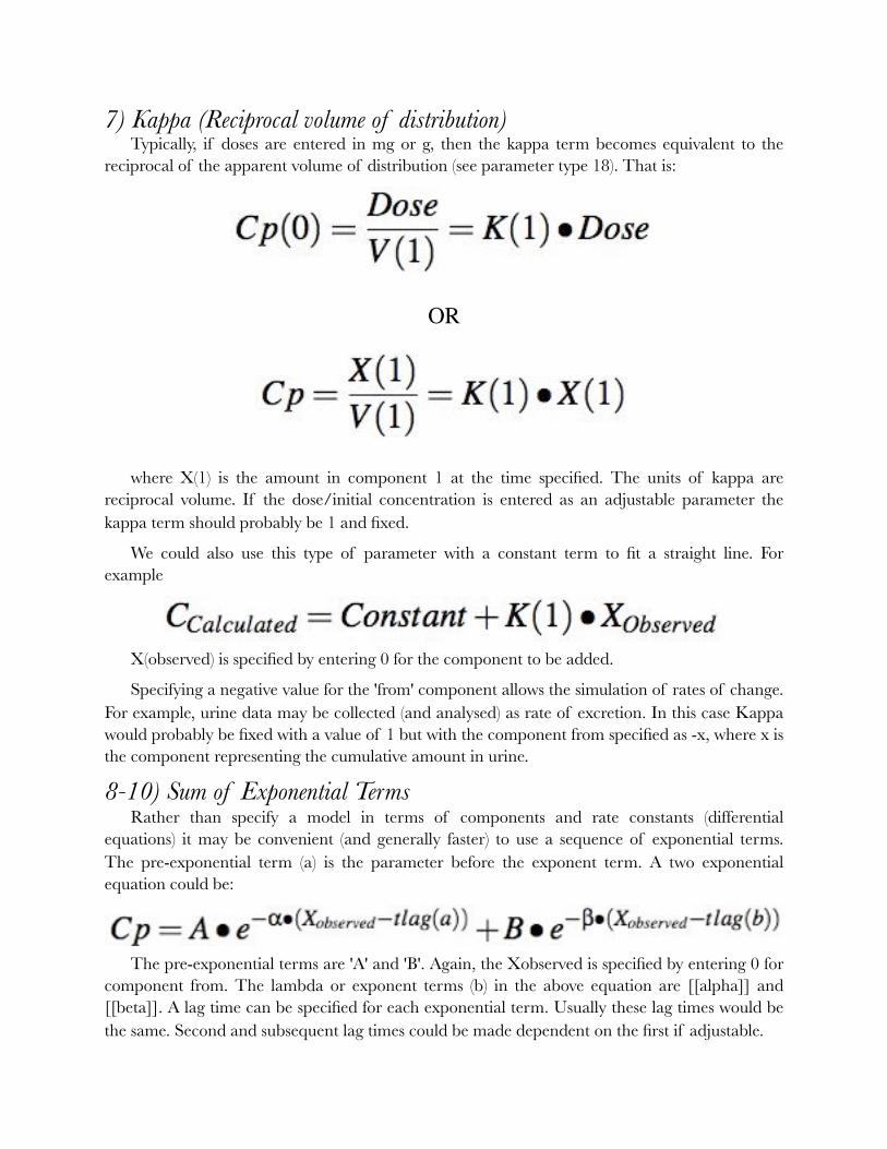
4-5) Michaelis-Menten Kinetic Parameters, Vm and Km Rate processes can be specified as Michaelis-Menten processes, for example the rate of

elimination may be as shown in the equation below.

�where Vm is the maximum rate and Km is the Michaelis-Menten constant. X(1) is the

amount (or concentration) in the from component. The Vm and Km are entered as two separate parameters, however, the to/from information remains the same for both. Be careful of the units. If doses (and thus the values in the components of the model) are given as mg or g, then, Vm units should be mg/hr or g/hr (mass/time). Dose/initial concentrations given as mg/L will mean Vm units of mg/L/hr (mass/volume/time).

The second half of the Michaelis-Menten entry process is the Km value. Only a value need by entered, unless the parameter is adjustable or dependent. Again, be careful of units. With a dose (in g or mg) entered the units of Km should also be g or mg. However if a Cp(zero) is used with mass/volume units, Km units should be the same.

6) Constant This is the first of the summing or intensity terms. It is necessary to distinguish between the

components (and their numbers) used to describe the system of differential equations and the observed data sets (and their numbers). For example in the pharmacokinetic model above there are two components not including the 'sink'. As shown, there is one data set, Plasma. We could also specify another, second data set called Tissue, and a third called Rate of Change. When a constant is specified only the name, value and data set line is required. We might use this to offset a fixed (or adjustable) background level? Or it could be used as a constant term in a Hill equation sequence or a linear fit sequence.

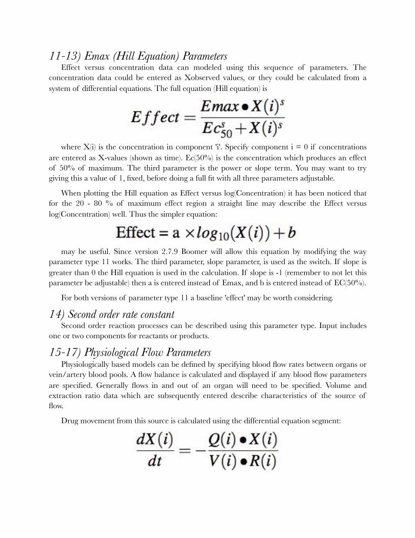
7) Kappa (Reciprocal volume of distribution) Typically, if doses are entered in mg or g, then the kappa term becomes equivalent to the

reciprocal of the apparent volume of distribution (see parameter type 18). That is:

�

OR

�

where X(1) is the amount in component 1 at the time specified. The units of kappa are reciprocal volume. If the dose/initial concentration is entered as an adjustable parameter the kappa term should probably be 1 and fixed.

We could also use this type of parameter with a constant term to fit a straight line. For example

�X(observed) is specified by entering 0 for the component to be added.

Specifying a negative value for the 'from' component allows the simulation of rates of change. For example, urine data may be collected (and analysed) as rate of excretion. In this case Kappa would probably be fixed with a value of 1 but with the component from specified as -x, where x is the component representing the cumulative amount in urine.

8-10) Sum of Exponential Terms Rather than specify a model in terms of components and rate constants (differential

equations) it may be convenient (and generally faster) to use a sequence of exponential terms. The pre-exponential term (a) is the parameter before the exponent term. A two exponential equation could be:

�The pre-exponential terms are 'A' and 'B'. Again, the Xobserved is specified by entering 0 for

component from. The lambda or exponent terms (b) in the above equation are [[alpha]] and [[beta]]. A lag time can be specified for each exponential term. Usually these lag times would be the same. Second and subsequent lag times could be made dependent on the first if adjustable.

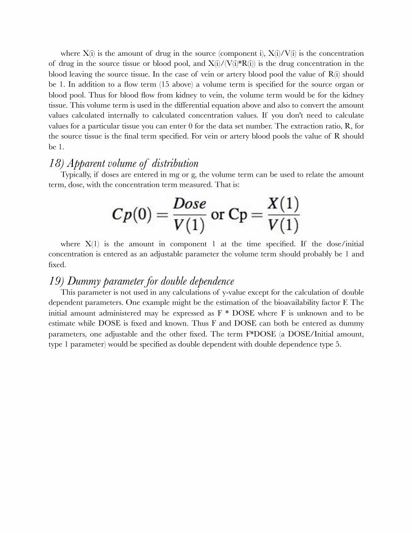
11-13) Emax (Hill Equation) Parameters Effect versus concentration data can modeled using this sequence of parameters. The

concentration data could be entered as Xobserved values, or they could be calculated from a system of differential equations. The full equation (Hill equation) is

�where X(i) is the concentration in component 'i'. Specify component i = 0 if concentrations

are entered as X-values (shown as time). Ec(50%) is the concentration which produces an effect of 50% of maximum. The third parameter is the power or slope term. You may want to try giving this a value of 1, fixed, before doing a full fit with all three parameters adjustable.

When plotting the Hill equation as Effect versus log(Concentration) it has been noticed that for the 20 - 80 % of maximum effect region a straight line may describe the Effect versus log(Concentration) well. Thus the simpler equation:

�may be useful. Since version 2.7.9 Boomer will allow this equation by modifying the way

parameter type 11 works. The third parameter, slope parameter, is used as the switch. If slope is greater than 0 the Hill equation is used in the calculation. If slope is -1 (remember to not let this parameter be adjustable) then a is entered instead of Emax, and b is entered instead of EC(50%).

For both versions of parameter type 11 a baseline 'effect' may be worth considering.

14) Second order rate constant Second order reaction processes can be described using this parameter type. Input includes

one or two components for reactants or products.

15-17) Physiological Flow Parameters Physiologically based models can be defined by specifying blood flow rates between organs or

vein/artery blood pools. A flow balance is calculated and displayed if any blood flow parameters are specified. Generally flows in and out of an organ will need to be specified. Volume and extraction ratio data which are subsequently entered describe characteristics of the source of flow.

Drug movement from this source is calculated using the differential equation segment:

�

where X(i) is the amount of drug in the source (component i), X(i)/V(i) is the concentration of drug in the source tissue or blood pool, and X(i)/(V(i)*R(i)) is the drug concentration in the blood leaving the source tissue. In the case of vein or artery blood pool the value of R(i) should be 1. In addition to a flow term (15 above) a volume term is specified for the source organ or blood pool. Thus for blood flow from kidney to vein, the volume term would be for the kidney tissue. This volume term is used in the differential equation above and also to convert the amount values calculated internally to calculated concentration values. If you don't need to calculate values for a particular tissue you can enter 0 for the data set number. The extraction ratio, R, for the source tissue is the final term specified. For vein or artery blood pools the value of R should be 1.

18) Apparent volume of distribution Typically, if doses are entered in mg or g, the volume term can be used to relate the amount

term, dose, with the concentration term measured. That is:

�where X(1) is the amount in component 1 at the time specified. If the dose/initial

concentration is entered as an adjustable parameter the volume term should probably be 1 and fixed.

19) Dummy parameter for double dependence This parameter is not used in any calculations of y-value except for the calculation of double

dependent parameters. One example might be the estimation of the bioavailability factor F. The initial amount administered may be expressed as F * DOSE where F is unknown and to be estimate while DOSE is fixed and known. Thus F and DOSE can both be entered as dummy parameters, one adjustable and the other fixed. The term F*DOSE (a DOSE/Initial amount, type 1 parameter) would be specified as double dependent with double dependence type 5.

�

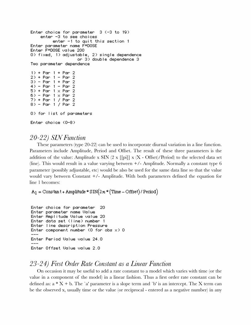
20-22) SIN Function These parameters (type 20-22) can be used to incorporate diurnal variation in a line function.

Parameters include Amplitude, Period and Offset. The result of these three parameters is the addition of the value: Amplitude x SIN (2 x [[pi]] x (X - Offset)/Period) to the selected data set (line). This would result in a value varying between +/- Amplitude. Normally a constant type 6 parameter (possibly adjustable, etc) would be also be used for the same data line so that the value would vary between Constant +/- Amplitude. With both parameters defined the equation for line 1 becomes:

�

�

23-24) First Order Rate Constant as a Linear Function On occasion it may be useful to add a rate constant to a model which varies with time (or the

value in a component of the model) in a linear fashion. Thus a first order rate constant can be defined as: a * X + b. The `a' parameter is a slope term and `b' is an intercept. The X term can be the observed x, usually time or the value (or reciprocal - entered as a negative number) in any

component. Thus zero or second order rate constant can be entered with this parameter type. For example, a zero order rate constant of 5.0 could be entered as a(SL) = 5.0 with drug from component 1 to 0, b = 0.0 and the F-dependence equal -1, the from component. The differential equation for this process is then:

�k is now a zero order rate constant.

�

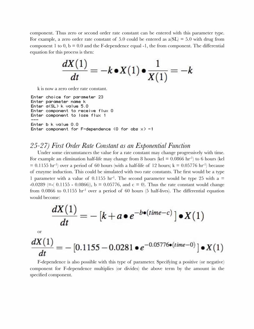
25-27) First Order Rate Constant as an Exponential Function Under some circumstances the value for a rate constant may change progressively with time.

For example an elimination half-life may change from 8 hours (kel = 0.0866 hr-1) to 6 hours (kel = 0.1155 hr-1) over a period of 60 hours (with a half-life of 12 hours; k = 0.05776 hr-1) because of enzyme induction. This could be simulated with two rate constants. The first would be a type 1 parameter with a value of 0.1155 hr-1. The second parameter would be type 25 with a = -0.0289 (=-( 0.1155 - 0.0866)), b = 0.05776, and c = 0). Thus the rate constant would change from 0.0866 to 0.1155 hr-1 over a period of 60 hours (5 half-lives). The differential equation would become:

�or

�F-dependence is also possible with this type of parameter. Specifying a positive (or negative)

component for F-dependence multiplies (or divides) the above term by the amount in the specified component.

�

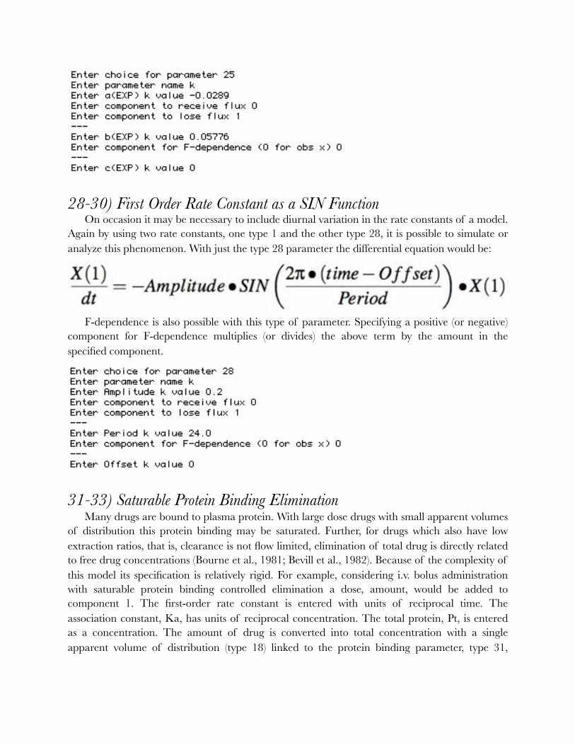
28-30) First Order Rate Constant as a SIN Function On occasion it may be necessary to include diurnal variation in the rate constants of a model.

Again by using two rate constants, one type 1 and the other type 28, it is possible to simulate or analyze this phenomenon. With just the type 28 parameter the differential equation would be:

�F-dependence is also possible with this type of parameter. Specifying a positive (or negative)

component for F-dependence multiplies (or divides) the above term by the amount in the specified component.

�

31-33) Saturable Protein Binding Elimination Many drugs are bound to plasma protein. With large dose drugs with small apparent volumes

of distribution this protein binding may be saturated. Further, for drugs which also have low extraction ratios, that is, clearance is not flow limited, elimination of total drug is directly related to free drug concentrations (Bourne et al., 1981; Bevill et al., 1982). Because of the complexity of this model its specification is relatively rigid. For example, considering i.v. bolus administration with saturable protein binding controlled elimination a dose, amount, would be added to component 1. The first-order rate constant is entered with units of reciprocal time. The association constant, Ka, has units of reciprocal concentration. The total protein, Pt, is entered as a concentration. The amount of drug is converted into total concentration with a single apparent volume of distribution (type 18) linked to the protein binding parameter, type 31,

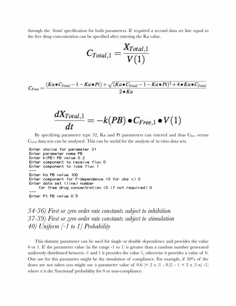
through the `from' specification for both parameters. If required a second data set line equal to the free drug concentration can be specified after entering the Ka value.

�

�

�By specifying parameter type 32, Ka and Pt parameters can entered and thus Cfree versus

Ctotal data sets can be analyzed. This can be useful for the analysis of in vitro data sets.

�

34-36) First or zero order rate constants subject to inhibition 37-39) First or zero order rate constants subject to stimulation 40) Uniform [-1 to 1] Probability

This dummy parameter can be used for single or double dependence and provides the value 0 or 1. If the parameter value (in the range -1 to 1) is greater than a random number generated uniformly distributed between -1 and 1 it provides the value 1, otherwise it provides a value of 0. One use for this parameter might be the simulation of compliance. For example, if 20% of the doses are not taken you might use a parameter value of 0.6 (= 2 x (1 - 0.2) - 1 = 2 x (1-x) -1) where x is the 'fractional' probability for 0 or non-compliance.

41) Normal [-3 to 3] Probability This dummy parameter can be used for single or double dependence and provides the value

0 or 1. If the parameter value (in the range -3 to 3) is greater than a random number, normally distributed with mean 0 and standard deviation of 1, it provides the value 1, otherwise it provides a value of 0. One use for this parameter might be the simulation of compliance. For example, if 68.3% of the doses are taken you might use a parameter value of 1 (= one standard deviation above the mean), if 95.4 use a value of 2).

42) Switch parameter Similar to parameter type 40 or 41 except change depends on the value of a specified

parameter. This parameter is set equal to 1 or 0 depending on the value of the control parameter.

43) Clone component Clone a component using this parameter. The new component will have the same numerical

value as the 'donor' component but will not influence the donor system. Uses ??

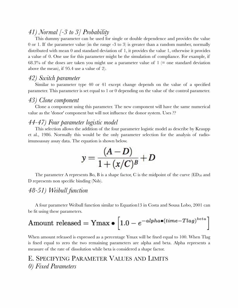
44-47) Four parameter logistic model This selection allows the addition of the four parameter logistic model as describe by Kraupp

et al., 1986. Normally this would be the only parameter selection for the analysis of radio-imunoassay assay data. The equation is shown below.

�The parameter A represents Bo, B is a shape factor, C is the midpoint of the curve (ED50 and

D represents non specific binding (Nsb).

48-51) Weibull function

A four parameter Weibull function similar to Equation13 in Costa and Sousa Lobo, 2001 can be fit using these parameters.

"

When amount released is expressed as a percentage Ymax will be fixed equal to 100. When Tlag is fixed equal to zero the two remaining parameters are alpha and beta. Alpha represents a measure of the rate of dissolution while beta is considered a shape factor.

E. SPECIFYING PARAMETER VALUES AND LIMITS 0) Fixed Parameters

If the method selected is a simulation, then all the parameters will be fixed and you won't be asked to specify fixed, adjustable, dependent, or double dependent. Alternately if a normal or bayesian fitting is to be performed some parameters can be specified as fixed. Often dose and time interrupt values will be fixed. You may wish to hold some rate constants fixed for one run and then allow them to be adjustable in a subsequent run. Enter 0 (or press return) to specify fixed parameters.

1) Adjustable parameters At least two adjustable parameters must be specified for a normal fitting problem. If 1 is

entered to specify adjustable, a lower and upper limit are requested. The fitting process will then keep the adjustable parameter values between these limits. To reduce the influence of parameter limits you could specify a very wide range between the upper and lower limit.

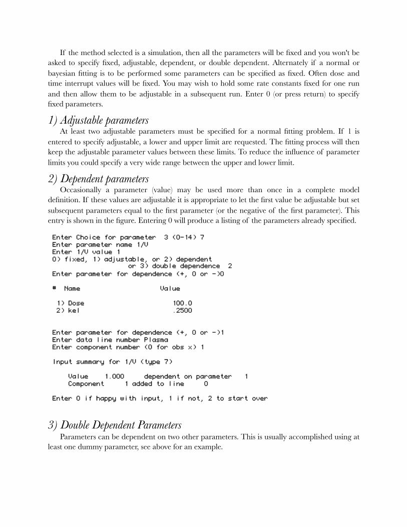
2) Dependent parameters Occasionally a parameter (value) may be used more than once in a complete model

definition. If these values are adjustable it is appropriate to let the first value be adjustable but set subsequent parameters equal to the first parameter (or the negative of the first parameter). This entry is shown in the figure. Entering 0 will produce a listing of the parameters already specified.

�

3) Double Dependent Parameters Parameters can be dependent on two other parameters. This is usually accomplished using at

least one dummy parameter, see above for an example.

After entering all the information required for each parameter the program will ask if you wish to make any changes. Entering 0 will bring up the list of parameter types on the screen for the next entry.

F. EXAMPLE MODELS - BOOMER

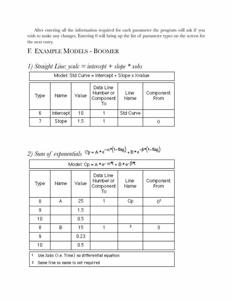
1) Straight Line: ycalc = intercept + slope * xobs

�

2) Sum of exponentials !

�

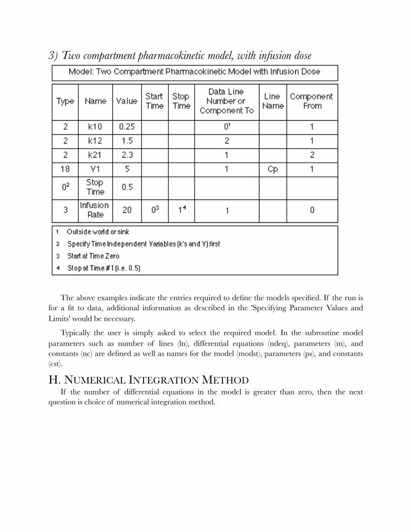
3) Two compartment pharmacokinetic model, with infusion dose

�

The above examples indicate the entries required to define the models specified. If the run is for a fit to data, additional information as described in the 'Specifying Parameter Values and Limits' would be necessary.

Typically the user is simply asked to select the required model. In the subroutine model parameters such as number of lines (ln), differential equations (ndeq), parameters (m), and constants (nc) are defined as well as names for the model (modst), parameters (ps), and constants (cst).

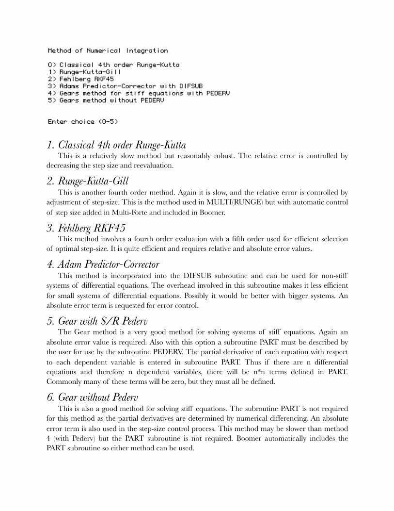
H. NUMERICAL INTEGRATION METHOD If the number of differential equations in the model is greater than zero, then the next

question is choice of numerical integration method.

�

1. Classical 4th order Runge-Kutta This is a relatively slow method but reasonably robust. The relative error is controlled by

decreasing the step size and reevaluation.

2. Runge-Kutta-Gill This is another fourth order method. Again it is slow, and the relative error is controlled by

adjustment of step-size. This is the method used in MULTI(RUNGE) but with automatic control of step size added in Multi-Forte and included in Boomer.

3. Fehlberg RKF45 This method involves a fourth order evaluation with a fifth order used for efficient selection

of optimal step-size. It is quite efficient and requires relative and absolute error values.

4. Adam Predictor-Corrector This method is incorporated into the DIFSUB subroutine and can be used for non-stiff

systems of differential equations. The overhead involved in this subroutine makes it less efficient for small systems of differential equations. Possibly it would be better with bigger systems. An absolute error term is requested for error control.

5. Gear with S/R Pederv The Gear method is a very good method for solving systems of stiff equations. Again an

absolute error value is required. Also with this option a subroutine PART must be described by the user for use by the subroutine PEDERV. The partial derivative of each equation with respect to each dependent variable is entered in subroutine PART. Thus if there are n differential equations and therefore n dependent variables, there will be n*n terms defined in PART. Commonly many of these terms will be zero, but they must all be defined.

6. Gear without Pederv This is also a good method for solving stiff equations. The subroutine PART is not required

for this method as the partial derivatives are determined by numerical differencing. An absolute error term is also used in the step-size control process. This method may be slower than method 4 (with Pederv) but the PART subroutine is not required. Boomer automatically includes the PART subroutine so either method can be used.

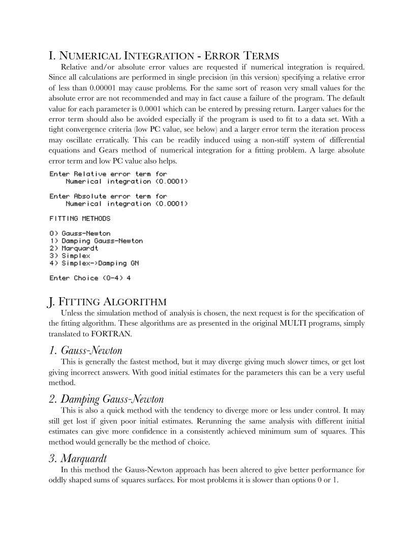
I. NUMERICAL INTEGRATION - ERROR TERMS Relative and/or absolute error values are requested if numerical integration is required.

Since all calculations are performed in single precision (in this version) specifying a relative error of less than 0.00001 may cause problems. For the same sort of reason very small values for the absolute error are not recommended and may in fact cause a failure of the program. The default value for each parameter is 0.0001 which can be entered by pressing return. Larger values for the error term should also be avoided especially if the program is used to fit to a data set. With a tight convergence criteria (low PC value, see below) and a larger error term the iteration process may oscillate erratically. This can be readily induced using a non-stiff system of differential equations and Gears method of numerical integration for a fitting problem. A large absolute error term and low PC value also helps.

�

J. FITTING ALGORITHM Unless the simulation method of analysis is chosen, the next request is for the specification of

the fitting algorithm. These algorithms are as presented in the original MULTI programs, simply translated to FORTRAN.

1. Gauss-Newton This is generally the fastest method, but it may diverge giving much slower times, or get lost

giving incorrect answers. With good initial estimates for the parameters this can be a very useful method.

2. Damping Gauss-Newton This is also a quick method with the tendency to diverge more or less under control. It may

still get lost if given poor initial estimates. Rerunning the same analysis with different initial estimates can give more confidence in a consistently achieved minimum sum of squares. This method would generally be the method of choice.

3. Marquardt In this method the Gauss-Newton approach has been altered to give better performance for

oddly shaped sums of squares surfaces. For most problems it is slower than options 0 or 1.

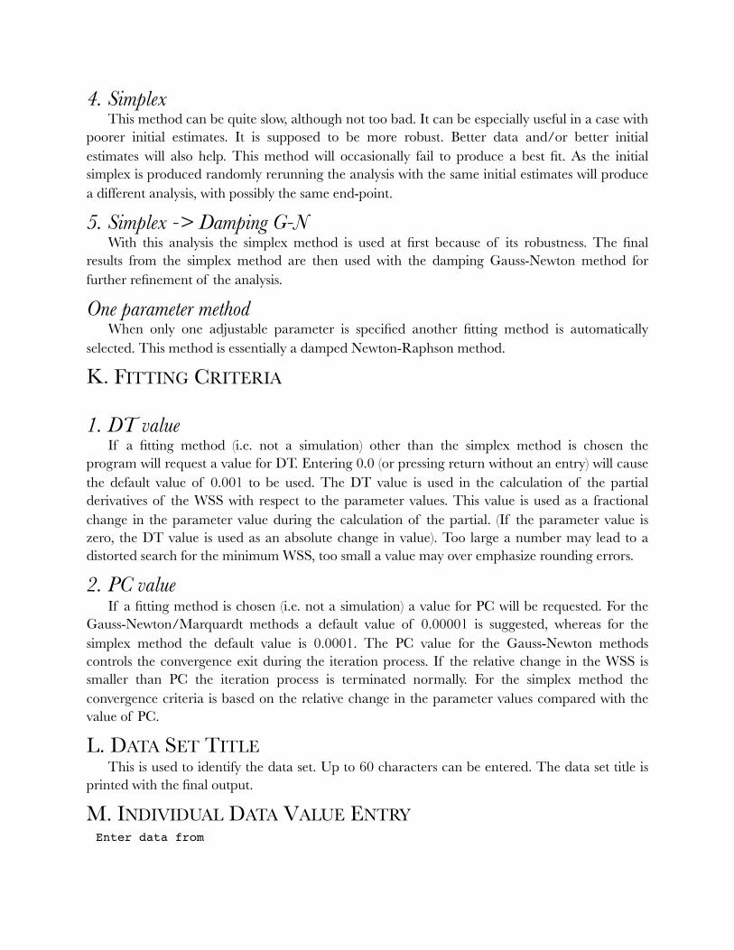
4. Simplex This method can be quite slow, although not too bad. It can be especially useful in a case with

poorer initial estimates. It is supposed to be more robust. Better data and/or better initial estimates will also help. This method will occasionally fail to produce a best fit. As the initial simplex is produced randomly rerunning the analysis with the same initial estimates will produce a different analysis, with possibly the same end-point.

5. Simplex -> Damping G-N With this analysis the simplex method is used at first because of its robustness. The final

results from the simplex method are then used with the damping Gauss-Newton method for further refinement of the analysis.

One parameter method When only one adjustable parameter is specified another fitting method is automatically

selected. This method is essentially a damped Newton-Raphson method.

K. FITTING CRITERIA

1. DT value If a fitting method (i.e. not a simulation) other than the simplex method is chosen the

program will request a value for DT. Entering 0.0 (or pressing return without an entry) will cause the default value of 0.001 to be used. The DT value is used in the calculation of the partial derivatives of the WSS with respect to the parameter values. This value is used as a fractional change in the parameter value during the calculation of the partial. (If the parameter value is zero, the DT value is used as an absolute change in value). Too large a number may lead to a distorted search for the minimum WSS, too small a value may over emphasize rounding errors.

2. PC value If a fitting method is chosen (i.e. not a simulation) a value for PC will be requested. For the

Gauss-Newton/Marquardt methods a default value of 0.00001 is suggested, whereas for the simplex method the default value is 0.0001. The PC value for the Gauss-Newton methods controls the convergence exit during the iteration process. If the relative change in the WSS is smaller than PC the iteration process is terminated normally. For the simplex method the convergence criteria is based on the relative change in the parameter values compared with the value of PC.

L. DATA SET TITLE This is used to identify the data set. Up to 60 characters can be entered. The data set title is

printed with the final output.

M. INDIVIDUAL DATA VALUE ENTRY Enter data from

0) Disk file 2) ...including weights 1) Keyboard 3) ...including weights

0) Disk File If the data has been previously entered and stored in a data file it may be read by the

program. This request is followed by a request for the .DAT filename. Again the .DAT part of the name should not be entered.

The data file format has changed from previous versions of MultiForte and Boomer. Data files now consist of two column data with a tab character between the `x' and the `y' value (and ‘weight’ if appropriate). A carriage return separates each data pair. This format is consistent with spreadsheet and graphing program formats. The current versions of Boomer will automatically read data in the older Boomer and MultiForte formats.

1) Keyboard With this option the individual time/concentration data are to be entered from the keyboard.

Entering -1 for time will end this data entry.

2-3) are the same except the user enter estimates of the weight to be applied to each data point.

This should usually be the reciprocal of the variance of the data point.

After data entry from the keyboard, or by choice after reading the data from a disk file, the data set may be viewed or edited. Editing is quite complete with options to change, delete, insert an individual data point or add an offset to the x-values of the data line. After data entry or editing the data set can be saved as a .DAT file by specifying the disk file name. Again reusing a file name will result in the loss of the older data.

N. WEIGHTING SCHEME If no weight is entered during the data entry process the program will ask for the user to

select from various formulas. The relative error in each data point may or may not be known. The user may have some information about the relative error in each measurement. This may be independent of the value or proportional to some function of the value. The fitting process can be made aware of this information by use of a weighting scheme. Boomer allows a number of different weighting schemes to be used, including specifying the weight for each data point using option 2 or 3 in the previous section.

Weighting function entry for [Drug]

0) Equal weights 1) Weight by 1/Cp(i) 2) Weight by 1/Cp(i)^2 3) Weight by 1/a*Cp(i)^b 4) Weight by 1/(a + b*Cp(i)^c) 5) Weight by 1/((a+b*Cp(i)^c)*d^(tn-ti))

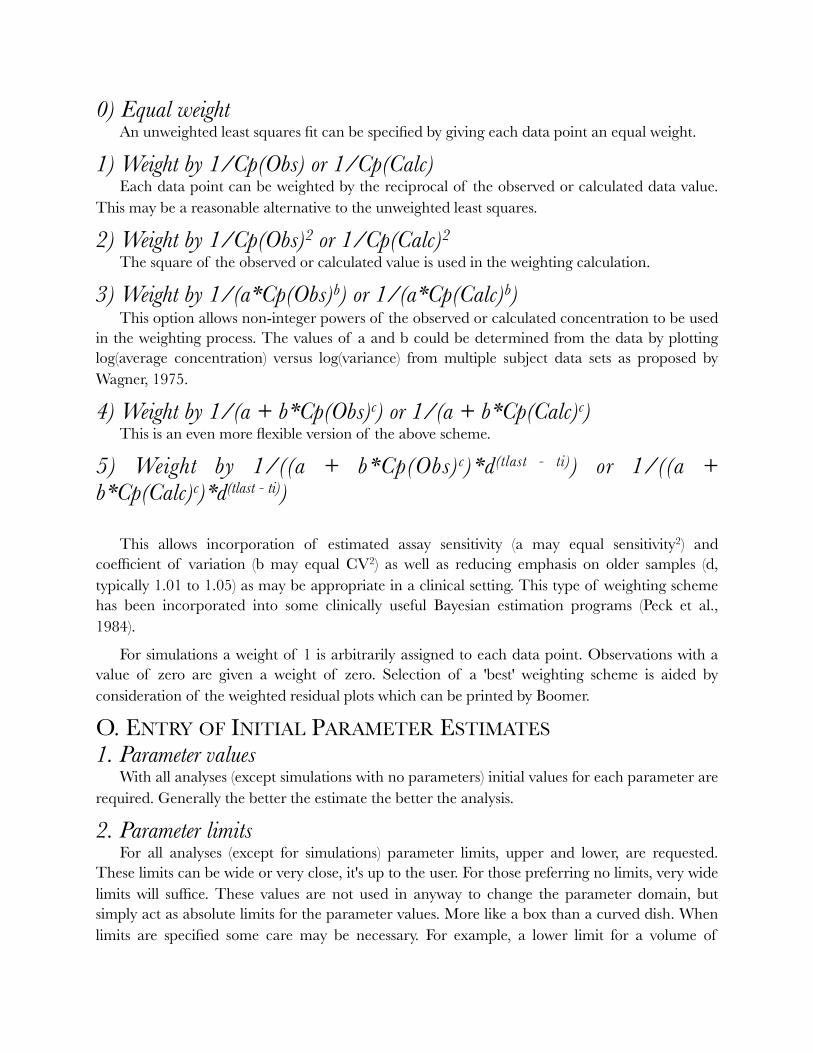
0) Equal weight An unweighted least squares fit can be specified by giving each data point an equal weight.

1) Weight by 1/Cp(Obs) or 1/Cp(Calc) Each data point can be weighted by the reciprocal of the observed or calculated data value.

This may be a reasonable alternative to the unweighted least squares.

2) Weight by 1/Cp(Obs)2 or 1/Cp(Calc)2 The square of the observed or calculated value is used in the weighting calculation.

3) Weight by 1/(a*Cp(Obs)b) or 1/(a*Cp(Calc)b) This option allows non-integer powers of the observed or calculated concentration to be used

in the weighting process. The values of a and b could be determined from the data by plotting log(average concentration) versus log(variance) from multiple subject data sets as proposed by Wagner, 1975.

4) Weight by 1/(a + b*Cp(Obs)c) or 1/(a + b*Cp(Calc)c) This is an even more flexible version of the above scheme.

5) Weight by 1/((a + b*Cp(Obs)c)*d(tlast - ti)) or 1/((a + b*Cp(Calc)c)*d(tlast - ti))

This allows incorporation of estimated assay sensitivity (a may equal sensitivity2) and coefficient of variation (b may equal CV2) as well as reducing emphasis on older samples (d, typically 1.01 to 1.05) as may be appropriate in a clinical setting. This type of weighting scheme has been incorporated into some clinically useful Bayesian estimation programs (Peck et al., 1984).

For simulations a weight of 1 is arbitrarily assigned to each data point. Observations with a value of zero are given a weight of zero. Selection of a 'best' weighting scheme is aided by consideration of the weighted residual plots which can be printed by Boomer.

O. ENTRY OF INITIAL PARAMETER ESTIMATES 1. Parameter values

With all analyses (except simulations with no parameters) initial values for each parameter are required. Generally the better the estimate the better the analysis.

2. Parameter limits For all analyses (except for simulations) parameter limits, upper and lower, are requested.

These limits can be wide or very close, it's up to the user. For those preferring no limits, very wide limits will suffice. These values are not used in anyway to change the parameter domain, but simply act as absolute limits for the parameter values. More like a box than a curved dish. When limits are specified some care may be necessary. For example, a lower limit for a volume of

distribution value entered as zero may cause problems if the limit is approached during the early part of an iterative run. A value for volume of zero will give infinite calculated plasma concentrations and can cause an early exit to the fitting. A lower limit of zero for rate constants is usually better tolerated.

3. Population values If the Bayesian estimation procedure is chosen then the user must supply estimates of the

population mean parameter value. Also required is an estimate of the uncertainty in the population value. This is entered as the population standard deviation. If a larger uncertainty is to be used a larger value for the population standard deviation would be entered.

P. SIMULATION WITH ERROR INPUT

Simulation with random ERROR

0) no error for line ( 1) 1) error = uniform error 2) error = normal error 3) error = uniform error x true value 4) error = normal error x true value 5) error = log normal error about true value 6) error = EXP(normal error)

Enter choice (0-6) 6 Enter error intensity factor

If a simulation is chosen, parameter limits etc are not required. When simulation with error is specified information about the type and magnitude of the error is requested. Uniform, normally distributed, log normal and exponentially distributed error can be specified. This error may be simply added to the calculated value (choices 1 and 2) or multiplied by and added to the calculated value (choices 3 and 4). The intensity factor refers to the magnitude of the error. With choices 1 and 2 this would be the maximum error or the standard deviation of the error added. For choices 3, 4, and 6 this is a fractional values. For example, a value of 0.1 with choice 3 would mean that the added error would have a standard deviation of 10% about the calculated value.

1) Valn = Valo + Uni x Int 2) Valn = Valo + Nor x Int 3) Valn = Valo x (1.0 + Uni x Int) 4) Valn = Valo x (1.0 + Nor x Int) 5) Valn = 10log(Valo) + Nor x Int 6) Valn = Valo x e(Nor x Int)

where

Valn = new value

Valo = original value

Int = intensity factor (standard deviation)

Uni = uniformly distributed random number between -1 and + 1

Nor = normally distributed random number with mean zero and standard deviation equal to the intensity value

Log = log normally distributed random number

Exp = exponentially distributed random number

Q. AUC, AUMC, AND MRT The program will automatically calculate the area under the curve (AUC), the area under the

first moment curve (AUMC), and the mean residence time (MRT) of any data set. For accurate numbers a zero (dummy or otherwise) data point is needed. The program uses the trapezoidal rule to calculate the areas. The program uses the last two calculated data points to calculate a terminal slope for extrapolation to zero. Calculated zero time values are used is an observed zero time value is zero. If no zero time value is given a warning is issued. Zero time values with zero value are given zero weight in any fitting analysis. Enter 0 to exit this section.

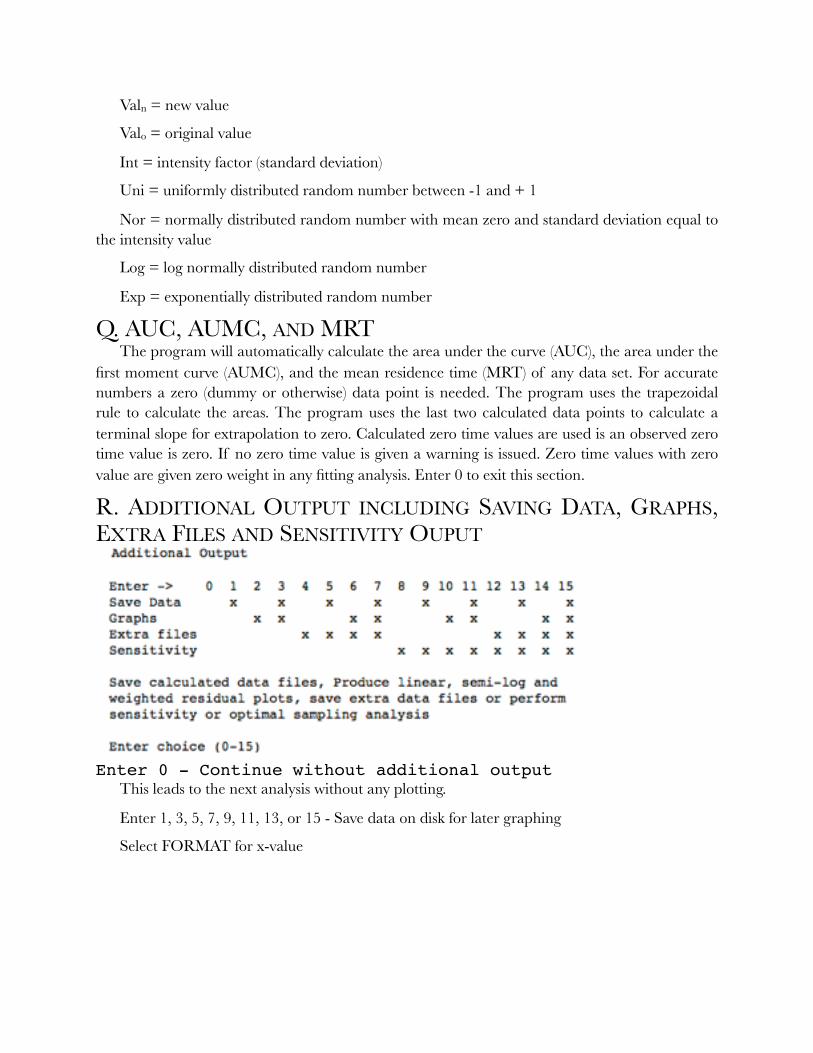
R. ADDITIONAL OUTPUT INCLUDING SAVING DATA, GRAPHS, EXTRA FILES AND SENSITIVITY OUPUT

!Enter 0 - Continue without additional output

This leads to the next analysis without any plotting.

Enter 1, 3, 5, 7, 9, 11, 13, or 15 - Save data on disk for later graphing

Select FORMAT for x-value

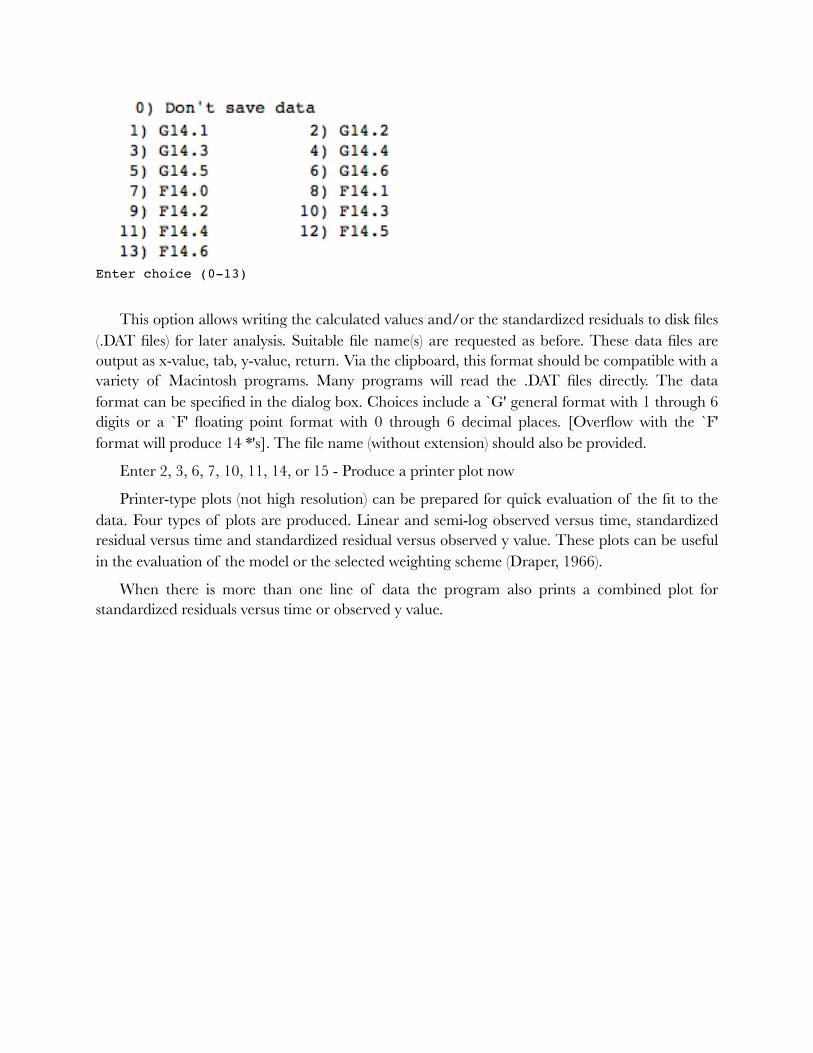
!Enter choice (0-13)

This option allows writing the calculated values and/or the standardized residuals to disk files (.DAT files) for later analysis. Suitable file name(s) are requested as before. These data files are output as x-value, tab, y-value, return. Via the clipboard, this format should be compatible with a variety of Macintosh programs. Many programs will read the .DAT files directly. The data format can be specified in the dialog box. Choices include a `G' general format with 1 through 6 digits or a `F' floating point format with 0 through 6 decimal places. [Overflow with the `F' format will produce 14 *'s]. The file name (without extension) should also be provided.

Enter 2, 3, 6, 7, 10, 11, 14, or 15 - Produce a printer plot now

Printer-type plots (not high resolution) can be prepared for quick evaluation of the fit to the data. Four types of plots are produced. Linear and semi-log observed versus time, standardized residual versus time and standardized residual versus observed y value. These plots can be useful in the evaluation of the model or the selected weighting scheme (Draper, 1966).

When there is more than one line of data the program also prints a combined plot for standardized residuals versus time or observed y value.

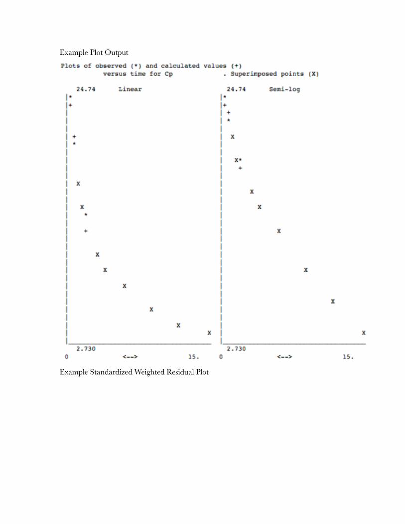
Example Plot Output

"

Example Standardized Weighted Residual Plot

!

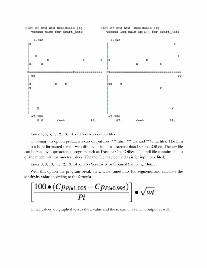
Enter 4, 5, 6, 7, 12, 13, 14, or 15 - Extra output files

Choosing this option produces extra output files. ***.htm, ***.csv and ***.mdl files. The htm file is a html formatted file for web display or input as external data by OpenOffice. The csv file can be read by a spreadsheet program such as Excel or OpenOffice. The mdl file contains details of the model with parameter values. The mdl file may be used as is for input or edited.

Enter 8, 9, 10, 11, 12, 13, 14, or 15 - Sensitivity or Optimal Sampling Output

With this option the program break the x scale (time) into 100 segments and calculate the sensitivity value according to the formula.

"

These values are graphed versus the x value and the maximum value is output as well.

"

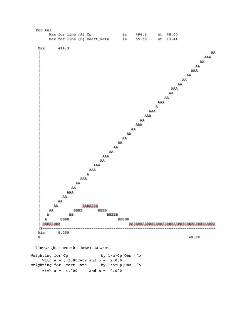
The weight scheme for these data were:

Weighting for Cp by 1/a*Cp(Obs )^b With a = 0.2500E-02 and b = 2.000 Weighting for Heart_Rate by 1/a*Cp(Obs )^b

With a = 4.000 and b = 0.000

Three Dimensional WSS Output Table

If the grid search method is chosen the program may output the WSS at each point on the specified grid with the parameter values to two disk files per pair of parameters. One disk file is in SYLK format for entry into the DeltaGraph(c) graphing program. The other file is in tab-return delimited format for entry into spreadsheets etc. With this output WSS surface plots can be generated.

S. NOTES

1. Batch Files Creating a batch file on the run could be useful if you have a large number of data sets

requiring similar analyses. Alternately, a single data set may be analyzed by different weighting schemes. You could enter the first set of information from the keyboard, creating a batch file as you go. The batch file could then be edited and the section containing data repeatedly duplicated using the copy and paste commands. An entry of -1 is used to terminate the data entry. This will need to be changed to 0 at the end of each set except the last. (This final -1 must be followed by a carriage return or it will not be properly recognized.) When editing the batch file, be sure to change data file names and initial estimates for parameter values. Do not change the integer or real number description starting in column 40.

References

Abramowitz, M and Stegun, I.A. 1964. Handbook of Mathematical Functions with Formulas, Graphs, and Mathematical Tables, Applied Mathematics Series 55, National Bureau of Standards, 953

Bevill, R.F., Koritz, G.D., Rudawsky, G., Dittert, L.W., Huang, C.H., Hayashi, M., and Bourne, D.W.A. 1982 Disposition of Sulfadimethoxine in Swine: Inclusion of Protein Binding Factors in a Pharmacokinetic Model, J. Pharmacokin. Biopharm., 10, 539-550

Bourne, D.W.A., Bialer, M., Dittert, L.W., Hayashi, M., Rudawsky, G., Koritz, G.D., and Bevill, R.F. 1981 Disposition of Sulfadimethoxine in Cattle: Inclusion of Protein Binding Factors in a Pharmacokinetic Model, J. Pharm.Sci., 70, 1068-1072

Costa, P., and Sousa Lobo, J.M. 2001 Modeling and comparison of dissolution profiles. Eur. J. Pharm. Sci. 13 (2) 123-33

Draper, N.R. and Smith, H. 1966 Applied Regression Analysis. Wiley, New York, NY pp 86-100

Duddy, J., Hayden, T.L., Bourne, D.W.A., Fiske, W.D., Benedek, I.H., Stanley, D., Gonzalez, A., and Heierman, W. 1984 Physiological Model for Distribution of Sulfathiazole in Swine, J. Pharm. Sci., 73, 1525-1528

Hill, A.V. 1910 The possible effects of the aggregation of the molecules of haemoglobin on its dissociation curves. J. Physiol., 40 iv-vii

Kraupp, M., Marz, R., Legenstein, E., Knerer and Szekeres, T. 1986 Evaluation of Radioimmunoassay Calculations by Four Parameter Logistic and Spline functions, J. Clin. Chem. Clin. biochem., 24, 1023-1028

Michaelis, L. and Menten, M.L. 1913 Die Kinetik der Invertinwirkung, Biochem. Z., 49, 333

Peck, C.C., Beal, S.L., Sheiner, L.B., and Nichols, A.I. 1984 Extended Least Squares Nonlinear Regression: A possible solution to the "Choice of Weights" problem in analysis of individual pharmacokinetic data. J. Pharmacokin. Biopharm., 12, 545-558

Peck, C.C., Sheiner, L.B., and Nichols, A.I. 1984 The problem of choosing weights in nonlinear regression analysis of pharmacokinetic data. Drug Metab. Rev., 15, 133-148

Portmann, G.A. 1970 "Pharmacokinetics," Chapter 1 in Current Concepts in the Pharmaceutical Sciences - Biopharmaceutics, Swarbrick, J. ed., Lea & Febiger, Philadelphia, PA p 37

Rubinow, S.I. 1975 Introduction to Mathematical Biology. Wiley, New York, NY, p 65

Wagner, J.G. 1975 Fundamentals of Clinical Pharmacokinetics. Drug Intelligence Publications, Hamilton, IL p 289

Chapter 5

5. Output Information Boomer can output the final results to the terminal screen or a disk file (.OUT file).

Intermediate results may also be output to the terminal screen. [Be careful, command-C or command-. will cause an exit from the program]. The output is headed by the version number and the system date and time. The title, fitting algorithm, weighting information, DT (if appropriate), PC, number of iteration loops, and damping (if appropriate) are printed next. For simulations, the elapsed time is displayed for comparison purposes.

The next section displays the final parameter values. The number, name, final fitted value, standard deviation (SD), percent coefficient of variation (CV), inputted lower limit and upper limit are displayed for each parameter. A warning is given if any of the parameter values are within 5% of the upper or lower limit.. A coefficient of variation of greater than 50% can indicate that the model selected has too many parameters, or that the data are insufficient or too 'noisy'. The SD or CV information is more an indication of how good the fit is or how noisy the data appears and does not give much information about the population statistics of the parameters.

If a Bayesian analysis was selected the population mean and standard deviation inputted, the square root of the weight for the parameter (1/standard deviation), and the weighted residual are printed. The weighted residual is calculated as (parameter value-population mean value) times the square root of the weight. Thus the weighted residual squared is the contribution of this parameter to the overall WSS.

The model fit can be evaluated in part by looking at the next output. The sum of the weighted squared residuals (WSS), the unweighted coefficient of determination (R2), and the unweighted correlation coefficient (R) between the observed and calculated y-values. The mean error (ME), mean absolute error (MAE) and root mean squared error (RMSE) are useful parameters for determining how useful the model might be at predicting future results. Akaike's information criterion (AIC), Schwarz criteria (SC), and log likehood (LL) are useful criteria for determining which model is best (Note always use the same weighting scheme when making this determination.

AIC = N • ln (WSS) + 2 • MSC = N • ln (WSS) + M • ln(N)LL = -N/2 • [ln (2 • π) + ln (WSS/N) + 1] (from http://www.xycoon.com/)

where N = number of data points (weighted); WSS = the weighted sum of squares; and M = the number of adjustable parameters.

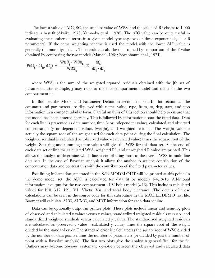
The lowest value of AIC, SC, the smallest value of WSS, and the value of R2 closest to 1.000 indicate a best fit (Akaike, 1973; Yamaoka et al., 1978). The AIC value can be quite useful in evaluating the number of terms in a given model type (e.g. two or three exponentials, 4 or 6 parameters). If the same weighting scheme is used the model with the lower AIC value is generally the more significant. This result can also be determined by comparison of the F value obtained by comparing the two models (Mandel, 1964; Boxenbaum et al., 1974).

�

where WSSj is the sum of the weighted squared residuals obtained with the jth set of parameters. For example, j may refer to the one compartment model and the k to the two compartment fit.

In Boomer, the Model and Parameter Definition section is next. In this section all the constants and parameters are displayed with name, value, type, from, to, dep, start, and stop information in a compact tabular form. Careful analysis of this section should help to ensure that the model has been entered correctly. This is followed by information about the fitted data. Data for each line is presented as data number, time (x or independent value), calculated and observed concentration (y or dependent value), (weight), and weighted residual. The weight value is actually the square root of the weight used for each data point during the final calculation. The weighted residual is calculated as (observed value - calculated value) times the square root of the weight. Squaring and summing these values will give the WSS for this data set. At the end of each data set or line the calculated WSS, weighted R2, and unweighted R value are printed. This allows the analyst to determine which line is contributing most to the overall WSS in multi-line data sets. In the case of Bayesian analysis it allows the analyst to see the contribution of the concentration data and contrast this with the contribution of the fitted parameter values.

Post fitting information generated in the S/R MODELOUT will be printed at this point. In the demo model set, the AUC is calculated for data fit by models 1-4,13-16. Additional information is output for the two compartment - I.V. bolus model (#13). This includes calculated values for k10, k12, k21, V1, Vbeta, Vss, and total body clearance. The details of these calculations can be seen in the source code for this subroutine in the MODEL.DEMO text file. Boomer will calculate AUC, AUMC, and MRT information for each data set line.

Data can be optionally output in printer plots. These plots include linear and semi-log plots of observed and calculated y values versus x values, standardized weighted residuals versus x, and standardized weighted residuals versus calculated y values. The standardized weighted residuals are calculated as (observed y value - calculated y value) times the square root of the weight divided by the standard error. The standard error is calculated as the square root of WSS divided by the number of data points minus the number of parameters (or divided by just the number of point with a Bayesian analysis). The first two plots give the analyst a general 'feel' for the fit. Outliers may become obvious, systematic deviation between the observed and calculated data

points may be obvious. The two residual plot can be very useful in the evaluation of the weighting scheme selected or the model selected. Non-random residuals may well mean a poor weighting scheme or a model with insufficient parameters (Draper and Smith, 1966).

Again, all of the above output can be directed to a disk file for inclusion, as a text file, into a report etc. Calculated values versus time or the standardized residuals versus time data can be saved as disk files for later enhancement with a plotting program such as DeltaGraph® (Mac graphing program). The data is saved as a text file with x and y values separated by a tab and each data pair separated with a carriage return.

Reference

Akaike, H. 1973 A new look at the statistical model identification, IEEE Trans. Automat. Control., 19, 716-723

Boxenbaum, H.G., Riegelman, S., and Elashoff, R.M. 1974 Statistical Estimation in Pharmacokinetics. J. Pharmacokin. Biopharm., 2, 123-148

Draper, N.R. and Smith, H. 1966 Applied Regression Analysis. Wiley, New York, NY pp 86-100

Mandel, J. 1964 The Statistical Analysis of Experimental Data, Interscience, New York, p 164

Yamaoka, K., Nakagawa, T., and Uno, T. 1978 Application of Akaike's information criterion (AIC) in the evaluation of linear pharmacokinetic equations. J. Pharmacokin. Biopharm., 6, 165-175

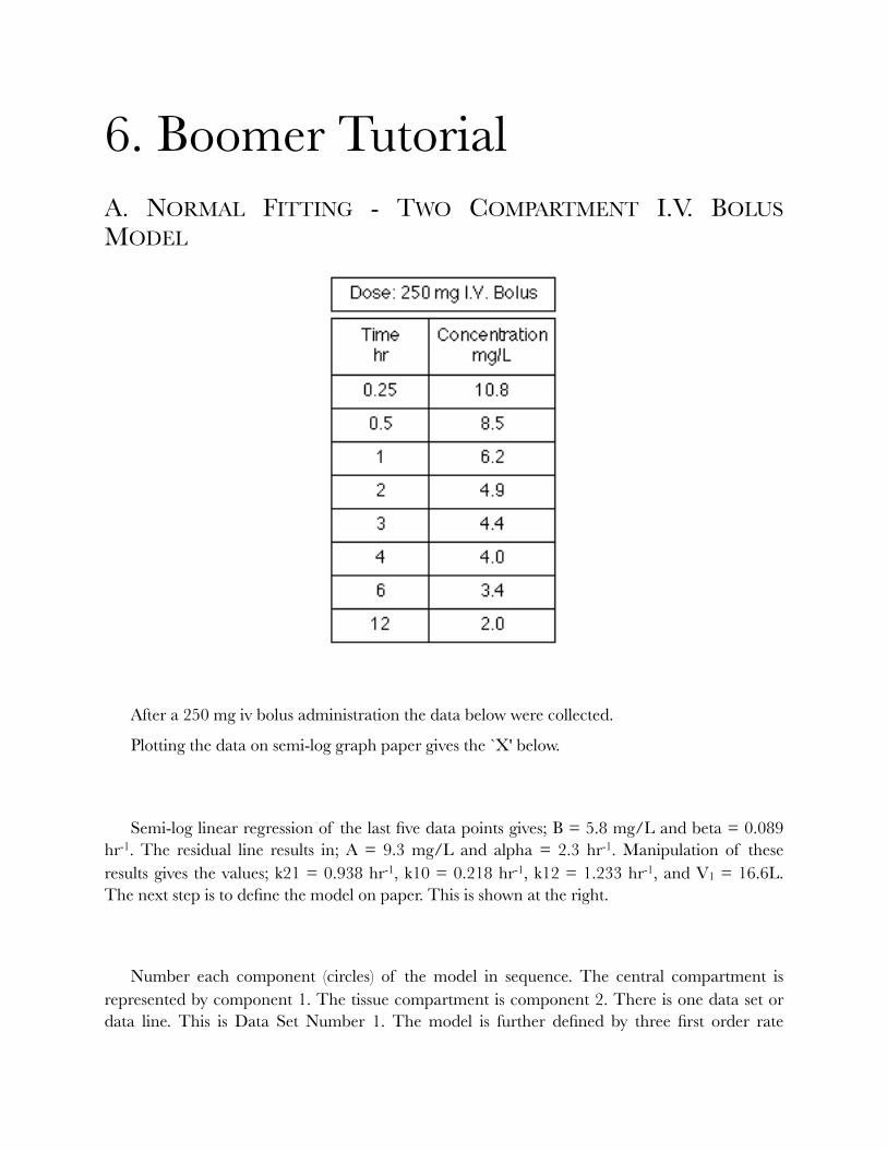
6. Boomer Tutorial A. NORMAL FITTING - TWO COMPARTMENT I.V. BOLUS MODEL

After a 250 mg iv bolus administration the data below were collected.

Plotting the data on semi-log graph paper gives the `X' below.

Semi-log linear regression of the last five data points gives; B = 5.8 mg/L and beta = 0.089 hr-1. The residual line results in; A = 9.3 mg/L and alpha = 2.3 hr-1. Manipulation of these results gives the values; k21 = 0.938 hr-1, k10 = 0.218 hr-1, k12 = 1.233 hr-1, and V1 = 16.6L. The next step is to define the model on paper. This is shown at the right.

Number each component (circles) of the model in sequence. The central compartment is represented by component 1. The tissue compartment is component 2. There is one data set or data line. This is Data Set Number 1. The model is further defined by three first order rate

constants (arrows) and one apparent volume of distribution (triangle). The apparent volume of distribution relates the amount of drug in the central compartment to the plasma concentrations in the data set. Including the dose there are five parameters needed to fully define the model. These are summarized in the table, below.

Start Boomer and select Keyboard entry. Select normal fitting (0), screen output (0) and proceed to parameter definition and entry. Enter each of the parameters from the table below. Enter -1 for parameter type to complete this section. Choose Runge-Kutta-Fehlberg (2) as the numerical integration technique and press return twice to accept the default values for relative and absolute error. Choose Damping Gauss-Newton (1) as the fitting algorithm and again press return twice to accept the default values of DT and PC. Enter a title for this run `Two

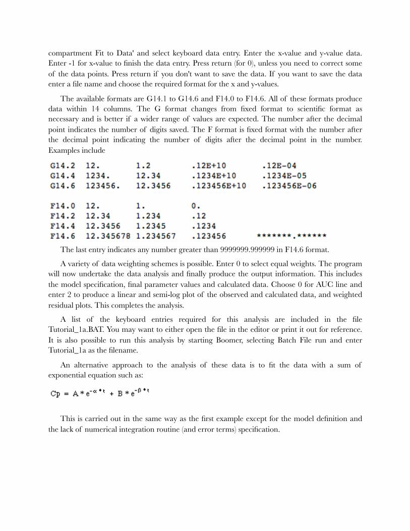
compartment Fit to Data' and select keyboard data entry. Enter the x-value and y-value data. Enter -1 for x-value to finish the data entry. Press return (for 0), unless you need to correct some of the data points. Press return if you don't want to save the data. If you want to save the data enter a file name and choose the required format for the x and y-values.

The available formats are G14.1 to G14.6 and F14.0 to F14.6. All of these formats produce data within 14 columns. The G format changes from fixed format to scientific format as necessary and is better if a wider range of values are expected. The number after the decimal point indicates the number of digits saved. The F format is fixed format with the number after the decimal point indicating the number of digits after the decimal point in the number. Examples include

!The last entry indicates any number greater than 9999999.999999 in F14.6 format.

A variety of data weighting schemes is possible. Enter 0 to select equal weights. The program will now undertake the data analysis and finally produce the output information. This includes the model specification, final parameter values and calculated data. Choose 0 for AUC line and enter 2 to produce a linear and semi-log plot of the observed and calculated data, and weighted residual plots. This completes the analysis.

A list of the keyboard entries required for this analysis are included in the file Tutorial_1a.BAT. You may want to either open the file in the editor or print it out for reference. It is also possible to run this analysis by starting Boomer, selecting Batch File run and enter Tutorial_1a as the filename.

An alternative approach to the analysis of these data is to fit the data with a sum of exponential equation such as:

�

This is carried out in the same way as the first example except for the model definition and the lack of numerical integration routine (and error terms) specification.

B. BAYESIAN ANALYSIS - I.V. INFUSION WITH KEL FUNCTION OF CREATININE CLEARANCE

This example set involves the analysis of plasma concentrations measured after an i.v. infusion of 200 mg/hr for 30 minutes to a patient with a creatinine clearance of 30 ml/min. The measured concentrations were:

Plasma concentration 1 hour after the start of the infusion = 4.0 mg/L Plasma concentration 12 hours after the start of the infusion = 1.7 mg/L

From previous experiments with this drug in similar patients it has been found that:

kel = a * CL(Cr) + b

 

where a = 0.0028 +/- 0.00028 b = 0.02 +/- 0.002and V(1) = 21 +/- 2.1 L

We can set up the model first on paper.

Component 1 represents the one compartment model with a first order elimination rate constant k10. Linking the amount of drug in component 1 with the concentration in data set 1 is

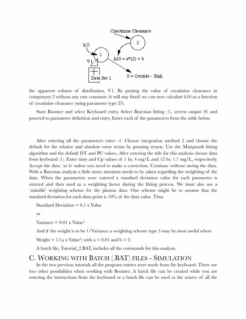
the apparent volume of distribution, V1. By putting the value of creatinine clearance in component 2 without any rate constants (it will stay fixed) we can now calculate k10 as a function of creatinine clearance (using parameter type 23).

Start Boomer and select Keyboard entry. Select Bayesian fitting (1), screen output (0) and proceed to parameter definition and entry. Enter each of the parameters from the table below.

After entering all the parameters enter -1. Choose integration method 2 and choose the default for the relative and absolute error terms by pressing return. Use the Marquardt fitting algorithm and the default DT and PC values. After entering the title for this analysis choose data from keyboard (1). Enter time and Cp values of 1 hr, 4 mg/L and 12 hr, 1.7 mg/L, respectively. Accept the data `as is' unless you need to make a correction. Continue without saving the data. With a Bayesian analysis a little more attention needs to be taken regarding the weighting of the data. When the parameters were entered a standard deviation value for each parameter is entered and then used as a weighting factor during the fitting process. We must also use a `suitable' weighting scheme for the plasma data. One scheme might be to assume that the standard deviation for each data point is 10% of the data value. Thus

Standard Deviation = 0.1 x Value

or

Variance = 0.01 x Value2

And if the weight is to be 1/Variance a weighting scheme type 3 may be most useful where

Weight = 1/(a x Value2) with a = 0.01 and b = 2.

A batch file, Tutorial_2.BAT, includes all the commands for this analysis.

C. WORKING WITH BATCH (.BAT) FILES - SIMULATION In the two previous tutorials all the program entries were made from the keyboard. There are

two other possibilities when working with Boomer. A batch file can be created while you are entering the instructions from the keyboard or a batch file can be used as the source of all the

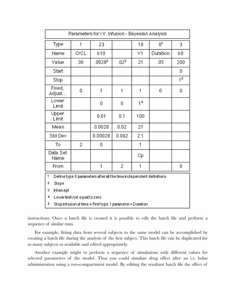
instructions. Once a batch file is created it is possible to edit the batch file and perform a sequence of similar runs.

For example, fitting data from several subjects to the same model can be accomplished by creating a batch file during the analysis of the first subject. This batch file can be duplicated for as many subjects as available and edited appropriately.

Another example might to perform a sequence of simulations with different values for selected parameters of the model. Thus you could simulate drug effect after an i.v. bolus administration using a two-compartment model. By editing the resultant batch file the effect of

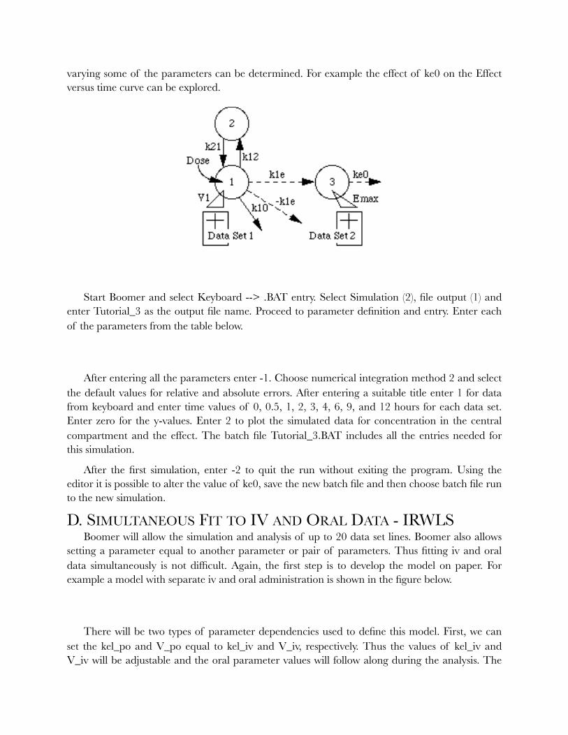
varying some of the parameters can be determined. For example the effect of ke0 on the Effect versus time curve can be explored.

Start Boomer and select Keyboard --> .BAT entry. Select Simulation (2), file output (1) and enter Tutorial_3 as the output file name. Proceed to parameter definition and entry. Enter each of the parameters from the table below.

After entering all the parameters enter -1. Choose numerical integration method 2 and select the default values for relative and absolute errors. After entering a suitable title enter 1 for data from keyboard and enter time values of 0, 0.5, 1, 2, 3, 4, 6, 9, and 12 hours for each data set. Enter zero for the y-values. Enter 2 to plot the simulated data for concentration in the central compartment and the effect. The batch file Tutorial_3.BAT includes all the entries needed for this simulation.

After the first simulation, enter -2 to quit the run without exiting the program. Using the editor it is possible to alter the value of ke0, save the new batch file and then choose batch file run to the new simulation.

D. SIMULTANEOUS FIT TO IV AND ORAL DATA - IRWLS Boomer will allow the simulation and analysis of up to 20 data set lines. Boomer also allows

setting a parameter equal to another parameter or pair of parameters. Thus fitting iv and oral data simultaneously is not difficult. Again, the first step is to develop the model on paper. For example a model with separate iv and oral administration is shown in the figure below.

There will be two types of parameter dependencies used to define this model. First, we can set the kel_po and V_po equal to kel_iv and V_iv, respectively. Thus the values of kel_iv and V_iv will be adjustable and the oral parameter values will follow along during the analysis. The

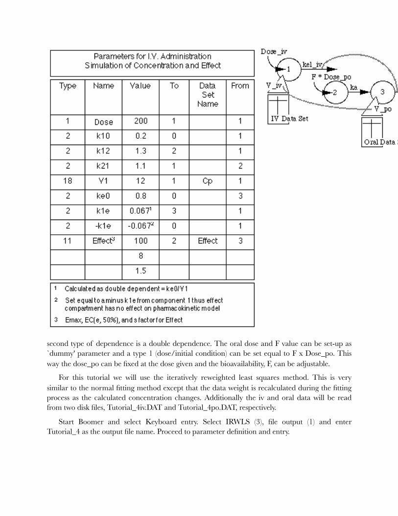
second type of dependence is a double dependence. The oral dose and F value can be set-up as `dummy' parameter and a type 1 (dose/initial condition) can be set equal to F x Dose_po. This way the dose_po can be fixed at the dose given and the bioavailability, F, can be adjustable.

For this tutorial we will use the iteratively reweighted least squares method. This is very similar to the normal fitting method except that the data weight is recalculated during the fitting process as the calculated concentration changes. Additionally the iv and oral data will be read from two disk files, Tutorial_4iv.DAT and Tutorial_4po.DAT, respectively.

Start Boomer and select Keyboard entry. Select IRWLS (3), file output (1) and enter Tutorial_4 as the output file name. Proceed to parameter definition and entry.

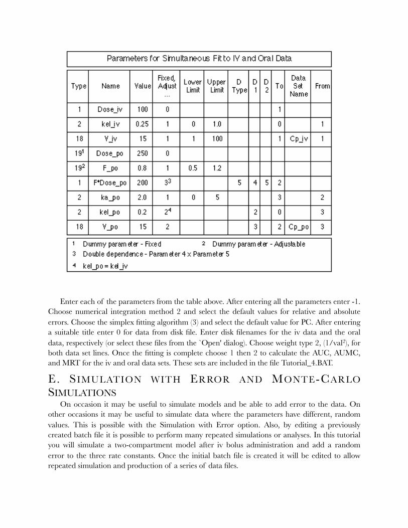
Enter each of the parameters from the table above. After entering all the parameters enter -1. Choose numerical integration method 2 and select the default values for relative and absolute errors. Choose the simplex fitting algorithm (3) and select the default value for PC. After entering a suitable title enter 0 for data from disk file. Enter disk filenames for the iv data and the oral data, respectively (or select these files from the `Open' dialog). Choose weight type 2, (1/val2), for both data set lines. Once the fitting is complete choose 1 then 2 to calculate the AUC, AUMC, and MRT for the iv and oral data sets. These sets are included in the file Tutorial_4.BAT.

E. SIMULATION WITH ERROR AND MONTE-CARLO SIMULATIONS

On occasion it may be useful to simulate models and be able to add error to the data. On other occasions it may be useful to simulate data where the parameters have different, random values. This is possible with the Simulation with Error option. Also, by editing a previously created batch file it is possible to perform many repeated simulations or analyses. In this tutorial you will simulate a two-compartment model after iv bolus administration and add a random error to the three rate constants. Once the initial batch file is created it will be edited to allow repeated simulation and production of a series of data files.

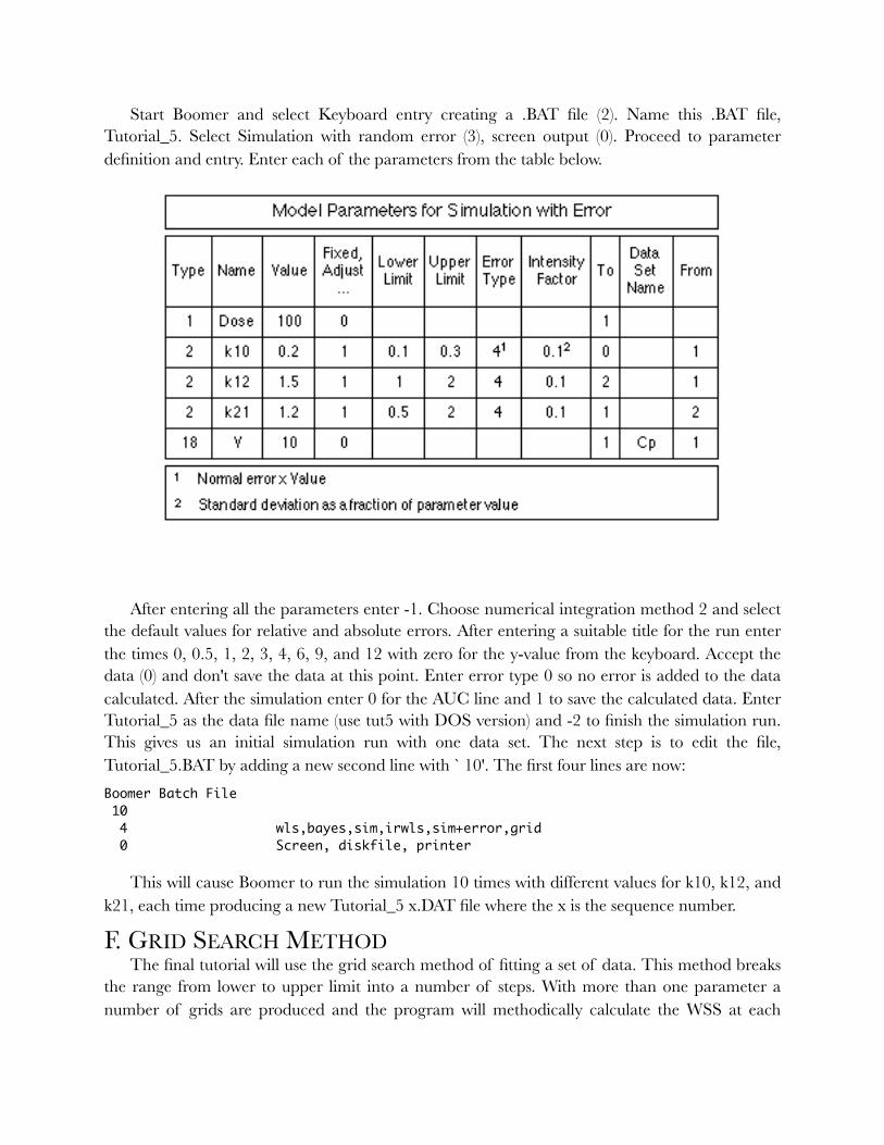
Start Boomer and select Keyboard entry creating a .BAT file (2). Name this .BAT file, Tutorial_5. Select Simulation with random error (3), screen output (0). Proceed to parameter definition and entry. Enter each of the parameters from the table below.

After entering all the parameters enter -1. Choose numerical integration method 2 and select the default values for relative and absolute errors. After entering a suitable title for the run enter the times 0, 0.5, 1, 2, 3, 4, 6, 9, and 12 with zero for the y-value from the keyboard. Accept the data (0) and don't save the data at this point. Enter error type 0 so no error is added to the data calculated. After the simulation enter 0 for the AUC line and 1 to save the calculated data. Enter Tutorial_5 as the data file name (use tut5 with DOS version) and -2 to finish the simulation run. This gives us an initial simulation run with one data set. The next step is to edit the file, Tutorial_5.BAT by adding a new second line with ` 10'. The first four lines are now: Boomer Batch File 10 4 wls,bayes,sim,irwls,sim+error,grid 0 Screen, diskfile, printer

This will cause Boomer to run the simulation 10 times with different values for k10, k12, and k21, each time producing a new Tutorial_5 x.DAT file where the x is the sequence number.

F. GRID SEARCH METHOD The final tutorial will use the grid search method of fitting a set of data. This method breaks

the range from lower to upper limit into a number of steps. With more than one parameter a number of grids are produced and the program will methodically calculate the WSS at each

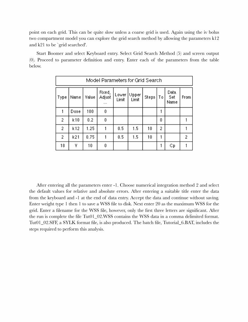
point on each grid. This can be quite slow unless a coarse grid is used. Again using the iv bolus two compartment model you can explore the grid search method by allowing the parameters k12 and k21 to be `grid searched'.

Start Boomer and select Keyboard entry. Select Grid Search Method (5) and screen output (0). Proceed to parameter definition and entry. Enter each of the parameters from the table below.

After entering all the parameters enter -1. Choose numerical integration method 2 and select the default values for relative and absolute errors. After entering a suitable title enter the data from the keyboard and -1 at the end of data entry. Accept the data and continue without saving. Enter weight type 1 then 1 to save a WSS file to disk. Next enter 20 as the maximum WSS for the grid. Enter a filename for the WSS file, however, only the first three letters are significant. After the run is complete the file Tut01_02.WSS contains the WSS data in a comma delimited format. Tut01_02.SFF, a SYLK format file, is also produced. The batch file, Tutorial_6.BAT, includes the steps required to perform this analysis.

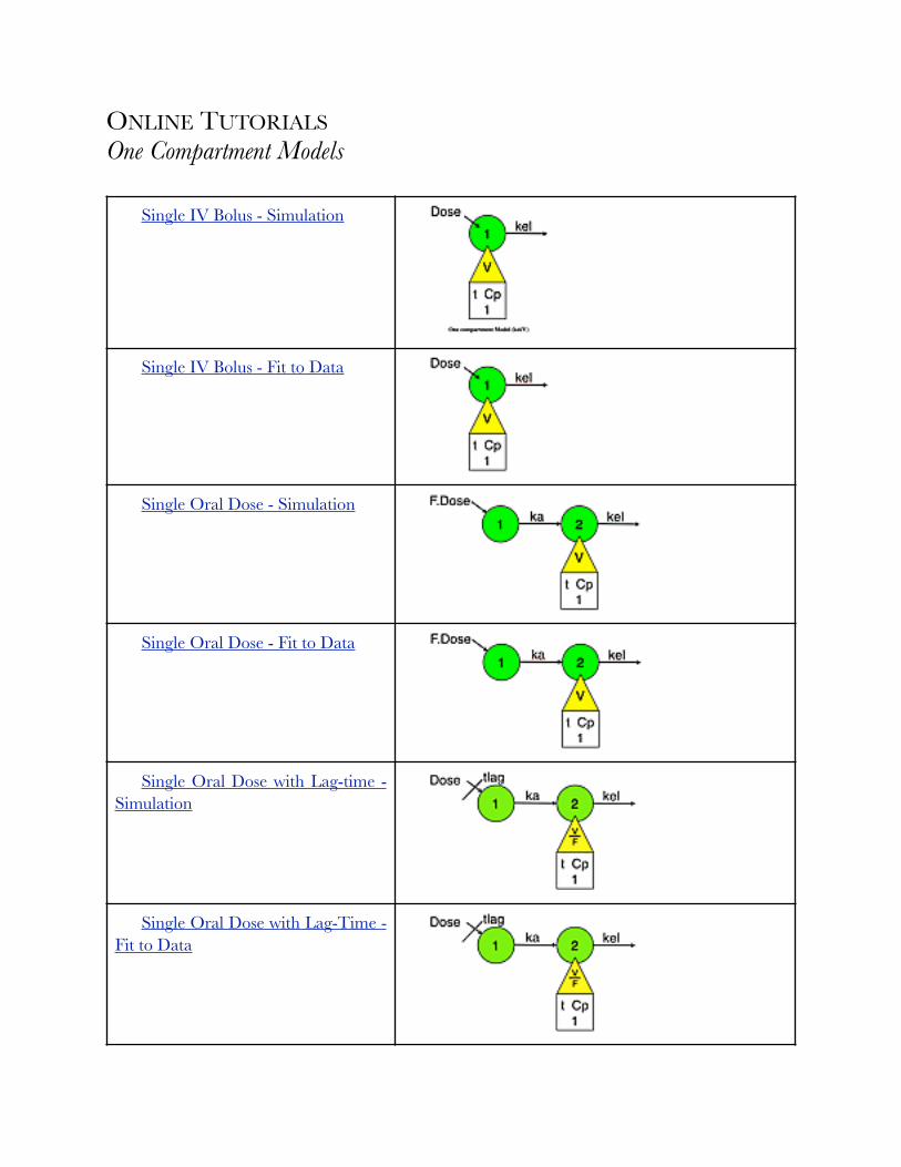
ONLINE TUTORIALS One Compartment Models

Single IV Bolus - Simulation

Single IV Bolus - Fit to Data

Single Oral Dose - Simulation

Single Oral Dose - Fit to Data

Single Oral Dose with Lag-time - Simulation

Single Oral Dose with Lag-Time - Fit to Data

"

"

"

"

"

"

Sing le Oral Dose - Three Absorption Sites - Simulation

Sing le Oral Dose - Three Absorption Sites with Lag-Times - Simulation

S i n g l e O r a l D o s e - Fo u r Absorption Sites with Lag-Times - Simulation

S i n g l e O r a l D o s e - F i v e Absorption Sites with Lag-Times - Simulation

"

"

"

"

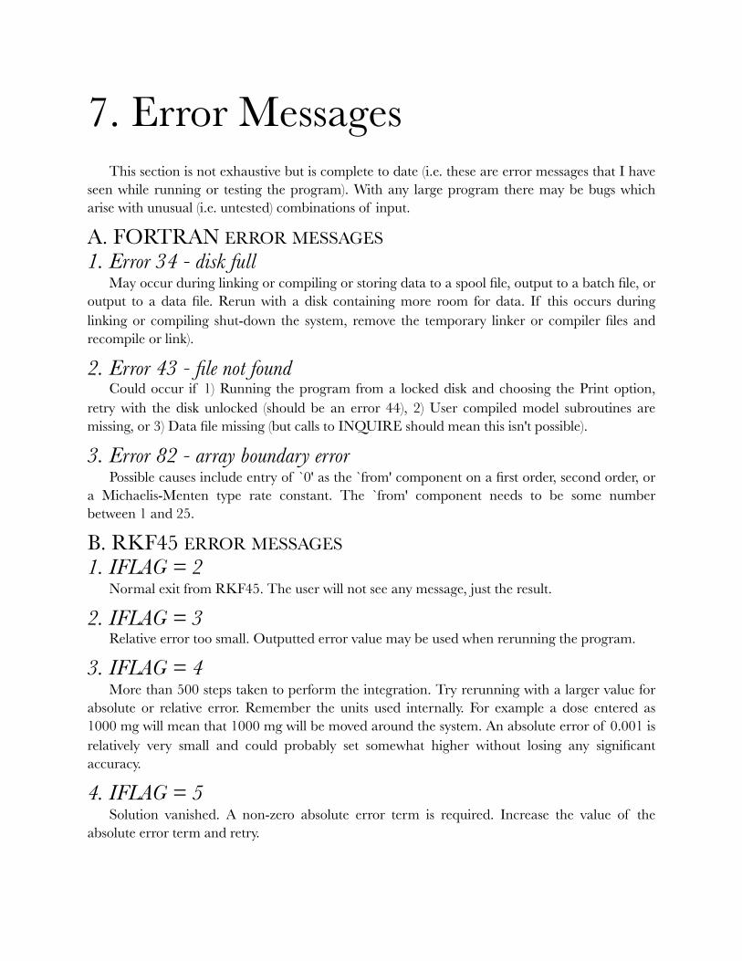
7. Error Messages This section is not exhaustive but is complete to date (i.e. these are error messages that I have

seen while running or testing the program). With any large program there may be bugs which arise with unusual (i.e. untested) combinations of input.

A. FORTRAN ERROR MESSAGES 1. Error 34 - disk full

May occur during linking or compiling or storing data to a spool file, output to a batch file, or output to a data file. Rerun with a disk containing more room for data. If this occurs during linking or compiling shut-down the system, remove the temporary linker or compiler files and recompile or link).

2. Error 43 - file not found Could occur if 1) Running the program from a locked disk and choosing the Print option,

retry with the disk unlocked (should be an error 44), 2) User compiled model subroutines are missing, or 3) Data file missing (but calls to INQUIRE should mean this isn't possible).

3. Error 82 - array boundary error Possible causes include entry of `0' as the `from' component on a first order, second order, or

a Michaelis-Menten type rate constant. The `from' component needs to be some number between 1 and 25.

B. RKF45 ERROR MESSAGES 1. IFLAG = 2

Normal exit from RKF45. The user will not see any message, just the result.

2. IFLAG = 3 Relative error too small. Outputted error value may be used when rerunning the program.

3. IFLAG = 4 More than 500 steps taken to perform the integration. Try rerunning with a larger value for

absolute or relative error. Remember the units used internally. For example a dose entered as 1000 mg will mean that 1000 mg will be moved around the system. An absolute error of 0.001 is relatively very small and could probably set somewhat higher without losing any significant accuracy.

4. IFLAG = 5 Solution vanished. A non-zero absolute error term is required. Increase the value of the

absolute error term and retry.

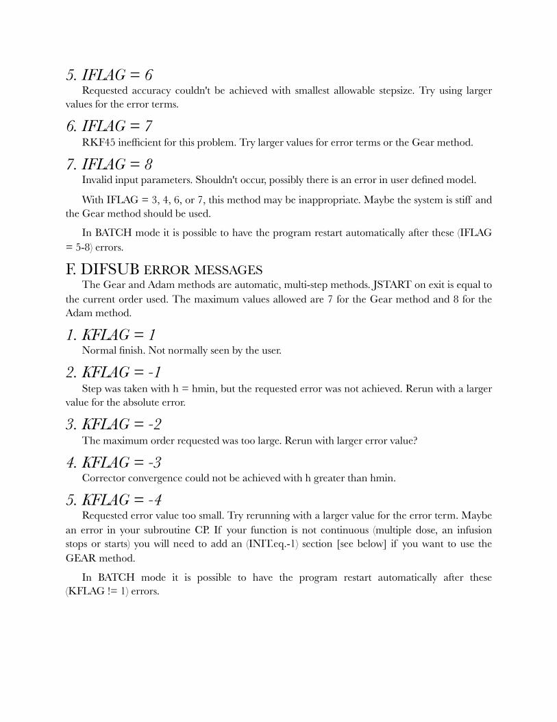
5. IFLAG = 6 Requested accuracy couldn't be achieved with smallest allowable stepsize. Try using larger

values for the error terms.

6. IFLAG = 7 RKF45 inefficient for this problem. Try larger values for error terms or the Gear method.

7. IFLAG = 8 Invalid input parameters. Shouldn't occur, possibly there is an error in user defined model.

With IFLAG = 3, 4, 6, or 7, this method may be inappropriate. Maybe the system is stiff and the Gear method should be used.

In BATCH mode it is possible to have the program restart automatically after these (IFLAG = 5-8) errors.

F. DIFSUB ERROR MESSAGES The Gear and Adam methods are automatic, multi-step methods. JSTART on exit is equal to

the current order used. The maximum values allowed are 7 for the Gear method and 8 for the Adam method.

1. KFLAG = 1 Normal finish. Not normally seen by the user.

2. KFLAG = -1 Step was taken with h = hmin, but the requested error was not achieved. Rerun with a larger

value for the absolute error.

3. KFLAG = -2 The maximum order requested was too large. Rerun with larger error value?

4. KFLAG = -3 Corrector convergence could not be achieved with h greater than hmin.

5. KFLAG = -4 Requested error value too small. Try rerunning with a larger value for the error term. Maybe

an error in your subroutine CP. If your function is not continuous (multiple dose, an infusion stops or starts) you will need to add an (INIT.eq.-1) section [see below] if you want to use the GEAR method.

In BATCH mode it is possible to have the program restart automatically after these (KFLAG != 1) errors.

8. Appendices Appendix A - Fitting Algorithms Methods

To be completed

Appendix B - Numerical Integration Methods To be completed

Appendix C - Methods of Analysis To be completed

9. Acknowledgments Dr Yamaoka et.al. for writing the original MULTI programs and showing that 'real'

pharmacokinetic analysis can be performed on microcomputers.

Trevor Smith for suggesting the RKF45 algorithm for ordinary differential equations.

John Holt for suggesting Gear's method for stiff equations.

Gary Koritz and Richard Bevill for encouragement and evaluation during the early translation stages.

Carl Peck for clearly describing the relevance of Bayesian methods and suggestions regarding weighting methods and plot output.

Ted Triggs for helpful evaluation during later refinement stages of Multi-Forte.

Monty Hampton for suggestions during the development of Boomer.

10. Applications Charles, B.G., Schneider, J.J., Norris, R.L.G., and Ravenscroft, P.J. 1987. Temelastine

does not affect theophylline pharmacokinetics in normal subjects, Brit. J. clin. Pharmacol., 24, 673-675

Kwon, K.I. and Bourne, D.W.A. 1987. Physiological pharmacokinetic model for distribution and elimination of tenoxicam, Int.J.Pharm., 37, 219-226

Bourne, D.W.A. and Hampton, E.M. 1988. Modeling and Analysis of Pharmacokinetic Data Using Multi-Forte and Boomer, Second Annual Symposium - Frontiers of Pharmacokinetics and Pharmacodynamics, Little Rock AR, 12-14 October

Clarke, C.R., Short, C.R., Bourne, D.W.A., and Usenik, E.A. 1989. Subcutaneously implanted tissue chambers -- a pharmacokinetic study, J. Vet. Pharmacol. Therap., 12, 312-321

Graves, N.M., Homes, G.B., Kriel, R.L., Jones-Saete, C., Ong, B. and Ehresman, D.J. 1989. Relative Bioavailability of Rectally Administered Phenobarbital Solution, DICP, Ann. Pharmacother., 23, 565-568

Ho, K.Y., Weissberger, A.J., Stuart, M.C., Day, R.O. and Lazarus, L. 1989. The Pharmacokinetics, Safety and Endocrine Effects of Authentic Biosynthetic Human Growth Hormone in Normal Subjects, Clin. Endocrin., 30, 335-345

Ismail, Z., Triggs, E.J., Smithurst, B.A., and Parke, W. 1989. The pharmacokinetics of amiloride-hydrochlorothiazide combination in the young and elderly, Eur. J. Clin. Pharmacol., 37, 167-171

Casto, D.T., Schnapf, B.M., Clotz, M.A. 1990. Lack of effect of short-term passive smoking on the metabolic disposition of theophylline, Eur. J. Clin. Pharmacol., 39, 399-402

Chen, G., Griffin, M., Poyer, J.L., McCay, P.B. and Bourne, D.W.A. 1990 HPLC procedure for the pharmacokinetic study of the spin-trapping agent, α-phenyl-N-tert-butyl nitrone (PBN), Free Radical Biology and Medicine, 9(2), 93-99

Hampton, E.M., Hrdlicka, K. and Bourne, D.W.A. 1991. Comparison of MS-DOS and Macintosh pharmacokinetic analysis programs using a two-compartment, two-infusion dosing scheme, Clin. Pharm., 10, 206-209

Paap, C.M., Nahata, M.C., Mentser, M.A., Mahan, J.D., Puri, S.K. and Hubbard, J.W. 1991 Pharmacokinetics of cefotaxime and its active metabolite in children with renal dysfunction, Antimicrob Agents Chemother., 35(9) 1879-1883

Markowsky, S.J., Zimmerman, C.L., Tholl, D., Soria, I. and Castillo, R. 1991. Methotrexate Disposition Following Disruption of the Blood-Brain Barrier, Therapeutic Drug Monitoring, 13, 24-31

Kim, H.C., McMillan, C.W., White, G.C., Bergman, G.E., Horton, M.W., and Saidi, P. 1992 Purified Factor IX Using Monoclonal Immunoaffinity Technique: Clinical Trials in Hemophilia B and Comparison to Prothrombin Complex Concentrates, Blood, 79(3) 568-57

Fan-Havard, P., Koshy, Z., Bais, R.M., Smith, C. and Eng, R.H.K. 1993 Effect of morphine or phenobarbital on teicoplanin elimination pharmacokinetics, J. of Antimicrobial Chemotherapy, 32 101-108

Paap, C.M. and Nahata, M.C. 1993 The relation between type of renal disease and renal drug clearance in children, European J. of Clin. Pharmacology, 44(2) 195-197

Pallapies, D., Peskar, B.A., Brune, K. and Geisslinger, G. 1994 Effects on platelet functions and pharmacokinetics of azapropazone and ketorolac tromethamine given as single parenteral doses, Br J Clin Pharmacol., 37(4) 335-339

Dachman, W.D., Adubofour, K.O., Bikin, D.S., Johnson, C.H., Mullin, P.D. and Winograd, M. 1994 Cimetidine-induced rise in praziquantel levels in a patient with neurocysticercosis being treated with anticonvulsants, J. of infectious Disease, 169, 689-91

Walker, J.L., Clarke, C.R. , Hague, C.M., Bourne, D.W. and Lessley, B.A. 1994 Effects of localized Pasteurella haemolytica infection on erythromycin-binding properties of bovine alpha-1-acid glycoprotein, albumin, serum, and tissue chamber fluids, Antimicrob Agents Chemother., 38(10) 2392-2397

Kobayashi, K., Vokes, E.E., Vogelzang, N.J., Janish, L., Soliven, B. and Ratain, M.J. 1995 Phase I study of suramin given by intermittent infusion without adaptive control in patients with advanced cancer, J. Clin. Oncology, 13, 2196-2207

Lau, C.E., Ma, F., Wang, Y. and Smith, C. 1996 Pharmacokinetics and bioavailability of midazolam after intravenous, subcutaneous, intraperitoneal and oral administration under a chronic food-limited regimen: relating DRL performance to pharmacokinetics, Psychopharmacology, 126(3) 241-248

Lau, C.E. and Wang, J. 1996 Alprazolam, caffeine and their interaction: relating DRL performance to pharmacokinetics, Psychopharmacology, 126(2) 115-124

Roder, J.D., Chen, C.L., Chen, H. and Sangiah, S. 1996 Bioavailability and pharmacokinetics of ibuprofen in the broiler chicken, J. of Vet. Pharmacology and Therapeutics, 19(3) 200-204

Manduru, M., Mihm, L.B., White, R.L., Friedrich, L.V., Flume, P.A. and Bosso, J.A. 1997 In vitro pharmacodynamics of ceftazidime against Pseudomonas aeruginosa isolates from cystic fibrosis patients, Antimicrob. Agents Chemother., 41(9) 2053-2056

Polikandritou Lambros, M., Bourne, D.W.A., Abbas, S.A., and Johnson, D.L. 1997 Disposition of aerosolized liposomal amphotericin B, J. of Pharmaceutical Sciences, 86(9) 1066-1069

Kwon, K-I. and Bourne, D.W.A. 1997 Gastrointestinal absorption of phenytoin from an oil-in-water microemulsion, Archives of Pharmacal Research, 20(5) 480-485

Browne, G.S., Nelson, C., Nguyen, T., Ellis, B.A., Day, R.O. and Williams, K.M. 1999 Stereoselective and substrate-dependent inhibition of hepatic mitochondrial β-oxidation and oxidative phosphorylation by the non-steroidal anti-inflammatory drugs ibuprofen, flurbiprofen, and ketorolac, Biochemical Pharmacology, 57(7) 837-844

Hakman, M. and Groth, T. 1999 Object-oriented biomedical system modeling-The Rationale, Computer methods and programs in biomedicine, 59(1) 1-17

Rusckowski, M., Qu, T., Pullman, J., Marcel, R., Ley, A. C., Ladner, R.C., and Hnatowich, D.J. 2000 Inflammation and Infection Imaging with a 99mTcNeutrophil Elastase Inhibitor in Monkeys, J. NucI Med, 41, 363-374

Alberts, M.K., Clarke, C.R., MacAllister, C.G., and Homer, L.M. 2000 Pharmacokinetics of acetazolamide after intravenous and oral administration in horses, Amer J. Vet. Res., 61(8) 965-968

Beier, E.B., Lehenbauerb, T.W. and Sangiah, S. 2000 Oral pharmacokinetics of fenbendazole in llamas, South American Camelids, Small Ruminant Research, 37(3) 209-214

White, R.L., Friedrich, L.V., Manduru, M., Mihm, L.B. and Bosso, J.A. 2001 Comparative in vitro pharmacodynamics of imipenem and meropenem against ATCC strains of Escherichia coli, Staphylococcus aureus and Bacteroides fragilis, Diagnostic microbiology and infectious disease, 39(1) 39-47

Kilic, K., Sproule, B.A., Turksen, I.B. and Naranjo, C.A. 2002 Fuzzy system modeling in pharmacology: an improved algorithm, Fuzzy Sets and Systems, 130(2) 253-264

Kilic, K., Sproule, B.A., Turksen, I.B. and Naranjo, C.A. 2004 Pharmacokinetic application of fuzzy structure identification and reasoning, Information Sciences, 162(2) 121-137

Gilmour, M.A., Clarke, C.R., MacAllister, C.G., Dedeo, J.M., Caudell, D.L., Morton, R.J. and Pugh, M. 2005 Ocular penetration of oral doxycycline in the horse, Veterinary Ophthalmology, 8(5) 331-335

Durisova, M. and Dedik, L. 2005 New Mathematical Methods in Pharmacokinetic Modeling, Basic and Clinical Pharmacology and Toxicology, 96(5) 335-342

Homer, L.M., Clarke, C.R. and Weingarten, A.J. 2005 Effect of dietary fat on oral bioavailability of tepoxalin in dogs, J. of Vet. Pharmacology and Therapeutics, 28(3) 287-291

Pizon, A.F., Becker, C.E. and Bikin, D. 2007 The Clinical Significance of Variations in Ethanol Toxicokinetics, J. Medical Toxicology, 3(2), 63-72

Maxwell, L.K., Bentz, B.G., Bourne, D.W.A. and Erkert, R.S. 2008 Pharmacokinetics of valacyclovir in the adult horse, J. of Vet. Pharmacology and Therapeutics, 31(4) 312-320

Georgopoulos, P.G., Sasso, A.F., Isukapalli, S.S., Lioy, P.J., Vallero, D.A., Okino, M. and Reiter, L. 2009 Reconstructing population exposures to environmental chemicals from biomarkers: Challenges and opportunities, J Expo Sci Environ Epidemiol., 19(2) 149–171

Goldsmith, M-R., Transue, T.R., Chang, D.T., Tornero-Velez, R., Breen, M.S. and Dary, C.C. 2010 PAVA: physiological and anatomical visual analytics for mapping of tissue-specific concentration and time-course data, J. Pharmacokin. Pharmacodyn., 37(3) 277-287

Some references found via Google Scholar