boom-bust cycles in housing: the changing role of ... · structure of mortgage markets in boom-bust...
TRANSCRIPT

WP/05/200
Boom-Bust Cycles in Housing: The Changing Role of Financial Structure
Calvin Schnure


© 2005 International Monetary Fund WP/05/200
IMF Working Paper
Western Hemisphere Department
Boom-Bust Cycles in Housing: The Changing Role of Financial Structure
Prepared by Calvin Schnure1
Authorized for distribution by Tamim Bayoumi
October 2005
Abstract
This Working Paper should not be reported as representing the views of the IMF. The views expressed in this Working Paper are those of the author(s) and do not necessarily represent those of the IMF or IMF policy. Working Papers describe research in progress by the author(s) and are published to elicit comments and to further debate.
Why are housing markets so prone to boom-bust cycles? The mortgage market structureprior to the Savings and Loan crisis contributed to the volatility in real housing activity which, in turn, amplified the volatility in housing prices. The subsequent development of a national, market-based system of securitized mortgage finance has damped this boom-bust cycle. We test whether deviations of actual housing prices from values forecast by a model based on economic fundamentals have responded to the change in financial structure, and find that pricing errors have fallen significantly since the mid-1980s. Tests of the relative importance of the change in financial market structure versus the reduction of inflation over this period indicate a primary role for market structure in improving pricing efficiency. JEL Classification Numbers: G21, R31 Keywords: Mortgage markets, housing prices, securitization Author(s) E-Mail Address: [email protected]
1 I would like to thank Tam Bayoumi, Toni Gravelle, Kornélia Krajnyák, Martin Mühleisen, and Chris Towe for comments on earlier drafts, and Ben Sutton for his careful assistance in this project. All remaining errors are my own.

- 2 -
Contents Page I. Introduction....................................................................................................................3 II. Structural Changes in Mortgage Finance.......................................................................4 III. House Prices and Fundamentals ....................................................................................5 IV. Will the Current Boom be Followed by a Bust?............................................................8 V. Mortgage Market Structure and Macroeconomic Volatility........................................10 VI. Conclusions..................................................................................................................11 References................................................................................................................................12 Tables 1. House Price Regressions..............................................................................................14 2. Pricing Errors ...............................................................................................................15 3. Pricing Error Regressions ............................................................................................16 Figures 1. Real Mortgage Growth and Real M1 Deposit Growth ................................................17 2. Mortgage Market Structure..........................................................................................17 3. Housing Starts and Residential Investment .................................................................18 4. Regional Housing Starts ..............................................................................................18 5. Regional House Prices .................................................................................................19 6. Pricing Errors from Panel Regression, (Mean Absolute errors) ..................................20 7. Pricing Errors from Panel Regression, (Standard Deviation of errors) .......................20 8. Real Residential Investment and Mortgage Growth....................................................21 9. Regional Pricing Errors, 1978–2004............................................................................22 10. Construction Status at Time of Sale.............................................................................23 11. New Home Sales and Supply.......................................................................................23 12. Housing Supply and Prices in the Pacific/West Region ..............................................24 13. Housing Supply and Prices in the North East/New England Region ..........................24 14. Volatility of Real Activity, Rolling Window...............................................................25 15. Volatility of Real Activity, 1960–83 vs. 1984–2004...................................................25

- 3 -
I. INTRODUCTION
Why are housing markets so prone to boom-bust cycles? This paper examines the role of the structure of mortgage markets in boom-bust cycles in real housing activity and housing prices. The financial structure in the United States prior to the mid-1980s helped generate a stop-and-go credit cycle in response to changes in monetary policy and local banking conditions. During periods of easy money this encouraged rapid expansions in real activity. During the tightening phase that followed, depositories bore the brunt of monetary policy, with housing finance being a main channel in the transmission mechanism. With the cost of housing finance rising sharply—or the lending spigot shut off entirely—real housing activity contracted. Considerable pent-up demand arose, setting the stage for the next boom cycle.
Sharp swings in real activity generated similar movements in housing prices. During periods of tight money, demand fell sharply, perhaps leading prices below their long-term fundamental values. When policy eased, potential buyers in a rush to buy before financing dried up again often bid prices up above fundamental values, leading to excess price volatility.
The system of U.S. housing finance underwent a fundamental restructuring following the Savings and Loan (S&L) crisis in the 1980s. Mortgage lending changed from being dominated by local and regional balance-sheet lending by depositories, to a national, market-based system of securitized mortgage finance. This structural shift provides a natural experiment for the influence of financial structure on real housing activity and prices.
The market-based system of housing finance that has emerged damps swings in mortgage credit flows, real housing activity, and housing prices. The availability of finance is no longer subject to quantitative restrictions associated with monetary policy but rather draws on the deep national bond market for financing. Lending is no longer constricted by limits on interstate banking, with the associated risks of a regional “capital crunch,” but is instead funded in a national market. These changes in financial structure have smoothed out the boom-bust cycle in lending flows, real activity, and prices. This smoother trend in housing has produced another benefit as well, by reducing pricing errors relative to fundamental valuations. Lower volatility of residential investment also appears to be a factor in the decrease in macroeconomic volatility over the same period.
Subsequent sections describe the structural changes in mortgage finance, and the changing patterns of real housing activity and housing prices. Next we present an econometric model of housing price dynamics based on economic fundamentals, which is used to analyze how price formation has changed over time. In addition, we explore whether the current system of housing finance may have reduced risks of a speculative boom-bust housing cycle, including through changes to homebuilders’ behavior and incentives to build inventories of new houses in advance of anticipated increases in demand. A final section explores the role of residential investment in the decline of the volatility of real GDP.

- 4 -
II. STRUCTURAL CHANGES IN MORTGAGE FINANCE
Through the mid-1980s, mortgage lending was mainly a local business. Most residential mortgages were originated and kept on the balance sheets of local lenders—such as savings and loan institutions (S&Ls) or thrifts—for the lifetime of the loan. The availability of mortgage credit in any region depended largely on local financial conditions, including the quality of bank and thrift loan portfolios and levels of capital, as restrictions on interstate banking inhibited the flow of lending between regions. Monetary policy and bank regulations contributed to the volatility of housing finance. Monetary policy had a first-order impact on housing activity (the mortgage lending channel) through the prominent role of depositories’ balance sheets in mortgage flows. The supply of credit fluctuated more severely—including through credit rationing under tight monetary conditions—than would have occurred through changes in interest rates alone. Bank regulations, such as Regulation Q (Reg Q), which limited the interest rate to be paid on bank deposits, also restricted mortgage finance. Under such a market structure, housing markets were subject to a boom-bust financing cycle. Real mortgage growth slowed sharply during several episodes in the 1960s when Reg Q ceilings on deposit rates became binding and banks and S&Ls were unable to retain deposits (Figure 1). Lending contracted in response to the declining funding base, and would subsequently rebound as monetary policy eased and deposit growth resumed. The S&L crisis precipitated a shift toward nationwide funding of housing activity based on mortgage securitization. S&Ls had funded long-term fixed-rate mortgage loans with short-term deposits, incurring large unhedged interest rate exposures. They suffered major capital losses when interest rates rose in the early 1980s, and many institutions failed. In their place, a system evolved under which loans originated by mortgage banks were subsequently pooled and securitized by Government Sponsored Enterprises (GSEs). In this new financial structure, home mortgages held by depositories dropped from above 70 percent of the market in the 1970s to about 30 percent in recent years (Figure 2). This market-based financial structure has reduced the volatility of mortgage lending. The availability of funds is no longer limited by conditions at local depository institutions or the strength of regional economies, and monetary policy no longer has a direct effect on the supply of mortgages through high-powered money expanding bank balance sheets. As a result, the correlation between growth of real deposits and real mortgage flows dropped from 0.72 between 1960 and 1984, to 0.06 between 1985 and 2004. Tighter or looser monetary conditions still affect market interest rates and the general willingness to lend, of course, but this has a smaller direct impact on the mortgage lending channel.2
2 See Peek and Wilcox (2005) for further discussion of how the GSEs and secondary mortgage markets have moderated the cyclicality of mortgage flows.

- 5 -
Changes in the structure of the mortgage market have coincided with lower volatility of real housing activity. In the past, housing construction and transactions tended to fluctuate strongly with the credit cycle, as evidenced by the boom-bust phases between the late 1960s and 1980s (Figure 3). Residential investment spending as measured in GDP also exhibited pronounced cycles, with growth rates of 40 percent or more not uncommon during booms, and declines of nearly the same magnitude during busts. This cyclical volatility has diminished markedly, however, and housing starts and investment spending have grown at a relatively stable pace since 1990. Although starts have risen somewhat faster in the past few years, their growth still remains well below rates reached in previous booms. Housing activity has also become more synchronized across regions. Cycles of housing starts in past decades often moved independently in different parts of the country, especially during the early 1960s and the 1980s (Figure 4). Beginning in 1990, however, growth trends in housing starts have been similar across all major regions, as might be expected with the shift of funding form a local to a national market. Housing prices have converged toward more steady growth since the early 1990s as well. Amid high volatility, housing prices increased strongly in the 1970s, both in nominal terms and relative to the overall consumer price index (Figure 5). Nominal gains slowed sharply during the recessions in the early 1980s and prices declined in real terms in most regions. During the mid- to late-1980s there was a series of price booms in New England, the Mid-Atlantic, and Pacific regions. Housing prices fell sharply in the West South Central region as the collapse of oil prices impacted the regional economies of Texas and Oklahoma, and contributed to a regional banking crisis. Since the late 1980s, in contrast, price swings have had lower amplitude, and price trends have converged across regions.
III. HOUSE PRICES AND FUNDAMENTALS
The smoothing of the boom-bust cycle in mortgage lending, real activity, and housing prices raises two questions. Have structural changes in mortgage finance improved the process of price formation? And what do these developments tell us about the risk of a sharp collapse in prices following the ongoing housing boom? To address the first question, an econometric approach is used to analyze the impact of financial market changes on price formation in the housing market. The results are subsequently used to address the second question. The empirical methodology follows two steps. First, housing prices are regressed on economic fundamentals, including regional variables for income, unemployment rates, and the labor force, as well as national variables to control for business cycle dynamics. 3 Specifically,
3 The model is estimated in log differences, as is common in the literature on housing prices. Tests of regional housing prices and income do not find evidence of a cointegrating relationship, suggesting that a cointegrating
(continued…)

- 6 -
hpii,t = β0 + β1 yi,t + β2 Ui,t + β3 lfi,t + β4 it + β5 cpit + β6 gdpt + εi,t where hpi is the Office of Federal Housing Enterprise Oversight (OFHEO)’s repeat sales housing price index for nine major regions, y, U, and lf are regional income, unemployment rates, and labor force, respectively, and i, cpi, and gdp are the (national) mortgage interest rate, cpi inflation, and gdp growth, respectively. The model was estimated allowing coefficients to vary by region in a set of stand-alone regressions, as well as in a fixed-effects panel in which only constants vary by location.4 The results suggest that fundamental factors generally have the expected impact on housing prices (Table 1). Regional income growth and unemployment rates have statistically significant and correctly signed effects on housing prices. The panel estimates imply that a 10 percent rise in regional incomes is associated with a 2.5 percent increase in housing prices (columns 1–3). Similarly, a 1 percentage point rise in the unemployment rate depresses housing prices by about 1 percent. National business cycle indicators are not estimated to have a significant impact, suggesting that their effect is captured by the regional measures. The coefficient on CPI inflation is small and insignificant as price effects may be captured through nominal incomes. Somewhat surprisingly, interest rates are not estimated to have a significant effect, which could reflect endogeneity problems. Results of the region-by-region regressions (not shown) are similar in character, although the standard errors are larger. The model’s fit improves considerably when estimated separately over the periods corresponding to different mortgage market structures. For example, the model explains more than twice as much of the overall variation in housing prices over 1990–2004 compared to estimates over the entire time horizon (columns 3 and 5). This improvement is consistent with the hypothesis that factors other than economic fundamentals may have had a greater impact on the formulation of housing prices under the earlier mortgage market structure, and that the current financial structure has reduced such unexplained errors in the pricing model. Moreover, the interest rate is now found to have the expected negative effect (also significant at the 1 percent level) in both the earlier and later time periods. The different coefficients suggest that housing prices have become more sensitive to long-term interest rates as the importance of quantity restrictions on mortgage lending has waned and as mortgages are increasingly funded in a national market. Assuming that estimation residuals represent pricing errors, the results also indicate significant improvements in the pricing process. It is instructive to break this time period into
equation may not be appropriate. See also Gallin (2003), who finds no cointegration between housing prices and income in metropolitan areas. 4 The availability of open land, as well as the presence of zoning restrictions may account for some of the regional differences in housing prices, including the more rapid appreciation in recent years in the mature cities of the East Coast and California (see McCarthy and Peach, 2004, and Glaeser and Gyourko, 2003).

- 7 -
three subgroups and examine the behavior of price errors during each. The period prior to 1982 can be characterized as a high inflation environment with a mortgage structure based on depository institutions. Between 1983 and 1990, inflation had declined but mortgage market structure was mixed, with mortgage securitization rapidly replacing balance-sheet lending by depositories through the period. Since 1991, there has been low inflation and a national securitized market for mortgages. Pricing errors in the earlier years often were quite large, with a median absolute error of nearly 5 percent under the depository-based market structure prior to 1982 (Table 2 and Figure 6). Median absolute errors decreased during the 1980s as inflation rates came down and the mortgage market structure was in transition. There has been an even greater reduction; however, since the 1990s, as changes to the market structure became more complete, with median absolute errors falling to 2 percent.
Price movements also appear to have converged across regions as the financial structure changed from a local and regional to a national basis (Figure 7). The standard deviation of pricing errors across regions declined from 5.6 percent in the first part of the sample period to 2.5 percent in the 1990s, as financial conditions in all regions became more directly determined by national rather than regional forces. Tests of the relative importance of mortgage market structure and macroeconomic variables suggest an important effect from financial structure. Average absolute pricing errors from the housing price model were regressed on the securitized share of the mortgage market (a proxy for structural change in housing finance) and the 4-quarter rate of CPI inflation (Table 3). The results indicate that changes in mortgage market structure are associated with improvements in the house price formation process: higher securitization tends to reduce pricing errors. The estimates suggest that the results are economically significant as well, with a 10 percentage point rise in securitized share, all else equal, lowering the average absolute pricing error by 0.8 percentage points. The rise in securitization from 10 percent of the total mortgage market to 60 percent or more between the mid-1970s and 2004 would thus be associated with a 4 percentage point decline in absolute pricing errors—essentially all of the improvement that is estimated to have occurred. The drop in inflation rates, in contrast, appears to have had little or no measurable effect on the accuracy of the pricing processes. The coefficient on CPI inflation is not statistically different from zero in any formulation (alternative specifications, for example, using either the variance of CPI inflation or the change in CPI inflation, found similar results and are not reported). Similar results obtain for the impact of lower inflation on the reduction of the variance of pricing errors across regions. The regressions explain a large portion of the time series variation in pricing errors. The adjusted R-squared for the pricing error regression is 0.40, while the equation regressing the variance of pricing errors across regions has an R-squared of 0.57. Pricing errors may have resulted from rational decisions by home buyers potentially facing credit rationing at some later date. When mortgage lending was subject to quantity restrictions, potential home buyers who otherwise would qualify for a loan may at times have been unable to obtain financing. Knowing this, a potential homebuyer may have rationally

- 8 -
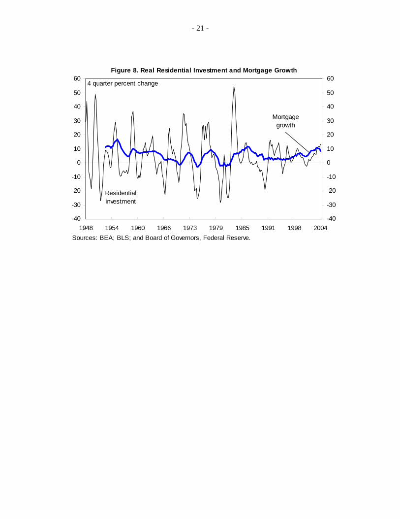
paid a premium over a house’s fundamental value during periods when financing was readily available, leading to positive errors in the pricing model. Conversely, homeowners forced to sell during periods when potential buyers had difficulty obtaining financing may have reduced sales prices, resulting in negative pricing errors. An alternative test using earlier historical data is performed to confirm the importance of the impact of mortgage market structure for the pricing process. While reliable data on house prices are available only for the most recent three decades, data on real and nominal residential investment spending are available since 1948. As inflation and macroeconomic volatility remained low until the late 1960s, spending data from 1948–1968 provide a control period for testing whether the elevated volatility of residential investment and price changes from the late 1960s through the early 1980s was more related to macroeconomic factors or to the structure of the mortgage market. Before the 1990s, boom-bust cycles were of similar magnitude during the low and high inflation decades, suggesting that the structure of the mortgage market was mainly responsible for generating large upswings and downswings in activity. Residential investment was highly procyclical from 1948 through the late 1960s (Figure 8). There were four episodes in which residential investment grew at more than a 25 percent rate over 4 or more quarters, with a surge of nearly 50 percent in the early 1950s. During bust periods, spending often declined at a 20 percent rate or faster. These swings in real activity were comparable to (and at times greater than) those that occurred during the higher-inflation years of the 1970s and early 1980s, before moderating in the 1990s.
IV. WILL THE CURRENT BOOM BE FOLLOWED BY A BUST?
There are widespread concerns about the recent run-up in housing prices, and while financing in a nationwide securitized market may have reduced the stop-go cycle of mortgage flows, it could also be argued that the freer flow of financing may aid in the development of a nationwide bubble. Indeed, nationwide housing prices have risen 50 percent over the past five years, with some metropolitan and regional markets soaring much higher. While some of these gains may reflect a catch-up following slow appreciation in previous years, recent increases have been particularly rapid, and may be ahead of fundamentals. Several indicators point to speculative pressures on prices. Purchases of second homes, often for investment purposes, have risen, as has the use of interest-only mortgages that allow a more expensive purchase for a given monthly payment. Surveys and anecdotal evidence suggest home buyers have extrapolated past gains into their expectations for future appreciation. The price-to-rent ratio has increased, suggesting that in some markets the valuations can only be justified by expectations of future rapid appreciation. These warning
- 9 -
signs could foretell a drop in prices, or an adjustment through a long period of slow nominal gains until real valuations came back in line with fundamentals.5 Other factors, however, mute some of these risks. Estimated pricing errors from the model presented earlier are not particularly large, suggesting that much of the recent gains can be explained by rising incomes, rising employment, and low interest rates. Moreover, the positive surprises in housing prices over the past five years follow a decade of negative surprises, especially on the East and West Coasts (Figure 9). These patterns suggest that much of the recent gains may be a catch-up after a prolonged period of prices lagging fundamentals. In addition, there have been other changes in homebuilders’ behavior since the 1980s—including in speculative housing starts and in the accumulation of inventories of new homes—that may moderate these risks. Speculative homebuilding used to dominate housing activity. Using data on the completion status of a new home sale, one can identify speculative building (sales of houses already completed or under construction) versus nonspeculative building (construction not yet started at the time of sale). From the 1960s through the 1980s, builders often engaged in speculative starts, largely due to the necessity to build an inventory of homes for sale in advance of a (relatively short) “hot” market (Figure 10). Speculative construction has declined since the 1980s. With builders’ demand no longer subject to stop-go cycles, the incentives to build an inventory of new homes in anticipation of a surge in demand are much diminished, limiting the overhang of new homes available for sale. Indeed, inventories of new homes have only recently returned to the levels of the early 1970s, despite a doubling of sales (Figure 11). During previous boom-bust cycles, a buildup of inventories preceded price collapses when demand waned. The amount of new home inventories divided by the monthly sales pace (referred to as the months’ supply) gives an indication of the vulnerability of housing markets to a drop-off in demand, and how long it may take to work off any excess inventories. In a typical cycle, an early increase in housing prices would have prompted more rapid building and a rise in months’ supply. As demand would wane later in the cycle—most often due to a constraints from the supply of mortgage finance, or a slowing of income and employment as monetary tightening restrains GDP growth—prices would decline to absorb the excess supply. For example, new home inventories reached nearly 10 months’ supply on the west coast during the early 1980s, and a high of 15 months’ supply during the boom in the northeast in the late1980s. (Figures 12 and 13). Prices subsequently fell as much as 10
5 Many observers have noted that the rapid rise in housing prices may more likely be followed by slow appreciation than a price collapse. See, for example, Case and Shiller (2003), Genesove and Mayer (2001), IMF (2003), IMF (2004), Macroeconomic Advisers (2004), McCarthy and Peach (2004). Angell and Williams (2005) find that booms may be followed by busts, but that “this pattern may be more the exception than the rule” (FDIC 2005).

- 10 -
percent in order to work off excess stocks of new homes. Only once months’ supply returned to more normal levels of 6 months or less did prices begin to rise again. The current boom, however, has seen months’ supply remain near historic lows even in the regions where housing markets are particularly strong. Current inventories are at less than 4 months’ supply in the northeast and less than 3 months’ on the west coast. These levels are below those at which housing prices stabilized during previous bust cycles, and suggest that housing supply has not gotten far ahead of demand.
V. MORTGAGE MARKET STRUCTURE AND MACROECONOMIC VOLATILITY
Changes in mortgage market structure may have contributed to the large and sustained decline in the volatility of U.S. output. The standard deviation of 4-quarter GDP growth decreased from 2.8 percent between 1960 and 1983 to 1.6 percent between 1984 and 2004. Previous authors have used a variety of time series and frequency domain techniques to determine whether this stabilization has resulted from a reduction in macroeconomic shocks, including from commodity and energy prices, from improved macroeconomic policies, or from other (unexplained) causes.6 Most authors identify the break in volatility as occurring in the mid-1980s, and find mixed support for a number of possible sources of stabilization, but no structural arguments for why it may have occurred.
The analysis presented above suggests a structural reason for decreased output volatility through the impact of the mortgage market structure on housing activity. Among major components of GDP, the volatility of residential investment since 1960 has been more than twice as large as any other item (Figure 14). More importantly, while volatility of all major categories has declined, residential investment has experienced the greatest reduction, with the annual standard deviation of growth falling more than half, from 17 percent to 7 percent (Figure 15).
The shift from a system of housing finance of on-balance sheet lending by local depository institutions, to a framework based on securitization and funding in a national bond market, has all but eliminated the stop-go credit cycle in mortgage finance that previously existed. With a smoother supply of mortgage finance, the volatility of real housing investment and turnover of the existing housing stock moderated. In addition to the direct contribution of residential investment to lower macroeconomic volatility, a steadier growth pattern of items typically associated with the purchase of a new or existing—furniture, household appliances, other home furnishings and other durable items—may have contributed to a further moderation of GDP volatility.
6 See, for example, Ahmed, Levin and Wilson (2004), Blanchard and Simon (2001), Kahn, McConnell and Perez-Quiros (2002), McConnell and Perez-Quiros (2000), and Stock and Watson (2002).

- 11 -
A structural explanation of the decline in the volatility of GDP would provide more assurance that the stabilization is not transitory. To the extent that an absence of macroeconomic or commodity shocks reduced volatility since the mid-1980s, or that sound policies have helped smooth output, future shocks or policy mistakes could undo any of these gains. In contrast, however, stabilization that results from structural changes to mortgage markets such as those described above is more likely to be enduring.
VI. CONCLUSIONS
The change in the mortgage market’s structure from a system based on balance sheet lending by depositories to a market-based system of securitized mortgage finance has damped the volatility of financing flows and real activity. With funding conditions now determined in a national market, trends in real activity and prices have become less cyclical and converged across all regions of the United States. As a result, a model of housing prices based on economic fundamentals finds that pricing errors—the deviations of actual prices from those estimated in the model—have fallen by half. Moreover, a change in homebuilders’ behavior—in particular, a move away from speculative starts and a reduction of levels of inventories of new homes—has reduced the risk of a sharp decline in housing prices, although some indicators suggest speculative pressures in a number of metropolitan areas. This stabilization of housing activity may have made an important contribution to the reduction of the volatility of GDP growth over the same period.
- 12 -
REFERENCES
Ahmed, S., A. Levin, and B.A. Wilson, 2004, “Recent U.S. Macroeconomic Stability: Good Policies, Good Practices, or Good Luck?” Review of Economics and Statistics, Vol. 6, No. 3, pp. 824–32.
Angell, C., and N. Williams, 2005, “U.S. Home Prices: Does Bust Always Follow Boom?,” FYI: An Update on Emerging Issues in Banking (Washington: Federal Deposit Insurance Corporation).
Blanchard, O., and J. Simon, 2001, “The Long and Large Decline in U.S. Output Volatility,” Brookings Papers on Economic Activity, Vol. 1, pp. 135–74.
Case, K.E., and R.J. Shiller, 2003, “Is There a Bubble in the Housing Market?” Brookings Papers on Economic Activity, Vol. 2, pp. 299–342.
Davis, M.A., and J. Heathcote, 2004, “The Price and Quantity of Residential Land in the United States” (unpublished; Washington: Federal Reserve Board).
Gallin, J., 2003, “The Long-Run Relationship between House Prices and Income: Evidence from Local Housing Markets” (unpublished; Washington: Federal Reserve Board).
Genesove, D., and C. Mayer, 2001, “Loss Aversion and Seller Behavior: Evidence from the Housing Market,” Quarterly Journal of Economics, Vol. 116, pp. 1233–60 (Cambridge, MA: MIT Press).
Glaeser, E.L., and J. Gyourko, 2003, “The Impact of Building Restrictions on Housing Affordability,” FRBNY Economic Policy Review, Vol. 9, No. 2, June, pp. 21–39 Federal Reserve Bank).
International Monetary Fund, 2003a, “Are U.S. House Prices Overvalued?,” United States: Selected Issues, IMF Country Report No. 03/245.
———, 2003b, “Real and Financial Effects of Bursting Asset Price Bubbles,” World Economic Outlook (April).
———, 2004, “The Global House Price Boom,” World Economic Outlook (September).
Kahn, J., M. McConnell, and G. Perez-Quiros, 2002, “On the Causes of the Increased Stability of the U.S. Economy,” FRBNY Economic Policy Review, Vol. 8, No. 1, June, pp. 183–202, Federal Reserve Bank).
Macroeconomic Advisers, 2004, “A Bubble in House Prices?,” Economic Outlook, June 18 (St. Louis, Missouri).
McCarthy, J., and R.W. Peach, 2004, “Are Home Prices the Next ‘Bubble’,” FRBNY Economic Policy Review, Vol. 10, No. 3, December (New York: Federal Reserve Board).
McConnell, M., and G. Perez-Quiros, 2000, “Output Fluctuations in the United States: What has Changed Since the Early 1980s?,” American Economic Review, Vol. 90, No. 5, pp. 1464–76.

- 13 -
Peek, J., and J.A. Wilcox, 2005, “Secondary Mortgage Markets, GSEs, and the Changing Cyclicality of Mortgage Flows” (unpublished; Berkeley: University of California).
Stock, J., and M. Watson, 2002, “Has the Business Cycle Changed and Why?” NBER Macroeconomics Annual (Cambridge, MA: National Bureau of Economic Research).

- 14 -
Table 1. House Price Regressions ___________________________________________________________________________ Regression (1) (2) (3) (4) (5) Panel Panel Panel Panel Panel Dependent Variable HPI HPI HPI HPI HPI Period 1978–2004 1978–2004 1978–2004 1978–89 1990–2004 __________________________________________________________________________________________ Constant 8.96 9.13 7.87 13.59 23.73 (11.08)** (11.04)** (9.58)** (5.85)** (20.43)** Income 0.254 0.282 0.234 0.246 0.206 (4.84)** (4.73)** (4.00)** (2.35)* (4.57)** Unemployment -1.056 -1.030 -0.877 -0.511 -1.200 (6.85)** (6.58)** (5.66)** (1.74) (9.03)** Interest rates 0.111 0.085 0.014 -0.606 -1.651 (1.12) (0.83) (0.14) (2.97)** (11.26)** CPI 0.054 0.039 -0.008 -0.083 -0.097 (0.72) (0.52) (0.11) (0.77) (0.80) GDP -0.068 -0.072 -0.177 -0.389 (1.00) (1.09) (1.72) (5.41)** Labor force 1.018 1.782 0.347 (6.67)** (5.69)** (3.14)** __________________________________________________________________________________________ Observations 946 946 946 406 531 Adjusted R-squared 0.11 0.11 0.15 0.20 0.39 __________________________________________________________________________________________ Absolute value of t-statistics in parentheses *significant at 5%; **significant at 1%

- 15 -
Table 2. Pricing Errors (Panel Regressions, percent)
___________________________________________________________________________ Pricing Errors Period Inflation Market Average Median Standard Structure Absolute Absolute Deviation ___________________________________________________________________________ 1978–82 High Depository 6.2 4.8 5.6 1983–90 Low Mixed 4.9 3.7 4.2 1991–2004 Low Market 2.7 2.0 2.5 ___________________________________________________________________________

- 16 -
Table 3. Pricing Error Regressions ___________________________________________________________________________ Regression (1) (2) (3) (4) OLS OLS OLS OLS Dependent Variable Av. Abs. Var. Av. Abs. Var. Pricing Error Pricing Error Pricing Error Pricing Error by Regions by Regions from Panel from Panel ___________________________________________________________________________ Constant 5.96 6.67 7.08 8.08 (7.54)** (9.01)** (8.91)** (11.41)** MBS share -0.064 -0.079 -0.083 -0.106 (4.59)** (6.01)** (5.88)** (8.48)** CPI 0.056 0.037 0.026 0.010 (0.78) (0.56) (0.37) (0.15) ___________________________________________________________________________ Observations 106 106 106 106 Adjusted R-squared 0.31 0.42 0.40 0.57 ___________________________________________________________________________ Absolute value of t-statistics in parentheses *significant at 5%; **significant at 1%

- 17 -
-25
-20
-15
-10
-5
0
5
10
15
20
1960 1965 1970 1975 1980 1985 1990 1995 2000-25
-20
-15
-10
-5
0
5
10
15
20
Deposits
Figure 1. Real Mortgage Growth and Real M1 Deposit Growth
4 quarter percent change
Mortgages
Source: Board of Governors, Federal Reserve.
0
10
20
30
40
50
60
70
80
90
100
1960 1965 1970 1975 1980 1985 1990 1995 20000
10
20
30
40
50
60
70
80
90
100
Depository share
Securitized plus GSEs
Securitized
Figure 2. Mortgage Market Structure
percent of total mortgages
Source: Board of Governors, Federal Reserve.

- 18 -
-60
-40
-20
0
20
40
60
80
100
1960 1965 1970 1975 1980 1985 1990 1995 2000-60
-40
-20
0
20
40
60
80
100
Housing startsReal residential
investment spending
Figure 3. Housing Starts and Residential Investment
4 quarter percent change
Sources: BEA and Census Bureau.
0
50
100
150
200
250
300
1960 1965 1970 1975 1980 1985 1990 1995 20000
50
100
150
200
250
300Figure 4. Regional Housing Starts
Housing starts, 12 mo. moving average, 1960=100
Source: Census Bureau.
South
West
Midwest
Northeast

- 19 -
-15
-10
-5
0
5
10
15
20
25
30
1976 1980 1984 1988 1992 1996 2000 2004-15
-10
-5
0
5
10
15
20
25
304 quarter percent change
Pacific
NewEngland
MiddleAtlantic
National average
3
Source: Office of Federal Housing Enterprise Oversight.
Figure 5. Regional House Prices
-15
-10
-5
0
5
10
15
20
25
30
1976 1980 1984 1988 1992 1996 2000 2004-15
-10
-5
0
5
10
15
20
25
304 quarter percent change
SouthAtlantic
East southcentralEast
north central
National average
-15
-10
-5
0
5
10
15
20
25
30
1976 1980 1984 1988 1992 1996 2000 2004-15
-10
-5
0
5
10
15
20
25
30
West south central
4 quarter percent change
Mountain
West north central
National average

- 20 -
0
2
4
6
8
10
12
1978 1982 1986 1990 1994 1998 20020
2
4
6
8
10
12
Moving average
Figure 7. Pricing Errors from Panel Regression
Standard deviation of panel errors
Sources: Office of Federal Housing Enterprise Oversight; BEA; BLS; and IMF staff estimates.
0
2
4
6
8
10
12
14
1978 1982 1986 1990 1994 1998 20020
2
4
6
8
10
12
14
Moving average
Figure 6. Pricing Errors from Panel Regression
Mean absolute panel errors
Sources: Office of Federal Housing Enterprise Oversight; BEA; BLS; and IMF staff estimates.
- 21 -
-40
-30
-20
-10
0
10
20
30
40
50
60
1948 1954 1960 1966 1973 1979 1985 1991 1998 2004-40
-30
-20
-10
0
10
20
30
40
50
604 quarter percent change
Residential investment
Mortgagegrowth
Figure 8. Real Residential Investment and Mortgage Growth
Sources: BEA; BLS; and Board of Governors, Federal Reserve.

- 22 -
-10
-8
-6
-4
-2
0
2
4
6
1978-1984
1985-1989
1990-1994
1995-1999
2000-2004
-10
-8
-6
-4
-2
0
2
4
6Pacific
-10
-8
-6
-4
-2
0
2
4
6
1978-1984
1985-1989
1990-1994
1995-1999
2000-2004
-10
-8
-6
-4
-2
0
2
4
6New England
-10
-8
-6
-4
-2
0
2
4
6
1978-1984
1985-1989
1990-1994
1995-1999
2000-2004
-10
-8
-6
-4
-2
0
2
4
6South Atlantic
-10
-8
-6
-4
-2
0
2
4
6
1978-1984
1985-1989
1990-1994
1995-1999
2000-2004
-10
-8
-6
-4
-2
0
2
4
6Mid Atlantic
-10
-8
-6
-4
-2
0
2
4
6
1978-1984
1985-1989
1990-1994
1995-1999
2000-2004
-10
-8
-6
-4
-2
0
2
4
6West North Central
-10
-8
-6
-4
-2
0
2
4
6
1978-1984
1985-1989
1990-1994
1995-1999
2000-2004
-10
-8
-6
-4
-2
0
2
4
6Mountain
-10
-8
-6
-4
-2
0
2
4
6
1978-1984
1985-1989
1990-1994
1995-1999
2000-2004
-10
-8
-6
-4
-2
0
2
4
6West South Central
-10
-8
-6
-4
-2
0
2
4
6
1978-1984
1985-1989
1990-1994
1995-1999
2000-2004
-10
-8
-6
-4
-2
0
2
4
6East North Central
-10
-8
-6
-4
-2
0
2
4
6
1978-1984
1985-1989
1990-1994
1995-1999
2000-2004
-10
-8
-6
-4
-2
0
2
4
6East South Central
Figure 9. Regional Pricing Errors, 1978–2004
Sources: Office of Federal Housing Enterprise Oversight; BEA; BLS; and IMF staff estimates.

- 23 -
0
200
400
600
800
1000
1200
1400
1963 1968 1973 1978 1983 1988 1993 1998 20030
200
400
600
800
1000
1200
1400
Sales (SAAR)
For sale
Thousands
Figure 11. New Home Sales and Supply
Source: Census Bureau.
0
10
20
30
40
50
60
70
80
90
100
1963 1968 1973 1978 1983 1988 1993 1998 20030
10
20
30
40
50
60
70
80
90
100
Not started
Under construction
Complete
Figure 10. Construction Status at Time of Sale
percent of new home sales
Source: Census Bureau.

- 24 -
0
2
4
6
8
10
12
1976 1980 1984 1988 1992 1996 2000 2004-10
-5
0
5
10
15
20
New house supply(months, right scale)
Figure 12. Housing Supply and Prices in the Pacific/West Region
Housing prices(4 quarter percent change, left scale)
Sources: Census Bureau; Office of Federal Housing Oversight; and IMF staff estimates.
0
2
4
6
8
10
12
14
16
18
1976 1980 1984 1988 1992 1996 2000 2004-15
-10
-5
0
5
10
15
20
25
New house supply(months, right scale)
Figure 13. Housing Supply and Prices in the North East/New England Region
Housing prices(4 quarter percent change, left scale)
Sources: Census Bureau; Office of Federal Housing Oversight; and IMF staff estimates.

- 25 -
0
5
10
15
20
25
30
1952 1956 1960 1964 1968 1972 1976 1980 1984 1988 1992 1996 2000 2004
Source: BEA.
Standard deviation of y/y growth rates, 5-year rolling window
Figure 14. Volatility of Real Activity
Residential investment
Non-residential investment
Consumption
Government
GDP
0
2
4
6
8
10
12
14
16
18
20
GDP NonresidentialInvestment
ResidentialInvestment
Consumption Government
1960-1983
1984-2004
Figure 15. Volatility of Real Activity
Source: BEA.
Standard deviation of 4-qtr growth rates, percent