book title: zigbee network protocols and...
TRANSCRIPT
Book Title: ZigBee Network Protocols and Applications
Editors: Chonggang Wang, Tao Jiang and Qian Zhang
September 9, 2009

ii

Contents
1 Performance Analysis of the IEEE 802.15.4 MAC Layer 1
1.1 Introduction . . . . . . . . . . . . . . . . . . . . . . . . . . . . . . . . . . . . 2
1.2 IEEE 802.15.4 WPANs: an Overview . . . . . . . . . . . . . . . . . . . . . . 4
1.2.1 Superframe Structure . . . . . . . . . . . . . . . . . . . . . . . . . . . 6
1.2.2 The Slotted CSMA/CA Mechanism . . . . . . . . . . . . . . . . . . . 8
1.3 Markov Chains for the Slotted CSMA/CA . . . . . . . . . . . . . . . . . . . 11
1.4 System Model and Notation . . . . . . . . . . . . . . . . . . . . . . . . . . . 15
1.4.1 Markov Chain Model . . . . . . . . . . . . . . . . . . . . . . . . . . . 15
1.4.2 Discussion of the Pollin Model . . . . . . . . . . . . . . . . . . . . . . 19
1.5 Results . . . . . . . . . . . . . . . . . . . . . . . . . . . . . . . . . . . . . . . 20
1.5.1 Average Delay . . . . . . . . . . . . . . . . . . . . . . . . . . . . . . . 20
1.5.2 Average Power Consumption . . . . . . . . . . . . . . . . . . . . . . . 21
1.5.3 Mean Number of Backoffs and CCAs . . . . . . . . . . . . . . . . . . 23
1.5.4 Efficiency . . . . . . . . . . . . . . . . . . . . . . . . . . . . . . . . . 28
i

ii CONTENTS
1.6 Analysis of the Model Assumptions . . . . . . . . . . . . . . . . . . . . . . . 29
1.6.1 Dependence of α and β on the Backoff Stage . . . . . . . . . . . . . . 29
1.6.2 Dependence of the Backoff Stage of a Node on That of Other Nodes . 30
1.7 Conclusion and Outlook . . . . . . . . . . . . . . . . . . . . . . . . . . . . . 32

Chapter 1
Performance Analysis of the IEEE
802.15.4 MAC Layer
M.R. Palattella, A. Faridi, G. Boggia, P. Camarda, L.A. Grieco, M. Dohler, A. Lozano
In this chapter, the IEEE 802.15.4 MAC layer is modeled using a per-node Markov
chain model. Using this model, expressions for various performance metrics including de-
lay, throughput, power consumption, and efficiency, are derived and such expressions are
subsequently validated against the corresponding values obtained via simulation. The sim-
plifying assumptions required by the Markov-chain analysis are studied and their impact on
the performance metrics is quantified.
1
2 CHAPTER 1. PERFORMANCE ANALYSIS OF THE IEEE 802.15.4 MAC LAYER
1.1 Introduction
As already alluded to in previous chapters of this book, ZigBee is arguably the most promi-
nent alliance dedicated to low-power embedded systems. It is a facilitator of applications
pertaining to home and building automation, smart metering, health care, among many
others. Its link and access protocols rely on the specifications of IEEE 802.15.4 [1], whereas
higher layers are subject to the profile definition of the ZigBee special interest group (SIG).
The internet engineering task force (IETF), however, has lately commenced standardizing
networking protocols within their 6LoWPAN [2] and ROLL [3] which are assuming IEEE
802.15.4 link layer technology; ZigBee may thus adopt IETFs networking solution in the
future. In short, ZigBee is gaining in importance and the underlying IEEE standard ensures
that technology is available from multiple vendors.
On the downside, true deployment success stories are fairly rare still which might be due
to the fact that it operates in the highly interfered 2.4 GHz ISM band. Also, Zigbee is not
alone and needs to compete with Wibree, a low-power solution based on Bluetooth; Wavenis,
the only ultra low-power solution on the smart metering market today; Zwave, a short range
solution backed by Intel and Cisco; IO-Homecontrol, an international alliance of worldwide
leaders for building management solutions; Konnex/KNX, a European standard for home &
building automation; Wireless HART, a SIG offering a interoperable wireless communication
standards for process measurement and control applications; just to mention a few.
The physical (PHY) layer, which is responsible for maintaining a reliable point-to-point
link, is comprised of at least six different solutions. As such, the 2006 revision of the IEEE
802.15.4 standard defines four PHY layers:
• 868/915 MHz Direct Sequence Spread Spectrum (DSSS) with binary phase shift keying;
• 868/915 MHz DSSS with offset quadrature phase shift keying;
• 2450 MHz DSSS with offset quadrature phase shift keying;
• 868/915 MHz Parallel Sequence Spread Spectrum (PSSS), a combination of binary
keying and amplitude shift keying.
1.1. INTRODUCTION 3
The 2007 IEEE 802.15.4a version includes two additional PHY layers:
• 2450 MHz Chirp Spread Spectrum (CSS);
• Direct Sequence Ultra-Wideband (UWB) below 1 GHz, or within 3–5 or 6–10 GHz.
Beyond these PHYs at the three bands, there are IEEE 802.15.4c for the 314–316, 430–434
and 779–787 MHz bands in China and IEEE 802.15.4d for the 950–956 MHz band in Japan
since these countries recognized that interference in the congested ISM bands is severely
deteriorating performance. The above PHY solutions trade complexity with performance
and energy efficiency but are all generally facilitating embedded operations at low power.
The medium access control (MAC) layer, which is responsible for maintaining a collision-
free schedule among neighbors, is tailored to the low-power needs of embedded radios. There
are generally two channel access methods, i.e., the non-beacon mode for low traffic and the
beacon-enabled mode for medium and high traffic. The former is a traditional multiple ac-
cess approach used in simple peer networks; it uses standard carrier sensing multiple access
(CSMA) for conflict resolution and positive acknowledgments for successfully received pack-
ets. The latter is a flexible approach able to mimic the behavior of a large set of previously
published wireless sensor network (WSN) MACs, such as framed MACs, contention-based
MACs with common active periods, sampling protocols with low duty cycles, and hybrids
thereof [4]; it follows a flexible superframe structure where the network coordinator trans-
mits beacons at predetermined intervals. It successfully combats the main sources of energy
drainage by minimizing idle listening, overhearing, collisions and protocol overheads — it
may not be the optimum MAC for all applications but covers a large number of envisaged
ZigBee applications sufficiently well.
The device classes that are supported by ZigBee are the full function device (FFD),
which can be a simple node as well as a network coordinator, and the reduced function
device (RFD), which cannot become a network coordinator and hence only talks to a network
coordinator. A combination of FDD and RFD allows one to realize any networking topology,
such as star, ring, mesh, etc.
Henceforth, we will assume that PHY and networking protocols are given. We will thus
4 CHAPTER 1. PERFORMANCE ANALYSIS OF THE IEEE 802.15.4 MAC LAYER
concentrate on formalizing the MAC behavior of IEEE 802.15.4 since it is a crucial step in a
successful system deployment with multiple parties suffering from contention. In this chapter,
we will only focus on the slotted CSMA/CA mechanism in the beacon-enabled mode. The
center of our investigations is to understand the parameters and system assumptions of said
MAC and to analyze its performance in terms of delay, throughput, power consumption and
efficiency. With these tools at hand, a synthesis of parameters which optimizes a given metric,
such as efficiency, becomes feasible. Such a synthesis, even though not explicitly conducted
here for space reasons, is central to system designers as it allows one to use derived formulas
to optimize the performance of the ZigBee network under given operating conditions. For
instance, one could derive analytical expression for a suitable number of contenting nodes
to satisfy some trade-off between delay and energy efficiency. Such expressions are currently
not available as the synthesis, i.e., inversion of equations characterizing performance, has
been deemed too complex. This leaves a field engineer no other choice but to parameterize
the rolled-out ZigBee network manually based on a visual inspection of performance graphs.
The below outlined approach is hence a significant step forward in that such parametrization
can henceforth be automated.
This chapter is structured as follows. In the following section, we will detail the IEEE
802.15.4 MAC structure and its key parameters. We will then review pror works that char-
acterized the performance of said MAC, using a Markov chain model. We then move on to
the characterization and analysis of the ZigBee MAC. Finally, conclusions are drawn and
future research indications given.
1.2 IEEE 802.15.4 WPANs: an Overview
An IEEE 802.15.4 network [1], known also as Low Rate Wireless Personal Area Network (LR-
WPAN), is composed of two different types of devices: FFDs and RFDs. An FFD can operate
in three distinct modes serving as: a personal area network (PAN) coordinator, a coordinator,
or a device. An FFD can exchange data with both RFDs and other FFDs, whereas an RFD
can communicate only with an FFD. RFDs are usually employed in applications that are
1.2. IEEE 802.15.4 WPANS: AN OVERVIEW 5
extremely simple, e.g., a light switch or a passive infrared sensor, where a very limited
amount of data has to be sent to a single FFD. They can be implemented using minimal
resources and memory capacity.
In an LR-WPAN, the PAN coordinator (i.e., the central controller) builds the network
in its personal operating space. Communications from nodes to coordinator (uplink), from
coordinator to nodes (downlink), or from node to node (ad hoc) are possible. Two network-
ing topologies are supported: star and peer-to-peer (Figure 1.1). The star topologies are
well suited to PANs covering small areas. In this case, the PAN coordinator controls the
communication, acting as a network master. In the peer-to-peer topology, any device can
communicate with any other device as long as they are in range of one another. With this
kind of topology, more complex networks can be realized (e.g., mesh networks), supporting
several types of applications, such as industrial control and monitoring, wireless sensor net-
works, asset and inventory tracking, and intelligent agriculture. In a peer-to-peer topology,
multiple hops can route messages from any device to any other device in the network. A
special case of a peer-to-peer network is the cluster tree in which most devices are FFDs. An
RFD connects to such a network as a leaf device at the end of a branch because RFDs do not
allow other devices to associate. Any of the FFDs can act as a coordinator, providing syn-
chronization services to other devices or other coordinators. Only one of these coordinators
can be the overall PAN coordinator, which may have greater computational resources than
any other device in the PAN. This requires a mechanism to decide the PAN coordinator and
a contention resolution mechanism if two or more FFDs simultaneously attempt to establish
themselves as PAN coordinator.
LR-WPANs can operate in two distinct modes: beacon-enabled and nonbeacon-enabled
modes. In the beacon-enabled mode, the time axis is structured as an endless sequence of
superframes. Each one comprises an active part and an optional inactive part. The ac-
tive part is made by a contention access period (CAP), during which a slotted CSMA/CA
mechanism is used for channel access, and an optional contention free period (CFP). During
the inactive part of the superframe, the devices do not interact with the PAN coordinator
and could enter in a low-power state to save energy. In the nonbeacon-enabled mode, the
superframe structure is not used, but the unslotted CSMA/CA mechanism is adopted. The

6 CHAPTER 1. PERFORMANCE ANALYSIS OF THE IEEE 802.15.4 MAC LAYER
� �
����������� � ������ ��������
� ��� ������������ ��� ��������������� ������������� ���
Figure 1.1: Example of IEEE 802.15.4 topologies.
use of beacon-enabled or nonbeacon-enabled modes depends on the application; for exam-
ple, beacon transmissions are disadvantageous when no periodic or frequent messages are
expected from the coordinator, and only sporadic traffic is transmitted by network devices.
It should be noted that the slotted CSMA/CA mechanism adopted with the beacon-
enabled mode is different from the well-known IEEE 802.11 CSMA/CA scheme [5]. The
main differences are: the time slotted behavior, the backoff algorithm, and the Clear Channel
Assessment (CCA) procedure used to sense whether the channel is idle. In the slotted
CSMA/CA algorithm, each operation (channel access, backoff count, CCA) can only begin
at the boundary of time slots, called backoff periods (BPs). Moreover, unlike in the IEEE
802.11 CSMA/CA scheme, the backoff counter value of a node decreases regardless of the
channel status. In fact, only when the backoff counter value reaches zero, the node performs
two CCAs, during which it senses the channel to verify if it is idle. This allows a great
energy saving compared to IEEE 802.11 CSMA/CA scheme, given that during the listening
a significant amount of energy is spent.
1.2.1 Superframe Structure
Herein, more details about the superframe structure adopted in the beacon-enabled mode
are given. The format of the superframe is defined by the PAN coordinator. As briefly
described before, the superframe consists of an active period and an optional inactive period.

1.2. IEEE 802.15.4 WPANS: AN OVERVIEW 7
All communications take place in the active period. In the inactive period, instead, nodes
are allowed to power down and save energy. Each superframe is bounded by two beacon
frames, as shown in Figure 1.2. The beacons are used to synchronize devices attached to the
PAN, to identify the PAN, and to give the description of the superframe structure. They
are also used for carrying service information for network maintenance, and to notify nodes
about pending data in the downlink.
� �
�������������������������������� ���
� ���� � ����
����������� �� �����
��
��� ���
�
�� �!"��
#$���
#$���
����������������
�������
� ����
Figure 1.2: MAC superframe.
The length of the superframe, called the Beacon Interval (BI ), and the length of its active
part, called the Superframe Duration (SD), are determined by the beacon order (BO) and
the superframe order (SO) as follows
BI = 2BO × aBaseSuperframeDuration (1.1)
SD = 2SO × aBaseSuperframeDuration (1.2)
The values of BO and SO are chosen by the coordinator, and have to fulfill the following
inequality: 0 ≤ SO ≤ BO ≤ 14. Instead, the quantity aBaseSuperframeDuration denotes
the minimum duration of the superframe (corresponding to SO = 0) and it is fixed to 960
modulation symbols. Note that in the 2.4 GHz ISM band, a modulation symbol period is
equal to 16 µs. We hereafter refer to modulations symbols as simply symbols.
The active portion of a superframe is divided into 16 time slots, each with a duration
of 2SO × aBaseSlotDuration symbols, where the constant aBaseSlotDuration is equal to 60

8 CHAPTER 1. PERFORMANCE ANALYSIS OF THE IEEE 802.15.4 MAC LAYER
symbols. Moreover, as shown in Figure 1.2, the active portion consists of three parts: the
beacon, a Contention Access Period (CAP) and a Contention Free Period (CFP). The beacon
is sent by the PAN coordinator in the first time slot of the superframe. During the CAP,
nodes access the channel using slotted CSMA/CA. The optional CFP is activated upon
request from the nodes to the PAN coordinator for allocating guaranteed time slots (GTS).
Each GTS consists of some integer multiple of CFP slots and up to 7 GTS are allowed in a
CFP.
1.2.2 The Slotted CSMA/CA Mechanism
The basic time unit of the IEEE 802.15.4 MAC protocol is the backoff period (BP), a time
slot of length tbp = aUnitBackoffPeriod = 20 symbols. In the slotted CSMA/CA algorithm,
each operation (channel access, backoff count, CCA) can only start at the beginning of a
BP.
Note that a BP is different and smaller than each of the 16 time slots that compose the
active period of the superframe shown in Figure 1.2. For example, if SO = 0, the superframe
slot duration is three times that of a BP. Therefore, a superframe slot duration is always
a multiple of three BPs. Moreover, for every node, the first BP boundary in a superframe
should be aligned with the first superframe slot boundary of the PAN coordinator.
Each node maintains three variables for each transmission attempt: NB, CW, and BE.
NB indicates the backoff stage, or equivalently, the number of times the CSMA/CA back-
off procedure has been repeated while attempting the current transmission. CW is the
contention window length, which defines the number of BPs the channel has to be sensed
idle before the transmission can start. BE is the backoff exponent, which is used to ex-
tract the random backoff value. The value of BE should fulfill the following inequality:
macMinBE ≤ BE ≤ macMaxBE, where macMinBE and macMaxBE are constants (see
Table 1.1).
The slotted CSMA/CA mechanism works as shown in Figure 1.3. Before every new
transmission, NB, CW and BE are initialized to 0, 2 and macMinBE, respectively. The

1.2. IEEE 802.15.4 WPANS: AN OVERVIEW 9
node waits for a random number of BPs specified by the backoff value, drawn uniformly in
the range [0, 2BE−1]. Then, it performs the first CCA, i.e., it senses the channel and verifies
whether it is idle. If the channel is idle, the first CCA succeeds and CW is decreased by
one. The node then performs the second CCA and, if that is also successful, it can transmit
the packet.
If either of the CCAs fail, both NB and BE are incremented by one, ensuring that BE is
not more than macMaxBE, and CW is reset to 2. The node repeats the procedure for the new
backoff stage by drawing a new backoff value, unless the value of NB has become greater than
a constant M = macMaxCSMABackoffs. In that case, the CSMA/CA algorithm terminates
with a Channel Access Failure status, and the concerned packet is discarded.
����� ��� ����
� ����� � ������
������� ���
����� ����
�������
������
������� �
�������!�� ����������"
�����
�##�$$�%�&'()�
����� �
������� � �
�����
�##�$$�*(���**
+
+
�
�
�
+
�����
������
��� ������
����� ��� ����
� ����� � ������
������� ���
����� ����
�������
������
������� �
�������!�� ����������"
�����
�##�$$�%�&'()�
����� �
������� � �
�����
�##�$$�*(���**
+
+
�
�
�
+
�����
������
��� ������
Figure 1.3: Flow chart of the channel access procedure.
A packet transmitted after a successful channel access procedure can be either received
successfully or have a collision. The network can be operating in either acknowledged or
unacknowledged transmission modes. Hereafter, we refer to these modes as ACK mode and
no-ACK mode, respectively.
In ACK mode, a successful transmission is accompanied by the reception of a MAC
acknowledgment (ACK), which has a fixed length Lack of 11 bytes (i.e., 22 symbols in the
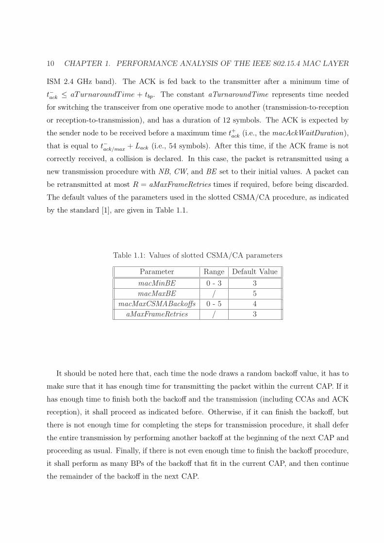
10 CHAPTER 1. PERFORMANCE ANALYSIS OF THE IEEE 802.15.4 MAC LAYER
ISM 2.4 GHz band). The ACK is fed back to the transmitter after a minimum time of
t−ack ≤ aTurnaroundT ime + tbp. The constant aTurnaroundTime represents time needed
for switching the transceiver from one operative mode to another (transmission-to-reception
or reception-to-transmission), and has a duration of 12 symbols. The ACK is expected by
the sender node to be received before a maximum time t+ack (i.e., the macAckWaitDuration),
that is equal to t−ack/max + Lack (i.e., 54 symbols). After this time, if the ACK frame is not
correctly received, a collision is declared. In this case, the packet is retransmitted using a
new transmission procedure with NB, CW, and BE set to their initial values. A packet can
be retransmitted at most R = aMaxFrameRetries times if required, before being discarded.
The default values of the parameters used in the slotted CSMA/CA procedure, as indicated
by the standard [1], are given in Table 1.1.
Table 1.1: Values of slotted CSMA/CA parameters
Parameter Range Default Value
macMinBE 0 - 3 3
macMaxBE / 5
macMaxCSMABackoffs 0 - 5 4
aMaxFrameRetries / 3
It should be noted here that, each time the node draws a random backoff value, it has to
make sure that it has enough time for transmitting the packet within the current CAP. If it
has enough time to finish both the backoff and the transmission (including CCAs and ACK
reception), it shall proceed as indicated before. Otherwise, if it can finish the backoff, but
there is not enough time for completing the steps for transmission procedure, it shall defer
the entire transmission by performing another backoff at the beginning of the next CAP and
proceeding as usual. Finally, if there is not even enough time to finish the backoff procedure,
it shall perform as many BPs of the backoff that fit in the current CAP, and then continue
the remainder of the backoff in the next CAP.

1.3. MARKOV CHAINS FOR THE SLOTTED CSMA/CA 11
1.3 Markov Chains for the Slotted CSMA/CA
In this section, we will briefly review the different Markov chain models available in the
literature which model the behavior of the IEEE 802.15.4 MAC protocol. We will then focus
in the next section on the model presented by Pollin et al. in [6], which is the model we will
be using for the present work.
The behavior of the slotted CSMA/CA in an IEEE 802.15.4 network has been widely
investigated in the literature using the same approach introduced by Bianchi [7] for the
traditional IEEE 802.11 CSMA/CA. In all these works, the behavior of the network is
analyzed through modeling a single node’s behavior with a discrete-time Markov chain. The
state of each node evolves through its corresponding Markov chain independently of other
nodes’ states except for when it is sensing the channel. As it was mentioned earlier, each node
can attempt a transmission only after it has sensed the channel idle for two consecutive time
slots (CCA1 and CCA2) after finishing its backoff. The probability that it senses the channel
idle in these two time slots depends on whether other nodes are transmitting or not. In all
the works discussed in this section, it is assumed that the probability of sensing the channel
idle is independent of the backoff stage in which CCA1 and CCA2 are performed. We will
base our model on the same assumption, but as we show in Section 1.6, these probabilities do
depend on the backoff stage their corresponding CCA is performed in. We will also discuss
the parameters that are most affected by this assumption.
To avoid any confusion, in the following discussion we will consistently refer to the proba-
bility of sensing the channel busy when performing CCA1 and CCA2 as α and β respectively,
independently of the notation used in the discussed work. Since the CCA states are the only
states in the Markov chain where the dependence of the nodes come into play, calculat-
ing α and β accurately is the key to the correct analysis of the network. For this reason,
in discussing the prior work, we will be mostly focused on the way these probabilities are
calculated as the main criteria for evaluating the accuracy of the models.
Misic et al. in [8] propose a Markov chain model to analyze the slotted CSMA/CA under
saturated and unsaturated traffic conditions in a beacon-enabled network in ACK mode.

12 CHAPTER 1. PERFORMANCE ANALYSIS OF THE IEEE 802.15.4 MAC LAYER
The superframe structure and the retransmissions are not considered in their model. In [9],
they extend the model of [8] in the unsaturated case, modeling also the superframe structure
and retransmissions. For the saturated case in [8], they construct a per-node Markov chain.
However, they only include one state for transmission, even though the transmission may
take more than one BP. They also do not include the corresponding states for the time spent
receiving and waiting for the ACK. Therefore, in the normalizing condition for the steady
state probabilities of the chain, the BPs spent for transmission and ACK are not accounted
for. Furthermore, even though when calculating α they do consider the ACK, they neglect
its effect when calculating β. Finally, when calculating both α and β, they implicitly assume
that the probability to start transmission is independent for all the nodes. But in fact,
this probability is highly correlated for different nodes since before a transmission a node
has to sense the channel idle for two BPs, and therefore, for two nodes to be transmitting
simultaneously, they have to have sensed the channel exactly at the same time. Since in such
a case both nodes observe the same channel state, the probability of two nodes transmitting
at the same BP is highly dependent. For the unsaturated condition in both [8] and [9], they
extend the Markov chain model of the saturated case, and therefore, all the aforementioned
issues apply to these cases as well. In neither case the analytical results are validated with
simulation.
It should be noted here that, in Bianchi’s work on IEEE 802.11 in [7], the transmission
states are also omitted from the chain. However, in that case this is justified and in fact
necessary due to the structural difference between the IEEE 802.11 and the IEEE 802.15.4
CSMA/CA mechanisms. In IEEE 802.11, nodes are constantly sensing the channel while
performing backoff, and freeze their backoff counter when there is a transmission on the
channel. This implies that even though the backoff states in the Markov chain in [7] do not
have a fixed duration, they all have the same expected duration. On the other hand, while
a node is transmitting, its transmission is never interrupted and therefore, the transmission
states cannot be included in the Markov chain model as they do not have the same expected
duration as the backoff states. Thus, in Bianchi’s model, all the states included in the
chain have the same expected duration, and therefore, the steady state probabilities are
well-defined. In IEEE 802.15.4, however, all transitions happen strictly at the boundaries
of backoff periods and no sensing is done during the backoff. Instead, the sensing is done
1.3. MARKOV CHAINS FOR THE SLOTTED CSMA/CA 13
only after the backoff during CCA1 and CCA2. This means that the backoff and sensing
states all have the same fixed duration of exactly one BP. Therefore, representing the entire
transmission (which lasts a fixed multiple of a BP) with only one state in the chain renders the
steady state probabilities ill-defined, because when they are calculated, states with different
duration are given the same weight.
2 4 6 8 10 12 14 16 18 200.2
0.4
0.6
0.8
1
1.2
1.4
1.6
1.8
N: Network Size
α
Pollin/Patro/Sahoo formula
Misic/Wen formula
simulation
2 4 6 8 10 12 14 16 18 200
0.1
0.2
0.3
0.4
0.5
0.6
0.7
0.8
N: Network Size
β
Pollin formula
Misic formula
Sahoo formula
Patro formula
Wen formula
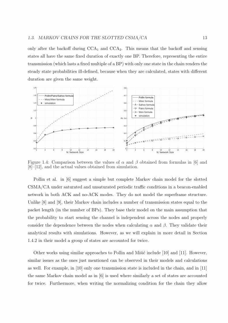
simulation
Figure 1.4: Comparison between the values of α and β obtained from formulas in [6] and[8]–[12], and the actual values obtained from simulation.
Pollin et al. in [6] suggest a simple but complete Markov chain model for the slotted
CSMA/CA under saturated and unsaturated periodic traffic conditions in a beacon-enabled
network in both ACK and no-ACK modes. They do not model the superframe structure.
Unlike [8] and [9], their Markov chain includes a number of transmission states equal to the
packet length (in the number of BPs). They base their model on the main assumption that
the probability to start sensing the channel is independent across the nodes and properly
consider the dependence between the nodes when calculating α and β. They validate their
analytical results with simulations. However, as we will explain in more detail in Section
1.4.2 in their model a group of states are accounted for twice.
Other works using similar approaches to Pollin and Misic include [10] and [11]. However,
similar issues as the ones just mentioned can be observed in their models and calculations
as well. For example, in [10] only one transmission state is included in the chain, and in [11]
the same Markov chain model as in [6] is used where similarly a set of states are accounted
for twice. Furthermore, when writing the normalizing condition for the chain they allow

14 CHAPTER 1. PERFORMANCE ANALYSIS OF THE IEEE 802.15.4 MAC LAYER
the backoff exponent to increase above macMaxBE. The packet discard probability is not
properly calculated either, as it does not include the cases where a packet fails the access
procedure during a retransmission.
In more recent works, Wen et al. in [12] use a proper Markov chain model, but they do
not consider the dependence in transmission probability of different nodes when calculating
α and β. Finally, in [13], Jung et al. propose a new model based on the Misic model in [9].
However, they too do not include all the transmission states in the Markov chain.
Figure 1.4 shows a comparison between the values of α and β obtained from the formulas
in the aforementioned works and those obtained from simulation. Note that in all cases,
we have plotted these parameters only for a network operating in no-ACK mode, with no
retransmissions, no superframe structure, and under saturated traffic condition. We see
that specially in the case of [8] and [12], the formulation for α and β offers an inacurate
approximation to the actual values of these parameters. This, as we mentioned before, is
due to the fact that they ignore the high dependence between the probabilities of starting
transmission for different nodes. All discussed models, except [8], [9], and [12], use the same
formulation for α. This is not the case for β, in which case, we note that Pollin et al’s model
offers the best estimate for most network sizes.
The IEEE 802.15.4 MAC features modelled in each of the works in [6] and [8]–[12] are
summarized in Table 1.2.
Table 1.2: Prior Work Summary
Model includesPollin Misic Misic Sahoo Patro Wen Jung
[6] [8] [9] [10] [11] [12] [13]
Saturated traffic Yes Yes No No Yes Yes No
Unsaturated traffic Yes Yes Yes Yes No Yes Yes
Retransmissions No No Yes Yes Yes No Yes
Superframe structure No No Yes No No No Yes
Correct # of TX states Yes No No No Yes Yes No
Correct # of CCA states No Yes Yes Yes No Yes Yes
1.4. SYSTEM MODEL AND NOTATION 15
1.4 System Model and Notation
In the present work, we will be using the Markov chain model presented by Pollin et al.
in [6], with some modifications, and will be mostly following the notation thereof, with
minor changes when necessary. Therefore, in this section, we will first describe this modified
Markov chain model and its corresponding formulation, and will then compare it to the
one presented in [6]. To validate our results, we will use simulations which reproduce the
CSMA/CA mechanism in IEEE 802.15.4. More details about the simulation are to come in
Section 1.5.
1.4.1 Markov Chain Model
In [6], the performances of a single hop LR-WPAN, made by N nodes and a PAN coordi-
nator (i.e., the sink in a WSN) have been evaluated for uplink traffic. Both saturated and
unsaturated periodic traffic conditions, and ACK and no-ACK modes have been considered.
We have focused our attention on the saturated case (i.e., when each of the N nodes in the
LR-WPAN, always has a packet available for transmission) in the no-ACK mode. The sat-
urated case reflects a sensor network scenario in which an event is detected by many sensor
nodes that want to transmit the gathered information, at the same time, to the sink node.
We will not be considering the superframe structure in our model, i.e., we are assuming that
the network is operating in a CAP with an infinite duration.
The behavior of a single node is modeled using a two-dimensional Markov chain, with
states represented by {s(t), c(t)} at a given backoff period t, as shown in Figure 1.5. Here-
after, we use the term time slot, or simply slot, to refer to a backoff period. All events
happen at the beginning of a time slot. At a given time slot t, the stochastic process
s(t) represents the backoff stage when s(t) ∈ {0, . . . ,M}, and the transmission stage when
s(t) = −1. When the node is in transmission (i.e., s(t) = −1), the stochastic process
c(t) ∈ {0, . . . , L− 1} represents the state of the transmission, i.e., the number of slots spent
on the current transmission. L is the packet size, measured in the number of slots it takes
for transmitting the packet, and includes the overhead introduced by the PHY and MAC

16 CHAPTER 1. PERFORMANCE ANALYSIS OF THE IEEE 802.15.4 MAC LAYER
headers. When the node is in backoff, c(t) ∈ {0, . . . , Wi − 1} represents the value of the
backoff counter, where Wi = 2min{macMinBE+i,macMaxBE} is the size of the backoff window at
backoff stage s(t) = i ∈ {0, . . . , M}. Finally, when the node is performing one of the CCAs,
c(t) represents the value of the CCA counter, with c(t) = 0 during CCA1 and c(t) = −1
during CCA2. Note that the state {s(t), c(t)} = {i, 0}, has to be seen as a CCA1 state and
not as a backoff state as in [6]. In fact, although the randomly picked backoff window size
at stage i can take any value in the set {0, . . . , Wi − 1}, the value zero indicates no waiting
and immediate sensing. In other words, if the backoff counter of a node is equal to zero, it
immediately starts sensing the channel (i.e., it performs CCA1).
� �
�����
��� �
�� �
�������
�����������������������������������������������������������������������������
����
����
��� �
β α��������� ���� �� � �
��������
�
β α��������� ���� ����
����
����
� � �
��������
�
β
β−�
�������� ���� ����
������ � �
��������
����������
�������� �������
���� ���������
α−�
α−�
α−�
β−�
β−�
��� �
��� �
����
����������������������������
Figure 1.5: Markov Model for slotted CSMA/CA.
The parameter α in Figure 1.5 is the probability of assessing the channel busy during
CCA1, and β is the probability of assessing it busy during CCA2, given that it was idle in
CCA1. In reality, the values of α and β for a given node depend not only on the backoff
stage of that node, but also on that of other nodes in the system. However, for simplicity,
we ignore this dependence and assume that the values of both α and β are the same for
different backoff stages and are also independent of the backoff stage of other nodes. This
assumption is used in all the prior work discussed in Section 1.3 and it is what allows us to
model the network by only analyzing the individual Markov chain of a node in the network
as shown in Figure 1.5. We will further scrutinize this assumption in Section 1.6. As it was

1.4. SYSTEM MODEL AND NOTATION 17
mentioned earlier, in this per-node Markov chain model, the effect of other nodes on the
behavior of a given node is captured only through the values of α and β, and therefore, these
two parameters play a key role in the model.
Let bi,k be the steady state probability of being in state {i, k}, i.e., bi,k = limt→∞ P{s(t) =
i, c(t) = k}. These steady-state probabilities are related to one another through the following
equations:
bi,k =Wi − k
Wi
bi,0 0 ≤ i ≤ M, 0 ≤ k ≤ Wi − 1 (1.3)
bi,0 = (1− y)ib0,0 1 ≤ i ≤ M (1.4)
bi,−1 = (1− α)bi,0 0 ≤ i ≤ M (1.5)
b−1,k = y
M∑j=0
bj,0 = yφ 0 ≤ k ≤ L− 1 (1.6)
where y = (1 − α)(1 − β), and φ is the probability that a randomly picked slot is spent
performing CCA1 which is given by
φ =M∑
j=0
bj,0 =1− (1− y)M+1
yb0,0. (1.7)
By determining the interactions between the N nodes on the medium, the expressions for
probabilities α and β have been derived in [6]. In short, the probability α, of finding channel
busy during the first CCA is given by
α = L[1− (1− φ)N−1
]y. (1.8)
In turn, β, the probability that there is a transmission in the medium when the considered
node does its second sensing, is given by
β =1− (1− φ)N
2− (1− φ)N. (1.9)

18 CHAPTER 1. PERFORMANCE ANALYSIS OF THE IEEE 802.15.4 MAC LAYER
The values of φ, α and β can be determined by imposing the following normalizing condition:
M∑i=0
Wi−1∑
k=0
bi,k +M∑i=0
bi,−1 +L−1∑
k=0
b−1,k = 1 (1.10)
which can be equivalently written as
b0,0
2
{[3− 2α + 2yL]
1− (1− y)M+1
y+ 2dW0
(1− y)d+1 − (1− y)M+1
y
+ W01− (2− 2y)d+1
2y − 1
}= 1 (1.11)
where W0 = 2macMinBE and d = macMaxBE−macMinBE.
As can be seen in Figure 1.6, (1.8) and (1.9) offer a good approximation to the values of α
and β for large network sizes. But for example at N = 2, the formulas introduce about 10%
and 30% approximation errors for α and β, respectively. As we will see in the next sections,
the impact of this error can be negligible when calculating some parameters of the network,
but for certain parameters, it has a noticeable negative impact.
2 4 6 8 10 12 14 16 18 200
0.1
0.2
0.3
0.4
0.5
0.6
0.7
0.8
0.9
1
N: Network Size
α
formula
simulation
2 4 6 8 10 12 14 16 18 200
0.1
0.2
0.3
0.4
0.5
0.6
0.7
0.8
0.9
1
N: Network Size
β
formula
simulation
Figure 1.6: Comparison between the values of α and β obtained from (1.8) and (1.9), andthose obtained from simulation.

1.4. SYSTEM MODEL AND NOTATION 19
1.4.2 Discussion of the Pollin Model
As was mentioned earlier, the model described in the previous section closely follows that of
Pollin model. However, there were some necessary modifications made to that model which
we list here.
The main assumptions: The main assumptions that enable us to use the described Markov
chain model are the following:
A1. The probability to start sensing the channel, φ, is independent across nodes;
A2. The probability to sense the channel busy during CCA1 and CCA2 does not depend
on the backoff stage where the corresponding CCA is performed. In other words,
αi = α and βi = β for i ∈ {0, . . . , M};
A3. The probability that a node is in a given backoff stage, is independent of that of other
nodes;
A4. The probability of sensing the channel busy during a CCA does not depend on the
random backoff value drawn in the backoff stage preceding the CCA.
In [6], A1 is the only stated assumption. In what follows, specially in Section 1.6, we will
discuss the significance of these assumptions .
The normalizing condition of the Markov chain steady state probabilities: In [6]
the following equation is given as the normalizing condition for the steady state probabilities:
M∑i=0
Wi−1∑
k=0
bi,k +M∑i=0
bi,−1 +M∑i=0
bi,−2 +L−1∑
k=0
b−1,k = 1 (1.12)
where bi,−1 and bi,−2 in their notation correspond to the first and second CCA, respectively.
On the other hand, states bi,0 also correspond to the first CCA, because, as we mentioned
earlier, when the backoff counter reaches zero, the node will immediately start sensing.
Even though the Markov chain depicted in [6] does not contain any state bi,0, in the above
normalizing condition, both of the states bi,0 and bi,−1 are counted and therefore, the states
bi,0, as per our notation, are counted twice. This normalizing condition together with (1.7),
(1.8), and (1.9) constitute a system of equations that is used in [6] to numerically obtain α,

20 CHAPTER 1. PERFORMANCE ANALYSIS OF THE IEEE 802.15.4 MAC LAYER
β, and φ. Therefore, the aforementioned overcount in the normalizing condition affects the
values obtained for these variables.
1.5 Results
In this section, we use the Markov chain model to calculate different important parameters
of the system, such as delay, energy consumption, throughput and efficiency.
In order to validate the analytical results, we simulate the behavior of the slotted CSMA/CA
using an event-driven simulator written in Matlab. We reproduce the network under the
same conditions of the analytical model, i.e., we analyze the channel access mechanism in
the no-ACK mode, and disregarding the superframe structure. It should be noted that for
the simulation we do not make any assumption on the dependence of the nodes or backoff
stages, and therefore, the simulation truly reflects the behavior of the network under the
aforementioned conditions, and not the behavior of the Markov chain model.
In what follows, all the parameters have been defined as functions of α, β and φ. In [6],
φ is calculated by numerically solving their corresponding (1.8) – (1.10). In our work, when
plotting the curves from the analytical formulation to validate their accuracy, we use the
value of φ found by simulation, and then calculate α, β, and the rest of the parameters from
φ. These curves are indicated in the figures’ legends by “formula”.
For the MAC parameters, we use the default values defined by the standard (see Table
1.1) and fix the packet length for all nodes to L = 7 time slots. The simulation is run for a
duration of T = 108 slots.
1.5.1 Average Delay
In the no-ACK mode, the average delay for a successfully transmitted packet, i.e., the number
of slots it takes from the moment it reaches the head of the line to the moment it arrives at
its destination, is given by
D = nBsuc
+ nCsuc
+ L (1.13)

1.5. RESULTS 21
where nBsuc
and nCsuc
are the mean number of slots spent performing backoff and CCA,
respectively, before a successful transmission. The average delay calculated above, can be
equivalently viewed as the packet service time in a saturated IEEE 802.15.4 network of
queues.
Note that based on assumptions A2 and A3, the number of slots spent in backoff or
CCA before transmission for packets that are successfully transmitted and those that end
up having a collision should be the same, i.e., nBsuc
= nBcol
= nBtx
and nCsuc
= nCcol
= nCtx
.
For this reason, in Section 1.5.3, we obtain the expressions for the values of nBtx
and nCtx
,
which we use to calculate the delay as described above.
2 4 6 8 10 12 14 16 18 2016
18
20
22
24
26
28
30
32
34
36
N: Network Size
Ave
rage
Del
ay (
time
slot
s)
formula
simulation
Figure 1.7: Comparison between formula and simulation values for D.
As can be seen in Figure 1.7, the value of delay calculated from (1.13) and that obtained
from simulation have a constant difference of about two slots for all values of network size
N . This difference is due to assumption A2. A similar difference is observed in the values of
nBtx
and nCtx
as we will see in Section 1.5.3, where we will discuss this issue in more detail.
1.5.2 Average Power Consumption
For every packet that is transmitted or discarded, the node uses different power levels de-
pending on whether it is in backoff, sensing, or transmission. Therefore, the average power
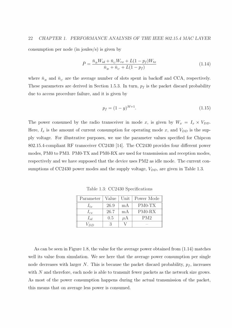
22 CHAPTER 1. PERFORMANCE ANALYSIS OF THE IEEE 802.15.4 MAC LAYER
consumption per node (in joules/s) is given by
P =n
BWid + n
CWrx + L(1− pf )Wtx
nB
+ nC
+ L(1− pf )(1.14)
where nB
and nC
are the average number of slots spent in backoff and CCA, respectively.
These parameters are derived in Section 1.5.3. In turn, pf is the packet discard probability
due to access procedure failure, and it is given by
pf = (1− y)M+1. (1.15)
The power consumed by the radio transceiver in mode x, is given by Wx = Ix × VDD.
Here, Ix is the amount of current consumption for operating mode x, and VDD is the sup-
ply voltage. For illustrative purposes, we use the parameter values specified for Chipcon
802.15.4-compliant RF transceiver CC2430 [14]. The CC2430 provides four different power
modes, PM0 to PM3. PM0-TX and PM0-RX are used for transmission and reception modes,
respectively and we have supposed that the device uses PM2 as idle mode. The current con-
sumptions of CC2430 power modes and the supply voltage, VDD, are given in Table 1.3.
Table 1.3: CC2430 Specifications
Parameter Value Unit Power Mode
Itx 26.9 mA PM0-TX
Irx 26.7 mA PM0-RX
Iid 0.5 µA PM2
VDD 3 V –
As can be seen in Figure 1.8, the value for the average power obtained from (1.14) matches
well its value from simulation. We see here that the average power consumption per single
node decreases with larger N . This is because the packet discard probability, pf , increases
with N and therefore, each node is able to transmit fewer packets as the network size grows.
As most of the power consumption happens during the actual transmission of the packet,
this means that on average less power is consumed.

1.5. RESULTS 23
2 4 6 8 10 12 14 16 18 200.01
0.015
0.02
0.025
0.03
0.035
0.04
N: Network Size
Ave
rage
Pow
er (
joul
es/s
ec)
formula
simulation
Figure 1.8: Comparison between formula and simulation values for P .
1.5.3 Mean Number of Backoffs and CCAs
As we saw earlier, in order to calculate the average delay and the average power consump-
tion, we need to know how many slots on average a node spends performing backoff and
CCA before transmitting or discarding every packet. In this section, we will derive these
parameters using the Markov chain model described earlier.
Mean Number of Backoffs
The average number of backoffs a transmitted packet goes through, nBtx
, is different from
that of a discarded packet, nBf
. This is because a discarded packet always goes through all
the backoff stages of the chain before exiting it, whereas a transmitted packet might exit the
chain from any backoff stage.
The mean number of slots spent in backoff stage i, every time it is entered, is given
by (Wi − 1)/2. This is because the backoff value is drawn according to a discrete uniform
distribution in [0,Wi−1]. Therefore, nBtx
, the mean number of backoffs before transmission,
is given by
nBtx
=M∑i=0
(i∑
k=0
Wk − 1
2
)p
Si
1− pf
(1.16)

24 CHAPTER 1. PERFORMANCE ANALYSIS OF THE IEEE 802.15.4 MAC LAYER
where pSi
is the probability that the channel access procedure ends successfully (i.e., the
packet is sent) in backoff stage i and it is given by
pSi
= y(1− y)i , 0 ≤ i ≤ M. (1.17)
After a bit of algebra, we obtain
nBtx
=1
1− pf
{W0y
1− (2− 2y)d+1
2y − 1− 1− y
2y− W0 + 1
2+ 2d−1W0
(3 +
1− y
y
)(1− y)d+1
−[W02
d−1(1− d)− W0 + 1
2+
(W02
d − 1
2
)(1− y
y
)](1− y)M+1
}. (1.18)
2 4 6 8 10 12 14 16 18 208
10
12
14
16
18
20
22
24
26
N: Network Size
E[#
bac
koffs
bef
ore
tran
smis
sion
] (t
ime
slot
s)
formula with αconst
formula with αi
simulation
(a) nBtx from simulation compared to its value from formulaapplied to the constant α, and to αi.
2 4 6 8 10 12 14 16 18 2050
55
60
65
N: Network Size
E[#
bac
koffs
bef
ore
failu
re]
(tim
e sl
ots)
formula
simulation
(b) nBffrom simulation and formula applied to constant α.
Figure 1.9: Comparison between formulas and simulation values for nBtx
and nBf
.
Figure 1.9(a) shows the value of nBtx
obtained from (1.16) and that obtained from simu-
lation. As we see here, there is an almost constant difference of less than two slots between
the analytical and simulation results. This is again due to assumption A2. For this reason,
in the same figure we have also plotted the value of nBtx
calculated using the actual values
of αi and βi for every backoff stage i obtained from simulation. In this case, the value of

1.5. RESULTS 25
nBtx
is still given by (1.16), but pSi
has to be calculated using the following expression
pSi
=
y0, i = 0,
yi
i−1∏
k=0
(1− yk), 1 ≤ i ≤ M(1.19)
where yi = (1− αi)(1− βi). Also, the probability pf has to be calculated as follows
pf =M∏
k=0
(1− yk). (1.20)
In turn, a packet is discarded when the node goes through every backoff stage in the chain
and fails to access the channel in all the M + 1 consecutive backoff stages. Therefore, nBf
,
the mean number of slots spent in backoff before an access procedure failure, is given by
nBf
=M∑
k=0
(Wk − 1
2
)p
SM
pf
=M∑
k=0
Wk − 1
2= W02
d
(1 +
M − d
2
)− W0 + M + 1
2. (1.21)
As seen in (1.21), nBf
is not a function of α and β and therefore, the expression is valid
independently of assumption A2. Moreover, nBf
is not a function of N , because every
discarded packet goes through all the backoff stages, and hence, the number of slots spent
in backoff for a discarded packet only depends on the random backoff value drawn at every
backoff stage. Assuming A4, for a given backoff stage i, an average of (Wi − 1)/2 slots
are spent in backoff before performing the CCA. Figure 1.9(b) shows the value of nBf
from
simulation and formula. We see here that the value obtained from (1.21) is very close
but always slightly lower than the one obtained from simulation. This is because α is not
completely independent of the random backoff value drawn. In fact, the packets that end
up being discarded are those that are less “fortunate” and draw a larger backoff value.
Finally, for a generic packet, the mean number of slots that a node spends in backoff
before transmitting or discarding the packet, is given by
nB
= nBtx
(1− pf ) + nBf
pf . (1.22)

26 CHAPTER 1. PERFORMANCE ANALYSIS OF THE IEEE 802.15.4 MAC LAYER
Mean Number of CCAs
For a packet to be transmitted, a node needs to succeed in the access procedure in some
backoff stage. If the access procedure succeeds in stage i, it means that it had two successful
CCAs in that stage, and at least one failed CCA in stages 0 to i− 1. In other words, it must
have had k successful CCA1’s and failed CCA2’s, for some k ≤ i, and i − k failed CCA1’s.
This event happens with probability
pfi,k=
(i
k
)[(1− α)β]k · αi−k. (1.23)
In this case, there will be a total of i + k CCAs performed during the failed accesses plus
an additional two successful CCAs at stage i where the access procedure succeeds. Thus,
considering that the successful access at stage i happens with probability y, the mean number
of CCAs before a successful access procedure is given by
nCtx
= y
M∑i=0
i∑
k=0
(i + k + 2)pfi,k
1− pf
(1.24)
= 2 + [2(1− y)− α]
[1
y− (M + 1)
(1− y)M
1− pf
].
In the case of an access procedure failure, there are M + 1 failed attempts and no successful
consecutive CCAs. Therefore, the mean number of CCAs due to an access failure is given
by
nCf
=M+1∑
k=0
(M + 1 + k)pfM+1,k
pf
= (M + 1)
(2− α
1− y
). (1.25)
Figure 1.10(a), shows the value of nCtx
obtained from (1.24) and from simulation. As in
the case of nBtx
, we see here that there is a difference (although smaller) between simulation
and formula. We conjecture that this difference is also due to assumption A2. However, we
will not validate this conjecture here, since calculating nCtx
as a function of αi and βi is a lot
more complicated than calculating it for a constant α and β. This is because to calculate
nCtx
as a function of αi and βi, we have to consider each different possible success sequence
separately. In other words, when we assume that α and β are constant, we only need to

1.5. RESULTS 27
2 4 6 8 10 12 14 16 18 202.5
3
3.5
4
N: Network Size
E[#
CC
As
befo
re s
ucce
ss]
(tim
e sl
ots)
formula
simulation
(a) nCtx from simulation and formula.
2 4 6 8 10 12 14 16 18 205.6
5.65
5.7
5.75
5.8
5.85
5.9
5.95
6
6.05
6.1
N: Network Size
E[#
CC
As
befo
re fa
ilure
] (t
ime
slot
s)
formula with αP
formula with αsim
simulation
(b) nCffrom simulation compared to its value obtained from
formula applied to αP (α calculated from formula proposed byPollin et. al), and to αsim (α from simulation).
Figure 1.10: Comparison between formula and simulation values for nCtx
and nCf
.
consider the number of CCA1’s and CCA2’s performed before a transmission. But when α
and β are a function of the backoff stage, we also need to consider what exactly happens in
each backoff stage for all possible cases.
The value of nCf
obtained from analysis and simulation is compared in Figure 1.10(b). In
this figure, we have plotted two different curves for the value of nCf
from formula. Indicated
by “formula with αP ” is what we have been thus far indicating by only “formula”, and it
is basically found by applying (1.25) to α and β as derived from (1.8) and (1.9). Instead,
the curve indicated by “formula with αsim” is plotted by applying the same equation to
the value of α and β directly obtained from simulation. We see that in the latter case, we
get significantly better results. This means that the difference between the simulation and
formula is not due to any inaccuracy in (1.25), but due to the inaccuracy in calculating α
and β using (1.8) and (1.9) for small values of N . This inaccuracy was also evidenced in
Figure 1.6.
Finally, the mean number of CCAs for a generic packet is given by
nC
= nCtx
(1− pf ) + nCf
pf . (1.26)
28 CHAPTER 1. PERFORMANCE ANALYSIS OF THE IEEE 802.15.4 MAC LAYER
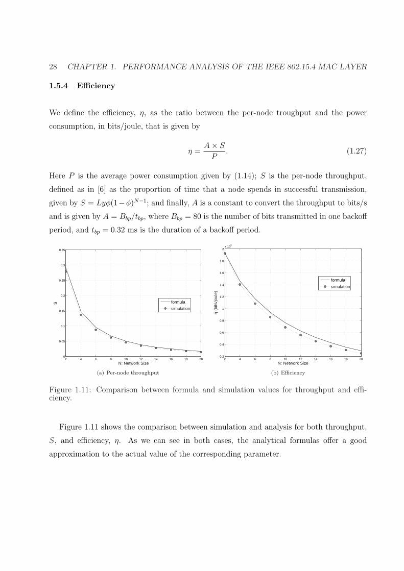
1.5.4 Efficiency
We define the efficiency, η, as the ratio between the per-node troughput and the power
consumption, in bits/joule, that is given by
η =A× S
P. (1.27)
Here P is the average power consumption given by (1.14); S is the per-node throughput,
defined as in [6] as the proportion of time that a node spends in successful transmission,
given by S = Lyφ(1−φ)N−1; and finally, A is a constant to convert the throughput to bits/s
and is given by A = Bbp/tbp, where Bbp = 80 is the number of bits transmitted in one backoff
period, and tbp = 0.32 ms is the duration of a backoff period.
2 4 6 8 10 12 14 16 18 200
0.05
0.1
0.15
0.2
0.25
0.3
0.35
N: Network Size
S
formula
simulation
(a) Per-node throughput
2 4 6 8 10 12 14 16 18 200.2
0.4
0.6
0.8
1
1.2
1.4
1.6
1.8
2x 10
6
N: Network Size
η (b
its/jo
ule)
formula
simulation
(b) Efficiency
Figure 1.11: Comparison between formula and simulation values for throughput and effi-ciency.
Figure 1.11 shows the comparison between simulation and analysis for both throughput,
S, and efficiency, η. As we can see in both cases, the analytical formulas offer a good
approximation to the actual value of the corresponding parameter.

1.6. ANALYSIS OF THE MODEL ASSUMPTIONS 29
1.6 Analysis of the Model Assumptions
1.6.1 Dependence of α and β on the Backoff Stage
As was mentioned earlier, in the Markov chain model of Figure 1.5, it was assumed for
simplicity that the probability of sensing the channel busy during CCA1 and CCA2 at a
given time t was independent of the backoff stage the node is in (assumption A2). This
allowed us to use a constant value for both α and β for all backoff stages, which in turn
greatly simplified the derivations and analysis which followed. But as we saw in the previous
section, when calculating the value of certain parameters, such as nBtx
, nCtx
, and therefore
the average delay D; this assumption does not result in a very good approximation of those
parameters.
2 3 4 5 6 7 8 9 100
0.1
0.2
0.3
0.4
0.5
0.6
0.7
0.8
0.9
1
N: Network Size
α
α0
α1
α2, α
3, α
4
αconst
(a) α for different backoff stages
2 3 4 5 6 7 8 9 100
0.1
0.2
0.3
0.4
0.5
0.6
0.7
0.8
0.9
1
N: Network Size
β
β0
β1
β2, β
3, β
4
βconst
(b) β for different backoff stages
Figure 1.12: Dependence of α and β on the backoff stage.
Figure 1.12 shows the values of αi and βi for each backoff stage i. As we see here, α is in
fact very dependent on the backoff stage. This difference is particularly noticeable between
the first backoff stage (i = 0) and the rest of the backoff stages. This can be explained by
observing that a node that is in the first backoff stage on average draws a smaller backoff
value than other nodes that are competing with it. Additionally, the joint probability of two
nodes being in the first backoff stage is particularly small (as we will see in Section 1.6.2).

30 CHAPTER 1. PERFORMANCE ANALYSIS OF THE IEEE 802.15.4 MAC LAYER
4 6 8 10 12 14 16 18 200
0.1
0.2
0.3
0.4
0.5
0.6
0.7
0.8
γ(N
)
N: Network Size
Figure 1.13: Dependence metric, γ(N).
This means that a node that is in the first backoff stage is given an opportunity with not
much competition compared to when it is in any other stage. Therefore, it is very likely for it
to find the channel idle. We further see that most of this dependence is absorbed by the first
CCA as when it comes to β, different backoff stages experience a very similar probability of
finding the channel busy.
1.6.2 Dependence of the Backoff Stage of a Node on That of Other Nodes
Figure 1.13 shows the dependence of the backoff stage of a node on that of other nodes. The
dependence metric γ(N) is defined as the maximum relative difference between the joint
probability and the product of the marginal probabilities of two nodes N1 and N2 being in
backoff stages i and j respectively, when there are N nodes in the network. In other words,
γ(N) = maxi,j
{fS1,S2|N(i, j)− fS1|N(i)fS2|N(j)
fS1,S2|N(i, j)
}(1.28)
where Si is the random variable indicating the backoff stage of node i at a randomly chosen
time slot in the steady state, and fX(x) indicates the probability mass function (pmf) of the
random variable X at a given point x.
As we see in Figure 1.13, for small number of nodes, there is a strong dependence be-

1.6. ANALYSIS OF THE MODEL ASSUMPTIONS 31
0
1
2
3
4
0
1
2
3
40
0.02
0.04
0.06
0.08
0.1
0.12
0.14
0.16
S1S2
f S1,
S2
| N=
2
0.02
0.04
0.06
0.08
0.1
0.12
0.14
(a) N = 2
0
1
2
3
4
0
1
2
3
40.01
0.02
0.03
0.04
0.05
0.06
0.07
0.08
S1S2
f S1,
S2
| N=
20
0.02
0.03
0.04
0.05
0.06
0.07
(b) N = 20
Figure 1.14: Joint pmf of the backoff stages of two nodes fS1,S2|N(i, j).
tween the backoff stages of different nodes. However, as the network grows, this dependence
becomes less and less noticeable.
Figure 1.14(a) shows the joint pmf for the backoff stages of two nodes for the two cases
of N = 2 and N = 20. We see that for N = 2, with high probability, at least one node is in
the first backoff stage, while the other is in one of the other backoff stages. In this case, the
probability of both nodes being in higher backoff stages simultaneously is extremely small.
This indicates a high chance of successful transmission for N = 2 (and in general for small
numbers of nodes). The situation is quite different in a network with a larger number of
nodes. We see in Figure 1.14(b) that for N = 20, the nodes spend more time in the higher
backoff stages of the chain, indicating a greater chance of failure. However, we observe that
in both cases, even though the probability of a node being in the first backoff stage is not
small (each packet has to go through the first backoff stage once in its lifetime irrespective of
the value of N), the joint probability of two nodes being in the first backoff stage is relatively
very small. As we mentioned earlier, this explains why α0 is different from αi for i > 0.

32 CHAPTER 1. PERFORMANCE ANALYSIS OF THE IEEE 802.15.4 MAC LAYER
1.7 Conclusion and Outlook
ZigBee, with IEEE 802.15.4 as its link and access technology, will undoubtedly play a central
part in the growth of the Internet of Things (IoT), the wireless, and heterogeneous extension
of the wireline Internet. This can not only be attributed to its large international support
by major vendors but also to its sufficiently good performance. This performance behavior
has been the focus of this chapter, where we concentrated solely on the MAC assuming PHY
and networking protocols given.
After having reviewed key parameters contributing to the MACs performance behavior
and prior publications in this field, we have moved on to its characterization and then
analysis. We have exposed the correct mathematical formulation of the throughput, delay
and energy efficiency behavior as a function of the number of contenting nodes, the packet
length, the depth of the backoff stage, etc. This formulation can then be used to tune the
system parameters in order to optimize a given metric, e.g., efficiency.
In the process of developing the aforementioned formulation, we have also been able to
pinpoint the reasons why the results obtained from event simulations sometimes differ from
those gathered from a Markov-chain-based analysis. This identifies the limitations of this
popular approach, thereby facilitating its adequate utilization.
At the same time, several important issues have not been touched upon, be it because
no analytical expressions are available yet or due to space limit. Far from being exhaustive,
some of these are summarized below and subsequently discussed in greater details:
• impact of finite buffer lengths;
• non-saturated traffic conditions;
• impact of capture effect due to shadowing;
• relayed traffic in more complicated topologies;
• parametric mapping to known WSN MAC families;
• extension to emerging IEEE 802.15.4e, .15.4g and .15.4f MACs.
Finite buffers lead to buffer overflows and hence to additional packet losses which have so
far not been catered for. These losses are non-linear functions of the packet arrival rate and

1.7. CONCLUSION AND OUTLOOK 33
the buffer length. To include this in the current analysis, some additional transitions need
to be introduced into the Markov state diagram.
Current analysis only caters for saturated traffic conditions, i.e. every node has always a
packet to transmit. To extend the analysis rigorously to any possible traffic arrival conditions,
additional states and transitions need to be introduced. However, some simplifying heuristics
can be invoked using a binomial expansion of active nodes and the results of the above
exposed theory.
Capture is referred to the effect when a node can receive a packet even though more
than one transmission happens simultaneously. This is facilitated by shadowing at link level
where an ongoing transmission is not perturbed simply because the receiver is shadowed by
larger objects from any other ongoing transmission. A rigorous analysis of the capture effect
is quite involved but, again, involving some simplifying heuristics may help finding a suitable
solution.
Relayed traffic is — in a sense — redundant traffic since it involves the re-transmission
of already received information. It clearly impacts end-to-end delay and throughput, as well
as the systems energy efficiency. Relayed packets are also usually treated differently from
newly generated packets. All this is currently not reflected in the analysis where a rigorous
approach is again seen to be prohibitively complex.
As already alluded to in the introduction, MACs for WSNs typically follow the following
taxonomy: framed MACs for delay-constrained high traffic loads; contention-based MACs
with common active periods for medium traffic loads; duty-cycled sampling protocols for low
traffic loads; and hybrids thereof [4]. These have proved to be optimum under respective
traffic conditions. A formal derivation of IEEE 802.15.4 MAC parameters realizing these
MACs is still an open problem and certainly worth investigating.
Finally, novel MAC families are emerging at the time of the writing of this book. These are
mainly the IEEE 802.15.4e, .15.4g and .15.4f MACs, where the first is for delay-constrained
embedded system solutions, the second for active RFID systems, and the last for smart
utility networks. Applying the derived analysis and synthesis to these emerging standards
34 CHAPTER 1. PERFORMANCE ANALYSIS OF THE IEEE 802.15.4 MAC LAYER
is an open issue deserving attention.
References
[1] IEEE std. 802.15.4. Part. 15.4: Wireless Medium Access Control (MAC) and Phys-
ical Layer (PHY) Specifications for Low-Rate Wireless Personal Area Networks (LR-
WPANs). IEEE standard for Information Technology, IEEE-SA Standards Board, Sept.
2006.
[2] IETF WG. IPv6 over Low power Wireless Personal Area Networks. Available online:
http://tools.ietf.org/wg/6lowpan/.
[3] IETF WG. Routing Over Low Power and Lossy Networks. Available online:
http://tools.ietf.org/wg/roll/.
[4] A. Bachir, M. Dohler, T. Watteyne, and K.K. Leung. MAC Essentials for Wireless
Sensor Networks. IEEE Communications Surveys and Tutorials, to appear.
[5] IEEE std. 802.11. Information Technology - Telecommun. and Information Exchange
between Systems. Local and Metropolitan Area Networks. Specific Requirements. Part
11: Wireless LAN MAC and PHY Specifications. ANSI/IEEE Std. 802.11, ISO/IEC
8802-11, 1st edition, 1999.
[6] S. Pollin, M. Ergen, S. C. Ergen, B. Bougard, L. Van der Perre, I. Moermann, A. Bahai,
P. Varaiya, and F. Catthoor. Performance Analysis of Slotted Carrier Sense IEEE
802.15.4 Medium Access Layer. IEEE Transactions on Wireless Communications, 7(9),
Sept. 2008.
[7] G. Bianchi. Performance Analysis of the IEEE 802.11 Distributed Cooridination Func-
tion. IEEE Journal on Selected Areas in Communications, 18(3):535–547, 2000.
[8] J. Misic, S. Shafi, and V. B. Misic. The Impact of MAC Parameters on the Performance
of 802.15.4 PAN. Ad Hoc Networks, 3(5):509–528, Sept. 2005.
[9] J. Misic and V. B. Misic. Access Delay for Nodes with Finite Buffers in IEEE 802.15.4
Beacon Enabled PAN with Uplink Transmissions. Computer Communications, 28(10),
Jun. 2005.
[10] P.K. Sahoo and J. Sheu. Modeling IEEE 802.15.4 based Wireless Sensor Network with
packet retry limits. In Proc. of the 5th ACM Symposium on Performance Evaluation of
1.7. CONCLUSION AND OUTLOOK 35
Wireless Ad Hoc, Sensor, and Ubiquitous Networks, Canada, Oct. 2008.
[11] R. K. Patro, M. Raina, V. Ganapathy, M. Shamaiah, and C. Thejaswi. Analysis and
improvement of contention access protocol in IEEE 802.15.4 star network. In Proc of
IEEE Internatonal Conference on Mobile Adhoc and Sensor Systems (MASS’07), 2007.
[12] H. Wen, C. Lin, Z.J. Chen, H. Yin, T. He, and E. Dutkiewicz. An Improved Markov
Model for IEEE 802.15. 4 Slotted CSMA/CA Mechanism. Journal of Computer Science
and Technology, 24(3):495–504, 2009.
[13] C.Y. Jung, H.Y.Hwang, D.K.Sung, and G.U.Hwang. Enhanced Markov Chain Model
and Throughput Analysis of the Slotted CSMA/CA for IEEE 802.15.4 Under Unsat-
urated Traffic Conditions. IEEE Transactions on Vehicular Technology, 58(1), Jan.
2009.
[14] Chipcon Products from Texas Instruments. CC2430 Preliminary Data Sheet (rev. 2.1)
SWRS036F, Jun. 2007.