bone segmentation in ct-liver images using k-means clustering …€¦ · · 2014-10-29bone...

Bone Segmentation in CT-Liver images using K-Means Clustering

for 3D Rib Cage Surface-Modeling

Walita NARKBUAKAEW1, Hiroshi NAGAHASHI2, Kota AOKI2, Yoshiki KUBOTA3

1Interdisciplinary Graduate School of Science and EngineeringTokyo Institute of Technology, Kanagawa, Japan

2Imaging Science and Engineering LaboratoryTokyo Institute of Technology, Kanagawa, Japan

3Gunma University Heavy-Ion Medical Center, Gunma, [email protected], [email protected],[email protected], and y [email protected]

Abstract: A 3D rib cage model helps to study anatomical structures in some medical applications suchas biomechanical and surgical operations. Its quality directly depends on rib cage segmentation if it isreconstructed from image data. This paper presents an optional segmentation method based on K-meansclustering. It uses a hierarchical concept to control the clustering, and it organizes clustered regions insubsequent indexes of background, soft-tissue, and hard-tissue regions. We applied the proposed methodto 3D CT-liver images acquired by a 4D-CT imaging system. The proposed method was comparedwith 2D K-means (KM) and 2D fuzzy C-means (FCM) clustering. From our experiment, the proposedmethod gave more stable clustering results under a condition of randomization in initial cluster-centers,and it performed faster than 1.5 times of 2D-KM and 7.7 times of 2D-FCM on average. For 3D surfacemodels, the results of the proposed method provided more information of bone regions in vertebra, ribs,and scapula areas than results of 2D-KM and 2D-FCM.

Key–Words: 2D K-mean clustering, 2D fuzzy C-mean clustering, and rib cage segmentation

1 Introduction

Rib cage [1] is a fundamental structure that protects

heart and lungs, and it supports respiration. It is

formed by sternum and costal cartilages, vertebral col-

umn, and ribs. In addition, a 3D model of the rib cage

probably assists in studying scoliosis, biomechanics,

and surgical operation [2, 3, 4].

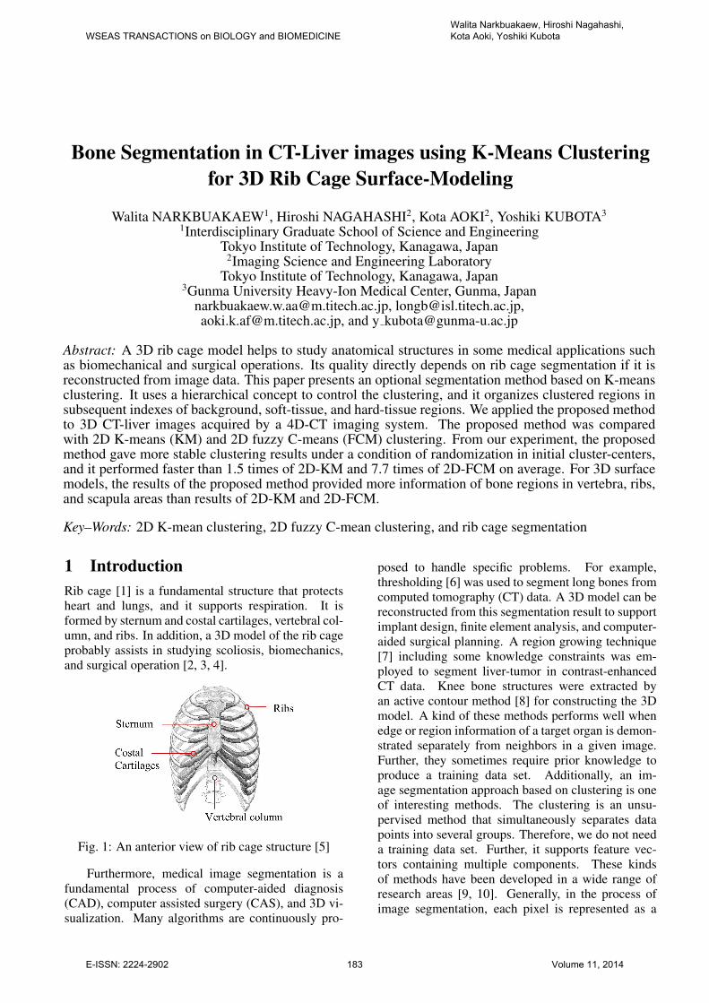
Fig. 1: An anterior view of rib cage structure [5]

Furthermore, medical image segmentation is a

fundamental process of computer-aided diagnosis

(CAD), computer assisted surgery (CAS), and 3D vi-

sualization. Many algorithms are continuously pro-

posed to handle specific problems. For example,

thresholding [6] was used to segment long bones from

computed tomography (CT) data. A 3D model can be

reconstructed from this segmentation result to support

implant design, finite element analysis, and computer-

aided surgical planning. A region growing technique

[7] including some knowledge constraints was em-

ployed to segment liver-tumor in contrast-enhanced

CT data. Knee bone structures were extracted by

an active contour method [8] for constructing the 3D

model. A kind of these methods performs well when

edge or region information of a target organ is demon-

strated separately from neighbors in a given image.

Further, they sometimes require prior knowledge to

produce a training data set. Additionally, an im-

age segmentation approach based on clustering is one

of interesting methods. The clustering is an unsu-

pervised method that simultaneously separates data

points into several groups. Therefore, we do not need

a training data set. Further, it supports feature vec-

tors containing multiple components. These kinds

of methods have been developed in a wide range of

research areas [9, 10]. Generally, in the process of

image segmentation, each pixel is represented as a

WSEAS TRANSACTIONS on BIOLOGY and BIOMEDICINEWalita Narkbuakaew, Hiroshi Nagahashi, Kota Aoki, Yoshiki Kubota

E-ISSN: 2224-2902 183 Volume 11, 2014

feature vector containing one or many components.

These components can be selected from the possible

features of geometry, texture, and gradient [11, 12].

Then, the pixel is clustered into an appropriate group

through an objective function that is designed to mea-

sure a distance or a similarity. For instance, Mignotte

M. [13] applied K-means clustering algorithm to dif-

ferent color channels and integrated the results in the

segmentation of natural images. Lee, T.H. et al. [14]

used K-means clustering to segment normal and ab-

normal regions in CT brain images. Then, a deci-

sion tree based on six features was constructed to

classify the abnormal regions. Further, they used an

expectation-maximization (EM) algorithm to extract

cerebrospinal fluid (CSF) and brain matter. Juang,

L.H. et al. [15] introduced a tumor tracking method

by applying K-means clustering to the MRI brain im-

ages in converted color-spaces. Yusoff I.A. et al. [16]

proposed an image segmentation method base on two-

dimensional clustering for natural-and cervical cells

images. Then, they introduced a method to deter-

mine the number of clusters in [17]. Selvy P.T. et

al. [18] examined MRI brain image segmentation

to detect Cerebrospinal Fluid (CSF). They combined

anisotropic diffusion and total variation regularization

with Fuzzy C-Means to handle image noise. Then,

they [19] applied a particle swarm optimization to

achieve a global optimal solution. Chu et al. [20] used

a clustering method to divide an atlas database for ac-

quiring the best matching between a given image and

a template image. Next, they constructed a dynamic

weight function and used maximum a posterior prob-

ability (MAP) estimation to perform multi-organ seg-

mentation. Actually, many studies presented their at-

tractive results under particular features and extension

of an objective function that possibly causes complex-

ity of computation. Further, most of these studies did

not mention about indexing that is necessary to iden-

tify some parts of all clustering regions. Therefore,

we are motivated to use the clustering method for rib

cage segmentation, which directly influences quality

of 3D surface reconstruction.

Indeed, we attempt to develop a segmentation

method under simple conditions to achieve a good

quality of 3D rib cage model. This paper presents a

2D K-means clustering method including a hierarchi-

cal concept and cluster indexing. We apply the pro-

posed method to 10 sets of 3D CT-liver images, which

were acquired by a 4D-CT imaging system. Then, the

proposed method is compared with 2D K-Means and

2D Fuzzy C-Means clustering by investigating differ-

ent points in clustered regions, stability in results of

clustering, and computation time.

The rest of this paper is organized as follows.

Section 2 briefly describes concepts of related meth-

ods. Then, we explain the proposed method in section

3. Next, section 4 shows experimental results. Lastly,

we summarize this study in section 5.

2 Related Method

2.1 K-means clustering (KM)

The K-mean clustering [21] is normally introduced to

divide data points X = {x1, . . . , xN} into K clusters.

It supports multi-dimensional vectors and gives high

efficiency of computation. The purpose of this algo-

rithm is to minimize the objective function of

JKM =

N∑

n=1

K∑

k=1

bnk‖xn − ck‖2, (1)

bnk =

{

1 if k = argmina ‖xn − ca‖2, a = 1, ...,K,

0 otherwise,

ck =1

Nk

∑

x∈Ck

x,

where ‖·‖ is a distance measure. The variables ck and

Nk denote the center and the number of data points in

the cluster Ck. This algorithm can be summarized as

follows.

Step 1: Initialize the cluster centers {c1, ..., cK} by

randomly sampling the data points from X .

Step 2: Measure distances among all data points

and all cluster centers.

Step 3: Label cluster index (k) to each data point

by considering the shortest distance.

Step 4: Determine new clusters centers from all

member points in the same cluster.

Step 5: Repeat step 2 to 4 until the cluster labels do

not change.

2.2 Fuzzy C-means (FCM)

The fuzzy C-means clustering [22] describes each

data point through a degree of memberships in all

clusters C instead of a binary clustering as K-means

clustering. If data is X = {x1, . . . , xN} , the objective

function to be minimized is

JFCM =N∑

n=1

C∑

j=1

(unj)m ‖xn − cj‖

2, (2)

unj =1

∑Ck=1

(

‖xn−cj‖‖xn−ck‖

) 2

m−1

,

cj =

∑Nn=1 u

mnj · xn

∑Nn=1 u

mnj

,


E-ISSN: 2224-2902 184 Volume 11, 2014

where unj is a degree of membership, and cj is the

cluster center. The variable m ≥ 1 is a weight expo-

nent, and its default parameter is equal to two. Sim-

ilarly, we can minimize the objective function of the

FCM clustering by using an iteration procedure.

Step 1: Initialize a matrix of membership U (t=0) ={unj} through randomization where t is an index of

iteration.

Step 2: Calculate the cluster center cjStep 3: Measure distances among all data points

and all clusters centers.

Step 4: Update a degree of membership U (t+1)

Step 5: Compare‖ U (t+1) − U t ‖< ε, where ε is a

constant that is used to stop the iteration. Otherwise,

return to step 2.

2.3 Two-dimensional K-means (2D-KM)

Yusoff I.A. et al. [16] defined each feature vector

including two components to represent each pixel in

the image. One component is gray intensity and the

other is median intensity that is obtained from apply-

ing a 3x3 median filter. This method was applied to

some natural and cervical-cell images. In their exper-

iment, the use of K-means clustering with two feature

components gave the better segmentation results than

the use of only gray intensity in K-means, Fuzzy C-

means, and moving K-means clustering [23].

However, although the results of Yusoff I.A. et

al [16] showed some improvement in 8-bits image,

it may not perform well in 16-bits CT-liver images

that include high levels of image noise and some arti-

facts. Moreover, they did not consider labeling in the

clustering results. Thus, if we have many images and

we randomly initialize cluster centers, it is impractical

to select a clustered region giving a desirable type of

tissue through an index of the cluster center because

cluster labels are normally random.

3 Proposed Method

This study proposes some specific conditions to im-

prove bone segmentation in CT-liver images based

on K-means clustering. We produce the proposed

method from two main ideas.

First, gray intensities inside CT images are de-

scribed by CT numbers in the Hounsfield unit (HU)

that is computed from the linear attenuation coeffi-

cients of tissues [24, 25]. The attenuation coefficient

of water is a reference. If material attenuates more

than water, a CT number will be positive. Otherwise,

it presents a negative CT number when its attenuation

is less than water. Therefore, no hard tissue regions

are expressed by an intensity range of soft tissues. For

instance, CT numbers of air, muscle, and bone are

-1000, 10, 1000 HU, respectively. Second, we should

remove undesirable information to reduce complexity

in clustering, and a binary-hierarchical concept helps

to achieve this assumption for CT-liver images. For

example, from a global point of view, a given image

contains air (background) and a patient’s body (fore-

ground) regions. Next, information inside the body

region consists of soft-and hard-tissue regions. There-

fore, we should remove information of air before per-

forming a new clustering process to separate soft and

hard tissue regions.

The proposed method (See Fig. 2) begins with

feature extraction to acquire statistical feature descrip-

tion of each pixel. Next, we apply K-means clustering

to feature vectors for dividing them into two clustered

regions. Then, we give simple conditions to identify

which one should be an object region. Afterwards,

we check some conditions to terminate the segmenta-

tion process. We stop the segmentation process when

proportions of differences in size and gray intensities

between two regions are small. Thus, if the stop con-

ditions are verified, we should merge both regions,

and integrate them into a final clustering result. Oth-

erwise, if the stop conditions are not satisfied, we will

repeat clustering on feature vectors inside the object

region. Further, the other region called a background

is combined to the final clustering result. Finally, we

identify the final clustered regions by giving subse-

quent indexes of background, soft-tissues and hard-

tissue regions.

3.1 Feature extraction

In this study, we explain a feature vector as a data

point that is mapped onto a feature space. Each com-

ponent in one feature vector presents a coordinate in

one axis. Thus, for example, if a given image con-

tains N pixels and one feature consists of M compo-

nents, we will get a set of feature-vectors F includ-

ing N vectors, which are located in a M -dimensional

clustering-space. We can explain this definition by

F = {f (i) | 1 ≤ i ≤ N} , (3)

f (i) = {v (i,m) | 1 ≤ m ≤ M} ,

where f (i) denotes a feature vector and v(i,m) is a

feature component of the vector f (i). The index of

feature vector is i = x+(y×width of image) and i =x+(y×width of image×height of image) in 2D and

3D discrete-space coordinate systems, respectively. In

this study, we use two methods to extract features:

a) Directly use gray intensity in each pixel x of a

given image v(i,m) = I (x), where x = (x, y) in 2D

and x = (x, y, z) in 3D image data.


E-ISSN: 2224-2902 185 Volume 11, 2014

Fig. 2: A diagram of a proposed procedure for CT

image-segmentation

b) Apply a filter (F ) to a given image, and then

gray intensity value in each pixel represents a feature

component v(i,m) = IF (x), where IF is a filtered

image.

3.2 Definition of cluster centers

We describe cluster centers in the form of a coordinate

system of feature components as

ck (m1, ...,mM )

=1

Nk

∑

p∈Ck

v (p, 1) , ...,∑

p∈Ck

v (p,M)

,(4)

where v(p, 1) and v(p,M) are the first and the last

components of a feature vector that is a member of

cluster Ck and indexed by p. The variable Nk de-

notes the total number of feature vectors in the cluster

Ck. Therefore, a mean value of each component in

the same cluster Ck represents a position of the clus-

ter center in each axis of the clustering space.

3.3 Object-region identification and stop

conditions

After feature vectors are clustered into two groups by

the K-mean clustering, we generate a region rk (or

volume in 3D data) for each group by backward trans-

forming indexes of feature vectors to the domain of a

given image and using the following condition.

rk(x) =

{

1 iff (i) ∈ Ck, k = 1, 2,

0 otherwise.(5)

Next, we need means of gray intensities µ1 and

µ2 to refer to the CT numbers of the both clus-

tered regions. Thus, these mean values approximately

demonstrate types of materials in the CT images. For

example, if µk is a negative value, the clustered region

is equivalent to air. However, each clustered region rkis described as a binary image. Therefore, in order to

determine the mean of gray intensities inside the clus-

tered region rk, we require a remapping function R (·)to remap gray intensities from a given image as

R (rk, I) = rk(x) · I(x). (6)

Furthermore, we use a threshold Tgray to limit a range

of intensities in the same type of materials or tissues.

Then, the sums of clustered members in the both clus-

tered regions (s1 and s2) are obtained, and we use a

threshold Tsize to define size of the small group that

should not be further clustered in the next iteration.

From parameters rk, µk, sk, Tgray, and Tsize, we

can produce conditions to identify the object region

robj and background region rbkg, and to stop iterations

of the binary-hierarchical clustering as shown in Al-

gorithm 1. In summary, we give three ideas to gen-

erate this algorithm. First, the difference in means of

gray intensities between two clustered regions should

be large adequately to verify that both clustered re-

gions are not the same type of materials or tissues.

Second, it is not necessary to further divide a region

possibly including one type of material or a small re-

gion into two particle regions. Third, the region giving

a higher mean of gray intensities is possible to be the

object region more than the background region if its

size is large adequately.

3.4 Cluster-indexing

Normally, the result of K-means clustering illustrates

a set of cluster labels in according with the indexes

of cluster centers. However, if we randomly initialize

cluster centers, the same index of cluster center will

not be moved to the same position in every time of

testing. Thus, the labels of the clustered regions will

be different. For example, a background region in the


E-ISSN: 2224-2902 186 Volume 11, 2014

Algorithm 1 Object-region identification and stop

conditionsInput: r1, r2, µ1, µ2, s1, s2, Tgray and Tsize

Output:robj,rbkg, flag of stop iteration

If |µ1 − µ2| > Tgray or (s1 + s2) > Tsize

If µ1 > µ2

If s1 > Tsize and s2 > 0robj= r1 and rbkg= r2

Else If s2 > Tsize and s1 > 0robj= r2 and rbkg= r1

Else stop iteration = true and rbkg= r1 ∪ r2End If

Else

If s2 > Tsize and s1 > 0robj= r2 and rbkg= r1

Else If s1 > Tsize and s2 > 0robj= r1 and rbkg= r2

Else stop iteration = true and rbkg= r1 ∪ r2End If

End If

Else

stop iteration = true and rbkg= r1 ∪ r2End If

first time of testing is labeled by one, but this back-

ground region may be labeled by two in the second

time of testing. Thus, it is difficult to access a desir-

able region through an index of a cluster center. This

problem is simply solved by using a mean of gray in-

tensities inside a region for deciding its label. How-

ever, this solution fails when we consider more than

one data set. Since, each material or tissue in CT

images is represented by a range of gray intensities

and some data sets are forced by some artifacts or im-

age noises. The means of gray intensities inside the

same type of tissue in different data sets occasionally

present different values.

Consequently, we propose a simple method to

solve this problem. It starts from remapping gray in-

tensities into each clustered region by using (6). Next,

we calculate mean value µk of all remapping regions,

and then we obtain cluster index T by comparing with

a set of possible means of gray intensities in different

clusters, e.g. P = {-1000, 0, 50, 200}≈{background,

soft-tissue1, soft-tissue2, hard-tissue}. These values

are designed and adjusted by considering average in-

tensities of standard CT numbers in each type of tis-

sues. The cluster indexing is defined by

T = argmint

|P (t)− µk|. (7)

Consequently, this method helps to organize the clus-

tered regions into subsequent indexes of background,

soft-tissue, and hard-tissue regions.

3.5 3D Rib cage surface modeling

We extensively use the 2D-KM, 2D-FCM, and the

proposed clustering method to segment the rib cage in

a 3D-CT data set. Thus, each voxel corresponds to a

feature vector. Then, we evaluated quality of rib cage

segmentation by comparing completeness of 3D sur-

face models in different viewpoints. Since, in our data

set, accurate ground truth of rib cage segmentation is

not available and manual labeling is a time consuming

process.

In order to construct a 3D surface model, we start

from selecting bone regions in the clustering results.

We manually choose the index of bone regions inside

the clustering results of 2D-KM and 2D-FCM. Mean-

while, the clustering results of the proposed method is

demonstrated by subsequent indexes of background,

soft-tissue and hard-tissue regions. Thus, we select

hard-tissue regions to represent bone regions.

Next, we apply a 5x5 median filter to each axial-

image plane in the 3D segmented data. We use this

filter to reduce particle regions, which are diffusely

appeared due to high level of image noises and some

artifacts. Afterwards, a surface model is reconstructed

by the Marching cubes [26] algorithm.

4 Experiment and Results

4.1 Data set

We applied the proposed method to 3D CT im-

ages of ten respiratory phases (i.e. 10 sets of 3D

CT data) of a 4D CT-liver data set. This data

is collected from a patient by using a GE Discov-

ery ST and a Varian RPM system in a cine mode.

Further, it is provided by the MIDAS community,

http://midas.kitware.com/community/view/47. Each

3D CT data set contains 150 slices of 16-bits ax-

ial image slices. A size of each axial image slice is

512x512 pixels with resolution 0.98 square millime-

ters, and slice thickness is 2.5 millimeters. Further, we

assigned the region of interest (ROI) to neglect com-

putation in unnecessary regions allocated outside the

patient’s body in each axial image. The ROI covers

an area from a top-left coordinate (30,70) to a bottom-

right coordinate (495,380); therefore, the remaining

data in each axial-image sizes 466x311 pixels.

4.2 2D-CT multiple-region segmentation

In this section, we randomly sampled 10 images from

a 3D-CT data set to investigate some properties of

the proposed clustering method. The slice indexes of

them were 14, 19, 41, 82, 94, 122, 135, 137, 140, and


E-ISSN: 2224-2902 187 Volume 11, 2014

Fig. 3: Ten examples of original axial images

143 (see Fig.3). Moreover, for the proposed method,

we assigned Tsize = 10% of the total image size, and

Tgray = 20, and applied these parameters to all exper-

iments. We obtained these thresholds from manually

adjustment through applying the proposed method to

an sample axial image.

4.2.1 Stability in results of clustering

Normally, initial cluster-centers from randomization

can cause different clustering results in both clustered

regions and labels (See Fig. 4). It is simply solved

by repeating the clustering processes until a desirable

result is released. However, it is a time-consuming

process when a given image contains a large number

of feature vectors and a target region is a small region.

Therefore, this condition causes clustering results to

be unstable. Consequently, we investigated the influ-

ence of random cluster-centers on the proposed clus-

tering method.

We randomly initialized cluster-centers and cre-

ated two feature components from gray intensity and

median gray value that was produced by applying a

3x3 median filter. We tested 100 times for each sam-

ple axial-images. Then, we observed the number of

different clustering results. The small number of dif-

ferences in clustering-results represents high stability.

Further, we considered a proportion of bone-region

appearance in the clustered results in order to recheck

possibility of rib cage segmentation. The results of

the proposed method were compared with the results

of 2D-KM and 2D-FCM clustering methods. In this

comparison, we applied the same feature components

and the results were shown on Table 1.

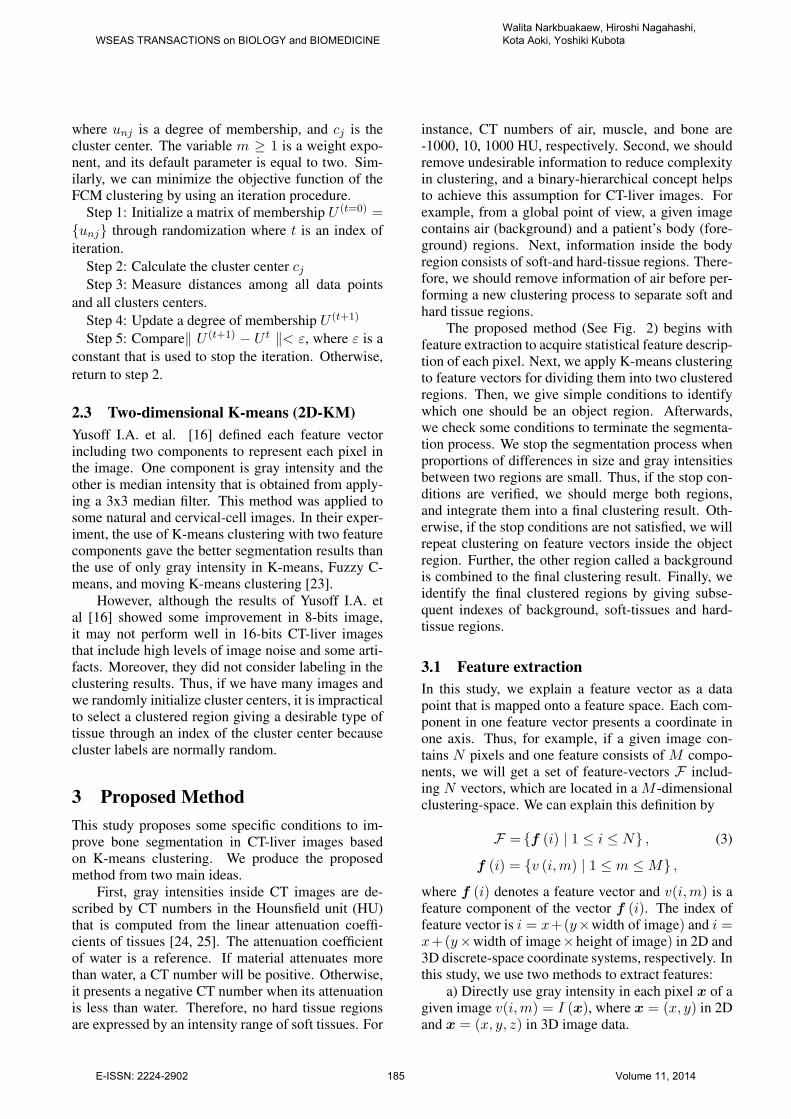
From Table 1, the proposed method showed the

most stability in clustering results when a number of

clusters in 2D-KM and 2D-FCM were equal to four,

five, and six clusters. Furthermore, it was able to illus-

Fig. 4: Five examples of 2D-KM clustering-results at

CT axial image slice 94 when initial cluster-centers

are random, the number of clusters is four and feature

components are gray intensity and median gray (re-

sults of convolution between 3x3 median filtering and

a given image); the percentage presents the number of

images that give the same regions from 100 times of

testing.

trate bone region in all results of clustering although

clustered regions were different (see Fig. 6 (a) and

(b)). Otherwise, it was possible to increase a possi-

bility of bone-region appearance in the results of 2D-

KM and 2D-FCM clustering by adding the number

of clusters. However, the increase of the number of

clusters caused stability of clustering to drop because

the number of different clustering results was raised

up. Moreover, it gradually improved the possibility of

bone-region appearance in some images as shown in

Fig. 5.

In addition, although the proposed method pre-

sented higher stability in results of clustering, it is oc-

casionally better to get only one type of clustering re-

sults if we consider multiple organs [27]. We achieved

this requirement by giving a simple condition (called

a mean-group) on the initial cluster centers. We sym-

metrically divide feature vectors into two sections for

every use of the proposed clustering method. Then,

we select mean value of each section to represent an

initial cluster-center.

ck =(

mkx,m

ky

)

, k = 1, 2 (8)

mkx =Mean

(

{v (i, 1)}D1

i=D0

)

,

mky =Mean

(

{v (i, 2)}D1

i=D0

)

,

D0 =N × (k − 1)

2+ 1, D1 =

N × k

2

where ck is cluster center indexed by k. The variable

N denotes the number of feature vectors. Further, this

condition did not change the final clustering results as

shown in Fig. 6 (c).


E-ISSN: 2224-2902 188 Volume 11, 2014

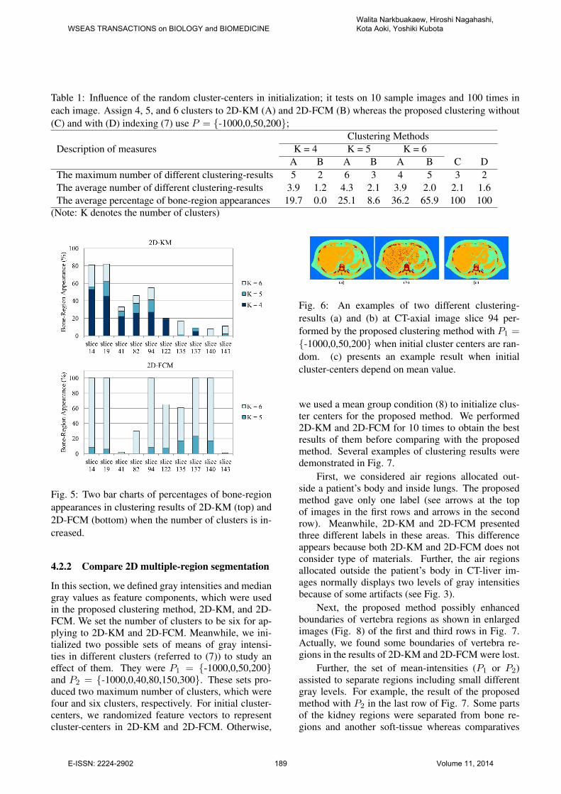
Table 1: Influence of the random cluster-centers in initialization; it tests on 10 sample images and 100 times in

each image. Assign 4, 5, and 6 clusters to 2D-KM (A) and 2D-FCM (B) whereas the proposed clustering without

(C) and with (D) indexing (7) use P = {-1000,0,50,200};

Description of measures

Clustering Methods

K = 4 K = 5 K = 6

A B A B A B C D

The maximum number of different clustering-results 5 2 6 3 4 5 3 2

The average number of different clustering-results 3.9 1.2 4.3 2.1 3.9 2.0 2.1 1.6

The average percentage of bone-region appearances 19.7 0.0 25.1 8.6 36.2 65.9 100 100

(Note: K denotes the number of clusters)

Fig. 5: Two bar charts of percentages of bone-region

appearances in clustering results of 2D-KM (top) and

2D-FCM (bottom) when the number of clusters is in-

creased.

4.2.2 Compare 2D multiple-region segmentation

In this section, we defined gray intensities and median

gray values as feature components, which were used

in the proposed clustering method, 2D-KM, and 2D-

FCM. We set the number of clusters to be six for ap-

plying to 2D-KM and 2D-FCM. Meanwhile, we ini-

tialized two possible sets of means of gray intensi-

ties in different clusters (referred to (7)) to study an

effect of them. They were P1 = {-1000,0,50,200}and P2 = {-1000,0,40,80,150,300}. These sets pro-

duced two maximum number of clusters, which were

four and six clusters, respectively. For initial cluster-

centers, we randomized feature vectors to represent

cluster-centers in 2D-KM and 2D-FCM. Otherwise,

Fig. 6: An examples of two different clustering-

results (a) and (b) at CT-axial image slice 94 per-

formed by the proposed clustering method with P1 ={-1000,0,50,200} when initial cluster centers are ran-

dom. (c) presents an example result when initial

cluster-centers depend on mean value.

we used a mean group condition (8) to initialize clus-

ter centers for the proposed method. We performed

2D-KM and 2D-FCM for 10 times to obtain the best

results of them before comparing with the proposed

method. Several examples of clustering results were

demonstrated in Fig. 7.

First, we considered air regions allocated out-

side a patient’s body and inside lungs. The proposed

method gave only one label (see arrows at the top

of images in the first rows and arrows in the second

row). Meanwhile, 2D-KM and 2D-FCM presented

three different labels in these areas. This difference

appears because both 2D-KM and 2D-FCM does not

consider type of materials. Further, the air regions

allocated outside the patient’s body in CT-liver im-

ages normally displays two levels of gray intensities

because of some artifacts (see Fig. 3).

Next, the proposed method possibly enhanced

boundaries of vertebra regions as shown in enlarged

images (Fig. 8) of the first and third rows in Fig. 7.

Actually, we found some boundaries of vertebra re-

gions in the results of 2D-KM and 2D-FCM were lost.

Further, the set of mean-intensities (P1 or P2)

assisted to separate regions including small different

gray levels. For example, the result of the proposed

method with P2 in the last row of Fig. 7. Some parts

of the kidney regions were separated from bone re-

gions and another soft-tissue whereas comparatives


E-ISSN: 2224-2902 189 Volume 11, 2014

Fig. 7: Four comparisons of example results of four

different clustering methods in axial slices 14, 41, 94,

and 122 from top-to-bottom rows; these methods are

2D-KM, 2D-FCM, the proposed method with P1 ={-1000,0,50,200} and P2 = {-1000,0,40,80,150,300}in left-to-right order.

Fig. 8: Two examples of bone-region enhancement

displayed through enlarged images of the 1st and 3rd

rows in Fig. 7.

methods failed to distinguish them. However, if this

set includes many levels of means of gray intensities,

the problem of noise or particle regions will be ap-

peared.

4.3 Compare 3D rib cage model

From 10 sets of 3D-CT data, we almost performed

three times of testing on 2D-KM and 2D-FCM to se-

lect the best clustering results for each set of 3D-CT

data. Occasionally, we further computed more than

three times when no clustering results presented bone

regions. Otherwise, although the proposed method

did not require replication of a clustering process, we

repeatedly computed it three times to obtain average

of computation time and compared with 2D-KM and

2D-FCM methods. We found the proposed method

spent 103 seconds to segment multi-regions in a 3D-

CT data set on average. Meanwhile, 2D-KM and 2D-

FCM required about 157 and 794 seconds. These

computations were performed under the MATLAB

Fig. 9: An example of manual threshold adjustment

(216,1235) at an axial image slice 94

environment on 3.40 GHz Intel(R) Core(TM) i7-2600

CPU.

Next, we examined quality of rib cage surface

models. We observed eight points labeled by (A) to

(H) labels (see Fig 10). We used color shade to ex-

plain the depth of model from front to back, and this

shade helped to observe ribs. This investigation fur-

ther included the result of manual threshold that was

adjusted through considering threshold labels at an ax-

ial image slice 94 as shown in Fig. 9. Then, we ap-

plied this threshold to a whole 3D-CT data set for get-

ting a rib cage segmented volume.

From our experiment, 3D rib cage surface mod-

els, which were reconstructed from segmentation re-

sults of manual threshold, 2D-KM, 2D-FCM, and the

proposed method, demonstrated some different view-

points.

First, the bone regions in the top area of the model

were labeled by (A). We did not found the lost re-

gions in the results of manual threshold and the pro-

posed method. Second, large areas of rib bones in the

front (B) and bottom (F) views disappeared in the re-

sults of 2D-KM and 2D-FCM. Otherwise, the results

of manual threshold and the proposed method gave

more details but they were unable to illustrate costal

cartilages. Further, in the results of manual threshold

and the proposed method, they presented clear bound-

aries of ribs in the bottom area of the side (G) and

back (E) views. Next, only the results of the proposed

method showed regions of scapular bones (D) without

losing the large areas. Subsequently, we considered

spine regions (H). The results of 2D-KM, 2D-FCM

presented lost regions around anterior areas of verte-

bras in many sections of spine. The results of manual

threshold illustrated small lost regions around anterior

areas of vertebras in the top and bottom sections of

spine. These lost regions were possibly found because

we adjusted threshold on the sample image allocated

around the center of a 3D-CT data set and this data set

includes large variation in gray intensities among dif-

ferent axial-image planes due to some artifacts. The

results of the proposed method did not show the lost

regions around anterior areas of vertebras, but small

regions of vertebras in the top section of spine were

merged. Lastly, the results of the proposed method


E-ISSN: 2224-2902 190 Volume 11, 2014

presented large areas of kidneys that were undesirable

regions. However, these kidney volumes separated

from bone regions. Thus, it is not difficult to remove

them. Otherwise, the results of manual threshold, 2D-

KM, and 2D-FCM displayed them in small areas.

5 Conclusion

This paper introduces an optional segmentation

method based on a K-mean clustering algorithm. It

is aimed to enhance bone-segmented regions in CT-

liver images under high levels of image noise and

some artifacts. The proposed method contains two

main conditions. First, we used a hierarchical con-

cept to manage feature vectors and clustering regions.

We produced a simple algorithm to identify type of

clustering region and control iteration. Thus, we do

not want to define the total number of clusters before

starting the process. Second, we created a cluster in-

dexing method to control labels of clustered regions

in the clustering results. Further, this indexing relates

to types of tissues or CT standard numbers by repre-

senting subsequent indexes of background, soft tissue,

and hard tissue regions.

We applied the proposed method to 10 sets of

3D CT data, and the results were compared with 2D-

KM and 2D-FCM methods. From comparison, the

proposed method gave more stable results when ini-

tial cluster centers were random. A percentage of

bone-region appearances in the clustering results of

the proposed method was higher than 2D-KM and 2D-

FCM. Further, boundary information of bone-regions

were illustrated more than two comparative methods.

We observed eight points allocated in different loca-

tions of 3D surface models to investigate different re-

sults. In summary, the segmentation results of the

proposed method seemed to give more information of

bone regions in vertebra, ribs, and scapula areas than

the results of 2D-KM and 2D-FCM. Conversely, the

proposed method cannot prevent appearance of large

kidney-regions in the segmentation results. In addi-

tion, the proposed method required computation time

less than 2D-KM and 2D-FCM for 1.5 and 7.7 times

of computation in one 3D-CT data on average.

However, the proposed method requires manual

adjustment on several parameters. Further, the clus-

tering relied on the basic feature components, gray

and median gray, that cannot completely remove some

undesirable regions appears in the clustering results.

Therefore, these limitations will be addressed in the

future work.

References:

[1] O. Faiz, S. Blackburn, and D. Moffat, Anatomy

at a Glance, vol. 66. John Wiley & Sons, 2011.

[2] L. Seoud, F. Cheriet, H. Labelle, and

J. Dansereau, “A novel method for the 3-d

reconstruction of scoliotic ribs from frontal

and lateral radiographs,” Biomedical Engi-

neering, IEEE Transactions on, vol. 58, no. 5,

pp. 1135–1146, 2011.

[3] N. Sverzellati, D. Colombi, G. Randi,

A. Pavarani, M. Silva, S. L. Walsh, M. Pistolesi,

V. Alfieri, A. Chetta, M. Vaccarezza, et al.,

“Computed tomography measurement of rib

cage morphometry in emphysema,” PloS one,

vol. 8, no. 7, p. e68546, 2013.

[4] F. S. Gayzik, M. M. Yu, K. A. Danelson, D. E.

Slice, and J. D. Stitzel, “Quantification of age-

related shape change of the human rib cage

through geometric morphometrics,” Journal of

biomechanics, vol. 41, no. 7, pp. 1545–1554,

2008.

[5] F. Henry Gray, Gray’s Anatomy of the Human

Body. 1918.

[6] K. Rathnayaka, T. Sahama, M. A. Schuetz, and

B. Schmutz, “Effects of CT image segmentation

methods on the accuracy of long bone 3d re-

constructions,” Medical Engineering & Physics,

vol. 33, no. 2, pp. 226 – 233, 2011.

[7] J.-Y. Zhou, D. W. Wong, F. Ding, S. K.

Venkatesh, Q. Tian, Y.-Y. Qi, W. Xiong, J. J. Liu,

and W.-K. Leow, “Liver tumour segmentation

using contrast-enhanced multi-detector ct data:

performance benchmarking of three semiauto-

mated methods,” European radiology, vol. 20,

no. 7, pp. 1738–1748, 2010.

[8] X. Pardo, M. Carreira, A. Mosquera, and D. Ca-

bello, “A snake for CT image segmentation inte-

grating region and edge information,” Image and

Vision Computing, vol. 19, no. 7, pp. 461 – 475,

2001.

[9] R. Xu, D. Wunsch, et al., “Survey of cluster-

ing algorithms,” Neural Networks, IEEE Trans-

actions on, vol. 16, no. 3, pp. 645–678, 2005.

[10] R. Xu and D. C. Wunsch, “Clustering algorithms

in biomedical research: a review,” Biomedical

Engineering, IEEE Reviews in, vol. 3, pp. 120–

154, 2010.


E-ISSN: 2224-2902 191 Volume 11, 2014

[11] H. Al-Shamlan and A. El-Zaart, “Feature extrac-

tion values for breast cancer mammography im-

ages,” in Bioinformatics and Biomedical Tech-

nology (ICBBT), 2010 International Conference

on, pp. 335–340, IEEE, 2010.

[12] M. Nixon and A. S. Aguado, Feature extraction

& image processing. Academic Press, 2008.

[13] M. Mignotte, “Segmentation by fusion of

histogram-based k-means clusters in different

color spaces,” IEEE Transactions on image pro-

cessing, vol. 17, no. 5, pp. 780–787, 2008.

[14] T. H. Lee, M. F. A. Fauzi, and R. Komiya,

“Segmentation of CT brain images using k-

means and em clustering,” in Computer Graph-

ics, Imaging and Visualisation, 2008. CGIV’08.

Fifth International Conference on, pp. 339–344,

IEEE, 2008.

[15] L.-H. Juang and M.-N. Wu, “Mri brain lesion

image detection based on color-converted k-

means clustering segmentation,” Measurement,

vol. 43, pp. 941–949, 2010.

[16] I. A. Yusoff and N. A. M. Isa, “Two-dimensional

clustering algorithms for image segmentation,”

WSEAS transactions on computers, vol. 10,

no. 10, pp. 332–342, 2011.

[17] I. A. Yusoff, N. A. Mat Isa, and K. Hasikin, “Au-

tomated two-dimensional k-means clustering al-

gorithm for unsupervised image segmentation,”

Computers & Electrical Engineering, pp. 907–

917, 2013.

[18] P. T. Selvy, V. Palanisamy, and M. Radhai, “An

improved mri brain image segmentation to de-

tect cerebrospinal fluid level using anisotropic

diffused fuzzy c means.,” WSEAS Transactions

on Computers, vol. 12, no. 4, pp. 145–154, 2013.

[19] P. T. Selvy, V. Palanisamy, and M. Radhai,

“A proficient clustering technique to detect csf

level in mri brain images using pso algorithm.,”

WSEAS Transactions on Computers, vol. 12,

no. 7, pp. 298–308, 2013.

[20] C. Chu, M. Oda, T. Kitasaka, K. Misawa,

M. Fujiwara, Y. Hayashi, R. Walz, D. Rueckert,

and K. Mori, “Multi-organ segmentation from

3d abdominal CT images using patient specific

weighted-probabilistic atlas,” in Medical Imag-

ing 2013: Image Processing, pp. 86693Y–1–

86693Y–7, Proc. of SPIE, 2013.

[21] C. M. Bishop and N. M. Nasrabadi, Pat-

tern recognition and machine learning, vol. 1.

springer New York, 2006.

[22] J. C. Bezdek, R. Ehrlich, and W. Full, “Fcm:

The fuzzy¡ i¿c¡/i¿-means clustering algorithm,”

Computers & Geosciences, vol. 10, no. 2,

pp. 191–203, 1984.

[23] M. Y. Mashor, “Improving the performance of k-

means clustering algorithm to position the cen-

ters of rbf network,” International Journal of the

Computer, The Internet and Management, vol. 6,

no. 2, pp. 121–124, 1998.

[24] N. B. Smith and A. Webb, Introduction to med-

ical imaging: Physics, engineering and clinical

applications. Cambridge University Press, 2010.

[25] K. Iniewski, Medical imaging: Principles, de-

tectors, and Electronics. John Wiley & Sons,

2009.

[26] W. E. Lorensen and H. E. Cline, “Marching

cubes: A high resolution 3d surface construction

algorithm,” in ACM Siggraph Computer Graph-

ics, vol. 21, pp. 163–169, ACM, 1987.

[27] W. Narkbuakaew, H. Nagahashi, K. Aoki, and

Y. Kubota, “Integration of modified k-means

clustering and morphological operations for

multi-organ segmentation in CT liver-images,”

in Biology and Biomedical Engineering, 2014.

BBE’14. International Conference on, pp. 34–

39, Europment, 2014.


E-ISSN: 2224-2902 192 Volume 11, 2014

Fig. 10: Examples of 3D rib cage surface-models reconstructed from binary images, which are results of manual

threshold, 2D-KM, 2D-FCM, and the proposed method. The 1st to 4th rows present front, back, bottom, and side

views. The last row represent enlargement of some parts of spine.


E-ISSN: 2224-2902 193 Volume 11, 2014

bone segmentation in ct-liver images using k-means clustering …€¦ · · 2014-10-29bone...

Documents