bonding methods of underground powerb cables.pdf

Seediscussions,stats,andauthorprofilesforthispublicationat:http://www.researchgate.net/publication/283119570

Bondingmethodsofundergroundcables

RESEARCH·OCTOBER2015

DOI:10.13140/RG.2.1.2305.3527

READS

41

2AUTHORS:

O.E.Gouda

CairoUniversity

158PUBLICATIONS132CITATIONS

SEEPROFILE

AdelFarag

CairoUniversity

5PUBLICATIONS0CITATIONS

SEEPROFILE

Availablefrom:O.E.Gouda

Retrievedon:20December2015

http://www.researchgate.net/publication/283119570_Bonding_methods_of_underground_cables?enrichId=rgreq-1a61da6d-5f14-497d-8487-e1fa99e91004&enrichSource=Y292ZXJQYWdlOzI4MzExOTU3MDtBUzoyODgwMzUyOTcwODc0ODhAMTQ0NTY4NDM3NDEyNQ%3D%3D&el=1_x_2

http://www.researchgate.net/publication/283119570_Bonding_methods_of_underground_cables?enrichId=rgreq-1a61da6d-5f14-497d-8487-e1fa99e91004&enrichSource=Y292ZXJQYWdlOzI4MzExOTU3MDtBUzoyODgwMzUyOTcwODc0ODhAMTQ0NTY4NDM3NDEyNQ%3D%3D&el=1_x_3

http://www.researchgate.net/?enrichId=rgreq-1a61da6d-5f14-497d-8487-e1fa99e91004&enrichSource=Y292ZXJQYWdlOzI4MzExOTU3MDtBUzoyODgwMzUyOTcwODc0ODhAMTQ0NTY4NDM3NDEyNQ%3D%3D&el=1_x_1

http://www.researchgate.net/profile/Oe_Gouda?enrichId=rgreq-1a61da6d-5f14-497d-8487-e1fa99e91004&enrichSource=Y292ZXJQYWdlOzI4MzExOTU3MDtBUzoyODgwMzUyOTcwODc0ODhAMTQ0NTY4NDM3NDEyNQ%3D%3D&el=1_x_4


http://www.researchgate.net/institution/Cairo_University3?enrichId=rgreq-1a61da6d-5f14-497d-8487-e1fa99e91004&enrichSource=Y292ZXJQYWdlOzI4MzExOTU3MDtBUzoyODgwMzUyOTcwODc0ODhAMTQ0NTY4NDM3NDEyNQ%3D%3D&el=1_x_6


http://www.researchgate.net/profile/Adel_Farag?enrichId=rgreq-1a61da6d-5f14-497d-8487-e1fa99e91004&enrichSource=Y292ZXJQYWdlOzI4MzExOTU3MDtBUzoyODgwMzUyOTcwODc0ODhAMTQ0NTY4NDM3NDEyNQ%3D%3D&el=1_x_4


http://www.researchgate.net/institution/Cairo_University3?enrichId=rgreq-1a61da6d-5f14-497d-8487-e1fa99e91004&enrichSource=Y292ZXJQYWdlOzI4MzExOTU3MDtBUzoyODgwMzUyOTcwODc0ODhAMTQ0NTY4NDM3NDEyNQ%3D%3D&el=1_x_6


1

TABLE OF CONTENTS

Page

CHAPTER (1): INTRODUCTION 14 Introduction 1.1 14 Book Outline 1.2

CHAPTER (2): SHEATH BONDING AND GROUNDING

17 Sheath Phenomena 2.1

17 Sheath voltage 2.1.1

18 Sheath current 2.1.2

18 Sheath Bonding Arrangements 2.2

18 Sheath bonded at two-points (solid bonding) 2.2.1

20 Sheath bonded at one end only 2.2.2

23 Cross bonding system 2.2.3

26 Types Of Metall ic Sheath Losses 2.3

26 Sheath eddy loss 2.3.1

27 Sheath circulating loss 2.3.2

CHAPTER (3): METHODS TO REDUCE THE SHEATH CURRENTS AND LOSSES 29 Introduction 3.1 29 Old Techniques To Reduce The Sheath Currents And Losses 3.2

29 Single-point and cross bonding methods 3.2.1

30 Continuous cross bonding method 3.2.2

30 Impedance bonding methods 3.2.3

30 Resistance bonding method 3.2.4

30 Modern Techniques To Reduce The Sheath Currents And Losses 3.3

30 Sheath current canceling device 3.3.1

33 Inductance compensation device 3.3.2

CHAPTER (4): FACTORS AFFECTING THE SHEATH LOSSES

IN SINGLE-CORE UNDERGROUND POWER 36 Introduction 4.1 36 Cable Layouts Formation 4.2

37 Mathematical Algorithm 4.3

37 Induced sheath voltages, sheath circulating currents and losses 4.3.1

39 Three-phase trefoil arrangement of cables 4.3.1.1

41 Three-phase flat arrangement of cables 4.3.1.2

46 Three-phase arrangement with sheaths cross bonded 4.3.1.3

46 Sheath eddy current and its loss 4.3.2

46 Introduction 4.3.2.1

47 Three-phase trefoil symmetrical arrangement of cables with sheaths bonded at a single-point or

two-points

4.3.2.2

47 Three-phase flat arrangement of cables with sheaths

bonded at a single-point or two-points 4.3.2.3

48 Three-phase arrangement with sheaths cross bond 4.3.2.4

49 Three-phase trefoil arrangement of cables 4.3.2.4.1

2

50 Three-phase arrangement in a flat 4.3.2.4.2

50 Center cable 4.3.2.4.2.1

50 Outer cable leading phase 4.3.2.4.2.2

50 Outer cable lagging phase 4.3.2.4.2.3

51 A.C resistance of conductor 4.3.3

51 Sheath resistance 4.3.4

52 Tubular metall ic sheath 4.3.4.1

52 Helical ly metall ic sheath 4.3.4.2

Factors Affecting the Sheath Losses in Single-Core Underground Power Cables 4.4

57 Effect of sheath bonding and cable layout formation on sheath losses 4.4.1


57 Cases study 4.4.1.2

58 Obtained results 4.4.1.3

64 Results discussion 4.4.1.4

68 Effect of cable parameters (conductor's size & its resistivity) on the sheath

losses 4.4.2



70 Obtained results 4.4.2.3

70 Conductor material resistivity effect on the sheath

losses

4.4.2.3.1

71 Conductor sizes effect on the sheath losses 4.4.2.3.2

75 Discussion of the obtained results 4.4.2.4

76 Effect of cable spacing on the sheath losses 4.4.3



77 Obtained results by using IEC 60287 4.4.3.3


82 Effect of sheath resistance on the sheath losses 4.4.4




82 Effect of sheath resistance on the sheath circulating

losses

4.4.4.3.1

84 Effect of sheath resistance on the sheath eddy losses 4.4.4.3.2


85 Factors affecting the sheath resistance 4.4.4.5

85 Introduction 4.4.4.5.1

86 Cases study 4.4.4.5.2

90 Obtained results 4.4.4.5.3

90 Obtained results of the effect of

Sheath material resistivity on the

sheath losses

4.4.4.5.3.1

90 Obtained results of the effect of

temperature of sheath material on the

sheath losses

4.4.4.5.3.2

104 Discussion of the obtained results 4.4.4.5.4

104 Results discussion of the effect of 4.4.4.5.4.1

3

sheath material resistivity on the

sheath losses

106 Results discussion of the effect of

sheath material resistivity on the

sheath losses

4.4.4.5.4.2

106 Effect of phase rotation on the sheath circulating loss factor for two-points

bonding – flat arrangements

4.4.5





108 Effect of conductor current on the sheath losses 4.4.6





111 Effect of power frequency ( 50 or 60 Hz) on the sheath losses 4.4.7





113 Effect of the minor section length on the sheath circulating current in cross-

bonding arrangement

4.4.8





117 Effect of cable armoring on the sheath losses 4.4.9





CHAPTER (5): SHEATH OVERVOLTAGES DUE TO EXTERNAL FAULTS IN SPECIALLY

BONDED CABLE SYSTEM

124 Introduction 5.1

125 Mathematical Algorithm 5.2

126 Single-point bonding cables 5.2.1

126 Three-phase symmetrical fault 5.2.1.1

126 Trefoil formation 5.2.1.1.1

127 Flat formation 5.2.1.1.2

128 Phase-to-phase fault 5.2.1.2



129 Fault between two outers cables 5.2.1.2.2.1

129 Fault between inner and outer

cables (phase 1 & phase 2)

5.2.1.2.2.2

129 Single-phase ground fault (solidly earthed neutral) 5.2.1.3


4


131 Cross bonding cables 5.2.2

131 Three-phase symmetrical fault 5.2.2.1

131 Phase-to-phase fault 5.2.2.2

131 Single-phase ground fault (solidly earthed neutral) 5.2.2.3



137 Case Study 5.3

137 Obtained Results 5.4

140 Discussion Of The Obtained Results 5.5

143 CHAPTER (6): CONCLUSIONS

REFRENCES 146

5

LIST OF TABLES

Table(4.1) :

Single-core cables 800 mm2 CU with lead screen parameters 57

Table(4.2-a) :

Sheath currents, their loss factors and sheath induced voltages in case of single-point bonding method with lead screens

59

Table (4-2-b) :

Sheath currents and their loss factors in case of two-points bonding method with lead screens

61

Table (4-2-c) : Sheath currents and their loss factors in case of cross-bonding method with lead screens

63

Table (4-3) : Electrical d.c resistances and temperature coefficients for 800 mm2 copper and aluminium conductors

69

Table (4- 4) :

Single-core cables 66 kV-CU with lead screens parameters 70

Table (4- 5-a) :

Sheath currents and their loss factors in single-core cables with two-points bonding method for copper and aluminium conductors

70

Table (4-5-b) :

Sheath currents and their loss factors in single-core cables with cross-bonding method for copper and aluminium conductors

71

Table (4-6-a) : Sheath currents and their loss factors for various sizes of single-core cables with two-points bonding method

72

Table (4-6-b) : Sheath currents and their loss factors for various sizes of single-core cables with cross-bonding method

74

Table (4-7-a) : Sheath currents and their loss factor with two-points bonding methods, for De and 2De spacing between cables

77

Table (4-7-b) : Sheath currents and their loss factor with cross bonding methods, for De and 2De spacing between cables

78

Table (4-8) : Electrical resistivities and temperature coefficients for different metallic sheaths materials

86

Table (4- 9) : Single-core cable 800 mm2 CU, with copper tape screen parameters

87

Table (4-10) : Single-core cable 800 mm2 CU with copper wire screen parameters

88

Table (4-11) : Single-core cable 800 mm2 CU with stainless steel screen parameters

88

Table (4-12) : Single-core cable 800 mm2 CU with aluminium screen

parameters

89

Table (4-13-a) : Sheath currents and their loss factors for single-core cables with two-points bonding method with copper tape screens

90

Table (4-13-b) : Sheath currents and their loss factors for single-core cables with cross-bonding methods with copper tape screens

92

Page

6

Table (4-14-a) : Sheath currents and their loss factors for single-core cables with two-points bonding method with copper wire screens

94

Table (4-14-b) : Sheath currents and their loss factors for single-core cables with cross-bonding method with copper wire screens

96

Table (4-15-a) : Sheath currents and their loss factors for single-core cables with two-points bonding method with stainless steel screens

97

Table (4-15-b) : Sheath currents and their loss factors for single-core cables with cross-bonding method with stainless steel screens

99

Table (4-16-a) : Sheath currents and their loss factors for single-core cables with two-points bonding method with aluminium screens

101

Table (4-16-b) : Sheath currents and their loss factors for single-core cables with cross-bonding method with aluminium screens

102

Table (4-17) : Sheath circulating loss factors for different configuration in flat formation

108

Table (4-18-a) : Sheath currents and their loss factors for single-core cables with full rating current and its half value for two-points bonding method

109

Table (4-18-b) : Sheath currents and their loss factors for single-core cables with full rating current and its half value for cross bonding method

110

Table (4-19-a) : Sheath currents and their loss factors for single-core cables with two-points bonding method with power frequencies 50 and 60 Hz

112

Table (4-19-b) : Sheath currents and their loss factors for single-core cables with cross bonding method with power frequencies 50 and 60 Hz

112

Table (4-20) : Armored Single-core cable 800 mm2 , 66 kV CU with lead covered and aluminium wire armored parameters

120

Table (4-21) : Sheath, armour currents and their loss factors for nonmagnetic armored single-core cables with two-points bonding method and cross bonding method

120

Table (5-1) : Voltages between sheaths and local earthing system due to different external faults in single-core cables with single-point bonding

138

Table (5-2) : Sheath to sheath voltages due to different external faults in single-core cables with cross bonding method for trefoil & flat layouts

139

7

List of Figures

Fig. (2-1) : Two-points bonding 19

Fig. (2-2-a) : Single-point bonding 21

Fig. ( 2-2-b) : Induced voltage in sheath with single-point bonding 21

Fig. (2-2-c) : Single-point bonding with SVL 22

Fig.(2-3-a) : Mid point bonding with SVL 22

Fig.(2-3-b) : Induced voltage in sheath with mid-point bonding 22

Fig. (2-3-c) : Sectionalized run with single-point bonding 23

Fig. (2-3-d) : Transposition of parallel conductor in flat formation or trefoil 23

Fig. (2-4) : Principle of cross -bonding 24

Fig. (2-5) : Cross bonded cables with transposition 26

Fig. (2-6) : Ungrounded metallic sheath 27

Fig. (2-7) : Sheath grounded at both ends 28

Fig. (3-1) : Sheath current canceling device in single phase 31

Fig. (3-2) : Sheath current canceling device for three single -core

cable

32

Fig. (3-3) : Residual voltage at the end of the sheath 33

Fig. (3-4) : Diagrammatic sketch of compensating inductance connect 34

Fig. (3-5) : Distribution diagram of voltage in metal shield before and

after compensating inductance

34

Fig. (3-6) : Compensating device and overvoltage protector 34

Fig. (4-1) : Single-core cable layouts 37

Fig. (4-1-a) : Trefoil formation 37

Fig. (4-1-b) : Flat formation 37

Fig. (4-2) : Unarmored single-core cable 37

Fig.(4-3-a) : Flowchart of the computation steps for trefoil layout 54

Fig.(4-3-b) : Flowchart of the computation steps for flat layout 55

Fig.(4-4) : Sheath induced voltage vs. cable spacing for single-core cable 66 kV

in trefoil and flat formations with single-point bonding

66

Fig. (4-5) : Sheath circulating loss factor vs. spacing for 66 kV single-core cable

trefoil formation with two-points bonding

79

Fig. (4-6) : Sheath circulating loss factor vs. spacing for 66 kV single-core cable

flat formation with two-points bonding

80

Page

8

Fig. (4-7) : Sheath eddy loss factor vs. spacing for 66 kV single-core cable trefoil

formation with two-points bonding

80

Fig. (4-8) : Sheath eddy loss factor vs. spacing factor for 66 kV single-core cable

flat formation with two-points bonding

81

Fig. (4-9) : Sheath circulating loss factor vs. sheath resistance in trefoil formation

with two-points bonding for De and 2De spacing between cables

82

Fig. (4-10) : Sheath circulating current vs. sheath resistance in trefoil formation

with two-points bonding for De and 2De spacing between cables

83

Fig. (4-11) : Sheath circulating loss factor vs. sheath resistance in touch flat


83

Fig. (4-12) : Sheath eddy loss factor vs. sheath resistance for trefoil formation with

two-points bonding

84

Fig. (4-13) : Sheath eddy loss factor vs. sheath resistance for flat formation with

two-points bonding

84

Fig. (4-14) : Sheath resistance vs. sheath temperature 104

Fig. (4-15) : Sheath loss factor vs. sheath temperature 104

Fig. (4-16) : Sheath resistance vs. sheath circulating loss factor with aluminium

screen

106

Fig.(4-17) : Phase rotation in flat formation 107

Fig.(4-17-a) : S-T-R configuration 107

Fig.(4-17-b) : S-R-T configuration 107

Fig.(4-18) : Cross-bonded cables without transposition 114

Fig. (4-19) : Sheath current vs. sheath length of minor section for trefoil formation

116

Fig. (4-20 ) : Sheath induced voltage vs. total sheath length for trefoil formation 117

Fig. (4-21) : Sheath, armour current vs. armour resistance 119

Fig. (5-1) : Arrangement of single-points bonded cables 126

Fig.(5-2-a) : Flowchart of the computation steps of sheath induced overvoltage for

trefoil layout with single-points bonding 133

Fig.(5-2-b) : Flowchart of the computation steps of sheath induced overvoltage for

trefoil layout with cross bonding

134

Fig.(5-2-c) : Flowchart of the computation steps of sheath induced overvoltage for

flat layout with single-point bonding

135

Fig.(5-2-d) : Flowchart of the computation steps of sheath induced overvoltage for

flat layout with cross bonding

136

Fig. (5-3) : Maximum induced sheath voltage gradients (sheath to earth) for

various faults in single-point bonded cable system-flat

141

Fig. (5-4) : Maximum induced sheath voltage gradients (sheath to sheath) for

various faults in cross bonded cable system-flat

142

9

LIST OF SYMBOLES

A.C : Alternating current

D.C : Direct current

MCT : Mutual couplings for current transformer

MVT : Mutual couplings for voltage transformer

MCS : Mutual couplings between conductor C and sheath S

emf : Electric motive force

Et : emf induced in the ground loop from the transformer

Ec : emf induced in the ground loop from the conductor current

CTs : Current transformers

VTs : Voltage transformers

ISr : Sheath circulating current in phase R

ISs : Sheath circulating current in phase S

ISt : Sheath circulating current in phase T

XLPE : Cross linked polyethylene

PVC : Polyvinyl Chloride

PE : Polyethylene

L3 : Minor section length no. 3

U t : Residual voltage at sheath terminal

IEEE : Institute of Electrical and Electronic Engineers.

SVLs : sheath voltage limiters

ecc : Earth continuity conductor

Ip : Sheath circulating current

ep : Sheath induced voltage

Ic : Conductor current

I1, I2, I3

:

The line current in phases (1), (2) and (3) respectively

VS1, VS2, VS3 : Induced voltage in sheaths (1), (2) and (3) respectively

ICS1, ICS2, ICS3 : The circulating currents in sheaths of phases (1), (2) and (3)

respectively

RS : The resistance of sheath at its maximum operating temperature

M1,2 : The mutual inductance between core (1) and sheath (2)


10


WCS : The circulating sheath loss per meter

I : The line currents in phases (1), (2) and (3) with balance condition

S : Spacing between axes of adjacent conductors

rsh : Mean of outer and inner radii of sheath

X : The reactance per unit length of sheath

R : The resistance of conductor at its maximum operating temperature

Xm : Mutual reactance per unit length of cable between the sheath of an

outer cable and the conductors of the other two, when cables are in flat

formation

V0 : Residual voltage along the cable sheath

IEC : International Electro-technical Commission

ISE1, ISE2, ISE3 : Sheath Eddy Current in phase no. 1,2 and 3 respectively

DS : The external diameter of cable sheath

tS : The thickness of sheath

m : factor depends on power frequency and metallic sheath resistance

Rd c : The d.c. resistance of the conductor at 90 oC

R2 0 : The d.c. resistance of the conductor at 20 oC

ys : The skin effect factor

yp : The proximity effect factor

AS : The sheath cross-sectional area

dS : The mean diameter of the sheath

DS e : The external diameter of the sheath

R s t ran d : Resistance of one strand

n : Number of strands

dC : Diameter of conductor

De : External diameter of cable

ICS-R, ICS-S, ICS-T : The sheath circulating currents in R, S and T phases respectively

h : an operator which rotates a phasor 120o counter clock-wise

IC SX , IC SY , IC S Z : The sheath circulating currents in sheath circuits X, Y and Z

respectively

ZX , ZY , ZZ : The sheath impedances of the X, Y and Z circuits

respectively

11

VX , VY, VZ : The induced voltages in sheaths of the X, Y and Z circuits

respectively

Re : The equivalent resistance of sheath and armour in parallel

RA : The resistance of armour per unit length of cable at its maximum

operating temperature

d : The mean diameter of sheath and armour

dS : The mean diameter of sheath

dA : The mean diameter of armour

IS : Sheath current (circulating or eddy)

IA : Armour current (circulating or eddy)

ISA : Sheath-armour combination current (circulating or eddy)

IAE1, IAE2, IAE3 : Armour Eddy Current in phase no. 1,2 and 3 respectively

IAC1, IAC2, IAC3 : Armour Circulating Current in phase no. 1,2 and 3

respectively

EAE,EBE,ECE : Voltages between sheaths of phases A,B and C respectively and the earth

conductor

IF : Short-circuit current in cable conductor

SAE,SBE,SCE : The geometric mean spacing between cables A, B and C respectively and

the earth conductor

RC : Resistance of earth conductor

rc : Geometric mean radius of earth conductor

EAB,EBC,ECA : Voltages between sheaths of phases A&B, B&C and C&A respectively

CIGRE : International Council on Large Electric Systems

rms : Root mean square

ƒ : power frequency ( 50 Hz)

ω : 2π x frequency (in cycles per second)

λCS : The circulating sheath loss factor

λCS1, λCS2, λCS3 : The circulating sheath loss factor for sheaths (1),

(2) and (3) respectively

λSE1 ,λSE3 ,λSE2 : Sheath Eddy loss factor in phase no. 1,2 and 3 respectively

ρS : The electrical resistivity of sheath material at operating temperature

Δ1 ,Δ2 : factors depend on the types of cable layouts formation

gS , β1 : factors depend on the cable parameters

12

θ s : sheath temperature

ρS20 : The electrical resistivity of sheath material at 20 oC

ℓ : The length of lay of the tape or wire

ρC2 0 : The electrical resistivity of conductor material at 20 oC

αC2 0 : The constant mass temperature coefficient at 20 oC for

conductor

θC max : maximum operating temperature of conductor

θS max : maximum operating temperature of sheath

ℓ i : The length of section number i

λAE1, λAE1, λAE1 : Armour Eddy Loss Factor in phase no. 1,2 and 3 respectively

λAC1, λAC2, λAC3 : Armour Circulating Loss Factor in phase no. 1,2 and 3

respectively

13

ABSTRACT

Single-core underground power cables can induce voltages and currents in their

metallic sheaths. The sheath induced currents are undesirable and generate power

losses and reduce the cable ampacity whereas the induced voltages can generate

electric shocks to the workers that keep the power line. This means that it is very

important to know the values of sheath currents and induced voltages and the factors

affecting them. So this thesis discussed the following:

- Calculations of the induced voltages in single-core cables with various voltages

levels from 11 kV to 500 kV with briefly studying the factors affecting them.

- Studying the factors affecting the sheath losses in single-core cables by calculating

the sheath currents (eddy-circulating) and their sheath losses in single-core cables

with various metallic sheath materials and various voltages levels from 11 kV to 500

kV with taking into consideration the following factors:

Types of sheath bonding methods (single-point bonding, two-points bonding, cross

bonding) and cable layouts (trefoil, flat), cable parameters, cable spacing, sheath

resistance, phase rotation, conductor current, power frequency, the minor section

length in cross bonding arrangement and cable armoring. This study is carried out

depending mainly on IEC 60287 by a proposed computer program using MATLAB.

- Studying the overvoltages in the metallic sheaths of single-point bonding and cross

bonding due to different types of external faults, which may cause the sheath multi-

points break-down and result in a large sheath circulating losses.

14

CHAPTER (1)

INTRODUCTION

1.1 Introduction

With the rapid increase in demand for electric energy and the trend for large infra-

structures and vast expansion of highly-populated metropolitan areas, the use of

underground power cables has grown significantly over the years [1].

Three separate single-core cables are usually used instead of three -core

cables. The principal reasons are [2, 3]:

1. To transmit large quantities of power, for which three-conductors cable would be

unwieldy.

2. To obtain phase isolation.

3. To gain advantage of the inherently higher unit dielectric strength of the insulation

in single-conductor cable.

4. The handling of large multi-conductors cable can be difficult, especially compared

to the relative ease of handling of several smaller conductors.

In a single-core power transmission cable, normally a metallic sheath

is coated outside the insulation layer to prevent the ingress o f

moisture, protect the core from possible mechanical damage, serves as

an electrostatic shield (the electric field is enclosed in between the

conductor and the sheath), and act as

a return path for fault current and capacit ive charging currents [4, 5].

When an isolated single conductor cable carries alternating current, an alternating

magnetic field is generated around it. If the cable has a metallic sheath, the sheath will

be in the field, the sheath of a single-conductor cable for A.C service acts as a

secondary of a transformer; the current in the conductor induces a voltage in the

sheath. When the sheaths of single-conductor cables are bonded to each other, as is

common practice for multi-conductor cables, the induced voltage causes current to

flow in the completed circuit. This current causes losses in the sheath [6].

The problems of the induced voltages and currents associated with using single-core

cables (for example, failure of sheath insulators, failure of cable jackets and sheath

corrosion) have been recognized since metallic sheathed cables were first used, and

15

the fundamentals of calculating sheath voltages and currents have been defined for

many years [6].

Much work has been done, for the purpose of minimizing sheath losses by introducing

various methods of bonding.

Any sheath bonding or grounding method must perform the following

functions [2, 6]:

1- Limit sheath voltages as required by the sheath section - alizing

joint.

2- Reduce or eliminate the sheath losses.

3- Provide low impedance path for faul t currents.

4- Maintain a continuous sheath circuit to permit adequate

lightning and switching surge protection.

5- Limit abnormal sheath voltages during failure to the lowest

possible values.

The above objects must be accomplished without causing the following objectionable

features [2]:

1- Excessive losses in the sheath bonding devices.

2- Introduction of triple or other harmonic currents into the sheath circuit

causing inductive interference with telephone circuits.

3- Interference with proper current drainage to prevent D.C electrolysis; also

adverse effect on operation of the A.C sheath bonding method by flow of

stray D.C currents.

4- Excessive size, weight, space, or cost of bonding devices.

Due to the importance of the sheath losses especially in single-core cables, the factors

affecting them in single-core underground cables have been studied in this thesis.

1.2 Book Outline

The remaining chapters in this thesis are arranged as follows:

Chapter (2): This chapter discusses some necessary theories and background

information that related to sheath losses in single-core cables such as the sheath

phenomena, types of sheath bonding and types of losses in the metallic

sheath.

16

Chapter (3): This chapter provides some of the methods used to reduce the sheath

circulating currents and losses in single-core cables.

Chapter (4): This chapter discusses the different factors affecting the

sheath losses in single-core underground power cables by using a

suitable mathematical algorithm by MATLAB progra mming depending

mainly on IEC 60287.

Chapter (5): In this chapter over voltages are calculated for single-point bonding

and cross bonding under different types of external faults for systems having solidly

earthed neutral.

Chapter (6): The conclusions obtained from this thesis are listed.

17

CHAPTER (2)

SHEATH BONDING AND GROUNDING

Before studying the factors affecting the sheath losses in single-core underground

cables it is reasonable to understand how are the voltage and current induced in the

metallic sheath which is known as sheath phenomena, also discussion of the various

methods of sheath bonding are carried out. Finally the types of metallic sheath

losses are discussed.

2.1 Sheath Phenomena

When single-core power cables are used in A.C systems, the presence of a metallic

sheath around each conductor causes one or both the following two phenomena:

2.1.1 Sheath voltage

The sheath of a single conductor cable acts as a secondary of a

transformer and the current in the conductor induces a voltage in the

sheath. This voltage does not depend upon the sheath material [7].

The value of this induced sheath voltage depe nds on the flux

interlinked with the metallic sheath, and it increases as the inter -axial

spacing of the cables is increased.

This value is also higher if cables are placed in separate ducts.

First, it was not industry practice to insulate the sheaths of cables,

hence under normal operating conditions it was necessary to limit the

sheath voltage to an acceptable level (12 V to 25 V) in order to avoid

electric shock to either operating personnel and also to avoid corrosion

[4].

However, with the advent of the insulating polyethylene jacket both of

these problems have been solved very largely since corrosion became

no longer a problem and operating personnel are protected so i t became

the presently accepted value of sheath voltage to 100 to 400 volts for normal load

conditions [4].

18

Since the fault currents are much higher than the load currents, it is usually considered

that the shield voltage during fault conditions be kept to a few thousand volts. This is

controlled by using sheath voltage limiters, which is a type of surge arrester [4].

Limitations remain on the upper value of permissible induced voltages

but at much higher level, these limitations are [6]:

1. Flashover voltage of the insulating jacket under faulty

conditions.

2. Flashover voltage of the insulating joints.

2.1.2 Sheath current

If the sheaths of single conductor cable are bonded to each other at

more one point, as is the common practice for three conductor cable,

the induced voltage causes current to flow in the completed circuit .

The circulating current value may achieve the same order as wire -core

current.

One other important concept regarding multiple grounds is that the distance between

the grounds has no effect on the magnitude of the current [4].

The circulating current will lead to energy loss a nd the falling of

transmission efficiency, on the other hand, the circulating current will

cause the cable temperature to rise, influence the cable‟s life, and

decrease the transmission capacity.

2.2 Sheath Bonding Arrangements

The IEEE Standard 575 [6] introduces guidelines into the various

methods of sheath bonding. The most common types of bonding are

single point , two-points or multiple points and cross bonding

2.2.1 Sheath bonded at two-points (solid bonding):

In a 3-phase circuit, with single -core cables, where the cables are solid

bonded the sheaths of al l 3 cables will be connected together at both

ends of the run. For safety reasons one end of the sheaths must a lso be

earthed. It is common practice to earth the sheaths at both ends of the

run, as given in Fig.(2-1),

19

to allow them to be used as an earth return conductor to carry through

fault currents.

Fig. (2-1): Two-points bonding

In a solid bonded system, where the sheaths are bonded and earthed at

each intermediate joint, the magnitude of the circulating curr ent is

independent of the circuit length [7, 8].

With modest loads sheath losses may be tolerated with each length

being solidly bonded.

This method of bonding is the one way of eliminating the induced

voltages. If the screen of a cable is bonded at both sides, the following

effects will appear:

1. Due to the magnetic field of the main cable and the closed loop

of the cable screen, a circulating current is flowing in the screen.

2. These currents can cause signifi cant sheath losses and

heating which can adversely affect the thermal rating of

the cable‟s core conductor, hence reducing the current carrying

capacity of the circuit.

This arrangement is most suitable for three-core cables and is not

usually used at voltages above 66 kV [ 9] where there is a need to

maximize the current carrying capacity of the circuits.

Also solid bonding would allow fault current to be transmitted along

the sheath of a healthy cable in the event of an earth fault at one

substation causing a rise in ground potential relative to that at another

connected substation. Such a flow of fault currents is undesirable [8].

20

When load requirements reached higher level, other sheath bonding

methods became necessary especially with the wider spacing of cables

in ducts bank rather than in direct buried trefoil.

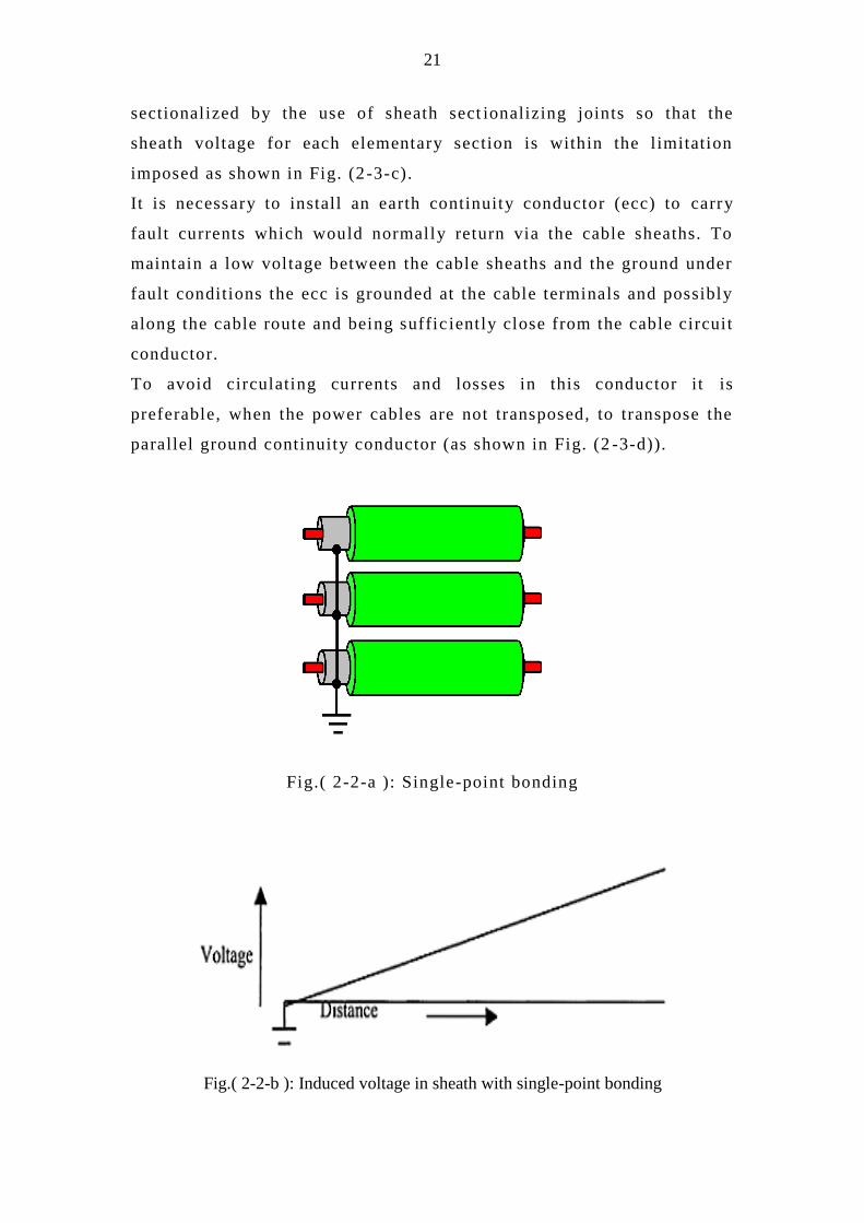
2.2.2 Sheath bonded at one end only:

The simplest form of bonding, for three-phase single-core cable,

consists in arranging for the sheaths of the three cables to be connected

together and earthed at one point only along their length, as given in

Fig. (2-2-a), at the other end of the run the cable sheaths will be

terminated at an insulated fi tting.

If the cable screen is bonded at one side only, the following effects are

appearing:

1. As the screen is open, there is no circulating current, hence,

there are practically no losses in the Screen and the ampacity is

higher compared with both sides bonding.

2. At all other points, a voltage will appear from sheath to

ground that will be a maximum at the farthest point from the

ground bond, as given in Fig.(2 -2-b), so particular care

must be taken to insulate and provide surge p rotection (using

sheath voltage limiters SVLs) at the free end of the sheath to

avoid danger from the induced transient voltages due to lighting

and switching surges as well as limiting the voltage under fault

current conditions, as given in Fig.(2 -2-c).

The maximum sheath voltage permitted at full load varies considerably

between different countries [6]; in most cases it precludes the use of

single point bonding for anything other than cable circuits of a few

hundred meters in length.

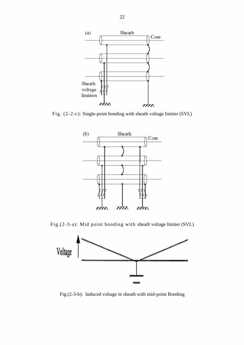
When the circuit length is such that sheath induced voltage l imitation

would be exceeded if the earth bond were connected at one end of the

circuit, this bond may be connected at some other p oint , for example

the centre of the length. In this situation, only half of the previous

voltage appears on the sheath (as shown in Fig. (2 -3-a,b)). If the

circuit is too long to be dealt with by this means it may be

21

sectionalized by the use of sheath sect ionalizing joints so that the

sheath voltage for each elementary section is within the l imitation

imposed as shown in Fig. (2 -3-c).

It is necessary to install an earth continuity conductor (ecc) to carry

fault currents which would normally return via the cable sheaths. To

maintain a low voltage between the cable sheaths and the ground under

fault conditions the ecc is grounded at the cable terminals and possibly

along the cable route and being suffic iently close from the cable circuit

conductor.

To avoid circulating currents and losses in this conductor it is

preferable, when the power cables are not transposed, to transpose the

parallel ground continuity conductor (as shown in Fig. (2 -3-d)).

Fig.( 2-2-a ): Single-point bonding

Fig.( 2-2-b ): Induced voltage in sheath with single-point bonding

22

Fig. (2-2-c): Single-point bonding with sheath voltage limiter (SVL)

Fig.(2-3-a): Mid point bonding with sheath voltage limiter (SVL)

Fig.(2-3-b): Induced voltage in sheath with mid-point Bonding

23

Fig. (2-3-c): Sectionalized run with single -point bonding

Fig. (2-3-d): Transposition of parallel conductor in flat formation or

trefoil

2.2.3 Cross bonding system:

If the sheaths of three single core cables are not bonded electrically

together, induction between conductors and each sheath can produce

unacceptable voltages between sheaths. On the other hand, bonding at

both ends will result in sheath currents following with associated

losses, which is again not acceptable, especially for long cable routes

[10]. Cross bonding of single core cable sheaths is a technique which

has been common in different countries for many years. It has been

Ground Continuity Conductor

Sheath

Voltage

Limiters

Joints With Sheath Interrupts

24

introduced in order to avoid circulating currents and excessive sheath voltages,

hence, increases its current-carrying capacity.

It achieves that by dividing the cable route into three equal lengths (or six, or

nine, etc.), and the sheath continuity is broken at each joint. The induced sheath

voltages in each section of each phase are equal in magnitude and 120° out of phase.

When the sheaths are cross connected each sheath circuit contains one section from

each phase such that the total voltage in each sheath circuit sums to zero as shown in

Fig. (2-4). If the sheaths are then bonded and earthed at the end of the run, the net

voltage in the loop and the circulating currents will be zero and the only sheath losses

will be those caused by eddy currents. This system provides a continuous

earth path via the sheaths between the earth systems at the two ends of

the cable, obviating the need for an auxiliary earth conductor.

Sheath voltage limiters (SVLs) are connected to earth at the

intermediate cross bonding positions to dissipate any sheath voltage

surges. This method of bonding allows the cables to be spaced to take advantage of

improved heat dissipation without incurring the penalty of increased circulating

current losses.

Fig. (2-4): Principle of cross-bonding

However, in practice it happens very often that the line is divided into

unequal sections, which results in an unsymmetrical cross bonding and

a residual voltage is measured at the end of the sheath, since the

voltage triangle doesn‟t close [11].

Yet i t is still useful to use this kind of bonding to at least reduce losses

considerably, instead of canceling them completely.

Applying the method of cross bonding depends on the length of the

cable and the length produced by the factory which is put on each drum

25

for transport, the length produced by the factory depends on many

factors like weight, dimensions and transport facilities and limitations.

Often cables produced in longer lengths than the average result in

additional difficult ies and are subjected to damage during transport or

laying.

The length of each section of cable depends on the nature of the area i n

which the cable will be laid and any natural or man -made obstacles.

Moreover, the costs of equipment necessary for cross bonding like

junctions and special connections and junction protection a gainst over

voltages, etc., count for economical application of cross bonding and

must be compared to the cost of the losses of sheath capitalized over

the life time of the cable which can be estimated as an average of thirty

years. It must be kept in mind that the cancellation or reduction of

sheath losses results in a smaller conductor, since it increases the

current carrying capacity and makes energy transmission more

economical.

Generally, the higher the voltage applied, the power transmitted and

the length of the cable line, the more is importance of the losses and

the more cross bonding becomes a must for the cable designer.

Single-core cables of more than 500 mm2 cross sectional conductor

area and 3 km length will prove more economical with cross bonded

sheaths in most cases [12].

In order to completely eliminate the sheath losses, the best arrangement is

where the cores of the three minor sections within each major section are perfectly

transposed but the sheaths are not, as shown in

Fig. (2-5).The voltages in the sheaths are now balanced and thereby

there is no residual voltage which could circulate sheat h currents and

therefore they are absent [5 , 9, and 11].

26

Fig. (2-5): Cross bonded cables with transposition

2.3 Types of Metallic Sheath Losses

Sheath losses are current dependent, and can be divided into two

categories according to the type of bonding [5, 9, 10, and 11]:

1- Sheath eddy losses

2- Sheath circulating losses

2.3.1 Sheath eddy losses

The metallic sheath is immerged in the magnetic field generated by the

conductor current (IC). Therefore an induced voltage (eP) appears in the

sheath, which induces currents in the metallic sheath. These currents

dissipate energy due to Joule effect .

The induced voltage is a maximum in the internal side of the sheath

and minimum in its external side, this si tuation induces the circulation

of eddy currents in the sheath as shown in Fig. (2 -6). This is the origin

of the eddy currents [13].

Eddy current losses occur in both 3 -core and single-core cables,

irrespective of the method of bonding [11].

27

Fig. (2-6): Ungrounded metallic sheath

Sheath eddy currents and losses produced by them reach their

maximum value when the cable conductors are situated as close as

possible to one another.

2.3.2 Sheath circulating losses

When both ends of the sheath are grounded, the sheath voltage (e p)

induces a sheath circulating current (Ip) along the sheath, which returns

through the ground circuit as shown in Fig.

(2-7).

The circulating currents Ip are usually much greater than the eddy

currents. Therefore the eddy currents can be ignored when dealing with

sheaths that have both ends grounded.

The sheath circulating loss occurs only in single-core cables systems [13].

28

Fig. (2-7): Sheath grounded at both ends

29

CHAPTER (3)

METHODS TO REDUCE THE SHEATH CURRENTS AND

LOSSES

3.1 Introduction

The sheath circulating current must be reduced in underground power

cable systems to a safety level, as if the sheath circulating current rises, the

loss caused by sheath circulating current will increase, and then the ratio

of loss dissipated in sheath per unit length to loss in conductor per unit

length will increase too. By such effect, the total thermal resistance of

the cable is increasing, and the permissible current i s reduced. Dry

zone may be formed around the underground cable may lead to thermal

failure of cable insulation [14]. So in this chapter the methods to

reduce the sheath circulating currents and their losses will be discussed

by classifying them into old and modern techniques.

3.2 Old Techniques to Reduce the Sheath Currents and

Losses

Some of these methods are using up to date, while the others are not.

So these methods will be discussed briefly .

3.2.1 Single-point and cross bonding methods

Prior to the development of outer coverings for cables that would

provide reliable, long term, insulation of the metall ic outer layer i t was

good practice to bond the metallic layers at both ends of the cable run.

Although this practice effectively eliminated standing voltages on the

metallic layer i t al lowed circulating currents to flow in the cable

sheaths.

The development of extruded outer coverings for cables allowed single

point bonded and cross bonded systems to be used in practice for either

30

eliminated or greatly reduced sheath circulating currents. These are

single point bonded and cross bonded systems. Such special bonding

systems were introduced into the UK in the late 1950s and e arly 1960s

[8]. For more details about them refer to clauses (2.2.2) and (2.2.3).

3.2.2 Continuous cross bonding method

In which the cable sheaths were cross-bonded continuously along the complete line

and the three sheaths are bonded and grounded at the two ends of the route only [2,

6].

3.2.3 Impedance bonding methods

The cable sheath sections are bonded together in some manner through impedance.

The impedance of the devices is made considerably higher than the impedance of the

sheaths, with the result that very little current flows and the voltage drop is almost

entirely in the device. This impedance may consist of simple reactors or of devices

such as saturable reactors and bonding transformers. To provide ground connections,

the impedance devices are normally designed with center taps or grounding points [2,

6].

3.2.4 Resistance bonding method

The flow of sheath currents may be reduced by the installation of resistance in series

with the cable sheaths. In general, resistance bonding is not practical, since the

resistors have to be sized to take the fault currents and they are considered very large

for high fault currents [2, 6].

3.3 Modern Techniques to Reduce the Sheath Currents and

Losses

These methods are not famous, so they will be discussed in details .

3.3.1 Sheath current canceling device

A patent is introduced [15] based on the principle of electro-magnetic

induction to reduce the circulating currents and the losses in the

31

metallic sheath loops of single -phase and three-phase system using

single-core high voltage transmission cables, where the sheaths are

grounded or bonded together at both ends of the cable run.

This invention consists of a current transformer at a sealing end of

each single-phase cable, connected in series with a voltage transformer

in the grounding or bonding connection of each sheath at the same

cable end. The primary winding of each current transformer is the

phase conductor, and the secondary winding of each voltage

transformer is a sheath loop. The method involves inducing locally an emf into

each sheath loop, essentially equal and opposite to that induced by the flux of the load

current in each conductor acting along the whole cable length. The circulating sheath

loop current and the losses are then nominally zero.

The principle of this method for a single-phase cable where the sheath ground loop (a-

b-c-d) includes the ground returns path (a-d) is illustrated in Fig. (3-1). The dot

notation ( • ) indicates the sense of the windings, and the mutual couplings, MCT for

transformer 1, MVT for transformer 2, and MCS between conductor C and sheath S

[15].

Fig. (3-1): Sheath current canceling device in single phase [15]

By a suitable choice of the windings of transformer 1, and transformer 2, the flux is

arranged to be essentially equal and opposite with the flux from the conductor linking

32

the loop. Thus both the driving emf ( Et + Ec), Et emf induced in the ground loop from

the transformer 2 and Ec emf induced in the ground loop from the conductor current,

and the circulating current IS in the sheath ground loop (a-b-c-d) are essentially zero.

Fig. (3-2), illustrates the three-phase system with three sets of CTs and VTs set up for

cancelling the normally circulating sheath currents ISr, ISs and ISt. The three current

transformers are clearly not connected in series, as the device is designed to operate

continuously in the steady state at power frequency, on high voltage single-phase

cables with a metal sheath. Each cable conductor load current is used to introduce a

continuous power frequency emf into its own sheath circuit via the VT, such that the

normal circulating sheath current in a sheath ground loop, or sheath loop between

phases is neutralized.

Exact equality between the opposing emfs is not necessary for the method to be

effective, as the sheath losses are proportional to IS2 (where IS

2 is the circulating

sheath current). Even with IS reduced by only 50 %, the losses are reduced by 75 %.

Fig. (3-2): Sheath current canceling device for three single -core cable

[15]

This invention characterized by:

It can be applied to cables which a re already laid, circulating sheath

currents arising due to sheath insulation failure at any location on the sheath can be

readily detected, as the secondary current in the current transformer is otherwise

nominally zero and the method is passive and adjusts automatically to the prevailing

load current on the cable.

33

3.3.2 Inductance compensation device

When laying down the cables asymmetrically or the length of three

sections of the sheath is not equal due to the development of city

constructions, there is will be a residual voltage appearing at the end

of the sheath, since the voltage triangle does not close (Fig.(3 -3)), the

circulating current is generated in metal shield.

Fig. (3-3): Residual voltage at the end of the sheath

These factors affecting the sheath losses lead to development a new

method to compensate the residual voltage by using an inductance

compensation device [16, 17].

Compensating the inductance in the cable terminal enwinding coil

around the iron core is used. One end of the winding connects to the

end of the metal shield (a short one of two ends), and the other end

connects to ground (Fig. (3 -4)).

When there is alternating current in the single -core cable, the

alternating magnetic field is generated around the single -core cable,

which links the compensating coil , then the induced electromotive

force is generated in the coil which can counter act the end voltage in

34

metal shield, hence the sheath current leads to zero, as shown in

Fig.(3-5), the voltage in L3 is U t , in the Fig.(3-5-a), and in the Fig.(3-

5-b), the current in L3 is zero because of compensation.

Fig. (3-4): Diagrammatic sketch of compensating inductance connect

Fig. (3-5): Distribution diagram of voltage in metal shield

before and after compensating inductance

To protect a compensating device against overvoltage which induc ed in

the metal shield due to short circuit earth fault of one phase or thunder

influences, the compensating device is made parallel to protection gap

of overvoltage (Fig. (3 -6)).

Fig. (3-6): Compensating device and overvoltage protector.

35

This method characterized by its easy installation, can be used for the

system of which two ends earthed directly and for the system of which

one end earthed with enhancing its length.

36

CHAPTER (4)

FACTORS AFFECTING THE SHEATH LOSSES IN SINGLE-CORE

UNDERGROUND POWER CABLES

4.1 Introduction

Power losses in underground cables cause temperature rise of the cables during their

operation, there are tow types of a power losses generated in the cables: current

dependent powers and voltage dependent powers. Current dependent powers refer to

the heat generated in metallic cable components (conductors, sheaths etc.); voltage

dependent powers refer to the powers in cable insulation [18]. Sheath losses are

current dependent and their values in single-core underground power cables can not

be disregarded as they, in some cases, could be greater than power losses in the

conductors. Sheath losses in single-core cables depend on a number of factors, these

factors are:

1- Sheath bonding and cable layout formation

2- Cable parameters (conductor resistivity & conductor size)

3- Cable spacing

4- Sheath resistance

5- Phase rotation

6- Conductor current

7- Power frequency

8- The minor section length in cross-bonding arrangement

9- Cable armoring

In this chapter these factors are investigated depending mainly on IEC 60287.

4.2 Cable Layouts Formation

Two types of cable layouts formation usually used in practice are studied in this

book:

1- A trefoil arrangement of three single-core cables, where the cables are laid as

at the corners of an equilateral triangle. In this formation two single-core

37

cables are laid close together with one cable forming an upward apex, Fig. (4-

1-a).

2- A flat arrangement of three single-core cables, where the three cables are

laid in the same horizontal plane with the middle cable equidistant from two

outer cables, Fig. (4-1-b).

(a) Trefoil formation (b) Flat formation

Fig. (4-1): Single-core cable layouts

4.3 Mathematical Algorithm

The single-core cables components are shown in Fig. (4-2).

Fig. (4-2): Unarmored single-core cable components

4.3.1 Induced sheath voltages, sheath circulating currents and losses

The following assumptions are introduced in order to simplify the

calculations of sheath losses in three ph ase power systems:

1- The sheath may be considered as a thin tube, of radius equal

38

to the mean of outer and inner radii of the sheath.

2- The capacitive currents returning along the cable sheaths will

not appreciably affect the sheath losses .

At balance, every cable in the three -phase circuit, comprising phases 1,

2 and 3 can be regarded as a return line of the two others, i .e.

I1 + I2 + I3 = 0 and Ic s1 + Ics2 + Ics3 = 0

213

312

321

CSCSCS

CSCSCS

CSCSCS

III

III

III

213

312

321

III

III

III

[10] (4-1)

In general, the following equations for the phasors of the voltage drop

per meter in the sheaths of each cable can be written as [10]

223,2113,133

333,2112,122

333,1222,111

CSCSSCSS

CSCSSCSS

CSCSSCSS

IIMjIIMjRIV

IIMjIIMjRIV

IIMjIIMjRIV

(4-2)

Where,

I1, I2, I3 : The line current in phases (1), (2) and (3) respectively in A.

VS1, VS2, VS3 : Induced voltage in sheaths (1), (2) and (3) respectively Vm-1

.


respectively in A.

RS : The resistance of sheath at its maximum operating temperature m-1

.

M1,2 : The mutual inductance between core (1) and sheath (2) in Hm-1

.


.


.

ω : 2π x frequency (in cycles per second).

39

4.3.1.1 Three phase trefoil arrangement of cables

Due to the symmetrical disposition of cables [10]

)

shr

SxMMMM ln102 7

3,13,22,1 H m-1 (4-3

Balanced currents only are considered here. Consequently, the i nduced

voltages and circulating currents in the sheaths will be respectively

equal to each other for this system.

From equations (4-2) and (4-3), for the first cable,

= ICS1 RS + j ω M ( I1 + ICS1 )

(4-4 )

VS1 = ICS1 RS - j ω M ( I2 + ICS2 ) - j ω M (I3 + ICS3)

All cable sheaths are bonded at one end only, then

ICS1 = 0 and Vs1 = j ω M I1

As a result , the induced sheath voltage per meter length will be

numerically equals to

sh

Sr

SIxMIV ln102 7

11

Or

sh

SSSSr

SIxMIVVVV ln102 7

321 (4-5)

When all cable sheaths are bonded at each end of this circuit, then

VS1 = VS2 =VS3 = 0

From equation (3-4) it follows that

IS1 RS + j ωM ( I2 + IS1 ) = 0

and MjR

MjII

S

CS

11

Or numerically in general form:

40

(4-6 )222222 MR

V

MR

MII

S

S

S

CS

The sheath loss per meter is

Wm-1 (4-7)

222

2222

MR

MRIRIW

S

SSCSCS

From equation (4-7) as this loss is proportional to the square of the power current, it is

most conveniently expressed as a ratio to the copper loss in the power conductor. This

ratio then represents the amount by which the apparent resistance of the copper

conductors is increased by the sheath losses.

The circulating sheath loss factor will be [20]:

(4-8)

1

12222

22

M

RR

R

MR

M

R

R

S

S

S

SCS

Let X = ω M

1

12

X

RR

R

S

SCS (4-9)

Where

I : The line currents in phases (1), (2) and (3) with balance condition

S : Spacing between axes of adjacent conductors in m

rsh : Mean of outer and inner radii of sheath in m

WCS : The circulating sheath loss in Wm-1

λCS : The circulating sheath loss factor

41

X : The reactance per unit length of sheath /m

R : The resistance of conductor at its maximum operating temperature m-1

.

4.3.1.2 Three phase flat arrangement of cables

It is assumed that the phase rotation is such that

2

3

2

1

2

3

2

1

23

21

jII

jII

(4-10)

When the cables are laid in a horizontal plane, with the middle cable

equidistant from the two others, then [1 0]

shr

SxMM ln102 7

3,22,1 H m-1

MMr

Sxx

r

SxM m

shsh

ln1022ln102

2ln102 777

3,1

Where

77 10389.12ln102 xxM m H m-1

H m-1

shr

SxM ln102 7

When all cable sheaths are bonded at one end only, then

IC S1 = ICS2 = ICS3 = 0

The induced voltages in the cable sheaths per meter length, which can

be found from equations (4 -1) and (4-2) are

22,113,13

22,132,112,12

33,122,11

IMjIMjV

IMjIMjIMjV

IMjIMjV

S

S

S

(4-11)

42

From equation (4-11) the numerical value of induced voltage in the

sheath of the middle cable (V S2 ) , is equal to that of the trefoil layout.

The numerical values of V S1 and VS3 can be found from equations (4 -

11)

Let X = ω M and X + Xm = ω ( M + Mm )

The sheath voltages, VS1 , VS2 , VS3 , can be expressed by the following

equations:

mmS

S

mmS

XXjXXI

V

XjIV

XXjXXI

V

32

32

23

22

21

(4-12)

The numerical values of these voltages will be, for balanced three

phase currents, as follows:

IIII

XIV

XXXXIVV

S

mmSS

321

2

22

31

(4-13)

When all cable sheaths are bonded at each end of this circuit, then the

circulating currents will flow and there may be a residual voltage a

long the cable sheaths equal to V 0 Vm-1

.

V0 could be zero when both ends of the cables are earthed.

Let

0321

0321

CSCSCS

SSS

III

VVVV (4 -1 4 )

From general equations (4 -2) the sheath circulating currents could be

found and therefore the sheath losses for the condition of balanced

power currents.

The following equations are deduced from equations (4 -2) and (4-10):

43

(4 -15)

From equations (4-15), the following equations can be obtained:

mCSSSS XIIjVVVV 2232103 (4-16)

(4-17)

Or

3

322

mS

m

CSX

XjR

XXj

II (4-18)

(4-19)

Let

m

m

XXP

XXQ

3

Equations (4-18) and (4-19) can then be writ ten respectively as

22

2

22312QR

QjRQI

jQR

jQIIII

S

S

S

CSCSCS

(4-20)

And

22

2

2231

33

PR

jPPRI

jPR

PIII

S

S

S

CSCS

(4-21)

mS

mCSCS

XXjR

XXIII

3231

XjIjXRIVV SCSS 2220 3333

mCSmmSCSS

SCSS

mCSmmSCSS

XjIXXIXXjIjXRIVV

XjIjXRIVV

XjIXXIXXjIjXRIVV

122303

2202

322101

2

3

2

1

2

3

2

1

44

From equations (4-20) and (4-21), ICS1 , ICS2 , ICS3 can be found

(4-22)

(4-23)

22

2

222222

2

23

33

2 PR

P

QR

QRj

PR

PR

QR

QII

SS

S

S

S

S

CS (4-24)

From equations (4-22) and (4-24), i t is interesting to note that the

sheath currents as well as the sheath losses in the two outer cables are

unequal. The un-equality is caused partly by the residual voltage along

the sheaths and partly by the reactive effect of the sheath circulating

currents.

Equations (4-22), (4-23) and (4-24) can be writ ten as

(4-52 )

222222

2

22

2

3

222

222222

2

22

2

1

2

3

4

3

4

2

3

4

3

4

PRQR

PQPQR

PR

P

QR

QII

QR

QII

PRQR

PQPQR

PR

P

QR

QII

SS

S

SS

CS

S

CS

SS

S

SS

CS

The sheath losses per meter in each sheath are

SCSCS RIW 2

33 , and SCSCS RIW 2

22 SCSCS RIW 2

11

The sheath loss factor in each sheath is:

22

2

222222

2

21

33

2 PR

P

QR

QRj

PR

PR

QR

QII

SS

S

S

S

S

CS

2222

2

22QR

QRj

QR

QII

S

S

S

CS

45

222222

2

22

2

12

34

3

4

1

PRQR

PQPQR

PR

P

QR

Q

R

R

SS

S

SS

SCS (4-26)

22

2

2QR

Q

R

R

S

SCS

(4-27)

222222

2

22

2

32

34

3

4

1

PRQR

PQPQR

PR

P

QR

Q

R

R

SS

S

SS

SCS (4-28)

The three later equations can be written as:

(4-29)

222222

2

22

2

13

24

3

4

1

PRQR

PQXR

PR

P

QR

Q

R

R

SS

mS

SS

SCS

(4-30)22

2

2QR

Q

R

R

S

SCS

222222

2

22

2

33

24

3

4

1

PRQR

PQXR

PR

P

QR

Q

R

R

SS

mS

SS

SCS (4-31)

Equations (4-9), (4-29), (4-30) and (4-31) are the same which have

been listed in IEC-287 [19] for unarmored single-core cable in trefoil

and flat formations.

Where

I1 ,I2 , I3 : The vector current of cables 1, 2 and 3 respectively in A

X : The reactance of sheath per unit length of cable for two adjacent

single-core cables m-1

Xm : Mutual reactance per unit length of cable between the sheath of an

outer cable and the conductors of the other two, when cables are in flat

46

Formation m-1

V0 : Residual voltage a long the cable sheath Vm-1


(2) and (3) respectively.

4.3.1.3 Three phase arrangement with sheaths cross-bonded

According to IEC-287 [19], the circulating current loss is zero for

installations where the sheaths are single-point bonded, and for installations

where the sheaths are cross-bonded and each major section is divided into

three electrically identical minor sections with keeping the currents flowing

in the conductors are balanced.

4.3.2 Sheath eddy current and its loss

4.3.2.1 Introduction

In the development of equations for the sheath losses in the preceding

section, it has been assumed that the sheath current density is uniform. In

reality the current density is not uniform and the divergence from uniformity

increases as the cables are brought closer together. Any lack of uniformity of

current density will increase the ohmic losses, and the increased loss due to a

non-uniform distribution will be referred to sheath eddy losses [20].

The eddy current losses occur in both 3 -core and single-core

cables, irrespective of the method of bonding [21]. Arnold [20],

who is the author of previous equations which have been listed in IEC-287,

has proved that the total loss in the sheath at any instant equals

to the sum of the losses caused by the main circulating current

and the eddy current, if considered separately, he also has

developed an approximate formulas that give t he sheath losses

due to eddy currents for single-core cable in trefoil and flat

formations with sheaths bonded at a single -point or two-points.

While IEC-287 introduced formula for calculating eddy sheath

47

losses for single-core cable with sheaths cross -bonded and at

the same time it is used for sheaths bonded at one end only.

In this book , Arnold‟s formulas have been used for calculating

eddy sheath losses for single-point bonding and two-points

bonding, while IEC-287 formula has been used for calcul ating

eddy sheath losses for cross -bonding.

4.3.2.2 Three phase trefoil arrangement of cables with sheaths bonded at a

single-point or two-points [20]

In this case the sheath eddy loss factor and sheath eddy current will be calculated by

equations (4-32) and (4-33).

14

22

103

S

r

RR

sh

S

SE

(4-32)

A (4 -33) 14

2

2

22

103

sshr

R

II

S

SE

Where

λSE : Sheath eddy-current loss factor

IS E : Sheath eddy-current in A

4.3.2.3 Three phase flat arrangement of cables with sheaths bonded at a

single-point or two-points [20]


equations (4-34) to (4-37).

48

(4-34) 14

22

31 102

3

S

r

RR

sh

S

SESE

14

2

2

22

31 102

3

sshr

R

III

S

SESE

A (4-35)

14

22

2 106

S

r

RR

sh

S

SE

(4-36)

14

2

2

22

2 106

sshr

R

II

S

SE

A (4-37)

Where

λSE1 , λSE3 : Sheath eddy-current loss factor in two outer cables

λSE2 : Sheath eddy-current loss factor in middle cable

IS E1 , IS E3 : Sheath eddy-current in two outer cables in A

IS E2 : Sheath eddy-current in middle cable in A

4.3.2.4 Three phase arrangement with sheaths cross-bonded [19]


equations (4-38) and (4-39).

12

4

1210

10121

x

tg

R

R SS

SSE

(4-38)

(4-39) S

SESE

R

RII

2

Where

49

6.1101 3

1

74.1

S

S

SS D

D

tg

S

7110

4

ρS : The electrical resistivity of sheath material at operating temperature ( .m)

DS : The external diameter of cable sheath (mm)

tS : The thickness of sheath (mm)

Δ1 and Δ2 are factors which their values depend on the types of cable layouts

formation.

gS and β1 are factors which their values depend on the cable parameters.

For lead-sheathed cables, gS can be taken as unity and

12

4

1

1012x

tScan be neglected.

For aluminum-sheathed cables both terms may need to be evaluated when sheath

diameter is greater than about 70 mm or the sheath is thicker than usual.

Formulae for λ0, 1 and 2 are given below:

(In which: 710SR

m

, for m ≤ 0.1, 1 and 2 can be neglected )

Where: „m‟ is a factor depends on power frequency and metallic sheath resistance.

4.3.2.4.1 Three phase trefoil arrangement of cables [19]


substituting the following parameters in equations (4-38) and (4-39).

2

2

2

021

3

S

d

m

m

66.192.0

45.2

12

33.014.1

S

dm

50

02

4.3.2.4.2 Three phase arrangement in a flat

4.3.2.4.2.1 Center cable [19]



2

2

2

021

6

S

d

m

m

7.04.1

08.3

12

86.0

m

S

dm

02

4.3.2.4.2.2 Outer cable leading phase [19]



2

2

2

021

5.1

S

d

m

m

216.0

7.0

12

7.4

m

S

dm

06.547.1

3.3

22

21

m

S

dm

4.3.2.4.2.3 Outer cable lagging phase [19]



51

2

2

2

021

5.1

S

d

m

m

1

2

5.0

123.02

274.0

m

S

d

m

mm

2

7.3

22

92.0

m

S

dm

4.3.3 A.C resistance of conductor

In order to calculate the conductor losses, a number of factors have to be calculated.

The A.C resistance, R, of a cable is given by equation

R = Rd c(1 + ys + yp) [19] (4-39)

[91( ]4-44) 201 2020 Cdc RR

ys and yp can be calculated as in [19]

Where

Rd c : The d.c. resistance of the conductor at 90 oC /m

R2 0 : The d.c. resistance of the conductor at 20 oC /m



α2 0 : The constant mass temperature coeff icient of conductor at

20 oC per Kelvin

θc : Conductor temperature

4.3.4 Sheath resistance

The sheath resistance depends on whether the sheath is a concentric neutral, a tape

shield, or tubular configuration.

52

The ohmic resistance of the metallic sheath at a sheath temperature (θ s)

above 20oC is obtained by using the following formula:

(4-41) 201 20

20 sS

S

SS

AR

Where

AS : The sheath cross-sectional area mm2

ρS20 : The electrical resistivity of sheath material at 20 oC

αS2 0 : The constant mass temperature coefficient at 20 oC per

Kelvin

4.3.4.1 Tubular metallic sheath

[19] (4-42) AS = π dS tS

In case of tubular metallic sheath:

[19] (4-43) dS=DS e-tS

Where

dS: The mean diameter of the sheath (mm)

tS : The thickness of sheath (mm)

DS e: The external diameter of the sheath ( mm)

4.3.4.2 Helically metallic sheath

In case of a helically metallic sheath ( tape or wires):

The sheath resistance is obtained taking into account that the length of

lay of the tape or wires [21].

53

2011 20

2

20

sS

S

S

SS

d

AR

(4-44)

Where:

:ℓThe length of lay of the tape or wire

The distance that it takes for one strand of the conductor to make one

complete revolution of the layer called the length of lay[22].

In case of a tape sheath, As will be calculated as tubular sheath.

In case of a wire sheath, As will be calculated per one strand and multiplied by the

number of strands [22].

i.e.

[6] (4-45)

Where

R s t ran d : Resistance of one strand, in /m

n : Number of strands

The above algorithm has been used through MATLAB program and the

flowchart of the computation steps is shown in figures (4 -3(a)) and (4-

3(b)).

Flowchart is given in Fig. (4-3-a) to show the computation steps of

sheath currents, their losses and induced sheath voltages for single -

core cable in trefoil layout with single -point bonding, two-points

bonding and cross-bonding.

Flowchart is given in Fig. (4-3-b) to show the computation steps of

sheath currents, their losses and induced sheath voltages for single -

n

RR strand

dc

54

core cable in flat layout with single-point bonding, two-points bonding

and cross-bonding.

Fig.(4-3-a): Flowchart of the computation steps for trefoil layout

55

Fig.(4-3-b): Flowchart of the computation steps for flat layout

56

Where:

ρS20 , ρC2 0 : The electrical resistivity of sheath & conductor material at

20 oC respectively.

αS2 0 , αC2 0 : The constant mass temperature coefficient at 20 oC

per Kelvin for sheath & conductor respectively.

dC : Diameter of conductor

θC max , θS max: maximum operating temperature of conductor & sheath

respectively.

ρS : The electrical resistivity of sheath material at operating temperature

tS : The thickness of sheath .

S : Spacing between axes of adjacent conductors

rsh : Mean of outer and inner radii of sheath

Rd c : The d.c. resistance of the conductor at 90 oC



R : The resistance of sheath at its maximum operating temperature

RS : The resistance of sheath at its maximum operating temperature.

M1,2 : The mutual inductance between core (1) and sheath (2).

M1,3 : The mutual inductance between core (1) and sheath (3).

ƒ : power frequency.



λSE1 , λSE2 , λSE3 : The eddy sheath loss factor for sheaths (1),


57

ISE1 , ISE2 , ISE3 : The eddy currents in sheaths of phases (1), (2) and (3)

respectively.

VS1, VS2, VS3 : Induced voltage in sheaths (1), (2) and (3) respectively.


respectively.

4.4 Factors Affecting the Sheath Losses in Single-Core Underground Power

Cables

4.4.1 Effect of sheath bonding and cable layout formation on sheath losses


Sheath circulating currents, sheath eddy currents and their corresponding loss

factors for single-point bonding, two-points bonding and cross-bonding and

also sheath induced voltages for single-point bonding have been calculated

for single-core cable in touch trefoil and touch flat formations with using

mathematical algorithm which is explained above to investigate the effect of

sheath bonding methods and cable layouts formations on the sheath losses.

4.4.1.2 Cases study

The study is carried out by using single-core cables made of a stranded

copper conductor with 800 mm2 insulated by XLPE and covered by a lead

screens, f = 50 Hz, with various voltage levels, to get a wide range of values

of these variables, which their parameters [23] are listed in table (4-1).

Table (4-1): Single-core cables 800 mm2 CU with lead screen parameters

Voltage level ( kV )

Cable parameters

500 220 132 66 22 11

800 800 800 800 800 800 Conductor size (mm2)

58

Ground temperature 20°C

Laying depth 1.0 m

Distance “S” between cable axes laid in flat formation De (De: the external diameter

of the cable)

Ground thermal resistivity 1.0 Km/W

Assuming the sheath temperature equals to 70°C

Current rating (A) for copper conductor 995 A

4.4.1.3 Obtained results

The outputs of the program which represents the results for unarmored single-core

cables are given in tables (4-2-a), (4-2-b) and (4-2-c).

Table (4-2-a) gives the values of sheath currents and their loss factors and induced

voltages in the metallic sheaths in case of single-point bonding for touch trefoil and

touch flat.

34 34 34 34 34 34 Diameter of the conductor (mm)

115.3 89.1 74.5 62.6 50.4 46 Mean sheath diameter (mm)

136 108 93 80 58 53 Outer diameter of cable (mm)

0.0221 DC Resistance of the copper conductor at 20 °C /km

21.4 x 10-8

Lead electrical resistivity at 20°C .m

1.7241 x 10-8

Copper electrical resistivity at 20°C .m

3.93 x 10-3

Temperature coefficient of copper per K at 20 °C

4 x 10-3

Temperature coefficient of lead per K at 20 °C

59

Table (4-2-a): Sheath currents, their loss factors and sheath induced voltages in case

of single-point bonding method with lead screens

Sheath bonding arrangement

Voltage

levels Phase

no.

Single-point bonding-touch flat

Single-point bonding-touch trefoil

VS

(V/km)

ISE

A

λSE

%

ICS

A

λCS

%

VS

(V/km)

ISE

A

λSE

%

(A) ICS

A

λCS

%

1 91.5 10.2

A

0.45 0 0 61.8 14.5

A

0.90 0 0

11 kV 2 61.8 20.5

A

1.80 0 0 61.8 14.5

A

0.90 0 0

3 91.5 10.2

A

0.45 0 0 61.8 14.5

A

0.90 0 0

1 90.7 12 A 0.54 0 0 60.9 17.1

A

1.07 0 0

22 kV 2 60.9 24.1

A

2.15 0 0 60.9 17.1

A

1.07 0 0

3 90.7 12 A 0.54 0 0 60.9 17.1

A

1.07 0 0

1 88.7 29.8

A

1.41 0 0 58.7 42.1

A

2.82 0 0

66 kV 2 58.7 59.6

A

5.64 0 0 58.7 42.1

A

2.82 0 0

3 88.7 29.8

A

1.41 0 0 58.7 42.1

A

2.82 0 0

1 87.3 40.5 1.98 0 0 57.2 57.4 3.96 0 0 132 kV

3 1 2

60

A A

2 57.2 81

A

7.91 0 0 57.2 57.4

A

3.96 0 0

3 87.3 40.5

A

1.98 0 0 57.2 57.4

A

3.96 0 0

1 85.7 60.2

A

3.05 0 0 55.4 85.2

A

6.10 0 0

220 kV 2 55.4 120.4

A

12.20 0 0 55.4 85.2

A

6.10 0 0

3 85.7 60.2

A

3.05 0 0 55.4 85.2

A

6.10 0 0

1 84.2 98.4

A

5.16 0 0 53.7 139.2

A

10.32 0 0

500 kV 2 53.7 196.8

A

20.64 0 0 53.7 139.2

A

10.32 0 0

3 84.2 98.4

A

5.16 0 0 53.7 139.2

A

10.32 0 0

Where:

λCS : The circulating sheath loss factor percentage of conductor loss

ICS : The circulating current in the sheath

λSE : The sheath eddy loss factor percentage of conductor loss

ISE : The eddy current in the sheath

VS : The induced voltage in the sheath per km

Table (4-2-b) shows the values of sheath currents and their loss factors in case of two-

points bonding for touch trefoil and touch flat.

61

Table (4-2-b): Sheath currents and their loss factors in case of two-points bonding

method with lead screens


Voltage

levels Phase

no.

Two-points bonding-touch flat

Two-points bonding-touch

trefoil

(A) ISE λSE % (A) ICS λCS % (A) ISE λSE % (A) ICS λCS

1 10.2

A

0.45 67

A

19.14 14.5

A

0.90 44.5

A

8.46

11 kV 2 20.5

A

1.80 34.1

A

4.97 14.5

A

0.90 44.5

A

8.46

3 10.2

A

0.45 68.4

A

19.94 14.5

A

0.90 44.5

A

8.46

1 12

A

0.54 76.8

A

21.65 17.1

A

1.07 50.8

A

9.51

22 kV 2 24.1

A

2.15 38.8

A

5.54 17.1

A

1.07 50.8

A

9.51

3 12

A

0.54 78.6

A

22.69 17.1

A

1.07 50.8

A

9.51

1 29.8

A

1.41 172.9

A

47.38 42.1

A

2.82 116

A

21.32

66 kV 2 59.6

A

5.64 87.7A 12.18 42.1

A

2.82 116

A

21.32

3 29.8

A

1.41 182.5

A

52.79 42.1

A

2.82 116

A

21.32

1 40.5

A

1.98 237.1

A

58.91 57.4

A

3.96 149.4

A

26.91 132 kV

3 1 2

62

2 81

A

7.91 112.2

A

15.19 57.4

A

3.96 149.4

A

26.91

3 40.5

A

1.98 237.1

A

67.77 57.4

A

3.96 149.4

A

26.91

1 60.2

A

3.05 298.8

A

75.07 85.2

A

6.10 206.6

A

35.87

220 kV 2 120.4

A

12.20 154.2

A

19.99 85.2

A

6.10 206.6

A

35.87

3 60.2

A

3.05 329.5

A

91.25 85.2

A

6.10 206.6

A

35.87

1 98.4

A

5.16 419.2

A

93.62 139.2

A

10.32 309.3

A

50.95

500 kV 2 196.8

A

20.64 231.3

A

28.50 139.2

A

10.32 309.3

A

50.95

3 98.4

A

5.16 485.4

A

125.4

8

139.2

A

10.32 309.3

A

50.95

Where:





Table (4-2-c) shows the values of sheath currents and their loss factors in case of

cross bonding for touch trefoil and touch flat.

63

Table (4-2-c): Sheath currents and their loss factors in case of cross-bonding method

with lead screens


Voltage

levels Phase

no.

Cross bonding-touch flat

Cross bonding-touch trefoil


1 10.2

A

0.45 0 0 14.5

A

0.90 0 0

11 kV 2 20.5

A

1.80 0 0 14.5

A

0.90 0 0

3 10.2

A

0.45 0 0 14.5

A

0.90 0 0

1 12

A

0.54 0 0 17 A 1.07 0 0

22 kV 2 24.1

A

2.15 0 0 17 A 1.07 0 0

3 12

A

0.54 0 0 17 A 1.07 0 0

1 29.7

A

1.4 0 0 42 A 2.81 0 0

66 kV 2 59.5

A

5.61 0 0 42 A 2.81 0 0

3 29.7

A

1.4 0 0 42 A 2.81 0 0

1 40.3

A

1.97 0 0 57.1

A

3.93 0 0

132 kV

2 80.7 7.86 0 0 57.1 3.93 0 0

3 1 2

64

A A

3 40.3

A

1.97 0 0 57.1

A

3.93 0 0

1 64.9

A

3.54 0 0 86 A 6.22 0 0

220 kV 2 119.6

A

12.04 0 0 86 A 6.22 0 0

3 56.7

A

2.71 0 0 86 A 6.22 0 0

1 108.4

A

6.27 0 0 139.3

A

10.34 0 0

500 kV 2 193.6

A

19.96 0 0 139.3

A

10.34 0 0

3 90.3

A

4.35 0 0 139.3

A

10.34 0 0

Where:





4.4.1.4 Results discussion

From the previous calculations for single-point bonding in table (4-2-a), it is noticed

that:

In case of single-point bonding there is no circulating current as no closed

circuit for the sheath, hence there is no sheath circulating losses but sheath

eddy losses are still present and they can be neglected as their values are

small, also there is induced voltage at the open end.

65

For trefoil layout the eddy losses are equal, while for flat layout the eddy

losses in the outer cable sheaths are equal and usually smaller than the value of

the middle cable sheath, for example, in case of 66 kV single-core cable:

For trefoil: λSE1=λSE2=λSE3=2.82 %.

For flat : λSE1= λSE3=1.41 % & λSE2 =5.64 %.

But it must be noticed that, the total sheath eddy losses per circuit in trefoil are

equal that in flat, i.e.

For trefoil: λSE1+λSE2+λSE3=3*2.82 = 8.46 %.

For flat : λSE1+ λSE3+ λSE2 =2*1.41 + 5.64 = 8.46 %.

For trefoil layout the induced sheath voltages are equal, while for flat layout

the voltages induced in the outer cable sheaths are equal and usually larger

than the voltage induced in the middle cable sheath, the values of induced

sheath voltages in trefoil are equal to the value of induced sheath voltage in

the middle cable sheath in flat formation, for example, in case of 66 kV single-

core cable:

For trefoil: VS1=VS2=VS3=58.7 V/km.

For flat : VS1=VS3=88.7 V/km & VS2=58.7 V/km.

Or this also may be clearly appearing in Fig.(4-4).

If the cables are laid in trefoil formation instead of flat arrangement, the

induced voltages in the screens can be minimized.

The sheath induced voltages for single-core cables with single-point bonding

may be reached to hazard values in normal operations, so the length of cables

must be limited to keep them within permissible limits, so it is expected the

cable length in case of trefoil is longer than flat layout.

The sheath induced voltages reduce with increasing the system voltages due

to reducing (S/rsh) ratio, factory cable design, as S in that case equals De.

Addition to conductor current and cable length, the induced sheath voltage

depends mainly on the spacing between phases as shown in Fig.(4-4)

66

Fig.(4-4): Sheath induced voltage vs. cable spacing for single-core cable 66 kV in

trefoil and flat formations with single-point bonding

From the previous calculations for two-points bonding in table (4-2-b), it is noticed

that:

Eddy loss could be disregarded with comparing to circulating loss but it must

be noticed that the eddy loss value of middle conductor in flat formation with

close spacing between phases especially for extra high system voltages cables

must be taken into consideration as its value approaches to the value of sheath

circulating loss for the same conductor, for example, in case of 500 kV single-

core cable in table (4-2-b):

For flat : λSE2 =20.64 % & λCS2 =28.50 %.

The trefoil configuration has lower total sheath losses than flat formation

when sheaths are bonded at both ends; also it introduces symmetrical results

for all calculations.

For cables in flat configuration when sheaths are bonded at both ends, the

sheath circulating losses have unequal magnitude; the least value occurs in the

sheath of the middle cable, values in sheaths of outer cables are of unequal

magnitude too. Thereby, the cable sheath of the lag phase has a higher value.

67

The sheath circulating losses in two-points bonding method could be

reached to more than the conductor losses, as in case of 500 kV single-

core cable in table (4-2-b) for two-points arrangement with flat

formation λCS3=125.48 %, this cause the insulation of the conductor to

be subjected to temperatures may be excess of the insulation ratings,

so the cable ampacity must be de-rated.

From the previous calculations for cross bonding in table (4-2-c), it is noticed that:

According to IEC 60287, the eddy loss only exists where the sheaths

are cross bonded and each major section is divided into three identical

minor sections.

In cross-bonding arrangement, the total sheaths losses per circuit in trefoil

formation are approximately equal the total sheath losses in flat formation.

From the previous calculations in tables (4-2-a), (4-2-b) and (4-2-c), it is noticed that:

Both single-point bonding and cross-bonding have sheath losses lower than

two-points bonding arrangement.

The sheath losses in single-point bonding are approximately the same

as in cross bonding as shown in tables (4-2-b) and (4-2-c). In single-

point bonding, the induced voltage limits the cable length, while cross

bonding is preferred in long run lengths due to sheath voltages

cancelation in each major section.

The sheath eddy losses in outer two phases in flat formation are equal for

single-point bonding and two-points bonding while for cross-bonding this is

true only for m factor 0.1 ( 710SR

m

), refer to clause 4.3.2.4 . For

example, in case of 500 kV single-core cable:

In table (4-2-a) for single-point bonding:

For flat : λSE1 = λSE3=5.16 % .

In table (4-2-b) for two-points bonding:

68

For flat : λSE1 = λSE3=5.16 %.

In table (4-2-c) for cross bonding:

For flat : λSE1 =6.27 % & λSE3=4.35 % (λSE1 ≠ λSE3).

While in case of 66 kV single-core cable:

In table (4-2-c) for cross bonding:

For flat : λSE1 = λSE3=1.4 %.

For the same layouts formations, Arnold equations for calculating

eddy losses (tables (4-2-a) & (4-2-b)) give approximately the same values

which have been given in case of using IEC-287 equation (table (4-2-c)),

less divergence occurs with increasing m factor over 0.1, so one of

equations could be used for calculating eddy losses to any sheath bonding

method. The maximum values of the total sheath currents per phase (i.e.

sheath eddy current + sheath circulating current) with sheaths bonded at

two-points in touch trefoil reached to 45 % of line current (in table (4-2-b)

in case of 500 kV ISE3 + ICS3= 45 % of rating current) while they reached

to 58.7 % in touch flat formations (in table (4-2-b) in case of 500 kV ISE3

+ ICS3= 58.7 % of rating current) and they reached to 14 % and 19.5 %

respectively with sheaths cross bonded (in table (4-2-c) in case of 500

kV). The total sheath loss factors per circuit in touch trefoil and flat

formations (i.e. λCS1+ λCS2+λCS3 +λSE1+ λSE2 +λSE3 ) with sheaths bonded

at two-points reached to 183.81 % and 278.56 % of conductor copper

losses respectively (in table (4-2-c) in case of 500 kV) while they reached

to 31.02 % and 30.58 % of conductor copper losses respectively with

sheaths cross bonded (in table (4-2-c) in case of 500 kV).

4.4.2 Effect of cable parameters (conductor size & its resistivity) on the sheath

losses in single-core cables


The purpose of the core conductor is to transmit the required current with low

losses. copper and aluminum of the metals are commonly used for

69

conductors with various conductor sizes, so the conductor material resistivity,

which is determined by the material the conductor is made from, and the

conductor sizes have been examined by using the mathematical algorithm,

which is explained in clause 4.3, by calculating the sheath losses for

aluminum and copper conductor with the same dimensions to examine the

effect of conductor resistivity on the sheath losses, and also using single-core

cables with various conductor sizes with the same voltage to examine the

effect of conductor sizes on the sheath losses.

4.4.2.2 Cases study

1- 66 kV single-core cable, made of a stranded copper conductor with 800

mm2 insulated by XLPE and covered by a lead screen, f = 50 Hz, which its

parameters have been listed in table (4-1), and another single-core cable

made of a stranded aluminum conductor with the same dimensions, which

their electrical properties have been listed in tables (4-3), are used to examine

the effect of conductor material resistivity on the sheath losses.

2- 66 kV Single-core cables, made of a stranded copper conductor with

various cross sectionals insulated by XLPE and covered by a lead screens ,f =

50 Hz, which their parameters have been listed in table (4-4), are used to

examine the effect of conductor's size on the sheath losses.

Table (4-3): Electrical dc resistances and temperature coefficients for 800

mm2 copper and aluminum conductors

Conductor material DC Resistance of the conductor at

20°C, /km

Temperature coefficient per K at

20°C

CU ( I=995 A ) 0.0221 3.93x10-3

AL ( I=795 A ) 0.0367 4.03x10-3

70

Table (4- 4): Single-core cables 66 kV-CU with lead screens parameters


4.4.2.3.1 Effect of conductor material resistivity on the sheath losses

Tables (4-5-a) and (4-5-b) show the values of sheath currents and their loss

factors for touch trefoil and touch flat layouts in two single-core cables, one

of them is made of a stranded copper conductor and the other is made of a

stranded aluminum conductor in case of two-points bonding and cross

bonding respectively to indicate the effect of conductor material resistivity on

the sheath losses.

Table (4- 5-a): Sheath currents and their loss factors in case of two-points bonding

method for copper and aluminum conductors


Conductor

material Phase

no.



trefoil

conductor size mm2

Cable parameters

800 630 500 400 300 240

995 889 776.6 683.6 599.9 530.1 Current rating (A)


62.6 61 57.1 53.8 50.8 46.2 Mean sheath diameter (mm)

0.0221 0.0283 0.0366 0.0470 0.0601 0.0754 DC Resistance of the copper

conductor (20°C), /km

34 30.2 26.3 23.2 20.4 18.1 diameter of the conductor (mm)

3 1 2

71


1 29.8

A

1.41 172.9

A

47.38 42.1

A

2.82 116

A

21.32

CU 2 59.6

A

5.64 87.7A 12.18 42.1

A

2.82 116

A

21.32

3 29.8

A

1.41 182.5

A

52.79 42.1

A

2.82 116

A

21.32

1 23.8

A

0.91 138.1

A

30.62 33.7

A

1.82 92.6

A

13.78

AL 2 47.6

A

3.64 70

A

7.87 33.7

A

1.82 92.6

A

13.78

3 23.8

A

0.91 145.8

A

34.11 33.7

A

1.82 92.6

A

13.78

Table (4-5-b): Sheath currents and their loss factors in case of cross-bonding method

for copper and aluminum conductors


Conductor

material Phase

no.



(A) ISE λSE % (A) ISE λSE %

1 29.7 A 1.4 42 A 2.81

CU 2 59.5 A 5.61 42 A 2.81

3 29.7 A 1.4 42 A 2.81

1 23.7 A 0.91 33.6 A 1.81 AL

3 1 2

72

2 47.5 A 3.63 33.6 A 1.81

3 23.7 A 0.91 33.6 A 1.81

Where:





4.4.2.3.2 Effect of conductor sizes on the sheath losses

Tables (4-6-a) and (4-6-b) show the values of sheath currents and their loss

factors for touch trefoil and touch flat layouts in single-core cables with

various sizes in case of two-points bonding and cross bonding to indicate the

effect of conductor sizes on the sheath losses.

Table (4-6-a): Sheath currents and their loss factors for various sizes in case of two-

points bonding method


Cross

section

mm2

Phase

no.



trefoil


1 9 A 0.25 58 A 10.38 12.7

A

0.5 38.9

A

4.67

240 2 18 A 1 29.8

A

2.75 12.7

A

0.5 38.9

A

4.67

3 9 A 0.25 59.9 11.10 12.7 0.5 38.9 4.67

3 1 2

73

A A A

1 11.4

A

0.36 71.2

A

13.83 16.2

A

0.72 47.5

A

6.17

300 2 22.9

A

1.43 36.2

A

3.59 16.2

A

0.72 47.5

A

6.17

3 11.4

A

0.36 73.9

A

14.88 16.2

A

0.72 47.5

A

6.17

1 14.6

A

0.51 88.9

A

18.92 20.7

A

1.03 59.2

A

8.41

400 2 29.2

A

2.05 45

A

4.85 20.7

A

1.03 59.2

A

8.41

3 14.6

A

0.51 92.5

A

20.50 20.7

A

1.03 59.2

A

8.41

1 18.2

A

0.70 112.2

A

26.57 25.7

A

1.40 75.4

A

12.01

500 2 36.4

A

2.80 57.5

A

6.99 25.7

A

1.40 75.4

A

12.01

3 18.2

A

0.70 117.3

A

29.04 25.7

A

1.40 75.4

A

12.01

1 22.6

A

0.97 135.9

A

34.74 32

A

1.94 91.1

A

15.61

630 2 45.3

A

3.87 69.1

A

9 32

A

1.94 91.1

A

15.61

3 22.6

A

0.97 142.5

A

38.18 32

A

1.94 91.1

A

15.61

1 29.8

A

1.41 172.9

A

47.38 42.1

A

2.82 116

A

21.32

800

2 59.6

A

5.64 87.7A 12.18 42.1

A

2.82 116

A

21.32

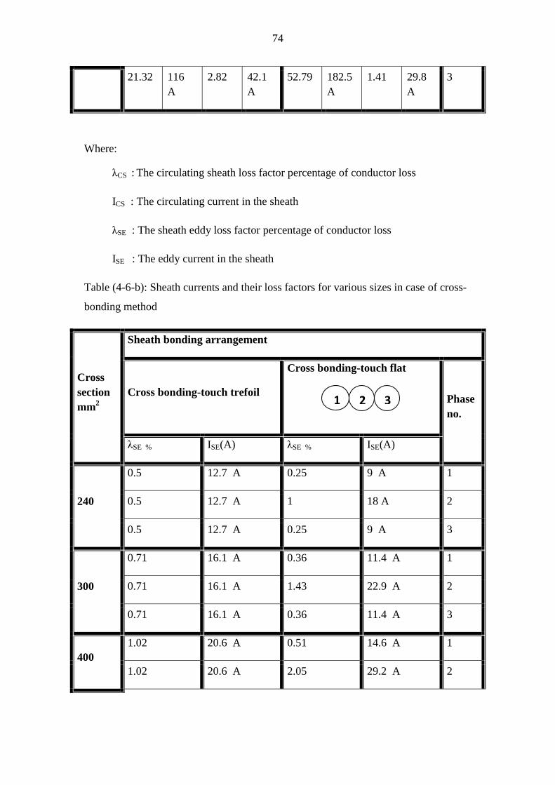
74

3 29.8

A

1.41 182.5

A

52.79 42.1

A

2.82 116

A

21.32

Where:





Table (4-6-b): Sheath currents and their loss factors for various sizes in case of cross-

bonding method


Cross

section

mm2

Phase

no.




1 9 A 0.25 12.7 A 0.5

240 2 18 A 1 12.7 A 0.5

3 9 A 0.25 12.7 A 0.5

1 11.4 A 0.36 16.1 A 0.71

300 2 22.9 A 1.43 16.1 A 0.71

3 11.4 A 0.36 16.1 A 0.71

1 14.6 A 0.51 20.6 A 1.02

400

2 29.2 A 2.05 20.6 A 1.02

3 1 2

75

3 14.6 A 0.51 20.6 A 1.02

1 18.2 A 0.70 25.7 A 1.40

500 2 36.4 A 2.79 25.7 A 1.40

3 18.2 A 0.70 25.7 A 1.40

1 22.6 A 0.96 32 A 1.93

630 2 45.3 A 3.86 32 A 1.93

3 22.6 A 0.96 32 A 1.93

1 29.7 A 1.4 42 A 2.81

800 2 59.5 A 5.61 42 A 2.81

3 29.7 A 1.4 42 A 2.81

Where:





4.4.2.4 Discussion of the obtained results

From tables (4-5-a) and (4-5-b) when the conductor materials are copper and

aluminum It is noticed that:

Both sheath circulating loss factor and sheath eddy loss factor decrease

as the conductor resistivity increase, i.e. the sheath loss factors (λSE &

λCS) are inversely proportional to the conductor resistivity.

The sheath losses in flat formation with two-points bonding have more

sensitivity to conductor material resistivity than other types of

bonding, as the total sheath losses factor per circuit in touch flat and

76

touch trefoil formations increased by 42.75 % and 25.62% of

conductor losses respectively in case of using copper conductor

instead of using aluminum conductor, as shown in table (4-5-a), i.e.(

(λCS1+ λCS2+λCS3 +λSE1+ λSE2 +λSE3) with CU)-( (λCS1+ λCS2+λCS3

+λSE1+ λSE2 +λSE3) with AL) = +42.75 in touch flat & +25.62 in touch

trefoil), while they increased by 2.96 % and 3.62 % of conductor

losses respectively with sheaths cross bonded, as shown in table

(4-5-b), i.e. ( (λCS1+ λCS2+λCS3 +λSE1+ λSE2 +λSE3) with CU)-( (λCS1+

λCS2+λCS3 +λSE1+ λSE2 +λSE3) with AL) = +2.96 in touch flat & +3.62 in

touch trefoil, i.e. conductor resistivity is one of the method for

controlling the sheath losses in two-points bonding arrangement.

From tables (4-6-a) and (4-6-b) with changing the conductor sizes, it is noticed that:

Both sheath circulating loss factor and sheath eddy loss factor increase

with increasing the conductor sizes.

The cross-bonding has very low sensitivity to the changing of small

conductor sizes, while flat formation with two-points bonding has more

sensitivity to the changing of small conductor sizes.

In lower conductor sizes, both sheath circulating loss factor and sheath

eddy loss factor can be neglected.

Trefoil layout introduces a good solution to overcome the problems of

high sheath circulating losses values in two-points bonding method rather

than flat layout.

4.4.3 Effect of cable spacing on the sheath losses


The previous mathematical algorithm, explained in clause 4.2, is used to

investigate the effect of varying the spacing between cables on the sheath

losses by varying the spacing between cables from De to 2De. (De: The

external diameter of the cable)

4.4.3.2 Cases study

77

66 kV single-core cable, made of a stranded copper conductor with 800 mm2 insulated

by XLPE and covered by a lead screen, f = 50 Hz, which its parameters have been

listed in table (4-1), is used in this case study.

4.4.3.3 Obtained results by using IEC 60287

The obtained results using IEC 60287 have been shown in tables (4-7-a) and (4-7-b).

In these tables sheath currents and their losses are calculated with changing the axial

spacing between the cables from De to 2 De in case of two-points bonding (trefoil &

flat) and cross bonding (trefoil & flat) respectively.

Table (4-7-a): Sheath currents and their loss factor in case of two-points bonding

methods with De and 2De spacing between cables


Spacing Phase

no.


Two-points bonding-touch trefoil


1 29.8

A 1.41

172.9

A 47.38

42.1

A 2.82 116 A 21.32

De mm 2 59.6

A 5.64 87.7A 12.18

42.1

A 2.82 116 A 21.32

3 29.8

A 1.41

182.5

A 52.79

42.1

A 2.82 116 A 21.32

1 14.9

A 0.36

246.4

A 98.92

21

A 0.72

198.9

A 64.47

2De mm 2 29.8

A 1.45

171.1

A 48.01

21

A 0.72

198.9

A 64.47

3 14.9

A 0.36

264.1

A 113.63

21

A 0.72

198.9

A 64.47

3 1 2

78

Table (4-7-b): Sheath currents and their loss factor in case of cross bonding methods

with De and 2De spacing between cables


Spacing Phase

no.




1 29.7 A 1.4 42 A 2.81

De mm 2 59.5 A 5.61 42 A 2.81

3 29.7 A 1.4 42 A 2.81

1 14.8 A 0.36 21 A 0.72

2De mm 2 29.7 A 1.44 21 A 0.72

3 14.8 A 0.36 21 A 0.72

Where:






From tables (4-7-a) and (4-7-b), it is seen that:

In case of trefoil and flat formation when sheaths are bonded at both ends,

the sheath circulating losses increase with increasing the cable spacing.

The sheath circulating losses could be reached to more than its double

values with duplicating the spacing between phases.

3 1 2

79

The sheath eddy losses decrease with increasing the cable spacing, so it

can be deduced that for larger cables the effect of spacing on total sheath

losses is much lesser than that on the sheath circulating losses alone.

In general, the effect of spacing on the sheath circulating losses and sheath eddy

losses for single-core cable can be shown in figures (4-5),(4-6), (4-7) and (4-8).

Figure (4-5) shows the values of sheath circulating loss factor with varying the

axial spacing between the conductors for single-core cable in case of its sheaths

bonded at two-points with trefoil formation.

Fig. (4-5): Sheath circulating loss factor vs. spacing for 66 kV single-core cable trefoil


Figure (4-6) shows the values of sheath circulating loss factor with varying the axial

spacing between the conductors for single-core cable in case of its sheaths bonded at

two-points with flat formation.

80

Fig. (4-6): Sheath circulating loss factor vs. spacing for 66 kV single-core cable flat


Figure (4-7) shows the values of sheath eddy loss factor with varying the axial

spacing between the conductors for single-core cable in case of its sheaths bonded

at two-points with trefoil formation.

Fig. (4-7): Sheath eddy loss factor vs. spacing for 66 kV single-core cable trefoil

formations with two-points bonding

81

Figure (4-8) shows the values of sheath eddy loss factor with varying the axial

spacing between the conductors for single-core cable in case of its sheaths bonded at

two-points with flat formation.

Fig. (4-8): Sheath eddy loss factor vs. spacing factor for 66 kV single-core cable flat

formations with two-points bonding

From figures (4-5) and (4-6) which show the effect of cable spacing on sheath

circulating losses, it can be seen that:

The sheath circulating losses are proportional to the spacing between phases.

The sheath circulating losses could be reached to more than two times the

conductor loss depending on the spacing between phases.

From figures (4-7) and (4-8) which show the effect of cable spacing on sheath eddy

losses, it is clearly appearing that:

The sheath eddy losses are inversely proportional to the spacing between

phases.

The sheath eddy losses reduce rapidly at lower spacing, while reduce very

slowly at large spacing.

The sheath eddy losses can be neglected at large spacing.

Cross-bonding method is more active method with increasing the spacing

between phases but in one condition which is keeping the minor section

lengths of sheath are equal, because according to IEC 60287 the eddy losses

are then only exist which are inversely proportional to spacing between cables.

82

4.4.4 Effect of sheath resistance on the sheath losses


Mathematical algorithm, which is explained in clause 4.3, is used to examine more

closely the effect of sheath resistance on the sheath losses.

4.4.4.2 Cases study



listed in table (4-1), is used in this case study. A.C sheath resistance (RS) at 70 oC =

0.5 Ω/km.


Figures (4-9), (4-10), (4-11), (4-12) and (4-13) show the obtained results.

4.4.4.3.1 Effect of sheath resistance on the sheath circulating losses

Figure (4-9) shows the sheath circulating loss factor with varying A.C sheath

resistance of single-core cable in trefoil formation in case of two-points bonding with

axial spacing between cables De and 2De.

Fig. (4-9): Sheath circulating loss factor vs. sheath resistance in trefoil formation with

two-points bonding for De and 2De spacing between cables

83

Figure (4-10) shows the sheath circulating current with varying A.C sheath resistance

of single-core cable in trefoil formation in case of two-points bonding with axial

spacing between cables De and 2De.

Fig. (4-10): Sheath circulating current vs. sheath resistance in trefoil formation with

two-points bonding for De and 2De spacing between cables

Figure (4-11) shows the sheath circulating loss factor with varying A.C sheath

resistance of single-core cable in flat formation in case of two-points bonding.

Fig. (4-11): Sheath circulating loss factor vs. sheath resistance in touch flat formation

with two-points bonding

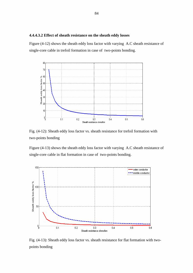
84

4.4.4.3.2 Effect of sheath resistance on the sheath eddy losses

Figure (4-12) shows the sheath eddy loss factor with varying A.C sheath resistance of

single-core cable in trefoil formation in case of two-points bonding.

Fig. (4-12): Sheath eddy loss factor vs. sheath resistance for trefoil formation with

two-points bonding

Figure (4-13) shows the sheath eddy loss factor with varying A.C sheath resistance of

single-core cable in flat formation in case of two-points bonding.

Fig. (4-13): Sheath eddy loss factor vs. sheath resistance for flat formation with two-

points bonding

85


From Figures (4-9), (4-10) and (4-11) which indicate the effect of sheath resistance on

the sheath circulating losses it is noticed that:

At the maximum sheath current, equal to full conductor current, (i.e.,

for the case of zero sheath resistance), the circulating-current loss is

obviously zero. While the sheath current falls with increasing sheath

resistance, i.e. the sheath current is inversely proportional to the sheath

resistance, the sheath circulating loss first rises to a maximum, and

then falls, again approaching zero at infinite sheath resistance, so the

sheath circulating loss would be eliminated when the sheath resistance

tends to either zero or infinity.

The value of sheath resistance which gives maximum-sheath

circulating-current loss is called critical sheath resistance, values of

sheath resistance higher or lower than this critical value will give

lower circulating-current losses than those for the critical sheath

resistance, so the cable designer must be aware to avoid this value.

Attention is also called to the fact, indicated in Fig. (4-9), that the

critical sheath resistance for a given cable is diminished when the

spacing between phases is reduced.

The critical value of sheath resistance in flat formation differs from

conductor to other in flat formation as shown in Fig. (4-11).

From Figures (4-12) and (4-13) which indicate the effect of sheath resistance on the

sheath eddy losses it can be seen that:

The sheath eddy losses are inversely proportional to the sheath resistance.

The sheath eddy losses can be neglected at large values of sheath resistances.

4.4.4.5 Factors affecting the sheath resistance

4.4.4.5.1 Introduction

By referring to equation (4-41), it can be noticed that the sheath resistance is

affecting by:

86

1-Sheath material resistivity

2- Temperature of the sheath material

The effect of each factor on the sheath losses is studied by using the mathematical

algorithm which is explained in clause 4.3.

4.4.4.5.2 Cases study

1- Single-core cables, made of a stranded copper conductor with 800 mm2

insulated by XLPE, f = 50 Hz, with various voltages levels and screens

(copper wire, copper tape, stainless steel and aluminum) , which their

parameters have been listed in tables (4-8), (4-9), (4-10), (4-11) and (4-12),

are used to investigate the effect of sheath material resistivities of different

metallic screens on the sheath losses.

2- 66 kV single-core cable, made of a stranded copper conductor with 800

mm2 insulated by XLPE and covered by a lead screen and laid in touch

trefoil with sheaths bonded at two-points, f = 50 Hz, which its parameters

have been listed in table (4-1), is used to see the effect of temperature of the

sheath material on the sheath losses.

Table (4-8): Electrical resistivities and temperature coefficients for different metallic

sheaths materials

Metal Resistivity (Ω m) at 20 oC

Temperature coefficient per K

at 20°C

Copper 1.7241 x 10-8

3.93x 10-3

Lead and its alloy 21. 4 x 10-8

4 x 10-3

Stainless steel 70 x 10-8

negligible

Aluminum 2.84 x 10-8

4.03 x 10-3

87

Table (4- 9): Single-core cable 800 mm2 CU, with copper tape screen parameters


Laying depth 1.0 m

Distance “S” between cable axes laid in flat formation De




Thickness of copper tape 2x0.15 mm


Cable parameters

500 220 132 66 22 11





33.6 33.7 33.7 33.7 33.7 33.7 Diameter of the conductor (mm)

103.9 81.9 65.9 55.9 46.9 42.7 Diameter over insulation (mm)

0.58 0.73 0.90 1.1 1.2 1.4 Ω sheath resistance at 70oC

88

Table (4-10): Single-core cable 800 mm2 CU with copper wire screen parameters


Laying depth 1.0 m





Table (4-11): Single-core cable 800 mm2 CU with stainless steel screen parameters


Cable parameters

500 220 132 66 22 11

185 185 95 35 35 35 Cross section of screen (mm2)


116 93 75 63 54 49 Mean sheath diameter (mm)




sheath (20°C), /km

33.6 33.7 33.7 33.7 33.7 33.7 diameter of the conductor (mm)

0.33 0.47 0.65 1.8 1.9 1.99 sheath resistance at 70oC /km


Cable parameters

500 220 132 66 22 11

136.2 108.2 93.2 80.2 58 53 Outer diameter of cable (mm)

89


Laying depth 1.0 m





Table (4-12): Single-core cable 800 mm2 CU with aluminum screen parameters


Laying depth 1.0 m




34 34 34 34 34 34 diameter of the conductor (mm)

0.44 0.69 1 1.3 2.9 3.7 sheath resistance at (70oC) /km


Cable parameters

500 220 132 66 22 11


114 88 73.8 61.9 50.4 46 Mean sheath diameter (mm)



34 34 34 34 34 34 diameter of the conductor (mm)

0.032 0.051 0.067 0.092 0.14 0.18 sheath resistance at 70oC /km

90





4.4.4.5.3 Obtained results

4.4.4.5.3.1 Results of the effect of sheath material resistivity on the sheath losses

Tables (4-13-a), (4-13-b), (4-14-a), (4-14-b), (4-15-a) (4-15-b), (4-16-a), (4-16-b)

show the values of sheath currents and their loss factors for single-core cables with

various voltage levels and metallic sheaths materials (copper wire, copper tape,

stainless steel and aluminum) to investigate the effect of sheath material resistivities

on the sheath losses in case of two-points bonding for touch trefoil and touch flat and

also in case of cross bonding touch trefoil and touch flat.

Table (4-13-a) shows the values of sheath currents and their loss factors for single-

core cables with various voltage levels and their metallic sheaths materials made of

copper tape in case of two-points bonding for touch trefoil and touch flat.

Table (4-13-a): Sheath currents and their loss factors in case of two-points bonding

method for copper tape screens


Voltage

levels Phase

no.



trefoil


1 12.3

A 0.63

60.8

A 15.10

17.5

A 1.25

37.5

A 5.74

11 kV

2 24.7

A 2.51

26.9

A 2.96

17.5

A 1.25

37.5

A 5.74

3 1 2

91

3 12.3

A 0.63

61.9

A 15.66

17.5

A 1.25

37.5

A 5.74

1 13.7

A 0.71

65.7

A 16.35

19.4

A 1.43

40.3

A 6.14

22 kV 2 27.4

A 2.85

28.7

A 3.12

19.4

A 1.43

40.3

A 6.14

3 13.7

A 0.71

67

A 17.01

19.4

A 1.43

40.3

A 6.14

1 16.5

A 0.89

76.6

A 19.17

23.3

A 1.78

46.6

A 7.11

66 kV 2 33

A 3.56

33

A 3.56

23.3

A 1.78

46.6

A 7.11

3 16.5

A 0.89

78.4

A 20.06

23.3

A 1.78

46.6

A 7.11

1 19.6

A 1.09

88.7

A 22.20

27.7

A 2.17

53.7

A 8.16

132 kV 2 39.2

A 4.34

37.7

A 4.02

27.7

A 2.17

53.7

A 8.16

3 19.6

A 1.09

91

A 23.41

27.7

A 2.17

53.7

A 8.16

1 24.5

A 1.40

107.7

A 26.89

34.7

A 2.80

65

A 9.80

220 kV 2 49.1

A 5.6

45.3

A 4.76

34.7

A 2.80

65

A 9.80

3 24.5

A 1.40

111.2

A 28.67

34.7

A 2.80

65

A 9.80

1 31.4

A 1.83

133.4

A 33.04

44.4

A 3.66

80.5

A 12.03

500 kV

2 62.8 7.33 55.6 5.75 44.4 3.66 80.5 12.03

92

A A A A

3 31.4

A 1.83

138.8

A 35.77

44.4

A 3.66

80.5

A 12.03

Where: λCS : The circulating sheath loss factor percentage of conductor loss




Table (4-13-b) shows the values of sheath currents and their loss factors for single-


copper tape in case of cross bonding for touch trefoil and touch flat.

Table (4-13-b): Sheath currents and their loss factors in case of cross-bonding

methods for copper tape screens


Voltage

levels Phase

no.




1 12.4 A 0.63 17.5 A 1.26

11 kV 2 24.7 A 2.51 17.5 A 1.26

3 12.4 A 0.63 17.5 A 1.26

1 13.7 A 0.71 19.4 A 1.43

22 kV 2 27.4 A 2.85 19.4 A 1.43

3 13.7 A 0.71 19.4 A 1.43

3 1 2

93

1 16.5 A 0.89 23.3 A 1.78

66 kV 2 33 A 3.56 23.3 A 1.78

3 16.5 A 0.89 23.3 A 1.78

1 19.6 A 1.09 27.7 A 2.17

132 kV 2 39.2 A 4.34 27.7 A 2.17

3 19.6 A 1.09 27.7 A 2.17

1 24.5 A 1.40 34.7 A 2.80

220 kV 2 49.1 A 5.59 34.7 A 2.80

3 24.5 A 1.40 34.7 A 2.80

1 31.3 A 1.83 44.3 A 3.66

500 kV 2 62.7 A 7.31 44.3 A 3.66

3 31.3 A 1.83 44.3 A 3.66

Where:





copper wire in case of two-points bonding for touch trefoil and touch flat.

94


method for copper wire screens


Voltage

levels Phase

no.



trefoil


1 10

A 0.54

45.7

A 11.10

14.2

A 1.07

27.4

A 3.99

11 kV 2 20.1

A 2.15

19.2

A 1.96

14.2

A 1.07

27.4

A 3.99

3 10

A 0.54

46.3

A 11.40

14.2

A 1.07

27.4

A 3.99

1 10.1

A 0.55

45.6

A 11.13

14.3

A 1.10

27.5

A 4

22 kV 2 20.2

A 2.21

19.3

A 1.97

14.3

A 1.10

27.5

A 4

3 10.1

A 0.55

46.4

A 11.44

14.3

A 1.10

27.5

A 4

1 10.2

A 0.57

45.7

A 11.16

14.4

A 1.15

27.6

A 4.08

66 kV 2 20.4

A 2.29

19.4

A 2

14.4

A 1.15

27.6

A 4.08

3 10.2

A 0.57

46.8

A 11.46

14.4

A 1.15

27.6

A 4.08

1 28

A 1.61

119.5

A 29.16

39.7

A 3.22

71.7

A 10.52

132 kV

2 56.1 6.44 49.5 5.02 39.7 3.22 71.7 10.52

3 1 2

95

A A A A

3 28

A 1.61

123.8

A 31.30

39.7

A 3.22

71.7

A 10.52

1 39.4

A 2.31

162.5

A 39.26

55.7

A 4.62

98.3

A 14.36

220 kV 2 78.8

A 9.24

67.6

A 6.79

55.7

A 4.62

98.3

A 14.36

3 39.4

A 2.31

170.6

A 43.27

55.7

A 4.62

98.3

A 14.36

1 55.6

A 3.32

220.4

A 52.01

78.7

A 6.54

135.5

A 19.65

500 kV 2 111.3

A 13.27

92.9

A 9.24

78.7

A 6.54

135.5

A 19.65

3 55.6

A 3.32

235.7

A 59.48

78.7

A 6.54

135.5

A 19.65

Where:







copper wire in case of cross bonding for touch trefoil and touch flat.

96

Table (4- 14-b): Sheath currents and their loss factors in case of cross-bonding

method for copper wire screens


Voltage

levels Phase

no.




1 10 A 0.54 14.2 A 1.07

11 kV 2 20.1 A 2.15 14.2 A 1.07

3 10 A 0.54 14.2 A 1.07

1 10.1 A 0.55 14.3 A 1.10

22 kV 2 20.2 A 2.21 14.3 A 1.10

3 10.1 A 0.55 14.3 A 1.10

1 10.2 A 0.57 14.4 A 1.15

66 kV 2 20.4 A 2.29 14.4 A 1.15

3 10.2 A 0.57 14.4 A 1.15

1 28 A 1.61 39.6 A 3.21

132 kV 2 56 A 6.42 39.6 A 3.21

3 28 A 1.61 39.6 A 3.21

1 39.3 A 2.30 55.6 A 4.60

220 kV 2 78.7 A 9.20 55.6 A 4.60

3 39.3 A 2.30 55.6 A 4.60

1 55.4 A 3.29 78.4 A 6.58 500 kV

3 1 2

97

2 110.8A 13.15 78.4 A 6.58

3 55.4 A 3.29 78.4 A 6.58

Where:





stainless steel in case of two-points bonding for touch trefoil and touch flat.


method for stainless steel screens


Voltage

levels Phase

no.



trefoil


1 4.4

A 0.22

22.6

A 5.78

6.3

A 0.45

14

A 2.20

11 kV 2 8.9

A 0.89

10.1

A 1.15

6.3

A 0.45

14

A 2.20

3 4.4

A 0.22

22.8

A 5.86

6.3

A 0.45

14

A 2.20

1 5.6

A 0.29

28.6

A 7.38

7.9

A 0.57

17.6

A 2.81

22 kV

2 11.2

A 1.15

12.7

A 1.47

7.9

A 0.57

17.6

A 2.81

3 1 2

98

3 5.6

A 0.29

28.8

A 7.51

7.9

A 0.57

17.6

A 2.81

1 11.3

A 0.54

68.3

A 19.37

16

A 1.07

44.5

A 8.25

66 kV 2 22.7

A 2.15

33.6

A 4.69

16

A 1.07

44.5

A 8.25

3 11.3

A 0.54

69.7

A 20.19

16

A 1.07

44.5

A 8.25

1 15.3

A 0.75

88.4

A 24.80

21.7

A 1.50

57.4

A 10.45

132 kV 2 30.7

A 3

42.9

A 5.85

21.7

A 1.50

57.4

A 10.45

3 15.3

A 0.75

90.8

A 26.17

21.7

A 1.50

57.4

A 10.45

1 22.7

A 1.15

123.1

A 33.72

32.1

A 2.30

79.5

A 14.10

220 kV 2 45.4

A 4.60

58.9

A 7.73

32.1

A 2.30

79.5

A 14.10

3 22.7

A 1.15

127.8

A 36.37

32.1

A 2.30

79.5

A 14.10

1 36.9

A 1.94

186.5

A 49.31

52.2

A 3.87

121.4

A 20.91

500 kV 2 73.9

A 7.75

89

A 11.25

52.2

A 3.87

121.4

A 20.91

3 36.9

A 1.94

197.6

A 55.38

52.2

A 3.87

121.4

A 20.91

Where:



99



Table (4-15-b) shows the values of sheath currents and their loss factors for

single-core cables with various voltage levels and their metallic sheaths

materials made of stainless steel in case of cross bonding for touch trefoil and

touch flat.


for stainless steel screens


Voltage

levels Phase

no.




1 4.4 A 0.22 6.3 A 0.45

11 kV 2 8.9 A 0.89 6.3 A 0.45

3 4.4 A 0.22 6.3 A 0.45

1 5.6 A 0.29 7.9 A 0.57

22 kV 2 11.2 A 1.15 7.9 A 0.57

3 5.6 A 0.29 7.9 A 0.57

1 11.4 A 0.54 16.1 A 1.08

66 kV 2 22.7 A 2.15 16.1 A 1.08

3 11.4 A 0.54 16.1 A 1.08

1 15.4 A 0.76 21.8 A 1.51

132 kV

2 30.8 A 3.01 21.8 A 1.51

3 1 2

100

3 15.4 A 0.76 21.8 A 1.51

1 22.8 A 1.16 32.2 A 2.31

220 kV 2 45.5 A 4.61 32.2 A 2.31

3 22.8 A 1.16 32.2 A 2.31

1 37 A 1.95 52.3 A 3.88

500 kV 2 73.9 A 7.75 52.3 A 3.88

3 37 A 1.95 52.3 A 3.88

Where:





aluminum in case of two-points bonding for touch trefoil and touch flat.


method for aluminum screens


Voltage

levels Phase

no.



trefoil


1 91.4

A 4.58

387

A 82.03

129.3

A 9.16

276

A 41.73

11 kV

2 182.918.32 203.422.66 129.39.16 276 41.73

3 1 2

101

A A A A

3 91.4

A 4.58

441.7

A

106.8

5

129.3

A 9.16

276

A 41.73

1 115.7

A 5.88

453.4

A 90.24

163.7

A 11.77

340.7

A 50.98

22 kV 2 231.5

A 23.54

253.5

A 28.22

163.7

A 11.77

340.7

A 50.98

3 115.7

A 5.88

533.3

A

124.8

6

163.7

A 11.77

340.7

A 50.98

1 147.4

A 6.37

612.7

A

109.9

7

208.5

A 12.74

572.3

A 95.94

66 kV 2 294.9

A 25.48

476.8

A 66.59

208.5

A 12.74

572.3

A 95.94

3 147.4

A 6.37

774.1

A

175.5

3

208.5

A 12.74

572.3

A 95.94

1 209

A 9.35

678.1

A 98.34

295.6

A 18.70

683.6

A 99.97

132 kV 2 418.1

A 37.40

585.9

A 73.41

295.6

A 18.70

683.6

A 99.97

3 209

A 9.35

882.3

A

166.5

0

295.6

A 18.70

683.6

A 99.97

1 282.3

A 13.18

719.6

A 85.63

399.3

A 26.36

760.2

A 95.56

220 kV 2 564.7

A 52.73

666.4

A 73.44

399.3

A 26.36

760.2

A 95.56

3 282.3

A 13.18

948.4

A

148.7

2

399.3

A 26.36

760.2

A 95.56

1 464.2

A 22.16

799

A 65.63

656.5

A 44.31

879.2

A 79.46 500 kV

102

2 928.5

A 88.62

815.5

A 68.36

656.5

A 44.31

879.2

A 79.46

3 464.2

A 22.16

1025.

3

108.0

7

656.5

A 44.31

879.2

A 79.46

Where:







aluminum in case of cross bonding for touch trefoil and touch flat.


for aluminum screens


Voltage

levels Phase

no.




1 100.9A 5.58 129.9A 9.25

11 kV 2 180.4A 17.82 129.9A 9.25

3 84.3 A 3.89 129.9A 9.25

1 128.9A 7.29 163.2A 11.70

22 kV

2 226.5A 22.54 163.2A 11.70

3 1 2

103

3 105 A 4.84 163.2A 11.70

1 157.1A 7.23 200.2A 11.75

66 kV 2 280.5A 23.05 200.2A 11.75

3 130.6A 5 200.2A 11.75

1 222.2A 10.57 275.4A 16.23

132 kV 2 385.9A 31.86 275.4A 16.23

3 178.3A 6.80 275.4A 16.23

1 293.2A 14.22 353.6A 20.68

220 kV 2 496.4A 40.75 353.6A 20.68

3 226.5A 8.49 353.6A 20.68

1 427.9A 18.83 501 A 25.80

500 kV 2 704.7A 51.06 501 A 25.80

3 321.4A 10.62 501 A 25.80

Where:



4.4.4.5.3.2 Obtained results of the effect of temperature of the sheath material on

the sheath losses

Figure (4-14) shows values of A.C resistance of lead sheath with varying its

temperature for 66 kV single-core cable.

104

Fig. (4-14): Sheath resistance vs. sheath temperature

Figure (4-15) shows the sheath circulating loss factor with varying A.C resistance

of lead sheath for 66 kV single-core cable in touch trefoil with its sheaths bonded

at two-points.

Fig. (4-15): Sheath loss factor vs. sheath temperature

4.4.4.5.4 Discussion of the obtained results

4.4.4.5.4.1 Results discussion of the effect of sheath material resistivity on the

sheath losses

From the above calculations according to IEC 60287 are given in tables

105

(4-2-b), (4-2-c), (4-13-a), (4-13-b), (4-14-a), (4-14-b), (4-15-a), (4-15-b), (4-16-a)

and (4-16-b) it is noticed that:

The sheath material plays a great role in controlling the values of

sheath losses, as, for example, the total sheath losses can be reduced

to more than 92 % by replacing the sheath material from aluminum to

copper tape (in case of 500 kV, two-points bonding, flat formation

lagging phase (phase no. 3)).

Single-core cables covered by copper wire screen, copper tape or

stainless steel introduce a best solution to reduce the sheath losses and

overcoming the problems of lead sheath especially at higher voltages.

Eddy losses could be neglected with respect to circulating losses

except in aluminum sheath as the eddy losses could be greater than the

circulating losses as shown in table (4-16-a) for 500 kV in touch flat

with two-points bonding, where λSE2 = 88.62 % and λCS2 = 68.36 % of

copper losses.

From calculations given in tables (4-16-a,b) in case of aluminum

screen, it can be noticed that:

1-Single-core cable with aluminum sheath introduces higher sheath losses

and currents due to its low resistivity as the total sheath current could be

reached to more than 149 % of line current (for 500 kV single-core cable

in touch flat with two-points bonding, where ISE3 + ICS3 = 149.7 % of

rated current), so IEEE std 536 recommended to overcome this problem

by selecting thinner sheaths and by using special sheath bonding methods

(single-point bonding or cross bonding).

2-Single-core cable covered by aluminum sheath introduces irregular

behavior towards the values of sheath circulating loss factors in extra high

voltages as they are reducing with increasing the system voltage levels, this is

due to reducing the sheath resistance to values lower than the critical sheath

resistance as explained in clause 3.4.4. This may be become clearly by

discussing the sheath circulating loss factors in trefoil formation with sheaths

bonded at two-points with referring to Fig. (4-16) where RS refers to the

value of sheath resistance corresponding to each cable of system voltages 66,

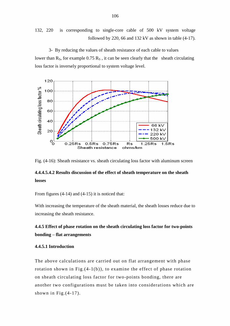
106

132, 220 is corresponding to single-core cable of 500 kV system voltage

followed by 220, 66 and 132 kV as shown in table (4-17).

3- By reducing the values of sheath resistance of each cable to values

lower than RS, for example 0.75 RS , it can be seen clearly that the sheath circulating

loss factor is inversely proportional to system voltage level.

Fig. (4-16): Sheath resistance vs. sheath circulating loss factor with aluminum screen

4.4.4.5.4.2 Results discussion of the effect of sheath temperature on the sheath

losses

From figures (4-14) and (4-15) it is noticed that:

With increasing the temperature of the sheath material, the sheath losses reduce due to

increasing the sheath resistance.

4.4.5 Effect of phase rotation on the sheath circulating loss factor for two-points

bonding – flat arrangements


The above calculations are carried out on flat arrangement with phase

rotation shown in Fig.(4-1(b)), to examine the effect of phase rotation

on sheath circulating loss factor for two-points bonding, there are

another two configurations must be taken into considerations which are

shown in Fig.(4-17).

107

(a) S-T-R configuration (b) S-R-T configuration

Fig.(4-17) Phase rotation in flat formation

The previous mathematical algorithm, which is explained in 4.3.1.2, is used but with

assuming the phase rotation for S -T-R configuration

2

3

2

1

2

3

2

1

13

12

jII

jII

And the phase rotation for S-R-T configuration

2

3

2

1

2

3

2

1

13

12

jII

jII

4.4.5.2 Cases study



listed in table (4-1), is used as case study.


The results are shown in table (4-17). In this table the sheath circulating loss factor in

each phase of single-core cable in flat formation is calculated with corresponding to

three different phase rotation arrangements of the cable.

108

Table (4-17): Sheath circulating loss factors for different configuration in flat

formation

SHEATH

CIRCULATING LOSS

FACTOR

(%)

CABLE CONFIGURATION

λCS-R 47.38 12.18 52.79

λCS-S 12.18 52.79 47.38

λCS-T 52.79 47.38 12.18

Where

λCS-R, λCS-S, λCS-T : The sheath circulating loss factors in R, S and T phases

respectively.


From table (4-17), it is noticed that:

Always the central conductor has the lowest sheath circulating loss value, due

to magnetic cancellation.

The sheath circulating losses of the outer conductors are depending mainly on

the phase rotation and its arrangement.

4.4.6 Effect of conductor current on the sheath losses


The previous mathematical algorithm, which is explained in clause 4.2, has been used

to investigate the effect of variations of conductor current on the sheath losses by

calculating sheath losses for full and half values of ampacity.

R S T T R S T S R

109

4.4.6.2 Cases study



listed in table (4-1), is used in this case study.


The results are shown in tables (4-18-a) and (4-18-b). In these tables sheath currents

and their losses are calculated with changing the conductor current from full rating

value to its half in case of two-points bonding (touch trefoil & touch flat) and cross

bonding (touch trefoil & touch flat) respectively.

Table (4-18-a): Sheath currents and their loss factors for single-core cables with full

rating current and its half value for two-points bonding method


Current Phase

no.




1 29.8

A

1.41 172.9

A

47.38 42.1

A

2.82 116 A 21.32

Full

rating

2 59.6

A

5.64 87.7A 12.18 42.1

A

2.82 116 A 21.32

3 29.8

A

1.41 182.5

A

52.79 42.1

A

2.82 116 A 21.32

1 14.9

A

1.41 86.4

A

47.38 21

A

2.82 58 A 21.32

Half rating

2 29.8

A

5.64 43.8

A

12.18 21

A

2.82 58 A 21.32

3 1 2

110

3 14.9

A

1.41 91.2

A

52.79 21

A

2.82 58 A 21.32

Table (4-18-b): Sheath currents and their loss factor for single-core cables with full

rating current and its half value for cross bonding method


current Phase

no.




1 29.7 A 1.4 42 A 2.81

Full

rating 2 59.5 A 5.61 42 A 2.81

3 29.7 A 1.4 42 A 2.81

1 14.8 A 1.4 21 A 2.81

Half rating 2 29.7 A 5.61 21 A 2.81

3 14.8 A 1.4 21 A 2.81

Where:





3 1 2

111


From tables (4-18-a) and (4-18-b), it is noticed that:

The sheath currents (eddy and circulating) duplicate with duplicating the

conductor current.

The sheath losses factors (eddy and circulating) did not changed because the

ratio of sheath current and conductor current is fixed.

4.4.7 Effect of power frequency (50 or 60 Hz) on the sheath losses


Power frequency in Egypt is 50 Hz, but in some other countries is 60 Hz, this

difference may be due to economical and other factors which are not suitable

to be mentioned here. The previous mathematical algorithm, which is

explained in clause 3.2, is used to study the effect of power frequencies on

the sheath losses by calculating the sheath losses for ƒ = 50 and 60 Hz.

4.4.7.2 Cases study


by XLPE and covered by a lead screen, 50 Hz, which its parameters have been listed

in table (4-1), is used as case study.


The results are shown in tables (4-19-a) and (4-19-b). In these tables sheath

currents and their losses are calculated for ƒ = 50 and 60 Hz in case of two-

points (touch trefoil & touch flat) and cross bonding (touch trefoil & touch

flat) respectively.

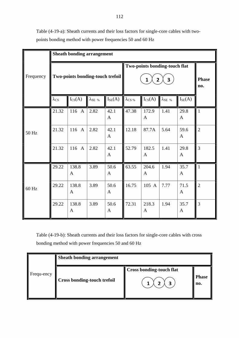
112

Table (4-19-a): Sheath currents and their loss factors for single-core cables with two-

points bonding method with power frequencies 50 and 60 Hz


Frequency Phase

no.




1 29.8

A

1.41 172.9

A

47.38 42.1

A

2.82 116 A 21.32

50 Hz 2 59.6

A

5.64 87.7A 12.18 42.1

A

2.82 116 A 21.32

3 29.8

A

1.41 182.5

A

52.79 42.1

A

2.82 116 A 21.32

1 35.7

A

1.94 204.6

A

63.55 50.6

A

3.89 138.8

A

29.22

60 Hz 2 71.5

A

7.77 105 A 16.75 50.6

A

3.89 138.8

A

29.22

3 35.7

A

1.94 218.3

A

72.31 50.6

A

3.89 138.8

A

29.22

Table (4-19-b): Sheath currents and their loss factors for single-core cables with cross

bonding method with power frequencies 50 and 60 Hz


Frequ-ency Phase

no.


Cross bonding-touch trefoil 3 1 2

3 1 2

113


1 29.7 A 1.4 42 A 2.81

50 Hz 2 59.5 A 5.61 42 A 2.81

3 29.7 A 1.4 42 A 2.81

1 35.6 A 1.93 50.4 A 3.86

60 Hz 2 71.3 A 7.73 50.4 A 3.86

3 35.6 A 1.93 50.4 A 3.86

Where:






From tables (4-19-a) and (4-19-b) it is noticed that:

Both sheath eddy losses and sheath circulating losses increase with increasing

power frequency.

The two-points bonding for flat formation has more sensitivity to the changing

of power frequency than other type of bonding arrangement.

4.4.8 Effect of the minor section length on the sheath circulating current in cross-

bonding arrangement


When the cables in each minor section have the same length, it is said the

cables are balanced and the length imbalance rate is zero [30]. Supposing

three single-core cables with the sheath of each single-core cable consists of

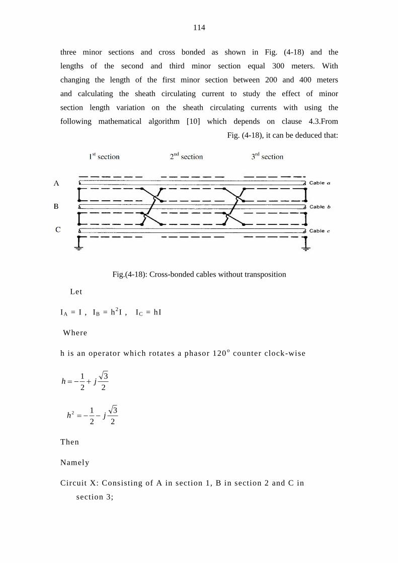
114

three minor sections and cross bonded as shown in Fig. (4-18) and the

lengths of the second and third minor section equal 300 meters. With

changing the length of the first minor section between 200 and 400 meters

and calculating the sheath circulating current to study the effect of minor

section length variation on the sheath circulating currents with using the

following mathematical algorithm [10] which depends on clause 4.3.From

Fig. (4-18), it can be deduced that:

Fig.(4-18): Cross-bonded cables without transposition

Let

IA = I , IB = h2I , IC = hI

Where

h is an operator which rotates a phasor 120o counter clock-wise

2

3

2

1jh

2

3

2

12 jh

Then

Namely

Circuit X: Consisting of A in section 1, B in section 2 and C in

section 3;

115

Circuit Y: Consisting of B in section 1, C in section 2 and A in

section 3;

Circuit Z: Consisting of C in section 1, A in section 2 and B in

section 3.

The induced sheath voltages of X, Y and Z circuits are given as

follows:

BACZ

ACBY

CBAX

XhXXhjIV

XXhXhjIV

XhXhXjIV

3

2

21

321

2

32

2

1

[10] (4-46)

Where ℓ i is the length of section number i, i=1 , 2, 3.

The sheath current in each sheath circuit can be calculated by the

following equations:

(4-44) X

XCSX

Z

VI ,

Y

YC S Y

Z

VI ,

Z

ZC S Z

Z

VI

Where ICS X , ICS Y and ICS Z are the sheath circulating currents in sheath

circuits X, Y and Z respectively and the sheath impedances of the X, Y

and Z circuits respectively are:

ZX = ℓ1(RS + jXA) + ℓ2(RS + jXB) + ℓ3(RS + jXC)

ZY = ℓ1(RS + jXB) + ℓ2(RS + jXC) + ℓ3(RS + jXA) (4-48)

ZZ = ℓ1(RS + jXC) + ℓ2(RS + jXA) + ℓ3(RS + jXB)

In trefoil formation:

sh

CBAr

SXXXX ln102 7 (4-49)

So ZX = ZY = ZZ , ICSX = ICSY = ICSZ = ICS (4-50)

So for ℓ2 = ℓ3 = 300 m and varying ℓ1 with calculating the sheath circulating

current.

116

So from equations (4-49) and (4-50) by substituting in equations (4 -

46), (4-47) and (4-48)

jXRjXRjXRZZZZ SSSZYX 3003001 (4-51)

hXXhXjIVVVV SZYX 300300 2

1 (4-52)

(4-53)

4.4.8.2 Cases study


by XLPE and covered by a lead screen, 50 Hz, which its parameters have been listed

in table (4-1), is used as case study.


The result is shown in Fig. (4-19). This figure shows the values of sheath circulating

current with varying the length of first minor section from 200 to 400 meters.

Fig. (4-19): Sheath current vs. sheath length of minor section for trefoil formation.


Z

VI S

CS

117

From Fig. (4-19) it can be seen that:

When the minor sections have the same length (300 m), the sheath circulating

current reaches zero because the vectorial summations of induced voltages in

the three minor sections of metallic sheath equal zero as shown in Fig. (4-20).

Fig. (4-20 ): Sheath induced voltage vs. total sheath length for trefoil formation.

Any unbalance in the length of the minor sections of the cross bonded

systems will result in circulating currents in the cable screens even when the

currents in the phase conductors are symmetric.

4.4.9 Effect of cable armoring on the sheath losses


In order to protect the cables from mechanical damage such as pick or spade blows,

ground subsidence or excessive vibrations cable armoring is employed [24].

Armored single-core cables for general use in A.C systems usually have nonmagnetic

armor. This is because of the very high losses that would occur in closely spaced

single-core cables with magnetic armor. On the other hand, when magnetic armor is

used, losses due to eddy currents and hysteresis in the steel must be considered. [25].

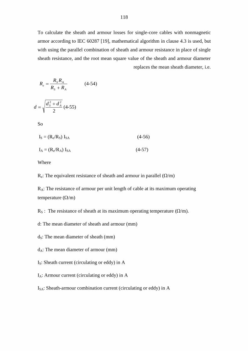
118

To calculate the sheath and armour losses for single-core cables with nonmagnetic

armor according to IEC 60287 [19], mathematical algorithm in clause 4.3 is used, but

with using the parallel combination of sheath and armour resistance in place of single

sheath resistance, and the root mean square value of the sheath and armour diameter

replaces the mean sheath diameter, i.e.

) AS

ASe

RR

RRR

(4-54

(4-55)2

22

AS ddd

So

IS = (Re/RS) ISA (4-56)

IA = (Re/RA) ISA (4-57)

Where

Re: The equivalent resistance of sheath and armour in parallel (/m)

RA: The resistance of armour per unit length of cable at its maximum operating

temperature (/m)

RS : The resistance of sheath at its maximum operating temperature (/m).

d: The mean diameter of sheath and armour (mm)

dS: The mean diameter of sheath (mm)

dA: The mean diameter of armour (mm)

IS: Sheath current (circulating or eddy) in A

IA: Armour current (circulating or eddy) in A

ISA: Sheath-armour combination current (circulating or eddy) in A

119

Thus the addition of the armour is at least equivalent to lowering of the sheath

resistance, so from discussion in clause 4.4.4, if Re is lower than the critical value of

sheath resistance, the addition of the armour may be tends to reduce or increase the

combined sheath-armour circulating losses, if Re is higher than the critical value of

sheath resistance, the addition of the armour, no doubt in that case, tends to increase

the combined sheath-armour circulating losses, while for combined sheath-armour

eddy loss as well as combined sheath-armour current (circulating or eddy) it is

expected increasing them because they are inversely proportional to sheath resistance.

It is of interest to show the effect of armour resistance on the sheath and armour

currents. Fig. (4-21) is prepared for this purpose, so if the armour resistance equals the

sheath resistance, ISA is equally divided between sheath and armour resistance i.e. the

armour current will be equal the sheath current (intersection point in Fig. (4-21)), and

if the armour resistance is lower than the sheath resistance, the armour current will be

higher than the sheath current and vice versa.

Fig. (4-21): Sheath, armour current vs. armour resistance

4.4.9.2 Cases study


by XLPE and covered by a lead screen and armored with aluminum wire, 50 Hz

which its parameters have been listed in table (4-20), is used as a case study.

120

Table (4-20): Armored Single-core cable 800 mm2, 66 kV CU with lead covered

and aluminum wire armored parameters

RS = 0.5 Ω /km , RA = 0.39 Ω/km and Re = 0.22 Ω/km


The results are shown in table (4-21). This table shows the values of sheath currents

and armor currents with their corresponding losses for armored single-core cable in

case of two-points bonding method and cross bonding method for touch trefoil and

touch flat.

.Table (4-21): Sheath, armour currents and their loss factors for nonmagnetic armored

single-core cable with two-points bonding and cross-bonding methods

Cross-bonding tdoonog idnob-owd

Parameters

Touch flat Touch trefoil Touch flat Touch trefoil

0 0 87.35 46.01 λAC1 λCS1 +

0 0 26.8 46.01 λAC2 λCS2 +

0 0 110.76 46.01 λAC3 λCS3 +

93 Outer diameter of cable (mm)

82.5 Mean armour diameter (mm)

62.6 Mean sheath diameter (mm)

0.0221 DC Resistance of the copper conductor at 20°C ohm/km

34 diameter of the conductor (mm)

2.6 Thickness of lead (mm)

50 No. of armour wires

121

3.82 6.66 3.30 6.59 λAE1 λSE1 +

12.93 6.66 13.19 6.59 λAE2 λSE2 +

2.9 6.66 3.30 6.59 λAE3 λSE3 +

0 0 154.4 A 112.1 A ICS1

0 0 85.5 A 112.1 A ICS2

0 0 173.9 A 112.1 A ICS3

0 0 38.16 20.10 λCS1

0 0 11.71 20.10 λCS2

0 0 48.39 20.10 λCS3

32.3 A 42.6 A 30 A 42.4 A ISE1

59.4 A 42.6 A 60 A 42.4 A ISE2

29.9 A 42.6 A 30 A 42.4 A ISE3

1.67 2.91 1.44 2.88 λSE1

5.65 2.91 5.76 2.88 λSE2

1.47 2.91 1.44 2.88 λSE3

0 0 199.1 A 144.5 A IAC1

0 0 110.2 A 144.5 A IAC2

0 0 224.2 A 144.5 A IAC3

0 0 49.19 25.91 λAC1

0 0 15.09 25.91 λAC2

0 0 62.37 25.91 λAC3

41.6 A 54.9 A 38.6 A 54.7 A IAE1

76.6 A 54.9 A 77.3 A 54.7 A IAE2

36.2 A 54.9 A 38.6 A 54.7 A IAE3

2.15 3.75 1.86 3.71 λAE1

7.28 3.75 7.43 3.71 λAE2

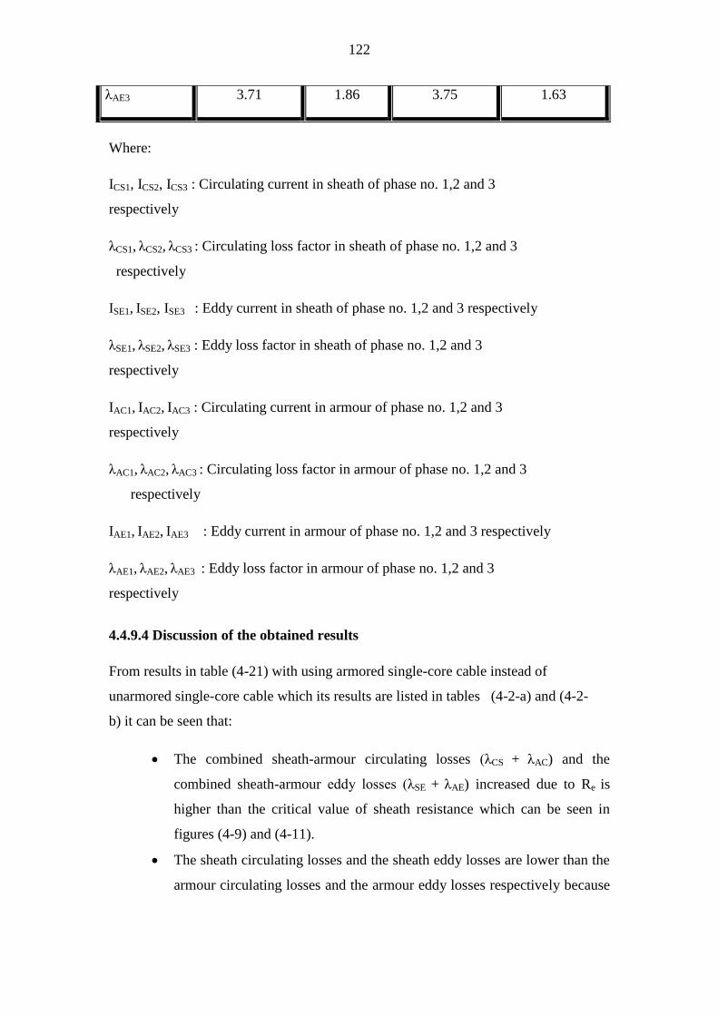
122

1.63 3.75 1.86 3.71 λAE3

Where:

ICS1, ICS2, ICS3 : Circulating current in sheath of phase no. 1,2 and 3

respectively

λCS1, λCS2, λCS3 : Circulating loss factor in sheath of phase no. 1,2 and 3

respectively

ISE1, ISE2, ISE3 : Eddy current in sheath of phase no. 1,2 and 3 respectively

λSE1, λSE2, λSE3 : Eddy loss factor in sheath of phase no. 1,2 and 3

respectively

IAC1, IAC2, IAC3 : Circulating current in armour of phase no. 1,2 and 3

respectively

λAC1, λAC2, λAC3 : Circulating loss factor in armour of phase no. 1,2 and 3

respectively

IAE1, IAE2, IAE3 : Eddy current in armour of phase no. 1,2 and 3 respectively

λAE1, λAE2, λAE3 : Eddy loss factor in armour of phase no. 1,2 and 3

respectively


From results in table (4-21) with using armored single-core cable instead of

unarmored single-core cable which its results are listed in tables (4-2-a) and (4-2-

b) it can be seen that:

The combined sheath-armour circulating losses (λCS + λAC) and the

combined sheath-armour eddy losses (λSE + λAE) increased due to Re is

higher than the critical value of sheath resistance which can be seen in

figures (4-9) and (4-11).

The sheath circulating losses and the sheath eddy losses are lower than the

armour circulating losses and the armour eddy losses respectively because

123

the armour resistance (RA = 0.39Ω/km) is lower than the sheath resistance

(RS = 0.5Ω /km).

The sheath current value in armored single-core cable is depending mainly

on the (Re/RS) ratio.

124

CHAPTER (5)

SHEATH OVERVOLTAGES DUE TO EXTERNAL FAULTS IN SPECIALLY

BONDED CABLE SYSTEM

5.1 Introduction

In chapter 4, It is shown that the types of the bonding are one of the

important factors which effect on the sheath losses in single-core cables, and

it is concluded that both single-point bonding and cross bonding, which are

known as special bonding, introduce the lowest losses in the metallic sheath

of the cable.

To take the advantages of the specially bonded cable systems it is necessary

to insulate the cable sheath from earth to avoid corrosion. This is achieved by

having an extruded serving of PVC or PE on the cables and housing the

joints in compound filled fiberglass boxes to insulate them from the

surrounding soil [26].

The use of special bonding gives rise to sheath over-voltages at sheath

sectionalizing insulators in cross bonded cable system and insulators in a

single-point bonded cable system due to lightning, switching surges or faults

[6,27].

One of the factors affecting the sheath losses in single-core underground

power cables in case of special bonding types is the sheath overvoltage.

Those over-voltages may cause the sheath multi-points break-down which

result in a large sheath currents and losses and hence may cause overheating

of the cables and finally leading to operation faults [6, 28].

As mentioned before, faults are one of reasons which cause sheath over-

voltages. System faults may be divided into internal faults occurring within

the cables themselves and external faults for which the cables carry some or

all of the fault current. The sheath voltages resulting from internal faults may

greatly exceed those caused by external faults [27].

125

A fault in the cables themselves inevitably involves repair work and hence it

is not so important if the sheath insulation adjacent to the fault is also

damaged. The sheath bonding design should preclude the damage cascading

to other parts of the cable system i.e. the cable installation must clearly be

capable of safely withstanding the effects of any fault in the system external

to the cables [6,27,29]. So it is important to consider the performance of

special sheath bonding methods in relation to power frequency external fault

currents. Three types of external faults are considered:

1- Three-phase symmetrical fault

2- Phase-to-phase fault

3- Single-phase ground fault

These three types represent extreme cases and, hence, may be expected to

show maximum values of sheath voltage [27]. Transient voltages induced in

the cable sheaths are particularly important because of the possibility of

excessive voltages that can cause harm to personnel, the cable or equipment

connected to the cable. Also the level of transient voltages induced in the

sheaths will have a direct bearing on measurement actuators and sensors used

in any cable monitoring system [8].Consideration must be given to assess the

magnitude of those over-voltages, so in this chapter over-voltages will be

calculated for single-point bonding and cross bonding under three types of

external faults which are listed above for systems having solidly earthed

neutral, with introducing a suitable method to protect the outer jacket sheath

of the cable.

5.2 Mathematical Algorithm

In deriving the equations that give the sheath voltage gradients due to the external

faults types which listed above for special sheath bonding methods, the following

assumptions are made [6, 27,29 ,30 , 31]:

1- The short circuit current is known and is unaffected in value by the characteristics

of the cable system.

2- Symmetric currents flow during three-phase faults.

126

3- No currents flow other than currents in phase conductors for phase to

phase fault and three-phase fault, i.e. no induced circulating currents in

screens, or any other parallel conductors are considered when calculating the

induced voltages. Parallel conductors which are connected to earth at both

ends will generally act as screening conductors reducing the induced

voltages. So this assumption will give results on the safe side.

4- The cables, for cross bonded systems, be laid with constant spacing and

equal lengths.

These assumptions have to be set up in a way that most of the practical cases

are covered and the deviations from the exact values will be on the safe side.

It must be refer here that, the studies support the use of the following

equations to within good accuracy and with the benefit of being simple to

apply [31].

5.2.1 Single-point bonding cables:

As mentioned in chapter 3, clause 3.2.2, the sheaths of single-point bonded

cables provide no path for returning fault current; hence, an additional earth

conductor is normally laid with such cables. To avoid circulating currents in

this earth conductor, it is laid where possible at spacing from the center cable

of 0.7 times the spacing of the main cables and transposed at the center of the

route when the power cables are not transposed as shown in Fig. (5-1).

Fig. (5-1): Arrangement of single-point bonded cables

5.2.1.1 Three phase symmetrical fault

For a symmetrical three-phase fault, the equations are the same as for normal

balanced load currents and are given as following:

127

5.2.1.1.1 Trefoil formation [6, 29, 30, 31]:

For cables in trefoil formation the induced voltages between sheath and local earth

reference are given by the formulae shown below:

d

SjIjE FAE

2ln

2

3

2

110.2 7 V/m (5-1)

(5-2) V/m

V/m (5-3)

From equations (5-1), (5-2) and (5-3) it can be said that, the magnitudes of the

voltages between sheath and local earth reference in trefoil formation are equal and

are given by:

V/m (5-4)

5.2.1.1.2 Flat formation [6, 27, 29, 30, and 31]:

For cables in flat formation the induced voltages between sheath and earth conductor

are given by the formulae shown below:

V/m (5-5)

d

Sj

d

SIjE FAE

4ln

2

3ln

2

110.2 7

V/m (5-6)

d

SIjE FBE

2ln10.2 7

d

SIjE FBE

2ln10.2 7

d

SjIjE FCE

2ln

2

3

2

110.2 7

d

SIE F

2ln10.2 7

128

(5-7) V/m

Where:

EAE,EBE,ECE : Voltages between sheaths of phases A,B and C respectively and the

earth conductor

IF : Short-circuit current in cable conductor (rms) in A


d : Mean of outer and inner diameter of sheath in m

ω : 2π x frequency (in cycles per second).

5.2.1.2 Phase-to-phase fault

If the fault current is asymmetrical in relation to the earth conductor, a

current will flow in this conductor of value depending on its resistance and

the earth resistances at its terminals and it will act as a screening conductor.

This small effect is ignored in the following equations so that they represent

the worst case. For a phase-to-phase fault, the equations are given as

following:


Assuming a fault is carried out between phases A and B.

d

SIjE FAE

2ln10.2 7 V/m (5-8)

d

SIjE FBE

2ln10.2 7 V/m (5-9)

0CEE V/m (5-10)

d

Sj

d

SIjE FCE

4ln

2

3ln

2

110.2 7

129

5.2.1.2.2 Flat formation:

For a phase-to-phase fault, two cases are possible; fault current in one outer cable

with return in either the other outer or the center cable, the formulae of each case are

shown below:

5.2.1.2.2.1 Fault between two outers cables [27]

d

SIjE FAE

4ln10.2 7 V/m (5-11)

0BEE V/m (5-12)

d

SIjE FCE

4ln10.2 7 V/m (5-13)

5.2.1.2.2.2 Fault between inner and outer cables (phase A & phase B) [6, 29, 30,

31]

(5-14)

d

SIjE FAE

2ln10.2 7 V/m

d

SIjE FBE

2ln10.2 7 V/m (5-15)

(2-96) 2ln10.2 7 FCE IjE V/m

5.2.1.3 Single-phase ground fault (solidly earthed neutral)

Under earth fault conditions the return current will flow through the mass of

the earth and through the earth continuity conductor. Calculating the division

of current between the mass of earth and the earth continuity conductor

depends on a number of factors that are not often known. Because of this, it

is assumed in this case that all fault current returns in the earth conductor and

none returns in the ground, this results in the highest values of sheath voltage.

If an earth fault is in phase A, the sheaths to earth conductor voltages are:

130

5.2.1.3.1 Trefoil formation [6, 29, 30, 31]

c

AECFAE

rd

SjRIE

.

2ln.10.2.

27 V/m (5-17)

c

BEAECFBE

rS

SSjRIE

.

.ln.10.2. 7 V/m (5-18)

c

CEAECFCE

rS

SSjRIE

.

.ln.10.2. 7 V/m (5-19)

5.2.1.3.2 Flat formation [6, 29, 30, and 31]

c

AECFAE

dr

SjRIE

27 2

ln.10.2. V/m (5-18)

c

BEAECFBE

rS

SSjRIE

.

.ln.10.2. 7 V/m (5-19)

V/m (5-20)

c

CEAECFCE

rS

SSjRIE

..2

.ln.10.2. 7

Where:

SAE,SBE,SCE: The geometric mean spacing between cables A, B and C respectively

and the earth conductor (SAE,SBE,SCE = 0.7S)

RC : Resistance of earth conductor, ohm/m

rc : Geometric mean radius of earth conductor (for stranded conductors take 0.75

overall radius)

From the above equations, it is appearing that the magnitude of the induced voltage

due to earth fault current rather than other external faults is characterized by that is a

function of the spacing between the earth continuity conductor and the line

conductors.

131

5.2.2 Cross bonding cables:

5.2.2.1 Three-phase symmetrical fault [6, 29, 30, 31]

The sheath voltage gradients are given by the same equations as those are given in

clause (5.2.1.1) of this chapter for single-point bonded systems with using the longest

minor section length in case of minor sections unbalance as a worst case.

5.2.2.2 Phase-to-phase fault [6, 29, 30, 31]

The sheath voltage gradients are given by the same equations as those are given in

clause (5.2.1.2) of this chapter for single-point bonded systems with using the longest

minor section length in case of minor sections unbalance as a worst case.

5.2.2.3 Single-phase ground fault (solidly earthed neutral)

Under single phase to earth fault conditions the return current divides

between the three sheaths in parallel and the earth. The proportion of current

returning via the earth depends on the sheath resistance and the earthing

resistances at the ends of the circuit. Equations can be given for the voltages

between sheaths but the voltages from sheath to ground will depend strongly

on the earthing resistances at the ends of the circuit and they can not be

simply calculated. The voltages between sheaths are given by the following

equations for earth fault in phase (A) by using the simple assumption that

sheaths are earthed at one point only and that the whole of the returning

current divides between the three sheaths:


d

SIjE FAB

2ln10.2 7 V/m (5-23)

0BCE V/m (5-24)

d

SIjE FCA

2ln10.2 7 V/m (5-25)

5.2.2.3.2 Flat formation [6, 29, 30, and 31]:

132

d

SjIE FAB

.22ln10.2

3/1

7 V/m (5-26)

3/27 2ln10.2 jIE FBC V/m (5-27)

d

SjIE FCA

4ln10.2 7 V/m (5-28)

Where:

EAB,EBC,ECA : Voltages between sheaths of phases A&B, B&C and C&A

respectively

The above algorithm has been used through MATLAB program

and the flowcharts of the computation steps are shown in

Figures (5-2-a), (5-2-b), (5-2-c) and (5-2-d). Flowcharts in Figs

(5-2-a) & (5-2-b) show the computation steps of induced sheath

voltages due to three phase symmetrical fault, phase to phase

fault and single phase ground fault for single -core cable in

trefoil layout with both single-point bonding & cross bonding

methods respectively. Flowcharts in Figs (5-2-c) & (5-2-d)

show the computation steps of induced sheath voltages due to

three phase symmetrical fault, phase to phase fault and single

phase ground fault for single-core cable in flat layout with both

single-point bonding & cross bonding methods respectively.

133

Fig.(5-2-a): Flowchart of the computation steps of sheath induced overvoltage for

trefoil layout with single-point bonding

134

Fig.(5-2-b): Flowchart of the computation steps of sheath induced overvoltage for

trefoil layout with cross bonding

135

Fig.(5-2-c): Flowchart of the computation steps of sheath induced overvoltage for flat

layout with single-point bonding

136

Fig.(5-2-d): Flowchart of the computation steps of sheath induced overvoltage for flat

layout with cross bonding

Where:

IF : Short-circuit current in cable conductor (rms) in A

137


d : Mean of outer and inner diameter of sheath in m

ƒ: power frequency ( 50 Hz)

RC : Resistance of earth conductor, ohm/m

rc : Geometric mean radius of earth conductor (for stranded conductors take 0.75

overall radius)

EAE,EBE,ECE : Voltages between sheaths of phases A,B and C respectively

and the earth conductor


respectively

5.3 Case Study

66 kV single-core cable made of a stranded copper conductor with 800 mm2

insulated by XLPE and covered by a lead screen, f = 50 Hz, which its

parameters have been listed in table (4-1) with taking the distance between

axial cable spacing (S) equals [ 2De ], an earth continuity conductor

(ecc) size 240 mm2 (rc = 13.5 mm & RC = 0.076 Ω/km), is used in this case

study to calculate the induced sheath voltages due to different types of

external faults for single-point bonding and cross bonding methods.

To compare between values of induced sheath voltages it is preferred to

calculate those values as between sheath and earth continuity conductor in

case of single-point bonding, while they are calculated as between sheaths in

case of cross bonding because it is not easy to calculate those values as a

sheath to ground in case of single ground fault as has mentioned before.

5.4 Obtained Results

The outputs of the program that represents the results for unarmored single-

core cables are shown in tables (5-1) and (5-2) for single-point bonding and

cross bonding methods respectively. Table (5-1) shows the values of the

voltages between sheaths and local earthing system in single-core cable due

138

to different types of external faults in case of single-point bonding for trefoil

and flat layouts with S = 2De. Table (5-2) shows the values of the sheath to

sheath voltages in single-core cable due to different types of external faults in

case of cross bonding for trefoil and flat layouts with S = 2De.

Table (5-1): Voltages between sheaths and local earthing system due to different

external faults in single-core cables with single-point bonding

Fault type

Sheath voltage to local earth V/(km.kA)

(Single-point bonding)

Trefoil-formation

Flat-formation

EAE EBE ECE EAE EBE ECE

3 phase sym.

fault 102.5 102.5 102.5 129.9 102.5 129.9

Phase to phase

fault

Fault between phases A&B Fault between two outers cables

102.5 102.5 0

146 0 146

Fault between inner & outer (A&B)

102.5 102.5 43.6

C A B

139

Single phase

ground fault 226.4 134.4 134.4 226.4 134.4 101.7

EAE,EBE,ECE : Voltages between sheaths of phases A,B and C respectively and the

earth conductor

Table (5-2): Sheath to sheath voltages due to different external faults in single-core

cables with cross bonding method for trefoil & flat layouts

Fault type

Sheath to sheath voltage V/(km.kA)

(Cross bonding)

Trefoil-formation

Flat-formation

EAB EBC ECA EAB EBC ECA

3 phase sym.

fault 177.6 177.6 177.6 182.8 182.8 253

Phase to phase

fault

Fault between phases A&B Fault between two outers cables

205 102.5 102.5

146 146 292.1

Fault between inner & outer (A&B)

C A B

140

205 59 146

Single phase

ground fault 102.5 0 102.5 117 29 146


respectively

5.5 Discussion of the Obtained Results:

From calculations in table (5-1) for single-point bonding method, it is noticed that:

In case of 3-phase symmetrical fault the values of voltages between

the sheath and earth continuity conductor (ecc) for trefoil layout are

equal, while for flat layout the voltages induced in the outer cable

sheaths are equal and usually larger than the voltage induced in the

middle cable sheath. The voltage induced in the middle cable sheath is

the same as in trefoil layout. This comment is the same as for the

normal case but with taking the fault current value into consideration

(refer to clause 4.4.1.4, Fig. (4-4)).

For the phase to phase fault, in case of trefoil layout, the sheath

voltage in the healthy phase will be zero due to symmetrical

arrangement of phases, while it will be equal in the two faulty phases

and their values are the same as three-phase symmetrical fault for the

same fault current. In case of flat formation, the sheath voltages in the

two faulty phases are equal and the highest sheath voltages result

when the fault is between the two outer cables, it is also noticed that

the voltage of the healthy phase in case of fault between two outer

cables equals zero due to symmetrical case rather than in case of fault

between inner and outer cables.

For an earth fault, for a fault in phase (A), the highest sheath voltage is in the

faulty phase for trefoil and flat formations and they have the same value in

case of the distance between the faulty phase and the earth continuity

conductor is equal for each, the effect of Rc can generally be neglected, so in

141

flat formation the equation (5-17) – which gives the maximum sheath voltage

– can be expressed as:

c

FAEr

d

d

SjIE .ln.10.2.

2

7 [6] V/m (5-29)

Maximum values of voltages between the sheath and earth continuity

conductor (ecc) under different faults in flat formation could be clearly

appearing in Fig. (5-3) as following:

Fig. (5-3): Maximum induced sheath voltage gradients (sheath to earth) for various

faults in single-point bonded cable system-flat

From Fig. (5-3) it can be seen that the sheath overvoltage due to the single

phase fault are much more important than with respect to the other types of

fault for systems having solidly earthed neutral and it also indicates the effect

of (d/rc), the ratio between mean of outer and inner diameter of metallic

sheath and geometric mean radius of earth conductor (ecc), on the sheath

induced voltage in case of single phase fault, as sheath induced voltage is

inversely proportional to that ratio. From calculations in table (5-2) for cross

bonding method, it is noticed that:

142

In case of 3-phase symmetrical fault the values of voltages between the

sheaths for trefoil layout are symmetrical, while for flat layout the maximum

voltage is reached between the two outer cables.

For the phase to phase fault, in case of trefoil layout, the highest sheath

voltage is between the sheaths of two faulty phases. In flat formation, the

highest sheath voltage is between the two outer cables in two cases which are

studied (fault between two outer cables & fault between inner and outer

cables).

For an earth fault, for a fault in phase (A), the highest sheath to sheath voltage

is between the two outer cables in case of flat layout.

In all cases, the maximum induced voltages between sheaths in flat layouts are

higher than the maximum induced voltages between sheaths in trefoil layouts.

Maximum values of voltages between the sheaths at the cross bond position

per unit length of km of the minor section length under different faults in flat

formation could be clearly appearing in Fig. (5-4).

Fig. (5-4): Maximum induced sheath voltage gradients (sheath to sheath) for various

faults in cross bonded cable system-flat

From Fig. (5-4) it can be seen that the sheath overvoltage due to the phase to phase

fault is much more important than other types of faults for systems having solidly

earthed neutral.

143

CHAPTER 6

CONCLUSION

From this study, some important conclusions are summarized as follows:

Arnold equations for calculating eddy losses give approximately the same

values which have been given in case of using IEC-287 equation, so one of

equations could be used for calculating eddy losses to any sheath bonding

method.

Trefoil layout introduces symmetrical values of voltages and currents in its

three metallic sheaths than flat layout. As for flat layout : the voltages induced

in the outer cable sheaths are equal and usually larger than the voltage

induced in the middle cable sheath in case of single-point bonding, the eddy

currents in the outer cable sheaths are equal and usually smaller than the

value of the middle cable sheath, the sheath circulating currents have unequal

magnitude; the least value occurs in the sheath of the middle cable, values in

sheaths of outer cables are of unequal magnitude too in case of two-points

bonding.

The sheath circulating losses could be reached to more than the conductor

losses, this causes the insulation of the conductor to be subjected to

temperatures may be excess of the insulation ratings, so the cable ampacity

must be de-rated.

Eddy loss could be disregarded with comparing to circulating loss but it must

be noticed that the eddy loss value of middle conductor in flat formation with

close spacing between phases especially for extra high system voltages cables

must be taken into consideration as its value approaches to the value of sheath

circulating loss for the same conductor.

Single-point bonding and cross bonding methods introduce a solution to

overcome the problems of sheath losses in case of two-points bonding

method.

The sheath loss factors (eddy & circulating) are inversely proportional to the

conductor resistivity while they are proportional to the conductor sizes.

The sheath circulating losses are proportional to the spacing between phases,

while the sheath eddy losses are inversely proportional to it so they can be

neglected at large spacing.

144

The sheath eddy currents, eddy losses and circulating currents are inversely

proportional to the spacing between phases.

The sheath circulating losses could be reduced by large increase in sheath

resistance or large reduce in the sheath resistance.

Single-core cables covered by copper wire screen, copper tape or stainless

steel introduce a best solution to reduce the sheath losses and overcoming the

problems of lead sheath especially at higher voltages.

Eddy losses could be neglected with respect to circulating losses except in

aluminum sheath as the eddy losses could be greater than the circulating

losses.

Single-core cable with aluminum sheath introduces higher sheath losses and

currents due to its low resistivity; it also introduces irregular behavior towards

the values of sheath circulating loss factors in extra high voltages as they are

reducing with increasing the system voltage levels.

In flat formation the central conductor always has the lowest sheath

circulating current value, while the values of two outer conductors are

depending on the phase rotation and its arrangement.

The sheath current duplicates with duplicating the conductor current.

The sheath loss factor increases with increasing power frequency.

Two-point bonding for flat formation has more sensitivity to the changing of

power frequency than other bonding types.

When the minor sections have the same length, the sheath current reaches

zero because the vectorial summation of induced voltages in the three minor

sections of metallic sheath equals zero.

Any unbalance in the length of the minor sections of the cross bonded

systems will result in circulating currents in the cable screens even when the

currents in the phase conductors are symmetric.

In case of armoring single-core cables, the combined sheath and armor

circulating losses could be lower or greater than the sheath circulating losses

without armoring depending mainly on the equivalent resistance of sheath and

armour in parallel (Re).

The values of sheath current and armor current are depending mainly on the

armour resistance (RA) and sheath resistance (Rs).

145

For systems having solidly earthed neutral, the overvoltage due to the single-

phase fault are much more important than the other types of fault, while the

overvoltage due to phase to phase fault are much more important than the

other types of fault in case single-point bonding and cross bonding

respectively.

Finally it can be said that “The studying of the factors affecting the sheath

losses in single-core underground cables helps engineers who dealing

with high voltage single-core cables to be more active by introducing a

suitable solutions to overcome the sheath losses problems".

146

REFERENCES

[1] : Mozan M.A., El-Kady M.A., Mazi A.A. 'Advanced Thermal Analysis of

Underground Power Cables' paper presented in Fifth International Middle East

Power Conference MEPCON'97, Alexandria, Egypt, Jan. 4-6, 1997.

[2] : Halperin, H. and Miller, K. W. 'Reduction of Sheath Losses in Single-Conductor

Cables', Transactions AIEE, April 1929, p 399.

[3] : Buller, F. H., 'Pulling Tension During Cable Installation in Ducts or Pipes',

General Electric Review, Schenectady, NY; Vol. 52, No. 8, August, 1949, pp.

21-33.

[4] : Thue, W.A., 'Electrical Power Cable Engineering' by Marcel Dekker, Inc., USA,

2003

[5] : Abdel-Slam M., Anis H., El-Morshedy A, Radwan R, 'High Voltage

Engineering Theory and Practice' by Marcel Dekker, Inc., New York, 2000

[6] IEEE Std. 575 - 1988, 'IEEE Guide for the Application of Sheath- Bonding

Methods for Single-Conductor Cables and the Calculation of Induced Voltages

and Currents in Cable Sheaths.'

[7] : British Standard BS 7430:1998, Code of Practice for Earthing

[8] : Coates M W, 'Assessment of Sheath Bonding System for Doha

South Super to Abu Hamour North 220 kV Cable Circuits ',

www.era.co.uk

[9] : Nasser D. Tleis, 'Power Systems Modeling and Fault Analysis'

Elsevier Ltd.,USA, 2008

[10] : King, S.Y. and Halfter, N.A., Power Cables, Longman, London,1982

[11] : Anders, G.J., 'Rating Of Electric Power Cables In Unfavorable Thermal

Environment', John Wiley & Sons, Inc. 2005

[12] : K. Kuwahra, C. Doench, 'Evaluation of Power Frequency Sheath Currents and

Voltages in Single Conductor Cables for Various Sheath Bonding Methods'

Trans. IEEE 1963 Vol. 82, p 206

[13] : J.R. Riba Ruiz, X. Alabern Morera , 'Effects of The Circulating

Sheath Currents in The Magnetic Field Generated by an Underground Power

Line' www.icrepq.com/icrepq06/217-riba.pdf

[14] : O. E. Gouda, A. Z. El Dein, and G. M. Amer, 'Effect of the Formation of the Dry

Zone Around Underground Power Cables on Their Ratings' IEEE Transactions

147

On Power Delivery, 2010

[15] : H Boyd 'Reduction of Sheath Losses on High Voltage Cables',

http://www.sumobrain.com/patents/wipo/Reduction-sheath-losses-high-

voltage/WO2002027890A1.pdf

[16] : Ma Hongzhong1, Song Jingang, Ju Ping., 'Research on Compensation and

Protection of Voltage in Metal Shield of 110 kV Power Cable under Three

Segments Unsymmetrical State' Power and Energy Society General Meeting –

Conversion and Delivery of Electrical Energy in the 21st Century, 2008 IEEE.

Date:20-24 July 2008, pp. 1-5

[17] : Ma Hongzhong1, Song Jingang, Ni Xinrong, Zhang Limin., Analysis of Induced

Voltage in Metal Shield of Power Cable and Resarch on Its Restraining

Technology Based on Asymmetric State' Electric Utility Deregulation and

Restructuring and Power Technologies, 2008. DRPT 2008. Third International

Conference on date:6-9 April 2008 pp. 948 - 951

[18] :

I. Sarajcev, M. Majstrovic, I. Medic 'Calculation of Losses in Electric Power

Cables as the Base for Cable Temperature Analysis' Advanced Computational

Methods in Heat Transfer, WIT Press Southampton, Boston, 2000, pp. 529-537

[19] :

IEC Standard 60287, 'Calculation of the Continuous Current Rating of Cables

(100% load factor)' 2nd edition 2001.

[20] : Arnold, A.H.M., „The theory of sheath losses in single-conductor lead-covered

cables‟, Jour. IEE, 67, 1929, PP. 69-89

[21] : J.S. Barrett, G.J.Anders. 'Circulating Current and Hysteresis Losses

in Screens, Sheaths and Armour of Electric Power Cables Mathe-matical Models

and Comparison with IEC Standard 287', IEE Proc.-Sei. Meas. Technol., Vol.

144, No. 3, May 1997 pp. 101- 110

[22] : Short, T.A. 'Electric Power Distribution Equipment and Systems', CRC London,

2006

[23] : ABB Catalogue, www.abb.com

[24] : Bayliss,C. R., and Hardy,B. J., 'Transmission and Distribution Electrical

Engineering' Charon Tec Ltd Great Britain, 2007

[25] : Schurig O. R., Kuehni H. P., Buller F. H., 'Losses in Armored

Conductor Lead Covered AC Cables'. AIEE Transactions, Vol. 48, Apr 1929, pp

417-435.

http://ieeexplore.ieee.org/xpl/mostRecentIssue.jsp?punumber=4511470



http://www.abb.com/

148

[26] : Moore G. F., 'Electric Cables Handbook' by Marcel Dekker, Inc.,

TJ International Ltd, England, 1997

[27] : E.H. BALL, E. OCCHINI, G. LUONI ' Sheath Over voltages in

High Voltage cables resulting from special sheath-bonding connections' IEEE

PAS 84, NO. 10, October 1965

[28] : Junhua Luo, Zuochun Zhou, Min Luo 'Optimizing Design of

Overvoltage Protector for HV Power Cable Metallic Shield

Grounding' Transmission and Distribution Conference and

Exposition IEEE PES 2008

[29] : 'The Design of Specially Bonded Systems'. Paper presented by Working Group

07 of Study Committee 21. Electra No.28, 1973.

[30] : 'Guide to The Protection of Specially Bonded Systems Against Sheath Over

voltages'. Paper presented by Working Group 07 of

Study Committee no.21. Electra No.128, 1990.

[31] : 'Special Bonding of High Voltage Power Cables ' Working Group

B1.18 October 2005

[32] : IEEE Std. 635 - 2003, ' Guide for Selection and Design of Aluminum Sheaths for

Power Cables'

bonding methods of underground powerb cables.pdf

Documents